HAL Id: hal-00748746https://hal.archives-ouvertes.fr/hal-00748746

Submitted on 16 Mar 2013

HAL is a multi-disciplinary open accessarchive for the deposit and dissemination of sci-entific research documents, whether they are pub-lished or not. The documents may come fromteaching and research institutions in France orabroad, or from public or private research centers.

L’archive ouverte pluridisciplinaire HAL, estdestinée au dépôt et à la diffusion de documentsscientifiques de niveau recherche, publiés ou non,émanant des établissements d’enseignement et derecherche français ou étrangers, des laboratoirespublics ou privés.

Metamodeling of Combined Discrete/ContinuousResponses

Martin Meckesheimer, Russell Barton, Timothy Simpson, Frej Limayem,Bernard Yannou

To cite this version:Martin Meckesheimer, Russell Barton, Timothy Simpson, Frej Limayem, Bernard Yannou. Metamod-eling of Combined Discrete/Continuous Responses. American Institute of Aeronautics and Astronau-tics, 2001, 39 (10), pp.1950-1959. <10.1.1.160.9842>. <hal-00748746>

American Institute of Aeronautics and Astronautics

Metamodeling of combined discrete/continuous responses

Martin Meckesheimer Russell R. Barton

*

and Timothy Simpson

Industrial and Manufacturing Engineering Department

310 Leonhard Building The Pennsylvania State University

University Park, PA 16802

Frej Limayem and Bernard Yannou

Laboratoire Productique Logistique Grande Voie des Vignes

Ecole Centrale Paris 92295 - Chatenay-Malabry – France

ABSTRACT

Metamodels are effective for providing fast-running surrogate approximations of product or

system performance. Since these approximations are generally based on continuous functions,

they can provide poor fits of discontinuous response functions. Many engineering models

produce functions that are only piecewise continuous, due to changes in modes of behavior or

other state variables. In this paper we investigate the use of a state-selecting metamodeling

approach that provides an accurate approximation for piecewise continuous responses. The

proposed approach is applied to a desk lamp performance model. Three types of metamodels—

quadratic polynomials, spatial correlation (kriging) models, and radial basis functions—and five

types of experimental designs—full factorial designs, D-best Latin hypercube designs, fractional

Latin hypercubes, Hammersley sampling sequences, and uniform designs—are compared based

on three error metrics computed over the design space. The state-selecting metamodeling

approach outperforms a combined metamodeling approach in this example, and radial basis

functions perform well for metamodel construction.

KEYWORDS: Metamodeling, surrogate model, discrete-response, parametric engineering

design, state-dependent output.

WORD COUNT: 6943

* Corresponding Author. Phone/fax: (814)863-7289/4745. Email: rbarton@psu.edu.

2

1. INTRODUCTION

1.1. Simulation-Based Design

Multidisciplinary design has many applications in concurrent engineering, where product

performance and manufacturing plans are designed simultaneously. The objective is to manage the

design process more effectively to allow the designer to carry out rapid evaluations of design

alternatives, analysis, and decision-making in a multidisciplinary design environment.

With the aid of computers for simulation and analysis, discipline-specific product and

process models can be formulated and used to analyze many complex engineering systems, as

opposed to exercising time consuming and expensive experimentation on these physical systems;

however, running complex computer models can also be expensive, especially during

optimization, since a single evaluation of an alternative may take several minutes or even hours

to complete.

Current research approximates the true input/output relationship of the disciplinary model

with a moderate number of computer experiments and then uses the approximate relationship to

make predictions at additional untried inputs. Since these simple mathematical approximations to

discipline-specific product and process models are models of an engineering model, we call them

metamodels because they provide a “model of the model”.1 Furthermore, metamodels facilitate

integrating subsystem and disciplinary analyses, as they are typically written on the same

computer system and use the same language. This may not be the case for the original

disciplinary analysis codes. Note that disciplinary computer simulation codes are deterministic in

nature, in which case the analysis differs from experiments on physical systems in the sense that

no random variations are observed; i.e., for a particular set of input settings, two deterministic

simulation runs will yield the exact same output. The implications of the deterministic nature of

3

computer experiments on metamodel construction and assessment are discussed further by

Simpson, et al.2

1.2. Metamodel-Based design

With a metamodel-based design approach researchers hope to simplify optimization and/or

examination of the system performance over the design space. Moreover, since metamodels

generally allow rapid calculation, the designer obtains a tool for conducting real time exploration

of the design space in the preliminary stages of design. For example, metamodels have been

successfully used for efficient Pareto frontier exploration3 and have found many applications in

structural4 and multidisciplinary optimization.

5 The mathematical approximation can be written

as y = f(x) (x), where f(x) represents the original disciplinary model function, and ŷ = (x) is

the metamodel approximation to y. While the use of metamodels allows a faster analysis than the

original, complex engineering models permits, the metamodel approximation introduces a new

element of uncertainty. As a result, efficient methods to assess metamodel fit at the system and

subsystem level are required. Validation strategies for metamodel assessment can involve the use

of additional data 6,7

or might be based on resampling strategies.8

Metamodeling is a process involving the choice of an experimental design, a metamodel type

and its functional form for fitting, and a validation strategy to assess the metamodel fit. With

these definitions in mind, we now briefly discuss the metamodel and experiment design types

that are utilized in this study.

1.2.1 Response Surface Methodology

4

Response Surface Methodology (RSM) 9 has been used effectively in a variety of

applications2,4,5

, to produce a metamodel with a low-order polynomial in a relatively small region

of the factor space. Typically, first and second order polynomial models of the form:

k

iii xx

10)( and

k

i i ijjiijiii

k

iii xxxxx

1

2

10)( (1)

are fit to the system response. The ß parameters of the polynomials are calculated using least

squares regression to fit the response surface approximations to empirical data or data generated

from simulation or analysis routines; these approximations can then be used for prediction.

Note that a second order response surface is not intended to fit well over the entire region of operability, but only in

a relatively narrow region of interest that has been located by prior experimentation. An advantage of using low

order polynomial metamodels is that they involve relatively few parameters and they permit gaining insight into the

model behavior, and identifying significant model parameters. Although approximation functions based on

low-order polynomials are the most widely used, other regional or global approximating

functions, such as radial basis functions, spatial correlation models, splines, or neural networks

have also been investigated.10, 11

Simpson, et al.12

compare response surface and kriging models

for multidisciplinary design optimization. While these metamodels may provide better

approximations to response functions of arbitrary shape than low-order polynomials, they may

be more difficult to interpret, and sometimes involve a larger number of model coefficients (e.g.,

radial basis functions), or more complex computations (e.g., kriging). In addition to quadratic

polynomial approximations, we also considered radial basis approximations and spatial

correlation (kriging) models for the present study.

1.2.2 Radial Basis Functions

5

A heuristic approach led Hardy13

to use linear combinations of a radially symmetric function

based on Euclidean distance or similar metric. A simple radial basis function form is:

i

i

i xxx)( (2)

where || • || represents the Euclidean norm, and the sum is over an observed set of system

responses, {(xi, f(x

i))}, i = 1, …, n. Replacing (x) with f(x

i), and solving the resulting linear

system yields the i coefficients. As commonly applied, the method is an interpolating

approximation. Radial basis function approximations have produced good fits to arbitrary

contours of both deterministic and stochastic response functions.14

1.2.3 Spatial Correlation (Kriging) Models

Spatial correlation metamodels are a class of approximation techniques that show good promise

for building accurate global approximations of a design space. Spatial correlation metamodeling

is also known as kriging15

or DACE (Design and Analysis of Computer Experiments—named

after the inaugural article by Sacks, et al.16

) modeling. In a spatial correlation metamodel the

design variables are assumed to be correlated as a function of distance during prediction, hence

the name spatial correlation metamodel. These metamodels are extremely flexible since the

metamodel can either “honor the data,” providing an exact interpolation of the data, or “smooth

the data,” providing an inexact interpolation, depending on the choice of the correlation

function.15

A spatial correlation metamodel is a combination of a polynomial model plus departures of the

form:

y(x) = f(x) + Z(x) (3)

6

where y(x) is the unknown function of interest, f(x) is a known polynomial function of x, and

Z(x) is the realization of a normally distributed Gaussian random process with mean zero,

variance 2, and non-zero covariance. The f(x) term in Eqn. (3) is similar to the polynomial

model in a response surface, providing a “global” model of the design space. In many cases f(x)

is simply taken to be a constant term (see Refs. 12, 16-17)

While f(x) globally approximates the design space, Z(x) creates localized deviations so

that the kriging model interpolates the ns sampled data points. The covariance matrix of Z(x) is

given by:

Cov[Z(xi), Z(x

j)] =

2 R (R = [R(x

i, x

j)]). (4)

In Eqn. (4), R is the correlation matrix, and R(xi, x

j) is the correlation function between

any two of the ns sampled data points xi and x

j. R is a (ns x ns) symmetric matrix with ones along

the diagonal. The correlation function R(xi, x

j) is specified by the user; example correlation

functions can be found in Refs. 16-18. In this work we employ a Gaussian correlation function of

the form:

]exp[),(1

2dvn

k

j

k

i

kk

ji xxR xx (5)

where ndv is the number of design variables, k are the unknown correlation parameters used to

fit the model, and the xki and xk

j are the k

th components of sample points x

i and x

j, respectively.

Predicted estimates, ˆ y , of the response at untried values of x are given by:

)()(ˆ ˆˆ 1fr yRx

Ty (6)

where y is the column vector of length ns which contains the values of the response at each

sample point, and f is a column vector of length ns which is filled with ones when f(x) is taken as

7

a constant as is the case in this paper. In Eqn. (6), rT(x) is the correlation vector of length ns

between an untried x and the sample points {x1, x

2, ..., x

ns} and is given by Eqn. (7).

rT(x) = [R(x,x

1), R(x,x

2), ..., R(x,x

ns)] (7)

Finally, in Eqn. (6), ˆ is estimated as:

ˆ (fTR

1f)

1fTR

1y . (8)

The estimate of the variance, ˆ 2, of the sample data, denoted as y, from the underlying

global model (not the variance in the observed data itself) is given by:

s

T

n

)()( ˆˆˆ

12 fyfy R

(9)

where y is the vector of y values and f(x) is assumed to be the constant ˆ . The maximum

likelihood estimates (i.e., “best guesses”) for the k in Eqn. (5) used to fit the model are found by

maximizing the expression:

max0,

n 2

|]|ln)ln([ 2ˆ Rsn

(10)

where ˆ2 and |R| are both functions of . While any values for k create an interpolative model,

the best kriging model is found by solving the k-dimensional unconstrained non-linear

optimization problem given by Eqn. (10). We use a simulated annealing algorithm19

to perform

this optimization.

1.2.4 Design of Experiments

The design of experiments for metamodel fitting is critical to the success of the method. If the

experimental runs of the model codes are not carefully chosen, the fitted metamodel

approximation can be poor. Experimental design issues for metamodels are discussed in Refs. 3

8

and 11. In this study, we use five different strategies to select points in the design space for

fitting each type of metamodel; the designs are described briefly as follows.

Full Factorial Designs

The most commonly used experimental design strategies are factorial designs20

which comprise

full-factorial and fractional-factorial designs. For factorial designs, each dimension of the design

space is covered by a series of (typically) uniformly spaced values; and their Cartesian product

provides a map of the system response. Since the number of points required in factorial designs

becomes prohibitively large as the number of factors in the model increases, fractional-factorials

are often used as an efficient alternative to full-factorial Designs; however, the effectiveness of

these designs depends largely on the nature of the response.

Latin Hypercube Designs

An alternative experimental design strategy is a Latin hypercube which was the first type of

design proposed specifically for computer experiments.21

Latin hypercubes offer flexible sample

sizes while distributing points randomly over the design factor space; it has been shown that

these designs can have relatively small variance when measuring output variance.16

Since Latin hypercube design points are selected at random, it is possible to generate poor

(e.g., diagonal) designs. In order to obtain a good Latin hypercube design, we create a set of

randomly generated candidate designs. The best design is then selected based on the D-

optimality criterion in which the volume of the confidence ellipsoid for the true value about the

observed random vector ˆ is minimized; this is equivalent to maximizing the determinant of the

matrix, X'X. Since we select the design from a set of candidate designs (rather than from all

possible Latin hypercube designs of that size), we refer to it as a D-best Latin hypercube design,

rather than a D-optimal Latin hypercube design.

9

Full Factorial Latin Hypercube Designs

We also consider the use of a slightly modified version of Factorial Hypercube Designs, a hybrid

design strategy which combines the use of Fractional Factorial Designs with Latin hypercube

sampling.22

In this strategy, the design space is divided into pp hypercubes, with p = k – m, where

k is the number of design variables, and m is the number of fractionation of the design. In each

hypercube, n points are generated using Latin hypercube sampling.

Hammersley Sampling Sequence

Latin hypercube techniques are designed for uniformity along a single dimension where

subsequent columns are randomly paired for placement on a k-dimensional cube. Hammersley

sequence sampling (HSS) provides a low-discrepancy experimental design for placing n points in

a k-dimensional hypercube,23

providing better uniformity properties over the k-dimensional

space than a Latin hypercube. Low discrepancy implies a uniform distribution of points in space.

One measure of discrepancy is the rectangular star discrepancy, defined in Eq. (1.2.3) in Ref.

24. It computes a numerical measure of the difference between the actual placement of the

design points and a perfectly uniform dispersion of design points across a rectangular design

region. The reader is referred to Ref. 23 for a formal definition of Hammersley points and an

explicit procedure for generating them.

Uniform Designs

Uniform designs are a class of designs based solely on number-theoretic methods in applied

statistics.24

A uniform design seeks to uniformly scatter n points in a k-dimensional design space

so as to minimize their discrepancy. Further details on uniform designs and their construction

can be found in Ref. 25.

10

1.3. Combined Discrete/Continuous Responses

Often, engineering applications are characterized by combined discrete/continuous responses.

For example, in chemical processes a discontinuity may correspond to the beginning of a

reaction. Similarly, the phase change of elastic-plastic deformation in materials represents a

discrete change in the nature of the response of a mechanical part or system, although the

response is continuous. Identifying the region in which the discontinuity occurs is not necessarily

trivial, since it may be defined by an implicit parameter relationship in the engineering model.

In this paper, we consider a model of light intensity versus position, used for the design of a

desk lamp. This model has a combined discrete/continuous nature, since the position at which a

light ray reaches the table surface can change discretely depending on whether the ray reaches

the table directly or is deflected by the lamp reflector. For example, the table position of a ray

that reflects near the outside edge of the reflector will change discretely when the design

parameter corresponding to the length of the reflector is shortened a small amount. The discrete

change in ray position corresponds to a change in the discrete state variable s S = {direct,

reflected}.

1.4. Objectives and Outline

The objective in this study is to analyze different strategies for modeling combined

discrete/continuous response problems. In the next section, we present a generic description of

the problem, followed by some possible solution approaches. The desk lamp example is

introduced in Section 3. Evaluation measures are discussed in Section 4, and the results are

presented in Section 5. A brief summary concludes the study in Section 6.

11

2. GENERIC PROBLEM DESCRIPTION

In this section, an artificial example with an imaginary system is used to describe the problem

and identify three distinct solutions. Consider the system composed of combined

discrete/continuous responses shown in Figure 1. The imaginary system has a set of continuous

calculations that produce the smooth input-output relationships for the original model; these are

shown in the left-hand plots of Figure 1. After the logic calculations, the overall response

function is no longer continuous; this is illustrated in the right-hand plot of Figure 1.

In general, such a system can be represented with a model consisting of S different states,

where in each state a different continuous function, fs(x), s S, establishes the map between the

input and output parameters. In other words, the design space that is being explored consists of a

finite number of design subspaces, which are accessed after activation of a logical switch or

discriminant function that indicates which design space is being explored. The challenge is to

find a strategy to metamodel the full design space accurately while modeling the continuous and

logical components of the system in an efficient manner.

Continuous

Models Design

Parameters Original Logic

Model 1

f1(x)

True Response

f(x)

Model 2

f2(x)

Domain of

Applicability

Logic

Function

s(x)

S = 1 S = 2

x

x

x

x

Figure 1—Original System

12

Since the approximation functions that are typically used for metamodeling are continuous, in

fact often differentiable, their capability to approximate combined discrete/continuous responses

is limited. In the following sections, we discuss three possible solution approaches to problems

with discrete/continuous responses.

2.1. Combined Metamodel Strategy

The combined metamodel strategy attempts to build a single approximation to the curve shown

in the right-hand plot of Figure 1. An advantage of this strategy is that no separate metamodels

need to be fit for each state or design subspace. Furthermore, the original system is treated as a

black box and need not be modified in order to fit the metamodel. However, due to the

discontinuity in the curve, the metamodel can never be completely successful using continuous

approximating functions. The qualitative nature of the resulting approximation is shown in the

plot for the combined metamodel strategy in Figure 2. The dashed line represents the true

response, while the solid line corresponds to the estimated response based on a single continuous

approximation.

Continuous Metamodels

Estimated Response

Design Parameters

f(x)

(x)

x

Figure 2—Combined Metamodel

2.2. Metamodel Plus Original Logic

It is less demanding to fit a metamodel to the continuous, differentiable curves in the left-hand

plots for the original system in Figure 1. This approximation is shown in the left-hand plots of

13

the “metamodel plus logic” strategy in Figure 3. If the logic calculations in the original model

can be separated from the continuous calculations, a metamodel can be constructed for the

continuous computations, and interfaced with the original code used for logical calculations.

Since the continuous (floating-point) calculations are often the computationally expensive ones,

the computational advantage of a metamodel approximation can be retained in large part, in

many cases.

Continuous Metamodels

Design Parameters

Original Logic

Model 1

Estimated Response

f(x)

(x)

Model 2

Logic

Function

s(x)

S = 1 S = 2

x

x

x

x

f1(x)

1(x)

f2(x)

2(x)

Figure 3—Metamodels Plus Original Logic

Since the original model’s logic code is then applied to the metamodel output, the resulting

overall metamodel-based output, the right-hand plot in Figure 3, looks very similar to the right-

hand plot in Figure 1. Although this seems to be a better option than the combined metamodel

strategy, in many cases it will not be practical to modify the original system model, extract the

logic component, and interface the logic unit with the metamodels. To clarify this one must

distinguish between cases where the original model logic is defined explicitly and implicitly.

Venter, et al.26

discuss an application of an isotropic plate in which the original model logic is

given by a simple geometric criterion. Thus, the logic component is known explicitly and can be

14

extracted. In Section 3.1, we consider the case of a Desk lamp design where the original model

logic is implicit and cannot be easily extracted.

2.3. State-selecting Metamodel

The third modeling solution is to use a state-selecting metamodel as shown in Figure 4, where

continuous metamodels for each sub-model are used with a logic metamodel to approximate the

discontinuous function. In this strategy, an approximation that takes into account the different

system states is constructed without modifying the original model. However, the success of this

strategy relies heavily on the capability of the logic metamodel to discriminate the different

states of the system based on the values of the design parameters. As illustrated in the right hand

plot of Figure 4, a shift between the metamodel and the true function might occur at the point of

discontinuity. This is not the case in the right hand plot of Figure 3 since it uses the original

logic. This approach is shown with more detail in Figures 5 and 6, where the metamodel

calibration and prediction stages have been separated.

Figure 4—State-selecting Metamodel

Design

Parameters

Continuous

MetamodelsEstimated

ResponseLogic

MM

(x)

f(x)

15

In the calibration stage (see Figure 5), the original system model to be approximated is

evaluated at points x prescribed by the design matrix XD, in order to obtain a response matrix,

YD. This information is used to fit a logic metamodel and fit |S| continuous metamodels, one for

each of the system states.

x

Logic MM

MM for s = 1

Calibration

System Model

(cont. subsys. and original

logic models)

x,s,y

MM for s = 2

MM for s = |S|

s = ?

x,s

s = 1

s = 2

s = |S|

x,y

x,y

x,y

Figure5—Fitting a State-selecting Metamodel

Once the logic metamodel ŝ = L(x) has been calibrated and the continuous-response

metamodels for each state have been fit, they can be combined and used for prediction purposes

at a new set of points x, prescribed by the prediction matrix, XP as illustrated in Figure 6.

x MM for s = 1

Prediction

Logic Metamodel

x,s

MM for s = 2

MM for s = |S|

s = ?

s = 1

s = 2

s = |S|

x

x

x

y

y

y

^

^

^

Figure 6—Predicting with a State-selecting Metamodel

16

2.4. Logic Metamodels

At the core of a logic metamodel lies essentially a pattern recognition problem, which is also

referred to as a classification or grouping problem, depending upon the area of application. In

our case, an observation is an input vector whose attributes are the parameter settings specified

by an experimental design, and a population is equivalent to a state of the system. Given a

sample set of observations from a population, the objective is to define a rule that allows us to

decide to which population (i.e., state, s) a new observation (i.e., x) belongs.

Different methods can be used for classifying the states of a system. Discriminant analysis is

a classical statistics method first introduced by Fisher.27

It has been used extensively for

identifying relationships between qualitative criterion variables and quantitative predictor

variables. In other words, discriminant analysis is a procedure for identifying boundaries

between the states of a system; a linear discriminant function uses a weighted combination of the

predictor variable values to classify an object into one of the criterion groups. An extension of

this method is quadratic discriminant analysis.

An alternative approach for discriminating between different states has emerged from the

field of Mathematical Programming (MP). One of the advantages of the MP approach over

traditional discriminant analysis is that the normality and equality of covariance matrices

assumptions are no longer required. The objective function minimizes the number of mis-

classified observations when using the metamodel for prediction purposes; i.e., the measure of

performance is the minimization of the weighted sum of the misclassifications. Ignizio and

Cavalier28

describe the Linear Programming formulation for a two-group classification problem

in detail. The complexity of the problem increases when classifying observations into more than

two groups.

17

Artificial Neural Networks29

(ANNs) are an attractive alternative classification tool. Based on

the functioning of the human brain, ANNs are models that consist of a number of computational

units, or neurons, which are organized into layers, and interconnected through modifiable

weights. During a training phase, a representative training data set is repeatedly presented to the

ANN, which adjusts the weights by means of a training rule until the sum of squared errors

between the network output (for classification: predicted state) and the desired output (actual

state) is minimized. Once this has been achieved, the ANN may be used for prediction purposes.

However, important concerns that affect the model prediction capabilities are how to avoid

overfitting and coming up with an appropriate network structure. De Veaux, et al.,30

discuss the

prediction properties of artificial neural networks for response functions. We are unaware of any

work identifying uncertainties in the classification boundary for ANNs used for discriminant

analysis.

Other approaches such as Logistic Discriminant Analysis, methods based on Nearest

Neighbor algorithms, and Likelihood-based nonparametric Kernel Smoothing exist. In this

article, we have chosen to use artificial neural networks based on the success of preliminary

results which are documented in Ref. 31; however, future work may involve the use of other

methods in order to evaluate their performances.

3. DESK LAMP DESIGN EXAMPLE

In this section we present a description of the desk lamp design model that is used to evaluate the

solution strategies proposed in the previous section. The code allows the user to study many

different aspects of the metamodeling process (see Ref. 32 for a more complete description). The

design objective is to maximize the light quality on a particular area of a desk, such as on a sheet

18

of paper or a book. The lamp and some of the key design and kinematics variables are illustrated

in Figure 7.

Figure 7—Desk Lamp Model

The lamp has two extendable arms and is described by the bulb characteristics and a kinematics

model; external kinematic parameters specify the adjustment of the lamp in terms of rod angle

(r), rod length (L2), rod twist angle (t), vertical rotation (v), and bulb rotation (h).

The desk lamp model can be studied as a full system but also as a group of subsystems which

presents different modeling challenges. In this study, the focus is on creating a metamodel for the

light intensity calculation model, since it is characterized by both discrete and continuous

responses. Figure 8 shows the structure of the desk lamp design model, and the location of the

light intensity calculation model considered in this paper; additional details can be found in Ref.

32. Since the light intensity module is part of the optimization loop within the global model, a

high quality approximation is desired in order to minimize error propagation during

optimization. The light intensity module computes the light ray position coordinates as well as

the angle of incidence for each light ray that is emitted from the bulb filament. The model also

19

generates a discrete response (state value), indicating whether a particular ray has been direct (s

= 1), reflected (s = 2), or does not reached the table (whether direct or reflected).

3.1. Logic Modeling Issues

The light intensity calculation model presents interesting issues for modeling combined

discrete/continuous responses; a continuous function provides the origin and angle for each light

ray, based on lamp geometry and kinematics parameters. As an example, imagine a light ray being

emitted from the bulb filament at a particular angle; varying a design parameter such as reflector length will affect

the trajectory of the light ray. Similarly, for a particular position of the lamp head, some emitted light rays may

never reach the desk surface. In order to simplify the problem, the lamp has been positioned so that all emitted rays

reach the table. Therefore, two distinct states are identified in this study:

s = 1 contact with the desk surface directly (without reflection from the lamp reflector), and

s = 2 contact with the desk surface after one reflection from the lamp reflector.

20

Figure 8—Map of Function Requirements for Analysis

3.2. Combined Discrete/Continuous Response Modeling for the Desk Lamp Problem

The light intensity subsystem of the desk lamp model has a structure similar to the structure of

the artificial example described in Section 2; however, the main difference is that there are

several inputs such as lamp geometry and initial angle of light ray, and several responses

(horizontal position, vertical position, angle). A piecewise continuous response, corresponding to

the location and angle of incidence of the light ray on the surface of the desk is produced. In

addition, the state response, either s=1 or s=2, is reported.

For the desk lamp example, only two of the three metamodeling strategies discussed in

Section 2 could be used. These approaches are explained in more detail as follows.

21

Combined Metamodel Strategy

In this approach, we fit a metamodel to the light intensity module, using it as a black box,

ignoring the presence of different states that specify whether light rays are reflected by the

reflector or reach the desk surface directly.

Metamodel Plus Original Logic

In this approach the combined discrete/continuous response vector from the original model is

used to fit a metamodel. When using the metamodel for prediction, the predicted responses from

the metamodel pass through the original model logic to determine to which state they belong.

Although a promising strategy, it was not possible to extract the original logic from the light

intensity model. The logic calculations are distributed throughout the code, making the elements

extremely difficult to extract. The state identification is based on intermediate calculations and

would have required building metamodels for a large number of intermediate variables.

State-selecting Metamodel

In the state-selecting metamodel approach, the original lamp model is used to build three

metamodels. A neural network logic metamodel is used. Several approaches are tested for

constructing the continuous-response metamodels for each state (see Section 4.1). For each

prediction run, the logic metamodel produces a predicted state value and activates the

corresponding continuous-response metamodel.

Calibrating the logic metamodel classifier is a critical part of this modeling strategy, since it

can be sensitive to the experimental design. Furthermore, the choice of the error tolerance for

neural network training is also quite important. By error we mean the percentage of incorrectly

classified states. A very small error tolerance may result in a longer model calibration; however,

relaxing the error tolerance may lead to misclassification during prediction. Incorrectly predicted

22

states generally result in large prediction errors. In the experiments described next, the error

tolerance for the logic metamodel unit is set to 0, i.e., during calibration, the logic metamodel is

required to classify all experiment design points into their correct state. This does not guarantee,

however, that it will classify all design points used in response prediction correctly.

4. EVALUATION

4.1. Experiment Factors

A computational study using the desk lamp model is conducted to compare several strategies for

metamodeling the desk lamp model. The factors considered are as follows.

1) Metamodeling Approach: combined, state-selecting

2) Continuous-response Metamodel Type: quadratic polynomial, kriging, radial basis function

3) Fitting Experiment Design: approximate D-optimal latin hypercube (DBEST), full factorial

designs (FFD), factorial hypercube (FFLH), a Hammersley Sampling Sequence design

(HSS), a random design with points selected from a multivariate uniform distribution (UNI)

4) Number of Fitting Runs: 25, 100, 225, 400 (generated from factorial designs of size 5x5,

10x10, 15x15, and 20x20)

4.2. Performance Measures

The performance measures relate to the ability of the metamodels to reproduce the behavior of

the lamp model over a range of values of the lamp design parameters. We have simplified the

lamp design problem in order to vary only one internal kinematics variable, the ray angle x1 that

specifies the angle at which a light ray is emitted from the bulb filament, and one controllable

design variable, the length of the lamp reflector, x2. The lower and upper bounds for these

variables are defined in Table 1.

23

Table 1—Model Parameter bounds

MODEL

PARAMATERS

LOW HIGH

1) Ray angle (x1) 0 rad 1.4 rad

2) Reflector length (x2) 60 mm 100 mm

To calculate our metamodel performance measures, the original lamp model is compared with

the continuous metamodel and the state-selecting metamodel. We consider three measures of

metamodel performance, computed over the lamp design parameter space given in Table 1. The

calculation of average errors and maximum errors are approximated by calculating the errors on

a 31x31 grid in the design space, yielding n = 961 error values. The resulting measures are:

Mean Squared Error: n

i

ii YYn

1

21)ˆ(MSE

Mean Absolute Error: n

i

ii YYn

1

1|ˆ|MAE , and

(1) Maximum Absolute Error: |ˆ|maxMAX iii

YY

At each experimental run, the coordinates and the angle of incidence of a light ray are computed.

To simplify presentation of the results, we only compare how well the solution strategies predict

the true horizontal position of the light ray on the desk.

5. RESULTS

The performance assessment of the combined and state-selecting metamodeling approaches is

summarized in Figures 9-11. The graphs are response-scaled design-plots32

where the circles on

the cubes are scaled according to the size of the error with smaller circles indicating better

24

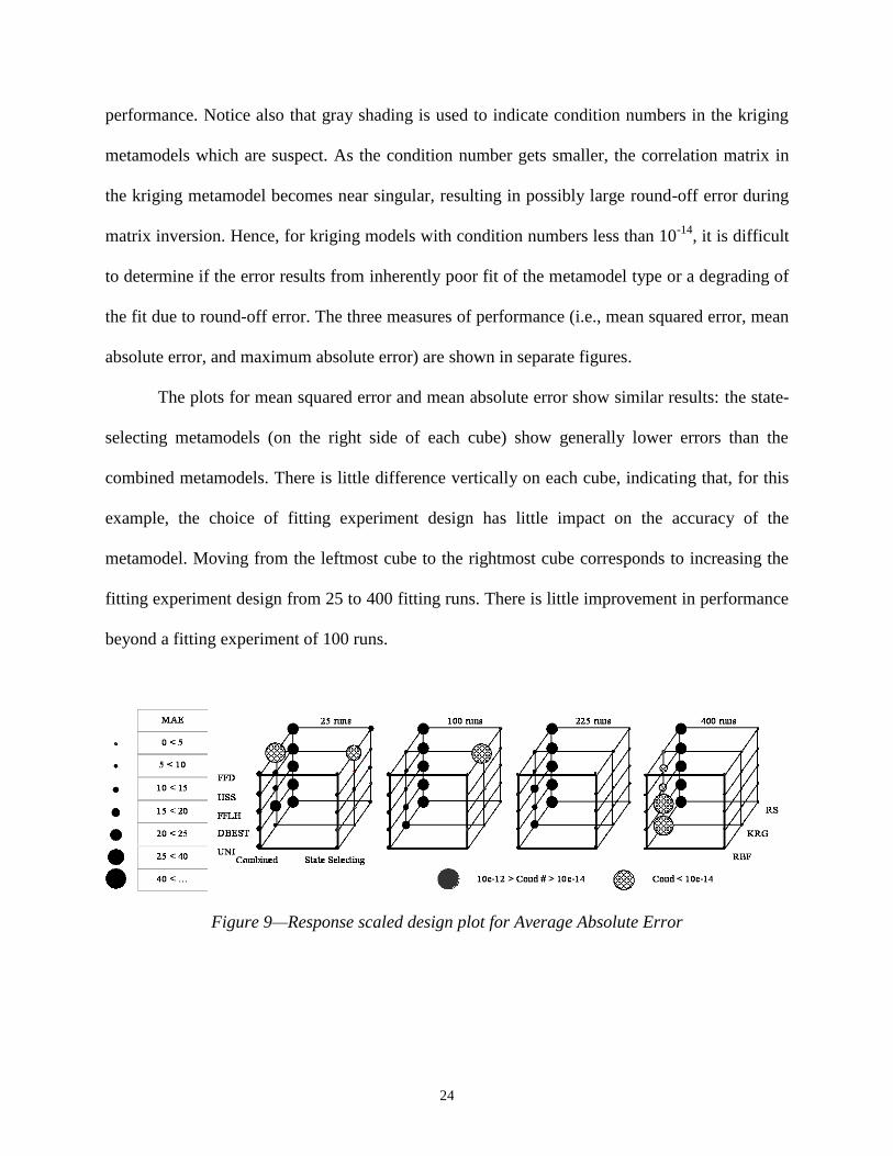
performance. Notice also that gray shading is used to indicate condition numbers in the kriging

metamodels which are suspect. As the condition number gets smaller, the correlation matrix in

the kriging metamodel becomes near singular, resulting in possibly large round-off error during

matrix inversion. Hence, for kriging models with condition numbers less than 10-14

, it is difficult

to determine if the error results from inherently poor fit of the metamodel type or a degrading of

the fit due to round-off error. The three measures of performance (i.e., mean squared error, mean

absolute error, and maximum absolute error) are shown in separate figures.

The plots for mean squared error and mean absolute error show similar results: the state-

selecting metamodels (on the right side of each cube) show generally lower errors than the

combined metamodels. There is little difference vertically on each cube, indicating that, for this

example, the choice of fitting experiment design has little impact on the accuracy of the

metamodel. Moving from the leftmost cube to the rightmost cube corresponds to increasing the

fitting experiment design from 25 to 400 fitting runs. There is little improvement in performance

beyond a fitting experiment of 100 runs.

Figure 9—Response scaled design plot for Average Absolute Error

25

Figure 10—Response scaled design plot for Root Mean Squared Error

Figure 11—Response scaled design plot for Maximum Absolute Error

The RBF metamodels (front face of each cube) show small error for both combined and

state-selecting strategies (left and right sides of each cube), for all but the leftmost cubes (only 25

fitting runs).

Finally, the Figure 11 shows no improvement in the maximum error for the state

selecting metamodels when compared with the combined metamodels, and no improvement as

the fitting experiment sample size is increased. This is because the maximum error occurs at

points near the state transition boundary: a slight misclassification of the transition results in a

large error for the state-selecting metamodel. Since the combined metamodel has a smooth

transition, the size of this error is reduced by approximately 1/2, although the abrupt feature in

the true response has been lost. This phenomenon can be seen by visually comparing the

26

maximum error in Figure 2 with the maximum error in Figure 4. Generally, we think that the

approximation in Figure 4 is superior to that in Figure 2; however, the maximum error in Figure

4 is actually larger.

For the state-selecting approach, we observe that using second-order polynomials as opposed

to radial basis functions results in a slightly lower MSE. However, when the number of design

points for fitting is increased, both MSE and MAE indicate that radial basis functions are better

suited than second-order polynomials for this example.

In general, relatively high maximum errors occur in all methods; these errors occur in regions

near the discontinuity. Furthermore, one expects the state-selecting metamodeling approach to

incur in high maximum errors when the logic metamodel unit incorrectly classifies a design

state. Unfortunately, even well calibrated logic metamodel units will incur state prediction errors

occasionally.

Plots of the original response, and the estimated responses for the combined and state-

selecting metamodels using polynomial regression, radial basis function, and spatial correlation

metamodels are shown in Figures 12-15, respectively. The metamodels in these figures are fitted

using the 25 run Uniform Design, and the predictions are over a 31x31 point grid. In the true

response in Figure 12, it is easy to see the discontinuity that results when the ray is reflected

versus direct. Notice also that the smooth fit of the combined radial basis function metamodel

(Figure 14, left) is comparable to Figure 2. The metamodel has difficulties approximating the

original model at the discontinuity.

27

Figure 12—True Response Surface

Figure 13—Combined (left) and State-Selecting (right) Quadratic Polynomial Metamodels

28

Figure 14—Combined (left) and State-Selecting (right) Radial Basis Function Metamodels

Figure 15—Combined (left) and State-Selecting (right) Spatial Correlation Metamodels

The error plots for all three metamodels fitted for the 25 point Uniform Design are shown in

Figures 16 (combined) and 17 (state-selecting). We observe how primarily small errors occur

over a wide range along the discontinuity for the combined metamodel approach, whereas

smaller regions characterize the state-selecting metamodeling approach. This again reflects the

previous discussion regarding the errors shown in Figures 2 and 4.

29

Quadratic Polynomial Radial Basis Function Spatial Correlation (Kriging)

Figure 16—Combined Metamodel Error Plots

Quadratic Polynomial Radial Basis Function Spatial Correlation (Kriging)

Figure 17—State-selecting Metamodel Error Plots

6. SUMMARY

In this paper we have discussed the use of metamodels for approximating combined

discrete/continuous responses. Three generic solution strategies are proposed, two of which are

illustrated through a desk lamp design example. From our preliminary experiments, we conclude

that the state-selecting metamodeling approach can outperform the combined metamodeling

approach, and second-order polynomials with the state-selecting approach can perform well

30

relative to the more flexible radial basis function and kriging models, especially when relatively

few fitting runs are possible. While the state-selecting approach is promising, and preserves the

discontinuous characteristic of the response function, misclassification by the logic metamodel

can produce large errors near the discontinuity.

The work presented in this paper will be expanded in the future in several aspects. For

instance, in order to fit different metamodels in a state-selecting metamodeling approach,

sufficient design points need to be generated for each of the states. This raises questions such as

how to generate additional points for different states, especially when these are not modeled

explicitly by the original system.

ACKNOWLEGMENTS

We are indebted to the editor and anonymous referees, whose comments helped us improve the

quality of this paper. This work is supported by the National Science Foundation under NSF

Grants DMI-9700040 and DMI-0084918 and by the Office of Naval Research under ONR Grant

N00014-00-G-0058. The cost of computer time is underwritten by the Laboratory for Intelligent

Systems and Quality at The Pennsylvania State University and the Laboratoire Productique

Logistique at Ecole Centrale in Paris.

REFERENCES

1Kleijnen, J. P. C., Statistical Tools for Simulation Practitioners, Marcel Dekker, New York,

1987.

2Simpson, T. W., Peplinski, J., Koch, P. N. and Allen, J. K., "On the Use of Statistics in

Design and the Implications for Deterministic Computer Experiments," Design Theory and

Methodology - DTM'97, Sacramento, CA, ASME, September 14-17, 1997.

31

3Wilson, B., Cappelleri, D. J., Frecker, M. I. and Simpson, T. W., "Efficient Pareto Frontier

Exploration Using Surrogate Approximations," Optimization and Engineering, to appear.

4Barthelemy, J.-F. M. and Haftka, R. T., "Approximation Concepts for Optimum Structural

Design - A Review," Structural Optimization, Vol. 5, 1993, pp. 129-144.

5Sobieszczanski-Sobieski, J. and Haftka, R. T., "Multidisciplinary Aerospace Design

Optimization: Survey of Recent Developments," Structural Optimization, Vol. 14, 1997, pp. 1-

23.

6Yesilyurt, S. and Patera, A. T., "Surrogates for Numerical Simulations; Optimization of

Eddy-Promoter Heat Exchangers," Computer Methods in Applied Mechanics and Engineering,

Vol. 121, No. 1-4, 1995, pp. 231-257.

7Yesilyurt, S., Ghaddar, C. K., Cruz, M. E. and Patera, A. T., "Bayesian-Validated Surrogates

for Noisy Copmuter Simulations: Application to Random Media," SIAM Journal of Scientific

Computing, Vol. 17, No. 4, 1996, pp. 973-992.

8Laslett, G. M., "Kriging and Splines: An Empirical Comparison of Their Predictive

Performance in Some Applications," Journal of the American Statistical Association, Vol. 89,

No. 426, 1994, pp. 391-400.

9Myers, R. H. and Montgomery, D. C., Response surface methodology: process and product

optimization using designed experiments, Wiley, New York, 1995.

10

Barton, R. R., "Metamodels for Simulation Input-Output Relations," Proceedings of the

1992 Winter Simulation Conference (Swain, J. J., Goldsman, D., et al., eds.), Arlington, VA,

IEEE, December 13-16, 1992, pp. 289-299.

32

11

Barton, R. R., "Metamodeling: A State of the Art Review," Proceedings of the 1994 Winter

Simulation Conference (Tew, J. D., Manivannan, S., et al., eds.), Lake Beuna Vista, FL, IEEE,

December 11-14, 1994, pp. 237-244.

12

Simpson, T. W., Mauery, T. M., Korte, J. J. and Mistree, F., "Comparison of Response

Surface and Kriging Models for Multidisciplinary Design Optimization," 7th

AIAA/USAF/NASA/ISSMO Symposium on Multidisciplinary Analysis & Optimization, St. Louis,

MO, AIAA, Vol. 1, September 2-4, 1998, pp. 381-391.

13

Hardy, R. L., "Multiquadratic Equations of Topography and Other Irregular Surfaces,"

Journal of Geophysical Research, Vol. 76, 1971, pp. 1905-1915.

14

Powell, M. J. D., "Radial Basis Functions for Multivariable Interpolation: A Review," IMA

Conference on Algorithms for the Approximation of Functions and Data (Mason, J. C. and Cox,

M. G., eds.), Oxford University Press, London, 1987, pp. 143-167.

15

Cressie, N. A. C., Statistics for Spatial Data, Revised, John Wiley & Sons, New York,

1993.

16

Sacks, J., Welch, W. J., Mitchell, T. J. and Wynn, H. P., "Design and Analysis of Computer

Experiments," Statistical Science, Vol. 4, No. 4, 1989, pp. 409-435.

17

Koehler, J. R. and Owen, A. B., "Computer Experiments," Handbook of Statistics (Ghosh, S.

and Rao, C. R., eds.), Elsevier Science, New York, 1996, pp. 261-308.

18

Journel, A. G. and Huijbregts, C. J., Mining Geostatistics, Academic Press, New York,

1978.

19

Goffe, W. L., Ferrier, G. D. and Rogers, J., "Global Optimization of Statistical Functions

with Simulated Annealing," Journal of Econometrics, Vol. 60, No. 1-2, 1994, pp. 65-100. Source

code is available online at http://netlib2.cs.utk.edu/opt/simann.f.

33

20

Montgomery, D. C., Design and Analysis of Experiments, Fifth Edition, John Wiley & Sons,

New York, 2001.

21

McKay, M. D., Beckman, R. J. and Conover, W. J., "A Comparison of Three Methods for

Selecting Values of Input Variables in the Analysis of Output from a Computer Code,"

Technometrics, Vol. 21, No. 2, 1979, pp. 239-245.

22

Salagame, R. R. and Barton, R. R., "Factorial Hypercube Designs for Spatial Correlation

Regression," Journal of Applied Statistics, Vol. 24, No. 4, 1997, pp. 453-473.

23

Kalagnanam, J. R. and Diwekar, U. M., "An Efficient Sampling Technique for Off-Line

Quality Control," Technometrics, Vol. 39, No. 3, 1997, pp. 308-319.

24

Fang, K.-T. and Wang, Y., Number-theoretic Methods in Statistics, Chapman & Hall, New

York, 1994.

25

Venter, G., Haftka, R. T. and Starnes, J. H., Jr., "Construction of Response Surface

Approximations for Design Optimization," AIAA Journal, Vol. 36, No. 12, 1998, pp. 2242-2249.

26

Fisher, R. A., "The Use of Multiple Measurements in Taxonomy Problems," Annals of

Eugenics, 1936, pp. 179-188.

27

Ignizio, J. P. and Cavalier, T. M., Linear Programming, Prentice Hall, Englewood Cliffs,

NJ, 1994.

28

Haykin, S., Neural Networks: A Comprehensive Foundation, Macmillan Publishing, New

York, 1994.

29

De Veaux, R. D., Schumi, J., Schweinsberg, J. and Ungar, L. H., "Prediction intervals for

neural networks via nonlinear regression," Technometrics, Vol. 40, No. 4, 1998, pp. 273-282.

30

Barton, R. R., Limayem, F., Meckesheimer, M. and Yannou, B., "Using Metamodels for

Modeling the Propagation of Design Uncertainties," 5th International Conference on Concurrent

34

Engineering (ICE'99) (Wogum, N., Thoben, K.-D., et al., eds.), The Hague, The Netherlands,

Centre for Concurrent Enterprising, March 15-17, 1999, pp. 521-528.