Method 201 8/4/2017

1

While we have taken steps to ensure the accuracy of this Internet version of the document, it is not the

official version. To see a complete version including any recent edits, visit:

https://www.ecfr.gov/cgi-bin/ECFR?page=browse and search under Title 40, Protection of

Environment.

METHOD 201 - DETERMINATION OF PM10 EMISSIONS (EXHAUST GAS RECYCLE

PROCEDURE)

1. Applicability and Principle

1.1 Applicability. This method applies to the in-stack measurement of particulate matter (PM)

emissions equal to or less than an aerodynamic diameter of nominally 10 µm (PM10) from

stationary sources. The EPA recognizes that condensible emissions not collected by an in-stack

method are also PM10, and that emissions that contribute to ambient PM10 levels are the sum of

condensible emissions and emissions measured by an in-stack PM10 method, such as this method

or Method 201A. Therefore, for establishing source contributions to ambient levels of PM10,

such as for emission inventory purposes, EPA suggests that source PM10measurement include

both in-stack PM10and condensible emissions. Condensible missions may be measured by an

impinger analysis in combination with this method.

1.2 Principle. A gas sample is isokinetically extracted from the source. An in-stack cyclone is

used to separate PM greater than PM10, and an in-stack glass fiber filter is used to collect the

PM10. To maintain isokinetic flow rate conditions at the tip of the probe and a constant flow rate

through the cyclone, a clean, dried portion of the sample gas at stack temperature is recycled into

the nozzle. The particulate mass is determined gravimetrically after removal of uncombined

water.

2. Apparatus

Note: Method 5 as cited in this method refers to the method in 40 CFR part 60, appendix A.

2.1 Sampling Train. A schematic of the exhaust of the exhaust gas recycle (EGR) train is shown

in Figure 1 of this method.

2.1.1 Nozzle with Recycle Attachment. Stainless steel (316 or equivalent) with a sharp tapered

leading edge, and recycle attachment welded directly on the side of the nozzle (see schematic in

Figure 2 of this method). The angle of the taper shall be on the outside. Use only straight

sampling nozzles. “Gooseneck” or other nozzle extensions designed to turn the sample gas flow

90°, as in Method 5 are not acceptable. Locate a thermocouple in the recycle attachment to

measure the temperature of the recycle gas as shown in Figure 3 of this method. The recycle

attachment shall be made of stainless steel and shall be connected to the probe and nozzle with

stainless steel fittings. Two nozzle sizes, e.g., 0.125 and 0.160 in., should be available to allow

isokinetic sampling to be conducted over a range of flow rates. Calibrate each nozzle as

described in Method 5, Section 5.1.

2.1.2 PM10Sizer. Cyclone, meeting the specifications in Section 5.7 of this method.

2.1.3 Filter Holder. 63mm, stainless steel. An Andersen filter, part number SE274, has been

found to be acceptable for the in-stack filter.

Method 201 8/4/2017

2

Note: Mention of trade names or specific products does not constitute endorsement by the

Environmental Protection Agency.

2.1.4 Pitot Tube. Same as in Method 5, Section 2.1.3. Attach the pitot to the pitot lines with

stainless steel fittings and to the cyclone in a configuration similar to that shown in Figure 3 of

this method. The pitot lines shall be made of heat resistant material and attached to the probe

with stainless steel fittings.

2.1.5 EGR Probe. Stainless steel, 15.9-mm (5/8-in.) ID tubing with a probe liner, stainless steel

9.53-mm (3/8-in.) ID stainless steel recycle tubing, two 6.35-mm (1/4-in.) ID stainless steel

tubing for the pitot tube extensions, three thermocouple leads, and one power lead, all contained

by stainless steel tubing with a diameter of approximately 51 mm (2.0 in.). Design considerations

should include minimum weight construction materials sufficient for probe structural strength.

Wrap the sample and recycle tubes with a heating tape to heat the sample and recycle gases to

stack temperature.

2.1.6 Condenser. Same as in Method 5, Section 2.1.7.

2.1.7 Umbilical Connector. Flexible tubing with thermocouple and power leads of sufficient

length to connect probe to meter and flow control console.

2.1.8 Vacuum Pump. Leak-tight, oil-less, noncontaminating, with an absolute filter, “HEPA”

type, at the pump exit. A Gast Model 0522–V103 G18DX pump has been found to be

satisfactory.

2.1.9 Meter and Flow Control Console. System consisting of a dry gas meter and calibrated

orifice for measuring sample flow rate and capable of measuring volume to ±2 percent,

calibrated laminar flow elements (LFE's) or equivalent for measuring total and sample flow rates,

probe heater control, and manometers and magnehelic gauges (as shown in Figures 4 and 5 of

this method), or equivalent. Temperatures needed for calculations include stack, recycle, probe,

dry gas meter, filter, and total flow. Flow measurements include velocity head (Δp), orifice

differential pressure (ΔH), total flow, recycle flow, and total back-pressure through the system.

2.1.10 Barometer. Same as in Method 5, Section 2.1.9.

2.1.11 Rubber Tubing. 6.35-mm (1/4-in.) ID flexible rubber tubing.

2.2 Sample Recovery.

2.2.1 Nozzle, Cyclone, and Filter Holder Brushes. Nylon bristle brushes property sized and

shaped for cleaning the nozzle, cyclone, filter holder, and probe or probe liner, with stainless

steel wire shafts and handles.

2.2.2 Wash Bottles, Glass Sample Storage Containers, Petri Dishes, Graduated Cylinder and

Balance, Plastic Storage Containers, and Funnels. Same as Method 5, Sections 2.2.2 through

2.2.6 and 2.2.8, respectively.

2.3 Analysis. Same as in Method 5, Section 2.3.

3. Reagents

Method 201 8/4/2017

3

The reagents used in sampling, sample recovery, and analysis are the same as that specified in

Method 5, Sections 3.1, 3.2, and 3.3, respectively.

4. Procedure

4.1 Sampling. The complexity of this method is such that, in order to obtain reliable results,

testers should be trained and experienced with the test procedures.

4.1.1 Pretest Preparation. Same as in Method 5, Section 4.1.1.

4.1.2 Preliminary Determinations. Same as Method 5, Section 1.2, except use the directions on

nozzle size selection in this section. Use of the EGR method may require a minimum sampling

port diameter of 0.2 m (6 in.). Also, the required maximum number of sample traverse points at

any location shall be 12.

4.1.2.1 The cyclone and filter holder must be in-stack or at stack temperature during sampling.

The blockage effects of the EGR sampling assembly will be minimal if the cross-sectional area

of the sampling assembly is 3 percent or less of the cross-sectional area of the duct and a pitot

coefficient of 0.84 may be assigned to the pitot. If the cross-sectional area of the assembly is

greater than 3 percent of the cross-sectional area of the duct, then either determine the pitot

coefficient at sampling conditions or use a standard pitot with a known coefficient in a

configuration with the EGR sampling assembly such that flow disturbances are minimized.

4.1.2.2 Construct a setup of pressure drops for various Δp's and temperatures. A computer is

useful for these calculations. An example of the output of the EGR setup program is shown in

Figure 6 of this method, and directions on its use are in section 4.1.5.2 of this method. Computer

programs, written in IBM BASIC computer language, to do these types of setup and reduction

calculations for the EGR procedure, are available through the National Technical Information

Services (NTIS), Accession number PB90–500000, 5285 Port Royal Road, Springfield, VA

22161.

4.1.2.3 The EGR setup program allows the tester to select the nozzle size based on anticipated

average stack conditions and prints a setup sheet for field use. The amount of recycle through the

nozzle should be between 10 and 80 percent. Inputs for the EGR setup program are stack

temperature (minimum, maximum, and average), stack velocity (minimum, maximum, and

average), atmospheric pressure, stack static pressure, meter box temperature, stack moisture,

percent 02, and percent CO2 in the stack gas, pitot coefficient (Cp), orifice Δ H2, flow rate

measurement calibration values [slope (m) and y-intercept (b) of the calibration curve], and the

number of nozzles available and their diameters.

4.1.2.4 A less rigorous calculation for the setup sheet can be done manually using the equations

on the example worksheets in Figures 7, 8, and 9 of this method, or by a Hewlett-Packard HP41

calculator using the program provided in appendix D of the EGR operators manual, entitled

Applications Guide for Source PM 10 Exhaust Gas Recycle Sampling System. This calculation

uses an approximation of the total flow rate and agrees within 1 percent of the exact solution for

pressure drops at stack temperatures from 38 to 260°C (100 to 500°F) and stack moisture up to

50 percent. Also, the example worksheets use a constant stack temperature in the calculation,

ingoring the complicated temperature dependence from all three pressure drop equations. Errors

for this at stack temperatures ±28°C (±50°F) of the temperature used in the setup calculations are

within 5 percent for flow rate and within 5 percent for cyclone cut size.

Method 201 8/4/2017

4

4.1.2.5 The pressure upstream of the LFE's is assumed to be constant at 0.6 in. Hg in the EGR

setup calculations.

4.1.2.6 The setup sheet constructed using this procedure shall be similar to Figure 6 of this

method. Inputs needed for the calculation are the same as for the setup computer except that

stack velocities are not needed.

4.1.3 Preparation of Collection Train. Same as in Method 5, Section 4.1.3, except use the

following directions to set up the train.

4.1.3.1 Assemble the EGR sampling device, and attach it to probe as shown in Figure 3 of this

method. If stack temperatures exceed 260°C (500°F), then assemble the EGR cyclone without

the O-ring and reduce the vacuum requirement to 130 mm Hg (5.0 in. Hg) in the leak-check

procedure in Section 4.1.4.3.2 of this method.

4.1.3.2 Connect the proble directly to the filter holder and condenser as in Method 5. Connect the

condenser and probe to the meter and flow control console with the umbilical connector. Plug in

the pump and attach pump lines to the meter and flow control console.

4.1.4 Leak-Check Procedure. The leak-check for the EGR Method consists of two parts: the

sample-side and the recycle-side. The sample-side leak-check is required at the beginning of the

run with the cyclone attached, and after the run with the cyclone removed. The cyclone is

removed before the post-test leak-check to prevent any disturbance of the collected sample prior

to analysis. The recycle-side leak-check tests the leak tight integrity of the recycle components

and is required prior to the first test run and after each shipment.

4.1.4.1 Pretest Leak-Check. A pretest leak-check of the entire sample-side, including the cyclone

and nozzle, is required. Use the leak-check procedure in Section 4.1.4.3 of this method to

conduct a pretest leak-check.

4.1.4.2 Leak-Checks During Sample Run. Same as in Method 5, Section 4.1.4.1.

4.1.4.3 Post-Test Leak-Check. A leak-check is required at the conclusion of each sampling run.

Remove the cyclone before the leak-check to prevent the vacuum created by the cooling of the

probe from disturbing the collected sample and use the following procedure to conduct a post-

test leak-check.

4.1.4.3.1 The sample-side leak-check is performed as follows: After removing the cyclone, seal

the probe with a leak-tight stopper. Before starting pump, close the coarse total valve and both

recycle valves, and open completely the sample back pressure valve and the fine total valve.

After turning the pump on, partially open the coarse total valve slowly to prevent a surge in the

manometer. Adjust the vacuum to at least 381 mm Hg (15.0 in. Hg) with the fine total valve. If

the desired vacuum is exceeded, either leak-check at this higher vacuum or end the leak-check as

shown below and start over.

Caution: Do not decrease the vacuum with any of the valves. This may cause a rupture of the

filter.

Note: A lower vacuum may be used, provided that it is not exceeded during the test.

Method 201 8/4/2017

5

4.1.4.3.2 Leak rates in excess of 0.00057 m3/min (0.020 ft3/min) are unacceptable. If the leak rate

is too high, void the sampling run.

4.1.4.3.3 To complete the leak-check, slowly remove the stopper from the nozzle until the

vacuum is near zero, then immediately turn off the pump. This procedure sequence prevents a

pressure surge in the manometer fluid and rupture of the filter.

4.1.4.3.4 The recycle-side leak-check is performed as follows: Close the coarse and fine total

valves and sample back pressure valve. Plug the sample inlet at the meter box. Turn on the

power and the pump, close the recycle valves, and open the total flow valves. Adjust the total

flow fine adjust valve until a vacuum of 25 inches of mercury is achieved. If the desired vacuum

is exceeded, either leak-check at this higher vacuum, or end the leak-check and start over.

Minimum acceptable leak rates are the same as for the sample-side. If the leak rate is too high,

void the sampling run.

4.1.5 EGR Train Operation. Same as in Method 5, Section 4.1.5, except omit references to

nomographs and recommendations about changing the filter assembly during a run.

4.1.5.1 Record the data required on a data sheet such as the one shown in Figure 10 of this

method. Make periodic checks of the manometer level and zero to ensure correct ΔH and Δp

values. An acceptable procedure for checking the zero is to equalize the pressure at both ends of

the manometer by pulling off the tubing, allowing the fluid to equilibrate and, if necessary, to re-

zero. Maintain the probe temperature to within 11°C (20°F) of stack temperature.

4.1.5.2 The procedure for using the example EGR setup sheet is as follows: Obtain a stack

velocity reading from the pitot manometer (Δp), and find this value on the ordinate axis of the

setup sheet. Find the stack temperature on the abscissa. Where these two values intersect are the

differential pressures necessary to achieve isokineticity and 10 µm cut size (interpolation may be

necessary).

4.1.5.3 The top three numbers are differential pressures (in. H2O), and the bottom number is the

percent recycle at these flow settings. Adjust the total flow rate valves, coarse and fine, to the

sample value (ΔH) on the setup sheet, and the recycle flow rate valves, coarse and fine, to the

recycle flow on the setup sheet.

4.1.5.4 For startup of the EGR sample train, the following procedure is recommended. Preheat

the cyclone in the stack for 30 minutes. Close both the sample and recycle coarse valves. Open

the fine total, fine recycle, and sample back pressure valves halfway. Ensure that the nozzle is

properly aligned with the sample stream. After noting the Δp and stack temperature, select the

appropriate ΔH and recycle from the EGR setup sheet. Start the pump and timing device

simultaneously. Immediately open both the coarse total and the coarse recycle valves slowly to

obtain the approximate desired values. Adjust both the fine total and the fine recycle valves to

achieve more precisely the desired values. In the EGR flow system, adjustment of either valve

will result in a change in both total and recycle flow rates, and a slight iteration between the total

and recycle valves may be necessary. Because the sample back pressure valve controls the total

flow rate through the system, it may be necessary to adjust this valve in order to obtain the

correct flow rate.

Note: Isokinetic sampling and proper operation of the cyclone are not achieved unless the correct

ΔH and recycle flow rates are maintained.

Method 201 8/4/2017

6

4.1.5.5 During the test run, monitor the probe and filter temperatures periodically, and make

adjustments as necessary to maintain the desired temperatures. If the sample loading is high, the

filter may begin to blind or the cyclone may clog. The filter or the cyclone may be replaced

during the sample run. Before changing the filter or cyclone, conduct a leak-check (Section

4.1.4.2 of this method). The total particulate mass shall be the sum of all cyclone and the filter

catch during the run. Monitor stack temperature and Δp periodically, and make the necessary

adjustments in sampling and recycle flow rates to maintain isokinetic sampling and the proper

flow rate through the cyclone. At the end of the run, turn off the pump, close the coarse total

valve, and record the final dry gas meter reading. Remove the probe from the stack, and conduct

a post-test leak-check as outlined in Section 4.1.4.3 of this method.

4.2 Sample Recovery. Allow the probe to cool. When the probe can be safely handled, wipe off

all external PM adhering to the outside of the nozzle, cyclone, and nozzle attachment, and place a

cap over the nozzle to prevent losing or gaining PM. Do not cap the nozzle tip tightly while the

sampling train is cooling, as this action would create a vacuum in the filter holder. Disconnect

the probe from the umbilical connector, and take the probe to the cleanup site. Sample recovery

should be conducted in a dry indoor area or, if outside, in an area protected from wind and free

of dust. Cap the ends of the impingers and carry them to the cleanup site. Inspect the components

of the train prior to and during disassembly to note any abnormal conditions. Disconnect the pitot

from the cyclone. Remove the cyclone from the probe. Recover the sample as follows:

4.2.1 Container Number 1 (Filter). The recovery shall be the same as that for Container Number

1 in Method 5, Section 4.2.

4.2.2 Container Number 2 (Cyclone or Large PM Catch). The cyclone must be disassembled and

the nozzle removed in order to recover the large PM catch. Quantitatively recover the PM from

the interior surfaces of the nozzle and the cyclone, excluding the “turn around” cup and the

interior surfaces of the exit tube. The recovery shall be the same as that for Container Number 2

in Method 5, Section 4.2.

4.2.3 Container Number 3 (PM10). Quantitatively recover the PM from all of the surfaces from

cyclone exit to the front half of the in-stack filter holder, including the “turn around” cup and the

interior of the exit tube. The recovery shall be the same as that for Container Number 2 in

Method 5, Section 4.2.

4.2.4 Container Number 4 (Silica Gel). Same as that for Container Number 3 in Method 5,

Section 4.2.

4.2.5 Impinger Water. Same as in Method 5, Section 4.2, under “Impinger Water.”

4.3 Analysis. Same as in Method 5, Section 4.3, except handle EGR Container Numbers 1 and 2

like Container Number 1 in Method 5, EGR Container Numbers 3, 4, and 5 like Container

Number 3 in Method 5, and EGR Container Number 6 like Container Number 3 in Method 5.

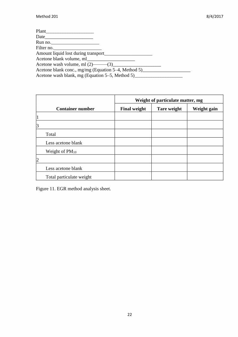
Use Figure 11 of this method to record the weights of PM collected.

4.4 Quality Control Procedures. Same as in Method 5, Section 4.4.

4.5 PM10 Emission Calculation and Acceptability of Results. Use the EGR reduction program or

the procedures in section 6 of this method to calculate PM10emissions and the criteria in section

6.7 of this method to determine the acceptability of the results.

Method 201 8/4/2017

7

5. Calibration

Maintain an accurate laboratory log of all calibrations.

5.1 Probe Nozzle. Same as in Method 5, Section 5.1.

5.2 Pitot Tube. Same as in Method 5, Section 5.2.

5.3 Meter and Flow Control Console.

5.3.1 Dry Gas Meter. Same as in Method 5, Section 5.3.

5.3.2 LFE Gauges. Calibrate the recycle, total, and inlet total LFE gauges with a manometer.

Read and record flow rates at 10, 50, and 90 percent of full scale on the total and recycle pressure

gauges. Read and record flow rates at 10, 20, and 30 percent of full scale on the inlet total LFE

pressure gauge. Record the total and recycle readings to the nearest 0.3 mm (0.01 in.). Record

the inlet total LFE readings to the nearest 3 mm (0.1 in.). Make three separate measurements at

each setting and calculate the average. The maximum difference between the average pressure

reading and the average manometer reading shall not exceed 1 mm (0.05 in.). If the differences

exceed the limit specified, adjust or replace the pressure gauge. After each field use, check the

calibration of the pressure gauges.

5.3.3 Total LFE. Same as the metering system in Method 5, Section 5.3.

5.3.4 Recycle LFE. Same as the metering system in Method 5, Section 5.3, except completely

close both the coarse and fine recycle valves.

5.4 Probe Heater. Connect the probe to the meter and flow control console with the umbilical

connector. Insert a thermocouple into the probe sample line approximately half the length of the

probe sample line. Calibrate the probe heater at 66°C (150°F), 121°C (250°F), and 177°C

(350°F). Turn on the power, and set the probe heater to the specified temperature. Allow the

heater to equilibrate, and record the thermocouple temperature and the meter and flow control

console temperature to the nearest 0.5°C (1°F). The two temperatures should agree within 5.5°C

(10°F). If this agreement is not met, adjust or replace the probe heater controller.

5.5 Temperature Gauges. Connect all thermocouples, and let the meter and flow control console

equilibrate to ambient temperature. All thermocouples shall agree to within 1.1°C (2.0°F) with a

standard mercury-in-glass thermometer. Replace defective thermocouples.

5.6 Barometer. Calibrate against a standard mercury-in-glass barometer.

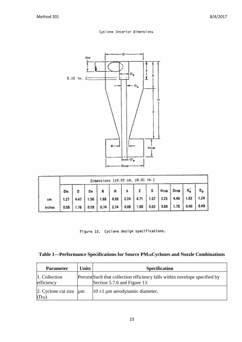
5.7 Probe Cyclone and Nozzle Combinations. The probe cyclone and nozzle combinations need

not be calibrated if the cyclone meets the design specifications in Figure 12 of this method and

the nozzle meets the design specifications in appendix B of the Application Guide for the Source

PM310 Exhaust Gas Recycle Sampling System, EPA/600/3–88–058. This document may be

obtained from Roy Huntley at (919) 541–1060. If the nozzles do not meet the design

specifications, then test the cyclone and nozzle combination for conformity with the performance

specifications (PS's) in Table 1 of this method. The purpose of the PS tests is to determine if the

cyclone's sharpness of cut meets minimum performance criteria. If the cyclone does not meet

design specifications, then, in addition to the cyclone and nozzle combination conforming to the

Method 201 8/4/2017

8

PS's, calibrate the cyclone and determine the relationship between flow rate, gas viscosity, and

gas density. Use the procedures in Section 5.7.5 of this method to conduct PS tests and the

procedures in Section 5.8 of this method to calibrate the cyclone. Conduct the PS tests in a wind

tunnel described in Section 5.7.1 of this method and using a particle generation system described

in Section 5.7.2 of this method. Use five particle sizes and three wind velocities as listed in Table

2 of this method. Perform a minimum of three replicate measurements of collection efficiency

for each of the 15 conditions listed, for a minimum of 45 measurements.

5.7.1 Wind Tunnel. Perform calibration and PS tests in a wind tunnel (or equivalent test

apparatus) capable of establishing and maintaining the required gas stream velocities within 10

percent.

5.7.2 Particle Generation System. The particle generation system shall be capable of producing

solid monodispersed dye particles with the mass median aerodynamic diameters specified in

Table 2 of this method. The particle size distribution verification should be performed on an

integrated sample obtained during the sampling period of each test. An acceptable alternative is

to verify the size distribution of samples obtained before and after each test, with both samples

required to meet the diameter and monodispersity requirements for an acceptable test run.

5.7.2.1 Establish the size of the solid dye particles delivered to the test section of the wind tunnel

using the operating parameters of the particle generation system, and verify the size during the

tests by microscopic examination of samples of the particles collected on a membrane filter. The

particle size, as established by the operating parameters of the generation system, shall be within

the tolerance specified in Table 2 of this method. The precision of the particle size verification

technique shall be at least ±0.5 µm, and the particle size determined by the verification technique

shall not differ by more than 10 percent from that established by the operating parameters of the

particle generation system.

5.7.2.2 Certify the monodispersity of the particles for each test either by microscopic inspection

of collected particles on filters or by other suitable monitoring techniques such as an optical

particle counter followed by a multichannel pulse height analyzer. If the proportion of multiplets

and satellites in an aerosol exceeds 10 percent by mass, the particle generation system is

unacceptable for purposes of this test. Multiplets are particles that are agglomerated, and

satellites are particles that are smaller than the specified size range.

5.7.3 Schematic Drawings. Schematic drawings of the wind tunnel and blower system and other

information showing complete procedural details of the test atmosphere generation, verification,

and delivery techniques shall be furnished with calibration data to the reviewing agency.

5.7.4 Flow Rate Measurement. Determine the cyclone flow rates with a dry gas meter and a

stopwatch, or a calibrated orifice system capable of measuring flow rates to within 2 percent.

5.7.5 Performance Specification Procedure. Establish the test particle generator operation and

verify the particle size microscopically. If mondispersity is to be verified by measurements at the

beginning and the end of the run rather than by an integrated sample, these measurements may

be made at this time.

5.7.5.1 The cyclone cut size (D50) is defined as the aerodynamic diameter of a particle having a

50 percent probability of penetration. Determine the required cyclone flow rate at which D50 is

10 µm. A suggested procedure is to vary the cyclone flow rate while keeping a constant particle

Method 201 8/4/2017

9

size of 10 µm. Measure the PM collected in the cyclone (mc), exit tube (mt), and filter (mf).

Compute the cyclone efficiency (Ec) as follows:

5.7.5.2 Perform three replicates and calculate the average cyclone efficiency as follows:

where E1, E2, and E3 are replicate measurements of Ec.

5.7.5.3 Calculate the standard deviation (σ) for the replicate measurements of Ec as follows:

if σ exceeds 0.10, repeat the replicate runs.

5.7.5.4 Using the cyclone flow rate that produces D50 for 10 µm, measure the overall efficiency

of the cyclone and nozzle, Eo, at the particle sizes and nominal gas velocities in Table 2 of this

method using this following procedure.

5.7.5.5 Set the air velocity in the wind tunnel to one of the nominal gas velocities from Table 2

of this method. Establish isokinetic sampling conditions and the correct flow rate through the

sampler (cyclone and nozzle) using recycle capacity so that the D50 is 10 µm. Sample long

enough to obtain ±5 percent precision on the total collected mass as determined by the precision

and the sensitivity of the measuring technique. Determine separately the nozzle catch (mn),

cyclone catch (mc), cyclone exit tube catch (mt), and collection filter catch (mf).

5.7.5.6 Calculate the overall efficiency (Eo) as follows:

5.7.5.7 Do three replicates for each combination of gas velocities and particle sizes in Table 2 of

this method. Calculate Eo for each particle size following the procedures described in this section

for determining efficiency. Calculate the standard deviation (σ) for the replicate measurements.

If σ exceeds 0.10, repeat the replicate runs.

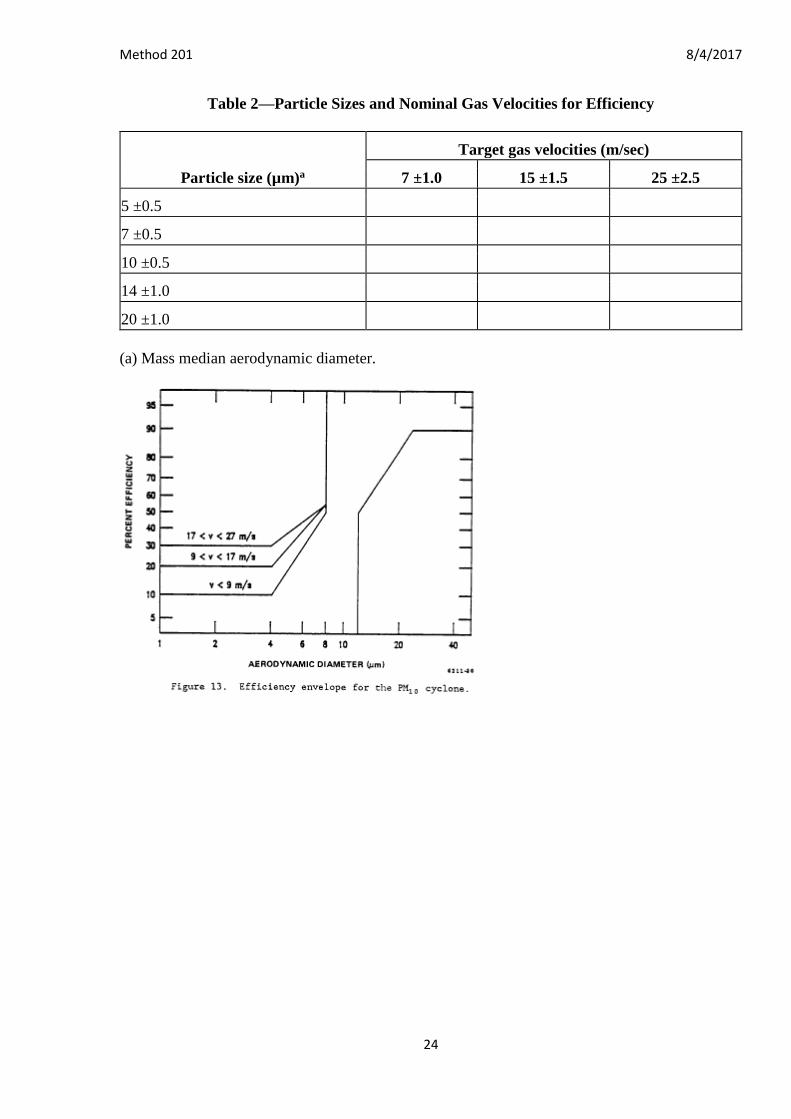
5.7.6 Criteria for Acceptance. For each of the three gas stream velocities, plot the average Eo as a

function of particle size on Figure 13 of this method. Draw a smooth curve for each velocity

Method 201 8/4/2017

10

through all particle sizes. The curve shall be within the banded region for all sizes, and the

average Ec for a D50 for 10 µm shall be 50 ±0.5 percent.

5.8 Cyclone Calibration Procedure. The purpose of this section is to develop the relationship

between flow rate, gas viscosity, gas density, and D50. This procedure only needs to be done on

those cyclones that do not meet the design specifications in Figure 12 of this method.

5.8.1 Calculate cyclone flow rate. Determine the flow rates and D50's for three different particle

sizes between 5 µm and 15 µm, one of which shall be 10 µm. All sizes must be within 0.5 µm.

For each size, use a different temperature within 60°C (108°F) of the temperature at which the

cyclone is to be used and conduct triplicate runs. A suggested procedure is to keep the particle

size constant and vary the flow rate. Some of the values obtained in the PS tests in Section 5.7.5

may be used.

5.8.1.1 On log-log graph paper, plot the Reynolds number (Re) on the abscissa, and the square

root of the Stokes 50 number [(STK50)1/2] on the ordinate for each temperature. Use the

following equations:

where:

Qcyc = Cyclone flow rate cm3/sec.

ρ = Gas density, g/cm3.

dcyc = Diameter of cyclone inlet, cm.

µcyc = Viscosity of gas through the cyclone, poise.

D50 = Cyclone cut size, cm.

5.8.1.2 Use a linear regression analysis to determine the slope (m), and the y-intercept (b). Use

the following formula to determine Q, the cyclone flow rate required for a cut size of 10 µm.

where:

Method 201 8/4/2017

11

Q = Cyclone flow rate for a cut size of 10 µm, cm3 /sec.

Ts = Stack gas temperature, °K,

d = Diameter of nozzle, cm.

K1 = 4.077×10−3.

5.8.2. Directions for Using Q. Refer to Section 5 of the EGR operators manual for directions in

using this expression for Q in the setup calculations.

6. Calculations

6.1 The EGR data reduction calculations are performed by the EGR reduction computer

program, which is written in IBM BASIC computer language and is available through NTIS,

Accession number PB90-500000, 5285 Port Royal Road, Springfield, Virginia 22161. Examples

of program inputs and outputs are shown in Figure 14 of this method.

6.1.1 Calculations can also be done manually, as specified in Method 5, Sections 6.3 through 6.7,

and 6.9 through 6.12, with the addition of the following:

6.1.2 Nomenclature.

Bc = Moisture fraction of mixed cyclone gas, by volume, dimensionless.

C1 = Viscosity constant, 51.12 micropoise for °K (51.05 micropoise for °R).

C2 = Viscosity constant, 0.372 micropoise/°K (0.207 micropoise/°R).

C3 = Viscosity constant, 1.05×10−4 micropoise/°K2 (3.24×10−5micropoise/° R2 ).

C4 = Viscosity constant, 53.147 micropoise/fraction O2.

C5 = Viscosity constant, 74.143 micropoise/fraction H2O.

D50 = Diameter of particles having a 50 percent probability of penetration, µm.

f02 = Stack gas fraction O2 by volume, dry basis.

K1 = 0.3858 °K/mm Hg (17.64 ° R/in. Hg).

Mc = Wet molecular weight of mixed gas through the PM10 cyclone, g/g-mole (lb/lb-mole).

Md = Dry molecular weight of stack gas, g/g-mole (lb/lb-mole).

Pbar = Barometer pressure at sampling site, mm Hg (in. Hg).

Pin1 = Gauge pressure at inlet to total LFE, mm H2O (in. H2O).

P3 = Absolute stack pressure, mm Hg (in. Hg).

Method 201 8/4/2017

12

Q2 = Total cyclone flow rate at wet cyclone conditions, m3/min (ft3/min).

Qs(std) = Total cyclone flow rate at standard conditons, dscm/min (dscf/min).

Tm = Average temperature of dry gas meter, °K (°R).

Ts = Average stack gas temperature, °K (°R).

Vw(std) = Volume of water vapor in gas sample (standard conditions), scm (scf).

XT = Total LFE linear calibration constant, m3/[(min)(mm H2O]) { ft3/[(min)(in. H2O)]}.

YT = Total LFE linear calibration constant, dscm/min (dscf/min).

Δ PT = Pressure differential across total LFE, mm H2O, (in. H2O).

Θ = Total sampling time, min.

µcyc = Viscosity of mixed cyclone gas, micropoise.

µLFE = Viscosity of gas laminar flow elements, micropoise.

µstd = Viscosity of standard air, 180.1 micropoise.

6.2 PM10 Particulate Weight. Determine the weight of PM10 by summing the weights obtained

from Container Numbers 1 and 3, less the acetone blank.

6.3 Total Particulate Weight. Determine the particulate catch for PM greater than PM10 from the

weight obtained from Container Number 2 less the acetone blank, and add it to the PM10

particulate weight.

6.4 PM10 Fraction. Determine the PM10fraction of the total particulate weight by dividing the

PM10particulate weight by the total particulate weight.

6.5 Total Cyclone Flow Rate. The average flow rate at standard conditions is determined from

the average pressure drop across the total LFE and is calculated as follows:

The flow rate, at actual cyclone conditions, is calculated as follows:

The flow rate, at actual cyclone conditions, is calculated as follows:

Method 201 8/4/2017

13

6.6 Aerodynamic Cut Size. Use the following procedure to determine the aerodynamic cut size

(D50).

6.6.1 Determine the water fraction of the mixed gas through the cyclone by using the equation

below.

6.6.2 Calculate the cyclone gas viscosity as follows:

µcyc = C1+ C2Ts+ C3Ts2 + C4f02− C5Bc

6.6.3 Calculate the molecular weight on a wet basis of the cyclone gas as follows:

Mc = Md(1 − Bc) + 18.0(Bc)

6.6.4 If the cyclone meets the design specification in Figure 12 of this method, calculate the

actual D50 of the cyclone for the run as follows:

where β1 = 0.1562.

6.6.5 If the cyclone does not meet the design specifications in Figure 12 of this method, then use

the following equation to calculate D50.

where:

m = Slope of the calibration curve obtained in Section 5.8.2.

b = y-intercept of the calibration curve obtained in Section 5.8.2.

6.7 Acceptable Results. Acceptability of anisokinetic variation is the same as Method 5, Section

6.12.

Method 201 8/4/2017

14

6.7.1 If 9.0 µm ≤ D50≤11 µm and 90 ≤ I ≤ 110, the results are acceptable. If D50 is greater than 11

µm, the Administrator may accept the results. If D50 is less than 9.0 µm, reject the results and

repeat the test.

7. Bibliography

1. Same as Bibliography in Method 5.

2. McCain, J.D., J.W. Ragland, and A.D. Williamson. Recommended Methodology for the

Determination of Particles Size Distributions in Ducted Sources, Final Report. Prepared for the

California Air Resources Board by Southern Research Institute. May 1986.

3. Farthing, W.E., S.S. Dawes, A.D. Williamson, J.D. McCain, R.S. Martin, and J.W. Ragland.

Development of Sampling Methods for Source PM–10 Emissions. Southern Research Institute

for the Environmental Protection Agency. April 1989.

4. Application Guide for the Source PM 10 Exhaust Gas Recycle Sampling System, EPA/600/3–

88–058.

Method 201 8/4/2017

15

Method 201 8/4/2017

16

Method 201 8/4/2017

17

EXAMPLE EMISSION GAS RECYCLE SETUP SHEET (VERSION 3.1 MAY 1986)

TEST I.D.: SAMPLE SETUP

RUN DATE: 11/24/86

LOCATION: SOURCE SIM

OPERATOR(S): RH JB

NOZZLE DIAMETER (IN): .25

STACK CONDITIONS:

AVERAGE TEMPERATURE (F): 200.0

AVERAGE VELOCITY (FT/SEC): 15.0

AMBIENT PRESSURE (IN HG): 29.92

STACK PRESSURE (IN H20): 0.10

GAS COMPOSITION:

H20=10.0% MD=28.84 O2 =20.9%MW=27.75 CO2 = 0.0%(LB/LB MOLE)

TARGET PRESSURE DROPS

TEMPERATURE (F)

DP(PTO) 150 161 172 183 194 206 217 228

0.026 SAMPLE .49 .49 .48 .47 .46 .45 .45

TOTAL 1.90 1.90 1.91 1.92 1.92 1.92 1.93

RECYCLE 2.89 2.92 2.94 2.97 3.00 3.02 3.05

% RCL 61% 61% 62% 62% 63% 63% 63%

.031 .58 .56 .55 .55 .55 .54 .53 .52

1.88 1.89 1.89 1.90 1.91 1.91 1.91 1.92

2.71 2.74 2.77 2.80 2.82 2.85 2.88 2.90

57% 57% 58% 58% 59% 59% 60% 60%

.035 .67 .65 .64 .63 .62 .61 .670 .59

1.88 1.88 1.89 1.89 1.90 1.90 1.91 1.91

2.57 2.60 2.63 2.66 2.69 2.72 2.74 2.74

54% 55% 55% 56% 56% 57% 57% 57%

.039 .75 .74 .72 .71 .70 .69 .67 .66

1.87 1.88 1.88 1.89 1.89 1.90 1.90 1.91

2.44 2.47 2.50 2.53 2.56 2.59 2.62 2.65

51% 52% 52% 53% 53% 54% 54% 55%

Figure 6. Example EGR setup sheet.

Method 201 8/4/2017

18

Barometric pressure, Pbar, in. Hg = ___

Stack static pressure, Pg, in. H2O = ___

Average stack temperature, ts, °F = ___

Meter temperature, tm, °F = ___

Gas analysis:

%CO2 = ___

%O2 = ___

%N2+%CO = ___

Fraction moisture content, Bws = ___

Calibration data:

Nozzle diameter, Dnin = ___

Pitot coefficient, Cp = ___

ΔH2, in. H2O = ___

Molecular weight of stack gas, dry basis:

Md=0.44

(%CO2)+0.32 = lb/lb mole

(%O2)+0.28

(%N2+%CO)

Molecular weight of stack gas, wet basis:

Mw=Md(1-Bws)+18Bws = ___ lb/lb mole

Absolute stack pressure:

Ps=Pbar+(Pg/13.6) = ___ in. Hg

Desired meter orifice pressure (ΔH) for velocity head of stack gas (Δp):

Figure 7. Example worksheet 1, meter orifice pressure head calculation.

Method 201 8/4/2017

19

Barometric pressure, Pbar, in. Hg = ___

Absolute stack pressure, Ps, in. Hg = ___

Average stack temperature, Ts, °R = ___

Meter temperature, Tm, °R = ___

Molecular weight of stack gas, wet basis, Mdlb/lb mole = ___

Pressure upstream of LFE, in. Hg = 0.6

Gas analysis:

%O2 = ___

Fraction moisture content, Bws = ___

Calibration data:

Nozzle diameter, Dn, in = ___

Pitot coefficient, Cp = ___

Total LFE calibration constant, Xt = ___

Total LFE calibration constant, Tt = ___

Absolute pressure upstream of LFE:

PLFE=Pbar+0.6 = ___ in. Hg

Viscosity of gas in total LFE:

µLFE=152.418+0.2552 Tm+3.2355×10−5Tm2+0.53147 (%O2) = ___

Viscosity of dry stack gas:

µd=152.418+0.2552 Ts+3.2355×10−5Ts2+0.53147 (%O2) = ___

Constants:

Total LFE pressure head:

Figure 8. Example worksheet 1, meter orifice pressure head calculation.

Method 201 8/4/2017

20

Barometric pressure, Pbar, in. Hg = ___

Absolute stack pressure, Ps, in. Hg = ___

Average stack temperature, Ts, °R = ___

Meter temperature, Tm, °R = ___

Molecular weight of stack gas, dry basis, Mdlb/lb mole = ___

Viscosity of LFE gasµLFE,poise = ___

Absolute pressure upstream of LFE, PPLEin. Hg = ___

Calibration data:

Nozzle diameter, Dn, in = ___

Pitot coefficient, Cp = ___

Recycle LFE calibration constant, Xt = ___

Recycle LFE calibration constant, Yt = ___

Pressure head for recycle LFE:

Figure 9. Example worksheet 3, recycle LFE pressure head.

Method 201 8/4/2017

21

Method 201 8/4/2017

22

Plant____________________

Date____________________

Run no.____________________

Filter no.____________________

Amount liquid lost during transport____________________

Acetone blank volume, ml____________________

Acetone wash volume, ml (2)———(3)____________________

Acetone blank conc., mg/mg (Equation 5–4, Method 5)____________________

Acetone wash blank, mg (Equation 5–5, Method 5)____________________

Container number

Weight of particulate matter, mg

Final weight Tare weight Weight gain

1

3

Total

Less acetone blank

Weight of PM10

2

Less acetone blank

Total particulate weight

Figure 11. EGR method analysis sheet.

Method 201 8/4/2017

23

Table 1—Performance Specifications for Source PM10Cyclones and Nozzle Combinations

Parameter Units Specification

1. Collection

efficiency

Percent Such that collection efficiency falls within envelope specified by

Section 5.7.6 and Figure 13.

2. Cyclone cut size

(D50)

µm 10 ±1 µm aerodynamic diameter.

Method 201 8/4/2017

24

Table 2—Particle Sizes and Nominal Gas Velocities for Efficiency

Particle size (µm)a

Target gas velocities (m/sec)

7 ±1.0 15 ±1.5 25 ±2.5

5 ±0.5

7 ±0.5

10 ±0.5

14 ±1.0

20 ±1.0

(a) Mass median aerodynamic diameter.

Method 201 8/4/2017

25

Emission Gas Recycle, Data Reduction, Version 3.4 MAY 1986

Test ID. Code: Chapel Hill 2.

Test Location: Baghouse Outlet.

Test Site: Chapel Hill.

Test Date: 10/20/86.

Operators(s): JB RH MH.

Entered Run Data

Temperatures:

T(STK) 251.0 F

T(RCL) 259.0 F

T(LFE) 81.0 F

T(DGM) 76.0 F

System Pressures:

DH(ORI) 1.18 INWG

DP(TOT) 1.91 INWG

P(INL) 12.15 INWG

DP(RCL) 2.21 INWG

DP(PTO) 0.06 INWG

Miscellanea:

P(BAR) 29.99 INWG

DP(STK) 0.10 INWG

V(DGM) 13.744 FT3

TIME 60.00 MIN

% CO2 8.00

% O2 20.00

NOZ (IN) 0.2500

Water Content:

Estimate 0.0%

Or

Condenser 7.0 ML

Column 0.0 GM

Raw Masses:

Cyclone 1 21.7 MG

Filter 11.7 MG

Impinger Residue 0.0 MG

Blank Values:

CYC Rinse 0.0 MG

Filter Holder Rinse 0.0 MG

Method 201 8/4/2017

26

Filter Blank 0.0 MG

Impinger Rinse 0.0 MG

Calibration Values:

CP(PITOT) 0.840

DH@(ORI) 10.980

M(TOT LFE) 0.2298

B(TOT LFE) −.0058

M(RCL LFE) 0.0948

B(RCL LFE) −.0007

DGM GAMMA 0.9940

Reduced Data

Stack Velocity (FT/SEC) 15.95

Stack Gas Moisture (%) 2.4

Sample Flow Rate (ACFM) 0.3104

Total Flow Rate (ACFM) 0.5819

Recycle Flow Rate (ACFM) 0.2760

Percent Recycle 46.7

Isokinetic Ratio (%) 95.1

(Particulate)

(MG/DNCM) (GR/ACF) (GR/DCF) (LB/DSCF) (X 1E6) (UM) (% <)

Cyclone 1 10.15 35.8 56.6 0.01794 0.02470 3.53701

Backup Filter 30.5 0.00968 0.01332 1.907

Particulate Total 87.2 0.02762 0.03802 5.444

Note: Figure 14. Example inputs and outputs of the EGR reduction program.