methodology note national & state level
TRANSCRIPT
Methodology Note National & State Level
Greenhouse Gas Estimates 2005 to 2015
September 2019
Agriculture, Forestry and Other Land Use Sector (AFOLU)
Sector Lead
Authors Samiksha Dhingra Deepshikha Singh Raman Mehta
Usage Policy Any re-production or re-distribution of the material(s) and information displayed and
published on the Website/GHG Platform India/Portal shall be accompanied by appropriate citation and due acknowledgment to Vasudha Foundation and the GHG Platform India for such material(s) and information. You must give appropriate credit, provide a link, and indicate if changes were made. You may do so in any reasonable manner, but not in any way that suggests the GHG Platform India endorses you or your use. Data sheets may be revised or updated from time to time. The latest version of each data sheet will be posted on the website. To keep abreast of these changes, please email us at [email protected] so that we may inform you when data sheets have been updated.
Citation Dhingra, S., Singh, D., and Mehta, R. (2019). Greenhouse Gas Emission Estimates from AFOLU (Agriculture, Forestry and Other Land Use) Sector in India at the Subnational Level (Version/edition 3.0). New Delhi. GHG Platform India Report – Vasudha Foundation. Available at: http://www.ghgplatform-india.org/methdolo-afolu-sector [Accessed Day, MO. Year]
Disclaimer The data used for arriving at the results of this study is from published, secondary sources, or wholly or in part from official sources that have been duly acknowledged. The veracity of the data has been corroborated to the maximum extent possible. However, GHG Platform India shall not be held liable and responsible to establish the veracity of or corroborate such content or data and shall not be responsible or liable for any consequences that arise from and/or any harm or loss caused by way of placing reliance on the material(s) and information displayed and published on the website or by further use and analysis of the results of this study. During peer review, inquiries and analytical procedures were followed to ascertain whether any or no material modifications to the findings are necessary and whether the methods followed are in conformity with generally accepted guidance and GHG accounting principles. The findings and conclusions in this methodology note are those of the author(s) and do not necessarily represent the views of the peer reviewers or WRI India.
Version Information / Revision history
Version Date Brief description on changes from previous version
3.0 25 September 2019 This document contains information on assumptions and the methodology followed to estimate emissions from the energy sector at the national level for the extended time period of 2005-15.
2.0 28 Sep 2017 This document contains information on assumptions and the methodology followed to estimate emissions from the energy sector at the national level for the extended time period of 2005-13.
1.0 15 July 2016 This document contains information on assumptions and the methodology followed to estimate emissions from the energy sector at the national level for the time period of 2007-13.

Foreword On December 2015, the international community took a significant step towards addressing the global challenge of climate change by endorsing the Paris Agreement at the 21st session of the Conference of Parties (COP) to the United Nations Framework Convention on Climate Change. The milestone Paris Agreement will serve as a foundation for concerted international action to address the threat posed by climate change. It is now more than clear that climate change is not the responsibility of national government only. It will impact every aspect of the society and therefore, role of non-state actors are more crucial in these testing times. Non-state actors like civil societies and research organizations can inform and help national government in devising robust climate actions and strategies. The first step to devise a robust climate action plan is creating greenhouse gas (GHG) estimates for all relevant economic sectors for recent years. With the above background, few Indian research organizations came together to form GHG Platform – India, which is a civil society initiative providing independent estimation and analysis of India’s GHG emissions. The platform is conceptualized with a noble intention to assist the national government by helping address existing data gaps and data accessibility issues, extending beyond the scope of national inventories, and increasing the volume of analytics and policy dialogue on India’s GHG emissions sources, profile, and related policies. The platform hosted GHG estimates for all key economic sectors for the period of 2005 – 2013 by accounting carbon dioxide, methane and nitrous oxide, both at national and state level. In the present edition, the time series have been extended and the report now presents GHG estimates for the period 2005 – 2015/16 across all key economic sectors. The report also highlights the trend in GHG emissions across the sectors and transparently documents all the assumptions, activity data and emission factors that were used to arrive at GHG estimates. The GHG estimates presented in the report follows 2006 IPCC guidelines for national GHG inventories and associated good practice guidance. Further, the report went through rigorous peer review and independent technical review process to ensure accuracy, transparency, consistency, completeness and relevance. On behalf of the platform, we hope that the report will be useful to all relevant stakeholders.
Credits
Led and coordinated by Srinivas Krishnaswamy Raman Mehta Samiksha Dhingra Deepshikha Singh
Peer Reviewer The authors would like to express their sincere gratitude to Mr. Subrata Chakrabarty and Mr. Chirag Gajjar from World Resources Institute India (WRII) for their valuable contribution towards comprehensive review of the methodology note.
Funder Special thanks to Shakti Sustainable Energy Foundation (SSEF) for providing financial support towards this endeavour.
Edit ing & Design Designed and formatted by Priya Kalia – Communications, Vasudha Foundation. Design reviewed by Communications Team (All partner Organizations), GHG Platform India Cover Image Photo by freestocks.org from Pexels

Contributors AFOLU Sector Samiksha Dhingra (Vasudha Foundation) Deepshikha Singh (Vasudha Foundation) Raman Mehta (Vasudha Foundation)
Acknowledgements
Vasudha Foundation would like to thank all the platform partners of the GHG Platform India, namely, Council on Energy, Environment and Water (CEEW), Center for Study of Science, Technology and Policy (CSTEP), ICLEI Local Governments for Sustainability- South Asia, and World Resources Institute (WRI) India for their continuous support to the Platform. We also express our deep gratitude to Shakti Sustainable Energy Foundation for the grant support. to the platform for the third year in a row. We acknowledge with gratitude, WRI India for providing us technical guidance in undertaking the study and conducting a comprehensive review of this report. We further would like to acknowledge and express our gratitude to the National Remote Sensing Centre, Hyderabad for providing us the Land Use Change Matrix for the period of 2006-2013.

CONTENTS Executive Summary ....................................................................................................................................... 4
Key Highlights ............................................................................................................................................ 4
ES 1. Background information of GHG emission estimates ...................................................................... 4
ES 2. Summary of GHG sources and sinks ................................................................................................. 5
ES 3. Summary of GHG trend .................................................................................................................... 5
1. Introduction and Background ............................................................................................................... 6
1.1 Context .......................................................................................................................................... 6
1.2 GHG Coverage ............................................................................................................................... 6
1.3 Key economic sectors covered...................................................................................................... 6
1.4 Boundary of GHG estimates.......................................................................................................... 7
1.5 Reporting Period ........................................................................................................................... 7
1.6 Outline of GHG estimates ............................................................................................................. 7
1.7 Institutional Information ............................................................................................................... 7
1.8 Data collection process and Storage ............................................................................................. 8
1.9 Quality Control (QC) and Quality Assurance (QA) ........................................................................ 8
1.10 General assessment of completeness .......................................................................................... 9
1.11 Recommended Improvements ................................................................................................... 10
2. Trends in GHG emissions .................................................................................................................... 10
2.1 Trend in aggregated GHG emissions ........................................................................................... 10
2.2 Trend in GHG emissions by type of GHG .................................................................................... 11
2.3 Key drivers of the emission trends in AFOLU sector ................................................................... 12
3. AFOLU ................................................................................................................................................. 14
3.1 Overview of the sector ................................................................................................................ 14
3.2 Analysis of sectoral emissions ..................................................................................................... 15
3.3 State-wise analysis of emissions ................................................................................................. 16
3.4 Sectoral Quality Control (QC) and Quality Assurance (QA) .......................................................... 0
3.5 3A Livestock ........................................................................................................................................ 0
3A1. Enteric Fermentation ........................................................................................................................ 0
3.5.1 Category description ..................................................................................................................... 0
3.5.2 Methodology ................................................................................................................................. 1
3.5.3 Recalculation ................................................................................................................................. 4
3.5.4 Uncertainties ................................................................................................................................. 4
3.5.5 Recommended Improvements ..................................................................................................... 5
3.6 3A2. Manure Management ................................................................................................................. 5

3.6.1 Category description ........................................................................................................................ 5
3.6.2 Methodology .................................................................................................................................... 6
3.6.3 Recalculation ............................................................................................................................... 11
3.6.4 Uncertainties ............................................................................................................................... 11
3.6.5 Recommended Improvements ................................................................................................... 12
3.7 3B Land .............................................................................................................................................. 12
3B1 Forestland ........................................................................................................................................ 12
3.7.1 Category description ................................................................................................................... 12
3.7.2 Methodology ............................................................................................................................... 13
3.7.3 Recalculation ............................................................................................................................... 14
3.7.4 Uncertainty ................................................................................................................................. 15
3.7.5 Recommended Improvements ................................................................................................... 15
3.8 3B2 Cropland ..................................................................................................................................... 15
3.8.1 Category description ...................................................................................................................... 15
3.8.2 Methodology ............................................................................................................................... 16
3.8.3 Recalculation ............................................................................................................................... 19
3.8.4 Uncertainty ................................................................................................................................. 19
3.8.5 Recommended Improvements ................................................................................................... 20
3.9 3B3 Grassland ............................................................................................................................. 21
3.9.1 Category description ...................................................................................................................... 21
3.9.2 Methodology ............................................................................................................................... 21
3.9.3 Recalculation ............................................................................................................................... 24
3.9.4 Uncertainty ................................................................................................................................. 24
3.9.5 Recommended Improvements ................................................................................................... 26
3.10 3B5 Settlements .......................................................................................................................... 26
3.10.1 Category description .................................................................................................................... 26
3.10.2 Methodology ............................................................................................................................... 26
3.10.3 Recalculation ............................................................................................................................... 28
3.10.4 Uncertainty ................................................................................................................................. 28
3.10.5 Recommended Improvements ................................................................................................... 30
3.11 3B6 Other Land ........................................................................................................................... 30
3.11.1 Category description .................................................................................................................... 30
3.11.2 Methodology ............................................................................................................................... 30
3.11.3 Recalculation ............................................................................................................................... 31
3.11.4 Uncertainty ................................................................................................................................. 31
3.11.5 Recommended Improvements ................................................................................................... 32
3.12 3C Aggregate Sources and Non-CO2 Emission Sources on Land ..................................................... 33
3C1a Biomass Burning in Forestland ...................................................................................................... 33
3.12.1 Category description ................................................................................................................... 33
3.12.2 Methodology ............................................................................................................................... 33
3.12.3 Recalculation ............................................................................................................................... 35
3.12.4 Uncertainty ................................................................................................................................. 35
3.12.5 Recommended Improvements ................................................................................................... 35
3.13 3C1b Biomass Burning in Cropland ............................................................................................. 36
3.13.1 Category description .................................................................................................................... 36
3.13.2 Methodology ................................................................................................................................ 36
3.13.3 Recalculation ............................................................................................................................... 38
3.13.4 Uncertainty ................................................................................................................................. 38
3.13.5 Recommended Improvements ................................................................................................... 38
3.13 Estimation of Emissions from Agricultural Soils, including from: ................................................... 38
3C4 Direct N2O emissions from managed soils and ................................................................................ 38
3C5 Indirect N2O emissions from Managed Soils.................................................................................... 38
3.14.1 Category description ................................................................................................................... 38
3.14.2 Methodology ............................................................................................................................... 39
3.14.3 Recalculation ............................................................................................................................... 41
3.14.4 Uncertainty ................................................................................................................................. 41
3.14.5 Recommended Improvements ................................................................................................... 41
3.15 3C7 Rice Cultivation .................................................................................................................... 42
3.15.1 Category description .................................................................................................................... 42
3.15.2 Methodology ............................................................................................................................... 42
3.15.3 Recalculation ............................................................................................................................... 44
3.15.4 Uncertainty ................................................................................................................................. 44
3.15.5 Recommended Improvements ................................................................................................... 44
4 Comparison with national inventories ................................................................................................ 45
Additional Information................................................................................................................................ 49
Appendix ..................................................................................................................................................... 50
Annexure I ............................................................................................................................................... 50
Annexure II ................................................................................................................................................ 0
Annexure III ............................................................................................................................................... 2
Annexure IV ............................................................................................................................................... 3

Annexure V ................................................................................................................................................ 5
Annexure VI ............................................................................................................................................... 7
ANNEXURE VII ........................................................................................................................................... 9
Annexure VIII ........................................................................................................................................... 11
Annexure IX ............................................................................................................................................. 13
Annexure X .............................................................................................................................................. 15
Annexure XI ............................................................................................................................................. 17
Annexure XII ............................................................................................................................................ 19
Annexure XIII ........................................................................................................................................... 21
Annexure IVX........................................................................................................................................... 23
Annexure XV............................................................................................................................................ 25
Annexure XVI........................................................................................................................................... 27
References .................................................................................................................................................. 30
Abbreviations .............................................................................................................................................. 38
List of Tables ............................................................................................................................................... 39
List of Figures .............................................................................................................................................. 41

Executive Summary
Key Highlights
• GHG emissions from this sector are dominated by two key source categories, viz., enteric fermentation and rice cultivation, which together accounts for approx. 76% of the GHG emissions in 2015 (excluding Land sub-sector). However, Land as a whole was a net remover of GHG emissions and removed nearly ~36% of the total emissions in 2015.
• CH4 contributes maximum to the GHG emissions with contributing percentage of ~80% within the AFOLU sector followed by N2O (~14%) and CO2 (~6%) in 20151.
ES 1. Background information of GHG emission estimates The AFOLU sector contributed almost 245.39 MtCO2e2 to the total GHG emissions of India in 2015. The detailed emissions of each of the key source categories and sub-categories is given in Table 1 below as per the IPCC format.
Table ES 1: Overview of GHG Emission Estimates by Gases and Sector for AFOLU sector3
IPCC ID Key Source category GHG Emissions (2015)
MtCO2 MtCH4 MtN2O MtCO2e
3 AFOLU -117.18 14.53 0.178 243.128
3A Livestock 10.86 0.002 228.75
3A1 Enteric Fermentation 9.86 206.97
3A2 Manure Management 1.00 0.002 21.78
3B Land -117.18 -117.18
3B1 Forest Land -124.44 -124.44
3B2 Cropland -1.32 -1.32
3B3 Grasslands 0.66 0.66
3B5 Settlements 0.49 0.49
3B6 Other Lands 7.43 7.43
3C Aggregate Sources and non-CO2 emission sources on land
3.67 0.176 131.56
3C1a Emissions from biomass burning in forest lands 0.21 0.003 5.27
3C1b Emissions from biomass burning in croplands 0.21 0.005 6.16
3C4 Direct N2O emissions from managed soils 0.134 41.46
3C5 Indirect N2O emissions from managed soils 0.034 10.52
3C7 Rice Cultivation 3.24 68.14
1 Please refer to AFOLU sector file, worksheet ‘Trends’ 2 Million tCO2 equivalent 3 Please refer to AFOLU sector file, worksheet ‘Summary”

ES 2. Summary of GHG sources and sinks GHG emissions from the AFOLU sector mainly arises from three sub-sectors namely, Livestock, Land and Aggregate sources and non-CO2 emissions sources on land. Notably, the Land sub-sector was a net remover of GHGs while the other two sub-sectors were net emitter. If the emissions were considered excluding the removals from the Land sub-sector, Livestock had the major contribution of 63% while Aggregate sources and non-CO2 emissions sources on land represented 37% of the remaining AFOLU emissions from 2005 to 2015. Livestock sub-sector is the major contributor because India has the highest cattle population in terms of density and absolute numbers. Notably, in 2015 the Land sub-sector removed nearly 36% of the GHG emissions of the AFOLU sector in India from the atmosphere.
ES 3. Summary of GHG trend In general, during the period of estimation, the GHG emissions from AFOLU sector have decreased, primarily due to increased removals of CO2 from the forests. However, a bump in the overall emissions was registered from 2012 to 2013 owing to decreased removals from the land sub-sector4. The India specific GHG emissions value has been attained by adding up the state values for all the sub-sectors. The major trends exhibited by this sector are depicted in the graph below.
4 GHG Platform India observes a dip in removals from 2012 to 2013 however, the BUR2 observes an increment from the same years in consideration. Commenting on the rationale for such increment is not possible as data and its source is unknown.
-150.00
-100.00
-50.00
0.00
50.00
100.00
150.00
200.00
250.00
300.00
350.00
2005 2006 2007 2008 2009 2010 2011 2012 2013 2014 2015
Emis
sio
n E
stim
ate
s (M
tCO
2e)
Figure 1: Trends of GHG Emissions from AFOLU sector(2005 to 2015)
Livestock Land Aggregate Sources and non-CO2 emissions sources on land AFOLU Total

1. Introduction and Background
1.1 Context The GHG estimates for the AFOLU sector being presented in this document are a part of a collaborative effort by GHG Platform India5 to build year on year estimates by collating and interpreting data that is available in the public domain. This can hopefully lead to greater discussion and debate on climate change policies and practises in India. The platform seeks to add value to various ongoing GHG estimation efforts by helping address existing data gaps and data accessibility issues, extending beyond the scope of national inventories, and by increasing the volume of analytics and policy dialogue on India's Greenhouse Gas emissions sources, profile, and related policies.
1.2 GHG Coverage The greenhouse gases (GHG) accounted for this sector are Carbon Dioxide (CO2), Methane (CH4) and Nitrous Oxide (N2O) with total carbon dioxide equivalent (CO2e) using global warming potential (GWP) and global temperature potential (GTP) from Intergovernmental Panel on Climate Change (IPCC) Assessment Reports – Second Assessment Report (SAR) and Fifth Assessment Report (AR5).
Table 1.2: Global warming potential as per IPCC assessment reports
Name of the gas Formula Global Warming Potential (GWP)
SAR AR5
Carbon dioxide CO2 1 1
Methane CH4 21 28
Nitrous oxide N2O 310 265
Source: SAR Values from (IPCC 2006); AR5 Values from (IPCC, 2014)
1.3 Key economic sectors covered Vasudha Foundation has estimated the GHG emissions for the AFOLU Sector based on the 2006 IPCC Guidelines for National GHG Inventories with all relevant calculation approaches. As indicated previously, specific source sub-categories included in the emission estimates are:
• 3A. Livestock o 3A1. Enteric Fermentation o 3A2. Manure Management
• 3B. Emissions from Land through various uses that land is put to by human interventions from o 3B1. Forest Land o 3B2. Cropland o 3B3. Grassland o 3B5. Settlements o 3B6. Other Lands
• 3C. Aggregate sources and non-CO2 emissions sources on land o 3C1a. Emissions from biomass burning in forests o 3C1b. Emissions from biomass burning in croplands
5 http://www.ghgplatform-india.org/
o 3C4. Direct N2O emissions from managed soils o 3C5. Indirect N2O emissions from managed soils o 3C7. Rice Cultivation
The emissions for all these categories have been estimated for the period 2005-2015. The emission estimates are based primarily on aggregated secondary data collected by Vasudha Foundation from nationally acceptable published documents and reports of relevant government departments, nodal agencies and research institutions in the AFOLU sector. Interactions were held with external experts and representatives to seek inputs on data availability and the emission estimation approach where required.
1.4 Boundary of GHG estimates In this study, GHG emissions have been estimated at state level and then aggregated to national level for the AFOLU sector. The greenhouse gases covered under this analysis are namely Carbon Dioxide (CO2), Methane (CH4) and Nitrous Oxide (N2O) with total carbon dioxide equivalent (CO2e). Section 1.3 of the present report provides the details of key source categories covered under the AFOLU sector.
1.5 Reporting Period Emissions are estimated from 2005 to 2015 in this study. The base year for these emission estimates is 2005. From the perspective of data availability and India’s NDC, which chooses 2005 as the base year for its pledges, the year 2005 is of historical and administrative importance and hence, has been considered as the base year for these calculations.
1.6 Outline of GHG estimates This exercise entails a time-series emission estimate for sectors mentioned in section 1.3 at the state (sub-national) level, for the period 2005 to 2015. The estimations were based on literature review and followed the 2006 IPCC Guidelines for National GHG Inventories and other internationally acceptable guidance. Emissions were estimated based on fuel sources, sub-sectoral activities, and emission factors. Chapter 2 provides the trends in GHG emissions and the key drivers of emission trends in various sectors. Chapter 3 provides the overview of the AFOLU sector, detailed analysis of the sectoral emissions, methodology involved, source of activity data, and emission factors. Chapter 4 broadly compares the emissions estimated for 2007, 2010, and 2014 with the emissions reported by MoEFCC.
1.7 Institutional Information Vasudha Foundation, New Delhi is involved in preparation of emission estimates from the AFOLU sector for GHG Platform India. Given below is the technical competence of the staff involved in this exercise: Raman Mehta Raman is currently the Director of Programmes at Vasudha Foundation. He is also the Lead for the work on Agriculture, Forests and Other Land Use Sector Emissions Estimations for the GHG Platform India Programme. [email protected]
Samiksha Dhingra Samiksha is a Programmes Manager at Vasudha Foundation. She is managing the GHG Platform India project at Vasudha Foundation. Along with the secretariat responsibilities, she is also involved in emission estimation for the AFOLU sector. At Vasudha she has also worked on projects related to adaptation, energy mapping, renewable energy, and climate policy. Her areas of interest include urban services, environment, renewable energy, climate change, and sustainability. [email protected] Deepshikha Singh Deepshikha mostly worked on projects related to GHG emission reduction. Her key areas of work are climate change, sustainable development, environmental impact assessment and climate change. Presently, she is part of GHG Platform India where she is responsible for handling the Secretariat as well as the GHG emission estimates from the AFOLU sector. [email protected]
1.8 Data collection process and Storage To ensure estimates from the emission source categories represent the AFOLU sector in India, state and country-specific data has been used in the assessment to the extent possible. The data has been primarily collected through an extensive secondary research. The data collection exercise focussed on gathering reliable information from peer-reviewed published documents and reports of relevant government departments, nodal agencies and research institutions including Ministry of Agriculture and Farmers Welfare (MoAFW), Ministry of Statistics and Programme Implementation (MOSPI), Forest Survey of India (FSI) and National Remote Sensing Centre (NRSC) among others. The data collected was in various forms and units and has been assessed to ensure its applicability within the emission estimation boundaries and subsequently processed for further use. All the data collected for emission estimation was in the form of a soft copy, no data was obtained in its hard form. The emission estimation method, reporting period, boundaries, year-wise activity data, emission factors and relevant parameters along with data sources and any assumptions to address gaps, and national-level emission results have been transparently recorded in this reporting document and in excel spreadsheets to provide clear understanding and to enable reconstruction of the emission estimations as required. All information collected and compiled for the emission estimates has been archived electronically in separate folders for future use as needed along with copies of relevant references or data sources. The final emission estimates and reporting documents are published and available on the GHG Platform India website (www.ghgplatform-india.org).
1.9 Quality Control (QC) and Quality Assurance (QA) To prepare the expanded national-level emission estimates, secondary data research was undertaken for the years 2005 to 2015 for all sub-sectors with regards to parameters such as agricultural production, livestock population, land use change matrix etc. Interactions have been held with relevant experts as needed. The aggregate sources emission estimates for 2005 to 2013 have been revisited and have been refined based on updated information on activity data and related parameters. The emission estimation process involved regular discussions and reporting of progress between the project partners. Reporting formats were also developed for clear and transparent documentation and reporting of the methodology and results of the emission estimation.

Quality controls applied to the emission estimates include generic quality checks in terms of the calculations, processing, consistency, and clear recording and documentation as follows:
• The input activity data for each emission source sub-category has been selected from that available in different datasets by duly factoring in its relative time-series consistency and temporal and spatial applicability;
• The input data in the calculation sheets has been checked internally for transcription errors on a sample basis for all the 3 key source categories;
• The calculation spreadsheets have been checked for correct application of formulae, activity and factors and to ensure that calculations are correct. Manual calculations have been carried out for a part of the emission estimates in all 3 key source categories to verify the spreadsheets results;
• Appropriate recording, conversions, processing and consistency of measurement units for parameters and emission has been checked across the reporting period;
• The emission estimates of each year of the reporting period have been compared on a year on year basis and with the published GoI inventory to check for consistency in trends and detect any major deviations which cannot be correlated with corresponding changes in activity data and/or emission factors;
• The emission calculation equations, relevant data and parameter values used, intermediate formulae and cells wherein these are linked, and emission results are clearly depicted in the calculation spreadsheets for all 3 key source categories;
• The reporting document has been checked to confirm all relevant references and secondary sources for activity data and emission factors have been included and documented;
• Emission source categories and sub-categories included and excluded in the emission estimates have been transparently reported. Any known gaps in the emission estimates along with rationale of assumptions used to address data gaps have been clearly indicated in the reporting document;
1.10 General assessment of completeness
Table 1.10: Details of key source categories excluded from present GHG estimates
Sector IPCC ID
Category description Reason for exclusion
AFOLU 3B4 Wetlands Lack of availability of activity data
3C1c Emissions from Biomass Burning in Grassland
Lack of availability of activity data
3C1d Emissions from Biomass Burning in Other Land
Negligible incidences of biomass burning in other land
3C2 Liming Lack of availability of activity data
3C3 Urea Fertilization Lack of availability of activity data
3C6 Indirect N2O emissions from Manure Management
Lack of availability of activity data
Emissions from the source categories mentioned above are not included in the estimates due to the lack of reliable data for these sources such as in the case of wetlands or biomass burning in other lands, or due to there being very negligible incidence of such activities in the country, such as liming.

Due to lack of availability of activity data and emission factors specific to IPCC 2006 methodology guidance, emissions from biomass burning in forestland and cropland are limited to the methodology available in NATCOM II6 in this assessment.
1.11 Recommended Improvements The major recommendations that emanate from this exercise are as follows: • While it is difficult for the platform to address the gap on its own, there is a need to engage with more
relevant authorities to begin doing the apt surveys to collect the required data regarding the AFOLU subsectors.
• More specific emission factors, disaggregated at the state level if possible, need to be developed to make more precise calculations for AFOLU sector as a whole.
2. Trends in GHG emissions
2.1 Trend in aggregated GHG emissions
The above graph shows that the total emissions from AFOLU sector followed a linear trend from 254.85 MtCO2e in 2005 to 243.12 MtCO2e in 2015. A slight rise in the overall emissions was registered in 2012 and 2013 which can be attributed to slight decrease in absorption of GHGs from India’s forests due to reduction in net carbon stock from 2011 to 2013.
Table 2.1: AFOLU Sector trend of GHG Emission estimates by source categories
Key source Category Emissions in million tCO2e %change
2005 2007 2010 2015 2005-2007
2005-2010
2005-2015
6http://www.environmentportal.in/files/NATCOM.pdf
254.85 261.86 267.42 267.30 264.36 266.28 270.06291.74 292.00
240.84 243.12
-150.00
-100.00
-50.00
0.00
50.00
100.00
150.00
200.00
250.00
300.00
350.00
2005 2006 2007 2008 2009 2010 2011 2012 2013 2014 2015
Emis
sio
n E
stim
ates
(M
tCO
2e)
Figure 2: Trends of GHG Emissions from AFOLU sector(2005 to 2015)
Livestock Land Aggregate Sources and non-CO2 emissions sources on land AFOLU Total

Livestock 219.79 230.28 226.29 228.75 4.78% 2.96% 4.08%
Land -90.20 -90.20 -92.07 -117.18 0.00% 2.03% 29.92%
Aggregate Sources and non-CO2 emission sources on land
125.26 127.34 132.06 131.56 1.66% 5.43% 5.03%
Emissions from the livestock sub-sector i.e. enteric fermentation and manure management contribute a major share in the AFOLU sector. The emissions from this sector saw an insignificant rise in 2007 after which they were found to decrease due to decline in the livestock population from 2007 onwards. However, emissions from the livestock sub-sector grew at a nominal CAGR of 0.43% from 219.05 MtCO2e in 2005 to 228.73 MtCO2e in 2015 and were mostly flat. As seen in the graph above, CO2 removals from the Land sub-sector followed a linear trend from 2005 to 2011 and saw a dip in 2012 and 2013. This deterioration in emission removals from -90.71 MtCO2e in 2011 to -65.09 MtCO2e in 2012 can be attributed to decrease in carbon stock in forest lands. However, a significant rise in the overall CO2removals was observed from 2014 (-117.18 MtCO2e) onwards. Emissions from the category (3C) Aggregate sources and non-carbon dioxide emission sources on land were found to increase marginally over the years with a CAGR of 0.41% from 124.77 MtCO2e in 2005 to 129.99 MtCO2e in 2015. Rice cultivation had the major share of ~51% in the total emissions of this sub-sector followed by emissions from the Agricultural Soils (~40%).
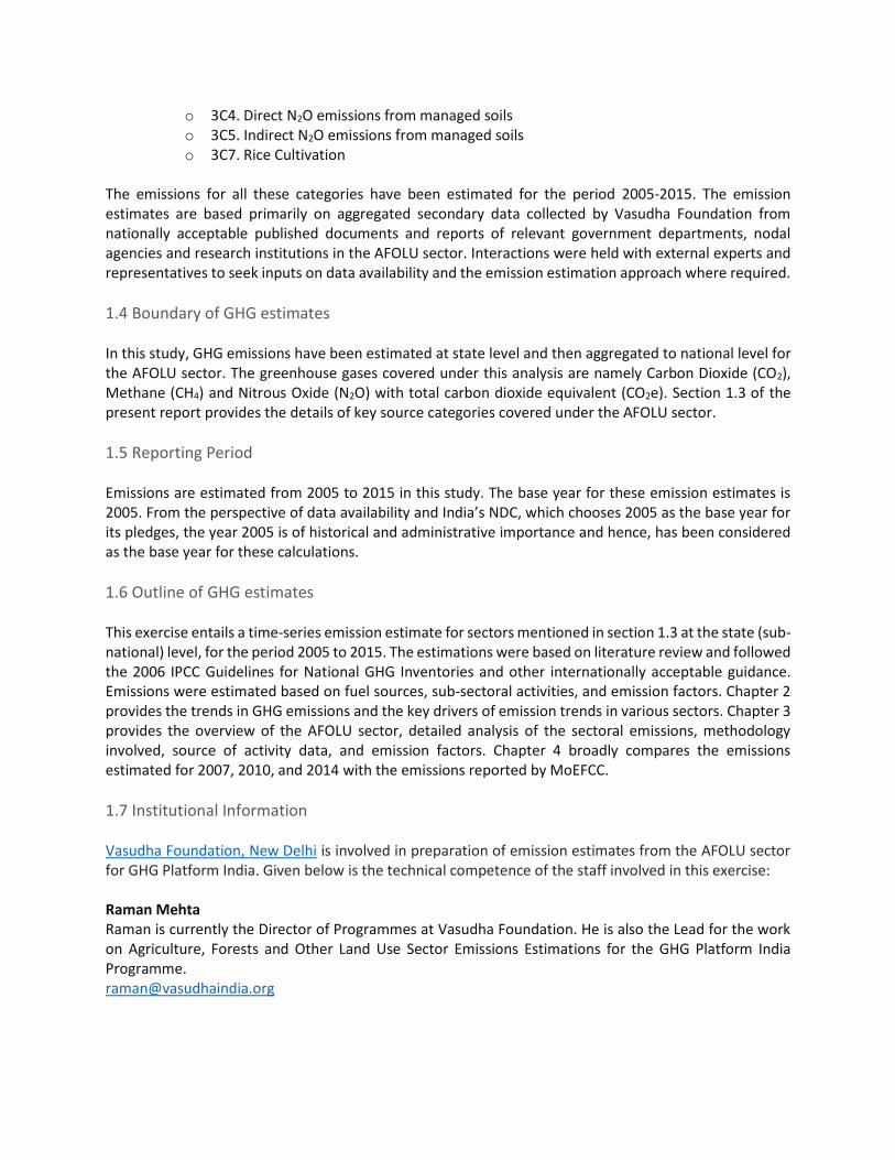
2.2 Trend in GHG emissions by type of GHG The Trend of GHG emissions by the type of GHG is given below. CH4 remained the maximum contributor to the emissions of the AFOLU sector across all the years. Significant emissions are also registered from N2O gas. Notably, CO2 gas was a net remover of GHG emissions throughout the reference period.
The overall share of each greenhouse gas (GHG) in the total AFOLU emissions is illustrated below.
2005 2006 2007 2008 2009 2010 2011 2012 2013 2014 2015
CO2 -90.20 -90.20 -90.20 -92.07 -92.07 -92.07 -90.71 -65.09 -65.09 -117.18 -117.18
N2O 47.34 47.86 48.37 50.15 51.76 54.71 57.35 56.49 54.28 54.05 55.19
CH4 297.71 304.20 309.25 309.23 304.67 303.64 303.42 300.34 302.82 303.97 305.12
Total 254.85 261.86 267.42 267.30 264.36 266.28 270.06 291.74 292.00 240.84 243.12
254.85 261.86 267.42 267.30 264.36 266.28 270.06 291.74 292.00240.84 243.12
-150.00-100.00
-50.000.00
50.00100.00150.00200.00250.00300.00350.00
Emis
sio
n e
stim
ates
(M
tCO
2e)
Figure 3: Trend of GHG Emissions by type of GHG in the AFOLU sector (2005 to 2015)
CO2 N2O CH4 Total
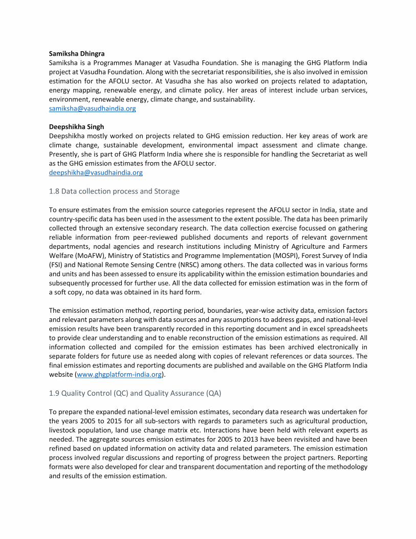
Distribution of emissions from different key source categories is given in the table 2.2 below.
2.3 Key drivers of the emission trends in AFOLU sector The key drivers of emissions from the AFOLU sector are livestock population, forests, rice cultivation and fertilizer use. Since these drivers are either stagnant or declining, the overall emissions of the AFOLU sector have remained stagnant. The emission estimates from each of the key category sources is elaborated below.
-60%
-40%
-20%
0%
20%
40%
60%
80%
100%
120%
140%
2005 2006 2007 2008 2009 2010 2011 2012 2013 2014 2015
% S
har
e in
to
tal G
HG
Em
issi
on
s
Figure 4: Overall Contribution of each Gas in the AFOLU sector Emissions(2005 to 2015)
CO2 N2O CH4
Table 2.2: AFOLU Sector distribution of emission contribution by sector for 2015
IPCC ID Key source category %CO2 %CH4 %N2O
3A Livestock 74.74% 1.26%
3B Land
100% (Removals)
- -
3C Aggregate Sources and non-CO2 emission sources on land
25.26% 98.74%

Emissions from the livestock category i.e. enteric fermentation and manure management contribute a major share in the AFOLU sector. The emissions from this sector saw an insignificant rise in 2007 after which they were found to decrease due to decline in the livestock population from 2007 onwards. However, emissions from the livestock category grew at a nominal CAGR of 0.40% from 219.79 MtCO2e in 2005 to 228.75 MtCO2e in 2015 and were mostly flat (Figure 5).
As seen in the figure 6 above, CO2 removals from the Land sub-sector followed a linear trend from 2005 to 2011 and saw a dip in 2012 and 2013. This deterioration in emission removals from 90.71 MtCO2e to -65.09 MtCO2e from 2011 to 2012 can be attributed to decrease in carbon stock in forest lands. However, a significant rise in the overall CO2removals was observed from 2014 (-117.18 MtCO2e) onwards.
219.79 225.03 230.28 228.95 227.62 226.29 224.96 223.63 224.60 226.30 228.75
0.00
50.00
100.00
150.00
200.00
250.00
2005 2006 2007 2008 2009 2010 2011 2012 2013 2014 2015
Emis
sio
n E
stim
ates
(M
tCO
2e)
Figure 5: Trends of GHG Emissions from (3A) Livestock Sub-sector (2005 to 2015)
Enteric Fermentation Manure Management Livestock
-90.20 -90.20 -90.20 -92.07 -92.07 -92.07 -90.71
-65.09 -65.09
-117.18 -117.18
-150.00
-130.00
-110.00
-90.00
-70.00
-50.00
-30.00
-10.00
10.00
2005 2006 2007 2008 2009 2010 2011 2012 2013 2014 2015
Emis
sio
n E
stim
ates
(M
tCO
2e)
Figure 6: Trends of GHG Emissions from the (3B) Land Sub-sector (2005 to 2015)
Cropland Forest Land Grassland Other Land Settlements Land
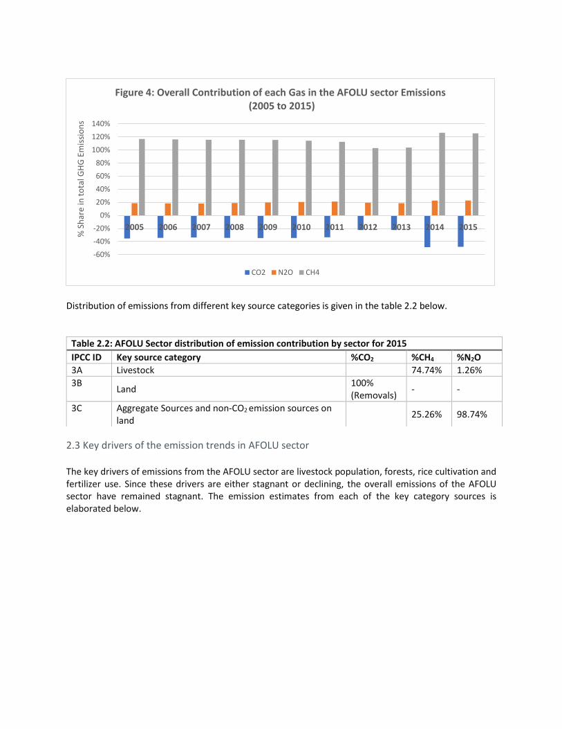
Emissions from the category (3C) Aggregate sources and non-carbon dioxide emission sources on land were found to increase marginally over the years with a CAGR of 0.41% from 124.77 MtCO2e in 2005 to 129.99 MtCO2e in 2015 (Figure 7). Rice cultivation had the major share of ~54% in the total emissions of this category followed by emissions from the Agricultural Soils (~38%).
From the above discussion it can be concluded that the most important contribution of GHG emissions in the AFOLU sector are from CH4 emissions of livestock and rice cultivation.
3. AFOLU
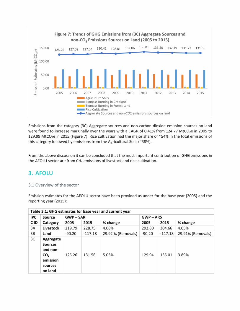
3.1 Overview of the sector Emission estimates for the AFOLU sector have been provided as under for the base year (2005) and the reporting year (2015):
Table 3.1: GHG estimates for base year and current year
IPCC ID
Source Category
GWP – SAR GWP – AR5
2005 2015 % change 2005 2015 % change
3A Livestock 219.79 228.75 4.08% 292.80 304.66 4.05%
3B Land -90.20 -117.18 29.92 % (Removals) -90.20 -117.18 29.91% (Removals)
3C Aggregate Sources and non-CO2
emission sources on land
125.26 131.56 5.03% 129.94 135.01 3.89%
125.26 127.02 127.34 130.42 128.81 132.06 135.81 133.20 132.49 131.72 131.56
0.00
50.00
100.00
150.00
2005 2006 2007 2008 2009 2010 2011 2012 2013 2014 2015Emis
sio
n E
stim
ates
(M
tCO
2e)
Figure 7: Trends of GHG Emissions from (3C) Aggregate Sources andnon-CO2 Emissions Sources on Land (2005 to 2015)
Agriculture SoilsBiomass Burning in CroplandBiomass Burning in Forest LandRice CultivationAggregate Sources and non-CO2 emissions sources on land

Between 2005 and 2015, there has been a decrease of approximately 0.48% compounded annually in the CO2 equivalent emissions from this sector for India. This is primarily due to increase of carbon dioxide removals from the atmosphere by the forests.
3.2 Analysis of sectoral emissions
Category wise analysis of sectoral emissions is as follows:
Table 3.2: Category wise Analysis of GHG Emissions Estimates (2005-2015) in million tCO2e IPCC ID
Category description
2005 2006 2007 2008 2009 2010 2011 2012 2013 2014 2015
3A Livestock 219.79 225.03 230.28 228.95 227.62 226.29 224.96 223.63 224.60 226.30 228.75
3B Land -90.20 -90.20 -90.20 -92.07 -92.07 -92.07 -90.71 -65.09 -65.09 -117.18
-117.18
3C Aggregate Sources and non-CO2 emissions sources on land
125.26 127.02 127.34 130.42 128.81 132.06 135.81 133.20 132.49 131.72 131.56
GHG emissions from the AFOLU sector mainly arises from three sub-sectors namely, Livestock, Land and Aggregate sources and non-CO2 emissions sources on land. Notably, the Land sub-sector was a net remover of GHGs while the other two sub-sectors were net emitter. In 2015, if the emissions were considered excluding the removals from the Forest Land sub-sector, Livestock had the major contribution of 59.98% while Aggregate sources and non-CO2 emissions sources on land contributed to 34.49% of the total AFOLU emissions followed by very minor contribution of 5.53% by the Land sector. Notably, Forest land sequestered 36.26% of the GHG emissions from the atmosphere.
0.24 0.25 0.25 0.24 0.24 0.23 0.230.25 0.24
0.20 0.20
-0.15
-0.10
-0.05
0.00
0.05
0.10
0.15
0.20
0.25
0.30
2005 2006 2007 2008 2009 2010 2011 2012 2013 2014 2015
tCO
2e p
er c
apit
a
Figure 8: Per Capita GHG Emissions from the AFOLU sector (2005 to 2015)
Aggregate Sources and non-CO2 emissions sources on land Land Livestock AFOLU Sector

The per capita GHG emissions of the AFOLU sector in the country were found to be decreasing at a compounded rate of 2.06% from 0.19 tCO2e in 2005 to 0.20 tCO2e in 2015. This decline in the per capita emissions can be attributed to the increase in removals from Indian forests and also an increase in the population of India coupled with an overall stagnation of the positive emissions from this sector.
The emissions intensity (emissions per unit of GDP PPP) of India from AFOLU sector witnessed a downward trend at a compounded rate of 6.77% due to a slight fall in emissions from this sector and a significant rise in India’s GDP contributions from sectors other than AFOLU (using GDP values from Ministry of Statistics Planning and Implementation7)
3.3 State-wise analysis of emissions States with maximum emissions from the AFOLU sector in year 2005 and 2015 are as follows.
Table 3.3: State-wise GHG estimates 2005 - 2015(in MtCO2e)
Name of the State 2005
2006
2007
2008
2009
2010
2011
2012
2013
2014
2015
Andaman and Nicobar Island
-7.11
-7.11
-7.10
-7.11
-7.11
-7.11
-7.13
-1.17
-1.17
0.36 0.36
Andhra Pradesh 5.35 5.84 6.13 6.42 5.47 6.55 6.23 -
8.25 -
9.63
-18.9
6
-19.7
2
Arunachal Pradesh -
20.64
-20.6
6
-20.6
6
-20.9
5
-20.9
4
-20.9
2
-20.7
5 5.47 5.49 6.42 6.28
7 For 2004-05 to 2011-12: http://pibphoto.nic.in/documents/rlink/2018/nov/p2018112801.pdf Fore 2011-12 to 2015-16: http://www.mospi.nic.in/sites/default/files/press_release/FRE%20of%20National%20Income%2C%20Consumption%20Expenditure%2C%20Saving%20and%20Capital%20Formation%20For%202017-18_0.pdf
43.0940.97
38.86 37.6834.55
32.08 30.91 31.67 29.79
22.88 21.38
-20.00
-10.00
0.00
10.00
20.00
30.00
40.00
50.00
2005 2006 2007 2008 2009 2010 2011 2012 2013 2014 2015
Emis
sio
ns/
GD
P
Figure 9: Emission Intensity of AFOLU Sector ( tCO2e per Crore)
Aggregate Sources and non-CO2 emissions sources on land Land Livestock Total

Assam 8.95 8.84 9.24 9.62 9.80 10.0
3 10.0
8 13.9
2 13.8
4 5.81 5.91
Bihar 24.2
6 25.2
3 25.9
2 25.8
0 25.2
4 24.7
4 25.8
6 26.0
2 25.8
3 25.1
8 26.2
9
Chandigarh 0.02 0.02 0.02 0.02 0.02 0.02 0.02 -
0.06 -
0.06 0.02 0.02
Chhattisgarh 9.92 10.0
6 10.1
9 10.1
1 10.1
4 10.2
0 9.96
15.80
15.82
15.00
14.91
Dadra and Nagar Haveli
0.12 0.13 0.13 0.13 0.12 0.12 0.12 0.14 0.14 0.03 0.03
Daman and Diu 0.00 0.00 0.00 0.00 0.00 0.00 -
0.01 -
0.08 -
0.08 0.00 0.00
Delhi 0.23 0.25 0.26 0.24 0.23 0.21 0.19 0.13 0.12 0.18 0.18
Goa -
1.01 -
1.01 -
1.02 -
1.02 -
1.03 -
1.03 -
1.03 0.27 0.26
-0.18
-0.18
Gujarat 19.0
5 19.4
5 19.8
8 20.5
1 20.9
2 21.9
1 22.5
0 20.2
3 21.0
5 22.0
4 22.4
0
Haryana 10.5
6 10.5
9 10.6
4 10.8
0 10.9
2 11.0
5 11.2
5 11.1
4 11.0
9 11.0
8 11.3
6
Himachal Pradesh -
0.60 -
0.60 -
0.59 -
0.65 -
0.69 -
0.72 -
0.59 2.20 2.18
-5.70
-5.70
Jammu and Kashmir -
0.19 -
0.10 -
0.02 -
0.33 -
0.47 -
0.62 -
0.61 -
5.41 -
5.54 -
1.39 -
1.47
Jharkhand 6.55 6.93 7.20 7.09 6.68 6.26 6.54 9.48 9.43 9.68 10.5
7
Karnataka 11.9
4 12.3
3 12.7
2 12.7
8 12.8
1 12.8
5 12.8
7 7.49 7.23
-10.9
0
-11.2
8
Kerala -
1.34 -
1.42 -
1.52 -
1.57 -
1.63 -
1.70 -
1.84
-30.8
4
-30.8
5
-23.7
4
-23.7
9
Lakshadweep 0.01 0.01 0.01 0.01 0.01 0.01 0.01 0.01 0.01 0.01 0.01
Madhya Pradesh 27.0
3 27.8
3 28.6
1 27.7
4 27.4
0 26.9
7 27.3
0 27.7
3 27.7
4 26.0
8 26.0
5
Maharashtra 34.4
0 34.5
2 34.7
7 34.5
8 34.6
3 35.0
3 34.3
6 22.8
2 23.0
5 24.4
7 24.0
2
Manipur -
0.61 -
0.63 -
0.66 -
0.65 -
0.66 -
0.63 -
0.61 -
0.47 -
0.42 -
2.95 -
3.00
Meghalaya -
2.29 -
2.28 -
2.25 -
2.28 -
2.28 -
2.27 -
2.25 1.33 1.34 2.85 2.86
Mizoram -
0.76 -
0.76 -
0.76 -
0.80 -
0.81 -
0.83 -
0.85 3.47 3.47 5.32 5.34
Nagaland 0.23 0.25 0.24 0.24 0.20 0.18 0.17 2.71 2.70 9.02 8.99
Odisha 11.5
5 11.2
7 10.8
0 10.1
8 9.95
10.22
9.73 16.8
3 17.0
3 4.17 3.88
Puducherry 0.15 0.14 0.14 0.12 0.12 0.12 0.10 0.01 0.01 0.15 0.15

Punjab 11.8
1 11.6
4 11.5
1 11.7
1 11.9
0 12.1
3 12.2
9 12.9
5 12.9
2 11.8
4 12.2
8
Rajasthan 25.0
2 25.4
7 25.9
2 25.1
3 25.4
8 26.2
0 28.2
1 26.9
3 27.3
9 23.5
4 24.4
3
Sikkim -
4.01 -
4.02 -
4.02 -
3.94 -
3.95 -
3.95 -
3.89 0.34 0.35 0.47 0.50
Tamil Nadu 18.5
3 19.0
5 19.3
5 19.1
4 18.4
9 18.0
1 17.5
7
-24.7
0
-25.0
9
11.50
11.78
Telangana 16.2
5 16.7
5 17.1
1 17.1
5 16.4
1 16.9
4 16.5
7 46.1
4 46.8
8 4.87 3.88
Tripura -
1.58 -
1.57 -
1.53 -
1.62 -
1.64 -
1.62 -
1.62 0.89 0.89 3.73 3.77
Uttar Pradesh 46.0
5 45.9
6 45.9
7 48.1
5 48.9
6 50.1
1 51.3
5 55.6
3 56.6
5 54.7
4 55.9
9
Uttarakhand 2.78 2.92 3.09 2.97 2.90 2.84 2.85 8.32 8.30 2.71 2.77
West Bengal 4.24 6.55 7.73 7.59 6.78 5.02 5.14 24.3
1 23.6
6 23.3
9 23.2
4
India 254.
85 261.
86 267.
42 267.
30 264.
36 266.
28 270.
06 291.
74 292.
00 240.
84 243.
12
As seen above, maximum GHG emissions arise from the state of Uttar Pradesh. This is because Uttar Pradesh has a high density of livestock population contributing to maximum livestock emissions from the country. Also, the removals of emissions from Uttar Pradesh’s forest are only around 4.34 MtCO2e, which is low compared to the other states.

3.4 Sectoral Quality Control (QC) and Quality Assurance (QA) A summary of the key source category-wise description of the quality assessment and quality control processes undertaken is given below.
Table 3.4: Summary of Quality Assessment and Quality Control Processes
IPCC Category Activity Data Source Type of Source
Emission Factor Data Processing Strategy
Bifurcation of data for Andhra Pradesh and Telangana from Unified Andhra Pradesh before 2012
3A1Enteric Fermentation
Livestock Census of India for 2007 and 2012
Official, Publicly Available
NATCOM-II: Indigenous cattle, Cross bred Cattle and Buffalo IPCC 2006: Rest of the Categories
Data has been interpolated and extrapolated for the years where the data was unavailable
District -wise proportion of the Livestock population was taken and apportioned to the total population of livestock before bifurcation to attain the new values. 3A2 Manure
Management
3B1 Forest Land Forest Survey of India
Official, Publicly Available
2005-2009: FSI, Carbon Report8 2010-2015: FSI, State of Forest Report,20179
Data has been interpolated and extrapolated for the years where the data was unavailable
Actual District-wise forest area has been taken for the calculations.
3B2 Cropland National Remote Sensing Centre (available on request)
Official, Available on Request
Biomass: Forest Survey of India, State of Forest report SOC: Sreenivas et.al SOC (Cropland): Expert Literature10
The Proportion of the new Andhra Pradesh and Telangana area were assigned to gain the land use change.
3B3 Grassland
3B4 Wetlands
3B5 Settlements
3B6 Other Lands
3C1a Biomass Burning in Forest Land
Forest Survey of India
Official, Publicly Available
NATCOM-II No Data Extrapolation/ Interpolation
Proportion of the forest area burnt in Andhra Pradesh and Telangana was available in Reddy et.al.
8 http://fsi.nic.in/carbon_stock/chapter-4.pdf 9 http://fsi.nic.in/isfr2017/isfr-carbon-stock-in-india-forest-2017.pdf 10 The values have been taken from various literatures the links to which can be found in the bibliography.
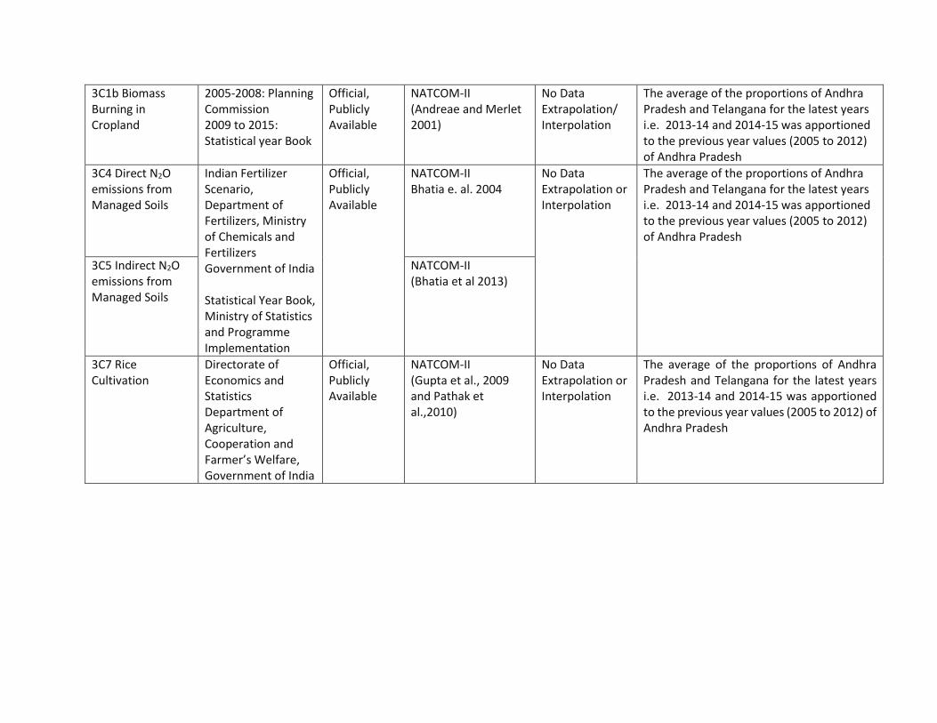
3C1b Biomass Burning in Cropland
2005-2008: Planning Commission 2009 to 2015: Statistical year Book
Official, Publicly Available
NATCOM-II (Andreae and Merlet 2001)
No Data Extrapolation/ Interpolation
The average of the proportions of Andhra Pradesh and Telangana for the latest years i.e. 2013-14 and 2014-15 was apportioned to the previous year values (2005 to 2012) of Andhra Pradesh
3C4 Direct N2O emissions from Managed Soils
Indian Fertilizer Scenario, Department of Fertilizers, Ministry of Chemicals and Fertilizers Government of India Statistical Year Book, Ministry of Statistics and Programme Implementation
Official, Publicly Available
NATCOM-II Bhatia e. al. 2004
No Data Extrapolation or Interpolation
The average of the proportions of Andhra Pradesh and Telangana for the latest years i.e. 2013-14 and 2014-15 was apportioned to the previous year values (2005 to 2012) of Andhra Pradesh
3C5 Indirect N2O emissions from Managed Soils
NATCOM-II (Bhatia et al 2013)
3C7 Rice Cultivation
Directorate of Economics and Statistics Department of Agriculture, Cooperation and Farmer’s Welfare, Government of India
Official, Publicly Available
NATCOM-II (Gupta et al., 2009 and Pathak et al.,2010)
No Data Extrapolation or Interpolation
The average of the proportions of Andhra Pradesh and Telangana for the latest years i.e. 2013-14 and 2014-15 was apportioned to the previous year values (2005 to 2012) of Andhra Pradesh

Given below is a detailed explanation of the quality assessment and quality control processes undertaken:
• All the parameters, units and conversion factors have been labelled properly. If any assumptions have been made for calculations, it has been cross-verified with the associated external expert and explanation for the same has been provided.
• The activity data and emission factors used has been properly archived within the calculation sheets. Extrapolation and interpolation for years for which data is not available has been done through assuming a linear trend.
• Data entry was done in-house, and validation of data was done through sample checks physically as well as through validation techniques such as through plotting and using trend charts.
• Sources of the data and emission factors has been cited across this document and the calculation sheets.
• The emission factors and other conversion factors applied for emission estimates are consistent across the categories and also across the years. If there is a different emission factor used for any source category, a valid justification regarding the same has been provided in this document.
• In terms of completeness, the exercise has covered all the categories and sub-categories from AFOLU sector responsible for emissions in India unless they are not relevant to the country or there is no data available for making any estimations what so ever.
• The draft estimates are peer reviewed by WRI India. WRI India reviewed the data points (including but not limited to AD, EF, etc.) on sample basis and ensured consistency of methodology with internationally acceptable standards and guidelines like IPCC, etc.
3.5 3A Livestock
3A1. Enteric Fermentation
3.5.1 Category description Enteric Fermentation resulting in emissions of CH4 arises out of the process of ingesting and digesting of food eaten by herbivores, primarily bovines and ovine. However, other animals such as camels, horses and mules etc. also emit small amounts of CH4. The activity data has been sourced from the Livestock Census of India and the type and quality of data is given below. The data quality is considered high because the activity data has been obtained from credible and relevant Government of India sources that have been engaged in collecting such data every five years for several decades. Further, the credibility of the data is acknowledged by all the relevant stakeholders both within and outside the Government.
Table 3.5A: Source category wise details on type of data, quality and source
IPCC ID GHG Source & Sink Categories Type Quality Source
3. AFOLU
3A Livestock
3A1 Enteric Fermentation
3A1a Cattle Secondary High 18th Livestock Census 19th Livestock Census 3A1ai Dairy cows (Indigenous and Cross Bred) Secondary High
3A1aii Other cattle or Non-dairy cows (Indigenous and Cross Bred)
Secondary High

3A1b Buffalo (dairy and non-dairy) Secondary High http://dahd.nic.in/documents/statistics/livestock-census
3A1c Sheep Secondary High
3A1d Goats Secondary High
3A1e Camels Secondary High
3A1f Horses and ponies Secondary High
3A1g Donkeys Secondary High
3A1h Pigs Secondary High
3.5.2 Methodology Methane emissions from Enteric Fermentation have been calculated using methodology prescribed in 2006 IPCC guidelines for national GHG inventories. To ensure consistency with India’s National Communication Reports and the Biennial Update Report 2010, the emission inventory for all sub-sectors has been prepared on a calendar year basis. Activity datasets for emission estimations available on financial year basis have been converted to calendar year datasets for a given calendar year by considering 3/4th of the value from the previous financial year (corresponding to 9 months from April to December out of 12 months in a year) and 1/4th from the next financial year (corresponding to 3 months from January to March out of 12 months in a year)11. CO2 emissions from livestock are not estimated because annual net CO2 emissions are assumed to be zero – the CO2 photosynthesized by plants is returned to the atmosphere as respired CO2. (Chapter 10, Volume 4, IPCC 2006). Similarly, as no nitrogen is released during the process of digestion in livestock, no nitrous oxide (N2O) emissions are reported. The methodological details for estimation of GHG emissions for enteric fermentation are as follows:
Table 3.5B: Source category wise details on tier approach and type of emission factor used
IPCC ID
GHG source & sink categories
CO2 CH4 N2O
Method Applied
Emission Factor
Method Applied
Emission Factor
Method Applied
Emission Factor
3A1 Enteric Fermentation Not Applicable Not Applicable
3A1a Cattle T2 CS
3A1ai Dairy cows (Indigenous and Cross Bred)
T2 CS
3A1aii Other cattle or Non-dairy cows (Indigenous and Cross Bred)
T2 CS
3A1b Buffalo (dairy and non-dairy)
T2 CS
3A1c Sheep T2 CS
3A1d Goats T2 CS
3A1e Camels T1 D
3A1f Horses and ponies T1 D
3A1g Donkeys T1 D
3A1h Pigs T1 D Note: T1: Tier 1; T2: Tier 2; T3: Tier 3; CS: Country-specific; PS: Plant-specific; D: IPCC default
11 This has been applied to the data sets of all key source categories unless otherwise mentioned.

The activity data i.e. the livestock population is sourced from the Livestock Census of India published every five years by the Department of Animal Husbandry, Dairying and Fisheries, Ministry of Agriculture and Farmers Welfare. The Livestock census have been used for the years 2002, 2007 and 2012. Emission factors for bovines12, sheep and goats have been sourced from the NATCOM II and for the remaining other animals IPCC Default emission factors have been used. Therefore, a Tier II methodology has been used for major methane emitting categories (i.e. bovines, sheep and goats) and Tier I methodology has been used where country specific emission factors were not available. The following steps were performed for emission estimation from enteric fermentation: Step 1. Livestock Population Estimation As a first step, the average annual population of animals was taken from the Census of Livestock. Categorization was done as per available categories in the emission factors viz. dairy and non-dairy for cattle (indigenous cows, crossbred cows and buffaloes). In this analysis, mules and asses are not added in the total livestock population as their population is miniscule and the relative emissions are negligible. The details regarding categorisation are given in the table 3.5C below:
Table 3.5C: Categorization of livestock for derivation of methane emission factors
Category Sub category
a) Mature dairy cows (Mature cows that have calved at least once and used principally for milk production)
“Cross-bred” dairy cows “Indigenous cows” (non-descript or desi) dairy cows. “Buffaloes”
b) Non-dairy cattle Young cattle (cross bred cows, indigenous cows and buffaloes):
• Below 1 year13
• 1-3 years14 Others (cross bred cows, indigenous cows and buffaloes):
• Male (Breeding, Working and Others)
• Female (Non-dairy adults)
c) Goats Mature (1 year and above) Young (less than 1 year)
d) Sheep Mature (1 year and above) Young (less than 1 year)
e) Camels No classification
f) Horses and ponies No classification
g) Pigs No classification
12 Bovines refers to Cattles and Buffaloes (both Dairy and Non-Dairy) 13 Based on NATCOM II, emission factors are available for cattle population categories of crossbred, buffalo, and indigenous cattle for age group below 1 year. However, census data category provides data for under 1 year. Therefore, the emission factor for population below one year has been applied to the category titled under one year. 14 Based on NATCOM II, emission factors are available for cattle population categories of crossbred, buffalo, and indigenous cattle for age group 1 to 3 years. However, census data category provides data for 1 to 2.5 years. Therefore, the emission factor for population between 1 to 3-year has been applied to the category titled 1 to 2.5 years.

Livestock populations for the intermediate years between the livestock census years were calculated from the annual increment of population between the two census years (For e.g. 2002 and 2007). Given below is an example of the formula used:
𝐴𝐼𝑅 =𝑃𝑜𝑝𝑢𝑙𝑎𝑡𝑖𝑜𝑛 𝑖𝑛 𝑌2 − 𝑃𝑜𝑝𝑢𝑙𝑎𝑡𝑖𝑜𝑛 𝑖𝑛 𝑌1
𝑛
𝑃𝑜𝑝𝑢𝑙𝑎𝑡𝑖𝑜𝑛 𝑖𝑛 𝑌3 = 𝑃𝑜𝑝𝑢𝑙𝑎𝑡𝑖𝑜𝑛 𝑖𝑛 𝑌2 + 𝐴𝐼𝑅
Where, AIR = Annual Increment Ratio Population in Y = Population in Year 1, 2, 3… etc n = Number of Years Livestock population from the succeeding year i.e. 2013 has been derived from the CAGR computed between 2007 and 2012 for the various categories of livestock populations. Formula used for calculating the future population:
𝐶𝐴𝐺𝑅 = (𝐹𝑉
𝐵𝑉)
1𝑛⁄
− 1
Where, CAGR = Compounded Annual Growth Rate FV = Future Value BV = Beginning Value n = Number of Years Step 2: Emission Factor Estimation Methane emission factors for the livestock categories have been sourced from NATCOM II and IPCC 2006. Table 3.5D below provides emission factors for each sub-group:
Table 3.5D: Emission factor of each sub-group in terms of kilograms of methane per animal per year
Category Sub-category Age group Methane emission factor Source
(kgCH4/head/year)
Indigenous Cattle
Dairy cattle Indigenous 28.00 NATCOM II, 2012
Non-dairy cattle (indigenous)
0-1 year 9.00 NATCOM II, 2012
1-3 year 23.00 NATCOM II, 2012
Adult 32.00 NATCOM II, 2012
Cross-bred cattle
Dairy cattle Cross-bred 43.00 NATCOM II, 2012
Non-dairy cattle (cross-bred)
0-1 year 11.00 NATCOM II, 2012
1-3 year 26.00 NATCOM II, 2012
Adult 33.00 NATCOM II, 2012
Buffalo Dairy buffalo 50.00 NATCOM II, 2012
Non-dairy buffalo
0-1 year 8.00 NATCOM II, 2012
1-3 year 22.00 NATCOM II, 2012
Adult 44.00 NATCOM II, 2012
Sheep 5.00 IPCC 2006
Goat 5.00 IPCC 2006
Horses & Ponies 18.00 IPCC 2006
Donkeys 10.00 IPCC 2006
Camels 46.00 IPCC 2006
Pigs 1.00 IPCC 2006
Poultry 0.00 IPCC 2006
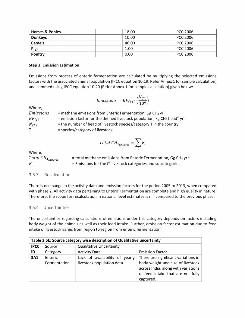
Step 3: Emission Estimation Emissions from process of enteric fermentation are calculated by multiplying the selected emissions factors with the associated animal population (IPCC equation 10.19, Refer Annex 1 for sample calculation) and summed using IPCC equation 10.20 (Refer Annex 1 for sample calculation) given below:
𝐸𝑚𝑖𝑠𝑠𝑖𝑜𝑛𝑠 = 𝐸𝐹(𝑇) ⋅ (𝑁(𝑇)
106)
Where, 𝐸𝑚𝑖𝑠𝑠𝑖𝑜𝑛𝑠 = methane emissions from Enteric Fermentation, Gg CH4 yr-1
𝐸𝐹(𝑇) = emission factor for the defined livestock population, kg CH4 head-1 yr-1
𝑁(𝑇) = the number of head of livestock species/category T in the country
T = species/category of livestock
𝑇𝑜𝑡𝑎𝑙 𝐶𝐻4𝐸𝑛𝑡𝑒𝑟𝑖𝑐= ∑ 𝐸𝑖
𝑖
Where, 𝑇𝑜𝑡𝑎𝑙 𝐶𝐻4𝐸𝑛𝑡𝑒𝑟𝑖𝑐
= total methane emissions from Enteric Fermentation, Gg CH4 yr-1
𝐸𝑖 = Emissions for the ith livestock categories and subcategories
3.5.3 Recalculation There is no change in the activity data and emission factors for the period 2005 to 2013, when compared with phase 2. All activity data pertaining to Enteric Fermentation are complete and high quality in nature. Therefore, the scope for recalculation in national level estimates is nil, compared to the previous phase.
3.5.4 Uncertainties The uncertainties regarding calculations of emissions under this category depends on factors including body weight of the animals as well as their feed intake. Further, emission factor estimation due to feed intake of livestock varies from region to region from enteric fermentation.
Table 3.5E: Source category wise description of Qualitative uncertainty
IPCC ID
Source Category
Qualitative Uncertainty
Activity Data Emission Factor
3A1 Enteric Fermentation
Lack of availability of yearly livestock population data
There are significant variations in body weight and size of livestock across India, along with variations of feed intake that are not fully captured.

3.5.5 Recommended Improvements As and when data that captures the diversity of livestock, for both body weight and feed intake, in India becomes available, it will be utilised for more precise emission estimations from this source.
3.6 3A2. Manure Management
3.6.1 Category description Manure management emissions arise from the process of animal’s manure decomposition. In general, emissions vary depending on the type of decomposition – aerobic or anaerobic. If manure is decomposed naturally i.e. aerobically, little or no emissions are produced. However, if manure is treated anaerobically, higher emissions are observed. Manure management results in CH4 and N2O emissions. CO2 emissions from livestock are not estimated because annual net CO2 emissions are assumed to be zero – the CO2 photosynthesized by plants is returned to the atmosphere as respired CO2 (Chapter 10, Volume 4, IPCC 2006). Methane emissions from manure management tend to be smaller than enteric emissions, with the most substantial emissions associated with confined animal management operations where manure is handled in liquid-based systems. Nitrous oxide emissions from manure management vary significantly between the types of management system used and can also result in indirect emissions due to other forms of nitrogen loss from the system (Chapter 10, Volume 4, IPCC 2006). The activity data has been sourced from the Livestock Census of India and the type and quality of data is given below. The data quality is considered high because the activity data has been obtained from credible and relevant Government of India sources that have been engaged in collecting such data every five years for several decades. Further, the credibility of the data is acknowledged by all the relevant stakeholders both within and outside the Government.
Table 3.6A: Source category wise details on type of data, quality and source
IPCC ID GHG Source & Sink Categories Type Quality Source
3. AFOLU
3A Livestock
3A2 Manure Management
3A2a Cattle Secondary High 18th Livestock Census 19th Livestock Census http://dahd.nic.in/documents/statistics/livestock-census
3A2ai Dairy cows (Indigenous and Cross Bred) Secondary High
3A2aii Other cattle or Non-dairy cows (Indigenous and Cross Bred)
Secondary High
3A2b Buffalo (dairy and non-dairy) Secondary High
3A2c Sheep Secondary High
3A2d Goats Secondary High
3A2e Camels Secondary High
3A2f Horses and ponies Secondary High
3A2g Donkeys Secondary High
3A2h Pigs Secondary High

3.6.2 Methodology Methane emissions from manure management have been calculated using the methodology provided in 2006 IPCC guidelines for national GHG inventories. The methodological details (Tier approach) for estimation of GHG emissions for manure management are as follows:
Table 3.6B: Source category wise details on tier approach and type of emission factor used
IPCC ID
GHG source & sink categories
CO2 CH4 N2O
Method Applied
Emission Factor
Method Applied
Emission Factor
Method Applied
Emission Factor
3A2a Manure Management Not Applicable
3A2ai Cattle T2 CS T1 D
3A2aii Dairy cows (Indigenous and Cross Bred)
T2 CS T1 D
3A2b Other cattle or Non-dairy cows (Indigenous and Cross Bred)
T2 CS T1 D
3A2c Buffalo (dairy and non-dairy)
T2 CS T1 D
3A2d Sheep T2 CS T1 D
3A2e Goats T2 CS T1 D
3A2f Camels T1 D T1 D
3A2g Horses and ponies T1 D T1 D
3A2h Donkeys T1 D T1 D
3A2a Pigs T1 D T1 D Note: T1: Tier 1; T2: Tier 2; T3: Tier 3; CS: Country-specific; PS: Plant-specific; D: IPCC default
The activity data i.e. the livestock population is sourced from the 18th and 19th Livestock Census of India, published every five years by the Department of Animal Husbandry, Dairying and Fisheries, Ministry of Agriculture and Farmers Welfare. The Livestock census has been used for the years 2002, 2007 and 2012. Methane emission factors for bovines15, sheep and goats have been sourced from the NATCOM II and for the other remaining animals IPCC default emission factors have been used. IPCC default emission factors16 have been used for estimating N2O emissions for all the categories. Therefore, for CH4 emissions, a Tier II methodology has been used for major methane emitting categories (i.e. bovines, sheep and goats) and Tier I methodology has been used where country specific emission factors were not available. For N2O emissions, a Tier I methodology has been adopted. The following steps were performed for CH4 emission estimation from manure management: Step 1. Livestock Population Estimation
15 Bovines refers to Cattles and Buffaloes (both Dairy and Non-Dairy) 16 Most expert literatures available in the public domain state that they are using IPCC, 2006 N2O for emissions factors but they still use the IPCC 1996 N2O emissions factors for calculations. The same has been done in the present study.

As a first step, the average annual population of animals was taken from the Census of Livestock. Categorization was done as per available categories in the census viz. dairy and non-dairy for cattle (indigenous cows, crossbred cows and buffaloes). In this analysis, mules and asses are not added in the total livestock population as there are no emissions from the same. The details regarding categorisation are given in the table 3.6C below:
Table 3.6C: Categorization of livestock for derivation of methane emission factors
Category Sub category
a) Mature dairy cows (Mature cows that have calved at least once and used principally for milk production)
“Cross-bred” dairy cows “Indigenous cows” (non-descript or desi) dairy cows. “Buffaloes”
b) Non-dairy cattle Young cattle (cross bred cows, indigenous cows and buffaloes):
• Below 1 year17
• 1-3 years18 Others (cross bred cows, indigenous cows and buffaloes):
• Male (Breeding, Working and Others)
• Female (Non-dairy adults)
c) Goats Mature (1 year and above) Young (less than 1 year)
d) Sheep Mature (1 year and above) Young (less than 1 year)
e) Camels No classification
f) Horses and ponies No classification
g) Pigs No classification
Livestock populations for the intermediate years between the livestock census years were calculated from the annual increment of population between the two census years (For e.g. 2002 and 2007). Given below is an example of the formula used:
𝐴𝐼𝑅 =𝑃𝑜𝑝𝑢𝑙𝑎𝑡𝑖𝑜𝑛 𝑖𝑛 𝑌2 − 𝑃𝑜𝑝𝑢𝑙𝑎𝑡𝑖𝑜𝑛 𝑖𝑛 𝑌1
𝑛
𝑃𝑜𝑝𝑢𝑙𝑎𝑡𝑖𝑜𝑛 𝑖𝑛 𝑌3 = 𝑃𝑜𝑝𝑢𝑙𝑎𝑡𝑖𝑜𝑛 𝑖𝑛 𝑌2 + 𝐴𝐼𝑅
where, AIR = Annual Increment Ratio Population in Y = Population in Year 1, 2, 3… etc n = Number of Years
17 Based on NATCOM II, emission factors are available for cattle population categories of crossbred, buffalo, and indigenous cattle for age group below 1 year. However, census data category provides data for under 1 year. Therefore, the emission factor for population below one year has been applied to the category titled under one year. 18 Based on NATCOM II, emission factors are available for cattle population categories of crossbred, buffalo, and indigenous cattle for age group 1 to 3 years. However, census data category provides data for 1 to 2.5 years. Therefore, the emission factor for population between 1 to 3-year has been applied to the category titled 1 to 2.5 years.

Livestock population from the succeeding year i.e. 2013 has been derived from the CAGR computed between 2007 and 2012 for the various categories of livestock populations. Formula used for calculating the future population:
𝐶𝐴𝐺𝑅 = (𝐹𝑉
𝐵𝑉)
1𝑛⁄
− 1
Where, CAGR = Compounded Annual Growth Rate FV = Future Value BV = Beginning Value n = Number of Years Step 2: Emission Factor Estimation Methane emission factors for the livestock categories have been sourced from NATCOM II and IPCC 2006. The table 3.6D mentioned below provides emission factors for each sub-group:
Table 3.6D: Emission factor of each sub-group in terms of kilograms of methane per animal per year
Category Sub-category Age group Methane emission factor Source
(kgCH4/head/year)
Indigenous Cattle Dairy cattle Indigenous 3.50 NATCOM II, 2012
Non-dairy cattle (indigenous)
0-2 year 1.20 NATCOM II, 2012
1-3 year 2.80 NATCOM II, 2012
Adult 2.90 NATCOM II, 2012
Cross-bred cattle Dairy cattle Cross-bred 3.80 NATCOM II, 2012
Non-dairy cattle (cross-bred)
0-1 year 1.10 NATCOM II, 2012
1-3 year 2.30 NATCOM II, 2012
Adult 2.50 NATCOM II, 2012
Buffalo Dairy buffalo 4.40 NATCOM II, 2012
Non-dairy buffalo
0-1 year 1.80 NATCOM II, 2012
1-3 year 3.40 NATCOM II, 2012
Adult 4.00 NATCOM II, 2012
Sheep 0.20 IPCC 2006
Goat 0.22 IPCC 2006
Horses & Ponies 2.19 IPCC 2006
Donkeys 0.90 IPCC 2006
Camels 2.56 IPCC 2006
Pigs 4.00 IPCC 2006
Poultry 0.00 IPCC 2006
Step 3: Emission Estimation Emissions from the process of manure management are calculated by multiplying the selected emissions factors with the associated animal population (IPCC equation 10.22, Refer Annex 1 for Sample Calculation) as given below:

𝐶𝐻4𝑀𝑎𝑛𝑢𝑟𝑒= ∑
(𝐸𝐹(𝑇) ⋅ 𝑁(𝑇))
106
(𝑇)
Where, 𝐶𝐻4𝑀𝑎𝑛𝑢𝑟𝑒
= methane emissions from Manure Management, Gg CH4 yr-1
𝐸𝐹(𝑇) = emission factor for the defined livestock population, kg CH4 head-1 yr-1
𝑁(𝑇) = the number of head of livestock species/category T in the country
T = species/category of livestock Step 4: Emissions from all livestock categories are added to get total methane emissions from manure management. The following steps were performed for N2O emission estimation from manure management: Step 1. Livestock Population Estimation As a first step, the average annual population of animals was taken from the Census of Livestock. Categorization was done as per available categories in the census viz. dairy and non-dairy for cattle (indigenous cows, crossbred cows and buffaloes). In this analysis, mules and asses are not added in the total livestock population as there are no emissions from the same. The details regarding categorisation are given in the table 3.6E below:
Table 3.6E: Categorization of livestock for derivation of methane emission factors
Category Sub category
a) Mature dairy cows (Mature cows that have calved at least once and used principally for milk production)
▪ “Cross-bred” dairy cows ▪ “Indigenous cows” (non-descript or desi) dairy cows. ▪ “Buffaloes”
b) Non-dairy cattle ▪ Young cattle (cross bred cows, indigenous cows and buffaloes): a) Below 1 year19 b) 1-3 years20
▪ Others (cross bred cows, indigenous cows and buffaloes): a) Male (Breeding, Working and Others) b) Female (Non-dairy adults)
c) Goats ▪ Mature (1 year and above) ▪ Young (less than 1 year)
d) Sheep ▪ Mature (1 year and above) ▪ Young (less than 1 year)
19 Based on NATCOM II, emission factors are available for cattle population categories of crossbred, buffalo, and indigenous cattle for age group below 1 year. However, census data category provides data for under 1 year. Therefore, the emission factor for population below one year has been applied to the category titled under one year. 20 Based on NATCOM II, emission factors are available for cattle population categories of crossbred, buffalo, and indigenous cattle for age group 1 to 3 years. However, census data category provides data for 1 to 2.5 years. Therefore, the emission factor for population between 1 to 3-year has been applied to the category titled 1 to 2.5 years.

e) Camels No classification
f) Horses and ponies No classification
g) Pigs No classification
Livestock populations for the intermediate years between the livestock census years was calculated from the annual increment of population between the two census years (For e.g. 2002 and 2007). Given below is an example of the formula used:
𝐴𝐼𝑅 =𝑃𝑜𝑝𝑢𝑙𝑎𝑡𝑖𝑜𝑛 𝑖𝑛 𝑌2 − 𝑃𝑜𝑝𝑢𝑙𝑎𝑡𝑖𝑜𝑛 𝑖𝑛 𝑌1
𝑛
𝑃𝑜𝑝𝑢𝑙𝑎𝑡𝑖𝑜𝑛 𝑖𝑛 𝑌3 = 𝑃𝑜𝑝𝑢𝑙𝑎𝑡𝑖𝑜𝑛 𝑖𝑛 𝑌2 + 𝐴𝐼𝑅
where, AIR = Annual Increment Ratio Population in Y = Population in Year 1, 2, 3… etc n = Number of Years Livestock population from the succeeding year i.e. 2013 has been derived from the CAGR computed between 2007 and 2012 for the various categories of livestock populations. Formula used for calculating the future population:
𝐶𝐴𝐺𝑅 = (𝐹𝑉
𝐵𝑉)
1𝑛⁄
− 1
Where, CAGR = Compounded Annual Growth Rate FV = Future Value BV = Beginning Value n = Number of Years Step 2: Emission Factor Estimation For calculating nitrogen excretion, IPCC values21 were used for estimating nitrogen excretion, per animal. The values adopted were: Dairy cattle - 60 kg N/ animal/ year Non-dairy cattle - 40 kg N/ animal/ year Pigs - 16 kg N/ animal/ year Poultry - 0.6 kg N/ animal/ year The following nitrogen emission factors were used as per 2006 IPCC Guidelines:
Table 3.6F: Nitrogen Emission Factors
Category of Livestock Nitrogen emissions per animal (kgN2O/head/year)
Dairy cattle 0.0006
Non-dairy cattle 0.0004
Pigs 0.0074
Poultry 0.0025
21 IPCC 2006 Guidelines, Chapter 10, Table 10.19, summarized from IPCC 1996 Guidelines, Chapter 4, Table B1, http://www.ipcc-nggip.iges.or.jp/public/gl/guidelin/ch4ref8.pdf

Step 3 & 4: Emission Estimation Total emissions were determined by multiplying the number of animals in each category with emission factor. Nitrogen emissions from manure management are calculated using the below mentioned equation in step 5. However, under this exercise, emission factor was obtained from India’s second national communications to the UNFCCC. N2O emissions were calculated in the following manner: IPCC equation 10.2522 (Refer Annex I for sample calculations) that was used was the following:
𝑁2𝑂𝑎𝑛𝑖𝑚𝑎𝑙𝑠 = 𝑁2𝑂𝐴𝑊𝑀𝑆 = ∑[𝑁𝑇 ⋅ 𝑁𝑒𝑥(𝑇) ⋅ 𝐴𝑊𝑀𝑆𝑇 ⋅ 𝐸𝐹3(𝐴𝑊𝑀𝑆)] ⋅44
28
where, 𝑁2𝑂𝑎𝑛𝑖𝑚𝑎𝑙𝑠 = N2O emissions from animal production in a country (kg N/yr) 𝑁2𝑂𝐴𝑊𝑀𝑆 = N2O emissions from Animal Waste Management System in the country (kg N/yr); 𝑁𝑇 = number of animals of type T in the country 𝑁𝑒𝑥(𝑇) = N excretion of animals of type T in the country (kg N/animal/yr)
𝐴𝑊𝑀𝑆𝑇 = fraction of 𝑁𝑒𝑥(𝑇) that is managed in one of the different distinguished animal waste
management systems for animals of type T in the country 𝐸𝐹3(𝐴𝑊𝑀𝑆) = N2O emission factor for an AWMS (kg N2O -N/ kg of 𝑁𝑒𝑥 in AWMS)
T = type of animal category 44/28 = conversion of (N2O-N) emissions to N2O emissions Step 5: Emissions from all categories are aggregated and total emission expressed as Gg N2O/ year. Emissions (Gg/ Year) = EF (kg/ head/ year) x population/ 10^6 kg/ Gg.
3.6.3 Recalculation No recalculation was performed for estimating emissions from this category because the activity data, emissions factor and methodology was the same as used for Phase II estimates. There was no new data source used, no error was observed and no new methodology was used.
3.6.4 Uncertainties Uncertainty in emission estimation from manure management arises due to activity data and emission factors. Activity data on manure yields and their end uses is not fully known in Indian context, and therefore, a quantitative measure of uncertainty cannot be made. Similarly, country specific emission factors are available only for bovines. There is uncertainty associated with the same as there is limited research available on country specific emission factors.
22 http://www.ipcc-nggip.iges.or.jp/public/2006gl/pdf/4_Volume4/V4_10_Ch10_Livestock.pdf - page 10.53

Table 3.6G: Source category wise description of Qualitative uncertainty
IPCC ID
Source Category
Qualitative Uncertainty
Activity Data Emission Factor
3A2 Manure Management
Lack of availability of yearly livestock population data
Precise data on manure yields and their end uses is not fully known under Indian conditions.
3.6.5 Recommended Improvements As and when data that captures the manure yields in the Indian subcontinent become available, as well as more precise information on manure management systems is also made available, these estimates can become more precise.
3.7 3B Land
3B1 Forestland
3.7.1 Category description This section provides details of emission estimates from Forestland due to changes in biomass, dead organic matter and soil organic matter on Forest Land and Land converted to Forest Land. For this study, Land Use Matrix for forestland remaining forestland and land converted to forestland has been derived from the biennially updated ‘State of Forest Report (SFR)’ from Forest Survey of India. For the State of Forest Report, FSI maps forest cover through satellite data with a Linear Imaging and Self Scanning Sensor (LISS) III sensor. In India, all lands that occupy an area more than one hectare and have a canopy density of more than 10% irrespective of the ownership and legal status are called Forest Cover. FSI does not make any distinction whether the forest is natural or man-made, government or private, recorded or not recorded. For stratification of the activity data, FSI uses two variables namely forest types and canopy density. It also includes bamboo, orchards, palms etc. Given below are details of activity data used in the sub-category. The data quality is considered high because the activity data has been obtained from credible and relevant Government of India sources that have been engaged in collecting such data every five years. Further, the credibility of the data is acknowledged by all the relevant stakeholders both within and outside the Government.
Table 3.7A: An overview of source categories of Forest Land
IPCC ID GHG source & sink categories Type Quality Source
3B Land
3B1 Forest Land23 Secondary Data High State of Forest Reports: 2017 2015
23 The estimates given in this report only refer to the overall areas under forests and the carbon stock contained within them. Data at the national level is not available for forest land remaining forest land and land other than forest land converted to forest land

2013 2011 2009 2005
3.7.2 Methodology For GHG estimation from forestland in India, the Stock-Difference Method is applied along with country specific estimates of activity data and emission factors, in-line with section 4.2.1.1 – choice of method, Volume 4, Chapter 4, 2006 IPCC Guidelines. As per IPCC equation 2.5, Volume 4, Chapter 2, 2006 IPCC Guidelines24, it can be used where carbon stocks in relevant pools are measured at two points in time to assess carbon stock changes, as represented in equation given below (Refer Annex I for sample calculations):
𝛥𝐶 =(𝐶𝑡2
− 𝐶𝑡1)
(𝑡2 − 𝑡1)
where, 𝛥𝐶 is Annual Carbon stock change in pool (tonnes C yr-1) 𝐶𝑡2
is Carbon stock in the pool at time t2
𝐶𝑡1 is Carbon stock in the pool at time t1
The following steps were performed for emission estimation from Forestland: Step 1. Estimation of Area Area under Forest Land Remaining Forestland and Land converted to Forestland is estimated. Table 3.7B below provides details of the tier approach and types of emission factors used for forest land:
Table 3.7B: An overview of emission factors used for forestland
IPCC ID GHG source & sink categories CO2
Method Applied Emission Factor
3B1 Forest Land T2 CS Notes: T1: Tier 1; T2: Tier 2; T3: Tier 3; CS: Country-specific; PS: Plant-specific; D: IPCC default
The area is sourced from the State of Forest Reports (SFR) for India published biannually by Forest Survey of India (FSI). The reports used in this study are SFR 2009, SFR 2011, SFR 2013, SFR 2015 and SFR 2017. The FSI provides Forestland remaining Forestland and Land converted to Forestland in these reports. For the years that FSI does not publish the data, the area is interpolated using a linear trend. Step 2: Emission Factor Estimation Emission factor estimation, i.e. the change in the carbon stock and biomass in case of forestland is registered from the Forest Survey of India’s Report on Carbon Stock in India. FSI’s Carbon Stock Report, 201125 gives the carbon stock density under five different pools for the forests in year 2009 for all states and UTs. The five pools mentioned in this report are Above Ground Biomass, Below Ground Biomass,
24 http://www.ipcc-nggip.iges.or.jp/public/2006gl/pdf/4_Volume4/V4_02_Ch2_Generic.pdf 25 See table 4.4 available at http://fsi.nic.in/carbon_stock/chapter-4.pdf

Deadwood, Litter and Soil Organic Carbon. The carbon stock density under these pools is updated and is provided in the SFR 2017 for all Indian states and UTs. Carbon stock for each year in consideration is estimated by multiplying the carbon stock density under different pools with the area under forestland for that year. From 2005 to 2010, the carbon stock density from the Carbon Stock Report is considered and is multiplied with the Forest area till 2010. From 2011 onwards, the carbon stock density is used from the SFR 2017 report. Step 3: Emission Estimation In cases where forestland remains as forestland, carbon removal from the atmosphere due to biomass growth and loss due to disturbance and biomass removals (both fuel wood and timber) are considered. The annual carbon stock changes for each land category is calculated as a sum of changes in all carbon pools of above-ground biomass, below-ground biomass, deadwood, litter, soils and harvested wood products. IPCC’s Stock Exchange Methodology has been used with Equation 2.5 (Refer the methodology section on Page 42, Section 3.6.2 for equation). A bottom up approach has been used for estimating emissions from forestland. Since, SFR reports carbon stock change in fiscal year, the platform reports emission estimates in fiscal year (assumed to be same as calendar year for LULUCF sector).
3.7.3 Recalculation
Table 3.7C: Source category wise details on the difference between GHG estimates
Year Key source category GHG Emission Estimates (MtCO2e) % Difference
Phase-II Phase-III
2005 Forest Land -145.62 -97.97 -33%
2006 Forest Land -145.62 -97.97 -33%
2007 Forest Land -145.62 -97.97 -33%
2008 Forest Land -145.62 -97.97 -33%
2009 Forest Land -145.62 -97.97 -33%
2010 Forest Land -145.62 -97.97 -33%
2011 Forest Land -188.83 -97.97 -48%
2012 Forest Land -188.83 -72.35 -62%
2013 Forest Land -188.83 -72.35 -62%
As decided amongst platform partners, a significance threshold of 5% is considered. Recalculation have been reported where the deviation between Phase III and Phase II results is higher than the threshold. As seen in table 3.7C above, some deviation in Phase -3 and Phase-2 emissions were observed in Forest land category. This deviation can be attributed to the usage of updated carbon stock values used from SFR 2017 as compared to the carbon stock values published in carbon stock report 2011. Under this method, we have assumed three time periods i.e. 2004-11, 2011-13, 2013-15 for which FSI has provided the actual carbon stock in India. Also, in this phase, the India value has been derived by totaling up the state emissions unlike phase-2, where the national data was used to derive the India emission values.

3.7.4 Uncertainty The activity data for the area under forests at the state level is from Forest Survey of India reports. The state level data has been aggregated to arrive at the national total for forestry. The forest cover assessment is based on satellite imagery. Internationally, the accuracy of classification of remote sensing data more than 85% is considered to be satisfactory. FSI prepared an error matrix for assessing the accuracy of classification based on remote sensing data by comparing agreement and disagreement between remote sensing derived classification with the reference data (ground truth) on a class by class basis at randomly selected locations. FSI has assessed the accuracy to be greater than 90% for all the years of survey considered for the inventory (FSI, 2011, 2013 and 2015). The emission factors for forest land i.e. the carbon stock estimation for above ground biomass, below ground biomass, SOC, dead wood and litter is from the FSI report. FSI have reported an accuracy for carbon stock estimation as 88% and the standard error percentage of the estimation of growing stock at national level arising from National Forest Inventory at about 2%. The standard error percentage of estimates of carbon content of dead wood, woody litter, shrubs, climbers, herbs and grasses at national level arising from special biomass study is about 30% due to regional variation. But the contribution of these pools is very low to the total forest carbon pool (FSI 2011) and hence not considered significant.
Table 3.7D: Source category wise description of Qualitative uncertainty
IPCC ID
Source Category
Qualitative Uncertainty
Activity Data Emission Factor
3B1 Forestland Lack of availability of year-on-year data on Forestland
Lack of data on underlying assumptions for carbon stock calculations such as stand age, species composition, etc.
3.7.5 Recommended Improvements For the estimation of GHG emissions/removals from land, we will be looking at generating change matrices for selected states to validate the change matrices that we have been able to obtain from official sources. In addition, we will continue to scan relevant literature for improvements in tools and methodologies, as well as more precise data in the future. 3.8 3B2 Cropland 3.8.1 Category description This section provides details of estimating emissions from Cropland. Cropland includes arable and tillable land, rice fields and agroforestry systems where the vegetation structure falls below thresholds used for Forest Land (Volume 4, Chapter 5, 2006 IPCC guidelines for national GHG inventories). Given below is an overview of the source categories. The data quality is considered high because the activity data has been obtained from credible and relevant Government of India sources that have been engaged in collecting such data every five years for several decades. Further, the credibility of the data is acknowledged by all the relevant stakeholders both within and outside the Government.

Table 3.8A: An overview of source categories of Cropland
IPCC ID GHG source & sink categories Type Quality Source
3B Land
3B2 Cropland Secondary Data High National Remote Sensing Centre (available on request)
3B2a Cropland Remaining Cropland Secondary Data High
3B2bi Forestland converted to Cropland Secondary Data High
3B2bv Other Land converted to Cropland Secondary Data High
3.8.2 Methodology Amount of carbon stored in and emitted or removed from permanent cropland depends on crop type, management practices and soil & climate variable. Annual crops (cereals, vegetable) are harvested each year, so there is no long-term storage of carbon in biomass and hence, not accounted. GHGs from Cropland are estimated from perennial woody vegetation in orchards, vineyards and agroforestry systems and soil. Carbon stored in biomass, depends on species type and cultivar, density, growth rates, harvesting and pruning practices (Volume 4, Chapter 5, 2006 IPCC guidelines for national GHG inventories). Steps followed Emission estimation for Cropland is done by categorizing land in two categories viz., Cropland Remaining Cropland and Land Converted to Cropland. This study uses 2006 IPCC Guidelines to estimate emissions from these categories. The steps followed in the estimation process for both the categories remain same with the only difference arising in choice/estimation of emission factors: Step 1: In this study, GHG emissions from change in perennial woody vegetation and soils is estimated using the Stock Difference Method from the following categories: (a) Cropland remaining cropland (b) Cropland Plantations Remaining Cropland Plantations (c) Forestland converted to Cropland (d) Grassland converted to Cropland (No Land use change observed by NRSC) (e) Settlements converted to Cropland (No Land use change observed by NRSC) (f) Other lands converted to Cropland (g) Forest Land converted to Agriculture Plantations (No Land use change observed by NRSC) (h) Cropland converted to Agriculture Plantations (No Land use change observed by NRSC) (i) Settlements converted to Agriculture Plantations (No Land use change observed by NRSC) (j) Other Land converted to Agricultural Plantations IPCC category (3B2biii) Wetlands converted to Cropland is not considered in this assessment primarily due to lack of data. For this category, Land Use Change Matrix has been derived from National Remote Sensing Centre (NRSC), Hyderabad. NRSC is a national organization hosted under Indian Space Research Organization (ISRO). Given below are details of the methodology approach used for emission estimation from cropland:
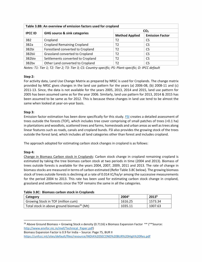
Table 3.8B: An overview of emission factors used for cropland
IPCC ID GHG source & sink categories CO2
Method Applied Emission Factor
3B2 Cropland T2 CS
3B2a Cropland Remaining Cropland T2 CS
3B2bi Forestland converted to Cropland T2 CS
3B2bii Grassland converted to Cropland T2 CS
3B2biv Settlements converted to Cropland T2 CS
3B2bv Other Land converted to Cropland T2 CS
Notes: T1: Tier 1; T2: Tier 2; T3: Tier 3; CS: Country-specific; PS: Plant-specific; D: IPCC default Step 2: For activity data, Land Use Change Matrix as prepared by NRSC is used for Croplands. The change matrix provided by NRSC gives changes in the land use pattern for the years (a) 2006-08, (b) 2008-11 and (c) 2011-13. Since, the data is not available for the years 2005, 2013, 2014 and 2015, land use pattern for 2005 has been assumed same as for the year 2006. Similarly, land use pattern for 2013, 2014 & 2015 has been assumed to be same as for 2012. This is because these changes in land use tend to be almost the same when looked at year-on-year basis. Step 3: Emission factor estimation has been done specifically for this study. FSI creates a detailed assessment of trees outside the forests (TOF), which includes tree cover comprising of small patches of trees (<0.1 ha) in plantations and woodlots, scattered trees and farms, homesteads and urban areas as well as trees along linear features such as roads, canals and cropland bunds. FSI also provides the growing stock of the trees outside the forest land, which includes all land categories other than forest and includes cropland. The approach adopted for estimating carbon stock changes in cropland is as follows: Step 4: Change in Biomass Carbon stock in Croplands: Carbon stock change in cropland remaining cropland is estimated by taking the tree biomass carbon stock at two periods in time (2004 and 2013). Biomass of trees outside forests is available for the years 2004, 2007, 2009, 2011 and 2013. The rate of change in biomass stocks are measured in terms of carbon estimated (Refer Table 3.8C below). The growing biomass stock of trees outside forests is declining at a rate of 0.014 tC/ha/yr among the successive measurements for the period 2004 to 2013. This rate has been used for estimating carbon stock change in cropland, grassland and settlements since the TOF remains the same in all the categories. Table 3.8C: Biomass carbon stock in Croplands
Category 2004a 2013b
Growing Stock in TOF (million cum) 1616.25 1573.34
Total stock in above ground biomass26 (Mt) 1035.11 1007.63
26 Above Ground Biomass = Growing Stock x density (0.7116) x Biomass Expansion Factor ** (**Source: http://www.envfor.nic.in/mef/Technical_Paper.pdf) Biomass Expansion Factor is 0.9 for India – Source: Page 75, BUR II https://unfccc.int/sites/default/files/resource/INDIA%20SECOND%20BUR%20High%20Res.pdf

Total stock in below ground biomass27 (Mt) 279.48 272.06
Total biomass (Mt) 1314.59 1279.69
Total biomass Carbon28 (MtC) 657.29 639.84
Rate of Change of Biomass Carbon (MtC/yr) -1.94
Rate of Change of Biomass Carbon (tC/ha/yr) -0.008
Source: a – Table 6.1, Page 40, SFR 2005 & b – Table 5.2, Page 81, SFR 2015 Step 5: Change in Soil Organic Carbon content in Croplands: Land is typically converted to Cropland from native lands, managed Forest Land and Grassland, but occasionally conversions can occur from Wetlands and seldom Settlements. Regardless of soil type (i.e., mineral or organic), the conversion of land to Cropland will, in most cases, result in a loss of soil C for some years following conversion (5.3.3, Chapter 5, Volume 4, 2006 IPCC Guidelines for national GHG inventories). For Cropland Remaining Cropland, the rate of change of SOC has been derived from multiple studies that have been listed in the bibliography accompanying this document. SOC reference values for Forestland has been used from M Kaul et al 2009 and SOC values for Cropland and Other Land has been derived from K. Sreenivas et al 2016. Further, the total change in soil C stocks for Land Converted to Cropland is estimated using Equation 2.25, chapter 2, Vol. 04 of {IPCC 2006 Guidelines} (Refer Annex I for sample calculations) given below:
𝛥𝐶𝑚𝑖𝑛𝑒𝑟𝑎𝑙 =(𝑆0𝐶0 − 𝑆0𝐶(0−𝑇))
𝐷
𝑆𝑂𝐶 = ∑ 𝑆𝑂𝐶𝑅𝐸𝐹𝐶,𝑆,𝐼⋅ 𝐹𝐿𝑈𝐶,𝑆,𝐼
⋅ 𝐹𝑀𝐺𝐶,𝑆,𝐼⋅ 𝐹𝐼𝐶,𝑆,𝐼
⋅ 𝐴𝐶,𝑆,𝐼
𝐶,𝑆,𝐼
where, 𝛥𝐶𝑚𝑖𝑛𝑒𝑟𝑎𝑙 = annual change in carbon stocks in mineral soils, tonnes C yr-1 𝑆0𝐶0 = soil organic carbon stock in the last year of an inventory time, tonnes C 𝑆0𝐶(0−𝑇) = soil organic carbon stock at the beginning of the inventory time, tonnes C
𝑆0𝐶0 and 𝑆0𝐶(0−𝑇) are calculated using the SOC equation in the box where the reference carbon stocks
and stock change factors are assigned according to the land-use and management activities and corresponding areas at each of the points in time (time = 0 and time = 0-T) D = Time Dependence, 20 years C = represents the climate zones, S the soil types, and I the set of management systems that
are present in a country. 𝑆𝑂𝐶𝑅𝐸𝐹 = the reference carbon stock, tonnes C ha-1 𝐹𝐿𝑈 = stock change factor for land-use systems or sub-system for a particular land-use,
dimensionless
27 Please See Table 1, Page 9 of https://www.academia.edu/26244255/Indias_Forest_and_Tree_Cover_Contribution_as_a_Carbon_Sink_Technical_Paper – Root Shoot Ratio is 0.27 28 Carbon Fraction is 0.49 (Default Value sourced from IPCC 2006 Guidelines. Please see table 4.3 (Tropical, Woody – Carbon Fraction value from https://www.ipcc-nggip.iges.or.jp/public/2006gl/pdf/4_Volume4/V4_04_Ch4_Forest_Land.pdf)

𝐹𝑀𝐺 = stock change factor for management regime, dimensionless 𝐹𝐼 = stock change factor for input of organic matter, dimensionless A = land area of the stratum being estimated, ha. All land in the stratum should have
common biophysical conditions (i.e., climate and soil type) and management history over the inventory time to be treated together for analytical purposes
Since, there is no land conversion from Grassland and Settlements to Cropland, no calculations have been performed for the same. Step 6: The total biomass and soil organic carbon content for each sub-category is calculated by multiplying the area within that sub-category with the respective change in biomass and soil organic carbon for that particular sub-category. The total change in carbon stocks is calculated by adding up all values of the sub-categories estimates.
3.8.3 Recalculation
Table 3.8D: Source category wise details on the difference between GHG estimates
Year Key source category GHG Emission Estimates (MtCO2e) % Difference
Phase-II Phase-III
2005 Cropland 2.30 -1.46 -164%
2006 Cropland 2.30 -1.46 -164%
2007 Cropland 2.30 -1.46 -164%
2008 Cropland 3.14 -0.62 -120%
2009 Cropland 3.14 -0.62 -120%
2010 Cropland 3.14 -0.62 -120%
2011 Cropland 2.47 -1.32 -154%
2012 Cropland 2.47 -1.32 -154%
2013 Cropland 2.47 -1.32 -154%
As decided amongst platform partners, a significance threshold of 5% is considered. Recalculation have been reported where the deviation between Phase III and Phase II results is higher than the threshold. As seen in table 3.8D above, high deviation was observed in phase-3 and phase-2 emissions from cropland. This is mainly because the emission factors used to calculate the emissions are now sourced from BUR II.
3.8.4 Uncertainty
NRSC has conducted accuracy assessment of the remote sensing land use and land classification. Stratified random points generated through image software was used to assess the accuracy of classification. The number sample points for each stratum was selected based on the proportion of the area. However, a minimum of 20 sample points was considered for each class to estimate the accuracy of the classified output. Ground truth data, legacy maps, and multi-temporal FCC have formed the basis for assessment and generation of Kappa co-efficient. For quality check, it was submitted to the QAS team. Refinement of crop classification areas obtained based on classification map at the end of the year was used.

The classification outputs were subjected to post classification accuracy assessment. The error matrix of accuracy assessment for different states was done. The overall classification accuracy is found to be 88.82% with a range of 83.05% to 95.31% in different states (NRSC 2007). For subsequent years, the planimetric accuracy was stated, wherein it is less than one pixel in plain areas and less than 2 pixels in hilly terrains (NRSC 2010), (NRSC 2012), (NRSC 2013) 29. During 2013-14 it was <1 pixel in plains. The standing stock or biomass stock outside forest area is which includes cropland is taken from the State of Forest Report (FSI). There are no estimates of precision levels. SOC reference values for Forestland from M Kaul et al 2009 has not estimated uncertainty. In fact, the research paper has reported uncertainties in input variables due to very large spatial heterogeneity that affect net Carbon flux from land use change. The SOC of land use was from the study conducted by K. Sreenivas et al 2016 from National Remote Sensing Centre (NRSC) wherein the SOC was spatially mapping at 250 m resolution and an estimate of their pool size in India was undertaken using many remote sensing derived data layers and data mining approach. The SOC densities were estimated for 1198 soil samples located across India using a stratified random sampling that integrated land use, soil, topography and agroecological regions. Using Random forests (RF) based spatial prediction procedure with climatic, land cover, rock type, soil type, multi-year Normalized Difference Vegetation Index (NDVI), irrigation status as independent input variables, models for predicting carbon density at 250 m spatial resolution were developed. For modelling with RF algorithm, about 898 soil profile observations (75% observations) were used, while the rest of 300 (25% of total observations) were used for validation. The Root Mean Square Error (RMSE) statistic was used to measure the degree of agreement between the predicted and observed values. The relationship between observed and predicted values was characterized by Mean Squared Deviations (MSD) parameter which was 3.19. Activity data in the public domain is available but cannot be verified independently due to lack of open access to remote sensing data that is used by governmental agencies.
Table 3.8E: Source category wise description of Qualitative uncertainty
IPCC ID
Source Category
Qualitative Uncertainty
Activity Data Emission Factor
3B2 Cropland Lack of access to finer resolution data to map land use changes
Lack of data on underlying assumptions for carbon stock calculations such as stand age, species composition, etc. Lack of availability of region-specific carbon stock data based on topography and climatic regions.
3.8.5 Recommended Improvements
For the estimation of GHG emissions/removals from land, we will be looking at generating change matrices for selected states to validate the change matrices that we have been able to obtain from official sources. In addition, we will continue to scan relevant literature for improvements in tools and methodologies, as well as more precise data in the future.

3.9 3B3 Grassland
3.9.1 Category description This section provides details of estimating emissions from Grassland. Grasslands are generally distinguished from “forest” as ecosystems having a tree canopy cover of less than a certain threshold, which varies from region to region. Below-ground carbon dominates in grassland and is mainly contained in roots and soil organic matter (Volume 4, Chapter 6, 2006 IPCC guidelines for national GHG inventories). In India, grasslands include many categories other than forest land and cropland.
Given below are details of activity data used in Grasslands. The data quality is considered high because the activity data has been obtained from credible and relevant Government of India sources that have been engaged in collecting such data every five years for several decades. Further, the credibility of the data is acknowledged by all the relevant stakeholders both within and outside the Government.
Table 3.9A: An overview of source categories of Grassland
IPCC ID GHG source & sink categories Type Quality Source
3B Land
3B3 Grassland Secondary Data High National Remote Sensing Centre (available on request)
3B3a Grassland Remaining Grassland Secondary Data High
3b3bv Other Land converted to Grassland Secondary Data High
3.9.2 Methodology
Inter-annual climatic variability is a crucial factor for consideration when estimating emissions from grasslands. Substantial changes in standing biomass can occur from year to year that is associated with differences in annual rainfall. Inter-annual rainfall variability may also affect management decisions such as irrigation or fertilizer application (Volume 4, Chapter 5, 2006 IPCC Guidelines for national GHG inventories) and thereby affecting emission estimates. Emission estimation for Grassland is done by categorizing land in two categories viz., Grassland Remaining Grassland and Land Converted to Grassland. This study uses 2006 IPCC Guidelines for national GHG inventories to estimate emissions from these categories. The steps followed in the estimation process for both the categories remain same with the only difference arising in choice/estimation of emission factors:
Steps followed: Step 1: In this study, GHG emissions from grasslands are estimated using the Stock Difference Method from the following categories: (a) Grassland remaining Grassland (b) Forest Land converted to Grassland (No Land use change observed by NRSC) (c) Cropland converted to Grassland (No Land use change observed by NRSC) (d) Settlements converted to Grassland (No Land use change observed by NRSC)

(e) Other Land converted to Grassland Given below are details of the methodology used for grasslands:
Notes: T1: Tier 1; T2: Tier 2; T3: Tier 3; CS: Country-specific; PS: Plant-specific; D: IPCC default
For this category, Land Use Change Matrix for grassland has been derived from National Remote Sensing Centre (NRSC), Hyderabad. NRSC is a national organization hosted under Indian Space Research Organization (ISRO).
Step 2: For activity data, Land Use Change Matrix as prepared by NRSC is used for Grasslands. The change matrix provided gives changes in the land use pattern for the years (a) 2006-08, (b) 2008-11 and (c) 2011-13. Since, the data is not available for the years 2005 and 2013, 2014 and 2015, land use pattern for 2005 has been assumed same as for the year 2006. Similarly, land use pattern for 2013, 2014 & 2015 has been assumed to be same as for 2012. This is because these changes in land use tend to be almost the same when looked at year on year. Step 3: Emission factor estimation has been done specifically for this study. FSI creates a detailed assessment of trees outside the forests (TOF), which includes tree cover comprising of small patches of trees (<0.1 ha) in plantations and woodlots, scattered trees and farms, homesteads and urban areas as well as trees along linear features such as roads, canals and cropland bunds. FSI also provides the growing stock of the trees outside the forest land, which includes all land categories other than forest and includes cropland. Step 4: The approach adopted for estimating carbon stock changes in grassland is as follows: Change in Biomass Carbon stock in Grassland: Carbon stock change in grassland remaining grassland is estimated by taking the tree biomass carbon stock at two periods in time (2004 and 2013). Biomass of trees outside forests is available for the years 2004, 2007, 2009, 2011 and 2013. The rate of change in biomass stocks are measured in terms of carbon estimated (Refer Table 3.9C below). The growing biomass stock of trees outside forests is declining at a rate of 0.014 tC/ha/yr among the successive measurements for the period 2004 to 2013. This rate has been used for estimating carbon stock change in cropland, grassland and settlements since the TOF remains the same in all the categories.
Table 3.9C: Biomass Carbon Stock in Grassland
Category 2004a 2013b
Growing Stock in TOF (million cum) 1616.25 1573.34
Table 3.9B: An overview of emission factors used for grasslands
IPCC ID GHG source & sink categories CO2
Method Applied Emission Factor
3B3 Grassland T2 CS
3B3a Grassland Remaining Grassland T2 CS
3b3bv Other Land converted to Grassland T2 CS

Total stock in above ground biomass30 (Mt) 1035.11 1007.63
Total stock in below ground biomass31 (Mt) 279.48 272.06
Total biomass (Mt) 1314.59 1279.69
Total biomass Carbon32 (MtC) 657.29 639.84
Rate of Change of Biomass Carbon (MtC/yr) -1.94
Rate of Change of Biomass Carbon (tC/ha/yr) -0.008 Source: : a – Table 6.1, Page 40, SFR 2005 & b – Table 5.2, Page 81, SFR 2015
Step 5: The annual change in organic C stocks in mineral soils is estimated using the equation given below of the IPCC methodology (Equation 2.25, (Refer Annex I for sample calculations)):
𝛥𝐶𝑚𝑖𝑛𝑒𝑟𝑎𝑙 =(𝑆0𝐶0 − 𝑆0𝐶(0−𝑇))
𝐷
𝑆𝑂𝐶 = ∑ 𝑆𝑂𝐶𝑅𝐸𝐹𝐶,𝑆,𝐼⋅ 𝐹𝐿𝑈𝐶,𝑆,𝐼
⋅ 𝐹𝑀𝐺𝐶,𝑆,𝐼⋅ 𝐹𝐼𝐶,𝑆,𝐼
⋅ 𝐴𝐶,𝑆,𝐼
𝐶,𝑆,𝐼
where, 𝛥𝐶𝑚𝑖𝑛𝑒𝑟𝑎𝑙 = annual change in carbon stocks in mineral soils, tonnes C yr-1 𝑆0𝐶0 = soil organic carbon stock in the last year of an inventory time, tonnes C 𝑆0𝐶(0−𝑇) = soil organic carbon stock at the beginning of the inventory time, tonnes C
𝑆0𝐶0 and 𝑆0𝐶(0−𝑇) are calculated using the SOC equation in the box where the reference carbon stocks
and stock change factors are assigned according to the land-use and management activities and corresponding areas at each of the points in time (time = 0 and time = 0-T) D = Time Dependence, yr C = represents the climate zones, S the soil types, and I the set of management systems that
are present in a country. 𝑆𝑂𝐶𝑅𝐸𝐹 = the reference carbon stock, tonnes C ha-1 𝐹𝐿𝑈 = stock change factor for land-use systems or sub-system for a land-use, dimensionless 𝐹𝑀𝐺 = stock change factor for management regime, dimensionless 𝐹𝐼 = stock change factor for input of organic matter, dimensionless A = land area of the stratum being estimated, ha. All land in the stratum should have
common biophysical conditions (i.e., climate and soil type) and management history over the inventory time to be treated together for analytical purposes
Due to lack of data during two points of time, the rate of change in SOC for grassland was determined from the country-specific reference soil organic C stocks from K. Sreenivas et al. 2016 and default stock
30 Above Ground Biomass = Growing Stock x density (0.7116) x Biomass Expansion Factor** (**Source: http://www.envfor.nic.in/mef/Technical_Paper.pdf) Biomass Expansion Factor is 0.9 for India – Source: Page 75, BUR II https://unfccc.int/sites/default/files/resource/INDIA%20SECOND%20BUR%20High%20Res.pdf 31 Please See Table 1, Page 9 of https://www.academia.edu/26244255/Indias_Forest_and_Tree_Cover_Contribution_as_a_Carbon_Sink_Technical_Paper – Root Shoot Ratio is 0.27 32 Carbon Fraction is 0.49 (Default Value sourced from IPCC 2006 Guidelines. Please see table 4.3 (Tropical, Woody – Carbon Fraction value from https://www.ipcc-nggip.iges.or.jp/public/2006gl/pdf/4_Volume4/V4_04_Ch4_Forest_Land.pdf

change factors (FLU, FMG, FI) as given by the 2006 IPCC guidelines (Vol 04, Chapter 06, Table 6.2, Page 6.16). Annual rates of stock change were calculated as the difference in stocks (over time) divided by the time dependence (D) of the stock change factors (with a default value of 20 years). The reference SOC is as determined by FSI for native forests. Based on the Tier I approach, for FLU, FMG and FI, a default value of 1, 0.97 and 1 was considered respectively for the rate of change which is for moderately degraded grasslands (2006 IPCC guidelines (Vol 04, Chapter 06, Table 6.2, Page 6.16)). The annual SOC change for lands converted to grassland was estimated as the difference on the SOC values from other lands to native vegetation. Since, there is no land conversion from Forest Land, Cropland and Settlements to Grassland, no calculations have been performed for the same. The total biomass and soil organic carbon content for each sub-category is calculated by multiplying the area within that sub-category with the respective change in biomass and soil organic carbon for that particular sub-category. The total change in carbon stocks is calculated by adding up all values of the sub-categories estimates.
3.9.3 Recalculation
Table 3.9D: Source category wise details on the difference between GHG estimates
Year Key source category GHG Emission Estimates (MtCO2e) % Difference
Phase-II Phase-III
2005 Grassland 0.63 0.58 -8%
2006 Grassland 0.63 0.58 -8%
2007 Grassland 0.63 0.58 -8%
2008 Grassland 0.47 0.42 -11%
2009 Grassland 0.47 0.42 -11%
2010 Grassland 0.47 0.42 -11%
2011 Grassland 0.71 0.66 -7%
2012 Grassland 0.71 0.66 -7%
2013 Grassland 0.71 0.66 -7%
As decided amongst platform partners, a significance threshold of 5% is considered. Recalculation have been reported where the deviation between Phase III and Phase II results is higher than the threshold. As seen in table 3.9D above, slight deviation was observed in phase-3 and phase-2 emissions from grassland. This is mainly because the biomass factor has been updated using the BUR II report.
3.9.4 Uncertainty
NRSC has conducted accuracy assessment of the remote sensing land use and land classification. Stratified random points generated through image software was used to assess the accuracy of classification. The number sample points for each stratum was selected based on the proportion of the area. However, a minimum of 20 sample points was considered for each class to estimate the accuracy of the classified output. Ground truth data, legacy maps, and multi-temporal FCC have formed the basis for assessment and generation of Kappa co-efficient. For quality check, it was submitted to the QAS team. Refinement of crop classification areas obtained based on classification map at the end of the year was used.

The classification outputs were subjected to post classification accuracy assessment. The error matrix of accuracy assessment for different states was done. The overall classification accuracy is found to be 88.82% with a range of 83.05% to 95.31% in different states for 2006 to 2007.33 For subsequent years, the planimetric accuracy was stated, wherein it is less than one pixel in plain areas and less than 2 pixels in hilly terrains34. During 2013-14 it was <1 pixel in plains35. The standing stock or biomass stock outside forest area is which includes grassland is taken from the State of Forest Report (SFR 2015). There are no estimates of precision levels. SOC reference values for Forestland from M Kaul et al 2009 has not estimated uncertainty. In fact, the research paper has reported uncertainties in input variables due to very large spatial heterogeneity that affect net Carbon flux from land use change. The SOC of land use was from the study conducted by K. Sreenivas et al 2016 from NRSC, wherein the SOC was spatially mapping at 250 m resolution and an estimate of their pool size in India was undertaken using many remote sensing derived data layers and data mining approach. The SOC densities were estimated for 1198 soil samples located across India using a stratified random sampling that integrated land use, soil, topography and agroecological regions. Using Random forests (RF) based spatial prediction procedure with climatic, land cover, rock type, soil type, multi-year NDVI, irrigation status as independent input variables, models for predicting carbon density at 250 m spatial resolution were developed. For modelling with RF algorithm, about 898 soil profile observations (75% observations) were used, while the rest of 300 (25% of total observations) were used for validation. The Root Mean Square Error (RMSE) statistic was used to measure the degree of agreement between the predicted and observed values. The relationship between observed and predicted values was characterized by Mean Squared Deviations (MSD) parameter which was 3.19. Activity data in the public domain is available but cannot be verified independently due to lack of open access to remote sensing data that is used by governmental agencies.
Table 3.9E: Source category wise description of Qualitative uncertainty
IPCC ID
Source Category
Qualitative Uncertainty
Activity Data Emission Factor
3B3 Grassland Lack of access to finer resolution data to map land use changes
Lack of data on underlying assumptions for carbon stock calculations such as stand age, species composition, etc. Lack of availability of region-specific carbon stock data based on topography and climatic regions.
33 http://bhuvan.nrsc.gov.in/gis/thematic/tools/document/LULC250/0607.pdf (refer section 3.5) 34 http://bhuvan.nrsc.gov.in/gis/thematic/tools/document/LULC250/0809.pdf (refer section 2.2), http://bhuvan.nrsc.gov.in/gis/thematic/tools/document/LULC250/1112.pdf (refer section 2.21), http://bhuvan.nrsc.gov.in/gis/thematic/tools/document/LULC250/1314.pdf (refer section 3.1) 35 http://bhuvan.nrsc.gov.in/gis/thematic/tools/document/LULC250/1314.pdf

3.9.5 Recommended Improvements
For the estimation of GHG emissions/removals from land, we will be looking at generating change matrices for selected states to validate the change matrices that we have been able to obtain from official sources. In addition, we will continue to scan relevant literature for improvements in tools and methodologies, as well as more precise data in the future.
3.10 3B5 Settlements
3.10.1 Category description This section provides details of estimating carbon stock changes and greenhouse gas emissions and removals associated with changes in biomass, dead organic matter (DOM), and soil carbon on lands classified as settlements. Settlements are defined as including all developed land -- i.e., residential, transportation, commercial, and production (commercial, manufacturing) infrastructure of any size, unless it is already included under other land-use categories. The land-use category Settlements includes soils, herbaceous perennial vegetation such as turf grass and garden plants, trees in rural settlements, homestead gardens and urban areas (Volume 4, Chapter 8, 2006 IPCC Guidelines for national GHG inventories). The area under settlement is estimated to be approximately 8-9 Mha, which is less than 2% of the total land use in India. The net emissions from this category are very low (almost negligible) and therefore, the share of emissions from settlements in LULUCF sector is also negligible. Given below are details of activity data used in Settlements. The data quality is considered high because the activity data has been obtained from credible and relevant Government of India sources that have been engaged in collecting such data every five years for several decades. Further, the credibility of the data is acknowledged by all the relevant stakeholders both within and outside the Government.
Table 3.10A: An overview of source categories of Settlements
IPCC ID GHG source & sink categories Type Quality Source
3B Land
3B5 Settlements Secondary Data High National Remote Sensing Centre (available on request)
3B5a Settlements Remaining Settlements Secondary Data High
3B5bii Cropland converted to Settlements Secondary Data High
3B5v Other Land converted to Settlements Secondary Data High
3.10.2 Methodology
Soils and DOM in Settlements may be sources or sinks of CO2, depending on previous land use, topsoil burial or removal during development, current management, particularly with respect to nutrient and water applications, and amount of vegetation cover spread among roads, buildings and associated infrastructure ({IPCC 2006 Guidelines}).

In this study, GHG emissions from settlements are estimated using the Stock Difference Method36 from the category Land converted to Settlements. Mostly Croplands and Other Land got converted to settlements based on the land use change matrix. The steps followed in the estimation process for both the categories remain same with the only difference arising in choice/estimation of emission factors:
Steps followed: Step 1: Given below are details of sub-categories of land converted to Settlements:
Notes: T1: Tier 1; T2: Tier 2; T3: Tier 3; CS: Country-specific; PS: Plant-specific; D: IPCC default
Step 2: For activity data, Land Use Change Matrix as prepared by NRSC is used for Settlements. The change matrix provided gives changes in the land use pattern for the years (a) 2006-08, (b) 2008-11 and (c) 2011-13. Since, the data is not available for the years 2005 and 2013, 2014 and 2015, land use pattern for 2005 has been assumed same as for the year 2006. Similarly, land use pattern for 2013, 2014 & 2015 has been assumed to be same as for 2012. This is because these changes in land use tend to be almost the same when looked at year on year. Step 3: The biomass stock change is estimated using the method and data described for croplands and grassland. In case of settlements, the input biomass is same as output biomass. Hence, the net biomass stock change is zero. Hence, there is no emission from settlement remaining settlement. Step 4: The annual change in organic C stocks in mineral soils is estimated using the equation given below of the {IPCC 2006 Guidelines } (Equation 2.25, chapter 2, Vol. 04 (Refer Annex I for sample calculations)):
𝛥𝐶𝑚𝑖𝑛𝑒𝑟𝑎𝑙 =(𝑆0𝐶0 − 𝑆0𝐶(0−𝑇))
𝐷
𝑆𝑂𝐶 = ∑ 𝑆𝑂𝐶𝑅𝐸𝐹𝐶,𝑆,𝐼⋅ 𝐹𝐿𝑈𝐶,𝑆,𝐼
⋅ 𝐹𝑀𝐺𝐶,𝑆,𝐼⋅ 𝐹𝐼𝐶,𝑆,𝐼
⋅ 𝐴𝐶,𝑆,𝐼
𝐶,𝑆,𝐼
where, 𝛥𝐶𝑚𝑖𝑛𝑒𝑟𝑎𝑙 = annual change in carbon stocks in mineral soils, tonnes C yr-1 𝑆0𝐶0 = soil organic carbon stock in the last year of an inventory time, tonnes C 𝑆0𝐶(0−𝑇) = soil organic carbon stock at the beginning of the inventory time, tonnes C
36 http://www.ipcc-nggip.iges.or.jp/public/2006gl/pdf/4_Volume4/V4_08_Ch8_Settlements.pdf
Table 3.10B: An overview of emission factors used for settlements
IPCC ID GHG source & sink categories CO2
Method Applied Emission Factor
3B5 Settlements
3B5a Settlements Remaining Settlements T2 CS
3B5bii Cropland converted to Settlements T2 CS
3B5v Other Land converted to Settlements T2 CS

𝑆0𝐶0 and 𝑆0𝐶(0−𝑇) are calculated using the SOC equation in the box where the reference carbon stocks
and stock change factors are assigned according to the land-use and management activities and corresponding areas at each of the points in time (time = 0 and time = 0-T) D = Time Dependence, yr C = represents the climate zones, S the soil types, and I the set of management systems that
are present in a country. 𝑆𝑂𝐶𝑅𝐸𝐹 = the reference carbon stock, tonnes C ha-1 𝐹𝐿𝑈 = stock change factor for land-use systems or sub-system for a particular land-use,
dimensionless 𝐹𝑀𝐺 = stock change factor for management regime, dimensionless 𝐹𝐼 = stock change factor for input of organic matter, dimensionless A = land area of the stratum being estimated, ha. All land in the stratum should have
common biophysical conditions (i.e., climate and soil type) and management history over the inventory time to be treated together for analytical purposes
Due to lack of data during two points of time, the rate of change in SOC for settlements was determined from the country-specific reference soil organic C stocks from K. Sreenivas et al. 2016 and default stock change factors (FLU, FMG, FI) as given by the {IPCC 2006 Guidelines}. Annual rates of stock change were calculated as the difference in stocks (over time) divided by the time dependence (D) of the stock change factors (with a default value of 20 years). The reference SOC is as determined by FSI for native forests. Based on the Tier I approach, for FLU, FMG and FI, a default value of 0.8, 1.22 and 1 was considered respectively for the land transition from settlements to cropland (Section 8.3.3.2, Chapter 8, Vol. 04 IPCC 2006 Guidelines). Since, there is no land conversion from Forest Land and Grassland to Settlements, no calculations have been performed for the same. Step 5: The total biomass and soil organic carbon content for each sub-category is calculated by multiplying the area within that sub-category with the respective change in biomass and soil organic carbon for that particular sub-category. The total change in carbon stocks is calculated by adding up all values of the sub-category estimates.
3.10.3 Recalculation No recalculation was performed for estimating emissions from this category because the activity data, emissions factor and methodology was the same as used for Phase II estimates. There was no new data source used, no error was observed and no new methodology was used.
3.10.4 Uncertainty
NRSC has conducted accuracy assessment of the remote sensing land use and land classification. Stratified random points generated through image software was used to assess the accuracy of classification. The number sample points for each stratum was selected based on the proportion of the area. However, a minimum of 20 sample points was considered for each class to estimate the accuracy of the classified output. Ground truth data, legacy maps, and multi-temporal FCC have formed the basis for assessment and generation of Kappa co-efficient. For quality check, it was submitted to the QAS team. Refinement of crop classification areas obtained based on classification map at the end of the year was used.

The classification outputs were subjected to post classification accuracy assessment. The error matrix of accuracy assessment for different states was done. The overall classification accuracy is found to be 88.82% with a range of 83.05% to 95.31% in different states (NRSC 2007). For subsequent years, the planimetric accuracy was stated, wherein it is less than one pixel in plain areas and less than 2 pixels in hilly terrains (NRSC 2010) (NRSC 2012) (NRSC 2013)37. During 2013-14 it was <1 pixel in plains. The standing stock or biomass stock outside forest area is which includes cropland is taken from the State of Forest Report (FSI). There are no estimates of precision levels. SOC reference values for Forestland from M Kaul et al 2009 has not estimated uncertainty. In fact, the research paper has reported uncertainties in input variables due to very large spatial heterogeneity that affect net Carbon flux from land use change. The SOC of land use was from the study conducted by K. Sreenivas et al 2016 from NRSC, wherein the SOC was spatially mapping at 250 m resolution and an estimate of their pool size in India was undertaken using many remote sensing derived data layers and data mining approach. The SOC densities were estimated for 1198 soil samples located across India using a stratified random sampling that integrated land use, soil, topography and agroecological regions. Using Random forests (RF) based spatial prediction procedure with climatic, land cover, rock type, soil type, multi-year NDVI, irrigation status as independent input variables, models for predicting carbon density at 250 m spatial resolution were developed. For modelling with RF algorithm, about 898 soil profile observations (75% observations) were used, while the rest of 300 (25% of total observations) were used for validation. The Root Mean Square Error (RMSE) statistic was used to measure the degree of agreement between the predicted and observed values. The relationship between observed and predicted values was characterized by Mean Squared Deviations (MSD) parameter which was 3.19. Activity data in the public domain is available but cannot be verified independently due to lack of open access to remote sensing data that is used by governmental agencies.
Table 3.10C: Source category wise description of Qualitative uncertainty
IPCC ID
Source Category
Qualitative Uncertainty
Activity Data Emission Factor
3B5 Settlements Lack of access to finer resolution data to map land use changes
Lack of data on underlying assumptions for carbon stock calculations such as stand age, species composition, etc. Lack of availability of region-specific carbon stock data based on topography and climatic regions.
37

3.10.5 Recommended Improvements For the estimation of GHG emissions/removals from land, we will be looking at generating change matrices for selected states to2 validate the change matrices that we have been able to obtain from official sources. In addition, we will continue to scan relevant literature for improvements in tools and methodologies, as well as more precise data in the future.
3.11 3B6 Other Land
3.11.1 Category description For the sub-category ‘other lands’, it includes wasteland, snow covered area, rocky surfaces, water bodies, etc. For this category, Land Use Change Matrix for Other Land has been derived from National Remote Sensing Centre (NRSC), Hyderabad. NRSC is a national organization hosted under Indian Space Research Organization (ISRO). Given below are details of activity data used in the sub-category. The data quality is considered high because the activity data has been obtained from credible and relevant Government of India sources that have been engaged in collecting such data every five years for several decades. Further, the credibility of the data is acknowledged by all the relevant stakeholders both within and outside the Government.
Table 3.11A: An overview of source categories of Other Land
IPCC ID GHG source & sink categories Type Quality Source
3B Land
3B6 Other Land Secondary Data High National Remote Sensing Centre (available on request)
3B6a Other Land Remaining Other Land Secondary Data High
3b6bii Cropland converted to Other Land Secondary Data High
3b6biii Grassland converted to Other Land Secondary Data High
3b6biv Settlements converted to Other Land Secondary Data High
3.11.2 Methodology In this study, GHG emissions from Other Lands is estimated using the Stock Difference Method from the category Other Land Remaining Other Land and Land converted to Other Land. Mostly Croplands, Grassland and Settlements got converted to Other Land based on the land use change matrix prepared by NRSC. The steps followed in the estimation process for both the categories remain same with the only difference arising in choice/estimation of emission factors: Steps followed: Step 1: Given below are details of the subcategories of land use type converted to Settlements:
Table 3.11B: An overview of Emission Factors used for Other Land
IPCC ID GHG source & sink categories CO2
Method Applied Emission Factor
3B5 Other land
3B6a Other Land Remaining Other Land T2 CS
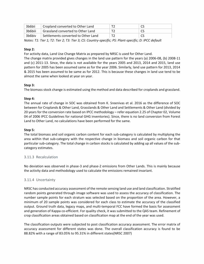
Notes: T1: Tier 1; T2: Tier 2; T3: Tier 3; CS: Country-specific; PS: Plant-specific; D: IPCC default Step 2: For activity data, Land Use Change Matrix as prepared by NRSC is used for Other Land. The change matrix provided gives changes in the land use pattern for the years (a) 2006-08, (b) 2008-11 and (c) 2011-13. Since, the data is not available for the years 2005 and 2013, 2014 and 2015, land use pattern for 2005 has been assumed same as for the year 2006. Similarly, land use pattern for 2013, 2014 & 2015 has been assumed to be same as for 2012. This is because these changes in land use tend to be almost the same when looked at year on year. Step 3: The biomass stock change is estimated using the method and data described for croplands and grassland. Step 4: The annual rate of change in SOC was obtained from K. Sreenivas et al. 2016 as the difference of SOC between for Croplands & Other Land, Grasslands & Other Land and Settlements & Other Land (divided by 20 years for the conversion rate based on IPCC methodology – refer equation 2.25 of Chapter 02, Volume 04 of 2006 IPCC Guidelines for national GHG inventories). Since, there is no land conversion from Forest Land to Other Land, no calculations have been performed for the same. Step 5: The total biomass and soil organic carbon content for each sub-category is calculated by multiplying the area within that sub-category with the respective change in biomass and soil organic carbon for that particular sub-category. The total change in carbon stocks is calculated by adding up all values of the sub-category estimates.
3.11.3 Recalculation No deviation was observed in phase-3 and phase-2 emissions from Other Lands. This is mainly because the activity data and methodology used to calculate the emissions remained invariant.
3.11.4 Uncertainty
NRSC has conducted accuracy assessment of the remote sensing land use and land classification. Stratified random points generated through image software was used to assess the accuracy of classification. The number sample points for each stratum was selected based on the proportion of the area. However, a minimum of 20 sample points was considered for each class to estimate the accuracy of the classified output. Ground truth data, legacy maps, and multi-temporal FCC have formed the basis for assessment and generation of Kappa co-efficient. For quality check, it was submitted to the QAS team. Refinement of crop classification areas obtained based on classification map at the end of the year was used. The classification outputs were subjected to post classification accuracy assessment. The error matrix of accuracy assessment for different states was done. The overall classification accuracy is found to be 88.82% with a range of 83.05% to 95.31% in different states(NRSC 2007)
3b6bii Cropland converted to Other Land T2 CS
3b6biii Grassland converted to Other Land T2 CS
3b6biv Settlements converted to Other Land T2 CS

For subsequent years, the planimetric accuracy was stated, wherein it is less than one pixel in plain areas and less than 2 pixels in hilly terrains (NRSC 2010) (NRSC 2012) (NRSC 2013). During 2013-14 it was <1 pixel in plains. The standing stock or biomass stock outside forest area is which includes Other Land is taken from the State of Forest Report (FSI). There are no estimates of precision levels. SOC reference values for Forestland from M Kaul et al 2009 has not estimated uncertainty. In fact, the research paper has reported uncertainties in input variables due to very large spatial heterogeneity that affect net Carbon flux from land use change. The SOC of land use was from the study conducted by K. Sreenivas et al 2016 from NRSA, wherein the SOC was spatially mapping at 250 m resolution and an estimate of their pool size in India was undertaken using many remote sensing derived data layers and data mining approach. The SOC densities were estimated for 1198 soil samples located across India using a stratified random sampling that integrated land use, soil, topography and agroecological regions. Using Random forests (RF) based spatial prediction procedure with climatic, land cover, rock type, soil type, multi-year NDVI, irrigation status as independent input variables, models for predicting carbon density at 250 m spatial resolution were developed. For modelling with RF algorithm, about 898 soil profile observations (75% observations) were used, while the rest of 300 (25% of total observations) were used for validation. The Root Mean Square Error (RMSE) statistic was used to measure the degree of agreement between the predicted and observed values. The relationship between observed and predicted values was characterized by Mean Squared Deviations (MSD) parameter which was 3.19.
Activity data in the public domain is available but cannot be verified independently due to lack of open access to remote sensing data that is used by governmental agencies.
Table 3.11C: Source category wise description of Qualitative uncertainty
IPCC ID
Source Category
Qualitative Uncertainty
Activity Data Emission Factor
3B6 Other Land Lack of access to finer resolution data to map land use changes
Lack of data on underlying assumptions for carbon stock calculations such as stand age, species composition, etc. Lack of availability of region-specific carbon stock data based on topography and climatic regions.
3.11.5 Recommended Improvements For the estimation of GHG emissions/removals from land, we will be looking at generating change matrices for selected states to validate the change matrices that we have been able to obtain from official sources. In addition, we will continue to scan relevant literature for improvements in tools and methodologies, as well as more precise data in the future.

3.12 3C Aggregate Sources and Non-CO2 Emission Sources on Land
3C1a Biomass Burning in Forestland 3.12.1 Category description
This section provides details of estimating non-carbon dioxide emissions from biomass burning in forest land. Both uncontrolled (wildfires) and managed (prescribed) fires can have a major impact on the non-CO2 greenhouse gas emissions from forests. For this category, there is no official data available on the area burnt in forests. The activity data has been derived for this category (please refer the methodology section for details) using the forest area as
provided by FSI. Given below are details of activity data used in the sub-category. The data quality is considered high because the activity data has been obtained from credible and relevant Government of India sources that have been engaged in collecting such data every five years for several decades. Further, the credibility of the data is acknowledged by all the relevant stakeholders both within and outside the Government.
Table 3.12A: An overview of source categories of Forestland
IPCC ID GHG source & sink categories Type Quality Source
3C Aggregate sources and non-CO2 Emissions Sources on Land
3C1a Biomass Burning in Forestland Secondary Data
High Forest Survey of India State of Forest Reports: 2017 2015 2013 2011 2009 2005
3.12.2 Methodology The methodological details for estimating emissions from Biomass burning in Forest Land are as under:
Table 3.12B: An overview of Emission factors used for Biomass burning in Forest Land
IPCC ID GHG source & sink categories CH4 N2O
Method Applied
Emission Factor
Method Applied
Emission Factor
3C Aggregate sources and non-CO2 Emissions Sources on Land
3C1a Biomass burning in Forestland T2 CS T2 CS Notes: T1: Tier 1; T2: Tier 2; T3: Tier 3; CS: Country-specific; PS: Plant-specific; D: IPCC default

2006 IPCC guidelines for national GHG inventories is adopted for estimating the GHG emissions from forest fire. The following equation (Equation 2.27, Chapter 2, Vol. 04 {IPCC 2006 Guidelines}, (Refer Annex 1 for sample calculation) was used to estimate methane and nitrous oxide emissions by burning of biomass in forestland.
𝐿𝑓𝑖𝑟𝑒 = 𝐴 ⋅ 𝑀𝐵 ⋅ 𝐶𝑓 ⋅ 𝐺𝑒𝑓 ⋅ 10−3
where, 𝐿𝑓𝑖𝑟𝑒 = amount of greenhouse gas emissions from fire, tonnes of each GHG e.g., CH4, N2O, etc.
A = area burnt, ha 𝑀𝐵 = mass of fuel available for combustion, tonnes ha-1. This includes biomass, ground litter and dead
wood. 𝐶𝑓 = combustion factor, dimensionless
𝐺𝑒𝑓 = emission factor, g kg-1 dry matter burnt
Steps followed: Step 1: Non-CO2 GHG emissions are estimated for the forestland subjected to biomass burning. The state-wise activity data for the area of the forest burnt was derived by (Reddy, 2017 n.d.)which gives the forest area burnt of each state it could further be apportioned to get the actual Area burnt by using the forest area of the particular state from FSI report. Step 2: Mass of fuel available for combustion (𝑀𝐵) is used from (NATCOM 2 n.d., p. 70)(in tonnes/ha). The value of the selected variable is 13.12 tonnes/ha as per NATCOM II and the same is adopted here as well. Step 3: In the absence of country specific values Combustion factor value (𝐶𝑓) is selected from 2006 IPCC 38
Guidelines. The selected value is 0.36 based on the category ‘all primary tropical forests. Step 4: Further mass of fuel available for combustion was multiplied with combustion factor to estimate the amount for fuel combusted (Value – 0.36 referred from Table 2. 6 (V4_02_Ch2_Generic.pdf, n.d.) Step 5: Country specific emission factors (𝐺𝑒𝑓) for methane and nitrous oxide gas were adopted from NATCOM
2 “indnc2.pdf,” n.d., p. 70 Step 6: Finally, the value calculated using Step 4 was multiplied with the area and the country specific emission factor and then added together to estimate emissions from biomass burning in forestland. The above steps were repeated for the methane and nitrous oxide emissions. (Refer to Annexure 1 for sample calculation)
38 Section 4.2.4.3, P-4.28, Chapter 4, Volume 4, 2006 IPCC Guidelines for National GHG Inventories. Values selected from Table 2.6, Chapter 2, Volume 4, 2006 IPCC Guidelines for National GHG Inventories.

3.12.3 Recalculation
Table 3.12C: Source category wise details on the difference between GHG estimates
Year Key source category GHG Emission Estimates (MtCO2e) % Difference
Phase-II Phase-III
2005 Biomass burning in forest land 0.32 5.02 1488%
2006 Biomass burning in forest land 0.32 5.04 1490%
2007 Biomass burning in forest land 0.32 5.06 1497%
2008 Biomass burning in forest land 0.32 5.08 1504%
2009 Biomass burning in forest land 0.32 5.10 1506%
2010 Biomass burning in forest land 0.32 5.12 1508%
2011 Biomass burning in forest land 0.32 5.14 1510%
2012 Biomass burning in forest land 0.32 5.16 1512%
2013 Biomass burning in forest land 0.32 5.18 1514%
As decided amongst platform partners, a significance threshold of 5% is considered. Recalculation have been reported where the deviation between Phase III and Phase II results is higher than the threshold. As seen in table 3.12C, a substantial deviation is observed in phase-3 and phase-2 emissions from the biomass burning in forest land. It is mainly because, in the present phase, we were able to get the state wise proportion of the forest area burnt unlike the previous phase where the total burnt area in year 2000 was taken from NATCOM II which was used to derive the Burnt area factor.
3.12.4 Uncertainty
The activity data for the area under forests at the state level is from Forest Survey of India reports. The area burnt is derived using appropriate proportions from (Reddy, et al. 2017)in activity data arises due to non-availability of data on forest burnt every year India. The emission factors for biomass burning on forest land is considered from NATCOM II. Uncertainty in emission factors for biomass burning in forest land is not ascertained in NATCOM II.
Table 3.12D: Source category wise description of Qualitative uncertainty
IPCC ID
Source Category
Qualitative Uncertainty
Activity Data Emission Factor
3C1a Biomass burning in Forestland
Uncertainty arise due to various variables used in the assessment such as fraction of forest burnt, area estimation.
Uncertainty arise due to various variables used in the assessment such as climatic conditions, soil type, water etc. Various biological, chemical and physical properties of soil and forest type influence the emissions from soil to the atmosphere
3.12.5 Recommended Improvements
As and when more detailed surveys are carried out, these estimations will be improved.
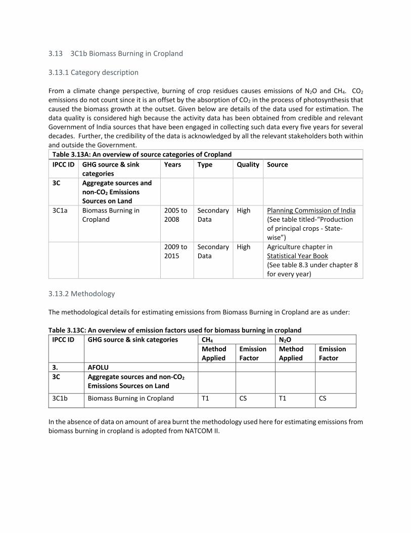
3.13 3C1b Biomass Burning in Cropland
3.13.1 Category description From a climate change perspective, burning of crop residues causes emissions of N2O and CH4. CO2 emissions do not count since it is an offset by the absorption of CO2 in the process of photosynthesis that caused the biomass growth at the outset. Given below are details of the data used for estimation. The data quality is considered high because the activity data has been obtained from credible and relevant Government of India sources that have been engaged in collecting such data every five years for several decades. Further, the credibility of the data is acknowledged by all the relevant stakeholders both within and outside the Government.
Table 3.13A: An overview of source categories of Cropland
IPCC ID GHG source & sink categories
Years Type Quality Source
3C Aggregate sources and non-CO2 Emissions Sources on Land
3C1a Biomass Burning in Cropland
2005 to 2008
Secondary Data
High Planning Commission of India (See table titled-“Production of principal crops - State-wise”)
2009 to 2015
Secondary Data
High Agriculture chapter in Statistical Year Book (See table 8.3 under chapter 8 for every year)
3.13.2 Methodology The methodological details for estimating emissions from Biomass Burning in Cropland are as under: Table 3.13C: An overview of emission factors used for biomass burning in cropland
IPCC ID GHG source & sink categories CH4 N2O
Method Applied
Emission Factor
Method Applied
Emission Factor
3. AFOLU
3C Aggregate sources and non-CO2 Emissions Sources on Land
3C1b Biomass Burning in Cropland T1 CS T1 CS
In the absence of data on amount of area burnt the methodology used here for estimating emissions from biomass burning in cropland is adopted from NATCOM II.

Steps followed: Step 1: Crop residue is burnt in many Indian states particularly in Punjab, Haryana and Western Uttar Pradesh leading to greenhouse gas emissions Jain et al. (2013)39. The crop considered for biomass burning in cropland in India for this study is rice, wheat, cotton, maize, millets, sugarcane, jute, mustard and groundnut). Emissions from crop residue burning was calculated using the following equation40:
𝐹𝐵𝐶𝑅 = ∑𝐶𝑟𝑜𝑝𝑠(𝐴 ⋅ 𝐵 ⋅ 𝐶 ⋅ 𝐷 ⋅ 𝐸 ⋅ 𝐹) Where, FBCR is the emissions from residue burning, A is the crop production, B is the residue to crop ratio, C is the dry matter fraction, D is the fraction burnt41 E is the fraction oxidized, F is the emission factor for CH4 and N2O (Refer Annex I for sample calculations) Step 2: State-wise crop production data for above mentioned crops were obtained from Planning Commission of India (from 2004-05 to 2007-08) and Statistical Year Books (2008-09 to 2015-16) and a ratio of residue to crop ratio was taken from Jain et. al. 2014. The production data is provided in fiscal years which was converted to calendar year values by considering 3/4th of the value from the previous financial year (corresponding to 9 months from April to December out of 12 months in a year) and 1/4th from the next financial year (corresponding to 3 months from January to March out of 12 months in a year). From years 2013-14 onwards, crop production data for only major states is provided by the government. Therefore, the data is apportioned by calculating an average from the corresponding previous years using a linear trend analysis. Step 3: Fractions of residues burned in field was taken from Gadde et al. (2009) for rice and for other crops (wheat, maize, millet, groundnut, rapeseed & mustered, cotton and sugarcane) was taken from Jain et al (2014). Fraction of residues oxidized was obtained from Turn et al (1997), and Rapeseed-Mustard crop from Streets et al. 1993 Streets et al. (2003a, b) and Venkatraman et al. (2006). Since, direct value for groundnut and rapeseed-mustard combustion efficiency wasn’t available; we have used value of other nuts as a proxy for groundnut from Turn et al (1997) The emission factors for different pollutants emitted from residue burning were taken from Andreae and Merlet (2001).
39http://www.aaqr.org/files/article/619/40_AAQR-13-01-OA-0031_422-430.pdf 40https://www.researchgate.net/publication/256376771_Methane_and_nitrous_oxide_emissions_from_Indian_rice_paddies_agricultural_soils_and_crop_residue_burning 41 Fraction Burnt for wheat straw (Rest of India) is 0.10 and Fraction Burnt for wheat in Haryana, Punjab, HP and UP is 0.23

3.13.3 Recalculation As decided amongst platform partners, a significance threshold of 5% is considered. Recalculation have been reported where the deviation between Phase III and Phase II results is higher than the threshold. Less than 5% deviation is observed in phase-3 and phase-2 emissions from the biomass burning in Cropland. This is primarily because of the fact that, in phase-3 there is a slight variation in the activity data of crop production which is now sourced from more reliable and publicly available sources unlike phase 2. Also, in this phase the national value has been obtained by totaling the state values.
3.13.4 Uncertainty Precise data on residue yields and their uses are not available. Assumptions have been made with regard to the amount of crop residue burnt every year in India. The uncertainty associated with the activity data cannot be quantified due to limitations of the data. Estimations are based on expert estimations that are available from published studies in the public domain. India specific emission factors have been derived from a study by Andrea and Merlet 200142. According to this study, uncertainty in emission factors arise due to climatic conditions, soil type, water usage etc. Various biological, chemical and physical properties of soil influence the emissions from soil to the atmosphere.
Table 3.13D: Source category wise description of Qualitative uncertainty
IPCC ID
Source Category
Qualitative Uncertainty
Activity Data Emission Factor
3C1a Biomass burning in cropland
No specific activity data on crop burning available. Therefore, assumptions have been made to estimate the proportion of crop residues burnt every year
Uncertainty arise due to various variables used in the assessment such as fraction of residue burnt, area estimation, climatic conditions, soil type, water usage etc. Various biological, chemical and physical properties of soil influence the emissions from soil to the atmosphere, etc.
3.13.5 Recommended Improvements As and when more detailed surveys are carried out, these estimations will be improved.
3.13 Estimation of Emissions from Agricultural Soils, including from:
3C4 Direct N2O emissions from managed soils and
3C5 Indirect N2O emissions from Managed Soils
3.14.1 Category description A portion of nitrogenous fertilisers applied in agricultural soils are lost into the atmosphere through direct emissions of N2O through nitrification and denitrification. In addition, there are also indirect emissions of
42 https://agupubs.onlinelibrary.wiley.com/doi/10.1029/2000GB001382

N2O through volatilization losses, leaching and runoffs. Given below are the details of data used. The data quality is considered high because the activity data has been obtained from credible and relevant Government of India sources that have been engaged in collecting such data every five years for several decades. Further, the credibility of the data is acknowledged by all the relevant stakeholders both within and outside the Government.
Table 3.14A: An overview of source categories of Aggregate sources and non-CO2 Emissions Sources on Land
IPCC ID GHG source & sink categories
Type Quality Source
3C Aggregate sources and non-CO2 Emissions Sources on Land
3C4 Direct N2O emissions from managed soils
Secondary High
3C5 Indirect N2O emissions from managed soils
Secondary High
Urea Indian Fertilizer Scenario, Department of Fertilizers, Ministry of Chemicals and Fertilizers Government of India http://fert.nic.in/sites/default/files/Fertilizers%20Scenario%202017.pdf http://fert.nic.in/sites/default/files/Full%20Book.pdf http://fert.nic.in/sites/default/files/Indian%20Fertilizer%20SCENARIO-2014.pdf
Nitrogen Consumption
Directorate of Economics and Statistics, Department of Agriculture, Cooperation and Farmers Welfare Ministry of Agriculture and Farmers Welfare, Govt of India https://eands.dacnet.nic.in/latest_2006.htm https://eands.dacnet.nic.in/Previous_AT_Glance.htm
3.14.2 Methodology
The methodological details for estimation of N2O emissions from agriculture soils are as under:
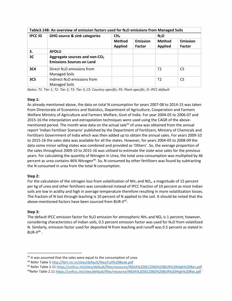
Table3.14B: An overview of emission factors used for N2O emissions from Managed Soils
IPCC ID GHG source & sink categories CH4 N2O
Method Applied
Emission Factor
Method Applied
Emission Factor
3. AFOLU
3C Aggregate sources and non-CO2 Emissions Sources on Land
3C4 Direct N2O emissions from Managed Soils
T2 CS
3C5 Indirect N2O emissions from Managed Soils
T2 CS
Notes: T1: Tier 1; T2: Tier 2; T3: Tier 3; CS: Country-specific; PS: Plant-specific; D: IPCC default
Step 1: As already mentioned above, the data on total N consumption for years 2007-08 to 2014-15 was taken from Directorate of Economics and Statistics, Department of Agriculture, Cooperation and Farmers Welfare Ministry of Agriculture and Farmers Welfare, Govt of India. For year 2004-05 to 2006-07 and 2015-16 the interpolation and extrapolation techniques were used using the CAGR of the above-mentioned period. The month wise data on the actual sale43 of urea was obtained from the annual report ‘Indian Fertilizer Scenario’ published by the Department of Fertilizers, Ministry of Chemicals and Fertilizers Government of India which was then added up to obtain the annual sales. For years 2009-10 to 2015-16 the sales data was available for all the states. However, for years 2004-05 to 2008-09 the data some minor selling states was combined and provided as ‘Others’. So, the average proportion of the sales throughout 2009-10 to 2015-16 was utilised to estimate the state wise sales for the previous years. For calculating the quantity of Nitrogen in Urea, the total urea consumption was multiplied by 46 percent as urea contains 46% Nitrogen44. So, N consumed by other fertilizers was found by subtracting the N consumed in urea from the total N consumption. Step 2: For the calculation of the nitrogen loss from volatilization of NH3 and NOx, a magnitude of 15 percent per kg of urea and other fertilizers was considered instead of IPCC fraction of 10 percent as most Indian soils are low in acidity and high in average temperature therefore resulting in more volatilization losses. The fraction of N lost through leaching is 10 percent of N applied to the soil. It should be noted that the above-mentioned factors have been sourced from BUR-II45. Step 3: The default IPCC emission factor for N2O emission for atmospheric NH3 and NOx is 1 percent; however, considering characteristics of Indian soils, 0.5 percent emission factor was used for N2O from volatilized N. Similarly, emission factor used for deposited N from leaching and runoff was 0.5 percent as stated in BUR-II46 .
43 It was assumed that the sales were equal to the consumption of urea. 44 Refer Table 5 http://fert.nic.in/sites/default/files/Full%20Book.pdf 45 Refer Table 2.11 https://unfccc.int/sites/default/files/resource/INDIA%20SECOND%20BUR%20High%20Res.pdf 46Refer Table 2.11 https://unfccc.int/sites/default/files/resource/INDIA%20SECOND%20BUR%20High%20Res.pdf `

3.14.3 Recalculation
Table 3.14C: Source category wise details on the difference between GHG estimates
Year Key source category GHG Emission Estimates (MtCO2e) % Difference
Phase-II Phase-III
2005 Agricultural Soils 37.54 44.66 19%
2006 Agricultural Soils 40.68 45.03 11%
2007 Agricultural Soils 42.92 45.43 6%
2008 Agricultural Soils 44.93 47.22 5%
2009 Agricultural Soils 46.54 48.87 5%
2010 Agricultural Soils 49.11 51.71 5%
2011 Agricultural Soils 51.52 54.22 5%
2012 Agricultural Soils 51.00 53.34 5%
2013 Agricultural Soils 50.48 51.07 1%
As decided amongst platform partners, a significance threshold of 5% is considered. Recalculation have been reported where the deviation between Phase III and Phase II results is higher than the threshold. As seen in table 3.14C above, a significant deviation is observed in phase-3 and phase-2 emissions from Agricultural soils. This deviation can be attributed to the change in the activity data which is now sourced from more reliable publicly available sources, unlike the previous phase where the data was made available on request. 3.14.4 Uncertainty Disaggregated data beyond state level in different parts of the country are not available. Assumptions have been made with regard to the usage of fertilizers applied to the agricultural fields. Therefore, the uncertainty associated with the activity data cannot be quantified due to limitations of the data. India specific emission factors have been derived from a study by Bhatia et al 2013. According to this study, uncertainty in emission factors arise due to climatic conditions, soil type, water usage etc. Various biological, chemical and physical properties of soil influence the emissions from soil to the atmosphere.
Table 3.14D: Source category wise description of Qualitative uncertainty
IPCC ID Source Category
Qualitative Uncertainty
Activity Data Emission Factor
3C4 & 3C5 Agriculture Soils
Lack of coverage of measurements, spatial aggregation, and lack of information on specific on-farm practices.
According to 2006 IPCC guidelines (Chapter 11, Volume 04)60, uncertainties in estimates of emissions from managed soils are caused by uncertainties related to the emission factors that arise from natural variability, partitioning fractions.
3.14.5 Recommended Improvements
As and when more detailed surveys are carried out, these estimations will be improved.

3.15 3C7 Rice Cultivation
3.15.1 Category description Paddy fields are a large source of methane emissions from agriculture. Methane emissions arise due to anaerobic decomposition of organic materials from flooded paddy fields. Given below are the details of data used. The data quality is considered high because the activity data has been obtained from credible and relevant Government of India sources that have been engaged in collecting such data every five years for several decades. Further, the credibility of the data is acknowledged by all the relevant stakeholders both within and outside the Government.
Table 3.15A: An overview of source categories of Rice Cultivation
IPCC ID
GHG source & sink categories
Type Quality Source
3C Aggregate sources and non-CO2 Emissions Sources on Land
3C7 Rice Cultivation
Secondary High Directorate of Economics and Statistics, Department of Agriculture, Cooperation and Farmer’s Welfare, Government of India Source: For years 2004-05 to 2012-13: Table 3.1, State-wise Area under Crops (Detailed Tables - State wise(2003-04 to 2012-13) available at: http://eands.dacnet.nic.in/LUS_2012-13.htm) For years 2013-14 to 2015-16: Table 3.1, State-wise Area under Crops (All India Summary Tables available at : http://eands.dacnet.nic.in/LUS_1999_2004.htm)
3.15.2 Methodology
The methodological details for estimation of emissions from rice cultivation are as under:
Table 3.15B: An overview of Emission Factors used for Rice Cultivation
IPCC ID GHG source & sink categories CH4 N2O
Method Applied
Emission Factor
Method Applied
Emission Factor
3. AFOLU
3C Aggregate sources and non-CO2 Emissions Sources on Land
3C7 Rice Cultivation T3 CS

Notes: T1: Tier 1; T2: Tier 2; T3: Tier 3; CS: Country-specific; PS: Plant-specific; D: IPCC default
The methodology used was the same as that used in NATCOMM II 2012. It has been referred from Gupta et al., (2009) and Pathak et al., (2010) using 2006 IPCC guidelines for national GHG Inventories. The methane emissions are estimated by multiplying the total paddy rice area under different water management regimes (ha) with corresponding Emission Factor. Separate calculations were made for each state and union territory (UT) of India and the national level as well as for each rice ecosystems (i.e., irrigated, rain-fed, and deep-water rice production) and then summed up to estimate the national total. The equation used was: ERC = AC˙EFW˙10-6 Where, ERC = CH4 emissions from rice cultivation (Gg year-1), AC = area of rice cultivation under management C (ha) EFW = factor applied for different types of water management (kg CH4 ha-1) 10-6 = to convert Kg into Gg (Refer Annex I for sample calculations) Step1: We first calculated the percentage of area under rice under respective water management regime for each state by multiplying the harvested area obtained by percentage area covered under a particular water management regime. The water management regimes in each state were assumed to be the same as that available in Pathak et al 2010, Bhatia et al 2013 and Huke & Huke 1997. The rainfed area was also sub-divided into rainfed flood prone (27.1%) and rainfed drought prone (72.9%) based on the literature reference Huke and Huke 1997. The irrigated rice area was further divided into the irrigated continuously flooded (26.9%), irrigated single aeration (35.7%) and irrigated multiple aeration (37.4%) based on Gupta et al. 2009. Step2: Next, we multiplied India specific emission factor of each water management regime with proportion of area under cultivation under each water management across all states in India. Step 3: To convert data into Kg to Gg, we multiplied by 10-6. The specific emission factors (from BUR-II) used were as follows:
Table 3.15C: Emission Factor for different water regime for Rice Cultivation
Emission from different water regime for rice cultivation Emission (kg CH4/ha)
Continuous Flooding 159.74
Single Aeration 66.2
Multiple Aeration 19.3
Flood Prone 189
Drought Prone 66.84
Deep Water 190
Upland 0
Source: (Table 2.10, “BUR Report,” n.d.)
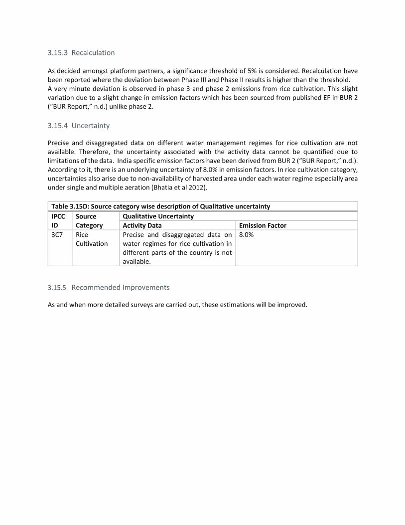
3.15.3 Recalculation As decided amongst platform partners, a significance threshold of 5% is considered. Recalculation have been reported where the deviation between Phase III and Phase II results is higher than the threshold. A very minute deviation is observed in phase 3 and phase 2 emissions from rice cultivation. This slight variation due to a slight change in emission factors which has been sourced from published EF in BUR 2 (“BUR Report,” n.d.) unlike phase 2.
3.15.4 Uncertainty
Precise and disaggregated data on different water management regimes for rice cultivation are not available. Therefore, the uncertainty associated with the activity data cannot be quantified due to limitations of the data. India specific emission factors have been derived from BUR 2 (“BUR Report,” n.d.). According to it, there is an underlying uncertainty of 8.0% in emission factors. In rice cultivation category, uncertainties also arise due to non-availability of harvested area under each water regime especially area under single and multiple aeration (Bhatia et al 2012).
Table 3.15D: Source category wise description of Qualitative uncertainty
IPCC ID
Source Category
Qualitative Uncertainty
Activity Data Emission Factor
3C7 Rice Cultivation
Precise and disaggregated data on water regimes for rice cultivation in different parts of the country is not available.
8.0%
3.15.5 Recommended Improvements
As and when more detailed surveys are carried out, these estimations will be improved.

4 Comparison with national inventories
Table 4: AFOLU Source category wise details of deviation in GHG estimates between GHGPI and official inventories published by Government of India (MtCO2e)
Key Source Category
2007 2010 2014
INCCA GHGPI % Deviation BUR GHGPI % Deviation BUR2 GHGPI % Deviation
3A1 Enteric Fermentation
212.1 208.42 -2% 227.03 204.79 -10% 227.16
204.76 -10%
3A2 Manure Management
2.44 21.86
796% 2.77 21.49 676% 28.10
21.52 -23%
3B1 Forest Land
-67.8 -97.97 45% -203.83 -97.97 -52% -69.67 -124.44 79%
3B2 Cropland -
207.52 -1.46 -99% -110.76 -0.62 -99%
-248.61
-1.32 -99%
3B3 Grasslands
10.49 0.58 -94% 55.65 0.42 -99% 17.22 0.66 -96%
3B5 Settlements
-0.04 0.45 -1214% 2.62 0.47 -82% -1.58 0.49 -131%
3B6 Other Land
- - - - - - - - -
3C1a Biomass burning in forest land
- - - 3.79 5.23 38% 157.47 5.12 -97%
3C1b Biomass burning in cropland
6.61 5.75 -12.96% 7.92 6.17 -22% 8.59 5.84 -32%
3C4&3C5 Direct and Indirect emissions from managed soils
43.4 45.43 4.68% 81.08 50.87 -37% 80.53 51.71 -36%
3C7 Rice Cultivation
69.87 71.10 1.13% 71.37 69.44 -3% 72.84 69.4 -5%
3A1 Enteric Fermentation All the necessary and required data from 18th and 19th Livestock Census of India for years 2007 and 2012 respectively47 have been used. The calculations are consistent with the requirements of best practice as per 2006 IPCC guidelines INCCA: GHGPI values deviated only by a slight magnitude of 2% from the INCCA estimates which can be attributed to the bottom’s up approach taken up by the platform to attain the National values. BUR-I and BUR-II: During both the years for which data is reported a deviation of 10% is observed which is mainly due to lack of greater details of data or of the assumptions that have been made used while in making their calculations that has been used while estimating emissions. In the absence of such details
47 http://dahd.nic.in/documents/statistics/livestock-census

unpacking the BUR inventory is challenging for further analysis. In the absence of such details unpacking the BUR inventory is challenging for further analysis. 3A2 Manure Management All the necessary and required data from Livestock Census of India for 2007 and 201248 have been used. The calculations are consistent with the requirements of best practice as per 2006 IPCC guidelines. INCCA: A huge deviation of 796% was observed from the INCCA values to the fact that it does not provide detailed population data, i.e., category-wise population details are not provided. Further, category wise emissions are also not provided for manure management, instead emissions are reported for the total livestock categories. Furthermore, INCCA report lacks clarity/ transparency on specific Methane emission factors used for Manure Management. BUR-I and BUR-II: In 2010 and 2014 a deviation of 676% and -23% respectively was observed which is mainly due to lack of greater details of data or of the assumptions that have been made used while in making their calculations that has been used while estimating emissions. In the absence of such details unpacking the BUR inventory is challenging for further analysis. In the absence of such details unpacking the BUR inventory is challenging for further analysis. 3B1 Forest Land All the necessary and required data from Forest Survey of India49 have been used. The calculations are consistent with the requirements of best practice as per 2006 IPCC guidelines. INCCA: A deviation of 45% was noted because the INCCA report uses Forest cover mapping and Forest area mapping for the activity data. For carbon stock calculation, the report analysis the strata layer using GIS mapping. Details of the different strata and the amount of carbon stock associated are not available in the INCCA report. Our analysis uses FSI reports on carbon stock and forest area, therefore, the variation in results. BUR-I and BUR-II: A deviation of 52% and 79% was observed in 2010 and 2014 respectively due to lack of greater details of data or of the assumptions that have been made used while in making their calculations that has been used while estimating emissions. In the absence of such details unpacking the BUR inventory is challenging for further analysis. 3B2 Cropland All the available data sources from National Remote Sensing Centre have been used. The calculations are consistent with the requirements of best practice as per 2006 IPCC guidelines. INCCA: A deviation of -99% was observed from the INCAA values because the INCCA report does not estimate emissions from the category ‘Land converted to Cropland’. It only estimates emissions from ‘Cropland remaining Cropland’. Hence, the variation from GHG Platform India results as both the
48 http://dahd.nic.in/documents/statistics/livestock-census 49 http://fsi.nic.in/

categories have been considered for emission estimation. Furthermore, rate of change of biomass and carbon stock is not available in detail in the INCCA report. BUR-I and BUR-II: A deviation of -99% was also observed from the BUR values in both the years for which the inventories have been reported i.e. 2010 and 2014. This is due to lack of greater details of data or of the assumptions that have been made used while in making their calculations that has been used while estimating emissions. In the absence of such details unpacking the BUR inventory is challenging for further analysis. 3B3 Grasslands All the available data sources from National Remote Sensing Centre have been used. The calculations are consistent with the requirements of best practice as per 2006 IPCC guidelines. INCCA: A deviation of -94% from the INCCA values was observed because the INCCA report does not estimate emissions from the category ‘Land converted to Grassland’. It only estimates emissions from ‘Grassland remaining Grassland’. Hence, the variation from GHG Platform India results as both the categories have been considered for emission estimation. Furthermore, rate of change of biomass and carbon stock is not available in detail in the INCCA report. BUR-I and BUR-II: A deviation of -99% and -96% was observed in 2010 and 2014 respectively due to lack of greater details of data or of the assumptions that have been made used while in making their calculations that has been used while estimating emissions. In the absence of such details unpacking the BUR inventory is challenging for further analysis. 3B5 Settlements All the available data sources from National Remote Sensing Centre have been used. The calculations are consistent with the requirements of best practice as per 2006 IPCC guidelines. INCCA: A deviation of -1214% from the INCCA values was observed because INCCA report does not estimate emissions from the category ‘Land converted to Settlement’. It only estimates emissions from ‘Settlement remaining Settlement’. Hence, the variation from GHG Platform India results as both the categories have been considered for emission estimation. Furthermore, rate of change of biomass and carbon stock is not available in detail in the INCCA report. BUR-I and BUR-II: A deviation of -82% and -131% was observed in 2010 and 2014 respectively due to lack of greater details of data or of the assumptions that have been made used while in making their calculations that has been used while estimating emissions. In the absence of such details unpacking the BUR inventory is challenging for further analysis. 3B6 Other Land Government of India does not estimate emissions from this category. Therefore, calculations of variance cannot be done.

3C1a. Biomass burning in Forest Land All the available data sources from Forest Survey of India50 have been used. The calculations are consistent with the requirements of best practice as per 2006 IPCC guidelines. INCCA: This category is not considered under emission estimation in the INCCA report. BUR-I and BUR-II: A deviation of 38% and -97% was observed in 2010 and 2014 respectively due to lack of greater details of data or of the assumptions that have been made used while in making their calculations that has been used while estimating emissions. In the absence of such details unpacking the BUR inventory is challenging for further analysis. 3C1b. Biomass Burning in Cropland The data that have been used for this estimation are calculated from Ministry of Agriculture and peer reviewed literature mentioned above in the methodology section. INCCA: A deviation of 12.96% from the INCCA values was observed because the INCCA report does not give detailed activity data in terms of residue burnt in Indian states. Hence, it is difficult to analyze the variation without comparing the base data. BUR-I and BUR-II: A deviation of -22% and -32% was observed in 2010 and 2014 respectively due to lack of greater details of data or of the assumptions that have been made used while in making their calculations that has been used while estimating emissions. In the absence of such details unpacking the BUR inventory is challenging for further analysis. 3C4&3C5 Direct and Indirect emissions from managed soils The calculations are consistent with the requirements of best practice as per 2006 IPCC Guidelines. INCCA: A slight deviation of 4.68% from the INCCA values was observed which can be attributed to rounding-off factors and adding up of the state values to get the national value. BUR-I and BUR-II: A deviation of -37% and -36% was observed in 2010 and 2014 respectively due to lack of greater details of data or of the assumptions that have been made used while in making their calculations that has been used while estimating emissions. In the absence of such details unpacking the BUR inventory is challenging for further analysis. 3C7 Rice Cultivation The calculations are consistent with the NATCOM 2 and BUR 2. INCCA: A very minute deviation of 1.13% from the INCCA values was observed which may be due to rounding off calculations adding up of the state values to get the national value. BUR-I and BUR-II: A deviation of -3% and -5% was observed in 2010 and 2014 respectively which may be due to rounding off calculations adding up of the state values to get the national value.
50 http://fsi.nic.in/

Additional Information To the extent possible, we have tried to adhere to the 2006 IPCC guidelines for national GHG inventories for estimations of emissions from the AFOLU sector for India. Exceptions, however, arise due to lack of availability of data that is required to adhere to IPCC 2006 guidelines. In these cases, we have tried to estimate emissions on the basis of the information obtained during the unpacking of official inventories that are available in the public domain. Specifically, the deviations are for the following sub-sectors:
• 3C1b Biomass Burning in Cropland: For this sub-sector, we have used the methodology that has been followed in NATCOM-II
• 3C4 Direct N2O emissions from Managed Soils: For this sub-sector, we have used the methodology that has been followed in NATCOM-II.
• 3C5 Indirect N2O emissions from Managed Soils: For this sub-sector, we have used the methodology that has been followed in NATCOM-II.
• 3C7 Rice Cultivation: For this sub-sector, we have used the methodology that has been followed in NATCOM-II.
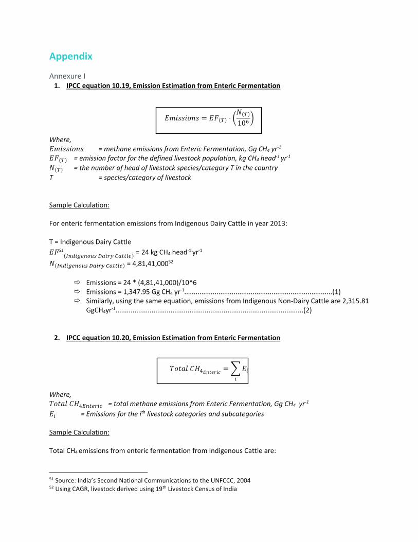
Appendix
Annexure I 1. IPCC equation 10.19, Emission Estimation from Enteric Fermentation
𝐸𝑚𝑖𝑠𝑠𝑖𝑜𝑛𝑠 = 𝐸𝐹(𝑇) ⋅ (𝑁(𝑇)
106)
Where, 𝐸𝑚𝑖𝑠𝑠𝑖𝑜𝑛𝑠 = methane emissions from Enteric Fermentation, Gg CH4 yr-1
𝐸𝐹(𝑇) = emission factor for the defined livestock population, kg CH4 head-1 yr-1
𝑁(𝑇) = the number of head of livestock species/category T in the country
T = species/category of livestock Sample Calculation: For enteric fermentation emissions from Indigenous Dairy Cattle in year 2013: T = Indigenous Dairy Cattle
𝐸𝐹51(𝐼𝑛𝑑𝑖𝑔𝑒𝑛𝑜𝑢𝑠 𝐷𝑎𝑖𝑟𝑦 𝐶𝑎𝑡𝑡𝑙𝑒)
= 24 kg CH4 head-1 yr-1
𝑁(𝐼𝑛𝑑𝑖𝑔𝑒𝑛𝑜𝑢𝑠 𝐷𝑎𝑖𝑟𝑦 𝐶𝑎𝑡𝑡𝑙𝑒) = 4,81,41,00052
Emissions = 24 * (4,81,41,000)/10^6 Emissions = 1,347.95 Gg CH4 yr-1..............................................................................(1) Similarly, using the same equation, emissions from Indigenous Non-Dairy Cattle are 2,315.81
GgCH4yr-1...................................................................................................(2)
2. IPCC equation 10.20, Emission Estimation from Enteric Fermentation
𝑇𝑜𝑡𝑎𝑙 𝐶𝐻4𝐸𝑛𝑡𝑒𝑟𝑖𝑐= ∑ 𝐸𝑖
𝑖
Where, 𝑇𝑜𝑡𝑎𝑙 𝐶𝐻4𝐸𝑛𝑡𝑒𝑟𝑖𝑐 = total methane emissions from Enteric Fermentation, Gg CH4 yr-1
𝐸𝑖 = Emissions for the ith livestock categories and subcategories Sample Calculation: Total CH4 emissions from enteric fermentation from Indigenous Cattle are:
51 Source: India’s Second National Communications to the UNFCCC, 2004 52 Using CAGR, livestock derived using 19th Livestock Census of India

Total CH4 emissions = Emissions (Indigenous Dairy Cattle) + Emissions (Indigenous Non Dairy Cattle)
Total CH4 emissions = (1) + (2) Total CH4 emissions = 1,347.95 GgCH4 yr-1 + 2,315.81 GgCH4yr-1 Total CH4 emissions = 3,662.76 GgCH4 yr-1
3. IPCC equation 10.21, Emission Factor for Enteric Fermentation
𝐸𝐹 =[𝐺𝐸 ⋅ 𝑌𝑚 ⋅ 365]
55.65
Where, 𝐸𝐹 = Emission factor (Kg methane / animal / year), 𝐺𝐸 = Gross energy intake (MJ53 / animal / year), 𝑌𝑚 = Methane conversion rate which is the fraction of gross energy feed converted to methane Sample Calculation: For indigenous dairy cattle in India, dry matter intake is approximately 2%54. Average body weight of indigenous dairy cattle is 175 kg. The conversion factor (CF) used for arriving at GE is 18.45 MJ/kg feed. These factors are used to calculate Gross Energy Intake. Now, GE = 60.99 MJ/animal/year Ym = 6%55 Therefore,
EF = (60.99 x 6% x 365)/(55.65) EF = 24 Kg CH4/animal/year
4. IPCC equation 10.22, Emission Estimation from Manure Management
𝐶𝐻4𝑀𝑎𝑛𝑢𝑟𝑒= ∑
(𝐸𝐹(𝑇) ⋅ 𝑁(𝑇))
106
(𝑇)
Where, 𝐶𝐻4𝑀𝑎𝑛𝑢𝑟𝑒
= methane emissions from Manure Management, Gg CH4 yr-1
𝐸𝐹(𝑇) = emission factor for the defined livestock population, kg CH4 head-1 yr-1
𝑁(𝑇) = the number of head of livestock species/category T in the country
T = species/category of livestock Sample Calculation: Considering methane emissions from manure management for indigenous dairy cattle in year 2013,
53 Assumed to be 18.45 54 Swamy and Bhattacharya (2006) 55 Swamy and Bhattacharya (2006)

T = Indigenous Dairy Cattle
𝐸𝐹56(𝐼𝑛𝑑𝑖𝑔𝑒𝑛𝑜𝑢𝑠 𝐷𝑎𝑖𝑟𝑦 𝐶𝑎𝑡𝑡𝑙𝑒)
= 3.50 kg CH4 head-1 yr-1
𝑁(𝐼𝑛𝑑𝑖𝑔𝑒𝑛𝑜𝑢𝑠 𝐷𝑎𝑖𝑟𝑦 𝐶𝑎𝑡𝑡𝑙𝑒) = 4,81,41,00057
Emissions = 3.5 * (4,81,41,000)/10^6 Emissions = 168.50 Gg CH4 yr-1…..............................................................................(3) Similarly, using the same equation, emissions from Indigenous Non-Dairy Cattle are 233.14
GgCH4yr-1.....................................................................................................(4) Total CH4 emissions (manure) = Manure Management Emissions (Indigenous Dairy Cattle) + Manure Management Emissions (Indigenous Non Dairy Cattle)
Total CH4 emissions (manure) = (3) + (4) Total CH4 emissions (manure) = 168.50 GgCH4 yr-1 + 233.14 GgCH4yr-1 Total CH4 emissions = 401.64 GgCH4 yr-1
5. IPCC equation 10.2558, Emission Estimation from Manure Management
𝑁2𝑂𝑎𝑛𝑖𝑚𝑎𝑙𝑠 = 𝑁2𝑂𝐴𝑊𝑀𝑆 = 𝑁𝑇 ⋅ (𝑁𝑒𝑥(𝑇) ⋅ 𝐴𝑊𝑀𝑆𝑇 ⋅ 𝐸𝐹3(𝐴𝑊𝑀𝑆))
Where, 𝑁2𝑂𝑎𝑛𝑖𝑚𝑎𝑙𝑠 = N2O emissions from animal production in a country (kg N/ yr) 𝑁2𝑂𝐴𝑊𝑀𝑆 = N2O emissions from Animal Waste Management System in the country (kg N/ yr); 𝑁𝑇 = number of animals of type T in the country 𝑁𝑒𝑥(𝑇) = N excretion of animals of type T in the country (kg N/animal/yr)
𝐴𝑊𝑀𝑆𝑇 = fraction of 𝑁𝑒𝑥(𝑇) that is managed in one of the different distinguished animal waste
management systems for animals of type T in the country 𝐸𝐹3(𝐴𝑊𝑀𝑆) = N2O emission factor for an AWMS (kg N2O -N/ kg of 𝑁𝑒𝑥 in AWMS)
T = type of animal category Sample Calculation: Nitrogen emissions from manure management are calculated using the above equation. However, under this exercise, emission factor was obtained from India’s second national communications to the UNFCCC. Therefore, the factors (𝑁𝑒𝑥(𝑇) ⋅ 𝐴𝑊𝑀𝑆𝑇 ⋅ 𝐸𝐹3(𝐴𝑊𝑀𝑆)) are directly sourced from NATCOMM II.
Considering nitrous dioxide emissions from manure management for indigenous dairy cattle in year 2013, Emission Factor = 0.0006 kgN2O/head/year Population = NT = 4,81,41,00059
56 Source: India’s Second National Communications to the UNFCCC, 2004 57 Using CAGR, livestock derived using 19th Livestock Census of India 58 http://www.ipcc-nggip.iges.or.jp/public/2006gl/pdf/4_Volume4/V4_10_Ch10_Livestock.pdf - page 10.53 59 Using CAGR, livestock derived using 19th Livestock Census of India

𝑁2𝑂𝑎𝑛𝑖𝑚𝑎𝑙𝑠 = 0.0006 x 4,81,41,000 𝑁2𝑂𝑎𝑛𝑖𝑚𝑎𝑙𝑠 = 28,884 Gg N2O
6. IPCC Equation 2.5, Emission Estimation from Land
Stock Difference Method
𝛥𝐶 =(𝐶𝑡2
− 𝐶𝑡1)
(𝑡2 − 𝑡1)
Where, 𝛥𝐶 = Annual Carbon stock change in pool (tonnes C yr-1) 𝐶𝑡2
= Carbon stock in the pool at time t2
𝐶𝑡1 = Carbon stock in the pool at time t1
Sample Calculation: Assuming: t2 = 2013 t1 = 2011 𝐶𝑡2
= 704460 MtC………………………………………………………………………………………….…………..(5)
𝐶𝑡1 = 694161 MtC ……………………………………………………………………………………………………..(6)
Therefore, ΔC = ((5)-(6))/(2013-2011)
ΔC = (7044 – 6941)/(2013-2011) MtC ΔC = -51.50 MtC
7. IPCC Equation 2.25 , Emission Estimation from Land
𝛥𝐶𝑚𝑖𝑛𝑒𝑟𝑎𝑙 =(𝑆0𝐶0 − 𝑆0𝐶(0−𝑇))
𝐷
𝑆𝑂𝐶 = ∑ 𝑆𝑂𝐶𝑅𝐸𝐹𝐶,𝑆,𝐼⋅ 𝐹𝐿𝑈𝐶,𝑆,𝐼
⋅ 𝐹𝑀𝐺𝐶,𝑆,𝐼⋅ 𝐹𝐼𝐶,𝑆,𝐼
⋅ 𝐴𝐶,𝑆,𝐼
𝐶,𝑆,𝐼
where, 𝛥𝐶𝑚𝑖𝑛𝑒𝑟𝑎𝑙 = annual change in carbon stocks in mineral soils, tonnes C yr-1 𝑆0𝐶0 = soil organic carbon stock in the last year of an inventory time, tonnes C 𝑆0𝐶(0−𝑇) = soil organic carbon stock at the beginning of the inventory time, tonnes C
60 State of Forest Report 2015 61 State of Forest Report 2013
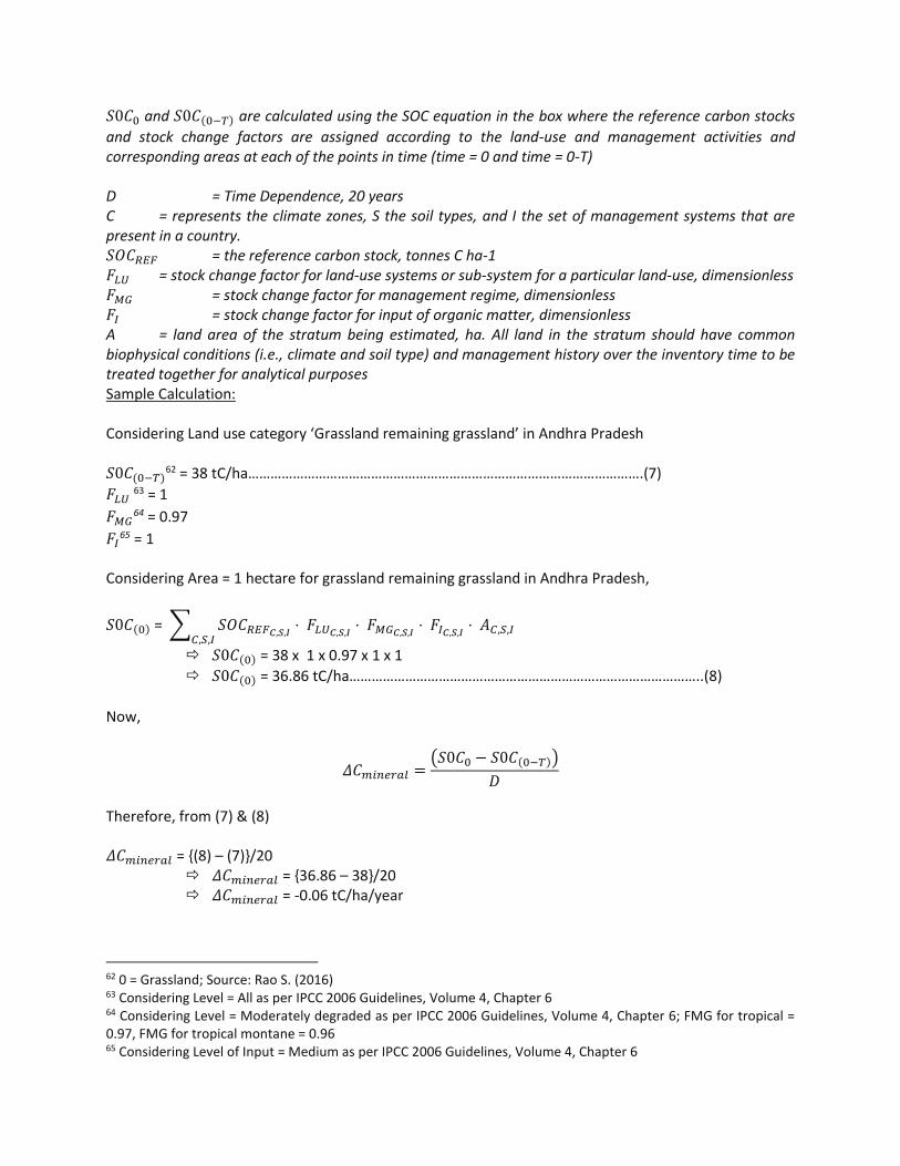
𝑆0𝐶0 and 𝑆0𝐶(0−𝑇) are calculated using the SOC equation in the box where the reference carbon stocks
and stock change factors are assigned according to the land-use and management activities and corresponding areas at each of the points in time (time = 0 and time = 0-T) D = Time Dependence, 20 years C = represents the climate zones, S the soil types, and I the set of management systems that are present in a country. 𝑆𝑂𝐶𝑅𝐸𝐹 = the reference carbon stock, tonnes C ha-1 𝐹𝐿𝑈 = stock change factor for land-use systems or sub-system for a particular land-use, dimensionless 𝐹𝑀𝐺 = stock change factor for management regime, dimensionless 𝐹𝐼 = stock change factor for input of organic matter, dimensionless A = land area of the stratum being estimated, ha. All land in the stratum should have common biophysical conditions (i.e., climate and soil type) and management history over the inventory time to be treated together for analytical purposes Sample Calculation: Considering Land use category ‘Grassland remaining grassland’ in Andhra Pradesh 𝑆0𝐶(0−𝑇)
62 = 38 tC/ha…………………………………………………………………………………………….(7)
𝐹𝐿𝑈 63 = 1
𝐹𝑀𝐺64 = 0.97
𝐹𝐼65 = 1
Considering Area = 1 hectare for grassland remaining grassland in Andhra Pradesh,
𝑆0𝐶(0) = ∑ 𝑆𝑂𝐶𝑅𝐸𝐹𝐶,𝑆,𝐼⋅ 𝐹𝐿𝑈𝐶,𝑆,𝐼
⋅ 𝐹𝑀𝐺𝐶,𝑆,𝐼⋅ 𝐹𝐼𝐶,𝑆,𝐼
⋅ 𝐴𝐶,𝑆,𝐼𝐶,𝑆,𝐼
𝑆0𝐶(0) = 38 x 1 x 0.97 x 1 x 1
𝑆0𝐶(0) = 36.86 tC/ha…………………………………………………………………………………..(8)
Now,
𝛥𝐶𝑚𝑖𝑛𝑒𝑟𝑎𝑙 =(𝑆0𝐶0 − 𝑆0𝐶(0−𝑇))
𝐷
Therefore, from (7) & (8) 𝛥𝐶𝑚𝑖𝑛𝑒𝑟𝑎𝑙 = {(8) – (7)}/20
𝛥𝐶𝑚𝑖𝑛𝑒𝑟𝑎𝑙 = {36.86 – 38}/20 𝛥𝐶𝑚𝑖𝑛𝑒𝑟𝑎𝑙 = -0.06 tC/ha/year
62 0 = Grassland; Source: Rao S. (2016) 63 Considering Level = All as per IPCC 2006 Guidelines, Volume 4, Chapter 6 64 Considering Level = Moderately degraded as per IPCC 2006 Guidelines, Volume 4, Chapter 6; FMG for tropical = 0.97, FMG for tropical montane = 0.96 65 Considering Level of Input = Medium as per IPCC 2006 Guidelines, Volume 4, Chapter 6

8. IPCC Equation 2.27, Emission Estimation from Biomass Burning
𝐿𝑓𝑖𝑟𝑒 = 𝐴 ⋅ 𝑀𝐵 ⋅ 𝐶𝑓 ⋅ 𝐺𝑒𝑓 ⋅ 10−3
Where, 𝐿𝑓𝑖𝑟𝑒 = amount of greenhouse gas emissions from fire, tonnes of each GHG e.g., CH4, N2O, etc.
A = area burnt, ha 𝑀𝐵 = mass of fuel available for combustion, tonnes ha-1. This includes biomass, ground litter and dead wood. 𝐶𝑓 = combustion factor, dimensionless
𝐺𝑒𝑓 = emission factor, g kg-1 dry matter burnt
Sample Calculation: Consider biomass burning66 in Indian Forests in year 2013. Area burnt in year 2013 (in ha) = A = 3,04,679 Mass of fuel available for combustion (in t/ha) = 13.12 Combustion Factor = 0.36 Emission factor for methane gas (g/kg dry matter burnt) = 9 Emission factor for nitrous dioxide gas (g/kg dry matter burnt) = 0.11 Therefore, Methane emissions from biomass burning can be calculated as:
𝐿𝑓𝑖𝑟𝑒 = (3,04,679 x 13.12 x 0.36 x 9)/1000
𝐿𝑓𝑖𝑟𝑒 = 12,760 tonnes of methane
Similarly, nitrous oxide emissions from biomass burning are 155.9 tonnes of N2O.
9. Equation used for Biomass Burning in cropland67
𝐹𝐵𝐶𝑅 = ∑𝐶𝑟𝑜𝑝𝑠(𝐴 ⋅ 𝐵 ⋅ 𝐶 ⋅ 𝐷 ⋅ 𝐸 ⋅ 𝐹) Where, FBCR is the emissions from residue burning, A is the crop production, B is the residue to crop ratio, C is the dry matter fraction, D is the fraction burnt E is the fraction oxidized, F is the emission factor for CH4 and N2O Sample Calculation: Consider Residue burning in rice field in Punjab for year 2013, Rice Production in year 2013 in Punjab (‘000 tonnes) = A = 11,294 Residue to Crop Ratio68 = B = 1.50
66 Note: Source for all the data in this calculation is from India’s Second National Communications. 67 Bhatia et al. (2013) 68 Jain et al. (2014)

Dry Matter Fraction69 = C = 0.86 Fraction Burnt70 = D = 0.80 Combustion Factor71 = E = 0.89 Emission Factor for CH4
72 = F = 2.70 g/kg Therefore, Emissions from Residue Burning in Punjab’s Rice fields =
FBCR = A * B * C * D * E * F FBCR = (11,294 x 1.50 x 0.86 x 0.80 x 0.89 x 2.70)/1000 FBCR = 28.007 Gg FBCR = 28,007.94 tCH4
10. Equation used for emission estimation from Rice Cultivation73
ERC = AC˙EFW˙10-6
Where, ERC = CH4 emissions from rice cultivation (Gg CH4 year-1), AC = area of rice cultivation under management C (ha) EFW = emission factor applied for different types of water management (kg CH4 ha-1) 10-6 = to convert Kg into Gg Sample Calculation Consider rice cultivation in Punjab in year 2013 and intermittent multiple aeration water management is used in Punjab. Area under intermittent multiple aeration water management is estimated by multiplying the total harvested area by the percentage of area falling under the said water management system based on various studies. So, in this sample calculation Area of Rice Cultivation under intermittent multiple aeration management= (2849 ha* 99.6)/100 Therefore, area of rice cultivation under intermittent multiple aeration management in Punjab in 2013 (in ‘000 ha) = AC = 2,837 Emission Factor for intermittent multiple aeration management74 = EFW = 18 kg CH4/ha Hence,
ERC = (2,837 * 18)/1000 ERC = 51.06 Gg CH4/year
69 Jain et al. (2014) 70 Calculations based on data from Gadde et al. (2009) 71 Turn et al. (1997) 72 Andrea and Merlot (2001) 73 Gupta et al. (2009) and Pathak et al. (2010) 74 India’s Second National Communications to the UNFCCC

Annexure II Emission estimates (in MtCO2e) from 3A. Livestock sector from 2005 to 15:
State/UT 2005 2006 2007 2008 2009 2010 2011 2012 2013 2014 2015
Andaman and Nicobar Island 0.05 0.05 0.05 0.05 0.05 0.05 0.05 0.05 0.05 0.05 0.04
Andhra Pradesh 10.13 10.61 11.09 10.76 10.44 10.11 9.79 9.47 9.21 8.98 8.77
Arunachal Pradesh 0.35 0.35 0.35 0.35 0.34 0.34 0.34 0.34 0.34 0.35 0.36
Assam 6.48 6.74 7.01 7.05 7.09 7.12 7.16 7.20 7.29 7.39 7.50
Bihar 13.08 13.57 14.05 14.17 14.28 14.40 14.52 14.63 14.96 15.37 15.89
Chandigarh 0.02 0.02 0.02 0.02 0.02 0.02 0.02 0.02 0.02 0.02 0.02
Chhattisgarh 7.43 7.55 7.67 7.64 7.62 7.60 7.58 7.56 7.59 7.65 7.71
Dadra and Nagar Haveli 0.04 0.04 0.04 0.04 0.04 0.04 0.03 0.03 0.03 0.03 0.03
Daman and Diu 0.00 0.00 0.00 0.00 0.00 0.00 0.00 0.00 0.00 0.00 0.00
Delhi 0.26 0.28 0.29 0.27 0.25 0.24 0.22 0.20 0.19 0.19 0.19
Goa 0.09 0.08 0.08 0.08 0.08 0.07 0.07 0.07 0.07 0.07 0.06
Gujarat 12.12 12.45 12.78 13.26 13.73 14.20 14.67 15.14 15.71 16.32 16.98
Haryana 5.67 5.63 5.59 5.63 5.66 5.69 5.72 5.76 5.82 5.90 6.00
Himachal Pradesh 2.37 2.38 2.38 2.35 2.33 2.30 2.27 2.24 2.23 2.22 2.21
Jammu and Kashmir 3.62 3.70 3.78 3.62 3.47 3.31 3.16 3.00 2.88 2.77 2.66
Jharkhand 7.11 7.33 7.54 7.49 7.44 7.38 7.33 7.28 7.26 7.26 7.26
Karnataka 11.39 11.73 12.08 11.78 11.49 11.20 10.90 10.61 10.40 10.23 10.08
Kerala 1.54 1.50 1.46 1.39 1.31 1.24 1.17 1.10 1.05 1.01 0.98
Lakshadweep 0.01 0.01 0.01 0.01 0.01 0.01 0.01 0.01 0.01 0.01 0.01
Madhya Pradesh 20.03 20.76 21.48 20.91 20.33 19.75 19.17 18.59 18.25 17.96 17.72
Maharashtra 17.23 17.19 17.16 16.93 16.71 16.48 16.26 16.03 15.88 15.75 15.63
Manipur 0.33 0.31 0.29 0.28 0.27 0.26 0.25 0.24 0.24 0.23 0.23
Meghalaya 0.61 0.63 0.65 0.65 0.66 0.66 0.67 0.67 0.69 0.70 0.72
Mizoram 0.06 0.06 0.06 0.06 0.06 0.06 0.06 0.06 0.06 0.06 0.06
Nagaland 0.41 0.41 0.41 0.38 0.34 0.31 0.27 0.24 0.22 0.20 0.19
Odisha 10.13 9.88 9.64 9.41 9.19 8.97 8.74 8.52 8.46 8.44 8.45
Puducherry 0.06 0.07 0.07 0.07 0.06 0.06 0.05 0.05 0.05 0.05 0.04
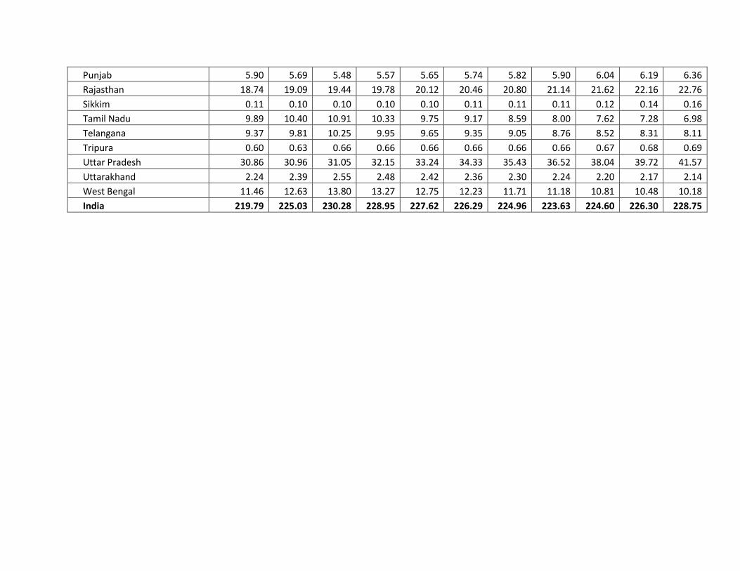
Punjab 5.90 5.69 5.48 5.57 5.65 5.74 5.82 5.90 6.04 6.19 6.36
Rajasthan 18.74 19.09 19.44 19.78 20.12 20.46 20.80 21.14 21.62 22.16 22.76
Sikkim 0.11 0.10 0.10 0.10 0.10 0.11 0.11 0.11 0.12 0.14 0.16
Tamil Nadu 9.89 10.40 10.91 10.33 9.75 9.17 8.59 8.00 7.62 7.28 6.98
Telangana 9.37 9.81 10.25 9.95 9.65 9.35 9.05 8.76 8.52 8.31 8.11
Tripura 0.60 0.63 0.66 0.66 0.66 0.66 0.66 0.66 0.67 0.68 0.69
Uttar Pradesh 30.86 30.96 31.05 32.15 33.24 34.33 35.43 36.52 38.04 39.72 41.57
Uttarakhand 2.24 2.39 2.55 2.48 2.42 2.36 2.30 2.24 2.20 2.17 2.14
West Bengal 11.46 12.63 13.80 13.27 12.75 12.23 11.71 11.18 10.81 10.48 10.18
India 219.79 225.03 230.28 228.95 227.62 226.29 224.96 223.63 224.60 226.30 228.75

Annexure III Emission estimates (in MtCO2e) from 3A1. Enteric Fermentation sector from 2005 to 15:
State/UT 2005 2006 2007 2008 2009 2010 2011 2012 2013 2014 2015
Andaman and Nicobar Island 0.04 0.04 0.04 0.04 0.04 0.04 0.04 0.04 0.04 0.04 0.04
Andhra Pradesh 9.22 9.66 10.10 9.80 9.51 9.21 8.91 8.62 8.39 8.18 7.98
Arunachal Pradesh 0.29 0.29 0.29 0.29 0.28 0.28 0.28 0.28 0.28 0.29 0.30
Assam 5.72 5.95 6.18 6.22 6.27 6.31 6.35 6.40 6.48 6.58 6.69
Bihar 11.83 12.27 12.72 12.83 12.94 13.05 13.16 13.27 13.57 13.95 14.43
Chandigarh 0.02 0.02 0.02 0.02 0.02 0.02 0.02 0.02 0.02 0.02 0.02
Chhattisgarh 6.69 6.80 6.92 6.90 6.88 6.86 6.84 6.82 6.85 6.89 6.95
Dadra and Nagar Haveli 0.03 0.04 0.04 0.04 0.03 0.03 0.03 0.03 0.03 0.02 0.02
Daman and Diu 0.00 0.00 0.00 0.00 0.00 0.00 0.00 0.00 0.00 0.00 0.00
Delhi 0.24 0.25 0.26 0.25 0.23 0.21 0.19 0.17 0.17 0.16 0.16
Goa 0.07 0.07 0.07 0.07 0.07 0.06 0.06 0.06 0.06 0.06 0.05
Gujarat 10.99 11.30 11.60 12.03 12.45 12.88 13.30 13.73 14.25 14.80 15.39
Haryana 5.11 5.07 5.03 5.06 5.09 5.11 5.14 5.17 5.23 5.30 5.38
Himachal Pradesh 2.17 2.17 2.17 2.15 2.12 2.10 2.08 2.05 2.04 2.03 2.02
Jammu and Kashmir 3.32 3.39 3.46 3.32 3.18 3.04 2.90 2.75 2.64 2.54 2.44
Jharkhand 6.40 6.60 6.81 6.76 6.71 6.66 6.61 6.56 6.54 6.53 6.53
Karnataka 10.36 10.67 10.99 10.72 10.45 10.19 9.92 9.65 9.46 9.30 9.17
Kerala 1.40 1.37 1.33 1.26 1.19 1.12 1.06 0.99 0.95 0.91 0.87
Lakshadweep 0.01 0.01 0.01 0.01 0.01 0.01 0.01 0.01 0.01 0.01 0.01
Madhya Pradesh 18.13 18.80 19.46 18.93 18.41 17.88 17.35 16.82 16.51 16.24 16.02
Maharashtra 15.66 15.62 15.58 15.38 15.17 14.96 14.76 14.55 14.41 14.29 14.18
Manipur 0.27 0.25 0.23 0.23 0.22 0.21 0.21 0.20 0.19 0.19 0.19
Meghalaya 0.52 0.53 0.54 0.55 0.55 0.56 0.56 0.57 0.58 0.59 0.61
Mizoram 0.03 0.03 0.03 0.03 0.03 0.03 0.03 0.03 0.03 0.03 0.03
Nagaland 0.32 0.32 0.32 0.29 0.26 0.24 0.21 0.18 0.16 0.15 0.14
Odisha 9.16 8.95 8.73 8.53 8.33 8.13 7.93 7.73 7.68 7.66 7.68
Puducherry 0.06 0.06 0.06 0.06 0.06 0.05 0.05 0.05 0.04 0.04 0.04

Punjab 5.35 5.16 4.97 5.05 5.13 5.20 5.28 5.35 5.47 5.61 5.76
Rajasthan 17.08 17.41 17.73 18.04 18.34 18.65 18.95 19.26 19.69 20.18 20.72
Sikkim 0.10 0.09 0.09 0.09 0.09 0.09 0.10 0.10 0.11 0.12 0.14
Tamil Nadu 8.99 9.46 9.93 9.40 8.87 8.34 7.81 7.28 6.93 6.61 6.34
Telangana 8.52 8.93 9.33 9.06 8.79 8.51 8.24 7.97 7.75 7.56 7.38
Tripura 0.52 0.55 0.58 0.57 0.57 0.57 0.57 0.57 0.57 0.58 0.59
Uttar Pradesh 27.84 27.94 28.04 29.03 30.02 31.01 32.00 32.99 34.36 35.88 37.56
Uttarakhand 2.04 2.18 2.31 2.26 2.20 2.15 2.09 2.04 2.00 1.97 1.95
West Bengal 10.35 11.39 12.42 11.96 11.49 11.02 10.55 10.08 9.75 9.45 9.19
India 198.84 203.63 208.42 207.21 206.00 204.79 203.58 202.37 203.24 204.76 206.97
Annexure IV Emission estimates (in MtCO2e) from 3A2. Manure Management sector from 2005 to 15:
State/UT 2005 2006 2007 2008 2009 2010 2011 2012 2013 2014 2015
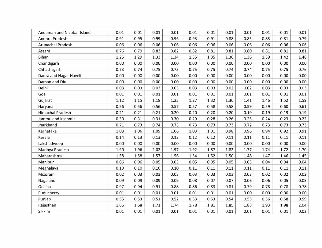
Andaman and Nicobar Island 0.01 0.01 0.01 0.01 0.01 0.01 0.01 0.01 0.01 0.01 0.01
Andhra Pradesh 0.91 0.95 0.99 0.96 0.93 0.91 0.88 0.85 0.83 0.81 0.79
Arunachal Pradesh 0.06 0.06 0.06 0.06 0.06 0.06 0.06 0.06 0.06 0.06 0.06
Assam 0.76 0.79 0.83 0.82 0.82 0.81 0.81 0.80 0.81 0.81 0.81
Bihar 1.25 1.29 1.33 1.34 1.35 1.35 1.36 1.36 1.39 1.42 1.46
Chandigarh 0.00 0.00 0.00 0.00 0.00 0.00 0.00 0.00 0.00 0.00 0.00
Chhattisgarh 0.73 0.74 0.75 0.75 0.75 0.75 0.74 0.74 0.75 0.75 0.76
Dadra and Nagar Haveli 0.00 0.00 0.00 0.00 0.00 0.00 0.00 0.00 0.00 0.00 0.00
Daman and Diu 0.00 0.00 0.00 0.00 0.00 0.00 0.00 0.00 0.00 0.00 0.00
Delhi 0.03 0.03 0.03 0.03 0.03 0.03 0.02 0.02 0.03 0.03 0.03
Goa 0.01 0.01 0.01 0.01 0.01 0.01 0.01 0.01 0.01 0.01 0.01
Gujarat 1.12 1.15 1.18 1.23 1.27 1.32 1.36 1.41 1.46 1.52 1.59
Haryana 0.56 0.56 0.56 0.57 0.57 0.58 0.58 0.59 0.59 0.60 0.61
Himachal Pradesh 0.21 0.21 0.21 0.20 0.20 0.20 0.20 0.19 0.19 0.19 0.19
Jammu and Kashmir 0.30 0.31 0.31 0.30 0.29 0.28 0.26 0.25 0.24 0.23 0.22
Jharkhand 0.71 0.73 0.74 0.73 0.73 0.73 0.73 0.72 0.73 0.73 0.73
Karnataka 1.03 1.06 1.09 1.06 1.03 1.01 0.98 0.96 0.94 0.92 0.91
Kerala 0.14 0.13 0.13 0.13 0.12 0.12 0.11 0.11 0.11 0.11 0.11
Lakshadweep 0.00 0.00 0.00 0.00 0.00 0.00 0.00 0.00 0.00 0.00 0.00
Madhya Pradesh 1.90 1.96 2.02 1.97 1.92 1.87 1.82 1.77 1.74 1.72 1.70
Maharashtra 1.58 1.58 1.57 1.56 1.54 1.52 1.50 1.48 1.47 1.46 1.45
Manipur 0.06 0.06 0.05 0.05 0.05 0.05 0.05 0.05 0.04 0.04 0.04
Meghalaya 0.10 0.10 0.10 0.10 0.11 0.11 0.11 0.11 0.11 0.11 0.11
Mizoram 0.02 0.03 0.03 0.03 0.03 0.03 0.03 0.03 0.02 0.02 0.02
Nagaland 0.09 0.09 0.09 0.09 0.08 0.07 0.07 0.06 0.06 0.05 0.05
Odisha 0.97 0.94 0.91 0.88 0.86 0.83 0.81 0.79 0.78 0.78 0.78
Puducherry 0.01 0.01 0.01 0.01 0.01 0.01 0.01 0.00 0.00 0.00 0.00
Punjab 0.55 0.53 0.51 0.52 0.53 0.53 0.54 0.55 0.56 0.58 0.59
Rajasthan 1.66 1.68 1.71 1.74 1.78 1.81 1.85 1.88 1.93 1.98 2.04
Sikkim 0.01 0.01 0.01 0.01 0.01 0.01 0.01 0.01 0.01 0.01 0.02

Tamil Nadu 0.90 0.94 0.98 0.93 0.88 0.83 0.78 0.73 0.69 0.66 0.64
Telangana 0.85 0.88 0.92 0.89 0.87 0.84 0.82 0.79 0.77 0.75 0.74
Tripura 0.08 0.08 0.08 0.09 0.09 0.09 0.09 0.09 0.09 0.10 0.10
Uttar Pradesh 3.02 3.02 3.01 3.12 3.22 3.32 3.43 3.53 3.68 3.84 4.01
Uttarakhand 0.20 0.22 0.24 0.23 0.22 0.22 0.21 0.20 0.20 0.20 0.19
West Bengal 1.11 1.24 1.37 1.32 1.26 1.21 1.15 1.10 1.06 1.02 0.99
India 20.94 21.40 21.86 21.74 21.62 21.50 21.38 21.26 21.36 21.53 21.78
Annexure V Emission estimates (in MtCO2e) from 3B. Land sector from 2005 to 15:
State/UT 2005 2006 2007 2008 2009 2010 2011 2012 2013 2014 2015
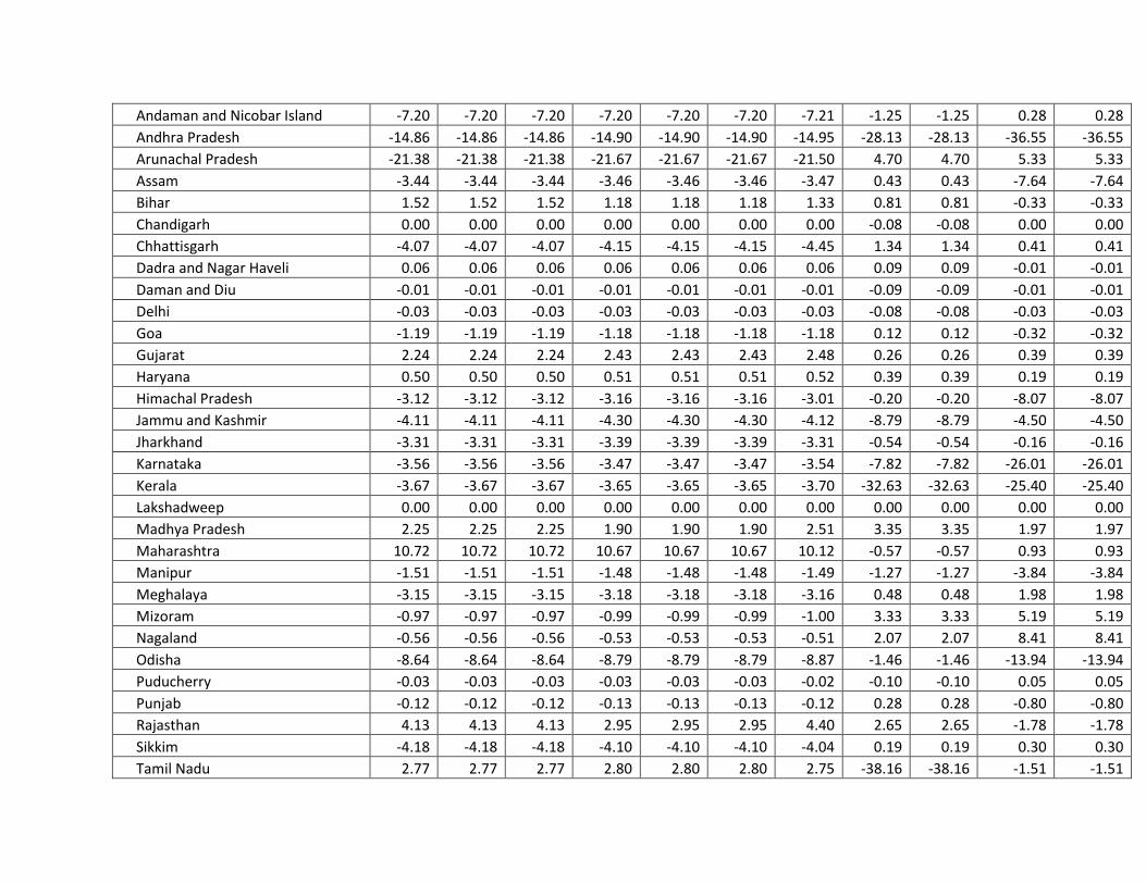
Andaman and Nicobar Island -7.20 -7.20 -7.20 -7.20 -7.20 -7.20 -7.21 -1.25 -1.25 0.28 0.28
Andhra Pradesh -14.86 -14.86 -14.86 -14.90 -14.90 -14.90 -14.95 -28.13 -28.13 -36.55 -36.55
Arunachal Pradesh -21.38 -21.38 -21.38 -21.67 -21.67 -21.67 -21.50 4.70 4.70 5.33 5.33
Assam -3.44 -3.44 -3.44 -3.46 -3.46 -3.46 -3.47 0.43 0.43 -7.64 -7.64
Bihar 1.52 1.52 1.52 1.18 1.18 1.18 1.33 0.81 0.81 -0.33 -0.33
Chandigarh 0.00 0.00 0.00 0.00 0.00 0.00 0.00 -0.08 -0.08 0.00 0.00
Chhattisgarh -4.07 -4.07 -4.07 -4.15 -4.15 -4.15 -4.45 1.34 1.34 0.41 0.41
Dadra and Nagar Haveli 0.06 0.06 0.06 0.06 0.06 0.06 0.06 0.09 0.09 -0.01 -0.01
Daman and Diu -0.01 -0.01 -0.01 -0.01 -0.01 -0.01 -0.01 -0.09 -0.09 -0.01 -0.01
Delhi -0.03 -0.03 -0.03 -0.03 -0.03 -0.03 -0.03 -0.08 -0.08 -0.03 -0.03
Goa -1.19 -1.19 -1.19 -1.18 -1.18 -1.18 -1.18 0.12 0.12 -0.32 -0.32
Gujarat 2.24 2.24 2.24 2.43 2.43 2.43 2.48 0.26 0.26 0.39 0.39
Haryana 0.50 0.50 0.50 0.51 0.51 0.51 0.52 0.39 0.39 0.19 0.19
Himachal Pradesh -3.12 -3.12 -3.12 -3.16 -3.16 -3.16 -3.01 -0.20 -0.20 -8.07 -8.07
Jammu and Kashmir -4.11 -4.11 -4.11 -4.30 -4.30 -4.30 -4.12 -8.79 -8.79 -4.50 -4.50
Jharkhand -3.31 -3.31 -3.31 -3.39 -3.39 -3.39 -3.31 -0.54 -0.54 -0.16 -0.16
Karnataka -3.56 -3.56 -3.56 -3.47 -3.47 -3.47 -3.54 -7.82 -7.82 -26.01 -26.01
Kerala -3.67 -3.67 -3.67 -3.65 -3.65 -3.65 -3.70 -32.63 -32.63 -25.40 -25.40
Lakshadweep 0.00 0.00 0.00 0.00 0.00 0.00 0.00 0.00 0.00 0.00 0.00
Madhya Pradesh 2.25 2.25 2.25 1.90 1.90 1.90 2.51 3.35 3.35 1.97 1.97
Maharashtra 10.72 10.72 10.72 10.67 10.67 10.67 10.12 -0.57 -0.57 0.93 0.93
Manipur -1.51 -1.51 -1.51 -1.48 -1.48 -1.48 -1.49 -1.27 -1.27 -3.84 -3.84
Meghalaya -3.15 -3.15 -3.15 -3.18 -3.18 -3.18 -3.16 0.48 0.48 1.98 1.98
Mizoram -0.97 -0.97 -0.97 -0.99 -0.99 -0.99 -1.00 3.33 3.33 5.19 5.19
Nagaland -0.56 -0.56 -0.56 -0.53 -0.53 -0.53 -0.51 2.07 2.07 8.41 8.41
Odisha -8.64 -8.64 -8.64 -8.79 -8.79 -8.79 -8.87 -1.46 -1.46 -13.94 -13.94
Puducherry -0.03 -0.03 -0.03 -0.03 -0.03 -0.03 -0.02 -0.10 -0.10 0.05 0.05
Punjab -0.12 -0.12 -0.12 -0.13 -0.13 -0.13 -0.12 0.28 0.28 -0.80 -0.80
Rajasthan 4.13 4.13 4.13 2.95 2.95 2.95 4.40 2.65 2.65 -1.78 -1.78
Sikkim -4.18 -4.18 -4.18 -4.10 -4.10 -4.10 -4.04 0.19 0.19 0.30 0.30
Tamil Nadu 2.77 2.77 2.77 2.80 2.80 2.80 2.75 -38.16 -38.16 -1.51 -1.51

Telangana 1.31 1.31 1.31 1.28 1.28 1.28 1.24 31.70 31.70 -9.32 -9.32
Tripura -2.78 -2.78 -2.78 -2.85 -2.85 -2.85 -2.87 -0.35 -0.35 2.48 2.48
Uttar Pradesh -3.50 -3.50 -3.50 -2.83 -2.83 -2.83 -3.18 -0.35 -0.35 -3.88 -3.88
Uttarakhand -0.32 -0.32 -0.32 -0.36 -0.36 -0.36 -0.30 5.25 5.25 -0.31 -0.31
West Bengal -20.00 -20.00 -20.00 -20.02 -20.02 -20.02 -20.04 -0.68 -0.68 -0.68 -0.68
India -90.20 -90.20 -90.20 -92.07 -92.07 -92.07 -90.71 -65.09 -65.09 -117.18 -117.18
Annexure VI
Emission estimates (in MtCO2e) from 3B1. Forest Land category from 2005 to 15:
State/UT 2005 2006 2007 2008 2009 2010 2011 2012 2013 2014 2015

Andaman and Nicobar Island -7.21 -7.21 -7.21 -7.21 -7.21 -7.21 -7.21 -1.25 -1.25 0.28 0.28
Andhra Pradesh -15.04 -15.04 -15.04 -15.04 -15.04 -15.04 -15.04 -28.22 -28.22 -36.63 -36.63
Arunachal Pradesh -21.66 -21.66 -21.66 -21.66 -21.66 -21.66 -21.66 4.55 4.55 5.17 5.17
Assam -2.37 -2.37 -2.37 -2.37 -2.37 -2.37 -2.37 1.53 1.53 -6.54 -6.54
Bihar 1.04 1.04 1.04 1.04 1.04 1.04 1.04 0.51 0.51 -0.63 -0.63
Chandigarh 0.00 0.00 0.00 0.00 0.00 0.00 0.00 -0.07 -0.07 0.00 0.00
Chhattisgarh -4.64 -4.64 -4.64 -4.64 -4.64 -4.64 -4.64 1.15 1.15 0.22 0.22
Dadra and Nagar Haveli 0.06 0.06 0.06 0.06 0.06 0.06 0.06 0.09 0.09 -0.01 -0.01
Daman and Diu -0.01 -0.01 -0.01 -0.01 -0.01 -0.01 -0.01 -0.09 -0.09 -0.01 -0.01
Delhi -0.04 -0.04 -0.04 -0.04 -0.04 -0.04 -0.04 -0.08 -0.08 -0.03 -0.03
Goa -1.16 -1.16 -1.16 -1.16 -1.16 -1.16 -1.16 0.14 0.14 -0.30 -0.30
Gujarat 1.44 1.44 1.44 1.44 1.44 1.44 1.44 -0.78 -0.78 -0.65 -0.65
Haryana 0.22 0.22 0.22 0.22 0.22 0.22 0.22 0.09 0.09 -0.11 -0.11
Himachal Pradesh -3.33 -3.33 -3.33 -3.33 -3.33 -3.33 -3.33 -0.51 -0.51 -8.39 -8.39
Jammu and Kashmir -5.12 -5.12 -5.12 -5.12 -5.12 -5.12 -5.12 -9.79 -9.79 -5.51 -5.51
Jharkhand -3.65 -3.65 -3.65 -3.65 -3.65 -3.65 -3.65 -0.88 -0.88 -0.50 -0.50
Karnataka -3.08 -3.08 -3.08 -3.08 -3.08 -3.08 -3.08 -7.35 -7.35 -25.54 -25.54
Kerala -2.38 -2.38 -2.38 -2.38 -2.38 -2.38 -2.38 -31.30 -31.30 -24.08 -24.08
Lakshadweep 0.00 0.00 0.00 0.00 0.00 0.00 0.00 0.00 0.00 0.00 0.00
Madhya Pradesh 0.74 0.74 0.74 0.74 0.74 0.74 0.74 1.58 1.58 0.20 0.20
Maharashtra 9.49 9.49 9.49 9.49 9.49 9.49 9.49 -1.19 -1.19 0.30 0.30
Manipur -1.63 -1.63 -1.63 -1.63 -1.63 -1.63 -1.63 -1.41 -1.41 -3.98 -3.98
Meghalaya -3.22 -3.22 -3.22 -3.22 -3.22 -3.22 -3.22 0.43 0.43 1.93 1.93
Mizoram -1.10 -1.10 -1.10 -1.10 -1.10 -1.10 -1.10 3.23 3.23 5.09 5.09
Nagaland -0.65 -0.65 -0.65 -0.65 -0.65 -0.65 -0.65 1.93 1.93 8.26 8.26
Odisha -9.25 -9.25 -9.25 -9.25 -9.25 -9.25 -9.25 -1.83 -1.83 -14.31 -14.31
Puducherry -0.03 -0.03 -0.03 -0.03 -0.03 -0.03 -0.03 -0.11 -0.11 0.05 0.05
Punjab -0.38 -0.38 -0.38 -0.38 -0.38 -0.38 -0.38 0.02 0.02 -1.06 -1.06
Rajasthan 1.55 1.55 1.55 1.55 1.55 1.55 1.55 -0.20 -0.20 -4.62 -4.62
Sikkim -4.10 -4.10 -4.10 -4.10 -4.10 -4.10 -4.10 0.13 0.13 0.24 0.24

Tamil Nadu 3.09 3.09 3.09 3.09 3.09 3.09 3.09 -37.82 -37.82 -1.17 -1.17
Telangana 1.18 1.18 1.18 1.18 1.18 1.18 1.18 31.64 31.64 -9.38 -9.38
Tripura -2.88 -2.88 -2.88 -2.88 -2.88 -2.88 -2.88 -0.36 -0.36 2.47 2.47
Uttar Pradesh -3.64 -3.64 -3.64 -3.64 -3.64 -3.64 -3.64 -0.81 -0.81 -4.34 -4.34
Uttarakhand -0.48 -0.48 -0.48 -0.48 -0.48 -0.48 -0.48 5.07 5.07 -0.49 -0.49
West Bengal -19.73 -19.73 -19.73 -19.73 -19.73 -19.73 -19.73 -0.37 -0.37 -0.37 -0.37
India -97.97 -97.97 -97.97 -97.97 -97.97 -97.97 -97.97 -72.35 -72.35 -124.44 -124.44
ANNEXURE VII Emission estimates (in MtCO2e) from 3B2. Cropland category from 2005 to 15:
State/UT 2005 2006 2007 2008 2009 2010 2011 2012 2013 2014 2015

Andaman and Nicobar Island 0.01 0.01 0.01 0.01 0.01 0.01 0.00 0.00 0.00 0.00 0.00
Andhra Pradesh -0.14 -0.14 -0.14 -0.11 -0.11 -0.11 -0.20 -0.20 -0.20 -0.20 -0.20
Arunachal Pradesh 0.10 0.10 0.10 -0.09 -0.09 -0.09 0.00 0.00 0.00 0.00 0.00
Assam -1.12 -1.12 -1.12 -1.14 -1.14 -1.14 -1.15 -1.15 -1.15 -1.15 -1.15
Bihar 0.18 0.18 0.18 0.06 0.06 0.06 0.12 0.12 0.12 0.12 0.12
Chandigarh 0.00 0.00 0.00 0.00 0.00 0.00 0.00 0.00 0.00 0.00 0.00
Chhattisgarh 0.20 0.20 0.20 0.25 0.25 0.25 0.02 0.02 0.02 0.02 0.02
Dadra and Nagar Haveli 0.00 0.00 0.00 0.00 0.00 0.00 0.00 0.00 0.00 0.00 0.00
Daman and Diu 0.00 0.00 0.00 0.00 0.00 0.00 0.00 0.00 0.00 0.00 0.00
Delhi 0.00 0.00 0.00 0.00 0.00 0.00 0.00 0.00 0.00 0.00 0.00
Goa -0.03 -0.03 -0.03 -0.03 -0.03 -0.03 -0.03 -0.03 -0.03 -0.03 -0.03
Gujarat 0.42 0.42 0.42 0.58 0.58 0.58 0.52 0.52 0.52 0.52 0.52
Haryana 0.23 0.23 0.23 0.25 0.25 0.25 0.23 0.23 0.23 0.23 0.23
Himachal Pradesh -0.11 -0.11 -0.11 -0.11 -0.11 -0.11 -0.08 -0.08 -0.08 -0.08 -0.08
Jammu and Kashmir -0.14 -0.14 -0.14 -0.15 -0.15 -0.15 -0.15 -0.15 -0.15 -0.15 -0.15
Jharkhand 0.06 0.06 0.06 0.09 0.09 0.09 0.06 0.06 0.06 0.06 0.06
Karnataka -0.75 -0.75 -0.75 -0.65 -0.65 -0.65 -0.73 -0.73 -0.73 -0.73 -0.73
Kerala -1.32 -1.32 -1.32 -1.33 -1.33 -1.33 -1.36 -1.36 -1.36 -1.36 -1.36
Lakshadweep 0.00 0.00 0.00 0.00 0.00 0.00 0.00 0.00 0.00 0.00 0.00
Madhya Pradesh 0.68 0.68 0.68 0.74 0.74 0.74 1.01 1.01 1.01 1.01 1.01
Maharashtra 0.40 0.40 0.40 0.37 0.37 0.37 0.01 0.01 0.01 0.01 0.01
Manipur 0.11 0.11 0.11 0.13 0.13 0.13 0.13 0.13 0.13 0.13 0.13
Meghalaya 0.03 0.03 0.03 0.01 0.01 0.01 0.03 0.03 0.03 0.03 0.03
Mizoram 0.13 0.13 0.13 0.10 0.10 0.10 0.10 0.10 0.10 0.10 0.10
Nagaland 0.06 0.06 0.06 0.09 0.09 0.09 0.13 0.13 0.13 0.13 0.13
Odisha 0.21 0.21 0.21 0.19 0.19 0.19 0.11 0.11 0.11 0.11 0.11
Puducherry 0.00 0.00 0.00 0.00 0.00 0.00 0.00 0.00 0.00 0.00 0.00
Punjab 0.21 0.21 0.21 0.21 0.21 0.21 0.20 0.20 0.20 0.20 0.20
Rajasthan 0.26 0.26 0.26 0.28 0.28 0.28 0.59 0.59 0.59 0.59 0.59
Sikkim -0.11 -0.11 -0.11 -0.02 -0.02 -0.02 0.01 0.01 0.01 0.01 0.01
Tamil Nadu -0.50 -0.50 -0.50 -0.45 -0.45 -0.45 -0.50 -0.50 -0.50 -0.50 -0.50

Telangana -0.10 -0.10 -0.10 -0.08 -0.08 -0.08 -0.15 -0.15 -0.15 -0.15 -0.15
Tripura 0.11 0.11 0.11 0.03 0.03 0.03 0.01 0.01 0.01 0.01 0.01
Uttar Pradesh -0.16 -0.16 -0.16 0.52 0.52 0.52 0.19 0.19 0.19 0.19 0.19
Uttarakhand 0.00 0.00 0.00 0.00 0.00 0.00 -0.02 -0.02 -0.02 -0.02 -0.02
West Bengal -0.39 -0.39 -0.39 -0.39 -0.39 -0.39 -0.42 -0.42 -0.42 -0.42 -0.42
India -1.46 -1.46 -1.46 -0.62 -0.62 -0.62 -1.32 -1.32 -1.32 -1.32 -1.32
Annexure VIII Emission estimates (in MtCO2e) from 3B3. Grassland category from 2005 to 15:
State/UT 2005 2006 2007 2008 2009 2010 2011 2012 2013 2014 2015
Andaman and Nicobar Island 0.00 0.00 0.00 0.00 0.00 0.00 0.00 0.00 0.00 0.00 0.00

Andhra Pradesh 0.00 0.00 0.00 0.00 0.00 0.00 0.00 0.00 0.00 0.00 0.00
Arunachal Pradesh 0.07 0.07 0.07 0.03 0.03 0.03 0.08 0.08 0.08 0.08 0.08
Assam 0.03 0.03 0.03 0.03 0.03 0.03 0.03 0.03 0.03 0.03 0.03
Bihar 0.00 0.00 0.00 0.00 0.00 0.00 0.00 0.00 0.00 0.00 0.00
Chandigarh 0.00 0.00 0.00 0.00 0.00 0.00 0.00 0.00 0.00 0.00 0.00
Chhattisgarh 0.00 0.00 0.00 0.00 0.00 0.00 0.00 0.00 0.00 0.00 0.00
Dadra and Nagar Haveli 0.00 0.00 0.00 0.00 0.00 0.00 0.00 0.00 0.00 0.00 0.00
Daman and Diu 0.00 0.00 0.00 0.00 0.00 0.00 0.00 0.00 0.00 0.00 0.00
Delhi 0.00 0.00 0.00 0.00 0.00 0.00 0.00 0.00 0.00 0.00 0.00
Goa 0.00 0.00 0.00 0.00 0.00 0.00 0.00 0.00 0.00 0.00 0.00
Gujarat 0.00 0.00 0.00 0.00 0.00 0.00 0.00 0.00 0.00 0.00 0.00
Haryana 0.02 0.02 0.02 0.02 0.02 0.02 0.02 0.02 0.02 0.02 0.02
Himachal Pradesh 0.16 0.16 0.16 0.11 0.11 0.11 0.18 0.18 0.18 0.18 0.18
Jammu and Kashmir 0.10 0.10 0.10 0.04 0.04 0.04 0.13 0.13 0.13 0.13 0.13
Jharkhand 0.00 0.00 0.00 0.00 0.00 0.00 0.00 0.00 0.00 0.00 0.00
Karnataka 0.01 0.01 0.01 0.01 0.01 0.01 0.01 0.01 0.01 0.01 0.01
Kerala 0.00 0.00 0.00 0.00 0.00 0.00 0.00 0.00 0.00 0.00 0.00
Lakshadweep 0.00 0.00 0.00 0.00 0.00 0.00 0.00 0.00 0.00 0.00 0.00
Madhya Pradesh 0.00 0.00 0.00 0.00 0.00 0.00 0.00 0.00 0.00 0.00 0.00
Maharashtra 0.00 0.00 0.00 0.00 0.00 0.00 0.00 0.00 0.00 0.00 0.00
Manipur 0.00 0.00 0.00 0.00 0.00 0.00 0.00 0.00 0.00 0.00 0.00
Meghalaya 0.00 0.00 0.00 0.00 0.00 0.00 0.00 0.00 0.00 0.00 0.00
Mizoram 0.00 0.00 0.00 0.00 0.00 0.00 0.00 0.00 0.00 0.00 0.00
Nagaland 0.00 0.00 0.00 0.00 0.00 0.00 0.00 0.00 0.00 0.00 0.00
Odisha 0.00 0.00 0.00 0.00 0.00 0.00 0.00 0.00 0.00 0.00 0.00
Puducherry 0.00 0.00 0.00 0.00 0.00 0.00 0.00 0.00 0.00 0.00 0.00
Punjab 0.00 0.00 0.00 0.00 0.00 0.00 0.00 0.00 0.00 0.00 0.00
Rajasthan 0.12 0.12 0.12 0.12 0.12 0.12 0.12 0.12 0.12 0.12 0.12
Sikkim 0.00 0.00 0.00 0.01 0.01 0.01 0.01 0.01 0.01 0.01 0.01
Tamil Nadu 0.02 0.02 0.02 0.02 0.02 0.02 0.02 0.02 0.02 0.02 0.02

Telangana 0.00 0.00 0.00 0.00 0.00 0.00 0.00 0.00 0.00 0.00 0.00
Tripura 0.00 0.00 0.00 0.00 0.00 0.00 0.00 0.00 0.00 0.00 0.00
Uttar Pradesh 0.01 0.01 0.01 0.01 0.01 0.01 0.00 0.00 0.00 0.00 0.00
Uttarakhand 0.05 0.05 0.05 0.03 0.03 0.03 0.06 0.06 0.06 0.06 0.06
West Bengal 0.00 0.00 0.00 0.00 0.00 0.00 0.00 0.00 0.00 0.00 0.00
India 0.58 0.58 0.58 0.42 0.42 0.42 0.66 0.66 0.66 0.66 0.66
Annexure IX Emission estimates (in MtCO2e) from 3B5. Settlements category from 2005 to 15:
State/UT 2005 2006 2007 2008 2009 2010 2011 2012 2013 2014 2015
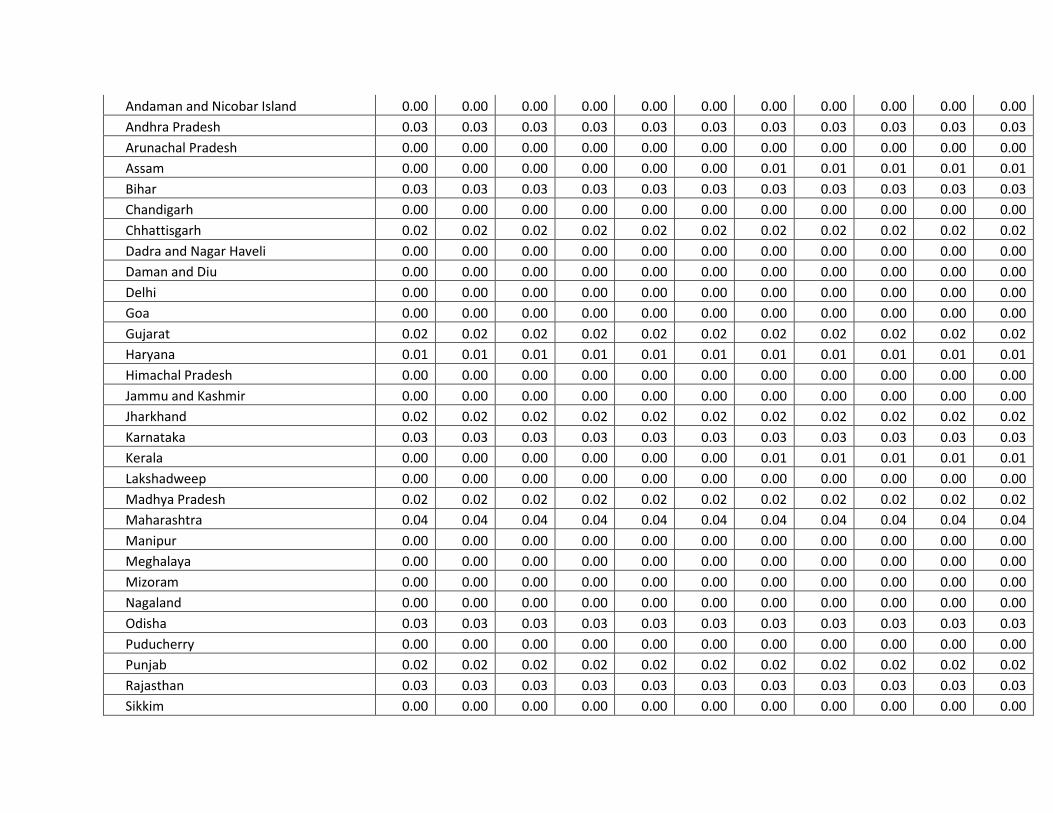
Andaman and Nicobar Island 0.00 0.00 0.00 0.00 0.00 0.00 0.00 0.00 0.00 0.00 0.00
Andhra Pradesh 0.03 0.03 0.03 0.03 0.03 0.03 0.03 0.03 0.03 0.03 0.03
Arunachal Pradesh 0.00 0.00 0.00 0.00 0.00 0.00 0.00 0.00 0.00 0.00 0.00
Assam 0.00 0.00 0.00 0.00 0.00 0.00 0.01 0.01 0.01 0.01 0.01
Bihar 0.03 0.03 0.03 0.03 0.03 0.03 0.03 0.03 0.03 0.03 0.03
Chandigarh 0.00 0.00 0.00 0.00 0.00 0.00 0.00 0.00 0.00 0.00 0.00
Chhattisgarh 0.02 0.02 0.02 0.02 0.02 0.02 0.02 0.02 0.02 0.02 0.02
Dadra and Nagar Haveli 0.00 0.00 0.00 0.00 0.00 0.00 0.00 0.00 0.00 0.00 0.00
Daman and Diu 0.00 0.00 0.00 0.00 0.00 0.00 0.00 0.00 0.00 0.00 0.00
Delhi 0.00 0.00 0.00 0.00 0.00 0.00 0.00 0.00 0.00 0.00 0.00
Goa 0.00 0.00 0.00 0.00 0.00 0.00 0.00 0.00 0.00 0.00 0.00
Gujarat 0.02 0.02 0.02 0.02 0.02 0.02 0.02 0.02 0.02 0.02 0.02
Haryana 0.01 0.01 0.01 0.01 0.01 0.01 0.01 0.01 0.01 0.01 0.01
Himachal Pradesh 0.00 0.00 0.00 0.00 0.00 0.00 0.00 0.00 0.00 0.00 0.00
Jammu and Kashmir 0.00 0.00 0.00 0.00 0.00 0.00 0.00 0.00 0.00 0.00 0.00
Jharkhand 0.02 0.02 0.02 0.02 0.02 0.02 0.02 0.02 0.02 0.02 0.02
Karnataka 0.03 0.03 0.03 0.03 0.03 0.03 0.03 0.03 0.03 0.03 0.03
Kerala 0.00 0.00 0.00 0.00 0.00 0.00 0.01 0.01 0.01 0.01 0.01
Lakshadweep 0.00 0.00 0.00 0.00 0.00 0.00 0.00 0.00 0.00 0.00 0.00
Madhya Pradesh 0.02 0.02 0.02 0.02 0.02 0.02 0.02 0.02 0.02 0.02 0.02
Maharashtra 0.04 0.04 0.04 0.04 0.04 0.04 0.04 0.04 0.04 0.04 0.04
Manipur 0.00 0.00 0.00 0.00 0.00 0.00 0.00 0.00 0.00 0.00 0.00
Meghalaya 0.00 0.00 0.00 0.00 0.00 0.00 0.00 0.00 0.00 0.00 0.00
Mizoram 0.00 0.00 0.00 0.00 0.00 0.00 0.00 0.00 0.00 0.00 0.00
Nagaland 0.00 0.00 0.00 0.00 0.00 0.00 0.00 0.00 0.00 0.00 0.00
Odisha 0.03 0.03 0.03 0.03 0.03 0.03 0.03 0.03 0.03 0.03 0.03
Puducherry 0.00 0.00 0.00 0.00 0.00 0.00 0.00 0.00 0.00 0.00 0.00
Punjab 0.02 0.02 0.02 0.02 0.02 0.02 0.02 0.02 0.02 0.02 0.02
Rajasthan 0.03 0.03 0.03 0.03 0.03 0.03 0.03 0.03 0.03 0.03 0.03
Sikkim 0.00 0.00 0.00 0.00 0.00 0.00 0.00 0.00 0.00 0.00 0.00

Tamil Nadu 0.03 0.03 0.03 0.03 0.03 0.03 0.03 0.03 0.03 0.03 0.03
Telangana 0.02 0.02 0.02 0.02 0.02 0.02 0.02 0.02 0.02 0.02 0.02
Tripura 0.00 0.00 0.00 0.00 0.00 0.00 0.00 0.00 0.00 0.00 0.00
Uttar Pradesh 0.05 0.05 0.05 0.06 0.06 0.06 0.06 0.06 0.06 0.06 0.06
Uttarakhand 0.00 0.00 0.00 0.00 0.00 0.00 0.00 0.00 0.00 0.00 0.00
West Bengal 0.04 0.04 0.04 0.05 0.05 0.05 0.05 0.05 0.05 0.05 0.05
India 0.45 0.45 0.45 0.47 0.47 0.47 0.49 0.49 0.49 0.49 0.49
Annexure X Emission estimates (in MtCO2e) from 3B6. Other Land category from 2005 to 15:
State/UT 2005 2006 2007 2008 2009 2010 2011 2012 2013 2014 2015
Andaman and Nicobar Island 0.00 0.00 0.00 0.00 0.00 0.00 0.00 0.00 0.00 0.00 0.00

Andhra Pradesh 0.30 0.30 0.30 0.23 0.23 0.23 0.26 0.26 0.26 0.26 0.26
Arunachal Pradesh 0.11 0.11 0.11 0.04 0.04 0.04 0.07 0.07 0.07 0.07 0.07
Assam 0.02 0.02 0.02 0.02 0.02 0.02 0.02 0.02 0.02 0.02 0.02
Bihar 0.27 0.27 0.27 0.06 0.06 0.06 0.15 0.15 0.15 0.15 0.15
Chandigarh 0.00 0.00 0.00 0.00 0.00 0.00 0.00 0.00 0.00 0.00 0.00
Chhattisgarh 0.34 0.34 0.34 0.22 0.22 0.22 0.14 0.14 0.14 0.14 0.14
Dadra and Nagar Haveli 0.00 0.00 0.00 0.00 0.00 0.00 0.00 0.00 0.00 0.00 0.00
Daman and Diu 0.00 0.00 0.00 0.00 0.00 0.00 0.00 0.00 0.00 0.00 0.00
Delhi 0.00 0.00 0.00 0.00 0.00 0.00 0.00 0.00 0.00 0.00 0.00
Goa 0.00 0.00 0.00 0.01 0.01 0.01 0.01 0.01 0.01 0.01 0.01
Gujarat 0.36 0.36 0.36 0.40 0.40 0.40 0.50 0.50 0.50 0.50 0.50
Haryana 0.02 0.02 0.02 0.01 0.01 0.01 0.03 0.03 0.03 0.03 0.03
Himachal Pradesh 0.17 0.17 0.17 0.16 0.16 0.16 0.21 0.21 0.21 0.21 0.21
Jammu and Kashmir 1.05 1.05 1.05 0.93 0.93 0.93 1.02 1.02 1.02 1.02 1.02
Jharkhand 0.26 0.26 0.26 0.16 0.16 0.16 0.27 0.27 0.27 0.27 0.27
Karnataka 0.23 0.23 0.23 0.22 0.22 0.22 0.23 0.23 0.23 0.23 0.23
Kerala 0.02 0.02 0.02 0.05 0.05 0.05 0.02 0.02 0.02 0.02 0.02
Lakshadweep 0.00 0.00 0.00 0.00 0.00 0.00 0.00 0.00 0.00 0.00 0.00
Madhya Pradesh 0.81 0.81 0.81 0.40 0.40 0.40 0.74 0.74 0.74 0.74 0.74
Maharashtra 0.80 0.80 0.80 0.77 0.77 0.77 0.58 0.58 0.58 0.58 0.58
Manipur 0.01 0.01 0.01 0.01 0.01 0.01 0.00 0.00 0.00 0.00 0.00
Meghalaya 0.03 0.03 0.03 0.02 0.02 0.02 0.02 0.02 0.02 0.02 0.02
Mizoram 0.00 0.00 0.00 0.00 0.00 0.00 0.00 0.00 0.00 0.00 0.00
Nagaland 0.02 0.02 0.02 0.03 0.03 0.03 0.01 0.01 0.01 0.01 0.01
Odisha 0.37 0.37 0.37 0.24 0.24 0.24 0.24 0.24 0.24 0.24 0.24
Puducherry 0.00 0.00 0.00 0.00 0.00 0.00 0.00 0.00 0.00 0.00 0.00
Punjab 0.03 0.03 0.03 0.02 0.02 0.02 0.03 0.03 0.03 0.03 0.03
Rajasthan 2.17 2.17 2.17 0.96 0.96 0.96 2.10 2.10 2.10 2.10 2.10
Sikkim 0.03 0.03 0.03 0.01 0.01 0.01 0.04 0.04 0.04 0.04 0.04
Tamil Nadu 0.13 0.13 0.13 0.11 0.11 0.11 0.11 0.11 0.11 0.11 0.11

Telangana 0.21 0.21 0.21 0.16 0.16 0.16 0.19 0.19 0.19 0.19 0.19
Tripura 0.00 0.00 0.00 0.00 0.00 0.00 0.00 0.00 0.00 0.00 0.00
Uttar Pradesh 0.25 0.25 0.25 0.23 0.23 0.23 0.21 0.21 0.21 0.21 0.21
Uttarakhand 0.11 0.11 0.11 0.09 0.09 0.09 0.14 0.14 0.14 0.14 0.14
West Bengal 0.07 0.07 0.07 0.06 0.06 0.06 0.06 0.06 0.06 0.06 0.06
India 8.21 8.21 8.21 5.63 5.63 5.63 7.43 7.43 7.43 7.43 7.43
Annexure XI Emission estimates (in MtCO2e) from 3C. Aggregate Sources and non-CO2 emissions sources on land sector from 2005 to 15:
State/UT 2005 2006 2007 2008 2009 2010 2011 2012 2013 2014 2015
Andaman and Nicobar Island 0.04 0.04 0.04 0.04 0.04 0.03 0.03 0.03 0.03 0.03 0.03
Andhra Pradesh 10.08 10.09 9.91 10.56 9.93 11.33 11.39 10.42 9.28 8.61 8.06

Arunachal Pradesh 0.39 0.37 0.37 0.38 0.38 0.41 0.41 0.43 0.44 0.75 0.59
Assam 5.92 5.54 5.68 6.03 6.17 6.36 6.39 6.29 6.12 6.07 6.06
Bihar 9.66 10.14 10.35 10.45 9.78 9.16 10.01 10.57 10.06 10.14 10.73
Chandigarh 0.00 0.00 0.00 0.00 0.00 0.00 0.00 0.00 0.00 0.00 0.00
Chhattisgarh 6.57 6.58 6.59 6.61 6.66 6.75 6.83 6.90 6.89 6.95 6.79
Dadra and Nagar Haveli 0.02 0.02 0.02 0.02 0.02 0.02 0.02 0.02 0.02 0.02 0.02
Daman and Diu 0.00 0.00 0.00 0.00 0.00 0.00 0.00 0.00 0.00 0.00 0.00
Delhi 0.00 0.00 0.00 0.01 0.01 0.01 0.00 0.01 0.01 0.03 0.02
Goa 0.09 0.09 0.09 0.08 0.08 0.08 0.08 0.08 0.07 0.07 0.08
Gujarat 4.69 4.75 4.85 4.82 4.76 5.28 5.36 4.84 5.09 5.33 5.03
Haryana 4.39 4.46 4.55 4.67 4.76 4.85 5.01 5.00 4.88 4.99 5.17
Himachal Pradesh 0.14 0.14 0.15 0.15 0.14 0.14 0.15 0.15 0.15 0.15 0.16
Jammu and Kashmir 0.30 0.30 0.31 0.34 0.36 0.36 0.35 0.38 0.37 0.35 0.37
Jharkhand 2.75 2.91 2.97 2.98 2.63 2.26 2.51 2.74 2.71 2.58 3.47
Karnataka 4.12 4.16 4.21 4.47 4.79 5.13 5.51 4.70 4.64 4.88 4.65
Kerala 0.79 0.76 0.69 0.69 0.70 0.70 0.70 0.69 0.72 0.65 0.64
Lakshadweep 0.00 0.00 0.00 0.00 0.00 0.00 0.00 0.00 0.00 0.00 0.00
Madhya Pradesh 4.74 4.82 4.87 4.93 5.17 5.33 5.62 5.79 6.14 6.15 6.36
Maharashtra 6.45 6.60 6.89 6.98 7.26 7.88 7.98 7.35 7.74 7.79 7.45
Manipur 0.57 0.56 0.56 0.55 0.55 0.59 0.63 0.56 0.61 0.65 0.61
Meghalaya 0.24 0.24 0.25 0.25 0.24 0.24 0.24 0.18 0.17 0.16 0.16
Mizoram 0.15 0.15 0.15 0.13 0.12 0.10 0.09 0.08 0.08 0.08 0.09
Nagaland 0.38 0.40 0.39 0.39 0.38 0.40 0.40 0.40 0.41 0.41 0.39
Odisha 10.06 10.03 9.80 9.55 9.55 10.04 9.86 9.76 10.02 9.67 9.37
Puducherry 0.11 0.10 0.09 0.08 0.09 0.09 0.07 0.06 0.06 0.05 0.05
Punjab 6.04 6.08 6.15 6.27 6.38 6.52 6.59 6.78 6.60 6.45 6.72
Rajasthan 2.15 2.24 2.34 2.40 2.42 2.79 3.01 3.14 3.12 3.16 3.44
Sikkim 0.05 0.06 0.05 0.05 0.05 0.04 0.04 0.04 0.04 0.04 0.04
Tamil Nadu 5.87 5.88 5.67 6.01 5.94 6.05 6.24 5.45 5.45 5.72 6.31
Telangana 5.58 5.63 5.55 5.91 5.48 6.30 6.27 5.69 6.66 5.88 5.09

Tripura 0.60 0.58 0.58 0.57 0.55 0.57 0.59 0.58 0.57 0.57 0.59
Uttar Pradesh 18.69 18.50 18.42 18.84 18.55 18.61 19.10 19.46 18.96 18.90 18.30
Uttarakhand 0.85 0.85 0.86 0.85 0.83 0.83 0.85 0.83 0.84 0.85 0.94
West Bengal 12.78 13.92 13.94 14.33 14.04 12.80 13.47 13.81 13.53 13.60 13.74
India 125.26 127.02 127.34 130.42 128.81 132.06 135.81 133.20 132.49 131.72 131.56
Annexure XII Emission estimates (in MtCO2e) from 3C1. Biomass Burning from Forest Land from 2005 to 15:
State/UT 2005 2006 2007 2008 2009 2010 2011 2012 2013 2014 2015
Andaman and Nicobar Island 0.00 0.00 0.00 0.00 0.00 0.00 0.00 0.00 0.00 0.00 0.00

Andhra Pradesh 0.60 0.61 0.63 0.65 0.65 0.65 0.67 0.68 0.70 0.73 0.75
Arunachal Pradesh 0.01 0.01 0.01 0.01 0.01 0.01 0.01 0.01 0.01 0.01 0.01
Assam 0.10 0.10 0.10 0.10 0.10 0.10 0.10 0.10 0.10 0.10 0.10
Bihar 0.17 0.17 0.17 0.18 0.18 0.19 0.19 0.19 0.19 0.19 0.19
Chandigarh 0.00 0.00 0.00 0.00 0.00 0.00 0.00 0.00 0.00 0.00 0.00
Chhattisgarh 0.49 0.49 0.49 0.49 0.49 0.49 0.49 0.48 0.48 0.48 0.48
Dadra and Nagar Haveli 0.00 0.00 0.00 0.00 0.00 0.00 0.00 0.00 0.00 0.00 0.00
Daman and Diu 0.00 0.00 0.00 0.00 0.00 0.00 0.00 0.00 0.00 0.00 0.00
Delhi 0.00 0.00 0.00 0.00 0.00 0.00 0.00 0.00 0.00 0.00 0.00
Goa 0.00 0.00 0.00 0.00 0.00 0.00 0.00 0.00 0.00 0.00 0.00
Gujarat 0.05 0.05 0.05 0.05 0.05 0.05 0.05 0.05 0.05 0.05 0.05
Haryana 0.00 0.00 0.00 0.00 0.00 0.00 0.00 0.00 0.00 0.00 0.00
Himachal Pradesh 0.00 0.00 0.00 0.00 0.00 0.00 0.00 0.00 0.00 0.00 0.00
Jammu and Kashmir 0.00 0.00 0.00 0.00 0.00 0.00 0.00 0.00 0.00 0.00 0.00
Jharkhand 0.26 0.27 0.27 0.27 0.27 0.27 0.27 0.27 0.27 0.27 0.27
Karnataka 0.20 0.20 0.20 0.20 0.20 0.20 0.20 0.20 0.20 0.21 0.21
Kerala 0.01 0.01 0.01 0.01 0.01 0.01 0.01 0.01 0.01 0.01 0.01
Lakshadweep 0.00 0.00 0.00 0.00 0.00 0.00 0.00 0.00 0.00 0.00 0.00
Madhya Pradesh 0.35 0.35 0.35 0.35 0.35 0.35 0.35 0.35 0.35 0.35 0.35
Maharashtra 0.53 0.53 0.53 0.53 0.53 0.53 0.53 0.53 0.53 0.53 0.53
Manipur 0.21 0.21 0.21 0.21 0.21 0.21 0.21 0.21 0.21 0.21 0.21
Meghalaya 0.05 0.05 0.05 0.05 0.05 0.05 0.05 0.05 0.05 0.05 0.05
Mizoram 0.04 0.04 0.04 0.04 0.04 0.04 0.04 0.04 0.04 0.04 0.04
Nagaland 0.11 0.11 0.11 0.10 0.10 0.10 0.10 0.10 0.10 0.10 0.10
Odisha 0.84 0.84 0.84 0.84 0.85 0.86 0.86 0.86 0.86 0.87 0.88
Puducherry 0.00 0.00 0.00 0.00 0.00 0.00 0.00 0.00 0.00 0.00 0.00
Punjab 0.00 0.00 0.00 0.00 0.00 0.00 0.00 0.00 0.00 0.00 0.00
Rajasthan 0.04 0.04 0.04 0.04 0.04 0.04 0.04 0.04 0.04 0.04 0.04
Sikkim 0.00 0.00 0.00 0.00 0.00 0.00 0.00 0.00 0.00 0.00 0.00
Tamil Nadu 0.44 0.44 0.45 0.45 0.45 0.45 0.47 0.48 0.50 0.50 0.50

Telangana 0.34 0.34 0.35 0.35 0.34 0.34 0.33 0.32 0.31 0.31 0.32
Tripura 0.08 0.08 0.08 0.08 0.08 0.08 0.08 0.08 0.08 0.08 0.08
Uttar Pradesh 0.05 0.05 0.05 0.05 0.05 0.05 0.05 0.05 0.05 0.05 0.05
Uttarakhand 0.00 0.00 0.00 0.00 0.00 0.00 0.00 0.00 0.00 0.00 0.00
West Bengal 0.03 0.03 0.03 0.03 0.04 0.04 0.04 0.04 0.04 0.04 0.04
India 5.02 5.04 5.06 5.08 5.10 5.12 5.14 5.16 5.18 5.23 5.27
Annexure XIII Emission estimates (in MtCO2e) from 3C2. Biomass Burning from Cropland from 2005 to 15:
State/UT 2005 2006 2007 2008 2009 2010 2011 2012 2013 2014 2015
Andaman and Nicobar Island 0.01 0.00 0.00 0.00 0.00 0.00 0.00 0.00 0.00 0.00 0.00
Andhra Pradesh 0.16 0.17 0.19 0.18 0.14 0.17 0.17 0.17 0.17 0.15 0.15
Arunachal Pradesh 0.00 0.00 0.00 0.00 0.00 0.00 0.00 0.00 0.00 0.00 0.00

Assam 0.04 0.04 0.04 0.04 0.05 0.05 0.05 0.05 0.05 0.06 0.06
Bihar 0.13 0.17 0.16 0.18 0.16 0.17 0.23 0.27 0.24 0.24 0.26
Chandigarh 0.00 0.00 0.00 0.00 0.00 0.00 0.00 0.00 0.00 0.00 0.00
Chhattisgarh 0.05 0.05 0.05 0.05 0.04 0.06 0.06 0.06 0.06 0.06 0.06
Dadra and Nagar Haveli 0.00 0.00 0.00 0.00 0.00 0.00 0.00 0.00 0.00 0.00 0.00
Daman and Diu 0.00 0.00 0.00 0.00 0.00 0.00 0.00 0.00 0.00 0.00 0.00
Delhi 0.00 0.00 0.00 0.00 0.00 0.00 0.00 0.00 0.00 0.00 0.00
Goa 0.00 0.00 0.00 0.00 0.00 0.00 0.00 0.00 0.00 0.00 0.00
Gujarat 0.18 0.18 0.20 0.20 0.17 0.20 0.21 0.17 0.22 0.21 0.18
Haryana 0.50 0.54 0.56 0.55 0.55 0.57 0.62 0.61 0.62 0.60 0.61
Himachal Pradesh 0.03 0.03 0.03 0.03 0.02 0.03 0.03 0.03 0.03 0.03 0.03
Jammu and Kashmir 0.05 0.05 0.05 0.05 0.05 0.05 0.05 0.06 0.06 0.05 0.04
Jharkhand 0.03 0.05 0.06 0.07 0.04 0.03 0.06 0.07 0.07 0.07 0.07
Karnataka 0.18 0.20 0.22 0.20 0.22 0.28 0.28 0.26 0.27 0.29 0.27
Kerala 0.01 0.01 0.01 0.01 0.01 0.01 0.01 0.01 0.01 0.01 0.01
Lakshadweep 0.00 0.00 0.00 0.00 0.00 0.00 0.00 0.00 0.00 0.00 0.00
Madhya Pradesh 0.13 0.13 0.12 0.13 0.14 0.15 0.18 0.21 0.22 0.26 0.29
Maharashtra 0.27 0.44 0.54 0.43 0.41 0.50 0.53 0.46 0.48 0.50 0.44
Manipur 0.00 0.00 0.00 0.00 0.00 0.01 0.01 0.01 0.01 0.01 0.01
Meghalaya 0.00 0.00 0.00 0.00 0.00 0.00 0.00 0.00 0.00 0.00 0.00
Mizoram 0.00 0.00 0.00 0.00 0.00 0.00 0.00 0.00 0.00 0.00 0.00
Nagaland 0.00 0.00 0.01 0.01 0.00 0.01 0.01 0.01 0.01 0.01 0.01
Odisha 0.07 0.07 0.08 0.07 0.07 0.07 0.06 0.07 0.08 0.08 0.06
Puducherry 0.00 0.00 0.00 0.00 0.00 0.00 0.00 0.00 0.00 0.00 0.00
Punjab 1.11 1.11 1.15 1.19 1.19 1.19 1.20 1.23 1.26 1.21 1.24
Rajasthan 0.18 0.19 0.19 0.20 0.18 0.21 0.22 0.23 0.22 0.23 0.22
Sikkim 0.00 0.00 0.00 0.00 0.00 0.00 0.00 0.00 0.00 0.00 0.00
Tamil Nadu 0.22 0.27 0.26 0.23 0.22 0.23 0.27 0.23 0.23 0.23 0.24
Telangana 0.08 0.08 0.09 0.09 0.07 0.09 0.09 0.09 0.10 0.09 0.07
Tripura 0.01 0.01 0.01 0.01 0.01 0.01 0.01 0.01 0.01 0.01 0.01

Uttar Pradesh 1.41 1.48 1.49 1.50 1.48 1.54 1.64 1.69 1.70 1.52 1.58
Uttarakhand 0.05 0.05 0.06 0.05 0.05 0.05 0.05 0.06 0.05 0.05 0.05
West Bengal 0.17 0.17 0.18 0.18 0.18 0.16 0.17 0.18 0.19 0.19 0.19
India 5.06 5.49 5.75 5.66 5.46 5.84 6.22 6.25 6.35 6.17 6.16
Annexure IVX Emission estimates (in MtCO2e) from 3C3. Direct N2O emissions from managed soils from 2005 to 15:
State/UT 2005 2006 2007 2008 2009 2010 2011 2012 2013 2014 2015
Andaman and Nicobar Island 0.00 0.00 0.00 0.00 0.00 0.00 0.00 0.00 0.00 0.00 0.00
Andhra Pradesh 4.17 3.97 3.79 4.04 4.11 4.57 4.74 4.39 3.11 2.62 2.49
Arunachal Pradesh 0.00 0.00 0.00 0.00 0.00 0.00 0.00 0.00 0.00 0.00 0.00
Assam 0.22 0.23 0.24 0.27 0.30 0.33 0.36 0.36 0.36 0.37 0.40

Bihar 2.07 2.14 2.21 2.25 2.17 2.17 2.34 2.47 2.37 2.37 2.85
Chandigarh 0.00 0.00 0.00 0.00 0.00 0.00 0.00 0.00 0.00 0.00 0.00
Chhattisgarh 0.60 0.62 0.65 0.65 0.73 0.77 0.84 0.87 0.87 0.89 0.93
Dadra and Nagar Haveli 0.00 0.00 0.00 0.00 0.00 0.00 0.00 0.00 0.00 0.00 0.00
Daman and Diu 0.00 0.00 0.00 0.00 0.00 0.00 0.00 0.00 0.00 0.00 0.00
Delhi 0.00 0.00 0.00 0.00 0.00 0.00 0.00 0.00 0.01 0.02 0.01
Goa 0.01 0.01 0.01 0.01 0.01 0.01 0.01 0.01 0.01 0.01 0.01
Gujarat 2.50 2.51 2.52 2.56 2.63 2.90 2.88 2.45 2.69 2.89 2.72
Haryana 2.20 2.23 2.25 2.27 2.30 2.33 2.42 2.32 2.31 2.40 2.48
Himachal Pradesh 0.08 0.08 0.08 0.08 0.08 0.08 0.08 0.08 0.08 0.08 0.09
Jammu and Kashmir 0.12 0.13 0.13 0.16 0.18 0.18 0.16 0.17 0.17 0.16 0.19
Jharkhand 0.20 0.21 0.21 0.21 0.22 0.20 0.26 0.27 0.22 0.21 0.28
Karnataka 1.80 1.84 1.89 2.03 2.25 2.41 2.80 2.34 2.24 2.37 2.37
Kerala 0.21 0.22 0.22 0.26 0.27 0.28 0.31 0.30 0.32 0.27 0.26
Lakshadweep 0.00 0.00 0.00 0.00 0.00 0.00 0.00 0.00 0.00 0.00 0.00
Madhya Pradesh 1.71 1.80 1.89 1.92 2.18 2.36 2.51 2.50 2.83 2.74 2.89
Maharashtra 2.93 2.98 3.02 3.17 3.47 3.87 3.90 3.43 3.68 3.73 3.54
Manipur 0.04 0.04 0.03 0.03 0.02 0.01 0.01 0.02 0.02 0.02 0.03
Meghalaya 0.01 0.01 0.01 0.01 0.01 0.01 0.01 0.01 0.01 0.00 0.00
Mizoram 0.00 0.00 0.00 0.00 0.00 0.00 0.00 0.00 0.01 0.00 0.00
Nagaland 0.00 0.00 0.00 0.00 0.00 0.00 0.00 0.00 0.00 0.00 0.00
Odisha 0.62 0.64 0.65 0.70 0.71 0.71 0.76 0.76 0.75 0.75 0.78
Puducherry 0.06 0.06 0.05 0.04 0.04 0.05 0.04 0.03 0.03 0.02 0.02
Punjab 3.08 3.12 3.15 3.19 3.25 3.34 3.39 3.36 3.34 3.25 3.42
Rajasthan 1.53 1.60 1.67 1.70 1.73 2.00 2.17 2.16 2.24 2.27 2.50
Sikkim 0.00 0.00 0.00 0.00 0.00 0.00 0.00 0.00 0.00 0.00 0.00
Tamil Nadu 1.23 1.26 1.30 1.49 1.48 1.52 1.62 1.43 1.33 1.41 1.59
Telangana 1.89 1.80 1.72 1.83 1.86 2.07 2.15 1.99 2.25 2.08 2.08
Tripura 0.02 0.02 0.02 0.02 0.02 0.02 0.02 0.03 0.03 0.02 0.02
Uttar Pradesh 6.51 6.55 6.60 6.84 6.95 7.06 7.30 7.55 7.33 7.49 7.18
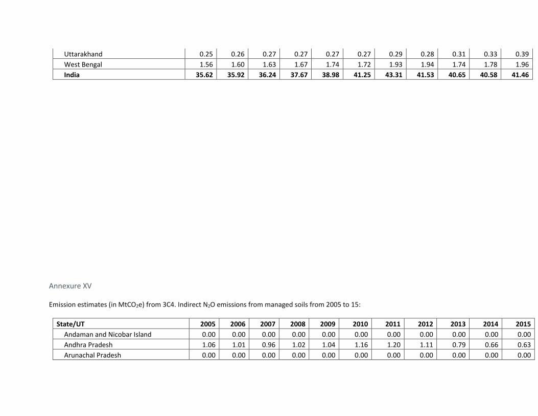
Uttarakhand 0.25 0.26 0.27 0.27 0.27 0.27 0.29 0.28 0.31 0.33 0.39
West Bengal 1.56 1.60 1.63 1.67 1.74 1.72 1.93 1.94 1.74 1.78 1.96
India 35.62 35.92 36.24 37.67 38.98 41.25 43.31 41.53 40.65 40.58 41.46
Annexure XV Emission estimates (in MtCO2e) from 3C4. Indirect N2O emissions from managed soils from 2005 to 15:
State/UT 2005 2006 2007 2008 2009 2010 2011 2012 2013 2014 2015
Andaman and Nicobar Island 0.00 0.00 0.00 0.00 0.00 0.00 0.00 0.00 0.00 0.00 0.00
Andhra Pradesh 1.06 1.01 0.96 1.02 1.04 1.16 1.20 1.11 0.79 0.66 0.63
Arunachal Pradesh 0.00 0.00 0.00 0.00 0.00 0.00 0.00 0.00 0.00 0.00 0.00

Assam 0.06 0.06 0.06 0.07 0.08 0.08 0.09 0.10 0.09 0.09 0.10
Bihar 0.53 0.54 0.56 0.57 0.55 0.55 0.53 0.75 0.62 0.60 0.72
Chandigarh 0.00 0.00 0.00 0.00 0.00 0.00 0.00 0.00 0.00 0.00 0.00
Chhattisgarh 0.15 0.16 0.16 0.16 0.18 0.20 0.21 0.24 0.22 0.22 0.24
Dadra and Nagar Haveli 0.00 0.00 0.00 0.00 0.00 0.00 0.00 0.00 0.00 0.00 0.00
Daman and Diu 0.00 0.00 0.00 0.00 0.00 0.00 0.00 0.00 0.00 0.00 0.00
Delhi 0.00 0.00 0.00 0.00 0.00 0.00 0.00 0.00 0.00 0.00 0.00
Goa 0.00 0.00 0.00 0.00 0.00 0.00 0.00 0.00 0.00 0.00 0.00
Gujarat 0.63 0.64 0.64 0.65 0.67 0.73 0.73 0.71 0.68 0.73 0.69
Haryana 0.56 0.56 0.57 0.58 0.58 0.59 0.61 0.74 0.61 0.61 0.63
Himachal Pradesh 0.02 0.02 0.02 0.02 0.02 0.02 0.02 0.02 0.02 0.02 0.02
Jammu and Kashmir 0.03 0.03 0.03 0.04 0.04 0.04 0.04 0.05 0.04 0.04 0.05
Jharkhand 0.05 0.05 0.05 0.05 0.06 0.05 0.07 0.07 0.05 0.05 0.07
Karnataka 0.46 0.47 0.48 0.51 0.57 0.61 0.71 0.59 0.57 0.60 0.60
Kerala 0.05 0.06 0.06 0.07 0.07 0.07 0.08 0.08 0.08 0.07 0.07
Lakshadweep 0.00 0.00 0.00 0.00 0.00 0.00 0.00 0.00 0.00 0.00 0.00
Madhya Pradesh 0.43 0.46 0.48 0.49 0.55 0.60 0.64 0.73 0.72 0.70 0.73
Maharashtra 0.74 0.75 0.77 0.80 0.88 0.98 0.99 0.87 0.93 0.95 0.90
Manipur 0.01 0.01 0.01 0.01 0.01 0.00 0.00 0.01 0.01 0.01 0.01
Meghalaya 0.00 0.00 0.00 0.00 0.00 0.00 0.00 0.00 0.00 0.00 0.00
Mizoram 0.00 0.00 0.00 0.00 0.00 0.00 0.00 0.00 0.00 0.00 0.00
Nagaland 0.00 0.00 0.00 0.00 0.00 0.00 0.00 0.00 0.00 0.00 0.00
Odisha 0.16 0.16 0.16 0.18 0.18 0.18 0.19 0.19 0.19 0.19 0.20
Puducherry 0.02 0.01 0.01 0.01 0.01 0.01 0.01 0.01 0.01 0.01 0.00
Punjab 0.78 0.79 0.80 0.81 0.82 0.85 0.86 1.04 0.86 0.83 0.87
Rajasthan 0.39 0.41 0.42 0.43 0.44 0.51 0.55 0.69 0.59 0.58 0.63
Sikkim 0.00 0.00 0.00 0.00 0.00 0.00 0.00 0.00 0.00 0.00 0.00
Tamil Nadu 0.31 0.32 0.33 0.38 0.38 0.39 0.41 0.38 0.34 0.36 0.40
Telangana 0.48 0.46 0.44 0.46 0.47 0.52 0.54 0.50 0.57 0.53 0.53
Tripura 0.01 0.01 0.00 0.00 0.01 0.01 0.01 0.01 0.01 0.01 0.01
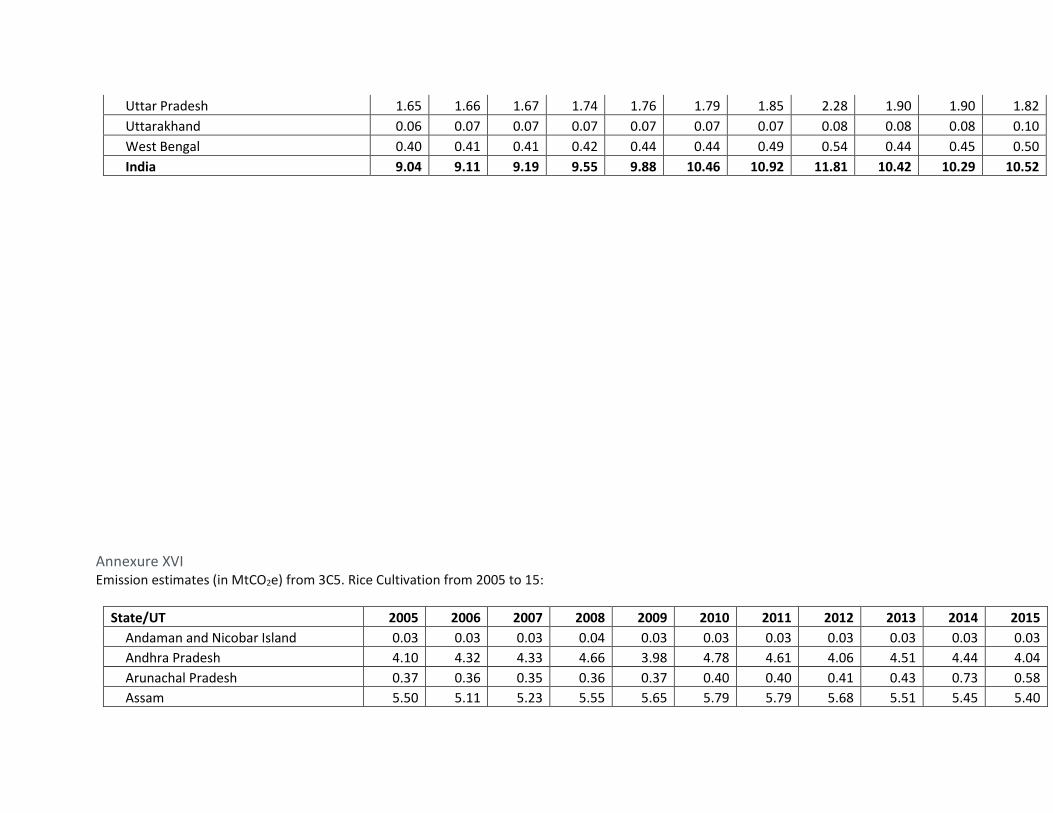
Uttar Pradesh 1.65 1.66 1.67 1.74 1.76 1.79 1.85 2.28 1.90 1.90 1.82
Uttarakhand 0.06 0.07 0.07 0.07 0.07 0.07 0.07 0.08 0.08 0.08 0.10
West Bengal 0.40 0.41 0.41 0.42 0.44 0.44 0.49 0.54 0.44 0.45 0.50
India 9.04 9.11 9.19 9.55 9.88 10.46 10.92 11.81 10.42 10.29 10.52
Annexure XVI Emission estimates (in MtCO2e) from 3C5. Rice Cultivation from 2005 to 15:
State/UT 2005 2006 2007 2008 2009 2010 2011 2012 2013 2014 2015
Andaman and Nicobar Island 0.03 0.03 0.03 0.04 0.03 0.03 0.03 0.03 0.03 0.03 0.03
Andhra Pradesh 4.10 4.32 4.33 4.66 3.98 4.78 4.61 4.06 4.51 4.44 4.04
Arunachal Pradesh 0.37 0.36 0.35 0.36 0.37 0.40 0.40 0.41 0.43 0.73 0.58
Assam 5.50 5.11 5.23 5.55 5.65 5.79 5.79 5.68 5.51 5.45 5.40

Bihar 6.75 7.12 7.24 7.27 6.71 6.08 6.72 6.90 6.64 6.73 6.71
Chandigarh 0.00 0.00 0.00 0.00 0.00 0.00 0.00 0.00 0.00 0.00 0.00
Chhattisgarh 5.29 5.27 5.24 5.27 5.22 5.24 5.24 5.24 5.25 5.29 5.08
Dadra and Nagar Haveli 0.02 0.02 0.02 0.02 0.02 0.02 0.02 0.02 0.02 0.02 0.02
Daman and Diu 0.00 0.00 0.00 0.00 0.00 0.00 0.00 0.00 0.00 0.00 0.00
Delhi 0.00 0.00 0.00 0.00 0.00 0.00 0.00 0.00 0.00 0.00 0.00
Goa 0.07 0.08 0.07 0.07 0.07 0.07 0.07 0.07 0.06 0.06 0.07
Gujarat 1.32 1.37 1.43 1.37 1.25 1.39 1.49 1.46 1.44 1.44 1.39
Haryana 1.14 1.13 1.16 1.28 1.32 1.35 1.35 1.32 1.35 1.39 1.46
Himachal Pradesh 0.02 0.02 0.02 0.02 0.02 0.02 0.02 0.02 0.02 0.02 0.02
Jammu and Kashmir 0.09 0.09 0.09 0.09 0.10 0.10 0.10 0.10 0.10 0.10 0.10
Jharkhand 2.20 2.34 2.37 2.38 2.04 1.71 1.86 2.06 2.10 1.97 2.79
Karnataka 1.48 1.45 1.42 1.52 1.55 1.63 1.52 1.31 1.37 1.41 1.20
Kerala 0.50 0.46 0.40 0.36 0.35 0.33 0.29 0.30 0.31 0.29 0.29
Lakshadweep 0.00 0.00 0.00 0.00 0.00 0.00 0.00 0.00 0.00 0.00 0.00
Madhya Pradesh 2.12 2.09 2.02 2.04 1.95 1.87 1.94 1.99 2.02 2.10 2.10
Maharashtra 1.98 1.90 2.03 2.03 1.97 1.99 2.04 2.06 2.12 2.08 2.04
Manipur 0.31 0.30 0.30 0.30 0.31 0.36 0.40 0.32 0.37 0.41 0.36
Meghalaya 0.19 0.19 0.19 0.19 0.19 0.18 0.18 0.12 0.11 0.11 0.11
Mizoram 0.10 0.10 0.10 0.08 0.07 0.05 0.04 0.04 0.03 0.03 0.04
Nagaland 0.26 0.28 0.28 0.28 0.27 0.29 0.29 0.29 0.30 0.30 0.28
Odisha 8.37 8.33 8.07 7.77 7.75 8.22 7.98 7.87 8.14 7.77 7.45
Puducherry 0.03 0.03 0.03 0.03 0.03 0.03 0.02 0.02 0.02 0.02 0.03
Punjab 1.07 1.06 1.05 1.09 1.12 1.14 1.14 1.15 1.15 1.16 1.19
Rajasthan 0.02 0.02 0.02 0.03 0.04 0.03 0.03 0.03 0.03 0.04 0.05
Sikkim 0.05 0.05 0.05 0.05 0.05 0.04 0.04 0.04 0.04 0.04 0.04
Tamil Nadu 3.67 3.58 3.34 3.46 3.41 3.45 3.47 2.92 3.05 3.23 3.58
Telangana 2.79 2.96 2.96 3.18 2.73 3.29 3.16 2.78 3.44 2.87 2.09
Tripura 0.49 0.47 0.47 0.46 0.44 0.46 0.47 0.45 0.45 0.46 0.48
Uttar Pradesh 9.07 8.76 8.61 8.71 8.31 8.17 8.26 7.89 7.98 7.94 7.67
Uttarakhand 0.48 0.46 0.45 0.45 0.43 0.44 0.42 0.40 0.39 0.39 0.39

West Bengal 10.62 11.72 11.68 12.03 11.65 10.44 10.84 11.11 11.12 11.14 11.05
India 70.52 71.47 71.10 72.46 69.38 69.40 70.23 68.45 69.89 69.46 68.14

References
• 16th Indian Livestock Census Report (1997) Department of Animal Husbandry, Dairying and Fisheries, Ministry of Agriculture, Government of India. http://dahd.nic.in/documents/statistics/livestock-census
• 17th Indian Livestock Census. All India Summary Report (2003) Department of Animal Husbandry, Dairying and Fisheries, Ministry of Agriculture, Government of India. http://dahd.nic.in/documents/statistics/livestock-census
• 18th Livestock Census. All India Report on Quick Tabulation Plan (2007) Department of Animal Husbandry, Dairying and Fisheries, Ministry of Agriculture, Government of India. http://dahd.nic.in/documents/statistics/livestock-census
• 19th Livestock Census. All India Report (2012) Department of Animal Husbandry, Dairying and Fisheries, Ministry of Agriculture, Government of India. http://dahd.nic.in/documents/statistics/livestock-census
• ALGAS, India national report on Asia least cost GH abatement strategy. ADB and UNDP, Manila, the Philippines, 1998 https://www.climate-eval.org/sites/default/files/evaluations/115%20Asia%20Least-Cost%20Greenhouse%20Gas%20Abatement%20Strategy%20%28ALGAS.pdf
• Andreae, M. O., & Merlet, P. (2001). Emission of trace gases and aerosols from biomass burning. Global Biogeochemical Cycles, 15(4), 955–966. https://doi.org/10.1029/2000GB001382
• Arora, G., Chaturvedi, S., Kaushal, R., Nain, A., Tewari, S., Alam, N. M., & Chaturvedi, O. P. (2014). Growth, biomass, carbon stocks, and sequestration in an age series of Populus deltoides plantations in Tarai region of central Himalaya. TURKISH JOURNAL OF AGRICULTURE AND FORESTRY, 38, 550–560. https://doi.org/10.3906/tar-1307-94
• Atzema, A. J. (1995). Determination of quality of forecast moisture content of cut grass using forecast weather elements. Journal of Agricultural Engineering Research, 61, 1–10.
• Badiyala, D., and Verma S.P. (1990) Effect of supplemental sources and fertilizer nitrogen on physio-chemical properties of acid soils of Himachal Pradesh, Indian Journal of Agronomy, Vol 35 (1&2):144-149
• Bandyopadhyay, S., Pathak, H., Kalra, N., Aggarwal, P.K., Kaur, R., Joshi, H.C., Choudhary, R. and Roetter, R.P. 2001. Yield estimation and agro-technical description of production systems. In Aggarwal, P.K., Roetter, R.P., Kalra, N., Keulen, H. van, Hoanh, C.T., Laar, H.H. van (eds.), Land Use Analysis and Planning for Sustainable Food Security: With an Illustration for the State of Haryana, India. New Delhi. pp. 61–89. http://library.wur.nl/WebQuery/wurpubs/316344
• BC Mandal, AK Mandal and AB Ghosh(1981), Changes in Organic Carbon in a Gangetic alluvium after five years of multiple cropping with jute-rice-wheat, Journal of Indian Society of Soil Science, Vol 30(1):38-42; http://agris.fao.org/agris-search/search.do?recordID=US201301994080
• Bhatia, A., Pathak, H., Aggarwal, P., 2004. Inventory of methane and nitrous oxide emissions from agricultural soils of India and their global warming potential. Curr. Sci. 317–324. https://www.researchgate.net/publication/248354019_Rice_straw_as_a_renewable_energy_source_in_India_Thailand_and_the_Philippines_Overall_potential_and_limitations_for_energy_contribution_and_greenhouse_gas_mitigation
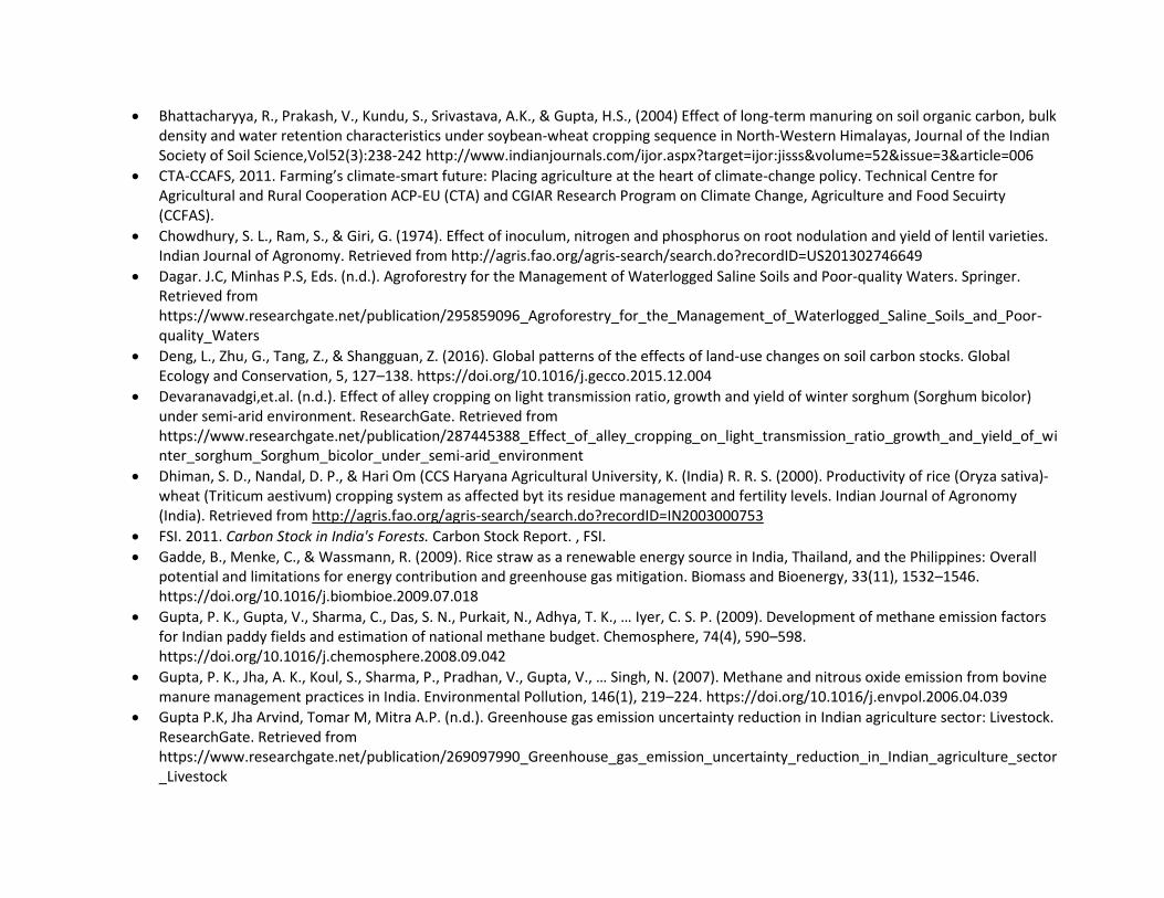
• Bhattacharyya, R., Prakash, V., Kundu, S., Srivastava, A.K., & Gupta, H.S., (2004) Effect of long-term manuring on soil organic carbon, bulk density and water retention characteristics under soybean-wheat cropping sequence in North-Western Himalayas, Journal of the Indian Society of Soil Science,Vol52(3):238-242 http://www.indianjournals.com/ijor.aspx?target=ijor:jisss&volume=52&issue=3&article=006
• CTA-CCAFS, 2011. Farming’s climate-smart future: Placing agriculture at the heart of climate-change policy. Technical Centre for Agricultural and Rural Cooperation ACP-EU (CTA) and CGIAR Research Program on Climate Change, Agriculture and Food Secuirty (CCFAS).
• Chowdhury, S. L., Ram, S., & Giri, G. (1974). Effect of inoculum, nitrogen and phosphorus on root nodulation and yield of lentil varieties. Indian Journal of Agronomy. Retrieved from http://agris.fao.org/agris-search/search.do?recordID=US201302746649
• Dagar. J.C, Minhas P.S, Eds. (n.d.). Agroforestry for the Management of Waterlogged Saline Soils and Poor-quality Waters. Springer. Retrieved from https://www.researchgate.net/publication/295859096_Agroforestry_for_the_Management_of_Waterlogged_Saline_Soils_and_Poor-quality_Waters
• Deng, L., Zhu, G., Tang, Z., & Shangguan, Z. (2016). Global patterns of the effects of land-use changes on soil carbon stocks. Global Ecology and Conservation, 5, 127–138. https://doi.org/10.1016/j.gecco.2015.12.004
• Devaranavadgi,et.al. (n.d.). Effect of alley cropping on light transmission ratio, growth and yield of winter sorghum (Sorghum bicolor) under semi-arid environment. ResearchGate. Retrieved from https://www.researchgate.net/publication/287445388_Effect_of_alley_cropping_on_light_transmission_ratio_growth_and_yield_of_winter_sorghum_Sorghum_bicolor_under_semi-arid_environment
• Dhiman, S. D., Nandal, D. P., & Hari Om (CCS Haryana Agricultural University, K. (India) R. R. S. (2000). Productivity of rice (Oryza sativa)-wheat (Triticum aestivum) cropping system as affected byt its residue management and fertility levels. Indian Journal of Agronomy (India). Retrieved from http://agris.fao.org/agris-search/search.do?recordID=IN2003000753
• FSI. 2011. Carbon Stock in India's Forests. Carbon Stock Report. , FSI.
• Gadde, B., Menke, C., & Wassmann, R. (2009). Rice straw as a renewable energy source in India, Thailand, and the Philippines: Overall potential and limitations for energy contribution and greenhouse gas mitigation. Biomass and Bioenergy, 33(11), 1532–1546. https://doi.org/10.1016/j.biombioe.2009.07.018
• Gupta, P. K., Gupta, V., Sharma, C., Das, S. N., Purkait, N., Adhya, T. K., … Iyer, C. S. P. (2009). Development of methane emission factors for Indian paddy fields and estimation of national methane budget. Chemosphere, 74(4), 590–598. https://doi.org/10.1016/j.chemosphere.2008.09.042
• Gupta, P. K., Jha, A. K., Koul, S., Sharma, P., Pradhan, V., Gupta, V., … Singh, N. (2007). Methane and nitrous oxide emission from bovine manure management practices in India. Environmental Pollution, 146(1), 219–224. https://doi.org/10.1016/j.envpol.2006.04.039
• Gupta P.K, Jha Arvind, Tomar M, Mitra A.P. (n.d.). Greenhouse gas emission uncertainty reduction in Indian agriculture sector: Livestock. ResearchGate. Retrieved from https://www.researchgate.net/publication/269097990_Greenhouse_gas_emission_uncertainty_reduction_in_Indian_agriculture_sector_Livestock

• Hansen, S. (n.d.). EXTERNAL EVALUATION OF THE CONCURRENT PHASE OF RETA 5592: A STUDY OF LEAST-COST GREENHOUSE GAS ABATEMENT STRATEGY (ALGAS PROJECT), 66.
• Hegde D.M. (1998). Long-term sustainability of productivity in rice (Oryza sativa)-wheat (Triticum aestivum) system in subhumid ecosystem through integrated nutrient supply. ResearchGate. Retrieved from https://www.researchgate.net/publication/289381108_Long-term_sustainability_of_productivity_in_rice_Oryza_sativa-wheat_Triticum_aestivum_system_in_subhumid_ecosystem_through_integrated_nutrient_supply
• Hegde D.M. (n.d.). Effect of integrated nutrient supply on crop productivity and soil fertility in rice (Oryza sativa) - Wheat (Triticum aestivum) system in semi-arid and humid ecosystems. ResearchGate. Retrieved from https://www.researchgate.net/publication/279714905_Effect_of_integrated_nutrient_supply_on_crop_productivity_and_soil_fertility_in_rice_Oryza_sativa_-_Wheat_Triticum_aestivum_system_in_semi-arid_and_humid_ecosystems
• ICAR [Indian Council of Agricultural Research] (1997) Handbook of Animal Husbandry, ICAR, New Delhi.
• ICAR, 2015. VISION 2020 - Indian Council of Agricultural Research, New Delhi, India. http://www.icar.org.in/files/vision-2020.pdf
• INCCA Indian Network for Climate Change Assessment. (2010). India: Greenhouse Gas Emissions 2007. Ministry of Environment and Forests Government of India.
• India-BUR [India First Biennial Update Report to the United Nations Framework Convention on Climate Change] (2015) Ministry of Environment, Forest and Climate Change, Government of India. http://unfccc.int/resource/docs/natc/indbur1.pdf
• India Fertilzer Scenario (2010), Department of Fertilizers Ministry of Chemicals and Fertilizers Government of India. http://fert.nic.in/sites/default/files/Indian-Fertilizer-Scenario.pdf
• India Fertilzer Scenario (2012), Department of Fertilizers Ministry of Chemicals and Fertilizers Government of India. http://fert.nic.in/sites/default/files/indian%20fertilizer%20scenario2012.pdf
• India Fertilzer Scenario (2014), Department of Fertilizers Ministry of Chemicals and Fertilizers Government of India. http://fert.nic.in/sites/default/files/Indian%20Fertilizer%20SCENARIO-2014.pdf
• India Fertilzer Scenario (2015), Department of Fertilizers Ministry of Chemicals and Fertilizers Government of India. http://fert.nic.in/sites/default/files/Indian%20Fertilizer%20SCENARIO-2015.pdf
• INDIAN COUNCIL OF FORESTRY RESEARCH AND EDUCATION. (2009). India’s Forest and Tree Cover: Contribution as a Carbon Sink. Dehradoon: Indian Council of Forestry Research and Education.
• IPCC [Inter-Governmental Panel on Climate Change] (2006) Contribution of Working Group III to the Fourth Assessment Report of the Intergovernmental Panel on Climate Change, 2007, by Metz, B., Davidson, O.R., Bosch, P.R., Dave, R. and Meyer, L.A. (eds). Cambridge University Press, Cambridge, United Kingdom and New York, NY, USA. http://www.ipcc-nggip.iges.or.jp/public/2006gl/vol4.html
• IPCC [Inter-Governmental Panel on Climate Change] (1996) Climate Change 1995: The Science of Climate Change - Contribution of WGI to the Second Assessment Report of the Intergovernmental Panel on Climate Change, by Houghton, J.T., Meira Filho, L.G., Callander, B.A., Harris, N., Kattenberg, A. and Markell, K. (Eds.) Cambridge University Press, Cambridge http://www.ipcc-nggip.iges.or.jp/public/gl/invs1.html

• Jain, N., Bhatia, A., Pathak, H., 2014. Emission of air pollutants from crop residue burning in India. Aerosol Air Qual. Res. 14, 422–430. https://www.researchgate.net/publication/277676603_Emission_of_Air_Pollutants_from_Crop_Residue_Burning_in_India
• Jha Gajanand,Chaudhary S.K,Thakur,R.B. (n.d.). Effect of combined use of green-manure crop and nitrogen on productivity of rice (Oryza sativa)-wheat (Triticum aestivum) system under lowland rice | Request PDF. ResearchGate. Retrieved from https://www.researchgate.net/publication/287445380_Effect_of_combined_use_of_green-manure_crop_and_nitrogen_on_productivity_of_rice_Oryza_sativa-wheat_Triticum_aestivum_system_under_lowland_rice
• Kaul, M., Dadhwal, V. K., & Mohren, G. M. J. (2009). Land use change and net C flux in Indian forests. Forest Ecology and Management, 258(2), 100–108. https://doi.org/10.1016/j.foreco.2009.03.049
• Khatua, K. B., Chaudhury, S. C., Panda, M., & Mishra, A. (Orissa U. of A. and T. (1976). Nitrogen, phosphorus and potash requirement of high yielding rice [India]. Indian Journal of Agronomy (India). Retrieved from http://agris.fao.org/agris-search/search.do?recordID=IN7701500
• Kumar, A. and Yadav, D.S. (2005) Influence of continuous cropping and fertilization on nutrient availability and productivity of an alluvial soil, Journal of the Indian Society of Soil Science,Vol53(2):194-198
• Lal, R. (2004). Soil Carbon Sequestration in India. Climatic Change, 65(3), 277–296. https://doi.org/10.1023/B:CLIM.0000038202.46720.37
• Maikhuri, R. K., Semwal, R. L., Rao, K. S., Singh, K., & Saxena, K. G. (2000). Growth and ecological impacts of traditional agroforestry tree species in Central Himalaya, India. Agroforestry Systems, 48(3), 257–271. https://doi.org/10.1023/A:1006344812127
• Mandal, B. C., Mandal, A. K., & Ghosh, A. B. (1982). Changes in organic carbon and total nitrogen in a Gangetic alluvium after five years of multiple cropping with jute-rice-wheat. Journal of the Indian Society of Soil Science. Retrieved from http://agris.fao.org/agris-search/search.do?recordID=US201301994080
• NATCOM I [National Communication I] (2004) India’s Initial National Communication to the United Nations Framework Convention on Climate Change. Ministry of Environment and Forests, Government of India; http://unfccc.int/resource/docs/natc/indnc1.pdf
• NRSC. 2007. National Land Use and Land Cover Mapping using Multi-Temporal AWiFS Data. Technical Document, Hyderabad: NRSC. https://bhuvan-app1.nrsc.gov.in/2dresources/thematic/LULC250/0506.pdf.
• NRSC. 2010. National Land Use and Land Cover Mapping Using Multi-Temporal AWiFS Data. Technical Document, Hyderabad: NSRC. https://bhuvan-app1.nrsc.gov.in/2dresources/thematic/LULC250/0809.pdf.
• NRSC. 2013. National Land Use and Land Cover Mapping Using Multi-Temporal AWiFS Data. Technical Document, Hyderabad: ISRO. https://bhuvan-app1.nrsc.gov.in/2dresources/thematic/LULC250/1314.pdf.
• NRSC. 2012. National Land Use and Land Cover Mapping Using Multi-Temporal AWiFS Data. Technical Document, Hyderabad: ISRO. https://bhuvan-app1.nrsc.gov.in/2dresources/thematic/LULC250/1213.pdf.
• Olander, L., Wollenberg, E., Tubiello, F., & Herold, M. (2013). Advancing agricultural greenhouse gas quantification *. Environmental Research Letters, 8(1), 011002. https://doi.org/10.1088/1748-9326/8/1/011002
• P. Bhattacharyya, Yadav, R.P.. & Agnihotri, Y. (2009), 'Impact of Prevalent Silviculture Systems on Soil Stability and Potential Carbon Storage in Shivalik Region of Lower Himalayas', Journal of Indian Society of soil science 57, 71-75. http://en.ustc.findplus.cn/?h=articles&db=edsijc&an=diva.jisss.57.1.012
• Pachauri, R. K., Mayer, L., & Intergovernmental Panel on Climate Change (Eds.). (2015b). Climate change 2014: synthesis report. Geneva, Switzerland: Intergovernmental Panel on Climate Change.
• Prabhakara Setty, T.K. & Janardhana Gowda, N.A.. (1997). Performance of rice (Oryza sativa)-based cropping systems in coastal Karnataka. 42. 5-8.
• Pathak, H., Singh, B., Society for Conservation of Nature (New Delhi, I., Indian Nitrogen Group, International Nitrogen Initiative, & South Asian Nitrogen Centre. (2010). Greenhouse gas emission and mitigation in Indian agriculture: a review. Noida: Published by Indian Nitrogen Group, Society for Conservation of Nature in association with South Asian Nitrogen Centre, International Nitrogen Initiative.
• Prasad N.K, Kumar S. (n.d.). Nutrient harvest and soil fertility as influenced by legume-wheat (Triticum aestivum) sequences. ResearchGate. Retrieved from https://www.researchgate.net/publication/285615500_Nutrient_harvest_and_soil_fertility_as_influenced_by_legume-wheat_Triticum_aestivum_sequences
• Pye-Smith C. (2011, December 1). Farming’s climate-smart future: placing agriculture at the heart of climate-change policy. Retrieved December 17, 2018, from https://ccafs.cgiar.org/publications/farmings-climate-smart-future-placing-agriculture-heart-climate-change-policy
• RB Thakur, SK Chaudhary and G Jha(1999)Effect of combined use of green-manure crop and nitrogen on productivity of rice (Oryza sativa)-wheat(Triticum aestivum) system under lowland rice,Indian J.Of agronomy,Vol44(4):664-668 (https://goo.gl/4Na4cp)
• RB Thakur,SK Choudhary,G Jha&VK Mishra(1998) Effect of crop-establishment practices on wheat (Triticum aestivum) productivity and soil health under lowland rice(Oryza sativa)-wheat cropping systems in coastal Karnataka,Indian J.Of agronomy,Vol43(4):567-571
• Reddy, C S, C S Jha, G Manaswani, VVL P Alekhya, S V Pasha, K V Satish, P G Diwakar, and V K Dadhwal. 2017. “Nationwide assessment of forest burnt area in India using Resourcesat-2 AWiFS data.” Current Science, 10 April: 1521-1532.
• RK Tondon and Chokhey Singh(1962) Rotational and cultural studies in wheat, Indian Journal of Agronomy, Vol 7:10-18 (pdfpills.com/i/isa-india.in1.html)
• Saha, R., & Jha, P. (n.d.). Carbon Sequestration Potentials of Agroforestry Systems under Climate Change Scenario – Brief Review with Special Emphasis on North-Eastern Hill Regions, 12, 7.
• Sandhu, S Parminder. (2016). PRODUCTIVITY, QUALITY AND SOIL HEALTH OF RICE-(Oryza sativa L.) Wheat (Triticum aestivum L.) CROPPING SYSTEM IN RELATION TO LONG TERM INTEGRATED NUTRIENT MANAGEMENT. PUNJAB AGRICULTURAL UNIVERSITY LUDHIANA - 141004, Ludhiana. Retrieved from https://www.researchgate.net/publication/296077703_Performance_of_rice_Oryza_sativa-based_cropping_systems_in_coastal_Karnataka
• Sanjay Kumar and NK Prasad(1999)Soil fertility and yield as influenced by different legume-wheat (Triticum aestivum) sequences,Indian J.Of agronomy,Vol44(3):488-492

(https://www.researchgate.net/publication/285615500_Nutrient_harvest_and_soil_fertility_as_influenced_by_legume-wheat_Triticum_aestivum_sequences)
• SASCOM [South Asian START Committee] (1998) GHG Emissions in India for the base year 1990. Scientific Report No 11, SASCOM Centre on Global Change, CSIR- NPL, New Delhi.
• Saxena, K. G., Rao, K. S., Sen, K. K., Maikhuri, R. K., & Semwal, R. L. (2001). Integrated Natural Resource Management: Approaches and Lessons from the Himalaya. Conservation Ecology, 5(2). https://doi.org/10.5751/ES-00289-050214
• SB Devaranavadgi, CS Hunashal, MB Patil, H Venkatesh and SY Wali(2003), Effect of alley cropping on light transmission ratio, growth and yield of winter sorghum (Sorghum bicoIor) under semi arid environment, Indian Journal Of agronomy, Vol 48(2):108-110 (https://www.researchgate.net/publication/287445388_Effect_of_alley_cropping_on_light_transmission_ratio_growth_and_yield_of_winter_sorghum_Sorghum_bicolor_under_semi-arid_environment)
• SD Dhiman, DP Nandal and hari Om(2000) Productivity of rice (Oryza sativa)-wheat (Triticum aestivum) cropping system as affected by its residue managemnt and fertility levels,Indian J.Of agronomy,Vol45(1)1-5 (http://agris.fao.org/agris-search/search.do?recordID=IN2003000753)
• SD Singh and DL Vyas(1970) Studies on manurial value of tumbia (Citrullus colocynthis)oil cake, Indian Journal of Agronomy, Vol 15:173-176 (https://eurekamag.com/research/014/690/014690276.php)
• Sengar, S. S. (z a. R. S., Wade, L. J. (International R. R. I., Baghel, S. S. (cau, Singh, R. K. (IRRI-R., & Singh, R. (nduat. (2000). Effect of nutrient management on rice (Oryza sativa) in rainfed lowland of southeast Madhya Pradesh. Indian Journal of Agronomy (India). Retrieved from http://agris.fao.org/agris-search/search.do?recordID=IN2003000414
• Shukla, P., & Pathak, A. N. (1974). Nitrogen, phosphorus and potash requirements of high yielding wheat in central and north eastern alluvial zones of Uttar Pradesh. Indian Journal of Agronomy. Retrieved from http://agris.fao.org/agris-search/search.do?recordID=US201303085849
• Singh, M., Warsi, A. S., & Agrawal, J. P. (1973). Optimum sowing depth of rainfed barley. Indian Journal of Agronomy. Retrieved from http://agris.fao.org/agris-search/search.do?recordID=US201302209736
• SL Chowdhury, Sewa Ram and Gajendra Giri(1974) Effect of inoculum, nitrogen and phosphorus on root nodulation and yield of lentil varieties, Indian Journal of Agronomy, Vol 19:274-276 (http://agris.fao.org/agris-search/search.do?recordID=US201302746649)
• Soil Carbon sequestrtion in India, R. Lal, Climatic Change, 65; 277-296, 2004 (https://link.springer.com/article/10.1023/B:CLIM.0000038202.46720.37)
• Sondara Rao, W. V. B., & Krishan, A. (1963). The effect of manuring and rotation on the soil fertility status and composition of barley crop in the permanent manurial series (A) at Pusa Bihar. Indian J. Agron. Retrieved from https://eurekamag.com/research/014/240/014240319.php
• Sreenivas, K., Dadhwal, V. K., Kumar, S., Harsha, G. S., Mitran, T., Sujatha, G., … Ravisankar, T. (2016). Digital mapping of soil organic and inorganic carbon status in India. Geoderma, 269, 160–173. https://doi.org/10.1016/j.geoderma.2016.02.002

• Stalin, P., Ramanathan, S., Nagarajan, R., and Natarajan, K., (2006) Long-term effect of continuous manurial practices on grain-yield and some soil chemical properties in rice based cropping systems, Journal of the Indian Society of oil Science, Vo54(1):30-37; http://www.indianjournals.com/ijor.aspx?target=ijor:jisss&volume=54&issue=1&article=006
• Streets, D. G., Yarber, K. F., Woo, J.-H., & Carmichael, G. R. (2003). Biomass burning in Asia: Annual and seasonal estimates and atmospheric emissions. Global Biogeochemical Cycles, 17(4). https://doi.org/10.1029/2003GB002040
• Sudhakar Reddy, C., Jha, C. S., Manaswini, G., Padma Alekhya, V. V. L., Vazeed Pasha, S., Satish, K. V., … Dadhwal, V. K. (2017). Nationwide Assessment of Forest Burnt Area in India Using Resourcesat-2 AWiFS Data. Current Science, 112(07), 1521. https://doi.org/10.18520/cs/v112/i07/1521-1532
• Swamy, M., & Bhattacharya, S. (2006). Budgeting anthropogenic greenhouse gas emission from Indian livestock using country-specific emission coefficients. CURRENT SCIENCE, 91(10), 15.
• Swamy, M. and Ramasami, T. (1997) Methane emission from India through Enteric Fermentation: An estimate: In Proc. IGBP Symposium on Changes in Global Climate due to Natural and Human Activities (suppl.)”, 15-17, Jan. 1997, Bhubaneswar. pp 24-26.
• Swamy, M. and Shashirekha V. (2003) Uncertainty Reduction in Estimation of Methane from Domestic Livestock and Abatement Stategy. In Proc: 4th All India People’s Technology Congress., EV-16 (69-73), 22-23, Feb. 2003, Kolkata
• Swamy, M. and Shashirekha, V. 2006. Managing methane emission from domestic livestock. In Collaborating to Combat Climate Change, Ahluwalia, J.S (Ed.) MM Publishing for World Environment Foundation, London. pp. 320 – 332. (https://goo.gl/VxSxx2)
• Swamy, M., Singhal, K.K., Gupta, P.K., Madhu Mohini and Mitra, A.P. (2004) Reduction in Uncertainties from Livestock Emissions. In Climate Change and India: Uncertainty reduction in GHG inventory estimates. A.P. Mitra et al., (Eds.) NATCOM – MoEF publication, University Press, New Delhi. pp: 223 – 241. (https://www.researchgate.net/publication/269097990_Greenhouse_gas_emission_uncertainty_reduction_in_Indian_agriculture_sector_Livestock)
• Swamy. M. and Shashirekha, V. (2003) Country Specific Emission Co-efficients for Estimation of Methane from Livestock Sector. In: Proc. NATCOM Workshop on Uncertainty Reduction in GHG Inventory Estimates, March 4 – 5, 2003, New Delhi. pp 128 – 138. (https://scholar.google.com/citations?user=VC5kCIsAAAAJ&hl=en)
• Swarup, A. and Singh, M. (2009) Soil carbon dynamics under intensive cropping systems, Journal of the Indian Society of Soil Science, Vol 57(4): 469-476 http://www.indianjournals.com/ijor.aspx?target=ijor:jisss&volume=57&issue=4&article=008
• Swarup, A. and Yaduvanshi, N.P.S. (2000) Effects of integrated nutrient management on soil properties and yield of rice in alkali soils, Journal of the Indian Society of Soil Science, Vol 48 (2) 279-282, https://www.researchgate.net/profile/Nps_Yaduvanshi2/publication/279923571_Effect_of_Integrated_nutrient_management_on_soil_properties_and_yield_of_rice_in_Alkali_soils/links/59c8889aaca272c71bc7f778/Effect-of-Integrated-nutrient-management-on-soil-properties-and-yield-of-rice-in-Alkali-soils.pdf
• TK prabhakara Shetty and NA Janardhana Gowda(1997)Performance of rice (Oryza sativa)-based cropping systems in coastal Karnataka,Indian J.Of agronomy,Vol42(1):5-8

(https://www.researchgate.net/publication/296077703_Performance_of_rice_Oryza_sativa-based_cropping_systems_in_coastal_Karnataka)
• Vani, K.P., and Bheemaiah, G., (2003) Effect of alley cropping of castor (Ricinus communis) and integrated nutrietn management practices on productivity status of soil under SAT regions, Indian Journal Of agronomy, Vol 48(3):224-228 http://www.indianjournals.com/ijor.aspx?target=ijor:ija&volume=48&issue=3&article=021
• Verma, K.P., (2001) Effect of crop residue incorporation and nitrogen on succeeding wheat (Triticum aestivum), Indian Journal of agronomy,Vol46(4):665-669 http://www.indianjournals.com/ijor.aspx?target=ijor:ija&volume=46&issue=4&article=016
• WVB Sundara Rao and Anoop Krishan(1963) The effect of manuring and rotation on the soil fertility status and composition of barley crop in the permanent manurial series (A) at Pusa Bihar, Indian Journal of Agronomy, Vol 8(1) :347-357
• Turn, S. Q., Jenkins, B. M., Chow, J. C., Pritchett, L. C., Campbell, D., Cahill, T., & Whalen, S. A. (1997). Elemental characterization of particulate matter emitted from biomass burning: Wind tunnel derived source profiles for herbaceous and wood fuels. Journal of Geophysical Research: Atmospheres, 102(D3), 3683–3699. https://doi.org/10.1029/96JD02979
• United Nations Framework Convention on Climate Change (Organization), & India (Eds.). (2004). India’s initial national communication to the United Nations Framework Convention on Climate Change. New Delhi: Ministry of Environment & Forests, Govt. of India.

Abbreviations
AFOLU Agriculture, Forestry and Other Land Use
AGB Above Ground Biomass
AWMS Animal Waste Management System
BGB Below Ground Biomass
BUR Biennial Update Report
CH4 Methane
CO2 Carbon Dioxide
EF Emission Factor
FSI Forest Survey of India
GHG Green House Gas
GoI Government of India
INCCA Indian Network on Climate Change Assessment
IPCC Intergovernmental Panel on Climate Change
MoA Ministry of Agriculture
MOEFCC Ministry of Environment, Forest and Climate Change
N2O Nitrous Dioxide
NATCOM National Communication to the UNFCCC
NRSC National Remote Sensing Centre
QA/QC Quality Assurance/Quality Control
SOC Soil Organic Carbon
List of Tables Table ES 1: Overview of GHG Emission Estimates by Gases and Sector for AFOLU sector Table 1.2: Global warming potential as per IPCC assessment reports Table 1.6: Category Wise Outline of GHG Emissions Estimates Table 1.10: Details of key source categories excluded from present GHG estimates Table 2.1 AFOLU Sector trend of GHG Emission estimates by source categories Table 2.2 AFOLU sector distribution of emission contribution by sector for 2015 Table 3.1: GHG estimates for base year and current year Table 3.2: Category wise Analysis of GHG Emissions Estimates (2005-2015) Table 3.3: State-wise GHG estimates (2005-2015) Table 3.4: Summary of Quality Assessment and Quality Control Processes Table 3.5A: Source category wise details on type of data, quality and source Table 3.5B: Source category wise details on tier approach and type of emission factor used Table 3.5C: Categorization of livestock for derivation of methane emission factors Table 3.5D: Emission factor of each sub-group in terms of kilograms of methane per animal per year Table 3.5E: Uncertainties in emission estimation from Enteric Fermentation Table 3.6A: Source category wise details on type of data, quality and source Table 3.6B: Source category wise details on tier approach and type of emission factor used Table 3.6C: Categorization of livestock for derivation of methane emission factors Table 3.6D: Emission factor of each sub-group in terms of kilograms of methane per animal per year Table 3.6E: Categorization of livestock for derivation of methane emission factors Table 3.6F: Nitrogen Emission Factors Table 3.6G: Source category wise description of Qualitative uncertainty Table 3.7A: An overview of source categories of Forest Land Table 3.7B: An overview of emission factors used for forestland Table 3.7C: Source category wise details on the difference between GHG estimates Table 3.7D: Source category wise description of Qualitative uncertainty Table 3.8A: An overview of source categories of Cropland Table 3.8B: An overview of emission factors used for cropland Table 3.8C: Biomass carbon stock in Croplands Table 3.8D: Source category wise details on the difference between GHG estimates Table 3.8E: Source category wise description of Qualitative uncertainty Table 3.9A: An overview of source categories of Grassland
Table 3.9B: An overview of emission factors used for grasslands Table 3.9C: Biomass Carbon Stock in Grassland Table 3.9D: Source category wise details on the difference between GHG estimates Table 3.9E: Source category wise description of Qualitative uncertainty Table 3.10A: An overview of source categories of Settlements Table 3.10B: An overview of emission factors used for settlements Table 3.10C: Source category wise description of Qualitative uncertainty Table 3.11A: An overview of source categories of Other Land Table 3.11B: An overview of Emission Factors used for Other Land Table 3.11C: Source category wise description of Qualitative uncertainty Table 3.12A: An overview of source categories of Forestland Table 3.12B: An overview of Emission factors used for Biomass burning in Forest Land Table 3.12C: Source category wise details on the difference between GHG estimates Table 3.12D: Source category wise description of Qualitative uncertainty Table 3.13A: An overview of source categories of Cropland: Table 3.13B: An overview of emission factors used for biomass burning in cropland Table 3.13C: Source category wise description of Qualitative uncertainty Table 3.14A: An overview of source categories of Aggregate sources and non-CO2 Emissions Sources on Land Table 3.14B: An overview of emission factors used for N2O emissions from Managed Soils Table 3.14C: Source category wise details on the difference between GHG estimates Table 3.14D: Source category wise description of Qualitative uncertainty Table 3.14E: An overview of source categories of Rice Cultivation Table 3.14F: An overview of Emission Factors used for Rice Cultivation Table 3.15A: Emission Factor for different water regime for Rice Cultivation Table 3.15B Source category wise description of Qualitative uncertainty Table 4: AFOLU: Source category wise details of deviation in GHG estimates between GHGPI and official inventories published by Government of India

List of Figures Figure 1: Trends of GHG Emissions from AFOLU sector (2005 to 2015) Figure 2: Trends of GHG Emissions from AFOLU sector (2005 to 15) Figure 3: Trend of GHG Emissions by type of GHG in the AFOLU sector (2005 to 2015) Figure 4: Overall Contribution of each Gas in the AFOLU sector Emissions (2005 to 2015) Figure 5: Trends of GHG Emissions from (3A) Livestock Sub-sector (2005 to 2015) Figure 6: Trends of GHG Emissions from the (3B) Land Sub-sector (2005 to 2015) Figure 7: Trends of GHG Emissions from (3C) Aggregate Sources and non-CO2 Emissions Sources on Land (2005 to 2015) Figure 8: Per Capita GHG Emissions from the AFOLU sector (2005 to 2015) Figure 9: Emission Intensity of AFOLU Sector (Million $ per tCO2e PPP)