Methods for Measuring Aggregate Costs of Conflict

Javier Gardeazabal∗†- University of the Basque Country

August 3, 2010

Abstract

This paper reviews the methods for measuring the economic cost of conflict. Estimat-

ing the economic costs of conflict requires a counterfactualcalculation, which makes this

a very difficult task. Social researchers have resorted to different estimation methods de-

pending on the particular effect in question. The method used in each case depends on

the units being analyzed (firms, sectors, regions or countries), the outcome variable under

study (aggregate output, market valuation of firms, market shares, etc.) and data availabil-

ity (a single cross-section, time series or panel data). This paper reviews existing methods

used in the literature to assess the economic impact of conflict: cost accounting, cross-

section methods, time series methods, panel data methods, gravity models, event studies,

natural experiments and comparative case studies. The paper ends with a discussion of

cost estimates and directions for further research.

∗Mailing address: Javier Gardeazabal, Universidad del PaísVasco, Lehendakari Aguirre 83, E-48015 Bilbao,Spain. E-mail: javier.gardeazabal@ehu.es

†I would like to thank Alberto Abadie, Esteban Klor, the editors Michelle Garfinkel and Stergios Skaperdasand seminar participants at the “Global Cost of Conflict Workshop” held at DIW, Berlin, Februrary 2010 fortheir helpful comments. Financial support from the SpanishMinistry of Science (ECO2009-09120) is gratefullyacknowledged.

1

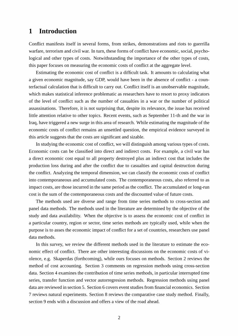
1 Introduction

Conflict manifests itself in several forms, from strikes, demonstrations and riots to guerrilla

warfare, terrorism and civil war. In turn, these forms of conflict have economic, social, psycho-

logical and other types of costs. Notwithstanding the importance of the other types of costs,

this paper focuses on measuring the economic costs of conflict at the aggregate level.

Estimating the economic cost of conflict is a difficult task. It amounts to calculating what

a given economic magnitude, say GDP, would have been in the absence of conflict - a coun-

terfactual calculation that is difficult to carry out. Conflict itself is an unobservable magnitude,

which makes statistical inference problematic as researchers have to resort to proxy indicators

of the level of conflict such as the number of casualties in a war or the number of political

assassinations. Therefore, it is not surprising that, despite its relevance, the issue has received

little attention relative to other topics. Recent events, such as September 11-th and the war in

Iraq, have triggered a new surge in this area of research. While estimating the magnitude of the

economic costs of conflict remains an unsettled question, the empirical evidence surveyed in

this article suggests that the costs are significant and sizable.

In studying the economic cost of conflict, we will distinguish among various types of costs.

Economic costs can be classified into direct and indirect costs. For example, a civil war has

a direct economic cost equal to all property destroyed plus an indirect cost that includes the

production loss during and after the conflict due to casualties and capital destruction during

the conflict. Analyzing the temporal dimension, we can classify the economic costs of conflict

into contemporaneous and accumulated costs. The contemporaneous costs, also referred to as

impact costs, are those incurred in the same period as the conflict. The accumulated or long-run

cost is the sum of the contemporaneous costs and the discounted value of future costs.

The methods used are diverse and range from time series methods to cross-section and

panel data methods. The methods used in the literature are determined by the objective of the

study and data availability. When the objective is to assessthe economic cost of conflict in

a particular country, region or sector, time series methodsare typically used, while when the

purpose is to asses the economic impact of conflict for a set ofcountries, researchers use panel

data methods.

In this survey, we review the different methods used in the literature to estimate the eco-

nomic effect of conflict. There are other interesting discussions on the economic costs of vi-

olence, e.g. Skaperdas (forthcoming), while ours focuses on methods. Section 2 reviews the

method of cost accounting. Section 3 comments on regressionmethods using cross-section

data. Section 4 examines the contribution of time series methods, in particular interrupted time

series, transfer function and vector autorregresion methods. Regression methods using panel

data are reviewed in section 5. Section 6 covers event studies from financial economics. Section

7 reviews natural experiments. Section 8 reviews the comparative case study method. Finally,

section 9 ends with a discussion and offers a view of the road ahead.

2

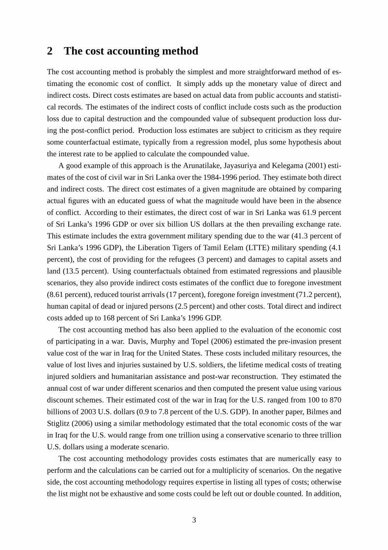
2 The cost accounting method

The cost accounting method is probably the simplest and morestraightforward method of es-

timating the economic cost of conflict. It simply adds up the monetary value of direct and

indirect costs. Direct costs estimates are based on actual data from public accounts and statisti-

cal records. The estimates of the indirect costs of conflict include costs such as the production

loss due to capital destruction and the compounded value of subsequent production loss dur-

ing the post-conflict period. Production loss estimates aresubject to criticism as they require

some counterfactual estimate, typically from a regressionmodel, plus some hypothesis about

the interest rate to be applied to calculate the compounded value.

A good example of this approach is the Arunatilake, Jayasuriya and Kelegama (2001) esti-

mates of the cost of civil war in Sri Lanka over the 1984-1996 period. They estimate both direct

and indirect costs. The direct cost estimates of a given magnitude are obtained by comparing

actual figures with an educated guess of what the magnitude would have been in the absence

of conflict. According to their estimates, the direct cost ofwar in Sri Lanka was 61.9 percent

of Sri Lanka’s 1996 GDP or over six billion US dollars at the then prevailing exchange rate.

This estimate includes the extra government military spending due to the war (41.3 percent of

Sri Lanka’s 1996 GDP), the Liberation Tigers of Tamil Eelam (LTTE) military spending (4.1

percent), the cost of providing for the refugees (3 percent)and damages to capital assets and

land (13.5 percent). Using counterfactuals obtained from estimated regressions and plausible

scenarios, they also provide indirect costs estimates of the conflict due to foregone investment

(8.61 percent), reduced tourist arrivals (17 percent), foregone foreign investment (71.2 percent),

human capital of dead or injured persons (2.5 percent) and other costs. Total direct and indirect

costs added up to 168 percent of Sri Lanka’s 1996 GDP.

The cost accounting method has also been applied to the evaluation of the economic cost

of participating in a war. Davis, Murphy and Topel (2006) estimated the pre-invasion present

value cost of the war in Iraq for the United States. These costs included military resources, the

value of lost lives and injuries sustained by U.S. soldiers,the lifetime medical costs of treating

injured soldiers and humanitarian assistance and post-warreconstruction. They estimated the

annual cost of war under different scenarios and then computed the present value using various

discount schemes. Their estimated cost of the war in Iraq forthe U.S. ranged from 100 to 870

billions of 2003 U.S. dollars (0.9 to 7.8 percent of the U.S. GDP). In another paper, Bilmes and

Stiglitz (2006) using a similar methodology estimated thatthe total economic costs of the war

in Iraq for the U.S. would range from one trillion using a conservative scenario to three trillion

U.S. dollars using a moderate scenario.

The cost accounting methodology provides costs estimates that are numerically easy to

perform and the calculations can be carried out for a multiplicity of scenarios. On the negative

side, the cost accounting methodology requires expertise in listing all types of costs; otherwise

the list might not be exhaustive and some costs could be left out or double counted. In addition,

3

the design of different scenarios is problematic as they arenot accompanied by their likelihood.

From a statistical point of view, the cost accounting methoddoes not allow the researcher to

perform statistical inference as the estimates do not come with standard errors.

3 Inference based on cross-section data

A simple way to asses the economic effect of conflict is by means of a simple regression model.

A regression equation is often postulated where some economic variable, the outcome, is re-

gressed on a measure of conflict and other control variables.When a cross-section data set on

these variables is available, one can exploit the cross-section variation in the conflict measure-

ment to asses its effect on the outcome variable. The quantitative value of these estimates can

be interpreted as a calculation of the effect of conflict on the average unit of analysis. Some

examples of this approach follow.

Venieris and Gupta (1986) provide a neat example of this methodology. They claim that

socio-political instability, an index composed by the number of deaths, protest demonstrations

and regime type, negatively affects savings. Using a sampleof 49 non communist countries,

they report the following estimates1

SY

= −0.022(−3.27)

SPI+other covariates

where the left hand side variable is the savings to GDP ratio and SPI stands for Socio-Political

Instability. This evidence supports the hypothesis that higher socio-political instability results

in lower savings. The fact that the socio-political instability variable is an index poses a problem

when evaluating its quantitative effect on the savings ratio as we do not know how to interpret

a change in the SPI index. An interpretation of the effect of the SPI index is possible using the

standard deviation of the index. Unfortunately, the authors do not report descriptive statistics

on the SPI index and therefore we cannot state precisely the quantitative effect of socio-political

instability on the savings to GDP ratio.

A quantitative estimate of the effect of socio-political instability on investment is feasible,

however, in a second example of this approach by Alesina and Perotti (1996). They argue

that the level of socio-political instability, an index reflecting political assassinations, coups

and other variables, should affect investment negatively.Using a sample of 71 countries and

sample averages of the period 1960-1985, they report the following estimated equation

IY

= − 0.50(−2.39)

SPI+other covariates

where the left hand side variable is the investment to GDP ratio and SPI stands for socio-

political instability. Alesina and Perotti note that thereexists the possibility of reverse causation

1Hereinafter figures within parentheses are t statistics.

4

from investment to socio-political instability. To avoid the reverse causation bias, Alesina and

Perotti used instrumental variable estimators. The regression coefficient estimates are mean-

ingless unless the scale of the explanatory variable is specified. This poses a problem when the

explanatory variable is an index, as in the present case. Oneway of conducting a simple quan-

titative assessment of the impact of the SPI index on the investment ratio is as follows. Alesina

and Perotti report a standard deviation of the SPI index of 11.95. To give an idea of what this

magnitude means, 11.95 would be the increase in the index of socio-political instability when

we compare the level of socio-political instability in the USA to that of Chile. A one standard

deviation increase in the index of socio-political instability would generate a fall in investment

of 0.5×11.95= 5.975 percentage points in the investment to GDP ratio.2 This quantitative

value requires two remarks. First, a one standard deviationchange in the SPI index is a change

in this index from a low value of SPI to a high value of SPI that could be difficult to observe

in any particular country in a short period of time. Second, this cross-section estimate of the

cost of conflict represents an average of the effect over countries. Therefore, particular conflict

episodes can have smaller or larger impacts on the investment ratio.

In his highly cited paper, Barro (1991) studied the sources of economic growth empirically

for a sample of 98 countries. He reports the following estimates

∆yi = −0.0075(−6.25)

y0i −0.0195(−3.10)

REVi −0.0333(−2.15)

ASSASSi +other covariates

(

IY

)

i= −0.0098

(−2.04)y0i −0.055

(−2.62)REVi −0.068

(−2.52)ASSASSi +other covariates

where∆yi is the average per capita rate of growth of countryi over the 1960-1985 period,( I

Y

)

i

is the average over the same period of the private investmentto GDP ratio,y0i is the initial per

capita GDP,REV measures the number of revolutions and coups per year andASSASSrecords

the number of political assassinations per million population per year. To avoid the problem

of reverse causation from growth to political instability Barro uses the instrumental variables

estimation technique. According to his findings,REV andASSASSare measures of political

instability negatively associated with growth. Using the standard deviations of these variables

we can again compute the quantitative effect. A one standarddeviation increase in the number

of revolutions and coups per year reduces per capita growth rate by almost half a percentage

point (−0.0195× 0.23= −0.0045) and private investment to GDP ratio by 1.26 percentage

points(−0.055×0.23=−0.0126). Similarly, a one standard deviation increase in the number

of political assassinations per million population per year reduces per capita growth rate by 0.29

percentage points(−0.0333×0.086= −0.0029) and the investment ratio by 0.58 percentage

points(−0.068×0.086= −0.0058).

2Multiplying the coefficient estimate by the standard deviation of the explanatory variable is equivalent tocomputing regression coefficients on standardized explanatory variables, a technique often used to compare theeffects of different explanatory variables.

5

Abadie and Gardeazabal (2008) analyze the effect of terrorism on the net foreign direct

investment position in a sample of 98 countries in 2003. Theyreport the following estimates

NFDI positionY

= − 0.0025(−2.0833)

GTI+other covariates

where the left hand side variable is the net foreign direct investment position (domestic assets

owned by foreign investors minus foreign assets held by domestic investors) over GDP and

GTI is a Global Terrorism Index. The standard deviation of the terrorism index is 19.82. A one

standard deviation change in this index would be the change in terrorist risk if we compare Italy

with the United States (Italy having a lower terrorist risk). According to their findings, a one

standard deviation increase in terrorist risk induces a fall in the net foreign direct investment

position over GDP ratio of 0.0025×19.82= 0.0495, almost 5 percentage points.

Interestingly, Koubi (2005) studied the effect of war on growth both during the war and

post-war periods. She reports the following cross-countrygrowth regressions for a sample of

78 countries

∆y60−89 = −0.266×(−1.87)

BD60−89+other covariates

∆y75−89 = 3.25×(1.94)

BD60−74+other covariates

where∆y60−89 and∆y75−89 stand for the average annual rate of real per capita growth during

the period 1960-1989 and 1975-1989 respectively andBD60−74 andBD60−89 are the number

of battle deaths in the 1960-1974 and 1960-1989 periods.3 Her findings indicate that contem-

poraneous effect of war on growth is negative, but the effectof war on the subsequent growth

rate during the post-war period is positive, the so called “peace dividend” effect. Koubi reports

a standard deviation of the battle deaths variable of 230,635.3, which can be used to compute

a quantitative value of the cost of conflict. A one standard deviation increase in the number of

battle deaths during the thirty year period would result in an average growth rate fall of 0.61

percentage points (−0.266×10−7×230,635.3 = 0.0061), more than half a percentage point

lower growth rate over a thirty year period.

Inference based on cross-section data suffers from some drawbacks. First, it is typically the

case that several covariates can be jointly determined withthe dependent variable or causality

might run backwards (reverse causation) and, therefore, parameter estimates might suffer from

the endogeneity bias. In order to circumvent this problem instrumental variables estimators can

be used. This is the approach followed by Alesina and Perotti(1996) and Barro (1991). Second,

the estimated economic effects of conflict using cross-section datasets are to be interpreted as

averages over units of analysis. Therefore, particular conflict episodes can have smaller or

larger impacts. Third, cross-section inference forces researchers to adopt a static specification

3The actual values reported by Koubi (2005) are those reported above times 10−7.

6

and cannot study the dynamic effect of conflict on the outcome.

4 Inference using time series

Time series methods have been used in the past to assess the economic impact of conflict,

particularly terrorism. The identification strategy exploits the time variation of the conflict

measurement for a single unit (region or country). These methods have been applied to aggre-

gate figures such as per capita gross domestic product and bilateral international trade flows as

well as to sectoral figures such as tourism revenue. Three approaches have been used in the

past: the interrupted time series approach, the transfer function and vector autorregresions.

4.1 The interrupted time series approach

The Interrupted Time Series (ITS) approach, sometimes called quasi-experimental time series

analysis, is a research technique designed for analyzing different types of interventions or poli-

cies. This methodology requires availability of time series data on the outcome for each subject.

Although the analysis is more robust when several subjects are analyzed, the method can be

applied to a single subject.

In the analysis of the economic effect of conflict, the intervention analyzed is a particular

conflict episode. A simple ITS model postulates that the outcome variable,yt , can be repre-

sented as

yt = β0+β1× Intervention Levelt +β2×Trendt +β3× Intervention Trendt + εt , (1)

where Intervention Levelt is a dummy variable equal to 1 during the intervention (conflict)

period and zero otherwise,Trendt is a count variable equal to 1 in the first period of the sample,

2 in the second and so on,Intervention Trendt is a count variable equal zero from the beginning

of the sample to the start of the intervention, equal to 1 in the first period of the intervention

period, 2 in the second and so on andεt is a zero mean uncorrelated disturbance. A significant

value ofβ1 indicates a level change after the intervention, whereas a significant value ofβ3

indicates a trend change after the intervention.

Anderson and Carter (2001) applied the ITS approach to analyze the effect of war on in-

ternational trade. Their specification was slightly different from (1), considering two interven-

tions: war and peace. They report ITS estimates for fourteenwar episodes. For instance, using

annual data for France-Germany bilateral trade (real exports plus imports) for the 1904-1928

period and considering the 1914-1918 war and subsequent peace, Anderson and Carter report

the following estimates

ln(France/Germany Trade)t = 7.03(16.74)

+ 0.06(0.75)

×Trendt − 1.21(1.41)

×War Levelt

7

−1.35(5.63)

×War Trendt + 6.80(9.19)

×Peace Levelt + 1.37(5.71)

×Peace Trendt + εt . (2)

According to these results, the 1914-1918 France-Germany war resulted in a significant fall in

the international trade trend and a significant increase in the level and trend during the post-

conflict peace period. Interestingly, the war and peace trends have almost the same impact with

different signs.

Equation (1) is probably the simplest ITS model, postulating a very simple time series rep-

resentation of the outcome variable as a trend plus noise model enhanced with level and trend

intervention variables. More sophisticated ITS models could accommodate other covariates,

seasonal components and serial correlation of the disturbance term, thus allowing for a more

flexible time series representation of the outcome variable.

ITS methods allow the researcher to make inference on the time evolution of the outcome

after the intervention. In particular, ITS allows for changes in the level and trend in the outcome,

something that is not the case with other methodologies. ITSrequires the exact moment to be

established when the intervention starts and ends, creating a problem when considering conflict

as an intervention, as it is difficult to determine exactly when a particular conflict starts or ends.

In addition, the artificially constructed level and trend intervention variables assume that the

intensity of the conflict is constant over the conflict period, an assumption that might not tally

with many conflict episodes.

4.2 The transfer function approach

In contrast with ITS, the transfer function approach resorts to measurements of conflict, such as

number of casualties, political assassinations, etc. It thus avoids the exact dating of the conflict

period and allows for different degrees of conflict over time. The transfer model provides a

framework for the quantitative assessment of the contemporaneous economic impact of conflict

as well as the dynamic period by period effect and the long-run accumulated effect. As an

example, consider the simplest of all possible transfer functions

yt = ayt−1+bxt + εt , (3)

where the outcome variable,yt , depends on its own lag,yt−1, the contemporaneous value of the

conflict measurement,xt , and a zero mean shock,εt . Suppose that the conflict measurement

experiments a unit increase in periodt and returns to its original level from timet +1 onwards.

The contemporaneous response of the outcome variable equals b, at timet + 1 the outcome

increases byab, at timet +2 bya2b, at timet +3 bya3b, and so on. Under the assumption that

parametera is smaller than unity in absolute value, the outcome variable time series is station-

ary and we can compute the accumulated response to a unit increase in conflict measurement as

b(1+a+a2 +a3 + ...) = b/(1−a). Therefore, the response of the outcome variable is higher

the larger the value ofb and this response is more persistent the closer the value ofa to unity.

8

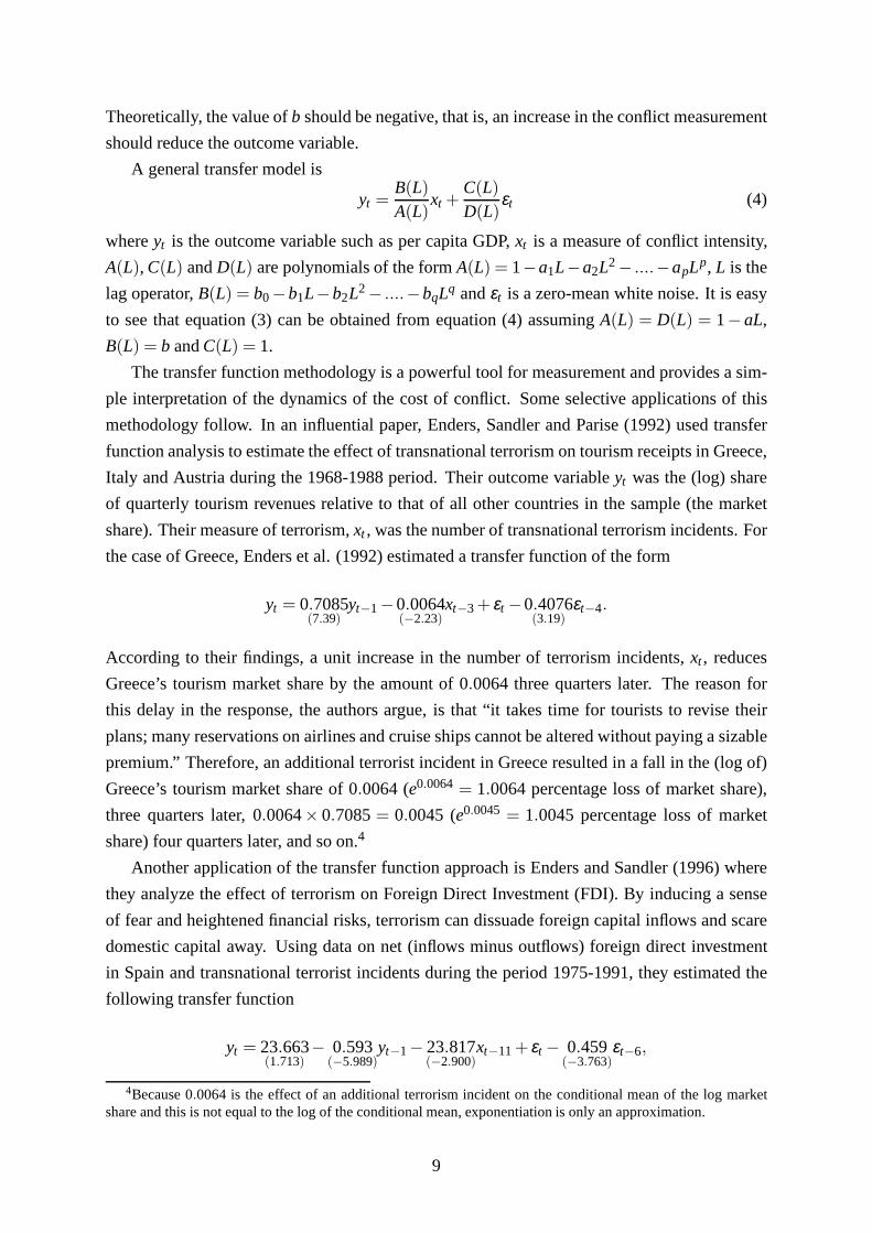
Theoretically, the value ofb should be negative, that is, an increase in the conflict measurement

should reduce the outcome variable.

A general transfer model is

yt =B(L)

A(L)xt +

C(L)

D(L)εt (4)

whereyt is the outcome variable such as per capita GDP,xt is a measure of conflict intensity,

A(L), C(L) andD(L) are polynomials of the formA(L) = 1−a1L−a2L2− ....−apLp, L is the

lag operator,B(L) = b0−b1L−b2L2− ....−bqLq andεt is a zero-mean white noise. It is easy

to see that equation (3) can be obtained from equation (4) assuming A(L) = D(L) = 1−aL,

B(L) = b andC(L) = 1.

The transfer function methodology is a powerful tool for measurement and provides a sim-

ple interpretation of the dynamics of the cost of conflict. Some selective applications of this

methodology follow. In an influential paper, Enders, Sandler and Parise (1992) used transfer

function analysis to estimate the effect of transnational terrorism on tourism receipts in Greece,

Italy and Austria during the 1968-1988 period. Their outcome variableyt was the (log) share

of quarterly tourism revenues relative to that of all other countries in the sample (the market

share). Their measure of terrorism,xt , was the number of transnational terrorism incidents. For

the case of Greece, Enders et al. (1992) estimated a transferfunction of the form

yt = 0.7085(7.39)

yt−1−0.0064(−2.23)

xt−3+ εt −0.4076(3.19)

εt−4.

According to their findings, a unit increase in the number of terrorism incidents,xt , reduces

Greece’s tourism market share by the amount of 0.0064 three quarters later. The reason for

this delay in the response, the authors argue, is that “it takes time for tourists to revise their

plans; many reservations on airlines and cruise ships cannot be altered without paying a sizable

premium.” Therefore, an additional terrorist incident in Greece resulted in a fall in the (log of)

Greece’s tourism market share of 0.0064 (e0.0064 = 1.0064 percentage loss of market share),

three quarters later, 0.0064× 0.7085= 0.0045 (e0.0045 = 1.0045 percentage loss of market

share) four quarters later, and so on.4

Another application of the transfer function approach is Enders and Sandler (1996) where

they analyze the effect of terrorism on Foreign Direct Investment (FDI). By inducing a sense

of fear and heightened financial risks, terrorism can dissuade foreign capital inflows and scare

domestic capital away. Using data on net (inflows minus outflows) foreign direct investment

in Spain and transnational terrorist incidents during the period 1975-1991, they estimated the

following transfer function

yt = 23.663(1.713)

− 0.593(−5.989)

yt−1− 23.817(−2.900)

xt−11+ εt − 0.459(−3.763)

εt−6,

4Because 0.0064 is the effect of an additional terrorism incident on theconditional mean of the log marketshare and this is not equal to the log of the conditional mean,exponentiation is only an approximation.

9

whereyt is the change in net foreign direct investment measured in millions of (real 1990) US

dollars andxt is the number of transnational terrorist incidents. According to their estimates, an

additional transnational terrorist incident in Spain leads to a fall of 23.8 millions of US dollars

in net FDI into Spain eleven quarters later. Since the estimated coefficient of the first lag of net

FDI is negative, the net FDI response to the incident oscillates from negative to positive, and so

on. Twelve quarters after the incident, net FDI rises by 23.8×0.593= 14.113 millions of US

dollars.

The transfer function methodology constitutes a powerful way of conducting an individual

case analysis of the economic effect of conflict at the aggregate (country or sector) level and

potentially could be used to analyze the microeconomic consequences of conflict, although we

have not been able to find any such application in the literature. As compared with the ITS

approach, transfer function applications typically provide a better time series representation of

the outcome variable by allowing for lags of the outcome and conflict measurements, as well

as a flexible disturbance dynamics. Transfer function modelling, however, cannot incorporate

other potential determinants of the outcome variable into the analysis, other than the conflict

measurement. In addition, the transfer function approach relies on the assumption of strict

exogeneity of the conflict measurement, yielding inconsistent estimates when there is reverse

causation from the outcome to the conflict variable.

4.3 Vector autorregresions

Another way to model the dynamic interaction between the outcome variable and conflict mea-

surement is the vector autorregresion (VAR) approach. Within this context, both the outcome

variable and the conflict measurement as well as possibly other variables are jointly determined

by lagged values of all variables considered. The simplest of all VAR models is a two-variable

one-lag model for the outcome,yt , and the conflict measurement,xt , of the form

yt = a11yt−1 +a12xt−1+ εyt (5)

xt = a21yt−1+a22xt−1 + εxt

where theai j ’s are parameters andεyt andεxt are zero mean random disturbances which can

be contemporaneously correlated. When the set of right handside variables is the same for all

equations and there are no restrictions on the parameters ofthe VAR, estimation boils down

to a simple ordinary least squares regression for each equation. The VAR captures the causal

effect of conflict on the outcome through the first equation and also allows for feedback from

the economic outcome to the conflict measurement through thesecond equation.

The VAR technique allows us to estimate the response of the outcome to a shock in the

conflict measurement. For illustration, supposey0 = x0 = 0; we shock the conflict measurement

in one unit,εx1 = 1 and keep all the other shocks equal to zero,εx2 = ... = εxt = εy1 = ... =

10

εyt = 0. As a result of this shock, the time path of the outcome wouldbe y1 = 0, y2 = a12,

y3 = (a11+a12)a22, ... and the time path of the conflict measurement would bex1 = 1,x2 = a22,

x3 = a21a12+ a222, ... These sequences are the Impulse Response Functions (IRF) and can be

computed as a function of the coefficients of the VAR. Adding up these responses would give us

the accumulated response. Note that, for the shock to have any effect on the outcome,a12 must

be non-zero. Otherwise, the time pattern of the outcome would be unchanged by the shock. In

the latter case, whena12 = 0, it is said thatxt does not Granger-causeyt .5

Enders and Sandler (1991) postulated a VAR for the number of tourists visiting Spain,nt ,

and the number of transnational terrorist incidents in Spain, it . Their specification was slightly

different from the simplest model (5)

nt = α1+A11(L)nt−1+A12(L)it−1+ εnt

it = α2+A21(L)nt−1+A22(L)it−1+ εit

where the alphas include a constant term and seasonal dummies and theAi j (L) are polynomials

in the lag operator. Using monthly data for the period 1970-1988, they fitted a 12-lag VAR

and found that the number of terrorist incidents Granger-caused the number of tourists (that is,

they rejected the hypothesisA12(L) = 0), but the number of tourists did not Granger-cause the

number of terrorist incidents. The VAR model allowed them tocompute the impulse response

function to a shock inεit . As a result of a unit shock in the disturbance of the incidents equation,

the accumulated response of the number of tourists was that 140,847 tourists did not visit Spain.

In addition to Granger-causality tests and IRF analysis, VARs can be used to generate short

term forecasts under different scenarios of the future pathof conflict measurements. An appli-

cation of this short term prediction capability is Ecksteinand Tsiddon (2004). They postulated a

VAR for the Israeli economy during the 1980-2003 period including (the logs of) four macroe-

conomic magnitudes, per capita GDP, investment, exports and non-durable consumption. They

used a terrorism index as a predetermined right hand side variable in all four equations of the

VAR. According to their findings, terrorism had a negative and significant coefficient in all but

the consumption equation.6 Using the estimated VAR up to the third quarter of 2003, Eckstein

and Tsiddon simulated the paths of all four variables for theperiod 2003:4 to 2005:3 under

three scenarios: (i) terror stops as of 2003:4, (ii) terror continues until 2004:3 and (iii) terror

continues until 2005:3. Under those scenarios, per capita GDP growth would have been 2.5

percent, 0 percent and -2 percent respectively.

Probably as VAR models are easy to estimate, the VAR methodology is very popular and

provides an easy way to compute of IRFs, Granger causality tests and short term forecasts.

However, VAR methods are bound to be applied to single subject analysis. With higher com-

5See Granger (1969).6Note that since all equations include lags of all variables,it is sufficient that the terrorism index is significant

in only one equation for it to have effects on all four variables.

11

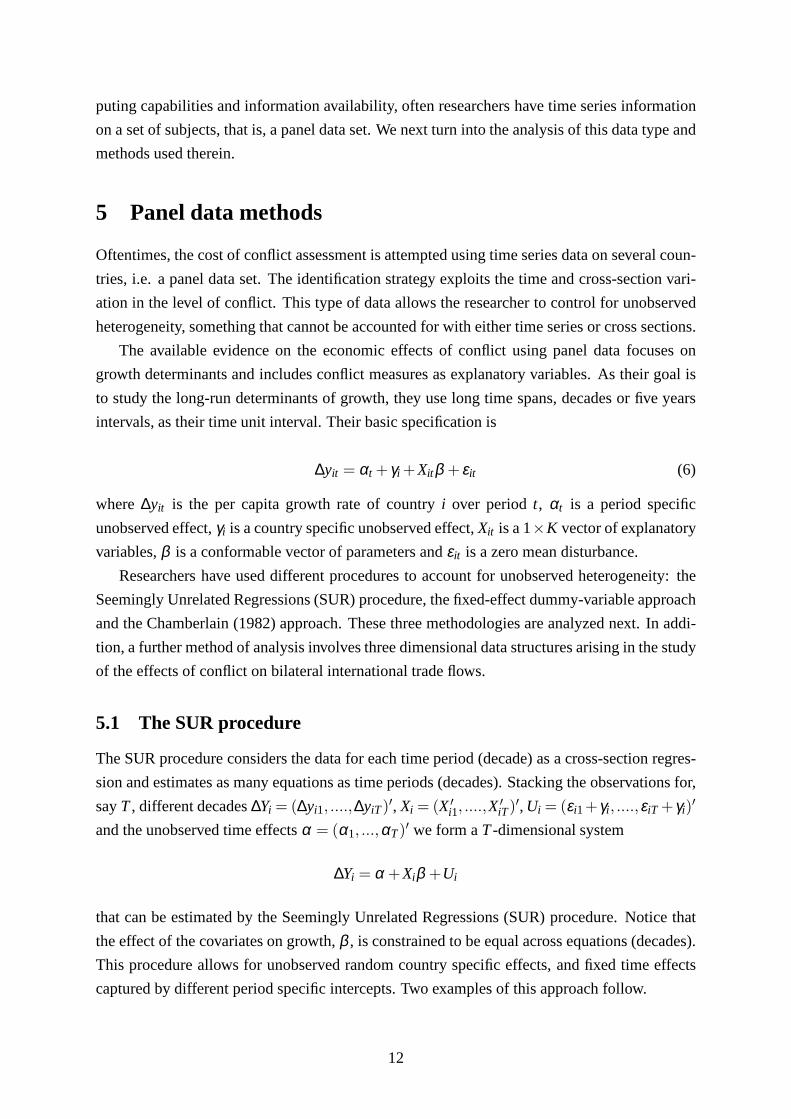
puting capabilities and information availability, often researchers have time series information

on a set of subjects, that is, a panel data set. We next turn into the analysis of this data type and

methods used therein.

5 Panel data methods

Oftentimes, the cost of conflict assessment is attempted using time series data on several coun-

tries, i.e. a panel data set. The identification strategy exploits the time and cross-section vari-

ation in the level of conflict. This type of data allows the researcher to control for unobserved

heterogeneity, something that cannot be accounted for witheither time series or cross sections.

The available evidence on the economic effects of conflict using panel data focuses on

growth determinants and includes conflict measures as explanatory variables. As their goal is

to study the long-run determinants of growth, they use long time spans, decades or five years

intervals, as their time unit interval. Their basic specification is

∆yit = αt + γi +Xit β + εit (6)

where∆yit is the per capita growth rate of countryi over periodt, αt is a period specific

unobserved effect,γi is a country specific unobserved effect,Xit is a 1×K vector of explanatory

variables,β is a conformable vector of parameters andεit is a zero mean disturbance.

Researchers have used different procedures to account for unobserved heterogeneity: the

Seemingly Unrelated Regressions (SUR) procedure, the fixed-effect dummy-variable approach

and the Chamberlain (1982) approach. These three methodologies are analyzed next. In addi-

tion, a further method of analysis involves three dimensional data structures arising in the study

of the effects of conflict on bilateral international trade flows.

5.1 The SUR procedure

The SUR procedure considers the data for each time period (decade) as a cross-section regres-

sion and estimates as many equations as time periods (decades). Stacking the observations for,

sayT, different decades∆Yi = (∆yi1, ....,∆yiT)′, Xi = (X′i1, ....,X

′iT)′, Ui = (εi1+γi , ....,εiT +γi)

′

and the unobserved time effectsα = (α1, ...,αT)′ we form aT-dimensional system

∆Yi = α +Xiβ +Ui

that can be estimated by the Seemingly Unrelated Regressions (SUR) procedure. Notice that

the effect of the covariates on growth,β , is constrained to be equal across equations (decades).

This procedure allows for unobserved random country specific effects, and fixed time effects

captured by different period specific intercepts. Two examples of this approach follow.

12

In their study on growth determinants, Barro and Lee (1994) use a sample of 95 countries

over two decades, 1965-1975 and 1975-1985. Thus, they analyze a two periods (decades) panel

data set. One of their covariates, the number of revolutionsis a measure of conflict similar to the

political instability covariates entered in the cross-section regressions discussed above. Using

the SUR technique, they report the following estimated equation

∆yit = −0.0171(−2.09)

revolutionsit +other covariates

where∆yit is the growth rate of per capita GDP of countryi over decadet. Therefore, an

additional revolution during a decade reduces the average growth rate during a decade in 1.71

per cent points.

Easterly and Levine (1997) use an unbalanced panel of 95 countries over the three decades

period 1960-1989 to shed light on the effect of ethnic diversity on growth. Although it was

not their goal to measure the effect of conflict on economic growth, their regressions included

the average number of political assassinations per capita during a decade as a proxy for the

level of political instability as a controlling factor. Using the SUR methodology, they report the

following estimated equation7

∆yit = −0.024(−2.26)

×assassinationsit +other covariates

Their findings indicate one additional (average per capita)political assassination during a

decade results in a fall of the average growth rate over a decade by 2.4 percentage points.

5.2 The fixed-effects dummy-variable approach

The fixed-effect dummy-variable approach assumes that the time and country unobserved ef-

fects,αt andγi , are fixed and uses period and country specific dummy variables. This is by far

the most popular method used in the literature. Some applications of this methodology for the

estimation of the effects of war and terrorism on growth follow.

Collier (1999) presents evidence on the effect of civil warson the rate of growth using

a sample of 78 countries over the three decades 1960-1989 (three time units, one for each

decade). He found a negative and significant effect of civil war on economic growth. He

reports the following fixed-effect estimates

∆yit = −0.00020(−2.34)

Wit +other covariates

where∆yit is countryi’s average annual per capita GDP growth rate in decadet andWit is the

number of months with civil war in countryi during decadet. The coefficient onWit gives us

7In fact, Easterly and Levine use the average number of political assassinations per thousand population overa decade and get an estimate equal to -23.78.

13

the marginal effect of an additional month of civil war on thedecade-average annual growth

rate. Therefore, an entire decade of war (120 months) reduces the average growth in 2.4 per

cent points (0.0002×120= 0.024).

Caplan (2002) analyzed the different effects of wars foughtat foreign and domestic soil

on growth, inflation, public expending, tax revenue and monetary growth. Using a sample of

annual data for 66 countries over the 1953-1992 period, he reports the following fixed-effect

estimates

∆yit = 2.333(1.80)

FWit −2.027(2.00)

DWit +other terms

whereFWit andDWit are dummy variables defined as equal to one if countryi in yeart fought

a war in foreign and domestic soil respectively and zero otherwise. The coefficient on the

foreign war dummy is positive and only significant at the ten per cent level. The coefficient

on the domestic war dummy is negative and marginally significant. Since growth rates are

measured in percentage points, an additional year of domestic war reduces the growth rate

by 2.03 percentage points. In contrast with Collier (1999),Caplan does not control for any

covariates but his estimate of the effect of domestic war is very similar to Collier’s estimate of

the effect of civil war.

Blomberg, Hess and Orphanides (2004) provide evidence on the effect of various forms of

conflict on economic growth. They consider terrorism, internal conflict and external conflict.

Using an unbalanced sample of 177 countries from 1968 to 2000they fit the following panel-

growth regression

∆yit = −5.545(−12.002)

yit−1−0.438(−1.773)

Tit −1.270(−5.226)

Iit −3.745(−4.458)

Eit +other covariates

where∆yit is the rate of growth of per capita GDP for countryi in period t, andTit , Iit and

Eit are dummy variables indicating whether in countryi in period t there was, respectively,

a terrorist incident, internal conflict and external conflict. Terrorism seems to have a lower

economic impact than internal conflict which in turn has a lower effect than external conflict

and this is in fact what the authors claim. However, multiplying coefficients estimates by the

standard deviation of the covariates yields 0.438×0.443= 0.194, 1.270×0.355= 0.451 and

3.745×0.094= 0.352 respectively, showing that the effect of external conflict is in fact lower

than the effect of internal conflict. Contrary to Caplan (2002) findings, the effect of external

conflict turns out to be negative.8

Tavares (2004) also provides evidence on the effect of terrorism on per capita GDP growth.

He uses a sample of unspecified countries for the period 1987-2001 and reports the following

8Blomberg, Hess and Orphanides’ (2004) definition of external conflict includes wars fought on domestic soilagainst foreign nations, whereas Caplan (2002) would include those as domestic wars.

14

estimated regression

∆yit = 0.261(4.80)

∆yit−1+0.017(1.20)

yit −0.029(−2.89)

Tit +0.121((3.15)

Tit ×PRit )+other covariates

whereTit is the number of terrorist attacks per 10 million inhabitants,PRit stands for the level of

political rights, an index ranging from 0 to 1. According to his results, a one standard deviation

increase in the level of terrorism leads to a fall in per capita GDP growth of about 0.17 per

cent(0.029×5.99= 0.17) in a country scoring at lower end of political rights index and to

an increase in per capita GDP growth of 0.55 per cent((−0.029+0.121)×5.99= 0.55) for a

country scoring at the upper end of the political rights index.

Neumayer (2004) estimates the effect of political violenceon tourist arrivals using a panel

of 194 countries during the period 1977-2000. He reports thefollowing estimates

nit = 0.63(3.56)

nit−1−0.12(3.51)

cit +other covariates

wherenit is the (log of) the number of annual tourist arrivals (overnight visitors) andcit is

Uppsala Conflict Data Project armed conflict intensity index. A one standard deviation increase

in the conflict index results in a(0.12×0.82= 0.0984) 9.8 per cent fall in the number of tourists

the same year,(0.0984×0.63= 0.062) a 6.2 per cent fall a year after, and so on.

5.3 The Chamberlain approach

The third approach to estimate the economic cost of conflict using panel data follows a pro-

cedure designed by Chamberlain (1982). Instead of assumingthat the unobserved effects are

fixed or random, Chamberlain suggested that unobserved effects could be linear functions of the

covariates, that is,γi = ψ +∑Tt=1Xit λt +vit . Under this assumption and ignoring time effects,

equation (6) becomes

∆yit = ψ +Xi1λ1+ ...+Xit (β +λt)+ ...+XiT λT + r it

wherer it = εit +vit . For illustration consider theT = 2 case where

∆yi1 = ψ +Xi1(β +λ1)+Xi2λ2+ r i1,

∆yi2 = ψ +Xi1λ1 +Xi2(β +λ2)+ r i2.

Chamberlain proposes a two-step estimation procedure of the vector of structural parameters

θ = (ψ,λ ′1,λ

′2,β

′)′. In the first step, the vector of reduced form parametersπ = (ψ,β ′ +

λ ′1,λ

′2,ψ,λ ′

1,β′ + λ ′

2)′ are estimated by OLS applied to each equation. In the second step,

the structural parameters are estimated by classical minimum distance, that is, minimizing

15

the quadratic form(π̂ −Hθ)′Ξ(π̂ −Hθ), whereΞ is a positive definite matrix andH is a

conformable auxiliary matrix with zeros and ones.

Knight, Loayza and Villanueva (1996) applied Chamberlain approach to quantify the effect

of wars on ouput per capita growth rates and the investment toGDP ratio using a panel of 79

countries over three five-year periods from 1971 to 1985. They report the following estimates

∆yit = −0.0132(−1.51)

Wit +0.0165(2.92)

(

IY

)

it+other covariates

(

IY

)

it= −1.3232

(−6.78)Wit +other covariates

whereWit is the number of war years in a particular five-year interval as a fraction of the total

number of years in the sample. They find a negative effect of war on per capita GDP growth

and investment to output ratio, although the former is not statistically significant.

Knight, Loayza and Villanueva (1996) acknowledge the existence of a two-channel mecha-

nism through which war affects growth. A direct effect of warcaptured by the growth equation

and an indirect effect through investment. According to their estimates, if the fraction of war

years in the sample increases 1.5 additional war years (a tenpercent of the number of years in

the sample), the total incidence of war cost of conflict wouldbe a reduction of the per capita

growth rate in 3.5 percentage points ((−0.0132−0.0165×1.3232)×0.1= −0.035).

5.4 Gravity equations

Gravity equations are very popular in international trade studies. They are specially designed to

fit a special type of three dimensional data arrays. For illustration consider a set ofJ countries

and letxi jt be countryi’s (log) exports to countryj in periodt. Thus, for a given time period

there are(J× (J−1)) trade flows. A gravity model assumes trade flows are proportional to the

countries’ income, their distance, and other control variables as given by

ln(xi jt ) = β1 ln(1+zit zjt )+β2 ln(yit y jt )+β3 ln(yit y jt/pit p jt )+β4 ln(di j )+other covariates

wherezit zjt is the product of the countries measurements of conflict at time t, yit y jt is the

product of countriesi and j real GDPs in periodt, pit p jt is the product of countries’ populations

anddi j is the distance between countries.

Nitsch and Schumacher (2004) report evidence for more than 200 countries during the

1968-1979 period on the effect of various forms of conflict ontrade. They report an estimate

of β1 equal to−0.041 (t-stat−5.87) whenzit is the number of terrorist incidents in countryi at

periodt. Since both trade flows and conflict are measured in logs, coefficients can be interpreted

as elasticities. Thus, a 100 percent change inzit zjt resulted in a 4 percent fall in exports.9 Nitsch

9The impact might look like small, but it is large. A 100 percent increase inzit zjt does not require such a

16

and Schumacher also used the number of political assassinations as a measure of conflict, their

estimate ofβ1 was in this case−0.160 (t-stat−16.0). Repeating the same exercise with conflict

measured as the fraction of the sample period involved in external war, their estimate ofβ1 was

−0.395 (t-stat−14.1).

Glick and Taylor (2010) used a gravity model to assess the effect of war on trade. They as-

sembled a sample of 172 countries during the 1870-1997 period from various sources and used

average exports and imports flows between country pairs. Instead of a continuous measurement

of conflict, Glick and Taylor included a dummy variableDi jt equal to one when countriesi and

j were engaged in war in periodt and zero otherwise, as well as up to ten lags of the dummy

variable. They report the following fixed effects estimates

ln(xi jt ) =− 1.78(−8.09)

Di jt − 1.28(−4.74)

Di jt−1− 1.32(−6.00)

Di jt−2− 1.12(−7.47)

Di jt−3− 0.70(−5.38)

Di jt−4− 0.55(−6.11)

Di jt−5

− 0.37(−4.63)

Di jt−6− 0.22(−3.14)

Di jt−7− 0.24(−3.00)

Di jt−8− 0.11(−1.83)

Di jt−9− 0.03(−0.50)

Di jt−10+other covariates

There is a clear decaying pattern in coefficient estimates, which are statistically significant up

to the eight lag. As trade is measured in logs but war is not, the interpretation of coefficients

is more involved. The contemporaneous contribution of the war dummy to (log) trade flows

is −1.78 as compared with the contribution of no war, 0. Thus, war reduces trade to eighty

three per cent (e0− e−1.78 = 0.83) contemporaneously, and to seventy two percent one year

later (e0−e−1.28 = 0.72), and so on.10

6 Event studies

A further methodology used in assessing the economic impactof conflict is the event study

methodology. Event studies are used to measure the effect onstock prices of certain types of

events such as the release of information on profits, dividend payments, corporate debt issuance,

investment decisions, etc. This methodology relies on the assumption of efficient markets ac-

cording to which share prices should reflect all available information, including any economic

or social event. Therefore, if conflict affects the economy,then conflict related events should

be accompanied by changes in stock prices.

The event study methodology identifies abnormal returns on stock prices as the difference

between the actual return and the normal return on a stock. Let Pt be the stock price at time

t andRt = (Pt −Pt−1)/Pt−1 its rate of return. Normal returns are computed as the mean daily

return on a window ofT trading days before each event: ift = 0 is the day of the event, the

change in both countries. For instance, if countriesi and j experience 5 terrorist attacks,zit zjt = 25. Then, anincrease to 7 terrorist attacks in both countries (a 40 percent increase) results in,zit zjt = 49, almost a 100 percentincrease inzit zjt .

10Because the estimated equation is the conditional mean of the log trade flows, exponentiation does not yieldthe conditional mean of trade flows. However, it should be taken as an approximation.

17

normal return is computed as the arithmetic mean of daily returns fromt =−t1 to t =−t2. The

abnormal return, computed as

ARt = Rt −1T

−t2

∑t=−t1

Rt

is considered the effect of the event on the stock return. In addition to abnormal returns, the

event study methodology also relies on accumulated abnormal returns defined as

CARt =I

∏i=0

(1+ARt+i)−1

whereI is the number of periods during which the returns are accumulated. Some applications

of this methodology follow.

Chen and Siems (2004) investigated the Dow Jones Industrialindex reaction to 14 terrorist

and military events. Out of the 14 events analyzed, 12 had a statistically significant abnormal

return and the September 11th was the event with the largest abnormal return (-7.14 per cent).

Chen and Siems also applied the same methodology to asses theeffect of the 9/11 event on

33 stock market indexes from 28 countries, 31 of which exhibited negative and statistically

significant abnormal returns.

A more sophisticated way of computing the normal return is the market model of financial

economics

Rit = βiRMt +uit

whereRit is the return on stocki on dayt in excess over the risk-free rate of return,RMt is

the return on the market portfolio (also measured in excess over the risk free rate of return)

and uit is a zero mean disturbance. Identifying the normal return asthe systematic part of

the previous equation implies that the residuals from this equation are the abnormal returns.

The market model is sometimes extended to a three-factor model à la Fama and French (1993,

1996). Using this framework, a few other papers provide evidence in favour of the hypothesis

that terrorism and violent conflict affects asset prices negatively, see Chesney and Reshetar

(2007), Guidolin and La Ferrara (2005) and Drakos (2004, 2009).

A monetary figure of the impact of terrorism on stock prices isprovided by Karolyi and

Martell (2005) who find that during the 1995-2002 period, the75 terrorist attacks against pub-

licly traded US companies had on average a direct impact on the firm’s stock rate of return of

-0.83 per cent, which amounted to 401 million US dollars in market capitalization.

Conflict does not always have a negative effect on stock prices, Guidolin and La Ferrara

(2007) found that the death of the rebel leader and the suddenend of the war in Angola in 2002

resulted in an abnormal return of−0.032 in the portfolio of diamond mining firms holding

concessions in Angola. This finding indicates that the war conflict had a positive effect of

those stocks. Similarly, Berrebi and Klor (2010) found thatterrorism has a 7 percent positive

abnormal return in a portfolio of Israeli defence stocks anda negative 5 percent abnormal return

18

in a portfolio of Israeli non-defence stocks.

7 Natural experiments

In an experiment, the scientist studies the effect of a treatment on a sample of subjects as

compared with a control sample of untreated subjects. In a controlled experiment, assignment

of subjects to treatment and control groups is random. In social science research, assignment of

subjects to treatment or control samples is oftentimes unethical, unlawful or unfeasible. In this

cases, scientists resort to quasi-experimental methods, sometimes referred to as observational

studies or natural experiments.11 In a natural experiment, the scientist has no control over

the assignment of subjects to treatment and control groups:sometimes subjects select their

own treatment, other times their environments impose the treatment upon them. Self-selection

into a treatment may generate an important bias in the results. A natural experiment exploits

an irrelevant event that results in haphazard assignment ofsubjects to treatment and control

groups. A natural experiment is more informative about a causal effect when the researcher

observes a large and clear change in the treatment that affects only a sub-population.

The quasi-experimental methodology has been applied to measure the effect of terrorist

conflict on various economic magnitudes. Two examples of this methodology follow. Abadie

and Gardeazabal (2003) used the September 18, 1998 - November 28, 1999 cease fire declared

by terrorist organization ETA as a natural experiment to asses the effect of terrorism on the stock

market valuation of Spanish companies. In experimental terms, the cease fire is the treatment.

If the terrorist conflict was perceived to have a negative impact on the Basque economy, Basque

stocks (stocks of firms with a significant part of their business in the Basque Country) should

have shown a positive performance relative to non-Basque stocks (stocks of firms without a

significant part of their business in the Basque Country) as the truce became credible. Similarly,

Basque stocks should have performed poorly, relative to non-Basque stocks, at the end of the

truce. The portfolio of Basque stocks can be viewed as the treated sample and the portfolio

of the non-Basque stocks the control group. Abadie and Gardeazabal reported the following

estimated regressions

RBasque= 0.6739(18.41)

RMarket+0.0049(2.33)

DGood−0.0017(−2.13)

DBad+other covariates

RNon−Basque= 0.8096(43.53)

RMarket+0.0005(0.56)

DGood+0.0001(0.25)

DBad+other covariates

whereRBasqueandRNon−Basquestand for the return on the Basque and non-Basque portfolios,

RMarket is the return on the market portfolio andDGood andDBad are dummy variables that take

the value of one during a “Good News” period when the cease-fire became credible and a “Bad

News” period when the peace process collapsed. In accordance with the theoretical prediction,

11See Rosenbaum (2005).

19

the dummy variables were significant for the Basque portfolio and not significant for the non-

Basque portfolio. Compounding the 0.0044 coefficient on theGood News dummy over the

22 trading sessions of the Good News period yields a compounded abnormal return of 10.14

percent for the Basque portfolio relative to the non-Basqueportfolio. Analogous calculations

yield a -11.21-percent compounded abnormal return for the Basque portfolio relative to the

non-Basque portfolio during the 66 trading sessions of the Bad News period.

Benmelech, Berrebi and Klor (2010) analyzed the cost in terms of employment opportuni-

ties and wages of harboring terrorism in Palestinian districts. They used a sample of all 143

suicide attacks in Israel by Palestinians between September 2000 and December 2006. Ben-

melech, Berrebi and Klor noticed that some of the suicide attack attempts were interrupted by

security forces or civilians while others reached their targets. This fact permits an experimental

interpretation of their results. The treatment in this caseis the “successfulness” of the attacks.

The treated sample would be the sample of all the attacks which reached their targets and the

untreated sample those attacks interrupted. These authorsreport the following estimates

∆uit = 0.0140(4.00)

Dit +other covariates

wherei indexes the district where the attack originated,∆uit is the change in districti’s un-

employment rate in the quarter when the attack took place andthe following quarter andDit

is a dummy variable that takes a value of 1 when the attack reached its target and zero other-

wise. Districts where “successful” attacks originated exhibited a 1.4 percentage points higher

increase in the unemployment rate.

Randomized experiments have good internal validity, that is, they are good for establish-

ing a causal relationship. Natural experiments, like the ones surveyed here, have less internal

validity than randomized experiments. Sometimes nature provides a haphazard treatment as-

signment, thus providing a fairly high internal validity. External validity, the possibility of

generalizing the results of the natural experiment to otherpopulations, might be low particu-

larly when, as in the Basque and Palestinian examples, the analysis corresponds to a specific

conflict.

8 Comparative case studies

A case study is a tool in social science research. It is a meticulous study of a single unit. This

methodology has also been used to asses the economic cost of conflict in countries or regions

under conflict. When analyzing a pool of countries, the resulting estimate of the economic cost

of conflict can be interpreted as the average effect. The average impact of conflict surely over

estimates the effect for some units and under estimates the effect for others. Case studies have

the potential of identifying particularly large or small effects for specific units. In addition, a

careful study of a single unit allows the researcher to pay more attention to particular mecha-

20

nisms that might pass unnoticed in the aggregate. Therefore, the case study methodology stands

up as a powerful tool of research. Having the possibility of analyzing a single unit in depth,

however, comes at the cost of losing external validity, as the results might be due to specific

characteristics of the particular unit being analyzed.

In fact, many of the previously mentioned papers are case studies. There are case studies

of the effect of armed conflict in Nicaragua (DiAddario, 1997), Nepal (Kumar, 2003) and Sri

Lanka (Arunatilake, Jayasuriya and Kelegama, 2001). Case studies have also been used in

order to study the economic effects of terrorism in Israel (Eckstein and Tsiddon, 2004) and

Spain (Enders and Sandler, 1991 and 1996). There are also examples of case studies of the

economic effect of conflicts in specific sectors such as the effect of the 9/11 terrorist events

on airline stocks (Drakos 2004) and Chicago real estate market (Abadie and Dermisi 2008 and

Dermisi 2007). The common denominator of these studies is the fact that they concentrate

on a single unit. These papers use some of the previously mentioned techniques to asses the

economic impact of conflict and therefore will not be reviewed here.

A particular type of case study deserves more attention: thecomparative case study. Com-

parative case studies are often used by researchers to studythe effect of events or policy mea-

sures on aggregate units such as regions or countries. The goal in these studies is to estimate

the evolution of outcomes for a unit affected by an event and compare it with the evolution of

a control group. It is often the case that there is not a singlecontrol unit with the same charac-

teristics of the unit exposed and therefore a combination ofcontrol units is a better comparison

group than any single unit. A particular way of carrying out this comparison is the synthetic

control method suggested by Abadie and Gardeazabal (2003) and refined by Abadie, Diamond

and Hainmueller (2010).

The synthetic control method can be easily described as follows. LetJ be the number of

available control units andW = (w1, ...,wJ) a vector of non negative weights which sum to

one. LetX1 be a(K × 1) vector of pre-conflict values ofK relevant characteristics for the

treated unit andX0 be a(K × J) matrix which contains the values of the same variables for

theJ possible controls. TheseK covariates are those factors the researcher believes affect the

outcome variable. LetV be a diagonal matrix with non-negative components. The values of the

diagonal elements ofV reflect the relative importance of the different covariates. The vector of

weightsW∗ is chosen to minimize(X1−X0W)′V(X1−X0W) subject tow j ≥ 0 ( j = 1,2, ...,J)

andw1 + ...+wJ = 1. The weights chosen in this manner define a synthetic control unit with

covariate valuesX0W∗, a linear combination of the potential control units characteristics. Once

the match between the treated unit and the synthetic controlis done, it remains to compute

the counterfactual value of the outcome variable during thepost-treatment period. LetY1 be

a (T × 1) vector whose elements are measurements of the outcome variable for the treated

unit during the post-treatment period. Similarly, letY0 be a(T ×J) matrix which contains the

values of the same variables for the control units. The counterfactual values of the outcome is

computed asY∗1 = Y0W∗. The difference between the actual and counterfactual values of the

21

outcome isY1−Y∗1 .

Abadie and Gardeazabal (2003) used this procedure to estimate the economic impact of

terrorism in the Basque Country economy. Using the synthetic control method, Abadie and

Gardeazabal formed a comparison group as a combination of other Spanish regions that was

“similar” in various economic dimensions (thought to be potential growth determinants) to

the Basque Country economy in the period prior to the uprising of terrorism. The output gap

between the actual and counterfactual values yielded a 10 percent annual per capita GDP loss

over a 20-year period, a sizable output loss.

The synthetic control method allows the researcher to conduct placebo analysis by apply-

ing the same procedure to an untreated subject. Abadie and Gardeazabal applied the same

procedure to another Spanish region, Catalonia, not directly affected by a terrorist conflict. The

placebo comparison for Catalonia displayed a very small output gap. Furthermore, conducting

the placebo study on all untreated subjects yields an empirical distribution of outcome gap (the

difference between the outcome of the treated and its synthetic control). This empirical distri-

bution can be used to assess the statistical significance of the outcome gap for the treated. This

method is specially suited for a single unit analysis. However, the method is potentially useful

for application to multiple units, although there is no guarantee that a good match can be found

for all units.

9 Discussion

This paper reviews the methods for assessing the economic cost of conflict and illustrates them

with a selective collection of examples. Overall, the literature reviewed shows that conflict

exerts significant economic costs. Since conflict is a latentvariable for which only proxy mea-

surements are available, classical error-in-variables econometrics suggests that regression esti-

mates of the effect of conflict should be downward biased, assuming errors of measurement are

uncorrelated with the latent variable.

After reviewing the literature, we believe there are several issues that deserve further atten-

tion. First, the papers reviewed offer a wide range of estimates from low to high quantities.

This is particularly true for the panel data evidence reported above. There are several reasons

for this heterogeneity of results. First, not all types of conflict have the same economic cost.

Political instability, terrorism and war have very different economic impacts. A second source

of variation accrues from the different samples (units and periods) and methods used by re-

searchers. Therefore, the findings of several independent studies need to be integrated. Even

though a meta-analysis seems rather difficult to carry out, some extra effort in this direction is

needed.

Second, the empirical evidence reviewed in this survey focuses primarily on establishing

a causal link between conflict and some economic magnitude and often little attention is paid

to determining the quantitative effect. As argued above, after the causal link is established,

22

generally by the statistical significance of a parameter estimate, researchers sometimes do not

take the further step of quantifying the effect. Examples ofthis practice are most of the cross-

section and panel data evidence reviewed. We have sometimesbeen able to take this further and

simple step. For instance, in some of the cross-section and panel data items reviewed above,

we have been able to quantify the costs by simple arithmetic.These require knowledge of the

scale of the conflict measurement which is not always reported.

Third, further research is needed in the area of policy analysis. It would be interesting to

estimate the economic cost of policies and the benefits they bring about so that a cost-benefit

analysis could be performed. Policy effectiveness and its quantitative assessment, however,

remains an unexplored issue.

23

References

[1] Abadie, Alberto and Dermisi, Sofia, 2008. "Is terrorism eroding agglomeration economies

in Central Business Districts? Lessons from the office real estate market in downtown

Chicago,"Journal of Urban Economics64(2), 451-463.

[2] Abadie, Alberto, Diamond, Alexis and Hainmueller, Jens, 2010. "Synthetic Control Meth-

ods for Comparative Case Studies: Estimating the Effect of California’s Tobacco Control

Program,"Journal of the American Statistical Association105, 493-505.

[3] Abadie, Alberto and Gardeazabal, Javier, 2003. "The Economic Costs of Conflict: A Case

Study of the Basque Country,"American Economic Review93(1), 113-132.

[4] Abadie, Alberto and Gardeazabal, Javier, 2008. "Terrorism and the world economy,"Eu-

ropean Economic Review52(1), 1-27.

[5] Alesina, Alberto and Perotti, Roberto, 1996. "Income distribution, political instability,

and investment,"European Economic Review40(6), 1203-1228.

[6] Anderton, Charles H. and Carter, John R. 2001. “The Impact of War on Trade: An Inter-

rupted Times-Series Study,”Journal of Peace Research38(4), 445-457.

[7] Arunatilake, Nisha, Jayasuriya, Sisira and Kelegama, Saman, 2001. "The Economic Cost

of the War in Sri Lanka,"World Development29(9), 1483-1500.

[8] Barro, Robert J, 1991. "Economic Growth in a Cross Section of Countries,"The Quarterly

Journal of Economics106(2), 407-43.

[9] Barro, Robert J. and Lee, Jong-Wha, 1994. "Sources of economic growth,"Carnegie-

Rochester Conference Series on Public Policy40(1), 1-46.

[10] Berrebi, Claude and Klor, Esteban, 2010. “The Impact ofTerrorism on The Defense In-

dustry,”Economica77, 518-543.

[11] Bilmes, Linda and Stiglitz, Joseph E., 2006. “The Economic Costs of the Iraq War:

An Appraisal Three Years After The Beginning of The Conflict.” NBER Working Paper

12054.

[12] Blomberg, S. Brock, Hess, Gregory D. and Orphanides, Athanasios, 2004. "The macroe-

conomic consequences of terrorism,"Journal of Monetary Economics51(5), 1007-1032.

[13] Caplan, B., 2002. “How does war shock the economy?Journal of International Money

and Finance21, 145-162.

[14] Chamberlain, G. 1982. “Multivariate regression models for panel data,”Journal of Econo-

metrics18, 5-46.

24

[15] Chen, Andrew H. and Siems, Thomas F., 2004. "The effectsof terrorism on global capital

markets,"European Journal of Political Economy20(2), 349-366.

[16] Chesney, Marc and Reshetar, Ganna, 2007. “The Impact ofTerrorism on Financial Mar-

kets: An Empirical Study.” Available at SSRN: http://ssrn.com/abstract=1029246

[17] Collier, Paul, 1999. "On the Economic Consequences of Civil War," Oxford Economic

Papers51(1), 168-83.

[18] Davis, Steven J., Murphy, Kevin M. and Topel, Robert H.,2009. “War in Iraq versus

Containment,” in “Guns and Butter,” Gregory D. Hess editor,CESifo Seminar Series,

The MIT Press.

[19] Dermisi, Sofia, 2007. “The Impact of Terrorism Fears on Downtown Real Estate Chicago

Office Market Cycles.”Journal of Real Estate Portfolio Management13(1), 57-73.

[20] DiAddario, Sabrina, 1997. “Estimating the Economic Costs of Conflict: An Examina-

tion of the Two-Gap Estimation Model for the Case of Nicaragua.” Oxford Development

Studies, 25(1), 123-141.

[21] Drakos, Konstantinos, 2004. "Terrorism-induced structural shifts in financial risk: air-

line stocks in the aftermath of the September 11th terror attacks,"European Journal of

Political Economy20(2), 435-446.

[22] Drakos, Konstantinos, 2009. "Big Questions, Little Answers : Terrorism Activity, In-

vestor Sentiment and Stock Returns," Economics of SecurityWorking Paper Series 8,

DIW Berlin, German Institute for Economic Research.

[23] Eckstein, Zvi and Tsiddon, Daniel, 2004. "Macroeconomic consequences of terror: theory

and the case of Israel,"Journal of Monetary Economics51(5), 971-1002.

[24] Enders, Walter, Sandler, Todd, 1991. “Causality Between Transnational Terrorism and

Tourism: The Case of Spain,”Terrorism14, 49–58.

[25] Enders, Walter, Sandler, Todd and Parise, Gerald F. (1992), “An Econometric Analysis of

the Impact of Terrorism on Tourism,”Kyklos45, 531-554.

[26] Enders, Walter and Sandler, Todd, 1996. "Terrorism andForeign Direct Investment in

Spain and Greece,"Kyklos, 49(3), 331-52.

[27] Easterly, William and Levine, Ross, 1997. "Africa’s Growth Tragedy: Policies and Ethnic

Divisions,"The Quarterly Journal of Economics112(4), 1203-50.

[28] Fama, E.F. and French, F.R. 1993. Common Risk Factors inthe Returns on Stocks and

Bonds.Journal of Financial Economics33, 3-56.

25

[29] Fama, E.F. and French, F.R. 1996. Multifactor Explanations of Asset Pricing Anomalies.

The Journal of Finance51(1), 55-84.

[30] Glick, Reuven and Alan M. Taylor, 2010. "Collateral Damage: Trade Disruption and the

Economic Impact of War,"Review of Economics and Statistics92, 102-127.

[31] Granger, C.W.J., 1969. "Investigating causal relations by econometric models and cross-

spectral methods".Econometrica37, 424–438.

[32] Guidolin, Massimo and La Ferrara, Eliana, 2005. "The economic effects of violent con-

flict: evidence from asset market reactions," Working Papers 2005-066, Federal Reserve

Bank of St. Louis.

[33] Guidolin, Massimo and La Ferrara, Eliana, 2007. “Diamonds Are Forever, Wars Are Not.

Is Conflict Bad for Private Firms?”American Economic Review97, 1978-93.

[34] Karolyi, George Andrew and Martell, Rodolfo, 2006. “Terrorism and the Stock Market.”

Available at SSRN: http://ssrn.com/abstract=823465

[35] Knight, Malcolm, Loayza, Norman and Villanueva, Delano, 1996. "The peace dividend

: military spending cuts and economic growth," Policy Research Working Paper Series

1577, The World Bank.

[36] Kumar, Dhruba, 2003. “Consequences of the MilitarizedConflict and the Cost of Violence

in Nepal.” Contributions to Nepalese Studies, 30(2), 167-216.

[37] Kouby, Vally, 2005. “War and Economic Performance.”Journal of Peace Research 42,

67-82.

[38] Neumayer, Eric, 2004. “The Impact of Political Violence on Tourism. Dynamic Cross-

National Estimation.”Journal of Conflict Resolution48(2), 259-281.

[39] Nitsch, Volker and Schumacher, Dieter, 2004. "Terrorism and international trade: an em-

pirical investigation,"European Journal of Political Economy20, 423-433.

[40] Rosenbaum, Paul R. 2005. “Observational Study” in Brian S. Everitt and David C. Howell

“Encyclopedia of Statistics and Behavioral Science” John Wiley and Sons.

[41] Skaperdas, Stergios, forthcoming. “The Costs of Organized Violence: A Review of the

Evidence,”Economics of Governance.

[42] Tavares, Jose, 2004. “The open society assesses its enemies: shocks, disasters and terrorist

attacks,”Journal of Monetary Economics51, 1039-1070.

26

[43] Venieris, Yiannis P. and Dipak K. Gupta, 1986. “Income distribution and sociopolitical in-

stability as determinants of savings: a cross-section model.” Journal of Political Economy

94, 873-883.

27