metody ilo Ściowe w badaniach ekonomicznychqme.sggw.pl/pdf/mibe_t15_z1.pdf · metody ilo Ściowe w...
TRANSCRIPT

METODY ILOŚCIOWE
W BADANIACH EKONOMICZNYCH

QUANTITATIVE METHODS
IN ECONOMICS
Vol. XV, No. 1
Warsaw University of Life Sciences – SGGW Faculty of Applied Informatics and Mathematics
Department of Econometrics and Statistics
METODY ILOŚCIOWE
W BADANIACH EKONOMICZNYCH
QUANTITATIVE METHODS IN ECONOMICS
Volume XV, No. 1
Warsaw 2014

EDITORIAL BOARD
Editor-in-Chief: Bolesław Borkowski Managing Editor: Hanna Dudek Theme Editors:
Econometrics & Financial Engineering: Bolesław Borkowski Multidimensional Data Analysis: Wiesław Szczesny Mathematical Economy: Zbigniew Binderman Analysis of Labour Market: Joanna Landmessser
Statistical Editor: Wojciech Zieliński Technical Editors: Jolanta Kotlarska, Elżbieta Saganowska Language Editor: Agata Kropiwiec Native Speaker: Yochanan Shachmurove Editorial Board Secretary: Monika Krawiec
SCIENTIFIC BOARD
Peter Friedrich (University of Tartu, Estonia) Paolo Gajo (University of Florence, Italy) Vasile Glavan (Moldova State University, Moldova) Yuriy Kondratenko (Black Sea State University, Ukraine) Vassilis Kostoglou (Alexander Technological Educational Institute of Thessaloniki, Greece) Robert Kragler (University of Applied Sciences, Weingarten, Germany) Karol Kukuła (University of Agriculture in Krakow) Alexander N. Prokopenya (Brest State Technical University, Belarus) Yochanan Shachmurove (The City College of The City University of New York, USA) Mirbulat B. Sikhov (al-Farabi Kazakh National University, Kazakhstan) Ewa Syczewska (Warsaw School of Economics, Poland) Andrzej Wiatrak (University of Warsaw, Poland) Dorota Witkowska (University of Lodz, Poland)
ISSN 2082 – 792X
© Copyright by Department of Econometrics and Statistics WULS – SGGW (Katedra Ekonometrii i Statystyki SGGW)
Warsaw 2014, Volume XV, No. 1
The original version is the paper version
Journal homepage: qme.sggw.pl
Published by Warsaw University of Life Sciences Press

QUANTITATIVE METHODS IN ECONOMICS Vol. XV, No. 1, 2014
CONTENTS
Katarzyna Bień-Barkowska – Boosting under quantile regression – can we use it for market risk evaluation? ..................................................................... 7
Ewa Cukrowska – Is it the labour market that undervalues women or women themselves? Evidence from Poland .................................................................. 18
Jan B. Gajda, Justyna Wiktorowicz – Labour market in Poland for women and men 50+ ............................................................................................................ 29
Agnieszka Gehringer, Stephan Klasen, Dorota Witkowska – Labour force participation and family policies in Europe: an empirical study ....................... 37
Andrzej Karpio, Dorota Żebrowska-Suchodolska – The influence of pension funds on the Polish capital market ................................................................... 50
Krzysztof Kompa, Tomasz Wiśniewski – “Security through diversity”: portfolio diversification of Private Pension Funds ........................................................... 58
Joanna Małgorzata Landmesser – Gender differences in exit rates from unemploy- ment in Poland .................................................................................................. 66
Barbara Liberda, Marek Pęczkowski – Life cycle income of women and men in Poland .............................................................................................................. 76
Anna Lucińska, Tomasz Schabek – Factors affecting the prices of artworks in the Polish auction market .................................................................................. 92
Witold Luciński – Analysis of selected market behaviours in the European and Polish private equity sectors in 2000–2012 ...................................................... 104
Aleksandra Matuszewska-Janica – Wages inequalities between men and women: Eurostat SES metadata analysis applying econometric models ........................ 113
Danuta Miłaszewicz, Kesra Nermend – Application of MAJR aggregate measure in the governance quality testing in the EU-28 ................................................ 125
José-María Montero, Gema Fernández-Avilés, María-Ángeles Medina – Using dissimilarity index for analyzing gender equity in childcare activities in Spain ............................................................................................................. 133
Kesra Nermend, Yasen Rajihy – A comparative study of FastICA and gradient algorithms for stock market analysis ................................................................. 142
Krzysztof Piasecki – Imprecise return rates on the Warsaw Stock Exchange ................ 153

6 Contents
Dominik Śliwicki, Maciej Ryczkowski – Gender Pay Gap in the micro level – case of Poland .................................................................................................. 159
Grażyna Trzpiot, Justyna Majewska – Analysis of tail dependence structure in global financial markets .................................................................................... 174
Grażyna Trzpiot, Barbara Glensk, Alicja Ganczarek-Gamrot – Risk and returns on Polish power exchange and european energy exchange .............................. 183
Dorota Witkowska – Determinants of wages in Poland .................................................. 192
Anna Zamojska – Portfolio performance measurement based on the multihorizon Sharpe ratio - wavelet analysis approach .......................................................... 209
Tomasz Karol Wiśniewski – Construction and properties of volatility index for Warsaw Stock Exchange .................................................................................. 218
Grzegorz Koszela, Luiza Ochnio – Women participation in European Union countries parliaments ....................................................................................... 224

QUANTITATIVE METHODS IN ECONOMICS Vol. XV, No. 1, 2014, pp. 7 – 17
BOOSTING UNDER QUANTILE REGRESSION – CAN WE USE IT FOR MARKET RISK EVALUATION?
Katarzyna Bień-Barkowska Institute of Econometrics, Warsaw School of Economics
e-mail: [email protected]
Abstract: We consider boosting, i.e. one of popular statistical machine-learning meta-algorithms, as a possible tool for combining individual volatility estimates under a quantile regression (QR) framework. Short empirical exercise is carried out for the S&P500 daily return series in the period of 2004-2009. Our initial findings show that this novel approach is very promising and the in-sample goodness-of-fit of the QR model is very good. However much further research should be conducted as far as the out-of-sample quality of conditional quantile predictions is concerned.
Keywords: boosting, quantile regression, GARCH models, value-at-risk
INTRODUCTION
Boosting refers to an iterative statistical machine learning meta-algorithm which aims to enhance the predictive accuracy of different weak classification algorithms (weak learners), i.e. classifiers that evidence a substantial error rate. In brief, the method is recognized as very complex and efficient when making a new prediction rule by combining different and often inaccurate individual classification rules. Different examples of specific boosting algorithms have been proposed in the literature so far, and perhaps the most renown one is the Adaptive Boosting algorithm (i.e. AdaBoost) (see [Freund and Schapire 1997]). In short, the AdaBoost algorithm iteratively evokes a new weak classification rule which assigns more weights to these data points that eluded correct classification by former classifiers. In this manner the algorithm keeps reinforcing the focus of additional weak learners on inappropriately classified data, thus improving the final accuracy of prediction. Final classification is obtained by appropriate weighting votes of single classifiers. A thorough discussion of the boosting mechanism from

8 Katarzyna Bień-Barkowska
the statistical perspective has been presented by [Friedman et al. 2000] or [Bühlmann and Hothorn 2007].
From an econometric viewpoint, boosting might be used as an optimization algorithm for choosing the best combination of explanatory variables (predictors) with respect to an economic question at hand. To this end, based upon the nature of the economic phenomenon under study as well as specific statistical features of dependent variable to be considered, many different cost functions can be easily accommodated in the boosting algorithm. These might be, for example, negative binominal log-likelihood for a binary classification problem, L1-norm loss function for median regression, L2-norm loss function for standard (mean) regression or a check function for quantile regression (see [Bühlmann and Yu 2003]; [Bühlmann 2006]; [Fenske at al. 2011]). Boosting methods have also been applied to density estimation by [Ridgeway 2002] or [Di Marzio and Taylor 2005] or to survival analysis by [Hothorn et al. 2006], [Lu and Li 2008] or [Chen et al. 2013]. In short, once the loss criterion is set, boosting algorithm performs sequential updates of an (parameter) estimator according to the steepest gradient descent of the loss function evaluated at the empirical data. At each iteration step, separate regression models (weak learners) are used to explain the negative of gradient of the evaluated cost function with the penalized ordinary least squares method (see [Fenske at al. 2011]).
The aim of this analysis is to provide a short pilot empirical study on possible application of boosting algorithm when combining different volatility estimates under a quantile regression (QR) framework (see [Koenker 2005]). We are inspired by the recent contribution of [Fenske at al. 2011], where the functional gradient boosting algorithm for quantile regression has been thoroughly discussed. For an empirical analysis we applied the software package (application ‘mboost’) developed under the R environment by [Hothorn et al. 2010] and [Hothorn et al. 2013] (see also [R Development Core Team 2008]). In this pilot study we intend to consider a boosting-based model for a conditional quantile of return distribution. The quantile regression model might be simply treated as a (percentage) value-at-risk model where the optimal combination of linear predictors has been selected (and accordingly weighted) from the set of volatility estimates based upon different specifications of GARCH models. In such a setup, individual parametric GARCH-based conditional quantile predictions might be even severely biased, whereas the boosting algorithm is awaited to combine them in an optimal way, hence enforcing the quality of emerging value-at-risk measures.
Boosting under Quantile Regression… 9
TEORETICAL FOUNDATIONS
The concept of value-at-risk is fundamentally related to the notion of a
quantile function. If tr denotes a return on portfolio between times 1−t and t , the
corresponding (percentage) α,tVaR would be equal to )( trqα i.e. the conditional
α -quantile of return distribution:
Pr(rt <VaRt ,α | Ft−1) = qα (rt ) , (1)
where 1−tF denotes an information set available at 1−t . In financial risk
management, VaR constitutes a popular risk measure. From equation (1) it becomes clear, that VaR is a threshold value for (percentage) loss. Thus, the probability that marked-to-market return on portfolio value (over given time horizon) will be lower than VaR will be equal to the chosen probability level α . There are plenty of value-at-risk models proposed in the literature (see [Jorion 2000]). The most popular VaR models are based upon: the RiskMetrics approach, parametric GARCH models, semiparametric methods which combine parametric GARCH models with nonparametric distribution estimates (i.e. filtered historical simulation) or CAViaR models that directly depict conditional quantiles as observation-driven autoregressive processes (see [Engle and Manganelli 2004]).
There is a strong trend in the recent literature to improve the prediction accuracy of different forecasts by combining them. For a standard regression problem, simple averages or weighted averages of individual forecasts (i.e. averages weighted by inverses of prediction errors) are usually used. For example, [Aiolfi et al. 2010] show that the equally-weighted average of survey forecasts and forecasts from various time-series models leads to smaller out-of-sample prediction errors. Quite recently, combining the individual volatility forecasts (see [Amendola and Storti 2008], [Jing-Rong et al. 2011]) or even density forecasts attracted much attention. For example, [Hall and Mitchell 2007] set the weights of individual density forecasts as the weights that minimize the ‘distance’ (measured by the Kullback–Leibler information criterion) between the forecasted and the true (unknown) density. The most modern approach is to combine forecasts under the quantile regression framework. [Chiriac and Pohlmeier 2012] propose new methods for combining individual value-at-risk forecasts directly. They show how to mix information from different VaR specifications in an optimal way using a method-of-moments estimator. Alternatively, they combine individual VaR forecasts under the QR framework. [Jeon and Tylor 2013] enrich the CAViaR model of [Engle and Manganelli 2004] with the implied volatility measure that reflects the market’s expectation of risk and carries new information in comparison to historical volatility estimates.

10 Katarzyna Bień-Barkowska
In this pilot study we consider seven different volatility estimates tσ . Each of these is derived from a different GARCH specification:
1. Standard ‘plain vanilla’ GARCH(1,1) model of [Bollerslev 1986]:
21
21
2 = −− ++ ttt βσαεωσ (2)
where 2tε denotes the residuals from the mean filtration process. (For the sake
of parsimony, ARMA(1,1) model has been used in the conditional mean equation.)
2. Integrated GARCH(1,1) model of [Engle and Bollerslev 1986]:
21
21
2 )1(= −− −++ ttt σααεωσ (3) 3. Exponential GARCH(1,1) model of Nelson (1991):
)ln(2
=)ln( 21
1
12
1
212
−−
−
−
− +
−++ t
t
t
t
tt σβ
πσε
γσεαωσ (4)
4. GJR GARCH model of [Glosten et al. 1993]:
21
211
21
2 = −−−− +++ ttttt I βσεγαεωσ (5)
where 1−tI denotes the indicator function ( 11 =−tI if 01 ≤−tε and 01 =−tI
otherwise).
5. The asymmetric power ARCH(1,1) (APARCH) model of [Ding et al. 1993]:
( ) δδδ βσγεεαωσ 111= −−− +−+ tttt (6)
where 0>δ denotes a parameter of the Box-Cox transformation of 2tσ .
6. The absolute value GARCH (AVGARCH) model of [Taylor 1986] and
[Schwert 1990]:
11= −− ++ ttt βσεαωσ (7)
7. The Nonlinear Asymmetric GARCH model of [Engle and Ng 1993]:
21
212
1
112
1
121
2 = −−−
−
−
−− +
−−−+ tt
t
t
t
ttt βσεη
σεηη
σεασωσ (8)
where 1η denotes a “rotation” parameter and 2η denotes a “shifts” parameter, respectively.

Boosting under Quantile Regression… 11
All the ‘sigma’ estimates obtained from the aforementioned models will be treated as explanatory variables in a boosting-based quantile regression analysis. Accordingly, we aim to search for the optimal weighting algorithm of these volatility estimates under the QR framework.
Under the QR setup the conditional quantile of return distribution is given as: ααα η βxx ttttrq ′== ,)|( (9)
where tx denotes an [ ]1xL vector of VaR predictors at time t (individual
explanatory variables, including the obtained sigma estimates) and αβ denotes a
corresponding [ ]1xL parameter vector. The parameter vector αβ can be estimated by finding a minimum of the following QR optimization problem:
( )ααρ βxtt
T
tr ′−∑
=1minarg where
0
0
)1()(
<≥
−=
u
u
u
uu
αα
ρα .
The functional gradient boosting algorithm looks for the minimum of the
empirical risk function: ∑=
T
ttL
T 1
1, where tL denotes its t-th contribution, which, in
the case of a quantile regression problem, is given as: )( ,ttt rL αα ηρ −= (where
t,αη denotes a theoretical value of a conditional α - quantile or, in other words, it
is a linear combination of individual predictors of a given conditional α -quantile).
In the following, we present the outline of boosting strategy after [Fenske at al. 2011] with slight modifications (and changes in notation) in order to adjust the algorithm to the setup of our study.
1. Choose an appropriate starting value for parameter vector 0αα ββ = . Define a
maximum number of boosting iterations stopm and set the iteration index at
0=m .
2. Compute 1]x[T vector of negative gradients of the empirical risk function (evaluated at each t):
[ ] TtL
u mtt
t
tt ,...,2,1,ˆ= 1
,,,
, ==∂∂− −
ααα
α ηηη
(10)
12 Katarzyna Bień-Barkowska
In the case of quantile regression, the first derivative of tL with respect to t,αη
is:
( )0ˆ
0ˆ
0ˆ
1
0ˆ=]1[
,
]1[,
]1[,
]1[,,
<−=−>−
−=−′
−
−
−
−
mtt
mtt
mtt
mttt
r
r
r
if
if
if
ru
α
α
α
ατα
ηηη
τ
τηρ (11)
3. With the OLS, fit possible explanatory variables to the obtained negative
gradients in order to obtain the m-step estimates: ][,
ˆ mlbα (for L,...,2,1=l ). These
regressions are the base learners assigned to individual parameters l,αβ .
Estimation of ][,
ˆ mlbα is done by minimizing the standard 2L loss:
)ˆ()ˆmin( αααα uuuu −′− where llb ,ˆ αα xu = (optimization is performed for
each lx variable separately).
4. If the best-fitting variable has an indicator *l ( L*1 ≤≤ l ), then the coefficient
that corresponds to this variable is updated accordingly as: ][*,
]1[*,
][*,
ˆˆˆ ml
ml
ml bααα νββ += −
where � ∈ (0,1]is a given step size, i.e. shrinkage
parameter. All other parameters are kept constant:
*,ˆˆ ]1[,
][, llm
lm
l ≠= −αα ββ
5. Increase m by one until stopmm = or go back to [2].
Functional gradient boosting has a very intuitive interpretation. In step [3] of the algorithm, L separate linear regression models are estimated, but only the best one (according to mean square criterion) is selected to update the m-step parameter
vector ][ mαβ . Accordingly, at each iteration, boosting algorithm chooses only one
variable that explains in the best way the negative gradient of the empirical loss function. In step [4] the parameter corresponding to this variable is changed
proportionally to the value of achieved ][,
ˆ mlbα , whereas some shrinkage should be
made according to the chosen size of ν .
EMPIRICAL EXERCISE
Time series of daily log returns on S&P500 close prices between January 2004 and December 2009 has been selected as the dataset for the exercise. The huge heterogeneity of the time span under study allows to cover a ‘calm’ period of 2004-2006 and the very turbulent period of a recent financial turmoil of 2007-

Boosting under Quantile Regression… 13
2009. In Table 1 we present some standard backtesting measures of individual GARCH-based quantile estimates of return distribution. These are the results of popular unconditional coverage test of [Kupiec 1995] (i.e. test statistics LLUC) and of conditional coverage test of [Christoffersen 1998] (i.e. test statistics LLCC). Large values of the obtained test statistics evidence that the in-sample fit of all GARCH-based conditional quantile forecast is very poor. This can be well understood if we take into account the structural break of July 2007 (first signals of the upcoming turmoil) or the crash of September 2008 (the fall of Lehman Brothers) that should have been taken into consideration while constructing GARCH models. Moreover, all GARCH specifications have been estimated with the assumption of Gaussian distribution for the error terms, which significantly underestimates the true thickness of the lower distribution tail.
Table 1. Quality of (in-sample) VaR estimates under different GARCH specifications. LLUC denotes the unconditional coverage statistics and LLCC denotes the conditional coverage statistics. Bolded values denote statistically significant (at 5%) outcomes.
model LLUC VaR0,05
LLCC VaR0,05
LLUC VaR0,01
LLCC VaR0,01
GARCH 4.972 713.883 22.902 370.251 IGARCH 1.237 655.023 11.579 305.938 EGARCH 2.809 684.453 8.927 287.563
GJR GARCH 3.841 696.225 8.926 287.563 APARCH 2.108 672.681 8.927 287.563
AVGARCH 2.447 678.567 7.708 278.376 NAGARCH 1.237 655.023 11.579 305.938
Source: own calculations.
Volatility estimates resulting from the seven different, but in fact incorrect GARCH specifications have been used as potential predictors in a boosting mechanism together with a one-day lagged “High-Low” price range measure for S&P500. As suggested by [Bühlmann, Hothorn 2007] we centered all individual predictors (by subtracting their mean value) before initializing boosting algorithm. The initial value for the intercept in the QR model has been selected as the unconditional 0.05-quantile or the unconditional 0.01-quantile, respectively. The shrinkage parameter has been set as 05.0=ν , thus we allow for more shrinkage than [Fenske et al 2011], in order to account for a considerable multicollinearity between predictors. The optimal number of boosting iterations (m) has been selected with the application of a standard 25-fold bootstrap procedure in order to avoid overfitting of the learning mechanism.

14 Katarzyna Bień-Barkowska
Figure 1. Value of the empirical loss function for increasing number of boosting iterations. Results from 25 individual subsamples corresponding to the 25-fold bootstrap procedure (grey lines) and their average (black line) with respect to the 0.05-quantile (left panel) and the 0.01-quantile (right panel).
Source: own calculations with the application of the ‘mboost’ library.
The results of the boosting-based model for the 0.05-quantile are the following. Out of eight potential individual predictors, five were selected by the algorithm:
• standard GARCH-based volatility ( 499.0ˆ05.0,1 −=β ),
• IGARCH-based volatility ( 160.0ˆ05.0,2 =β ),
• EGARCH-based volatility ( 573.0ˆ05.0,3 −=β ),
• GJR GARCH-based volatility ( 911.0ˆ05.0,4 −=β ), and the
• H-L price range ( 060.0ˆ05.0,8 =β ).
In the case of 0.01-quantile regression, once again
• standard GARCH-type volatility is selected 888.0ˆ01.0,1 −=β , and then
• IGARCH-based volatility ( 095.0ˆ01.0,2 =β ),
• EGARCH-type volatility ( 774.0ˆ01.0,3 −=β ),
• GJR GARCH-type volatility ( 650.0ˆ01.0,4 −=β ) and
• H-L price range ( 047.0ˆ01.0,8 −=β ).
Therefore, we can formulate the following conclusions. First, weights of volatility estimates selected by a boosting algorithm differ for 0.05-quantile and the 0.01-quantile, although the types of selected models stay the same. Second,
25-fold bootstrap
Number of boosting iterations
Em
pir
ical
loss
(Q
R)
1 13 27 41 55 69 83 97 113 131 149
0.0
012
0.0
014
0.0
016
0.0
018
0.0
020
25-fold bootstrap
Number of boosting iterations
Em
pir
ical
loss
(Q
R)
1 13 27 41 55 69 83 97 113 130 147
0.0
004
0.0
008
0.00
120.
001
6
Boosting under Quantile Regression… 15
majority of selected sigma-predictors have, as expected, negative impact for the conditional quantile. Third, leverage or non-linearity effects play an important role as suggested by a large parameter values for the asymmetric GARCH specifications, both for the 0.05-quantile and 0.01-quantile.
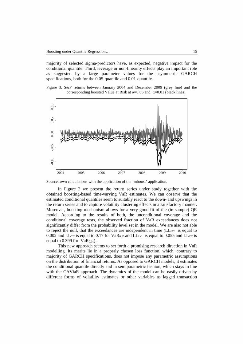
Figure 3. S&P returns between January 2004 and December 2009 (grey line) and the corresponding boosted Value at Risk at α=0.05 and α=0.01 (black lines).
Source: own calculations with the application of the ‘mboost’ application.
In Figure 2 we present the return series under study together with the obtained boosting-based time-varying VaR estimates. We can observe that the estimated conditional quantiles seem to suitably react to the down- and upswings in the return series and to capture volatility clustering effects in a satisfactory manner. Moreover, boosting mechanism allows for a very good fit of the (in sample) QR model. According to the results of both, the unconditional coverage and the conditional coverage tests, the observed fraction of VaR exceedances does not significantly differ from the probability level set in the model. We are also not able to reject the null, that the exceedances are independent in time (LLUC is equal to 0.002 and LLCC is equal to 0.17 for VaR0.05 and LLUC is equal to 0.055 and LLCC is equal to 0.399 for VaR0.01).
This new approach seems to set forth a promising research direction in VaR modelling. Its merits lie in a properly chosen loss function, which, contrary to majority of GARCH specifications, does not impose any parametric assumptions on the distribution of financial returns. As opposed to GARCH models, it estimates the conditional quantile directly and in semiparametric fashion, which stays in line with the CAViaR approach. The dynamics of the model can be easily driven by different forms of volatility estimates or other variables as lagged transaction
2004 2005 2006 2007 2008 2009 2010
-0.1
0-0
.05
0.00
0.05
0.10

16 Katarzyna Bień-Barkowska
volumes or implied volatility estimates. The drawback of this approach is its sensitivity to selection of a shrinkage factor or maximum numbers of performed boosting iterations. The approach can be also ‘fragile’ to possible structural breaks in the series, which may pose a further need for a time-varying weights. Moreover, much more effort should be put on a proper evaluation of the out-of-sample properties of the model, which is of utmost importance as far as the model application in the risk management is concerned.
REFERENCES:
Aiolfi M., Capistran C., Timmermann A. (2010) Forecast Combinations, forthcoming in Forecast Handbook (Oxford) ed. Clements, M. and Hendry, D.
Amendola A., Storti G. (2008) A GMM procedure for combining volatility forecasts, Computational Statistics and Data Analysis, 52(6), 3047–3060.
Bollerslev T. (1986) Generalized autoregressive conditional heteroskedasticity, Journal of Econometrics, 31, 307-327.
Bühlmann P. (2006) Boosting for high-dimensional linear models, Annals of Statistics 34, 559–583.
Bühlmann P., Hothorn T. (2007) Boosting Algorithms: Regularization, Prediction and Model Fitting (with Discussion), Statistical Science, 22(4), 477–505.
Bühlmann P., Yu B. (2003) Boosting with the L2 Loss: Regression and Classification, Journal of the American Statistical Association, 98, 324–339.
Chen Y., Zhenyu J., Mercola D., Xiaohui X. (2013) A Gradient Boosting Algorithm for Survival Analysis via Direct Optimization of Concordance Index, Computational and Mathematical Methods in Medicine 2013, 1-8.
Chiriac R., Rohlmeier W. (2012) Improving the Value at Risk Forecasts: Theory and Evidence from the Financial Crisis, Journal of Economic Dynamics and Control 36, 1212–1228.
Christoffersen P. F. (1998) Evaluating Interval Forecasts, International Economic Review 39, 841–862.
Engle R.F., Bollerslev T. (1986) Modelling the persistence of conditional variances, Econometric Reviews, 5(1), 1-50.
Engle R.F., Manganelli S. (2004) CAViaR: Conditional Autoregressive Value at Risk by Regression Quantiles, Journal of Business & Economic Statistics 22(4), p. 367-381.
Engle R.F., Ng V.K. (1993) Measuring and testing the impact of news on volatility, Journal of Finance, 48(5) 1749 - 1778.
Fenske N., Kneib T., Hothorn T. (2011) Identifying Risk Factors for Severe Childhood Malnutrition by Boosting Additive Quantile Regression, Journal of the American Statistical Association, 106, 494-510.
Freund Y., Schapire R.E. (1997) A decision-theoretic generalization of on-line learning and an application to boosting, Journal of Computer and System Sciences 55, p. 119-139.
Friedman J., Hastie T., Tibshirani R. (2000) Additive Logistic Regression: A statistical view of boosting, The Annals of Statistics 28, 337-407.
Boosting under Quantile Regression… 17
Glosten L.R., Jagannathan R., Runkle D.E. (1993) On the relation between the expected value and the volatility of the nominal excess return on stocks, Journal of Finance, 48(5), 1779-1801.
Hall S.G., Mitchell J. (2007) Combining density forecasts, International Journal of Forecasting 23, 1-13.
Hothorn T., Bühlmann P., Dudoit S., Molinaro A. and Van Der Laan M. (2006) Survival ensembles, Biostatistics 7, 355–373.
Hothorn T., Bühlmann P., Kneib T., Schmid M., and Hofner B. (2010) Model-Based Boosting 2.0, Journal of Machine Learning Research, 11, p. 1851–1855.
Hothorn T., Bühlmann P., Kneib T., Schmid M., Hofner B., Sobotka F., Scheipl F. (2013) Mboost: Model-Based Boosting, R package version 2.2-3, available at http://CRAN.R-project.org/package=mboost.
Jeon J., Taylor J.W. (2013) Using CAViaR Models with Implied Volatility for Value at Risk Estimation, Journal of Forecasting 32, p. 62-74.
Jing-Rong D., Yu-Ke C., Yan Z. (2011) Combining Stock Market Volatility Forecasts with analysis of Stock Materials under Regime Switching, Advances in Computer Science, Intelligent System and Environment, Springer, 393-402.
Jorion P. (2000) Value at Risk. The new benchmark for managing financial risk, McGraw-Hill.
Koenker R. (2005) Quantile Regression. Economic Society Monographs, Cambridge University Press, New York.
Kupiec P. H. (1995) Techniques for verifying the accuracy of risk measurement models, The Journal of Derivatives, 3(2), 73-84.
Li Y., and Zhu J. (2008) L1-Norm Quantile Regression, Journal of Computational and Graphical Statistics 17, 163–185.
Lu W., Li L. (2008) Boosting method for nonlinear transformation models with censored survival data, Biostatistics 9, 658-667.
Menardi G., Tedeschi F., Torelli N. (2011) On the Use of Boosting Procedures to Predict the Risk of Default, [in:] Classification and Multivariate Analysis for Complex Data Structures, Springer, Berlin, 211-218.
R Development Core Team (2008) R: A Language and Environment for Statistical Computing. R Foundation for Statistical Computing, Vienna, Austria, URL http://www.R-project.org.
Ridgeway G. (2002) Looking for lumps: Boosting and bagging for density estimation, Computational Statistics and Data Analysis 38, 379–392.
Schwert G. W. (1990) Stock volatility and the crash of '87, Review of Financial Studies, 3(1), 77-102.
Taylor S. J. (1986) Modelling financial time series, Wiley.
QUANTITATIVE METHODS IN ECONOMICS Vol. XV, No. 1, 2014, pp. 18 – 28
IS IT THE LABOUR MARKET THAT UNDERVALUES WOMEN OR WOMEN THEMSELVES? EVIDENCE FROM POLAND
Ewa Cukrowska1 Department of Macroeconomics and International Trade Theory
Faculty of Economic Sciences, University of Warsaw e-mail: [email protected]
Abstract: This article provides a comparative analysis of gender gaps in ob-servable and reservation wages. The analysis shows that women are able to accept lower wages than men before entering the labour market. Men’s and women’s differences in observable characteristics are not at all sufficient to explain the gaps both in observable and reservation wages. The article thus concludes that the prevalence of gender wage gap may be a result of wom-en’s lower self-valuation and not necessarily labour market discrimination against women.
Keywords: gender wage gap, reservation wage, decomposition, nonparamet-ric estimation, selection, discrimination
INTRODUCTION
The existence of a gender inequality in pay has been widely examined in empirical research focusing both on developed as well as developing and transition economies.2 Several factors, such as working experience, part time working sched-ule and occupational segregation have been found to be relevant for explaining women’s lower wages. Existing scholarship proves however that the gap in wages
1 The author would like to thank the participants of the Symposium on Gender Disparities
organized within the International Colloquium on Current Economic and Social Topics CEST’2013 for their valuable comments and suggestions to improve the quality of the paper.
2 The international review of gender wage gap analysis include for example Weichselbau-mer and Winter-Ebmer (2005); for transition economies see for example Brainerd (2000), Pailhé (2000), Newell and Reilly (2001), for Poland - Grajek (2003).
Is it the Labour Market that Undervalues Women … 19
of men and women is only partially explained by gender differences in these attrib-utes. The advocates of gender equality in pay thus argue that there is a significant measure of discrimination against women.
Notwithstanding broad research on gender wage inequality, none of the ex-isting studies accounts for the fact that the observable wage is a result of a hiring process and wage negotiation that are established in the setting of imperfect infor-mation with respect to the wage rate.3 This asymmetry of information reflected in the lack of transparent and a priori communicated wage offer may cause men and women to act differently and in consequence lead to distinct negotiated outcome. In particular, women may demand and agree to work for lower earnings than men do.
This article takes a novel approach in examining gender unequal distribution of wages and documents gender wage differentials in both observable and reserva-tion wages. The job search model of McCall (1970) resolves that the optimal strat-egy for an individual searching for a job is to accept the reservation wage as it is a wage that equalizes marginal cost from an additional search with a marginal ben-efit from such a search. If reservation wages of women are already lower than that of men, then it is straightforward that a similar gap in observable wages should be present.
The remainder of this article is structured into three major sections. The sub-sequent section presents data and the research methods. Section three presents and discusses main empirical results. The last section offers concluding remarks.
RESEARCH METHOD
Data and variables description
The empirical analysis is based on 2010 wave of Polish Labour Force Sur-vey data. Two samples are constructed. The first sample consists of individuals who: 1) are currently working, 2) are of working age (16-64) and 3) are not full time studying. Based on this sample a standard gender wage gap is estimated and decomposed. The second sample consists of unemployed individuals who are look-ing for a first job and are willing to undertake the job in the next two weeks. Indi-viduals who were previously employed are not considered in the analysis as their labour market experience might have been already influenced by the reservation wage they claim. The sample, which is used for the estimation of the gender gap in reservation wages, is thus restricted to school and university graduates that are looking for the first job and report lack of any labour market experience.
3 Only recently Brown et al. (2011) have investigated the gender wage gap in the reserva-
tion wages for Great Britain. However, in this research no relation to the existing gender wage gap is made and the reservation wage is examined among all unemployed workers suggesting that already incurred labour market patterns may influence the results.
Ewa Cukrowska 20
Determination of the wage equations
The analysis starts with a determination of a conditional gender wage gap. Following specifications are used to estimate the wage equations:
ln(wobsj
) = Xi , j' α
j+α
J+1female+ε
j (1)
ln(wresj
) = Zi , j' β
j+ β
J+1female+ϑ
j (2)
The dependent variables are natural logarithm of observable and reservation wages (����and ���� respectively). Since the dataset provides only the infor-mation on a minimum net monthly salary an unemployed individual agrees to work for, the reservation wage is defined as monthly earnings. To ensure comparability of the results for observable and reservation wages, in the observable wage equa-tion (equation 1) the dependant variable is also expressed as the net monthly earn-ings and the actual hours worked are additionally controlled for. The equations are estimated by the OLS with White heteroscedasticity consistent standard errors.
In the observable wage equation a set of control variables represented by a vector� involves labour market experience, educational dummies and a dummy for individual marital status. In addition, dummy variables representing a sector of work (i.e. private/public), a size of the company and regional disparities, i.e. the size of the place of living, the region of the country and whether an individual is living in the province, in which the capital is located, are also controlled for.
When determining the factors that influence reservation wage (denoted by a vector ) one needs to refer to the job search theory, which defines the concept of a reservation wage.4 Drawing on the theory and existing empirical literature the de-terminants of the reservation wage include: age, marital status and education as well as regional macroeconomic determinants. Moreover, a dummy variable indi-cating whether an individual is registered as unemployed and average duration of unemployment are also included.5 Additionally control variables describing the field of a study are added. By including these variables the possibility of occupa-tional segregation is accounted for.6
The coefficients of interest in equations (1) and (2) are �� for the gender wage gap and ��� for the gap in the reservation wages. They indicate an impact of being a woman on a wage rates assuming that all other control variables are kept
4 For a brief literature review on determinants of a reservation wages see [Christensen
2001]. Empirical analyses include [Jones 1989; Hogan 1999]. 5 Examples of the research on the relation between unemployment duration and the reserva-
tion wage include [Lancaster and Chesher 1984; Jones 1988]. 6 It is assumed that the field of the study determines the occupational choice of the individ-
uals. The assumption is based on the empirical evidence showing that the field of the studies is found to be a key factor contributing to occupational sex segregation at the la-bour market [Borghans and Groot 1999].

Is it the Labour Market that Undervalues Women … 21
fixed. In these equations it is therefore assumed that men and women have equal returns to their characteristics. As the returns to men’s and women’s characteristics are likely to vary, in the second step of the analysis, this rather restrictive assump-tion is eased and wage equations are estimated separately for the subsamples of men and women.
The above wage equations are likely to suffer from the problem of a sample selection, i.e. a selection into being working and a selection into being unemployed in the case of a first and second sample respectively. To correct for the problem of a sample selection, Heckman selection model [Heckman 1979] is used. Variables indicating a total number of people living in the household, a dummy variable whether the spouse is employed, a total number of kids an individual has and the main source of income are used as exclusion restrictions for the identification of the model.
Decomposition of the gender gaps in wages
Once the wage equations are estimated, the focus is placed on the determina-tion of the gender wage gap and its decomposition. Two methods that are broadly applied in the empirical research on the gender wage inequality are also adapted in this article. These include: Oaxaca-Blinder (1973) and Ñopo (2008) decomposition methods.
The method due to Oaxaca and Blinder calculates and decomposes the gap in the average wages of men and women based and the estimated wage equations:
∆ = ln(wobsm) − ln(wobsf
) = (Xm − X f )α + [(αm −α)Xm + (α −α f )X f ] (3)
where subscripts m and f stand for male and female and α represents non-discriminatory wage structure that is usually assigned to men’s wage coefficients ([Oaxaca 1973], [Cotton 1988], [Fortin et al. 2011]). If the men’s wage coefficients are chosen then the expression may be rewritten as:
∆ = ln(wobsm) − ln(wobsf
) = (Xm − X f )αm + (αm −α f )X f (4)
The first component on the right hand side represents the ‘explained’ part of the gender wage gap, i.e. the part that is explained by the differences in the distri-bution of the characteristics of men and women; the second component in turn rep-resents the ‘unexplained’ part that cannot be explained by these differences and is mostly attributed to the difference in the labour market valuation of men & women.
In addition to Oaxaca-Blinder decomposition, this article uses Ñopo decom-position that has certain advantages over the former method. Ñopo’s method is a nonparametric matching method and does not depend on the structural form of the wage equations. It also accounts for the curse of insufficient ‘common-support’ in terms of the distribution of observable characteristics. The lack of a ‘common-support’ refers to the situation when the probability of observing an individual, who shares comparable observable characteristics is close to zero.
Ewa Cukrowska 22
The decomposition brings down to four major steps. In the first step, one female is selected from the sample. In step two all men that have the same charac-teristics as a woman from the step one are also selected. In step three, an artificial man that has an average of characteristics of all the selected men is constructed and matched with a woman from the step one. In step four, matched pair is restored and the procedure is repeated for the next women. In the end the matched sample is constructed and their average wages are compared.7 Eventually, the gap in the av-erage wages between two groups of individuals is decomposed into four compo-nents that consider the distribution of the characteristics:
∆ = ∆X
+ ∆M
+ ∆F
+ ∆O
(5)
Where ∆� is an explained gap over the common support (the part of the gap that can be explained by the differences in the distribution of the characteristics of a matched sample); ∆� is an explained part that can be explained by the differences in the distribution of characteristics of males that are in and out of the common support; ∆� is an explained part that can be explained by the differences in the dis-tribution of the characteristics of females that are in and out of the common sup-port; ∆� is an unexplained part (the part that cannot be explained by the differences in the observable characteristics). The ‘explained’ and ‘unexplained’ parts are in-terpreted in the similar manner as in the standard mean decomposition due to Oaxaca and Blinder (1973).
RESULTS
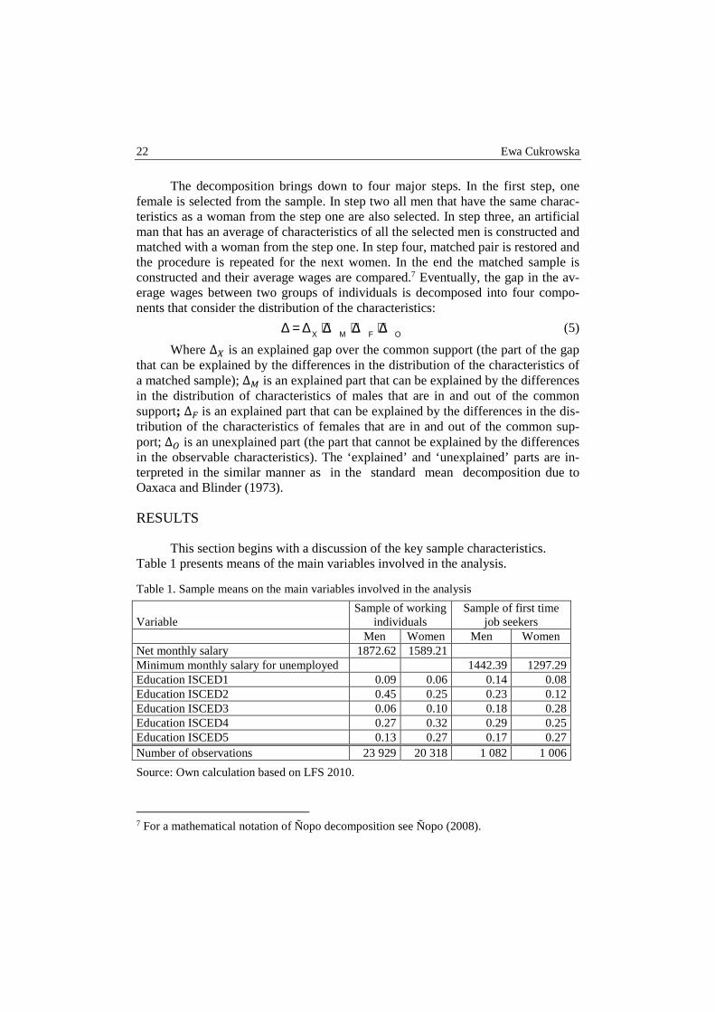
This section begins with a discussion of the key sample characteristics. Table 1 presents means of the main variables involved in the analysis.
Table 1. Sample means on the main variables involved in the analysis
Variable Sample of working
individuals Sample of first time
job seekers Men Women Men Women
Net monthly salary 1872.62 1589.21 Minimum monthly salary for unemployed 1442.39 1297.29 Education ISCED1 0.09 0.06 0.14 0.08 Education ISCED2 0.45 0.25 0.23 0.12 Education ISCED3 0.06 0.10 0.18 0.28 Education ISCED4 0.27 0.32 0.29 0.25 Education ISCED5 0.13 0.27 0.17 0.27 Number of observations 23 929 20 318 1 082 1 006
Source: Own calculation based on LFS 2010.
7 For a mathematical notation of Ñopo decomposition see Ñopo (2008).
Is it the Labour Market that Undervalues Women … 23
The reported net monthly salary for men and women differs: women in Po-land receive on average a net monthly wage of 1589 PLN, whereas men 1872 PLN (app. 373.3 EUR and 439.57 EUR).8 The resulting gender wage gap is equal to ap-proximately 15% in favour of men. Men on average tend to work by three hours per week more than women. In consequence, long working hours cause the gender wage gap calculated based on the hourly wages to be lower - around 6%. On the other hand, the average minimum net monthly wage unemployed women that are looking for the first job would agree to work for is equal to 1297.3 PLN (app. 304.7 EUR). For men the respective value is around 1442.4 PLN (app. 338.8 EUR). The resulting gender gap in reservation wages amounts to 10%.
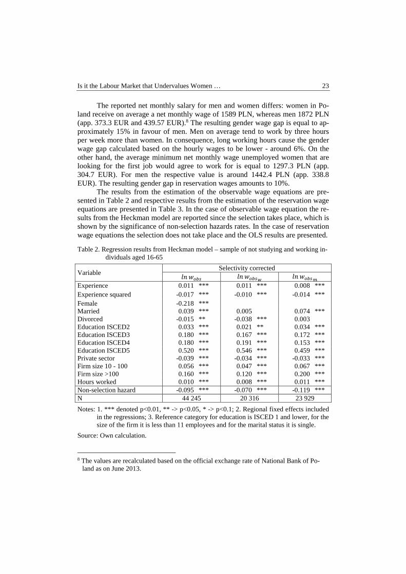
The results from the estimation of the observable wage equations are pre-sented in Table 2 and respective results from the estimation of the reservation wage equations are presented in Table 3. In the case of observable wage equation the re-sults from the Heckman model are reported since the selection takes place, which is shown by the significance of non-selection hazards rates. In the case of reservation wage equations the selection does not take place and the OLS results are presented.
Table 2. Regression results from Heckman model – sample of not studying and working in-dividuals aged 16-65
Variable Selectivity corrected
������ ������� ������� Experience 0.011 *** 0.011 *** 0.008 *** Experience squared -0.017 *** -0.010 *** -0.014 *** Female -0.218 *** Married 0.039 *** 0.005 0.074 *** Divorced -0.015 ** -0.038 *** 0.003 Education ISCED2 0.033 *** 0.021 ** 0.034 *** Education ISCED3 0.180 *** 0.167 *** 0.172 *** Education ISCED4 0.180 *** 0.191 *** 0.153 *** Education ISCED5 0.520 *** 0.546 *** 0.459 *** Private sector -0.039 *** -0.034 *** -0.033 *** Firm size 10 - 100 0.056 *** 0.047 *** 0.067 *** Firm size >100 0.160 *** 0.120 *** 0.200 *** Hours worked 0.010 *** 0.008 *** 0.011 *** Non-selection hazard -0.095 *** -0.070 *** -0.119 *** N 44 245 20 316 23 929
Notes: 1. *** denoted p<0.01, ** -> p<0.05, * -> p<0.1; 2. Regional fixed effects included in the regressions; 3. Reference category for education is ISCED 1 and lower, for the size of the firm it is less than 11 employees and for the marital status it is single.
Source: Own calculation.
8 The values are recalculated based on the official exchange rate of National Bank of Po-
land as on June 2013.
Ewa Cukrowska 24
The estimation results of the observable wage equations show that when the labour market experience and education are controlled for women receive on aver-age by 22% lower wages than men. When interpreting these results it has to be acknowledged that the returns to education and experience are kept fixed for men and women. The estimation outputs for the subsamples of men and women show that this is not necessarily true and the returns to education and experience for women fairly differ from those of men.
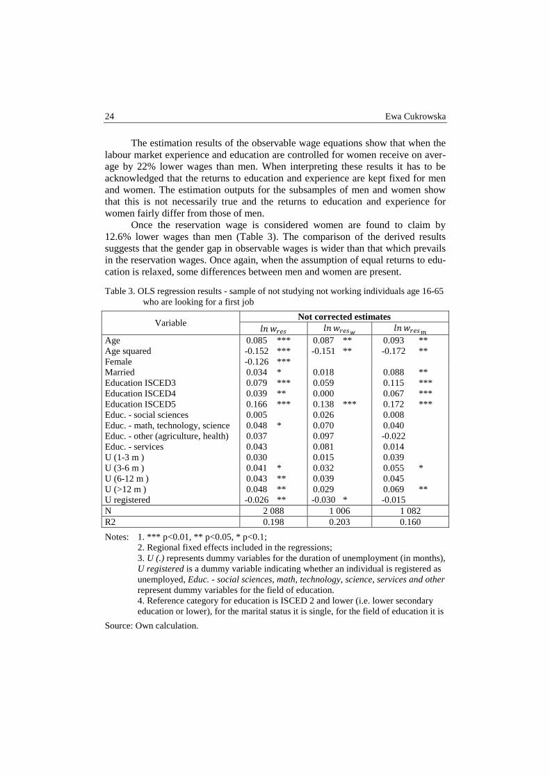
Once the reservation wage is considered women are found to claim by 12.6% lower wages than men (Table 3). The comparison of the derived results suggests that the gender gap in observable wages is wider than that which prevails in the reservation wages. Once again, when the assumption of equal returns to edu-cation is relaxed, some differences between men and women are present.
Table 3. OLS regression results - sample of not studying not working individuals age 16-65 who are looking for a first job
Variable Not corrected estimates
������ ������� ������� Age 0.085 *** 0.087 ** 0.093 ** Age squared -0.152 *** -0.151 ** -0.172 ** Female -0.126 *** Married 0.034 * 0.018 0.088 ** Education ISCED3 0.079 *** 0.059 0.115 *** Education ISCED4 0.039 ** 0.000 0.067 *** Education ISCED5 0.166 *** 0.138 *** 0.172 *** Educ. - social sciences 0.005 0.026 0.008 Educ. - math, technology, science 0.048 * 0.070 0.040 Educ. - other (agriculture, health) 0.037 0.097 -0.022 Educ. - services 0.043 0.081 0.014 U (1-3 m ) 0.030 0.015 0.039 U (3-6 m ) 0.041 * 0.032 0.055 * U (6-12 m ) 0.043 ** 0.039 0.045 U (>12 m ) 0.048 ** 0.029 0.069 ** U registered -0.026 ** -0.030 * -0.015 N 2 088 1 006 1 082 R2 0.198 0.203 0.160
Notes: 1. *** p<0.01, ** p<0.05, * p<0.1; 2. Regional fixed effects included in the regressions; 3. U (.) represents dummy variables for the duration of unemployment (in months), U registered is a dummy variable indicating whether an individual is registered as unemployed, Educ. - social sciences, math, technology, science, services and other represent dummy variables for the field of education. 4. Reference category for education is ISCED 2 and lower (i.e. lower secondary education or lower), for the marital status it is single, for the field of education it is
Source: Own calculation.
Is it the Labour Market that Undervalues Women … 25
no specialization (general education), for the duration of unemployment it is less than a month.
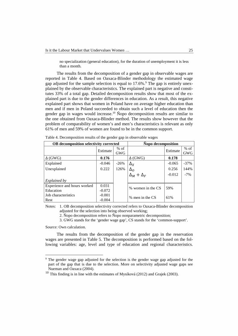
The results from the decomposition of a gender gap in observable wages are reported in Table 4. Based on Oaxaca-Blinder methodology the estimated wage gap adjusted for the sample selection is equal to 17.6%.9 The gap is entirely unex-plained by the observable characteristics. The explained part is negative and consti-tutes 33% of a total gap. Detailed decomposition results show that most of the ex-plained part is due to the gender differences in education. As a result, this negative explained part shows that women in Poland have on average higher education than men and if men in Poland succeeded to obtain such a level of education then the gender gap in wages would increase.10 Ñopo decomposition results are similar to the one obtained from Oaxaca-Blinder method. The results show however that the problem of comparability of women’s and men’s characteristics is relevant as only 61% of men and 59% of women are found to be in the common support.
Table 4. Decomposition results of the gender gap in observable wages
OB decomposition selectivity corrected Ñopo decomposition
Estimate
% of GWG
Estimate % of GWG
∆ (GWG) 0.176
∆ (GWG) 0.178 Explained -0.046 -26% ∆� -0.065 -37%
Unexplained 0.222 126% ∆� 0.256 144%
∆� + ∆� -0.012 -7%
Explained by Experience and hours worked 0.031
% women in the CS 59% Education -0.072
Job characteristics -0.001
% men in the CS 61% Rest -0.004
Notes: 1. OB decomposition selectivity corrected refers to Oaxaca-Blinder decomposition
adjusted for the selection into being observed working; 2. Ñopo decomposition refers to Ñopo nonparametric decomposition; 3. GWG stands for the ‘gender wage gap’, CS stands for the ‘common-support’.
Source: Own calculation.
The results from the decomposition of the gender gap in the reservation wages are presented in Table 5. The decomposition is performed based on the fol-lowing variables: age, level and type of education and regional characteristics.
9 The gender wage gap adjusted for the selection is the gender wage gap adjusted for the
part of the gap that is due to the selection. More on selectivity adjusted wage gaps see Nueman and Oaxaca (2004).
10 This finding is in line with the estimates of Mysíková (2012) and Grajek (2003).

Ewa Cukrowska 26
At this stage of the analysis the average duration of unemployment and unemploy-ment official registration are not accounted for. This is because of a very low common support that is present when these variables are included among the matching variables. When the variables are excluded from the analysis, there are 62% of women and 59% of men in the common support. Based on Oaxaca-Blinder methodology the gender gap in the reservation wages is equal to 10.3% of men’s average reservation wage. The corresponding estimate from the Ñopo’s method is 11.2%. The gap is lower by about one third when compared with the gap in actual-ly realized wages. On the other hand, the features of the gap in the minimum wages men and women would agree to work for are similar to those present in the actually prevailing wage gap.
The findings show that there exist some other complex structural factors be-sides age, level and type of education that may cause women’s lower reservation wages. In particular, this unobservable factors that lead to difference in men’s and women’s average reservation wages may refer to unobserved individual self-valuation and self-assessment. If women of the same education as men claim lower reservation wage then it might be a signal that they value their skills lower. The high unexplained part may be however already a sign of differences in the labour market treatment of men and women as women may undervalue their skills in re-sponse to the future – potential – labour market prospects. This means that they may value their skills lower to be as competitive at the labour market as men are.
Table 5. Decomposition results of the gender gap in reservation wages among individuals first time looking for a job
OB decomposition Ñopo decomposition
Estimate % of GWG
Estimate % of GWG
∆ (GWG) 0.103 ∆ (GWG) 0.112
Explained -0.029 -28% ∆� -0.025 -22%
Unexplained 0.132 128% ∆� 0.159 142%
∆� + ∆� -0.022 -20%
Explained by Age -0.005
% women in the CS 62% Education -0.024 Education type 0.009
% men in the CS 59% Rest -0.009
Notes: 1. OB decomposition refers to Oaxaca-Blinder decomposition; 2. Ñopo decomposition refers to Ñopo nonparametric decomposition. 3. GWG stands for the ‘gender wage gap’, CS stands for the ‘common-support’.
Source: Own calculation.
Is it the Labour Market that Undervalues Women … 27
CONCLUSION
This article documents gender based differences in the observable and reser-vation wages, i.e. the minimum wages unemployed individuals would agree to work for. In general, the research shows that the gender gap in reservation wages is smaller than the gender gap in actually prevailing wages. The nature of the gaps is however comparable as both the gaps remain unexplained by the observable fac-tors. The decomposition results show that the differences in observable characteris-tics of men and women are not at all sufficient to explain the inequalities. Women have on average higher acquired skills, particularly education, than men but still are rewarded worse by the labour market. Similarly in terms of reservation wages – women are equipped with higher levels of education but still demand lower wages.
The results of this article shed an additional light on the foregoing gender gap research. The gender gap in wages is found to be present even in ‘potential’ minimum wages, i.e. it is present even before entering the labour market. The arti-cle concludes that there exist unobservable factors, which may include individual self-valuation of skills, which lead to the existence of the gender gap in reservation wages. Consequently, the fact that women are able to accept lower wages is associ-ated with women’s lower self-valuation and self-esteem or alternatively men’s higher self-valuation. Women’s lower valuation may however result from their dis-advantaged position since if they demanded more they might have been unable to find a job.
REFERENCES
Blinder A.S. (1973) Wage Discrimination: Reduced Form and Structural Estimates, Journal of Human Resources 8: 436-455.
Borghans L., Groot L. (1999) Educational presorting and occupational segregation, Labour Economics 6(3): 375-395.
Brainerd E. (2000) Women in transition: changes in gender wage differentials in Eastern Europe and the Former Soviet Union, Industrial and Labor Relations Review 54(1): 138-162.
Brown S., Roberts J., Taylor K. (2011) The Gender Reservation Wage Gap: Evidence form British Panel Data, IZA Discussion Papers 5457, Institute for the Study of Labor (IZA).
Christensen B. (2001) The Determinants of Reservation Wages in Germany Does a Motiva-tion Gap Exist?, Kiel Working Papers 1024, Kiel Institute for the World Economy.
Cotton J. (1988) On the Decomposition of Wage Differentials,. The Review of Econom-icsand Statistics 70: 236–243.
Fortin N., Lemieux T., Firpo S. (2011) Chapter 1 - Decomposition Methods in Economics. In: Ashenfelter O., Card D. (eds.), Handbook of Labor Economics: Elsevier, Volume 4,. Part A, 1-102.
Grajek M (2003) Gender Pay Gap in Poland, Economic Change and Restructuring 36(1): 23-44.

Ewa Cukrowska 28
Heckman J. (1979) Sample selection bias as a specification error, Econometrica 47 (1): 153 - 161.
Hogan V. (1999) The Determinants of the Reservation Wage. Working Paper WP99/16, University College Dublin, Department of Economics, Dublin.
Jones S.R.G. (1988) The Relationship Between Unemployment Spells and Reservation Wages as a Test of Search Theory, Quarterly Journal of Economics 103 (4): 741-765.
Jones S.R.G. (1989) Reservation Wages and the Cost of Unemployment, Economica 56: 225–246.
Lancaster T., Chesher A. (1983) An Econometric Analysis of Reservation Wages, Econometrica 51(6): 1661-76.
McCall J.J. (1970) Economics of information and job search, Quarterly Journal of Econo-mics 84 (1): 113–126.
Mysíková M. (2012) Gender Wage Gap In The Czech Republic And Central European Countries, Prague Economic Papers, University of Economics, Prague 2012(3): 328-346.
Neuman S., Oaxaca R.L. (2004) Wage Differentials in the 1990s in Israel: Endowments, Discrimination and Selectivity, CEPR Discussion Papers 4709.
Newell A., Reilly B. (2001) The gender pay gap in the transition from communism: some empirical evidence, Economic Systems 25(4): 287-304.
Ñopo H. (2008) Matching as a Tool to Decompose Wage Gaps, The Review for Economics and Statistics 90(2): 290-299.
Oaxaca R.L. (1973) Male-Female Wage Differentials in Urban Labor Markets, Internatio-nal Economic Review 14: 693-709.
Pailhé A. (2000) Gender Discrimination in Central Europe During the Systemic Transition, Economics of Transition 8(2): 505-535.
Prasad E. (2003) What Determines the Reservation Wages of Unemployed Workers? New Evidence from German Micro Data, IMF Working Papers 03/4, International Monetary Fund.
Weichselbaumer D., Winter-Ebmer R. (2005) A Meta-Analysis of the International Gender Wage Gap, Journal of Economic Surveys 19: 479-511.
QUANTITATIVE METHODS IN ECONOMICS Vol. XV, No. 1, 2014, pp. 29 – 36
LABOUR MARKET IN POLAND FOR WOMEN AND MEN 50+
Jan B. Gajda Department of Operational Research, University of Lodz
e-mail: [email protected] Justyna Wiktorowicz
Department of Economic and Social Statistics, University of Lodz e-mail: [email protected]
Abstract: Population ageing is one of the major challenges of modern Europe. In this context is worth to assessment the differences in the situation of women and men aged 50+ on the labour market. In the area of interest are primarily people aged 50-59/64, which are at this stage of life in which the situation on the labour market is particularly difficult. Paper was prepared mainly on the basis of the unpublished data developed within the project “Equalisation of Opportunities in the Labour Market for People Aged 50+”. The analysis was conducted with the application of basic descriptive statistics, as well as chi-squared test. Comparing income of women and men aged 50+, t-Student test and median test for independent samples, as well as one- and two-way analysis of variance were used.
Keywords: ageing, economic activity, employment, multivariate statistics
INTRODUCTION
Population ageing is one of the major challenges of modern Europe. This is the effect of both shrinking and ageing of potential labour resources as well as the fact that professional competences of older employees are becoming increasingly outdated. Another thing is that due to the improvement of quality of live, people tend to live longer. Health of the population is improving regardless of their age, also at the threshold of becoming old. These processes should be accompanied by extending the period of economic activity. In this context, very low economic activity of Poles (especially women) nearing retirement is a huge challenge faced by the Polish economy.
Jan B. Gajda, Justyna Wiktorowicz
30
This paper compares the overall situation of women and men aged 50+ as well as certain characteristics of this group. In the area of interest are primarily persons aged 50-59/64 which are at the stage of life in which - in accordance with the Act on employment promotion and labour market institutions [2004] - their situation on the labour market is considered to be particularly difficult. This will allow relating the analyses carried out to solutions regarding this group in the context of active labour market policies.
Paper was prepared on the basis of the unpublished data developed within the project “Equalisation of opportunities in the labour market for people aged 50+”. Additionally, Eurostat data are used.
DATA AND METHODS
This paper presents mainly the results of the research conducted in the framework “Diagnosis of situation of females and males 50+ on the labour market in Poland” (Diagnosis), within the project “Equalisation of Opportunities in the Labour Market for People Aged 50+” co-financed by the European Union from the European Social Fund. This diagnosis covered among others quantitative component – questionnaire research among ‘people aged 45+’ (i.e. inhabitants of Poland aged 45-69), realized on representative sample 3,200 persons. As a result of non-proportional sampling, weights were applied. Finally, estimation error is max 1.8%. The research was carried out with the CAPI method.
The analysis was conducted with the application of basic descriptive statistics, as well as chi-squared test and analysis of variance. Chi-squared test will be applied to assess the relations between qualitative variables. When comparing the incomes of men and women aged 50+ t-Student test and median test for independent samples, and two-way analysis of variance factors were also used. As far as the last mentioned method is concerned, less commonly used in socio-economic analyses, it belongs to the multivariate statistics methods [Stockburger 1998; Walesiak i in. 2009; Wuensche 2007; Szymczak 2011]. Multiple analysis of variance is used to see the main and interaction effects of categorical variables on multiple dependent interval variables. For example, two-way analysis of variance model can be expressed as: ysri = µ +αs + βr + (αβ )sr +εsri
, (1)
where: µ - total mean, αs i βr – main effects of factors xA i xB, (αβ)sr – interaction effect between xA i xB, εsri – within-group error;εsri ~ N (0,σ ) .
In the analysis standard level of significance (α = 0.05) was adopted. The calculation was made in SPSS 20.0

Labour market in Poland for women and men 50+
31
ECONOMIC ACTIVITY OF WOMEN AND MEN AGED 50+
Polish people over 50 years of age, as well as people in the entire European Union, are characterized by a relatively low economic activity. In 2012, in the age group 50-64, the economic activity rate reached in the EU-27 an average of about 63%, whereas in the group of 55-64 - less than 53%. Poland is at the bottom of the ranking of economic activity of people aged 50/55-64 among the EU Member States - the economic activity rate of people aged 50-64 reaches about 53%, and compared to 2000 it has increased by 5 percentage points. As far as the group of 55-64 year olds is concerned the increase of this rate is more pronounced - from 31.3% in 2000 to 41.8% in 2012, but still the economic activity of women aged 55-64 is the lowest in Europe. Compared to such countries as Sweden (the economic activity rate of approximately 80% for both age groups) and Germany (approx. 70%), the situation in Poland leaves much to be desired. Compared with other EU Member States only Malta, Hungary and Slovakia have a lower economic activity of older workers [Eurostat, lfsi_act_a, lfsa_argan]. In Poland, as in almost all EU Member States, the economic activity of men is higher than of women - the European Union average economic activity rate of men aged 50-64 years amounts to 71.2%, while of women - 55.7%, and only Finnish women are more economically active than men. The biggest differences in this respect (to the disadvantage of women) can be observed in Malta - the difference is as high as 44 percentage points.
Similar trends were recorded as far as employment of people from these groups of people is concerned - the employment rate was in most countries (with the exception of Finland and Estonia) higher for men than for women, similarly, the biggest difference between men and women was observed in Malta, Cyprus, Greece, Italy and Poland. In Poland, nearly two-thirds of men aged 50-64 are economically active (compared to 40% of women), and every other male in the age group 55-64 (compared to less than 30% of women) [ibidem].
Taking into account the not averaged (used by Eurostat), but the actual upper limit of working age in Poland, an assessment of the economic activity of Poles was made with the use of results from the "Diagnosis of the current situation of women and men aged 50+ in the labour market in Poland" research. Approximately 65% of women and men aged 50-59/64 identified themselves as economically active. Most of them are employed under a contract of employment (mostly for an indefinite period). There is a quite high proportion of retirees among men and women aged 50-59/64. The situation of women is at the same time significantly different (in a statistical sense) from the situation of men - this applies to both the group of 50-59/64 year olds and 45-49 year olds (the situation of women and men aged 60/65 + is, however, not so significantly different). Let us look at features characteristic for older workers, focusing on population aged 50-59/64. In Table 1 typical characteristics of men and women as employees are indicated.

Jan B. Gajda, Justyna Wiktorowicz
32
Table 1. Main characteristics of the employed aged 50-59/64 by sex
Specification Females aged 50-59 Males aged 50-64 property sector
public (46%) private, Polish capital (51%)
the employer's business profile
trade, repair of motor vehicles (15%), health care and social assistance (14%), education (13%), public administration, national defense, compulsory social security (13%)
industry, mining, metallurgy (23%), construction (22%), transport and storage (17%), trade, repair of motor vehicles (12%)
number of employees
small (37%) and medium (28%) small (38%) and medium (24%)
employer location
mainly in the place of residence (77%)
slightly more often at the place of residence (58%) than elsewhere
professional position
skilled worker (35%) or specialist (31%)
skilled worker (69%) or specialist (18%)
type of work performed
specialist (21%) or production (average physical workload) (20%)
production (an average physical workload) (31%) or specialist (18%)
type of agreement in the workplace
contract of employment for an indefinite period (79%) or for a specified period (16%)
contract of employment for an indefinite period (78%) or for a specified period (20%)
working time full-time (89%), part-time (7%) full-time (97%), part-time (1%) overtime 35% ; average of 20.4 hours and a
median of 10 hours 40%; average of 24.1 hours and a median of 15 hours
seniority mean - 14.4, median - 12 mean - 13.9, median - 12 the nature of work
max: work in a sitting position (43%), work in a standing position, with low physical workload (34%) min: work requiring a significant physical exertion (1%)
max: work in a standing position, with low physical load (31%), physically demanding work (30%) min: work requiring a significant physical exertion (16%)
reserve of time (farmers)
throughout the year (10%) seasonally (9%)
throughout the year (4%) seasonally (32%)
Source: own elaborations on the basis unpublished materials of “Diagnosis of situation of females and males 50+ on the labour market in Poland” developed within the project Equalisation of Opportunities in the Labour Market for People Aged 50+.
It is clear that the conditions of employment of women aged 50+ are in most discussed dimensions slightly different than those of men (Table 1). Women are more likely to work in the public sector than men, in companies involved in trade, education, health and social care and public administration, equally on skilled worker and professional positions, whereas men - mostly in domestic private companies, on skilled worker positions, in industry, construction, transport and materials, and thus women do a lighter work than men. Men commute to work more often than women, they work longer overtime hours, while women work
Labour market in Poland for women and men 50+
33
more often part-time (which is often associated with caring responsibilities towards their parents or grandchildren and is related to the traditional model of the family). It should also be noted that every third male farmer could seasonally work off-farm (in the case of women one in ten could start work off-farm seasonally, also one in ten - throughout the year).
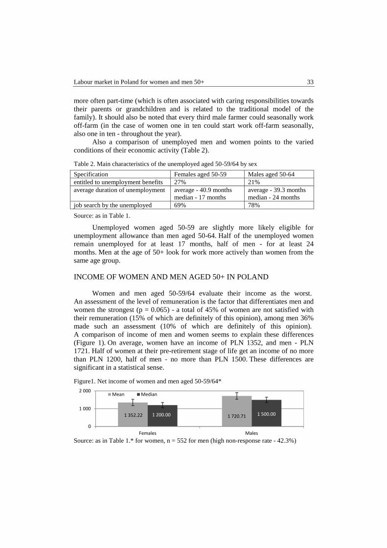
Also a comparison of unemployed men and women points to the varied conditions of their economic activity (Table 2).
Table 2. Main characteristics of the unemployed aged 50-59/64 by sex
Specification Females aged 50-59 Males aged 50-64 entitled to unemployment benefits 27% 21% average duration of unemployment average - 40.9 months
median - 17 months average - 39.3 months median - 24 months
job search by the unemployed 69% 78%
Source: as in Table 1.
Unemployed women aged 50-59 are slightly more likely eligible for unemployment allowance than men aged 50-64. Half of the unemployed women remain unemployed for at least 17 months, half of men - for at least 24 months. Men at the age of 50+ look for work more actively than women from the same age group.
INCOME OF WOMEN AND MEN AGED 50+ IN POLAND
Women and men aged 50-59/64 evaluate their income as the worst. An assessment of the level of remuneration is the factor that differentiates men and women the strongest (p = 0.065) - a total of 45% of women are not satisfied with their remuneration (15% of which are definitely of this opinion), among men 36% made such an assessment (10% of which are definitely of this opinion). A comparison of income of men and women seems to explain these differences (Figure 1). On average, women have an income of PLN 1352, and men - PLN 1721. Half of women at their pre-retirement stage of life get an income of no more than PLN 1200, half of men - no more than PLN 1500. These differences are significant in a statistical sense.
Figure1. Net income of women and men aged 50-59/64*
Source: as in Table 1.* for women, n = 552 for men (high non-response rate - 42.3%)
1 352.22 1 720.711 200.00 1 500.00
0
1 000
2 000
Females Males
Mean Median
Jan B. Gajda, Justyna Wiktorowicz
34
In the t-Student's t test, p <0.001. Similarly, in the median test for independent samples p <0.001. Error bars express a standard error.
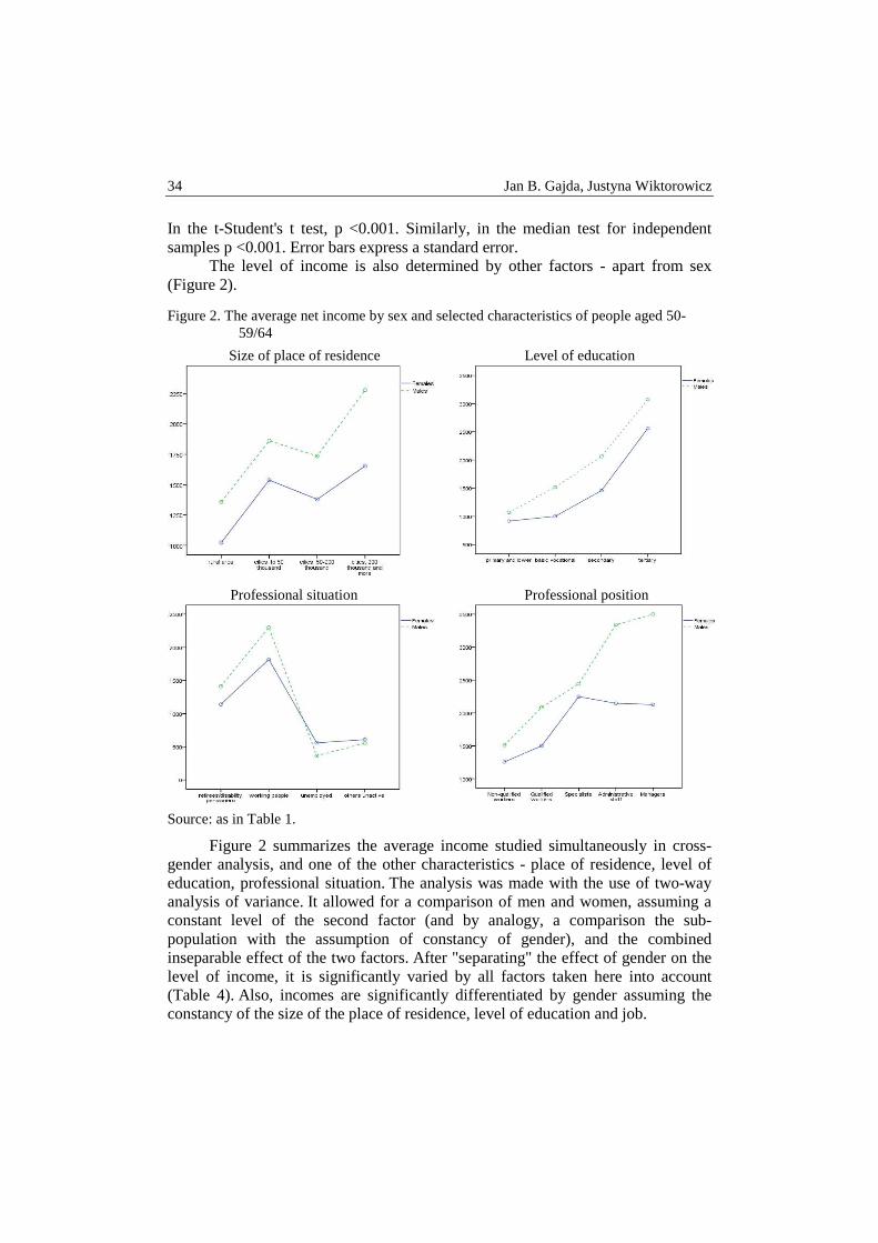
The level of income is also determined by other factors - apart from sex (Figure 2).
Figure 2. The average net income by sex and selected characteristics of people aged 50-59/64
Size of place of residence Level of education
Professional situation Professional position
Source: as in Table 1.
Figure 2 summarizes the average income studied simultaneously in cross-gender analysis, and one of the other characteristics - place of residence, level of education, professional situation. The analysis was made with the use of two-way analysis of variance. It allowed for a comparison of men and women, assuming a constant level of the second factor (and by analogy, a comparison the sub-population with the assumption of constancy of gender), and the combined inseparable effect of the two factors. After "separating" the effect of gender on the level of income, it is significantly varied by all factors taken here into account (Table 4). Also, incomes are significantly differentiated by gender assuming the constancy of the size of the place of residence, level of education and job.

Labour market in Poland for women and men 50+
35
Table 4. Results of two-way factors analysis of variance
Other factors - specification Effect (p in test F)
sex other factor interaction Size of place of residence <0.001* <0.001* 0.5750 Level of education <0.001* <0.001* 0.2130 Professional situation 0.2470 <0.001* 0.022* Professional position <0.001* <0.001* 0.028*
Source: as in Tabl. 1.
Taking into account the place of residence, rural residents (of both sexes) have a lower level of income than those living in cities, especially large cities and the smallest towns. The course of these differences for men and women is, however, similar (the interaction effect is not statistically significant). The level of education also shows no statistically significant interaction with gender with respect to the income level. In general, the higher the level of education, the higher the income. While in the case of education not higher than lower secondary, women and men achieve similar income, in next groups, however, differences are greater. The interaction effect is statistically significant for sex and professional situation (and professional position). Working and retired men aged 50+ have a higher income than women, while in the case of the unemployed the situation is opposite (other economically inactive people do not differ by gender). On the other hand, taking into account the position, men and women in the lower professional positions achieve similar income, while managerial and administrative positions are associated with higher income of men than women 50+1.
FINAL REMARKS
Economic activity of women and men shortly before retiring is low in Poland as well as in other EU Member States for the population aged 50-64 and 55-64 is higher for women than for men. Taking into account the maximum working age set by retirement age, in Poland these proportion converge. About one person in three aged 50-59/64 (and therefore still of working age) remains economically inactive, mainly due to a pension or annuity.
Employment of women aged 50+ is characterized by slightly different characteristics than of men in the same age - women more often than men work in the public sector, trade, health care and social assistance, education and administration, doing work which is lighter physically, often specialized,
1 A high percentage of non-response to the question about the level of income should be
noted. The structure of the sub-samples of which income is known, however, is analogous as far as sex and the professional situation is concerned to the structure of sub-samples for which there is no data on income.

Jan B. Gajda, Justyna Wiktorowicz
36
particularly in the place of residence and they less likely suffer accidents at work. Working conditions are more difficult for men than for women, which is a consequence of how the roles of men and women are perceived in our society. What is more, when unemployed men face greater difficulties in finding a new job, although they seek it more actively and are more spatially mobile. They are, however, less likely to re-qualify or improve their skills and qualifications than women, what reduces their adaptability in case of dismissal, especially due to the fact that their education level is significantly lower than that of women in the same age group. Therefore, in a situation of possible retirement or annuity, they take advantage of it even more often than women. On the other hand, after retirement they get another job more often than women - it results from the necessity of taking care of grandchildren, but also elderly parents by women.
Presented picture of the professional situation of women and men aged 50+ in Poland is - due to the high degree of generalization - simplified, however, it allows identifying some regularities characterizing the conditions of women and men in the pre-retirement labour market. Apart from the noted differences, the situation of women and men is similar in many respects - both groups usually work under a contract of employment for an indefinite period, they are burdened with overtime work to a similar extent, they have similar seniority, they retire at a similar age, the assessment of working conditions analogous in both groups. The results of the Diagnosis, however, confirm the disparities in salaries between men and women aged 50-59/64 - even cross their professional situation or position, and according to the respondents, higher salaries as well as flexible working hours and form of work are the most important incentives for extending the period of economic activity. The findings of studies and experiences of the institutions involved in the implementation of actions aimed at the older group of employees clearly indicate that actions aimed at delaying retirement should involve primarily maintaining employment. As can be seen from these studies the principle of gender equality cannot be overlooked in these actions.
REFERENCES
Act of April 20th, 2004 on Promotion of Employment and Labour Market Institutions, Dziennik Ustaw of 2004 No. 99, item 1001 as amended.
Stockburger D.W. (1998) Multivariate Statistics: Concepts, Models and Applications, Missouri State University, on-line version.
Szymczak W. (2011) Podstawy statystyki dla psychologów, Difin, Warszawa. Walesiak M., Gatnar E. (2009) Statystyczna analiza danych z wykorzystaniem programu R,
PWN, Warszawa. Wuensche K.E. (2007) Statistics Lessons, East Karolina University, Greenville 2007. Eurostat, lfsi_act_a, lfsa_argan, 10.04.2013. Unpublished data of “Diagnosis of situation of females and males 50+ on the labour market
in Poland” developed within the project Equalisation of Opportunities in the Labour Market for People Aged 50+.

QUANTITATIVE METHODS IN ECONOMICS Vol. XV, No. 1, 2014, pp. 37 – 49
LABOUR FORCE PARTICIPATION AND FAMILY POLICIES IN EUROPE: AN EMPIRICAL STUDY
Agnieszka Gehringer University of Göttingen
e-mail: [email protected] Stephan Klasen
University of Göttingen e-mail: [email protected]
Dorota Witkowska Faculty of Management, University of Lodz
e-mail: [email protected]
Abstract: The aim of our research is the identification of factors affecting labour force participation (LFP) in the EU in the years 1998-2007 with a specific focus made on family policies. We perform the analysis separately for men and women, taking into account differences in the LFP levels and patterns observable among age and country groups. Our main findings suggest that generally the family policies are relevant for the age groups 15-24 and 40-59 in determining their LFS, while less influential for the age group 25-39. Nevertheless, significant differences in the sign and the magnitude of the influence exist between specific policy instruments.
Keywords: labour force participation, family policies, age-group specific effects
INTRODUCTION
Over the last few decades, the continues focus of EU policy making on increasing employment was paralleled by gender specific discussion. The aim was put here on improving labour force participation of women, relative to men. Indeed, gender participation gap continues to persists, despite the fact that it decreased in the recent years. From the policy perspective, family policies were often seen as an instrument helping to close the gap. Such recognition led to formal steps taken at the European level: in 1996 the Council adopted the so called

38 Agnieszka Gehringer, Stephan Klasen, Dorota Witkowska
Parental Leave Directive requiring from the member states to implement employment-related family policies permitting to reconcile the life-work balance of both men and women. More concrete, the directive was establishing a minimum of three months of parental leave on the occasion of the birth or adoption of a child. Further steps were taken at the EU summit in Barcelona in 2002. It was recommended that by 2010 member states would introduce childcare measures for at least 33% of children aged under three and for at least 90% of children between the age of three and the mandatory school age.
Considering such policy objectives, the paper investigates empirically the impact of family policies on the LFP of men and women in the EU. After offering a short theoretical background in the next section, in Section 3 we describe our empirical strategy, the data and analyse the results obtained. The last section concludes the paper.
LABOUR FORCE PARTICIPATION AND FAMILY POLICIES – A THEORETICAL VIEW
Determinants of labour supply
In the static labour supply model [Blundell and MaCurdy 1999], one can expect a diminishing demand for leisure following an increase in earnings from work. This is because the relative value of work increases with respect to leisure. This results in the so called substation effect, according to which an increase in the wage rate will exercise a positive effect on labour supply. At the same time, however, the increase in non-labour income could have a negative effect on labour supply, as it enhances the valuation of leisure on the cost of labour activity. This effect is called income effect. Depending on the strength of the two effects, the net effect on labour supply is a priori unsure.
For the purposes of our investigation, it does make sense to consider the labour supply within a family or household framework. This context delivers a series of relevant considerations in terms of determinants of labour supply. Indeed, for each individual within the family, the income effect will depend not only on the own non-labour income, but also on wage and non-wage income of the other family members. Additionally, the decision over participation in the labour market could depend on other factors, like fertility rate, or labour market policy interventions, like taxation or the family policies [Blundell and MaCurdy 1999]. With this respect, the arrival of the family policies might result in disequilibrium, followed by an adjustment process towards a new equilibrium situation corresponding to a higher level of labour market participation. But the new equilibrium conditions will crucially depend on the precise characteristics of family policies. For instance, better childcare opportunities will incentive to increase the labour force participation, only if the wage rate – net of the cost of childcare – is sufficiently high to result in a positive substitution effect. On the contrary, long and
Labour force participation and family policies … 39
well-paid parental leave might contribute to a strong and long-lasting income effect, with the depressing effect on the life-time level of labour force participation.
Family policies
The broad group of family policies refers to different policy measures. According to Eurostat and OECD, a distinction often adopted is between family allowance, maternity and parental leave, other cash benefits and daycare. Such policies are part of a broader category of welfare-state policies. But more precisely, family policies are expected to impact in one way or another LFP of both men and women. Indeed, they influence the time distribution between working and family-related activities. The direction of the precise influence could favor either work or family, depending on the policy design and political goals adopted. For instance, long and generous maternity leave schemes could exercise a negative effect on women’s LFP, as they would sustain income effect. Conversely, short and unpaid parental leave should enhance LFP of both men and women, as they would increase the opportunity cost of staying at home with respect to working and earning positive labour income.
From the above discussion it emerges that due to different policy priorities, the average outcome of the family policies on the labour market will be unsure, with diametrically different tendencies generated by single family policy measures. More precisely, Thevenon (2011) identifies six main goals of family policies: 1) poverty reduction and income maintenance, 2) direct compensation for the economic cost of children, 3) fostering employment, 4) improving gender equality, 5) support for early childhood development, and 6) raising birth rates. Regarding the third, the sixth and partly the fourth goal one could expect that they should encourage pro-LFP family policies. The remaining goals, instead, would be favourable to policy measures diminishing LFP. The effect here could be expected to be stronger for women than for men, given that women still more often assume family responsibilities. Thus, it becomes clear that the impact of family policies is ambiguous and as such is an empirical matter.
ESTIMATION STRATEGY
The main estimation strategy consists in estimating our baseline model considering different age groups and different geographic composition of the countries in the sample. More precisely, our overall sample consists of men and women from the 21 EU member states, observed annually over the period 1998-2007 and divided in four age groups: young (15-24), two prime-age groups (25-39 and 40-59) and old age group (60-64). In that way, we cover almost the whole working force, but moreover we are able to observe the between group heterogeneity that is perceived when looking at the specific determinants of labour force participation of men and women.
40 Agnieszka Gehringer, Stephan Klasen, Dorota Witkowska
Concerning the empirical strategy, after comparing the results from different procedures, we decided to present the outcomes obtained from the heteroskedasticity robust pooled OLS and from feasible GLS (FGLS). The choice of pooled OLS is driven by the fact that we want to explore the panel dimension of our dataset and at the same time account for age group and country group effects, in addition to time dummies. In that vein, we consider pooled OLS superior over fixed or random effect estimations that would save some degrees of freedom, but at the same time would cancel out group specific effects that do not vary over time, yet are of interest for our conceptual framework. Moreover, we checked for the first order serial correlation in residuals that appeared to be a potential issue.1 In this case, when ���, ��� ≠ �, it is reasonable to make use of feasible GLS rather than pooled OLS (Wooldridge, 2002). For this reason, after the first set of estimations, in which we compare FGLS to pooled OLS results, we configure our main estimations around the former method.
The model
The baseline model to estimate, each time separately for men and for women, is given by:
�� � = �� + �′� �� + �′� ��� + �′� ��� + �� � (1)
where �� � refers to the labour market participation rate, either of men or of women in country k, age group a and at time t. Nevertheless, in order to investigate more precisely whether there is some specific impact coming from our family policy variables on full-time participation, we compare the estimations using alternatively overall and full-time LFP rates. More precisely, overall LFP measures the average rate for men and women involved in either part-time or full time employment. Instead, full-time LFP refers to those being actively involved in full-time employment (or search thereof). In vectors �� �, �� � and �� � we classified our explanatory variables that, respectively, might be labeled as standard determinants of LFP considered in the past literature, or they refer to the public expenditure on family related policies, or, finally, they include age-group, time or regional dummies, depending on the specification.
More precisely, among the standard determinants, authors were usually considering some measure of potential earnings in order to account for the net outcome of two opposite effects, substitution effect and income effect, operating when persons are to choose between being active or not on the labour market. The positive net balance between the substitution and income effect will determine higher labour market participation [Blundell and MaCurdy 1999; Klasen and Pieters 2012]. Such effect might be expected to be stronger for women than for men, given that the former belong relatively more often to the not working part of 1 For the reference on the methodology used, see Drukker D. M. (2003) Testing for serial correlation in linear panel-data models, Stata Journal 3, 168 – 177.

Labour force participation and family policies … 41
the population, for which the increase in wages provokes only the substitution effect to operate [Klasen and Pieters 2012]. The problem here is, however, in choosing the appropriate measure of the potential earnings. Taking average wages, observed for a specific age group, they reflect the actual earnings of the working population, so they more likely match the skills and thus self-selection into a particular group rather than determining the decision to participate or not. Moreover, it might be argued that not the level but an increase in wages might be more incisive in influencing the decision to participate.2 As a proxy measure of potential earnings, the past literature used some measures of educational attainment of each particular age group.3 Our choice was to apply both the growth rate of wages and two measures of educational attainment, namely, the percentage ratio of persons with the secondary school and university attainment to the total population.
Other standard determinants comprise fertility rate, part-time employment and unemployment rate. Regarding fertility, it can be argued that becoming parents (mothers or fathers) should potentially influence the choice between assuming family responsibilities and market activity. In particular, the intensity of tasks connected with the parental responsibilities make parents leave the job market at least in the very first period of the child’s life. However, the role played by public policies aiming at reconciliation between work and family would justify the positive association between fertility and labour market participation [Sleebos 2003]. For women, the past literature on the link between LFP and fertility provides more evidence that there would be a negative association between both [Xie 1997; Kumar et al. 2006]. Additionally, Genre et al. (2010) find that such a negative impact is only observed, if country specific coefficients are allowed. Nevertheless, the reversal causality has been also investigated. Accordingly, in a study related to the UK women’s labour market participation and fertility, McNown and Ridao-Cano (2005) find some evidence confirming reversal causality existing between the two variables. For men, both conceptual and empirical framework is missing, but we believe that similar arguments as for women are valid - all the more in a context of an increasing tendencies towards equalization between men and women. In our investigation, thus, we adopt the hypothesis that fertility might determine the decision to participate of both men and women. Moreover, we believe that this association is valid within the same year, but to cope with the endogeneity issues, we estimated our baseline specifications with fertility instrumented with its lags. The results confirmed the ones obtained without the instrumentation.
2 Additionally, not the increase in real but in nominal wages might be more important in practice, given that this kind of information is more available for an average potential worker. 3 For the discussion of this and other determinants, see Genre V., Gomez Salvador R., Lamo A. (2010) European women: why do(n’t) they work, Applied Economics, 42, 1499 – 1514.

42 Agnieszka Gehringer, Stephan Klasen, Dorota Witkowska
Regarding part-time employment, the opportunity to reduce the working hours could additionally alleviate the balance between family responsibilities and working [Genre et al. 2010]. Nevertheless, we expect that the inclusion of the share of the part-time employment as an indicator of part-time opportunities might be sub-optimal. This is because the share of the actual part-time employment might not exactly correspond to the underlying framework of part-time jobs being available on the market. Moreover, there might exist endogeneity problems when including both part-time and unemployment variable, because both could result from similar economic causes related to the business cycle situation. This notwithstanding, to remain coherent with the past literature, in the first specification we include part-time employment.
Finally, unemployment rate is aimed to measure the prevailing economic circumstances and business cycle developments that could in principle have also some influence on labour force participation patterns [Bover and Arellano 1995; Genre et al. 2010].
We focus on different types of family related policies included in vector�� �.
4 Among them, we consider public expenditures as a share of per head GDP given as family allowance, parental leave, other cash benefits and daycare assistance. In the first set of estimations, we consider such policy variables irrespectively of the age group. Subsequently, however, and given the strong evidence showing the importance of age group differences, we interact each of the family policies with the three age group dummies, namely, for the groups 15-24, 25-39 and 40-59.
Finally, vector �� � includes all remaining variables and, in particular, different dummy variables. More precisely, we include year dummies and – when suitable - age group dummies.
Data source and variables’ definitions
Our major source of data constitutes Eurostat that provides extensive statistical information on labour market variables (including the aggregated data from the Labour Force Survey), on education and training, on income, social inclusion and living conditions as well as on social protection. Additionally, we referred to the OECD Social Expenditure database from which we obtained the information on public expenditure on family.
The variable of interest in our analysis refers to the labour force participation rate, measured as an annual average separately for men and women. This is defined as active persons in percentage of same age total population, where active
4 We have data on family related policies both aggregated and separately for different instruments. In our regressions, we concentrate on differences in the influence exercised by each single instrument, so we include only disaggregated variables. This notwithstanding, we run also the regressions with the aggregated variable that - probably due to differences in the direction of influence between single instruments - was almost always insignificant.

Labour force participation and family policies … 43
population comprises actually working and unemployed but currently searching work persons. Alternatively, in order to disentangle effects that are typical for full-time labour market participation, we consider two further dependent variables, namely, overall LFP and full-time LFP. The former is defined as the average (over men and women) labour market participation rate, whereas the latter expresses the residual rate between the overall LFP and the part-time employment rate.
Wage growth rate expresses the percentage change in the nominal wage index on the previous period. We include an educational variable, being the percentage share of the population with the secondary and tertiary educational attainment. Those variables are gender specific in our main estimations, whereas they are averaged over genders, when we estimate the equations for overall and full-time LFP.
Fertility rate is measured for each age group as the number of births to mothers of each group to the average female population of this group. Given the endogeneity concerns expressed before regarding fertility, we instrument this variable with its lags, as well as by including a variable expressing the number of children below 15 years for each woman in a given year.
The part-time variable expresses the part-time employment as percentage of the total employment. Regarding our measures of the economic conditions, we included the unemployment rate of the total population.
The original family policies variables refer to four distinctive categories of public expenditures expressed in current US $ PPPs per head of population. The four categories include family allowance, maternity and paternal leave, other cash benefits and, finally, day care / home-help services. Nevertheless, given the differences in the degree of economic development still existing between the EU members, to enhance the interpretation of our results, we transform the per head of population variables into per head GDP measures. To this end, we retrieved the data on GDP per capita and on population from Penn World Tables (variables cgdp and pop from the version 7.1 of the database). Finally, all the policy variables are expressed in terms of natural logarithm.
In Table 1, we show the descriptive statistics referring to our dataset. LFP variables confirm the discussion offered in the previous section that men are on average more active than women. On the contrary, women are more often graduating from the tertiary education, whereas apparently no difference can be observed regarding the secondary educational attainment. The remaining variables are not gender specific.
Overall, we have the maximum of 840 observations, but for some variables, like fertility, this number shrinks to a little more than 618. Finally, the panel is unbalanced, as for some variables (educational attainment in particular) there are some observations missing in particular years. As the results, for our estimations we have around more than 430 observations, if the entire sample is considered

44 Agnieszka Gehringer, Stephan Klasen, Dorota Witkowska
Table 1. Descriptive statistics
Obs. Mean St. Dev. Min. Max. LFP men 840 65.3 26.5 9.3 97.0 LFP women 840 53.4 25.2 3.1 91.4 LFP overall 840 58.4 25.5 6.8 92.8 LFP full-time 798 51.1 28.9 0.0 90.3
Standard determinants: Wage growth 840 1.70 0.80 -0.1 4.7 Uni men 738 0.28 0.11 0.001 0.64 Uni women 738 0.39 0.17 0.002 0.94 Sec. edu. men 742 0.56 0.17 0.013 1.43 Sec. edu women 742 0.60 0.18 0.015 1.17 Fertility 618 0.04 0.03 0.001 0.1 Part-time 798 8.50 9.30 0.7 60.8
Family policies: Family allowance 828 11.4 1.20 8.6 13.7 Parental leave 828 10.1 1.50 6 12.4 Other cash benef. 788 8.80 2.10 3.8 13.6 Daycare 828 10.9 1.50 7.4 13.5
Source: own calculations
Results
Comparing the outcomes reported in Tables 2 and 3, the results from the pooled OLS and FGLS estimations seem to broadly indicate the same direction of impact. In particular, among the standard determinants of labour force participation, wage growth doesn’t seem to produce any significant effect. Instead, the educational attainment variable in terms of the tertiary education has a clear negative impact especially on women’s LFP. This might be explained with the fact that through the university education women prolong their staying outside of the labour market even for a time going beyond their graduation: once completed the studies, they decide to set up family and become mothers. For men, this effect doesn’t appear, although they seem to take some time out on the occasion of offspring, as the fertility variable would suggest. Finally, the part-time variable for both men and women (with a stronger effect for women than for men) suggests a positive impact on the LFP. Nevertheless, as mentioned before, this variable might be somehow misleading, as it measures the actual rates of the part-time employment and not the job market opportunities for part-time occupation. For that reason, we do not include this variable in the alternative specification.

Labour force participation and family policies … 45
Table 2. Determinants of men’s labour force participation in the EU
OLS FGLS OLS FGLS Standard determinants:
Wage growth -0.212 -0.120 -0.553 -0.334
(0.460) (0.173) (0.450) (0.173) *
Uni 0.968 -0.824 -0.688 -1.195
(3.012) (1.331) (3.145) (1.408)
Sec. edu. -7.364 -4.864 -1.680 -0.464
(1.829) *** (0.780) *** (1.689) (0.862)
Fertility -45.220 -45.426 -90.769 -86.068 (23.587) * (14.694) ** (25.154) *** (13.363) ***
Unemployment -0.077 -0.002 -0.112 -0.046
(0.091) (0.042) (0.083) (0.040)
Part-time 0.394 0.396
(0.046) *** (0.032) *** Family policies:
Family allowance 1.058 0.348 0.544 0.199
(0.455) ** (0.203) * (0.456) (0.183)
Parental leave -0.734 -0.303 -2.234 -1.181 (0.283) ** (0.152) ** (0.374) *** (0.210) ***
Other cash benef. 0.704 0.595 0.651 0.477 (0.144) *** (0.084) *** (0.167) *** (0.084) ***
Daycare -1.052 -0.876 0.740 0.240
(0.365) ** (0.183) *** (0.470) (0.213) Other
Age group dummies yes yes yes yes Time dummies yes yes yes yes R2 0.939 0.928 Wald 12607 15906 N. obs. 438 438 450 450
Note: *, ** and *** refer to 1%, 5% and 10% significance level, respectively. OLS means estimation the pooled OLS model, with heteroskedasticity-robust error terms. FGLS – feasible GLS model for serial correlation. Collinearity tests were applied, checking for and excluding all variables with VIF higher than 10. In parenthesis standard errors are reported.
Source: own calculations
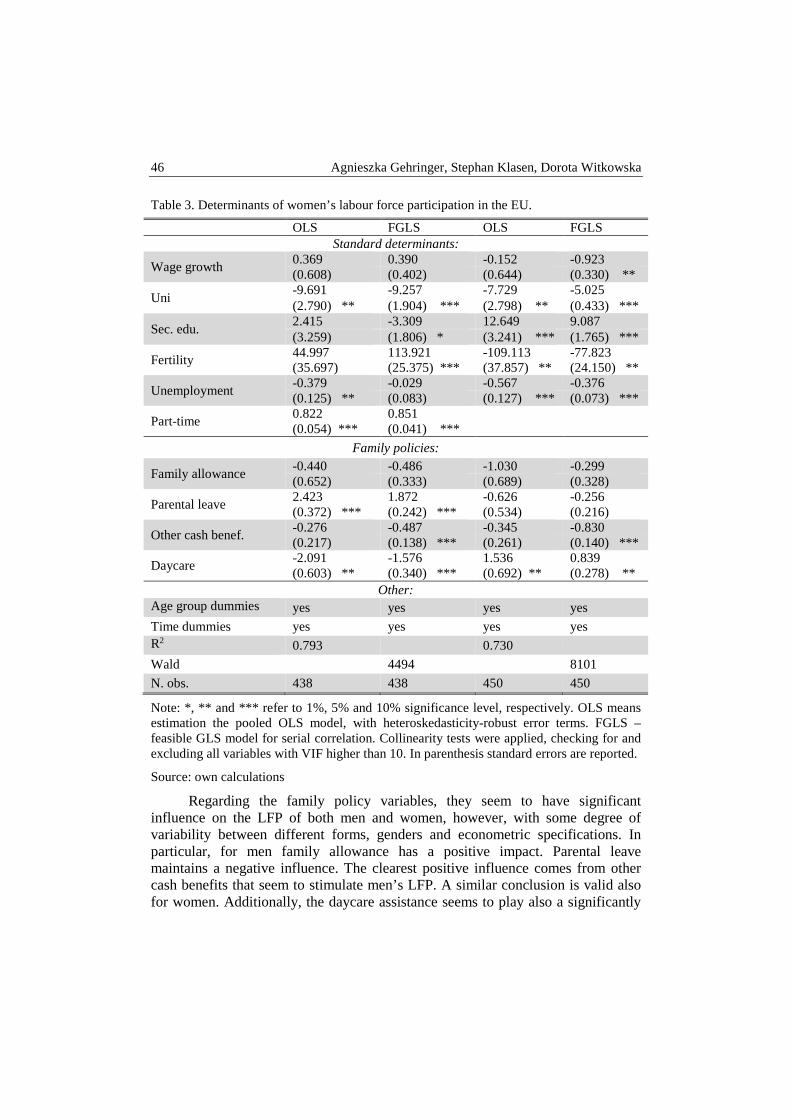
46 Agnieszka Gehringer, Stephan Klasen, Dorota Witkowska
Table 3. Determinants of women’s labour force participation in the EU.
OLS FGLS OLS FGLS Standard determinants:
Wage growth 0.369 0.390 -0.152 -0.923 (0.608) (0.402) (0.644) (0.330) **
Uni -9.691 -9.257 -7.729 -5.025 (2.790) ** (1.904) *** (2.798) ** (0.433) ***
Sec. edu. 2.415 -3.309 12.649 9.087 (3.259) (1.806) * (3.241) *** (1.765) ***
Fertility 44.997 113.921 -109.113 -77.823 (35.697) (25.375) *** (37.857) ** (24.150) **
Unemployment -0.379 -0.029 -0.567 -0.376 (0.125) ** (0.083) (0.127) *** (0.073) ***
Part-time 0.822 0.851 (0.054) *** (0.041) ***
Family policies:
Family allowance -0.440 -0.486 -1.030 -0.299 (0.652) (0.333) (0.689) (0.328)
Parental leave 2.423 1.872 -0.626 -0.256 (0.372) *** (0.242) *** (0.534) (0.216)
Other cash benef. -0.276 -0.487 -0.345 -0.830 (0.217) (0.138) *** (0.261) (0.140) ***
Daycare -2.091 -1.576 1.536 0.839 (0.603) ** (0.340) *** (0.692) ** (0.278) **
Other: Age group dummies
yes yes yes yes
Time dummies yes yes yes yes R2
0.793 0.730
Wald 4494 8101
N. obs. 438 438 450 450
Note: *, ** and *** refer to 1%, 5% and 10% significance level, respectively. OLS means estimation the pooled OLS model, with heteroskedasticity-robust error terms. FGLS – feasible GLS model for serial correlation. Collinearity tests were applied, checking for and excluding all variables with VIF higher than 10. In parenthesis standard errors are reported.
Source: own calculations
Regarding the family policy variables, they seem to have significant influence on the LFP of both men and women, however, with some degree of variability between different forms, genders and econometric specifications. In particular, for men family allowance has a positive impact. Parental leave maintains a negative influence. The clearest positive influence comes from other cash benefits that seem to stimulate men’s LFP. A similar conclusion is valid also for women. Additionally, the daycare assistance seems to play also a significantly

Labour force participation and family policies … 47
positive and strong influence in enhancing women’s labour involvement. Instead, no clear statement can be made for family allowance and for parental leave variable.
Table 4. Determinants of labour force participation for men and women – age group specific effects
Age Family policies Man Woman
15 - 24
Family allowance -1.191 -1.672 (0.509) ** (0.473)***
Parental leave -5.819 -6.500 (0.161) *** (0.259)***
Other cash benef. 0.893 0.948 (0.182) *** (0.203)***
Daycare 2.881 4.399 (0.436) *** (0.436)***
25 - 39
Family allowance 1.796 1.071 (0.256) *** (0.334)**
Parental leave -0.255 0.769 (0.173) (0.306)**
Other cash benef. 0.095 -1.164 (0.083) (0.174)***
Daycare -0.636 -0.422 (0.246) ** (0.382)
40 - 59
Family allowance -0.476 -4.939 (0.239)** (0.874)***
Parental leave -0.799 1.955 (0.092)*** (0.485)***
Other cash benef. 0.887 -0.384 (0.073)*** (0.262)
Daycare 0.965 3.635 (0.195)*** (0.831)***
Age group dummies no no
Time dummies yes yes
Wald 18628 8608
Observation number. 450 450
Note: *, ** and *** refer to 1%, 5% and 10% significance level, respectively. All estima-tions were run according to the FGLS model, accounting for heteroskedasticity and serial correlation. Collinearity tests were applied, checking for and excluding all variables with VIF higher than 10. In parenthesis standard errors are reported.
Source: own calculations
Given, however, remarkable differences in the labour force participation of both men and women and between age groups, we performed further estimations trying to disentangle such age-group specific effects of family policies. The results

48 Agnieszka Gehringer, Stephan Klasen, Dorota Witkowska
are summarized in Table 4 where we report the coefficient estimated for the interaction terms between the family policy measures and the three age-groups dummies. For brevity, we do not report the results for the standard determinants. Summarizing the results, independently of the age group and country group, family allowance exercises negative effect on labour force participation. This is true for women and almost true for men, except for the case of the first prime-age men group for whom enhanced participation due to paternal leave appeared to be the case. Also rather clear pattern of influence could be confirmed for maternity leave that for women contributed to more intensive labour force participation. Other cash benefits were influencing men almost always positively, whereas the evidence for women is mixed. Finally, similar but the reverse conclusion regards the daycare expenditures.
CONCLUSIONS
The importance of enhancing LFP of women and – related to this – of closing the gap in the labour market participation between men and women has been often confirmed in the European and national policy making. One of the ways to achieve such goals is supposed to be through adequately designed family policies. Nevertheless, due to a variety of other goals often assigned to family policies, the achievement of higher LFP is not assured.
Our study confirms generally that family policy variables have some significant influence on the LFP of both men and women. There seem, however, to exist differences between different forms, genders and age groups. In particular, family allowance has a positive impact for men. Parental leave exercises on average negative influence. The clearest positive effect on LFP of men and women comes from other cash benefits. For women the daycare assistance seems to play a particularly important role in enhancing their labour involvement. Also between the age groups differences in the influence persist. Whereas family policies were effective for the youngest women and women in the age group 40-59, the impact on the intermediate age group was very moderate.
From the policy perspective, thus, the establishment of particular forms of family policies should first of all clearly set the precise goals to achieve. Moreover, if the goal is the enhancement of labour force participation of women, the precise design of policy measures should account for significant differences in effectiveness of such policy schemes.
REFERENCES
Akgunduz Y. E., Plantenga J. (2012) Labour market effects of parental leave in Europe, Cambridge Journal of Economics, 1 – 18.
Blau D. M., Hagy A. P. (1998) The Demand for Quality in Child Care, Journal of Political Economy, 106(1), 104 – 146.

Labour force participation and family policies … 49
Blundell R., MaCurdy T. (1999) Labor Supply: a Review of Alternative Approaches, In: Ashenfelter O., Card D. (eds.), Handbook of Labor Economics, edition 1,volume 3, chapter 27, 1559 – 1695, Elsevier.
Plantega J., Remery Ch. (2009) The provision of childcare services. A comparative review of 30 European countries, DG for Employment, Social Affairs and Equal Opportunities, European Commission, Brussles.
Drukker D.M. (2003) Testing for serial correlation in linear panel-data models, Stata Journal 3, 168 – 177.
Eurofound (2013) Parenting support in Europe, accesed at: http://www.eurofound.europa. eu/pubdocs/2012/70/en/1/EF1270EN.pdf
European Commission (2009) Implementation of the Barcelona objectives concerning childcare facilities for pre-school-age children, Commission Staff Working Document accompanying the Report from the Commission to the European Parliament, the Council, the European Economic and Social Committee and the Committee of the Regions.
Genre V., Gomez Salvador R., Lamo A. (2010) European women: why do(n’t) they work, Applied Economics, 42, 1499 – 1514.
Jaumotte F. (2003) Labour force participation of women: empirical evidence on the role of policy and other determinants in OECD countries, OECD Economic Studies, No. 37, 2003/2.
Klasen S., Pieters A. (2012). Push or Pull? Drivers of Female Labor Force Participation during India’s Economic Boom, IZA Discussion Paper No. 6395.
Kumar Narayan P., Smyth R. (2006) Female labour force participation, fertility and infant mortality in Australia: some empirical evidence from Granger causality tests, Applied Economics, 39, 563 – 72.
McNown R., Ridao-Cano C. (2005) A time series model of fertility and female labour supply in the UK, Applied Economics, 37, 521 – 32.
Ruhm C.J. (1998) The Economic Consequences of Parental Leave Mandates: Lessons from Europe, The Quarterly Journal of Economics, 113(1), 285 – 317.
Sleebos J. (2003) Low Fertility Rates in OECD Countries: Facts and Policy Responses, OECD Labour Market and Social Policy Occasional Papers, No. 15, OECD Publishing.
Stiglitz J. E. (2000) Economics of the Public Sector, 3rd edition, New York, Norton. Thevenon O. (2011) Family Policies in OECD Countries: A Comparative Analysis,
Population and Development Review, 37(1), 57 – 87. Wooldridge J.M. (2002), Econometric Analysis of Cross Section and Panel Data,
Cambridge, MA, MIT Press. Xie X. (1997) Children and female labour supply behaviour, Applied Economics, 29, 1303
– 10.
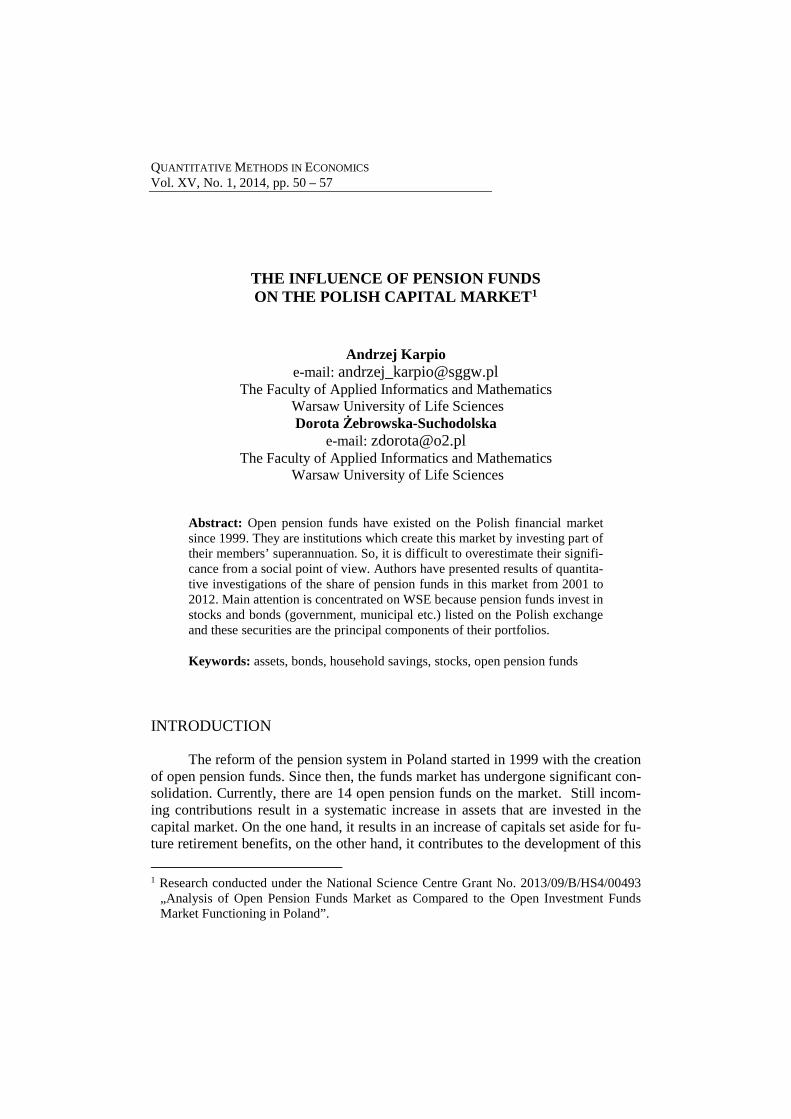
QUANTITATIVE METHODS IN ECONOMICS Vol. XV, No. 1, 2014, pp. 50 – 57
THE INFLUENCE OF PENSION FUNDS ON THE POLISH CAPITAL MARKET1
Andrzej Karpio e-mail: [email protected]
The Faculty of Applied Informatics and Mathematics Warsaw University of Life Sciences
Dorota Żebrowska-Suchodolska e-mail: [email protected]
The Faculty of Applied Informatics and Mathematics Warsaw University of Life Sciences
Abstract: Open pension funds have existed on the Polish financial market since 1999. They are institutions which create this market by investing part of their members’ superannuation. So, it is difficult to overestimate their signifi-cance from a social point of view. Authors have presented results of quantita-tive investigations of the share of pension funds in this market from 2001 to 2012. Main attention is concentrated on WSE because pension funds invest in stocks and bonds (government, municipal etc.) listed on the Polish exchange and these securities are the principal components of their portfolios.
Keywords: assets, bonds, household savings, stocks, open pension funds
INTRODUCTION
The reform of the pension system in Poland started in 1999 with the creation of open pension funds. Since then, the funds market has undergone significant con-solidation. Currently, there are 14 open pension funds on the market. Still incom-ing contributions result in a systematic increase in assets that are invested in the capital market. On the one hand, it results in an increase of capitals set aside for fu-ture retirement benefits, on the other hand, it contributes to the development of this
1 Research conducted under the National Science Centre Grant No. 2013/09/B/HS4/00493
„Analysis of Open Pension Funds Market as Compared to the Open Investment Funds Market Functioning in Poland”.

The Influence of Pension Funds on the Polish Capital … 51
market. In this article, the second aspect of the functioning of pension funds over the years from 2001 to 2012 is shown in summary. The work is more qualitative than quantitative. No econometric or financial indicators are calculated, while the focus is on showing the importance and impact of open pension funds on govern-ment debt, savings of the society and Warsaw Stock Exchange. Quantitative ap-proach can be found in [Chybalski 2013, s. 77-89], [Sawicz 2012, s. 306-322] as well as the comparison of open pension funds and open-end stable funds markets was done in the work [Karpio, Żebrowska-Suchodolska 2012, s. 91-110].
CHANGES OF THE ASSETS OF PENSION FUNDS
In contrast to the type of collective investment institutions of open invest-ment funds type, pension funds have a guaranteed supply of payments. Thus, their marketing activities are aimed only at persuading individuals starting their em-ployment to choose a particular fund, or stop existing members from changing the fund. In practice, few people consciously make a selection and rely on the result of drawing. Transfer of members is relatively small. All these factors contribute to the fact that, from the start of their activity, business assets invested in pension funds grew steadily. Changes over the years 2001-2012 are shown in Figure 1.
Figure 1. The value of open pension fund assets in thousands PLN (as of 31 December)
* status as of quarter 2
Source: own study based on the Financial Supervision Authority data
-
50 000 000
100 000 000
150 000 000
200 000 000
250 000 000
2001 2002 2003 2004 2005 2006 2007 2008 2009 2010 2011 2012*
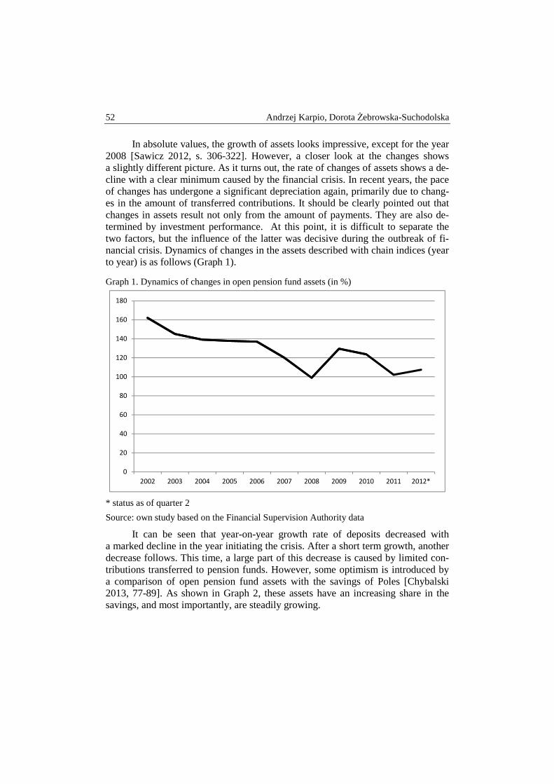
Andrzej Karpio, Dorota Żebrowska-Suchodolska 52
In absolute values, the growth of assets looks impressive, except for the year 2008 [Sawicz 2012, s. 306-322]. However, a closer look at the changes shows a slightly different picture. As it turns out, the rate of changes of assets shows a de-cline with a clear minimum caused by the financial crisis. In recent years, the pace of changes has undergone a significant depreciation again, primarily due to chang-es in the amount of transferred contributions. It should be clearly pointed out that changes in assets result not only from the amount of payments. They are also de-termined by investment performance. At this point, it is difficult to separate the two factors, but the influence of the latter was decisive during the outbreak of fi-nancial crisis. Dynamics of changes in the assets described with chain indices (year to year) is as follows (Graph 1).
Graph 1. Dynamics of changes in open pension fund assets (in %)
* status as of quarter 2
Source: own study based on the Financial Supervision Authority data
It can be seen that year-on-year growth rate of deposits decreased with a marked decline in the year initiating the crisis. After a short term growth, another decrease follows. This time, a large part of this decrease is caused by limited con-tributions transferred to pension funds. However, some optimism is introduced by a comparison of open pension fund assets with the savings of Poles [Chybalski 2013, 77-89]. As shown in Graph 2, these assets have an increasing share in the savings, and most importantly, are steadily growing.
0
20
40
60
80
100
120
140
160
180
2002 2003 2004 2005 2006 2007 2008 2009 2010 2011 2012*
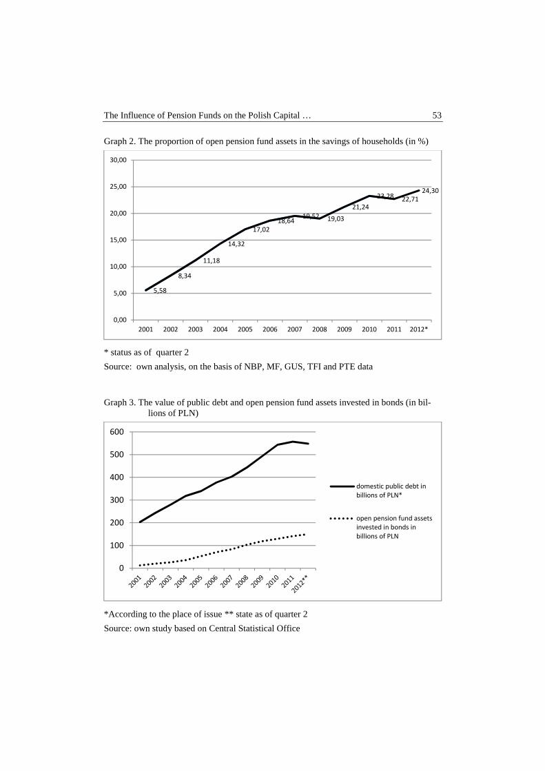
The Influence of Pension Funds on the Polish Capital … 53
Graph 2. The proportion of open pension fund assets in the savings of households (in %)
* status as of quarter 2
Source: own analysis, on the basis of NBP, MF, GUS, TFI and PTE data
Graph 3. The value of public debt and open pension fund assets invested in bonds (in bil-lions of PLN)
*According to the place of issue ** state as of quarter 2
Source: own study based on Central Statistical Office
5,58
8,34
11,18
14,32
17,02
18,6419,52 19,03
21,24
23,28 22,71
24,30
0,00
5,00
10,00
15,00
20,00
25,00
30,00
2001 2002 2003 2004 2005 2006 2007 2008 2009 2010 2011 2012*
0
100
200
300
400
500
600
domestic public debt in
billions of PLN*
open pension fund assets
invested in bonds in
billions of PLN
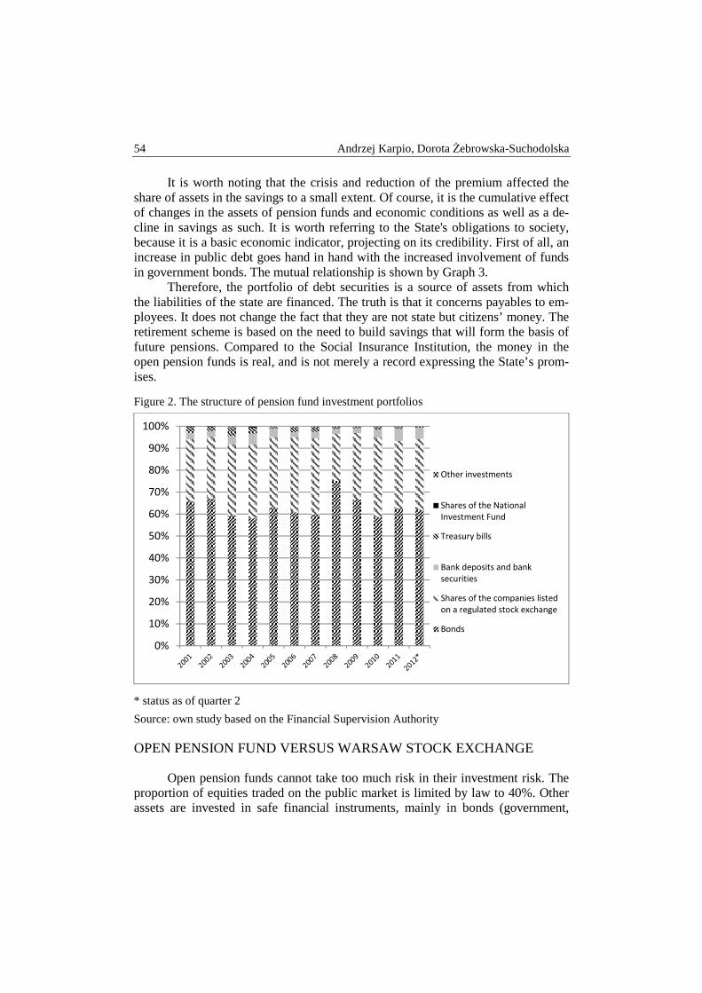
Andrzej Karpio, Dorota Żebrowska-Suchodolska 54
It is worth noting that the crisis and reduction of the premium affected the share of assets in the savings to a small extent. Of course, it is the cumulative effect of changes in the assets of pension funds and economic conditions as well as a de-cline in savings as such. It is worth referring to the State's obligations to society, because it is a basic economic indicator, projecting on its credibility. First of all, an increase in public debt goes hand in hand with the increased involvement of funds in government bonds. The mutual relationship is shown by Graph 3.
Therefore, the portfolio of debt securities is a source of assets from which the liabilities of the state are financed. The truth is that it concerns payables to em-ployees. It does not change the fact that they are not state but citizens’ money. The retirement scheme is based on the need to build savings that will form the basis of future pensions. Compared to the Social Insurance Institution, the money in the open pension funds is real, and is not merely a record expressing the State’s prom-ises.
Figure 2. The structure of pension fund investment portfolios
* status as of quarter 2
Source: own study based on the Financial Supervision Authority
OPEN PENSION FUND VERSUS WARSAW STOCK EXCHANGE
Open pension funds cannot take too much risk in their investment risk. The proportion of equities traded on the public market is limited by law to 40%. Other assets are invested in safe financial instruments, mainly in bonds (government,
0%
10%
20%
30%
40%
50%
60%
70%
80%
90%
100%
Other investments
Shares of the National
Investment Fund
Treasury bills
Bank deposits and bank
securities
Shares of the companies listed
on a regulated stock exchange
Bonds

The Influence of Pension Funds on the Polish Capital … 55
municipal, corporate). The structure of investment portfolios is presented as fol-lows (Figure 2):
Depending on the year, the share of stocks is now around 30% and the bonds between 60% -70%. Therefore, these instruments form the basis of investments made by pension funds. From the point of view of the Stock Exchange, they are a major investor. Their share in the market capitalization is shown by the next fig-ure.
Figure 3. The proportion of shares from the portfolio of open pension funds in the stock market capitalization (in %)
Source: own study based on the Financial Supervision Authority and the Warsaw Stock Ex-change data. * status as of quarter 2
If we combine the changes in market capitalization over the years, this situa-tion is as follows. Again, the impact of financial crisis can be observed, but as of 2008 a dynamic increase in the open pension funds in the capitalization of the Stock Exchange follows. It is so large that it cannot be ignored. Due to statutory prudential requirements, pension fund investments cannot be and are not too risky. As a result, they are limited to large liquid companies. Furthermore, the invest-ments are not made overnight, mainly because of the scale of purchases. Assuming somewhat arbitrarily that the characteristic period of change in the portfolio is comparable with the period of payment of pension contributions, i.e. it takes place every month, the graph below shows a 30-day average of WIG 20 index.
It is clear that the share of assets invested in equities is steadily growing. What's more, the crisis has very little impact on the situation - only within one year. It can be inferred from this that pension funds are extremely important inves-
4,08
7,73
8,52
7,10
6,41 6,26
4,48
6,37
7,59
10,08
10,84
11,72
0
2
4
6
8
10
12
14
2001 2002 2003 2004 2005 2006 2007 2008 2009 2010 2011 2012*
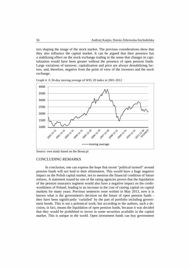
Andrzej Karpio, Dorota Żebrowska-Suchodolska 56
tors shaping the image of the stock market. The previous considerations show that they also influence the capital market. It can be argued that their presence has a stabilizing effect on the stock exchange trading in the sense that changes in capi-talization would have been greater without the presence of open pension funds. Large variations of turnover, capitalization and price are always destabilizing fac-tors, and, therefore, negative from the point of view of the investors and the stock exchange.
Graph 4. A 30-day moving average of WIG 20 index in 2001-2012
Source: own study based on the Bossa.pl
CONCLUDING REMARKS
In conclusion, one can express the hope that recent "political turmoil" around pension funds will not lead to their elimination. This would have a huge negative impact on the Polish capital market, not to mention the financial condition of future retirees. A statement issued by one of the rating agencies proves that the liquidation of the pension insurance segment would also have a negative impact on the credit-worthiness of Poland, leading to an increase in the cost of raising capital on capital markets for many years. Previous sentences were written in May 2013, now it is known what is the government's decision on the future of open pension funds - they have been significantly ‘curtailed’ by the part of portfolio including govern-ment bonds. This is not a polemical work, but according to the authors, such a de-cision, in fact, means the liquidation of open pension funds, because it was decided that they would be prohibited to invest in some securities available in the capital market. This is unique in the world. Open investment funds can buy government
1000
1500
2000
2500
3000
3500
4000
moving average
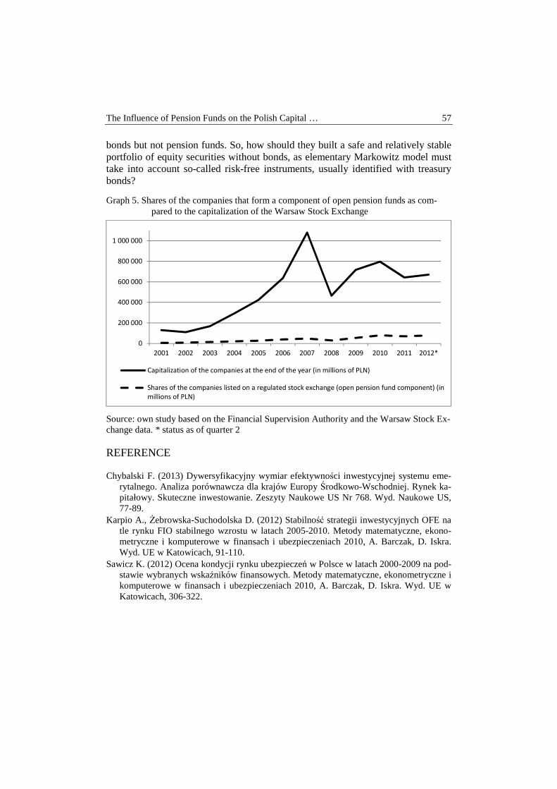
The Influence of Pension Funds on the Polish Capital … 57
bonds but not pension funds. So, how should they built a safe and relatively stable portfolio of equity securities without bonds, as elementary Markowitz model must take into account so-called risk-free instruments, usually identified with treasury bonds?
Graph 5. Shares of the companies that form a component of open pension funds as com-pared to the capitalization of the Warsaw Stock Exchange
Source: own study based on the Financial Supervision Authority and the Warsaw Stock Ex-change data. * status as of quarter 2
REFERENCE
Chybalski F. (2013) Dywersyfikacyjny wymiar efektywności inwestycyjnej systemu eme-rytalnego. Analiza porównawcza dla krajów Europy Środkowo-Wschodniej. Rynek ka-pitałowy. Skuteczne inwestowanie. Zeszyty Naukowe US Nr 768. Wyd. Naukowe US, 77-89.
Karpio A., Żebrowska-Suchodolska D. (2012) Stabilność strategii inwestycyjnych OFE na tle rynku FIO stabilnego wzrostu w latach 2005-2010. Metody matematyczne, ekono-metryczne i komputerowe w finansach i ubezpieczeniach 2010, A. Barczak, D. Iskra. Wyd. UE w Katowicach, 91-110.
Sawicz K. (2012) Ocena kondycji rynku ubezpieczeń w Polsce w latach 2000-2009 na pod-stawie wybranych wskaźników finansowych. Metody matematyczne, ekonometryczne i komputerowe w finansach i ubezpieczeniach 2010, A. Barczak, D. Iskra. Wyd. UE w Katowicach, 306-322.
0
200 000
400 000
600 000
800 000
1 000 000
2001 2002 2003 2004 2005 2006 2007 2008 2009 2010 2011 2012*
Capitalization of the companies at the end of the year (in millions of PLN)
Shares of the companies listed on a regulated stock exchange (open pension fund component) (in
millions of PLN)
QUANTITATIVE METHODS IN ECONOMICS Vol. XV, No. 1, 2014, pp. 58 – 65
“SECURITY THROUGH DIVERSITY”: PORTFOLIO DIVERSIFICATION OF PRIVATE PENSION FUNDS 1
Krzysztof Kompa Katedra Ekonometrii i Statystyki, SGGW w Warszawie
e-mail: [email protected] Tomasz Wiśniewski
Giełda Papierów Wartościowych w Warszawie e-mail: [email protected]
Abstract: The program for pension system reform, launched at the beginning of 1997 in Poland, was called by its authors “Security through Diversity”. This title emphasizes that pension reform, which is designed to guarantee security for the insured, has to combine pay-as-you-go pillar together with mandatory, fully funded pillar as well as voluntary, funded pillar. This paper discusses consequences of the changes implemented in the year 2013 and consequently analyzes the changes in the composition of the pension funds’ portfolio, in particular the prohibition of investing in debt securities issued and guaranteed by the State Treasury.
Keywords: open pension funds (OFE), pension system reform, portfolio effectivity, investment strategies
INTRODUCTION
Reform of the pension system in Poland, which took place in 1999, was a symptom of new and complex thinking about social policy and economy as integrity instead of treating them as opposing issues. The original reform replaced the one-pillar – pay as you go system (PAYG), by the three-pillars funded system, based on the general rule that expected discounted sum of withdrawals from the system equals discounted sum of payments enlarged by the return on capital. Such
1 Research conducted under the National Science Centre Grant No. 2013/09/B/HS4/00493 „Analysis of Open Pension Funds Market as Compared to the Open Investment Funds Market Functioning in Poland”.
“Security Through Diversity”: diversification… 59
system intends to provide pensioners adequate income compared with the level of wages, which they had been obtained during their activity in the labor market. This program of the pension system reform was called by its authors “Security through Diversity” [Security 1997].
Under the system introduced in 1999, pension benefits consist of three pillars. The first and second pillars are universal and mandatory, and the third one voluntary. The first pillar remained to be pay-as-you-go financed, whereas the second and third pillars are to be funded. In fact PAYG system was downsized and converted to a “notional defined-contribution” system, forming the new first pillar. In both the first and the second, funded pillar, contributions are registered in individual accounts, and the pension benefit depends on contributions paid, not contributions that were due2.
The second pillar is the base for the creation of Open Pension Funds (OFE in Polish: Otwarty Fundusz Emerytalny). Each participant is allowed to choose its fund, and is also able to change funds with no charge or penalty after a statutory minimum of 12-month period of contribution to a fund. Each person can select only one fund. There is free choice between the funds which means that pension funds are not permitted to reject entry or restrict the right to transfer to another funds, either directly or indirectly, through the imposition of fees. Pension funds operate like other open mutual funds. However their effectiveness is evaluated due to the average return of all pension funds.
The first manipulation in original pension reform was made in 2011 when the contribution to pension funds was reduced from 7.3% to 2.3% of monthly wages. The new law, which went into affect in February 2014, shifts 51.5% of the assets, held by the OFEs (about 150 billions PLN) to the state-run PAYG pension system i.e., to the Social Insurance Institution (ZUS), including all debt securities issued and guaranteed by the State Treasury. According to the new regulations, pension funds are no longer obligatory and each employed person has four months every four years to decide whether 2.92 percent of their income goes to a chosen private fund or to ZUS. The overhaul of the pension system also concerns changes in the OFEs’ investment portfolio since private pension funds are no longer allowed to invest in government bonds3. That leaves the pension funds with most of their assets held in shares of companies listed on the Warsaw Stock Exchange and give them an increasingly peripheral role in the future retirement benefits of Polish citizens.
Therefore, the aim of this research is to analyze the consequences of the introduced changes in the pension funds’ portfolio composition, especially the
2 Detailed description of the pension reform can be found in [Góra, Rutkowski 2000],
[Hausner, 2002] among others. 3 It is worth mentioning that however President Bronisław Komorowski signed the bill in-
troducing changes to Poland's pension system, he also asked the Constitutional Tribunal to review the regulation [President 2013].
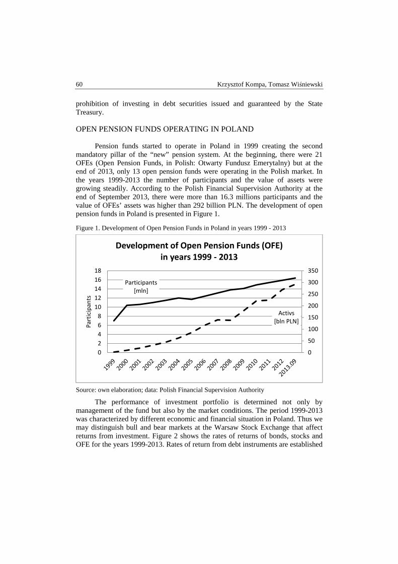
60 Krzysztof Kompa, Tomasz Wiśniewski
prohibition of investing in debt securities issued and guaranteed by the State Treasury.
OPEN PENSION FUNDS OPERATING IN POLAND
Pension funds started to operate in Poland in 1999 creating the second mandatory pillar of the “new” pension system. At the beginning, there were 21 OFEs (Open Pension Funds, in Polish: Otwarty Fundusz Emerytalny) but at the end of 2013, only 13 open pension funds were operating in the Polish market. In the years 1999-2013 the number of participants and the value of assets were growing steadily. According to the Polish Financial Supervision Authority at the end of September 2013, there were more than 16.3 millions participants and the value of OFEs’ assets was higher than 292 billion PLN. The development of open pension funds in Poland is presented in Figure 1.
Figure 1. Development of Open Pension Funds in Poland in years 1999 - 2013
Source: own elaboration; data: Polish Financial Supervision Authority
The performance of investment portfolio is determined not only by management of the fund but also by the market conditions. The period 1999-2013 was characterized by different economic and financial situation in Poland. Thus we may distinguish bull and bear markets at the Warsaw Stock Exchange that affect returns from investment. Figure 2 shows the rates of returns of bonds, stocks and OFE for the years 1999-2013. Rates of return from debt instruments are established
Participants
[mln]
Activs
[bln PLN]
0
50
100
150
200
250
300
350
0
2
4
6
8
10
12
14
16
18
Pa
rtic
ipa
nts
Development of Open Pension Funds (OFE)
in years 1999 - 2013
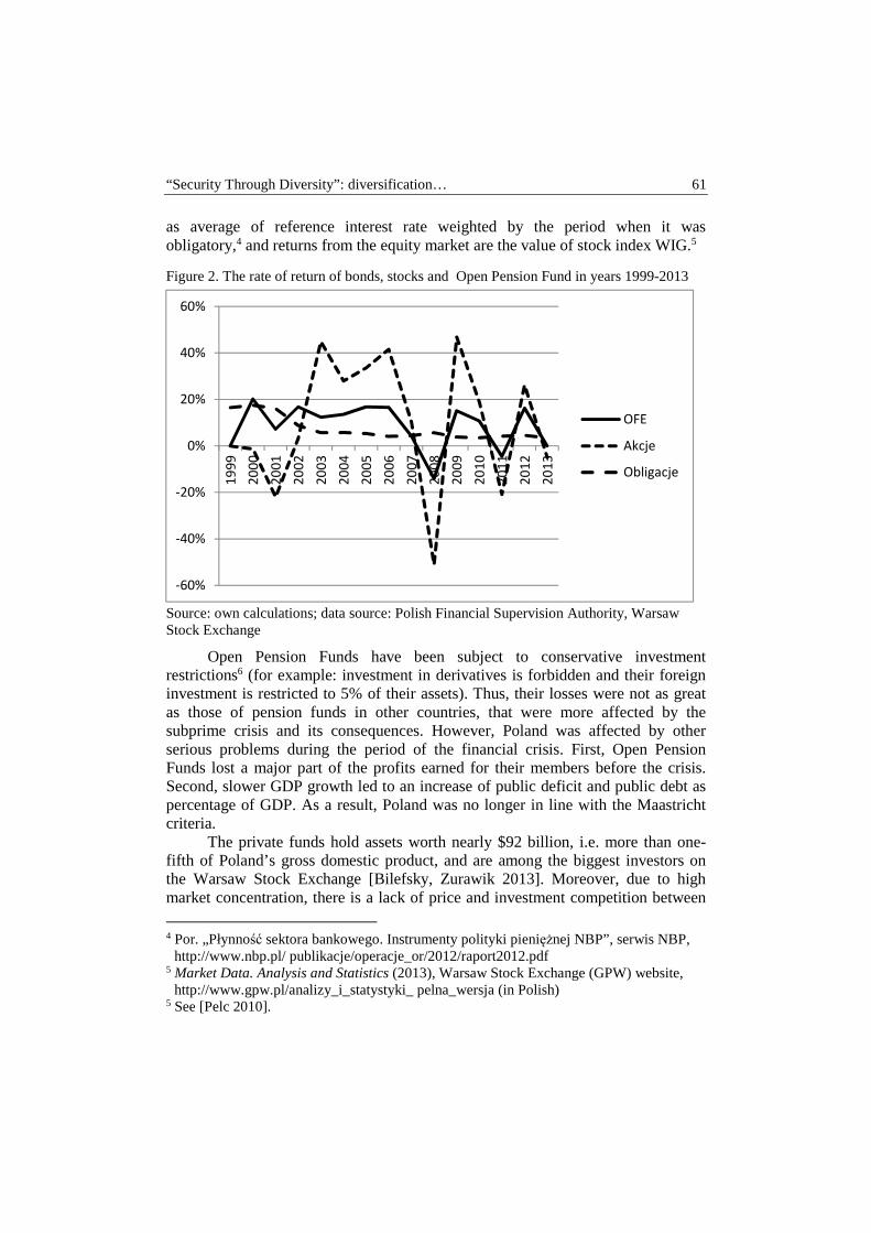
“Security Through Diversity”: diversification… 61
as average of reference interest rate weighted by the period when it was obligatory,4 and returns from the equity market are the value of stock index WIG.5
Figure 2. The rate of return of bonds, stocks and Open Pension Fund in years 1999-2013
Source: own calculations; data source: Polish Financial Supervision Authority, Warsaw Stock Exchange
Open Pension Funds have been subject to conservative investment restrictions6 (for example: investment in derivatives is forbidden and their foreign investment is restricted to 5% of their assets). Thus, their losses were not as great as those of pension funds in other countries, that were more affected by the subprime crisis and its consequences. However, Poland was affected by other serious problems during the period of the financial crisis. First, Open Pension Funds lost a major part of the profits earned for their members before the crisis. Second, slower GDP growth led to an increase of public deficit and public debt as percentage of GDP. As a result, Poland was no longer in line with the Maastricht criteria.
The private funds hold assets worth nearly $92 billion, i.e. more than one-fifth of Poland’s gross domestic product, and are among the biggest investors on the Warsaw Stock Exchange [Bilefsky, Zurawik 2013]. Moreover, due to high market concentration, there is a lack of price and investment competition between
4 Por. „Płynność sektora bankowego. Instrumenty polityki pieniężnej NBP”, serwis NBP,
http://www.nbp.pl/ publikacje/operacje_or/2012/raport2012.pdf 5 Market Data. Analysis and Statistics (2013), Warsaw Stock Exchange (GPW) website,
http://www.gpw.pl/analizy_i_statystyki_ pelna_wersja (in Polish) 5 See [Pelc 2010].
-60%
-40%
-20%
0%
20%
40%
60%
19
99
20
00
20
01
20
02
20
03
20
04
20
05
20
06
20
07
20
08
20
09
20
10
20
11
20
12
20
13
OFE
Akcje
Obligacje
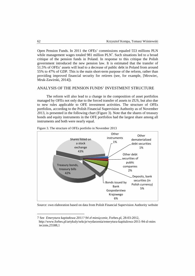
62 Krzysztof Kompa, Tomasz Wiśniewski
Open Pension Funds. In 2011 the OFEs’ commissions equaled 553 millions PLN while management wages totaled 981 million PLN7. Such situations led to a broad critique of the pension funds in Poland. In response to this critique the Polish government introduced the new pension law. It is estimated that the transfer of 51.5% of OFEs’ assets will lead to a decrease of public debt in Poland from around 55% to 47% of GDP. This is the main short-term purpose of the reform, rather than providing improved financial security for retirees (see, for example, [Mrowiec, Mruk-Zawirski, 2014]).
ANALYSIS OF THE PENSION FUNDS’ INVESTMENT STRUCTURE
The reform will also lead to a change in the composition of asset portfolios managed by OFEs not only due to the forced transfer of assets to ZUS, but also due to new rules applicable to OFE investment activities. The structure of OFEs portfolios, according to the Polish Financial Supervision Authority as of November 2013, is presented in the following chart (Figure 3). Note that the shares of treasury bonds and equity instruments in the OFE portfolios had the largest share among all instruments and both were nearly equal.
Figure 3. The structure of OFEs portfolio in November 2013
Source: own elaboration based on data from Polish Financial Supervision Authority website
7 See Emerytura kapitałowa 2011? 94 zł miesięcznie, Forbes.pl, 28-03-2012, http://www.forbes.pl/artykuly/sekcje/wydarzenia/emerytura-kapitalowa-2011-94-zl-mies
iecznie,25588,1
Other
dematerialized
debt securities
1%
Other debt
securities of
public
companies
2%
Deposits, bank
securities (in
Polish currency)
5%
Bonds issued by
Bank
Gospodarstwa
Krajowego
6%
Treasury bonds,
treasury bills
42%
Shares listed on
a stock
exchange
43%
Other
instruments
1%

“Security Through Diversity”: diversification… 63
This paper evaluates the impact of the prohibition of investment in government’s securities by simulating the performance of the portfolios containing treasury bonds and shares. Therefore, we construct hypothetical OFE portfolios characterized by different structure of shares listed on the Warsaw Stock Exchange and debt securities issued by the State Treasury (see Table 1). We assume that the portfolio structure is the same in the whole analyzed period i.e., in the years 1999-2013. We also assume that superannuation in the first year equaled 5,000 PLN and it was rising by 4% annually. Transaction costs are ommited.
Table 1. Structure of constructed portfolios
Sym
bo
l of
po
rtfo
lio
Percentage share of
Sym
bo
l of
po
rtfo
lio
Percentage share of shares listed on the Warsaw Stock Exchange
debt securities issued and guaranteed by the State Treasury
shares listed on the Warsaw Stock Exchange
debt securities issued and guaranteed by the State Treasury
100-0 100 0 40-60 40 60 90-10 90 10 30-70 30 70 80-20 80 20 20-80 20 80 70-30 70 30 10-90 10 90 60-40 60 40 0-10 0 100 50-50 50 50
Source: Own elaboration
Simulation of the returns for the whole period of investigation includes different market tendencies observed in Poland. Figures 4 and 5 contain compari-sons of simulated results obtained by hypothetical portfolios and OFE.
The results demonstrates that neither portfolio containing 100% of debt instruments nor the one including only shares generate the best financial performance. It is also visible that the rates of return from “average” Open Pension Fund are worse than returns from hypothetical portfolios i.e., OFEs could have generated better results. The portfolio containing 30% of treasury bonds and 70% of shares obtains the best result, and the fund containing 40% of bonds and 60% of equity instruments is only slightly worse.
CONCLUSION
Presented analysis is biased by the assumptions that are made to provide the simulation experiments. Although we use real data, we also assume that the portfolio structure is constant during the whole period of investigation, and the stable increase of superannuation. It is worth mentioning that situation in Poland, observed in the years 1999-2013, was characterized by essential changes. Thus, our simulations cover all types of possible tendencies of the Polish capital market. The conclusion from the simulations indicates that changes in the program and law is

64 Krzysztof Kompa, Tomasz Wiśniewski
required to achive higher returns to the most vulnerable part of the society i.e., pensioners’’.
Figure 3. Cumulative return on OFE hypothetical portfolios in years 1999-2013
Source: own calculation
Figure 4. Cumulative return on OFE hypothetical portfolios; investment period 1999-2013
Source: own calculation
0
20 000
40 000
60 000
80 000
100 000
120 000
140 000
160 000
180 000
200 000
199920002001200220032004200520062007200820092010201120122013
100-0 90-10 80-20 70-30 60-40 50-50
40-60 30-70 20-80 10-90 0-100 OFE
100-0 90-10 80-20 70-30 60-40 50-50 40-60 30-70 20-80 10-90 0-100 OFE
portfel 148 74 155 04 160 74 165 69 169 75 172 76 174 55 174 99 173 92 171 21 166 73 173 08
174 997173 088
135 000
140 000
145 000
150 000
155 000
160 000
165 000
170 000
175 000
180 000
“Security Through Diversity”: diversification… 65
Therefore taking into account the new Polish government regulations and the results of our simulations we state that the prohibition of investment in government’s debt by Open Pension Funds in Poland is unacceptable. It leads to an increase of risk and decrease of the efficiency of investments made by pension funds. The watchword “Security through Diversity” has been still valid also in construction of OFEs’ portfolios and the new government regulations seem to be contrary to future interest of the Polish pensioners’. This paper calls for reform in line with the results of this research. At the end all Poles will become pensioners.
REFERENCES
Bilefsky D., Zurawik M. (2013) Polish Plan on Pensions Arouses Sharp Criticism, The New York Times. October, 9, 2013, http://www.nytimes.com/2013/10/10/business/ international/polish-plan-on-pensions-arouses-sharp-criticism.html?_r=0
Góra M., Rutkowski M. (2000) The quest for pension reform : Poland's security through diversity, William Davidson Institute Working Papers Series 286, William Davidson Institute at the University of Michigan, USA, http://deepblue.lib.umich.edu/bitstream/ handle/2027.42/39670/wp286.pdf?sequence=3
Góra M. (2001) Koszty, oszczędności oraz efekty zewnętrzne związane z wprowadzeniem nowego system emerytalnego, Zeszyty BRE Bank – CASE, nr 57, 7-36, Warszawa.
Emerytura kapitałowa 2011? 94 zł miesięcznie, Forbes.pl, 28-03-2012, http://www.for bes.pl/artykuly/sekcje/wydarzenia/emerytura-kapitalowa-2011-94-zl-miesiecznie, 25588,1
Hausmer J. (2002) Poland Security through Diversity, Feldstein M. and Siebert H. (ed.), Social Security Pension Reform in Europe University of Chicago Press, 349 – 364, http://www.nber.org/chapters/c10678.pdf
Market Data. Analysis and statistics (2013), Warsaw Stock Exchange (GPW) website, http://www.gpw.pl/analizy_i_statystyki_ pelna_wersja (in Polish)
Mrowiec Z., Mruk-Zawirski P (2014) How the Polish pension fund reform will affect the fund’s investments, Allen and Overy, Warsaw, Poland.
Pelc P. (2010) Polish Pension Reform – Lost Decade? http://www.pawelpelc.pl/index.ph p?display=5&artykul=167
Płynność sektora bankowego. Instrumenty polityki pieniężnej NBP (2012), serwis NBP, http://www.nbp.pl/publikacje/operacje_or/2012/raport2012.pdf
President signs pension reform (2013) Warsaw Bussiness Journal, December, 30, 2013, http://www.wbj.pl/article-64697-president-signs-pension-reform.html
Rozłucki W. (2001) Znaczenie funduszy emerytalnych dla rozwoju Warszawskiej Giełdy Papierów Wartościowych, BRE Bank – CASE, nr 57, 37-41, Warszawa.
Security (1997) Security through diversity: Reform of the pension system in Poland, Warsaw: Office of the Government Plenipotentiary for Social Insurance Reform.

QUANTITATIVE METHODS IN ECONOMICS Vol. XV, No. 1, 2014, pp. 66 – 75
GENDER DIFFERENCES IN EXIT RATES FROM UNEMPLOYMENT IN POLAND
Joanna Małgorzata Landmesser Department of Econometrics and Statistics, Warsaw University of Life Sciences
e-mail: [email protected]
Abstract: The behaviour of women and men in the labour market is diverse. Traditionally, men have closer attachment to the labour market. Women, however, have more family responsibilities. In the paper, we analyse the exit rates from unemployment for each sex separately, and find out that the effects of the explanatory variables in estimated duration models depend upon gender. We begin our study with a single risk hazard model. These estimations are extended to a competing risks model with two destinations: employment and non-participation.
Keywords: gender differences, exit rates from unemployment, duration models, hazard
INTRODUCTION
Men and women behave differently in the labour market. Usually, men are more involved in the labour market, and women spend more time with family. It is thought that women have a weaker position in the labour market than men, especially these with young children. Women are often discriminated against even if their qualifications and job-search activity are higher than for men.
The literature, which refers to the study of gender inequality in the labour force participation or in wages, is extensive (e.g. [Altonji, Blank 1999] for a survey of these topics). However, studies that examine differences in the exit rates from unemployment are much rarer. Sex is an important variable affecting the movements between labour market states and it is a significant factor in determining the chances of finding a job. Some studies have shown that women are exposed to more frequent periods without work ([Steiner 1989], [Jensen, Wester-gard-Nielsen 1990]), and have a lower probability of finding a new job [Katz, Meyer 1990b], especially on a permanent basis [Edin 1989].

Gender differences in exit rates from unemployment … 67
Numerous empirical research that study the exit rates from unemployment in Poland disregard the issue of gender behaviour in the labour market. Most of these studies do not consider that the effect of different factors may depend on gender. They point out that gender only shifts the dependent variable in econometric models and do not estimate separate equations for men and women (see [Landmesser 2008b], [Stolorz 2010]). The opposite approach was applied abroad by [Gonzalo and Saarela 2000] or [Tansel, Taşçi 2010] and for Poland by [Landmesser 2008a], who estimated separate hazard models for both sexes.
Our study focuses on a deeper examination of the differences in the exit rates by gender. In the paper, we analyze the flows between labour market states and estimate duration models for the probability of leaving unemployment. We investigate the exit rates from unemployment for each sex separately and find out that the effects of the explanatory variables in estimated duration models depend on gender. We start our study with a single risk hazard model. These estimations are extended to a competing risks model with two destinations: employment and non-participation.
DATABASE USED IN THE STUDY
The empirical research is based on data from the Labour Force Survey in Poland (LFS) in 2008. The survey focuses on the situation of population from the viewpoint of economic activity of people, i.e. the fact of being employed, unemployed or economically inactive during the reference week. Based on the retrospective questions in LFS-questionnaire we can specify how long a person is unemployed or how long he was unemployed and whether the exit was to the employment or to non-participation (“out-of-labour-force”-state).
Six mini panels were created for the study, each of them included two neighbouring quarters. Of all people involved in the LFS in 2008 only those that were in the samples 35, 36, 37, 39, 40 and 41 were selected. In the next step, from the sample individuals who were not unemployed because they either worked or were inactive were removed. We chose only observations for people of working age. In this way the whole LFS-sample has been limited to a subsample of 2639 persons aged 18-65, who are or were unemployed at least for one month. At the end of the study, these people were either employed (377 persons) or out-of-labour-force (229) (economically inactive) or still classified as unemployed (2033).
Table 1. Distribution of unemployment spells by destination and gender
Gender Destination Total Censored Employment Non-participation
Male 984 (77.1%) 205 (16.1%) 87 (6.8%) 1276 (100%) Female 1049 (77.0%) 172 (12.6%) 142 (10.4%) 1363 (100%)
Source: own calculations

Joanna Małgorzata Landmesser 68
The unemployment spells ended due to employment are 16.1% for men and 12.6% for women, while those in the case of transition into OLF-state are 6.8% and 10.4% respectively. (Table 1). The individual unemployment duration (in months) for each person built a variable duration (T). The mean unemployment duration is 12.19 months for uncensored spells and 15.06 months for censored spells. For men, the average duration of unemployment is 12 months for spells that ended due to employment, whereas it is 11.01 months for those who completed due to the lack of participation. For the sample of women, the corresponding numbers are 9.36 and 16.62 months.
METHOD OF THE ANALYSIS
The variable we are interested in is the duration of time an individual spends in the unemployment state (T). An appropriate approach, which considers right censoring of unemployment spells, and which controls characteristics of individuals that influence the unemployment duration, is the use of hazard models [Lancaster 1979]. The survivor function gives the probability that the duration exceeds a moment t: �(�) = Pr[ > 1] = 1 − �(�). S(t) is the probability of surviving past t. Kaplan-Meier nonparametric estimate of survival function is given
by ����� = ∏ (
�����
��)
���� , where nk – number of individuals at risk at time tk,
dk – number of failures at time tk. The most frequently applied demonstration of the duration period
distribution is hazard function. The hazard function is the instantaneous probability
of leaving a certain state conditional on survival to time t: ℎ(�) =�(�)
�(�)=
lim��→#
$%[�&'(�)��|'+�]
��. The hazard function h(t) is the limit of probability that the
spell is completed during the interval [t, t+dt] given that it has not been completed before the time t, for dt→0.The hazard rates describe the intensity of transition from one state to another (for the theoretical backgrounds see [Kalbfleisch, Prentice 1980], [Cox, Oakes 1984]).
Hazard models usually comprise present duration of the phenomenon as a determinant for the probability of its occurrence and also other parameters. In the proportional hazard models, the conditional hazard rate ℎ(�|,) can be factored into separate functions: ℎ(�|,) = ℎ#(�)exp(,12), where ℎ#(�) is called the baseline hazard, exp(,12)is a function of explanatory variables vector x. Cox’s approach to the proportional hazard model is the semiparametric method of analysing the effect of covariates on the hazard rate [Cox 1972]. In the Cox model ℎ(�|,) =
ℎ#(�)3,4(,12) and the baseline hazard ℎ#(�) is estimated non-parametrically.

Gender differences in exit rates from unemployment … 69
RESULTS OF MODELS ESTIMATION
We begin with a descriptive analysis of the duration data. The first step is to plot the Kaplan-Meier survival curves for all exits from unemployment according to sex (Fig. 1A). The survival curves decline slowly. It shows that either women or men are more likely to remain unemployed.
Figure 1. Plots of the Kaplan-Meier survival curves and smoothed hazard functions for all exits from unemployment according to sex
Exit from unemployment
(A) (B)
Source: own computations using Stata Statistical Software
In Figure 1B we plot the estimates of the hazard functions. The hazard of exit from unemployment first, declines rapidly and then, increases for both sexes in a similar manner. There is no difference between men and women.
In many situations, there are several possible risks of failure. The competing risks model formulation is applicable to modelling time in one state when the exit occurs to a number of competing states [Narendranathan, Stewart 1993]. Since determinants of the exit rate and their effects depend on the destination state, we distinguish between two possible destinations from unemployment: employment and non-participation (“out-of-labour-force”-state).
In Figure 2, we plot the survival functions for exits into employment and into OLF according to sex. Fig. 2A shows that in the case of exits into employment, women are more likely to remain unemployed than men. Fig. 2B shows that in the case of exits into OLF, men are more likely to remain unemployed than women. The results achieved from the Log-rank test for the equality of survivor functions confirmed the findings (p-values in the Log-rank test for equality of survivor functions are respectively 0.0317 and 0.0197). The variable gender does not distinguish in a statistically significant manner between survival function for exits from unemployment in any other state, but gender plays an important role for the exits in two separate states: a state of employment and OLF-state.
0.00
0.25
0.50
0.75
1.00
0 20 40 60 80 100analysis time
gender = 0 gender = 1
Kaplan-Meier survival estimates
.008
.01
.012
.014
0 20 40 60 80 100analysis time
gender = 0 gender = 1
Smoothed hazard estimates
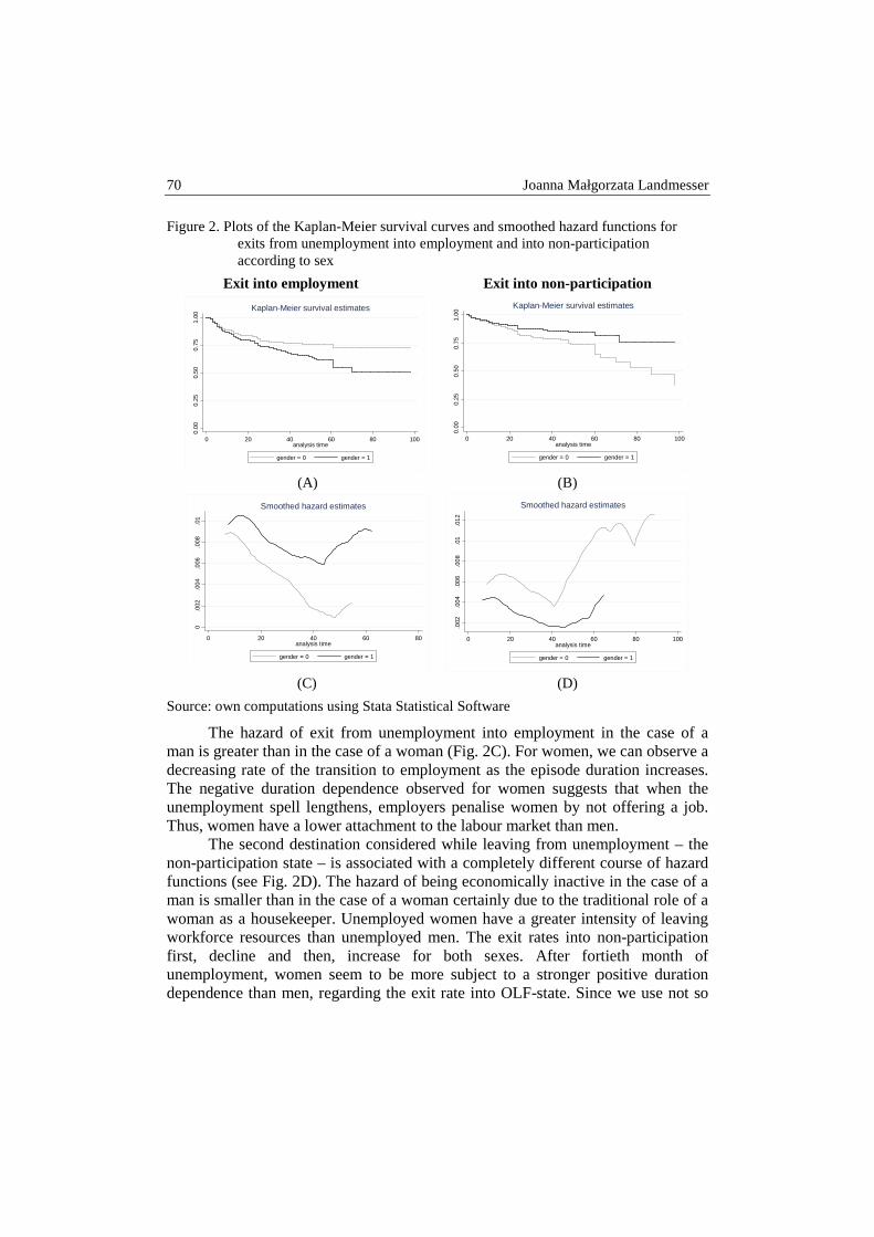
Joanna Małgorzata Landmesser 70
Figure 2. Plots of the Kaplan-Meier survival curves and smoothed hazard functions for exits from unemployment into employment and into non-participation according to sex
Exit into employment Exit into non-participation
(A) (B)
(C) (D)
Source: own computations using Stata Statistical Software
The hazard of exit from unemployment into employment in the case of a man is greater than in the case of a woman (Fig. 2C). For women, we can observe a decreasing rate of the transition to employment as the episode duration increases. The negative duration dependence observed for women suggests that when the unemployment spell lengthens, employers penalise women by not offering a job. Thus, women have a lower attachment to the labour market than men.
The second destination considered while leaving from unemployment – the non-participation state – is associated with a completely different course of hazard functions (see Fig. 2D). The hazard of being economically inactive in the case of a man is smaller than in the case of a woman certainly due to the traditional role of a woman as a housekeeper. Unemployed women have a greater intensity of leaving workforce resources than unemployed men. The exit rates into non-participation first, decline and then, increase for both sexes. After fortieth month of unemployment, women seem to be more subject to a stronger positive duration dependence than men, regarding the exit rate into OLF-state. Since we use not so
0.00
0.25
0.50
0.75
1.00
0 20 40 60 80 100analysis time
gender = 0 gender = 1
Kaplan-Meier survival estimates
0.00
0.25
0.50
0.75
1.00
0 20 40 60 80 100analysis time
gender = 0 gender = 1
Kaplan-Meier survival estimates
0.0
02.0
04.0
06.0
08.0
1
0 20 40 60 80analysis time
gender = 0 gender = 1
Smoothed hazard estimates
.002
.004
.006
.008
.01
.012
0 20 40 60 80 100analysis time
gender = 0 gender = 1
Smoothed hazard estimates

Gender differences in exit rates from unemployment … 71
many observations for individuals that went out of the labour market, we must be very careful with drawing conclusions regarding the duration dependence.
The results achieved of semiparametric Cox model estimation for exits from unemployment are presented in table 2.
Table 2. Cox regressions for exits from unemployment
Variable
Exit from unemployment
Exit into employment non-participation
Haz. Ratio
Std. Err.
Haz. Ratio
Std. Err.
Haz. Ratio
Std. Err.
gender (1=male) 1.107 0.095 1.453 *** 0.158 0.702 ** 0.101 Age-group (Base age2534)
age1824 1.539 *** 0.193 1.534 *** 0.235 1.554 ** 0.344 age3544 0.734 *** 0.097 0.671 ** 0.113 0.856 0.187 age4554 0.679 *** 0.089 0.613 *** 0.103 0.805 0.170 age5565 0.609 *** 0.100 0.485 *** 0.108 0.836 0.211 Education level (Base tertiary)
vocational secondary
0.681 *** 0.101 0.593 *** 0.108 0.888 0.233
general secondary 0.745 * 0.130 0.720 0.153 0.838 0.260 basic vocational 0.692 *** 0.098 0.627 *** 0.107 0.858 0.219 lower second. or primary
0.598 *** 0.098 0.442 *** 0.091 0.984 0.273
head of the household
1.278 ** 0.141 1.319 * 0.188 1.243 0.220
living with a partner
1.191 * 0.117 1.124 0.140 1.314 * 0.210
disabled 0.703 * 0.143 0.541 ** 0.162 0.928 0.261 part time job 1.760 *** 0.381 0.859 0.330 3.252 *** 0.876 No. of obs. 2639 2639 2639 No. of failures 606 377 229 lnL -4250.2 -2655.0 -1573.5
*** Significant at 1%; ** Significant at 5%; * Significant at 1%.
Source: own computations using Stata Statistical Software
Variables included in x are socio-economic characteristics of the individual such as gender, age, education level. A competing risks model is assumed since there are two possible destinations. The transition probabilities are assumed to be independent, conditional on the explanatory variables. The transition probabilities for each destination can be considered as a hazard rate of each destination and can be estimated as a single risk by treating spells that finish into other destinations as right censored.

Joanna Małgorzata Landmesser 72
If we analyse the exits from unemployment into any other state, we find out that it does not persist a significant difference between unemployment durations of men and women. The hazard is not dependent on gender. But the hazard of exit into employment in the case of a man is 45.3% greater than in the case of a woman. The hazard of exit into non-participation in case of a man is 29.8% lower than in the case of a woman. The age coefficients imply that older people are at a disadvantage. The older age of the individual leads to a decrease of chance for exiting unemployment into employment. For exits into non-participation, age does not play a role. Higher education levels lead to a significant increase of opportunities to find a job, but the effects for exits into OLF are insignificant. Being the head of the family increases the chances of finding a job, but does not affect the exit into inactivity. Those who live in relationships are exposed to a higher risk of non-participation. Disability leads to a strong decline (46%) of the risk of exiting into employment. The effects for exits into OLF are moderate and insignificant. Looking for a part time job increases only the risk of being inactive.
Unfortunately, in the case of variable gender the estimated models for exits into employment or into non-participation violate the proportional hazard assumption. Therefore, there is a need to estimate separate models for men and women. In table 3 we present results of estimation of the exit rates from unemployment into employment for both sexes (we reduced models to the forms with fewer parameters, all of which are significant).
Table 3. Cox regressions for exits into employment for men and women separately
Variable
Exit into employment Men Women
Haz. Ratio Std. Err. Haz. Ratio Std. Err. Age age 0.975 *** 0.006 0.856 *** 0.050 age^2 1.002 ** 0.001 Education level tertiary 1.890 ** 0.537 secondary 1.438 * 0.324 0.685 * 0.145 basic vocational 1.504 ** 0.308 0.627 ** 0.149 lower second. or primary 0.553 * 0.168 head of the household 1.518 ** 0.276 disabled 0.505 * 0.186 full time job 1.298 * 0.189 1.671 *** 0.268 No. of observations 1276 1363 No. of failures 205 172 lnL -1278.1 -1109.7
*** Significant at 1%; ** Significant at 5%; * Significant at 1%.
Source: own computations using Stata Statistical Software
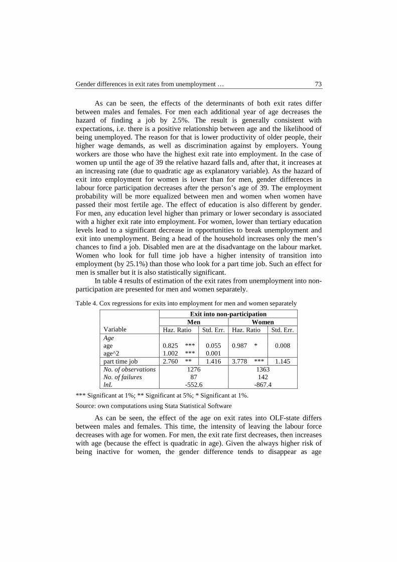
Gender differences in exit rates from unemployment … 73
As can be seen, the effects of the determinants of both exit rates differ between males and females. For men each additional year of age decreases the hazard of finding a job by 2.5%. The result is generally consistent with expectations, i.e. there is a positive relationship between age and the likelihood of being unemployed. The reason for that is lower productivity of older people, their higher wage demands, as well as discrimination against by employers. Young workers are those who have the highest exit rate into employment. In the case of women up until the age of 39 the relative hazard falls and, after that, it increases at an increasing rate (due to quadratic age as explanatory variable). As the hazard of exit into employment for women is lower than for men, gender differences in labour force participation decreases after the person’s age of 39. The employment probability will be more equalized between men and women when women have passed their most fertile age. The effect of education is also different by gender. For men, any education level higher than primary or lower secondary is associated with a higher exit rate into employment. For women, lower than tertiary education levels lead to a significant decrease in opportunities to break unemployment and exit into unemployment. Being a head of the household increases only the men’s chances to find a job. Disabled men are at the disadvantage on the labour market. Women who look for full time job have a higher intensity of transition into employment (by 25.1%) than those who look for a part time job. Such an effect for men is smaller but it is also statistically significant.
In table 4 results of estimation of the exit rates from unemployment into non-participation are presented for men and women separately.
Table 4. Cox regressions for exits into employment for men and women separately
Variable
Exit into non-participation Men Women
Haz. Ratio Std. Err. Haz. Ratio Std. Err. Age age 0.825 *** 0.055 0.987 * 0.008 age^2 1.002 *** 0.001 part time job 2.760 ** 1.416 3.778 *** 1.145 No. of observations 1276 1363 No. of failures 87 142 lnL -552.6 -867.4
*** Significant at 1%; ** Significant at 5%; * Significant at 1%.
Source: own computations using Stata Statistical Software
As can be seen, the effect of the age on exit rates into OLF-state differs between males and females. This time, the intensity of leaving the labour force decreases with age for women. For men, the exit rate first decreases, then increases with age (because the effect is quadratic in age). Given the always higher risk of being inactive for women, the gender difference tends to disappear as age
Joanna Małgorzata Landmesser 74
increases. In the case of transitions into non-participation state there is no statistically significant effect of education level, position in the family or disability, on the intensity of exit of unemployment. We have only found that women who look for a part time job have higher exit rate into OLF-state than men. However, we should remember that since we have estimated separate equations for each sex our results are not directly comparable when it comes to the strength of the impact.
RESUMEE
The aim of the research work was to analyse the exit rates from unemployment for men and women separately. Findings confirm the lower female involvement in the labor market and a higher female payoff from household responsibilities.
We also intended to investigate which factors influence the probability of leaving the unemployment state upon gender. Using the hazard models we estimated the impact of such personal characteristics of individuals such as age, education level, position in the family, disability on individual’s unemployment period of men and women. The effects of explanatory variables differ between both sexes. The differences are due to the lower labour market attachment of women in the fertile age. In this period women are much more affected by the family related responsibilities than men. The results obtained show that drawing conclusions when gender differences are not considered can lead to misperceptions. Disregarding various exit states from the unemployment can also be misleading.
For women, the exit rate into employment is lower than in the case of men. There persists the negative duration dependence for women. However, the gender difference decreases after the age of about 40. The exit rate into non-participation state is higher for women than for men, but this difference also disappears as age increases.
The inequalities between sexes while leaving unemployment concern first of all people aged up to 40, that is people frequently with young children. Therefore, a more flexible family policy would probably help to reduce the effect of gender differences.
LITERATURE
Altonji J.G., Blank R.M. (1999) Race and Gender In the Labor Market, [in:] Ashen-felter O., Card D. (eds.): Handbook of Labor Economics, Volume III. North-Holland, Amsterdam.
Cox D.R. (1972) Regression Models and Life Tables (with Discussion), Journal of the Royal Statistical Society, Series B 34, 187 – 220.
Cox D.R., Oakes D. (1984) Analysis of Survival Data, Chapman and Hall, London. Edin P.A. (1989) Unemployment Duration and Competing Risks: Evidence from Sweden,
Scandinavian Journal of Economics, 91(4), 639 – 653.
Gender differences in exit rates from unemployment … 75
Gonzalo M.T., Saarela J. (2000) Gender Differences in Exit Rates from Unemployment: Evidence from a Local Finnish Labour Market, Finnish Economic Papers, 13(2), 129 – 139.
Jensen P., Westergård-Nielsen N. (1990) Temporary Layoffs, [in:] Hartog J., Ridder G., Theeuwes J. (eds.): Panel Data and Labour Market Studies, North-Holland, Amsterdam.
Kalbfleisch J., Prentice R. (1980) The Statistical Analysis of Failure Time Data. John Wiley and Sons, New York.
Katz L.F., Meyer B.D. (1990b) Unemployment Insurance, Recall Expectations, and Unemployment Outcomes. Quarterly Journal of Economics, 105(4), pp. 973 – 1002.
Lancaster T. (1979) Econometric Methods for the Duration of Unemployment, Econometrica, 47, 939 – 956.
Landmesser J. (2008a) Analiza aktywności ekonomicznej kobiet wiejskich z wykorzys-taniem ekonometrycznych modeli hazardu, Roczniki Naukowe Stowarzyszenia Ekonomistów Rolnictwa i Agrobiznesu, Zeszyt 1, Tom X, 233 – 239.
Landmesser J. (2008b) Determinanty czasu trwania w bezrobociu w wypadku osób zare-jestrowanych w urzędzie pracy, [in:] Borkowski B. (ed.): Metody ilościowe w bada-niach ekonomicznych – IX, Wielowymiarowa analiza danych, Wydawnictwo SGGW, Warszawa, 97 – 106.
Narendranathan W., Stewart M.B. (1993) Modelling the Probability of Leaving Un-employment: Competing Risks Models with Flexible Baseline Hazards, Journal of the Royal Statistical Society, Applied Statistics, 42, 63 – 83.
Steiner V. (1989) Causes of Recurrent Unemployment - An Empirical Analysis, Empirica, 16, 53 – 65.
Stolorz B. (2010) Czynniki czasu wpływające na poszukiwanie pracy, Wiadomości Statystyczne, 1, 81-91.
Tansel A., Taşçi H.M. (2010) Hazard Analysis of Unemployment Duration by Gender in a Developing Country: The Case of Turkey, IZA Discussion Paper, 4844, Bonn.
QUANTITATIVE METHODS IN ECONOMICS Vol. XV, No. 1, 2014, pp. 76 – 91
LIFE CYCLE INCOME OF WOMEN AND MEN IN POLAND1
Barbara Liberda University of Warsaw
[email protected] Marek Pęczkowski
University of Warsaw [email protected]
Abstract: We examine the contribution of married and cohabited women and men to the joint income of the couple. We use individual income data from Household Budget Surveys for Poland in 2011 from a sample of 16,538 married and cohabited couples. The results of analysis show that contribution of men to total household income is higher than contribution of their female partners through the life cycle, controlling for type of a couple, education levels of genders and number of children. The contribution of married and cohabited women to total income of the couple remains almost flat during the life cycle.
Keywords: gender, income, life cycle, married, cohabited, couple, Poland
INTRODUCTION
The contribution of women to the household income is based in the historical trends of the labour force participation of women and the gender gap in earnings. The differences in earnings of women and men were explained in the context of the human capital theory due to the differences in individual characteristics like education, training and experience [Becker 1964, Mincer 1974]. More limited experience and less investment in education reduce the productivity of women which translates into lower wages. However, the human capital theory does not explain the discrimination and segregation of women at the labour
1 The research was done in 2013 in the Project InnoGend within the Norwegian Financial Mechanism.

Life cycle income of women and men in Poland 77
markets which are based in unexplained prejudices [Becker, 1957; Oaxaca 1973; Blinder 1973].
The distribution of income of the couples is also determined by the patterns of marriage formation. Marriages tend to form between individuals who are in similar age, have similar level of education, similar status and live close to each other. Akerlof and Kranton (2000) incorporated the theory of identity from psychology and sociology into the economic model of human behaviour. Identity is associated with different social categories and how people belonging to these categories should behave. Gender categories are associated with specific behavioural prescriptions such as: a man should earn more than his wife.
The gender identity norms explain the marriage formation, likelihood to divorce, labour market participation of women, distribution of relative income within households and division of home production activities between partners [Bertrand et al 2013]. The authors used data for 1970 - 2010 from the US Census Bureau and 2008-2010 data from American community Survey. They noticed that couples where wife earns more than husband are less satisfied with their marriage and are more likely to divorce.
During the last decades women improved their educational background and in many countries, including Poland, their educational level exceeds the education level of men. Women have fewer children and shorter periods of employment interruptions. The gender pay gap still exists, although it has diminished since the 1970. However, it is fairly stable over the last decades. Median annual earnings of women fulltime workers in the United States are currently reported to be at 76% of earnings of men. The situation is similar in other countries. In Europe the gender wage gap is 82%, in Australia 82% and 82.4% in OECD [Lips 2013, p. 169].
Differences between women and men in professional experience still remain significant. However, human capital variables explain no more than 20-35% of differences in earnings [Plantenga, Remery 2006]. More important factors are the horizontal and vertical occupational segregation and the wage structure. Historically, women tend to work in different occupations and industries than men and have been segregated because of that. Even within occupations dominated by women, women are paid less than men. There is no broad occupational category in which the earnings of women equal those of men. Even within organizations, women and men with similar level of education and doing the same work are often assigned different job titles and work in different parts of company.
The gender pay gap tends to widen with age. It is smaller in the public sector than in the private sector, higher for married employees and significantly lower for singles [Plantenga, Remery 2006; Wechselbaumer, Winter-Ebmer 2005]. Ahituv and Lerman (2011) examined the relationship between job stability, wage rates and the marital stability. They used the panel data from National Longitudinal Survey [NLSY79] in which individuals were interviewed in 1994-2006. They have pointed out that married men work longer hours, work harder on the job, have lower absenteeism from work, and are less likely to be fired than single men. Married

78 Barbara Liberda, Marek Pęczkowski
men have higher wages than single men. Men in their first marriage have higher wages than those in their second marriage and divorced men have lower wages than married or remarried men. The difference increases with age and is similar among men with different levels of education.
Maître, Whelan and Nolan (2003) use European Community Household Panel (ECHP) data to look at the income contribution of the female partner to the household income in twelve European countries. Income from work of each individual includes wage and salary earnings and self-employment income. The mean contribution of women to the household income for full time working men and women in the ECHP 1996 study oscillates from 32% in Greece to 41% in the Netherlands. For the part time working women, the contribution of women to the household income stretches from 17% in Greece to 28% in Denmark. For the couples with no children the mean contribution of women varies from 23% in Greece to 35% in Denmark and UK. But for couples with 3 children below 6 years of age the mean contribution of women to the household income was less than 20% and only 7% in Germany.
When a woman has attained a tertiary education, her contribution is greater than for the secondary or lower than secondary level of education. For example, in Portugal the contribution of women to the household income reaches 20% for primary educated women, 28% for secondary educated and 42% for tertiary level of education of women. For other countries the women contribution rate is about 30% for tertiary education and is higher by about 10 percentage points than for the secondary level and about 20 percentage points for the lower than secondary level of education [Maître, Whelan and Nolan 2003, pp. 19-22].
Women contribution to the household income is highest for young couples in the age below 30. In every case the contribution of the female partner increases systematically with total income of the household. Female income plays a role in influencing whether a household is poor or not. The share of poor households below 60% of the median household income is 30% in Denmark and 27% in the United Kingdom when a female partner does not earn income. When the female income is added to the total household income, the share of poor households falls to 2.6% in Denmark and 9.9% in the United Kingdom (calculated from Table 8 in [Maître et al., 2003]).
Soobedar (2011) analyses the trends in the relative earnings of men and women in the household between 1994 and 2004 in the United Kingdom. She used data from the Family Resource Surveys for years 1994, 1997, 2001, 2004 for men aged 24-64 and women in partnership in the age 24-55. The author applied the semiparametric approach to quantify the impact of explanatory factors (male and female characteristics, patterns of mating) on the relative position of women within families. In this period hourly earnings in real terms increased more among the female partners (by 32%) than among the males (by 7%). The labour force participation increased by 0.5 percentage points for men and by 7 percentage points for women (p. 419).

Life cycle income of women and men in Poland 79
The main factor which accounts for the increase in the relative female earnings share was the rising labour force participation of women. Alteration in the characteristics of females accounts on average for about 1/4 of the rise in the female breadwinner index, e. g. the relative female earnings share. Increases in returns of men to male characteristics have acted in the opposite direction. Bloemen and Stancanelli (2008) analysed couples in France between 1990 and 2002 where the wife was the main earner in the household. They concluded that female breadwinner families are mainly observed when the husbands are low educated and face labour market difficulties.
In this paper we examine the contribution of income of married and cohabited women and men to the joint income through the life cycle of the couple. To do this we first construct the life cycle age structure of married and cohabited couples in Poland. Then we analyze inputs of income of married and cohabited women and men to the household income during the life cycle of the couple, controlling for the education level of women and men and the presence of children. We examine the relative income of women and men in Polish households based on data from Household Budget Surveys in 2011.
DATA DESCRIPTION AND MATCHING OF COUPLES
We use the sample data for 37,099 households from Household Budget Surveys for Poland in 2011. The Household Budget Surveys are performed by Central Statistical Office (GUS) on a fully representative basis for Polish households.
The structure of the 37,099 households sample is the following:
• 25% of the sample consists of one-person households, mostly retired women, not sharing income with any other person,
• 62% of households are couples with or without children, • 2% of all households are single parents, mostly women, with children, • 11% of the sample consists of households with composite structure: the non-
nuclear families or households with some members not relative to the head of the household. They may be composed of more than one adult man or more than one adult woman (Table 1).
In our analysis we consider the households consisting of one couple of a man and a woman who are formally married or declaring as living together (cohabited). There are 23,141 couples in the sample (62% of the total number of households). Married couples form 58% of all households (21,542 households) and the cohabited couples run 4% of all households (1,599 households).
Out of the sample of all couples we only examine couples with two streams of income earned by women and men. We omitted couples when only one person is earning or there is an income of a child. Finally our sample under study consists of 16,538 couples (45% of all households). Among them there are 15,237 formally

80 Barbara Liberda, Marek Pęczkowski
married couples (41% of all households) and 1,301 cohabited couples (3.5% of all households and 8% of couples under study) (Table 1).
Table 1. The structure of households in Poland in 2011
Count %
All households 37,099 100 One person households 9,203 25
Couples without children 6,643 18 married 9,203
cohabited 670
Couples with children 9,895 27
married 9,264
cohabited 631
Couples under study 16,538 45 married 15,237 41
cohabited 1,301 4 Single parents with children 630 2
Other households 10728 29
Source: Own calculations based on data from Household Budget Surveys, Poland, 2011.
We use individual data on personal income earned from different sources (hired employment, self-employment, pension, farming) by married and cohabited women and men from the Household Budget Surveys of Polish households in 2011 (Table 2).
Table 2. Average monthly income of women and men in the couples (in zlotys)
Men Women
All households 2013 1492 One person households 1868 1599
Couples without children 2037 1495 married 2006 1465
cohabited 2302 1732 Couples with children 2601 1781
married 2614 1699 cohabited 2370 1557
Couples under study 2371 1655 married 2364 1649
cohabited 2341 1716 Single parents with children 2356 1948
Other households 1610 1273
Source: Own calculations based on data from Household Budget Surveys, Poland, 2011.
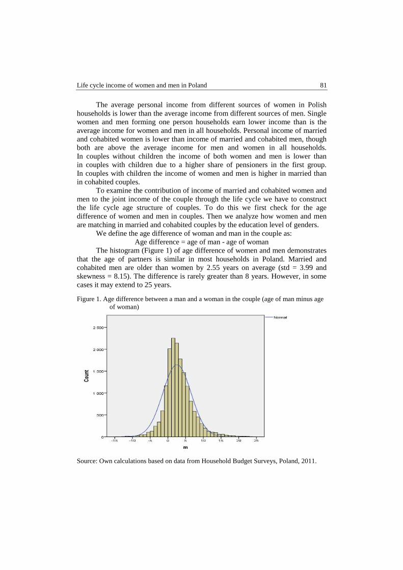
Life cycle income of women and men in Poland 81
The average personal income from different sources of women in Polish households is lower than the average income from different sources of men. Single women and men forming one person households earn lower income than is the average income for women and men in all households. Personal income of married and cohabited women is lower than income of married and cohabited men, though both are above the average income for men and women in all households. In couples without children the income of both women and men is lower than in couples with children due to a higher share of pensioners in the first group. In couples with children the income of women and men is higher in married than in cohabited couples.
To examine the contribution of income of married and cohabited women and men to the joint income of the couple through the life cycle we have to construct the life cycle age structure of couples. To do this we first check for the age difference of women and men in couples. Then we analyze how women and men are matching in married and cohabited couples by the education level of genders.
We define the age difference of woman and man in the couple as: Age difference = age of man - age of woman
The histogram (Figure 1) of age difference of women and men demonstrates that the age of partners is similar in most households in Poland. Married and cohabited men are older than women by 2.55 years on average (std = 3.99 and skewness = 8.15). The difference is rarely greater than 8 years. However, in some cases it may extend to 25 years.
Figure 1. Age difference between a man and a woman in the couple (age of man minus age of woman)
Source: Own calculations based on data from Household Budget Surveys, Poland, 2011.
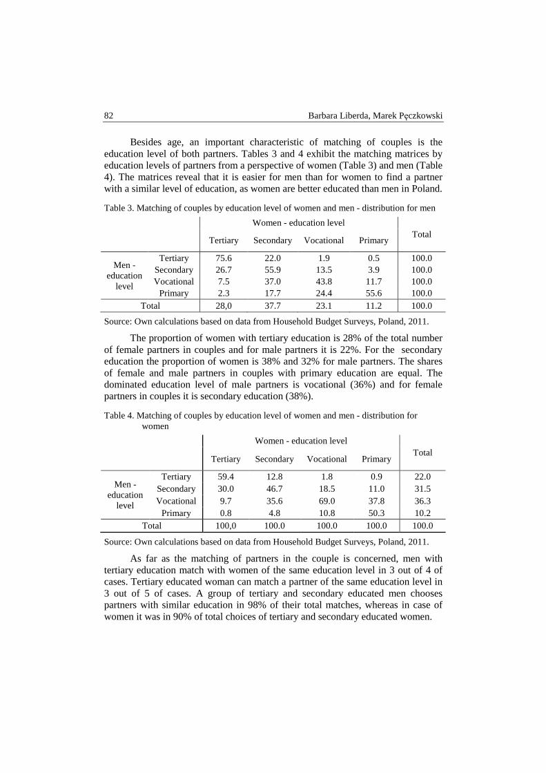
82 Barbara Liberda, Marek Pęczkowski
Besides age, an important characteristic of matching of couples is the education level of both partners. Tables 3 and 4 exhibit the matching matrices by education levels of partners from a perspective of women (Table 3) and men (Table 4). The matrices reveal that it is easier for men than for women to find a partner with a similar level of education, as women are better educated than men in Poland.
Table 3. Matching of couples by education level of women and men - distribution for men
Women - education level
Total Tertiary Secondary Vocational Primary
Men - education
level
Tertiary 75.6 22.0 1.9 0.5 100.0 Secondary 26.7 55.9 13.5 3.9 100.0 Vocational 7.5 37.0 43.8 11.7 100.0
Primary 2.3 17.7 24.4 55.6 100.0 Total 28,0 37.7 23.1 11.2 100.0
Source: Own calculations based on data from Household Budget Surveys, Poland, 2011.
The proportion of women with tertiary education is 28% of the total number of female partners in couples and for male partners it is 22%. For the secondary education the proportion of women is 38% and 32% for male partners. The shares of female and male partners in couples with primary education are equal. The dominated education level of male partners is vocational (36%) and for female partners in couples it is secondary education (38%).
Table 4. Matching of couples by education level of women and men - distribution for women
Women - education level
Total Tertiary Secondary Vocational Primary
Men - education
level
Tertiary 59.4 12.8 1.8 0.9 22.0 Secondary 30.0 46.7 18.5 11.0 31.5 Vocational 9.7 35.6 69.0 37.8 36.3
Primary 0.8 4.8 10.8 50.3 10.2 Total 100,0 100.0 100.0 100.0 100.0
Source: Own calculations based on data from Household Budget Surveys, Poland, 2011.
As far as the matching of partners in the couple is concerned, men with tertiary education match with women of the same education level in 3 out of 4 of cases. Tertiary educated woman can match a partner of the same education level in 3 out of 5 of cases. A group of tertiary and secondary educated men chooses partners with similar education in 98% of their total matches, whereas in case of women it was in 90% of total choices of tertiary and secondary educated women.
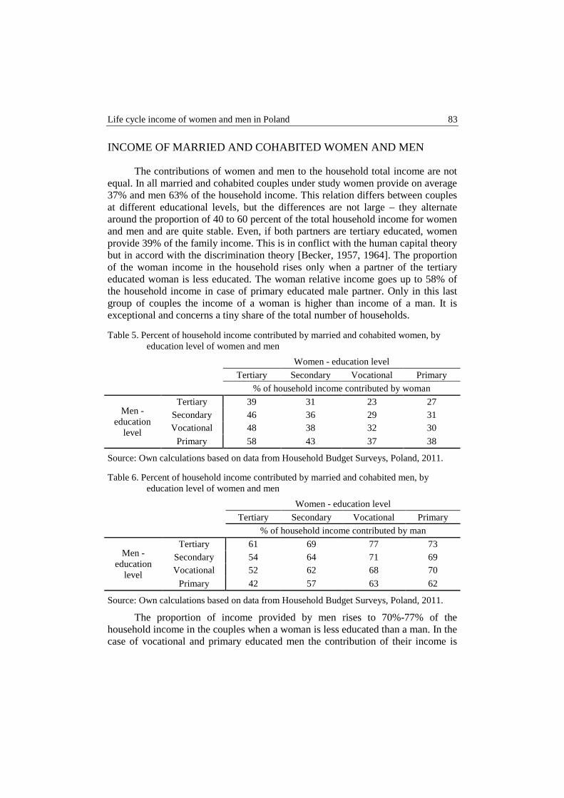
Life cycle income of women and men in Poland 83
INCOME OF MARRIED AND COHABITED WOMEN AND MEN
The contributions of women and men to the household total income are not equal. In all married and cohabited couples under study women provide on average 37% and men 63% of the household income. This relation differs between couples at different educational levels, but the differences are not large – they alternate around the proportion of 40 to 60 percent of the total household income for women and men and are quite stable. Even, if both partners are tertiary educated, women provide 39% of the family income. This is in conflict with the human capital theory but in accord with the discrimination theory [Becker, 1957, 1964]. The proportion of the woman income in the household rises only when a partner of the tertiary educated woman is less educated. The woman relative income goes up to 58% of the household income in case of primary educated male partner. Only in this last group of couples the income of a woman is higher than income of a man. It is exceptional and concerns a tiny share of the total number of households.
Table 5. Percent of household income contributed by married and cohabited women, by education level of women and men
Women - education level
Tertiary Secondary Vocational Primary
% of household income contributed by woman
Men - education
level
Tertiary 39 31 23 27 Secondary 46 36 29 31 Vocational 48 38 32 30
Primary 58 43 37 38
Source: Own calculations based on data from Household Budget Surveys, Poland, 2011.
Table 6. Percent of household income contributed by married and cohabited men, by education level of women and men
Women - education level
Tertiary Secondary Vocational Primary
% of household income contributed by man
Men - education
level
Tertiary 61 69 77 73 Secondary 54 64 71 69 Vocational 52 62 68 70
Primary 42 57 63 62
Source: Own calculations based on data from Household Budget Surveys, Poland, 2011.
The proportion of income provided by men rises to 70%-77% of the household income in the couples when a woman is less educated than a man. In the case of vocational and primary educated men the contribution of their income is

84 Barbara Liberda, Marek Pęczkowski
above 60% of total household income. It is true also for couples when women are more educated than their partners, except for the tertiary educated women and primary educated men (as described above).
The above structure of relative incomes of female and male partners in couples concerns the average incomes of all age groups. To examine the influence of the age of partners on their contribution to the household income we constructed five categories of married and cohabited couples through their life cycle. The categories take into account the age of partners, which - as we mentioned above - is mostly similar. Table 7 shows the construction of categories of married and cohabited couples through the life cycle of the couple. Table 8 shows the personal income earned by women and men during the life cycle of the couple.
Table 7. Life cycle categories of married and cohabited couples
< 35 both partners are less than 35 years old < 45, max >= 35 both partners are less than 45 years old
but at least one is 35 years old or more <55, max >= 45 both partners are less than 55 years old
but at least one is 45 years old or more < 65, max >= 55 both partners are less than 65 years old
but at least one is 55 years old or more max >= 65 both partners are 65 years old or more
Source: Own calculations.
Table 8: Income of married and cohabited women and men during the life cycle of the couple
Age of women and men in the couple
Income [monthly in zlotys]
Income of woman
as % of total household
income
Number of children
Men Women
< 35 2441 1301 35 1.23 < 45, max >= 35 2601 1446 36 1.93 < 55, max >= 45 2209 1440 39 1.43 < 65, max >= 55 1868 1250 40 0.30
max >= 65 1814 1188 40 0.02 Total 2238 1340 37 1.10
Source: Own calculations based on data from Household Budget Surveys, Poland, 2011.
The female partner income is lower than income of male partner during the whole life cycle. Incomes of women and men in couples rise till the age of 45-55. The female partner income is rising slightly faster than the male partner income which may be due to longer training in her human capital. As a result, the relative income of female partners rises from 35% of the household income in young couples, below 35 years of age of both partners, to 39-40% of the couple income in
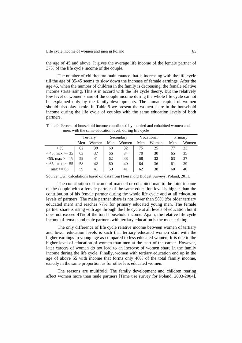
Life cycle income of women and men in Poland 85
the age of 45 and above. It gives the average life income of the female partner of 37% of the life cycle income of the couple.
The number of children on maintenance that is increasing with the life cycle till the age of 35-45 seems to slow down the increase of female earnings. After the age 45, when the number of children in the family is decreasing, the female relative income starts rising. This is in accord with the life cycle theory. But the relatively low level of women share of the couple income during the whole life cycle cannot be explained only by the family developments. The human capital of women should also play a role. In Table 9 we present the women share in the household income during the life cycle of couples with the same education levels of both partners.
Table 9. Percent of household income contributed by married and cohabited women and men, with the same education level, during life cycle
Tertiary Secondary Vocational Primary Men Women Men Women Men Women Men Women
< 35 62 38 68 32 75 25 77 23 < 45, max >= 35 63 37 66 34 70 30 65 35 <55, max >= 45 59 41 62 38 68 32 63 37 < 65, max >= 55 58 42 60 40 64 36 61 39
max >= 65 59 41 59 41 62 38 60 40
Source: Own calculations based on data from Household Budget Surveys, Poland, 2011.
The contribution of income of married or cohabited man to the joint income of the couple with a female partner of the same education level is higher than the contribution of his female partner during the whole life cycle and at all education levels of partners. The male partner share is not lower than 58% (for older tertiary educated men) and reaches 77% for primary educated young men. The female partner share is rising with age through the life cycle at all levels of education but it does not exceed 41% of the total household income. Again, the relative life cycle income of female and male partners with tertiary education is the most striking.
The only difference of life cycle relative income between women of tertiary and lower education levels is such that tertiary educated women start with the higher earnings in young age as compared to less educated women. It is due to the higher level of education of women than men at the start of the career. However, later careers of women do not lead to an increase of women share in the family income during the life cycle. Finally, women with tertiary education end up in the age of above 55 with income that forms only 40% of the total family income, exactly in the same proportion as for other less educated women.
The reasons are multifold. The family development and children rearing affect women more than male partners [Time use survey for Poland, 2003-2004].
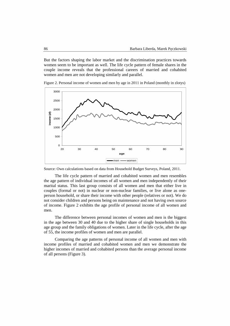
86 Barbara Liberda, Marek Pęczkowski
But the factors shaping the labor market and the discrimination practices towards women seem to be important as well. The life cycle pattern of female shares in the couple income reveals that the professional careers of married and cohabited women and men are not developing similarly and parallel.
Figure 2. Personal income of women and men by age in 2011 in Poland (monthly in zlotys)
Source: Own calculations based on data from Household Budget Surveys, Poland, 2011.
The life cycle pattern of married and cohabited women and men resembles the age pattern of individual incomes of all women and men independently of their marital status. This last group consists of all women and men that either live in couples (formal or not) in nuclear or non-nuclear families, or live alone as one-person household, or share their income with other people (relatives or not). We do not consider children and persons being on maintenance and not having own source of income. Figure 2 exhibits the age profile of personal income of all women and men.
The difference between personal incomes of women and men is the biggest in the age between 30 and 40 due to the higher share of single households in this age group and the family obligations of women. Later in the life cycle, after the age of 55, the income profiles of women and men are parallel.
Comparing the age patterns of personal income of all women and men with income profiles of married and cohabited women and men we demonstrate the higher incomes of married and cohabited persons than the average personal income of all persons (Figure 3).
0
500
1000
1500
2000
2500
3000
20 30 40 50 60 70 80 90
age
inco
me
(zł)
men women
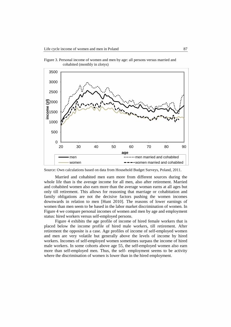
Life cycle income of women and men in Poland 87
Figure 3. Personal income of women and men by age: all persons versus married and cohabited (monthly in zlotys)
Source: Own calculations based on data from Household Budget Surveys, Poland, 2011.
Married and cohabited men earn more from different sources during the whole life than is the average income for all men, also after retirement. Married and cohabited women also earn more than the average woman earns at all ages but only till retirement. This allows for reasoning that marriage or cohabitation and family obligations are not the decisive factors pushing the women incomes downwards in relation to men [Hunt 2010]. The reasons of lower earnings of women than men seem to be based in the labor market discrimination of women. In Figure 4 we compare personal incomes of women and men by age and employment status: hired workers versus self-employed persons.
Figure 4 exhibits the age profile of income of hired female workers that is placed below the income profile of hired male workers, till retirement. After retirement the opposite is a case. Age profiles of income of self-employed women and men are very volatile but generally above the levels of income by hired workers. Incomes of self-employed women sometimes surpass the income of hired male workers. In some cohorts above age 55, the self-employed women also earn more than self-employed men. Thus, the self- employment seems to be activity where the discrimination of women is lower than in the hired employment.
0
500
1000
1500
2000
2500
3000
3500
20 30 40 50 60 70 80 90
inco
me
(zł)
agemen men married and cohabited
women women married and cohabited
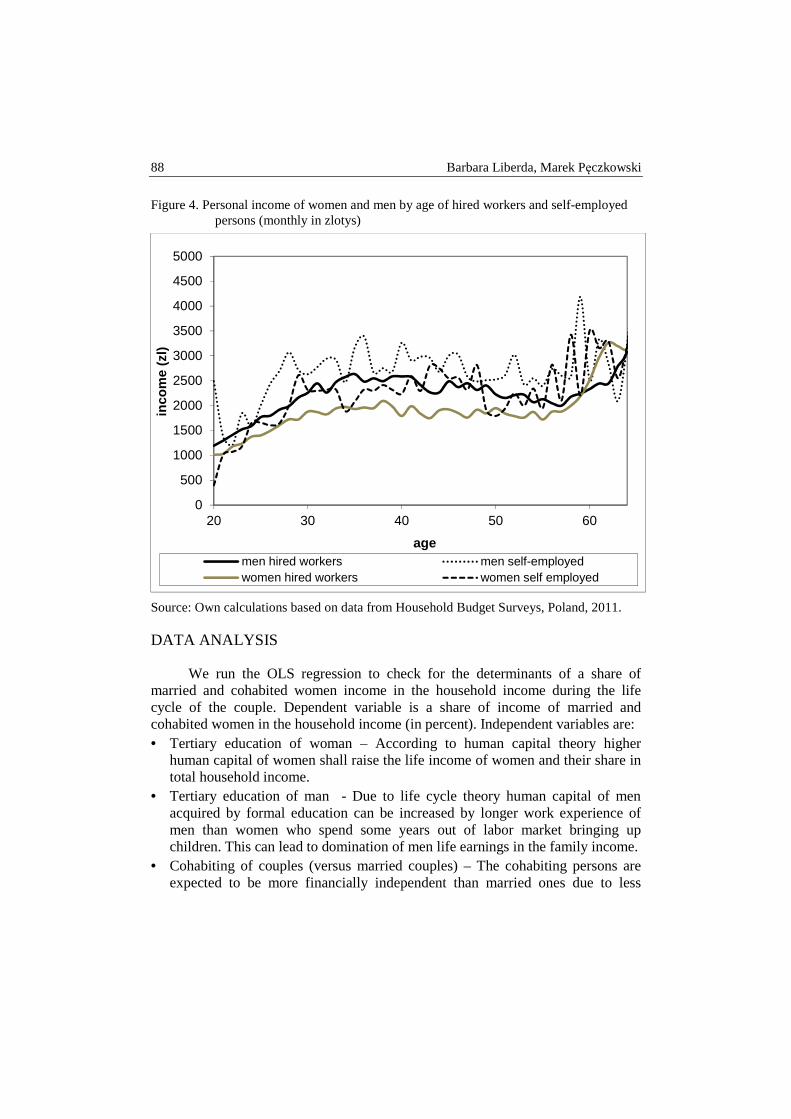
88 Barbara Liberda, Marek Pęczkowski
Figure 4. Personal income of women and men by age of hired workers and self-employed persons (monthly in zlotys)
Source: Own calculations based on data from Household Budget Surveys, Poland, 2011.
DATA ANALYSIS
We run the OLS regression to check for the determinants of a share of married and cohabited women income in the household income during the life cycle of the couple. Dependent variable is a share of income of married and cohabited women in the household income (in percent). Independent variables are: • Tertiary education of woman – According to human capital theory higher
human capital of women shall raise the life income of women and their share in total household income.
• Tertiary education of man - Due to life cycle theory human capital of men acquired by formal education can be increased by longer work experience of men than women who spend some years out of labor market bringing up children. This can lead to domination of men life earnings in the family income.
• Cohabiting of couples (versus married couples) – The cohabiting persons are expected to be more financially independent than married ones due to less
0
500
1000
1500
2000
2500
3000
3500
4000
4500
5000
20 30 40 50 60
inco
me
(zl)
agemen hired workers men self-employedwomen hired workers women self employed

Life cycle income of women and men in Poland 89
legally supported security for cohabiting couples than for married couples. The effect of cohabitation for women share in household income may be positive.
• Presence of children in age 0-2 − Expected effect on women share in total household income is negative, due to very probable breaks in career for women in the present legal status for sharing the maternity leave by parents in Poland (man can take only 2 weeks of parental leave).
• Presence of children in age 3-7 − The effect may be negative or positive depending on institutional basis and particular work organization for working mothers in specific industries and firms.
Life cycle age categories of couples: • age35-44 − if both partners are less than 45 years old,
but at least one is 35 years old or more • age45-54 − if both partners are less than 55 years old,
but at least one is 45 years old or more • age55-64 − if both partners are less than 55 years old,
but at least one is 45 years old or more • age>=65 − if both partners are 65 years old or more • Household disposable income − The level of total disposable income of the
household shall be neutral to the share of women income in it, but with very high household income there may be more social pressure for women to make them stop working and earning.
Variables age35-44, age45-54, age55-64, age>=65 are the indicator variables for life cycle categories where category age<35 (both partners are less than 35 years old) is a reference category. Variables woman_tertiary and man_tertiary can be both equal to 1 when both partners have tertiary level of education, and can be equal to 0 when neither of partners has tertiary level of education. Variables child_0-2 and child_3-7 can be both equal to 1 where the couple has children of age 0-2 years as well as children of age 3-7 years. These variables are both equal to 0 where there are no children in age 0-7 years. Household disposable income is given in zlotys.
Using the variables defined above the equation estimated (OLS) is the following:
woman share_of_income = 13.702 woman_tertiary – 3.768 man_tertiary + 4.159 cohabited – 5.925 child_0-2 –2.249 child_3-7 + 2.966 age35-44 + 5.774 age45-54 + 7.798 age55-64 + 6.705 age>=65–0.000 household_income + 36.766
The results of the regression analysis for determinants of the share of personal income of married and cohabited women in the total family income show that the women tertiary education increases the women share in total income of the couple by almost 14 percentage points. Tertiary education of men decreases the share of women personal income in the household income by 4 percentage points.
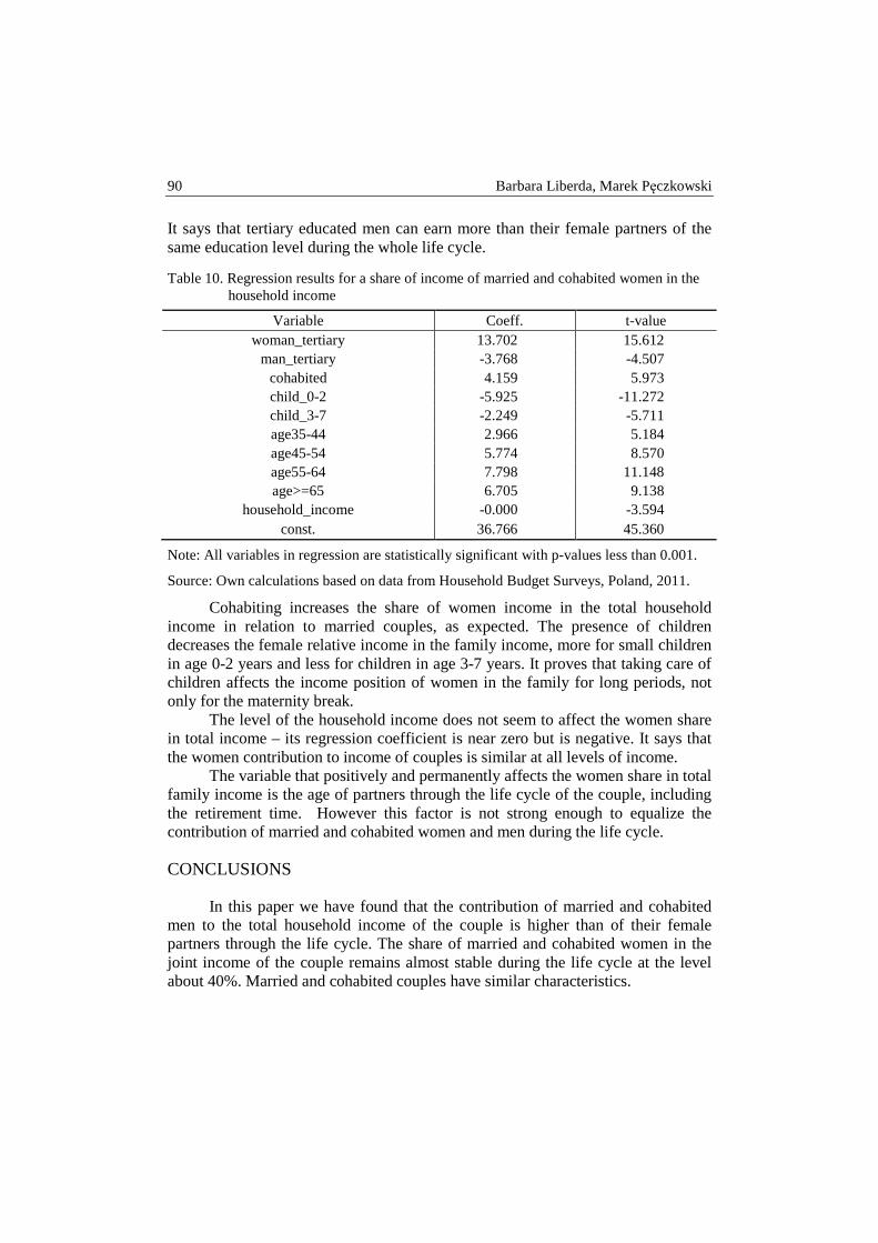
90 Barbara Liberda, Marek Pęczkowski
It says that tertiary educated men can earn more than their female partners of the same education level during the whole life cycle.
Table 10. Regression results for a share of income of married and cohabited women in the household income
Variable Coeff. t-value woman_tertiary 13.702 15.612
man_tertiary -3.768 -4.507 cohabited 4.159 5.973 child_0-2 -5.925 -11.272 child_3-7 -2.249 -5.711 age35-44 2.966 5.184 age45-54 5.774 8.570 age55-64 7.798 11.148 age>=65 6.705 9.138
household_income -0.000 -3.594 const. 36.766 45.360
Note: All variables in regression are statistically significant with p-values less than 0.001.
Source: Own calculations based on data from Household Budget Surveys, Poland, 2011.
Cohabiting increases the share of women income in the total household income in relation to married couples, as expected. The presence of children decreases the female relative income in the family income, more for small children in age 0-2 years and less for children in age 3-7 years. It proves that taking care of children affects the income position of women in the family for long periods, not only for the maternity break.
The level of the household income does not seem to affect the women share in total income – its regression coefficient is near zero but is negative. It says that the women contribution to income of couples is similar at all levels of income.
The variable that positively and permanently affects the women share in total family income is the age of partners through the life cycle of the couple, including the retirement time. However this factor is not strong enough to equalize the contribution of married and cohabited women and men during the life cycle.
CONCLUSIONS
In this paper we have found that the contribution of married and cohabited men to the total household income of the couple is higher than of their female partners through the life cycle. The share of married and cohabited women in the joint income of the couple remains almost stable during the life cycle at the level about 40%. Married and cohabited couples have similar characteristics.
Life cycle income of women and men in Poland 91
The results of the regression for determinants of women contribution to the household income show that the factors positively affecting women share in the family income are: a tertiary education of women, cohabitation and the age of partners through the life cycle of the couple. Male tertiary education and the presence of children affect negatively the contribution of women personal income to the family income.
The final conclusion says that the labor market discrimination of women rather than the family situation may be responsible for the lower contribution of women to the household income through the life cycle of the couple. One should however consider that the gender pay gap and the family situation are interrelated.
BIBLIOGRAPHY
Ahituv A., Lerman R.I. (2011) Job turnover, wage rates, and marital stability: How are they related?, Review of Economics of the Household, 9, 221-249.
Akerlof G.A, Kranton R. E. (2000) Economics and identity, Quarterly Journal of Economics, 115 (3), 715-753.
Becker G. (1957) The economics of discrimination, The University of Chicago Press, Chicago.
Becker G. (1964) Human capital, The University of Chicago Press, Chicago. Bertrand M, Pan J., Kamenica E. (2013) Gender identity and relative income within
households, NBER Working Paper No. 19023. Blinder A. (1973) Wage Discrimination: Reduced Form and Structural Estimates, The
Journal of Human Resources, VII, 4, pp. 436-55. Bloemen H., Stancanelli E. (2008) Modelling the employment and wage outcomes of
spouses. Is she outearning him?, IZA Discussion Paper, 3455, Bonn, Germany. Hunt J. (2010) Why do women leave science and engineering? NBER Working Paper No.
15853. Lips H.M. (2013) The Gender Pay gap: Challenging the Rationalizations. Perceived Equity,
Discrimination, and the Limits of Human Capital Models, Sex Roles, 68, 169-185. Maître B., Whelan C.T., Nolan B. (2003) Female Partner’s Income Contribution to the
Household Income in the European Union, EPAG Working Papers, 43, Colchester: University of Essex.
Mincer J. (1974) Schooling, experience and earnings, National Bureau of Economic Res. Oaxaca R. (1973) Male-Female Wage Differentials in Urban Labor Market, International
Economic Review, Vol. 14, No. 3, 693-709. Plantenga J., Remery C. (2006) The gender pay gap. Origins and policy responses. A
comparative review of thirty European countries. The co-ordinators’ synthesis report prepared for the Equality Unit, European Commission.
Soobedar Z. (2011) A semiparametric analysis of the rising breadwinner role of women in the UK, Review of Economics of the Household, 9, 415-428.
Time use survey for Poland, 2003-2004, GUS, (Badanie budżetu czasu ludności), Warsaw. Weichselbaumer D., Winter-Ember R. (2005) A meta-analysis of the international gender
pay gap, Journal of Economic Surveys, 19 (3), 479-511.

QUANTITATIVE METHODS IN ECONOMICS Vol. XV, No. 1, 2014, pp. 92 – 103
FACTORS AFFECTING THE PRICES OF ARTWORKS IN THE POLISH AUCTION MARKET1
Anna Lucińska Department of Economics of Industry and Capital Markets, University of Łódź
e-mail: [email protected] Tomasz Schabek
Department of Economics of Industry and Capital Markets, University of Łódź e-mail: [email protected]
Abstract: The turbulences of the contemporary financial markets lead to exploration of alternative assets such as art. The aim of this pilot study is to investigate for the price determinants of paintings on the Polish art market using transaction data from art auctions involving the works of 50 most significant Polish artists. The study proved that some factors are statistically significant for the price of paintings; these include the subject (i.e., self-portrait), the age and size of the artwork, and the reputation of the artist.
Keywords: art market, determinants of prices, hedonic regression
INTRODUCTION
The turbulences characterizing contemporary financial markets lead to exploration of assets providing diversification of the portfolio, hence the increased interest in alternative investments such as art. Successful investment in art requires extensive knowledge of factors affecting price value of art. One of them relate to the work of art and include its features, i.e.: the subject of the painting (abstract painting, figures, portraits, self-portraits, nude portraits, genre painting, still life, marines, landscapes, cityscapes, nocturnes, historic/religious/battle painting), art movement (i.e. Romanticism, Positivism and Historicism, Modernism, Ecole de Paris, Modern and Contemporary Art), the size of painting, auction house that traded the painting and age (productivity profile). Factors related to the artist 1 Research conducted under the National Science Centre Grant No. 2012/05/B/HS4/04188. „Investing in Painting on the Financial Market”.
Factors Affecting the Prices of Artworks … 93
include reputation (the number of paintings sold and maximum price) and date of birth.
There is a broad discussion in the world literature concerning various aspects of art as an investment. The aim of this article is the attempt to fill the gap as far as Polish art market is concerned. Using transaction data from art auctions for the works of 50 most significant (in terms of number and value of paintings sold in Polish auction houses in the years 2007 – 2010) polish artists the paper discusses the relationship between the price of a painting and above-mentioned factors.
The present article addresses the question of whether some subjects are appreciated more than others by the buyers of paintings in the auction market. Are changes in the content and form of artworks across the various art movements reflected in the prices of paintings? Is it true that price is proportional to the area of the artwork? Does a painter’s reputation influence the price of his or her paintings? The objective of the paper is to identify statistical relationships between the prices of paintings and the factors affecting the price.
PRICE DETERMINANTS: THE SUBJECT OF THE PAINTING AND ART MOVEMENT
This article is a part of a research project NCN 2012/05/B/HS4/04188 "Investing in the painting on the financial market" funded by the National Science Centre in Krakow.
The prices of artworks are influenced by many factors, namely [Mamarbachi et al. 2008]: • features of the artwork – its subject, technique, size, authenticity, rarity, state of
preservation, genre, provenance, wall power, etc.; • features related to the artist – career stage, reputation, market value of his or her
other paintings and the frequency of their appearance in the market, other information concerning the life and work of the artist;
• properties of the art market – type (primary or secondary), supply of paintings and demand for them as well as the relationship between supply and demand, the functioning of market institutions (art dealers, galleries, museums, auction houses, and certifying institutions) [Towse 2011];
• macroeconomic factors – state of the economy, economic cycles affecting the art market, legal regulations concerning trade in works of art, etc.
The price determinants analyzed in the present paper include: the subject of the painting, art movement, the size of the painting (area), and the market value of the artists’ other works. The last of the above-mentioned factors is linked to another feature of the painter, that is, his or her reputation. It was assumed that if a painter is highly popular, then the prestige connected to owning his or her artworks would result in higher market prices. Painting subjects include the following categories:

94 Anna Lucińska, Tomasz Schabek
• abstract paintings – do not represent any real objects – form and color are used without any restraints;
• religious paintings – depict divine figures, scenes from the Old and New Testament, images of saints, and events from the history and life of the Church;
• mythological paintings – usually based on themes from Greek and Roman mythology;
• historical paintings – represent scenes and figures from the past or contemporary events;
• battle scenes – often treated as a subgenre of historical painting, depict wars, battles, camp life, marching armies, etc.;
• landscapes – portray the beauty of nature – there are several types of landscape painting: cityscapes – represent small fragments of a city (e.g., quaint streets, squares, greens, etc.) or panoramic views with landmark buildings, nocturnes – landscapes or cityscapes depicted at night, marine scenes – views of the sea, seashore, ports, or sea battles, landscapes with staffage – landscapes with human or animal figures,
• genre paintings – based on observation of real life, portray ordinary, anonymous persons engaged in everyday activities, customs, rituals, work, or resting; the images are realistic without embellishment;
• still life paintings – compositions made up of small, still, usually inanimate objects such as flowers, books, vessels, weapons, musical instruments, candles, food products (e.g., fruits, vegetables, fish, bread, etc.), dead animals, skulls;
• portraits – of importance here are the appearance and personality of the depicted person (in an individual portrait) or persons (in a collective portrait); the different types of portraits include: head portraits, busts, full-figure or knee-length portraits, and self-portraits;
• nudes – portray naked persons (typically females). Each of the above-mentioned subject categories has evolved over time,
which can be seen by every potential investor researching the paintings available in the market. The subject of a painting is frequently connected to the way it is expressed (its form, or, the art movement). Therefore, the review of the subjects of paintings in the Polish auction market presented below includes a brief discussion of the major art movements. The following classification of movements has been adopted for the needs of the present paper: Romanticism, Positivism and Historicism, Modernism, École de Paris, Colorism, Constructivism, Formism, Expressionism, Cubism, and others.
The paintings traded in the Polish auction market were produced by 19th and 20th century Polish artists. The development of the fine arts in Poland was closely linked to the turbulent history of the country [Dobrowolski 1989]. The stormy years immediately following the partitioning of Poland, changes of borders, and uprisings gave rise to a mission, undertaken by Romantic painters, which was to
Factors Affecting the Prices of Artworks … 95
cultivate a sense of patriotism by emphasizing the beauty of Polish landscapes and showing the heroic past of the nation in military art, images of insurrection and Sarmatian themes, and portraits of knights, hetmans, and war heroes. In the second part of the 19th century, the Spring of Nations and the January Uprising failed to bring freedom for Poland. The policy of eradicating Polish national identity pursued by Russia and Prussia left an imprint on the fine arts, which continued the mission of nurturing a patriotic sentiment. Polish art aspired to present contemporary events and the nation’s drama. The art movements that arose in Poland at that time are termed Positivism and Historicism. Artists focused on the grand moments in Polish history, battles, Sarmatian motives, as well as genre scenes with historical costumes. Nature and landscapes were recognized as attractive subjects of artworks [Małkowska 2010], which led to a number of paintings depicting the beautiful lands of Polesie, Podole, Ukraine, etc. Many artworks also represented genre scenes located in the countryside and Warsaw, nocturnes (night scenes), and peripheral city districts strewn with wooden shacks and littered with junk.
The art of the years 1890–1914 is subsumed under the term of Modernism. It was characterized by a plethora of art currents and opposition to the 19th century realist and naturalist conventions with their emphasis on imitating reality. Historical art was rejected on the grounds that an artwork should not be utilitarian or didactic and that it must not convey any particular message to the viewer; rather, it should communicate through purely artistic means alone. This thesis constitutes one of the foundations of modern art theory [Dobrowolski 1989] and explains the prolific development of forms and means of artistic expression, which obviously influenced the perception of paintings. Instead of cultivating the national spirit, artists started to search for ways to represent the notions of life and death, as well as mental states such as suffering, despair, or madness. Works of art conveyed sensual and expressive visions of dangers looming over the Western civilization, a sense of helplessness and a crisis of values. Still life images with a focus on color as a means of expression were appreciated. Landscapes and nature images (flowers and trees), genre scenes, portraits (sometimes with symbolic staffage) were shown in a new, impressionist manner (aimed at capturing a fleeting moment) or with an expressionist touch (deforming reality).
École de Paris consisted of a group of mostly Jewish artists living in Montparnasse in the years 1905–1930 who did not embrace any particular artistic program, form a movement, or hold joint exhibitions. They did not intend to represent nature accurately, but rather transform it in such a way as to best communicate the underlying essence of the depicted objects. Thus, they produced landscapes, cityscapes, nudes, and portraits inspired by new currents, such as Colorism, Fauvism, Cubism, Primitivism, and Surrealism.
Following Poland regaining independence, the country saw the rise of many artistic groups which formulated innovative programs. That period also abounded in individual artists who did not yield to group ideas. The dynamism of modernity
96 Anna Lucińska, Tomasz Schabek
was reflected in surrealist paintings full of visions, deformed monsters, and hallucinations refuting the logical foundations of reality. There was a departure from figurative painting, as artists embraced abstract art with geometric compositions made up of planes and lines. Different conventions were combined in portraits, genre scenes showing unreal, cubist, geometric creatures, genre paintings showing Jews, symbolic compositions, and landscapes. Rural children, nymphs, and dancers were portrayed in colorful paintings vibrant with energy. Artists painted a white Zakopane as well as grotesque, expressionist portraits, subdued cityscapes of industrial districts, as well as Hutsul and emigration landscapes. As the previous ideals lost their validity, new artworks conveyed a sense of longing for color. This gave rise to Colorism, which came to be an important trend in Polish painting. Popular still life images were full of hot and cold hues, but did not necessarily offer faithful representations, as artists found color-based esthetic effects to be more important than likeness. However, many painters remained outside the main art movements, painting Napoleonic battles, horses, landscapes, cityscapes, urban genre paintings, as well as portraits of Jews and still life images.
After World War II, new ideas emerged in the isolated countries of the Eastern Bloc during periods of political thaw. Following socialist realism (which was enforced by public administration in 1949–1956), new movements exploded. Artists created metaphorical paintings depicting scenes from everyday life, as well as evocative and uncompromising images of senselessness, suffering, and death, often subjected to expressionist deformation; they created fantastic figures and visions of disaster in phosphorescent colors, and produced abstract paintings containing objects-signs, elements giving an impression of movement or pulsating light. Genre scenes, landscapes, and still life pictures were freely and strongly transformed. The interpretation of abstract paintings is not obvious: e.g., a red rectangular plane with hardly visible green dots framed with a white-green line may be taken to represent an affirmation of the order of the world as red and green are opposites in the color spectrum [Włodarczyk 2010].
LITERATURE DATA
The literature concerning the studied problem is so rich that its review might be the subject of a separate paper. A particularly well-researched issue is the productivity profile, that is, the relationship between the stage in the artistic development of a painter and the price of their paintings. A connection has been found between the prices of paintings and the artist’s age for painters living in different periods in the French market [Galenson 1999], international market [Lanyon, Smith 1999], American market [Galenson, Weinberg 2000], Polish market [Lucińska 2012], and South-American market [Edwards 2004]. In most cases, a statistical correlation has been identified between price and artist age such that painters born earlier (e.g., prior to 1850 in France) created their greatest and most expensive works towards the end of their careers, while those born later – at
Factors Affecting the Prices of Artworks … 97
an early stage in their careers. This is explained by the theory of innovation in art [Galenson 2004], according to which a radically innovative approach to art has become a prerequisite for attaining maximum economic gains [Galenson 2008]. The factors influencing the prices of paintings in the Canadian market include [Hodgson 2011]: year of sale (the macroeconomic recession had a major influence on the art market), auction house (prices were found to be highly correlated with auction houses), medium (the most expensive being oil paintings on canvas), subject (the greatest influence was exerted by genre scenes and still life), and height and width (strong influence). The painter’s reputation and the provenance of the painting (previously sold on auction; owned by a private or public collector, gallery, or museum; appeared in prestigious exhibitions; present in major art publications and catalogs) were found to strongly impact the price of the painting [Campos, Barbosa 2008]. Furthermore, a significant correlation between prices and the medium and surface area has been identified [e.g., Burton, Jacobsen 1999; Kompa, Witkowska 2013]. Some authors have also explored the relationship between auction prices and time of the day, finding that prices in subsequent auctions in a sequence decreased (the so-called “declining price anomaly” or “the afternoon effect”) [Ashenfelter, Graddy 2003].
STUDY SAMPLE
The study sample was constructed based on 10,400 auction records obtained from the art websites www.artinfo.pl and www.agraart.pl. These records concern paintings produced by 2,938 artists and sold in the years 2007–2010 on auctions held by 41 auction houses and foundations. These records were manually entered into a data set. Painters were qualified to the study sample based on the criterion of their influence on the art market, which was measured by the product of the number and value of works sold [Lucinska, 2011].
As a result, the study sample consists of auction records concerning the sale of paintings by fifty painters, listed in Annex 1. Each record in the set of selected data contains the following information about the painting: the symbol and name of the painter, ln of price (in PLN), the maximum price commanded by any painting by the painter, ln of surface area (in cm2), date of painting (this information was available only for dated artworks), subject, and year of sale. The initial number of 1,989 auction records for the selected 50 painters was reduced to a final total of 1,074 (Annex 1) as 915 records did not provide information about the date of the painting, which made it impossible to calculate its age.
RESEARCH METHOD
The essential characteristic of a work of art is its uniqueness, hence a lack of comparability of paintings and the difficulty of determining which feature of a painting affects its price. The price of an artwork depends on many factors, some of

98 Anna Lucińska, Tomasz Schabek
them are of quantitative type, among others: the surface, frequency of the appearance of a given painter in the market (reflecting popularity measured by the number of his or her artworks), the maximum price of an artwork by the painter (reflecting his or her reputation), the age of painting et al. Other price determinants are of qualitative type, for instance: the subject of the painting or the art movement the artwork represents. Of course, it is very difficult to determine quantitatively the influence of these factors on the prices of the artworks. Therefore, there is a need to use the hedonic OLS regression method to include these characteristics in the regression model as explanatory variables and to estimate parameters of hedonic regression model i.e. the implicit prices for artistic characteristic of paintings. This approach takes the assumption that the hedonic prices of the artworks are the prices of a set of different attributes that bear some quality. Qualitative variables take a form of binary variables with the value of 1 or 0 to indicate whether given price determinant is present or not.
The characteristics of paintings were estimated econometrically. Due to the pilot character of the research, multiple regression with backward elimination was used. A model containing many potential explanatory variables was constructed, and then those variables that turned out not to be statistically significant were eliminated. Initially, one of the variables was a dummy variable – a 13-element vector in which the value “1” was assigned respectively to one of the following subjects: • landscape, • landscape with staffage, • cityscape, • marine scene, • portrait, • self-portrait, • nude, • religious painting, • genre painting, • historical painting, • battle scene, • abstract painting, • still life.
The other elements of the vector were assigned the value “0.” Only one of the above-mentioned subjects (and the corresponding variable), that is, self-portrait, was found to be statistically significant.
Another studied variable was art movement. Information about movements was contained in a 10-element vector, in which the element with the value “1” corresponded to one of the following:

Factors Affecting the Prices of Artworks … 99
• 1st half of the 19th century – Romanticism, • 2nd half of the 19th century – Positivism and Historicism, • 1890–1914 – Modernism, • 1890–1914 – outside art movements (this category includes the artworks of
those painters who were active during the period of Modernism, but who were not influenced by this movement, e.g., Feliks Wygrzywalski, Michał Gorstkin-Wywiórski),
• 1905–1930 – École de Paris, • 1914–1939 – Colorism, Constructivism, Formism, Expressionism, Cubism and
others, • 1914–1939 – outside art movements (similarly to the category “1890–1914 –
outside art movements,” this category includes the artworks of those painters who were not influenced by the art movements of the time, such as Nikifor, Władysław Chmieliński-Stachowicz, Erno Erb, Jerzy Kossak),
• 2nd half of the 20th century to present. No variable reflecting art movements was found to be statistically
significant. Thus, another variable was introduced to the model in its place, that is, the age of the painting. It was assumed that it would reflect variability in both content and form (corresponding to subjects and art movements) and the influence of this variability on prices.
The reputation of the artist was represented by variables based on the market value of his or her paintings and the frequency of transactions involving them. The first variable was defined as the highest value of a painting included in the study sample for each artist. The frequency of the appearance of a given painter in the market (popularity) was defined as the number of his or her artworks contained in the study sample. It was found that this variable was not statistically significant.
Finally, the regression equation was as follows:
iiwiekpowi AUTCCCCPiii
ξββββ +++++= 432max1 where �� is dependent variable, the price of the i-th painting. The determinants of price i.e. explanatory variables in the hedonic regression comprise the personal characteristic of the artist (
iCmax – the maximum price of an artwork by the painter
who produced the i-th painting, variable reflecting the reputation of the painter) and the physical attributes of an artwork:
ipowC – natural logarithm of the surface
area of the i-th painting (expressed in cm2), iwiekC – age of the i-th painting at the
time of sale (in years, year of sale minus year of painting) and iAUT – binary
variable indicating the subject of the painting: “1” stands for self-portrait and “0” for any other subject, the element iξ stands for random error, C is an intercept and
beta coefficients are estimated regression coefficients.
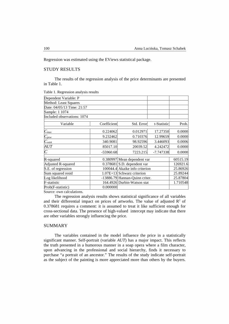
100 Anna Lucińska, Tomasz Schabek
Regression was estimated using the EViews statistical package.
STUDY RESULTS
The results of the regression analysis of the price determinants are presented in Table 1.
Table 1. Regression analysis results
Dependent Variable: P Method: Least Squares Date: 04/05/13 Time: 21:57 Sample: 1 1074 Included observations: 1074
Variable Coefficient Std. Error t-Statistic Prob.
Cmax 0.224062 0.012971 17.27350 0.0000 Cpow 9.232462 0.710376 12.99659 0.0000 Cwiek 340.9081 98.92596 3.446093 0.0006 AUT 85017.10 20039.52 4.242472 0.0000 C -55960.68 7223.215 -7.747338 0.0000
R-squared 0.380997 Mean dependent var 60515.19 Adjusted R-squared 0.378681 S.D. dependent var 126921.6 S.E. of regression 100044.4 Akaike info criterion 25.86926 Sum squared resid 1.07E+13 Schwarz criterion 25.89244 Log likelihood -13886.79 Hannan-Quinn criter. 25.87804 F-statistic 164.4926 Durbin-Watson stat 1.710548 Prob(F-statistic) 0.000000 Source: own calculations.
The regression analysis results shows statistical significance of all variables and their differential impact on prices of artworks. The value of adjusted R2 of 0.378681 requires a comment: it is assumed to treat it like sufficient enough for cross-sectional data. The presence of high-valued intercept may indicate that there are other variables strongly influencing the price.
SUMMARY
The variables contained in the model influence the price in a statistically significant manner. Self-portrait (variable AUT) has a major impact. This reflects the truth presented in a humorous manner in a soap opera where a film character, upon advancing in the professional and social hierarchy, finds it necessary to purchase “a portrait of an ancestor.” The results of the study indicate self-portrait as the subject of the painting is more appreciated more than others by the buyers.
Factors Affecting the Prices of Artworks … 101
Another variable that has a significant impact on price is Cwiek which represents the age of the painting at the time of sale. This shows the influence of the subject and art movement on price: the greater the value of this variable, the higher the price is, that is, the older the painting, the higher the price it commands. Polish buyers are reluctant to purchase contemporary and modern art, as opposed to older art. They prefer landscapes or historic scenes evoking a patriotic sentiment over artworks depicting psychological states and reality deformed and transformed into an abstract form. This is consistent with the opinions of experts on the Polish art market: “one should think that Polish society is conservative and potential art buyers are not interested in contemporary issues. Regrettably, our culture may not transmit the refined snobbery that is linked to collecting contemporary art or interest in it” [Potocka 2013]. Another significant variable is the surface area of the painting (Cpow). Its influence on the price may be described as a statistical relationship – the larger the painting the higher the price. In turn, the significance of the variable Cmax may be interpreted as the influence of the artists’ reputation on price – the better the reputation, the higher the price of the painting. An artwork by a highly reputed painter will be expensive, while low reputation will be reflected in low artwork prices.
Presented paper shows the results of one of the first pilot studies on Polish art market. The efforts are made to construct a model that would show in the best way the relationship of price of an artwork with variety of factors. Being aware of the imperfections of the present model, authors have attempted to present the results of the studies due to their innovative - in Polish conditions - nature. These efforts will continue.
LITERATURE
1. Ashenfelter O., Graddy K. (2003) Auctions and the Price of Art, Journal of Economic Literature, September, 782 – 785.
2. Burton B., Jacobsen J. (1999) Measuring Returns on Investments in Collectibles, Journal of Economic Perspectives, Vol.13, No. 4, 193 – 212.
3. Campos N., Barbosa R. (2008) Painting and Number: An Econometric Investigation of Sales Rates, Prices and Returns in Latin American Art Auctions, The Institute for the Study of Labor IZA, Bonn, IZA Discussion Paper No. 3445, 18 – 25.
4. Dobrowolski T. (1989) Malarstwo polskie, ZN Ossolineum, Wrocław, p. 48, 149. 5. Edwards S. (2004) The Economics of Latin American Art.: Creativity Patterns and Rate
of Return, NBER Working Paper No. 10302, 14 – 17. 6. Galenson D.W. (1999) The Lives of the Painters of Modern Life: the Careers of Artists
in France from Impressionism to Cubism, NBER Working Paper No. 6888, 13 – 39. 7. Galenson D.W. (2004) A Portrait of the Artist as a Very Young or Very Old Innovator:
Creativity at the Extremes of the Life Cycle, NBER Working Paper No. 10515, 3 – 12, 63 – 66.
8. Galenson D.W (2008) The Back Story of Twentieth-Century Art, NBER Working Paper No. w14066, 9 – 27.

102 Anna Lucińska, Tomasz Schabek
9. Galenson D. W., Weinberg B. A. (2000) Age and the Quality of Work: The Case of Modern American Painters, Journal of Political Economy, Vol. 108, No. 4, 761 -777.
10. Hodgson D. J. (2011), Age-Price Profiles for Canadian Painters at Auction, CIRANO Scientific Publications, No. 2011, 13 – 15.
11. Kompa K., Witkowska D. (2013) Indeks rynku sztuki. Badania pilotażowe dla wybranych malarzy polskich, Journal of Management and Finance, Vol. 3, No. 2, 39 – 42.
12. Lanyon G. R., Smith L. (1999) A portrait of an Artist as a Young, Middle-Aged and Elderly Man, http://dx.doi.org/10.2139/ssrn.18221, access 04.07.2013, 3 – 9.
13. Lucińska A. (2011) Malarstwo na polskim rynku aukcyjnym, Rynki finansowe. Nowe wyzwania i możliwości, Prace Naukowe Wyższej Szkoły Bankowej w Gdańsku, CeDeWu, Gdańsk, 254.
14. Lucińska A. (2012) Rozwój artystyczny malarzy a ceny obrazów na polskim rynku sztuki, Zeszyty Naukowe Uniwersytetu Szczecińskiego nr 690 Finanse, rynki finansowe, ubezpieczenia nr 5, Wydawnictwo Uniwersytetu Szczecińskiego, Szczecin, p. 715 – 725.
15. Małkowska M. (2010) Historia na wodzie, Rzeczpospolita, Księga Kresów Wschodnich nr 29, 19.08.2010, 15.
16. Mamarbachi R., Day M., Favato G. (2008) Art as an alternative investment asset, http://papers.ssrn.com/sol3/papers.cfm?abstract id=1112630, access 03.07.2013, 4.
17. Potocka M. A. (2013) Sztuka w ekonomii, exhibition catalogue Economy in Art., Muzeum Sztuki Współczesnej, Kraków, 99.
18. Towse R. (2011) Ekonomia kultury Kompendium, Narodowe Centrum Kultury, Warszawa, 102 – 104, 174.
19. Włodarczyk W. (2010) interview , Rzeczpospolita, 23–24.01.2010, A20 – A21.
ANNEX 1
Table 2. The most prominent painters in terms of the number and value of paintings sold in the Polish auction market in the years 2007–2010
No Name Number of paintings
Value of paintings [PLN]
1 MALCZEWSKI Jacek 39 7.981.000 2 NOWOSIELSKI Jerzy 70 5.093.500 3 WYCZÓŁKOWSKI Leon 39 2.407.300 4 MUTER Mela 17 2.530.200 5 HOFMAN Vlastimil 49 1.080.750 6 KOSSAK Wojciech 45 1.623.000 7 FAŁAT Julian 36 1.588.800 8 KOSSAK Jerzy 66 870.600 9 MENKES Zygmunt Józef 15 835.000
10 TRUSZ Iwan 6 251.000 11 PANKIEWICZ Józef 18 2.095.500 12 KOSSAK Juliusz 26 1.556.960 13 KOWALSKI-WIERUSZ Alfred 14 3.825.000 14 WITKACY 37 1.780.000
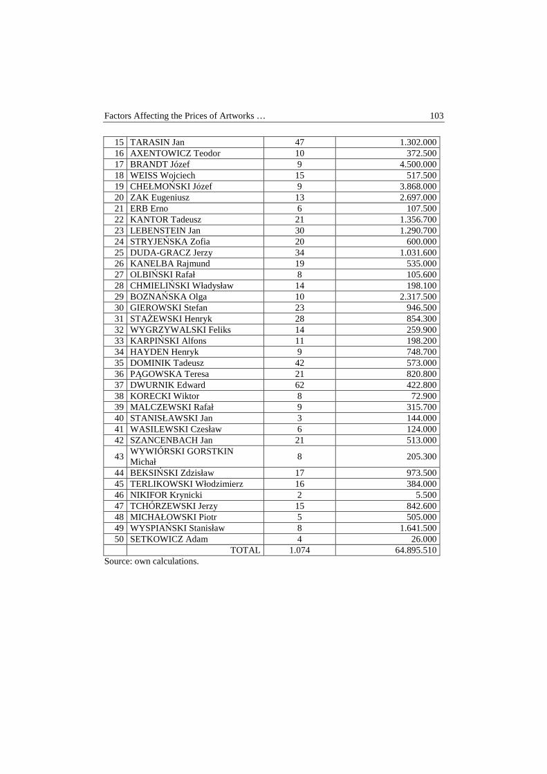
Factors Affecting the Prices of Artworks … 103
15 TARASIN Jan 47 1.302.000 16 AXENTOWICZ Teodor 10 372.500 17 BRANDT Józef 9 4.500.000 18 WEISS Wojciech 15 517.500 19 CHEŁMOŃSKI Józef 9 3.868.000 20 ZAK Eugeniusz 13 2.697.000 21 ERB Erno 6 107.500 22 KANTOR Tadeusz 21 1.356.700 23 LEBENSTEIN Jan 30 1.290.700 24 STRYJEŃSKA Zofia 20 600.000 25 DUDA-GRACZ Jerzy 34 1.031.600 26 KANELBA Rajmund 19 535.000 27 OLBIŃSKI Rafał 8 105.600 28 CHMIELIŃSKI Władysław 14 198.100 29 BOZNAŃSKA Olga 10 2.317.500 30 GIEROWSKI Stefan 23 946.500 31 STAŻEWSKI Henryk 28 854.300 32 WYGRZYWALSKI Feliks 14 259.900 33 KARPIŃSKI Alfons 11 198.200 34 HAYDEN Henryk 9 748.700 35 DOMINIK Tadeusz 42 573.000 36 PĄGOWSKA Teresa 21 820.800 37 DWURNIK Edward 62 422.800 38 KORECKI Wiktor 8 72.900 39 MALCZEWSKI Rafał 9 315.700 40 STANISŁAWSKI Jan 3 144.000 41 WASILEWSKI Czesław 6 124.000 42 SZANCENBACH Jan 21 513.000
43 WYWIÓRSKI GORSTKIN Michał
8 205.300
44 BEKSIŃSKI Zdzisław 17 973.500 45 TERLIKOWSKI Włodzimierz 16 384.000 46 NIKIFOR Krynicki 2 5.500 47 TCHÓRZEWSKI Jerzy 15 842.600 48 MICHAŁOWSKI Piotr 5 505.000 49 WYSPIAŃSKI Stanisław 8 1.641.500 50 SETKOWICZ Adam 4 26.000
TOTAL 1.074 64.895.510 Source: own calculations.
QUANTITATIVE METHODS IN ECONOMICS Vol. XV, No. 1, 2014, pp. 104 – 112
ANALYSIS OF SELECTED MARKET BEHAVIOURS IN THE EUROPEAN AND POLISH PRIVATE EQUITY SECTORS
IN 2000–2012
Witold Luci ński Lodz University of Technology
email: [email protected]
Abstract: The Polish private equity sector is a relatively new segment of the Polish financial market, as it emerged only at the beginning of the 1990s. In terms of capital, it is strongly linked to firms from outside Poland, especially European and American ones. Moreover, international firms are also significant capital donors for private equity funds in Poland. Thus, the question arises as to how these facts influence the market behaviours of Polish private equity funds. The study is based on data from 2000–2012, with Poland compared to the European market.
Keywords: private equity, emerging market, correlation, private equity funds
INTRODUCTION
The term private equity denotes a class of transactions involving private capital investments either in private companies or in publicly listed companies on the stock exchange with a view to withdrawing them from the stock exchange in the near future. Such transactions may provide funding to companies at the early stages of their development in order to boost their growth or may be used to buy out mature companies, also publicly traded ones. In the first case, private equity funds become minority shareholders, while in the second case they usually acquire a majority stake. Such companies become part of the investment portfolios of private equity firms. The objective of private equity transactions is increase the value of the portfolio company as compared to the purchase price. Private equity firms receive capital from investors who believe that the transactions they make will lead to much higher returns than those in the other segments of the capital market [Payne 2011]. Private equity funds (initially understood as venture capital) emerged in the USA in the 1940s and 1950s. This technology of financing and
Analysis of Selected Market Behaviours … 105
organization of investments was not brought to Europe until almost 30 years later. In Poland, such ideas appeared only at the beginning of the 1990s.
The benefits of private equity are manifold and include financial backing, managerial support, and the everyday presence of representatives of private equity firms in the activities of their portfolio companies [Kaplan, Stromberg 2008]. Private equity firms are a source of capital to their companies but are not interested in short-term returns, as in the short term their stakes are not liquid. Therefore, the focus is on long-term development of portfolio companies by new investments. Furthermore, the partial debt financing mode makes the companies use their cash prudently, as the management teams are aware of the repayment obligations. The management teams are strongly involved in initiating changes due to personal shareholding. Thus, private equity funds ensure close supervision of their companies’ business [Kaplan, Stromberg 2008].
Many studies have shown that private equity plays an invaluable role in the developed economies. It is emphasized that private equity leads to faster growth of portfolio companies than that of stock indexes such as S&P 500 [Kaplan, Schoar 2003]. Private equity is also thought to alleviate unemployment, enhance remunerations in portfolio companies, boost the value of the companies, as well as increase the volume and value of their output [The Global… 2010]. Many authors argue that private equity firms exert a major, even if indirect, influence on national economies. They also lead to greater competition in capital markets, at the same time forcing companies outside private equity financing to improve their management standards [Campbell, Campbell 2008]. In many countries the role of private equity has become so prominent that this sector is now considered a major vehicle for enhancing recovery from the economic crisis. For instance, this is the general expectation in Great Britain, which is the European leader in the private equity sector. Some even believe that private equity funds may not only be instrumental in overcoming the crisis, but subsequently they could help keep pace with the fastest growing economies of the world (China, India, Brazil) [Barber 2010].
A BRIEF OUTLINE OF THE SITUATION OF THE PRIVATE EQUITY SECTOR IN THE 21ST CENTURY
The history of the private equity sector in Europe, which has been professionally monitored since the 1980s, shows that it has been developing in a cyclical manner. Growth periods have been followed by downturns [Kaplan, Stromberg 2008]. Around 1995, euphoria driven by IT companies and the related sectors took hold of the stock markets around the world. As a result, companies that conducted business on the Internet or intended to do so became increasingly overvalued. A period of realization of tremendous profits (of the order of 65%) through IPOs on American stock exchanges in 1999–2000 was followed by
106 Witold Luciński
a dramatic decline to 12% in 2001–2003 [Loughran, Ritter 2004]. This downturn is commonly called the burst of the Dot-com bubble [Ljungqvist, William 2003]. Looking back, one can argue that it was not caused by a global recession of the world’s economy, but rather by adjustment processes within the IT sector (and IT companies are often backed by private equity funds due to their innovativeness). Statistical data show that the aforementioned crash, which hit hard private equity sectors around the globe, was followed by another period of dynamic development of this business model [EVCA 2001-2013].
The current situation differs in that the private equity sector, being an element of the financial market, has been affected by shock waves of the 2008 subprime mortgage crisis [Kaplan, Stromberg 2008], in which a major role was played by dysfunctional debt securitization [Christopoulos et al. 2011]. A global disaster was averted only thanks to the wide array of active measures undertaken by the governments around the world [Cohen 2012].
Initially, the understanding of the ongoing crisis in the context of the private equity sector was rather limited [Gurung, Lerner 2010]. The first reports on the global financial sector from 2008 and 2009 seemed to justify a quite optimistic outlook for the sector in Europe. Investments made by private equity firms exhibited high resilience to the crisis, at least in its early stage. As a rule, the portfolio companies of investment funds were not listed on stock exchanges, so they were not subjected to the often hysterical reactions of the destabilized financial markets.
Still, the number of new investments, and especially so-called mega buyouts, declined [Thomson 2009]. According to preliminary data for 2008, the volume of buyout transactions in Europe reached only EUR 49.9 billion, which means a decrease of almost 40% on the previous year. Thus, the investment volume shrank even more than in 2001, when the amount of capital invested was reduced by 30% from 2000 [EVCA 2003]. This situation was explained by the fact that many banks were no longer interested in leveraging transactions. Furthermore, if the cost of shareholder’s equity is lower than the cost of debt financing, then private equity companies take advantage of that difference [Kaplan, Stromberg 2008]. Obviously, the cost of debt surged due to increased risk and a crisis of confidence in the financial markets. Consequently, the managers of private equity firms no longer perceived leveraged transactions to be a viable option.
Paradoxically, at the beginning of the financial crisis, considerable capital resources were channelled to the private equity sector, especially in the United States, as a result of withdrawal from other capital market sectors. Major contributors at the time were pension funds [Thomson 2009]. It was estimated that in the United States, where the crisis emerged as early as in the second half of 2007, the amount of capital raised by the private equity sector in the first half of 2008 was greater than in any other half-year in the history of private equity. Some even foresaw the beginning of a golden age for private equity [Butler 2008]. However, in 2009 this optimism waned [Thomson 2009].

Analysis of Selected Market Behaviours … 107
Nevertheless, at a time of overwhelming uncertainty in the financial markets, investing in an area with strong fundamentals was undoubtedly a sound idea. Due to the low market value of many companies, the investment capacity of private equity firms significantly increased, while many other sectors faced technical or liquidity problems. This gave the private equity sector an opportunity to reinforce its position in the long term [Coller 2008].
On the other hand, private equity funds were now presented with problems concerning those companies that had been present in their portfolios for a longer time and were scheduled for divestment in the near future. Due to the low demand in the financial markets, the prices offered for their portfolio companies were unsatisfactory for the funds. This tendency hit the very foundations of the functioning of private equity firms. While making divestment decisions, they were faced with the dilemma of whether they should realize a low profit now or keep their capital frozen in their portfolio companies and bear additional management costs [Nazelle 2008].
Despite numerous difficulties, one could argue that the private equity sector is one of the few areas of the financial market that was, and, according to EVCA publications, still is, characterized by relatively good financial standing. However, given the above considerations, private equity managers will need to exercise considerable caution in the coming years [Coller 2008].
RESEARCH HYPOTHESIS
The Polish private equity sector is relatively little experienced or developed. Due to political reasons, it did not emerge until the transformation initiated at the end of the 1980s. However, despite its short presence in Poland, the section has gained an important place in the financial market in this country. This is confirmed by the fact that since the end of the 1990s it has been continuously, on individual basis monitored by EVCA, the top institution monitoring activity and implementing standards in this area. EVCA regularly releases data concerning about 20 countries having the most developed private equity sectors in Europe, including Poland.
A characteristic feature of the Polish private equity sector is a relatively small share of domestic capital as compared to the European standards, as can be seen from Tables 1 and 2.
Analysis of the above data shows that the private equity sector in Poland differs from the European sector in terms of the geographic distribution of the sources of funding. Table 1 shows that in Europe an important role is played by capital contributed by investors who are located in the same countries as the private equity firms they invest in. In the period 2000–2012, the share of such funding exceeded 40%, with another 20.5% of capital raised from other European countries. The remaining 40% came from non-European and unknown sources.
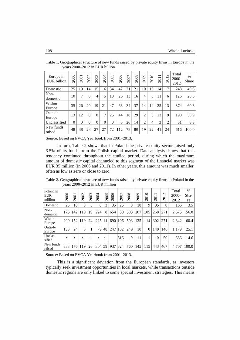
108 Witold Luciński
Table 1. Geographical structure of new funds raised by private equity firms in Europe in the years 2000–2012 in EUR billion
Europe in EUR billion 2
00
0
20
01
20
02
20
03
20
04
20
05
20
06
20
07
20
08
20
09
20
10
20
11
20
12 Total
2000-2012
% Share
Domestic 25 19 14 15 16 34 42 21 21 10 10 14 7 248 40.3 Non-domestic
10 7 6 4 5 13 26 13 16 4 5 11 6 126 20.5
Within Europe
35 26 20 19 21 47 68 34 37 14 14 25 13 374 60.8
Outside Europe
13 12 8 8 7 25 44 18 29 2 3 13 9 190 30.9
Unclassified 0 0 0 0 0 0 0 26 14 2 4 3 2 51 8.3 New funds raised
48 38 28 27 27 72 112 78 80 19 22 41 24 616 100.0
Source: Based on EVCA Yearbook from 2001–2013.
In turn, Table 2 shows that in Poland the private equity sector raised only 3.5% of its funds from the Polish capital market. Data analysis shows that this tendency continued throughout the studied period, during which the maximum amount of domestic capital channeled to this segment of the financial market was EUR 35 million (in 2006 and 2011). In other years, this amount was much smaller, often as low as zero or close to zero.
Table 2. Geographical structure of new funds raised by private equity firms in Poland in the years 2000–2012 in EUR million
Poland in EUR million 2
00
0
20
01
20
02
20
03
20
04
20
05
20
06
20
07
20
08
20
09
20
10
20
11
20
12 Total
2000-2012
% Sha-re
Domestic 25 10 0 5 0 3 35 25 0 18 9 35 0 166 3.5 Non-domestic 175 142 119 19 224 8 654 80 503 107 105 268 271 2 675 56.8
Within Europe 200 152 119 24 225 11 690 106 503 125 114 302 271 2 842 60.4
Outside Europe 133 24 0 1 79 48 247 102 249 10 0 140 146 1 179 25.1
Unclas-sified : : : : : :
616 9 11 1 0 50 686 14.6
New funds raised 333 176 119 26 304 59 937 824 760 145 115 443 467 4 707 100.0
Source: Based on EVCA Yearbook from 2001–2013.
This is a significant deviation from the European standards, as investors typically seek investment opportunities in local markets, while transactions outside domestic regions are only linked to some special investment strategies. This means
Analysis of Selected Market Behaviours … 109
that the Polish capital market is not particularly interested in private equity processes.
This largely results from the low supply of cash in the capital market. In Europe, the predominant investors are pension funds, banks, and funds of funds (in the years 2000–2012 they contributed 22.7%, 15.4%, and 13.8% of the capital, respectively in average) [EVCA 2001-2013]. However, in Poland, pension funds emerged very recently (at the turn of the century) and are subjected to severe investment limitations with a view to the safety of future pensions. This means that pension funds may not actively support the Polish private equity market. The decisions made in Poland very recently (in 2011 and 2012) as well as the current sentiment imply a decline of pension funds in this country.
The Polish banking sector is relatively small as compared to its counterparts in Europe, and is mostly interested in deposit and lending activity and related services rather than in capital market investments.
In turn, funds of funds represent a relatively new idea in Poland and are at an early stage of development, so they cannot function as a major player in the Polish financial market.
Under the circumstances, the question arises to what extent Polish private equity firms, most of which were established by foreign entities and 97% of whose capital comes from foreign sources, mirror the patterns of market behaviours typical of the private equity markets in other countries in terms of the amount of capital raised, investments, divestments, and size of investment portfolios. The overwhelming dominance of foreign firms in the Polish private equity market would suggest that the pattern of its activity is closely connected to the European market in the aforementioned four areas. This research problem is addressed by means of statistical analysis presented below.
DATA AND METHODOLOGY
European and Polish private equity firms are compared based on the data provided for each year of the period 2000–2012 by EVCA in the form of yearbooks. The data were released in cooperation with PEREP_Analytics and some other contributors.
Analysis concerns Europe as represented by the European Union Member States plus Ukraine, the group of former Yugoslav countries with Slovakia, the group of the Baltic states, Norway, and Switzerland, and with the exclusion of Bulgaria, Cyprus, and Malta. To determine the strength of the relationship between the activity of the Polish and European private equity sectors, statistical correlations were computed.
110 Witold Luciński
CONCLUSIONS
Analysis of data from consecutive EVCA Yearbooks revealed the strength of the relationship between the activity of the private equity sectors in Europe and in Poland in the years 2000–2012. The results are presented in Table 3.
Table 3. Correlation of the activity of the private equity sectors in Europe and in Poland in the years 2000–2012
Type of activity Funds raised Funds invested Divestments Portfolio
Correlation coefficient 0.76 0.36 0.66 0.94
Source: Based on EVCA Yearbooks from 2001–2013.
Analysis of Table 3 shows that in contrast to expectations, Polish and European private equity firms do not behave in unison. This in particular concerns investment of the capital raised, as a coefficient of 0.36 indicates poor correlation. This means that decisions as to the amount of funds expended over consecutive years were made by Polish firms as a result of their independent market analysis, while suggestions from the owners (capital donors) and European market behaviour trends (e.g., those resulting from the crisis) had a lesser influence on those decisions.
The amount of funds raised (a correlation coefficient of 0.76) and divestments (0.66) are more consistent with the European patterns. Indeed, this correlation may be deemed strong, but even in this case Polish private equity firms do not seem to mirror the trends followed elsewhere in Europe.
The strongest correlation (0.94) was observed for the size of investment portfolios in the private equity sectors. This can be explained by the nature of economic developments, which were similar for Poland and Europe. Every year, the value of portfolios changes, as new investments and divestments are made. The value of both Polish and European portfolios increased each year throughout the studied period.
Increased portfolio values in non-crisis periods are a beneficial phenomenon and show that the sector is growing, as the size of investment portfolios reflects the volume of investments continued by private equity funds. This augurs well for prosperity in the sector over the following years, when the companies maturing in the portfolios will present an opportunity for the realization of capital profits.
In periods of crisis, portfolios grow for a different reason, which was mentioned earlier in this paper. The activity of private equity funds consists of purchasing assets interesting from the point of view of the buyer (the private equity firm), their restructuring, and selling in the capital market. The difference between the sale and purchase prices, less management costs, constitutes the profit of the funds. The investments typically have a time horizon of 5 to 8 years. In many
Analysis of Selected Market Behaviours … 111
cases, in periods of crisis companies facing financial hardship sell off their property, including real estate and organized assets, at very low prices.
On the other hand, private equity firms whose portfolio companies have matured and are ready to be sold face obstacles in the form of low prices that potential buyers would be willing to pay for those companies. This leads to prolonged investment time as companies are retained in the portfolio with a view to obtaining higher prices in the capital market in the future. Thus, the fact that the growth trend in European and Polish portfolios is almost identical shows that the private equity sector in Poland is growing strong and follows the adaptation processes related to the crisis that hit Europe in 2008 and continues to this day.
In summary, it is not true that capital ties between Polish private equity firms and their foreign shareholders or other international entities contributing capital to be invested impose certain market behaviour patterns on the firms. It turned out that the private equity sector has elaborated independent features and it is relatively mature to pursue their own objectives within the framework of the Polish emerging market. A similar situation can be observed in the Polish banking sector, which is in 60% dependent on foreign capital.
REFERENCES
Barber L. (2010) Post-Crisis Britain: What Is to Be Done? Vital Speeches International. Vol. 2 Issue 4.
Butler R. (2008) Private Equity after the Crunch: A Route Map for the New Investment Landscape, Reuters IFR Market Intelligence.
Campbell D., Campbell M. (2008) The economic impact of private equity 360°, Ashridge Journal (Spring), Ashridge Businee School.
Christopoulos A., Mylonakis J., Koromilas Ch. (2011) Measuring the Impact of Financial Crisis on International Markets: An Application of the Financial Stress Index, Review of European Studies, Vol. 3, No. 1.
Cohen H.R. (2012) Preventing the Fire Next Time: Too Big To Fail, Academic Journal Texas Law Review, Vol. 90, Issue 7.
Coller J. (2008) What Goes Up, Must Come Down EVCA Yearbook, Zaaventem Belgium. Decree of the Council of Ministers on the maximum portion of assets of Open Pension
Funds that can be invested in particular types of assets and additional limitations on the investment activity conducted by Pension Funds of February 3, 2004 (Journal of Laws 2004 no. 32, item 276).
EVCA Yearbooks 2001–2013, Brussels, Belgium. Gurung A., Lerner J. (2010) Executive summary [in:] The Global Economic Impact of
Private Equity Report, The Globalization of Alternative Investments Working Papers, Vol. 3: World Economic Forum, Geneva.
Kaplan S.N., Stromberg P. (2008) Leveraged Buyouts and Private Equity, Journal of Economic Perspectives, Vol. 22, No. 4.
Kaplan S., Schoar A. (2003) Private Equity Performance: Returns, Persistence and Capital Flow, MIT Sloan School of Management, Working Paper 4446–03.
112 Witold Luciński
Ljungqvist A., William J. W., (2003) IPO pricing in the Dot-Com bubble, Journal of Finance, Vol. 58, April, 723-752.
Loughran T., Ritter J. R. (2004) Why Has IPO Underpricing Changed Over Time?, Financial Management, Vol. 33, No. 3.
Nazelle N. (2008) Back to basics, EVCA Yearbook, Zaaventem Belgium. Payne J. (2011) Private Equity and Its Regulation in Europe, European Business
Organization Law Review, 12:559–585. The Global Economic Impact of Private Equity Report (2010) The Globalization of
Alternative Investments Working Papers, Vol. 3: World Economic Forum Geneva. Thomson Reuters (2009a) European Private Equity Industry at Lowest Ebb Since 2001,
Data Room, European Venture Capital Journal, 30 March, 2009. Thomson Reuters (2009b) Pension funds weigh up private equity prospects, Analysis,
European Venture Capital Journal, 29 January, 2009.

QUANTITATIVE METHODS IN ECONOMICS Vol. XV, No. 1, 2014, pp. 113 – 124
WAGES INEQUALITIES BETWEEN MEN AND WOMEN: EUROSTAT SES METADATA ANALYSIS APPLYING
ECONOMETRIC MODELS1
Aleksandra Matuszewska-Janica Department of Econometrics and Statistics, Warsaw University of Life Sciences
Abstract: In this paper there are presented the results of investigation of the various factors impact on the level of male and female wages inequality. These factors are as follows: level of wages in employees group in comparison to the national average wages, the proportion of women in the group of employees, women labor market activity in the states, and variables such as the age, job seniority, level of education of the employees, type of employment contract, occupation (ISCO88), branch where the enterprises operate (NACE rev. 1.1), size of the company and collective pay agreement.
Keywords: labor market, the wage gap, the gender wage gap, SES
INTRODUCTION
Eurostat estimated that in 2012 in the EU women earned on average 16.4% less than men. This rate (GPG – Gender Pay Gap) varies e.g. among EU countries, economic sectors. We can also observe that at the GPG rate affect age, education, job seniority of employees and size of enterprise among other. The wage differences between men and women are largely explained on the basis of human capital theory (see e.g. [Haager 2000], [Polachek 2004]) and the discrimination theory (see e.g. [Becker 1971]). This phenomenon has a social dimension as well as economic importance (see e.g. discussion presented in [Klasen 1999], [Seguino 2000], [Blecker and Seguino 2002], [Löfström 2009], [Sinha et al. 2007]).
1 Work performed within the project that has been funded by the National Science Centre, decision number DEC-2011/01/B/HS4/06346 “Wages Inequalities between Men and Women in Poland in the Framework of the European Union”.

114 Aleksandra Matuszewska-Janica
Situation of women in the labor market is subject to European Union policy. Prevention of discrimination against women has been included in Strategy for equality between women and men 2010-2015.
The aim of the study is to estimate the impact of various factors on the level of men and women wages inequality in different countries and different groups of employees. Groups of employees are characterized by one of the following features: economic branch, age, occupation, job seniority, size of enterprise, collective pay agreement, type of employment contract. There is observe that on the gender wage differences influence some other factors like: feminization of employees groups, level of wages in employees groups or women activity rate at labor market in individual countries. So such variables also are included into estimated models. For the analysis is employed Eurostat SES metadata.
DATA DESCRIPTION
Analysis is provided upon the European Union Structure of Earnings Survey (SES) data collected in 2006.2 There are used aggregated data, that Eurostat calls Metadata. SES is a survey conducted in accordance with the Council Regulation No. 530/1999 and the Commission Regulation No. 1916/2000 as amended by Commission Regulation No. 1738/2005. The SES for 2006 is the second of a series of four yearly. The SES is a survey providing information on relationships between the level of remuneration, individual characteristics of employees and their employer (economic branch, age, occupation, job seniority, size of enterprise, collective pay agreement, type of employment contract among others). The statistics of the SES refer to the enterprises with at least 10 employees.
Data on employment and wages are encompassed in the database that contain different characteristics, as is presented in Figure 1.
To measure income inequality is often used GPG (Gender Pay Gap) coefficient. GPG represents the difference between average gross hourly earnings of male paid employees (���������
�) and of female paid employees (����������) as
a percentage of average gross hourly earnings of male paid employees (see Fernandez-Aviles et al. 2010):
1001 ⋅
−=
M
F
GHE
GHEGPG (1)
where:
2 Structure of Earnings Survey has been provided every four year since 2002. There are some differences between metadata because of imported correction in every survey. For example in each survey (2002, 2006 and 2010) was different definition (SES 2006 and SES 2010) or different range (SES 2002 and SES 2006) of economic branches. So in presented analysis is used database from 2006.

Wages inequalities between men and women… 115
GPCFPCMHEGHE
GHEGPG
M
F ==⋅=− _100100 (2)
is publicized by Eurostat.
Figure 1. Structure of SES database
DATA ON EMPLOYMENT AND WAGES
NUMBER
OF EMPLOYEES
HOURLY
EARNINGS
MONTHLY
EARNINGS
ANNUAL
EARNINGS
HOURS
PAID
ANNUAL
HOLIDAYS
CHARACTERISTICS OF EMPLOYEES/EMPLOYERS IN INDIVIDUAL DATASETS
SEX;
COUNTRY;
ECONOMIC
ACTIVITY;
AGE
SEX;
COUNTRY;
ECONOMIC
ACTIVITY;
TYPE OF
CONTRACT
SEX;
COUNTRY;
ECONOMIC
ACTIVITY;
EDUCATION
SEX;
COUNTRY;
ECONOMIC
ACTIVITY;
OCCUPATION
SEX;
COUNTRY;
ECONOMIC
ACTIVITY;
JOB
SENIORITY
SEX;
COUNTRY;
OCCUPATION;
SIZE OF
ENTERPRISE
SEX;
COUNTRY;
OCCUPATION;
AGE
SEX;
COUNTRY;
ECONOMIC
ACTIVITY;
COLL. PAY
AGREEMENT
Source: own elaboration.
In the SES 2006 we can distinguish eight types of sets of aggregated data. Every data sets contained two types of information: measurable and no measurable. Measurable variable were mean hourly earnings and number of employees given for men, women and total employees. No measurable were variables as follows: sex, country and two others that were different for each data set (see Figure 2).
Figure 2. The variables that differentiate data sets
Source: own elaboration. In parentheses are given dataset names.
• (D1) CONOMIC ACTIVITY, GROUP OF AGE
• (D2) GROUP OF AGE, OCCUPATION
• (D3) ECONOMIC ACTIVITY, TYPE OF
EMPLOYMENT CONTRACT
• (D4) ECONOMIC ACTIVITY, JOB SENIORITY
• (D5) ECONOMIC ACTIVITY, OCCUPATION
• (D6) ECONOMIC ACTIVITY, EDUCATION
• (D7) OCCUPATION, SIZE OF ENTERPRISE
• (D8) ECONOMIC ACTIVITY, COLLECTIVE PAY
AGREEMENT
NUMBER OF
EMPLOYEES
AND
MEAN HOURLY
EARNINGS

116 Aleksandra Matuszewska-Janica
METHODOLOGY
In the analysis were estimated one equation econometric models:
ij
m
kkijki
ijijij
DummyActiv
FEMWagesFPCMHE
εγβ
βββ
+++
+++=
∑=1
3
210
ln
lnln_ln
(3)
HE_FPCM is share of average gross hourly earnings of female paid employees (���������
�) as a percentage of average gross hourly earnings of male paid employees (���������
�). In the paper Witkowska (2013) this rate was named as gender pay convergence ratio. HE_FPCM is published by Eurostat (see formula 2). Value of HE_FPCM equals 100 inform that between men and women wages there are no differences. When HE_FPCM is greater than 100 – women earn more than men on average.
In the models was used gender pay convergence coefficients calculated as:
Mij
Fijij
GHE
GHEFPCMHE ln_ln = (4)
where:����������� – average hourly female earnings of employees in i-th country and
j-th group of employees; ����������� – average hourly male earnings of employees in
i-th country and j-th group of employees; in each model groups of employees refers to one of the employee’s or enterprise’s characteristic like economic branch, age, occupation, job seniority, size of enterprise, collective pay agreement, type of employment contract.
Variable Wages refers to the structure of hourly earnings in selected group of employees in each country. In the models variable Wages was calculated as natural logarithm of the ratio of the average wage in the j-th group of employees to average wages in the country:
i
ijij
GHE
GHEWages lnln = (5)
where: ���������� – average hourly earnings of employees in i-th country and j-th
group of employees; ���������� – average hourly earnings of employees in i-th country.
Previous analysis indicated that higher wages ratio is positive associated with gender wag gap (see [Witkowska et al. 2013]).
Feminization rate (FEM) is a variable that refers to gender employment structure in selected group of employees. In the models this variable was calculated as:
ijij
ijij EMEF
EFFEM
+= lnln (6)

Wages inequalities between men and women… 117
where: �� – number of employed women in i-th country and j-th group of employees; ��� – number of employed men in i-th country and j-th group of employees.
Activity rate lnActivi is a natural logarithm of share of active women in the labor market in the i-th country in whole women population in working age 20-64 in i-th country. Previous analysis indicated that higher women’s activity at the labor market is positive associated with gender wag gap (see [Witkowska et al. 2013]).
Each model contains dummy variable. Every of them refers to one of the employee’s or enterprise’s characteristic like economic branch, age, occupation, job seniority, size of enterprise, collective pay agreement, type of employment contract. It is defined as: � ����� = 1 – when the variable concerns k-th option in j-th group of employees and i-th country, � ����� = 0 – otherwise. Options of dummy variables are presented in Table 1. In presented models is not investigated country effect.
Table 1. Dummy variables and theirs options
Dummy variable
Options
Age Y0_29 - less than 30 years Y30_39 - between 30 and 39 years Y40_49 - between 40 and 49 years Y50_59 - between 50 and 59 years Y_GE60 - 60 years and over
Branch (economic sector)
C - Mining and quarrying D - manufacturing E - electricity, gas and water supply F - construction G - wholesale and retail trade; repair of motor vehicles, motorcycles and personal and household goods H - hotels and restaurants I - transport, storage and communication J - financial intermediation K - real estate, renting and business activities L - public administration and defense; compulsory social security M - education N - health and social work O - other community, social, personal service activities
Size of Enterprise (number of employees)
10_49 - between 10 and 49 50_249 - between 250 and 499 250_499 - between 500 and 999 500_999 - between 50 and 249 gt_1000 - more than 1 000
Source: own elaboration.

118 Aleksandra Matuszewska-Janica
Table 1. (cont.) Dummy variables and theirs options
Dummy variable
Options
Occupation ISCO1 - Legislators, senior officials and managers ISCO2 - Professionals ISCO 3 - Technicians and associate professionals ISCO 4 - Clerks ISCO 5 - Service workers and shop and market sales workers ISCO 7 - Craft and related trades workers ISCO 8 - Plant and machine operators and assemblers ISCO 9 - Elementary occupations
Education (ISCED 1997)
ED0_1 - Pre-primary and primary education - levels 0-1 ED2 - lower secondary education – level 2 ED3_4 Upper secondary and post-secondary non-tertiary education - levels 3-4 ED5A Tertiary education - level 5A ED5B Tertiary education - level 5B ED6 Tertiary education - level 6
Collective pay agreement
NAT - A national level or interconfederal agreement IND - B industry agreement IND1 - C agreement for individual industries in individual regions ENT - D enterprise or single employer agreement UNIT - E agreement applying only to workers in the local unit OTH - F any other type of agreement NONE - N no collective agreement exists
Type of contract
INDEF - Indefinite duration FIX - Fixed term (except apprentice and trainee) APPR – apprentice or trainee
Job seniority
Y_LT1 – less than 1 year Y1_5 – between 1 and 5 years Y6_9 – between 6 and 9 years Y10_14 – between 10 and 14 years Y15_19 – between 15 and 19 years Y20_29 – between 20 and 29 years Y_GE30 – 30 years or more
Source: own elaboration based on Structure of Earnings Survey 2006: Eurostat’s arrangements for implementing the Council Regulation 530/1999, the Commission Regulations 1916/2000 and 1738/2005.
RESULTS
In this section were presented eight models. In each model are included three the same (in respect of variable construction) quantitative variables: lnWages, lnFEM and lnActiv. Models differs in dummy variables. Characteristics of each model are presented in the Table 2.
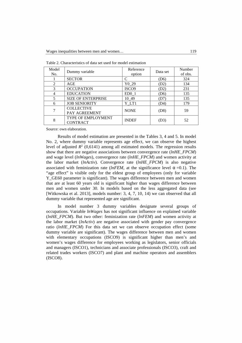
Wages inequalities between men and women… 119
Table 2. Characteristics of data set used for model estimation
Model No.
Dummy variable Reference
option Data set
Number of obs.
1 SECTOR C (D6) 324 2 AGE Y0_29 (D2) 134 3 OCCUPATION ISCO9 (D2) 231 4 EDUCATION ED0_1 (D6) 135 5 SIZE OF ENTERPRISE 10_49 (D7) 135 6 JOB SENIORITY Y_LT1 (D4) 179
7 COLLECTIVE PAY AGREEMENT
NONE (D8) 59
8 TYPE OF EMPLOYMENT CONTRACT
INDEF (D3) 52
Source: own elaboration.
Results of model estimation are presented in the Tables 3, 4 and 5. In model No. 2, where dummy variable represents age effect, we can observe the highest level of adjusted R2 (0,6141) among all estimated models. The regression results show that there are negative associations between convergence rate (lnHE_FPCM) and wage level (lnWages), convergence rate (lnHE_FPCM) and women activity at the labor market (lnActiv). Convergence rate (lnHE_FPCM) is also negative associated with feminization rate (lnFEM, at the significance level α =0.1). The “age effect” is visible only for the eldest group of employees (only for variable Y_GE60 parameter is significant). The wages difference between men and women that are at least 60 years old is significant higher than wages difference between men and women under 30. In models based on the less aggregated data (see [Witkowska et al. 2013], models number: 3, 4, 7, 10, 14) we can observed that all dummy variable that represented age are significant.
In model number 3 dummy variables designate several groups of occupations. Variable lnWages has not significant influence on explained variable (lnHE_FPCM). But two other: feminization rate (lnFEM) and women activity at the labor market (lnActiv) are negative associated with gender pay convergence ratio (lnHE_FPCM) For this data set we can observe occupation effect (some dummy variable are significant). The wages difference between men and women with elementary occupations (ISCO9) is significant higher than men’s and women’s wages difference for employees working as legislators, senior officials and managers (ISCO1), technicians and associate professionals (ISCO3), craft and related trades workers (ISCO7) and plant and machine operators and assemblers (ISCO8).

120 Aleksandra Matuszewska-Janica
Table 3. Parameters of estimated models (1)
Model No. 2 Dummy variable: AGE
Model No. 3 Dummy variable: OCCUPATION
Model No. 4 Dummy variable:
EDUCATION variable coefficient variable coefficient Variable coefficient const -0,3159 *** const -0,2388 *** const -0,2701 *** lnWages -0,3065 *** lnWages 0,0727 lnWages -0,0080 lnFEM -0,0927 * lnFEM -0,0521 *** lnFEM 0,0374 * lnActiv -0,2403 *** lnActiv -0,1987 *** lnActiv -0,1919 *** Y30_39 -0,0227 ISCO1 -0,2450 *** ED2 0,0053 Y40_49 -0,0361 ISCO2 -0,0765 ED3_4 0,0109 Y50_59 -0,0326 ISCO3 -0,0838 ** ED5A -0,0367 Y_GE60 -0,0873 *** ISCO4 0,0131 ED5B -0,0143 ISCO5 0,0009 ED6 0,0254 ISCO6 0,0110 ISCO7 -0,2151 *** ISCO8 -0,1493 *** R2 adj. 0,6141 R2 adj. 0,3880 R2 adj. 0,4533 F 31,24 *** F 14,25 *** F 14,89 ***
Source: own calculation. *** denotes significance level α = 0.10, ** α = 0.05 and * α = 0.1
In model number 4 dummy variables represents several education groups. In this model variable lnWages also has not significant influence on dependent variable (lnHE_FPCM). Women’s activity rate (lnActiv) has significant negative impact on the gender pay convergence ratio (lnHE_FPCM). Increasing feminization rate (lnFEM) causes increase of lnHE_FPCM. In examined data set differences between wages of men and women with the different education level are similar. All dummy variable are not significant. This result is opposite to obtained by [Witkowska et al. 2013], see models number: 1, 9, 12, 16). In these models we observed significant differences between gender wag gaps for employees with elementary and highest level of education.
Job seniority was investigated in model number 6. There we can observe that in groups of employees with greater job seniority gender pay convergence ratio is smaller than for employees shorter than one year. The same results was obtained for less aggregated data (see [Witkowska et al. 2013], models number: 2, 8, 11, 15). In this model variable lnWages was not significant, but we observed significant negative influence on gender wages convergence other two variable: lnFEM and lnActiv.
In models No. 1 and 5 were take onto account such attributes of enterprise like economic branch and size of enterprise. In bigger companies gender wage inequalities are greater than in smaller enterprises (see results obtained for model number 5). Also differences between wages of men and women varies among branches. Gender wage gap is significant smaller (gender wage convergence ratio is higher) in construction (F), hotels and restaurants (H), transport, storage and
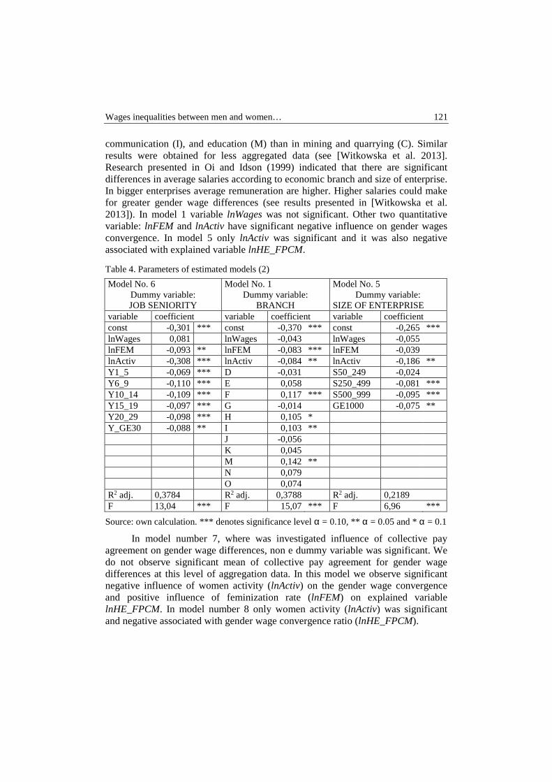
Wages inequalities between men and women… 121
communication (I), and education (M) than in mining and quarrying (C). Similar results were obtained for less aggregated data (see [Witkowska et al. 2013]. Research presented in Oi and Idson (1999) indicated that there are significant differences in average salaries according to economic branch and size of enterprise. In bigger enterprises average remuneration are higher. Higher salaries could make for greater gender wage differences (see results presented in [Witkowska et al. 2013]). In model 1 variable lnWages was not significant. Other two quantitative variable: lnFEM and lnActiv have significant negative influence on gender wages convergence. In model 5 only lnActiv was significant and it was also negative associated with explained variable lnHE_FPCM.
Table 4. Parameters of estimated models (2)
Model No. 6 Dummy variable: JOB SENIORITY
Model No. 1 Dummy variable:
BRANCH
Model No. 5 Dummy variable:
SIZE OF ENTERPRISE variable coefficient variable coefficient variable coefficient const -0,301 *** const -0,370 *** const -0,265 *** lnWages 0,081 lnWages -0,043 lnWages -0,055 lnFEM -0,093 ** lnFEM -0,083 *** lnFEM -0,039 lnActiv -0,308 *** lnActiv -0,084 ** lnActiv -0,186 ** Y1_5 -0,069 *** D -0,031 S50_249 -0,024 Y6_9 -0,110 *** E 0,058 S250_499 -0,081 *** Y10_14 -0,109 *** F 0,117 *** S500_999 -0,095 *** Y15_19 -0,097 *** G -0,014 GE1000 -0,075 ** Y20_29 -0,098 *** H 0,105 * Y_GE30 -0,088 ** I 0,103 ** J -0,056 K 0,045 M 0,142 ** N 0,079 O 0,074 R2 adj. 0,3784 R2 adj. 0,3788 R2 adj. 0,2189 F 13,04 *** F 15,07 *** F 6,96 ***
Source: own calculation. *** denotes significance level α = 0.10, ** α = 0.05 and * α = 0.1
In model number 7, where was investigated influence of collective pay agreement on gender wage differences, non e dummy variable was significant. We do not observe significant mean of collective pay agreement for gender wage differences at this level of aggregation data. In this model we observe significant negative influence of women activity (lnActiv) on the gender wage convergence and positive influence of feminization rate (lnFEM) on explained variable lnHE_FPCM. In model number 8 only women activity (lnActiv) was significant and negative associated with gender wage convergence ratio (lnHE_FPCM).
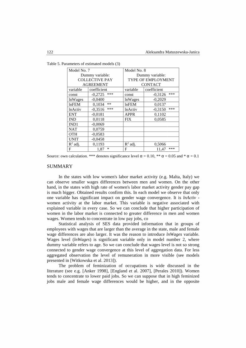
122 Aleksandra Matuszewska-Janica
Table 5. Parameters of estimated models (3)
Model No. 7 Dummy variable:
COLLECTIVE PAY AGREEMENT
Model No. 8 Dummy variable:
TYPE OF EMPLOYMENT CONTACT
variable coefficient variable coefficient const -0,2725 *** const -0,3126 *** lnWages -0,0400 lnWages -0,2029 lnFEM 0,1034 ** lnFEM 0,0137 lnActiv -0,3516 *** lnActiv -0,3150 *** ENT -0,0181 APPR 0,1102 IND 0,0118 FIX 0,0585 IND1 -0,0069 NAT 0,0759 OTH -0,0583 UNIT -0,0458 R2 adj. 0,1193 R2 adj. 0,5066 F 1,87 * F 11,47 ***
Source: own calculation. *** denotes significance level α = 0.10, ** α = 0.05 and * α = 0.1
SUMMARY
In the states with low women's labor market activity (e.g. Malta, Italy) we can observe smaller wages differences between men and women. On the other hand, in the states with high rate of women's labor market activity gender pay gap is much bigger. Obtained results confirm this. In each model we observe that only one variable has significant impact on gender wage convergence. It is lnActiv - women activity at the labor market. This variable is negative associated with explained variable in every case. So we can conclude that higher participation of women in the labor market is connected to greater difference in men and women wages. Women tends to concentrate in low pay jobs, co
Statistical analysis of SES data provided information that in groups of employees with wages that are larger than the average in the state, male and female wage differences are also larger. It was the reason to introduce lnWages variable. Wages level (lnWages) is significant variable only in model number 2, where dummy variable refers to age. So we can conclude that wages level is not so strong connected to gender wage convergence at this level of aggregation data. For less aggregated observation the level of remuneration in more visible (see models presented in [Witkowska et al. 2013]).
The problem of feminization of occupations is wide discussed in the literature (see e.g. [Anker 1998], [England et al. 2007], [Perales 2010]). Women tends to concentrate to lower paid jobs. So we can suppose that in high feminized jobs male and female wage differences would be higher, and in the opposite
Wages inequalities between men and women… 123
situation - GPG would be lower. Feminization rate applied in analyzed models gives different results. In two models number 4 (education) and number 7 (collective pay agreement) is positive associated with gender pay convergence coefficient. In two other models (no. 5 (size of enterprise) and no. 8 (type of employment contract)) this variable has none significant impact on the explained variable lnHE_FPCM. In four models (models number 1, 2, 3, 6) feminization rate has negative impact on lnHE_FPCM. So we can conclude that feminization of labor market has both negative and positive effects on gender wage differences.
Effects that are represented by dummy variable (economic branch, age, occupation, job seniority, size of enterprise, collective pay agreement, type of employment contract) in not so strong for analyzed data like for less aggregated data. In presented model we can observe significant differences in wage inequalities especially in branches, different size enterprises, for groups of employees with different job seniority, occupation and age. There are not detected differences between groups of employees with different level of education, type of employment contract or collective pay agreement. Next step of the study will be analysis with the use of low aggregated and more detailed data.
REFERENCES
Anker R. (1998) Gender and Jobs: Sex Segregation of Occupations in the World, Interna-tional Labor Office.
Becker G.S. (1971) The Economics of Discrimination. Blecker R., Seguino S. (2002) Macroeconomic Effects of Reducing Gender Wage Inequa-
lity in an Export-Oriented, Semi-industrialized Economy, Review of Development Economics, Wiley Blackwell, Vol. 6(1), 103-119.
England P., Allison P.D., Wu Y. (2007) Does bad pay cause occupations to feminize, Does feminization reduce pay, and How can we tell with longitudinal data?, Social Science Research, Vol. 36, 1237-1256.
Fernández-Avilés G., Montero J.M., Witkowska D. (2010) Gender Wage Gap in EU States. Application of Taxonomic and Spatial Methods, [in:] Witkowska D., Nermend K. (ed.), Regional Analysis: Globalization, Integration, Transformation, Wydawnictwo Uniwersytetu Szczecińskiego, Szczecin, 71-95.
Haager D.M. (2000) How do Investments in Human Capital Differentially Affect Gender Income? An Analysis of the Gender Wage Gap, The Park Place Economist, vol. VIII.
Klasen S. (1999) Does Gender Inequality Reduce Growth and Development? Evidence from Cross-Country Regressions, World Bank Working Paper Series, No. 7.
Löfström Å. (2009) Gender equality, economic growth and employment, working paper. Morrison A., Raju D. Sinha N. (2007) Gender Equality, Poverty and Economic Growth,
Policy World Bank Policy Research Working Paper, No. 4349. Oi W.Y., Idson T.L. (1999) Firm Size and Wages in. Handbook of Income Distribution,
vol. 3B, ed. Ashenfelter O., Card D., Elsevier, Amsterdam, 2165-2214.
124 Aleksandra Matuszewska-Janica
Perales F. (2010) Occupational Feminization, Specialized Human Capital and Wages: Evidence from the British Labour Market, ISER Working Paper Series: 2010-31.
Polachek S.W. (2004) How the Human Capital Model Explains Why the Gender Wage Gap Narrowed, IZA Bonn Discussion Paper, No. 1102.
Seguino S. (2000) Gender Inequality and Economic Growth: A Cross-Country Analysis, World Development, Elsevier, vol. 28(7), 1211-1230.
Witkowska D. (2013) Gender Disparities in the Labor Market in the EU, International Atlantic Economic Research, Vol. 19(4), 331-254.
Witkowska D., Kompa K., Matuszewska-Janica A. (2013) Gender Earning Differences in the European Union Member States, European Journal of Management, Vol. 13(4), 129-148.
QUANTITATIVE METHODS IN ECONOMICS Vol. XV, No. 1, 2014, pp. 125 – 132
APPLICATION OF MAJR AGGREGATE MEASURE IN THE GOVERNANCE QUALITY TESTING IN THE EU-28
Danuta Miłaszewicz Department of Macroeconomics,
Faculty of Economics and Management, University of Szczecin e-mail: [email protected]
Kesra Nermend Department of Computer Methods in Experimental Economics, Faculty of Economics and Management, University of Szczecin
e-mail: [email protected]
Abstract: The type of governance applied in an economy as well as its quali-ty determines the quality of life. Decisions that result in the improved gover-nance quality should be preceded by operationalisation of this category and by the related research. The purpose of this article is to present the concepts of governance and good governance as well as to propose the application of an aggregate measure of the governance quality constructed on the basis of the World Bank indices in the time cross-sectional analysis of 28 EU member states over the period of 2002-2012.
Keywords: good governance, aggregate measure of governance quality
INTRODUCTION
Institutional solutions in economy are largely conditioned by cultural, histor-ical, geographical, political and social factors. Therefore, adopted in the economy, institutional solutions create specific conditions for the functioning of the entities, allocation of resources and realization of individual and social interests [Miłasze-wicz 2011, Miłaszewicz 2013]. Being the area for functioning of two principal mechanisms of human activity, i.e. the state and the market, the type of institution-al order influences the local economic performance. Consequently, a high level of social development and quality of life can not be reached without a good quality institutional environment.
126 Danuta Miłaszewicz, Kesra Nermend
While the market mechanism functions more effectively when the state sup-ports it by creating right institutional conditions (e.g. by defining property rights), the state itself can improve or sometimes eliminate its weaknesses by making pub-lic institutions and the public sector function better. In other words, the state can act upon the advantage of the governance quality. In view of the good governance concept, proper institutional solutions, that shape the governance and affect its quality, contribute to lower transaction costs, reduced insecurity, more stable busi-ness environment as well as to the sustainable, socially acceptable growth and im-proved quality of life. At the same time they involve the members of society into the process of public decision making [Miłaszewicz 2011, 11]. This is why it is so important for any process of public sector restructuring, which is undertaken in many economies, to operationalise the categories of the governance quality, to run studies on it and compare the results of its assessment.
The purpose of the theoretical part of this article is to present the concepts of governance and good governance. In the empirical part the authors demonstrate how the aggregate measure of governance quality constructed on the basis of six World Bank indicators can be used in a cross-sectional and temporal analysis. The analysis covers the time period of 2002-2012, while the cross-sectional area of re-search includes 28 Member States of the European Union.
GOVERNANCE AND ITS QUALITY - THE CONCEPT AND MEAS-UREMENT
Initially governance was the term which referred to the private sphere and businesses operating therein. For the last 30 years, however, it has been a term that is useful in explaining how the public sphere functions.
Governance is defined differently by various international organizations which, while evaluating its quality, build many measures that are used when mak-ing ranking lists of world or regional economies. The broadest understanding of governance has been proposed by the United Nations Organization according to which it is “the system of values, policies and institutions by which a society man-ages its economic, political and social affairs through interactions within and among the state, civil society and private sector. It is the way a society organizes it-self to make and implement decisions — achieving mutual understanding, agree-ment and action. It comprises the mechanisms and processes for citizens and groups to articulate their interests, mediate their differences and exercise their legal rights and obligations. It is the rules, institutions and practices that set limits and provide incentives for individuals, organizations and firms. Governance, including its social, political and economic dimensions, operates at every level of human en-terprise” [UNDP 2004].
According to the European Commission the way of governance refers to the capacity of the state to serve its citizens, which means that it cannot be regarded as

Application of MAJR Aggregate Measure in the … 127
a specific public value. “Governance means rules, processes and behaviour by means of which public interests are expressed, resources managed and powers ex-ercised. The main issues to be discussed in this context are: the way of exercising public functions, of managing public funds and exercising public regulatory pow-ers” [CEC 2001]. Pointing out the openness and complexity of governance, the Eu-ropean Commission emphasises the practical importance of this concept which re-fers to the most principal aspects of functioning of every society and is the elemen-tary measure of its stability and quality because it originates from the ideas of hu-man rights, democratization and democracy, the rule of law, decentralisation and reasonable public administration. When, along the social development, the above ideas gain in importance, we should use the term good governance rather than gov-ernance.
Since the good governance concept is so rich in essence, it requires disam-biguation of its basic elements, which are the subject of numerous studies. The World Bank, regarded as the concept precursor that also introduced it into the area of international studies, developed the methodology of evaluating its quality [Ru-dolf 2010]. This organisation defines the governance from the macro perspective as a set of processes and institutions by which the authority in a country is exercised. This includes the processes by which governments are selected, monitored and re-placed, the capacity of the government to create and implement policies, and the respect of citizens and the state for the institutions that govern economic and social interactions among them. [Kaufmann et al. 2007].
Basing on this definition since 1996 the World Bank has studied the quality of governance in an increasing number of countries. Founding the studies on the concept of good governance and on defining its principal element, the World Bank examines the governance quality in six dimensions [Kaufmann et al. 2009]: 1. Voice and Accountability – assessing the extent to which a country's citizens
are able to participate in selecting their government, as well as freedom of ex-pression, freedom of association, and a free media;
2. Rule of Law – assessing the extent to which agents have confidence in and abide by the rules of society, and in particular the quality of contract enforce-ment, property rights as well as capturing the independence and predictability of law enforcement (the police and the courts);
3. Regulatory Quality – assessing the ability of the government to formulate and implement sound policies and regulations that permit and promote private sec-tor development as well as the credibility of the governmental policies;
4. Political Stability and Absence of Violence/Terrorism – assessing the likelihood that the government will be destabilized or overthrown by unconstitutional or violent means, including politically-motivated violence and terrorism;
5. Government Effectiveness – assessing the government’ s potential and the ca-pacity of the civil service to offer public services, the degree of its independence

128 Danuta Miłaszewicz, Kesra Nermend
from political pressures the effectiveness of the budget and public debt man-agement and the quality of policy formulation and the government credibility;
6. Control of Corruption – assessing the extent to which public power is exercised for private gain, including both petty and grand forms of corruption, as well as "capture" of the state by elites and private interests.
In order to capture the progress of good governance implementation in dif-ferent countries the World Bank uses the Worldwide Governance Indicators (WGI). The studies allow us to compare the changes that have undergone in the six aforementioned governance dimensions. The indicators that refer to each of them are constructed basing on several hundreds of variables capturing the percep-tion of the governance quality. The variables come from 31 data sources created by 32 organisations around the world. Each indicator assesses one of the gov-ernance quality domains on a scale from +2.5 to –2.5 [Kaufmann et al. 2008].
Thus obtained indicators, which comprise many elements of actual perfor-mance of public institutions, allow to conduct a temporal and spatial comparative analysis of every governance dimension individually. In the course of comparing individual countries a lot of information is revealed concerning the quality of a par-ticular dimension of their governance and the analysis of their success in imple-menting good governance in each of the dimensions.
Practically speaking, however, individual countries can have at the same time higher, lower or equal governance indicators depending on the country they are compared to. What is more, in case of each country the assessment of six gov-ernance quality dimensions can change over time in different directions. The more countries are compared regarding their indicators and the longer is the adopted pe-riod of study, the more difficult it is to conduct the analysis and to draw accurate conclusions. In order to eliminate these difficulties, further in this paper the au-thors use the aggregate measure of governance quality (MAJR) to conduct the analysis the purpose of which is to assess the trends and dynamics of changes in the governance quality in 28 countries over the period of 11 years. Before that, however, they describe the methodology of their study.
EMPIRICAL STUDIES
The MAJR measure was built by means of the method of the vector aggre-gate measure [Hellwig 1968, Kolenda 2006, Kukuła 2000, Nermend 2006, Nermend 2007, Nermend 2008a, Nermend 2008b, Nermend 2009]. The research procedure of constructing the measure described in the article was carried out in five stages: selecting, eliminating and standardizing variables, defining a pattern and an antipattern as well as defining a synthetic vectoral measure.
In order to conduct a comparative analysis of the governance quality in the EU-28 in the period of 2002-2012 the authors used six diagnostic variables being the stimulants in the construction of the MAJR aggregate measure:

Application of MAJR Aggregate Measure in the … 129
• X1 - Control of Corruption, • X2 – Government Effectiveness, • X3 – Political Stability and Absence of Violence/Terrorism, • X4 – Regulatory Quality, • X5 – Rule of Law, • X6 – Voice and Accountability.
Figure 1. The comparison of MAJR for Poland with its values for the neighbouring coun-tries as well as for the new EU Member States.
Source: developed on the basis of the author’s own study results
The obtained values of MAJR indicate that in the period of observation the quality of governance in Poland was relatively low in comparison to other coun-tries. And this is the only conclusion confirmed by other studies on the governance quality based on the WGI or other popular aggregate indicators [Wojciechowski et al. 2008]. Figure 1, however, allows for the assumption that starting from 2006 Po-land has improved considerably its governance quality. It not only has caught up, but even surpassed some countries (such as Hungary, Slovakia and Lithuania) that, in almost the same time span, initiated the system transformation and joined the European Union on the same day as Poland. Despite the initial decrease up to 2004 and the period of stagnation in 2004-2005, the aggregate measure MAJR calculated for Poland started rising quickly after 2006. This upward trend slowed down a little in 2011-2012. These fluctuations distinguish Poland from other European countries where the measure values have been relatively stable or falling over the time of ob-servation.
-1
-0,5
0
0,5
1
1,5
Lithuania
Germany
Czech Republic
Slovak Republic
Poland
Sweden
Bulgaria
Croatia
Hungary
Romania

130 Danuta Miłaszewicz, Kesra Nermend
Figure 2. Classification of the EU-28 countries measured by means of MAJR in 2002, 2004, 2008, 2012.
Source: developed on the basis of the author’s own study results
It should be noted that there is one more difference between Poland and the majority of other countries. Alike Finland, the Netherlands and Sweden, Poland be-longs to this group of countries where governance quality improved after 2008. In the remaining part of Europe the world financial crisis led to the decrease in the governance quality. Hungary is another exception from this trend. After an initially high value of this measure in 2002, a steady downward tendency was observed, re-flecting Hungary’s transition from the group of countries with a medium level of

Application of MAJR Aggregate Measure in the … 131
governance quality to the group where the governance quality is the worst in the EU-28.
Taking into consideration the countries that have recently joined the EU, in 2012 Poland, as well as the Czech Republic, could be regarded as the leaders in this group. Unfortunately, it lags far behind such developed countries as Germany or Sweden. The classification of the EU-28 countries in the period of observation can be found in Figure 2. The maps clearly show the division into the countries en-joying the high governance quality (classes one and two) and those where the MAJR measure values are average to low (classes three and four). Scandinavian countries are the leaders in this classification, while the new EU members prevail in the classes three and four. The lowest positions in the ranking belong to the most recent newcomers - Bulgaria, Romania and Croatia.
Also Greece is rated low, with its MAJR measure plummeting after 2008. In 2012 Greece, immediately behind Romania, was the country where the quality of governance was the worst among the 28 observed economies. What is more, in the same year the governance quality worsened (i.e. the value of the MAJR decreased) in Austria, Spain, Portugal and Italy, which is clearly demonstrated by their fall in the above classification.
CONCLUSIONS
The multi-aspect concept of governance at the national level is transformed, with the view to its operationalisation, into the rules of good governance. Thus cre-ated dimensions of the governance quality comprise a wide range of public tasks implemented on behalf of the society. Distinguishing these dimensions facilitates the observation and measurement of changes within each of them. Yet, the obser-vation of changes in the constituent indicators does not make it easier to draw con-clusions about the governance quality as a whole. Only the overall view allows to assess the governance and its modifications in the longer perspective, without re-ferring to individual dimensions. In this article the authors carried out the compara-tive analysis of the governance quality in EU-28 expressed by means of the vector aggregate measure built of six constituent WGI indicators. The analysis allowed to divide the observed countries into four groups according to the level of their gov-ernance quality. Moreover, the authors could draw somewhat surprising conclu-sions from the analysis of the governance quality dynamics in individual countries, as well as from the cross-sectional study in the whole group.
REFERENCES
Aczel A.D. (2000) Statystyka w zarządzaniu, Warszawa, PWN. CEC (2001) European Governance. A White Paper, Commission of the European Commu-
nities, Brussels, 25.7.2001, COM(2001) 428 final.
132 Danuta Miłaszewicz, Kesra Nermend
Hellwig Z. (1968) Zastosowanie metody taksonomicznej do typologicznego podziału kra-jów ze względu na poziom ich rozwoju oraz zasoby i strukturę wykwalifikowanych kadr, Przegląd Statystyczny, 4.
Kaufmann D., Kraay A. (2007) Governance Indicators: Where Are We, Where Should We Be Going?, Policy Research Working Paper, No. 4370.
Kaufmann D., Kraay A., Mastruzzi M. (2008) Governance Matters VII: Aggregate and In-dividual Governance Indicators 1996–2007, Policy Research Working Paper, No. 4654.
Kaufmann D., Kraay A., Mastruzzi M. (2009) Governance Matters VIII: Aggregate and In-dividual Governance Indicators 1996–2008, Policy Research Working Paper, No. 4978.
Miłaszewicz D. (2010) Fundamental Determinants of Economic Growth, [in:] Economic Challenges of Contemporary World, PRINT GROUP Daniel Krzanowski, Szczecin, 62-75.
Miłaszewicz D. (2011) Jakość instytucji a wzrost gospodarczy, [in:] Problemy teorii i poli-tyki makroekonomicznej, Studia i Prace WNEiZ nr 19, Szczecin, 5-24.
Miłaszewicz D. (2013) Wolność ekonomiczna i sposób rządzenia jako uwarunkowania zrównoważonego rozwoju, [in:] Wolska G. (ed.), Współczesne problemy ekonomiczne. Polityka państwa a procesy globalizacji, Studia Ekonomiczne Zeszyty Naukowe Uni-wersytetu w Katowicach, 139, Katowice, 103-113.
Kolenda M. (2006) Taksonomia numeryczna. Klasyfikacja, porządkowanie i analiza obiek-tów wielocechowych, Wydawnictwo Akademii Ekonomicznej im. Oskara Langego we Wrocławiu, Wrocław.
Kukuła K. (2000) Metoda unitaryzacji zerowanej, Warszawa, PWN. Nermend K. (2006) A synthetic measure of sea environment pollution, Polish Journal of
Environmetal Studies, Vol. 15, No. 4b, 127-129. Nermend K. (2007) Taxonomic Vector Measure of Region Development (TWMRR). Po-
lish Journal of Environmental Studies, No. 4A. Nermend K. (2008) Rachunek wektorowy w analizie rozwoju regionalnego, Wydawnictwo
Naukowe Uniwersytetu Szczecińskiego, Szczecin. Nermend K. (2008) Zastosowanie rzutu wektora do budowy miernika syntetycznego, Prze-
gląd Statystyczny, No. 3. Nermend K. (2009) Vector Calculus in Regional Development Analysis, Series: Contribu-
tions to Economics, Springer. Rudolf W. (2010) Koncepcja governance i jej zastosowanie – od instytucji międzynarodo-
wych do niższych szczebli władzy, Acta Universitatis Lodziensis, Folia Oeconomica, No. 245, 73-83.
UNDP (2004) Governance Principles, Institutional Capacity and Quality [in:] Towards Human Resilience: Sustaining MDG Progress in an Age of Economic Uncertainty, http://www.undp.org/content/dam/undp/library/Poverty%20Reduction/Inclusive%20development/Towards%20Human%20Resilience/Towards_SustainingMDGProgress_Ch8. pdf, (last access 12.01.2014).
Wojciechowski E., Podgórniak-Krzykacz A. (2008) Pomiar jakości rządzenia, Gospodarka Narodowa, 3, 19-38.
QUANTITATIVE METHODS IN ECONOMICS Vol. XV, No. 1, 2014, pp. 133 – 141
USING DISSIMILARITY INDEX FOR ANALYZING GENDER EQUITY IN CHILDCARE ACTIVITIES IN SPAIN
José-María Montero
University of Castilla-La Mancha, Spain e-mail: [email protected]
Gema Fernández-Avilés
University of Castilla-La Mancha, Spain [email protected]
María-Ángeles Medina Complutense University of Madrid, Spain
Abstract: This paper uses dissimilarity indexes to examine whether there is equity or not in the time dedicated by mothers and fathers to childcare activities, since according to the literature, it is recommended that both the mother and the father participate in them together. The study focuses on Spain, a country where currently there is a great debate on this topic. The data were provided by the Time-Use Survey, conducted by the Spanish Statistics Office in years 2009-2010 and the final database consists of 1,878 heterosexual households with children. Results indicate that male participation in childcare is still far from female participation, although the way both men and women distribute their childcare time among childcare activities is certainly similar.
Keywords: Time use, childcare, gender, dissimilarity index, Time-Use survey
INTRODUCTION
Time use is one of the topics that have generated the most interest among economists and social researchers since the middle of last century. A well know series of gender gap questions, including the need to know the distribution of roles within households and to value unpaid work to adapt social policies to the new reality, among others, led to the collection of time-use data [del Val García 2012].

134 José-María Montero, Gema Fernández-Avilés, María-Ángeles Medina
However, the list of benefits that can be obtained from analyzing time-use data is very much longer, including social trends, ageing and life-cycle, educational differences, well-being and health, the estimation of household production outputs, etc.
According to the literature on time use, both mothers and fathers have increased the amount of time they devote to childcare ([Gauthier et al. 2004], [Bianchi et al. 2006], [Gray 2006], [Sullivan 2006], [Craig 2006], [Craig et al. 2010]). One of the main reasons for this might be the change in social expectations of what constitutes adequate parenting [Coltrane 2007]. As a consequence, the amount of time necessary to produce a “good” childhood has ratcheted up tremendously [Sayer et al. 2004]. However, this increase in the time that parents devote to childcare does not mean that the average distribution of care has become more gender-equal. As women entered the labor market, the number of families with parents sharing childcare could be expected to increase significantly. However, while men have increased their participation in childcare (and other domestic tasks), this rise does not match the extent to which women have taken up market work ([Sayer 2005], [Sullivan 2006], [Fisher et al. 2007]).
Here we study the distribution of roles in Spanish households for childcare activities. According to the Spanish Time Use Survey (STUS) 2009-2010, the childcare activities we consider are physical childcare and supervision, teaching the children, reading, playing and talking with the children, accompanying the children and other childcare, whether specified or not. More specifically, we focus on the distribution of that time among the childcare activities considered. That is, we pursue to check for parent specialization in those tasks.
In order to study parent specialization in childcare tasks, we will use the Dissimilarity Index (DI), a particular case of the Duncan and Duncan index (DDI) [Duncan and Duncan 1955]. Both the DDI and the DI have been widely used in the literature to study segregation, but could be interpreted as specialization indexes, especially the DI.
The article is structured as follows. In Section 2 is devoted to data and methods. In that section we introduce the main characteristics of the STUS 2009-2010 and point out its main drawbacks, and also define the dissimilarity index. In Section 3 we present the main results of this research. Finally, we highlight the most relevant conclusions reached through this research.

Using dissimilarity index for analyzing … 135
DATA AND METHODS
Data
As said above, the data we have used come from STUS 2009-2010, which is based on the preceding STUS 2002-2003 and the new guidelines of the Harmonized European Surveys on Time Use compiled by Eurostat.
The three basic units of observation and analysis that are considered in STUS 2009-2010 are (i) the individual members of the household aged 10 and above, (ii) private households residing in main family dwellings, (iii) the days of the week.
According to the STUS 2009-2010, a household is defined as the ensemble of people who occupy a main family dwelling, or part of it, in common and consume and/or share food and other goods charged to the same budget. Each household selected in the sample is allocated a day of the week (from Monday to Sunday) to complete the activity diary. All household members aged 10 years old and over should complete the diary for the selected day. The diary timesheet covers 24 consecutive hours (from 6 a.m. to 6 a.m. the following day) and is divided into 10-minute intervals, in which the respondent has to note the main activity, the secondary activity (simultaneous) that he or she performed at the same time (where applicable), whether he or she was with other known persons at that time, where he or she was or the means of transport used, as well as whether or not he or she was using a computer or the Internet when performing these activities. Nevertheless, even though STUS 2009-2010 collects information on both main and secondary activities, we only proceed with main activities because of the small number of households reporting that they perform secondary childcare activities (less than 800) and the inconsistency of their responses. This cannot be considered a problem if we do not conflate primary child care activities with the time that parents spend with children.
The size of the planned sample was around 11,538 dwellings, but after removing the empty dwellings and the dwellings that could not be sampled, the sample was reduced to 9,541. Since the households of interest for childcare research are those made up of at least one heterosexual couple with children, we initially selected households where the reference person was part of a heterosexual couple. However, surprisingly, we could not use the classification used in STUS 2009-2010 because of the discrepancy between the type of household and the kinship of household members (this is a serious drawback of STUS 2009-2010). Consequently, we set up our own classification and select 6,259 households of interest (including a heterosexual couple). Finally, only 1,878 of these households reported having devoted at least ten minutes to childcare activities the day they filled the one-day diary (we exclude Ceuta y Melilla from the database). Therefore, the final database of households with heterosexual parents and children contains
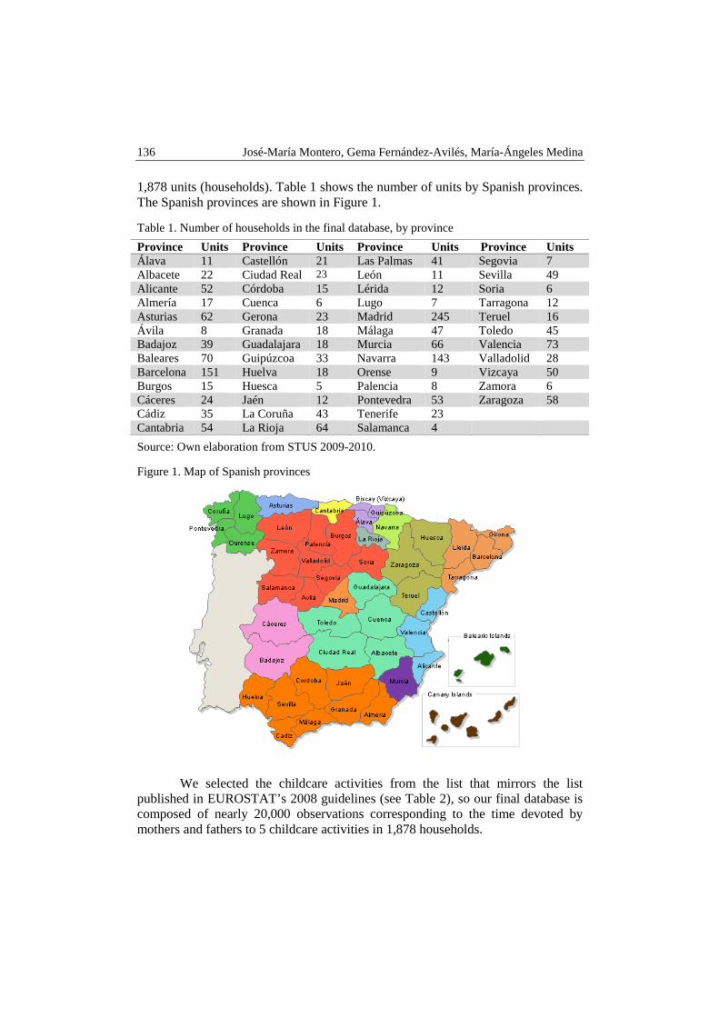
136 José-María Montero, Gema Fernández-Avilés, María-Ángeles Medina
1,878 units (households). Table 1 shows the number of units by Spanish provinces. The Spanish provinces are shown in Figure 1.
Table 1. Number of households in the final database, by province
Province Units Province Units Province Units Province Units Álava 11 Castellón 21 Las Palmas 41 Segovia 7 Albacete 22 Ciudad Real 23 León 11 Sevilla 49 Alicante 52 Córdoba 15 Lérida 12 Soria 6 Almería 17 Cuenca 6 Lugo 7 Tarragona 12 Asturias 62 Gerona 23 Madrid 245 Teruel 16 Ávila 8 Granada 18 Málaga 47 Toledo 45 Badajoz 39 Guadalajara 18 Murcia 66 Valencia 73 Baleares 70 Guipúzcoa 33 Navarra 143 Valladolid 28 Barcelona 151 Huelva 18 Orense 9 Vizcaya 50 Burgos 15 Huesca 5 Palencia 8 Zamora 6 Cáceres 24 Jaén 12 Pontevedra 53 Zaragoza 58 Cádiz 35 La Coruña 43 Tenerife 23 Cantabria 54 La Rioja 64 Salamanca 4
Source: Own elaboration from STUS 2009-2010.
Figure 1. Map of Spanish provinces
We selected the childcare activities from the list that mirrors the list published in EUROSTAT’s 2008 guidelines (see Table 2), so our final database is composed of nearly 20,000 observations corresponding to the time devoted by mothers and fathers to 5 childcare activities in 1,878 households.
Using dissimilarity index for analyzing … 137
Table 2. Childcare activities
Definition Example
CHILDCARE Childcare by parents or older siblings of children, other household members
Grandparents who are members of the household...) of child household members
Physical childcare and supervision of children
Feeding them, dressing them, putting them to bed, rocking them, getting them up, washing them... Supervising them at home and outside.
Changing my baby's nappies
Teaching the children
Helping the children with their homework, teaching them to do specific things.
Checking their homework
Reading, playing and talking with the children
Reading, playing and talking to children Reading them a story
Accompanying the children
Going to the doctor’s with the children. Waiting for them at a sports center, music class... if no activity different from waiting is specified. Visiting school or the nursery. It includes parents' meetings with teachers
At school with my children
Other childcare, whether specified or not
Other childcare Listen to my daughter playing the piano at home
Source: Own elaboration from the Spanish Statistics Office (INE).
Methods
As stated in the introductory section, DI is a particular case of the well-known DDI which have usually been used to indicate whether a population group is segregated or not. A population group is said not to be segregated if the percentage it represents over the total population of a region is replicated when considering the different parts in which that region can be, administratively or not, divided. By contrast, it is said to be segregated if that population group is confined to some parts of that region. The DI (Duncan and Duncan 1955) is the particular case of a DDI when the number of groups is only two. Thus, the DI compares the difference in percentages between the two groups across the area under study.
Here the population we consider is parents with children, the population groups being fathers and mothers, and the non-spatial region being the space of childcare activities (it could also be interesting to consider the space of households). Then, we use the DI (which in our case coincides with the DDI since there are two population groups) to compare the distribution of the time employed by fathers and mothers across the artificial space of childcare activities we have created.
138 José-María Montero, Gema Fernández-Avilés, María-Ángeles Medina
The standard formula for the dissimilarity index is as follows:
1
1, 0 1
2
ni i
i
x yDI DI
X Y=
= − ≤ ≤∑
where ix and iy represent the size of the minority and majority population groups,
respectively, (usually) in census tract i, and X and Y are the size of the minority and majority groups, respectively, in the area under study (usually a municipality).
In our research, ��represents the time devoted by men to childcare activity i, � is the time men devote to childcare activities, �� is the time devoted by women to childcare activity i, and Y the time women devote to all the childcare activities.
The DI is bounded between zero and one. Zero indicates minimum dissimilarity/segregation across activities; that is, the percentage of time that men and women spend on each of the activities considered is the same across the space of activities. By contrast, one indicates maximum dissimilarity/segregation. In other words, if we construct a bi-dimensional table of relative frequencies, the rows indicating the different childcare activities and columns containing the two genders: men and women (see Table 3), DI=0 when factors, childcare activities and gender are independent (both marginal distributions, expressed in relative frequencies, are the same). A value of DI=1 will be obtained in the case of functional dependence, that is, when one of the two cells in the marginal distributions of the activities contains a zero (full specialization).
Table 3. Theoretical frequency distribution of childcare
Men Women Total
Activity 1 1x 1y 1 1x y+
Activity 2 2x 2y 2 2x y+
Activity n nx ny n nx y+
Total X Y X+Y
Source: own elaboration from Spanish Statistics Office (INE).
RESULTS
As said above, the main objective of this article is to analyze whether the distribution of the time that fathers (and consequently mothers) devote to childcare activities is the same across the artificial space of activities or, by contrast, whether they specialize in some activities. This information is provided by dissimilarity indexes. To better understand the results obtained, it is necessary to take into account that, according to STUS 2009-2010, in Spain one third of total childcare time corresponds to men and the remaining two thirds to women.
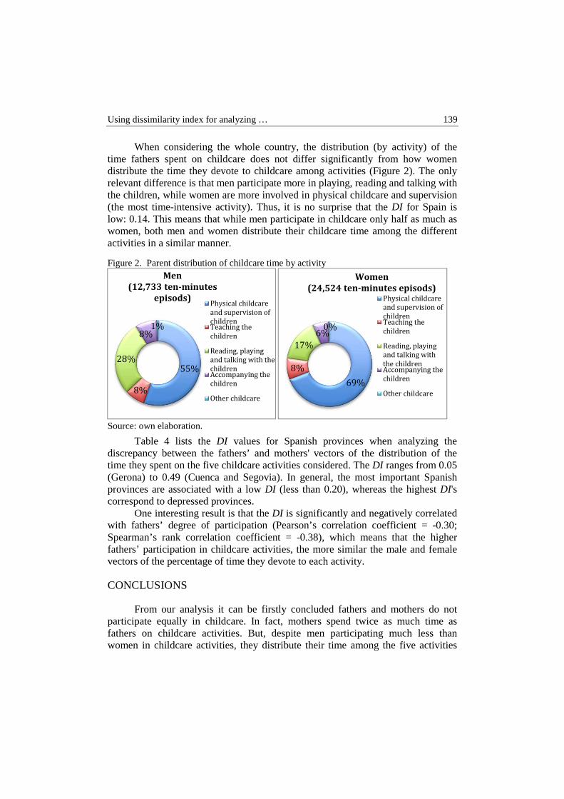
Using dissimilarity index for analyzing … 139
When considering the whole country, the distribution (by activity) of the time fathers spent on childcare does not differ significantly from how women distribute the time they devote to childcare among activities (Figure 2). The only relevant difference is that men participate more in playing, reading and talking with the children, while women are more involved in physical childcare and supervision (the most time-intensive activity). Thus, it is no surprise that the DI for Spain is low: 0.14. This means that while men participate in childcare only half as much as women, both men and women distribute their childcare time among the different activities in a similar manner.
Figure 2. Parent distribution of childcare time by activity
Source: own elaboration.
Table 4 lists the DI values for Spanish provinces when analyzing the discrepancy between the fathers’ and mothers' vectors of the distribution of the time they spent on the five childcare activities considered. The DI ranges from 0.05 (Gerona) to 0.49 (Cuenca and Segovia). In general, the most important Spanish provinces are associated with a low DI (less than 0.20), whereas the highest DI's correspond to depressed provinces.
One interesting result is that the DI is significantly and negatively correlated with fathers’ degree of participation (Pearson’s correlation coefficient = -0.30; Spearman’s rank correlation coefficient = -0.38), which means that the higher fathers’ participation in childcare activities, the more similar the male and female vectors of the percentage of time they devote to each activity.
CONCLUSIONS
From our analysis it can be firstly concluded fathers and mothers do not participate equally in childcare. In fact, mothers spend twice as much time as fathers on childcare activities. But, despite men participating much less than women in childcare activities, they distribute their time among the five activities
55%
8%
28%
8%1%
Men
(12,733 ten-minutes
episods)Physical childcare
and supervision of
childrenTeaching the
children
Reading, playing
and talking with the
childrenAccompanying the
children
Other childcare
69%
8%
17%
6%0%
Women
(24,524 ten-minutes episods)Physical childcare
and supervision of
childrenTeaching the
children
Reading, playing
and talking with
the childrenAccompanying the
children
Other childcare
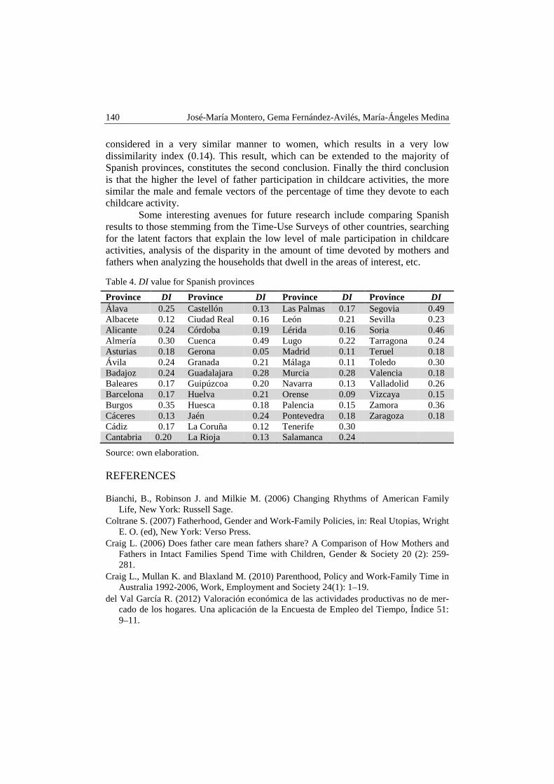
140 José-María Montero, Gema Fernández-Avilés, María-Ángeles Medina
considered in a very similar manner to women, which results in a very low dissimilarity index (0.14). This result, which can be extended to the majority of Spanish provinces, constitutes the second conclusion. Finally the third conclusion is that the higher the level of father participation in childcare activities, the more similar the male and female vectors of the percentage of time they devote to each childcare activity.
Some interesting avenues for future research include comparing Spanish results to those stemming from the Time-Use Surveys of other countries, searching for the latent factors that explain the low level of male participation in childcare activities, analysis of the disparity in the amount of time devoted by mothers and fathers when analyzing the households that dwell in the areas of interest, etc.
Table 4. DI value for Spanish provinces
Province DI Province DI Province DI Province DI Álava 0.25 Castellón 0.13 Las Palmas 0.17 Segovia 0.49 Albacete 0.12 Ciudad Real 0.16 León 0.21 Sevilla 0.23 Alicante 0.24 Córdoba 0.19 Lérida 0.16 Soria 0.46 Almería 0.30 Cuenca 0.49 Lugo 0.22 Tarragona 0.24 Asturias 0.18 Gerona 0.05 Madrid 0.11 Teruel 0.18 Ávila 0.24 Granada 0.21 Málaga 0.11 Toledo 0.30 Badajoz 0.24 Guadalajara 0.28 Murcia 0.28 Valencia 0.18 Baleares 0.17 Guipúzcoa 0.20 Navarra 0.13 Valladolid 0.26 Barcelona 0.17 Huelva 0.21 Orense 0.09 Vizcaya 0.15 Burgos 0.35 Huesca 0.18 Palencia 0.15 Zamora 0.36 Cáceres 0.13 Jaén 0.24 Pontevedra 0.18 Zaragoza 0.18 Cádiz 0.17 La Coruña 0.12 Tenerife 0.30 Cantabria 0.20 La Rioja 0.13 Salamanca 0.24
Source: own elaboration.
REFERENCES
Bianchi, B., Robinson J. and Milkie M. (2006) Changing Rhythms of American Family Life, New York: Russell Sage.
Coltrane S. (2007) Fatherhood, Gender and Work-Family Policies, in: Real Utopias, Wright E. O. (ed), New York: Verso Press.
Craig L. (2006) Does father care mean fathers share? A Comparison of How Mothers and Fathers in Intact Families Spend Time with Children, Gender & Society 20 (2): 259-281.
Craig L., Mullan K. and Blaxland M. (2010) Parenthood, Policy and Work-Family Time in Australia 1992-2006, Work, Employment and Society 24(1): 1–19.
del Val García R. (2012) Valoración económica de las actividades productivas no de mer-cado de los hogares. Una aplicación de la Encuesta de Empleo del Tiempo, Índice 51: 9–11.

Using dissimilarity index for analyzing … 141
Duncan O. B. and Duncan B. (1955) Residential distribution and occupational stratifica-tion, American Journal of Sociology 60(5): 493–503.
Fisher K., Egerton M., Gershuny J. and Robinson J. (2007) Gender Convergence in the American Heritage Time Use Study (AHTUS). Social Indicators Research 82(1): 1–33.
Gauthier A., Smeeding T. M. and Furstenberg F. (2004) Do we invest less time in children? Trends in parental time in selected industrialised countries since the 1960s, Population and Development Review 30(4): 647–671.
Gray A. (2006) The Time Economy of Parenting, Sociological Research Online, 11(3). Sayer L., Bianchi S., Robinson J. (2004) Are Parents Investing Less in Children? Trends in
Mothers and Fathers time with Children, American Journal of Sociology 110(1): 1–43. Sayer L. (2005) Gender, Time and Inequality: Trends in Women's and Men's Paid Work,
Unpaid Work and Free Time, Social Forces 84(1): 285–303. Sullivan O. (2006) Changing Gender Relations, Changing Families: Tracing the Pace of
Change over Time, New York: Rowman & Littlefield.

QUANTITATIVE METHODS IN ECONOMICS Vol. XV, No. 1, 2014, pp. 142 – 152
A COMPARATIVE STUDY OF FastICA AND GRADIENT ALGORITHMS FOR STOCK MARKET ANALYSIS
Kesra Nermend Institute of IT in Management, University of Szczecin, Szczecin 71-415, Poland
email: [email protected] Yasen Rajihy
Department of Computer Science, University of Babylon, Babylon 09332, Iraq email: [email protected]
Abstract: In this paper we proved that a fast fixed point algorithm known as FastICA algorithm depending on maximization the nongaussianity by using the negentropy approach is one of the best algorithm for solving ICA model. We compare this algorithm with Gradient algorithm. The Abu Dhabi Islamic Bank (ADIB) used as illustrative example to evaluate the performance of these two algorithms. Experimental results show that the FastICA algorithm is more robust and faster than Gradient algorithm in stock market analysis.
Keywords: independent component analysis, nangaussianity, negentropy, stock market analysis
INTRODUCTION
Independent Component Analysis (ICA) is a mathematical and computation-al technique for revealing hidden factors that underlie sets of random signals (vari-ables) [Comon 1994; Jutten, Herault 1991; Hyvärinen et al. 2001]. These underly-ing latent variables are called sources or independent components (ICs) and they are assumed to be statistically independent of each other and nongaussian. The technique of ICA is a relatively new invention. In the middle of 1990s, some highly successful new algorithms for solving the ICA model were introduced by several research groups [Hyvärinen, Oja 2000; Hyvärinen 1999; Cardoso, Souloumiac 1993; Choi et al. 2001; Pham, Cardoso 2000; Pham, Garat 1997; Belouchrani et al. 1996; Jutten 2000; Jutten, Herault 1991]. The main mathematical problem of ICA

A Comparative Study of FastICA and Gradient … 143
can be described as follows: we observe m random variables ��, ��, ⋯��, which are modeled as linear combinations of n random variables ��, ��,⋯ ��: �� = ���� + ����⋯���� (1)
for all i = 1, 2, ..., m, where ai,j are some real mixing coefficients. The si are statisti-cally mutually independent. The matrix representation of equation (1) can be ex-pressed as: x = As (2) where x is an observed m-dimensional vector, s is n-dimensional (latent) random vector whose components are assumed mutually independent, and A is a constant m×n matrix to be estimated. It is usually further assumed that the dimensions of x and s are equal, i.e. m=n. Basic ICA model describes how the observed data are generated by a process of mixing the independent components ��. The independent components ��are the latent variables which means that they are not observable di-rectly. Also the mixing coefficients �� are unknown. ICA uses solely the observed data �� to estimate both the ICs �� and the mixing coefficients ��. The task in ICA is to find both the latent variables or sources �� and the mixing process; in the line-ar case, the latter task consists of finding the mixing matrix A. A popular approach is to find a demixing matrix W so that variables �� in y=Wx are estimates of �� up to scaling and permutation. Hence W is an estimate of the (pseudo)inverse of A up to scaling and permutation of the rows of W. Often the latent variables si are esti-mated one by one, by finding a column vector �� (this will be stored as a row of W) such that �� = ��
�� is an estimate of ��. In order to calculate a demixing matrix W (i.e. to estimate ICs), numerous
ICA algorithms have been developed with various approaches. In this paper we try to review the most important two algorithms to solve the ICA model based on max-imization of nongaussianity by using negentropy approach, namely Gradient algo-rithm and FastICA algorithm [Hyvarinen 1997; Hyvärinen 1999; Hyvarinen, Oja 1997]. In practice, before application of these two algorithms, suitable prepro-cessing is often compulsory i.e. centering and whitening. The observed vector X is first centered by removing its mean. A zero-mean random vector z=(z1,z2,…,zn)T is said to be white or sphere if its components zi are uncorrelated and have unit vari-ances. This means that the covariance matrix (as well as the correlation matrix) of z equals the identity matrix. Centering and whitening can be accomplished by prin-cipal component analysis (PCA).
Abu Dhabi Islamic Bank (ADIB) used as illustrative example to evaluate the performance of these two algorithms. Experimental results show that FastICA is more robust and faster than Gradient algorithm in stock market analysis.

144 Kesra Nermend, Yasen Rajihy
RESEARCH METHODOLOGY
Estimation the independent components (ICs) is a challenging task because ICA uses solely the observed data xi to estimate both the ICs si and the mixing co-efficients ai,j. Several approaches for solving ICA model are presented during last decade. Maximization of nongaussianity based on negentropy is one of these ap-proaches. Maximization of nongoussianity based on negentropy is a simple and in-tuitive principle for estimating the model of independent component analysis (ICA). Nongaussian components are independent. Nongaussianity is actually of high importance in ICA estimation. If the nongaussianity does not valid, then the estimation is not possible at all. To use nongaussianity in ICA estimation, we must have a quantitative measure of nongaussianity of a random variable, say x. To sim-plify things, let us assume that x is centered (zero-mean) and has variance equal to one. Actually, one of the functions of preprocessing in ICA algorithms is to make this simplification possible [Hyvärinen, Oja 2000]. One of the most important quantitative measures of nongaussianity is a negentropy as we show below.
Negentropy
Negentropy is based on the information theoretic quantity of (differential) entropy [Hyvärinen et al. 2001]. The entropy of a random variable can be interpret-ed as the information degrees of a given observe variable. The entropy H of a ran-dom vector x with density f(x) is defined as:
∫−= dxxfxfH )(log)()(x (3)
A fundamental result of the information theory is that a gaussian variable has the largest entropy among all random variables of equal variance [Hyvarinen 1999]. The entropy is small when variables are far from the gaussian, hence it can be used in the measure of nongaussianity. The negentropy N of a nongaussian ran-dom vector X is defined as: N(X ) = H (Xg) − H (X ) (4)
where Xg is a gaussian random vector whose covariance matrix is equal to that of X. Note that negentropy is non-negative and zero if and only if the vector X has a gaussian distribution. The main problem in using negentropy is that it is computa-tionally very difficult. Hence simpler approximations of negentropy are very use-ful. A classical method to approximate negentropy is using higher-order cumulants, for example as follows [Jones, Sibson 1987]:
N(X ) ≈ 1
12E{ X 3} 2 + 1
48kurt{ X} 2 (5)
where X is assumed to be a zero mean and a unit variance. If the random variable X has a symmetric distribution, then the first term in the right-hand side of Eq. (8) is equal to zero, and so this approximation often leads to the use of kurtosis as in the

A Comparative Study of FastICA and Gradient … 145
preceding section. To avoid this problem we can perform the approximation by us-ing a non-quadratic function G as follows:
���� ∝ [������� − �������]� (6) where � is a gaussian variable with a zero mean and a unit variance (i.e. standard-ized). Here, one must choose G wisely. In particular, choosing G that does not grow too fast one obtains more robust estimators. The following choices of G have proved very useful
����� = �� log $%�ℎ�� (7)
����� = −��' ()*+
� , (8)
Where 1 ≤ � ≤ 2 is a constant often taken equal one. Negentropy, based on the information theoretic quantity of entropy is a best
method of measuring nongaussianity, it can be conceptually simple, fast to com-pute, more robust, enable the deflationary (i.e. one-by-one estimation of independ-ent components), and force the estimations of the independent components to be uncorrelated.
Gradient algorithm using negentropy
The main task in the independent component analysis (ICA) problem is to estimate a demixing matrix W that will give us the independent components. In this subsection we derive a simple gradient algorithm for maximizing negentropy. Tak-ing the gradient of the approximation of negentropy in (6) with respect to w, and taking the normalization �����0��� = ‖�‖� into account, one obtains the follow-ing algorithm [Hyvärinen et al. 2001]
∆� ∝ 3��04���0�� (9)
� ← 6‖6‖ (10)
where 3 = ������0�� − �������. The function 4 is the derivative of the function G used in equations (7) and (8). The parameter 3 can be estimated on-line as fol-lows: ∆3 ∝ [����0� − �������] − 3 (11) The final form of the gradient algorithm is summarized as follows: 1. Center the data to make its mean zero. 2. Whiten the data to give z. 3. Choose an initial random vector w of unit norm, and an initial value forγ. 4. Update∆� ∝ 304���0�. 5. Normalize � ← 6
‖6‖ .
6. If the sign of γ is not known a priori, update ∆3 ∝ [����0� − �������] − 3. 7. If not converged, go back to step 4.

146 Kesra Nermend, Yasen Rajihy
FastICA algorithm using negentropy
In this subsection we derive the fixed-point algorithm (FastICA) using negentropy for maximizes the nongaussianity [Hyvärinen et al. 2001]. The result-ing FastICA algorithm finds a direction, i.e., a unite vector�, such that the projec-tion ��0 maximizes the nongaussianity. Here nongaussianity measured by the ap-proximation of negentropy ����0�given in (6). Recall that ��0 must constrain-ing to have a unit variance, this is equivalent to ‖�‖ = 1. Looking at the gradient method in (9) immediately suggests the following fixed-point itera-tion:
0 ← ��04���0�� (12)
� ← 6‖6‖ (13)
The iteration in (12) has to be modified because it doesn’t have a good conver-gence. This can easily do as follows: �1 + 9� = ��04���0�� + 9� (14) where 9 is a constant. One must choose 9wisely to obtain an algorithm that con-verges faster than gradient algorithm.
FastICA can be found using Newton’s method approximation. To derive the approximative Newton method, first note that the maxima of the approximation of the negentropy of ��0 are typically obtained at certain optima of������0��. According to the Lagrange conditions, the optima of ������0�� under the con-straint �����0��� = ‖�‖� = 1 are obtained at points where the gradient of the Lagrangian is zero [Hyvärinen et al. 2001]: ��04���0�� + :� = 0 (15) To simply solve equation (15) by Newton’s method, let< = ��04���0�� + :�, we obtain its gradient as:
∂F∂w
=E�zzT4���0�� + :> (16)
Since the data is whitened, we can simplify the inversion of this matrix by approximate the first term in (16) as follows:
E�zzT4���0�� ≈ ��zzT���4���0�� = ��4���0��>. Thus the gradient becomes diagonal, and can easily be inverted. Thus we obtain the following approximative Newton iteration:
� ← � − @ABCD6EBFGHI6E�C�6EB��HI (17)
After straightforward algebraic simplification we give the basic fixed-point iteration in FastICA: � ← ��04���0�� − E�4���0��� (18)
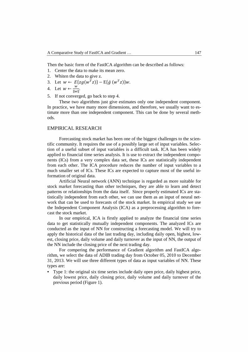
A Comparative Study of FastICA and Gradient … 147
Then the basic form of the FastICA algorithm can be described as follows: 1. Center the data to make its mean zero. 2. Whiten the data to give z. 3. Let � ← ��04���0�� − E�4���0���.
4. Let� ← 6‖6‖.
5. If not converged, go back to step 4. These two algorithms just give estimates only one independent component.
In practice, we have many more dimensions, and therefore, we usually want to es-timate more than one independent component. This can be done by several meth-ods.
EMPIRICAL RESEARCH
Forecasting stock market has been one of the biggest challenges to the scien-tific community. It requires the use of a possibly large set of input variables. Selec-tion of a useful subset of input variables is a difficult task. ICA has been widely applied to financial time series analysis. It is use to extract the independent compo-nents (ICs) from a very complex data set, these ICs are statistically independent from each other. The ICA procedure reduces the number of input variables to a much smaller set of ICs. These ICs are expected to capture most of the useful in-formation of original data.
Artificial Neural network (ANN) technique is regarded as more suitable for stock market forecasting than other techniques, they are able to learn and detect patterns or relationships from the data itself. Since properly estimated ICs are sta-tistically independent from each other, we can use them as an input of neural net-work that can be used to forecasts of the stock market. In empirical study we use the Independent Component Analysis (ICA) as a preprocessing algorithm to fore-cast the stock market.
In our empirical, ICA is firstly applied to analyze the financial time series data to get statistically mutually independent components. The analyzed ICs are conducted as the input of NN for constructing a forecasting model. We will try to apply the historical data of the last trading day, including daily open, highest, low-est, closing price, daily volume and daily turnover as the input of NN, the output of the NN include the closing price of the next trading day.
For compering the performance of Gradient algorithm and FastICA algo-rithm, we select the data of ADIB trading day from October 05, 2010 to December 31, 2013. We will use three different types of data as input variables of NN. These types are: • Type 1: the original six time series include daily open price, daily highest price,
daily lowest price, daily closing price, daily volume and daily turnover of the previous period (Figure 1).
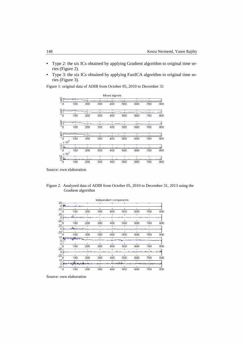
148 Kesra Nermend, Yasen Rajihy
• Type 2: the six ICs obtained by applying Gradient algorithm to original time se-ries (Figure 2).
• Type 3: the six ICs obtained by applying FastICA algorithm to original time se-ries (Figure 3).
Figure 1: original data of ADIB from October 05, 2010 to December 31
Source: own elaboration
Figure 2. Analyzed data of ADIB from October 05, 2010 to December 31, 2013 using the Gradient algorithm
Source: own elaboration
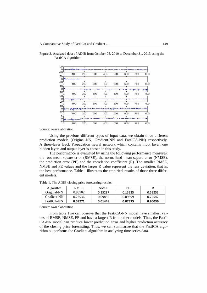
A Comparative Study of FastICA and Gradient … 149
Figure 3. Analyzed data of ADIB from October 05, 2010 to December 31, 2013 using the FastICA algorithm
Source: own elaboration
Using the previous different types of input data, we obtain three different prediction models (Original-NN, Gradient-NN and FastICA-NN) respectively. A three-layer Back Propagation neural network which contains input layer, one hidden layer, and output layer is chosen in this study.
The performance is evaluated by using the following performance measures: the root mean square error (RMSE), the normalized mean square error (NMSE), the prediction error (PE) and the correlation coefficient (R). The smaller RMSE, NMSE and PE values and the larger R value represent the less deviation, that is, the best performance. Table 1 illustrates the empirical results of those three differ-ent models.
Table 1. The ADIB closing price forecasting results
Algorithm RMSE NMSE PE R
Original-NN 0.98902 0.25287 0.13325 0.59253
Gradient-NN 0.23536 0.09855 0.09899 0.75547
FastICA-NN 0.09271 0.01448 0.07375 0.96036
Source: own elaboration
From table 1we can observe that the FastICA-NN model have smallest val-ues of RMSE, NMSE, PE and have a largest R from other models. Thus, the FastI-CA-NN model can produce lower prediction error and higher prediction accuracy of the closing price forecasting. Thus, we can summarize that the FastICA algo-rithm outperforms the Gradient algorithm in analyzing time series data.
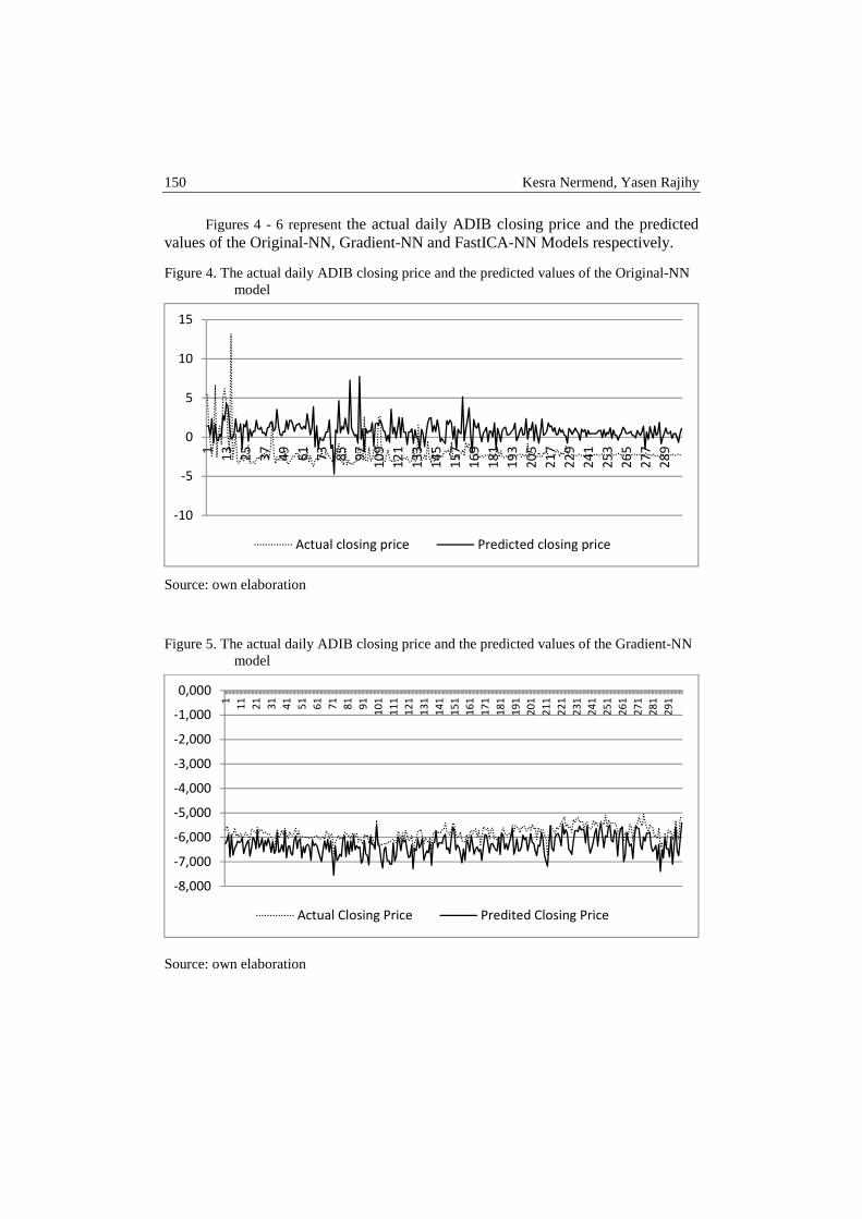
150 Kesra Nermend, Yasen Rajihy
Figures 4 - 6 represent the actual daily ADIB closing price and the predicted values of the Original-NN, Gradient-NN and FastICA-NN Models respectively.
Figure 4. The actual daily ADIB closing price and the predicted values of the Original-NN model
Source: own elaboration
Figure 5. The actual daily ADIB closing price and the predicted values of the Gradient-NN model
Source: own elaboration
-10
-5
0
5
10
15
1
13
25
37
49
61
73
85
97
10
9
12
1
13
3
14
5
15
7
16
9
18
1
19
3
20
5
21
7
22
9
24
1
25
3
26
5
27
7
28
9
Actual closing price Predicted closing price
-8,000
-7,000
-6,000
-5,000
-4,000
-3,000
-2,000
-1,000
0,000
1
11
21
31
41
51
61
71
81
91
10
1
11
1
12
1
13
1
14
1
15
1
16
1
17
1
18
1
19
1
20
1
21
1
22
1
23
1
24
1
25
1
26
1
27
1
28
1
29
1
Actual Closing Price Predited Closing Price
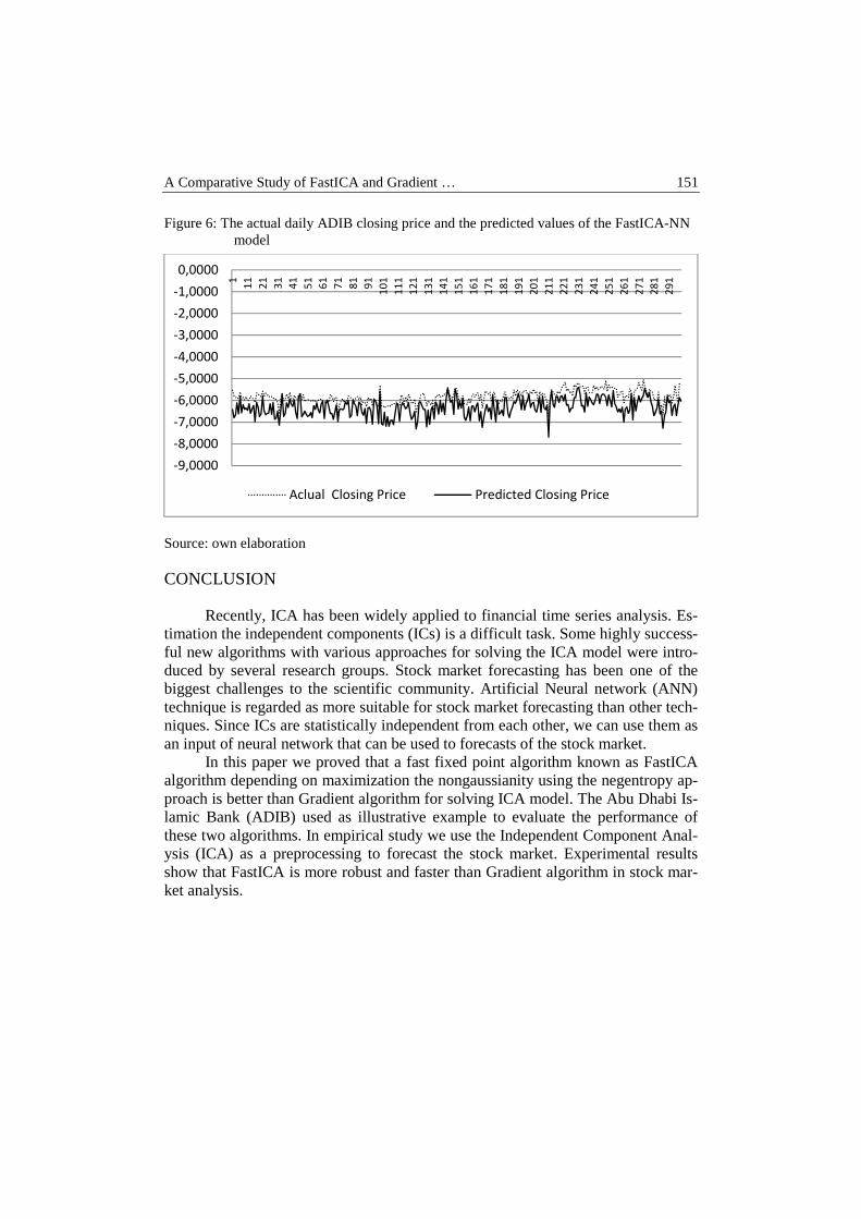
A Comparative Study of FastICA and Gradient … 151
Figure 6: The actual daily ADIB closing price and the predicted values of the FastICA-NN model
Source: own elaboration
CONCLUSION
Recently, ICA has been widely applied to financial time series analysis. Es-timation the independent components (ICs) is a difficult task. Some highly success-ful new algorithms with various approaches for solving the ICA model were intro-duced by several research groups. Stock market forecasting has been one of the biggest challenges to the scientific community. Artificial Neural network (ANN) technique is regarded as more suitable for stock market forecasting than other tech-niques. Since ICs are statistically independent from each other, we can use them as an input of neural network that can be used to forecasts of the stock market.
In this paper we proved that a fast fixed point algorithm known as FastICA algorithm depending on maximization the nongaussianity using the negentropy ap-proach is better than Gradient algorithm for solving ICA model. The Abu Dhabi Is-lamic Bank (ADIB) used as illustrative example to evaluate the performance of these two algorithms. In empirical study we use the Independent Component Anal-ysis (ICA) as a preprocessing to forecast the stock market. Experimental results show that FastICA is more robust and faster than Gradient algorithm in stock mar-ket analysis.
-9,0000
-8,0000
-7,0000
-6,0000
-5,0000
-4,0000
-3,0000
-2,0000
-1,0000
0,0000
1
11
21
31
41
51
61
71
81
91
10
1
11
1
12
1
13
1
14
1
15
1
16
1
17
1
18
1
19
1
20
1
21
1
22
1
23
1
24
1
25
1
26
1
27
1
28
1
29
1
Aclual Closing Price Predicted Closing Price
152 Kesra Nermend, Yasen Rajihy
REFERENCES
Belouchrani A., Abed Meraim K., Cardoso J.F. and Moulines E. (1996) A blind source se-paration technique using second order statistics, IEEE Trans. Signal Processing, vol. 45, 434–444.
Cardoso J.F., Souloumiac A. (1993) Blind beam forming for non-Gaussian signals, IEEE Proceedings-F, 140(6), 362-370.
Choi S., Cichocki A., Deville Y. (2001) Differential decorrelation for nonstationary source separation, [in:] Proceedings of 3rd International Conference on Independent Compo-nent Analysis and Blind Signal Separation, (San Diego, California, USA), 319-322.
Comon P. (1994) Independent component analysis — a new concept?, Signal Processing, 36, 287–314.
Hyvarinen A. (1997) A family of fixed-point algorithms for independent component Analy-sis, [in:] Proc. ICASSP, Munich, Germany, April 20-24, 3917–3920.
Hyvärinen A. (1999) Fast and Robust Fixed-Point Algorithms for Independent Component Analysis, IEEE Trans. on Neural Networks, 10(3), 626-634.
Hyvarinen A. (1999) Survey of Independent Component Analysis, Neural Computing Surveys, 2, 150, 1-36, 94-128.
Hyvarinen A., Oja E. (1997) A fast fixed-point algorithm for independent component ana-lysis, Neural Computation, 9(7), 1483–1492.
Hyvärinen A., Oja E. (2000) Independent Component Analysis: Algorithms and Applica-tions, Neural Networks, 13(4-5), 411-430.
Hyvärinen A., Karhunen J. and Oja E. (2001) Independent Component Analysis, John Wi-ley & Sons, New York.
Jones M., Sibson R. (1987) What is projection pursuit? Journal of the Royal Statistical So-ciety, Ser., A150, 1-36.
Jutten C. (2000) Source separation: from dust till dawn, [in:] Proc. 2nd Int. Workshop on Independent Component Analysis and Blind Source Separation (ICA’ 2000), 15-26.
Jutten C., Herault J. (1991) Blind separation of sources, part I: An adaptive algorithm based on neuromimetic architecture, Signal Processing, 24, 1–10.
Pham D.T., Cardoso J. F. (2000) Blind separation of instantaneous mixtures of nonstationa-ry sources, in Proc. ICA, (Helsinki, Finland), 187–192.
Pham D.T., Garat P. (1997) Blind separation of mixture of independent sources through a quasimaximum likelihood approach, IEEE Trans. Signal Processing, vol. 45, 1712–1725.
QUANTITATIVE METHODS IN ECONOMICS Vol. XV, No. 1, 2014, pp. 153 – 158
IMPRECISE RETURN RATES ON THE WARSAW STOCK EXCHANGE
Krzysztof Piasecki Department of Operations Research, Poznań University of Economics
e-mail: [email protected]
Abstract: The return rate in imprecision risk may be described as a fuzzy probabilistic set [Piasecki, 2011a]. On the other side, in [Piasecki, Tomasik 2013] is shown that the Normal Inverse Gaussiandistribution is the best matching probability distribution of logarithmic returns on Warsaw Stock Exchange. There will be presented the basic properties if imprecise return with the Normal Inverse Gaussian distribution of future value logarithm. The existence of distribution of expected return rate is discussed. All obtained re-sults may be immediately applied for effectiveness analysis at risk of uncer-tainty and imprecision [Piasecki, 2011c]
Keywords: Normal Inverse Gaussian distribution, uncertainty risk, impreci-sion risk, fuzzy present value
INTRODUCTION
Typically, the analysis of properties of any security is kept, as analysis of re-turn rate properties. The future value of a security is presented as a random varia-ble. Distribution of this random variable is formal image of uncertainty risk. In [Pi-asecki, Tomasik2013] is shown that the Normal Inverse Gaussiandistribution is the best matching probability distribution of logarithmic one-day return rates on War-saw Stock Exchange.
On the other side, any present value is approximately equal to market price. For this reason a present value may be given as a fuzzy number. Then the return rate of is given as a fuzzy probabilistic set. Properties of this return are considered in [Piasecki 2011b] for the case of any probability distribution of future value. In [Piasecki 2014] the fuzzy probabilistic return is applied for financial decision mak-ing.

154 Krzysztof Piasecki
Taking into account all above results, we see that imprecise return rates on Warsaw Stock Exchange may be determined by one-day logarithmic returns as fuzzy probabilistic set under the Normal Inverse Gaussian distribution. Basic properties of these returns will be investigated in this paper. The main goal of our considerations will be to define a three-dimensional risk image for such logarith-mic return rate.
RETURN RATES
Let us assume that the time horizon � > 0 of an investment is fixed. Then any security is determined by two values:
− anticipated future value (FV) �� ∈ ℝ� , − assessed present value (PV) � ∈ ℝ�. The basic characteristic of benefits from owning this instrument is a return
rate ∈ ℝ given by the identity = ��, ���. (1)
In the general case, the function :ℝ� × ℝ� → ℝis a decreasing function of PV and an increasing function of FV.
Let the set of all securities be denoted by the symbol�. Each security ���� is represented by its return rate �. According to the principle of maximizing benefits, the set of all securities may be ordered by the relation ��� ⊂ � × � defined as fol-lows ������� ⟺ � ≥ �. (2)
In the special case we have here logarithmic return rate
� = ln !"!#. (3)
For any returns and logarithmic returns � we have = �1, %&�. (4)
It means that any return rate is an increasing function of logarithmic returns. Therefore any return ' defines order ��� equivalent to the order ���� defined by logarithmic return�. This observation prompts us to replace the study of any re-turns by the study of logarithmic returns.
The FV is at risk of uncertainty. A formal model of this uncertainty is the presentation of FV �� as a random variable �(�: Ω = *+, ⟶ ℝ�. The set Ω is a set of financial marketelementary states. In the classical approach to the problem of re-turn rate determination, PV of a security is identified with the observed market price ./. Then the return rate is a random variable, which is at uncertainty risk. This random variable is determined by the identity
�(�+� = ln !0"�1�2/ . (5)
In practice of financial markets analysis, the uncertainty risk is usually de-scribed by probability distribution of return rates. At the moment, we have an ex-tensive knowledge on this subject. Empirical studies have shown that capital mar-
Imprecise return rates on the Warsaw Stock Exchange 155
kets can differ from each other type of best suited distribution returns. That conclu-sion is the result of a comparison research results relating to the German capital market [Eberlein, Keller 1994] with the results from research dedicated to the American capital market.[Weron, Weron1999]. This points out validity of a search for type of return rates distribution applicable to the Polish capital market. From the literature it is known to a lot of sub-studies of empirical distributions of returns on the Polish capital market. These results have been discussed in [Piasecki, Tomasik 2013]. In the same book have been studied returns on shares making up the portfolios defining stock indexes WIG20,mWIG40 and sWIG80. The survey covered all quotations for the period from 09.21.1998 till 03.03.2010. This period is divided into a bull market periods and bear market periods. Distinct studies cov-ered duration of each bull or bear market. In total, there were tested 694 time series of quotations. The study subject was one-day logarithmic return. Piasecki and To-masik (2013)have shown that the Normal Inverse Gaussian distribution is the best matching probability distribution of logarithmic returns on Warsaw Stock Ex-change.
TheNormal Inverse Gaussian distribution was introduced in [Barndorff-Nielsen 1977]. This distribution is characterized by 3 = �4, 5, 6, 7� of four para-meters fulfilling 4 ∈ ℝ�, 5 ∈ �−4, 4�, 6 ∈ ℝ�, 7 ∈ ℝ. The density function 9:;<�∙ |3�: ℝ ⟶ ℝ�of the Normal Inverse Gaussian distribution is given by the identity 9:;<�?|3� = 9:;<�?|4, 5, 6, 7� =
= @ABCD@EAF��GHI�FJKEAF��GHI�F ∙ expO6E4P − 5P + 5�? − 7�R (6)
whereST:ℝ� ⟶ℝ�is the modified Bessel function of the third kind determined by the identity
ST�?� = TPU %?V O− G
P DW +TXJR YW
Z . (7)
Let us take into account fixed security. If the distribution of its logarithmic return rate is given by the identity (6), then the density function 9![∙ \./, 3]: ℝ� ⟶ℝ� of FV distribution is defined as follows
9![?\./,3] = 9:;< Dln G2/ ^3J. (8)
Assessment of security FV is based on objective measurement only. It means that the density function of FV distributionis independent of how the PV is determined. Expected FV and its variance exist always. This is due to the fact that expected value and variance exist for each Normal Inverse Gaussian distribu-tion [Bølviken, Benth2000].
The security PV security is approximately equal to security market price ./. Thus it may be at imprecision risk. Then PV is described by fuzzy number in the sense given by Dubois and Prade(1979). This approach is studied by Ward (1985), Buckley (1987, 1992), Gutierrez (1989), Greenhutet al. (1995), Kuchta(2000),
156 Krzysztof Piasecki
Lesage (2001), Sheen (2005) and Piasecki(2011a, 2011b). The security PV is a fuzzy number dependent on market price ./. Each PV membership function 7[∙ \./]:ℝ� ⟶ �0; 1� fulfils following properties
7[./\./] = 1 , (9)
∀?, W, a�ℝ�:? ≤ W ≤ a ⇒ 7[W\./] ≥ efgh7[?\./], 7[a\./]i. (10)
The above-mentioned imprecision risk is caused by behavioural reasons. Each investor takes into account the lowest possible market price and the biggest one. The security PV should be greater than the lowest possible price. Also, the se-curity PV should be less than the biggest possible price. Therefore, we additionally assume about any PV membership function 7[∙ \./]:ℝ� ⟶ �0; 1�that it fulfills fol-lowing condition ∀./ ∈ ℝ�: ∃./klm , ./knG ∈ ℝ�: ./klm < ./ < ./knG ∧ 7[./klm\./] = 7[./knG\./] = 0. (11)
Immediately from (10) and (11) we obtain
∀./ ∈ ℝ�: ? ∉ [./klm, ./knG] ⟹∧ 7[?\./] = 0 (12)
Some example of defined above PV is described in [Piasecki2011a]. Then the return rate is at risk of coincidence uncertainty and imprecision.
According to the Zadeh extension principle, for each fixed elementary state +�Ω of financial market, membership function s[∙, +\./]:ℝ → �0; 1� of logarithmic return rate is determined by the identity
s[∙, +\./] = et? O7[W\./]: W�ℝ�, = ln !0"�1�X R = 7[%H& ∙ �(��+�\./] . (13)
It means that the logarithmic return rate considered here is represented by fuzzy probabilistic set defined by Hiroto (1981). For this reason, this logarithmic return rate is called fuzzy probabilistic logarithmic return.
IMPRECISE ASSESSMENT OF RETURN RATE
For any fuzzy probabilistic logarithmic return we determine the parameters of its distribution. We have here distribution of expected logarithmic return rate
'[�\./] = U 7[%H& ∙ ?\./] ∙ 9![?\./,3]Y?�Z . (14)
Integrating by substitution we obtain
'[�\./] = %H& ∙ U 7[�\./] ∙ 9![%& ∙ �\./,3]Y� =�Z %H& ∙ U 7[�\./] ∙ 9![%& ∙ �\./, 3]Y�2/uvw
2/uxy .
It proves that distribution of expected logarithmic return rate always exists. Distribu-tion of expected return rate '[∙ \./]: ℝ ⟶ �0; 1� is a membership function of fuzzy subset �( in the real line. This subset �( represents both rational and behavioural aspects in the ap-proach to estimate the expected benefits. Then the expected logarithmic return rate is de-fined as follows
�z = �z[./] = U &∙{D�^./J|&}~�~U {D�^./J|&}~�~
. (15)

Imprecise return rates on the Warsaw Stock Exchange 157
Similarly as in the case of precisely defined return rate, there are such distri-butions of expected logarithmic return rate for which the expected logarithmic re-turn rate does not exist. We then replace this distribution with a distribution trun-cated on both sides, for which the expected logarithmic return rate always exists. This procedure finds its justification in the theory of perspective [Kahneman, Tversky 1979]. Among other things, this theory describes the behavioural phenom-enon of the extremes’ rejection.
The expected logarithmic return rate is at risk of uncertainty and impreci-sion. The image of this risk is described in [Piasecki 2011c].
We use the following variance of return rate as the assessment of the risk uncertainty
�P = �P[./] = U U G∙�D?, W^./J∙��D?^./,3J|X|G}~#
}~�~U U �D?, W^./J∙��D?^./,3J|X|G}~
#}~�~
(16)
where
�[?, �(��+�\./] = �et?hs[�z + √?,+\./], s[�z + √?,+\./]i? ≥ 00? < 0 . (17)
Imprecision is composed of ambiguity and indistinctness. Ambiguity is the lack of clear recommendation of one alternative from among various alternatives. In accordance with the suggestion given in [Czogałaet al.1982], we evaluate the ambiguity risk by energy measureY[�(]of expected logarithmic return rate distribu-tion �(. This measure is determined by the identity
6 = 6[./] = U {D?^./J|G}~�~
T�U {D?^./J|G}~�~
∙ . (18)
Indistinctness is the lack of explicit distinction between the information pro-vided and its negation. According to the suggestion given in [Gottwald et al., 1982], we evaluate the indistinctness risk by entropy measure%[�(] of distribution of expected logarithmic return rate �(. This measure is described as follows
� = �[./] = U klmO{D?^./J,TH{D?^./JR|G}~�~
T�U klmO{D?^./J,TH{D?^./JR|G}~�~
. (19)
In this way we describe security with imprecision return as the pair [�z, ��P, 6, ��] where �z is expected logarithmic return rate and ��P, 6, �� is the three-dimensional image of risk of uncertainty, ambiguity and indistinctness. In [Piasecki2011c] this pair is applied for analysis of security effectiveness.
CONCLUSIONS
In this paper is shown that for the Normal Inverse Gaussian distribution the expected logarithmic return rate distribution and three-dimensional risk image al-
158 Krzysztof Piasecki
ways exist. Due to results obtained in [Piasecki 2014] these tools may be applied for decision- making on Warsaw Stock Exchange. Let us note that for any security all above models are depend on its current market price.
REFERENCES
Barndorff-Nielsen O.E. (1977) Exponentially decreasing distributions for the logarithm of particle size, Proceedings of the Royal Society of London, Series A, Mathematical and Physical Sciences 353.
Bølviken E., Benth F.E. (2000) Quantification of risk in Norwegian stocks via the normal inverse Gaussian distribution, Proceedings of the AFIR 2000 Colloquium, Tromsø.
Buckley J.J. (1987) Fuzzy mathematics of finance, Fuzzy Sets and Systems, 21, 257-273. Buckley J.J. (1992) Solving fuzzy equations in economics and finance, Fuzzy Sets and Sys-
tems, 48, 289-296. Czogała E., Gottwald S., Pedrycz W. (1982) Contribution to application of energy measure
of fuzzy sets, Fuzzy Sets and System 8, 205-214. Dubois J., Prade H.(1979) Fuzzy real algebra: some results, Fuzzy Sets and Systems 2, 327-
348. Gottwald S., Czogała E., Pedrycz W.(1982), Measures of fuzziness and operations with
fuzzy sets, Stochastica 6, 187-205. Greenhut J.G., Norman G., Temponi C.(1995) Towards a fuzzy theory of oligopolistic
competetion, IEEE Proceedings of ISUMA-NAFIPS 1995, 286-291. Gutierrez I., (1989), Fuzzy numbers and Net Present Value, Scand. J. Mgmt. 5(2), 149-159. Hiroto K.(1981) Concepts of probabilistic sets, Fuzzy Sets and Systems 5, 31-46. Kahneman D., Tversky A.(1979) Prospect theory: an analysis of decision under risk, Econ-
ometrica 47, 263-292. Kuchta D. (2000)Fuzzy capital budgeting, Fuzzy Sets and Systems, 111, 367-385. Lesage C. (2001) Discounted cash-flows analysis.An interactive fuzzy arithmetic appro-
ach, European Journal of Economic and Social Systems, 15(2), 49-68. Piasecki K. (2011a) Behavioural Present Value, Behavioral & Experimental Finance eJour-
nal 2011/4. Available at SSRN: http://dx.doi.org/10.2139/ssrn.1729351. Piasecki K. (2011b) Rozmyte zbiory probabilistyczne jako narzędzie finansów behawior-
ralnych, Poznań. Piasecki K. (2011c) Effectiveness of securities with fuzzy probabilistic return, Operations
Research and Decisions 2/2011, 65-78. Piasecki K. (2014) On imprecise investment recommendations, Studies in Logic Grammar
and Rhetoric, 37(50), 25-37. Piasecki K., Tomasik E. (2013) Rozkłady stóp zwrotu z instrumentów polskiego rynku ka-
pitałowego, edu-libri, Kraków. Sheen J.N. (2005) Fuzzy financial profitability analyses of demand side management alter-
natives from participant perspective, Information Sciences, 169, 329-364. Ward T.L. (1985) Discounted fuzzy cash flow analysis, 1985 Fall Industrial Engineering
Conference Proceedings, 476-481. Weron A., Weron R. (1999) Inżynieria finansowa, WNT, Warszawa.
QUANTITATIVE METHODS IN ECONOMICS Vol. XV, No. 1, 2014, pp. 159 – 173
GENDER PAY GAP IN THE MICRO LEVEL – CASE OF POLAND
Dominik Śliwicki Statistical Office in Bydgoszcz
University of Economy in Bydgoszcz e-mail: [email protected]
Maciej Ryczkowski Statistical Office in Bydgoszcz
Nicolaus Copernicus University in Torun e-mail: [email protected]
Abstract: The paper analyzes the size of the GPG in enterprises located in Poland and with at least 10 employees. For this purpose a linear model is constructed for individual data that allows to distinguish the influence of sex, occupation and education on the earnings. That allows to explain the size of income discrepancies caused by external, objective factors and assess the magnitude of sex discrimination.
Keywords: gender pay gap, wage inequality
MEASUREMENT OF GENDER PAY GAP
Introductory remarks
Official statistics publish Gender Pay Gap (GPG) on the basis of Structure of Earnings Survey which is carried out in Poland every two years. Calculated values are presented by Eurostat in separate tables for six age classes, private and public ownership, for full and part timers and for economic activities used in statistical classification according to NACE Rev. 2. Gender Pay Gap calculated for such aggregations may be misleading and gives poor insight into possible salary discrimination. For instance in particular sections women and men may be polarized in different occupations. Aggregated GPG cannot also explain the influence of additional factors such as job experience and education level. As a result virtual GPG in the micro level remains unknown.
160 Dominik Śliwicki, Maciej Ryczkowski
Gender pay gap in mainstream economics
Differences in wages between men and women have not been an extended field of research in mainstream economics. In the classic economics maximum incomes appear when marginal productivity of labour equals real wage. The lower the real wage the more the enterprise may employ at a benefit. Real wages automatically adjust to the supply and demand for work. In the classical model it is assured by assumptions of perfectly competitive markets, flexible prices and full information. In such world wage discrimination is not possible. Companies will simply pay wages to men and to women to the amount that maximizes the companies’ income. Exceptions in the model are allowed but they are never permanent. Keynes models and articles also do not refer to possible wage discrimination. It is so because Keynes revolution was especially designed against the idea of voluntary unemployment advocated by the classics. Keynes himself did not bother about wage discrimination. Much more serious was for him the idea that the overall demand may be not sufficient to guarantee full employment. Elastic nominal nor real wages were for him not a proper solution for curing economy diseased with involuntary unemployment. Monetarist revolution neither addressed the possible wage discrimination. For monetarists the key issue was to control the inflation, to control the money supply and to limit state activity to a necessary minimum. New Classical Economics followed the steps of old classics and by imposing assumptions of rational expectations, by imposing that individuals maximize utility – companies maximize profits and by assuming that full and relevant information is available it also excludes the possibility of wage discrimination. Production and employment fluctuations are explained mainly by unexpected money supply changes which probably affect both women and men with the same strength. Rational expectations, flexible prices and only voluntary unemployment in the Real Convergence Cycle Theory also do not emphasize wage discrimination. Exogenous productivity shocks presumably influence male and female’s level of wages equivalently. With some help of shedding the light on possible wage discrepancies comes New Keynesian Economics. It raised from the Keynesian economics in response to its weaknesses, especially to the one which is particularly important for the purposes of this article: lack of proper micro foundations. New keynesian economists believe that classical microeconomics is not relevant in real, complex environment. New Keynesians inhabit the theoretical world with imperfect competition, incomplete markets, heterogeneous labour force and asymmetric information. In this micro area one may search for explanations of differences in individual wages. However as most of the models describe variety of reasons, seldom can they successfully deal with distinction between male and female’s earnings. Implicit Contracts explain what might be the cause of Walras’ Auction’s Mechanism disfunction in the labour market as wages often diverge from marginal efficiency of labour. Besides other flaws of this model (for instance: in times of economic downturn the model does not predict redundancies) it is not

Gender Pay Gap in the micro level – case of Poland 161
clear at all why women ought to have less profitable implicit contracts than men. The Efficiency-Wage Theory would justify those differences but only on the basis that men on average do work more efficiently than women and that is why men are allowed by the market forces to earn more. Selections models ground the existence of wages above market clearing rate by claiming that higher wages are an excellent incentive to lure better and more efficient employees and so to reduce high costs of doing business (interviews, redundancies of inefficient employees etc.). According to those models wage discrepancies between man and woman may appear if men are on average better employees than women. Possible cause for this may be the assumption that men are on average better educated or that on average they have broader or longer job experience. Dubious is the explanation of shirking models that men need to be paid on average more than women to ensure the quality of their efforts. Minimizing turnover again seems to apply to males and females with the same attitude. Even sociological theories that emphasize the importance of fairness and higher wages for increasing morale and raising productivity are helpless to explain GPG. Besides recent criticism of Efficiency-Wage Theory that it denials some basic facts that those who are most efficient, valuable for society do not earn most at all and quite opposite, those who contributed to the subprime crisis by irresponsible banking policy got high wages and received in reward enormous bonuses, the Efficiency-Wage Theory turned out to help implicitly to isolate some factors that might be responsible for the gap between male and female’s wages. Those could be level of finished education, job experience and individual, sociological characteristics affecting efficiency of labour and thus wages. Some additional ideas about the GPG indicator may come from Insider-Outsider model as it has implications for the structure of unemployment. Higher wages in this model result from exploiting by employees the economic rent which is generated by turnover costs. Higher wages may get employees with longer job experience and those who negotiate more aggressively and efficiently. As for mentioned models objective causes of the pay gap could be education, job experience, productivity and traits of character. The last sociologic variable could be of certain importance1 as men may have different patterns in society and it can influence their more “aggressive” behavior at the labour market. However it is not easy to measure features of character. In the article it is assumed that this factor is insignificant. It could be argued that in modern societies patterns of both men and women become similar and that women have the same goals as men in the labour market. However this issue is not measured in this article and needs more research especially in the sociologic grounds. As a replacement for this variable it is desirable to take into account a responsibility that an individual has on his/her post.
1 Zon np. Leibbrandt A., List J.A. (2012) Do Women Avoid Salary Negotiations?
Evidence From A Large Scale Natural Field Experiment, NBER Working Paper, No. 18511, 2012.

162 Dominik Śliwicki, Maciej Ryczkowski
The higher the responsibility and the complexity of tasks the higher the wage ought to be.
Summing up, if men are on average better educated, have longer job experience, are more productive, have more desirable traits of character and carry out more responsible and complex tasks they should earn more. In such case there is no wage discrimination. Only objective reasons explain the pay gap.2 However if these objective explanatory variables do not help to explain the differences of women’s and men’s wages then we might have a situation of gender pay discrimination, which could be defined as a situation where one sex earns higher wages than opposite sex without any objective causes.
DATA AND EMPIRICAL MODEL
Official statistics and empirical analyses of GPG
According to Eurostat on the basis of Structure of Earnings Survey, GPG in industry, construction and services (except public administration, defence, compulsory social security) in Poland represented by the difference between average gross hourly earnings of male paid employees and of female paid employees as a percentage of average gross hourly earnings of male paid employees accounted for merely 4.5% in 2010. It turned out to be a significant drop as in 2008 GPG indicator equaled 11.4%. The indicator was slightly different in industry, construction and services except activities of households as employers and extra-territorial organizations and bodies. GPG in 2010 amounted to 4.9% and in 2008 to 11.1%. Such values in 2010 seem low in comparison to other European countries. Developed countries, among which one could list for instance Germany 22.2%, United Kingdom 20.1%, Austria 23.7% had significantly higher numbers. Neighbors of Poland from socialistic block also are in much worse situation – Czech Republic 21.0%, Estonia 27.3%, Latvia 13.6%, Lithuania 11.9%, Slovakia 20.5%. Much higher than Poland’s outcome is the average GPG for UE (16.2%) and for the Euro area (16.3%) too. Among countries for which data are available, only Slovenia (2.3%) and Italy have small GPG, in the first case lower than GPG for Poland and in the second case similar to polish GPG. Such small GPG for Poland and high for most of other countries raises crucial questions and doubts. Explanation for these discrepancies between countries could be that in Poland woman are simply less discriminated than in other European countries. Other possible interpretation is that there might be in fact no discrimination as wage differences in particular countries result from objective factors. This interpretation may be grounded by family patterns. In Poland in most cases both parents work
2 For possible objective reasons of GPG see for example: Amaram D.I. (2010) The gender pay gap: Review and update, China-USA Business Review, Volume 9, No.6 (Serial No.84).
Gender Pay Gap in the micro level – case of Poland 163
full time. One of the reason might be their pursuit to maintain certain level of living standard. Contrary to Poland, in Germany, where purchasing power of average income is higher, women were often interested only in part-time job. This could have influenced the level of GPG as usually (except for high specialists) part-timers earn less than full-timers. Among other objective factors on the basis of economic theory mentioned earlier influencing GPG level in European countries could be that men are on average better educated, have longer job experience, are more productive, have more desirable traits of character and carry out more responsible tasks. This would mean however that woman in Poland are on average better educated, have longer job experience, are more productive, have more desirable traits of character and carry out more responsible tasks than their female colleagues from other countries. That however seems not plausible to become the responsible cause for such huge differences between countries. This leaves us with two possibilities: either woman in Poland are less discriminated or they are more valuable for employers due to certain reason. Third possibility is that GPG calculated for aggregated values might not measure the discrimination effect correctly. Official statistics publish Gender Pay Gap (GPG) on the basis of Structure of Earnings Survey which is carried out in Poland every two years. Calculated values are presented by Eurostat in separate tables for six age classes, private and public ownership, for full and part timers and for economic activities used in statistical classification according to NACE Rev. 2. Gender Pay Gap calculated for such aggregations may be misleading and gives poor insight into possible salary discrimination. For instance in particular sections sexes may be polarized in different occupations. A good example is construction. In this section men usually do simple works and can be accounted for so called middle staff while woman employed in this section generally concentrate in specialists posts. Average wages differ from each other in those groups so the wage discrepancies not necessarily imply that any sex is discriminated even within this one section. It can be taken almost for granted that aggregated GPG for all sections, that is for whole country, will be heavily biased. Moreover the issue raised above is not the only reason for the bias. Aggregated GPG can neither explain the influence of additional factors, such as job experience and education level. As a result it is doubtful that officially published GPG is significant in the micro level. It should be treated only as an introductory value which limits ought to be known before drawing conclusions about possible wage discrimination in particular countries. To estimate the level of discrimination and the “less unbiased” value of GPG it is unavoidable to construct an econometric model. For this purpose a linear model for Poland is constructed that allows to distinguish the influence of sex, occupation and education (and other variables, see next chapter) in individual companies on the earnings. That allows to explain the size of income discrepancies caused by external, objective factors and assess the magnitude of sex discrimination.
There are other papers that measure and quantify GPG. Paper of Adamchik and Bedi measure using different methodologies and specifications estimated GPG

164 Dominik Śliwicki, Maciej Ryczkowski
for Poland. They support the view that most of the explained wage gap can be attributed to industrial and occupational segregation. However they still find that substantial fraction (between 40-50%) of the wage gap (estimated to amount to 21-22%) remains unexplained.3 The existence of GPG both in formal and informal Poland’s economy proved M. Rokicka and A. Ruzik (2010). They found that the inequality of earnings between unregistered women and men is bigger at the bottom of the earnings distribution. In the case of formal employees, the inequality at the top of the distributions tends to increase.4 Even within homogenous group of national MBA’s, detailed demographic, family, and human capital measures explained only 58 percent of the raw gender wage gap equaled 15.5%, claim Grove, Hussey and Jetter (2011). Authors proved that experiences, noncognitive skills, and priorities distinctly influenced men's and women's outcomes. After including extended set of covariates, the unexplained gap shrinked to merely 6.1 percent at the 25th percentile, 4.3 percent at the 50th percentile, and only 1.3 percent at the 75th percentile.5 Similar outcomes (while not taking into account soft skills) concerning magnitude of discrimination, but for completely other sample – for south Italy citizens, obtained Giaimo, Bono and Magno (2007). According to their research 35,9% of wage differential can be attributed to discrimination.6 O’Darchai (2011) compared GPG among chosen occupations and their subcategories (group of legislators, senior officials and managers) for 23 European Countries. He found that in Poland within this high-qualified group of professions GPG is relatively stronger and wage inequality greater than in chosen sample (30.95%). The total, average wage gap for Poland on the basis of data from year 2006 the author estimated to the amount of 17.03% [O’Darchai 2011]. N. Catia using quantile regression and counterfactual decomposition methods showed that wage gap is positive in each Mediterranean country. He found that the most part of it is composed of discrimination effect, while the characteristics effect is small [Catia, 2009]. All the papers regardless of the time, region, population sample indicate that GPG exists and that there always remains a fraction that cannot be explained by objective causes. This magnitude of discrimination amounts from few percents (while taking into consideration also soft skills) to circa 40%. It is crucial to answer whether the unexplained gap calculated by Adamchik and Bedi (2001) has shrinked in Poland since year 1996. It is also important to compare result
3 Adamchik V.A., Bedi A.S. (2001) Persistence Of The Gender Pay Differential in a Transition Economy, ISS Working Paper, No.349., Hague: Institute of Social Studies. 4 Rokicka M., Ruzik A. (2010) The Gender Pay Gap In Informal Employment in Poland, Case Network Studies and Analyses, No.406, Warszawa. 5 Grove W.A., Hussey A., Jetter M. (2011) The Gender Pay Gap Beyond Human Capital, Heterogeneity in Noncognitive Skills and in Labor Market Tastes, The Journal of Human Resources. 6 Giaimo R., Bono F., Magno (2007), Interpreting the Decomposition of the Gender Earnings Gap, new.sis-statistica.org.
Gender Pay Gap in the micro level – case of Poland 165
obtained by the model and simple GPG calculated by Eurostat to draw proper conclusions about usefulness of this measure.
In the paper, GPG is estimated as a differential between logarithms of men’s
and women’s arithmetic hourly average wages: )ln()ln( km WW − . The calculated
indicator may be decomposed into two effects: a discrimination effect and an equipment effect. Equipment effect represents the fraction of the wage gap explained by particular characteristics of men and women. The unexplained part is called the discrimination effect and might be treated as potential discrimination. The discrimination effect consists of sum of discrimination on men’s behalf and the discrimination on women’s behalf. To measure each effect one must use the extended Oaxaca-Blinder decomposition.
kk
mm
kmkm XXXXWW )ˆˆ()ˆˆ(ˆ)()ln()ln( *** βββββ −++−+−=−
where:
mW – average men’s hourly wage,
kW – average women’s hourly wage,
mX – vector of average men’s characteristics,
kX – vector of average women’s characteristics, mβ – coefficient vector of men´s wage function, kβ – coefficient vector of women´s wage function, *β – coefficient vector of the equilibrium wage (non-discriminatory wage).
Functions’ men’s and women’s wage coefficients are estimated on the basis of the estimator of classical least square method:
ln(Wm) − ln(Wk ) = (Xm − Xk )β * + (β m − β * )Xm + +(β * − β k )Xk (1)
)ln()(ˆ 1 WXXX TT −=β (2)
where:X is a matrix of observations of independent variables representing employees’ characteristics, )ln(W is a vector of hourly wages’ natural logarithms.
The expression *ˆ)( βkm XX − from equation (1) represents the part of GPG
which is explained by characteristics of men and women. This part is called the equipment effect. It comes from the word „equipped” as both men and women can be appropriately equipped in experience, human capital etc. which allows to receive particular wages.
The expression kk
mm XX )ˆˆ()ˆˆ( ** ββββ −++− represents the unexplained
fraction of the wage gap. This is the discrimination effect.

166 Dominik Śliwicki, Maciej Ryczkowski
Key problem rests on determining the function of equilibrium wage. Reimers (1983) uses as parameters of the equilibrium wage function arithmetical average of the regression coefficients of men’s and women’s wage functions:
2
ˆˆˆ *
km
R
βββ += (3)
Cotton (1988) weighs the average with shares of men and women in the total sample population:
βC* =
nmβ m + nkβk
nm + nk
(4)
where: mn and kn are respectively number of men and women in the sample of
employees. Neumark (1988) estimates regression coefficients of the equilibrium wage
function together for men and for women:
ln(W) = X β * + u (5)
where: � is a vector of random variables. In the paper equilibrium wage was determined on the basis of all three
approaches.
Data used for analysis
Coefficients of the econometric models were estimated using the data from Structure of Earnings survey, a research carried out in Poland every two years on the statistical form Z-12 Sprawozdanie o strukturze wynagrodzeń według zawodów. Last available data come from edition of the survey for October 2010.
Explanatory variables that are incorporated into wage functions vary across different studies. In most studies it is assumed that variables affecting wages are: education, experience, working position, industry, responsibility, duty, the company size, number of years worked in the company, labour union membership, region, marital status and number of children.7 In the article as explanatory variables were taken: region (represented for Poland by 16 voivodships), size of the company (small for less than 10 employees, medium for between 10 and 49 employees and big for more than 49 employees), way of determining wages, working position represented by 9 separate classes with different duties and responsibilities, completed education, type of employment contract, working time system, age, length of job experience, contract type (full or part-time), sector of
7 Hedija V., Musil P. (2010), Genderová Mzdová Mezera, Working paper CVKS, Brno: Ekonomicko-Správní Fakulta MU, (issn 1801-4496), Hedija V., Musil P. (2011) Gender Pay Gap – Application In The Specific Enterprise, Review Of Economic Perspectives – národohospodářský obzor, Vol. 11, issue 4.
Gender Pay Gap in the micro level – case of Poland 167
activity (public or private), place of job (if in headquarters or not) and type of economic activity. Data for marital status and number of children were unavailable.
It is impossible to incorporate into the model all the dummy variables describing particular characteristics due to their dichotomy, which causes colinearity with intercept in the models. To eliminate this effect, one of the variables within certain characteristics was omitted. Variables excluded from the models are called reference variables and they are bolded in Table 1.
Table 1. Set of independent variables
Voivodship WOJ.02 dolnośląskie WOJ.18 podkarpackie WOJ.04 kujawsko-pomorskie WOJ.20 podlaskie WOJ.06 lubelskie WOJ.22 pomorskie WOJ.08 lubuskie WOJ.24 śląskie WOJ.10 łódzkie WOJ.26 świętokrzyskie WOJ.12 małopolskie WOJ.28 warmińsko-mazurskie WOJ.14 mazowieckie WOJ.30 wielkopolskie WOJ.16 opolskie WOJ.32 zachodniopomorskie Size of the entity MALE small DUZE big SREDNIE middle-size Way of determining earnings SUW1 settlements regulated
by group of entities SUW3 on the basis of other
regulations SUW2 labour settlements
within the company
Profession groups ZAW1 Politicians, higher
Officials and managers
ZAW6 Farmers, Gardeners, Fishermen and Foresters
ZAW2 Specialists ZAW7 Manufactury Workers and Craftsmen
ZAW3 Technicians and middle staff
ZAW8 Fitters and Machine Operators
ZAW4 Office employees ZAW9 Simple work employees ZAW5 Shop assistants and
personal services employees
Education WYKSZ_WY higher WYKSZ_ZZ basic vocational
Cont. on the next page

168 Dominik Śliwicki, Maciej Ryczkowski
Table 1. (cont.) Set of independent variables
WYKSZ_PO post-secondary WYKSZ_GM gimnasium WYKSZ_SZ secondary vocational WYKSZ_PP elementary and not full
elementary WYKSZ_SO general secondary Type of employment contract RUOP1 for indefinite duration ROUP3 till the time of finishing
ordered job RUOP2 for definite duration RUOP4 probation Working Time System SCP10 basic SCP50 weekend job SCP20 balanced SCP60 shortened week SCP30 intermittent time system SCP70 constant job SCP40 task system Age WIEK Number of years in specific company STAZ Contract type
PEŁNY full-time NIEPEŁNY part-time Sector
PUBLICZNY public PRYWATNY private Job in
headquarters
SIEDZIBA Statistical Classification of Economic Activities in the European Community, Rev. 2 SEK_A Agriculture, Forestry
And Fishing SEK_K Financial And Insurance
Activities SEK_B Mining And Quarrying SEK_L Real Estate Activities SEK_C Manufacturing SEK_M Professional, Scientific
And Technical Activities SEK_D Electricity, Gas, Steam
And Air Conditioning Supply
SEK_N Administrative And Support Service Activities
SEK_E Water Supply; Sewerage, Waste Management and Remediation Activities
SEK_O Public Administration and Defence; Compulsory Social Security
SEK_F Construction SEK_P Education SEK_G Wholesale And Retail
Trade; Repair Of Motor Vehicles And Motorcycles
SEK_Q Human Health And Social Work Activities
Cont. on the next page

Gender Pay Gap in the micro level – case of Poland 169
Table 1. (cont.) Set of independent variables
SEK_H Transportation And Storage
SEK_R Arts, Entertainment And Recreation
SEK_I Accommodation And Food Service Activities
SEK_S Other Service Activities
SEK_J Information And Communication
Source: own work
Functions’ men’s and women’s wage coefficients estimated on the basis of the estimator of classical least square method are presented in Table 2. All the variables turned out to be statistically significant at the level of at least 10%.
Table 2. Wage functions parameters and average values of independent variables
Men Women Total Average M Average W 1 2 3 4 5 6
const 3.4546 3.1297 3.3069 1 1 WON02 -0.0942 -0.1090 -0.1077 0.08051 0.08226 WON04 -0.1749 -0.1402 -0.1623 0.05010 0.05043 WON06 -0.2285 -0.1840 -0.2049 0.04157 0.04770 WON08 -0.1843 -0.1447 -0.1731 0.02300 0.02434 WON10 -0.1717 -0.1325 -0.1550 0.05486 0.05994 WON12 -0.1460 -0.1254 -0.1388 0.07811 0.08829 WON16 -0.1687 -0.1391 -0.1580 0.02053 0.02106 WON18 -0.2329 -0.1793 -0.2049 0.05250 0.05003 WON20 -0.1464 -0.1421 -0.1485 0.02497 0.02875 WON22 -0.0850 -0.0888 -0.0905 0.05296 0.05235 WON24 -0.1020 -0.1245 -0.1152 0.15072 0.12023 WON26 -0.2187 -0.1686 -0.1915 0.02636 0.02490 WON28 -0.1792 -0.1623 -0.1755 0.02955 0.03403 WON30 -0.1370 -0.1195 -0.1319 0.09977 0.09662 WON32 -0.1483 -0.1285 -0.1445 0.02868 0.03644 DUZE 0.3407 0.1576 0.2459 0.79304 0.71505 SREDNIE 0.1474 0.0919 0.1243 0.19841 0.26894 SUW2 -0.0218 -0.0274 -0.0224 0.46933 0.35376 SUW3 -0.0334 -0.0204 -0.0255 0.48403 0.58691 ZAW2 -0.2918 -0.0923 -0.1979 0.19041 0.38199 ZAW3 -0.4822 -0.3697 -0.4426 0.10142 0.12693 ZAW4 -0.6531 -0.4714 -0.5857 0.06215 0.11707 ZAW5 -0.7754 -0.6037 -0.7238 0.07362 0.11035 ZAW6 -0.7468 -0.6976 -0.7134 0.00323 0.00138 ZAW7 -0.6281 -0.5860 -0.5449 0.22849 0.04351 ZAW8 -0.6051 -0.4649 -0.5100 0.19128 0.03982
Cont. on the next page
170 Dominik Śliwicki, Maciej Ryczkowski
Table 2. (cont.) Wage functions parameters and average values of independent variables
1 2 3 4 5 6 ZAW9 -0.7674 -0.7432 -0.7843 0.06774 0.11085 WYKSZ_PO -0.2383 -0.2767 -0.2687 0.03483 0.06978 WYKSZ_SZ -0.2559 -0.3264 -0.2881 0.23311 0.19206 WYKSZ_SO -0.2620 -0.2927 -0.2893 0.06857 0.09020 WYKSZ_ZZ -0.3292 -0.4077 -0.3649 0.31112 0.13736 WYKSZ_GM -0.3557 -0.2053 -0.2956 0.00183 0.00042 WYKSZ_PP -0.3598 -0.4083 -0.3934 0.05863 0.04449 RUOP2 -0.1511 -0.1212 -0.1453 0.25647 0.22969 RUOP3 -0.0625 -0.1259 -0.0750 0.00401 0.00267 RUOP4 -0.2635 -0.1937 -0.2339 0.00732 0.00625 SCP20 0.0000 0.0104 0.0000 0.14137 0.14583 SCP30 -0.2245 -0.1029 -0.2055 0.00183 0.00029 SCP40 0.1877 0.1650 0.2011 0.02520 0.01410 SCP60 0.0000 0.1485 0.0796 0.00048 0.00025 SCP70 0.1123 0.1105 0.1495 0.01887 0.00252 PELNY 0.0128 -0.0417 -0.0188 0.94547 0.90559 SEKTOR 0.0184 0.0521 0.0363 0.37618 0.60002 SIEDZIBA -0.0569 0.0066 -0.0246 0.85212 0.88657 WIEK 0.0025 0.0064 0.0038 40.8340 40.8570 STAZ_WJS 0.0058 0.0052 0.0055 9.77520 10.6180 SEK_A 0.0565 0.0732 0.1247 0.01428 0.00510 SEK_B 0.4471 0.3590 0.5668 0.04392 0.00522 SEK_C 0.0000 0.0360 0.0601 0.31342 0.14793 SEK_D 0.1772 0.2257 0.2799 0.03545 0.00989 SEK_E 0.0174 0.0434 0.1054 0.02457 0.00692 SEK_F -0.0063 -0.0374 0.0944 0.07608 0.01031 SEK_G 0.0000 0.0158 0.0429 0.10059 0.11258 SEK_H -0.0539 0.0524 0.0476 0.08213 0.03354 SEK_I -0.0490 0.0000 0.0000 0.00690 0.01215 SEK_J 0.1395 0.1332 0.1838 0.02628 0.01543 SEK_K 0.1713 0.1355 0.1411 0.02027 0.04580 SEK_L 0.0000 0.0752 0.0733 0.01211 0.01326 SEK_M -0.0114 0.0454 0.0438 0.02300 0.02462 SEK_N -0.3229 -0.0631 -0.1541 0.03754 0.02602 SEK_P 0.1230 0.2164 0.2045 0.09189 0.27403 SEK_Q -0.0985 -0.0932 -0.1045 0.03125 0.13719 SEK_R -0.1131 -0.1176 -0.0903 0.01152 0.01512 SEK_S -0.1286 -0.0800 -0.0885 0.00165 0.00235
Source: own calculations
Next, according to presented methodology there were calculated equipment and discrimination effects for three possible equilibrium wages. Estimated GPG for Poland turned out to be equal merely 1.85%. It means that however men on
Gender Pay Gap in the micro level – case of Poland 171
average receive higher wages than women. The difference between average wages is relatively small. To answer the question of discrimination existence and its magnitude one must compare equipment effect and discrimination effect.
Table 3. Particular effects and Gender Pay Gap
Equilibrium wage of
equipment effect
discrimination effect
discrimination on men's behalf
discrimination on women's behalf GPG
Reimers -0.1269 0.1454 0.0916 0.0537 0.0185 Cotton -0.1275 0.1460 0.0931 0.0529 0.0185 Neumark -0.0829 0.1013 0.0515 0.0499 0.0185
Source: own calculations
Figure1. Equipment effect and discrimination effect as a percentage of GPG
Source: own calculations
Equipment effect represents in Poland -690% to -480% of existing GPG. This is the part explained by different, objective, taken into the model characteristics of men and women. Negative values of the equipment effect can be explained by claiming that women have on average better characteristics than men, so women should earn higher wages in comparison to men. However one must notice that discrimination effect is positive and a little smaller than equipment effect. The unexplained by objective factors difference of men’s and woman’s wages is of similar magnitude. It means that objective factors explain less than 50% of the wage differences of the adjusted for objective variables GPG. Rest, the unexplained part may be treated as potential discrimination. Discrimination effect
-800%
-600%
-400%
-200%
0%
200%
400%
600%
800%
1000%
Reimers Cotton Neumark Reimers Cotton Neumark
equipment effect discrimination effect
discrimination on men's behalf discrimination on women's behalf
172 Dominik Śliwicki, Maciej Ryczkowski
is a sum of favoritism of men (accounted for 5% to 9%) and a pure discrimination component accounted to be equal 5%. Women have on average 5 to 9% lower wages than men, because men are treated more favorably in the labour market. It is however not clear whether to treat it as discrimination. However the model indicated that women receive ca. 5% lower wages due to pure discrimination component. It means that lower by 5% wages are caused only by the fact that they are women. It is obvious that such outcome indicates and measures the magnitude of discrimination. However if to treat favoritism of men and pure discrimination component together as a general sex discrimination, we can summarize in simplification that women get wages lower than men’s wages by 10.13% to 14.6% due to discrimination. However the level of discrimination might be little lower as a result of sociological, psychological and social factors that were not taken into account for the decomposition.
CONCLUDING REMARKS
It was proved in the research that aggregated, unadjusted GPG calculated by Eurostat may differ significantly from the GPG adjusted for objective determinants of wages. Research carried out in the paper indicate that simple GPG indicator is not capable of detecting discrimination of wages between women and men. According to unadjusted GPG for Poland discrimination of wages was relatively small in 2010. GPG calculated using Oaxaca-Blinder decomposition is also not an appropriate measure of discrimination of wages between women and men. According to this GPG potential discrimination would have been very low in 2010. However results of carried out Oaxaca-Blinder decomposition show that woman in Poland are better „equipped” for market needs and should earn more. That is why GPG itself might be low, but even though the discrimination exists. The analysis proves that in simplification women in Poland receive on average from 10.1% to 14.6% lower wages in comparison to men as a result of potential discrimination. However the level of virtual discrimination might be little lower due to sociological, psychological and social factors that were not taken into account for the decomposition. The pure discrimination component equals ca. 5%.
LITERATURE
Adamchik V.A., Bedi A.S. (2001) Persistence Of The Gender Pay Differential in a Transition Economy, ISS Working Paper, No. 349, Hague: Institute of Social Studies.
Amaram D.I. (2010) The gender pay gap: Review and update, China-USA Business Review, Vol. 9, No. 6 (Serial No.84).

Gender Pay Gap in the micro level – case of Poland 173
Blinder A. (1973) Wage discrimination: Reduced Form and Structural Estimates, The Journal of Human Resources, 8 (4), 436-455.
Catia N. (2009) Gender Gap and Quantile Regression in European Families, IZA Discussion Paper No. 3978.
Cotton J. (1988) On the decomposition of Wage Differentials, The Review of Economic and Statistics, 70 (4), 236-243.
Giaimo R., Bono F., Magno G.L. (2007) Interpreting the Decomposition of the Gender Earnings Gap, available on line: http://new.sis-statistica.org/wp-content/uploads/2013/0 9/RS10-Interpreting-the-Decomposition-of-the-Gender-Earnings-Gap.pdf .
Grove W.A., Hussey A., Jetter M. (2011) The Gender Pay Gap Beyond Human Capital, Heterogeneity in Noncognitive Skills and in Labor Market Tastes, The Journal of Human Resources, 46(04), 827-874.
Hedija V., Musil P. (2010) Genderová Mzdová Mezera, Working paper cvks, brno: ekonomicko-správní fakulta mu, (issn 1801-4496).
Hedija V., Musil P. (2011) Gender Pay Gap – Application In The Specific Enterprise, Review Of Economic Perspectives – národohospodářský obzor, Vol. 11, issue 4.
Leibbrandt A., List J.A. (2012) Do Women Avoid Salary Negotiations? Evidence From A Large Scale Natural Field Experiment, NBER Working Paper, No. 18511.
Neumark D. (1988) Employer’s Discriminatory Behavior and the Estimation of Wage Discrimination, The Journal of Human Resources, 14 (3), 693-709.
O’Darchai S. (2011) The Gender Pay Gap In Research: A Comparison Of 23 European Countries, Brussels Economic Review - Cahiers Economiques De Bruxelles, Vol. 54 (2/3).
Reimers C. (1983) Labour Market Discrimination Against Hispanics and Black Men, The Review of Economic and Statistics, 65 (4), 570-579.
Rokicka M., Ruzik A. (2010) The Gender Pay Gap In Informal Employment in Poland, Case Network Studies and Analyses, No. 406, Warszawa.
QUANTITATIVE METHODS IN ECONOMICS Vol. XV, No. 1, 2014, pp. 174 – 182
ANALYSIS OF TAIL DEPENDENCE STRUCTURE IN GLOBAL FINANCIAL MARKETS
Grażyna Trzpiot, Justyna Majewska Katedra Demografii i Statystyki Ekonomicznej
Uniwersytet Ekonomiczny w Katowicach e-mails: [email protected], [email protected]
Abstract: The identification of tail (in)dependencies has drawn major attention in empirical financial studies. We concern on the structure of dependence which refers to dependence as symmetric or asymmetric, tail-dependent or tail-independent. We present the proper procedure of analysis dependence structure between some financial instruments. Our empirical results demonstrate different tail dependence structures underlying various global financial markets.
Keywords: tail-dependence, extremes, extreme value theory, copula
INTRODUCTION
Dependencies between financial asset-returns have significantly increased during recent time periods in almost all international markets. This phenomenon is a direct consequence of globalization and relaxed market regulation in finance and insurance industry. Especially during bear markets many empirical surveys like Karolyi and Stulz (1996), Longin and Solnik (2001), Campbell, Koedijk and Kofman (2002) show evidence of increasing dependencies between financial asset-returns.
When investors and/or risk managers would have a better knowledge of the dependence during crises periods, they are able to make better allocation decisions and they can get a clearer view of the risks they are bearing. Estimating dependence between risky asset returns is the cornerstone of portfolio theory and many other finance applications. Common dependence measures such as Pearson’s correlation coefficient are not always suited for a proper understanding of dependencies in financial markets [Embrechts et al. 2002]. In particular, dependencies between extreme events such as extreme negative stock returns or

Analysis of tail-dependence structure in global … 175
large portfolio losses cause the need for alternative dependence measures. Several empirical surveys such as Ané, Kharoubi (2003) and Malevergne, Sornette (2004) exhibited that the concept of tail dependence is a useful tool to describe the dependence between extremal data. Tail dependence is described via the tail-dependence coefficient introduced by Sibuya (1960).
Investigating stock markets is relevant, because institutional investors (for example pension funds) often allocate more than 50% of their portfolios to stocks. So correct understanding of the dependence of asset process is important for proper risk measurement and portfolio diversification.
Motivated by these considerations in this paper we perform empirical analysis of extreme dependence between selected indices from Central and East Europe stock exchange markets, namely Polish WIG20, Hungarian BUX, Russian RTS, Czech PX50. Extreme dependence is defined as the dependence between extremely large returns. Central and Eastern European markets can become a very attractive option for global investors who want to diversify their portfolios internationally. We concern on the structure of dependence. Structure refers to dependence as symmetric or asymmetric, tail-dependent or tail-independent.
One objective of this paper is to present the proper procedure of analysis dependence structure between some financial instruments. Another objective is to test asymmetric tail dependence between Polish WIG20, Hungarian BUX, Russian RTS and Czech PX50 (if exists) is statistically significant.
The paper is organized as follows. Section 1 describes briefly the most important properties of extremes in financial stock returns. Section 2 discusses tail dependence concept and outlines the estimation method. Section 3 describe concept of tail dependence. Section 4 discusses the empirical results.
EXTREMES IN FINANCIAL ASSET- RETURNS
Stock prices can be used to gain significant insight into corporations. For observable asset prices we use daily data on the log-returns. An extreme return is a return that exceeds a certain preestablished threshold (normally, a high order (95% or 99%) conditional quantile, i.e. a value of return that is exceeded with low probability: 5% or 1%). The most important properties of stock returns are: • gain-loss asymmetry: rises are less than falls, • volatility clusters: returns of high volatility keep together.
Frequently, single extreme events like extremely large negative asset-returns (for example during a market crash or bear markets) account for most of companies. For investors building their portfolios globally the main goal is “not to predict what or when – but instead be prepared and able to respond in an informed and planned manner to minimize the impact of a disruption” [Steven Culp, Global Managing Director, Accenture Risk Management].
176 Grażyna Trzpiot, Justyna Majewska
Extreme value theory is the natural choice for inferences on extreme values. The classical extreme bivariate theory is concerned with the limit behaviour of
)max,max())(),((,...1,...1
ini
ini
nn YXYMXM==
= as ∞→n . Because of the definition, the
marginals of ))(),(( YMXM nn belong to the generalized extreme value (GEV)
distribution family. The general form of a generalized extreme value GEV distribution is
)]1[exp()( 1,,
ξξσµ σ
µξ −−+−= xxGEV
with R∈µ , 0>σ , R∈ξ (Coles, 2001). To simplify the presentation, Coles
(2001) assumes without loss of generality that FFF YX ≡≡ , where )(⋅F is the unit Frechet distribution. The following theorem (de Haan and Resnick, 1977) characterizes the limit joint distribution of ))(),(( YMXM nn :
If ),())(,)(( yxGnyYMnxXMPnnn →≤≤ ∞→
where G is a non-degenerate distribution function, then ),( ⋅⋅G takes the form
)),(exp(),( yxVyxG −= with
)())1(,max(2),(1
0
ωωω dHyxyxV −= ∫ and H is a distribution on ]1,0[ with
mean 21 .
CONCEPT OF TAIL DEPENDENCE AND COPULA
The dependence between asset returns typically has pronounced nonlinear and time-varying features. In particular, the co-movement of asset prices tends to be stronger when returns are negative or when financial markets are more volatile (see [Longin and Solnik 2001; Ang and Chen 2002; Ang and Bekaert 2002; Cappiello et al. 2006]). Also, the dependence does not disappear when returns take extreme (negative) values (see [Longin and Solnik 2001; Butler and Joaquin 2002; Hartmann et al. 2004]).
These properties of asymmetric dependence and (lower) tail dependence invalidate the use of the Pearson’s correlation coefficient as a measure of dependence. For the same reason the multivariate normal distribution is inappropriate for asset returns, as it implies symmetric dependence and tail independence (Embrechts et al. 2002).
The tail dependence coefficient is the probability that a random variable exceeds a certain threshold given that another random variable has already exceeded that threshold. The following approach, Sibuya (1960) and Joe (1997) among others, represents the most common definition of tail dependence. Let
Analysis of tail-dependence structure in global … 177
),( YX be a random pair with joint cumulative distribution function F and
marginals xF and yF . The quantity
))(|)((lim 11
1vFYvFXP YX
vu
−−
−→>>=λ
is the upper tail-dependence coefficient (upper TDC), provided the limit exists. We say that ),( YX is upper tail dependent if 0>uλ and upper tail independent if
0<uλ . Similarly, we define the lower tail-dependence coefficient Lλ .
Frahm et al. (2005) give estimators for the TDC under different assumptions: using a specific distribution (e.g. t-distribution), within a class of distributions (e.g. elliptically contoured distributions), using a specific copula (e.g. Gumbel), within a class of copulae (e.g. Archimedean) or a nonparametric estimation (without any parametric assumption). The authors compare the performance of the different estimators for different cases: whether the assumption is true or wrong and whether there is tail dependence or not. It turns out that some of the estimators perform well if there is tail dependence but bad if there is not. In practical applications, one will never know which copula model is the correct one. The estimation can only be under misspecification.
In recent years, copula functions have become a popular tool for describing nonlinear dependence between asset returns. Copulas separate the dependence structure from the marginal distributions and allow for a great deal of exibility in the construction of an appropriate multivariate distribution for returns. So now we write the TDC via the notion of copula, introduced by Sklar (1959).
A copula C is a cumulative distribution function whose margins are uniformly distributed on [0, 1]. The joint distribution function F of any random pair ),( YX can be represented as (refer to [Joe 1997]) for more information on copulas)
))(),(()( yFxFCxF YX= . The coefficient of upper tail dependence can be written in terms of copula
v
vvCvv
U −+−=
−→ 1
),(21lim
1λ
. Analogously, we have
v
vvCov
L
),(lim
+→=λ
. A copula is useful because it can be used to analyze the dependence structure
of variables in a multivariate distribution. Some commonly used copulas in economics and finance include: the
bivariate Gaussian copula, the student-t copula, the Gumbel copula, the Clayton
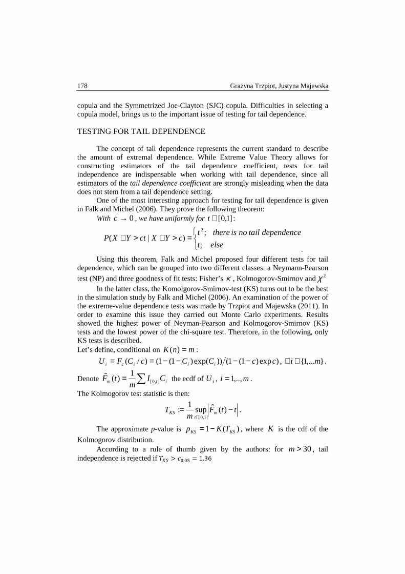
178 Grażyna Trzpiot, Justyna Majewska
copula and the Symmetrized Joe-Clayton (SJC) copula. Difficulties in selecting a copula model, brings us to the important issue of testing for tail dependence.
TESTING FOR TAIL DEPENDENCE
The concept of tail dependence represents the current standard to describe the amount of extremal dependence. While Extreme Value Theory allows for constructing estimators of the tail dependence coefficient, tests for tail independence are indispensable when working with tail dependence, since all estimators of the tail dependence coefficient are strongly misleading when the data does not stem from a tail dependence setting.
One of the most interesting approach for testing for tail dependence is given in Falk and Michel (2006). They prove the following theorem:
With 0→c , we have uniformly for ]1,0[∈t :
=>+>+elset
dependencetailnoistheretcYXctYXP
;
;)|(
2
. Using this theorem, Falk and Michel proposed four different tests for tail
dependence, which can be grouped into two different classes: a Neymann-Pearson
test (NP) and three goodness of fit tests: Fisher’s κ , Kolmogorov-Smirnov and 2χ In the latter class, the Komolgorov-Smirnov-test (KS) turns out to be the best
in the simulation study by Falk and Michel (2006). An examination of the power of the extreme-value dependence tests was made by Trzpiot and Majewska (2011). In order to examine this issue they carried out Monte Carlo experiments. Results showed the highest power of Neyman-Pearson and Kolmogorov-Smirnov (KS) tests and the lowest power of the chi-square test. Therefore, in the following, only KS tests is described. Let’s define, conditional on mnK =)( :
)exp)1(1())exp()1(1()/( ccCCcCFU iiici −−−−== , },...1{ mi ∈∀ .
Denote ∑= itm CIm
tF ],0[
1)(ˆ the ecdf of iU , mi ,..,1= .
The Kolmogorov test statistic is then:
ttFm
T mt
KS −=∈
)(ˆsup1
:]1,0[
.
The approximate p-value is )(1 KSKS TKp −= , where K is the cdf of the
Kolmogorov distribution. According to a rule of thumb given by the authors: for 30>m , tail
independence is rejected if ��� > ��.�� = 1.36

Analysis of tail-dependence structure in global … 179
RESULTS FOR THE DEPENDENCE STRUCTURE. EMPIRICAL STRUCTURE
For the empirical analysis we use daily series of four indices from Central and East Europe stock exchange markets, namely Polish WIG20, Hungarian BUX, Russian RTS, Czech PX50. Data for the period April 6th 2011 to March 29th 2012 come from the stock exchanges websites.
Dependence structure examination procedure is preceded in the four steps. First look at dependence (with conventional measure). Now we consider the results of dependence between each pair of stock returns. The well known Spearman’s ρ and Kendall’s τ rank correlation coefficients provide alternative nonparametric measures of dependence between variables that, unlike the simple correlation coefficient, do not require a linear relationship between the variables. For this reason they are commonly studied with copula models.
According to the conventional measure of dependence – Kendall’s rank correlation the weakness rank correlation is between RTX and PX50.
Sense of dependence structure
In order to get a sense of the dependence structure in the data, following Knight, Lizieri and Satchel (2005), we calculate an empirical copula table. To do this, we first rank the pairs of return series in ascending order and then we divide each series evenly into 6 bins. Bin 1 includes the observations with the lowest values and bin 6 includes observations with the highest values. We want to know how the values of one series are associated with the values of the other series, especially whether lower returns in - for example – WIG20 are associated with lower returns in the PX50. Thus, we count the numbers of observations that are in cell (i, j).
The dependence information we can obtain from the frequency table is as follows: • if the two series are perfectly positively correlated, most observations lie on the
diagonal, • if they are independent, then we would expect that the numbers in each cell are
about the same, • if the series are perfectly negatively correlated, most observations should lie on
the diagonal connecting the upper-right corner and the lower- left corner, • if there is positive lower tail dependence between the two series, we would
expect that more observations in cell (1,1), • if positive upper tail dependence exists, we would expect large number in cell
(6,6). Table 1 shows the dependence structure for real returns between WIG20 and
PX50, as an example. Cell (1,1) has a joint frequency of 61, which means that out of 186 observations, there are 61 occurrences when both the FeDex and UPS

180 Grażyna Trzpiot, Justyna Majewska
returns lie in their respective lowest 6th percentiles (1/6th quantile). This number is the largest among all cells, and it is much bigger than numbers in other cells, pointing to evidence of lower tail dependence. There are 43 occurrences in cell (6,6), which is not apparently larger than other cells, indicating no or not strong evidence of upper tail dependence. Clearly, the table shows evidence of asymmetric tail dependence.
Table 1. Joint frequency table for pair of stock return: WIG20 and PX50
1 2 3 4 5 6 1 61 36 31 28 19 11 2 41 54 34 29 23 5 3 26 27 21 43 17 44 4 19 34 38 20 47 28 5 22 25 41 23 34 41 6 17 10 21 43 39 43
Source: own calculation
Testing significance of tail dependence
We estimate and test for asymmetric tail dependence between all pairs returns. First, we select a flexible copula function to model the joint distribution of the each pair of returns. Because of empirical evidence of asymmetric tail proper selection is SJC copula (Symmetrized Joe-Clayton). SJC copula allows for both asymmetric upper and lower tail dependence and symmetric dependence as a special case. It is defined as:
)1),|1,1((
),|,((5,0),|,(
+++−−++⋅=
vuvuC
vuCvuC
luJC
luJCluSJC
λλλλλλ
where
krrkrkluJC vuvuC 11 )}1])1(1[])1(1{[11),|,( −−− −−−+−−−−=λλ
and
)2(log1 2 uk λ−= , )(log1 2 lr λ−= , )1,0(∈lλ , )1,0(∈uλ .
Then we compute for all ),( ji ( 7,...1, =ji ) pairs of returns the upper and lower tail dependence coefficients using the copulas parameters estimates (Table 2 and Table 3). We also employed KS test for tail dependence.
The most important conclusions are: • existence of dependence between Poland-Czech, Poland-Hungary stock markets
(the strongest between Poland-Czech), • Polish, Czech and Hungarian equity markets are dependent on the Russian
market (as the largest financial market in consideration).
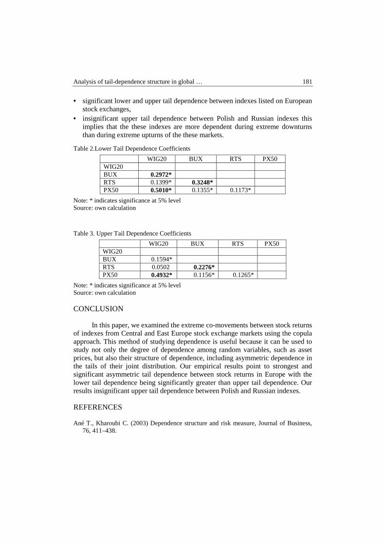
Analysis of tail-dependence structure in global … 181
• significant lower and upper tail dependence between indexes listed on European stock exchanges,
• insignificant upper tail dependence between Polish and Russian indexes this implies that the these indexes are more dependent during extreme downturns than during extreme upturns of the these markets.
Table 2.Lower Tail Dependence Coefficients
WIG20 BUX RTS PX50 WIG20 BUX 0.2972* RTS 0.1399* 0.3248* PX50 0.5010* 0.1355* 0.1173*
Note: * indicates significance at 5% level Source: own calculation
Table 3. Upper Tail Dependence Coefficients
WIG20 BUX RTS PX50 WIG20 BUX 0.1594* RTS 0.0502 0.2276* PX50 0.4932* 0.1156* 0.1265*
Note: * indicates significance at 5% level Source: own calculation
CONCLUSION
In this paper, we examined the extreme co-movements between stock returns of indexes from Central and East Europe stock exchange markets using the copula approach. This method of studying dependence is useful because it can be used to study not only the degree of dependence among random variables, such as asset prices, but also their structure of dependence, including asymmetric dependence in the tails of their joint distribution. Our empirical results point to strongest and significant asymmetric tail dependence between stock returns in Europe with the lower tail dependence being significantly greater than upper tail dependence. Our results insignificant upper tail dependence between Polish and Russian indexes.
REFERENCES
Ané T., Kharoubi C. (2003) Dependence structure and risk measure, Journal of Business, 76, 411–438.
182 Grażyna Trzpiot, Justyna Majewska
Ang A. Bekaert G. (2002) International Asset Allocation with Regime Shifts, Review of Financial Studies, 15, 1137-1187.
Ang A., Chen J. (2002) Asymmetric Correlations of Equity Portfolios, Journal of Financial Economics, 63, 443-494.
Butler K.C., Joaquin D.C., (2002) Are the Gains from International Portfolio Diversification Exaggerated? The Influence of Downside Risk in Bear Markets, Journal of International Money and Finance 21, 981-1011.
Campbell R., Koedijk K., Kofman P. (2002) Increased correlation in bear markets. Financial Analysts Journal, Jan-Feb, 87–94.
Cappiello L., Engle R.F., Sheppard K., (2006) Asymmetric Dynamics in the Correlations of Global Equity and Bond Returns, Journal of Financial Econometrics, 4, 537-572.
Coles S. (2001) An Introduction to Statistical Modeling of Extreme Values, Springer, Berlin.
Embrechts P., Klüppelberg C., Mikosch T. (1997) Modelling Extremal Events for Insurance and Finance, Springer, Berlin.
Embrechts P., McNeil A., Straumann D. (2002) Correlation and dependency in risk management: properties and pitfalls, [in:] Dempster M.A.H. (ed.) Risk Management: Value at Risk and Beyond, Cambridge University Press, 176–223.
Falk M., Michel R. (2006) Testing for tail independence in extreme value models, Annals of the Institute of Statistical Mathematics, 58, 261–290.
Frahm G., Junker M., Schmidt R. (2005) Estimating the tail-dependence coefficient: Properties and pitfalls, Insurance: Mathematics and Economics, 37, 80-100.
Frank M.J. (1979) On the Simultaneous Associativity of F(x,y) and xyF(x,y), Aequationes Mathematicae, 19, 194 – 226.
Haan L. de, Resnick S.I. (1977) Limit theory for multivariate sample extremes, Zeitschrift fuer Wahrscheinlichkeitsteorie und verwandte Gebiete, 40, 317-337.
Hartmann P., Straetmans S., De Vries C.G. (2004) Asset Market Linkages in Crisis Periods, Review of Economics and Statistics 86, 313-326.
Joe H. (1997) Multivariate Models and Dependence Concepts, Chapman and Hall, London. Karolyi G. A., Stulz R.M. (1996) Why do markets move together? An investigation of
U.S.-Japan stock return comovements, Journal of Finance, 51(3), 951-986. Knight J., Lizieri C., Satchell S. (2006) Diversification when it hurts? The joint distribution
of real estate and equity markets, Journal of Property Research, 22, 309-323. Longin F., Solnik B. (2001) Extreme correlation of international equity markets, Journal of
Finance 56, 649-676. Malevergne Y., Sornette D. (2004) Investigating extreme dependencies. Extreme Financial
Risks (From dependence to risk management) Springer, Heidelberg, 2006. Sibuya M. (1960) Bivariate extreme statistics I. Annals of Institute of the Statistical
Mathematics, 11, 195-210. Sklar A. (1959) Fonctions de répartition à n dimensions et leurs marges. Publications de
l’Institut de Statistique de l’Université de Paris, 8, 229-231. Trzpiot G., Majewska J. (2012) Tail independence in extreme value models – an
application for East and Central Europe Stock Exchange Markets, Badania Operacyjne i Decyzje 1/2012, Oficyna Wydawnicza Politechniki Wrocławskiej, Wrocław.

QUANTITATIVE METHODS IN ECONOMICS Vol. XV, No. 1, 2014, pp. 183 – 191
RISK AND RETURNS ON POLISH POWER EXCHANGE AND EUROPEAN ENERGY EXCHANGE
Grażyna Trzpiot Katedra Demografii i Statystyki Ekonomicznej,
Uniwersytet Ekonomiczny w Katowicach e-mail: [email protected]
Barbara Glensk Institute for Future Energy Consumer Needs and Behavior, E.ON Energy Research Center, RWTH Aachen University
e-mail: [email protected] Alicja Ganczarek-Gamrot
Katedra Demografii i Statystyki Ekonomicznej, Uniwersytet Ekonomiczny w Katowicach
e-mail: [email protected]
Abstract: The aim of this paper is a comparative analysis of contracts on electric energy at Polish Power Exchange (POLPX) and European Energy Exchange (EEX) spot markets. The approach considered in this article is based on minimization of the Conditional Value at Risk and maximization of portfolio rates of return. The analyzed portfolios were constructed with contracts noted on POLEX and EEX from 1st January 2011 to 31st December 2012.
Keywords: risk, portfolio, electric energy market,
INTRODUCTION
The Polish Power Exchange (POLPX) was started in July 2000. Investors on POLPX may participate in the Day Ahead Market (DAM, spot market), the Commodity Derivatives Market (CDM, future market), the Electricity Auctions, the Property Right Market, the Emission Allowances Market (CO2 spot) and the Intraday Market. All these markets differ with respect to an investment horizon length and the traded commodity.

184 Grażyna Trzpiot, Barbara Glensk, Alicja Ganczarek-Gamrot
The result of the merger of the two German power exchanges in Leipzig and Frankfurt was the establishment in 2002 the European Energy Exchange AG (EEX) in Leipzig. This is one of the European trading and clearing platforms for energy and energy-related products, such as natural gas, CO2 emission allowances and coal. The EEX consists of three sub-markets (EEX Spot Markets, EEX Power Derivatives and EEX Derivatives Markets) and one Joint Venture (EPEX Spot Market). Moreover, EEX is trying to become the leader among European Energy Exchanges assuming an active role in the development and integration process of the European market.
Indices POLPX base and POLPX peak in EUR/MWh were noted on POLPX from 2011, calculated in the same way as indices on EEX. Figure 1 shows indices POLPX base noted on POLPX and PHELIX base noted on EEX, which represent average prices of electric energy during a day. The indices exhibit similar behavior, but on EEX greater changes of the index and negative prices are observed.
Figure 1. Time series of POLPX base and PHELIX base
Source: own calculations
On box plot of indexes (Figure 2) one can observe asymmetry, high volatility, outliers and extreme value in average electric energy prices. Negative value of PHELIX base were registered on Christmas Eve 25 and 26 December
POLPX base PHELIX base
20
11
/01
/01
20
11
/02
/20
20
11
/04
/11
20
11
/05
/31
20
11
/07
/20
20
11
/09
/08
20
11
/10
/28
20
11
/12
/17
20
12
/02
/05
20
12
/03
/26
20
12
/05
/15
20
12
/07
/04
20
12
/08
/23
20
12
/10
/12
20
12
/12
/01
-80
-60
-40
-20
0
20
40
60
80
100
120
EU
R/M
Wh

Risk and returns on Polish Power Exchange and European Energy Exchange 185
2012 year. Prices observed on POLPX were quite stable. In the night hours on EEX prices were negative: investors had to pay for selling electric energy.
Figure 2. Box plot of POLPX base and PHELIX base
Source: own calculations
Figure 3. Box plot of POLPX base and PHELIX base linear rates of return
Source: own calculations
M edian 25%-75% M in.-M aks. Outlaier Extrim ePOLPX base
PHELIX base
-80
-60
-40
-20
0
20
40
60
80
100
120
EU
R/M
Wh
M edian 25%-75% M in.-M aks. Outla ier Extrim e
zt POLPX zt PHELIX-5
-4
-3
-2
-1
0
1
2
3
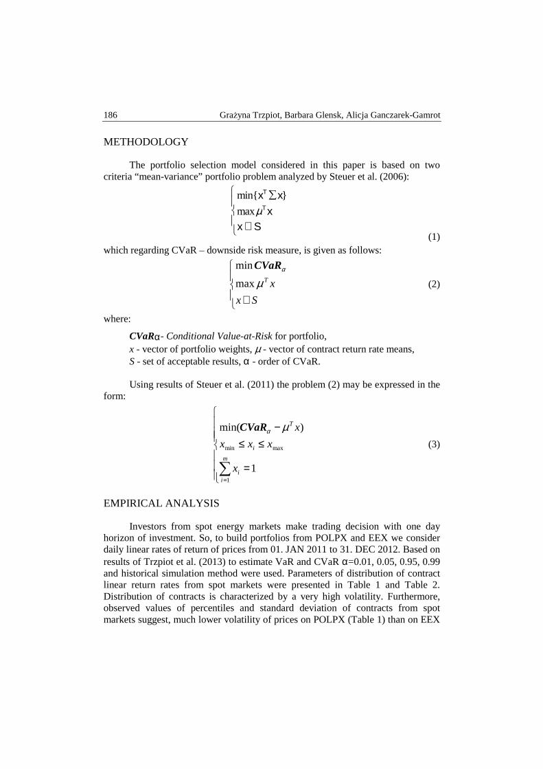
186 Grażyna Trzpiot, Barbara Glensk, Alicja Ganczarek-Gamrot
METHODOLOGY
The portfolio selection model considered in this paper is based on two criteria “mean-variance” portfolio problem analyzed by Steuer et al. (2006):
(1) which regarding CVaR – downside risk measure, is given as follows:
∈ Sx
xTµα
max
minCVaR
(2)
where:
CVaRα- Conditional Value-at-Risk for portfolio, x - vector of portfolio weights, µ - vector of contract return rate means, S - set of acceptable results, α - order of CVaR. Using results of Steuer et al. (2011) the problem (2) may be expressed in the
form:
=
≤≤−
∑=
1
)min(
1
maxmin
m
ii
i
T
x
xxx
xµαCVaR
(3)
EMPIRICAL ANALYSIS
Investors from spot energy markets make trading decision with one day horizon of investment. So, to build portfolios from POLPX and EEX we consider daily linear rates of return of prices from 01. JAN 2011 to 31. DEC 2012. Based on results of Trzpiot et al. (2013) to estimate VaR and CVaR α=0.01, 0.05, 0.95, 0.99 and historical simulation method were used. Parameters of distribution of contract linear return rates from spot markets were presented in Table 1 and Table 2. Distribution of contracts is characterized by a very high volatility. Furthermore, observed values of percentiles and standard deviation of contracts from spot markets suggest, much lower volatility of prices on POLPX (Table 1) than on EEX
min { x T ∑x }
ma xµ T x
x ∈ S

Risk and returns on Polish Power Exchange and European Energy Exchange 187
(Table 2). Additionally the highest volatility on EEX was observed for contracts of night hour and in 16th hour.
Table 1. Distribution parameters of rates of return of contracts on POLPX
Co
ntr
acts
Mea
n
Sta
nd
. d
ev.
Med
ian
Min
Per
cen
tile
1%
Per
cen
tile
5%
Per
cen
tile
95
%
Per
cen
tile
99
%
Max
1 0.001 0.07 0.001 -0.29 -0.18 -0.10 0.11 0.17 0.33 2 0.002 0.08 0.002 -0.33 -0.23 -0.11 0.12 0.22 0.37 3 0.002 0.08 0.001 -0.31 -0.23 -0.13 0.15 0.25 0.35 4 0.003 0.09 0.004 -0.33 -0.25 -0.15 0.15 0.27 0.37 5 0.003 0.09 0.003 -0.33 -0.24 -0.15 0.17 0.32 0.42 6 0.006 0.12 -0.003 -0.35 -0.27 -0.18 0.24 0.41 0.66 7 0.017 0.20 -0.007 -0.50 -0.32 -0.23 0.45 0.76 1.24 8 0.014 0.18 -0.006 -0.51 -0.33 -0.21 0.43 0.66 1.31 9 0.012 0.17 -0.008 -0.55 -0.26 -0.20 0.35 0.50 1.53
10 0.009 0.15 -0.007 -0.56 -0.27 -0.19 0.31 0.46 1.48 11 0.007 0.12 -0.004 -0.48 -0.24 -0.18 0.25 0.37 0.94 12 0.006 0.12 -0.005 -0.45 -0.23 -0.16 0.25 0.37 0.88 13 0.006 0.11 -0.006 -0.39 -0.22 -0.16 0.25 0.33 0.65 14 0.006 0.11 -0.005 -0.39 -0.23 -0.16 0.23 0.36 0.65 15 0.005 0.11 -0.008 -0.34 -0.21 -0.15 0.23 0.33 0.63 16 0.005 0.11 -0.008 -0.32 -0.21 -0.14 0.23 0.35 0.68 17 0.006 0.12 -0.006 -0.33 -0.28 -0.15 0.24 0.44 0.65 18 0.006 0.12 -0.005 -0.52 -0.28 -0.14 0.21 0.41 0.66 19 0.005 0.11 -0.001 -0.47 -0.25 -0.13 0.20 0.30 0.71 20 0.004 0.09 -0.002 -0.45 -0.25 -0.12 0.17 0.28 0.69 21 0.003 0.08 -0.001 -0.33 -0.18 -0.11 0.13 0.23 0.56 22 0.001 0.06 0.000 -0.28 -0.15 -0.09 0.09 0.14 0.65 23 0.001 0.05 -0.001 -0.32 -0.13 -0.08 0.11 0.17 0.23 24 0.001 0.06 -0.003 -0.20 -0.15 -0.09 0.11 0.21 0.33
Source: own calculations

188 Grażyna Trzpiot, Barbara Glensk, Alicja Ganczarek-Gamrot
Table 2. Distribution parameters of rates of return of contracts on EEX
Co
ntr
acts
Mea
n
Sta
nd
. d
ev.
Med
ian
Min
Per
cen
tile
1%
Per
cen
tile
5%
Per
cen
tile
95
%
Per
cen
tile
99
%
Max
1 -0.620 17.67 0.005 -477.3 -0.83 -0.42 0.58 1.80 6.04
2 -5.871 113.6 0.002 -2555 -1.76 -0.53 0.69 2.42 228.1
3 2.771 127.9 -0.002 -1063 -1.58 -0.58 0.82 2.43 3273
4 -6.178 100.6 -0.001 -2467 -1.31 -0.58 0.91 2.12 41.48
5 -0.831 41.64 -0.001 -1004 -1.11 -0.54 0.87 2.11 477.5
6 -0.571 12.11 -0.005 -274.1 -1.30 -0.61 0.84 2.75 13.93
7 -3.582 125.5 -0.030 -2795 -1.79 -0.62 1.25 3.60 1577
8 -0.274 20.28 -0.033 -479.9 -1.08 -0.55 1.74 5.14 198.6
9 -0.602 55.23 -0.030 -1283 -0.83 -0.47 1.27 3.01 761.5
10 -1.852 55.24 -0.021 -1491 -0.71 -0.39 0.91 2.31 88.42
11 0.060 0.44 -0.018 -0.84 -0.60 -0.38 0.77 1.93 4.88
12 0.047 0.39 -0.015 -0.83 -0.54 -0.36 0.68 1.54 5.18
13 0.052 0.41 -0.009 -0.82 -0.57 -0.38 0.65 1.67 5.07
14 0.074 0.51 -0.020 -0.81 -0.64 -0.41 0.85 2.30 5.36
15 0.128 1.33 -0.030 -0.96 -0.67 -0.43 0.99 2.34 32.19
16 -4.941 115.5 -0.036 -3067 -0.69 -0.44 0.94 2.38 4.67
17 -0.083 3.78 -0.028 -101.5 -0.60 -0.39 0.85 1.93 4.53
18 0.056 0.67 -0.024 -0.93 -0.49 -0.33 0.59 1.46 16.01
19 0.028 0.31 -0.015 -0.80 -0.40 -0.28 0.48 1.01 5.18
20 0.018 0.21 -0.011 -0.61 -0.39 -0.24 0.38 0.87 1.83
21 0.015 0.20 -0.001 -0.58 -0.38 -0.23 0.32 0.80 1.56
22 0.012 0.18 -0.002 -0.60 -0.35 -0.23 0.28 0.59 1.56
23 0.012 0.17 0.000 -0.58 -0.37 -0.22 0.28 0.49 1.76
24 1.581 42.03 0.000 -1.80 -0.62 -0.28 0.31 1.43 1136
Source: own calculations
Values of CVaR for contracts with α=0.01, 0.05, 0.95, 0.99 (Table 3) confirm the initial assessment. Moreover on EEX one can observe much greater risk for investors which can sell electric energy on POLPX and little greater risk for investors who can buy electric energy, but the risk is much lower than the risk on EEX.
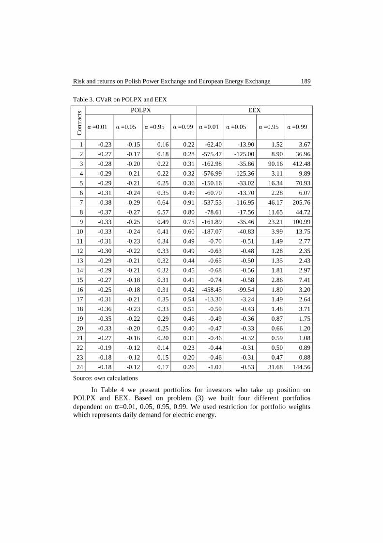
Risk and returns on Polish Power Exchange and European Energy Exchange 189
Table 3. CVaR on POLPX and EEX
Co
ntr
acts
POLPX EEX
α =0.01 α =0.05 α =0.95 α =0.99 α =0.01 α =0.05 α =0.95 α =0.99
1 -0.23 -0.15 0.16 0.22 -62.40 -13.90 1.52 3.67
2 -0.27 -0.17 0.18 0.28 -575.47 -125.00 8.90 36.96
3 -0.28 -0.20 0.22 0.31 -162.98 -35.86 90.16 412.48
4 -0.29 -0.21 0.22 0.32 -576.99 -125.36 3.11 9.89
5 -0.29 -0.21 0.25 0.36 -150.16 -33.02 16.34 70.93
6 -0.31 -0.24 0.35 0.49 -60.70 -13.70 2.28 6.07
7 -0.38 -0.29 0.64 0.91 -537.53 -116.95 46.17 205.76
8 -0.37 -0.27 0.57 0.80 -78.61 -17.56 11.65 44.72
9 -0.33 -0.25 0.49 0.75 -161.89 -35.46 23.21 100.99
10 -0.33 -0.24 0.41 0.60 -187.07 -40.83 3.99 13.75
11 -0.31 -0.23 0.34 0.49 -0.70 -0.51 1.49 2.77
12 -0.30 -0.22 0.33 0.49 -0.63 -0.48 1.28 2.35
13 -0.29 -0.21 0.32 0.44 -0.65 -0.50 1.35 2.43
14 -0.29 -0.21 0.32 0.45 -0.68 -0.56 1.81 2.97
15 -0.27 -0.18 0.31 0.41 -0.74 -0.58 2.86 7.41
16 -0.25 -0.18 0.31 0.42 -458.45 -99.54 1.80 3.20
17 -0.31 -0.21 0.35 0.54 -13.30 -3.24 1.49 2.64
18 -0.36 -0.23 0.33 0.51 -0.59 -0.43 1.48 3.71
19 -0.35 -0.22 0.29 0.46 -0.49 -0.36 0.87 1.75
20 -0.33 -0.20 0.25 0.40 -0.47 -0.33 0.66 1.20
21 -0.27 -0.16 0.20 0.31 -0.46 -0.32 0.59 1.08
22 -0.19 -0.12 0.14 0.23 -0.44 -0.31 0.50 0.89
23 -0.18 -0.12 0.15 0.20 -0.46 -0.31 0.47 0.88
24 -0.18 -0.12 0.17 0.26 -1.02 -0.53 31.68 144.56
Source: own calculations
In Table 4 we present portfolios for investors who take up position on POLPX and EEX. Based on problem (3) we built four different portfolios dependent on α=0.01, 0.05, 0.95, 0.99. We used restriction for portfolio weights which represents daily demand for electric energy.
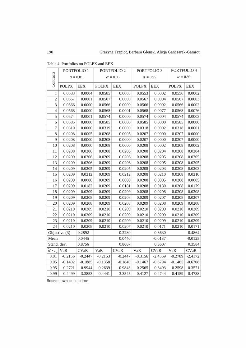
190 Grażyna Trzpiot, Barbara Glensk, Alicja Ganczarek-Gamrot
Table 4. Portfolios on POLPX and EEX
Co
ntr
acts
PORTFOLIO 1
01.0=α
PORTFOLIO 2
05.0=α
PORTFOLIO 3
95.0=α
PORTFOLIO 4
99.0=α
POLPX EEX POLPX EEX POLPX EEX POLPX EEX
1 0.0583 0.0004 0.0585 0.0003 0.0553 0.0002 0.0556 0.0002
2 0.0567 0.0001 0.0567 0.0000 0.0567 0.0004 0.0567 0.0003
3 0.0566 0.0000 0.0566 0.0000 0.0566 0.0002 0.0566 0.0002
4 0.0568 0.0000 0.0568 0.0001 0.0568 0.0077 0.0568 0.0076
5 0.0574 0.0001 0.0574 0.0000 0.0574 0.0004 0.0574 0.0003
6 0.0585 0.0000 0.0585 0.0000 0.0585 0.0000 0.0585 0.0000
7 0.0319 0.0000 0.0319 0.0000 0.0318 0.0002 0.0318 0.0001
8 0.0208 0.0005 0.0208 0.0005 0.0207 0.0000 0.0207 0.0000
9 0.0208 0.0000 0.0208 0.0000 0.0207 0.0000 0.0207 0.0000
10 0.0208 0.0000 0.0208 0.0000 0.0208 0.0002 0.0208 0.0002
11 0.0208 0.0206 0.0208 0.0206 0.0208 0.0204 0.0208 0.0204
12 0.0209 0.0206 0.0209 0.0206 0.0208 0.0205 0.0208 0.0205
13 0.0209 0.0206 0.0209 0.0206 0.0208 0.0205 0.0208 0.0205
14 0.0209 0.0205 0.0209 0.0205 0.0208 0.0203 0.0208 0.0203
15 0.0209 0.0212 0.0209 0.0212 0.0208 0.0210 0.0208 0.0210
16 0.0209 0.0000 0.0209 0.0000 0.0208 0.0005 0.0208 0.0005
17 0.0209 0.0182 0.0209 0.0181 0.0208 0.0180 0.0208 0.0179
18 0.0209 0.0209 0.0209 0.0209 0.0208 0.0208 0.0208 0.0208
19 0.0209 0.0208 0.0209 0.0208 0.0209 0.0207 0.0208 0.0207
20 0.0209 0.0208 0.0209 0.0208 0.0209 0.0208 0.0209 0.0208
21 0.0210 0.0209 0.0210 0.0209 0.0210 0.0209 0.0210 0.0209
22 0.0210 0.0209 0.0210 0.0209 0.0210 0.0209 0.0210 0.0209
23 0.0210 0.0209 0.0210 0.0209 0.0210 0.0209 0.0210 0.0209
24 0.0210 0.0208 0.0210 0.0207 0.0210 0.0171 0.0210 0.0171
Objective (3) 0.2892 0.2280 0.3630 0.4864
Mean 0.0445 0.0440 -0.0137 -0.0125
Stand. dev. 0.8756 0.8667 0.3607 0.3584
α VaR CVaR VaR CVaR VaR CVaR VaR CVaR
0.01 -0.2156 -0.2447 -0.2153 -0.2447 -0.3156 -2.4569 -0.2789 -2.4172
0.05 -0.1402 -0.1885 -0.1358 -0.1840 -0.1467 -0.6794 -0.1465 -0.6708
0.95 0.2721 0.9944 0.2639 0.9843 0.2565 0.3493 0.2598 0.3571
0.99 0.4499 3.3853 0.4441 3.3545 0.4127 0.4744 0.4159 0.4738
Source: own calculations

Risk and returns on Polish Power Exchange and European Energy Exchange 191
For every value of α we obtained portfolios consisting only of contract from POPLPX for night hour and in 16 hour. Portfolio weights of daily contracts are very close on two exchanges (see Table 4). This result is specific for the electric energy as particular commodity. The demand is greater during a day than in the night irrespective of prices. The negative value of portfolio returns for α=0.95, 0.99 (see Table 4) as well as for EEX may result from negative electricity prices observed on EEX.
4. CONCLUSION
In conclusion one can say. that despite similar price levels the risk of price changes on EEX is much greater than risk on POLPX, but based on problem (3) to build the portfolio, the investor should buy and sell electricity on EEX too. Contracts in night and early morning hour on POLPX are more attractive than on EEX, but for odd hours contracts on two spot markets give very similar distance between risk and profit. independently on level of α. Very similar results was obtained for from 01 JAN 2009 to 24 OCT 2012 [Trzpiot et al. 2014].
REFERENCES
Blanco C. (1998) Value at risk for energy: Is VaR useful to manage energy price risk? Financial Engineering Associates.
Jajuga K., Jajuga T. (1998) Inwestycje. Instrumenty finansowe. Ryzyko finansowe. Inżynieria finansowa. PWN. Warszawa.
Rockafellar R.T., Uryasev S. (2000) Optimization of Conditional Value-at-Risk. “The Journal of Risk”. 2(3): 21-41.
Steuer R.E., Qi Y., Hirscheberger M. (2006) Developments in multi-attribute portfolio selection. Multiple Criterion decision making. (ed. Trzaskalik T.). UE. Katowice. 251-262.
Steuer R.E., Qi Y., Hirscheberger M. (2011) Comparative issues in large-scale mean–variance efficient frontier computation. “Decision Support Systems”. 51(2): 250-255.
Trzpiot G., Glensk B., Ganczarek-Gamrot A. (2013) Validation of Market Risk on the Electric Energy Market – an IRC Approach. Studia Ekonomiczne 162. UE in Katowice. 38-49.
Trzpiot G., Glensk B., Ganczarek-Gamrot A. (2014) Portfolio Analysis on Polish Power Exchange and European Energy Exchange. [in] Multiple Criterion decision making. (ed. Trzaskalik T.). UE. Katowice. (in press)
Weron A., Weron R. (2000) Giełda Energii. Strategie zarządzania ryzykiem, Wrocław.
QUANTITATIVE METHODS IN ECONOMICS Vol. XV, No. 1, 2014, pp. 192 – 208
DETERMINANTS OF WAGES IN POLAND1
Dorota Witkowska Department of Finance and Enterprise Strategy
Faculty of Management University of Lodz e-mail: [email protected]
Abstract: The aim of our research is to identify determinants influencing wages in Poland in the years 2001, 2003, 2006 and 2009. We want to find out if there is any changes in time and if gender can be considered as significant factor influencing wages. Investigation is provided on the basis of data from the Polish Labor Force Survey, applying ordered logit models.
Keywords: labor market, wage determinats, ordered logit model
INTRODUCTION
There is no doubt that level of wages differ essentially even if the local labor market is considered since numerous forces operate as earning determinants. These might be roughly classified as economic, institutional, behavioral, and equity considerations. Wage decisions appear to be made by comparison to labor markets, so many of the determinants appear to be economic. Both the meaning and force of economic variables are interpreted by organization decision makers, and these determinants are tempered by institutional, behavioral, and ethical variables.
Riley (2012) analyzing situation in the UK, claims that there is a wide gulf in pay and earnings rates between different occupations in labor market. He mentions several factors that differentiate wages.
1 Research conducted under the National Science Centre Grant No. 2011/01/B/HS4/06346 “Wages Inequalities between Men and Women in Poland in the Framework of the European Union”.
Determinants of wages in Poland 193
1. Compensating wage differentials i.e. higher pay can often be a reward for risk-taking in certain jobs, working in poor conditions and having to work on holidays or in unsocial hours.
2. Equalizing difference and human capital. In a competitive labor market, wage differentials compensate workers for the opportunity costs and direct costs of human capital acquisition.
3. Different skill levels. The gap between poorly and highly skilled workers gets wider each year. Market demand for skilled labor grows more quickly than for semi-skilled workers. This pushes up pay levels. Highly skilled workers are often in inelastic supply and rising demand forces up the "going wage rate" in an industry.
4. Differences in labor productivity and revenue creation. Workers whose efficiency is highest and ability to generate revenue for a firm should be rewarded with higher pay (for instance sport stars can command top wages because of their potential to generate extra revenue from ticket sales and merchandising).
5. Trade unions and their collective bargaining power. Unions might exercise their bargaining power to offset the power of an employer in a particular occupation and in doing so achieve a mark-up on wages compared to those on offer to non-union members
6. Employer discrimination is a factor that cannot be ignored despite equal pay legislation
Wage determinants can be divided into three groups [Kot 1999, p. 142]: (a) human capital (i.e. level of education, job seniority, etc.), (b) situation on the labor market (e.g. supply for skilled workers, unemployment rate), and (c) other such as: gender, marital status, place of living, etc.
Identified factors, that affect wages, are used to construct "earnings function" which has been applied to a wide variety of problems such as [Willis 1986, p. 525], (a) studies of discrimination by race or sex (see [Cain 1986 p. 693]), (b) the estimation of the "value of life" from data on job safety [Thaler and Rosen 1975], or (c) compensation for increased unemployment probabilities [Abowd and Ashenfelter 1981]. The premier application, of course, was to the study of the effects of investment in schooling and on-the-job training on the level, pattern, and interpersonal distribution of life cycle earnings associated with the pioneering work on human capital by Becker (1964)2.
The aim of our research is to identify determinants that affect earnings in Poland, in the years 2001 – 2009. Another issue is to find out if there is any changes in time and if gender can be consider as a significant factor influencing wages. Investigation is provided applying ordered logit models, that are estimated
2 The standard human capital earnings function was developed by Mincer (1974).

194 Dorota Witkowska
by maximum likelihood method, employing individual data from the Polish Labor Force Survey (PLFS).
SITUATION IN POLAND AFTER 1989
In 1989 the radical set of reforms was introduced in Poland which were followed by other countries belonging to the former Soviet bloc [Keane and Prasad 2006]. The privatization of state owned enterprises and implementation of market mechanisms were the main goals of transformation in post-communist countries. The transition also involved significant changes in labor market institutions.
On the basis of profound analysis made for years 1989 – 2010, Brzeziński et al. (2012) claim that both individual and household based indices show that labor market participation declined. At the same time all data sources agree that there was a substantial increase in earnings inequality. However, educational attainment has improved significantly over the last decade. The share of tertiary graduates almost doubled since 1997 (rising from 7.7% to 13.8% in the year 2008).
It seems that the single most important factor accounting for the inequality rise was the increase of earnings inequality caused by rising educational premium for highly‐qualified workers employed in highly‐skilled occupations coupled with the worsening of relative position of workers employed in low‐paying occupations. The major underlying causes of inequality growth during transition in Poland are the change from centrally‐planned wage setting to decentralized wage setting and radical structural and technological changes of the economy shifting labor demand from public sector to private sector and from manual workers to professionals and highly‐qualified workers.
In the conclusion of the report on structure and changes in wage distribution in years 1996 – 2006, prepared by Marcinkowska et al. (2008), it is said that so called “skill-biased technical change” together with changes of the bargaining power of employees has played the increasing role in wage setting. While the influence of factors concerning economic branches decreased and concerning regions remain stable.
Newell and Socha (2005) analyze the changes in the distribution of wages in Poland in years 1992 - 2002. They find out that privatization was the main force tending to increase wage inequality, partly because it generated major increases in the relative wages of professional and managerial workers. The main force contracting the variance of wages was the decline, between 1992 and 1998 in labor market participation of those with low levels of education. Wage inequality seems to have increased since 2000. Suggestively, whereas privatization has continued, the decline in participation has halted. Newell and Socha (2007) have demonstrated that the private sector in Poland tends to pay more unequally than the state sector, and since there was a surge of privatization 1998-2002, this contributed to the rise in wage inequality. It is also true that inequality, in the forms of hourly wage
Determinants of wages in Poland 195
variance and of regression wage premiums to education and occupation is consistently higher, and in the case of education premiums, rose more quickly in the private sector data.
Kean and Prasad (2006) examine the evolution of the structure of labor earnings in Poland over the period 1985–1996 using micro data from the Polish Household Budget Surveys. The relatively long span of the dataset allows them to trace out changes for an extended period leading up to and following the “big bang”. They find that overall earnings inequality rose markedly during the transition period of 1989–1996. Kean and Prasad (2006) also conduct a detailed examination of the sources of the increase in earnings inequality. Prior to the transition, the wage structure in Poland was highly compacted, with wages of college-educated white-collar workers a little different from those of manual workers. A common view is that the rise of the private sector, in which there is competitive wage setting and, hence, a more unequal wage distribution, is the main source of increasing earnings inequality during transition.
In Poland, earnings inequality is indeed higher in the private sector (e.g., the log 90–10 earnings differential in 1996 was 1.19 in the private sector and 1.05 in the public sector), and the private sector share of (non-agricultural) employment increased from 5% in 1988 to 39% in 1996. Still, Kean and Prasad (2006) find that reallocation of labor from the public to the private sector accounted for only 39% of the total increase in earnings inequality (as measured by the change in the variance of log earnings).
The majority of the increase in earnings inequality during the Polish transition (52%) was due to increased variance of wages within both the public and private sectors. That is, earnings inequality within both the private and public sectors grew substantially, and by similar amounts. This is consistent with the view that even state-owned enterprises in Poland have engaged in substantial restructuring, as suggested by Pinto et al. (1993) and others. Consistent with their finding of increased earnings inequality within the public sector, Commander and Dhar (1998) report (p. 127) a substantial increase in the heterogeneity of wages across state owned enterprises between 1990 and 1994, with those that performed better in terms of sales offering higher wages. Kean and Prasad also find that educational wage premiums increased substantially. Nevertheless, the majority of the increase in overall earnings inequality (60%) in Poland is attributable to changes in within-group inequality. A striking result is that increases in within-group inequality were concentrated among workers with higher levels of formal education3.
3 This is quite different from the patterns documented for the U.S. and the U.K. of sharp increases over the last two decades in between-group inequality at all levels of education (see [Kean and Prasad 2006]).
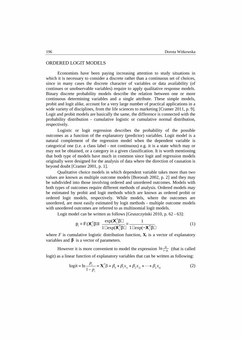
196 Dorota Witkowska
ORDERED LOGIT MODELS
Economists have been paying increasing attention to study situations in which it is necessary to consider a discrete rather than a continuous set of choices, since in many cases the discrete character of variables or data availability (of continues or unobservable variables) require to apply qualitative response models. Binary discrete probability models describe the relation between one or more continuous determining variables and a single attribute. These simple models, probit and logit alike, account for a very large number of practical applications in a wide variety of disciplines, from the life sciences to marketing [Cramer 2011, p. 9]. Logit and probit models are basically the same, the difference is connected with the probability distribution - cumulative logistic or cumulative normal distribution, respectively.
Logistic or logit regression describes the probability of the possible outcomes as a function of the explanatory (predictor) variables. Logit model is a natural complement of the regression model when the dependent variable is categorical one (i.e. a class label - not continuous) e.g. it is a state which may or may not be obtained, or a category in a given classification. It is worth mentioning that both type of models have much in common since logit and regression models originally were designed for the analysis of data where the direction of causation is beyond doubt [Cramer 2001, p. 1].
Qualitative choice models in which dependent variable takes more than two values are known as multiple outcome models [Borooah 2002, p. 2] and they may be subdivided into those involving ordered and unordered outcomes. Models with both types of outcomes require different methods of analysis. Ordered models may be estimated by probit and logit methods which are known as ordered probit or ordered logit models, respectively. While models, where the outcomes are unordered, are most easily estimated by logit methods - multiple outcome models with unordered outcomes are referred to as multinomial logit models.
Logit model can be written as follows [Gruszczyński 2010, p. 62 - 63]:
pi = F (X iTβ) =
exp(X iTβ)
1+ exp(X iTβ)
= 1
1+ exp(−X iTβ)
(1)
where F is cumulative logistic distribution function, Xi is a vector of explanatory variables and is a vector of parameters.
However it is more convenient to model the expression (that is called
logit) as a linear function of explanatory variables that can be written as following:
(2)
β
i
i
pp−1ln

Determinants of wages in Poland 197
Probability models are - as rule - estimated from survey data, which provide large sample of independent observations with a wide range of variation of the explanatory variables. The preferred method of estimation is maximum likelihood4 since maximum likelihood estimates (MLE) are consistent and asymptotically efficient [Cramer 2001, p. 17].
The value of the loglikelihood function for particular sets of parameter estimates5 is useful when we wish to consider and test restrictions on the parameter vector β (for instance simplifying assumptions like zero coefficient or the absence of certain variables from the model). Provided the restricted model is nested as a special case within the general or unrestricted model, this can be tested by the loglikelihood ratio or LR test. In our investigation we apply likelihood ratio tests to verify null hypothesis H0: β1 = β2 = … = βk = 0 versus alternative hypothesis H1 saying that at least one parameter differs from zero, employing chi-squared statistics with k degrees of freedom [Gruszczyński 2010, p. 65, 128]:
LR= 2(lnLUR − lnLR) (3)
where LUR, LR are values of the likelihood functions of the unrestricted (in our case investigated) model and restricted one (in our case the model containing constant only), respectively, k is a number of restrictions (i.e. explanatory variables).
For the model verification we also verify hypothesis of significance of each coefficient of the model to check if explanatory variables influence the investigated phenomenon. Parameters of logit model have similar interpretation as regression coefficients i.e. the sign of parameters defines the direction of the relation observed between variables. To interpret the results of the estimation results odds ratio pi/(1-pi) can be used [Gruszczyński 2010, p. 67 - 68].
Goodness of fit in logit models6 is evaluated on the basis of several measures such as: McFadden pseudo R2:
RMcFadden2 =1−
ln LUR
ln LR
(4)
or fraction of observations with correct predicted outcomes so called count R2:
count R2 =Ncor
N⋅100 (5)
4 Detailed discussion about ordered logit models construction and estimation can be found
in Borooah (2002), Cramer (2001), Boes and Winkelmann (2009) and Gruszczyński (2010), among others.
5 Loglikelihood ratio describes value of the natural logarithm of the likelihood function that is maximized in order to find MLE of the parameters.
6 Broad discussion about goodness of fit measures can be found in [Gruszczyński 2002, p. 64 – 68] and [Gruszczyński 2010, p. 71 – 74, 128 – 135].

198 Dorota Witkowska
where N and Ncor are numbers of all and correctly predicted outcomes, respectively. Another group of measures contains information criteria that can be used to compare models with different specification7.
DATA AND VARIABLE DESCRIPTION
In our investigation we employ individual data from the Polish Labor Force Survey (PLFS) from selected quarters in years: 2001, 2003, 2006 and 2009 since we assume that changes of factors affecting wages require time and they do not appear year by year. The years for our research are selected arbitrary however, to some extend, it was connected with data availability.
It is worth mentioning that in the Labor Force Survey the household is the investigated unit for the representative investigation. Therefore among PLFS data there are also records concerning people in pre- and post-working age, as well as unemployed. In addition some respondents do not answer all questions, especially they are not willing to inform about their wages. Therefore it is necessary to select records concerning only employed who answered the questions that create data which are to be used in the model building. There are 32,939 records in our samples that is 21.3% of all PLFS multidimensional observations.
Wages depend on different factors which describes either respondents’ or employment characteristics. In our research we employ explanatory variables, that are selected arbitrarily however they are often used in the research concerning wages (e.g. [Newell and Socha 2007]; [Witkowska 2012]). The majority of variables are defined as qualitative therefore all variants of these variables are described below. The reference variants of qualitative variables are underlined since definition of the reference variant is necessary for interpretation of the parameter estimates. The selected employees’ features are: 1. GEN – gender: women or men; 2. OCC – occupation: (a) army, (b) managerial, (c) professional, (d) technical,
(e) clerical, (f) sales and services, (g) farmers, fishers, etc., (h) industry workers, (i) skilled workers or (j) unskilled workers8;
3. EDU - level of education: (a) tertiary, (b) post-secondary and vocational secondary, (c) general secondary, (d) basic vocational, (e) lower secondary, primary and incomplete primary9;
4. RES - size class of the place of residence given in numbers of inhabitants: (a) more than 100 thousands citizens, (b) from 50 to 100 thousands citizens,
7 Program GRETL evaluates Akaike, Bayes-Schwarz and Hannan-Quinn criteria. 8 Our classification corresponds to the International Standard Classification of Occupations ISCO-08. 9 We use international standard classification of education ISCED 97.
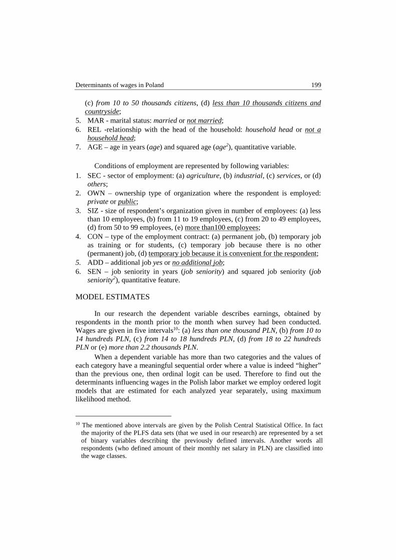
Determinants of wages in Poland 199
(c) from 10 to 50 thousands citizens, (d) less than 10 thousands citizens and countryside;
5. MAR - marital status: married or not married; 6. REL -relationship with the head of the household: household head or not a
household head; 7. AGE – age in years (age) and squared age (age2), quantitative variable.
Conditions of employment are represented by following variables:
1. SEC - sector of employment: (a) agriculture, (b) industrial, (c) services, or (d) others;
2. OWN – ownership type of organization where the respondent is employed: private or public;
3. SIZ - size of respondent’s organization given in number of employees: (a) less than 10 employees, (b) from 11 to 19 employees, (c) from 20 to 49 employees, (d) from 50 to 99 employees, (e) more than100 employees;
4. CON – type of the employment contract: (a) permanent job, (b) temporary job as training or for students, (c) temporary job because there is no other (permanent) job, (d) temporary job because it is convenient for the respondent;
5. ADD – additional job yes or no additional job; 6. SEN – job seniority in years (job seniority) and squared job seniority (job
seniority2), quantitative feature.
MODEL ESTIMATES
In our research the dependent variable describes earnings, obtained by respondents in the month prior to the month when survey had been conducted. Wages are given in five intervals10: (a) less than one thousand PLN, (b) from 10 to 14 hundreds PLN, (c) from 14 to 18 hundreds PLN, (d) from 18 to 22 hundreds PLN or (e) more than 2.2 thousands PLN.
When a dependent variable has more than two categories and the values of each category have a meaningful sequential order where a value is indeed “higher” than the previous one, then ordinal logit can be used. Therefore to find out the determinants influencing wages in the Polish labor market we employ ordered logit models that are estimated for each analyzed year separately, using maximum likelihood method.
10 The mentioned above intervals are given by the Polish Central Statistical Office. In fact
the majority of the PLFS data sets (that we used in our research) are represented by a set of binary variables describing the previously defined intervals. Another words all respondents (who defined amount of their monthly net salary in PLN) are classified into the wage classes.
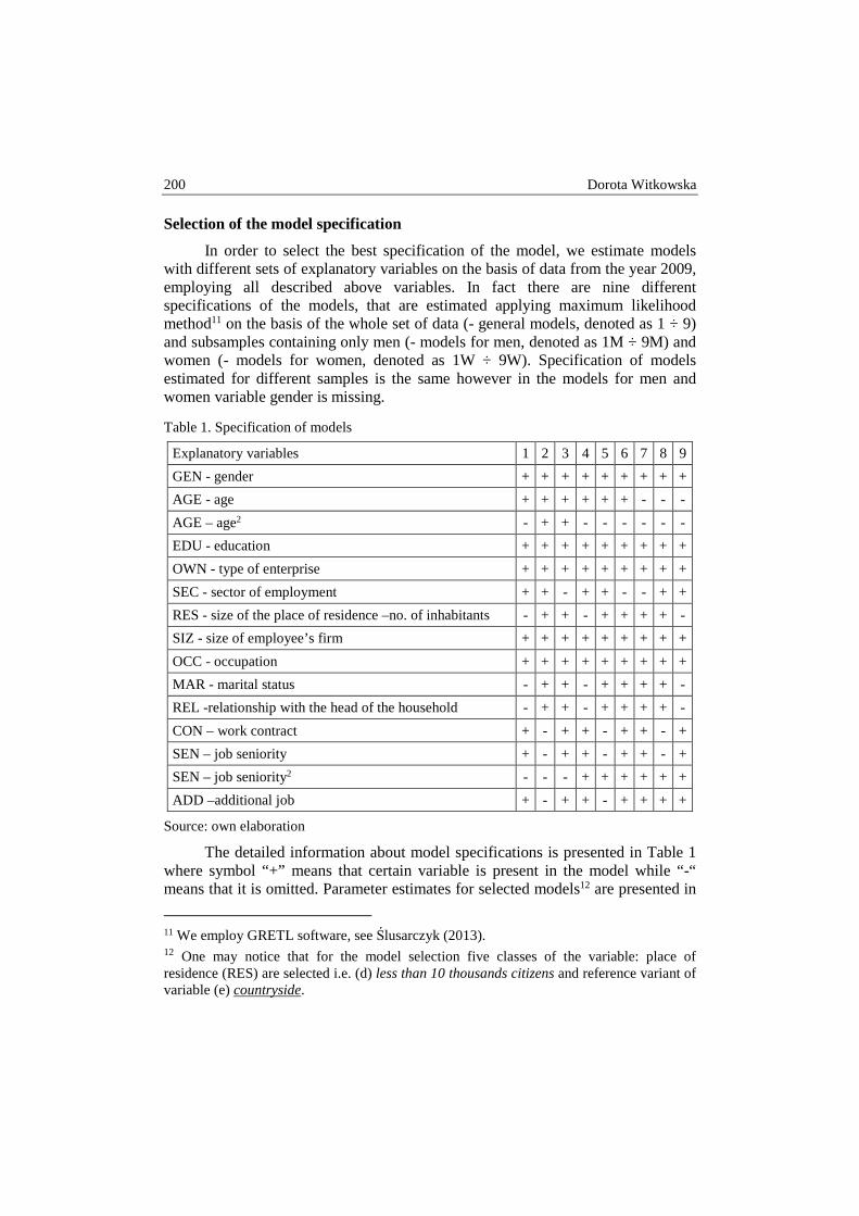
200 Dorota Witkowska
Selection of the model specification
In order to select the best specification of the model, we estimate models with different sets of explanatory variables on the basis of data from the year 2009, employing all described above variables. In fact there are nine different specifications of the models, that are estimated applying maximum likelihood method11 on the basis of the whole set of data (- general models, denoted as 1 ÷ 9) and subsamples containing only men (- models for men, denoted as 1M ÷ 9M) and women (- models for women, denoted as 1W ÷ 9W). Specification of models estimated for different samples is the same however in the models for men and women variable gender is missing.
Table 1. Specification of models
Explanatory variables 1 2 3 4 5 6 7 8 9
GEN - gender + + + + + + + + +
AGE - age + + + + + + - - -
AGE – age2 - + + - - - - - -
EDU - education + + + + + + + + +
OWN - type of enterprise + + + + + + + + +
SEC - sector of employment + + - + + - - + +
RES - size of the place of residence –no. of inhabitants - + + - + + + + -
SIZ - size of employee’s firm + + + + + + + + +
OCC - occupation + + + + + + + + +
MAR - marital status - + + - + + + + -
REL -relationship with the head of the household - + + - + + + + -
CON – work contract + - + + - + + - +
SEN – job seniority + - + + - + + - +
SEN – job seniority2 - - - + + + + + +
ADD –additional job + - + + - + + + +
Source: own elaboration
The detailed information about model specifications is presented in Table 1 where symbol “+” means that certain variable is present in the model while “-“ means that it is omitted. Parameter estimates for selected models12 are presented in
11 We employ GRETL software, see Ślusarczyk (2013). 12 One may notice that for the model selection five classes of the variable: place of residence (RES) are selected i.e. (d) less than 10 thousands citizens and reference variant of variable (e) countryside.

Determinants of wages in Poland 201
Tables 3 ÷ 6, the symbol × denotes lack of variables, stars – significance level: α=0.01 - *, α=0.05 - **, and α=0.001 - ***.
Table 2 contains major characteristics of the selected models (i.e. all models estimated for the whole sample and the best models estimated for subsamples of men and women) including mentioned above measures. As one can notice, regardless the set of explanatory variables models, estimated on the basis of the whole sample, do not essentially differ. However taking into consideration interpretation of the parameters (see Tables 3 ÷ 5) we select the model 3 to the further analysis. Since all models, except the one denoted as 3 has proper signs of the parameter standing by significant variables: age, age2, and job seniority. Also each group of explanatory variables is statistically significant in this model. Although the model denoted as 7 is quite similar in specification (in comparison to the model 3, variables age and age2 are missing but it contains the additional variable: job seniority2) but the model 7 has slightly worse statistical properties than the model 3.
Table 2. Models fitting parameters Model 1 2 3 4 5 6
Log likelihood -17071 -17119 -16816 -16965 -17226 -16808 Akaike criterion 34206 34306 33703 33997 34520 33688 Bayes-Schwarz criterion 34445 34560 33972 34243 34774 33957 Hannan-Quinn criterion 34286 34391 33793 34079 34605 33778 Number and fraction of correctly predicted outcomes
5316 (41.1)
5209 (40.3)
5360 (41.5)
5349 (41.40)
5209 (40.30)
5363 (41.50)
LR Chi2 9107 9012 9619 9319 8798 9634 Model 7 8 9 1W 2W 3W Log likelihood -16858 -17219 -16997 -7591 -7659 -7509 Akaike criterion 33786 34505 34059 15243 15384 15089 Bayes-Schwarz criterion 34047 34759 34298 15452 15606 15324 Hannan-Quinn criterion 33873 34590 34139 15315 15461 15170 Number and fraction of correctly predicted outcomes
5334 (41.30)
5191 (40.20)
5304 (41.10)
2699 (43.9)
2645 (43.1)
2736 (44.5)
LR Chi2 9534 8813 9255 4711 4574 4873 Model 4W 5W 6W 1M 2M 3M Log likelihood -7565 -7702 -7511 -9418 -9325 -9179 Akaike criterion 15194 15470 15091 18897 18716 18427 Bayes-Schwarz criterion 15409 15692 15327 19102 18941 18666 Hannan-Quinn criterion 15269 15547 15173 18968 18794 18510 Number and fraction of correctly predicted outcomes
2686 (43.7)
2629 (42.80)
2715 (44.20)
2614 (38.6)
2636 (38.9)
2717 (40.1)
LR Chi2 4762 4488 4871 3860 4047 4340
Source: own elaboration

202 Dorota Witkowska
One may also notice in Table 2 that models estimated for women are characterized by the best properties among all constructed models while the ones estimated for men seem to be the least satisfactory. It is also visible that models denoted as 3M and 3W fit the data in the best way, that additionally justifies selection of the model specification denoted as 3 for the further analysis.
Table 3. Parameter estimates of the models estimated for the whole sample: models 1÷3 Explanatory variables Model 1 Model 2 Model 3
GEN woman -1.2188 *** -1.2127 *** -1.1665 ***
AGE age -0.0280 *** 0.1749 *** 0.0964 ***
age2 -0.0021 *** -0.0017 ***
EDU university 1.6263 *** 1.6132 *** 1.5727 ***
post secondary or vocational 0.7983 *** 0.9034 *** 0.7788 ***
general secondary 0.7225 *** 0.8625 *** 0.7442 ***
lower vocational 0.4187 *** 0.4425 *** 0.2985 ***
OWN private 0.1848 *** 0.0527 0.1823 ***
SEC agriculture -0.7304 -0.4116
industry -0.4738 -0.2500
services -0.5260 -0.3471
RES >100*103 *** 0.4085 *** 0.4241 ***
50-100*103 -0.0128 0.0065
10-50*103 -0.0347 -0.0341
town <10*103 -0.1660 ** -0.1519 **
SIZ <10 -1.1145 *** -1.0502 *** -1.0368 ***
11-19 -0.7460 *** -0.6873 *** -0.6739 ***
20-49 -0.6304 *** -0.5815 *** -0.5672 ***
50-99 -0.5289 *** -0.4774 *** -0.4806 ***
OCC army 3.6142 *** 3.4144 *** 3.3980 ***
managerial 2.9992 *** 3.0579 *** 2.9084 ***
professional 2.1097 *** 2.1392 *** 2.0109 ***
technical 1.7891 *** 1.8692 *** 1.7079 ***
clerical 1.0364 *** 1.1275 *** 1.0025 ***
sales & services 0.5268 *** 0.5951 *** 0.4761 ***
farmers. fishers. etc. 0.3291 0.3753 0.2337
industry workers 0.9448 *** 1.0394 *** 0.9672 ***
skilled workers 1.1005 *** 1.1888 *** 1.0929 ***
MAR married 0.3157 *** 0.2669 ***
REL household head 0.4250 *** 0.4090 ***
CON permanent 0.9549 *** 0.7985 ***
temporary-study -0.5558 *** -0.4875 ***
temporary-no other job 0.1114 0.0479
SEN job seniority 0.0389 *** 0.0412 ***
ADD additional job -0.2449 *** -0.2831 ***
Source: own elaboration

Determinants of wages in Poland 203
Table 4. Parameter estimates of the models estimated for the whole sample: models 4÷6 Explanatory variables Model 4 Model 5 Model 6
GEN woman -1.2865 *** -1.1109 *** -1.1591 ***
AGE age -0.0344 *** 0.0004 -0.0435 ***
EDU university 1.6813 *** 1.6367 *** 1.6132 ***
post secondary or vocational 0.7971 *** 0.9443 *** 0.7940 ***
general secondary 0.7647 *** 0.8327 *** 0.7378 ***
lower vocational 0.3532 *** 0.5405 *** 0.3219 ***
OWN private 0.2039 *** 0.0315 0.1833 ***
SEC agriculture -0.6375 -0.4027
industry -0.3834 -0.2615
services -0.4387 -0.3562
RES >100*103 0.3791 *** 0.4227 ***
50-100*103 -0.0141 0.0189
10-50*103 -0.0401 -0.0300
town <10*103 -0.1758 *** -0.1505 **
SIZ <10 -1.0915 *** -1.0836 *** -1.0485 ***
11-19 -0.7360 *** -0.7105 *** -0.6843 ***
20-49 -0.6272 *** -0.5972 *** -0.5776 ***
50-99 -0.5297 *** -0.4906 *** -0.4934 ***
OCC army 3.5071 *** 3.4203 *** 3.3588 ***
managerial 2.9772 *** 3.0618 *** 2.9045 ***
professional 2.1063 *** 2.1459 *** 2.0142 ***
technical 1.8031 *** 1.8684 *** 1.7240 ***
clerical 1.0769 *** 1.0918 *** 1.0175 ***
sales & services 0.5500 *** 0.5671 *** 0.4829 ***
farmers. fishers. etc. 0.3012 0.3649 0.2075
industry workers 0.9377 *** 1.0425 *** 0.9725 ***
skilled workers 1.1048 *** 1.1856 *** 1.1045 ***
MAR married 0.4954 *** 0.2912 ***
REL household head 0.4880 *** 0.4184 ***
CON permanent 0.8104 *** 0.8294 ***
temporary-study -0.4935 *** -0.4560 ***
temporary-no other job 0.0608 0.0837
SEN job seniority 0.1209 *** 0.1077 ***
job seniority2 -0.0019 *** 0.0000 -0.0017 ***
ADD additional job -0.2944 *** -0.2802 ***
Source: own elaboration
Analyzing parameter estimates of the models 3M and 3W (Table 6), one can see that the determinants affecting wages obtained by men and women are slightly different. Lover vocational education and work for military service increase odds of higher wages in comparison to the reference variant of variables only for men. While work in the private (versus public) sector rises the log odds of increasing
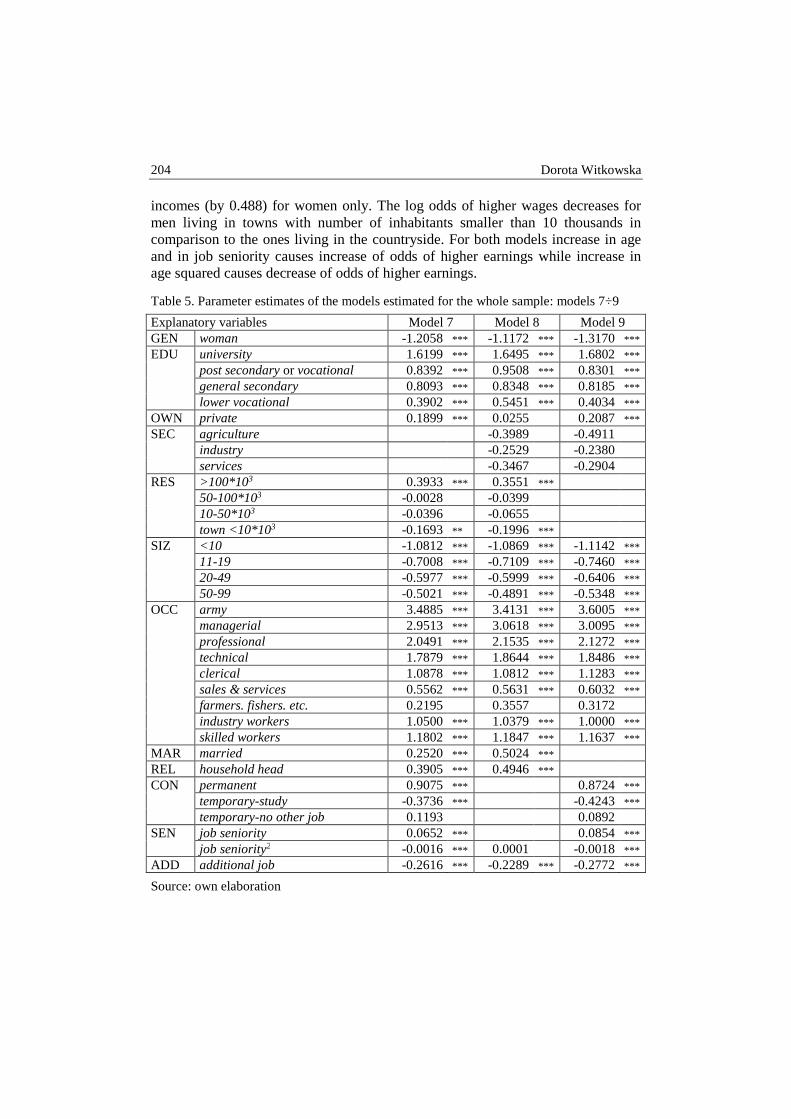
204 Dorota Witkowska
incomes (by 0.488) for women only. The log odds of higher wages decreases for men living in towns with number of inhabitants smaller than 10 thousands in comparison to the ones living in the countryside. For both models increase in age and in job seniority causes increase of odds of higher earnings while increase in age squared causes decrease of odds of higher earnings.
Table 5. Parameter estimates of the models estimated for the whole sample: models 7÷9 Explanatory variables Model 7 Model 8 Model 9 GEN woman -1.2058 *** -1.1172 *** -1.3170 ***
EDU university 1.6199 *** 1.6495 *** 1.6802 ***
post secondary or vocational 0.8392 *** 0.9508 *** 0.8301 ***
general secondary 0.8093 *** 0.8348 *** 0.8185 ***
lower vocational 0.3902 *** 0.5451 *** 0.4034 ***
OWN private 0.1899 *** 0.0255 0.2087 ***
SEC agriculture -0.3989 -0.4911
industry -0.2529 -0.2380
services -0.3467 -0.2904
RES >100*103 0.3933 *** 0.3551 ***
50-100*103 -0.0028 -0.0399
10-50*103 -0.0396 -0.0655
town <10*103 -0.1693 ** -0.1996 ***
SIZ <10 -1.0812 *** -1.0869 *** -1.1142 ***
11-19 -0.7008 *** -0.7109 *** -0.7460 ***
20-49 -0.5977 *** -0.5999 *** -0.6406 ***
50-99 -0.5021 *** -0.4891 *** -0.5348 ***
OCC army 3.4885 *** 3.4131 *** 3.6005 ***
managerial 2.9513 *** 3.0618 *** 3.0095 ***
professional 2.0491 *** 2.1535 *** 2.1272 ***
technical 1.7879 *** 1.8644 *** 1.8486 ***
clerical 1.0878 *** 1.0812 *** 1.1283 ***
sales & services 0.5562 *** 0.5631 *** 0.6032 ***
farmers. fishers. etc. 0.2195 0.3557 0.3172
industry workers 1.0500 *** 1.0379 *** 1.0000 ***
skilled workers 1.1802 *** 1.1847 *** 1.1637 ***
MAR married 0.2520 *** 0.5024 ***
REL household head 0.3905 *** 0.4946 ***
CON permanent 0.9075 *** 0.8724 ***
temporary-study -0.3736 *** -0.4243 ***
temporary-no other job 0.1193 0.0892
SEN job seniority 0.0652 *** 0.0854 ***
job seniority2 -0.0016 *** 0.0001 -0.0018 ***
ADD additional job -0.2616 *** -0.2289 *** -0.2772 ***
Source: own elaboration
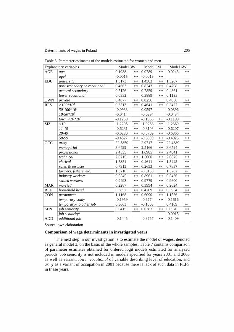
Determinants of wages in Poland 205
Table 6. Parameter estimates of the models estimated for women and men Explanatory variables Model 3W Model 3M Model 6W
AGE age 0.1038 *** 0.0789 *** -0.0243 ***
age2 -0.0015 *** -0.0016 ***
EDU university 1.5173 *** 1.4503 *** 1.5207 ***
post secondary or vocational 0.4663 *** 0.8743 *** 0.4708 ***
general secondary 0.5126 *** 0.7859 *** 0.4861 ***
lower vocational 0.0952 0.3889 *** 0.1135
OWN private 0.4877 *** 0.0256 0.4856 ***
RES >100*103 0.3513 *** 0.4641 *** 0.3427 ***
50-100*103 -0.0933 0.0597 -0.0896
10-50*103 -0.0414 -0.0294 -0.0434
town <10*103 -0.1259 -0.1968 ** -0.1199
SIZ <10 -1.2295 *** -1.0268 *** -1.2360 ***
11-19 -0.6231 *** -0.8103 *** -0.6207 ***
20-49 -0.6286 *** -0.5709 *** -0.6366 ***
50-99 -0.4827 *** -0.5090 *** -0.4925 ***
OCC army 22.5850 2.9717 *** 22.4389
managerial 3.6499 *** 2.5166 *** 3.6594 ***
professional 2.4535 *** 1.6985 *** 2.4641 ***
technical 2.0715 *** 1.5000 *** 2.0875 ***
clerical 1.5351 *** 0.4611 *** 1.5445 ***
sales & services 0.7913 *** 0.2653 ** 0.7837 ***
farmers. fishers. etc. 1.3716 ** -0.0150 1.3282 **
industry workers 0.5545 *** 0.8961 *** 0.5436 ***
skilled workers 0.9493 *** 0.9779 *** 0.9600 ***
MAR married 0.2287 *** 0.3994 *** 0.2624 ***
REL household head 0.3857 *** 0.4209 *** 0.3954 ***
CON permanent 1.1168 *** 0.6090 *** 1.1536 ***
temporary-study -0.1959 -0.6774 *** -0.1616
temporary-no other job 0.3663 ** -0.1063 0.4109 **
SEN job seniority 0.0415 *** 0.0387 *** 0.0970 ***
job seniority2 -0.0015 ***
ADD additional job -0.1445 -0.3757 *** -0.1409
Source: own elaboration
Comparison of wage determinants in investigated years
The next step in our investigation is to estimate the model of wages, denoted as general model 3, on the basis of the whole samples. Table 7 contains comparison of parameter estimates obtained for ordered logit models estimated for analyzed periods. Job seniority is not included in models specified for years 2001 and 2003 as well as variant: lower vocational of variable describing level of education, and army as a variant of occupation in 2001 because there is lack of such data in PLFS in these years.
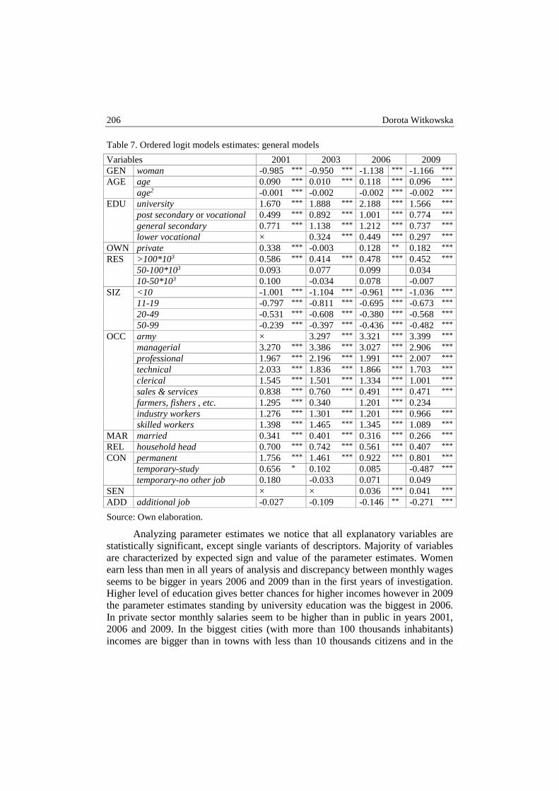
206 Dorota Witkowska
Table 7. Ordered logit models estimates: general models
Variables 2001 2003 2006 2009 GEN woman -0.985 *** -0.950 *** -1.138 *** -1.166 ***
AGE age 0.090 *** 0.010 *** 0.118 *** 0.096 ***
age2 -0.001 *** -0.002 -0.002 *** -0.002 ***
EDU university 1.670 *** 1.888 *** 2.188 *** 1.566 ***
post secondary or vocational 0.499 *** 0.892 *** 1.001 *** 0.774 ***
general secondary 0.771 *** 1.138 *** 1.212 *** 0.737 ***
lower vocational × 0.324 *** 0.449 *** 0.297 ***
OWN private 0.338 *** -0.003 0.128 ** 0.182 ***
RES >100*103 0.586 *** 0.414 *** 0.478 *** 0.452 ***
50-100*103 0.093 0.077 0.099 0.034
10-50*103 0.100 -0.034 0.078 -0.007
SIZ <10 -1.001 *** -1.104 *** -0.961 *** -1.036 ***
11-19 -0.797 *** -0.811 *** -0.695 *** -0.673 ***
20-49 -0.531 *** -0.608 *** -0.380 *** -0.568 ***
50-99 -0.239 *** -0.397 *** -0.436 *** -0.482 ***
OCC army × 3.297 *** 3.321 *** 3.399 ***
managerial 3.270 *** 3.386 *** 3.027 *** 2.906 ***
professional 1.967 *** 2.196 *** 1.991 *** 2.007 ***
technical 2.033 *** 1.836 *** 1.866 *** 1.703 ***
clerical 1.545 *** 1.501 *** 1.334 *** 1.001 ***
sales & services 0.838 *** 0.760 *** 0.491 *** 0.471 ***
farmers, fishers , etc. 1.295 *** 0.340 1.201 *** 0.234
industry workers 1.276 *** 1.301 *** 1.201 *** 0.966 ***
skilled workers 1.398 *** 1.465 *** 1.345 *** 1.089 ***
MAR married 0.341 *** 0.401 *** 0.316 *** 0.266 ***
REL household head 0.700 *** 0.742 *** 0.561 *** 0.407 ***
CON permanent 1.756 *** 1.461 *** 0.922 *** 0.801 ***
temporary-study 0.656 * 0.102 0.085 -0.487 ***
temporary-no other job 0.180 -0.033 0.071 0.049
SEN ×
× 0.036 *** 0.041 ***
ADD additional job -0.027 -0.109 -0.146 ** -0.271 ***
Source: Own elaboration.
Analyzing parameter estimates we notice that all explanatory variables are statistically significant, except single variants of descriptors. Majority of variables are characterized by expected sign and value of the parameter estimates. Women earn less than men in all years of analysis and discrepancy between monthly wages seems to be bigger in years 2006 and 2009 than in the first years of investigation. Higher level of education gives better chances for higher incomes however in 2009 the parameter estimates standing by university education was the biggest in 2006. In private sector monthly salaries seem to be higher than in public in years 2001, 2006 and 2009. In the biggest cities (with more than 100 thousands inhabitants) incomes are bigger than in towns with less than 10 thousands citizens and in the
Determinants of wages in Poland 207
countryside, and it is the only statistically significant variant of the variable: place of residence.
Bigger enterprises offer higher wages since parameters of all variants, describing size of the enterprise, are significantly smaller than zero. Occupation, except the variant describing farmers and fishers in 2003 and 2009, also affects significantly earnings as well as type of employment contract, fact of being married and the household head. Parameters standing by age and squared age are significant with expected signs. Job seniority influence positively earnings in years 2006 and 2009 while it is difficult to interpret negative signs of the variable describing additional job.
CONCLUSIONS
In our research we analyze situation on the Polish labor market in years 2001, 2003, 2006 and 2009 based on LFS data, applying ordered logit model. The main determinants of wages are: gender, age or job seniority, level of education, size of firm and occupation in all analyzed years. However the influence of these factors in following periods may be different. The investigation shows that women’s monthly incomes are significantly lower than men’s one and the discrepancy seems to be the biggest in the last year of analysis however it may be caused by different factors.
REFERENCES
Abowd J.M., Ashenfelter O. (1981) Anticipated unemployment, temporary layoffs and compensating wage differentials, in: Rosen S. (ed.) Studies in labor markets. Chicago: University of Chicago Press.
Atchison T.J., Belcher D.W., Thomsen D.J. (2013) The wage level and its determinants, ERI Economic Research Institute, Library of Congress Cataloging-in-Publication Data, http://dlc.erieri.com/onlinetextbook/chpt07/text_main.htm.
Becker G.S. (1964) Human capital: a theoretical analysis with special reference to education, New York: Columbia University Press for NBER.
Boes S., Winkelmann R. (2009) Analysis of microdata, Springer, Berlin, Heidelberg. Borooah V.K. (2002) Logit and probit: ordered and multinomial models, Thousand Oaks,
CA, Sage Publications. Brzeziński M., Jancewicz B., Letki N. (2012) Country Report: Poland, Prepared for GINI:
Growing Inequalities’ Impacts Project, retrieved 14/09/2013 on http://coin.wne.uw. edu.pl/mbrzezinski/research/GINI_REPORT_POLAND_September_2012.pdf.
Cain G.G. (1986) The Economic Analysis of labor Market Discrimination: A Survey, in: Ashenfeler O., Layard R. (ed.), Handbook of Labour Economics, Vol. I, Elsevier Science Publishers BV, 693 – 785.
Commander S., Dhar S. (1998) Enterprises in the Polish Transition, in: Commander, S. (ed.) Enterprise Restructuring and Unemployment in Models of Transition, Washington, DC: The World Bank.
208 Dorota Witkowska
Cramer J.S. (2001) An Introduction to the Logit Model for Economists, Timberlake Con-sultants Ltd., London.
Cramer J. S. (2011) Logit Models from Economics and Other Fields, Cambridge University Press.
Gruszczyński M. (2002) Mikroekonometria. Modele i prognozy zmiennych jakościowych w finansach i bankowości, Oficyna Wydawnicza SGH, Warszawa.
Gruszczyński M. (ed.) (2010) Mikroekonometria. Modele i metody analizy danych indywidualnych, Wolters Kluwer Polska, Warszawa.
Keane M.P. and Prasad E. (2006) Changes in the Structure of Earnings During the Polish Transition, Journal of Development Economics, Vol. 80, 389- 427.
Kot S.M. (ed.) (1999) Analiza ekonometryczna kształtowania się płac w Polsce w okresie transformacji, Warszawa, Kraków, PWN.
Marcinkowska I., Ruzik A., Strawiński P., Walewski M. (2008) Badanie struktury i zmian rozkładu wynagrodzeń w Polsce w latach 2000 – 2006, Departament Analiz Ekonomicznych i Prognoz, Ministerstwo Pracy i Polityki Społecznej, Warszawa, retrieved 14/09/2013 on http://www.mpips.gov.pl/userfiles/File/Analizy/Raport%20ba danie %20struktury.pdf.
Mincer J. (1974) Schooling, Experience and Earnings, National Bureau of Economic Research, New York.
Newell A., Socha M.W. (2005) The Distribution of Wages in Poland, 1992-2002, IZA Discussion Paper 1485.
Newell A., Socha M.W. (2007) The Polish Wage Inequality Explosion, IZA Discussion Paper No. 2644.
Pinto B., Belka M., Krajewski S. (1993) Transforming State Enterprises in Poland: Evidence on Adjustment by Manufacturing Firms, Brookings Papers on Economic Activity, 213-70.
Riley G. (2012) Determination of wages in the labour market, retrieved 14/12/2013 on http://tutor2u.net/economics/revision-notes/a2-micro-wage-determination-competitive-markets.html.
Ślusarczyk K. (2013) Analiza ekonometryczna kształtowania się płac w Polsce w latach 2001 – 2009, Master Thesis prepared under supervision of D. Witkowska, SGGW, Warszawa.
Thaler R., Rosen S. (1975) The value of saving a life: evidence from the labor market, [in:] Terleckyj N. (ed.) Household production and consumption, New York: National Bureau of Economic Research.
Willis R. J. (1986) Wage Determinants: A Survey And Reinterpretation of Human Capital Earnings Functions (Chapter 10) in Handbook of Labor Economics, Volume L Edited by O. Ashenfelter and R. Layard ©Elsevier Science Publishers BV, 1986.
Witkowska D. (2012) Wage Disparities in Poland: Econometric Models of Wages, Metody Ilościowe w Badaniach Ekonomicznych, Vol. XIII, No. 2, SGGW, Warszawa, 115-124.
QUANTITATIVE METHODS IN ECONOMICS Vol. XV, No. 1, 2014, pp. 209 – 217
PORTFOLIO PERFORMANCE MEASUREMENT BASED ON THE MULTIHORIZON SHARPE RATIO
- WAVELET ANALYSIS APPROACH
Anna Zamojska Department of Econometrics, University of Gdańsk
e-mail: [email protected]
Abstract: The aim of the study is to evaluate and compare the performance of mutual funds. The proposed approach evaluates the effectiveness of the fund's investment strategy in terms of the investment horizon. As a tool wavelet analysis that has been applied to the decomposition of the excess returns of funds for the six scales was used. The Sharpe ratios calculated on the basis of the so-transformed series formed the basis for the arrangement of funds. The results indicate that the variance of rate of return in the analyzed funds decline as the wavelet scale increases.
Keywords: wavelet analysis, multihorizon Sharpe ratio, investment horizon
INTRODUCTION
The Sharpe ratio is one of the oldest and the most popular measures of the performance of assets allocation portfolios. This ratio is sensitive to the selected sample. A common approach in portfolio evaluation is the calculation of the one-period investment Sharpe ratio [Levy 1972]. It is suggested in the literature that for n-period investment the scaling factor should be taken into account. In empirical analysis researchers and experts usually calculate only the one-period Sharpe ratio [Kim, In 2005]. The portfolio managers make decisions over different time periods, and they especially concentrate on the performance at the end of the clearing period. So the problem is how to create the performance measure resistant to above restrictions. The main purpose of this paper is to investigate the usefulness of wavelet analysis for evaluating the performance of mutual funds.
The starting point in applied methodology is the Sharpe ratio, defined as the level of the expected excess of return of portfolio per unit of risk associated with the portfolio. Then wavelet analysis is suggested, in terms of wavelet and

210 Anna Zamojska
scaling filters. Such an approach allows for decomposing the unconditional variance into different time scales, which means different sample windows. The advantage of the approach is that it enables the analysis of the non-normally distributed portfolio returns [Bruzda 2003]. The results of the empirical analysis of mutual fund portfolios, operating in the financial market in Poland, support the fact that the application of the wavelet analysis in multihorizon evaluation of performance enables providing more useful information about behaviour of portfolios.
PORTFOLIO MANAGEMENT AND INVESTMENT HORIZON
Asset allocation is a process that identifies the optimal portfolio for a particular investor over a given investment horizon. An investment horizon depends on when and how much profit the investor expects in the future. This assumption implies that the duration of the investment horizon influences the optimal investment strategy. Investment horizon identifies the total duration that an investor/portfolio manager expects to hold the portfolio. The investment horizon is used to determine the investor's income needs and desired risk exposure. In general, the shorter the investor’s horizon, the lower the acceptance for a given profit. According to the above, in portfolio performance evaluation process the investment horizon should be taken into account.
Table 1. The ranks of mutual funds of Legg Mason and WIG according to the Sharpe ratio
Duration (year) Fund type
WIG MIXED STOCK BOND MONEY
1 3 2 4 5 1
2 4 2 3 5 1
3 4 2 3 5 1
4 4 1 3 5 2
5 4 1 3 5 2
6 3 1 4 5 2
7 4 1 3 5 2
8 3 1 4 5 2
9 4 1 3 5 2
10 4 1 3 5 2
Source: Author’s calculation
There are many portfolio performance ratios in use [Cogneau, Hubner 2009a, 2009b]. Their disadvantage is that they refer to only one period of time. It is obvious that they change and consequently the rank of portfolio changes as well. Table 1 presents the ranks of market index and four mutual funds with different
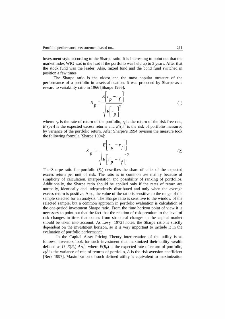
Portfolio performance measurement based on… 211
investment style according to the Sharpe ratio. It is interesting to point out that the market index WIG was in the lead if the portfolio was held up to 3 years. After that the stock fund was the leader. Also, mixed fund and the bond fund switched in position a few times.
The Sharpe ratio is the oldest and the most popular measure of the performance of a portfolio in assets allocation. It was proposed by Sharpe as a reward to variability ratio in 1966 [Sharpe 1966]:
2
−
=
prE
fr
prE
pS (1)
where: rp is the rate of return of the portfolio, rf is the return of the risk-free rate, E[rp-rf] is the expected excess returns and E[rp]2 is the risk of portfolio measured by variance of the portfolio return. After Sharpe’s 1994 revision the measure took the following formula [Sharpe 1994]:
2
−
−
=
fr
prE
fr
prE
pS (2)
The Sharpe ratio for portfolio (Sp) describes the share of units of the expected excess return per unit of risk. The ratio is in common use mainly because of simplicity of calculation, interpretation and possibility of ranking of portfolios. Additionally, the Sharpe ratio should be applied only if the rates of return are normally, identically and independently distributed and only when the average excess return is positive. Also, the value of the ratio is sensitive to the range of the sample selected for an analysis. The Sharpe ratio is sensitive to the window of the selected sample, but a common approach in portfolio evaluation is calculation of the one-period investment Sharpe ratio. From the time horizon point of view it is necessary to point out that the fact that the relation of risk premium to the level of risk changes in time that comes from structural changes in the capital market should be taken into account. As Levy [1972] notes, the Sharpe ratio is strictly dependent on the investment horizon, so it is very important to include it in the evaluation of portfolio performance.
In the Capital Asset Pricing Theory interpretation of the utility is as follows: investors look for such investment that maximized their utility wealth defined as U=E(Rp)-Aσp
2, where E(Rp) is the expected rate of return of portfolio, σp
2 is the variance of rate of returns of portfolio, A is the risk-aversion coefficient [Berk 1997]. Maximization of such defined utility is equivalent to maximization

212 Anna Zamojska
the Sharpe ratio given by Sp=E(Rp-Rf)/σp. In the formula an ex ante approach appears. An ex post version is possible as the historical average rate of return and it’s standard deviation is applied.
If rates of return of portfolios have finite expected rate of return and variance and the assumption of normality of distribution of returns is fulfilled, then the Sharpe ratio estimator is a function of expected return and the variance of returns of portfolios [Lo 2002]. The asymptotic distribution of the Sharpe ratio is as follows:
( ) ( )iid
a
pp VNSST ,0~ˆ − (3)
The asymptotic variance V is weighted average of the asymptotic variances of expected values and variances:
42
22
2
2σσ
σµ
∂∂+
∂∂= gg
Viid
(4)
Where g is the function of the Sharpe ratio defined as g(µ,σ2). The asymptotic variance of the Sharpe ratio can be calculated as follows [Lo, 2002]:
2
21
1 piid SV += (5)
And the standard error of the Sharpe ratio estimator [Lo, 2002]:
( ) TSSSE pp /
21
1 2
+= (6)
In the formula (6) the number of periods is included. It is suggested in the literature that for T-period investment scaling factor
should be taken into account, but in empirical analysis researchers and experts usually calculate only one-period Sharpe ratio [Kim, In 2005]. The portfolio managers make decisions over different time periods and they especially focus on the performance at the end of the clearing period. So the problem is how to create the performance measure resistant to the above restrictions. Kim and In proposed the wavelet analysis as a tool for measurement of portfolio performance. That approach allows for decomposition of the unconditional variance into a different time scale, which means different sample windows. The advantage of the approach is the possibility of analysis of the non-normally distributed portfolio returns and non-stationary series.
WAVELET ANALYSIS
Wavelet analysis is a natural tool available to investigate the disaggregation of performance into various time scales, as it enables decomposing of the data on a
Portfolio performance measurement based on… 213
scale-by-scale basis. Wavelet analysis is an approach used to evaluating the portfolio performance which enables analysis the multihorizon Sharpe ratio. The great advantage of this approach is a possibility to decompose data into several time scales so we can observe which investment horizons are important contributors to time series variance. We can also construct the local average of the portfolio returns over each scale. These properties provide an effective way of constructing the multihorizon Sharpe ratio. Wavelet analysis is a kind of frequency analysis, in which the process is represented in both: the time and the frequency domain. This analysis is a technique of windows, the size of which can increase or decrease depending on the fluctuation (long-or short-term analysis) [Bruzda 2003]. Due to its local nature the wavelet analysis is appropriate for testing non-stationary processes. Wavelet analysis, also known as a filtering technique, provides a tool that allows taking the dynamic of economic/financial time series into account [Gencay et al. 2002].
The purpose of the wavelet analysis is to decompose process into components, which are shifted and scaled versions of the basic function (called the mother wavelet). Wavelet analysis has a time-scale nature, which means that there is correspondence between the small scale and high frequency as well as large scale and low frequency [Bruzda 2003]. The Haar wavelet is the simplest dyadic wavelet. The Haar wavelet can be used to decompose a time series into two components: a high-frequency oscillations represent deviations from the time trend and the coefficients of the smoothed time trend. The decomposition is performed by using two filters called (quadrature) mirror filters [Bruzda 2003]: a low-pass filter (coarse representation), high-pass filter (detailed representation).
The wavelet transformation is able to capture all the information in a time series and associate it with a specific time horizon and locations in time [Gencay et al. 2002]. Kim and In [2005] proposed to use the wavelet analysis as a portfolio performance measure. This approach allows for decomposition of the unconditional variance of excess returns on various scales. The Sharpe ratio for different scales reflects the assessment of the effectiveness of portfolio management for different horizons. An additional advantage of using wavelet analysis is that is not necessary to fulfil the assumptions of normality and stationarity of returns.
Multihorizon Sharpe ratio is created in the same way as its standard version (1). The main difference is the application of the wavelet variance (σp
2(k)) and the local average of the excess rate of return (Ȓp(k)) for the scale k:
( )
( )kp
kp
R
pWS
2σ= (7)
The application of the wavelet analysis is the evaluation of the results of portfolio management which assumes treating returns as signals. So it is possible to analyse
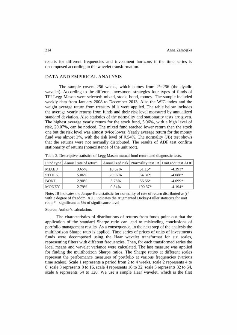
214 Anna Zamojska
results for different frequencies and investment horizons if the time series is decomposed according to the wavelet transformation.
DATA AND EMPIRICAL ANALYSIS
The sample covers 256 weeks, which comes from 28=256 (the dyadic wavelet). According to the different investment strategies four types of funds of TFI Legg Mason were selected: mixed, stock, bond, money. The sample included weekly data from January 2008 to December 2013. Also the WIG index and the weight average return from treasury bills were applied. The table below includes the average yearly returns from funds and their risk level measured by annualized standard deviation. Also statistics of the normality and stationarity tests are given. The highest average yearly return for the stock fund, 5.06%, with a high level of risk, 20.07%, can be noticed. The mixed fund reached lower return than the stock one but the risk level was almost twice lower. Yearly average return for the money fund was almost 3%, with the risk level of 0.54%. The normality (JB) test shows that the returns were not normally distributed. The results of ADF test confirm stationarity of returns (nonexistence of the unit root).
Table 2. Descriptive statistics of Legg Mason mutual fund return and diagnostic tests.
Fund type Annual rate of return Annualized risk Normality test JB Unit root test ADF
MIXED 3.65% 10.62% 51.15* -4.393*
STOCK 5.06% 20.07% 54.31* -4.088*
BOND 2.90% 3.75% 56.66* -4.099*
MONEY 2.79% 0.54% 190.37* -4.194*
Note: JB indicates the Jarque-Bera statistic for normality of rate of return distributed as χ2 with 2 degree of freedom; ADF indicates the Augmented Dickey-Fuller statistics for unit root; * - significant at 5% of significance level
Source: Author’s calculation.
The characteristics of distributions of returns from funds point out that the application of the standard Sharpe ratio can lead to misleading conclusions of portfolio management results. As a consequence, in the next step of the analysis the multihorizon Sharpe ratio is applied. Time series of prices of units of investments funds were decomposed using the Haar wavelet transformat for six scales, representing filters with different frequencies. Then, for each transformed series the local means and wavelet variance were calculated. The last measure was applied for finding the multihorizon Sharpe ratios. The Sharpe ratios at different scales represent the performance measures of portfolio at various frequencies (various time scales). Scale 1 represents a period from 2 to 4 weeks, scale 2 represents 4 to 8, scale 3 represents 8 to 16, scale 4 represents 16 to 32, scale 5 represents 32 to 64, scale 6 represents 64 to 128. We use a simple Haar wavelet, which is the first

Portfolio performance measurement based on… 215
Wavelet scale
1 2 3 4 5 6
MIXEDSTOCK
BONDMONEY
wavelet filter. Such simple wavelet allows for receiving two types of elements of the time series. The first one (dk, k=1,..,6), which captures the higher-frequency oscillations, represents increasingly fine scale deviations’ from the smooth trend, and the second (ak, k=1,..,6), represents the smooth coefficients that capture the trend.
We analyzed the variance of the mutual fund rates of return against various time scales. Figure 1 presents that the variance of all funds decline as the wavelet scale increases and all curves peak at scale 5. We can notice a big difference between curves at scale 1 and almost no difference at scales 5 and 6. It implies that investor with a short investment horizon reacts to every fluctuation in analysed rates of return, while the investor with a medium and long horizon would react much slower. In the long-run the investment risk is significantly lower. Figure 1 shows a pattern similar to that presented by Siegiel [2008] and Kim, In [2005]. They suggest that the standard deviation of average return falls with the square root of the length of the holding period, due to the random walk of the asset returns [Kim, In 2005].
Figure 1. Estimated Wavelet Variance
Source: Author’s calculation
Multihorizon Sharpe ratios, using treasury bills as a benchmark, are presented in table 3. The value of Sharpe ratio for each fund rises as the holding period lengthens. The Sharpe ratio for a mixed fund is -0.08 for the first wavelet scale which is a 2- to 4-week period and increases to 231.88 for the longest wavelet scale 64- to 128-week period. We can conclude that the Sharpe ratio is not time-
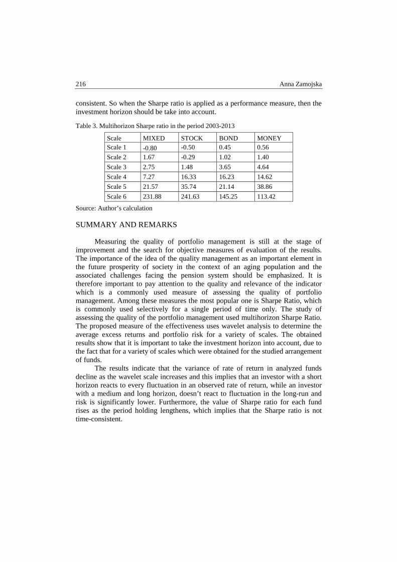
216 Anna Zamojska
consistent. So when the Sharpe ratio is applied as a performance measure, then the investment horizon should be take into account.
Table 3. Multihorizon Sharpe ratio in the period 2003-2013
Scale MIXED STOCK BOND MONEY Scale 1 -0.80 -0.50 0.45 0.56
Scale 2 1.67 -0.29 1.02 1.40
Scale 3 2.75 1.48 3.65 4.64
Scale 4 7.27 16.33 16.23 14.62
Scale 5 21.57 35.74 21.14 38.86
Scale 6 231.88 241.63 145.25 113.42
Source: Author’s calculation
SUMMARY AND REMARKS
Measuring the quality of portfolio management is still at the stage of improvement and the search for objective measures of evaluation of the results. The importance of the idea of the quality management as an important element in the future prosperity of society in the context of an aging population and the associated challenges facing the pension system should be emphasized. It is therefore important to pay attention to the quality and relevance of the indicator which is a commonly used measure of assessing the quality of portfolio management. Among these measures the most popular one is Sharpe Ratio, which is commonly used selectively for a single period of time only. The study of assessing the quality of the portfolio management used multihorizon Sharpe Ratio. The proposed measure of the effectiveness uses wavelet analysis to determine the average excess returns and portfolio risk for a variety of scales. The obtained results show that it is important to take the investment horizon into account, due to the fact that for a variety of scales which were obtained for the studied arrangement of funds.
The results indicate that the variance of rate of return in analyzed funds decline as the wavelet scale increases and this implies that an investor with a short horizon reacts to every fluctuation in an observed rate of return, while an investor with a medium and long horizon, doesn’t react to fluctuation in the long-run and risk is significantly lower. Furthermore, the value of Sharpe ratio for each fund rises as the period holding lengthens, which implies that the Sharpe ratio is not time-consistent.
Portfolio performance measurement based on… 217
REFERENCES
Berk J. (1997) Necessary Condition for CAPM, Journal of Economic Theory, Vol. 73(1), 245-257.
Bruzda J. (2013), Wavelet analysis in economic applications, Wydawnictwo Naukowe Uniwersytetu Ekonomicznego, Toruń.
Cogneau P., Hubner G. (2009a) The (More Than) 100 Ways to Measure Portfolio Performance. Part 1: Standardized Risk-Adjusted Measures, Journal of Performance Measurement, Vol. 13(4), 56-71.
Cogneau P., Hubner G. (2009b) The (More Than) 100 Ways to Measure Portfolio Performance: Part 2: Special Measures and Comparison, Journal of Performance Measurement, Vol. 14(1), 56-69.
Gencay R.F., Selcuk F., Whitcher B. (2002) An Introduction to Wavelets and Other Filtering Methods in Finance and Economics, Academic Press, San Diego.
Kim S., In F. (2005) Multihorizon Sharpe Ratios, Journal of Portfolio Management, Vol. 31(2), 105-111.
Levy H. (1972) Portfolio Performance and the Investment Horizon, Management Science, Vol. 18(12), 645-653.
Lo A.W. (2002) The Statistics of Sharpe Ratios, Financial Analysts Journal, Vol. 58(4), 36-52.
Sharpe W.F. (1966) Mutual Fund Performance, Journal of Business, Vol. 39(1), 119-138. Sharpe W.F. (1994) The Sharpe Ratio, Journal of Portfolio Management, Vol. 21(1), 49-58. Siegel J.J. (2008) Stock for the Long Term, McGraw-Hill, New York.

QUANTITATIVE METHODS IN ECONOMICS Vol. XV, No. 1, 2014, pp. 218 – 223
CONSTRUCTION AND PROPERTIES OF VOLATILITY INDEX FOR WARSAW STOCK EXCHANGE
Tomasz Karol Wiśniewski Warsaw Stock Exchange, Indices and Statistics Unit
e-mail: [email protected]
Abstract: Volatility indices became a important factors on capital markets and are considered as fear factors. First volatility index VIX, was defined for Chicago Board of Trade in 1993, and was developed in 2003. In next years we observed growing numbers of volatility indices on main capital market around of the world. There were more than 20 volatility indices on capital markets at the end of 2012. The aim of this study is construction of the volatility index considering to Warsaw Stock Exchange trading rules and market participants. We also test the “fear factor” properties of this index.
Keywords: option, capital market, stock market index, volatility index
INTRODUCTION
The first volatility index - VIX, introduced by the CBOE in 1993, was a weighted measure of the implied volatility of eight S&P 100 at-the-money put and call options and it was constructed according to proposal of Whaley1. Ten years later Goldman Sachs analyst proposed modification based methodology of VIX, and expanded to use options based on a broader index, the S&P 500, which allows for a more accurate view of investors' expectations on future market volatility2.
1 Whaley R. (1993) 2 Demeterfi K., Derman E., Kamal M., Zou J. (1999)

Construction and properties of volatility index … 219
VIX values greater than 30 are generally associated with a large amount of volatility as a result of investor fear or uncertainty, while values below 20 generally correspond to less stressful, even complacent, times in the markets.
OPTION MARKET ON WARSAW STOCK EXCHANGE
Options have been traded on Warsaw Stock Exchange since September 22, 2003. This day saw the first appearance of European style options on the WIG20 index. There are no price variation limits applied to trading in options. The WSE offers European style options, which means that they can be exercised only on the expiry date. As is the case with futures, trading in options is supported by market makers: under a contract signed with the WSE they are obliged to place their own sell/buy orders in the order book. The reference price for options is the theoretical price calculated according to the Black-Scholes model. Given the nature of the instrument, margins are required only from option writers (those opening short positions). Option buyers do not pay margins. Table 1 contains basic characteristics of option on WIG20 index.
Table 1. WIG20 options – key characteristics
Position Description Multiplier PLN 10 per index point Option value Product of option price and multiplier Quotation unit Index points Expiry months Four nearest months of the following cycle: March, June,
September, December Expiry date The third Friday of the expiry month for the series. If there
is no trading session on that date, the last trading session day preceding the third Friday of the expiry month is taken
Last trading day The same as expiry date Exercise price Equal to the value of the underlying instrument, with
respect to which the settlement balance will be determined taking the multiplier into account
Exercise value Product of exercise price and multiplier Settlement price Settlement price is determined on the expiry date as the
arithmetic mean of all WIG20 values during the last hour of continuous trading and the WIG20 value as determined at the session close, having rejected 5 top and 5 bottom index values
Settlement value Product of settlement price and multiplier Settlement date First business day following the date on which settlement
price is determined Settlement method Cash settlement in PLN
Source: Warsaw Stock Exchange Factbook, 2013

220 Tomasz Karol Wiśniewski
Due to Warsaw Stock Exchange rules, option are traded in continuous system. Each issue expiry in three months cycle on the third Friday of March, June, September and December. Price on settlement day is determined as the arithmetic mean of WIG20 index values from last hour of trading, the WIG20 values at the day closing, without 5 top and 5 bottom values of underlying index.
At the end of 2012 a total of 120 series of options were traded (all of them were WIG20 options). The trading volume for these instruments reached 715,400. The open interest at the end of 2012 amounted to 14,500. WIG20 options held the 13th position in 2012 in terms of trading volume among index options in Europe. Table 2 contain basic data of option on WIG20 for last 5 years.
Table 2. Option on WIG20 – key figures, annual data (2012 – 2008)
Position 2012 2011 2010 2009 2008 Total turnover value (PLN mill) 15 672 21 819 13 653 7 878 8 261 Average turnover value (per session, PLN mill) 62.94 86.93 53.97 31.27 32.92 Turnover value by premium (PLN mill) 179.47 276.72 158.31 192.09 231.59 Total volume of trades (thousand) 680 064 832 106 546 842 399 708 325 203 Average volume of transaction (per session) 2 731 3 315 2 161 1 586 1 296 Average number of trades (per session) 650 789 688 590 485 Open interest (year end) 14 462 17 517 43 583 20 850 6 925 Liquidity ratio (%) 10.49 11.37 8.98 6.34 6.60 Number of series (year end) 120 122 106 110 138
Source: Warsaw Stock Exchange Factbook, 2013
Option trading on Warsaw Stock Exchange is open for all type of investors: foreign (all type of investors registered outside of Poland), domestic institutional (brokerage houses, investment funds or banks) and domestic retail (all individuals investors, Polish citizens). Domestic retail investors play main role in trading of option on WIG20 index. In last 5 years domestic retail investors account for more than 50% of option trading: from 50% in 2012 to 65% in 2009. Table 3 contains investors structure in trading of option on WIG20 index.
Table 3. Investors structure in option trading on Warsaw Stock Exchange (in %)
Investors 2012 2011 2010 2009 2008 Foreign 11 24 12 4 12 Domestic institutional 39 12 28 31 30 Domestic retail 50 64 60 65 58
Source: Warsaw Stock Exchange Factbook, 2013
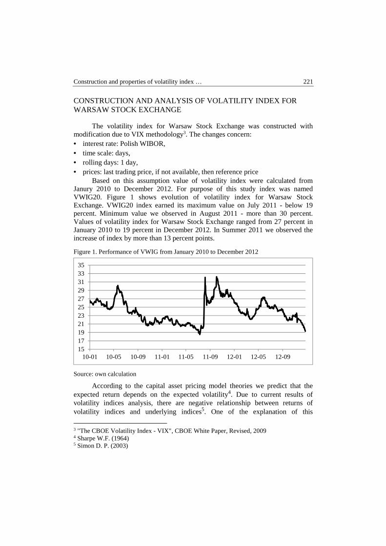
Construction and properties of volatility index … 221
CONSTRUCTION AND ANALYSIS OF VOLATILITY INDEX FOR WARSAW STOCK EXCHANGE
The volatility index for Warsaw Stock Exchange was constructed with modification due to VIX methodology3. The changes concern: • interest rate: Polish WIBOR, • time scale: days, • rolling days: 1 day, • prices: last trading price, if not available, then reference price
Based on this assumption value of volatility index were calculated from Janury 2010 to December 2012. For purpose of this study index was named VWIG20. Figure 1 shows evolution of volatility index for Warsaw Stock Exchange. VWIG20 index earned its maximum value on July 2011 - below 19 percent. Minimum value we observed in August 2011 - more than 30 percent. Values of volatility index for Warsaw Stock Exchange ranged from 27 percent in January 2010 to 19 percent in December 2012. In Summer 2011 we observed the increase of index by more than 13 percent points.
Figure 1. Performance of VWIG from January 2010 to December 2012
Source: own calculation
According to the capital asset pricing model theories we predict that the expected return depends on the expected volatility4. Due to current results of volatility indices analysis, there are negative relationship between returns of volatility indices and underlying indices5. One of the explanation of this
3 "The CBOE Volatility Index - VIX", CBOE White Paper, Revised, 2009 4 Sharpe W.F. (1964) 5 Simon D. P. (2003)
1517192123252729313335
10-01 10-05 10-09 11-01 11-05 11-09 12-01 12-05 12-09
222 Tomasz Karol Wiśniewski
relationship says that the demand for puts increase when the market declines. Increased demand means high put prices, and hence higher implied volatility. Furthermore, the relationship is asymmetric: an equal size positive/negative shock on implied volatility does not have the same effect on the index return. Hence, analyst are calling the volatility index as “fear gauge”; the further volatility index increase in value, the more panic there is in the market. Further decline of the volatility index value, implies more complacency in the market.
To verify properties of volatility index more precisely the relation between the returns of the WIG20 index and changes in the VWIG20, we use regression analysis. We regress the daily return of the WIG20 on the daily changes of the VWIG20 and the change of VWIG20, when the change is positive:
�� = ��∆��20� + ��∆��20��+ ��
where: Rt – daily returns of WIG20 index, ∆WIG20t – daily changes of VWIG20, ∆WIG20+
t – daily changes of VWIG20, if VWIG20>0 then ∆VWIG20, otherwise 0 The regression results are (t-values in brackets):
�� = −0.248∆��20� − 0.097∆��20���
�= 0.128
(-5.53) (-1.63)
All regression coefficients are significantly different from zero at a 1% significance level. The interpretation of the coefficients is the following: if VWIG20 falls by one percent, then the WIG20 return will increase 0.0028 index point. In other case, if VWIG rise by 1%, the WIG20 index return will decrease by 0.0034 index point. We can say, the cash market on Warsaw Stock Exchange is affected negatively more by an increase in VWIG20 than it is affected positively by an equal size decrease in VWIG20.
Additionally, we checked relationship in two different periods: bull market and bear market. Bull market we define as a period from February 8, 2010 to April 7, 2011, when the WIG20 index increase by 34%, but bear market is define from April 7, 2011 to May 23, 2012, when WIG20 index fall by 19%. The regression results for bull market are (t-values in brackets):
�� = −0.253∆��20� + 0.088∆��20���
�= 0.05
(-3.30) (0.79)
In case of bear market we found that (t-values in brackets):
�� = −20.071∆��20� − 0.187∆��20���
�= 0.185
(-2.72) (-2.07)

Construction and properties of volatility index … 223
We can see that the coefficient a2 in bull market model is statistically insignificant. In bear market model both coefficients are statistically significant, and R2 statistics is on higher level in compare to the first and the second models. This implies that bear market affect the risk – return relationship in the WIG20 options market.
CONCLUSIONS
We have constructed a volatility index - VWIG20 - for the Warsaw Stock Exchange using the WIG20 options. The construction methodology differs from the standard VIX methodology due to trading rules on Warsaw Stock Exchange and less liquidity than it is observed on developed market.
Next, the properties of VWIG20 have been studied. In line with other study, we found that the index can be used as a gauge of the investor’s fear. This measure is stable over time, but the signaling results are better in bear market period, than during bull market.
REFERENCES
The CBOE Volatility Index - VIX, CBOE White Paper, Revised, 2009 Demeterfi K., Derman E., Kamal M., Zou J. (1999) More Than You Ever Wanted To Know
About Volatility Swap, Quantitative Strategies Research Notes. Sharpe W.F. (1964) Capital Asset Prices: A Theory of Market Equilibrium Under
Conditions of Risk, Journal of Finance, 19, 425 – 442. Simon D.P. (2003) The NASDAQ volatility index During and After the Bubble, Journal of
Derivatives, Winter, 9–24. Whaley, R. (1993) Derivatives on Market Volatility: Hedging Tools Long Overdue, Journal
of Derivatives, 1 (Fall), 71– 84. Whaley, R. (2000), The Investor Fear Gauge. Explication of the CBOE VIX, Journal of
Portfolio Management, (Spring), 12–17.
QUANTITATIVE METHODS IN ECONOMICS Vol. XV, No. 1, 2014, pp. 224 - 229
WOMEN PARTICIPATION IN EUROPEAN UNION COUNTRIES PARLIAMENTS (RESEARCH NOTE)
Grzegorz Koszela Department of Econometrics and Statistics
Warsaw University of Life Sciences - SGGW e-mail: [email protected]
Luiza Ochnio Department of Informatics
Warsaw University of Life Sciences - SGGW e-mail: [email protected]
Abstract: There are large differences in number of women MPs in EU countries parliaments. Some countries try to regulate this by determining quotas of women in the electoral lists, but in some cases the percentage of women elected is high without any regulations. There are also differences in the citizens standards of life depending on the state. The aim of the paper was to compare the women participation in the lower or in the single house of parliament of 28 countries belonging to EU. Beside this calculation, the comparison of Human Development Index (HDI) was compared in correlation to women presence in the government.
Keywords: European Union parliaments, the lower house, women MP, human development index
INTRODUCTION
Almost 20% of the world's parliamentary seats are now occupied by women. Europe, Africa and Asia follow with around 19-20% of total seats. Arab states still trail behind, with less than 12% women parliamentarians [IPU 2012]1.
Parliaments all around the world try to regulate the number of female MP’s by legislated quota implementation to election. According to IPU women continued to fare better when either legislated or voluntary quotas were used. In
1 Inter-Parliamentary Union website: http://www.ipu.org/english/home.htm

Women participation in European Union countries… 225
2012, electoral quotas were used in 22 countries holding elections. European countries have made substantial improvements over the past 10 years. The region now has an average of 23,2 per cent women MPs, up from 17,4 per cent in 2002 [IPU 2012]. But there are countries which proved that quotas are not necessary to gain seats by women in national parliament.
The Human Development Index (HDI) is a summary of human development in the world and implies whether a country is developed, still developing, or underdeveloped based on some factors such as life expectancy, education, literacy, gross domestic product per capita. This index measures the average achievement in three dimensions of human development – long and healthy life, access to knowledge and decent standard of living and is commonly used to countries comparison [Atkinson et al. 2005; Głodowska 2011]. The results of the HDI are yearly published, and in those ratings the highest developed countries score well in terms of women’s economic empowerment, but not all of them record progress in terms of women’s political empowerment.
The aim of the paper was to compare the women participation in the lower or in the single house of parliament of European Union countries and to compare Human Development Index (HDI) in correlation to women presence in the national government. The purpose was to evaluate if women participation in the parliament was still not satisfied, if differ in high developed countries and if the legislative quotas are needed to improve those proportions.
Data were collected from various sources. Actual percentage of women MP’s in European Union countries (and Croatia - member of EU from July 1st 2013) were evaluated on the basis on the official websites of parliaments and Inter-Parliamentary Union website. Obtained data were often confirmed by parliaments contact person to make corrections up to date. Population size data was collected on the basis of CIA database [CIA World Factbook]. Human Development Indices were taken from Human Development Report [UNDP 2013]. HDI value enables to classify countries in the world into four tiers. The same was applied within EU countries, which were divided for classes according to HDI mean value [Kompa 2009]. Four classes were received (Table 1).
Table 1. Levels of development of EU countries according to HDI value.
Level of development Criterion 1. Class – Very high level of development ��� ≥ �������
2. Class – High level of development ������� ≤ ��� < �������
3. Class – Medium level of development �������
�≤ ��� < �������
4. Class – Low level of development ��� < ��������
Note: HDI – the value of HDI for the country, HDIMEAN – the value of the average HDI for 28 countries: 0.862; �������
� – the value of the average HDI for the countries for which: HDI< HDIMEAN: 0,824;�������
– the value of the average HDI for the countries for which: HDI> HDIMEAN: 0.825
Source: Own elaboration.

226 Grzegorz Koszela, Luiza Ochnio
RESULTS AND DISCUSSION
Total number of parliament members is varied depending on the EU Member State and there is different number of citizens per one member of parliament.
European Union countries parliaments are differently composed having one or two houses (lower and upper house). From all 28 Member States exactly half (14) parliaments are unicameral and half are bicameral. Only members of single or lower house was taken under consideration and legislated quotas were examined in countries where the low were adopted before the date of last election.
Women to men ratio in parliaments shown on the Figure 1. presents disproportion of female deputies to male MP’s. The highest percentage of women in national parliaments is in Sweden (43,55%), then in Finland (43,00%), Spain (40,00%), Belgium (40,00%), Denmark (39,11%) and Netherlands (38,67%). The lowest percentage is in Hungary (9,33%) and Cyprus (10,71%).
Fig. 1. Women to men ratio in parliaments
Source: Own elaboration
Among Member States with the highest share of women in the lower or single house of parliament only two (Belgium and Spain) adopted legislated quotas to the electoral lists. Scandinavian countries are leaders in that field, but while Sweden has voluntary political party’s quotas, in Denmark there is no quotas at all. The other countries have different types of legislated quota.
Research frequently attributes the high representation of women in politics to the introduction of gender quotas [Dahlerup, Drude 2006]. Although gender quotas have been introduced in Sweden, this discourse is misleading since quota provisions were first introduced in the 1980s, at a time women occupied more than
0,00%
20,00%
40,00%
60,00%
80,00%
100,00%
SE FI ES BE DK NL SI DE IT PT AT FR HR LT PL LV UK EE LU CZ GR BG SK IE MT RO CY HU
Women Men

Women participation in European Union countries… 227
30 per cent of seats in parliament [Freidenvall 2006]. France achieved its highest participation rate for women, 12 years after the adoption of a gender parity law. In some countries, like United Kingdom it is still very fierce debate about quota legislation, many parties demand it for years [Sawyer et al.2006].
According to Human Development Report 2013 all EU countries are very high developed (the first group consist of 47), except Bulgaria and Romania which belongs to the second group of high developed countries. Four human development classes were calculated for Member States and the percentage of women in parliaments was compared (Figure 2).
Fig. 2. Percent of women in parliaments in four classes of Human Development Index calculated for European Union countries.
Source: Own elaboration. White columns indicate women percent value below the average for the 28 Member States.
In the first class (very high human development) there are almost all countries with women percentage above the mean value (which is equal to 26,34%) except the Ireland. In high developed countries more women are elected to parliament mainly because of better education which helps to remove social inequalities. In the second class most countries have above average percentage of women in parliaments. Surprisingly, in the 3rd class there are parliaments with the lowest women presence. From the 4th class countries only Portugal is above mean value – which means that only that country has more than 26,34% of women in parliament.
43,55%40,00% 39,11% 38,67%
33,23%
15,66%
0%5%
10%15%20%25%30%35%40%45%
SE BE DK NL DE IE
I class of HDI
43,00%40,00%
34,44%31,43%
28,96%26,13%
22,50%21,67%21,50%
0%5%
10%15%20%25%30%35%40%45%
FI ES SI IT AT FR UK LU CZ
II class of HDI
30,00%25,83%24,11%23,91%23,00%21,25%
13,35%
0%5%
10%15%20%25%30%35%40%45%
PT HR LT PL LV BG RO
IV class of HDI
21,78% 21,33%18,67%
14,49%10,71% 9,33%
0%5%
10%15%20%25%30%35%40%45%
EE GR SK MT CY HU
III class of HDI

228 Grzegorz Koszela, Luiza Ochnio
On the Figure 3 are shown countries in order of HDI value and rank of percent of women in parliament (both increasingly). Calculated Spearman’s rank correlation coefficient for 28 countries was equal to 0,57 and was statistically significant. The higher HDI rank the higher percentage of women in parliament of the Member State. Countries with the legislated quotas were not on the very top, except Belgium which was ranked quite high. The leaders were Netherlands, Germany, Sweden, Denmark. Romania and Bulgaria had the smallest HDI value and the lowest position in women percentage ranking. The apparent outlier is Ireland – having not enough women in the parliament and in the same time very high human development.
Fig.3. Positions in rankings: women percent in parliaments and HDI index.
Source: Own elaboration. Countries marked grey adopted legislated quotas.
CONCLUSIONS
On the basis of our research we can conclude that the highest percent of women participation in EU parliaments is still in the Scandinavian countries (Sweden, Finland) and the lowest is in Hungary, then in Cyprus and Romania. It is correlation between HDI value and women MP’s percentage in national parliaments - countries with the higher women representation in parliament also have the highest human development index. Less developed countries are still not convinced to elect women to government. Legislative quotas are not necessary to
SE
FIES
BEDK
NL
SI
DE
IT
PT
ATFR
HR
LTPL
LV
UK
EE
LUCZ
GR
BG
SK
IE
MT
RO
CY
HU
0 1 2 3 4 5 6 7 8 9 10 11 12 13 14 15 16 17 18 19 20 21 22 23 24 25 26 27 28 29 30
Position in ranking of women MPs percentage (increasingly)
0
1
2
3
4
5
6
7
8
9
10
11
12
13
14
15
16
17
18
19
20
21
22
23
24
25
26
27
28
29
30
Position in
HDI r
anking (in
crea
singly)
SE
FIES
BEDK
NL
SI
DE
IT
PT
ATFR
HR
LTPL
LV
UK
EE
LUCZ
GR
BG
SK
IE
MT
RO
CY
HU

Women participation in European Union countries… 229
receive higher percent of women contribution in the lower house of the parliament but voluntary political parties quotas might be very helpful to optimize women MP’s/men MP’s ratio.
REFFERENCES
Atkinson T., Cantillon B., Marlier E., Nolan B. (2005) Social indicators. The EU and Social Inclusion, University Press, Oxford.
Dahlerup, Drude ed. (2006) Women, Quotas and Politics. London: Routledge. Freidenvall L. (2006) The Political Representation of Women in Sweden: Women’s
Struggle for Institutional and Discursive Change, Gender Quotas and Electoral Democracy I, RC 19 Gender Politics and Policy, at the International Political Science Association World Congress in Fukuoka, Japan, July 9-14, 2006.
Głodowska A. (2011) Wpływ rozwoju gospodarczego na sytuację demograficzną w krajach Unii Europejskiej. Nierówności społeczne a wzrost gospodarczy. Modernizacja dla spójności społeczno-ekonomicznej. z.18 pod red. M.G. Woźniak, Wyd. Uniwersytetu Rzeszowskiego 2011, pp. 394-408
Kompa K. (2009) Budowa mierników agregatowych do oceny poziomu rozwoju społeczno-gospodarczego, in. Zeszyty Naukowe SGGW w Warszawie. Ekonomika i Organizacja Gospodarki Żywnościowej 2009 no. 74 pp. 5-26
Sawer M., Tremblay M., Trimble L. (2006) Representing women in parliament. A compa-rative study. Routledge.
United Nations Development Program website: http://hdr.undp.org/en/ Inter-Parliamentary Union website: http://www.ipu.org/english/home.htm CIA World Factbook: https://www.cia.gov/library/publications/the-world-factbook/(dated
on April 2013).

REVIEWERS COOPERATING WITH THE JOURNAL IN 2014
Hanna Adamkiewicz-Drwiłło Aleksandra Baszczyńska Jarosław Becker Jacek Bednarz Piotr Bilski Zbigniew Binderman Dariusz Błaszczuk Lucyna Błażejczyk-Majka Bolesław Borkowski Jadwiga Bożek Ryszard Budziński Mariola Chrzanowska Wiesław Dębski Robert W. Dimand Hanna Dudek Marcin Dudziński Gema Fernández-Avilés Calderón Jennifer P. Foo Peter Friedrich Konrad Furmańczyk Paolo Gajo Stanislaw Gędek Vasile Glavan Marek Gruszczyński Urszula Grzybowska Mariusz Hamulczuk Stanisław Jaworski Andrzej Karpio Krzysztof Karpio Marek Karwański Stanisław Kasiewicz Joanna Kisielińska Stephan Klasen Paweł Kliber Marek Kociński Krzysztof Kompa Yuriy Kondratenko Vassilis Kostoglou Grzegorz Koszela Stanisław Kot Robert Kragler Monika Krawiec Tadeusz Kufel Justyna Kujawska Karol Kukuła
Tadeusz Kwater Joanna Landmesser Barbara Z. Liberda Andrzej Łodziński Piotr Łukasiewicz Wanda Marcinkowska-Lewandowska Jerzy Marzec Aleksandra Matuszewska-Janica Jose-María Montero Lorenzo Rafik Nafkha Magdalena Osińska Maria Parlińska Mariola Piłatowska Marian Podstawka Iwona Pomianek Artur Prędki Alexander Prokopenya Mariusz Próchniak Ryszarda Rempała Janina Sawicka Yochanan Shachmurove Mirbulat B. Sikhov Agnieszka Sompolska-Rzechuła Stanisław Stańko Aleksander Strasburger Jacek Strojny Ewa Syczewska Wiesław Szczesny Waldemar Tarczyński Grażyna Trzpiot Beata Turyna–Pułaska Ewa Wędrowska Andrzej Wiatrak Marek Wierzbicki Dorota Witkowska Bartosz Witkowski Michał Zasada Jan Zawadzki Jarosław Zawadzki Tomasz Ząbkowski Beata Zduniak Monika Zielińska-Sitkiewicz Wojciech Zieliński Krzysztof Zmarzłowski Dorota Żebrowska-Suchodolska