michael manga - university of california, berkeleyseismo.berkeley.edu/~manga/paper41.pdf · tage...

P1: GDL

March 28, 2001 9:49 Annual Reviews AR125-08

Annu. Rev. Earth Planet. Sci. 2001. 29:201–28Copyright c© 2001 by Annual Reviews. All rights reserved

USING SPRINGS TO STUDY GROUNDWATER

FLOW AND ACTIVE GEOLOGIC PROCESSES

Michael Manga1Department of Earth and Planetary Sciences, University of California, Berkeley,California 94720; e-mail: [email protected]

Key Words springs, isotope tracers, groundwater, geothermal heat, magmadegassing

■ Abstract Spring water provides a unique opportunity to study a range of sub-surface processes in regions with few boreholes or wells. However, because springsintegrate the signal of geological and hydrological processes over large spatial areasand long periods of time, they are an indirect source of information. This review illus-trates a variety of techniques and approaches that are used to interpret measurementsof isotopic tracers, water chemistry, discharge, and temperature. As an example, a setof springs in the Oregon Cascades is considered. By using tracers, temperature, anddischarge measurements, it is possible to determine the mean-residence time of water,infer the spatial pattern and extent of groundwater flow, estimate basin-scale hydraulicproperties, calculate the regional heat flow, and quantify the rate of magmatic intrusionbeneath the volcanic arc.

INTRODUCTION

How fast is water moving? How much water is flowing? Where did the wateroriginate and where is it going? These fundamental questions address both thetemporal and spatial aspects of groundwater flow and water supply issues in hy-drologic systems. As groundwater flows through an aquifer, its composition andtemperature may change depending on the aquifer through which it flows. Thus,hydrologic investigations can also provide information about the subsurface geol-ogy of a region. But because such studies investigate processes that occur belowthe Earth’s surface, obtaining the information necessary to answer these questionsis not always easy. Springs, which discharge groundwater directly, afford a uniqueopportunity to study subsurface hydrogeological processes.

Drilling wells (often at great cost and difficulty) is the most common methodused to obtain information about the subsurface. Because a well samples a small

1Review was written while at: Department of Geological Sciences, University of Oregon,Eugene, Oregon 97403; e-mail: [email protected]

0084-6597/01/0515-0201$14.00 201

P1: GDL


202 MANGA

fraction of the region of interest, however, it is sometimes not feasible to makeenough measurements, in both space and time, to adequately constrain geologicor hydrologic models. Spring water is therefore particularly useful in regions withfew or no wells. However, because springs focus groundwater, the composition,temperature, and discharge variations of the spring water reflect processes thatoccur over the entire subsurface and history of transport. Thus, by using springsto understand the subsurface, rather than a set of point measurements, we need tointerpret integrated information.

Interpreting both integrated and point measurements can be challenging becausenatural geological materials and settings are often complicated and heterogeneous.If characterizing the geological complexity of an aquifer system is not straight-forward, developing a suitable mathematical representation of flow is not likelyto be straightforward. Indeed, “heterogeneity has been one of the major areas ofconcern in ground water hydrology for the last 60 years” (Wood 2000). Thus, eventhough the questions listed at the beginning of this introduction may appear to beclearly defined, they involve stochastic issues (which, despite their importance, arenot the focus of this review) as a result of the scale-dependence and the complexityof hydrogeologic properties and variables.

Rather than summarizing all the work done on springs and associated ground-water systems, in this review I outline a variety of measurement-based approachesthat are often used to understand subsurface hydrological processes in spring sys-tems. As a preliminary exercise, it is instructive to consider what can be learnedfrom straightforward mass balance estimates. Consider an aquifer with surfaceareaA, mean thicknessH , porosityφ, and mean dischargeq (Figure 1). The meanresidence time of water, hereafter called the mean ageTageis given by

Tage= AHφ/q = Hφ/N, (1)

whereN = q/A is the mean recharge rate. Equation 1 provides a connectionbetween the mean residence time of water (Tageand the question “How fast is thewater moving?”), the volume of circulating water (q and the question “How much

Figure 1 Schematic illustration of an aquifer and a spring.

P1: GDL


SPRINGS AND THE SUBSURFACE 203

water is flowing?”), and the source of the water (related toA and the question“Where did the water originate and where is it going?”).

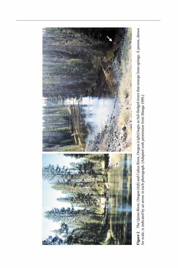
To illustrate some approaches that are used to interpret averaged informa-tion, I consider, as an example, a set of large volume springs that issue frombasalt flows in the Oregon Cascades. Because these springs are located in anactive volcanic arc, their waters provide an opportunity to learn about subsur-face magmatic and geothermal processes. Photographs of two of the springs areshown in Figure 2, a map of their locations is shown in Figure 3, and some key

Figure 3 Location of springs discussed in this review.

P1: GDL


204 MANGA

measurements are listed in Table 1. These springs range from cold (a few◦C) tohot (approaching the boiling point of water), and from small (liters per second) tolarge (several m3/s). A more thorough discussion of the hydrogeologic setting ofthese particular springs can be found in Meinzer (1927), Ingebritsen et al (1992),and James et al (1999).

ORIGIN OF SPRINGS

A spring is a location where groundwater emerges from the Earth’s subsurface inan amount large enough to form something resembling a stream. Natural springsmay also discharge directly into lakes and oceans (Church 1996).

Rivers flowing out of the Earth have captured the imagination of scientistsand philosophers for millenia and inspired some of the earliest ideas about thehydrologic cycle. Until the seventeenth century, the most widely held views inthe Western world were that, given the large amount of water that can emergeat springs, springs must discharge water that “condenses” below the surface orwater that is ultimately derived from the ocean and somehow flows uphill. Fol-lowing watershed mass balance measurements and calculations done in the late1600s, it became apparent that precipitation can supply more than enough wa-ter for rivers and springs. Adams (1938, Chapter XII) discusses the historicaldevelopment of ideas on the formation of springs and related hydrogeologicalprocesses.

For many people, springs are the most obvious, interesting, and practical mani-festation of the occurrence of groundwater. Springs have played a geographic rolein human settlement, especially in arid environments. Spring waters, in particularthose from mineral and hot springs, have long been purported to have medicinalor therapeutic value (Crook 1899, Waring 1915). Spring water is also associated

TABLE 1 Oregon springs discussed as examples

Elevation Estimated Recharge Area Discharge TemperatureName (m) (km2) (m3/s) ◦C

Quinn River (QR) 1354 33a 0.67b 3.4c

Brown’s Creek (BC) 1332 60a 1.1b 3.8c

Cultus River (CR) 1356 44a 1.8b 3.4c

Metolius River (MH) 920 400c 3.1d 8.2c

Breitenbush Hot Springe 682 — 0.013 8.4

aFrom Manga 1997.bAverage between 1939 and 1989.cFrom James et al 2000. Temperatures change by less than 0.2◦C over a period of several years.dFrom Meinzer 1927.eFrom Ingebritsen et al 1992.

P1: GDL



in the public’s mind with exceptional purity—witness the rapid growth in sales ofbottled water in the United States, from 1.8% to 6.9% of bottled beverage salesbetween 1981 and 1997; in 1998 bottled water sales were $4.3 billion in the UnitedStates alone (all data from www.bottledwaterweb.com).

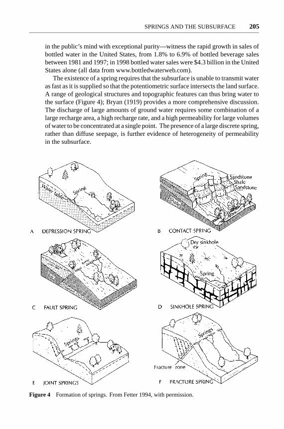
The existence of a spring requires that the subsurface is unable to transmit wateras fast as it is supplied so that the potentiometric surface intersects the land surface.A range of geological structures and topographic features can thus bring water tothe surface (Figure 4); Bryan (1919) provides a more comprehensive discussion.The discharge of large amounts of ground water requires some combination of alarge recharge area, a high recharge rate, and a high permeability for large volumesof water to be concentrated at a single point. The presence of a large discrete spring,rather than diffuse seepage, is further evidence of heterogeneity of permeabilityin the subsurface.

Figure 4 Formation of springs. From Fetter 1994, with permission.

P1: GDL


206 MANGA

ISOTOPE TRACERS

Isotopic tracer measurements and interpretations are widely used to determinehow “old” groundwater is, and from where it came. Radiogenic isotopes (andtracers whose concentrations change in time) are particularly useful for estimatinggroundwater ages; stable isotopes are more useful for determining the originalsource of spring water. The study of a set of isotope tracers can thus provideinformation about groundwater sources and transport rates. This can be particu-larly valuable for the sometimes complicated geological settings of springs (forexample, Nativ et al 1999, Davisson et al 1999). An analysis of tracer data inspring water, however, is complicated by the fact that recharge usually doesn’toccur at a single location, but instead occurs over a large region, often over theentire length of the aquifer. The “age” of the water is thus a mean residence timefor all the water that emerges at the spring. The unavoidable interaction of waterand subsurface geology provides additional complications (Rose et al 1996), butalso provides an opportunity to learn about subsurface geological processes (Jameset al 1999).

In this section I discuss some of the more commonly studied isotopes andfocus on the key ideas involved in interpreting isotopic measurements. Fritz &Fontes (1980) and Clark & Fritz (1997) provide a more comprehensive summaryand discussion of the use of isotopes in hydrogeologic studies, including a briefoverview of recommended sampling and measurement techniques. The samplingand analytical methodology used for measurements discussed here are describedin James et al (1999) and James (1999).

Besides the isotopic tracers discussed next, a variety of other tracers have beenused to study spring flow, including alkalinity (Chandler & Bisogni 1999), sus-pended sediment (Mahler & Lynch 1999), temperature (Bundschuh 1993), anddye (Smart 1988).

How Old Is the Water?

The ideal tracer for estimating ground water ages changes its recharge concen-trationcin over time, i.e.,cin = cin(t), and/or the tracer decays at a known rateλ

(= ln 2/t1/2, wheret1/2 is the half-life). Ideally the tracer is also otherwise con-servative and nonreactive so that chemical reactions and other sources or sinks ofthe tracer can be neglected. In the absence of mixing or dispersion the measuredtracer concentrationcout can be used to obtain a water age by

Tage= t1/2ln 2

ln

(cout

cin

). (2)

Here I focus on interpreting measurements of the two most widely used radio-genic tracers for estimating ages in hydrological problems:3H (t1/2 = 12.3 years)and its decay product3He, and14C (t1/2 = 5730 years).3H is thus useful for“young” waters (recharged within the last few decades) and14C is useful for“old” waters,O (102−104) years. As discussed later, determining ages from14C

P1: GDL



measurements of dissolved inorganic carbon is notoriously difficult except in verysimple systems, and many models and approaches have been developed to interpretmeasurements. Given the mass balance constraints of Equation 1, most largesprings should discharge young water, though there are notable exceptions in aridclimates where recharge rates are low and length scales are large (e.g. Winograd& Pearson 1976).

Other tracers that have been used for young waters include the anthropogenicradioisotope85Kr (Ekwurzel et al 1994) and anthropogenic chemicals such aschlorofluorocarbons introduced in the atmosphere (Busenberg & Plummer 1992).Interpretation of the measurements of these gases requires some care: The lagtime for their transport through a thick unsaturated zone (>10 m) can lead to ageoverestimates as large as 10 years (Cook & Solomon 1995).36Cl (t1/2 = 301,000years) has been used to study “ancient” groundwaters, such as those found in theGreat Artesian Basin in Australia (Torgersen et al 1991). Dating “middle-aged”waters, with ages in the range of several decades to a few hundred years, is morechallenging. The cosmogenic isotope39Ar has a suitable half-life of 269 years andcan be applied to hydrogeological problems (Loosli 1983). However, sampling andmeasurement is not routine (Clark & Fritz 1997), and in situ subsurface productionof 39Ar must be accounted for (Andrews et al 1989). Solomon et al (1996) suggestthat in some cases radiogenic4He, which is often used to trace ancient water(Heaton 1984), might be useful for ages in the range 101−103 years due to itsdiffusive loss from aquifer rocks.

Mixing Models

Owing to the mixing and dispersion of water recharged at different times and loca-tions, models are often used to interpret tracer measurements. Integral-balance orlumped-parameter models representing the relationship between input and outputcan be described by a convolution integral,

cout(t) =∫ t

−∞cin(τ )g(t − τ)e−λ(t−τ)dτ. (3)

Here,g(t) is the impulse response function (or weighting function),cin andcoutare the input and output concentrations, respectively,t is time,τ is an integrationvariable, andλ is the radioactive decay constant. Particular models are defined interms of their response functions,g(t).

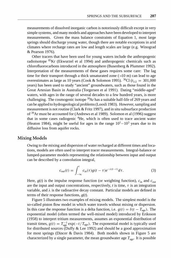
Figure 5 illustrates two examples of mixing models. The simplest model is theso-called piston flow model in which water travels without mixing or dispersion.In this case the response function is a delta function, i.e.g(t) = δ(t − Tage). Theexponential model (often termed the well-mixed model) introduced by Eriksson(1958) to interpret tritium measurements, assumes an exponential distribution oftransit times,g(t) = T−1

age exp(−t/Tage). The exponential model is typically usedfor distributed sources (Duffy & Lee 1992) and should be a good approximationfor most springs (Dincer & Davis 1984). Both models shown in Figure 5 arecharacterized by a single parameter, the mean groundwater ageTage. It is possible

P1: GDL


208 MANGA

Figure 5 Schematic illustration of two commonly applied mixing models: (a) the “pistonflow” model and (b) the “exponential” model.g(t) is the weighting function for each model,andTageis the mean residence time of water defined by Equation 1.

to develop more sophisticated models that will be characterized by additional pa-rameters. For example, if dispersion is accounted for in the piston-flow modelthen g(t) will depend on the ratio of flow velocity to dispersion rate, which ischaracterized by a Peclet number (Maloszewski & Zuber 1982). Mixing modelscan also account for geometric and transport properties in the system of interest.For example, in a dual porosity system, such as fracture-dominated flow througha porous matrix, apparent tracer ages will be affected by diffusive transfer of thetracer between the fractures and matrix (Sudicky & Frind 1982, Sanford 1997).

Given a single measurement of a tracer the inferredTage is thus a model-dependent age. It is possible, in principle, to distinguish between mixing modelsin two ways. First, becausecout(t) is a function ofg(t), time series of output-concentration measurements can be used to determineg(t) or to distinguishbetween models (Amin & Campana 1996). It is then possible to estimate modelparameters such as volume, travel time, and dispersivity (Duffy & Gelhar 1986).Second, because different tracers may have different diffusivities, the analysis ofmultiple tracers may be helpful (Maloszewski & Zuber 1990).

3H and 3He/3H Ages In principle, the measurement of both3H and its decayproduct,3He, allows a “true” mean age (referred to hereafter as the3He/3H age)

P1: GDL



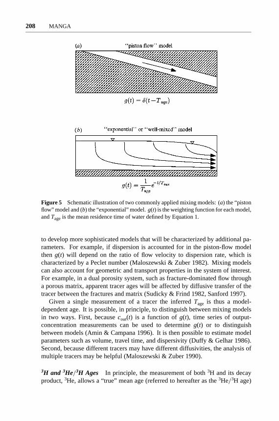
Figure 6 (a) 3H concentration in spring water (measured in tritium units, TU), and (b) 3He/3Hage as a function of groundwater age,Tage, for the exponential model (see Figure 5). The measured3H concentration at the Rising River springs is 4.23± 0.5 TU (Rose et al 1995), which implies amean groundwater age of about 7–9 years. The measured3He/3H age is 20.5 years (Rose et al1995), which implies a groundwater age of about 8 years. From Manga 1999, with permission.

to be obtained without relying on the uncertain3H input function, i.e. the detailedvalues ofcin (t) (Torgersen et al 1979):

3He/3H age= 12.43

ln 2ln(1+3Hetrit/

3H), (4)

where the subscript trit indicates He produced by the decay of3H. Again, mixingwill affect the 3He/3H age, and a model of the form of Equation 3 still needsto be applied for an aquifer with distributed recharge and measurements madeat the spring. For example, in Figure 6, I show estimates ofTage for RisingRiver in northern California based on isotopic measurements reported by Roseet al (1995) and the exponential model. Both estimates are consistent withTage≈8 years. Notice in Figure 6b that for Tage less than about 10 years, the3He/3Hage overestimatesTage, whereas forTagegreater than about 30 years, the3He/3Hage will remain close to about 30 years. In both cases, the contribution of3Heand3H from≈30 year old water associated with the largest atmospheric nucleartesting peaks biases the age inferred from discharged3He and3H concentrations(Aeschbach-Hertig et al 1998, Manga 1999).

The analysis of He can be more complicated but also more geologically infor-mative. He in groundwater can be derived from reservoirs in the atmosphere, themantle, and the crust. Fortunately, the ratio of3He/4He in each reservoir differsby up to several orders of magnitude so that in principle the contribution from eachreservoir can be identified (Stute et al 1992). The contribution of atmosphericallyderived He can be determined by measuring the concentration of Ne and assumingan appropriate recharge temperature (Schlosser et al 1989). Three of the large-volume, cold springs listed in Table 1, the Quinn River, Brown’s Creek, andCultus River, contain only atmospherically derived4He (James et al 2000). Thus,

P1: GDL


210 MANGA

excess3He is produced by the decay of3H and for these three springs3He/3Hages are 2.1, 0.7, and 2.5 years, respectively (James et al 2000). A short residencetime, for example, 2 years, combined with an estimated recharge rate of 1 m/year(Manga 1997) and a porosity of 10%, implies a mean aquifer thickness of 20 m(from Equation 1). The Metolius River, on the other hand, has nonatmospheric3Heand4He requiring a contribution from a deep (mantle) source and, presumably, alonger residence time and a deeper flowpath. Magmatically derived He is oftenfound in springs in regions that are, or have recently been, volcanically active(Kennedy et al 1985) and permits an estimate of magma degassing rates (Soreyet al 1998).

14C Dating Figure 7 shows the relationship between14C andδ13C for the springslisted in Table 1 (data from James et al 1999). The three end-members shown inFigure 7 represent dissolved inorganic carbon (DIC) equilibrated with soil CO2,DIC equilibrated with the atmosphere, and typical magmatic CO2 in a volcanic

Figure 7 14C vsδ13C for the 4 cold springs shown in Figure 3. Stippled boxes represent threeendmember isotopic compositions of dissolved inorganic carbon (DIC) for pH between 6.5 and8.5: DIC equilibrated with the atmosphere, DIC equilibrated with soil CO2, and “dead” carbon ofmagmatic origin. The endmember for the latter is represented by Minnehaha soda spring in thesouthern Oregon Cascades (Rose & Davisson 1996). This spring is saturated in CO2 (and thusbubbling, hence the name “soda” spring). The inset illustrates schematically why some springsobtain, or remain free of, magmatic carbon.

P1: GDL



arc, represented by the isotopic composition of Minnehaha soda spring (Rose &Davisson 1996, James et al 1999). In the Oregon Cascades, carbonate mineralsare generally absent, at least at shallow depths, so that sources of DIC other thanthose shown in Figure 7 can be neglected. Present day14C concentrations aregreater than 100% modern carbon (pmc) due to14C produced by nuclear weaponstests. One interpretation of the low14C concentration in the Metolius River isthat, rather than representing aging of the water (a few thousand years), the14Cconcentration reflects the addition of magmatically derived carbon (14C≈ 0). Anold age is precluded by Equation 1 becauseq is large. Measurements such asthose shown in Figure 7 have been used in other regions to study magmatic CO2degassing (Allard et al 1997, Rose & Davisson 1996, Sorey et al 1998), though it isnotable that there has not been any surface volcanic activity in central Oregon formore than 1300 years. James et al (1999) show that the rate of magmatic intrusionbeneath the Cascades arc required to supply the magmatic CO2 flux dischargedat springs is consistent with the rate of intrusion inferred from heat flow studies(Ingebritsen et al 1989, Blackwell et al 1990).

The other three cold springs from Table 1 have no detectable magmatic C, con-sistent with the absence of magmatic He (see above section). The inset of Figure 7illustrates schematically the different subsurface flow paths that the spring watermay follow. Quinn River, Cultus River, and Brown’s Creek discharge a shallowlocal-scale flow that does not dissolve magmatic CO2, whereas the Metolius Riverdischarges a more deeply circulating regional-scale flow. In the following section Idemonstrate that these flow patterns are consistent with the temperature measure-ments made at the springs.

As illustrated in Figure 7, the most significant complication for14C dating is theaddition of “dead” carbon, from a magmatic or metamorphic source as discussedhere, or more commonly, from carbonate dissolution. Dead carbon added to theflow system biases inferred ages to older ages. There are a variety of approachesto account for this dead carbon addition. These range from isotopic and chemicalmass balance calculations, e.g. using the NETPATH geochemical model (Plummeret al 1994), to measurement-based approaches. One example of the latter is tocorrect the “initial” 14C activity for dissolution in the unsaturated zone based on14C measurements made in the recharge area (Bajjali et al 1997). Another example,similar to that illustrated in Figure 7, is to useδ13C measurements to trace carbonatedissolution (Wigley et al 1978). Mook (1980) and Fontes (1992) provide reviewsof 14C dating of groundwaters.

Where Did the Water Originate?

One isotopic approach to answering this question is to examine the oxygen andhydrogen isotopes in the spring water—see Winograd & Friedman (1972),Christodoulou et al (1993), and Scholl et al (1996) for studies in a variety of geologi-cal and climatological settings. The usefulness of these isotopes stems from the factthat they fractionate (relative abundances change) in a predictable manner as water

P1: GDL


212 MANGA

moves through the hydrologic cycle depending on the physical and chemicalprocesses that operate (Criss 1999).

In mountainous regions, the isotopic composition of precipitation often variessystematically and in a quantifiable way with elevation. Analysis of snow coreand small spring data in the central Oregon Cascades, for example, shows thatδ18O decreases by 0.18 per ml per 100 m rise in elevation (James 1999). Thisvalue is similar to those found farther north in British Columbia (−0.25 permil/100 m; Clark et al 1982) and farther south in Northern California (−0.23 permil/100 m; Rose et al 1996). The slightly lower rate of decrease in central Oregon maybe caused by being in a rain shadow. The comparison of precipitation and springdischarge is appropriate here for two reasons. First, given the young ages foundin the above section, discharge should be comparable to modern precipitation interms of its O isotopic composition. Second, given the large volume of circulatingwater, there should be little isotopic effect from the possible addition of mag-matic water (Giggenbach 1992). Nor should there be a “δ18 O-shift” produced bywater-rock interactions, as is common in hot spring waters (Craig 1963). The iso-topic composition of the spring water can thus be projected to the elevation atwhich precipitation is comparable, as shown in Figure 8, in order to infer a meanrecharge elevation. From a topographic map and mass balance considerations itis then possible to estimate the recharge area for the springs.

If the mean residence time of water is sufficiently short, or if there is a componentof rapid groundwater flow, there may be temporal variations inδ18 O at the spring.The isotopic composition of discharge and precipitation can then be used to perform

Figure 8 Elevation versusδ18O in the central Oregon Cascades; line is a best-fit to datafrom snow cores and small springs (after James 1999), and symbols are data from largecold springs. The mean recharge elevation can be inferred by determining the elevationat which precipitation has a comparable isotopic composition. BC, Brown’s Creek; CR,Cultus River; MH, Metolius River; QR, Quinn River.

P1: GDL



a hydrograph separation to identify the volumes and rates associated with fast andslow flow paths (Lakey & Krothe 1996). For the springs studied hereδ18 O isapproximately constant over a period of several years (James 1999).

On the other hand, if the mean residence time of water is long and there islimited mixing of different water masses, the composition of the water reflectsthe conditions at the time of recharge. Thus, paleotemperature or atmosphericconditions (e.g. prevailing wind directions) can be inferred fromδ18 O andδ D(Claassen 1986, Weyhenmeyer et al 2000).

TEMPERATURE MEASUREMENTS

Temperature is by far the easiest and least expensive property to measure at aspring. The temperature of groundwaters was first systematically studied in the1700s (Davis 1999). These early studies demonstrated the key idea of the followingdiscussion, namely that warming of groundwater reflects primarily the input of heatfrom within the Earth.

The use of temperature measurements to quantify the motion of groundwaterhas several advantages. Once a borehole has been drilled, it is inexpensive andstraightforward to measure temperature accurately and obtain a high spatial reso-lution of measurements (Woodbury & Smith 1988). The temperature distributionsatisfies an advective-diffusion equation in which the dispersivity tensor can bereplaced (in most cases) by the thermal diffusivity of saturated rock because heatconduction through the rock dominates the macroscopic dispersion in interstices.Thus, variations in temperature can be related to the pattern and rate of ground-water flow rather than to the dispersive properties of the flow and porous material.The heterogeneity of porous materials that is so troublesome for problems of tracerand geochemical transport should therefore be less so for heat transport.

A wide range of solutions for the heat transport problem can be obtained forsimple model geometries and compared with temperature records from singleboreholes (Bredehoeft & Papadopulos 1965, Ziagos & Blackwell 1986, Ge 1998).At the regional scale, numerical groundwater flow models can be employed tostudy the relationship between groundwater circulation and the temperature dis-tribution (Smith & Chapman 1983). Temperature measurements are only useful,however, when they deviate from the conductive solution. It is worth noting thattemporal changes in surface temperature, uplift and erosion, topographic relief,and variations of thermal conductivity all produce nonconstant temperature gra-dients. These effects must be separated from those associated with groundwaterflow. In many settings, a darcy velocity>O(1) cm/year is sufficient to distortthe conductive geothermal gradient. In the Oregon Cascades, recharge rates are≈ 1 m/year and indeed borehole temperature measurements indicate that near-surface temperature gradients and the surface heat flux are approximately zero inthe High Cascades (Ingebritsen et al 1989). In this case, it is possible to applystraightforward energy balance ideas to the entire groundwater system (Brott et al

P1: GDL


214 MANGA

1981), at least when spring temperatures are constant as they are here (Manga1998).

Consider an aquifer with mean heat fluxQ entering its base (see Figure 1).Assume that all this heatH=Q A is advected horizontally by groundwater flow inthe aquifer and is then discharged at the springs. The total heat discharged at thespring is related to the temperature change1θ by

H = ρCq1θ, (5)

whereρ andC are the density and heat capacity of water, respectively, and againq is the mean spring discharge. In Northern California, there is a set of largesprings that discharge about 40 m3/s into the Fall River (Meinzer 1927). Springtemperatures are about 12◦C, whereas small springs in the recharge area (on theflanks of the Medicine Lake shield volcano) are about 7◦C (Davisson & Rose1997). Thus, the “cold” Fall River springs discharge about 103 MW of geothermalheat, a value equivalent to a mean heat flux of about 0.56 W/m2 (about 10 timesthe mean continental heat flux) over an estimated 2× 103 km2 recharge area.For comparison, the total amount of heat discharged by the large and very activehydrothermal system at Yellowstone is about 5× 103 MW (Fournier 1989), andthe total worldwide geothermal power being exploited in 1995 was 8.7×103 MW(Freeston 1996).

For the Metolius River, the estimated recharge area is about 400 km2 (Table 1),and the background heat flux is about 120 mW/m2 (Blackwell et al 1990). Assum-ing that all heat is removed advectively, I expect a temperature increase of about4◦C based on Equation 5. This value is consistent with Figure 9 if I make thereasonable assumption that the mean recharge temperature is close to the meanannual surface temperature (Taniguchi 1993, Perez 1997).

In contrast to the Metolius River, the other large springs shown in Figure 9discharge water at temperatures that are nearly equal to the mean annual surfacetemperatures at the mean recharge elevations found in Figure 8. These springs thusdischarge water that is colder (by about 1–3◦C) than the mean surface temperatureat the discharge elevation, an observation first noticed and explained by Humboldtin 1844 (see Davis 1999). The lack of geothermal warming combined with the near-zero near-surface heat flux implies that there is a larger-scale and more deeplycirculating groundwater flow that advectively removes the geothermal heat. Inthe Oregon Cascades, much of this heat is discharged at lower elevations at hotsprings (Ingebritsen et al 1989). Manga (1998) shows how the recharge ratesof these two different systems (deep vs shallow) can be estimated from energybalance considerations.

It is sometimes assumed that the depth of groundwater circulation can be de-duced by dividing the increase of the water’s temperature by the geothermal gradi-ent. Such a calculation implicitly makes two assumptions. First, groundwater flowdoes not affect the subsurface temperature distribution and thus flow rates must below. Second, the spring water must rise sufficiently rapidly that it does not cool.Sanz & Yelamos (1998), for example, applied this argument to springs in Spainand inferred a reasonable circulation depth of 900 m. However, the total heat of

P1: GDL



46 MW discharged by their thermal spring implies an unrealistically large geother-mal heat flux over the 100 km2 basin estimated by Sanz & Y´elamos (1998),supporting the contention of other authors (S´anchez Navarro et al 2000) thatthe thermal water has a different origin. Thus, simple energy balance argu-ments can be useful for testing the reasonableness of conceptual hydrogeologicalmodels.

In summary, the temperature of spring water reflects the interaction between theadvective and conductive transport of heat. The numerical calculations of Forster &Smith (1989) offer a particularly clear illustration of this relationship. In rockswith low permeabilities, velocities are low, conductive heat transport is dominant,and spring temperatures will be low. In rocks with high permeabilities, velocitieswill be high and advective transport of heat will dominate. High permeability alsoresults in large volumes of circulating water, and spring temperatures will againremain low (as shown in Figure 9). The warmest springs occur for an intermediaterange of permeabilities. Thus, spring temperatures will reflect a balance between

Figure 9 Relationship between elevation and temperature for climate stations in the OregonCascades (crosses). Spring temperature is shown as a function of the inferred mean rechargeelevation (from Figure 8). The Metolius River water is warmed substantially by geothermal heat,whereas the other spring waters show little evidence of geothermal warming. The inset illustrateshow deeply circulating groundwater can aquire geothermal heat, whereas water that remains atshallow depths will remain at temperatures close to the mean annual surface temperature. Theseinferences are consistent with those based on carbon isotopes (Figure 7).

P1: GDL


216 MANGA

the amount of heat transported advectively and the volume of water that must bewarmed.

DISCHARGE MEASUREMENTS

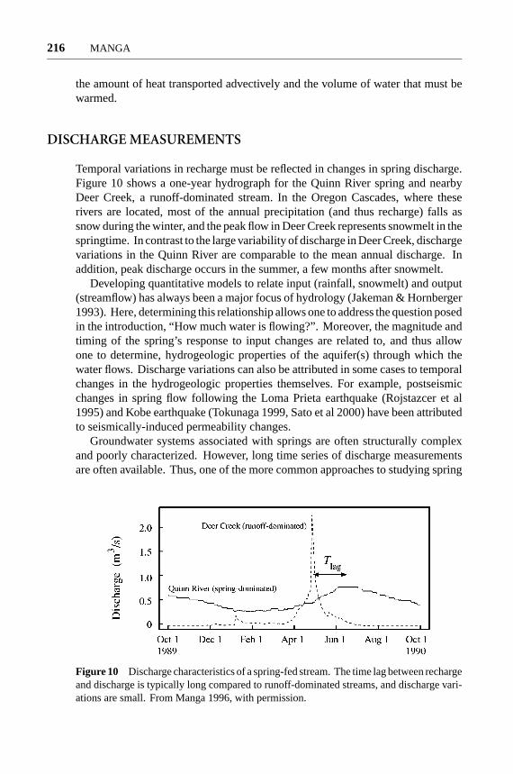
Temporal variations in recharge must be reflected in changes in spring discharge.Figure 10 shows a one-year hydrograph for the Quinn River spring and nearbyDeer Creek, a runoff-dominated stream. In the Oregon Cascades, where theserivers are located, most of the annual precipitation (and thus recharge) falls assnow during the winter, and the peak flow in Deer Creek represents snowmelt in thespringtime. In contrast to the large variability of discharge in Deer Creek, dischargevariations in the Quinn River are comparable to the mean annual discharge. Inaddition, peak discharge occurs in the summer, a few months after snowmelt.

Developing quantitative models to relate input (rainfall, snowmelt) and output(streamflow) has always been a major focus of hydrology (Jakeman & Hornberger1993). Here, determining this relationship allows one to address the question posedin the introduction, “How much water is flowing?”. Moreover, the magnitude andtiming of the spring’s response to input changes are related to, and thus allowone to determine, hydrogeologic properties of the aquifer(s) through which thewater flows. Discharge variations can also be attributed in some cases to temporalchanges in the hydrogeologic properties themselves. For example, postseismicchanges in spring flow following the Loma Prieta earthquake (Rojstazcer et al1995) and Kobe earthquake (Tokunaga 1999, Sato et al 2000) have been attributedto seismically-induced permeability changes.

Groundwater systems associated with springs are often structurally complexand poorly characterized. However, long time series of discharge measurementsare often available. Thus, one of the more common approaches to studying spring

Figure 10 Discharge characteristics of a spring-fed stream. The time lag between rechargeand discharge is typically long compared to runoff-dominated streams, and discharge vari-ations are small. From Manga 1996, with permission.

P1: GDL



discharge is to use time series and spectral analysis (Mangin 1984, Padilla &Pulido-Bosch 1995, Angelini 1997). Properties such as the cross-correlation ofrecharge and discharge (Figure 11) and autocorrelation of spring flow are usefulfor characterizing the nature of temporal discharge variations. More recent studieshave applied the techniques of nonlinear time series analysis (Jian et al 1998) andartificial neural networks (Lambrakis et al 2000); both approaches offer improvedpredictive abilities relative to more traditional time series approaches.

Spectral analysis of spring flow is also informative. Consider an aquifer fromwhich the outflow is a linear function of the average water level in the aquifer. Thetransfer function,η(ω), which describes the amplitude filtering characteristics ofthe system as a function of frequency,ω, is given by

|η(ω)|2 = Sout

Sin= 1

1+ ω2T2h

, (6)

whereSout andSin are the power spectra of discharge and recharge, respectively,andTh is a characteristic hydraulic relaxation timescale. For an unconfined aquifer,with water level changes¿ the mean water depthH , Th = φL2/3KH , whereK ishydraulic conductivity andL is the aquifer length (Gelhar 1993). Figure 11 (right)shows that a transfer function with a form given by Equation 6 is compatible withmeasurements from the Quinn River. Other spectral properties, such as coherenceand phase can be interpreted in a similar fashion (Duffy & Gelhar 1986).

Figure 11 (Left) Cross-correlation between recharge (discharge in a runoff-dominated stream)and spring discharge for the Quinn River. The mean time lag is 64 days. The dashed curve shows theautocorrelation for the Quinn River. (Right) Ratio of output (spring discharge) and input (recharge)spectral densities as a function of frequency. Discharge in a runoff-dominated stream (Deer Creekin Figure 10) is used as a proxy for recharge, and is scaled so that the mean input equals the meanoutput. Solid curve is the prediction of the linear model (Equation 6). Circles are based on 50years of discharge measurements withTh = φL2/3KH = 1.1 years. Modified from Manga 1999,with permission.

P1: GDL


218 MANGA

It is also possible to simulate groundwater flow and the resulting spring dis-charge with models that describe the spatial distribution and values of hydroge-ologic properties as well as boundary conditions for the flow. Gvirtzman et al(1997), Angelini & Dragoni (1997), and Eisenlohr et al (1997) provide examplesin a range of hydrogeologic settings. Despite the large degree of heterogeneityimplicitly associated with springs (see Figure 4), through calibration, such modelspermit the representation of known and hypothesized geometries and hydraulicproperties (Larocque et al 1999). By introducing spatial dimensions to the prob-lem, physically-based flow models are typically characterized by a large numberof parameters, many of which may be interrelated. Thus, it is sometimes ques-tioned whether discharge measurements have the ability to resolve more than justa few parameters (Jakeman & Hornberger 1993). Indeed, simplified models basedon one-dimensional versions of groundwater flow equations, such as the Boussi-nesq equation, are often successful at explaining observed stream flow in a widerange of geological settings (Leonardi et al 1996, Manga 1997, Brutsaert & Lopez1998).

Consider briefly one example of a simple one-dimensional model for flow tothe Quinn River in central Oregon. Here the geology consists of stacked layersof Quaternary lava flows. Most of the horizontal groundwater flow occurs withinthe blocky top of each lava flow—a horizontally conductive layer—whereas inthe relatively thick middle of the lava flow, groundwater flow is primarily in thevertical direction through cooling joints (Figure 12). By using Darcy’s equation to

Figure 12 Groundwater flow geometry: (a) basin-scale regional flow system (see Figures 7 and9); (b) flow at the scale of individual lava flow units; (c) origin of different hydraulic conductivities.The blocky tops of lava flows will have much higher horizontal permeabilities than the dense butjointed interior of flows.

P1: GDL



describe flow (not necessarily valid in spring systems because of high flow rates)and conservation of mass, and assuming one-dimensional flow in thex direction,the evolution of headh in the horizontally conductive layer is described by

∂h

∂t= KH

φ

∂2h

∂x2+ N(x, t)

φ, (7)

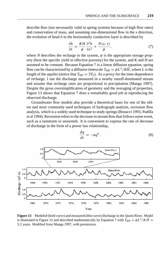
whereN describes the recharge to the system,φ is the appropriate storage prop-erty (here the specific yield or effective porosity) for the system, andK andH areassumed to be constant. Because Equation 7 is a linear diffusion equation, springflow can be characterized by a diffusive timescaleTdiff = φL2/KH , whereL is thelength of the aquifer (notice thatTdiff = 3Th). As a proxy for the time-dependenceof recharge, I use the discharge measured in a nearby runoff-dominated streamand assume that recharge rates are proportional to precipitation (Manga 1997).Despite the gross oversimplification of geometry and the averaging of properties,Figure 13 shows that Equation 7 does a remarkably good job at reproducing theobserved discharge.

Groundwater flow models also provide a theoretical basis for one of the old-est and most commonly used techniques of hydrograph analysis, recession flowanalysis, which is a widely used technique to study springs (Bonacci 1993, Padillaet al 1994). Recession refers to the decrease in stream flow that follows some event,such as a rainstorm or snowmelt. It is convenient to express the rate of decreaseof discharge in the form of a power law relationship,

dq

dt= −aqb. (8)

Figure 13 Modeled (bold curve) and measured (thin curve) discharge in the Quinn River. Modelis illustrated in Figure 12 and described mathematically by Equation 7 withTdiff = φL2/K H =3.2 years. Modified from Manga 1997, with permission.

P1: GDL


220 MANGA

The coefficientsa andb can be related to hydraulic and geometric propertiesof the aquifer through a comparison with appropriate groundwater flow solutions(Szilagyi et al 1998). For an unconfined aquifer, the oldest and classic solution ofBoussinesq (1903) hasb= 1 (an exponential decrease in discharge) and describesthe long-term behavior of the aquifer; by contrast, the short-term solution, repre-senting the discharge of near-stream water, hasb= 3 (Polubarinova-Kochina 1962).

One attractive feature of recession flow, time series, and spectral analyses is thatthe techniques involve a statistical analysis of data, which can then be interpretedwithin a framework provided by simple models. The value of such models isnicely summarized by Gelhar (1993):

Models of this type are appropriate to treat situations where the timevariation of aquifer conditions is the primary concern. Such an approachoften will be appropriate when addressing the problems of overall policy andmanagement decisions relating to the behavior of the aquifer over extendedperiods of time. This kind of model, obviously, cannot be used to addressquestions of the spatial distribution of the water level. Also, lumped-parameter models are often consistent with the kind of limited data that isavailable for analyzing such problems.

GEOCHEMICAL MEASUREMENTS

The geochemical composition of spring water is governed by water-mineral equi-libria, reaction kinetics, the initial composition of the water and composition of theaquifer rocks, and the rate of groundwater transport. Interpreting the compositionof groundwater can thus be complicated. Nevertheless, the composition of springwaters still contains information that can be useful. For example, in a classicstudy, Garrels & MacKenzie (1967) showed that it is possible to estimate the typeand amount of weathering reactions from the chemical composition of spring wa-ters. Geochemical time-series can also be interpreted with the same ideas used tointerpret isotopic and discharge time-series, and can provide information about thesources and mixing of different waters (Mazor & Vuataz 1990).

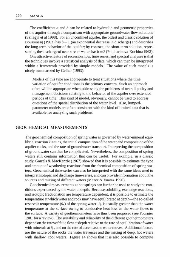
Geochemical measurements at hot springs can further be used to study the con-ditions experienced by the water at depth. Because solubility, exchange reactions,and isotopic fractionation are temperature dependent, it is possible to estimate thetemperature at which water and rock may have equilibrated at depth—the so-calledreservoir temperature (θr ) of the spring water.θr is usually greater than the watertemperature at the surface owing to conductive heat loss as the water flows tothe surface. A variety of geothermometers have thus been proposed (see Fournier1981 for a review). The suitability and reliability of the different geothermometersdepend on the rates of fluid flow at depth relative to the rate of equilibration of waterwith minerals atθr , and on the rate of ascent as the water moves. Additional factorsare the nature of the rocks the water traverses and the mixing of deep, hot waterswith shallow, cool waters. Figure 14 shows that it is also possible to compute

P1: GDL



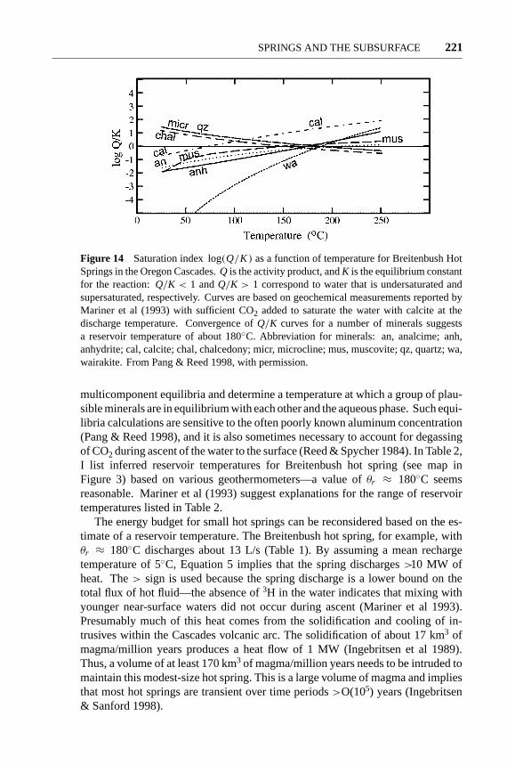
Figure 14 Saturation index log(Q/K ) as a function of temperature for Breitenbush HotSprings in the Oregon Cascades.Q is the activity product, andK is the equilibrium constantfor the reaction:Q/K < 1 andQ/K > 1 correspond to water that is undersaturated andsupersaturated, respectively. Curves are based on geochemical measurements reported byMariner et al (1993) with sufficient CO2 added to saturate the water with calcite at thedischarge temperature. Convergence ofQ/K curves for a number of minerals suggestsa reservoir temperature of about 180◦C. Abbreviation for minerals: an, analcime; anh,anhydrite; cal, calcite; chal, chalcedony; micr, microcline; mus, muscovite; qz, quartz; wa,wairakite. From Pang & Reed 1998, with permission.

multicomponent equilibria and determine a temperature at which a group of plau-sible minerals are in equilibrium with each other and the aqueous phase. Such equi-libria calculations are sensitive to the often poorly known aluminum concentration(Pang & Reed 1998), and it is also sometimes necessary to account for degassingof CO2 during ascent of the water to the surface (Reed & Spycher 1984). In Table 2,I list inferred reservoir temperatures for Breitenbush hot spring (see map inFigure 3) based on various geothermometers—a value ofθr ≈ 180◦C seemsreasonable. Mariner et al (1993) suggest explanations for the range of reservoirtemperatures listed in Table 2.

The energy budget for small hot springs can be reconsidered based on the es-timate of a reservoir temperature. The Breitenbush hot spring, for example, withθr ≈ 180◦C discharges about 13 L/s (Table 1). By assuming a mean rechargetemperature of 5◦C, Equation 5 implies that the spring discharges>10 MW ofheat. The> sign is used because the spring discharge is a lower bound on thetotal flux of hot fluid—the absence of3H in the water indicates that mixing withyounger near-surface waters did not occur during ascent (Mariner et al 1993).Presumably much of this heat comes from the solidification and cooling of in-trusives within the Cascades volcanic arc. The solidification of about 17 km3 ofmagma/million years produces a heat flow of 1 MW (Ingebritsen et al 1989).Thus, a volume of at least 170 km3 of magma/million years needs to be intruded tomaintain this modest-size hot spring. This is a large volume of magma and impliesthat most hot springs are transient over time periods>O(105) years (Ingebritsen& Sanford 1998).

P1: GDL


222 MANGA

TABLE 2 Reservoir temperatures forBreitenbush hotspring (Figure 3) inferred fromgeothermometers. Surface temperature is 84◦C

Geothermometer Temperaturea (◦C)

Quartzb 166

SO4-H2Oc 178

Anhydrite saturationd 176

K-Mgd 129

Na-Kd 171

Na-K-Cad 148

Na-Lid 202

fixAl c ∼180

aAll results are from Mariner et al 1993 except the fixAl resultof Pang & Reed 1998.bBased on mineral solubility.cBased on temperature-dependent isotope fractionation.dBased on empirical relation of various cation ratios to temper-ature.eBased on multiple mineral equilibria with adjusted Al concen-tration.

CONCLUDING REMARKS

A variety of hydrological problems can be studied from measurements made atsprings. These problems include determining from where the water came, theresidence time and velocity of water, hydraulic properties of the aquifers, andthe spatial scale and subsurface extent of the flow system. Because the waterinteracts with its geological environment, there is also the possibility of obtaininginformation about subsurface geological and geophysical processes. Examplesdiscussed here include determining heat flow, quantifying magmatic degassing,and estimating geothermal reservoir temperatures. Finally, not only do springsprovide access to water that has sampled distant regions, but in some cases theyalso discharge water from distant periods in time and preserve information aboutpaleoclimate.

Signs posted at the headwaters of two of the springs I have discussed in thisreview illustrate some of the issues that can be addressed by studying springs. Atthe source of the Quinn River a sign states:

The crystal clear water from this spring may have fallen several years ago assnow in the high Cascades. Each year, as the snow melts, most of the waterseeps into the cracks of this “geologically young” country and travelsthrough underground channels.

P1: GDL



By using the stable isotopes of O and H, I confirm that recharge occurs along thecrest of the Cascades. The analysis of radiogenic3H and its decay product3He sug-gests a mean age of about 1 year. The sign notes that the terrain is also “young.”As water flows through these young volcanic rocks, it may dissolve and dis-charge gases released at depth from the solidification of magmas—measurementsat springs provide a means of quantifying this degassing and inferring intrusionrates. At the headwaters of the Metolius River, a sign reads

Down this path a full-sized river, the Metolius, flows ice cold from hugesprings. The springs appear to originate from beneath Black Butte.However, geologists say this is misleading and believe the springs have theirorigin in the Cascade Mountains to the west.

Again, I use stable isotopes of O and H to confirm that the water originated asmeteoric water along the crest of the Cascades. The sign also emphasizes the coldtemperature of the water (8.3◦C). In fact, despite the low temperature, because thisspring is “huge” it carries virtually all the geothermal heat produced in the drainagebasin (area about 400 km2) from a region with a high background heat flux.

In summary, measurements made at springs integrate the signal of geologicaland hydrological processes over large spatial areas and possibly long periods oftime—this can be either good, bad, or ugly, depending on the hydrogeologic infor-mation that is sought and the geological processes being studied. The challenge isthat springs do not always directly measure the geological or hydraulic propertiesof interest. Thus, the interpretation of measurements requires the development ofa model or mathematical framework in which a set of measurements can be relatedto processes.

ACKNOWLEDGMENTS

The author’s work discussed in this review was supported by NSF grant EAR-9701768. The author appreciated helpful and critical comments by B Dugan,R Haggerty, ER James, MH Reed, TP Rose, and MO Saar. Permissions to re-produce the figures in this review were granted by Prentice-Hall, the AmericanGeophysical Union, and Elsevier.

Visit the Annual Reviews home page at www.AnnualReviews.org

LITERATURE CITED

Adams FD. 1938.The Birth and Developmentof the Geological Sciences. Toronto, Can.:Dover. 506 pp.

Aeschbach-Hertig W, Schlosser P, Stute M,Simpson HJ, Ludin A, Clark JF. 1998. A

3He/4He study of ground water flow ina fractured bedrock aquifer.Ground Water34:661–70

Allard P, Jean-Baptiste P, D’Alessandro W,Parello F, Parisi B, Flehoc C. 1997.

P1: GDL


224 MANGA

Mantle-derived helium and carbon ingroundwaters and gases of Mount Etna, Italy.Earth Planet. Sci. Lett.148:501–16

Amin IE, Campana ME. 1996. A generallumped parameter model for the interpreta-tion of tracer data and transit time calculationin hydrologic systems.J. Hydrol.179:1–21

Andrews JN, Davis SN, Fabryka-Martin J,Fontes JCh, Lehmann BE, et al. 1989. Thein situ production of radioisotopes in rockmatrices with particular reference to theStripa granite.Geochim. Cosmochim. Acta53:1803–15

Angelini P. 1997. Correlation and spectral anal-ysis of two hydrogeological systems in Cen-tral Italy. Hydrol. Sci. J.42:425–38

Angelini P, Dragoni W. 1997. The problem ofmodeling limestone springs: the case of Bag-nara (North Apennines, Italy).Ground Water35:612–18

Bajjali W, Clark ID, Fritz P. 1997. The artesianthermal groundwaters of northern Jordan:insights to their recharge history and age.J. Hydrol.187:355–82

Blackwell DD, Steele JL, Frohme MK, Mur-phey CF, Priest GR, Black GL. 1990. Heatflow in the Oregon Cascade range andits correlation with regional gravity, Curiepoint depths, and geology.J. Geophys. Res.95:19475–94

Bonacci O. 1993. Karst springs hydrographs asindicators of karst aquifers.Hydrol. Sci. J.38:51–62

Boussinesq J. 1903. Recherches théoriques surl’ ecoulement des nappes d’eau infiltrées dansle sol et sur le débit des sources.J. Math.Pures Appl.10:5–78

Bredehoeft JD, Papadopulos IS. 1965. Ratesof vertical groundwater movement estimatedfrom the Earth’s thermal profile.Water Re-sour. Res.1:325–29

Brott CA, Blackwell DD, Ziagos JP. 1981. Ther-mal and tectonic implications of heat flow inthe eastern Snake River Plain, Idaho.J. Geo-phys. Res.86:11709–34

Brutsaert W, Lopez JP. 1998. Basin-scale geo-hydrologic drought flow features of riparian

aquifers in the southern Great Plains.WaterResour. Res.34:233–40

Bryan K. 1919. Classification of springs.J.Geol.27:522–61

Bundschuh J. 1993. Modeling annual variationsof spring and groundwater temperatures as-sociated with shallow aquifer systems.J. Hy-drol. 142:427–44

Busenberg E, Plummer LN. 1992. Use ofchlorofluorocarbons (CCl3F and CCl2F2) ashydrologic tracers and age-dating tools: thealluvium and terrace system of Central Okla-homa.Water Resour. Res.28:2257–83

Chandler DG, Bisogni JJ. 1999. The use of al-kalinity as a conservative tracer in a studyof near-surface hydrologic change in tropi-cal karst.J. Hydrol.216:172–82

Christodoulou Th, Leontiadis IL, Morfis A,Payne BR, Tzimourtas S. 1993. Isotopehydrology study of the Axios River plain innorthern Greece.J. Hydrol.146:391–404

Church TM. 1996. An underground route forthe water cycle.Nature380:579–80

Claassen HC. 1986. Late-Wisconsin paleohy-drology of the west central Amargosa Desert,Nevada, USA.Chem. Geol.58:311–23

Clark ID, Fritz P. 1997.Environmental Isotopesin Hydrogeology. New York: Lewis. 328 pp.

Clark ID, Fritz P, Michel FA, Souther JG. 1982.Isotope hydrology and geothermometry ofthe Mount Meager geothermal area.Can. J.Earth Sci.19:1454–73

Cook PG, Solomon DK. 1995. Transport ofatmospheric trace gases to the water table:implications for groundwater dating withchlorofluorocarbons and krypton 85.WaterResour. Res.31:263–70

Craig H. 1963. The isotope geochemistry ofwater and carbon in geothermal areas. InNuclear Geology of Geothermal Areas, ed.E Tongiorgi, pp 17–53. Pisa: Cons. Naz.Richerche, Lab. Geol. Nucl.

Criss RE. 1999.Principles of Stable IsotopeDistribution. New York: Oxford. 254 pp.

Crook JK. 1899.The Mineral Waters of theUnited States and Their Therapeutic Uses.New York: Lea Brothers. 588 pp.

P1: GDL



Davis SN. 1999. Humboldt, Arago, and thetemperature of groundwater.Hydrogeol. J.7:501–3

Davisson ML, Rose TP. 1997.ComparativeIsotope Hydrology Study of GroundwaterSources and Transport in Three Cascade Vol-canoes of Northern California. Rep. UCRL-ID-128423. Lawrence Livermore Natl. Lab.,Livermore, Calif.

Davisson ML, Smith DK, Kenneally J, Rose TP.1999. Isotope hydrology of southern Nevadagroundwater: stable isotopes and radiocar-bon.Water Resour. Res.35:279–94

Dincer T, Davis GH. 1984. Application of en-vironmental isotope tracers to modeling inhydrology.J. Hydrol.68:95–113

Duffy CJ, Gelhar LW. 1986. A frequency do-main analysis of groundwater quality fluc-tuations: interpretation of field data.WaterResour. Res.22:1115–28

Duffy CJ, Lee DH. 1992. Base flow responsefrom nonpoint source contamination: sim-ulated spatial variability in source, struc-ture, and initial condition.Water Resour. Res.28:905–14

Eisenlohr L, Kiraly L, Bouzelboudjen M,Rossier Y. 1997. Numerical simulation as atool for checking the interpretation of karstspring hydrographs.J. Hydrol. 193:306–25

Ekwurzel B, Schlosser P, Smethie WM, Plum-mer LN, Busenberg E, et al. 1994. Datingof shallow groundwater: comparison of thetransient tracers3H/3He, chlorofluorocar-bons, and85Kr. Water Resour. Res.30:1693–1709

Eriksson E. 1958. The possible use of tritiumfor estimating groundwater storage.Tellus10:472–78

Fetter CW. 1994.Applied Hydrogeology. En-glewood Clifts, NJ: Prentice-Hall. 691 pp.3rd ed.

Fontes JCh. 1992. Chemical and isotopic con-straints on14C dating of groundwater. InRa-diocarbon after Four Decades, ed. RE Tay-lor, A Long, RS Kra, pp. 242–61. New York:Springer-Verlag

Forster C, Smith L. 1989. The influence ofgroundwater flow on thermal regimes inmountainous terrain: a model study.J. Geo-phys. Res.94:9439–51

Fournier RO. 1981. Application of water chem-istry to geothermal exploration and reservoirengineering. InGeothermal Systems: Prin-ciples and Case Studies, ed. L Rybach, LJPMuffler, pp. 109–43. New York: Wiley

Fournier RO. 1989. Geochemistry and dynam-ics of the Yellowstone National Park hy-drothermal system.Annu. Rev. Earth Planet.Sci.17:13–53

Freeston DH. 1996. Direct uses of geothermalenergy 1995.Geothermics25:189–214

Fritz P, Fontes JCh, eds. 1980.Handbook ofEnvironmental Isotope Geochemistry, Vols.1, 2, 3. New York: Elsevier

Garrels RM, MacKenzie FT. 1967. Origin ofthe chemical composition of some springsand lakes. InEquilibrium Concepts in Nat-ural Water Systems, ed. RF Gould, Adv.Chem. Ser. 67:222–42. Washington, DC:Am. Chem. Soc.

Ge SM. 1998. Estimation of groundwater veloc-ity in localized fracture zones from well tem-perature profiles.J. Volcan. Geotherm. Res.84:93–101

Gelhar LW. 1993.Stochastic Subsurface Hy-drology. Upper Saddle River, NJ: Prentice-Hall. 390 pp.

Giggenbach WF. 1992. Isotopic shifts in watersfrom geothermal and volcanic systems alongconvergent plate boundaries and their origin.Earth Planet. Sci. Lett.113:495–510

Gvirtzman H, Garven G, Gvirtzman G. 1997.Hydrogeological modeling of the saline hotsprings at the Sea of Galilee, Israel.WaterResour. Res.33:913–26

Heaton THE. 1984. Rates and sources of4Heaccumulation in groundwater.Hydrol. Sci. J.29:29–47

Ingebritsen SE, Sanford WE. 1998.Groundwa-ter in Geologic Processes. Cambridge: Cam-bridge Univ. Press. 341 pp.

Ingebritsen SE, Sherrod DR, Mariner RH. 1989.Heat flow and hydrothermal circulation in

P1: GDL


226 MANGA

Cascade range, north-central Oregon.Sci-ence243:1458–62

Ingebritsen SE, Sherrod DR, Mariner RH. 1992.Rates and patterns of groundwater flow in theCascade Range volcanic arc, and the effectson subsurface temperature.J. Geophys. Res.97:4599–627

Jakeman AJ, Hornberger GM. 1993. How muchcomplexity is warranted in a rainfall-runoffmodel?Water Resour. Res.29:2637–49

James ER. 1999.Isotope tracers and regional-scale groundwater flow: application to theOregon Cascades. MS thesis. Univ. Or.,Eugene. 150 pp.

James ER, Manga M, Rose TP. 1999. CO2 de-gassing in the Oregon Cascades.Geology27:823–26

James ER, Manga M, Rose TP, Hudson GB.2000. The use of temperature and the iso-topes of O, H, C, and noble gases to determinethe pattern and spatial extent of groundwaterflow. J. Hydrol.237:100–12

Jian WB, Yao H, Wen XH, Chen BR. 1998. Anonlinear time series model for spring flow:an example from Shanxi Province, China.Ground Water36:147–50

Kennedy BM, Lynch MA, Reynolds JH, SmithSP. 1985. Intensive sampling of noble gasesin fluids at Yellowstone: I. Early overviewof the data; regional patterns.Geochim. Cos-mochim. Acta49:1251–61

Lakey B, Krothe NC. 1996. Stable isotopic vari-ation of storm discharge from a perennialkarst spring.Water Resour. Res.32:721–31

Lambrakis N, Andreou AS, Polydoropoulos P,Georgopoulos E, Bountis T. 2000. Nonlinearanalysis and forecasting of a brackish karsticspring.Water Resour. Res.36:875–84

Larocque M, Banton O, Ackerer P, RazackM. 1999. Determining karst transmissivi-ties with inverse modeling and an equiva-lent porous media.Ground Water37:897–903

Leonardi V, Arthaud F, Grillot JC, AvetissianV, Bochnaghian P. 1996. Modelling of a frac-tured basaltic aquifer with respect to geolog-ical setting, and climatic and hydraulic con-

ditions: the case of perched basalts at Garni(Armenia).J. Hydrol.179:87–109

Loosli HH. 1983. A dating method with39Ar.Earth Planet. Sci. Lett.63:51–62

Mahler BJ, Lynch FL. 1999. Muddy waters:temporal variation in sediment dischargingfrom a karst spring.J. Hydrol.214:165–78

Maloszewski P, Zuber A. 1982. Determining theturnover time of groundwater systems withthe aid of environmental tracers. 1. Modelsand their applicability.J. Hydrol.57:207–31

Maloszewski P, Zuber A. 1990. Mathematicalmodeling of tracer behavior in short-termtracer experiments in fissured rocks.WaterResour. Res.26:1517–28

Manga M. 1996. Hydrology of spring-dominated streams in the Oregon Cascades.Water Resour. Res.32:2435–39

Manga M. 1997. A model for discharge inspring-dominated streams and implicationsfor the transmissivity and recharge of Quater-nary volcanics in the Oregon Cascades.WaterResour. Res.33:1813–22

Manga M. 1998. Advective heat transport bylow-temperature discharge in the OregonCascades.Geology26:799–802

Manga M. 1999. On the timescales charac-terizing groundwater discharge.J. Hydrol.219:56–69

Mangin A. 1984. Pour une meilleure conais-sance des systémes hydrologiques á partir desanalyses corrélatoire et spectrale.J. Hydrol.67:25–43

Mariner RH, Presser TS, Evans WC. 1993.Geothermometry and water-rock interactionin selected thermal systems in the CascadeRange and Modoc Plateau, western UnitedStates.Geothermics22:1–15

Mazor E, Vuataz FD. 1990. Hydrology ofa spring complex, studied by geochemicaltime-series data, Acquarossa, Switzerland.Appl. Geochem.5:563–69

Meinzer OE. 1927.Large springs in the UnitedStates. US Geol. Surv. Water Supp. Pap. 557.94 pp.

Mook WG. 1980. Carbon-14 in hydrogeolog-ical studies. InHandbook of Environmental

P1: GDL



Geochemistry, ed. P Fritz, JCh Fontes, 1:49–74. Amsterdam: Elsevier

Nativ R, Gunay G, Hotzl H, Reichert B,Solomon DK, Tezcan L. 1999. Separation ofgroundwater-flow components in a karstifiedaquifer using environmental tracers.Appl.Geochem.14:1001–14

Padilla A, Pulido-Bosch A. 1995. Study of hy-drographs of karstic aquifers by means ofcorrelation and cross-spectral analysis.J. Hy-drol. 168:73–89

Padilla A, Pulido-Bosch A, Mangin A. 1994.Relative importance of baseflow and quick-flow from hydrographs of karst springs.Ground Water32:267–77

Pang ZH, Reed M. 1998. Theoretical chemicalthermometry on geothermal waters: prob-lems and methods.Geochim. Cosmochim.Acta62:1083–91

Perez ES. 1997. Estimation of basin-widerecharge rates using spring flow, precipita-tion, and temperature data.Ground Water35:1058–65

Plummer LN, Prestemon DL, Parkhurst DL.1994. An interactive code (NETPATH) formodeling NET geochemical reactions alonga flow PATH, version 2.0. US Geol. Surv.Water Res. Invest. Rep. 94–4169, US Geol.Surv., Reston, VA. 130 pp.

Polubarinova-Kochina PY-A. 1962.Theoryof Groundwater Movement. Princeton, NJ:Princeton Univ Press. 613 pp.

Reed M, Spycher N. 1984. Calculation of pHand mineral equilibria in hydrothermal wa-ters with application to geothermometry andstudies of boiling and dilution.Geochim.Cosmochim. Acta48:1479–92

Rojstaczer S, Wolf S, Michel R. 1995. Perme-ability enhancement in the shallow crust asa cause of earthquake induced hydrologicalchanges.Nature373:237–39

Rose TP, Davisson ML. 1996. Radiocarbon inhydrologic systems containing dissolvedmagmatic carbon dioxide.Science 273:1367–70

Rose TP, Davisson ML, Criss RE. 1996. Iso-tope hydrology of voluminous cold springs in

fractured rock from an active volcanic region,northeastern California.J. Hydrol.179:207–36

Rose TP, Davisson ML, Hudson GB, Criss RE.1995. Distinguishing biogenic from volcaniccarbon isotope reservoirs in a fracture flowhydrologic system.EOS76:211 (Abstr.)

Sanchez Navarro JA, Coloma P, Maestro A.2000. Methodology for the study of unex-ploited aquifers with thermal waters: ap-plication to the aquifer of the Alhama deAragon Hot Spring, discussion.Ground Wa-ter 38:224–25

Sanford WE. 1997. Correcting for diffusion incarbon-14 dating of ground water.GroundWater35:357–61

Sanz E, Yelamos JG. 1998. Methodology forthe study of unexploited aquifers with ther-mal waters: application to the aquifer of theAlhama de Arag´on Hot Spring.Ground Wa-ter 6:913–23

Sato T, Sakai R, Furuya K, Kodama T. 2000. Co-seismic spring flow changes associated withthe 1995 Kobe earthquake.Geophys. Res.Lett.27:1219–22

Schlosser P, Stute M, Sonntag M, Munnich KO.1989. Tritogenic3He in shallow groundwa-ter.Earth Planet. Sci. Lett.94:245–56

Scholl MA. Ingebritsen SE, Janik CJ,Kauahikaua JP. 1996. Use of precipitationand groundwater isotopes to interpretregional hydrology on a tropical volcanicisland: Kilauea volcano area, Hawaii.WaterResour. Res.32:3525–37

Smart CC. 1988. Artificial tracer techniques forthe determination of the structure of conduitaquifers.Ground Water26:445–53

Smith L, Chapman DS. 1983. On the thermaleffects of groundwater flow. 1. Regional scalesystems.J. Geophys. Res.88:593–608

Solomon DK, Hunt A, Poreda RJ. 1996. Sourceof radiogenic helium 4 in shallow aquifers:implications for dating young groundwater.Water Resour. Res.32:1805–13

Sorey ML, Evans WC, Kennedy BM, FarrarCD, Hainsworth LJ, Hausback B. 1998. Car-bon dioxide and helium emissions from a

P1: GDL


228 MANGA

reservoir of magmatic gas beneath Mam-moth Mountain, California.J. Geophys. Res.103:15303–23

Stute M, Sonntag C, Deak J, Schlosser P. 1992.Helium in deep circulating groundwater inthe Great Hungarian Plain: flow dynamicsand crustal mantle helium fluxes.Geochim.Cosmochim. Acta56:2051–67

Sudicky EA, Frind EO. 1982. Contaminanttransport in fractured porous media: analyt-ical solutions for a system of parallel frac-tures.Water Resour. Res.18:1634–42

Szilagyi J, Parlange MB, Albertson JD. 1998.Recession flow analysis for aquifer pa-rameter determination.Water Resour. Res.34:1851–57

Taniguchi M. 1993. Evaluation of verticalgroundwater fluxes and thermal propertiesof aquifers based on transient temperature-depth profiles.Water Resour. Res.29:2021–26

Tokunaga T. 1999. Modeling of earthquake-induced hydrological changes and possiblepermeability enhancement due to the 17 Jan-uary 1995 Kobe Earthquake, Japan.J. Hy-drol. 223:221–29

Torgersen T, Clarke WB, Jenkins WJ. 1979.The tritium/helium-3 method in hydrology.Isotope Hydrology 1978, Vol II, pp. 913–30.IAEA Symp. 228

Torgersen T, Habermehl MA, Phillips FM, El-more D, Kubik P, et al. 1991. Chlorine 36dating of very old groundwater. 3. Further

studies in the Great Artesian Basin.WaterResour. Res.27:3201–13

Waring GA. 1915.Spring of California. USGeol. Surv. Wat. Supp. Pap. 338, US Geol.Surv., Washington, DC, GPO. 410 pp.

Weyhenmeyer CE, Burns SJ, Waber HN,Aeschbach-Hertig W, Kipfer R, et al. 2000.Cool glacial temperatures and changes inmoisture source recorded in Oman ground-waters.Science454:842–45

Wigley TML, Plummer LN, Pearson FJ. 1978.Mass transfer and carbon evolution in naturalwater systems.Geochim. Cosmochim. Acta42:1117–39

Winograd IJ, Friedman I. 1972. Deuterium as atracer of regional groundwater flow, southernGreat Basin, Nevada and California.Geol.Soc. Am. Bull.83:3691–3708

Winograd IJ, Pearson FJ. 1976. Major carbon-14 anomaly in a regional carbonate aquifer:possible evidence for megascale channeling,south central Great Basin.Water Resour. Res.12:1125–43

Wood WW. 2000. It’s the heterogeneity.GroundWater38:1

Woodbury AD, Smith L. 1998. Simultaneousinversion of hydrogeologic and thermal data.2. Incorporation of thermal data.Water Re-sour. Res.24:356–72

Ziagos JP, Blackwell DD. 1986. A model forthe transient temperature effects of horizontalfluid flow in geothermal systems.J. Volcan.Geotherm. Res.27:371–97

P1: FQP

March 30, 2001 10:28 Annual Reviews AR125-08-COLOR

Fig

ure

2T

heQ

uinn

Riv

er,O

rego

n(l

eft)

and

Cul

tus

Riv

er,O

rego

n(r

ight

)be

gin

asfu

ll-fl

edge

dri

vers

that

emer

gefr

omsp

ring

s.A

pers

on,s

how

nfo

rsc

ale,

isin

dica

ted

byan

arro

win

each

phot

ogra

ph.(

Ada

pted

with

perm

issi

onfr

omM

anga

1999

.)

michael manga - university of california, berkeleyseismo.berkeley.edu/~manga/paper41.pdf · tage...

Documents