reader supplement i - university of california,...

EPS 3: The Water Planet Summer, 2002

Reader Supplement

I

EPS 3: The Water Planet Summer, 2002

Reader Supplement

I

Section Topic Page Numbers 1 Where Water Comes From: 3 - 6

the global hydrological cycle 2 Water Circulation from Atmosphere to Earth: 7 - 10

precipitation, evaporation and infiltration 3 Surface Water: storage, runoff, and 11 - 16

the hydrograph 4 Formation and Maintenance of 17 - 25

River Channels Useful References 26

1 Where Water Comes From: the global hydrological cycle There are 1.4 billion cubic kilometers of water on Earth, of which approximately 517 × 103 cubic kilometers are annually evaporated and re-precipitated across the globe. This amount is roughly equivalent to a 1-meter thick layer of water spread over the entire Earth. The annual circulation of water is the largest movement of a chemical substance at the Earth’s surface. Movement of water through the atmosphere determines the quantity and distribution of rainfall on Earth. This movement is dictated by the general circulation of the atmosphere, which in turn is determined by differences in solar heating across the globe. Table 1-1 shows the major stocks of water in the global hydrologic cycle and the surface area occupied by each stock. Of the freshwater stocks, 69% is frozen, 30% is groundwater, and only 1% is available as surface water.

Table 1-1 Major Stocks of Water in the Global Hydrological Cycle (adapted from Dingman, 2002).

Form of Water Area Covered (km2)

Volume (km3)

% Total Water Reserves

World oceans 361,300,000 1,338,000,000 96.5 Groundwater 134,800,000 23,400,000 1.7 Glaciers and permanent snowpack

324,600,000 48,128,200 3.48

Ground ice in permafrost zone

21,000,000 300,000 0.022

Freshwater lakes 1,236,400 91,000 0.007 Saltwater lakes 822,300 85,400 0.006 Marsh water 2,682,600 11,470 0.0008 River water 148,800,000 2,120 0.0002 Water in biosphere 510,000,000 1,120 0.0001 Atmospheric water 510,000,000 12,900 0.001 TOTAL WATER RESERVES

510,000,000 1,385,984,610 100

FRESH WATER 148,800,000 35,029,210 2.53

The major features of the global cycle are:

1. Oceans lose more water by evaporation than they gain by precipitation. 2. Land surfaces receive more precipitation than they lose by evaporation. 3. The excess water on the land returns to the oceans as runoff, balancing the deficit in the ocean-

atmosphere exchange.

Ocean fluxes dominate the water cycle, receiving 79% of the total precipitation and contributing 88% of global evaporation.

Figure 1-1 Proportion of water in various storages (from Summerfield, 1997)

Summary of Earth’s water:

a) 1.4 billion km3 – sufficient to cover the conterminous USA to a depth of 150 km b) Total renewable water supplied by precipitation to the continents each year is approximately 40,000

km3 – enough to cover the USA to a depth of 4.4 meters 1.(i) The Global Water Budget The oceans are the dominant pool in the global water cycle, containing over 97% of all water at the surface of the Earth. The equivalent depth of seawater is approximately 3.5 km – the mean depth of the oceans. As Figure 1-1 illustrates the water available to human society is a relatively small pool of liquid fresh water, chiefly in rivers and lakes.

Figure 1-2 Major fluxes and stores in the global water cycle (from Schlesinger, 1997).

Figure 1-2 shows the various fluxes and pools in the global water cycle. Evaporation removes approximately 425,000 km3 from the oceans annually. Given information on the flux and the quantity stored in a pool one can calculate the residence time of water. The residence time, which is the ratio of the volume of a store (or reservoir) to the flow rate (or flux) in or out, is a measure of the average transport time for a parcel of water through the pool. The concept assumes that the amount of stock is constant (i.e., the input rate is equal to the output rate). Mathematically, the residence time (T) is given as,

Residence time, T (years) = M (km3) / F (km3/yr) where M is the stock and F is the flux. The mean residence time of ocean water with respect to the atmosphere, using the data provided in Figure 1-2, is:

1.35 × 109 km3 / 425,000 km3/yr ≈ 3,180 years

Only 385,000 km3 of the 425,000 km3 is precipitated back to the ocean; the remainder contributes to the 111,000 km3 that is precipitated on the land. However, evaporation from oceans is not uniform, varying from approximately 4mm/day in the tropics to <1mm/day near the poles. 1.(ii) U.S. Water Budget The annual average precipitation across the USA is approximately, 762 mm, of which 534 mm is evaporated and transpired, leaving 228 mm, which returns to the oceans as runoff.

1.(iii) A Brief History of the Water Cycle The formation of the Earth was largely completed 3.8 billion years ago. Most of the water that was released into the atmosphere by volcanic outgassing, cooled, condensed and formed the oceans. Importantly, some remained as water vapor (≈ 0.1%). Water vapor is a greenhouse gas and this small fraction of vapor in the atmosphere served to trap outgoing longwave radiation thus raising Earth’s temperature (global average temperature of Earth is 15ºC) above freezing. Throughout Earth’s history, sea level changes have been driven both by tectonic activity and by several ice ages. The most recent glacial maximum (approximately 18,000 years ago) at the end of the Pleistocene epoch, sequestered approximately 42 million km3 of seawater into the continental and polar ice caps. The continental glaciations profoundly disrupted the global water cycle. Estimates suggest that 18,000 years ago, global precipitation was reduced by as much as 14%. Streamflow is climatically determined and hence climate changes over historical time periods have important implications for water availability for human consumption. Examining the existing records of streamflow and precipitation are crucial for managing these water resources. Unfortunately the length of these records is comparatively brief. Precipitation records for Sante Fe, NM, go back to 1849. However, this is short compared to records for the Yangtse, which go back 1,000 years, and the Nile, which go back as far as 1,500 years ago.

2 Water Circulation from Atmosphere to Earth: precipitation, infiltration and evaporation

The hydrologic cycle is powered by heat energy delivered by the sun. About 33% (12.3 × 1016 Watts) of the sun’s energy that reaches the Earth’s surface is devoted to the global water cycle alone, and most of this energy (85%) is invested in evaporating water from the ocean’s surface. Globally, approximately 1-meter of precipitation falls annually. Compare this to the 2.5 cm (approximately 1-inch) of water that exists in the atmosphere at any one time. The discrepancy gives some indication of how rapidly water vapor is cycled through the hydrosphere. Residence time of water in the atmosphere is approximately 9-11 days. 2.(i) Overview of the meteorological processes relevant to hydrology

The global distribution of precipitation (both rain and snow) and the relative amounts and intensities depend on several factors. Regions characterized by rising air tend to have relatively high average precipitation. By contrast, regions characterized by descending air tend to have low average precipitation. The general circulation of the atmosphere produces belts of relatively high precipitation at the equator and at 60° North and South. Arid and semi-arid regions are observed in the belts around 30° North and South. The general circulation of the atmosphere and the distribution of moist and dry regions, is well described by a 3-cell model (see figure 2-1 below). The model is, however, just an approximation of the circulation. In reality, the bands of high and low pressure predicted by the three-cell model deviate from a zonal configuration due to differential heating of the Earth's surface and the effects of topography.

Figure 2-1 Three-Cell model of atmospheric general circulation (modified from: Milich, L., 1997. Why are deserts dry? http://ag.arizona.edu/~lmilich/dry.html).

http://ag.arizona.edu/~lmilich/dry.html

2.(ii) Formation of precipitation The formation of precipitation is a four-stage process:

a) Cooling of air to its dewpoint (the temperature at which an air sample becomes saturated) b) Condensation on nuclei to form cloud droplets or ice crystals. c) Growth of droplets or crystals into raindrops or snowflakes. d) Importing of water vapor to sustain the process.

The causes of cooling which result in condensation of water vapor and ultimately precipitation can be broadly categorized into three processes:

1. Convergence of air masses of difference temperatures and water vapor content. Figure 2-2(a) and (b) show examples of the convergence of air masses in a warm front and cold front. In 2-2(a), a warm air mass passes over retreating cold air. The lifting of the warm air causes cooling and hence condensation. The zone of precipitation for this type of frontal system may stretch 200-300 miles. In 2-2(b) a cold front forms when warm air is forced upward by an advancing mass of cold air.

2. Convective thunderstorms. Figure 2-2(c) shows the unstable updrafts and downdrafts of warm, moist air, characteristic of summertime thunderstorms. Air warmer than its surroundings rises and condenses and if fed by sufficient moisture from the surrounding atmosphere, allows large thunderstorm clouds to develop.

3. Orographic precipitation. Figure 2-2(d) illustrates the precipitation caused by the uplift of an air mass when it is forced upward against a mountain barrier. If lifted high enough, the air mass cools, water vapor condenses and precipitates out as snow or rain. On the lee side of the mountain range a rain-shadow effect is often observed.

2.(iii) Rainfall amounts and duration In the USA, Eastern states receive 1,000 to 1,750 mm of precipitation annually. Moving westward, this amount steadily declines. Most non-mountainous areas of the West receive less than 500 mm annually. The Sierra Nevada and the Coast Range of Northern California are exceptions. The former receives between 1,500 and 1,700 mm annually, and the latter receives 500 to 2,500 mm annually. Orographic precipitation is the chief explanation for the anomalously high precipitation received in the Sierra. Globally, precipitation amounts and durations vary dramatically. Some record amounts are shown in Table 2-1.

Table 2-1. Locations, Dates, and Amounts of Record Rainfalls for Various Durations (modified from Dingman, 2002)

Duration Depth (mm) Location Date 1 min 38 Barot, Guadeloupe 11/26/1970 15 min 198 Plumb Point, Jamaica 5/12/1916 42 min 305 Holt, MO 6/22/1947 2 hr 45 min 559 D’Hanis, TX 5/31/1935 9 hr 1,087 Belouve, Rénunion 2/28/1964 2 days 2,500 Cilaos, Rénunion Mar 15-17, 1952 15 days 4,798 Cherrapunji, India June 24-July 8, 1931 2 months 12,767 Cherrapunji, India June – July, 1861 1 year 26,461 Cherrapunji, India Aug 1860 – July 1861

Figure 2-2. Types of precipitation.

2.(iv) Infiltration Water falling on the Earth follows one of three routes: it evaporates; it sinks into the ground; or it runs off the surface. The relative portion allocated to each of these pathways is largely determined by climate, soil, vegetation, and human influence. Prior to reaching the ground surface, and in regions with substantial vegetative cover, significant quantities of precipitation may be intercepted and evaporated back to the atmosphere. Of the water that does reach the ground surface, most of it infiltrates – the process by which water arriving at the surface enters the soil substrate. The rate at which infiltration occurs depends on several factors:

a) How dry the soil is prior to the precipitation event. b) The intensity and duration of the rainfall event. c) The characteristics of the soil column (for example, sandy soils have much more rapid infiltration rates than clay-rich soils because there are many spaces (or pores) in the sandy soil matrix). d) The slope (or inclination) of the surface. e) The type and density of vegetation growing.

Water that enters the soil matrix initially fills the available pore spaces. In fine-grained soils (silts and clays), some initial swelling of the soil matrix is observed. A combination of gravitational pull and molecular attraction results in an advancing wetting front of water above which, all the pore spaces are saturated.

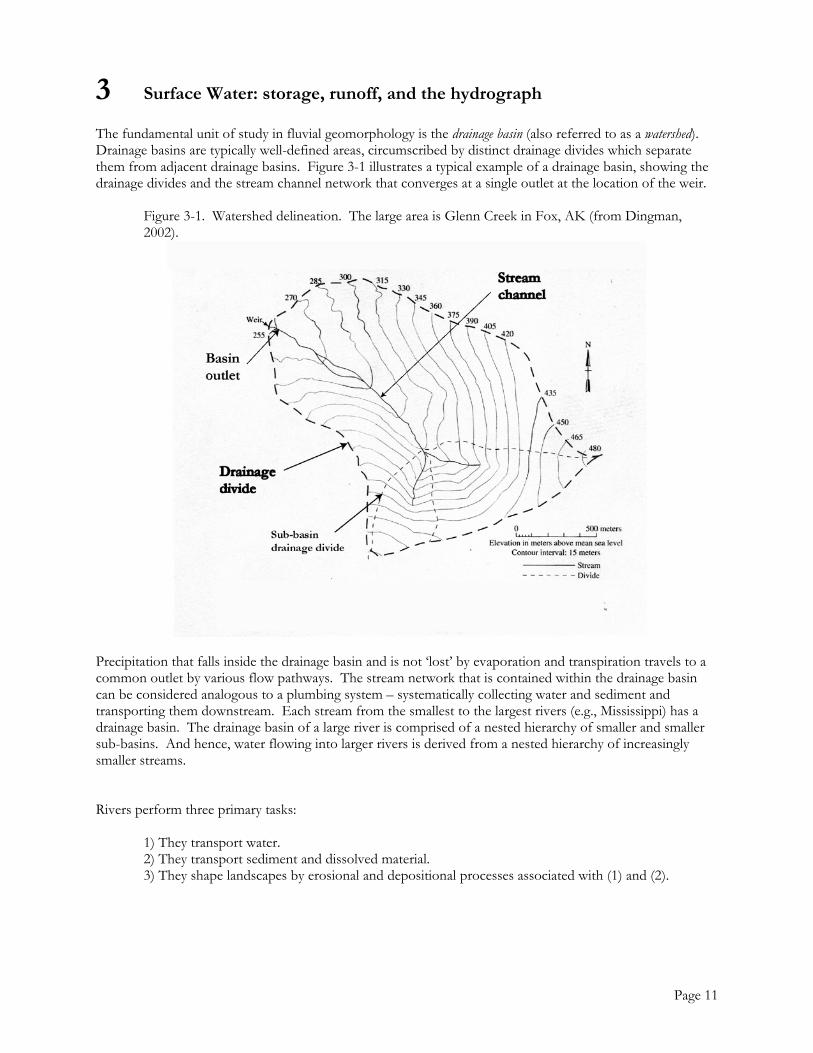
3 Surface Water: storage, runoff, and the hydrograph The fundamental unit of study in fluvial geomorphology is the drainage basin (also referred to as a watershed). Drainage basins are typically well-defined areas, circumscribed by distinct drainage divides which separate them from adjacent drainage basins. Figure 3-1 illustrates a typical example of a drainage basin, showing the drainage divides and the stream channel network that converges at a single outlet at the location of the weir.

Figure 3-1. Watershed delineation. The large area is Glenn Creek in Fox, AK (from Dingman, 2002).

Precipitation that falls inside the drainage basin and is not ‘lost’ by evaporation and transpiration travels to a common outlet by various flow pathways. The stream network that is contained within the drainage basin can be considered analogous to a plumbing system – systematically collecting water and sediment and transporting them downstream. Each stream from the smallest to the largest rivers (e.g., Mississippi) has a drainage basin. The drainage basin of a large river is comprised of a nested hierarchy of smaller and smaller sub-basins. And hence, water flowing into larger rivers is derived from a nested hierarchy of increasingly smaller streams. Rivers perform three primary tasks:

1) They transport water. 2) They transport sediment and dissolved material. 3) They shape landscapes by erosional and depositional processes associated with (1) and (2).

3(i) Pathways of water from land to sea The pathways by which water moves downhill into the stream channel are determined by climate, vegetation, topography, geology, soil characteristics, and land use. Four distinct pathways are described below. Page 244 of the Reader shows an illustration of these four runoff pathways. 1) Baseflow or groundwater flow (GF): Water that infiltrates deep into the ground reaching the water table (the layer of free-standing water in fissures and pores at the top of the saturated zone) and makes its way to the stream channel. The rate of delivery of this pathway is very slow, and is measured in days, weeks, and even years. Importantly, groundwater flow is the pathway that maintains flow year round in rivers. In a Mediterranean climate, which is characteristic of California, cool wet winters are followed by long dry summers. Continuous flow in the stream channels during the summer months is maintained by the slow movement of water through the bedrock or soil matrix. Groundwater flow that emerges at the stream channel during summer was likely precipitated (as snow or rainfall) in the preceding winter. 2) Horton overland flow (HOF): When the rainfall rate exceeds the infiltration rate, water ponds on the surface, and any surface water in excess of depression storage capacity will run off as an irregular sheet of overland flow. The mechanism was first described by Robert E. Horton (1933, as reported in Leopold, 1997). For three decades, this mechanism was assumed to be the chief delivery pathway of water to the stream channel. In the 1960’s, forestry hydrologists in the Eastern USA challenged the universality of Horton overland flow. They noted that in forested areas water was rarely observed to flow overland. By contrast, they observed that only a small portion of the drainage basin contributed directly to storm runoff and that the this portion of the basin increased and decreased in spatial extent depending on storm duration and intensity and how saturated the ground was prior to the storm event. The previous work motivated research into identifying what additional pathways were responsible for delivering storm runoff to the channel. Two additional mechanisms were identified: 3) Shallow subsurface stormflow (SSSF): Represents the water that infiltrates into the upper soil column and then moves downhill toward the stream channel, often via preferential pathways (including animal burrows, old plant root conduits, and so forth). While a slower process than Horton overland flow, it is considerable faster than groundwater flow 4) Saturation overland flow (SOF): The flow pathway that is comprised of direct precipitation on the saturated surface adjacent to the channel and infiltrated water that returns to the surface. The area where SOF predominates is flat, low-lying or convergent topography adjacent to the stream channel. Velocities of SOF can be up to one hundred times faster than SSSF. The area which contributes SOF varies not only in a storm event, but also seasonally and may be completely absent during dry months.

3.(ii) Stream Discharge The shape of the stream hydrograph is strongly determined by which of the four runoff pathway predominates. The stream hydrograph is a measure of discharge or flow rate plotted against time. The units of discharge are volume per time. Formulaically,

Discharge (Q) = width (w) × depth (d) × velocity (v) = area × velocity

Calculating discharge involves measuring the cross-sectional area of the flowing water and its average velocity. The product of these two measurements yields discharge. Velocity can be measured using a mechanical propeller current meter or with electronic devices. Measurements should be made two-thirds (or more accurately, 0.6) of the distance from the stream surface to the stream bed (which is the depth at which velocity is approximately its average value), and at several positions across the stream. At these same positions, the width and depth of the flowing water for that polygon-shaped zone is measured. And thus the discharge for that zone equals the product of width, depth, and velocity. Total discharge for the channel cross-section is simply the sum of all the discharges for the individual zones. 3.(iii) Rating Curves and Hydrographs The United States Geological Survey monitors discharge for many rivers across the US (see http://water.usgs.gov/realtime.html). At the gauging stations where this information is gathered, water surface elevations, measured as gauge heights, are continuously recorded. At several different elevations or gauge heights, the cross-sectional area of the channel has been carefully measured. With the additional measurement of flow velocity for those different gauge heights, discharge can be computed. By plotting discharge against the water surface elevation, or gauge height, a point on the rating curve is generated. Figure 3-1 shows a rating curve for Seneca Creek in Maryland. Both axes on the figure are logarithmic, allowing for a large range of discharge values to be displayed on the same graph. The rating curve is thus an empirical relation between discharge and the height of the water surface. It allows for interpolation of discharge values for a given gauge height within the range of recorded gauge heights.

Figure 3-1. Rating curve for Seneca Creek, Maryland (from Leopold, 1997)

http://water.usgs.gov/realtime.html

Plotting discharge against time, where the units of time may be measured in minutes, hours, or days, provides insight into which flow pathways are responsible for runoff. Figure 3-2 illustrates the main features of a storm hydrograph, including the rising and falling (or recession) limbs, the peak discharge, and the baseflow curve. The area under the hydrograph yields the amount of water supplied by the storm event.

Figure 3-2. Typical form of a storm hydrograph.

Groundwater flow is principally responsible for maintaining baseflow. The shape of the storm hydrograph is dependent on how much surface runoff makes its way to the stream channel versus subsurface flow. Events dominated by subsurface flow typically have a hydrograph with a flatter rising limb and lower peak discharge (i.e., a longer time of rise and a longer flow duration). Storm events which are dominated by surface runoff have hydrographs with more rapidly rising limbs, higher peak discharges, and equally rapid declining limbs. Figure 3-3 shows a theoretical hydrograph, illustrating the expected response in discharge for a watershed that has undergone urbanization. The process of urbanization increases the land area occupied by buildings and paved surfaces. These surfaces are impermeable (i.e., water can’t infiltrate into the subsurface) and result in considerably more surface runoff – especially overland flow. The hydrograph response for the urbanized scenario, as depicted in Figure 3-3, shows a more rapidly rising limb and peak discharge.

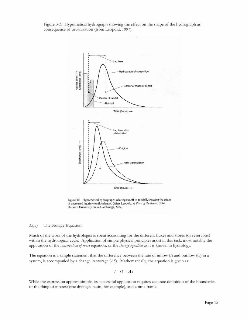
Figure 3-3. Hypothetical hydrograph showing the effect on the shape of the hydrograph as consequence of urbanization (from Leopold, 1997).

3.(iv) The Storage Equation Much of the work of the hydrologist is spent accounting for the different fluxes and stores (or reservoirs) within the hydrological cycle. Application of simple physical principles assist in this task, most notably the application of the conservation of mass equation, or the storage equation as it is known in hydrology. The equation is a simple statement that the difference between the rate of inflow (I) and outflow (O) in a system, is accompanied by a change in storage (∆S). Mathematically, the equation is given as:

I – O = ∆S While the expression appears simple, its successful application requires accurate definition of the boundaries of the thing of interest (the drainage basin, for example), and a time frame.

The storage equation may be applied to surface runoff and channel storage problems, and also groundwater flow and reservoir storage. Its application to runoff issues takes the form of defining precipitation (minus evaporation) as the input, and streamflow as output. The bedrock and soil matrix, surface depressions, and the channel itself (which acts both as temporary storage and an output) represent the storage. Accurate accounting of the inputs and output provides important insight into the quantities and residence time of water held in storage. The task of accurately accounting for various fluxes and stores becomes increasingly difficult as basin size increases. Whereas for small basins the entire area may contribute to runoff (output) at a common outlet during the course of a single storm event, that is not the case for larger basins. As basin size increases, the lag time in runoff response from different parts of the basin results in a rather more complicated hydrograph. The channel itself represents an important, albeit transient, water storage reservoir. During a flood event there is a lag time from when water drains from the upper to the lower portions of the basin. The water that is in transit in the river is in channel storage. After the storm has finished, the upper portions of the basin contribute increasingly less flow, and the water that is in transit gradually flows out. Enormous volumes of water are present in the channel during large flood events. During a flood in the Ohio River in 1937, approximately 69 cubic kilometers of water was estimated to be held in the stream channel system (Hoyt and Langbein, 1937, as referenced in Leopold, 1997). This form of temporary storage also has the effect of reducing the height of the flood. As a flood moves downstream temporary channel storage will tend to reduce the magnitude of the flood peak and at the same time, increase its duration.

4 Formation and Maintenance of River Channels. The form or shape of the stream channel is determined by the flows it carries and the sediment it transports. And so while the flowing water is responsible for sculpting the channel, it is the sediment that controls its morphology. The sediment is removed from the adjacent hillslopes by various erosional and weathering processes and transported to the stream channel system. The fluvial system can be conveniently subdivided into three zones: a zone of sediment production (primarily the headwaters areas), a zone of sediment transport, and a zone of sediment deposition. This categorization necessarily simplifies the processes occurring in the different zones, but it does reasonably capture the dominant process for each zone. An important characteristic of the natural channel system is its ability to accommodate a broad range of flows and associated sediment volumes without long-term changes in morphology. It is the sediment load, not the water volume that keeps the channel shape approximately constant. Channel shape and size, and its properties are determined by the interaction of erosional and depositional processes described below. 4.(i) Sediment Properties The sediment carried in streams varies considerably in size, shape and mineral composition. The sediment load is categorized into three components based on the size of the sediment and the manner in which it is transported:

a) Dissolved load, consisting of material transported in solution. b) Suspended load, consisting of fine particles carried in suspension (generally sizes < 0.062 mm) c) Bedload, consisting of all material carried along the bed of the channel (generally sizes > 0.062 mm).

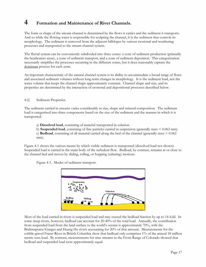
Figure 4-1 shows the various means by which visible sediment is transported (dissolved load not shown). Suspended load is carried in the main body of the turbulent flow. Bedload, by contrast, remains at or close to the channel bed and moves by sliding, rolling, or hopping (saltating) motions.

Figure 4-1. Modes of sediment transport.

Most of the load carried in rivers is suspended load and may exceed the bedload fraction by up to 14-fold. In some steep rivers, however, bedload can account for 20-40% of the total load. Annually, the contribution from suspended load from the land surface to the world’s oceans is approximately 70%, with the Brahmaputra/Ganges and Huang Ho rivers accounting for 20% of that amount. Measurements for the cobble-gravel Fraser River in British Columbia show that bedload only comprises 1% of the annual 18 million metric tons load. By contrast, measurements for nine streams in the Front Range of Colorado showed that bedload and suspended load were approximately equal.

An important characteristic of sediment is the size of the grains. The common grain size classification is provided in Table 4-1.

Table 4-1. Grain size classification.

Class Name Size Range (mm)

Boulders ≥ 256 Cobbles 64 – 256 Gravel 2 – 64 Sand 0.062 – 2 Silt 0.004 – 0.062 Clay ≤ 0.004

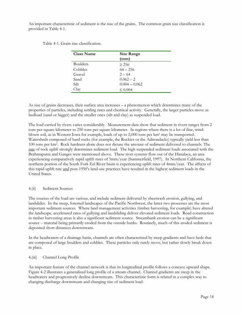
As size of grains decreases, their surface area increases – a phenomenon which determines many of the properties of particles, including settling rates and chemical activity. Generally, the larger particles move as bedload (sand or bigger) and the smaller ones (silt and clay) as suspended load. The load carried by rivers varies considerably. Measurement data show that sediment in rivers ranges from 2 tons per square kilometer to 250 tons per square kilometer. In regions where there is a lot of fine, wind-blown soil, as in Western Iowa for example, loads of up to 2,000 tons per km2 may be transported. Watersheds composed of hard rocks (for example, the Rockies or the Adirondacks) typically yield less than 100 tons per km2. Rock hardness alone does not dictate the amount of sediment delivered to channels. The rate of rock uplift strongly determines sediment load. The high suspended sediment loads associated with the Brahmaputra and Ganges were mentioned above. These river systems flow out of the Himalaya, an area experiencing comparatively rapid uplift rates of 5mm/year (Summerfield, 1997). In Northern California, the northern portion of the South Fork Eel River basin is experiencing uplift rates of 4mm/year. The affects of this rapid uplift rate and post-1950’s land-use practices have resulted in the highest sediment loads in the United States. 4.(ii) Sediment Sources The sources of the load are various, and include sediment delivered by sheetwash erosion, gullying, and landslides. In the steep, forested landscapes of the Pacific Northwest, the latter two processes are the most important sediment sources. Where land management activities (timber harvesting, for example) have altered the landscape, accelerated rates of gullying and landsliding deliver elevated sediment loads. Road construction in timber harvesting areas is also a significant sediment source. Streambank erosion can be a significant source – material being primarily eroded from the outside banks. Routinely, much of this eroded sediment is deposited short distances downstream. In the headwaters of a drainage basin, channels are often characterized by steep gradients and have beds that are composed of large boulders and cobbles. These particles only rarely move, but rather slowly break down in place. 4.(iii) Channel Long Profile An important feature of the channel network is that its longitudinal profile follows a concave upward shape. Figure 4-2 illustrates a generalized long profile of a stream channel. Channel gradients are steep in the headwaters and progressively decline downstream. This characteristic form is related in a complex way to changing discharge downstream and changing size of sediment load.

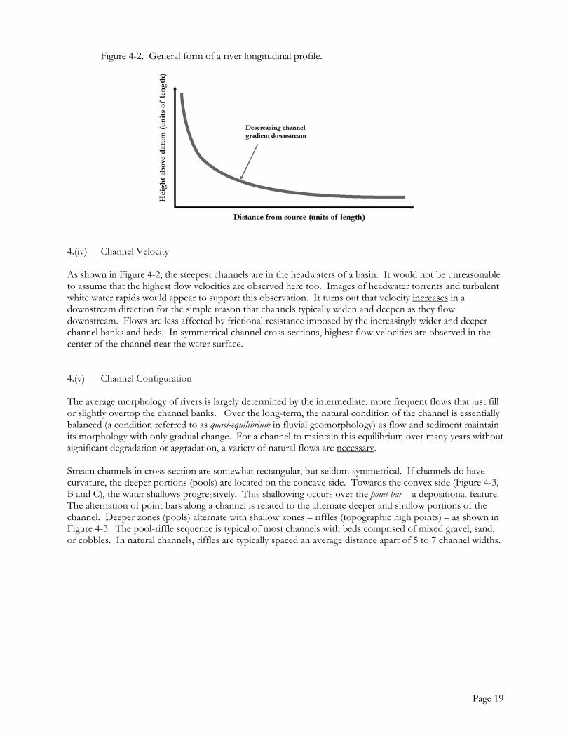
Figure 4-2. General form of a river longitudinal profile.

4.(iv) Channel Velocity As shown in Figure 4-2, the steepest channels are in the headwaters of a basin. It would not be unreasonable to assume that the highest flow velocities are observed here too. Images of headwater torrents and turbulent white water rapids would appear to support this observation. It turns out that velocity increases in a downstream direction for the simple reason that channels typically widen and deepen as they flow downstream. Flows are less affected by frictional resistance imposed by the increasingly wider and deeper channel banks and beds. In symmetrical channel cross-sections, highest flow velocities are observed in the center of the channel near the water surface. 4.(v) Channel Configuration The average morphology of rivers is largely determined by the intermediate, more frequent flows that just fill or slightly overtop the channel banks. Over the long-term, the natural condition of the channel is essentially balanced (a condition referred to as quasi-equilibrium in fluvial geomorphology) as flow and sediment maintain its morphology with only gradual change. For a channel to maintain this equilibrium over many years without significant degradation or aggradation, a variety of natural flows are necessary. Stream channels in cross-section are somewhat rectangular, but seldom symmetrical. If channels do have curvature, the deeper portions (pools) are located on the concave side. Towards the convex side (Figure 4-3, B and C), the water shallows progressively. This shallowing occurs over the point bar – a depositional feature. The alternation of point bars along a channel is related to the alternate deeper and shallow portions of the channel. Deeper zones (pools) alternate with shallow zones – riffles (topographic high points) – as shown in Figure 4-3. The pool-riffle sequence is typical of most channels with beds comprised of mixed gravel, sand, or cobbles. In natural channels, riffles are typically spaced an average distance apart of 5 to 7 channel widths.

Figure 4-3. Pool-riffle sequence (from Mount, 1995).

In mountain streams with very steep gradients, pools and shallows have even more pronounced relief and are referred to as step-pool features. The steps in these profiles may even be small waterfalls. 4.(vi) Channel Classification Channels can be broadly classified into three morphologic categories: straight, meandering, and braided. This simple taxonomy captures the main morphologic distinctions but in doing so, lumps the rich variety of forms observed in nature into just three categories.

a) Straight channels: typically observed in steep headwaters and having little or no connected floodplain. These channels are analogous to water chutes. Downstream of headwater reaches, and into the parts of the drainage basin which have floodplains, perfectly straight channels are rare or are comparatively short in length.

b) Meandering channels: these channels are by far the most ubiquitous natural forms. The curviness or sinuosity of these forms reflect the shape that best conserves energy and at the same time makes energy expenditure along the streamline most uniform. The physical forces which tend to promote a curvilinear form are related to the river’s efforts to carry its load and balance its energy expenditures. The adjustments in energy expenditures and load transport are initiated by the tendency of the flow to be diverted or deflected by heterogeneities of both the bed and bank material. As a consequence, channels tend to develop an asymmetric profile, which in turn forces a river to develop meanders.

c) Braided rivers: rivers that have several interconnected channels. These forms are typically unstable, such that the size and form of the channels are constantly changing. The condition conducive for braiding includes high-energy environments (with steeper channels and high or variable discharges) and high rates of sediment supply. Braided channels can be observed on fans at the mouths of canyons, in the outwash plains of melting glaciers, or in valleys with high gravel loads.

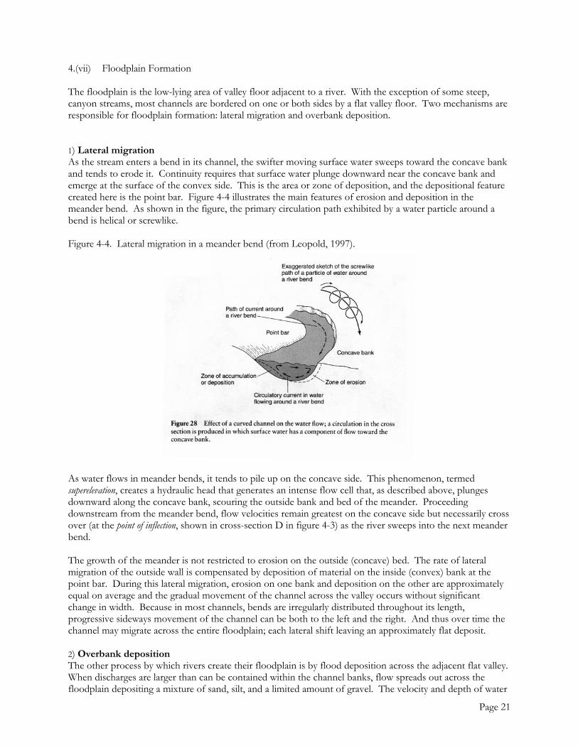
4.(vii) Floodplain Formation The floodplain is the low-lying area of valley floor adjacent to a river. With the exception of some steep, canyon streams, most channels are bordered on one or both sides by a flat valley floor. Two mechanisms are responsible for floodplain formation: lateral migration and overbank deposition. 1) Lateral migration As the stream enters a bend in its channel, the swifter moving surface water sweeps toward the concave bank and tends to erode it. Continuity requires that surface water plunge downward near the concave bank and emerge at the surface of the convex side. This is the area or zone of deposition, and the depositional feature created here is the point bar. Figure 4-4 illustrates the main features of erosion and deposition in the meander bend. As shown in the figure, the primary circulation path exhibited by a water particle around a bend is helical or screwlike. Figure 4-4. Lateral migration in a meander bend (from Leopold, 1997).

As water flows in meander bends, it tends to pile up on the concave side. This phenomenon, termed superelevation, creates a hydraulic head that generates an intense flow cell that, as described above, plunges downward along the concave bank, scouring the outside bank and bed of the meander. Proceeding downstream from the meander bend, flow velocities remain greatest on the concave side but necessarily cross over (at the point of inflection, shown in cross-section D in figure 4-3) as the river sweeps into the next meander bend. The growth of the meander is not restricted to erosion on the outside (concave) bed. The rate of lateral migration of the outside wall is compensated by deposition of material on the inside (convex) bank at the point bar. During this lateral migration, erosion on one bank and deposition on the other are approximately equal on average and the gradual movement of the channel across the valley occurs without significant change in width. Because in most channels, bends are irregularly distributed throughout its length, progressive sideways movement of the channel can be both to the left and the right. And thus over time the channel may migrate across the entire floodplain; each lateral shift leaving an approximately flat deposit. 2) Overbank deposition The other process by which rivers create their floodplain is by flood deposition across the adjacent flat valley. When discharges are larger than can be contained within the channel banks, flow spreads out across the floodplain depositing a mixture of sand, silt, and a limited amount of gravel. The velocity and depth of water

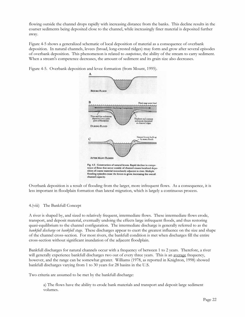
flowing outside the channel drops rapidly with increasing distance from the banks. This decline results in the coarser sediments being deposited close to the channel, while increasingly finer material is deposited further away. Figure 4-5 shows a generalized schematic of local deposition of material as a consequence of overbank deposition. In natural channels, levees (broad, long-crested ridges) may form and grow after several episodes of overbank deposition. This phenomenon is related to competence, the ability of the stream to carry sediment. When a stream's competence decreases, the amount of sediment and its grain size also decreases. Figure 4-5. Overbank deposition and levee formation (from Mount, 1995).

Overbank deposition is a result of flooding from the larger, more infrequent flows. As a consequence, it is less important in floodplain formation than lateral migration, which is largely a continuous process. 4.(viii) The Bankfull Concept A river is shaped by, and sized to relatively frequent, intermediate flows. These intermediate flows erode, transport, and deposit material, eventually undoing the effects large infrequent floods, and thus restoring quasi-equilibrium to the channel configuration. The intermediate discharge is generally referred to as the bankfull discharge or bankfull stage. These discharges appear to exert the greatest influence on the size and shape of the channel cross-section. For most rivers, the bankfull condition is met when discharges fill the entire cross-section without significant inundation of the adjacent floodplain. Bankfull discharges for natural channels occur with a frequency of between 1 to 2 years. Therefore, a river will generally experience bankfull discharges two out of every three years. This is an average frequency, however, and the range can be somewhat greater. Williams (1978, as reported in Knighton, 1998) showed bankfull discharges varying from 1 to 30 years for 28 basins in the U.S. Two criteria are assumed to be met by the bankfull discharge:

a) The flows have the ability to erode bank materials and transport and deposit large sediment volumes.

b) They occur often enough that their effects are not subdued by smaller, more frequent discharge events.

Bankfull discharges are generally considered to be the significant or critical channel forming (or channel maintaining) flow, determining the size and shape of the river channel. One of the most important aspects of the bankfull discharge is that no bedload moves at flows much less than bankfull. This is important in the context of building the point bar, which is primarily composed of bedload deposition. The bulk of bedload movement occurs at flows ranging from 90% of bankfull to twice the bankfull discharge. 4.(ix) Floods and Flood Frequency A flood occurs when the drainage basin experiences an unusually intense or prolonged water input event. The resulting streamflow rate exceeds channel capacity, which, as described in the previous section, are only sized by the more frequent, intermediate flows. Floods are natural events, which occur fairly frequently. They are the most destructive natural hazards in the U.S., causing an average of $4 billion in damages per year (Dingman, 2002). Estimating the frequency with which floods occur and the size of those floods, is studied as a probability problem, where flood occurrence is treated as a random event. For example, if the largest flood in a 30-year period was of a certain size, it is assumed that a flood of equal size will likely recur during the next 30 years. Analysis of flood frequency typically takes for the form of estimating the ‘1-in-N-year’ event of a flood of a given size or larger. Thus a 1-in-100 year flood has the probability of 0.01 (1%) of occurring in any year, and the average recurrence interval between two floods of that magnitude is 100 years. The recurrence interval (in years) for an individual flood is calculated as,

T = ( n + 1 ) / m = 1 / p Where n is the number of years in the record, m is the ranking of the magnitude of that flood, and p is the exceedence probability of occurrence. Data used to calculate recurrence intervals are drawn from records of annual maximum floods, preferably peak discharges. Figure 4-6 shows a graph of recurrence interval against discharge for Seneca Creek in Maryland. Note that both axes are scaled logarithmically, allowing a large range of values to be displayed on the same graph. A flood frequency graph such as this one can be used to reliably calculate the recurrence interval for various discharges within the range of recorded data. The last point is worth emphasizing. Most discharge records in the United States are comparatively short (30-60 years), and therefore estimating the likelihood of rare events is partially a speculative endeavor. Figure 4-7, shows estimated heights of the 10, 100, and 500-year floods for downtown Lisbon in New Hampshire. The 100-year and certainly the 500-year floods are extrapolated estimates far beyond the existing recorded data.

Figure 4-6. Recurrence interval against discharge, Seneca Creek, Maryland (from Leopold, 1997).

The recurrence interval refers to the average spacing of events. It is therefore possible to have 1-in-100 year events occur in consecutive years (although the probability of this happening is very low: 0.01 × 0.01 = 0.0001 or in percent, 0.01%). If we wish to calculate the probability of an event of some magnitude occurring within a specified timeframe, we use the following formula,

q = 1 – ( 1 – p )n where p is the exceedence probability, and n is the number of years of record. So, for example, a probability of the 100-year event occurring within the next 20 years is given by,

q = 1 ( 1 – 0.01 )20 = 0.18 or 18%

Figure 4-7. Flood heights for different recurrence intervals, Lisbon, NH (from Dingman, 2002).

The 1993 floods of the Upper Mississippi were of such magnitude that they might not be repeated for 1,000 years. Official damage estimates exceeded $10 billion, as millions of acres of land were inundated. Given the extraordinary magnitude of the discharges, it’s interesting to note that comparatively little change was observed in the channel morphology. For small basins, flood frequency is strongly influenced by human activities, including, for example, urbanization, agricultural activities, and grazing. The effects of these activities are an alteration of the land surface with the result that peak discharges are typically higher and have shorter time lags. 4.(x) River Terraces. Significant shifts in climate, mountain-building rates or base flow result in an ‘abandonment’ of the floodplain that was previously connected to the stream channel. This abandonment may be a consequence of aggradation or incision. Where incision rates increase, the river cuts through its floodplain leaving a terrace – an abandoned surface no longer related to the present stream. Figure 4-8 shows a generalized cross-section of a sequence of terraces near Sante Fe, NM. The sequence shows the current river bordered by two former floodplains, both at different heights above the present channel. If incision or aggradation occurs repeatedly, it is possible to develop many terrace surfaces at different elevations and composed, in some instances, of different sediment types. Figure 4-8. Former terraces, Sante Fe, NM (from Leopold, 1997).

Terrace formation is also interesting from an archaeological perspective. The relation of human artifacts to their stratigraphic position in the alluvial terrace deposits, provides useful insight into prehistoric cultures. Climate changes are the primary cause of floodplain abandonment and terrace formation. More recently, however, human activities are the main cause for accelerated rates of channel aggradation and incision.

Useful References Global Water Cycle Dingman, S.L. 2002. Physical hydrology. Prentice-Hall. Goudie, A. et al (Ed.). 1994. The encyclopedic dictionary of physical geography. Blackwell. Harte, J. 1988. Consider a spherical cow. University Science Books. Schlesinger, W.H. 1997. Biogeochemistry: An analysis of global Change. Academic Press. Jones, J.A.A. 1997. Global hydrology: Processes, resources and environmental management. Longman. Climate and Meterology Ahrens, C.D. 1994. Meteorology today. West Publishing Company. Dingman, S.L. (op cit). Manning, J.C. 1992. Applied principles of hydrology. Macmillan. Floods Dunne, T. and L.B. Leopold. 1978. Water in environmental planning. Freeman Rivers Allan, J.D. 1996. Stream ecology: structure and function of running waters. Chapman and Hall. Knighton, D. 1998. Fluvial forms and processes. Arnold. Leopold, L.B. 1997. Water, rivers and creeks. University Science Books. Mount, J.M. 1995. California rivers and streams. University of California Press. Summerfield, M.A. 1997. Global geomorphology. Longman

reader supplement i - university of california,...

Documents