michael oberguggenberger alexander ostermann analysis for
TRANSCRIPT
Undergraduate Topics in Computer Science
Michael Oberguggenberger Alexander Ostermann
Analysis for Computer ScientistsFoundations, Methods, and Algorithms
Second Edition

Undergraduate Topics in ComputerScience
Series editor
Ian Mackie
Advisory Board
Samson Abramsky, University of Oxford, Oxford, UKChris Hankin, Imperial College London, London, UKMike Hinchey, University of Limerick, Limerick, IrelandDexter C. Kozen, Cornell University, Ithaca, USAAndrew Pitts, University of Cambridge, Cambridge, UKHanne Riis Nielson, Technical University of Denmark, Kongens Lyngby, DenmarkSteven S. Skiena, Stony Brook University, Stony Brook, USAIain Stewart, University of Durham, Durham, UK

Undergraduate Topics in Computer Science (UTiCS) delivers high-qualityinstructional content for undergraduates studying in all areas of computing andinformation science. From core foundational and theoretical material to final-yeartopics and applications, UTiCS books take a fresh, concise, and modern approachand are ideal for self-study or for a one- or two-semester course. The texts are allauthored by established experts in their fields, reviewed by an international advisoryboard, and contain numerous examples and problems. Many include fully workedsolutions.
More information about this series at http://www.springer.com/series/7592
Michael OberguggenbergerAlexander Ostermann
Analysis for ComputerScientistsFoundations, Methods, and Algorithms
Second Edition
123
Translated in collaboration with Elisabeth Bradley
Michael OberguggenbergerUniversity of InnsbruckInnsbruckAustria
Alexander OstermannUniversity of InnsbruckInnsbruckAustria
ISSN 1863-7310 ISSN 2197-1781 (electronic)Undergraduate Topics in Computer ScienceISBN 978-3-319-91154-0 ISBN 978-3-319-91155-7 (eBook)https://doi.org/10.1007/978-3-319-91155-7
Library of Congress Control Number: 2018941530
1st edition: © Springer-Verlag London Limited 20112nd edition: © Springer Nature Switzerland AG 2018This work is subject to copyright. All rights are reserved by the Publisher, whether the whole or partof the material is concerned, specifically the rights of translation, reprinting, reuse of illustrations,recitation, broadcasting, reproduction on microfilms or in any other physical way, and transmissionor information storage and retrieval, electronic adaptation, computer software, or by similar or dissimilarmethodology now known or hereafter developed.The use of general descriptive names, registered names, trademarks, service marks, etc. in thispublication does not imply, even in the absence of a specific statement, that such names are exempt fromthe relevant protective laws and regulations and therefore free for general use.The publisher, the authors and the editors are safe to assume that the advice and information in thisbook are believed to be true and accurate at the date of publication. Neither the publisher nor theauthors or the editors give a warranty, express or implied, with respect to the material contained herein orfor any errors or omissions that may have been made. The publisher remains neutral with regard tojurisdictional claims in published maps and institutional affiliations.
This Springer imprint is published by the registered company Springer Nature Switzerland AGThe registered company address is: Gewerbestrasse 11, 6330 Cham, Switzerland

Preface to the Second Edition
We are happy that Springer Verlag asked us to prepare the second edition of ourtextbook Analysis for Computer Scientists. We are still convinced that the algo-rithmic approach developed in the first edition is an appropriate concept for pre-senting the subject of analysis. Accordingly, there was no need to make largerchanges.
However, we took the opportunity to add and update some material. In partic-ular, we added hyperbolic functions and gave some more details on curves andsurfaces in space. Two new sections have been added: One on second-order dif-ferential equations and one on the pendulum equation. Moreover, the exercisesections have been extended considerably. Statistical data have been updated whereappropriate.
Due to the essential importance of the MATLAB programs for our concept, wehave decided to provide these programs additionally in Python for the users’convenience.
We thank the editors of Springer, especially Simon Rees and Wayne Wheeler,for their support during the preparation of the second edition.
Innsbruck, Austria Michael OberguggenbergerMarch 2018 Alexander Ostermann
v
Preface to the First Edition
Mathematics and mathematical modelling are of central importance in computerscience. For this reason the teaching concepts of mathematics in computer sciencehave to be constantly reconsidered, and the choice of material and the motivationhave to be adapted. This applies in particular to mathematical analysis, whosesignificance has to be conveyed in an environment where thinking in discretestructures is predominant. On the one hand, an analysis course in computer sciencehas to cover the essential basic knowledge. On the other hand, it has to convey theimportance of mathematical analysis in applications, especially those which will beencountered by computer scientists in their professional life.
We see a need to renew the didactic principles of mathematics teaching incomputer science, and to restructure the teaching according to contemporaryrequirements. We try to give an answer with this textbook which we have devel-oped based on the following concepts:
1. algorithmic approach;2. concise presentation;3. integrating mathematical software as an important component;4. emphasis on modelling and applications of analysis.
The book is positioned in the triangle between mathematics, computer science andapplications. In this field, algorithmic thinking is of high importance. The algo-rithmic approach chosen by us encompasses:
a. development of concepts of analysis from an algorithmic point of view;b. illustrations and explanations using MATLAB andmaple programs as well as Java
applets;c. computer experiments and programming exercises as motivation for actively
acquiring the subject matter;d. mathematical theory combined with basic concepts and methods of numerical
analysis.
Concise presentation means for us that we have deliberately reduced the subjectmatter to the essential ideas. For example, we do not discuss the general conver-gence theory of power series; however, we do outline Taylor expansion with anestimate of the remainder term. (Taylor expansion is included in the book as it is an
vii
indispensable tool for modelling and numerical analysis.) For the sake of read-ability, proofs are only detailed in the main text if they introduce essential ideas andcontribute to the understanding of the concepts. To continue with the exampleabove, the integral representation of the remainder term of the Taylor expansion isderived by integration by parts. In contrast, Lagrange’s form of the remainder term,which requires the mean value theorem of integration, is only mentioned. Never-theless we have put effort into ensuring a self-contained presentation. We assign ahigh value to geometric intuition, which is reflected in a large number ofillustrations.
Due to the terse presentation it was possible to cover the whole spectrum fromfoundations to interesting applications of analysis (again selected from the view-point of computer science), such as fractals, L-systems, curves and surfaces, linearregression, differential equations and dynamical systems. These topics give suffi-cient opportunity to enter various aspects of mathematical modelling.
The present book is a translation of the original German version that appeared in2005 (with the second edition in 2009). We have kept the structure of the Germantext, but took the opportunity to improve the presentation at various places.
The contents of the book are as follows. Chapters 1–8, 10–12 and 14–17 aredevoted to the basic concepts of analysis, and Chapters 9, 13 and 18–21 are ded-icated to important applications and more advanced topics. The Appendices A andB collect some tools from vector and matrix algebra, and Appendix C suppliesfurther details which were deliberately omitted in the main text. The employedsoftware, which is an integral part of our concept, is summarised in Appendix D.Each chapter is preceded by a brief introduction for orientation. The text is enrichedby computer experiments which should encourage the reader to actively acquire thesubject matter. Finally, every chapter has exercises, half of which are to be solvedwith the help of computer programs. The book can be used from the first semesteron as the main textbook for a course, as a complementary text or for self-study.
We thank Elisabeth Bradley for her help in the translation of the text. Further, wethank the editors of Springer, especially Simon Rees and Wayne Wheeler, for theirsupport and advice during the preparation of the English text.
Innsbruck, Austria Michael OberguggenbergerJanuary 2011 Alexander Ostermann
viii Preface to the First Edition

Contents
1 Numbers. . . . . . . . . . . . . . . . . . . . . . . . . . . . . . . . . . . . . . . . . . . . . . . . 11.1 The Real Numbers . . . . . . . . . . . . . . . . . . . . . . . . . . . . . . . . . . . 11.2 Order Relation and Arithmetic on R. . . . . . . . . . . . . . . . . . . . . . 51.3 Machine Numbers. . . . . . . . . . . . . . . . . . . . . . . . . . . . . . . . . . . . 81.4 Rounding . . . . . . . . . . . . . . . . . . . . . . . . . . . . . . . . . . . . . . . . . . 101.5 Exercises. . . . . . . . . . . . . . . . . . . . . . . . . . . . . . . . . . . . . . . . . . . 11
2 Real-Valued Functions . . . . . . . . . . . . . . . . . . . . . . . . . . . . . . . . . . . . 132.1 Basic Notions . . . . . . . . . . . . . . . . . . . . . . . . . . . . . . . . . . . . . . . 132.2 Some Elementary Functions . . . . . . . . . . . . . . . . . . . . . . . . . . . . 172.3 Exercises. . . . . . . . . . . . . . . . . . . . . . . . . . . . . . . . . . . . . . . . . . . 23
3 Trigonometry . . . . . . . . . . . . . . . . . . . . . . . . . . . . . . . . . . . . . . . . . . . . 273.1 Trigonometric Functions at the Triangle . . . . . . . . . . . . . . . . . . . 273.2 Extension of the Trigonometric Functions to R . . . . . . . . . . . . . 313.3 Cyclometric Functions . . . . . . . . . . . . . . . . . . . . . . . . . . . . . . . . 333.4 Exercises. . . . . . . . . . . . . . . . . . . . . . . . . . . . . . . . . . . . . . . . . . . 35
4 Complex Numbers . . . . . . . . . . . . . . . . . . . . . . . . . . . . . . . . . . . . . . . . 394.1 The Notion of Complex Numbers. . . . . . . . . . . . . . . . . . . . . . . . 394.2 The Complex Exponential Function . . . . . . . . . . . . . . . . . . . . . . 424.3 Mapping Properties of Complex Functions . . . . . . . . . . . . . . . . . 444.4 Exercises. . . . . . . . . . . . . . . . . . . . . . . . . . . . . . . . . . . . . . . . . . . 46
5 Sequences and Series. . . . . . . . . . . . . . . . . . . . . . . . . . . . . . . . . . . . . . 495.1 The Notion of an Infinite Sequence . . . . . . . . . . . . . . . . . . . . . . 495.2 The Completeness of the Set of Real Numbers . . . . . . . . . . . . . 555.3 Infinite Series . . . . . . . . . . . . . . . . . . . . . . . . . . . . . . . . . . . . . . . 585.4 Supplement: Accumulation Points of Sequences. . . . . . . . . . . . . 625.5 Exercises. . . . . . . . . . . . . . . . . . . . . . . . . . . . . . . . . . . . . . . . . . . 65
6 Limits and Continuity of Functions . . . . . . . . . . . . . . . . . . . . . . . . . . 696.1 The Notion of Continuity . . . . . . . . . . . . . . . . . . . . . . . . . . . . . . 696.2 Trigonometric Limits . . . . . . . . . . . . . . . . . . . . . . . . . . . . . . . . . 74
ix
6.3 Zeros of Continuous Functions . . . . . . . . . . . . . . . . . . . . . . . . . . 756.4 Exercises. . . . . . . . . . . . . . . . . . . . . . . . . . . . . . . . . . . . . . . . . . . 78
7 The Derivative of a Function . . . . . . . . . . . . . . . . . . . . . . . . . . . . . . . 817.1 Motivation . . . . . . . . . . . . . . . . . . . . . . . . . . . . . . . . . . . . . . . . . 817.2 The Derivative . . . . . . . . . . . . . . . . . . . . . . . . . . . . . . . . . . . . . . 837.3 Interpretations of the Derivative . . . . . . . . . . . . . . . . . . . . . . . . . 877.4 Differentiation Rules . . . . . . . . . . . . . . . . . . . . . . . . . . . . . . . . . . 907.5 Numerical Differentiation . . . . . . . . . . . . . . . . . . . . . . . . . . . . . . 967.6 Exercises. . . . . . . . . . . . . . . . . . . . . . . . . . . . . . . . . . . . . . . . . . . 101
8 Applications of the Derivative . . . . . . . . . . . . . . . . . . . . . . . . . . . . . . 1058.1 Curve Sketching . . . . . . . . . . . . . . . . . . . . . . . . . . . . . . . . . . . . . 1058.2 Newton’s Method . . . . . . . . . . . . . . . . . . . . . . . . . . . . . . . . . . . . 1108.3 Regression Line Through the Origin. . . . . . . . . . . . . . . . . . . . . . 1158.4 Exercises. . . . . . . . . . . . . . . . . . . . . . . . . . . . . . . . . . . . . . . . . . . 118
9 Fractals and L-systems . . . . . . . . . . . . . . . . . . . . . . . . . . . . . . . . . . . . 1239.1 Fractals . . . . . . . . . . . . . . . . . . . . . . . . . . . . . . . . . . . . . . . . . . . . 1249.2 Mandelbrot Sets . . . . . . . . . . . . . . . . . . . . . . . . . . . . . . . . . . . . . 1309.3 Julia Sets . . . . . . . . . . . . . . . . . . . . . . . . . . . . . . . . . . . . . . . . . . 1319.4 Newton’s Method in C . . . . . . . . . . . . . . . . . . . . . . . . . . . . . . . . 1329.5 L-systems . . . . . . . . . . . . . . . . . . . . . . . . . . . . . . . . . . . . . . . . . . 1349.6 Exercises. . . . . . . . . . . . . . . . . . . . . . . . . . . . . . . . . . . . . . . . . . . 138
10 Antiderivatives . . . . . . . . . . . . . . . . . . . . . . . . . . . . . . . . . . . . . . . . . . . 13910.1 Indefinite Integrals . . . . . . . . . . . . . . . . . . . . . . . . . . . . . . . . . . . 13910.2 Integration Formulas . . . . . . . . . . . . . . . . . . . . . . . . . . . . . . . . . . 14210.3 Exercises. . . . . . . . . . . . . . . . . . . . . . . . . . . . . . . . . . . . . . . . . . . 146
11 Definite Integrals . . . . . . . . . . . . . . . . . . . . . . . . . . . . . . . . . . . . . . . . . 14911.1 The Riemann Integral . . . . . . . . . . . . . . . . . . . . . . . . . . . . . . . . . 14911.2 Fundamental Theorems of Calculus . . . . . . . . . . . . . . . . . . . . . . 15511.3 Applications of the Definite Integral . . . . . . . . . . . . . . . . . . . . . . 15811.4 Exercises. . . . . . . . . . . . . . . . . . . . . . . . . . . . . . . . . . . . . . . . . . . 161
12 Taylor Series . . . . . . . . . . . . . . . . . . . . . . . . . . . . . . . . . . . . . . . . . . . . 16512.1 Taylor’s Formula . . . . . . . . . . . . . . . . . . . . . . . . . . . . . . . . . . . . 16512.2 Taylor’s Theorem . . . . . . . . . . . . . . . . . . . . . . . . . . . . . . . . . . . . 16912.3 Applications of Taylor’s Formula . . . . . . . . . . . . . . . . . . . . . . . . 17012.4 Exercises. . . . . . . . . . . . . . . . . . . . . . . . . . . . . . . . . . . . . . . . . . . 173
13 Numerical Integration . . . . . . . . . . . . . . . . . . . . . . . . . . . . . . . . . . . . . 17513.1 Quadrature Formulas . . . . . . . . . . . . . . . . . . . . . . . . . . . . . . . . . 17513.2 Accuracy and Efficiency . . . . . . . . . . . . . . . . . . . . . . . . . . . . . . . 18013.3 Exercises. . . . . . . . . . . . . . . . . . . . . . . . . . . . . . . . . . . . . . . . . . . 182
x Contents
14 Curves . . . . . . . . . . . . . . . . . . . . . . . . . . . . . . . . . . . . . . . . . . . . . . . . . 18514.1 Parametrised Curves in the Plane . . . . . . . . . . . . . . . . . . . . . . . . 18514.2 Arc Length and Curvature . . . . . . . . . . . . . . . . . . . . . . . . . . . . . 19314.3 Plane Curves in Polar Coordinates . . . . . . . . . . . . . . . . . . . . . . . 20014.4 Parametrised Space Curves . . . . . . . . . . . . . . . . . . . . . . . . . . . . . 20214.5 Exercises. . . . . . . . . . . . . . . . . . . . . . . . . . . . . . . . . . . . . . . . . . . 204
15 Scalar-Valued Functions of Two Variables . . . . . . . . . . . . . . . . . . . . 20915.1 Graph and Partial Mappings . . . . . . . . . . . . . . . . . . . . . . . . . . . . 20915.2 Continuity. . . . . . . . . . . . . . . . . . . . . . . . . . . . . . . . . . . . . . . . . . 21115.3 Partial Derivatives. . . . . . . . . . . . . . . . . . . . . . . . . . . . . . . . . . . . 21215.4 The Fréchet Derivative . . . . . . . . . . . . . . . . . . . . . . . . . . . . . . . . 21615.5 Directional Derivative and Gradient . . . . . . . . . . . . . . . . . . . . . . 22115.6 The Taylor Formula in Two Variables . . . . . . . . . . . . . . . . . . . . 22315.7 Local Maxima and Minima. . . . . . . . . . . . . . . . . . . . . . . . . . . . . 22415.8 Exercises. . . . . . . . . . . . . . . . . . . . . . . . . . . . . . . . . . . . . . . . . . . 228
16 Vector-Valued Functions of Two Variables . . . . . . . . . . . . . . . . . . . . 23116.1 Vector Fields and the Jacobian . . . . . . . . . . . . . . . . . . . . . . . . . . 23116.2 Newton’s Method in Two Variables . . . . . . . . . . . . . . . . . . . . . . 23316.3 Parametric Surfaces . . . . . . . . . . . . . . . . . . . . . . . . . . . . . . . . . . 23616.4 Exercises. . . . . . . . . . . . . . . . . . . . . . . . . . . . . . . . . . . . . . . . . . . 238
17 Integration of Functions of Two Variables . . . . . . . . . . . . . . . . . . . . 24117.1 Double Integrals . . . . . . . . . . . . . . . . . . . . . . . . . . . . . . . . . . . . . 24117.2 Applications of the Double Integral . . . . . . . . . . . . . . . . . . . . . . 24717.3 The Transformation Formula . . . . . . . . . . . . . . . . . . . . . . . . . . . 24917.4 Exercises. . . . . . . . . . . . . . . . . . . . . . . . . . . . . . . . . . . . . . . . . . . 253
18 Linear Regression . . . . . . . . . . . . . . . . . . . . . . . . . . . . . . . . . . . . . . . . 25518.1 Simple Linear Regression . . . . . . . . . . . . . . . . . . . . . . . . . . . . . . 25518.2 Rudiments of the Analysis of Variance . . . . . . . . . . . . . . . . . . . 26118.3 Multiple Linear Regression. . . . . . . . . . . . . . . . . . . . . . . . . . . . . 26518.4 Model Fitting and Variable Selection . . . . . . . . . . . . . . . . . . . . . 26718.5 Exercises. . . . . . . . . . . . . . . . . . . . . . . . . . . . . . . . . . . . . . . . . . . 271
19 Differential Equations . . . . . . . . . . . . . . . . . . . . . . . . . . . . . . . . . . . . . 27519.1 Initial Value Problems . . . . . . . . . . . . . . . . . . . . . . . . . . . . . . . . 27519.2 First-Order Linear Differential Equations . . . . . . . . . . . . . . . . . . 27819.3 Existence and Uniqueness of the Solution . . . . . . . . . . . . . . . . . 28319.4 Method of Power Series . . . . . . . . . . . . . . . . . . . . . . . . . . . . . . . 28619.5 Qualitative Theory . . . . . . . . . . . . . . . . . . . . . . . . . . . . . . . . . . . 28819.6 Second-Order Problems . . . . . . . . . . . . . . . . . . . . . . . . . . . . . . . 29019.7 Exercises. . . . . . . . . . . . . . . . . . . . . . . . . . . . . . . . . . . . . . . . . . . 294
Contents xi
20 Systems of Differential Equations . . . . . . . . . . . . . . . . . . . . . . . . . . . . 29720.1 Systems of Linear Differential Equations . . . . . . . . . . . . . . . . . . 29720.2 Systems of Nonlinear Differential Equations. . . . . . . . . . . . . . . . 30820.3 The Pendulum Equation . . . . . . . . . . . . . . . . . . . . . . . . . . . . . . . 31220.4 Exercises. . . . . . . . . . . . . . . . . . . . . . . . . . . . . . . . . . . . . . . . . . . 317
21 Numerical Solution of Differential Equations . . . . . . . . . . . . . . . . . . 32121.1 The Explicit Euler Method . . . . . . . . . . . . . . . . . . . . . . . . . . . . . 32121.2 Stability and Stiff Problems . . . . . . . . . . . . . . . . . . . . . . . . . . . . 32421.3 Systems of Differential Equations . . . . . . . . . . . . . . . . . . . . . . . . 32721.4 Exercises. . . . . . . . . . . . . . . . . . . . . . . . . . . . . . . . . . . . . . . . . . . 328
Appendix A: Vector Algebra . . . . . . . . . . . . . . . . . . . . . . . . . . . . . . . . . . . 331
Appendix B: Matrices . . . . . . . . . . . . . . . . . . . . . . . . . . . . . . . . . . . . . . . . . 343
Appendix C: Further Results on Continuity . . . . . . . . . . . . . . . . . . . . . . . 353
Appendix D: Description of the Supplementary Software . . . . . . . . . . . . 365
References . . . . . . . . . . . . . . . . . . . . . . . . . . . . . . . . . . . . . . . . . . . . . . . . . . 367
Index . . . . . . . . . . . . . . . . . . . . . . . . . . . . . . . . . . . . . . . . . . . . . . . . . . . . . . 369
xii Contents
1Numbers
The commonly known rational numbers (fractions) are not sufficient for a rigor-ous foundation of mathematical analysis. The historical development shows that forissues concerning analysis, the rational numbers have to be extended to the real num-bers. For clarity we introduce the real numbers as decimal numbers with an infinitenumber of decimal places. We illustrate exemplarily how the rules of calculation andthe order relation extend from the rational to the real numbers in a natural way.
A further section is dedicated to floating point numbers, which are implementedinmost programming languages as approximations to the real numbers. In particular,we will discuss optimal rounding and in connection with this the relative machineaccuracy.
1.1 The Real Numbers
In this book we assume the following number systems as known:
N = {1, 2, 3, 4, . . .} the set of natural numbers;N0 = N ∪ {0} the set of natural numbers including zero;Z = {. . . , −3, −2, −1, 0, 1, 2, 3, . . .} the set of integers;Q = { k
n ; k ∈ Z and n ∈ N}
the set of rational numbers.
Two rational numbers kn and �
m are equal if and only if km = �n. Further an integerk ∈ Z can be identified with the fraction k
1 ∈ Q. Consequently, the inclusions N ⊂Z ⊂ Q are true.
© Springer Nature Switzerland AG 2018M. Oberguggenberger and A. Ostermann, Analysis for Computer Scientists,Undergraduate Topics in Computer Science,https://doi.org/10.1007/978-3-319-91155-7_1
1

2 1 Numbers
Let M and N be arbitrary sets. Amapping from M to N is a rule which assigns toeach element in M exactly one element in N .1 A mapping is called bijective, if foreach element n ∈ N there exists exactly one element in M which is assigned to n.
Definition 1.1 Two setsM and N have the same cardinality if there exists a bijectivemapping between these sets. A set M is called countably infinite if it has the samecardinality as N.
The sets N, Z andQ have the same cardinality and in this sense are equally large.All three sets have an infinite number of elements which can be enumerated. Eachenumeration represents a bijective mapping to N. The countability of Z can be seenfrom the representation Z = {0, 1,−1, 2,−2, 3, −3, . . .}. To prove the countabilityof Q, Cantor’s2 diagonal method is being used:
11 → 2
131 → 4
1 . . .
↙ ↗ ↙12
22
32
42 . . .
↓ ↗ ↙13
23
33
43 . . .
↙14
24
34
44 . . .
......
......
The enumeration is carried out in direction of the arrows, where each rational numberis only counted at its first appearance. In this way the countability of all positiverational number (and therefore all rational numbers) is proven.
To visualise the rational numbers we use a line, which can be pictured as aninfinitely long ruler, on which an arbitrary point is labelled as zero. The integers aremarked equidistantly starting from zero. Likewise each rational number is allocateda specific place on the real line according to its size, see Fig. 1.1.
However, the real line also contains points which do not correspond to rationalnumbers. (We say thatQ is not complete.) For instance, the length of the diagonal din the unit square (see Fig. 1.2) can be measured with a ruler. Yet, the Pythagoreansalready knew that d2 = 2, but that d = √
2 is not a rational number.
2a112
130− 1
2−1−2
Fig. 1.1 The real line
1We will rarely use the term mapping in such generality. The special case of real-valued functions,which is important for us, will be discussed thoroughly in Chap. 2.2G. Cantor, 1845–1918.

1.1 The Real Numbers 3
Fig. 1.2 Diagonal in the unitsquare
1
1
√2
Proposition 1.2√2 /∈ Q.
Proof This statement is proven indirectly. Assume that√2 were rational. Then√
2 can be represented as a reduced fraction√2 = k
n ∈ Q. Squaring this equa-tion gives k2 = 2n2 and thus k2 would be an even number. This is only possible ifk itself is an even number, so k = 2l. If we substitute this into the above we obtain4l2 = 2n2 which simplifies to 2l2 = n2. Consequently n would also be even whichis in contradiction to the initial assumption that the fraction k
n was reduced. �
As it is generally known,√2 is the unique positive root of the polynomial x2 − 2.
The naive supposition that all non-rational numbers are roots of polynomials withinteger coefficients turns out to be incorrect. There are other non-rational numbers(so-called transcendental numbers) which cannot be represented in this way. Forexample, the ratio of a circle’s circumference to its diameter
π = 3.141592653589793... /∈ Q
is transcendental, but can be represented on the real line as half the circumferenceof the circle with radius 1 (e.g. through unwinding).
In the following we will take up a pragmatic point of view and construct themissing numbers as decimals.
Definition 1.3 A finite decimal number x with l decimal places has the form
x = ± d0.d1d2d3 . . . dl
with d0 ∈ N0 and the single digits di ∈ {0, 1, . . . , 9}, 1 ≤ i ≤ l, with dl �= 0.
Proposition 1.4 (Representing rational numbers as decimals) Each rational num-ber can be written as a finite or periodic decimal.
Proof Let q ∈ Q and consequently q = kn with k ∈ Z and n ∈ N. One obtains the
representation of q as a decimal by successive division with remainder. Since theremainder r ∈ N always fulfils the condition 0 ≤ r < n, the remainder will be zeroor periodic after a maximum of n iterations. �
Example 1.5 Let us take q = − 57 ∈ Q as an example. Successive division with re-
mainder shows that q = −0.71428571428571... with remainders 5, 1, 3, 2, 6, 4, 5,1, 3, 2, 6, 4, 5, 1, 3, . . . The period of this decimal is six.

4 1 Numbers
Each nonzero decimal with a finite number of decimal places can be written as aperiodic decimal (with an infinite number of decimal places). To this end one dimin-ishes the last nonzero digit by one and then fills the remaining infinitelymany decimalplaces with the digit 9. For example, the fraction − 17
50 = −0.34 = −0.3399999...becomes periodic after the third decimal place. In this way Q can be considered asthe set of all decimals which turn periodic from a certain number of decimal placesonwards.
Definition 1.6 The set of real numbers R consists of all decimals of the form
± d0.d1d2d3...
with d0 ∈ N0 and digits di ∈ {0, ..., 9}, i.e. decimals with an infinite number ofdecimal places. The set R \ Q is called the set of irrational numbers.
Obviously Q ⊂ R. According to what was mentioned so far the numbers
0.1010010001000010... and√2
are irrational. There are much more irrational than rational numbers, as is shown bythe following proposition.
Proposition 1.7 The set R is not countable and has therefore higher cardinalitythan Q.
Proof This statement is proven indirectly. Assume the real numbers between 0 and1 to be countable and tabulate them:
1 0. d11 d12 d13 d14...
2 0. d21 d22 d23 d24...
3 0. d31 d32 d33 d34...
4 0. d41 d42 d43 d44...
. ...
. ...
With the help of this list, we define
di ={1 if dii = 2,2 else.
Then x = 0.d1d2d3d4... is not included in the above list which is a contradiction tothe initial assumption of countability. �

1.1 The Real Numbers 5
30
1;24,51,10
42;25,35
Fig. 1.3 Babylonian cuneiform inscription YBC 7289 (Yale Babylonian Collection, with authori-sation) from 1900 before our time with a translation of the inscription according to [1]. It representsa square with side length 30 and diagonals 42; 25, 35. The ratio is
√2 ≈ 1; 24, 51, 10
However, although R contains considerably more numbers than Q, every realnumber can be approximated by rational numbers to any degree of accuracy, e.g.π to nine digits
π ≈ 314159265
100000000∈ Q.
Good approximations to the real numbers are sufficient for practical applications.For
√2, already the Babylonians were aware of such approximations:
√2 ≈ 1; 24, 51, 10 = 1 + 24
60+ 51
602+ 10
603= 1.41421296... ,
see Fig. 1.3. The somewhat unfamiliar notation is due to the fact that the Babyloniansworked in the sexagesimal system with base 60.
1.2 Order Relation and Arithmetic onR
In the followingwewrite real numbers (uniquely) as decimalswith an infinite numberof decimal places, for example, we write 0.2999... instead of 0.3.
Definition 1.8 (Order relation) Let a = a0.a1a2... and b = b0.b1b2... be non-negative real numbers in decimal form, i.e. a0, b0 ∈ N0.
(a) One says that a is less than or equal to b (and writes a ≤ b), if a = b or if thereis an index j ∈ N0 such that a j < b j and ai = bi for i = 0, . . . , j − 1.
(b) Furthermore one stipulates that always −a ≤ b and sets −a ≤ −b wheneverb ≤ a.
This definition extends the known orders of N and Q to R. The interpretation ofthe order relation ≤ on the real line is as follows: a ≤ b holds true, if a is to the leftof b on the real line, or a = b.
6 1 Numbers
The relation ≤ obviously has the following properties. For all a, b, c ∈ R it holdsthat
a ≤ a (reflexivity),
a ≤ b and b ≤ c ⇒ a ≤ c (transitivity),
a ≤ b and b ≤ a ⇒ a = b (antisymmetry).
In case of a ≤ b and a �= b one writes a < b and calls a less than b. Furthermoreone defines a ≥ b, if b ≤ a (in words: a greater than or equal to b), and a > b, ifb < a (in words: a greater than b).
Addition and multiplication can be carried over from Q to R in a similar way.Graphically one uses the fact that each real number corresponds to a segment onthe real line. One thus defines the addition of real numbers as the addition of therespective segments.
A rigorous and at the same time algorithmic definition of the addition starts fromthe observation that real numbers can be approximated by rational numbers to anydegree of accuracy. Let a = a0.a1a2... and b = b0.b1b2... be two non-negative realnumbers. By cutting them off after k decimal places we obtain two rational approxi-mations a(k) = a0.a1a2...ak ≈ a and b(k) = b0.b1b2...bk ≈ b. Then a(k) + b(k) is amonotonically increasing sequence of approximations to the yet to be defined num-ber a + b. This allows one to define a + b as supremum of these approximations.To justify this approach rigorously we refer to Chap.5. The multiplication of realnumbers is defined in the same way. It turns out that the real numbers with additionandmultiplication (R, +, ·) are a field. Therefore the usual rules of calculation apply,e.g., the distributive law
(a + b)c = ac + bc.
The following proposition recapitulates some of the important rules for ≤. Thestatements can easily be verified with the help of the real line.
Proposition 1.9 For all a, b, c ∈ R the following holds:
a ≤ b ⇒ a + c ≤ b + c,
a ≤ b and c ≥ 0 ⇒ ac ≤ bc,
a ≤ b and c ≤ 0 ⇒ ac ≥ bc.
Note that a < b does not imply a2 < b2. For example −2 < 1, but nonetheless4 > 1. However, for a, b ≥ 0 it always holds that a < b ⇔ a2 < b2.
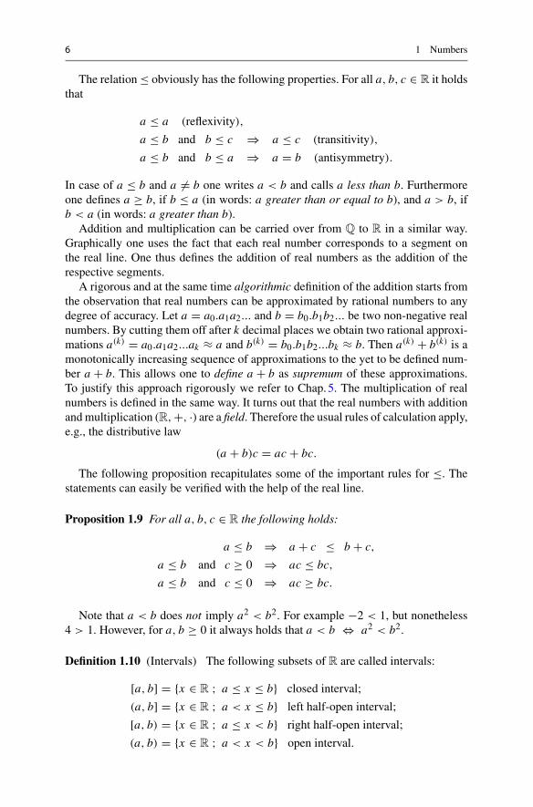
Definition 1.10 (Intervals) The following subsets of R are called intervals:
[a, b] = {x ∈ R ; a ≤ x ≤ b} closed interval;
(a, b] = {x ∈ R ; a < x ≤ b} left half-open interval;
[a, b) = {x ∈ R ; a ≤ x < b} right half-open interval;
(a, b) = {x ∈ R ; a < x < b} open interval.

1.2 Order Relation and Arithmetic onR 7
fedcba
Fig. 1.4 The intervals (a, b), [c, d] and (e, f ] on the real line
Intervals can be visualised on the real line, as illustrated in Fig. 1.4.It proves to be useful to introduce the symbols −∞ (minus infinity) and ∞
(infinity), by means of the property
∀a ∈ R : −∞ < a < ∞.
One may then define, e.g., the improper intervals
[a,∞) = {x ∈ R ; x ≥ a}(−∞, b) = {x ∈ R ; x < b}
and furthermore (−∞, ∞) = R. Note that −∞ and ∞ are only symbols and notreal numbers.
Definition 1.11 The absolute value of a real number a is defined as
|a| ={
a, if a ≥ 0,−a, if a < 0.
As an application of the properties of the order relation given in Proposition 1.9we exemplarily solve some inequalities.
Example 1.12 Find all x ∈ R satisfying −3x − 2 ≤ 5 < −3x + 4. In this examplewe have the following two inequalities
−3x − 2 ≤ 5 and 5 < −3x + 4.
The first inequality can be rearranged to
−3x ≤ 7 ⇔ x ≥ −7
3.
This is the first constraint for x . The second inequality states
3x < −1 ⇔ x < −1
3
and poses a second constraint for x . The solution to the original problem must fulfilboth constraints. Therefore the solution set is
S ={x ∈ R; −7
3≤ x < −1
3
}=
[−7
3,−1
3
).
8 1 Numbers
Example 1.13 Find all x ∈ R satisfying x2 − 2x ≥ 3. By completing the square theinequality is rewritten as
(x − 1)2 = x2 − 2x + 1 ≥ 4.
Taking the square root we obtain two possibilities
x − 1 ≥ 2 or x − 1 ≤ −2.
The combination of those gives the solution set
S = {x ∈ R ; x ≥ 3 or x ≤ −1} = (−∞, −1] ∪ [3, ∞).
1.3 Machine Numbers
The real numbers can be realised only partially on a computer. In exact arithmetic,like for example in maple, real numbers are treated as symbolic expressions, e.g.√2 = RootOf(_Zˆ2-2). With the help of the command evalf they can be
evaluated, exact to many decimal places.The floating point numbers that are usually employed in programming languages
as substitutes for the real numbers have a fixed relative accuracy, e.g. double precisionwith 52 bit mantissa. The arithmetic rules of R are not valid for these machinenumbers, e.g.
1 + 10−20 = 1
in double precision. Floating point numbers are standardised by the Institute ofElectrical and Electronics Engineers IEEE 754-1985 and by the International Elec-trotechnical Commission IEC 559:1989. In the following we give a short outline ofthese machine numbers. Further information can be found in [20].
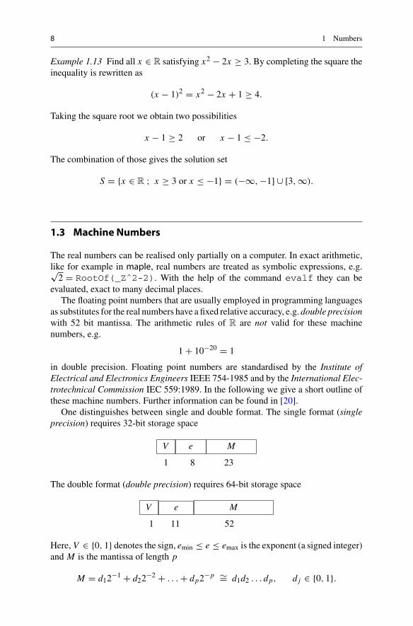
One distinguishes between single and double format. The single format (singleprecision) requires 32-bit storage space
V e M
1 8 23
The double format (double precision) requires 64-bit storage space
V e M
1 11 52
Here, V ∈ {0, 1} denotes the sign, emin ≤ e ≤ emax is the exponent (a signed integer)and M is the mantissa of length p
M = d12−1 + d22
−2 + . . . + dp2−p ∼= d1d2 . . . dp, d j ∈ {0, 1}.
1.3 Machine Numbers 9
2emin+12emin2emin−10
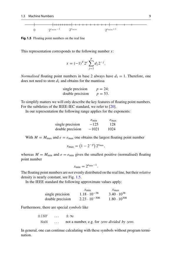
Fig. 1.5 Floating point numbers on the real line
This representation corresponds to the following number x :
x = (−1)V 2ep∑
j=1
d j2− j .
Normalised floating point numbers in base 2 always have d1 = 1. Therefore, onedoes not need to store d1 and obtains for the mantissa
single precision p = 24;double precision p = 53.
To simplify matters we will only describe the key features of floating point numbers.For the subtleties of the IEEE-IEC standard, we refer to [20].
In our representation the following range applies for the exponents:
emin emaxsingle precision −125 128double precision −1021 1024
With M = Mmax and e = emax one obtains the largest floating point number
xmax = (1 − 2−p) 2emax ,
whereas M = Mmin and e = emin gives the smallest positive (normalised) floatingpoint number
xmin = 2emin−1.
Thefloating point numbers are not evenly distributed on the real line, but their relativedensity is nearly constant, see Fig. 1.5.
In the IEEE standard the following approximate values apply:
xmin xmax
single precision 1.18 · 10−38 3.40 · 1038double precision 2.23 · 10−308 1.80 · 10308
Furthermore, there are special symbols like
±INF . . . ± ∞NaN . . . not a number, e.g. for zero divided by zero.
In general, one can continue calculating with these symbols without program termi-nation.
10 1 Numbers
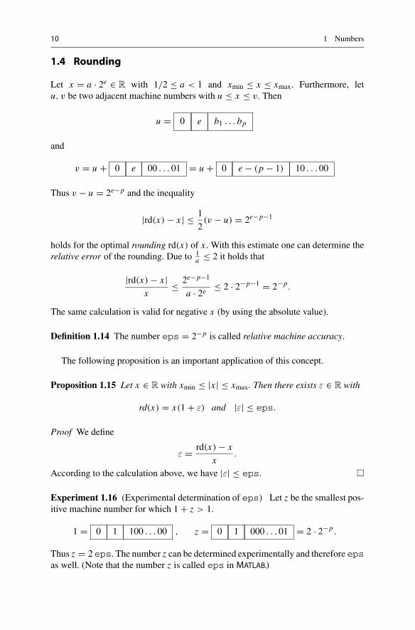
1.4 Rounding
Let x = a · 2e ∈ R with 1/2 ≤ a < 1 and xmin ≤ x ≤ xmax. Furthermore, letu, v be two adjacent machine numbers with u ≤ x ≤ v. Then
u = 0 e b1 . . . bp
and
v = u + 0 e 00 . . . 01 = u + 0 e − (p − 1) 10 . . . 00
Thus v − u = 2e−p and the inequality
|rd(x) − x | ≤ 1
2(v − u) = 2e−p−1
holds for the optimal rounding rd(x) of x . With this estimate one can determine therelative error of the rounding. Due to 1
a ≤ 2 it holds that
|rd(x) − x |x
≤ 2e−p−1
a · 2e ≤ 2 · 2−p−1 = 2−p.
The same calculation is valid for negative x (by using the absolute value).
Definition 1.14 The number eps = 2−p is called relative machine accuracy.
The following proposition is an important application of this concept.
Proposition 1.15 Let x ∈ R with xmin ≤ |x | ≤ xmax. Then there exists ε ∈ R with
rd(x) = x(1 + ε) and |ε| ≤ eps.
Proof We define
ε = rd(x) − x
x.
According to the calculation above, we have |ε| ≤ eps. �
Experiment 1.16 (Experimental determination of eps) Let z be the smallest pos-itive machine number for which 1 + z > 1.
1 = 0 1 100 . . . 00 , z = 0 1 000 . . . 01 = 2 · 2−p.
Thus z = 2eps. The number z can be determined experimentally and therefore epsas well. (Note that the number z is called eps in MATLAB.)

1.4 Rounding 11
In IEC/IEEE standard the following applies:
single precision : eps = 2−24 ≈ 5.96 · 10−8,
double precision : eps = 2−53 ≈ 1.11 · 10−16.
In double precision arithmetic an accuracy of approximately 16 places is available.
1.5 Exercises
1. Show that√3 is irrational.
2. Prove the triangle inequality
|a + b| ≤ |a| + |b|
for all a, b ∈ R.Hint. Distinguish the cases where a and b have either the same or different signs.
3. Sketch the following subsets of the real line:
A = {x : |x | ≤ 1}, B = {x : |x − 1| ≤ 2}, C = {x : |x | ≥ 3}.
More generally, sketch the set Ur (a) = {x : |x − a| < r} (for a ∈ R, r > 0).Convince yourself that Ur (a) is the set of points of distance less than r to thepoint a.
4. Solve the following inequalities by hand as well as withmaple (using solve).State the solution set in interval notation.
(a) 4x2 ≤ 8x + 1, (b)1
3 − x> 3 + x,
(c)∣∣2 − x2
∣∣ ≥ x2, (d)1 + x
1 − x> 1,
(e) x2 < 6 + x, (f)∣∣|x | − x
∣∣ ≥ 1,
(g) |1 − x2| ≤ 2x + 2, (h) 4x2 − 13x + 4 < 1.
5. Determine the solution set of the inequality
8(x − 2) ≥ 20
x + 1+ 3(x − 7).
6. Sketch the regions in the (x, y)-plane which are given by
(a) x = y; (b) y < x; (c) y > x; (d) y > |x |; (e) |y| > |x |.
Hint. Consult Sects.A.1 and A.6 for basic plane geometry.

12 1 Numbers
7. Compute the binary representation of the floating point number x = 0.1 in singleprecision IEEE arithmetic.
8. Experimentally determine the relative machine accuracy eps.Hint. Write a computer program in your programming language of choice whichcalculates the smallest machine number z such that 1 + z > 1.
2Real-Valued Functions
The notion of a function is the mathematical way of formalising the idea that oneor more independent quantities are assigned to one or more dependent quantities.Functions in general and their investigation are at the core of analysis. They help tomodel dependencies of variable quantities, from simple planar graphs, curves andsurfaces in space to solutions of differential equations or the algorithmic constructionof fractals. One the one hand, this chapter serves to introduce the basic concepts. Onthe other hand, the most important examples of real-valued, elementary functionsare discussed in an informal way. These include the power functions, the exponentialfunctions and their inverses. Trigonometric functions will be discussed in Chap.3,complex-valued functions in Chap.4.
2.1 Basic Notions
The simplest case of a real-valued function is a double-row list of numbers, consistingof values from an independent quantity x and corresponding values of a dependentquantity y.
Experiment 2.1 Study the mapping y = x2 with the help of MATLAB. First choosethe region D in which the x-values should vary, for instance D = {x ∈ R : −1 ≤x ≤ 1}. The command
x = −1 : 0.01 : 1;produces a list of x-values, the row vector
x = [x1, x2, . . . , xn] = [−1.00,−0.99,−0.98, . . . , 0.99, 1.00].
© Springer Nature Switzerland AG 2018M. Oberguggenberger and A. Ostermann, Analysis for Computer Scientists,Undergraduate Topics in Computer Science,https://doi.org/10.1007/978-3-319-91155-7_2
13
14 2 Real-Valued Functions
Using
y = x.ˆ2;
a row vector of the same length of corresponding y-values is generated. Finallyplot(x,y) plots the points (x1, y1), . . . , (xn, yn) in the coordinate plane and con-nects them with line segments. The result can be seen in Fig. 2.1.
In the general mathematical framework we do not just want to assign finite listsof values. In many areas of mathematics functions defined on arbitrary sets areneeded. For the general set-theoretic notion of a function we refer to the literature,e.g. [3, Chap.0.2]. This section is dedicated to real-valued functions, which arecentral in analysis.
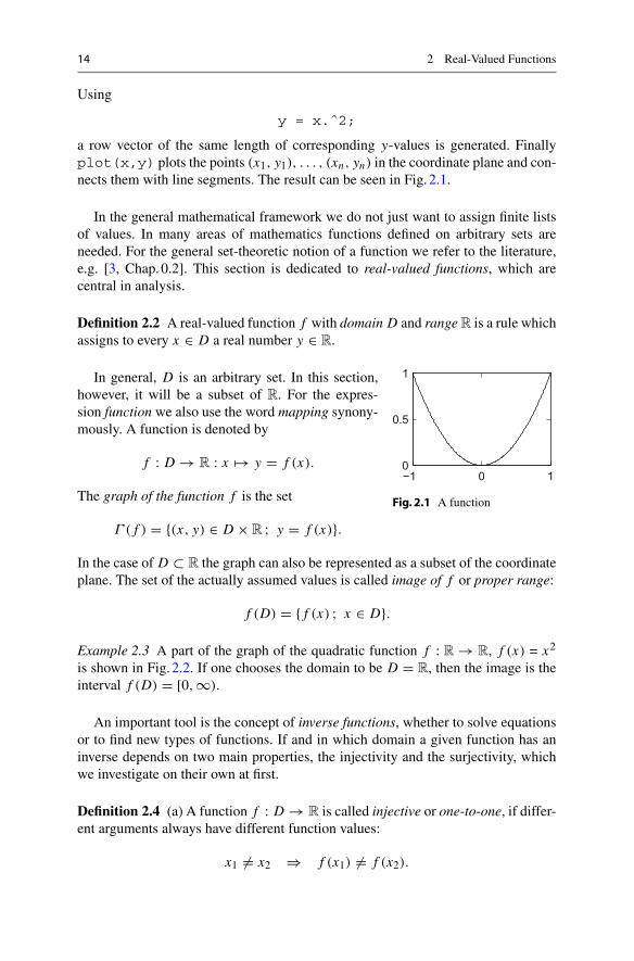
Definition 2.2 A real-valued function f with domain D and range R is a rule whichassigns to every x ∈ D a real number y ∈ R.
−1 0 10
0.5
1
Fig. 2.1 A function
In general, D is an arbitrary set. In this section,however, it will be a subset of R. For the expres-sion function we also use the word mapping synony-mously. A function is denoted by
f : D → R : x �→ y = f (x).
The graph of the function f is the set
Γ ( f ) = {(x, y) ∈ D × R ; y = f (x)}.
In the case of D ⊂ R the graph can also be represented as a subset of the coordinateplane. The set of the actually assumed values is called image of f or proper range:
f (D) = { f (x) ; x ∈ D}.
Example 2.3 A part of the graph of the quadratic function f : R → R, f (x) = x2
is shown in Fig. 2.2. If one chooses the domain to be D = R, then the image is theinterval f (D) = [0,∞).
An important tool is the concept of inverse functions, whether to solve equationsor to find new types of functions. If and in which domain a given function has aninverse depends on two main properties, the injectivity and the surjectivity, whichwe investigate on their own at first.
Definition 2.4 (a) A function f : D → R is called injective or one-to-one, if differ-ent arguments always have different function values:
x1 �= x2 ⇒ f (x1) �= f (x2).

2.1 Basic Notions 15
−1 0 1−0.5
0
0.5
1
1.5
D = R
Γ (f)(x, x2)
y
x
Fig. 2.2 Quadratic function
(b) A function f : D → B ⊂ R is called surjective or onto from D to B, if eachy ∈ B appears as a function value:
∀y ∈ B ∃x ∈ D : y = f (x).
(c) A function f : D → B is called bijective, if it is injective and surjective.
Figures2.3 and 2.4 illustrate these notions.Surjectivity can always be enforced by reducing the range B; for example,
f : D → f (D) is always surjective. Likewise, injectivity can be obtained by restrict-ing the domain to a subdomain.
If f : D → B is bijective, then for every y ∈ B there exists exactly one x ∈ Dwith y = f (x). The mapping y �→ x then defines the inverse of the mapping x �→ y.
Definition 2.5 If the function
f : D → B : y = f (x),
is bijective, then the assignment
f −1 : B → D : x = f −1(y),
−1 0 1
−0.5
0
0.5
1
1.5
−1 0 1−1.5
−1
−0.5
0
0.5
1
1.5
injective
y = x3
x
not injective
y = x2
x
Fig. 2.3 Injectivity

16 2 Real-Valued Functions
−1 0 1
−0.5
0
0.5
1
1.5
−1 0 1−1.5
−1
−0.5
0
0.5
1
1.5
surjective
y = 2x3 − x
x
not surjective on B = R
y = x4
x
Fig. 2.4 Surjectivity
Fig. 2.5 Bijectivity andinverse function
y = f(x) = x2
x = f−1(y) =√
y
y
x
which maps each y ∈ B to the unique x ∈ D with y = f (x) is called the inversefunction of the function f .
Example 2.6 The quadratic function f (x) = x2 is bijective from D = [0,∞) toB = [0,∞). In these intervals (x ≥ 0, y ≥ 0) one has
y = x2 ⇔ x = √y.
Here√
y denotes the positive square root. Thus the inverse of the quadratic functionon the above intervals is given by f −1(y) = √
y ; see Fig. 2.5.
Once one has found the inverse function f −1, it is usually written with variablesy = f −1(x). This corresponds to flipping the graph of y = f (x) about the diagonaly = x , as is shown in Fig. 2.6.
Experiment 2.7 The term inverse function is clearly illustrated by the MATLAB plotcommand. The graph of the inverse function can easily be plotted by interchangingthe variables, which exactly corresponds to flipping the lists y ↔ x . For example,
2.1 Basic Notions 17
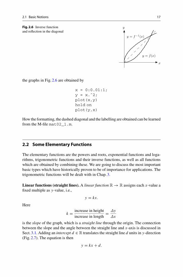
Fig. 2.6 Inverse functionand reflection in the diagonal
y = f−1(x)
y = f(x)
y
x
the graphs in Fig. 2.6 are obtained by
x = 0:0.01:1;y = x.ˆ2;plot(x,y)hold onplot(y,x)
How the formatting, the dashed diagonal and the labelling are obtained can be learnedfrom the M-file mat02_1.m.
2.2 Some Elementary Functions
The elementary functions are the powers and roots, exponential functions and loga-rithms, trigonometric functions and their inverse functions, as well as all functionswhich are obtained by combining these. We are going to discuss the most importantbasic types which have historically proven to be of importance for applications. Thetrigonometric functions will be dealt with in Chap.3.
Linear functions (straight lines). A linear function R → R assigns each x-value afixed multiple as y-value, i.e.,
y = kx .
Here
k = increase in height
increase in length= Δy
Δx
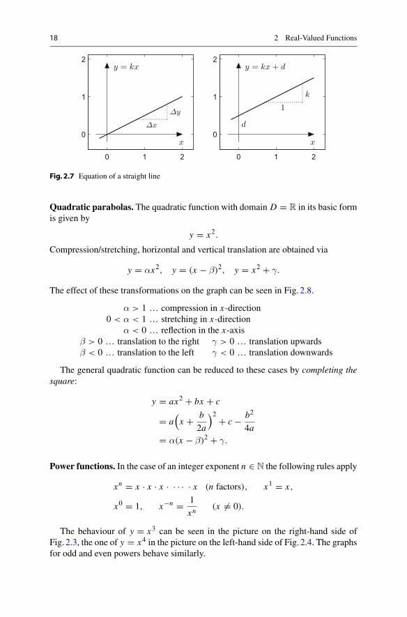
is the slope of the graph, which is a straight line through the origin. The connectionbetween the slope and the angle between the straight line and x-axis is discussed inSect. 3.1. Adding an intercept d ∈ R translates the straight line d units in y-direction(Fig. 2.7). The equation is then
y = kx + d.
18 2 Real-Valued Functions
0 1 2
0
1
2
0 1 2
0
1
2
d
1
k
y = kx + d
x
Δx
Δy
y = kx
x
Fig. 2.7 Equation of a straight line
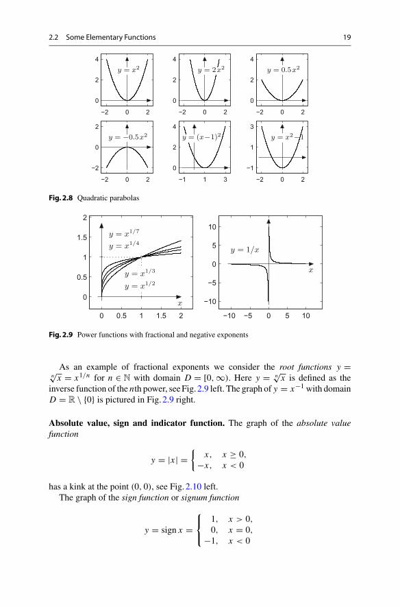
Quadratic parabolas. The quadratic function with domain D = R in its basic formis given by
y = x2.
Compression/stretching, horizontal and vertical translation are obtained via
y = αx2, y = (x − β)2, y = x2 + γ.
The effect of these transformations on the graph can be seen in Fig. 2.8.
α > 1 … compression in x-direction0 < α < 1 … stretching in x-direction
α < 0 … reflection in the x-axisβ > 0 … translation to the right γ > 0 … translation upwardsβ < 0 … translation to the left γ < 0 … translation downwards
The general quadratic function can be reduced to these cases by completing thesquare:
y = ax2 + bx + c
= a(
x + b
2a
)2 + c − b2
4a= α(x − β)2 + γ.
Power functions. In the case of an integer exponent n ∈ N the following rules apply
xn = x · x · x · · · · · x (n factors), x1 = x,
x0 = 1, x−n = 1
xn(x �= 0).
The behaviour of y = x3 can be seen in the picture on the right-hand side ofFig. 2.3, the one of y = x4 in the picture on the left-hand side of Fig. 2.4. The graphsfor odd and even powers behave similarly.
2.2 Some Elementary Functions 19
−2 0 2
0
2
4
−2 0 2
0
2
4
−2 0 2
0
2
4
−2 0 2
−2
0
2
−1 1 3
0
2
4
−2 0 2
−1
1
3y = x2−1y = (x−1)2y = −0.5x2
y = 0.5x2y = 2x2y = x2
Fig. 2.8 Quadratic parabolas
0 0.5 1 1.5 2
0
0.5
1
1.5
2
−10 −5 0 5 10
−10
−5
0
5
10
y = 1/x
x
y = x1/2
y = x1/3
y = x1/4
y = x1/7
x
Fig. 2.9 Power functions with fractional and negative exponents
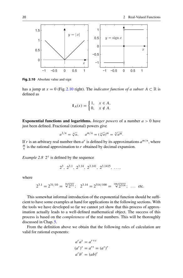
As an example of fractional exponents we consider the root functions y =n√
x = x1/n for n ∈ N with domain D = [0, ∞). Here y = n√
x is defined as theinverse function of the nth power, seeFig. 2.9 left. The graph of y = x−1 with domainD = R \ {0} is pictured in Fig. 2.9 right.
Absolute value, sign and indicator function. The graph of the absolute valuefunction
y = |x | ={
x, x ≥ 0,−x, x < 0
has a kink at the point (0, 0), see Fig. 2.10 left.The graph of the sign function or signum function
y = sign x =⎧⎨⎩
1, x > 0,0, x = 0,
−1, x < 0
20 2 Real-Valued Functions
−1 −0.5 0 0.5 1
0
0.5
1
1.5
−1 −0.5 0 0.5 1
−1
−0.5
0
0.5
1
y = sign x
x
y = |x|
x
Fig. 2.10 Absolute value and sign
has a jump at x = 0 (Fig. 2.10 right). The indicator function of a subset A ⊂ R isdefined as
11A(x) ={1, x ∈ A,
0, x /∈ A.
Exponential functions and logarithms. Integer powers of a number a > 0 havejust been defined. Fractional (rational) powers give
a1/n = n√a, am/n = ( n√a)m = n√am .
If r is an arbitrary real number then ar is defined by its approximations am/n , wheremn is the rational approximation to r obtained by decimal expansion.
Example 2.8 2π is defined by the sequence
23, 23.1, 23.14, 23.141, 23.1415, . . . ,
where
23.1 = 231/10 = 10√231 ; 23.14 = 2314/100 = 100√
2314 ; . . . etc.
This somewhat informal introduction of the exponential function should be suffi-cient to have some examples at hand for applications in the following sections. Withthe tools we have developed so far we cannot yet show that this process of approx-imation actually leads to a well-defined mathematical object. The success of thisprocess is based on the completeness of the real numbers. This will be thoroughlydiscussed in Chap.5.
From the definition above we obtain that the following rules of calculation arevalid for rational exponents:
ar as = ar+s
(ar )s = ars = (as)r
ar br = (ab)r
2.2 Some Elementary Functions 21
Fig. 2.11 Exponentialfunctions
−2 0 20
2
4
6
8
−2 0 20
2
4
6
8
y = (1/2)x
x
y = 2x
x
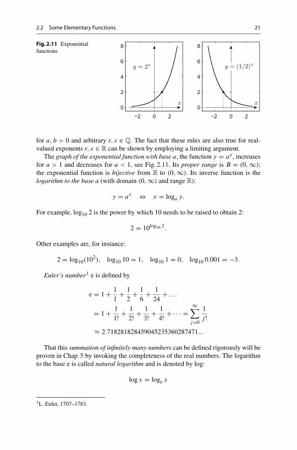
for a, b > 0 and arbitrary r, s ∈ Q. The fact that these rules are also true for real-valued exponents r, s ∈ R can be shown by employing a limiting argument.
The graph of the exponential function with base a, the function y = ax , increasesfor a > 1 and decreases for a < 1, see Fig. 2.11. Its proper range is B = (0,∞);the exponential function is bijective from R to (0, ∞). Its inverse function is thelogarithm to the base a (with domain (0, ∞) and range R):
y = ax ⇔ x = loga y.
For example, log10 2 is the power by which 10 needs to be raised to obtain 2:
2 = 10log10 2.
Other examples are, for instance:
2 = log10(102), log10 10 = 1, log10 1 = 0, log10 0.001 = −3.
Euler’s number1 e is defined by
e = 1 + 1
1+ 1
2+ 1
6+ 1
24+ . . .
= 1 + 1
1! + 1
2! + 1
3! + 1
4! + · · · =∞∑j=0
1
j !≈ 2.718281828459045235360287471...
That this summation of infinitely many numbers can be defined rigorously will beproven in Chap.5 by invoking the completeness of the real numbers. The logarithmto the base e is called natural logarithm and is denoted by log:
log x = loge x
1L. Euler, 1707–1783.
22 2 Real-Valued Functions
0 2 4 6 8 10−2−10123
0 2 4 6 8 10−2−10123
y = log x
e 1 x
y = log10 x
101 x
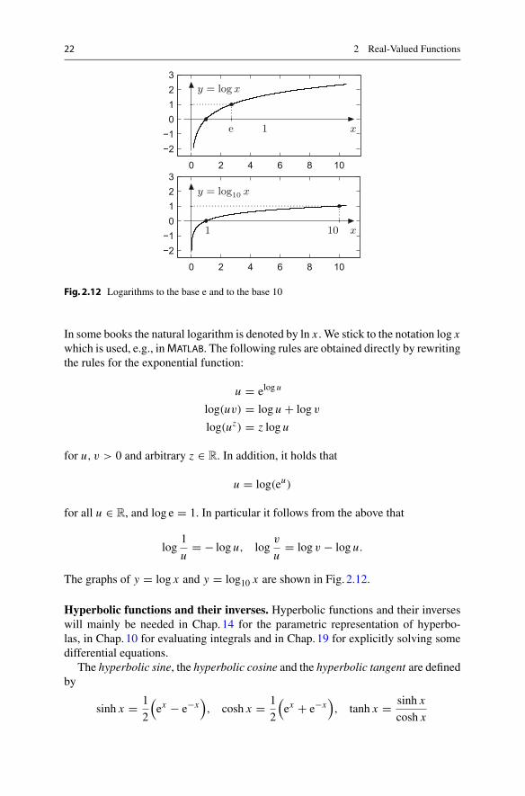
Fig. 2.12 Logarithms to the base e and to the base 10
In some books the natural logarithm is denoted by ln x . We stick to the notation log xwhich is used, e.g., inMATLAB. The following rules are obtained directly by rewritingthe rules for the exponential function:
u = elog u
log(uv) = log u + log v
log(uz) = z log u
for u, v > 0 and arbitrary z ∈ R. In addition, it holds that
u = log(eu)
for all u ∈ R, and log e = 1. In particular it follows from the above that
log1
u= − log u, log
v
u= log v − log u.
The graphs of y = log x and y = log10 x are shown in Fig. 2.12.
Hyperbolic functions and their inverses. Hyperbolic functions and their inverseswill mainly be needed in Chap.14 for the parametric representation of hyperbo-las, in Chap.10 for evaluating integrals and in Chap.19 for explicitly solving somedifferential equations.
The hyperbolic sine, the hyperbolic cosine and the hyperbolic tangent are definedby
sinh x = 1
2
(ex − e−x
), cosh x = 1
2
(ex + e−x
), tanh x = sinh x
cosh x
2.2 Some Elementary Functions 23
-6 -4 -2 0 2 4 6
-1
0
1y
x
-4 -2 0 2 4
-4
-2
0
2
4
y = cosh x
y = sinhx
01
y
x
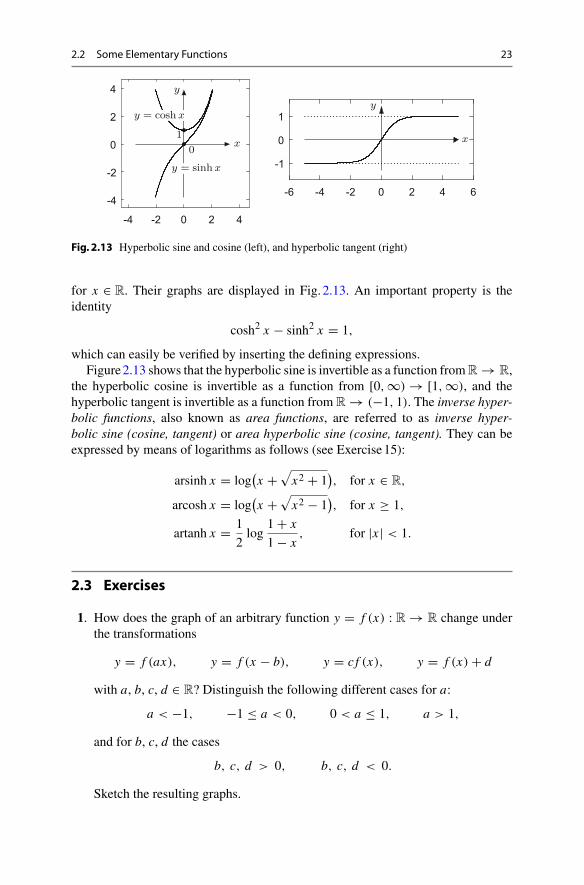
Fig. 2.13 Hyperbolic sine and cosine (left), and hyperbolic tangent (right)
for x ∈ R. Their graphs are displayed in Fig. 2.13. An important property is theidentity
cosh2 x − sinh2 x = 1,
which can easily be verified by inserting the defining expressions.Figure2.13 shows that the hyperbolic sine is invertible as a function fromR → R,
the hyperbolic cosine is invertible as a function from [0,∞) → [1, ∞), and thehyperbolic tangent is invertible as a function from R → (−1, 1). The inverse hyper-bolic functions, also known as area functions, are referred to as inverse hyper-bolic sine (cosine, tangent) or area hyperbolic sine (cosine, tangent). They can beexpressed by means of logarithms as follows (see Exercise15):
arsinh x = log(x +
√x2 + 1
), for x ∈ R,
arcosh x = log(x +
√x2 − 1
), for x ≥ 1,
artanh x = 1
2log
1 + x
1 − x, for |x | < 1.
2.3 Exercises
1. How does the graph of an arbitrary function y = f (x) : R → R change underthe transformations
y = f (ax), y = f (x − b), y = c f (x), y = f (x) + d
with a, b, c, d ∈ R? Distinguish the following different cases for a:
a < −1, −1 ≤ a < 0, 0 < a ≤ 1, a > 1,
and for b, c, d the cases
b, c, d > 0, b, c, d < 0.
Sketch the resulting graphs.
24 2 Real-Valued Functions
2. Let the function f : D → R : x �→ 3x4 − 2x3 − 3x2 + 1 be given. UsingMATLAB plot the graphs of f for
D = [−1, 1.5], D = [−0.5, 0.5], D = [0.5, 1.5].
Explain the behaviour of the function for D = R and find
f ([−1, 1.5]), f ((−0.5, 0.5)), f ((−∞, 1]).
3. Which of the following functions are injective/surjective/bijective?
f : N → N : n �→ n2 − 6n + 10;g : R → R : x �→ |x + 1| − 3;h : R → R : x �→ x3.
Hint. Illustrative examples for the use of the MATLAB plot command may befound in the M-file mat02_2.m.
4. Sketch the graph of the function y = x2 − 4x and justify why it is bijective as afunction from D = (−∞, 2] to B = [−4, ∞). Compute its inverse function onthe given domain.
5. Check that the following functions D → B are bijective in the given regionsand compute the inverse function in each case:
y = −2x + 3, D = R, B = R;y = x2 + 1, D = (−∞, 0] , B = [1,∞) ;y = x2 − 2x − 1, D = [1,∞) , B = [−2,∞) .
6. Find the equation of the straight line through the points (1, 1) and (4, 3) as wellas the equation of the quadratic parabola through the points (−1, 6), (0, 5) and(2, 21).
7. Let the amount of a radioactive substance at time t = 0 be A grams. Accordingto the law of radioactive decay, there remain A · qt grams after t days. Computeq for radioactive iodine 131 from its half life (8 days) and work out after howmany days 1
100 of the original amount of iodine 131 is remaining.Hint. The half life is the time span after which only half of the initial amount ofradioactive substance is remaining.
8. Let I [Watt/cm2] be the sound intensity of a sound wave that hits a detector sur-face. According to theWeber–Fechner law, its sound level L [Phon] is computedby
L = 10 log10(I/I0
)
where I0 = 10−16 W/cm2. If the intensity I of a loudspeaker produces a soundlevel of 80 Phon, which level is then produced by an intensity of 2I by twoloudspeakers?
2.3 Exercises 25
9. For x ∈ R the floor function �x� denotes the largest integer not greater than x ,i.e.,
�x� = max {n ∈ N ; n ≤ x}.Plot the following functions with domain D = [0, 10] using the MATLAB com-mand floor:
y = �x�, y = x − �x�, y = (x − �x�)3 , y = (�x�)3 .
Try to program correct plots in which the vertical connecting lines do not appear.10. A function f : D = {1, 2, . . . , N } → B = {1, 2, . . . , N } is given by the list of
its function values y = (y1, . . . , yN ), yi = f (i).Write aMATLAB programwhichdetermines whether f is bijective. Test your program by generating random y-values using
(a) y = unirnd(N,1,N), (b) y = randperm(N).
Hint. See the two M-files mat02_ex12a.m and mat02_ex12b.m or thePython-file python02_ex12.
11. Draw thegraphof the function f : R → R : y = ax + sign x for different valuesof a. Distinguish between the cases a > 0, a = 0, a < 0. For which values of ais the function f injective and surjective, respectively?
12. Let a > 0, b > 0. Verify the laws of exponents
ar as = ar+s, (ar )s = ars, ar br = (ab)r
for rational r = k/ l, s = m/n.Hint. Start by verifying the laws for integer r and s (and arbitrary a, b > 0). Toprove the first law for rational r = k/ l, s = m/n, write
(ak/ lam/n)ln = (ak/ l)ln(am/n)ln = aknalm = akn+lm
using the third law for integer exponents and inspection; conclude that
ak/ lam/n = a(kn+lm)/ ln = ak/ l+m/n .
13. Using the arithmetics of exponentiation, verify the rules log(uv) = log u + log v
and log uz = z log u for u, v > 0 and z ∈ R.Hint. Set x = log u, y = log v, so uv = exey . Use the laws of exponents andtake the logarithm.
14. Verify the identity cosh2 x − sinh2 x = 1.15. Show that arsinh x = log
(x + √
x2 + 1)for x ∈ R.
Hint. Set y = arsinh x and solve the identity x = sinh y = 12 (e
y − e−y) for y.Substitute u = ey to derive the quadratic equation u2 − 2xu − 1 = 0 for u.Observe that u > 0 to select the appropriate root of this equation.

3Trigonometry
Trigonometric functions play a major role in geometric considerations as well as inthemodelling of oscillations.We introduce these functions at the right-angled triangleand extend them periodically toR using the unit circle. Furthermore, we will discussthe inverse functions of the trigonometric functions in this chapter. As an applicationwe will consider the transformation between Cartesian and polar coordinates.
3.1 Trigonometric Functions at the Triangle
The definitions of the trigonometric functions are based on elementary properties ofthe right-angled triangle. Figure 3.1 shows a right-angled triangle. The sides adjacentto the right angle are called legs (or catheti), the opposite side hypotenuse.
One of the basic properties of the right-angled triangle is expressed by Pythagoras’theorem.1
Proposition 3.1 (Pythagoras) In a right-angled triangle the sum of the squares ofthe legs equals the square of the hypotenuse. In the notation of Fig. 3.1 this says thata2 + b2 = c2.
Proof According to Fig. 3.2 one can easily see that
(a + b)2 − c2 = area of the grey triangles = 2ab.
From this it follows that a2 + b2 − c2 = 0. �
1Pythagoras, approx. 570–501 B.C.
© Springer Nature Switzerland AG 2018M. Oberguggenberger and A. Ostermann, Analysis for Computer Scientists,Undergraduate Topics in Computer Science,https://doi.org/10.1007/978-3-319-91155-7_3
27
28 3 Trigonometry
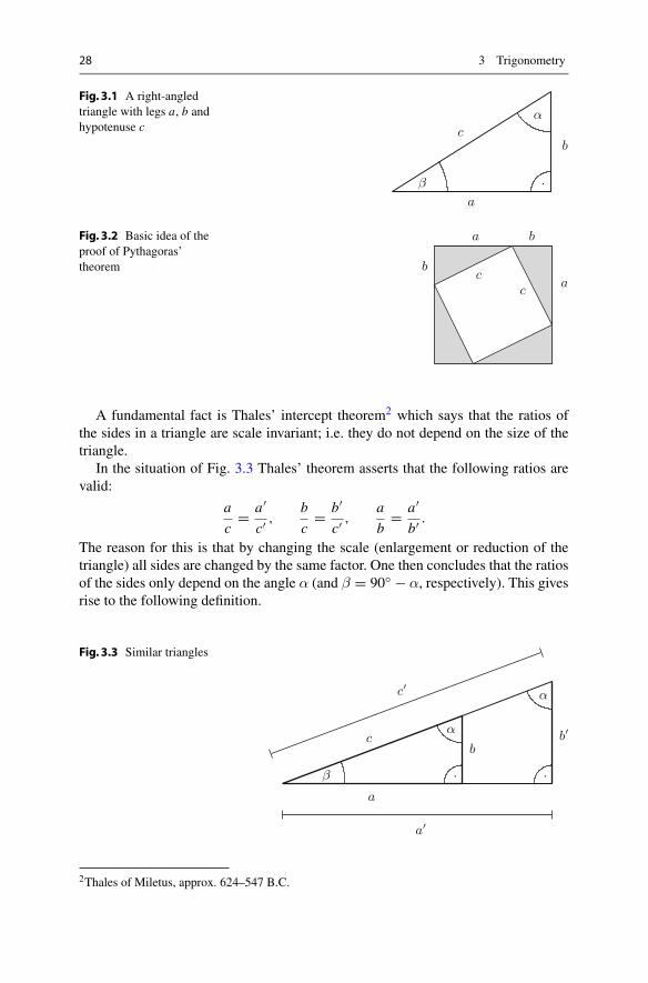
Fig. 3.1 A right-angledtriangle with legs a, b andhypotenuse c
α
β
cb
a
Fig. 3.2 Basic idea of theproof of Pythagoras’theorem
A fundamental fact is Thales’ intercept theorem2 which says that the ratios ofthe sides in a triangle are scale invariant; i.e. they do not depend on the size of thetriangle.
In the situation of Fig. 3.3 Thales’ theorem asserts that the following ratios arevalid:
a
c= a′
c′ ,b
c= b′
c′ ,a
b= a′
b′ .
The reason for this is that by changing the scale (enlargement or reduction of thetriangle) all sides are changed by the same factor. One then concludes that the ratiosof the sides only depend on the angle α (and β = 90◦ − α, respectively). This givesrise to the following definition.
Fig. 3.3 Similar triangles
β
α
α
c
c bb
a
a
2Thales of Miletus, approx. 624–547 B.C.
3.1 Trigonometric Functions at the Triangle 29
Definition 3.2 (Trigonometric functions) For 0◦ ≤ α ≤ 90◦ we define
sinα = a
c= opposite leg
hypotenuse(sine),
cosα = b
c= adjacent leg
hypotenuse(cosine),
tanα = a
b= opposite leg
adjacent leg(tangent),
cot α = b
a= adjacent leg
opposite leg(cotangent).
Note that tanα is not defined for α = 90◦ (since b = 0) and that cot α is notdefined for α = 0◦ (since a = 0). The identities
tanα = sinα
cosα, cot α = cosα
sinα, sinα = cosβ = cos (90◦ − α)
follow directly from the definition, the relationship
sin2 α + cos2 α = 1
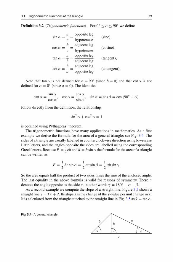
is obtained using Pythagoras’ theorem.The trigonometric functions have many applications in mathematics. As a first
example we derive the formula for the area of a general triangle; see Fig. 3.4. Thesides of a triangle are usually labelled in counterclockwise direction using lowercaseLatin letters, and the angles opposite the sides are labelled using the correspondingGreek letters. Because F = 1
2ch and h = b sinα the formula for the area of a trianglecan be written as
F = 1
2bc sinα = 1
2ac sin β = 1
2ab sin γ.
So the area equals half the product of two sides times the sine of the enclosed angle.The last equality in the above formula is valid for reasons of symmetry. There γdenotes the angle opposite to the side c, in other words γ = 180◦ − α − β.
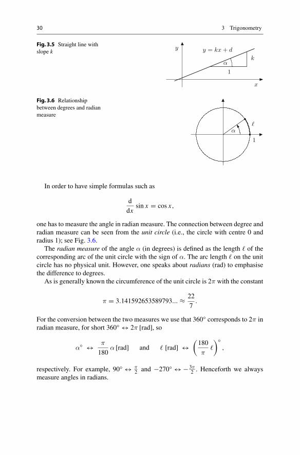
As a second example we compute the slope of a straight line. Figure 3.5 shows astraight line y = kx + d. Its slope k is the change of the y-value per unit change in x .It is calculated from the triangle attached to the straight line in Fig. 3.5 as k = tanα.
Fig. 3.4 A general triangle
βα
hb a
c
30 3 Trigonometry
Fig. 3.5 Straight line withslope k
α
1
k
y = kx + dy
x
Fig. 3.6 Relationshipbetween degrees and radianmeasure
1
α
In order to have simple formulas such as
d
dxsin x = cos x,
one has to measure the angle in radian measure. The connection between degree andradian measure can be seen from the unit circle (i.e., the circle with centre 0 andradius 1); see Fig. 3.6.
The radian measure of the angle α (in degrees) is defined as the length � of thecorresponding arc of the unit circle with the sign of α. The arc length � on the unitcircle has no physical unit. However, one speaks about radians (rad) to emphasisethe difference to degrees.
As is generally known the circumference of the unit circle is 2π with the constant
π = 3.141592653589793... ≈ 22
7.
For the conversion between the two measures we use that 360◦ corresponds to 2π inradian measure, for short 360◦ ↔ 2π [rad], so
α◦ ↔ π
180α [rad] and � [rad] ↔
(180
π�
)◦,
respectively. For example, 90◦ ↔ π2 and −270◦ ↔ − 3π
2 . Henceforth we alwaysmeasure angles in radians.

3.2 Extension of the Trigonometric Functions toR 31
3.2 Extension of the Trigonometric Functions toR
For 0 ≤ α ≤ π2 the values sinα, cosα, tanα and cot α have a simple interpretation
on the unit circle; see Fig. 3.7. This representation follows from the fact that thehypotenuse of the defining triangle has length 1 on the unit circle.
One now extends the definition of the trigonometric functions for 0 ≤ α ≤ 2π bycontinuation with the help of the unit circle. A general point P on the unit circle,which is defined by the angle α, is assigned the coordinates
P = (cosα, sinα),
see Fig. 3.8. For 0 ≤ α ≤ π2 this is compatible with the earlier definition. For larger
angles the sine and cosine functions are extended to the interval [0, 2π] by thisconvention. For example, it follows from the above that
sinα = − sin(α − π), cosα = − cos(α − π)
for π ≤ α ≤ 3π2 , see Fig. 3.8.
For arbitrary values α ∈ R one finally defines sinα and cosα by periodic contin-uation with period 2π. For this purpose one first writes α = x + 2kπ with a uniquex ∈ [0, 2π) and k ∈ Z. Then one sets
sinα = sin (x + 2kπ) = sin x, cosα = cos (x + 2kπ) = cos x .
Fig. 3.7 Definition of thetrigonometric functions onthe unit circle
tanα
cotα
sinα
cosα
1
1
α
Fig. 3.8 Extension of thetrigonometric functions onthe unit circle
sinα
cosα
1
1
P
α

32 3 Trigonometry
−6 −4 −2 0 2 4 6
−1
0
1
−6 −4 −2 0 2 4 6
−1
0
1
x
y y = cosx
− 3π2
−π2−2π
−π
3π2
π2 2π
π
x
y y = sin x
− 3π2
−π2
−2π −π
3π2
π2 2ππ
Fig. 3.9 The graphs of the sine and cosine functions in the interval [−2π, 2π]
With the help of the formulas
tanα = sinα
cosα, cot α = cosα
sinα
the tangent and cotangent functions are extended as well. Since the sine functionequals zero for integermultiples ofπ, the cotangent is not defined for such arguments.Likewise the tangent is not defined for odd multiples of π
2 .The graphs of the functions y = sin x , y = cos x are shown inFig. 3.9. The domain
of both functions is D = R.The graphs of the functions y = tan x and y = cot x are presented in Fig. 3.10.
The domain D for the tangent is, as explained above, given by D = {x ∈ R ; x �=π2 + kπ, k ∈ Z}, the one for the cotangent is D = {x ∈ R ; x �= kπ, k ∈ Z}.Many relations are valid between the trigonometric functions. For example, the
following addition theorems, which can be proven by elementary geometrical con-siderations, are valid; see Exercise 3. Themaple commandsexpand andcombineuse such identities to simplify trigonometric expressions.
Proposition 3.3 (Addition theorems) For x, y ∈ R it holds that
sin (x + y) = sin x cos y + cos x sin y,
cos (x + y) = cos x cos y − sin x sin y.
3.3 Cyclometric Functions 33
−4 −2 0 2 4
−4
−2
0
2
4
−4 −2 0 2 4
−4
−2
0
2
4 y = cotx
x
y
ππ2−π
2
y = tanx
x
y
ππ2−π
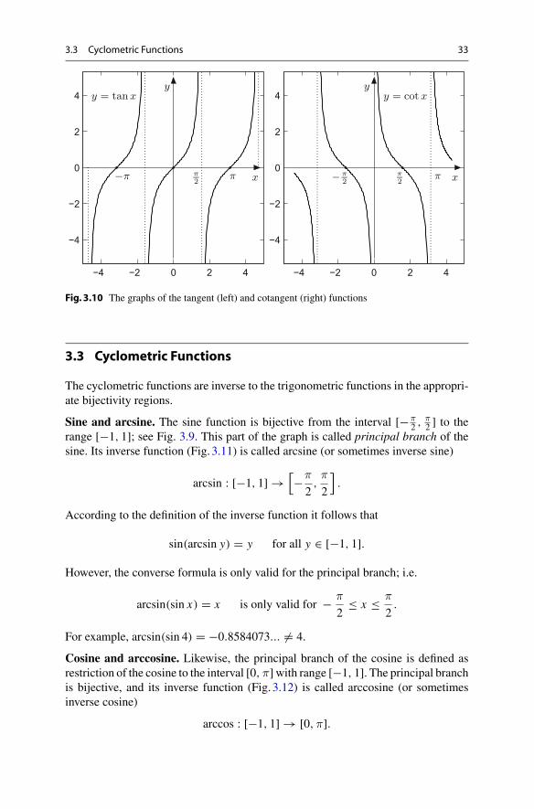
Fig. 3.10 The graphs of the tangent (left) and cotangent (right) functions
3.3 Cyclometric Functions
The cyclometric functions are inverse to the trigonometric functions in the appropri-ate bijectivity regions.
Sine and arcsine. The sine function is bijective from the interval [−π2 , π
2 ] to therange [−1, 1]; see Fig. 3.9. This part of the graph is called principal branch of thesine. Its inverse function (Fig. 3.11) is called arcsine (or sometimes inverse sine)
arcsin : [−1, 1] →[−π
2,π
2
].
According to the definition of the inverse function it follows that
sin(arcsin y) = y for all y ∈ [−1, 1].
However, the converse formula is only valid for the principal branch; i.e.
arcsin(sin x) = x is only valid for − π
2≤ x ≤ π
2.
For example, arcsin(sin 4) = −0.8584073... �= 4.
Cosine and arccosine. Likewise, the principal branch of the cosine is defined asrestriction of the cosine to the interval [0,π]with range [−1, 1]. The principal branchis bijective, and its inverse function (Fig. 3.12) is called arccosine (or sometimesinverse cosine)
arccos : [−1, 1] → [0,π].

34 3 Trigonometry
−2 −1 0 1 2−2
−1
0
1
2
−2 −1 0 1 2−2
−1
0
1
2
y = arcsinx
−π
2
π
2
1
−1
y = sin x
1
−1
−π
2π
2
Fig. 3.11 The principal branch of the sine (left); the arcsine function (right)
0 1 2 3−2
−1
0
1
2
−2 −1 0 1 2
0
1
2
3y = arccos x
π
2
πy = cosx
π
2
π
Fig. 3.12 The principal branch of the cosine (left); the arccosine function (right)
Tangent and arctangent.As can be seen in Fig. 3.10 the restriction of the tangent tothe interval (−π
2 , π2 ) is bijective. Its inverse function is called arctangent (or inverse
tangent)
arctan : R →(−π
2,π
2
).
To be precise this is again the principal branch of the inverse tangent (Fig. 3.13).
−6 −4 −2 0 2 4 6−2
−1
0
1
2
y = arctan x
x
π2
−π2
Fig. 3.13 The principal branch of the arctangent
3.3 Cyclometric Functions 35
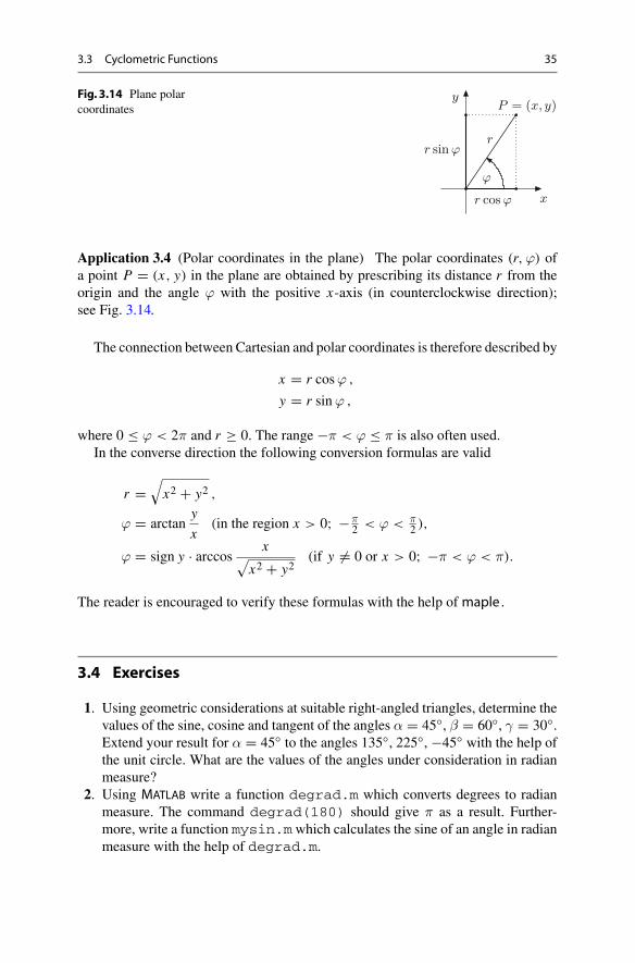
Fig. 3.14 Plane polarcoordinates P = (x, y)
r sinϕ
r cosϕ
y
x
r
ϕ
Application 3.4 (Polar coordinates in the plane) The polar coordinates (r,ϕ) ofa point P = (x, y) in the plane are obtained by prescribing its distance r from theorigin and the angle ϕ with the positive x-axis (in counterclockwise direction);see Fig. 3.14.
The connection between Cartesian and polar coordinates is therefore described by
x = r cosϕ ,
y = r sinϕ ,
where 0 ≤ ϕ < 2π and r ≥ 0. The range −π < ϕ ≤ π is also often used.In the converse direction the following conversion formulas are valid
r =√x2 + y2 ,
ϕ = arctany
x(in the region x > 0; −π
2 < ϕ < π2 ),
ϕ = sign y · arccos x√x2 + y2
(if y �= 0 or x > 0; −π < ϕ < π).
The reader is encouraged to verify these formulas with the help ofmaple .
3.4 Exercises
1. Using geometric considerations at suitable right-angled triangles, determine thevalues of the sine, cosine and tangent of the angles α = 45◦, β = 60◦, γ = 30◦.Extend your result for α = 45◦ to the angles 135◦, 225◦, −45◦ with the help ofthe unit circle. What are the values of the angles under consideration in radianmeasure?
2. Using MATLAB write a function degrad.m which converts degrees to radianmeasure. The command degrad(180) should give π as a result. Further-more, write a function mysin.mwhich calculates the sine of an angle in radianmeasure with the help of degrad.m.
36 3 Trigonometry
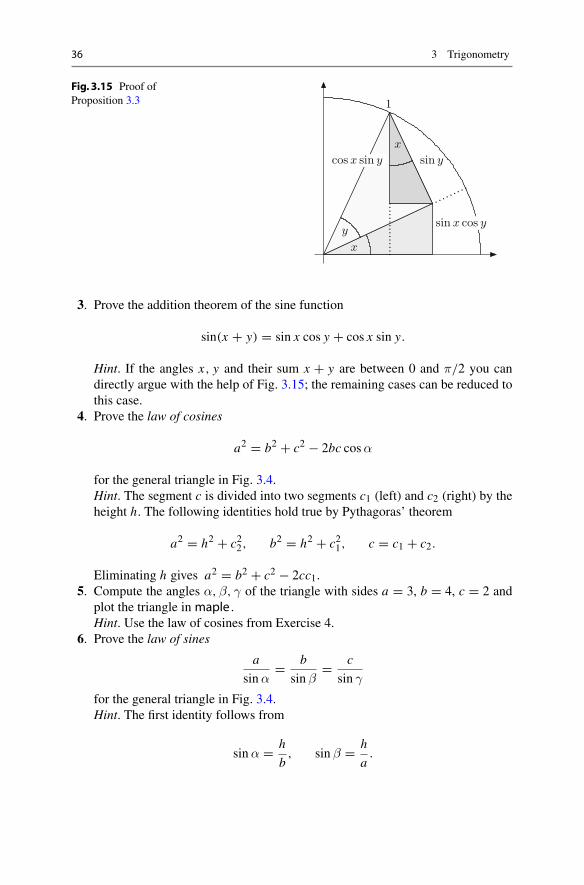
Fig. 3.15 Proof ofProposition 3.3
cosx sin y sin y
x
y
x
1
sin x cos y
3. Prove the addition theorem of the sine function
sin(x + y) = sin x cos y + cos x sin y.
Hint. If the angles x, y and their sum x + y are between 0 and π/2 you candirectly argue with the help of Fig. 3.15; the remaining cases can be reduced tothis case.
4. Prove the law of cosines
a2 = b2 + c2 − 2bc cosα
for the general triangle in Fig. 3.4.Hint. The segment c is divided into two segments c1 (left) and c2 (right) by theheight h. The following identities hold true by Pythagoras’ theorem
a2 = h2 + c22, b2 = h2 + c21, c = c1 + c2.
Eliminating h gives a2 = b2 + c2 − 2cc1.5. Compute the angles α, β, γ of the triangle with sides a = 3, b = 4, c = 2 and
plot the triangle inmaple .Hint. Use the law of cosines from Exercise 4.
6. Prove the law of sines
a
sinα= b
sin β= c
sin γ
for the general triangle in Fig. 3.4.Hint. The first identity follows from
sinα = h
b, sin β = h
a.
3.4 Exercises 37
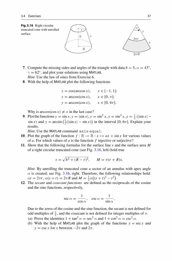
Fig. 3.16 Right circulartruncated cone with unrolledsurface
t
s2πr
2πR
α
h s
R
r
7. Compute the missing sides and angles of the triangle with data b = 5, α = 43◦,γ = 62◦, and plot your solutions using MATLAB.Hint. Use the law of sines from Exercise 6.
8. With the help of MATLAB plot the following functions
y = cos(arccos x), x ∈ [−1, 1];y = arccos(cos x), x ∈ [0,π];y = arccos(cos x), x ∈ [0, 4π].
Why is arccos(cos x) �= x in the last case?9. Plot the functions y = sin x , y = |sin x |, y = sin2 x , y = sin3 x , y = 1
2 (|sin x | −sin x) and y = arcsin
( 12 (|sin x | − sin x)
)in the interval [0, 6π]. Explain your
results.Hint. Use the MATLAB command axis equal.
10. Plot the graph of the function f : R → R : x �→ ax + sin x for various valuesof a. For which values of a is the function f injective or surjective?
11. Show that the following formulas for the surface line s and the surface area Mof a right circular truncated cone (see Fig. 3.16, left) hold true
s =√h2 + (R − r)2, M = π(r + R)s.
Hint. By unrolling the truncated cone a sector of an annulus with apex angleα is created; see Fig. 3.16, right. Therefore, the following relationships hold:αt = 2πr , α(s + t) = 2πR and M = 1
2α((s + t)2 − t2
).
12. The secant and cosecant functions are defined as the reciprocals of the cosineand the sine functions, respectively,
secα = 1
cosα, cscα = 1
sinα.
Due to the zeros of the cosine and the sine function, the secant is not defined forodd multiples of π
2 , and the cosecant is not defined for integer multiples of π.(a) Prove the identities 1 + tan2 α = sec2 α and 1 + cot2 α = csc2 α.(b) With the help of MATLAB plot the graph of the functions y = sec x and
y = csc x for x between −2π and 2π.
4ComplexNumbers
Complex numbers are not just useful when solving polynomial equations but playan important role in many fields of mathematical analysis. With the help of complexfunctions transformations of the plane can be expressed, solution formulas for dif-ferential equations can be obtained, and matrices can be classified. Not least, fractalscan be defined by complex iteration processes. In this section we introduce complexnumbers and then discuss some elementary complex functions, like the complexexponential function. Applications can be found in Chaps. 9 (fractals), 20 (systemsof differential equations) and in Appendix B (normal form of matrices).
4.1 The Notion of Complex Numbers
The set of complex numbers C represents an extension of the real numbers, in whichthe polynomial z2 + 1 has a root. Complex numbers can be introduced as pairs (a, b)of real numbers for which addition and multiplication are defined as follows:
(a, b) + (c, d) = (a + c, b + d),
(a, b) · (c, d) = (ac − bd, ad + bc).
The real numbers are considered as the subset of all pairs of the form (a, 0), a ∈ R.Squaring the pair (0, 1) shows that
(0, 1) · (0, 1) = (−1, 0).
The square of (0, 1) thus corresponds to the real number −1. Therefore, (0, 1) pro-vides a root for the polynomial z2 + 1. This root is denoted by i; in other words
i2 = −1.
© Springer Nature Switzerland AG 2018M. Oberguggenberger and A. Ostermann, Analysis for Computer Scientists,Undergraduate Topics in Computer Science,https://doi.org/10.1007/978-3-319-91155-7_4
39

40 4 Complex Numbers
Using this notation and rewriting the pairs (a, b) in the form a + ib, one obtains acomputationally more convenient representation of the set of complex numbers:
C = {a + ib ; a ∈ R, b ∈ R}.
The rules of calculation with pairs (a, b) then simply amount to the common cal-culations with the expressions a + ib like with terms with the additional rule thati2 = −1:
(a + ib) + (c + id) = a + c + i(b + d),
(a + ib)(c + id) = ac + ibc + iad + i2bd
= ac − bd + i(ad + bc).
So, for example,
(2 + 3i)(−1 + i) = −5 − i.
Definition 4.1 For the complex number z = x + iy,
x = Re z, y = Im z
denote the real part and the imaginary part of z, respectively. The real number
|z| =√x2 + y2
is the absolute value (or modulus) of z, and
z = x − iy
is the complex conjugate to z.
A simple calculation shows that
zz = (x + iy)(x − iy) = x2 + y2 = |z|2,
which means that zz is always a real number. From this we obtain the rule forcalculating with fractions
u + iv
x + iy=
(u + iv
x + iy
)(x − iy
x − iy
)= (u + iv)(x − iy)
x2 + y2= ux + vy
x2 + y2+ i
vx − uy
x2 + y2.
It is achieved by expansion with the complex conjugate of the denominator. Appar-ently one can therefore divide by any complex number not equal to zero, and the setC forms a field.
4.1 The Notion of Complex Numbers 41
Experiment 4.2 Type in MATLAB: z = complex(2,3) (equivalently z = 2+3*ior z = 2+3*j) as well as w = complex(-1,1) and try out the commands z * w,z/w as well as real(z), imag(z), conj(z), abs(z).
Clearly every negative real x has two square roots inC, namely i√|x | and−i
√|x |.More than that the fundamental theorem of algebra says that C is algebraicallyclosed. Thus every polynomial equation
αnzn + αn−1z
n−1 · · · + α1z + α0 = 0
with coefficients α j ∈ C, αn �= 0 has n complex solutions (counted with theirmultiplicity).
Example 4.3 (Taking the square root of complex numbers) The equation z2 = a +ib can be solved by the ansatz
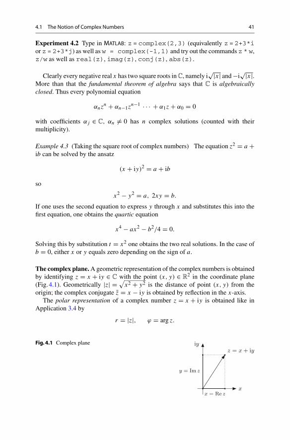
(x + iy)2 = a + ib
so
x2 − y2 = a, 2xy = b.
If one uses the second equation to express y through x and substitutes this into thefirst equation, one obtains the quartic equation
x4 − ax2 − b2/4 = 0.
Solving this by substitution t = x2 one obtains the two real solutions. In the case ofb = 0, either x or y equals zero depending on the sign of a.
The complex plane.A geometric representation of the complex numbers is obtainedby identifying z = x + iy ∈ C with the point (x, y) ∈ R
2 in the coordinate plane(Fig. 4.1). Geometrically |z| = √
x2 + y2 is the distance of point (x, y) from theorigin; the complex conjugate z = x − iy is obtained by reflection in the x-axis.
The polar representation of a complex number z = x + iy is obtained like inApplication 3.4 by
r = |z|, ϕ = arg z.
Fig. 4.1 Complex planez = x + iy
y = Im z
x = Re z
iy
x
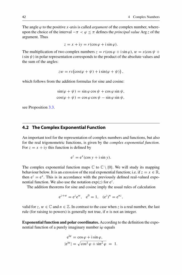
42 4 Complex Numbers
The angle ϕ to the positive x-axis is called argument of the complex number, where-upon the choice of the interval −π < ϕ ≤ π defines the principal valueArg z of theargument. Thus
z = x + iy = r(cosϕ + i sin ϕ).
The multiplication of two complex numbers z = r(cosϕ + i sin ϕ), w = s(cosψ +i sinψ) in polar representation corresponds to the product of the absolute values andthe sum of the angles:
zw = rs(cos(ϕ + ψ) + i sin(ϕ + ψ)
),
which follows from the addition formulas for sine and cosine:
sin(ϕ + ψ) = sin ϕ cosψ + cosϕ sinψ,
cos(ϕ + ψ) = cosϕ cosψ − sin ϕ sinψ,
see Proposition 3.3.
4.2 The Complex Exponential Function
An important tool for the representation of complex numbers and functions, but alsofor the real trigonometric functions, is given by the complex exponential function.For z = x + iy this function is defined by
ez = ex (cos y + i sin y).
The complex exponential function maps C to C \ {0}. We will study its mappingbehaviour below. It is an extension of the real exponential function; i.e. if z = x ∈ R,then ez = ex . This is in accordance with the previously defined real-valued expo-nential function. We also use the notation exp(z) for ez .
The addition theorems for sine and cosine imply the usual rules of calculation
ez+w = ezew, e0 = 1, (ez)n = enz,
valid for z, w ∈ C and n ∈ Z. In contrast to the case when z is a real number, the lastrule (for raising to powers) is generally not true, if n is not an integer.
Exponential function and polar coordinates.According to the definition the expo-nential function of a purely imaginary number iϕ equals
eiϕ = cosϕ + i sin ϕ,
|eiϕ | =√cos2 ϕ + sin2 ϕ = 1.
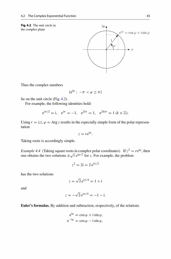
4.2 The Complex Exponential Function 43
Fig. 4.2 The unit circle inthe complex plane
eiϕ = cosϕ + i sinϕ
iy
x
1
ϕ
Thus the complex numbers
{eiϕ ; −π < ϕ ≤ π}lie on the unit circle (Fig. 4.2).
For example, the following identities hold:
eiπ/2 = i, eiπ = −1, e2iπ = 1, e2kiπ = 1 (k ∈ Z).
Using r = |z|, ϕ = Arg z results in the especially simple form of the polar represen-tation
z = reiϕ.
Taking roots is accordingly simple.
Example 4.4 (Taking square roots in complex polar coordinates) If z2 = reiϕ , thenone obtains the two solutions ±√
r eiϕ/2 for z. For example, the problem
z2 = 2i = 2 eiπ/2
has the two solutions
z = √2 eiπ/4 = 1 + i
and
z = −√2 eiπ/4 = −1 − i.
Euler’s formulas. By addition and subtraction, respectively, of the relations
eiϕ = cosϕ + i sin ϕ,
e−iϕ = cosϕ − i sin ϕ,

44 4 Complex Numbers
one obtains at once Euler’s formulas
cosϕ = 1
2
(eiϕ + e−iϕ)
,
sin ϕ = 1
2i
(eiϕ − e−iϕ)
.
They permit a representation of the real trigonometric functions by means of thecomplex exponential function.
4.3 Mapping Properties of Complex Functions
In this sectionwe study themapping properties of complex functions.More precisely,we ask how their effect can be described geometrically. Let
f : D ⊂ C → C : z �→ w = f (z)
be a complex function, defined on a subset D of the complex plane. The effect of thefunction f can best be visualised by plotting two complex planes next to each other,the z-plane and the w-plane, and studying the images of rays and circles under f .
Example 4.5 The complex quadratic function maps D = C to C : w = z2. Usingpolar coordinates one obtains
z = x + iy = r eiϕ ⇒ w = u + iv = r2e2iϕ.
From this representation it can be seen that the complex quadratic function maps acircle of radius r in the z-plane onto a circle of radius r2 in the w-plane. Further, itmaps half-rays
{z = reiψ : r > 0}with the angle of inclinationψ onto half-rays with angle of inclination 2ψ (Fig. 4.3).
Particularly important are the mapping properties of the complex exponentialfunction w = ez because they form the basis for the definition of the complex loga-rithm and the root functions. If z = x + iy then ez = ex (cos y + i sin y). We alwayshave that ex > 0; furthermore cos y + i sin y defines a point on the complex unitcircle which is unique for −π < y ≤ π . If x moves along the real line then thepoints ex (cos y + i sin y) form a half-ray with angle y, as can be seen in Fig. 4.4.Conversely, if x is fixed and y varies between −π and π one obtains the circle withradius ex in the w-plane. For example, the dotted circle (Fig. 4.4, right) is the imageof the dotted straight line (Fig. 4.4, left) under the exponential function.
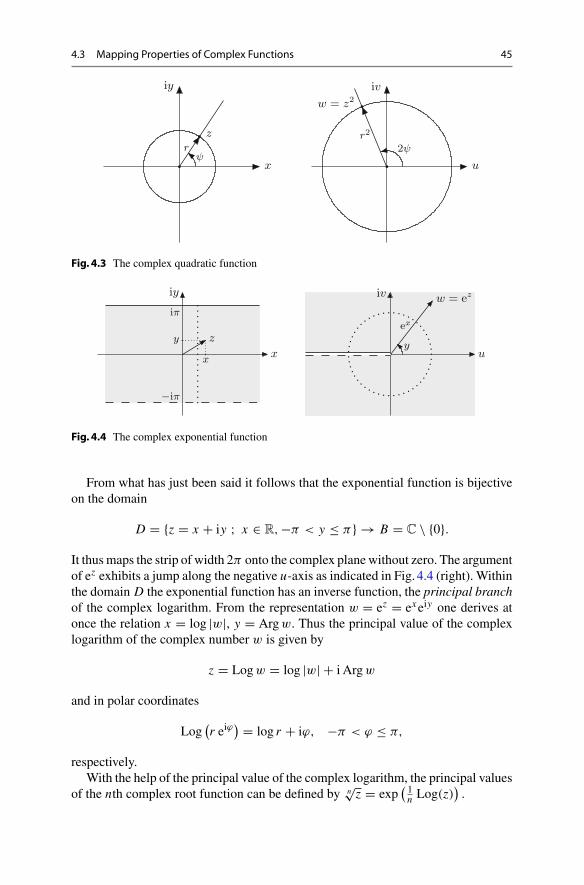
4.3 Mapping Properties of Complex Functions 45
w = z2iv
u
r2
2ψz
iy
x
rψ
Fig. 4.3 The complex quadratic function
w = eziv
u
ex
y
−iπ
iπ
y
x
z
iy
x
Fig. 4.4 The complex exponential function
From what has just been said it follows that the exponential function is bijectiveon the domain
D = {z = x + iy ; x ∈ R, −π < y ≤ π} → B = C \ {0}.It thusmaps the strip of width 2π onto the complex planewithout zero. The argumentof ez exhibits a jump along the negative u-axis as indicated in Fig. 4.4 (right). Withinthe domain D the exponential function has an inverse function, the principal branchof the complex logarithm. From the representation w = ez = exeiy one derives atonce the relation x = log |w|, y = Argw. Thus the principal value of the complexlogarithm of the complex number w is given by
z = Logw = log |w| + i Argw
and in polar coordinates
Log(r eiϕ
) = log r + iϕ, −π < ϕ ≤ π,
respectively.With the help of the principal value of the complex logarithm, the principal values
of the nth complex root function can be defined by n√z = exp
( 1n Log(z)
).
46 4 Complex Numbers
Experiment 4.6 Open the applet 2D visualisation of complex functions and inves-tigate how the power functions w = zn, n ∈ N, map circles and rays of the complexplane. Set the pattern polar coordinates and experiment with different sectors (inter-vals of the argument [α, β] with 0 ≤ α < β ≤ 2π ).
Experiment 4.7 Open the applet 2D visualisation of complex functions and investi-gate how the exponential functionw = ez maps horizontal and vertical straight linesof the complex plane. Set the pattern grid and experiment with different strips, forexample 1 ≤ Re z ≤ 2,−2 ≤ Im z ≤ 2.
4.4 Exercises
1. Compute Re z, Im z, z and |z| for each of the following complex numbers z:
z = 3 + 2i, z = −i, z = 1 + i
2 − i, z = 3 − i + 1
3 − i, z = 1 − 2i
4 − 3i.
Perform these calculations in MATLAB as well.2. Rewrite the following complex numbers in the form z = reiϕ and sketch them
in the complex plane:
z = −1 − i, z = −5, z = 3i, z = 2 − 2i, z = 1 − i√3.
What are the values of ϕ in radian measure?3. Compute the two complex solutions of the equation
z2 = 2 + 2i
with the help of the ansatz z = x + iy and equating the real and the imaginaryparts. Test and explain the MATLAB commands
roots([2,0,-2 - 2 *i])sqrt(2 + 2 *i)
4. Compute the two complex solutions of the equation
z2 = 2 + 2i
in the form z = reiϕ from the polar representation of 2 + 2i.5. Compute the four complex solutions of the quartic equation
z4 − 2z2 + 2 = 0
by hand and with MATLAB (command roots).
4.4 Exercises 47
6. Let z = x + iy, w = u + iv. Check the formula ez+w = ezew by using the def-inition and applying the addition theorems for the trigonometric functions.
7. Compute z = Logw for
w = 1 + i, w = −5i, w = −1.
Sketch w and z in the complex plane and verify your results with the help of therelation w = ez and with MATLAB (command log).
8. The complex sine and cosine functions are defined by
sin z = 1
2i
(eiz − e−iz), cos z = 1
2
(eiz + e−iz)
for z ∈ C.(a) Show that both functions are periodic with period 2π , that is sin(z + 2π) =
sin z, cos(z + 2π) = cos z.(b) Verify that, for z = x + iy,
sin z = sin x cosh y + i cos x sinh y, cos z = cos x cosh y − i sin x sinh y.(c) Show that sin z = 0 if and only if z = kπ , k ∈ Z, and cos z = 0 if and only
if z = (k + 12 )π , k ∈ Z.
5Sequences andSeries
The concept of a limiting process at infinity is one of the central ideas of mathematical analysis.It forms the basis for all its essential concepts, like continuity, differentiability, series expansionsof functions, integration, etc. The transition from a discrete to a continuous setting constitutes themodelling strength of mathematical analysis. Discrete models of physical, technical or economicprocesses can often be better andmore easily understood, provided that the number of their atoms—their discrete building blocks—is sufficiently big, if they are approximated by a continuous modelwith the help of a limiting process. The transition from difference equations for biological growthprocesses in discrete time to differential equations in continuous time are examples for that, as isthe description of share prices by stochastic processes in continuous time. The majority of modelsin physics are field models, that is, they are expressed in a continuous space and time structure.Even though the models are discretised again in numerical approximations, the continuous modelis still helpful as a background, for example for the derivation of error estimates.
The following sections are dedicated to the specification of the idea of limiting processes. Thischapter starts by studying infinite sequences and series, gives some applications and covers thecorresponding notion of a limit. One of the achievements which we especially emphasise is thecompleteness of the real numbers. It guarantees the existence of limits for arbitrary monotonicallyincreasing bounded sequences of numbers, the existence of zeros of continuous functions, ofmaximaand minima of differentiable functions, of integrals, etc. It is an indispensable building block ofmathematical analysis.
5.1 The Notion of an Infinite Sequence
Definition 5.1 Let X be a set. An (infinite) sequence with values in X is a mappingfrom N to X .
© Springer Nature Switzerland AG 2018M. Oberguggenberger and A. Ostermann, Analysis for Computer Scientists,Undergraduate Topics in Computer Science,https://doi.org/10.1007/978-3-319-91155-7_5
49
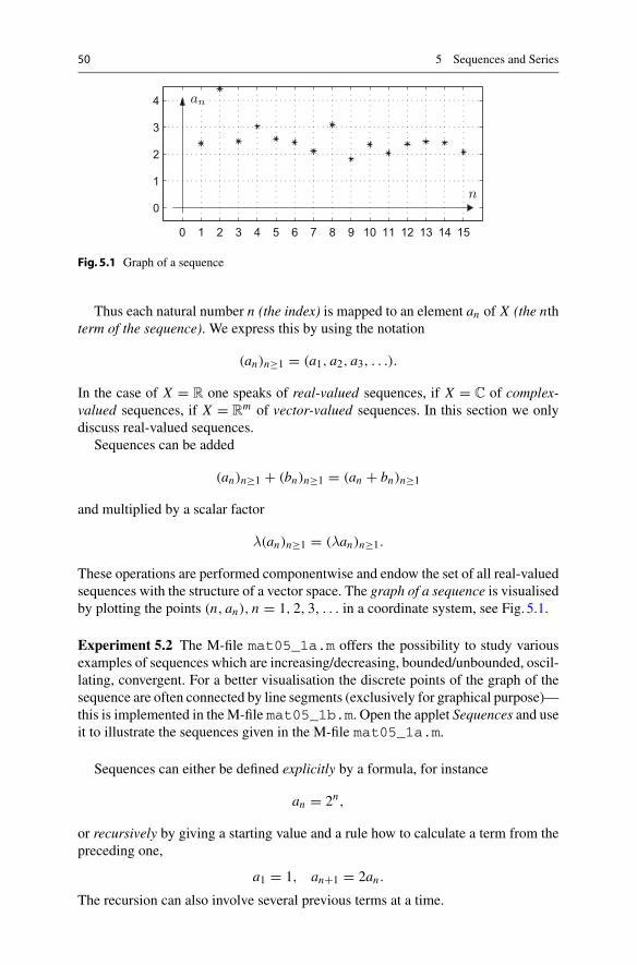
50 5 Sequences and Series
0 1 2 3 4 5 6 7 8 9 10 11 12 13 14 15
0
1
2
3
4 an
n
Fig. 5.1 Graph of a sequence
Thus each natural number n (the index) is mapped to an element an of X (the nthterm of the sequence). We express this by using the notation
(an)n≥1 = (a1, a2, a3, . . .).
In the case of X = R one speaks of real-valued sequences, if X = C of complex-valued sequences, if X = R
m of vector-valued sequences. In this section we onlydiscuss real-valued sequences.
Sequences can be added
(an)n≥1 + (bn)n≥1 = (an + bn)n≥1
and multiplied by a scalar factor
λ(an)n≥1 = (λan)n≥1.
These operations are performed componentwise and endow the set of all real-valuedsequences with the structure of a vector space. The graph of a sequence is visualisedby plotting the points (n, an), n = 1, 2, 3, . . . in a coordinate system, see Fig. 5.1.
Experiment 5.2 The M-file mat05_1a.m offers the possibility to study variousexamples of sequences which are increasing/decreasing, bounded/unbounded, oscil-lating, convergent. For a better visualisation the discrete points of the graph of thesequence are often connected by line segments (exclusively for graphical purpose)—this is implemented in theM-file mat05_1b.m. Open the applet Sequences and useit to illustrate the sequences given in the M-file mat05_1a.m.
Sequences can either be defined explicitly by a formula, for instance
an = 2n,
or recursively by giving a starting value and a rule how to calculate a term from thepreceding one,
a1 = 1, an+1 = 2an .
The recursion can also involve several previous terms at a time.

5.1 The Notion of an Infinite Sequence 51
Example 5.3 A discrete population model which goes back to Verhulst1 (limitedgrowth) describes the population xn at the point in time n (using time intervals oflength 1) by the recursive relation
xn+1 = xn + βxn(L − xn).
Here β is a growth factor and L the limiting population, i.e. the population whichis not exceeded in the long-term (short-term overruns are possible, however, leadto immediate decay of the population). Additionally one has to prescribe the initialpopulation x1 = A. According to themodel the population increase xn+1 − xn duringone time interval is proportional to the existing population and to the difference tothe population limit. The M-file mat05_2.m contains aMATLAB function, called as
x = mat05_2(A,beta,N)
which computes and plots the first N terms of the sequence x = (x1, . . . , xN ). Theinitial value is A, the growth rate β; L was set to L = 1. Experiments with A = 0.1,N = 50 and β = 0.5, β = 1, β = 2, β = 2.5, β = 3 show convergent, oscillatingand chaotic behaviour of the sequence, respectively.
Below we develop some concepts which help to describe the behaviour ofsequences.
Definition 5.4 A sequence (an)n≥1 is called monotonically increasing, if
n ≤ m ⇒ an ≤ am;
(an)n≥1 is called monotonically decreasing, if
n ≤ m ⇒ an ≥ am;
(an)n≥1 is called bounded from above, if
∃T ∈ R ∀n ∈ N : an ≤ T .
Wewill show in Proposition5.13 below that the set of upper bounds of a boundedsequence has a smallest element. This least upper bound T0 is called the supremumof the sequence and denoted by
T0 = supn∈N
an .
1P.-F. Verhulst, 1804–1849.

52 5 Sequences and Series
The supremum is characterised by the following two conditions:
(a) an ≤ T0 for all n ∈ N;
(b) if T is a real number and an ≤ T for all n ∈ N, then T ≥ T0.
Note that the supremum itself does not have to be a term of the sequence. However,if this is the case, it is called maximum of the sequence and denoted by
T0 = maxn∈N an .
A sequence has a maximum T0 if the following two conditions are fulfilled:
(a) an ≤ T0 for all n ∈ N;
(b) there exists at least one m ∈ N such that am = T0.
In the same way, a sequence (an)n≥1 is called bounded from below, if
∃S ∈ R ∀n ∈ N : S ≤ an .
The greatest lower bound is called infimum (or minimum, if it is attained by a termof the sequence).
Experiment 5.5 Investigate the sequences produced by the M-file mat05_1a.mwith regard to the concepts developed above.
As mentioned in the introduction to this chapter, the concept of convergence isa central concept of mathematical analysis. Intuitively it states that the terms of thesequence (an)n≥1 approach a limit a with growing index n. For example, in Fig. 5.2with a = 0.8 one has
|a − an| < 0.2 from n = 6, |a − an| < 0.05 from n = 21.
0 5 10 15 20 25 30
0
0.4
0.8
1.2
1.6an
n
Fig. 5.2 Convergence of a sequence
5.1 The Notion of an Infinite Sequence 53
For a precise definition of the concept of convergence we first introduce the notionof an ε-neighbourhood of a point a ∈ R (ε > 0):
Uε(a) = {x ∈ R ; |a − x | < ε} = (a − ε, a + ε).
We say that a sequence (an)n≥1 settles in a neighbourhood Uε(a), if from a certainindex n(ε) on all subsequent terms an of the sequence lie in Uε(a).
Definition 5.6 The sequence (an)n≥1 converges to a limit a if it settles in eachε-neighbourhood of a.
These facts can be expressed in quantifier notation as follows:
∀ε > 0 ∃n(ε) ∈ N ∀n ≥ n(ε) : |a − an| < ε.
If a sequence (an)n≥1 converges to a limit a, one writes
a = limn→∞ an or an → a as n → ∞.
In the example of Fig. 5.2 the limit a is indicated as a dotted line, the neighbourhoodU0.2(a) as a strip with a dashed boundary line and the neighbourhood U0.05(a) as astrip with a solid boundary line.
In the case of convergence the limit can be interchanged with addition, multipli-cation and division (with the exception of zero), as expected.
Proposition 5.7 (Rules of calculation for limits) If the sequences (an)n≥1 and(bn)n≥1 are convergent then the following rules hold:
limn→∞(an + bn) = lim
n→∞ an + limn→∞ bn
limn→∞(λan) = λ lim
n→∞ an (for λ ∈ R)
limn→∞(anbn) = ( lim
n→∞ an)( limn→∞ bn)
limn→∞(an/bn) = ( lim
n→∞ an)/( limn→∞ bn) (if lim
n→∞ bn = 0)
Proof The verification of these trivialities is left to the reader as an exercise. Theproofs are not deep, but one has to carefully pick the right approach in order to verifythe conditions of Definition5.6. In order to illustrate at least once how such proofsare done, we will show the statement about multiplication. Assume that
limn→∞ an = a and lim
n→∞ bn = b.
Let ε > 0. According to Definition5.6 we have to find an index n(ε) ∈ N satisfying
|ab − anbn| < ε

54 5 Sequences and Series
for all n ≥ n(ε). Due to the convergence of the sequence (an)n≥1 we can first findan n1(ε) ∈ N so that |a − an| ≤ 1 for all n ≥ n1(ε). For these n it also applies that
|an| = |an − a + a| ≤ 1 + |a|.
Furthermore, we can find n2(ε) ∈ N and n3(ε) ∈ N which guarantee that
|a − an| < ε
2max(|b|, 1) and |b − bn| < ε
2(1 + |a|)for all n ≥ n2(ε) and n ≥ n3(ε), respectively. It thus follows that
|ab − anbn| = |(a − an)b + an(b − bn)| ≤ |a − an||b| + |an||b − bn|≤ |a − an||b| + (|a| + 1)|b − bn| ≤ ε
2+ ε
2≤ ε
for all n ≥ n(ε)with n(ε) = max(n1(ε), n2(ε), n3(ε)). This is the statement that wasto be proven. �
The important ideas of the proof were: Splitting in two summands with the help ofthe triangle inequality (see Exercise 2 of Chap.1); bounding |an| by 1 + |a| using theassumed convergence; upper bounds for the terms |a − an| and |b − bn| by fractionsof ε (again possible due to the convergence) so that the summands together stay lessthan ε. All elementary proofs of convergence in mathematical analysis proceed in asimilar way.
Real-valued sequences with terms that increase to infinity with growing index nhave no limit in the sense of the definition given above. However, it is practical toassign them the symbol ∞ as an improper limit.
Definition 5.8 A sequence (an)n≥1 has the improper limit ∞ if it has the propertyof unlimited increase
∀T ∈ R ∃n(T ) ∈ N ∀n ≥ n(T ) : an ≥ T .
In this case one writes
limn→∞ an = ∞.
In the same way one defines
limn→∞ bn = −∞, if lim
n→∞(−bn) = ∞.
5.1 The Notion of an Infinite Sequence 55
Example 5.9 We consider the geometric sequence (qn)n≥1. It obviously holds that
limn→∞ qn = 0, if |q| < 1,
limn→∞ qn = ∞, if q > 1,
limn→∞ qn = 1, if q = 1.
For q ≤ −1 the sequence has no limit (neither proper nor improper).
5.2 The Completeness of the Set of Real Numbers
As remarked in the introduction to this chapter, the completeness of the set of realnumbers is one of the pillars of real analysis. The property of completeness can beexpressed in different ways. We will use a simple formulation which is particularlyhelpful in many applications.
Proposition 5.10 (Completeness of the set of real numbers) Each monotonicallyincreasing sequence of real numbers that is bounded from above has a limit (in R).
Proof Let (an)n≥1 be a monotonically increasing, bounded sequence. First we provethe theorem in the case that all terms an are non-negative. We write the terms asdecimal numbers
an = A(n).α(n)1 α(n)
2 α(n)3 . . .
with A(n)∈ N0, α(n)j ∈ {0, 1, . . . , 9}. By assumption there is a bound T ≥ 0 so that
an ≤ T for all n. Therefore, also A(n) ≤ T for all n. But the sequence (A(n))n≥1is a monotonically increasing, bounded sequence of integers and therefore musteventually reach its least upper bound A (and stay there). In other words, there existsn0 ∈ N such that
A(n) = A for all n ≥ n0.
Thus we have found the integer part of the limit a to be constructed:
a = A. . . .
Let now α1 ∈ {0, . . . , 9} be the least upper bound for α(n)1 . As the sequence is mono-
tonically increasing there is again an n1 ∈ N with
α(n)1 = α1 for all n ≥ n1
56 5 Sequences and Series
and consequently
a = A.α1 . . .
Let now α2 ∈ {0, . . . , 9} be the least upper bound for α(n)2 . There is an n2 ∈ N with
α(n)2 = α2 for all n ≥ n2
and consequently
a = A.α1α2 . . .
Successively one defines a real number
a = A.α1α2α3α4 . . .
in that way. It remains to show that a = limn→∞ an . Let ε > 0. We first choosej ∈ N so that 10− j < ε. For n ≥ n j
a − an = 0.000 . . . 0α(n)j+1 α(n)
j+2 . . . ,
since the first j digits after the decimal point in a coincide with those of an providedn ≥ n j . Therefore,
|a − an| ≤ 10− j < ε for n ≥ n j .
With n(ε) = n j the condition required in Definition5.6 is fulfilled.If the sequence (an)n≥1 also has negative terms, it can be transformed to a sequence
with non-negative terms by adding the absolute value of the first term which resultsin the sequence (|a1| + an)n≥1. Using the obvious rule lim(c + an) = c + lim anallows one to apply the first part of the proof. �
Remark 5.11 The set of rational numbers is not complete. For example, the decimalexpansion of
√2,
(1, 1.4, 1.41, 1.414, 1.4142, . . .)
is a monotonically increasing, bounded sequence of rational numbers (an upperbound is, e.g. T = 1.5, since 1.52 > 2), but the limit
√2 does not belong to Q (as it
is an irrational number).
Example 5.12 (Arithmetic of real numbers) Due to Proposition5.10 the arithmeti-cal operations on the real numbers introduced in Sect. 1.2 can be legitimised a poste-riori. Let us look, for instance, at the addition of two non-negative real numbersa = A.α1α2 . . . and b = B.β1β2 . . . with A, B ∈ N0, α j ,β j ∈ {0, 1, . . . , 9}. By
5.2 The Completeness of the Set of Real Numbers 57
truncating them after the nth decimal place we obtain two approximating sequencesof rational numbers an = A.α1α2 . . .αn and bn = B.β1β2 . . .βn with
a = limn→∞ an, b = lim
n→∞ bn .
The sum of two approximations an + bn is defined by the addition of rational num-bers in an elementary way. The sequence (an + bn)n≥1 is evidently monotonicallyincreasing andbounded fromabove, for instance, by A + B + 2.According toPropo-sition5.10 this sequence has a limit and this limit defines the sum of the real numbers
a + b = limn→∞(an + bn).
In this way the addition of real numbers is rigorously justified. In a similar wayone can proceed with multiplication. Finally, Proposition5.7 allows one to prove theusual rules for addition and multiplication.
Consider a sequence with upper bound T . Each real number T1 > T is also anupper bound. We can now show that there always exists a smallest upper bound. Abounded sequence thus actually has a supremum as claimed earlier.
Proposition 5.13 Each sequence (an)n≥1 of real numbers which is bounded fromabove has a supremum.
Proof Let Tn = max{a1, . . . , an} be the maximum of the first n terms of thesequence. These maxima on their part define a sequence (Tn)n≥1 which is boundedfrom above by the same bounds as (an)n≥1 but is additionally monotonically increas-ing. According to the previous proposition it has a limit T0. We are going to showthat this limit is the supremum of the original sequence. Indeed, as Tn ≤ T0 for all n,we have an ≤ T0 for all n as well. Assume that the sequence (an)n≥1 had a smallerupper bound T < T0, i.e. an ≤ T for all n. This in turn implies Tn ≤ T for all n andcontradicts the fact that T0 = lim Tn . Therefore, T0 is the least upper bound. �
Application 5.14 We are now in a position to show that the construction of theexponential function for real exponents given informally in Sect. 2.2 is justified.Let a > 0 be a basis for the power ar to be defined with real exponent r ∈ R. Itis sufficient to treat the case r > 0 (for negative r , the expression ar is definedby the reciprocal of a|r |). We write r as the limit of a monotonically increasingsequence (rn)n≥1 of rational numbers by choosing for rn the decimal representationof r , truncated at the nth digit. The rules of calculation for rational exponents implythe inequality arn+1 − arn = arn
(arn+1−rn − 1
) ≥ 0. This shows that the sequence(arn )n≥1 is monotonically increasing. It is also bounded from above, for instance,by aq , if q is a rational number bigger than r . According to Proposition5.10 thissequence has a limit. It defines ar .
58 5 Sequences and Series
Application 5.15 Let a > 0. Then limn→∞ n√a = 1.
In the proof we can restrict ourselves to the case 0 < a < 1 since otherwise theargument can be used for 1/a. One can easily see that the sequence ( n
√a )n≥1 is
monotonically increasing; it is also bounded from above by 1. Therefore, it has alimit b. Suppose that b < 1. From n
√a ≤ b we infer that a ≤ bn → 0 for n → ∞,
which contradicts the assumption a > 0. Consequently b = 1.
5.3 Infinite Series
Sums of the form
∞∑
k=1
ak = a1 + a2 + a3 + · · ·
with infinitely many summands can be given a meaning under certain conditions.The starting point of our considerations is a sequence of coefficients (ak)k≥1 of realnumbers. The nth partial sum is defined as
Sn =n∑
k=1
ak = a1 + a2 + · · · + an,
thus
S1 = a1,
S2 = a1 + a2,
S3 = a1 + a2 + a3, etc.
As needed we also use the notation Sn = ∑nk=0 ak without further comment if the
sequence a0, a1, a2, a3, . . . starts with the index k = 0.
Definition 5.16 The sequence of the partial sums (Sn)n≥1 is called a series. If thelimit S = limn→∞ Sn exists, then the series is called convergent, otherwise divergent.
In the case of convergence one writes
S =∞∑
k=1
ak = limn→∞
(n∑
k=1
ak
)
.
In this way the summation problem is reduced to the question of convergence of thesequence of the partial sums.

5.3 Infinite Series 59
Experiment 5.17 TheM-file mat05_3.m, when called as mat05_3(N,Z), gen-erates the first N partial sums with time delay Z [seconds] of five series, i.e. itcomputes Sn for 1 ≤ n ≤ N in each case:
Series 1 : Sn =n∑
k=1
k−0.99 Series 2 : Sn =n∑
k=1
k−1
Series 3 : Sn =n∑
k=1
k−1.01 Series 4 : Sn =n∑
k=1
k−2
Series 5 : Sn =n∑
k=1
1
k!
Experiment with increasing values of N and try to see which series shows conver-gence or divergence.
In the experiment the convergence of Series 5 seems obvious, while the observa-tions for the other series are rather not as conclusive. Actually, Series 1 and 2 aredivergent while the others are convergent. This shows the need for analytical toolsin order to be able to decide the question of convergence. However, we first look ata few examples.
Example 5.18 (Geometric series) In this example we are concerned with the series∑∞k=0 q
k with real factor q ∈ R. For the partial sums we deduce that
Sn =n∑
k=0
qk = 1 − qn+1
1 − q.
Indeed, by subtraction of the two lines
Sn = 1 + q + q2 + · · · + qn ,qSn = q + q2 + q3 + · · · + qn+1
one obtains the formula (1 − q)Sn = 1 − qn+1 from which the result follows.The case |q| < 1: As qn+1 → 0 the series converges with value
S = limn→∞
1 − qn+1
1 − q= 1
1 − q.
The case |q| > 1: For q > 1 the partial sum Sn = (qn+1 − 1)/(q − 1) → ∞ andthe series diverges. In the case ofq < −1 thepartial sums Sn = (1 − (−1)n+1|q|n+1)/
(1 − q) are unbounded and oscillate. They thus diverge as well.
60 5 Sequences and Series
The case |q| = 1: For q = 1 we have Sn = 1 + 1 + · · · + 1 = n + 1 which tendsto infinity; for q = −1, the partial sums Sn oscillate between 1 and 0. In both casesthe series diverges.
Example 5.19 The nth partial sum of the series∑∞
k=11
k(k+1) is
Sn =n∑
k=1
1
k(k + 1)=
n∑
k=1
(1
k− 1
k + 1
)
= 1 − 1
2+ 1
2− 1
3+ 1
3− 1
4+ · · · − 1
n+ 1
n− 1
n + 1= 1 − 1
n + 1.
It is called a telescopic sum. The series converges to
S =∞∑
k=1
1
k(k + 1)= lim
n→∞
(1 − 1
n + 1
)= 1.
Example 5.20 (Harmonic series) We consider the series∑∞
k=11k . By combining
blocks of two, four, eight, sixteen, etc., elements, one obtains the grouping
1+ 12 + ( 1
3 + 14
) + ( 15 + 1
6 + 17 + 1
8
) + ( 19 + · · · + 1
16
) + ( 117 + · · · ) + · · ·
≥ 1 + 12 + ( 1
4 + 14
) + ( 18 + 1
8 + 18 + 1
8
) + ( 116 + · · · + 1
16
) + ( 132 + · · · ) + · · ·
= 1 + 12 + 1
2 + 12 + 1
2 + 12 + · · · → ∞.
The partial sums tend to infinity, therefore, the series diverges.
There are a number of criteriawhich allowone to decidewhether a series convergesor diverges. Here we only discuss two simple comparison criteria, which suffice forour purpose. For further considerations we refer to the literature, for instance [3,Chap.9.2].
Proposition 5.21 (Comparison criteria) Let 0 ≤ ak ≤ bk for all k ∈ N or at leastfor all k greater than or equal to a certain k0. Then we have:
(a) If the series∑∞
k=1 bk is convergent then the series∑∞
k=1 ak converges, too.
(b) If the series∑∞
k=1 ak is divergent then the series∑∞
k=1 bk diverges, too.
Proof (a) The partial sums fulfill Sn = ∑nk=1 ak ≤ ∑∞
k=1 bk = T and Sn ≤ Sn+1,hence are bounded and monotonically increasing. According to Proposition5.10 thelimit of the partial sums exists.
(b) This time, we have for the partial sums
Tn =n∑
k=1
bk ≥n∑
k=1
ak → ∞,
since the latter are positive and divergent. �
5.3 Infinite Series 61
Under the condition 0 ≤ ak ≤ bk of the proposition one says that∑∞
k=1 bk dom-inates
∑∞k=1 ak . A series thus converges if it is dominated by a convergent series; it
diverges if it dominates a divergent series.
Example 5.22 The series∑∞
k=11k2
is convergent. For the proof we use that
n∑
k=1
1
k2= 1 +
n−1∑
j=1
1
( j + 1)2and a j = 1
( j + 1)2≤ 1
j ( j + 1)= b j .
Example5.19 shows that∑∞
j=1 b j converges. Proposition5.21 then implies conver-gence of the original series.
Example 5.23 The series∑∞
k=1 k−0.99 diverges. This follows from the fact that
k−1 ≤ k−0.99. Therefore, the series∑∞
k=1 k−0.99 dominates the harmonic series
which itself is divergent, see Example5.20.
Example 5.24 In Chap.2 Euler’s number
e =∞∑
j=0
1
j ! = 1 + 1 + 1
2+ 1
6+ 1
24+ 1
120+ · · ·
was introduced. We can now show that this definition makes sense, i.e. the seriesconverges. For j ≥ 4 it is obvious that
j ! = 1 · 2 · 3 · 4 · 5 · · · · · j ≥ 2 · 2 · 2 · 2 · 2 · · · · · 2 = 2 j .
Thus the geometric series∑∞
j=0(12 )
j is a dominating convergent series.
Example 5.25 The decimal notation of a positive real number
a = A.α1α2α3 . . .
with A ∈ N0,αk ∈ {0, . . . , 9} can be understood as a representation by the series
a = A +∞∑
k=1
αk10−k .
The series converges since A + 9∑∞
k=1 10−k is a dominating convergent series.
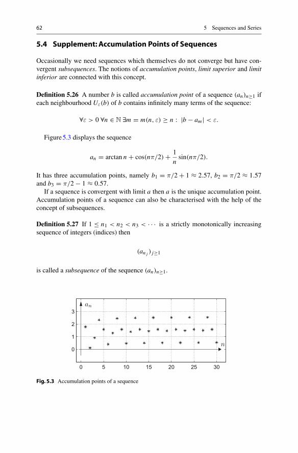
62 5 Sequences and Series
5.4 Supplement: Accumulation Points of Sequences
Occasionally we need sequences which themselves do not converge but have con-vergent subsequences. The notions of accumulation points, limit superior and limitinferior are connected with this concept.
Definition 5.26 A number b is called accumulation point of a sequence (an)n≥1 ifeach neighbourhood Uε(b) of b contains infinitely many terms of the sequence:
∀ε > 0 ∀n ∈ N ∃m = m(n, ε) ≥ n : |b − am | < ε.
Figure5.3 displays the sequence
an = arctan n + cos(nπ/2) + 1
nsin(nπ/2).
It has three accumulation points, namely b1 = π/2 + 1 ≈ 2.57, b2 = π/2 ≈ 1.57and b3 = π/2 − 1 ≈ 0.57.
If a sequence is convergent with limit a then a is the unique accumulation point.Accumulation points of a sequence can also be characterised with the help of theconcept of subsequences.
Definition 5.27 If 1 ≤ n1 < n2 < n3 < · · · is a strictly monotonically increasingsequence of integers (indices) then
(an j ) j≥1
is called a subsequence of the sequence (an)n≥1.
0 5 10 15 20 25 30
0
1
2
3an
n
Fig. 5.3 Accumulation points of a sequence

5.4 Supplement: Accumulation Points of Sequences 63
Example 5.28 We start with the sequence an = 1n . If we take, for instance, n j = j2
then we obtain the sequence an j = 1j2
as subsequence:
(an)n≥1 = (1, 12 ,
13 ,
14 ,
15 ,
16 ,
17 ,
18 ,
19 ,
110 , . . . ),
(an j ) j≥1 = (1, 14 ,
19 , . . . ).
Proposition 5.29 A number b is an accumulation point of the sequence (an)n≥0 ifand only if b is the limit of a convergent subsequence (an j ) j≥1.
Proof Let b be an accumulation point of the sequence (an)n≥0. Step by step we willconstruct a strictly monotonically increasing sequence of indices (n j ) j≥1 so that
|b − an j | <1
j
is fulfilled for all j ∈ N. According to Definition5.26 for ε1 = 1 we have
∀n ∈ N ∃m ≥ n : |b − am | < ε1.
We choose n = 1 and denote the smallest m ≥ n which fulfills this condition by n1.Thus
|b − an1 | < ε1 = 1.
For ε2 = 12 one again obtains according to Definition5.26:
∀n ∈ N ∃m ≥ n : |b − am | < ε2.
This time we choose n = n1 + 1 and denote the smallest m ≥ n1 + 1 which fulfillsthis condition by n2. Thus
|b − an2 | < ε2 = 1
2.
It is clear how one has to proceed. Once n j is constructed one sets ε j+1 = 1/( j + 1)and uses Definition5.26 according to which
∀n ∈ N ∃m ≥ n : |b − am | < ε j+1.
We choose n = n j + 1 and denote the smallest m ≥ n j + 1 which fulfills this con-dition by n j+1. Thus
|b − an j+1 | < ε j+1 = 1
j + 1.
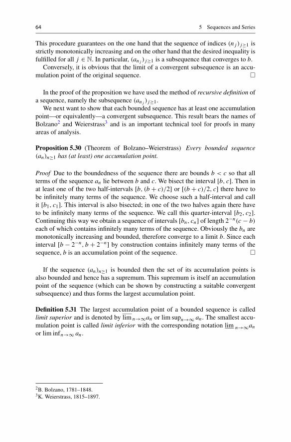
64 5 Sequences and Series
This procedure guarantees on the one hand that the sequence of indices (n j ) j≥1 isstrictly monotonically increasing and on the other hand that the desired inequality isfulfilled for all j ∈ N. In particular, (an j ) j≥1 is a subsequence that converges to b.
Conversely, it is obvious that the limit of a convergent subsequence is an accu-mulation point of the original sequence. �
In the proof of the proposition we have used the method of recursive definition ofa sequence, namely the subsequence (an j ) j≥1.
We next want to show that each bounded sequence has at least one accumulationpoint—or equivalently—a convergent subsequence. This result bears the names ofBolzano2 and Weierstrass3 and is an important technical tool for proofs in manyareas of analysis.
Proposition 5.30 (Theorem of Bolzano–Weierstrass) Every bounded sequence(an)n≥1 has (at least) one accumulation point.
Proof Due to the boundedness of the sequence there are bounds b < c so that allterms of the sequence an lie between b and c. We bisect the interval [b, c]. Then inat least one of the two half-intervals [b, (b + c)/2] or [(b + c)/2, c] there have tobe infinitely many terms of the sequence. We choose such a half-interval and callit [b1, c1]. This interval is also bisected; in one of the two halves again there haveto be infinitely many terms of the sequence. We call this quarter-interval [b2, c2].Continuing this way we obtain a sequence of intervals [bn, cn] of length 2−n(c − b)each of which contains infinitely many terms of the sequence. Obviously the bn aremonotonically increasing and bounded, therefore converge to a limit b. Since eachinterval [b − 2−n, b + 2−n] by construction contains infinitely many terms of thesequence, b is an accumulation point of the sequence. �
If the sequence (an)n≥1 is bounded then the set of its accumulation points isalso bounded and hence has a supremum. This supremum is itself an accumulationpoint of the sequence (which can be shown by constructing a suitable convergentsubsequence) and thus forms the largest accumulation point.
Definition 5.31 The largest accumulation point of a bounded sequence is calledlimit superior and is denoted by lim n→∞an or lim supn→∞ an . The smallest accu-mulation point is called limit inferior with the corresponding notation lim n→∞anor lim infn→∞ an .
2B. Bolzano, 1781–1848.3K. Weierstrass, 1815–1897.
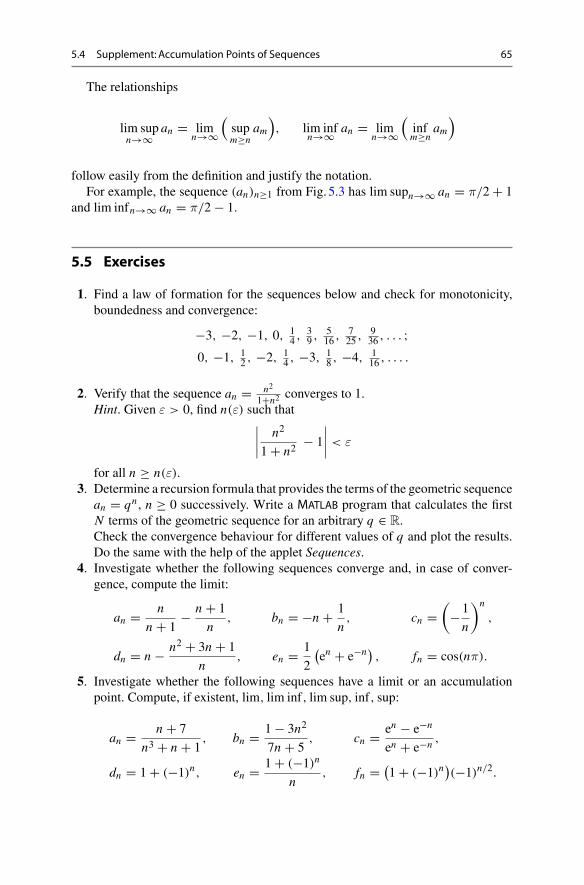
5.4 Supplement: Accumulation Points of Sequences 65
The relationships
lim supn→∞
an = limn→∞
(supm≥n
am), lim inf
n→∞ an = limn→∞
(infm≥n
am)
follow easily from the definition and justify the notation.For example, the sequence (an)n≥1 from Fig. 5.3 has lim supn→∞ an = π/2 + 1
and lim infn→∞ an = π/2 − 1.
5.5 Exercises
1. Find a law of formation for the sequences below and check for monotonicity,boundedness and convergence:
−3, −2, −1, 0, 14 ,
39 ,
516 ,
725 ,
936 , . . . ;
0, −1, 12 , −2, 1
4 , −3, 18 , −4, 1
16 , . . . .
2. Verify that the sequence an = n2
1+n2converges to 1.
Hint. Given ε > 0, find n(ε) such that∣∣∣∣
n2
1 + n2− 1
∣∣∣∣ < ε
for all n ≥ n(ε).3. Determine a recursion formula that provides the terms of the geometric sequence
an = qn , n ≥ 0 successively. Write a MATLAB program that calculates the firstN terms of the geometric sequence for an arbitrary q ∈ R.Check the convergence behaviour for different values of q and plot the results.Do the same with the help of the applet Sequences.
4. Investigate whether the following sequences converge and, in case of conver-gence, compute the limit:
an = n
n + 1− n + 1
n, bn = −n + 1
n, cn =
(−1
n
)n
,
dn = n − n2 + 3n + 1
n, en = 1
2
(en + e−n) , fn = cos(nπ).
5. Investigate whether the following sequences have a limit or an accumulationpoint. Compute, if existent, lim, lim inf, lim sup, inf, sup:
an = n + 7
n3 + n + 1, bn = 1 − 3n2
7n + 5, cn = en − e−n
en + e−n,
dn = 1 + (−1)n, en = 1 + (−1)n
n, fn = (
1 + (−1)n)(−1)n/2.
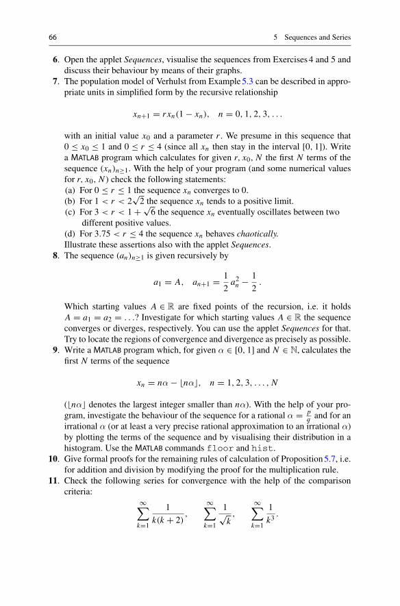
66 5 Sequences and Series
6. Open the applet Sequences, visualise the sequences from Exercises4 and 5 anddiscuss their behaviour by means of their graphs.
7. The population model of Verhulst from Example5.3 can be described in appro-priate units in simplified form by the recursive relationship
xn+1 = r xn(1 − xn), n = 0, 1, 2, 3, . . .
with an initial value x0 and a parameter r . We presume in this sequence that0 ≤ x0 ≤ 1 and 0 ≤ r ≤ 4 (since all xn then stay in the interval [0, 1]). Writea MATLAB program which calculates for given r, x0, N the first N terms of thesequence (xn)n≥1. With the help of your program (and some numerical valuesfor r, x0, N ) check the following statements:(a) For 0 ≤ r ≤ 1 the sequence xn converges to 0.(b) For 1 < r < 2
√2 the sequence xn tends to a positive limit.
(c) For 3 < r < 1 + √6 the sequence xn eventually oscillates between two
different positive values.(d) For 3.75 < r ≤ 4 the sequence xn behaves chaotically.Illustrate these assertions also with the applet Sequences.
8. The sequence (an)n≥1 is given recursively by
a1 = A, an+1 = 1
2a2n − 1
2.
Which starting values A ∈ R are fixed points of the recursion, i.e. it holdsA = a1 = a2 = . . .? Investigate for which starting values A ∈ R the sequenceconverges or diverges, respectively. You can use the applet Sequences for that.Try to locate the regions of convergence and divergence as precisely as possible.
9. Write a MATLAB program which, for given α ∈ [0, 1] and N ∈ N, calculates thefirst N terms of the sequence
xn = nα − nα�, n = 1, 2, 3, . . . , N
( nα� denotes the largest integer smaller than nα). With the help of your pro-gram, investigate the behaviour of the sequence for a rational α = p
q and for anirrational α (or at least a very precise rational approximation to an irrational α)by plotting the terms of the sequence and by visualising their distribution in ahistogram. Use the MATLAB commands floor and hist.
10. Give formal proofs for the remaining rules of calculation of Proposition5.7, i.e.for addition and division by modifying the proof for the multiplication rule.
11. Check the following series for convergence with the help of the comparisoncriteria:
∞∑
k=1
1
k(k + 2),
∞∑
k=1
1√k,
∞∑
k=1
1
k3.
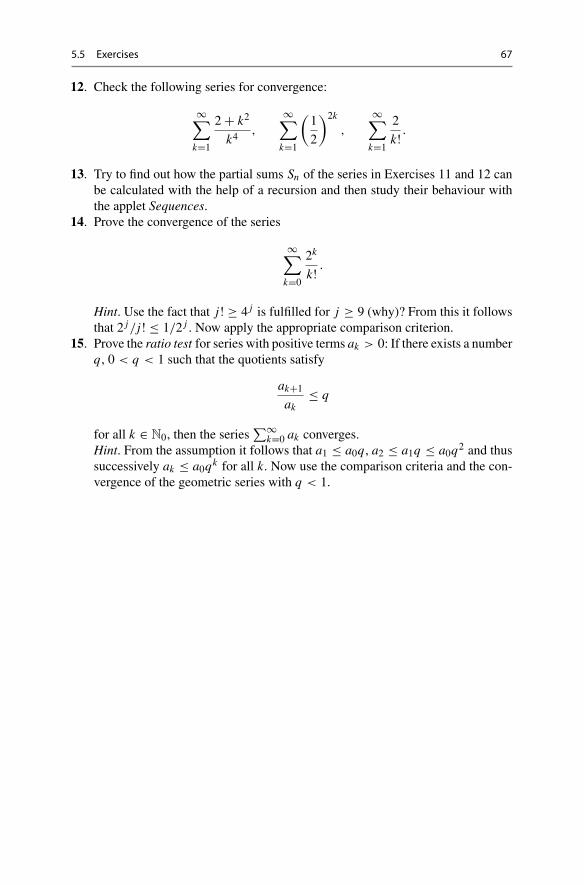
5.5 Exercises 67
12. Check the following series for convergence:
∞∑
k=1
2 + k2
k4,
∞∑
k=1
(1
2
)2k
,
∞∑
k=1
2
k! .
13. Try to find out how the partial sums Sn of the series in Exercises 11 and 12 canbe calculated with the help of a recursion and then study their behaviour withthe applet Sequences.
14. Prove the convergence of the series
∞∑
k=0
2k
k! .
Hint. Use the fact that j ! ≥ 4 j is fulfilled for j ≥ 9 (why)? From this it followsthat 2 j/j ! ≤ 1/2 j . Now apply the appropriate comparison criterion.
15. Prove the ratio test for series with positive terms ak > 0: If there exists a numberq , 0 < q < 1 such that the quotients satisfy
ak+1
ak≤ q
for all k ∈ N0, then the series∑∞
k=0 ak converges.Hint. From the assumption it follows that a1 ≤ a0q , a2 ≤ a1q ≤ a0q2 and thussuccessively ak ≤ a0qk for all k. Now use the comparison criteria and the con-vergence of the geometric series with q < 1.
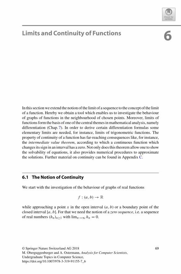
6Limits andContinuity of Functions
In this sectionwe extend the notion of the limit of a sequence to the concept of the limitof a function. Hereby we obtain a tool which enables us to investigate the behaviourof graphs of functions in the neighbourhood of chosen points. Moreover, limits offunctions form the basis of one of the central themes inmathematical analysis, namelydifferentiation (Chap.7). In order to derive certain differentiation formulas someelementary limits are needed, for instance, limits of trigonometric functions. Theproperty of continuity of a function has far-reaching consequences like, for instance,the intermediate value theorem, according to which a continuous function whichchanges its sign in an interval has a zero.Not only does this theoremallowone to showthe solvability of equations, it also provides numerical procedures to approximatethe solutions. Further material on continuity can be found in Appendix C.
6.1 The Notion of Continuity
We start with the investigation of the behaviour of graphs of real functions
f : (a, b) → R
while approaching a point x in the open interval (a, b) or a boundary point of theclosed interval [a, b]. For that we need the notion of a zero sequence, i.e. a sequenceof real numbers (hn)n≥1 with limn→∞ hn = 0.
© Springer Nature Switzerland AG 2018M. Oberguggenberger and A. Ostermann, Analysis for Computer Scientists,Undergraduate Topics in Computer Science,https://doi.org/10.1007/978-3-319-91155-7_6
69
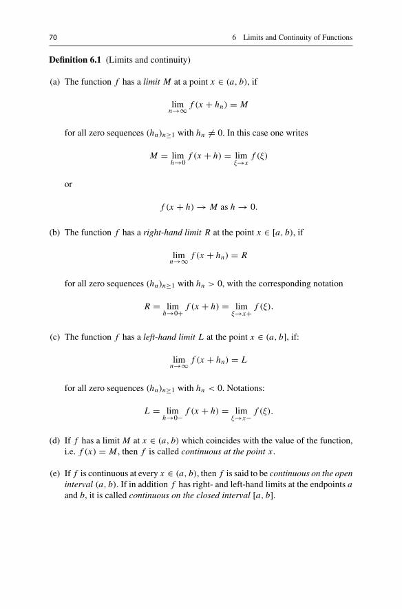
70 6 Limits and Continuity of Functions
Definition 6.1 (Limits and continuity)
(a) The function f has a limit M at a point x ∈ (a, b), if
limn→∞ f (x + hn) = M
for all zero sequences (hn)n≥1 with hn �= 0. In this case one writes
M = limh→0
f (x + h) = limξ→x
f (ξ)
or
f (x + h) → M as h → 0.
(b) The function f has a right-hand limit R at the point x ∈ [a, b), if
limn→∞ f (x + hn) = R
for all zero sequences (hn)n≥1 with hn > 0, with the corresponding notation
R = limh→0+ f (x + h) = lim
ξ→x+f (ξ).
(c) The function f has a left-hand limit L at the point x ∈ (a, b], if:
limn→∞ f (x + hn) = L
for all zero sequences (hn)n≥1 with hn < 0. Notations:
L = limh→0− f (x + h) = lim
ξ→x−f (ξ).
(d) If f has a limit M at x ∈ (a, b) which coincides with the value of the function,i.e. f (x) = M , then f is called continuous at the point x .
(e) If f is continuous at every x ∈ (a, b), then f is said to be continuous on the openinterval (a, b). If in addition f has right- and left-hand limits at the endpoints aand b, it is called continuous on the closed interval [a, b].

6.1 The Notion of Continuity 71
f(x+h)
f(x) = M
x+hx
R
f(x)
L
x
Fig. 6.1 Limit and continuity; left- and right-hand limits
Figure6.1 illustrates the idea of approaching a point x for h → 0 as well aspossible differences between left-hand and right-hand limits and the value of thefunction.
If a function f is continuous at a point x , the function evaluation can be inter-changed with the limit:
limξ→x
f (ξ) = f (x) = f ( limξ→x
ξ).
The following examples show some further possibilities how a function can behavein the neighbourhood of a point: Jump discontinuity with left- and right-hand limits,vertical asymptote, oscillations with non-vanishing amplitude and ever-increasingfrequency.
Example 6.2 The quadratic function f (x) = x2 is continuous at every x ∈ R since
f (x + hn) − f (x) = (x + hn)2 − x2 = 2xhn + h2n → 0
as n → ∞ for any zero sequence (hn)n≥1. Therefore
limh→0
f (x + h) = f (x).
Likewise the continuity of the power functions x �→ xm for m ∈ N can be shown.
Example 6.3 The absolute value function f (x) = |x | and the third root g(x) = 3√x
are everywhere continuous. The former has a kink at x = 0, the latter a verticaltangent; see Fig. 6.2.
Example 6.4 The sign function f (x) = sign x has different left- and right-hand lim-its L = −1, R = 1 at x = 0. In particular, it is discontinuous at that point. At all otherpoints x �= 0 it is continuous; see Fig. 6.3.

72 6 Limits and Continuity of Functions
y = 3√
x
x
y = |x|
x
Fig. 6.2 Continuity and kink or vertical tangent
1
0
y = (sign x)2
x
1
0
−1
y = sign x
x
Fig. 6.3 Discontinuities: jump discontinuity and exceptional value
Example 6.5 The square of the sign function
g(x) = (sign x)2 ={1, x �= 00, x = 0
has equal left- and right-hand limits at x = 0. However, they are different from thevalue of the function (see Fig. 6.3):
limξ→0
g(ξ) = 1 �= 0 = g(0).
Therefore, g is discontinuous at x = 0.
Example 6.6 The functions f (x) = 1x and g(x) = tan x have vertical asymptotes at
x = 0 and x = π2 + kπ, k ∈ Z, respectively, and in particular no left- or right-hand
limit at these points. At all other points, however, they are continuous. We refer toFigs. 2.9 and 3.10.
Example 6.7 The function f (x) = sin 1x has no left- or right-hand limit at x = 0
but oscillates with non-vanishing amplitude (Fig. 6.4). Indeed, one obtains differentlimits for different zero sequences. For example, for
hn = 1
nπ, kn = 1
π/2 + 2nπ, ln = 1
3π/2 + 2nπ
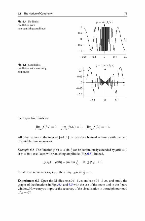
6.1 The Notion of Continuity 73
Fig. 6.4 No limits,oscillation withnon-vanishing amplitude
−0.2 −0.1 0 0.1 0.2
−1
−0.5
0
0.5
1
y = sin(1/x)
x
Fig. 6.5 Continuity,oscillation with vanishingamplitude
−0.1 0 0.1
−0.1
−0.05
0
0.05
0.1
y = x sin(1/x)
x
the respective limits are
limn→∞ f (hn) = 0, lim
n→∞ f (kn) = 1, limn→∞ f (ln) = −1.
All other values in the interval [−1, 1] can also be obtained as limits with the helpof suitable zero sequences.
Example 6.8 The function g(x) = x sin 1x can be continuously extended by g(0) = 0
at x = 0; it oscillates with vanishing amplitude (Fig. 6.5). Indeed,
|g(hn) − g(0)| = |hn sin 1hn
− 0| ≤ |hn| → 0
for all zero sequences (hn)n≥1, thus limh→0 h sin 1h = 0.
Experiment 6.9 Open the M-files mat06_1.m and mat06_2.m, and study thegraphs of the functions in Figs. 6.4 and 6.5 with the use of the zoom tool in the figurewindow.Howcan you improve the accuracy of the visualisation in the neighbourhoodof x = 0?

74 6 Limits and Continuity of Functions
6.2 Trigonometric Limits
Comparing the areas in Fig. 6.6 shows that the area of the grey triangle with sidescos x and sin x is smaller than the area of the sector which in turn is smaller or equalto the area of the big triangle with sides 1 and tan x .
The area of a sector in the unit circle (with angle x in radian measure) equals x/2as is well-known. In summary we obtain the inequalities
1
2sin x cos x ≤ x
2≤ 1
2tan x
or after division by sin x and taking the reciprocal
cos x ≤ sin x
x≤ 1
cos x,
valid for all x with 0 < |x | < π/2.With the help of these inequalities we can compute several important limits. From
an elementary geometric consideration, one obtains
|cos x | ≥ 1
2for − π
3≤ x ≤ π
3,
and together with the previous inequalities
|sin hn| ≤ |hn||cos hn| ≤ 2 |hn| → 0
for all zero sequences (hn)n≥1. This means that
limh→0
sin h = 0.
Fig. 6.6 Illustration oftrigonometric inequalities
cos x
tan xxsin x
1
1

6.2 Trigonometric Limits 75
The sine function is therefore continuous at zero. From the continuity of the squarefunction and the root function as well as the fact that cos h equals the positive squareroot of 1 − sin2 h for small h it follows that
limh→0
cos h = limh→0
√1 − sin2 h = 1.
With this the continuity of the sine function at every point x ∈ R can be proven:
limh→0
sin(x + h) = limh→0
(sin x cos h + cos x sin h
) = sin x .
The inequality illustrated at the beginning of the section allows one to deduce oneof the most important trigonometric limits. It forms the basis of the differentiationrules for trigonometric functions.
Proposition 6.10 limx→0sin xx = 1.
Proof We combine the above result limx→0 cos x = 1 with the inequality deducedearlier and obtain
1 = limx→0
cos x ≤ limx→0
sin x
x≤ lim
x→0
1
cos x= 1,
and therefore limx→0sin xx = 1. �
6.3 Zeros of Continuous Functions
Figure6.7 shows the graph of a function that is continuous on a closed interval[a, b] and that is negative at the left endpoint and positive at the right endpoint.Geometrically the graph has to intersect the x-axis at least once since it has no jumpsdue to the continuity. This means that f has to have at least one zero in (a, b). Thisis a criterion that guarantees the existences of a solution to the equation f (x) = 0.A first rigorous proof of this intuitively evident statement goes back to Bolzano.
Proposition 6.11 (Intermediate value theorem) Let f : [a, b] → R be continuousand f (a) < 0, f (b) > 0. Then there exists a point ξ ∈ (a, b) with f (ξ) = 0.
Proof The proof is based on the successive bisection of the intervals and the com-pleteness of the set of real numbers.One startswith the interval [a, b] and sets a1 = a,b1 = b.
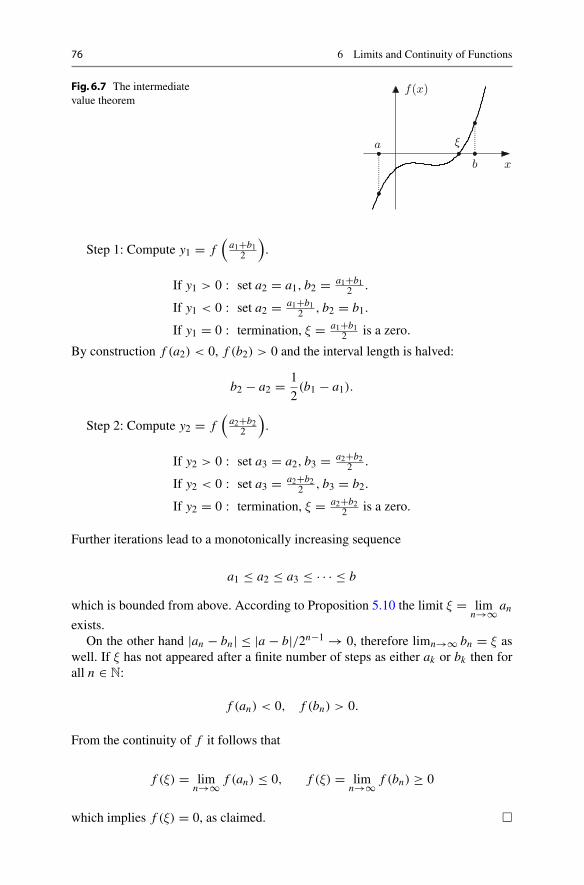
76 6 Limits and Continuity of Functions
Fig. 6.7 The intermediatevalue theorem
b
ξa
f(x)
x
Step 1: Compute y1 = f(a1+b1
2
).
If y1 > 0 : set a2 = a1, b2 = a1+b12 .
If y1 < 0 : set a2 = a1+b12 , b2 = b1.
If y1 = 0 : termination, ξ = a1+b12 is a zero.
By construction f (a2) < 0, f (b2) > 0 and the interval length is halved:
b2 − a2 = 1
2(b1 − a1).
Step 2: Compute y2 = f(a2+b2
2
).
If y2 > 0 : set a3 = a2, b3 = a2+b22 .
If y2 < 0 : set a3 = a2+b22 , b3 = b2.
If y2 = 0 : termination, ξ = a2+b22 is a zero.
Further iterations lead to a monotonically increasing sequence
a1 ≤ a2 ≤ a3 ≤ · · · ≤ b
which is bounded from above. According to Proposition 5.10 the limit ξ = limn→∞ an
exists.On the other hand |an − bn| ≤ |a − b|/2n−1 → 0, therefore limn→∞ bn = ξ as
well. If ξ has not appeared after a finite number of steps as either ak or bk then forall n ∈ N:
f (an) < 0, f (bn) > 0.
From the continuity of f it follows that
f (ξ) = limn→∞ f (an) ≤ 0, f (ξ) = lim
n→∞ f (bn) ≥ 0
which implies f (ξ) = 0, as claimed. �
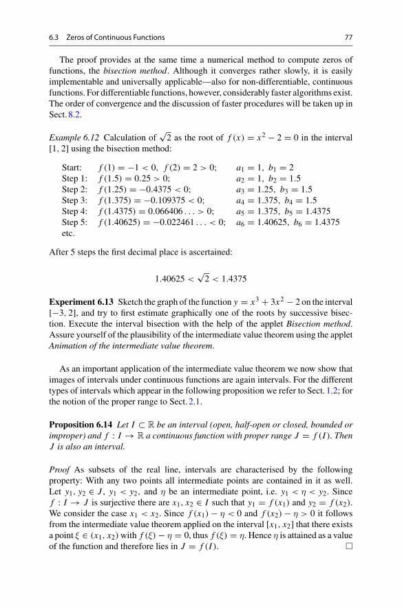
6.3 Zeros of Continuous Functions 77
The proof provides at the same time a numerical method to compute zeros offunctions, the bisection method. Although it converges rather slowly, it is easilyimplementable and universally applicable—also for non-differentiable, continuousfunctions. For differentiable functions, however, considerably faster algorithms exist.The order of convergence and the discussion of faster procedures will be taken up inSect. 8.2.
Example 6.12 Calculation of√2 as the root of f (x) = x2 − 2 = 0 in the interval
[1, 2] using the bisection method:
Start: f (1) = −1 < 0, f (2) = 2 > 0; a1 = 1, b1 = 2Step 1: f (1.5) = 0.25 > 0; a2 = 1, b2 = 1.5Step 2: f (1.25) = −0.4375 < 0; a3 = 1.25, b3 = 1.5Step 3: f (1.375) = −0.109375 < 0; a4 = 1.375, b4 = 1.5Step 4: f (1.4375) = 0.066406 . . . > 0; a5 = 1.375, b5 = 1.4375Step 5: f (1.40625) = −0.022461 . . . < 0; a6 = 1.40625, b6 = 1.4375etc.
After 5 steps the first decimal place is ascertained:
1.40625 <√2 < 1.4375
Experiment 6.13 Sketch the graph of the function y = x3 + 3x2 − 2 on the interval[−3, 2], and try to first estimate graphically one of the roots by successive bisec-tion. Execute the interval bisection with the help of the applet Bisection method.Assure yourself of the plausibility of the intermediate value theorem using the appletAnimation of the intermediate value theorem.
As an important application of the intermediate value theorem we now show thatimages of intervals under continuous functions are again intervals. For the differenttypes of intervals which appear in the following proposition we refer to Sect. 1.2; forthe notion of the proper range to Sect. 2.1.
Proposition 6.14 Let I ⊂ R be an interval (open, half-open or closed, bounded orimproper) and f : I → R a continuous function with proper range J = f (I ). ThenJ is also an interval.
Proof As subsets of the real line, intervals are characterised by the followingproperty: With any two points all intermediate points are contained in it as well.Let y1, y2 ∈ J , y1 < y2, and η be an intermediate point, i.e. y1 < η < y2. Sincef : I → J is surjective there are x1, x2 ∈ I such that y1 = f (x1) and y2 = f (x2).We consider the case x1 < x2. Since f (x1) − η < 0 and f (x2) − η > 0 it followsfrom the intermediate value theorem applied on the interval [x1, x2] that there existsa point ξ ∈ (x1, x2)with f (ξ) − η = 0, thus f (ξ) = η. Hence η is attained as a valueof the function and therefore lies in J = f (I ). �
78 6 Limits and Continuity of Functions
Proposition 6.15 Let I = [a, b] be a closed, bounded interval and f : I → R acontinuous function. Then the proper range J = f (I ) is also a closed, boundedinterval.
Proof According to Proposition 6.14 the range J is an interval. Let d be the leastupper bound (possibly d = ∞). We take a sequence of values yn ∈ J which con-verges to d. The values yn are function values of certain arguments xn ∈ I = [a, b].The sequence (xn)n≥1 is bounded and, according to Proposition 5.30, has an accu-mulation point x0, a ≤ x0 ≤ b. Thus a subsequence (xn j ) j≥1 exists which convergesto x0 (see Sect. 5.4). From the continuity of the function f it follows that
d = limj→∞ yn j = lim
j→∞ f (xn j ) = f (x0).
This shows that the upper endpoint of the interval J is finite and is attained as functionvalue. The same argument is applied to the lower boundary c; the range J is thereforea closed, bounded interval [c, d]. �
From the proof of the proposition it is clear that d is the largest and c the smallestvalue of the function f on the interval [a, b]. We thus obtain the following importantconsequence.
Corollary 6.16 Each continuous function defined on a closed interval I = [a, b]attains its maximum and minimum there.
6.4 Exercises
1. (a) Investigate the behaviour of the functions
x + x2
|x | ,
√1 + x − 1
x,
x2 + sin x√1 − cos2 x
in a neighbourhood of x = 0 by plotting their graphs for arguments in[−2,− 1
100 ) ∪ ( 1100 , 2].
(b) Find out by inspection of the graphs whether there are left- or right-handlimits at x = 0. Which value do they have? Explain your results by rear-ranging the expressions in (a).Hint. Some guidance for part (a) can be found in theM-filemat06_ex1.m.Expand the middle term in (b) with
√1 + x + 1.
6.4 Exercises 79
2. Do the following functions have a limit at the given points? If so, what is itsvalue?(a) y = x3 + 5x + 10, x = 1.(b) y = x2−1
x2+x, x = 0, x = 1, x = −1.
(c) y = 1−cos xx2
, x = 0.Hint. Expand with (1 + cos x).
(d) y = sign x · sin x, x = 0.(e) y = sign x · cos x, x = 0.
3. Let fn(x) = arctan nx, gn(x) = (1 + x2)−n . Compute the limits
f (x) = limn→∞ fn(x), g(x) = lim
n→∞ gn(x)
for each x ∈ R, and sketch the graphs of the thereby defined functions f and g.Are they continuous? Plot fn and gn usingMATLAB, and investigate the behaviourof the graphs for n → ∞.Hint. An advice can be found in the M-file mat06_ex3.m.
4. With the help of zero sequences, carry out a formal proof of the fact that theabsolute value function and the third root function ofExample 6.3 are continuous.
5. Arguewith the help of the intermediate value theorem that p(x) = x3 + 5 x + 10has a zero in the interval [−2, 1]. Compute this zero up to four decimal placesusing the applet Bisection method.
6. Compute all zeros of the following functions in the given interval with accuracy10−3, using the applet Bisection method.
f (x) = x4 − 2, I = R;g(x) = x − cos x, I = R;h(x) = sin 1
x , I = [ 120 ,
110
].
7. Write aMATLAB programwhich locates—with the help of the bisectionmethod—the zero of an arbitrary polynomial
p(x) = x3 + c1x2 + c2x + c3
of degree three. Your program should automatically provide starting values a, bwith p(a) < 0, p(b) > 0 (why do such values always exist?). Test your programby choosing the coefficient vector (c1, c2, c3) randomly, for example by usingc = 1000*rand(1,3).Hint. A solution is suggested in the M-file mat06_ex7.m.
7TheDerivative of a Function
Starting from theproblem todefine the tangent to the graphof a function,we introducethe derivative of a function. Two points on the graph can always be joined by a secant,which is a goodmodel for the tangentwhenever these points are close to each other. Ina limiting process, the secant (discrete model) is replaced by the tangent (continuousmodel). Differential calculus, which is based on this limiting process, has becomeone of the most important building blocks of mathematical modelling.
In this section we discuss the derivative of important elementary functions aswell as general differentiation rules. Thanks to the meticulous implementation ofthese rules, expert systems such as maple have become helpful tools in mathemat-ical analysis. Furthermore, we will discuss the interpretation of the derivative aslinear approximation and as rate of change. These interpretations form the basis ofnumerous applications in science and engineering.
The concept of the numerical derivative follows the opposite direction. The contin-uous model is discretised, and the derivative is replaced by a difference quotient. Wecarry out a detailed error analysis which allows us to find an optimal approximation.Further, we will illustrate the relevance of symmetry in numerical procedures.
7.1 Motivation
Example 7.1 (The free fall according toGalilei1) Imagine an object,which releasedat time t = 0, falls down under the influence of gravity. We are interested in theposition s(t) of the object at time t ≥ 0 as well as in its velocity v(t), see Fig. 7.1.Due to the definition of velocity as change in travelled distance divided by change
1G. Galilei, 1564–1642.
© Springer Nature Switzerland AG 2018M. Oberguggenberger and A. Ostermann, Analysis for Computer Scientists,Undergraduate Topics in Computer Science,https://doi.org/10.1007/978-3-319-91155-7_7
81
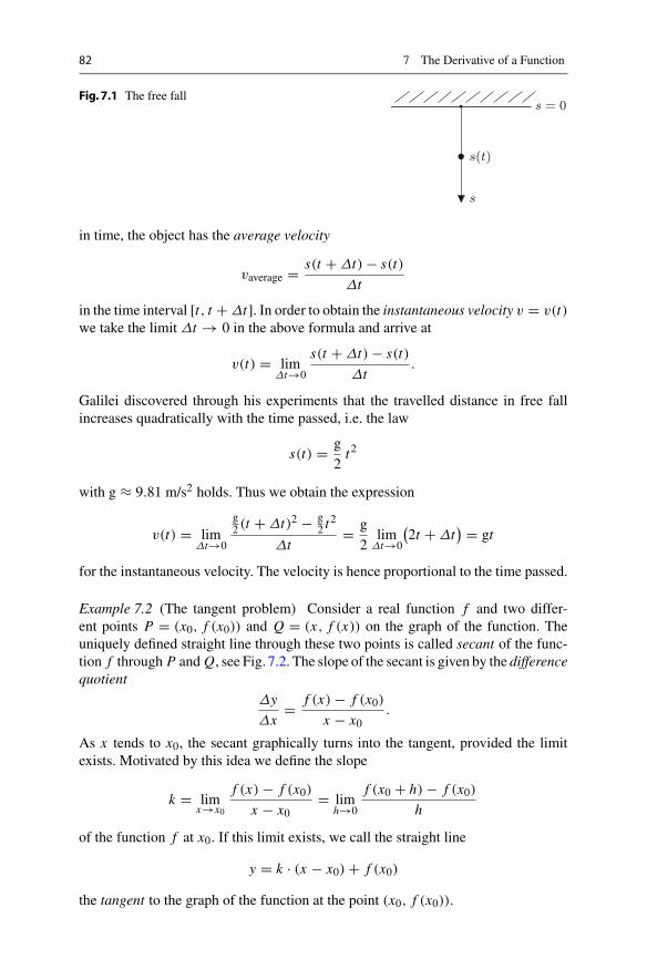
82 7 The Derivative of a Function
Fig. 7.1 The free fall
s
s = 0
s(t)
in time, the object has the average velocity
vaverage = s(t + Δt) − s(t)
Δt
in the time interval [t, t + Δt]. In order to obtain the instantaneous velocity v = v(t)we take the limit Δt → 0 in the above formula and arrive at
v(t) = limΔt→0
s(t + Δt) − s(t)
Δt.
Galilei discovered through his experiments that the travelled distance in free fallincreases quadratically with the time passed, i.e. the law
s(t) = g
2t2
with g ≈ 9.81 m/s2 holds. Thus we obtain the expression
v(t) = limΔt→0
g2 (t + Δt)2 − g
2 t2
Δt= g
2lim
Δt→0
(2t + Δt
) = gt
for the instantaneous velocity. The velocity is hence proportional to the time passed.
Example 7.2 (The tangent problem) Consider a real function f and two differ-ent points P = (x0, f (x0)) and Q = (x, f (x)) on the graph of the function. Theuniquely defined straight line through these two points is called secant of the func-tion f through P and Q, see Fig. 7.2. The slope of the secant is given by the differencequotient
Δy
Δx= f (x) − f (x0)
x − x0.
As x tends to x0, the secant graphically turns into the tangent, provided the limitexists. Motivated by this idea we define the slope
k = limx→x0
f (x) − f (x0)
x − x0= lim
h→0
f (x0 + h) − f (x0)
h
of the function f at x0. If this limit exists, we call the straight line
y = k · (x − x0) + f (x0)
the tangent to the graph of the function at the point (x0, f (x0)).
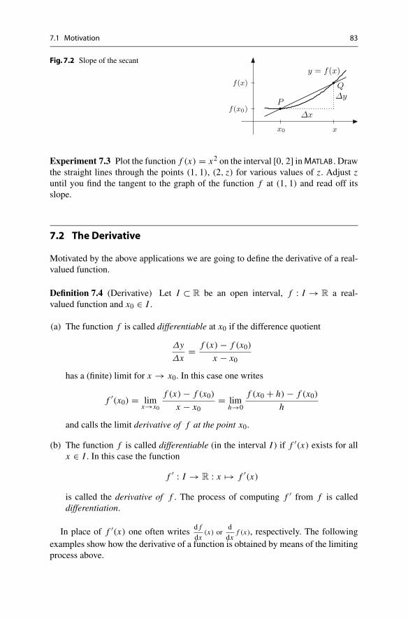
7.1 Motivation 83
Fig. 7.2 Slope of the secant
Q
P
Δx
Δy
y = f(x)f(x)
f(x0)
xx0
Experiment 7.3 Plot the function f (x) = x2 on the interval [0, 2] inMATLAB . Drawthe straight lines through the points (1, 1), (2, z) for various values of z. Adjust zuntil you find the tangent to the graph of the function f at (1, 1) and read off itsslope.
7.2 The Derivative
Motivated by the above applications we are going to define the derivative of a real-valued function.
Definition 7.4 (Derivative) Let I ⊂ R be an open interval, f : I → R a real-valued function and x0 ∈ I .
(a) The function f is called differentiable at x0 if the difference quotient
Δy
Δx= f (x) − f (x0)
x − x0
has a (finite) limit for x → x0. In this case one writes
f ′(x0) = limx→x0
f (x) − f (x0)
x − x0= lim
h→0
f (x0 + h) − f (x0)
h
and calls the limit derivative of f at the point x0.
(b) The function f is called differentiable (in the interval I ) if f ′(x) exists for allx ∈ I . In this case the function
f ′ : I → R : x �→ f ′(x)
is called the derivative of f . The process of computing f ′ from f is calleddifferentiation.
In place of f ′(x) one often writesd f
dx(x) or
d
dxf (x), respectively. The following
examples show how the derivative of a function is obtained by means of the limitingprocess above.
84 7 The Derivative of a Function
Example 7.5 (The constant function f (x) = c)
f ′(x) = limh→0
f (x + h) − f (x)
h= lim
h→0
c − c
h= lim
h→0
0
h= 0.
The derivative of a constant function is zero.
Example 7.6 (The affine function g(x) = ax + b)
g′(x) = limh→0
g(x + h) − g(x)
h= lim
h→0
ax + ah + b − ax − b
h= lim
h→0a = a.
The derivative is the slope a of the straight line y = ax + b.
Example 7.7 (The derivative of the quadratic function y = x2)
y′ = limh→0
(x + h)2 − x2
h= lim
h→0
2hx + h2
h= lim
h→0(2x + h) = 2x .
Similarly, one can show for the power function (with n ∈ N):
f (x) = xn ⇒ f ′(x) = n · xn−1.
Example 7.8 (The derivative of the square root function y = √x for x > 0)
y′ = limξ→x
√ξ − √
x
ξ − x= lim
ξ→x
√ξ − √
x
(√
ξ − √x)(
√ξ + √
x)= lim
ξ→x
1√ξ + √
x= 1
2√
x.
Example 7.9 (Derivatives of the sine and cosine functions) We first recall fromProposition6.10 that
limt→0
sin t
t= 1.
Due to
(cos t − 1)(cos t + 1) = − sin2 t
it also holds that
cos t − 1
t= − sin t︸︷︷︸
→ 0
· sin t
t︸︷︷︸→ 1
· 1
cos t + 1︸ ︷︷ ︸→ 1/2
→ 0 for t → 0,
and thus
limt→0
cos t − 1
t= 0.
7.2 The Derivative 85
Due to the addition theorems (Proposition3.3) we get with the preparations fromabove
sin′ x = limh→0
sin(x + h) − sin x
h= lim
h→0
sin x cos h + cos x sin h − sin x
h
= limh→0
sin x · cos h − 1
h+ lim
h→0cos x · sin h
h
= sin x · limh→0
cos h − 1
h︸ ︷︷ ︸= 0
+ cos x · limh→0
sin h
h︸ ︷︷ ︸= 1
= cos x .
This proves the formula sin′ x = cos x . Likewise it can be shown that cos′ x =− sin x .
Example 7.10 (The derivative of the exponential functionwith base e) Rearrangingterms in the series expansion of the exponential function (PropositionC.12)we obtain
eh − 1
h=
∞∑
k=0
hk
(k + 1)! = 1 + h
2+ h2
6+ h3
24+ · · ·
From that one infers∣∣∣∣eh − 1
h− 1
∣∣∣∣ ≤ |h|
(1
2+ |h|
6+ |h|3
24+ · · ·
)≤ |h|e|h|.
Letting h → 0 hence gives the important limit
limh→0
eh − 1
h= 1.
The existence of the limit
limh→0
ex+h − ex
h= ex · lim
h→0
eh − 1
h= ex
shows that the exponential function is differentiable and that (ex )′ = ex .
Example 7.11 (New representationofEuler’s number) By substituting y = eh − 1,h = log(y + 1) in the above limit one obtains
limy→0
y
log(y + 1)= 1
and in this way
limy→0
log(1 + αy)1/y = limy→0
log(1 + αy)
y= α lim
y→0
log(1 + αy)
αy= α.
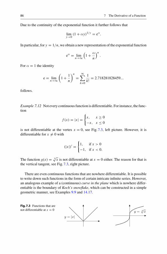
86 7 The Derivative of a Function
Due to the continuity of the exponential function it further follows that
limy→0
(1 + αy)1/y = eα.
In particular, for y = 1/n, we obtain a new representation of the exponential function
eα = limn→∞
(1 + α
n
)n.
For α = 1 the identity
e = limn→∞
(1 + 1
n
)n
=∞∑
k=0
1
k! = 2.718281828459...
follows.
Example 7.12 Not every continuous function is differentiable. For instance, the func-tion
f (x) = |x | ={
x, x ≥ 0
−x, x ≤ 0
is not differentiable at the vertex x = 0, see Fig. 7.3, left picture. However, it isdifferentiable for x = 0 with
(|x |)′ ={1, if x > 0
−1, if x < 0.
The function g(x) = 3√
x is not differentiable at x = 0 either. The reason for that isthe vertical tangent, see Fig. 7.3, right picture.
There are even continuous functions that are nowhere differentiable. It is possibleto write down such functions in the form of certain intricate infinite series. However,an analogous example of a (continuous) curve in the plane which is nowhere differ-entiable is the boundary of Koch’s snowflake, which can be constructed in a simplegeometric manner, see Examples 9.9 and 14.17.
Fig. 7.3 Functions that arenot differentiable at x = 0
y = |x|y = 3
√x
7.2 The Derivative 87
Definition 7.13 If the function f ′ is again differentiable then
f ′′(x) = d2
dx2f (x) = d2 f
dx2(x) = lim
h→0
f ′(x + h) − f ′(x)
h
is called the second derivative of f with respect to x . Likewise higher derivativesare defined recursively as
f ′′′(x) = (f ′′(x)
)′ ord3
dx3f (x) = d
dx
(d2
dx2f (x)
), etc.
Differentiating withmaple.Usingmaple one can differentiate expressions as wellas functions. If the expression g is of the form
g := xˆ2 - a*x;
then the corresponding function f is defined by
f := x -> xˆ2 - a*x;
The evaluation of functions generates expressions, for example f(t) produces theexpression t2 − at . Conversely, expressions can be converted to functions usingunapply
h := unapply(g,x);
The derivative of expressions can be obtained using diff, those of functions usingD. Examples can be found in themaple worksheet mp07_1.mws.
7.3 Interpretations of the Derivative
We introduced the derivative geometrically as the slope of the tangent, and we sawthat the tangent to a graph of a differentiable function f at the point (x0, f (x0)) isgiven by
y = f ′(x0)(x − x0) + f (x0).
Example 7.14 Let f (x) = x4 + 1 with derivative f ′(x) = 4x3.
(i) The tangent to the graph of f at the point (0, 1) is
y = f ′(0) · (x − 0) + f (0) = 1
and thus horizontal.

88 7 The Derivative of a Function
(ii) The tangent to the graph of f at the point (1, 2) is
y = f ′(1)(x − 1) + 2 = 4(x − 1) + 2 = 4x − 2.
The derivative allows further interpretations.
Interpretation as linear approximation. We start off by emphasising that everydifferentiable function f can be written in the form
f (x) = f (x0) + f ′(x0)(x − x0) + R(x, x0),
where the remainder R(x, x0) has the property
limx→x0
R(x, x0)
x − x0= 0.
This follows immediately from
R(x, x0) = f (x) − f (x0) − f ′(x0)(x − x0)
by dividing by x − x0, since
f (x) − f (x0)
x − x0→ f ′(x0) as x → x0.
Application 7.15 As we have just seen, a differentiable function f is characterisedby the property that
f (x) = f (x0) + f ′(x0)(x − x0) + R(x, x0),
where the remainder term R(x, x0) tends faster to zero than x − x0. Taking thelimit x → x0 in this equation shows in particular that every differentiable functionis continuous.
Application 7.16 Let g be the function given by
g(x) = k · (x − x0) + f (x0).
Its graph is the straight line with slope k passing through the point (x0, f (x0)). Since
f (x) − g(x)
x − x0= f (x) − f (x0) − k · (x − x0)
x − x0= f ′(x0) − k + R(x, x0)
x − x0︸ ︷︷ ︸→0
7.3 Interpretations of the Derivative 89
as x → x0, the tangent with k = f ′(x0) is the straight line which approximates thegraph best. One therefore calls
g(x) = f (x0) + f ′(x0) · (x − x0)
the linear approximation to f at x0. For x close to x0 one can consider g(x) as agood approximation to f (x). In applications the (possibly complicated) function fis often replaced by its linear approximation g which is easier to handle.
Example 7.17 Let f (x) = √x = x1/2. Consequently,
f ′(x) = 1
2x− 1
2 = 1
2√
x.
We want to find the linear approximation to the function f at x0 = a. According tothe formula above it holds that
√x ≈ g(x) = √
a + 1
2√
a(x − a)
for x close to a, or, alternatively with h = x − a,
√a + h ≈ √
a + 1
2√
ah for small h.
If we now substitute a = 1 and h = 0.1, we obtain the approximation
√1.1 ≈ 1 + 0.1
2= 1.05.
The first digits of the actual value are 1.0488...
Physical interpretation as rate of change. In physical applications the derivativeoften plays the role of a rate of change. A well-known example from everyday life isthe velocity, see Sect. 7.1. Consider a particle which is moving along a straight line.Let s(t) be the position where the particle is at time t . The average velocity is givenby the quotient
s(t) − s(t0)
t − t0(difference in displacement divided by difference in time).
In the limit t → t0 the average velocity turns into the instantaneous velocity
v(t0) = ds
dt(t0) = s(t0) = lim
t→t0
s(t) − s(t0)
t − t0.
Note that one often writes f (t) instead of f ′(t) if the time t is the argument of thefunction f . In particular, in physics the dot notation is most commonly used.
90 7 The Derivative of a Function
Likewise one obtains the acceleration by differentiating the velocity
a(t) = v(t) = s(t).
The notion of velocity is also used in the modelling of other processes that vary overtime, e.g. for growth or decay.
7.4 Differentiation Rules
In this section I ⊂ R denotes an open interval. We first note that differentiation is alinear process.
Proposition 7.18 (Linearity of the derivative) Let f, g : I → R be two functionswhich are differentiable at x ∈ I and take c ∈ R. Then the functions f + g and c · fare differentiable at x as well and
(f (x) + g(x)
)′ = f ′(x) + g′(x),(c f (x))′ = c f ′(x).
Proof The result follows from the corresponding rules for limits. The first statementis true because
f (x + h) + g(x + h) − ( f (x) + g(x))
h= f (x + h) − f (x)
h︸ ︷︷ ︸→ f ′(x)
+ g(x + h) − g(x)
h︸ ︷︷ ︸→ g′(x)
as h → 0. The second statement follows similarly. �
Linearity togetherwith the differentiation rule (xm)′ = m xm−1 for powers impliesthat every polynomial is differentiable. Let
p(x) = an xn + an−1xn−1 + · · · + a1x + a0.
Then its derivative has the form
p′(x) = nan xn−1 + (n − 1)an−1xn−2 + · · · + a1.
For example, (3x7 − 4x2 + 5x − 1)′ = 21x6 − 8x + 5.The following two rules allow one to determine the derivative of products and
quotients of functions from their factors.
Proposition 7.19 (Product rule) Let f, g : I → R be two functions which are dif-ferentiable at x ∈ I . Then the function f · g is differentiable at x and
(f (x) · g(x)
)′ = f ′(x) · g(x) + f (x) · g′(x).
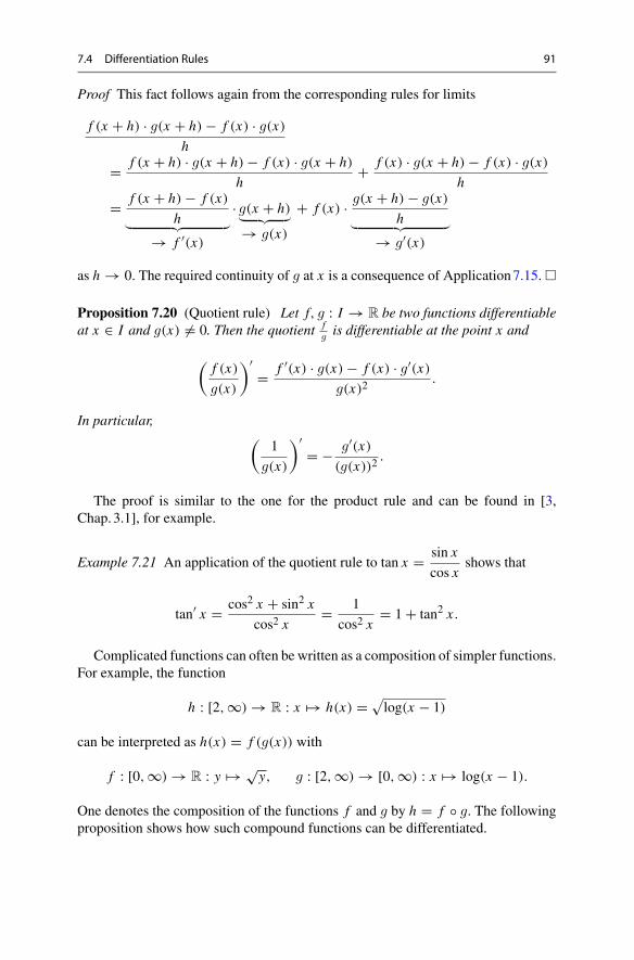
7.4 Differentiation Rules 91
Proof This fact follows again from the corresponding rules for limits
f (x + h) · g(x + h) − f (x) · g(x)
h
= f (x + h) · g(x + h) − f (x) · g(x + h)
h+ f (x) · g(x + h) − f (x) · g(x)
h
= f (x + h) − f (x)
h︸ ︷︷ ︸→ f ′(x)
· g(x + h)︸ ︷︷ ︸→ g(x)
+ f (x) · g(x + h) − g(x)
h︸ ︷︷ ︸→ g′(x)
as h → 0. The required continuity of g at x is a consequence of Application7.15. �
Proposition 7.20 (Quotient rule) Let f, g : I → R be two functions differentiableat x ∈ I and g(x) = 0. Then the quotient f
gis differentiable at the point x and
(f (x)
g(x)
)′= f ′(x) · g(x) − f (x) · g′(x)
g(x)2.
In particular,(
1
g(x)
)′= − g′(x)
(g(x))2.
The proof is similar to the one for the product rule and can be found in [3,Chap.3.1], for example.
Example 7.21 An application of the quotient rule to tan x = sin x
cos xshows that
tan′ x = cos2 x + sin2 x
cos2 x= 1
cos2 x= 1 + tan2 x .
Complicated functions can often be written as a composition of simpler functions.For example, the function
h : [2,∞) → R : x �→ h(x) = √log(x − 1)
can be interpreted as h(x) = f (g(x)) with
f : [0,∞) → R : y �→ √y, g : [2,∞) → [0,∞) : x �→ log(x − 1).
One denotes the composition of the functions f and g by h = f ◦ g. The followingproposition shows how such compound functions can be differentiated.
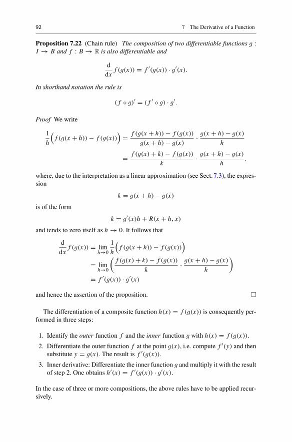
92 7 The Derivative of a Function
Proposition 7.22 (Chain rule) The composition of two differentiable functions g :I → B and f : B → R is also differentiable and
d
dxf (g(x)) = f ′(g(x)) · g′(x).
In shorthand notation the rule is
( f ◦ g)′ = ( f ′ ◦ g) · g′.
Proof We write
1
h
(f (g(x + h)) − f (g(x))
)= f (g(x + h)) − f (g(x))
g(x + h) − g(x)· g(x + h) − g(x)
h
= f (g(x) + k) − f (g(x))
k· g(x + h) − g(x)
h,
where, due to the interpretation as a linear approximation (see Sect. 7.3), the expres-sion
k = g(x + h) − g(x)
is of the form
k = g′(x)h + R(x + h, x)
and tends to zero itself as h → 0. It follows that
d
dxf (g(x)) = lim
h→0
1
h
(f (g(x + h)) − f (g(x))
)
= limh→0
(f (g(x) + k) − f (g(x))
k· g(x + h) − g(x)
h
)
= f ′(g(x)) · g′(x)
and hence the assertion of the proposition. �
The differentiation of a composite function h(x) = f (g(x)) is consequently per-formed in three steps:
1. Identify the outer function f and the inner function g with h(x) = f (g(x)).
2. Differentiate the outer function f at the point g(x), i.e. compute f ′(y) and thensubstitute y = g(x). The result is f ′(g(x)).
3. Inner derivative: Differentiate the inner function g and multiply it with the resultof step 2. One obtains h′(x) = f ′(g(x)) · g′(x).
In the case of three or more compositions, the above rules have to be applied recur-sively.

7.4 Differentiation Rules 93
Example 7.23 (a) Let h(x) = (sin x)3. We identify the outer function f (y) = y3
and the inner function g(x) = sin x . Then
h′(x) = 3 (sin x)2 · cos x .
(b) Let h(x) = e−x2 . We identify f (y) = ey and g(x) = −x2. Thus
h′(x) = e−x2 · (−2x).
The last rule that we will discuss concerns the differentiation of the inverse of adifferentiable function.
Proposition 7.24 (Inverse function rule) Let f : I → J be bijective, differentiableand f ′(y) = 0 for all y ∈ I . Then f −1 : J → I is also differentiable and
d
dxf −1(x) = 1
f ′( f −1(x)).
In shorthand notation this rule is
(f −1)′ = 1
f ′ ◦ f −1 .
Proof We set y = f −1(x) and η = f −1(ξ). Due to the continuity of the inversefunction (see PropositionC.3) we have that η → y as ξ → x . It thus follows that
d
dxf −1(x) = lim
ξ→x
f −1(ξ) − f −1(x)
ξ − x= lim
η→y
η − y
f (η) − f (y)
= limη→y
(f (η) − f (y)
η − y
)−1
= 1
f ′(y)= 1
f ′( f −1(x))
and hence the statement of the proposition. �
Figure7.4 shows the geometric background of the inverse function rule: The slopeof a straight line in x-direction is the inverse of the slope in y-direction.
If it is known beforehand that the inverse function is differentiable then its deriva-tive can also be obtained in the following way. One differentiates the identity
x = f ( f −1(x))
with respect to x using the chain rule. This yields
1 = f ′( f −1(x)) · ( f −1)′(x)
and one obtains the inverse rule by division by f ′( f −1(x)).

94 7 The Derivative of a Function
1/k
k1
1
y = f−1(x)
y
x x = f(y)
1k= f (y)
k = (f−1) (x)1
1
Fig. 7.4 Derivative of the inverse function with detailed view of the slopes
Example 7.25 (Derivative of the logarithm) Since y = log x is the inverse functionto x = ey , it follows from the inverse function rule that
(log x
)′ = 1
elog x= 1
x
for x > 0. Furthermore
log |x | ={log x, x > 0,
log (−x) , x < 0,
and thus
(log |x |)′ =
⎧⎪⎨
⎪⎩
(log x
)′ = 1
x, x > 0,
(log (−x)
)′ = 1
(−x)· (−1) = 1
x, x < 0.
Altogether one obtains the formula
(log |x |)′ = 1
xfor x = 0.
For logarithms to the base a one has
loga x = log x
log a, thus
(loga x
)′ = 1
x log a.
Example 7.26 (Derivatives of general power functions) From xα = eα log x weinfer by the chain rule that
(xα
)′ = eα log x · α
x= xα · α
x= α xα−1.
Example 7.27 (Derivative of the general exponential function) For a > 0 we haveax = ex log a . An application of the chain rule shows that
(ax)′ = (
ex log a)′ = ex log a · log a = ax log a.
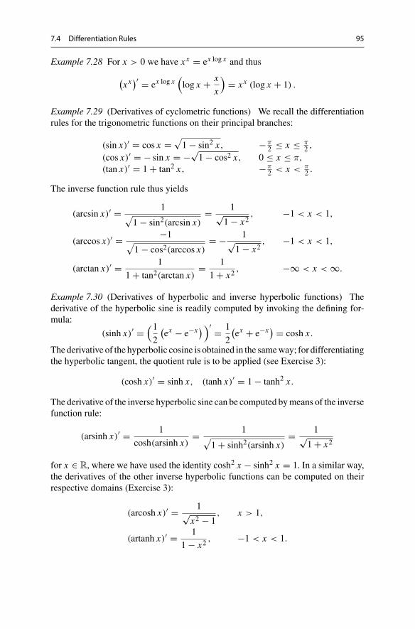
7.4 Differentiation Rules 95
Example 7.28 For x > 0 we have xx = ex log x and thus
(xx)′ = ex log x
(log x + x
x
)= xx (log x + 1) .
Example 7.29 (Derivatives of cyclometric functions) We recall the differentiationrules for the trigonometric functions on their principal branches:
(sin x)′ = cos x =√1 − sin2 x, −π
2 ≤ x ≤ π2 ,
(cos x)′ = − sin x = −√1 − cos2 x, 0 ≤ x ≤ π,
(tan x)′ = 1 + tan2 x, −π2 < x < π
2 .
The inverse function rule thus yields
(arcsin x)′ = 1√1 − sin2(arcsin x)
= 1√1 − x2
, −1 < x < 1,
(arccos x)′ = −1√1 − cos2(arccos x)
= − 1√1 − x2
, −1 < x < 1,
(arctan x)′ = 1
1 + tan2(arctan x)= 1
1 + x2, −∞ < x < ∞.
Example 7.30 (Derivatives of hyperbolic and inverse hyperbolic functions) Thederivative of the hyperbolic sine is readily computed by invoking the defining for-mula:
(sinh x)′ =(12
(ex − e−x)
)′ = 1
2
(ex + e−x) = cosh x .
Thederivative of the hyperbolic cosine is obtained in the sameway; for differentiatingthe hyperbolic tangent, the quotient rule is to be applied (see Exercise 3):
(cosh x)′ = sinh x, (tanh x)′ = 1 − tanh2 x .
The derivative of the inverse hyperbolic sine can be computed bymeans of the inversefunction rule:
(arsinh x)′ = 1
cosh(arsinh x)= 1
√1 + sinh2(arsinh x)
= 1√1 + x2
for x ∈ R, where we have used the identity cosh2 x − sinh2 x = 1. In a similar way,the derivatives of the other inverse hyperbolic functions can be computed on theirrespective domains (Exercise 3):
(arcosh x)′ = 1√x2 − 1
, x > 1,
(artanh x)′ = 1
1 − x2, −1 < x < 1.
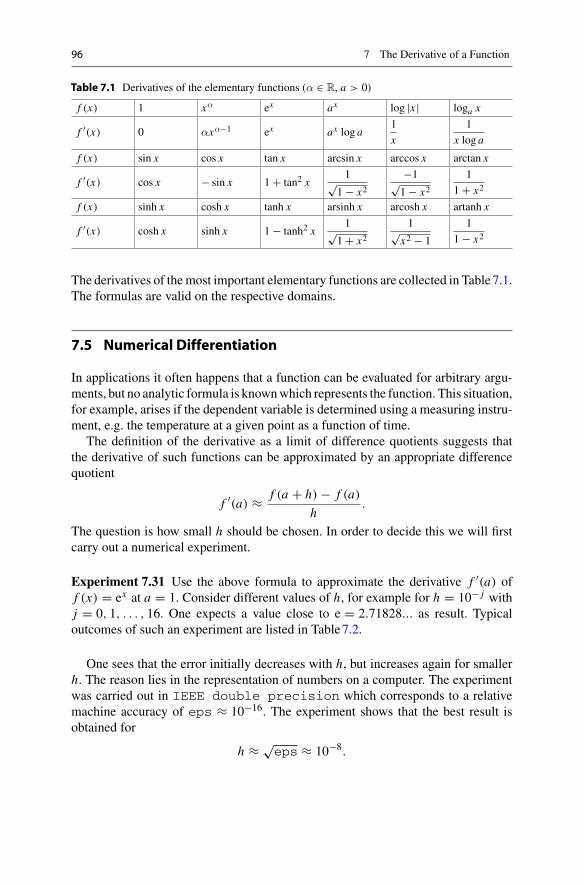
96 7 The Derivative of a Function
Table 7.1 Derivatives of the elementary functions (α ∈ R, a > 0)
f (x) 1 xα ex ax log |x | loga x
f ′(x) 0 αxα−1 ex ax log a1
x
1
x log a
f (x) sin x cos x tan x arcsin x arccos x arctan x
f ′(x) cos x − sin x 1 + tan2 x1√
1 − x2−1√1 − x2
1
1 + x2
f (x) sinh x cosh x tanh x arsinh x arcosh x artanh x
f ′(x) cosh x sinh x 1 − tanh2 x1√
1 + x21√
x2 − 1
1
1 − x2
The derivatives of themost important elementary functions are collected in Table7.1.The formulas are valid on the respective domains.
7.5 Numerical Differentiation
In applications it often happens that a function can be evaluated for arbitrary argu-ments, but no analytic formula is knownwhich represents the function. This situation,for example, arises if the dependent variable is determined using a measuring instru-ment, e.g. the temperature at a given point as a function of time.
The definition of the derivative as a limit of difference quotients suggests thatthe derivative of such functions can be approximated by an appropriate differencequotient
f ′(a) ≈ f (a + h) − f (a)
h.
The question is how small h should be chosen. In order to decide this we will firstcarry out a numerical experiment.
Experiment 7.31 Use the above formula to approximate the derivative f ′(a) off (x) = ex at a = 1. Consider different values of h, for example for h = 10− j withj = 0, 1, . . . , 16. One expects a value close to e = 2.71828... as result. Typicaloutcomes of such an experiment are listed in Table7.2.
One sees that the error initially decreases with h, but increases again for smallerh. The reason lies in the representation of numbers on a computer. The experimentwas carried out in IEEE double precision which corresponds to a relativemachine accuracy of eps ≈ 10−16. The experiment shows that the best result isobtained for
h ≈ √eps ≈ 10−8.
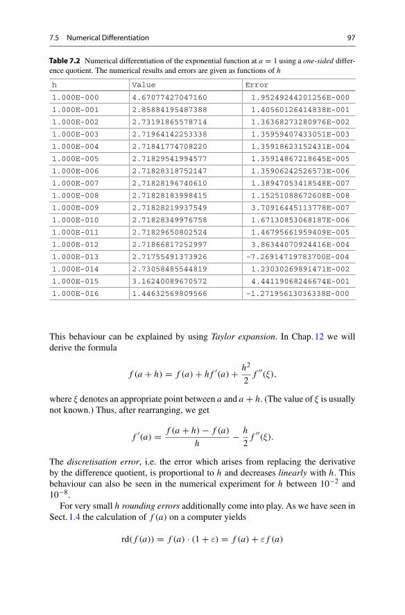
7.5 Numerical Differentiation 97
Table 7.2 Numerical differentiation of the exponential function at a = 1 using a one-sided differ-ence quotient. The numerical results and errors are given as functions of h
h Value Error
1.000E-000 4.67077427047160 1.95249244201256E-000
1.000E-001 2.85884195487388 1.40560126414838E-001
1.000E-002 2.73191865578714 1.36368273280976E-002
1.000E-003 2.71964142253338 1.35959407433051E-003
1.000E-004 2.71841774708220 1.35918623152431E-004
1.000E-005 2.71829541994577 1.35914867218645E-005
1.000E-006 2.71828318752147 1.35906242526573E-006
1.000E-007 2.71828196740610 1.38947053418548E-007
1.000E-008 2.71828183998415 1.15251088672608E-008
1.000E-009 2.71828219937549 3.70916445113778E-007
1.000E-010 2.71828349976758 1.67130853068187E-006
1.000E-011 2.71829650802524 1.46795661959409E-005
1.000E-012 2.71866817252997 3.86344070924416E-004
1.000E-013 2.71755491373926 -7.26914719783700E-004
1.000E-014 2.73058485544819 1.23030269891471E-002
1.000E-015 3.16240089670572 4.44119068246674E-001
1.000E-016 1.44632569809566 -1.27195613036338E-000
This behaviour can be explained by using Taylor expansion. In Chap.12 we willderive the formula
f (a + h) = f (a) + h f ′(a) + h2
2f ′′(ξ),
where ξ denotes an appropriate point between a and a + h. (The value of ξ is usuallynot known.) Thus, after rearranging, we get
f ′(a) = f (a + h) − f (a)
h− h
2f ′′(ξ).
The discretisation error, i.e. the error which arises from replacing the derivativeby the difference quotient, is proportional to h and decreases linearly with h. Thisbehaviour can also be seen in the numerical experiment for h between 10−2 and10−8.
For very small h rounding errors additionally come into play. As we have seen inSect. 1.4 the calculation of f (a) on a computer yields
rd( f (a)) = f (a) · (1 + ε) = f (a) + ε f (a)
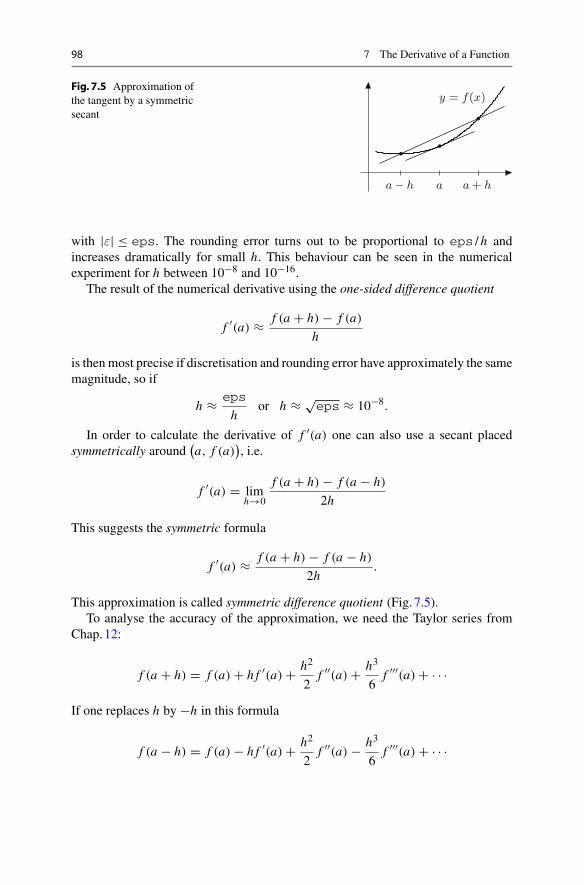
98 7 The Derivative of a Function
Fig. 7.5 Approximation ofthe tangent by a symmetricsecant
y = f(x)
a + ha a− h
with |ε| ≤ eps. The rounding error turns out to be proportional to eps /h andincreases dramatically for small h. This behaviour can be seen in the numericalexperiment for h between 10−8 and 10−16.
The result of the numerical derivative using the one-sided difference quotient
f ′(a) ≈ f (a + h) − f (a)
h
is then most precise if discretisation and rounding error have approximately the samemagnitude, so if
h ≈ eps
hor h ≈ √
eps ≈ 10−8.
In order to calculate the derivative of f ′(a) one can also use a secant placedsymmetrically around
(a, f (a)
), i.e.
f ′(a) = limh→0
f (a + h) − f (a − h)
2h
This suggests the symmetric formula
f ′(a) ≈ f (a + h) − f (a − h)
2h.
This approximation is called symmetric difference quotient (Fig. 7.5).To analyse the accuracy of the approximation, we need the Taylor series from
Chap.12:
f (a + h) = f (a) + h f ′(a) + h2
2f ′′(a) + h3
6f ′′′(a) + · · ·
If one replaces h by −h in this formula
f (a − h) = f (a) − h f ′(a) + h2
2f ′′(a) − h3
6f ′′′(a) + · · ·
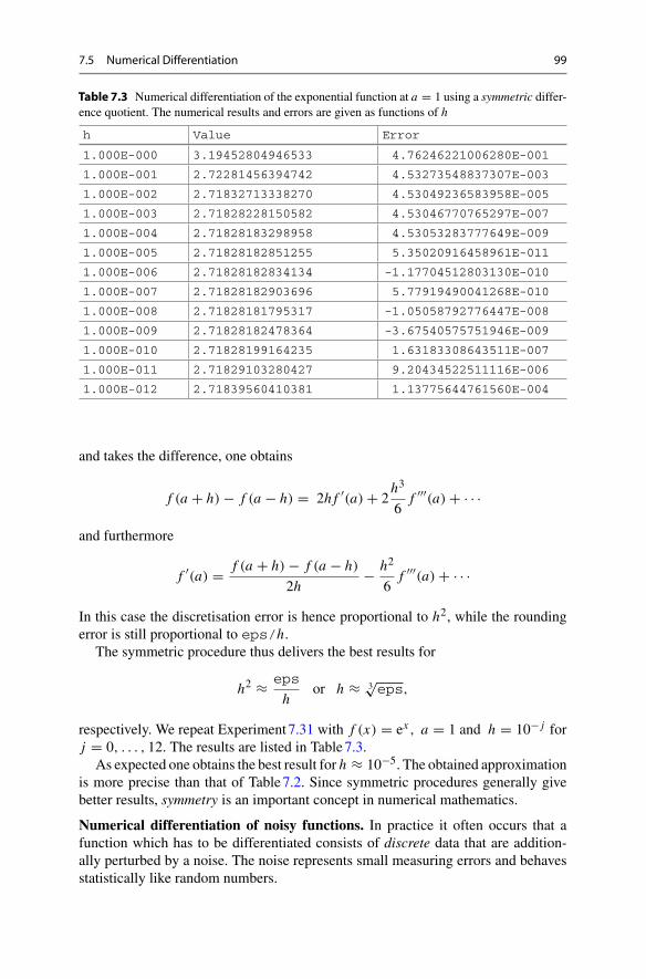
7.5 Numerical Differentiation 99
Table 7.3 Numerical differentiation of the exponential function at a = 1 using a symmetric differ-ence quotient. The numerical results and errors are given as functions of h
h Value Error
1.000E-000 3.19452804946533 4.76246221006280E-001
1.000E-001 2.72281456394742 4.53273548837307E-003
1.000E-002 2.71832713338270 4.53049236583958E-005
1.000E-003 2.71828228150582 4.53046770765297E-007
1.000E-004 2.71828183298958 4.53053283777649E-009
1.000E-005 2.71828182851255 5.35020916458961E-011
1.000E-006 2.71828182834134 -1.17704512803130E-010
1.000E-007 2.71828182903696 5.77919490041268E-010
1.000E-008 2.71828181795317 -1.05058792776447E-008
1.000E-009 2.71828182478364 -3.67540575751946E-009
1.000E-010 2.71828199164235 1.63183308643511E-007
1.000E-011 2.71829103280427 9.20434522511116E-006
1.000E-012 2.71839560410381 1.13775644761560E-004
and takes the difference, one obtains
f (a + h) − f (a − h) = 2h f ′(a) + 2h3
6f ′′′(a) + · · ·
and furthermore
f ′(a) = f (a + h) − f (a − h)
2h− h2
6f ′′′(a) + · · ·
In this case the discretisation error is hence proportional to h2, while the roundingerror is still proportional to eps/h.
The symmetric procedure thus delivers the best results for
h2 ≈ eps
hor h ≈ 3
√eps,
respectively. We repeat Experiment7.31 with f (x) = ex , a = 1 and h = 10− j forj = 0, . . . , 12. The results are listed in Table7.3.As expected one obtains the best result for h ≈ 10−5. The obtained approximation
is more precise than that of Table7.2. Since symmetric procedures generally givebetter results, symmetry is an important concept in numerical mathematics.
Numerical differentiation of noisy functions. In practice it often occurs that afunction which has to be differentiated consists of discrete data that are addition-ally perturbed by a noise. The noise represents small measuring errors and behavesstatistically like random numbers.
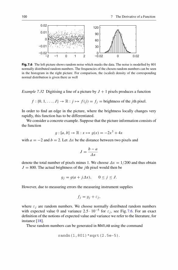
100 7 The Derivative of a Function
−2 −1 0 1 2−0.02
−0.01
0
0.01
0.02
−0.02 0 0.020
30
60
90
120
Fig.7.6 The left picture shows random noise which masks the data. The noise is modelled by 801normally distributed random numbers. The frequencies of the chosen random numbers can be seenin the histogram in the right picture. For comparison, the (scaled) density of the correspondingnormal distribution is given there as well
Example 7.32 Digitising a line of a picture by J + 1 pixels produces a function
f : {0, 1, . . . , J } → R : j �→ f ( j) = f j = brightness of the j th pixel.
In order to find an edge in the picture, where the brightness locally changes veryrapidly, this function has to be differentiated.
We consider a concrete example. Suppose that the picture information consists ofthe function
g : [a, b] → R : x �→ g(x) = −2x3 + 4x
with a = −2 and b = 2. Let Δx be the distance between two pixels and
J = b − a
Δx
denote the total number of pixels minus 1. We choose Δx = 1/200 and thus obtainJ = 800. The actual brightness of the j th pixel would then be
g j = g(a + jΔx), 0 ≤ j ≤ J.
However, due to measuring errors the measuring instrument supplies
f j = g j + ε j ,
where ε j are random numbers. We choose normally distributed random numberswith expected value 0 and variance 2.5 · 10−5 for ε j , see Fig. 7.6. For an exactdefinition of the notions of expected value and variance we refer to the literature, forinstance [18].
These random numbers can be generated in MATLAB using the command
randn(1,801)*sqrt(2.5e-5).

7.5 Numerical Differentiation 101
−2 0 2−10
−5
0
5
10
−2 0 2−10
−5
0
5
10
−2 0 2−10
−5
0
5
10
f
f
f
f
f
f
Fig.7.7 Numerically obtained derivative of a noisy function f , consisting of 801 data values (left);derivative of the same function after filtering using a Gaussian filter (middle) and after smoothingusing splines (right)
Differentiating f using the previous rules generates
f ′j ≈ f j − f j−1
Δx= g j − g j−1
Δx+ ε j − ε j−1
Δx
and the part with g gives the desired value of the derivative, namely
g j − g j−1
Δx= g(a + jΔx) − g(a + jΔx − Δx)
Δx≈ g′(a + jΔx).
The sequence of random numbers results in a non-differentiable graph. The expres-sion
ε j − ε j−1
Δx
is proportional to J · max0≤ j≤J |ε j |. The errors become dominant for large J , seeFig. 7.7, left picture.
To still obtain reliable results, the data have to be smoothed before differentiating.The simplest method is a so-called convolutionwith aGaussian filter which amountsto a weighted averaging of the data (Fig. 7.7, middle). Alternatively one can also usesplines for smoothing, for example the routine csaps in MATLAB. For the rightpicture in Fig. 7.7 this method has been used.
Experiment 7.33 Generate Fig. 7.7 using the MATLAB program mat07_1.m andinvestigate the influence of the choice of random numbers and the smoothing param-eter in csaps on the result.
7.6 Exercises
1. Compute the first derivative of the functions
f (x) = x3, g(t) = 1
t2, h(x) = cos x, k(x) = 1√
x, �(t) = tan t
using the definition of the derivative as a limit.
102 7 The Derivative of a Function
2. Compute the first derivative of the functions
a(x) = x2−1x2+2x+1
, b(x) = (x3 − 1) sin2 x, c(t) = √1 + t2 arctan t,
d(t) = t2ecos(t2+1), e(x) = x2 sin x , f (s) = log
(s + √
1 + s2)
.
Check your results withmaple .3. Derive the remaining formulas in Example 7.30. Start by computing the deriva-
tives of the hyperbolic cosine and hyperbolic tangent. Use the inverse functionrule to differentiate the inverse hyperbolic cosine and inverse hyperbolic tangent.
4. Compute an approximation of√34 by replacing the function f (x) = √
x atx = 36 by its linear approximation. How accurate is your result?
5. Find the equation of the tangent line to the graph of the function y = f (x)
through the point (x0, f (x0)), where
f (x) = x
2+ x
log xand (a) x0 = e; (b) x0 = e2.
6. Sand runs from a conveyor belt onto a heap with a velocity of 2 m3/min. Thesand forms a cone-shaped pile whose height equals 4
3 of the radius. With whichvelocity does the radius grow if the sand cone has a diameter of 6 m?Hint. Determine the volume V as a function of the radius r , consider V and r asfunctions of time t and differentiate the equation with respect to t . Compute r .
7. Use the Taylor series
y(x + h) = y(x) + hy′(x) + h2
2y′′(x) + h3
6y′′′(x) + h4
24y(4)(x) + · · ·
to derive the formula
y′′(x) = y(x + h) − 2y(x) + y(x − h)
h2 − h2
12y(4)(x) + · · ·
and read off from that a numerical method for calculating the second derivative.The discretisation error is proportional to h2, and the rounding error is propor-tional to eps/h2. By equating the discretisation and the rounding error deducethe optimal step size h. Check your considerations by performing a numericalexperiment in MATLAB , computing the second derivative of y(x) = e2x at thepoint x = 1.
8. Write aMATLAB program which numerically differentiates a given function on agiven interval and plots the function and its first derivative. Test your programon the functions
f (x) = cos x, 0 ≤ x ≤ 6π,
and
g(x) = e− cos(3x), 0 ≤ x ≤ 2.
7.6 Exercises 103
9. Show that the nth derivative of the power function y = xn equals n! for n ≥1. Verify that the derivative of order n + 1 of a polynomial p(x) = an xn +an−1xn−1 + · · · + a1x + a0 of degree n equals zero.
10. Compute the second derivative of the functions
f (x) = e−x2 , g(x) = log(
x +√1 + x2
), h(x) = log
x + 1
x − 1.

8Applications of theDerivative
This chapter is devoted to some applications of the derivative which form part ofthe basic skills in modelling. We start with a discussion of features of graphs. Moreprecisely,we use the derivative to describe geometric properties likemaxima,minimaand monotonicity. Even though plotting functions with MATLAB ormaple is simple,understanding the connection with the derivative is important, for example, when afunction with given properties is to be chosen from a particular class of functions.
In the following section we discuss Newton’s method and the concept of orderof convergence. Newton’s method is one of the most important tools for computingzeros of functions. It is nearly universally in use.
The final section of this chapter is devoted to an elementary method from dataanalysis. We show how to compute a regression line through the origin. There aremany areas of application that involve linear regression. This topic will be developedin more detail in Chap.18.
8.1 Curve Sketching
In the following we investigate some geometric properties of graphs of functionsusing the derivative: maxima and minima, intervals of monotonicity and convexity.We further discuss the mean value theorem which is an important technical tool forproofs.
Definition 8.1 A function f : [a, b] → R has
(a) a global maximum at x0 ∈ [a, b] if
f (x) ≤ f (x0) for all x ∈ [a, b];© Springer Nature Switzerland AG 2018M. Oberguggenberger and A. Ostermann, Analysis for Computer Scientists,Undergraduate Topics in Computer Science,https://doi.org/10.1007/978-3-319-91155-7_8
105
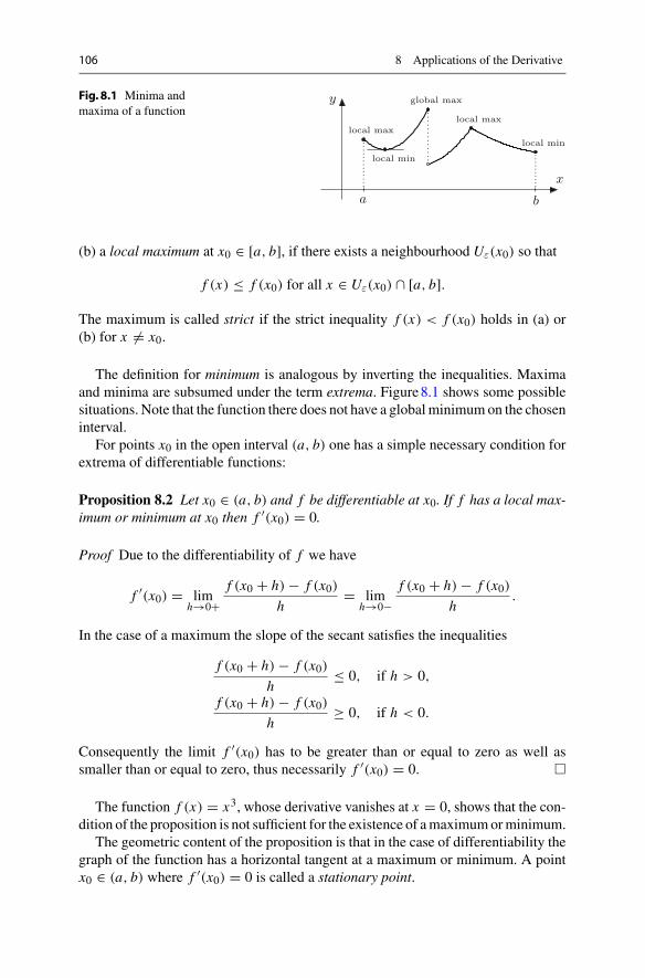
106 8 Applications of the Derivative
Fig. 8.1 Minima andmaxima of a function
local min
local maxlocal max
y
x
ba
global max
local min
(b) a local maximum at x0 ∈ [a, b], if there exists a neighbourhood Uε(x0) so that
f (x) ≤ f (x0) for all x ∈ Uε(x0) ∩ [a, b].
The maximum is called strict if the strict inequality f (x) < f (x0) holds in (a) or(b) for x �= x0.
The definition for minimum is analogous by inverting the inequalities. Maximaand minima are subsumed under the term extrema. Figure8.1 shows some possiblesituations. Note that the function there does not have a globalminimumon the choseninterval.
For points x0 in the open interval (a, b) one has a simple necessary condition forextrema of differentiable functions:
Proposition 8.2 Let x0 ∈ (a, b) and f be differentiable at x0. If f has a local max-imum or minimum at x0 then f ′(x0) = 0.
Proof Due to the differentiability of f we have
f ′(x0) = limh→0+
f (x0 + h) − f (x0)
h= lim
h→0−f (x0 + h) − f (x0)
h.
In the case of a maximum the slope of the secant satisfies the inequalities
f (x0 + h) − f (x0)
h≤ 0, if h > 0,
f (x0 + h) − f (x0)
h≥ 0, if h < 0.
Consequently the limit f ′(x0) has to be greater than or equal to zero as well assmaller than or equal to zero, thus necessarily f ′(x0) = 0. �
The function f (x) = x3, whose derivative vanishes at x = 0, shows that the con-dition of the proposition is not sufficient for the existence of amaximumorminimum.
The geometric content of the proposition is that in the case of differentiability thegraph of the function has a horizontal tangent at a maximum or minimum. A pointx0 ∈ (a, b) where f ′(x0) = 0 is called a stationary point.

8.1 Curve Sketching 107
Fig. 8.2 The mean valuetheorem
f(b)
f(a)
ξ ba
y
x
Remark 8.3 The proposition shows that the following point sets have to be checkedin order to determine the maxima and minima of a function f : [a, b] → R:
(a) the boundary points x0 = a, x0 = b;
(b) points x0 ∈ (a, b) at which f is not differentiable;
(c) points x0 ∈ (a, b) at which f is differentiable and f ′(x0) = 0.
The following proposition is a useful technical tool for proofs. One of its applica-tions lies in estimating the error of numerical methods. Similarly to the intermediatevalue theorem, the proof is based on the completeness of the real numbers.We are notgoing to present it here but instead refer to the literature, for instance [3, Chap.3.2].
Proposition 8.4 (Mean value theorem) Let f be continuous on [a, b] and differ-entiable on (a, b). Then there exists a point ξ ∈ (a, b) such that
f (b) − f (a)
b − a= f ′(ξ).
Geometrically this means that the tangent at ξ has the same slope as the secantthrough (a, f (a)), (b, f (b)). Figure8.2 illustrates this fact.
We now turn to the description of the behaviour of the slope of differentiablefunctions.
Definition 8.5 A function f : I → R is called monotonically increasing, if
x1 < x2 ⇒ f (x1) ≤ f (x2)
for all x1, x2 ∈ I . It is called strictly monotonically increasing, if
x1 < x2 ⇒ f (x1) < f (x2).
A function f is said to be (strictly) monotonically decreasing, if − f is (strictly)monotonically increasing.
Examples of strictly monotonically increasing functions are the power functionsx → xn with odd powers n; a monotonically, but not strictly monotonically increas-ing function is the sign function x → sign x , for instance. The behaviour of the slopeof a differentiable function can be described by the sign of the first derivative.
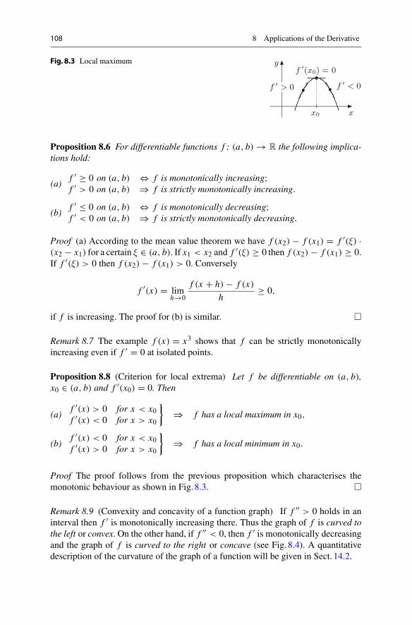
108 8 Applications of the Derivative
Fig. 8.3 Local maximumf (x0) = 0
f < 0f > 0
x0
y
x
Proposition 8.6 For differentiable functions f : (a, b) → R the following implica-tions hold:
(a)f ′ ≥ 0 on (a, b) ⇔ f is monotonically increasing;f ′ > 0 on (a, b) ⇒ f is strictly monotonically increasing.
(b)f ′ ≤ 0 on (a, b) ⇔ f is monotonically decreasing;f ′ < 0 on (a, b) ⇒ f is strictly monotonically decreasing.
Proof (a) According to the mean value theorem we have f (x2) − f (x1) = f ′(ξ) ·(x2 − x1) for a certain ξ ∈ (a, b). If x1 < x2 and f ′(ξ) ≥ 0 then f (x2) − f (x1) ≥ 0.If f ′(ξ) > 0 then f (x2) − f (x1) > 0. Conversely
f ′(x) = limh→0
f (x + h) − f (x)
h≥ 0,
if f is increasing. The proof for (b) is similar. �
Remark 8.7 The example f (x) = x3 shows that f can be strictly monotonicallyincreasing even if f ′ = 0 at isolated points.
Proposition 8.8 (Criterion for local extrema) Let f be differentiable on (a, b),x0 ∈ (a, b) and f ′(x0) = 0. Then
(a)f ′(x) > 0 for x < x0f ′(x) < 0 for x > x0
}⇒ f has a local maximum in x0,
(b)f ′(x) < 0 for x < x0f ′(x) > 0 for x > x0
}⇒ f has a local minimum in x0.
Proof The proof follows from the previous proposition which characterises themonotonic behaviour as shown in Fig. 8.3. �
Remark 8.9 (Convexity and concavity of a function graph) If f ′′ > 0 holds in aninterval then f ′ is monotonically increasing there. Thus the graph of f is curved tothe left or convex. On the other hand, if f ′′ < 0, then f ′ is monotonically decreasingand the graph of f is curved to the right or concave (see Fig. 8.4). A quantitativedescription of the curvature of the graph of a function will be given in Sect. 14.2.
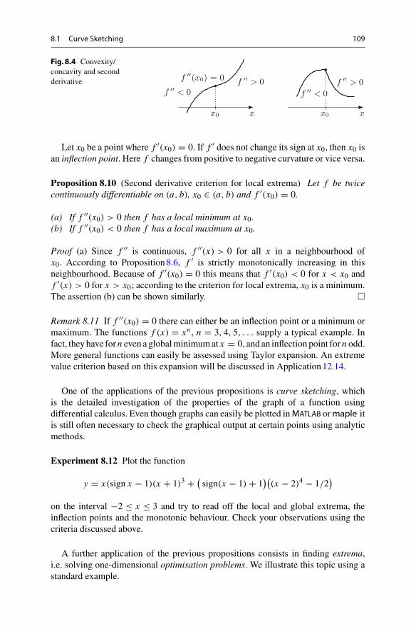
8.1 Curve Sketching 109
Fig. 8.4 Convexity/concavity and secondderivative
x0
f > 0f < 0
xx0
f (x0) = 0 f > 0f < 0
x
Let x0 be a point where f ′(x0) = 0. If f ′ does not change its sign at x0, then x0 isan inflection point. Here f changes from positive to negative curvature or vice versa.
Proposition 8.10 (Second derivative criterion for local extrema) Let f be twicecontinuously differentiable on (a, b), x0 ∈ (a, b) and f ′(x0) = 0.
(a) If f ′′(x0) > 0 then f has a local minimum at x0.(b) If f ′′(x0) < 0 then f has a local maximum at x0.
Proof (a) Since f ′′ is continuous, f ′′(x) > 0 for all x in a neighbourhood ofx0. According to Proposition8.6, f ′ is strictly monotonically increasing in thisneighbourhood. Because of f ′(x0) = 0 this means that f ′(x0) < 0 for x < x0 andf ′(x) > 0 for x > x0; according to the criterion for local extrema, x0 is a minimum.The assertion (b) can be shown similarly. �
Remark 8.11 If f ′′(x0) = 0 there can either be an inflection point or a minimum ormaximum. The functions f (x) = xn , n = 3, 4, 5, . . . supply a typical example. Infact, they have forn even a globalminimumat x = 0, and an inflection point forn odd.More general functions can easily be assessed using Taylor expansion. An extremevalue criterion based on this expansion will be discussed in Application12.14.
One of the applications of the previous propositions is curve sketching, whichis the detailed investigation of the properties of the graph of a function usingdifferential calculus. Even though graphs can easily be plotted inMATLAB ormaple itis still often necessary to check the graphical output at certain points using analyticmethods.
Experiment 8.12 Plot the function
y = x(sign x − 1)(x + 1)3 + (sign(x − 1) + 1
)((x − 2)4 − 1/2
)
on the interval −2 ≤ x ≤ 3 and try to read off the local and global extrema, theinflection points and the monotonic behaviour. Check your observations using thecriteria discussed above.
A further application of the previous propositions consists in finding extrema,i.e. solving one-dimensional optimisation problems. We illustrate this topic using astandard example.
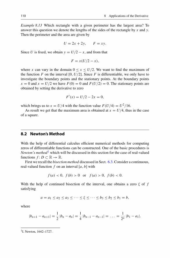
110 8 Applications of the Derivative
Example 8.13 Which rectangle with a given perimeter has the largest area? Toanswer this question we denote the lengths of the sides of the rectangle by x and y.Then the perimeter and the area are given by
U = 2x + 2y, F = xy.
Since U is fixed, we obtain y = U/2 − x , and from that
F = x(U/2 − x),
where x can vary in the domain 0 ≤ x ≤ U/2. We want to find the maximum ofthe function F on the interval [0,U/2]. Since F is differentiable, we only have toinvestigate the boundary points and the stationary points. At the boundary pointsx = 0 and x = U/2 we have F(0) = 0 and F(U/2) = 0. The stationary points areobtained by setting the derivative to zero
F ′(x) = U/2 − 2x = 0,
which brings us to x = U/4 with the function value F(U/4) = U 2/16.As result we get that the maximum area is obtained at x = U/4, thus in the case
of a square.
8.2 Newton’s Method
With the help of differential calculus efficient numerical methods for computingzeros of differentiable functions can be constructed. One of the basic procedures isNewton’s method1 which will be discussed in this section for the case of real-valuedfunctions f : D ⊂ R → R.
First we recall the bisection method discussed in Sect. 6.3. Consider a continuous,real-valued function f on an interval [a, b] with
f (a) < 0, f (b) > 0 or f (a) > 0, f (b) < 0.
With the help of continued bisection of the interval, one obtains a zero ξ of fsatisfying
a = a1 ≤ a2 ≤ a3 ≤ · · · ≤ ξ ≤ · · · ≤ b3 ≤ b2 ≤ b1 = b,
where
|bn+1 − an+1| = 1
2|bn − an| = 1
4|bn−1 − an−1| = . . . = 1
2n|b1 − a1|.
1I. Newton, 1642–1727.
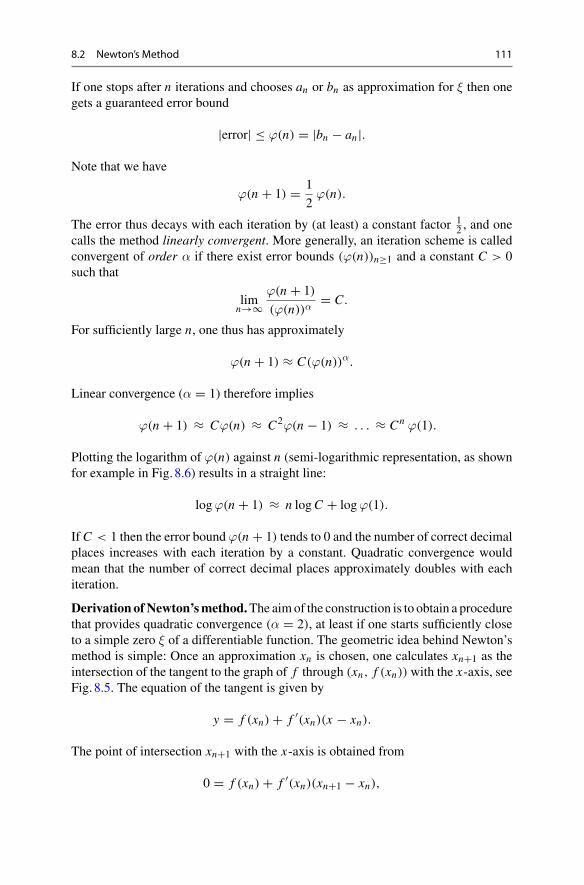
8.2 Newton’s Method 111
If one stops after n iterations and chooses an or bn as approximation for ξ then onegets a guaranteed error bound
|error| ≤ ϕ(n) = |bn − an|.
Note that we have
ϕ(n + 1) = 1
2ϕ(n).
The error thus decays with each iteration by (at least) a constant factor 12 , and one
calls the method linearly convergent. More generally, an iteration scheme is calledconvergent of order α if there exist error bounds (ϕ(n))n≥1 and a constant C > 0such that
limn→∞
ϕ(n + 1)
(ϕ(n))α= C.
For sufficiently large n, one thus has approximately
ϕ(n + 1) ≈ C(ϕ(n))α.
Linear convergence (α = 1) therefore implies
ϕ(n + 1) ≈ Cϕ(n) ≈ C2ϕ(n − 1) ≈ . . . ≈ Cn ϕ(1).
Plotting the logarithm of ϕ(n) against n (semi-logarithmic representation, as shownfor example in Fig. 8.6) results in a straight line:
logϕ(n + 1) ≈ n logC + logϕ(1).
If C < 1 then the error bound ϕ(n + 1) tends to 0 and the number of correct decimalplaces increases with each iteration by a constant. Quadratic convergence wouldmean that the number of correct decimal places approximately doubles with eachiteration.
Derivation ofNewton’smethod.The aimof the construction is to obtain a procedurethat provides quadratic convergence (α = 2), at least if one starts sufficiently closeto a simple zero ξ of a differentiable function. The geometric idea behind Newton’smethod is simple: Once an approximation xn is chosen, one calculates xn+1 as theintersection of the tangent to the graph of f through (xn, f (xn))with the x-axis, seeFig. 8.5. The equation of the tangent is given by
y = f (xn) + f ′(xn)(x − xn).
The point of intersection xn+1 with the x-axis is obtained from
0 = f (xn) + f ′(xn)(xn+1 − xn),
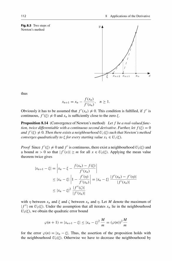
112 8 Applications of the Derivative
Fig. 8.5 Two steps ofNewton’s method
ξ xn+2 xn+1 xn
y
x
thus
xn+1 = xn − f (xn)
f ′(xn), n ≥ 1.
Obviously it has to be assumed that f ′(xn) �= 0. This condition is fulfilled, if f ′ iscontinuous, f ′(ξ) �= 0 and xn is sufficiently close to the zero ξ.
Proposition 8.14 (Convergence of Newton’s method) Let f be a real-valued func-tion, twice differentiable with a continuous second derivative. Further, let f (ξ) = 0and f ′(ξ) �= 0. Then there exists a neighbourhood Uε(ξ) such that Newton’s methodconverges quadratically to ξ for every starting value x1 ∈ Uε(ξ).
Proof Since f ′(ξ) �= 0 and f ′ is continuous, there exist a neighbourhoodUδ(ξ) anda bound m > 0 so that | f ′(x)| ≥ m for all x ∈ Uδ(ξ). Applying the mean valuetheorem twice gives
|xn+1 − ξ| =∣∣∣∣xn − ξ − f (xn) − f (ξ)
f ′(xn)
∣∣∣∣≤ |xn − ξ|
∣∣∣∣1 − f ′(η)f ′(xn)
∣∣∣∣ = |xn − ξ| | f ′(xn) − f ′(η)|| f ′(xn)|
≤ |xn − ξ|2 | f ′′(ζ)|| f ′(xn)|
with η between xn and ξ and ζ between xn and η. Let M denote the maximum of| f ′′| on Uδ(ξ). Under the assumption that all iterates xn lie in the neighbourhoodUδ(ξ), we obtain the quadratic error bound
ϕ(n + 1) = |xn+1 − ξ| ≤ |xn − ξ|2 M
m= (ϕ(n))2
M
m
for the error ϕ(n) = |xn − ξ|. Thus, the assertion of the proposition holds withthe neighbourhood Uδ(ξ). Otherwise we have to decrease the neighbourhood by
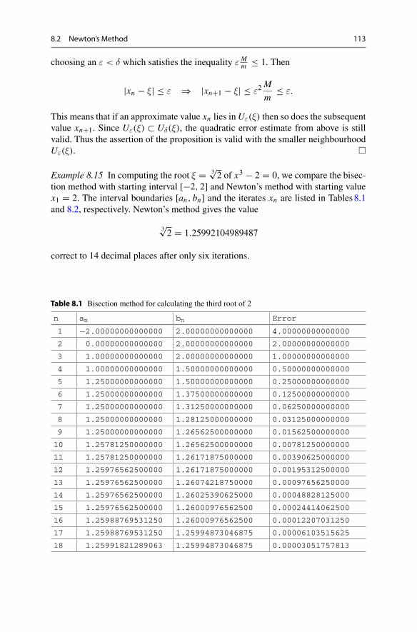
8.2 Newton’s Method 113
choosing an ε < δ which satisfies the inequality εMm ≤ 1. Then
|xn − ξ| ≤ ε ⇒ |xn+1 − ξ| ≤ ε2M
m≤ ε.
This means that if an approximate value xn lies inUε(ξ) then so does the subsequentvalue xn+1. Since Uε(ξ) ⊂ Uδ(ξ), the quadratic error estimate from above is stillvalid. Thus the assertion of the proposition is valid with the smaller neighbourhoodUε(ξ). �
Example 8.15 In computing the root ξ = 3√2 of x3 − 2 = 0, we compare the bisec-
tion method with starting interval [−2, 2] and Newton’s method with starting valuex1 = 2. The interval boundaries [an, bn] and the iterates xn are listed in Tables8.1and 8.2, respectively. Newton’s method gives the value
3√2 = 1.25992104989487
correct to 14 decimal places after only six iterations.
Table 8.1 Bisection method for calculating the third root of 2
n an bn Error
1 −2.00000000000000 2.00000000000000 4.00000000000000
2 0.00000000000000 2.00000000000000 2.00000000000000
3 1.00000000000000 2.00000000000000 1.00000000000000
4 1.00000000000000 1.50000000000000 0.50000000000000
5 1.25000000000000 1.50000000000000 0.25000000000000
6 1.25000000000000 1.37500000000000 0.12500000000000
7 1.25000000000000 1.31250000000000 0.06250000000000
8 1.25000000000000 1.28125000000000 0.03125000000000
9 1.25000000000000 1.26562500000000 0.01562500000000
10 1.25781250000000 1.26562500000000 0.00781250000000
11 1.25781250000000 1.26171875000000 0.00390625000000
12 1.25976562500000 1.26171875000000 0.00195312500000
13 1.25976562500000 1.26074218750000 0.00097656250000
14 1.25976562500000 1.26025390625000 0.00048828125000
15 1.25976562500000 1.26000976562500 0.00024414062500
16 1.25988769531250 1.26000976562500 0.00012207031250
17 1.25988769531250 1.25994873046875 0.00006103515625
18 1.25991821289063 1.25994873046875 0.00003051757813

114 8 Applications of the Derivative
Table 8.2 Newton’s methodfor calculating the third rootof 2
n xn Error
1 2.00000000000000 0.74007895010513
2 1.50000000000000 0.24007895010513
3 1.29629629629630 0.03637524640142
4 1.26093222474175 0.00101117484688
5 1.25992186056593 0.00000081067105
6 1.25992104989539 0.00000000000052
7 1.25992104989487 0.00000000000000
The error curves for the bisection method and Newton’s method can be seen inFig. 8.6. A semi-logarithmic representation (MATLAB command semilogy) is usedthere.
Remark 8.16 The convergence behaviour of Newton’s method depends on the con-ditions of Proposition8.14. If the starting value x1 is too far away from the zero ξ,then the method might diverge, oscillate or converge to a different zero. If f ′(ξ) = 0,which means the zero ξ has a multiplicity > 1, then the order of convergence maybe reduced.
Experiment 8.17 Open the applet Newton’s method and test—using the sinefunction—how the choice of the starting value influences the result (in the applet theright interval boundary is the initial value). Experiment with the intervals [−2, x0]for x0 = 1, 1.1, 1.2, 1.3, 1.5, 1.57, 1.5707, 1.57079 and interpret your observations.Also carry out the calculations with the same starting values with the help of theM-file mat08_2.m.
Experiment 8.18 With the help of the appletNewton’s method, study how the orderof convergence drops for multiple zeros. For this purpose, use the two polynomialfunctions given in the applet.
Remark 8.19 Variants of Newton’s method can be obtained by evaluating the deriva-tive f ′(xn) numerically. For example, the approximation
f ′(xn) ≈ f (xn) − f (xn−1)
xn − xn−1
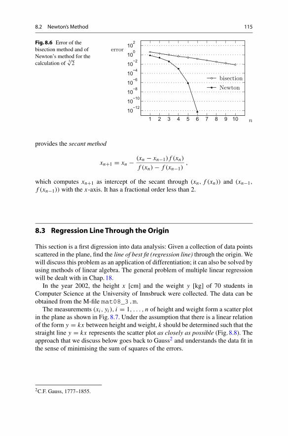
8.2 Newton’s Method 115
Fig. 8.6 Error of thebisection method and ofNewton’s method for thecalculation of 3
√2
1 2 3 4 5 6 7 8 9 1010
−1210
−1010
−810
−610
−410
−210
010
2
error
n
Newton
bisection
provides the secant method
xn+1 = xn − (xn − xn−1) f (xn)
f (xn) − f (xn−1),
which computes xn+1 as intercept of the secant through (xn, f (xn)) and (xn−1,
f (xn−1)) with the x-axis. It has a fractional order less than 2.
8.3 Regression Line Through the Origin
This section is a first digression into data analysis: Given a collection of data pointsscattered in the plane, find the line of best fit (regression line) through the origin. Wewill discuss this problem as an application of differentiation; it can also be solved byusing methods of linear algebra. The general problem of multiple linear regressionwill be dealt with in Chap.18.
In the year 2002, the height x [cm] and the weight y [kg] of 70 students inComputer Science at the University of Innsbruck were collected. The data can beobtained from the M-file mat08_3.m.
The measurements (xi , yi ), i = 1, . . . , n of height and weight form a scatter plotin the plane as shown in Fig. 8.7. Under the assumption that there is a linear relationof the form y = kx between height and weight, k should be determined such that thestraight line y = kx represents the scatter plot as closely as possible (Fig. 8.8). Theapproach that we discuss below goes back to Gauss2 and understands the data fit inthe sense of minimising the sum of squares of the errors.
2C.F. Gauss, 1777–1855.
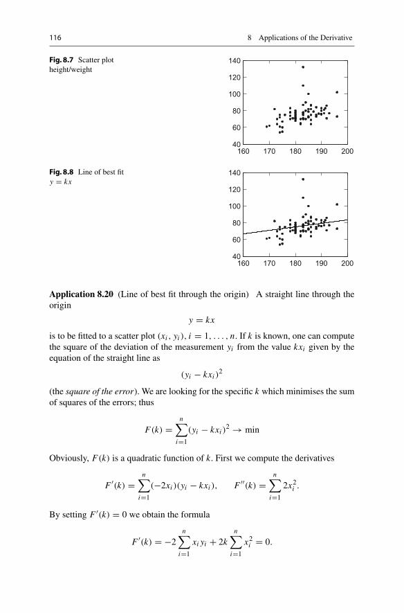
116 8 Applications of the Derivative
Fig. 8.7 Scatter plotheight/weight
160 170 180 190 20040
60
80
100
120
140
Fig. 8.8 Line of best fity = kx
160 170 180 190 20040
60
80
100
120
140
Application 8.20 (Line of best fit through the origin) A straight line through theorigin
y = kx
is to be fitted to a scatter plot (xi , yi ), i = 1, . . . , n. If k is known, one can computethe square of the deviation of the measurement yi from the value kxi given by theequation of the straight line as
(yi − kxi )2
(the square of the error). We are looking for the specific k which minimises the sumof squares of the errors; thus
F(k) =n∑
i=1
(yi − kxi )2 → min
Obviously, F(k) is a quadratic function of k. First we compute the derivatives
F ′(k) =n∑
i=1
(−2xi )(yi − kxi ), F ′′(k) =n∑
i=1
2x2i .
By setting F ′(k) = 0 we obtain the formula
F ′(k) = −2n∑
i=1
xi yi + 2kn∑
i=1
x2i = 0.

8.3 Regression Line Through the Origin 117
Since evidently F ′′ > 0, its solution
k =∑
xi yi∑x2i
is the global minimum and gives the slope of the line of best fit.
Example 8.21 To illustrate the regression line through the origin we use the Austrianconsumer price index 2010–2016 (data taken from [26]):
year 2010 2011 2012 2013 2014 2015 2016index 100.0 103.3 105.8 107.9 109.7 110.7 111.7
For the calculation it is useful to introduce new variables x and y, where x = 0corresponds to the year 2010 and y = 0 to the index 100. This means that x =(year − 2010) and y = (index − 100); y describes the relative price increase (in percent) with respect to the year 2010. The re-scaled data are
xi 0 1 2 3 4 5 6yi 0.0 3.3 5.8 7.9 9.7 10.7 11.7
We are looking for the line of best fit to these data through the origin. For this purposewe have to minimise
F(k) = (3.3 − k · 1)2 + (5.8 − k · 2)2 + (7.9 − k · 3)2 + (9.7 − k · 4)2+ (10.7 − k · 5)2 + (11.7 − k · 6)2
which results in (rounded)
k = 1 · 3.3 + 2 · 5.8 + 3 · 7.9 + 4 · 9.7 + 5 · 10.7 + 6 · 11.71 · 1 + 2 · 2 + 3 · 3 + 4 · 4 + 5 · 5 + 6 · 6 = 201.1
91= 2.21.
The line of best fit is thus
y = 2.21x
or transformed back
index = 100 + (year − 2010) · 2.21.
The result is shown in Fig. 8.9, in a year/index-scale as well as in the transformedvariables. For the year 2017, extrapolation along the regression line would forecast
index(2017) = 100 + 7 · 2.21 = 115.5.
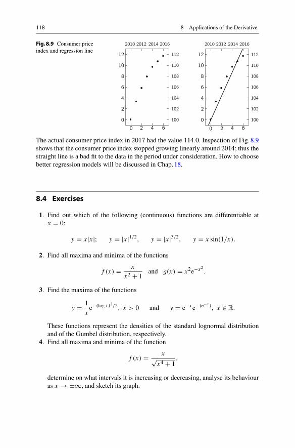
118 8 Applications of the Derivative
Fig. 8.9 Consumer priceindex and regression line
6420
12
10
8
6
4
2
0
112
110
108
106
104
102
100
2010 2012 2014 2016
6420
12
10
8
6
4
2
0
112
110
108
106
104
102
100
2010 2012 2014 2016
The actual consumer price index in 2017 had the value 114.0. Inspection of Fig. 8.9shows that the consumer price index stopped growing linearly around 2014; thus thestraight line is a bad fit to the data in the period under consideration. How to choosebetter regression models will be discussed in Chap.18.
8.4 Exercises
1. Find out which of the following (continuous) functions are differentiable atx = 0:
y = x |x |; y = |x |1/2, y = |x |3/2, y = x sin(1/x).
2. Find all maxima and minima of the functions
f (x) = x
x2 + 1and g(x) = x2e−x2 .
3. Find the maxima of the functions
y = 1
xe−(log x)2/2, x > 0 and y = e−xe−(e−x ), x ∈ R.
These functions represent the densities of the standard lognormal distributionand of the Gumbel distribution, respectively.
4. Find all maxima and minima of the function
f (x) = x√x4 + 1
,
determine on what intervals it is increasing or decreasing, analyse its behaviouras x → ±∞, and sketch its graph.
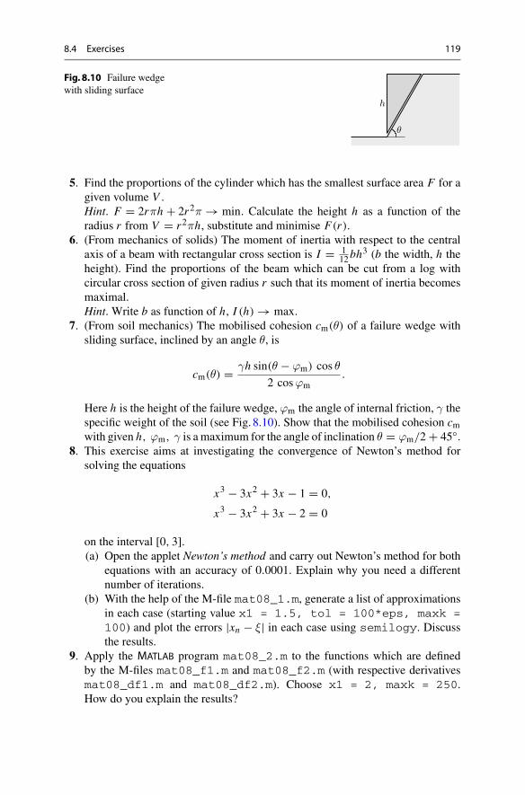
8.4 Exercises 119
Fig. 8.10 Failure wedgewith sliding surface
θ
h
5. Find the proportions of the cylinder which has the smallest surface area F for agiven volume V .Hint. F = 2rπh + 2r2π → min. Calculate the height h as a function of theradius r from V = r2πh, substitute and minimise F(r).
6. (From mechanics of solids) The moment of inertia with respect to the centralaxis of a beam with rectangular cross section is I = 1
12bh3 (b the width, h the
height). Find the proportions of the beam which can be cut from a log withcircular cross section of given radius r such that its moment of inertia becomesmaximal.Hint. Write b as function of h, I (h) → max.
7. (From soil mechanics) The mobilised cohesion cm(θ) of a failure wedge withsliding surface, inclined by an angle θ, is
cm(θ) = γh sin(θ − ϕm) cos θ
2 cosϕm.
Here h is the height of the failure wedge, ϕm the angle of internal friction, γ thespecific weight of the soil (see Fig. 8.10). Show that the mobilised cohesion cmwith given h, ϕm, γ is a maximum for the angle of inclination θ = ϕm/2 + 45◦.
8. This exercise aims at investigating the convergence of Newton’s method forsolving the equations
x3 − 3x2 + 3x − 1 = 0,
x3 − 3x2 + 3x − 2 = 0
on the interval [0, 3].(a) Open the applet Newton’s method and carry out Newton’s method for both
equations with an accuracy of 0.0001. Explain why you need a differentnumber of iterations.
(b) With the help of the M-file mat08_1.m, generate a list of approximationsin each case (starting value x1 = 1.5, tol = 100*eps, maxk =100) and plot the errors |xn − ξ| in each case using semilogy. Discussthe results.
9. Apply the MATLAB program mat08_2.m to the functions which are definedby the M-files mat08_f1.m and mat08_f2.m (with respective derivativesmat08_df1.m and mat08_df2.m). Choose x1 = 2, maxk = 250.How do you explain the results?
120 8 Applications of the Derivative
10. Rewrite the MATLAB program mat08_2.m so that termination occurs wheneither the given number of iterationsmaxk or a given error boundtol is reached(termination at the nth iteration, if either n > maxk or | f (xn)| < tol). Com-pute n, xn and the error | f (xn)|. Test your program using the functions fromExercise8 and explain the results.Hint. Consult the M-file mat08_ex9.m.
11. Write aMATLAB program which carries out the secant method for cubic polyno-mials.
12. (a) By minimising the sum of squares of the errors, derive a formula forthe coefficient c of the regression parabola y = cx2 through the data(x1, y1), ..., (xn, yn).
(b) A series of measurements of braking distances s [m] (without taking intoaccount the perception-reaction distance) of a certain type of car in depen-dence on the velocity v [km/h] produced the following values:
vi 10 20 40 50 60 70 80 100 120si 1 3 8 13 18 23 31 47 63
Calculate the coefficient c of the regression parabola s = cv2 and plot the result.13. Show that the best horizontal straight line y = d through the data points
(xi , yi ), i = 1, . . . , n is given by the arithmetic mean of the y-values:
d = 1
n
n∑i=1
yi .
Hint. Minimise G(d) = ∑ni=1(yi − d)2.
14. (From geotechnics) The angle of internal friction of a soil specimen can beobtained by means of a direct shear test, whereby the material is subjected tonormal stress σ and the lateral shear stress τ at failure is recorded. In casethe cohesion is negligible, the relation between τ and σ can be modelled by aregression line through the origin of the form τ = kσ. The slope of the regressionline is interpreted as the tangent of the friction angleϕ, k = tanϕ. In a laboratoryexperiment, the following data have been obtained for a specimen of glacial till(data from [25]):
σi [kPa] 100 150 200 300 150 250 300 100 150 250 100 150 200 250τi [kPa] 68 127 135 206 127 148 197 76 78 168 123 97 124 157
Calculate the angle of internal friction of the specimen.15. (a) Convince yourself by applying the mean value theorem that the function
f (x) = cos x is a contraction (see DefinitionC.17) on the interval [0, 1]and compute the fixed point x∗ = cos x∗ up to two decimal places using theiteration of PropositionC.18.

8.4 Exercises 121
(b) Write a MATLAB program which carries out the first N iterations for thecomputation of x∗ = cos x∗ for a given initial value x1 ∈ [0, 1] and displaysx1, x2, . . . , xN in a column.
9Fractals and L-systems
In geometry objects are often defined by explicit rules and transformations whichcan easily be translated into mathematical formulas. For example, a circle is the setof all points which are at a fixed distance r from a centre (a, b):
K = {(x, y) ∈ R2 ; (x − a)2 + (y − b)2 = r2}
or
K = {(x, y) ∈ R2 ; x = a + r cosϕ, y = b + r sinϕ, 0 ≤ ϕ < 2π}.
In contrast to that, the objects of fractal geometry are usually given by a recur-sion. These fractal sets (fractals) have recently found many interesting applications,e.g. in computer graphics (modelling of clouds, plants, trees, landscapes), in imagecompression and data analysis. Furthermore fractals have a certain importance inmodelling growth processes.
Typical properties of fractals are often their non-integer dimension and the self-similarity of the entire set with its pieces. The latter can frequently be found in nature,e.g. in geology. There it is often difficult to decide from a photograph without a givenscale whether the object in question is a grain of sand, a pebble or a large piece ofrock. For that reason fractal geometry is often exuberantly called the geometry ofnature.
In this chapter we exemplarily have a look at fractals in R2 and C. Furthermore
we give a short introduction to L-systems and discuss, as an application, a simpleconcept for modelling the growth of plants. For a more in-depth presentation werefer to the textbooks [21,22].
© Springer Nature Switzerland AG 2018M. Oberguggenberger and A. Ostermann, Analysis for Computer Scientists,Undergraduate Topics in Computer Science,https://doi.org/10.1007/978-3-319-91155-7_9
123

124 9 Fractals and L-systems
9.1 Fractals
To start with we generalise the notions of open and closed interval to subsets of R2.For a fixed a = (a, b) ∈ R
2 and ε > 0 the set
B(a, ε) ={(x, y) ∈ R
2 ;√
(x − a)2 + (y − b)2 < ε
}
is called an ε-neighbourhood of a. Note that the set B(a, ε) is a circular disc (withcentre a and radius ε) where the boundary is missing.
Definition 9.1 Let A ⊆ R2.
(a) A point a ∈ A is called interior point of A if there exists an ε-neighbourhoodof a which itself is contained in A.
(b) A is called open if each point of A is an interior point.
(c) A point c ∈ R2 is called boundary point of A if every ε-neighbourhood of c
contains at least one point of A as well as a point ofR2 \ A. The set of boundarypoints of A is denoted by ∂A (boundary of A).
(d) A set is called closed if it contains all its boundary points.
(e) A is called bounded if there is a number r > 0 with A ⊆ B(0, r).
Example 9.2 The square
Q = {(x, y) ∈ R2 ; 0 < x < 1 and 0 < y < 1}
is open since every point of Q has an ε-neighbourhood which is contained in Q, seeFig. 9.1, left picture. The boundary of Q consists of four line segments
{0, 1} × [0, 1] ∪ [0, 1] × {0, 1}.
(0, 0)
(1, 1)
Fig.9.1 Open (left), closed (middle) and neither open nor closed (right) square with side length 1
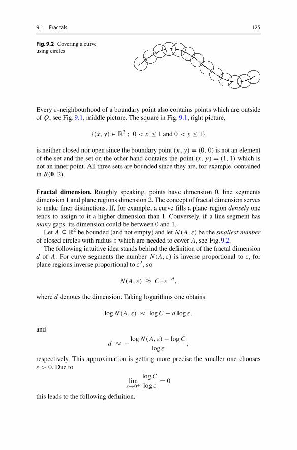
9.1 Fractals 125
Fig. 9.2 Covering a curveusing circles
Every ε-neighbourhood of a boundary point also contains points which are outsideof Q, see Fig. 9.1, middle picture. The square in Fig. 9.1, right picture,
{(x, y) ∈ R2 ; 0 < x ≤ 1 and 0 < y ≤ 1}
is neither closed nor open since the boundary point (x, y) = (0, 0) is not an elementof the set and the set on the other hand contains the point (x, y) = (1, 1) which isnot an inner point. All three sets are bounded since they are, for example, containedin B(0, 2).
Fractal dimension. Roughly speaking, points have dimension 0, line segmentsdimension 1 and plane regions dimension 2. The concept of fractal dimension servesto make finer distinctions. If, for example, a curve fills a plane region densely onetends to assign to it a higher dimension than 1. Conversely, if a line segment hasmany gaps, its dimension could be between 0 and 1.
Let A ⊆ R2 be bounded (and not empty) and let N (A, ε) be the smallest number
of closed circles with radius ε which are needed to cover A, see Fig. 9.2.The following intuitive idea stands behind the definition of the fractal dimension
d of A: For curve segments the number N (A, ε) is inverse proportional to ε, forplane regions inverse proportional to ε2, so
N (A, ε) ≈ C · ε−d ,
where d denotes the dimension. Taking logarithms one obtains
log N (A, ε) ≈ logC − d log ε,
and
d ≈ − log N (A, ε) − logC
log ε,
respectively. This approximation is getting more precise the smaller one choosesε > 0. Due to
limε→0+
logC
log ε= 0
this leads to the following definition.
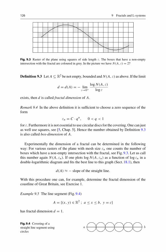
126 9 Fractals and L-systems
Fig. 9.3 Raster of the plane using squares of side length ε. The boxes that have a non-emptyintersection with the fractal are coloured in grey. In the picture we have N (A, ε) = 27
Definition 9.3 Let A ⊆ R2 be not empty, bounded and N (A, ε) as above. If the limit
d = d(A) = − limε→0+
log N (A, ε)
log ε
exists, then d is called fractal dimension of A.
Remark 9.4 In the above definition it is sufficient to choose a zero sequence of theform
εn = C · qn, 0 < q < 1
for ε. Furthermore it is not essential to use circular discs for the covering. One can justas well use squares, see [5, Chap. 5]. Hence the number obtained by Definition 9.3is also called box-dimension of A.
Experimentally the dimension of a fractal can be determined in the followingway: For various rasters of the plane with mesh size εn one counts the number ofboxes which have a non-empty intersection with the fractal, see Fig. 9.3. Let us callthis number again N (A, εn). If one plots log N (A, εn) as a function of log εn in adouble-logarithmic diagram and fits the best line to this graph (Sect. 18.1), then
d(A) ≈ − slope of the straight line.
With this procedure one can, for example, determine the fractal dimension of thecoastline of Great Britain, see Exercise 1.
Example 9.5 The line segment (Fig. 9.4)
A = {(x, y) ∈ R2 ; a ≤ x ≤ b, y = c}
has fractal dimension d = 1.
Fig. 9.4 Covering of astraight line segment usingcircles
a b

9.1 Fractals 127
Fig. 9.5 A set of points with box-dimension d = 12
We choose
εn = (b − a) · 2−n, q = 1/2.
Due to N (A, εn) = 2n−1 the following holds
− log N (A, εn)
log εn= − (n − 1) log 2
log(b − a) − n log 2→ 1 as n → ∞.
Likewise, it can easily be shown: Every set that consists of finitely many pointshas fractal dimension 0. Plane regions in R
2 have fractal dimension 2. The fractaldimension is in this way a generalisation of the intuitive notion of dimension. Still,caution is advisable here as can be seen in the following example.
Example 9.6 The set F = {0, 1, 1
2 ,13 ,
14 , . . .
}displayed in Fig. 9.5 has box-dimen-
sion d = 1/2. We check this claim with the following MATLAB experiment.
Experiment 9.7 To determine the dimension of F approximately with the helpof MATLAB we take the following steps. For j = 1, 2, 3, . . . we split the interval[0, 1] into 4 j equally large subintervals, set ε j = 4− j and determine the numberN j = N (F, ε j ) of subintervals which have a non-empty intersection with F . Thenwe plot log N j as a function of log ε j in a double-logarithmic diagram. The slope ofthe secant
d j = − log N j+1 − log N j
log ε j+1 − log ε j
is an approximation to d which is steadily improving with growing j . The valuesobtained by using the program mat09_1.m are given in the following table:
4 j 4 16 64 256 1024 4096 16384 65536 262144 1048576d j 0.79 0.61 0.55 0.52 0.512 0.5057 0.5028 0.5014 0.5007 0.50035
Verify the given values and determine that the approximations given byDefinition 9.3
d j = − log N j
log ε j
are much worse. Explain this behaviour.
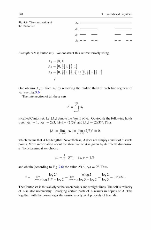
128 9 Fractals and L-systems
Fig. 9.6 The construction ofthe Cantor set
A3
A2
A1
A0
Example 9.8 (Cantor set) We construct this set recursively using
A0 = [0, 1]A1 = [
0, 13
] ∪ [ 23 , 1
]A2 = [
0, 19
] ∪ [ 29 ,
13
] ∪ [ 23 ,
79
] ∪ [ 89 , 1
]...
One obtains An+1 from An by removing the middle third of each line segment ofAn , see Fig. 9.6.
The intersection of all these sets
A =∞⋂n=0
An
is called Cantor set. Let |An| denote the length of An . Obviously the following holdstrue: |A0| = 1, |A1| = 2/3, |A2| = (2/3)2 and |An| = (2/3)n . Thus
|A| = limn→∞ |An| = lim
n→∞(2/3)n = 0,
which means that A has length 0. Nevertheless, A does not simply consist of discretepoints. More information about the structure of A is given by its fractal dimensiond. To determine it we choose
εn = 1
2· 3−n, i.e. q = 1/3,
and obtain (according to Fig. 9.6) the value N (A, εn) = 2n . Thus
d = − limn→∞
log 2n
log 3−n − log 2= lim
n→∞n log 2
n log 3 + log 2= log 2
log 3= 0.6309...
The Cantor set is thus an object between points and straight lines. The self-similarityof A is also noteworthy. Enlarging certain parts of A results in copies of A. Thistogether with the non-integer dimension is a typical property of fractals.
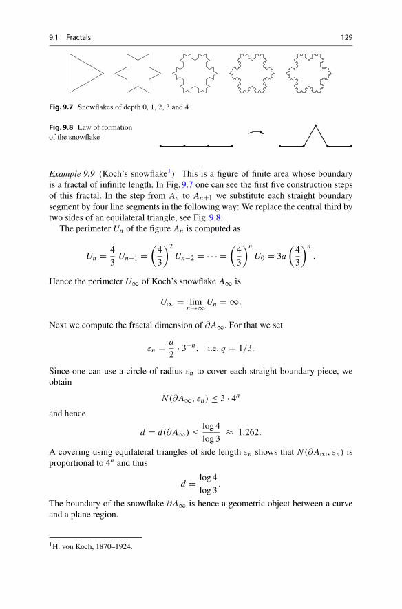
9.1 Fractals 129
Fig. 9.7 Snowflakes of depth 0, 1, 2, 3 and 4
Fig. 9.8 Law of formationof the snowflake
Example 9.9 (Koch’s snowflake1) This is a figure of finite area whose boundaryis a fractal of infinite length. In Fig. 9.7 one can see the first five construction stepsof this fractal. In the step from An to An+1 we substitute each straight boundarysegment by four line segments in the following way: We replace the central third bytwo sides of an equilateral triangle, see Fig. 9.8.
The perimeter Un of the figure An is computed as
Un = 4
3Un−1 =
(4
3
)2
Un−2 = · · · =(4
3
)n
U0 = 3a
(4
3
)n
.
Hence the perimeter U∞ of Koch’s snowflake A∞ is
U∞ = limn→∞Un = ∞.
Next we compute the fractal dimension of ∂A∞. For that we set
εn = a
2· 3−n, i.e. q = 1/3.
Since one can use a circle of radius εn to cover each straight boundary piece, weobtain
N (∂A∞, εn) ≤ 3 · 4nand hence
d = d(∂A∞) ≤ log 4
log 3≈ 1.262.
A covering using equilateral triangles of side length εn shows that N (∂A∞, εn) isproportional to 4n and thus
d = log 4
log 3.
The boundary of the snowflake ∂A∞ is hence a geometric object between a curveand a plane region.
1H. von Koch, 1870–1924.

130 9 Fractals and L-systems
9.2 Mandelbrot Sets
An interesting class of fractals can be obtained with the help of iteration methods.As an example we consider in C the iteration
zn+1 = z2n + c.
Setting z = x + iy and c = a + ib one obtains, by separating the real and the imag-inary part, the equivalent real form of the iteration
xn+1 = x2n − y2n + a,
yn+1 = 2xn yn + b.
The real representation is important when working with a programming languagethat does not support complex arithmetic.
First we investigate for which values of c ∈ C the iteration
zn+1 = z2n + c, z0 = 0
remains bounded. In the present case this is equivalent to |zn| → ∞ for n → ∞.The set of all c with this property is obviously not empty since it contains c = 0. Onthe other hand it is bounded since the iteration always diverges for |c| > 2 as caneasily be verified with MATLAB .
Definition 9.10 The set
M = {c ∈ C ; |zn| → ∞ as n → ∞}is called Mandelbrot set2 of the iteration zn+1 = z2n + c, z0 = 0.
To get an impression of M we carry out a numerical experiment in MATLAB.
Experiment 9.11 To visualise the Mandelbrot set M one first chooses a raster of acertain region, for example
−2 ≤ Re c ≤ 1, −1.15 ≤ Im c ≤ 1.15.
Next for each point of the raster one carries out a large number of iterations (e.g. 80)and decides then whether the iterations remain bounded (for example |zn| ≤ 2). Ifthis is the case one colours the point in black. This way one successively obtainsa picture of M . For your experiments use the MATLAB program mat09_2.m andmodify it as required. This way generate in particular the pictures in Fig. 9.9 in highresolution.
2B. Mandelbrot, 1924–2010.
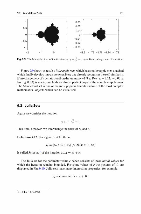
9.2 Mandelbrot Sets 131
−2 −1 0 1
−1
−0.5
0
0.5
1
−1.8 −1.78 −1.76 −1.74 −1.72
−0.03−0.02−0.01
00.01
0.020.03
Fig. 9.9 The Mandelbrot set of the iteration zn+1 = z2n + c, z0 = 0 and enlargement of a section
Figure9.9 shows as result a little apple manwhich has smaller apple men attachedwhichfinally develop into anantenna.Here one already recognises the self-similarity.If an enlargement of a certain detail on the antenna (−1.8 ≤ Re c ≤ −1.72, −0.03 ≤Im c ≤ 0.03) is made, one finds an almost perfect copy of the complete apple man.The Mandelbrot set is one of the most popular fractals and one of the most complexmathematical objects which can be visualised.
9.3 Julia Sets
Again we consider the iteration
zn+1 = z2n + c.
This time, however, we interchange the roles of z0 and c.
Definition 9.12 For a given c ∈ C, the set
Jc = {z0 ∈ C ; |zn| → ∞ as n → ∞}
is called Julia set3 of the iteration zn+1 = z2n + c.
The Julia set for the parameter value c hence consists of those initial values forwhich the iteration remains bounded. For some values of c the pictures of Jc aredisplayed in Fig. 9.10. Julia sets have many interesting properties; for example,
Jc is connected ⇔ c ∈ M.
3G. Julia, 1893–1978.
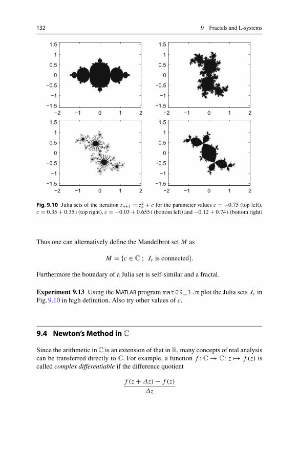
132 9 Fractals and L-systems
−2 −1 0 1 2−1.5
−1
−0.5
0
0.5
1
1.5
−2 −1 0 1 2−1.5
−1
−0.5
0
0.5
1
1.5
−2 −1 0 1 2−1.5
−1
−0.5
0
0.5
1
1.5
−2 −1 0 1 2−1.5
−1
−0.5
0
0.5
1
1.5
Fig. 9.10 Julia sets of the iteration zn+1 = z2n + c for the parameter values c = −0.75 (top left),c = 0.35 + 0.35 i (top right), c = −0.03 + 0.655 i (bottom left) and −0.12 + 0.74 i (bottom right)
Thus one can alternatively define the Mandelbrot set M as
M = {c ∈ C ; Jc is connected}.
Furthermore the boundary of a Julia set is self-similar and a fractal.
Experiment 9.13 Using theMATLAB program mat09_3.m plot the Julia sets Jc inFig. 9.10 in high definition. Also try other values of c.
9.4 Newton’s Method inC
Since the arithmetic in C is an extension of that in R, many concepts of real analysiscan be transferred directly to C. For example, a function f : C → C: z �→ f (z) iscalled complex differentiable if the difference quotient
f (z + Δz) − f (z)
Δz
9.4 Newton’s Method inC 133
has a limit as Δz → 0. This limit is again denoted by
f ′(z) = limΔz→0
f (z + Δz) − f (z)
Δz
and called complex derivative of f at the point z. Since differentiation inC is definedin the same way as differentiation in R, the same differentiation rules hold. In par-ticular any polynomial
f (z) = anzn + · · · + a1z + a0
is complex differentiable and has the derivative
f ′(z) = nanzn−1 + · · · + a1.
Like the real derivative (see Sect. 7.3), the complex derivative has an interpretationas a linear approximation
f (z) ≈ f (z0) + f ′(z0)(z − z0)
for z close to z0.Let f : C → C: z �→ f (z) be a complex differentiable function with f (ζ) = 0
and f ′(ζ) = 0. In order to compute the zero ζ of the function f , one first computesthe linear approximation starting from the initial value z0, so
z1 = z0 − f (z0)
f ′(z0).
Subsequently z1 is used as the new initial value and the procedure is iterated. In thisway one obtains Newton’s method in C:
zn+1 = zn − f (zn)
f ′(zn).
For initial values z0 close to ζ the procedure converges (as in R) quadratically.Otherwise, however, the situation can become very complicated.
In 1983 Eckmann [9] investigated Newton’s method for the function
f (z) = z3 − 1 = (z − 1)(z2 + z + 1).
This function has three roots in C
ζ1 = 1, ζ2,3 = −1
2± i
√3
2.
Naively one could think that the complex plane C is split into three equally largesectors where the iteration with initial values in sector S1 converges to ζ1, the onesin S2 to ζ2, etc., see Fig. 9.11.

134 9 Fractals and L-systems
S3
S2
S1
ζ1
ζ3
ζ2
Fig. 9.11 Possible regions of attraction of Newton’s iteration for finding the roots of z3 − 1
−1
0
1
−2 −1 0 1 2
−0.3
−0.2
−0.10
0.1
0.20.3
−0.8 −0.6 −0.4 −0.2 0
Fig. 9.12 Actual regions of attraction of Newton’s iteration for finding the roots of z3 − 1 andenlargement of a part
A numerical experiment, however, shows that it is not that way. If one colours theinitial values according to their convergence, one obtains a very complex picture.One can prove (however, not easily imagine) that at every point where two coloursmeet, the third colour is also present. The boundaries of the regions of attraction aredominated by pincer-like motifs which reappear again and again when enlarging thescale, see Fig. 9.12. The boundaries of the regions of attraction are Julia sets. Againwe have found fractals.
Experiment 9.14 Using theMATLABprogrammat09_4.m carry out an experiment.Ascertain yourself of the self-similarity of the appearing Julia sets by producingsuitable enlargements of the boundaries of the region of attraction.
9.5 L-systems
The formalism of L-systems was developed by Lindenmayer4 around 1968 in orderto model the growth of plants. It also turned out that many fractals can be created thisway. In this section we give a brief introduction to L-systems and discuss a possibleimplementation inmaple.
4A. Lindenmayer, 1925–1989.
9.5 L-systems 135
Definition 9.15 An L-system consists of the following five components:
(a) A finite set B of symbols, the so-called alphabet. The elements of B are calledletters, and any string of letters is called a word.
(b) Certain substitution rules. These rules determine how the letters of the currentword are to be replaced in each iteration step.
(c) The initial word w ∈ W . The initial word is also called axiom or seed.
(d) The number of iteration steps which one wants to carry out. In each of thesesteps, every letter of the current word is replaced according to the substitutionrules.
(e) A graphical interpretation of the word.
Let W be the set of all words that can be formed in the given L-system. Thesubstitution rules can be interpreted as a mapping from B to W :
S : B → W : b �→ S(b).
Example 9.16 Consider the alphabet B = {f,p,m} consisting of the three letters f,p and m. As substitution rules for this alphabet we take
S(f) = fpfmfmffpfpfmf, S(p) = p, S(m) = m
and consider the axiom w = fpfpfpf. An application of the substitution rulesshows that, after one substitution, the word fpf becomes the new wordfpfmfmffpfpfmfpfpfmfmffpfpfmf. If one applies the substitution rules onthe axiom then one obtains a new word. Applying the substitution rules on that againgives a new word, and so on. Each of these words can be interpreted as a polygonby assigning the following meaning to the individual letters:
f means forward by one unit;p stands for a rotation of α radians (plus);m stands for a rotation of −α radians (minus).
Thereby 0 ≤ α ≤ π is a chosen angle. One plots the polygon by choosing an arbitraryinitial point and an arbitrary initial direction. Then one sequentially processes theletters of the word to be displayed according to the rules above.
Inmaple lists and the substitution command subs lend themselves to the imple-mentation of L-systems. In the example above the axiom would hence be defined by
a := [f,p,f,p,f,p,f]
136 9 Fractals and L-systems
the substitution rules would be
a− > subs(f = (f,p,f,m,f,m,f,f,p,f,p,f,m,f),a).
The letters p and m do not change in the example, and they are fixed points in theconstruction. For the purpose of visualisation one can use polygons inmaple, givenby lists of points (in the plane). These lists can be plotted easily using the commandplot.
Construction of fractals. With the graphical interpretation above and α = π/2,the axiom fpfpfpf is a square which is passed through in a counterclockwisedirection. The substitution rule converts a straight line segment into a zigzag line.By an iterative application of the substitution rule the axiom develops into a fractal.
Experiment 9.17 Using themaple worksheet mp09_1.mws create different frac-tals. Further, try to understand the procedure fractal in detail.
Example 9.18 The substitution rule for Koch’s curve is
a -> subs(f=(f,p,f,m,m,f,p,f),a).
Depending on which axiom one uses, one can build fractal curves or snowflakesfrom that, see themaple worksheet mp09_1.mws.
Simulation of plant growth.As a new element branchings (ramifications) are addedhere. Mathematically one can describe this using two new symbols:
v stands for a ramification;e stands for the end of the branch.
Let us look, for example, at the word
[f,p,f,v,p,p,f,p,f,e,v,m,f,m,f,e,f,p,f,v,p,f,p,f,e,f,m,f].
If one removes all branchings that start with v and end with e from the list then oneobtains the stem of the plant
stem := [f,p,f,f,p,f,f,m,f].
After the second f in the stem obviously a double branching is taking place and thebranches sprout
branch1 := [p,p,f,p,f] and branch2 := [m,f,m,f].
Further up the stem branches again with the branch [p,f,p,f].
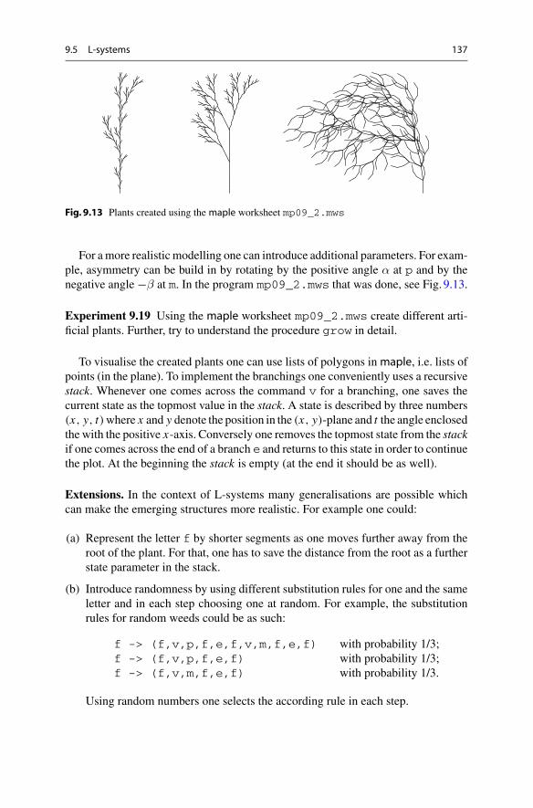
9.5 L-systems 137
Fig. 9.13 Plants created using the maple worksheet mp09_2.mws
For amore realistic modelling one can introduce additional parameters. For exam-ple, asymmetry can be build in by rotating by the positive angle α at p and by thenegative angle −β at m. In the program mp09_2.mws that was done, see Fig. 9.13.
Experiment 9.19 Using the maple worksheet mp09_2.mws create different arti-ficial plants. Further, try to understand the procedure grow in detail.
To visualise the created plants one can use lists of polygons inmaple, i.e. lists ofpoints (in the plane). To implement the branchings one conveniently uses a recursivestack. Whenever one comes across the command v for a branching, one saves thecurrent state as the topmost value in the stack. A state is described by three numbers(x, y, t)where x and y denote the position in the (x, y)-plane and t the angle enclosedthe with the positive x-axis. Conversely one removes the topmost state from the stackif one comes across the end of a branch e and returns to this state in order to continuethe plot. At the beginning the stack is empty (at the end it should be as well).
Extensions. In the context of L-systems many generalisations are possible whichcan make the emerging structures more realistic. For example one could:
(a) Represent the letter f by shorter segments as one moves further away from theroot of the plant. For that, one has to save the distance from the root as a furtherstate parameter in the stack.
(b) Introduce randomness by using different substitution rules for one and the sameletter and in each step choosing one at random. For example, the substitutionrules for random weeds could be as such:
f -> (f,v,p,f,e,f,v,m,f,e,f) with probability 1/3;f -> (f,v,p,f,e,f) with probability 1/3;f -> (f,v,m,f,e,f) with probability 1/3.
Using random numbers one selects the according rule in each step.
138 9 Fractals and L-systems
Experiment 9.20 Using themapleworksheet mp09_3.mws create random plants.Further, try to understand the implemented substitution rule in detail.
9.6 Exercises
1. Determine experimentally the fractal dimension of the coastline of Great Britain.In order to do that, take a map of Great Britain (e.g. a copy from an atlas) andraster the map using different mesh sizes (e.g. with 1/64th, 1/32th, 1/16th,1/8th and 1/4th of the North–South expansion). Count the boxes which containparts of the coastline and display this number as a function of the mesh size in adouble-logarithmic diagram. Fit the best line through these points and determinethe fractal dimension in question from the slope of the straight line.
2. Using the program mat09_3.m visualise the Julia sets of zn+1 = z2n + c forc = −1.25 and c = 0.365 − 0.3 i. Search for interesting details.
3. Let f (z) = z3 − 1 with z = x + iy. Use Newton’s method to solve f (z) = 0and separate the real part and the imaginary part, i.e. find the functions g1 andg2 with
xn+1 = g1(xn, yn),
yn+1 = g2(xn, yn).
4. Modify the procedure grow in the program mp09_2.mws by representing theletter f by shorter segments depending on how far it is away from the root. Withthat plot the umbel from Experiment 9.19 again.
5. Modify the program mp09_3.mws by attributing new probabilities to the exist-ing substitution rules (or invent new substitution rules). Use your modified pro-gram to plot some plants.
6. Modify the program mat09_3.m to visualise the Julia sets of zn+1 = z2kn − cfor c = −1 and integer values of k. Observe how varying k affects the shape ofthe Julia set. Try other values of c as well.
7. Modify the program mat09_3.m to visualise the Julia sets of
zn+1 = z3n + (c − 1)zn − c.
Study especially the behaviour of the Julia sets when c ranges between 0.60 and0.65.
10Antiderivatives
The derivative of a function y = F(x) describes its local rate of change, i.e. thechange Δy of the y-value with respect to the change Δx of the x-value in the limitΔx → 0; more precisely
f (x) = F ′(x) = limΔx→0
Δy
Δx= lim
Δx→0
F(x + Δx) − F(x)
Δx.
Conversely, the question about the reconstruction of a function F from its local rateof change f leads to the notion of indefinite integrals which comprises the totalityof all functions that have f as their derivative, the antiderivatives of f . Chapter10addresses this notion, its properties, some basic examples and applications.
Bymultiplying the rate of change f (x)with the changeΔx one obtains an approx-imation to the change of the values of the function of the antiderivative F in thesegment of length Δx :
Δy = F(x + Δx) − F(x) ≈ f (x)Δx .
Adding up these local changes in an interval, for instance between x = a and x = bin steps of length Δx , gives an approximation to the total change F(b) − F(a). Thelimit Δx → 0 (with an appropriate increase of the number of summands) leads tothe notion of the definite integral of f in the interval [a, b], which is the subject ofChap.11.
10.1 Indefinite Integrals
In Sect. 7.2 it was shown that the derivative of a constant is zero. The followingproposition shows that the converse is also true.
© Springer Nature Switzerland AG 2018M. Oberguggenberger and A. Ostermann, Analysis for Computer Scientists,Undergraduate Topics in Computer Science,https://doi.org/10.1007/978-3-319-91155-7_10
139
140 10 Antiderivatives
Proposition 10.1 If the function F is differentiable on (a, b) and F ′(x) = 0 for allx ∈ (a, b) then F is constant. This means that F(x) = c for a certain c ∈ R and allx ∈ (a, b).
Proof We choose an arbitrary x0 ∈ (a, b) and set c = F(x0). If now x ∈ (a, b) then,according to the mean value theorem (Proposition8.4),
F(x) − F(x0) = F ′(ξ)(x − x0)
for a point ξ between x and x0. Since F ′(ξ) = 0 it follows that F(x) = F(x0) = c.This holds for all x ∈ (a, b), consequently F has to be equal to the constant functionwith value c. �
Definition 10.2 (Antiderivatives) Let f be a real-valued function on an interval(a, b). An antiderivative of f is a differentiable function F : (a, b) → R whosederivative F ′ equals f .
Example 10.3 The function F(x) = x33 is an antiderivative of f (x) = x2, as is
G(x) = x33 + 5.
Proposition10.1 implies that antiderivatives are unique up to an additive constant.
Proposition 10.4 Let F and G be antiderivatives of f in (a, b). Then F(x) =G(x) + c for a certain c ∈ R and all x ∈ (a, b).
Proof Since F ′(x) − G ′(x) = f (x) − f (x) = 0 for all x ∈ (a, b), an applicationof Proposition10.1 gives the desired result. �
Definition 10.5 (Indefinite integrals) The indefinite integral
∫f (x) dx
denotes the totality of all antiderivatives of f .
Once a particular antiderivative F has been found, one writes accordingly
∫f (x) dx = F(x) + c.
Example 10.6 The indefinite integral of the quadratic function (Example10.3) is∫x2 dx = x3
3 + c.
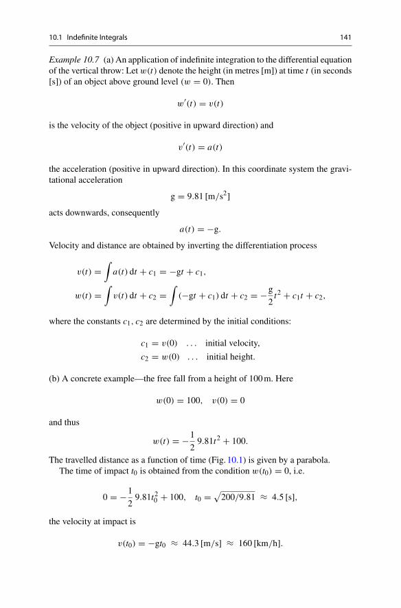
10.1 Indefinite Integrals 141
Example 10.7 (a) An application of indefinite integration to the differential equationof the vertical throw: Let w(t) denote the height (in metres [m]) at time t (in seconds[s]) of an object above ground level (w = 0). Then
w′(t) = v(t)
is the velocity of the object (positive in upward direction) and
v′(t) = a(t)
the acceleration (positive in upward direction). In this coordinate system the gravi-tational acceleration
g = 9.81 [m/s2]acts downwards, consequently
a(t) = −g.
Velocity and distance are obtained by inverting the differentiation process
v(t) =∫a(t) dt + c1 = −gt + c1,
w(t) =∫
v(t) dt + c2 =∫
(−gt + c1) dt + c2 = −g
2t2 + c1t + c2,
where the constants c1, c2 are determined by the initial conditions:
c1 = v(0) . . . initial velocity,
c2 = w(0) . . . initial height.
(b) A concrete example—the free fall from a height of 100m. Here
w(0) = 100, v(0) = 0
and thus
w(t) = −1
29.81t2 + 100.
The travelled distance as a function of time (Fig. 10.1) is given by a parabola.The time of impact t0 is obtained from the condition w(t0) = 0, i.e.
0 = −1
29.81t20 + 100, t0 = √
200/9.81 ≈ 4.5 [s],
the velocity at impact is
v(t0) = −gt0 ≈ 44.3 [m/s] ≈ 160 [km/h].

142 10 Antiderivatives
Fig. 10.1 Free fall: travelleddistance as function of time
0 2 4 6
0
50
100w(t)
c2
tt0
10.2 Integration Formulas
It follows immediately from Definition 10.5 that indefinite integration can be seenas the inversion of differentiation. It is, however, only unique up to a constant:
(∫f (x) dx
)′= f (x),
∫g′(x) dx = g(x) + c.
With this consideration and the formulas from Sect. 7.4 one easily obtains the basicintegration formulas stated in the following table. The formulas are valid in theaccording domains.
The formulas in Table10.1 are a direct consequence of those in Table7.1.
Experiment 10.8 Antiderivatives can be calculated in maple using the commandint. Explanations and further integration commands can be found in the maple
Table 10.1 Integrals of some elementary functions
f (x) xα, α �= −11
xex ax
∫f (x) dx
xα+1
α + 1+ c log |x | + c ex + c
1
log aax + c
f (x) sin x cos x1√
1 − x21
1 + x2∫f (x) dx − cos x + c sin x + c arcsin x + c arctan x + c
f (x) sinh x cosh x1√
1 + x21√
x2 − 1∫f (x) dx cosh x + c sinh x + c arsinh x + c arcosh x + c
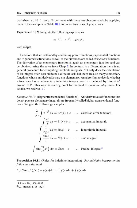
10.2 Integration Formulas 143
worksheet mp10_1.mws. Experiment with these maple commands by applyingthem to the examples of Table10.1 and other functions of your choice.
Experiment 10.9 Integrate the following expressions
xe−x2 , e−x2 , sin(x2)
withmaple.
Functions that are obtained by combining power functions, exponential functionsand trigonometric functions, aswell as their inverses, are called elementary functions.The derivative of an elementary function is again an elementary function and canbe obtained using the rules from Chap.7. In contrast to differentiation there is nogeneral procedure for computing indefinite integrals. Not only does the calculationof an integral often turn out to be a difficult task, but there are also many elementaryfunctions whose antiderivatives are not elementary. An algorithm to decide whethera functions has an elementary indefinite integral was first deduced by Liouville1
around 1835. This was the starting point for the field of symbolic integration. Fordetails, we refer to [7].
Example 10.10 (Higher transcendental functions) Antiderivatives of functions thatdo not possess elementary integrals are frequently called higher transcendental func-tions. We give the following examples:
2√π
∫e−x2 dx = Erf(x) + c . . . Gaussian error function;
∫ex
xdx = Ei(x) + c . . . exponential integral;
∫1
log xdx = �i(x) + c . . . logarithmic integral;
∫sin x
xdx = Si(x) + c . . . sine integral;
∫sin
(π
2x2
)dx = S(x) + c . . . Fresnel integral.2
Proposition 10.11 (Rules for indefinite integration) For indefinite integration thefollowing rules hold:
(a) Sum:∫ (
f (x) + g(x))dx = ∫
f (x) dx + ∫g(x) dx
1J. Liouville, 1809–1882.2A.J. Fresnel, 1788–1827.
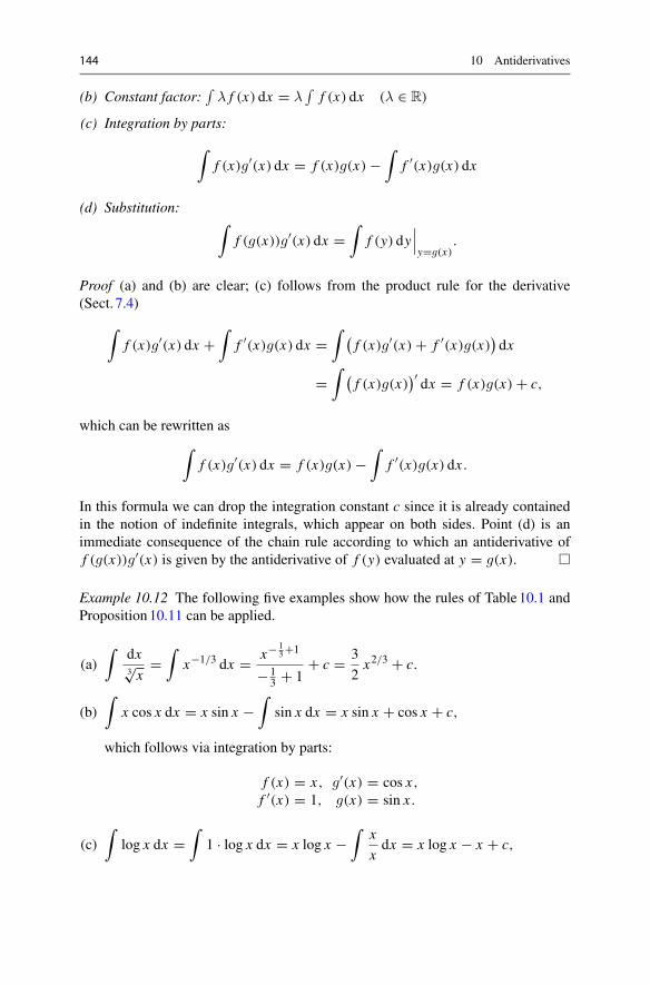
144 10 Antiderivatives
(b) Constant factor:∫
λ f (x) dx = λ∫
f (x) dx (λ ∈ R)
(c) Integration by parts:
∫f (x)g′(x) dx = f (x)g(x) −
∫f ′(x)g(x) dx
(d) Substitution: ∫f (g(x))g′(x) dx =
∫f (y) dy
∣∣∣y=g(x)
.
Proof (a) and (b) are clear; (c) follows from the product rule for the derivative(Sect. 7.4)
∫f (x)g′(x) dx +
∫f ′(x)g(x) dx =
∫ (f (x)g′(x) + f ′(x)g(x)
)dx
=∫ (
f (x)g(x))′ dx = f (x)g(x) + c,
which can be rewritten as∫
f (x)g′(x) dx = f (x)g(x) −∫
f ′(x)g(x) dx .
In this formula we can drop the integration constant c since it is already containedin the notion of indefinite integrals, which appear on both sides. Point (d) is animmediate consequence of the chain rule according to which an antiderivative off (g(x))g′(x) is given by the antiderivative of f (y) evaluated at y = g(x). �
Example 10.12 The following five examples show how the rules of Table10.1 andProposition10.11 can be applied.
(a)∫
dx3√x
=∫
x−1/3 dx = x− 13+1
− 13 + 1
+ c = 3
2x2/3 + c.
(b)∫
x cos x dx = x sin x −∫
sin x dx = x sin x + cos x + c,
which follows via integration by parts:
f (x) = x, g′(x) = cos x,f ′(x) = 1, g(x) = sin x .
(c)∫
log x dx =∫
1 · log x dx = x log x −∫
x
xdx = x log x − x + c,
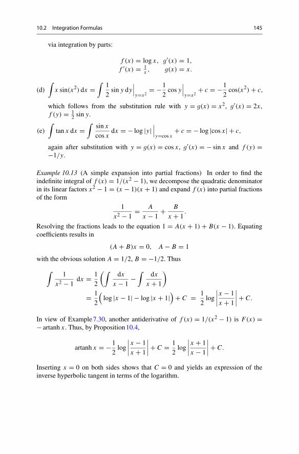
10.2 Integration Formulas 145
via integration by parts:
f (x) = log x, g′(x) = 1,f ′(x) = 1
x , g(x) = x .
(d)∫
x sin(x2) dx =∫
1
2sin y dy
∣∣∣y=x2
= −1
2cos y
∣∣∣y=x2
+ c = −1
2cos(x2) + c,
which follows from the substitution rule with y = g(x) = x2, g′(x) = 2x ,f (y) = 1
2 sin y.
(e)∫
tan x dx =∫
sin x
cos xdx = − log |y|
∣∣∣y=cos x
+ c = − log |cos x | + c,
again after substitution with y = g(x) = cos x , g′(x) = − sin x and f (y) =−1/y.
Example 10.13 (A simple expansion into partial fractions) In order to find theindefinite integral of f (x) = 1/(x2 − 1), we decompose the quadratic denominatorin its linear factors x2 − 1 = (x − 1)(x + 1) and expand f (x) into partial fractionsof the form
1
x2 − 1= A
x − 1+ B
x + 1.
Resolving the fractions leads to the equation 1 = A(x + 1) + B(x − 1). Equatingcoefficients results in
(A + B)x = 0, A − B = 1
with the obvious solution A = 1/2, B = −1/2. Thus
∫1
x2 − 1dx = 1
2
(∫dx
x − 1−
∫dx
x + 1
)
= 1
2
(log |x − 1| − log |x + 1|
)+ C = 1
2log
∣∣∣∣ x − 1
x + 1
∣∣∣∣ + C.
In view of Example7.30, another antiderivative of f (x) = 1/(x2 − 1) is F(x) =− artanh x . Thus, by Proposition10.4,
artanh x = −1
2log
∣∣∣∣ x − 1
x + 1
∣∣∣∣ + C = 1
2log
∣∣∣∣ x + 1
x − 1
∣∣∣∣ + C.
Inserting x = 0 on both sides shows that C = 0 and yields an expression of theinverse hyperbolic tangent in terms of the logarithm.
146 10 Antiderivatives
10.3 Exercises
1. An object is thrown vertically upwards from the ground with a velocity of10 [m/s]. Find its height w(t) as a function of time t , the maximum heightas well as the time of impact on the ground.Hint. Integrate w′′(t) = −g ≈ 9.81 [m/s2] twice indefinitely and determine theintegration constants from the initial conditions w(0) = 0, w′(0) = 10.
2. Compute the following indefinite integrals by hand and withmaple:
(a)∫
(x + 3x2 + 5x4 + 7x6) dx, (b)∫
dx√x,
(c)∫
xe−x2 dx (substitution), (d)∫
xex dx (integration by parts).
3. Compute the indefinite integrals
(a)∫
cos2 x dx, (b)∫ √
1 − x2 dx
by hand and check the results usingmaple.Hints. For (a) use the identity
cos2 x = 1
2(1 + cos 2x);
for (b) use the substitution y = g(x) = arcsin x , f (y) = 1 − sin2 y.4. Compute the indefinite integrals
(a)∫
dx
x2 + 2x + 5dx, (b)
∫dx
x2 + 2x − 3
by hand and check the results usingmaple.Hints. Write the denominator in (a) in the form (x + 1)2 + 4 and reduce it toy2 + 1 by means of a suitable substitution. Factorize the denominator in (b) andfollow the procedure of Example10.13.
5. Compute the indefinite integrals
(a)∫
dx
x2 + 2xdx, (b)
∫dx
x2 + 2x + 1
by hand and check the results usingmaple.6. Compute the indefinite integrals
(a)∫
x2 sin x dx, (b)∫
x2e−3x dx .
Hint. Repeated integration by parts.
10.3 Exercises 147
7. Compute the indefinite integrals
(a)∫
ex
ex + 1dx, (b)
∫ √1 + x2 dx .
Hint.Substitution y = ex in case (a), substitution y = sinh x in case (b), invokingthe formula cosh2 y − sinh2 y = 1 and repeated integration by parts or recourseto the definition of the hyperbolic functions.
8. Show that the functions
f (x) = arctan x and g(x) = arctan1 + x
1 − x
differ in the interval (−∞, 1) by a constant. Compute this constant. Answer thesame question for the interval (1, ∞).
9. Prove the identity arsinh x = log(x + √
1 + x2).
Hint. Recall from Chap.7 that the functions f (x) = arsinh x and g(x) =log
(x + √
1 + x2)
have the same derivative. (Compare with the algebraic
derivation of the formula in Exercise 15 of Sect. 2.3.)
11Definite Integrals
In the introduction to Chap.10 the notion of the definite integral of a function f on aninterval [a, b] was already mentioned. It arises from summing up expressions of theform f (x)Δx and taking limits. Such sums appear in many applications includingthe calculation of areas, surface areas and volumes as well as the calculation oflengths of curves. This chapter employs the notion of Riemann integrals as the basicconcept of definite integration. Riemann’s approach provides an intuitive concept inmany applications, as will be elaborated in examples at the end of the chapter.
The main part of this chapter is dedicated to the properties of the integral. Inparticular, the two fundamental theorems of calculus are proven. The first theoremallows one to calculate a definite integral from the knowledge of an antiderivative.The second fundamental theorem states that the definite integral of a function fon an interval [a, x] with variable upper bound provides an antiderivative of f .Since the definite integral can be approximated, for example by Riemann sums, thesecond fundamental theorem offers a possibility to approximate the antiderivativenumerically. This is of importance, for example, for the calculation of distributionfunctions in statistics.
11.1 The Riemann Integral
Example 11.1 (From velocity to distance) How can one calculate the distance w
which a vehicle travels between time a and time b if one only knows its velocity v(t)for all times a ≤ t ≤ b? If v(t) ≡ v is constant, one simply gets
w = v · (b − a).
© Springer Nature Switzerland AG 2018M. Oberguggenberger and A. Ostermann, Analysis for Computer Scientists,Undergraduate Topics in Computer Science,https://doi.org/10.1007/978-3-319-91155-7_11
149

150 11 Definite Integrals
Fig. 11.1 Subdivision of thetime axis t
· · ·τnτ2τ1
tn = btn−1t2t1a = t0
If the velocity v(t) is time-dependent, one divides the time axis into smaller subin-tervals (Fig. 11.1): a = t0 < t1 < t2 < · · · < tn = b.
Choosing intermediate points τ j ∈ [t j−1, t j ] one obtains approximately
v(t) ≈ v(τ j ) for t ∈ [t j−1, t j ],
if v is a continuous function of time. The approximation is the more precise, theshorter the intervals [t j−1, t j ] are chosen. The distance travelled in this interval isapproximately equal to
w j ≈ v(τ j )(t j − t j−1).
The total distance covered between time a and time b is then
w =n∑
j=1
w j ≈n∑
j=1
v(τ j )(t j − t j−1).
Letting the length of the subintervals [t j−1, t j ] tend to zero, one expects to obtainthe actual value of the distance in the limit.
Example 11.2 (Area under the graph of a nonnegative function) In a similar wayone can try to approximate the area under the graph of a function y = f (x) by usingrectangles which are successively refined (Fig. 11.2).
The sum of the areas of the rectangles
F ≈n∑
j=1
f (ξ j )(x j − x j−1)
form an approximation to the actual area under the graph.
Fig. 11.2 Sums ofrectangles as approximationto the area
y
x· · ·ξnξ3ξ2ξ1
xn = bxn−1x3x2x1a = x0
11.1 The Riemann Integral 151
The two examples are based on the same concept, the Riemann integral,1 whichwe will now introduce. Let an interval [a, b] and a function f = [a, b] → R begiven. Choosing points
a = x0 < x1 < x2 < · · · < xn−1 < xn = b,
the intervals [x0, x1], [x1, x2], . . . , [xn−1, xn] form a partition Z of the interval[a, b]. We denote the length of the largest subinterval by Φ(Z), i.e.
Φ(Z) = maxj=1,...,n
|x j − x j−1|.
For arbitrarily chosen intermediate points ξ j ∈ [x j−1, x j ] one calls the expression
S =n∑
j=1
f (ξ j )(x j − x j−1)
a Riemann sum. In order to further specify the idea of the limiting process above, wetake a sequence Z1, Z2, Z3, . . . of partitions such that Φ(ZN ) → 0 as N → ∞ andcorresponding Riemann sums SN .
Definition 11.3 A function f is called Riemann integrable in [a, b] if, for arbitrarysequences of partitions (ZN )N≥1 with Φ(ZN ) → 0, the corresponding Riemannsums (SN )N≥1 tend to the same limit I ( f ), independently of the choice of theintermediate points. This limit
I ( f ) =∫ b
af (x) dx
is called the definite integral of f on [a, b].
The intuitive approach in the introductory Examples11.1 and 11.2 can now bemade precise. If the respective functions f and v are Riemann integrable, then theintegral
F =∫ b
af (x) dx
represents the area between the x-axis and the graph, and
w =∫ b
av(t) dt
gives the total distance covered.
1B. Riemann, 1826–1866.

152 11 Definite Integrals
Experiment 11.4 Open the M-file mat11_1.m, study the given explanations andexperiment with randomly chosen Riemann sums for the function f (x) = 3x2 in theinterval [0, 1]. What happens if you take more and more partition points n?
Experiment 11.5 Open the applet Riemann sums and study the effects of changingthe partition. In particular, vary the maximum length of the subintervals and thechoice of intermediate points. How does the sign of the function influence the result?
The following examples illustrate the notion of Riemann integrability.
Example 11.6 (a) Let f (x) = c = constant. Then the area under the graph of thefunction is the area of the rectangle c(b − a). On the other hand, any Riemann sumis of the form
f (ξ1)(x1 − x0) + f (ξ2)(x2 − x1) + · · · + f (ξn)(xn − xn−1)
= c(x1 − x0 + x2 − x1 + · · · + xn − xn−1)
= c(xn − x0) = c(b − a).
All Riemann sums are equal and thus, as expected,
∫ b
ac dx = c(b − a).
(b) Let f (x) = 1x for x ∈ (0, 1], f (0) = 0. This function is not integrable in [0, 1].
The corresponding Riemann sums are of the form
1
ξ1(x1 − 0) + 1
ξ2(x2 − x1) + · · · + 1
ξn(xn − xn−1).
By choosing ξ1 close to 0 every such Riemann sum can be made arbitrarily large;thus the limit of the Riemann sums does not exist.
(c) Dirichlet’s function2
f (x) ={1, x ∈ Q
0, x /∈ Q
is not integrable in [0, 1]. The Riemann sums are of the form
SN = f (ξ1)(x1 − x0) + · · · + f (ξn)(xn − xn−1).
If all ξ j ∈ Q then SN = 1. If one takes all ξ j /∈ Q then SN = 0; thus the limit dependson the choice of intermediate points ξ j .
2P.G.L. Dirichlet, 1805–1859.
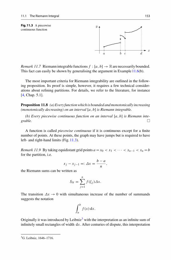
11.1 The Riemann Integral 153
Fig. 11.3 A piecewisecontinuous function
y
xdcba
Remark 11.7 Riemann integrable functions f : [a, b] → R are necessarily bounded.This fact can easily be shown by generalising the argument in Example11.6(b).
The most important criteria for Riemann integrability are outlined in the follow-ing proposition. Its proof is simple, however, it requires a few technical consider-ations about refining partitions. For details, we refer to the literature, for instance[4, Chap. 5.1].
Proposition 11.8 (a)Every functionwhich is boundedandmonotonically increasing(monotonically decreasing) on an interval [a, b] is Riemann integrable.
(b) Every piecewise continuous function on an interval [a, b] is Riemann inte-grable. �
A function is called piecewise continuous if it is continuous except for a finitenumber of points. At these points, the graph may have jumps but is required to haveleft- and right-hand limits (Fig. 11.3).
Remark 11.9 By taking equidistant grid points a = x0 < x1 < · · · < xn−1 < xn = bfor the partition, i.e.
x j − x j−1 =: Δx = b − a
n,
the Riemann sums can be written as
SN =n∑
j=1
f (ξ j )Δx .
The transition Δx → 0 with simultaneous increase of the number of summandssuggests the notation
∫ b
af (x) dx .
Originally it was introduced by Leibniz3 with the interpretation as an infinite sum ofinfinitely small rectangles of width dx . After centuries of dispute, this interpretation
3G. Leibniz, 1646–1716.
154 11 Definite Integrals
can be rigorously justified today within the framework of nonstandard analysis (see,for instance, [27]).
Note that the integration variable x in the definite integral is a bound variableand can be replaced by any other letter:
∫ b
af (x) dx =
∫ b
af (t) dt =
∫ b
af (ξ) dξ = · · ·
This can be used with advantage in order to avoid possible confusion with otherbound variables.
Proposition 11.10 (Properties of the definite integral) In the following let a < band f, g be Riemann integrable on [a, b].
(a) Positivity:
f ≥ 0 in [a, b] ⇒∫ b
af (x) dx ≥ 0,
f ≤ 0 in [a, b] ⇒∫ b
af (x) dx ≤ 0.
(b) Monotonicity:
f ≤ g in [a, b] ⇒∫ b
af (x) dx ≤
∫ b
ag(x) dx .
In particular, with
m = infx∈[a,b] f (x), M = sup
x∈[a,b]f (x),
the following inequality holds
m(b − a) ≤∫ b
af (x) dx ≤ M(b − a).
(c) Sum and constant factor (linearity):
∫ b
a
(f (x) + g(x)
)dx =
∫ b
af (x) dx +
∫ b
ag(x) dx
∫ b
aλ f (x) dx = λ
∫ b
af (x) dx (λ ∈ R).
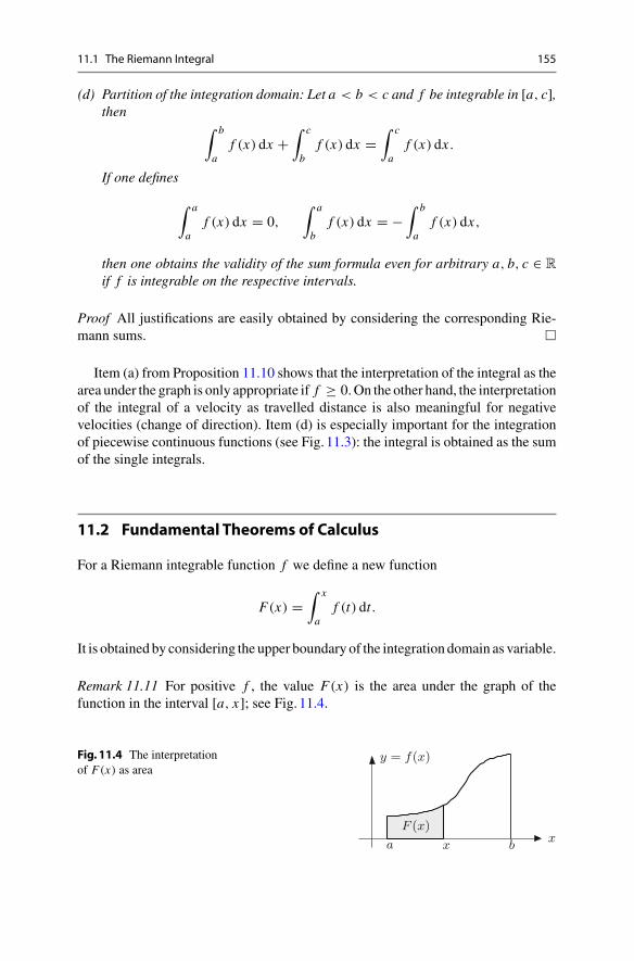
11.1 The Riemann Integral 155
(d) Partition of the integration domain: Let a < b < c and f be integrable in [a, c],then
∫ b
af (x) dx +
∫ c
bf (x) dx =
∫ c
af (x) dx .
If one defines
∫ a
af (x) dx = 0,
∫ a
bf (x) dx = −
∫ b
af (x) dx,
then one obtains the validity of the sum formula even for arbitrary a, b, c ∈ R
if f is integrable on the respective intervals.
Proof All justifications are easily obtained by considering the corresponding Rie-mann sums. �
Item (a) from Proposition 11.10 shows that the interpretation of the integral as thearea under the graph is only appropriate if f ≥ 0.On the other hand, the interpretationof the integral of a velocity as travelled distance is also meaningful for negativevelocities (change of direction). Item (d) is especially important for the integrationof piecewise continuous functions (see Fig. 11.3): the integral is obtained as the sumof the single integrals.
11.2 Fundamental Theorems of Calculus
For a Riemann integrable function f we define a new function
F(x) =∫ x
af (t) dt.
It is obtained by considering the upper boundary of the integration domain as variable.
Remark 11.11 For positive f , the value F(x) is the area under the graph of thefunction in the interval [a, x]; see Fig. 11.4.
Fig. 11.4 The interpretationof F(x) as area
F (x)
y = f(x)
xbxa
156 11 Definite Integrals
Proposition 11.12 (Fundamental theorems of calculus) Let f be continuous in[a, b]. Then the following assertions hold:
(a) First fundamental theorem: If G is an antiderivative of f then
∫ b
af (x) dx = G(b) − G(a).
(b) Second fundamental theorem: The function
F(x) =∫ x
af (t) dt
is an antiderivative of f , that is, F is differentiable and F ′(x) = f (x).
Proof In the first step we prove the second fundamental theorem. For that letx ∈ (a, b), h > 0 and x + h ∈ (a, b). According to Proposition 6.15 the functionf has a minimum and a maximum in the interval [x, x + h]:
m(h) = mint∈[x,x+h] f (t), M(h) = max
t∈[x,x+h] f (t).
The continuity of f implies the convergence m(h) → f (x) and M(h) → f (x) ash → 0. According to item (b) in Proposition 11.10 we have that
m(h) · h ≤ F(x + h) − F(x) =∫ x+h
xf (t) dt ≤ M(h) · h.
This shows that F is differentiable at x and
F ′(x) = limh→0
F(x + h) − F(x)
h= f (x).
The first fundamental theorem follows from the second fundamental theorem
∫ b
af (t) dt = F(b) = F(b) − F(a),
since F(a) = 0. If G is another antiderivative then G = F + c according to Propo-sition 10.1; hence
G(b) − G(a) = F(b) + c − (F(a) + c) = F(b) − F(a).
Thus G(b) − G(a) = ∫ ba f (x) dx as well. �
11.2 Fundamental Theorems of Calculus 157
Remark 11.13 For positive f , the second fundamental theorem of calculus has anintuitive interpretation. The value F(x + h) − F(x) is the area under the graph ofthe function y = f (x) in the interval [x, x + h], while h f (x) is the area of theapproximating rectangle of height f (x). The resulting approximation
F(x + h) − F(x)
h≈ f (x)
suggests that in the limit as h → 0, F ′(x) = f (x). The given proof makes the argu-ment rigorous.
Applications of the first fundamental theorem. The most important applicationconsists in evaluating definite integrals
∫ ba f (x) dx . For that, one determines an
antiderivative F(x), for instance as indefinite integral, and substitutes:
∫ b
af (x) dx = F(x)
∣∣∣x=b
x=a= F(b) − F(a).
Example 11.14 As an application we compute the following integrals.
(a)∫ 3
1x2 dx = x3
3
∣∣∣∣x=3
x=1= 27
3− 1
3= 26
3.
(b)∫ π/2
0cos x dx = sin x
∣∣∣∣x=π/2
x=0= sin
π
2− sin 0 = 1.
(c)∫ 1
0x sin(x2) dx = −1
2cos(x2)
∣∣∣∣x=1
x=0= −1
2cos 1 − ( − 1
2cos 0
)
= −1
2cos 1 + 1
2(see Example 10.12).
Remark 11.15 In maple the integration of expressions and functions is carried outusing the command int, which requires the analytic expression and the domain asarguments, for instance
int(xˆ2, x = 1..3);
Applications of the second fundamental theorem. Usually, such applications areof theoretical nature, like the description of the relation between travelled distanceand velocity,
w(t) = w(0) +∫ t
0v(s) ds, w′(t) = v(t),
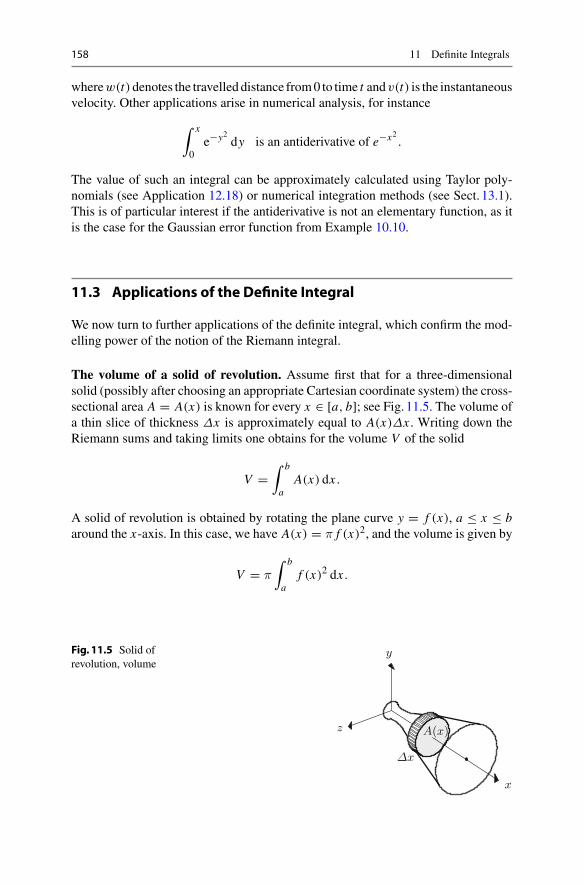
158 11 Definite Integrals
wherew(t)denotes the travelled distance from0 to time t andv(t) is the instantaneousvelocity. Other applications arise in numerical analysis, for instance
∫ x
0e−y2 dy is an antiderivative of e−x2 .
The value of such an integral can be approximately calculated using Taylor poly-nomials (see Application 12.18) or numerical integration methods (see Sect. 13.1).This is of particular interest if the antiderivative is not an elementary function, as itis the case for the Gaussian error function from Example 10.10.
11.3 Applications of the Definite Integral
We now turn to further applications of the definite integral, which confirm the mod-elling power of the notion of the Riemann integral.
The volume of a solid of revolution. Assume first that for a three-dimensionalsolid (possibly after choosing an appropriate Cartesian coordinate system) the cross-sectional area A = A(x) is known for every x ∈ [a, b]; see Fig. 11.5. The volume ofa thin slice of thickness Δx is approximately equal to A(x)Δx . Writing down theRiemann sums and taking limits one obtains for the volume V of the solid
V =∫ b
aA(x) dx .
A solid of revolution is obtained by rotating the plane curve y = f (x), a ≤ x ≤ baround the x-axis. In this case, we have A(x) = π f (x)2, and the volume is given by
V = π
∫ b
af (x)2 dx .
Fig. 11.5 Solid ofrevolution, volume
Δx
A(x)
y
z
x
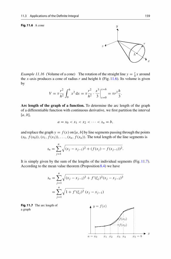
11.3 Applications of the Definite Integral 159
Fig. 11.6 A cone
r
h
y
z
x
Example 11.16 (Volume of a cone) The rotation of the straight line y = rh x around
the x-axis produces a cone of radius r and height h (Fig. 11.6). Its volume is givenby
V = πr2
h2
∫ h
0x2 dx = π
r2
h2· x
3
3
∣∣∣∣x=h
x=0= πr2
h
3.
Arc length of the graph of a function. To determine the arc length of the graphof a differentiable function with continuous derivative, we first partition the interval[a, b],
a = x0 < x1 < x2 < · · · < xn = b,
and replace the graph y = f (x) on [a, b] by line segments passing through the points(x0, f (x0)), (x1, f (x1)), . . . , (xn, f (xn)). The total length of the line segments is
sn =n∑
j=1
√(x j − x j−1)2 + ( f (x j ) − f (x j−1))2.
It is simply given by the sum of the lengths of the individual segments (Fig. 11.7).According to the mean value theorem (Proposition8.4) we have
sn =n∑
j=1
√(x j − x j−1)2 + f ′(ξ j )2(x j − x j−1)2
=n∑
j=1
√1 + f ′(ξ j )2 (x j − x j−1)
Fig. 11.7 The arc length ofa graph
y = f(x)
x
f(x3)
f(x2)
x5 = bx4x3x2x1a = x0
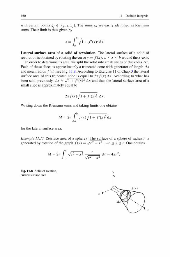
160 11 Definite Integrals
with certain points ξ j ∈ [x j−1, x j ]. The sums sn are easily identified as Riemannsums. Their limit is thus given by
s =∫ b
a
√1 + f ′(x)2 dx .
Lateral surface area of a solid of revolution. The lateral surface of a solid ofrevolution is obtained by rotating the curve y = f (x), a ≤ x ≤ b around the x-axis.
In order to determine its area, we split the solid into small slices of thickness Δx .Each of these slices is approximately a truncated cone with generator of length Δsand mean radius f (x); see Fig. 11.8. According to Exercise 11 of Chap.3 the lateralsurface area of this truncated cone is equal to 2π f (x)Δs. According to what hasbeen said previously, Δs ≈ √
1 + f ′(x)2 Δx and thus the lateral surface area of asmall slice is approximately equal to
2π f (x)√1 + f ′(x)2 Δx .
Writing down the Riemann sums and taking limits one obtains
M = 2π∫ b
af (x)
√1 + f ′(x)2 dx
for the lateral surface area.
Example 11.17 (Surface area of a sphere) The surface of a sphere of radius r isgenerated by rotation of the graph f (x) = √
r2 − x2, −r ≤ x ≤ r . One obtains
M = 2π∫ r
−r
√r2 − x2
r√r2 − x2
dx = 4πr2.
Fig. 11.8 Solid of rotation,curved surface area
Δs
f(x)
y
z
x

11.4 Exercises 161
11.4 Exercises
1. Modify theMATLAB program mat11_1.m so that it evaluates Riemann sums ofgiven lengths n for polynomials of degree k on arbitrary intervals [a, b] (MATLAB
command polyval).2. Prove that every function which is piecewise constant in an interval [a, b] is
Riemann integrable (use Definition 11.3).3. Compute the area between the graphs of y = sin x and y = √
x on the interval[0, 2π].
4. (From engineering mechanics; Fig. 11.9) The shear force Q(x) and the bendingmoment M(x) of a beam of length L under a distributed load p(x) obey therelationships M ′(x) = Q(x), Q′(x) = −p(x), 0 ≤ x ≤ L . Compute Q(x) andM(x) and sketch their graphs for
(a) a simply supportedbeamwithuniformlydistributed load: p(x) = p0, Q(0) =p0L/2, M(0) = 0;
(b) a cantilever beam with triangular load: p(x) = q0(1 − x/L), Q(L) = 0,M(L) = 0.
5. Write a MATLAB program which provides a numerical approximation to theintegral
∫ 1
0e−x2 dx .
For this purpose, use Riemann sums of the form
L =n∑
j=1
e−x2j Δx, U =n∑
j=1
e−x2j−1 Δx
with x j = jΔx, Δx = 1/n and try to determine Δx and n, respectively, sothat U − L ≤ 0.01; i.e. the result should be correct up to two digits. Com-pare your result with the value obtained by means of the MATLAB commandsqrt(pi)/2*erf(1).Additional task: Extend your program such that it allows one to compute∫ a0 e−x2 dx for arbitrary a > 0.
q0
L0x
p0
L0
x
Fig.11.9 Simply supported beam with uniformly distributed load, cantilever beam with triangularload
162 11 Definite Integrals
6. Show that the error of approximating the integral in Exercise 5 either by L orUis at most U − L . Use the applet Integration to visualise this fact.Hint. Verify the inequality
L ≤∫ 1
0e−x2 dx ≤ U.
Thus, L and U are lower and upper sums, respectively.7. Rotation of the parabola y = 2
√x, 0 ≤ x ≤ 1 around the x-axis produces a
paraboloid. Sketch it and compute its volume and its lateral surface area.8. Compute the arc length of the graph of the following functions:
(a) the parabola f (x) = x2/2 for 0 ≤ x ≤ 2;(b) the catenary g(x) = cosh x for −1 ≤ x ≤ 3.Hint. See Exercise 7 in Sect. 10.3.
9. The surface of a cooling tower can be described qualitatively by rotating thehyperbola y = √
1 + x2 around the x-axis in the bounds −1 ≤ x ≤ 2.(a) Compute the volume of the corresponding solid of revolution.(b) Show that the lateral surface area is given by M = 2π
∫ 2−1
√1 + 2x2 dx .
Evaluate the integral directly and by means ofmaple.Hint. Reduce the integral to the one considered in Exercise 7 of Sect. 10.3 by asuitable substitution.
10. A lens-shaped body is obtained by rotating the graph of the sine function y =sin x around the x-axis in the bounds 0 ≤ x ≤ π.(a) Compute the volume of the body.(b) Compute its lateral surface area.Hint. For (a) use the identity sin2 x = 1
2 (1 − cos 2x); for (b) use the substitutiong(x) = cos x .
11. (From probability theory) Let X be a random variable with values in an inter-val [a, b] which possesses a probability density f (x), that is, f (x) ≥ 0 and∫ ba f (x) dx = 1. Its expectation value μ = E(X), its second moment E(X2)
and its variance V(X) are defined by
E(X) =∫ b
ax f (x) dx, E(X2) =
∫ b
ax2 f (x) dx,
V(X) =∫ b
a(x − μ)2 f (x) dx .
Show that V(X) = E(X2) − μ2.
11.4 Exercises 163
12. Compute the expectation value and the variance of a random variable which has(a) a uniform distribution on [a, b], i.e. f (x) = 1/(b − a) for a ≤ x ≤ b;(b) a (special) beta distribution on [a, b]with density f (x) = 6(x − a)(b − x)/
(b − a)3.13. Compute the expectation value and the variance of a random variable which has
a triangular distribution on [a, b] with modal value m, i.e.
f (x) =
⎧⎪⎪⎨
⎪⎪⎩
2(x − a)
(b − a)(m − a)for a ≤ x ≤ m,
2(b − x)
(b − a)(b − m)for m ≤ x ≤ b.
12Taylor Series
Approximations of complicated functions by simpler functions play a vital part inapplied mathematics. Starting with the concept of linear approximation we discussthe approximation of a function by Taylor polynomials and by Taylor series in thischapter. As important applications we will use Taylor series to compute limits offunctions and to analyse various approximation formulas.
12.1 Taylor’s Formula
In this section we consider the approximation of sufficiently smooth functions bypolynomials as well as applications of these approximations. We have already seenan approximation formula in Chap.7: Let f be a function that is differentiable at a.Then
f (x) ≈ g(x) = f (a) + f ′(a) · (x − a),
for all x close to a. The linear approximation g is a polynomial of degree 1 in x , andits graph is just the tangent to f at a. We now want to generalise this approximationresult.
Proposition 12.1 (Taylor’s formula1) Let I ⊆ Rbe an open interval and f : I → R
an (n + 1)-times continuously differentiable function (i.e., the derivative of order(n + 1) of f exists and is continuous). Then, for all x, a ∈ I ,
1B. Taylor, 1685–1731.© Springer Nature Switzerland AG 2018M. Oberguggenberger and A. Ostermann, Analysis for Computer Scientists,Undergraduate Topics in Computer Science,https://doi.org/10.1007/978-3-319-91155-7_12
165
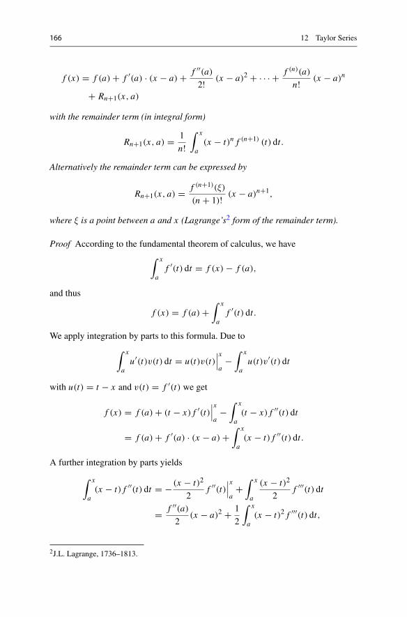
166 12 Taylor Series
f (x) = f (a) + f ′(a) · (x − a) + f ′′(a)2! (x − a)2 + · · · + f (n)(a)
n! (x − a)n
+ Rn+1(x, a)
with the remainder term (in integral form)
Rn+1(x, a) = 1
n!∫ x
a(x − t)n f (n+1) (t) dt.
Alternatively the remainder term can be expressed by
Rn+1(x, a) = f (n+1)(ξ)
(n + 1)! (x − a)n+1,
where ξ is a point between a and x (Lagrange’s2 form of the remainder term).
Proof According to the fundamental theorem of calculus, we have∫ x
af ′(t) dt = f (x) − f (a),
and thus
f (x) = f (a) +∫ x
af ′(t) dt.
We apply integration by parts to this formula. Due to∫ x
au′(t)v(t) dt = u(t)v(t)
∣∣∣x
a−
∫ x
au(t)v′(t) dt
with u(t) = t − x and v(t) = f ′(t) we get
f (x) = f (a) + (t − x) f ′(t)∣∣∣x
a−
∫ x
a(t − x) f ′′(t) dt
= f (a) + f ′(a) · (x − a) +∫ x
a(x − t) f ′′(t) dt.
A further integration by parts yields
∫ x
a(x − t) f ′′(t) dt = − (x − t)2
2f ′′(t)
∣∣∣x
a+
∫ x
a
(x − t)2
2f ′′′(t) dt
= f ′′(a)2
(x − a)2 + 1
2
∫ x
a(x − t)2 f ′′′(t) dt,
2J.L. Lagrange, 1736–1813.
12.1 Taylor’s Formula 167
and one recognises that repeated integration by parts leads to the desired formula(with the remainder term in integral form). The other representation of the remainderterm follows from the mean value theorem for integrals [4, Chap. 5, Theorem 5.4].
��
Example 12.2 (Important special case) If one sets x = a + h and replaces a by xin Taylor’s formula, then one obtains
f (x + h) = f (x) + h f ′(x) + h2
2f ′′(x) + · · · + hn
n! f (n)(x) + hn+1
(n + 1)! f (n+1)(ξ)
with a point ξ between x and x + h. For small h this formula describes how thefunction f behaves near x .
Remark 12.3 Often one does not know the remainder term
Rn+1(x, a) = f (n+1)(ξ)
(n + 1)! (x − a)n+1
explicitly since ξ is unknown in general. Let M be the supremum of∣∣ f (n+1)
∣∣ in theconsidered interval around a. For x in this interval we obtain the bound
∣∣Rn+1(x, a)∣∣ ≤ M
(n + 1)! (x − a)n+1.
The remainder term is thus bounded by a constant times hn+1, where h = x − a. Inthis situation, one writes for short
Rn+1(a + h, a) = O(hn+1)
as h → 0 and calls the remainder a term of order n + 1. This notation is also usedbymaple .
Definition 12.4 The polynomial
Tn(x, a) = f (a) + f ′(a) · (x − a) + · · · + f (n)(a)
n! (x − a)n
is called nth Taylor polynomial of f around the point of expansion a.
The graphs of the functions y = Tn(x, a) and y = f (x) both pass through thepoint (a, f (a)). Their tangents in this point have the same slope T ′
n(x, a) = f ′(a)and the graphs have the same curvature (due to T ′′
n (x, a) = f ′′(a), see Chap.14). Itdepends on the size of the remainder term how well the Taylor polynomial approxi-mates the function.
168 12 Taylor Series
Example 12.5 (Taylor polynomial of the exponential function) Let f (x) = ex anda = 0. Due to (ex )′ = ex we have f (k)(0) = e0 = 1 for all k ≥ 0 and hence
ex = 1 + x + x2
2+ · · · + xn
n! + eξ
(n + 1)! xn+1,
where ξ denotes a point between 0 and x .Wewant to determine theminimal degree ofthe Taylor polynomial which approximates the function in the interval [0, 1], correctto 5 digits. For that we require the following bound on the remainder term
∣∣∣∣ ex − 1 − x − · · · − xn
n!∣∣∣∣ = eξ
(n + 1)! xn+1 ≤ 10−5.
Note that x ∈ [0, 1] as well as eξ are non-negative. The above remainder will bemaximal for x = ξ = 1.Thuswedeterminen from the inequality e/(n + 1)! ≤ 10−5.Due to e ≈ 3 this inequality is certainly fulfilled from n = 8 onwards; in particular,
e = 1 + 1 + 1
2+ · · · + 1
8! ± 10−5.
One has to choose n ≥ 8 in order to determine the first 5 digits of e.
Experiment 12.6 Repeat the above calculations with the help of the maple work-sheet mp12_1.mws. In this worksheet the required maple commands for Taylor’sformula are explained.
Example 12.7 (Taylor polynomial of the sine function) Let f (x) = sin x anda = 0. Recall that (sin x)′ = cos x and (cos x)′ = − sin x as well as sin 0 = 0 andcos 0 = 1. Therefore,
sin x =2n+1∑k=0
sin(k)(0)
k! xk + R2n+2(x, 0) =
= x − x3
3! + x5
5! − x7
7! + · · · + (−1)n x2n+1
(2n + 1)! + R2n+2(x, 0).
Note that the Taylor polynomial consists of odd powers of x only. According toTaylor’s formula, the remainder has the form
R2n+2(x, 0) = sin(2n+2)(ξ)
(2n + 2)! x2n+2.
Since all derivatives of the sine function are bounded by 1, we obtain
|R2n+2(x, 0)| ≤ x2n+2
(2n + 2)! .
12.1 Taylor’s Formula 169
For fixed x the remainder term tends to zero as n → ∞, since the expressionx2n+2/(2n + 2)! is a summand of the exponential series, which converges for allx ∈ R. The above estimate can be interpreted as follows: For every x ∈ R and ε > 0,there exists an integer N ∈ N such that the difference of the sine function and its nthTaylor polynomial is small; more precisely,
| sin t − Tn(t, 0)| ≤ ε
for all n ≥ N and t ∈ [−x, x].
Experiment 12.8 Using the maple worksheet mp12_2.mws compute the Taylorpolynomials of sin x around the point 0 and determine the accuracy of the approxi-mation (by plotting the difference to sin x). In order to achieve high accuracy for largex , the degree of the polynomials has to be chosen sufficiently high. Due to roundingerrors, however, this procedure quickly reaches its limits (unless one increases thenumber of significant digits).
Example 12.9 The 4th degree Taylor polynomial T4(x, 0) of the function
f (x) =⎧⎨⎩
x
ex − 1x �= 0,
1 x = 0,
is given by
T4(x, 0) = 1 − x
2+ 1
12x2 − 1
720x4.
Experiment 12.10 The maple worksheet mp12_3.mws shows that, for suffi-ciently large n, the Taylor polynomial of degree n gives a good approximation to thefunction from Example 12.9 on closed subintervals of (−2π, 2π). For x ≥ 2π (aswell as for x ≤ −2π) the Taylor polynomial is, however, useless.
12.2 Taylor’s Theorem
The last example gives rise to the question for which points the Taylor polynomialconverges to the function as n → ∞.
Definition 12.11 Let I ⊆ R be an open interval and let f : I → R have arbitrarilymany derivatives. Given a ∈ I , the series
T (x, a, f ) =∞∑
k=0
f (k)(a)
k! (x − a)k
is called Taylor series of f around the point a.
170 12 Taylor Series
Proposition 12.12 (Taylor’s theorem) Let f : I → R be a function with arbitrarilymany derivatives and let T (x, a, f ) be its Taylor series around the point a. Then thefunction and its Taylor series coincide at x ∈ I , i.e.,
f (x) =∞∑
k=0
f (k)(a)
k! (x − a)k,
if and only if the remainder term
Rn(x, a) = f (n)(ξ)
n! (x − a)n
tends to 0 as n → ∞.
Proof According to Taylor’s formula (Proposition 12.1),
f (x) − Tn(x, a) = Rn+1(x, a)
and hence
f (x) = limn→∞ Tn(x, a) = T (x, a, f ) ⇔ lim
n→∞ Rn(x, a) = 0,
which was to be shown. ��
Example 12.13 Let f (x) = sin x and a = 0. Due to Rn(x, 0) = sin(n)(ξ)n! xn we have
|Rn(x, 0)| ≤ |x |nn! → 0
for x fixed and n → ∞. Hence for all x ∈ R
sin x =∞∑
k=0
(−1)k x2k+1
(2k + 1)! = x − x3
3! + x5
5! − x7
7! + x9
9! ∓ . . .
12.3 Applications of Taylor’s Formula
To complete this chapter we discuss a few important applications of Taylor’s formula.
Application 12.14 (Extremum test) Let the function f : I → R be n-times contin-uously differentiable in the interval I and assume that
f ′(a) = f ′′(a) = · · · = f (n−1)(a) = 0 and f (n)(a) �= 0.
12.3 Applications of Taylor’s Formula 171
Then the following assertions hold:
(a) The function f has an extremum at a if and only if n is even;
(b) if n is even and f (n)(a) > 0, then a is a local minimum of f ;if n is even and f (n)(a) < 0, then a is a local maximum of f .
Proof Due to Taylor’s formula, we have
f (x) − f (a) = f (n)(ξ)
n! (x − a)n, x ∈ I.
If x is close to a, f (n)(ξ) and f (n)(a) have the same sign (since f (n) is continuous).For n odd the right-hand side changes its sign at x = a because of the term (x − a)n .Hence an extremum can only occur for n even. If now n is even and f (n)(a) > 0then f (x) > f (a) for all x close to a with x �= a. Thus a is a local minimum. ��
Example 12.15 The polynomial f (x) = 6 + 4x + 6x2 + 4x3 + x4 has the deriva-tives
f ′(−1) = f ′′(−1) = f ′′′(−1) = 0, f (4)(−1) = 24
at the point x = −1. Hence x = −1 is a local minimum of f .
Application 12.16 (Computation of limits of functions) As an example, we inves-tigate the function
g(x) = x2 log(1 + x)
(1 − cos x) sin x
in the neighbourhood of x = 0. For x = 0 we obtain the undefined expression 00 . In
order to determine the limit when x tends to 0, we expand all appearing functions inTaylor polynomials around the point a = 0. Exercise 1 yields that cos x = 1 − x2
2 +O(x4). Taylor’s formula for log(1 + x) around the point a = 0 reads
log(1 + x) = x + O(x2)
because of log 1 = 0 and log(1 + x)′|x=0 = 1. We thus obtain
g(x) = x2(x + O(x2)
)(1 − 1 + x2
2 + O(x4))(
x + O(x3)) = x3 + O(x4)
x32 + O(x5)
= 1 + O(x)12 + O(x2)
and consequently limx→0
g(x) = 2.
Application 12.17 (Analysis of approximation formulas) When differentiatingnumerically in Chap.7, we considered the symmetric difference quotient
f ′′(x) ≈ f (x + h) − 2 f (x) + f (x − h)
h2

172 12 Taylor Series
as an approximation to the second derivative f ′′(x). We are now in the position toinvestigate the accuracy of this formula. From
f (x + h) = f (x) + h f ′(x) + h2
2f ′′(x) + h3
6f ′′′(x) + O(h4),
f (x − h) = f (x) − h f ′(x) + h2
2f ′′(x) − h3
6f ′′′(x) + O(h4)
we infer that
f (x + h) + f (x − h) = 2 f (x) + h2 f ′′(x) + O(h4)
and hencef (x + h) − 2 f (x) + f (x − h)
h2 = f ′′(x) + O(h2).
One calls this formula second-order accurate. If one reduces h by the factor λ, thenthe error reduces by the factor λ2, as long as rounding errors do not play a decisiverole.
Application 12.18 (Integration of functions that do not possess elementary inte-grals) As already mentioned in Sect. 10.2 there are functions whose antiderivativescannot be expressed as combinations of elementary functions. For example, thefunction f (x) = e−x2 does not have an elementary integral. In order to compute thedefinite integral
∫ 1
0e−x2 dx,
we approximate e−x2 by the Taylor polynomial of degree 8
e−x2 ≈ 1 − x2 + x4
2− x6
6+ x8
24
and approximate the integral sought after by
∫ 1
0
(1 − x2 + x4
2− x6
6+ x8
24
)dx = 5651
7560.
The error of this approximation is 6.63 · 10−4. For more precise results one takes aTaylor polynomial of a higher degree.
Experiment 12.19 Using the maple worksheet mp12_4.mws repeat the calcula-tions from Application 12.18. Subsequently modify the program such that you canintegrate g(x) = cos
(x2
)with it.
12.4 Exercises 173
12.4 Exercises
1. Compute the Taylor polynomials of degree 0, 1, 2, 3 and 4 of the function g(x) =cos x around the point of expansion a = 0. For which x ∈ R does the Taylorseries of cos x converge?
2. Compute the Taylor polynomials of degree 1, 3 and 5 of the function sin xaround the point of expansion a = 9π. Further, compute the Taylor polynomialof degree 39 with maple and plot the graph together with the graph of thefunction in the interval [0, 18π]. In order to be able to better distinguish the twographs you should plot them in different colours.
3. Compute the Taylor polynomials of degree 1, 2 and 3 of the function f (t) =√1 + t around the point of expansion a = 0. Further compute the Taylor poly-
nomial of degree 10 withmaple .4. Compute the following limits using Taylor series expansion:
limx→0
x sin x − x2
2 cos x − 2 + x2, lim
x→0
e2x − 1 − 2x
sin2 x,
limx→0
e−x2 − 1
sin2(3x), lim
x→0
x2(log(1 − 2x)
)21 − cos(x2)
.
Verify your results withmaple .5. For the approximate evaluation of the integral
∫ 1
0
sin(t2)
tdt
replace the integrand by its Taylor polynomial of degree 9 and integrate thispolynomial. Verify your result withmaple .
6. Prove the formula
eiϕ = cosϕ + i sinϕ
by substituting the value iϕ for x into the series of the exponential function
ex =∞∑
k=0
xk
k!
and separating real and imaginary parts.7. Compute the Taylor series of the hyperbolic functions f (x) = sinh x and
g(x) = cosh x around the point of expansion a = 0 and verify the convergenceof the series.Hint. Compute the Taylor polynomials of degree n − 1 and show that the remain-der terms Rn(x, 0) can be estimated by (cosh M)Mn/n! whenever |x | ≤ M .
174 12 Taylor Series
8. Show that the Taylor series of f (x) = log(1 + x) around a = 0 is given by
log(1 + x) =∞∑
k=1
(−1)k−1 xk
k= x − x2
2+ x3
3− x4
4± . . .
for |x | < 1.Hint. A formal calculation, namely an integration of the geometric seriesexpansion
1
1 + t= 1
1 − (−t)=
∞∑j=0
(−1) j t j
from t = 0 to t = x , suggests the result. For a rigorous proof of convergence,the remainder term has to be estimated. This can be done by integrating theremainder term in the geometric series
1
1 + t−
n−1∑j=0
(−1) j t j = 1
1 + t− 1 − (−1)ntn
1 + t= (−1)ntn
1 + t,
observing that 1 + t ≥ δ>0 for somepositive constant δ as long as |t | ≤ |x | < 1.
13Numerical Integration
The fundamental theorem of calculus suggests the following approach to thecalculation of definite integrals: one determines an antiderivative F of the integrandf and computes from that the value of the integral
∫ b
af (x) dx = F(b) − F(a).
In practice, however, it is difficult and often even impossible to find an antiderivativeF as a combination of elementary functions. Apart from that, antiderivatives canalso be fairly complex, as the example
∫x100 sin x dx shows. Finally, in concrete
applications the integrand is often given numerically and not by an explicit formula.In all these cases one reverts to numerical methods. In this chapter the basic conceptsof numerical integration (quadrature formulas and their order) are introduced andexplained. By means of instructive examples we analyse the achievable accuracy forthe Gaussian quadrature formulas and the required computational effort.
13.1 Quadrature Formulas
For the numerical computation of∫ ba f (x) dx we first split the interval of integration
[a, b] into subintervals with grid points a = x0 < x1 < x2 < . . . < xN−1 < xN = b,seeFig. 13.1. From the additivity of the integral (Proposition 11.10 (d)) we get
∫ b
af (x) dx =
N−1∑j=0
∫ x j+1
x jf (x) dx .
© Springer Nature Switzerland AG 2018M. Oberguggenberger and A. Ostermann, Analysis for Computer Scientists,Undergraduate Topics in Computer Science,https://doi.org/10.1007/978-3-319-91155-7_13
175
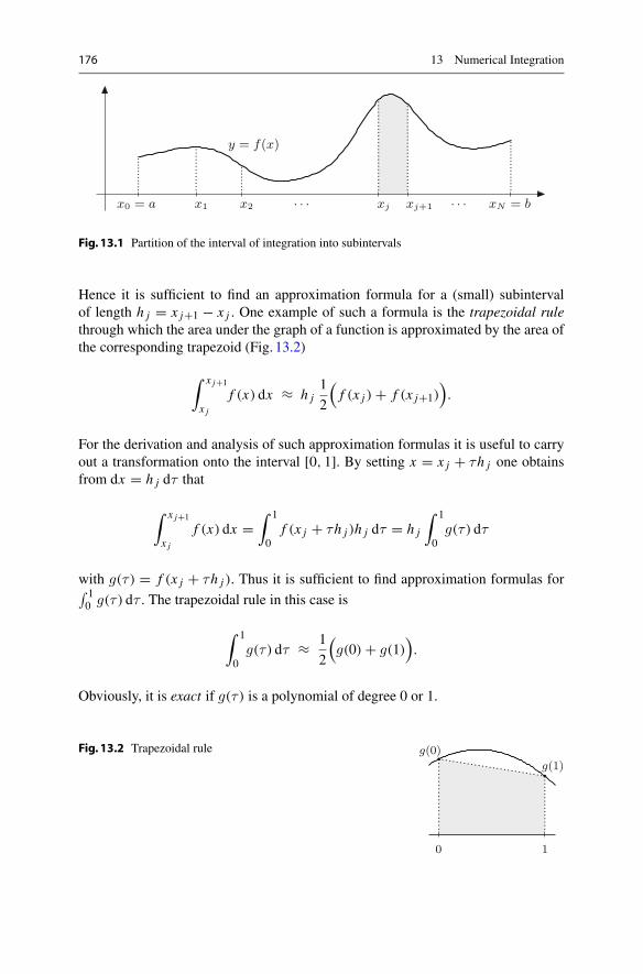
176 13 Numerical Integration
y = f(x)
xN = b· · ·xj+1xj· · ·x2x1x0 = a
Fig. 13.1 Partition of the interval of integration into subintervals
Hence it is sufficient to find an approximation formula for a (small) subintervalof length h j = x j+1 − x j . One example of such a formula is the trapezoidal rulethrough which the area under the graph of a function is approximated by the area ofthe corresponding trapezoid (Fig. 13.2)
∫ x j+1
x jf (x) dx ≈ h j
1
2
(f (x j ) + f (x j+1)
).
For the derivation and analysis of such approximation formulas it is useful to carryout a transformation onto the interval [0, 1]. By setting x = x j + τh j one obtainsfrom dx = h j dτ that
∫ x j+1
x jf (x) dx =
∫ 1
0f (x j + τh j )h j dτ = h j
∫ 1
0g(τ ) dτ
with g(τ ) = f (x j + τh j ). Thus it is sufficient to find approximation formulas for∫ 10 g(τ ) dτ . The trapezoidal rule in this case is
∫ 1
0g(τ ) dτ ≈ 1
2
(g(0) + g(1)
).
Obviously, it is exact if g(τ ) is a polynomial of degree 0 or 1.
Fig. 13.2 Trapezoidal rule
g(1)g(0)
10

13.1 Quadrature Formulas 177
In order to obtain amore accurate formula, we demand that quadratic polynomialsare integrated exactly as well. For the moment let
g(τ ) = α + βτ + γτ2
be a general polynomial of degree 2. Due to g(0) = α, g( 12
) = α + 12β + 1
4γ andg(1) = α + β + γ we get by a short calculation
∫ 1
0
(α + βτ + γτ2
)dτ = α + 1
2β + 1
3γ = 1
6
(g(0) + 4g
( 12
) + g(1)).
The corresponding approximation formula for general g reads
∫ 1
0g(τ ) dτ ≈ 1
6
(g(0) + 4g
( 12
) + g(1)).
By construction, it is exact for polynomials of degree less than or equal to 2; it iscalled Simpson’s rule.1
The special forms of the trapezoidal and of Simpson’s rule motivate the followingdefinition.
Definition 13.1 The approximation formula
∫ 1
0g(τ ) dτ ≈
s∑i=1
bi g(ci )
is called a quadrature formula. The numbers b1, . . . , bs are called weights, and thenumbers c1, . . . , cs are called nodes of the quadrature formula; the integer s is calledthe number of stages.
A quadrature formula is determined by the specification of the weights and nodes.Thus we denote a quadrature formula by {(bi , ci ), i = 1, . . . , s} for short. Withoutloss of generality the weights bi are not zero, and the nodes are pairwise different(ci �= ck for i �= k).
Example 13.2 (a) The trapezoidal rule has s = 2 stages and is given by
b1 = b2 = 1
2, c1 = 0, c2 = 1.
1T. Simpson, 1710–1761.
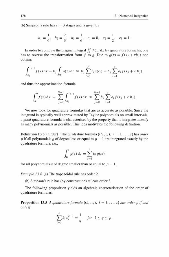
178 13 Numerical Integration
(b) Simpson’s rule has s = 3 stages and is given by
b1 = 1
6, b2 = 2
3, b3 = 1
6, c1 = 0, c2 = 1
2, c3 = 1.
In order to compute the original integral∫ ba f (x) dx by quadrature formulas, one
has to reverse the transformation from f to g. Due to g(τ ) = f (x j + τh j ) oneobtains
∫ x j+1
x jf (x) dx = h j
∫ 1
0g(τ ) dt ≈ h j
s∑i=1
big(ci ) = h j
s∑i=1
bi f (x j + ci h j ),
and thus the approximation formula
∫ b
af (x) dx =
N−1∑j=0
∫ x j+1
x jf (x) dx ≈
N−1∑j=0
h j
s∑i=1
bi f (x j + ci h j ).
We now look for quadrature formulas that are as accurate as possible. Since theintegrand is typically well approximated by Taylor polynomials on small intervals,a good quadrature formula is characterised by the property that it integrates exactlyas many polynomials as possible. This idea motivates the following definition.
Definition 13.3 (Order) The quadrature formula {(bi , ci ), i = 1, . . . , s} has orderp if all polynomials g of degree less or equal to p − 1 are integrated exactly by thequadrature formula; i.e.,
∫ 1
0g(τ ) dτ =
s∑i=1
bi g(ci )
for all polynomials g of degree smaller than or equal to p − 1.
Example 13.4 (a) The trapezoidal rule has order 2.
(b) Simpson’s rule has (by construction) at least order 3.
The following proposition yields an algebraic characterisation of the order ofquadrature formulas.
Proposition 13.5 A quadrature formula {(bi , ci ), i = 1, . . . , s} has order p if andonly if
s∑i=1
bi cq−1i = 1
qfor 1 ≤ q ≤ p.
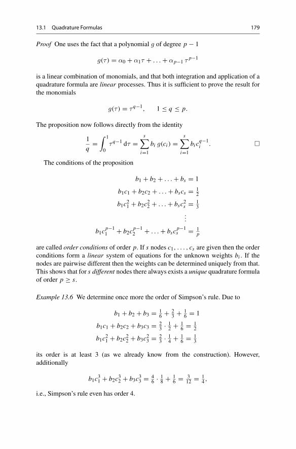
13.1 Quadrature Formulas 179
Proof One uses the fact that a polynomial g of degree p − 1
g(τ ) = α0 + α1τ + . . . + αp−1 τ p−1
is a linear combination of monomials, and that both integration and application of aquadrature formula are linear processes. Thus it is sufficient to prove the result forthe monomials
g(τ ) = τq−1, 1 ≤ q ≤ p.
The proposition now follows directly from the identity
1
q=
∫ 1
0τq−1 dτ =
s∑i=1
bi g(ci ) =s∑
i=1
bi cq−1i . �
The conditions of the proposition
b1 + b2 + . . . + bs = 1
b1c1 + b2c2 + . . . + bscs = 12
b1c21 + b2c
22 + . . . + bsc
2s = 1
3
...
b1cp−11 + b2c
p−12 + . . . + bsc
p−1s = 1
p
are called order conditions of order p. If s nodes c1, . . . , cs are given then the orderconditions form a linear system of equations for the unknown weights bi . If thenodes are pairwise different then the weights can be determined uniquely from that.This shows that for s different nodes there always exists a unique quadrature formulaof order p ≥ s.
Example 13.6 We determine once more the order of Simpson’s rule. Due to
b1 + b2 + b3 = 16 + 2
3 + 16 = 1
b1c1 + b2c2 + b3c3 = 23 · 1
2 + 16 = 1
2
b1c21 + b2c
22 + b3c
23 = 2
3 · 14 + 1
6 = 13
its order is at least 3 (as we already know from the construction). However,additionally
b1c31 + b2c
32 + b3c
33 = 4
6 · 18 + 1
6 = 312 = 1
4 ,
i.e., Simpson’s rule even has order 4.

180 13 Numerical Integration
The best quadrature formulas (high accuracy with little computational effort) arethe Gaussian quadrature formulas. For that we state the following result whose proofcan be found in [23, Chap.10, Corollary10.1].
Proposition 13.7 There is no quadrature formula with s stages of order p > 2s. Onthe other hand, for every s ∈ N there exists a (unique) quadrature formula of orderp = 2s. This formula is called s-stage Gaussian quadrature formula.
The Gaussian quadrature formulas for s ≤ 3 are
s = 1 : c1 = 1
2, b1 = 1, order 2 (midpoint rule);
s = 2 : c1 = 1
2−
√3
6, c2 = 1
2+
√3
6, b1 = b2 = 1
2, order 4;
s = 3 : c1 = 1
2−
√15
10, c2 = 1
2, c3 = 1
2+
√15
10,
b1 = 5
18, b2 = 8
18, b3 = 5
18, order 6.
13.2 Accuracy and Efficiency
In the following numerical experiment the accuracy of quadrature formulas will beillustrated. With the help of the Gaussian quadrature formulas of order 2, 4 and 6 wecompute the two integrals
∫ 3
0cos x dx = sin 3 and
∫ 1
0x5/2 dx = 2
7.
For that we choose equidistant grid points
x j = a + jh, j = 0, . . . , N
with h = (b − a)/N and N = 1, 2, 4, 8, 16, . . . , 512. Finally,we plot the costs of thecalculation as a function of the achieved accuracy in a double-logarithmic diagram.
A measure for the computational cost of a quadrature formula is the number ofrequired function evaluations, abbreviated by fe. For an s-stage quadrature formula,it is the number
fe = s · N .
The achieved accuracy err is the absolute value of the error. The according resultsare presented in Fig. 13.3. One makes the following observations:
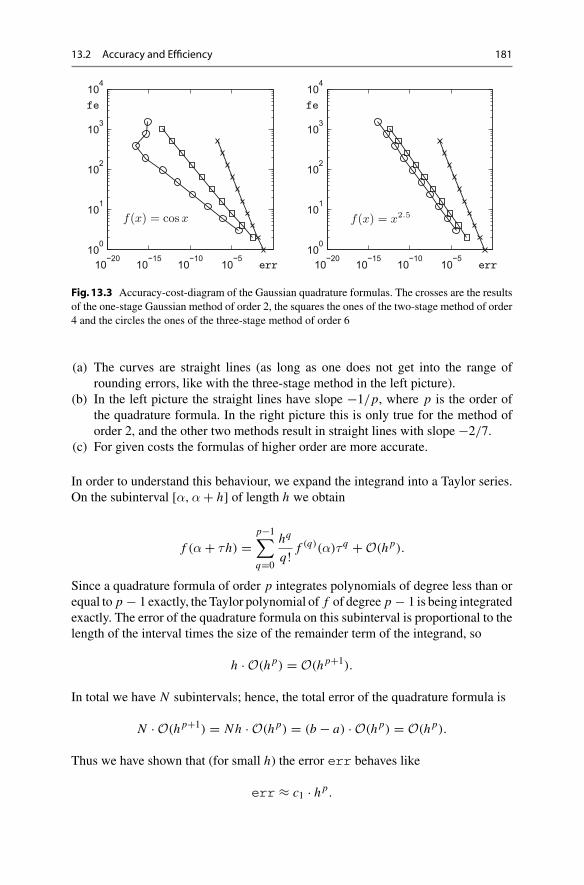
13.2 Accuracy and Efficiency 181
10−20
10−15
10−10
10−5
100
101
102
103
104
10−20
10−15
10−10
10−5
100
101
102
103
104
f(x) = x2.5
err
fe
err
fe
f(x) = cosx
Fig.13.3 Accuracy-cost-diagram of the Gaussian quadrature formulas. The crosses are the resultsof the one-stage Gaussian method of order 2, the squares the ones of the two-stage method of order4 and the circles the ones of the three-stage method of order 6
(a) The curves are straight lines (as long as one does not get into the range ofrounding errors, like with the three-stage method in the left picture).
(b) In the left picture the straight lines have slope −1/p, where p is the order ofthe quadrature formula. In the right picture this is only true for the method oforder 2, and the other two methods result in straight lines with slope −2/7.
(c) For given costs the formulas of higher order are more accurate.
In order to understand this behaviour, we expand the integrand into a Taylor series.On the subinterval [α,α + h] of length h we obtain
f (α + τh) =p−1∑q=0
hq
q! f (q)(α)τq + O(h p).
Since a quadrature formula of order p integrates polynomials of degree less than orequal to p − 1 exactly, the Taylor polynomial of f of degree p − 1 is being integratedexactly. The error of the quadrature formula on this subinterval is proportional to thelength of the interval times the size of the remainder term of the integrand, so
h · O(h p) = O(h p+1).
In total we have N subintervals; hence, the total error of the quadrature formula is
N · O(h p+1) = Nh · O(h p) = (b − a) · O(h p) = O(h p).
Thus we have shown that (for small h) the error err behaves like
err ≈ c1 · h p.
182 13 Numerical Integration
Since furthermore
fe = sN = s · Nh · h−1 = s · (b − a) · h−1 = c2 · h−1
holds true, we obtain
log(fe) = log c2 − log h and log(err) ≈ log c1 + p · log h,
so altogether
log(fe) ≈ c3 − 1
p· log(err).
This explains why straight lines with slope −1/p appear in the left picture.In the right picture it has to be noted that the second derivative of the integrand
is discontinuous at 0. Hence the above considerations with the Taylor series are notvalid anymore. The quadrature formula also detects this discontinuity of the highderivatives and reacts with a so-called order reduction; i.e., the methods show alower order (in our case p = 7/2).
Experiment 13.8 Compute the integrals
∫ 3
0
√x dx and
∫ 2
1
dx
x
using the Gaussian quadrature formulas and generate an accuracy-cost-diagram.For that purpose modify the programs mat13_1.m, mat13_2.m, mat13_3.m,mat13_4.m and mat13_5.m with which Fig. 13.3 was produced.
Commercial programs for numerical integration determine the grid points adap-tively based on automatic error estimates. The user can usually specify the desiredaccuracy. In MATLAB the routines quad.m and quadl.m serve this purpose.
13.3 Exercises
1. For the calculation of∫ 10 x100 sin x dx first determine an antiderivative F of the
integrand f using maple . Then evaluate F(1) − F(0) to 10, 50, 100, 200 and400 digits and explain the surprising results.
2. Determine the order of the quadrature formula given by
b1 = b4 = 1
8, b2 = b3 = 3
8, c1 = 0, c2 = 1
3, c3 = 2
3, c4 = 1.
13.3 Exercises 183
3. Determine the unique quadrature formula of order 3 with the nodes
c1 = 1
3, c2 = 2
3, c3 = 1.
4. Determine the unique quadrature formula with the nodes
c1 = 1
4, c2 = 1
2, c3 = 3
4.
Which order does it have?5. Familiarise yourself with theMATLAB programs quad.m and quadl.m for the
computation of definite integrals and test the programs for
∫ 1
0e−x2 dx and
∫ 1
0
3√x dx .
6. Justify the formulas
π = 4∫ 1
0
dx
1 + x2and π = 4
∫ 1
0
√1 − x2 dx
and use them to calculate π by numerical integration. To do so divide the interval[0, 1] into N equally large parts (N = 10, 100, . . .) and use Simpson’s rule onthose subintervals. Why are the results obtained with the first formula alwaysmore accurate?
7. Write a MATLAB program that allows you to evaluate the integral of any given(continuous) function on a given interval [a, b], both by the trapezoidal rule andby Simpson’s rule. Use your program to numerically answering the questions ofExercises 7–9 from Sect. 11.4 and Exercise 5 from Sect. 12.4.
8. Use your program from Exercise 7 to produce tables (for x = 0 to x = 10 insteps of 0.5) of some higher transcendental functions:(a) the Gaussian error function
Erf(x) = 2√π
∫ x
0e−y2 dy,
(b) the sine integral
Si(x) =∫ x
0
sin y
ydy,
(c) the Fresnel integral
S(x) =∫ x
0sin
(π
2y2
)dy.
184 13 Numerical Integration
9. (Experimental determination of expectation values) The family of standard betadistributions on the interval [0, 1] is defined through the probability densities
f (x; r, s) = 1
B(r, s)xr−1(1 − x)s−1, 0 ≤ x ≤ 1,
where r, s > 0. Here B(r, s) = ∫ 10 yr−1(1 − y)s−1 dy is the beta function,
which is a higher transcendental function for non-integer values of r, s. Forinteger values of r, s ≥ 1 it is given by
B(r, s) = (r − 1)!(s − 1)!(r + s − 1)! .
With the help of theMATLAB program quad.m, compute the expectation valuesμ(r, s) = ∫ 1
0 x f (x; r, s) dx for various integer values of r and s and guess ageneral formula for μ(r, s) from your experimental results.

14Curves
The graph of a function y = f (x) represents a curve in the plane. This concept,however, is too tight to represent more intricate curves, like loops, self-intersections,or even curves of fractal dimension. The aim of this chapter is to introduce theconcept of parametrised curves and to study, in particular, the case of differentiablecurves. For the visualisation of the trajectory of a curve, the notions of velocityvector, moving frame, and curvature are important. The chapter contains a collectionof geometrically interesting examples of curves and several of their constructionprinciples. Further, the computation of the arc length of differentiable curves isdiscussed, and an example of a continuous, bounded curve of infinite length is given.The chapter ends with a short outlook on spatial curves. For the vector algebra usedin this chapter, we refer to Appendix A.
14.1 Parametrised Curves in the Plane
Definition 14.1 A parametrised plane curve is a continuous mapping
t �→ x(t) =[
x(t)y(t)
]
of an interval [a, b] to R2; i.e., both the components t �→ x(t) and t �→ y(t) are
continuous functions.1 The variable t ∈ [a, b] is called parameter of the curve.
1Concerning the vector notation we remark that x(t), y(t) actually represent the coordinates of apoint in R2. It is, however, common practise and useful to write this point as a position vector, thusthe column notation.
© Springer Nature Switzerland AG 2018M. Oberguggenberger and A. Ostermann, Analysis for Computer Scientists,Undergraduate Topics in Computer Science,https://doi.org/10.1007/978-3-319-91155-7_14
185

186 14 Curves
Example 14.2 An object that is thrown at height h with horizontal velocity vH andvertical velocity vV has the trajectory
x(t) = vH t,y(t) = h + vV t − g
2 t2,0 ≤ t ≤ t0,
where t0 is the positive solution of the equation h + vV t0 − g2 t20 = 0 (time of
impact, see Fig. 14.1). In this example, we can eliminate t and represent the tra-jectory as the graph of a function (ballistic curve). We have t = x/vH , and thus
y = h + vV
vHx − g
2v2Hx2.
Example 14.3 A circle of radius R with centre at the origin has the parametricrepresentation
x(t) = R cos t,y(t) = R sin t,
0 ≤ t ≤ 2π.
In this case, t can be interpreted as the angle between the position vector and thepositive x-axis (Fig. 14.1). The components x = x(t), y = y(t) satisfy the quadraticequation
x2 + y2 = R2;
however, one cannot represent the circle in its entirety as the graph of a function.
Experiment 14.4 Open the M-file mat14_1.m and discuss which curve is beingrepresented. Compare with the M-files mat14_2.m to mat14_4.m. Are these thesame curves?
Experiment 14.4 suggests that one can view curves statically as a set of points inthe plane or dynamically as the trajectory of a moving point. Both perspectives areof importance in applications.
[x(t), y(t)]T
0 R
y
xt
t = t0
h
t = 0[x(t), y(t)]T
y
x
Fig. 14.1 Parabolic trajectory and circle

14.1 Parametrised Curves in the Plane 187
The kinematic point of view. In the kinematic interpretation, one considers theparameter t of the curve as time and the curve as path. Different parametrisations ofthe same geometric object are viewed as different curves.
The geometric point of view. In the geometric interpretation, the location, the mov-ing sense and the number of cycles are considered as the defining properties of acurve. The particular parametrisation, however, is irrelevant.
A strictly monotonically increasing, continuous mapping of an interval [α, β] to[a, b],
ϕ : [α, β] → [a, b]
is called a change of parameter. The curve
τ �→ ξ(τ ), α ≤ τ ≤ β
is called a reparametrisation of the curve
t �→ x(t), a ≤ t ≤ b,
if it is obtained through a change of parameter t = ϕ(τ ); i.e.,
ξ(τ ) = x(ϕ(τ )).
From the geometric point of view, the parametrised curves τ �→ ξ(τ ) and t �→ x(t)are identified. A plane curve Γ is an equivalence class of parametrised curves whichcan be transformed to one another by reparametrisation.
Example 14.5 We consider the segment of a parabola, parametrised by
Γ : x(t) =[
tt2
], −1 ≤ t ≤ 1.
Reparametrisations are for instance
ϕ : [− 12 ,
12
] → [−1, 1], ϕ(τ ) = 2τ ,
ϕ : [−1, 1] → [−1, 1], ϕ(t) = τ3.
Consequently,
ξ(τ ) =[2τ4τ2
], − 1
2 ≤ τ ≤ 12

188 14 Curves
and
η(τ ) =[τ3
τ6
], −1 ≤ τ ≤ 1
geometrically represent the same curve. However,
ψ : [−1, 1] → [−1, 1], ψ(τ ) = −τ ,
ψ : [0, 1] → [−1, 1], ψ(τ ) = −1 + 8τ (1 − τ )
are not reparametrisations and yield other curves, namely
y(τ ) =[−τ
τ2
], −1 ≤ τ ≤ 1,
z(τ ) =[ −1 + 8τ (1 − τ )
(−1 + 8τ (1 − τ ))2
], 0 ≤ τ ≤ 1.
In the first case, the moving sense of Γ is reversed, and in the second case, the curveis traversed twice.
Experiment 14.6 Modify the M-files from Experiment 14.4 so that the curves fromExample 14.5 are represented.
Algebraic curves. These are obtained as the set of zeros of polynomials in twovariables. As examples we had already parabola and circle
y − x2 = 0, x2 + y2 − R2 = 0.
One can also create cusps and loops in this way.
Example 14.7 Neil’s2 parabola
y2 − x3 = 0
has a cusp at x = y = 0 (Fig. 14.2). Generally, one obtains algebraic curves from
y2 − (x + p)x2 = 0, p ∈ R.
For p > 0 they have a loop. A parametric representation of this curve is, for instance,
x(t) = t2 − p,
y(t) = t (t2 − p),− ∞ < t < ∞.
2W. Neil, 1637–1670.

14.1 Parametrised Curves in the Plane 189
−1 0 1 2 3−2
−1
0
1
2
−2 −1 0 1 2−2
−1
0
1
2
−1 0 1 2 3−2
−1
0
1
2y
x
y
x
y
x
Fig. 14.2 Neil’s parabola, the α -curve and an elliptic curve
In the following we will primarily deal with curves which are given by differen-tiable parametrisations.
Definition 14.8 If a plane curve Γ : t �→ x(t) has a parametrisation whose compo-nents t �→ x(t), t �→ y(t) are differentiable, then Γ is called a differentiable curve.If the components are k-times differentiable, then Γ is called a k-times differentiablecurve.
The graphical representation of a differentiable curve does not have to be smoothbut may have cusps and corners, as Example 14.7 shows.
Example 14.9 (Straight line and half ray) The parametric representation
t �→ x(t) =[
x0y0
]+ t
[r1r2
], −∞ < t < ∞
describes a straight line through the point x0 = [x0, y0]T in the directionr = [r1, r2]T. If one restricts the parameter t to 0 ≤ t < ∞ one obtains a half ray.The parametrisation
xH (t) =[
x0y0
]+ t2
[r1r2
], −∞ < t < ∞
leads to a double passage through the half ray.
Example 14.10 (Parametric representation of an ellipse) The equation of an ellipseis
x2
a2 + y2
b2= 1.
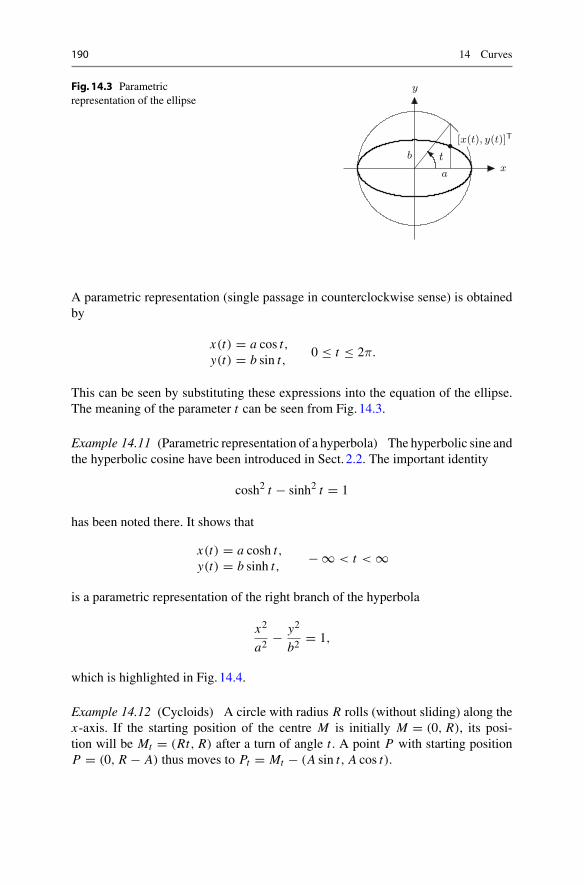
190 14 Curves
Fig. 14.3 Parametricrepresentation of the ellipse
b
a
[x(t), y(t)]T
y
xt
A parametric representation (single passage in counterclockwise sense) is obtainedby
x(t) = a cos t,y(t) = b sin t,
0 ≤ t ≤ 2π.
This can be seen by substituting these expressions into the equation of the ellipse.The meaning of the parameter t can be seen from Fig. 14.3.
Example 14.11 (Parametric representation of a hyperbola) The hyperbolic sine andthe hyperbolic cosine have been introduced in Sect. 2.2. The important identity
cosh2 t − sinh2 t = 1
has been noted there. It shows that
x(t) = a cosh t,y(t) = b sinh t,
− ∞ < t < ∞
is a parametric representation of the right branch of the hyperbola
x2
a2 − y2
b2= 1,
which is highlighted in Fig. 14.4.
Example 14.12 (Cycloids) A circle with radius R rolls (without sliding) along thex-axis. If the starting position of the centre M is initially M = (0, R), its posi-tion will be Mt = (Rt, R) after a turn of angle t . A point P with starting positionP = (0, R − A) thus moves to Pt = Mt − (A sin t, A cos t).
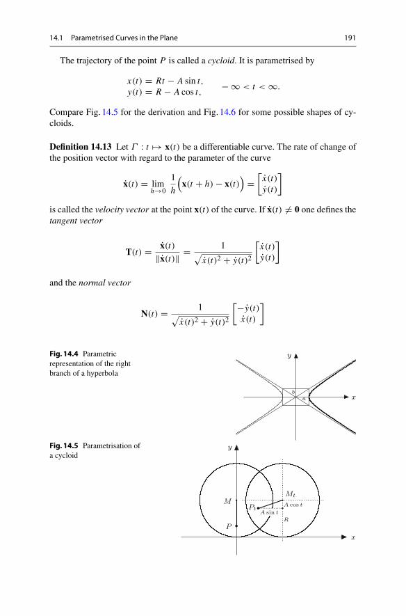
14.1 Parametrised Curves in the Plane 191
The trajectory of the point P is called a cycloid. It is parametrised by
x(t) = Rt − A sin t,y(t) = R − A cos t,
− ∞ < t < ∞.
Compare Fig. 14.5 for the derivation and Fig. 14.6 for some possible shapes of cy-cloids.
Definition 14.13 Let Γ : t �→ x(t) be a differentiable curve. The rate of change ofthe position vector with regard to the parameter of the curve
x(t) = limh→0
1
h
(x(t + h) − x(t)
)=
[x(t)y(t)
]
is called the velocity vector at the point x(t) of the curve. If x(t) �= 0 one defines thetangent vector
T(t) = x(t)‖x(t)‖ = 1√
x(t)2 + y(t)2
[x(t)y(t)
]
and the normal vector
N(t) = 1√x(t)2 + y(t)2
[−y(t)x(t)
]
Fig. 14.4 Parametricrepresentation of the rightbranch of a hyperbola
ba
y
x
Fig. 14.5 Parametrisation ofa cycloid
A sin t
R
A cos t
Mt
Pt
P
M
y
x
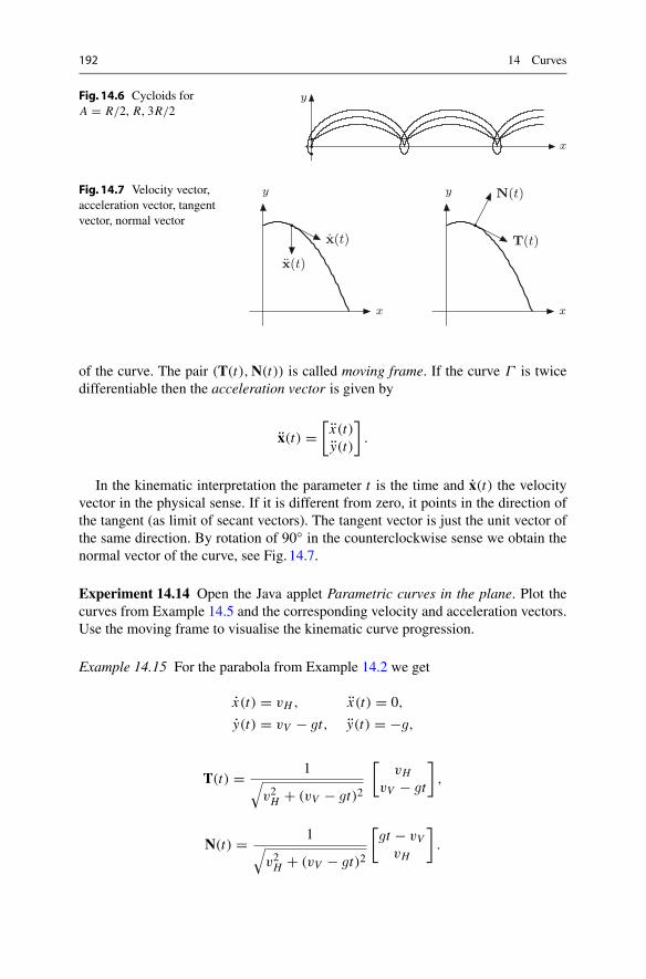
192 14 Curves
Fig. 14.6 Cycloids forA = R/2, R, 3R/2
y
x
Fig. 14.7 Velocity vector,acceleration vector, tangentvector, normal vector
y
x
N(t)
T(t)
y
x
x(t)
x(t)
of the curve. The pair (T(t),N(t)) is called moving frame. If the curve Γ is twicedifferentiable then the acceleration vector is given by
x(t) =[
x(t)y(t)
].
In the kinematic interpretation the parameter t is the time and x(t) the velocityvector in the physical sense. If it is different from zero, it points in the direction ofthe tangent (as limit of secant vectors). The tangent vector is just the unit vector ofthe same direction. By rotation of 90◦ in the counterclockwise sense we obtain thenormal vector of the curve, see Fig. 14.7.
Experiment 14.14 Open the Java applet Parametric curves in the plane. Plot thecurves from Example 14.5 and the corresponding velocity and acceleration vectors.Use the moving frame to visualise the kinematic curve progression.
Example 14.15 For the parabola from Example 14.2 we get
x(t) = vH , x(t) = 0,
y(t) = vV − gt, y(t) = −g,
T(t) = 1√v2H + (vV − gt)2
[vH
vV − gt
],
N(t) = 1√v2H + (vV − gt)2
[gt − vV
vH
].

14.2 Arc Length and Curvature 193
14.2 Arc Length and Curvature
We start with the question whether and how a length can be assigned to a curvesegment. Let a continuous curve
Γ : t �→ x(t) =[
x(t)y(t)
], a ≤ t ≤ b
be given. For a partition Z : a = t0 < t1 < · · · < tn = b of the parameter interval weconsider the (inscribed) polygonal chain through the points
x(t0), x(t1), . . . , x(tn).
The length of the largest subinterval is again denoted by Φ(Z). The length of thepolygonal chain is
Ln =n∑
i=1
√(x(ti ) − x(ti−1))2 + (y(ti ) − y(ti−1))2 .
Definition 14.16 (Curves of finite length) A plane curveΓ is called rectifiable or offinite length if the lengths Ln of all inscribed polygonal chains Zn converge towardsone (and the same) limit provided that Φ(Zn) → 0.
Example 14.17 (Koch’s snowflake) Koch’s snowflake was introduced in Sect. 9.1as an example of a finite region whose boundary has the fractal dimensiond = log 4/ log 3 and infinite length. This was proven by the fact that the boundarycan be constructed as the limit of polygonal chains whose lengths tend to infinity.It remains to verify that the boundary of Koch’s snowflake is indeed a continuous,parametrised curve. This can be seen as follows. The snowflake of depth 0 is anequilateral triangle, for instance with the vertices p1, p2, p3 ∈ R
2. Using the unitinterval [0, 1] we obtain a continuous parametrisation
x0(t) =
⎧⎪⎨⎪⎩p1 + 3t (p2 − p1), 0 ≤ t ≤ 1
3 ,
p2 + (3t − 1)(p3 − p2),13 ≤ t ≤ 2
3 ,
p3 + (3t − 2)(p1 − p3),23 ≤ t ≤ 1.
We parametrise the snowflake of depth 1 by splitting the three intervals [0, 13 ],
[ 13 , 23 ], [ 23 , 1] into three parts each and using the middle parts for the parametrisation
of the inserted next smaller angle (Fig. 14.8). Continuing in this way we obtain asequence of parametrisations
t �→ x0(t), t �→ x1(t), . . . , t �→ xn(t), . . .
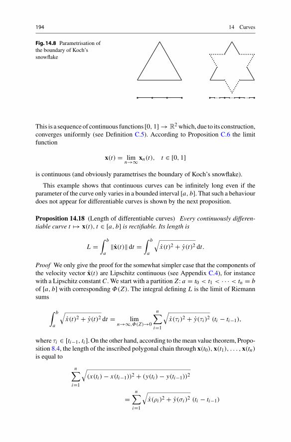
194 14 Curves
Fig. 14.8 Parametrisation ofthe boundary of Koch’ssnowflake
This is a sequence of continuous functions [0, 1] → R2 which, due to its construction,
converges uniformly (see Definition C.5). According to Proposition C.6 the limitfunction
x(t) = limn→∞ xn(t), t ∈ [0, 1]
is continuous (and obviously parametrises the boundary of Koch’s snowflake).
This example shows that continuous curves can be infinitely long even if theparameter of the curve only varies in a bounded interval [a, b]. That such a behaviourdoes not appear for differentiable curves is shown by the next proposition.
Proposition 14.18 (Length of differentiable curves) Every continuously differen-tiable curve t �→ x(t), t ∈ [a, b] is rectifiable. Its length is
L =∫ b
a‖x(t)‖ dt =
∫ b
a
√x(t)2 + y(t)2 dt.
Proof We only give the proof for the somewhat simpler case that the components ofthe velocity vector x(t) are Lipschitz continuous (see Appendix C.4), for instancewith a Lipschitz constant C . We start with a partition Z : a = t0 < t1 < · · · < tn = bof [a, b] with corresponding Φ(Z). The integral defining L is the limit of Riemannsums
∫ b
a
√x(t)2 + y(t)2 dt = lim
n→∞,Φ(Z)→0
n∑i=1
√x(τi )2 + y(τi )2 (ti − ti−1),
where τi ∈ [ti−1, ti ]. On the other hand, according to themean value theorem, Propo-sition 8.4, the length of the inscribed polygonal chain through x(t0), x(t1), . . . , x(tn)
is equal to
n∑i=1
√(x(ti ) − x(ti−1))2 + (y(ti ) − y(ti−1))2
=n∑
i=1
√x(ρi )2 + y(σi )2 (ti − ti−1)
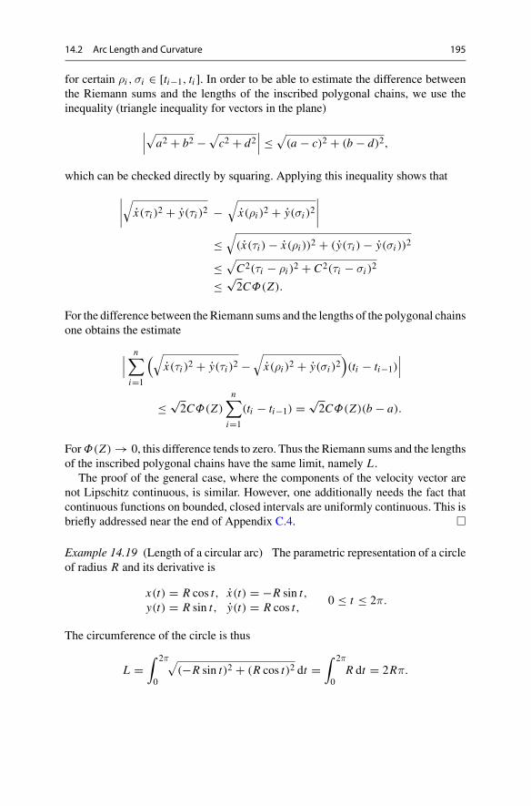
14.2 Arc Length and Curvature 195
for certain ρi ,σi ∈ [ti−1, ti ]. In order to be able to estimate the difference betweenthe Riemann sums and the lengths of the inscribed polygonal chains, we use theinequality (triangle inequality for vectors in the plane)
∣∣∣√a2 + b2 −√
c2 + d2∣∣∣ ≤
√(a − c)2 + (b − d)2,
which can be checked directly by squaring. Applying this inequality shows that
∣∣∣∣√
x(τi )2 + y(τi )2 −√
x(ρi )2 + y(σi )2
∣∣∣∣≤
√(x(τi ) − x(ρi ))2 + (y(τi ) − y(σi ))2
≤√
C2(τi − ρi )2 + C2(τi − σi )2
≤ √2CΦ(Z).
For the difference between the Riemann sums and the lengths of the polygonal chainsone obtains the estimate
∣∣∣n∑
i=1
(√x(τi )2 + y(τi )2 −
√x(ρi )2 + y(σi )2
)(ti − ti−1)
∣∣∣
≤ √2CΦ(Z)
n∑i=1
(ti − ti−1) = √2CΦ(Z)(b − a).
ForΦ(Z) → 0, this difference tends to zero. Thus the Riemann sums and the lengthsof the inscribed polygonal chains have the same limit, namely L .
The proof of the general case, where the components of the velocity vector arenot Lipschitz continuous, is similar. However, one additionally needs the fact thatcontinuous functions on bounded, closed intervals are uniformly continuous. This isbriefly addressed near the end of Appendix C.4. �
Example 14.19 (Length of a circular arc) The parametric representation of a circleof radius R and its derivative is
x(t) = R cos t, x(t) = −R sin t,y(t) = R sin t, y(t) = R cos t,
0 ≤ t ≤ 2π.
The circumference of the circle is thus
L =∫ 2π
0
√(−R sin t)2 + (R cos t)2 dt =
∫ 2π
0R dt = 2Rπ.
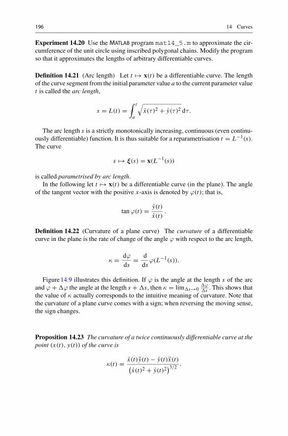
196 14 Curves
Experiment 14.20 Use the MATLAB program mat14_5.m to approximate the cir-cumference of the unit circle using inscribed polygonal chains. Modify the programso that it approximates the lengths of arbitrary differentiable curves.
Definition 14.21 (Arc length) Let t �→ x(t) be a differentiable curve. The lengthof the curve segment from the initial parameter value a to the current parameter valuet is called the arc length,
s = L(t) =∫ t
a
√x(τ )2 + y(τ )2 dτ .
The arc length s is a strictly monotonically increasing, continuous (even continu-ously differentiable) function. It is thus suitable for a reparametrisation t = L−1(s).The curve
s �→ ξ(s) = x(L−1(s))
is called parametrised by arc length.In the following let t �→ x(t) be a differentiable curve (in the plane). The angle
of the tangent vector with the positive x-axis is denoted by ϕ(t); that is,
tanϕ(t) = y(t)
x(t).
Definition 14.22 (Curvature of a plane curve) The curvature of a differentiablecurve in the plane is the rate of change of the angle ϕ with respect to the arc length,
κ = dϕ
ds= d
dsϕ(L−1(s)).
Figure14.9 illustrates this definition. If ϕ is the angle at the length s of the arcand ϕ + �ϕ the angle at the length s + �s, then κ = lim�s→0
�ϕ�s . This shows that
the value of κ actually corresponds to the intuitive meaning of curvature. Note thatthe curvature of a plane curve comes with a sign; when reversing the moving sense,the sign changes.
Proposition 14.23 The curvature of a twice continuously differentiable curve at thepoint (x(t), y(t)) of the curve is
κ(t) = x(t)y(t) − y(t)x(t)(x(t)2 + y(t)2
)3/2 .
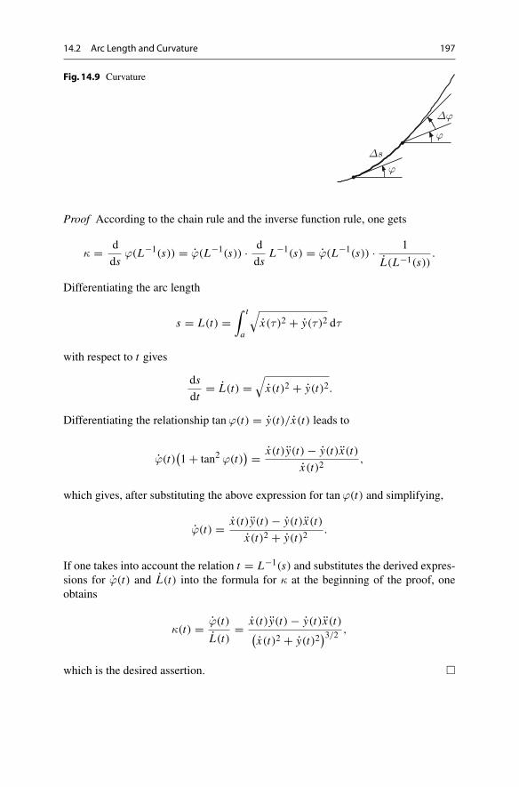
14.2 Arc Length and Curvature 197
Fig. 14.9 Curvature
Δs
Δϕ
ϕ
ϕ
Proof According to the chain rule and the inverse function rule, one gets
κ = d
dsϕ(L−1(s)) = ϕ(L−1(s)) · d
dsL−1(s) = ϕ(L−1(s)) · 1
L(L−1(s)).
Differentiating the arc length
s = L(t) =∫ t
a
√x(τ )2 + y(τ )2 dτ
with respect to t gives
ds
dt= L(t) =
√x(t)2 + y(t)2.
Differentiating the relationship tanϕ(t) = y(t)/x(t) leads to
ϕ(t)(1 + tan2 ϕ(t)
) = x(t)y(t) − y(t)x(t)
x(t)2,
which gives, after substituting the above expression for tanϕ(t) and simplifying,
ϕ(t) = x(t)y(t) − y(t)x(t)
x(t)2 + y(t)2.
If one takes into account the relation t = L−1(s) and substitutes the derived expres-sions for ϕ(t) and L(t) into the formula for κ at the beginning of the proof, oneobtains
κ(t) = ϕ(t)
L(t)= x(t)y(t) − y(t)x(t)(
x(t)2 + y(t)2)3/2 ,
which is the desired assertion. �
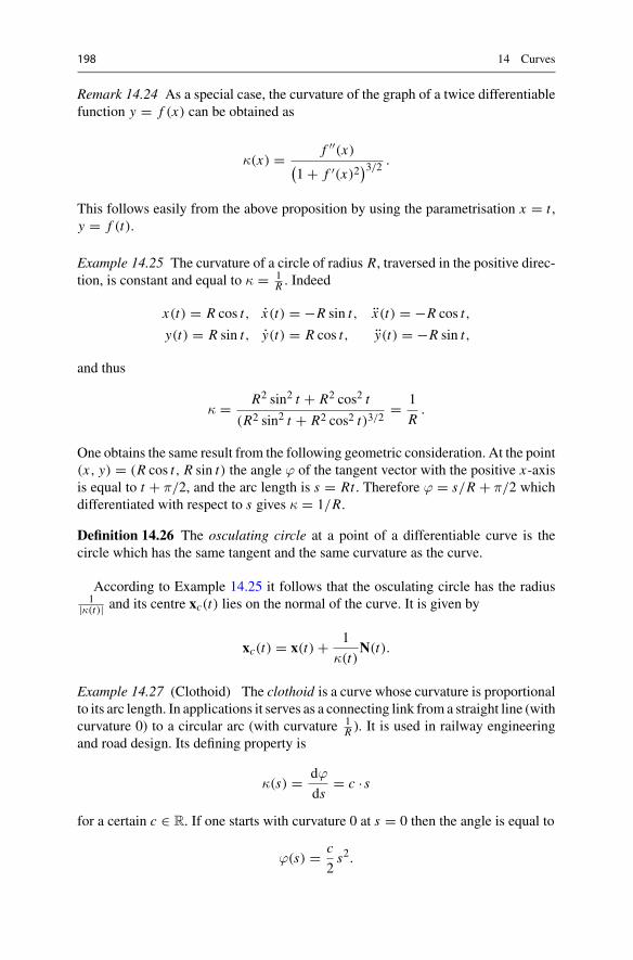
198 14 Curves
Remark 14.24 As a special case, the curvature of the graph of a twice differentiablefunction y = f (x) can be obtained as
κ(x) = f ′′(x)(1 + f ′(x)2
)3/2 .
This follows easily from the above proposition by using the parametrisation x = t ,y = f (t).
Example 14.25 The curvature of a circle of radius R, traversed in the positive direc-tion, is constant and equal to κ = 1
R . Indeed
x(t) = R cos t, x(t) = −R sin t, x(t) = −R cos t,
y(t) = R sin t, y(t) = R cos t, y(t) = −R sin t,
and thus
κ = R2 sin2 t + R2 cos2 t
(R2 sin2 t + R2 cos2 t)3/2= 1
R.
One obtains the same result from the following geometric consideration. At the point(x, y) = (R cos t, R sin t) the angle ϕ of the tangent vector with the positive x-axisis equal to t + π/2, and the arc length is s = Rt . Therefore ϕ = s/R + π/2 whichdifferentiated with respect to s gives κ = 1/R.
Definition 14.26 The osculating circle at a point of a differentiable curve is thecircle which has the same tangent and the same curvature as the curve.
According to Example 14.25 it follows that the osculating circle has the radius1
|κ(t)| and its centre xc(t) lies on the normal of the curve. It is given by
xc(t) = x(t) + 1
κ(t)N(t).
Example 14.27 (Clothoid) The clothoid is a curve whose curvature is proportionalto its arc length. In applications it serves as a connecting link from a straight line (withcurvature 0) to a circular arc (with curvature 1
R ). It is used in railway engineeringand road design. Its defining property is
κ(s) = dϕ
ds= c · s
for a certain c ∈ R. If one starts with curvature 0 at s = 0 then the angle is equal to
ϕ(s) = c
2s2.

14.2 Arc Length and Curvature 199
Fig. 14.10 Clothoid
−1 −0.5 0 0.5 1−1
−0.5
0
0.5
1
x
y
We use s as the curve parameter.Differentiating the relation
s =∫ s
0
√x(σ)2 + y(σ)2 dσ
shows that
1 =√
x(s)2 + y(s)2;
thus, the velocity vector of a curve parametrised by arc length has length one. Thisimplies in particular
dx
ds= cosϕ(s),
dy
ds= sinϕ(s).
From there we can compute the parametrisation of the curve:
x(s) =∫ s
0
dx
ds(σ) dσ =
∫ s
0cosϕ(σ) dσ =
∫ s
0cos
( c
2σ2
)dσ,
y(s) =∫ s
0
dy
ds(σ) dσ =
∫ s
0sinϕ(σ) dσ =
∫ s
0sin
( c
2σ2
)dσ.
The components of the curve are thus given by Fresnel’s integrals. The shape of thecurve is displayed in Fig. 14.10, its numerical calculation can be seen in theMATLAB
program mat14_6.m.
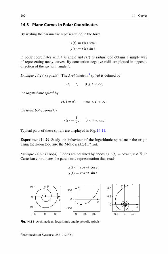
200 14 Curves
14.3 Plane Curves in Polar Coordinates
By writing the parametric representation in the form
x(t) = r(t) cos t,
y(t) = r(t) sin t
in polar coordinates with t as angle and r(t) as radius, one obtains a simple wayof representing many curves. By convention negative radii are plotted in oppositedirection of the ray with angle t .
Example 14.28 (Spirals) The Archimedean3 spiral is defined by
r(t) = t, 0 ≤ t < ∞,
the logarithmic spiral by
r(t) = et , −∞ < t < ∞,
the hyperbolic spiral by
r(t) = 1
t, 0 < t < ∞.
Typical parts of these spirals are displayed in Fig. 14.11.
Experiment 14.29 Study the behaviour of the logarithmic spiral near the originusing the zoom tool (use the M-file mat14_7.m).
Example 14.30 (Loops) Loops are obtained by choosing r(t) = cos nt , n ∈ N. InCartesian coordinates the parametric representation thus reads
x(t) = cos nt cos t,
y(t) = cos nt sin t.
−10 0 10
−10
0
10
x
y
0 300 600
−300
0
300
x
y
−0.3 0 0.3
0
0.3
0.6
x
y
Fig. 14.11 Archimedean, logarithmic and hyperbolic spirals
3Archimedes of Syracuse, 287–212 B.C.
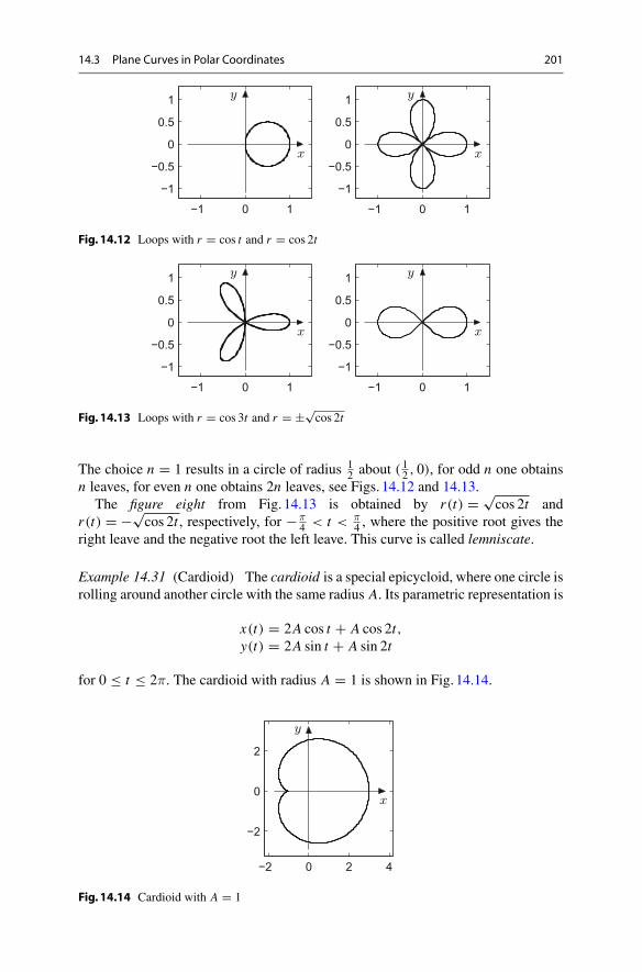
14.3 Plane Curves in Polar Coordinates 201
−1 0 1
−1
−0.5
0
0.5
1
x
y
−1 0 1
−1
−0.5
0
0.5
1
x
y
Fig. 14.12 Loops with r = cos t and r = cos 2t
−1 0 1
−1
−0.5
0
0.5
1
x
y
−1 0 1
−1
−0.5
0
0.5
1
x
y
Fig. 14.13 Loops with r = cos 3t and r = ±√cos 2t
The choice n = 1 results in a circle of radius 12 about ( 12 , 0), for odd n one obtains
n leaves, for even n one obtains 2n leaves, see Figs. 14.12 and 14.13.The figure eight from Fig. 14.13 is obtained by r(t) = √
cos 2t andr(t) = −√
cos 2t , respectively, for −π4 < t < π
4 , where the positive root gives theright leave and the negative root the left leave. This curve is called lemniscate.
Example 14.31 (Cardioid) The cardioid is a special epicycloid, where one circle isrolling around another circle with the same radius A. Its parametric representation is
x(t) = 2A cos t + A cos 2t,y(t) = 2A sin t + A sin 2t
for 0 ≤ t ≤ 2π. The cardioid with radius A = 1 is shown in Fig. 14.14.
−2 0 2 4
−2
0
2
x
y
Fig. 14.14 Cardioid with A = 1
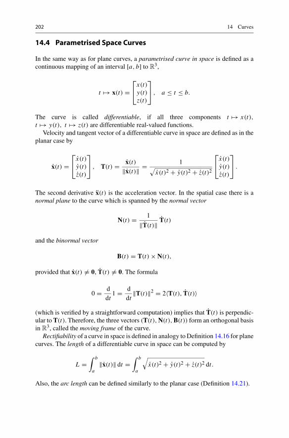
202 14 Curves
14.4 Parametrised Space Curves
In the same way as for plane curves, a parametrised curve in space is defined as acontinuous mapping of an interval [a, b] to R3,
t �→ x(t) =⎡⎣x(t)
y(t)z(t)
⎤⎦ , a ≤ t ≤ b.
The curve is called differentiable, if all three components t �→ x(t),t �→ y(t), t �→ z(t) are differentiable real-valued functions.
Velocity and tangent vector of a differentiable curve in space are defined as in theplanar case by
x(t) =⎡⎣x(t)
y(t)z(t)
⎤⎦ , T(t) = x(t)
‖x(t)‖ = 1√x(t)2 + y(t)2 + z(t)2
⎡⎣x(t)
y(t)z(t)
⎤⎦ .
The second derivative x(t) is the acceleration vector. In the spatial case there is anormal plane to the curve which is spanned by the normal vector
N(t) = 1
‖T(t)‖ T(t)
and the binormal vector
B(t) = T(t) × N(t),
provided that x(t) �= 0, T(t) �= 0. The formula
0 = d
dt1 = d
dt‖T(t)‖2 = 2〈T(t), T(t)〉
(which is verified by a straightforward computation) implies that T(t) is perpendic-ular to T(t). Therefore, the three vectors (T(t),N(t),B(t)) form an orthogonal basisin R3, called the moving frame of the curve.
Rectifiability of a curve in space is defined in analogy to Definition 14.16 for planecurves. The length of a differentiable curve in space can be computed by
L =∫ b
a‖x(t)‖ dt =
∫ b
a
√x(t)2 + y(t)2 + z(t)2 dt.
Also, the arc length can be defined similarly to the planar case (Definition 14.21).

14.4 Parametrised Space Curves 203
−1
0
1
−1
0
10
0.5
1
1.5
2 B(t)N(t)
T(t)
z
y x
Fig. 14.15 Helix with tangent, normal and binormal vector
Example 14.32 (Helix) The parametric representation of the helix is
x(t) =⎡⎣cos tsin t
t
⎤⎦ , −∞ < t < ∞.
We obtain
x(t) =⎡⎣− sin t
cos t1
⎤⎦ , T(t) = 1√
2
⎡⎣− sin t
cos t1
⎤⎦ ,
T(t) = 1√2
⎡⎣− cos t
− sin t0
⎤⎦ , N(t) =
⎡⎣− cos t
− sin t0
⎤⎦
with binormal vector
B(t) = 1√2
⎡⎣− sin t
cos t1
⎤⎦ ×
⎡⎣− cos t
− sin t0
⎤⎦ = 1√
2
⎡⎣ sin t
− cos t1
⎤⎦ .
The formula for the arc length of the helix, counting from the origin, is particularlysimple:
L(t) =∫ t
0‖x(τ )‖ dτ =
∫ t
0
√2 dτ = √
2 t.

204 14 Curves
Figure14.15 was drawn using the MATLAB commands
t=0 : pi/100 : 6 * pi;
plot3(cos(t), sin(t), t/10).
The Java applet Parametric curves in space offers dynamic visualising possibilitiesof those and other curves in space and of their moving frames.
14.5 Exercises
1. Find out which geometric formation is represented by the set of zeros of the poly-nomial y2 − x(x2 − 1) = 0. Visualise the curve in maple using the commandimplicitplot. Can you parametrise it as a continuous curve?
2. Verify that the algebraic curves y2 − (x + p)x2 = 0, p ∈ R (Example 14.7) canbe parametrised by
x(t) = t2 − p,
y(t) = t (t2 − p),− ∞ < t < ∞.
Visualise the curves for p = −1, 0, 1 in maple using the commandimplicitplot.
3. Using MATLAB ormaple , investigate the shape of Lissajous figures4
x(t) = sin(w1t), y(t) = cos(w2t)
and
x(t) = sin(w1t), y(t) = cos(w2t + π
2
).
Consider the cases w2 = w1, w2 = 2w1, w2 = 32w1 and explain the results.
The following exercises use the Java applets Parametric curves in the planeand Parametric curves in space.
4. (a) Using the Java applet analyse where the cycloid
x(t) = t − 2 sin t,
y(t) = 1 − 2 cos t,− 2π ≤ t ≤ 2π.
has its maximal speed (‖x(t)‖ → max) and check your result by hand.
4J.A. Lissajous, 1822–1880.
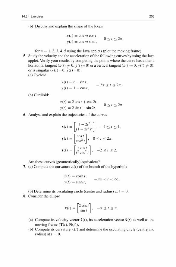
14.5 Exercises 205
(b) Discuss and explain the shape of the loops
x(t) = cos nt cos t,
y(t) = cos nt sin t,0 ≤ t ≤ 2π.
for n = 1, 2, 3, 4, 5 using the Java applets (plot the moving frame).5. Study the velocity and the acceleration of the following curves by using the Java
applet. Verify your results by computing the points where the curve has either ahorizontal tangent (x(t) �= 0, y(t)=0) or a vertical tangent (x(t)=0, y(t) �= 0),or is singular (x(t)=0, y(t)=0).(a) Cycloid:
x(t) = t − sin t,
y(t) = 1 − cos t,− 2π ≤ t ≤ 2π.
(b) Cardioid:
x(t) = 2 cos t + cos 2t,
y(t) = 2 sin t + sin 2t,0 ≤ t ≤ 2π.
6. Analyse and explain the trajectories of the curves
x(t) =[
1 − 2t2
(1 − 2t2)2
], −1 ≤ t ≤ 1,
y(t) =[cos tcos2 t
], 0 ≤ t ≤ 2π,
z(t) =[
t cos tt2 cos2 t
], −2 ≤ t ≤ 2.
Are these curves (geometrically) equivalent?7. (a) Compute the curvature κ(t) of the branch of the hyperbola
x(t) = cosh t,
y(t) = sinh t,− ∞ < t < ∞.
(b) Determine its osculating circle (centre and radius) at t = 0.8. Consider the ellipse
x(t) =[2 cos tsin t
], −π ≤ t ≤ π.
(a) Compute its velocity vector x(t), its acceleration vector x(t) as well as themoving frame (T(t),N(t)).
(b) Compute its curvature κ(t) and determine the osculating circle (centre andradius) at t = 0.

206 14 Curves
9. (a) Analyse the trajectory of the astroid
x(t) =[cos3 tsin3 t
], 0 ≤ t ≤ 2π.
(b) Compute the length of the part of the astroid which lies in the first quadrant.10. (a) Compute the velocity vector x(t) and the moving frame (T(t),N(t)) for the
segment
x(t) =[et cos tet sin t
], 0 ≤ t ≤ π/2
of the logarithmic spiral. At what point in the interval [0,π/2] does it havea vertical tangent?
(b) Compute the length of the segment. Deduce a formula for its arc lengths = L(t).
(c) Reparametrise the spiral by its arc length, i.e., compute ξ(s) = x(L−1(s)
)and verify that ‖ξ(s)‖ = 1.
11. (Application of the secant and cosecant functions) Analyse what plane curvesare determined in polar coordinates by
r(t) = sec t, −π/2 < t < π/2 and r(t) = csc t, 0 < t < π.
12. (a) Determine the tangent and the normal to the graph of the function y = 1/xat (x0, y0) = (1, 1) and compute its curvature at that point.
(b) Suppose the graph of the function y = 1/x is to be replaced by a circulararc at x0, i.e., for x ≥ 1. Find the centre and the radius of a circle whichadmits a smooth transition (same tangent, same curvature).
13. (a) Analyse the space curve
x(t) =⎡⎣ cos t
sin t2 sin t
2
⎤⎦ , 0 ≤ t ≤ 4π
using the applet.(b) Check that the curve is the intersection of the cylinder x2 + y2 = 1 with the
sphere (x + 1)2 + y2 + z2 = 4.
Hint. Use sin2 t2 = 1
2 (1 − cos t).14. Using MATLAB,maple or the applet, sketch and discuss the space curves
x(t) =⎡⎣t cos t
t sin t2t
⎤⎦ , 0 ≤ t < ∞,
14.5 Exercises 207
and
y(t) =⎡⎣cos tsin t0
⎤⎦ , 0 ≤ t ≤ 4π.
15. Sketch and discuss the space curves
x(t) =⎡⎣ t
tt3
⎤⎦ , y(t) =
⎡⎣ t
t2
t3
⎤⎦ , 0 ≤ t < 1.
Compute their velocity vectors x(t), y(t) and their acceleration vectors x(t),y(t).
16. Sketch the space curve
x(t) =⎡⎣
√2 t
cosh tcosh t
⎤⎦ , 0 ≤ t < 1.
Compute its moving frame (T(t),N(t),B(t)) as well as its length.17. Sketch the space curve
x(t) =⎡⎣cos tsin tt3/2
⎤⎦ , 0 ≤ t < 2π,
and compute its length.

15Scalar-Valued Functions ofTwoVariables
This chapter is devoted to differential calculus of functions of two variables. Inparticular we will study geometrical objects such as tangents and tangent planes,maxima and minima, as well as linear and quadratic approximations. The restrictionto two variables has beenmade for simplicity of presentation. All ideas in this and thenext chapter can easily be extended (although with slightly more notational effort)to the case of n variables.
We begin by studying the graph of a function with the help of vertical cuts andlevel sets. As a further tool we introduce partial derivatives, which describe the rateof change of the function in the direction of the coordinate axes. Finally the notionof the Fréchet derivative allows us to define the tangent plane to the graph. As forfunctions of one variable the Taylor formula plays a central role. We use it, e.g., todetermine extrema of functions of two variables.
In the entire chapter D denotes a subset of R2, and
f : D ⊂ R2 → R : (x, y) �→ z = f (x, y)
denotes a scalar-valued function of two variables. Details of vector and matrix alge-bra used in this chapter can be found in AppendicesA and B.
15.1 Graph and Partial Mappings
The graph
G = {(x, y, z) ∈ D × R ; z = f (x, y)
} ⊂ R3
© Springer Nature Switzerland AG 2018M. Oberguggenberger and A. Ostermann, Analysis for Computer Scientists,Undergraduate Topics in Computer Science,https://doi.org/10.1007/978-3-319-91155-7_15
209
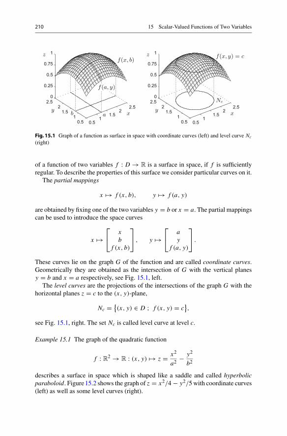
210 15 Scalar-Valued Functions of Two Variables
0.51
1.52
2.5
0.51
1.52
2.50
0.25
0.5
0.75
1
0.51
1.52
2.5
0.51
1.52
2.50
0.25
0.5
0.75
1f(x, y) = c
Nc
z
yx
f(a, y)
f(x, b)
b a
z
yx
Fig. 15.1 Graph of a function as surface in space with coordinate curves (left) and level curve Nc
(right)
of a function of two variables f : D → R is a surface in space, if f is sufficientlyregular. To describe the properties of this surface we consider particular curves on it.
The partial mappings
x �→ f (x, b), y �→ f (a, y)
are obtained by fixing one of the two variables y = b or x = a. The partial mappingscan be used to introduce the space curves
x �→⎡
⎣xb
f (x, b)
⎤
⎦ , y �→⎡
⎣ay
f (a, y)
⎤
⎦ .
These curves lie on the graph G of the function and are called coordinate curves.Geometrically they are obtained as the intersection of G with the vertical planesy = b and x = a respectively, see Fig. 15.1, left.
The level curves are the projections of the intersections of the graph G with thehorizontal planes z = c to the (x, y)-plane,
Nc = {(x, y) ∈ D ; f (x, y) = c
},
see Fig. 15.1, right. The set Nc is called level curve at level c.
Example 15.1 The graph of the quadratic function
f : R2 → R : (x, y) �→ z = x2
a2 − y2
b2
describes a surface in space which is shaped like a saddle and called hyperbolicparaboloid. Figure15.2 shows the graph of z = x2/4 − y2/5 with coordinate curves(left) as well as some level curves (right).

15.1 Graph and Partial Mappings 211
−4 −2 0 2 4
−4−2
02
4−4
−2
0
2
4
−4 −2 0 2 4−4
−2
0
2
4
y
x
z
y
x
Fig.15.2 The picture on the left shows the graph of the function z = x2/4 − y2/5 with coordinatecurves. Furthermore, it shows the intersections with the planes z = c for selected values of c. Thepicture on the right illustrates the level curves of the function for the same values of c (lower levelscorrespond to thicker lines). The two intersecting straight lines are the level curves at level c = 0
Experiment 15.2 With the help of theMATLAB program mat15_1.m visualise theelliptic paraboloid z = x2 + 2y2 − 4x + 1. Choose a suitable domain D and plotthe graph and some level curves.
15.2 Continuity
Like for functions in one variable (see Chap.6) we characterise the continuity offunctions of two variables by means of sequences. Thus we need the concept ofconvergence of vector-valued sequences.
Let (an)n≥1 = (a1, a2, a3, ...) be a sequence of points in D with terms
an = (an, bn) ∈ D ⊂ R2.
The sequence (an)n≥1 is said to converge to a = (a, b) ∈ D as n → ∞, if and onlyif both components of the sequence converge, i.e.
limn→∞ an = a and lim
n→∞ bn = b.
This is denoted by
(an, bn) = an → a = (a, b) as n → ∞ or limn→∞ an = a.
Otherwise the sequence is called divergent.
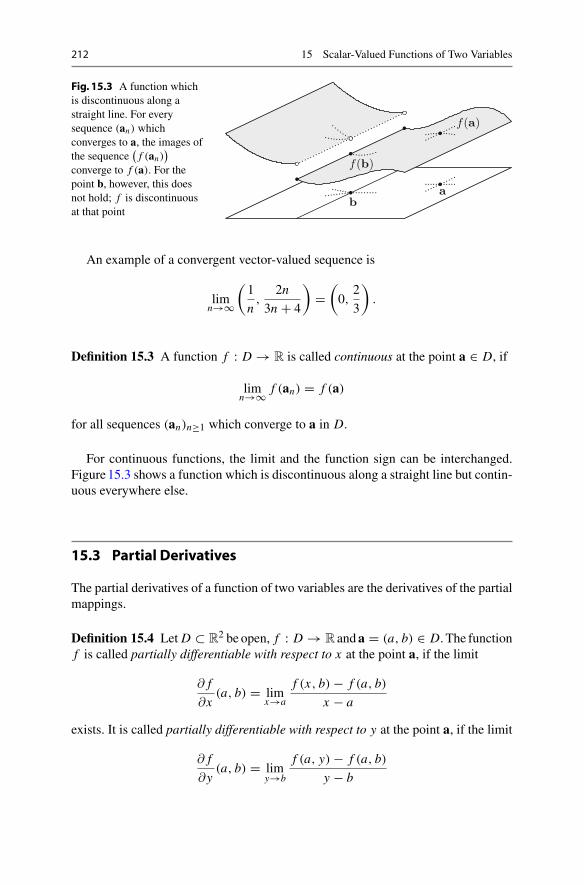
212 15 Scalar-Valued Functions of Two Variables
Fig. 15.3 A function whichis discontinuous along astraight line. For everysequence (an) whichconverges to a, the images ofthe sequence
(f (an)
)
converge to f (a). For thepoint b, however, this doesnot hold; f is discontinuousat that point
f(b)
b
f(a)
a
An example of a convergent vector-valued sequence is
limn→∞
(1
n,
2n
3n + 4
)=
(0,
2
3
).
Definition 15.3 A function f : D → R is called continuous at the point a ∈ D, if
limn→∞ f (an) = f (a)
for all sequences (an)n≥1 which converge to a in D.
For continuous functions, the limit and the function sign can be interchanged.Figure15.3 shows a function which is discontinuous along a straight line but contin-uous everywhere else.
15.3 Partial Derivatives
The partial derivatives of a function of two variables are the derivatives of the partialmappings.
Definition 15.4 Let D ⊂ R2 be open, f : D → R and a = (a, b) ∈ D. The function
f is called partially differentiable with respect to x at the point a, if the limit
∂ f
∂x(a, b) = lim
x→a
f (x, b) − f (a, b)
x − a
exists. It is called partially differentiable with respect to y at the point a, if the limit
∂ f
∂y(a, b) = lim
y→b
f (a, y) − f (a, b)
y − b
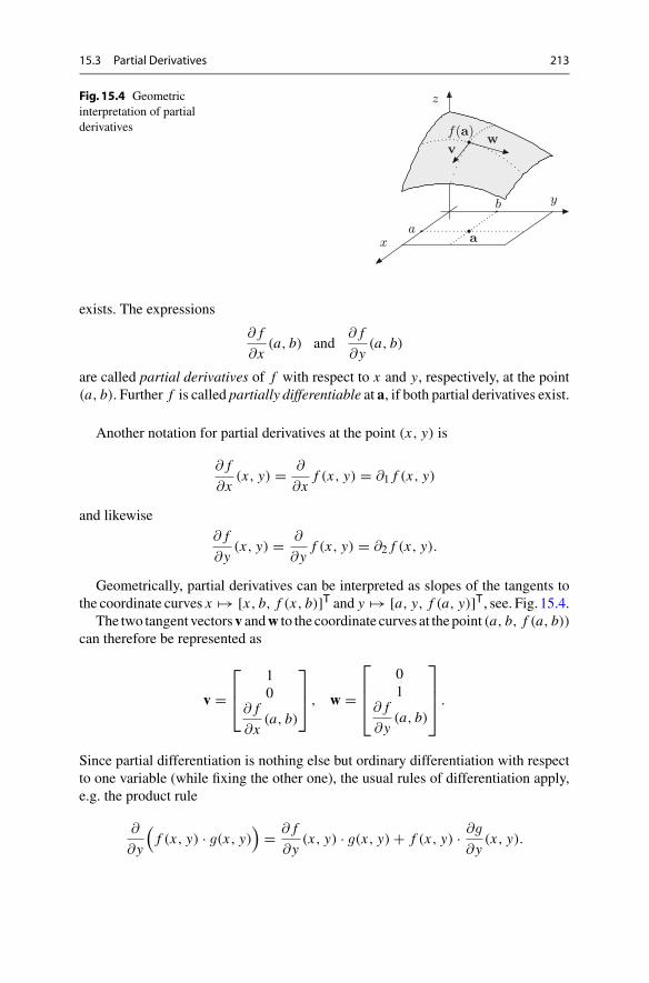
15.3 Partial Derivatives 213
Fig. 15.4 Geometricinterpretation of partialderivatives f(a) w
v
a
b
a
z
y
x
exists. The expressions
∂ f
∂x(a, b) and
∂ f
∂y(a, b)
are called partial derivatives of f with respect to x and y, respectively, at the point(a, b). Further f is called partially differentiable at a, if both partial derivatives exist.
Another notation for partial derivatives at the point (x, y) is
∂ f
∂x(x, y) = ∂
∂xf (x, y) = ∂1 f (x, y)
and likewise∂ f
∂y(x, y) = ∂
∂yf (x, y) = ∂2 f (x, y).
Geometrically, partial derivatives can be interpreted as slopes of the tangents tothe coordinate curves x �→ [x, b, f (x, b)]T and y �→ [a, y, f (a, y)]T, see. Fig. 15.4.
The two tangent vectorsv andw to the coordinate curves at the point (a, b, f (a, b))can therefore be represented as
v =⎡
⎢⎣
10
∂ f
∂x(a, b)
⎤
⎥⎦ , w =
⎡
⎢⎢⎣
01
∂ f
∂y(a, b)
⎤
⎥⎥⎦ .
Since partial differentiation is nothing else but ordinary differentiation with respectto one variable (while fixing the other one), the usual rules of differentiation apply,e.g. the product rule
∂
∂y
(f (x, y) · g(x, y)
)= ∂ f
∂y(x, y) · g(x, y) + f (x, y) · ∂g
∂y(x, y).
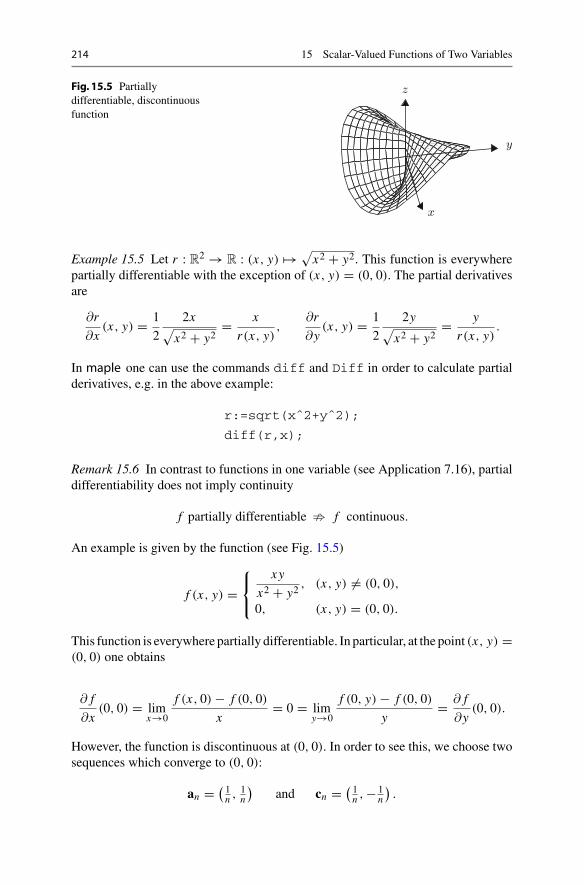
214 15 Scalar-Valued Functions of Two Variables
Fig. 15.5 Partiallydifferentiable, discontinuousfunction
z
y
x
Example 15.5 Let r : R2 → R : (x, y) �→ √
x2 + y2. This function is everywherepartially differentiable with the exception of (x, y) = (0, 0). The partial derivativesare
∂r
∂x(x, y) = 1
2
2x√
x2 + y2= x
r(x, y),
∂r
∂y(x, y) = 1
2
2y√
x2 + y2= y
r(x, y).
In maple one can use the commands diff and Diff in order to calculate partialderivatives, e.g. in the above example:
r:=sqrt(xˆ2+yˆ2);
diff(r,x);
Remark 15.6 In contrast to functions in one variable (see Application 7.16), partialdifferentiability does not imply continuity
f partially differentiable � f continuous.
An example is given by the function (see Fig. 15.5)
f (x, y) =⎧⎨
⎩
xy
x2 + y2, (x, y) �= (0, 0),
0, (x, y) = (0, 0).
This function is everywhere partially differentiable. In particular, at the point (x, y) =(0, 0) one obtains
∂ f
∂x(0, 0) = lim
x→0
f (x, 0) − f (0, 0)
x= 0 = lim
y→0
f (0, y) − f (0, 0)
y= ∂ f
∂y(0, 0).
However, the function is discontinuous at (0, 0). In order to see this, we choose twosequences which converge to (0, 0):
an = ( 1n ,
1n
)and cn = ( 1
n ,− 1n
).
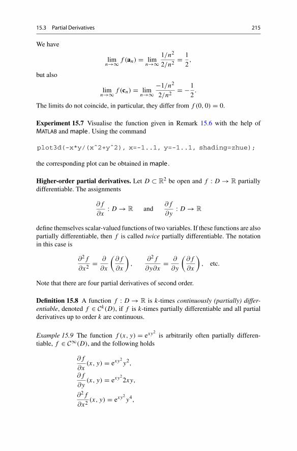
15.3 Partial Derivatives 215
We have
limn→∞ f (an) = lim
n→∞1/n2
2/n2 = 1
2,
but also
limn→∞ f (cn) = lim
n→∞−1/n2
2/n2 = −1
2.
The limits do not coincide, in particular, they differ from f (0, 0) = 0.
Experiment 15.7 Visualise the function given in Remark 15.6 with the help ofMATLAB and maple . Using the command
plot3d(-x*y/(xˆ2+yˆ2), x=-1..1, y=-1..1, shading=zhue);
the corresponding plot can be obtained in maple .
Higher-order partial derivatives. Let D ⊂ R2 be open and f : D → R partially
differentiable. The assignments
∂ f
∂x: D → R and
∂ f
∂y: D → R
define themselves scalar-valued functions of two variables. If these functions are alsopartially differentiable, then f is called twice partially differentiable. The notationin this case is
∂2 f
∂x2= ∂
∂x
(∂ f
∂x
),
∂2 f
∂y∂x= ∂
∂y
(∂ f
∂x
), etc.
Note that there are four partial derivatives of second order.
Definition 15.8 A function f : D → R is k-times continuously (partially) differ-entiable, denoted f ∈ Ck(D), if f is k-times partially differentiable and all partialderivatives up to order k are continuous.
Example 15.9 The function f (x, y) = exy2 is arbitrarily often partially differen-tiable, f ∈ C∞(D), and the following holds
∂ f
∂x(x, y) = exy2 y2,
∂ f
∂y(x, y) = exy22xy,
∂2 f
∂x2(x, y) = exy2 y4,
216 15 Scalar-Valued Functions of Two Variables
∂2 f
∂y2(x, y) = exy2(4x2y2 + 2x),
∂2 f
∂y∂x(x, y) = ∂
∂y
(∂ f
∂x(x, y)
)= exy2(2xy3 + 2y),
∂2 f
∂x∂y(x, y) = ∂
∂x
(∂ f
∂y(x, y)
)= exy2(2xy3 + 2y).
The identity
∂2 f
∂y∂x(x, y) = ∂2 f
∂x∂y(x, y)
which is evident in this example is generally valid for twice continuously differen-tiable functions f . This observation is also true for higher derivatives: For k-timescontinuously differentiable functions the order of differentiation of the kth partialderivatives is irrelevant (Theorem of Schwarz1), see [3, Chap.15, Theorem 1.1].
15.4 The Fréchet Derivative
Our next topic is the study of a simultaneous variation of both variables of thefunction. This leads us to the notion of the Fréchet2 derivative. For functions of onevariable, ϕ : R → R, the derivative was defined by the limit
ϕ′(a) = limx→a
ϕ(x) − ϕ(a)
x − a.
For functions of two variables this expression does not make sense anymore as onecannot divide by vectors. We therefore will make use of the equivalent definition ofthe derivative as a linear approximation
ϕ(x) = ϕ(a) + A · (x − a) + R(x, a)
with A = ϕ′(a) and the remainder term R(x, a) satisfying
limx→a
R(x, a)
|x − a| = 0.
This formula can be generalised to functions of two variables.
1H.A. Schwarz, 1843–1921.2M. Fréchet, 1878–1973.
15.4 The Fréchet Derivative 217
Definition 15.10 Let D ⊂ R2 be open and f : D → R. The function f is called
Fréchet differentiable at the point (a, b) ∈ D, if there exists a linear mapping A :R2 → R such that
f (x, y) = f (a, b) + A(x − a, y − b) + R(x, y; a, b)
with a remainder R(x, y; a, b) fulfilling the condition
lim(x,y)→(a,b)
R(x, y; a, b)√(x − a)2 + (y − b)2
= 0.
The linear mapping A is called derivative of f at the point (a, b). Instead of A wealso write D f (a, b). The (1 × 2)-matrix of the linear mapping is called Jacobian3
of f . We denote it by f ′(a, b).
The question whether the derivative of a function is unique and how it can becalculated, is answered in the following proposition.
Proposition 15.11 Let D ⊂ R2 be open and f : D → R. If f is Fréchet differen-
tiable at (x, y) ∈ D, then f is also partially differentiable at (x, y) and
f ′(x, y) =[∂ f
∂x(x, y),
∂ f
∂y(x, y)
].
The components of the Jacobian are the partial derivatives. In particular, the Jaco-bian and consequently the Fréchet derivative are unique.
Proof Exemplarily, we compute the second component and show that
(f ′(x, y)
)2 = ∂ f
∂y(x, y).
Since f is Fréchet differentiable at (x, y), it holds that
f (x, y + h) = f (x, y) + f ′(x, y)
[0h
]+ R(x, y + h; x, y).
Therefore
f (x, y + h) − f (x, y)
h− (
f ′(x, y))2 = R(x, y + h; x, y)
h→ 0 as h → 0.
Consequently f is partially differentiable with respect to y, and the second compo-nent of the Jacobian is the partial derivative of f with respect to y.
3C.G.J. Jacobi, 1804–1851.
218 15 Scalar-Valued Functions of Two Variables
The next proposition follows immediately from the identity
lim(x,y)→(a,b)
f (x, y) = lim(x,y)→(a,b)
(f (a, b) + D f (a, b)(x − a, y − b) + R(x, y; a, b)
)
= f (a, b).
Proposition 15.12 If f is Fréchet differentiable then f is continuous. �
In particular, the function
f (x, y) =⎧⎨
⎩
xy
x2 + y2, (x, y) �= (0, 0),
0, (x, y) = (0, 0)
is not Fréchet differentiable at the point (0, 0).Fréchet differentiability follows from partial differentiability under certain regu-
larity assumptions. In fact, one can show that a continuously partially differentiablefunction is Fréchet differentiable, see [4, Chap. 7, Theorem 7.12].
Example 15.13 The function f : R2 → R : (x, y) �→ x2e3y is Fréchet differen-
tiable, its derivative is
f ′(x, y) = [2xe3y, 3x2e3y] = xe3y [2, 3x].
Example 15.14 The affine function f : R2 → R with
f (x, y) = αx + βy + γ = [α,β][
xy
]+ γ
is Fréchet differentiable and f ′(x, y) = [α,β].
Example 15.15 The quadratic function f : R2 → R with
f (x, y) = αx2 + 2βxy + γy2 + δx + εy + ζ
= [x, y][α ββ γ
] [xy
]+ [δ, ε]
[xy
]+ ζ
is Fréchet differentiable with the Jacobian
f ′(x, y) = [2αx + 2βy + δ, 2βx + 2γy + ε] = 2[x, y][α ββ γ
]+ [δ, ε].
The chain rule. Now we are in the position to generalise the chain rule to the caseof two variables.
15.4 The Fréchet Derivative 219
Proposition 15.16 Let D ⊂ R2 be open and f : D → R : (x, y) �→ f (x, y) Fré-
chet differentiable. Furthermore let I ⊂ R be an open interval and φ,ψ : I → R
differentiable. Then the composition of functions
F : I → R : t �→ F(t) = f(φ(t),ψ(t)
)
is also differentiable and
dF
dt(t) = ∂ f
∂x
(φ(t),ψ(t)
)dφdt
(t) + ∂ f
∂y
(φ(t),ψ(t)
)dψdt
(t).
Proof From the Fréchet differentiability of f it follows that
F(t + h) − F(t) = f(φ(t + h),ψ(t + h)
) − f(φ(t),ψ(t)
)
= f ′(φ(t),ψ(t)) [
φ(t + h) − φ(t)ψ(t + h) − ψ(t)
]+ R
(φ(t + h),ψ(t + h);φ(t),ψ(t)
).
We divide this expression by h and subsequently examine the limit as h → 0. Letg(t, h)= (
φ(t + h) − φ(t))2 + (
ψ(t + h) − ψ(t))2. Then, due to thedifferentiability
of f , φ and ψ, we have
limh→0
R(φ(t + h),ψ(t + h); φ(t),ψ(t)
)
√g(t, h)
·√
g(t, h)
h= 0.
Therefore, the function F is differentiable and the formula stated in the propositionis valid. �
Example 15.17 Let D ⊂ R2 be an open set that contains the circle x2 + y2 = 1 and
let f : D → R be a differentiable function. Then the restriction F of f to the circle
F : R → R : t �→ f (cos t, sin t)
is differentiable as a function of the angle t and
dF
dt(t) = −∂ f
∂x
(cos t, sin t
) · sin t + ∂ f
∂y
(cos t, sin t
) · cos t.
For instance, for f (x, y) = x2 − y2 the derivative is dFdt (t) = −4 cos t sin t .
Interpretation of the Fréchet derivative. Using the Fréchet derivative we obtain,like in the case of one variable, the linear approximation g(x, y) to the graph of thefunction at (a, b)
g(x, y) = f (a, b) + f ′(a, b)
[x − ay − b
]≈ f (x, y).
220 15 Scalar-Valued Functions of Two Variables
Now we want to interpret the plane
z = f (a, b) + f ′(a, b)
[x − ay − b
]
geometrically. For this we use the fact that the components of the Jacobian are thepartial derivatives. With that we can write the above equation as
z = f (a, b) + ∂ f
∂x(a, b) · (x − a) + ∂ f
∂y(a, b) · (y − b),
or alternatively in parametric form (x − a = λ, y − b = μ)
⎡
⎣xyz
⎤
⎦ =⎡
⎣ab
f (a, b)
⎤
⎦ + λ
⎡
⎣10
∂ f∂x (a, b)
⎤
⎦ + μ
⎡
⎣01
∂ f∂y (a, b)
⎤
⎦ .
The plane intersects the graph of f at the point (a, b, f (a, b)) and is spanned by thetangent vectors to the coordinate curves. The equation
z = f (a, b) + ∂ f
∂x(a, b) · (x − a) + ∂ f
∂y(a, b) · (y − b),
consequently describes the tangent plane to the graph of f at the point (a, b).The example shows that the graph of a function which is Fréchet differentiable
at the point (x, y) possesses a tangent plane at this point. Note that the existence oftangents to the coordinate curves does not imply the existence of a tangent plane,see Remark 15.6.
Example 15.18 We calculate the tangent plane at a point on the northern hemisphere(with radius r )
f (x, y) = z =√
r2 − x2 − y2.
Let c = f (a, b) = √r2 − a2 − b2. The partial derivatives of f at (a, b) are
∂ f
∂x(a, b) = − a√
r2 − a2 − b2= −a
c,
∂ f
∂y(a, b) = − b√
r2 − a2 − b2= −b
c.
Therefore, the equation of the tangent plane is
z = c − a
c(x − a) − b
c(y − b),
or alternatively
a(x − a) + b(y − b) + c(z − c) = 0.
The last formula actually holds for all points on the surface of the sphere.
15.5 Directional Derivative and Gradient 221
15.5 Directional Derivative and Gradient
So far functions f : D ⊂ R2 → R were defined on R
2 as a point space. For the pur-pose of directional derivatives it is useful and customary to write the arguments(x, y) ∈ R
2 as position vectors x = [x, y]T. In this way each function f : D ⊂R2 → R can also be considered as a function of column vectors. We identify these
two functions and will not distinguish between f (x, y) and f (x) henceforth.In Sect. 15.3 we have defined partial derivatives along coordinate axes. Now we
want to generalise this concept to differentiation in any direction.
Definition 15.19 Let D ⊂ R2 be open, x = [x, y]T ∈ D and f : D → R. Further-
more let v ∈ R2 with ‖v‖ = 1. The limit
∂v f (x) = ∂ f
∂v(x) = lim
h→0
f (x + hv) − f (x)h
= limh→0
f (x + hv1, y + hv2) − f (x, y)
h
(in case it exists) is called directional derivative of f at x in direction v.
The partial derivatives are special cases of the directional derivative, namely thederivatives in direction of the coordinate axes.
The directional derivative ∂v f (x) describes the rate of change of the function fat the point x in the direction of v. Indeed, this can been seen from the following.Consider the straight line {x + tv | t ∈ R} ⊂ R
2 and the function
g(t) = f (x + tv) ( f restricted to this straight line)
with g(0) = f (x). Then
g′(0) = limh→0
g(h) − g(0)
h= lim
h→0
f (x + hv) − f (x)h
= ∂v f (x).
Next we clarify how the directional derivative can be computed. For that we needthe following definition.
Definition 15.20 Let D ⊂ R2 be open and f : D → R partially differentiable. The
vector
∇ f (x, y) =
⎡
⎢⎢⎣
∂ f
∂x(x, y)
∂ f
∂y(x, y)
⎤
⎥⎥⎦ = f ′(x, y)T
is called gradient of f .

222 15 Scalar-Valued Functions of Two Variables
Fig. 15.6 Geometricinterpretation of ∇ f
Nf(x)
∇f(x)
vx
Proposition 15.21 Let D ⊂ R2 be open,v = [v1, v2]T ∈ R
2,‖v‖ = 1and f : D →R Fréchet differentiable at x = [x, y]T. Then
∂v f (x) = 〈∇ f (x), v〉 = f ′(x, y) v = ∂ f
∂x(x, y) v1 + ∂ f
∂y(x, y) v2.
Proof Since f is Fréchet differentiable at x, it holds that
f (x + hv) = f (x) + f ′(x) · hv + R(x + hv1, y + hv2; x, y)
and hence
f (x + hv) − f (x)h
= f ′(x) · v + R(x + hv1, y + hv2; x, y)
h.
Letting h → 0 proves the desired assertion. �
Proposition 15.22 (Geometric interpretation of ∇) Let D ⊂ R2 be open and f :
D → R continuously differentiable at x = (x, y) with f ′(x) �= [0, 0]. Then ∇ f (x)is perpendicular to the level curve N f (x) = {x ∈ R
2 ; f (x) = f (x)} and points indirection of the steepest ascent of f , see Fig. 15.6.
Proof Let v be a tangent vector to the level curve at the point x. From the implicitfunction theorem (see [4, Chap. 14.1]) it follows that N f (x) can be parametrised asa differentiable curve γ(t) = [x(t), y(t)]T, with
γ(0) = x and γ(0) = v
in a neighbourhood of x. Thus, for all t near t = 0,
f(γ(t)
) = f (x) = const.
Since f and γ are differentiable, it follows from the chain rule (Proposition 15.16)that
0 = d
dtf(γ(t)
)∣∣∣t=0
= f ′(γ(0))γ(0) = 〈∇ f (x), v〉
15.5 Directional Derivative and Gradient 223
because γ(0) = x and γ(0) = v. Hence ∇ f (x) is perpendicular to v. Letw ∈ R2 be
a further unit vector. Then
∂w f (x) = ∂ f
∂w(x) = 〈∇ f (x),w〉 = ‖∇ f (x)‖ · ‖w‖ · cos�,
where� denotes the angle enclosed by∇ f (x) andw. From this formula one deducesthat∂w f (x) ismaximal if and only if cos� = 1,whichmeans∇ f (x) = λw for someλ > 0. �
Example 15.23 Let f (x, y) = x2 + y2. Then ∇ f (x, y) = 2[x, y]T.
15.6 TheTaylor Formula in TwoVariables
Let f : D ⊂ R2 → R be a function of two variables. In the following calculation we
assume that f is at least three times continuously differentiable. In order to expandf (x + h, y + k) into a Taylor series in a neighbourhood of (x, y), we first fix thesecond variable and expand with respect to the first:
f (x + h, y + k) = f (x, y + k)+ ∂ f
∂x(x, y + k) · h + 1
2
∂2 f
∂x2(x, y + k) · h2 +O(h3).
Then we also expand the terms on the right-hand side with respect to the secondvariable (while fixing the first one):
f (x, y + k) = f (x, y) + ∂ f
∂y(x, y) · k + 1
2
∂2 f
∂y2(x, y) · k2 + O(k3),
∂ f
∂x(x, y + k) = ∂ f
∂x(x, y) + ∂2 f
∂y∂x(x, y) · k + O(k2),
∂2 f
∂x2(x, y + k) = ∂2 f
∂x2(x, y) + O(k).
Inserting these expressions into the equation above, we obtain
f (x + h, y + k) = f (x, y) + ∂ f
∂x(x, y) · h + ∂ f
∂y(x, y) · k
+ 1
2
∂2 f
∂x2(x, y) · h2 + 1
2
∂2 f
∂y2(x, y) · k2 + ∂2 f
∂y∂x(x, y) · hk
+ O(h3) + O(h2k) + O(hk2) + O(k3).
In matrix-vector notation we can also write this equation as
f (x + h, y + k) = f (x, y) + f ′(x, y)
[hk
]+ 1
2[h, k] · H f (x, y)
[hk
]+ . . .
224 15 Scalar-Valued Functions of Two Variables
with the Hessian matrix4
H f (x, y) =
⎡
⎢⎢⎢⎣
∂2 f
∂x2(x, y)
∂2 f
∂y∂x(x, y)
∂2 f
∂x∂y(x, y)
∂2 f
∂y2(x, y)
⎤
⎥⎥⎥⎦
collecting the second-order partial derivatives. By the above assumptions, thesederivatives are continuous. Thus the Hessian matrix is symmetric due to Schwarz’stheorem.
Example 15.24 We compute the second-order approximation to the function f :R2 → R : (x, y) �→ x2 sin y at the point (a, b) = (2, 0). The partial derivatives are
f∂ f
∂x
∂ f
∂y
∂2 f
∂x2∂2 f
∂y∂x
∂2 f
∂y2
General x2 sin y 2x sin y x2 cos y 2 sin y 2x cos y −x2 sin yAt (2, 0) 0 0 4 0 4 0
Therefore, the quadratic approximation g(x, y) ≈ f (x, y) is given by the formula
g(x, y) = f (2, 0) + f ′(2, 0)[
x − 2y
]+ 1
2[x − 2, y] · H f (2, 0)
[x − 2
y
]
= 0 + [0, 4][
x − 2y
]+ 1
2[x − 2, y]
[0 44 0
] [x − 2
y
]
= 4y + 4y(x − 2) = 4y(x − 1).
15.7 Local Maxima andMinima
Let D ⊂ R2 be open and f : D → R. In this section we investigate the graph of the
function f with respect to maxima and minima.
Definition 15.25 The scalar function f has a local maximum (respectively, localminimum) at (a, b) ∈ D, if
f (x, y) ≤ f (a, b) (respectively, f (x, y) ≥ f (a, b)).
4L.O. Hesse, 1811–1874.
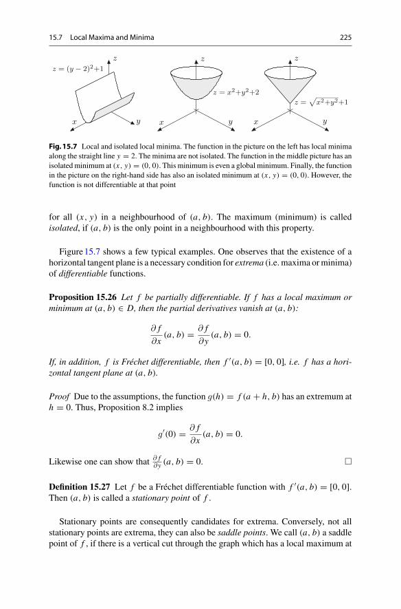
15.7 Local Maxima and Minima 225
z = x2+y2+1
z
x y
z = x2+y2+2
z
x y
z = (y − 2)2+1z
x y
Fig.15.7 Local and isolated local minima. The function in the picture on the left has local minimaalong the straight line y = 2. The minima are not isolated. The function in the middle picture has anisolatedminimum at (x, y) = (0, 0). This minimum is even a global minimum. Finally, the functionin the picture on the right-hand side has also an isolated minimum at (x, y) = (0, 0). However, thefunction is not differentiable at that point
for all (x, y) in a neighbourhood of (a, b). The maximum (minimum) is calledisolated, if (a, b) is the only point in a neighbourhood with this property.
Figure15.7 shows a few typical examples. One observes that the existence of ahorizontal tangent plane is a necessary condition for extrema (i.e. maxima orminima)of differentiable functions.
Proposition 15.26 Let f be partially differentiable. If f has a local maximum orminimum at (a, b) ∈ D, then the partial derivatives vanish at (a, b):
∂ f
∂x(a, b) = ∂ f
∂y(a, b) = 0.
If, in addition, f is Fréchet differentiable, then f ′(a, b) = [0, 0], i.e. f has a hori-zontal tangent plane at (a, b).
Proof Due to the assumptions, the function g(h) = f (a + h, b) has an extremum ath = 0. Thus, Proposition 8.2 implies
g′(0) = ∂ f
∂x(a, b) = 0.
Likewise one can show that ∂ f∂y (a, b) = 0. �
Definition 15.27 Let f be a Fréchet differentiable function with f ′(a, b) = [0, 0].Then (a, b) is called a stationary point of f .
Stationary points are consequently candidates for extrema. Conversely, not allstationary points are extrema, they can also be saddle points. We call (a, b) a saddlepoint of f , if there is a vertical cut through the graph which has a local maximum at
226 15 Scalar-Valued Functions of Two Variables
(a, b), and a secondvertical cutwhich has a localminimumat (a, b), see, for example,Fig. 15.2. In order to decidewhat is the case, one resorts toTaylor expansion, similarlyas for functions of one variable.
Let a = [a, b]T be a stationary point of f and v ∈ R2 any unit vector. We investi-
gate the behaviour of f , restricted to the straight line a + λv, λ ∈ R. Taylor expan-sion shows that
f (a + λv) = f (a) + f ′(a) · λv + 12λ
2vTH f (a) v + O(λ3).
Since a is a stationary point, it follows that f ′(a) = [0, 0] and consequently
f (a + λv) − f (a)λ2 = 1
2 vTH f (a) v + O(λ).
For small λ the sign on the left-hand side is therefore determined by the sign ofvTH f (a) v. We ask how this can be expressed by conditions on H f (a). Writing
H f (a) =[α ββ γ
]and v =
[v
w
]
we get
vT H f (a) v = αv2 + 2βvw + γw2.
For an isolated local minimum this expression has to be positive for all v �= 0. Ifw = 0 and v �= 0, then αv2 > 0 and therefore necessarily
α > 0.
If w �= 0, we substitute v = tw with t ∈ R and obtain
αt2w2 + 2βtw2 + γw2 > 0,
or alternatively (multiplying by α > 0 and simplifying by w2)
t2α2 + 2tαβ + αγ > 0.
Therefore,
(tα + β)2 + αγ − β2 > 0
for all t ∈ R. The left-hand side is smallest for t = −β/α. Inserting this we obtainthe second condition
det H f (a) = αγ − β2 > 0
in terms of the determinant, see AppendixB.1.We have thus shown the following result.
15.7 Local Maxima and Minima 227
Proposition 15.28 The function f has an isolated local minimum at the stationarypoint a, if the conditions
∂2 f
∂x2(a) > 0 and det H f (a) > 0
are fulfilled.
By replacing f by − f one gets the corresponding result for isolated maxima.
Proposition 15.29 The function f has an isolated local maximum at the stationarypoint a, if the conditions
∂2 f
∂x2(a) < 0 and det H f (a) > 0
are fulfilled.
In a similar way one can prove the following assertion.
Proposition 15.30 The stationary point a of the function f is a saddle point, ifdet H f (a) < 0.
If the determinant of the Hessian matrix equals zero, the behaviour of the functionneeds to be investigated along vertical cuts. One example is given in Exercise 12.
Example 15.31 We determine the maxima, minima and saddle points of the functionf (x, y) = x6 + y6 − 3x2 − 3y2. The condition
f ′(x, y) = [6x5 − 6x, 6y5 − 6y] = [0, 0]
gives the following nine stationary points
x1 = 0, x2,3 = ±1, y1 = 0, y2,3 = ±1.
The Hessian matrix of the function is
H f (x, y) =[30x4 − 6 0
0 30y4 − 6
].
Applying the criteria of Propositions 15.28 through 15.30, we obtain the followingresults: The point (0, 0) is an isolated local maximum of f , the points (−1,−1),(−1, 1), (1,−1) and (1, 1) are isolated local minima, and the points (−1, 0), (1, 0),(0,−1) and (0, 1) are saddle points. The reader is advised to visualise this functionwithmaple .

228 15 Scalar-Valued Functions of Two Variables
15.8 Exercises
1. Compute the partial derivatives of the functions
f (x, y) = arcsin( y
x
), g(x, y) = log
1√
x2 + y2.
Verify your results withmaple .2. Show that the function
v(x, t) = 1√texp
(−x2
4t
)
satisfies the heat equation
∂v
∂t= ∂2v
∂x2
for t > 0 and x ∈ R.3. Show that the function w(x, t) = g(x − kt) satisfies the transport equation
∂w
∂t+ k
∂w
∂x= 0
for any differentiable function g.4. Show that the function g(x, y) = log(x2 + 2y2) satisfies the equation
∂2g
∂x2+ 1
2
∂2g
∂y2= 0
for (x, y) �= (0, 0).5. Represent the ellipsoid x2 + 2y2 + z2 = 1 as graph of a function (x, y) �→
f (x, y). Distinguish between positive and negative z-coordinates, respectively.Compute the partial derivatives of f and sketch the level curves of f . Find thedirection in which ∇ f points.
6. Solve Exercise 5 for the hyperboloid x2 + 2y2 − z2 = 1.7. Compute the directional derivative of the function f (x, y) = xy in the direction
v at the four points a1, . . . a4, where
a1 = (1, 2), a2 = (−1, 2), a3 = (1,−2), a4 = (−1,−2) and v = 1√5
[21
].
At the given points a1, . . . a4, determine the direction for which the directionalderivative is maximal.
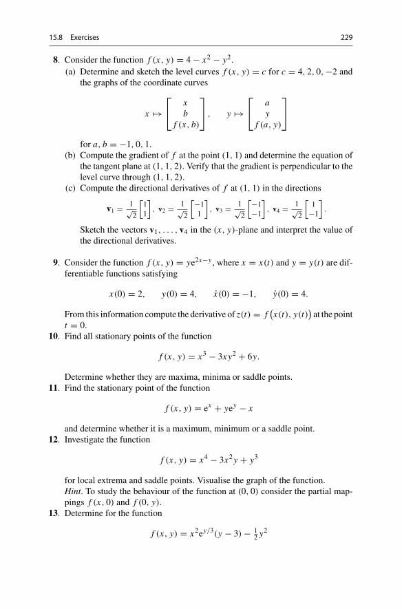
15.8 Exercises 229
8. Consider the function f (x, y) = 4 − x2 − y2.(a) Determine and sketch the level curves f (x, y) = c for c = 4, 2, 0,−2 and
the graphs of the coordinate curves
x �→⎡
⎣xb
f (x, b)
⎤
⎦ , y �→⎡
⎣ay
f (a, y)
⎤
⎦
for a, b = −1, 0, 1.(b) Compute the gradient of f at the point (1, 1) and determine the equation of
the tangent plane at (1, 1, 2). Verify that the gradient is perpendicular to thelevel curve through (1, 1, 2).
(c) Compute the directional derivatives of f at (1, 1) in the directions
v1 = 1√2
[11
], v2 = 1√
2
[−11
], v3 = 1√
2
[−1−1
], v4 = 1√
2
[1
−1
].
Sketch the vectors v1, . . . , v4 in the (x, y)-plane and interpret the value ofthe directional derivatives.
9. Consider the function f (x, y) = ye2x−y , where x = x(t) and y = y(t) are dif-ferentiable functions satisfying
x(0) = 2, y(0) = 4, x(0) = −1, y(0) = 4.
From this information compute the derivative of z(t) = f(x(t), y(t)
)at the point
t = 0.10. Find all stationary points of the function
f (x, y) = x3 − 3xy2 + 6y.
Determine whether they are maxima, minima or saddle points.11. Find the stationary point of the function
f (x, y) = ex + yey − x
and determine whether it is a maximum, minimum or a saddle point.12. Investigate the function
f (x, y) = x4 − 3x2y + y3
for local extrema and saddle points. Visualise the graph of the function.Hint. To study the behaviour of the function at (0, 0) consider the partial map-pings f (x, 0) and f (0, y).
13. Determine for the function
f (x, y) = x2ey/3(y − 3) − 12 y2
230 15 Scalar-Valued Functions of Two Variables
(a) the gradient and the Hessian matrix;(b) the second-order Taylor approximation at (0, 0);(c) all stationary points. Find out whether they are maxima, minima or saddle
points.14. Expand the polynomial f (x, y) = x2 + xy + 3y2 in powers of x − 1 and y − 2,
i.e. in the form
f (x, y) = α(x − 1)2 + β(x − 1)(y − 2) + γ(y − 2)2
+ δ(x − 1) + ε(y − 2) + ζ.
Hint. Use the second-order Taylor expansion at (1, 2).15. Compute (0.95)2.01 numerically byusing the second-orderTaylor approximation
to the function f (x, y) = x y at (1, 2).

16Vector-Valued Functions ofTwoVariables
In this section we briefly touch upon the theory of vector-valued functions in severalvariables. To simplify matters we limit ourselves again to the case of two variables.
First we define vector fields in the plane and extend the notions of continuityand differentiability to vector-valued functions. Then we discuss Newton’s methodin two variables. As an application we compute a common zero of two nonlinearfunctions. Finally, as an extension of Sect. 15.1, we show how smooth surfaces canbe described mathematically with the help of parameterisations.
For the required basic notions of vector and matrix algebra we refer to the Appen-dicesA and B.
16.1 Vector Fields and the Jacobian
In the entire section D denotes an open subset of R2 and
F : D ⊂ R2 → R
2 : (x, y) �→[uv
]= F(x, y) =
[f (x, y)g(x, y)
]
a vector-valued function of two variables with values in R2. Such functions are alsocalled vector fields since they assign a vector to every point in the plane. Importantapplications are provided in physics. For example, the velocity field of a flowingliquid or the gravitational field are mathematically described as vector fields.
In the previous chapter we have already encountered a vector field, namely thegradient of a scalar-valued function of two variables f : D → R : (x, y) �→ f (x, y).
© Springer Nature Switzerland AG 2018M. Oberguggenberger and A. Ostermann, Analysis for Computer Scientists,Undergraduate Topics in Computer Science,https://doi.org/10.1007/978-3-319-91155-7_16
231
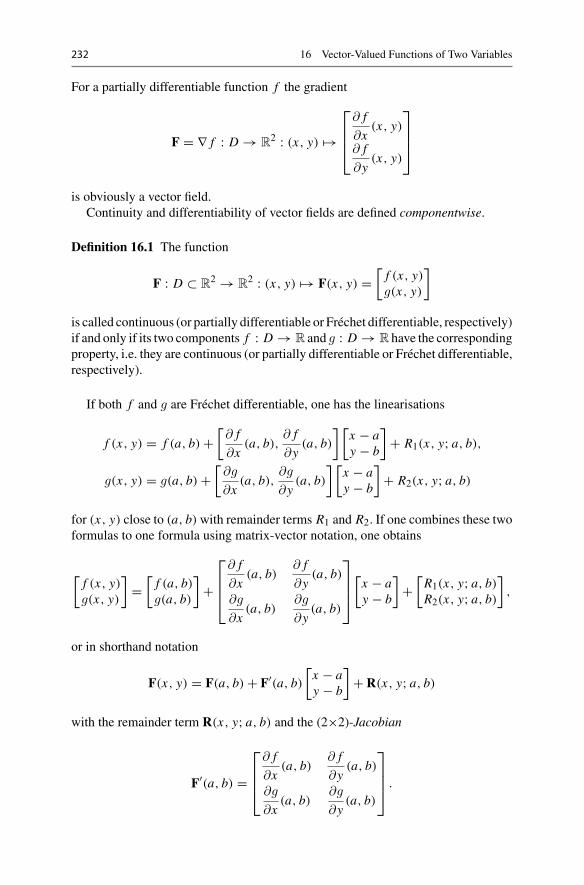
232 16 Vector-Valued Functions of Two Variables
For a partially differentiable function f the gradient
F = ∇ f : D → R2 : (x, y) �→
⎡⎢⎢⎣
∂ f
∂x(x, y)
∂ f
∂y(x, y)
⎤⎥⎥⎦
is obviously a vector field.Continuity and differentiability of vector fields are defined componentwise.
Definition 16.1 The function
F : D ⊂ R2 → R
2 : (x, y) �→ F(x, y) =[f (x, y)g(x, y)
]
is called continuous (or partially differentiable or Fréchet differentiable, respectively)if and only if its two components f : D → R and g : D → R have the correspondingproperty, i.e. they are continuous (or partially differentiable or Fréchet differentiable,respectively).
If both f and g are Fréchet differentiable, one has the linearisations
f (x, y) = f (a, b) +[∂ f
∂x(a, b),
∂ f
∂y(a, b)
] [x − ay − b
]+ R1(x, y; a, b),
g(x, y) = g(a, b) +[
∂g
∂x(a, b),
∂g
∂y(a, b)
] [x − ay − b
]+ R2(x, y; a, b)
for (x, y) close to (a, b)with remainder terms R1 and R2. If one combines these twoformulas to one formula using matrix-vector notation, one obtains
[f (x, y)g(x, y)
]=
[f (a, b)g(a, b)
]+
⎡⎢⎢⎣
∂ f
∂x(a, b)
∂ f
∂y(a, b)
∂g
∂x(a, b)
∂g
∂y(a, b)
⎤⎥⎥⎦
[x − ay − b
]+
[R1(x, y; a, b)R2(x, y; a, b)
],
or in shorthand notation
F(x, y) = F(a, b) + F′(a, b)[x − ay − b
]+ R(x, y; a, b)
with the remainder term R(x, y; a, b) and the (2×2)-Jacobian
F′(a, b) =
⎡⎢⎢⎣
∂ f
∂x(a, b)
∂ f
∂y(a, b)
∂g
∂x(a, b)
∂g
∂y(a, b)
⎤⎥⎥⎦ .
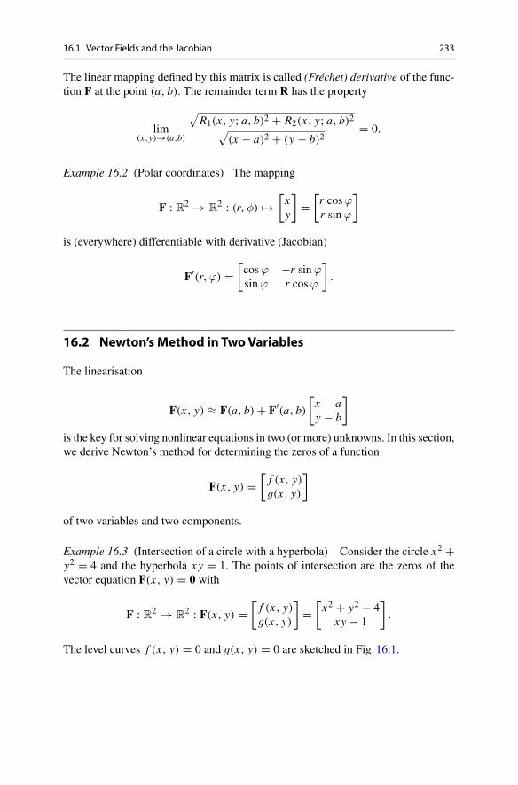
16.1 Vector Fields and the Jacobian 233
The linear mapping defined by this matrix is called (Fréchet) derivative of the func-tion F at the point (a, b). The remainder term R has the property
lim(x,y)→(a,b)
√R1(x, y; a, b)2 + R2(x, y; a, b)2√
(x − a)2 + (y − b)2= 0.
Example 16.2 (Polar coordinates) The mapping
F : R2 → R2 : (r,φ) �→
[xy
]=
[r cosϕr sinϕ
]
is (everywhere) differentiable with derivative (Jacobian)
F′(r,ϕ) =[cosϕ −r sinϕsinϕ r cosϕ
].
16.2 Newton’s Method in TwoVariables
The linearisation
F(x, y) ≈ F(a, b) + F′(a, b)[x − ay − b
]
is the key for solving nonlinear equations in two (or more) unknowns. In this section,we derive Newton’s method for determining the zeros of a function
F(x, y) =[f (x, y)g(x, y)
]
of two variables and two components.
Example 16.3 (Intersection of a circle with a hyperbola) Consider the circle x2 +y2 = 4 and the hyperbola xy = 1. The points of intersection are the zeros of thevector equation F(x, y) = 0 with
F : R2 → R2 : F(x, y) =
[f (x, y)g(x, y)
]=
[x2 + y2 − 4
xy − 1
].
The level curves f (x, y) = 0 and g(x, y) = 0 are sketched in Fig. 16.1.

234 16 Vector-Valued Functions of Two Variables
Fig. 16.1 Intersection of acircle with a hyperbola
x
y
Newton’s method for determining the zeros is based on the following idea. For astarting value (x0, y0) which is sufficiently close to the solution, one computes animproved value by replacing the function by its linear approximation at (x0, y0)
F(x, y) ≈ F(x0, y0) + F′(x0, y0)[x − x0y − y0
].
The zero of the linearisation
F(x0, y0) + F′(x0, y0)[x − x0y − y0
]=
[00
]
is taken as improved approximation (x1, y1), so
F′(x0, y0)[x1 − x0y1 − y0
]= −F(x0, y0),
and [x1y1
]=
[x0y0
]−
(F′(x0, y0)
)−1F(x0, y0),
respectively. This can only be carried out if the Jacobian is invertible, i.e. its deter-minant is not equal to zero. In the example above the Jacobian is
F′(x, y) =[2x 2yy x
]
with determinant det F′(x, y) = 2x2 − 2y2. Thus it is singular on the straight linesx = ±y. These lines are plotted as dashed lines in Fig. 16.1.
The idea now is to iterate the procedure, i.e. to repeat Newton’s step with theimproved value as new starting value
[xk+1yk+1
]=
[xkyk
]−
⎡⎢⎢⎣
∂ f
∂x(xk, yk)
∂ f
∂y(xk, yk)
∂g
∂x(xk, yk)
∂g
∂y(xk, yk)
⎤⎥⎥⎦
−1 [f (xk, yk)g(xk, yk)
]
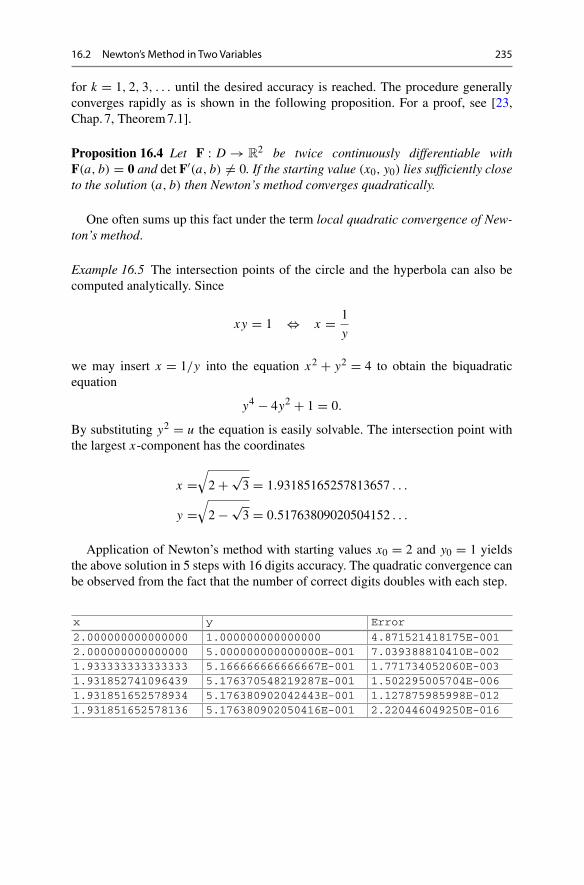
16.2 Newton’s Method in Two Variables 235
for k = 1, 2, 3, . . . until the desired accuracy is reached. The procedure generallyconverges rapidly as is shown in the following proposition. For a proof, see [23,Chap.7, Theorem7.1].
Proposition 16.4 Let F : D → R2 be twice continuously differentiable with
F(a, b) = 0 and det F′(a, b) �= 0. If the starting value (x0, y0) lies sufficiently closeto the solution (a, b) then Newton’s method converges quadratically.
One often sums up this fact under the term local quadratic convergence of New-ton’s method.
Example 16.5 The intersection points of the circle and the hyperbola can also becomputed analytically. Since
xy = 1 ⇔ x = 1
y
we may insert x = 1/y into the equation x2 + y2 = 4 to obtain the biquadraticequation
y4 − 4y2 + 1 = 0.
By substituting y2 = u the equation is easily solvable. The intersection point withthe largest x-component has the coordinates
x =√2 + √
3 = 1.93185165257813657 . . .
y =√2 − √
3 = 0.51763809020504152 . . .
Application of Newton’s method with starting values x0 = 2 and y0 = 1 yieldsthe above solution in 5 steps with 16 digits accuracy. The quadratic convergence canbe observed from the fact that the number of correct digits doubles with each step.
x y Error
2.000000000000000 1.000000000000000 4.871521418175E-0012.000000000000000 5.000000000000000E-001 7.039388810410E-0021.933333333333333 5.166666666666667E-001 1.771734052060E-0031.931852741096439 5.176370548219287E-001 1.502295005704E-0061.931851652578934 5.176380902042443E-001 1.127875985998E-0121.931851652578136 5.176380902050416E-001 2.220446049250E-016
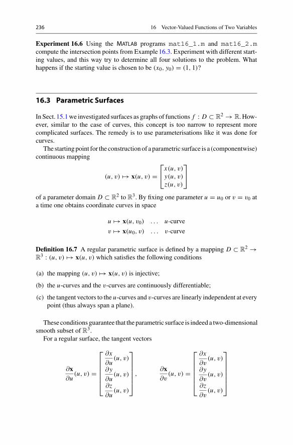
236 16 Vector-Valued Functions of Two Variables
Experiment 16.6 Using the MATLAB programs mat16_1.m and mat16_2.mcompute the intersection points from Example16.3. Experiment with different start-ing values, and this way try to determine all four solutions to the problem. Whathappens if the starting value is chosen to be (x0, y0) = (1, 1)?
16.3 Parametric Surfaces
In Sect. 15.1we investigated surfaces as graphs of functions f : D ⊂ R2 → R. How-
ever, similar to the case of curves, this concept is too narrow to represent morecomplicated surfaces. The remedy is to use parameterisations like it was done forcurves.
The startingpoint for the constructionof a parametric surface is a (componentwise)continuous mapping
(u, v) �→ x(u, v) =⎡⎣x(u, v)y(u, v)z(u, v)
⎤⎦
of a parameter domain D ⊂ R2 to R3. By fixing one parameter u = u0 or v = v0 at
a time one obtains coordinate curves in space
u �→ x(u, v0) . . . u-curve
v �→ x(u0, v) . . . v-curve
Definition 16.7 A regular parametric surface is defined by a mapping D ⊂ R2 →
R3 : (u, v) �→ x(u, v) which satisfies the following conditions
(a) the mapping (u, v) �→ x(u, v) is injective;
(b) the u-curves and the v-curves are continuously differentiable;
(c) the tangent vectors to the u-curves and v-curves are linearly independent at everypoint (thus always span a plane).
These conditions guarantee that the parametric surface is indeed a two-dimensionalsmooth subset of R3.
For a regular surface, the tangent vectors
∂x∂u
(u, v) =
⎡⎢⎢⎢⎢⎢⎣
∂x
∂u(u, v)
∂y
∂u(u, v)
∂z
∂u(u, v)
⎤⎥⎥⎥⎥⎥⎦,
∂x∂v
(u, v) =
⎡⎢⎢⎢⎢⎢⎣
∂x
∂v(u, v)
∂y
∂v(u, v)
∂z
∂v(u, v)
⎤⎥⎥⎥⎥⎥⎦
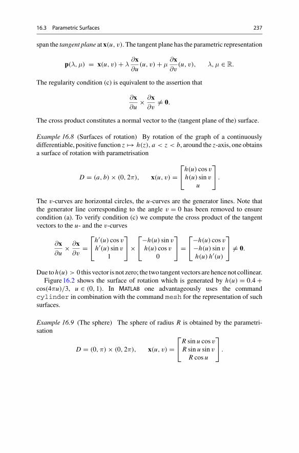
16.3 Parametric Surfaces 237
span the tangent plane at x(u, v). The tangent plane has the parametric representation
p(λ,μ) = x(u, v) + λ∂x∂u
(u, v) + μ∂x∂v
(u, v), λ,μ ∈ R.
The regularity condition (c) is equivalent to the assertion that
∂x∂u
× ∂x∂v
�= 0.
The cross product constitutes a normal vector to the (tangent plane of the) surface.
Example 16.8 (Surfaces of rotation) By rotation of the graph of a continuouslydifferentiable, positive function z �→ h(z), a < z < b, around the z-axis, one obtainsa surface of rotation with parametrisation
D = (a, b) × (0, 2π), x(u, v) =⎡⎣h(u) cos vh(u) sin v
u
⎤⎦ .
The v-curves are horizontal circles, the u-curves are the generator lines. Note thatthe generator line corresponding to the angle v = 0 has been removed to ensurecondition (a). To verify condition (c) we compute the cross product of the tangentvectors to the u- and the v-curves
∂x∂u
× ∂x∂v
=⎡⎣h′(u) cos vh′(u) sin v
1
⎤⎦ ×
⎡⎣−h(u) sin v
h(u) cos v0
⎤⎦ =
⎡⎣−h(u) cos v
−h(u) sin vh(u) h′(u)
⎤⎦ �= 0.
Due to h(u) > 0 this vector is not zero; the two tangent vectors are hence not collinear.Figure16.2 shows the surface of rotation which is generated by h(u) = 0.4 +
cos(4πu)/3, u ∈ (0, 1). In MATLAB one advantageously uses the commandcylinder in combination with the command mesh for the representation of suchsurfaces.
Example 16.9 (The sphere) The sphere of radius R is obtained by the parametri-sation
D = (0,π) × (0, 2π), x(u, v) =⎡⎣R sin u cos vR sin u sin vR cos u
⎤⎦ .
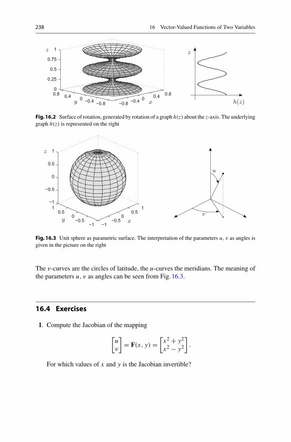
238 16 Vector-Valued Functions of Two Variables
−0.8 −0.4 0 0.4 0.8
−0.8−0.400.40.80
0.25
0.5
0.75
1
h(z)
zz
y x
Fig.16.2 Surface of rotation, generated by rotation of a graph h(z) about the z-axis. The underlyinggraph h(z) is represented on the right
−1−0.5
00.5
1
−1−0.5
00.5
1−1
−0.5
0
0.5
1
v
u
z
y x
Fig. 16.3 Unit sphere as parametric surface. The interpretation of the parameters u, v as angles isgiven in the picture on the right
The v-curves are the circles of latitude, the u-curves the meridians. The meaning ofthe parameters u, v as angles can be seen from Fig. 16.3.
16.4 Exercises
1. Compute the Jacobian of the mapping
[uv
]= F(x, y) =
[x2 + y2
x2 − y2
].
For which values of x and y is the Jacobian invertible?
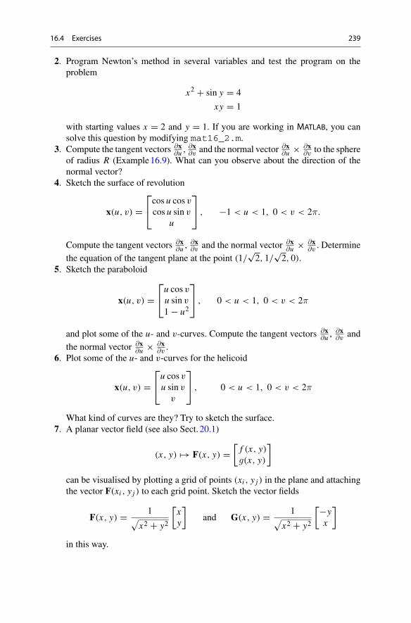
16.4 Exercises 239
2. Program Newton’s method in several variables and test the program on theproblem
x2 + sin y = 4
xy = 1
with starting values x = 2 and y = 1. If you are working in MATLAB, you cansolve this question by modifying mat16_2.m.
3. Compute the tangent vectors ∂x∂u ,
∂x∂v and the normal vector ∂x
∂u × ∂x∂v to the sphere
of radius R (Example16.9). What can you observe about the direction of thenormal vector?
4. Sketch the surface of revolution
x(u, v) =⎡⎣cos u cos vcos u sin v
u
⎤⎦ , −1 < u < 1, 0 < v < 2π.
Compute the tangent vectors ∂x∂u ,
∂x∂v and the normal vector ∂x
∂u × ∂x∂v . Determine
the equation of the tangent plane at the point (1/√2, 1/
√2, 0).
5. Sketch the paraboloid
x(u, v) =⎡⎣u cos vu sin v1 − u2
⎤⎦ , 0 < u < 1, 0 < v < 2π
and plot some of the u- and v-curves. Compute the tangent vectors ∂x∂u ,
∂x∂v and
the normal vector ∂x∂u × ∂x
∂v .6. Plot some of the u- and v-curves for the helicoid
x(u, v) =⎡⎣u cos vu sin v
v
⎤⎦ , 0 < u < 1, 0 < v < 2π
What kind of curves are they? Try to sketch the surface.7. A planar vector field (see also Sect. 20.1)
(x, y) �→ F(x, y) =[f (x, y)g(x, y)
]
can be visualised by plotting a grid of points (xi , y j ) in the plane and attachingthe vector F(xi , y j ) to each grid point. Sketch the vector fields
F(x, y) = 1√x2 + y2
[xy
]and G(x, y) = 1√
x2 + y2
[−yx
]
in this way.
17Integrationof Functions ofTwoVariables
In Sect. 11.3 we have shown how to calculate the volume of solids of revolution. Ifthere is no rotational symmetry, however, one needs an extension of integral calculusto functions of two variables. This arises, for example, if onewants to find the volumeof a solid that lies between a domain D in the (x, y)-plane and the graph of a non-negative function z = f (x, y). In this section we will extend the notion of Riemannintegrals from Chap.11 to double integrals of functions of two variables. Importanttools for the computation of double integrals are their representation as iteratedintegrals and the transformation formula (change of coordinates). The integration offunctions of several variables occurs in numerous applications, a few of which wewill discuss.
17.1 Double Integrals
We start with the integration of a real-valued function z = f (x, y) which is definedon a rectangle R = [a, b] × [c, d].More general domains of integration D ⊂ R
2 willbe discussed below. Sincewe know fromSect. 11.1 thatRiemann integrable functionsare necessarily bounded, we assume in the whole section that f is bounded. If fis non-negative, the integral should be interpretable as the volume of the solid withbase R and top surface given by the graph of f (see Fig. 17.2). This motivates thefollowing approach in which the solid is approximated by a sum of cuboids.
We place a rectangular grid G over the domain R by partitioning the intervals[a, b] and [c, d] like in Sect. 11.1:
Zx : a = x0 < x1 < x2 < · · · < xn−1 < xn = b,
Zy : c = y0 < y1 < y2 < · · · < ym−1 < ym = d.
© Springer Nature Switzerland AG 2018M. Oberguggenberger and A. Ostermann, Analysis for Computer Scientists,Undergraduate Topics in Computer Science,https://doi.org/10.1007/978-3-319-91155-7_17
241
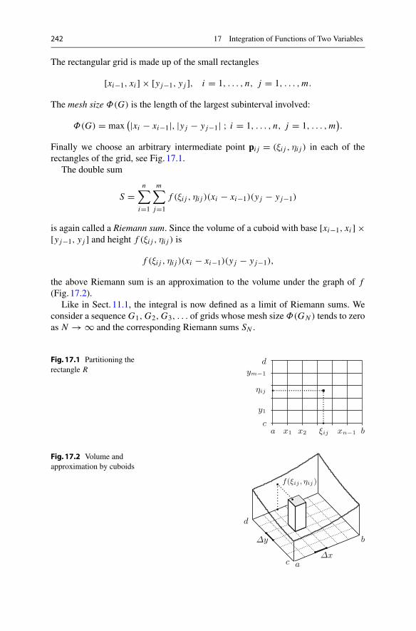
242 17 Integration of Functions of Two Variables
The rectangular grid is made up of the small rectangles
[xi−1, xi ] × [y j−1, y j ], i = 1, . . . , n, j = 1, . . . ,m.
The mesh size Φ(G) is the length of the largest subinterval involved:
Φ(G) = max(|xi − xi−1|, |y j − y j−1| ; i = 1, . . . , n, j = 1, . . . ,m
).
Finally we choose an arbitrary intermediate point pi j = (ξi j , ηi j ) in each of therectangles of the grid, see Fig. 17.1.
The double sum
S =n∑
i=1
m∑
j=1
f (ξi j , ηi j )(xi − xi−1)(y j − y j−1)
is again called a Riemann sum. Since the volume of a cuboid with base [xi−1, xi ] ×[y j−1, y j ] and height f (ξi j , ηi j ) is
f (ξi j , ηi j )(xi − xi−1)(y j − y j−1),
the above Riemann sum is an approximation to the volume under the graph of f(Fig. 17.2).
Like in Sect. 11.1, the integral is now defined as a limit of Riemann sums. Weconsider a sequence G1,G2,G3, . . . of grids whose mesh size Φ(GN ) tends to zeroas N → ∞ and the corresponding Riemann sums SN .
Fig. 17.1 Partitioning therectangle R
dym−1
ηij
y1
cbxn−1ξijx2x1a
Fig. 17.2 Volume andapproximation by cuboids
f(ξij , ηij )
d
c
Δy b
aΔx
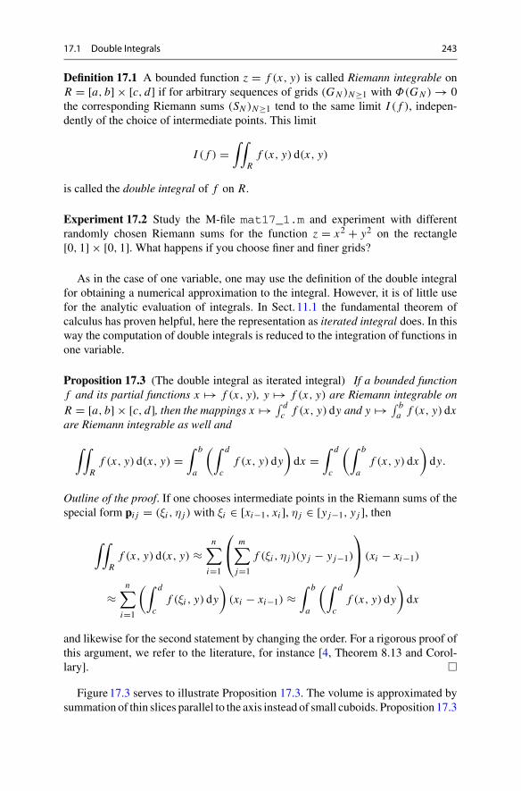
17.1 Double Integrals 243
Definition 17.1 A bounded function z = f (x, y) is called Riemann integrable onR = [a, b] × [c, d] if for arbitrary sequences of grids (GN )N≥1 with Φ(GN ) → 0the corresponding Riemann sums (SN )N≥1 tend to the same limit I ( f ), indepen-dently of the choice of intermediate points. This limit
I ( f ) =∫∫
Rf (x, y) d(x, y)
is called the double integral of f on R.
Experiment 17.2 Study the M-file mat17_1.m and experiment with differentrandomly chosen Riemann sums for the function z = x2 + y2 on the rectangle[0, 1] × [0, 1]. What happens if you choose finer and finer grids?
As in the case of one variable, one may use the definition of the double integralfor obtaining a numerical approximation to the integral. However, it is of little usefor the analytic evaluation of integrals. In Sect. 11.1 the fundamental theorem ofcalculus has proven helpful, here the representation as iterated integral does. In thisway the computation of double integrals is reduced to the integration of functions inone variable.
Proposition 17.3 (The double integral as iterated integral) If a bounded functionf and its partial functions x �→ f (x, y), y �→ f (x, y) are Riemann integrable onR = [a, b] × [c, d], then the mappings x �→ ∫ d
c f (x, y) dy and y �→ ∫ ba f (x, y) dx
are Riemann integrable as well and
∫∫
Rf (x, y) d(x, y) =
∫ b
a
(∫ d
cf (x, y) dy
)dx =
∫ d
c
(∫ b
af (x, y) dx
)dy.
Outline of the proof. If one chooses intermediate points in the Riemann sums of thespecial form pi j = (ξi , η j ) with ξi ∈ [xi−1, xi ], η j ∈ [y j−1, y j ], then
∫∫
Rf (x, y) d(x, y) ≈
n∑
i=1
⎛
⎝m∑
j=1
f (ξi , η j )(y j − y j−1)
⎞
⎠ (xi − xi−1)
≈n∑
i=1
(∫ d
cf (ξi , y) dy
)(xi − xi−1) ≈
∫ b
a
(∫ d
cf (x, y) dy
)dx
and likewise for the second statement by changing the order. For a rigorous proof ofthis argument, we refer to the literature, for instance [4, Theorem 8.13 and Corol-lary]. �
Figure17.3 serves to illustrate Proposition 17.3. The volume is approximated bysummation of thin slices parallel to the axis instead of small cuboids. Proposition 17.3
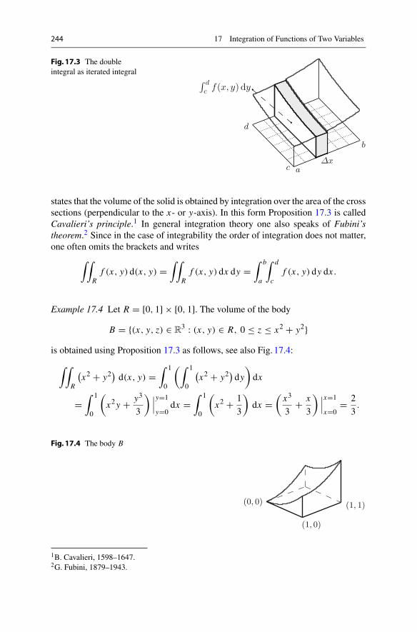
244 17 Integration of Functions of Two Variables
Fig. 17.3 The doubleintegral as iterated integral
d
c f(x, y) dy
d
c
b
aΔx
states that the volume of the solid is obtained by integration over the area of the crosssections (perpendicular to the x- or y-axis). In this form Proposition 17.3 is calledCavalieri’s principle.1 In general integration theory one also speaks of Fubini’stheorem.2 Since in the case of integrability the order of integration does not matter,one often omits the brackets and writes
∫∫
Rf (x, y) d(x, y) =
∫∫
Rf (x, y) dx dy =
∫ b
a
∫ d
cf (x, y) dy dx .
Example 17.4 Let R = [0, 1] × [0, 1]. The volume of the body
B = {(x, y, z) ∈ R3 : (x, y) ∈ R, 0 ≤ z ≤ x2 + y2}
is obtained using Proposition 17.3 as follows, see also Fig. 17.4:
∫∫
R
(x2 + y2
)d(x, y) =
∫ 1
0
(∫ 1
0
(x2 + y2
)dy
)dx
=∫ 1
0
(x2y + y3
3
) ∣∣∣y=1
y=0dx =
∫ 1
0
(x2 + 1
3
)dx =
(x3
3+ x
3
) ∣∣∣x=1
x=0= 2
3.
Fig. 17.4 The body B
(1, 1)
(1, 0)
(0, 0)
1B. Cavalieri, 1598–1647.2G. Fubini, 1879–1943.
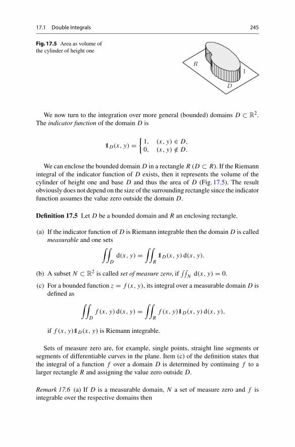
17.1 Double Integrals 245
Fig. 17.5 Area as volume ofthe cylinder of height one
R
D
1
We now turn to the integration over more general (bounded) domains D ⊂ R2.
The indicator function of the domain D is
11D(x, y) ={1, (x, y) ∈ D,
0, (x, y) /∈ D.
We can enclose the bounded domain D in a rectangle R (D ⊂ R). If the Riemannintegral of the indicator function of D exists, then it represents the volume of thecylinder of height one and base D and thus the area of D (Fig. 17.5). The resultobviously does not depend on the size of the surrounding rectangle since the indicatorfunction assumes the value zero outside the domain D.
Definition 17.5 Let D be a bounded domain and R an enclosing rectangle.
(a) If the indicator function of D is Riemann integrable then the domain D is calledmeasurable and one sets
∫∫
Dd(x, y) =
∫∫
R11D(x, y) d(x, y).
(b) A subset N ⊂ R2 is called set of measure zero, if
∫∫N d(x, y) = 0.
(c) For a bounded function z = f (x, y), its integral over a measurable domain D isdefined as
∫∫
Df (x, y) d(x, y) =
∫∫
Rf (x, y)11D(x, y) d(x, y),
if f (x, y)11D(x, y) is Riemann integrable.
Sets of measure zero are, for example, single points, straight line segments orsegments of differentiable curves in the plane. Item (c) of the definition states thatthe integral of a function f over a domain D is determined by continuing f to alarger rectangle R and assigning the value zero outside D.
Remark 17.6 (a) If D is a measurable domain, N a set of measure zero and f isintegrable over the respective domains then
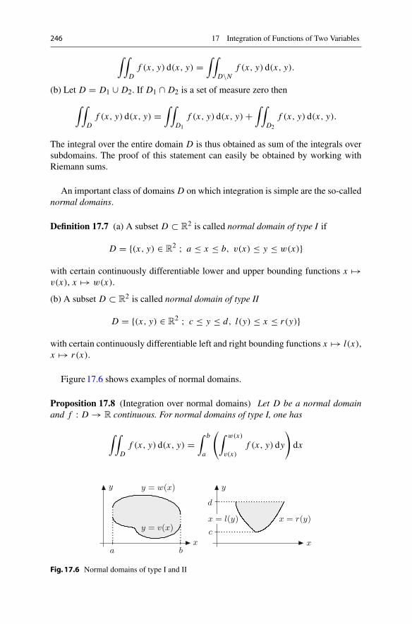
246 17 Integration of Functions of Two Variables
∫∫
Df (x, y) d(x, y) =
∫∫
D\Nf (x, y) d(x, y).
(b) Let D = D1 ∪ D2. If D1 ∩ D2 is a set of measure zero then
∫∫
Df (x, y) d(x, y) =
∫∫
D1
f (x, y) d(x, y) +∫∫
D2
f (x, y) d(x, y).
The integral over the entire domain D is thus obtained as sum of the integrals oversubdomains. The proof of this statement can easily be obtained by working withRiemann sums.
An important class of domains D on which integration is simple are the so-callednormal domains.
Definition 17.7 (a) A subset D ⊂ R2 is called normal domain of type I if
D = {(x, y) ∈ R2 ; a ≤ x ≤ b, v(x) ≤ y ≤ w(x)}
with certain continuously differentiable lower and upper bounding functions x �→v(x), x �→ w(x).
(b) A subset D ⊂ R2 is called normal domain of type II
D = {(x, y) ∈ R2 ; c ≤ y ≤ d, l(y) ≤ x ≤ r(y)}
with certain continuously differentiable left and right bounding functions x �→ l(x),x �→ r(x).
Figure17.6 shows examples of normal domains.
Proposition 17.8 (Integration over normal domains) Let D be a normal domainand f : D → R continuous. For normal domains of type I, one has
∫∫
Df (x, y) d(x, y) =
∫ b
a
(∫ w(x)
v(x)f (x, y) dy
)
dx
d
c
x = r(y)x = l(y)
y
xa b
y = w(x)
y = v(x)
y
x
Fig. 17.6 Normal domains of type I and II
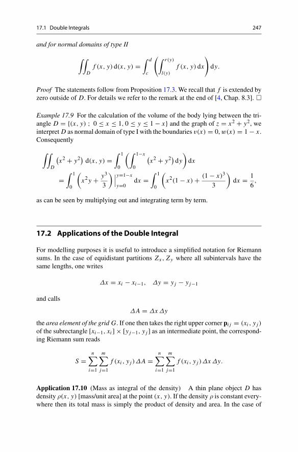
17.1 Double Integrals 247
and for normal domains of type II
∫∫
Df (x, y) d(x, y) =
∫ d
c
(∫ r(y)
l(y)f (x, y) dx
)
dy.
Proof The statements follow from Proposition 17.3. We recall that f is extended byzero outside of D. For details we refer to the remark at the end of [4, Chap. 8.3]. �
Example 17.9 For the calculation of the volume of the body lying between the tri-angle D = {(x, y) ; 0 ≤ x ≤ 1, 0 ≤ y ≤ 1 − x} and the graph of z = x2 + y2, weinterpret D as normal domain of type I with the boundaries v(x) = 0,w(x) = 1 − x .Consequently
∫∫
D
(x2 + y2
)d(x, y) =
∫ 1
0
(∫ 1−x
0
(x2 + y2
)dy
)dx
=∫ 1
0
(x2y + y3
3
) ∣∣∣y=1−x
y=0dx =
∫ 1
0
(x2(1 − x) + (1 − x)3
3
)dx = 1
6,
as can be seen by multiplying out and integrating term by term.
17.2 Applications of the Double Integral
For modelling purposes it is useful to introduce a simplified notation for Riemannsums. In the case of equidistant partitions Zx , Zy where all subintervals have thesame lengths, one writes
Δx = xi − xi−1, Δy = y j − y j−1
and calls
ΔA = ΔxΔy
the area element of the grid G. If one then takes the right upper corner pi j = (xi , y j )of the subrectangle [xi−1, xi ] × [y j−1, y j ] as an intermediate point, the correspond-ing Riemann sum reads
S =n∑
i=1
m∑
j=1
f (xi , y j )ΔA =n∑
i=1
m∑
j=1
f (xi , y j )ΔxΔy.
Application 17.10 (Mass as integral of the density) A thin plane object D hasdensity ρ(x, y) [mass/unit area] at the point (x, y). If the density ρ is constant every-where then its total mass is simply the product of density and area. In the case of
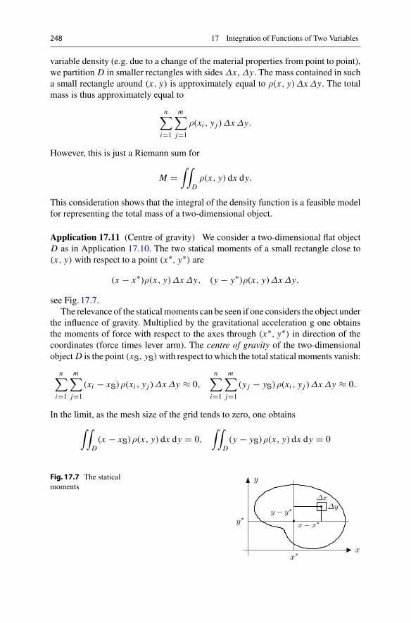
248 17 Integration of Functions of Two Variables
variable density (e.g. due to a change of the material properties from point to point),we partition D in smaller rectangles with sides Δx , Δy. The mass contained in sucha small rectangle around (x, y) is approximately equal to ρ(x, y)ΔxΔy. The totalmass is thus approximately equal to
n∑
i=1
m∑
j=1
ρ(xi , y j )ΔxΔy.
However, this is just a Riemann sum for
M =∫∫
Dρ(x, y) dx dy.
This consideration shows that the integral of the density function is a feasible modelfor representing the total mass of a two-dimensional object.
Application 17.11 (Centre of gravity) We consider a two-dimensional flat objectD as in Application 17.10. The two statical moments of a small rectangle close to(x, y) with respect to a point (x∗, y∗) are
(x − x∗)ρ(x, y)ΔxΔy, (y − y∗)ρ(x, y)ΔxΔy,
see Fig. 17.7.The relevance of the staticalmoments can be seen if one considers the object under
the influence of gravity. Multiplied by the gravitational acceleration g one obtainsthe moments of force with respect to the axes through (x∗, y∗) in direction of thecoordinates (force times lever arm). The centre of gravity of the two-dimensionalobject D is the point (xS, yS)with respect to which the total statical moments vanish:
n∑
i=1
m∑
j=1
(xi − xS)ρ(xi , y j )ΔxΔy ≈ 0,n∑
i=1
m∑
j=1
(y j − yS)ρ(xi , y j )ΔxΔy ≈ 0.
In the limit, as the mesh size of the grid tends to zero, one obtains∫∫
D(x − xS)ρ(x, y) dx dy = 0,
∫∫
D(y − yS)ρ(x, y) dx dy = 0
Fig. 17.7 The staticalmoments
y∗
x∗
x − x∗y − y∗
ΔxΔy
y
x
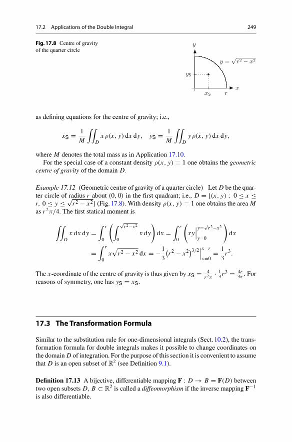
17.2 Applications of the Double Integral 249
Fig. 17.8 Centre of gravityof the quarter circle
y =√
r2 − x2
yS
rxS
y
x
as defining equations for the centre of gravity; i.e.,
xS = 1
M
∫∫
Dx ρ(x, y) dx dy, yS = 1
M
∫∫
Dyρ(x, y) dx dy,
where M denotes the total mass as in Application 17.10.For the special case of a constant density ρ(x, y) ≡ 1 one obtains the geometric
centre of gravity of the domain D.
Example 17.12 (Geometric centre of gravity of a quarter circle) Let D be the quar-ter circle of radius r about (0, 0) in the first quadrant; i.e., D = {(x, y) ; 0 ≤ x ≤r, 0 ≤ y ≤ √
r2 − x2} (Fig. 17.8). With density ρ(x, y) ≡ 1 one obtains the area Mas r2π/4. The first statical moment is
∫∫
Dx dx dy =
∫ r
0
(∫ √r2−x2
0x dy
)
dx =∫ r
0
(
xy∣∣∣y=√
r2−x2
y=0
)
dx
=∫ r
0x√r2 − x2 dx = −1
3
(r2 − x2
)3/2∣∣∣x=r
x=0= 1
3r3.
The x-coordinate of the centre of gravity is thus given by xS = 4r2π
· 13r
3 = 4r3π . For
reasons of symmetry, one has yS = xS.
17.3 TheTransformation Formula
Similar to the substitution rule for one-dimensional integrals (Sect. 10.2), the trans-formation formula for double integrals makes it possible to change coordinates onthe domain D of integration. For the purpose of this section it is convenient to assumethat D is an open subset of R2 (see Definition 9.1).
Definition 17.13 A bijective, differentiable mapping F : D → B = F(D) betweentwo open subsets D, B ⊂ R
2 is called a diffeomorphism if the inverse mapping F−1
is also differentiable.
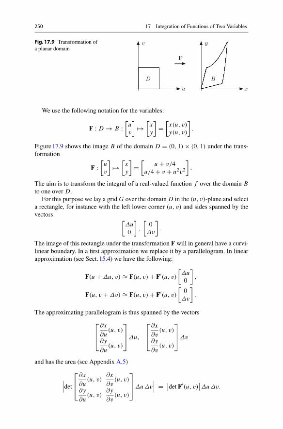
250 17 Integration of Functions of Two Variables
Fig. 17.9 Transformation ofa planar domain
B
y
x
F
D
v
u
We use the following notation for the variables:
F : D → B :[uv
]�→
[xy
]=
[x(u, v)
y(u, v)
].
Figure17.9 shows the image B of the domain D = (0, 1) × (0, 1) under the trans-formation
F :[uv
]�→
[xy
]=
[u + v/4
u/4 + v + u2v2
].
The aim is to transform the integral of a real-valued function f over the domain Bto one over D.
For this purpose we lay a grid G over the domain D in the (u, v)-plane and selecta rectangle, for instance with the left lower corner (u, v) and sides spanned by thevectors
[Δu0
],
[0
Δv
].
The image of this rectangle under the transformation F will in general have a curvi-linear boundary. In a first approximation we replace it by a parallelogram. In linearapproximation (see Sect. 15.4) we have the following:
F(u + Δu, v) ≈ F(u, v) + F′(u, v)
[Δu0
],
F(u, v + Δv) ≈ F(u, v) + F′(u, v)
[0
Δv
].
The approximating parallelogram is thus spanned by the vectors
⎡
⎢⎣
∂x
∂u(u, v)
∂y
∂u(u, v)
⎤
⎥⎦Δu,
⎡
⎢⎣
∂x
∂v(u, v)
∂y
∂v(u, v)
⎤
⎥⎦Δv
and has the area (see Appendix A.5)
∣∣∣det
⎡
⎢⎣
∂x
∂u(u, v)
∂x
∂v(u, v)
∂y
∂u(u, v)
∂y
∂v(u, v)
⎤
⎥⎦ ΔuΔv
∣∣∣ = ∣
∣det F′(u, v)∣∣ΔuΔv.

17.3 The Transformation Formula 251
Fig. 17.10 Transformationof an area element
ΔF(A)
y
x
ΔA
v
u
In short, the area element ΔA = ΔuΔv is changed by the transformation F to thearea element ΔF(A) = ∣
∣det F′(u, v)∣∣ΔuΔv (see Fig. 17.10).
Proposition 17.14 (Transformation formula for double integrals) Let D, B beopen, bounded subsets of R2, F : D → B a diffeomorphism and f : B → R abounded mapping. Then
∫∫
Bf (x, y) dx dy =
∫∫
Df(F(u, v)
)∣∣det F′(u, v)
∣∣ du dv,
as long as the functions f and f (F)∣∣det F′∣∣ are Riemann integrable.
Outline of the proof. We use Riemann sums on the transformed grid and obtain
∫∫
Bf (x, y) dx dy ≈
n∑
i=1
m∑
j=1
f (xi , y j )ΔF(A)
≈n∑
i=1
m∑
j=1
f(x(ui , v j ), y(ui , v j )
)∣∣det F′(ui , v j )
∣∣ΔuΔv
≈∫∫
Df(x(u, v), y(u, v)
)∣∣det F′(u, v)
∣∣ du dv.
A rigorous proof is tedious and requires a careful study of the boundary of the domainD and the behaviour of the transformation F near the boundary (see for instance [3,Chap. 19, Theorem 4.7]). �
Example 17.15 The area of the domain B from Fig. 17.9 can be calculated using thetransformation formula with f (x, y) = 1 as follows. We have
F′(u, v) =[
1 1/41/4 + 2uv2 1 + 2u2v
],
∣∣det F′(u, v)
∣∣ =
∣∣∣15
16+ 2u2v − 1
2uv2
∣∣∣
252 17 Integration of Functions of Two Variables
and thus∫∫
Bdx dy =
∫∫
D
∣∣det F′(u, v)∣∣ du dv
=∫ 1
0
(∫ 1
0
(15
16+ 2u2v − 1
2uv2
)dv
)du
=∫ 1
0
(15
16+ u2 − 1
6u
)du = 15
16+ 1
3− 1
12= 19
16.
Example 17.16 (Volume of a hemisphere in polar coordinates) We represent ahemisphere of radius R by the three-dimensional domain
{(x, y, z) ; 0 ≤ x2 + y2 ≤ R2, 0 ≤ z ≤√R2 − x2 − y2}.
Its volume is obtained by integration of the function f (x, y) = √R2 − x2 − y2 over
the base B = {(x, y) ; 0 ≤ x2 + y2 ≤ R2}. In polar coordinates
F : R2 → R2 :
[rϕ
]�→
[xy
]=
[r cosϕr sinϕ
]
the area B can be represented as the image F(D) of the rectangle D = [0, R] ×[0, 2π]. However, in order to fulfil the assumptions of Proposition 17.14 we haveto switch to open domains on which F is a diffeomorphism. We can obtain this, forinstance, by removing the boundary and the half ray {(x, y) ; 0 ≤ x ≤ R, y = 0}of the circle B and the boundary of the rectangle D. On the smaller domains D′, B ′obtained in this way, F is a diffeomorphism. However, since B differs from B ′ andD differs from D′ by sets of measure zero, the value of the integral is not changedif one replaces B by B ′ and D by D′, see Remark 17.6. We have
F′(r, ϕ) =[cosϕ −r sinϕsinϕ r cosϕ
],
∣∣det F′(r, ϕ)
∣∣ = r.
Substituting x = r cosϕ, y = r sinϕ results in x2 + y2 = r2 and we obtain the vol-ume from the transformation formula as
∫∫
B
√R2 − x2 − y2 dx dy =
∫ R
0
∫ 2π
0
√R2 − r2 r dϕ dr
=∫ R
02πr
√R2 − r2 dr
= −2π
3
(R2 − r2
)3/2∣∣∣r=R
r=0= 2π
3R3,
which coincides with the known result from elementary geometry.

17.4 Exercises 253
17.4 Exercises
1. Compute the volume of the parabolic dome z = 2 − x2 − y2 above the quadraticdomain D : −1 ≤ x ≤ 1, −1 ≤ y ≤ 1.
2. (From statics)Compute the axialmoment of inertia∫∫
D y2 dx dy of a rectangularcross section D : 0 ≤ x ≤ b, −h/2 ≤ y ≤ h/2, where b > 0, h > 0.
3. Compute the volume of the body bounded by the plane z = x + y above thedomain D : 0 ≤ x ≤ 1, 0 ≤ y ≤ √
1 − x2.4. Compute the volume of the body bounded by the plane z = 6 − x − y above
the domain D, which is bounded by the y-axis and the straight lines x + y = 6,x + 3y = 6 (x ≥ 0, y ≥ 0).
5. Compute the geometric centre of gravity of the domain D : 0 ≤ x ≤ 1, 0 ≤ y ≤1 − x2.
6. Compute the area and the geometric centre of gravity of the semi-ellipse
x2
a2+ y2
b2≤ 1, y ≥ 0.
Hint. Introduce elliptic coordinates x = ar cosϕ, y = br sinϕ, 0 ≤ r ≤ 1, 0 ≤ϕ ≤ π, compute the Jacobian and use the transformation formula.
7. (From statics) Compute the axial moment of inertia of a ring with inner radiusR1 and outer radius R2 with respect to the central axis, i.e. the integral
∫∫D(x2 +
y2) dx dy over the domain D : R1 ≤ √x2 + y2 ≤ R2.
8. Modify the M-file mat17_1.m so that it can evaluate Riemann sums overequidistant partitions with Δx �= Δy.
9. Let the domain D be bounded by the curves
y = x and y = x2, 0 ≤ x ≤ 1.
(a) Sketch D.(b) Compute the area of D by means of the double integral F = ∫∫
D d(x, y).(c) Compute the statical moments
∫∫D x d(x, y) und
∫∫D y d(x, y).
10. Compute the statical moment∫∫
D y d(x, y) of the half-disk
D = {(x, y) ∈ R2; −1 ≤ x ≤ 1, 0 ≤ y ≤
√1 − x2}
(a) as a double integral, writing D as a normal domain of type I;(b) by transformation to polar coordinates.
11. The following integral is written in terms of a normal domain of type II:
1∫
0
y2+1∫
y
x2y dxdy.

254 17 Integration of Functions of Two Variables
(a) Compute the integral.(b) Sketch the domain and represent it as a normal domain of type I.(c) Interchange the order of integration and recompute the integral.Hint. In (c) two summands are needed.
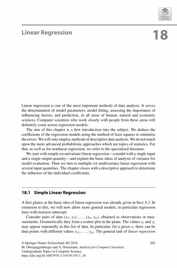
18Linear Regression
Linear regression is one of the most important methods of data analysis. It servesthe determination of model parameters, model fitting, assessing the importance ofinfluencing factors, and prediction, in all areas of human, natural and economicsciences. Computer scientists who work closely with people from these areas willdefinitely come across regression models.
The aim of this chapter is a first introduction into the subject. We deduce thecoefficients of the regression models using the method of least squares to minimisethe errors.Wewill only employmethods of descriptive data analysis.We do not touchupon the more advanced probabilistic approaches which are topics of statistics. Forthat, as well as for nonlinear regression, we refer to the specialised literature.
We start with simple (or univariate) linear regression—amodel with a single inputand a single output quantity—and explain the basic ideas of analysis of variance formodel evaluation. Then we turn to multiple (or multivariate) linear regression withseveral input quantities. The chapter closes with a descriptive approach to determinethe influence of the individual coefficients.
18.1 Simple Linear Regression
A first glance at the basic idea of linear regression was already given in Sect. 8.3. Inextension to this, we will now allow more general models, in particular regressionlines with nonzero intercept.
Consider pairs of data (x1, y1), . . . , (xn, yn), obtained as observations or mea-surements. Geometrically they form a scatter plot in the plane. The values xi and yimay appear repeatedly in this list of data. In particular, for a given xi there can bedata points with different values yi1, . . . , yip. The general task of linear regression
© Springer Nature Switzerland AG 2018M. Oberguggenberger and A. Ostermann, Analysis for Computer Scientists,Undergraduate Topics in Computer Science,https://doi.org/10.1007/978-3-319-91155-7_18
255
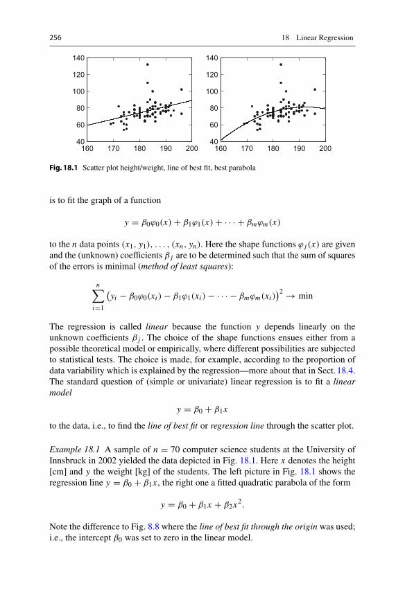
256 18 Linear Regression
160 170 180 190 20040
60
80
100
120
140
160 170 180 190 20040
60
80
100
120
140
Fig. 18.1 Scatter plot height/weight, line of best fit, best parabola
is to fit the graph of a function
y = β0ϕ0(x) + β1ϕ1(x) + · · · + βmϕm(x)
to the n data points (x1, y1), . . . , (xn, yn). Here the shape functions ϕ j (x) are givenand the (unknown) coefficients β j are to be determined such that the sum of squaresof the errors is minimal (method of least squares):
n∑
i=1
(yi − β0ϕ0(xi ) − β1ϕ1(xi ) − · · · − βmϕm(xi )
)2 → min
The regression is called linear because the function y depends linearly on theunknown coefficients β j . The choice of the shape functions ensues either from apossible theoretical model or empirically, where different possibilities are subjectedto statistical tests. The choice is made, for example, according to the proportion ofdata variability which is explained by the regression—more about that in Sect. 18.4.The standard question of (simple or univariate) linear regression is to fit a linearmodel
y = β0 + β1x
to the data, i.e., to find the line of best fit or regression line through the scatter plot.
Example 18.1 A sample of n = 70 computer science students at the University ofInnsbruck in 2002 yielded the data depicted in Fig. 18.1. Here x denotes the height[cm] and y the weight [kg] of the students. The left picture in Fig. 18.1 shows theregression line y = β0 + β1x , the right one a fitted quadratic parabola of the form
y = β0 + β1x + β2x2.
Note the difference to Fig. 8.8 where the line of best fit through the origin was used;i.e., the intercept β0 was set to zero in the linear model.
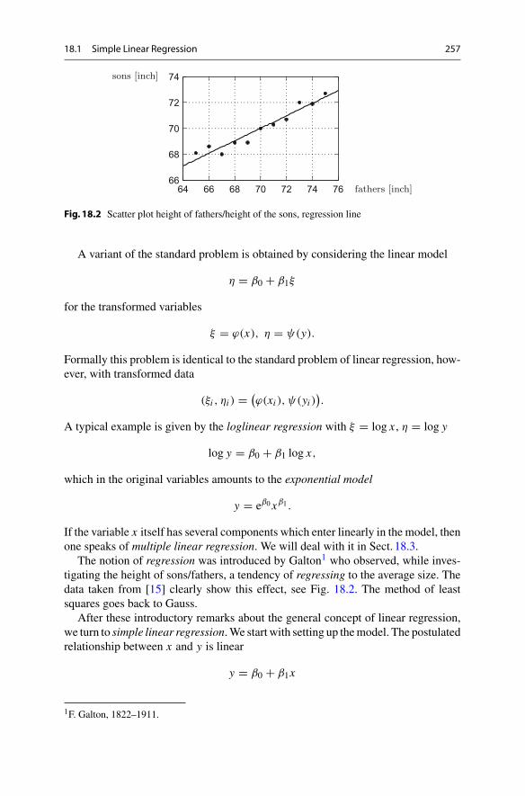
18.1 Simple Linear Regression 257
64 66 68 70 72 74 7666
68
70
72
74sons [inch]
fathers [inch]
Fig. 18.2 Scatter plot height of fathers/height of the sons, regression line
A variant of the standard problem is obtained by considering the linear model
η = β0 + β1ξ
for the transformed variables
ξ = ϕ(x), η = ψ(y).
Formally this problem is identical to the standard problem of linear regression, how-ever, with transformed data
(ξi , ηi ) = (ϕ(xi ), ψ(yi )
).
A typical example is given by the loglinear regression with ξ = log x , η = log y
log y = β0 + β1 log x,
which in the original variables amounts to the exponential model
y = eβ0xβ1 .
If the variable x itself has several components which enter linearly in the model, thenone speaks of multiple linear regression. We will deal with it in Sect. 18.3.
The notion of regression was introduced by Galton1 who observed, while inves-tigating the height of sons/fathers, a tendency of regressing to the average size. Thedata taken from [15] clearly show this effect, see Fig. 18.2. The method of leastsquares goes back to Gauss.
After these introductory remarks about the general concept of linear regression,we turn to simple linear regression.We start with setting up themodel. The postulatedrelationship between x and y is linear
y = β0 + β1x
1F. Galton, 1822–1911.
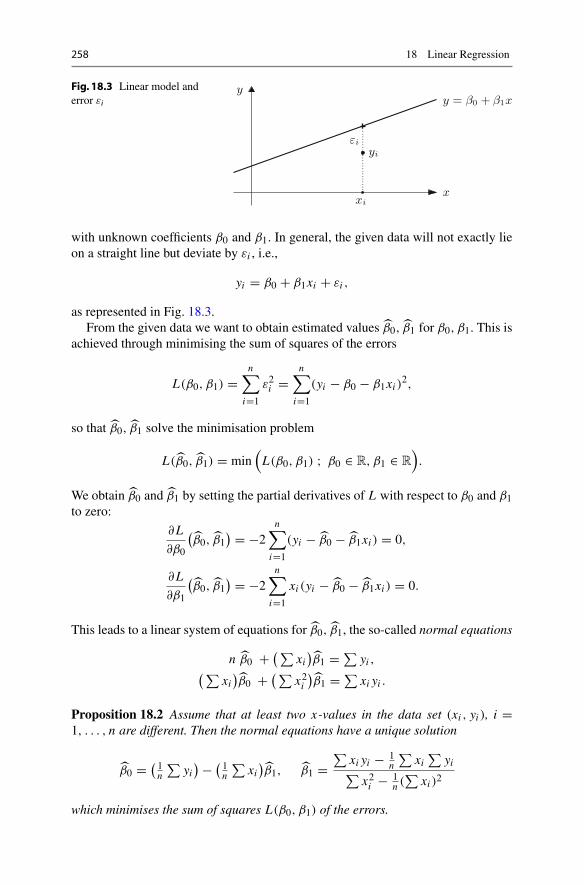
258 18 Linear Regression
Fig. 18.3 Linear model anderror εi y = β0 + β1x
yi
εi
xix
y
with unknown coefficients β0 and β1. In general, the given data will not exactly lieon a straight line but deviate by εi , i.e.,
yi = β0 + β1xi + εi ,
as represented in Fig. 18.3.From the given data we want to obtain estimated values β0, β1 for β0, β1. This is
achieved through minimising the sum of squares of the errors
L(β0, β1) =n∑
i=1
ε2i =n∑
i=1
(yi − β0 − β1xi )2,
so that β0, β1 solve the minimisation problem
L(β0, β1) = min(L(β0, β1) ; β0 ∈ R, β1 ∈ R
).
We obtain β0 and β1 by setting the partial derivatives of L with respect to β0 and β1to zero:
∂L
∂β0
(β0, β1
) = −2n∑
i=1
(yi − β0 − β1xi ) = 0,
∂L
∂β1
(β0, β1
) = −2n∑
i=1
xi (yi − β0 − β1xi ) = 0.
This leads to a linear system of equations for β0, β1, the so-called normal equations
n β0 + ( ∑xi
)β1 = ∑
yi ,( ∑xi
)β0 + ( ∑
x2i)β1 = ∑
xi yi .
Proposition 18.2 Assume that at least two x-values in the data set (xi , yi ), i =1, . . . , n are different. Then the normal equations have a unique solution
β0 = ( 1n
∑yi
) − ( 1n
∑xi
)β1, β1 =
∑xi yi − 1
n
∑xi
∑yi∑
x2i − 1n (
∑xi )2
which minimises the sum of squares L(β0, β1) of the errors.

18.1 Simple Linear Regression 259
Fig. 18.4 Linear model,prediction, residual
y = β0 + β1xyi
y = β0 + β1x
yiei
xix
y
Proof With the notations x = (x1, . . . , xn) and 1 = (1, . . . , 1) the determinant of thenormal equations is n
∑x2i − (
∑xi )2 = ‖x‖2‖1‖2 − 〈x, 1〉2. For vectors of length
n = 2 and n = 3we know that 〈x, 1〉 = ‖x‖‖1‖ · cos�(x, 1), see Appendix A.4, andthus ‖x‖‖1‖ ≥ |〈x, 1〉|. This relation, however, is valid in any dimension n (see forinstance [2, Chap. VI, Theorem 1.1]), and equality can only occur if x is parallel to1, so all components xi are equal. As this possibility was excluded, the determinantof the normal equations is greater than zero and the solution formula is obtained bya simple calculation.
In order to show that this solution minimises L(β0, β1), we compute the Hessianmatrix
HL =⎡
⎣∂2L∂β2
0
∂2L∂β0∂β1
∂2L∂β1∂β0
∂2L∂β2
1
⎤
⎦ = 2
[n
∑xi∑
xi∑
x2i
]= 2
[‖1‖2 〈x, 1〉〈x, 1〉 ‖x‖2
].
The entry ∂2L/∂β20 = 2n and det HL = 4
(‖x‖2‖1‖2 − 〈x, 1〉2) are both positive.According to Proposition 15.28, L has an isolated local minimum at the point(β0, β1). Due to the uniqueness of the solution, this is the only minimum of L . �
The assumption that there are at least two different xi -values in the data set is nota restriction since otherwise the regression problem is not meaningful. The result ofthe regression is the predicted regression line
y = β0 + β1x .
The values predicted by the model are then
yi = β0 + β1xi , i = 1, . . . , n.
Their deviations from the data values yi are called residuals
ei = yi − yi = yi − β0 − β1xi , i = 1, . . . , n.
The meaning of these quantities can be seen in Fig. 18.4.With the above specifications, the deterministic regression model is completed. In
the statistical regression model the errors εi are interpreted as random variables with

260 18 Linear Regression
mean zero. Under further probabilistic assumptions the model is made accessible tostatistical tests and diagnostic procedures. As mentioned in the introduction, we willnot pursue this path here but remain in the framework of descriptive data analysis.
In order to obtain a more lucid representation, we will reformulate the normalequations. For this we introduce the following vectors and matrices:
y =
⎡
⎢⎢⎢⎣
y1y2...
yn
⎤
⎥⎥⎥⎦ , X =
⎡
⎢⎢⎢⎣
1 x11 x2...
...
1 xn
⎤
⎥⎥⎥⎦ , β =[β0β1
], ε =
⎡
⎢⎢⎢⎣
ε1ε2...
εn
⎤
⎥⎥⎥⎦ .
By this, the relations
yi = β0 + β1xi + εi , i = 1, . . . , n,
can be written simply as
y = Xβ + ε.
Further
XTX =[1 1 . . . 1x1 x2 . . . xn
]⎡
⎢⎢⎢⎣
1 x11 x2...
...
1 xn
⎤
⎥⎥⎥⎦ =[
n∑
xi∑xi
∑x2i
],
XTy =[1 1 . . . 1x1 x2 . . . xn
]⎡
⎢⎢⎢⎣
yiy2...
yn
⎤
⎥⎥⎥⎦ =[ ∑
yi∑xi yi
],
so that the normal equations take the form
XTXβ = XTy
with solution
β = (XTX)−1 XTy.
The predicted values and residuals are
y = Xβ, e = y − y.
Example 18.3 (Continuation of Example 18.1) The data for x = height and y =weight can be found in theM-file mat08_3.m; the matrixX is generated inMATLAB
by
X = [ones(size(x)), x];
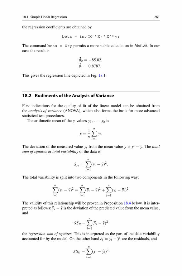
18.1 Simple Linear Regression 261
the regression coefficients are obtained by
beta = inv(X’* X) * X’* y;
The command beta = X\y permits a more stable calculation in MATLAB. In ourcase the result is
β0 = −85.02,
β1 = 0.8787.
This gives the regression line depicted in Fig. 18.1.
18.2 Rudiments of the Analysis of Variance
First indications for the quality of fit of the linear model can be obtained fromthe analysis of variance (ANOVA), which also forms the basis for more advancedstatistical test procedures.
The arithmetic mean of the y-values y1, . . . , yn is
y = 1
n
n∑
i=1
yi .
The deviation of the measured value yi from the mean value y is yi − y. The totalsum of squares or total variability of the data is
Syy =n∑
i=1
(yi − y)2.
The total variability is split into two components in the following way:
n∑
i=1
(yi − y)2 =n∑
i=1
(yi − y)2 +n∑
i=1
(yi − yi )2.
The validity of this relationship will be proven in Proposition 18.4 below. It is inter-preted as follows: yi − y is the deviation of the predicted value from the mean value,and
SSR =n∑
i=1
(yi − y)2
the regression sum of squares. This is interpreted as the part of the data variabilityaccounted for by the model. On the other hand ei = yi − yi are the residuals, and
SSE =n∑
i=1
(yi − yi )2
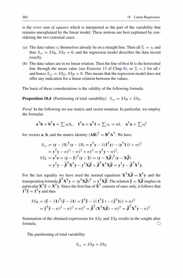
262 18 Linear Regression
is the error sum of squares which is interpreted as the part of the variability thatremains unexplained by the linear model. These notions are best explained by con-sidering the two extremal cases.
(a) The data values yi themselves already lie on a straight line. Then all yi = yi andthus Syy = SSR , SSE = 0, and the regression model describes the data recordexactly.
(b) The data values are in no linear relation. Then the line of best fit is the horizontalline through the mean value (see Exercise 13 of Chap.8), so yi = y for all iand hence Syy = SSE , SSR = 0. This means that the regression model does notoffer any indication for a linear relation between the values.
The basis of these considerations is the validity of the following formula.
Proposition 18.4 (Partitioning of total variability) Syy = SSR + SSE .
Proof In the following we use matrix and vector notation. In particular, we employthe formulas
aTb = bTa = ∑aibi , 1Ta = aT1 = ∑
ai = na, aTa = ∑a2i
for vectors a, b, and the matrix identity (AB)T = BTAT. We have
Syy = (y − y1)T(y − y1) = yTy − y(1Ty) − (yT1)y + n y2
= yTy − n y2 − n y2 + n y2 = yTy − n y2,
SSE = eTe = (y − y)T(y − y) = (y − Xβ)T(y − Xβ)
= yTy − βTXTy − yTXβ + β
TXTXβ = yTy − β
TXTy.
For the last equality we have used the normal equations XTXβ = XTy and the
transposition formula βTXTy = (yTXβ)T = yTXβ. The relation y = Xβ implies in
particularXTy = XTy. Since the first line ofXT consists of ones only, it follows that1Ty = 1Ty and thus
SSR = (y − y1)T (y − y1) = yTy − y( 1Ty ) − ( yT1)y + n y2
= yTy − n y2 − n y2 + n y2 = βT(XTXβ) − n y2 = β
TXTy − n y2.
Summation of the obtained expressions for SSE and SSR results in the sought afterformula. �
The partitioning of total variability
Syy = SSR + SSE
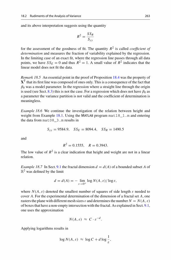
18.2 Rudiments of the Analysis of Variance 263
and its above interpretation suggests using the quantity
R2 = SSRSyy
for the assessment of the goodness of fit. The quantity R2 is called coefficient ofdetermination and measures the fraction of variability explained by the regression.In the limiting case of an exact fit, where the regression line passes through all datapoints, we have SSE = 0 and thus R2 = 1. A small value of R2 indicates that thelinear model does not fit the data.
Remark 18.5 An essential point in the proof of Proposition 18.4 was the property ofXT that its first line was composed of ones only. This is a consequence of the fact thatβ0 was a model parameter. In the regression where a straight line through the originis used (see Sect. 8.3) this is not the case. For a regression which does not have β0 asa parameter the variance partition is not valid and the coefficient of determination ismeaningless.
Example 18.6 We continue the investigation of the relation between height andweight from Example 18.1. Using the MATLAB program mat18_1.m and enteringthe data from mat08_3.m results in
Syy = 9584.9, SSE = 8094.4, SSR = 1490.5
and
R2 = 0.1555, R = 0.3943.
The low value of R2 is a clear indication that height and weight are not in a linearrelation.
Example 18.7 In Sect. 9.1 the fractal dimension d = d(A) of a bounded subset A ofR2 was defined by the limit
d = d(A) = − limε→0+ log N (A, ε)/ log ε,
where N (A, ε) denoted the smallest number of squares of side length ε needed tocover A. For the experimental determination of the dimension of a fractal set A, onerasters the planewith differentmesh sizes ε and determines the number N = N (A, ε)
of boxes that have a non-empty intersectionwith the fractal. As explained in Sect. 9.1,one uses the approximation
N (A, ε) ≈ C · ε−d .
Applying logarithms results in
log N (A, ε) ≈ logC + d log1
ε,
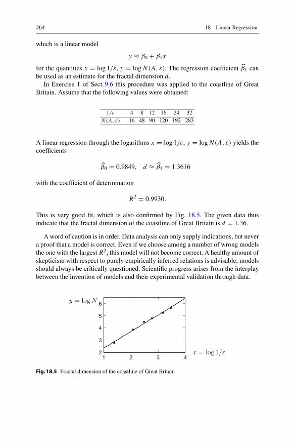
264 18 Linear Regression
which is a linear model
y ≈ β0 + β1x
for the quantities x = log 1/ε, y = log N (A, ε). The regression coefficient β1 canbe used as an estimate for the fractal dimension d.
In Exercise 1 of Sect. 9.6 this procedure was applied to the coastline of GreatBritain. Assume that the following values were obtained:
1/ε 4 8 12 16 24 32N (A, ε) 16 48 90 120 192 283
A linear regression through the logarithms x = log 1/ε, y = log N (A, ε) yields thecoefficients
β0 = 0.9849, d ≈ β1 = 1.3616
with the coefficient of determination
R2 = 0.9930.
This is very good fit, which is also confirmed by Fig. 18.5. The given data thusindicate that the fractal dimension of the coastline of Great Britain is d = 1.36.
A word of caution is in order. Data analysis can only supply indications, but nevera proof that a model is correct. Even if we choose among a number of wrong modelsthe one with the largest R2, this model will not become correct. A healthy amount ofskepticism with respect to purely empirically inferred relations is advisable; modelsshould always be critically questioned. Scientific progress arises from the interplaybetween the invention of models and their experimental validation through data.
1 2 3 42
3
4
5
6y = logN
x = log 1/ε
Fig. 18.5 Fractal dimension of the coastline of Great Britain
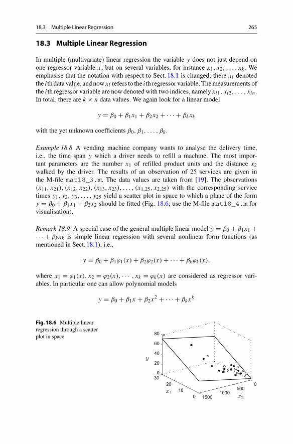
18.3 Multiple Linear Regression 265
18.3 Multiple Linear Regression
In multiple (multivariate) linear regression the variable y does not just depend onone regressor variable x , but on several variables, for instance x1, x2, . . . , xk . Weemphasise that the notation with respect to Sect. 18.1 is changed; there xi denotedthe i th data value, and now xi refers to the i th regressor variable. Themeasurements ofthe i th regressor variable are now denotedwith two indices, namely xi1, xi2, . . . , xin .In total, there are k × n data values. We again look for a linear model
y = β0 + β1x1 + β2x2 + · · · + βk xk
with the yet unknown coefficients β0, β1, . . . , βk .
Example 18.8 A vending machine company wants to analyse the delivery time,i.e., the time span y which a driver needs to refill a machine. The most impor-tant parameters are the number x1 of refilled product units and the distance x2walked by the driver. The results of an observation of 25 services are given inthe M-file mat18_3.m. The data values are taken from [19]. The observations(x11, x21), (x12, x22), (x13, x23), . . . , (x1,25, x2,25) with the corresponding servicetimes y1, y2, y3, . . . , y25 yield a scatter plot in space to which a plane of the formy = β0 + β1x1 + β2x2 should be fitted (Fig. 18.6; use the M-file mat18_4.m forvisualisation).
Remark 18.9 A special case of the general multiple linear model y = β0 + β1x1 +· · · + βk xk is simple linear regression with several nonlinear form functions (asmentioned in Sect. 18.1), i.e.,
y = β0 + β1ϕ1(x) + β2ϕ2(x) + · · · + βkϕk(x),
where x1 = ϕ1(x), x2 = ϕ2(x), · · · , xk = ϕk(x) are considered as regressor vari-ables. In particular one can allow polynomial models
y = β0 + β1x + β2x2 + · · · + βk x
k
Fig. 18.6 Multiple linearregression through a scatterplot in space
010
2030
0500
10001500
0
20
40
60
80
y
x1x2
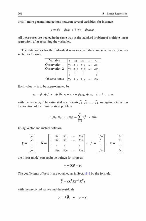
266 18 Linear Regression
or still more general interactions between several variables, for instance
y = β0 + β1x1 + β2x2 + β3x1x2.
All these cases are treated in the same way as the standard problem of multiple linearregression, after renaming the variables.
The data values for the individual regressor variables are schematically repre-sented as follows:
Variable y x1 x2 . . . xkObservation 1 y1 x11 x21 . . . xk1Observation 2 y2 x12 x22 . . . xk2
......
......
...
Observation n yn x1n x2n . . . xkn
Each value yi is to be approximated by
yi = β0 + β1x1i + β2x2i + · · · + βk xki + εi , i = 1, . . . , n
with the errors εi . The estimated coefficients β0, β1, . . . , βk are again obtained asthe solution of the minimisation problem
L(β0, β1, . . . , βk) =n∑
i=1
ε2i → min
Using vector and matrix notation
y =
⎡
⎢⎢⎢⎣
y1y2...
yn
⎤
⎥⎥⎥⎦ , X =
⎡
⎢⎢⎢⎣
1 x11 x21 . . . xk11 x12 x22 . . . xk2...
......
...
1 x1n x2n . . . xkn
⎤
⎥⎥⎥⎦ , β =
⎡
⎢⎢⎢⎣
β0β1...
βk
⎤
⎥⎥⎥⎦ , ε =
⎡
⎢⎢⎢⎣
ε1ε2...
εn
⎤
⎥⎥⎥⎦
the linear model can again be written for short as
y = Xβ + ε.
The coefficients of best fit are obtained as in Sect. 18.1 by the formula
β = (XTX)−1XTy
with the predicted values and the residuals
y = Xβ, e = y − y.

18.3 Multiple Linear Regression 267
The partitioning of total variability
Syy = SSR + SSE
is still valid; the multiple coefficient of determination
R2 = SSR/Syy
is an indicator of the goodness of fit of the model.
Example 18.10 We continue the analysis of the delivery times from Example 18.8.Using the MATLAB program mat18_2.m and entering the data from mat18_3.mresults in
β =⎡
⎣2.34121.61590.0144
⎤
⎦ .
We obtain the model
y = 2.3412 + 1.6159 x1 + 0.0144 x2
with the multiple coefficient of determination of
R2 = 0.9596
and the partitioning of total variability
Syy = 5784.5, SSR = 5550.8, SSE = 233.7
In this example merely (1 − R2) · 100% ≈ 4% of the variability of the data is notexplained by the regression, a very satisfactory goodness of fit.
18.4 Model Fitting andVariable Selection
A recurring problem is to decide which variables should be included in the model.Would the inclusion of x3 = x22 and x4 = x1x2, i.e., the model
y = β0 + β1x1 + β2x2 + β3x22 + β4x1x2,
lead to better results, and can, e.g., the term β2x2 be eliminated subsequently? It isnot desirable to have too many variables in the model. If there are as many variablesas data points, then one can fit the regression exactly through the data and the modelwould loose its predictive power. A criterion will definitely be to reach a value ofR2 which is as large as possible. Another aim is to eliminate variables that do not
268 18 Linear Regression
contribute essentially to the total variability.An algorithmic procedure for identifyingthese variables is the sequential partitioning of total variability.
Sequential partitioning of total variability. We include variables stepwise in themodel, thus consider the increasing sequence of models with corresponding SSR :
y = β0 SSR(β0),
y = β0 + β1x1 SSR(β0, β1),
y = β0 + β1x1 + β2x2 SSR(β0, β1, β2),
......
y = β0 + β1x1 + β2x2 + · · · + βk xk SSR(β0, β1, . . . , βk) = SSR .
Note that SSR(β0) = 0, since in the initial model β0 = y. The additional explana-tory power of the variable x1 is measured by
SSR(β1|β0) = SSR(β0, β1) − 0,
the power of variable x2 (if x1 is already in the model) by
SSR(β2|β0, β1) = SSR(β0, β1, β2) − SSR(β0, β1),
the power of variable xk (if x1, x2, . . . , xk−1 are in the model) by
SSR(βk |β0, β1, . . . , βk−1) = SSR(β0, β1, . . . , βk) − SSR(β0, β1, . . . , βk−1).
Obviously,
SSR(β1|β0) + SSR(β2|β0, β1) + SSR(β3|β0, β1, β2) + · · ·+ SSR(βk |β0, β1, β2, . . . , βk−1) = SSR .
This shows that one can interpret the sequential, partial coefficient of determination
SSR(β j |β0, β1, . . . , β j−1)
Syy
as explanatory power of the variables x j , under the condition that the variablesx1, x2, . . . , x j−1 are already included in the model. This partial coefficient of deter-mination depends on the order of the added variables. This dependency can be elim-inated by averaging over all possible sequences of variables.
Average explanatorypowerof individual coefficients.Onefirst computes all possi-ble sequential, partial coefficients of determination which can be obtained by addingthe variable x j to all possible combinations of the already included variables. Sum-ming up these coefficients and dividing the result by the total number of possibilities,one obtains ameasure for the contribution of the variable x j to the explanatory powerof the model.
18.4 Model Fitting and Variable Selection 269
Average over orderings was proposed by [16]; further details and advanced con-siderations can be found, for instance, in [8,10]. The concept does not use proba-bilistically motivated indicators. Instead it is based on the data and on combinatorics,thus belongs to descriptive data analysis. Such descriptive methods, in contrast to thecommonly used statistical hypothesis testing, do not require additional assumptionswhich may be difficult to justify.
Example 18.11 We compute the explanatory power of the coefficients in the deliverytime problem of Example 18.8. First we fit the two univariate models
y = β0 + β1x1, y = β0 + β2x2
and from that obtain
SSR(β0, β1) = 5382.4, SSR(β0, β2) = 4599.1,
with the regression coefficients β0 = 3.3208, β1 = 2.1762 in the first and β0 =4.9612, β2 = 0.0426 in the second case. With the already computed values of thebivariate model
SSR(β0, β1, β2) = SSR = 5550.8, Syy = 5784.5
from Example 18.10 we obtain the two sequences
SSR(β1|β0) = 5382.4 ≈ 93.05% of SyySSR(β2|β0, β1) = 168.4 ≈ 2.91% of Syy
and
SSR(β2|β0) = 4599.1 ≈ 79.51% of SyySSR(β1|β0, β2) = 951.7 ≈ 16.45% of Syy .
The average explanatory power of the variable x1 (or of the coefficient β1) is
1
2
(93.05 + 16.45
)% = 54.75%,
the one of the variable x2 is
1
2
(2.91 + 79.51
)% = 41.21%;
the remaining 4.04% stay unexplained. The result is represented in Fig. 18.7.
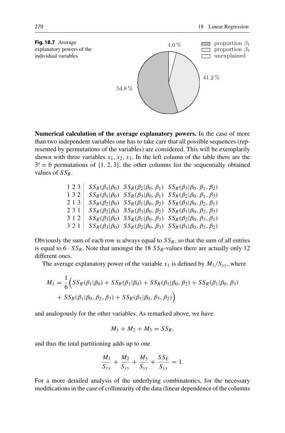
270 18 Linear Regression
Fig. 18.7 Averageexplanatory powers of theindividual variables
54.8%
41.2%
4.0%
unexplainedproportion β2
proportion β1
Numerical calculation of the average explanatory powers. In the case of morethan two independent variables one has to take care that all possible sequences (rep-resented by permutations of the variables) are considered. This will be exemplarilyshown with three variables x1, x2, x3. In the left column of the table there are the3! = 6 permutations of {1, 2, 3}, the other columns list the sequentially obtainedvalues of SSR .
1 2 3 SSR(β1|β0) SSR(β2|β0, β1) SSR(β3|β0, β1, β2)
1 3 2 SSR(β1|β0) SSR(β3|β0, β1) SSR(β2|β0, β1, β3)
2 1 3 SSR(β2|β0) SSR(β1|β0, β2) SSR(β3|β0, β2, β1)
2 3 1 SSR(β2|β0) SSR(β3|β0, β2) SSR(β1|β0, β2, β3)
3 1 2 SSR(β3|β0) SSR(β1|β0, β3) SSR(β2|β0, β3, β1)
3 2 1 SSR(β3|β0) SSR(β2|β0, β3) SSR(β1|β0, β3, β2)
Obviously the sum of each row is always equal to SSR , so that the sum of all entriesis equal to 6 · SSR . Note that amongst the 18 SSR-values there are actually only 12different ones.
The average explanatory power of the variable x1 is defined by M1/Syy , where
M1 = 1
6
(SSR(β1|β0) + SSR(β1|β0) + SSR(β1|β0, β2) + SSR(β1|β0, β3)
+ SSR(β1|β0, β2, β3) + SSR(β1|β0, β3, β2))
and analogously for the other variables. As remarked above, we have
M1 + M2 + M3 = SSR,
and thus the total partitioning adds up to one
M1
Syy+ M2
Syy+ M3
Syy+ SSE
Syy= 1.
For a more detailed analysis of the underlying combinatorics, for the necessarymodifications in the case of collinearity of the data (linear dependence of the columns
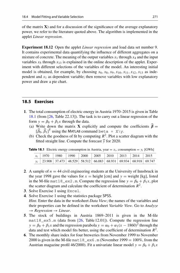
18.4 Model Fitting and Variable Selection 271
of the matrix X) and for a discussion of the significance of the average explanatorypower, we refer to the literature quoted above. The algorithm is implemented in theapplet Linear regression.
Experiment 18.12 Open the applet Linear regression and load data set number 9.It contains experimental data quantifying the influence of different aggregates on amixture of concrete. The meaning of the output variables x1 through x4 and the inputvariables x5 through x13 is explained in the online description of the applet. Exper-iment with different selections of the variables of the model. An interesting initialmodel is obtained, for example, by choosing x6, x8, x9, x10, x11, x12, x13 as inde-pendent and x1 as dependent variable; then remove variables with low explanatorypower and draw a pie chart.
18.5 Exercises
1. The total consumption of electric energy in Austria 1970–2015 is given in Table18.1 (from [26, Table 22.13]). The task is to carry out a linear regression of theform y = β0 + β1x through the data.(a) Write down the matrix X explicitly and compute the coefficients β =
[β0, β1]T using the MATLAB command beta = X\y.(b) Check the goodness of fit by computing R2. Plot a scatter diagram with the
fitted straight line. Compute the forecast y for 2020.
Table 18.1 Electric energy consumption in Austria, year = xi , consumption = yi [GWh]
xi 1970 1980 1990 2000 2005 2010 2013 2014 2015
yi 23.908 37.473 48.529 58.512 66.083 68.931 69.934 68.918 69.747
2. A sample of n = 44 civil engineering students at the University of Innsbruck inthe year 1998 gave the values for x = height [cm] and y = weight [kg], listedin the M-file mat18_ex2.m. Compute the regression line y = β0 + β1x , plotthe scatter diagram and calculate the coefficient of determination R2.
3. Solve Exercise 1 using Excel.4. Solve Exercise 1 using the statistics package SPSS.
Hint. Enter the data in the worksheet Data View; the names of the variables andtheir properties can be defined in the worksheet Variable View. Go to Analyze→ Regression → Linear.
5. The stock of buildings in Austria 1869–2011 is given in the M-filemat18_ex5.m (data from [26, Table12.01]). Compute the regression liney = β0 + β1x and the regression parabola y = α0 + α1(x − 1860)2 through thedata and test which model fits better, using the coefficient of determination R2.
6. The monthly share index for four breweries from November 1999 to November2000 is given in the M-file mat18_ex6.m (November 1999= 100%, from theAustrian magazine profil 46/2000). Fit a univariate linear model y = β0 + β1x
272 18 Linear Regression
to each of the four data sets (x . . . date, y . . . share index), plot the results infour equally scaled windows, evaluate the results by computing R2 and checkwhether the caption provided by profil is justified by the data. For the calculationyou may use the MATLAB program mat18_1.m.Hint. A solution is suggested in the M-file mat18_exsol6.m.
7. Continuation of Exercise 5, stock of buildings in Austria. Fit the model
y = β0 + β1x + β2(x − 1860)2
and compute SSR = SSR(β0, β1, β2) and Syy . Further, analyse the increase ofexplanatory power through adding the respective missing variable in the modelsof Exercise 5, i.e., compute SSR(β2|β0, β1) and SSR(β1|β0, β2) as well as theaverage explanatory power of the individual coefficients. Comparewith the resultfor data set number 5 in the applet Linear regression.
8. TheM-file mat18_ex8.m contains the mileage per gallon y of 30 cars depend-ing on the engine displacement x1, the horsepower x2, the overall length x3 andthe weight x4 of the vehicle (from: Motor Trend 1975, according to [19]). Fitthe linear model
y = β0 + β1x1 + β2x2 + β3x3 + β4x4
and estimate the explanatory power of the individual coefficients through a sim-ple sequential analysis
SSR(β1|β0), SSR(β2|β0, β1), SSR(β3|β0, β1, β2), SSR(β4|β0, β1, β2, β3).
Compare your result with the average explanatory power of the coefficients fordata set number 2 in the applet Linear regression.Hint. A suggested solution is given in the M-file mat18_exsol8.m.
9. Check the results of Exercises 2 and 6 using the applet Linear regression (datasets 1 and 4); likewise for the Examples 18.1 and 18.8 with the data sets 8 and3. In particular, investigate in data set 8 whether height, weight and the risk ofbreaking a leg are in any linear relation.
10. Continuation of Exercise 14 from Sect. 8.4. A more accurate linear approxima-tion to the relation between shear strength τ and normal stress σ is deliveredby Coulomb’s model τ = c + kσ where k = tan ϕ and c [kPa] is interpretedas cohesion. Recompute the regression model of Exercise 14 in Sect. 8.4 withnonzero intercept. Check that the resulting cohesion is indeed small as comparedto the applied stresses, and compare the resulting friction angles.
11. (Change point analysis) The consumer prize data from Example 8.21 suggestthat there might be a change in the slope of the regression line around the year2013, see also Fig. 8.9. Given data (x1, y1), . . . , (xn, yn)with ordered data pointsx1 < x2 < . . . < xn , phenomena of this type can be modelled by a piecewiselinear regression
y ={
α0 + α1x, x ≤ x∗,β0 + β1x, x ≥ x∗.
18.5 Exercises 273
If the slopes α1 and α2 are different, x∗ is called a change point. A change pointcan be detected by fitting models
yi ={
α0 + α1xi , i = 1, . . . ,m,
β0 + β1xi , i = m + 1, . . . , n
and varying the index m between 2 and n − 1 until a two-line model with thesmallest total residual sum of squares SSR(α0, α1) + SSR(β0, β1) is found. Thechange point x∗ is the point of intersection of the two predicted lines. (If theoverall one-line model has the smallest SSR , there is no change point.)Find out whether there is a change point in the data of Example 8.21. If so, locateit and use the two-line model to predict the consumer price index for 2017.
12. Atmospheric CO2 concentration has been recorded at Mauna Loa, Hawai, since1958. The yearly averages (1959–2008) in ppm can be found in the MATLAB
program mat18_ex12.m; the data are from [14].(a) Fit an exponential model y = α0 eα1x to the data and compare the prediction
with the actual data (2017: 406.53 ppm).Hint. Taking logarithms leads to the linear model z = β0 + β1x with z =log y, β0 = logα0, β1 = α1. Estimate the coefficients β0, β1 and computeα0, α1 as well as the prediction for y.
(b) Fit a square exponential model y = α0 eα1x+α2x2 to the data and checkwhether this yields a better fit and prediction.
19Differential Equations
In this chapter we discuss the theory of initial value problems for ordinary differentialequations. We limit ourselves to scalar equations here; systems will be discussed inthe next chapter.
After presenting the general definition of a differential equation and the geometricsignificance of its direction field, we start with a detailed discussion of first-orderlinear equations. As important applications we discuss the modelling of growth anddecay processes. Subsequently, we investigate questions of existence and (local)uniqueness of the solution of general differential equations and discuss the methodof power series. We also study the qualitative behaviour of solutions close to anequilibrium point. Finally, we discuss the solution of second-order linear problemswith constant coefficients.
19.1 Initial Value Problems
Differential equations are equations involving a (sought after) function and its deriva-tive(s). They play a decisive role in modelling time-dependent processes.
Definition 19.1 Let D ⊂ R2 be open and f : D ⊂ R
2 → R continuous. The equa-tion
y′(x) = f(x, y(x)
)
is called (an ordinary) first-order differential equation. A solution is a differentiablefunction y : I → D which satisfies the equation for all x ∈ I .
© Springer Nature Switzerland AG 2018M. Oberguggenberger and A. Ostermann, Analysis for Computer Scientists,Undergraduate Topics in Computer Science,https://doi.org/10.1007/978-3-319-91155-7_19
275
276 19 Differential Equations
One often suppresses the independent variable x in the notation and writes theabove problem for short as
y′ = f (x, y).
The sought after function y in this equation is also called the dependent variable(depending on x).
Inmodelling time-dependent processes, one usually denotes the independent vari-able by t (for time) and the dependent variable by x = x(t). In this case one writesthe first-order differential equation as
x(t) = f(t, x(t)
)
or for short as x = f (t, x).
Example 19.2 (Separation of the variables) We want to find all functions y = y(x)satisfying the equation y′(x) = x · y(x)2. In this example one obtains the solutionsby separating the variables. For y �= 0 one divides the differential equation by y2
and gets
1
y2· y′ = x .
The left-hand side of this equation is of the form g(y) · y′. LetG(y) be an antideriva-tive of g(y). According to the chain rule, and recalling that y is a function of x , weobtain
d
dxG(y) = d
dyG(y) · dy
dx= g(y) · y′.
In our example we have g(y) = y−2 and G(y) = −y−1, consequently
d
dx
(−1
y
)= 1
y2· y′ = x .
Integration of this equation with respect to x results in
−1
y= x2
2+ C,
where C denotes an arbitrary integration constant. By elementary manipulations wefind
y = 1
−x2/2 − C= 2
K − x2
with the constant K = −2C .The function y = 0 is also a solution of the differential equation. Formally, one
obtains it from the above solution by setting K = ∞. The example shows that differ-ential equations have infinitely many solutions in general. By requiring an additionalcondition, a unique solution can be selected. For example, setting y(0) = 1 givesy(x) = 2/(2 − x2).

19.1 Initial Value Problems 277
Fig. 19.1 The direction fieldof y′ = −2xy/(x2 + 2y)
−2 0 2−4
−2
0
2
y
x
Definition 19.3 The differential equation y′(x) = f(x, y(x)
)together with the
additional condition y(x0) = y0, i.e.,
y′(x) = f(x, y(x)
), y(x0) = y0,
is called initial value problem. A solution of an initial value problem is a (continu-ously) differentiable function y(x), which satisfies the differential equation and theinitial condition y(x0) = y0.
Geometric interpretation of a differential equation. For a given first-order differ-ential equation
y′ = f (x, y), (x, y) ∈ D ⊂ R2
one searches for a differentiable function y = y(x)whose graph lies in D and whosetangents have the slopes tanϕ = y′(x) = f
(x, y(x)
)for each x . By plotting short
arrowswith slopes tanϕ = f (x, y) at the points (x, y) ∈ D one obtains the directionfield of the differential equation.Thedirectionfield is tangential to the solution curvesand offers a good visual impression of their shapes. Figure19.1 shows the directionfield of the differential equation
y′ = − 2xy
x2 + 2y.
The right-hand side has singularities along the curve y = −x2/2 which is reflectedby the behaviour of the arrows in the lower part of the figure.
Experiment 19.4 Visualise the direction field of the above differential equationwiththe applet Dynamical systems in the plane.
278 19 Differential Equations
19.2 First-Order Linear Differential Equations
Let a(x) and g(x) be functions defined on some interval. The equation
y′ + a(x) y = g(x)
is called a first-order linear differential equation.The function a is the coefficient, theright-hand side g is called inhomogeneity. The differential equation is called homo-geneous, if g = 0, otherwise inhomogeneous. First we state the following importantresult.
Proposition 19.5 (Superposition principle) If y and z are solutions of a lineardifferential equation with possibly different inhomogeneities
y′(x) + a(x) y(x) = g(x),
z′(x) + a(x) z(x) = h(x),
then their linear combination
w(x) = αy(x) + βz(x), α, β ∈ R
solves the linear differential equation
w′(x) + a(x) w(x) = αg(x) + βh(x).
Proof This so-called superposition principle follows from the linearity of the deriva-tive and the linearity of the equation. �
In a first step we compute all solutions of the homogeneous equation. We will usethe superposition principle later to find all solutions of the inhomogeneous equation.
Proposition 19.6 The general solution of the homogeneous differential equation
y′ + a(x) y = 0
is
yh(x) = K e−A(x)
with K ∈ R and an arbitrary antiderivative A(x) of a(x).
Proof For y �= 0 we separate the variables
1
y· y′ = −a(x)

19.2 First-Order Linear Differential Equations 279
0 2 4 6 8 10
−4
−2
0
2
4
y
x 0 2 4 6 8 10
−4
−2
0
2
4
y
x
Fig. 19.2 The direction field of y′ = y (left) and y′ = −y (right)
and used
dylog |y| = 1
y
to obtain
log |y| = −A(x) + C
by integrating the equation. From that we infer
|y(x)| = e−A(x)eC .
This formula shows that y(x) cannot change sign since the right-hand side is neverzero. Thus K = eC · sign y(x) is a constant as well, and the formula
y(x) = sign y(x) · |y(x)| = K e−A(x), K ∈ R
yields all solutions of the homogeneous equation. �
Example 19.7 The linear differential equation
x = ax
with constant coefficient a has the general solution
x(t) = K eat , K ∈ R.
The constant K is determined by x(0), for example.
The direction field of the differential equation y′ = ay (depending on the sign ofthe coefficient) is shown in Fig. 19.2.
Interpretation. Let x(t) be a time-dependent function which describes a growth ordecay process (population increase/decrease, change of mass, etc.). We consider a
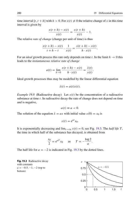
280 19 Differential Equations
time interval [t, t + h] with h > 0. For x(t) �= 0 the relative change of x in this timeinterval is given by
x(t + h) − x(t)
x(t)= x(t + h)
x(t)− 1.
The relative rate of change (change per unit of time) is thus
x(t + h) − x(t)
t + h − t· 1
x(t)= x(t + h) − x(t)
h · x(t) .
For an ideal growth process this rate only depends on time t . In the limit h → 0 thisleads to the instantaneous relative rate of change
a(t) = limh→0
x(t + h) − x(t)
h · x(t) = x(t)
x(t).
Ideal growth processes thus may be modelled by the linear differential equation
x(t) = a(t)x(t).
Example 19.8 (Radioactive decay) Let x(t) be the concentration of a radioactivesubstance at time t . In radioactive decay the rate of change does not depend on timeand is negative,
a(t) ≡ a < 0.
The solution of the equation x = ax with initial value x(0) = x0 is
x(t) = eat x0.
It is exponentially decreasing and limt→∞ x(t) = 0, see Fig. 19.3. The half life T ,the time in which half of the substance has decayed, is obtained from
x02
= eaT x0 as T = − log 2
a.
The half life for a = −2 is indicated in Fig. 19.3 by the dotted lines.
Fig. 19.3 Radioactive decaywith constantsa = −0.5,−1,−2 (top tobottom)
0 0.5 1 1.50
0.25
0.5
0.75
1
t
a = −0.5
x
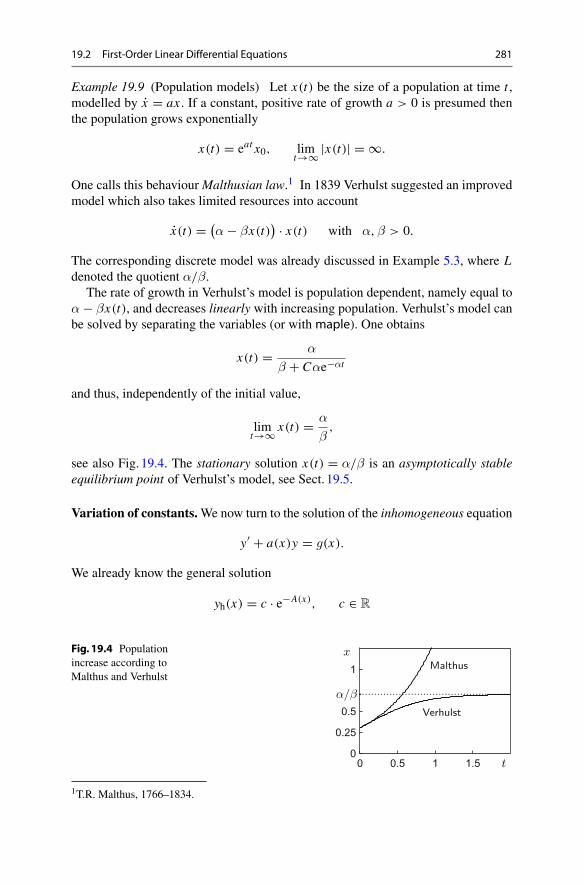
19.2 First-Order Linear Differential Equations 281
Example 19.9 (Population models) Let x(t) be the size of a population at time t ,modelled by x = ax . If a constant, positive rate of growth a > 0 is presumed thenthe population grows exponentially
x(t) = eat x0, limt→∞ |x(t)| = ∞.
One calls this behaviourMalthusian law.1 In 1839 Verhulst suggested an improvedmodel which also takes limited resources into account
x(t) = (α − βx(t)
) · x(t) with α,β > 0.
The corresponding discrete model was already discussed in Example 5.3, where Ldenoted the quotient α/β.
The rate of growth in Verhulst’s model is population dependent, namely equal toα − βx(t), and decreases linearly with increasing population. Verhulst’s model canbe solved by separating the variables (or withmaple). One obtains
x(t) = α
β + Cαe−αt
and thus, independently of the initial value,
limt→∞ x(t) = α
β,
see also Fig. 19.4. The stationary solution x(t) = α/β is an asymptotically stableequilibrium point of Verhulst’s model, see Sect. 19.5.
Variation of constants.We now turn to the solution of the inhomogeneous equation
y′ + a(x)y = g(x).
We already know the general solution
yh(x) = c · e−A(x), c ∈ R
Fig. 19.4 Populationincrease according toMalthus and Verhulst
0 0.5 1 1.50
0.25
0.5
1
α/β
t
x
Verhulst
Malthus
1T.R. Malthus, 1766–1834.
282 19 Differential Equations
of the homogeneous equation with the antiderivative
A(x) =∫ x
x0a(ξ) dξ.
We look for a particular solution of the inhomogeneous equation of the form
yp(x) = c(x) · yh(x) = c(x) · e−A(x),
where we allow the constant c = c(x) to be a function of x (variation of constants).Substituting this formula into the inhomogeneous equation and differentiating usingthe product rule yields
y′p(x) + a(x) yp(x) = c′(x) yh(x) + c(x) y′
h(x) + a(x) yp(x)
= c′(x) yh(x) − a(x) c(x) yh(x) + a(x) yp(x)
= c′(x) yh(x).
If one equates this expression with the inhomogeneity g(x), one recognises that c(x)fulfils the differential equation
c′(x) = eA(x)g(x)
which can be solved by integration
c(x) =∫ x
x0eA(ξ)g(ξ) dξ.
We thus obtain the following proposition.
Proposition 19.10 The differential equation
y′ + a(x)y = g(x)
has the general solution
y(x) = e−A(x)(∫ x
x0eA(ξ)g(ξ) dξ + K
)
with A(x) = ∫ xx0a(ξ) dξ and an arbitrary constant K ∈ R.
Proof By the above considerations, the function y(x) is a solution of the differen-tial equation y′ + a(x)y = g(x). Conversely, let z(x) be any other solution. Then,according to the superposition principle, the difference z(x) − y(x) is a solution ofthe homogeneous equation, so
z(x) = y(x) + c e−A(x).
Therefore, z(x) also has the form stated in the proposition. �

19.2 First-Order Linear Differential Equations 283
Corollary 19.11 Let yp be an arbitrary solution of the inhomogeneous linear dif-ferential equation
y′ + a(x)y = g(x).
Then, its general solution can be written as
y(x) = yp(x) + yh(x) = yp(x) + K e−A(x), K ∈ R.
Proof This statement follows from the proof of Proposition 19.10 or directly fromthe superposition principle. �
Example 19.12 We solve the problem y′ + 2y = e4x + 1. The solution of the homo-geneous equation is yh(x) = c e−2x . A particular solution can be found by variationof constants. From
c(x) =∫ x
0e2ξ
(e4ξ + 1
)dξ = 1
6e6x + 1
2e2x − 2
3
it follows that
yp(x) = 1
6e4x − 2
3e−2x + 1
2.
The general solution is thus
y(x) = yp(x) + yh(x) = K e−2x + 1
6e4x + 1
2.
Here, we have combined the two terms containing e−2x . The new constant K can bedetermined from an additional initial condition y(0) = α, namely
K = α − 2
3.
19.3 Existence and Uniqueness of the Solution
Finding analytic solutions of differential equations can be a difficult problem andis often impossible. Apart from some types of differential equations (e.g., linearproblems or equations with separable variables), there is no general procedure todetermine the solution explicitly. Thus numerical methods are used frequently (seeChap.21). In the following we discuss the existence and uniqueness of solutions ofgeneral initial value problems.

284 19 Differential Equations
Proposition 19.13 (Peano’s theorem2) If the function f is continuous in a neigh-bourhood of (x0, y0), then the initial value problem
y′ = f (x, y), y(x0) = y0
has a solution y(x) for x close to x0.
Instead of a proof (see [11, Part I, Theorem7.6]), we discuss the limitations ofthis proposition. First it only guarantees the existence of a local solution in theneighbourhood of the initial value. The next example shows that one cannot expectmore, in general.
Example 19.14 We solve the differential equation x = x2, x(0) = 1. Separation ofthe variables yields
∫dx
x2=
∫dt = t + C,
and thus
x(t) = 1
1 − t.
This function has a singularity at t = 1, where the solution ceases to exist. Thisbehaviour is called blow up.
Furthermore, Peano’s theorem does not give any information on how many solu-tions an initial value problem has. In general, solutions need not be unique, as it isshown in the following example.
Example 19.15 The initial value problem y′ = 2√|y|, y(0) = 0 has infinitely many
solutions
y(x) =
⎧⎪⎨
⎪⎩
(x − b)2, b < x,
0, −a ≤ x ≤ b,
−(x − a)2, x < −a,
a, b ≥ 0 arbitrary.
For example, for x < −a, one verifies at once
y′(x) = −2(x − a) = 2(a − x) = 2|x − a| = 2√
(x − a)2 = 2√|y|.
Thus the continuity of f is not sufficient to guarantee the uniqueness of the solutionof initial value problems. One needs somewhat more regularity, namely Lipschitz3
continuity with respect to the second variable (see also Definition C.14).
2G. Peano, 1858–1932.3R. Lipschitz, 1832–1903.
19.3 Existence and Uniqueness of the Solution 285
Definition 19.16 Let D ⊂ R2 and f : D → R. The function f is said to satisfy
a Lipschitz condition with Lipschitz constant L on D, if the inequality | f (x, y) −f (x, z)| ≤ L |y − z| holds for all points (x, y), (x, z) ∈ D.
According to the mean value theorem (Proposition 8.4)
f (x, y) − f (x, z) = ∂ f
∂y(x, ξ)(y − z)
for every differentiable function. If the derivative is bounded, then the function sat-isfies a Lipschitz condition. In this case one can choose
L = sup
∣∣∣∣∂ f
∂y(x, ξ)
∣∣∣∣ .
Counterexample 19.17 The function g(x, y) = √|y| does not satisfy a Lipschitzcondition in any D that contains a point with y = 0 because
|g(x, y) − g(x, 0)||y − 0| =
√|y||y| = 1√|y| → ∞ for y → 0.
Proposition 19.18 If the function f satisfies a Lipschitz condition in the neighbour-hood of (x0, y0), then the initial value problem
y′ = f (x, y), y(x0) = y0
has a unique solution y(x) for x close to x0.
Proof We only show uniqueness, the existence of a solution y(x) on the interval[x0, x0 + H ] follows (for small H ) from Peano’s theorem. Uniqueness is provenindirectly. Assume that z is another solution, different from y, on the interval[x0, x0 + H ] with z(x0) = y0. The number
x1 = inf{x ∈ R ; x0 ≤ x ≤ x0 + H and y(x) �= z(x)
}
is thus well-defined. We infer from the continuity of y and z that y(x1) = z(x1).Now we choose h > 0 so small that x1 + h ≤ x0 + H and integrate the differentialequation
y′(x) = f(x, y(x)
)
from x1 to x1 + h. This gives
y(x1 + h) − y(x1) =∫ x1+h
x1y′(x) dx =
∫ x1+h
x1f(x, y(x)
)dx

286 19 Differential Equations
and
z(x1 + h) − y(x1) =∫ x1+h
x1f(x, z(x)
)dx .
Subtracting the first formula above from the second yields
z(x1 + h) − y(x1 + h) =∫ x1+h
x1
(f(x, z(x)
) − f(x, y(x)
))dx .
The Lipschitz condition on f gives
|z(x1 + h) − y(x1 + h)| ≤∫ x1+h
x1
∣∣ f
(x, z(x)
) − f(x, y(x)
)∣∣ dx
≤ L∫ x1+h
x1|z(x) − y(x)| dx .
Let now
M = max{|z(x) − y(x)| ; x1 ≤ x ≤ x1 + h
}.
Due to the continuity of y and z, this maximum exists, see the discussion afterProposition 6.15. After possibly decreasing h this maximum is attained at x1 + hand
M = |z(x1 + h) − y(x1 + h)| ≤ L∫ x1+h
x1M dx ≤ Lh M.
For a sufficiently small h, namely Lh < 1, the inequality
M ≤ Lh M
implies M = 0. Since one can choose h arbitrarily small, y(x) = z(x) holds true forx1 ≤ x ≤ x1 + h in contradiction to the definition of x1. Hence the assumed differentsolution z does not exist. �
19.4 Method of Power Series
We have encountered several examples of functions that can be represented as series,e.g. in Chap.12. Motivated by this we try to solve the initial value problem
y′ = f (x, y), y(x0) = y0
by means of a series
y(x) =∞∑
n=0
an(x − x0)n .

19.4 Method of Power Series 287
Wewill use the fact that convergent power series can be differentiated and rearrangedterm by term, see for instance [3, Chap.9, Corollary7.4].
Example 19.19 We solve once more the linear initial value problem
y′ = y, y(0) = 1.
For that we differentiate the ansatz
y(x) =∞∑
n=0
anxn = a0 + a1x + a2x
2 + a3x3 + · · ·
term by term with respect to x
y′(x) =∞∑
n=1
nanxn−1 = a1 + 2a2x + 3a3x
2 + 4a4x3 + · · ·
and substitute the result into the differential equation to get
a1 + 2a2x + 3a3x2 + 4a4x
3 + · · · = a0 + a1x + a2x2 + a3x
3 + · · ·
Since this equation has to hold for all x , the unknowns an can be determined byequating the coefficients of same powers of x . This gives
a1 = a0, 2a2 = a1,3a3 = a2, 4a4 = a3,
and so on. Due to a0 = y(0) = 1 this infinite system of equations can be solvedrecursively. One obtains
a0 = 1, a1 = 1, a2 = 1
2! , a3 = 1
3! , . . . , an = 1
n!and thus the (expected) solution
y(x) =∞∑
n=0
xn
n! = ex .
Example 19.20 (A particular Riccati differential equation4) For the solution of theinitial value problem
y′ = y2 + x2, y(0) = 1,
4J.F. Riccati, 1676–1754.
288 19 Differential Equations
we make the ansatz
y(x) =∞∑
n=0
anxn = a0 + a1x + a2x
2 + a3x3 + · · ·
The initial condition y(0) = 1 immediately gives a0 = 1. First, we compute theproduct (see also PropositionC.10)
y(x)2 = (1 + a1x + a2x2 + a3x
3 + · · · )2= 1 + 2a1x + (a21 + 2a2)x
2 + (2a3 + 2a2a1)x3 + · · ·
and substitute it into the differential equation
a1 + 2a2x + 3a3x2 + 4a4x
3 + · · ·= 1 + 2a1x + (1 + a21 + 2a2)x
2 + (2a3 + 2a2a1)x3 + · · ·
Equating coefficients results in
a1 = 1,
2a2 = 2a1, a2 = 1
3a3 = 1 + a21 + 2a2, a3 = 4/3
4a4 = 2a3 + 2a2a1, a4 = 7/6, . . .
Thus we obtain a good approximation to the solution for small x
y(x) = 1 + x + x2 + 4
3x3 + 7
6x4 + O(x5).
Themaple command
dsolve({diff(y(x),x)=xˆ2+y(x)ˆ2, y(0)=1}, y(x), series);
carries out the above computations.
19.5 Qualitative Theory
Often one can describe the qualitative behaviour of the solutions of differential equa-tions without solving the equations themselves. As the simplest case we discuss thestability of nonlinear differential equations in the neighbourhood of an equilibriumpoint. A differential equation is called autonomous, if its right-hand side does notexplicitly depend on the independent variable.
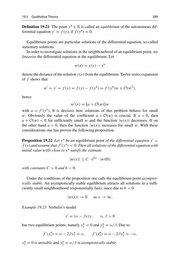
19.5 Qualitative Theory 289
Definition 19.21 The point y� ∈ R is called an equilibrium of the autonomous dif-ferential equation y′ = f (y), if f (y�) = 0.
Equilibrium points are particular solutions of the differential equation, so-calledstationary solutions.
In order to investigate solutions in the neighbourhood of an equilibrium point, welinearise the differential equation at the equilibrium. Let
w(x) = y(x) − y�
denote the distance of the solution y(x) from the equilibrium. Taylor series expansionof f shows that
w′ = y′ = f (y) = f (y) − f (y�) = f ′(y�)w + O(w2),
hence
w′(x) = (a + O(w)
)w
with a = f ′(y�). It is decisive how solutions of this problem behave for smallw. Obviously the value of the coefficient a + O(w) is crucial. If a < 0, thena + O(w) < 0 for sufficiently small w and the function |w(x)| decreases. If onthe other hand a > 0, then the function |w(x)| increases for small w. With theseconsiderations one has proven the following proposition.
Proposition 19.22 Let y� be an equilibrium point of the differential equation y′ =f (y) and assume that f ′(y�) < 0. Then all solutions of the differential equation withinitial value w(0) close to y� satisfy the estimate
|w(x)| ≤ C · ebx · |w(0)|with constants C > 0 and b < 0.
Under the conditions of the proposition one calls the equilibrium point asymptot-ically stable. An asymptotically stable equilibrium attracts all solutions in a suffi-ciently small neighbourhood (exponentially fast), since due to b < 0
|w(x)| → 0 as x → ∞.
Example 19.23 Verhulst’s model
y′ = (α − βy)y, α,β > 0
has two equilibrium points, namely y�1 = 0 and y�
2 = α/β. Due to
f ′(y�1) = α − 2βy�
1 = α, f ′(y�2) = α − 2βy�
2 = −α,
y�1 = 0 is unstable and y�
2 = α/β is asymptotically stable.
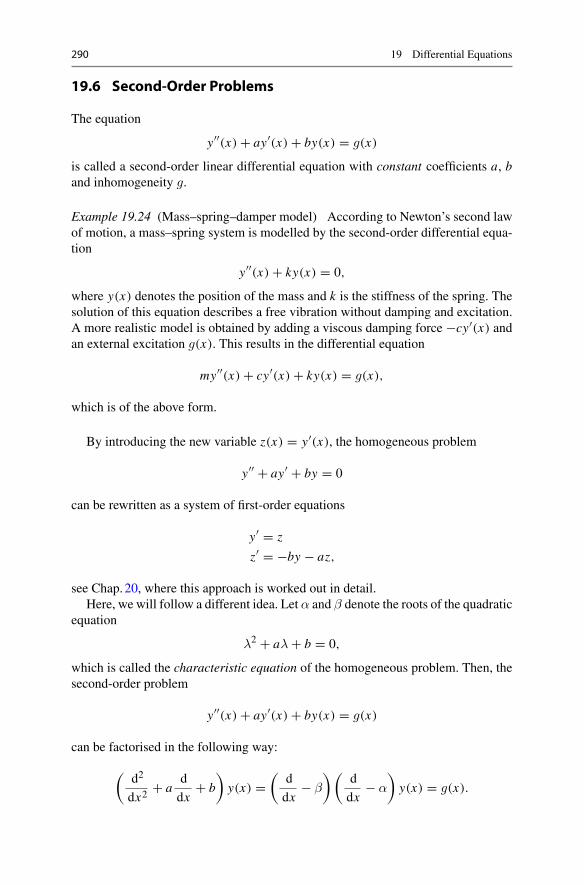
290 19 Differential Equations
19.6 Second-Order Problems
The equation
y′′(x) + ay′(x) + by(x) = g(x)
is called a second-order linear differential equation with constant coefficients a, band inhomogeneity g.
Example 19.24 (Mass–spring–damper model) According to Newton’s second lawof motion, a mass–spring system is modelled by the second-order differential equa-tion
y′′(x) + ky(x) = 0,
where y(x) denotes the position of the mass and k is the stiffness of the spring. Thesolution of this equation describes a free vibration without damping and excitation.A more realistic model is obtained by adding a viscous damping force −cy′(x) andan external excitation g(x). This results in the differential equation
my′′(x) + cy′(x) + ky(x) = g(x),
which is of the above form.
By introducing the new variable z(x) = y′(x), the homogeneous problem
y′′ + ay′ + by = 0
can be rewritten as a system of first-order equations
y′ = z
z′ = −by − az,
see Chap.20, where this approach is worked out in detail.Here, we will follow a different idea. Let α and β denote the roots of the quadratic
equation
λ2 + aλ + b = 0,
which is called the characteristic equation of the homogeneous problem. Then, thesecond-order problem
y′′(x) + ay′(x) + by(x) = g(x)
can be factorised in the following way:
(d2
dx2+ a
d
dx+ b
)y(x) =
(d
dx− β
) (d
dx− α
)y(x) = g(x).
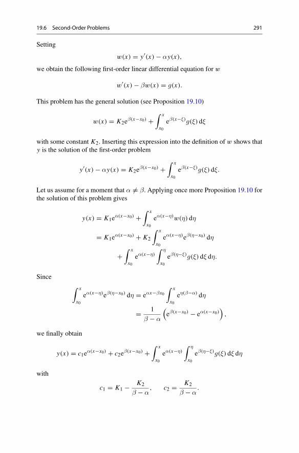
19.6 Second-Order Problems 291
Setting
w(x) = y′(x) − αy(x),
we obtain the following first-order linear differential equation for w
w′(x) − βw(x) = g(x).
This problem has the general solution (see Proposition 19.10)
w(x) = K2eβ(x−x0) +
∫ x
x0eβ(x−ξ)g(ξ) dξ
with some constant K2. Inserting this expression into the definition of w shows thaty is the solution of the first-order problem
y′(x) − αy(x) = K2eβ(x−x0) +
∫ x
x0eβ(x−ξ)g(ξ) dξ.
Let us assume for a moment that α �= β. Applying once more Proposition 19.10 forthe solution of this problem gives
y(x) = K1eα(x−x0) +
∫ x
x0eα(x−η)w(η) dη
= K1eα(x−x0) + K2
∫ x
x0eα(x−η)eβ(η−x0) dη
+∫ x
x0eα(x−η)
∫ η
x0eβ(η−ξ)g(ξ) dξ dη.
Since∫ x
x0eα(x−η)eβ(η−x0) dη = eαx−βx0
∫ x
x0eη(β−α) dη
= 1
β − α
(eβ(x−x0) − eα(x−x0)
),
we finally obtain
y(x) = c1eα(x−x0) + c2e
β(x−x0) +∫ x
x0eα(x−η)
∫ η
x0eβ(η−ξ)g(ξ) dξ dη
with
c1 = K1 − K2
β − α, c2 = K2
β − α.
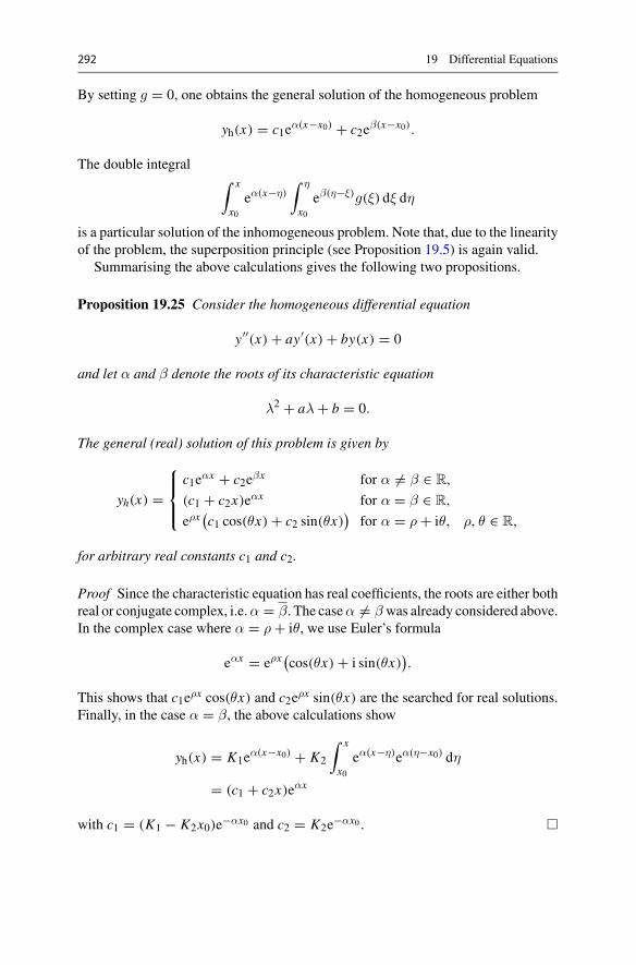
292 19 Differential Equations
By setting g = 0, one obtains the general solution of the homogeneous problem
yh(x) = c1eα(x−x0) + c2e
β(x−x0).
The double integral∫ x
x0eα(x−η)
∫ η
x0eβ(η−ξ)g(ξ) dξ dη
is a particular solution of the inhomogeneous problem. Note that, due to the linearityof the problem, the superposition principle (see Proposition 19.5) is again valid.
Summarising the above calculations gives the following two propositions.
Proposition 19.25 Consider the homogeneous differential equation
y′′(x) + ay′(x) + by(x) = 0
and let α and β denote the roots of its characteristic equation
λ2 + aλ + b = 0.
The general (real) solution of this problem is given by
yh(x) =
⎧⎪⎨
⎪⎩
c1eαx + c2eβx for α �= β ∈ R,
(c1 + c2x)eαx for α = β ∈ R,
eρx(c1 cos(θx) + c2 sin(θx)
)for α = ρ + iθ, ρ, θ ∈ R,
for arbitrary real constants c1 and c2.
Proof Since the characteristic equation has real coefficients, the roots are either bothreal or conjugate complex, i.e.α = β. The caseα �= β was already considered above.In the complex case where α = ρ + iθ, we use Euler’s formula
eαx = eρx(cos(θx) + i sin(θx)).
This shows that c1eρx cos(θx) and c2eρx sin(θx) are the searched for real solutions.Finally, in the case α = β, the above calculations show
yh(x) = K1eα(x−x0) + K2
∫ x
x0eα(x−η)eα(η−x0) dη
= (c1 + c2x)eαx
with c1 = (K1 − K2x0)e−αx0 and c2 = K2e−αx0 . �

19.6 Second-Order Problems 293
Proposition 19.26 Let yp be an arbitrary solution of the inhomogeneous differentialequation
y′′(x) + ay′(x) + by(x) = g(x).
Then its general solution can be written as
y(x) = yh(x) + yp(x)
where yh is the general solution of the homogeneous problem.
Proof Superposition principle. �
Example 19.27 In order to find the general solution of the inhomogeneous differen-tial equation
y′′(x) − 4y(x) = ex
we first consider the homogeneous part. Its characteristic equation λ2 − 4 = 0 hasthe roots λ1 = 2 and λ2 = −2. Therefore,
yh(x) = c1e2x + c2e
−2x .
A particular solution of the inhomogeneous problem is found by the general formula
yp(x) =∫ x
0e2(x−η)
∫ η
0e−2(η−ξ)eξ dξ dη
= e2x∫ x
0e−4η 1
3
(e3η − 1
)dη
= 1
3e2x
((1 − e−x) + 1
4
(e−4x − 1
))
.
Comparing this with yh shows that the choice yp(x) = − 13e
x is possible as well,since the other terms solve the homogeneous equation.
In general, however, it is simpler to use as ansatz for yp a linear combinationof the inhomogeneity and its derivatives. In our case, the ansatz would be yp(x) =aex . Inserting this ansatz into the inhomogeneous problem gives a − 4a = 1, whichresults again in yp(x) = − 1
3ex .
Example 19.28 The characteristic equation of the homogeneous problem
y′′(x) − 10y′(x) + 25y(x) = 0
has the double root λ1 = λ2 = 5. Therefore, its general solution is
y(x) = c1e5x + c2xe
5x .
294 19 Differential Equations
Example 19.29 The characteristic equation of the homogeneous problem
y′′(x) + 2y′(x) + 2y(x) = 0
has the complex conjugate roots λ1 = −1 + i and λ2 = −1 − i. The complex formof its general solution is
y(x) = c1e−(1+i)x + c2e
−(1−i)x
with complex coefficients c1 and c2.The real form is
y(x) = e−x(d1 cos x + d2 sin x)
with real coefficients d1 and d2.
19.7 Exercises
1. Find the general solution of the following differential equations and sketch somesolution curves
(a) x = x
t, (b) x = t
x, (c) x = −t
x.
The direction field is most easily plotted withmaple, e.g. with DEplot.2. Using the applet Dynamical systems in the plane, solve Exercise 1 by rewrit-
ing the respective differential equation as an equivalent autonomous system byadding the equation t = 1.Hint. The variables are denoted by x and y in the applet. For example, Exer-cise 1(a) would have to be written as x ′ = x/y and y′ = 1.
3. According to Newton’s law of cooling, the rate of change of the temperature xof an object is proportional to the difference of its temperature and the ambienttemperature a. This is modelled by the differential equation
x = k(a − x),
where k is a proportionality constant. Find the general solution of this differentialequation.How long does it take to cool down an object from x(0) = 100◦ to 40◦ at anambient temperature of 20◦, if it cooled down from 100◦ to 80◦ in 5 minutes?
4. Solve Verhulst’s differential equation from Example 19.9 and compute the limitt → ∞ of the solution.
19.7 Exercises 295
5. A tank contains 100 l of liquid A. Liquid B is added at a rate of 5 l/s, while atthe same time the mixture is pumped out with a rate of 10 l/s. We are interestedin the amount x(t) of the liquid B in the tank at time t . From the balanceequation x(t) = rate(in) − rate(out) = rate(in) − 10 · x(t)/total amount(t) oneobtains the differential equation
x = 5 − 10x
100 − 5t, x(0) = 0.
Explain the derivation of this equation in detail and use maple (with dsolve)to solve the initial value problem. When is the tank empty?
6. Solve the differential equations
(a) y′ = ay, (b) y′ = ay + 2
with the method of power series.7. Find the solution of the initial value problem
x(t) = 1 + x(t)2
with initial value x(0) = 0. In which interval does the solution exist?8. Find the solution of the initial value problem
x(t) + 2x(t) = e4t + 1
with initial value x(0) = 0.9. Find the general solutions of the differential equations
(a) x + 4x − 5x = 0, (b) x + 4x + 5x = 0, (c) x + 4x = 0.
10. Find a particular solution of the problem
x(t) + x(t) − 6x(t) = t2 + 2t − 1.
Hint. Use the ansatz yp(t) = at2 + bt + c.11. Find the general solution of the differential equation
y′′(x) + 4y(x) = cos x
and specify the solution for the initial data y(0) = 1, y′(0) = 0.Hint. Consider the ansatz yp(x) = k1 cos x + k2 sin x .
12. Find the general solution of the differential equation
y′′(x) + 4y′(x) + 5y(x) = cos 2x
and specify the solution for the initial data y(0) = 1, y′(0) = 0.Hint. Consider the ansatz yp(x) = k1 cos 2x + k2 sin 2x .
13. Find the general solution of the homogeneous equation
y′′(x) + 2y′(x) + y(x) = 0.
20SystemsofDifferential Equations
Systems of differential equations, often called differentiable dynamical systems, playa vital role in modelling time-dependent processes in mechanics, meteorology, biol-ogy, medicine, economics and other sciences.We limit ourselves to two-dimensionalsystems, whose solutions (trajectories) can be graphically represented as curves inthe plane. The first section introduces linear systems, which can be solved ana-lytically as will be shown. In many applications, however, nonlinear systems arerequired. In general, their solution cannot be given explicitly. Here it is of primaryinterest to understand the qualitative behaviour of solutions. In the second sectionof this chapter, we touch upon the rich qualitative theory of dynamical systems. Thethird section is devoted to analysing the mathematical pendulum in various ways.Numerical methods will be discussed in Chap.21.
20.1 Systems of Linear Differential Equations
Westartwith the description of various situationswhich lead to systemsof differentialequations. In Chap.19 Malthus’ population model was presented, where the rate ofchange of a population x(t) was assumed proportional to the existing population:
x(t) = ax(t).
The presence of a second population y(t) could result in a decrease or increase ofthe rate of change of x(t). Conversely, the population x(t) could also affect the rateof change of y(t). This results in a coupled system of equations
x(t) = ax(t) + by(t),
y(t) = cx(t) + dy(t),
© Springer Nature Switzerland AG 2018M. Oberguggenberger and A. Ostermann, Analysis for Computer Scientists,Undergraduate Topics in Computer Science,https://doi.org/10.1007/978-3-319-91155-7_20
297

298 20 Systems of Differential Equations
with positive or negative coefficients b and c, which describe the interaction of thepopulations. This is the general form of a linear system of differential equations intwo unknowns, written for short as
x = ax + by,
y = cx + dy.
Refined models are obtained, if one takes into account the dependence of the rate ofgrowth on food supply, for instance. For one species this would result in an equationof the form
x = (v − n)x,
where v denotes the available food supply and n a threshold value. So, the populationis increasing if the available quantity of food is larger than n, and is otherwisedecreasing. In the case of a predator–prey relationship of species x to species y, inwhich y is the food for x , the relative rates of change are not constant. A commonassumption is that these rates contain a term that depends linearly on the other species.Under this assumption, one obtains the nonlinear system
x = (ay − n)x,
y = (d − cx)y.
This is the famous predator–prey model of Lotka1 and Volterra2 (for a detailedderivation we refer to [13, Chap.12.2]).
The general form of a system of nonlinear differential equations is
x = f (x, y),
y = g(x, y).
Geometrically this can be interpreted in the following way. The right-hand sidedefines a vector field
(x, y) �→[f (x, y)g(x, y)
]
on R2; the left-hand side is the velocity vector of a plane curve
t �→[x(t)y(t)
].
The solutions are thus plane curves whose velocity vectors are given by the vectorfield.
1A.J. Lotka, 1880–19492V. Volterra, 1860–1940
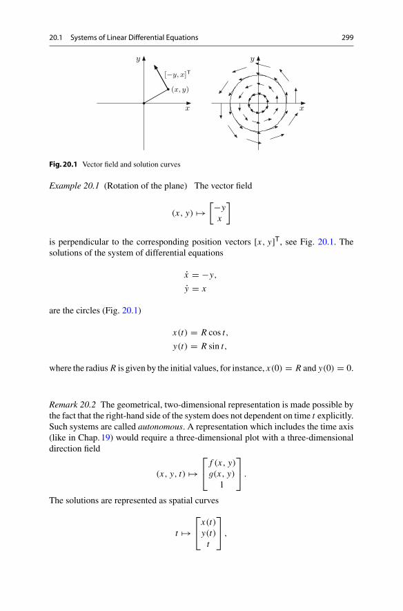
20.1 Systems of Linear Differential Equations 299
y
x
[−y, x]T
(x, y)
y
x
Fig. 20.1 Vector field and solution curves
Example 20.1 (Rotation of the plane) The vector field
(x, y) �→[−yx
]
is perpendicular to the corresponding position vectors [x, y]T, see Fig. 20.1. Thesolutions of the system of differential equations
x = −y,
y = x
are the circles (Fig. 20.1)
x(t) = R cos t,
y(t) = R sin t,
where the radius R is given by the initial values, for instance, x(0) = R and y(0) = 0.
Remark 20.2 The geometrical, two-dimensional representation is made possible bythe fact that the right-hand side of the system does not dependent on time t explicitly.Such systems are called autonomous. A representation which includes the time axis(like in Chap.19) would require a three-dimensional plot with a three-dimensionaldirection field
(x, y, t) �→⎡⎣ f (x, y)
g(x, y)1
⎤⎦ .
The solutions are represented as spatial curves
t �→⎡⎣x(t)y(t)t
⎤⎦ ,
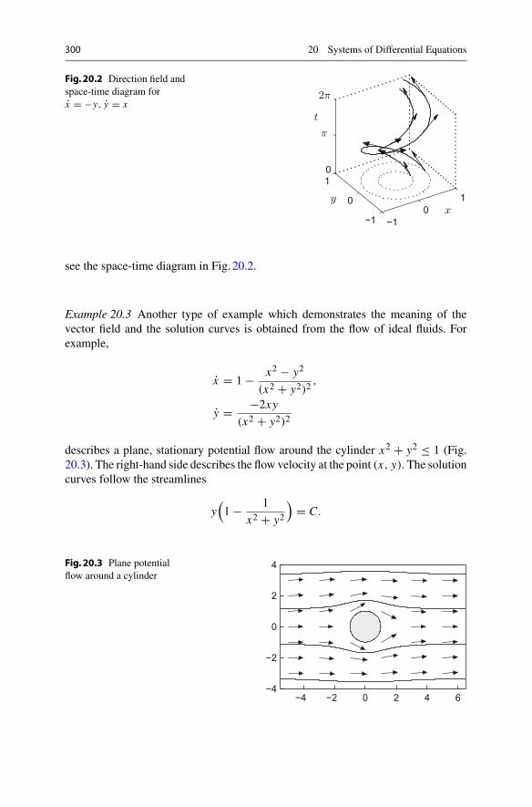
300 20 Systems of Differential Equations
Fig.20.2 Direction field andspace-time diagram forx = −y, y = x
−10
1
−1
0
10
2π
π
t
yx
see the space-time diagram in Fig. 20.2.
Example 20.3 Another type of example which demonstrates the meaning of thevector field and the solution curves is obtained from the flow of ideal fluids. Forexample,
x = 1 − x2 − y2
(x2 + y2)2,
y = −2xy
(x2 + y2)2
describes a plane, stationary potential flow around the cylinder x2 + y2 ≤ 1 (Fig.20.3). The right-hand side describes the flow velocity at the point (x, y). The solutioncurves follow the streamlines
y(1 − 1
x2 + y2
)= C.
Fig. 20.3 Plane potentialflow around a cylinder
−4 −2 0 2 4 6−4
−2
0
2
4

20.1 Systems of Linear Differential Equations 301
Here C denotes a constant. This can be checked by differentiating the above relationwith respect to t and substituting x and y by the right-hand side of the differentialequation.
Experiment 20.4 Using the applet Dynamical systems in the plane, study the vec-tor field and the solution curves of the system of differential equations from Exam-ples 20.1 and 20.3. In a similar way, study the systems of differential equations
x = y,y = −x,
x = y,y = x,
x = −y,y = −x,
x = x,y = x,
x = y,y = y
and try to understand the behaviour of the solution curves.
Before turning to the solution theory of planar linear systems of differential equa-tions, it is useful to introduce a couple of notions that serve to describe the qualitativebehaviour of solution curves. The system of differential equations
x(t) = f(x(t), y(t)
),
y(t) = g(x(t), y(t)
)
together with prescribed values at t = 0
x(0) = x0, y(0) = y0,
is again called an initial value problem. In this chapter we assume the functionsf and g to be at least continuous. By a solution curve or a trajectory we meana continuously differentiable curve t �→ [x(t) y(t)]T whose components fulfil thesystem of differential equations.
For the case of a single differential equation the notion of an equilibrium pointwas introduced in Definition 19.21. For systems of differential equations one has ananalogous notion.
Definition 20.5 (Equilibrium point) A point (x∗, y∗) is called equilibrium point orequilibrium of the system of differential equations, if f (x∗, y∗) = 0 andg(x∗, y∗) = 0.
The name comes from the fact that a solution with initial value x0 = x∗, y0 = y∗remains at (x∗, y∗) for all times; in other words, if (x∗, y∗) is an equilibrium point,then x(t) = x∗, y(t) = y∗ is a solution to the system of differential equations sinceboth the left- and right-hand sides will be zero.
From Chap.19 we know that solutions of differential equations do not have toexist for large times. However, if solutions with initial values in a neighbourhood ofan equilibrium point exist for all times then the following notions are meaningful.
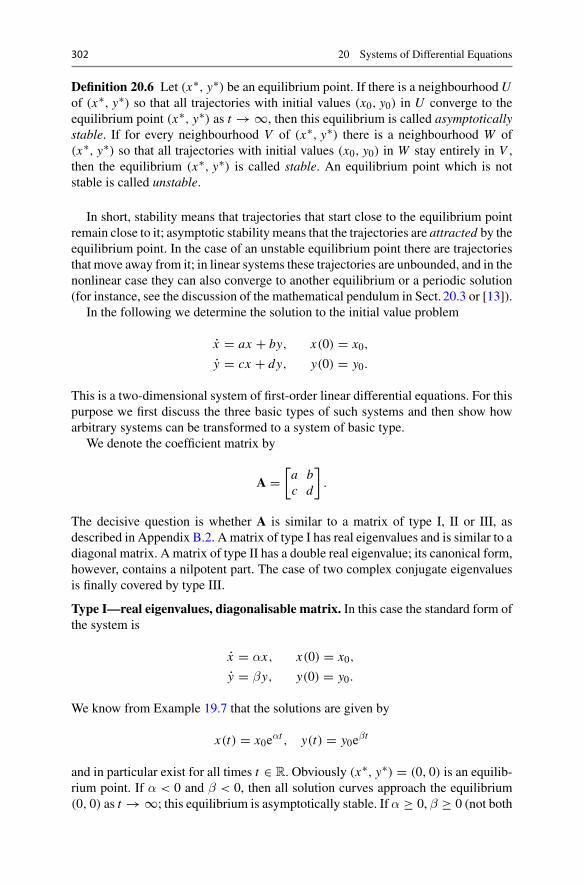
302 20 Systems of Differential Equations
Definition 20.6 Let (x∗, y∗) be an equilibrium point. If there is a neighbourhoodUof (x∗, y∗) so that all trajectories with initial values (x0, y0) in U converge to theequilibrium point (x∗, y∗) as t → ∞, then this equilibrium is called asymptoticallystable. If for every neighbourhood V of (x∗, y∗) there is a neighbourhood W of(x∗, y∗) so that all trajectories with initial values (x0, y0) in W stay entirely in V ,then the equilibrium (x∗, y∗) is called stable. An equilibrium point which is notstable is called unstable.
In short, stability means that trajectories that start close to the equilibrium pointremain close to it; asymptotic stability means that the trajectories are attracted by theequilibrium point. In the case of an unstable equilibrium point there are trajectoriesthat move away from it; in linear systems these trajectories are unbounded, and in thenonlinear case they can also converge to another equilibrium or a periodic solution(for instance, see the discussion of the mathematical pendulum in Sect. 20.3 or [13]).
In the following we determine the solution to the initial value problem
x = ax + by, x(0) = x0,
y = cx + dy, y(0) = y0.
This is a two-dimensional system of first-order linear differential equations. For thispurpose we first discuss the three basic types of such systems and then show howarbitrary systems can be transformed to a system of basic type.
We denote the coefficient matrix by
A =[a bc d
].
The decisive question is whether A is similar to a matrix of type I, II or III, asdescribed in Appendix B.2. A matrix of type I has real eigenvalues and is similar to adiagonal matrix. A matrix of type II has a double real eigenvalue; its canonical form,however, contains a nilpotent part. The case of two complex conjugate eigenvaluesis finally covered by type III.
Type I—real eigenvalues, diagonalisable matrix. In this case the standard form ofthe system is
x = αx, x(0) = x0,
y = βy, y(0) = y0.
We know from Example 19.7 that the solutions are given by
x(t) = x0eαt , y(t) = y0e
βt
and in particular exist for all times t ∈ R. Obviously (x∗, y∗) = (0, 0) is an equilib-rium point. If α < 0 and β < 0, then all solution curves approach the equilibrium(0, 0) as t → ∞; this equilibrium is asymptotically stable. If α ≥ 0, β ≥ 0 (not both
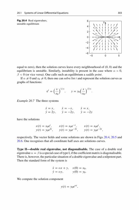
20.1 Systems of Linear Differential Equations 303
Fig. 20.4 Real eigenvalues,unstable equilibrium
−5 0 5−6
−4
−2
0
2
4
6 y
x
equal to zero), then the solution curves leave every neighbourhood of (0, 0) and theequilibrium is unstable. Similarly, instability is present in the case where α > 0,β < 0 (or vice versa). One calls such an equilibrium a saddle point.
If α = 0 and x0 = 0, then one can solve for t and represent the solution curves asgraphs of functions:
et =( x
x0
)1/α, y = y0
( x
x0
)β/α.
Example 20.7 The three systems
x = x,y = 2y,
x = −x,y = −2y,
x = x,y = −2y
have the solutions
x(t) = x0et ,y(t) = y0e2t ,
x(t) = x0e−t ,
y(t) = y0e−2t ,
x(t) = x0et ,y(t) = y0e−2t ,
respectively. The vector fields and some solutions are shown in Figs. 20.4, 20.5 and20.6. One recognises that all coordinate half axes are solutions curves.
Type II—double real eigenvalue, not diagonalisable. The case of a double realeigenvalueα = β is a special case of type I, if the coefficientmatrix is diagonalisable.There is, however, the particular situation of a double eigenvalue and a nilpotent part.Then the standard form of the system is
x = αx + y,y = αy,
x(0) = x0,y(0) = y0.
We compute the solution component
y(t) = y0eαt ,

304 20 Systems of Differential Equations
Fig. 20.5 Real eigenvalues,asymptotically stableequilibrium
−5 0 5−6
−4
−2
0
2
4
6 y
x
Fig. 20.6 Real eigenvalues,saddle point
−5 0 5−5
0
5 y
x
Fig. 20.7 Double realeigenvalue, matrix notdiagonalisable
−5 0 5−5
0
5 y
x
substitute it into the first equation
x(t) = αx(t) + y0eαt , x(0) = x0
and apply the variation of constants formula from Chap.19:
x(t) = eαt(x0 +
∫ t
0e−αs y0e
αs ds)
= eαt(x0 + t y0).
The vector fields and some solution curves for the case α = −1 are depicted inFig. 20.7.

20.1 Systems of Linear Differential Equations 305
Type III—complex conjugate eigenvalues. In this case the standard form of thesystem is
x = αx − βy, x(0) = x0,
y = βx + αy, y(0) = y0.
By introducing the complex variable z and the complex coefficients γ, z0 as
z = x + iy, γ = α + iβ, z0 = x0 + iy0,
we see that the above system represents the real and the imaginary parts of theequation
(x + i y) = (α + iβ)(x + iy), x(0) + iy(0) = x0 + iy0.
From the complex formulation
z = γz, z(0) = z0,
the solutions can be derived immediately:
z(t) = z0eγt .
Splitting the left- and right-hand sides into real and imaginary parts, one obtains
x(t) + iy(t) = (x0 + iy0)e(α+iβ)t
= (x0 + iy0)eαt (cosβt + i sin βt).
From that we get (see Sect. 4.2)
x(t) = x0eαt cosβt − y0e
αt sin βt,
y(t) = x0eαt sin βt + y0e
αt cosβt.
The point (x∗, y∗) = (0, 0) is again an equilibrium point. In the case α < 0 it isasymptotically stable; for α > 0 it is unstable; for α = 0 it is stable but not asymp-totically stable. Indeed the solution curves are circles and hence bounded, but arenot attracted by the origin as t → ∞.
Example 20.8 The vector fields and solutions curves for the two systems
x = 110 x − y,
y = x + 110 y,
x = − 110 x − y,
y = x − 110 y
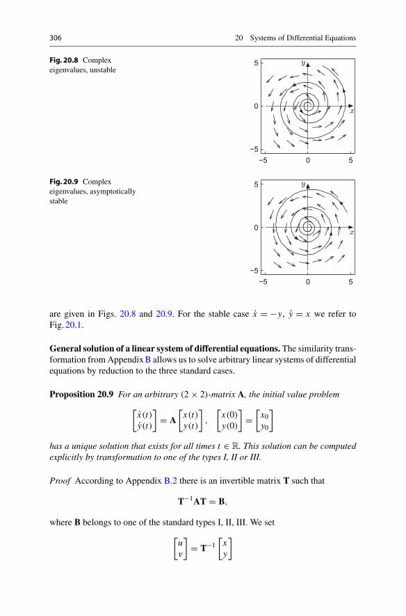
306 20 Systems of Differential Equations
Fig. 20.8 Complexeigenvalues, unstable
−5 0 5−5
0
5 y
x
Fig. 20.9 Complexeigenvalues, asymptoticallystable
−5 0 5−5
0
5 y
x
are given in Figs. 20.8 and 20.9. For the stable case x = −y, y = x we refer toFig. 20.1.
General solution of a linear system of differential equations. The similarity trans-formation fromAppendixB allows us to solve arbitrary linear systems of differentialequations by reduction to the three standard cases.
Proposition 20.9 For an arbitrary (2 × 2)-matrix A, the initial value problem[x(t)y(t)
]= A
[x(t)y(t)
],
[x(0)y(0)
]=
[x0y0
]
has a unique solution that exists for all times t ∈ R. This solution can be computedexplicitly by transformation to one of the types I, II or III.
Proof According to Appendix B.2 there is an invertible matrix T such that
T−1AT = B,
where B belongs to one of the standard types I, II, III. We set
[uv
]= T−1
[xy
]
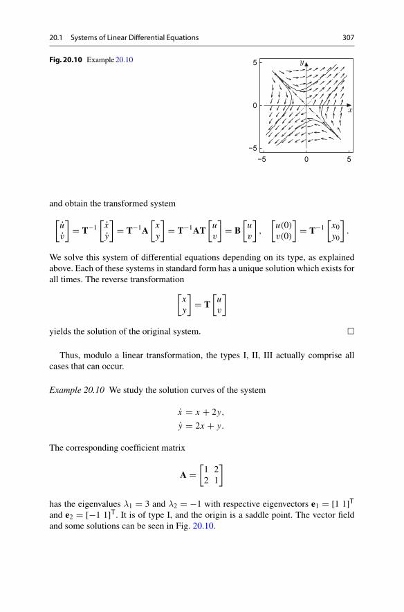
20.1 Systems of Linear Differential Equations 307
Fig. 20.10 Example20.10
−5 0 5−5
0
5 y
x
and obtain the transformed system
[uv
]= T−1
[xy
]= T−1A
[xy
]= T−1AT
[uv
]= B
[uv
],
[u(0)v(0)
]= T−1
[x0y0
].
We solve this system of differential equations depending on its type, as explainedabove. Each of these systems in standard form has a unique solution which exists forall times. The reverse transformation
[xy
]= T
[uv
]
yields the solution of the original system. �
Thus, modulo a linear transformation, the types I, II, III actually comprise allcases that can occur.
Example 20.10 We study the solution curves of the system
x = x + 2y,
y = 2x + y.
The corresponding coefficient matrix
A =[1 22 1
]
has the eigenvalues λ1 = 3 and λ2 = −1 with respective eigenvectors e1 = [1 1]Tand e2 = [−1 1]T. It is of type I, and the origin is a saddle point. The vector fieldand some solutions can be seen in Fig. 20.10.

308 20 Systems of Differential Equations
Remark 20.11 The proof of Proposition 20.9 shows the structure of the generalsolution of a linear system of differential equations. Assume, for example, that theroots λ1,λ2 of the characteristic polynomial of the coefficient matrix are real anddistinct, so the system is of type I. The general solution in transformed coordinatesis given by
u(t) = C1eλ1t , v(t) = C2e
λ2t .
If we denote the columns of the transformation matrix by t1, t2, then the solution inthe original coordinates is
[x(t)y(t)
]= t1u(t) + t2v(t) =
[t11C1eλ1t + t12C2eλ2t
t21C1eλ1t + t22C2eλ2t
].
Every component is a particular linear combination of the transformed solutionsu(t), v(t). In the case of complex conjugate roots μ ± iν (type III) the componentsof the general solution are particular linear combinations of the functions eμt cos νtand eμt sin νt . In the case of a double root α (type II), the components are given aslinear combinations of the functions eαt and teαt .
20.2 Systems of Nonlinear Differential Equations
In contrast to linear systems of differential equations, the solutions to nonlinearsystems can generally not be expressed by explicit formulas. Apart from numericalmethods (Chap.21) the qualitative theory is of interest. It describes the behaviour ofsolutions without knowing them explicitly. In this section we will demonstrate thiswith the help of an example from population dynamics.
The Lotka–Volterra model. In Sect. 20.1 the predator–prey model of Lotka andVolterra was introduced. In order to simplify the presentation, we set all coefficientsequal to one. Thus the system becomes
x = x(y − 1),
y = y(1 − x).
The equilibrium points are (x∗, y∗) = (1, 1) and (x∗∗, y∗∗) = (0, 0). Obviously, thecoordinate half axes are solution curves given by
x(t) = x0e−t , x(t) = 0,y(t) = 0, y(t) = y0et .
The equilibrium (0, 0) is thus a saddle point (unstable); we will later analyse thetype of equilibrium (1, 1). In the following we will only consider the first quadrantx ≥ 0, y ≥ 0, which is relevant in biological models. Along the straight line x = 1the vector field is horizontal, and along the straight line y = 1 it is vertical. It looks
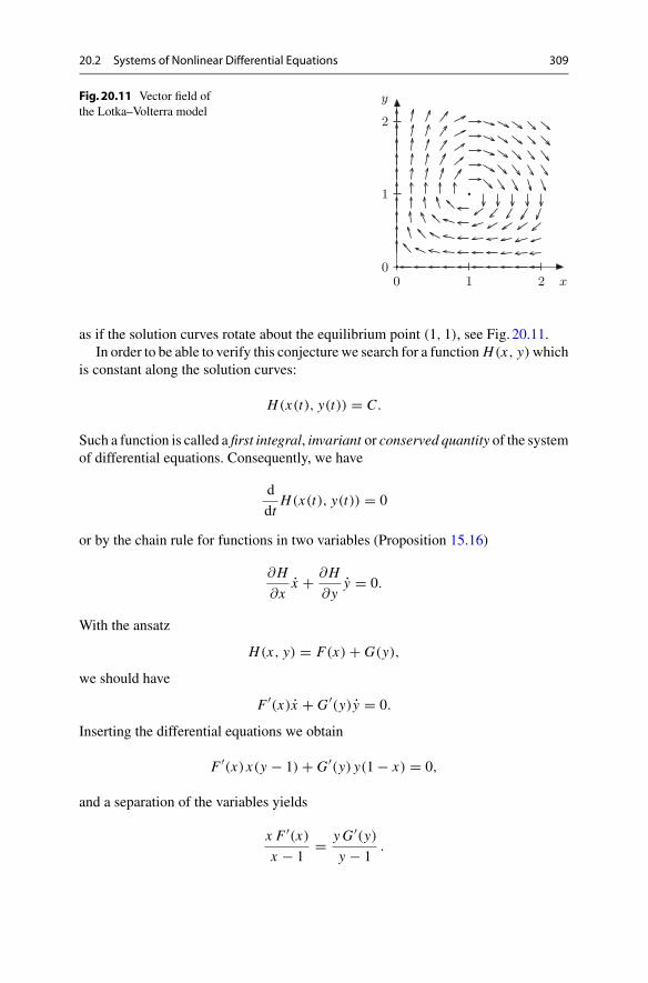
20.2 Systems of Nonlinear Differential Equations 309
Fig. 20.11 Vector field ofthe Lotka–Volterra model
2
1
0210
y
x
as if the solution curves rotate about the equilibrium point (1, 1), see Fig. 20.11.In order to be able to verify this conjecture we search for a function H(x, y)which
is constant along the solution curves:
H(x(t), y(t)) = C.
Such a function is called a first integral, invariant or conserved quantity of the systemof differential equations. Consequently, we have
d
dtH(x(t), y(t)) = 0
or by the chain rule for functions in two variables (Proposition 15.16)
∂H
∂xx + ∂H
∂yy = 0.
With the ansatz
H(x, y) = F(x) + G(y),
we should have
F ′(x)x + G ′(y)y = 0.
Inserting the differential equations we obtain
F ′(x)x(y − 1) + G ′(y) y(1 − x) = 0,
and a separation of the variables yields
x F ′(x)x − 1
= yG ′(y)y − 1
.
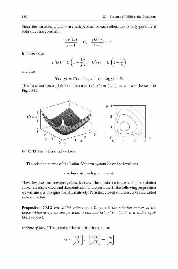
310 20 Systems of Differential Equations
Since the variables x and y are independent of each other, this is only possible ifboth sides are constant:
x F ′(x)x − 1
= C,yG ′(y)y − 1
= C.
It follows that
F ′(x) = C
(1 − 1
x
), G ′(y) = C
(1 − 1
y
)
and thus
H(x, y) = C(x − log x + y − log y) + D.
This function has a global minimum at (x∗, y∗) = (1, 1), as can also be seen inFig. 20.12.
01
23
01
232
3
4
0 1 2 30
1
2
3y
x
H(x, y)
yx
Fig. 20.12 First integral and level sets
The solution curves of the Lotka–Volterra system lie on the level sets
x − log x + y − log y = const.
These level sets are obviously closed curves. The question arises whether the solutioncurves are also closed, and the solutions thus are periodic. In the followingpropositionwewill answer this question affirmatively. Periodic, closed solution curves are calledperiodic orbits.
Proposition 20.12 For initial values x0 > 0, y0 > 0 the solution curves of theLotka–Volterra system are periodic orbits and (x∗, y∗) = (1, 1) is a stable equi-librium point.
Outline of proof The proof of the fact that the solution
t �→[x(t)y(t)
],
[x(0)y(0)
]=
[x0y0
]
20.2 Systems of Nonlinear Differential Equations 311
exists (and is unique) for all initial values x0 ≥ 0, y0 ≥ 0 and all times t ∈ R requiresmethods that go beyond the scope of this book. The interested reader is referred to[13, Chap. 8]. In order to prove periodicity, we take initial values (x0, y0) = (1, 1)and show that the corresponding solution curves return to the initial value after finitetime τ > 0. For that we split the first quadrant x > 0, y > 0 into four regions
Q1 : x > 1, y > 1; Q2 : x < 1, y > 1;Q3 : x < 1, y < 1; Q4 : x > 1, y < 1
and show that every solution curve moves (clockwise) through all four regions infinite time. For instance, consider the case (x0, y0) ∈ Q3, so 0 < x0 < 1, 0 < y0 < 1.We want to show that the solution curve reaches the region Q2 in finite time; i.e.y(t) assumes the value one. From the differential equations it follows that
x = x(y − 1) < 0, y = y(1 − x) > 0
in region Q3 and thus
x(t) < x0, y(t) > y0, y(t) > y0(1 − x0),
as long as (x(t), y(t)) stays in region Q3. If y(t) were less than one for all timest > 0, then the following inequalities would hold:
1 > y(t) = y0 +∫ t
0y(s) ds > y0 +
∫ t
0y0(1 − x0) ds = y0 + t y0(1 − x0).
However, the latter expression diverges to infinity as t → ∞, a contradiction. Con-sequently, y(t) has to reach the value 1 and thus the region Q2 in finite time. Like-wise one reasons for the other regions. Thus there exists a time τ > 0 such that(x(τ ), y(τ )) = (x0, y0).
From that the periodicity of the orbit follows. Since the system of differentialequations is autonomous, t �→ (x(t + τ ), y(t + τ )) is a solution as well. As justshown, both solutions have the same initial value at t = 0. The uniqueness of thesolution of initial value problems implies that the two solutions are identical, so
x(t) = x(t + τ ), y(t) = y(t + τ )
is fulfilled for all times t ∈ R. However, this proves that the solution t �→ (x(t), y(t))is periodic with period τ .
All solution curves in the first quadrant with the exception of the equilibrium arethus periodic orbits. Solution curves that start close to (x∗, y∗) = (1, 1) stay close,see Fig. 20.12. The point (1, 1) is thus a stable equilibrium. �
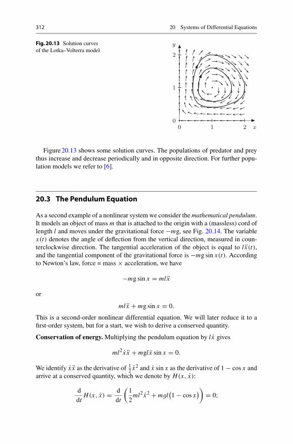
312 20 Systems of Differential Equations
Fig. 20.13 Solution curvesof the Lotka–Volterra model
2
1
0210
y
x
Figure20.13 shows some solution curves. The populations of predator and preythus increase and decrease periodically and in opposite direction. For further popu-lation models we refer to [6].
20.3 The Pendulum Equation
As a second example of a nonlinear systemwe consider themathematical pendulum.It models an object of mass m that is attached to the origin with a (massless) cord oflength l and moves under the gravitational force −mg, see Fig. 20.14. The variablex(t) denotes the angle of deflection from the vertical direction, measured in coun-terclockwise direction. The tangential acceleration of the object is equal to l x(t),and the tangential component of the gravitational force is −mg sin x(t). Accordingto Newton’s law, force = mass × acceleration, we have
−mg sin x = mlx
or
mlx + mg sin x = 0.
This is a second-order nonlinear differential equation. We will later reduce it to afirst-order system, but for a start, we wish to derive a conserved quantity.
Conservation of energy.Multiplying the pendulum equation by l x gives
ml2 x x + mgl x sin x = 0.
We identify x x as the derivative of 12 x
2 and x sin x as the derivative of 1 − cos x andarrive at a conserved quantity, which we denote by H(x, x):
d
dtH(x, x) = d
dt
(1
2ml2 x2 + mgl
(1 − cos x
)) = 0;
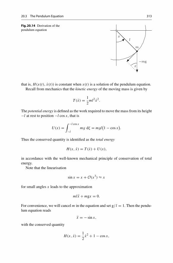
20.3 The Pendulum Equation 313
Fig. 20.14 Derivation of thependulum equation
x
xl
m
−mg
that is, H(x(t), x(t)) is constant when x(t) is a solution of the pendulum equation.Recall from mechanics that the kinetic energy of the moving mass is given by
T (x) = 1
2ml2 x2.
The potential energy is defined as the work required to move the mass from its height−l at rest to position −l cos x , that is
U (x) =∫ −l cos x
−lmg dξ = mgl
(1 − cos x
).
Thus the conserved quantity is identified as the total energy
H(x, x) = T (x) +U (x),
in accordance with the well-known mechanical principle of conservation of totalenergy.
Note that the linearisation
sin x = x + O(x3) ≈ x
for small angles x leads to the approximation
mlx + mgx = 0.
For convenience, we will cancel m in the equation and set g/ l = 1. Then the pendu-lum equation reads
x = − sin x,
with the conserved quantity
H(x, x) = 1
2x2 + 1 − cos x,
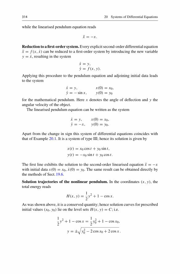
314 20 Systems of Differential Equations
while the linearised pendulum equation reads
x = −x .
Reduction to a first-order system.Every explicit second-order differential equationx = f (x, x) can be reduced to a first-order system by introducing the new variabley = x , resulting in the system
x = y,y = f (x, y).
Applying this procedure to the pendulum equation and adjoining initial data leadsto the system
x = y, x(0) = x0,y = − sin x, y(0) = y0
for the mathematical pendulum. Here x denotes the angle of deflection and y theangular velocity of the object.
The linearised pendulum equation can be written as the system
x = y, x(0) = x0,y = −x, y(0) = y0.
Apart from the change in sign this system of differential equations coincides withthat of Example 20.1. It is a system of type III; hence its solution is given by
x(t) = x0 cos t + y0 sin t,
y(t) = −x0 sin t + y0 cos t.
The first line exhibits the solution to the second-order linearised equation x = −xwith initial data x(0) = x0, x(0) = y0. The same result can be obtained directly bythe methods of Sect. 19.6.
Solution trajectories of the nonlinear pendulum. In the coordinates (x, y), thetotal energy reads
H(x, y) = 1
2y2 + 1 − cos x .
As was shown above, it is a conserved quantity; hence solution curves for prescribedinitial values (x0, y0) lie on the level sets H(x, y) = C ; i.e.
1
2y2 + 1 − cos x = 1
2y20 + 1 − cos x0,
y = ±√y20 − 2 cos x0 + 2 cos x .

20.3 The Pendulum Equation 315
Fig. 20.15 Solution curves,mathematical pendulum
−5 0 5−4
−2
0
2
4 y
x
Figure20.15 shows some solution curves. There are unstable equilibria at y = 0,x = . . . ,−3π,−π,π, 3π, . . . which are connected by limit curves. One of the twolimit curves passes through x0 = 0, y0 = 2. The solution with these initial valueslies on the limit curve and approaches the equilibrium (π, 0) as t → ∞, and (−π, 0)as t → −∞. Initial values that lie between these limit curves (for instance the valuesx0 = 0, |y0| < 2) give rise to periodic solutions of small amplitude (less than π). Thesolutions outside represent large oscillations where the pendulum loops. We remarkthat effects of friction are not taken into account in this model.
Power series solutions.Themethod of power series for solving differential equationshas been introduced in Chap.19.We have seen that the linearised pendulum equationx = −x can be solved explicitly by the methods of Sects. 19.6 and 20.1. Also, thenonlinear pendulum equation can be solved explicitly with the aid of certain highertranscendental functions, the Jacobian elliptic functions. Nevertheless, it is of interestto analyse the solutions of these equations by means of powers series, especially inview of the fact that they can be readily obtained inmaple.
Example 20.13 (Power series for the linearised pendulum) As an example,we solvethe initial value problem
x = −x, x(0) = a, x(0) = 0
by means of the power series ansatz
x(t) =∞∑n=0
cntn = c0 + c1t + c2t
2 + c3t3 + c4t
4 + · · ·
We have
x(t) =∞∑n=1
ncntn−1 = c1 + 2c2t + 3c3t
2 + 4c4t3 + · · ·
x(t) =∞∑n=2
n(n − 1)cntn−2 = 2c2 + 6c3t + 12c4t
2 + · · ·
316 20 Systems of Differential Equations
We know that c0 = a and c1 = 0. Equating x(t) with −x(t) gives, up to seconddegree,
2c2 + 6c3t + 12c4t2 + · · · = −a − c2t
2 − · · ·thus
c2 = −a
2, c3 = 0, c4 = − c2
12= a
24, . . .
The power series expansion starts with
x(t) = a(1 − 1
2t2 + 1
24t4 ∓ . . .
)
and seemingly coincides with the Taylor series of the known solution x(t) = a cos t .
Example 20.14 (Power series for the nonlinear pendulum) We turn to the initialvalue problem for the nonlinear pendulum equation
x = − sin x, x(0) = a, x(0) = 0,
making the same power series ansatz as in Example 20.13. Developing the sinefunction into its Taylor series, inserting the lowest order terms of the power series ofx(t) and noting that c0 = a, c1 = 0 yields
− sin x(t) = −(x(t) − 1
3! x(t)3 + 1
5! x(t)5 + . . .
)
= −(a + c2t
2 + · · · ) + 1
3!(a + c2t
2 + . . .)3 − 1
5!(a + c2t
2 + · · · )5
= −(a + c2t
2 + · · · ) + 1
6
(a3 + 3a2c2t
2 + · · · )
− 1
120
(a5 + 5a4c2t
2 + · · · ),where we have used the binomial formulas. Equating the last line with
x(t) = 2c2 + 6c3t + 12c4t2 + · · ·
shows that
2c2 = −a + 1
6a3 − 1
120a5 ± . . .
6c3 = 0
12c4 = c2(
− 1 + 3
6a2 − 5
120a4 ± . . .
)
which suggests that
c2 = −1
2sin a, c4 = 1
24sin a cos a.
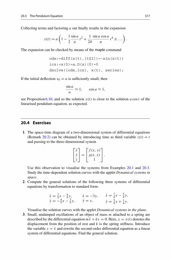
20.3 The Pendulum Equation 317
Collecting terms and factoring a out finally results in the expansion
x(t) = a
(1 − 1
2
sin a
at2 + 1
24
sin a cos a
at4 ± . . .
).
The expansion can be checked by means of themaple command
ode:=diff(x(t),[t$2])=-sin(x(t))
ics:=x(0)=a,D(x)(0)=0
dsolve({ode,ics}, x(t), series);
If the initial deflection x0 = a is sufficiently small, then
sin a
a≈ 1, cos a ≈ 1,
see Proposition6.10, and so the solution x(t) is close to the solution a cos t of thelinearised pendulum equation, as expected.
20.4 Exercises
1. The space-time diagram of a two-dimensional system of differential equations(Remark 20.2) can be obtained by introducing time as third variable z(t) = tand passing to the three-dimensional system
⎡⎣xyz
⎤⎦ =
⎡⎣ f (x, y)
g(x, y)1
⎤⎦ .
Use this observation to visualise the systems from Examples 20.1 and 20.3.Study the time-dependent solution curves with the applet Dynamical systems inspace.
2. Compute the general solutions of the following three systems of differentialequations by transformation to standard form:
x = 35 x − 4
5 y,y = − 4
5 x − 35 y,
x = −3y,y = x,
x = 74 x − 5
4 y,
y = 54 x + 1
4 y.
Visualise the solution curves with the applet Dynamical systems in the plane.3. Small, undamped oscillations of an object of mass m attached to a spring are
described by the differential equationmx + kx = 0. Here, x = x(t) denotes thedisplacement from the position of rest and k is the spring stiffness. Introducethe variable y = x and rewrite the second-order differential equation as a linearsystem of differential equations. Find the general solution.

318 20 Systems of Differential Equations
4. A company deposits its profits in an account with continuous interest rate a%.The balance is denoted by x(t). Simultaneously the amount y(t) is withdrawncontinuously from the account, where the rate of withdrawal is equal to b% ofthe account balance. With r = a/100, s = b/100 this leads to the linear systemof differential equations
x(t) = r(x(t) − y(t)),y(t) = s x(t).
Find the solution (x(t), y(t)) for the initial values x(0) = 1, y(0) = 0 and anal-yse how big s can be in comparison with r so that the account balance x(t) isincreasing for all times without oscillations.
5. A national economy has two sectors (for instance industry and agriculture) withthe production volumes x1(t), x2(t) at time t . If one assumes that the invest-ments are proportional to the respective growth rate, then the classical model ofLeontief 3 [24, Chap.9.5] states
x1(t) = a11x1(t) + a12x2(t) + b1 x1(t) + c1(t),x2(t) = a21x1(t) + a22x2(t) + b2 x2(t) + c2(t).
Here ai j denotes the required amount of goods from sector i to produce oneunit of goods in sector j . Further bi xi (t) are the investments, and ci (t) is theconsumption in sector i . Under the simplifying assumptions a11 = a22 = 0,a12 = a21 = a (0 < a < 1), b1 = b2 = 1, c1(t) = c2(t) = 0 (no consumption)one obtains the system of differential equations
x1(t) = x1(t) − ax2(t),x2(t) = −ax1(t) + x2(t).
Find the general solution and discuss the result.6. Use the applet Dynamical systems in the plane to analyse the solution curves
of the differential equations of the mathematical pendulum and translate themathematical results to statements about the mechanical behaviour.
7. Derive the conserved quantity H(x, y) = 12 y
2 + 1 − cos x of the pendulumequation by means of the ansatz H(x, y) = F(x) + G(y) as for the Lotka–Volterra system.
8. Usingmaple, find the power series solution to the nonlinear pendulum equationx = − sin x with initial data
x(0) = a, x(0) = 0 and x(0) = 0, x(0) = b.
Check by how much its coefficients differ from the ones of the power seriessolution of the corresponding linearised pendulum equation x = −x for variousvalues of a, b between 0 and 1.
3W. Leontief, 1906–1999.

20.4 Exercises 319
9. The differential equation mx(t) + kx(t) + 2cx3(t) = 0 describes a nonlinearmass–spring system where x(t) is the displacement of the mass m, k is thestiffness of the spring and the term cx3 models nonlinear effects (c > 0 . . .hardening, c < 0 . . . softening).(a) Show that
H(x, x) = 1
2
(mx2 + kx2 + cx4
)is a conserved quantity.
(b) Assume that m = 1, k = 1 and x(0) = 0, x(0) = 1. Reduce the second-order equation to a first-order system.Making use of the conserved quantity,plot the solution curves for the values of c = 0, c = −0.2, c = 0.2 and c = 5.Hint. A typicalmaple command is
with(plots,implicitplot); c:=5;
implicitplot(yˆ2+xˆ2+c*xˆ4=1,x=-1.5..1.5,y=-1.5..1.5);
10. Usingmaple, find the power series solution to the nonlinear differential equationx(t) + x(t) + 2cx3(t) = 0 with initial data x(0) = a, x(0) = b. Compare it tothe solution with c = 0.
21Numerical SolutionofDifferentialEquations
As we have seen in the last two chapters, only particular classes of differentialequations can be solved analytically. Especially for nonlinear problems one has torely on numerical methods.
In this chapter we discuss several variants of Euler’s method as a prototype. Moti-vated by the Taylor expansion of the analytical solution we deduce Euler approxi-mations and study their stability properties. In this way we introduce the reader toseveral important aspects of the numerical solution of differential equations.Wepointout, however, that for most real-life applications one has to use more sophisticatednumerical methods.
21.1 The Explicit Euler Method
The differential equation
y′(x) = f(x, y(x)
)
defines the slope of the tangent to the solution curve y(x). Expanding the solutionat the point x + h into a Taylor series
y(x + h) = y(x) + hy′(x) + O(h2)
and inserting the above value for y′(x), one obtains
y(x + h) = y(x) + h f(x, y(x)
) + O(h2)
© Springer Nature Switzerland AG 2018M. Oberguggenberger and A. Ostermann, Analysis for Computer Scientists,Undergraduate Topics in Computer Science,https://doi.org/10.1007/978-3-319-91155-7_21
321
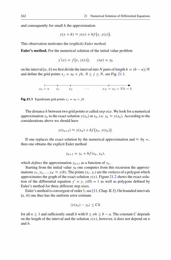
322 21 Numerical Solution of Differential Equations
and consequently for small h the approximation
y(x + h) ≈ y(x) + h f(x, y(x)
).
This observation motivates the (explicit) Euler method.
Euler’s method. For the numerical solution of the initial value problem
y′(x) = f(x, y(x)
), y(a) = y0
on the interval [a, b]wefirst divide the interval into N parts of length h = (b − a)/Nand define the grid points x j = x0 + jh, 0 ≤ j ≤ N , see Fig. 21.1.
xN = x0 +Nh = b· · ·x2x1x0 = a
Fig. 21.1 Equidistant grid points x j = x0 + jh
The distance h between two grid points is called step size. We look for a numericalapproximation yn to the exact solution y(xn) at xn , i.e. yn ≈ y(xn). According to theconsiderations above we should have
y(xn+1) ≈ y(xn) + h f(xn, y(xn)
).
If one replaces the exact solution by the numerical approximation and ≈ by = ,then one obtains the explicit Euler method
yn+1 = yn + h f (xn, yn),
which defines the approximation yn+1 as a function of yn .Starting from the initial value y0 one computes from this recursion the approxi-
mations y1, y2,…, yN ≈ y(b). The points (xi , yi ) are the vertices of a polygon whichapproximates the graph of the exact solution y(x). Figure21.2 shows the exact solu-tion of the differential equation y′ = y, y(0) = 1 as well as polygons defined byEuler’s method for three different step sizes.
Euler’s method is convergent of order 1, see [11, Chap. II.3]. On bounded intervals[a, b] one thus has the uniform error estimate
|y(xn) − yn| ≤ Ch
for all n ≥ 1 and sufficiently small h with 0 ≤ nh ≤ b − a. The constant C dependson the length of the interval and the solution y(x), however, it does not depend on nand h.

21.1 The Explicit Euler Method 323
Fig. 21.2 Eulerapproximation toy′ = y, y(0) = 1
0 0.25 0.5 0.75 1
1
1.6
2.2
2.815 Euler steps5 Euler steps2 Euler steps
Example 21.1 The solution of the initial value problem y′ = y, y(0) = 1 is y(x) =ex. For nh = 1 the numerical solution yn approximates the exact solution at x = 1.Due to
yn = yn−1 + hyn−1 = (1 + h)yn−1 = · · · = (1 + h)n y0
we have
yn = (1 + h)n =(1 + 1
n
)n
≈ e .
The convergence of Euler’s method thus implies
e = limn→∞
(1 + 1
n
)n
.
This formula for e was already deduced in Example 7.11.
In commercial software packages, methods of higher order are used for the numer-ical integration, for example Runge–Kutta or multi-step methods. All these methodsare refinements of Euler’s method. In modern implementations of these algorithmsthe error is automatically estimated and the step size adaptively adjusted to the prob-lem. For more details, we refer to [11,12].
Experiment 21.2 InMATLAB you can find information on the numerical solution ofdifferential equations by calling help funfun. For example, one can solve theinitial value problem
y′ = y2, y(0) = 0.9
324 21 Numerical Solution of Differential Equations
on the interval [0, 1] with the command
[x,y] = ode23(’qfun’, [0,1], 0.9);
The file qfun.m has to contain the definition of the function
function yp = f(x,y)
yp = y.ˆ2;
For a plot of the solution, one sets the option
myopt = odeset(’OutputFcn’,’odeplot’)
and calls the solver by
[x,y] = ode23(’qfun’, [0,1], 0.9, myopt);
Start the program with different initial values and observe the blow up for y(0) ≥ 1.
21.2 Stability and Stiff Problems
The linear differential equation
y′ = ay, y(0) = 1
has the solution
y(x) = eax.
For a ≤ 0 this solution has the following qualitative property, independent of thesize of a :
|y(x)| ≤ 1 for all x ≥ 0.
We are investigating whether numerical methods preserve this property. For that wesolve the differential equation with the explicit Euler method and obtain
yn = yn−1 + hayn−1 = (1 + ha)yn−1 = · · · = (1 + ha)n y0 = (1 + ha)n .
For −2 ≤ ha ≤ 0 the numerical solution obeys the same bound
|yn| = ∣∣(1 + ha)n
∣∣ = ∣
∣1 + ha∣∣n ≤ 1

21.2 Stability and Stiff Problems 325
as the exact solution. However, for ha < −2 a dramatic instability occurs althoughthe exact solution is harmless. In fact, all explicit methods have the same difficultiesin this situation: The solution is only stable under very restrictive conditions on thestep size. For the explicit Euler method the condition for stability is
−2 ≤ ha ≤ 0.
For a � 0 this implies a drastic restriction on the step size, which eventually makesthe method in this situation inefficient.
In this case a remedy is offered by implicit methods, for example, the implicitEuler method
yn+1 = yn + h f (xn+1, yn+1).
It differs from the explicit method by the fact that the slope of the tangent is nowtaken at the endpoint. For the determination of the numerical solution, a nonlinearequation has to be solved in general. Therefore, such methods are called implicit.The implicit Euler method has the same accuracy as the explicit one, but by far betterstability properties, as the following analysis shows. If one applies the implicit Eulermethod to the initial value problem
y′ = ay, y(0) = 1, with a ≤ 0,
one obtains
yn = yn−1 + h f (xn, yn) = yn−1 + hayn,
and therefore
yn = 1
1 − hayn−1 = · · · = 1
(1 − ha)ny0 = 1
(1 − ha)n.
The procedure is thus stable, i.e. |yn| ≤ 1, if
∣∣(1 − ha)n
∣∣ ≥ 1.
However, for a ≤ 0 this is fulfilled for all h ≥ 0. Thus the procedure is stable forarbitrarily large step sizes.
Remark 21.3 A differential equation is called stiff, if for its solution the implicitEuler method is more efficient (often dramatically more efficient) than the explicitmethod.

326 21 Numerical Solution of Differential Equations
0 5 10−2
−1
0
1
2
0 5 10−2
−1
0
1
2
0 5 10−2
−1
0
1
2n = 246n = 248n = 250
Fig.21.3 Instability of the explicit Euler method. In each case the picture shows the exact solutionand the approximating polygons of Euler’s method with n steps
0 5 10−2
−1
0
1
2
0 5 10−2
−1
0
1
2
0 5 10−2
−1
0
1
2n = 16n = 8n = 4
Fig. 21.4 Stability of the implicit Euler method. In each case the picture shows the exact solutionand the approximating polygons of Euler’s method with n steps
Example 21.4 (From [12, Chap. IV.1]) We integrate the initial value problem
y′ = −50(y − cos x), y(0) = 0.997.
Its exact solution is
y(x) = 2500
2501cos x + 50
2501sin x − 6503
250100e−50x
≈ cos(x − 0.02) − 0.0026 e−50x.
The solution looks quite harmless and resembles cos x , but the equation is stiff witha = −50. Warned by the analysis above we expect difficulties for explicit methods.
We integrate this differential equation numerically on the interval [0, 10] withthe explicit Euler method and step sizes h = 10/n with n = 250, 248 and 246.For n < 250, i.e. h > 1/25, exponential instabilities occur, see Fig. 21.3. This isconsistent with the considerations above because the product ah satisfies ah ≤ −2for h > 1/25.
However, if one integrates the differential equationwith the implicit Eulermethod,then even for very large step sizes no instabilities arise, see Fig. 21.4. The implicitEuler method is more costly than the explicit one, as the computation of yn+1 from
yn+1 = yn + h f (xn+1, yn+1)
generally requires the solution of a nonlinear equation.

21.3 Systems of Differential Equations 327
21.3 Systems of Differential Equations
For the derivation of a simple numerical method for solving systems of differentialequations
x(t) = f(t, x(t), y(t)
), x(t0) = x0,
y(t) = g(t, x(t), y(t)
), y(t0) = y0,
one again starts from the Taylor expansion of the analytic solution
x(t + h) = x(t) + hx(t) + O(h2),
y(t + h) = y(t) + h y(t) + O(h2)
and replaces the derivatives by the right-hand sides of the differential equations. Forsmall step sizes h this motivates the explicit Euler method
xn+1 = xn + h f(tn, xn, yn
),
yn+1 = yn + hg(tn, xn, yn
).
One interprets xn and yn as numerical approximations to the exact solution x(tn) andy(tn) at time tn = t0 + nh.
Example 21.5 In Sect. 20.2 we have investigated the Lotka–Volterra model
x = x(y − 1),
y = y(1 − x).
In order to compute the periodic orbit through the point (x0, y0) = (2, 2)numerically,we apply the explicit Euler method and obtain the recursion
xn+1 = xn + hxn(yn − 1),
yn+1 = yn + hyn(1 − xn).
Starting from the initial values x0 = 2 and y0 = 2 this recursion determines thenumerical solution for n ≥ 0. The results for three different step sizes are depictedin Fig. 21.5. Note the linear convergence of the numerical solution for h → 0.
This numerical experiment shows that one has to choose a very small step size inorder to obtain the periodicity of the true orbit in the numerical solution.Alternatively,one can use numerical methods of higher order or—in the present example—alsothe following modification of Euler’s method
xn+1 = xn + hxn(yn − 1),
yn+1 = yn + hyn(1 − xn+1).
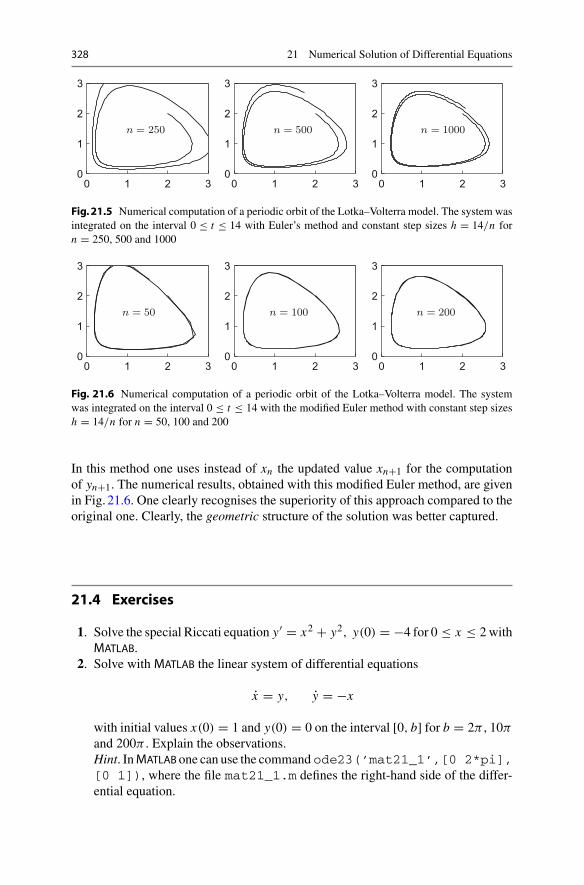
328 21 Numerical Solution of Differential Equations
0 1 2 30
1
2
3
0 1 2 30
1
2
3
0 1 2 30
1
2
3
n = 1000n = 500n = 250
Fig.21.5 Numerical computation of a periodic orbit of the Lotka–Volterra model. The system wasintegrated on the interval 0 ≤ t ≤ 14 with Euler’s method and constant step sizes h = 14/n forn = 250, 500 and 1000
0 1 2 30
1
2
3
0 1 2 30
1
2
3
0 1 2 30
1
2
3
n = 200n = 100n = 50
Fig. 21.6 Numerical computation of a periodic orbit of the Lotka–Volterra model. The systemwas integrated on the interval 0 ≤ t ≤ 14 with the modified Euler method with constant step sizesh = 14/n for n = 50, 100 and 200
In this method one uses instead of xn the updated value xn+1 for the computationof yn+1. The numerical results, obtained with this modified Euler method, are givenin Fig. 21.6. One clearly recognises the superiority of this approach compared to theoriginal one. Clearly, the geometric structure of the solution was better captured.
21.4 Exercises
1. Solve the special Riccati equation y′ = x2 + y2, y(0) = −4 for 0 ≤ x ≤ 2withMATLAB.
2. Solve with MATLAB the linear system of differential equations
x = y, y = −x
with initial values x(0) = 1 and y(0) = 0 on the interval [0, b] for b = 2π , 10πand 200π . Explain the observations.Hint. InMATLAB one can use the command ode23(’mat21_1’,[0 2*pi],[0 1]), where the file mat21_1.m defines the right-hand side of the differ-ential equation.
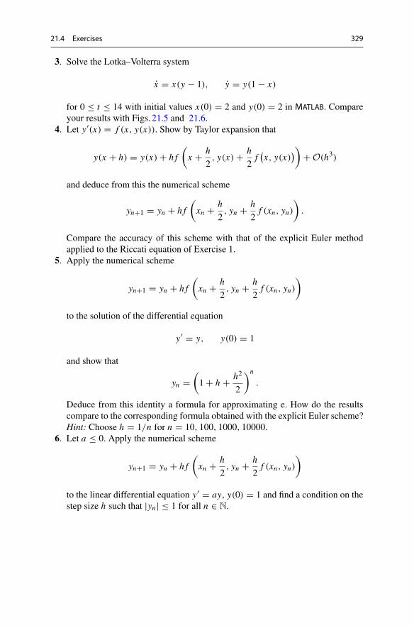
21.4 Exercises 329
3. Solve the Lotka–Volterra system
x = x(y − 1), y = y(1 − x)
for 0 ≤ t ≤ 14 with initial values x(0) = 2 and y(0) = 2 in MATLAB. Compareyour results with Figs. 21.5 and 21.6.
4. Let y′(x) = f (x, y(x)). Show by Taylor expansion that
y(x + h) = y(x) + h f
(x + h
2, y(x) + h
2f(x, y(x)
))
+ O(h3)
and deduce from this the numerical scheme
yn+1 = yn + h f
(xn + h
2, yn + h
2f (xn, yn)
).
Compare the accuracy of this scheme with that of the explicit Euler methodapplied to the Riccati equation of Exercise 1.
5. Apply the numerical scheme
yn+1 = yn + h f
(xn + h
2, yn + h
2f (xn, yn)
)
to the solution of the differential equation
y′ = y, y(0) = 1
and show that
yn =(1 + h + h2
2
)n
.
Deduce from this identity a formula for approximating e. How do the resultscompare to the corresponding formula obtained with the explicit Euler scheme?Hint: Choose h = 1/n for n = 10, 100, 1000, 10000.
6. Let a ≤ 0. Apply the numerical scheme
yn+1 = yn + h f
(xn + h
2, yn + h
2f (xn, yn)
)
to the linear differential equation y′ = ay, y(0) = 1 and find a condition on thestep size h such that |yn| ≤ 1 for all n ∈ N.
AVectorAlgebra
In various sections of this book we referred to the notion of a vector. We assumedthe reader to have a basic knowledge on standard school level. In this appendix werecapitulate some basic notions of vector algebra. For a more detailed presentationwe refer to [2].
A.1 Cartesian Coordinate Systems
A Cartesian coordinate system in the plane (in space) consists of two (three) reallines (coordinate axes) which intersect in right angles at the point O (origin). Wealways assume that the coordinate system is positively (right-handed) oriented. In aplanar right-handed system, the positive y-axis lies to the left in viewing direction ofthe positive x-axis (Fig.A.1). In a positively oriented three-dimensional coordinatesystem, the direction of the positive z-axis is obtained by turning the x-axis in thedirection of the y-axis according to the right-hand rule, see Fig.A.2.
The coordinates of a point are obtained by parallel projection of the point ontothe coordinate axes. In the case of the plane, the point A has the coordinates a1 anda2, and we write
A = (a1, a2) ∈ R2.
In an analogous way a point A in space with coordinates a1, a2 and a3 is denoted as
A = (a1, a2, a3) ∈ R3.
Thus one has a unique representation of points by pairs or triples of real numbers.
© Springer Nature Switzerland AG 2018M. Oberguggenberger and A. Ostermann, Analysis for Computer Scientists,Undergraduate Topics in Computer Science,https://doi.org/10.1007/978-3-319-91155-7
331
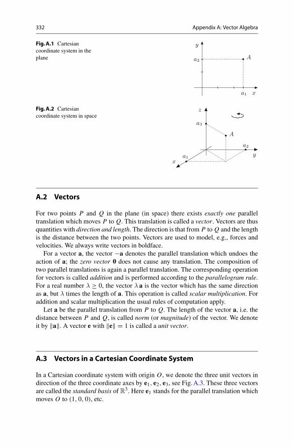
332 Appendix A: Vector Algebra
Fig.A.1 Cartesiancoordinate system in theplane a2
a1
A
y
x
Fig.A.2 Cartesiancoordinate system in space
a3
a2
a1
A
z
xy
A.2 Vectors
For two points P and Q in the plane (in space) there exists exactly one paralleltranslation which moves P to Q. This translation is called a vector. Vectors are thusquantities with direction and length. The direction is that from P to Q and the lengthis the distance between the two points. Vectors are used to model, e.g., forces andvelocities. We always write vectors in boldface.
For a vector a, the vector −a denotes the parallel translation which undoes theaction of a; the zero vector 0 does not cause any translation. The composition oftwo parallel translations is again a parallel translation. The corresponding operationfor vectors is called addition and is performed according to the parallelogram rule.For a real number λ ≥ 0, the vector λ a is the vector which has the same directionas a, but λ times the length of a. This operation is called scalar multiplication. Foraddition and scalar multiplication the usual rules of computation apply.
Let a be the parallel translation from P to Q. The length of the vector a, i.e. thedistance between P and Q, is called norm (or magnitude) of the vector. We denoteit by ‖a‖. A vector e with ‖e‖ = 1 is called a unit vector.
A.3 Vectors in a Cartesian Coordinate System
In a Cartesian coordinate system with origin O , we denote the three unit vectors indirection of the three coordinate axes by e1, e2, e3, see Fig.A.3. These three vectorsare called the standard basis of R3. Here e1 stands for the parallel translation whichmoves O to (1, 0, 0), etc.
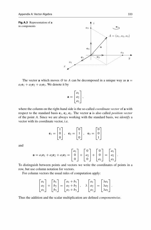
Appendix A: Vector Algebra 333
Fig.A.3 Representation of ain components
e3
e2e1
a
a3
a2
a1
A = (a1, a2, a3)
z
x
y
The vector a which moves O to A can be decomposed in a unique way as a =a1e1 + a2e2 + a3e3. We denote it by
a =⎡⎣a1a2a3
⎤⎦ ,
where the column on the right-hand side is the so-called coordinate vector of a withrespect to the standard basis e1, e2, e3. The vector a is also called position vectorof the point A. Since we are always working with the standard basis, we identify avector with its coordinate vector, i.e.
e1 =⎡⎣100
⎤⎦ , e2 =
⎡⎣010
⎤⎦ , e3 =
⎡⎣001
⎤⎦
and
a = a1e1 + a2e2 + a3e3 =⎡⎣a100
⎤⎦+
⎡⎣0a20
⎤⎦+
⎡⎣00a3
⎤⎦ =
⎡⎣a1a2a3
⎤⎦ .
To distinguish between points and vectors we write the coordinates of points in arow, but use column notation for vectors.
For column vectors the usual rules of computation apply:
⎡⎣a1a2a3
⎤⎦+
⎡⎣b1b2b3
⎤⎦ =
⎡⎣a1 + b1a2 + b2a3 + b3
⎤⎦ , λ
⎡⎣a1a2a3
⎤⎦ =
⎡⎣
λa1λa2λa3
⎤⎦ .
Thus the addition and the scalar multiplication are defined componentwise.
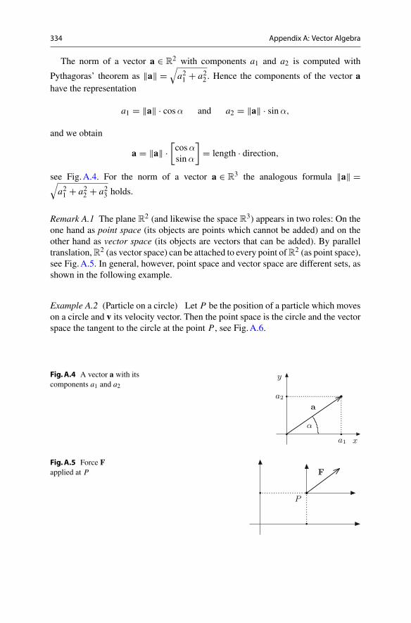
334 Appendix A: Vector Algebra
The norm of a vector a ∈ R2 with components a1 and a2 is computed with
Pythagoras’ theorem as ‖a‖ =√a21 + a22 . Hence the components of the vector a
have the representation
a1 = ‖a‖ · cosα and a2 = ‖a‖ · sinα,
and we obtain
a = ‖a‖ ·[cosαsinα
]= length · direction,
see Fig.A.4. For the norm of a vector a ∈ R3 the analogous formula ‖a‖ =√
a21 + a22 + a23 holds.
Remark A.1 The plane R2 (and likewise the space R3) appears in two roles: On theone hand as point space (its objects are points which cannot be added) and on theother hand as vector space (its objects are vectors that can be added). By paralleltranslation,R2 (as vector space) can be attached to every point ofR2 (as point space),see Fig.A.5. In general, however, point space and vector space are different sets, asshown in the following example.
Example A.2 (Particle on a circle) Let P be the position of a particle which moveson a circle and v its velocity vector. Then the point space is the circle and the vectorspace the tangent to the circle at the point P , see Fig.A.6.
Fig.A.4 A vector a with itscomponents a1 and a2
a2
a1
α
a
y
x
Fig.A.5 Force Fapplied at P F
P
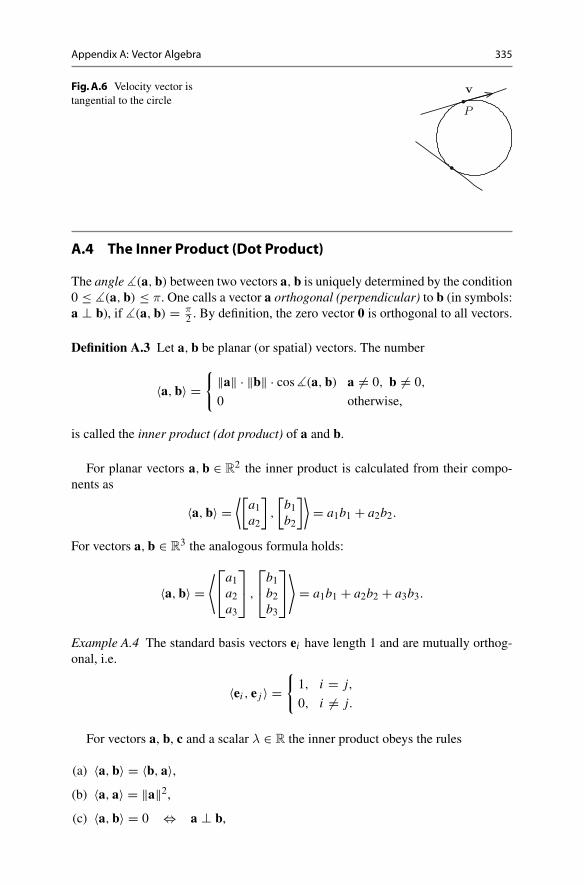
Appendix A: Vector Algebra 335
Fig.A.6 Velocity vector istangential to the circle
P
v
A.4 The Inner Product (Dot Product)
The angle �(a, b) between two vectors a,b is uniquely determined by the condition0 ≤ �(a, b) ≤ π. One calls a vector a orthogonal (perpendicular) to b (in symbols:a ⊥ b), if �(a,b) = π
2 . By definition, the zero vector 0 is orthogonal to all vectors.
Definition A.3 Let a,b be planar (or spatial) vectors. The number
〈a,b〉 ={
‖a‖ · ‖b‖ · cos�(a, b) a = 0, b = 0,
0 otherwise,
is called the inner product (dot product) of a and b.
For planar vectors a, b ∈ R2 the inner product is calculated from their compo-
nents as
〈a,b〉 =⟨[a1a2
],
[b1b2
]⟩= a1b1 + a2b2.
For vectors a,b ∈ R3 the analogous formula holds:
〈a,b〉 =⟨⎡⎣a1a2a3
⎤⎦ ,
⎡⎣b1b2b3
⎤⎦⟩
= a1b1 + a2b2 + a3b3.
Example A.4 The standard basis vectors ei have length 1 and are mutually orthog-onal, i.e.
〈ei , e j 〉 ={1, i = j,
0, i = j.
For vectors a, b, c and a scalar λ ∈ R the inner product obeys the rules
(a) 〈a, b〉 = 〈b, a〉,(b) 〈a, a〉 = ‖a‖2,(c) 〈a, b〉 = 0 ⇔ a ⊥ b,
336 Appendix A: Vector Algebra
(d) 〈λa,b〉 = 〈a,λb〉 = λ〈a,b〉,(e) 〈a + b, c〉 = 〈a, c〉 + 〈b, c〉.
Example A.5 For the vectors
a =⎡⎣
2−40
⎤⎦ , b =
⎡⎣634
⎤⎦ , c =
⎡⎣
10
−1
⎤⎦
we have
‖a‖2 = 4 + 16 = 20, ‖b‖2 = 36 + 9 + 16 = 61, ‖c‖2 = 1 + 1 = 2,
and
〈a, b〉 = 12 − 12 = 0, 〈a, c〉 = 2.
From this we conclude that a is perpendicular to b and
cos�(a, c) = 〈a, c〉‖a‖ · ‖c‖ = 2√
20√2
= 1√10
.
The value of the angle between a and c is thus
�(a, c) = arccos1√10
= 1.249 rad.
A.5 The Outer Product (Cross Product)
For vectors a,b in R2 one defines
a × b =[a1a2
]×[b1b2
]= det
[a1 b1a2 b2
]= a1b2 − a2b1 ∈ R,
the cross product of a and b. An elementary calculation shows that
|a × b| = ‖a‖ · ‖b‖ · sin�(a,b).
Thus |a × b| is the area of the parallelogram spanned by a and b.For vectors a,b ∈ R
3 one defines the cross product as
a × b =⎡⎣a1a2a3
⎤⎦×
⎡⎣b1b2b3
⎤⎦ =
⎡⎣a2b3 − a3b2a3b1 − a1b3a1b2 − a2b1
⎤⎦ ∈ R
3.
This product has the following geometric interpretation: If a = 0 or b = 0 or a = λbthen a × b = 0. Otherwise a × b is the vector
Appendix A: Vector Algebra 337
(a) which is perpendicular to a and b : 〈a × b, a〉 = 〈a × b,b〉 = 0;
(b) which is directed such that a, b, a × b forms a right-handed system;
(c) whose length is equal to the area F of the parallelogram spanned by a and b :F = ‖a × b‖ = ‖a‖ · ‖b‖ · sin�(a,b).
Example A.6 Let E be the plane spanned by the two vectors
a =⎡⎣
1−12
⎤⎦ and b =
⎡⎣101
⎤⎦ .
Then
a × b =⎡⎣
1−12
⎤⎦×
⎡⎣101
⎤⎦ =
⎡⎣
−111
⎤⎦
is a vector perpendicular to this plane.
For a, b, c ∈ R3 and λ ∈ R the following rules apply
(a) a × a = 0, a × b = −(b × a),
(b) λ(a × b) = (λa) × b = a × (λb),
(c) (a + b) × c = a × c + b × c.
However, the cross product is not associative and
a × (b × c) = (a × b) × c
for general a, b, c. For instance, the standard basis vectors of the R3 satisfy the
following identities
e1 × (e1 × e2) = e1 × e3 = −e2,
(e1 × e1) × e2 = 0 × e2 = 0.
A.6 Straight Lines in the Plane
The general equation of a straight line in the (x, y)-plane is
ax + by = c,
338 Appendix A: Vector Algebra
where at least one of the coefficients a and bmust be different from zero. The straightline consists of all points (x, y) which satisfy the above equation,
g = {(x, y) ∈ R
2; ax + by = c}.
If b = 0 (and thus a = 0) we get
x = c
a,
and thus a line parallel to the y-axis. If b = 0, one can solve for y and obtains thestandard form of a straight line
y = −a
bx + c
b= kx + d
with slope k and intercept d.The parametric representation of the straight line is obtained from the general
solution of the linear equation
ax + by = c.
Since this equation is underdetermined, one replaces the independent variable by aparameter and solves for the other variable.
Example A.7 In the equation
y = kx + d
x is considered as independent variable. One sets x = λ and obtains y = kλ + d andthus the parametric representation
[xy
]=[0d
]+ λ
[1k
], λ ∈ R.
Example A.8 In the equation
x = 4
y is the independent variable (it does not even appear). This straight line in parametricrepresentation is
[xy
]=[40
]+ λ
[01
].
In general, the parametric representation of a straight line is of the form
[xy
]=[pq
]+ λ
[uv
], λ ∈ R
Appendix A: Vector Algebra 339
(position vector of a point plus a multiple of a direction vector). A vector perpendic-ular to this straight line is called a normal vector. It is a multiple of
[v
−u
], since
⟨[uv
],
[v
−u
]⟩= 0.
The conversion to the nonparametric form is obtained by multiplying the equationin parametric form by a normal vector. Thereby the parameter is eliminated. In theexample above one obtains
vx − uy = pv − qu.
In particular, the coefficients of x and y in the nonparametric form are just thecomponents of a normal vector of the straight line.
A.7 Planes in Space
The general form of a plane in R3 is
ax + by + cz = d,
where at least one of the coefficients a, b, c is different from zero. The plane consistsof all points which satisfy the above equation, i.e.
E = {(x, y, z) ∈ R
3; ax + by + cz = d}.
Since at least one of the coefficients is nonzero, one can solve the equation for thecorresponding unknown.
For example, if c = 0 one can solve for z to obtain
z = −a
cx − b
cy + d
c= kx + ly + e.
Here k represents the slope in x-direction, l is the slope in y-direction and e is theintercept on the z-axis (because z = e for x = y = 0). By introducing parametersfor the independent variables x and y
x = λ, y = μ, z = kλ + lμ + e
one thus obtains the parametric representation of the plane:
⎡⎣xyz
⎤⎦ =
⎡⎣00e
⎤⎦+ λ
⎡⎣10k
⎤⎦+ μ
⎡⎣01l
⎤⎦ , λ,μ ∈ R.
340 Appendix A: Vector Algebra
In general, the parametric representation of a plane in R3 is
⎡⎣xyz
⎤⎦ =
⎡⎣pqr
⎤⎦+ λ
⎡⎣v1v2v3
⎤⎦+ μ
⎡⎣w1w2w3
⎤⎦
with v × w = 0. If one multiplies this equation with v × w and uses
〈v, v × w〉 = 〈w, v × w〉 = 0,
one again obtains the nonparametric form
⟨⎡⎣xyz
⎤⎦ , v × w
⟩=⟨⎡⎣pqr
⎤⎦ , v × w
⟩.
Example A.9 We compute the nonparametric form of the plane
⎡⎣xyz
⎤⎦ =
⎡⎣311
⎤⎦+ λ
⎡⎣
1−12
⎤⎦+ μ
⎡⎣101
⎤⎦ .
A normal vector to this plane is given by
v × w =⎡⎣
1−12
⎤⎦×
⎡⎣101
⎤⎦ =
⎡⎣
−111
⎤⎦ ,
and thus the equation of the plane is
−x + y + z = −1.
A.8 Straight Lines in Space
A straight line in R3 can be seen as the intersection of two planes:
g :{ax + by + cz = d,ex + f y + gz = h.
The straight line is the set of all points (x, y, z) which fulfil this system of equations(two equations in three unknowns). Generically, the solution of the above systemcan be parametrised by one parameter (this is the case of a straight line). However,it may also happen that the planes are parallel. In this situation they either coincide,or they do not intersect at all.
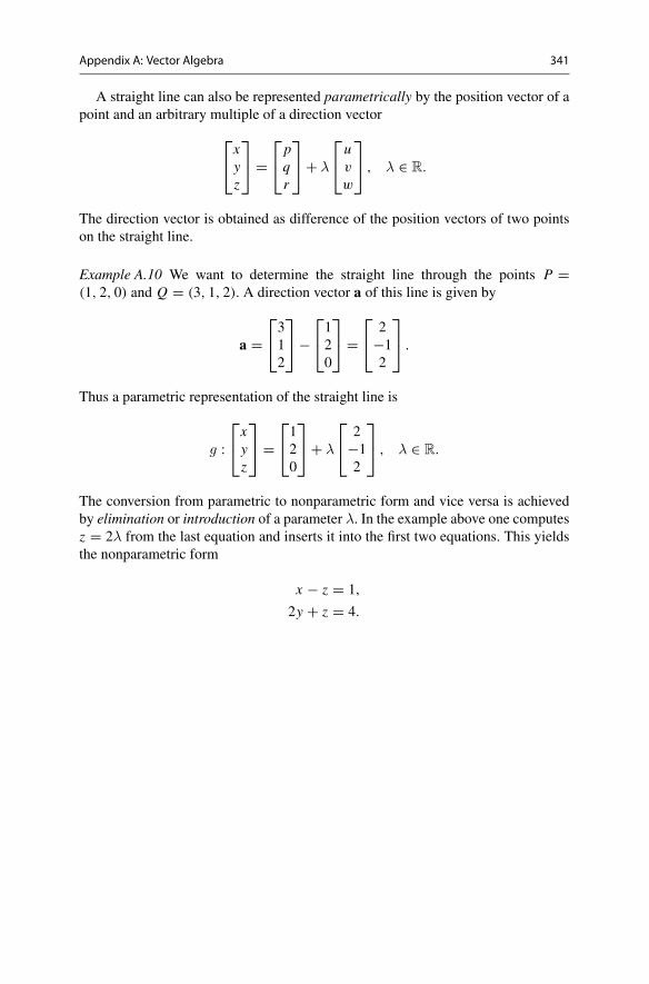
Appendix A: Vector Algebra 341
A straight line can also be represented parametrically by the position vector of apoint and an arbitrary multiple of a direction vector
⎡⎣xyz
⎤⎦ =
⎡⎣pqr
⎤⎦+ λ
⎡⎣uv
w
⎤⎦ , λ ∈ R.
The direction vector is obtained as difference of the position vectors of two pointson the straight line.
Example A.10 We want to determine the straight line through the points P =(1, 2, 0) and Q = (3, 1, 2). A direction vector a of this line is given by
a =⎡⎣312
⎤⎦−
⎡⎣120
⎤⎦ =
⎡⎣
2−12
⎤⎦ .
Thus a parametric representation of the straight line is
g :⎡⎣xyz
⎤⎦ =
⎡⎣120
⎤⎦+ λ
⎡⎣
2−12
⎤⎦ , λ ∈ R.
The conversion from parametric to nonparametric form and vice versa is achievedby elimination or introduction of a parameter λ. In the example above one computesz = 2λ from the last equation and inserts it into the first two equations. This yieldsthe nonparametric form
x − z = 1,
2y + z = 4.

BMatrices
In this book matrix algebra is required in multi-dimensional calculus, for systems ofdifferential equations and for linear regression. This appendix serves to outline thebasic notions. A more detailed presentation can be found in [2].
B.1 Matrix Algebra
An (m × n)-matrix A is a rectangular scheme of the form
A =
⎡⎢⎢⎣
a11 a12 . . . a1na21 a22 . . . a2n...
......
am1 am2 . . . amn
⎤⎥⎥⎦ .
The entries (coefficients, elements) ai j , i = 1, . . . ,m, j = 1, . . . , n of the matrix Aare real or complex numbers. In this section we restrict ourselves to real numbers.An (m × n)-matrix has m rows and n columns; if m = n, and the matrix is calledsquare. Vectors of length m can be understood as matrices with one column, i.e as(m × 1)-matrices. In particular, one refers to the columns
a j =
⎡⎢⎢⎣
a1 ja2 j...
amj
⎤⎥⎥⎦ , j = 1, . . . , n
of a matrix A as column vectors and accordingly also writes
A = [a1 ... a2... . . .
... an]© Springer Nature Switzerland AG 2018M. Oberguggenberger and A. Ostermann, Analysis for Computer Scientists,Undergraduate Topics in Computer Science,https://doi.org/10.1007/978-3-319-91155-7
343
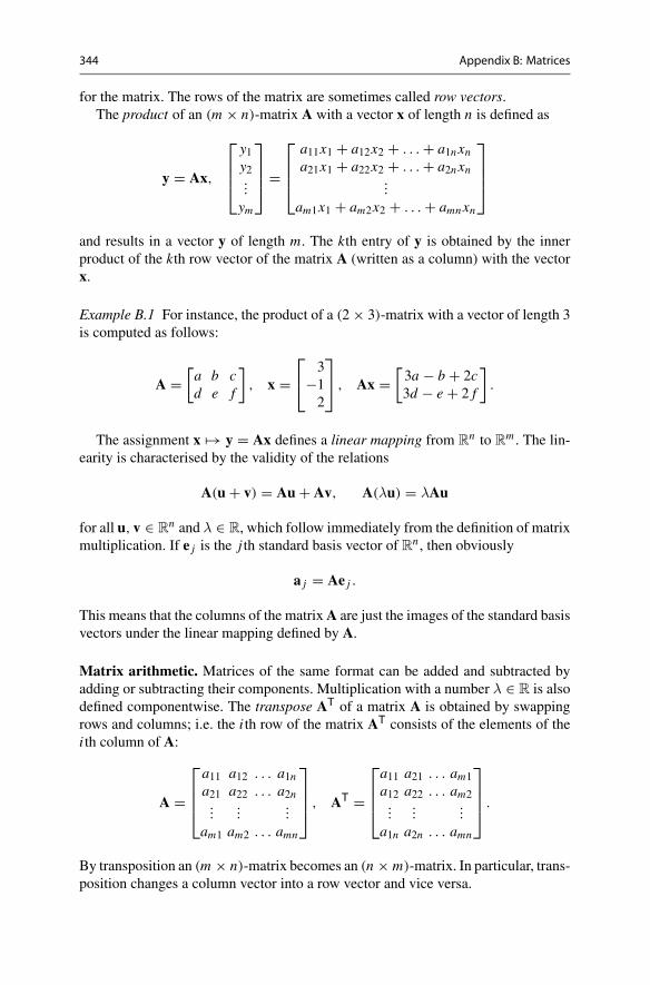
344 Appendix B: Matrices
for the matrix. The rows of the matrix are sometimes called row vectors.The product of an (m × n)-matrix A with a vector x of length n is defined as
y = Ax,
⎡⎢⎢⎣
y1y2...
ym
⎤⎥⎥⎦ =
⎡⎢⎢⎣
a11x1 + a12x2 + . . . + a1nxna21x1 + a22x2 + . . . + a2nxn
...
am1x1 + am2x2 + . . . + amnxn
⎤⎥⎥⎦
and results in a vector y of length m. The kth entry of y is obtained by the innerproduct of the kth row vector of the matrix A (written as a column) with the vectorx.
Example B.1 For instance, the product of a (2 × 3)-matrix with a vector of length 3is computed as follows:
A =[a b cd e f
], x =
⎡⎣
3−12
⎤⎦ , Ax =
[3a − b + 2c3d − e + 2 f
].
The assignment x �→ y = Ax defines a linear mapping from Rn to R
m . The lin-earity is characterised by the validity of the relations
A(u + v) = Au + Av, A(λu) = λAu
for all u, v ∈ Rn and λ ∈ R, which follow immediately from the definition of matrix
multiplication. If e j is the j th standard basis vector of Rn , then obviously
a j = Ae j .
This means that the columns of the matrixA are just the images of the standard basisvectors under the linear mapping defined by A.
Matrix arithmetic. Matrices of the same format can be added and subtracted byadding or subtracting their components. Multiplication with a number λ ∈ R is alsodefined componentwise. The transpose AT of a matrix A is obtained by swappingrows and columns; i.e. the i th row of the matrix AT consists of the elements of thei th column of A:
A =
⎡⎢⎢⎣
a11 a12 . . . a1na21 a22 . . . a2n...
......
am1 am2 . . . amn
⎤⎥⎥⎦ , AT =
⎡⎢⎢⎣
a11 a21 . . . am1a12 a22 . . . am2...
......
a1n a2n . . . amn
⎤⎥⎥⎦ .
By transposition an (m × n)-matrix becomes an (n × m)-matrix. In particular, trans-position changes a column vector into a row vector and vice versa.
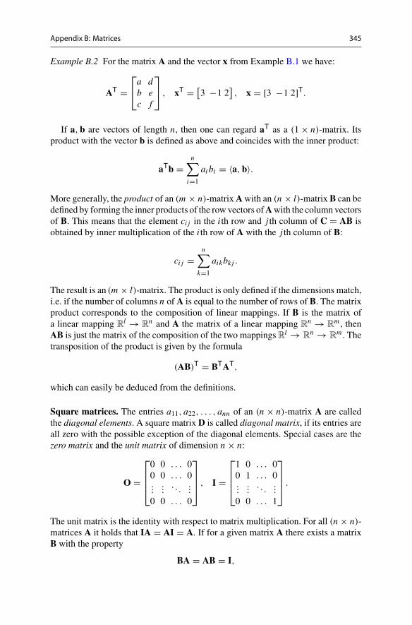
Appendix B: Matrices 345
Example B.2 For the matrix A and the vector x from Example B.1 we have:
AT =⎡⎣a db ec f
⎤⎦ , xT = [
3 −1 2], x = [3 −1 2]T.
If a,b are vectors of length n, then one can regard aT as a (1 × n)-matrix. Itsproduct with the vector b is defined as above and coincides with the inner product:
aTb =n∑
i=1
aibi = 〈a,b〉.
More generally, the product of an (m × n)-matrixAwith an (n × l)-matrix B can bedefined by forming the inner products of the row vectors ofAwith the column vectorsof B. This means that the element ci j in the i th row and j th column of C = AB isobtained by inner multiplication of the i th row of A with the j th column of B:
ci j =n∑
k=1
aikbk j .
The result is an (m × l)-matrix. The product is only defined if the dimensions match,i.e. if the number of columns n of A is equal to the number of rows of B. The matrixproduct corresponds to the composition of linear mappings. If B is the matrix ofa linear mapping R
l → Rn and A the matrix of a linear mapping R
n → Rm , then
AB is just the matrix of the composition of the two mappingsRl → Rn → R
m . Thetransposition of the product is given by the formula
(AB)T = BTAT,
which can easily be deduced from the definitions.
Square matrices. The entries a11, a22, . . . , ann of an (n × n)-matrix A are calledthe diagonal elements. A square matrix D is called diagonal matrix, if its entries areall zero with the possible exception of the diagonal elements. Special cases are thezero matrix and the unit matrix of dimension n × n:
O =
⎡⎢⎢⎣
0 0 . . . 00 0 . . . 0...
.... . .
...
0 0 . . . 0
⎤⎥⎥⎦ , I =
⎡⎢⎢⎣
1 0 . . . 00 1 . . . 0...
.... . .
...
0 0 . . . 1
⎤⎥⎥⎦ .
The unit matrix is the identity with respect to matrix multiplication. For all (n × n)-matrices A it holds that IA = AI = A. If for a given matrix A there exists a matrixB with the property
BA = AB = I,
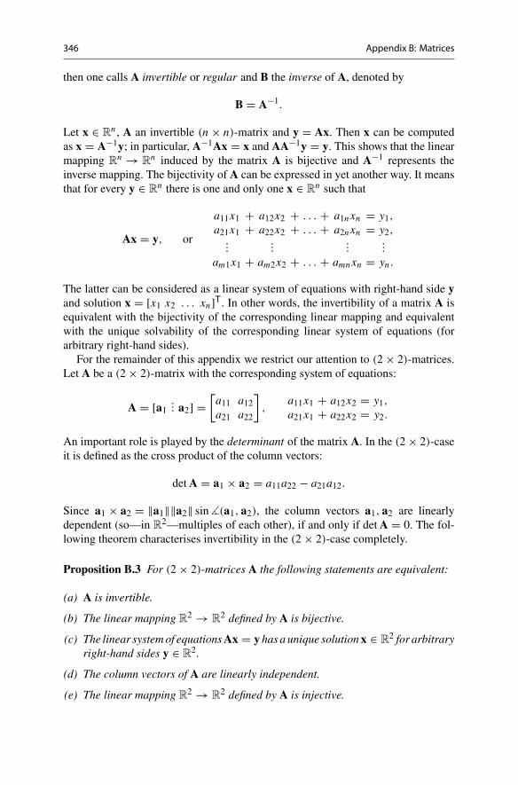
346 Appendix B: Matrices
then one calls A invertible or regular and B the inverse of A, denoted by
B = A−1.
Let x ∈ Rn , A an invertible (n × n)-matrix and y = Ax. Then x can be computed
as x = A−1y; in particular, A−1Ax = x and AA−1y = y. This shows that the linearmapping R
n → Rn induced by the matrix A is bijective and A−1 represents the
inverse mapping. The bijectivity of A can be expressed in yet another way. It meansthat for every y ∈ R
n there is one and only one x ∈ Rn such that
Ax = y, or
a11x1 + a12x2 + . . . + a1nxn = y1,a21x1 + a22x2 + . . . + a2nxn = y2,...
......
...
am1x1 + am2x2 + . . . + amnxn = yn .
The latter can be considered as a linear system of equations with right-hand side yand solution x = [x1 x2 . . . xn]T. In other words, the invertibility of a matrix A isequivalent with the bijectivity of the corresponding linear mapping and equivalentwith the unique solvability of the corresponding linear system of equations (forarbitrary right-hand sides).
For the remainder of this appendix we restrict our attention to (2 × 2)-matrices.Let A be a (2 × 2)-matrix with the corresponding system of equations:
A = [a1 ... a2] =[a11 a12a21 a22
],
a11x1 + a12x2 = y1,a21x1 + a22x2 = y2.
An important role is played by the determinant of the matrix A. In the (2 × 2)-caseit is defined as the cross product of the column vectors:
detA = a1 × a2 = a11a22 − a21a12.
Since a1 × a2 = ‖a1‖‖a2‖ sin�(a1, a2), the column vectors a1, a2 are linearlydependent (so—in R
2—multiples of each other), if and only if detA = 0. The fol-lowing theorem characterises invertibility in the (2 × 2)-case completely.
Proposition B.3 For (2 × 2)-matrices A the following statements are equivalent:
(a) A is invertible.
(b) The linear mapping R2 → R2 defined by A is bijective.
(c) The linear systemof equationsAx = y has aunique solutionx ∈ R2 for arbitrary
right-hand sides y ∈ R2.
(d) The column vectors of A are linearly independent.
(e) The linear mapping R2 → R2 defined by A is injective.

Appendix B: Matrices 347
(f) The only solution of the linear system of equations Ax = 0 is the zero solutionx = 0.
(g) detA = 0.
Proof The equivalence of the statements (a), (b) and (c) was already observed above.The equivalence of (d), (e) and (f) can easily be seen by negation. Indeed, if thecolumn vectors are linearly dependent, then there exists x = [x1 x2]T = 0 withx1a1 + x2a2 = 0. On the one hand, this means that the vector x is mapped to 0by A; thus this mapping is not injective. On the other hand, x is a nontrivial solutionof the linear system of equations Ax = 0. The converse implications are shown inthe same way. Thus (d), (e) and (f) are equivalent. The equivalence of (g) and (d) isobvious from the geometric meaning of the determinant. If the determinant does notvanish then
A−1 = 1
a11a22 − a21a12
[a22 −a12
−a21 a11
]
is an inverse to A, as can be verified at once. Thus (g) implies (a). Finally, (e)obviously follows from (b). Hence all statements (a)–(g) are equivalent. �
PropositionB.3 holds for matrices of arbitrary dimension n × n. For n = 3 onecan still use geometrical arguments. The cross product, however, has to be replaced bythe triple product 〈a1 × a2, a3〉 of the three column vectors, which then also definesthe determinant of the (3 × 3)-matrix A. In higher dimensions the proof requirestools from combinatorics, for which we refer to the literature.
B.2 Canonical Form of Matrices
In this subsection we will show that every (2 × 2)-matrix A is similar to a matrixof standard type, which means that it can be put into standard form by a basistransformation. We need this fact in Sect. 20.1 for the classification and solution ofsystems of differential equations. The transformation explained below is a specialcase of the Jordan canonical form1 for (n × n)-matrices.
If T is an invertible (2 × 2)-matrix, then the columns t1, t2 form a basis of R2.This means that every element x ∈ R
2 can be written in a unique way as a linearcombination c1t1 + c2t2; the coefficients c1, c2 ∈ R are the coordinates of x withrespect to t1 and t2. One can regard T as a linear transformation of R2 which mapsthe standard basis {[1 0]T, [0 1]T} to the basis {t1, t2}.
Definition B.4 Two matrices A,B are called similar, if there exists an invertiblematrix T such that T−1AT = B.
1C. Jordan, 1838–1922.

348 Appendix B: Matrices
The three standard types which will define the similarity classes of (2 × 2)-matrices are of the following form:
type I type II type III[λ1 00 λ2
] [λ 10 λ
] [μ −νν μ
]
Here the coefficients λ1,λ2,λ,μ, ν are real numbers.In what follows, we need the notion of eigenvalues and eigenvectors. If the equa-
tion
Av = λv
has a solution v = 0 ∈ R2 for some λ ∈ R, then λ is called eigenvalue and v eigen-
vector of A. In other words, v is the solution of the equation
(A − λI)v = 0,
where I denotes again the unit matrix. For the existence of a nonzero solution v it isnecessary and sufficient that the matrix A − λI is not invertible, i.e.
det(A − λI) = 0.
By writing
A =[a bc d
]
we see that λ has to be a solution of the characteristic equation
det
[a − λ bc d − λ
]= λ2 − (a + d)λ + ad − bc = 0.
If this equation has a real solution λ, then the system of equations (A − λI)v = 0 isunderdetermined and thus has a nonzero solution v = [v1 v2]T. Hence one obtainsthe eigenvectors to the eigenvalue λ by solving the linear system
(a − λ) v1 + b v2 = 0,
c v1 + (d − λ) v2 = 0.
Depending on whether the characteristic equation has two real, a double real or twocomplex conjugate solutions, we obtain one of the three similarity classes of A.
Proposition B.5 Every (2 × 2)-matrix A is similar to a matrix of type I, II or III.

Appendix B: Matrices 349
Proof (1) The case of two distinct real eigenvalues λ1 = λ2. With
v1 =[v11v21
], v2 =
[v12v22
]
we denote the corresponding eigenvectors. They are linearly independent and thusform a basis of theR2. Otherwise they would bemultiples of each other and so cv1 =v2 for some nonzero c ∈ R. ApplyingAwould result in cλ1v1 = λ2v2 = λ2cv1 andthus λ1 = λ2 in contradiction to the hypothesis. According to Proposition B.3 thematrix
T = [v1 ... v2] =[v11 v12v21 v22
]
is invertible. Using
Av1 = λ1v1, Av2 = λ2v2,
we obtain the identities
T−1AT = T−1A [v1 ... v2] = T−1[λ1v1...λ2v2]
= 1
v11v22 − v21v12
[v22 −v12
−v21 v11
] [λ1v11 λ2v12λ1v21 λ2v22
]=[λ1 00 λ2
].
The matrix A is similar to a diagonal matrix and thus of type I.(2) The case of a double real eigenvalue λ = λ1 = λ2. Since
λ = 1
2
(a + d ±
√(a − d)2 + 4bc
)
is the solution of the characteristic equation, this case occurs if
(a − d)2 = −4bc, λ = 1
2(a + d) .
If b = 0 and c = 0, then a = d and A is already a diagonal matrix of the form
A =[a 00 a
],
thus of type I. If b = 0, we compute c from (a − d)2 = −4bc and find
A − λI =[a − λ bc d − λ
]=[
12 (a − d) b
− 14b (a − d)2 − 1
2 (a − d)
].
Note that[
12 (a − d) b
− 14b (a − d)2 − 1
2 (a − d)
][12 (a − d) b
− 14b (a − d)2 − 1
2 (a − d)
]=[0 00 0
],
350 Appendix B: Matrices
or (A − λI)2 = O. In this case, A − λI is called a nilpotent matrix. A similar cal-culation shows that (A − λI)2 = O if c = 0. We now choose a vector v2 ∈ R
2 forwhich (A − λI)v2 = 0. Due to the above consideration this vector satisfies
(A − λI)2v2 = 0.
If we set
v1 = (A − λI)v2,
then obviously
Av1 = λv1, Av2 = v1 + λv2.
Further v1 and v2 are linearly independent (because if v1 were a multiple of v2, thenAv2 = λv2 in contradiction to the construction of v2). We set
T = [v1 ... v2].The computation
T−1AT = T−1[λv1 ... v1 + λv2]
= 1
v11v22 − v21v12
[v22 −v12
−v21 v11
] [λv11 v11 + λv12λv21 v21 + λv22
]=[λ 10 λ
].
shows that A is similar to a matrix of type II.(3) The case of complex conjugate solutions λ1 = μ + iν,λ2 = μ − iν. This casearises if the discriminant (a − d)2 + 4bc is negative. The most elegant way to dealwith this case is to switch to complex variables and to perform the computations inthe complex vector space C2. We first determine complex vectors v1, v2 ∈ C
2 suchthat
Av1 = λ1v1, Av2 = λ2v2
and then decompose v1 = f + ig into real and imaginary parts with vectors f , g inR2. Since λ1 = μ + iν,λ2 = μ − iν, it follows that
v2 = f − ig.
Note that {v1, v2} forms a basis of C2. Thus {g, f} is a basis of R2 and
A(f + ig) = (μ + iν)(f + ig) = μf − νg + i(νf + μg),
consequently
Ag = νf + μg, Af = μf − νg.
Again we set
T = [g ... f] =[g1 f1g2 f2
]
Appendix B: Matrices 351
from which we deduce
T−1AT = T−1[νf + μg...μf − νg]
= 1
g1 f2 − g2 f1
[f2 − f1
−g2 g1
] [ν f1 + μg1 μ f1 − νg1ν f2 + μg2 μ f2 − νg2
]=[μ −νν μ
].
Thus A is similar to a matrix of type III.

CFurther Results onContinuity
This appendix covers further material on continuity which is not central for this bookbut on the other hand is required in various proofs (like in the chapters on curvesand differential equations). It includes assertions about the continuity of the inversefunction, the concept of uniform convergence of sequences of functions, the powerseries expansion of the exponential function and the notions of uniform and Lipschitzcontinuity.
C.1 Continuity of the Inverse Function
Weconsider a real-valued function f defined on an interval I ⊂ R. The interval I canbe open, half-open or closed. By J = f (I )we denote the image of f . First, we showthat a continuous function f : I → J is bijective, if and only if it is strictly mono-tonically increasing or decreasing. Monotonicity was introduced in Definition 8.5.Subsequently, we show that the inverse function is continuous if f is continuous,and we describe the respective ranges.
Proposition C.1 A real-valued, continuous function f : I → J = f (I ) is bijectiveif and only if it is strictly monotonically increasing or decreasing.
Proof We already know that the function f : I → f (I ) is surjective. It is injectiveif and only if
x1 = x2 ⇒ f (x1) = f (x2).
Strict monotonicity thus implies injectivity. To prove the converse implication westart by choosing two points x1 < x2 ∈ I . Let f (x1) < f (x2), for example. We willshow that f is strictly monotonically increasing on the entire interval I . First weobserve that for every x3 ∈ (x1, x2) we must have f (x1) < f (x3) < f (x2). This
© Springer Nature Switzerland AG 2018M. Oberguggenberger and A. Ostermann, Analysis for Computer Scientists,Undergraduate Topics in Computer Science,https://doi.org/10.1007/978-3-319-91155-7
353
354 Appendix C: Further Results on Continuity
is shown by contradiction. Assuming f (x3) > f (x2), Proposition 6.14 implies thatevery intermediate point f (x2) < η < f (x3) would be the image of a point ξ1 ∈(x1, x3) and also the image of a point ξ2 ∈ (x3, x2), contradicting injectivity.
If we now choose x4 ∈ I such that x2 < x4, then once again f (x2) < f (x4). Oth-erwisewewould have x1 < x2 < x4 with f (x2) > f (x4); this possibility is excludedas in the previous case. Finally, the points to the left of x1 are inspected in a simi-lar way. It follows that f is strictly monotonically increasing on the entire intervalI . In the case f (x1) > f (x2), one can deduce similarly that f is monotonicallydecreasing. �
The function y = x · 11(−1,0](x) + (1 − x) · 11(0,1)(x), where 11I denotes the indi-cator function of the interval I (see Sect. 2.2), shows that a discontinuous functioncan be bijective on an interval without being strictly monotonically increasing ordecreasing.
Remark C.2 If I is an open interval and f : I → J a continuous and bijective func-tion, then J is an open interval as well. Indeed, if J were of the form [a, b), thena would arise as function value of a point x1 ∈ I , i.e. a = f (x1). However, since Iis open, there are points x2 ∈ I , x2 < x1 and x3 ∈ I with x3 > x1. If f is strictlymonotonically increasing then we would have f (x2) < f (x1) = a. If f is strictlymonotonically decreasing then f (x3) < f (x1) = a. Both cases contradict the factthat a was assumed to be the lower boundary of the image J = f (I ). In the sameway, one excludes the possibilities that J = (a, b] or J = [a, b].
Proposition C.3 Let I ⊂ R be an open interval and f : I → J continuous andbijective. Then the inverse function f −1 : J → I is continuous as well.
Proof We take x ∈ I , y ∈ J with y = f (x), x = f −1(y). For small ε > 0 the ε-neighbourhoodUε(x) of x is contained in I . According to Remark C.2 f (Uε(x)) isan open interval and therefore contains a δ-neighbourhood Uδ(y) of y for a certainδ > 0. Consider a sequence of values yn ∈ J which converges to y as n → ∞. Thenthere is an index n(δ) ∈ N such that all elements of the sequence yn with n ≥ n(δ) liein the δ-neighbourhood Uδ(y). That, however, means that the values of the functionf −1(yn) from n(δ) onwards lie in the ε-neighbourhoodUε(x) of x = f −1(y). Thuslimn→∞ f −1(yn) = f −1(y) which is the continuity of f −1 at y. �
C.2 Limits of Sequences of Functions
We consider a sequence of functions fn : I → R, defined on an interval I ⊂ R. Ifthe function values fn(x) converge for every fixed x ∈ I , then the sequence ( fn)n≥1is called pointwise convergent. The pointwise limits define a function f : I → R byf (x) = limn→∞ fn(x), the so-called limit function.
Appendix C: Further Results on Continuity 355
Example C.4 Let I = [0, 1] and fn(x) = xn . Then limn→∞ fn(x) = 0 if 0 ≤ x < 1,and limn→∞ fn(1) = 1. The limit function is thus the function
f (x) ={0, 0 ≤ x < 1,1, x = 1.
This example shows that the limit function of a pointwise convergent sequence ofcontinuous functions is not necessarily continuous.
Definition C.5 (Uniform convergence of sequences of functions) A sequence offunctions ( fn)n≥1 defined on an interval I is called uniformly convergent with limitfunction f , if
∀ε > 0 ∃n(ε) ∈ N ∀n ≥ n(ε) ∀x ∈ I : | f (x) − fn(x)| < ε.
Uniform convergence means that the index n(ε) after which the sequence offunction values ( fn(x))n≥1 settles in the ε-neighbourhood Uε( f (x)) can be chosenindependently of x ∈ I .
Proposition C.6 The limit function f of a uniformly convergent sequence of func-tions ( fn)n≥1 is continuous.
Proof We take x ∈ I and a sequence of points xk converging to x as k → ∞. Wehave to show that f (x) = limk→∞ f (xk). For this we write
f (x) − f (xk) = (f (x) − fn(x)
)+ (fn(x) − fn(xk)
)+ (fn(xk) − f (xk)
)
and choose ε > 0. Due to the uniform convergence it is possible to find an indexn ∈ N such that
| f (x) − fn(x)| < ε
3and | fn(xk) − f (xk)| < ε
3
for all k ∈ N. Since fn is continuous, there is an index k(ε) ∈ N such that
| fn(x) − fn(xk)| < ε
3
for all k ≥ k(ε). For such indices k we have
| f (x) − f (xk)| < ε
3+ ε
3+ ε
3= ε.
Thus f (xk) → f (x) as k → ∞, which implies the continuity of f . �
356 Appendix C: Further Results on Continuity
Application C.7 The exponential function f (x) = ax is continuous onR. In Appli-cation5.14 it was shown that the exponential function with base a > 0 can be definedfor every x ∈ R as a limit. Let rn(x) denote the decimal representation of x , truncatedat the nth decimal place. Then
rn(x) ≤ x < rn(x) + 10−n .
The value of rn(x) is the same for all real numbers x , which coincide up to thenth decimal place. Thus the mapping x �→ rn(x) is a step function with jumps at adistance of 10−n . We define the function fn(x) by linear interpolation between thepoints
(rn(x), a
rn(x))
and(rn(x) + 10−n, arn(x)+10−n )
,
which means
fn(x) = arn(x) + x − rn(x)
10−n
(arn(x)+10−n − arn(x)
).
The graph of the function fn(x) is a polygonal chain (with kinks at the distance of10−n), and thus fn is continuous. We show that the sequence of functions ( fn)n≥1converges uniformly to f on every interval [−T, T ], 0 < T ∈ Q. Since x − rn(x) ≤10−n , it follows that
| f (x) − fn(x)| ≤ ∣∣ax − arn(x)∣∣+ ∣∣arn(x)+10−n − arn(x)
∣∣.
For x ∈ [−T, T ] we have
ax − arn(x) = arn(x)(ax−rn(x) − 1
) ≤ aT(a10
−n − 1)
and likewise
arn(x)+10−n − arn(x) ≤ aT(a10
−n − 1).
Consequently
| f (x) − fn(x)| ≤ 2aT(
10n√a − 1
),
and the term on the right-hand side converges to zero independently of x , as wasproven in Application 5.15.
The rules of calculation for real exponents can now also be derived by takinglimits. Take, for example, r, s ∈ R with decimal approximations (rn)n≥1, (sn)n≥1.Then Proposition 5.7 and the continuity of the exponential function imply
aras = limn→∞
(arnasn
) = limn→∞
(arn+sn
) = ar+s .
With the help of Proposition C.3 the continuity of the logarithm follows as well.
Appendix C: Further Results on Continuity 357
C.3 The Exponential Series
The aimof this section is to derive the series representationof the exponential function
ex =∞∑
m=0
xm
m!
by using exclusively the theory of convergent series without resorting to differentialcalculus. This is important for our exposition because the differentiability of theexponential function is proven with the help of the series representation in Sect. 7.2.
As a tool we need two supplements to the theory of series: Absolute convergenceand Cauchy’s2 formula for the product of two series.
Definition C.8 A series∑∞
k=0 ak is called absolutely convergent, if the series∑∞k=0 |ak | of the absolute values of its coefficients converges.
Proposition C.9 Every absolutely convergent series is convergent.
Proof We define the positive and the negative parts of the coefficient ak by
a+k =
{ak, ak ≥ 0,0, ak < 0,
a−k =
{0, ak ≥ 0,|ak |, ak < 0.
Obviously, we have 0 ≤ a+k ≤ |ak | and 0 ≤ a−
k ≤ |ak |. Thus the two series∑∞k=0 a
+k
and∑∞
k=0 a−k converge due to the comparison criterion (Proposition 5.21) and the
limit
limn→∞
n∑k=0
ak = limn→∞
n∑k=0
a+k − lim
n→∞
n∑k=0
a−k
exists. Consequently, the series∑∞
k=0 ak converges. �
We consider two absolutely convergent series∑∞
i=0 ai and∑∞
j=0 b j and ask howtheir product can be computed. Term-by-term multiplication of the nth partial sumssuggests to consider the following scheme:
a0b0 a0b1 . . . a0bn−1 a0bna1b0 a1b1 . . . a1bn−1 a1bn... . .
. ...
an−1b0 an−1b1 . . . an−1bn−1 an−1bnanb0 anb1 . . . anbn−1 anbn
2A.L. Cauchy, 1789–1857.
358 Appendix C: Further Results on Continuity
Adding all entries of the quadratic scheme one obtains the product of the partial sums
Pn =n∑
i=0
ai
n∑j=0
b j .
In contrast, adding only the upper triangle containing the bold entries (diagonal bydiagonal), one obtains the so-called Cauchy product formula
Sn =n∑
m=0
(m∑
k=0
akbm−k
).
We want to show that, for absolutely convergent series, the limits are equal:
limn→∞ Pn = lim
n→∞ Sn .
Proposition C.10 (Cauchy product) If the series∑∞
i=0 ai and∑∞
j=0 b j convergeabsolutely then
∞∑i=0
ai
∞∑j=0
b j =∞∑
m=0
(m∑
k=0
akbm−k
).
The series defined by the Cauchy product formula also converges absolutely.
Proof We set
cm =m∑
k=0
akbm−k
and obtain that the partial sums
Tn =n∑
m=0
|cm | ≤n∑
i=0
|ai |n∑j=0
|b j | ≤∞∑i=0
|ai |∞∑j=0
|b j |
remain bounded. This follows from the facts that the triangle in the scheme above hasfewer entries than the square and the original series converge absolutely. Obviouslythe sequence Tn is also monotonically increasing; according to Proposition 5.10 itthus has a limit. This means that the series
∑∞m=0 cm converges absolutely, so the
Cauchy product exists. It remains to be shown that it coincides with the product ofthe series. For the partial sums, we have
∣∣∣Pn − Sn∣∣∣ =
∣∣∣∣n∑
i=0
ai
n∑j=0
b j −n∑
m=0
cm
∣∣∣∣ ≤∣∣∣∣
∞∑m=n+1
cm
∣∣∣∣,
since the difference can obviously be approximated by the sum of the terms belowthe nth diagonal. The latter sum, however, is just the difference of the partial sum

Appendix C: Further Results on Continuity 359
Sn and the value of the series∑∞
m=0 cm . It thus converges to zero and the desiredassertion is proven. �
Let
E(x) =∞∑
m=0
xm
m! , En(x) =n∑
m=0
xm
m! .
The convergence of the series for x = 1 was shown in Example 5.24 and for x = 2in Exercise 14 of Chap.5. The absolute convergence for arbitrary x ∈ R can eitherbe shown analogously or by using the ratio test (Exercise 15 in Chap.5). If x variesin a bounded interval I = [−R, R], then the sequence of the partial sums En(x)converges uniformly to E(x), due to the uniform estimate
∣∣∣E(x) − En(x)∣∣∣ =
∣∣∣∣∞∑
m=n+1
xm
m!∣∣∣∣ ≤
∞∑m=n+1
Rm
m! → 0
on the interval [−R, R]. Proposition C.6 implies that the function x �→ E(x) iscontinuous.
For the derivation of the product formula E(x)E(y) = E(x + y) we recall thebinomial formula:
(x + y)m =m∑
k=0
(mk
)xk ym−k with
(mk
)= m!
k!(m − k)! ,
valid for arbitrary x, y ∈ R and n ∈ N, see, for instance, [17, Chap.XIII, Theo-rem7.2].
Proposition C.11 For arbitrary x, y ∈ R it holds that
∞∑i=0
xi
i !∞∑j=0
y j
j ! =∞∑
m=0
(x + y)m
m! .
Proof Due to the absolute convergence of the above series, Proposition C.10 yields
∞∑i=0
xi
i !∞∑j=0
y j
j ! =∞∑
m=0
m∑k=0
xk
k!ym−k
(m − k)! .
An application of the binomial formula
m∑k=0
xk
k!ym−k
(m − k)! = 1
m!m∑
k=0
(mk
)xk ym−k = 1
m! (x + y)m
shows the desired assertion. �
360 Appendix C: Further Results on Continuity
Proposition C.12 (Series representation of the exponential function) The exponen-tial function possesses the series representation
ex =∞∑
m=0
xm
m! ,
valid for arbitrary x ∈ R.
Proof By definition of the number e (see Example 5.24) we obviously have
e0 = 1 = E(0), e1 = e = E(1).
From Proposition C.11 we get in particular
e2 = e1+1 = e1 e1 = E(1)E(1) = E(1 + 1) = E(2)
and recursively
em = E(m) for m ∈ N.
The relation E(m)E(−m) = E(m − m) = E(0) = 1 shows that
e−m = 1
em= 1
E(m)= E(−m).
Likewise, one concludes from(E(1/n)
)n = E(1) that
e1/n = n√e = n
√E(1) = E(1/n).
So far this shows that ex = E(x) holds for all rational x = m/n. From ApplicationC.7 we know that the exponential function x �→ ex is continuous. The continuityof the function x �→ E(x) was shown above. But two continuous functions whichcoincide for all rational numbers are equal. More precisely, if x ∈ R and x j is thedecimal expansion of x truncated at the j th place, then
ex = limj→∞ ex j = lim
j→∞ E(x j ) = E(x),
which is the desired result. �
Remark C.13 The rigorous introduction of the exponential function is surprisinglyinvolved and is handled differently by different authors. The total effort, however, isapproximately the same in all approaches. We took the following route: Introductionof Euler’s number e as the value of a convergent series (Example 5.24); definitionof the exponential function x �→ ex for x ∈ R by using the completeness of the
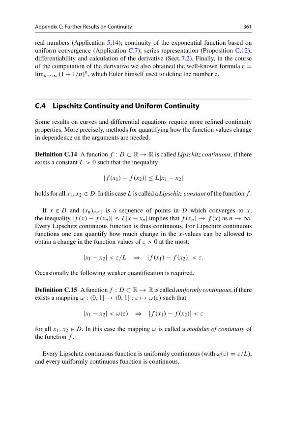
Appendix C: Further Results on Continuity 361
real numbers (Application 5.14); continuity of the exponential function based onuniform convergence (Application C.7); series representation (Proposition C.12);differentiability and calculation of the derivative (Sect. 7.2). Finally, in the courseof the computation of the derivative we also obtained the well-known formula e =limn→∞ (1 + 1/n)n , which Euler himself used to define the number e.
C.4 Lipschitz Continuity and Uniform Continuity
Some results on curves and differential equations require more refined continuityproperties. More precisely, methods for quantifying how the function values changein dependence on the arguments are needed.
Definition C.14 A function f : D ⊂ R → R is called Lipschitz continuous, if thereexists a constant L > 0 such that the inequality
| f (x1) − f (x2)| ≤ L|x1 − x2|
holds for all x1, x2 ∈ D. In this case L is called a Lipschitz constant of the function f .
If x ∈ D and (xn)n≥1 is a sequence of points in D which converges to x ,the inequality | f (x) − f (xn)| ≤ L|x − xn| implies that f (xn) → f (x) as n → ∞.Every Lipschitz continuous function is thus continuous. For Lipschitz continuousfunctions one can quantify how much change in the x-values can be allowed toobtain a change in the function values of ε > 0 at the most:
|x1 − x2| < ε/L ⇒ | f (x1) − f (x2)| < ε.
Occasionally the following weaker quantification is required.
Definition C.15 Afunction f : D ⊂ R → R is called uniformly continuous, if thereexists a mapping ω : (0, 1] → (0, 1] : ε �→ ω(ε) such that
|x1 − x2| < ω(ε) ⇒ | f (x1) − f (x2)| < ε
for all x1, x2 ∈ D. In this case the mapping ω is called a modulus of continuity ofthe function f .
Every Lipschitz continuous function is uniformly continuous (with ω(ε) = ε/L),and every uniformly continuous function is continuous.
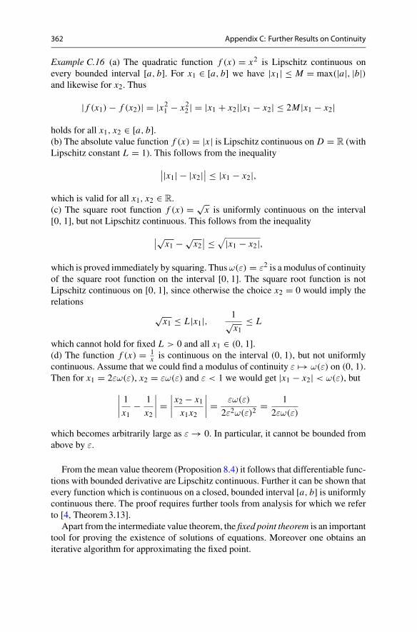
362 Appendix C: Further Results on Continuity
Example C.16 (a) The quadratic function f (x) = x2 is Lipschitz continuous onevery bounded interval [a, b]. For x1 ∈ [a, b] we have |x1| ≤ M = max(|a|, |b|)and likewise for x2. Thus
| f (x1) − f (x2)| = |x21 − x22 | = |x1 + x2||x1 − x2| ≤ 2M |x1 − x2|
holds for all x1, x2 ∈ [a, b].(b) The absolute value function f (x) = |x | is Lipschitz continuous on D = R (withLipschitz constant L = 1). This follows from the inequality
∣∣|x1| − |x2|∣∣ ≤ |x1 − x2|,
which is valid for all x1, x2 ∈ R.(c) The square root function f (x) = √
x is uniformly continuous on the interval[0, 1], but not Lipschitz continuous. This follows from the inequality
∣∣√x1 − √x2∣∣ ≤ √|x1 − x2|,
which is proved immediately by squaring. Thusω(ε) = ε2 is a modulus of continuityof the square root function on the interval [0, 1]. The square root function is notLipschitz continuous on [0, 1], since otherwise the choice x2 = 0 would imply therelations
√x1 ≤ L|x1|, 1√
x1≤ L
which cannot hold for fixed L > 0 and all x1 ∈ (0, 1].(d) The function f (x) = 1
x is continuous on the interval (0, 1), but not uniformlycontinuous. Assume that we could find a modulus of continuity ε �→ ω(ε) on (0, 1).Then for x1 = 2εω(ε), x2 = εω(ε) and ε < 1 we would get |x1 − x2| < ω(ε), but
∣∣∣∣1
x1− 1
x2
∣∣∣∣ =∣∣∣∣x2 − x1x1x2
∣∣∣∣ = εω(ε)
2ε2ω(ε)2= 1
2εω(ε)
which becomes arbitrarily large as ε → 0. In particular, it cannot be bounded fromabove by ε.
From the mean value theorem (Proposition 8.4) it follows that differentiable func-tions with bounded derivative are Lipschitz continuous. Further it can be shown thatevery function which is continuous on a closed, bounded interval [a, b] is uniformlycontinuous there. The proof requires further tools from analysis for which we referto [4, Theorem3.13].
Apart from the intermediate value theorem, the fixed point theorem is an importanttool for proving the existence of solutions of equations. Moreover one obtains aniterative algorithm for approximating the fixed point.
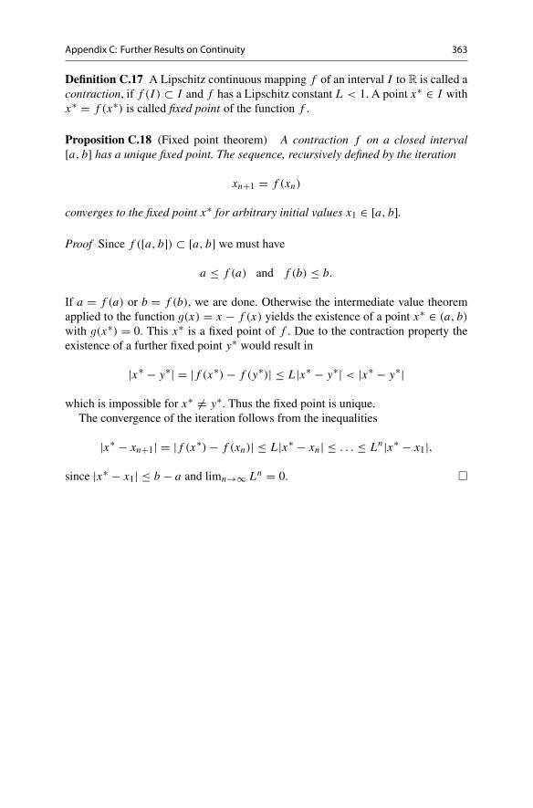
Appendix C: Further Results on Continuity 363
Definition C.17 A Lipschitz continuous mapping f of an interval I to R is called acontraction, if f (I ) ⊂ I and f has a Lipschitz constant L < 1. A point x∗ ∈ I withx∗ = f (x∗) is called fixed point of the function f .
Proposition C.18 (Fixed point theorem) A contraction f on a closed interval[a, b] has a unique fixed point. The sequence, recursively defined by the iteration
xn+1 = f (xn)
converges to the fixed point x∗ for arbitrary initial values x1 ∈ [a, b].
Proof Since f ([a, b]) ⊂ [a, b] we must have
a ≤ f (a) and f (b) ≤ b.
If a = f (a) or b = f (b), we are done. Otherwise the intermediate value theoremapplied to the function g(x) = x − f (x) yields the existence of a point x∗ ∈ (a, b)with g(x∗) = 0. This x∗ is a fixed point of f . Due to the contraction property theexistence of a further fixed point y∗ would result in
|x∗ − y∗| = | f (x∗) − f (y∗)| ≤ L|x∗ − y∗| < |x∗ − y∗|
which is impossible for x∗ = y∗. Thus the fixed point is unique.The convergence of the iteration follows from the inequalities
|x∗ − xn+1| = | f (x∗) − f (xn)| ≤ L|x∗ − xn| ≤ . . . ≤ Ln|x∗ − x1|,
since |x∗ − x1| ≤ b − a and limn→∞ Ln = 0. �
DDescriptionof the SupplementarySoftware
In our view using and writing software forms an essential component of an analysiscourse for computer scientists. The software that has been developed for this bookis available on the website
https://www.springer.com/book/9783319911540
This site contains the Java applets referred to in the text as well as some source filesinmaple, Python and MATLAB.
For the execution of the maple and MATLAB programs additional licences areneeded.
Java applets.The available applets are listed in TableD.1. The applets are executableand only require a current version of Java installed.
Source codes in MATLAB and maple. In addition to the Java applets, you can findmaple andMATLAB programs on this website. These programs are numbered accord-ing to the individual chapters and are mainly used in experiments and exercises. Torun the programs the corresponding software licence is required.
Source codes in Python. For each MATLAB program, an equivalent Python programis provided. To run these programs, a current version of Python has to be installed.We do not specifically refer these programs in the text; the numbering is the same asfor the M-files.
© Springer Nature Switzerland AG 2018M. Oberguggenberger and A. Ostermann, Analysis for Computer Scientists,Undergraduate Topics in Computer Science,https://doi.org/10.1007/978-3-319-91155-7
365

366 Appendix D: Description of the Supplementary Software
Table D.1 List of available Java applets
Sequences
2D-visualisation of complex functions
3D-visualisation of complex functions
Bisection method
Animation of the intermediate value theorem
Newton’s method
Riemann sums
Integration
Parametric curves in the plane
Parametric curves in space
Surfaces in space
Dynamical systems in the plane
Dynamical systems in space
Linear regression
References
Textbooks
1. E. Hairer, G. Wanner, Analysis by Its History (Springer, New York, 1996)2. S. Lang, Introduction to Linear Algebra, 2nd edn. (Springer, New York, 1986)3. S. Lang, Undergraduate Analysis (Springer, New York, 1983)4. M.H. Protter, C.B. Morrey, A First Course in Real Analysis, 2nd edn. (Springer, New York,
1991)
Further Reading
5. M. Barnsley, Fractals Everywhere (Academic Press, Boston, 1988)6. M. Braun, C.C. Coleman, D.A. Drew (eds.), Differential Equation Models (Springer, Berlin,
1983)7. M. Bronstein, Symbolic Integration I: Transcendental Functions (Springer, Berlin, 1997)8. A. Chevan, M. Sutherland, Hierarchical partitioning. Am. Stat. 45, 90–96 (1991)9. J.P. Eckmann, Savez-vous résoudre z3 = 1? La Recherche 14, 260–262 (1983)10. N. Fickel, Partition of the coefficient of determination in multiple regression, in Operations
Research Proceedings 1999, ed. by K. Inderfurth (Springer, Berlin, 2000), pp. 154–15911. E.Hairer, S.P.Nørsett,G.Wanner, SolvingOrdinaryDifferential Equations I. Nonstiff Problems,
2nd edn. (Springer, Berlin, 1993)12. E. Hairer, G. Wanner, Solving Ordinary Differential Equations II. Stiff and Differential-
Algebraic Problems, 2nd edn. (Springer, Berlin, 1996)13. M.W. Hirsch, S. Smale, Differential Equations, Dynamical Systems, and Linear Algebra (Aca-
demic Press, New York, 1974)14. R.F. Keeling, S.C. Piper, A.F. Bollenbacher, J.S. Walker, Atmospheric CO2 records from sites
in the SIO air sampling network, in Trends: A Compendium of Data on Global Change. CarbonDioxide Information Analysis Center, Oak Ridge National Laboratory, U.S. Department ofEnergy (Oak Ridge, Tennessy, USA, 2009). https://doi.org/10.3334/CDIAC/atg.035
© Springer Nature Switzerland AG 2018M. Oberguggenberger and A. Ostermann, Analysis for Computer Scientists,Undergraduate Topics in Computer Science,https://doi.org/10.1007/978-3-319-91155-7
367
368 References
15. E. Kreyszig, StatistischeMethoden und ihre Anwendungen, 3rd edn. (Vandenhoeck&Ruprecht,Göttingen, 1968)
16. W. Kruskal, Relative importance by averaging over orderings. Am. Stat. 41, 6–10 (1987)17. S. Lang, A First Course in Calculus, 5th edn. (Springer, New York, 1986)18. M. Lefebvre, Basic Probability Theory with Applications (Springer, New-York, 2009)19. D.C. Montgomery, E.A. Peck, G.G. Vining, Introduction to Linear Regression Analysis, 3rd
edn. (Wiley, New York, 2001)20. M.L. Overton, Numerical Computing with IEEE Floating Point Arithmetic (SIAM, Philadel-
phia, 2001)21. H.-O. Peitgen, H. Jürgens, D. Saupe, Fractals for the Classroom. Part One: Introduction to
Fractals and Chaos (Springer, New York, 1992)22. H.-O. Peitgen, H. Jürgens, D. Saupe, Fractals for the Classroom. Part Two: Complex Systems
and Mandelbrot Set (Springer, New York, 1992)23. A. Quarteroni, R. Sacco, F. Saleri, Numerical Mathematics (Springer, New York, 2000)24. H. Rommelfanger, Differenzen- und Differentialgleichungen (Bibliographisches Institut,
Mannheim, 1977)25. B. Schuppener, Die Festlegung charakteristischer Bodenkennwerte – Empfehlungen des
Eurocodes 7 Teil 1 und die Ergebnisse einer Umfrage. Geotechnik Sonderheft (1999), pp.32–35
26. STATISTIK AUSTRIA, Statistisches Jahrbuch Österreich. Verlag Österreich GmbH, Wien2018. http://www.statistik.at
27. M.A. Väth, Nonstandard Analysis (Birkhäuser, Basel, 2007)
Index
SymbolsC, 39N, 1N0, 1Q, 1R, 4Z, 1e, 21, 61, 85, 168, 323i, 39π, 3, 30∇, 222∞, 7
AAbsolute value, 7, 40
function, 19Acceleration, 90
vector, 192, 202Addition theorems, 32, 42, 85Affine function
derivative, 84Analysis of variance, 261Angle, between vectors, 335ANOVA, 261Antiderivative, 140Approximation
linear, 88, 89, 219quadratic, 224
Arccosine, 33derivative, 95graph, 34
Archimedean spiral, 200Archimedes, 200
Arc length, 30, 196graph, 159parametrisation, 196
Arcosh, 23derivative, 95
Arcsine, 33derivative, 95graph, 33
Arctangent, 34derivative, 95graph, 34
Areasector, 74surface of sphere, 160triangle, 29under a graph, 150
Area element, 247Area functions, 23Area hyperbolic
cosine, 23sine, 23tangent, 23
Argument, 42Arithmetic of real numbers, 56Arsinh, 23
derivative, 95Artanh, 23
derivative, 95Ascent, steepest, 222Axial moment, 253
BBasis, standard, 332Beam, 119Bijective, see function
© Springer Nature Switzerland AG 2018M. Oberguggenberger and A. Ostermann, Analysis for Computer Scientists,Undergraduate Topics in Computer Science,https://doi.org/10.1007/978-3-319-91155-7
369
370 Index
Binomial formula, 359Binormal vector, 202Bisection method, 77, 110, 114Bolzano, B., 64, 75Bolzano–Weierstrass
theorem of, 64Box-dimension, 126
CCantor, G., 2
set, 128Cardioid, 201
parametric representation, 201Cauchy, A.L., 357
product, 358Cavalieri, B., 244Cavalieri’s priciple, 244Centre of gravity, 248
geometric, 249Chain rule, 91, 219Characteristic equation, 348Circle
of latitude, 238osculating, 198parametric representation, 186unit, 30
Circular arclength, 195
Clothoid, 198parametric representation, 198
Coastline, 126, 264Coefficient of determination, 263
multiple, 267partial, 268
Column vector, 343Completeness, 2, 55Complex conjugate, 40Complex exponential function, 42Complex logarithm, 44, 45
principal branch, 45Complex number, 39
absolute value, 40argument, 42conjugate, 40imaginary part, 40modulus, 40polar representation, 41real part, 40
Complex plane, 41Complex quadratic function, 44Complex root, principal value, 45
Concavity, 108, 109Cone, volume, 159Consumer price index, 117Continuity, 70, 212
componentwise, 232Lipschitz, 194, 361uniform, 361
Contraction, 363Convergence
linear, 111Newton’s method, 112order, 111quadratic, 111sequence, 53
Convexity, 108, 109Coordinate curve, 210, 236Coordinates
of a point, 331polar, 35, 42
Coordinate systemCartesian, 331positively oriented, 331right-handed, 331
Coordinate vector, 333Cosecant function, 37Cosine, 28
antiderivative, 142derivative, 85graph, 32hyperbolic, 22
Cotangent, 28graph, 32
Countability, 2Cuboid, 241Curvature
curve, 196graph, 198
Curve, 185algebraic, 188arc length, 196ballistic, 186change of parameter, 187curvature, 196differentiable, 189figure eight, 201in the plane, 185, 187length, 193, 194normal vector, 191parameter, 185polar coordinates, 200rectifiable, 193
Index 371
reparametrisation, 187Curve in space, 202
arc length, 202binormal vector, 202differentiable, 202length, 202normal plane, 202normal vector, 202rectifiable, 202
Curve sketching, 105, 109Cusp, 188Cycloid, 190
parametric representation, 190Cyclometric functions, 33
derivative, 95
DDamping, viscous, 290Density, 247Derivative, 83, 217
affine function, 84arccosine, 95arcosh, 95arcsine, 95arctangent, 95arsinh, 95artanh, 95complex, 133cosine, 84cyclometric functions, 95directional, 221elementary functions, 96exponential function, 85, 94Fréchet, 217, 233geometric interpretation, 213higher, 87higher partial, 215hyperbolic functions, 95inverse function, 93inverse hyperbolic functions, 95linearity, 90logarithm, 93numerical, 96of a real function, 83partial, 212power function, 94quadratic function, 84root function, 84second, 87sine, 85tangent, 91
Determinant, 346Diagonal matrix, 345Diffeomorphism, 249Difference quotient, 82, 83
accuracy, 171one-sided, 97, 98symmetric, 98, 99
Differentiabilitycomponentwise, 232
Differentiable, 83continuously, 215Fréchet, 217nowhere, 86partially, 212
Differential equationautonomous, 288, 299blow up, 284characteristic equation, 290conserved quantity, 309dependent variable, 276direction field, 277equilibrium, 289existence of solution, 284first integral, 309first-order, 275homogeneous, 278, 292independent variable, 276inhomogeneous, 278, 293initial condition, 277initial value problem, 301invariant, 309linear, 278, 290linear system, 298Lotka–Volterra, 298nonlinear system, 298particular solution, 282power series, 286, 315qualitative theory, 288saddle point, 303second-order, 290separation of variables, 276solution, 275solution curve, 301stationary solution, 281, 289stiff, 325trajectory, 301uniqueness of solution, 285
Differentiation, 83Differentiation rules, 90
chain rule, 91inverse function rule, 93
372 Index
product rule, 90quotient rule, 91
Dimensionbox, 126experimentally, 126fractal, 126
Directional derivative, 221Direction field, 277Dirichlet, P.G.L., 152
function, 152Discretisation error, 97Distribution
Gumbel, 118lognormal, 118
Domain, 14Double integral, 243
transformation formula, 251
EEigenvalue, 348Eigenvector, 348Ellipse, 189
parametric representation, 189Ellipsoid, 228Energy
conservation of, 313kinetic, 313potential, 313total, 313
Epicycloid, 201eps, 10Equilibrium, 289, 301
asymptotically stable, 289, 302stable, 302unstable, 302
Equilibrium point, 301Error sum of squares, 262Euler, L., 21Euler method
explicit, 322, 327implicit, 325modified, 328stability, 325
Euler’s formulas, 43Euler’s number, 21, 61, 85, 168, 323Exponential function, 20, 57
antiderivative, 142derivative, 85, 94series representation, 360Taylor polynomial, 168
Exponential integral, 143
Extremum, 106, 109, 225local, 108, 109necessary condition, 106
Extremum test, 170
FFailure wedge, 119Field, 40First integral, 309Fixed point, 120, 363Floor function, 25Fractal, 124Fraction, 1Fréchet, M., 216Free fall, 81Fresnel, A.J., 143
integral, 143, 199Fubini, G., 244Fubini’s theorem, 244Function, 14
affine, 218antiderivative, 140bijective, 2, 15complex, 44complex exponential, 42complex quadratic, 44composition, 91compound, 91concave, 108continuous, 70, 212convex, 108cyclometric, 33derivative, 83differentiable, 83elementary, 143exponential, 57floor, 25graph, 14, 209higher transcendental, 143hyperbolic, 22image, 14injective, 14inverse, 16inverse hyperbolic, 23linear, 17linear approximation, 89monotonically decreasing, 107monotonically increasing, 107noisy, 99nowhere differentiable, 86piecewise continuous, 153
Index 373
quadratic, 14, 18, 218range, 14real-valued, 14slope, 107strictly monotonically increasing, 107surjective, 15trigonometric, 27, 44vector valued, 231zero, 75
Fundamental theoremof algebra, 41of calculus, 156
GGalilei, Galileo, 81Galton, F., 257Gauss, C.F., 115, 257Gaussian error function, 143Gaussian filter, 101Gradient, 221, 232
geometric interpretation, 222Graph, 14, 209
tangent plane, 220Grid
mesh size, 242rectangular, 241
Grid points, 175
HHalf life, 280Half ray, 189Heat equation, 228Helix, 203
parametric form, 203Hesse, L.O., 224Hessian matrix, 224Hyperbola, 190
parametric representation, 190Hyperbolic
cosine, 22function, 22sine, 22spiral, 200tangent, 22
Hyperbolic functions, 22derivative, 95
Hyperboloid, 228
IImage, 14Imaginary part, 40Indicator function, 20, 245Inequality, 7INF, 9Infimum, 52Infinity, 7Inflection point, 109Initial value problem, 277, 301Injective, see functionIntegrable, Riemann, 151, 243Integral
definite, 149, 151double, 241, 243elementary function, 142indefinite, 140iterated, 243properties, 154Riemann, 149
Integrationby parts, 144numerical, 175rules of, 143substitution, 144symbolic, 143Taylor series, 172
Integration variable, 154Intermediate value theorem, 75Interval, 6
closed, 6half-open, 6improper, 7open, 6
Interval bisection, 75Inverse function rule, 93Inverse hyperbolic
cosine, 23sine, 23tangent, 23
Inverse hyperbolic functions, 23derivative, 95
Inverse, of a matrix, 346Iterated integral, 243Iteration method, 363
JJacobian, 217, 232Jacobi, C.G.J., 217Jordan, C., 347Julia, G., 131
374 Index
set, 131Jump discontinuity, 71, 72
KKoch, H. von, 129Koch’s snowflake, 129, 136, 193
LLagrange, J.L., 166Lateral surface area
solid of revolution, 160Law of cosines, 36Law of sines, 36Least squares method, 256Leibniz, G., 153Lemniscate, 201
parametric representation, 201Length
circular arc, 195differentiable curve, 194differentiable curve in space, 202
Leontief, W., 318Level curve, 210Limit
computation with Taylor series, 171improper, 54inferior, 64left-hand, 70of a function, 70of a sequence, 53of a sequence of functions, 354right-hand, 70superior, 64trigonometric, 74
Limit function, 354Lindemayer, A., 134Linear approximation, 88, 89, 165, 219Line of best fit, 115, 256
through origin, 115, 116Line, parametric representation, 189Liouville, J., 143Lipschitz, R., 284
condition, 285constant, 285, 361continuous, 361
Lissajous, J.A., 204figure, 204
Little apple man, 131Logarithm, 21
derivative, 93
natural, 21Logarithmic
integral, 143spiral, 200
Loop, 200parametric representation, 200
Lotka, A.J., 298Lotka–Volterra model, 308, 327L-system, 135
MMachine accuracy
relative, 10, 12Malthus, T.R., 281Mandelbrot, B., 130
set, 130Mantissa, 8Mapping, 2, 14
linear, 344Mass, 247Mass–spring–damper system, 290Mass–spring system, nonlinear, 319Matrix, 343
coefficient, 343determinant, 346diagonal element, 345element, 343entry, 343inverse, 346invertible, 346Jordan canonical form, 347nilpotent, 350product, 345product with vector, 344regular, 346similar, 347square, 343transposed, 344unit, 345zero, 345
Matrix algebra, 343Maximum, 52
global, 105isolated local, 227local, 106, 108, 170, 224strict, 106
Mean value theorem, 107Measurable, 245Meridian, 238Minimum, 52
global, 106

Index 375
isolated local, 227local, 106, 170, 224
Mobilised cohesion, 119Model, linear, 256, 265Modulus, 40Modulus of continuity, 361Moment
of inertia, 119statical, 248
Monotonically decreasing, 107Monotonically increasing, 107Moving frame, 192, 202Multi-step method, 323
NNaN, 9Neighbourhood, 53, 124Neil, W., 188Newton, I., 110, 294Newton’s method, 111, 114, 119
in C, 133local quadratic convergence, 235two variables, 233
Nonstandard analysis, 154Normal domain, 246
of type I, 246of type II, 246
Normal equations, 258Numbers, 1
complex, 39decimal, 3floating point, 8largest, 9normalised, 9smallest, 9
integer, 1irrational, 4natural, 1random, 100rational, 1real, 4transcendental, 3
Numerical differentiation, 96
OOptimisation problem, 109Orbit, periodic, 310Order relation, 5
properties, 6rules of computation, 6
Osculating circle, 198
PParabola
Neil’s, 188quadratic, 18
Paraboloidelliptic, 211hyperbolic, 210
Partial mapping, 210Partial sum, 58Partition, 151
equidistant, 153Peano, G., 284Pendulum, mathematical, 312, 314Plane
in space, 339intercept, 339normal vector, 340parametric representation, 339slope, 339
Plantgrowth, 136random, 138
Point of expansion, 167Point space, 334Polar coordinates, 233Population model, 281
discrete, 51Malthusian, 281Verhulst, 51, 66, 281
Position vector, 333Power function, 18
antiderivative, 142derivative, 94
Power series, equating coefficients, 287Precision
double, 8single, 8
Predator-prey model, 298Principal value
argument, 42Product rule, 90Proper range, 14Pythagoras, 27
theorem, 27
QQuadratic function
derivative, 84
376 Index
graph, 18Quadrature formula, 177
efficiency, 180error, 181Gaussian, 180nodes, 177order, 178order conditions, 179order reduction, 182Simpson rule, 177stages, 177trapezoidal rule, 176weights, 177
Quotient rule, 91
RRadian, 30Radioactive decay, 24, 280Rate of change, 89, 280Ratio test, 67Real part, 40Rectifiable, 193Regression
change point, 273exponential model, 257, 273linear, 255loglinear, 257multiple linear, 265multivariate linear, 265simple linear, 256univariate linear, 256
Regression line, 256predicted, 259through origin, 115
Regression parabola, 120Regression sum of squares, 261Remainder term, 166Residual, 259Riccati, J.F., 287
equation, 287, 328Riemann, B., 149
integrable, 151, 243integral, 151sum, 151, 242
Right-hand rule, 331Root, complex, 41, 43Root function, 19
derivative, 84Rounding, 10Rounding error, 97Row vector, 344
Rules of calculationfor limits, 53
Runge–Kutta method, 323
SSaddle point, 225, 227Saddle surface, 210Scalar multiplication, 332Scatter plot, 115, 255Schwarz, H.A., 216
theorem, 216Secant, 82
slope, 83Secant function, 37Secant method, 115Self-similarity, 123Semi-logarithmic, 111Sequence, 49
accumulation point, 62bounded from above, 51bounded from below, 52complex-valued, 50convergent, 53geometric, 55graph, 50infinite, 49limit, 53monotonically decreasing, 51monotonically increasing, 51real-valued, 50recursively defined, 50settling, 53vector-valued, 50, 211convergence, 211
Sequence of functionspointwise convergent, 354uniformly convergent, 355
Series, 58absolutely convergent, 357Cauchy product, 358comparison criteria, 60convergent, 58divergent, 58geometric, 59harmonic, 60infinite, 58partial sum, 58ratio test, 67
Setboundary, 124boundary point, 124
Index 377
bounded, 124Cantor, 128cardinality, 2closed, 124covering, 125interior point, 124Julia, 131Mandelbrot, 130of measure zero, 245open, 124
Sexagesimal, 5Shape function, 256Sign function, 19Simpson, T., 177
rule, 177Sine, 28
antiderivative, 142derivative, 84graph, 32hyperbolic, 22Taylor polynomial, 168Taylor series, 170
Sine integral, 143Snowflake, 129Solid of revolution
lateral surface area, 160volume, 158
Space-time diagram, 300Sphere, 237
surface area, 160Spiral, 200
Archimedean, 200hyperbolic, 200logarithmic, 200parametric representation, 200
Spline, 101Spring, stiffness, 290Square of the error, 116Standard basis, 332Stationary point, 106, 225Step size, 322Straight line
equation, 337in space, 340intercept, 17, 338normal vector, 339parametric representation, 338slope, 17, 29, 338
Subsequence, 62Substitution, 144Superposition principle, 278, 292
Supremum, 51Surface
in space, 210normal vector, 237of rotation, 237parametric, 236regular parametric, 236tangent plane, 237tangent vector, 213
Surjective, see functionSymmetry, 99
TTangent, 28
graph, 32, 82, 87hyperbolic, 22plane, 220problem, 82slope, 87vector, 191, 202
Taylor, B., 165expansion, 97formula, 165, 223polynomial, 167series, 169theorem, 170
Telescopic sum, 60Thales of Miletus, 28
theorem, 28Total variability, 261Transformation formula, 251Transport equation, 228Transpose
of a matrix, 344Trapezoidal rule, 176Triangle
area, 29hypotenuse, 27inequality, 11leg, 27right-angled, 27
Triangle inequality, 195Trigonometric functions, 27, 28
addition theorems, 32, 36inverse, 33
Triple product, 347Truncated cone
surface area, 37surface line, 37
378 Index
UUniform
continuity, 361convergence, 355
Unit circle, 30, 43Unit matrix, 345Unit vector, 332
VVariability
partitioning, 262sequential, 268
total, 261Variation of constants, 281Vector, 332
cross product, 336dot product, 335inner product, 335magnitude, 332norm, 332orthogonal, 335perpendicular, 335unit, 332
zero, 332Vector algebra, 331Vector field, 231Vector space, 50, 334Velocity, 89
average, 81instantaneous, 82, 89
Velocity vector, 191, 202Verhulst, P.-F., 51, 66, 281, 289Vertical throw, 141Volterra, V., 298Volume
cone, 159solid of revolution, 158
WWeber–Fechner law, 24Weierstrass, K., 64
ZZero matrix, 345Zero sequence, 69Zero vector, 332