mid-term adequacy forecast 2018 - entso-e

ENTSO-E AISBL • Avenue de Cortenbergh 100 • 1000 Brussels • Belgium • Tel + 32 2 741 09 50 • Fax + 32 2 741 09 51 • [email protected] • www. entsoe.eu

Mid-term Adequacy Forecast 2018

Appendix 1: Methodology and Detailed Results

2018 edition



2

Table of Contents

1 Methodology and assumptions ............................................................................................... 3

1.1 Methodology – advanced tools for probabilistic market modelling .................................................4

Adequacy Indices .....................................................................................................................7

Reliability indices and model convergence ..............................................................................8

Reliability indices in practice .................................................................................................10

1.2 Assumptions – comprehensive datasets for all parts of the system ................................................10

Scenarios and Pan-European Market Modelling Data Base (PEMMDB) ..............................10

Demand time series - Temperature dependency of demand ...................................................11

Climate data - Pan-European Climate Database (PECD) .......................................................15

Net Transfer Capacities .........................................................................................................17

Thermal generation maintenance profile ................................................................................17

Reserves ..................................................................................................................................18

Demand Side Response (DSR) ...............................................................................................20

Other relevant parameters .......................................................................................................20

1.3 Limitations of the MAF methodology ............................................................................................21

2 Detailed Model Results ........................................................................................................ 22

2.1 Base case results .............................................................................................................................22

Adequacy in numbers – EENS and LOLE in 2020 and 2025 ...............................................22

Detailed results of all modelling tools ....................................................................................26

2.2 Low-carbon sensitivity ...................................................................................................................37

2.3 Level of imports during single and simultaneous scarcity situations .............................................41

2.4 Flow-based innovations ..................................................................................................................43

2020 Flow-Based sensitivity for Continental Western Europe (CWE) ..................................43

2025 Flow-based sensitivity applied on a complete transmission model ...............................44

2.5 Impact of hydro constraints and its relaxation................................................................................46

2.6 Flexibility .......................................................................................................................................47

3 Market modeling tools used .................................................................................................. 48

3.1 ANTARES......................................................................................................................................48

3.2 BID3 ...............................................................................................................................................52

3.3 GRARE ..........................................................................................................................................53

3.4 PLEXOS .........................................................................................................................................56

3.5 PowrSym ........................................................................................................................................57

4 Glossary ............................................................................................................................... 61

4.1 Zone codes and corresponding countries .......................................................................................61

4.2 Abbreviations .................................................................................................................................61



3

1 Methodology and assumptions

The methodology for adequacy assessments has been successfully implemented in five different market

modelling tools1. All tools cover the same geographic perimeter (as presented in Figure 1 and the

corresponding graphs of the MAF 2018 executive report) as well as the same time horizon (i.e. the target

years 2020 and 2025). In the same vein, all tools deploy the same methodological approach, i.e. probabilistic

market modelling. This approach has enabled a thorough analysis and benchmarking of the different models,

and thus led to substantial improvements in terms of consistency and trust.

Figure 1: The interconnected European power system perimeter modelled in MAF 2018

Figure 2 provides an overview of the overall approach that has been chosen and followed in the MAF. Broadly

speaking, adequacy refers to the relationship of available resources and demand which is balanced via

network infrastructure. In this assessment, the supply and demand side are composed by a deterministic

forecast, combined with stochastic uncertainty. The deterministic forecast is in line with ENTSOs’ Scenarios

which are published as a separate document. Stochastic uncertainty, driven by climatic variables and the risk

of unplanned generator and line outages, is accommodated by means of Monte Carlo simulations, as

explained hereafter.

1 ANTARES, BID3, GRARE, PLEXOS and PowrSym. See Section 3 for a short presentation of the individual tools.



4

Figure 2: Overview of the methodological approach

1.1 Methodology – advanced tools for probabilistic market modelling

Our methodology compares supply and demand levels in an interconnected European power system by

simulating the market operations on an hourly basis over a full year. In each of the scenarios for 2020 and

2025, we build upon ENTSOs’ scenarios, forecasting net generating capacity (NGC), cross-border

transmission capacity and annual level of demand. In addition, the simulations consider the main stochastic

contingencies that may affect security of supply, including:

1. Outdoor temperatures (which result in load variations, principally driven by the heating and cooling

patterns in winter and summer respectively),

2. Wind and photovoltaic power production,

3. Unscheduled outages of thermal generation units and relevant HVDC interconnectors,

4. Maintenance schedules,

5. Extended hydro database, including dry, wet or normal hydro conditions.

For each of these contingencies, all market modelling tools perform a large number of Monte Carlo

simulations, built by the combinatorial stochastic process schematically depicted in Figure 3 below.



5

Figure 3: Graphical illustration of the number of Monte Carlo years required for convergence of the results

Monte Carlo simulations are built combining the aforementioned variables in the following way: climate

years (1982-2015) are first selected one-by-one. Each climate year, consisting of a combination of demand

(accounting temperature sensitivity), wind and solar time series, is assigned with one of the three possible

hydro conditions (wet, dry, normal) or with historical year-specific time series of hydro generation. Each set

of climate and hydro conditions is further associated with a relatively large number of Monte Carlo

realisations, randomly assigning forced outage patterns for thermal units and interconnections.

In general, the tools employed are built upon a market simulation engine. Such an engine is not meant for

modelling or simulating the behaviour of market players or optimal bidding, e.g. gaming, explicit capacity

withdrawal from markets, etc., but is, rather, meant for simulating marginal costs (not prices) of the whole

system and the different market nodes. Therefore, the main assumption is that the market is perfectly

competitive, with no strategic behaviours present.

The tools calculate marginal costs as part of the outcome of a system cost-minimisation problem. Such a

mathematical problem, also known as ‘Optimal Unit Commitment and Economic Dispatch’, is often

formulated as a large-scale Mixed-Integer Linear-Programming (MILP) problem. In other words, the program

attempts to find the least-cost solution while respecting all operational constraints (e.g. ramping, minimum

up/down time, transfer capacity limits, etc.). In order to avoid infeasible solutions, very often the constraints

are modelled as ‘soft’ constraints, i.e. constraints can potentially be violated at the expense of a high penalty

in terms of cost. Most optimisation solvers nowadays are capable of solving large-scale MILP problems

within acceptable computation times. However, with the presence of integer variables it is still common in

commercial tools to solve the overall problem by applying a combination of heuristics and MILP. Moreover,

the extensive number of Monte Carlo simulations makes the computation an intensive and challenging task.

In the MAF study, the size of the problem is immense, i.e. including thousands of variables and constraints.

Additionally, the size increases with the optimisation time horizon and resolution. The time horizon of the

optimisation problem, e.g. hydro optimisation, maintenance or fault duration, etc., is one week, and the

resolution of the simulation is hourly, i.e. given the constraints and boundary conditions, the total system cost

is minimised for each week of the year on an hourly basis. The weekly optimisation horizon means that the



6

optimal values for each hour of the whole year are calculated, with the optimisation problem broken up on a

weekly basis, to reduce computation time. A weekly optimisation horizon is also common practice for market

simulations at many TSOs for network planning. The latter means that the results such as generation output

of the thermal and hydro plants, marginal costs, etc. are provided per hour. This setting of the parameters is

also common practice for the market simulations which are conducted under the context of the ENTSO-E

TYNDP and PLEF Generation Adequacy Assessment.

These tools also have the functionality to include network constraints to a varying degree of detail. Nowadays,

the status-quo approach for pan-European or regional market studies is based on Net Transfer Capacity (NTC)

Market Coupling. This means that the network constraints between the market nodes are modelled as limits

only on the commercial exchanges at the border. This approach is followed in the current study as well.

The EU Internal Energy Market target model is based on Flow-Based Market Coupling (FBMC). In this

model, the network constraints are modelled as real physical limits on selected ‘critical branches’. Most TSO

tools nowadays can perform FBMC, even though they have not been thoroughly tested for large-scale

applications. There are also tools which can model the physical network explicitly including all the technical

constraints such as contingencies, thermal and voltage constraints, therefore incorporating what is commonly

known as Optimal Power Flow (OPF). Such a feature is not yet common in Europe since there is no agreement

or plans for a regional scale application of nodal pricing. The possibility of including FBMC for future MAF

reports is currently being evaluated within ENTSO-E. In this version of the MAF, in addition to the common

NTC approach for the base case scenarios, additional innovative FB studies are conducted. More specifically,

a FBMC approach is considered for the target year 2020 similarly to the PLEF study, while an explicit

physical-network representation is considered on the simulations for the year 2025, paving the way for

improvements to come in MAF future studies.

Five different tools were used in parallel in the current study, which are referred to as ‘Voluntary Parties

(VP)’. A comparison of results between the different tools ensures the quality and robustness of inputs and

calculations, as well as outcomes. Meanwhile, it should be noted that a full alignment of results between

different tools is not possible due to differences in the intrinsic optimisation logic of the ‘Optimal Unit

Commitment and Economic Dispatch’ used by the different tools. Different features of the participating tools

are also exploited in the simulations to understand the sensitivity of the results to the different optimisation

objectives, while the input dataset remains identical among all tools. The aim of using different tools and the

comparison of their output is to obtain consolidated and reliable results, while understanding their sensitivity

to the assumptions and modelling choices made. The process is illustrated in Figure 4.



7

The comparison of results was performed in the following four-step process:

a) Preparation of aggregated output data of the models

b) Visualisation of the output data in the form of comparison charts

c) Discussions and analyses within the MAF market study group

d) Specification of actions regarding model or input data improvement

Figure 4: Use of multiple models and tools (principle)

The current MAF probabilistic methodology is considered as a reference at the pan-European perimeter.

However, the methodology followed in each MAF report should be understood as an ‘implementation

release’ of ENTSO-E’s Target Methodology, which is in itself subject to constant evolution and further

improvements. It is worth mentioning that the expected major improvements for the base case in future MAF

reports are, among others, the implementation of flow-based modelling as the base case and the extension of

the climate database to cover hydrological conditions for all geographical areas of the study, as well as a unit-

by-unit representation of the generation units in the longer term.

Adequacy Indices

System adequacy refers to the existence of sufficient resources to meet the consumers’ demand and the

operating requirements of the power system. As a metric, the so-called adequacy indices are used. These

indices can be quantified as deterministic indicators (capacity margins) or as probabilistic indicators,

according to the methodologies used for the adequacy assessments.

With respect to the definition and scope of the indices of adequacy studies, three main functional zones of

power systems are involved in the adequacy evaluation:

• Generation adequacy level (or hierarchical level I), which considers the total system generation

including the effect of transmission constraints in the form of NTCs.

• Transmission adequacy level (or hierarchical level II), which includes both the generation and

transmission facilities in an adequacy evaluation.

• The overall hierarchical level (or hierarchical level III), which involves all three functional zones, from

the generating points to the individual consumer load points, typically connected at the distribution

level.

Traditionally, the adequacy indices can have different designations depending on the hierarchical levels

involved in the adequacy study. In this edition of the MAF 2018 report, the focus is on the hierarchical level

I, generation adequacy level. The results of the simulations are expressed in terms of the following indices:

• Expected Energy Not Served (EENS) [MWh/year or GWh/year] is the average energy not supplied per year

by the generating system due to the demand exceeding the available generating and import capacity. In

reliability studies, it is common that Energy Not Served (ENS) is examined in expectation over a number of

Market

Modelling

Database

Results’

Comparison

Validation

Consolidated

Results

VP1

VP2

VP3

VP4

VP5



8

Monte Carlo simulations. To this end, EENS is a metric that measures security of supply in expectation and

is mathematically described by (1) below:

EENS =1

𝑁∑ 𝐸𝑁𝑆𝑗𝑗∈𝑆 (1)

where ENSj is the energy not supplied of the system state j (j ϵ S) associated with a loss of load event of the

jth-Monte Carlo simulation and where N is the number of Monte Carlo simulations considered.

• Loss Of Load Expectation2 (h/year) LOLE is the average number of hours per year in which the available

generation plus import cannot cover the load in an area or region.

LOLE =1

𝑁∑ 𝐿𝐿𝐷𝑗𝑗∈𝑆 (2)

where, LLDj is the loss of load duration of the system state j (j ϵ S) associated with the loss of load event of

the jth Monte Carlo simulation and where N is the number of Monte Carlo simulations considered. It should

be noted that the LLD of the jth Monte Carlo simulation can only be reported as an integer of hours because

of the hourly resolution of the simulation. Thus, it does not indicate the severity of the deficiency or the

duration of the loss of load within that hour.

The proposed metrics above are quantified by probabilistic modelling of the available flexible resources.

Additional indices to measure, for example, the frequency and duration of the EENS or the power system

flexibility can be considered in future evolutions.

Reliability indices and model convergence

With respect to the relationship of the probabilistic indices and convergence of the models, when multiple

Monte Carlo simulations are conducted, these indices can also be expressed in average, minimum and

maximum values accordingly. Annual values can also be used to construct a probability distribution curve.

Figure 5: Example of EENS convergence over a number of Monte Carlo simulations

2 When reported for a single Monte Carlo simulation as the sum of all the hourly contributions with ENS, this quantity

refers to the number of hours (events) within one year for which ENS occurs/is observed and this quantity should be

referred to as a Loss of Load Event. The quantity calculated in Eq. (2) refers to the average over the whole ensemble of

Events and it therefore provides the statistical measure of the expectation of the number of hours with ENS over that

ensemble.

0

100

200

300

400

500

600

700

800

1 9 17 25 33 41 49 57 65 73 81 89 97 105 113 121 129 137 145 153 161 169 177 185 193 201 209 217 225 233 241 249 257 265

GW

h/y

ear

Simulated YearsENS Incremental Average

1982 1983 1984 1985 1986 1987 1988 1989 1990 1991 1992 1993 1994 1995 1996 1997 1998 1999 2000 20012002 2003 2004 2005 2006 2007 2008 2009 2010 2011 2012 2013 2014 2015

95% (2σ) probability



9

The trend of the moving average of EENS against the total number of Monte Carlo simulations performed

provides a good indication of the convergence of the simulations (example shown in Figure 5). When N is

sufficiently large (i.e. when The Strong Law of Large Numbers and Central Limit Theorem hold), the error

between the expected value and its average exhibits a Gaussian distribution and its upper bound with a

probability of 95% can be calculated using the following formula:

|ε𝑛| ≤ 1.96𝜎

√𝑛 (3)

where ε𝑛 is the error at 𝑛 iterations, and 𝜎 the standard deviation.

Correspondingly, the confidence interval can be calculated using the following formula:

[ X̅𝑁 − 1.96𝜎𝑁̅̅ ̅̅

√𝑁, X̅𝑁 + 1.96

𝜎𝑁̅̅ ̅̅

√𝑁] (4)

where X̅𝑁 is the sample average.

Figure 6: Example of confidence interval achieved by the simulations

Noticeably, some inputs and parameters can have a significant impact on the numerical results of these indices

and their convergence, such as

- Hydro power data usage and modelling

- NTCs

- Extreme historical climatic years (e.g. year 1985)

- Outages and their modelling: this refers to both maintenance and forced outages. To understand the

impact of forced outages, which are random by definition, it is important for all the tools to use one

commonly agreed maintenance schedule. This maintenance schedule should respect the different

constraints specific to the thermal plants in different countries, as provided by TSOs.

In order to obtain a satisfactory analysis of the influence of different inputs, parameters, outages and

modelling with the use of different tools, various sensitivity analyses have been conducted in this report, as

presented in the MAF Executive Report.

0

10

20

30

40

50

60

70

80

90

100

0 200 400 600 800 1000 1200

%

Simulated years



10

Reliability indices in practice

With respect to the various reliability indices introduced in the previous section, Table 1 presents a

comprehensive overview of the different metrics that EU Member States apply to assess their national

generation adequacy.

As is evident, the most relevant index is expressed in LOLE (h/year), which is also the main indicator used

in this report. Target reliability levels in terms of LOLE are typically in the range of 3-8 h/year. It should be

noted that setting such reliability targets is a sensitive issue which needs to consider economic and technical

aspects. For instance, these targets could be determined by means of counterbalancing the value of lost load

(VoLL) against the costs related to maintaining a reliable generation capacity.

Other than Europe, it is worth mentioning that AEMO’s mid-term adequacy assessment for Australia sets an

EENS threshold of 0.002% of the annual demand, instead of the LOLE threshold used in Europe.3 This, for

instance, would correspond for Germany to around 2 million households not supplied for 5 hours.

Table 1: Situation of metrics used in EU Member States to assess generation adequacy at national level in 2015

Sources: ACER, CEER, Assessment of electricity generation adequacy in European countries, Staff Working Document accompanying the Interim Report of the Sector Inquiry on CMs and Pentalateral generation adequacy probabilistic assessment. * Information about BE, GR and PT have been updated to reflect recent changes. Note: NS: Not specified reliability standard, LOLE: Loss of Load Expectation, LOLE P95: 95th percentile of LOLE (1 in 20 years probability).

1.2 Assumptions – comprehensive datasets for all parts of the system

All models use the same data input for their calculations. In order to have a consistent dataset, a common

scenario framework is agreed upon. Therefore, a harmonised and centralised Pan-European Market

Modelling Data Base (PEMMDB) for market studies has been prepared based on national generation data

and outlooks provided to ENTSO-E by each individual TSO. The focus of the study is on the calibration of

the models for two time horizons: years 2020 and 2025. This section describes the most important

assumptions and how they are incorporated in the different tools to run the Pan-European market simulations.

Scenarios and Pan-European Market Modelling Data Base

The PEMMDB is the main source of data for the MAF. The PEMMDB contains collected data from TSOs

for bottom-up scenarios as well as centrally analysed data for top-down scenarios.

The MAF framework uses collected data for 2020 and 2025 (i.e. bottom-up scenarios). Even though a detailed

description of the PEMMDB is provided in the ENTSOs’ scenario report4, Figure 7 provides an overview of

the most important data characteristics, i.e shares of the different electricity generation sources for 2020 and

3 http://www.aemo.com.au/Electricity/National-Electricity-Market-NEM/Planning-and-forecasting/Energy-Adequacy-

Assessment-Projection 4 https://tyndp.entsoe.eu/tyndp2018/scenario-report/

Country AT BE* BG CH CY CZ DE DK EE ES FI FR GB GR* HR HU IE IT LT LU LV MT NL NO PL PT* RO SE SI SK

Reliability

Standard No Yes NS No NS No No No No Yes No Yes Yes Yes NS Yes NS No No NS NS No No No No Yes NS No NS No

LOLE

(h/y) 3 13 3 3 3 8 8 4 5

LOLE

P95 (h/y) 20

Capacity

Margin 10% 9%

http://www.aemo.com.au/Electricity/National-Electricity-Market-NEM/Planning-and-forecasting/Energy-Adequacy-Assessment-Projection

http://www.aemo.com.au/Electricity/National-Electricity-Market-NEM/Planning-and-forecasting/Energy-Adequacy-Assessment-Projection

https://tyndp.entsoe.eu/tyndp2018/scenario-report/



11

2025. Generation capacities are categorized based on the generation technology, e.g. total thermal capacity

consists of coal, lignite, gas, nuclear, oil and biofuel.

Figure 7: Distribution of generation capacity for all ENTSO-E zones (base case scenarios 2020 and 2025)

In addition to the above figures, the PEMMDB covers further elements important for the modelling of

electricity markets, such as:

• Demand and Demand Side Response forecasts

• Information on thermal generation units, e.g. must-run properties, number of units etc.

• Information on hydro generation units

• Information on renewable generation capacities

• Reserves and exchanges with non ENTSO-E countries

Information about decommissioning of units due to an accelerated coal phase-out have been independently

collected from the TSOs and are not part of the PEMMDB database. For further details and information on

all scenarios, please refer to the ENTSO-E Scenario report and the accompanying MAF 2018 dataset.

Demand time series - Temperature dependency of demand

The electrical demand is dependent on weather conditions. The most important influencing factor is the

temperature. Especially in the commercial and domestic sector, the widespread use of electrical heating and

cooling has a significant impact on the electrical demand. The general change of temperature throughout the

year leads to fluctuating demand. In addition, cold spells in winter and heat waves in summer represent

extreme events that have a strong impact on demand. It is crucial to integrate these extreme conditions into

the probabilistic models. Based on a refined sensitivity analysis of demand and temperature, time series of

electrical demand are created and form fundamental inputs for the MAF.

Quantifying the impact of heating and cooling

Heating and cooling devices allow us to maintain a comfortable temperature in our indoor environment. Many

of these devices work either directly or indirectly with electrical energy. This dependency of electrical

demand and temperature can be illustrated as follows:



12

Figure 8: Temperature dependency of consumed energy

For very low temperatures, a lot of energy is consumed for heating (heating zone). When the outdoor

temperature remains around 20 degrees, households generally neither use heating nor cooling and therefore

the extra energy consumed by the devices is low. With rising temperatures, an increasing number of cooling

devices are turned on, which in turn leads again to higher electrical demand (cooling zone).

For a Pan-European assessment such as the MAF, it is crucial to observe what impact the heating and cooling

have on the total consumption of electrical energy. Furthermore, it is important to quantify this effect for the

different assessed areas. By finding mathematical correlations between the ambient temperature in an area

and its consumption, the demand – temperature sensitivity can be calculated. This cubical polynomial

approximation is the basis for creating synthetic hourly demand profiles for each area.

Pmin dependency of daily temperature Pmax dependency of daily temperature

Figure 9: Cubical approximation of demand and daily average temperature

Figure 9 shows such cubical approximations (red lines). The blue dots represent the daily minimum (on the

left graph) and maximum (on the right graph) demand respectively for a certain daily average temperature. It

can be observed that most of the blue dots are clustered around the approximation. Only a couple of outliers

0 5 10 15 20 25 30

De

man

d M

Wh

Temperature °C

SaturationSaturation

CoolingZone

HeatingZone

ComfortZone

Outliers

Each dot is a combination of consumption and daily average temperature for one day



13

with significant lower demand can be found. These points are bank and school holidays for which a majority

of the commercial and industrial demand is lower. The outliers are not considered in the cubical

approximations. The described analysis is carried out for all assessed market zones for the year 2015. The

daily average temperature is calculated from a data set which includes 34 years of meteorological data.

A demand profile for average temperatures

The next step is to calculate a demand profile under normal temperature conditions. The previously described

polynomials are applied onto the measured demand profile of 2015. The outcome is an hourly profile that

represents the demand of the market zones as if the daily temperature is equal to the 34-year average.

Summing up every hour of this normalised demand profile would result in the total electrical demand of 2015

of each zone. It is now necessary to up- or downscale this to a specified demand for the target years. The

target annual consumption of 2020 or 2025 is part of the PEMMDB (see Section 1.2.1).

Creating a synthetic demand profile on historical temperatures

The last step is to calculate a synthetic demand profile for each available year of temperature measurement.

See the following simplified example for clarification: Day 358 of year 1999 had an average temperature of

6.5°C. By observing all 34 years, we know that the temperature of this day on average was 8.5°C, i.e. colder

than average by 2°C. Thus, the electrical load is expected to be comparatively higher than usual (since there

is a need for more heating). To quantify this, the polynomial with the temperature difference is used and the

expected daily maximum and minimum demand are calculated. With these two values, the load profile can

now be rescaled for that specific day, as illustrated in Figure 10. The same approach is applied for every day

of 34 years of the available temperature data for all market zones.

Figure 10: Stretch rescaling of a daily demand profile

Changing the shape of the demand profiles

The structure of the demand and the consumption patterns are subject to change in the future. In particular,

electric vehicles (EV) and heat pumps (HP) are considered as changing the shape of the daily demand profile.



14

Therefore, they are treated separately. The following factors are considered to represent the electrical energy

consumed by these devices (the example below refers to EVs):

1. Number of devices 2. Daily load profile of device 3. Seasonality

PEMMDB data

collection

Figure 11: The figure illustrates the factors influencing electricity demand profiles from devices such as EVs and HPs.

Using EVs as an example, the first factor is the number of EVs (collected through the PEMMDB), the second factor is an

assumption on the daily demand profile of the EVs and, finally, the last factor refers to variations on the demand profile

due to seasonality.

0.00

0.10

0.20

0.30

0.40

0.50

0.60

0.70

0.80

0.90

1.00

1 2 3 4 5 6 7 8 9 10 11 12 13 14 15 16 17 18 19 20 21 22 23 24

Load

per

EV

(kW

) →

EV s

eas

on

alit

y fa

cto

r →

Days of the year →

Demand in a nutshell

1. Hourly demand profiles for 34 years representing a large range of realistic temperature conditions

2. Scaled to the target annual consumption of each zone in each scenario (2020, 2025)

3. EVs and HPs considered

4. Consistent approach for all MAF zones



15

Climate data - Pan-European Climate Database (PECD)

The PECD is a database developed by ENTSO-E, which consists of reanalysed hourly weather data and load

factors of variable generation (namely, wind and solar). PECD data sets are prepared by external experts

using best practice in industry, thus ensuring a representative estimation of demand, variable generation and

other climate-dependent variables.

For this study, PECD was employed extensively to estimate a number of climate-dependent variables.

Representative demand profiles were built, as explained in Section 1.2.2. Furthermore, estimates of variable

generation were made based on information about load factors in PECD and variable generation capacities

within PEMMDB. Different types of hydrological conditions were defined and applied for each climate year.

These hourly time series were then combined with other random samples, as explained in Section 1.1, in

sufficient number of Monte Carlo years, to give a statistically representative data set to be used in the

adequacy study.

The PECD was launched in 2014 through a centralised approach to re-analyse climatic data ensuring a

coherent data set. Key benefits include the precise representation of simultaneous extreme events (e.g. heat

waves) as well as realistic wind and solar generation forecast for the whole study perimeter. Furthermore,

since its creation PECD has been continuously developing to improve data quality, extend the geographical

perimeter coverage and increase the number of historical years re-analysed. The use of the PECD is an

important data quality improvement, recognised by all ENTSO-E’s members and used in pan-European and

national studies.



16

ENTSO-E PECD consists of the following data sets:

Wind speed, radiation and nebulosity time series

• Hourly average reference wind speed at 100 m for each market node [m/s], to be calculated according

to the formula below:

𝐴𝑣𝑒𝑟𝑎𝑔𝑒 𝑟𝑒𝑓𝑒𝑟𝑒𝑛𝑐𝑒 𝑤𝑖𝑛𝑑 𝑠𝑝𝑒𝑒𝑑 ሺ𝑡, 𝑚𝑎𝑟𝑘𝑒𝑡 𝑛𝑜𝑑𝑒ሻ = ඨ1

𝑛∑ ቆට𝑈𝑡,𝑖

2 + 𝑉𝑡,𝑖2ቇ

3

𝑛𝑖=1

3

(5)

t: time [h]

U: Zonal component of the wind speed at 100m height (west-east direction) [m/s]

V: Meridional component of the wind speed at 100m height (north-south direction) [m/s]

n: total number of grid points in the market node

i: grid point

• Hourly average global horizontal irradiance for each market node [W/m2]

• Hourly average cloud cover (nebulosity) for each market node [okta]

Onshore, offshore wind, solar PV and Concentrated Solar Power load factor time series

• Hourly normalised load factor time series for onshore and (if applicable) offshore wind production for

each market node

• Hourly normalised load factor time series for solar PV production for each market node

• Hourly normalised load factor time series for concentrated solar power for each market node where

relevant

Temperature time series

• Hourly city temperature time series [°C]



17

Net Transfer Capacities

Assumptions on NTCs for each scenario 2020 and 2025 are based on TSO expertise (bottom up data

collection). The transfer capacity between borders/ bidding zones, agreed between the respective TSOs, will

be available within the data set published together with the present report.

TSOs were also asked to propose values for simultaneous importable / exportable capacities – meaning

the maximum possible flow at the same time through all NTC corridors respecting N-1 and operational

security of these countries. For adequacy simulations, such constraints should be considered since they might

be imposed for some borders (e.g. in the flow-based market coupling area) for reasons linked to internal grid

stability and operational constraints.

Although an implementation of FBMC is already in place in some parts of the ENTSO-E zone (CWE), it is

not considered in the MAF 2018 main results. The FBMC is only considered as an additional sensitivity

analysis, testing different flow-based approaches. On the one hand, this is due to the fact that most ENTSO-

E areas are still using an NTC approach. On the other hand, a common flow-based approach should be agreed,

which would be applicable to the whole European perimeter and feasible to implement in all tools used in

MAF.

In the MAF, forced outages (e.g. unexpected failure of a line resulting in unavailability) are considered for

all High-Voltage Direct Current (HVDC) interconnections and some High Voltage Alternating Current

interconnections.

Thermal generation maintenance profile

The maintenance is understood as scheduled out-of-service network elements and in this case refers to

thermal generating units. In the PEMMDB, it is possible to specify the number of days for maintenance and

the percentage of maintenance that should be planned in winter/summer; additional constraints can be

specified providing the maximum number of units for each generation technology type (nuclear, coal, etc.)

being in maintenance for each week of the year.

An automated procedure has been adopted for the definition of the maintenance schedule of thermal

generators for each area of the electrical system. The process is based on the principle of ‘constant reserve’:

for each week of the year the difference between available thermal generation and residual load to be covered

is calculated and the maintenance of each generator is never broken into discontinuous weeks.

A single maintenance schedule was calculated for each year horizon (2020, 2025) to be adopted from all the

tools involved. Furthermore, maintenance schedules were not different among the various climatic years.

This is conservative, however, and in line with the limited possibilities of adjusting planned maintenance

work in reality (which is typically fixed between 6 and 12 months in advance).

It was verified that the use of a constant maintenance schedule for all climatic years does not significantly

affect the adequacy evaluations. For a year with a high risk of unserved energy due to climatic conditions, a

special maintenance profile has been tailored. Both evaluations with the common and the special maintenance

schedule have shown similar results. Furthermore, it is worth mentioning that the maintenance schedule was

calculated with two different tools and the adequacy results were comparable.



18

Reserves

Balancing reserves or ancillary services are fundamental to a power system. As foreseen in the Electricity

Balancing Guideline, each TSO shall contract/procure ancillary services to ensure a secure, reliable and

efficient electricity grid. These are agreements with certain producers and consumers to increase or decrease

the production or demand of certain sites. The aim is to compensate for the unbalance that could be caused

by unforeseen loss of a production unit or demand/renewable forecasting errors. The balancing reserves are

not responsible for maintaining the large-scale adequacy, and are deducted from available resources in the

MAF.

Reserves

To permanently guarantee the balance between demand and generation of electrical energy, the TSO

has to maintain certain levels of reserves. The reserve capacity is then requested when the electrical

frequency deviates from its nominal value, possibly due to an unforeseen outage event which threatens

the electrical stability of the system. Typically, fast acting conventional power plants are suitable for

providing reserve capacity. In some cases, hydro power plants and interruptible loads are contracted.

In the event of major frequency deviations, the restoration process is guided by three reserve

products:

1. Frequency Containment Reserve (FCR)

refers to the active power reserves (automatically activated) available to contain system

frequency after the occurrence of an unbalance.

2. Automatic Frequency Restoration Reserve (aFRR)

stabilises the frequency and ensures the availability of the FCR is guaranteed. It is also

utilised to maintain the balance of power imports and exports of a control area.

3. Manual Frequency Restoration Reserve (mFRR)

guarantees the availability of the aFRR. It is manually activated (e.g. by ramping up/down

generators) and is mostly used when there is a major disruption of the grid operation (e.g.

failure of a generator).



19

74MW [0%]

80MW [14%]

100MW [7%]

110MW [6%]

126MW [7%]

135MW [16%]

150MW [3%]

150MW [5%]

152MW [10%]

163MW [8%]

187MW [3%]

200MW [18%]

200MW [6%]

200MW [12%]

255MW [2%]

266MW [12%]

282MW [12%]

325MW [4%]

400MW [20%]

402MW [8%]

412MW [11%]

470MW [10%]

500MW [3%]

500MW [7%]

530MW [8%]

545MW [4%]

600MW [4%]

700MW [11%]

700MW [2%]

700MW [19%]

714MW [27%]

800MW [4%]

882MW [8%]

899MW [20%]

920MW [7%]

1140MW [4%]

1215MW [13%]

1230MW [11%]

1280MW [3%]

1355MW [2%]

1570MW [10%]

2020MW [3%]

2071MW [2%]

5200MW [6%]

SE3

MT

LV

AL

NI

ME

NOm

NOn

MK

SI

IE

CY

HR

ITsar

PT

SE1

BA

BG

LT

DKw

SE2

TN00

BE

RS

HU

AT

NOs

ITcn

ITn

ITsic

DKe

NL

CH

SK

GR

PL

RO

CZ

ES

GB

FI

TR

FR

DE

0 1000 2000 3000 4000 5000 6000 7000

Reserves [MW]

Reserve as extra load Reserve as reduced hydro

Figure 12: Reserved generation capacity as specified in the PEMMDB for 2020. Total reserved capacity is reported as a %

of peak demand inside brackets.



20

The market simulations are not real-time and have a resolution of one hour. Balancing reserves are assigned

to deal with the hazards that can occur within this time step. They must therefore be removed from the

available generation capacity. From a modelling perspective, this can be implemented in two ways: reducing

the respective thermal generation capacity or increasing the demand by the hourly reserved capacity. For

practical reasons, it was preferred to take reserves into account by adding them to consumption rather than

applying a thermal capacity reduction. While this is easier to implement into the market models, it has the

disadvantage of distorting the reported energy balance since ‘virtual consumption’ is added. Notably, in some

countries, reserves are provided by hydroelectrical generation. In these cases, the maximum possible hydro

generation is reduced by the reserved value. Furthermore, in special cases (e.g. where a TSO has agreements

with large electricity users on demand reduction when needed or dedicated back-up power plants) the reserve

specifications were directly coordinated with the data correspondent of the TSO.

Further assumptions regarding the modelling of operational reserves might be considered in future reports,

in line with the implementation of the pertinent Network Codes and further considerations regarding the

impact of sharing operational reserves on a real-time basis, across synchronously-connected countries in

ENTSO-E. Figure 12 presents an overview of the aforementioned data as used for the MAF assessment of

year 2020.

Demand Side Response (DSR)

Based on the information specified in the PEMMDB, DSR is not modelled as a reduction of load, but as a set

of flexible generators with discretely specified parameters. This modelling approach is feasible since Long-

Term Adequacy Correspondents provided hourly availability of DSR assets in several price bands. The four

distinctly modelled price bands enable more detailed simulations by considering, for example, industrial DSR

and domestic DSR separately. Price bands are defined by a price (€/MWh) and a maximum number of hours

of continuous availability of typical DSR installations. Since no economic analyses of the findings are carried

out in the MAF framework5, the price for the entirety of DSR assets is arbitrarily set to 500€/MWh, while the

maximum number of available hours is respected in each band. The high price ensures its activation before

loss of load, without interfering with the merit order dispatching. Thorough tests were conducted with all

market modelling tools to ensure that this modelling approach is valid.

Other relevant parameters

To allow for a more accurate reflection of the diversity of generation technologies and better approach the

operation in practice with respect to the simulated power plants and HVDC lines, basic parameters such as

NGC, Number of Units and other additional technical parameters have been considered in the data collection.

Some of these parameters present boundary conditions or thresholds that the VPs should comply with during

the simulations.

Availability of the power system elements is considered in the simulation in two ways: i) Forced Outages

and ii) Planned Outages. In the MAF, availability is considered on thermal power plants active in the market

and HVDC lines.

Planned outages refer to maintenance, and are defined as the number of days, on an annual basis,

that a given unit (blocks of-) is expected to be offline due to maintenance. Further restrictions

regarding the minimum percentage of the outages which can occur in each season of the year, with a

focus on winter and summer, as well as the maximum number of simultaneously offline thermal units

allowed within each month of the year, were specified by TSOs. Within these restrictions, an

optimised maintenance schedule, common to all modelling tools, is prepared. Optimisation of the

5 Note that investigations of economic indicators are foreseen for future editions of the MAF.



21

maintenance schedule refers to the minimisation of the number of units (simultaneously) in

maintenance and the optimal distribution of the maintenance schedules to reduce the occurrence of

potential adequacy problems, while respecting the constraints of their national power system

provided by TSOs.

Forced outages are represented by the parameter Forced Outage Rate (FOR) which defines the

annual rate of forced outage occurrences of thermal power plants or grid elements. Forced outages

are simulated by random occurrences of outages within the probabilistic Monte Carlo scheme, while

respecting the annual rate defined. Simulated random forced outages are useful for assessing the

impact of the availability of base-load thermal generation and its relationship with the available

flexible thermal and hydro generation, renewable generation and imports. Simulating the forced

outages allows the resilience of a given area to be tested subject to such contingencies, potential

adequacy problems that might occur and the ability of the area to share power (via spot market power

and/or reserves).

Minimum stable generation (MW) is a parameter defining the technical minimum of the power output of a

unit. The simulation does not allow the unit to run under this limit. It is defined by a percentage of the

maximum power output of the unit.

Ramp up/down rates (MW/h) define the ability of the thermal power plant, which is already in operation,

to increase/decrease its generation output within the range of its stable working area, which is constrained by

the minimum stable generation parameter and the maximum power output.

Minimum Up Time parameter defines the minimum number of hours a unit must stay in operation before it

can be idled.

Minimum Down Time parameter defines the minimum number of hours a unit must remain idle before it

can be restarted. These parameters guarantee the optimal operation of units, e.g. prevents simulating units

from being in and out in consecutive hours, if this is not compliant with the unit normal operation.

In addition to the main characteristics, other thermal characteristics have also been defined in the PEMMDB

to allow for a more accurate reflection of the diversity of the different generation technologies.

1.3 Limitations of the MAF methodology

The current MAF methodology relies on an advanced probabilistic market modelling approach. Yet, like

every modelling approach it has its inherent limitations, which are briefly presented below:

• Perfect foresight and flexibility is assumed. Wind, solar and demand forecast errors are considered

to be modelled within the day-ahead fixed reserves, as MAF approach assumes a perfect day-ahead

forecast. The anticipation of the future (next week, month) variables affecting optimal hydro dispatch

is assumed in the model, while this is not the case in reality.

• Energy-only market is considered in MAF simulations. The MAF model considers neither the

capacity nor the balancing market, both comprising an important topic that deserves further

investigation in the future.

• Perfect competition is considered in the MAF simulations, assuming that no strategic behaviours

are present in the market and all market agents behave competitively, revealing their true costs to the

market.



22

• Uncertainty of decommissioning date of thermal units. ENTSO-E is building a pan-European

database with a higher level of granularity in terms of generation assets, to better cope with

uncertainties related to decommissioning of thermal units.

• Internal grid limitations within a bidding zone are not considered in the base case approach.

However, this was further investigated in innovative flow-based studies conducted as sensitivity

analyses, which are presented in section 2.4. This topic needs further development and detailed

comparison with the current MAF approach, also considering possible evolutions of the European

market.

2 Detailed Model Results

This Section contains the detailed results of the market modelling studies for the MAF 2018. Primarily, it

contains the detailed results of the base case scenario in years 2020 and 2025. In addition, several sensitivities

and complementary results are presented.

Section 2 is divided into the following parts: Section 2.1 outlines the detailed results of the base case scenarios

for the target years 2020 and 2025, while Section 2.2 presents the detailed results of the low-carbon sensitivity

analysis. Section 2.3 offers a closer look at the hourly levels of imports and exports focusing on a test case

for FR, BE and GB. The scope of this section is to investigate the hours of single or multiple simultaneous

scarcity events. The innovative flow-based approaches are presented and explained in detail in Section 2.4,

for both years 2020 and 2025. The impact of hydro constraints and their relaxation is then investigated in

Section 462.5. Finally, a brief description of the methodology behind the Flexibility analysis, seen in the

executive report, is presented in Section 2.6.

2.1 Base case results

In this section, the detailed simulation results of base case studies for the target years 2020 and 2025 are

presented. In Section 2.1.1 below Table 2 and Table 3 present detailed results of the EENS and LOLE

respectively, for all zones of the MAF. Apart from the LOLE and EENS values, which correspond to the

average of all simulated results, the 50th and 95th percentiles of the distributions are also presented in the

same tables. In Section 2.1.2, the LOLE results are illustrated for each of the modelling tools, i.e. results from

VP1 to VP5, providing information about the statistical range of the simulation outcomes for each tool.

Adequacy in numbers – EENS and LOLE in 2020 and 2025

In this section, the base case scenario results are reported in tables. Results presented in the following tables

correspond to the values extracted from the corresponding simulations and averaged among all tools, e.g. in

base scenario 2020, the P50 value of Albania represents the average value of all P50 values of Albania

considering all tools. Results of EENS and LOLE are provided, hereafter, for the base case scenarios 2020

and 2025.



23

Table 2: EENS results for base case scenarios 2020 and 2025 by zone 6

Zone

Code

EENS - Base case scenario 2020 EENS - Base case scenario 2025

EENS

[GWh]

EENS / Annual

Demand [%]

P50

[GWh]

P95

[GWh]

EENS

[GWh]

EENS / Annual

Demand [%]

P50

[GWh]

P95

[GWh]

AL 0.1 0.001% 0.0 0.4 0.1 0.001% 0.0 0.3

AT 0.0 0.000% 0.0 0.0 0.0 0.000% 0.0 0.0

BA 0.0 0.000% 0.0 0.0 0.0 0.000% 0.0 0.0

BE 0.1 0.000% 0.0 0.0 3.4 0.004% 0.2 17.5

BG 6.7 0.017% 3.7 22.7 0.0 0.000% 0.0 0.1

CH 0.0 0.000% 0.0 0.0 0.0 0.000% 0.0 0.0

CY 6.0 0.102% 5.0 13.8 146.1 2.116% 143.6 197.9

CZ 0.0 0.000% 0.0 0.0 0.0 0.000% 0.0 0.0

DE 0.0 0.000% 0.0 0.0 0.0 0.000% 0.0 0.0

DEkf 0.0 0.000% 0.0 0.0 0.0 0.000% 0.0 0.0

DKe 0.0 0.000% 0.0 0.0 0.1 0.000% 0.0 0.3

DKkf 0.0 0.000% 0.0 0.0 0.0 0.000% 0.0 0.0

DKw 0.0 0.000% 0.0 0.0 0.0 0.000% 0.0 0.0

EE 0.0 0.000% 0.0 0.0 0.0 0.000% 0.0 0.0

ES 0.0 0.000% 0.0 0.0 0.0 0.000% 0.0 0.0

FI 1.2 0.001% 0.2 5.0 0.3 0.000% 0.0 1.5

FR 8.4 0.002% 0.0 18.1 10.0 0.002% 0.0 27.4

GB 1.4 0.000% 0.2 7.7 2.8 0.001% 0.4 15.2

GR 0.9 0.002% 0.1 4.7 0.2 0.000% 0.0 0.9

GR037 2.6 0.083% 2.0 7.5 2.7 0.077% 1.8 8.1

HR 0.0 0.000% 0.0 0.0 0.0 0.000% 0.0 0.0

HU 0.0 0.000% 0.0 0.0 0.0 0.000% 0.0 0.0

IE 0.0 0.000% 0.0 0.0 0.7 0.002% 0.3 2.9

IS 0.0 0.000% 0.0 0.0 0.2 0.000% 0.0 0.6

ITcn 0.0 0.000% 0.0 0.0 0.6 0.002% 0.2 2.8

ITcs 0.0 0.000% 0.0 0.0 0.0 0.000% 0.0 0.0

ITn 0.1 0.000% 0.0 0.1 1.6 0.001% 0.0 4.7

ITs 0.0 0.000% 0.0 0.0 0.0 0.000% 0.0 0.0

ITsar 0.0 0.000% 0.0 0.0 0.1 0.001% 0.0 0.6

ITsic 0.7 0.004% 0.3 2.4 0.1 0.000% 0.0 0.5

LT 0.0 0.000% 0.0 0.1 0.0 0.000% 0.0 0.0

LUb 0.0 0.006% 0.0 0.1 0.1 0.028% 0.0 0.4

LUf 0.3 0.025% 0.0 1.0 0.4 0.034% 0.0 1.7

LUg 0.0 0.000% 0.0 0.0 0.3 0.006% 0.1 1.2

LUv 0.0 0.000% 0.0 0.0 0.0 0.000% 0.0 0.0

6 For the definition of zone codes, see Section 4.1. 7 Considering recent development plans of the Independent Power Transmission Operator (Greece), it is estimated that

Crete will have better adequacy levels for year 2025 than the ones presented in the table, as a result of higher

interconnection capacity.



24

LV 0.0 0.000% 0.0 0.1 0.0 0.000% 0.0 0.0

ME 0.0 0.000% 0.0 0.0 0.0 0.000% 0.0 0.0

MK 0.0 0.000% 0.0 0.0 0.0 0.000% 0.0 0.0

MT 0.4 0.017% 0.2 1.6 0.7 0.025% 0.2 2.8

NI 0.3 0.003% 0.1 1.4 0.4 0.004% 0.1 1.8

NL 0.0 0.000% 0.0 0.0 0.2 0.000% 0.0 0.9

NOm 0.0 0.000% 0.0 0.0 0.0 0.000% 0.0 0.0

NOn 0.0 0.000% 0.0 0.0 0.0 0.000% 0.0 0.0

NOs 1.0 0.001% 0.0 5.5 0.0 0.000% 0.0 0.1

PL 0.0 0.000% 0.0 0.0 0.7 0.000% 0.1 3.8

PT 0.0 0.000% 0.0 0.0 0.0 0.000% 0.0 0.0

RO 0.0 0.000% 0.0 0.0 0.0 0.000% 0.0 0.0

RS 0.0 0.000% 0.0 0.0 0.0 0.000% 0.0 0.0

SE1 0.0 0.000% 0.0 0.0 0.0 0.000% 0.0 0.0

SE2 0.0 0.000% 0.0 0.0 0.0 0.000% 0.0 0.0

SE3 0.0 0.000% 0.0 0.0 0.0 0.000% 0.0 0.0

SE4 0.0 0.000% 0.0 0.0 0.0 0.000% 0.0 0.0

SI 0.0 0.000% 0.0 0.0 0.0 0.000% 0.0 0.0

SK 0.0 0.000% 0.0 0.0 0.0 0.000% 0.0 0.0

TN00 7.8 0.031% 6.0 20.8 0.2 0.001% 0.0 1.1

TR 0.0 0.000% 0.0 0.0 0.0 0.000% 0.0 0.0

Table 3: LOLE [h/year] results for base case scenarios 2020 and 2025 by zone

Zone

Code

LOLE - Base case scenario 2020 LOLE - Base case scenario 2025

LOLE

[h/year]

P50 [h/year] P95 [h/year] LOLE

[h/year]

P50 [h/year] P95 [h/year]

AL 0.43 0.00 2.02 0.21 0.00 1.00

AT 0.00 0.00 0.00 0.00 0.00 0.00

BA 0.00 0.00 0.00 0.00 0.00 0.00

BE 0.07 0.00 0.06 2.02 0.22 10.83

BG 20.71 15.52 57.84 0.14 0.00 0.30

CH 0.01 0.00 0.00 0.04 0.00 0.01

CY 76.50 69.23 144.20 1199.47 1198.56 1469.07

CZ 0.00 0.00 0.00 0.01 0.00 0.00

DE 0.00 0.00 0.00 0.00 0.00 0.00

DEkf 0.00 0.00 0.00 0.00 0.00 0.00

DKe 0.02 0.00 0.00 0.15 0.00 0.62

DKkf 0.00 0.00 0.00 0.00 0.00 0.00

DKw 0.00 0.00 0.00 0.00 0.00 0.00

EE 0.06 0.03 0.24 0.00 0.00 0.02

ES 0.00 0.00 0.00 0.00 0.00 0.00

FI 3.56 0.80 18.65 0.72 0.00 4.61

FR 1.96 0.00 7.25 2.08 0.00 8.44



25

GB 1.29 0.29 6.14 1.30 0.41 6.33

GR 2.25 0.63 11.41 0.43 0.00 1.88

GR03 59.21 51.03 141.58 54.06 42.78 141.72

HR 0.00 0.00 0.00 0.00 0.00 0.00

HU 0.00 0.00 0.00 0.00 0.00 0.00

IE 0.01 0.00 0.00 3.23 1.84 11.65

IS 0.00 0.00 0.00 0.27 0.20 0.80

ITcn 0.04 0.00 0.06 1.31 0.44 5.85

ITcs 0.00 0.00 0.00 0.01 0.00 0.00

ITn 0.07 0.00 0.11 0.85 0.00 3.74

ITs 0.00 0.00 0.00 0.00 0.00 0.00

ITsar 0.04 0.00 0.20 0.97 0.33 4.17

ITsic 3.56 2.04 11.00 0.51 0.12 2.35

LT 0.21 0.18 0.52 0.01 0.00 0.03

LUb 0.62 0.00 2.48 2.62 0.46 14.49

LUf 2.36 0.00 7.91 3.10 0.00 12.94

LUg 0.00 0.00 0.00 1.09 0.20 5.88

LUv 0.00 0.00 0.00 0.00 0.00 0.00

LV 0.18 0.10 0.64 0.01 0.00 0.02

ME 0.00 0.00 0.00 0.00 0.00 0.00

MK 0.00 0.00 0.00 0.00 0.00 0.00

MT 8.55 4.15 32.34 13.56 5.12 54.51

NI 2.80 0.76 12.57 2.64 1.20 11.94

NL 0.00 0.00 0.00 0.21 0.00 1.13

NOm 0.01 0.00 0.03 0.00 0.00 0.00

NOn 0.00 0.00 0.00 0.00 0.00 0.00

NOs 0.80 0.00 4.28 0.04 0.00 0.40

PL 0.03 0.00 0.09 1.44 0.57 6.39

PT 0.00 0.00 0.00 0.04 0.00 0.02

RO 0.00 0.00 0.00 0.00 0.00 0.00

RS 0.00 0.00 0.00 0.00 0.00 0.00

SE1 0.00 0.00 0.00 0.00 0.00 0.00

SE2 0.00 0.00 0.00 0.00 0.00 0.00

SE3 0.00 0.00 0.00 0.00 0.00 0.00

SE4 0.11 0.00 0.25 0.11 0.00 0.25

SI 0.00 0.00 0.00 0.00 0.00 0.00

SK 0.00 0.00 0.00 0.01 0.00 0.05

TN00 38.51 34.61 82.93 1.05 0.13 5.73

TR 0.00 0.00 0.00 0.00 0.00 0.00



26

Detailed results of all modelling tools

Bar charts in Section Error! Reference source not found. indicate the probabilistic range of the adequacy

index LOLE in 2020, namely the 50th and 95th percentiles of the distributions of simulation results (or in other

words, the results for the risk of 1 in 2 years to 1 in 20 years). Moreover, average values of adequacy indices

(LOLE) of all simulated climatic years are represented as dots for all simulation tools. Figure 13 below

illustrates how the results are presented in this section.

Figure 13: How to read the illustrated detailed MAF results

How to read the results?

Example: A market modelling tool calculates LOLE for 100 Monte Carlo years. The 95th percentile (often abbreviated as P95) of the results’ distribution is the 5th highest value observed. This corresponds to a probability of ‘1 in 20’.



27

2.1.2.1 Adequacy results in 2020

Figure 14 - Base Case 2020 - LOLE results by tool



28



29



30



31



32

2.1.2.2 Adequacy results in 2025

Compared to the 2020 scenario, MAF 2018 results for 2025 demonstrate better results for Bulgaria (due to

the envisaged commissioning of new CCGT plants) and Finland, which experiences some risk of high LOLE

in the 2020 scenario. On the other hand, a comparative increase in the LOLE values appears for Belgium,

Italy, Ireland and Poland in the 2025 assessment.

Figure 15 - Base Case 2025 - LOLE results by tool



33



34



35



36



37

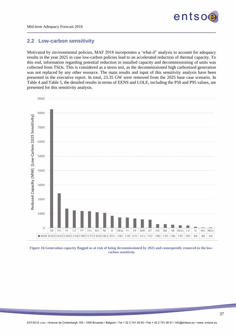
2.2 Low-carbon sensitivity

Motivated by environmental policies, MAF 2018 incorporates a ‘what-if’ analysis to account for adequacy

results in the year 2025 in case low-carbon policies lead to an accelerated reduction of thermal capacity. To

this end, information regarding potential reduction in installed capacity and decommissioning of units was

collected from TSOs. This is considered as a stress test, as the decommissioned high carbonized generation

was not replaced by any other resource. The main results and input of this sensitivity analysis have been

presented in the executive report. In total, 23.35 GW were removed from the 2025 base case scenario. In

Table 4 and Table 5, the detailed results in terms of EENS and LOLE, including the P50 and P95 values, are

presented for this sensitivity analysis.

Figure 16:Generation capacity flagged as at risk of being decommissioned by 2025 and consequently removed in the low-

carbon sensitivity



38

Table 4: EENS results for low-carbon sensitivity 2025 by zone

Zone Code

EENS - Low-carbon Sensitivity 2025

EENS

[GWh]

EENS / Annual

Demand [%]

P50 [GWh] P95 [GWh]

AL 0.8 0.009% 0.4 3.1

AT 0.6 0.001% 0.0 3.4

BA 0.1 0.000% 0.0 0.4

BE 34.2 0.040% 4.9 197.5

BG 0.2 0.001% 0.0 1.1

CH 1.1 0.002% 0.0 5.1

CY 147.2 2.132% 146.1 196.9

CZ 4.8 0.007% 0.6 25.2

DE 9.7 0.002% 0.3 52.6

DEkf 0.0 0.000% 0.0 0.0

DKe 1.9 0.012% 0.2 9.7

DKkf 0.0 0.000% 0.0 0.0

DKw 0.6 0.002% 0.0 2.8

EE 0.5 0.005% 0.0 2.7

ES 0.0 0.000% 0.0 0.0

FI 1.5 0.002% 0.0 8.2

FR 31.2 0.007% 0.0 171.7

GB 13.2 0.004% 2.5 71.7

GR 1.3 0.002% 0.3 6.1

GR03 4.0 0.115% 2.6 11.6

HR 0.2 0.001% 0.0 1.5

HU 0.9 0.002% 0.0 4.8

IE 28.3 0.090% 25.7 58.2

IS 0.3 0.000% 0.4 0.6

ITcn 6.2 0.017% 2.7 25.0

ITcs 0.3 0.001% 0.0 1.6

ITn 26.7 0.014% 4.2 135.4

ITs 0.0 0.000% 0.0 0.0

ITsar 0.5 0.005% 0.1 2.1

ITsic 0.3 0.002% 0.0 1.6

LT 0.7 0.005% 0.0 3.6

LUb 0.5 0.193% 0.1 2.2

LUf 1.7 0.137% 0.2 8.6

LUg 9.2 0.163% 2.6 45.5

LUv 0.0 0.000% 0.0 0.0

LV 0.2 0.002% 0.0 1.0

ME 0.0 0.000% 0.0 0.0

MK 0.6 0.007% 0.1 2.8

MT 0.7 0.024% 0.3 2.4

NI 2.9 0.031% 1.9 8.8



39

NL 5.7 0.005% 2.3 22.6

NOm 0.0 0.000% 0.0 0.0

NOn 0.0 0.000% 0.0 0.0

NOs 0.4 0.000% 0.0 2.1

PL 7.0 0.004% 3.1 28.4

PT 0.9 0.002% 0.0 4.5

RO 0.2 0.000% 0.0 1.3

RS 0.1 0.000% 0.0 0.5

SE1 0.0 0.000% 0.0 0.0

SE2 0.0 0.000% 0.0 0.0

SE3 0.0 0.000% 0.0 0.2

SE4 1.0 0.004% 0.0 4.2

SI 0.1 0.000% 0.0 0.5

SK 1.2 0.004% 0.2 5.7

TN00 0.3 0.001% 0.0 1.6

TR 0.1 0.000% 0.0 0.7

Table 5: LOLE [h/year] results for low-carbon sensitivity 2025 by zone

Zone Code

LOLE - Low-carbon Sensitivity 2025

LOLE

[h/year]

P50 [h/year] P95 [h/year]

AL 2.35 1.50 7.54

AT 0.67 0.00 4.40

BA 0.17 0.00 1.20

BE 12.28 2.95 60.26

BG 0.70 0.00 3.66

CH 0.88 0.00 4.83

CY 1205.60 1206.65 1488.69

CZ 6.02 1.50 29.72

DE 3.26 0.62 15.80

DEkf 0.00 0.00 0.00

DKe 3.94 1.23 20.29

DKkf 0.00 0.00 0.00

DKw 1.70 0.43 8.03

EE 1.82 0.16 8.88

ES 0.01 0.00 0.00

FI 3.25 0.13 17.83

FR 6.07 0.00 33.82

GB 5.02 1.95 24.66

GR 2.28 0.83 9.56

GR03 58.05 46.18 148.04

HR 0.29 0.00 1.98

HU 0.76 0.00 4.02

IE 92.72 87.95 165.50



40

IS 0.41 0.40 0.80

ITcn 8.97 4.80 34.13

ITcs 0.61 0.02 3.43

ITn 8.59 2.26 42.68

ITs 0.01 0.00 0.00

ITsar 2.72 0.88 10.85

ITsic 1.24 0.29 5.95

LT 1.90 0.29 10.16

LUb 17.77 5.23 82.51

LUf 13.33 2.26 68.60

LUg 11.86 3.91 56.43

LUv 0.00 0.00 0.00

LV 0.97 0.08 5.23

ME 0.07 0.00 0.40

MK 1.39 0.42 5.85

MT 12.83 6.43 44.95

NI 20.77 16.81 55.41

NL 5.24 2.38 20.74

NOm 0.03 0.00 0.00

NOn 0.03 0.00 0.00

NOs 0.28 0.00 1.60

PL 9.33 6.32 27.90

PT 0.95 0.00 4.02

RO 0.44 0.00 2.20

RS 0.18 0.00 1.26

SE1 0.00 0.00 0.00

SE2 0.00 0.00 0.00

SE3 0.08 0.00 0.40

SE4 1.03 0.00 4.97

SI 0.27 0.00 1.94

SK 2.49 0.50 12.19

TN00 1.34 0.14 6.66

TR 0.11 0.00 0.80



41

2.3 Level of imports during single and simultaneous scarcity situations

Interconnections are crucial for supporting adequacy in large systems. Specifically, interconnections can help

to balance supply and demand on a broader geographical scope, thus allowing the deployment of benefits

from statistical balancing effects in demand and variable renewable generation. Intuitively, when considering

two interconnected countries there is a high chance that the two countries do not face the most critical ramp

at the exact same time. This can be explained by uncorrelated climatic conditions and different periods of

peak demand occurrence. Another factor can be time zone differences that cause time shifts of demand peaks.

It is, thus expected that in a large number of situations, adequacy problems in a country will not be correlated

with adequacy problems in neighbouring ones. In these cases, the importance of interconnectors is obvious

as countries would be able to rely on imports from their neighbours to ensure their adequacy. We refer to

these as individual or single scarcity situations. In those cases, it is expected that countries will present

import levels close to their maximum simultaneous importable capacity.

On the other hand, ‘critical or extreme situations’ can occur which are highly correlated in time and

geographical perimeter (e.g. cold spell, heat waves, large rain-snow storms, etc.). In those situations, a lack

of available power might occur inside a geographical area encompassing more than one country. We refer to

these as simultaneous scarcity situations in a certain macro-area.

Lack of power in these situations is typically related to the lack of available resources to generate the needed

power in the specific macro-area8. Typically in those cases, although the adequacy problems are not linked

to a lack of interconnection capacity, the affected countries (part of the macro-area) might present import

levels lower than their maximum simultaneous importable capacity. Such low levels of imports are,

rather, related to a global/regional deficit of available power generation inside the perimeter

encompassed by the countries in scarcity.

Below, we have performed a detailed analysis of the results obtained for the 2020 scenario. For illustration

purposes, we have focused on the area between France (FR), Great Britain (GB) and Belgium (BE) and

analysed the hourly results of EENS vs ‘Country Net Balance (Balance)’. Note that a negative (country net)

balance corresponds to a country import. Furthermore, each dot in the figures below corresponds to an hourly

situation, so ‘Balance’ and ‘EENS’ are provided in MW.

It is possible to identify the following 3 regimes (A, B.1 & B.2, C):

• A: Triple simultaneous scarcity – hours when all 3 ‘GB+FR+BE’ have EENS

• B.1: Simultaneous scarcity GB+FR– hours when ‘GB+FR’ have EENS

• B.2: Simultaneous scarcity BE+FR– hours when ‘BE+FR’ have EENS

• C: Hours when GB or FR are in ‘individual’ scarcity

Regarding the import levels (negative balance) during these regimes, we identify that:

- Situation A relates to lowest imports, much below the maximum simultaneous import capacity, in agreement

with a ‘resource scarcity’ storyline of not having enough power regionally inside the area encompassed

between these three countries.

- Situations B.1 and B.2 relate to mid levels of imports below the maximum simultaneous import– in

agreement with a ‘resource scarcity’ storyline of not having enough power inside the area between the two

countries considered (GB-FR B.1 and BE-FR B.2)

8 For example, low or too strong winds, dry rivers reducing availability of hydro power or cooling capabilities of nuclear

reactors, frozen rivers and roads limiting the transportation of fuels like coal or gas, extended low temperatures leading

to unexpected large and long-lasting levels of electricity demand, etc.



42

- Situation C relates to scarcity in FR, GB – EENS for those countries occurs individually while imports are

close to the maximum simultaneous import for those countries FR ~ 12GW, GB ~ 4.5 GW. Furthermore, the

adequacy problems of BE appear to be highly correlated with the ‘resource scarcity’ adequacy problems in

FR and FR+GB.

Figure 17: The impact of simultaneous scarcity events with a focus on FR. Negative balance corresponds to imports.

Figure 18: The impact of simultaneous scarcity events with a focus on GB. Negative balance corresponds to imports.



43

Figure 19: The impact of simultaneous scarcity events with a focus on BE. Negative balance corresponds to imports.

In conclusion, interconnectors contribution is of key importance in periods of scarcity. In case of single

country scarcity, it is expected that the country in scarcity will import close to its maximum simultaneous

importable capacity. In case of several countries' simultaneous scarcity, more moderate imports might thus

occur despite sufficient interconnection capacity being available, due to lack of power resources within the

scarcity area. However, still high imports should be expected towards the simultaneous scarcity (macro-)

area.

2.4 Flow-based innovations

In this edition of MAF we have investigated different approaches for flow-based modelling which are

presented in this section. At this stage, the outcomes of these innovative studies are qualitative only and

confirm the need to invest more resources in further investigations.

2020 Flow-Based sensitivity for Continental Western Europe (CWE)

The FB approach implemented for the year 2020 follows the implementation of FBMC performed at the

regional level by the PLEF study9. The approach for FBMC is an important step towards the more realistic

modelling of operational planning in practice nowadays. In this approach, representative historical FB

domains, considering the effect of grid reinforcements until 2019, are implemented for CWE countries (BE,

FR, DE, NL) as a basis for modelling cross-border capacity. The different types of FB domains used represent

several situations with different levels of congestion in the grid. Their implementation in the model is further

9 Pentalateral Energy Forum, Support Group 2, ‘Generation Adequacy Assessment’, January 2018,

http://www.benelux.int/nl/kernthemas/holder/energie/pentalateral-energy-forum

http://www.benelux.int/nl/kernthemas/holder/energie/pentalateral-energy-forum



44

correlated to expected climate and consumption conditions of each day of the simulations, which are the main

drivers for congestions in the grid.

More realistic modelling of cross-border exchange capacities means that the simulation results better reflect

the tight situations observed in practice. This leads to a more realistic adequacy assessment of the region

considered, compared to a constant NTC approach, as used in the main simulations in the MAF and as

traditionally used in long-term planning studies.

An important evolution is the incorporation of the so called ‘minimum remaining available margin

(MinRAM)’, which was considered in the FBMC approach presented in this section. The PLEF agreed a

MinRAM level equal to 20% of the maximum allowed power flow, which is applied on each critical network

element and contingency. The feasibility of the MinRAM application is currently verified by CWE TSOs for

each day. The implementation of a MinRAM will provide more capacity for commercial exchanges inside

the CWE flow-based market coupling. Planned grid development between 2018/19 until 2020 will play an

important role for TSOs in this respect, so that commercial exchanges can be realized in a safe manner through

the physical grid in real time.

The simulations for the 2020 case have been performed with the same two market tools used by TSOs in the

PLEF study. Similar results were obtained by both tools. The implementation of MinRAM20% provides

more capacity for commercial exchanges and, thus, has a positive effect on the adequacy results. Thus, the

FB approach is generally in line with the base case results of the NTC approach for this particular study,

leading however to a marginal increase in the LOLE and EENS values in countries around CWE (FR, BE,

LU, GB in this case). The reason that the results of the FB simulation for 2020 are close to the NTC results

is largely due to the effect of the MinRAM20% implementation. This was, e.g., not the case in the PLEF

study, where no MinRAM20% was considered. Still the higher values of LOLE observed in FB than NTC,

stem from the more accurate modelling of the network, which allows the model to capture the

interdependencies between the commercial exchange of neighbouring countries and the physical flows

occurring in the grid. Such interdependence is important when modelling, for example, cases of so-called

'simultaneous scarcity'.

2025 Flow-based sensitivity applied on a complete transmission model

The FB approach for the year 2025 was conducted on the whole Continental Europe perimeter using a

complete transmission network model. The detailed grid model for Continental Europe (CGMES format) has

been built in the framework of TYNDP 2018, including a detail of voltage levels from 100 kV up to 400 kV.

Table 6: CGMES network consistency

Element Number

Nodes 19599

Transformers 9683

Lines 19454

Stations 8740

Generators 21129

Loads 10258

The complete transmission grid has been complemented using MAF data with respect to:

• Bidding Zones;

• Exchange limits among market areas (defined in 1.2.4.);



45

• Countries outside the network model but present in the MAF perimeter were modelled with bus-bar

equivalents (the simplification has a low impact since most of the missing countries are connected

with a HVDC link or in a radial position with respect to modelled countries);

• Hourly exchange time series associated to not modelled countries;

• Hourly demand time series;

• Identification of all generation in the network by typology and association with costs for thermal

generation and time series for RES and imposed generation;

The size of the optimization problem to be solved is completely different between the MAF base case

adequacy analysis and the one considering the network, due to the much higher level of detail entailed in the

network representation (scale 1 to 10).

The integration of MAF additional data in the network model has been validated by reproducing MAF base

case results with the same NTC approach, making the following assumptions:

• exchanges are variables of the optimization problem included in the balance equation of each market

area;

• exchanges respect NTC limits;

• dispatching of generating units depends on costs and exchange limits.

After its validation, the complete network model has been used to apply a FB approach that considers:

• the impact of the distribution of generation and load in the network, on the interconnection lines and,

therefore, on the exchanges (‘flow equations’);

• relaxed NTC limits derived from the thermal capacity of the interconnection lines considering a

Transient Reliability Margin (TRM);

• dispatching of generating units depending on their costs and sensitivities on exchanges;

• monitoring10 of interconnection lines and all 400 kV lines inside market areas, to avoid possible

overloads (solved by economic re-dispatching, lowering the risk of additional load curtailment);

• additional sampling in the Monte Carlo process network elements faults (lines, transformers) rather

than only generators and a subset of interconnection lines, as in the MAF base case.

Two approaches of FB simulations in 2025 were investigated:

• only interconnection lines (~200) are monitored to detect possible overloads

• the complete 400 kV perimeter (~4500 lines) is monitored along with the interconnections

The simulations have been tested for an ensemble of 100 MC years.

Preliminary conclusions from the comparison with the MAF reference case results for 2025:

✓ In the FB approach there is a higher system cost due to the effect of congestions on dispatching and

the need for re-dispatching. This is because, in the FB approach, the optimization problem has to

respect additional grid constraints, due to the ‘flow equations’. These additional constraints also lead

to higher EENS in the system in situations of scarcity;

✓ The number of market zones in scarcity situations (when EENS occurs) also increases from NTC to

FB, because the bottlenecks observed in the NTC study can propagate in the FB one (in the form of

loop-flows, transit-flows, etc.), when impedances are considered and the network representation is

linked to generators and load locations;

✓ The computational time required for the MAF base simulation is considerably higher, depending on

the monitored perimeter.

10 A monitored line refers to a line that is ensured never to be overloaded (additional constraint). When the line is not

monitored, only its impedance is considered.



46

The possibility to perform Monte Carlo simulations on the TYNDP complete network model while

incorporating MAF data has been achieved, exploiting the available ENTSO-E data and applying FB methods

to the entire continental Europe perimeter.

2.5 Impact of hydro constraints and its relaxation

Modelling and optimization of hydro generation is an arduous task and increases the complexity of the market

modelling process. Furthermore, due to the use of five different tools during the MAF 2018 assessment, it is

extremely relative to explore and compare the various ways that hydro optimization is performed by the

different tools, in an effort to understand the impact on adequacy results and reach a better alignment among

the tools.

Specific experiments were performed, which aimed at understanding the impact of relevant assumptions and

hydro optimization constraints on the adequacy results. More precisely, after calibrating the models, a

sensitivity analysis was performed, evaluating the following cases:

- Hydro generation is optimized, imposing strict constraints regarding weekly reservoir trajectory

(referred to as ‘Strict Constraints’)

- Hydro generation is optimized, relaxing the constraints related to weekly reservoir trajectory and

imposing monthly ones (referred to as ‘Relaxed Constraints 1’)

- Hydro generation is optimized, relaxing weekly reservoir constraints and only considering yearly

initial and final reservoir levels (performed by one tool only – referred to as ‘Relaxed Constraints 2’)

Note that all other constraints and variables remained identical. In Figure 20 and Figure 21, the results for

three zones are presented as an example to showcase the differences between the three approaches. The

sensitivity is based on the 2025 base case scenario and was performed by two of the five tools , i.e. VP3 and

VP5.

Figure 20: Hydro constraint relaxation for base case 2025 - Two relaxation levels of constraints (VP5)



47

Figure 21: Hydro constraint relaxation for base case 2025 - Single relaxation level of constraints (VP3)

From Figure 20 and Figure 21, it is observed that imposing strict constraints regarding hydro weekly reservoir

trajectory leads to more pessimistic results in terms of adequacy. The difference is considerable comparing

the strictly constrained case with monthly relaxation, i.e. imposing the constraints on a monthly time scale

(red bar), and even more so if constraints are not imposed at all (green bar). This result indicates how sensitive

the model is on hydro modelling, but also highlights the importance of having different tools and calibrating

them, since each tool applies a different methodology to model hydro.

2.6 Flexibility In an energy system mainly driven by renewable energy sources, the fluctuating weather conditions directly

impact the balance of generation and consumption of electrical energy. This balance is important to ensure

safe system operation. Therefore, it is crucial to quantify the fluctuation of the renewable power generation

as well as the demand volatility.

Although weather forecasts have become increasingly accurate, a perfectly accurate prediction is not possible.

This naturally leads to uncertainty in terms of the expected power generation of solar and wind generators.

On the demand side, climatic conditions play a minor role in the investigations of flexibility. A more

significant impact is caused by the individual load profiles of each area. The natural behaviour, e.g. a demand

peak in the evening caused by the simultaneous processes of all consumers in a region (cooking, heating,

switch-on of electrical consumers) leads to a pronounced change in consumption from one hour to the next.

By subtracting the fluctuating generation from the demand curve, the residual load is calculated. The residual

load describes the demand that is required to be covered by conventional and flexible power plants.

𝑅𝐿ሺℎ𝑖ሻ = 𝐷ሺℎ𝑖ሻ – 𝑊ሺℎ𝑖ሻ – 𝑆ሺℎ𝑖ሻ (6)

𝐷ሺℎ𝑖ሻ … Demand in hour i

𝑊ሺℎ𝑖ሻ … Wind generation (offshore and onshore) in hour i

𝑆ሺℎ𝑖ሻ … Solar generation (PV and CSP) in hour i

A further analysis of the residual load quantifies the change from one hour to another and is referred as

residual load ramps analysis.

𝑅ሺℎ𝑖,𝑖+1ሻ = 𝑅𝐿ሺℎ𝑖+1ሻ – 𝑅𝐿ሺℎ𝑖ሻ (7)



48

These calculation steps are performed with the MAF data set for each time step. The 99.9th percentile of the

positive and negative residual load ramps are shown in Figure 22. This means that, on average, only 8 hours

per year (0.1%) experience higher positive residual load ramps and only 8 hours per year (0.1%) experience

higher negative residual load ramps.

Figure 22: Hourly residual load ramps on a national basis (99.9th Percentile)

3 Market modelling tools used

3.1 ANTARES

ANTARES - A New Tool for the generation Adequacy Reporting of Electric Systems – is a sequential Monte

Carlo multi-area adequacy and market simulator developed by RTE. The rationale behind an adequacy or

market analysis with a Monte Carlo sequential simulator is the following: situations are the outcome of

random events whose possible combinations form a set of scenarios so large that their comprehensive

examination is out of the question. The basis of the model is an optimiser connected in output of random

simulators.

Antares has been tailored around the following specific core requirements:

a) Representation of large interconnected power systems by simplified equivalent models (at least one

node per country, at most #500 nodes for all Europe)

b) Sequential simulation throughout a year with a one hour time-step

c) For every kind of 8760-hour time series handled in the simulation (fossil-fuel plants available

capacity, wind power, load, etc.), use of either historical/forecasted time series or of stochastic

Antares-generated time series



49

d) Regarding hydro power, definition of local heuristic water management strategies at the

monthly/annual scales. Explicit economic optimisation comes into play only at the hourly and daily

scales (no attempt at dynamic stochastic programming)

e) Regarding intermittent generation, development of new stochastic models that reproduce correctly

the main features of the physical processes (power levels statistical distribution, correlations through

time and space)

At its core, each Monte Carlo year of simulation calls for two different kinds of modelling, the first one being

devoted to the setting up of a ‘Monte Carlo scenario’ consisting of comprehensive sets of assumptions

regarding all technical and meteorological parameters (time series of fossil fuel fleet availability, of hydro

inflows, of wind power generation, etc.), while the second modelling deals with the economic response

expected from the system when facing this scenario.

The latter necessarily involves a layer of market modelling which, ultimately, can be expressed under the

form of a tractable optimisation problem.

The former ‘scenario builder’ was designed with a concern for openness, that is to say to ensure the use of

different data pools, from a ‘ready-made’ time series to an entirely ‘Antares-generated’ time series.

The figure below describes the general pattern that characterises Antares simulations.

Time series analysis and generation

When ready-made time series are not available or too scarce (e.g. only a handful of wind power time series)

for carrying out proper MC simulations, the built-in Antares time series generators aim to fill the gap. The

different kinds of physical phenomena to model call for as many generators:

• The daily thermal fleet availability generator relies on the animation of a most classical three-state

Markov chain for each plant (available, planned outage, forced outage)



50

• The monthly hydro energies generator is based on the assumption that, at the monthly time scale, the

energies generated in each area of the system can be approximated by Log Normal variables whose

spatial correlations are about the same as those of the annual rainfalls.

• The hourly wind power generator is based on a model [5] in which each area’s generation, once

detrended from diurnal and seasonal patterns, is approximated by a stationary stochastic process.

The different processes are eventually simulated with the proper restitution of their expected correlations

through time and space. The identification of the parameters that characterise at best the stochastic processes

to simulate can be made outside Antares but this can also be achieved internally by a built-in historical time

series analyser.

Economy simulations

When simulating the economic behaviour of the system in a ‘regular’ scenario (in the sense that generation

can meet all the demand), it is clear enough that the operating costs of the plants disseminated throughout the

system have a heavy bearing on the results of the competition to serve the load. As is known, the most simple

way to model the underlying market rationale is to assume that competition and information are both perfect,

in which ideal case the system’s equilibrium would be reached when the overall operating cost of the

dispatched units is minimal.

Altogether different is the issue of the time-frame for the economic optimisation: realism dictates that

optimisation should neither attempt to go much further than one week (leaving aside the specific case of the

management of hydro resources) nor be as short-sighted as a one-hour snapshot.

Put together, these assumptions lead, for economic simulations, to the formulation of a daily/weekly linear

program, whose solution can be found using the standard simplex algorithm.

Yet, since a very large number of weekly simulations are carried out in a row (52 for each MC year, several

hundreds of MC years for a session) and considering the fact that many features of the problems to be solved

may be transposed from one week to the next (e.g. grid topology), it proved very efficient to implement in

Antares a variant of the dual-simplex algorithm instead of the standard algorithm. For each area of the

system, the main outcomes of economy simulations are the estimates at different time scales (hourly, daily,

weekly, monthly, annual) and through different standpoints (expectation, standard deviations, extreme

values) of the main economic variables:

• Area-related variables: operating cost, marginal price, greenhouse gas emissions, power balance,

power generated from each fleet, unsupplied energy, spilled energy.

• Interconnection-related variables: power flow, congestion frequency, congestion rent (flow

multiplied by the difference between upstream and downstream prices), congestion marginal value

(decrease of the overall optimal operating cost brought by 1MW additional transmission capacity).

Grid modelling

The tool offers different features which, combined together, provide a versatile framework for the

representation of the grid behaviour.

• Interconnectors (actual components or equivalent inter-regional corridors) may be given hourly

transfer/transmission asymmetric capacities, defined with a one-hour time step.

• Asymmetric hurdle costs (cost of transit for 1MW) may be defined for each interconnector, again

with a one-hour time-step.

An arbitrary number of either equality, two-side bounded or one-side bounded linear constraints may be

defined on a set of hourly power flows, daily energy flows or weekly energy flows. In parts of the system



51

where no such constraints are defined, power is deemed to circulate freely (with respect to the capacities

defined in [a]). In other parts, the resulting behaviour depends on the constraints definition. A typical choice

consists of obtaining DC flows by using either PTDF-based or impedance-based hourly linear constraints.

Note that the latter is a usually more efficient way to model the grid because it is much sparser than the

former. Other constraints may be defined to serve quite different purposes, such as the modelling of FB

domains defined at an hourly level or of pumped-storage power plants operated on a daily or weekly cycle.

Open-source approach

Since July 2018, Antares has been open-source. The source code of the software as well as its installer can

be downloaded freely on Github: https://github.com/AntaresSimulatorTeam/Antares_Simulator. In parallel,

a users’ club has been created to offer support with training content, access to training sessions and

maintenance.

https://github.com/AntaresSimulatorTeam/Antares_Simulator



52

3.2 BID3

BID3 is Pöyry Management Consulting's power market model, used to simulate the dispatch of all supply

and demand in electricity markets. Equally capable of covering both short-term analyses for trading and long-

term scenarios, BID3 is a fast, powerful and flexible tool that provides comprehensive price projections in an

intuitive and user-friendly interface.

What is BID3?

BID3 is an economic dispatch model based around optimisation. It models the hourly generation of all power

stations on the system, considering fuel prices and operational constraints such as the cost of starting a plant.

It accurately models renewable sources of generation such as hydro, reflecting the option value of water, and

intermittent sources of generation, such as wind and solar, using detailed and consistent historical wind speed

and solar radiation.

What is BID3 used for?

BID3 provides a simulation of all the major power market metrics on an hourly basis – electricity prices,

dispatch of power plants and flows across interconnectors. BID3 can be run for both short term market

forecasts and long term scenario analysis. It is the perfect tool to assess the market value of power plants

under a range of situations, through outputs like market revenue, load factor, fuel and CO2 costs, or the

number of starts per year. These results can be computed for a single plant, or for an entire project portfolio

for planning and investment purposes, assessing the effect of both internal decisions and a large range of

external factors. BID3 can be used for the economic assessment of interconnectors, outlining flows and

congestion rent, as well as socioeconomic and other commercial benefits. BID3 has a very detailed

description of intermittent renewable sources, basing generation on historically observed wind speed and

solar irradiation data.

BID3 combines state-of-the-art simulation of thermal-dominated markets, reservoir hydro dispatch under

uncertainty, demand side response and scenario-building tools.

Key features:

i. Sophisticated hydro modelling, incorporating stochastic Dynamic Programming to calculate the

option value of stored water.

ii. Detailed modelling of intermittent generation, such as wind and solar, allowing users to understand

the impact of renewables and requirements for flexibility.

iii. Advanced treatment of commercial aspects, such as scarcity rent and bidding above short-run

marginal cost.



53

3.3 GRARE

GRARE (Grid Reliability and Adequacy Risk Evaluator) is a powerful computer-based tool of Terna,

developed by CESI11, that evaluates reliability and economic operational capability using a probabilistic

Monte Carlo analysis.

GRARE has been developed to support medium and long-term planning studies and is particularly useful for

evaluating the reliability of large power systems, modelling in detail the transmission networks.

The tool is developed to take advantage of a high performance multi-threaded code and it is integrated into

the SPIRA application that is designed to perform steady-state analyses (e.g. load-flow, short-circuits, OPF,

power quality) and is based on a network database of the system being analysed.

The calculation process is performed as a series of sequential steps starting from a high-level system

representation and drilling down to low-level network details. Thanks to the ability to couple the economic

dispatch of the generation with the complete structure of the electrical network, GRARE is able to offer a

unique support for the planning and evaluation of the benefits related to network investments.

The complete network model (lines, generators, transformers, etc.) includes different voltage level detail,

and the power flow derived from generation dispatching to feed the load is obtained by applying a DC load

flow with the possibility of obtaining power losses and voltage profile estimation. Starting from a complete

network model, GRARE is able to automatically obtain simplified bus-bar models to complete unit

commitment and market analyses where the network detail is not needed. The analysis of the full network

model allows for the feasibility of the economic dispatching to be verified and the necessity to apply a re-

dispatching or load shedding to operate the network in accordance with security criteria.

11 www.cesi.it/grare

http://www.cesi.it/grare



54

Algorithm and main optimisation process

• The time horizon is a single year with a minimum time unit of one hour. Many Monte Carlo Years

can be simulated, each one being split into 52 weeks, with each week independently optimised.

• The Probabilistic Monte Carlo method uses statistical sampling based on a ‘Sequential’ or ‘Non

Sequential’ approach.

• Monte Carlo convergence analysis to verify the accuracy of the results obtained.

• Optimised Maintenance schedule based on residual load distribution over the year.

• Reservoir and pumping hydro optimisation, mindful of water value as an opportunity cost for water

in respect to other generation sources.

• Different hydro conditions managed (dry, normal, wet).

System model

• Network detail to represent each single area (grid dimension up to 5,000 buses). A DC load flow is

calculated and an estimate of voltage level can be obtained using the Sauer algorithm.

• Area modelling to optimise Unit commitment and Dispatching consistent with transfer capacities.

• Unit Commitment and Dispatching with a Flow or NTC-based approach.

Market analyses

• Single year day-ahead market analysis with area modelling detail, but with no Monte Carlo drawings.

• The general restrictions of the Unit Commitment such as minimal uptime and downtime of generation

units are considered for each optimisation period.

• Dispatchable units characterised by power limits, costs, must-run or dispatching priority, power

plants configurations, start-up and shutdown flexibility, and CO2 emissions.

Adequacy analyses

• System adequacy level measured with Reliability Indexes (ENS, LOLE, LOLP).

• Renewable production calculated by a random drawing starting from producibility figures.

• Operational reserve level evaluation, considering the largest generating unit, uncertainty of load and

RES forecast, and possible aggregation of area and fixed percentage of load.

• Demand side management as rewarded load to be shed with priority without any impact on adequacy.

• Over-generation management with possible priority on generation to be reduced.



55

Main applications

The high level of versatility and flexibility of the GRARE tool has been appreciated in Europe first and then

in several countries globally. The program has been developed to be applied in the design phase for the Italian

framework and it is now used for ENTSOE-E adequacy studies. Various TSO/Institutions have benefited

from the potentiality of the tool by using it directly or through specialist consultancy services.

• Designed for technical analyses of large electric systems.

• Evaluation of electric systems

• Generation & Transmission adequacy.

• Optimal level of RES integration.

• Cost Benefits Analysis for network reinforcements and storage, which factors in Security of

Supply, network overloads, RES integration, network losses, CO2 emissions and over-generation.

• Calculation of Total Transfer Capacity of interconnections.

• Generation reward evaluation for the Capacity Remuneration Mechanism.

• Point Of Connection and sizing for new power plants.



56

3.4 PLEXOS

PLEXOS, developed by Energy Exemplar, is a sophisticated power systems modelling tool. It uses mixed

integer optimisation techniques to determine the least cost unit commitment and dispatch solution to meet

demand, while respecting generator technical-economic constraints.

Advanced Mixed Integer Programming (MIP) is the core algorithm of the simulation and optimisation.

PLEXOS 4.0 was first released in 2000. It is used by utilities, system operators, regulators and consulting

firms for:

1. Operations

2. Planning and Risk

3. Market Analysis

4. Transmission (Network) Analysis

PLEXOS features:

1. State-of-the-art optimisation-based engine using latest theories in mathematical modelling and

game-theory

2. Co-optimises thermal and hydro generation, transmission and ancillary services given operational,

fuel and regulatory constraints

3. Dispatch and pricing solutions are mathematically correct, robust and defensible

4. Applies optimisation across multiple timeframes

5. Benchmarked against real market outcomes and existing large-scale models

Solving Unit Commitment and Economic Dispatch using MIP

Unit Commitment and Economic Dispatch can be formulated as a linear problem (after linearisation) with

integer variables representing generator on-line status.

Minimise Cost = generator fuel and VOM cost + generator start cost

+ contract purchase cost –contract sale saving

+ transmission wheeling

+ energy / AS / fuel / capacity market purchase cost

–energy / AS / fuel / capacity market sale revenue

Subject to:

1. Energy balance constraints

2. Operation reserve constraints

3. Generator and contract chronological constraints: ramp, min up/down, min capacity

4. Generator and contract energy limits: hourly / daily / weekly / …

5. Transmission limits

6. Fuel limits: pipeline, daily / weekly/ …

7. Emission limits: daily / weekly / …

8. Others

Hydro-Thermal planning

Particularly important for the MAF studies was the co-ordination of Hydro-Thermal planning. The goal of

the hydro-thermal planning tool is to minimise the expected thermal costs along the simulation period. The

PLEXOS Integrated Energy Model offers a seamless integration of phases, making it possible to determine:

1) An optimal planning solution in the medium-term

2) Then use the obtained results in a detailed short-term unit commitment and economic dispatch

problem with increased granularity.

E.g. weekly targets as constraints filter down to produce hourly electricity spot prices.



57

3.5 PowrSym

PowrSym is a probabilistic Monte Carlo tool developed by Operation Simulation Associates, Inc., used to

model the operation of large interconnected electricity production and transmission systems12. The supply

may consist of power and heat production units, wind, solar and (pumped) hydro resources. The simulation

uses an equal incremental cost computation method to optimally dispatch hydro, thermal and other resources,

subject to grid constraints. In principle, PowrSym can model an unlimited number of grid nodes and

generation stations. In current practice, PowrSym models have been built for up to 1000 grid nodes and 5000

generating stations with 100 or more generating units per station. The base optimizing periods are weeks or

months, with the possibility of using different time steps, e.g. one hour or 10 minutes.

Input Data

The input for PowrSym consists of two parts: time series data, and description of generator and grid

characteristics. Time series data include loads, solar resources, wind resources, and certain other data13.

System characteristics such as generating unit data and grid constraints are not time series but may change

by week or season. Input data is prepared using database facilities and/or spreadsheets. While a large amount

of data is required to set up a base case, it is very easy to make data changes for various scenarios of the base

case.

Planned Maintenance Schedule

PowrSym may accept a planned maintenance schedule as input, or may use an internal maintenance

scheduling algorithm to scheduled required planned maintenance optimally, or a combination of two. The

planned maintenance scheduler produces an output file for use in other models or to maintain consistency

across study scenarios.

Treatment of uncertainties by using Monte Carlo Scenarios and Climate Dependent Time series

PowrSym uses a Monte Carlo simulator to include the effects of uncertainties on generating unit availability,

transmission link capacity, and variants in loads and hydro, solar and wind availability. These may be used

in combination with pre-defined climate dependent time series. In FB grid mode, Monte Carlo draws are used

to select the FB equations by date. A specified number of scenarios, driven by random number selection, are

selected for simulation.

Spinning and Operating Reserve

PowrSym features a detailed model of spinning and operating reserve with a variety of specification methods

and constraints on the reserve contributions of individual generating units. Spinning reserve requirements

must be met by un-dispatched capacity of on-line generating units. Operating reserve includes spinning

reserve plus off-line quick-start generating units. Operating and spinning reserve requirements may be

specified for any combination of system, transarea and control areas. Reserve requirements may be specified

as a constant amount, a percent of load, the largest on-line unit or some combination of these amounts.

The contribution of each generating unit to reserves can also be controlled. A non-firm unit does not

contribute to reserves - a firm unit does. A quick-start unit contributes to operating reserves while off-line.

An upper bound may be placed on a unit’s contribution, thus limiting its contribution when partially

dispatched during low load periods. A lower bound may be placed on a unit’s contribution to reserves,

effectively preventing the unit from being fully dispatched unless reserve constraints must be violated. A

summary report of spinning reserve violations is produced.

12 The PowrSym tool also includes a detailed module to model supplies, transport and storage of different fuels 13 PowrSym also has many options to model various types of demand side flexibilities



58

Hydro Scheduling

PowrSym respects the reservoir constraints of each hydro station. Reservoir constraints are specified as

maximum level, minimum level, hourly inflow, and required levels at the beginning and ending of the

simulation period (week or month). The model will allocate water and pumping across the simulation period,

respecting reservoir levels and system requirements. The PowrSym hydro pre-scheduler will schedule the

hydro generation and pumping across the period to levelize the loads in the area where the hydro is located.

This pre-schedule may be left in place for the thermal optimization or the hydro thermal optimization may

reschedule the hydro in a cost-optimal manner. For adequacy studies, PowrSym will skip the computationally

intensive hydro-thermal optimization for periods in which unserved energy is below a specified level.

Hydro Thermal Optimization

The hydro thermal optimization schedules the hydro and the thermal resources across the period (week or

month) to minimize production costs and unserved energy in the system. The thermal optimization creates a

marginal cost curve for each hour of the period. The hydro generation and pumping is then scheduled against

the array of hourly marginal cost curves to minimize total system costs, by using the so-called value of energy

(water) method. This generally finds a more optimal hydro schedule than the pre-schedule going against only

the loads, but is computationally intensive.

Final Optimization

PowrSym optimizes the unit commitment and dispatch of the thermal units using the method of equal

incremental cost. The marginal cost for each hour is determined and units with operating cost less than the

system marginal cost can be expected to be at full output during the hour. Units with higher marginal cost

may be either offline or partially dispatched. The equal incremental cost theory applies not just to generating

units, but also to interaction between the system areas subject to the grid constraints. For example, two

interconnected areas will have the same marginal cost unless the link between the areas is at capacity. The

grid model may be one or some combination of three methods. The three grid methods used are the NTC

method, the PTDF method and the FB method. The model respects the power curve, heat rate curve, ramp

rates, minimum up times and minimum down times of the generating units. Generating unit costs include fuel

cost, operation and maintenance cost, and emissions-related costs. Wind and solar stations may be treated as

either must-take stations or optionally curtailment can be allowed when necessary to meet minimum loads.

The thermal optimization includes a robust operating and spinning reserve model.

Grid Model

PowrSym includes three distinct grid models which may be used individually or in combination allowing

different models for different areas of a large system. The NTC model allows free flows between the areas

limited only by link capacities, wheeling charges, hurdle costs, and link losses. The PTDF model utilizes

transfer factors between each area and the defined centre area. Internally, the logic expands the transfer factors

array to define the factors for exchange between each area and each other area. The third model is an

implementation of the FB market coupling method used in CWE and uses constraint equations based on the

net positions of selected areas to further bound the NTC model based on the FB model.

The grid model has three methods for the priority of scheduling flows. The first method schedules power

flows incrementally from the surplus areas to the areas with the largest unserved energy in each hour. This

method will tend to levelized unserved energy across the areas and results in minimum total unserved energy

for the system. The second method is the opposite of the first; it schedules power flows incrementally from

the surplus areas to the areas with the least unserved energy. The second method tends to concentrate the

unserved energy in a few areas and minimizes loss of load hours but generally results in an increase of both

system unserved energy and costs. The standard method combines the first method with some cost factors in

an attempt to minimize total system costs.



59

Combined Heat and Power Stations (CHP)

While the district and industrial heat requirements are often represented simply as minimum generation

requirements on selected stations, PowrSym offers a fully integrated and optimized CHP model. In CHP

mode, a time series of hourly heat loads are specified for each defined heat area and both CHP and heat boiler

stations are assigned to each area. The heat rate functions for each CHP station are functions of both the

electrical and heat loading of the station. The CHP model is fully integrated into the hydro-thermal-grid

optimization, resulting in a global optimum for serving both the electrical and heat loads. The PowrSym

output reports include costs, fuel consumption and emissions associated with heat production.

CWE flow-based calculations in PowrSym

PowrSym is able to incorporate the mechanism of the FBMC as applied in the CWE FB market coupling in

the Monte Carlo economic dispatch optimisation.

• Selection of the Flow-based domains: On forehand each day of the reference year 2018/2019 is

categorised based on the season, day of the week, French load, German wind generation, and German

solar PV generation. Based on this category, a set of flow-based domains and the chances for specific

domains are determined for each day. During the (Monte Carlo) simulations, one of the pre-selected

domains is chosen with a weighted draw.

• FB domains in PowrSym: A FB domain consist of 24 lists of constrains, one for each hour, which

reflects the physical network limitations. The constrains in one list describe together the space for

exchange between the four CWE zones. In the simulations with FB domains, the tool selects for each

hour a corresponding list and optimizes the flow with the given space or exchange. This in contrary

to the non-FB calculations, which use fixed values for the interconnector capacities. The FB domains

might both be less restricting and more restricting depending on the fixed interconnector capacities

and depending on the used FB domains, and the direction and magnitude of the market power flows.

Reporting

PowrSym produces detailed output reports by hour, day, week, month and year. Output results include system

reliability measures such as EENS and LOLE, emissions totals, fuel costs, fuel consumption, and other cost

factors. Output reports include files designed for input into database and spreadsheet models allowing

flexibility in the preparation of charts and graphics.



60

Figure 23: Main structure of PowrSym



61

4 Glossary

4.1 Zone codes and corresponding countries

AL Albania GR Greece MK FYR of Macedonia

AT Austria GR03 Greece Crete MT Malta

BA Bosnia and

Herzegovina

HR Croatia NI Northern Ireland

BE Belgium HU Hungary NL Netherlands

BG Bulgaria IE Ireland NOm Norway Mid

CH Switzerland IS Iceland NOn Norway North

CY Cyprus ITcn Italy Central North NOs Norway South

CZ Czech Republic ITcs Italy Central South PL Poland

DE Germany ITn Italy North PT Portugal

DEkf Germany KF ITs Italy South RO Romania

DKe Denmark East ITsar Italy Sardinia RS Serbia

DKkf Denmark KF ITsic Italy Sicily SE1 Sweden

DKw Denmark West LT Lithuania SE2 Sweden

EE Estonia LUb Luxembourg SE3 Sweden

ES Spain LUf Luxembourg SE4 Sweden

FI Finland LUg Luxembourg SI Slovenia

FR France LUv Luxembourg SK Slovak Republic

FR15 France Corsica LV Latvia TN00 Tunisia

GB United Kingdom ME Montenegro TR Republic of Turkey

4.2 Abbreviations

CCGT Combined Cycle Gas Turbine

CGMES Common Grid Model Exchange Specification

CHP Combined Heat and Power

CWE Continental West Europe

DSR Demand Side Response

EENS Expected Energy Not Served

ENS Energy Not Served

EV Electric Vehicle

FB Flow based

FBMC Flow-Based Market Coupling

HP Heat Pump

HVDC High Voltage Direct Current

IEA International Energy Agency

LOLE Loss of Load Expectation

LOLP Loss of Load Probability

MAF Mid-term Adequacy Forecast

MILP Mixed-Integer Linear-Programming

NGC Net Generating Capacity

NRA National Regulatory Authority

NTC Net Transfer Capacity



62

OCGT Open Cycle Gas Turbine

OPF Optimal Power Flow

PECD Pan-European Climate Database

PEMMDB Pan-European Market Modelling Database

PLEF Pentalateral Energy Forum incl. (AT, BE, CH, DE, FR, LU, NL)

PTDF Power Transfer Distribution Factor

PV Photovoltaics

TYNDP Ten Year Development Plan

VP Voluntary Party (refers to a market modelling tool)

mid-term adequacy forecast 2018 - entso-e

Documents