MIDDLE SCHOOL ALGEBRA FROM A FUNCTIONAL PERSPECTIVE: A

CONCEPTUAL ANALYSIS OF QUADRATIC FUNCTIONS

Author

This study presents a model of three conceptual advances in understanding quadratic

functions based on a teaching experiment with 6 8th-grade students. Using a covariation

approach, students investigated quadratic growth as a coordinated change of x- and y-

values. Qualitative analysis yielded three major shifts in students’ understanding: a)

developing an understanding of the first and second differences for y as rates of growth with

!x implicit; b) explicitly coordinating !x with the constant second differences; and c)

coordinating covariation and correspondence views through meanings for the parameter “a”

in y = ax2.

Objectives

Calls for “algebra for all” have grown in frequency in recent years, influencing district

policies nationwide. For instance, the National Mathematics Advisory Panel (2008)

recommends that districts prepare to enroll increasing numbers of students in algebra by

Grade 8. Similarly, the NCTM (2000) Principles and Standards calls for including algebraic

ideas throughout the K-12 curriculum and recommends that middle school students in

particular focus on learning concepts in algebra. Successful implementation of “algebra for

all”, however, depends on finding ways to help students understand fundamental algebraic

concepts such as equality, the use of variables, and functional relationships. Research

suggests that traditional courses focused on strategies for manipulating symbols, simplifying

expressions, and solving equations yield poor results in overcoming students’ well-

documented difficulties in understanding algebraic relations (e.g., Knuth et al., 2006). These

limitations have led to efforts to expand notions of what constitutes school algebra, and one

major set of recommendations emphasizes a functional perspective as a central concept for

organizing algebra instruction (Schliemann, Carraher, & Brizuela, 2007), with the early

introduction of functional relationships in the middle grades. Placing functions at the center

of algebraic reasoning can support students’ abilities to make sense of quantitative situations

relationally and provide an important foundation for future success in mathematics.

Given the importance of functional understanding for developing algebraic reasoning, one

of the critical challenges remains better understanding how students’ early function

conceptions develop. As Asquith et al. (2007) noted, the challenges in learning more about

students’ reasoning “are particularly relevant at the middle school level, at which time the

transition from arithmetic to algebraic thinking is arguably most salient” (p. 250). This study

investigated middle school students’ emerging understanding of quadratic relationships.

Drawing on the tool of conceptual analysis, the paper presents a model of three conceptual

advances students experienced as they explored quadratic functions and discusses

implications for algebra understanding.

Students’ Understanding of Quadratic Functions

Quadratic functions represent the basis of the more advanced mathematics to come at the

secondary level and as such can act as a transitional topic for supporting students’ developing

algebraic reasoning. However, attempts to effectively introduce quadratic relationships have

proved difficult. Students struggle to understand the role that the parameters “a”, “b”, and “c”

play in y = ax2 + bx + c, and have difficulty describing the effects that changing the

parameters can have on a function’s graph (Zazkis, Liljedahl, & Gadowsky, 2003). Studies

have also documented students’ tendencies to inappropriately generalize from linearity in

order to make sense of quadratic relationships (Chazan, 2006), including using linear

interpolation and attempts to find a slope and a point (Eraslan, 2007). The phenomenon of

generalizing from linearity suggests a need to consider introducing non-linear functions

earlier in students’ algebraic reasoning. A secondary aim of this study was to identify the

concepts that middle school students developed when investigating quadratic relationships

from the perspective of reasoning about quantities.

Conceptual Analysis and the Development of Models of Students’ Thinking

Conceptual analysis as a tool in mathematics education can be employed to satisfy a

number of different goals. One can develop a conceptual analysis in order to specify the

mental operations required to obtain a particular set of concepts, to describe conceptual

operations in ways that approach the kinds of reasoning one hopes to explain, or to analyze

ways of understanding a body of ideas based on describing the coherence between their

meanings (Glasersfeld, 1995; Moore, 2010). Thompson (2008) identified four uses of

conceptual analysis: a) to build models of what students actually know at a specific time and

in specific situations, b) to describe propitious ways of knowing for students’ mathematical

learning, c) to describe ways of knowing that might be problematic to students’

understanding of important ideas, and d) to analyze the coherence of various ways of

understanding a body of ideas. The purpose of this study is compatible with (a); its aim is to

build a model of what students know and comprehend about a particular type of quadratic

growth. In so doing, the model introduces advances in understanding quadratic growth that

may be favorable for fostering a deeper understanding of functional relationships.

Following Glasersfeld’s theory of radical constructivism (1995), the analysis presented

here is based on the understanding that a student’s knowledge is fundamentally unknowable,

and thus any conceptual model is simply a researcher’s tool for making sense of the student’s

mathematics. From this perspective it becomes important to refine tentative models over

time. The use of the teaching-experiment methodology (Steffe & Thompson, 2000) supported

the creation, testing, and revision of models of students’ mathematics over multiple iterations.

One aim of the teaching experiment was to investigate the viability of an introduction to

quadratic function that emphasized the covariation approach (Confrey & Smith, 1995) within

a quantitatively-rich setting. Within this approach, students examine quadratic growth as a

coordinated change of x- and y-values. An open question was whether students could make

quantitative sense of the phenomenon of constant second increases for y coordinated with

uniform increases for x, and whether this understanding could support a more robust view of

quadratic function that could be meaningfully connected to the correspondence rule y = ax2.

Methods

Participants and the Teaching Experiment

The study occurred at a public middle school with 6 8th-grade students, whose teachers

identified them as high performers (2 students), medium performers (2 students), or low

performers (2 students). Students across a range of performance were included in order to

create a heterogeneous group in terms of mathematical backgrounds, knowledge, and skills.

The students participated in a 15-day teaching experiment, which met for 1 hour a day. The

students worked with a computer simulation of growing rectangles in Geometer’s Sketchpad,

in which they could manipulate the size of the rectangle. By adjusting the rectangle’s height,

the length would adjust automatically, preserving the height/length ratio (Figure 1):

Figure 1: Image Capture of a GSP growing rectangle script

The students explored relationships between the heights, lengths, and areas of various

rectangles by using scripts in Geometer’s Sketchpad and by creating their own drawings,

tables, graphs, and equations. The author taught the sessions, which were observed by two

project team members who offered reactions and commentary after each session.

Data Sources and Analysis

All sessions were videotaped and transcribed, and additional data sources included

students’ written work and the author’s written reflections on each session. Data were

analyzed via the constant comparison method with an open and axial coding technique.

Retrospective analysis (Steffe & Thompson, 2000) of the videotapes supported the creation

of an initial model of each student’s evolving understanding of quadratic growth. The

development of the initial models of conceptual change led to the identification of 4 major

categories of interest across all students: (a) students’ meaning for the first differences; (b)

students’ meaning for the constant second differences; (c) the coordination of the increases in

height with the increases in area; and (d) the relationships between the constant second

differences, the rectangle’s dimensions, and the parameter “a” in y = ax2. Identifying the

students’ operations for each category led to the development of the model presented below.

Results: A Three-Stage Model of Students’ Conceptual Development

Three major conceptual advances occurred during the teaching experiment that shifted the

students’ evolving understanding of quadratic growth. Figure 2 provides an overview of each

of the conceptual advances and the sub-categories of shifts that occurred within each stage.

1a: 1st Differences as the rate of growth of the area Stage 1: Understanding

differences as rates of

growth with !x implicit 1b: 2nd Differences as the rate of rate of growth of the area

2a: There is a relationship between !x and the 2nd differences

2b: Connecting the 2nd differences to the rectangle

Stage 2: Understanding

differences as rates of

growth with !x explicit 2c: Identifying how !x is related to the 2nd differences

3a: Viewing “a” as change in length per 1-unit change in height

3b: Viewing “a” as the ratio of the change in length to the change

in height

3c: Understanding “a” as " the 2nd differences (!x implicit)

Stage 3: Coordinating the

covariation and

correspondence views

3d: Understanding “a” as " the 2nd differences (!x explicit)

Figure 2: Three stages and sub-categories of conceptual advances

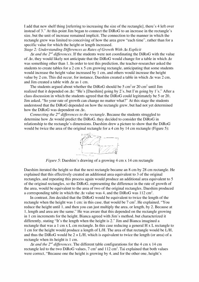
The following table is one student’s record of a 2 cm by 3 cm rectangle:

Figure 3: Table of length/width/area values of a growing rectangle

All of the students’ discussions about quadratic growth relied on the growing rectangles

context. The students created tables of data to record the height, length, and area values they

observed in Geometer’s Sketchpad such as the one seen in Figure 3. The students’ propensity

to represent data in well-ordered tables in which the height or the length values increased by

uniform increments of 1 cm encouraged a focus on what is often referred to in textbooks as

the “first differences” and the “second differences” for y. The first transition the students

experienced was one in which they shifted from understanding these values as differences to

understanding them as rates of growth.

Stage 1: Understanding Differences as Rates of Growth With !x Implicit

1st differences. The students initially focused only on the differences between successive

area values without coordinating with the way the height or the length grew. For instance,

when describing the first differences for height/area table of a square that grew by 1-cm

increments, Jim explained, “it goes 1 and then 3 and then 5 and then…and then you go to 3,

5, 7,…just keeps going.” Attention to coordinating the growth in area with how the height

grew was absent from Jim’s description. The teacher-researcher asked the students to draw

diagrams of growing rectangles that depicted the increases in area. Figure 4 shows Ally’s 2 x

3 rectangle that grew to become a 3 x 4.5 rectangle and then a 4 x 6 rectangle:

Figure 4: Ally’s depiction of the additional area produced as the rectangle grows

Ally explained, “So we added 7.5 to this part [pointing to the 2 x 3 rectangle], we added 10.5

to this part [the 3 x 4.5 rectangle], and then, because it’s the difference, it’s [the second

differences] how many more squares you had to add to this one [the 3 x 4.5 rectangle],

instead of compared to this one [the 2 x 3 rectangle].” In this depiction Ally began to

coordinate the number of squares making up the additional area to each time the rectangle

“grew”. The increments were not explicit for Ally, but she and the other students began to

attend to the fact that the first differences represented the growth of the area for each increase

in the rectangle’s size. The next day, Jim more generally stated that the first differences

represented “How many new squares it’s gaining every time it grows.” Jim’s use of the term

“every time” suggests that he was coordinating the growth in area with some growth in height

and length, but did not explicitly attend to the unit of growth.

2nd differences. The students initially described the second differences as “the second

level sort of thing”, and when creating pictures, they described the second differences as “the

new outside area.” Ally’s picture in Figure 4 helped her explain that “every time it grows it

adds 3”, but it was unclear whether she saw this as the rate at which the rate of growth of the

area grew.

A continued emphasis on creating drawings helped the students clarify the meaning of the

second differences. For instance, Bianca explained that they represented “the area of the next

shape minus the area of the previous shape”, or the “amount added to the amount added to the

area.” Jim noted that the students should name this value, stating, “I think we should give it

names, like, the amount added to the amount added is so confusing!” Ally suggested

“Difference in the Rate of Growth” and the students settled on this term, eventually

shortening it to the “DiRoG”. Jim characterized the DiRoG as, “So the rate of rate of growth

is how many square units it’s gaining from the rate of growth.”

When the students created a table for the height, length, and area of a 1 x 2 growing

rectangle, Jim found the DiRoG to be 4 square units, and then exclaimed, “it’s going up by

the rate of the rate…the rate that the rate of growth is growing!” Elaborating, he said, “When

I add that new shelf thing [referring to increasing the size of the rectangle], there’s 4 left over

instead of 3.” At this point Jim began to connect the DiRoG to an increase in the rectangle’s

size, but the unit of increase remained implicit. The connection to the manner in which the

rectangle grew was limited to conceiving of how the area grew “each time”, rather than for a

specific value for which the height or length increased.

Stage 2: Understanding Differences as Rates of Growth With !x Explicit

!x and the 2nd differences. If the students were not coordinating the DiRoG with the value

of !x, they would likely not anticipate that the DiRoG would change for a table in which !x

was something other than 1. In order to test this prediction, the teacher-researcher asked the

students to create tables for a 2 cm x 5 cm growing rectangle, anticipating that some students

would increase the height value increased by 1 cm, and others would increase the height

value by 2 cm. This did occur, for instance, Daeshim created a table in which !x was 2 cm,

and Jim created a table with !x as 1 cm.

The students argued about whether the DiRoG should be 5 cm2 or 20 cm2 until Jim

realized that it depended on !x: “He’s [Daeshim] going by 2’s, but I’m going by 1’s.” After a

class discussion in which the students agreed that the DiRoG could legitimately be 5 or 20,

Jim asked, “So your rate of growth can change no matter what?” At this stage the students

understood that the DiRoG depended on how the rectangle grew, but had not yet determined

how the DiRoG was dependent on !x.

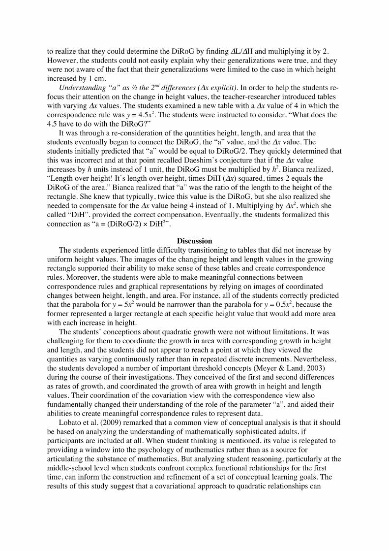
Connecting the 2nd differences to the rectangle. Because the students struggled to

determine how !x would predict the DiRoG, they decided to consider the DiRoG in

relationship to the rectangle’s dimensions. Daeshim drew a picture to show that the DiRoG

would be twice the area of the original rectangle for a 4 cm by 14 cm rectangle (Figure 5):

Figure 5: Daeshim’s drawing of a growing 4 cm x 14 cm rectangle

Daeshim iterated the height so that the next rectangle became an 8 cm by 28 cm rectangle. He

explained that this effectively created an additional area equivalent to 3 of the original

rectangles, and repeating this process again would produce an additional area equivalent to 5

of the original rectangles, so the DiRoG, representing the difference in the rate of growth of

the area, would be equivalent to the area of two of the original rectangles. Daeshim produced

a corresponding table in which the !x value was 4, and the DiRoG was 112 cm2.

In contrast, Jim decided that the DiRoG would be equivalent to twice the length of the

rectangle when the height was 1 cm: in this case, that would be 7 cm2. He explained, “You

reduce the height until 1, and then you can just multiply the area, or length, by 2. Because at

1, length and area are the same.” He was aware that this depended on the rectangle growing

in 1 cm increments for the height. Bianca agreed with Jim’s method, but characterized it

differently, stating “It’s the length when the height is 2.” Jim and Bianca imagined a

rectangle that was a 1 cm x L cm rectangle. In this case reducing a general H x L rectangle to

1 cm for the height would produce a length of L/H. The area of that rectangle would be L/H,

and thus the DiRoG would be 2 ! L/H, which is equivalent to twice the length (or area) of a

rectangle when its height is 1 cm.

!x and the 2nd differences. The different table configurations for the 4 cm x 14 cm

rectangle led to the two DiRoG values, 7 cm2 and 112 cm2. Tai explained that both values

were correct, “Because one the height is growing by 4, and for the other one, height’s

growing by 1.” Daeshim then explained that when the DiRoG, 7, is multiplied by the square

of the !x value in the other table, 4, the result is 112: 7 ! 42 = 112. However, the students

were not sure whether this was a general relationship, i.e., that if the !x value increases by h

units instead of 1 unit, the DiRoG must be multiplied by h2. After working with many

different table configurations, the students decided that this relationship was true, but were

not able to explain why. It was at this point that shifting to a correspondence view became

necessary to move the students’ thinking forward.

Stage 3: Coordinating the covariation and correspondence views

Viewing “a” as the change in length per 1-unit change in height. The students examined

a table of height and area values and had to predict the area when h = 82 (Figure 6).

Figure 6: Student’s work on a far prediction problem

The students introduced a third length column and found length values by dividing the

area by the height. Tai explained, “The area divided by the height is the length. And if you

can find out the length, then for this then you can find out the area.” The constant increase of

4.5 cm in the length helped the students create a general strategy. Jim explained, “It would go

over 4.5 for every time you go up the height 1.” Jim determined that he could find the area by

multiplying the length by the height, i.e., “n ! 4.5 ! n”, which the students then shortened to

4.5n2. Jim and the other students’ ongoing attention to coordinated changes even as they

identified a general correspondence rule marked the beginning of their coordination of the

covariation view and the correspondence view.

Viewing “a” as the ratio of the change in length to the change in height. Once the

students created equations in the form y = ax2, they began to examine connections between

“a” and the quantities height and length. The parameter “a” can be thought of as the ratio of

the rectangle’s length to its height. However, this view did not gain purchase with the

students, who were entrenched in a dynamic view, preferring to think about how the heights,

lengths, and areas changed as the rectangle grew. Tai explained, “The number in the front is

always the difference in the length divided by the difference in the height.” Daeshim

formalized this as “dL/dH”, where “dL” and “dH” referred to the constant differences in

successive length and height values. The students’ ability to relate “a” to a coordinated

change in height and length values served to further connect the covariation and

correspondence views.

Understanding “a” as " the 2nd differences (!x implicit). The students noticed that the

“a” in y = ax2 was half the DiRoG. This is true only for tables in which !x is 1, but the

students did not initially attend to this limitation. After creating the correspondence rule A =

0.75h2, Jim explained, “The difference of the rate of growth, half of that is here [points to

.75].” After working with multiple tables, the students agreed with Jim’s conclusion and

Bianca formalized it as “DiRoG/2 = a”. At this point, the students understood the parameter

“a” in two ways: as half the DiRoG (although this depends on the height growing in 1-cm

increments), and as the ratio of the change in length to the change in height. This led Bianca

to realize that they could determine the DiRoG by finding !L/!H and multiplying it by 2.

However, the students could not easily explain why their generalizations were true, and they

were not aware of the fact that their generalizations were limited to the case in which height

increased by 1 cm.

Understanding “a” as " the 2nd differences (!x explicit). In order to help the students re-

focus their attention on the change in height values, the teacher-researcher introduced tables

with varying !x values. The students examined a new table with a !x value of 4 in which the

correspondence rule was y = 4.5x2. The students were instructed to consider, “What does the

4.5 have to do with the DiRoG?”

It was through a re-consideration of the quantities height, length, and area that the

students eventually began to connect the DiRoG, the “a” value, and the !x value. The

students initially predicted that “a” would be equal to DiRoG/2. They quickly determined that

this was incorrect and at that point recalled Daeshim’s conjecture that if the !x value

increases by h units instead of 1 unit, the DiRoG must be multiplied by h2. Bianca realized,

“Length over height! It’s length over height, times DiH (!x) squared, times 2 equals the

DiRoG of the area.” Bianca realized that “a” was the ratio of the length to the height of the

rectangle. She knew that typically, twice this value is the DiRoG, but she also realized she

needed to compensate for the !x value being 4 instead of 1. Multiplying by !x2, which she

called “DiH”, provided the correct compensation. Eventually, the students formalized this

connection as “a = (DiRoG/2) ! DiH2”.

Discussion

The students experienced little difficulty transitioning to tables that did not increase by

uniform height values. The images of the changing height and length values in the growing

rectangle supported their ability to make sense of these tables and create correspondence

rules. Moreover, the students were able to make meaningful connections between

correspondence rules and graphical representations by relying on images of coordinated

changes between height, length, and area. For instance, all of the students correctly predicted

that the parabola for y = 5x2 would be narrower than the parabola for y = 0.5x2, because the

former represented a larger rectangle at each specific height value that would add more area

with each increase in height.

The students’ conceptions about quadratic growth were not without limitations. It was

challenging for them to coordinate the growth in area with corresponding growth in height

and length, and the students did not appear to reach a point at which they viewed the

quantities as varying continuously rather than in repeated discrete increments. Nevertheless,

the students developed a number of important threshold concepts (Meyer & Land, 2003)

during the course of their investigations. They conceived of the first and second differences

as rates of growth, and coordinated the growth of area with growth in height and length

values. Their coordination of the covariation view with the correspondence view also

fundamentally changed their understanding of the role of the parameter “a”, and aided their

abilities to create meaningful correspondence rules to represent data.

Lobato et al. (2009) remarked that a common view of conceptual analysis is that it should

be based on analyzing the understanding of mathematically sophisticated adults, if

participants are included at all. When student thinking is mentioned, its value is relegated to

providing a window into the psychology of mathematics rather than as a source for

articulating the substance of mathematics. But analyzing student reasoning, particularly at the

middle-school level when students confront complex functional relationships for the first

time, can inform the construction and refinement of a set of conceptual learning goals. The

results of this study suggest that a covariational approach to quadratic relationships can

provide a foundation for understanding the nature of quadratic growth and can support a

meaningful transition to correspondence relationships.

References

Asquith, P., Stephens, A., Knuth, P. & Alibali, M. (2007). Middle School Mathematics

Teachers’ Knowledge of Students’ Understanding of Core Algebraic Concepts: Equal

Sign and Variable. Mathematical Thinking and Learning, 9(3), 249–272.

Chazan, D. (2006). "What if not?" and teachers' mathematics. In F. Rosamund & L. Copes

(Eds.), Educational Transformations: Changing our lives through mathematics; A tribute to

Stephen Ira Brown (pp. 3-20). Bloomington, Indiana: Author House.

Confrey, J., & Smith, E. (1995). Splitting, covariation, and their role in the development of

exponential function. Journal for Research in Mathematics Education, 26(1), 66 – 86.

Eraslan, A. (2007). The notion of compartmentalization: The case of Richard. International

Journal of Mathematical Education in Science and Technology, 38(8), 1065 – 1073.

Glasersfeld, E.V. (1995). Radical Constructivism: A Way of Knowing and Learning. London:

The Falmer Press.

Knuth, E., Stephens, A., McNeil, N., & Alibali, M. (2006). Does understanding the equal

sign matter? Evidence from solving equations. Journal for Research in Mathematics

Education, 37, 297 – 312.

Lobato, J., Hohensee, C., & Rhodehamel, B. (2009). Reasoning quantitatively with Quadratic

Functions: What are appropriate learning goals for 8th graders? Paper presented at

National Council of Teachers of Mathematics Research Presession, Washington, D.C.

Meyer, J.H.F., & Land, R. (2003). Threshold concepts and troublesome knowledge: linkages

to ways of thinking and practising within the disciplines. In C. Rust (Ed.), Improving

Student Learning. Improving Student Learning Theory and Practice - 10 years on (pp.

412 – 424). Oxford: OCSLD.

Moore, K.C. (2010). The role of quantitative and covariational reasoning in developing

precalculus students’ images of angle measure and central concepts of trigonometry.

Paper presented at the 13th Annual Conference on Research in Undergraduate

Mathematics Education.

National Council of Teachers of Mathematics. (2000). Principles and standards for school

mathematics. Reston, VA: Author.

National Mathematics Advisory Panel (2008). Foundations for success: The final report of

the National Mathematics Advisory Panel (U.S. Dept. of Education, Washington, DC)

Schliemann, A. D., Carraher, D. W., &Brizuela, B. (2007). Bringing Out the Algebraic

Character of Arithmetic: From Children’s Ideas to Classroom Practice. Mahwah:

Lawrence Erlbaum Associates.

Steffe, L.P., & Thompson, P.W. (2000). Teaching experiment methodology: Underlying

principles and essential elements. In A. Kelly & R. Lesh (Eds.), Handbook of research

design in mathematics and science education (pp. 267-306). Mahwah, NJ: Lawrence

Erlbaum Associates.

Thompson, P. W. (2008). Conceptual analysis of mathematical ideas: Some spadework at the

foundations of mathematics education. In O. Figueras, J. L. Cortina, S. Alatorre, T.

Rojano & A. Sépulveda (Eds.), Plenary Paper presented at the Annual Meeting of the

International Group for the Psychology of Mathematics Education, (Vol 1, pp. 45-64).

Morélia, Mexico: PME.

Zazkis, R., Liljedahl, P., & Gadowsky, K. (2003). Conceptions of function translation:

Obstacles, intuitions, and rerouting. Journal of Mathematical Behavior, 22(4), 435-448.