MIKKO LAAJA

GENERAL PLANNING PRINCIPLES OF HIGH VOLTAGE DISTRIBUTION

NETWORKS INCLUDING WIND POWER

Master of Science Thesis

Examiner: Professor Pertti Järventausta The examiner and the topic approved in the Faculty of Computing and Electrical Engineering Council meeting on 7.9.2011

II

ABSTRACT

TAMPERE UNIVERSITY OF TECHNOLOGY Master’s Degree Programme in Electrical Engineering LAAJA, MIKKO: General planning principles of high voltage distribution networks including wind power Master of Science Thesis, 72 Pages, 9 Appendix pages August 2012 Major: Power systems and market Examiner: Professor Pertti Järventausta Keywords: Network planning, high voltage distribution network, wind power, demand side management

In Finland, the high voltage distribution networks (HVDNs) include all 110 kV lines

which are not part of the transmission network of the Finnish electricity transmission

system operator, Fingrid. Currently, the role of the HVDNs in the business operations of

the network companies is generally relatively small. This is because the amount of

network renovations to the networks and the construction needs for new HVDNs are

small. However, this will probably change in the future, since the planning needs of the

HVDNs will increase with the increasing amount of wind power in the networks. In

addition, the effects of wind power on the HVDNs are relatively unknown, since the

majority of the wind power research focuses on the effects of wind power on the whole

power network or on the effects of small wind plants on 20 kV or low-voltage networks.

This thesis is a part of a Finnish national 5-year research program called Smart Grid

and Energy Market (SGEM). The main purpose of this thesis is to describe the general

planning principles of the HVDNs and to analyze the effects of large-scale wind power

production on the different types of HVDNs in Finland. Moreover, the thesis aims to

examine what kind of impacts the wind power plants in the HVDNs have on the

planning and operation of the networks. In addition, the thesis will study the advantages

and disadvantages of demand side management (DSM) in the planning and operation of

the HVDNs with wind power.

The thesis consists of making a literature survey about the subject, which is

supported by general level network simulations with a HVDN test system with two

wind farms and by interviews with some network operator personnel. The simulations

of the thesis examine the wind power capacity of the different types of HVDNs, the

variability of the load and wind power production in relation to each other, the voltage

variations and power losses in the HVDNs with wind power and, finally, the effects of

DSM on the wind power capacity, voltages and power losses of the networks. Actual

measured data is being used in the simulations in the modelling of the fluctuations of

the wind power production and network loads. In the end, the conclusions about the

wind power effects on the HVDN planning and operation are made based on the

literature survey, interviews and simulations.

III

TIIVISTELMÄ

TAMPEREEN TEKNILLINEN YLIOPISTO Sähkötekniikan koulutusohjelma LAAJA, MIKKO: Tuulivoimaa sisältävien suurjännitteisten jakeluverkkojen yleissuunnittelun periaatteet Diplomityö, 72 sivua, 9 liitesivua Elokuu 2012 Pääaine: Sähköverkot ja -markkinat Tarkastaja: Professori Pertti Järventausta Avainsanat: Sähköverkon suunnittelu, suurjännitteinen jakeluverkko, tuulivoima, kysynnän hallinta

Suurjännitteisiin jakeluverkkoihin kuuluvat kaikki 110 kV:n voimajohdot, jotka eivät

ole Suomen kantaverkkoyhtiö Fingridin omistuksessa. Tällä hetkellä suurjännitteisen

jakeluverkon rooli verkkoyhtiöiden liiketoiminnassa on yleisesti melko vähäinen, mikä

johtuu verkkojen vähäisestä saneeraustarpeesta ja pienestä uusien verkkojen

rakennustarpeesta. Tämä asia tulee kuitenkin todennäköisesti muuttumaan

tulevaisuudessa, sillä suurjännitteisten jakeluverkkojen suunnittelutarpeet tulevat

kasvamaan tuulivoiman määrän kasvaessa verkoissa. Tämän lisäksi tuulivoiman

vaikutukset suurjännitteisiin jakeluverkkoihin ovat suhteellisen tuntemattomia, koska

suurin osa tutkimuksista keskittyy tuulivoiman vaikutuksiin koko voimansiirtoverkon

tasolla tai pienten voimaloiden vaikutuksiin 20 kV:n verkon tai pienjänniteverkon

tasolla.

Tämä työ on osa Suomessa käynnissä olevaa kansallista viisivuotista Smart Grid

and Energy Market (SGEM) -tutkimusohjelmaa. Työn pääasiallinen tavoite on selvittää

suurjännitteisen jakeluverkon yleissuunnittelun perusteita ja analysoida laajamittaisen

tuulivoiman vaikutuksia erityyppisiin suurjännitteisiin jakeluverkkoihin Suomessa.

Lisäksi työ pyrkii selvittämään, minkälaisia vaikutuksia suurjännitteisissä

jakeluverkoissa olevilla tuulivoimaloilla on verkkojen suunnitteluun ja käyttöön. Työ

myös selvittää kysynnän hallinnan hyödyt ja haitat tuulivoimaa sisältävien

suurjännitteisten jakeluverkkojen suunnittelussa ja käytössä.

Työ koostuu aiheesta tehdystä kirjallisuusselvityksestä, jonka tukena toimivat

yleisen tason simuloinnit kaksi tuulipuistoa sisältävän suurjännitteisen jakeluverkon

simulointimallin avulla ja haastattelut sähköverkon toimijoiden henkilökunnan kanssa.

Työn simuloinnit tarkastelevat erityyppisten suurjännitteisten jakeluverkkojen

tuulivoimakapasiteettia, verkon kuormien ja tuulivoimatuotannon vaihteluiden suhdetta,

tuulivoimaa sisältävien suurjännitteisten jakeluverkkojen jännitteitä ja häviöitä ja

lopuksi kysynnän hallinnan vaikutuksia verkkojen tuulivoimakapasiteettiin, jännitteisiin

ja häviöihin. Simuloinneissa käytetään todellista mitattua dataa tuulivoimatuotannon ja

verkon kuormien vaihteluiden mallintamisessa. Työn lopuksi tehdään päätelmät

tuulivoiman vaikutuksista suurjännitteisen jakeluverkon suunnitteluun ja käyttöön

perustuen kirjallisuusselvitykseen, haastatteluihin ja simulointeihin.

IV

PREFACE

This Master of Science Thesis was carried out at the Department of Electrical Energy

Engineering of Tampere University of Technology as a part of Smart Grid and Energy

Market (SGEM) project. The supervisors and examiners of the thesis were Professor

Pertti Järventausta and Lic.Tech. Juhani Bastman.

First of all, I would like to thank Prof. Pertti Järventausta for giving me this

interesting topic, ideas and feedback during the work. I would also like to thank

Lic.Tech. Juhani Bastman for his guidance, advice and feedback. I also want to thank all

of my other colleagues of the Department for the pleasant working environment and

ideas. My last gratitude goes to my wife, Emma, and my family for the invaluable

support throughout my studies.

Tampere, August 2012

Mikko Laaja

V

CONTENTS

1. INTRODUCTION ..................................................................................................... 1

1.1. Smart Grids ......................................................................................................... 2

2. HIGH VOLTAGE DISTRIBUTION NETWORKS ................................................. 5

2.1. Definition and structure of Finnish HVDNs ...................................................... 5

2.2. Role of HVDNs from network point of view ..................................................... 7

2.3. Wind farm’s impacts on the role ........................................................................ 8

2.4. HVDN calculation .............................................................................................. 9

2.4.1. Calculation model of HVDN ........................................................................ 10

3. GENERAL PLANNING OF ELECTRICITY NETWORKS ................................. 14

3.1. Planning principles ........................................................................................... 14

3.1.1. Determination of network’s current state ..................................................... 15

3.1.2. Drafting of network trends and forecasts ...................................................... 15

3.1.3. Comparison of action proposals and decision making ................................. 16

3.2. Boundary conditions of planning ..................................................................... 17

3.2.1. Maximum thermal capacity .......................................................................... 18

3.2.2. Voltage drop ................................................................................................. 18

3.2.3. Short-circuit current capacity and protection................................................ 20

3.2.4. Earth fault protection .................................................................................... 21

3.2.5. Mechanical condition .................................................................................... 22

3.2.6. Quality of supply .......................................................................................... 22

3.2.7. Environmental issues .................................................................................... 23

3.3. Planning tools ................................................................................................... 24

3.4. General planning of HVDNs ............................................................................ 24

3.5. Effects of Energy Market Authority regulation model on planning................. 26

4. WIND POWER AS PART OF HVDN .................................................................... 29

4.1. General ............................................................................................................. 29

4.2. Interconnection laws and regulations ............................................................... 30

4.3. Network effects of wind power ........................................................................ 35

4.4. Wind power effects on network planning ........................................................ 37

4.5. Wind power effects on network operation ....................................................... 39

4.6. HVDN network simulations ............................................................................. 42

VI

4.6.1. Network capacity .......................................................................................... 43

4.6.2. Load and wind power variability .................................................................. 46

4.6.3. Voltage variations ......................................................................................... 48

4.6.4. Losses............................................................................................................ 57

4.6.5. Demand side management ............................................................................ 58

4.6.6. Summary ....................................................................................................... 62

4.7. Noticing wind power in HVDN planning and operation ................................. 63

4.8. Development needs .......................................................................................... 65

5. CONCLUSIONS ...................................................................................................... 67

REFERENCES ................................................................................................................ 69

APPENDIX 1 - HVDN NETWORK TEST SYSTEM ................................................... 73

APPENDIX 2 - INTRODUCTION OF HVDN NETWORK TEST SYSTEM ............. 74

APPENDIX 3 - NETWORK CAPACITY SIMULATIONS ......................................... 79

VII

ABBREVIATIONS AND NOTATION

Sb Base power

Ub Base voltage

Un Nominal voltage

Zb Base impedance

AMR Automatic Meter Reading

CIS Customer Information System

DG Distributed Generation

DNO Distribution Network Operator

DSM Demand Side Management

ENTSO-E European Network of Transmission System

FRT Fault Ride-Through

HVDN High Voltage Distribution Network

ICT Information and Communications Technology

MIS Maintenance Information System

MVDN Medium Voltage Distribution Network

NIS Network Information System

pu Per-unit

RES Renewable Energy Source

SGEM Smart Grid and Energy Market

SLFE Static Load Flow Equations

StoNED Stochastic Non-smooth Envelopment of Data

TSO Transmission System Operator

WACC Weighted Average Cost of Capital

1

1. INTRODUCTION

International actions to reduce global warming have increased electricity generation

from renewable energy sources (RES), especially from wind. Consequently, worldwide

installed wind power capacity has exploded during the last decade and the growth is

estimated to be continued in the future. This has highlighted the role of wind power in

energy production, which has increased research on wind power and also on defining

the impacts of the increased wind power on the power system. Usually these studies

focus either on the impacts of large-scale wind power production on the whole power

system and transmission network or on the impacts of distributed wind power

generation on a medium voltage distribution network (MVDN), while effects on a high

voltage distribution network (HVDN) are generally neglected. The HVDN is a new

term for a sub-transmission network and it is used in this thesis since the HVDN is

currently the official term for the case in the Finnish network business regulation.

This thesis is a part of a Finnish national 5-year research program called Smart Grid

and Energy Market (SGEM), objective of which is to enable the implementation of the

smart grid vision for network planning and operation. The project involves a number of

Finnish universities, network companies and industrial partners.

The purpose of this thesis is to describe the general planning principles of the

HVDNs and to analyze the effects of large-scale wind power production on the different

types of HVDNs. Moreover, the thesis attempts to determine what issues must be taken

into account by network operators when interconnecting wind farms to the network. The

issues are being considered from the point of view of both the network planning and the

network operation. The analysis is performed primarily for the Finnish HVDNs

The thesis consists of making a literature survey about the subject and carrying out

some illustrative simulations with a network test system. The objectives of the

simulations are to specify the effects of variable wind production on the HVDNs and to

define the benefits for network planning and operation by using demand side

management (DSM). The simulations are being executed with Power World Version 15

simulation software. Hence, one of the minor objectives of the thesis is to obtain

experiences from the advanced functionalities of the program and to clarify, what kind

of different matters can be examined by the software. In addition to the literature survey

and to the simulations, the thesis consists of carrying out some interviews with network

operator personnel.

The thesis begins with a short introduction to the smart grid vision, mainly from the

SGEM program’s point of view. After this, the thesis introduces the HVDNs in the

Finnish electrical system and considers their role in the power delivery system at the

moment and in the future. Also, the simulation model for the HVDNs is being

explained. Next, the practises of the general planning of the electrical network are being

introduced as well as some of the matters that have an influence on the general planning

2

of the HVDNs. Then, the thesis studies the interconnection of wind power to the

HVDN. The impacts of wind power on the HVDNs are examined from both the

network planning and the operation point of view. Also, the current laws and

regulations related to the interconnection are presented. At the end of the thesis,

conclusions and recommendations about the planning and operation of the HVDNs with

the increased number of wind power are made considering all the examinations

completed within the thesis. Lastly, a conclusion about the whole thesis is produced.

1.1. Smart Grids

Energy production from RES has grown rapidly in the past decades and will presumably

continue to increase even faster due to the countries’ strict objectives to reduce

greenhouse gas emissions. Many of the power plants using RES are small-scale plants

that are geographically distributed. For that reason, the plants are usually connected to a

distribution network instead of a transmission network. Traditionally, the electrical

network includes centralized power plants connected to the transmission network and

uncontrollable loads connected to the distribution network, which means that almost all

of the production is located in the transmission network. This enables the power to be

transferred in one direction from the transmission network to the consumption through

the distribution network, in which case the power flow in the distribution network is

unidirectional and quite simple to control from the network’s point of view. However,

the increase of distributed generation (DG) in the distribution network leads to a multi-

directional power flow in the network, which will add complexity to the network

planning and operation. Therefore, a demand for more intelligent and flexible power

networks, ‘smart grids’, has emerged.

There are many drivers, in addition to the penetration of DG, for transforming the

current power network towards the smart grid vision. One of the most significant of the

drivers is the demand to increase the energy efficiency, especially at a customer level.

The network’s energy efficiency can be improved with the smart grids by increasing the

network’s utilization rate, which will lead to more optimized network planning and

operation. At the customer level, this mainly means that the loads will become more

active and controllable from the network’s point of view. On that account, the using of

real-time data on the planning and operation of the network should probably be

increased in the future. Another driver for the smart grids is the fact that power quality

requirements are rising at the same time as the disturbances caused by the weather are

increasing due to climate change. Moreover, climate change will also raise the risk of

major disturbances, which is serious because of the society’s high dependency on the

electric power. Maybe the simplest driver for the smart grids is the fact that many of the

components of the existing networks are close to the end of their lifetime and

consequently must be replaced anyway in the near future. This enhances the cost-

effectiveness of the novel components needed for the smart grid. (Järventausta et al.

2010)

3

As mentioned above, the smart grids increase the intelligence and flexibility of the

power networks. The intelligence is achieved by adding more information and

communications technology (ICT) components to the network, which will enable the

real-time monitoring and operation of the network. This will also increase the reliability

and energy efficiency of the network. Simultaneously, a high amount of ICT will enable

the network interconnection of a large number of controllable resources, for example

directly controllable loads, energy storages, plug-in electric vehicles and DSM, which

will significantly increase the flexibility of the network. Basically, DSM means that the

loads of the network are controlled in some way which is beneficial for the network.

This can mean that the peak loads of the network are being smoothed or the loads of the

network are being increased or decreased temporarily to improve the adequacy of the

network or to adjust the frequency of the network.

Generally, it can be said that the smart grid has the following characteristics

(Hashmi 2011):

- Accessible, by granting connection access to all network users, particularly for

RES and high efficiency local generation with zero or low carbon emissions.

- Integrated, in terms of real-time communications and control functions.

- Interactive between customers and markets.

- Flexible, by fulfilling customers’ needs while responding to the changes

and challenges ahead.

- Predictive, in terms of applying operational data to equipment maintenance

practices and even identifying potential outages before they occur.

- Adaptive, with less reliance on operators, particularly in responding rapidly to

changing conditions.

- Reliable, by assuring and improving security and quality of supply, consistent

with the demands of the digital age with resilience to hazards and uncertainties.

- Economic, by providing the best value through innovation, efficient energy

management, competition and regulation.

- Secure from attack and naturally occurring disruptions.

- Optimized to maximize reliability, availability, efficiency and economic

performance.

The conversion of the existing networks to the smart grids also leads to other

benefits for different stakeholders. At first, network operators will experience lower

distribution losses and potentially peak demand could be reduced, due to the more

optimized use of the network. In addition, the more optimized use of the network will

also reduce CO2 emissions and benefit the environment. Furthermore, the smart grids

will expedite the proliferation of RES, which also benefits the environment. Finally,

consumers will have an opportunity to control their energy costs by controlling their

consumption and possible own generation. This will raise energy efficiency in the

consumer level and also reduce emissions. (ABB 2009)

The transition of the networks to the smart grids will raise the operations of the

power delivery system to the next level and it will benefit all stakeholders of the

4

networks. However, the transition will be complicated and difficult, since it will be as

radical as all the advances of the power networks in total over last hundred years and it

must be performed in a much shorter period of time. Therefore, a fruitful cooperation

between all the stakeholders, for example network operators, industry players and both

public and regulatory bodies, is essential. (ABB 2009)

5

2. HIGH VOLTAGE DISTRIBUTION NETWORKS

2.1. Definition and structure of Finnish HVDNs

Two types of networks are used in the Finnish power system for transferring electrical

power from production to consumption. These types are a transmission network and

distribution network. The transmission network forms the core of the Finnish power

system as all the major power plants are connected to it. The network is designed and

operated by Fingrid Oyj, which is the electricity transmission system operator (TSO) in

Finland. The transmission network is a meshed network and it includes all 400 kV, 220

kV and 110 kV lines operated as meshed. The function of the transmission network is to

transfer electricity from power plants to areas of consumption, from where the

electricity is transferred to the majority of final consumers via distribution network,

since only some of the largest consumers are connected directly to the transmission

network. The distribution networks, the latter of the types mentioned above, are

operated by regional network companies. The distribution networks can be divided into

two different parts, medium voltage distribution networks (MVDNs) and high voltage

distribution networks (HVDNs). The MVDNs are operated radially and they contain

networks with voltages under 110 kV, according to the Finnish Electricity Market Act

(Energy Market Authority 2007). Most of the consumers are connected to the MVDN

directly or to a low voltage network, which is part of the MVDN.

The thesis concentrates on the HVDNs, especially on the rural HVDNs. The

characteristics of these networks are next examined in detail. The term ‘HVDN’ has

replaced an old term ‘sub-transmission network’ in the Finnish legislation and network

business regulation. The HVDN can have similar characteristics with both the MVDN

and the transmission network and, at the moment, there is no direct definition for the

HVDN. Therefore, it is not entirely easy to say, which parts of the network are part of

the HVDNs. (Bastman 2011)

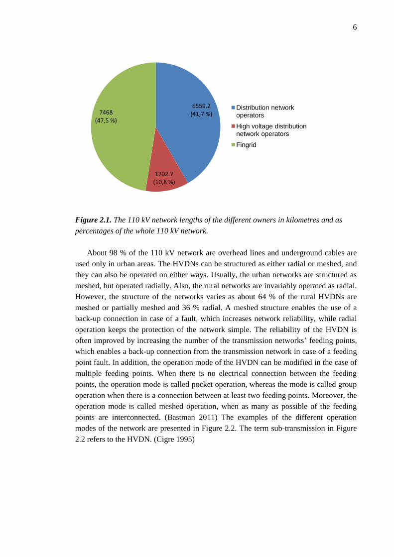
According to the Finnish Electricity Market Act, the HVDNs consist of 110 kV lines

which are not part of the Fingrid’s transmission network (Energy Market Authority

2010a). In 2010, the length of this 110 kV HVDN network in Finland was about 8262

km, from which about 6559 km were possessed by 54 different distribution network

operators (DNOs) and about 1703 km by 12 different high voltage distribution network

operators. For comparison, the length of the Fingrid’s 110 kV network was 7468 km, so

about 52.5 % of the Finnish 110 kV lines are part of the HVDN. Figure 2.1 illustrates

the distribution of the network ownership. (Energy Market Authority 2010b)

6

Figure 2.1. The 110 kV network lengths of the different owners in kilometres and as

percentages of the whole 110 kV network.

About 98 % of the 110 kV network are overhead lines and underground cables are

used only in urban areas. The HVDNs can be structured as either radial or meshed, and

they can also be operated on either ways. Usually, the urban networks are structured as

meshed, but operated radially. Also, the rural networks are invariably operated as radial.

However, the structure of the networks varies as about 64 % of the rural HVDNs are

meshed or partially meshed and 36 % radial. A meshed structure enables the use of a

back-up connection in case of a fault, which increases network reliability, while radial

operation keeps the protection of the network simple. The reliability of the HVDN is

often improved by increasing the number of the transmission networks’ feeding points,

which enables a back-up connection from the transmission network in case of a feeding

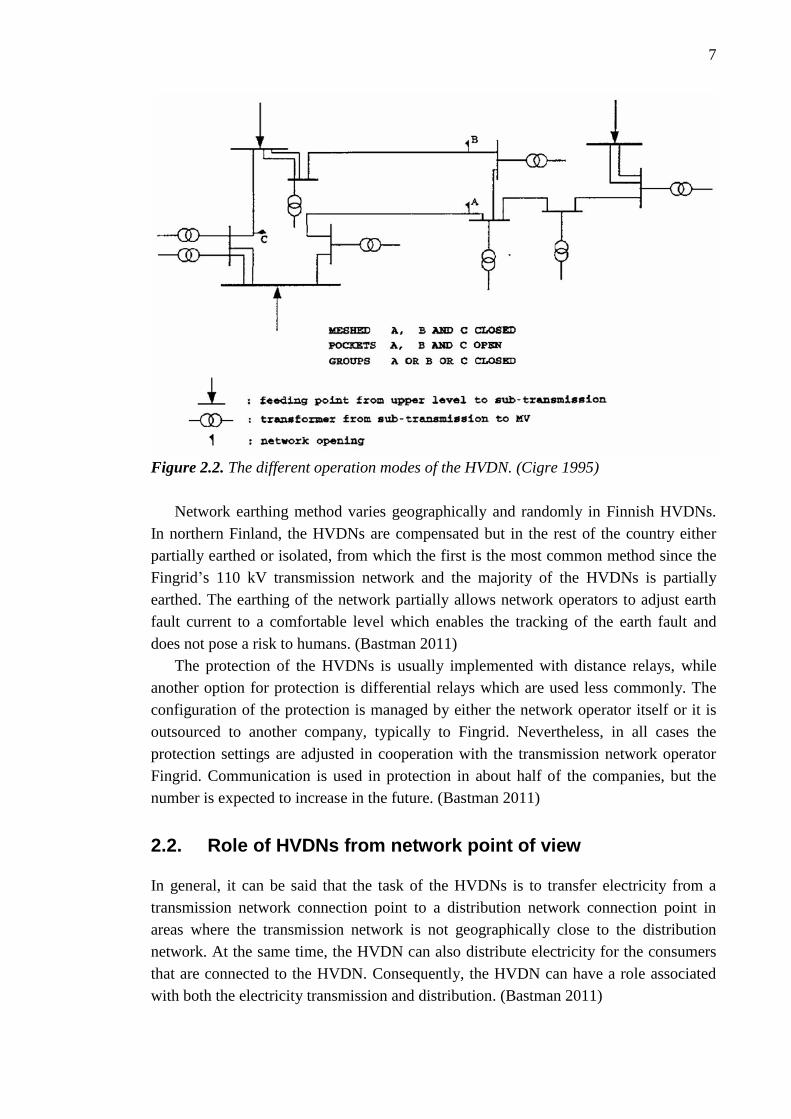
point fault. In addition, the operation mode of the HVDN can be modified in the case of

multiple feeding points. When there is no electrical connection between the feeding

points, the operation mode is called pocket operation, whereas the mode is called group

operation when there is a connection between at least two feeding points. Moreover, the

operation mode is called meshed operation, when as many as possible of the feeding

points are interconnected. (Bastman 2011) The examples of the different operation

modes of the network are presented in Figure 2.2. The term sub-transmission in Figure

2.2 refers to the HVDN. (Cigre 1995)

6559.2 (41,7 %)

1702.7 (10,8 %)

7468 (47,5 %)

Distribution network operators

High voltage distribution network operators

Fingrid

7

Figure 2.2. The different operation modes of the HVDN. (Cigre 1995)

Network earthing method varies geographically and randomly in Finnish HVDNs.

In northern Finland, the HVDNs are compensated but in the rest of the country either

partially earthed or isolated, from which the first is the most common method since the

Fingrid’s 110 kV transmission network and the majority of the HVDNs is partially

earthed. The earthing of the network partially allows network operators to adjust earth

fault current to a comfortable level which enables the tracking of the earth fault and

does not pose a risk to humans. (Bastman 2011)

The protection of the HVDNs is usually implemented with distance relays, while

another option for protection is differential relays which are used less commonly. The

configuration of the protection is managed by either the network operator itself or it is

outsourced to another company, typically to Fingrid. Nevertheless, in all cases the

protection settings are adjusted in cooperation with the transmission network operator

Fingrid. Communication is used in protection in about half of the companies, but the

number is expected to increase in the future. (Bastman 2011)

2.2. Role of HVDNs from network point of view

In general, it can be said that the task of the HVDNs is to transfer electricity from a

transmission network connection point to a distribution network connection point in

areas where the transmission network is not geographically close to the distribution

network. At the same time, the HVDN can also distribute electricity for the consumers

that are connected to the HVDN. Consequently, the HVDN can have a role associated

with both the electricity transmission and distribution. (Bastman 2011)

8

As mentioned earlier, the HVDNs are owned by two different network operators,

DNOs and high voltage distribution network companies. The planning and operation of

the HVDNs are based on objectives depending on the ownership of the network.

Therefore, the HVDNs owned by the DNOs are optimized to serve the needs of the

distribution networks connected to the HVDN and the HVDNs owned by the HVDN

companies are optimized without considering the benefits of other networks. In

conclusion, it can be said that the role of the HVDNs depends on the local network

conditions and ownership.

According to the network company survey about the HVDNs in Finland, the

companies value the HVDNs, especially the planning of the HVDNs, in different ways

in their business. In one company, software capable of calculating meshed networks is

used for planning the HVDN. On the contrary, in almost all other companies the

planning calculations of the HVDNs are outsourced for another company, for example

Fingrid, which might be reasonable, as Fingrid has capabilities for the 110 kV network

planning. The planning of the HVDNs is further discussed in Chapter 3.4. (Bastman

2011)

Based on the Bastman’s survey, it can also be noted that the fault statistics of the

HVDNs are not at the same level as the MVDNs’ statistics since the HVDNs’ statistics

are compiled by only 80 % of the companies and none of the companies have inclusive

statistics on the prolonged time span. (Bastman 2011) In addition, the effects of faults

on the regulation model of the Finnish Energy Market Authority are different in the

cases of MVDN and HVDN, since the short interruptions and the number of the planned

interruptions do not affect on the regulation model of the HVDNs. However, this will

probably be changed for the next regulation period. (Energy Market Authority 2011)

This issue will be discussed in more detail in Chapter 3.5.

These facts reflect the smaller role of the HVDNs from the network companies’

point of view. On the other hand, the compiling of the HVDNs’ fault statistics may not

be so important for the companies, because faults occur in the HVDNs significantly less

frequently than in the MVDNs. Nonetheless, the effects of the HVDN faults are much

greater and spread over a larger area in the network than the effects of the MVDN

faults.

2.3. Wind farm’s impacts on the role

Based on the previous chapter, it can be noted that the importance of the HVDNs from

the network operator’s point of view is not at the same level with the importance of the

MVDNs. The difference is justified by the small size of the operators’ HVDNs or by the

low need for the HVDN expansions. These arguments are unlikely to apply in the

future, because the HVDNs will probably be interconnected with a large number of

wind farms. (Bastman 2011)

There were about 7 800 MW of wind power projects published in Finland by the

end of January 2012 but it is difficult to say how many of those will be realized. Still, a

9

large part of the projects is covered by wind farms which will be connected to 110 kV

network. Hence, a significant amount of wind power will most likely be connected to

the HVDNs. (Finnish Wind Power Association 2012) The interconnection of the wind

farms and the HVDN has several effects on the network, which will be identified in

Chapter 4. In summary, the interconnection must be taken carefully into account in the

planning, operation and protection of the network and it will emphasize the role of the

HVDNs from the network operators’ point of view. Handling of these issues by network

planning and operation will be considered later also in Chapter 4.

2.4. HVDN calculation

In addition to making a literature survey about the HVDN planning, this thesis consists

of carrying out some illustrative simulations with a HVDN test system. The objectives

of the simulations are to specify the effects of variable wind production on the HVDNs

and to define the benefits for network planning and operation by using demand side

management (DSM).

The simulations were executed with Power World Version 15 simulation software

which was chosen because it is simple, known and free software for performing load

flow calculations in both the radial and meshed networks. Moreover, it is easy to

transfer data from the software to Microsoft Excel and the software can be used to

perform load flow calculations separately for each hour of the year, which means that

the hourly fluctuations of the loads and wind power can be simulated conveniently.

Power World can be used for wide range of network calculations including load flow

calculations and fault calculations. However, the simulations of this thesis contain only

load flow calculations so the other calculation features of the software are not being

utilized. (PowerWorld Corporation 2012)

Power World simulation software includes a few different solution methods for load

flow calculations, for example, a full Newton-Raphson, Decoupled Power Flow or

Gauss-Seidel methods. Nonetheless, all of the calculations performed in the thesis are

made using the full Newton-Raphson method, which is an effective and efficient

calculation method for solving power flows of all sizes of networks. The solution solves

the power flow of the network iteratively by solving Static Load Flow Equations

(SLFE) for all system buses using the known parameters of the buses and bus

admittance matrix. Moreover, if the calculation does not converge, the results of the

power flow calculations are not reliable. (PowerWorld Corporation 2012; Bastman

2012)

Generally, when calculating the power flow of the network, the buses of the network

are being divided into different categories depending on the known and unknown

variables of the bus. These four variables, two of which are always known and two are

calculated, are called the bus voltage, the angle of the voltage, the real power of the bus

and the reactive power of the bus. Furthermore, the different categories for the network

buses are SL -bus, PV -bus and PQ -bus. Firstly, the PV -buses, which are also known

10

as generator buses, are buses from which the real power of the generator and bus

voltage are known and, in contrast, the reactive power of the generator and the angle of

the voltage must be calculated. Secondly, the PQ -buses, also called as load busses, are

buses from which the real and reactive power of the load are known and the amplitude

and angle of the voltage are unknown. Lastly, the SL -bus is a bus from which the

amplitude and the angle of the voltage are known and the real and the reactive power of

the bus are unknown. Moreover, the SL -bus operates as a reference bus of the

calculated network, and the real and the reactive power of the bus are determined so that

the power balance of the network is achieved. Therefore, there is usually only one SL -

bus in the network, and it is typically chosen to be the bus with the largest generator in

the network or the bus which connects the calculated network to the larger network.

(Bastman 2012)

2.4.1. Calculation model of HVDN

The HVDN test system used in the simulations of this thesis is based on the test system

which has been presented in work (Bastman 2011). The test system has been built to

perform general level power flow and fault calculations in the HVDN and, therefore, the

system is well suited for the calculations carried out in this thesis. (Bastman 2011)

Additionally, certain modifications and improvements have been made to the system in

the thesis, including the addition of two wind farms into the system and modifications

of the parameters of some power lines in the system.

The test system used in the thesis includes three 400 kV substations, few 110 kV

substations and two 20 kV substations. In addition, the test system includes seven load

points with a maximum total load of 300 MW. Moreover, there are two wind farms in

the system which both can be connected to two different points in the 110 kV network.

The structure of the test system is shown in Figure 2.3 and Appendix 1. The 110 kV

buses of the test system, which are mainly examined in the thesis, are shown in bold in

Figure 2.3.

11

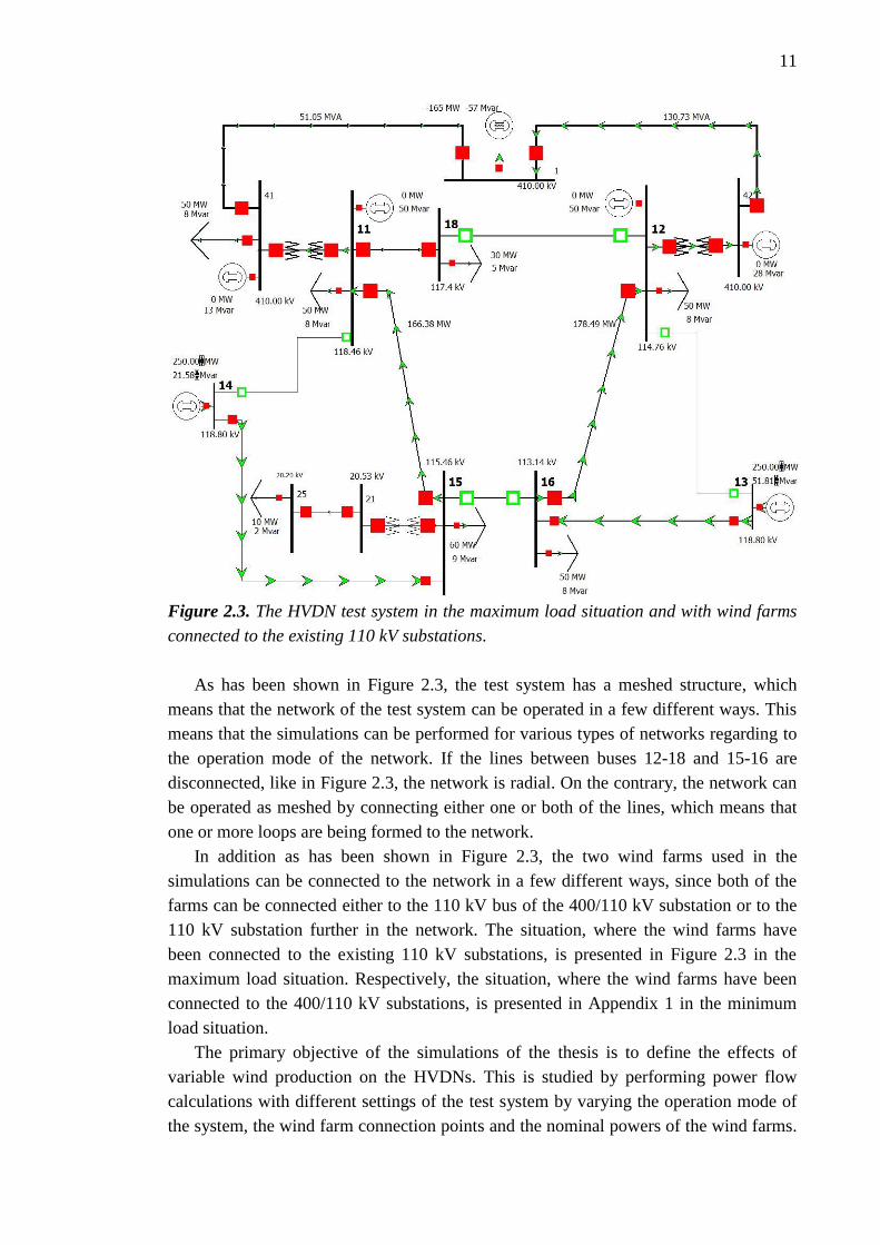
Figure 2.3. The HVDN test system in the maximum load situation and with wind farms

connected to the existing 110 kV substations.

As has been shown in Figure 2.3, the test system has a meshed structure, which

means that the network of the test system can be operated in a few different ways. This

means that the simulations can be performed for various types of networks regarding to

the operation mode of the network. If the lines between buses 12-18 and 15-16 are

disconnected, like in Figure 2.3, the network is radial. On the contrary, the network can

be operated as meshed by connecting either one or both of the lines, which means that

one or more loops are being formed to the network.

In addition as has been shown in Figure 2.3, the two wind farms used in the

simulations can be connected to the network in a few different ways, since both of the

farms can be connected either to the 110 kV bus of the 400/110 kV substation or to the

110 kV substation further in the network. The situation, where the wind farms have

been connected to the existing 110 kV substations, is presented in Figure 2.3 in the

maximum load situation. Respectively, the situation, where the wind farms have been

connected to the 400/110 kV substations, is presented in Appendix 1 in the minimum

load situation.

The primary objective of the simulations of the thesis is to define the effects of

variable wind production on the HVDNs. This is studied by performing power flow

calculations with different settings of the test system by varying the operation mode of

the system, the wind farm connection points and the nominal powers of the wind farms.

12

Then, the purpose is to compare the results of the different cases and make conclusions

based on that.

In addition, since the objective of the simulations is to analyse the effects of wind

power variability, the fluctuations of the wind farms’ output power must be modelled in

the simulations. This has been implemented by using actually measured wind power

output data, which has been measured from one under 1 MW wind turbine in Hailuoto,

Finland. The data contains the output of the wind turbine for each hour of the year,

which enables the modelling of the hourly wind power variability. However, the output

variations of one turbine differ from those of the whole wind farm and, therefore, the

data has been modified so that one wind farm has been assumed to be consisting of two

wind turbines of which outputs are experiencing the same phenomena with the

difference of one hour. In other words, there is a one-hour delay in the production of the

second wind turbine compared with the production of the first. Consequently, the output

power of the wind farm is the average output of the two turbines, which models more

realistically the output power of the wind farm.

Moreover, it is assumed that the two wind farms, which are connected to the test

system, are located so that it takes also one hour for the weather events to move from

the territory of the first wind farm to the territory of the second one. This is due to the

fact that the wind farms, which are connected to the same HVDN, are generally not

geographically adjacent to each other. Lastly, the output data of the two wind farms can

be scaled to the appropriate level depending on the nominal powers of the simulated

farms in each case.

The data modification balances the wind farm output variations compared to the

output of the single wind turbine and, hence, improves the correlation of the data with

the actual wind farm. However, the data does not probably fully correlate the output

data of the actual wind farm with several 1-5 MW wind turbines, since it is impossible

to model the stabilization of the wind farm’s output power with the measuring data of

one power plant. Moreover, the 1-5 MW wind turbines are higher than the under 1 MW

turbines, which means that also the wind speeds experienced by the plants differ from

each other. All in all, the main thing is that with the modification, the variability of the

wind farm output can be modelled at some level, so that the effects of variability on the

HVDNs can be studied.

Also the fluctuations of the network loads have been modelled in the simulations.

This has been performed by using the hourly measured consumption of one distribution

network operator (DNO). The data contains the consumption of the operator for each

hour of the year and the minimum and maximum consumptions of the operator are

about 7.5 MW and 33.7 MW, respectively. The real and reactive power consumption of

the load points of the test system are assumed to vary identically throughout the year.

Consequently, the measured consumption data has been scaled for each load point

individually depending on the maximum load value of the point.

The reference bus of the test system is Bus 1 which has been thought to be

connecting the system to the rest of the 400 kV transmission network. The voltage

13

control of the system has been implemented so that the voltages in the 400 kV

substations are kept at 410 kV by the generators in the substations. The voltage control

in the 110 kV network operates so that the voltages in the 110 kV buses of the 400/110

kV substations as well as the voltages at the connection point of the wind farm

generators are intended to be kept at 1.08 pu, which is 118.8 kV. The details of the

structure and operation of the test system have been described in Appendix 2.

14

3. GENERAL PLANNING OF ELECTRICITY

NETWORKS

3.1. Planning principles

The objective of network planning is to ensure the reliability and sufficiency of the

network in the future, which enables the distribution of good quality electricity to

customers without unnecessary interruptions. This is being attempted to do as

economically as possible and filling the technical requirements of the network. This

means that the investments and other costs of the network, such as the costs of losses

and maintenance costs, are being minimized while the electricity distribution must

remain safe for the people, property and environment. However, maintaining or

increasing the reliability of the network requires investments which reduce the

economic efficiency of the network. In summary, it can be said that the network

planning is an optimization task between the network investment costs, costs of losses,

outage costs and maintenance costs (Lakervi & Partanen 2009).

The network planning is performed in a short-term and long-term. The short-term

planning is usually implemented in no longer than a few years time period. Therefore,

short-term plans are usually ultimate and more detailed than long-term plans. On the

contrary, the time period of the long-term planning can be even 30 years so the plans are

not made in such detail. Usually, the time period of the long-term planning is 10-20

years. The purpose of the long-term planning is to determine the main guidelines for the

development of the network, and provide a basis for the short-term planning. The thesis

focuses on the general planning of the network, which is long-term planning, so the

short-term planning is not discussed in the thesis. (Lakervi & Partanen 2009; Vierimaa

2007; Jussila 2002)

The general planning of the network is affected by many different factors. The basis

of the general planning is the current state of the network, in particular, how the

network meets its reliability and safety objectives. The most important of the factors

affecting on the general planning is load and production forecasting which provides a

basic direction for the plans. Other important factors are the regulations imposed by

authorities, for example, Energy Market Authority and the goals and requirements set

by the companies themselves, which depend on the planning strategy of the company.

In addition, the planning strategy of the company defines the appreciation of electric

quality and landscape factors in the company which also affect on the general planning.

Furthermore, the expertise of the planner and the efficiency of the information systems

and planning tools can facilitate the general planning significantly. (Lakervi & Partanen

2009)

The general planning is slightly different in different network levels, depending on

the size of the planned network. In MVDN companies, the planning is carried out only

15

for the company’s own network, while other parts of the network are insignificant. On

the contrary, in transmission network planning the whole network must be taken into

account as well as the synchronously interconnected networks of the neighbouring

countries. In Finland, the transmission network operator, Fingrid, forms plans for the

transmission network based on the Ten-Year Network Development Plan of the

European Network of Transmission System Operators for Electricity (ENTSO-E)

(Reilander 2012a).

The planning of the HVDNs is in between the previous two planning practices.

Since the HVDN planning is performed in cooperation with Fingrid, it is based on the

transmission network plans. However, the planning is carried out regionally so the

whole network does not need to be taken into account. The general planning of the

HVDNs is further discussed in Chapter 3.4. (Reilander 2012a)

In general, the general planning of the network can be divided into three stages. The

stages are the determination of network’s current state, the drafting of network trends

and forecasts, and the comparison of action proposals and decision making. (Jussila

2002)

3.1.1. Determination of network’s current state

The general planning starts from the determination of network’s current state which

defines the electrotechnical and mechanical condition and the economic situation of the

network. Moreover, the reinforcement needs of the existing network are being

diagnosed. Most of the data required for the process, for example, the network structure,

consumption data and information about the condition of the components, is being

obtained from the network information systems. In addition to this, the information

systems can be used to perform load flow and fault current calculations.

The load flow and fault current calculations are used to determine, for example, the

losses, voltage drops, load currents, short circuit and earth fault currents and operation

of the network protection. The calculations are also being performed in unusual

situations, such as fault or work interruption situations. With the calculations, the

reliability, load capacity and safety of the current network can be evaluated and the

possible parts of the network in need of reinforcements can be detected.

3.1.2. Drafting of network trends and forecasts

At the second stage of the general planning process, the drafts about the network trends

in the future and the forecast are being made. The most significant function in the

process is the forecasting of loads, since the incorrectly predicted direction or speed of

the load evolution leads to notable additional financial costs. Usually, loads increase

rapidly in the urban networks and slowly or even not at all in the rural network. What

makes the forecasting difficult, is the fact that the load changes may differ greatly

within a small area, for example, in the rural network the loads can increase in the

16

summer cottage area and decrease in the other areas. The difficulty of the aggregation of

these changes makes the forecasting more complicated and unpredictable. (Jussila 2002)

A wide range of means are used in load forecasting, for example, population,

construction and business forecasts. Usually, the forecasts are mainly made using the

local land use plans, which can be used to determine the types and amount of the loads

expected to appear in the area in the near future. In addition, electricity price trends

affect on the load forecasts and, therefore, assumptions about the prices must also be

made. (Jussila 2002)

Equally important in the planning with the load forecasting is production

forecasting, particularly in the transmission network and HVDN planning. Also in the

MVDN planning, the production forecasting will be emphasized due to the increasing

number of DG. The production forecasting is performed using virtually the same

resources as in the load forecasting, since the most significant source for forecasts are

the local land use plans of the municipality. However, the production forecasting is

somewhat easier, at least in short-term, than the load forecasting because the electricity

producers must inform the network operators directly about new power plant projects,

since the producers need a network connection for their plants.

In addition to the previous, network development trends and changes in network’s

objectives also affect on the planning. Examples of these are the increasing appreciation

of delivery reliability and the changes in the structure of the network due to the higher

number of DG. Both of these will set new challenges for the network planning.

On the basis of all the issues presented, forecasts are made about power demand and

supply in the network. The forecasts can be used to estimate the peak powers transferred

in the network in the future. Hence, the development needs of the network can be

assessed.

3.1.3. Comparison of action proposals and decision making

In the last stage of the general planning, the action proposals are being made based on

the forecasts about the future. Since the time span of the general planning is several

years long, the forecasts and estimates for the future are not particularly accurate. This

causes considerable uncertainty for the general planning. Therefore, flexibility is needed

in the planning. This is achieved by making a few different versions, scenarios, about

the plans with each having a different assessment of the future. This way, the plans can

adapt to the future more flexibly. (Vierimaa 2007)

After making the network action proposals, the proposals are being considered, and

after that final investment decisions are being made. Consequently, all the variety plans

are compared, and on the basis of the comparisons the most suitable one is selected for

execution. The main questions in making the decisions are (Lakervi & Partanen 2009;

Jussila 2002):

- Should investments be made?

- Where the investments should be made?

17

- What kind of investment would be the most profitable to implement?

- When the investment should be implemented?

The general planning of the network is successful when the answers to these questions

can be provided.

The comparison of the action proposals is not entirely easy and simple since the

proposals can be compared in many different ways. The main requirement is that the

proposal meets the technical boundary conditions of the network, such as regulations

regarding the voltages and protection of the network. If the conditions are fulfilled, the

order of the proposals is usually determined by costs. Nonetheless, the planning strategy

of the company has notable influence on the final decision making, since the strategy

can highlight some of the values of the proposals, such as the environmental impacts,

network reliability or quality of the delivered electricity. In this case, the financially

cheapest proposal is not necessarily the most suitable. Also, the interest rate and time

period used in the calculations have impact on the decision making. (Lakervi &

Partanen 2009; Jussila 2002)

Finally, the decisions about the investments in the network should be made based on

the comparisons of the proposals. At this stage, the size of the investment plays a major

role as it must be decided how substantial investments will be implemented. Since, it is

more reasonable to do solely minor enhancement investment in some situations, for

example, if major investments must be postponed or the forecasts indicate that the

network’s evolution will be small. Such investments are small individual changes in the

network, such as wire exchanges or adding remote-controlled disconnectors. On the

contrary, in some cases radical investments, such as the construction of new substation,

are indispensable. The large investments are riskier than the small investments due to

the uncertainty of the power forecasts. On this basis, network planners tend to make

several minor investments instead of one major investment. The major investments are

usually done only when large consumer or producer is joining the network, or the power

quality must be significantly improved.

3.2. Boundary conditions of planning

The general planning of the network is always based on the economic efficiency. The

main objective of the planning is to optimize the costs within the imposed boundary

conditions. Therefore, the final planning decisions depend substantially on the boundary

conditions of the planning.

The boundary conditions include the technical boundary conditions, safety

requirements and environmental issues of the network. To be precise, the following

boundary conditions must be taken into account in the general planning (Lakervi &

Partanen 2009; Jussila 2002):

- Maximum thermal capacity

- Voltage drop

- Short-circuit current capacity and protection

18

- Earth fault voltages and protection

- Mechanical condition

- Quality of supply

- Environmental issues

The planning of the network is done by keeping in mind the worst possible situation

in the network. Therefore, the planning is performed using N-1 criterion which means

that not a single fault must cause a network fall. The N-1 criterion has been found to be

the optimal option in terms of the reliability and economy of the network.

3.2.1. Maximum thermal capacity

Maximum thermal current carrying capacity determines how large load current can be

conducted through the network for a certain period of time. In other words, it defines

the power transmission capacity of the network lines. The maximum thermal capacity

depends on the maximum temperature which can be allowed for the line on the basis of

material, insulation or environment. In the case of 110 kV transmission lines, the

dimensioning factor is usually the dip of the line which increases with increasing

temperature. Consequently, the maximum thermal capacity of the line depends

significantly on the outdoor temperature and wind speed, since both affect on the heat

transmission of the line. (Reilander 2012a) The optimal current capacity of the line is

determined with a term natural load of the line, since when the line is operating at its

natural load, it produces as much reactive power as it consumes. This means that the

line can be loaded with a maximum amount of active current, because a reactive current

does not participate in the loading of the line.

The maximum thermal capacity of the network lines must be adequate in both load

and fault current situations. In fault situations, the thermal capacity is higher because

network protection limits the duration of the fault current. The thermal capacity is a

dimensioning factor mainly with cables as the cooling characteristics of the overhead

lines are better due to the favourable environmental conditions.

The importance of the maximum thermal capacity is highlighted in stand-by supply

situations when the loads of the lines may grow significantly from normal loading

situation. The thermal capacity may not be exceeded under any circumstances so all of

the stand-by supply situations must be examined individually in the planning process, in

order to determine the allowed load currents in all situations. Usually, one of the stand-

by supply situations is a dimensioning case for planning in terms of thermal capacity.

(Jussila 2002)

3.2.2. Voltage drop

A voltage drop is typically the dimensioning factor of planning in overhead line

networks, therefore its role as a planning factor is important. The voltage drop is caused

by power transmission in the network, because the transmission creates the voltage drop

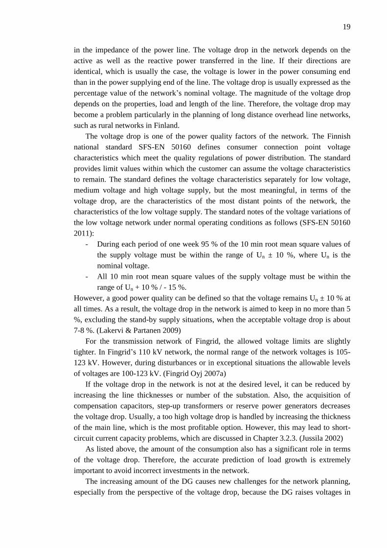
19

in the impedance of the power line. The voltage drop in the network depends on the

active as well as the reactive power transferred in the line. If their directions are

identical, which is usually the case, the voltage is lower in the power consuming end

than in the power supplying end of the line. The voltage drop is usually expressed as the

percentage value of the network’s nominal voltage. The magnitude of the voltage drop

depends on the properties, load and length of the line. Therefore, the voltage drop may

become a problem particularly in the planning of long distance overhead line networks,

such as rural networks in Finland.

The voltage drop is one of the power quality factors of the network. The Finnish

national standard SFS-EN 50160 defines consumer connection point voltage

characteristics which meet the quality regulations of power distribution. The standard

provides limit values within which the customer can assume the voltage characteristics

to remain. The standard defines the voltage characteristics separately for low voltage,

medium voltage and high voltage supply, but the most meaningful, in terms of the

voltage drop, are the characteristics of the most distant points of the network, the

characteristics of the low voltage supply. The standard notes of the voltage variations of

the low voltage network under normal operating conditions as follows (SFS-EN 50160

2011):

- During each period of one week 95 % of the 10 min root mean square values of

the supply voltage must be within the range of Un ± 10 %, where Un is the

nominal voltage.

- All 10 min root mean square values of the supply voltage must be within the

range of Un + 10 % / - 15 %.

However, a good power quality can be defined so that the voltage remains Un ± 10 % at

all times. As a result, the voltage drop in the network is aimed to keep in no more than 5

%, excluding the stand-by supply situations, when the acceptable voltage drop is about

7-8 %. (Lakervi & Partanen 2009)

For the transmission network of Fingrid, the allowed voltage limits are slightly

tighter. In Fingrid’s 110 kV network, the normal range of the network voltages is 105-

123 kV. However, during disturbances or in exceptional situations the allowable levels

of voltages are 100-123 kV. (Fingrid Oyj 2007a)

If the voltage drop in the network is not at the desired level, it can be reduced by

increasing the line thicknesses or number of the substation. Also, the acquisition of

compensation capacitors, step-up transformers or reserve power generators decreases

the voltage drop. Usually, a too high voltage drop is handled by increasing the thickness

of the main line, which is the most profitable option. However, this may lead to short-

circuit current capacity problems, which are discussed in Chapter 3.2.3. (Jussila 2002)

As listed above, the amount of the consumption also has a significant role in terms

of the voltage drop. Therefore, the accurate prediction of load growth is extremely

important to avoid incorrect investments in the network.

The increasing amount of the DG causes new challenges for the network planning,

especially from the perspective of the voltage drop, because the DG raises voltages in

20

its vicinity when it produces power to the network. In some situations, the voltage rise

may become the dimensioning factor instead of the voltage drop. Therefore, the voltage

rise must be noticed in the planning also without forgetting the possible situation where

the DG is disconnected and not producing power. Moreover, the production of the DG

may vary more frequently compared with the traditional production, since the DG plants

typically use renewable energy sources, like wind or solar power. This means that also

the voltages of the network experience the similar changes than the power outputs of the

DG plants. Therefore, also the voltage fluctuations in the network are expected to

increase.

3.2.3. Short-circuit current capacity and protection

A conductive connection between two live parts of the network causes a short circuit, in

which case a short circuit current begins to flow in the network. The current can damage

the network components or pose a risk to humans or animals. The magnitude of the

current depends on the impedances of the lines, the reactances of the transformers and

the short circuit powers of the feeding fault current sources. Respectively, the waveform

of the current depends on the types and properties of the feeding generators. In general,

it can be said that the short circuit current is the weaker the smaller the cross-sectional

areas of the lines are and the further the fault occurs in the network, as long as all the

fault current sources of the network are at the beginning of the network, in which case

the fault current flows simply from the beginning of the network towards the fault.

(Jussila 2002)

A basic requirement for the distribution of electricity is that it must not pose a risk to

humans, animals and the environment. For that reason, network protection is used to

ensure the safety of electricity distribution in all circumstances, particularly in the fault

situations. In addition, the network protection ensures that no damages are caused to the

network itself by the faults. Each network company must ensure that both the short

circuit protection and earth fault protection of the network are designed so that the

network fulfils the company’s own safety objectives and especially the current safety

regulations and standards that have been imposed by the authorities. The safety

standards specify the authorized values for the touch voltages and fault currents in the

network as well as for their durations. (Lakervi & Partanen 2009)

The network must also be planned so that the short circuit capacity of the network

components is sufficient to withstand all the short circuit currents occurred in the

network. Generally, the smaller is the magnitude of the current, and the shorter is the

current’s impact time, the better the components can withstand the short circuit current.

Therefore, the protection of the network must be designed so that it disconnects the

short circuit currents fast enough, so that the short circuit capacity of the network is not

exceeded. Also, the protection must operate selectively which means that only the

protective device closest to the fault location operates and solves the fault.

21

The adequacy of the network short circuit capacity can be examined with fault

current calculations. These calculations are used in planning to determine the most

suitable structure of the network and to select appropriate network components and

settings for protective devices in terms of short circuit current capacity. In addition, the

current capacity must be adequate for all possible connection situations, including all

the stand-by supply situations. These short circuit current capacity examinations are

being performed every time a new network is being planned. Additionally, the

examinations should be performed periodically for the entire existing network. If

insufficient part of the network in terms of short circuit current capacity is detected, the

network improvements increasing the short circuit capacity should be diagnosed and

accomplished. The short circuit capacity of the network can be increased by

accelerating the disconnection time of the fault, limiting the fault current or increasing

the thickness of the lines. However, increasing the thickness of the lines may cause

problems for other parts of the network, as for an example, changing the main line to

thicker increases the short circuit currents which may lead to the exceeding of the short

circuit current capacity in a branch line. Also, the construction of a new substation may

cause similar effects since it increases the short circuit currents. (Jussila 2002) In

summary, it can be said that the adequacy of the network short circuit current capacity

must be ensured in all locations and all situations in the network and especially after the

network improvements have been made.

3.2.4. Earth fault protection

An earth fault is a situation in the network where a conductive connection between a

live part of the network and earth is generated. Usually, the earth fault is caused by an

arc or contact between a phase conductor and grounded part of the network. The earth

fault may cause a touch voltage which can be dangerous for humans. As a result, the

earth fault voltages must be limited with earth fault protection. The authorized values

for the earth fault voltages are being defined in the electrical safety regulations. The

values depend on the earthing conditions of the network, the earth fault current and the

duration of the fault current. (SFS 6001 2009)

The earth fault protection can be enhanced by improving the earthing of the network

or decreasing the earth fault current, in which cases the earth fault voltage decreases.

The earth fault protection can also be enhanced by shortening the tripping time of the

earth fault protection, which reduces the impact time of the touch voltage. In Finland,

the resistance of the soil is high and, therefore, the earthing conditions are usually

always poor. Hence, improving the earthing of the network often requires significant

investments in the network, which means that it is not much used in Finland.

Consequently, the earth fault protection is usually enhanced by decreasing the

amplitude or duration of the fault current. The amplitude of the current can be reduced

by using insulated or compensated earthing method. Respectively, the duration of the

fault current can be decreased by changing the protection configurations. In addition,

22

when setting the protection configurations the earthing method must always be

considered, because the amplitude of the earth fault current depends substantially on the

earthing method. (Lakervi & Partanen 2009; Jussila 2002)

3.2.5. Mechanical condition

The mechanical condition of the network has a significant impact on the continuity of

electric supply because the mechanical failures of the network components usually

cause fault situations and outages in the network. Therefore, it is important to take the

mechanical condition of the network into account in network’s general planning.

The mechanical condition of the network may force network operators to renew

their networks before the electrotechnical boundary conditions are met in order to

guarantee the reliability of the network. Hence, the condition monitoring of the network

components is important in network planning and operation, especially for the most

stressed components like wooden poles, isolators and disconnectors. The general

planning of the network should be executed so that both the mechanical and

electrotechnical conditions of the network are considered. This is done by executing

network renovations resulting from both the poor mechanical and electrotechnical

conditions of the network co-ordinately and simultaneously. For instance, if the poles of

the overhead lines are replaced due to the poor mechanical condition, it might be cost-

effective to replace the wires simultaneously even thought it would not be

electrotechnically necessary. (Jussila 2002)

3.2.6. Quality of supply

The appreciation of the quality of electric supply has grown from the perspective of the

electric users and, therefore, it has become one of the major boundary conditions of the

network planning. The quality of electric supply depends on both the quality of the

voltage and continuity of the electric supply. An adequate voltage quality for users is

precisely defined in the standard SFS-EN 50160. The standard determines the allowable

border values for the amplitude of the voltage, voltage fluctuations, harmonics and etc.

These border values must be taken into account in the network planning. (SFS-EN

50160 2011)

The continuity of the electric supply determines the reliability of the electric

distribution, and it is aimed to improve by legislative actions. The Finnish Electricity

Market Act obligates the network operators to pay standard compensations for

customers from over 12-hour interruptions. The compensation is paid depending on the

duration of the interruption, but the maximum compensation for one user is 700 euro

per year. (Energy Market Authority 2007)

In addition, the continuity of the electric supply is also emphasized by Energy

Market Authority regulation model, which determines the allowed profit for the

network company. The regulation model works so that the allowed profit is the bigger

23

the higher is the reliability of the electric distribution. The Energy Market Authority

regulation model is further discussed in Chapter 3.5. (Energy Market Authority 2011)

The quality of the electric supply can be improved in several ways, for example, by

reinforcing the network, adding circuit breakers and disconnectors to the network or

reducing the failure rate of the network. However, all of these methods require financial

investments in the network, which reduces the economic efficiency of the network.

Therefore, the optimum conditions between quality and economic efficiency must be

found in the network planning.

3.2.7. Environmental issues

The environmental impacts of the electrical networks can be divided into ecological

impacts and impacts associated with landscape. The ecological impacts are impacts that

affect on the surrounding environment of the network, such as humans, animals and

plants. For example, when a new power line is constructed, it causes changes to the

surroundings of humans and animals. Also, the direct impacts of the power network,

such as the effects of the electric and magnetic fields on humans, animals and other

electric devices, are included in the ecological impacts. The impacts associated with

landscape are impacts that cause damage mainly to the satisfaction of humans. This is

mainly due to the fact that the power lines are perceived as ugly in terms of a landscape

and view. (Jussila 2002)

In addition, the space requirements of the networks can be considered as an

environmental issue because they are significantly affected by the environment.

Particularly, in the urban networks the available construction space often dimensions

the planning of the network significantly. (Jussila 2002)

The role of the networks’ environmental impacts in the network planning is

growing and, therefore, more attention has been paid to reducing the impacts. The

ecological impacts can be prevented by selecting line routes so that they cause minimal

changes for the nature. Also, preventing transformer oil from leaking to the ground in

case of a transformer breakdown is important, especially in the groundwater areas. The

effects of the electric and magnetic fields can be mitigated by using metal barriers or

cases or using cables or PAS lines instead of overhead lines, in which case the

generated fields abate effectively. The network’s impacts on the landscape can be

decreased also by using cables or PAS lines and by selecting line routes appropriately.

(Jussila 2002)

The implementation of the environmentally most favourable network is usually not

economically feasible, which means that the economic efficiency of the network

decreases when the environmental impacts are being reduced. Consequently, the

relationship between economy and environmental friendliness must be defined in the

network planning.

24

3.3. Planning tools

The most important planning tools of network planning are different information

systems of which the most significant is the network information system (NIS) which

includes information about the network components. The NIS can be used to perform

network calculations which will provide information about the electrical condition of

the network and realization of the boundary conditions. The information is used as a

basis of the network planning. (Lakervi & Partanen 2009)

Other important information systems for the planning are customer information

system (CIS) and maintenance information system (MIS). The CIS contains all

information about customers, for example, customer type, customer’s energy

consumption and customer’s billing information. This information can be used in the

network planning to determine the demand for electricity in the certain area. The MIS

includes the condition information of the network components that can be used to

determine the components and parts of the network that require renovations. In many

cases, the MIS is included in the NIS. (Jussila 2002)

In addition, one important issue is the planning strategy of the network company.

The planning strategy determines the principles and boundary conditions that are used

in network planning. Moreover, the planning strategy ensures that the reliability, power

quality and environmental impacts of the network are at optimal levels at the same time

with network economy. These optimal levels depend on which values and boundary

conditions the company appreciates in its planning strategy. (Vierimaa 2007)

3.4. General planning of HVDNs

As was stated in Chapter 3.1, the general planning of the HVDNs is a mixture of the

transmission network planning and the MVDN planning since the HVDN planning

contains elements from both. In Finland, the HVDN network operators usually carry out

the general planning of the HVDNs in cooperation with the transmission network

operator, Fingrid, since the general planning of the HVDNs is based on Fingrid’s

regional network planning.

The term regional network planning comes from the fact that Fingrid has divided the

Finnish power transmission system in 13 separate planning regions based on the

geographical and electrotechnical conditions, and the planning of the network is done

independently in each of these regions. However, the plans are based on the Fingrid’s

long-term transmission network development plan and, thereby, also on the Ten-Year

Network Development Plan of the ENTSO-E. The main focus of the Fingrid’s regional

network planning is on the planning of 110 kV and 220 kV transmission networks

owned by Fingrid, but the planning also takes into account 110 kV networks owned by

other operators than Fingrid. The time span of the regional network planning is

normally 15-20 years and the plans are updated every 3-5 years. The planning is based

on the national electricity consumption forecasts and electricity consumption and

25

generation forecasts and measurements which have been obtained from the local

network companies, producers and industry. In addition, the needs of network condition

management and operation are considered in the regional network planning. Usually,

the planning includes meetings involving Fingrid and all or part of the network

operators of the planning region, who own some HVDN. These meetings help to take

into account the interests of all stakeholders in the development and planning of the

HVDNs. Moreover, Fingrid can receive feedback from the other network operators and

the operators can declare the planning needs of their own HVDNs to Fingrid through

the meetings. The initiative for the meetings can become from either party. (Reilander

2012a; Reilander 2012b)

Fingrid completes the planning of the networks with its network calculation model

which includes the entire Finnish 110 kV, 220 kV and 400 kV networks. The

calculation model is also used in interaction with the HVDN network operators to

facilitate the HVDN network planning, especially to determine the suitable network

protection settings in the HVDN or to verify the functioning of the new HVDN network

plans. (Bastman 2011, Reilander 2012a; Reilander 2012b)

The planning criteria of 110 kV networks are usually not as tight as the criteria of

400 kV transmission networks. This is due to the fact that the N-1 criterion must be

realized completely in 400 kV networks and, therefore, the network must withstand any

single fault that is being occurred in the network. On the contrary, 110 kV and also 220

kV networks must only withstand any single fault without it causing overload to the

network or the fault is spread. Hence, a fault can cause a regional interruption in 110 kV

network. In addition, the dimensioning factor in 110 kV network is usually the thermal

capacity or the short-circuit current capacity of the lines or the voltage drop in the

network. In some special cases the dimensioning factor of 110 kV network can also be

the stability of the network. (Reilander 2012a; Elenia Verkko 2012)

The planning of the HVDN is somewhat more complicated than the planning of the

MVDN, since the HVDN planning requires close cooperation between the transmission

network operator, network companies and significant network users. Additionally, the

Finnish legislation affects on the HVDN planning because the construction of the line

with voltage at least 110 kV requires a construction permit from the Energy Market

Authority. Moreover, the network companies do not have a monopoly on the

construction of 110 kV network in their own area, as they have in the case of the

MVDN. Therefore, the construction needs of new 110 kV lines must be justified for the

Energy Market Authority, which will ultimately decide which of the lines will be built.

(Energy Market Authority 2010a)

In conclusion, it can be said that, in Finland, the planning of all 400 kV, 220 kV and

110 kV networks, including HVDNs, is generally performed by Fingrid. This is largely

due to the fact that the functionality of the majority of the HVDN plans must be verified

and accepted by Fingrid before implementation. Also, all the switching changes in the

HVDNs must be accepted by Fingrid. Therefore, the majority of the network

companies, who own HVDN, do not perform the network calculations required in the

26

HVDN planning by themselves, since the similar calculations are performed by Fingrid

anyway. Instead, the companies usually acquire the calculations as a service from

Fingrid, who does not charge any additional fees from the calculations and planning.

Especially, the planning of HVDN protection settings is normally always performed by

Fingrid, because it requires the use of the Fingrid’s calculation model. Moreover, at the

moment the HVDN companies think that the changes in the HVDNs will be relatively

small, so the planning and calculations need to be performed quite rarely. However, the

increasing amount of wind power connected to the HVDN is expected to change the

case in the future. Consequently, the investments in the HVDNs may increase in the

future and increase the need for the planning of the new HVDN. This may lead to the

situation where the resources of Fingrid are no longer sufficient to manage the

calculations of the entire 110 kV network. (Bastman 2011, Elenia Verkko 2012,

Reilander 2012b)

3.5. Effects of Energy Market Authority regulation model on

planning

In a Finnish electric power system, the distribution network companies have a

monopoly on the construction and operation of the MDVN network of their own region.

This significantly reduces the competition, especially in the pricing of electricity

transmission and distribution. Therefore, the business of the network companies must be

monitored in order to prevent the abuse of the monopolistic position. For this purpose,

the Finnish Energy Market Authority has developed a regulation model to determine the

reasonable pricing of network operations. The regulation model is redefined for each

regulatory period, each of which lasting four years, expect the first one. The first

regulatory period was valid from 2005 to 2007, the second from 2008 to 2011 and the

third will be valid from 2012 to 2015.

The regulation model defines a reasonable return for each network company

regardless of the voltage levels where the company is operating. The reasonable return

is determined differently for a transmission system operator, Fingrid, and distribution

network companies. For the MVDN companies as well as for the companies that own

some HVDN network, the determination of the reasonable return is described in the

document of Energy Market Authority. The document assesses the reasonableness of

the pricing of both the electricity distribution network services and high voltage

distribution network services. Consequently, the term ‘HVDN’ has been introduced in

this thesis since the term is used in that document. Although the methods have been

introduced in the same document for both the HVDN and the MVDN operators, the

determination of the reasonable return for the HVDN operators differs slightly from the

one for the MVDN operators. This chapter introduces the determination of the

reasonable return for the HVDN and MVDN operators and explains the differences

between the two cases. (Energy Market Authority 2011)

27

The reasonable return depends on the capital invested in the network operations and

the current value of the company’s electricity network, which depends on the size of the

network and age, type and life time of the network components. In addition, the

reasonable return is affected by a reasonable rate of return for all capital invested in the

network, which is determined using the Weighted Average Cost of Capital method

(WACC). When the reasonable return has been determined, it is compared with the

company’s actual adjusted profit. The actual adjusted profit consists of the actual profit

of the company added with the effects of incentives that may reduce or increase the

actual adjusted profit. The regulation model requires that the actual adjusted profit

should not be higher than the determined reasonable return of the company in the long-

term. Therefore, the actual profit of the company can be the larger the more effectively

the incentives are being fulfilled. (Energy Market Authority 2011)

The incentives in the third regulatory period are the investment, quality, innovation

incentive and the incentive to improve efficiency. The incentives are calculated

annually. The investment incentive encourages the network company to develop its

network and invest in it sufficiently. The investment incentive works in such way that

the more the company invests in the network, the greater the company’s profit can be.

(Energy Market Authority 2011)

The quality incentive aims to improve the quality of the electric transmission and

distribution. It compares the company’s realized costs of interruptions with the network

operator specific reference level and the difference between the figures defines the

impact of the incentive, so that the better the quality of the electric supply is, the more

profit the company is allowed to generate. The calculations of the company’s realized

costs of interruptions are different in case of the MVDN and HVDN, since in the case of

the MVDN, the calculations take into account both the number and the duration of both

the long planned and the long unexpected interruptions as well as the number of both

the high-speed automatic and the delayed automatic reclosings, which are short

interruptions. On the contrary, in the case of the HVDN, the calculations are affected

only by the number and duration of the long unexpected interruptions and the duration

of the planned interruptions. The short interruptions do not affect on the incentive in

case of the HVDN in the third regulatory period, but the Energy Market Authority

begins to collect information about the short interruptions from the HVDN operators

with an objective to add the impact of the short interruptions to incentive in the fourth

regulatory period. In conclusion, the quality incentive enhances the quality of power

delivery in the network planning and encourages improving the quality of electric

supply by increasing its economic competitiveness. (Energy Market Authority 2011)

The incentive to improve the efficiency aims to improve the cost-efficiency in the

network company’s operations. The incentive determines an individual objective to

improve efficiency for each network company. For the MVDN operators, the objective

consists of a general and company specific objective to improve efficiency; and for the

HVDN operators, the objective consists solely of the general objective to improve

efficiency. The general objective to improve efficiency aims to encourage all companies

28

to develop their operations in accordance with the technological development. In the

third regulatory period, the general objective to improve efficiency is 2.06 % per year.

The company specific objective to improve efficiency aims to enhance especially the

cost-efficiency of the inefficient companies. The company specific objective will

determine the company’s potential to improve the cost-efficiency in relation to the most

efficient companies. Thus, the inefficient companies receive greater benefits from the

incentive than the most efficient companies and, therefore, the inefficient companies

have higher interest to develop their cost-efficiency. (Energy Market Authority 2011)

The incentive to improve the efficiency measures the cost-efficiency of the company

with the StoNED method (Stochastic Non-smooth Envelopment of Data). The method

compares the potential effectiveness of the company, which has been calculated using

the company’s company specific objective to improve efficiency, with the realized

effectiveness using the costs of cost-efficiency. Therefore, more efficient operation

enables taking greater profit. The realized costs of cost-efficiency are affected by

controllable operational costs and interruption costs, which affect also on the quality

incentive. Consequently, the incentive to improve efficiency also encourages improving

the quality of electric supply as well as the quality incentive does. (Energy Market

Authority 2011)

A novel incentive in the third regulatory period is the innovation incentive, which

aims to encourage the network companies to promote innovative technical and

functional solutions in network operations. The company may increase its allowed

profit with the innovation incentive by increasing the use of automatic meter reading

(AMR) in operation points equipped with a fuse of less than 63 A, or by investing more

in general research and development which promotes the penetration of new

technology. However, it is only possible to implement the increase in the use of AMR

by the MVDN operators, because there are no operation points with a fuse less than 63

A in the HVDNs. Altogether, the innovation incentive promotes the observing of novel

technologies in the investments and planning of both networks. (Energy Market

Authority 2011)

In conclusion, the regulation model of the Energy Market Authority encourages the

network companies to invest and increase the value of their electric networks. In

particular, the regulation model emphasizes the investments in the quality of the power

delivery since it is enhanced by both the quality incentive and the incentive to improve

the efficiency. In addition, the investing in novel technologies is stimulated by the

innovation incentive. All in all, the main notice is the fact that the regulation model

highlights the role of electric supply’s quality as a boundary condition of the network

planning.

29

4. WIND POWER AS PART OF HVDN

4.1. General

The most important construction criterion of a wind power plant is windiness, as it is

the main factor in determining the power generated by the power plant. The wind is

distributed unevenly depending on the geographical conditions. Therefore, also the

wind plants are typically constructed geographically unevenly so that in windy areas the

density of the plants can be considerably high. These areas are typically sparsely

populated and, thus, situated poorly in terms of the electric network since the network is

often weak and planned to transfer only small amounts of power. Consequently,

connecting wind power to the network causes substantial investments, and the aligning

of the investments may cause problems for the network companies. The investments

consist of the interconnection costs of the wind plant and network, the network

reinforcement costs and the costs to increase the reserve capacity of the network. The

allocation principles of the investments vary by country. In Finland, the wind producer

usually pays the costs up to the connection point, and the network operator, whose

network the plant is being connected, pays the required network reinforcements and

reserve capacity. (Matilainen 2011)

The connection method of wind power depends on the size of the wind power unit

and the type of the surrounding network. Small individual wind power units are usually

connected to the MVDN, while the wind farms consisting of several wind turbines are

connected to the HVDN or transmission network. This is due the fact that the higher the

voltage of the network is, the lower are the power losses, and the better the network

stands the major increase in power transfer. Small wind power units can be connected

directly to the power network whereas bigger wind farms must be connected via

switching station. The network connection voltages and connection methods are defined

by interconnection laws and regulations which are discussed in Chapter 4.2.

Currently all over the world, the majority of the research in the effects of wind

power on the network is focused on the effects on the whole network while the effects

on the HVDNs receive appreciably lower attention (Holttinen et al. 2009; ENTSO-E.

2010; EWEA 2010). Consequently, there is very little research data available on the

wind power effects on the HVDNs. However, since a large part of the future wind

plants in the network will be connected to the HVDNs, at least in Finland, the wind

power effects on the HVDNs should be examined more precisely in the future.

30

4.2. Interconnection laws and regulations

Since the thesis concentrates on the HVDNs, the interconnection laws and regulations in

the MVDNs are not being discussed in the thesis. The thesis describes only the

interconnection laws and regulations of the HVDNs and transmission networks.

The Finnish transmission system operator, Fingrid, determines the requirements of

the network connection. These requirements are defined in Fingrid’s connection

conditions and technical requirements of the power plants (Fingrid 2007a; Fingrid

2007b). In addition, Fingrid has defined detailed regulations for connecting wind

turbines to the Finnish network which are based on Nordel Connection Code for Wind

Turbines (Tuulivoimalaitosten järjestelmätekniset vaatimukset 2011). Nordel was

disbanded in 2009, when a new pan-European administrator organization ENTSO-E

was established. The ENTSO-E unified all six former TSO organizations including

Nordel (Partanen 2011). However, Nordel’s code will remain in force in Nordic

countries until ENTSO-E publishes its own network code, which will be valid in almost

all European countries. The network code of ENTSO-E will be based on currently valid

network codes in Europe, so the code will be largely similar with Nordel’s code, since it

will also provide country specific regulations. (Fingrid 2010)

The Fingrid’s regulations are designed to ensure the compatibility and correct

operation of the electric networks in all operation conditions. The regulations apply to

all kinds of network connections. However, since Fingrid has no contractual

relationship with customers outside of the transmission network, the local network

operators are responsible for ensuring that the wind farms connected to their network

meet the Fingrid’s regulations. (Tuulivoimalaitosten järjestelmätekniset vaatimukset

2011)

The Fingrid’s regulations apply to the wind power units whose connection point

power exceeds 0.5 MVA. However, for power units with power from 0.5 MVA to 10

MVA, eased requirements are valid. (Fingrid 2011) Since this thesis focuses on the

HVDNs and the wind power units connected to the HVDN are usually over 10 MVA

units, only the Fingrid’s requirements valid for over 10 MVA units are discussed.

The Fingrid’s regulations insist that wind farms with power larger than 250 MVA

must be connected to 400 kV transmission network and wind farms with power less

than 250 MVA can be connected to 110 kV network, as long as the capacity of the

network is sufficient. In addition to that, wind farms with power more than 25 MVA

must be connected to the network via switching station. On the contrary, wind farms

with power up to 25 MVA can be connected directly to the network’s power line under

certain conditions determined by Fingrid. (Fingrid 2012)

Moreover, Fingrid will charge a connection fee from the power plants that are

connected to its network. Fingrid has just introduced the new practises for connection

fees in its networks. The connection fees of Fingrid have been listed in Table 4.1.

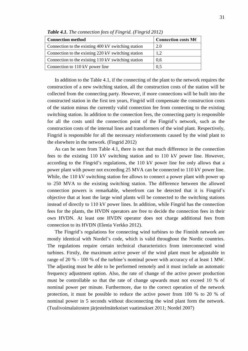
31

Table 4.1. The connection fees of Fingrid. (Fingrid 2012)

Connection method Connection costs M€

Connection to the existing 400 kV switching station 2.0

Connection to the existing 220 kV switching station 1,2

Connection to the existing 110 kV switching station 0,6

Connection to 110 kV power line 0,5

In addition to the Table 4.1, if the connecting of the plant to the network requires the

construction of a new switching station, all the construction costs of the station will be

collected from the connecting party. However, if more connections will be built into the

constructed station in the first ten years, Fingrid will compensate the construction costs

of the station minus the currently valid connection fee from connecting to the existing

switching station. In addition to the connection fees, the connecting party is responsible

for all the costs until the connection point of the Fingrid’s network, such as the

construction costs of the internal lines and transformers of the wind plant. Respectively,

Fingrid is responsible for all the necessary reinforcements caused by the wind plant to

the elsewhere in the network. (Fingrid 2012)

As can be seen from Table 4.1, there is not that much difference in the connection

fees to the existing 110 kV switching station and to 110 kV power line. However,

according to the Fingrid’s regulations, the 110 kV power line fee only allows that a

power plant with power not exceeding 25 MVA can be connected to 110 kV power line.

While, the 110 kV switching station fee allows to connect a power plant with power up

to 250 MVA to the existing switching station. The difference between the allowed

connection powers is remarkable, wherefrom can be detected that it is Fingrid’s

objective that at least the large wind plants will be connected to the switching stations

instead of directly to 110 kV power lines. In addition, while Fingrid has the connection

fees for the plants, the HVDN operators are free to decide the connection fees in their

own HVDN. At least one HVDN operator does not charge additional fees from

connection to its HVDN (Elenia Verkko 2012).

The Fingrid’s regulations for connecting wind turbines to the Finnish network are

mostly identical with Nordel’s code, which is valid throughout the Nordic countries.

The regulations require certain technical characteristics from interconnected wind

turbines. Firstly, the maximum active power of the wind plant must be adjustable in

range of 20 % - 100 % of the turbine’s nominal power with accuracy of at least 1 MW.

The adjusting must be able to be performed remotely and it must include an automatic

frequency adjustment option. Also, the rate of change of the active power production

must be controllable so that the rate of change upwards must not exceed 10 % of

nominal power per minute. Furthermore, due to the correct operation of the network

protection, it must be possible to reduce the active power from 100 % to 20 % of

nominal power in 5 seconds without disconnecting the wind plant form the network.

(Tuulivoimalaitosten järjestelmätekniset vaatimukset 2011; Nordel 2007)

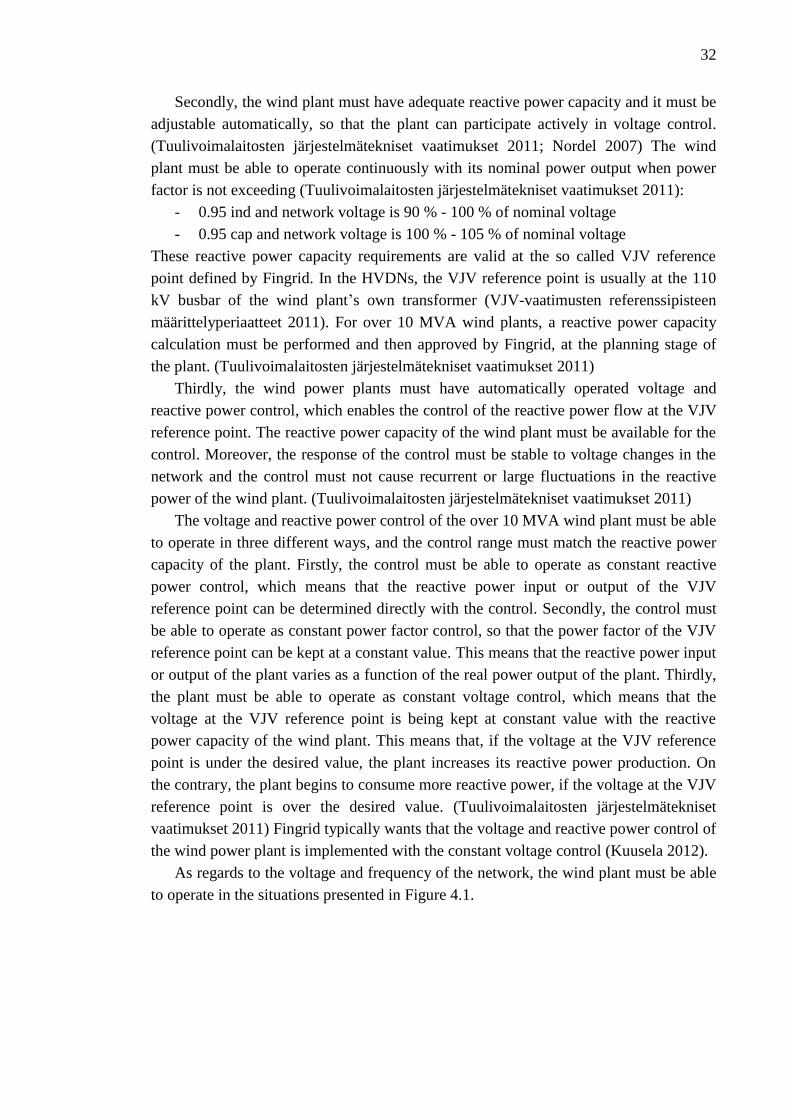
32

Secondly, the wind plant must have adequate reactive power capacity and it must be

adjustable automatically, so that the plant can participate actively in voltage control.

(Tuulivoimalaitosten järjestelmätekniset vaatimukset 2011; Nordel 2007) The wind

plant must be able to operate continuously with its nominal power output when power

factor is not exceeding (Tuulivoimalaitosten järjestelmätekniset vaatimukset 2011):

- 0.95 ind and network voltage is 90 % - 100 % of nominal voltage

- 0.95 cap and network voltage is 100 % - 105 % of nominal voltage

These reactive power capacity requirements are valid at the so called VJV reference

point defined by Fingrid. In the HVDNs, the VJV reference point is usually at the 110

kV busbar of the wind plant’s own transformer (VJV-vaatimusten referenssipisteen

määrittelyperiaatteet 2011). For over 10 MVA wind plants, a reactive power capacity

calculation must be performed and then approved by Fingrid, at the planning stage of

the plant. (Tuulivoimalaitosten järjestelmätekniset vaatimukset 2011)

Thirdly, the wind power plants must have automatically operated voltage and

reactive power control, which enables the control of the reactive power flow at the VJV

reference point. The reactive power capacity of the wind plant must be available for the

control. Moreover, the response of the control must be stable to voltage changes in the

network and the control must not cause recurrent or large fluctuations in the reactive

power of the wind plant. (Tuulivoimalaitosten järjestelmätekniset vaatimukset 2011)

The voltage and reactive power control of the over 10 MVA wind plant must be able

to operate in three different ways, and the control range must match the reactive power

capacity of the plant. Firstly, the control must be able to operate as constant reactive

power control, which means that the reactive power input or output of the VJV

reference point can be determined directly with the control. Secondly, the control must

be able to operate as constant power factor control, so that the power factor of the VJV

reference point can be kept at a constant value. This means that the reactive power input

or output of the plant varies as a function of the real power output of the plant. Thirdly,

the plant must be able to operate as constant voltage control, which means that the

voltage at the VJV reference point is being kept at constant value with the reactive

power capacity of the wind plant. This means that, if the voltage at the VJV reference

point is under the desired value, the plant increases its reactive power production. On

the contrary, the plant begins to consume more reactive power, if the voltage at the VJV

reference point is over the desired value. (Tuulivoimalaitosten järjestelmätekniset

vaatimukset 2011) Fingrid typically wants that the voltage and reactive power control of

the wind power plant is implemented with the constant voltage control (Kuusela 2012).

As regards to the voltage and frequency of the network, the wind plant must be able

to operate in the situations presented in Figure 4.1.

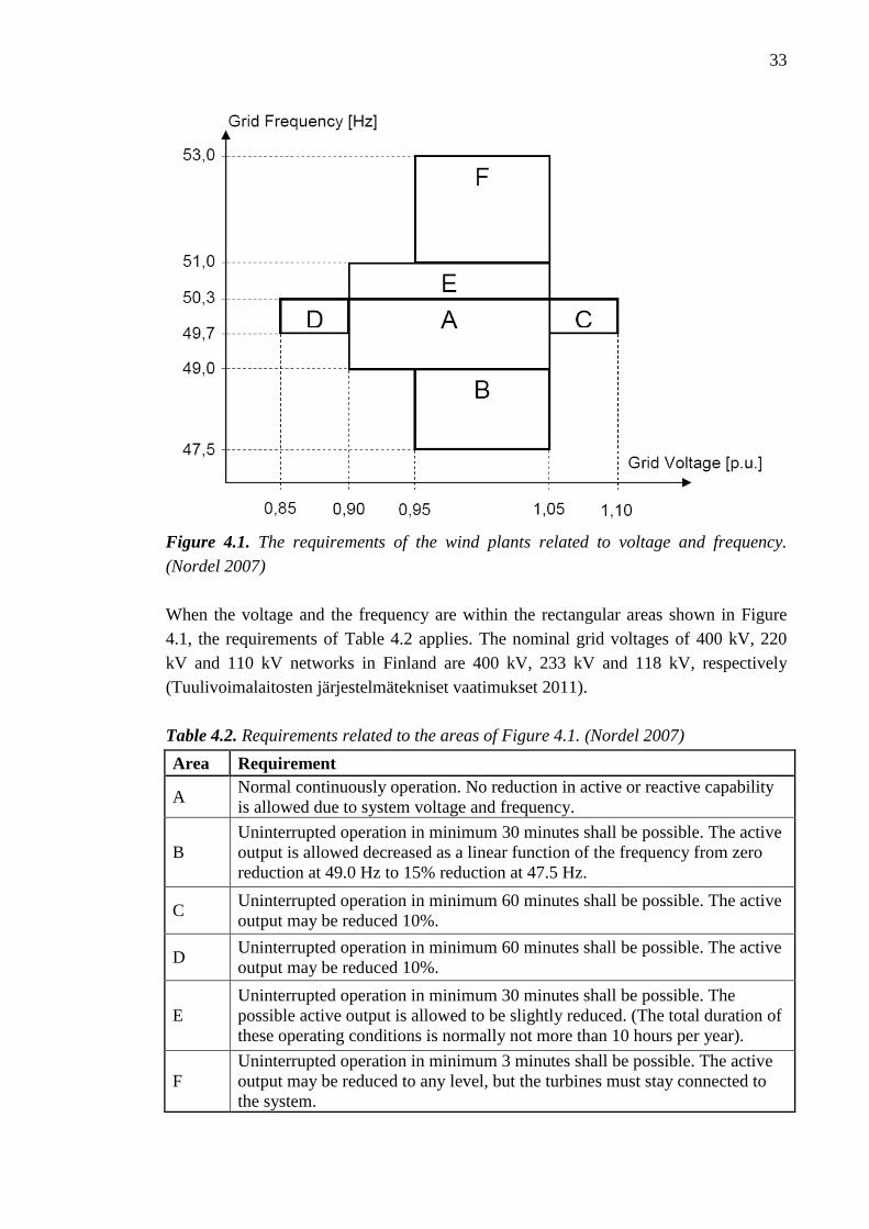
33

Figure 4.1. The requirements of the wind plants related to voltage and frequency.

(Nordel 2007)

When the voltage and the frequency are within the rectangular areas shown in Figure

4.1, the requirements of Table 4.2 applies. The nominal grid voltages of 400 kV, 220

kV and 110 kV networks in Finland are 400 kV, 233 kV and 118 kV, respectively

(Tuulivoimalaitosten järjestelmätekniset vaatimukset 2011).

Table 4.2. Requirements related to the areas of Figure 4.1. (Nordel 2007)

Area Requirement

A Normal continuously operation. No reduction in active or reactive capability

is allowed due to system voltage and frequency.

B

Uninterrupted operation in minimum 30 minutes shall be possible. The active

output is allowed decreased as a linear function of the frequency from zero

reduction at 49.0 Hz to 15% reduction at 47.5 Hz.

C Uninterrupted operation in minimum 60 minutes shall be possible. The active

output may be reduced 10%.

D Uninterrupted operation in minimum 60 minutes shall be possible. The active

output may be reduced 10%.

E

Uninterrupted operation in minimum 30 minutes shall be possible. The

possible active output is allowed to be slightly reduced. (The total duration of

these operating conditions is normally not more than 10 hours per year).

F

Uninterrupted operation in minimum 3 minutes shall be possible. The active

output may be reduced to any level, but the turbines must stay connected to

the system.

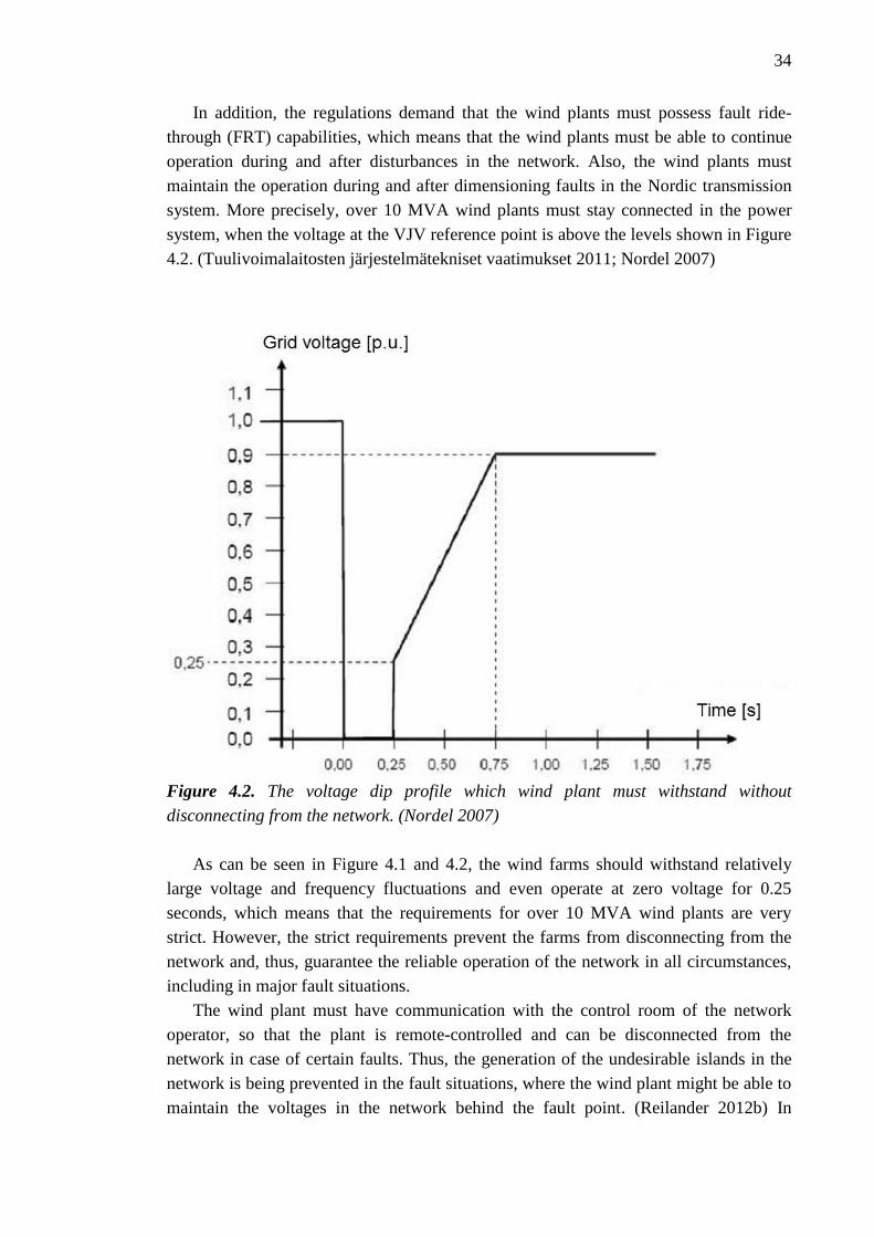
34

In addition, the regulations demand that the wind plants must possess fault ride-

through (FRT) capabilities, which means that the wind plants must be able to continue

operation during and after disturbances in the network. Also, the wind plants must

maintain the operation during and after dimensioning faults in the Nordic transmission

system. More precisely, over 10 MVA wind plants must stay connected in the power

system, when the voltage at the VJV reference point is above the levels shown in Figure

4.2. (Tuulivoimalaitosten järjestelmätekniset vaatimukset 2011; Nordel 2007)

Figure 4.2. The voltage dip profile which wind plant must withstand without

disconnecting from the network. (Nordel 2007)

As can be seen in Figure 4.1 and 4.2, the wind farms should withstand relatively

large voltage and frequency fluctuations and even operate at zero voltage for 0.25

seconds, which means that the requirements for over 10 MVA wind plants are very

strict. However, the strict requirements prevent the farms from disconnecting from the

network and, thus, guarantee the reliable operation of the network in all circumstances,

including in major fault situations.

The wind plant must have communication with the control room of the network

operator, so that the plant is remote-controlled and can be disconnected from the

network in case of certain faults. Thus, the generation of the undesirable islands in the

network is being prevented in the fault situations, where the wind plant might be able to

maintain the voltages in the network behind the fault point. (Reilander 2012b) In

35

addition, the starting of the wind plant must not cause any significant harmonics or

voltage fluctuations that are over 0.03 pu to the voltage of the VJV reference point.

Also, the wind turbines of the wind farm must not stop at the same time due to high

wind speed, but the stop must be graduated. Furthermore, the calculation models of the

wind plant must be submitted to the Fingrid, who uses the models in measures related to

the planning and operation of the network. (Tuulivoimalaitosten järjestelmätekniset

vaatimukset 2011)

As it was stated above, ENTSO-E is currently preparing new connection

requirements which are applicable to all generators. The process is currently at the draft

stage, and the novel code will replace the currently used network codes in 2013 at the

earliest. The requirements of ENTSO-E will include country specific requirements,

which will be based on the currently used regional requirements, such as Nordel’s grid

code. On the basis of the published drafts of ENTSO-E, the requirements will be

slightly stricter than in Nordel’s code, especially for voltage dips and frequency

fluctuations. Also, the requirements of ENTSO-E demand that the wind plants

participate even more rapidly in voltage support and control by their reactive power

production and consumption. Moreover, the transmission system operator will have the

right to demand temporarily higher active power production than nominal from wind

plants. In addition, the requirements will depend more on the size of the power plant

unit, because the plants are being divided into four groups according to size and the

requirements will vary by group, so that the largest plants have the highest

requirements. (ENTSO-E 2011)

4.3. Network effects of wind power

Connecting wind power to the electric network causes several effects on the network.

These effects can be divided into local and system-wide effects, depending on their area

of impact, and into short-term and long-term effects, depending on the time-scale of the

effects. The time-scale of the short-term effects is from a few seconds to hours and the

time-scale of the long-term effects is from months to years. All of the effects are not

negative, as some of them may be beneficial for the network. Moreover, the penetration

level of wind power in the network defines the tone of the effects since the effects

typically change to more and more negative as the penetration level increases. All in all,

it can be said that the effects of wind power are perceived largely as negative. (EWEA

2005; EWEA 2010)

Local effects

The greatest local network effects of wind power are targeted to the network voltages

and power quality, because wind plants increase the network voltages in the vicinity of

their connection point. The time-scale of these effects is from a couple of seconds to

minutes. The main impact of the effects is the fact that they complicate the voltage

36

control of the network, as the network voltages near the wind plants may rise above the

boundary conditions during windy conditions, while the voltages in the adjacent feeder

may be close to the lower limits due to heavy load. However, the voltage control of both

feeders is typically combined, which means that in this case the voltage control of the

network is unviable due to the large difference between the feeder voltages. (EWEA

2005)

In addition, the voltage fluctuations of the network can increase locally due to the

high production variations of the wind plants. This is because the power production of

the wind plant depends greatly on wind speed, which is characterized by high and fast

fluctuations. Whenever the wind speed changes from strong wind to weak or from

strong wind to stormy wind, which leads to the disconnection of the plant for security

reasons, the output power of the wind plant changes rapidly from nominal power to

zero. Since the power flows in the network affect on the voltages of the network, the

voltage at the connection point of the plant will also experience a change when the

output power of the plant changes. These voltage fluctuations may exceed the allowed

values unless they are being limited. (Mäki 2011)

The wind plants also affect on the network’s power quality by increasing voltage

transients and harmonics in the network. The voltage transients are generated mostly

when generators or capacitors are connected to the network. The capacitors are used in

some cases to compensate the reactive power needed by the plants, so that the reactive

power flow at the connection point of the plant is minimized. Respectively, the increase

in the harmonics results from the fact that the converters of the wind plants produce the

variety of harmonics in the network. The amount of the harmonics depends on the type

of the wind plant concept and converter. The harmonics cause resonances to the

network, increase the network losses and complicate the operation of motors and

generators. (Mäki 2011)

On the other hand, the wind plants can also influence the network voltages and

power quality positively. Firstly, the voltage rise caused by the plant can also be utilized

by placing the connection point of the plant in an area where voltage is generally lower,

for example, in the area where significant power is transferred through a long power

line. Therefore, by placing the wind plant in the area, the power transmission and

voltage drop of the line will be reduced and, thus, the voltages in the area will be

increased. Secondly, the power quality of the network can be improved with wind plants

by accepting only wind plants that completely meet the newest interconnection laws and

regulations of the plants. In this case, the wind plants can participate actively in

network’s voltage control, support the network voltage and reduce the voltage

fluctuations. (EWEA 2005)

In addition to these, the high production variation and challenging predictability of

the wind plants cause other effects on the network such as effects on the network

efficiency. The high variation in the production of the wind plants means that the

network power flows vary widely, which causes difficulties for the network

dimensioning. These effects can be categorized either as local or system-wide effects,

37

since the wind plants affect on the network’s power flows broadly. The effects cause

additional investments for the network operators, because of the difficulties in the

network dimensioning, as the network components must be oversized due to the

changing power flows. In addition, the change in the power flows due to the wind plants

may increase the power losses of the network locally or system-widely, which also

causes economic losses for the network operators. (EWEA 2005)

On the contrary, the changes in the power flows caused by the wind plants might

also affect positively on the network efficiency, for example in the situations when there

is a significant amount of load close to the connection point of the wind plant. In this

case, the magnitudes of the power flows in the network would be decreased, which

means that also the power losses of the network would be reduced. (Mäki 2011)

System-wide effects

The greatest system-wide effects of wind power are caused by the high production

variation and unpredictability of the wind power production. These effects affect on the

regulation reserves, system production and transmission adequacy and production

efficiency of the network in both the short-term and long-term scale. Firstly, the

regulation reserves, the production and transmission adequacy of the network must be at

a sufficient level to ensure the balance between production and consumption in the

system, especially in situations when there is no wind. Consequently, wind power may

cause additional investment needs to maintain a sufficient level of system adequacy and

regulation reserves in the network. Moreover, the unpredictability of wind power may

decrease the production efficiency of the other production forms, such as thermal and

hydro power, since the planning of the production unit commitment is more difficult

with variable wind power in the network. (EWEA 2005)

4.4. Wind power effects on network planning

The increase in the amount of wind power in the network causes several effects on the

network planning. Most of these effects are caused by the high variability of wind and

wind power production. The effects require special attention in the network planning to

ensure the reliability, safety and cost-effectiveness of the network in the future. The

effects are usually perceived as negative for the network, but some of them may also be

beneficial from the network’s point of view.

The increase in the number of wind power increases uncertainty in the network

general planning, since the realization probabilities of the announced wind power

projects are difficult to estimate. The realization of the projects is the easier to evaluate,

the closer the realization point of the project is. Therefore, the increase in the wind

power production will probably require the average time span of the network general

planning to be shortened, so that the evaluation of the realization would be more

accurate.

38

In addition, the voltage rises and fluctuations caused by wind plants should be taken

into account in the network planning because they affect on the dimensioning of the

network significantly. The network planning should ensure that the network voltages

and voltage fluctuations can be kept within the limits defined by the authorities under

all circumstances. Exceeding the limit values leads to a need for the strengthening of the

network and investments in the network, which increases the additional costs of wind

power for the network. (Mäki 2011)

Traditionally, the dimensioning situation in the network has been the situation of

maximum consumption and minimum production, since in this situation the power

flows in the network are at their highest and, thus, the voltages of the network are at

their lowest due to the high voltage drops. However, the increase in the connection of

the production to the HVDN and MVDN changes the case so that also the situation of

the minimum consumption and maximum production must be considered in the network

planning and dimensioning. This is because the voltages and voltage fluctuations of the

network may rise above the limits due to the increased amount of DG, such as wind

plants, as was also described in Chapter 4.3. (EWEA 2005)

On the contrary, as stated in Chapter 4.3, the voltage rise caused by a wind plant

may be beneficial for the network planning, since the modern wind plants can

participate in network voltage control, increase the fault current levels and support the

voltage, even when there is no wind. Therefore, the wind plants can also be used in the

network planning to strengthen the network and reduce the investment needs resulting

from low network voltages. (Mäki 2011)

Additionally, since the wind plants affect substantially on the power flows of the

network, the adequacy of the network’s power transmission capacity must be ensured in

all wind and load conditions. Because the wind plants may increase the load or fault

currents in the network, the network planning must ensure that the thermal capacities of

the power lines and other network components, such as transformers, should not be

exceeded in either situation.

On the other hand, as said in Chapter 4.3, the wind plants may decrease the power

flows and currents in the network, if they are situated near the consumption points. On

the basis of this, the wind plants may increase the transmission capacity of the network

in some situations, if the planning of the network connection points of the plants is

being performed properly.

The high variability of the wind power production also affects on the needed amount

of the active power regulation reserves in the network, since in case of no wind the

reserves must be able to replace the power produced by the wind plants. The mission of

reserves is to take care of the active power balance in the network and, hence, manage

the frequency control of the network. Wind power increases the need for regulation

reserves in the network because the power variations are increased due to the variability

of the wind. (EWEA 2005) However, the need for regulation reserves could be

potentially handled and reduced by using DSM system-widely, in which case the loads

of the network could be reduced in the case of no wind.

39

The amount of needed new regulation power to the network due to wind power is

difficult to estimate, since the implementation of the wind plant projects is challenging

to forecast. Fingrid is responsible for the frequency control of the Finnish electric power

system and, therefore, the wind power effects on the network reserves are mostly

concerns of Fingrid.

The variations of wind power increase mainly the need for reserve power in

secondary or tertiary control time scales, which means that the reserve power can be

acquired from the balancing market. This reduces the construction needs of the reserve

power plants and, thus, also the additional balancing costs caused by wind power. In

addition, the need for the reserve power and the additional balancing costs depend

highly on the penetration and geographic distribution of the wind power, as well as the

flexibility and adjustability of the production methods of the system, the deadlines of

the electricity market offers and accuracy of the wind power production forecasts.

Therefore, more attention in the network planning should be paid on these issues,

especially by Fingrid, if the penetration of wind power in the network increases.

(EWEA 2005)

All in all, most of the wind plants’ effects on the network planning cause additional

investments in the network and, therefore, reduce the cost-effectiveness of the wind

power. These costs can be, for example, additional balancing costs due to the increased

need for reserve capacity or additional investment costs resulting from the strengthening

of the network. On the contrary, in some cases by connecting wind plants in the network

the investment costs can be avoided or reduced by, for example, reducing the overall

power flows in the network. In addition, novel functional tools are needed in the

planning and operation of the network to evaluate these costs and the effects of wind

power on the different types of networks. In conclusion, the network planning and

operation should take into consideration all the specific characteristics of the wind

plants and the wind plants should be connected to the network so that the cost-

effectiveness and reliability of the network are optimized while the safety of the

network is not jeopardized.

4.5. Wind power effects on network operation

The increase in the amount of wind power in the network must be also considered in the

network operation, because the wind power plants increase problems and affect on the

network operation considerably. However, as in the case of effects on the network

planning, the effects of wind power on the network operation can be either positive or

negative. In addition, the effects are mainly caused by the same wind power

characteristics as in the case of network planning, the variability of the wind power

production being the greatest.

The effects of wind power on the network operation can affect on the network on

two different levels: locally or system-widely. Moreover, some of the effects may affect

on the network both locally and system-widely. The system-wide effects of wind power

40

affect mainly on the activities of Fingrid since it is responsible for the functionality of

the whole Finnish electric power system. Therefore, mostly the local effects of wind

power affect on the operation of the HVDN. Since this thesis concentrates on the

planning and operation of the HVDN, the main focus of the Chapter is on the local

effects of wind power on the network operation. However, the system-wide effects are

being briefly introduced before proceeding to the local effects.

System-wide effects

All the most significant system-wide wind power effects on the network operation are

caused by the variability and unpredictability of the wind power production. The

magnitude of the system-wide effects depends greatly on the penetration level of the

wind power production in the network, as the effects will become increasingly serious,

when more wind power is being connected to the network. However, the tone of the

effects depends significantly on the geographical distribution of the plants, because if

the plants are geographically decentralized, the variability in the production is being

compensated and reduced due to the fact that certain wind conditions prevail in different

areas at different times. In other words, even if some of the wind plants in the certain

area of the network are stalled because of too low or high wind, still the wind plants in

the other areas are usually generating power. Thus, the situation, when all wind power

production of the network is stalled, is extremely unlikely. (EWEA 2005)

Due to the uncertainty and difficulty in the forecasting of the wind power, the

amount of needed system-wide regulation reserves for network power balancing is

increased, which increases the balancing costs of the network. Also, the power

fluctuations within the power network and between interconnected networks are

increased due to the same reason. In addition, the uncertainty and difficulty may result

in that the wind power production may have to be curtailed in some situations, if the

consumption or transfer capacity of the system is not adequate. This is not desirable,

because when the wind production is curtailed, a proportion of the wind energy is

wasted, since in such case all the available energy form wind is not used in electric

power production. The curtailing of the wind production reduces the cost-effectiveness

of the power production and network. (EWEA 2005)

The increase in the balancing reserves and in the needed transfer capacity due to

wind power and the curtailing of wind power in the system-wide scale might possibly

be avoided or decreased by improving the forecasting of the wind power production

generally, by ensuring adequate transfer capacity in the network and especially between

interconnected networks, by using DSM in the network or by changing the operation of

the electricity market so that the closure times of the market are being reduced.

Especially, the latter would effectively reduce the uncertainty of the wind production,

since the wind power forecasts would become more and more accurate if their time

interval was shortened. (ENTSO-E 2010)

41

Another major system-wide effect of wind power is the effect of wind power on

system stability. Traditionally, wind plants have been designed in such way that they are

disconnected from the network in the event of disturbance or fault. This approach

decreases the stability of the network and, therefore, it is functional only when the

amount of wind power in the network is relatively small, since it also increases the risk

for a major disturbance in the network. Consequently, since the penetration levels of

wind power in the networks are growing, in order to maintain the current level of

network stability, the behaviour of the wind plants during the faults should be changed.

Therefore, the network operators have begun to require stricter laws and regulations for

connecting wind plants in the network, for example FRT capabilities. (EWEA 2005)

These regulations were discussed in Chapter 4.2. All in all, more studies are needed to

diagnose the effects of wind plants on the system stability; however, some studies

indicate that when the connected wind plants meet the latest requirements, the overall

stability of the network can be even improved with wind power (Piwko et al. 2005).

Local effects

As it was stated above, primarily only the local effects of wind power affect on the

operation of the HVNDs. However, some of the system-wide effects of wind power on

the network operation can be rendered as local, for example, the impacts on the

network’s transfer capacity or power fluctuations also influence the network locally.

The most significant locally affecting effect of wind power is the increase in power

fluctuations due to the variability in the production of the wind plant. The increase

causes the same effects locally as it causes system-widely. Firstly, the adequacy of the

network transfer capacity may be compromised, which means that additional

investments in the capacity may become mandatory. Secondly, voltages in the network

vary depending on the power flows in the network, which means that the voltage

fluctuations in the network increase and may exceed the allowable values imposed by

the authorities. Thirdly, the power flows in the network affect on the network power

losses, which means that the magnitude of the power losses in the network may change

as the power flows of the network change. This means that more attention should be

paid in the network operation to the optimization of the losses in the network. In

addition, the increased power fluctuations in the network may lead to the curtailment of

the wind power production, if the wind plants generate more power than what can be

transferred and consumed in the network. (Mäki 2011)

Other considerable local effect of wind power is an increase in the complexity of the

network protection, which occurs if the protection of the network has been designed

assuming that the power flows in the network are unidirectional. However, since the

protection of the transmission network and most of the HVDNs is implemented by

distance or differential relays, this effect should only have a little impact on these

networks. On the other hand, the impact on the MVDN is significant and, thus, the

operation of the MVDN protection must be modified so that it will be able to handle

42

multidirectional fault currents and take into account the fault current sources all over the

network. (Mäki 2011)

Generally, the wind power effects on the network operation can be managed by

increasing the intelligence of the network, in other words, increasing automation in the

network and communication between power plants, network components and loads.

Thus, the power flows of the network could be better monitored and controlled and the

power flow variations would be reduced. Moreover, the intelligence in the network

protection would help the protection to cope with multidirectional fault currents. In

addition, with distributed wind plants and adequate intelligent network operation,

controlled islands could possibly be formed in the network in fault situations. This

means that the voltage can be maintained in the part of the network behind the fault,

which means that the disturbance area of the fault would be smaller and, consequently,

the reliability of the network would be increased. (Mäki 2011)

4.6. HVDN network simulations

This thesis includes HVDN simulations which have been carried out with the network

test system. The network test system has been introduced in Chapter 2.4.1 and in

Appendix 2. The structure of the test system has been presented in Figure 2.3 and

Appendix 1. The main purpose of the simulations is to identify the effects of variable

wind production on the HVDN planning and operation and, in addition, to clarify the

benefits of DSM for the planning and operation.

The simulations have been performed with three different network cases regarding

to the lengths of the network lines, as it has been said in Appendix 2. However, only

some of the lengths vary case by case, as can be seen from Table A2.3.

In Case 1, the lines of the network are the longest. In this case, Lines 11-15 and 12-

16, which are the lines that are connected to the 110 kV busbars of the 400/110 kV

transformers, are 60 and 100 km long, respectively. Moreover, Lines 11-14 and 12-13,

which are the lines that connect the wind farms to the 110 kV busbars of the 400/110

kV transformers, are 70 and 110 km long, respectively. Lines 14-15 and 13-16, which

are the lines that connect the wind farms to the 110 kV substations further in the

network, are both 30 km long. All in all, Case 1 models the situation, where the

locations of the wind farms are near the existing 110 kV substations, but almost as far

from the 400/110 kV substations than the locations of the 110 kV substations are.

In Case 2, Lines 11-14 and 12-13, which connect the wind farms to 400/110 kV

substations, are 50 and 70 km long. Other lines of the test system in Case 2 are identical

with Case 1. Case 2 has been thought to model the situation, where the wind farms are

located closer to the 400/110 kV substations than in Case 1, but the wind farms can still

be connected to the 110 kV substations with 30 km lines, as in Case 1.

In Case 3, Lines 11-14 and 12-13, which connect the wind farms to the 400/110 kV

substations, are 50 and 70 km long; and Lines 11-15 and 12-16, which interconnect the

400/110 kV and the 110 kV substations, are 50 and 70 km long, respectively. This

43

means that both lines that are connected to the same 400/110 kV substation have the

same length. Lines 14-15 and 13-16 that connect the wind farms to the 110 kV

substations (Buses 15 and 16) are only 10 km long. Case 3 models basically the same

situation as Case 1, where the locations of the wind farms are near the existing 110 kV

substations, but almost as far from the 400/110 kV substations than the locations of the

110 kV substations are. However in Case 3, all distances of the test system are

significantly smaller than in Case 1.

As can be seen in all cases, the distances between the wind farms and the 110 kV

substations from the 400/110 kV substations are larger in the right branch of the 110 kV

network of the test system than in the left branch. This has been done in order to

simulate and model the effects of the various network lengths on the results.

In addition to the line lengths, the loads of the network are varied in the simulations.

There are two different load situations in the network test system, as it has been said in

Appendix 2, the maximum and minimum load situations. The maximum load situation

is a situation with a total load of 300 MW and 45 MVar. On the contrary, the minimum

load situation is a situation with a total load of 22.1 % of the maximum, which means

that the total load of the test system is 66.4 MW and 10 MVar. The maximum load

situation has been presented in Figure 2.3 and the minimum load situation in Appendix

1.

4.6.1. Network capacity

The first task of the simulations is to determine how much wind power can be

connected to the test system and, therefore, the maximum amount of wind power, which

can be connected to the test system under certain conditions, has been calculated. The

simulations have been performed for all three line length cases with both maximum and

minimum load situations. The results of the simulations have been presented in

Appendix 3 in Tables A3.1, A3.2 and A3.3.

In addition, the network capacity simulations have been performed for 12 different

operation modes of the test system in all three cases. Firstly, the wind farms have been

connected to the test system in four different ways in the simulations: both farms

connected to the 110 kV busbars of the 400/110 kV substations (Buses 11 and 12), both

farms connected to the 110 kV substations further in 110 kV network (Buses 15 and

16), the farm at Bus 14 connected to Bus 11 and the farm at Bus 13 connected to Bus

16, and the farm at Bus 14 connected to Bus 15 and the farm at Bus 13 connected to

Bus 12. In addition, the simulations have been performed for each of the four wind farm

connection modes with three different operation modes of the 110 kV network. The first

operation mode is pure radial use, which means that Line 12-18 as well as Line 15-16 is

open. In the second mode, Line 12-18 is open and Line 15-16 is closed, which means

that a loop is being formed in the test system via 110 kV and 400 kV network. The third

operation mode is completely meshed operation, which means that both Line 12-18 and

Line 15-16 are closed.

44

Boundary conditions

The boundary conditions of the network capacity simulations have been selected as

realistically as possible to match the situations of actual network. The maximum

thermal capacity of the lines is difficult to determine, since it depends on the several

things, as has been said in Chapter 3.2.1. For transmission lines, the most important

factor is the maximum allowed dip of the line which depends on the maximum

temperature that can be allowed for the line. The maximum thermal capacities of 400

kV lines usually have no influence on the adequacy of the network and they are not

exceeded in the simulations. However, the thermal capacities of 110 kV 2-Duck lines

have an impact on the simulations. In Fingrid’s networks, the maximum allowed

temperature for new 2-Duck lines is 80 ºC, which means that the maximum capacity of

the lines is about 345 MVA, when the outdoor temperature is 20 ºC. Still, the maximum

capacity of 110 kV breakers is 1.2 kA, which is about 245 MVA, if the voltage in the

network is 118 kV. Moreover, the maximum capacity of the traditional 2-Duck lines is

1.28 kA. The difference between the new and the traditional lines is due to the fact that

Fingrid uses higher value for the maximum allowed temperature in the case of the new

line. This has been accomplished by changing the pole structures so that a greater dip

can be allowed for the line. However, since the simulations model the HVDNs which

are not part of Fingrid’s network, the maximum thermal capacity of 110 kV 2-Duck

lines in the test system is traditional 1.28 kA, which means that a maximum power of

about 260 MVA can be transferred through the line, if the voltage in the line is 118 kV.

(Pihkala 2009; Reilander 2012a; Reilander 2012b)

In addition to the maximum thermal capacities of the lines, it has been decided that

the voltages in 400 kV and 110 kV networks of the test system must remain within the

normal limits defined by Fingrid, which are 395-420 kV and 105-123 kV, respectively

(Fingrid 2007a). The voltages in 20 kV network must be within the range of Un ± 10 %,

which means that the voltages must be within the borders of 18-22 kV. In addition, the

voltages in Buses 11 and 12, which are the 110 kV busbars of the 400/110 kV

substations, must remain within the borders of 115-119 kV (Kuusela 2012). This is

because the voltage in the 110 kV busbar of 400/110 kV substation affect on the

voltages of all 110 kV feeders of the 400/110 kV substations. In traditional 110 kV

feeder, the direction of the power flow is from the 110 kV busbar of 400/110 kV

substation to the rest of 110 kV network and, therefore, the voltage is lower in the far

end of the network than in the 110 kV busbar due to the voltage drop. Consequently, by

keeping the voltage in the 110 kV busbar high, also the magnitudes of the voltages are

greater in the network onwards from that.

Analysis of results

The results of the network capacity simulations, which have been presented in

Appendix 3, show that the maximum wind power capacity, which can be connected to

45

the network, depends on the structure, operation mode and load of the network.

Generally, it can be noted that the shorter the lengths of the network lines are, the

greater is the amount of connectable wind power due to the smaller voltage drops in the

lines. However, the effects of the operation mode and load of the network on the

amount of connectable wind power are not as unequivocal as the effects of the line

lengths. In all cases, more wind power can be connected to the network, when the loads

of the network are maximum than when they are minimum. Still, the size of the

difference in the connectable wind power between the maximum and minimum load

situations varies case by case, since it depends significantly on the operation mode of

the network. The difference is the greatest, when both wind farms are connected to the

110 kV busbars further in the network (Buses 15 and 16); and the smallest, when both

farms are connected to the 110 kV busbars of the 400/110 kV substations (Buses 11 and

12). When both farms are connected to Buses 15 and 16, the wind power capacity of the

network in the minimum load situation is 86 % of the wind power capacity in the

maximum load situation. On the contrary, when wind farms are connected to Buses 11

and 12, the wind power capacity in the minimum load situation is 97.8 % of the wind

power capacity in the maximum load situation. With other two remaining connection

modes of the wind farms, the difference between the maximum and minimum load

situations settles between the previous two.

The difference between the situations depends on the dimensioning factor of the

situation and on how much the loads of the network reduce the wind power which is

being transferred through the network. For example in Case 1, in which all the lines of

the network are the longest of the situations, the dimensioning factors are usually the

voltages in Buses 11 and 12 and the maximum connectable wind power capacities are

so small in the minimum load situations that the load capacities of the lines are

completely sufficient in most of the situations. In this case, the amount of connectable

wind power to the network is significantly larger in the maximum load situations, since

the connection lines of wind farms withstand the power increase and the loads of the

network consume part of the wind power so that the voltages in Buses 11 and 12 do not

decrease due to the voltage drop as much as in the case of the minimum load situation.

In addition, the results of the network capacity simulations can be used to compare

the operation modes of the network. In Case 1, when the lines are the longest, the total

connectable wind power capacity of the maximum and minimum load situations is the

lowest, when both farms are connected to Buses 11 and 12. In addition, as has been said

above, the difference between the maximum and minimum load situations in

connectable wind power capacity is the smallest in the same connection mode. Hence,

the connection situation appears to be the worst in the case of long network lines.

However, the connection mode also has strengths over the other modes since with the

connection mode the amount of connectable wind power to the network in the minimum

load situation is higher than in other modes. Moreover, the small difference in the

connectable wind power between the load situations can be strength, since it might

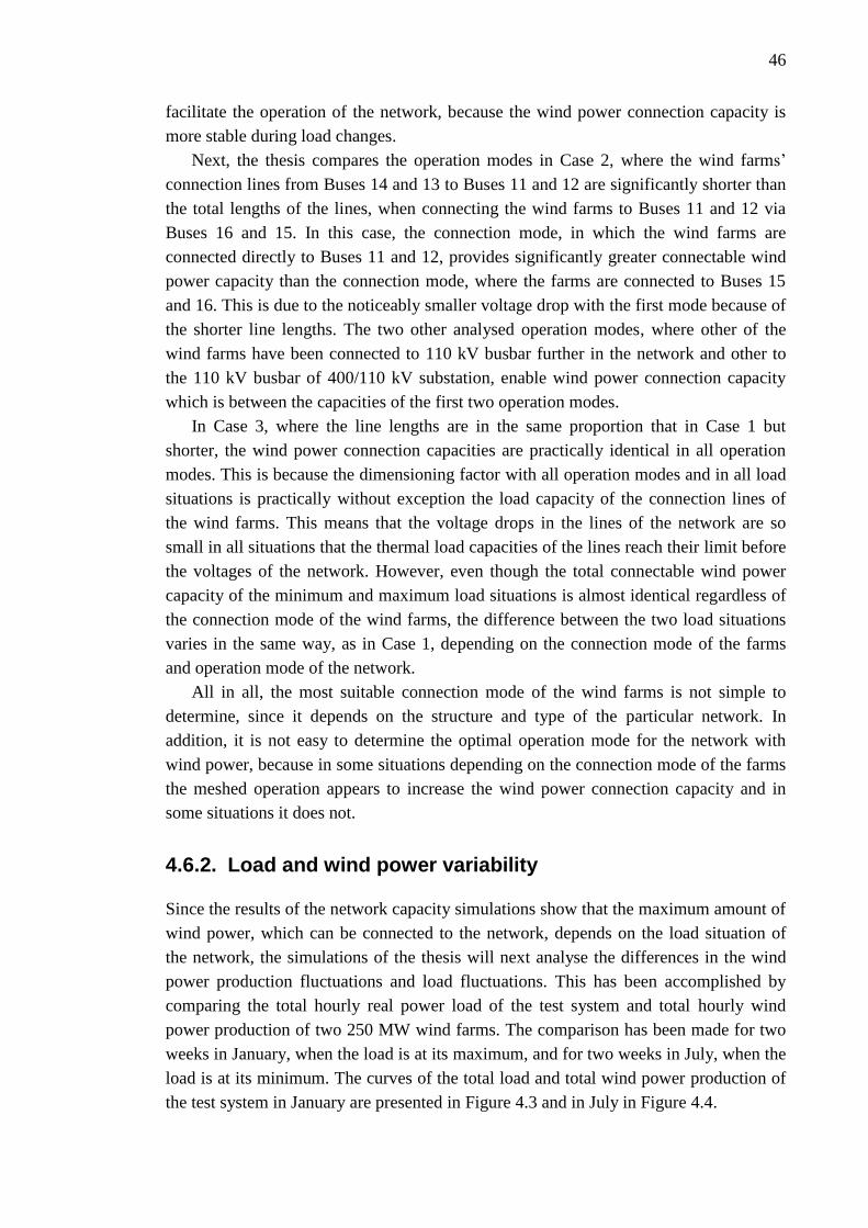
46

facilitate the operation of the network, because the wind power connection capacity is

more stable during load changes.

Next, the thesis compares the operation modes in Case 2, where the wind farms’

connection lines from Buses 14 and 13 to Buses 11 and 12 are significantly shorter than

the total lengths of the lines, when connecting the wind farms to Buses 11 and 12 via

Buses 16 and 15. In this case, the connection mode, in which the wind farms are

connected directly to Buses 11 and 12, provides significantly greater connectable wind

power capacity than the connection mode, where the farms are connected to Buses 15

and 16. This is due to the noticeably smaller voltage drop with the first mode because of

the shorter line lengths. The two other analysed operation modes, where other of the

wind farms have been connected to 110 kV busbar further in the network and other to

the 110 kV busbar of 400/110 kV substation, enable wind power connection capacity

which is between the capacities of the first two operation modes.

In Case 3, where the line lengths are in the same proportion that in Case 1 but

shorter, the wind power connection capacities are practically identical in all operation

modes. This is because the dimensioning factor with all operation modes and in all load

situations is practically without exception the load capacity of the connection lines of

the wind farms. This means that the voltage drops in the lines of the network are so

small in all situations that the thermal load capacities of the lines reach their limit before

the voltages of the network. However, even though the total connectable wind power

capacity of the minimum and maximum load situations is almost identical regardless of

the connection mode of the wind farms, the difference between the two load situations

varies in the same way, as in Case 1, depending on the connection mode of the farms

and operation mode of the network.

All in all, the most suitable connection mode of the wind farms is not simple to

determine, since it depends on the structure and type of the particular network. In

addition, it is not easy to determine the optimal operation mode for the network with

wind power, because in some situations depending on the connection mode of the farms

the meshed operation appears to increase the wind power connection capacity and in

some situations it does not.

4.6.2. Load and wind power variability

Since the results of the network capacity simulations show that the maximum amount of

wind power, which can be connected to the network, depends on the load situation of

the network, the simulations of the thesis will next analyse the differences in the wind

power production fluctuations and load fluctuations. This has been accomplished by

comparing the total hourly real power load of the test system and total hourly wind

power production of two 250 MW wind farms. The comparison has been made for two

weeks in January, when the load is at its maximum, and for two weeks in July, when the

load is at its minimum. The curves of the total load and total wind power production of

the test system in January are presented in Figure 4.3 and in July in Figure 4.4.

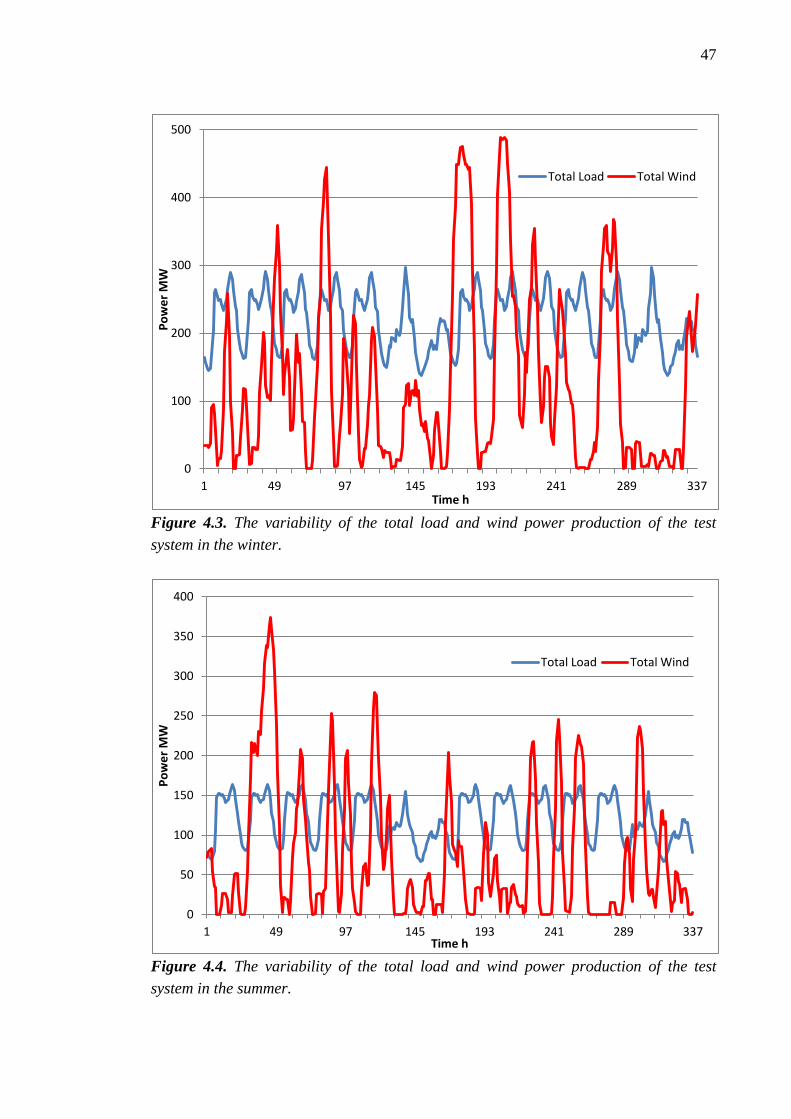
47

Figure 4.3. The variability of the total load and wind power production of the test

system in the winter.

Figure 4.4. The variability of the total load and wind power production of the test

system in the summer.

0

100

200

300

400

500

1 49 97 145 193 241 289 337

Po

we

r M

W

Time h

Total Load Total Wind

0

50

100

150

200

250

300

350

400

1 49 97 145 193 241 289 337

Po

we

r M

W

Time h

Total Load Total Wind

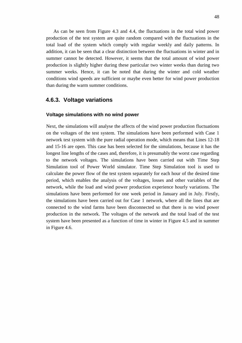
48

As can be seen from Figure 4.3 and 4.4, the fluctuations in the total wind power

production of the test system are quite random compared with the fluctuations in the

total load of the system which comply with regular weekly and daily patterns. In

addition, it can be seen that a clear distinction between the fluctuations in winter and in

summer cannot be detected. However, it seems that the total amount of wind power

production is slightly higher during these particular two winter weeks than during two

summer weeks. Hence, it can be noted that during the winter and cold weather

conditions wind speeds are sufficient or maybe even better for wind power production

than during the warm summer conditions.

4.6.3. Voltage variations

Voltage simulations with no wind power

Next, the simulations will analyse the affects of the wind power production fluctuations

on the voltages of the test system. The simulations have been performed with Case 1

network test system with the pure radial operation mode, which means that Lines 12-18

and 15-16 are open. This case has been selected for the simulations, because it has the

longest line lengths of the cases and, therefore, it is presumably the worst case regarding

to the network voltages. The simulations have been carried out with Time Step

Simulation tool of Power World simulator. Time Step Simulation tool is used to

calculate the power flow of the test system separately for each hour of the desired time

period, which enables the analysis of the voltages, losses and other variables of the

network, while the load and wind power production experience hourly variations. The

simulations have been performed for one week period in January and in July. Firstly,

the simulations have been carried out for Case 1 network, where all the lines that are

connected to the wind farms have been disconnected so that there is no wind power

production in the network. The voltages of the network and the total load of the test

system have been presented as a function of time in winter in Figure 4.5 and in summer

in Figure 4.6.

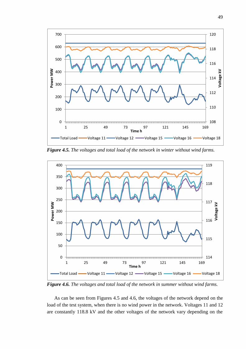
49

Figure 4.5. The voltages and total load of the network in winter without wind farms.

Figure 4.6. The voltages and total load of the network in summer without wind farms.

As can be seen from Figures 4.5 and 4.6, the voltages of the network depend on the

load of the test system, when there is no wind power in the network. Voltages 11 and 12

are constantly 118.8 kV and the other voltages of the network vary depending on the

108

110

112

114

116

118

120

0

100

200

300

400

500

600

700

1 25 49 73 97 121 145 169

Vo

ltag

e k

V

Po

we

r M

W

Time h

Total Load Voltage 11 Voltage 12 Voltage 15 Voltage 16 Voltage 18

114

115

116

117

118

119

0

50

100

150

200

250

300

350

400

1 25 49 73 97 121 145 169

Vo

ltag

e k

V

Po

we

r M

W

Time h

Total Load Voltage 11 Voltage 12 Voltage 15 Voltage 16 Voltage 18

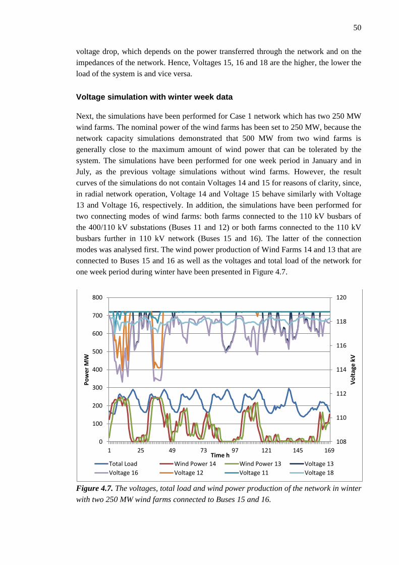
50

voltage drop, which depends on the power transferred through the network and on the

impedances of the network. Hence, Voltages 15, 16 and 18 are the higher, the lower the

load of the system is and vice versa.

Voltage simulation with winter week data

Next, the simulations have been performed for Case 1 network which has two 250 MW

wind farms. The nominal power of the wind farms has been set to 250 MW, because the

network capacity simulations demonstrated that 500 MW from two wind farms is

generally close to the maximum amount of wind power that can be tolerated by the

system. The simulations have been performed for one week period in January and in

July, as the previous voltage simulations without wind farms. However, the result

curves of the simulations do not contain Voltages 14 and 15 for reasons of clarity, since,

in radial network operation, Voltage 14 and Voltage 15 behave similarly with Voltage

13 and Voltage 16, respectively. In addition, the simulations have been performed for

two connecting modes of wind farms: both farms connected to the 110 kV busbars of

the 400/110 kV substations (Buses 11 and 12) or both farms connected to the 110 kV

busbars further in 110 kV network (Buses 15 and 16). The latter of the connection

modes was analysed first. The wind power production of Wind Farms 14 and 13 that are

connected to Buses 15 and 16 as well as the voltages and total load of the network for

one week period during winter have been presented in Figure 4.7.

Figure 4.7. The voltages, total load and wind power production of the network in winter

with two 250 MW wind farms connected to Buses 15 and 16.

108

110

112

114

116

118

120

0

100

200

300

400

500

600

700

800

1 25 49 73 97 121 145 169

Vo

ltag

e k

V

Po

we

r M

W

Time h

Total Load Wind Power 14 Wind Power 13 Voltage 13

Voltage 16 Voltage 12 Voltage 11 Voltage 18

51

As can be seen from Figure 4.7, in contrast to the case of no wind power in the

network, in this case the total load and voltages of the network have no direct

similarities with an exception of Voltage 18, since Bus 18 is in the different 110 kV

feeder than the wind farms. Instead, the voltages of the network depend mostly on the

production of the wind farms. When the power production of the wind farms is zero, the

wind farms do not participate in the voltage control of the network due to the

insufficient reactive power capacity. In this case, the voltages of the network depend

only on the load of the network, as in the previous simulation case without wind power.

On the contrary, when the wind farms are producing real power, they participate in

the voltage control with their reactive power capacity. This means that the voltages in

the connection points of the wind farms (Buses 13 and 14) are constantly 118.8 kV and

the real power is being transferred from the buses to Buses 16 and 15, which means that

Voltages 15 and 16 are lower than the wind farm voltages due to the voltage drop.

Moreover, when the wind power production in Bus 13 exceeds the amount of real

power load in Bus 16, the real power flow in Line 12-16 turns towards Bus 12.

However, since the loads and high loaded 110 kV lines consume reactive power, the

reactive power flow and the reactive component of the voltage drop will remain towards

Bus 16 in Line 12-16. The reactive component of the voltage drop in Line 12-16 is

greater than the real component, which means that Voltage 12 is higher than Voltage 16.

In addition, when the wind power production continues to increase, the power lines will

consume even more reactive power. This means that the reactive power flows from

Buses 13 and 12 to Bus 16 must be increased. At some point, the reactive power

capacity of the generator in Bus 12 will no longer be sufficient to increase its

production, in which case Voltage 12 starts to fall. This can be seen in Figure 4.7, for

example, at the time of 35 hours. The same phenomena also occur in similar situations

in the 110 kV feeder of the other 400/110 kV substations, to which the other wind farm

has been connected.

Next, the simulations will analyse the voltages of the network with the same winter

week data as above. However, now the wind farms have been connected straight to the

110 kV busbars of the 400/110 kV substations (Buses 11 and 12). The wind power

productions of Wind Farms 14 and 13 as well as the voltages and total load of the

network for one week period in winter have been presented in Figure 4.8.

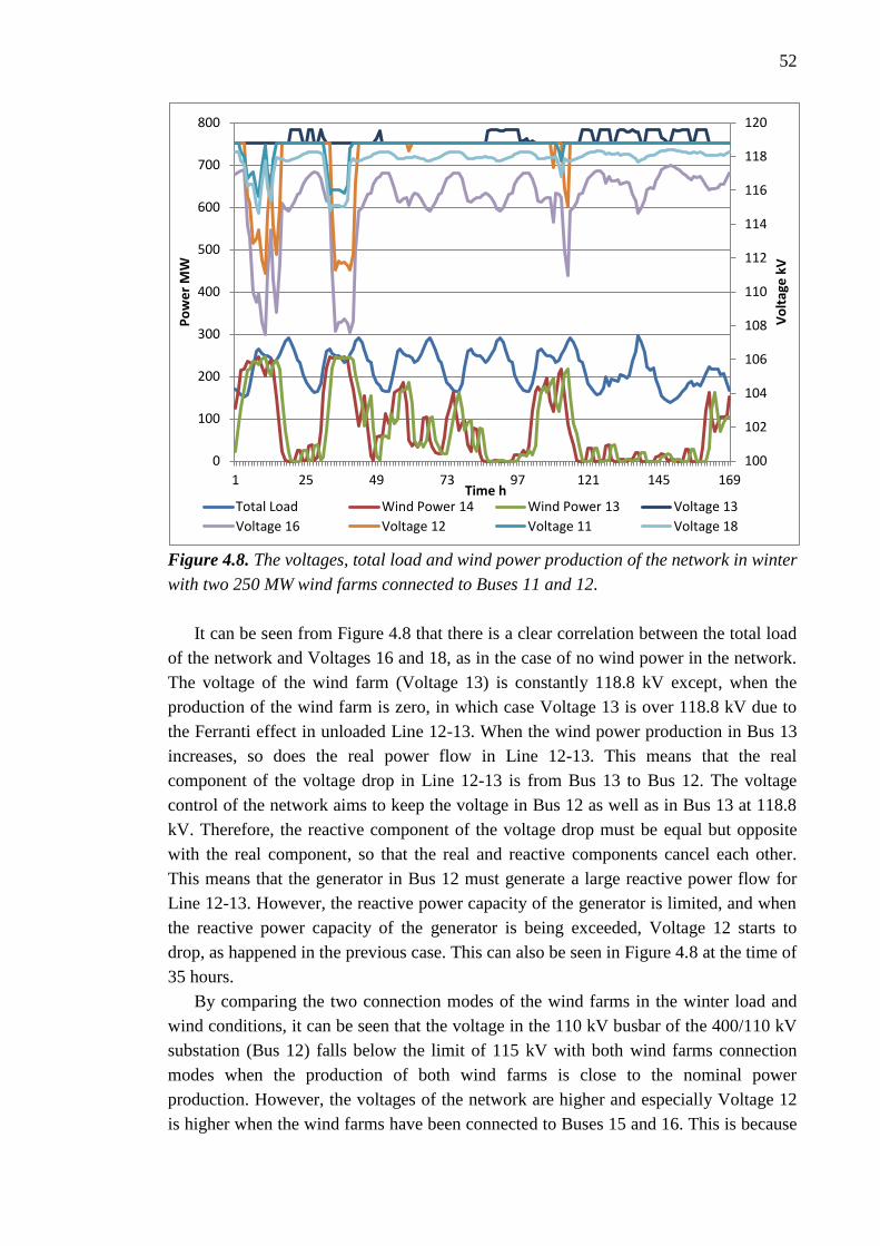
52

Figure 4.8. The voltages, total load and wind power production of the network in winter

with two 250 MW wind farms connected to Buses 11 and 12.

It can be seen from Figure 4.8 that there is a clear correlation between the total load

of the network and Voltages 16 and 18, as in the case of no wind power in the network.

The voltage of the wind farm (Voltage 13) is constantly 118.8 kV except, when the

production of the wind farm is zero, in which case Voltage 13 is over 118.8 kV due to

the Ferranti effect in unloaded Line 12-13. When the wind power production in Bus 13

increases, so does the real power flow in Line 12-13. This means that the real

component of the voltage drop in Line 12-13 is from Bus 13 to Bus 12. The voltage

control of the network aims to keep the voltage in Bus 12 as well as in Bus 13 at 118.8

kV. Therefore, the reactive component of the voltage drop must be equal but opposite

with the real component, so that the real and reactive components cancel each other.

This means that the generator in Bus 12 must generate a large reactive power flow for

Line 12-13. However, the reactive power capacity of the generator is limited, and when

the reactive power capacity of the generator is being exceeded, Voltage 12 starts to

drop, as happened in the previous case. This can also be seen in Figure 4.8 at the time of

35 hours.

By comparing the two connection modes of the wind farms in the winter load and

wind conditions, it can be seen that the voltage in the 110 kV busbar of the 400/110 kV

substation (Bus 12) falls below the limit of 115 kV with both wind farms connection

modes when the production of both wind farms is close to the nominal power

production. However, the voltages of the network are higher and especially Voltage 12

is higher when the wind farms have been connected to Buses 15 and 16. This is because

100

102

104

106

108

110

112

114

116

118

120

0

100

200

300

400

500

600

700

800

1 25 49 73 97 121 145 169

Vo

ltag

e k

V

Po

we

r M

W

Time h Total Load Wind Power 14 Wind Power 13 Voltage 13

Voltage 16 Voltage 12 Voltage 11 Voltage 18

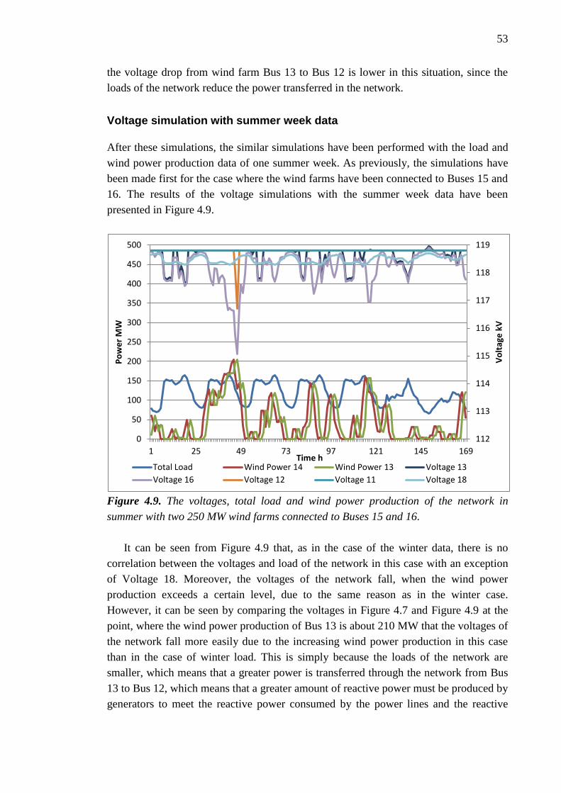
53

the voltage drop from wind farm Bus 13 to Bus 12 is lower in this situation, since the

loads of the network reduce the power transferred in the network.

Voltage simulation with summer week data

After these simulations, the similar simulations have been performed with the load and

wind power production data of one summer week. As previously, the simulations have

been made first for the case where the wind farms have been connected to Buses 15 and

16. The results of the voltage simulations with the summer week data have been

presented in Figure 4.9.

Figure 4.9. The voltages, total load and wind power production of the network in

summer with two 250 MW wind farms connected to Buses 15 and 16.

It can be seen from Figure 4.9 that, as in the case of the winter data, there is no

correlation between the voltages and load of the network in this case with an exception

of Voltage 18. Moreover, the voltages of the network fall, when the wind power

production exceeds a certain level, due to the same reason as in the winter case.

However, it can be seen by comparing the voltages in Figure 4.7 and Figure 4.9 at the

point, where the wind power production of Bus 13 is about 210 MW that the voltages of

the network fall more easily due to the increasing wind power production in this case

than in the case of winter load. This is simply because the loads of the network are

smaller, which means that a greater power is transferred through the network from Bus

13 to Bus 12, which means that a greater amount of reactive power must be produced by

generators to meet the reactive power consumed by the power lines and the reactive

112

113

114

115

116

117

118

119

0

50

100

150

200

250

300

350

400

450

500

1 25 49 73 97 121 145 169

Vo

ltag

e k

V

Po

we

r M

W

Time h Total Load Wind Power 14 Wind Power 13 Voltage 13

Voltage 16 Voltage 12 Voltage 11 Voltage 18

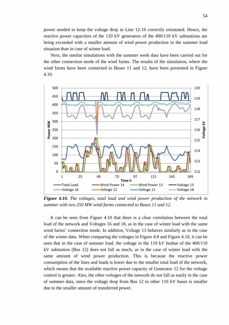
54

power needed to keep the voltage drop in Line 12-16 correctly orientated. Hence, the

reactive power capacities of the 110 kV generators of the 400/110 kV substations are

being exceeded with a smaller amount of wind power production in the summer load

situation than in case of winter load.

Next, the similar simulations with the summer week data have been carried out for

the other connection mode of the wind farms. The results of the simulation, where the

wind farms have been connected to Buses 11 and 12, have been presented in Figure

4.10.

Figure 4.10. The voltages, total load and wind power production of the network in

summer with two 250 MW wind farms connected to Buses 11 and 12.

It can be seen from Figure 4.10 that there is a clear correlation between the total

load of the network and Voltages 16 and 18, as in the case of winter load with the same

wind farms’ connection mode. In addition, Voltage 13 behaves similarly as in the case

of the winter data. When comparing the voltages in Figure 4.8 and Figure 4.10, it can be

seen that in the case of summer load, the voltage in the 110 kV busbar of the 400/110

kV substation (Bus 12) does not fall as much, as in the case of winter load with the

same amount of wind power production. This is because the reactive power

consumption of the lines and loads is lower due to the smaller total load of the network,

which means that the available reactive power capacity of Generator 12 for the voltage

control is greater. Also, the other voltages of the network do not fall as easily in the case

of summer data, since the voltage drop from Bus 12 to other 110 kV buses is smaller

due to the smaller amount of transferred power.

112

113

114

115

116

117

118

119

120

0

50

100

150

200

250

300

350

400

450

500

1 25 49 73 97 121 145 169

Vo

ltag

e k

V

Po

we

r M

W

Time h Total Load Wind Power 14 Wind Power 13 Voltage 13 Voltage 16 Voltage 12 Voltage 11 Voltage 18

55

Analysis of results

By comparing the two connection modes of the wind farms in the summer load and

wind conditions, it can be seen that the voltages in the network are approximately at the

same level with both connection modes of the wind farms. This is because the voltage

drop from wind farm Bus 13 to Bus 12 is about the same in both situations, because the

loads do not reduce the transferred power significantly.

By comparing the results of these voltage simulations with the results of the network

capacity simulations in Case 1 network, it can be seen that the results are in line with

each other. The voltages in the network are higher in the simulations with the high

winter loads, when the wind farms have been connected to Buses 15 and 16 than, when

they have been connected to Buses 11 and 12. Also, the results of the network capacity

simulations show that the connectable wind power capacity is greater during the

maximum load situation when the wind farms have been connected to Buses 15 and 16.

On the other hand, as has been said before, the voltages in the network are

approximately at the same level with both wind farm connection modes during the low

summer loads. However, the network capacity simulations showed that the connectable

wind power capacity is higher in the minimum load situation, when the wind farms have

been connected to Buses 11 and 12, which means that also the voltages should be higher

in the voltage simulations with the same connection mode. Nonetheless, the voltages in

the network are nearly equal in the voltage simulations with summer data with both

wind farm connection modes, because the maximum wind production of the simulations

is about 200 MW from both farms, which is insufficient for exceeding the connectable

wind power capacity of the network in either of the connection mode cases.

Voltage simulations with whole year data

Next, similar voltage simulations have been performed with the hourly data of the

whole year with the same two wind farm connection modes. The results of the

simulations have been presented in Figure 4.11, when the wind farms have been

connected to Buses 15 and 16, and in Figure 4.12, when the wind farms have been

connected to Buses 11 and 12.

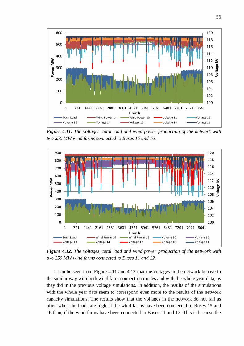
56

Figure 4.11. The voltages, total load and wind power production of the network with

two 250 MW wind farms connected to Buses 15 and 16.

Figure 4.12. The voltages, total load and wind power production of the network with

two 250 MW wind farms connected to Buses 11 and 12.

It can be seen from Figure 4.11 and 4.12 that the voltages in the network behave in

the similar way with both wind farm connection modes and with the whole year data, as

they did in the previous voltage simulations. In addition, the results of the simulations

with the whole year data seem to correspond even more to the results of the network

capacity simulations. The results show that the voltages in the network do not fall as

often when the loads are high, if the wind farms have been connected to Buses 15 and

16 than, if the wind farms have been connected to Buses 11 and 12. This is because the

100

102

104

106

108

110

112

114

116

118

120

0

100

200

300

400

500

600

1 721 1441 2161 2881 3601 4321 5041 5761 6481 7201 7921 8641

Vo

ltag

e k

V

Po

we

r M

W

Time h Total Load Wind Power 14 Wind Power 13 Voltage 12 Voltage 16

Voltage 15 Voltage 14 Voltage 13 Voltage 18 Voltage 11

100

102

104

106

108

110

112

114

116

118

120

0

100

200

300

400

500

600

700

800

900

1 721 1441 2161 2881 3601 4321 5041 5761 6481 7201 7921 8641

Vo

ltag

e k

V

Po

we

r M

W

Time h Total Load Wind Power 14 Wind Power 13 Voltage 16 Voltage 15

Voltage 13 Voltage 14 Voltage 12 Voltage 18 Voltage 11

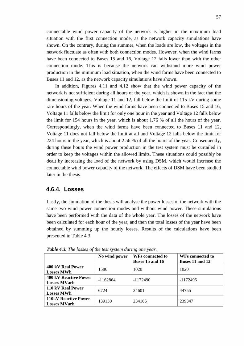
57

connectable wind power capacity of the network is higher in the maximum load

situation with the first connection mode, as the network capacity simulations have

shown. On the contrary, during the summer, when the loads are low, the voltages in the

network fluctuate as often with both connection modes. However, when the wind farms

have been connected to Buses 15 and 16, Voltage 12 falls lower than with the other

connection mode. This is because the network can withstand more wind power

production in the minimum load situation, when the wind farms have been connected to

Buses 11 and 12, as the network capacity simulations have shown.

In addition, Figures 4.11 and 4.12 show that the wind power capacity of the

network is not sufficient during all hours of the year, which is shown in the fact that the

dimensioning voltages, Voltage 11 and 12, fall below the limit of 115 kV during some

rare hours of the year. When the wind farms have been connected to Buses 15 and 16,

Voltage 11 falls below the limit for only one hour in the year and Voltage 12 falls below

the limit for 154 hours in the year, which is about 1.76 % of all the hours of the year.

Correspondingly, when the wind farms have been connected to Buses 11 and 12,

Voltage 11 does not fall below the limit at all and Voltage 12 falls below the limit for

224 hours in the year, which is about 2.56 % of all the hours of the year. Consequently,

during these hours the wind power production in the test system must be curtailed in

order to keep the voltages within the allowed limits. These situations could possibly be

dealt by increasing the load of the network by using DSM, which would increase the

connectable wind power capacity of the network. The effects of DSM have been studied

later in the thesis.

4.6.4. Losses

Lastly, the simulation of the thesis will analyse the power losses of the network with the

same two wind power connection modes and without wind power. These simulations

have been performed with the data of the whole year. The losses of the network have

been calculated for each hour of the year, and then the total losses of the year have been

obtained by summing up the hourly losses. Results of the calculations have been

presented in Table 4.3.

Table 4.3. The losses of the test system during one year.

No wind power WFs connected to

Buses 15 and 16

WFs connected to

Buses 11 and 12

400 kV Real Power

Losses MWh 1586 1020 1020

400 kV Reactive Power

Losses MVarh -1162864 -1172490 -1172495

110 kV Real Power

Losses MWh 6724 34601 44755

110kV Reactive Power

Losses MVarh 139130 234165 239347

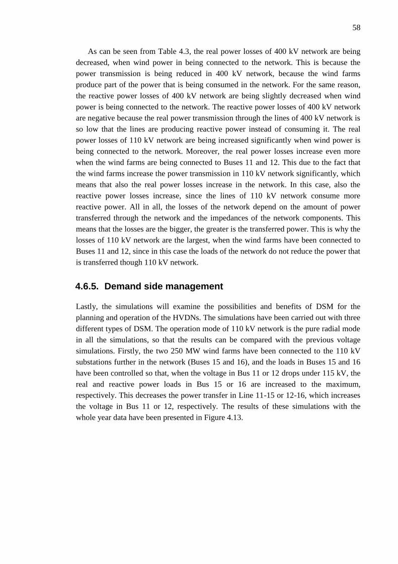
58

As can be seen from Table 4.3, the real power losses of 400 kV network are being

decreased, when wind power in being connected to the network. This is because the

power transmission is being reduced in 400 kV network, because the wind farms

produce part of the power that is being consumed in the network. For the same reason,

the reactive power losses of 400 kV network are being slightly decreased when wind

power is being connected to the network. The reactive power losses of 400 kV network

are negative because the real power transmission through the lines of 400 kV network is

so low that the lines are producing reactive power instead of consuming it. The real

power losses of 110 kV network are being increased significantly when wind power is

being connected to the network. Moreover, the real power losses increase even more

when the wind farms are being connected to Buses 11 and 12. This due to the fact that

the wind farms increase the power transmission in 110 kV network significantly, which

means that also the real power losses increase in the network. In this case, also the

reactive power losses increase, since the lines of 110 kV network consume more

reactive power. All in all, the losses of the network depend on the amount of power

transferred through the network and the impedances of the network components. This

means that the losses are the bigger, the greater is the transferred power. This is why the

losses of 110 kV network are the largest, when the wind farms have been connected to

Buses 11 and 12, since in this case the loads of the network do not reduce the power that

is transferred though 110 kV network.

4.6.5. Demand side management

Lastly, the simulations will examine the possibilities and benefits of DSM for the

planning and operation of the HVDNs. The simulations have been carried out with three

different types of DSM. The operation mode of 110 kV network is the pure radial mode

in all the simulations, so that the results can be compared with the previous voltage

simulations. Firstly, the two 250 MW wind farms have been connected to the 110 kV

substations further in the network (Buses 15 and 16), and the loads in Buses 15 and 16

have been controlled so that, when the voltage in Bus 11 or 12 drops under 115 kV, the

real and reactive power loads in Bus 15 or 16 are increased to the maximum,

respectively. This decreases the power transfer in Line 11-15 or 12-16, which increases

the voltage in Bus 11 or 12, respectively. The results of these simulations with the

whole year data have been presented in Figure 4.13.

59

Figure 4.13. The voltages, total load and wind power production of the network with

two 250 MW wind farms connected to Buses 15 and 16, and with controllable loads in

Buses 15 and 16.

It can be seen by comparing the results in Figure 4.13 and Figure 4.11 that the

lowest values of Voltage 12 and 16 are significantly higher, when DSM is used in the

network. In addition, without DSM, Voltage 11 falls below 115 kV for one hour in the

year and Voltage 12 falls below 115 kV for 154 hours in the year. On the contrary, with

DSM, Voltage 11 does not fall below 115 kV and Voltage 12 falls below 115 kV for 39

hours in the year, which is about 25 % of the value without DSM. Moreover, the lowest

values of Voltage 12 are just slightly less than 115 kV, which means that by using DSM

the voltages in the network will remain better within the allowed boundaries. All in all,

DSM reduces the need for the curtailment of wind power, in which case the potential

electrical energy which can be produced by wind is being used more efficiently.

Next, the simulation will analyse the situation, where the wind farms have been

connected to Buses 11 and 12 and the loads in Buses 11 and 12 are controllable. The

loads have been controlled so that, when the voltage in Bus 11 or 12 drops under 115

kV, the real and reactive power loads in Bus 11 or Bus 12 are increased to the

maximum, respectively. However, as the previous simulations have shown, Voltage 11

does not drop below 115 kV with this wind farm connection mode, which means that

only the DSM feature of Load 12 will be used in the simulations. The results of the

simulations have been presented in Figure 4.14.

105

107

109

111

113

115

117

119

0

100

200

300

400

500

600

1 721 1441 2161 2881 3601 4321 5041 5761 6481 7201 7921 8641

Vo

ltag

e k

V

Po

we

r M

W

Time h Total MW Load Wind Power 14 Wind Power 13 Voltage 16 Voltage 12

Voltage 15 Voltage 14 Voltage 13 Voltage 18 Voltage 11

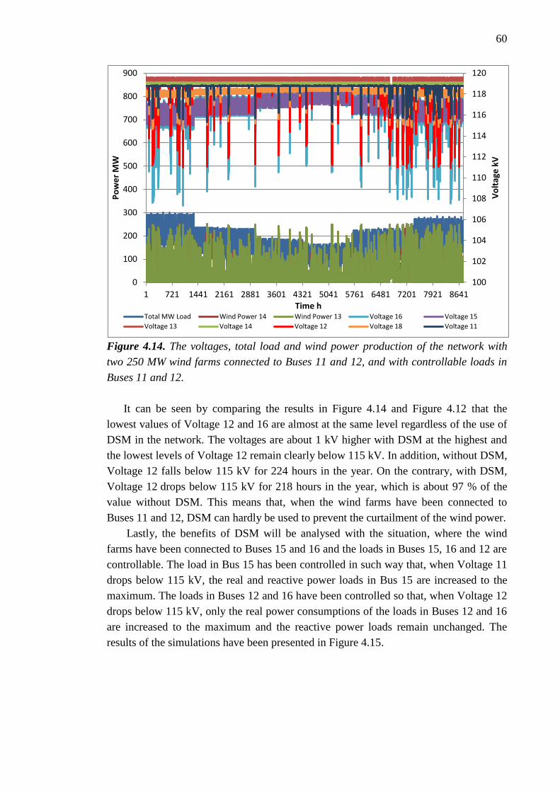
60

Figure 4.14. The voltages, total load and wind power production of the network with

two 250 MW wind farms connected to Buses 11 and 12, and with controllable loads in

Buses 11 and 12.

It can be seen by comparing the results in Figure 4.14 and Figure 4.12 that the

lowest values of Voltage 12 and 16 are almost at the same level regardless of the use of

DSM in the network. The voltages are about 1 kV higher with DSM at the highest and

the lowest levels of Voltage 12 remain clearly below 115 kV. In addition, without DSM,

Voltage 12 falls below 115 kV for 224 hours in the year. On the contrary, with DSM,

Voltage 12 drops below 115 kV for 218 hours in the year, which is about 97 % of the

value without DSM. This means that, when the wind farms have been connected to

Buses 11 and 12, DSM can hardly be used to prevent the curtailment of the wind power.

Lastly, the benefits of DSM will be analysed with the situation, where the wind

farms have been connected to Buses 15 and 16 and the loads in Buses 15, 16 and 12 are

controllable. The load in Bus 15 has been controlled in such way that, when Voltage 11

drops below 115 kV, the real and reactive power loads in Bus 15 are increased to the

maximum. The loads in Buses 12 and 16 have been controlled so that, when Voltage 12

drops below 115 kV, only the real power consumptions of the loads in Buses 12 and 16

are increased to the maximum and the reactive power loads remain unchanged. The

results of the simulations have been presented in Figure 4.15.

100

102

104

106

108

110

112

114

116

118

120

0

100

200

300

400

500

600

700

800

900

1 721 1441 2161 2881 3601 4321 5041 5761 6481 7201 7921 8641

Vo

ltag

e k

V

Po

we

r M

W

Time h Total MW Load Wind Power 14 Wind Power 13 Voltage 16 Voltage 15

Voltage 13 Voltage 14 Voltage 12 Voltage 18 Voltage 11

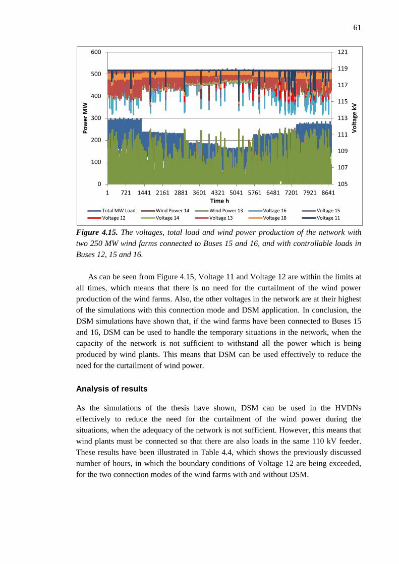
61

Figure 4.15. The voltages, total load and wind power production of the network with

two 250 MW wind farms connected to Buses 15 and 16, and with controllable loads in

Buses 12, 15 and 16.

As can be seen from Figure 4.15, Voltage 11 and Voltage 12 are within the limits at

all times, which means that there is no need for the curtailment of the wind power

production of the wind farms. Also, the other voltages in the network are at their highest

of the simulations with this connection mode and DSM application. In conclusion, the

DSM simulations have shown that, if the wind farms have been connected to Buses 15

and 16, DSM can be used to handle the temporary situations in the network, when the

capacity of the network is not sufficient to withstand all the power which is being

produced by wind plants. This means that DSM can be used effectively to reduce the

need for the curtailment of wind power.

Analysis of results

As the simulations of the thesis have shown, DSM can be used in the HVDNs

effectively to reduce the need for the curtailment of the wind power during the

situations, when the adequacy of the network is not sufficient. However, this means that

wind plants must be connected so that there are also loads in the same 110 kV feeder.

These results have been illustrated in Table 4.4, which shows the previously discussed

number of hours, in which the boundary conditions of Voltage 12 are being exceeded,

for the two connection modes of the wind farms with and without DSM.

105

107

109

111

113

115

117

119

121

0

100

200

300

400

500

600

1 721 1441 2161 2881 3601 4321 5041 5761 6481 7201 7921 8641

Vo

ltag

e k

V

Po

we

r M

W

Time h

Total MW Load Wind Power 14 Wind Power 13 Voltage 16 Voltage 15

Voltage 12 Voltage 14 Voltage 13 Voltage 18 Voltage 11

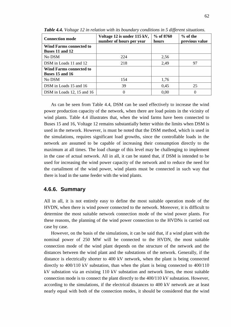
62

Table 4.4. Voltage 12 in relation with its boundary conditions in 5 different situations.

Connection mode Voltage 12 is under 115 kV,

number of hours per year

% of 8760

hours

% of the

previous value

Wind Farms connected to

Buses 11 and 12

No DSM 224 2,56

DSM in Loads 11 and 12 218 2,49 97

Wind Farms connected to

Buses 15 and 16

No DSM 154 1,76

DSM in Loads 15 and 16 39 0,45 25

DSM in Loads 12, 15 and 16 0 0,00 0

As can be seen from Table 4.4, DSM can be used effectively to increase the wind

power production capacity of the network, when there are load points in the vicinity of

wind plants. Table 4.4 illustrates that, when the wind farms have been connected to

Buses 15 and 16, Voltage 12 remains substantially better within the limits when DSM is

used in the network. However, is must be noted that the DSM method, which is used in

the simulations, requires significant load growths, since the controllable loads in the

network are assumed to be capable of increasing their consumption directly to the

maximum at all times. The load change of this level may be challenging to implement

in the case of actual network. All in all, it can be stated that, if DSM is intended to be

used for increasing the wind power capacity of the network and to reduce the need for

the curtailment of the wind power, wind plants must be connected in such way that

there is load in the same feeder with the wind plants.

4.6.6. Summary

All in all, it is not entirely easy to define the most suitable operation mode of the

HVDN, when there is wind power connected to the network. Moreover, it is difficult to

determine the most suitable network connection mode of the wind power plants. For

these reasons, the planning of the wind power connection to the HVDNs is carried out

case by case.

However, on the basis of the simulations, it can be said that, if a wind plant with the

nominal power of 250 MW will be connected to the HVDN, the most suitable

connection mode of the wind plant depends on the structure of the network and the

distances between the wind plant and the substations of the network. Generally, if the

distance is electrically shorter to 400 kV network, when the plant is being connected

directly to 400/110 kV substation, than when the plant is being connected to 400/110

kV substation via an existing 110 kV substation and network lines, the most suitable

connection mode is to connect the plant directly to the 400/110 kV substation. However,

according to the simulations, if the electrical distances to 400 kV network are at least

nearly equal with both of the connection modes, it should be considered that the wind

63

plant should be connected to the existing 110 kV substation, since the voltages in the

network would be slightly higher on average in the case. In addition, in this situation the

power losses in the HVDN would be significantly lower if the plant was connected to

the existing 110 kV substation. Moreover, if DSM is intended to be used with wind

power, the wind plants should be connected to further in 110 kV network to existing

110 kV substations, since DSM benefits the planning and operation of the network only

when there are loads in the vicinity of the wind plants. However, DSM can also be

harmful in terms of the wind power capacity of the network, since DSM can reduce the

wind power capacity. This is the case, if the loads of the network are controlled for the

purpose of some other matter than the wind power capacity of the network, for example,

in terms of the frequency control of the whole power network or by using electricity

market price based DSM. In these cases, the loads of the network are being reduced

when the electricity market price increases or the frequency of the network falls to a

certain level. As the network capacity simulations have been demonstrated, this would

reduce the connectable wind power capacity of the network when wind plants have been

connected to the existing 110 kV substations further in the network.

4.7. Noticing wind power in HVDN planning and operation

It is not simple to determine how the increase in the amount of wind power production

in the HVDNs will change the planning and operation of the HVDNs and how the wind

power production should be noticed in the planning and operation. This is because there

is only a small amount of wind power in the HVDNs at the moment and, hence, the

practical experiences on the subject are rather limited in Finland. In addition, the

existing wind power plants are technically different than the new wind plants that will

be connected to the network, because the interconnection laws and regulations of wind

power and power networks have become significantly stricter.

As has been said in Chapters 4.4 and 4.5, the most of the effects of wind power on

the network planning and operation are caused by the high variability of the wind power

production. In the HVDNs, the increase in the amount of variable wind power

production in the network would lead to the fact that the variations in the network

power flows would be increased significantly. This means that also the fluctuations in

the network voltages would increase, as the voltage simulations of the thesis have

shown. Consequently, the HVDN planning must take into account all the possible

power flow situations in the network and ensure that the network is able to continue its

normal operation in all situations. This means that the dimensioning situation of the

network is not necessarily the situations of the maximum load in the case when there is

wind power connected to the HVDN. Instead the planning must consider all the

combinations of the wind production and network load, like for example, the situation

of the maximum load and no wind power as well as the situation of the minimum load

and maximum wind power.

64

Also, the operation of the HVDN becomes more difficult when wind plants are

connected to the network. If the power flows of the network vary frequently, the

monitoring and control of the network should be more active, which requires more

resources or more automation into the network. Moreover, the finding and maintaining

of the optimal power flow situation in the HVDN in terms of power losses and network

adequacy is significantly more complicated when there are wind plants in the network.

In addition, one of the major challenges for the HVDN planning and operation,

which is caused by the increase in wind power production, is related to the

dimensioning of the network. As the results of the simulation have demonstrated, the

dimensioning of the network is not entirely simple with variable wind power connected

to the network. According to the network capacity simulations in Case 1 network with

the pure radial operation mode, the maximum connectable wind power production

capacity of the network is 430-500 MW depending on the connection mode of the wind

power and the load situation of the network. However, the voltage simulations show

that the capacity of the network is insufficient only during a small proportion of the

hours of the year, when there is two 250 MW wind farms connected to the network, due

to the variability of the wind power production and network loads. Hence, these

overload situations could be handled, for example, by curtailing the wind power

production or possibly by DSM, as the DSM simulations have shown, instead of

reinforcing the network to withstand the maximum power of two wind farms constantly

during all load situations.

In addition to these, wind power plants in the HVDN increase the power losses in

110 kV network significantly due to the increased power transfer in the network, as the

simulations of this thesis have demonstrated. In addition, the simulations have shown

that especially the real power losses of 110 kV network depend significantly on the

connection mode of the wind plants. Therefore, also the losses of the network should be

considered in the HVDN planning and operation and in the determination of the most

suitable network structure and connection mode of the wind plants.

The wind plants in the HVDN can also be used to improve the voltages in the

network locally, in which case the expensive reinforcements of the network can be

potentially avoided or postponed. This means that wind plants must be connected

further to the network instead of 400/110 kV substations.

As the simulations have shown, the selection of the connection mode of wind power

is one of the key decisions in the HVDN planning, because all of the modes have their

own strengths and weaknesses. Fingrid’s attempt is at the moment that the wind plants

in 110 kV network will be connected as close to 400/110 kV substation as possible.

However, as the simulations have shown, by connecting the wind plants on 110 kV

substations further in 110 kV network and closer to the loads, the power losses of 110

kV network are smaller and the connection mode is more preferable in terms of DSM

than the connection mode which is currently favoured by Fingrid. Therefore, all the

connection modes of wind power should be considered in the HVDN planning in the

future by the HVDN operators and Fingrid.

65

As has been said in Chapter 4.2, the FRT capabilities that are required for wind

power plants are very tight. This means that communication must be used to disconnect

wind plants from the network, when a fault is being occurred in the vicinity of the plant,

in which case the plant could compromise the safety of the network by feeding the fault

current too long or by forming an unwanted island. Hence, the communication must be

fast and reliable, so that the safety of the network is not jeopardized in any situation.

Consequently, the wind plants in the HVDN increase the challenges in the planning of

the HVDN protection settings and in the operation of the protection.

4.8. Development needs

As has been described in the thesis, the planning of the HVDNs is currently performed

mainly by Fingrid in Finland, since only Fingrid has a calculation model which is

covering the entire Finnish power network. In addition, Fingrid wants to verify all the

plans, which are affecting the transmission network, with their own calculations. In the

future, the planning needs of the HVDNs are likely to be increased due to the increase

in the amount of wind power in the networks. (Reilander 2012b) This means that the

planning resources of Fingrid may become insufficient. Therefore, it may be sensible to

consider that whether it could be possible to move from a case by case method to some

generally applicable methods in the planning of the HVDNs with wind power.

Moreover, Fingrid influences the operation of the HVDNs, since all the connection and

operation mode changes in the HVDN must be approved by Fingrid, which also

consumes the resources of Fingrid. Therefore, it should be considered that whether it is

wise that Fingrid is responsible for the HVDN planning as comprehensively in the

future, since it probably means that Fingrid must increase its planning resources.

This leads to another issue, which is that whether Fingrid should increase their fees

or begin to charge additional fees from the HVDN planning. Currently, the situation is

that the planning services of Fingrid for the HVDN operators are included in the

network transfer fees (Reilander 2012b). However, if Fingrid has to increase its

planning resources, the increased costs must be covered somehow.

Another option would be that the HVDN operators would begin to plan and operate

their networks more by themselves. This would mean that the operators would have to

acquire appropriate software for the planning and operation of radial and meshed 110

kV networks. However, this change would probably be sensible only if Fingrid gave

more freedom to the HVDN operators for the HVDN planning and operation. In

addition, Fingrid should provide the operators with the calculation model of the

transmission network. If Fingrid was not willing to give the calculation model of the

whole Finnish network for the HVDN operators, Fingrid should provide the operators

with the model which is accurate enough to be used in the HVDN planning. However,

this would not be entirely simple, since the model’s sufficient level of accuracy for the

planning of the HVDNs with wind plants would be difficult to determine due to the

limited practical experiences on the subject.

66

The uncertainty in the realization of the wind power projects causes problems in the

HVDN planning, since the time horizon of the planning must probably be reduced.

Therefore, the time spans of the Fingrid’s regional network planning and the HVDN

planning should be shortened, in which case the actual amount of wind power which

will be connected to the network could be properly considered in the planning.

As the simulations of this thesis have illustrated, DSM can be effectively used to

increase the wind power capacity of the HVDNs if necessary and to decrease the need

for the curtailment of the wind power production. However, if DSM is used for the

purpose of some other matter, like the frequency control of the network or electricity

market price based DSM, DSM may reduce the controllable wind power capacity of the

HVDN. In this case, it would be reasonable to control the 110 kV loads near the wind

plants so that the wind power capacity of the HVDN is optimized and to use the other

110 kV loads and the loads at the other voltage levels of the network for the purposes of

the other matters.

One of the most important issues in connecting wind plants to the HVDNs is the

selection of the connection mode of the wind plants. As the simulations have shown, it

affects significantly on the operation, wind power capacity and losses of the network. In

addition, the exploitation potential of DSM depends significantly on the connection

mode of the wind plants. Fingrid is currently aiming with its connection fee pricing that

the new wind plants in the HVDN will be connected as close to 400/110 kV substations

as possible or directly to the substations. As can be seen from the results of the network

capacity simulations, this connection mode is the most suitable, if the electrical distance

from the wind plant to the 400/110 kV substation is shorter, when the plant is connected

directly to the substation than, when the plant is connected to 400/110 kV substation via

existing 110 kV substation. However, with the connection mode DSM can be used

poorly to increase the wind power capacity of the network. Consequently, as the

simulations have shown, when the electrical distances with these two connection modes

are nearly at the same level, the connection mode, where the plant is connected to the

existing 110 kV substation, seems to be slightly better. In addition, with the connection

mode, DSM can be used effectively to increase the wind power capacity of the network

and reduce the curtailment of the wind power which will increase the energy efficiency

of the wind power. Moreover, the power losses of the HVDN are lower with the

connection mode. For these reasons, Fingrid should consider in its 110 kV network

planning that whether it would be reasonable in some situations to connect the wind

plants in 110 kV networks to the existing 110 kV substations instead of 400/110 kV

substations. Moreover, it is essential to connect the wind plants to the vicinity of the

loads, if DSM is intended to be used in the managing of the fluctuations in the wind

power production in the future.

67

5. CONCLUSIONS

The purpose of the thesis was to describe the general planning principles of the HVDNs

and to analyze the effects of large-scale wind power production on the different types of

HVDNs. This was accomplished by making a literature survey about the subject,

carrying out some interviews with network operator personnel and performing

illustrative network simulations with the network test system containing wind power.

In Finland, the HVDNs include all 110 kV network lines, which are not part of the

transmission network of Fingrid. In 2010, the length of the HVDNs was about 8262 km

and the networks were possessed by 66 different network operators. The structure and

role of the networks varied between the owners but, generally, the role was minor in the

business operations of the owners. However, it was noted in the thesis that the

increasing amount of wind power in the HVDNs will probably emphasize the role in the

future, since the planning needs of the networks will increase.

The general planning of electricity networks is generally an optimization task

between the investment costs, costs of losses, outage costs and maintenance costs,

which means that in the planning the costs of the network are minimized in terms of the

reliability, power quality and safety of the network. The boundary conditions of the

planning determine the required level of the reliability, power quality and safety. At the

moment, the reasonable pricing regulation model of Energy Market Authority highlights

the reliability and power quality as a boundary condition of the planning.

It was revealed that the planning of the HVDNs is currently performed mainly by

Fingrid, because changes in the HVDNs affect on the transmission network, which is

why Fingrid wants to control the planning and operation of the HVDNs. In addition,

only Fingrid has the sufficient calculation model, which covers the entire Finnish

transmission network and all 110 kV lines, for the HVDN planning in the case when the

transmission network must be considered in the plans.

Wind power causes many kinds of effects on the HVDNs. These effects are aimed

to be reduced by the strict interconnection laws and regulations of wind power. In

Finland, the regulations are determined by Fingrid. The regulations require that the

wind plants in the HVDN participate in the network’s voltage control, are equipped

with a large reactive power capacity and withstand considerable voltage and frequency

fluctuations without disconnecting from the network.

The simulation of the thesis examined the wind power capacity of the different types

of HVDNs, the variability of the load and wind power production in relation to each

other, the voltage variations and power losses in the HVDNs with wind power and,

finally, the effects of DSM on the wind power capacity, voltages and power losses of

the networks. The simulations were carried out with Power World simulation software

with the actual measured hourly data of the wind power production and network loads

68

to simulate the hourly fluctuations of the power flows and voltages in the HVDN test

system.

On the basis of the literature survey, interviews and simulations, the wind plants in

the HVDN will increase the power and voltage fluctuations in the networks. This means

that all wind and load situations should be considered in the network planning. In

addition, the dimensioning and operation of the network becomes more complicated,

since the dimensioning situations of the network might be more severe but rare, and the

situations could possibly be handled by curtailing the wind power production or by

DSM. Moreover, wind power will probably increase the power losses of the HVDN and

the optimizing of the losses becomes more complicated due to the fluctuations in the

power flows of the network. Eventually, the effects of wind power on the planning and

operation of the HVDNs depend significantly on the selection of the connection mode

of wind power and, therefore, the planning should be made carefully considering all the

possible connection modes.

The planning resources of Fingrid are unlikely to be sufficient when the amount of

wind power increases in the HVDNs in the future. Therefore, Fingrid may need to raise

its fees or the HVDN planning must be outsourced to some other parties. In addition as

the simulations of the thesis showed, Fingrid should consider in its 110 kV network

planning that whether it would be reasonable in some situations to connect the wind

plants in 110 kV networks so that there would be more load in the vicinity of the plants,

especially if DSM was used in the managing of the fluctuations in the network.

69

REFERENCES

ABB. 2009. Toward a smarted grid, ABB’s Vision for the power system of the future.

White paper. 8 p.

Bastman, J. 2011. Kartoitus alueverkkojen nykytilasta. Tampere University of

Technology. Research report, SGEM-project. 48 p.

Bastman, J. 2012. SVT-4200 Sähköverkkojen mallintaminen ja analyysi, Modelling and

analysis of electrical networks, study materials 2012. Tampere University of

Technology, Department of Electrical Energy Engineering.

Cigre. 1995. Interaction between transmission and distribution system planning.

Cigre/Cired WG CC 01 (Cigre 37.07-Cired 6). October, 1995. 134 p.

Energy Market Authority. 2007. Electricity Market Act 386/1995 including changes

1018/1995, 332/1998, 138/1999, 466/1999, 623/1999, 444/2003, 1130/2003,

1172/2004, 624/2007, 1326/2007. 18 p.

Energy Market Authority. 2010a. Selvitys Suomen kanta- alue- ja jakeluverkkojen

rajauksesta ja ehdotus rajauskriteereiksi. 5.3.2010. Pöyry Management Consulting Oy.

33 p.

Energy Market Authority. 2010b. Sähköverkkotoiminnan tunnusluvut vuodelta 2010

[statistics]. [Cited 14.5.2012] Available at: http://www.energiamarkkinavirasto.fi/data.

asp?articleid=2647&pgid=69&languageid=246.

Energy Market Authority. 2011. Sähkön jakeluverkkotoiminnan ja suurjännitteisen

jakeluverkkotoiminnan hinnoittelun kohtuullisuuden valvontamenetelmien suuntaviivat

vuosille 2012-2015. 29.6.2011. 84 p.

ENTSO-E. 2010. Impact of increased amounts of renewable energy on Nordic power

system operation. 31.8.2010. Research report. 25 p.

ENTSO-E. 2011. Draft Requirements for Grid Connection Applicable to all Generators.

22.3.2011. Draft. 83 p.

EWEA. 2005. Large scale integration of wind energy in the European power supply:

analysis, issues and recommendations. Research report. 172 p.

70

EWEA. 2010. Powering Europe: wind energy and the electricity grid. Research report.

179 p.

Fingrid Oyj. 2007a. Fingrid Oyj:n Yleiset liittymisehdot (YLE 2007). 31.8.2007. 4 p.

Fingrid Oyj. 2007b. Voimalaitosten järjestelmätekniset vaatimukset (VJV 2007).

4.6.2007. 7 p.

Fingrid Oyj. 2010. Tuulivoimapuiston liittäminen kantaverkkoon, Fingrid Oyj:n ohjeet

ja vaatimukset. 30.8.2010. 10 p.

Fingrid Oyj. 2011. Voimalaitosten järjestelmätekniset vaatimukset tuulivoimalaitospro-

jektin yhteydessä. 21.12.2011. 21 p.

Fingrif Oyj. 2012. Kantaverkon liittymismaksu. 17.1.2012. 4 p.

Finnish Wind Power Association. 2012. Wind power projects in Finland. [WWW].

[Cited 14.5.2012] Available at: http://www.tuulivoimayhdistys.fi/hankkeet.

Hashmi, M. 2011. Survey of smart grids consepts worldwide. VTT Technical Research

Centre of Finland. Research report. 56 p.

Holttinen, H., Meibom, P., Orths, A., van Hulle, F., Lange, B., O’Malley, M., Pierik, J.,

Ummels, B., Tande, J.O., Estanqueiro, A., Matos, M., Gomez, E., Söder, L., Strbac, G.,

Shakoor, A., Ricardo, J., Smith, J.C., Milligan, M., Ela, E. 2009. Design and operation

of power systems with large amounts of wind power. Final report, IEA WIND Task 25,

Phase one 2006-2008. Espoo 2009. VTT Tiedotteita - Research Notes 2493. 239 p.

Jussila, J. 2002. Sähkönjakeluverkon yleissuunnittelumenetelmien kehittämisperiaatteet.

Master of Science Thesis, Tampere, TTKK, Institute of Power Engineering. 138 p.

Järventausta, P., Repo, S., Rautiainen, A., Partanen, J. 2010. Smart grid power system

control in distributed generation environment. The International Federation of

Automatic Control (IFAC). Annual Reviews in Control. Volume 34. Issue 2. pp. 277-

286.

Lakervi, E., Partanen, J. 2009. Sähkönjakelutekniikka. 2nd rewised edition. Helsinki,

Gaudeamus Helsinki University Press Oy Yliopistokustannus. 295 p.

Matilainen J. 2011. Tuulivoima. S-18.3201 Sähkönsiirtojärjestelmät 2, study materials.

24.2.2011. Aalto University. 59 p.

71

Mäki, K. 2011. Tuulivoiman vaikutukset sähköverkossa. SMG-4500 Tuulivoima, study

materials. 19.4.2011. Tampere University of Technology. VTT. 31 p.

Nordel. 2007. Nordic Grid Code 2007. 189 p.

Partanen, J. 2011. Tuulivoiman verkkoliityntä, perusteet. BL20A1200 Tuuli- ja

aurinkovoimateknologia ja liiketoiminta, study materials. 15.3.2011. Lappeenranta

University of Technology. 36 p.

Pihkala, A. 2009. Helsingin 110 ja 400 kV sähkönsiirtoverkon kehittäminen. Master of

Science Thesis, Helsinki, Helsinki University of Technology, Department of Electrical

and Communications Engineering. 180 p.

Piwko, R., Bai, X., Clark, K., Jordan, G., Miller, N., Zimberlin, J. 2005. The effects of

integrating wind power on transmission system planning, reliability and, operations.

Albany, NY. GE Energy, Energy Consulting. Research report. 171 p.

PowerWorld Corporation. 2012. PowerWorld Simulator. [WWW]. [Cited 14.5.2012]

Available at: http://www.powerworld.com.

Reilander, A. 2012a. Alueellinen verkostosuunnittelu. S-18.3201 Sähkönsiirtojärjestel-

mät 2, study materials. 10.2.2010. Aalto University. 80 p.

SFS 6001. 2009. Finnish Standards Association SFS. High voltage electrical

installations. 118 p.

SFS-EN 50160. 2011. Finnish Standards Association SFS. Voltage characteristics of

electricity supplied by public electricity networks. 64 p.

Tuulivoimalaitosten järjestelmätekniset vaatimukset. 2011. In work: Fingrid.

Voimalaitosten järjestelmätekniset vaatimukset (VJV 2007). 19 p.

Vierimaa, H. 2007. Verkkotietojärjestelmän kehittämistarpeet yleissuunnittelun

näkökulmasta. Master of Science Thesis, Espoo, TKK, Department of Electrical and

Communications Engineering. 101 p.

VJV-vaatimusten referenssipisteen määrittelyperiaatteet. 2011. In work: Fingrid.

Voimalaitosten järjestelmätekniset vaatimukset (VJV 2007). 5 p.

Interviews

Elenia Verkko Oy. 2012. Lammi, H., Paasikivi, V., Mäkelä, T. Tampere. Interview,

8.2.2012.

72

Kuusela, A. 2012. Planning Engineer. Fingrid Oyj. Helsinki. Interview, 23.3.2012.

Reilander, A. 2012b. Network planner, Fingrid Oyj. Helsinki. Interview, 23.3.2012.

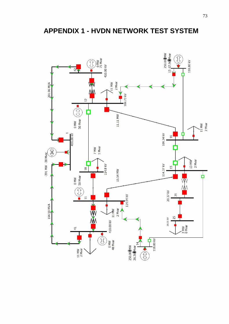
73

APPENDIX 1 - HVDN NETWORK TEST SYSTEM

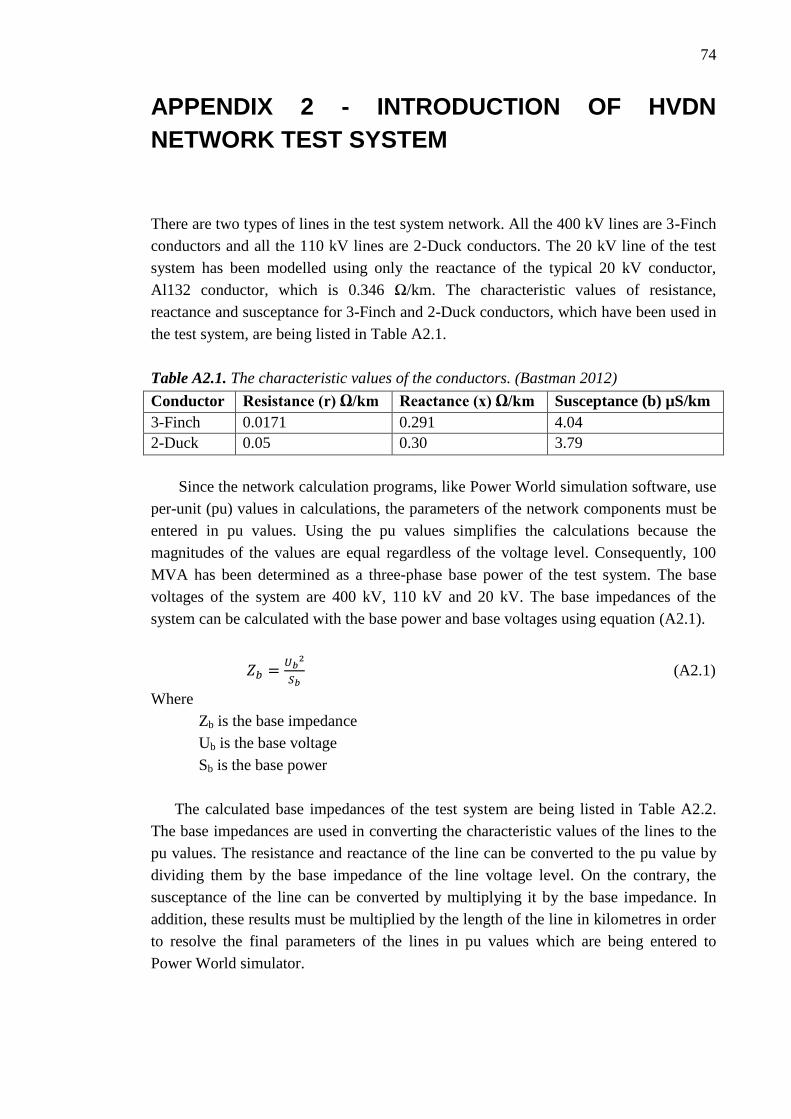
74

APPENDIX 2 - INTRODUCTION OF HVDN

NETWORK TEST SYSTEM

There are two types of lines in the test system network. All the 400 kV lines are 3-Finch

conductors and all the 110 kV lines are 2-Duck conductors. The 20 kV line of the test

system has been modelled using only the reactance of the typical 20 kV conductor,

Al132 conductor, which is 0.346 Ω/km. The characteristic values of resistance,

reactance and susceptance for 3-Finch and 2-Duck conductors, which have been used in

the test system, are being listed in Table A2.1.

Table A2.1. The characteristic values of the conductors. (Bastman 2012)

Conductor Resistance (r) Ω/km Reactance (x) Ω/km Susceptance (b) µS/km

3-Finch 0.0171 0.291 4.04

2-Duck 0.05 0.30 3.79

Since the network calculation programs, like Power World simulation software, use

per-unit (pu) values in calculations, the parameters of the network components must be

entered in pu values. Using the pu values simplifies the calculations because the

magnitudes of the values are equal regardless of the voltage level. Consequently, 100

MVA has been determined as a three-phase base power of the test system. The base

voltages of the system are 400 kV, 110 kV and 20 kV. The base impedances of the

system can be calculated with the base power and base voltages using equation (A2.1).

(A2.1)

Where

Zb is the base impedance

Ub is the base voltage

Sb is the base power

The calculated base impedances of the test system are being listed in Table A2.2.

The base impedances are used in converting the characteristic values of the lines to the

pu values. The resistance and reactance of the line can be converted to the pu value by

dividing them by the base impedance of the line voltage level. On the contrary, the

susceptance of the line can be converted by multiplying it by the base impedance. In

addition, these results must be multiplied by the length of the line in kilometres in order

to resolve the final parameters of the lines in pu values which are being entered to

Power World simulator.

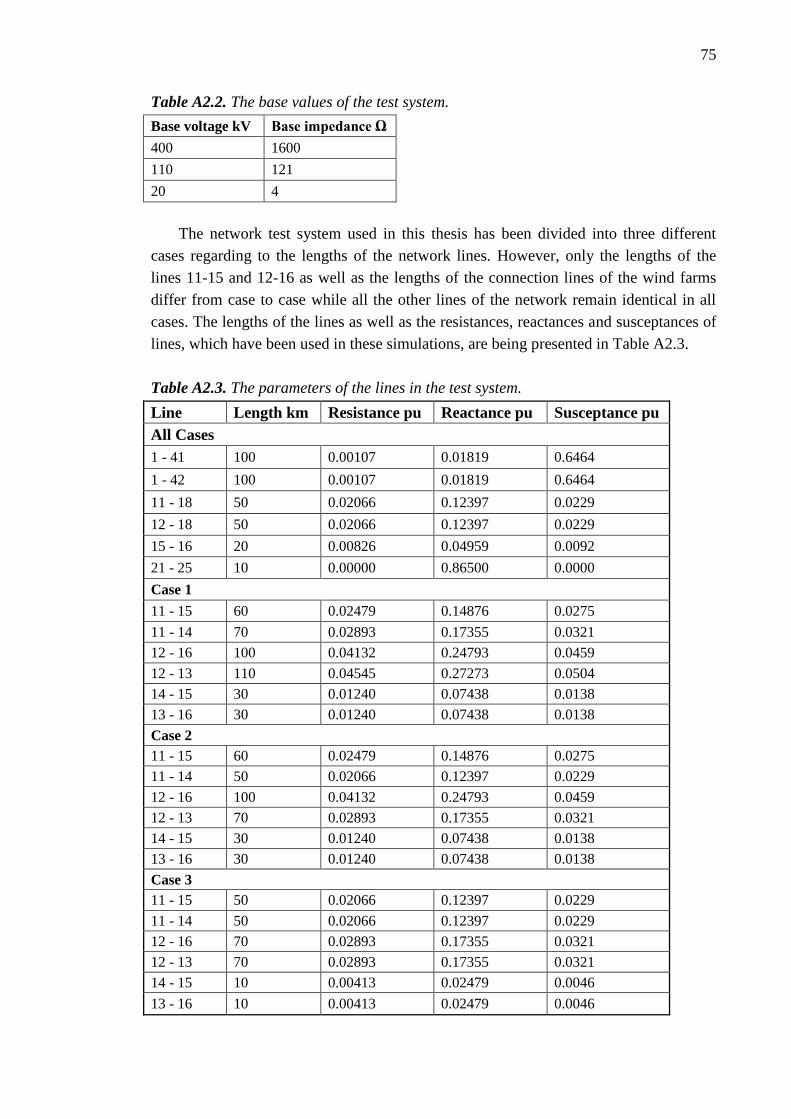
75

Table A2.2. The base values of the test system.

Base voltage kV Base impedance Ω

400 1600

110 121

20 4

The network test system used in this thesis has been divided into three different

cases regarding to the lengths of the network lines. However, only the lengths of the

lines 11-15 and 12-16 as well as the lengths of the connection lines of the wind farms

differ from case to case while all the other lines of the network remain identical in all

cases. The lengths of the lines as well as the resistances, reactances and susceptances of

lines, which have been used in these simulations, are being presented in Table A2.3.

Table A2.3. The parameters of the lines in the test system.

Line Length km Resistance pu Reactance pu Susceptance pu

All Cases

1 - 41 100 0.00107 0.01819 0.6464

1 - 42 100 0.00107 0.01819 0.6464

11 - 18 50 0.02066 0.12397 0.0229

12 - 18 50 0.02066 0.12397 0.0229

15 - 16 20 0.00826 0.04959 0.0092

21 - 25 10 0.00000 0.86500 0.0000

Case 1

11 - 15 60 0.02479 0.14876 0.0275

11 - 14 70 0.02893 0.17355 0.0321

12 - 16 100 0.04132 0.24793 0.0459

12 - 13 110 0.04545 0.27273 0.0504

14 - 15 30 0.01240 0.07438 0.0138

13 - 16 30 0.01240 0.07438 0.0138

Case 2

11 - 15 60 0.02479 0.14876 0.0275

11 - 14 50 0.02066 0.12397 0.0229

12 - 16 100 0.04132 0.24793 0.0459

12 - 13 70 0.02893 0.17355 0.0321

14 - 15 30 0.01240 0.07438 0.0138

13 - 16 30 0.01240 0.07438 0.0138

Case 3

11 - 15 50 0.02066 0.12397 0.0229

11 - 14 50 0.02066 0.12397 0.0229

12 - 16 70 0.02893 0.17355 0.0321

12 - 13 70 0.02893 0.17355 0.0321

14 - 15 10 0.00413 0.02479 0.0046

13 - 16 10 0.00413 0.02479 0.0046

76

There are three transformers in the test system, two 400/110 kV transformers and

one 110/20 kV transformer. All of the transformers have been modelled as two-winding

transformers so that the system remains simple. However, especially the 400/110 kV

transformers in the electric networks are in practise always three-winding transformers.

Moreover, since the simulations of this thesis contain only power flow calculations, the

vector groups of the transformers do not affect on the simulations. Solely, the

resistances and reactances of the transformers have an influence on the simulations. For

simplicity, the transformers have been assumed to be completely reactive and, therefore,

only the series reactances of the transformers have been modelled in the test system.

Usually, the transformers are equipped with a tap changer, in which case the voltage

control of the network can be performed by changing the transformation ratio of the

transformer. However, the transformers of the test system have conveniently selected

constant transformation ratios because the voltage control of the system has been

performed by using only generators. The voltage control of the network and the

selection criteria of the transformation ratios are described later. The parameters of the

transformers have been listed in Table A2.4.

Table A2.4. The parameters of the transformers in the test system.

Voltages kV Buses Resistance pu Reactance pu Tap Ratio

400/110 41 - 11 0 0.20 0.90

400/110 42 - 12 0 0.20 0.90

110/20 15 - 21 0 0.10 0.98

There are seven load points in the test system, one in 400 kV network, five in 110

kV network and one in 20 kV network. The total maximum real power of the loads is

300 MW. The reactive power of each load point is constantly 15 % of the real power. In

addition to the maximum load situation, the simulations consider the situation of the

minimum load. The minimum load of the test system has been determined with the real

measured load data of one distribution network operator (DNO). It was found that the

minimum load of the DNO is about 22.1 % of the maximum load. Consequently, the

total minimum real power load and reactive power load of the test system are about 66.4

MW and 9.95 MVar, respectively. The loads of the test system have been listed in Table

A2.5.

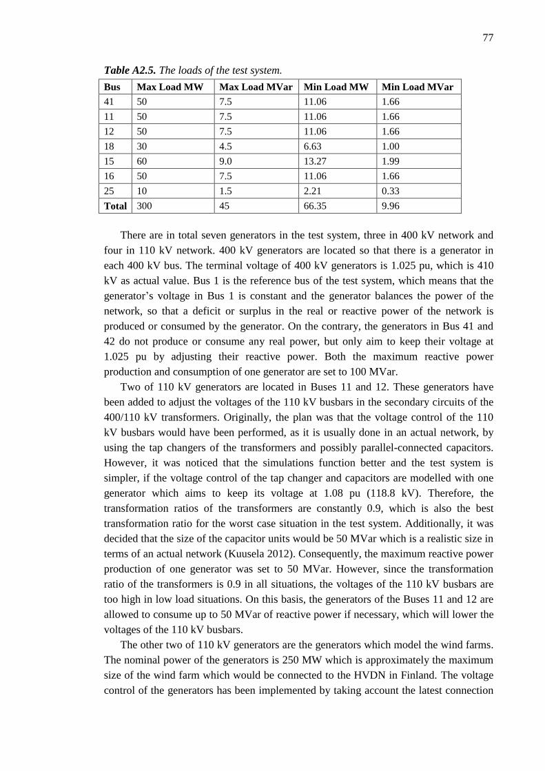
77

Table A2.5. The loads of the test system.

Bus Max Load MW Max Load MVar Min Load MW Min Load MVar

41 50 7.5 11.06 1.66

11 50 7.5 11.06 1.66

12 50 7.5 11.06 1.66

18 30 4.5 6.63 1.00

15 60 9.0 13.27 1.99

16 50 7.5 11.06 1.66

25 10 1.5 2.21 0.33

Total 300 45 66.35 9.96

There are in total seven generators in the test system, three in 400 kV network and

four in 110 kV network. 400 kV generators are located so that there is a generator in

each 400 kV bus. The terminal voltage of 400 kV generators is 1.025 pu, which is 410

kV as actual value. Bus 1 is the reference bus of the test system, which means that the

generator’s voltage in Bus 1 is constant and the generator balances the power of the

network, so that a deficit or surplus in the real or reactive power of the network is

produced or consumed by the generator. On the contrary, the generators in Bus 41 and

42 do not produce or consume any real power, but only aim to keep their voltage at

1.025 pu by adjusting their reactive power. Both the maximum reactive power

production and consumption of one generator are set to 100 MVar.

Two of 110 kV generators are located in Buses 11 and 12. These generators have

been added to adjust the voltages of the 110 kV busbars in the secondary circuits of the

400/110 kV transformers. Originally, the plan was that the voltage control of the 110

kV busbars would have been performed, as it is usually done in an actual network, by

using the tap changers of the transformers and possibly parallel-connected capacitors.

However, it was noticed that the simulations function better and the test system is

simpler, if the voltage control of the tap changer and capacitors are modelled with one

generator which aims to keep its voltage at 1.08 pu (118.8 kV). Therefore, the

transformation ratios of the transformers are constantly 0.9, which is also the best

transformation ratio for the worst case situation in the test system. Additionally, it was

decided that the size of the capacitor units would be 50 MVar which is a realistic size in

terms of an actual network (Kuusela 2012). Consequently, the maximum reactive power

production of one generator was set to 50 MVar. However, since the transformation

ratio of the transformers is 0.9 in all situations, the voltages of the 110 kV busbars are

too high in low load situations. On this basis, the generators of the Buses 11 and 12 are

allowed to consume up to 50 MVar of reactive power if necessary, which will lower the

voltages of the 110 kV busbars.

The other two of 110 kV generators are the generators which model the wind farms.

The nominal power of the generators is 250 MW which is approximately the maximum

size of the wind farm which would be connected to the HVDN in Finland. The voltage

control of the generators has been implemented by taking account the latest connection

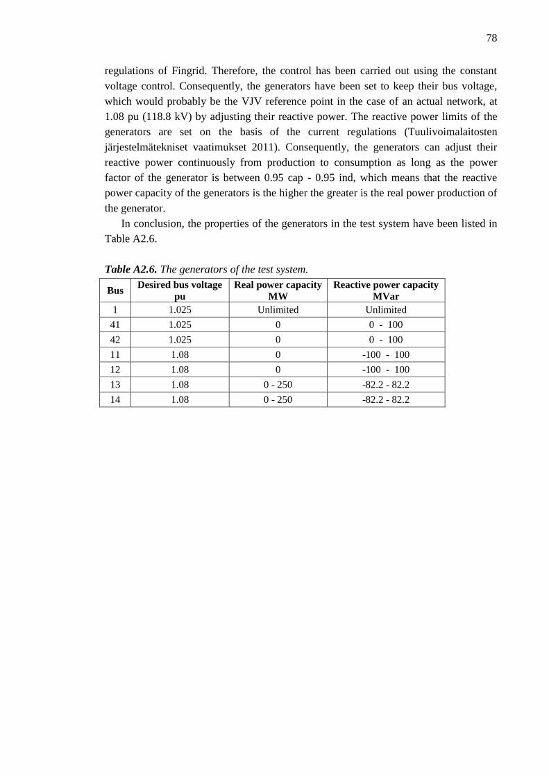
78

regulations of Fingrid. Therefore, the control has been carried out using the constant

voltage control. Consequently, the generators have been set to keep their bus voltage,

which would probably be the VJV reference point in the case of an actual network, at

1.08 pu (118.8 kV) by adjusting their reactive power. The reactive power limits of the

generators are set on the basis of the current regulations (Tuulivoimalaitosten

järjestelmätekniset vaatimukset 2011). Consequently, the generators can adjust their

reactive power continuously from production to consumption as long as the power

factor of the generator is between 0.95 cap - 0.95 ind, which means that the reactive

power capacity of the generators is the higher the greater is the real power production of

the generator.

In conclusion, the properties of the generators in the test system have been listed in

Table A2.6.

Table A2.6. The generators of the test system.

Bus Desired bus voltage

pu

Real power capacity

MW

Reactive power capacity

MVar

1 1.025 Unlimited Unlimited

41 1.025 0 0 - 100

42 1.025 0 0 - 100

11 1.08 0 -100 - 100

12 1.08 0 -100 - 100

13 1.08 0 - 250 -82.2 - 82.2

14 1.08 0 - 250 -82.2 - 82.2

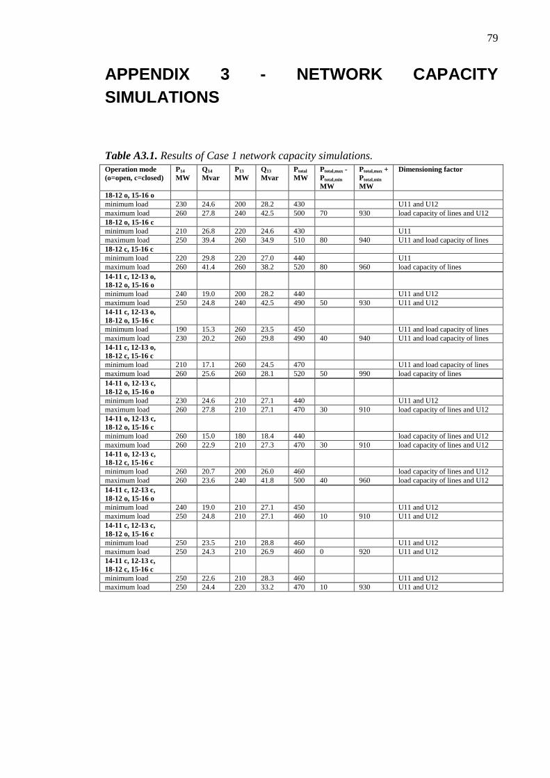
79

APPENDIX 3 - NETWORK CAPACITY

SIMULATIONS

Table A3.1. Results of Case 1 network capacity simulations. Operation mode

(o=open, c=closed)

P14

MW

Q14

Mvar

P13

MW

Q13

Mvar

Ptotal

MW

Ptotal,max -

Ptotal,min

MW

Ptotal,max +

Ptotal,min

MW

Dimensioning factor

18-12 o, 15-16 o

minimum load 230 24.6 200 28.2 430

U11 and U12

maximum load 260 27.8 240 42.5 500 70 930 load capacity of lines and U12

18-12 o, 15-16 c

minimum load 210 26.8 220 24.6 430

U11

maximum load 250 39.4 260 34.9 510 80 940 U11 and load capacity of lines

18-12 c, 15-16 c

minimum load 220 29.8 220 27.0 440

U11

maximum load 260 41.4 260 38.2 520 80 960 load capacity of lines

14-11 c, 12-13 o,

18-12 o, 15-16 o

minimum load 240 19.0 200 28.2 440

U11 and U12

maximum load 250 24.8 240 42.5 490 50 930 U11 and U12

14-11 c, 12-13 o,

18-12 o, 15-16 c

minimum load 190 15.3 260 23.5 450

U11 and load capacity of lines

maximum load 230 20.2 260 29.8 490 40 940 U11 and load capacity of lines

14-11 c, 12-13 o,

18-12 c, 15-16 c

minimum load 210 17.1 260 24.5 470

U11 and load capacity of lines

maximum load 260 25.6 260 28.1 520 50 990 load capacity of lines

14-11 o, 12-13 c,

18-12 o, 15-16 o

minimum load 230 24.6 210 27.1 440

U11 and U12

maximum load 260 27.8 210 27.1 470 30 910 load capacity of lines and U12

14-11 o, 12-13 c,

18-12 o, 15-16 c

minimum load 260 15.0 180 18.4 440

load capacity of lines and U12

maximum load 260 22.9 210 27.3 470 30 910 load capacity of lines and U12

14-11 o, 12-13 c,

18-12 c, 15-16 c

minimum load 260 20.7 200 26.0 460

load capacity of lines and U12

maximum load 260 23.6 240 41.8 500 40 960 load capacity of lines and U12

14-11 c, 12-13 c,

18-12 o, 15-16 o

minimum load 240 19.0 210 27.1 450

U11 and U12

maximum load 250 24.8 210 27.1 460 10 910 U11 and U12

14-11 c, 12-13 c,

18-12 o, 15-16 c

minimum load 250 23.5 210 28.8 460

U11 and U12

maximum load 250 24.3 210 26.9 460 0 920 U11 and U12

14-11 c, 12-13 c,

18-12 c, 15-16 c

minimum load 250 22.6 210 28.3 460

U11 and U12

maximum load 250 24.4 220 33.2 470 10 930 U11 and U12

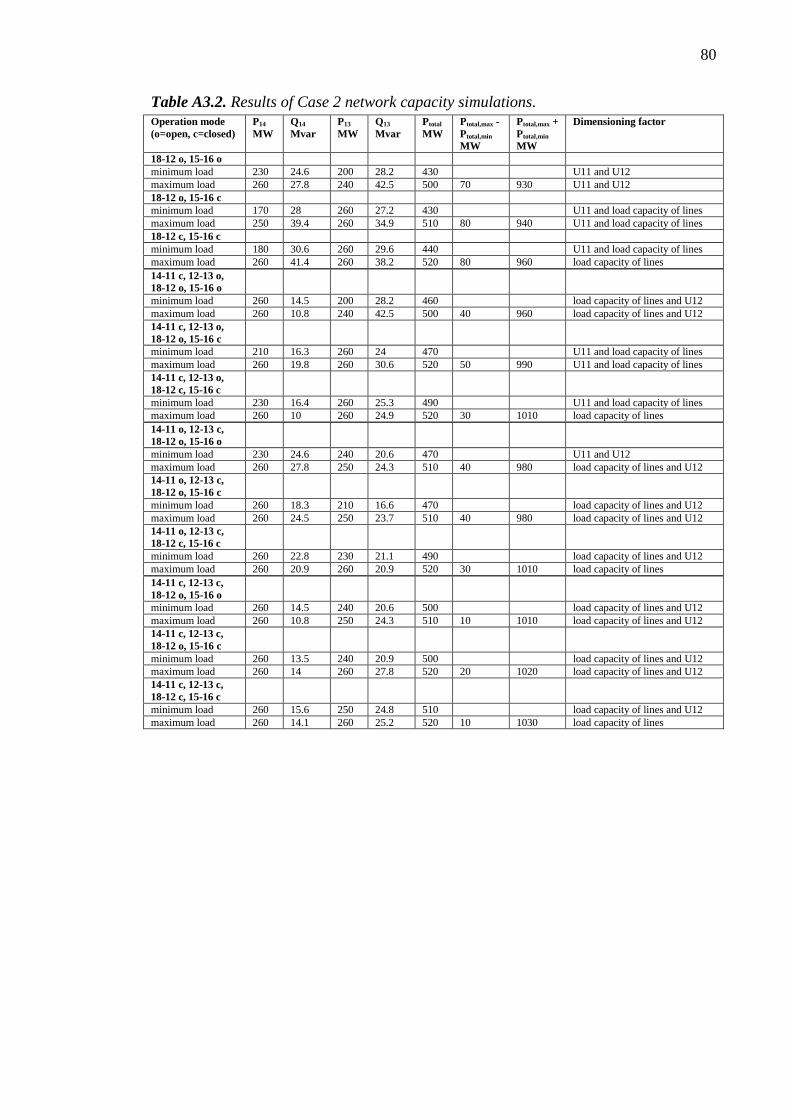
80

Table A3.2. Results of Case 2 network capacity simulations. Operation mode

(o=open, c=closed)

P14

MW

Q14

Mvar

P13

MW

Q13

Mvar

Ptotal

MW

Ptotal,max -

Ptotal,min

MW

Ptotal,max +

Ptotal,min

MW

Dimensioning factor

18-12 o, 15-16 o

minimum load 230 24.6 200 28.2 430

U11 and U12

maximum load 260 27.8 240 42.5 500 70 930 U11 and U12

18-12 o, 15-16 c

minimum load 170 28 260 27.2 430

U11 and load capacity of lines

maximum load 250 39.4 260 34.9 510 80 940 U11 and load capacity of lines

18-12 c, 15-16 c

minimum load 180 30.6 260 29.6 440

U11 and load capacity of lines

maximum load 260 41.4 260 38.2 520 80 960 load capacity of lines

14-11 c, 12-13 o,

18-12 o, 15-16 o

minimum load 260 14.5 200 28.2 460

load capacity of lines and U12

maximum load 260 10.8 240 42.5 500 40 960 load capacity of lines and U12

14-11 c, 12-13 o,

18-12 o, 15-16 c

minimum load 210 16.3 260 24 470

U11 and load capacity of lines

maximum load 260 19.8 260 30.6 520 50 990 U11 and load capacity of lines

14-11 c, 12-13 o,

18-12 c, 15-16 c

minimum load 230 16.4 260 25.3 490

U11 and load capacity of lines

maximum load 260 10 260 24.9 520 30 1010 load capacity of lines

14-11 o, 12-13 c,

18-12 o, 15-16 o

minimum load 230 24.6 240 20.6 470

U11 and U12

maximum load 260 27.8 250 24.3 510 40 980 load capacity of lines and U12

14-11 o, 12-13 c,

18-12 o, 15-16 c

minimum load 260 18.3 210 16.6 470

load capacity of lines and U12

maximum load 260 24.5 250 23.7 510 40 980 load capacity of lines and U12

14-11 o, 12-13 c,

18-12 c, 15-16 c

minimum load 260 22.8 230 21.1 490

load capacity of lines and U12

maximum load 260 20.9 260 20.9 520 30 1010 load capacity of lines

14-11 c, 12-13 c,

18-12 o, 15-16 o

minimum load 260 14.5 240 20.6 500

load capacity of lines and U12

maximum load 260 10.8 250 24.3 510 10 1010 load capacity of lines and U12

14-11 c, 12-13 c,

18-12 o, 15-16 c

minimum load 260 13.5 240 20.9 500

load capacity of lines and U12

maximum load 260 14 260 27.8 520 20 1020 load capacity of lines and U12

14-11 c, 12-13 c,

18-12 c, 15-16 c

minimum load 260 15.6 250 24.8 510

load capacity of lines and U12

maximum load 260 14.1 260 25.2 520 10 1030 load capacity of lines

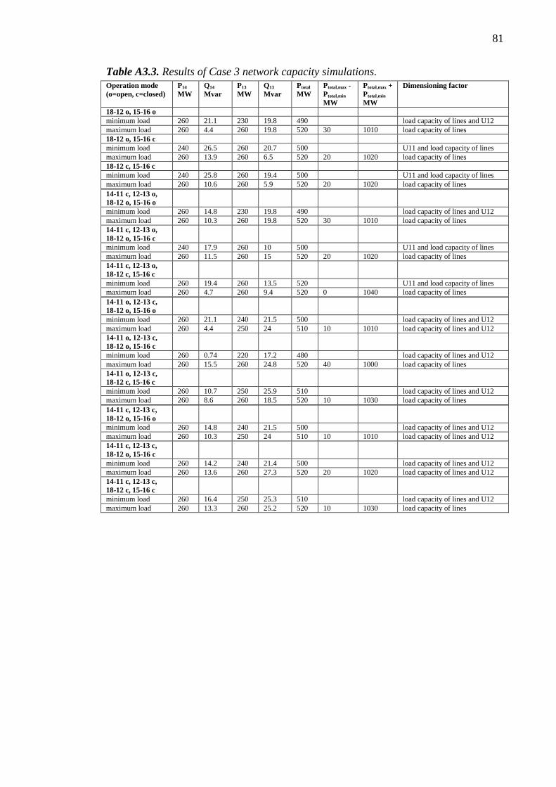
81

Table A3.3. Results of Case 3 network capacity simulations. Operation mode

(o=open, c=closed)

P14

MW

Q14

Mvar

P13

MW

Q13

Mvar

Ptotal

MW

Ptotal,max -

Ptotal,min

MW

Ptotal,max +

Ptotal,min

MW

Dimensioning factor

18-12 o, 15-16 o

minimum load 260 21.1 230 19.8 490

load capacity of lines and U12

maximum load 260 4.4 260 19.8 520 30 1010 load capacity of lines

18-12 o, 15-16 c

minimum load 240 26.5 260 20.7 500

U11 and load capacity of lines

maximum load 260 13.9 260 6.5 520 20 1020 load capacity of lines

18-12 c, 15-16 c

minimum load 240 25.8 260 19.4 500

U11 and load capacity of lines

maximum load 260 10.6 260 5.9 520 20 1020 load capacity of lines

14-11 c, 12-13 o,

18-12 o, 15-16 o

minimum load 260 14.8 230 19.8 490

load capacity of lines and U12

maximum load 260 10.3 260 19.8 520 30 1010 load capacity of lines

14-11 c, 12-13 o,

18-12 o, 15-16 c

minimum load 240 17.9 260 10 500

U11 and load capacity of lines

maximum load 260 11.5 260 15 520 20 1020 load capacity of lines

14-11 c, 12-13 o,

18-12 c, 15-16 c

minimum load 260 19.4 260 13.5 520

U11 and load capacity of lines

maximum load 260 4.7 260 9.4 520 0 1040 load capacity of lines

14-11 o, 12-13 c,

18-12 o, 15-16 o

minimum load 260 21.1 240 21.5 500

load capacity of lines and U12

maximum load 260 4.4 250 24 510 10 1010 load capacity of lines and U12

14-11 o, 12-13 c,

18-12 o, 15-16 c

minimum load 260 0.74 220 17.2 480

load capacity of lines and U12

maximum load 260 15.5 260 24.8 520 40 1000 load capacity of lines

14-11 o, 12-13 c,

18-12 c, 15-16 c

minimum load 260 10.7 250 25.9 510

load capacity of lines and U12

maximum load 260 8.6 260 18.5 520 10 1030 load capacity of lines

14-11 c, 12-13 c,

18-12 o, 15-16 o

minimum load 260 14.8 240 21.5 500

load capacity of lines and U12

maximum load 260 10.3 250 24 510 10 1010 load capacity of lines and U12

14-11 c, 12-13 c,

18-12 o, 15-16 c

minimum load 260 14.2 240 21.4 500

load capacity of lines and U12

maximum load 260 13.6 260 27.3 520 20 1020 load capacity of lines and U12

14-11 c, 12-13 c,

18-12 c, 15-16 c

minimum load 260 16.4 250 25.3 510

load capacity of lines and U12

maximum load 260 13.3 260 25.2 520 10 1030 load capacity of lines