missouri coordinate system...introduction the missouri state coordinate system was developed in 1933...
TRANSCRIPT

MISSOURI COORDINATE
SYSTEM OF
1983
Standards of Practice No. 7
A Manual for Land Surveyors Revised 1996
Q Ill 11111 111111111111111111 Ill
,i Ill
' © MISSOURI DEPARTMENT OF NATURAL RESOURCES
Division of Geology and Land Survey P.O. Box 250, Rolla, MO 65402
{573) 368-2300

MISSOURI COORDINATE
SYSTEM OF
1983
A MANUAL FOR LAND SURVEYORS
REVISED 1996
1;1:1
Standards of Practice No. 7
MISSOURI DEPARTMENT OF NATURAL RESOURCES Division of Geology and Land Survey P.O. Box 250, Rolla, MO 65402-0250
(573) 368-2300

Missouri Classification Number: MO/NR. Ge 25:7
Missouri Department of Natural Resources, 1996, MISSOURI COORDINATE SYSTEM OF 1983-A MANUAL FOR LAND SURVEYORS, REVISED 1996, Missouri Department of Natural Resources' Division of Geology and Land Survey, 50 p., 21 ill., 6 tbls.
As a recipient of federal funds, the Missouri Department of Natural Resources cannot discriminate against anyone on the basis of race, color,· national origin, age, sex, or handicap. If anyone believes he/she has been subjected to discrimination for any of these reasons, he/she may file a complaint with either the Missouri Department of Natural Resources or the Office of Equal Opportunity, U.S. Department of the Interior, Washington, DC, 20240.
ii

STATE COORDINATES FOR LAND SURVEYORS
The Manual of the Missouri Coordinate System of 1983 Standards of Practice No. 7
CONTENTS
INTRODUCTION ....................................................................................................................... 1
CHAPTER 1 THE BASIC RECTANGULAR PLANE COORDINATE CONCEPT ........................................ 3
CHAPTER2 THE CURVED EARTH .......................................................................................................... 7
CHAPTER3 REPRESENTATION OF THE CURVED SURFACE ON A FLAT PLANE (The Transverse Mercator Projection) ................................................................................. 11
CHAPTER4 THE MISSOURI COORDINATE SYSTEM OF 1983 ............................................................ 15
CHAPTERS GRID DISTANCES, GRID BEARINGS, AND THEIR COMPUTATION ................................ 21
CHAPTER6 ARC-TO-CHORD CORRECTION ........................................................................................ 35
CHAPTER 7 USE OF THE MISSOURI COORDINATE SYSTEM 1983 ................................................... 41
iii

' ,:t
LIST OF FIGURES
Figure 1. Example of Cartesian Coordinates ....................................................................... .4 Figure 2. Example of a Lot Survey ........................................................................................ 4 Figure 3. Ellipsoid of Revolution ............................................................................................ 6 Figure 4. Geoid - Spheroid .................................................................................................... 7 Figure 5. Dimension of Ellipsoid ............................................................................................ 8 Figure 6. Surfaces at Station JA-21 .................................................................................... 1 0 Figure 7. The Transverse Mercator Projection .................................................................... 11 Figure 8. Developable Cylinder ........................................................................................... 12 Figure 9. Developed Cylinder .............................................................................................. 12 Figure 10. Section of Ellipsoid .............................................................................................. 14 Figure 11. Missouri Coordinate System Zones ..................................................................... 16 Figure 12. East Zone ............................................................................................................ 18 Figure 13. Central Zone ........................................................................................................ 19 Figure 14. West Zone ........................................................................................................... 20 Figure 15. Section of Earth ................................................................................................... 21 Figure 16. Grid Azimuth and Geodetic North ........................................................................ 31 Figure 17. Grid Bearing and Geodetic North ......................................................................... 31 Figure 18. Arc-to-Chord Correction ....................................................................................... 35 Figure 19. Traverse Missouri Central Zone ........................................................................... 39 Figure 20. Station Diagram - PL-13 ..................................................................................... .45 Figure 21. Station Diagram -JA-25 ....................................................................................... 49
Table 1. Table 2. Table 3. Table 4. Table 5. Table 6.
LIST OF TABLES
Elevation Factor Table ......................................................................................... 22 Scale Factor- East and Central Zones ................................................................ 25 Scale Factor- West Zone .................................................................................... 26 Convergence Tables - East and Central Zones ................................................... 30 Convergence Tables - West Zone ....................................................................... 32 Second Term Correction in Seconds .................................................................. .40
iv

INTRODUCTION
The Missouri State Coordinate System was developed in 1933 by Dr. O.S. Adams, mathematician in the Division of Geodesy, United States Coast and Geodetic Survey. This coordinate system was adopted as the official coordinate system for the State of Missouri by the Missouri Legislature in 1965. In 1984 the statute was revised to add the definition of the Missouri Coordinate System of 1983. The statute designates two legal systems, the older system based upon the Clarke Spheroid of 1866 and the North American Datum of 1927 and the newer system based upon the GRS 1980 and the North American Datum 1983. Either system was legally used until July 1990, but after that date only the new system may be used. The Missouri Department of Natural Resources' Division of Geology and Land Survey, Land Survey program supports only the Missouri Coordinate System of 1983; therefore, this manual is limited to that system.
The proper use of the State Coordinate System depends upon three factors: 1) The surveyor's knowledge of the system; 2) The end user's knowledge of the system; and . 3) The existence of accurate horizontal control on which to base coordinate
determinations.
The purpose of this manual is to meet the first two factors. The third factor is the responsibility of the Land Survey Program of the Department of Natural Resources.

CHAPTER 1 THE BASIC RECTANGULAR PLANE COORDINATE CONCEPT
The idea of combining the analytical methods of algebra and trigonometry with the concepts of geometry by means of a coordinate system was due largely to Descartes, a French mathematician. In 1637 he published the first systematic work on this subject under the title La Geometrie. The subject is sometimes called Cartesian geometry after the Latinized name of Descartes, Carteslus. The rectangular coordinates used in your courses on algebra and trigonometry are called Cartesian coordinates. Webster's New World Dictionary defines the Cartesian coordinates as 1) a pair of numbers that locate a point by its distance from two intersecting, often perpendicular, lines in the same plane; each distance is measured parallel to the other line; and 2) a triad of numbers which locate a point by its distance from three fixed planes that intersect one another at right angles.
The basic concept of the Cartesian Coordinate System is straight forward (fig.1 ). There are two mutually perpendicular lines, XX' and YY' called the X and Y axes. The axes intersect at point O called the origin. We may regard the line OX as east-west and the line OOY as north-south. We can choose a unit of measure and measure or mark those units and the axis with zero at the origin.
On the horizontal line we put positive numbers to the right and negative numbers to the left. On the vertical line we put positive numbers up and negative numbers down. In this way we designate that a positive direction on a horizontal line is to the right and on a vertical line as upward. Let's consider any point P in the plane of the axes. Its distance from the Y axis is called its X or east coordinate. This distance is positive if P is to the right of the Y axis, and negative if to the left. The distance of point P from the X axis is called its Y or north coordinate. This distance is positive if Pis above the X axis and negative if below. These two coordinates together are called the rectangular coordinate or, simply, the coordinates of P.
In surveying and mapping the same type of Cartesian Coordinate System is used and the horizontal coordinates are referred to as the Rectangular Plane Coordinate System or Grid. The axes are north (up) and east (right); therefore, a point has a north and east coordinate. It can be readily seen that ifwe have the coordinate axes defined, and if we know the coordinates of a point, that point is defined in that plane. A properly drawn survey plat is the same as a graph. Each of the points which define the lines and corners of a project, therefore, can be defined by coordinates as long as reference axes are defined.
Figure 2 is an example of a lot survey using coordinates. The X and Y coordinate axes have been established in the plane of the paper, and the various coordinate values are shown for each one of the corner points. The use of a basic coordinate system such as this is quite common today. Most surveyors, draftsmen, and others use this basic concept for plotting maps and drawings. Computerized geographic information systems also use coordinates as a frame of reference. In order to plot data from computer files, the coordinate values of the points to be plotted must be known. -.
3

y
CJ)
X <{
>-
0
X
• POINT P ___,,,,,,..
y
X1--+-------------'--X X AXIS
yl
Figure 1. Example of Cartesian Coordinates
y
200
100
POINT 4 POINT 3 X=IOO ./X:150 Y = 150"' , Y = 150
•,------.
~ LOT I
100'
POINT · 1 :,' ~ 50. ~ I' POINT 2 X = 100 /r X = 150 Y:: 50 Y = 50
0 .+-L....L-L--'--'--'--'--.L...L-L..J.....11.-.L-'-.J......l--'--L-.L...L-
o 100 200
Figure 2. Example of Lot SuNey
4
X

The coordinate system is not an abstract concept to most surveyors today. Coordinates are being used in all surveying and mapping. An individual plane coordinate system may be defined by one point having known coordinates and directions of the coordinate axes. The system may also be defined by two points having known coordinates. It is not necessary to know the physical location of the coordinate axes. Many computing and plotting programs used by surveyors, engineers, and mappers, require the adoption of a coordinate system. Usually one point, the starting point, is assigned positive X and Y coordinates and a direction from the starting point to the next point in the system is assigned. In this way the coordinate system is defined.
It is important to note that these assumed or local coordinate systems are adequate for the specific area or application but are limited in their use. In order to have a uniform system that can be expanded to cover adjoining surveys, cities, or counties and even adjoining states, a common system must be used.
The State Coordinate System provides a common datum for referencing the horizontal position of all surveys in the same way that mean sea level has provided a common datum for vertical position. It avoids the problem of having several surveys in an area, each based on its own assumed coordinate system, none of which are related to each other or to any other survey. The legally defined State Coordinate System is based upon a defined geodetic reference system. This reference system must possess the following features:
1) A collection of permanently marked and maintained points; 2) Coverage of an extensive area; 3) A spatial relationship of known accuracy; 4) Relationships expressed in a common mathematical language or in a language
translatable into other languages; and 5) Universal availability of geodetic information.
5

N AXIS OF ROTATION
EQUATOR
s
M = GRAVITATIONAL FORCE C = CENTRIFUGAL FORtE G = GRAVITY CTHE RESULTANT FORCE)
Figure 3. Ellipsoid of Revolution
6

CHAPTER2 THE CURVED EARTH
The land surveyor is not normally concerned with the fact that his work is taking place on a curved surface. The modern surveyor has increased his technical ability to measure distances, directions, and astronomical azimuths to the point that the effect of curvature is a measurable quantity. This increased ability means that the professional surveyors must have an understanding of the curved surface on which he measures.
The earth is similar to a semi-fluid mass which is spinning on its axis. Every particle in this mass is acted upon by two forces. They are a gravitational force and centrifugal force. The resultant of these two forces is the force of gravity. Centrifugal force is greatest at the equator and therefore, the semi-fluid takes the shape of an ellipsoid of revolution. The shape is not a pure ellipsoid because of the varying density and stiffness of the crust (fig. 3).
When a surveyor uses a spirit level to determine elevation he is using a reference surface that is not a plane but a curved surface perpendicular to the force of gravity. The direction of the force of gravity does not point to the center mass of the earth but varies according to the values of gravitation and centrifugal forces. This surface is called the geoid and is an irregular surface (fig. 4).
It is impossible to compute or define a system of coordinates on an irregular surface like the geoid; therefore, a mathematical surface must be chosen that closely represents the shape of the geoid. The selection of the "best fit" ellipsoid has been a major concern of geodesists since the early 18th century.
N
EQUATOR
Figure 4. Geoid - Spheroid
7

Satellite data has provided geodesists with new measurements to define the best earth-fitting ellipsoid and for relating existing coordinate systems to the earth's center of mass. The ellipsoid used in the North American Datum 1983 (NAD83) was adopted by I UGG in 1980 and is called Geodetic Reference System 80 (GRSB0) (fig. 5). The dimensions of GRSBO are:
Equatorial semi-axis= a= 6,378,137.0 m (exact by definition)
Polar semi-axis= b = 6,356,752.3 m (computed)
The term eccentricity of the ellipse is defined to 10 significant digits as:
For GRSB0 e2 = 0.0066943800
The geocentric gravitational constant of earth, dynamic form factor of earth, and angular velocity are also defined. The semi-minor axis (b), flattening (f), and all other constants are computed from the defined constants, and should be given to a stated number of significant
digits. N
I
b
s a = EQUATORIAL SEMI AXIS
b = POLAR SEMI AXIS
Figure 5. Dimensions of Ellipsoid
8

The relative position of the ellipsoid, the geoid, and the surface of the earth is important. Look at a small segment of the earth in Missouri at Station JA-21 (fig. 6). Curvature is not apparent at this single station. Three planes are shown - ellipsoid (GRS80), ground surface, and the geoid (NAVD88). The normal to the geoid is the direction of local gravity or plumb line. The normal to the ellipsoid is the vertical of the computational surface. The angle between these two verticals is called the deflection of the vertical and varies from 1 to 3 seconds in Missouri.
The orthometric height (H) which is very nearly the elevation of the ground surface is the distance measured from the geoid to the ground surface. Ellipsoidal height is the distance from the ellipsoid to the ground surface. Geoid separation is the distance from the ellipsoid to the geoid. Note that measurements up from the ellipsoid are positive and down negative.
In the state of Missouri the geoid separations are all negative. The geoid averages approximately 30.5 m below the ellipsoid.
It is important to note that elevations on the earth are reported relative to the geoid, not the ellipsoid. Latitude and longitude, on the other hand, are determined with respect to the ellipsoid. The height obtained from GPS observation is the ellipsoidal height.
9

H
h = N + H
! %• uJ• N'
~
N
STATION JA-21
;ITTH SURFACE
.
\: i-~--+--h- NORMAL TO ELLIPSOID
I II
I
I\ I
~ELLIPSOID (GRS 80)
~ NORMAL TO GEOID I OR PLUMB LINE l : '\- (DIRECTION OF LOCAL GRAVITY
I DEFLECTION OF THE VERTICAL
H = ORTHOMETRIC HEIGHT OR ELEVATION (DISTANCE FROM GEOID TO EARTH .SURFACE)
h = ELLIPSOIDAL HEIGHT OR GEODETIC HEIGHT (DISTANCE FROM ELLIPSOID TO EARTH SURFACE)
N = GEOID SEPARATION OR GEOID HEIGHT (DISTANCE FROM ELLIPSOID TO GEOID)
Figure 6. Surfaces at Station JA-21
10

CHAPTER3 REPRESENTATION OF THE CURVED SURFACE ON A FLAT PLANE
(THE TRANSVERSE MERCATOR PROJECTION)
The earth on which all survey work is performed is essentially a sphere. Map makers for at least 500 years have attempted to prepare a flat map of a curved surface with as little distortion as possible.
A map projection is a systematic representation of all or part of the surface of a round body, especially the earth, on a plane. A map projection also serves as the basis for the development of a coordinate system that represents a curved surface on a plane. The transverse Mercator projection has been adopted for the Missouri Coordinate System of 1983. Therefore, in order to understand the coordinates we need to understand the characteristics of th is projection.
The transverse Mercator projection was invented by the mathematician and cartographer Johann Heinrich Lambert in 1772. This projection uses the concepts of the Mercator projection developed by Gerardus Mercator in 1569.
In the transverse Mercator projection, a cylinder is wrapped around the sphere so that it touches a central meridian throughout its length. The other meridians and parallels of latitude are projected on the cylinder. The cylinder is cut along some parallel and rolled flat showing this projection. The central meridian can be made true scale no matter how far north the projection extends north and south.
In the general form of the transverse Mercator projection, one selected ~central meridian" is rectified into a straight-line segment (N-S in fig. 7). The equator is represented by a straight line perpendicular to the central meridian. The other meridians and parallels of latitudes are curved lines of a complex nature. The central meridian becomes the Y axis and the equator becomes the X axis.
N
s Figure 7. The Transverse Mercator Projection
11

, I
I I I I I I I I I I \ \ \ \
DEVELOPABLE CYLINDER
Figure B. Deve/opable Cylinder
A C
a: a: UJ
Cl) UJ UJ
I- UJ I- UJ c( :::, Cl) :::, c( :::, UJ a: Wa: UJ a: a: I- ...I I- a: I-c,z Wz c,z UJc( ...I c( UJ c( ..I :::c c( :::c ..I :::c c( I- 01- c( ... 0
Cl) 0 U) U)
B D
DEVELOPED CYLINDER
Figure 9. Developed Cylinder
12

The basic projection employed in the Missouri Coordinate System of 1983 is the transverse Mercator projection. It uses an imaginary cylinder as its developable surface, which is illustrated in figures 8 and 9. The cylinder is placed secant to the spheroid in the State Coordinate System. That is, it intersects the spheroid in two places - as along lines AB and CD in figure 8. Figure 9 illustrates the front half of the plane surface developed from the cylinder.
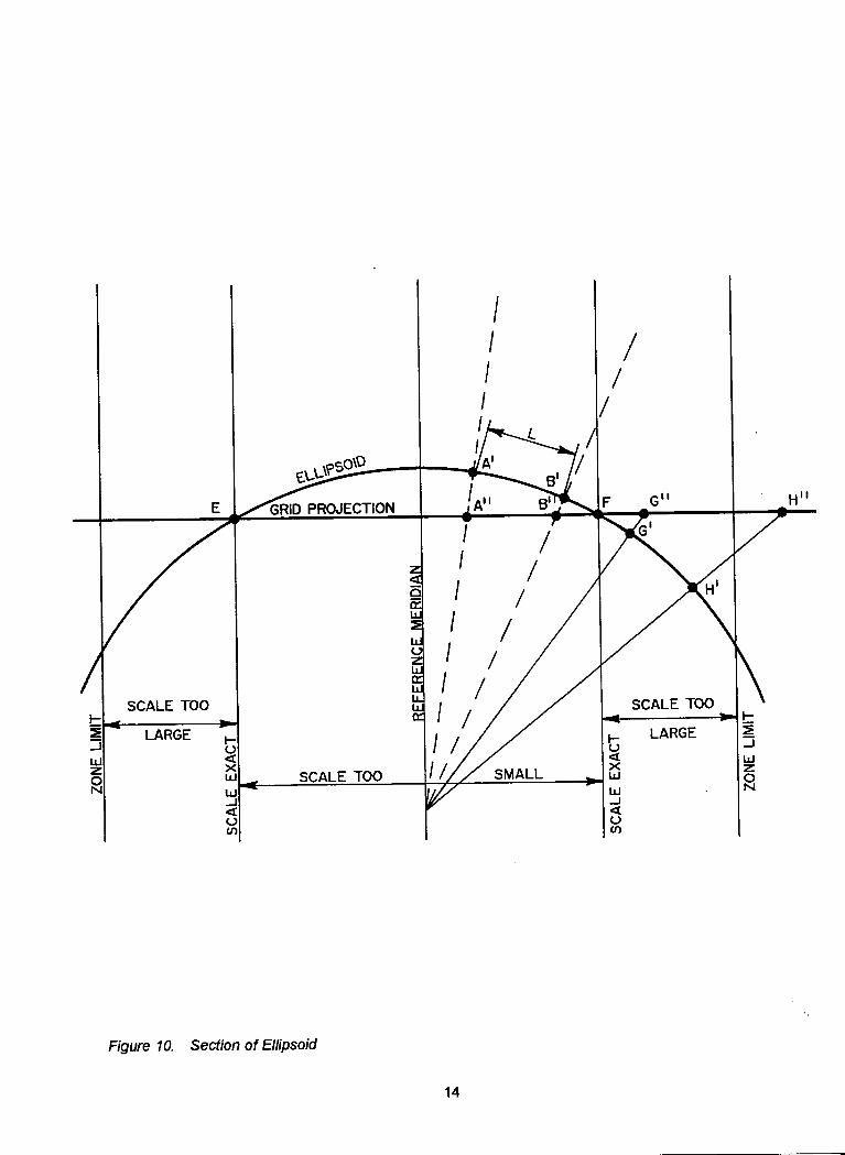
A section showing the relationship of the projected surface and the ellipsoid is taken perpendicular to the central meridian at the approximate center of the north-south range of the system (fig. 10).
In computing projections, points are projected mathematically from the ellipsoid along lines normal to the ellipsoid to the surface of the imaginary cylinder. Figure 1 0 illustrates graphically the projection of points, and also illustrates the relative length of a line on the ellipsoid and the length of that line when projected to the surface of the cylinder. Note for example, that the distance G"H" on the projection surface is greater than G'H' on the ellipsoid. It can be seen that the map projection scale is greater than the true spheroid scale where the, cylinder is outside the ellipsoid. Conversely the distance A" B" on the projection is less than A'B' on the ellipsoid. The map scale is less than true spheroid scale where the projection surface is inside the ellipsoid. Points F and E occur at the intersection of the projection surface and the ellipsoid surface, and it may therefore be stated that map scale equals true ellipsoid scale along these lines of intersection.
As illustrated, it is impossible to project points from the ellipsoid to any developable surface without introducing distortions in the length of lines or in the shapes of areas. These distortions are held to a minimum, however, by placing the cylinder secant and by limiting the size of the zone or the extent of coverage of the earth's surface for any one projection. If the width of the zones are held to 158 miles or less, distortions are held to one part in 10,000 or less.
It will be noted that the state is divided into three zones. The maximum distortion at the central meridian has been held to one part in 15,000 too small in both the Eastern and Central Zones, and one part in 17,000 too small in the Western Zone.
The central meridian, in the exact center of the zone, defines the direction of the rectangular coordinate system. The grid direction is equal to geodetic north at the central meridian. The central meridian is also assigned a large X value or false easting so that all X values in the zone will be positive. The Y coordinate value is kept positive by placing the X axis, or origin, south of the state boundary.
13
I
Figure 10. Section of Ellipsoid
14
I
I I
I
SCALE TOO
LARGE
w z 2

CHAPTER4 THE MISSOURI COORDINATE SYSTEM OF 1983
The Missouri Coordinate System of 1983 is defined by Missouri State Statute. This statute was first passed in 1965 and revised in 1984. The statute is as follows:
MISSOURI STATE COORDINATE SYSTEM
60.401. Missouri state coordinate system established. - The systems of plane coordinates which have been established by the National Ocean Survey/National Geodetic Survey, or its successors, for defining and stating the geographic positions or locations of points on the surface of the earth within the state of Missouri are hereafter to be known and designated as the "Missouri Coordinate System of 1927" and the "Missouri Coordinate System of 1983."
60.41 0 State divided into three zones-descriptions. - 1. For the purpose of the use of this system, Missouri is divided into three separate zones, to be officially known as "The East Zone," "The Central Zone," and "The West Zone." (See fig. 11).
2) The area now included in the following counties, shall constitute the east zone: Bollinger, Butler, Cape Girardeau, Carter, Clark, Crawford, Dent, Dunklin, Franklin, Gasconade, Iron, Jefferson, Lewis, Lincoln, Madison, Marion, Mississippi, Montgomery, New Madrid, Oregon, Pemiscot, Perry, Pike, Ralls, Reynolds, Ripley, St. Charles, Ste. Genevieve, St. Francois, St. Louis, St. Louis (city), Scott, Shannon, Stoddard, Warren, Washington, and Wayne.
3) The area now included in the following counties shall constitute the central zone: Adair, Audrain, Benton, Boone, Callaway, Camden, Carroll, Chariton, Christian, Cole, Cooper, Dallas, Douglas, Greene, Grundy, Hickory, Howard, Howell, Knox, Laclede, Linn, Livingston, Macon, Maries, Mercer, Miller, Moniteau, Monroe, Morgan, Osage, Ozark, Pettis, Phelps, Polk, Pulaski, Putnam, Randolph, Saline, Schuyler, Scotland, Shelby, Stone, Sullivan, Taney, Texas, Webster, and Wright.
4. The area now included in the following counties shall constitute the west zone: Andrew, Atchison, Barry, Barton, Bates, Buchanan, Caldwell, Cass, Cedar, Clay, Clinton, Dade, Daviess, DeKalb, Gentry, Harrison, Henry, Holt, Jackson, Jasper, Johnson, Lafayette, Lawrence, McDonald, Newton, Nodaway, Platte, Ray, St. Clair, Vernon, and Worth.
60.421. Zones, official names. - 1. As established for use in the east zone, the Missouri coordinate system of 1927 or the Missouri coordinate system of 1983 shall be named; and, in any land description in which it is used, it shall be designated the "Missouri Coordinate System of 1927, East Zone" or "Missouri Coordinate System of 1983, East Zone."
2. As established for use in the central zone, the Missouri coordinate system of 1927 or the Missouri coordinate system of 1983 shall be named; and, in any land description in which it is used, it shall be designated the "Missouri Coordinate System of 1927, Central Zone" or "Missouri Coordinate System of 1983, Central Zone."
3. As established for use in the west zone, the Missouri coordinate system of 1927 or the Missouri coordinate system of 1983 shall be named; and, in any land description in which it is used, it shall be designated the "Missouri Coordinate System of 1927, West Zone" or "Missouri Coordinate System of 1983, West Zone."
15

I CASS ~-SON
WE-S~ H·::-·
z~~'"" VllNON t---i_
I CU)Al
0
r-----i
IAlTON OADl
1 JASPll
NEWTON
t=? IAUY
Figure 11. Missouri Coordinate System Zones
16

60.431. Location use of plane coordinate, to establish. - The plane coordinate values for a point on the earth's surface, used to express the geographic position or locations of such point in the appropriate zone of this system, shall consist of t:wo distances expressed in U.S. Survey Feet and decimals of a foot when using the Missouri coordinate system of 1927 and expressed in meters and decimals of a meter when using the Missouri coordinate system of 1983. One of these distances, to be known as the ''x-coordinate," shall give the position in an east-and-west direction; the other, to be known as the ''y-coordinate," shall give the position in a north-and-south direction. These coordinates shall be made to depend upon and conform to plane rectangular coordinate values for the monumented points of the North American Horizontal Geodetic Control Network, as published by the National Ocean Survey/ National Geodetic Survey, or its successors, and whose plane coordinates have been computed on the systems defined in sections 60.401 to 60.481. Any such station may be used for establishing a survey connection to either Missouri coordinate system.
60.441. Descriptions involving more than one zone. - When any tract of land to be defined by a single description extends from one into another of the coordinate zones set out in section 60.410, the positions of all points on its boundaries may be referred to as either of the zones and the zone which is used shall be specifically named in the description.
60.451. Missouri coordinate system zones precisely defined. - 1. For the purpose of more precisely defining the Missouri coordinate system of 1927, the following definition by the United States Coast and Geodetic Survey is adopted:
(1) The Missouri coordinate system of 1927, east zone, is a transverse Mercator projection of the Clarke spheroid of 1866, having a central meridian 90 degrees-30 minutes west of Greenwich, on which meridian the scale is set at one part in fifteen thousand too small. The origin of coordinates is at the intersection of the meridian 90 degrees-30 minutes west of Greenwich and the parallel 35 degrees-50 minutes north latitude. This origin is given the coordinates: x = 500,000 feet and y = O feet;
(2) The Missouri coordinate system of 1927, central zone, is a transverse Mercator projection of the Clarke spheroid of 1866, having a central meridian 92 degrees-30 minutes west of Greenwich, on which meridian the scale is set at one part in fifteen thousand too small. The origin of coordinates is at the intersection of the meridian 92 degrees-30 minutes west of Greenwich and the parallel of 35 degrees-50 minutes north latitude. This origin is given the coordinates: x = 500,000 feet and y = O feet;
(3) The Missouri coordinate system of 1927, west zone, is a transverse Mercator projection of the Clarke spheroid of 1866, having a central meridian 94 degrees-30 minutes west of Greenwich, on which meridian the scale is set at one part in seventeen thousand too small. The origin of coordinates is at the intersection of the meridian 94 degrees-30 minutes west of Greenwich and the parallel 36 degrees-10 minutes north latitude. This origin is given the coordinates: x = 500,000 feet and y = O feet.
2. For purposes of more precisely defining the Missouri coordinate system of 1983, the following definition by the National Ocean Survey/National Geodetic Survey is adopted:
(1) The Missouri coordinate system 1983, east zone, is a transverse Mercator projection of the North American Datum of 1983 having a central meridian 90 degrees-30 minutes west of Greenwich, on which meridian the scale is set at one part in fifteen thousand too small. The origin of coordinates is at the intersection of the meridian 90 degrees-30 minutes west of Greenwich and the parallel 35 degrees-50 minutes north latitude. This origin is given the coordinates: x = 250,000 meters and y = O meters; (see fig. 12).
17

(2) The Missouri coordinate system 1983, central zone, is a transverse Mercator projection of the North American Datum of 1983 having a central meridian 92 degrees-30 minutes west of Greenwich, on which meridian the scale is set at one part in fifteen thousand too small. The origin of coordinates is at the intersection of the meridian 92 degrees-30 minutes west of Greenwich and the parallel of 35 degrees-50 minutes north latitude. This origin is given the coordinates: x = 500,000 meters and y = 0 meters; (see fig. 13).
(3) The Missouri coordinate system 1983, west zone, is a transverse Mercator projection of the North American Datum of 1983 having a central meridian 94 degrees-30 minutes west of Greenwich, on which meridian the scale is set at one part in seventeen thousand too small. The origin of coordinates is at the intersection of the meridian 94 degrees-30 minutes west of Greenwich and the parallel 36 degrees-10 minutes north latitude. This origin is given the coordinates: x = 850,000 meters and y = O meters (see fig. 14).
3. The position of either Missouri coordinate system shall be as marked on the ground by horizontal control stations established in conformity with the standards adopted by the department of natural resources for first-order and second-order work, whose geodetic positions have been rigidly adjusted on the appropriate datum and whose coordinates have been computed on the system defined in this section. Any such station may be used for establishing a suNey connection with the Missouri coordinate system.
MO. COORDINATE SYSTEM 1983
Om.
Figure 12. East Zone
18
A
0 C') 0 0 a,
.,, N
lo ,cc >< w w -I ,cc 0 ti)
EAST ZONE STATE OF MISSOURI
35°50'

60.461. Property descriptions not to be recorded unless containing a point within one kilometer of horizontal control station. - No coordinates based on either Missouri coordinate system purporting to define the position of a land point on a land boundary shall be presented to be recorded in any public land records or deed records unless the point is within one kilometer of a horizontal control station established in conformity with the standards prescribed in section 60.451; except that, such one kilometer limitation may be modified by the department of natural resources to meet local conditions.
60.471. Use of term limited. - The use of the term "Missouri Coordinate System of 1927" or "Missouri Coordinate System of 1983" on any map, report of survey, or other document shall be limited to coordinates based on the Missouri coordinate system as defined in section 60.401 to 60.491.
MO. COORDINATE SYSTEM 1983
Om.
Figure 13. Central Zone
19
0 C') 0 N 0)
. E 0 0 0 ~
0 0 U)
CENTRAL ZONE STATE OF MISSOURI

60.480. Property description based on United States public land survey recognized. - Descriptions of tracts of land by reference to subdivisions, lines, or corners of the United States public land survey, or other original pertinent surveys, are hereby recognized as the basic and prevailing method for describing such tracts. Whenever coordinates of the Missouri coordinate system are used in such descriptions they shall be construed as being supplementary to descriptions of such subdivisions, lines, or corners contained in official plats and field notes of record; and, in the event of any conflict, the descriptions by reference to the subdivisions, lines, or corners of the United States public land surveys, or other original pertinent surveys shall prevail over the description by coordinates.
60.491. Missouri coordinate system of 1983 to be sole system after July 1990. -The Missouri coordinate system of 1927 shall not be used after July, 1990; and the Missouri coordinate system of 1983 shall be the sole system after this date.
MO. COORDINATE SYSTEM 1983
Figure 14. West Zone
Om.
lo < >< w w ..J < 0 Cl)
. E 0 0
~
0 II)
co
20
36°10'
WEST· ZONE STATE OF MISSOURI

CHAPTERS GRID DISTANCES, GRID BEARINGS, AND THEIR COMPUTATION
MEASUREMENT OF DISTANCES
ELEVATION FACTOR
The surveyor measures all his distances on the earth's surface; therefore, the first step in using state plane coordinates is the reduction of these measurements to distances on the reference ellipsoid (fig. 15).
The general concept is to multiply the ground distance by a factor (table 1) which is dependent upon the mean elevation of the line being measured.
S=Sm ( R~H) ( 1 • *) S = Sm times elevation factor
Elevation factor = (R:H) (1- Z) Where S = Ellipsoid distance
Sm = Measured ground distance
R = Ellipsoid radius in feet
N = Geoid separation in feet
H = Mean elevation of measurements in feet
For Missouri Coordinate System 1983: (Hin feet)
Elevation factor = (
2019091689 ) (1.00000479)
20,909,689 + H
Figure 15. Section of Earth
SCALE TOO
~ LARGE :J l,J z 2
SCALE TOO
z <{
i5 ir l,J ::!: l,J u z l,J a: l,J
"-l,J a:
I I I I I I I I I I I I
I / NORMAL TO ELLIPSOID AT B'
V
LARGE I-I- i u <{ ..J X
l,J l,J z l,J 2 ..J <{ u U)

TABLE 1 - ELEVATION FACTOR TABLE I (GEOID SEPARATION -30.5 METERS)
Proportional Elevation Elevation Part of
(feet) Factor Difference Feet 0.00000024
50 1.0000024 100 1.0000000 0.0000024 1 0.0000000 150 0.9999976 0.0000024 3 0.0000001 200 0.9999952 0.0000024 5 0.0000002 250 0.9999928 0.0000024 7 0.0000003 300 0.9999904 0.0000024 9 0.0000004 350 0.9999880 0.0000024 11 0.0000005 400 0.9999857 0.0000024 13 0.0000006 450 0.9999833 0.0000024 15 0.0000007 500 0.9999809 0.0000024 17 0.0000008 550 0.9999785 0.0000024 19 0.0000009 600 0.9999761 0.0000024 21 0.0000010 650 0.9999737 0.0000024 23 0.0000011 700 0.9999713 0.0000024 25 0.0000012 750 0.9999689 0.0000024 27 0.0000013 800 0.9999665 0.0000024 29 0.0000014 850 0.9999641 0.0000024 31 0.0000015 900 0.9999617 0.0000024 33 0.0000016 950 0.9999594 0.0000024 35 0.0000017
1000 0.9999570 0.0000024 37 0.0000018 1050 0.9999546 0.0000024 39 0.0000019 1100 0.9999522 0.0000024 41 0.0000020 1150 0.9999498 0.0000024 43 0.0000021 1200 0.9999474 0.0000024 45 0.0000022 1250 0.9999450 0.0000024 47 0.0000023 1300 0.9999426 0.0000024 49 0.0000024 1350 0.9999402 0.0000024 50 0.0000024 1400 0.9999378 0.0000024 1450 0.9999354 0.0000024 1500 0.9999331 0.0000024 1550 0.9999307 0.0000024 1600 0.9999283 0.0000024 1650 0.9999259 0.0000024 1700 0.9999235 0.0000024 1750 0.9999211 0.0000024 1800 0.9999187 0.0000024 1850 0.9999163 0.0000024 1900 0.9999139 0.0000024 1950 0.9999115 0.0000024 2000 0.9999091 0.0000024 2050 0.9999068 0.0000024 , I
I
22

ERROR IN DISTANCE DUE TO ELEVATION FACTOR
Error in Elevation Proportional Error in
Error Part ppm
50 1:416,667 2 100 1:208,333 5 200 104,167 10 300 52,083 19 400 26,042 38 500 13,021 77 600 6,510 154 700 3,255 307 800 1,628 614 900 814 1,229
1000 407 2,458 1100 203 4,915 1200 102 9,830 1300 51 19,661 1400 25 39,322 1500 13 78,643 1600 6 157,286
EXAMPLE CALCULATIONS FOR ELEVATION FACTOR (using table 1)
Station elevation in feet is 306 From table for 300
' 0.9999904
Proportional part for 6 -0.0000002
Elevation factor 0.9999902
Station elevation in feet is 322 From table for 300 0.9999904 Proportional part for 22 -0.0000010
Elevation factor 0.9999894
Station elevation in feet is 1005 From table for 1000 0.9999570 Proportional part for -0.0000003
Elevation factor 0.9999567
Station elevation in feet is 1056 From table for 1050 0.9999546 Proportional part for 6 -0.0000002
Elevation factor 0.9999544
23

SCALE FACTOR
Distances on the reference ellipsoid must be projected to the plane surface of the coordinate system. As with the change of distances from the earth's surface to the reference ellipsoid, distances are multiplied by a factor called the scale factor (see fig. 15).
In the traverse Mercator projection the scale factor varies with the distance from the central meridian. The scale factor is a constant in a north-south direction.
For land surveys the scale factor is computed by the formula:
M = M0
(1 + X" 2),
Where M = Scale factor
M0
= Scale factor of central meridian
X"=2S:.... Q
X' = X - X0
or east coordinate of point - east coordinate of central meridian
Q = Constant for each zone and ellipsoid
Table 2 shows the computed scale factors for various distances from the central meridian for the east and central zones.
Table 3 shows the computed scale factors for various distances from the central
meridian for the west zone.
24

TABLE 2 - SCALE FACTOR - EAST AND CENTRAL ZONES MISSOURI COORDINATE SYSTEM OF 1983
(East Zone - Central Meridian Equals 250,000 Meters) (Central Zone - Central Meridian Equals 500,000 Meters)
X' X' Meters M Difference Meters M Difference
0 0.9999333 61,500 0.9999799 0.0000022 1,500 0.9999334 0.0000000 63,000 0.9999822 0.0000023 3,000 0.9999334 0.0000001 64,500 0.9999845 0.0000024 4,500 0.9999336 0.0000001 66,000 0.9999869 0.0000024 6,000 0.9999338 0.0000002 67,500 0.9999894 0.0000025 7,500 0.9999340 0.0000002 69,ooo· 0.9999919 0.0000025 9,000 0.9999343 0.0000003 70,500 0.9999945 0.0000026
10,500 0.9999347 0.0000004 72,000 0.9999971 0.0000026 12,000 0.9999351 0.0000004 73,500 0.9999998 0.0000027 13,500 0.9999356 0.0000005 75,000 1.0000026 0.0000027 15,000 0.9999361 0.0000005 76,500 1.0000054 0.0000028 16,500 0.9999367 0.0000006 78,000 1.0000082 0.0000029 18,000 0.9999373 0.0000006 79,500 1.0000111 0.0000029 19,500 0.9999380 0.0000007 81,000 1.0000141 0.0000030 21,000 0.9999388 0.0000007 82,500 1.0000171 0.0000030 22,500 0.9999396 0.0000008 84,000 1.0000202 0.0000031 24,000 0.9999404 0.0000009 85,500 1.0000233 0.0000031 25,500 0.9999413 0.0000009 87,000 1.0000265 0.0000032 27,000 0.9999423 0.0000010 88,500 1.0000297 0.0000032 28,500 0.9999433 0.0000010 90,000 1.0000330 0.0000033 30,000 0.9999444 0.0000011 91,500 1.0000364 0.0000034 31,500 0.9999455 0.0000011 93,000 1.0000398 0.0000034 33,000 0.9999467 0.0000012 94,500 1.0000433 0.0000035 34,500 0.9999480 0.0000012 96,000 1.0000468 0.0000035 36,000 0.9999493 0.0000013 97,500 1.0000503 0.0000036 37,500 0.9999506 0.0000014 99,000 1.0000540 0.0000036 39,000 0.9999521 0.0000014 100,500 1.0000577 0.0000037 40,500 0.9999535 0.0000015 102,000 1.0000614 0.0000037 42,000 0.9999550 0.0000015 103,500 1.0000652 0.0000038 43,500 0.9999566 0.0000016 105,000 1.0000690 0.0000038 45,000 0.9999583 0.0000016 106,500 1.0000729 0.0000039 46,500 0.9999599 0.0000017 108,000 1.0000769 0.0000040 48,000 0.9999617 0.0000017 109,500 1.0000809 0.0000040 49,500 0.9999635 0.0000018 111,000 1.0000850 0.0000041 51,000 0.9999653 0.0000019 112,500 1.0000891 0.0000041 52,500 0.9999673 0.0000019 114,000 1.0000933 0.0000042 54,000 0.9999692 0.0000020 115,500 1.0000975 0.0000042 55,500 0.9999712 0.0000020 117,000 1.0001018 0.0000043 57,000 0.9999733 0.0000021 118,500 1.0001062 0.0000043 58,500 0.9999755 0.0000021 120,000 1.0001106 0.00000·"4 60,000 0.9999776 0.0000022
25

...
TABLE 3 - SCALE FACTOR -WEST ZONES MISSOURI COORDINATE SYSTEM OF 1983
(West Zone - Central Meridian Equals 850,000 Meters)
X' X' Meters M Difference Meters M Difference
0 0.9999412 61,500 0.9999878 0.0000022 1,500 0.9999412 0.0000000 63,000 0.9999901 0.0000023 3,000 0.9999413 0.0000001 64,500 0.9999924 0.0000024 4,500 0.9999414 0.0000001 66,000 0.9999948 0.0000024 6,000 0.9999416 0.0000002 67,500 0.9999973 0.0000025 7,500 0.9999419 0.0000002 69,000 0.9999998 0.0000025 9,000 0.9999422 0.0000003 70,500 1.0000024 0.0000026
10,500 0.9999426 0.0000004 72,000 1.0000050 0.0000026 12,000 0.9999430 0.0000004 73,500 1.0000077 0.0000027 13,500 0.9999434 0.0000005 75,000 1.0000104 0.0000027 15,000 0.9999770 0.0000005 76,500 1.0000132 0.0000028 16,500 0.9999446 0.0000006 78,000 1.0000161 0.0000029 18,000 0.9999452 0.0000006 79,500 1.0000190 0.0000029 19,500 0.9999459 0.0000007 81,000 1.0000220 0.0000030 21,000 0.9999466 0.0000007 82,500 1.0000250 0.0000030 22,500 0.9999474 0.0000008 84,000 1.0000280 0.0000031 24,000 0.9999483 0.0000009 85,500 1.0000312 0.0000031 25,500 0.9999492 0.0000009 87,000 1.0000344 0.0000032 27,000 0.9999502 0.0000010 88,500 1.0000376 0.0000032 28,500 0.9999512 0.0000010 90,000 1.0000409 0.0000033 30,000 0.9999523 0.0000011 91,500 1.0000443 0.0000034 31,500 0.9999534 0.0000011 93,000 1.0000477 0.0000034 33,000 0.9999546 0.0000012 94,500 1.0000511 0.0000035 34,500 0.9999559 0.0000012 96,000 1.0000546 0.0000035 36,000 0.9999572 0.0000013 97,500 1.0000582 0.0000036 37,500 0.9999585 0.0000014 99,000 1.0000618 0.0000036 39,000 0.9999599 0.0000014 100,500 1.0000655 0.0000037 40,500 0.9999614 0.0000015 102,000 1.0000693 0.0000037 42,000 0.9999629 0.0000015 103,500 1.0000731 0.0000038 43,500 0.9999645 0.0000016 105,000 1.0000769 0.0000038 45,000 0.9999661 0.0000016 106,500 1.0000808 0.0000039 46,500 0.9999678 0.0000017 108,000 1.0000848 0.0000040 48,000 0.9999696 0.0000017 109,500 1.0000888 0.0000040 49,500 0.9999714 0.0000018 111,000 1.0000929 0.0000041 51,000 0.9999732 0.0000019 112,500 1.0000970 0.0000041 52,500 0.9999751 0.0000019 114,000 1.0001012 0.0000042 54,000 0.9999771 0.0000020 115,500 1.0001097 0.0000042 55,500 0.9999791 0.0000020 117,000 1.0001097 0.0000043 57,000 0.9999812 0.0000021 118,500 1.0001140 0.0000043 58,500 0.9999833 0.0000021 120,000 1.0001184 0.0000044 60,000 0.9999855 0.0000022
26

----
EXAMPLE CALCULATIONS FOR SCALE FACTOR
Station coordinates - north 348,962.558 meters, east 829, 520.371 meters West Zone
East coordinate of central meridian Subtract east coordinate of station
From table
For X' = Actual = Part
Proportional part Percentage
Difference =
19,500 20,480
980
Difference times percentage
Scale Factor
X' =
980/1500 65% 0.0000007
850,000 meters 829,520
20,480
M 0.9999459
0.0000005
0.9999464
Station coordinates - north 303,646.220 meters, east 860,950.555 meters West Zone
East coordinate of central meridian Subtract east coordinate of station
From table
For X' = Actual = Part
Proportional part Percentage
Difference =
10,500 10,951
451
Difference times percentage
Scale Factor
X'=
451/1500 30% 0.0000004
850,000 meters 860,951
10,951
M 0.9999426
0.0000001
0.9999427
Station coordinates - north 152,967.424 meters, east 429,608.566 meters Central Zone
East coordinate of central meridian Subtract east coordinate of station
From table
For X' = Actual = Part
Proportional part Percentage
Difference =
69,000 70,391
1,391
Difference times percentage
Scale Factor
X'=
1391/1500 93% 0.0000025
27
500,000 meters 429,609
70,391
M 0.9999919
0.0000023
0.9999942

GRID FACTOR
The surveyor can combine the scale factor and the elevation factor to form one factor. The product of EF and M is called the Grid Factor. This factor is most often given and is required to be shown on a plat using state coordinates.
USE OF THE GRID FACTOR
In order to reduce the length of a line to the grid distance the ground length is multiplied by the average grid factor for that line. In most cases that grid factor is the average of the grid factors at each end of the line.
If the lines are long and in the east-west direction, the mean grid factor may be computed by the following formula.
GF = GF1 + 4GF + GF2 L 6
Where GF is the grid factor at the midpoint of the line.
EXAMPLE CALCULATIONS FOR GRID FACTOR
For station Elevation factor 0.9999902 Scale factor 0.9999464
Grid factor (EF x SF) = 0.9999366
For station Elevation factor 0.9999894 Scale factor 0.9999427
Grid factor (EF x SF) = 0.9999321
28

MEASUREMENT OF DIRECTIONS
Surveyors are already familiar with the use of astronomic, magnetic, and assumed meridians as a basis of the bearing system of their survey. In the state plane coordinate system, the basis of direction is the coordinate grid lines.
The relationship between grid and geodetic north must be understood. In the transverse Mercator projection, grid north and geodetic north are the same along the central meridian. All grid lines in the plane system are parallel or perpendicular to the central meridian. The true meridians, however, converge, and therefore, the grid meridian and true meridian coincide only at the central meridian (see figs. 16 and 17).
The amount that the grid north differs from geodetic north is called the grid convergence. The value of this convergence varies with the distance from the central meridian and the latitude.
This convergence can be computed from the geographic coordinates (latitude and longitude) or from the grid coordinates.
Using Latitude and Longitude:
C = !).. "' sin qi,
Where
C = Convergence
!)..l=l - l o
"' = Longitude of point
l0
= Longitude of central meridan
qi = Latitude of points
Using grid coordinates:
C = M x' + E (x)3,
Where
C = Convergence (in seconds)
X' = X -X 0
x = East coordinate of point
x0
= East coordinate of central meridian
M & E = Factors dependent upon Y or the north coordinate
Tables 4 and 5 show computed values of M and E for the Missouri Coordinate System of 1983.
29

rr
TABLE 4 - CONVERGENCE TABLES - CENTRAL AND EAST ZONES MISSOURI COORDINATE SYSTEM OF 1983
(East Zone - Central Meridian Equals 250,000 Meters) (Central Zone - Central Meridian Equals 500,000 Meters)
North M E Coordinate Sec per Meter Difference Sec per Meter
0 0.233257 -2.9E-16 20,000 0.0234804 0.0001547 -2.9E-16 40,000 0.0236359 0.0001554 -3.0E-16 60,000 0.0237920 0.0001562 -3.0E-16 80,000 0.0239489 0.0001569 -3.0E-16
100,000 0.0241065 0.0001576 -3.1 E-16 120,000 0.0242648 0.0001583 -3.1 E-16 140,000 0.0244239 0.0001591 -3.1 E-16 160,000 0.0245837 0.0001598 -3.2E-16 180,000 0.0247443 0.0001606 -3.2E-16 200,000 0.0249057 0.0001614 -3.2E-16 220,000 0.0250678 0.0001621 -3.2E-16 240,000 0.0252307 0.0001629 -3.3E-16 260,000 0.0253944 0.0001637 -3.3E-16 280,000 0.0255589 0.0001645 -3.4E-16 300,000 0.0257243 0.0001653 -3.4E-16 320,000 0.0258904 0.0001662 -3.5E-16 340,000 0.0260574 0.0001670 -3.5E-16 360,000 0.0262252 0.0001678 -3.5E-16 380,000 0.0263939 0.0001687 -3.6E-16 400,000 0.0265634 0.0001695 -3.6E-16 420,000 0.0267339 0.0001704 -3.7E-16 440,000 0.0269051 0.0001713 -3.7E-16 460,000 0.0270773 0.0001722 -3.8E-16 480,000 0.0272504 0.0001731 -3.8E-16 500,000 0.0274244 0.0001740 -3.8E-16 · 520,000 0.0275993 0.0001749 -3.9E-16 540,000 0.0277752 0.0001759 -3.9E-16 560,000 0.0279520 0.0001768 -4.0E-16 580,000 0.0281298 0.0001778 -4.0E-16 600,000 0.0283085 0.0001787 -4.1 E-16 620,000 0.0284882 0.0001797 -4.1 E-16
I
30

GEODETIC NORTH
I
* I
t- I-Cl:'. Cl:'. 0
l 0
z z 0 CJ - -Cl:'. Cl:'. l!J l!J
I I-
:r Cl:'. -,,., ~ I- 0
Cl:'. z 0 -.. z u " - ~ 0 I-- 1-Ll tJ Cl:'. CJ l!J 0 ~
1-Ll ~ l!J I-.;.
I z <I -0
G'J? ID AZ I t'l'J~1/ -0:: t,.J ~
.....l ~EST <I EAST
0:: I-z t,.J u
Figure 16. Grid Azimuth and Geodetic North
N N \ \'8
i \~ 1c~ ,PP,
P, I ~I I z
\ I 4(
Q a: a: w w 2 2 ..J
..J 4( a:
MERIDIAN / I ,: ~l OF P, ......___.___ I ' \ MERIDIAN I- I ,__,..........- OF P,
z w w 0 0
I I
I I w ... I E
T = A + C T = A - C
Figure 17. Grid Bearing and Geodetic North
31
-----

-
TABLE 5 - CONVERGENCE TABLES -WEST ZONE MISSOURI COORDINATE SYSTEM OF 1983
(West Zone - Central Meridian Equals 850,000 Meters)
North M E Coordinate Sec per Meter Difference Sec per Meter
0 0.0236124 -3.0E-16 20,000 0.0237684 0.0001560 -3.0E-16 40,000 0.0239252 0.0001568 -3.0E-16 60,000 0.0240827 0.0001575 -3.0E-16 80,000 0.0242409 0.0001582 -3.1 E-16
100,000 0.0243998 0.0001590 -3.1 E-16 120,000 0.0245596 0.0001597 -3.2E-16 140,000 0.0247200 0.0001605 -3.2E-16 160,000 0.0248813 0.0001612 -3.2E-16 180,000 0.0250433 0.0001620 -3.3E-16 200,000 0.0252061 0.0001628 -3.3E-16 220,000 0.0253967 0.0001636 -3.3E-16 240,000 0.0255341 0.0001644 -3.4E-16 260,000 0.0256993 0.0001652 -3.4E-16 280,000 0.0258653 0.0001660 -3.5E-16 300,000 0.0260321 0.0001669 -3.5E-16 320,000 0.0261998 0.0001677 -3.5E-16 340,000 0.0263684 0.0001685 -3.6E-16 360,000 0.0265378 0.0001694 -3.6E-16 380,000 0.0267081 0.0001703 -3.7E-16 400,000 0.0268792 0.0001712 -3.7E-16 420,000 0.0270513 0.0001720 -3.8E-16 440,000 0.0272242 0.0001729 -3.8E-16 460,000 0.0273981 0.0001739 -3.8E-16 480,000 0.0275729 0.0001748 -3.9E-16 500,000 0.0277486 0.0001757 -3.9E-16 520,000 0.0279252 0.0001767 -4.0E-16 540,000 0.0281028 0.0001776 -4.0E-16 560,000 0.0282814 0.0001786 -4.1 E-16 580,000 0.0284610 0.0001796 -4.1E-16 600,000 0.0286415 0.0001805 -4.2E-16 620,000 0.0288231 0.0001816 -4.2E-16
t
I 32

EXAMPLE CALCULATIONS FOR CONVERGENCE USING COORDINATES
Station coordinates - north 348,962.558 meters, east 829, 520.371 meters West Zone
East coordinate of central meridian Subtract east coordinate of station
850,000 meters 829,520
From table
For North= Actual Part
Proportional part Percentage
=
Difference =
340,000 348,963
8,963
X' = 20,480
8963/20000 45% 0.0001694
M 0.0263684
Difference times percentage
M Factor
0.0000759
0.0264443
From table
E Factor
Sum
CALCCONV M timesX' = E times X' cubed =
-3.6E-16
542 sec. -0 sec.
542 sec.
Convergence = 542 sec. or 9 min., 2 sec.
Station coordinates - north 303,646.220 meters, east 860,950.555 meters West Zone
East coordinate of central meridian Subtract east coordinate of station
850,000 meters 860,951
From table
For North= Actual Part
Proportional part Percentage
=
Difference =
Difference times percentage
M Factor
From table
E Factor
CALC CONV
X'=
300,000 303,646
3,646
10,951
3646/20000 18% 0.0001677
M timesX' = E times X' cubed =
Sum
-3.6E-16
285 sec. -0 sec.
285 sec.
M 0.0260321
0.0000306
0.0260627
Convergence 285 sec. or 4 min., 45 sec.
33

EXAMPLE CALCULATIONS FOR CONVERGENCE USING LATITUDE AND LONGITUDE
Station Coordinates in Missouri West Zone
Latitude Longitude Central Meridian
Convergence
(A) (8)
degrees
39 94 94
delta Longitude sin Latitude
=
degrees 0
minutes
18 44 30
o· 45' 45" = 855 sec 0.6335234214
(A)* (8) 542 secs
minutes -9
Station Coordinates in Missouri Central Zone
degrees minutes
Latitude 39 18 Longitude 91 44 Central Meridian 92 30
(A) delta Longitude o· 45' 45" = 2745 sec. (8) sin Latitude p.6335234214
Convergence = (A)* (8) 1739 secs.
degrees minutes 0 28
Station Coordinates in Missouri East Zone
degrees minutes
Latitude Longitude Central Meridian
(A) (8)
Convergence
39 90 90
delta Longitude sin Latitude
18 59 30
o· 29' 15" = 1755 sec 0.6335234214
(A)* (8) 1112 secs
degrees 0
34
minutes -18
seconds
38 15 0
seconds -2
seconds
38 15 0
seconds 59
seconds
38 15 0
seconds -32

CHAPTERS ARC-TO-CHORD CORRECTION
The land surveyor does not normally work with traverses of the length or high precision that requires using the arc-to-chord correction. Nevertheless, it is important for the land surveyor to understand when the correction should be made and how it is computed.
The surveyor measures on a curved surface but as we have seen, these measurements are projected on a plane surface for computation of the survey. The distance between two points on the curved ground surface is corrected to the plane by using the grid factor. A line connecting two points on the plane are straight lines but the line connecting the same points on the ground surface will be curved when projected on the plane. The surveyor actually measures the angle between the lines on the ground. They are the spherical angles and not the same angle that we use on the plane surface. The difference between the angle measured on the ground and the angle used on the plane is called the arc-to-chord or t-T correction. This correction is usually very small but may become significant for long lines near the edge of the zones. See figure 18.
The amount of curvature of the projected lines is dependent upon the distance from the central meridian and the direction of the line. In the Missouri Coordinate System, eastwest lines project as straight lines and north-south lines project as curved lines. The northsouth line at the central meridian is a straight line and increases in curvature as it moves east or west.
A
I 1-0::: 0 z 0
0::: t.'J
t ~
----/
/ /
/ /
B
/~PROJECTION OF LINE ON / THE PLANE
ARC TO CHORD CORRECTION
Figure 1 B. Arc to Chord Correction
35

The following example from Dr. Joe Senne, illustrates the procedure for using the arcto-chord correction:
EXAMPLE TRAVERSE
Calculations for a traverse between two known points utilizing scale and elevation factors and the t-T (arc-to chord) correction.
This simulated traverse is located near the east edge of the Missouri central zone and runs from a south to northerly direction in order to maximize the t-T (arc-to-chord) correction. NAD83 SPC are used.
Because the lines are fairly long, a scale factor (SF) and elevation factor (EF) is computed for the midpoint of each line. The grid factor (GF) is equal to SF x EF.
An approximate but excellent expression is used to compute the t-T correction which is the difference between grid and projected geodetic azimuth of a line. The formula as shown is for the transverse mercator projection and automatically gives the correct sign.
Where X0
X y1 y2
(t-T) = .00254 x X0
- Xx Y2 - Y1 (arc-seconds)
= = = =
Easting of the central meridian (km), Easting of the midpoint of the line (km), Northing of beginning of line (km), Northing of end of line (km).
Since t-T usually amounts to only a few arc-seconds, the coordinates need only be measured to within about 500 meters, and can either be roughly computed or scaled from a map.
FIELD MEASUREMENTS
STA. ANGLE RT. AZIMUTH NORTHING EASTING DIST. ELEV. (0 I ") (0 I ") (meters) Meas. hori. (feet)
(meters) MK1
337 01 12 •A-H
1 61 47 17 230335.536 586377.142** 1000 7726.519
2 286 05 06 236300.000 591200.000* 1050 4650.277
3 28 31 47 232500.000 593800.000* 920 12283.604
4 234 01 15 244700.000 592500.000* 887 8926.324
5 288 11 04 250792.215 599061.421 ** 950 155 37 14***
MK2 * - Estimated values ** - Fixed values *** - (Fixed grid azimuth mark from North)
36

COMPUTE t-T CORRECTION AND CORRECT ANGLES
STA ANGLE RT. U2-Y1 X-X 0 t-T t-T TOTAL CORR. (0 I ") (km) (km) BS(") (FS (") t-T ANGLE
(") (")* MK1
1 61 47 17 0.0 -1.4 -1.4 15.6 6.00 -88.80
2 286 05 06 -1.4 0.9 -0.5 05.5 -3.80 -92.50
3 28 31 47 0.9 -2.9 -2.0 45.0 12.20 -93.15
4 234 01 15 -2.9 -1.5 -4.4 10.6 6.10 -95.75
5 288 11 04 -1.5 0.0 -1.5 02.5 MK2
* - Arc-seconds part of angle right
CALCULATE SF, EF, AND REDUCE MEASURED DISTANCE TO ELLIPSOID Geoid height = 30.5m or -100.0 ft (below ellipsoid)
The scale factor (SF) can either be computed using the relationships between the ellipsoid and the mercator projection or by use of tables constructed specifically for each of the three zones in Missouri.
Where
LINE
1-2 2-3 3-4 4-5
EF = ( 20909689 ) 1 00000479
29898689+ H '
= elevation scale factor EF H = elevation of surface at midpoint of line (feet)
Grid distance = SF x EF x measured distance.
SF EF GF MEAS. DIST. GRID DIST. (meters) (meters)
1.0000305 0.9999558 0.9999865 7726.519 7726.415 1.0000388 0.9999577 0.9999966 4650.277 4650.261 1.0000403 0.9999616 1.0000019 12283.604 12283.627 1.0000464 0.9999608 1.0000072 8926.324 8926.388
37


