Mixed Sum-Product Networks: A Deep Architecture for Hybrid Domains

Alejandro Molina∗

alejandro.molina@tu-dortmund.deTU Dortmund, Germany

Antonio Vergari*

antonio.vergari@uniba.itUniversity of Bari, Italy

Nicola Di Mauronicola.dimauro@uniba.itUniversity of Bari, Italy

Sriraam Natarajannatarasr@indiana.edu

Indiana University, USA

Floriana Espositofloriana.esposito@uniba.itUniversity of Bari, Italy

Kristian Kerstingkersting@cs.tu-darmstadt.de

TU Darmstadt, Germany

Abstract

While all kinds of mixed data—from personal data, overpanel and scientific data, to public and commercial data—arecollected and stored, building probabilistic graphical modelsfor these hybrid domains becomes more difficult. Users spendsignificant amounts of time in identifying the parametric formof the random variables (Gaussian, Poisson, Logit, etc.) in-volved and learning the mixed models. To make this diffi-cult task easier, we propose the first trainable probabilisticdeep architecture for hybrid domains that features tractablequeries. It is based on Sum-Product Networks (SPNs) withpiecewise polynomial leaf distributions together with novelnonparametric decomposition and conditioning steps usingthe Hirschfeld-Gebelein-Renyi Maximum Correlation Coef-ficient. This relieves the user from deciding a-priori the para-metric form of the random variables but is still expressiveenough to effectively approximate any distribution and per-mits efficient learning and inference. Our experiments showthat the architecture, called Mixed SPNs, can indeed capturecomplex distributions across a wide range of hybrid domains.

IntroductionMachine learning has achieved considerable successes in re-cent years, and an ever-growing number of disciplines relyon it. Data is now ubiquitous, and there is great value inunderstanding the data, building probabilistic models andmaking predictions with them. However, in most cases, thissuccess crucially relies on the data scientists to posit theright parametric form of the probabilistic model underlyingthe data, to select a good algorithm to fit their data, and fi-nally to perform inference on it. These can be quite chal-lenging even for experts and often go beyond non-experts’capabilities, specifically in hybrid domains, consisting ofmixed—continuous, discrete and/or categorical—statisticaltypes. Building a probabilistic model that is both expres-sive enough to capture complex dependencies among ran-dom variables of different types as well as allows for effec-tive learning and efficient inference is still an open problem.

More precisely, most existing graphical models for hy-brid domains—also called mixed models—are limited toparticular combinations of variables of parametric forms

∗Contributed equallyCopyright c© 2018, Association for the Advancement of ArtificialIntelligence (www.aaai.org). All rights reserved.

such as the Gaussian-Ising mixed model (Lauritzen andWermuth 1989), where there are Gaussian and multinomialrandom variables, and the continuous variables are condi-tioned on all configurations of the discrete variables. Un-fortunately, inference in this Gaussian-Ising mixed graphi-cal model scales exponentially with the number of discretevariables, and only recently, 3-way dependencies have beenrealized (Cheng et al. 2014). Therefore it is not surpris-ing that hybrid Bayesian networks (HBNs) have restrictedtheir attention to simpler parametric forms for the condi-tional distributions such as conditional linear Gaussian mod-els (Heckerman and Geiger 1995). While extensions basedon copulas aim to provide more flexibility (Elidan 2010),selecting the best parametric copula distribution for eachapplication requires significant engineering effort. Proba-bly the most recent approach is Manichean graphical mod-els (Yang et al. 2014), and we refer to this paper for anexcellent and current overview of mixed graphical mod-els. Manichean models specify that each of the conditionaldistributions is a member of a possibly different univari-ate exponential family. Although indeed more flexible thanGaussian-Ising mixed models, Manichean models are stilldemanding, in particular when it comes to inference. Alter-natively, one may make a piecewise approximation to con-tinuous distributions (Shenoy and West 2011). In their purestform, piecewise constant functions are often adopted in theform of histograms or staircase functions, and more expres-sive approximations comprise mixtures of truncated poly-nomials (Langseth et al. 2012) and exponentials (Moral,Rumi, and Salmeron 2001). This has resulted in a num-ber of novel inference approaches for hybrid domains (San-ner and Abbasnejad 2012; Belle, Passerini, and Van denBroeck 2015; Belle, Van den Broeck, and Passerini 2015;Morettin, Passerini, and Sebastiani 2017). Although expres-sive, learning these non-parametric models does not scale.

To overcome the difficultness of mixed probabilis-tic graphical modeling and inspired by the successes ofdeep models, we introduce Mixed Sum-Product Networks(MSPNs). They are a general class of mixed probabilisticmodels that, by combining Sum-Product Networks (Poonand Domingos 2011) and piecewise polynomials, allow fora broad range of exact and tractable inference without mak-ing distributional assumptions. Learning MSPNs from data,however, requires different decomposition and conditioning

steps for Sum-Product Networks (SPNs) tailored towardsnonparametric distributions. Providing them based on theRenyi Maximum Correlation Coefficient (Lopez-Paz, Hen-nig, and Scholkopf 2013)—the first application of it to learn-ing sum-product networks—via a series of variable transfor-mations is our main technical contribution. This then natu-rally results in the first automated tool for learning multi-variate distributions over hybrid domains without requiringusers to decide the parametric form of random variables ortheir dependencies, yet enabling them to answer complexprobabilistic queries efficiently on tasks previously unfeasi-ble by classical mixed models.

We proceed as follows. We start off by reviewing SPNs.Afterwards, we introduce MSPNs and show how to learntree-structured MSPNs from data using the Renyi MaximumCorrelation Coefficient. Before concluding, we present ourexperimental evaluation.

Sum-Product Networks (SPNs)Recent years have seen a significant interest in tractableprobabilistic representations such as Arithmetic Circuits(ACs), see (Choi and Darwiche 2017) for a discussion. Inparticular, SPNs, an instance of ACs, are deep probabilis-tic models that can represent high-treewidth models (Zhao,Melibari, and Poupart 2015) and facilitate exact inferencefor a range of queries in time polynomial in the network size(Poon and Domingos 2011; Bekker et al. 2015).

Definition of SPNs: Formally, an SPN is a rooted directedacyclic graph, comprising sum, product or leaf nodes. Thescope of an SPN is the set of random variables appearing onthe network. An SPN can be defined recursively as follows:(1) a tractable univariate distribution is an SPN; (2) a prod-uct of SPNs defined over different scopes is an SPN; and(3), a convex combination of SPNs over the same scope isan SPN. Thus, a product node in an SPN represents a factor-ization over independent distributions defined over differentrandom variables, while a sum node stands for a mixtureof distributions defined over the same variables. From thisdefinition, it follows that the joint distribution modeled bysuch an SPN is a valid probability distribution, i.e., eachcomplete and partial evidence inference query producesa consistent probability value (Poon and Domingos 2011;Peharz et al. 2015). This also implies that we can constructmultivariate distributions from simpler univariate ones. Fur-thermore, any node in the network could be replaced by anytractable multivariate distribution over the same scope, ob-taining still a valid SPN.

Tractable Inference in SPNs: To answer probabilis-tic queries in an SPN, we evaluate the nodes starting atthe leaves. Given some evidence, the probability output ofquerying leaf distributions is propagated bottom up. Forproduct nodes, the values of the children nodes are multi-plied and propagated to their parents. For sum nodes, in-stead, we sum the weighted values of the children nodes. Thevalue at the root indicates the probability of the asked query.To compute marginals, i.e., the probability of partial config-urations, we set the probability at the leaves for those vari-ables to 1 and then proceed as before. Conditional probabil-ities can then be computed as the ratio of partial configura-

tions. To compute MPE states, we replace sum by max nodesand then evaluate the graph first with a bottom-up pass, butinstead of weighted sums, we pass along the weighted max-imum value. Finally, in a top-down pass, we select the pathsthat lead to the maximum value, finding approximate MPEstates (Poon and Domingos 2011). All these operations tra-verse the tree at most twice and therefore can be achieved inlinear time w.r.t. the size of the SPN.

Learning SPNs: While it is possible to craft a valid SPNstructure by hand, doing so would require domain knowl-edge and weight learning afterwards (Poon and Domingos2011). Here, we focus on a top-down approach (Gens andDomingos 2013) that directly learns both the structure andweights of (tree) SPNs at once.

It uses three steps: (1) base case, (2) decomposition and(3) conditioning. In the base case, if only one variable re-mains, the algorithm learns a univariate distribution and ter-minates. In the decomposition step, it tries to partition thevariables into independent components Vj ⊂ V such thatP (V) =

∏j P (Vj) and recurses on each component, in-

ducing a product node. If both the base case and the de-composition step are not applicable, then training samplesare partitioned into clusters (conditioning), inducing a sumnode, and the algorithm recurses on each cluster.

This scheme for learning tree SPNs has been instantiatedfor several well-known distributions with parametric forms.Conditioning for Gaussians can be realized using hard clus-tering with EM or K-means (Gens and Domingos 2013;Rooshenas and Lowd 2014). For Poissons, mixtures ofPoisson Dependency Networks have been proven success-ful (Molina, Natarajan, and Kersting 2017). For the decom-position step, one typically employs pairwise independencetests with some associated independence score ρ. For cate-gorical variables, Gens and Domingos (2013) proposed touse the G-test, and Rooshenas and Lowd (2014) a pair-wise mutual information test. For variables of the general-ized linear model family, Molina et al. (2017) proposed theuse of parameter instability tests based on generalized M-fluctuation processes. Then, one creates an undirected graphwhere there is an edge between random variables Vi and Vjif the value ρ(Vi, Vj) passes a threshold of significance α.That is, the decomposition step equals to partitioning thegraph into its connected components. It is rejected if thereis only a single connected component.

Mixed Sum-Product Networks (MSPNs)Unfortunately, all previous decomposition and condition-ing approaches for SPNs are only suitable for multivari-ate distributions of known parametric form: categorical,binomial, Gaussian and Poisson distributions (Poon andDomingos 2011; Vergari, Di Mauro, and Esposito 2015;Molina, Natarajan, and Kersting 2017). To model hybrid do-mains without making parametric assumptions, one has tointroduce new conditioning and decomposition approachestailored towards mixed models.

Renyi Decomposition: We approach the problem ofseeking independent subsets of random variables of mixedbut unknown types as a dependency discovery problem. Al-

× ×

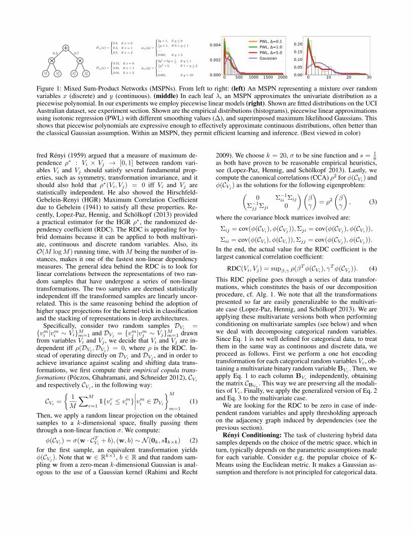
λx1 λy

2 λx3 λy

4

0.3 0.7

Pλ1(x) =

0.2, if x = 0

0.3, if x = 1

0.5, if x = 2

pλ2(y) =

3y + 1, if y ≤ 012y + 1, if 0 < y ≤ 1

. . .

0.001, if y > 5

Pλ3(x) =

0.15, if x = 0

0.81, if x = 1

0.04, if x = 2

pλ4(y) =

2y2 + 5y + 12, if y ≤ 1

12y2 + 5, if 1 < y ≤ 2

. . .

0.001, if y > 10 0 500 1000 1500 20000.000

0.002

0.004PWL, =0.1PWL, =1.0PWL, =5.0Gaussian

0 10 20 300.000.050.100.150.20

Figure 1: Mixed Sum-Product Networks (MSPNs). From left to right: (left) An MSPN representing a mixture over randomvariables x (discrete) and y (continuous). (middle) In each leaf λi an MSPN approximates the univariate distribution as apiecewise polynomial. In our experiments we employ piecewise linear models (right). Shown are fitted distributions on the UCIAustralian dataset, see experiment section. Shown are the empirical distributions (histograms), piecewise linear approximationsusing isotonic regression (PWL) with different smoothing values (∆), and superimposed maximum likelihood Gaussians. Thisshows that piecewise polynomials are expressive enough to effectively approximate continuous distributions, often better thanthe classical Gaussian assumption. Within an MSPN, they permit efficient learning and inference. (Best viewed in color)

fred Renyi (1959) argued that a measure of maximum de-pendence ρ∗ : Vi × Vj → [0, 1] between random vari-ables Vi and Vj should satisfy several fundamental prop-erties, such as symmetry, transformation invariance, and itshould also hold that ρ∗(Vi, Vj) = 0 iff Vi and Vj arestatistically independent. He also showed the Hirschfeld-Gebelein-Renyi (HGR) Maximum Correlation Coefficientdue to Gebelein (1941) to satisfy all these properties. Re-cently, Lopez-Paz, Hennig, and Scholkopf (2013) provideda practical estimator for the HGR ρ∗, the randomized de-pendency coefficient (RDC). The RDC is appealing for hy-brid domains because it can be applied to both multivari-ate, continuous and discrete random variables. Also, itsO(M logM) running time, with M being the number of in-stances, makes it one of the fastest non-linear dependencymeasures. The general idea behind the RDC is to look forlinear correlations between the representations of two ran-dom samples that have undergone a series of non-lineartransformations. The two samples are deemed statisticallyindependent iff the transformed samples are linearly uncor-related. This is the same reasoning behind the adoption ofhigher space projections for the kernel-trick in classificationand the stacking of representations in deep architectures.

Specifically, consider two random samples DVi=

{vmi |vmi ∼ Vi}Mm=1 and DVj= {vmj |vmj ∼ Vj}Mm=1 drawn

from variables Vi and Vj , we decide that Vi and Vj are in-dependent iff ρ(DVi ,DVj ) = 0, where ρ is the RDC. In-stead of operating directly on DVi and DVj , and in order toachieve invariance against scaling and shifting data trans-formations, we first compute their empirical copula trans-formations (Poczos, Ghahramani, and Schneider 2012), CVi

and respectively CVj, in the following way:

CVi=

{1

M

∑M

r=11{vri ≤ vmi }

∣∣∣∣vmi ∈ DVi

}Mm=1

(1)

Then, we apply a random linear projection on the obtainedsamples to a k-dimensional space, finally passing themthrough a non-linear function σ. We compute:

φ(CVi) = σ(w · CTVi

+ b), (w, b) ∼ N (0k, sIk×k) (2)for the first sample, an equivalent transformation yieldsφ(CVj

). Note that w ∈ Rk×1, b ∈ R and that random sam-pling w from a zero-mean k-dimensional Gaussian is anal-ogous to the use of a Gaussian kernel (Rahimi and Recht

2009). We choose k = 20, σ to be sine function and s = 16

as both have proven to be reasonable empirical heuristics,see (Lopez-Paz, Hennig, and Scholkopf 2013). Lastly, wecompute the canonical correlations (CCA) ρ2 for φ(CVi

) andφ(CVj

) as the solutions for the following eigenproblem:(0 Σ−1ii Σij

Σ−1jj Σji 0

)(βγ

)= ρ2

(βγ

), (3)

where the covariance block matrices involved are:

Σij = cov(φ(CVi), φ(CVj

)),Σji = cov(φ(CVj), φ(CVi

)),

Σii = cov(φ(CVi), φ(CVi

)),Σjj = cov(φ(CVj), φ(CVj

)).

In the end, the actual value for the RDC coefficient is thelargest canonical correlation coefficient:

RDC(Vi, Vj) = supβ,γ ρ(βTφ(CVi), γTφ(CVj )). (4)

This RDC pipeline goes through a series of data transfor-mations, which constitutes the basis of our decompositionprocedure, cf. Alg. 1. We note that all the transformationspresented so far are easily generalizable to the multivari-ate case (Lopez-Paz, Hennig, and Scholkopf 2013). We areapplying these multivariate versions both when performingconditioning on multivariate samples (see below) and whenwe deal with decomposing categorical random variables.Since Eq. 1 is not well defined for categorical data, to treatthem in the same way as continuous and discrete data, weproceed as follows. First we perform a one hot encodingtransformation for each categorical random variables Vc, ob-taining a multivariate binary random variable BVc

. Then, weapply Eq. 1 to each column BVc

independently, obtainingthe matrix CBVc

. This way we are preserving all the modali-ties of Vc. Finally, we apply the generalized version of Eq. 2and Eq. 3 to the multivariate case.

We are looking for the RDC to be zero in case of inde-pendent random variables and apply thresholding approachon the adjacency graph induced by dependencies (see theprevious section).

Renyi Conditioning: The task of clustering hybrid datasamples depends on the choice of the metric space, which inturn, typically depends on the parametric assumptions madefor each variable. Consider e.g. the popular choice of K-Means using the Euclidean metric. It makes a Gaussian as-sumption and therefore is not principled for categorical data.

Algorithm 1 splitFeaturesRDC (D, α)

1: Input: samples D = {vm = (vm1 , . . . , vmN )|vm ∼

V}Mm=1 over a set of random variables V ={V1, . . . , VN}; α: threshold of significance

2: Output: a feature partition {PD}3: for each Vi ∈ V do

4: CVi←{

1M

∑Mr=1 1{vri ≤ vmi }

∣∣∣∣vmi ∈ DVi

}Mm=1

5: (wi, bi) ∼ N (0k, sIk×k)6: φ(CVi

)← sin(wi · CTVi+ bi)

7: G ← Graph({})8: for each Vi, Vj ∈ V do9: ci,j ← CCA(φ(CVi

), φ(CVj))

10: if ci,j > α then11: G ← G ∪ {(i, j)}12: return ConnectedComponents(G)

Algorithm 2 clusterSamplesRDC (D)

1: Input: samples D = {vm = (vm1 , . . . , vmN )|vm ∼

V}Mm=1 over a set of random variables V ={V1, . . . , VN}

2: Output: a data partition {PD}

3: CVi←{

1M

∑Mr=1 1{vri ≤ vmi }

∣∣∣∣vmi ∈ DVi

}Mm=1

4: (w, b) ∼ N (0s, sIk×k)5: φ(CVi

)← sin(w · CTVi+ b)

6: E ← {φ(CV1), . . . , φ(CVN)}

7: return KMeans(E , 2)

To eliminate the reliance on knowing the type, we proposeto cluster multivariate hybrid samples after the RDC pipelinehas processed them. Not only does the series of non-lineartransformations produce a feature space in which clustersmay be more easily separable, but no distributional assump-tions are required. More formally, given a set of samples Dover RVs V we split it into a sample partitioning PD =

{Dc}Cc=1,⋃Cc=1DC = D, andDq∩Dr = ∅,∀Dq,Dr ∈ PD.

The weights for the convex combination on the sum nodesare estimated as the proportions of the data belonging toeach cluster, i.e., wc = |Dc|

|D| . The procedure is sketchedin Alg. 2. First, we transform every feature Vi in D usingEq 2: E = {φ(DVn)|DVn}Nn=1. Then, all our features areprojected into a new k-dimensional non-linear space. In thisnew space, we can safely apply now K-Means to obtain cclusters. In Alg. 2, we set c = 2 as this generally leads todeeper networks (Vergari, Di Mauro, and Esposito 2015).

Nonparametric Univariate Leave Distributions: Fi-nally, to be fully type agnostic, i.e., to realize MSPNs, weadopt piecewise polynomial approximations of the univari-ate leaf densities. The simplest and most straightforward ap-proximation we consider are piecewise constant functions,i.e. histograms. More precisely, we adopt the scheme pro-posed in (Rozenholc, Mildenberger, and Gather 2010) of-

Algorithm 3 LearnMSPN (D, ∆, η, α)

1: Input: samples D = {vm = (vm1 , . . . , vmN )|vm ∼

V}Mm=1 over a set of random variables V ={V1, . . . , VN}; η: minimum number of instances to split;∆: histogram smoothing factor; α: threshold of signifi-cance

2: Output: an MSPN S encoding a joint pdf over Vlearned from D

3: if |V| = 1 then4: {Dc}Cc=1 ← clusterSamplesRDC(D)5: if C > 1 then6: S ←∑C

i=1|Dc||D| LearnMSPN(Dc,∆, η)

7: else8: S ← LearnIsotonicLeaf(D,∆)

9: else if |D| < η then

10: S ←|V|∏n=1

LearnMSPN({vmn |vmn ∼ Vn}Mm=1,∆, η)

11: else12: {Vc}Cc=1 ← splitFeaturesRDC(D, α)13: if C > 1 then14: Dc ← {vmc |vmc ∼ Vc}Mm=1

15: S ←∏Cc=1 LearnMSPN(Dc,∆, η)

16: else17: {Dc}Cc=1 ← clusterSamplesRDC(D)

18: S ←∑Ci=1

|Dc||D| LearnMSPN(Dc,∆, η)

return S

fering an adaptive binning, i.e. with irregular intervals, thatis learned from data by optimizing a penalized likelihoodfunction. This allows MSPNs to model both multimodal andskewed univariate distributions without further assumptions.We apply Laplacian smoothing by a factor ∆ to cope withunseen values and the natural overfitting of histograms.

Indeed, by increasing the degree of leaf polynomial ap-proximations, one can favor more expressive models. To bal-ance between the complexity of learning resp. inference andexpressiveness, however, we restrain to piecewise linear ap-proximations. We reframe the unsupervised task of estimat-ing the density of univariate leaf distributions into a super-vised one by fitting a nonparametric unimodal distributionfunction through isotonic regression (Frisen 1986), referredto as LearnIsotonicLeaf. Once we have collected a set ofpairs of points, e.g. from the previously estimated histogram,we employ them as labeled instances to fit a monotonicallyincreasing (resp. decreasing) piecewise linear function up to(resp. down from) the estimated distribution mode. To copewith this unimodality assumption we accommodate Learn-MSPN, cf. Alg. 3, to grow a leaf only after no more cluster-ing steps are possible, i.e. it is difficult if not impossible toseparate two modalities in the observed data. Note how iso-tonic regression acts as an additional regularizer: to preservemonotonicity, it does not fit exactly the data points, resultingin a smoother piecewise function.

Now we have everything together to evaluate MSPNs em-pirically. Before doing so, we would like to stress that wehere focused on a general setting. Instead of piecewise lin-

MSPNGower RDC

dataset HBNMMHC hist iso hist iso

anneal-U -42.647 -63.553 -38.836 -60.314 -38.312australian -38.423 -18.513 -30.379 -17.891 -31.021auto -71.530 -72.998 -69.405 -73.378 -70.066balance-scale -7.483 -8.038 -7.045 -7.932 -7.302breast -30.572 -34.027 -23.521 -34.272 -24.035breast-cancer -9.193 -15.373 -9.500 -16.277 -9.990cars -28.596 -30.467 -31.082 -29.132 -30.516cleave -26.296 -26.132 -25.869 -25.707 -25.441crx -34.563 -22.422 -31.624 -24.036 -31.727diabetes -29.797 -15.286 -26.968 -15.930 -27.242german -34.356 -40.828 -33.480 -38.829 -32.361german-org -29.051 -43.611 -26.852 -37.450 -27.294heart -28.519 -20.691 -26.994 -20.376 -25.906iris -1.670 -3.616 -2.892 -3.446 -2.843

wins over HBNMMHC - 4/14 11/14 4/14 11/14wins 3/14 11/14

Table 1: Average test set log likelihoods for UCI hybriddatasets (the higher, the better). The best results are bold.MSPNs win in 11 out of 14 cases, even without informationabout the statistical types (RDC, iso). A Wilcoxon sign testshows that this is significant (p = 0.05).

ear leaves, one can also employ existing hybrid densities asleave distributions such as HBNs, mixtures of truncated ex-ponential families, or other nonparametric density estima-tors such as Kernel Density Estimators (KDEs) and even de-noising and variational autoencoders.

Experimental EvaluationWe intend to investigate the benefits of MSPNs comparedto other mixed probabilistic models concerning accuracyand flexibility of inference. Specifically, we investigate thefollowing questions: (Q1) Is the MSPN distribution flexi-ble for hybrid domains? (Q2) How do MSPNs compare toexisting mixed models? (Q3) How do MSPNs compare tostate-of-the-art parametric models in a single-type domain?(Q4) Can MSPNs effectively answer several inference querytypes over hybrid domains? (Q5) Can we leverage MSPNsfor interpretability over hybrid domains, even via symboliccomputation? We implemented MSPNs1 in Python and R.

Hybrid UCI Benchmarks (Q1, Q2): We considered the14 preprocessed UCI benchmarks from the MLC++ library2

listed in Table 1. The domains span from survey data tomedical and biological domains, and they contain both con-tinuous, discrete and categorical variables in different pro-portions. As a baseline density estimator, we consideredHBNs whose conditional dependencies are modeled as con-ditional linear gaussians (Heckerman and Geiger 1995).To learn their structure we explored both score-based andconstrained-based approaches, finding the Max-Min Hill-

1https://github.com/alejandromolinaml/MSPN2https://www.sgi.com/tech/mlc/download.

html

Dirichlet, train points

1.590.051.693.334.976.628.269.9011.5413.18

SPN, train points

1.590.051.693.334.976.628.269.9011.5413.18

Figure 2: Simplex Distributions: Density of the topics span-ning a 2-simplex from the NIPS dataset using (left) Dirichletand (right) MSPN distributions. The more flexible MSPNdistribution fits the topic distribution well and the lower-lefttopic better. (Best viewed in color).

Climbing (MMHC) algorithm (Tsamardinos, Brown, andAliferis 2006) to perform the best on the holdout data. Forweight learning, we optimized the BDeu score. As an addi-tional sanity check of our nonparametric RDC pipeline, wealso trained MSPNs employing K-Medoids using the Gowerdistance (GowerMSPNs). The Gower distance (Gower andGower 1971) defines a metric over hybrid domains, at thecost of making distributional assumptions for each variableinvolved: take the average d(i, j)=(1/N)

∑Nn=1 d

ni,j of dis-

tances dni,j per feature n. We assumed continuous variablesto be Gaussian and discrete ones to be binomial.

The results are summarized in Table 1. MSPNs clearlyoutperform HBNs. Moreover, the performance of MSPNsis comparable to GowerMSPNs, proving that using RDC isa sensible idea and frees the user from making parametricassumptions. Using histogram representations allows one tocapture mixtures, which turns out to be beneficial for somedatasets, but also results in a higher variance in performanceacross datasets, showing the benefit of isotonic regression.This answers (Q1, Q2) affirmatively.

Learning Simplex Distributions (Q3): We considereddata common in text and chemistry domains: proportionaldata, i.e., data lying on the probability simplex, the valuesare in [0, 1] and sum up to 1. The Dirichlet distribution is ar-guably the most famous parametric distribution for this typeof data. Hence, we used it as a baseline.

First, we considered the NIPS corpus, containing 1,500documents over the 100 most frequent words. We ran LatentDirichlet Allocation (LDA) (Blei 2012) with different num-bers of topics (3,5,10,20,50) generating different data repre-sentations. Fig. 2 shows that the MSPN accurately fits thedensity, better than a Dirichlet. On NIPS, we also comparedMSPNS to Poisson SPNs (PSPNs) of Molina et al. (2017),learning both models with η = 200. The average test log-likelihood of MSPNs was better than PSPNs: -144.41 vs -227.74. This proves how MSPNs are competitive to domain-specific models.

Then, we investigated the Air Quality dataset3 contain-ing 6,941 measurements for 12 features about air composi-

3https://archive.ics.uci.edu/ml/datasets/Air+Quality. We used only complete instances and ignoredthe time feature and C6H6

0 5 10 15 20 25

0

5

10

15

20

25

0 5 10 15 20 25

0

5

10

15

20

25

(a) (b) (c) (d)

Figure 3: Towards symbol grounding using MSPN. (a) On the top left, the decoded sample predicted for the visual code{0, 0, 1, 0, 1, 1} (corresponding to a “3”), on the bottom left its training closest sample. On the right, decoded conditionalsamples for the same visual code. (b,c) Decoded conditional samples for codes in between classes “3” and “5” ({0, 0, 1, 1, 1, 1})as well as “1” and “5” ({1, 0, 1, 1, 1, 0}), respectively. (d) Some test images on the left and their MSPN reconstructions (left,right, up, down) on the right. The reconstructed parts are denoted by a red background. (Best viewed in color)

Dimension Dirichlet MSPN(RDC,iso) MSPN(Grower,iso)

NIPS + LDA3 2.045 (± 0.297) 4.071 (± 0.66) 4.333 (± 0.627)5 7.311 (± 0.406) 10.376 (± 0.671) 10.419 (± 0.711)

10 25.047 (± 0.787) 35.927 (± 1.755) 34.205 (± 1.716)20 69.668 (± 2.014) 109.222 (± 4.179) 92.981 (± 4.245)50 245.008 (± 3.573) 338.477 (± 6.976) 349.259 (± 9.916)

Air Quality + Archetypes3 2.939 (± 1.536) 5.852 (± 2.261) 7.114 (± 2.272)5 14.625 (± 4.678) 16.494 (± 7.574) 15.099 (± 4.888)

10 61.317 (± 4.81) 84.124 (± 6.575) 85.645 (± 5.887)20 174.171 (± 5.799) 232.075 (± 7.74) 242.482 (± 10.224)

Hydrochemicals12 59.546 (± 1.781) 71.013 (± 3.591) 82.377 (± 1.445)

wins over Dir. - 10/10 10/10wins 0/10 10/10

Table 2: Average test set log likelihoods (the higher, the bet-ter) on proportional data; best results bold. Clearly, MSPNsoutperform the less flexible Dirichlet distribution, even with-out information about the statistical type (RDC, iso). Posi-tive values are due to continuous random variables.

tion. We ran Archetypal Analysis (Cutler and Breiman 1994;Thurau et al. 2012) for 3, 5, and 10 archetypes and extractedthe convex reconstructions of the original data. We alsoconsidered the hydro-chemical dataset of Tolosana-Delgadoet al. (2005), containing 485 observations of 14 chemicalmeasurements of a river. We fit MSPNs and the Dirich-let over relative concentrations. The 10-fold cross-validatedmean log-likelihoods for all models on the three datasetsare summarized in Table 2. As one can see, in all casesMSPNs can capture the distribution on the simplex betterthan the Dirichlet. This is to be expected as MSPNs can cap-ture more complex (in)dependencies, whereas the Dirichletmakes stronger independence assumptions. All simplex ex-periments together answer (Q3) affirmatively.

Leveraging symbolic-semantic information (Q4):Symbol grounding is at the heart of AI, and we exploredMSPNs as a step towards tackling this classical AI problem.We considered the 28×28 MNIST digit images, representedas 16 continuous features extracted from an autoencoder(AE) trained on the training split: we trained two layers

2 4 8 16 32 64semantic code length

+0%

+5%

+10%

+15%

+20%

mar

gina

l log

-like

lihoo

dre

lativ

e im

prov

emen

t

histiso

2 4 8 16 32 64semantic code length

+0%

+2%

+4%

accu

racy

rela

tive

impr

ovem

ent

histiso

Figure 4: Average relative improvement over ten trials (yaxis) for (left) the marginal test log-likelihood P (X) and(right) for the class accuracy based on P (C) of MSPNslearned an autoencodings augmented with semantic classcodes of increasing length (x axis). (Best viewed in color)

of 256 and 128 ReLU neurons for both the encoder andthe decoder for 200 epochs using adam (learning rate0.002 with no decay, β1 and β2 coefficients set to 0.9resp. 0.999). We then augmented MNIST with symbolicsemantic information encoded as binary codes. Each bit ofthe code is 1 if a digit contains one of the following visualfeatures: (i) a vertical stroke (true for 1, 4 and 7), (ii) a circle(0, 6, 8 and 9), (iii) a left curvy stroke (2, 3, 5, 8 and 9), (iv)a right curvy stroke (5 and 6), (v) a horizontal stroke (7, 2, 3,4, and 5), (vi) a double curve stroke (3 and 8). For instance,images representing a “3” are encoded as (0, 0, 1, 0, 1, 1)while (0, 0, 1, 1, 1, 0) corresponds to “5”. We also addedthe class label C as a feature. Let X denote the continuousembedding variables, Y the additional 6 binary symbolicfeatures, and C the categorical class variable.

In a first experiment, we trained an MSPN on a 10000subsample of the augmented MNIST training data to modelP (X,Y), setting η = 200 and ∆ = 1, k = 20. Then, weevaluated on the augmented MNIST test split whether thelearned MSPN had captured the non-explicit dependenciesbetween the three different feature domains. First, we pre-dict x∗ = argmaxx P (x|Y = yc), for each visual code ycbelonging to class c ∈ C. Fig. 3 (a) visualizes the predictionx∗ as decoded by the autoencoder back in pixel space. Asone can see, the MSPN is not only able to recover the cor-rect class but also does not just memorize a training sample.

Conditional sampling provides an additional visual proof:after propagating bottom-up the evidence for an observedcode yc, we sample a configuration x (applying Vergari, DiMauro, and Esposito’s (2016) top-down approach). Decodedsamples clearly belong to the class c, cf. Fig. 3 (a). Then, toevaluate how good the MSPN was able to glue the contin-uous and binary domains, we performed conditional sam-pling starting from unseen visual codes. For instance, forthe code (0, 0, 1, 1, 1, 1), merging the visual codes for 3 and5, we expect a digit in between the two classes. Fig. 3 (b)confirms this: decoded samples belong to either class or areclosely in between them. Similarly, Fig. 3 (c) shows samplesconditioned on code {1, 0, 1, 1, 1, 0}, merging classes 5 and1. Next, we investigated how much symbol groundings canhelp density estimation and classification. On the MNISTtest split, we investigated the benefit of using visual codesY of length 2,4,8,16,32,64. We measured the improvementof the marginal likelihood P (X) resp. the classification ac-curacy based on P (C) of an MSPN B trained on (X,Y, C)over an MSPN A trained only over (X, C): (`B − `A)/`A · 100 for both measures `. The results are summarizedin Fig. 4. As one can see, increasing the number of sym-bolic features positively improves both the marginal likeli-hood over X and the classification performance. Note thatfor computing P (X) and to predict c∗ = argmaxc P (c|X),one has to marginalize over Y, which cannot be done effi-ciently using classical mixed graphical models. Finally, weemployed MSPNs for MNIST reconstruction. We processedthe original images as two halves—left (l) and right (r), up(u) and down (d)—and encoded each half into 16 continu-ous features by learning one autoencoder independently foreach one of them. Note that each variable set Xl, Xr, Xu

and Xd forms a domain with a different distribution. Welearned MSPNs for P (Xl,Xr) and P (Xu,Xd) and per-formed MPE inference to predict one half of a test imagegiven the other. Predicted samples are shown in Fig. 3 (d).As one can see, the reconstructions are indeed very plausi-ble. This suggests that MSPNs are a valuable tool to effec-tively learn distributions and make predictions across dif-ferent domains. The experiments on leveraging symbolic-semantic information answer (Q4) affirmatively.

Mixed Mutual Information (Q5): Recall, an MSPN en-codes a polynomial over leaf piecewise polynomials. Con-sequently, one can employ a symbolic solver to evalu-ate the overall network polynomial to efficiently computeinformation-theoretic measures that would be difficult tocalculate otherwise, in particular for hybrid domains. To il-lustrate this for MSPNs, we consider computing mutual in-formation (MI) in hybrid domains. MI also provides a wayto extract the gist of MSPNs as it highlights relevant variableassociations only. Fig. 5 shows the MI network induced overthe Autism Dataset (Deserno et al. 2016), which reflects nat-ural semantic connections. This not only answers (Q5) affir-matively but also indicates that MSPNs may pave the wayto automated mixed statisticians: the MI together with thetree structure of MSPNs can automatically be compiled intotextual descriptions of the model.

To summarize our experimental results as a whole, allquestions (Q1)-(Q5) can be answered affirmatively.

Satisfaction Treatment

Satisfaction Work

Age

Success selfrating

Satisfaction Medication

Age diagnosis

IQ

No of unfinished Educations

Figure 5: Visualizing the Autism MSPN via normalized mu-tual information (the thicker, the higher). The strong naturalinteractions between Age and Age of diagnosis and betweenSatisfaction Work and No of unfinished Education are cor-rectly recovered as in the results of (Haslbeck and Waldorp2015) using a pairwise mixed graphical model with knownparametric forms from the exponential family (Yang et al.2014). Node colors encode different feature groups: Demo-graphics (green), Psychological (blue), Social Environment(orange) and Medical (red). (Best viewed in color)

ConclusionsThe Mixed Sum-Product Networks (MSPNs), are a novelcombination of nonparametric probability distributions anddeep probabilistic models. In contrast to classical shallowmixed graphical models, they provide effective learning,tractable inference and enhanced interpretability. Our exper-iments demonstrate that MSPNs are competitive to parame-terized distributions as well as mixed graphical models andmake probabilistic queries easier to compute. They allowusers to train multivariate mixed distributions more easilythan previous approaches across a wide range of domains.

MSPNs suggest several avenues for future work: scal-ing structure learning to large number of instances or high-dimensional data; learning boosted and mixtures of MSPNsalong with exploring other nonparametric leaves such KDE,other mixed graphical models, and variational autoencoders,or extending them to other instances of arithmetic cir-cuits (Choi and Darwiche 2017); making use of weightedmodel integration solvers for capturing more complex typesof queries (Belle, Passerini, and Van den Broeck 2015;Morettin, Passerini, and Sebastiani 2017). One interestingavenue is to turn MSPNs into automated statisticians, ableto predict the statistical type of a variable—is it continuousor ordinal?—and ultimately its parametric form—is it Gaus-sian or Poisson (Valera and Ghahramani 2017)?

Acknowledgements: The authors would like to thank theanonymous reviewer for the valuable feedback. This work ismotivated and partly supported by the BMEL/BLE projectDePhenSe, FKZ 313-06.01-28-1-82.047-15. AM has beensupported by the DFG CRC 876 ”Providing Information byResource-Constrained Analysis”, project B4. SN has beensupported by the CwC Program Contract W911NF-15-1-0461 with the US Defense Advanced Research ProjectsAgency (DARPA) and the Army Research Office (ARO).KK acknowledges the support by the Centre for CognitiveScience at the TU Darmstadt.

ReferencesBekker, J.; Davis, J.; Choi, A.; Darwiche, A.; and Van denBroeck, G. 2015. Tractable learning for complex probabilityqueries. In Proc. of NIPS.Belle, V.; Passerini, A.; and Van den Broeck, G. 2015. Prob-abilistic inference in hybrid domains by weighted model in-tegration. In In Proc. of IJCAI, 2770–2776.Belle, V.; Van den Broeck, G.; and Passerini, A. 2015.Hashing-based approximate probabilistic inference in hy-brid domains. In UAI, 141–150.Blei, D. M. 2012. Probabilistic topic models. CACM55(4):77–84.Cheng, W.; Kok, S.; Pham, H. V.; Chieu, H. L.; and Chai,K. M. A. 2014. Language modeling with Sum-Product Net-works. In Proc. of Interspeech.Choi, A., and Darwiche, A. 2017. On relaxing determinismin arithmetic circuits. In Proceedings of ICML, 825–833.Cutler, A., and Breiman, L. 1994. Archetypal analysis. Tech-nometrics 36(4):338–347.Deserno, M. K.; Borsboom, D.; Begeer, S.; and Geurts,H. M. 2016. Multicausal systems ask for multicausal ap-proaches: A network perspective on subjective well-beingin individuals with autism spectrum disorder. Autism1362361316660309.Elidan, G. 2010. Copula bayesian networks. In Proc. ofNIPS.Frisen, M. 1986. Unimodal regression. Journal of the RoyalStatistical Society. Series D 35(4):479–485.Gebelein, H. 1941. Das statistische Problem der Korrela-tion als Variations- und Eigenwertproblem und sein Zusam-menhang mit der Ausgleichsrechnung. Zeitschrift fur Ange-wandte Mathematik und Mechanik 21(6):364–379.Gens, R., and Domingos, P. 2013. Learning the Structure ofSum-Product Networks. In Proc. of ICML.Gower, J. C., and Gower, J. C. 1971. A general coefficientof similarity and some of its properties. Biometrics.Haslbeck, J. M. B., and Waldorp, L. J. 2015. mgm:Estimating time-varying mixed graphical models in high-dimensional data. ArXiv 1510.06871.Heckerman, D., and Geiger, D. 1995. Learning bayesiannetworks: a unification for discrete and gaussian domains.In Proc. of UAI.Langseth, H.; Nielsen, T. D.; Rumı, R.; and Salmeron, A.2012. Mixtures of truncated basis functions. InternationalJournal of Approximate Reasoning 53(2):212–227.Lauritzen, S., and Wermuth, N. 1989. Graphical models forassociations between variables, some of which are qualita-tive and some quantitative. Annals of Statistics 17(1):31–57.Lopez-Paz, D.; Hennig, P.; and Scholkopf, B. 2013. Therandomized dependence coefficient. In Advances in neuralinformation processing systems, 1–9.Molina, A.; Natarajan, S.; and Kersting, K. 2017. Pois-son sum-product networks: A deep architecture for tractablemultivariate poisson distributions. In Proc. of AAAI.

Moral, S.; Rumi, R.; and Salmeron, A. 2001. Mixtures oftruncated exponentials in hybrid bayesian networks. In Ben-ferhat, S., and Besnard, P., eds., Proc. of ECSQARU.Morettin, P.; Passerini, A.; and Sebastiani, R. 2017. Ef-ficient weighted model integration via smt-based predicateabstraction. In Proc. of IJCAI.Peharz, R.; Tschiatschek, S.; Pernkopf, F.; and Domingos, P.2015. On theoretical properties of sum-product networks. InProc. of AISTATS.Poczos, B.; Ghahramani, Z.; and Schneider, J. G.2012. Copula-based kernel dependency measures. arXiv1206.4682.Poon, H., and Domingos, P. 2011. Sum-Product Networks:a New Deep Architecture. Proc. of UAI.Rahimi, A., and Recht, B. 2009. Weighted sums of randomkitchen sinks: Replacing minimization with randomizationin learning. In Proc. of NIPS.Renyi, A. 1959. On measures of dependence. Acta mathe-matica hungarica 10(3-4):441–451.Rooshenas, A., and Lowd, D. 2014. Learning sum-productnetworks with direct and indirect variable interactions. InProc. of ICML, 710–718.Rozenholc, Y.; Mildenberger, T.; and Gather, U. 2010. Com-bining regular and irregular histograms by penalized likeli-hood. Comp. Statistics & Data Analysis 54(12):3313–3323.Sanner, S., and Abbasnejad, E. 2012. Symbolic variableelimination for discrete and continuous graphical models. InProc. of AAAI.Shenoy, P., and West, J. 2011. Inference in hybrid bayesiannetworks using mixtures of polynomials. International Jour-nal of Approximate Reasoning 52(5):641–657.Thurau, C.; Kersting, K.; Wahabzada, M.; and Bauckhage,C. 2012. Descriptive matrix factorization for sustainabilityadopting the principle of opposites. DAMI 24(2):325–354.Tolosana-Delgado, R.; Otero, N.; Pawlowsky-Glahn, V.; andSoler, A. 2005. Latent compositional factors in the llobre-gat river basin (spain) hydrogeochemistry. Math. Geology37(7):681–702.Tsamardinos, I.; Brown, L. E.; and Aliferis, C. F. 2006. Themax-min hill-climbing bayesian network structure learningalgorithm. MLJ 65(1):31–78.Valera, I., and Ghahramani, Z. 2017. Automatic discoveryof the statistical types of variables in a dataset. In ICML.Vergari, A.; Di Mauro, N.; and Esposito, F. 2015. Simplify-ing, Regularizing and Strengthening Sum-Product NetworkStructure Learning. In Proc. of ECML-PKDD.Vergari, A.; Di Mauro, N.; and Esposito, F. 2016. Vi-sualizing and understanding sum-product networks. arXiv1608.08266.Yang, E.; Baker, Y.; Ravikumar, P.; Allen, G.; and Liu, Z.2014. Mixed graphical models via exponential families. InProc. of AISTATS.Zhao, H.; Melibari, M.; and Poupart, P. 2015. On the Rela-tionship between Sum-Product Networks and Bayesian Net-works. In Proc. of ICML.