mk7227 postgraduate dissertation - roarroar.uel.ac.uk/4571/1/impact of macroeconomic variables on uk...
TRANSCRIPT

MK7227 Postgraduate Dissertation
Student Number: 1149955
Comments Max Mark
Actual Mark
Introduction
Identification of a valid topic, research question and objectives framed to Masters Level standard with academic rationale developed, clear industry contextualisation of the research topic
Supervisor Comments:
10%
2nd marker Comments:

1149955
2
Critical Literature Review
Depth and breadth of literature search, engagement with seminal authors and papers, evidence of a critical approach toward the scholarly literature
Supervisor Comments:
25%
2nd marker Comments:
Research Methodology
Evaluation of research philosophies and perspectives. Justification of methodological approach, sampling strategy, data analysis and reliability and validity measures as applicable
Supervisor Comments:
15%
2nd marker Comments:
Supervisor Comments:
35%

1149955
3
Data Analysis and Interpretation
Evidence of rigor in data analysis and interpretation procedures, identification of key patterns and themes in the research data, integration of academic theory into explanation of findings
2nd marker Comments:
Conclusions and Recommendations
Research question and objectives addressed with implications to theoretical and managerial concepts considered. Recommendations provided for theory, practice and future research
Supervisor Comments:
10%
2nd marker Comments:

1149955
4
Organisation, presentation and references.
Well structured and ordered dissertation with correct use of grammar and syntax. In-text citation and bibliography conforming to “Cite Them Right”
Supervisor Comments:
5%
2nd marker Comments:
Total
First Marker Total
100%
Second Marker Total
Supervisor General Comments:
Agreed Mark:

1149955
5
2nd Marker General Comments:
Supervisor’s Name: ……………………………………….. Signature: …………………………
2nd Marker’s Name: ………………………………………. Signature: …………………………
Impact of macroeconomic variables on UK stock market: A case study of FTSE100 index.

1149955
6
A dissertation submitted in partial fulfilment of the requirements of the Royal Docks Business School, University of East London for the degree of MSc. Finance and Risk Management.
[September, 2015]
[13,409]
I declare that no material contained in the thesis has been used in any other submission for an academic award
Student Number:____1149955___________________ Date:___08/09/15______
Contents Dissertation Deposit Agreement....................................................................................................9
Dissertation Details....................................................................................10
Dedication..................................................................................................11
Acknowledgement......................................................................................12
Abstract......................................................................................................13
Chapter1: Introduction..........................................................................14-15

1149955
7
1.1Objective of study .................................................................................16 1.2 Limitation.............................................................................................16 1.3 Overview of chapters.......................................................................16-17 Chapter2: Literature review.....................................................................................18-25 Chapter 3: Research Methodology...............................................................26
3.1 Research Question and Objectives..............................................................26
3.2Research Paradigm...........................................................................26-27
3.3Research Hypotheses........................................................................27-28
3.4Vector Error Correction Model..........................................................28-29
3.5 Research Data..................................................................................29-30
3.6 Research theories............................................................................32-33
Chapter4: Data Analysis.............................................................................34
4.1 Descriptive Statistics........................................................................34-40
4.2 Correlation......................................................................................40-41
4.3 Vector Error Correction Model .........................................................41-45
4.4 interpretations of results.................................................................46-48
4.5 Granger Causality test.....................................................................48-52
Chapter 5:Conclusions...........................................................................53-55
Chapter 6:Recommendations.....................................................................56
7References...........................................................................................57-62
8 Appendixes........................................................................................63-83
8.1-Tables8: Eviews Output- Descriptive statistic tables........................ 64-66
8.2- Tables 9A-9C: Eviews Output- Unit root tests.................................66-75
8.3-Table 10: Eviews Output- Vector autoregression estimates...............75-76

1149955
8
8.4- Table 11: Eviews Output- VAR lag order selection criteria............... 76-77
8.5- Table 12: Eviews Output- Johansen Cointegration test....................77-80
8.6- Table 13: Eviews Output- Vector Error Correction Estimates............80-82
8.7- Table 14: Eviews Output- Granger Causality test.............................82-83
8.8- figure 7:Q seasonally adjusted production and manufacturing ...............83 8.9- figure 8: CPI inflation (%) and contributions from broad expenditure categories (percentage points)....................................................................84
Dissertation Deposit Agreement Libraries and Learning Services at UEL is compiling a collection of dissertations identified by academic staff as being of high quality. These dissertations will be included on ROAR the UEL Institutional Repository as examples for other students following the same courses in the future, and as a showcase of the best student work produced at UEL.
This Agreement details the permission we seek from you as the author to make your dissertation available. It allows UEL to add it to ROAR and make it available to others. You can choose whether you only want the dissertation seen by other students and staff at UEL (“Closed Access”) or by everyone worldwide (“Open Access”).

1149955
9
I DECLARE AS FOLLOWS:
• That I am the author and owner of the copyright in the Work and grant the University of East London a licence to make available the Work in digitised format through the Institutional Repository for the purposes of non-commercial research, private study, criticism, review and news reporting, illustration for teaching, and/or other educational purposes in electronic or print form
• That if my dissertation does include any substantial subsidiary material owned by third-party copyright holders, I have sought and obtained permission to include it in any version of my Work available in digital format via a stand-alone device or a communications network and that this permission encompasses the rights that I have granted to the University of East London.
• That I grant a non-exclusive licence to the University of East London and the user of the Work through this agreement. I retain all rights in the Work including my moral right to be identified as the author.
• That I agree for a relevant academic to nominate my Work for adding to ROAR if it meets their criteria for inclusion, but understand that only a few dissertations are selected.
• That if the repository administrators encounter problems with any digital file I supply, the administrators may change the format of the file. I also agree that the Institutional Repository administrators may, without changing content, migrate the Work to any medium or format for the purpose of future preservation and accessibility.
• That I have exercised reasonable care to ensure that the Work is original, and does not to the best of my knowledge break any UK law, infringe any third party's copyright or other Intellectual Property Right, or contain any confidential material.
• That I understand that the University of East London does not have any obligation to take legal action on behalf of myself, or other rights holders, in the event of infringement of intellectual property rights, breach of contract or of any other right, in the Work.
I FURTHER DECLARE:
• That I can choose to declare my Work “Open Access”, available to anyone worldwide using ROAR without barriers and that files will also be available to automated agents, and may be searched and copied by text mining and plagiarism detection software.
• That if I do not choose the Open Access option, the Work will only be available for use by accredited UEL staff and students for a limited period of time.
/cont

1149955
10
Dissertation Details
Field Name Details to complete
Title of thesis
Full title, including any subtitle
Impact of macroeconomic variables on UK stock market: A case study of FTSE100 index.
Supervisor(s)/advisor
Separate the surname (family name) from the forenames, given names or initials with a comma, e.g. Smith, Andrew J.
Shabani, Mimoza
Author Affiliation
Name of school where you were based
Royal Docks Business School
Qualification name
E.g. MA, MSc, MRes, PGDip
MSc
Course Title
The title of the course e.g.
Finance and Risk Management
Date of Dissertation
Date submitted in format: YYYY-MM
8th September 2015
2015-09
Does your dissertation contain primary research data? (If the answer to this question is yes, please make sure to include your Research Ethics application as an appendices to your dissertation)
Yes No
Do you want to make the dissertation Open Access (on the public web) or Closed Access (for UEL users only)?
Open Closed
By returning this form electronically from a recognised UEL email address or UEL network system, I grant UEL the deposit agreement detailed above. I understand inclusion on and removal from ROAR is at UEL’s discretion.
Student Number: .............1149955.............. Date: ....8 September 2015....
√
√

1149955
11
Dedication To God be the glory for completing this dissertation in health and vitality. I dedicate this dissertation to God the Father, God the Son and God the Holy Spirit. I will like to dedicate this dissertation also to my beloved mother Late Mrs Catherine Ekei Henshaw, mummy I miss you always, you have always been my inspiration and I know you will be happy for me for my success although you are gone but I keep hearing your word of wisdom and this has kept me going and I am grateful for the love we shared together.

1149955
12
Acknowledgement
I will like to acknowledge my supervisor Dr. Mimoza Shabani for her guidance throughout this dissertation.

1149955
13
Impact of macroeconomic variables on UK stock market: A case study of FTSE100 index. Abstract The relationship between macroeconomic variables and stock market has been studied over the years by researchers and there are documented literatures over several decades but it is still a debatable issue whether macroeconomic variables determine stock market prices.
This paper investigates the impact of macroeconomic variables on FTSE100 Index. The selected macroeconomic variables are consumer price index (CPI) as a proxy for inflation, industrial production index (IPI), money supply (M1), exchange rate(ER) and interest rate (IR). The data for the analysis are monthly time series from January 1995 to December of 2014. The study employed Error Vector Correction Model to determine the long run and short run equilibrium relationships. The unit root tests and Johansen cointegration test were carried out. The empirical results suggested long-term relationship among the variables in as there exists a cointegration relationship between the variables. The industrial production index, money supply and interest rate are cointegrated and have a long run equilibrium relationship. The consumer price index and exchange rate showed positive relationship with the FTSE100 Index over the long run, whereas the industrial production index, money supply and interest rate showed negative long-run relationships with the FTSE100 Index. The Vector Error Correction Model in the short run suggest that exchange rate and industrial production index restore equilibrium as they both deviate in the short run but adjust to equilibrium in the long run. Further test was conducted using Granger causality test and the result showed bi-directional causality between consumer price index and industrial production index and unidirectional causality between FTSE100 and exchange rate, FTSE100 and industrial production index, money supply (M1) and interest rate, interest rate and industrial production index, exchange rate and money supply (M1), money supply (M1) and industrial production index, exchange rate and industrial production index. Keywords: Stock market, Macroeconomic variables, Vector error connection model, Unit root test, Johansen cointegration test, Granger causality test.

1149955
14
Chapter1- Introduction
Introduction
Stock market is a leading economic indicator for the performance of a
country or nation. The growth of the economy is sometimes determined by
the stock returns from its stock market. This is because stock market is a
major investment of any economy, a market where stock is issued and sells
to the public and these companies in trade are able to raise funds to finance
their activities. Stock market is also an important factor in business
decisions because the prices of shares affect the amount of fund that can be
raised by selling newly issued stock to finance investment spending (Mishkin,
2013, p.46).
People often speculate about the market movement whether the market is
heading for a big kill or at a loss. Stock market is a place where people can
get rich or poor quickly. Investors observe the stock market trend or listen to
economic news to enable them chose or decide what stock market or
company they can invest in. Some investors prefer to diversify their
investments because of risk. This risk could be economical or social or
political.
We cannot possibly examine all the macroeconomic variables efficiently by
daily monitoring of the stock market movement or fluctuation so carrying
out an empirical research will enable us to determine or identify the
macroeconomic variables responsible for the fluctuation of UK stock market.
Stock market movement or behaviour is determined by several
macroeconomic variables, therefore its fluctuation. The common or key
macroeconomic variables of an economy are inflation and interest rate
because expected inflation will lead to a rise in interest rate and so some
nations will also try to target inflation and reduce interest rate.
The Bank of England set interest rate much lower after the financial crisis of
2007- 2009 which the stock market of Dow Jones Stock Exchange (DJSE)
crashed and this affected the stock market of UK since the two stock
markets are interconnected which means a risk to one stock market will
affect the other stock market. This kind of risk is called systemic risk.

1149955
15
The central bank has statutory right to set policy goals, the goal policy goals
set may constitute inflation targeting, to control supply of money or
maintain a fixed exchange rate but this has to be executed in partnership
with the government. All this is to help stabilize the economy for better
productivity and growth since the health of an economy is determined by its
stability.
The monetary policy committee of Bank of England set interest rate at 0.5%
at their recent meeting on5 March 2015(Trading Economics,2015).Also the
inflation reported by the office for national statistics stated that inflation rate
was recorded at 0% percent in March of 2015( Trading Economics,2015).
Monetary policy set by the Bank of England is to help maintain price stability
and currency value. This in turn promotes the growth of the economy.
Macroeconomic theories and debate are about the concern of long run
growth rate and short run stability of the economy (Robert, 1993, p.12).
Therefore, the researcher will be examining the long run and the short run
relationship between the macroeconomic variables and UK stock market and
this will establish the impact on UK stock market.

1149955
16
1.1Objective of study
Stock price fluctuation is still debatable by researchers and this paper will
help identify macroeconomic variables responsible.
The objective of this study is to examine the relationship between selected
macroeconomic variables and FTSE100 index for the period March 1995 to
December 2014.
I have selected five macroeconomic variables which are consumer price index as a proxy for inflation, industrial production index, interest rate, exchange rate and money supply. The reason for studying the behaviour of stock market and determining the macroeconomic variables influencing stock prices will be for policy makers, for researchers and economists and also could safeguard investors and traders. 1.2 Limitation of study
The limitation in this research was the use of industrial production index as
a proxy for Gross Domestic Product because the data for Gross Domestic
product are produced quarterly and my data collection is 243 monthly
observations of all variables from March 1995 to December 2014. Also UK
stock market used is FTSE100 index of London Stock Exchange.
1.3 Overview of chapters
To achieve my objectives the dissertation is outlined into chapters, the
introduction is this current chapter.
Chapter two focuses on empirical literature from previous researchers on the
impact of macroeconomic variables on stock markets. These include their
methodologies and empirical results.
Chapter three focuses on research methodology.This chapter will explain the
research methodology used in answering the research question and research
objectives. The research methodology is single methodology, the use of
secondary data and the research approach will be quantitative. The research
methodology encompass research paradigm, research hypotheses, model
specification, research data, research related theories which will be
discussed in this chapter.

1149955
17
Chapter four focuses on data analysis and interpretation of results. This
chapter focuses on the data analysis using Eviews software. The secondary
data will be collected from data stream and collated onto the Microsoft excel
spreadsheet and are then transported into Eviews software for data analysis.
The time series data are described using descriptive statistics and the nature
of their relationship determined by correlation. The time series data will be
tested for stationarity and cointegration before employing the Vector Error
Correction Model to determine the long run and short run equilibrium
relationship between dependent variable and independent variables. Further
test will be conducted using Granger causality to determine causal
relationships between variables. The empirical results for this research will
be interpreted and this will answer the research question and research
objectives.
Chapter five focuses on summary and conclusion. This chapter summarises
the empirical results for this research and draw its conclusion from the
results obtained.
Chapter Six focuses on recommendation. This chapter gives suggestion and
further research for researcher on this topic.
1149955
18
Chapter 2: Literature review 2.1 Empirical Studies on Macroeconomic variables and Stock Market The relationship between stock markets and macroeconomic variable has been a debatable issue over the year, so conducting a research on the impact of macroeconomic variables on stock price is vital as macroeconomic variables can cause change in stock prices in stock markets. It is of great importance to determine the effect of macroeconomic variables on stock prices since they have impact on the performance or growth of an economy and can also influence investment decisions and guide policy makers when making policy decisions. Therefore, this has employ researchers and economists to carry out investigations and report findings. Some researchers observed one macroeconomic variable and stock market while other researchers observed two or more macroeconomic variables and stock market behaviour. These were their findings. Early research by Homa and Jaffe (1971), Hamburger and Kochin (1972) have reported that there is a relationship between money supply and stock market return. They found that past increases in money lead to increases in equity prices. These previous works were later disputed by Cooper (1974), Rozeff (1974), and others. Employing various econometric techniques, these researchers demonstrate that causal relation may actually run from stock prices to money supply. This means that stock prices and money supply was uni-directional, the two variables move in one direction only. Rogalski and Vinso (1977) argued that causal relationship is bi- directional. Boyle (1990) used monetary model to determine the relationship between money velocity and stock prices and he reported that expected change in money growth can affect the expected real equity return and inflation. Hernadez (1999) conducted Granger causality tests on 6 developed economies (Canada, France, Germany, UK, United States and Japan) about stock markets efficiency to capture information about change in money supply and stock prices. The result found by the author suggested there was no causal relationship between past changes in the money supply and current changes in stock prices for Canada, France, Germany, UK and United states but for Japan changes in money supply led to change in stock prices. This result for Japan, agrees with Homa and Jaffe (1971), Hamburger and Kochin (1972). There was uni-directional causality between the two variables. The author said that 5 developed economies are market efficient which means they are able to adjust to information quickly. This will prevent arbitrage from investors in these countries.

1149955
19
Early research by Jaffe and Mandelker (1976) and Fama and Schwert (1977) examine the relationship between inflation and stock prices. They used Fisher hypothesis, also called the Fisher effect which states that ‘the nominal interest rate fully reflects the available information concerning the possible future values of the rate of inflation’, (Fisher, 1930, cited in Jaffe and Mandelker, 1976, p.447). The empirical result reported by the authors suggested a negative relationship between inflation and stock returns. Jaffe and Mandelker (1976) also suggested that there was market inefficiency and a positive relationship between the two variables over a much longer period of time in their research. Jaffe and Mandelker used monthly data for the period January 1951 to December 1971. Firth (1979) suggested a positive relationship between inflation and nominal stock returns when he studied the relationship between stock returns and rate of inflation in UK. But Fama (1982) and Geske and Roll (1983) found different views of the relationship between stock prices and inflation. They reported that ‘stock returns signal real activity changes which in turn may lead to monetary responses’.
Hassan (2008) investigated the relationship between stock returns and
inflation in UK using linear regression and vector correction models to
explain Fisher hypothesis, also called the Fisher effect. The empirical results
reported by the author were positive and significant relationship between
the two variables for the first method. The second method, cointegration
tests suggested a long run relationship between price levels, share prices
and interest rates and this imply that macroeconomic variables are long run
determinants of stock returns in UK. This result agrees with Firth (1979) and
disagrees with Jaffe and Mandelker (1977) and Fama and Schwert (1977).
Aggarwal (1981) studied the relationship between exchange rates and stock
prices and his case study was U.S. capital market. He used floating exchange
rates of dollar for the period 1974 to 1978 and monthly stock prices of US
market. The author result showed a significant and positive correlation
between stock prices and the currency of U.S.
Vanita and Khushboo (2015) examine the long run relationship between
exchange rate and stock prices of BIRCS countries. They used Johansen
cointegration test and a daily data spanning from 1997 to 2014 and they
reported a negative and significant relationship between exchange rate and
stock prices of Russia, India and South Africa. This result disagrees with
Aggarwal (1981).
Morley and Pentecost ( 2000) examine relationship between stock market
returns and spot exchange rates of the G7 countries (Canada, France,

1149955
20
Germany, Italy, Japan, the UK, and the United States) . They used
cointegration test for a monthly data from January 1982 to January 1994 for
G-7 Countries to test the long run relationship between stock price and spot
exchange rate. Their results showed little correlation between bilateral
exchange rates and stock prices. It showed cyclical patterns but no
common trend. This means stock prices and exchange rates do not have
common trends. This means the spot exchange rates of G7 countries does
not influence their stock market returns and vice versa. This result agrees
with Vanita and Khushboo (2015) explaining that exchange rate and stock
prices move in an opposite direction. Morley and Pentecost concluded their
research by suggesting that there was a need for error connection technique
to be used rather than using long run cointegration test.
Asprem (1989) investigates the relationship between stock indices, asset
portfolios and macroeconomic variables in ten European countries. The
result from the author showed that employment, imports, inflation and
interest rates are inversely related to stock prices. The relationship between
stock prices and macroeconomic variables were strongest in Germany, the
Netherlands, Switzerland and the UK. This means that the selected
macroeconomic variables in this research have significant influence on stock
indices and asset portfolio of Germany, Netherlands, Switzerland and the UK.
The investors and policy maker of the four countries should have
information about the selected macroeconomic variables when making
decisions. The result concerning inflation and stock price relationship agrees
with Jaffe and Mandelker (1977) and Fama and Schwert (1977).
Dritsaki (2005) tested for a long run relationship between the Greek stock
market index of Athens stock exchange and 3 selected macroeconomic
variables (industrial production, inflation and interest rates). The author
used quarterly data for the period 1989 to 2003 and applied cointegration
analysis and Granger causality test. The result from author showed a
significant causal relationship between the Athens stock exchange and
selected macroeconomic variables. This means the 3 selected
macroeconomic variables of Greek stock market index are the cause of
change in stock prices in Greece.
Ratanapakorn and Sharma (2007) investigated the long term and short term
relationships between the US stock price index (S&P 500) and six
macroeconomic variables for the period 1975 to 1999.The six
macroeconomic variables are long term and short term interest rate, money

1149955
21
supply, industrial production, inflation and exchange rate. Their results
suggested that the stock prices are negatively related to the long-term
interest rate but positively related to the money supply, inflation, exchange
rate and industrial production. The Granger causality test by Ratanapakorn
and Sharma suggested that macroeconomic variable causes the stock price
in the long run but not in the short run.
Humpe and Macmillan (2009) investigated the macroeconomic variables that
influence stock prices in US and Japan. The authors used cointegration
analysis to examine the long term relationship between industrial
production, consumer price index, money supply, long term interest rate and
stock prices in US and Japan. Their empirical results showed that stock
prices in US are positively related to industrial production and negatively
related to consumer price index and long term interest rate, Also their result
further showed money supply was insignificant but showed a positive
relationship with stock prices in US. For Japan, they found stock prices are
positively related to industrial production and negatively related to money
supply. Also their result showed industrial production was negatively
influenced by the consumer price index and a long term interest rate.
Büyüksalvarci and Abdioglu (2010) reported that there was unidirectional long run causality from stock price to macroeconomic variables of Turkey stock market when they conducted a research to determine the casual long run relationship between stock prices and macroeconomic variables of Turkey. This implies that stock market price of turkey is not determined by the selected macroeconomic variables. The stock market prices determine the selected macroeconomic variables. The selected macroeconomic variables were foreign exchange rate, gold price, broad money supply (M2), industrial production index and consumer price index and ISE-100 index (Istanbul stock exchange-100) using monthly data for the period 2001 to 2010. Büyüksalvarci and Abdioglu used Toda-Yamamoto non- granger causality test. This methodology used modified Wald (MWALD) test. They concluded that the stock market of turkey is a leading indicator for future growth of the selected macroeconomic variables in this research. This result disagrees with the macroeconomic variables of Greek stock market. Pilinkus (2010) examine the long run and short run relationship between stock market indices of Lativa, Estonia and Lithuania and macroeconomic indicators using monthly data from January 2000 to December 2008. The author used vector autoregression for the short run and Johansen cointegration for the long run relationship. Also the author employed Granger causality to determine the causality between macroeconomic indicators and the mentioned stock market indices. The macroeconomic indicators were consumer price index, import, export, unemployment, gross domestic product, money supply, short term interest rate, state debt, foreign investment and trade balance. The causality test by Pilinkus suggested a

1149955
22
relationship between macroeconomic indicators and stock market indices. The vector autoregression also showed a short term relationship and Johansen cointegration test showed a long run relationship between the macroeconomic indicators and stock market indices. Pilinkus concludes the research advising investors to pay attention to the macroeconomic indicators used as they influences or have impact on the stock market indices of Lativa, Estonia and Lithuania. Sohail and Zahir (2010) they investigated the long run and short run relationships between Karachi stock exchange and selected macroeconomic variables (consumer price index, real effective exchange rate, industrial production index, money supply and three month treasury bills rate). The authors used cointegration test and vector error correction model. The result obtained from authors reported three long run relationship among variables and showed that consumer price index, real effective exchange rate and industrial production index had positive impacts on stock prices while money supply and three month treasury bills rate had a negative impact on stock prices in the long run. Aamir et al. (2011) they determine the impact of macroeconomic indicators (exchange rate and inflation) on stock market of Pakistan. They used yearly data for the period 1995 to 2010 for exchange rate of US dollars, real interest rate and Karachi stock exchange 100 index. They applied co-integration analysis and error correction model and they found that there were significant impacts in the short run and long run relationship of exchange rate and interest rate with stock market. Pal and Mittal (2011) examined the long-run relationship between the Indian capital markets and key macroeconomic variables such as interest rates, inflation rate, exchange rates and gross domestic savings of Indian economy. They used quarterly time series data for the period January 1995 to December2008. The unit root test, the co-integration test and error correction mechanism (ECM) were applied to determine the long run and short-term relationship of stock market and the selected macroeconomic variables. The findings of their study establish that there is cointegration between macroeconomic variables and Indian stock indices which connote that there is a long-run relationship. The ECM result by Pal and Mittal shows that the rate of inflation has a significant impact on both the BSE Sensex and the S&P CNX Nifty whereas Interest rates have a significant impact on S&P CNX Nifty only and foreign exchange rate has a significant impact on BSE Sensex only. Srinivasan (2011) examine the long-run and short run relationships between NSE-Nifty share price index and macroeconomic variables (index of industrial production, money supply, interest rate, exchange rate, consumer price index of India and the US stock price index). The author used Johansen and Juselius multivariate cointegration techniques and Error correction model with a quarterly data set for the period 1991 to 2010.The author’s result using cointegration test showed that the NSE-Nifty share price index has a

1149955
23
significantly positive long-run relationship with money supply, interest rate, index of industrial production, and the US stock market index. But there was a significant negative relationship between the NSE-Nifty share price index and exchange rate in the long run. The ECM showed a strong unidirectional causation running from interest rate and the US stock market return to NSE stock market return in India. This means that interest rate affect US market and this in turn affect NSE stock market return of India. Also result by Srinivasan showed that there is a significant short-run causality between money supply and interest rate, inflation and money supply, and the US stock market and exchange rate. This implies that the selected macroeconomic variables of India and US stock market affect NSE-Nifty share price index of India. Khan and Zaman (2011) reported that the selected macroeconomic variables influence stock prices of Pakistan when the authors conducted a research on the relationship between macroeconomic variables and stock prices in Karachi Stock Exchange (KSE). They used yearly data of macroeconomic variables from 1998 to 2009. The seven macroeconomic variables selected were gross domestic product, exports, consumer price index, money supply (M2), exchange rate, foreign direct investment and oil prices. Their research used Multiple regression analysis with fixed effects model.Gross domestic product and exchange rate were positively related to stock prices while consumer price was negatively related to stock prices and export, money supply, foreign direct investment and oil prices were insignificant. Khan and Zaman noticed a strong correlation between stock prices and macroeconomic variables except consumer price index which the result showed a weak correlation. They concluded their research and gave advice to investors to note the information about the selected macroeconomic variables since they affect the stock prices movement. Zakaria and Shamsuddin(2012) examines the relationship between stock market returns volatility in Malaysia with five selected macroeconomic volatilities; GDP, inflation, exchange rate, interest rates, and money supply based on monthly data from January 2000 to June 2012. Their result from regression analysis shows that only money supply volatility is significantly related to stock market volatility. The volatilities of macroeconomic variables as a group are not significantly related to stock market volatility. This can imply that stock market volatility is not influenced by the macroeconomic variables of Malaysia. This agrees with the stock market of Turkey. Cakan (2013) examined the relationship between inflation uncertainty and stock returns for UK and United States using linear and non- linear Granger causality tests and the author’s result from non linear causality test suggested a bi- directional relationship between stock returns and inflation uncertainty. The GARCH model suggested that stock returns cannot be determined by inflation uncertainty. Iqbal et al. (2013) conducted empirical study on the long and short run macroeconomic variables on stock returns in Pakistan. Iqbal and others used monthly data from January 2001 to December 2010 and employed 3

1149955
24
econometric models namely auto regressive distributed lag, augmented dickey fuller and vector error correction model. Their result suggested both long run and short run relationship between macroeconomic variables and stock returns. For long run relationship with stock prices, money supply, exchange rate and consumer price index were significant and oil price showed no significant with stock returns. For short run, money supply and exchange rate showed positive significant with stock prices but consumer price and oil prices had no significance with stock returns. Naik (2013) analyzed the macroeconomic factors on India stock market behaviour using monthly data of five macroeconomic variables namely industrial production index, inflation, money supply, short term interest rate, and exchange rates and India stock market index for the period 1994-2011. The Johansen's co-integration test and vector error correction model were applied to establish the long-run equilibrium relationship between stock market index and macroeconomic variables. The cointegration analysis by author suggested that macroeconomic variables and the stock market index are cointegrated and a long-run equilibrium relationship exists between them. The author also found that the stock prices positively relate to the money supply and industrial production but negatively relates to inflation. The exchange rate and the short-term interest rate are found to be insignificant in determining stock prices. Also Granger causality test by Naik showed that macroeconomic variable causes the stock prices in the long-run as well as in the short-run. Mohi-u-Din and Mubasher (2013) reported that a significant relationship occurs between macroeconomic variables of India and the stock price index. They selected six macroeconomic variables for their study namely inflation, exchange rate, industrial production, money supply, gold price and interest rate. They used regression model and a monthly time series data collected from April 2008 to June 2012 to established this relationship between dependent variables(Sensex, Nifty and BSE 100 )and independent variables(inflation, exchange rate, Industrial production, money supply, gold price and interest rate). Their statistical results also showed that other factor could affect stock price volatility of India so further research should be conducted using different macroeconomic variables not included in this research. Talla (2013) reported that inflation and exchange rate influence the Stockholm stock exchange (OMXS30) of Swedish stock market when the author conducted a research on the impact of macroeconomic variables on Swedish stock market. Talla selected four macroeconomic variables namely consumer price index, Industrial production, money supply (M0) and exchange rate. The author used multivariate regression model and standard ordinary linear square method to estimate the dependent variable (OMXS30) and independent variables (consumer price index, Industrial production, money supply and exchange rate). The result showed negative relationships of inflation and currency depreciation on stock prices. Also interest rate was negative on stock prices. Money supply showed positive influence on stock prices. Granger causality test showed no unidirectional between stock prices

1149955
25
and selected macroeconomic variables except one unidirectional causal relation from stock prices to inflation. Forson and Janrattanagul(2014) reported long run equilibrium relationship with Thai stock exchange index and four selected macroeconomic variables which are money supply (M2), consumer price index, interest rate and industrial production index (as a proxy for gross domestic product) using time series data of over 20 years and employing Johansen cointegration test and vector error connection model. They further used Toda and Yamamoto(1995) augmented granger causality test to establish the long run relationship between depend variable ( Thai stock exchange) and independent variables (money supply (M2), consumer price index, interest rate and industrial production index. The empirical results by authors showed the Thai stock exchange index and selected macroeconomic variables were cointegrated and have a significant equilibrium relationship over a long run. Money supply showed a strong positive relationship whereas the industrial production index and customer price index both showed negative long run relationship with Thai stock exchange index. The causal relationship was bi-directional between industrial production and money supply and unilateral causal relationship between consumer price index and industrial production, industrial production and consumer price index, money supply and consumer price index, and consumer price index and Thai stock exchange index.

1149955
26
Chapter3: Research Methodology
The researcher will start by outlining the research question and research objectives for the benefit of the reader as the focus of the research work is now clearer as the literature review in the previous chapter give support to the Research Methodology.
3.1 Research Question and Objectives
Research Question : What is the impact of macroeconomic variables on UK stock market?
Objective 1: The correlation of macroeconomic variables and stock market.
Objectives 2: to establish the long run relationship between stock market and macroeconomic variables selected.
Objective 3: to establish the short run relationship between stock market and macroeconomic variables selected.
Objective 4: to establish causal relationships between variables.
3.2Research Paradigm
It is imperative to mention the research paradigm for this study.
Research paradigm comprises of the research methods, techniques, and approach and research philosophies.
The research philosophy will help to know the research approach applicable for this research.
The research philosophy is Axiology of Epistemology philosophy. The reason why the philosophy is Axiology is because the philosophy talks about ‘the science inquiring into the ultimate values of life as a whole; and economics: the science of wealth and ill’ (Bahm, 1993, p.4). The research topic is about stock market which is economics.
The positivism of Axiology philosophy is part of the philosophy that deals with quantitative analysis. Quantitative research is the research that deals with analysing of data generated by financial software and interpreting the data for the appropriate information necessary for research topic. In quantitative research, it also talks about variables and their relationship and how they move or correlate over time. In my research topic the independent variables are consumer

1149955
27
price index (proxy for inflation), industrial production index, interest rate, exchange rate and money supply while my dependent variable is the FTSE100 index. The reason why positivism philosophy is preferred is because of how the research question is to be answered as it will involve experimental research where data are analyzed using statistical analysis, using hypothesis testing to answer the research question and research objectives. This will be similar to the empirical literature review. In this study the research method is quantitative approach and my research philosophy is positivism of Axiology philosophy.
3.3Research hypotheses
In my literature review, many of the researchers showed that their selected macroeconomic variables had impact on stock prices except Buyuksalvarci and Abdioglu (2010) and Zakaria and Shamsuddin (2012).
Consumer price index which is proxy for inflation is contradictory with results from researchers as some researchers said inflation affect stock market prices positively suggested a positive relationship while other researchers found a negative relationship, Jaffe and Mandelker (1976), Fama and Schwert (1977), Asprem (1989), Sohail and Zahir (2010), Naik(2013), Talla(2013) and Forson and Jarattanagul (2014). Money supply - the research hypothesis is positive relationship with stock price movement as most of the researchers’ results were positive, Homa and Jaffe (1971), Hamburger and Kochin (1972),Ratanapakorn and Sharma (2007) ,Srnivasan(2011), Naik(2013), Talla(2013) and Forson and Jarattanagul (2014) except Sohail and Zahir(2010) as their result was negative relationship with stock price. Exchange rate - the research hypotheses are contradictory as some researchers obtained a positive relationship while others obtained a negative relationship with stock price. Aggarwal (1981), Ratanapakorn and Sharma (2007), Sohail and Zahir (2010) and Khan et al. (2011) showed positive relationships while Sohail and Zahir (2010) and Talla (2013) showed negative relationships in their researches. Industrial production Index - the research hypotheses are positive and negative as the empirical results from researchers Sohail and Zahir (2010) and Naik (2013) showed positive relationships with stock price but the empirical result from Forson and Janrattanagul (2014) showed a negative relationship with stock price. Interest rate – the research hypothesis is negative relationship with stock price. Asprem (1989), Sohail and Zahir (2010) and Talla (2013) reported negative relationships in their researches. But I will like to say depending on the type of interest rate used it can affect stock price positively or negatively.

1149955
28
If it is a risk free rate then it is less risky to stock market. The risk free rate example is the treasury bills. According to the dividend discount model, the interest rate set by the bank affect the stock price return as it affect the discount rate (K). Some of the researchers conducted long run and short run equilibrium relationships of selected macroeconomic variables and stock prices using vector error correction model. Sohail and Zahir (2010), Aamir et al. (2011), Pal and Mittal (2011), Srinivasan (2011), Iqbal et al. (2013) applied error correction model. Sohail and Zahir (2010), Srinivasan (2011) and Iqbal et al. (2013) used similar macroeconomic variables. Aamir et al. (2011) and Iqbal et al. (2013) reported long run and short run equilibrium relationships between selected macroeconomic variables and stock market. While Sohail and Zahir (2010), Pal and Mittal (2011), Srinivasan (2011), Forson and Janrattanagul (2014) established long run relationships of the selected macroeconomic variables and their stock markets. The researcher will be using the same model specification as Forson and Janrattanagul (2014). They used Johansen cointegration test to test for the long run relationship between dependent variables and independent variables. They existed a cointegrating equation so they went further using vector error correction model as this model enables us to adjust in short term on the path toward the long run equilibrium. This adjustment means it eliminate error term. In statistics the test with minimum variance is considered as the best test. Then the researcher concludes the empirical test by using Granger causality test to establish causal relationships between variables. 3.4 Vector Error Correction Model This is the best model for time series data as it observe variables over time and also determine the long run and short run relationship equilibrium of the selected macroeconomic variables and FTSE100 index. The model specification is vector error correction model. Vector error correction model is multiple time series model. The model determine how Y (dependent variable return to equilibrium after a change in X (independent variable). The vector error correction model is also called the equilibrium correction model. As shown by (Brooks, 2008, p.338) in eqn. (7.47) the vector error correction model equation is expressed as ∆𝑦𝑡 = 𝛽1∆𝑥𝑡 + 𝛽2(𝑦𝑡 − 𝛾𝑥𝑡 − 1)+u
i .................................
eqn.1
And this model is known as an error correction model or an equilibrium correction model, and Y t-1 – 𝛾xt-1 is known as the error correction term. But the variables have to be cointegrated yt and xt with cointegrating coefficient 𝛾 and Y
t-1 – γx
t-1 will be I(0) although yt and xt are I(1).

1149955
29
We can now use the ordinary least square to estimate the equation. We can now have an intercept in eqn1 as yt-1 – α – γx
t-1 or as ∆𝑦𝑡 = 𝛽0+
𝛽1∆𝑥𝑡 + 𝛽2 𝑦𝑡 − 𝛾𝑥t− 1 +ui
γ defines the long run relationship between x and y, while ß1 describes the short run relationship between changes in x and changes in y and ß2 describes the speed of adjustment back to equilibrium. The eqn.1 is for single variable or one independent variable but were the equation involves more than one independent variable, as shown by (Brooks, 2008, p.339) in eqn.(7.48) the equation can be expressed as ∆𝑦𝑡 = 𝛽1∆𝑥𝑡 + 𝛽2∆𝑤𝑡 + 𝛽3 𝑦𝑡 − 1− 𝛾1𝑥𝑡 − 1− 𝛾2𝑤𝑡 − 1 + 𝑢𝑡 ------ eqn.2 Where xt, wt and yt are co integrated variables and the eqn. 2 is called error correction model for more than one variable. 𝛽1 = coefficient change in x and changes in y in the short run relationship. 𝛽2 = coefficient change in w and changes in y in the short run relationship. 𝛽3 = measure or describe the speed of adjustment back to equilibrium. You can say that it measures the proportion of last period’s equilibrium error that is corrected for (Brooks, 2008, p.339). After explaining the theoretical aspect of the model for this research, the researcher explains the data collection process. 3.5 Research Data 3.51Sample design In statistical analysis we always select a sample denoted by n from a population denoted by N. A sample of a population is the subset of the population. As the number of observations gets larger the less accurate the result will be. So using a sample the observation will be smaller and more accurate in terms of result. FTSE100 index is subset of London stock exchange so FTSE100 index is sample, n of a population N (London stock exchange). The generalization of the data collection process is when a sample size used in the research can be generalised for the population of that sample size. In this research the sample size (FTSE100 index will be used to generalise the impact of macroeconomic variables on UK stock market) because FTSE100 index is a widely used market in world and most popular market in the UK. 3.52 Data collection: The researcher collected secondary data from Data stream 5.1 Thomson Reuters. Monthly time series data for five selected macroeconomic variables and FTSE100 index for the period March 1995 to December 2014. This data

1149955
30
collection is secondary data which implies that data was not collected by the researcher but generated from reliable financial software called data stream 5.1. This software collect information from various sources such as Financial times, Office for National Statistics, Bank of England, Euro stat, UK Debt management office and others. This is not time consuming as collecting financial data from various sites and sources can be cumbersome and you can easily make mistakes when you collate them together. The data stream software has excel spreadsheet option on its tool bar which enables you to export data from data stream onto the Microsoft excel spreadsheet directly. The researcher collected time series data because the research topic deals with observation of variables over time. This time series data collected from data stream will be tested for stationary as non stationary time series data gives spurious regression which is inaccurate and misleading when interpreting the results obtained from data analysis. The data stream is a collection of financial data from different sources. The data stream collection sources are: FTSE100 index source is Financial Times Stock Exchange. Consumer price index is office for national statistics, UK. Interest rate (UK Treasury bill tender 3M- middle rate) is UK Debt management office. Effective exchange rate and Money supply is from Bank of England. Industrial production index is from Eurostat. Each of these macroeconomic variables will be described for readers to understand them and how they could influence stock price movement. 3.53 Variables description The dependent variable is FTSE100 index and the independent variables are Industrial production index, exchange rate, consumer price index as a proxy for inflation, interest rate and money supply.
FTSE100 index
The FTSE100 index is the share index of the largest 100 qualifying companies in term of the company’s net worth. The FTSE100 index is part of the London Stock Exchange. FTSE stands for Financial Times Exchange.
Industrial production Index

1149955
31
The industrial production index is a proxy for gross domestic product as I was unable to obtain a monthly time series from data stream, all data from gross domestic product are produced quarterly.
Industrial production measures physical output in factories, mines and utilities. Industrial production is one of the important economic indicators in an economy, it is uninfluenced by prices as it measures the actual volume of output in goods- producing industries. Goods- producing industries make up some 40% of real GDP (Bloomberg, 2015).
The industrial production index measures the production of goods- whole sale product from the industries. If production increases the stock return of the companies’ increases also and this will give the stock markets an upward movement.
The more the industrial production the greater the return of the stock and this will increase the industrial production index and vice versa.
Exchange rate
Exchange rate means currency exchange. Exchange rate fluctuates as there are several factors affecting the exchange rate such as inflation, interest rate, government control and expectation. When British pound sterling exchange rate appreciates this will affect demand and supply of currencies as investor will like to buy pound sterling and sell it when it is weak. The appreciation of pound sterling exchange rate will give the stock prices an upward movement and depreciation of pound sterling exchange rate to another currency will give the stock prices a downward movement. So, these factors affect exchange rate and this in turn affect stock price when traders are trading currency exchange. This also affect demand and supply hence the law of one price must be applied when two countries are carrying out exchange rate transaction. The law of one price says that when purchasing goods in foreign currencies it must be the equivalent to the currency of that country.
Consumer Price Index Consumer price index: Consumer price index is a proxy for inflation. Consumer price index measures the consumption basket of goods from individual. It is recorded that bread and beverages are the highest consumption in family (Bloomberg, 2015). So rising food prices will increase the change in consumer producer for those goods. The consumer price index covers both goods and services. The consumer price index measures the consumption of good daily and if this consumption is high the return of stock or stock prices increases. Interest rate

1149955
32
The interest rate used in this research is UK Treasury bill tender 3M- middle rate. UK Treasury bill tender 3M middle rate is one of the treasury bills held by Debt Management Office. This UK Treasury bill rate is set by the Bank of England so this interest rate is less risky compare to the bank rate. If interest rate set by the bank of England is low this will imply increase in stock prices and vice versa because the required rate of return will be low and this will add value to stock prices. Money Supply There are different types of money supply. This research will only use M1. Money supply or stock of money is the total money in circulation in an economy at a specific time or period. Money supply for the research is M1. M1 is called narrow money and it includes all coins and notes in circulation. Increase in money supply will boost economic growth and this means more borrowing and the companies will purchase more stocks and more profits and hence greater stock return. Dependent and independent variables for my research have been explained and I will conclude this chapter by mentioning the theories for this study which are market efficiency theory and arbitrage pricing theory.
3.6The theoretical studies associated with stock market The two theories are the market efficient theory and arbitrage pricing theory For a stock market to be productive, it has to capture all available information if not the market will be termed to be a weak market and so Investors or traders will not want to invest in such a market. Also stock market should ensure that all macroeconomic news or factors are reflected in their stock prices to prevent arbitrage. 3.61 The Efficient Market theory According to Fama (1970), a market is said to be efficient if it is able to capture all available information and stock prices adjust to information quickly and therefore prevent arbitrage from investors or trader. Then the market is said to applying the theory of efficient market. In Efficient Market we have 3 forms of market efficiency. Weak-Form Efficiency - states that security prices reflect all market-related information, such as historical security price movements and volume of securities trades (Madura, 2012, p.268). This form of Market efficiency will not be beneficial to investors because they use past price movement or past price trend and this cannot predict the future prices.

1149955
33
Semi-strong-Form Efficiency - states that security prices fully reflect all public information, such as firm announcements, economic news, or political news (Madura, 2012, p.268). This form of market efficiency make use of all public information like announcements from news both political and economic news. Also the semi-strong efficiency include announcements by firms. Strong-Form Efficiency - states that security prices fully reflect all information, including private or insider information (Madura, 2012, p.268). The inside information is only know to employees of the firm or the board members. The employees might exploit the inside information and purchase a particular stock before it goes public before investors. This research work, the market efficiency form is semi strong market efficiency because in real world stock market are not termed as strong market efficiency because inside information are not publicly available hence arbitrage will not apply. As a matter of fact, the semi strong hypothesis as earlier mentioned include all publicly available information that is already incorporated into current prices; that is the asset prices reflect all available public information. 3.62 Arbitrage pricing theory The APT( Arbitrage pricing theory) was developed by Ross (1976) and this opposed CAPM ( Capital Asset pricing model) because it was only limited to one risk factor which is the market risk premium but APT states that there could be other factors affecting the stock prices apart from the stock market. such as inflation, interest rate or other macroeconomic variables. This APT has its limitation but the advantage of the theory that it allows investor to put various factors when deriving the required rate of return for a particular firm. The sensitivity of asset is influenced by industry conditions not the market conditions only and this allows you to capture the industrial factors which could be responsible for affecting the required rate of return.

1149955
34
Chapter 4: Data analysis
Time series data with 243 monthly observations for 5 selected macroeconomic variables (consumer price index as a proxy for inflation, industrial production index, interest rate and money supply) and FTSE100 index will be rigorously analysed using statistical analysis. Firstly, all the time series data for each variable under study are transformed into the logarithmic form.
4.1Descriptive statistics
This statistic gives the present or previous observation of variables over times. The figures 1-5 give the line graphical presentations of all variables for this study for the period 1995 to 2014 as shown below. The line graphs show the movements of all variables and you can identify trends or patterns.
Figure 1
Source : Data stream
Figure 2
3.48
3.52
3.56
3.60
3.64
3.68
3.72
3.76
3.80
3.84
96 98 00 02 04 06 08 10 12 14
FTSE

1149955
35
Source: Data Stream
Figure 3
Source: Data stream
Figure 4
1.94
1.96
1.98
2.00
2.02
2.04
2.06
2.08
2.10
96 98 00 02 04 06 08 10 12 14
IPI
-2.5
-2.0
-1.5
-1.0
-0.5
0.0
0.5
1.0
96 98 00 02 04 06 08 10 12 14
IR

1149955
36
Source: Data Stream
Figure 5
5.3
5.4
5.5
5.6
5.7
5.8
5.9
6.0
6.1
6.2
96 98 00 02 04 06 08 10 12 14
M1
1.86
1.88
1.90
1.92
1.94
1.96
1.98
2.00
2.02
2.04
96 98 00 02 04 06 08 10 12 14
ER

1149955
37
Source: Data Stream
Figure 6
Source: Data Stream
Figure 1: FTSE100 index
This graph is our dependent variable, it shows the trend which is upward and down ward movement of FTSE100 index. During the financial crisis 2007-2009 you can see the FTSE100 index fall drastically and also in between 2002 and 2004 there was a downward movement. After the recent financial crisis, the FTSE100 index shows an upward trend but there are still stock market fluctuations but minimal compared to the period of financial crisis 2007 -2009. The collapse in business investment during the recession could be a potential cause of stock market fluctuations.
Figure 2: Industrial production Index
Industrial production index is the return of the industrial production the present against the previous. The graph shows upward and downward trend and it tends to move in the same direction with FTSE100 index.
1.92
1.96
2.00
2.04
2.08
2.12
96 98 00 02 04 06 08 10 12 14
CPI

1149955
38
Figure 3: Interest rate
Interest rate graph shows a downward movement from 1995 to 2014, UK’s interest rate started with a high interest rate and interest rate started diminishing and at present is very low. After the financial crisis 2007-2009, interest rate has been set low by the bank of England to maintain economic stability. The interest rate moves in an opposite direction with FTSE100 index. Decrease in interest rate will imply increase in stock prices and this will give the FTSE100 index an upward movement.
Figure 4: Money supply
Money supply shows upward movement which indicate increase in money supply. There is money circulation over time. Money supply and FTSE100 index tend to move in the same direction. The more money in circulation, the more stocks the investors will purchase and this will give FTSE100 index an upward movement.
Figure 5: Exchange rate
Exchange rate shows upward movement which means there currency was appreciating but during the financial crisis there was downward movement of exchange rate. The currency depreciates when there is a downward trend but will appreciate for the law of one price to apply as supply and demand of currency will reach equilibrium. The effective exchange rate and FTSE100 index move in the same direction.
For descriptive statistic summary table for all variables, see (Appendix8.1-Tables8). This table will determine if the variables show or follow normal distribution N (0,ϭ2).
For consumer price index, the mean is 2.0 and the standard deviation is 0.05. This shows how dispersed the consumer price index values are from the mean. The median is the middle value of the distribution which is 2.1. The maximum and minimum are the highest and the lowest value in the distribution. The highest value is 2.1 and the lowest value is 1.9.
For exchange rate, the mean is 1.9 and the standard deviation is 0.05. This shows how dispersed the exchange rate values are from the mean. The median is the middle value of the distribution which is 2.0 approx (1d.p). The maximum and minimum are the highest and the lowest value in the distribution. The highest value is2.0 and the lowest value is 1.9.

1149955
39
For FTSE100 index, the mean is 3.7 and the standard deviation is 0.08. This shows how dispersed the FTSE100 index values are from the mean. The median is the middle value of the distribution which is 3.7. The maximum and minimum are the highest and the lowest value in the distribution. The highest value is 3.8 and the lowest value is 3.5 approx (1d.p).
For industrial production index, the mean is 2.0 and the standard deviation is 0.02. This shows how dispersed the industrial production index values are from the mean. The median is the middle value of the distribution which is 2.0. The maximum and minimum are the highest and the lowest value in the distribution. The highest value is 2.1 approx (1d.p) and the lowest value is 1.9.
For interest rate, the mean is -0.8, and the standard deviation is 0.97. This shows how dispersed the interest rate values are from the mean. The median is the middle value of the distribution which is-0.8. The maximum and minimum are the highest and the lowest value in the distribution. The highest value is 0.8 approx (1d.p) and the lowest value is -2.5 approx (1d.p).
For money supply, the mean is 5.8 and the standard deviation is 0.2. This shows how dispersed the money supply values are from the mean. The median is the middle value of the distribution which is 5.8. The maximum and minimum are the highest and the lowest value in the distribution. The highest value is 6.1 and the lowest value is 5.4 approx (1d.p).
The industrial production index has the smallest standard deviation while interest rate has the largest standard deviation. The largest mean is FTSE100 index and the smallest mean is interest rate.
The skewness and kurtosis for consumer price index are 0.5 and 2.0 approx (1d.p). The skewness and kurtosis for exchange rate are -0.3 and 1.5. The skewness and kurtosis for FTSE100 index are -0.6 and -2.4 approx (1d.p). The skewness and kurtosis for industrial production index are -0.1 and 2.7. The skewness and kurtosis for interest rate are 0.11 and 2.0 approx (1d.p). The skewness and kurtosis for money supply are -0.3 and 1.8.
CPI and IR are positively skewed distribution (the tail of the distribution is longer on the right side of the distribution) while ER, FTSE, IPI and M1 are negatively skewed distribution (the tail of the distribution is longer on the left hand side of the distribution). The kurtoses of all variables are positive which means they are all leptokurtic, slender or sharper at the peak with longer tails. This is an example of a t distribution as t-distribution is leptokurtic. So these variables are t- distribution in shape. These variables are not normally distributed which indicate that their means are not zeros

1149955
40
and standard deviations are not one in their distributions .This means the time series data are non stationary. Therefore a unit root test will be conducted to test for stationarity of time series data.
4.2Correlation
Correlation connotes the relationship between two variables to show whether they are closely related or not.
The relationship between FTSE100 and all independent variables (consumer price index, industrial price index, exchange rate, interest rate and money supply) the correlation results are shown below and they are obtained from Eviews.
Correlation Table1: correlation matrix for FTSE and ER
FTSE ER
FTSE 1.000000 0.254054 ER 0.254054 1.000000
The correlation between FTSE and ER is 0.254 which means both variables are positively correlated but not perfectly correlated. As perfectly correlated means it has to be 1 or -1, the correlation range is 1≤ ρ≤-1. This implies a positive relationship between FTSE100 index and exchange rate and they tend to move in the same direction. The 1s in the correlation relation matrix indicate that any variable is perfectly correlated with itself. The larger the correlation value the stronger the correlation between the variables.
Table2: correlation matrix for IPI and FTSE IPI FTSE
IPI 1.000000 0.141541 FTSE 0.141541 1.000000
Also a positive relationship with Industrial production index and FTSE100 index, IPI and FTSE shows a positive correlation. The correlation value is 0.142 approx (2d.p).
Table 3: Correlation matrix for IR and FTSE
IR FTSE IR 1.000000 -0.519372
FTSE -0.519372 1.000000 But the relationship between FTSE100 index and interest rate is a negative

1149955
41
correlation. The correlation value is -0.519. The negative relationship between the two variables shows that they move in an opposite direction. As FTSE100 index increases the interest rate decreases and this agrees with dividend discount model. If the interest rate decreases the required rate of return decreases and the stock value increases.
Table:4 correlation matrix for CPI and FTSE CPI
FTSE
CPI 1.000000 0.499199 FTSE 0.499199 1.000000
The relationship between CPI and FTSE shows a positive correlation. The correlation value is 0.499.
Table 5: Correlation matrix for M1 and FTSE
M1 FTSE
M1 1.000000 0.495913 FTSE 0.495913 1.000000
Finally the relationship between FTSE100 index and Money supply shows a positive correlation. The correlation value is 0.496.
Comparing the line graph and the correlation results, you can see that only interest rate has a negative correlation with FTSE100 and also line graph shows that FTSE100 index moves in a positive direction and interest rate moves in a negative direction which is opposite to FTSE100 index movement. This is good in that decrease in interest rate will connote increase in stock price and this it is beneficial to the stock market as high funds are generated.
4.3 Vector Error Correction Model
To analyse research data using the Vector Error Correction Model, the researcher will conduct two tests. The Unit root tests and Cointegration test.

1149955
42
To check the stationarity of time series data used in this study the unit root tests will be conducted. To check if variables are cointegrated, cointegration test will be conducted.
4.31Unit Root Test
Time series data are tested for stationarity as we need to get an accurate result for this research as non stationary data always give a spurious regression which is misleading. We are going to use the Unit Root Test to test the time series data for stationarity. This unit root test was employed by Dickey and Fuller (Fuller, 1976; Dickey and Fuller, 1979).
If the test statistic is more negative than the critical values of 10%,5% and 1% then null hypothesis is rejected and this means the variable has no unit root. See Eviews results in appendix8.2 tables 9A-9C for unit root tests for all variables using augmented dickey fuller test. The augmented dickey fuller test is the augmented version of the dickey fuller test. The first unit root test is at level.
For CPI,
Null hypothesis: CPI has a unit root
Alternative hypothesis: CPI has no unit root
The test statistic -1.7 > critical value at 1%, 5% and 10% so we accept the null hypothesis that CPI has a unit root and this implies that CPI is non stationary at level.
For ER ,
Null hypothesis: ER has a unit root
Alternative hypothesis: ER has no unit root
The test statistic is -2.8 > t-critical value is at 5% and 10%. The test statistic is > critical value at 1%, 5% and 10%. So we accept the null hypothesis that exchange rate has a unit root which implies non stationary at level.
For FTSE,
Null hypothesis: FTSE has a unit root
Alternative hypothesis: FTSE has no unit root

1149955
43
The test statistic is -2.8 > t-critical value at 1% and 5%. So we accept the null hypothesis that FTSE 100 index has a unit root which implies non stationary at level.
For IPI ,
Null hypothesis: IPI has a unit root
Alternative hypothesis: IPI has no unit root
The test statistic is -3.7 < t-critical value at 1%, 5% and 10%. So we reject the null hypothesis and accept the alternative hypothesis has no unit root which implies that industrial production index is stationary at level.
For IR,
Null hypothesis: IR has a unit root
Alternative hypothesis: IR has no unit root
The test statistic is -0.08> critical value at 1%, 5% and 10%. So we accept the null hypothesis that interest rate has a unit root which implies non stationary at level.
For M1,
Null hypothesis: M1 has a unit root
Alternative hypothesis: M1 has no unit root
The test statistic is -2.5 > t-critical value at 1%, 5% and 10%. So we accept the null hypothesis that money supply has a unit root which implies non stationary at level.
Therefore, the unit root tests at levels are non stationary for all variables except industrial production index.
We have to conduct the second unit root tests at first difference to check if variables are now all stationary.
(See Appendix 8.2- Table 9B)
For CPI, the unit root test suggested that CPI has a unit root has first difference this implies CPI is still non stationary at first difference. So we will still need to conduct another unit root test at second difference for consumer price index.

1149955
44
Exchange rate, FTSE 100 index, industrial production index, interest rate and money supply the unit root test suggested that the four variables have no unit roots, they are all stationary at first difference.
Since CPI has unit root at first difference another unit root test will be conducted at second difference for consumer price index only. (See Appendix8.2-table 9C) for result. The result showed that CPI has no unit root because the test statistic < critical value at 1%, 5% and 10% so we reject the null hypothesis and accept the alternative hypothesis that CPI has no unit root.
One variable was stationary at level that is industrial production index and all variables except consumer price index were stationary at first difference. Consumer price index was stationary at second difference.
As the time series data are now stationary we can run a regression. When data are stationary it is describe as a weakly stationary this means it has constant mean, constant variance and constant auto covariance. When time series are stationary the shock or unexpected change will not affect the series much as it will adjust itself or the shock fades away gradually but this is not same with non stationary series as any shock to the series will be infinite.
Since all variables are now stationary then we can establish whether the systems of variables are cointegrated.
4.32 Cointegration Test
For the purpose of this research as variables are more than two the researcher will be using the Johansen’s cointegration method. We need to find at most one cointegrating relationship no matter how many variables are in the system. The Ordinary least square will find the minimum variance stationary linear combination of the variables.
We will test and estimate cointegrating systems using the Johansen cointegration based on vector autoregression (VAR).
The first step is to estimate VAR and this is called a system equation model. The variables are now all dependent variables (see Appendix8.3-table 10).
After this we now have to determine the lag specification so we selected the optimal lag length as 3 and run the VAR called VAR Lag Order Selection Criteria. After running the regression we will see if 3 is the best choice for the optimal lag length. (See Appendix 8.4-table11 for result).

1149955
45
From VAR Lag order selection criteria the best choice is two. The suggested lag bases on the VAR lag order selection criteria is 2 as the best system model. We have 5 criteria for Lag length selection as shown in Appendix 8.4 – table11(Eviews output for selecting the lag length) and they are 1) LR: sequential modified LR test statistic (each test at 5% level) 2) FPE: Final prediction error 3) AIC: Akaike information 4) Schwarz information 5) HQ: Hannan-Quinn information criterion *Indicates lag order selected by the criterion
Vector error connection model is the best model for establishing the long run and short run equilibrium of variables as earlier mentioned. We run the vector error correction model using the VAR. See the result below extracted from Appendix8.6- table13. For full vector correction estimates result (see Appendix8.6-table13).
Vector Correction Error Estimates Table 6:Cointergating equation 1
FTSE(-1) CPI(-‐1) IR(-‐1) M1(-‐1) ER(-‐1) IPI(-‐1) C
1 0.409737 -
0.00451 -0.54153 2.976969 -14.1479 21.29063
Source: Appendix 8.6-‐ table13: Eviews output Vector Error Connection Model
Table 7: Error correction : Cointegrating equation1
D(FTSE) D(CPI) D(IR) D(M1) D(ER) D(IPI) 0.007206 0.000561 -0.00344 -0.00036 -0.00033 0.085713
Source: Appendix8.6-‐ Table13: Eviews output Vector Error Connection Model
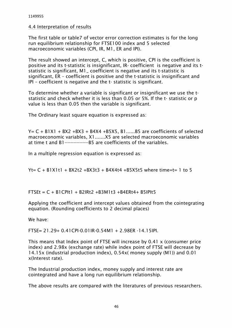
1149955
46
4.4 Interpretation of results The first table or table7 of vector error correction estimates is for the long run equilibrium relationship for FTSE100 index and 5 selected macroeconomic variables (CPI, IR, M1, ER and IPI). The result showed an intercept, C, which is positive, CPI is the coefficient is positive and its t-statistic is insignificant, IR- coefficient is negative and its t-statistic is significant, M1_ coefficient is negative and its t-statistic is significant, ER – coefficient is positive and the t-statistic is insignificant and IPI – coefficient is negative and the t- statistic is significant. To determine whether a variable is significant or insignificant we use the t- statistic and check whether it is less than 0.05 or 5%. If the t- statistic or p value is less than 0.05 then the variable is significant. The Ordinary least square equation is expressed as: Y= C + B1X1 + BX2 +BX3 + B4X4 +B5X5, B1......B5 are coefficients of selected macroeconomic variables, X1.......X5 are selected macroeconomic variables at time t and B1----------------B5 are coefficients of the variables. In a multiple regression equation is expressed as: Yt= C + B1X1t1 + BX2t2 +BX3t3 + B4X4t4 +B5X5t5 where time=t= 1 to 5 FTSEt = C + B1CPIt1 + B2IRt2 +B3M1t3 +B4ERt4+ B5IPIt5 Applying the coefficient and intercept values obtained from the cointegrating equation. (Rounding coefficients to 2 decimal places) We have: FTSE= 21.29+ 0.41CPI-0.01IR-0.54M1 + 2.98ER -14.15IPI. This means that Index point of FTSE will increase by 0.41 x (consumer price index) and 2.98x (exchange rate) while index point of FTSE will decrease by 14.15x (industrial production index), 0.54x( money supply (M1)) and 0.01 x(Interest rate). The Industrial production index, money supply and interest rate are cointegrated and have a long run equilibrium relationship. The above results are compared with the literatures of previous researchers.

1149955
47
Consumer price index which is a proxy for inflation, this shows that inflation is positive relationship with FTSE100 index and this agrees with Firth (1979), Ratanapakorn and Sharma (2007) and Hassan (2008). Firth(1979) and conducted empirical research about inflation and stock return of UK. Also Ratanapakorn and Sharma(2007) reported a positive relationship of inflation and US stock price index. This means inflation and FTSE100 index move together, increase in inflation means increase in stock prices of FTSE100 but inflation is insignificant which means inflation will not have effect on FTSE100 prices. At the moment, current inflation rate is set at 0.00% on 5th March 2015 for UK (Trading Economics, 2015). So inflation will not affect UK and this will in turn not have affect on FTSE100 index. Interest rate is negative relationship with FTSE100 index, if interest rate value is more negative it will increase FTSE100 index and if is more positive it will decrease FTSE100 index. Asprem (1989), Sohail and Zahir (2010) and Talla (2013) reported negative relationships in their researches. All researchers in my literature review had negative relationships. According to Trading Economics (2015), the current interest rate is set at 0.50% on 9 April 2015 by bank of England policy committee and it is same with bank rate. This implies that interest rate will be low and negative movement with FTSE100 index. Money supply has a negative relationship with FTSE100 index. The more negative the M1 value the higher FTSE100 index or stock return. The more positive M1 value the lower the stock price of FTSE100 or stock return. The negative relationship of money supply and stock price agrees with Sohail and Zahir (2010). Their research was on Karachi stock exchange. Exchange rate has a positive relationship with FTSE100 index by 2.98. Exchange rate will triple the FTSE100 index. This means increase in exchange rate will connote increase in FTSE100 price index. This result agree with Aggarwal (1981), Ratanapakorn and Sharma (2007), Sohail and Zahir (2010) and Khan et al. (2011). Finally Industrial production index showed a negative relationship with FTSE100 index by14 time downward return for FTSE100 stock return. This agrees with empirical result by Forson and Janrattanagul (2014). The more positive the IPI value the lower the stock return and the more negative the value of IPI the higher the stock return. The second Table (Table 8) of vector error correction estimates is the short run adjustments of cointegrated variables and this can be written in equation form as: 0.007206 D(FTSE) =0.000561D(CPI)– 0.003435 D(IR) -0.000357D(M1) – 0.000326 D(ER) +0.085713D(IPI)

1149955
48
The adjusted coefficient of consumer price index is (+0.000561). As CPI changes the FTSE changes which implies∆ CPI causes ∆ FTSE. This means that the movement of consumer price index adjust in the short run, approaches its long-term equilibrium value in the long run. The adjusted coefficient of interest rate is (-0.003435) and it approaches its long run equilibrium value. As IR changes the FTSE changes which implies ∆ IR causes ∆FTSE until it reaches its long run equilibrium. The adjusted coefficient of money supply is (-0.000357) in the short run, and in long run remains negative which means there is no deviation but it increases in the long run. As money supply changes the FTSE changes which implies ∆ M1 causes ∆FTSE in the short run until it reaches it long run equilibrium. The adjusted coefficient of exchange rate is (-0.000326) it deviates in the short run by (-0.00326) from its long run equilibrium value. As exchange rate changes the FTSE changes which implies ∆ ER causes ∆FTSE, adjustment is corrected and ER coefficient reaches it equilibrium in the long run. On the other hand, the adjusted coefficient of IPI is (+0.085713) in the short run and it deviates by (+0.085713) from its long term equilibrium value in the short run. The explanatory variables or independent variables of FTSE100 index causes FTSE100 index to deviate from its equilibrium value by 0.007206. After obtaining the empirical results on how the selected macroeconomic variables affect FTSE100 index in the vector error correction model, the researcher further conducts a granger causality test to find out the cause and effect of the macroeconomic variables and FTSE100 index and also each macroeconomic variable and impact on one another. Lag length is 2 which was obtained when we determine the optimal lag length. Using F Statistics to test the null hypothesis, if the P value is more than 5% or 0.05 we cannot reject null hypothesis and we accept the null hypothesis. 4.5Granger Causality Test From the Pairwise Granger causality table (see Appendix8.7- table 14) Null Hypothesis CPI does not Granger Cause FTSE
FTSE does not Granger Cause CPI The P values are more than 5% or 0.05 so we cannot reject the above null hypotheses so we accept that CPI does not cause FTSE and FTSE does not cause CPI. There is no causality relationship between CPI and FTSE and it is bi-directional non-causation. Null hypothesis IR does not Granger Cause FTSE FTSE does not Granger Cause IR

1149955
49
We also accept the null hypothesis because the P values are greater than 0.05. No causality relationship between FTSE and IR and it is bi-directional non-causation. Also the same with next null hypothesis M1 does not Granger Cause FTSE FTSE does not Granger Cause M1 We accept the above null hypothesis, no causality relationship between M1 and FTSE and it is bi-directional non-causation. Null hypothesis ER does not Granger Cause FTSE FTSE does not Granger Cause ER The 2nd null hypothesis, the p value is less than 0.05 so we reject the NH and accept the alternative hypothesis which is FTSE does granger cause ER. The causation is unidirectional.
IPI does not Granger Cause FTSE FTSE does not Granger Cause IPI The 2nd null hypothesis, the p value is less than 0.05 so we reject the NH and accept the alternative hypothesis which is FTSE does granger cause IPI. The causation is unidirectional. Null hypothesis
IPI does not Granger Cause CPI
CPI does not Granger Cause IPI The 1st and 2nd null hypotheses, the p values are less than 0.05 so we reject the NH and accept the alternative hypotheses which are IPI does granger cause CPI and CPI does cause IPI. The causation is bi-directional. Null hypothesis
M1 does not Granger Cause IR
IR does not Granger Cause M1 The 1st null hypothesis the p value is less than 0.05 so we reject the NH and accept the alternative hypothesis which is M1 does cause IR. The causation is uni-directional.

1149955
50
Null hypothesis IPI does not Granger Cause IR
IR does not Granger Cause IPI The 2nd null hypothesis, the p value is less than 0.05 so we reject the NH and accept the alternative hypothesis which is IR does cause IPI. The causation is unidirectional. Null hypothesis ER does not Granger Cause M1 M1 does not Granger Cause ER The 1st null hypothesis, the p value is less than 0.05 so we reject the NH and accept the alternative hypothesis which is ER does cause M1. The causation is uni-directional. Null hypothesis IPI does not Granger Cause M1 M1 does not Granger Cause IPI The 2nd null hypothesis the p value is less than 0.05 so we reject the NH and accept the alternative hypothesis which is M1 does cause IPI. The causation is unidirectional.
IPI does not Granger Cause ER ER does not Granger Cause IPI The 2nd null hypothesis the p value is less than 0.05 so we reject the NH and accept the alternative hypothesis which is ER does cause IPI. The causation is unidirectional. Granger Causality results in summary Non- causation: CPI and FTSE, FTSE and IR, M1 and FTSE and the non causation is bi-directional. Causation: bi-directional: CPI and IPI Uni-directional: FTSE and ER, FTSE and IPI, M1and IR, IR and IPI, ER and M1, M1and IPI, ER and IPI. There is bi-directional causal relationship between CPI and IPI. This means consumer price index cause industrial production index and vice versa in

1149955
51
ER and M1 Exchange rate will cause money supply. This means increase in exchange rate will cause British pounds to appreciate and so there will demand for British pounds (notes and coins) and this will cause supply of British pounds and vice versa.
UK. Increase (decrease) in consumer price index will lead to increase (decrease) in Industrial production index. There is also Uni-directional causal relationship between FTSE and ER, FTSE and IPI, M1and IR, IR and IPI, ER and M1, M1and IPI, ER and IPI in UK. FTSE and ER FTSE 100 index cause Exchange rate fluctuation. This means increase (decrease) in FTSE100 index will lead to increase (decrease) in exchange rate or give exchange rate an upward/downward movement. For upward movement, the currency will appreciate and there will be demand and supply of British pounds until it reaches equilibrium state where demand equal supply then the British pound depreciates. For downward movement, the reverse is the case. FTSE and IPI FTSE100 index will cause Industrial production Index. This means increase (decrease) in FTSE100 index will cause increase (decrease) in industrial production index (see line graph of FTSE and IPI). When there is increase in stock return this will means investors are purchasing goods and this will means the industries will produce more of the goods and so the industrial production index will increase. When there is decrease in stock return this will means that investors are not purchasing goods and this will means the industries will stop to produce some certain goods and this will lead to decrease in industrial production index. M1 and IR Money Supply (M1) will cause interest rate to decrease (increase). Increase in money supply will lead to decrease in interest rate (see line graph of M1 and IR) and this will mean low inflation. The decrease in interest rate will means the required rate of return will decrease and the value of stock will increase. This will mean that stock holder will sell their stocks and buy more stocks. Excess of money supply will means investors can purchase more stock. IR and IPI Interest rate will cause industrial production index to increase or decrease. From the line graph of IR and IPI we can see that when interest rate is low or reduces it causes industrial production index to fluctuate upward and downward.

1149955
52
M1and IPI, Money supply will cause industrial production index. This means money supply or supply of money will cause industrial production to increase as there is money supply in circulation and thus industrial production index will increase and vice versa. ER and IPI Exchange rate cause industrial production index. This means increase (decrease) in exchange rate will cause increase (decrease) in industrial production index. The research question and objectives have been answered through data analysis and its interpretation. In the next chapter, the researcher will summary the results obtained from data analysis and this will conclude the research for this study.

1149955
53
Chapter 5: Summary and Conclusion In summary, this paper was to investigate the impact of macroeconomic variables on UK stock market. The UK stock market for this study was FTSE100 index. We first conducted a unit root test and the time series data for all variables were stationary at first difference except consumer price index which showed stationarity at second difference. The cointegration test using the Johansen’s cointegration test suggested that one cointegration vector existed. We then employ vector error correction model and result obtained establishes that Industrial production index, money supply and interest rate are cointegrated and have a long run equilibrium relationship. Consumer price index which is a proxy for inflation and exchange rate showed positive relationships with FTSE100 index but were insignificant while Interest rate, money supply and industrial production index showed negative and significant relationships with FTSE100 index. The granger causality relationship showed that CPI and FTSE, FTSE and IR, M1 and FTSE have no causal relationship while there existed a Uni-directional causal relationship between FTSE and ER, FTSE and IPI, M1and IR, IR and IPI, ER and M1, M1and IPI, ER and IPI and also a bi-directional causal relationship between CPI and IPI. The summary of the empirical research suggest that macroeconomic variables used in this research have impact on FTSE100 index especially industrial production index. The coefficient for Industrial production index was negative (-14) and the coefficient denotes the risk factor which means there is a risk in industrial production index which affects the FTSE100 index negatively and decreases FTSE100 index by 14. Also money supply showed negative impact on FTSE100 index and decreases FTSE100 index by 0.5. This result support the Arbitrage pricing theory which suggest that coefficients of the variables exhibit risk factors to stock market prices and this in turn affect the stock market movement. Arbitrage pricing theory suggests that there could be other factors affecting the stock prices apart from the stock market such as inflation, interest rate or other macroeconomic variables. The reason for decrease in industrial production index maybe as a result of ‘UK GDP growth at 2years low’ (Trading economics, 2015) as mining and construction falling and also slowdown in services and manufacturing. As reported by trading economics(2015), the national office of statistics recorded fall for mining sector was the largest drop at -3.2% followed by water supply and sewage at -2.8% and construction at -0.8%. Also

1149955
54
Manufacturing rose to 1.3 percent, and then fell to 2.6 percent in the last three months of 2014.
Also Appendix 8.8- fig.7 shows between 2003 and 2007 according to office of national statistics (2013) that index of manufacturing were higher than index of production. Then between 2011 and 2013, the reverse is the case, the index of manufacturing become lower than index of production, production output fell by 0.7% and manufacturing output fell by 0.4%. According to statistical bulletin August 2013 release from Office for National statistics there has been a downturn pressure on production as a result of decline in gas and oil extraction over 13 years.
To explain the reason for the money supply slightly negative by (-0.54) is because of quantitative easing or QE. This is where by the central bank stimulate the economy since interest rate is at its lowest by buying government bonds. According to BBC News (2015), the Bank of England report estimated that the £200bn ($300bn) worth of bonds it bought between March and November 2009 helped to increase the UK's annual economic output by between 1.5% and 2%. Also UK debt to GDP in 2014 by trading economics (2015) was reported high of 89.40% and this could be a contributory factor to money supply decreasing. Consumer price index showed positive relationship with FTSE100 index by (+0.4). This is because interest rate is low and this implies low inflation because a rise in interest rate will lead to a rise in inflation and this will affect consumption as the basket of goods will be expensive. As prices of goods are low because of low interest rate and low inflation, the consumer will consume more and this will indicate a positive relationship with FTSE100 index. The interest rate showed a negative relationship by (-0.01), the present value of stock price increases when interest rate is smaller. However there is risk factor exhibited by interest rate it means that if interest rate is a positive value it will affect FTSE100 index negatively and if interest rate value is a negative it will affect the FTSE100 index positively. In the UK, interest rate has been set by monetary policy committee from 2010 to date as 0.5% (Trading Economics, 2015). As the risk factor is quite small, it will not have too much effect on FTSE100 index but because the result also showed that interest rate was significant this means interest rate should be monitored. . In granger causality test, it suggested that only CPI and IPI are bi-directional causation. The Appendix 8.9-(figure8) shows information from Office for National Statistics (2015) shows that CPI is determined by industrial production output and this will determine the inflation rate for UK. As the UK economy is gradually recovering after the recent financial crisis, the annual rate of consumer price inflation remained at a record low of 0.0% in March 2015(trading economics, 2015). Appendix 8.9- figure 8 give breaks down of the annual rate of CPI inflation since 2003 into the contributions from six broad expenditure categories. The food and drink are lower out of

1149955
55
all the broad expenditures in percentage points. The inflation rate is set as the result of the overall consumption. The higher the broad expenditures the higher the inflation rate. Also the granger causality test result suggested that FTSE100 index cause Exchange rate and industrial production index to change but no macroeconomic variables causes FTSE100 index. Therefore, the research can be concluded that three out of the five selected macroeconomic variables are relatively significant and likely to influence the FTSE100 index. These macroeconomic variables are industrial production, money supply and interest rate.

1149955
56
Chapter 6: Recommendations Based on the conclusion of my research, the FTSE100 index is affected or influenced by three macroeconomic variables. These are industrial production index, interest rate and money supply. I will recommend that further research to be conducted using different variables not used in this research. I suggest oil prices, export prices, import prices, UK government debt and foreign exchange reserve to be investigated and establish their impact on FTSE100 index. The mentioned variables relate to international trade as their impact on FTSE100 index can affect its stock return and this may slow investment in the UK. The control of oil prices is important as inflation may rise if oil prices increase and this could cause economic melt-down in the UK. Government debt determines how much spending cuts are made as the UK economy is running at a deficit according to Office of national statistics (2015) ‘Current account, income balance and net international investment position’, Released: 23 January 2015 reported that the current account deficit widened in Q3 2014, to 6.0% of nominal Gross Domestic Product GDP, representing the joint largest deficit since Office for National Statistics (ONS) records began in 1955. Also import and export are economic indicators that contribute to the growth of an economy as UK stock market import and export goods and services from and to other countries and generate financial turnovers. As industrial production index has affected FTSE100 index and industrial production was low this imply that different variables suggested may affect FTSE100 index. Investors are unlikely to invest in countries that are greatly affected by diverse macroeconomic variables so they will strategize by employing short term hedging in order to prevent losses as the observed macroeconomic variables affected FTSE100 index in the long run. Investors will decide to diversify their investments to other markets. Investors should listen to public information, such as firm announcements, economic news, or political news before making investment decisions. Policy makers should be careful when making monetary policy decisions as interest rate in the long run exhibit a risk factor to FTSE100 index. Interest rate for UK is low at the moment, in the short run it will benefit the UK economy but the reverse is the case in the long run. Also interest rate exhibiting a risk factor in the long run will cause inflation to rise and this will affect the stability of UK economy.

1149955
57
7-Reference
Aamir, M., Akram, M.N., Shafique, M.F. and Atif, M. (2011)
‘Impact of macroeconomic indicators on the stock market performance;
A case from Pakistan’, Interdisciplinary Journal of Contemporary Research
In Business, 3(7), pp.1008-1015.
Aggarwal, R. (1981) ‘Exchange Rates and Stock Prices: a Study of the US
Capital Markets under Floating Exchange Rates’, Akron Business and
Economic Review, 12(3), pp.7-12.
Asprem, M. (1989) ‘Stock Prices, Asset Portfolios and Macroeconomic Variables in Ten European Countries’, Journal of Banking and Finance, 13(4), pp. 589.
Bahm, A. J. (1993) ‘Why Axiology?’ Axiology: Science of Value, pp.3-6.
BBC News (2015) what is quantitative easing? Has QE worked elsewhere? Available at: http://www.bbc.co.uk/news/business-15198789 (Accessed: 19/05/2015).
Bloomberg (2015) Industrial production. Available at:
http://www.bloomberg.com (Accessed: 30/03/15)
Bloomberg(2015) Consumer price index. Available at:
http://www.bloomberg.com (Accessed :30/03/15)
Boyle, G.W. (1990) ‘Money Demand and Stock Market in General Equilibrium
Model with Variable Velocity, Journal of Political Economy,’ 98(5), pp.1039-
1053.
Brooks (2008) Introductory Econometrics for Finance. 2nd edn. Cambridge: University Press.

1149955
58
Büyüksalvarci, A. and Abdioglu, H. (2010) ‘The causal relationship between stock prices and macroeconomic variables: A case study for turkey’, International Journal of Economic Perspectives, 4(4), pp.601-610.
Cakan, E. (2013) ‘Non-linear causality between stock returns and inflation uncertainty: Evidence from the US and the UK’, The international business and economics research journal, 12(1), pp. 63-n/a.
Cooper, R.V. (1974) ‘Efficient Capital Markets and the Quantity Theory of Money’, Journal of Finance, 24, pp. 887-921.
Dhawan, S. (2010) Research Methodology for Business and Management Studies. Eblib [Online]. Available at: http://uel.eblib.com/patron/FullRecord.aspx?p=588276 (Accessed: 10/03/15).
Dickey, D. A. and W. A. Fuller (1979) Distribution of estimators for time series regressions with a unit root, Journal of the American Statistical association 74, pp. 427-431, JSTOR [Online]. Available at: http://www.jstor.org/(Accessed: 26/05/15)
Dickey, D. A. and W. A. Fuller (1981) Likelihood ratio statistics for autoregressive time series with a unit root, Econometrica, 49(4), p.1057.
Dritsaki, M. (2005) ‘Linkage between stock market and macroeconomic fundamentals: Case study of Athens Stock Exchange’, Journal of Financial Management and Analysis, 18(1), pp. 38-47.
Fama, E. (1970) ‘Efficient Capital Markets: A Review of Theory and Empirical Work’, The Journal of Finance, 25(2), pp. 383-417.
Fama, E.F. and Schwert, W., (1977) ‘Asset returns and inflation’, Journal of Financial Economics, Vol. 5(2), pp. 115-146.
Firth, M. (1979) ‘The relationship between stock market returns and rates of
inflation’, Journal of Finance, Vol. 34(3), pp.743-749.
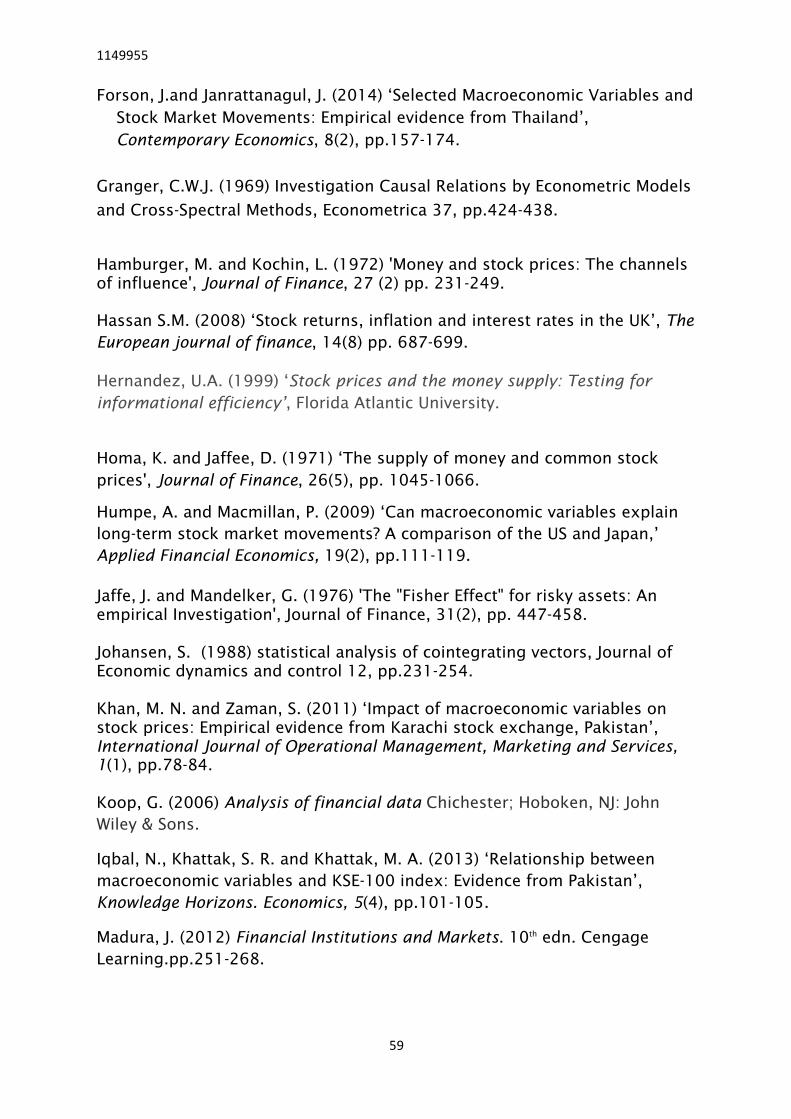
1149955
59
Forson, J.and Janrattanagul, J. (2014) ‘Selected Macroeconomic Variables and Stock Market Movements: Empirical evidence from Thailand’, Contemporary Economics, 8(2), pp.157-174.
Granger, C.W.J. (1969) Investigation Causal Relations by Econometric Models
and Cross-Spectral Methods, Econometrica 37, pp.424-438.
Hamburger, M. and Kochin, L. (1972) 'Money and stock prices: The channels of influence', Journal of Finance, 27 (2) pp. 231-249. Hassan S.M. (2008) ‘Stock returns, inflation and interest rates in the UK’, The European journal of finance, 14(8) pp. 687-699.
Hernandez, U.A. (1999) ‘Stock prices and the money supply: Testing for informational efficiency’, Florida Atlantic University.
Homa, K. and Jaffee, D. (1971) ‘The supply of money and common stock prices', Journal of Finance, 26(5), pp. 1045-1066.
Humpe, A. and Macmillan, P. (2009) ‘Can macroeconomic variables explain long-term stock market movements? A comparison of the US and Japan,’ Applied Financial Economics, 19(2), pp.111-119. Jaffe, J. and Mandelker, G. (1976) 'The "Fisher Effect" for risky assets: An empirical Investigation', Journal of Finance, 31(2), pp. 447-458. Johansen, S. (1988) statistical analysis of cointegrating vectors, Journal of Economic dynamics and control 12, pp.231-254. Khan, M. N. and Zaman, S. (2011) ‘Impact of macroeconomic variables on stock prices: Empirical evidence from Karachi stock exchange, Pakistan’, International Journal of Operational Management, Marketing and Services, 1(1), pp.78-84. Koop, G. (2006) Analysis of financial data Chichester; Hoboken, NJ: John Wiley & Sons.
Iqbal, N., Khattak, S. R. and Khattak, M. A. (2013) ‘Relationship between macroeconomic variables and KSE-100 index: Evidence from Pakistan’, Knowledge Horizons. Economics, 5(4), pp.101-105.
Madura, J. (2012) Financial Institutions and Markets. 10th edn. Cengage Learning.pp.251-268.

1149955
60
Mohi-u-Din, S. and Mubasher, H. M. (2013) ‘Macroeconomic variables on
stock market interactions: The Indian experience’, Advances in Management,
6(8), pp. 39-51.
Morley, B. and Pentecost, E. (2000) 'Common trends and cycles in G-7
countries exchange rates and stock prices', Applied Economics Letters, 7(1)
pp. 7-10.
Mishkin, F.S. (2013) Economics of money, banking and financial markets
10th edn. Pearson Education Limited ISBN9780273765851.
Naik, P.K. (2013) 'Does Stock Market Respond to Economic Fundamentals? Time-series Analysis from Indian Data', Journal of Applied Economics and Business Research, 3(1), pp.34-50.
Office for national statistics (2013) Statistical bulletin: Index of Production,
August 2013. Available at: http://www.ons.gov.uk/ons/rel/iop/index-of-
production/august-2013/stb-iop-aug-2013.html# (accessed: 8/05/15).
Office for national statistics (2015) Economic Review, May 2015 available at:
http://www.ons.gov.uk/ons/dcp171766_403187.pdf (accessed: 8/05/15).
Office for national statistics (2015) Current account, income balance and net international investment position. Exploring the deterioration in the UK’s current account in recent years. Available at: http://www.ons.gov.uk/ons/rel/bop/balance-of-payments/q3-2014/sty-current-account--income-balance-and-net-international-investment-position.html (Accessed: 27/06/15).
Pal, K. and Mittal, R. (2011) ‘Impact of macroeconomic indicators on Indian capital markets', Journal of Risk Finance (Emerald Group Publishing Limited), 12 (2), pp.84-97.
Pilinkus, D. (2010) 'Macroeconomic indicators and their impact on stock market performance in the short and long run: The case of the Baltic States', Technological & Economic Development of Economy, 16(2), pp. 291-304. Ratanapakorn, O. and Sharma, S. C. (2007) ‘Dynamic analysis between the US stock returns and the macroeconomic variables’, Applied Financial Economics, 17(5), pp. 369-377. Robert, J. G. (1993) Macroeconomics.6th edn. New York: HarperCollins College Publishers, p.12.

1149955
61
Rogalski, R. and Vinson, J. (1977) ‘Price level variations as predictors of flexible exchange rates,’ Journal of International Business Studies, 8(1), pp.71-82. Ross, Stephen (1976) ‘The arbitrage theory of capital asset pricing’, Journal of Economic Theory 13 (3), pp. 341–360. Rozeff, M. S. (1974) ‘The money supply and the stock market,’ Financial Analysts Journal, 31(5), p.18.
Sohail, N. and Zakir, H. (2010) ‘Macroeconomic policies and stock returns in Pakistan: A comparative analysis of three stock exchanges’, Journal of Advanced Studies in Finance, 1(2), pp. 181-187.
Srinivasan, P. (2011) ‘Causal nexus between stock market return and selected macroeconomic variables in India: Evidence from the national stock exchange (NSE)’, IUP Journal of Financial Risk Management, 8(4), pp.7-24. Talla, T.J. (2013) Impact of Macroeconomic Variables on the Stock Market Prices of the Stockholm Stock Exchange (OMXS30). Unpublished MSc Thesis Jönköping University. Available at: http://www.diva-portal.org/smash/get/diva2:630705/FULLTEXT02 (Accessed: 19/03/15).
Trading Economics (2015) UK interest rate. Available at: http://www.tradingeconomics.com/united-kingdom/interest-rate (accessed: 25/03/15).
Trading Economics (2015) UK inflation rate. Available at: http://www.tradingeconomics.com/united-kingdom/inflation-cpi (accessed: 25/03/15).
Trading Economics (2015) UK interest rate. Available at: http://www.tradingeconomics.com/united-kingdom/interest-rate (accessed: 25/04/15).
Trading Economics (2015) UK GDP Growth at 2-Year Low. Available at: http://www.tradingeconomics.com/united-kingdom/gdp-growth-annual (accessed: 8/05/15).
Trading Economics (2015) United Kingdom Government debt to GDP. Available at: http://www.tradingeconomics.com/united-kingdom/government-debt-to-gdp (accessed: 20/06/15).

1149955
62
Vanita, T. and Khushboo, A. (2015) ‘Long Run Co-integrating Relationship between Exchange Rate and Stock Prices: Empirical Evidence from BRICS Countries’, Advances in Management, 8(1), pp. 15-25.
Zakaria, Z. and Shamsuddin, S. (2012) 'Empirical Evidence on the Relationship between Stock Market Volatility and Macroeconomics Volatility in Malaysia', Journal Of Business Studies Quarterly, 4(2), pp. 61-71.

1149955
63
8 Appendix
8.1- tables 8: Eviews Output - Descriptive statistics summary tables for all variables
Date: 03/31/15 Time: 20:45
Sample: 1995M03 2014M12 CPI Mean 2.010676
Median 1.995580 Maximum 2.109035 Minimum 1.930949 Std. Dev. 0.052672 Skewness 0.474182 Kurtosis 1.954009
Jarque-Bera 19.76877 Probability 0.000051
Sum 478.5410 Sum Sq. Dev. 0.657513
Observations 238
Date: 03/31/15 Time: 20:46
Sample: 1995M03 2014M12 ER Mean 1.956936
Median 1.977860 Maximum 2.022057 Minimum 1.876391 Std. Dev. 0.045865 Skewness -0.333958 Kurtosis 1.519294
Jarque-Bera 26.16616 Probability 0.000002
Sum 465.7507 Sum Sq. Dev. 0.498547
Observations 238

1149955
64
Date: 03/31/15 Time: 20:47
Sample: 1995M03 2014M12 FTSE Mean 3.718603
Median 3.739726 Maximum 3.834933 Minimum 3.496431 Std. Dev. 0.083581 Skewness -0.647316 Kurtosis 2.386159
Jarque-Bera 20.35767 Probability 0.000038
Sum 885.0275 Sum Sq. Dev. 1.655645
Observations 238
Date: 03/31/15 Time: 20:47
Sample: 1995M03 2014M12 IPI Mean 2.015841
Median 2.015904 Maximum 2.082139 Minimum 1.941213 Std. Dev. 0.026824 Skewness -0.109879 Kurtosis 2.733420
Jarque-Bera 1.183638 Probability 0.553320
Sum 479.7702 Sum Sq. Dev. 0.170532
Observations 238
Date: 03/31/15 Time: 20:48
Sample: 1995M03 2014M12 IR Mean -0.811485
Median -0.811485 Maximum 0.769350 Minimum -2.453007

1149955
65
Std. Dev. 0.969750 Skewness 0.117745 Kurtosis 1.953177
Jarque-Bera 11.41699 Probability 0.003318
Sum -193.1333 Sum Sq. Dev. 222.8782
Observations 238
Date: 03/31/15 Time: 20:49
Sample: 1995M03 2014M12 M1 Mean 5.806452
Median 5.832684 Maximum 6.136534 Minimum 5.359908 Std. Dev. 0.228156 Skewness -0.336648 Kurtosis 1.832898
Jarque-Bera 18.00326 Probability 0.000123
Sum 1381.936 Sum Sq. Dev. 12.33704
Observations 238 8.2 Tables 9A: Eviews Output- unit root test at level
Null Hypothesis: CPI has a unit root Exogenous: Constant Lag Length: 13 (Automatic based on SIC, MAXLAG=14)
t-Statistic Prob.* Augmented Dickey-Fuller test statistic 0.676179 0.9914
Test critical values: 1% level -3.459494 5% level -2.874258 10% level -2.573625 *MacKinnon (1996) one-sided p-values.
Augmented Dickey-Fuller Test Equation Dependent Variable: D(CPI) Method: Least Squares Date: 03/31/15 Time: 20:24 Sample (adjusted): 1996M05 2014M12 Included observations: 224 after adjustments
Variable Coefficient Std. Error t-Statistic Prob.

1149955
66
CPI(-1) 0.001149 0.001699 0.676179 0.4997
D(CPI(-1)) 0.123079 0.068273 1.802743 0.0729 D(CPI(-2)) -0.023364 0.053278 -0.438540 0.6614 D(CPI(-3)) -0.027873 0.053270 -0.523238 0.6014 D(CPI(-4)) -0.032200 0.053248 -0.604726 0.5460 D(CPI(-5)) -0.032521 0.052798 -0.615963 0.5386 D(CPI(-6)) 0.143097 0.052951 2.702468 0.0074 D(CPI(-7)) -0.013729 0.053743 -0.255465 0.7986 D(CPI(-8)) -0.027558 0.053350 -0.516538 0.6060 D(CPI(-9)) -0.058330 0.053020 -1.100143 0.2725
D(CPI(-10)) -0.027190 0.053022 -0.512802 0.6086 D(CPI(-11)) -0.049646 0.053021 -0.936347 0.3502 D(CPI(-12)) 0.626340 0.053273 11.75719 0.0000 D(CPI(-13)) -0.194725 0.068136 -2.857861 0.0047
C -0.001895 0.003320 -0.570828 0.5687 R-squared 0.570679 Mean dependent var 0.000729
Adjusted R-squared 0.541921 S.D. dependent var 0.001557 S.E. of regression 0.001054 Akaike info criterion -10.80842 Sum squared resid 0.000232 Schwarz criterion -10.57997 Log likelihood 1225.544 Hannan-Quinn criter. -10.71621 F-statistic 19.84394 Durbin-Watson stat 2.033880 Prob(F-statistic) 0.000000
Null Hypothesis: ER has a unit root Exogenous: Constant Lag Length: 1 (Automatic based on SIC, MAXLAG=14)
t-Statistic Prob.* Augmented Dickey-Fuller test statistic -1.790081 0.3849
Test critical values: 1% level -3.457984 5% level -2.873596 10% level -2.573270 *MacKinnon (1996) one-sided p-values.
Augmented Dickey-Fuller Test Equation Dependent Variable: D(ER) Method: Least Squares Date: 03/31/15 Time: 20:26 Sample (adjusted): 1995M05 2014M12 Included observations: 236 after adjustments
Variable Coefficient Std. Error t-Statistic Prob. ER(-1) -0.015652 0.008744 -1.790081 0.0747
D(ER(-1)) 0.195247 0.063810 3.059794 0.0025 C 0.030835 0.017119 1.801277 0.0730

1149955
67
R-squared 0.049681 Mean dependent var 0.000239 Adjusted R-squared 0.041524 S.D. dependent var 0.006270 S.E. of regression 0.006138 Akaike info criterion -7.335882 Sum squared resid 0.008779 Schwarz criterion -7.291850 Log likelihood 868.6340 Hannan-Quinn criter. -7.318132 F-statistic 6.090397 Durbin-Watson stat 2.017289 Prob(F-statistic) 0.002641
Null Hypothesis: FTSE has a unit root Exogenous: Constant Lag Length: 0 (Automatic based on SIC, MAXLAG=14)
t-Statistic Prob.* Augmented Dickey-Fuller test statistic -2.759539 0.0658
Test critical values: 1% level -3.457865 5% level -2.873543 10% level -2.573242 *MacKinnon (1996) one-sided p-values.
Augmented Dickey-Fuller Test Equation Dependent Variable: D(FTSE) Method: Least Squares Date: 03/31/15 Time: 20:29 Sample (adjusted): 1995M04 2014M12 Included observations: 237 after adjustments
Variable Coefficient Std. Error t-Statistic Prob. FTSE(-1) -0.046696 0.016922 -2.759539 0.0062
C 0.174986 0.062933 2.780502 0.0059 R-squared 0.031387 Mean dependent var 0.001363
Adjusted R-squared 0.027266 S.D. dependent var 0.022008 S.E. of regression 0.021706 Akaike info criterion -4.814040 Sum squared resid 0.110722 Schwarz criterion -4.784774 Log likelihood 572.4638 Hannan-Quinn criter. -4.802244 F-statistic 7.615057 Durbin-Watson stat 2.306292 Prob(F-statistic) 0.006244
Null Hypothesis: IPI has a unit root Exogenous: Constant Lag Length: 14 (Automatic based on SIC, MAXLAG=14)
t-Statistic Prob.* Augmented Dickey-Fuller test statistic -3.686081 0.0049
Test critical values: 1% level -3.459627 5% level -2.874317 10% level -2.573656 *MacKinnon (1996) one-sided p-values.

1149955
68
Augmented Dickey-Fuller Test Equation Dependent Variable: D(IPI) Method: Least Squares Date: 03/31/15 Time: 20:30 Sample (adjusted): 1996M06 2014M12 Included observations: 223 after adjustments
Variable Coefficient Std. Error t-Statistic Prob. IPI(-1) -0.226853 0.061543 -3.686081 0.0003
D(IPI(-1)) -0.698887 0.079743 -8.764226 0.0000 D(IPI(-2)) -0.470333 0.087989 -5.345350 0.0000 D(IPI(-3)) -0.018535 0.087425 -0.212008 0.8323 D(IPI(-4)) 0.018583 0.085338 0.217752 0.8278 D(IPI(-5)) 0.018758 0.081544 0.230031 0.8183 D(IPI(-6)) 0.104359 0.080465 1.296951 0.1961 D(IPI(-7)) -0.005698 0.080364 -0.070903 0.9435 D(IPI(-8)) 0.059166 0.079214 0.746916 0.4560 D(IPI(-9)) 0.018095 0.079004 0.229033 0.8191
D(IPI(-10)) -0.130740 0.078116 -1.673663 0.0957 D(IPI(-11)) -0.028591 0.077145 -0.370613 0.7113 D(IPI(-12)) 0.730437 0.074812 9.763635 0.0000 D(IPI(-13)) 0.677283 0.075317 8.992489 0.0000 D(IPI(-14)) 0.484298 0.060211 8.043352 0.0000
C 0.457437 0.124077 3.686724 0.0003 R-squared 0.866691 Mean dependent var -4.77E-05
Adjusted R-squared 0.857031 S.D. dependent var 0.032913 S.E. of regression 0.012445 Akaike info criterion -5.865999 Sum squared resid 0.032058 Schwarz criterion -5.621538 Log likelihood 670.0589 Hannan-Quinn criter. -5.767312 F-statistic 89.71881 Durbin-Watson stat 1.932485 Prob(F-statistic) 0.000000
Null Hypothesis: IR has a unit root Exogenous: Constant Lag Length: 0 (Automatic based on SIC, MAXLAG=14)
t-Statistic Prob.* Augmented Dickey-Fuller test statistic -0.077316 0.9493
Test critical values: 1% level -3.457865 5% level -2.873543 10% level -2.573242 *MacKinnon (1996) one-sided p-values.
Augmented Dickey-Fuller Test Equation Dependent Variable: D(IR) Method: Least Squares Date: 03/31/15 Time: 20:34 Sample (adjusted): 1995M04 2014M12 Included observations: 237 after adjustments
Variable Coefficient Std. Error t-Statistic Prob. IR(-1) -0.000258 0.003340 -0.077316 0.9384

1149955
69
C -0.013439 0.004193 -3.205275 0.0015 R-squared 0.000025 Mean dependent var -0.013232
Adjusted R-squared -0.004230 S.D. dependent var 0.049449 S.E. of regression 0.049554 Akaike info criterion -3.163122 Sum squared resid 0.577056 Schwarz criterion -3.133856 Log likelihood 376.8300 Hannan-Quinn criter. -3.151326 F-statistic 0.005978 Durbin-Watson stat 1.687981 Prob(F-statistic) 0.938438
Null Hypothesis: M1 has a unit root Exogenous: Constant Lag Length: 0 (Automatic based on SIC, MAXLAG=14)
t-Statistic Prob.* Augmented Dickey-Fuller test statistic -2.485558 0.1203
Test critical values: 1% level -3.457865 5% level -2.873543 10% level -2.573242 *MacKinnon (1996) one-sided p-values.
Augmented Dickey-Fuller Test Equation Dependent Variable: D(M1) Method: Least Squares Date: 03/31/15 Time: 20:33 Sample (adjusted): 1995M04 2014M12 Included observations: 237 after adjustments
Variable Coefficient Std. Error t-Statistic Prob. M1(-1) -0.003824 0.001539 -2.485558 0.0136
C 0.025456 0.008938 2.848011 0.0048 R-squared 0.025616 Mean dependent var 0.003257
Adjusted R-squared 0.021470 S.D. dependent var 0.005439 S.E. of regression 0.005380 Akaike info criterion -7.603889 Sum squared resid 0.006802 Schwarz criterion -7.574623 Log likelihood 903.0609 Hannan-Quinn criter. -7.592093 F-statistic 6.177998 Durbin-Watson stat 2.080398 Prob(F-statistic) 0.013631
8.2- Tables 9B: Eviews Output Unit root test at first difference Null Hypothesis: D(CPI) has a unit root Exogenous: Constant Lag Length: 12 (Automatic based on SIC, MAXLAG=14)
t-Statistic Prob.* Augmented Dickey-Fuller test statistic -2.443760 0.1310
Test critical values: 1% level -3.459494 5% level -2.874258 10% level -2.573625

1149955
70
*MacKinnon (1996) one-sided p-values.
Augmented Dickey-Fuller Test Equation Dependent Variable: D(CPI,2) Method: Least Squares Date: 03/31/15 Time: 20:36 Sample (adjusted): 1996M05 2014M12 Included observations: 224 after adjustments
Variable Coefficient Std. Error t-Statistic Prob. D(CPI(-1)) -0.498188 0.203861 -2.443760 0.0154
D(CPI(-1),2) -0.376058 0.205497 -1.829994 0.0687 D(CPI(-2),2) -0.391870 0.195026 -2.009328 0.0458 D(CPI(-3),2) -0.412206 0.184894 -2.229419 0.0268 D(CPI(-4),2) -0.436817 0.175594 -2.487651 0.0136 D(CPI(-5),2) -0.462383 0.167239 -2.764803 0.0062 D(CPI(-6),2) -0.311819 0.159085 -1.960072 0.0513 D(CPI(-7),2) -0.317710 0.148563 -2.138551 0.0336 D(CPI(-8),2) -0.336611 0.133482 -2.521772 0.0124 D(CPI(-9),2) -0.386949 0.118300 -3.270924 0.0013
D(CPI(-10),2) -0.405763 0.102629 -3.953694 0.0001 D(CPI(-11),2) -0.447026 0.084556 -5.286750 0.0000 D(CPI(-12),2) 0.187896 0.067297 2.792048 0.0057
C 0.000347 0.000170 2.040757 0.0425 R-squared 0.800812 Mean dependent var -1.03E-05
Adjusted R-squared 0.788481 S.D. dependent var 0.002288 S.E. of regression 0.001052 Akaike info criterion -10.81517 Sum squared resid 0.000233 Schwarz criterion -10.60194 Log likelihood 1225.299 Hannan-Quinn criter. -10.72910 F-statistic 64.94458 Durbin-Watson stat 2.030838 Prob(F-statistic) 0.000000
Null Hypothesis: D(ER) has a unit root Exogenous: Constant Lag Length: 0 (Automatic based on SIC, MAXLAG=14)
t-Statistic Prob.* Augmented Dickey-Fuller test statistic -12.62661 0.0000
Test critical values: 1% level -3.457984 5% level -2.873596 10% level -2.573270 *MacKinnon (1996) one-sided p-values.
Augmented Dickey-Fuller Test Equation Dependent Variable: D(ER,2) Method: Least Squares Date: 03/31/15 Time: 20:37 Sample (adjusted): 1995M05 2014M12 Included observations: 236 after adjustments
Variable Coefficient Std. Error t-Statistic Prob. D(ER(-1)) -0.808949 0.064067 -12.62661 0.0000

1149955
71
C 0.000200 0.000402 0.497982 0.6190 R-squared 0.405233 Mean dependent var 3.56E-05
Adjusted R-squared 0.402691 S.D. dependent var 0.007980 S.E. of regression 0.006167 Akaike info criterion -7.330697 Sum squared resid 0.008900 Schwarz criterion -7.301343 Log likelihood 867.0223 Hannan-Quinn criter. -7.318864 F-statistic 159.4314 Durbin-Watson stat 2.012378 Prob(F-statistic) 0.000000
Null Hypothesis: D(FTSE) has a unit root Exogenous: Constant Lag Length: 0 (Automatic based on SIC, MAXLAG=14)
t-Statistic Prob.* Augmented Dickey-Fuller test statistic -18.18383 0.0000
Test critical values: 1% level -3.457984 5% level -2.873596 10% level -2.573270 *MacKinnon (1996) one-sided p-values.
Augmented Dickey-Fuller Test Equation Dependent Variable: D(FTSE,2) Method: Least Squares Date: 03/31/15 Time: 20:38 Sample (adjusted): 1995M05 2014M12 Included observations: 236 after adjustments
Variable Coefficient Std. Error t-Statistic Prob. D(FTSE(-1)) -1.171494 0.064425 -18.18383 0.0000
C 0.001574 0.001420 1.108206 0.2689 R-squared 0.585585 Mean dependent var -7.90E-05
Adjusted R-squared 0.583814 S.D. dependent var 0.033745 S.E. of regression 0.021770 Akaike info criterion -4.808156 Sum squared resid 0.110897 Schwarz criterion -4.778801 Log likelihood 569.3624 Hannan-Quinn criter. -4.796322 F-statistic 330.6518 Durbin-Watson stat 2.012805 Prob(F-statistic) 0.000000
Null Hypothesis: D(IPI) has a unit root Exogenous: Constant Lag Length: 13 (Automatic based on SIC, MAXLAG=14)
t-Statistic Prob.* Augmented Dickey-Fuller test statistic -2.684711 0.0783
Test critical values: 1% level -3.459627 5% level -2.874317 10% level -2.573656
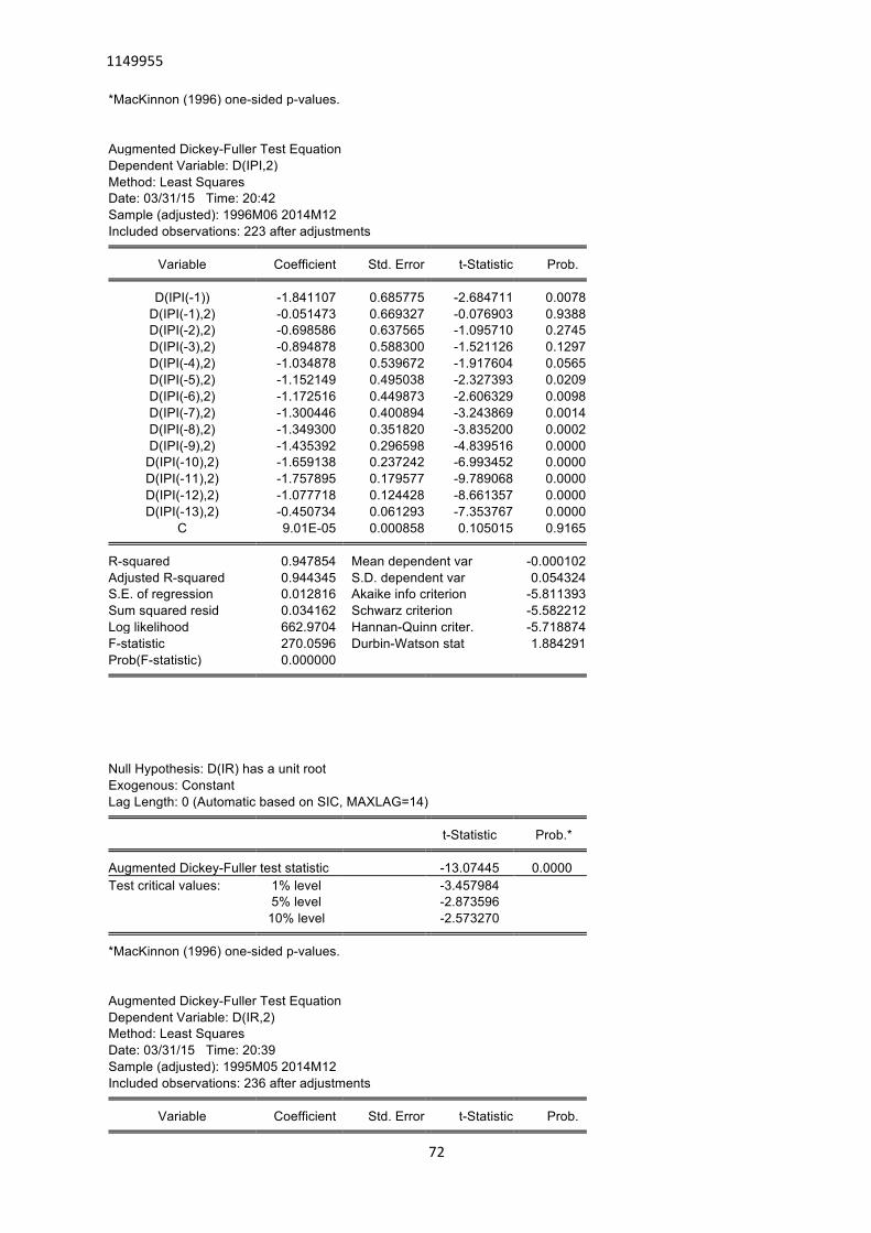
1149955
72
*MacKinnon (1996) one-sided p-values.
Augmented Dickey-Fuller Test Equation Dependent Variable: D(IPI,2) Method: Least Squares Date: 03/31/15 Time: 20:42 Sample (adjusted): 1996M06 2014M12 Included observations: 223 after adjustments
Variable Coefficient Std. Error t-Statistic Prob. D(IPI(-1)) -1.841107 0.685775 -2.684711 0.0078
D(IPI(-1),2) -0.051473 0.669327 -0.076903 0.9388 D(IPI(-2),2) -0.698586 0.637565 -1.095710 0.2745 D(IPI(-3),2) -0.894878 0.588300 -1.521126 0.1297 D(IPI(-4),2) -1.034878 0.539672 -1.917604 0.0565 D(IPI(-5),2) -1.152149 0.495038 -2.327393 0.0209 D(IPI(-6),2) -1.172516 0.449873 -2.606329 0.0098 D(IPI(-7),2) -1.300446 0.400894 -3.243869 0.0014 D(IPI(-8),2) -1.349300 0.351820 -3.835200 0.0002 D(IPI(-9),2) -1.435392 0.296598 -4.839516 0.0000
D(IPI(-10),2) -1.659138 0.237242 -6.993452 0.0000 D(IPI(-11),2) -1.757895 0.179577 -9.789068 0.0000 D(IPI(-12),2) -1.077718 0.124428 -8.661357 0.0000 D(IPI(-13),2) -0.450734 0.061293 -7.353767 0.0000
C 9.01E-05 0.000858 0.105015 0.9165 R-squared 0.947854 Mean dependent var -0.000102
Adjusted R-squared 0.944345 S.D. dependent var 0.054324 S.E. of regression 0.012816 Akaike info criterion -5.811393 Sum squared resid 0.034162 Schwarz criterion -5.582212 Log likelihood 662.9704 Hannan-Quinn criter. -5.718874 F-statistic 270.0596 Durbin-Watson stat 1.884291 Prob(F-statistic) 0.000000
Null Hypothesis: D(IR) has a unit root Exogenous: Constant Lag Length: 0 (Automatic based on SIC, MAXLAG=14)
t-Statistic Prob.* Augmented Dickey-Fuller test statistic -13.07445 0.0000
Test critical values: 1% level -3.457984 5% level -2.873596 10% level -2.573270 *MacKinnon (1996) one-sided p-values.
Augmented Dickey-Fuller Test Equation Dependent Variable: D(IR,2) Method: Least Squares Date: 03/31/15 Time: 20:39 Sample (adjusted): 1995M05 2014M12 Included observations: 236 after adjustments
Variable Coefficient Std. Error t-Statistic Prob.

1149955
73
D(IR(-1)) -0.844232 0.064571 -13.07445 0.0000 C -0.011202 0.003305 -3.388984 0.0008 R-squared 0.422138 Mean dependent var -3.31E-05
Adjusted R-squared 0.419669 S.D. dependent var 0.064389 S.E. of regression 0.049052 Akaike info criterion -3.183452 Sum squared resid 0.563016 Schwarz criterion -3.154098 Log likelihood 377.6474 Hannan-Quinn criter. -3.171619 F-statistic 170.9412 Durbin-Watson stat 2.018857 Prob(F-statistic) 0.000000
Null Hypothesis: D(M1) has a unit root Exogenous: Constant Lag Length: 0 (Automatic based on SIC, MAXLAG=14)
t-Statistic Prob.* Augmented Dickey-Fuller test statistic -15.71262 0.0000
Test critical values: 1% level -3.457984 5% level -2.873596 10% level -2.573270 Null Hypothesis: D(CPI,2) has a unit root
Exogenous: Constant Lag Length: 11 (Automatic based on SIC, MAXLAG=14)
t-Statistic Prob.* Augmented Dickey-Fuller test statistic -8.631856 0.0000
Test critical values: 1% level -3.459494 5% level -2.874258 10% level -2.573625 *MacKinnon (1996) one-sided p-values.
Augmented Dickey-Fuller Test Equation Dependent Variable: D(CPI,3) Method: Least Squares Date: 05/21/15 Time: 11:37 Sample (adjusted): 1996M05 2014M12 Included observations: 224 after adjustments
Variable Coefficient Std. Error t-Statistic Prob. D(CPI(-1),2) -8.105400 0.939010 -8.631856 0.0000
D(CPI(-1),3) 6.254914 0.892000 7.012236 0.0000 D(CPI(-2),3) 5.430113 0.833717 6.513141 0.0000 D(CPI(-3),3) 4.626296 0.765779 6.041296 0.0000 D(CPI(-4),3) 3.838796 0.688573 5.575001 0.0000 D(CPI(-5),3) 3.065620 0.601975 5.092606 0.0000 D(CPI(-6),3) 2.483988 0.506598 4.903269 0.0000 D(CPI(-7),3) 1.933892 0.407569 4.744939 0.0000 D(CPI(-8),3) 1.406281 0.312953 4.493586 0.0000 D(CPI(-9),3) 0.868502 0.223507 3.885796 0.0001
D(CPI(-10),3) 0.353181 0.140209 2.518972 0.0125 D(CPI(-11),3) -0.161842 0.067225 -2.407457 0.0169
C -3.12E-05 7.12E-05 -0.438731 0.6613 R-squared 0.931931 Mean dependent var 2.81E-06
Adjusted R-squared 0.928059 S.D. dependent var 0.003969 S.E. of regression 0.001065 Akaike info criterion -10.79606 Sum squared resid 0.000239 Schwarz criterion -10.59806 Log likelihood 1222.158 Hannan-Quinn criter. -10.71613
*MacKinnon (1996) one-sided p-values.
Augmented Dickey-Fuller Test Equation Dependent Variable: D(M1,2) Method: Least Squares Date: 03/31/15 Time: 20:41 Sample (adjusted): 1995M05 2014M12 Included observations: 236 after adjustments
Variable Coefficient Std. Error t-Statistic Prob. D(M1(-1)) -1.022178 0.065055 -15.71262 0.0000
C 0.003363 0.000412 8.158291 0.0000 R-squared 0.513399 Mean dependent var 3.88E-05
Adjusted R-squared 0.511319 S.D. dependent var 0.007774 S.E. of regression 0.005435 Akaike info criterion -7.583542 Sum squared resid 0.006912 Schwarz criterion -7.554188 Log likelihood 896.8580 Hannan-Quinn criter. -7.571709 F-statistic 246.8864 Durbin-Watson stat 1.996779 Prob(F-statistic) 0.000000

1149955
74
8.2- Table 9c: Eviews Output Unit root at second difference
Null Hypothesis: D(CPI,2) has a unit root Exogenous: Constant Lag Length: 11 (Automatic based on SIC, MAXLAG=14)
t-Statistic Prob.* Augmented Dickey-Fuller test statistic -8.631856 0.0000
Test critical values: 1% level -3.459494 5% level -2.874258 10% level -2.573625 *MacKinnon (1996) one-sided p-values.
Augmented Dickey-Fuller Test Equation Dependent Variable: D(CPI,3) Method: Least Squares Date: 05/21/15 Time: 11:37 Sample (adjusted): 1996M05 2014M12 Included observations: 224 after adjustments
Variable Coefficient Std. Error t-Statistic Prob. D(CPI(-1),2) -8.105400 0.939010 -8.631856 0.0000
D(CPI(-1),3) 6.254914 0.892000 7.012236 0.0000 D(CPI(-2),3) 5.430113 0.833717 6.513141 0.0000 D(CPI(-3),3) 4.626296 0.765779 6.041296 0.0000 D(CPI(-4),3) 3.838796 0.688573 5.575001 0.0000 D(CPI(-5),3) 3.065620 0.601975 5.092606 0.0000 D(CPI(-6),3) 2.483988 0.506598 4.903269 0.0000 D(CPI(-7),3) 1.933892 0.407569 4.744939 0.0000 D(CPI(-8),3) 1.406281 0.312953 4.493586 0.0000 D(CPI(-9),3) 0.868502 0.223507 3.885796 0.0001
D(CPI(-10),3) 0.353181 0.140209 2.518972 0.0125 D(CPI(-11),3) -0.161842 0.067225 -2.407457 0.0169
C -3.12E-05 7.12E-05 -0.438731 0.6613 R-squared 0.931931 Mean dependent var 2.81E-06
Adjusted R-squared 0.928059 S.D. dependent var 0.003969 S.E. of regression 0.001065 Akaike info criterion -10.79606 Sum squared resid 0.000239 Schwarz criterion -10.59806 Log likelihood 1222.158 Hannan-Quinn criter. -10.71613 F-statistic 240.7312 Durbin-Watson stat 2.016340 Prob(F-statistic) 0.000000
8.3- Table10: Eviews Output Vector Autoregression Estimates
Vector Autoregression Estimates Date: 04/07/15 Time: 14:43 Sample (adjusted): 1995M05 2014M12 Included observations: 236 after adjustments Standard errors in ( ) & t-statistics in [ ]
FTSE CPI IPI ER IR M1

1149955
75
FTSE(-1) 0.818597 0.007453 -0.056037 0.059619 -0.040666 -0.004095 (0.06610) (0.00469) (0.06635) (0.01874) (0.15000) (0.01640) [ 12.3844] [ 1.58943] [-0.84458] [ 3.18171] [-0.27110] [-0.24978]
FTSE(-2) 0.116488 -0.003606 0.126792 -0.051618 -0.011511 0.000741 (0.06631) (0.00470) (0.06656) (0.01880) (0.15048) (0.01645) [ 1.75669] [-0.76656] [ 1.90489] [-2.74593] [-0.07649] [ 0.04505]
CPI(-1) -0.892974 0.859409 6.113167 0.187442 0.092154 -0.019560 (0.93699) (0.06647) (0.94053) (0.26562) (2.12637) (0.23242) [-0.95302] [ 12.9299] [ 6.49971] [ 0.70567] [ 0.04334] [-0.08416]
CPI(-2) 1.092678 0.109248 -6.098358 -0.193421 -0.451500 0.090842 (0.92248) (0.06544) (0.92596) (0.26151) (2.09342) (0.22881) [ 1.18451] [ 1.66952] [-6.58601] [-0.73964] [-0.21568] [ 0.39701]
IPI(-1) 0.107432 0.007578 0.024311 0.010622 -0.114694 -0.014698 (0.05915) (0.00420) (0.05937) (0.01677) (0.13423) (0.01467) [ 1.81629] [ 1.80601] [ 0.40946] [ 0.63347] [-0.85446] [-1.00181]
IPI(-2) -0.102497 -0.009726 -0.252426 -0.002930 -0.265267 0.010883 (0.05861) (0.00416) (0.05883) (0.01662) (0.13301) (0.01454) [-1.74879] [-2.33943] [-4.29066] [-0.17637] [-1.99437] [ 0.74857]
ER(-1) 0.270073 0.003334 0.129389 1.179729 0.208716 -0.138659 (0.23137) (0.01641) (0.23224) (0.06559) (0.52505) (0.05739) [ 1.16730] [ 0.20314] [ 0.55714] [ 17.9869] [ 0.39752] [-2.41614]
ER(-2) -0.235670 -0.017168 0.142530 -0.204090 -0.119508 0.174871 (0.23544) (0.01670) (0.23633) (0.06674) (0.53429) (0.05840) [-1.00099] [-1.02793] [ 0.60310] [-3.05785] [-0.22368] [ 2.99442]
IR(-1) -0.038900 -0.000600 0.030856 -0.005077 1.117540 0.008798 (0.02938) (0.00208) (0.02949) (0.00833) (0.06666) (0.00729) [-1.32423] [-0.28791] [ 1.04644] [-0.60970] [ 16.7637] [ 1.20741]
IR(-2) 0.043274 0.000885 -0.037166 0.004612 -0.170591 -0.008999 (0.02893) (0.00205) (0.02904) (0.00820) (0.06566) (0.00718) [ 1.49567] [ 0.43122] [-1.27974] [ 0.56235] [-2.59814] [-1.25394]
M1(-1) 0.332273 0.003028 0.240182 0.046493 -0.878708 0.900960 (0.26913) (0.01909) (0.27015) (0.07629) (0.61076) (0.06676) [ 1.23461] [ 0.15863] [ 0.88908] [ 0.60939] [-1.43872] [ 13.4962]
M1(-2) -0.348054 0.004577 -0.303645 -0.052022 0.734267 0.079481 (0.26852) (0.01905) (0.26954) (0.07612) (0.60937) (0.06661) [-1.29618] [ 0.24030] [-1.12655] [-0.68340] [ 1.20496] [ 1.19331]
C -0.141612 0.037001 2.009081 0.045921 2.294635 -0.076844 (0.31287) (0.02219) (0.31405) (0.08869) (0.71002) (0.07761) [-0.45262] [ 1.66716] [ 6.39726] [ 0.51775] [ 3.23179] [-0.99018] R-squared 0.935099 0.999210 0.392612 0.983337 0.997613 0.999478
Adj. R-squared 0.931607 0.999168 0.359927 0.982440 0.997484 0.999450 Sum sq. resids 0.101240 0.000509 0.102005 0.008136 0.521381 0.006229 S.E. equation 0.021307 0.001511 0.021387 0.006040 0.048353 0.005285 F-statistic 267.7511 23513.40 12.01215 1096.660 7765.464 35601.25 Log likelihood 580.1140 1204.563 579.2252 877.6159 386.7130 909.1338 Akaike AIC -4.806051 -10.09799 -4.798518 -7.327253 -3.167059 -7.594354 Schwarz SC -4.615246 -9.907190 -4.607714 -7.136449 -2.976255 -7.403550 Mean dependent 3.720449 2.011341 2.015819 1.957540 -0.824123 5.810216 S.D. dependent 0.081473 0.052394 0.026733 0.045582 0.964017 0.225400

1149955
76
Determinant resid covariance (dof adj.) 1.04E-24
Determinant resid covariance 7.37E-25 Log likelihood 4547.652 Akaike information criterion -37.87841 Schwarz criterion -36.73358
8.4 Table 11: Eviews Output VAR Lag order Selection criteria
VAR Lag Order Selection Criteria Endogenous variables: FTSE IPI IR M1 ER CPI Exogenous variables: C Date: 04/07/15 Time: 15:07 Sample: 1995M03 2014M12 Included observations: 235
Lag LogL LR FPE AIC SC HQ 0 2074.745 NA 9.10e-16 -17.60634 -17.51801 -17.57073
1 4466.361 4640.753 1.79e-24 -37.65414 -37.03583* -37.40487 2 4527.829 116.1350 1.44e-24* -37.87089* -36.72260 -37.40795* 3 4563.700 65.94066* 1.44e-24 -37.86978 -36.19152 -37.19318 * indicates lag order selected by the criterion
LR: sequential modified LR test statistic (each test at 5% level) FPE: Final prediction error AIC: Akaike information criterion SC: Schwarz information criterion HQ: Hannan-Quinn information criterion
8.5- Table12: Eviews output -Johansen Cointegration Test Date: 04/07/15 Time: 15:13 Sample (adjusted): 1995M06 2014M12 Included observations: 235 after adjustments Trend assumption: Linear deterministic trend Series: FTSE ER CPI M1 IPI IR Lags interval (in first differences): 1 to 2
Unrestricted Cointegration Rank Test (Trace) Hypothesized Trace 0.05
No. of CE(s) Eigenvalue Statistic Critical Value Prob.** None * 0.347725 161.1794 95.75366 0.0000
At most 1 0.125616 60.76663 69.81889 0.2126 At most 2 0.058024 29.22132 47.85613 0.7577 At most 3 0.035945 15.17406 29.79707 0.7687 At most 4 0.024079 6.571375 15.49471 0.6279 At most 5 0.003583 0.843607 3.841466 0.3584
Trace test indicates 1 cointegrating eqn(s) at the 0.05 level * denotes rejection of the hypothesis at the 0.05 level **MacKinnon-Haug-Michelis (1999) p-values
Unrestricted Cointegration Rank Test (Maximum Eigenvalue)

1149955
77
Hypothesized Max-Eigen 0.05 No. of CE(s) Eigenvalue Statistic Critical Value Prob.**
None * 0.347725 100.4128 40.07757 0.0000
At most 1 0.125616 31.54531 33.87687 0.0925 At most 2 0.058024 14.04726 27.58434 0.8193 At most 3 0.035945 8.602687 21.13162 0.8631 At most 4 0.024079 5.727768 14.26460 0.6484 At most 5 0.003583 0.843607 3.841466 0.3584
Max-eigenvalue test indicates 1 cointegrating eqn(s) at the 0.05 level * denotes rejection of the hypothesis at the 0.05 level **MacKinnon-Haug-Michelis (1999) p-values
Unrestricted Cointegrating Coefficients (normalized by b'*S11*b=I): FTSE ER CPI M1 IPI IR
-5.891480 -17.53875 -2.413958 3.190385 83.35231 0.026585 -7.011749 30.53698 67.98956 -19.05229 -0.469072 -0.780022 10.77139 2.085023 19.06122 9.921373 5.382214 3.760786 -5.444762 -2.481476 52.56050 5.941686 -0.358734 4.180609 -13.27900 31.03857 40.79210 -1.840799 -4.122006 0.372695 -0.586542 -7.559290 -55.54593 11.67932 -0.992744 0.537747
Unrestricted Adjustment Coefficients (alpha): D(FTSE) -0.001223 -0.000378 -0.002681 0.002825 0.001133 0.000311
D(ER) 5.54E-05 0.000320 -0.000334 0.000232 -0.000802 -9.68E-05 D(CPI) -9.52E-05 -0.000426 6.41E-06 -8.80E-06 -6.33E-05 4.34E-05 D(M1) 6.06E-05 0.001292 0.000233 -0.000135 -0.000116 0.000214 D(IPI) -0.014549 0.000374 -0.000154 -0.000415 -0.000173 -4.60E-05 D(IR) 0.000583 0.000822 -0.008692 -0.005519 -0.000978 0.000348
1 Cointegrating Equation(s): Log likelihood 4533.316 Normalized cointegrating coefficients (standard error in parentheses)
FTSE ER CPI M1 IPI IR 1.000000 2.976969 0.409737 -0.541525 -14.14794 -0.004512
(0.64437) (1.54624) (0.36383) (1.27554) (0.08829)
Adjustment coefficients (standard error in parentheses) D(FTSE) 0.007206
(0.00822) D(ER) -0.000326
(0.00230) D(CPI) 0.000561
(0.00058) D(M1) -0.000357
(0.00210) D(IPI) 0.085713
(0.00798) D(IR) -0.003435
(0.01871) 2 Cointegrating Equation(s): Log likelihood 4549.089 Normalized cointegrating coefficients (standard error in parentheses)
FTSE ER CPI M1 IPI IR 1.000000 0.000000 -3.693599 0.781578 -8.376440 0.042487
(1.09093) (0.26824) (0.90128) (0.07821)

1149955
78
0.000000 1.000000 1.378361 -0.444447 -1.938717 -0.015788 (0.31957) (0.07858) (0.26401) (0.02291)
Adjustment coefficients (standard error in parentheses) D(FTSE) 0.009856 0.009910
(0.01278) (0.04913) D(ER) -0.002572 0.008810
(0.00356) (0.01370) D(CPI) 0.003546 -0.011329
(0.00087) (0.00333) D(M1) -0.009413 0.038379
(0.00316) (0.01217) D(IPI) 0.083091 0.266585
(0.01240) (0.04767) D(IR) -0.009196 0.014866
(0.02908) (0.11182) 3 Cointegrating Equation(s): Log likelihood 4556.113 Normalized cointegrating coefficients (standard error in parentheses)
FTSE ER CPI M1 IPI IR 1.000000 0.000000 0.000000 0.941891 -1.800558 0.262632
(0.35207) (1.12645) (0.08292) 0.000000 1.000000 0.000000 -0.504272 -4.392675 -0.097940
(0.15747) (0.50381) (0.03709) 0.000000 0.000000 1.000000 0.043403 1.780345 0.059602
(0.10558) (0.33781) (0.02487)
Adjustment coefficients (standard error in parentheses) D(FTSE) -0.019018 0.004321 -0.073842
(0.01956) (0.04880) (0.09773) D(ER) -0.006167 0.008114 0.015283
(0.00549) (0.01370) (0.02745) D(CPI) 0.003615 -0.011316 -0.028592
(0.00134) (0.00333) (0.00668) D(M1) -0.006900 0.038865 0.092117
(0.00488) (0.01218) (0.02439) D(IPI) 0.081429 0.266263 0.057602
(0.01914) (0.04776) (0.09565) D(IR) -0.102817 -0.003257 -0.111215
(0.04413) (0.11010) (0.22050) 4 Cointegrating Equation(s): Log likelihood 4560.414 Normalized cointegrating coefficients (standard error in parentheses)
FTSE ER CPI M1 IPI IR 1.000000 0.000000 0.000000 0.000000 12.52487 -0.016638
(3.74767) (0.07095) 0.000000 1.000000 0.000000 0.000000 -12.06225 0.051576
(2.02141) (0.03827) 0.000000 0.000000 1.000000 0.000000 2.440471 0.046733
(0.43751) (0.00828) 0.000000 0.000000 0.000000 1.000000 -15.20921 0.296499
(3.44218) (0.06517)
Adjustment coefficients (standard error in parentheses) D(FTSE) -0.034401 -0.002690 0.074655 -0.006510
(0.02076) (0.04846) (0.12066) (0.03085) D(ER) -0.007430 0.007539 0.027471 -0.007860
(0.00588) (0.01373) (0.03418) (0.00874) D(CPI) 0.003663 -0.011294 -0.029054 0.007818

1149955
79
(0.00143) (0.00334) (0.00832) (0.00213) D(M1) -0.006164 0.039201 0.085014 -0.022902
(0.00523) (0.01220) (0.03038) (0.00777) D(IPI) 0.083687 0.267292 0.035812 -0.057535
(0.02051) (0.04786) (0.11919) (0.03047) D(IR) -0.072768 0.010438 -0.401291 -0.132819
(0.04695) (0.10959) (0.27288) (0.06977) 5 Cointegrating Equation(s): Log likelihood 4563.278 Normalized cointegrating coefficients (standard error in parentheses)
FTSE ER CPI M1 IPI IR 1.000000 0.000000 0.000000 0.000000 0.000000 0.069392
(0.02420) 0.000000 1.000000 0.000000 0.000000 0.000000 -0.031277
(0.01893) 0.000000 0.000000 1.000000 0.000000 0.000000 0.063496
(0.00620) 0.000000 0.000000 0.000000 1.000000 0.000000 0.192031
(0.02117) 0.000000 0.000000 0.000000 0.000000 1.000000 -0.006869
(0.00415)
Adjustment coefficients (standard error in parentheses) D(FTSE) -0.049452 0.032489 0.120889 -0.008597 -0.121886
(0.02756) (0.06437) (0.13277) (0.03090) (0.11441) D(ER) 0.003219 -0.017353 -0.005243 -0.006383 0.005893
(0.00774) (0.01809) (0.03730) (0.00868) (0.03215) D(CPI) 0.004503 -0.013257 -0.031634 0.007935 -0.007441
(0.00190) (0.00444) (0.00916) (0.00213) (0.00790) D(M1) -0.004621 0.035595 0.080275 -0.022689 0.006228
(0.00695) (0.01623) (0.03348) (0.00779) (0.02885) D(IPI) 0.085982 0.261927 0.028760 -0.057217 -1.212813
(0.02727) (0.06368) (0.13135) (0.03057) (0.11319) D(IR) -0.059775 -0.019931 -0.441203 -0.131018 0.007445
(0.06242) (0.14578) (0.30067) (0.06999) (0.25910) 8.6 Table13: Eviews Output- Vector Error Correction Estimates Vector Error Correction Estimates Date: 04/07/15 Time: 15:22 Sample (adjusted): 1995M06 2014M12 Included observations: 235 after adjustments Standard errors in ( ) & t-statistics in [ ]
Cointegrating Eq: CointEq1 FTSE(-1) 1.000000
CPI(-1) 0.409737 (1.54624) [ 0.26499]
IR(-1) -0.004512 (0.08829) [-0.05111]
M1(-1) -0.541525 (0.36383)

1149955
80
[-1.48839]
ER(-1) 2.976969 (0.64437) [ 4.61993]
IPI(-1) -14.14794 (1.27554) [-11.0917]
C 21.29063 Error Correction: D(FTSE) D(CPI) D(IR) D(M1) D(ER) D(IPI) CointEq1 0.007206 0.000561 -0.003435 -0.000357 -0.000326 0.085713 (0.00822) (0.00058) (0.01871) (0.00210) (0.00230) (0.00798) [ 0.87664] [ 0.96448] [-0.18359] [-0.17007] [-0.14215] [ 10.7447]
D(FTSE(-1)) -0.165680 0.004701 0.009888 -0.000972 0.069639 -0.142097 (0.06715) (0.00475) (0.15285) (0.01715) (0.01876) (0.06517) [-2.46727] [ 0.98918] [ 0.06469] [-0.05669] [ 3.71287] [-2.18047]
D(FTSE(-2)) -0.021624 0.009472 -0.045329 0.009295 0.067302 -0.149085 (0.06758) (0.00478) (0.15383) (0.01726) (0.01888) (0.06559) [-0.31996] [ 1.98025] [-0.29467] [ 0.53864] [ 3.56531] [-2.27306]
D(CPI(-1)) -1.068609 -0.127613 0.552629 -0.154434 0.113395 5.898844 (0.93495) (0.06617) (2.12808) (0.23874) (0.26114) (0.90734) [-1.14295] [-1.92845] [ 0.25968] [-0.64688] [ 0.43422] [ 6.50123]
D(CPI(-2)) 0.878032 -0.150751 -1.711642 0.010199 0.096303 -2.035273 (1.01751) (0.07202) (2.31600) (0.25982) (0.28420) (0.98746) [ 0.86292] [-2.09326] [-0.73905] [ 0.03925] [ 0.33885] [-2.06111]
D(IR(-1)) -0.041900 -0.001909 0.168418 0.009284 -0.004044 0.022541 (0.02944) (0.00208) (0.06700) (0.00752) (0.00822) (0.02857) [-1.42333] [-0.91620] [ 2.51353] [ 1.23514] [-0.49187] [ 0.78901]
D(IR(-2)) 0.031993 0.003601 0.082361 -0.000246 -0.006109 0.044078 (0.02940) (0.00208) (0.06693) (0.00751) (0.00821) (0.02854) [ 1.08807] [ 1.73014] [ 1.23060] [-0.03270] [-0.74386] [ 1.54468]
D(M1(-1)) 0.420709 -0.012153 -0.938484 -0.033289 0.059828 0.217466 (0.26796) (0.01897) (0.60992) (0.06842) (0.07485) (0.26005) [ 1.57002] [-0.64076] [-1.53870] [-0.48651] [ 0.79935] [ 0.83625]
D(M1(-2)) 0.162912 -0.011470 0.298063 0.092783 -0.042696 -0.550203 (0.26819) (0.01898) (0.61044) (0.06848) (0.07491) (0.26027) [ 0.60744] [-0.60424] [ 0.48827] [ 1.35485] [-0.56997] [-2.11394]
D(ER(-1)) 0.183731 -0.000961 0.193150 -0.138772 0.169103 0.087706 (0.23721) (0.01679) (0.53993) (0.06057) (0.06626) (0.23021) [ 0.77454] [-0.05725] [ 0.35773] [-2.29104] [ 2.55223] [ 0.38099]
D(ER(-2)) 0.473212 -0.012928 0.319469 0.092387 0.052805 -0.403175 (0.23516) (0.01664) (0.53526) (0.06005) (0.06568) (0.22822) [ 2.01229] [-0.77670] [ 0.59685] [ 1.53857] [ 0.80394] [-1.76663]
D(IPI(-1)) 0.172513 0.018288 -0.072049 -0.019775 0.009059 0.270449 (0.08397) (0.00594) (0.19112) (0.02144) (0.02345) (0.08149) [ 2.05449] [ 3.07718] [-0.37698] [-0.92232] [ 0.38625] [ 3.31883]
D(IPI(-2)) 0.071085 0.007913 -0.373378 -0.007120 0.011194 -0.013505

1149955
81
(0.06245) (0.00442) (0.14215) (0.01595) (0.01744) (0.06061) [ 1.13822] [ 1.79009] [-2.62666] [-0.44651] [ 0.64175] [-0.22283]
C -0.000535 0.001024 -0.007054 0.003328 -0.000339 -0.000509 (0.00240) (0.00017) (0.00546) (0.00061) (0.00067) (0.00233) [-0.22295] [ 6.02592] [-1.29093] [ 5.42889] [-0.50480] [-0.21835] R-squared 0.114188 0.113723 0.092125 0.046737 0.145944 0.621558
Adj. R-squared 0.062082 0.061589 0.038721 -0.009338 0.095705 0.599297 Sum sq. resids 0.101102 0.000506 0.523787 0.006592 0.007888 0.095219 S.E. equation 0.021389 0.001514 0.048683 0.005461 0.005974 0.020757 F-statistic 2.191438 2.181362 1.725045 0.833474 2.905008 27.92106 Log likelihood 577.3169 1199.646 384.0344 898.1246 877.0413 584.3614 Akaike AIC -4.794186 -10.09060 -3.149229 -7.524465 -7.345033 -4.854140 Schwarz SC -4.588083 -9.884501 -2.943126 -7.318362 -7.138930 -4.648037 Mean dependent 0.001285 0.000733 -0.013300 0.003290 0.000246 -5.23E-05 S.D. dependent 0.022085 0.001563 0.049654 0.005436 0.006282 0.032791
Determinant resid covariance (dof adj.) 1.02E-24
Determinant resid covariance 7.07E-25 Log likelihood 4533.316 Akaike information criterion -37.81546 Schwarz criterion -36.49051
8.7- Table14 : Eviews Output- Granger Causality Pairwise Granger Causality Tests Date: 04/07/15 Time: 16:36 Sample: 1995M03 2014M12 Lags: 2
Null Hypothesis: Obs F-Statistic Prob. CPI does not Granger Cause FTSE 236 1.59349 0.2054
FTSE does not Granger Cause CPI 0.46533 0.6285 IR does not Granger Cause FTSE 236 0.56251 0.5706
FTSE does not Granger Cause IR 1.11825 0.3286 M1 does not Granger Cause FTSE 236 0.93018 0.3960
FTSE does not Granger Cause M1 0.63864 0.5289 ER does not Granger Cause FTSE 236 0.60467 0.5471
FTSE does not Granger Cause ER 5.18824 0.0063 IPI does not Granger Cause FTSE 236 2.96596 0.0535
FTSE does not Granger Cause IPI 3.26739 0.0399 IR does not Granger Cause CPI 236 0.24564 0.7824
CPI does not Granger Cause IR 1.72075 0.1812 M1 does not Granger Cause CPI 236 1.07340 0.3435
CPI does not Granger Cause M1 0.12380 0.8836 ER does not Granger Cause CPI 236 0.72707 0.4844
CPI does not Granger Cause ER 2.02289 0.1346 IPI does not Granger Cause CPI 236 4.40590 0.0132
CPI does not Granger Cause IPI 18.2942 4.E-08 M1 does not Granger Cause IR 236 3.72343 0.0256

1149955
82
IR does not Granger Cause M1 0.25657 0.7739 ER does not Granger Cause IR 236 0.26986 0.7637
IR does not Granger Cause ER 2.13769 0.1203 IPI does not Granger Cause IR 236 2.50584 0.0838
IR does not Granger Cause IPI 3.82723 0.0232 ER does not Granger Cause M1 236 4.28809 0.0148
M1 does not Granger Cause ER 2.30264 0.1023 IPI does not Granger Cause M1 236 1.05759 0.3490
M1 does not Granger Cause IPI 3.47423 0.0326 IPI does not Granger Cause ER 236 0.62504 0.5361
ER does not Granger Cause IPI 21.6960 2.E-09
8.8- figure 7 : Quarterly seasonally adjusted production and manufacturing Source: Office for National Statistics

1149955
83
8.9- Figure 8: Consumer Price Index inflation (%) and contributions from broad expenditure categories (percentage points). Source: Office for National Statistics