9/9/2011 Classical Control 1

MM9 Frequency Response Analysis (II) – Nyquist Diagram

Readings: • Section 6.3 (Nyquist stability criterion, page361-375);• Section 6.4 (stability margins, page 375-383)

9/9/2011 Classical Control 2

What Have We Talked about in MM8? Bode plot analysis

How to get a Bode plot What we can gain from Bode plot

How to use bode plot for design purpose Stability margins (Gain margin and phase margin) Transient performance Steady-state performance

Matlab functions: bode(), margin()

9/9/2011 Classical Control 3

Goals for this lecture (MM9) A design example based on Bode plot

Open-loop system feature analysis Bode plot based design

Nyquist Diagram What’s Nyquist diagram? What we can gain from Nyquist diagram

Matlab functions: nyquist()

9/9/2011 Classical Control 4

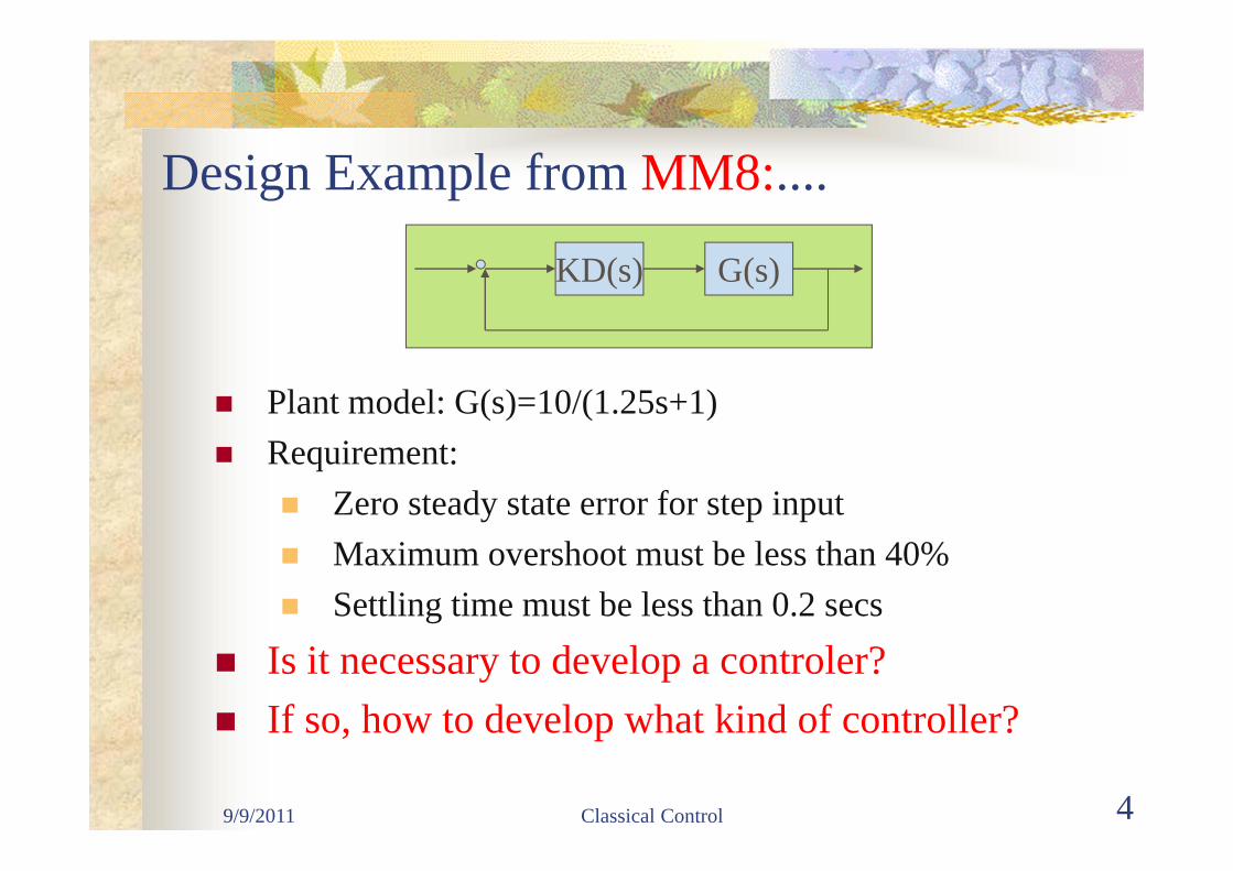
Design Example from MM8:....

Plant model: G(s)=10/(1.25s+1) Requirement:

Zero steady state error for step input Maximum overshoot must be less than 40% Settling time must be less than 0.2 secs

Is it necessary to develop a controler? If so, how to develop what kind of controller?

G(s)KD(s)

9/9/2011 Classical Control 5

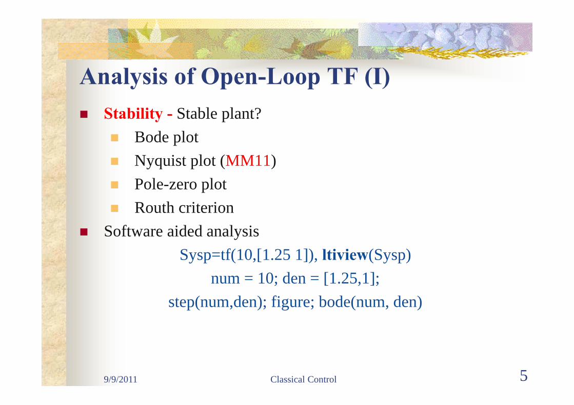
Analysis of Open-Loop TF (I) Stability - Stable plant?

Bode plot Nyquist plot (MM11) Pole-zero plot Routh criterion

Software aided analysisSysp=tf(10,[1.25 1]), ltiview(Sysp)

num = 10; den = [1.25,1]; step(num,den); figure; bode(num, den)

9/9/2011 Classical Control 6

Analysis of Open-Loop TF (II)Open-loop performance

Req1: Zero steady state error for step input?

Req2: Maximum overshoot must be less than 40%?

Req3: Settling time must be less than 0.2 secs?

num = 10; den = [1.25,1]; step(num,den); figure; bode(num, den)

9/9/2011 Classical Control 7

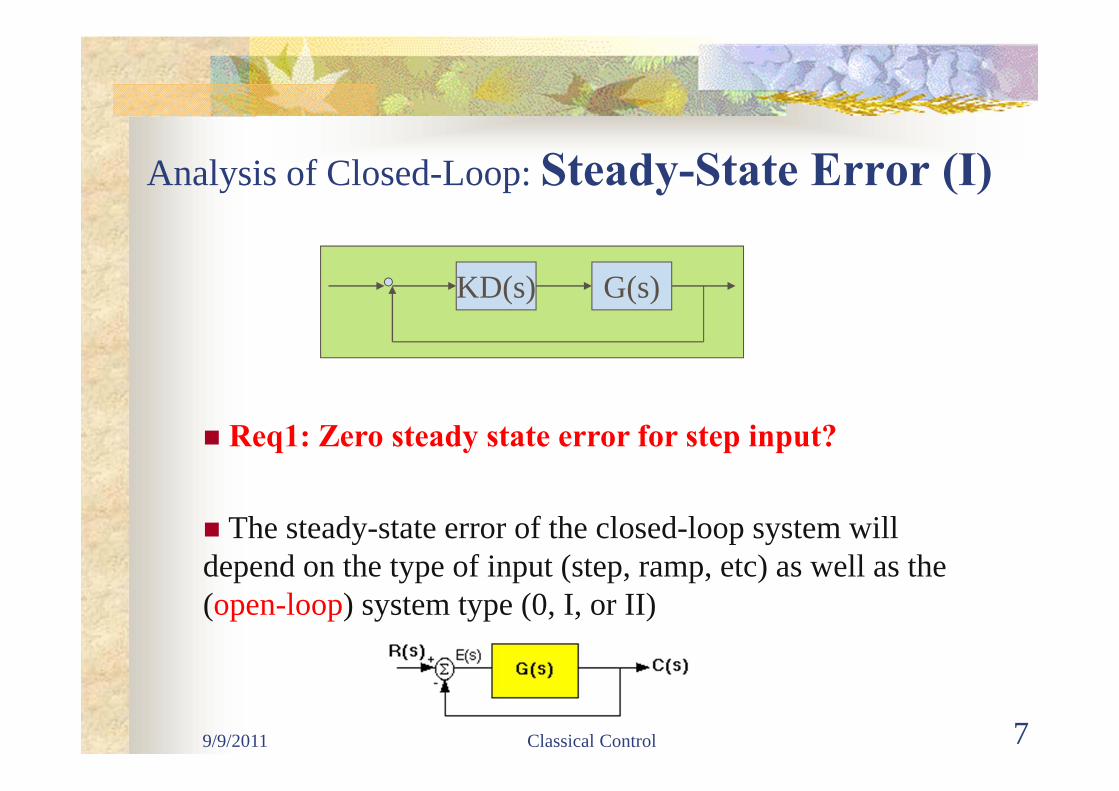
Analysis of Closed-Loop: Steady-State Error (I)

G(s)KD(s)

Req1: Zero steady state error for step input?

The steady-state error of the closed-loop system will depend on the type of input (step, ramp, etc) as well as the (open-loop) system type (0, I, or II)

9/9/2011 Classical Control 8

Revisit of System Types & Steady State Error (MM5)

Step Input (R(s) = 1/s):

Ramp Input (R(s) = 1/s^2):

Parabolic Input (R(s) = 1/s^3):

9/9/2011 Classical Control 9

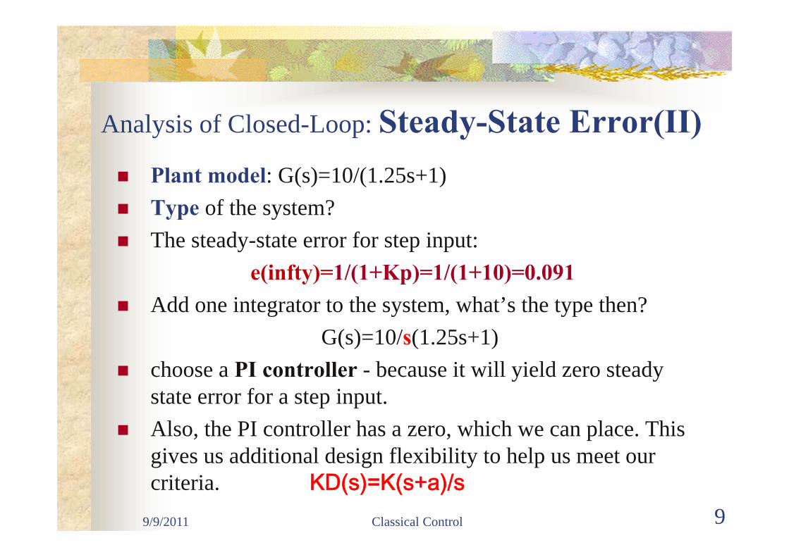
Analysis of Closed-Loop: Steady-State Error(II) Plant model: G(s)=10/(1.25s+1) Type of the system? The steady-state error for step input:

e(infty)=1/(1+Kp)=1/(1+10)=0.091 Add one integrator to the system, what’s the type then?

G(s)=10/s(1.25s+1) choose a PI controller - because it will yield zero steady

state error for a step input. Also, the PI controller has a zero, which we can place. This

gives us additional design flexibility to help us meet our criteria. KD(s)=K(s+a)/s

9/9/2011 Classical Control 10

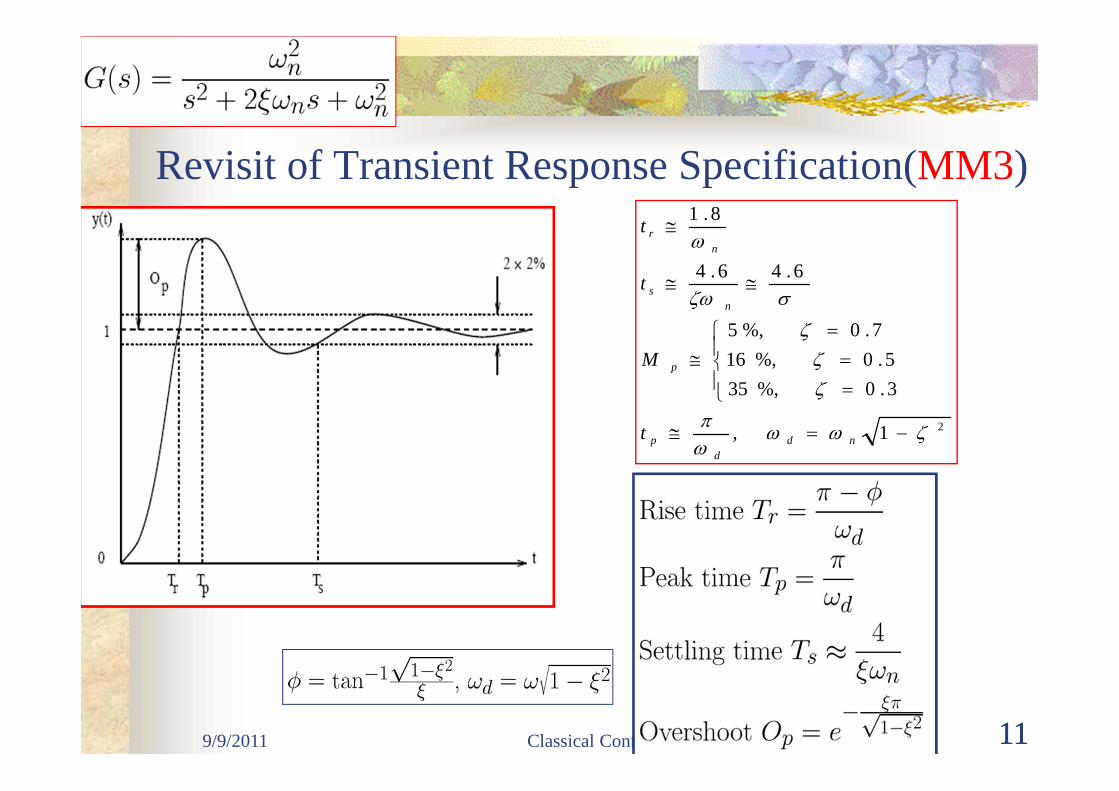
Analysis of Closed-Loop: Transient Response (I)

G(s)K(s+a)/s

Req2: Overshoot must be less than 40%? Req3: Settling time must be less than 0.2 secs?

MM3 lecture

9/9/2011 Classical Control 11

Revisit of Transient Response Specification(MM3)

11

21,

3.0%,355.0%,16

7.0%,5

6.46.4

8.1

ndd

p

p

ns

nr

t

M

t

t

9/9/2011 Classical Control 12

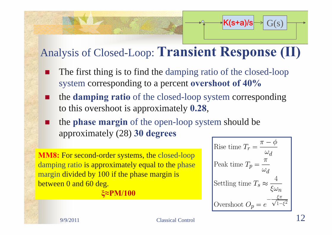
Analysis of Closed-Loop: Transient Response (II) The first thing is to find the damping ratio of the closed-loop

system corresponding to a percent overshoot of 40% the damping ratio of the closed-loop system corresponding

to this overshoot is approximately 0.28, the phase margin of the open-loop system should be

approximately (28) 30 degrees

MM8: For second-order systems, the closed-loop damping ratio is approximately equal to the phase margin divided by 100 if the phase margin is between 0 and 60 deg.

ξ≈PM/100

G(s)K(s+a)/s

9/9/2011 Classical Control 13

Analysis of Closed-Loop: Transient Response (III) The seond thing is to find the bandwidth of the closed-loop

system corresponding to a settling time 0.2 second the damping ratio corresponding to 40% overshoot is

approximately 0.28, The natural frequency of the closed-loop (bandwidth

frequency) should greater than or equal to 71 rad/sec

Relationship: wgc ≤ wbw ≤ 2wgc

num = [10]; den = [1.25, 1]; numPI = [1]; denPI = [1 0]; newnum = conv(num,numPI); newden = conv(den,denPI); margin(newnum, newden); grid

G(s)K(s+a)/s

9/9/2011 Classical Control 14

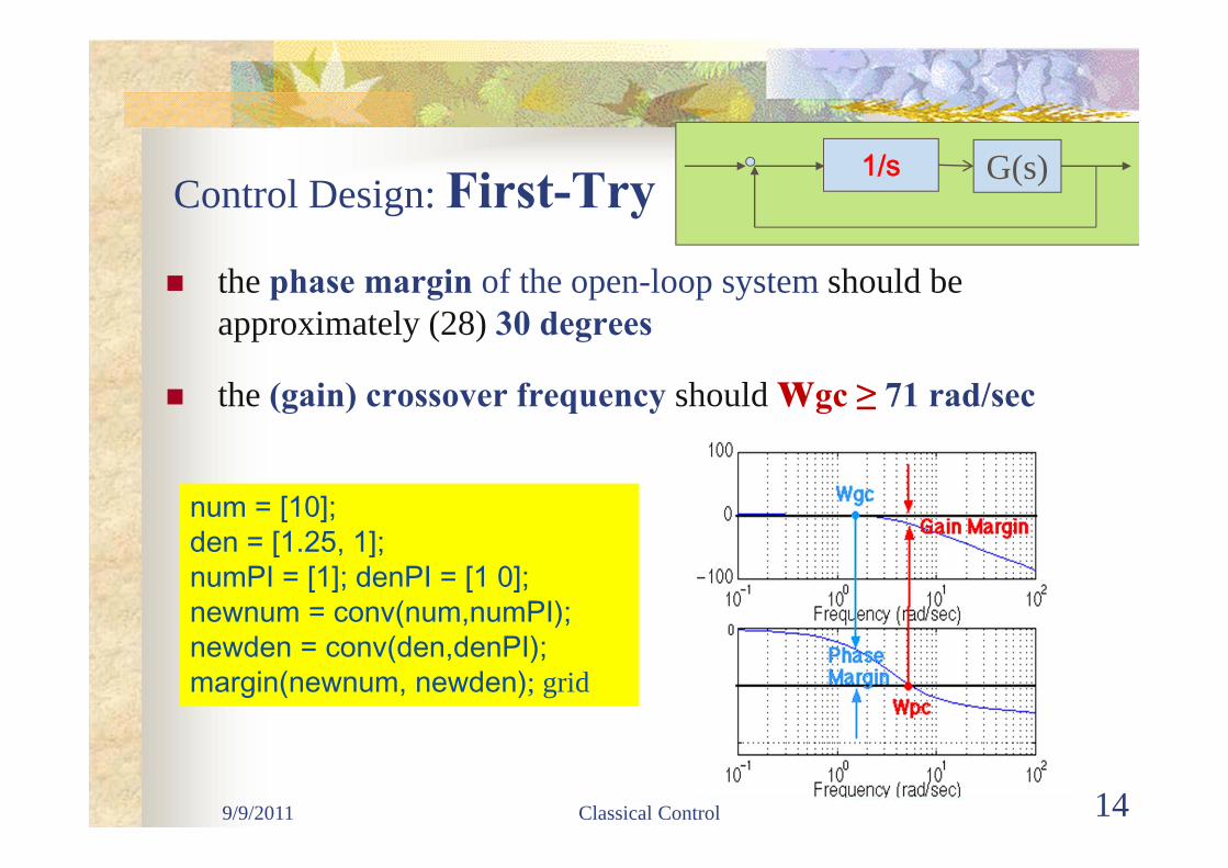
Control Design: First-Try the phase margin of the open-loop system should be

approximately (28) 30 degrees

the (gain) crossover frequency should wgc ≥ 71 rad/sec

num = [10]; den = [1.25, 1]; numPI = [1]; denPI = [1 0]; newnum = conv(num,numPI); newden = conv(den,denPI); margin(newnum, newden); grid

G(s)1/s

9/9/2011 Classical Control 15

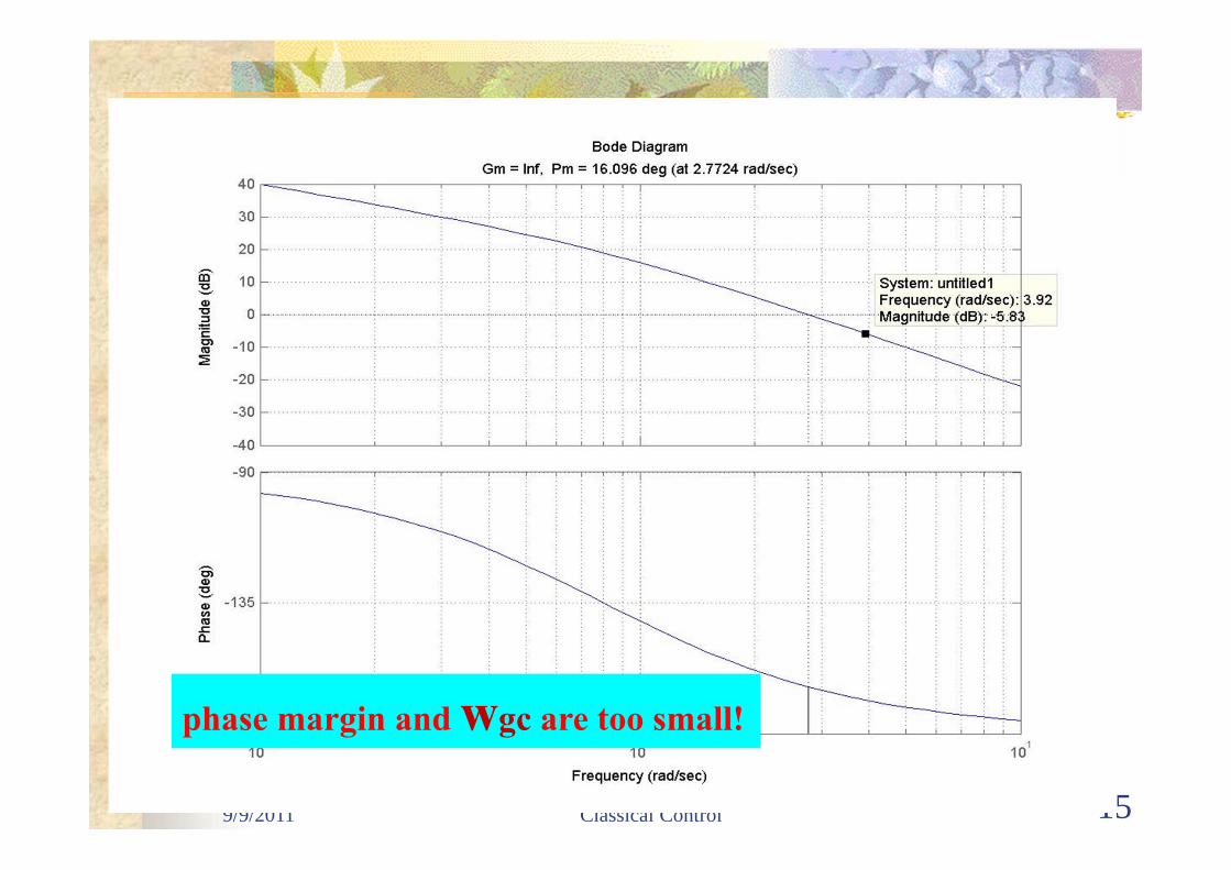
phase margin and wgc are too small!

9/9/2011 Classical Control 16

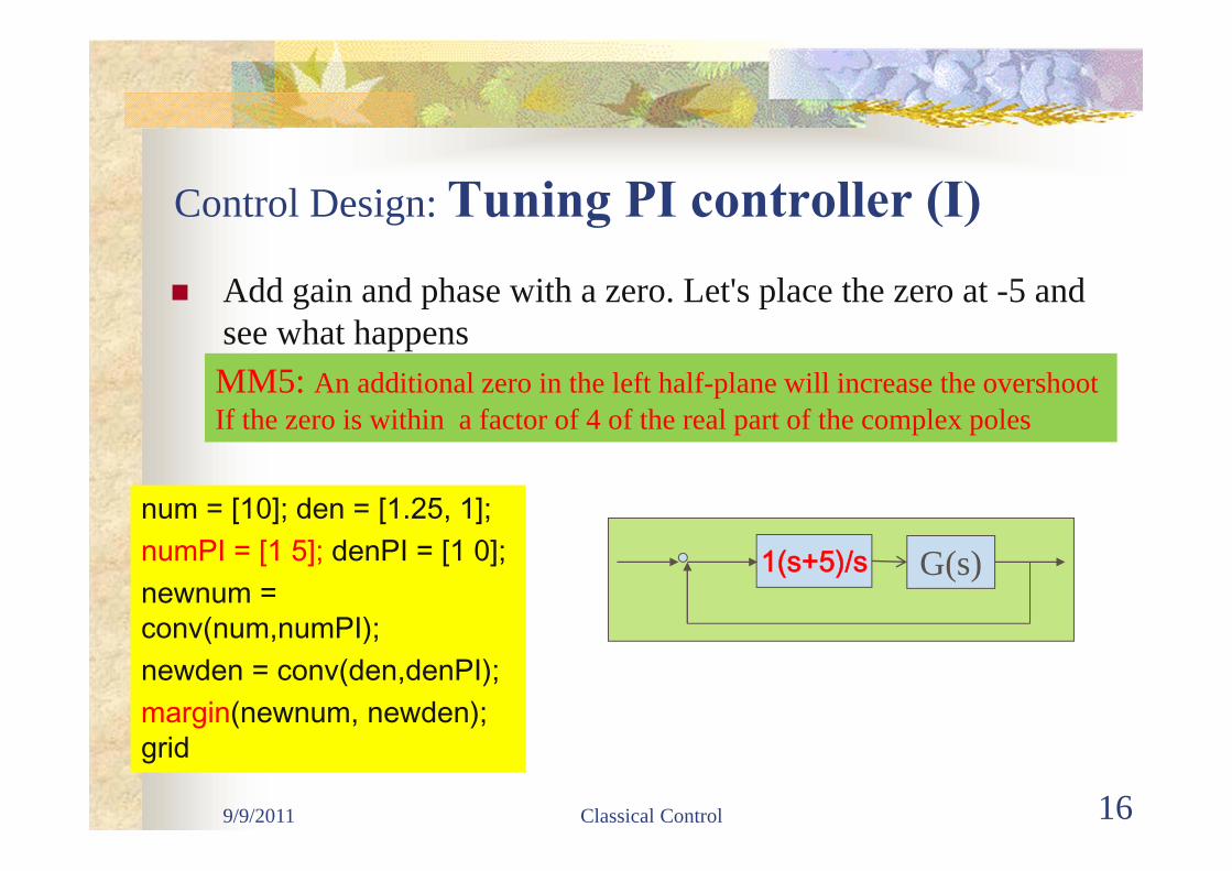
Control Design: Tuning PI controller (I) Add gain and phase with a zero. Let's place the zero at -5 and

see what happens

num = [10]; den = [1.25, 1]; numPI = [1 5]; denPI = [1 0]; newnum = conv(num,numPI); newden = conv(den,denPI); margin(newnum, newden); grid

G(s)1(s+5)/s

MM5: An additional zero in the left half-plane will increase the overshootIf the zero is within a factor of 4 of the real part of the complex poles

9/9/2011 Classical Control 17

Control Design: Tuning PI controller (II) try to get a larger crossover frequency with satisfactory phase

margin. Let's try to increase the gain to 10

num = [10]; den = [1.25, 1]; numPI = 10*[1 5]; denPI = [1 0]; newnum = conv(num,numPI); newden = conv(den,denPI); margin(newnum, newden); grid

G(s)K(s+a)/s

MM8: Adding gain only shifts the magnitude plot up. Finding the phase margin is simply the matter of finding the new cross-over frequency and reading off the phase margin

9/9/2011 Classical Control 18

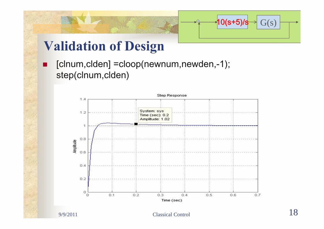
Validation of Design [clnum,clden] =cloop(newnum,newden,-1);

step(clnum,clden)

G(s)10(s+5)/s

9/9/2011 Classical Control 19

Goals for this lecture (MM9) A design example based on Bode plot

Open-loop system feature analysis Bode plot based design

Nyquist Diagram What’s Nyquist diagram? What we can gain from Nyquist diagram

Matlab functions: nyquist()

9/9/2011 Classical Control 20

Nyquist Diagram: Motivation

Motivation:to predict the stability and performance of a closed-loop system by observing its open-loop system’s feautre

Benefit:can be used for design purposes regardless of open-loop stability (remember that the Bode design methods assume that the system is stable in open loop)

http://www.engin.umich.edu/group/ctm/freq/nyq.html

9/9/2011 Classical Control 21

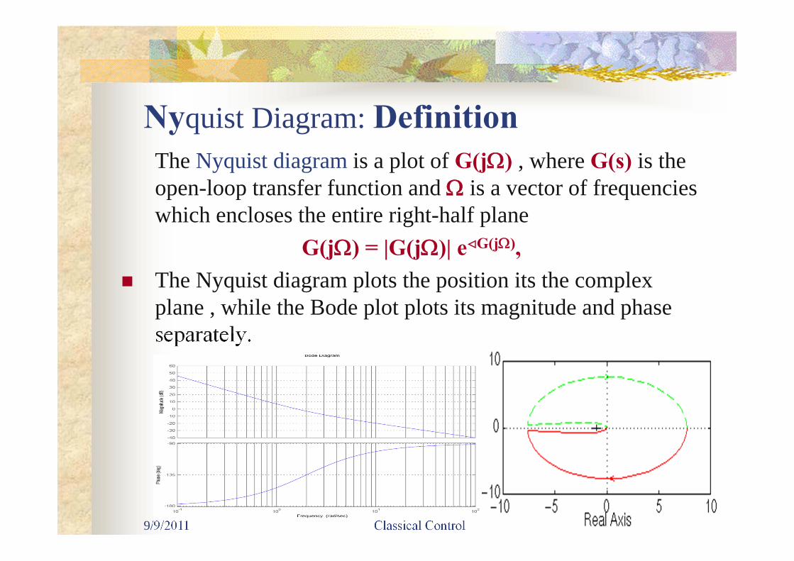
Nyquist Diagram: DefinitionThe Nyquist diagram is a plot of G(j) , where G(s) is the open-loop transfer function and is a vector of frequencies which encloses the entire right-half plane

G(j) = |G(j)| eG(j), The Nyquist diagram plots the position its the complex

plane , while the Bode plot plots its magnitude and phase separately.

9/9/2011 Classical Control 22

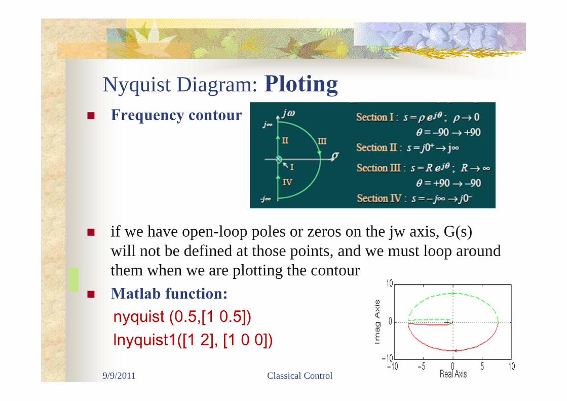
Nyquist Diagram: Ploting Frequency contour

if we have open-loop poles or zeros on the jw axis, G(s) will not be defined at those points, and we must loop around them when we are plotting the contour

Matlab function: nyquist (0.5,[1 0.5]) lnyquist1([1 2], [1 0 0])

What’s the Usefulness of Nyquist Diagram

Predict the Stability of the closed-loop based on open-loop plot

Check the stability margins Not limited by the open-loop stability

How to use that?

9/9/2011 Classical Control 23

9/9/2011 Classical Control 24

Nyquist Criterion for StabilityThe Nyquist criterion states that: P = the number of open-loop (unstable) poles of G(s)H(s) N = the number of times the Nyquist diagram encircles –1

clockwise encirclements of -1 count as positive encirclements

counter-clockwise (or anti-clockwise) encirclements of -1 count as negative encirclements

Z = the number of right half-plane (positive, real) poles of the closed-loop system

The important equation: Z = P + N

Cauchy Criterion - Complex Analysis (I) when taking a closed contour in the complex plane,

9/9/2011 Classical Control 25

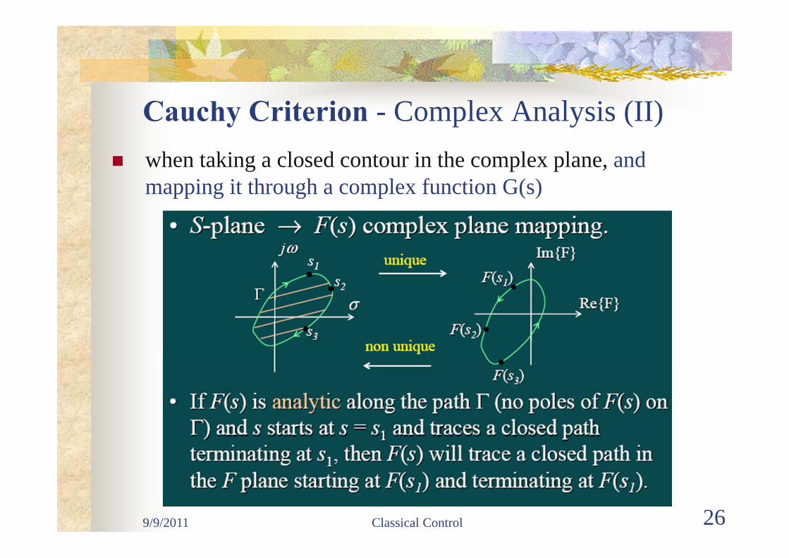
Cauchy Criterion - Complex Analysis (II) when taking a closed contour in the complex plane, and

mapping it through a complex function G(s)

9/9/2011 Classical Control 26

Cauchy Criterion - Complex Analysis (III) when taking a closed contour in the complex plane, and

mapping it through a complex function G(s) the number of times (N) that the plot of G(s) encircles the

origin is equal to the number of zeros of G(s) (Z) enclosed by the frequency contour minus the number of poles of G(s) enclosed by the frequency contour (P).

Encirclements of the origin are counted as positive if they are in the same direction as the original closed contour or negative if they are in the opposite direction.

9/9/2011 Classical Control 27

N = Z - P

Cauchy Criterion: for feedback Control (I) When studying feedback controls, the closed-loop transfer

function: Gcl(s)=G(s)/[1 + G(s)]

If 1+ G(s) encircles the origin, then G(s) will enclose the point -1

Since we are interested in the closed-loop stability, we want to know if there are any closed-loop poles (zeros of 1 + G(s)) in the right-half plane

9/9/2011 Classical Control 28

Cauchy Criterion: for feedback Control (II)

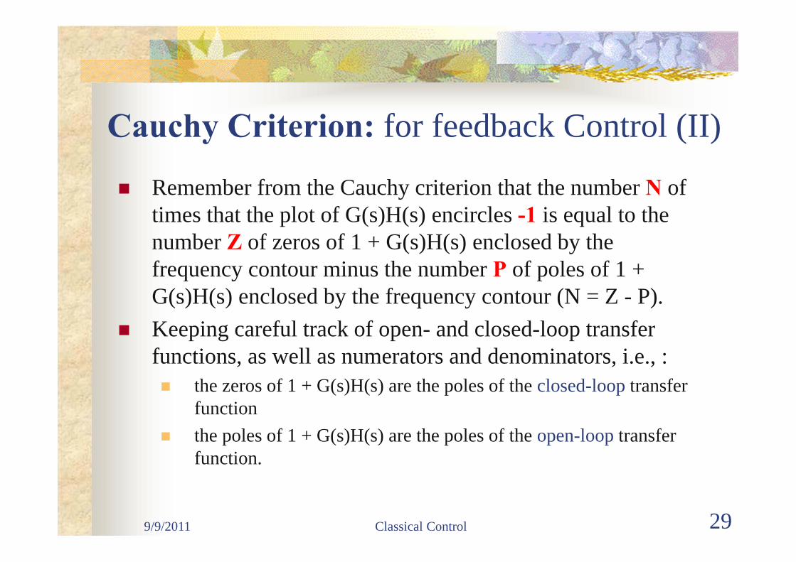
Remember from the Cauchy criterion that the number N of times that the plot of G(s)H(s) encircles -1 is equal to the number Z of zeros of 1 + G(s)H(s) enclosed by the frequency contour minus the number P of poles of 1 + G(s)H(s) enclosed by the frequency contour (N = Z - P).

Keeping careful track of open- and closed-loop transfer functions, as well as numerators and denominators, i.e., : the zeros of 1 + G(s)H(s) are the poles of the closed-loop transfer

function the poles of 1 + G(s)H(s) are the poles of the open-loop transfer

function.

9/9/2011 Classical Control 29

9/9/2011 Classical Control 30

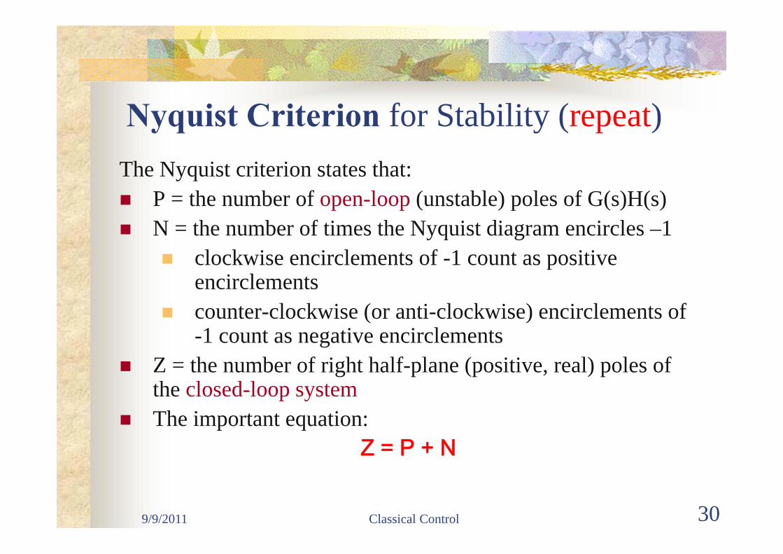
Nyquist Criterion for Stability (repeat)The Nyquist criterion states that: P = the number of open-loop (unstable) poles of G(s)H(s) N = the number of times the Nyquist diagram encircles –1

clockwise encirclements of -1 count as positive encirclements

counter-clockwise (or anti-clockwise) encirclements of -1 count as negative encirclements

Z = the number of right half-plane (positive, real) poles of the closed-loop system

The important equation: Z = P + N

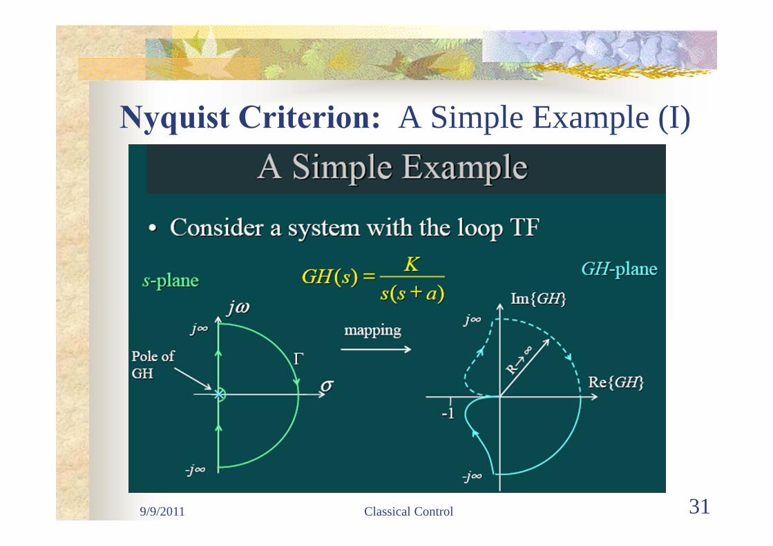
Nyquist Criterion: A Simple Example (I)

9/9/2011 Classical Control 31

Nyquist Criterion: A Simple Example (II)

9/9/2011 Classical Control 32

9/9/2011 Classical Control 33

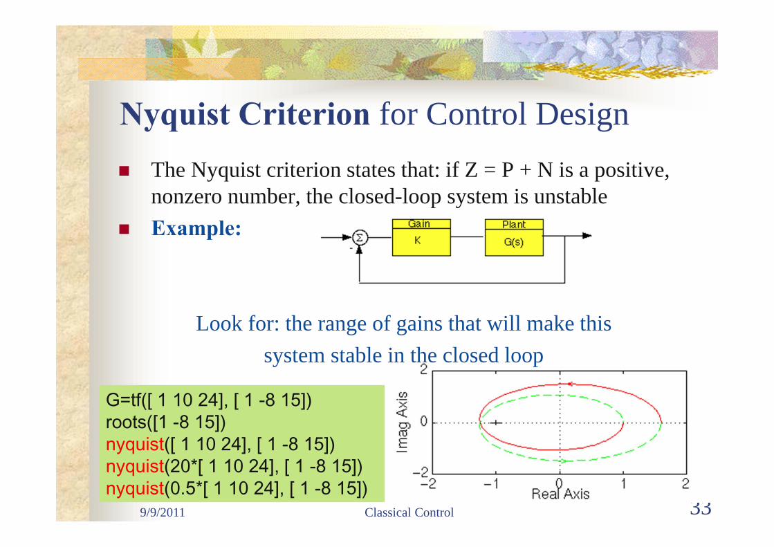
Nyquist Criterion for Control Design The Nyquist criterion states that: if Z = P + N is a positive,

nonzero number, the closed-loop system is unstable Example:

Look for: the range of gains that will make this system stable in the closed loop

G=tf([ 1 10 24], [ 1 -8 15]) roots([1 -8 15]) nyquist([ 1 10 24], [ 1 -8 15])nyquist(20*[ 1 10 24], [ 1 -8 15]) nyquist(0.5*[ 1 10 24], [ 1 -8 15])

9/9/2011 Classical Control 34

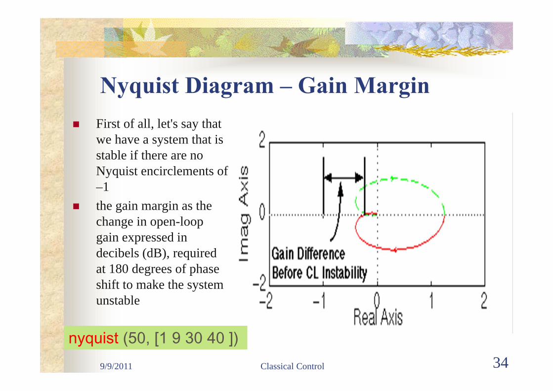
Nyquist Diagram – Gain Margin First of all, let's say that

we have a system that is stable if there are no Nyquist encirclements of –1

the gain margin as the change in open-loop gain expressed in decibels (dB), required at 180 degrees of phase shift to make the system unstable

nyquist (50, [1 9 30 40 ])

9/9/2011 Classical Control 35

Nyquist Diagram – Phase Margin First of all, let's say that

we have a system that is stable if there are no Nyquist encirclements of –1

the phase margin as the change in open-loop phase shift required at unity gain to make a closed-loop system unstable.

nyquist (50, [1 9 30 40 ])

9/9/2011 Classical Control 36

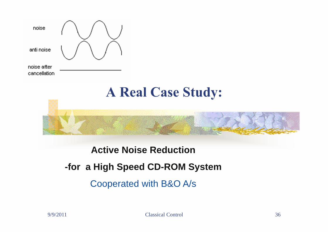
A Real Case Study:

Active Noise Reduction

-for a High Speed CD-ROM System

Cooperated with B&O A/s

9/9/2011 Classical Control 37

Active and Passive Approaches for ANR

The effective areas of passive and active reduction:

9/9/2011 Classical Control 38

Feedback ANR

9/9/2011 Classical Control 39

Testing facility

9/9/2011 Classical Control 40

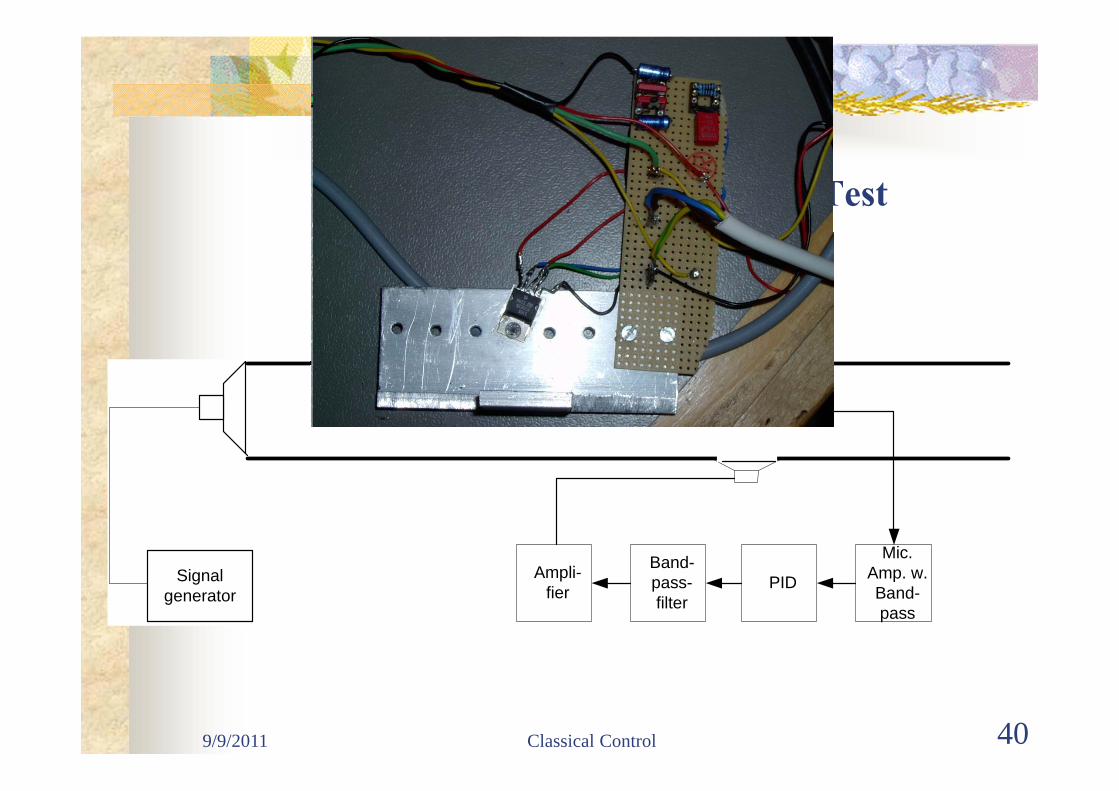
3 Controller Design – Test

Mic.Amp. w.Band-pass

PIDBand-pass-filter

Ampli-fier

Signalgenerator

9/9/2011 Classical Control 41

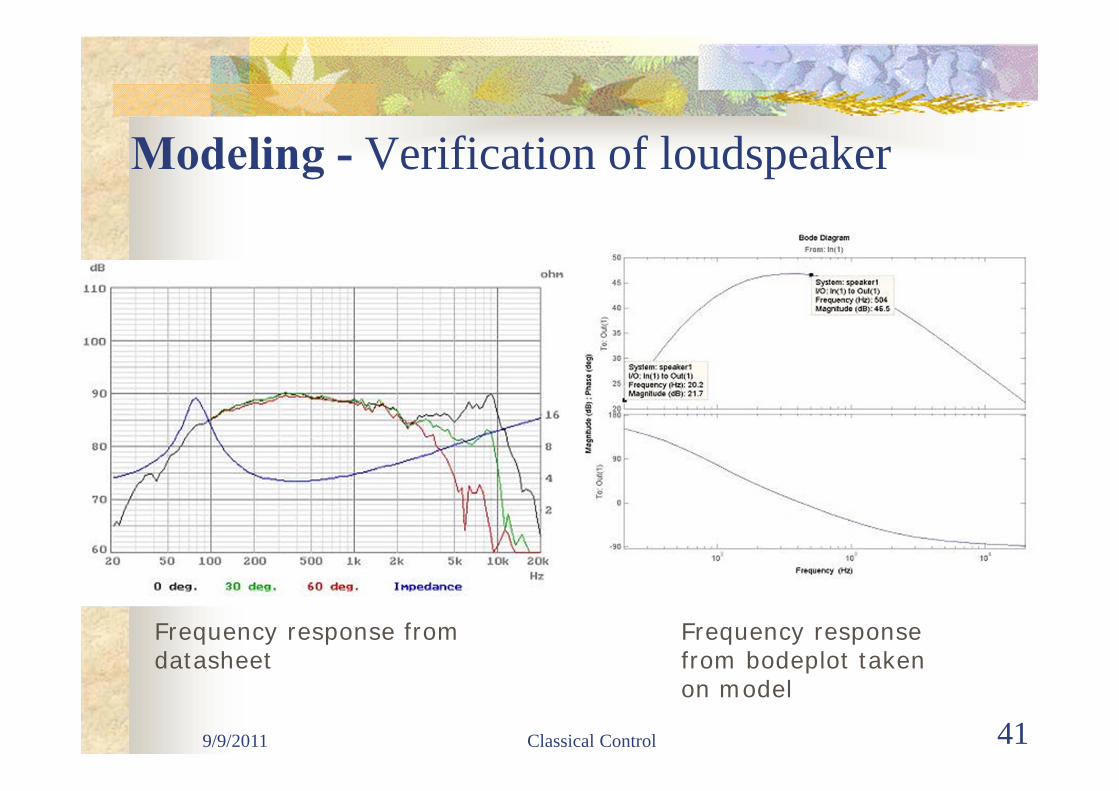
Modeling - Verification of loudspeaker

Frequency response from datasheet

Frequency response from bodeplot taken on model

9/9/2011 Classical Control 42Frequency response of estimated and mathematical model

Modeling - Acoustic Duct

Impedance Verification:

9/9/2011 Classical Control 43

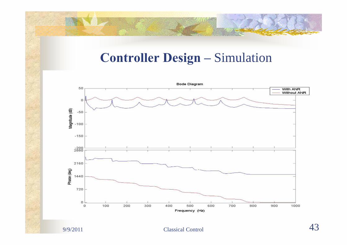
Controller Design – Simulation

9/9/2011 Classical Control 44

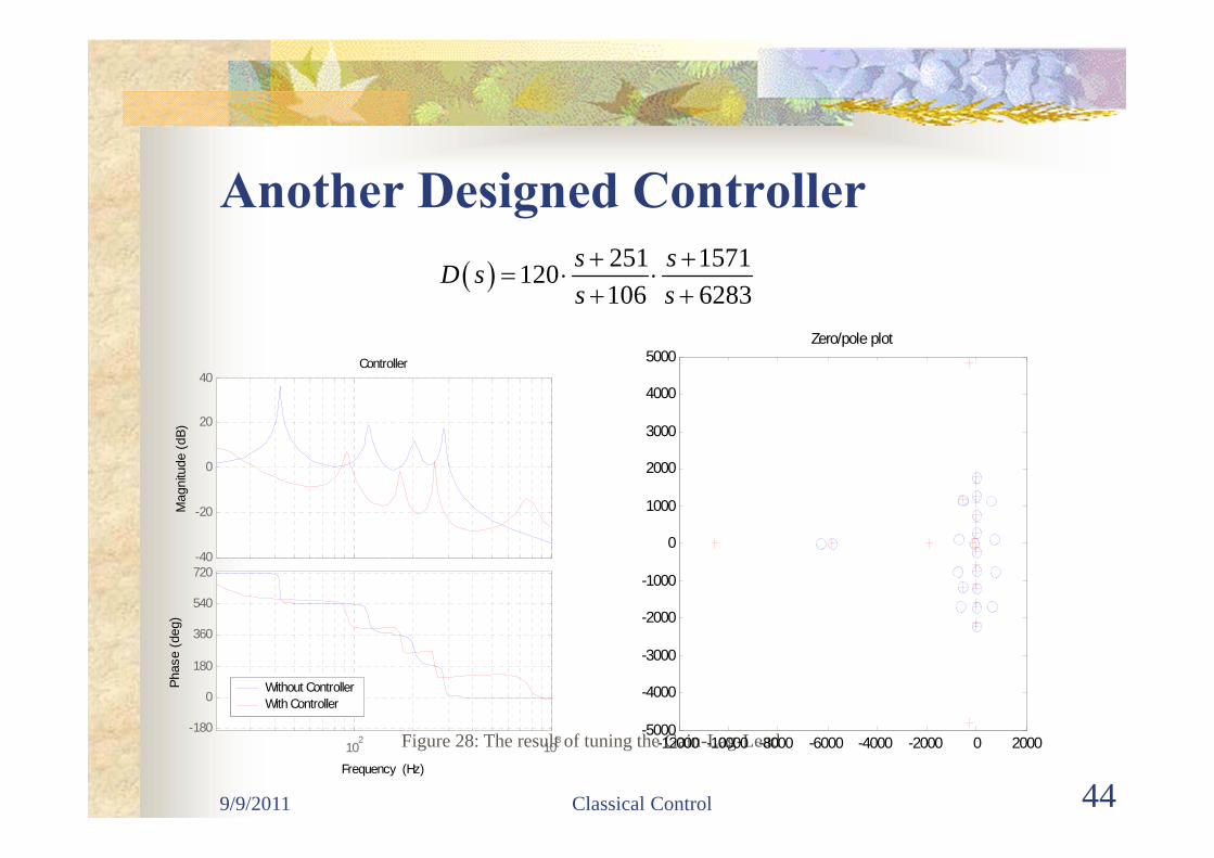
Another Designed Controller

Figure 28: The result of tuning the Gain-Lag-Lead

-40

-20

0

20

40

Mag

nitu

de (d

B)

102

103

-180

0

180

360

540

720

Phas

e (d

eg)

Without ControllerWith Controller

-12000 -10000 -8000 -6000 -4000 -2000 0 2000-5000

-4000

-3000

-2000

-1000

0

1000

2000

3000

4000

5000Zero/pole plot

Controller

Frequency (Hz)

251 1571120106 6283

s sD ss s

9/9/2011 Classical Control 45

Controller for CD-ROM Noise

9/9/2011 Classical Control 46

Summary of MM 8-9

How to use bode plot to Analyze the stability (GM,PM) Determine the bandwidth Determine the transient response Determine the system types and steady-state errors

How to use nyquist diagram Determine the stability Determine the GM,PM