mobile communications -...
TRANSCRIPT

Z. Ghassemlooy
Mobile Communications
Part IV- Propagation CharacteristicsPart IV- Propagation Characteristics
Professor Z Ghassemlooy
Faculty of Engineering and
Environment
University of Northumbria
U.K.
http://soe.unn.ac.uk/ocr
Professor Z Ghassemlooy
Faculty of Engineering and
Environment
University of Northumbria
U.K.
http://soe.unn.ac.uk/ocr
Z. Ghassemlooy
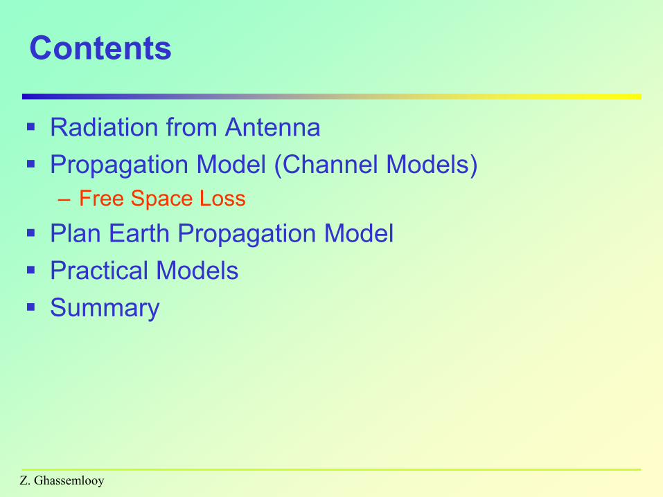
Contents
Radiation from Antenna
Propagation Model (Channel Models)
– Free Space Loss
Plan Earth Propagation Model
Practical Models
Summary

Z. Ghassemlooy
Wireless Communication System
UserSource
Decoder
Channel
Decoder
Demod-
ulator
Estimate of
Message signalEstimate of
channel code word
Received
Signal
Channel code word
SourceSource
Encoder
Channel
Encoder
Mod-
ulator
Message SignalModulated
Transmitted
Signal
Wireless
Channel
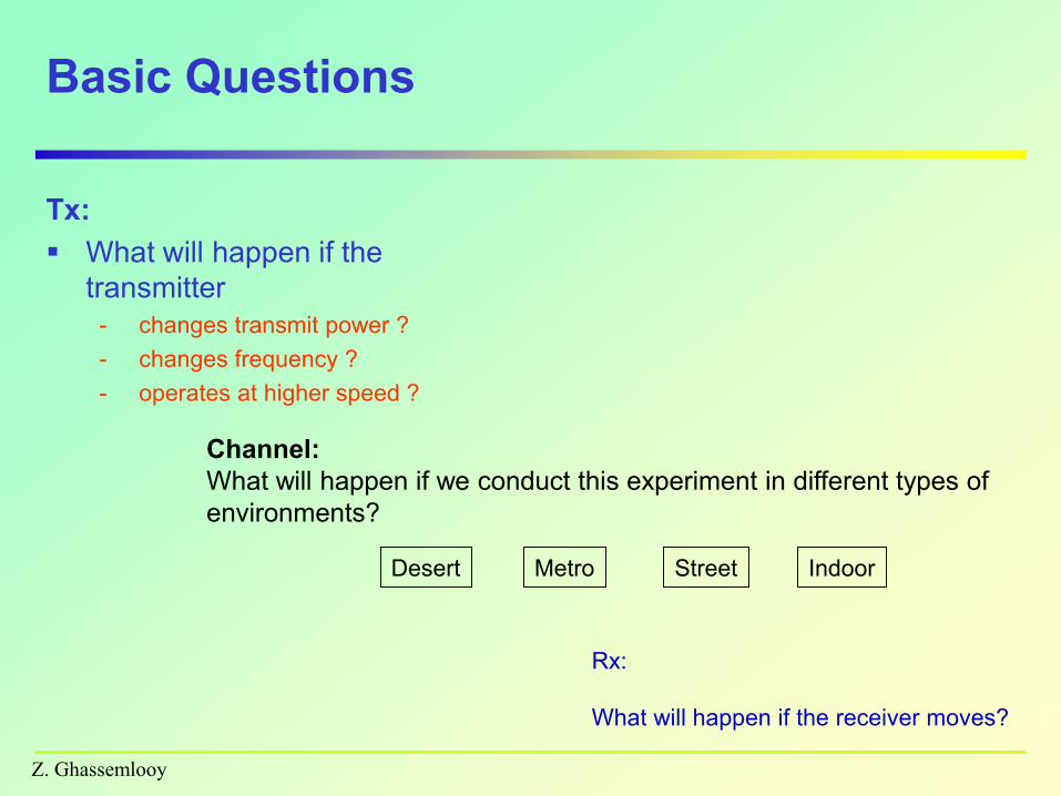
Basic Questions
Tx:
What will happen if the
transmitter
- changes transmit power ?
- changes frequency ?
- operates at higher speed ?
Z. Ghassemlooy
Desert Metro Street Indoor
Channel:
What will happen if we conduct this experiment in different types of
environments?
Rx:
What will happen if the receiver moves?

Z. Ghassemlooy
dd
Antenna - Ideal
Isotropics antenna: In free space radiates power equally in
all direction. Not realizable physically
dE
H
Pt
Distance d
Area• d- distance directly away from the
antenna.
• is the azimuth, or angle in the horizontal
plane.
• is the zenith, or angle above the horizon.
EM fields around a
transmitting antenna
, a polar coordinate
Z. Ghassemlooy
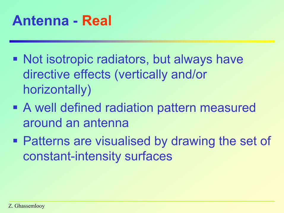
Antenna - Real
Not isotropic radiators, but always have
directive effects (vertically and/or
horizontally)
A well defined radiation pattern measured
around an antenna
Patterns are visualised by drawing the set of
constant-intensity surfaces
Z. Ghassemlooy
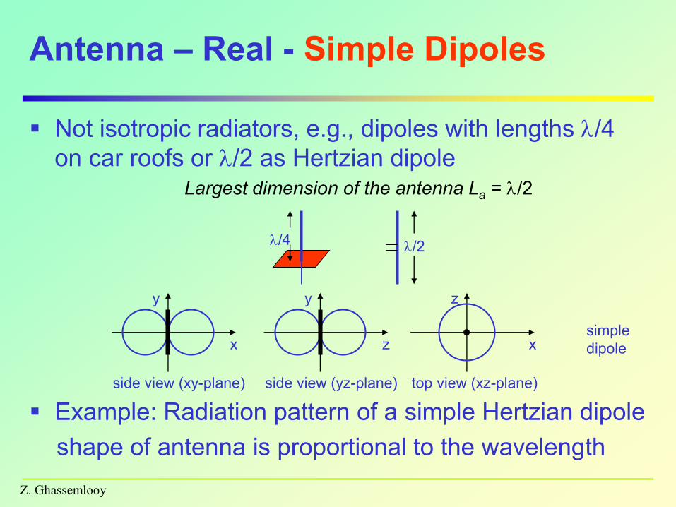
Antenna – Real - Simple Dipoles
Not isotropic radiators, e.g., dipoles with lengths /4
on car roofs or /2 as Hertzian dipole
Example: Radiation pattern of a simple Hertzian dipole
shape of antenna is proportional to the wavelength
side view (xy-plane)
x
y
side view (yz-plane)
z
y
top view (xz-plane)
x
z
simple
dipole
/4 /2
Largest dimension of the antenna La = /2
Z. Ghassemlooy
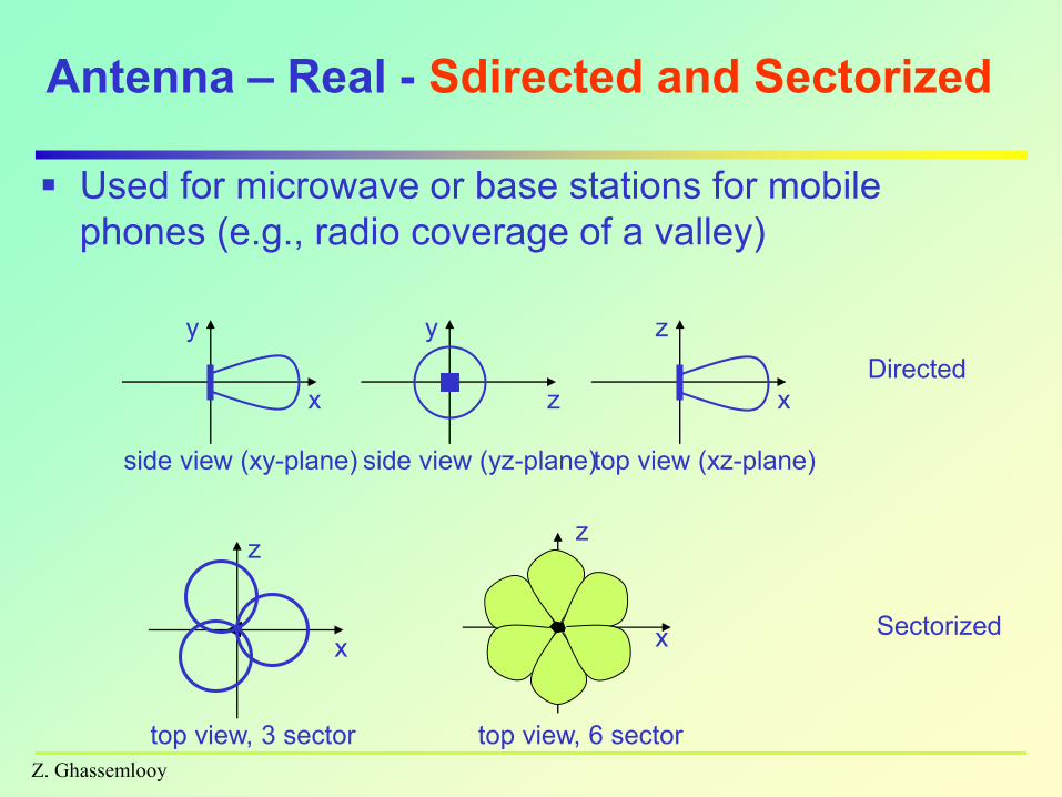
Antenna – Real - Sdirected and Sectorized
Used for microwave or base stations for mobile
phones (e.g., radio coverage of a valley)
side view (xy-plane)
x
y
side view (yz-plane)
z
y
top view (xz-plane)
x
z
Directed
top view, 3 sector
x
z
top view, 6 sector
x
z
Sectorized
Z. Ghassemlooy
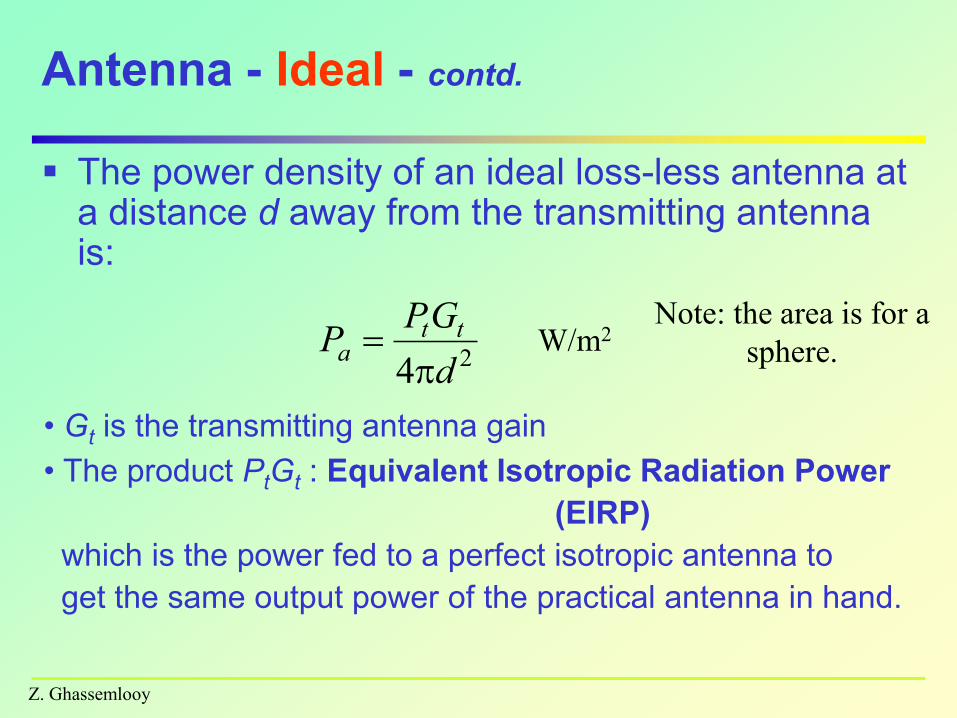
Antenna - Ideal - contd.
The power density of an ideal loss-less antenna at a distance d away from the transmitting antenna is:
24 d
GPP tt
a
• Gt is the transmitting antenna gain
• The product PtGt : Equivalent Isotropic Radiation Power
(EIRP)
which is the power fed to a perfect isotropic antenna to
get the same output power of the practical antenna in hand.
Note: the area is for a
sphere.W/m2
Z. Ghassemlooy
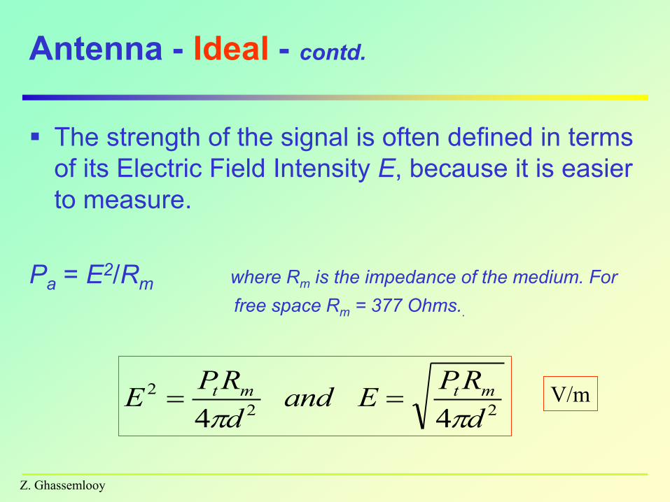
Antenna - Ideal - contd.
The strength of the signal is often defined in terms
of its Electric Field Intensity E, because it is easier
to measure.
Pa = E2/Rm where Rm is the impedance of the medium. For
free space Rm = 377 Ohms..
22
2
44 d
RPEand
d
RPE mtmt
V/m
Z. Ghassemlooy
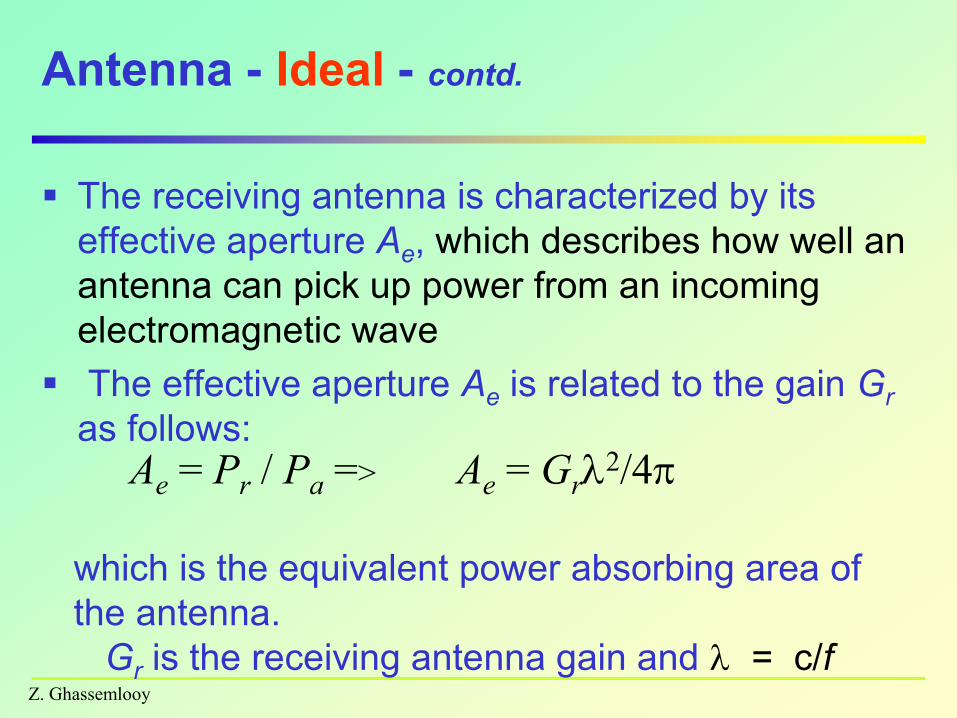
Antenna - Ideal - contd.
The receiving antenna is characterized by its
effective aperture Ae, which describes how well an
antenna can pick up power from an incoming
electromagnetic wave
The effective aperture Ae is related to the gain Gr
as follows:Ae = Pr / Pa => Ae = Gr
2/4
which is the equivalent power absorbing area of
the antenna.
Gr is the receiving antenna gain and = c/f

Z. Ghassemlooy
Signal Propagation
(Channel Models)
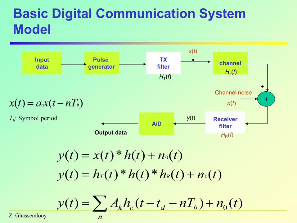
Basic Digital Communication System
Model
Z. Ghassemlooy
Input
data
Pulse
generator
TX
filterchannel
x(t)
Receiver
filterA/D
+Channel noise
n(t)
Output data
+
HT(f)
HR(f)
y(t)
Hc(f)
n
bdck tnnTtthAty
tnthththty
tnthtxty
RT
)()()(
)()(*)(*)()(
)()(*)()(
0
0
0
)()( bn nTtxatx
Tb: Symbol period

Fourier Representation of Periodic
Signals
)2cos()2sin(2
1)(
11
nftbnftactgn
n
n
n
1
0
1
0t t
ideal periodic signal real composition
(based on harmonics)
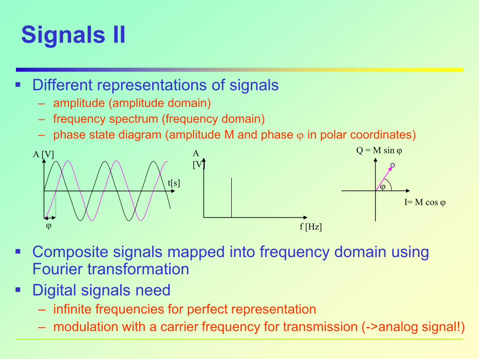
Different representations of signals – amplitude (amplitude domain)
– frequency spectrum (frequency domain)
– phase state diagram (amplitude M and phase in polar coordinates)
Composite signals mapped into frequency domain using Fourier transformation
Digital signals need– infinite frequencies for perfect representation
– modulation with a carrier frequency for transmission (->analog signal!)
Signals II
f [Hz]
A
[V]
I= M cos
Q = M sin
A [V]
t[s]
Z. Ghassemlooy
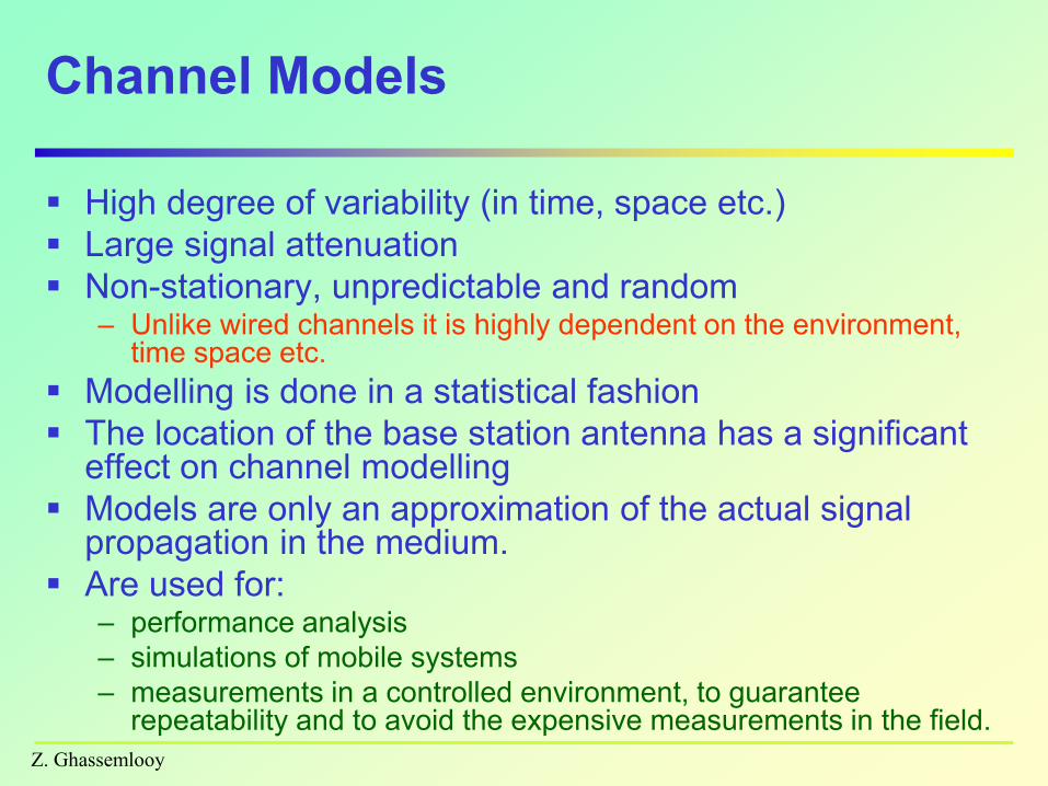
Channel Models
High degree of variability (in time, space etc.)
Large signal attenuation
Non-stationary, unpredictable and random – Unlike wired channels it is highly dependent on the environment,
time space etc.
Modelling is done in a statistical fashion
The location of the base station antenna has a significant effect on channel modelling
Models are only an approximation of the actual signal propagation in the medium.
Are used for:– performance analysis
– simulations of mobile systems
– measurements in a controlled environment, to guarantee repeatability and to avoid the expensive measurements in the field.

Z. Ghassemlooy
Channel Models - Classifications
System Model - Deterministic
Propagation Model- Deterministic– Predicts the received signal strength at a distance from the
transmitter
– Derived using a combination of theoretical and empirical method.
Stochastic Model - Rayleigh channel
Semi-empirical (Practical +Theoretical) Models
Z. Ghassemlooy
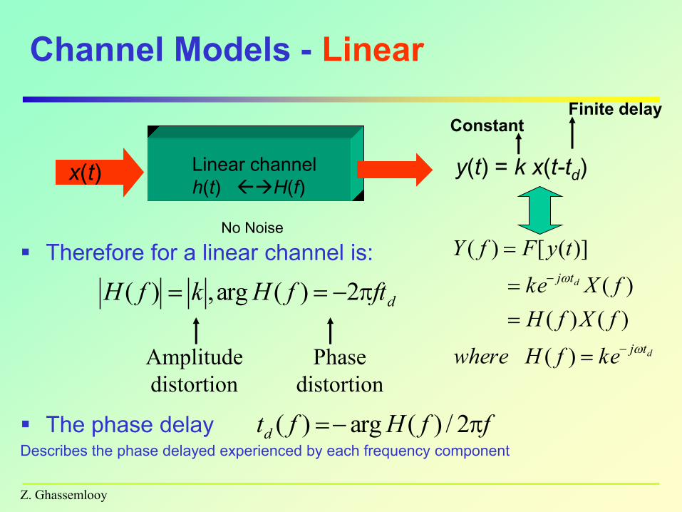
Channel Models - Linear
Therefore for a linear channel is:
Linear channel
h(t) H(f)x(t) y(t) = k x(t-td)
ConstantFinite delay
d
d
tj
tj
kefHwhere
fXfH
fXke
tyFfY
)(
)()(
)(
)]([)(
dftfHkfH 2)(arg,)(
Amplitude
distortion
Phase
distortion
The phase delayDescribes the phase delayed experienced by each frequency component
ffHftd 2/)(arg)(
No Noise
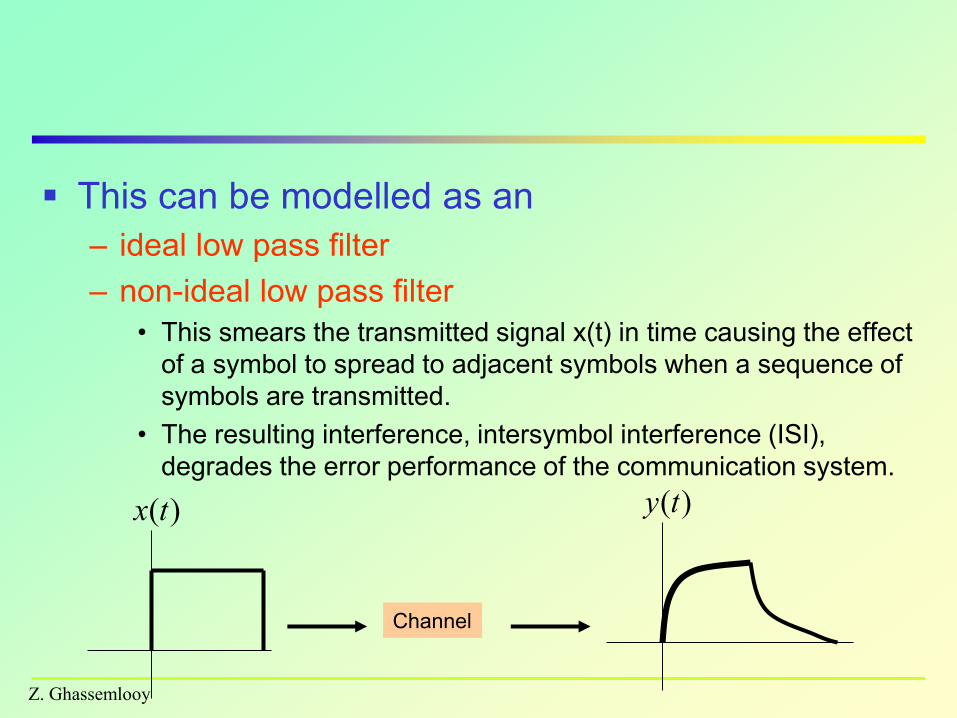
This can be modelled as an
– ideal low pass filter
– non-ideal low pass filter
• This smears the transmitted signal x(t) in time causing the effect
of a symbol to spread to adjacent symbols when a sequence of
symbols are transmitted.
• The resulting interference, intersymbol interference (ISI),
degrades the error performance of the communication system.
Z. Ghassemlooy
)(tx
Channel
)(ty
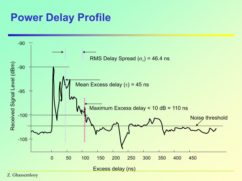
Power Delay Profile
Z. Ghassemlooy
Receiv
ed S
ignal Level (d
Bm
)
-105
-100
-95
-90
-90
0 50 100 150 200 250 300 350 400 450
Excess delay (ns)
RMS Delay Spread () = 46.4 ns
Mean Excess delay () = 45 ns
Maximum Excess delay < 10 dB = 110 ns
Noise threshold
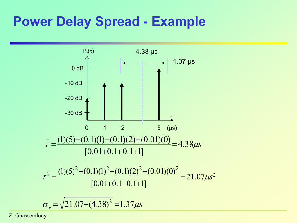
Power Delay Spread - Example
Z. Ghassemlooy
-30 dB
-20 dB
-10 dB
0 dB
0 1 2 5
Pr()
(µs)
s 38.4
]11.01.001.0[
)0)(01.0()2)(1.0()1)(1.0()5)(1(_
2
2222_2 07.21
]11.01.001.0[
)0)(01.0()2)(1.0()1)(1.0()5)(1(s
s
37.1)38.4(07.21 2
1.37 µs
4.38 µs
Z. Ghassemlooy
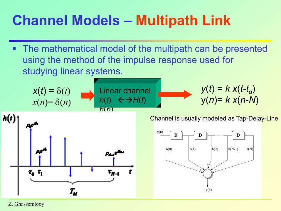
Channel Models – Multipath Link
The mathematical model of the multipath can be presented
using the method of the impulse response used for
studying linear systems.
Linear channel
h(t) H(f)
h(n)
x(t) = (t)
x(n)= (n)
y(t) = k x(t-td)
y(n)= k x(n-N)
D D D
h(0) h(1) h(2) h(N-1) h(N)
y(n)
x(n)
++
++
+
Channel is usually modeled as Tap-Delay-Line
Z. Ghassemlooy
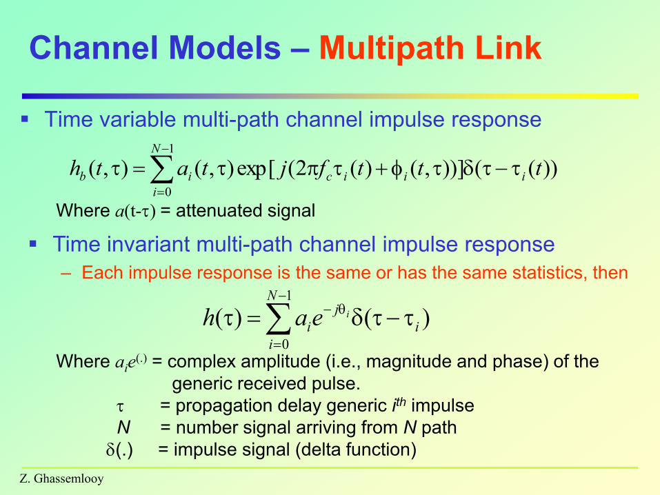
Channel Models – Multipath Link
Time variable multi-path channel impulse response
))(())],()(2(exp[),(),(1
0
tttfjtath iii
N
i
cib
Time invariant multi-path channel impulse response
– Each impulse response is the same or has the same statistics, then
1
0
)()(N
i
i
j
iieah
Where aie(.) = complex amplitude (i.e., magnitude and phase) of the
generic received pulse.
= propagation delay generic ith impulse
N = number signal arriving from N path
(.) = impulse signal (delta function)
Where a(t-) = attenuated signal
Z. Ghassemlooy
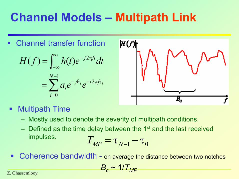
Channel Models – Multipath Link
Multipath Time
– Mostly used to denote the severity of multipath conditions.
– Defined as the time delay between the 1st and the last received
impulses.01 NMPT
1
0
2
2)()(
N
i
fij
i
ftj
ii eea
dtethfH
Channel transfer function
Coherence bandwidth - on average the distance between two notches
Bc ~ 1/TMP

Z. Ghassemlooy
)(tx
Time domain view
High correlation of amplitude
between two different freq.
components
Range of freq over
which response is flat
Bc RMS delay spread
)( fX
Freq. domain view
.50
1coB For 0.9 correlation
.5
1coB For 0.5 correlation
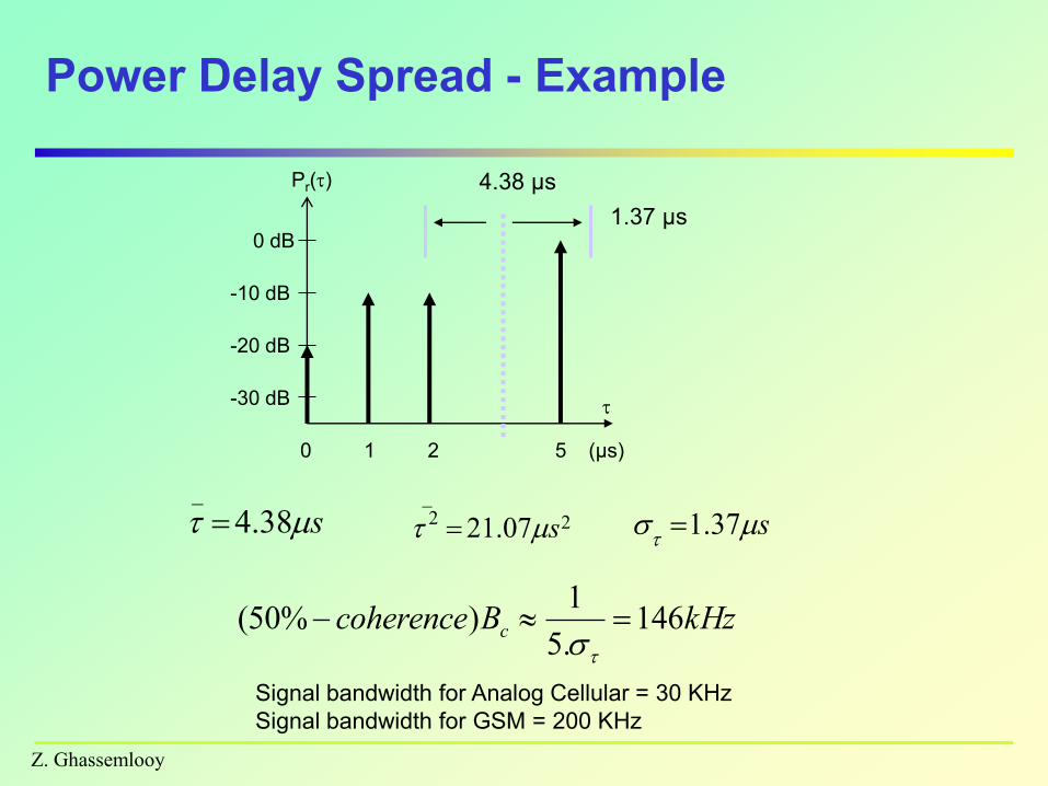
Power Delay Spread - Example
Z. Ghassemlooy
-30 dB
-20 dB
-10 dB
0 dB
0 1 2 5
Pr()
(µs)
s 38.4_
2
_2 07.21 s s
37.1
1.37 µs
4.38 µs
kHzBcoherence c 146.5
1)%50(
Signal bandwidth for Analog Cellular = 30 KHz
Signal bandwidth for GSM = 200 KHz

Multipath Delay
With a 52 meter separation, in a LOS environment, a large 753.5 ns
excess delay
NLOS excess delay over 423 meters extended to 1388.4 ns.
Office building: RMS delay spread = 10-60 ns
Z. Ghassemlooy
Cell size (km) Max Delay Spread
Pico cell 0.1 300 nn
Micro cell 5 15 us
Macro cell 20 40 us
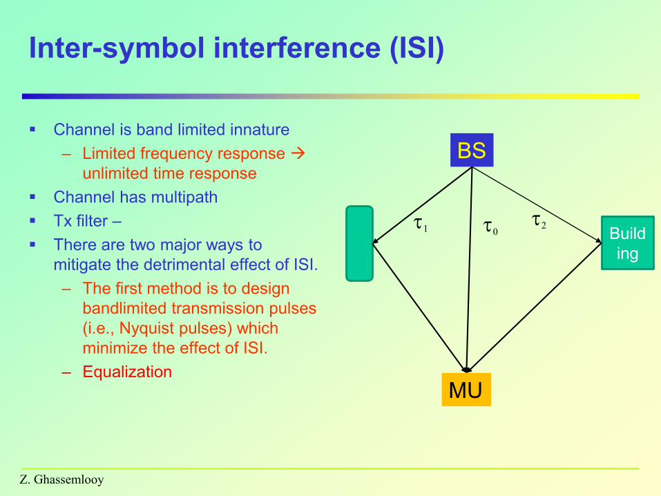
Inter-symbol interference (ISI)
Channel is band limited innature
– Limited frequency response
unlimited time response
Channel has multipath
Tx filter –
There are two major ways to
mitigate the detrimental effect of ISI.
– The first method is to design
bandlimited transmission pulses
(i.e., Nyquist pulses) which
minimize the effect of ISI.
– Equalization
Z. Ghassemlooy
BS
MU
Build
ing
01
2
ISI
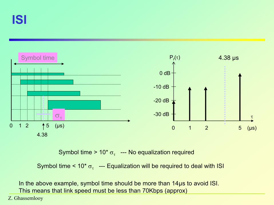
Z. Ghassemlooy
-30 dB
-20 dB
-10 dB
0 dB
0 1 2 5
Pr()
(µs)
4.38 µs
0 1 2 5 (µs)
Symbol time
4.38
Symbol time > 10* --- No equalization required
Symbol time < 10* --- Equalization will be required to deal with ISI
In the above example, symbol time should be more than 14µs to avoid ISI.
This means that link speed must be less than 70Kbps (approx)
Z. Ghassemlooy
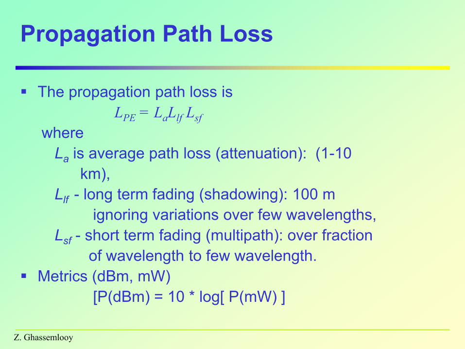
Propagation Path Loss
The propagation path loss is
LPE = LaLlf Lsf
where
La is average path loss (attenuation): (1-10
km),
Llf - long term fading (shadowing): 100 m
ignoring variations over few wavelengths,
Lsf - short term fading (multipath): over fraction
of wavelength to few wavelength.
Metrics (dBm, mW)
[P(dBm) = 10 * log[ P(mW) ]
Z. Ghassemlooy
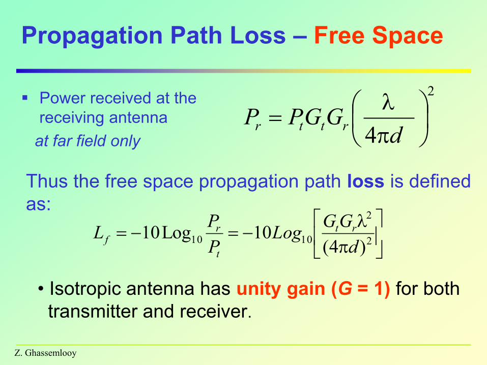
Propagation Path Loss – Free Space
Power received at the
receiving antenna
at far field only
2
4
dGGPP rttr
• Isotropic antenna has unity gain (G = 1) for both
transmitter and receiver.
Thus the free space propagation path loss is defined
as:
2
2
1010)4(
10Log10d
GGLog
P
PL rt
t
rf
Z. Ghassemlooy
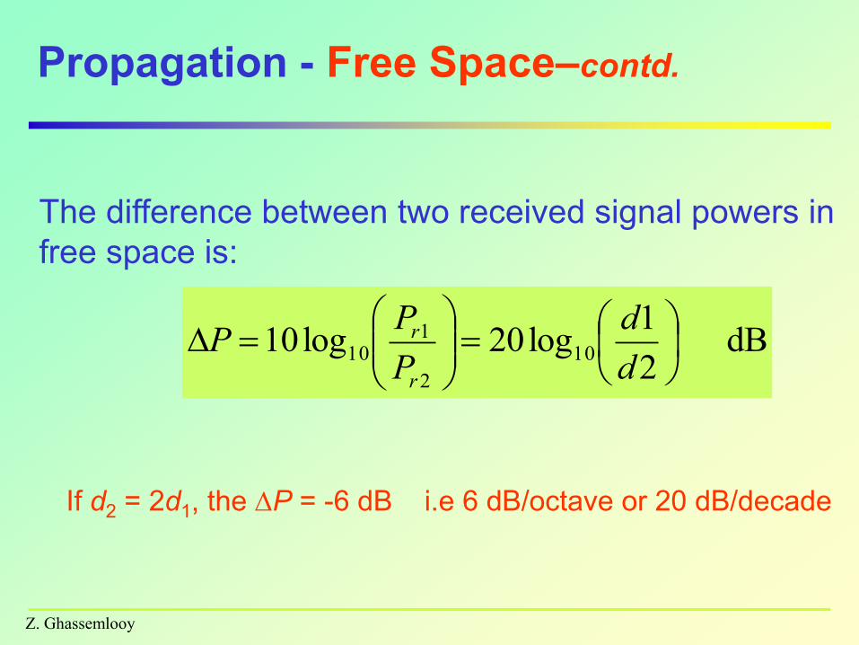
Propagation - Free Space–contd.
The difference between two received signal powers in
free space is:
dB2
1log20log10 10
2
110
d
d
P
PP
r
r dB2
1log20log10 10
2
110
d
d
P
PP
r
r
If d2 = 2d1, the P = -6 dB i.e 6 dB/octave or 20 dB/decade
Z. Ghassemlooy
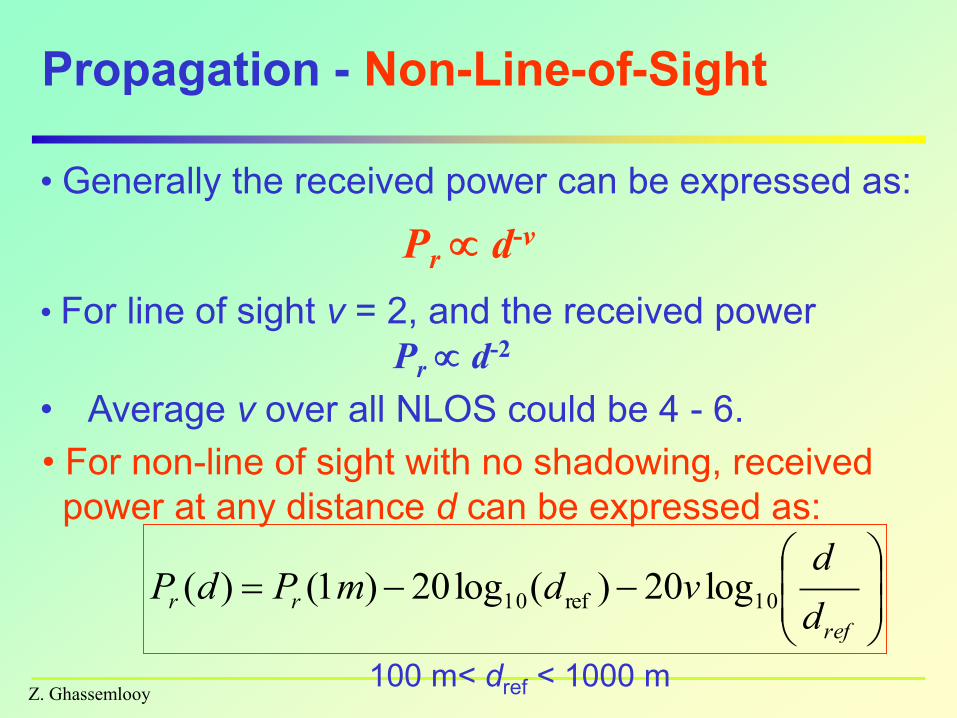
Propagation - Non-Line-of-Sight
• Generally the received power can be expressed as:
Pr d-v
• For line of sight v = 2, and the received power
Pr d-2
• Average v over all NLOS could be 4 - 6.
• For non-line of sight with no shadowing, received
power at any distance d can be expressed as:
ref
rrd
dvdmPdP 10ref10 log20)(log20)1()(
100 m< dref < 1000 m
Z. Ghassemlooy
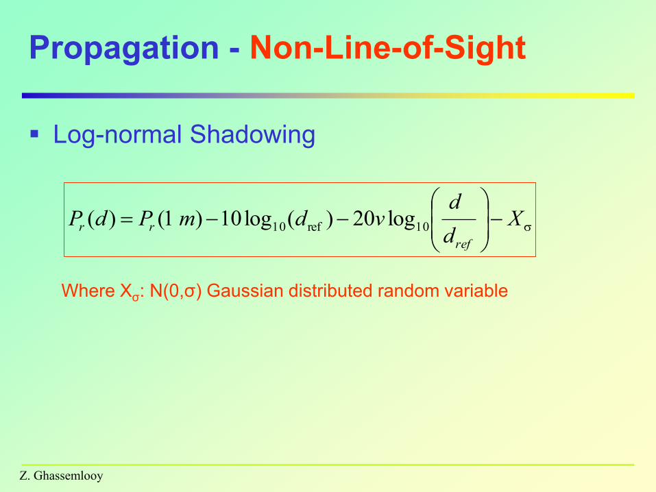
Propagation - Non-Line-of-Sight
Log-normal Shadowing
Where Xσ: N(0,σ) Gaussian distributed random variable
X
d
dvdmPdP
ref
rr 10ref10 log20)(log10)1()(
Z. Ghassemlooy
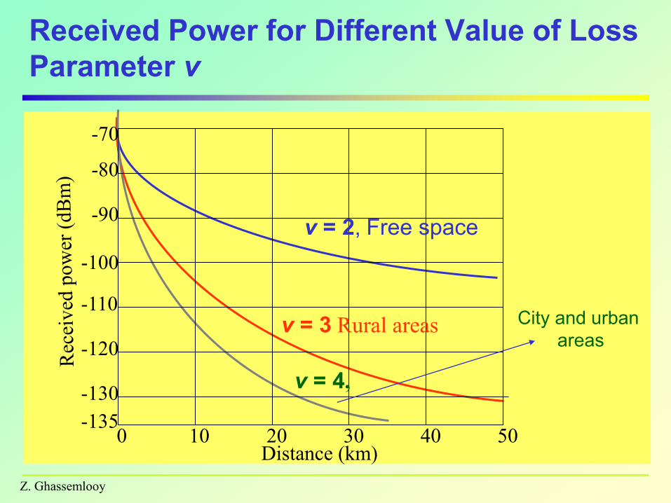
Received Power for Different Value of Loss
Parameter v
Distance (km)0 10 20 30 40 50
-70
-80
-90
-100
-110
-120
-130
-135
v = 2, Free space
v = 3 Rural areas
v = 4,
City and urban
areas
Z. Ghassemlooy
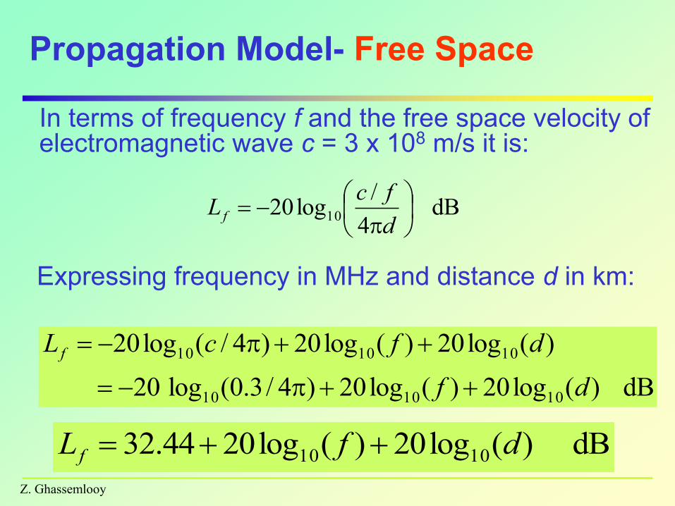
Propagation Model- Free Space
dB)(log20)(log2044.32 1010 dfL f dB)(log20)(log2044.32 1010 dfL f
Expressing frequency in MHz and distance d in km:
dB)(log20)(log20)4/3.0(log20
)(log20)(log20)4/(log20
101010
101010
df
dfcL f
dB)(log20)(log20)4/3.0(log20
)(log20)(log20)4/(log20
101010
101010
df
dfcL f
In terms of frequency f and the free space velocity of electromagnetic wave c = 3 x 10⁸ m/s it is:
dB4
/log20 10
d
fcL f
Z. Ghassemlooy
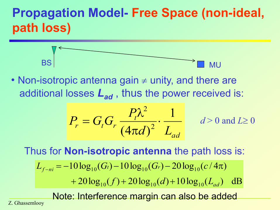
Propagation Model- Free Space (non-ideal,
path loss)
• Non-isotropic antenna gain unity, and there are
additional losses Lad , thus the power received is:
ad
trtr
Ld
PGGP
1
)4( 2
2
ad
trtr
Ld
PGGP
1
)4( 2
2
d > 0 and L 0
Thus for Non-isotropic antenna the path loss is:
dB)(log10)(log20)(log20
)4/(log20)(log10)(log10
101010
101010
ad
rtnif
Ldf
cGGL
dB)(log10)(log20)(log20
)4/(log20)(log10)(log10
101010
101010
ad
rtnif
Ldf
cGGL
BS MU
Note: Interference margin can also be added
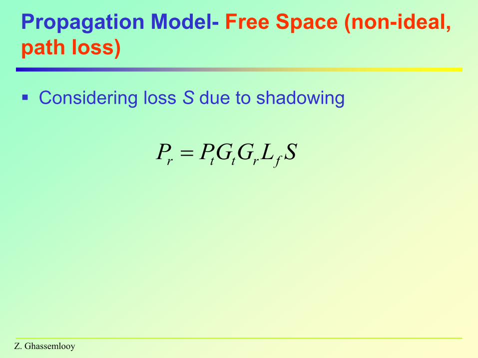
Considering loss S due to shadowing
Z. Ghassemlooy
SLGGPP frttr
Propagation Model- Free Space (non-ideal,
path loss)
Z. Ghassemlooy
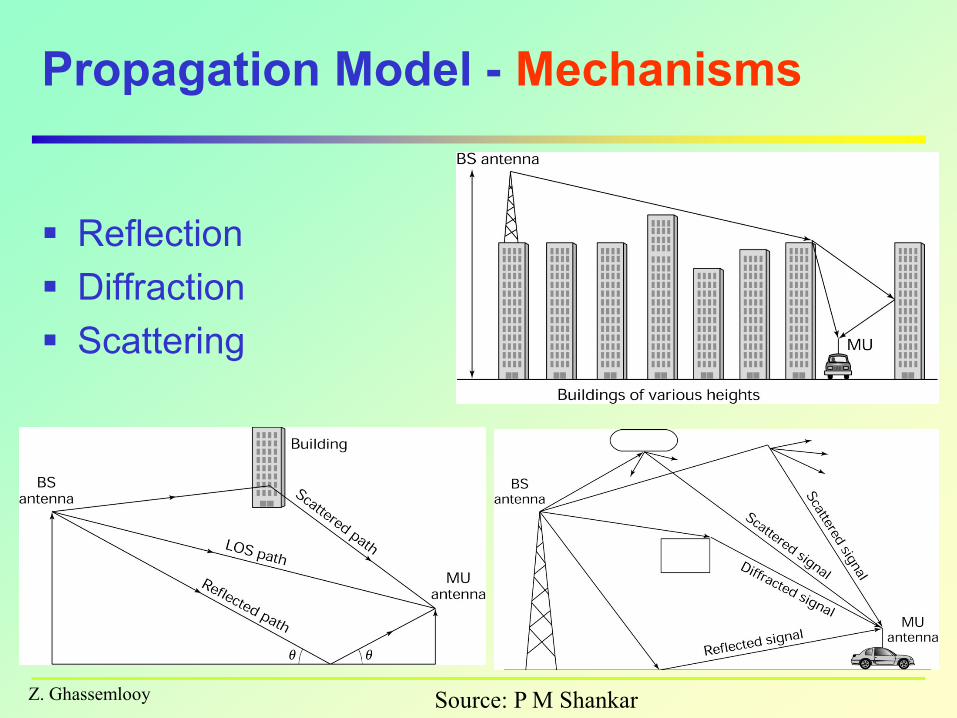
Propagation Model - Mechanisms
Reflection
Diffraction
Scattering
Source: P M Shankar
Z. Ghassemlooy
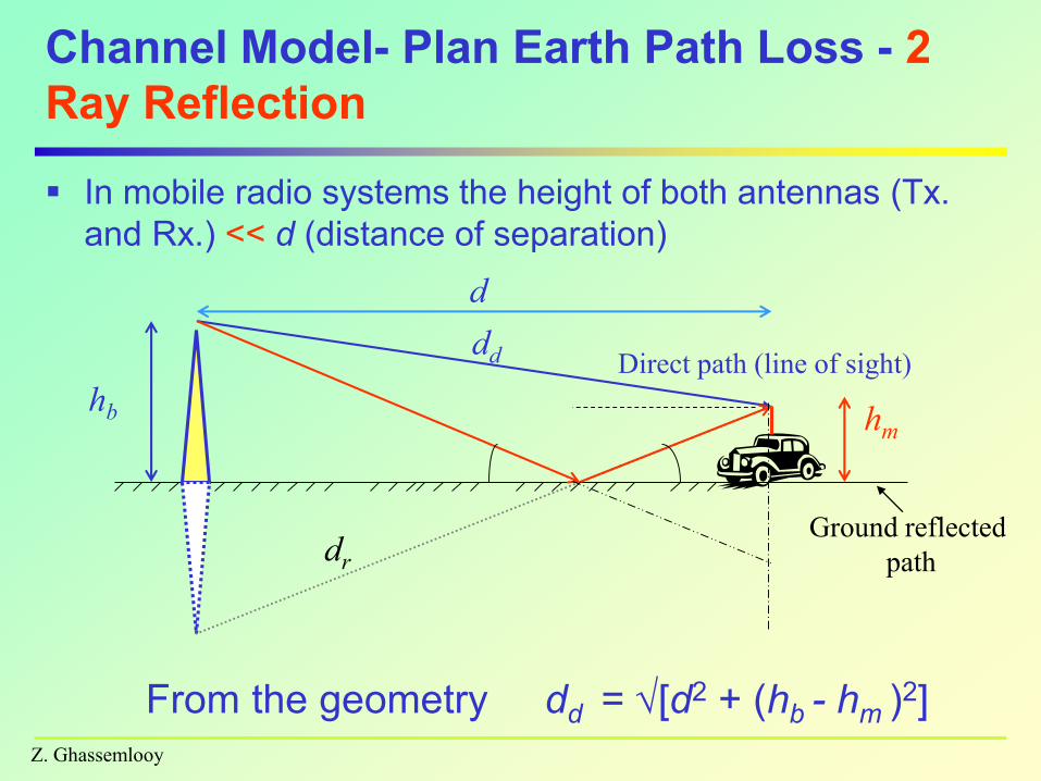
Channel Model- Plan Earth Path Loss - 2
Ray Reflection
In mobile radio systems the height of both antennas (Tx.
and Rx.) << d (distance of separation)
From the geometry dd = [d2 + (hb - hm )2]
hb
dd
dr
hm
Direct path (line of sight)
Ground reflected
path
d
Z. Ghassemlooy
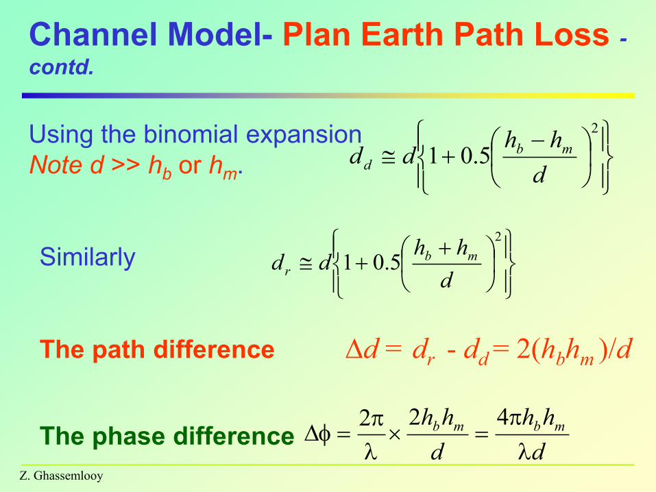
Channel Model- Plan Earth Path Loss -
contd.
Using the binomial expansion
Note d >> hb or hm.
2
5.01d
hhdd mb
d
The path difference d = dr - dd = 2(hbhm )/d
Similarly
2
5.01d
hhdd mb
r
The phase differenced
hh
d
hh mbmb
422

Z. Ghassemlooy
Channel Model- Plan Earth Path
Loss– contd.
Total received power
22
14
j
rttr ed
GGPP
Where is the reflection coefficient.
For = -1 (low angle of incident) and .
)2/(sin4
)cos1(2sin)cos1(1
sincos11
2
222
j
j
eHence
je
Z. Ghassemlooy
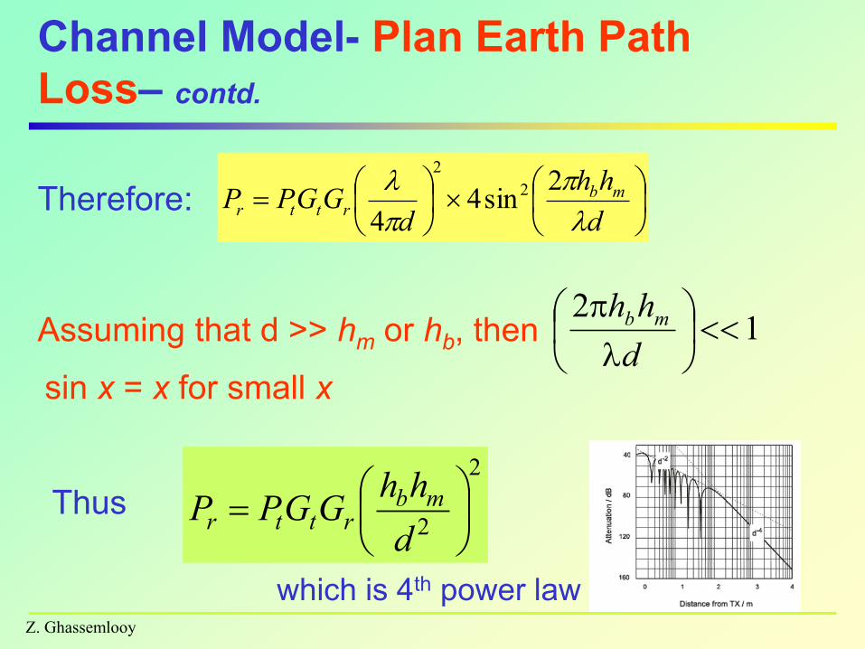
Channel Model- Plan Earth Path
Loss– contd.
Therefore:
d
hh
dGGPP mb
rttr
2sin4
4
2
2
d
hh
dGGPP mb
rttr
2sin4
4
2
2
Assuming that d >> hm or hb, then 12
d
hh mb
sin x = x for small x
Thus2
2
d
hhGGPP mb
rttr
2
2
d
hhGGPP mb
rttr
which is 4th power law

Z. Ghassemlooy
Channel Model- Plan Earth Path Loss– contd.
In a more general form (no fading due to multipath),
path attenuation is
dΒlog40log20
log20log10log10
1010
101010
dh
hGGL
m
brtPE
dΒlog40log20
log20log10log10
1010
101010
dh
hGGL
m
brtPE
• LPE increases by 40 dB each time d increases by 10
Propagation path
loss (mean loss)
2
2log10log10
d
hhGG
P
PL mb
rt
t
rPE
Compared with the free space = Pr= 1/ d2
Z. Ghassemlooy
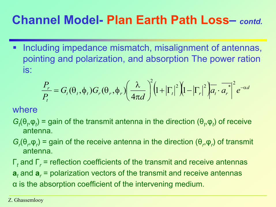
Channel Model- Plan Earth Path Loss– contd.
Including impedance mismatch, misalignment of antennas,
pointing and polarization, and absorption The power ration
is:
where
Gt(θt,φt) = gain of the transmit antenna in the direction (θt,φt) of receive
antenna.
Gr(θr,φr) = gain of the receive antenna in the direction (θr,φr) of transmit
antenna.
Γt and Γr = reflection coefficients of the transmit and receive antennas
at and ar = polarization vectors of the transmit and receive antennas
α is the absorption coefficient of the intervening medium.
d
rtrtrrrttt
t
r eaad
GGP
P
2*22
2
114
),(),(
Z. Ghassemlooy
LOS Channel Model - Problems
Simple theoretical models do not take into account
many practical factors:
– Rough terrain
– Buildings
– Refection
– Moving vehicle
– Shadowing
Thus resulting in bad accuracy
Solution: Semi- empirical Model

Z. Ghassemlooy
Sem-iempirical Model
Practical models are based on combination of measurement and theory. Correction factors are introduced to account for:– Terrain profile
– Antenna heights
– Building profiles
– Road shape/orientation
– Lakes, etc.
Okumura model
Hata model
Saleh model
SIRCIM model
Outdoor
Indoor
Y. Okumura, et al, Rev. Elec. Commun. Lab., 16( 9), 1968.
M. Hata, IEEE Trans. Veh. Technol., 29, pp. 317-325, 1980.

Z. Ghassemlooy
Okumura Model
Widely used empirical model (no analytical basis!) in macrocellular environment
Predicts average (median) path loss
“Accurate” within 10-14 dB in urban and suburban areas
Frequency range: 150-1500 MHz
Distance: > 1 km
BS antenna height: > 30 m.
MU antenna height: up to 3m.
Correction factors are then added.

Z. Ghassemlooy
Hata Model
Consolidate Okumura’s model in standard formulas for macrocells in urban, suburban and open rural areas.
Empirically derived correction factors are incorporated into the standard formula to account for:– Terrain profile
– Antenna heights
– Building profiles
– Street shape/orientation
– Lakes
– Etc.
Z. Ghassemlooy
Hata Model – contd.
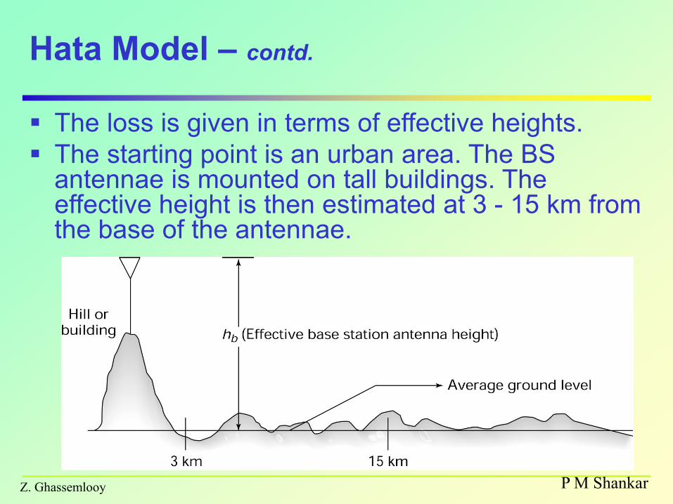
The loss is given in terms of effective heights.
The starting point is an urban area. The BS antennae is mounted on tall buildings. The effective height is then estimated at 3 - 15 km from the base of the antennae.
P M Shankar
Z. Ghassemlooy
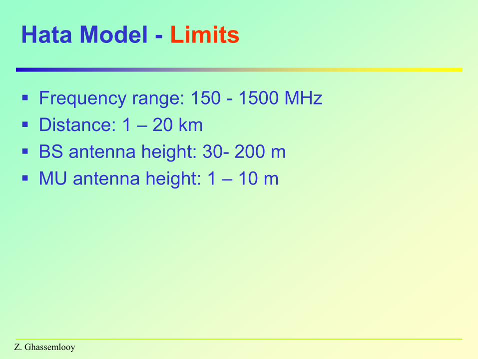
Hata Model - Limits
Frequency range: 150 - 1500 MHz
Distance: 1 – 20 km
BS antenna height: 30- 200 m
MU antenna height: 1 – 10 m
Z. Ghassemlooy
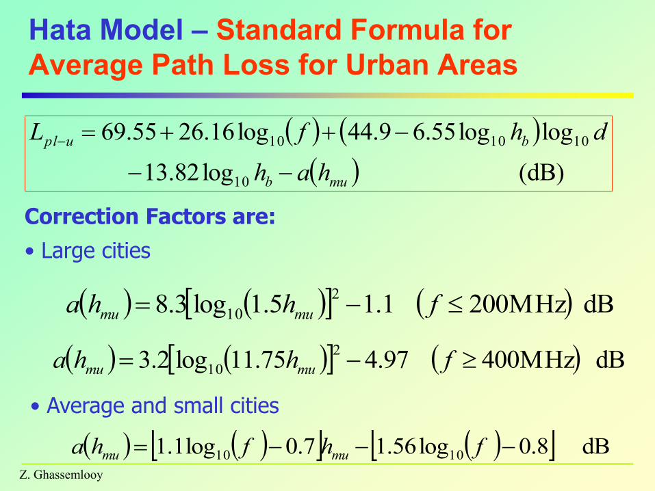
Hata Model – Standard Formula for
Average Path Loss for Urban Areas
Correction Factors are:
• Large cities
(dB)log82.13
loglog55.69.44log16.2655.69
10
101010
mub
bupl
hah
dhfL
dBMHz400 97.475.11log2.32
10 fhha mumu
dB 8.0log56.17.0log1.1 1010 fhfha mumu
dBMHz200 1.15.1log3.82
10 fhha mumu
• Average and small cities

Z. Ghassemlooy
Hata Model – Average Path Loss for Urban
Areas contd.
Carrier frequency
• 900 MHz,
BS antenna height
• 150 m,
MU antenna height
• 1.5m.
P M Shankar

Z. Ghassemlooy
Hata Model – Average Path Loss for
Suburban and Open Areas
Suburban Areas
Open Areas
94.40Log33.18)(Log78.4 2
10 ffLL uplopl 94.40Log33.18)(Log78.4 2
10 ffLL uplopl
4.528
Log2
2
10
fLL uplsupl 4.5
28Log2
2
10
fLL uplsupl
Z. Ghassemlooy
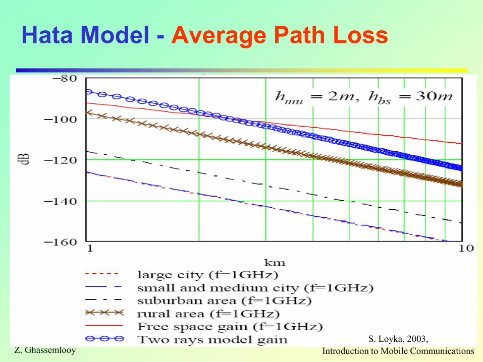
Hata Model - Average Path Loss
S. Loyka, 2003,
Introduction to Mobile Communications
Z. Ghassemlooy
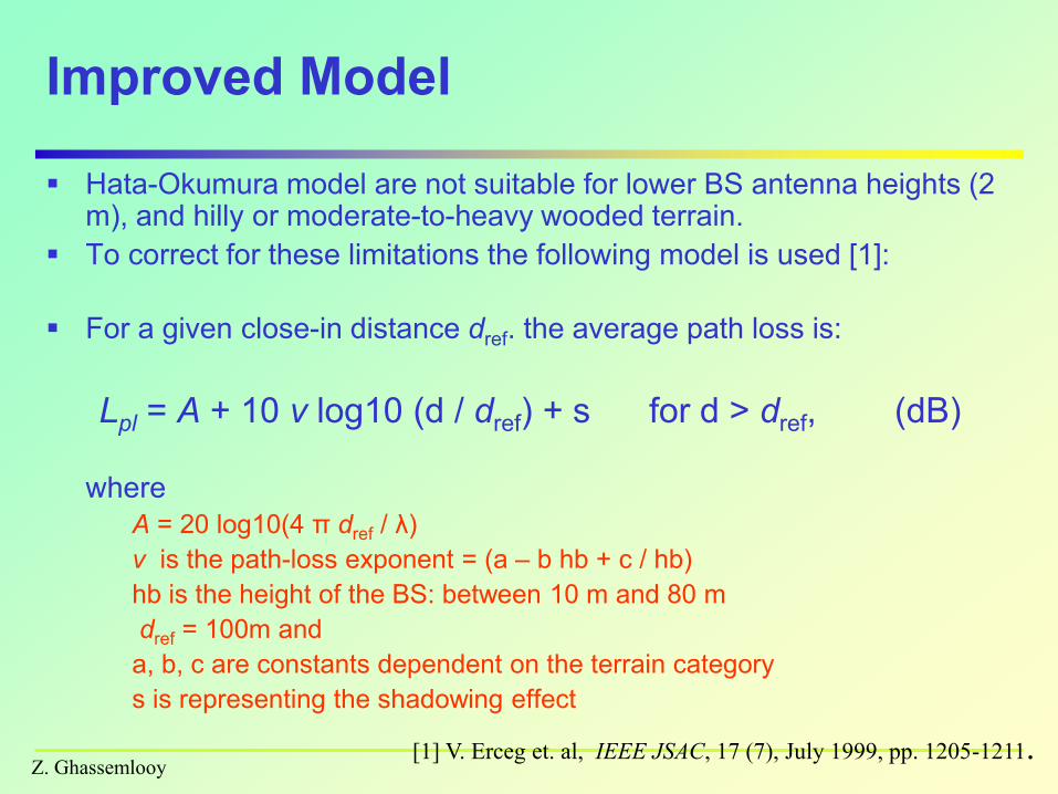
Improved Model
Hata-Okumura model are not suitable for lower BS antenna heights (2 m), and hilly or moderate-to-heavy wooded terrain.
To correct for these limitations the following model is used [1]:
For a given close-in distance dref. the average path loss is:
Lpl = A + 10 v log10 (d / dref) + s for d > dref, (dB)
where
A = 20 log10(4 π dref / λ)
v is the path-loss exponent = (a – b hb + c / hb)
hb is the height of the BS: between 10 m and 80 m
dref = 100m and
a, b, c are constants dependent on the terrain category
s is representing the shadowing effect
[1] V. Erceg et. al, IEEE JSAC, 17 (7), July 1999, pp. 1205-1211.
Z. Ghassemlooy
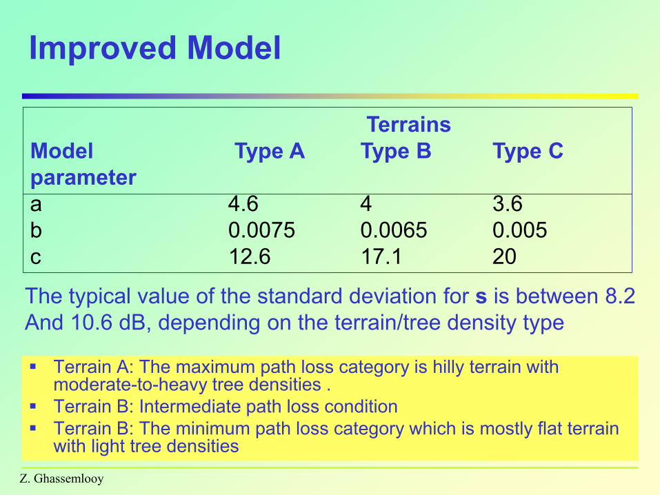
Improved Model
Terrain A: The maximum path loss category is hilly terrain with moderate-to-heavy tree densities .
Terrain B: Intermediate path loss condition
Terrain B: The minimum path loss category which is mostly flat terrain with light tree densities
Terrains
Model Type A Type B Type C
parameter
a 4.6 4 3.6
b 0.0075 0.0065 0.005
c 12.6 17.1 20
The typical value of the standard deviation for s is between 8.2
And 10.6 dB, depending on the terrain/tree density type
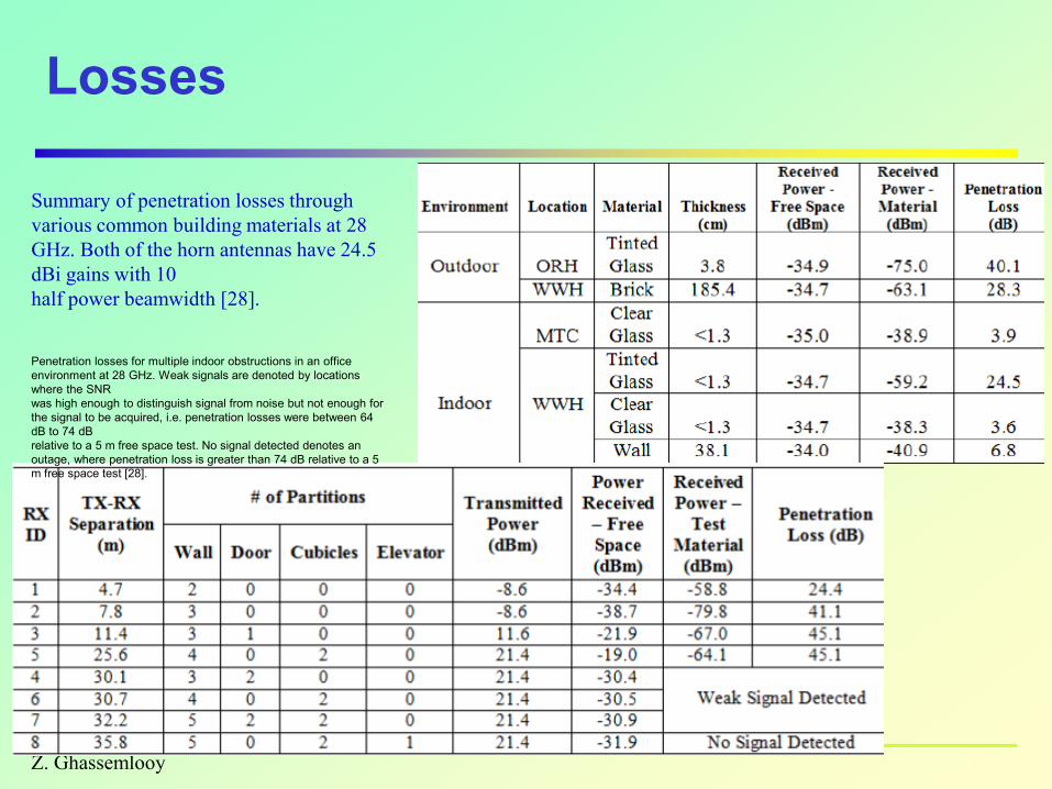
Losses
Z. Ghassemlooy
Summary of penetration losses through
various common building materials at 28
GHz. Both of the horn antennas have 24.5
dBi gains with 10�
half power beamwidth [28].
Penetration losses for multiple indoor obstructions in an office
environment at 28 GHz. Weak signals are denoted by locations
where the SNR
was high enough to distinguish signal from noise but not enough for
the signal to be acquired, i.e. penetration losses were between 64
dB to 74 dB
relative to a 5 m free space test. No signal detected denotes an
outage, where penetration loss is greater than 74 dB relative to a 5
m free space test [28].
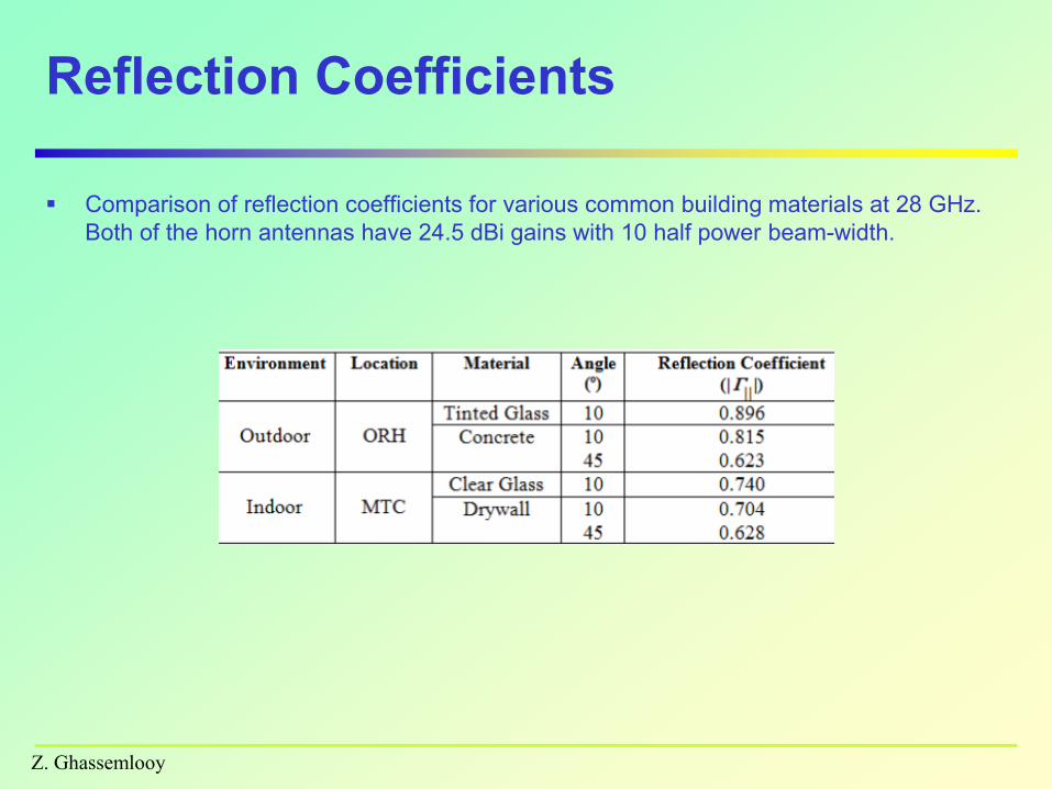
Reflection Coefficients
Comparison of reflection coefficients for various common building materials at 28 GHz.
Both of the horn antennas have 24.5 dBi gains with 10 half power beam-width.
Z. Ghassemlooy
Z. Ghassemlooy
Summary
• Attenuation is a result of reflection, scattering, diffraction and
reflection of the signal by natural and human-made structures
• The received power is inversely proportional to (distance)v,
where v is the loss parameter.
• Studied channel models and their limitations
Z. Ghassemlooy
Questions and Answers
Tell me what you think about this lecture
Next lecture: Multi-path Propagation- Fading