mobile robot path planning using exact cell decomposition
TRANSCRIPT
Mobile robot path planning using exact cell decomposition and potential field methods
Dusan Glavaski, Mario Volf, Mirjana Bonkovic
Faculty of Electrical Enginnering, Mechanical Engineering and Naval Architecture
University of Split, Ruđera Boškovića bb
[email protected], [email protected], [email protected]
Abstract: - In this paper two classic path planning procedures have been explained and adopted to reduce
computational time. When studying mobile robotics and robot motion planning, there is always a gap which
exists between theoretical achievements and practical considerations of the described methods. This paper
clearly overrides the mentioned problem describing minutely the procedures necessary for practical
implementations and simulation in the Matlab and MobileSim environment. The algorithms have been
presented together with their pseudo codes. The simulation results clearly show the advantages and
drawbacks of each of the method.
Key-Words: - path planning, mobile robot, exact cell decomposition, potential field
1. Introduction The research in the field of robotics is focused
on the algorithms used to accomplish
fundamental tasks. The typical task is path
planning for which exist numerous software [1],
[2], [5], [6], [7], [8] as well as hardware [2], [3],
[4] implementations for problem solving. In this
paper we compare the efficacy through
advantages and drawbacks of two methods for
basic robot motion problem solutions, together
with a practical implementations using Aria
programming library, adopted for Amigo Bot
mobile robot, produced by Active Media
Robotics Ltd. The solutions are based on the
classic path planning algorithms, namely exact
cell decomposition and potential field methods.
Therefore, the introduction follows with the
basic motion problem and configuration space
specifications. In Section 3, the path planning
algorithms are presented together with the
pseudo code of the concrete implementations.
Section 4 presents the simulation results
whereas Section 5 concludes the paper.
2. Basic motion problem and
configuration space specifications
In the basic problem, it is assumed that the robot
is the only moving object in the workspace and
the dynamic properties of the robot are ignored,
thus avoiding temporal issues. The motions are
resticted to non-contact motions, so that the
issue related to the mechanical interaction
between two physical objects in contact can be
ignored. These assumptions essential transform
the "physical" motion planning problem into a
purely geometrical path planning problem. The
geometrical issues are simplified even further
by assuming that the robot is a single rigid
object. The motions of this object are only
constrained by the obstacles.
The basic motion planning problem resulting
from these simplifications is the following:
● Let be a single rigid object (the robot)
moving in Euclidean space , called
workspace, represented as , with =2 or 3.
● Let be fixed rigid object
distributed in . These objects are called
obstacles.
● Assume that both the geometry of ,
and the locations of the βi in are
accurately known. Assume further that no
kinematic constrains limit the motions of A (we
say that A is a free-flying object).
The problem is: Given an initial position and
orientation and a goal position and orientation
WSEAS TRANSACTIONS on CIRCUITS and SYSTEMS Dusan Glavaski, Mario Volf, Mirjana Bonkovic
ISSN: 1109-2734 789 Issue 9, Volume 8, September 2009
of in , generate a path specifying a
continuous sequence of positions and
orientations of avoiding contact with ,
starting at an initial position and orientation, and
terminating at the goal position and orientation.
Report failure if no such path exists.
The underlying idea of the configuration space
is to represent the robot as a point in an
appropriate space (the robot’s configuration
space) and to map the obstacles in this space.
This mapping transforms the problem of
planning the motion of a dimensioned object
into the problem of planning the motion of a
point.
Let the robot (at a certain position and
orientation) be described as a compact subset of
, =2 or 3, and the obstacles
be closed subsets of . In addition let and
be Cartesian frames embedded in and ,
respectively. is a moving frame, while is a
fixed one. By definition, since is rigid, every
point of has a fixed position with respect to
. But as position depends on the position
and orientation of relative in . Since the
's are both rigid and fixed in , every point of
, for all , has a fixed position with
respect to .
A configuration of an arbitrary object is a
specification of the position of every point of
this object relative to a fixed reference frame.
Therefore, a configuration of is a
specification of the position and orientation
of with respect to . The configuration
space of is the space of all the configuration
of .
The path of from the configuration to the
configuration is a continuous map:
with:
, and .
and are the initial and goal
configurations of the path, respectably. Saying
that is a “free-flying” object means that, in the
absence of obstacles, any path defined as above
is feasible.
The above definition of a path does not take
obstacles into consideration. The set of paths
which are solutions to the basic problem when
there are obstacles in the workspace will be
characterized.
Every obstacle , to , in the work space
maps in to a region:
which is called a . The union of all
the :
is called the , and the set:
is called the free space.
Any configuration in is called a free
configuration.
A free path between two free configurations
and is a continuous map formula.
Two configurations belong to the same
connected component of if and only if
they are connected by a free path.
Given an initial and a goal configuration, the
basic motion planning problem is to generate a
free path between the two configurations, if they
belong to the same connected component of
, and to report failure otherwise.
A semi-free path is a continuous map formula,
where formula denotes the closure of .
Hence, as it moves along such a path, the robot
may touch obstacles.
WSEAS TRANSACTIONS on CIRCUITS and SYSTEMS Dusan Glavaski, Mario Volf, Mirjana Bonkovic
ISSN: 1109-2734 790 Issue 9, Volume 8, September 2009

More details and formal notations have been
taken from [1].
3. Planning methods There exist a large number of methods for
solving the basic motion planning problem. Not
all of them solve the problem in its full
generality. Despite many external differences,
the methods are based on few different general
approaches which are roadmap, cell
decomposition and potential field. These
approaches will be briefly introduced bellow.
The first type of motion planning algorithm is
referred to as roadmap method. There are
several different methods for developing the
roadmap such as visibility graph and Voronoi
diagrams. The roadmap method vs. cell
decomposition has been deeply studied in [2]. In
this paper we study more deeply cell
decomposition method and path planning
algorithms. In the next section these two
methods have been described more deeply,
together with the basic idea of the roadmap
method.
3.1 Roadmap
The roadmap approach to path generation
consists of reducing the environmental
information to a network of one-dimensional
curves, called the roadmap. Once the roadmap
has been constructed, a path can be calculated
by connection the initial and final
configurations to the network and finding a path
in the roadmap. Examples of roadmap methods
are the visibility graph, Voronoi diagram, free
way net and silhouette graphs.
In general roadmap methods are fast and most
of them are easy to implement, but they do not
provide an intrinsic way of describing the
environmental information [1].
3.2 Cell decomposition
The basic idea behind this method is that a path
between the initial configuration and the goal
configuration can be determined by subdividing
the free space of the robot's configuration into
smaller regions called cells. After this
decomposition, a connectivity graph, as shown
below, is constructed according to the adjacency
relationships between the cells, where the nodes
represent the cells in the free space, and the
links between the nodes show that the
corresponding cells are adjacent to each other.
From this connectivity graph, a continuous path,
or channel, can be determined by simply
following adjacent free cells from the initial
point to the goal point. Cell decomposition can
be used in path planning in the following way:
1. The free space of the polygonal two-
dimensional configuration space is
determined.
2. The free space is partitioned into a
collection of cells.
3. A connectivity graph is constructed by
connecting the cells that share a
common boundary (a hole in the
bounding polygon corresponds to a cycle
in the connectivity graph).
In the on-line phase:
1. A sequence of cells, a channel, which
the robot must traverse in order to go
from the initial position to the goal
position, is obtained from the
connectivity graph.
2. A free path is constructed from the
channel. [9]
If the robot is not a point and can turn in any
direction then computing the free space is a
major part of the calculation. Most methods
assume a point-sized robot or a convex
polygonal robot with fixed orientation and
increase the thickness of the wall by the width
of the robot. The resulting free space is taken as
an input. The triangular robot has a fixed
orientation and a reference point p. Given the
workspace defined by the interior of the bold
polygon, the free space of the robot, with
respect to the point p, is the white area with the
bold line. However, it now becomes more
difficult to describe the actual environment
around a cell and most robots do not have a
fixed orientation.
WSEAS TRANSACTIONS on CIRCUITS and SYSTEMS Dusan Glavaski, Mario Volf, Mirjana Bonkovic
ISSN: 1109-2734 791 Issue 9, Volume 8, September 2009
3.3 Potential field
Potential field method treats the robot
represented as a point in configuration space as
a particle under the influence of an artificial
potential field U whose local variations are
expected to reflect the "structure" of the free
space [1].
The potential fields can be imagined either as a
charged particle navigating through a magnetic
field or a marble rolling down a hill. The basic
idea is that behavior exhibited by the
particle/marble will depend on the combination
of the shape of the field/hill [10]. Unlike
fields/hills where the topology is externally
specified by environmental conditions, the
topology of the potential fields that a robot
experiences are determined by the designer.
More specifically, the designer creates multiple
behaviors, each assigned a particular task or
function, represents each of these behaviors as a
potential field, and combines all of the
behaviors to produce the robot's motion by
combining the potential fields. The potential
function is typically defined over free space as
the sum of an attractive potential pulling the
robot toward the goal configuration and a
repulsive potential pushing the robot away from
the obstacles. At each iteration an artificial force
)()( qUqF introduced by the potential
function at the current configuration is regarded
as the most promising direction of motion, and
path generation proceeds along this direction by
some increment.
The potential is calculated as the sum of two or
more elementary potential functions:
)()()( qUqUqU repatt
The attractive potential field can be simply
defined as a parabolic well:
2))((2
1)( qpeqU goalatt
where e is a positive scaling factor and denotes
the Euclidean distance. The function is positive
or null, and attains its minimum at qgoal , where
Uatt is singular.
The main idea underlying the definition of the
repulsive potential is to create a potential barrier
around the C−obstacle area that cannot be
traversed by the robots configuration. In
addition, it is usually desirable that the repulsive
potential does not affect the motion of the robot
when it is sufficiently far away from
C−obstacle. Formula for the repulsive potential:
0
0
0
)(0
)(,1
)(1
2
1
)(
qif
qifqqU rep
where is a positive scaling factor, 0 denotes
the distance from to the C−obstacle region, and
is a positive constant called the distance of
influence of the C−obstacle.
4. Exact cell decomposition
algorithm In this section, the exact cell decomposition
method which was used for the software
implementation of the algorithm is introduced.
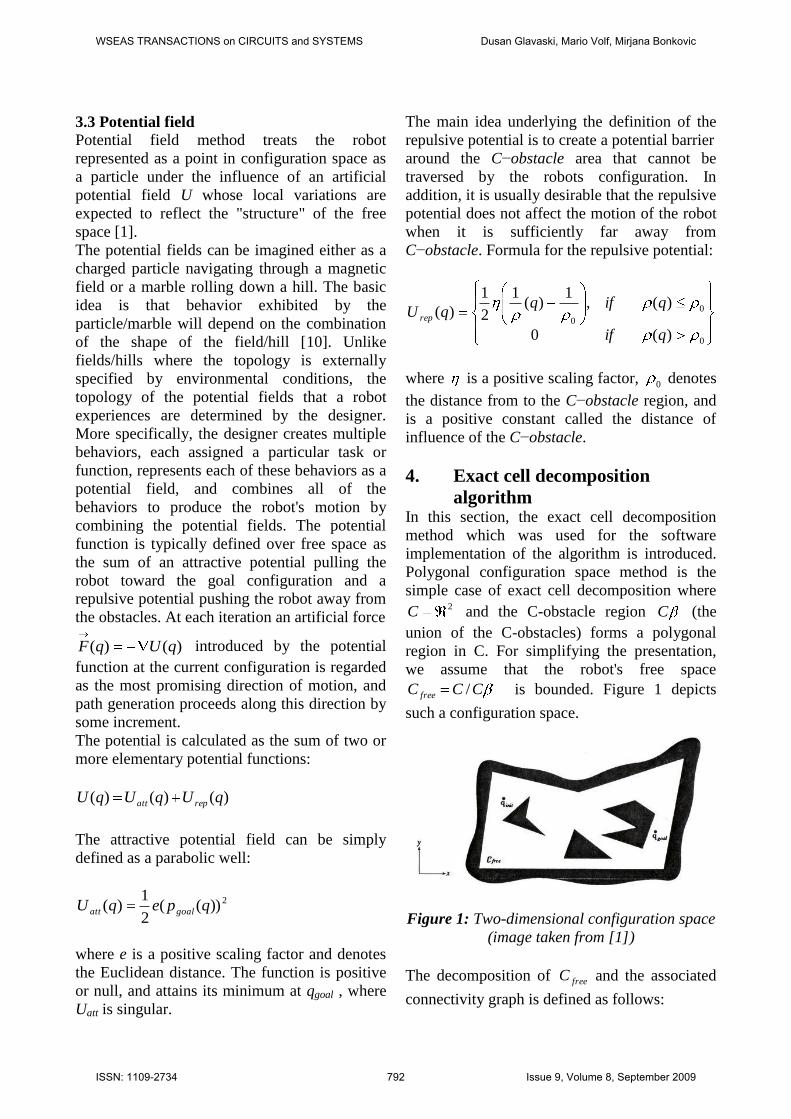
Polygonal configuration space method is the
simple case of exact cell decomposition where 2C and the C-obstacle region C (the
union of the C-obstacles) forms a polygonal
region in C. For simplifying the presentation,
we assume that the robot's free space
CCC free / is bounded. Figure 1 depicts
such a configuration space.
Figure 1: Two-dimensional configuration space
(image taken from [1])
The decomposition of freeC and the associated
connectivity graph is defined as follows:
WSEAS TRANSACTIONS on CIRCUITS and SYSTEMS Dusan Glavaski, Mario Volf, Mirjana Bonkovic
ISSN: 1109-2734 792 Issue 9, Volume 8, September 2009
A convex polygonal decomposition K
of freeC is a finite collection of convex
polygons, called cells, such that the
interior of any two cells do not intersect
and the union of all the cells is equal to
freeC . Two cells and in K are
adjacent if only if is a line
segment of non-zero length.
The connectivity graph G associated
with a convex polygonal decomposition
K of freeC is the non-directed graph
specified as follows:
o G's nodes are the cells in K .
o Two nodes in G are connected by
a link if and only if the
corresponding cells are adjacent.
Consider an initial configuration initq and a goal
configuration goalq in freeC . The exact cell
decomposition algorithm for planning a free
path connecting the two configurations is the
following:
1. Generate a convex polygonal
decomposition K of freeC .
2. Construct the connectivity graph G
associated with K .
3. Search G for a sequence of adjacent cells
between initq and goalq .
4. If the search terminates successfully,
return the generated sequence of cells;
otherwise, return failure.
The output of the algorithm is a sequence
p,...1 of cells such that 1initq , pgoalq
and for every , j and 1j are
adjacent. This sequence is called a channel.
One simple way to generate a free path
contained in the interior of the channel produced
by the search of G is to consider the midpoint
jQ of every segment j and to connect initq to
goalq by a polygonal line whose successive
vertices are 1Q ,…, )1( pQ .
The optimal convex decomposition of a polygon
is computable in polynomial time. The degree
of a polynomial is proportional to the number of
vertices n. Unfortunately, the presence of holes
in the polygon makes this problem NP-hard.
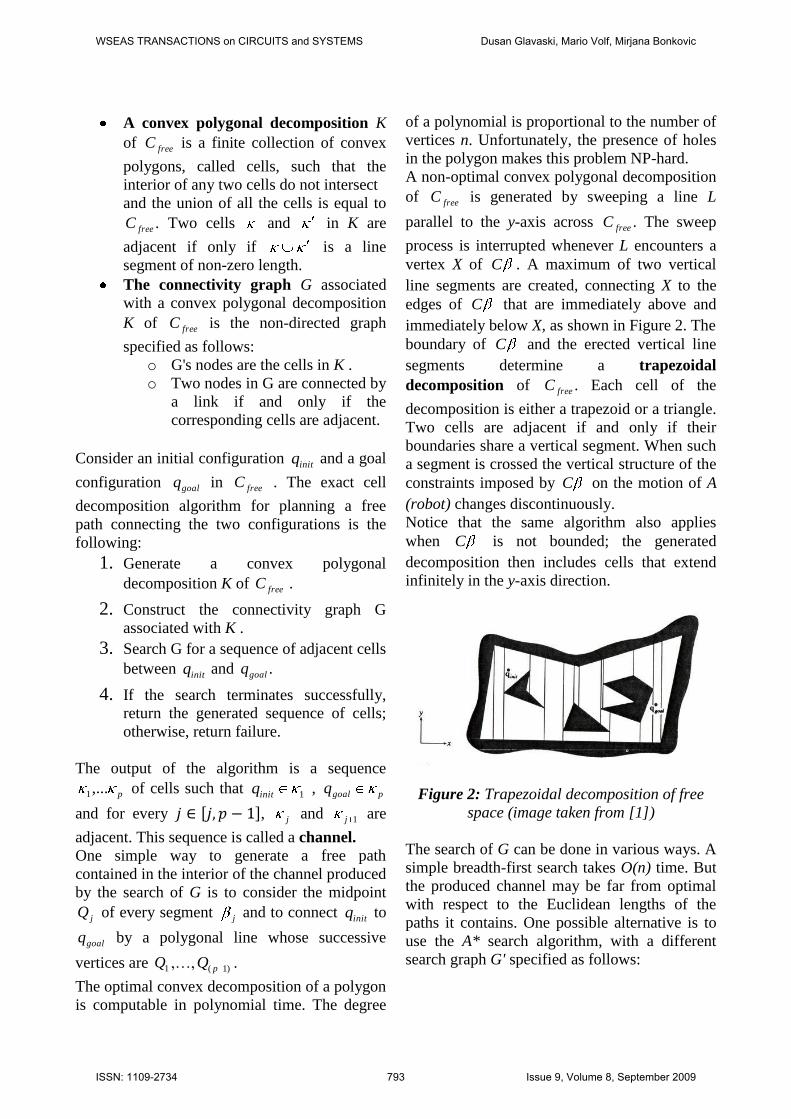
A non-optimal convex polygonal decomposition
of freeC is generated by sweeping a line L
parallel to the y-axis across freeC . The sweep
process is interrupted whenever L encounters a
vertex X of C . A maximum of two vertical
line segments are created, connecting X to the
edges of C that are immediately above and
immediately below X, as shown in Figure 2. The
boundary of C and the erected vertical line
segments determine a trapezoidal
decomposition of freeC . Each cell of the
decomposition is either a trapezoid or a triangle.
Two cells are adjacent if and only if their
boundaries share a vertical segment. When such
a segment is crossed the vertical structure of the
constraints imposed by C on the motion of A
(robot) changes discontinuously.
Notice that the same algorithm also applies
when C is not bounded; the generated
decomposition then includes cells that extend
infinitely in the y-axis direction.
Figure 2: Trapezoidal decomposition of free
space (image taken from [1])
The search of G can be done in various ways. A
simple breadth-first search takes O(n) time. But
the produced channel may be far from optimal
with respect to the Euclidean lengths of the
paths it contains. One possible alternative is to
use the A* search algorithm, with a different
search graph G' specified as follows:
WSEAS TRANSACTIONS on CIRCUITS and SYSTEMS Dusan Glavaski, Mario Volf, Mirjana Bonkovic
ISSN: 1109-2734 793 Issue 9, Volume 8, September 2009
The nodes of G are initq , goalq , and the
midpoints jQ of all the portions of
boundary shared by adjacent cells.
Two nodes are connected by a link if
and only if they belong to the same cell
(they can be joined by a straight line
segment in the cell).
Each link is weighted by the Euclidean length of
the straight line segment joining the two nodes.
If a free path exists, the search produces the
shortest free path contained in G'. It also
determines a sequence of cells from which
another path can be extracted. The search takes
nn log time.
5. Potential field algorithm The algorithm that is used in the implementation
is called best-first planning. It consists of
throwing a fine regular grid of configurations
across C. The grid is denoted by GC. GC can be
defined by considering a single chart over C and
discretizing each of the m corresponding
coordinate axes. Given a configuration q in the
m-dimensional grid GC, its p-neighbors are
defined as all the configurations in GC having at
most p coordinates differing from those of q, the
amount of the difference being exactly one
increment in absolute value. In addition, for
simplifying the presentation, we make the
following assumptions:
Both initq and goalq are configurations in
GC .
If two neighbors in GC are in free space,
the straight line segment connecting
them in R also lies in free space.
The grid GC is bounded and forms a
rectangle.
Best-first planning consists of iteratively
constructing a tree T whose odes are
configurations in GC.
The root of T is initq . At every iteration, the
algorithm examines the neighbors of the leaf of
T that has the smallest potential value, retains
the neighbors not already in T at which the
potential function is less than some large
threshold M, and installs the retained neighbors
in T as successors of the currently considered
leaf. The algorithm terminates when the goal
configuration goalq has been attained or when
the free subset of GC accessible from qinit has
been fully explored. Each node in T has a
pointer toward its parent. If goalq is attained, a
path is generated by racing the pointers from jq
to 1jq . The pseudo code will now be explained.
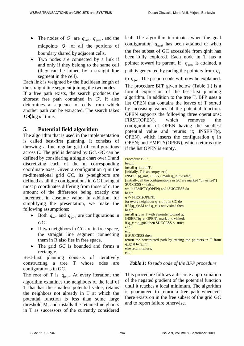
The procedure BFP given below (Table 1.) is a
formal expression of the best-first planning
algorithm. In addition to the tree T, BFP uses a
list OPEN that contains the leaves of T sorted
by increasing values of the potential function.
OPEN supports the following three operations:
FIRST(OPEN), which removes the
configuration of OPEN having the smallest
potential value and returns it; INSERT(q,
OPEN), which inserts the configuration q in
OPEN; and EMPTY(OPEN), which returns true
if the list OPEN is empty.
Procedure BFP;
begin;
install q_init in T;
[initially, T is an empty tree]
INSERT(q_init, OPEN); mark q_init visited;
[initially, all the configurations in GC are marked "unvisited"]
SUCCESS <- false;
while !EMPTY(OPEN) and !SUCCESS do
begin
q <- FIRST(OPEN);
for every neighbour q_c of q in GC do
if U(q_c)<M and q_c is not visited then
begin
install q_c in T with a pointer toward q;
INSERT(q_c, OPEN); mark q_c visited;
if q_c = q_goal then SUCCESS <- true;
end;
end;
if SUCCESS then
return the constructed path by tracing the pointers in T from
q_goal to q_init;
else return failure;
end;
Table 1: Pseudo code of the BFP procedure
This procedure follows a discrete approximation
of the negated gradient of the potential function
until it reaches a local minimum. The algorithm
is guaranteed to return a free path whenever
there exists on in the free subset of the grid GC
and to report failure otherwise.
WSEAS TRANSACTIONS on CIRCUITS and SYSTEMS Dusan Glavaski, Mario Volf, Mirjana Bonkovic
ISSN: 1109-2734 794 Issue 9, Volume 8, September 2009

6. Implementation
Implementation was done using ARIA
programming library, MATLAB, C++, Mapper
and MobileSim robot simulator. A short
description for the above (less known)
programming packages will be given:
1. ARIA - is an object-oriented, robot control
applications-programming interface for
MobileRobots (and ActivMedia) intelligent
mobile robots. Written in the C++ language,
ARIA is client-side software for easy, high-
performance access to and management of the
robot, as well as to the many accessory robot
sensors and effectors. ARIA includes many
useful utilities for general robot programming
and cross-platform (Linux and Windows)
programming as well. ARIA can be run multi-
or single-threaded, using its own wrapper
around Linux threads or Win32 threads. You
can access ARIA at different levels, from
simply sending commands to the robot through
ArRobot to development of higher-level
intelligent behaviour using Actions.[11]
2. Mapper – Mapper is application from
ActivMedia Robotics company which provides
the tools needed to construct a map of robot's
real operating space.[11]
3. MobileSim - is software for simulating
MobileRobots/ActivMedia platforms and their
environments, for debugging and
experimentation with ARIA . It replaces SRIsim
previously distributed with ARIA. MobileSim
builds upon the Stage simulator, created by
Richard Vaughan, Andrew Howard, and others
as part of the Player/Stage project, with some
modifications by MobileRobots. [12]
6.1 Best-first path
The algorithm is implemented using MATLAB
and ARIA. The source code can be found in [3].
The BFP algorithm includes a tree structure. In
the implementation a tree structure was not used
because of its complexity. Instead, a so called
checking function was designed and used.
Consequently, for every iteration starting at the
initial point initq it looks up its p-neighbors.
Then, it returns the neighbor configuration that
has the lowest potential value. This returned
configuration is marked as a1 and b1. The
current configuration is marked simply as a and
b. After the configuration with the minimal
potential value is returned, it is checked if that
value corresponds to the goal configuration. If it
does than the path from initial to the goal
configuration can be constructed. Otherwise, a
and b become a1 and b1 and the iteration
process continues.
Also the GC space is represented as a 100x100
grid. Every point is accessed through two
counters I and J representing x and y of the
configuration. In the example two obstacles are
introduced: a rectangle and a square. The first
iteration calculates the repulsive potential from
every point of C-obstacles to the current point
(note that the Euclidean distance between every
point in C-obstacle and the current point must
first be calculated). Than the attractive potential
between the current point and the goal
configuration is calculated. At the end these two
potentials are added and the value of the
potential in the current point attained. The
checking function will now be explained in
more detail. It takes the matrix of all potential
values in a 100x100 space, current position (a,b)
and the maximal configuration in 100x100
which is naturally (100,100) or (X,Y). Than it
examines the following conditions:
1. if (a>=2)&(b>=2)&(a<X)&(b<Y)
2. elseif (a>=2)&(b>=2)&(a<X) % eliminates b+1
3. elseif (a>=2)&(a<X)&(b<Y) % eliminates b-1
4. elseif (a>=2)&(b>=2)&(b<Y) % eliminates a+1
5. elseif (b>=2)&(a<X)&(b<Y) % eliminates a-1
6. elseif (a==1)&(b==1)
7. elseif (a==X)&(b==1)
8. elseif (a==1)&(b==Y)
9. elseif (a==X)&(b==Y)
10. elseif (a==1)
11. elseif (a==X)
12. elseif (b==1)
13. elseif (b==Y)
These conditions are used to see where the
current configuration is in the map and to
generate the p-neighbours A11, A12, A13, A21,
A23, A31, A32, A33. As you can see A22 is the
current location. Now the algorithm must return
the value of the neighbour that has the lowest
potential value. Before this step is performed
several conditions must be examined:
WSEAS TRANSACTIONS on CIRCUITS and SYSTEMS Dusan Glavaski, Mario Volf, Mirjana Bonkovic
ISSN: 1109-2734 795 Issue 9, Volume 8, September 2009

% A13 A23 A33
% A12 X A32
% A11 A21 A31
if (A11<A21)&(A11<A31)&(A11<A12)&
(A11<A32)&(A11<A13)&(A11<A23)&(A11<A33)
x=a-1;
y=b-1;
elseif (A21<A31)&(A21<A12)&(A21<A32)&
(A21<A13)&(A21<A23)&(A21<A33)
x=a;
y=b-1;
elseif (A31<A12)&(A31<A32)&(A31<A13)&
(A31<A23)&(A31<A33)
x=a+1;
y=b-1;
elseif (A12<A32)&(A12<A13)&(A12<A23)&
(A12<A33)
x=a-1;
y=b;
elseif (A32<A13)&(A32<A23)&(A32<A33)
x=a+1;
y=b;
elseif (A13<A23)&(A13<A33)
x=a-1;
y=b+1;
elseif (A23<A33)
x=a;
y=b+1;
else
x=a+1;
y=b+1;
end
6.1 Polygonal configuration space
The algorithm is implemented using ARIA
library and C++ programming language. The
maps for the simulation are made with the
Mapper application. Implementation of exact
cell decomposition algorithm has two separate
parts:
1. Graphical analysis and processing of the
map.
2. Robot movement through coordinates of
the shortest path for the given map.
In this paper the focus is on the second step of
the implementation. It is up to the user of the
application to calculate the coordinates of all
possible paths for the given map.
For input, the application uses file created by
the user which contains coordinates of all
possible paths. The file must be formatted in a
way that one line represents one path and each
point is divided by a space character from
another. Each path must contain robots initial
configuration for purposes of calculating
Euclidean distance for them. The sample of
such file can be seen in Table 2.
1.01 1.01 2 1.5 3 1 4 1.5 5 1 6 0.5 6.51 1.52 7.5 4
1.01 1.01 2 1.5 3 1 4 1.5 5 3.5 6 4.5 6.31 4.02 7.5 4
1.01 1.01 2 4 4 4 5 3.5 6 4.5 6.31 4.02 7.5 4
1.01 1.01 2 4 4 4 5 1 6 0.5 6.31 1.52 7.5 4
Table 2: Sample of map configuration file
Class Coord (Table 3.) is created for purposes
of storing x and y points for single coordinate:
class Coord {
public:
Double xt;
Double yt;
Coord(){};
Coord(double x, double y) : xt(x), yt(y) {};
};
Table 3: Class Coord
The application reads the contents of file and
stores data in vector of classes Coord; the
collection of all paths is stored in vector of
vectors Paths (Table 4.):
typedef vector<Coord>Dots
typedef vector<Dots>Paths
Table 4: Vectors used for storing paths
When all the data has been stored the Euclidean
distance is calculated for each path and these
values are used to determine the shortest path:
double distance (Dots d) {
double dist, tmp;
for (Dots::size_type i=0; i < d.size();i++) {
for (Dots::size_type j=i+1; j<=i+1; j++ )
tmp += pow((d[i].xt - d[j].xt),2) + pow((d[i].yt -
d[j].yt),2);
}
dist = sqrt(tmp);
return dist;
}
Table 5: Function for calculating Euclidean
distance of paths
WSEAS TRANSACTIONS on CIRCUITS and SYSTEMS Dusan Glavaski, Mario Volf, Mirjana Bonkovic
ISSN: 1109-2734 796 Issue 9, Volume 8, September 2009

Once the shortest path has been chosen it is
stored in a file called shortest. The initial
configuration of robot isn't stored in this file (it
is only used for the calculation of distance from
initial to goal configuration of the robot). While
creating the map user can position the robot
anywhere in the free space. When the
simulation
is started MobileSim uses robots initial
configuration as the beginning of the coordinate
system (0,0). To solve this problem offset has to
be subtracted from each point in the coordinates
before moving of the robot occurs. Notice that
the initial configuration of the robot
(coordinates of robots starting point) represents
the offset. ARIA with needed classes and
methods is initialized for purposes of
controlling robot movement (Table 6.).
Aria::init()
ArArgumentParser
parser(&argc, argv)
parser.loadDefaultArguments()
ArSimpleConnector
simpleConnector(&parser)
ArRobot robot
ArSonarDevice sonar
ArAnalogGyro gyro(&robot)
robot.addRangeDevice(&sonar)
Table 6: Initialization of ARIA classes and
method
The method gotoPoseAction.setGoal(ArPose(x, y)) is
used for the movement of the robot. The
setGoa(ArPosegoal) method sets a new goal of the
robot and sets the action to go to the given goal.
This action goes to a given ArPose coordinate
very naively. The action drives straight towards
a given ArPose and it stops when it gets close
enough to the goal. setGoal method is used for
giving a new goal to the robot, while
haveAchievedGoal is used to check if the robot has
achieved the given goal. ArPose takes
coordinates in millimetres. For this reason the
coordinates of the paths given in a file should be
multiplied by 1000, because the values in the
file are given in metres (Mapper application
uses metres as coordinate values). The whole
procedure can be seen in Table 7.
7. Simulation results
7.1. Best-first path
The algorithm is simulated in Matlab and on
MobileSim as well. For the purpose of the
simulation a map with two rectangle obstacles is
used. In the example which follows, the goal
point is (8,8). Figure 3 illustrates only the
repulsive potential.
It can be easily seen that the repulsive potential
does not depend on the position of the goal
configuration. Figure 4 represents only the
attractive potential. The difference between
these two graphs is that the attractive potential
depends on the position of the goal
configuration.
if (gotoPoseAction.haveAchievedGoal()) {
shortest >> x;
shortest >> y;
if(shortest.eof())
break;
x=x-x_offset; //offset rescission
y=y-y_offset;
x=x*1000; //conversion of coordinates to millimetres
y=y*1000;
gotoPoseAction.setGoal(ArPose(x, y)); //sending robot to
the next calculated goal
}
Table 7: Procedure of robot movement
Adding up repulsive (negative) and attractive
(positive) potential fields, a graph which can be
seen in the Figure 5, is attained. Similarly, as in
previous example, Figure 6 shows how the
algorithm works when it is embedded in
MobileSim. The movement of the robot depends
on the potential function. It determines the value
of the potential in each point of space. Also the
C-obstacle region is controlled with the distance
of influence. If it has a large value than the C-
obstacle space spreads out in space creating a
potential barrier that can not be traversed by the
robot. If a goal configuration is inside the radius
of the distance of radius than the algorithm
would run for infinity. This is one problem that
we must pay a close attention to. Another
problem is the local minima. The local minima
is a point in which the value of the potential
equals zero but it is not a goal point.
WSEAS TRANSACTIONS on CIRCUITS and SYSTEMS Dusan Glavaski, Mario Volf, Mirjana Bonkovic
ISSN: 1109-2734 797 Issue 9, Volume 8, September 2009

Aside from obvious problems potential field
method is the simplest and wittiest technique for
robot motion planning. Its main attribute is its
simplicity.
a)
b)
Figure 3: Potential field in case where there
are two obstacles: a) perspective
representation; b) plane view
Figure 4: The map represents the attractive
potential
Figure 5: Attractive+repulsive potential
field+free path
WSEAS TRANSACTIONS on CIRCUITS and SYSTEMS Dusan Glavaski, Mario Volf, Mirjana Bonkovic
ISSN: 1109-2734 798 Issue 9, Volume 8, September 2009

Figure 6: Trace of the path generated in
MobileSim
7.2 Polygonal configuration space
MobileSim application was used for the
simulation of the algorithm. The application
works from a command line. A user must pass
three arguments to application:
Name of the file with coordinates of all
possible paths for a certain map
Wanted speed of the robot (mm/s)
Close distance (used to set the distance
which is close enough to the goal (mm)).
The program prints out values of all possible
paths, values of Euclidean distances and the
coordinates of the shortest path. The motion and
path of the robot can be seen in the MobileSim
application. It is easily noticed that the robots
path is determined by the midpoints Qj of
segments j . The path of the robot is highly
influenced by the layout of the obstacles in free
space. The distance between obstacles and the
edge of robots free space determines how
widely
the robot avoid an obstacle (Figure 7). During
the simulation problems occurred with higher
speed values on certain maps. The robot would
rotate too fast and miss its next goal, resulting in
a random circular movement of the robot around
the missed coordinate (Figure 8). Similar
problems occurred when the robot would come
too close to the obstacle during the rotation. The
possible solutions to this problem are lowering
robots speed or increasing close distance
through application arguments.
Figure 7: Path generated by the application
(simulation in MobileSim)
Figure 8: Robot movement problem as a high
speed result
WSEAS TRANSACTIONS on CIRCUITS and SYSTEMS Dusan Glavaski, Mario Volf, Mirjana Bonkovic
ISSN: 1109-2734 799 Issue 9, Volume 8, September 2009

Figure 9: Path generated by polygonal
configuration space method
This method, in most cases, avoids obstacles
more widely than other methods, while the
paths not being significantly longer. The paths
generated by this method are usually
significantly better than those generated using
the visibility graph method. The simulation on
the same map as shown in the best-first path
chapter can be seen in Figure 9.
The main disadvantage of this method is hard
implementation of map analysis and processing.
On the other hand, it is very logical and easy to
understand.
8. Conclusion
Two typical methods used in robot motion
planning were shown. Potential field method
was originally developed as an on-line collision
avoidance approach, applicable when the robot
does not have prior knowledge of the obstacles,
but senses them during motion execution.
Emphasis was put on real-time efficiency, rather
than on guaranteeing the attainment of the goal.
It may get stuck at a local minimum of the
potential function other than the goal
configuration. However, the idea underlying
potential field can be combined with graph
searching techniques. Then, using a prior model
of the workspace, it can be turned into
systematic motion planning approach and this
was done in the previous examples. In contrast
to potential field method the exact cell
decomposition method is not meant for real time
path planning. It is a graphical method used
when a prior model of the workspace is known.
The method guarantees finding a free path if
one exists and if it is attainable by the robot.
9. References [1] Latombe, J., "Robot Motion Planning", 1991.
[2] Lucia Vacariu, Flaviu Roman, Mihai Timar, Tudor
Stanciu, Radu Banabic, Octavian Cret, Software and
Hardware Implementation of Mobile Robot Path
Planning, WSEAS Transactions on Systems and
Control, Issue 2, Volume 2, February 2007.
[3] O. Hachour AND N. Mastorakis, Avoiding obstacles
using FPGA –a new solution and application ,5th
WSEAS international conference on automation &
information (ICAI 2004) , WSEAS transaction on
systems, issue9 ,volume 3 , Venice , italy15-17 ,
November 2004 , ISSN 1109-2777, pp2827-2834 .
[4] O. Hachour AND N. Mastorakis, FPGA
implementation of navigation approach, WSEAS
international multiconference 4th WSEAS
robotics,distance learning and intelligent
communication systems (ICRODIC2004), in Rio de
Janeiro Brazil, October 1-15 , 2004, pp2777.
[5] M. Šeda, A Comparison of Roadmap and Cell
Decomposition Methods in Robot Motion Planning,
WSEAS Transactions on Systems and Control, Vol.
2, Issue 2, 2007, pp. 101-108.
[6] Planning Algorithms, Steven M. LaValle,2006,
Cambridge University Press, ISBN 0-521-86205-1.
Available online at http://planning.cs.uiuc.edu/
[7] Principles of Robot Motion: Theory, Algorithms,
and Implementation, H. Choset, W. Burgard, S.
Hutchinson, G. Kantor, L. E. Kavraki, K. Lynch,
and S. Thrun, MIT Press, April 2005.
[8] Mark de Berg, Marc van Kreveld, Mark Overmars,
and Otfried Schwarzkopf (2000). Computational
Geometry (2nd revised ed.). Springer-Verlag. ISBN
3-540-65620-0. Chapter 13: Robot Motion Planning:
pp.267–290.
[9] Nora H. Sleumer, Nadine Tschichold-Gűrman, 1999,
"Exact cell decomposition of arrangements used for
path planning in robotics",
http://www.inf.ethz.ch/publications/abstract.php3?n
o=tech-reports/3xx/329
[10] Michael A. Goodrich, 2000, “Potential fields
tutorial”,
http://borg.cc.gatech.edu/ipr/files/goodrich_potential
_fields.pdf
[11] www.activmediarobotics.com
[12] www.wikipedia.com
WSEAS TRANSACTIONS on CIRCUITS and SYSTEMS Dusan Glavaski, Mario Volf, Mirjana Bonkovic
ISSN: 1109-2734 800 Issue 9, Volume 8, September 2009