mobility management algorithms for reducing signaling
TRANSCRIPT
Budapest University of Technology and Economics
Department of Telecommunications
Mobility Management Algorithms for Reducing Signaling Overhead in Next
Generation Mobile Networks
PhD. Theses
Vilmos Simon
Research supervisor: Sándor Imre DSc.
Budapest, 2008.
Declaration I hereby certify that this material, which I now submit for assessment on the programme of study leading to the award of PhD is entirely my own work and has not been taken from the work of others save and to the extent that such work has been cited and acknowledged within the text of my work. Nyilatkozat Alulírott Simon Vilmos kijelentem, hogy ezt a doktori értekezést magam készítettem, és abban csak a megadott forrásokat használtam fel. Minden olyan részt, amelyet szó szerint, vagy azonos tartalomban, de átfogalmazva más forrásból átvettem, egyértelműen, a forrás megadásával megjelöltem. Budapest, 2008.07.03. .................................. Simon Vilmos A dolgozat bírálata és a védésről készült jegyzőkönyv a későbbiekben a dékáni hivatalban elérhető.
2

Köszönetnyilvánítás
Vannak számomra olyan fontos emberek, akik nélkül e disszertáció nem születhetett volna meg. Mélységesen köszönöm szüleimnek és testvéremnek mindazt a szeretetet és gondoskodást amit kaptam tőlük, az élettapasztalatot amit átadtak, mindenki a maga módján. Köszönöm Zorának a sok megértést, szerelmet és türelmet, és hogy végig biztatott a cél felé vezető úton. Továbbá köszönöm barátaimnak, hogy nem okoztak csalódást, mindig akkor és úgy voltak ott, ahogy szükségem volt rájuk. Köszönöm Imre Sándornak, hogy mindig szakított rám időt és a sok hasznos tanácsot amit adott a disszertációm születése közben, sokszor hosszú ideig együtt gondolkodva és rajzolva a dolgozószobája táblájánál. Köszönöm Pap Lászlónak, hogy „megfertőzött” a mobil hálózatok kutatásának nagyszerű vírusával, mindazt a lenyűgöző előadást amivel e tématerületet megszeretette velem. Köszönöm Szabó Sándornak, hogy első konzulensemként a Mobil Laborba kalauzolt és sok hasznos szakmai és emberi tanáccsal látott el. Köszönöm Cinkler Tibornak, hogy nap mint nap biztatott, amikor már lankadtam. Köszönet illeti a Mobil Labor összes tagját, kik nap mint nap katalizátorként hatottak kutatási ötleteimre.
3

Contents 1 INTRODUCTION............................................................................................................................... 6
1.1 THESIS CONTRIBUTIONS............................................................................................................. 10 1.2 RESEARCH OBJECTIVES.............................................................................................................. 11 1.3 RESEARCH METHODOLOGY ....................................................................................................... 13
2 LOCATION AREA OPTIMIZATION ALGORITHMS FOR A HETEROGENEOUS MOBILITY ENVIRONMENT ................................................................................................................. 14
2.1 COMPUTATIONAL COMPLEXITY OF THE PROBLEM ..................................................................... 14 2.2 THE PAGING COST FUNCTION .................................................................................................... 15 2.3 THE LOCATION UPDATE COST FUNCTION .................................................................................. 16 2.4 THE LOCATION AREA FORMING ALGORITHM (LAFA) .............................................................. 17
2.4.1 Definitions ............................................................................................................................ 17 2.4.2 The Location Area Forming Algorithm (LAFA) ................................................................... 18
2.5 THE CELL REGROUPING ALGORITHM (CEREAL)...................................................................... 20 2.5.1 The Algorithm....................................................................................................................... 20
2.6 NUMERICAL ANALYSIS .............................................................................................................. 21 2.6.1 The Mobility Simulator ......................................................................................................... 21 2.6.2 The Traffic-Based Static Location Area Design algorithm................................................... 22 2.6.3 The Simulation Results ......................................................................................................... 24 2.6.4 Results Using the Vehicular Mobility Simulator .................................................................. 27
2.7 SUMMARY.................................................................................................................................. 31 3 LOCATION AREA OPTIMIZATION ALGORITHMS FOR A HOMOGENEOUS MOBILITY ENVIRONMENT ................................................................................................................. 32
3.1 THE COST FORMULATION .......................................................................................................... 32 3.1.1 Assumptions.......................................................................................................................... 32 3.1.2 Location Update Cost ........................................................................................................... 33 3.1.3 Paging Cost .......................................................................................................................... 34 3.1.4 Optimization of the Location Update Cost ........................................................................... 35
3.2 LOCATION AREA PLANNING ALGORITHMS ................................................................................ 36 3.2.1 The Greedy Algorithm (GREAL) .......................................................................................... 36 3.2.2 The Simulated Annealing Based Location Area Forming Algorithm (SABLAF).................. 37
3.3 SIMULATION RESULTS ............................................................................................................... 40 3.4 SUMMARY.................................................................................................................................. 41
4 NETWORK DESIGN ALGORITHM FOR OPTIMIZING THE UPPER HIERARCHICAL MOBILE STRUCTURES.......................................................................................................................... 42
4.1 RELATED WORKS....................................................................................................................... 43 4.2 THE OPTIMIZATION PROBLEM.................................................................................................... 44 4.3 THE COST STRUCTURE............................................................................................................... 46
4.3.1 The Location Update Cost .................................................................................................... 46 4.3.2 The Packet Delivery Cost ..................................................................................................... 47 4.3.3 The Total Signaling Cost ...................................................................................................... 48
4.4 THE HIERARCHICAL NETWORK DESIGN ALGORITHM (HIENDA).............................................. 48 4.4.1 Definitions ............................................................................................................................ 48 4.4.2 The Algorithm....................................................................................................................... 50
4.5 SIMULATION RESULTS ............................................................................................................... 52 4.6 SUMMARY.................................................................................................................................. 58
4
5 OVERHEAD REDUCING INFORMATION DISSEMINATION STRATEGIES FOR DISCONNECTED MOBILE AD HOC NETWORKS ........................................................................... 59
5.1 INTRODUCTION........................................................................................................................... 59 5.2 RELATED WORKS....................................................................................................................... 61 5.3 NOVEL INFORMATION DISSEMINATION ALGORITHMS FOR A DISCONNECTED MANET ............. 63
5.3.1 The IOBIO Algorithm (InfOrmation Dissemination Protocol for BIOlogically Inspired autonomic Networks and Services) ..................................................................................................... 63 5.3.2 The Modified IOBIO Algorithm (MIOBIO) .......................................................................... 65 5.3.3 Multi-Message Scalable Broadcast Algorithm (MMSBA) .................................................... 65 5.3.4 Mobility Models for Disconnected Networks........................................................................ 66
5.4 THE SIMULATION FRAMEWORK ................................................................................................. 67 5.5 SIMULATION RESULTS ............................................................................................................... 67 5.6 NATURAL SELECTION OF THE INFORMATION DISSEMINATION ALGORITHMS ............................. 69
5.6.1 The Natural Selection Framework........................................................................................ 69 5.6.2 Simulation Results ................................................................................................................ 72
5.7 SUMMARY.................................................................................................................................. 77 6 CONCLUSIONS ............................................................................................................................... 78 LIST OF FIGURES.................................................................................................................................... 80 LIST OF ABBREVIATIONS.................................................................................................................... 81 REFERENCES ........................................................................................................................................... 83 PUBLICATIONS........................................................................................................................................ 88
5

Chapter 1
1 Introduction
A key technical challenge for next-generation mobile networks is to provide seamless access guarantees for mobile users. The seamless access and low delays can only be achieved by means of efficient mobility management to handle the frequent handovers that is experienced by a typical Mobile Terminal (MT). Therefore mobility tracking is critical for the next generation mobile networks to enable seamless handover [1]. Future mobile networks will provide ubiquitous services to a large number of MTs and the design of such networks is based on a cellular architecture that allows the efficient use of the limited available spectrum. As it is well-known, cellular communications have experienced an explosive expansion due to recent technological advances in cellular networks and cellular phone manufacturing and it is expected that they will experience even more growth in the next decade.
In a cellular network, a service coverage area is divided into smaller areas of hexagonal shape, referred to as cells, where each cell is served by a base station (BS). These fixed BSs are interconnected through a fixed network (the BSs are connected to the mobile switching center (MSC), which is, in turn, connected to the public switched telephone network), while the MTs communicate with the BSs via wireless links. Neighbouring cells overlap with each others, ensuring continuity of communications when the users move from one cell to another. To terminate a call, the network first needs to identify the MSC and the cell in which the mobile station is presently located. How to locate the current residing cell of a MT is an issue of Location Management (LM) [2].
Upon the arrival of a mobile-terminated call, the system tries to locate the MT by searching for it among a set of base stations over the current area knowledge of the mobile. This search is called paging [3], and the set of base stations in which a mobile is paged is called the Location Area (LA). At each LA boundary crossing, MTs register their new locations through signalling in order to update the location management databases (location update procedure). MTs are free to move with a given LA without updating their location, informing the network only when crossing to a new LA. If a call is to be forwarded to the MT, the network must now page every cell within the LA to find out their exact location. Network cost is incurred on location updates and paging, the balance of these defining the field of Location Management, therefore the two basic operations involved in LM are the location update procedure and paging. The tradeoff between these two operations could be illustrated with two extreme scenarios, the always-update (proactive) and the never-update (reactive) case. In the always-update case each MT sends an update message every time it moves to a new cell, while in the never-update scenario the MNs never send update information regarding their current location. Obviously in the always-update scenario the overhead due to the transmission of update messages is very high, particularly in mobile networks with small cells and a large number of highly mobile nodes, while the overhead of finding MTs namely the paging is
6

zero, since the precise position of each MT is all the time known. In the never-update scheme there is no overhead for the updating procedure, but each time when there is a need to find a MT, the paging overhead will be extremely high, especially in a case of a large network or for high call arrival rates.
These two updating scenarios demonstrate the basic handoff problem of LM. Frequent location updates can be a very costly operation, especially for users with
comparatively low call arrival rates. The update overhead not only puts load on the core (wired) network but also reduces accessible bandwidth in the mobile spectrum, including the modification cost of the location databases. The heavy power consumption of the MTs is also a major drawback of needless location updating. On the other side network-wide searches load both the backbone and the wireless network.
Therefore a huge number of schemes have been proposed to decrease the amount of location update messages required by a MT in a cellular network. Location update schemes are often classified into the categories of static and dynamic [3].
In the static location update solutions a predetermined set of cells is used at which location updates must be generated by a MN independently from any user characteristics.
Contrarily to this in the dynamic case a location update can be generated by a MN in any cell depending on its mobility. Accordingly static solutions provide a lower level of cost reduction and a lack of independent user tracking and parameterization, but allow efficient implementation and a reduced computational complexity.
Dynamic schemes allow per-user parameterization of the location update frequency and hence may achieve lower location update costs, but a higher degree of computational overhead is required.
A widely used static (or global) location update solution is the zone-based scheme, where the coverage area of the network is divided into the above-mentioned Location Areas, where each LA consists of a group of cells. When a MT crosses a boundary of a LA, the user updates the system with its new location information. The LAs are determined in advance based on static movement probabilities. The existing standards for location management in current mobile networks such as GSM [4], IS-41 [5] and UMTS [6] use zone-based schemes for mobility management, the difference between the employed zone-based techniques will be explained later on.
The location update process may be triggered periodically or on LA boundary crossings, which is more common. The former scheme is much simpler to implement, only requiring the MT to send a location update message containing its present LA at regular time intervals. The drawback of this method that it is not capturing the details of user movement and therefore the update frequency could be much higher than appropriate to the current rate of the MT movement. On the end there are no guarantees that the network will have precise information of the exact LA the MT resides in. The boundary crossing method is more precise; the updating process is triggered only when crossing to another LA. The weakness of this method is the ping-ponging effect [7], where the MT moves repetitively between the boundaries of two or more LAs, generating a huge number of location update messages with comparatively low physical mobility.
A variety of new LA based schemes are introduced in the literature, presenting improvements to the basic LA solutions. For instance several schemes have been proposed to address the ping-ponging problem, such as the Two Location Area (TLA) [8] and Three Location Area (TrLA) [7] mechanisms. In these papers multiple LAs are
7

assigned to a MT, location updates are needed only when one of the respective two or three LAs has been exited.
To terminate an incoming call the network needs to find the accurate location cell of the MT, by sending a paging message to all of the cells where the MT could be in that moment. Various paging procedures have been proposed, the most commonly used are blanket paging (also known as simultaneous), sequential paging and intelligent paging.
In the blanket paging scheme the paging area will be equal to the LA, which means all the cells in the given LA are paged simultaneously to deliver an incoming call. This paging procedure will cause a low paging delay, but may produce excessive paging traffic; it is used in the current GSM networks. In sequential paging the LA is divided into smaller areas called a Paging Area (PA), polling these groups of cells in a paging area one-by-one, in a polling cycle. This polling cycle is defined by the round trip time from the time when a paging message is transmitted to the time when the response is received. While this scheme is capable of reducing the paging load, it may introduce high paging delay (increasing it exponentially), therefore it is important that the PAs are formed from a larger number of cells. The order of paging each area and the number of cells per PA is crucial to the performance of this scheme. The simplest ordering of PAs in the sequential paging procedure is the random one, where each PA is polled in a random order. It is outperforming the blanket scheme in terms of total number of polling messages, but solutions where the next polled PA is located geographically close to the previously updated location can reduce even more the number of polling messages. The main drawback of this method is that it requires the knowledge of the geographical structure of the network and for MTs with high mobility will perform disappointingly.
A lot of research has been done on an intelligent paging scheme [9], [10], where the paging order is based on pre-established probability metrics. The basic principle of intelligent paging is to page cells sequentially based on particular user information like residence probabilities, MT speed and etc. Research of intelligent paging primarily focused on the estimation of the user location probability; therefore the cells with higher probability of being the location cell of the user are paged first to reduce the paging traffic and delay. The user location probability can be assigned based on the latest registration location, MT mobility and the time elapsed since the last location update. Although the paging traffic and delay can be decreased this way, the computational overhead is high for this solution, so it is infeasible for large cellular networks.
As mentioned above, unlike static location update mechanisms, the dynamic ones allow per-user parameterization of the location update rate. Therefore the location update may be performed from any cell in the network, taking into consideration the call arrival and mobility patterns of the user. One group of the dynamic location update solutions are the threshold-based schemes, where each MT updates its location when a given parameter increases beyond a defined threshold. There is no notion of LAs, the selected thresholds are adapted to the individual user mobility patterns and communication traffic.
The location update can be performed due to the time elapsed since the last registration process [11], which has the advantage of simple implementation, but a disadvantage of poor performance caused by unnecessary LUs performed by stationary MTs. The two most significant spatial domain threshold-based LU strategies are the distance-based [12] and the movement-based [13]. In the distance-based strategy the location update will be performed, when the MT moves a threshold number of cells away
8

from the cell where the last registration process was carried out. This threshold distance can be adjusted for each MT dynamically. In the movement-based LU strategy the number of cell boundary crossings measured since the previous update is counted by the MT, and when this number exceeds a given threshold value, the MT performs a location update. Bar-Noy et al. [3] have compared time-, distance-, and movement based schemes in terms of location management cost, and they have shown that the distance-based one performs best. However, its implementation is quite hard in a real-world network [14], since the distance of the mobile terminal has to be computed dynamically as it moves from cell to cell and this not only requires the device to maintain information about its starting position, but also to possess some concept of a coordinate system, allowing the calculation of distance between the two points. The hybrid of distance-based and zone-based approach is studied by Casares-Giner et al. [15].
A large group of dynamic location update schemes are the profile-based solutions, where the network database maintains the individual mobility patterns for each user. One of these solutions is the personal LA approach, where different LA sizes are defined for each user, like in [16], where a new location tracking strategy based on each mobile's moving behavior is introduced. From the moving behavior of each MT a time-varying probability of the mobile is estimated and then the optimal paging area of each time region is derived. Another profiled-based solution is when the network has a list of the most probable cells for the users to be located in [17]. When a location update occurs, the network management sends the list to the MT, containing what may be considered a complex LA. Therefore the MT will send its location information only when entering a cell which is not on the list. Sen et al. recommend that users can skip some update operations while they cross the LAs boundaries [18]. When a call comes in, the network uses the profile information to estimate the probability for each LA that it is the current LA of the user. The network then starts the paging procedure for the LAs in order of decreasing probability.
While the dynamic location update schemes, especially the profile-based solutions offer better utilization of wireless network resources, they add significant complexity to mobility management. Furthermore they require modification of the current standards, changes of the mobile network infrastructures and the update of handsets. Thus many dynamic location update schemes are still only theories, but not functional under real-world circumstances.
The current cellular networks use static location update solutions, namely the zone-based schemes combined with different paging strategies. The currently two commonly used standards for location management in the Public Land Mobile Network (PLMN): the Electronic and Telephone Industry Associations EIA/TIA Interim Standard (IS-41) and the Global System for Mobile Communications (GSM) Mobile Application Part (MAP) both deploy the classical Location Area based location update scheme combined with a blanket paging scheme. In GSM the MT triggers a location update periodically also, i.e. after a certain time threshold T expires.
Zone-based location update solutions are used in UMTS also; the cells are grouped into Routing Areas (RAs) and further grouped into UTRAN registration areas (URAs) [19]. Therefore UMTS utilizes a three-level location management strategy, i.e., a MT is tracked at cell level during packet transmission session, at the URA level during the idle period of an ongoing session, and at the RA level when the MS is not in any
9

communication session. The LA planning principles introduced in my Theses could be used also for forming of these location management areas.
Given the increasing number of MTs and transitions occurring from 2G to 3G it is crucial to improve location update and paging costs by allocating Location Areas in an optimal, implementable fashion.
1.1 Thesis Contributions The theses are organized around four concepts that make the mobility management framework efficient and applicable in next generation mobile networks:
I. Location Area optimization algorithms for a heterogeneous mobility environment II. Location Area optimization algorithms with for a homogeneous mobility
environment III. Network design algorithm for optimizing the upper hierarchical mobile network
levels IV. Overhead reducing information dissemination strategies for disconnected mobile
networks Chapter 2 (Thesis I, Heterogeneous Mobility Environment):
• The mathematical description of the paging and location update cost function is introduced.
• An LA forming algorithm (LAFA) is designed based on the statistical probabilities of the moving directions chosen by the mobile users.
• A cell regrouping algorithm (CEREAL) is proposed for a refinement optimization
• A mobility simulator is developed for the generation of a realistic border crossing and incoming call pattern as an input for the algorithms.
• Results show that significant reduction was achieved in the amount of the signalling traffic.
Chapter 3 (Thesis I, Homogeneous Mobility Environment):
• A mathematical analysis for the determination of optimum number of cells per LA is presented.
• The location update cost and paging constraint is introduced. • An LA forming algorithm is proposed that contains two phases: a greedy
algorithm (GREAL) is adopted which forms a basic partition of cells into LAs, and then a simulated annealing based algorithm (SABLAF) is applied for getting the final partition.
• By comparing the values of the location update cost function significant reduction was achieved in the amount of the registration signalling traffic.
10

Chapter 4 (Thesis II):
• Location update and packet delivery cost structure is introduced. • A hierarchical network design algorithm (HIENDA) is created based on
the structure given by the LA planning algorithm from Thesis I, aligned with a MAP allocation algorithm.
• A simulation evaluation is presented. Chapter 5 (Thesis III):
• The communication architecture of a disconnected mobile network is introduced.
• Two novel information dissemination strategies (MIOBIO, Multi-Message SBA) for disconnected mobile networks are presented.
• The performance of the two novel information dissemination algorithms is evaluated using the BIONETS Simulation Platform, comparing them with the recent algorithms chosen from the literature.
• A novel approach is introduced to use an evolution based decision mechanism which utilizes natural selection for choosing the adequate information dissemination algorithm for different mobility environments in a self-managing MANET
Chapter 6 is devoted to the summary
1.2 Research Objectives
As highlighted above one of the key tasks in the field of Location Management is to find balance between the network cost caused by location update and paging operations. This tradeoff can be found in the zone-based schemes by means of efficient LA planning. Therefore the question arises, what size the LA should be for reducing the cost of paging and LU signalling (or registration signalling).
Both, increasing and decreasing the size have their own benefit. On the one hand if we join more and more cells into one LA, then the number of LA handovers will be smaller, so the number of location update messages sent to the upper levels will decrease. However in the case of large number of cells belonging to LA, an incoming call will cause lot of paging messages [20], since we must send one to every cell to find where is the mobile user inside that LA. These network-wide searches will load both the backbone and the wireless network. On the other hand if we decrease the number of cells, then we do not need to send so much paging messages, but then the number of LA changes will increase. This will cause a remarkable update overhead which puts load not only on the core (wired) network but also reduces accessible bandwidth in the mobile spectrum, including the modification cost of the location databases. The heavy power consumption of the MTs is also a major drawback of needless location updating. Therefore the overall
11

problem in LA planning comes from the tradeoff between the paging cost and the registration cost. Figure 1 shows a mobility management scenario, dividing the cell handovers into two major groups: inside the mobility management zone (intra-domain) or between these zones (inter-domain), the domains correspond in this case to Location Areas.
Figure 1 The Location Area planning problem
Location Area planning in zone-based schemes is widely studied; these LA planning methods can be grouped into two categories. In the first group a uniform user distribution and inter-cell movement rate is assumed, and with these assumptions optimal LA planning is introduced [21], [22]. These results can not be applicable to most of the practical cases where these network properties are heterogeneous [23]. The second group consists of LA planning solutions where the network is described by a graph [24], [25] where the cells of the network are represented with the nodes, and the inter-cell movement rates with the edges of the graph. This way the LA planning is mapped to a graph partitioning problem. In [26] a LA planning scheme is introduced for covering highways where a homogeneous traffic and user density is assumed. This contribution, as papers [13] and [27] also, are dealing with the determination of the optimal number of cells in an LA, but they were not focusing on the selection of the optimal set of cells for each LA.
Instead of this, the objective of my thesis was to propose a solution to obtain the optimal partition of cells for every LA. As mentioned above, the uniform inter-cell movement rate distribution is not always realistic, therefore I present a LA planning solution for the heterogeneous mobility environment and for the homogeneous also, and this gives the real novelty of my work. In the heterogeneous case, the optimisation goal was to reduce the Location Update and the aggregated cost, while in the second case the
12
Paging Cost is considered as a constraint; therefore the Location Update Cost is left alone in the objective function.
This two-case LA planning scheme (Thesis I) gives the input to my hierarchical network design algorithm (Thesis II), therefore these two design methods constitute an integral cellular network planning framework.
To address not only the designing aspects of a cellular network, in Thesis III novel information dissemination strategies are introduced for a non-traditional communication approach: my research interest was in developing novel information dissemination solutions for disconnected, autonomous networks, lacking any central infrastructure, to decrease the signalling overload of message forwarding. Thus beside the practical designing methods for already world widely used networks, new algorithms are presented for autonomic networks which is a cutting edge area in the field of information science, and it is believed to cause a marked shift in the way communication systems and networks are conceived. An important objective was to use a bio-inspired framework which utilizes natural selection for choosing the adequate information dissemination algorithm for different mobility environments in a self-managing mobile ad hoc network. In this framework the cooperation between the nodes can be examined, how they improve the overall parameters of the system like throughput and data age.
1.3 Research Methodology
Two classical approaches were used in my theses: analytical considerations and simulations. In the analytical part the cost structure was defined for the first three optimization issues (Theses I.-II.) and the mobile network was modelled with a graph, introducing the mathematical description of the algorithms. In Thesis III. the mobility models were developed by modifying the existing group mobility models taken from the literature, adapting them to a disconnected mobility environment.
All the algorithms are implemented in the simulators together with the recent contributions in the field, providing a useful tool for the performance evaluation of the new mobility management framework. The input of the algorithms was generated by the mobility simulator, producing a realistic cell boundary crossing (inter-cell movement rate) and incoming call database in a given mobile system, which is a good representation of the mobility patterns in real life.
To use real world measurements and prototyping for cellular and disconnected networks is a heavily money consuming process, which I could not afford in my research.
13

Chapter 2
2 Location Area Optimization Algorithms for a Heterogeneous Mobility Environment
2.1 Computational Complexity of the Problem
As explained in Chapter 1, most of the references related to the LA design are focused on how to determine the optimal number of cells for an LA,, while in this thesis an algorithm is presented which can give us the optimal partition of cells into LAs.
In this chapter a LA planning method is introduced for a heterogeneous mobility environment, which means the inter-cell movement rate distribution is not near uniform, as it is assumed in the majority of LA planning schemes published earlier. Therefore the goal was to reduce the sum of the location update and paging cost, while in the near-uniform distribution case (Chapter 3) the final goal is the determination of optimum number of cells per LA for which the location update cost is minimum, with the paging cost as an inequality constraint function, which gives the novelty of this research, namely for both environments the LA structure can be optimized.
My LA planning solution uses the basic idea to group cells according to the inter-cell movement rates, in such a way to reduce the inter-LA movements of the MTs. This means that the final goal was to maximize the intra-LA traffic, because in this way the number of the LA handovers can be decreased, and therefore the total amount of administrative messages. The number of LA handovers can be reduced by joining the cells, along the dominant moving directions, as it will be introduced later.
The problem of partitioning the given set of cells into a family of disjoint subsets such that the cardinality of each subset is lower than or equal to a constraint (number of cells in a LA) and the total inter-cell movement rate between the members of each subset is maximized was found in [28] as NP-complete, with a detailed proof.
Since the time required to solve this problem grows exponentially in the size of the problem, no algorithm exists that ensures optimal results in reasonable amount of time. Therefore, techniques that offer near-optimal solutions within acceptable run times are required. An adequate approach is the use of heuristic algorithms for approximating the optimum location area configuration. Only simulation examinations could be carried out to compare different LA planning solutions, analytical results could not be derived because of the complexity of the problem.
Just to demonstrate the calculation time needed for finding the optimal partition of cells, which would require of examining all of the possible partitions. The number of ways a set of elements can be n partitioned into nonempty subsets is called a Bell number and denoted . The Bell numbers satisfy this recursion formula nB
14
k
n
kn B
kn
B ∑=
+ ⎟⎟⎠
⎞⎜⎜⎝
⎛=
01 , and also satisfy ∑
∞
==
0 !1
k
n
n kk
eB . The first few Bell numbers are from
to : 1, 2, 5, 15, 52, 203, 877, 4140, 21147, 115975, 678570, 4213597. From these expressions it can be seen that the number of partitions on a given set is the exponential function of the number of the set members, as the
1=n 12=n
exponential generating function of the Bell numbers is ( ) 1−=
xeexf . While using an average PC in the case of the time required for the calculation of the partitions will be around 2 minutes and
the memory of the file around 230 Mb, for 12=n
13=n the running time would take around 15-16 minutes, while the memory demand will be around 1.7Gb. As it is the exponential function of , in the case of 3G cellular networks, where the number of cells can be few thousand, it is clear that the calculation of the optimal partition is beyond possibility. Not mentioning that the changes of mobility patterns in some areas should be followed from time to time, by recalculating the LA partitions.
n
I have developed a LA planning method for a heterogeneous environment which is composed of two phases: reducing the location update cost with a heuristic algorithm (LA forming algorithm) first, and after using that basic partition as an input to a regrouping algorithm, which will reduce the aggregated cost function.
2.2 The Paging Cost Function
On the arrival of an incoming call, the network sends a paging message to every base station which belongs to the LA where the MT resides, in order to find out the called MT [29]. So each cell in the given LA will carry all the paging traffic associated with the called MTs within that LA. In order to characterize a network configuration a paging cost function is defined for the LA by which we can describe the bandwidth seized by the paging operations in a unit time interval:
thl
, (1) p
K
iillp BNC
l
l⋅⋅=∑
=1λ
where • is the number of cells in the given LA lN thl• ilλ is the incoming call rate to the given MT (number of calls in the unit time
interval)
thi
• is the cost required for transmitting a paging message pB
• is the number of MTs in the LA in the unit time interval lK thl Using (1) the cost of the traffic can be determined, induced by paging messages for a given LA, generated by the incoming calls in the unit time interval. The total paging cost for the LAs in the system:
15
, (2) ∑ ∑∑∑= ===
⋅⋅=⋅⋅==M
l
M
l
K
iillp
K
iplil
M
lpp
ll
lNBBNCC
1 111λλ ∑
=1
where M is the number of LAs in the system.
2.3 The Location Update Cost Function
I define also a location update cost function for the network, where the location update overhead is caused by the LA boundary crossings; these inter-LA movements will generate additional location update traffic, by informing their home agents about their new location.
The location update cost for the LA in a unit time interval: thl
, (3) ∑=
⋅=l
l
D
jjllulu qBC
1
where • is the cost required for transmitting a location update message luB• is the intensity of cell boundary crossings on the boundary (number of
crossings in the unit time interval) of the LA in the unit time interval jlq thj
thl• is the number of the exterior cell border-lines of the LA lD thl
The total location update cost for the LAs in the system in the unit time interval:
, (4) ∑∑∑= ==
==M
l
D
jjllu
M
llulu
l
lqBCC
1 11.
where M is the number of LAs in the system.
The aim of the LA planning scheme is to reduce of the aggregated cost function, with variable weight factors, which takes into consideration both aspects of forming LAs. The
and weight factors depend on the preferences of the network designer, typically the and :
1w 2w
12 wHw pref ⋅= [ ]10,2∈prefH
{ }luprefptotal CwHCwC ⋅+⋅= 11 .minmin . (5)
On the basis of the importance of paging or rather location update cost, different weights can be used, and in that way we can dynamically adjust weights to suit the actual requirements.
16

2.4 The Location Area Forming Algorithm (LAFA)
Let us model the mobile network with the ( )EVG , graph, where the cells are the graph nodes , and the cell border crossing directions are represented by the edges
of the graph (see Figure 2). Vv∈
Ee∈
2.4.1 Definitions
• If then the cells represented by and are adjacent. { } Evv ∈21, 1v 2v• If and { are the end points of { 21,vv } }21,mm Efe ∈, , and { } { } 0,, 2121 ≠∩ mmvv ,
then the cell border crossing directions are adjacent. fe,• If the set of nodes of graph is equalled with the set of nodes of graph and
the edges of graph are an acyclic and connected subset of edges of graph G , then the graph is the spanning tree of the graph .
F GF
F G• If the weight function ℜ→Ec : is defined on the edges of graph G and the sum
of the edge weights of graph is maximal among the spanning trees of graph , then the graph is the maximum weight spanning tree of graph G .
FG F
• If graph is a forest (acyclic graph) and every component of graph is a spanning tree of the corresponding component of graph G , then graph is a spanning forest of graph G .
F FF
Figure 2 The representation of the mobile system by a graph
17
2.4.2 The Location Area Forming Algorithm (LAFA)
Moving direction rates can be defined to every cell, they correspond to the probabilities of the moving directions chosen by the mobile users, when they step across the cell borders.
This way weights can be defined to the edges of the graph G , non negative real numbers in the range [0,1], based on the probability values, namely the weights of the edges corresponds to the cell border crossing probabilities (the same term like inter-cell movement probabilities). The zone-based Location Area scheme is a static solution, therefore it takes the mobility patterns from a stationary state, it is wise to consider a longer time interval for a unit one (for example one day). In a longer time unit interval the majority of the mobile users use the same paths on their both ways (daily trips between home and workplace), therefore they will cross the same cell boundaries in both directions, so there is no sense to distinguish the concrete directions, only to register the rate of handovers on the given cell boundaries. This will determine the number of the location update messages also.
As described above the Location Area Forming Algorithm (LAFA) needs to address the problem of partitioning the given set of cells into a family of disjoint subsets such that the cardinality of each subset is lower than or equal to a constraint (number of cells in a LA) and the total inter-cell movement rate between the members of each subset is maximized. This means graph ( )EVG , should be divided into subgraphs , in such a way to find the maximum spanning forest of graph , where the components of this maximum spanning forest are the maximum weight spanning trees of the correspondent subgraphs, while the number of nodes in each subgraph is lower than or equal to a constraint; or a special stopping rule should be introduced.
( EVGi , ))
)
( EVG ,
( EVGi ,
Since this problem is NP-complete [28], I developed LAFA, which is a heuristic algorithm for approximating the optimum location area configuration, by finding the maximum weight spanning forest of graph ( )EVG , .
The LAFA starts by creating a list of edges of graph ( )EVG , in monotonically decreasing order by weight. In the first step of the algorithm, the first edge on the list (the one, which has the biggest weight , if there is more than one biggest weight, then we choose one of them randomly) is included into the set of edges ( ) (Figure 3). The two nodes connected by this edge are included into set
maxc
1L { }11 eL ={ }211 ,vvU = . In the next step,
the second largest weight is selected (if there is more than one, we choose it in the same way as in the first step), and the two nodes which are connected by this edge are examined if they belong to the set. If both are in the setV \ , then the edge, which connects them, is included into the set of edges (
1U 1U
2L { }22 eL = ) and the two belonging nodes into the set . If one of the nodes is in the set , then we must make an evaluation step.
2U 1U
18

We must check if inequality
Kc
n
cn
ii
m >⋅∑
=1
1, (6)
is satisfied, where is the weight of the examined edge, and are the weights of
edges in the set . mc ic
1U K is the lower bound, given by the designer of the network, later I will give recommendations for the values of K derived from the results in Subchapter 2.6.3. If the inequality is satisfied, the edge with the weight can be included into this set ( ). If the inequality is not satisfied, this weighted edge can not be included into this set. In parallel another upper bound is used in every evaluation step: the maximum number of nodes for a set of nodes, where the constraint is introduced because of the finite paging capacities of the network elements (
mc{ 211 ,eeL = } mc
maxN
max1 NU ≤ ). The algorithm is terminated, when every node of graph ( )EVG , is included to a set of nodes, the node members of the sets are actually the nodes of the MUUU ,....,, 21 ( )EVGi , subgraphs (which are the components of the searched maximum weight spanning forest). These sets of nodes will give us the partitioning of cells into LAs, namely the
node sets are the LA cell groups, which were searched. MUUU ,....,, 21
In the case of near-uniform cell border crossing probabilities (which will be the case in Chapter 3, in the homogenous mobility environment) where ji cc ≈ for and if
, then the final outcome of LAFA will be only one node set where every node of graph is a member, accordingly all the cells would be grouped into one single LA. Because of this, a different LA planning method is introduced for the homogenous mobility environment.
ji,∀
maxNN ≤( EVG , )
Regarding the scalability of the algorithm the running time of the LAFA is dependent on the two most resource consuming operations: the comparison sorting of the weights, which has a time complexity of ( )EE log⋅Ο and the union-find type algorithm (finding if the examined node pairs are already members of existing sets and merging the sets) with a disjoint-set data structure, the time complexity is ( )VE +Ο .
Therefore LAFA offers near-optimal solution within acceptable run times for a heterogeneous mobility environment, approximating the optimum LA configuration.
{ }11
max
eLcp==
Figure 3 Joining the two nodes (cells) into one set (LA)
19

2.5 The Cell Regrouping Algorithm (CEREAL)
First drawback of the LAFA algorithm is that there could be node sets, where is only one element on the end of the grouping process because of (6), and the second is that it is minimizing the inter-LA traffic, therefore the Location Update Cost, but it is not optimizing the LA structure in the terms of the aggregated cost function (5), because the Paging Cost is not considered in LAFA.
To improve the performance of LAFA in the terms of the aggregated cost function, I have developed also a regrouping algorithm, which would help to refine the cell grouping of the LAFA algorithm in cases when it is necessary.
2.5.1 The Algorithm
The goal is to reduce the aggregated cost function by transposing the cells into adjacent LAs which were determined by the LAFA. Steps: 1. The initial setup of and weight factors for the aggregated cost function (5) on the basis of the importance of Paging or Location Update Cost
1w 2w
2. Create a list of cells, which are located on the boundaries of LAs given by the LAFA algorithm (call them boundary cells, from [C3] the approximate number of boundary cells is NN p ⋅= κ ). 3. For the first arbitrary chosen boundary cell and the adjacent LA (or LAs) with this cell, calculate the new aggregated cost for the whole system, if we regroup this cell from its original LA to the neighbouring LA. If there are more neighbouring LAs, calculate for each one the new aggregated cost caused by the regrouping of this boundary cell to the given adjacent LA. If ( ) 0min
itotalnew1<−
≤≤ totaloldRiCC (7)
where R is the number of neighbouring LAs of this cell, is the aggregated cost after regrouping the cell to the neighbouring LA and is the aggregated cost before this regrouping, then the cell should be included into the neighboring LA for which the new LA structure will generate the minimal .
itotalnewC
totaloldC
itotalnewC
3. Iterate the step for every boundary cell. nd24. If there is no more improvement of the aggregated cost by running a complete cycle on all the boundary cells, we can stop, otherwise repeat step 2.
20

This CEREAL algorithm will give a more effective LA partitioning than LAFA in the terms of aggregated cost, by finding a tradeoff between the two costs.
2.6 Numerical Analysis
As it was explained in detail above, the introduced problem of partitioning cells into LAs is an NP-complete problem, so I could give only a numerical analysis of the problem and evaluate the algorithms with a mobility simulator in two different heterogeneous mobility environments. I have also shown the effectiveness of the algorithms on a simple example network.
In this section I will present the cost evaluation results, using the mobility simulator, as an input generator for the algorithms. The simulator produces the inter-cell movement rate and incoming call statistics, which are the input data of the algorithms to form the LA structure and calculate the cost functions.
2.6.1 The Mobility Simulator
A simulator (see screenshot in Figure 4) has been developed, which will give a realistic cell boundary crossing and incoming call database in a given mobile system, as an input to the algorithms. In the simulator an arbitrary road grid can be given, covered by cells of different size (for example WLAN, UMTS, GSM cell). We can choose between mobile terminals of different velocities, and we can give the incoming call arrival parameter to every mobile.
This way different types of mobility environments can be designed (rural environment with highways or a densely populated urban environment with roads and carriageways), and grids of cells adapted to these environments. The mobile terminals will move on that road grid, choosing randomly a point on the road, just like in a real life. Because in everyday action the mobile users typically move to manage their duty tasks or entertainment (for example workplace, school, cinema, bank), and they want to arrive there in the shortest time, so the Dijkstra's algorithm was implemented in the mobility simulator, to find the shortest path of mobile terminals to their wanted destination. For every mobile terminal an incoming call arrival parameter is defined. When a call arrives to the mobile, the program assigns it to the cell where the mobile is in that moment. It is the same case when a mobile terminal changes a cell, the simulator registers that a cell boundary crossing happened in this cell-pair. On the end of the simulation; we get a cell boundary crossing and an incoming call distribution for every cell in our system.
The numerical analysis could have been done without the mobility simulator also, but my goal was to provide a tool, which gives the possibility to plan the Location Area partitions for different type of networks, by choosing the road grid and cell structure. Another important aspect was to exclude the extreme scenarios, which can not happen in real-world networks and finally it speeded up the database creating process.
21
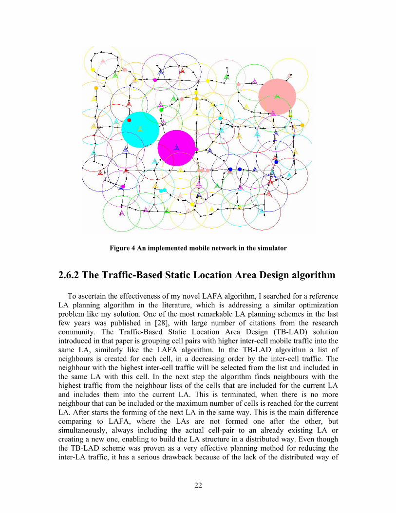
Figure 4 An implemented mobile network in the simulator
2.6.2 The Traffic-Based Static Location Area Design algorithm
To ascertain the effectiveness of my novel LAFA algorithm, I searched for a reference LA planning algorithm in the literature, which is addressing a similar optimization problem like my solution. One of the most remarkable LA planning schemes in the last few years was published in [28], with large number of citations from the research community. The Traffic-Based Static Location Area Design (TB-LAD) solution introduced in that paper is grouping cell pairs with higher inter-cell mobile traffic into the same LA, similarly like the LAFA algorithm. In the TB-LAD algorithm a list of neighbours is created for each cell, in a decreasing order by the inter-cell traffic. The neighbour with the highest inter-cell traffic will be selected from the list and included in the same LA with this cell. In the next step the algorithm finds neighbours with the highest traffic from the neighbour lists of the cells that are included for the current LA and includes them into the current LA. This is terminated, when there is no more neighbour that can be included or the maximum number of cells is reached for the current LA. After starts the forming of the next LA in the same way. This is the main difference comparing to LAFA, where the LAs are not formed one after the other, but simultaneously, always including the actual cell-pair to an already existing LA or creating a new one, enabling to build the LA structure in a distributed way. Even though the TB-LAD scheme was proven as a very effective planning method for reducing the inter-LA traffic, it has a serious drawback because of the lack of the distributed way of
22

LA forming. This drawback can be shown in Figure 5 on a graph representation of a simple example network. First we apply the TB-LAD scheme on the network and after the LAFA to obtain the LA structure. For both schemes 3max =N , which means maximum three cells could be grouped into one LA. In the case of TB-LAD, in the first step cell and will be included into one , because the inter-cell traffic between them is the highest in the network. In the next step the highest inter-cell traffic connecting the neighbours of with the cells of is searched and that will result in including of cell to . The forming of will be finished with this step, because of the
constraint. The second LA ( ) will be formed from and . Therefore the two LA sets generated by TB-LAD will be
1v 2v 1LA
1LA 1LA
3v 1LA 1LA
maxN 2LA 4v 5v{ }3211 ,, vvvLA = and { }542 ,vvLA = as it can be
seen in Figure 5 they are marked with dotted line circles. If we apply the LAFA, the first step will be the same like in the case of TB-LAD, and will be included into , because the inter-traffic between them is the highest in the network. The real difference will appear in the second step, because in LAFA we will not search for the highest inter-cell traffic between the neighbour cells of and the cells of , but for the highest inter-cell traffic between all of the cells in the network. Accordingly in this step we will not join to , but we will create a new LA ( ) with and , because they are connected by the highest biggest inter-cell traffic in the network which was not already included to . The cell will be also joined to . So the final outcome of LAFA will be and
1v 2v 1LA
1LA 1LA
3v 1LA 2LA 3v 4v
1LA 5v 2LA{ 211 ,vvLA = } { }5432 ,, vvvLA = . There is a significant difference between the
two LA structures; in the case of TB-LAD the inter-LA traffic is much larger than for the LA structure obtained by LAFA. This simple example shows that my novel LA planning solution can improve the performance of an earlier important LA scheme by introducing a distributive LA forming method.
1v
200
2v
1
3v
199
4v
5v
5
Figure 5 An example network for comparing TB-LAD and LAFA
23

2.6.3 The Simulation Results
To obtain a more thorough comparison of the two LA planning solutions, both algorithms were implemented in the simulator, to compare the performance of the two by using two typical mobility environments.
A rural and an urban mobility environment has been designed in the mobility simulator, the first one is rarely populated, but on the belonging highways a big number of mobile terminals are moving with high speeds, while the second environment is densely populated, with mobile terminals moving with smaller velocities. In the rural environment the average cell size is larger then in the urban, accordingly there is a smaller number of cells. I run the simulation on a moderate sized example network, the rural mobile system consisted of 99 base stations, while in the urban system was about 123 base stations. This moderate sized network can be representative for a larger network too, the size of the simulated network was chosen after studying the literature of the cellular network simulations. Saving the two above mentioned structures (road-system, cell allocation) the reproducibility of the results can be guaranteed. This made possible to run 10 independent simulations in the same simulation scenario, the output of the simulations was stored and averaged, a cell boundary crossing matrix and the incoming call distribution for every cell. This database was the input of the LA forming program, which designed the two LA structures for both mobility environments. A) Employing only the LAFA: Based on these LA partitions, the location update cost was computed for the LAFA created partition and the same cost was calculated for the LA partition designed by the TB-LAD reference scheme.
For the rural environment the results of the simulation are given in Figure 6, where the Upper Bound of LA axis represent the maximum number of cells which can be included into one LA, namely the . In Figure 6 the Location Update Cost decreases as the upper bound becomes higher, but if we increase this upper bound, then the Paging Cost will increase, too. So in the TB-LAD partition we can decrease the Location Update Cost if we increase the size of the LAs, but then the Paging Cost will be a serious problem. A significant advantage of the LAFA is that it reduces the Location Update Cost very significantly, by not increasing the average number of cells in one LA (because it is not reaching the upper bound, the other stopping rule (6) takes effect before) so the Paging Cost can be kept on a lower level. In the domain of 5-10 cells for an upper bound per LA, my new scheme reduces the inter-LA traffic by 40-60 percents on the average by comparing it to the TB-LAD scheme.
maxN
24

0
500
1000
1500
2000
5 6 7 8 9 10 11 12 13 14
Upper Bound of LA (number of cells)
Loc
atio
n U
pdat
e C
ost
15
TB-LAD
LA FormingAlgorithm
Figure 6 The Location Update Cost in rural environment for the TB-LAD and the LAFA partition
In Figure 7 the results for the urban environment can be seen. It is very similar to the
rural, however the Location Update Cost is remarkably reduced, without increasing the paging signalling load. The decrease is very significant in the interval of five to eleven cells. In the interval between 12 and 15, it does not mean that by increasing the number of cells the Location Update Cost does not decrease significantly, but the Eq.(6) is not satisfied, therefore the LAFA stops on a smaller number of cells per LA than the upper bound. The TB-LAD algorithm is always increasing the number of cells per LA till the upper bound; therefore it is producing a higher Location Update Cost for a higher number of cells per LA, which will cause a higher Paging Cost also.
0
500
1000
1500
5 6 7 8 9 10 11 12 13 14 1
Upper Bound of LA (number of cells)
Loc
atio
n U
pdat
e C
ost
5
TB-LAD
LA FormingAlgorithm
Figure 7 The Location Update Cost in urban environment for the TB-LAD and the LAFA
partition
25
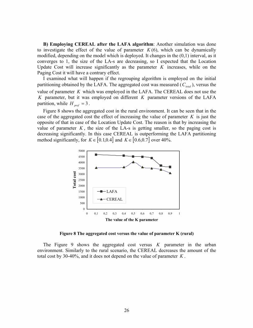
B) Employing CEREAL after the LAFA algorithm: Another simulation was done to investigate the effect of the value of parameter K (6), which can be dynamically modified, depending on the model which is deployed. It changes in the (0,1) interval, as it converges to 1, the size of the LA-s are decreasing, so I expected that the Location Update Cost will increase significantly as the parameter K increases, while on the Paging Cost it will have a contrary effect.
I examined what will happen if the regrouping algorithm is employed on the initial partitioning obtained by the LAFA. The aggregated cost was measured ( ), versus the value of parameter
totalCK which was employed in the LAFA. The CEREAL does not use the
K parameter, but it was employed on different K parameter versions of the LAFA partition, while . 3=prefH
Figure 8 shows the aggregated cost in the rural environment. It can be seen that in the case of the aggregated cost the effect of increasing the value of parameter K is just the opposite of that in case of the Location Update Cost. The reason is that by increasing the value of parameter K , the size of the LA-s is getting smaller, so the paging cost is decreasing significantly. In this case CEREAL is outperforming the LAFA partitioning method significantly, for and [ ]4.0,1.0∈K [ ]7.0,6.0∈K over 40%.
0
500
1000
1500
2000
2500
3000
3500
4000
4500
5000
0 0,1 0,2 0,3 0,4 0,5 0,6 0,7 0,8 0,9 1
The value of the K parameter
Tot
al c
ost
LAFA
CEREAL
Figure 8 The aggregated cost versus the value of parameter K (rural)
The Figure 9 shows the aggregated cost versus K parameter in the urban environment. Similarly to the rural scenario, the CEREAL decreases the amount of the total cost by 30-40%, and it does not depend on the value of parameter K .
26

0
1000
2000
3000
4000
5000
6000
7000
8000
9000
0 0,1 0,2 0,3 0,4 0,5 0,6 0,7 0,8 0,9 1
The value of the K parameter
Tot
al c
ost
LAFA
CEREAL
Figure 9 The aggregated cost versus the value of parameter K (urban)
Depending on the objective we can deploy only the LAFA algorithm or followed by the regrouping algorithm. If we want to decrease the Location Update Cost, the LAFA is the solution, however if we want to decrease the aggregated cost, we need to employ after the LAFA the regrouping algorithm also.
2.6.4 Results Using the Vehicular Mobility Simulator
To confirm the results obtained by my mobility simulator, I used a vehicular mobility simulator for generating the input metrics for the LA forming and regrouping algorithm. This is an extendable JAVA mobility simulator that can simulate the behaviour of mobile users on a given street plan in a realistic way, using an extended version of the Nagel-Schreckenberg model [30]. The environment physically limits the freedom of users (e.g. cars, trains), they can only move inside certain areas and react to the changing environment and the behaviour of other vehicles. For example, if a car approaches a traffic jam at a junction, it has to slow down and eventually stop. Every other car on the same road is affected by this: they have to slow down or stop as well. In this way, the simulator can, to a certain extent, mimic real vehicular movements in a (semi-) urban environment. The mobility simulator applies the Dijkstra algorithm for every vehicle to determine the path to their destination. The cost of each road is determined by its length, its speed limit and the number of vehicles on it. In this way, the main roads with higher speed limit will be preferred. Additionally, in case of a traffic jam, the vehicles will try to avoid this congested road and choose an alternative road to get to their destination. At the beginning of the simulation, the vehicles are placed on the map and will be assigned a given call arrival intensity, a destination and a maximum speed. After the simulation, cell change and call arrival intensity matrices will be produced and fed to the LA forming algorithm.
27

I compared the performance of the TB-LAD and the LAFA partition in the terms of different classes of traffic conditions, by using two typical mobility environments for urban areas (two urban environments, see Fig. 10).
Figure 10 The Manhattan city model and the European city model with main roads in bold
In the Manhattan city model, two roads (bold) have a higher speed limit, which makes
them more attractive for drivers. Each junction has traffic lights in order to avoid dead locks. In the European city model, the inner ring (bold) is more likely to be chosen as destination. This represents the morning rush hour situation where people converge to work in the city centre.
Furthermore, four classes of traffic conditions were defined ranging from low to high average vehicle density and from low to high call arrival rate per vehicle (Poisson distribution, calls per hour) (Table 1). Note that during the simulation, the local vehicle density will be much higher, especially in the area around junctions. A number of cells with diameter of 0.78 km were deployed on the city map, such that coverage was total.
TABLE 1 MOBILITY SIMULATION PARAMETERS
Vehicle density Call arrival rate (λ) Manh. Euro. Manh. Euro.
Class I 0.5% 0.4% 1 1 Class II 0.5% 0.4% 8 8 Class III 3.3% 2.8% 1 1 Class IV 3.3% 2.8% 8 8
A) Employing only the LAFA: Once the LA partitions have been determined, the Location Update Cost was computed for the TB-LAD and the LAFA partition.
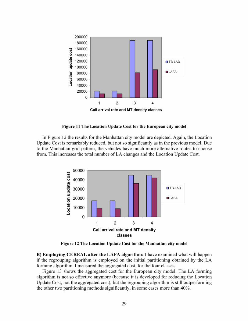
For the European city model the results of the simulation are given in Figure 11, where the call arrival and MT density axis represent the four classes, combining the two means of call arrival rate and two different vehicle densities. Obviously, the more vehicles in the environment, the higher the total LA update cost for the network. Figure 11 shows that the LAFA algorithm can significantly reduce the location update cost, even in high call arrival rate.
28
020000400006000080000
100000120000140000160000180000200000
1 2 3 4
Call arrival rate and MT density classes
Loca
tion
upda
te c
ost
TB-LAD
LAFA
Figure 11 The Location Update Cost for the European city model
In Figure 12 the results for the Manhattan city model are depicted. Again, the Location
Update Cost is remarkably reduced, but not so significantly as in the previous model. Due to the Manhattan grid pattern, the vehicles have much more alternative routes to choose from. This increases the total number of LA changes and the Location Update Cost.
0
10000
20000
30000
40000
50000
1 2 3 4Call arrival rate and MT density
classes
Loca
tion
upda
te c
ost
TB-LAD
LAFA
Figure 12 The Location Update Cost for the Manhattan city model
B) Employing CEREAL after the LAFA algorithm: I have examined what will happen if the regrouping algorithm is employed on the initial partitioning obtained by the LA forming algorithm. I measured the aggregated cost, for the four classes.
Figure 13 shows the aggregated cost for the European city model. The LA forming algorithm is not so effective anymore (because it is developed for reducing the Location Update Cost, not the aggregated cost), but the regrouping algorithm is still outperforming the other two partitioning methods significantly, in some cases more than 40%.
29

0
100000
200000
300000
400000
500000
600000
1 2 3 4Call arrival rate and MT density
classes
Tota
l cos
t TB-LAD
LAFA
CEREAL
Figure 13 The aggregated cost for the European city model
In the Figure 14 the aggregated cost for the Manhattan city model is displayed. Again, the regrouping algorithm proves to be very effective in reducing the signalling cost.
050000
100000150000200000250000300000350000400000450000
1 2 3 4
Call arrival rate and MT density
Tota
l cos
t
TB-LAD
LAFA
CEREAL
Figure 14 The aggregated cost for the Manhattan city model
The conclusion is the same like in the case, when using the other mobility simulator, if the objective is to decrease the Location Update Cost, the LA forming algorithm is the solution, however if we want to decrease the aggregated signalling cost, we need to employ the regrouping algorithm after the LAFA.
30

2.7 Summary
An important benefit of optimized LA planning is preventing needless radio resource usage, but the most important is that we can support global network performance parameters, like signalling delay and delay variation, which can be critical in time sensitive services of the next generation mobile systems.
It can be achieved by reducing the signalling cost, which means that the inter LA movement must be minimized. A novel static LA planning method was introduced for a heterogeneous mobility environment, where the inter-cell traffic patterns are not uniform.
The input of this algorithm was obtained by a mobility simulator that produces network information (cell boundary crossing rates, incoming call distribution to every cell) in a realistic manner. I also proposed a cell regrouping algorithm, which uses the LA partitions obtained by the LAFA algorithm, like an initial step.
To evaluate the performance of my new scheme, I designed a rural and an urban environment in the mobility simulator, and with this database the LA forming algorithm was run. Then it was compared with a well-known reference algorithm chosen from the literature, examining the relation of the Location Update Cost with an upper bound on the number of cells.
The simulation results show that the LA forming technique reduces the Location Update Cost by 40-60 percents. The regrouping algorithm performs well if we want to decrease the aggregated cost of our system, it can reduce the total cost by 30-40%, sometimes over 50%.
To confirm the results obtained by my mobility simulator, I used a vehicular mobility simulator for generating the input to the algorithms (cell boundary crossing rates, incoming call distribution to every cell) for realistic vehicle mobility behavior. On the end I get the same results like in the previous case.
It can be recognized, that by employing my LA forming schemes, a significant reduction was attained in the signalling traffic that causes delay and delay variation, helping us improving network performance parameters in general.
31

Chapter 3
3 Location Area Optimization Algorithms for a Homogeneous Mobility Environment
As highlighted in the previous two chapters the novelty of my contribution to LA
planning is that beside these LA planning methods are more effective than the earlier introduced schemes, they can be applicable for both mobility environments, for heterogeneous and homogeneous network usage (for non-uniform and near-uniform inter-cell rates also).
In Chapter 2 a LA planning method was introduced for a heterogeneous mobility environment, therefore the goal was to reduce the Location Update and aggregated cost, while in this chapter I give a solution for a near-uniform inter-cell rate distribution case, where the final goal is the determination of the optimum number of cells per LA for which the Location Update Cost is minimum, with the Paging Cost as an inequality constraint function. The Paging Cost was limited, because if the (6) stopping rule would be applied for near-uniform inter-cell rates, all the cells will be included into one LA, not considering the capacities of the cellular network, since the paging capacities of base stations and switching centres should not be exceeded. The upper bound of cells per LA ( ) introduced in LAFA can not be used like a paging constraint here, because that is a “weaker” stopping rule than (6), while here all the LAs will consist of the same number of cells because of the uniform rates. Therefore the goal is to reach the minimum value of the Location Update cost, by calculating the optimal number of cells per LA from the paging constraint function and using the LA planning algorithms to obtain an effective grouping of cells into LAs.
maxN
This LA forming process contains two phases, first a greedy algorithm (GREAL) is adopted which forms a basic partition of cells into LAs, and then a simulated annealing based algorithm (SABLAF) is applied for getting the final partition. The same realistic mobility environment simulator was used as in Chapter 2, for the generation of the algorithm input metrics (cell boundaries crossing and incoming call statistics).
3.1 The Cost Formulation
3.1.1 Assumptions
The aim of employing LAs is to hide the cell boundary crossing inside the LA from the upper levels; therefore an administrative message for the registration of the new location of the MT will not be generated during the cell handover if it is an intra-domain movement. To make calculations about the movement of MTs among the LAs (with near-uniform inter-cell movement rates), the best is the fluid flow model [31]. The fluid flow
32

model characterizes the aggregate mobility of the MTs in a given region (for example a LA) as a flow of liquid. It assumes that MTs are moving with an average speed , and their direction of movement is uniformly distributed in the region. Hence the rate of outflow from that region can be described in a unit time interval by [32]
v
⎟⎠⎞
⎜⎝⎛ ⋅⋅
=πρ Pv
outR, (8)
where is the average speed of the MTs, v ρ is the density of MTs in the region and P is the perimeter of the given region.
This model is very simple to analyze and to use for the definition of the registration cost function. We can define easily the density of the MTs in the LA: thk
SN
K
kk ⋅=ρ , (9)
where K is the number of MTs in the LA, is the number of cells in the LA, and is the area of a cell.
thk kN thkS
3.1.2 Location Update Cost
Every time when a MT crosses a cell boundary which is a LA boundary also, a registration process is initiated, a Location Update message is sent to the upper level (home agent or gateway). Therefore the intra-LA boundary crossing cost is negligible, and this handoff cost should be not considered in the Location Update Cost. Hence we need to determine the number of cells located on the boundary of the LA (the set of the boundary cells is a subset of ), and the proportion of the boundary cells perimeter which contributes to the LA perimeter.
thkkN
thkThe perimeter of the LA can be expressed as: thk
( )kkpkpk NNP δ⋅= , (10) where is the number of boundary cells in the LA and
kpN thkkpδ is the average
proportion of the boundary cell perimeter in the LA perimeter in the function of . thk kNThe number of the boundary cells can be approximated from my earlier work [C3],
(where [ 9,7∈ ]κ for a hexagonal cell approximation): kkp NN ⋅= κ . (11)
33

The average proportion of the cell perimeter which will be the part of the LA perimeter too can be expressed with an empirical relation [33]: ( ) ( )1−⋅+⋅≈ ηδ kckkp NbaPN , (12) where is the perimeter of a cell and cP 3333.0=a , 309.0=b , 574965.0=η .
Substituting the values of and kpN ( )kp N
kδ in (10), the expression for the perimeter of
the LA becomes: thk ( )1−⋅+⋅⋅⋅= ηκ kckk NbaPNP . (13)
By substituting the values of ρ and in the outflow rate of the fluid flow model (the outflow rate will be equal with the number of crossing the LA boundary):
kPthk
( )
⎟⎟⎟⎟
⎠
⎞
⎜⎜⎜⎜
⎝
⎛ ⋅+⋅⋅⋅⋅⋅
⋅=
−
π
κ 425.0309.0333.0 kckk
out
NPNSN
KvR . (14)
As mentioned earlier a registration process is initiated when the MT crosses a cell
boundary which is a LA boundary too, hence the Location Update Cost will be for a unit time interval: outLULU RBC
k⋅= , (15)
⎟⎟⎠
⎞⎜⎜⎝
⎛
⋅⋅+⋅
⋅⋅⋅⋅⋅=−−
⋅ SNN
PKvBC kkcLULU k π
κ925.05.0 309.0333.0
(16)
where is the cost required for transmitting a location update message. LUB
The final goal is determining the optimum number of cells per LA for which the Location Update cost is minimal, with the Paging Cost as an inequality constraint function.
3.1.3 Paging Cost
The Paging Cost is a result of the arriving calls to the MTs, because the called MT has to be searched within the LA. The goal is to decrease the Location Update Cost by increasing the number of cells in one LA, hiding the cell crossings from the upper levels.
34

However to have a feasible network, the paging capacities should not be exceeded, therefore we need to define a paging constraint per a LA.
Therefore considering the paging capacities of a cellular network, the Paging Cost for the LA, the same like (1), should not exceed the paging cost constraint: thk
, (17) kp
K
iikkP CBNC
k
k<⋅⋅= ∑
=1λ
, (18) ∑=
<⋅⋅=k
k
K
ikikkPP CNBC
1λ
where , , PB kN ikλ and are the same like introduced in (1). kK
If we assume that the mobile users have the same average number of terminated calls for the all cells in the unit time interval in the LA (thk λλ =k ), the paging cost reduces to
kkkPP CKNBC
k<⋅⋅⋅= λ . (19)
3.1.4 Optimization of the Location Update Cost
The first part of solving the problem is to find the optimum number of cells per LA for which the Location Update Cost is minimal and the paging constraint ( must not be exceeded) is satisfied. The second part is to obtain efficient LA partitions with the help of the two-phase LA planning algorithm.
kC
If we know that the call arrivals (λ ) follow a Poisson process and the function of the Location Update Cost (16) is monotonically decreasing in the function of (while the Paging Cost is monotonically increasing in the function of ), the paging constraint can be expressed in the following way:
kN
kN
, (20) γ−−<< eCCP kPk
1)( where [ 100,10∈ ]γ , depending on the accuracy of the paging constraint.
The monotonically decreasing attribute of the Location Update cost in the function of will mean, that we need to find the highest value of for which the (20) will be still
satisfied. kN kN
Substituting the expression of the Paging Cost in (20):
(21) γλ −−<<⋅⋅⋅ eCKNBP kkP 1)( .
35

Furthermore, if we know that the λ probability variable follows a Poisson process, then the maximum value ( ) of can be easily calculated: optN kN
γλ −−=⋅⋅
< eKNB
CP
kP
k 1)( . (22)
Substituting the calculated value of in (16) will give the minimum of the
Location Update Cost. This calculated will be used as an input for the GREAL and SABLAF algorithm.
optN
optN
3.2 Location Area Planning Algorithms
The LAFA algorithm introduced in Chapter 2 was modified to be useable for a near-uniform inter-cell movement rate distribution, while in the second phase of LA planning the technique of simulated annealing is applied. This can ensure to reduce the Location Update Cost, while taking into account the paging capacities of the network.
3.2.1 The Greedy Algorithm (GREAL)
As stated before the Location Update Cost is proportional to the number of handovers among different LAs, therefore the Location Update Cost can be reduced by designing the LAs such that the cells belonging to one LA have the lowest boundary crossing rates among each other. It is the same problem like introduced in Chapter 2 (which is an N-complete complexity problem), graph ( )EVG , should be divided into subgraphs
, in such a way to find the maximum spanning forest of graph , where the components of this maximum spanning forest are the maximum weight spanning trees of the correspondent subgraphs, while the number of nodes in each subgraph is lower than or equal to a constraint ( ); but here there is no special stopping rule like (6). Than will mean the GREAL algorithm will have the same steps like LAFA, but without the stopping rule (6), only the maximal number of cells per LA constraint will stop the forming of a single LA.
( EVGi , ) )
)
)
}
( EVG ,
( EVGi ,
optN
Therefore the GREAL also starts by creating a list of edges of graph in monotonically decreasing order by weight. In the first step of the algorithm, the first edge on the list (the one, which has the biggest weight , if there is more than one biggest weight, then we choose one of them randomly) is included into the set of edges ( ). The two nodes connected by this edge are included into set . In the next step as in LAFA, the second largest weight is selected and the two nodes which are connected by this edge are examined if they belong to the set. If both are in the set
\ , then the edge, which connects them, is included into the set of edges
( EVG ,
maxc
1L{ }11 eL = { 211 ,vvU =
1UV 1U 2L
36

( ) and the two belonging nodes into the set . If one of the nodes is in the set , then it must be checked what is the cardinality of , because the node set can not have more members than . Therefore, if
{ }22 eL = 2U
1U 1U
optN
optNU <1 (23)
then the other node can be also included into the set. 1UIf the inequality is not satisfied, this node can not be included into this set, to prevent
exceeding the paging cost constraint (19). This stopping rule will ensure to take into account the paging capacities of the network while reaching the minimal Location Update Cost for the LA, where the thi opti NU = .
The algorithm ends when every node of graph ( )EVG , is included to a set of nodes, the node members of the sets are actually the nodes of the MUUU ,....,, 21 ( )EVGi , subgraphs. These sets of nodes will provide us the partitioning of cells into LAs, namely the node sets are the LA cell groups. This will be only an initial LA partition which will serve as an input to the simulated annealing based LA forming algorithm, to arrive at an optimal or near-optimal solution.
MUUU ,....,, 21
3.2.2 The Simulated Annealing Based Location Area Forming Algorithm (SABLAF)
GREAL is a greedy LA planning solution; therefore the initial LA partitions produced
by GREAL could be improved furthermore in the terms of Location Update Cost. In the homogeneous case, where the size of the LAs is determined by the , the leeway is not so wide like in the heterogeneous case where the neighbouring cells can be regrouped in a freer way. Therefore I have chosen the simulated annealing method which locates a good approximation to the
optN
global optimum, meaning that the system may move to the new state even when it is worse than the current one and this way it can lead to an optimum state through these intermediate states.
Simulated annealing (SA) is considered an approximation algorithm which is applicable to various problems in general. Metropolis algorithm [34] was the original idea behind the optimization technique of SA. Kirkpatrick et. al, [35] has used Metropolis algorithm as a global optimizer. Simulated annealing finds a near-optimal solution without searching the entire solution space, in polynomial running time. Using the simulated annealing for the purpose of LA planning was recently presented in [36] (published later than my solution), but there a GSM-like scheme is used to obtain the initial partition (which is not so effective as the GREAL algorithm) and then further refined by the SA based algorithm.
In my solution the simulated annealing based algorithm here finds a basic LA partition formed by the GREAL algorithm, with the handover rate database among the cell pairs. The SABLAF algorithm starts with the initial solution given by GREAL ( ). A neighbour to this solution is then generated as the next solution by simulated
0s
1s
37

annealing, and the change in the Location Update Cost ),( 10 ssCLU∆ is evaluated. If a reduction in cost is found, the current solution is replaced by the generated neighbour,
otherwise we decide with a certain probability set to ⎟⎠
⎞⎜⎝
⎛ ∆−
TCLU
e (usually called the acceptance function) whether it remains the current solution, where T is the control parameter (corresponds to temperature in the analogy with the physical annealing process). The SABLAF algorithm is started with a relatively high value of T , to have a better chance to avoid being prematurely trapped in a local minimum. The cooling schedule consists of three parameters, used like an input to SABLAF algorithm: the initial temperature (T ), step of decreasing, and the stopping rule of the algorithm. The stopping rule is the maximal iteration step number or maximum number of steps when the do not changes. LUC∆
Another important input parameter is the calculated maximum number of cells in a LA ( ). The performance of the SABLAF depends heavily on the cooling schedule and the initial partition; in this case the initial partition is already an effective LA partition (see the flowchart of SABLAF on Figure 15).
optN
38

Current solution=Output of GREAL ( s ) 0
Setup of initial control parameters
New solution=Neighbour of current solution
New solution N ? optN≤
Figure 15 Flowchart of SABLAF
Calculation of LUC∆
0>∆ LUC
Current solution=New solution
Decrement T
Maximum number of steps when do not changes > threshold LUC∆
Save the best solution so far: End of SABLAF
Yes
No
No
Yes
No
Yes
39
Current solution=New solution ⎟⎞
⎜⎛ ∆−
CLU
with probability ⎟⎠
⎜⎝ Te

3.3 Simulation Results
The performance of the GREAL and SABLAF algorithm and the TB-LAD algorithm (introduced in Chapter 2) solution was compared, by using the two mobility environments (rural and urban). The input data, the boundary crossing and incoming call database, for the algorithms was generated by the mobile environment simulator presented also in Chapter 2.
As it is well-known, the rural mobility environment is rarely populated, but on the belonging highways a big number of mobile terminals are moving with high speeds, while the urban mobility environment is densely populated, with mobile terminals moving with smaller velocities. In the rural environment the average cell size is larger then in the urban, accordingly there is a smaller number of cells. In this manner the two mobility environments were designed, the rural environment consisted of 42 cells, while in the urban system it was about 79 cells. It was examined how the Location Update Cost changes by increasing the maximum number of cells in one LA. This way it can be checked if the Location Update Cost reaches the minimum value for . Figure 16 shows the Location Update Cost in rural environment, where the horizontal axis represents the maximal number of cells per LA. As it can be seen the GREAL can decrease the Location Update Cost compared to the TB-LAD algorithm, but only the SA based solution finds the best solution for every value of the maximal number of cells per LA. For the calculated value of
optN
12=optN , the Location Update Cost reaches the minimum value using the SA based technique.
0
500
1000
1500
2000
2500
3000
1 3 5 7 9 11
Maximum number of cells per LA
Loca
tion
Upd
ate
Cos
t
TB-LADGREALSABLAF
Figure 16 The Location Update Cost in rural environment
On Figure 17 the Location Update cost is depicted in urban environment, where we have more cells, but the size of the cells is smaller. In the initial stages (where the value of maximal number of cells per LA is less than 5) SABLAF algorithm almost always accepts the partition formed by the GREAL algorithm or a very similar partition (which do not decreases the Location Update Cost appreciably), but as the number of cells increases, the SABLAF is outperforming the other two solutions significantly. Using
40

again (22) the was calculated (higher value than for the rural environment, because of the cell sizes and numbers), for that value the SABLAF algorithm gives again the minimum of the Location Update Cost , therefore we can summarize, that for both mobility environments the SABLAF algorithm gives the best results, decreasing the registration cost almost for 50% more effective than the reference solution, and for approximately 20% more than the GREAL algorithm.
14=optN
0200400600800
1000120014001600180020002200
1 2 3 4 5 6 7 8 9 10 11 12 13 14
Maximum number of cells per LA
Loca
tion
Upda
te C
ost
TB-LADGREALSABLAF
Figure 17 The Location Update Cost in urban environment
3.4 Summary
In order to design a feasible mobile network, optimized LA planning is needed, considering the constraints like paging handling capacity of mobile switching centers. In this Chapter, I presented a LA planning method for a near-uniform network usage, defining the Location Update Cost function with the help of the fluid flow model together with a paging constraint, and a method for calculating the number of cells per LA for which the Location Update Cost is minimal. I also proposed a two-step LA forming solution, which consists of a greedy algorithm that gives the basic partition and a simulated annealing based algorithm which gives an efficient LA partition in reasonable running time. To evaluate the performance of the new scheme, a rural and an urban environment was designed in the mobility simulator, and with this database the LA forming algorithms were run. Then I compared them with the TB-LAD algorithm, examining the Location Update Cost in the function of maximal number of cells per LA.
For the both mobility environments the SABLAF algorithm delivered the best performance, reducing the Location Update Cost almost 50% more effective than the reference solution.
41

Chapter 4
4 Network design algorithm for optimizing the upper hierarchical mobile structures
While IP is declared as the key technology of the future’s wired and mobile
communication, the currently used version of IP, IPv4 itself is not suitable to be used in mobile scenarios. The new tendency is to solve the mobility management problems in the network layer or the upper layers [37]. This support must be transparent to mobile users and also has to be scalable, which means that despite the growth of the number of mobile terminals, the amount of signalling overhead must not increase significantly [38]. The increasing trend towards smaller cell sizes makes efficient mobility management strategies indispensable for radio resource management and network planning in next generation cellular networks. The common practice in designing radio resource management or network planning techniques is to apply static mobility models which do not take the dynamics of user mobility into account. However, this does not reflect the realistic behaviour of mobile clients, because their handover rate, location area change rate, dwell time, etc are dependent on their interaction. Therefore, the network signalling load will be very different depending on the location and the user density dynamics. For a given environment, the cellular network needs to be designed with these user mobility characteristics in mind, such that it is able to guarantee the necessary quality of service to its customers.
The handover signalling overhead is due to the management of the mobile users’ location information: when they change location areas, their home agents need to be updated. The popularity of the Internet multimedia services provides strong incentive to service providers to support seamless user mobility.
Mobile IPv6 (MIPv6) [39] is an extension to IPv6 (which is the next version after IPv4) to manage the mobile terminal’s mobility, but not capable of supporting real-time handovers. It is a simple and scalable global mobility solution; however it is not a satisfactory solution for mobile users with high mobility rate [40]. Mobile IPv6 requires that whenever a Mobile Node (MN) (it is the same term like MT which was used before in this work, but IP uses this term, hence in this Chapter term MN will be used) moves from one subnet to another one, its location and routes must be updated by sending a location update to its Home Agent (HA). As the number of MNs increases significantly the location updates may cause an excessive signalling cost [41]. Moreover, if the MN is far away from its HA or the HA processing capability is overwhelmed by the huge volume of location update messages, the signalling delay for the location registration could be large, which will result in the loss of a huge amount of in-flight packets and losing the capability to guarantee quality-of-service (QoS). For example, many real-time wireless applications (e.g., voice over IP) would experience noticeable degradation of service with frequent handoff.
42

A solution is to make Mobile IPv6 responsible for macro-mobility, and to have a separate protocol to manage local handovers inside micro-mobility domains. While macro-mobility is for the case when an MN moves across different administrative domains or geographical regions and it occurs less frequent, the micro-mobility means the MN is moving across multiple subnets within a single network of domain. For these cases, which occurs quite often, a separate protocol is needed, to improve the shortcomings of the Mobile IPv6.
4.1 Related Works
Over the past several years a number of IP micro-mobility protocols have been proposed, designed and implemented that complement the base Mobile IP protocol. The development of these protocols has generated considerable interest in industry and academia, as a joint effort to improve the Mobile IP micro-mobility handling capability.
The Cellular IP (CIP) protocol [42] was developed at Columbia University and Ericsson Research, and it supports paging and a number of handoff techniques. To minimize control messaging, regular data packets transmitted by mobile hosts are used to refresh host location information. A similar approach is the Handoff-aware Wireless Access Internet Infrastructure (HAWAII) [43], which is a separate routing protocol to handle micro-mobility. In TeleMIP [44] a mobility agent is used to reduce the location update traffic, leading to a new architecture. TIMIP [45] (Terminal Independent Mobility for IP) combines some advantages from CIP and HAWAII, where terminals with legacy IP stacks have the same degree of mobility as terminals with mobility-aware IP stacks. Nevertheless, it still uses Mobile IP for macro-mobility scenarios.
One of the most significant micro-mobility solutions to reduce the number of signalling messages to the home network and also to reduce the signalling delay is the Hierarchical Mobile IPv6 [46]. The basic idea of this hierarchical approach is to use domains organized in a hierarchical architecture with a mobility agent on the top of the domain hierarchy. Hierarchical Mobile IPv6 (HMIPv6) is an extension of Mobile IPv6, aimed at reducing the amount of signalling overload and speeding up handovers in cases when the Mobile Node (MN) is located far away from its Home Agent and Correspondent Nodes (any IPv6 node communicating or corresponding with the given MN, henceforth CN). HMIPv6 utilizes a hierarchical network of routers and introduces a new MobileIPv6 node, called the Mobility Anchor Point (MAP). It can be located at any level in a hierarchical network of routers, including the Access Router (AR), which is the Mobile Node’s default router, aggregating the outbound traffic of MNs. The deployment of the MAP concept will further reduce the signalling load over the air interface produced by Mobile IPv6, by limiting the amount of Mobile IPv6 signalling outside the local domain.
The MN has two kinds of care-of addresses: the Regional Care-of Address (RCoA) and the On-link Care-of Address (LCoA). MN obtains the RCoA from the MAP of the visited network, which remains unchanged as long as the MN is roaming within the given domain. The LCoA identifies the current position of the terminal, and if it changes within the logical domain, it must update it only to the MAP (it sends a Binding Update). The Home Agent and Correspondent Nodes are not aware of this change, the visible care-of
43

address (RCoA) remains the same for them while the MN keeps changing its point of attachment inside the visited domain. Therefore the RCoA does not change as long as the MN moves within a MAP domain. The MAP captures the messages sent to the MN’s RCoA, and forwards them to the MN’s LCoA using local routing mechanism. A MAP domain’s boundaries are defined by the Access Routers (ARs) advertising the MAP information to the attached MNs (via Router Advertisements). In this way the MAP can help providing seamless mobility for the MN as it moves from one AR to another. As a result of this, the amount of signalling messages leaving the domain is reduced significantly, and so is the resulting delay.
4.2 The Optimization Problem
The problem is that the RFC 4140 or other drafts do not address the realization of the hierarchical structure in detail during the network design. It is not clear and usually hard to determine the size of a regional network. Several important questions arise: what kind of principles must be used to configure the hierarchical levels, how to group cells under a given AR, and in which hierarchical level is advisable to implement the MAP function. The MNs traffic load and mobility may vary; therefore a fixed structure is lack of flexibility.
In Chapter 2-3 I already gave mobility management solutions for Location Area domain forming which are capable of reducing the signalling overhead caused by the LA boundary crossing. As explained earlier the cell border crossings inside the LA domain will remain hidden for the upper hierarchical levels, thus reducing signalling overhead. Only when an LA border is crossed, the location is updated; not on each cell handover. Therefore with these Location Area planning algorithms, we can obtain the optimal partition of cells for a given Access Router, which will represent a Location Area router.
A key issue is how to group these Access Routers on the next level of hierarchy, and on which level of hierarchy to implement the MAP functionalities, actually how many Access Routers should be beneath a MAP within a domain. The number of ARs under a MAP is very critical for the system performance. An obvious solution is to group those ARs into one domain, which has a high rate of handovers among each others. In that way the number of AR changes for the MNs will be decreased. But joining too much ARs into one domain would degrade the overall performance since it will generate a high traffic load on MAPs, which results in a high cost of packet delivery [47]. Contrarily a small number of ARs will lead to a huge amount of location updates to the home network.
The LA optimizing solution can reduce the signalling load; however there are some differences between optimization methods for cellular systems and those for Mobile IP. The cellular network is geographical oriented, while the distance between two end points in Mobile IP has nothing to do with the geographic location of these two points. Therefore in our analysis the distance unit will be the number of hops packets travel. Another difference is that in cellular networks upon an arrival of a call, the MN is searched with a paging procedure within the cells of a LA, while in Mobile IP the HAs or the MAPs know the adjusted AR of each MN. But because of triangular routing, the packet delivery cost will generate an additional transmission and processing cost. Based on this, a Location Update and Packet Delivery cost structure is introduced, and the goal
44

is to minimize the Location Update Cost, while with the right placement of MAPs, to reduce the Packet Delivery Cost simultaneously.
With the increasing popularity of IP based services on mobile devices, future cellular networks will be IP based and designed more as an extension to the Internet rather than the telephone network. Managing mobile hosts within a IP based network is a challenge especially when fast handoff are required. Eventually, the hybrid voice and data third generation networks will evolve into All-IP cellular networks which will be just an extension to the Internet. As cellular packet data services become widely deployed by the rollout of UMTS cellular networks, the packet-switched cellular network is emerging as an alternative to the existing circuit-switched cellular network. As it was expound earlier the third generation packet-switched cellular networks like UMTS also use static LAs, therefore the LA planning principles can be also used in these networks together with the micro-mobility IP based solutions.
Therefore I created a hierarchical network design algorithm (HIENDA) based on the structure given by the LA planning algorithm, aligned with a MAP allocation algorithm in Hierarchical Mobile IPv6 to optimize the mobility management in the Mobil IP networks. The signalling cost is proportional to the number of handovers among different hierarchical entities; therefore the signalling cost can be reduced by designing a HMIPv6 network such that the ARs (or the LAs assigned to them) belonging to one hierarchical entity have the lowest boundary crossing rates among each other (see Figure 18). In this way the signalling messages will only be sent one level up in the hierarchy, and not to the top of the hierarchy. Accordingly my goal was to develop hierarchical entity forming algorithms, which consider the topology constraints, and take the available mobility pattern and LA boundary crossing information as input, and find an optimal or near optimal hierarchical structure for which the signalling cost will be minimal.
Figure 18 A Hierarchical Mobile IPv6 network MAP optimization
45

4.3 The Cost Structure
According to the differences between cellular networks and Mobile IP presented above, I defined the Location Update Cost and the Packet Delivery Cost for a HMIPv6 type network.
4.3.1 The Location Update Cost
If the location registration message flow in HMIPv6 is examined between the home network and the MN covered by a MAP function, we can calculate the cost of a MN movement from one subnet to another: ARMAPHAMNARARMAPMAPHALU pppTTTC ⋅+⋅++⋅+⋅+⋅= −−− 22222 , (24) where
MAPHAT − : the transmission cost of location update between the HA and the MAP
ARMAPT − : the transmission cost of location update between the MAP and the AR
MNART − : the transmission cost of location update between the AR and the MN
HAp : the processing cost of location update at the HA
MAPp : the processing cost of location update at the MAP
ARp : the processing cost of location update at the AR
Where the MN is moving within a local MAP domain the RCoA remains unchanged, it only needs to register the new LCoA, but the Correspondent Nodes and the Home Agent will not be informed about this local change. That means if a MN is changing an AR, but not a MAP, a localized location update cost will be produced: ARMAPMNARARMAPLUl ppTTC ⋅++⋅+⋅= −− 222 . (25)
We can make an assumption, that the transmission cost is proportional to the distance between the source and the destination in terms of the number of hops packets travel ( ) and the proportionality constant is , then the transmission costs can be expressed as:
DSn − TK
TMAPHAMAPHA KnT ⋅= −− (26) TARMAPARMAP KnT ⋅= −− . (27)
The transmission cost of the wireless link is usually higher, than that of the wired link (µ times higher), therefore the transmission cost between the AR and the MN is:
46

TMNARMNAR KnT ⋅⋅= −− µ (28)
If we consider that only an ε fraction of the MNs subnet changes (then the MN moves from an AR to another) is a MAP change, then the total amount of the registration signaling cost can be expressed as: ( ) LULUlLUtotal CqCqC ⋅⋅+⋅⋅−= εε1 (29)
( )( )ARMAPHATMNARTARMAPTMAPHALUtotal pppKnKnKnqC ⋅+⋅++⋅+⋅⋅⋅+⋅⋅+⋅⋅⋅⋅= −−− 21222 . εεµε (30) where is the number of AR changes (or LA boundary crossing) in the system in the unit time period.
q
4.3.2 The Packet Delivery Cost
As we mentioned earlier in a cellular network upon an arrival of a call, the MN is searched with a paging procedure within the cells of a LA, while in Mobile IP the HAs or the MAPs know the adjusted AR of each MN. But because of triangular routing, in Mobile IP every IP packet destined for the MN is first intercepted by the HA and then tunneled to the MAP where MN is registered, forwarding the packet to the current serving AR of the MN. This will produce an additional transmission and processing cost:
, (31) )(1
MAPHAARMAPMAPHA
N
kiPD hhDDC +++= −−
=∑θ
where N : the number of the MNs in the system θ : the number of arriving packets to the MN in the given time period
MAPHAD − : the transmission cost of packet delivery between the HA and the MAP
ARMAPD − : the transmission cost of packet delivery between the MAP and the AR
HAh : the processing cost of packet delivery at the HA
MAPh : the processing cost of packet delivery at the MAP
Similar to the location registration cost, the transmission cost is proportional to the number of hops packets travel between the source and the destination, with a proportionality constant for packet delivery and then the packet delivery cost will be:
DK
. (32) )(1
MAPHADARMAPDMAPHA
N
kiPD hhKnKnC ++⋅+⋅= −−
=∑θ
47
4.3.3 The Total Signaling Cost
After defining the two cost functions, the total signalling cost for a given time period will be: PDLUtotalSC CCC += (33)
Assigning too much ARs to one domain would generate a high traffic load on MAPs, which results in a high cost of packet delivery, but a small number of ARs will lead to a huge amount of location updates to the home network. Therefore Location Update Cost should be minimized, while in the same with the right placement of MAPs the Packet Delivery Cost should be kept on a low level simultaneously.
4.4 The Hierarchical Network Design Algorithm (HIENDA)
An analysis of the Location Update and Packet Delivery Cost was carried out, which
showed that the only way to reduce the overall cost is to reduce the number of the AR changes which are at the same time MAP changes also. The hierarchy of the ARs, MAPs and network routers should be designed in a manner which will take into account the mobility parameters of the users, specially the AR handover rates of the MNs. Accordingly if we join those ARs which have a high handover rate among each other into one MAP domain, the number of MAP domain changes will decrease significantly. Therefore this should be the design principle of an optimized HMIPv6 network.
Thus my goal was to develop an algorithm, which will assign an optimal tree structure to a given source of AR handover rates. I modified some already existing information theory solutions to apply them for hierarchy planning.
4.4.1 Definitions
The optimal tree hierarchy of HMIPv6 (or any other Proxy Agent Architecture used in micro-mobility management) for a given source of AR handover rates could be described, as a probability tree, where the probabilities assigned to the terminal nodes (leaf nodes) will be the handover probabilities of the ARs. This means the HMIPv6 probability tree is a finite tree-graph and for every node of the tree-graph a non-negative number is assigned, based on the next definitions:
• A probability tree is a labelled tree, in which each internal node represents a variable and each leaf node represents a probability value.
• The probability of the root node is equal to 1. • Probability of every node is equal with the sum of the probabilities of the
belonging sub-tree (a tree originating from this node).
48

• The probabilities of the terminal nodes are calculated on the base of the AR handover rates, the ratio of the given AR handover and the total amount of handovers in the network.
Path Length Lemma (Huffman coding):
The average distance of the terminal nodes from the root node (where is a probability variable of the route length) is equal to the sum of the probabilities assigned to the non-terminal nodes, considering the root node as a non-terminal node too.
[ ]LΕ L
It follows from the above stated definition that the probability of every internal node is equal with the sum of the probabilities of the belonging sub-tree (the sum of the child node probabilities). Adopting this to the HMIPv6 tree hierarchy (or generally to another Proxy Agent Architecture used in micro-mobility management), the handover rates among the upper hierarchical domains will be the sum of the handover rates between the belonging lower domains. If an AR (which is a leaf node) is number of hops away from the top router (root node), it means the travelling packet will pass through number of interval routers, accordingly the sum of handover rates of the different interval routers (probabilities assigned to the interval nodes) will contain n times the handover rate of the AR (probability assigned to the leaf node). Since the average distance from the top router can be calculated like the sum of the products of the ARs hop numbers from the top node and handover rates (this is the definition of the average distance in a probability tree), and this sum is identical with the sum of the handover rates allocated to the internal routers including the top router also:
nn
( ) ( )LhPnPPPPT
iiHiIRIIroot Ε=⋅=++++ ∑
=121 ... , (34)
where R is the number of the interval routers, T is the number of ARs and is the AR handover rate probability distribution.
( )iH hP
Example
For the probability tree presented in Figure 19 the average distance can be calculated: ( ) 221.021.023.022.021.022.02.03.05.01 =⋅+⋅+⋅+⋅+⋅+⋅=+++=Ε L
49

Figure 19 An example of a HMIPv6 probability tree
4.4.2 The Algorithm
As above explained, the overall goal is to reduce the number of hops the packets are travelling through, in this way we can minimize the Location Update Cost. With the right placement of MAPs, the Packet Delivery Cost can be reduced too, simultaneously. However the mobility patterns of MNs and the handover rates of ARs should be considered also.
Therefore the objective is to define an algorithm, which will build a probability tree, where the average distance of the terminal nodes from the root node is minimal for a given AR handover rate probability distribution (
( )LΕ( )iH hP ) and given number of
terminal nodes (T ). That means, on the basis of Lemma I., a probability tree should be created with
terminal nodes, such as the sum of the non-terminal node probabilities is minimal. For this purpose, the Huffman-algorithm can be used, but it needs to be modified for this kind of hierarchy optimization.
Accordingly I propose a Hierarchical Network Design Algorithm (HIENDA), based on a modified Huffman-algorithm and a MAP allocation scheme.
The initial step of the algorithm is to define how many ARs namely how many terminal nodes should be aggregated in every step of the algorithm, beginning from the first level of the optimized probability tree. This number depends on the topology constraints of the given network.
First the two terminal node aggregation case is introduced, which means always two terminal nodes will be joined on the next level of the hierarchy. It consists from the following steps:
1. Map the AR topology of a given HMIPv6 network to a T number of terminal nodes, assigning the ratios of the given AR handover rate and the total amount of
50

handover to the belonging terminal nodes as probabilities on the lowest level of the tree. If the ARs are adjacent in the HMIPv6 network, the belonging terminal nodes should be neighbours too. These nodes will be called active nodes.
2. Create a new node on the upper level, by aggregating the two adjacent active nodes with the lowest probabilities, and assign the new node a probability, which will be the sum of these two probabilities. Delete these two nodes from the list of active nodes, and add this new node to the list of active nodes. In this step should be examined if
MAPKpp ≥+ 2min1min . (35)
This means if the sum of handover probabilities exceeds a calculated constraint, a MAP must be deployed on this level of hierarchy, to reduce the signalling load on this branch. Namely if the sum of handover probabilities is too high, there will be a lot of AR changes, which will generate a huge number of Location Update messages. In this way the MAP will hide this AR change from the upper levels, therefore the Location Update Cost will be decreased. In this point a reasonable idea would be to deploy in every aggregated node a MAP, accordingly to minimize the Location Update Cost. But in this case the Packet Delivery Cost would increase, causing unacceptable delay variations. To have a fair tradeoff between this two costs, the should be carefully calculated, on the basis of the network characteristics.
MAPK
The final step of the algorithm is:
3. If there are not any active nodes left, then the last aggregated node should be assigned to the root node and stop the algorithm. If there are still active nodes, go back to step 2.
This was the case when two nodes were aggregated in each step of the algorithm. I
generalized this algorithm for number of aggregated nodes. SFor this the number of unused terminal nodes need to be determined, these nodes will
not represent any ARs (0 probability will be assigned to them), they are needed only for building the aggregation level probability tree. S The steps:
1. Map the AR topology of a given HMIPv6 network to a T number of terminal nodes, assigning the ratios of the given AR handover rate and the total amount of handover to the belonging terminal nodes as probabilities on the lowest level of the tree. If the ARs are adjacent in the HMIPv6 network, the belonging terminal nodes should be neighbors too. These nodes will be called active nodes.
2. Determine the number of unused terminal nodes: ( ) ([ ]21 )−⋅−= − SSTRT Sun , where R is the residue operator. These unused terminal nodes will have 0 value
51
of possibility and they will not represent any AR, after the creation of the optimal tree, they should be deleted.
3. Create a new node on the upper level, by aggregating ( )unTS − adjacent active nodes with the lowest probabilities and an unused terminal node, and assign the new node a probability, which will be the sum of these ( )unTS − probabilities. Delete these ( nodes from the list of active nodes, and add this new node to the list of active nodes. In this step should be examined if
)unTS −
( ) MAPTS Kppp
un≥+++ −min2min1min ... (36)
then in the same way as in the previous algorithm, a MAP should be deployed in the aggregated node.
4. If there are no any active nodes left, then the last aggregated node should be assigned to the root node and stop the algorithm. If there are still active nodes then set and go back to step 2. 0=unT
On the end of the HIENDA algorithm, we will get a near optimal probability tree
where the average distance of the terminal nodes from the root node is minimal for a given AR handover rate probability distribution (
( )LΕ( )iH hP ) and given number of terminal
nodes (T ). This means the number of hops packets travel is minimal, in this way we can minimize the Location Update Cost, simultaneously keeping the Packet Delivery Cost low by the MAP deployment, obtaining an optimal tradeoff between the two costs.
4.5 Simulation Results
The HIENDA algorithm is developed to optimize the hierarchy of the ARs, MAPs and network routers in a manner which will take into account the mobility parameters of the users, specially the AR handover rates of the MNs. Accordingly if we join those ARs which have a high handover rate among each other into one MAP domain, the number of MAP domain changes will decrease significantly.
Therefore I designed a simulation examination scenario for comparing the performance of the HIENDA algorithm with another hierarchy optimizing solution introduced in [47], henceforward Multi-Level HMIPv6. It is an analytic model based on a multilevel HMIPv6 architecture, while in terms of AR and MAP location, they assume that the ARs are uniformly located in each leaf MAP domain. For example, let’s assume that there are 128 ARs and the hierarchy level is determined as 3 in binary tree architecture. Then, the number of leaf MAPs is and the number of ARs in a leaf MAP domain is 128/8 = 16. The assignment technique of AR groups to MAPs is not clarified, but I assumed that the ARs with the highest handover rates are placed into one MAP domain, decreasing the number of MAP handovers in this way.
823 =
For the generation of the mobility patterns I used the mobility environment simulator introduced in Chapter 2-3. Also the LA forming process was performed by the LAFA and
52

CEREAL algorithms described in Chapter 2. By employing these two algorithms the input for the HIENDA algorithm was created, adjusting the cell groups to the given ARs, see the overall AR-cell group assignment process on Figure 20, Figure 21 and Figure 22. This way I demonstrated that my LA and hierarchy forming methods can be utilized jointly in network planning.
Figure 20 The designed mobility environment
53
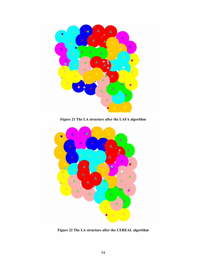
Figure 21 The LA structure after the LAFA algorithm
Figure 22 The LA structure after the CEREAL algorithm
54

The cells marked by identical colours will be connected to the same AR. I ran the HIENDA algorithm on the above presented AR structure, assigning the ratios of the given AR handover rate and the total amount of handover in the AR topology to the belonging terminal nodes as probabilities on the lowest level of the tree. On the Figures 23, 24 and 25 can be seen the second, the third and the fourth level of the hierarchy viewed from above after running the HIENDA algorithm.
Figure 23 The second level of the hierarchy viewed from above
55
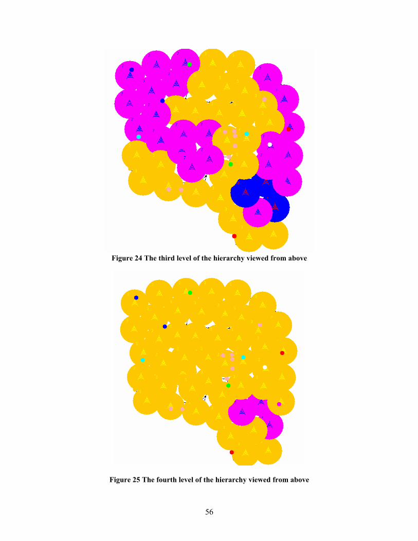
Figure 24 The third level of the hierarchy viewed from above
Figure 25 The fourth level of the hierarchy viewed from above
56

For the simulated MN movements (AR and MAP handovers) the Location Update and the Packet Delivery Cost was calculated for both hierarchical structures (created by the HIENDA and the Multi-Level HMIPv6 scenario).
Figure 26 shows the Location Update Cost for the two hierarchical scenarios, in the function of the aggregated ARs (for 2=S and 3=S ). In the case of when two terminal nodes were aggregated in each step of the algorithm, the HIENDA algorithm outperforms the Multi-Level HMIPv6 scenario in point of the location update signalling load. When three ARs are aggregated in each step of the hierarchy building, the difference gets significant; the hierarchical structure created by the HIENDA algorithm is producing only half of location update messages that the Multi-Level HMIPV6 does.
2=S
0
200
400
600
800
1000
1200
1400
2 3Number of aggregated ARs (S)
Loca
tion
Upd
ate
Cos
t
Multi-Level HMIPv6HIENDA algorithm
Figure 26 The Location Update Cost for the two hierarchical structures
Another important issue is the Packet Delivery Cost, because if the hierarchical structure is designed in a manner to reduce the Location Update Cost but simultaneously it is increasing the signalling load caused by the triangular routing, it is not effective anymore. Therefore the Total Signalling Cost is an important performance evaluation parameter too, because it keeps maintaining a tradeoff between the two cost functions.
Figure 27 shows the Total Signalling Cost for the two competitive hierarchical scenarios in the same mobility environment, in the function of . The HIENDA is outperforming again the Multi-Level solution, it can be seen that they are producing almost the same Packet Delivery Cost, but the Location Update Cost is much lower in both cases when HIENDA is used. This means that in this way we can minimize the Location Update Cost, simultaneously keeping the Packet Delivery Cost low by the MAP deployment, obtaining an optimal tradeoff between the two costs.
S
57

0
500
1000
1500
2000
2500
2 3Number of aggregated ARs (S)
Tota
l Sig
nalin
g C
ost
Multi-Level HMIPv6HIENDA algorithm
Figure 27 The Total Signaling Cost for the two hierarchical structures
4.6 Summary
My aim in Chapter 4 was to highlight the main questions and optimization problems of designing mobile network architectures based on Hierarchical Mobile IP, and to present a novel hierarchical network design algorithm (called HIENDA) in order to optimize mobility management in Mobil IP networks. The main goal of HIENDA is to assign an optimal tree structure to a given source of Access Router handover rates. Therefore HIENDA considers the topology constraints, and takes the available mobility pattern and Access Router handover information as input, and finds a near optimal HMIP hierarchical structure (it can be used for planning an optimal Proxy Agent Architecture in micro-mobility management) for which the total signalling cost will be minimum.
A HMIP simulation environment was implemented integrating the cost functions and network designing schemes in order to extensively analyze and evaluate the capabilities of the hierarchical optimization technique, comparing them with a solution from the literature. From the simulations results the conclusion could be drawn that the HIENDA is outperforming the other existing hierarchy optimizing solution in the terms of Location Update Cost, at the same time keeping the Packet Delivery Cost on a low level.
58

Chapter 5
5 Overhead reducing information dissemination strategies for disconnected mobile ad hoc networks
In Chapter 2-4 effective network designing algorithms were introduced for signalling
load optimization, in a traditional, fully-connected communication environment. As I wish to give planning principles for the next generation mobile networks, another way of communication should be envisaged too, due to the spreading of concepts about autonomic and self-organizing, disconnected networks.
Therefore a totally different, lateral thinking was needed in this research area of my Theses, to investigate how overhead of information dissemination can be decreased in a disconnected network architecture where highly mobile nodes form the network. The overhead can be defined in such networks as the overall sum of all the not useful data messages, which are called duplicates (they do not provide any new information for the nodes, which receive it) and the signalling messages needed for the algorithm operations. While there are a huge number of message forwarding algorithms described in the literature, the environment is changing so rapidly that there is no hope for choosing a theoretically optimal algorithm. Therefore I introduced a biologically inspired solution based on the phenomena of natural selection.
5.1 Introduction
Most wireless networks are built around an infrastructure, where all communications is routed through base stations that act as gateways between the wireless and wired network. However, there may be situations in which it is impossible or not desirable to construct such an infrastructure. There can be cases when a collection of wireless mobile nodes forms a temporary network lacking the centralized administration or standard support services regularly available on conventional networks.
The motivation for disconnected, autonomic networks comes from emerging trends towards pervasive computing and communication environments, where myriads of networked devices with very different features will enhance our five senses, our communication and tool manipulation capabilities. Our everyday environments will be more and more populated by multitudes of decentralized and networked computing systems [48] (e.g., multiagent systems [49], ad hoc networks of mobile computer-based devices [50], sensor networks [51] and spray computers [52]). Most of these systems will be able to autonomously perform activities on our behalf—typically by interacting with each other—letting us “out of the loop” [53]. The complexity of such environments will not be far from that of biological organisms, ecosystems, and socio-economic communities. Traditional communication approaches are ineffective in this context, since
59

they fail to address several new features: a huge number of nodes including low-cost sensing/identifying devices, a wide heterogeneity in node capabilities, high node mobility, the management complexity, and the possibility of exploiting spare node resources.
The distributed and self-configuring nature of Multihop Mobile Ad Hoc Networks (MANETs), combined with the ease and flexibility of deployment of such networks, make MANETs appealing for a wide range of application scenarios, where their presence becomes ubiquitous in many life sectors [54]. These networks are basically characterized by the lack of a fixed infrastructure, where each participating node can initiate a peer to peer communication with any other node through one hop or multihop paths, and where nodes will behave as routers or relays within the data delivery chain. Node mobility has introduced new challenges on the communication characteristics in these networks related basically to connectivity and packet routing among the nodes. These two latter issues are closely related and are the major factors impacting the throughput, end-to-end delay and other performance metrics of the network. While the connectivity of two nodes is generally determined by the physical distance between them, packet transfer between two remote nodes is generally the outcome of the routing protocol and involve either the establishment of an end-to-end path between the two remote nodes [55, 56], or the assistance of intermediate mobile nodes to relay and disseminate the packets [57, 58].
The transmission power of the nodes is limited however the packets may have to be forwarded by several nodes before they reach their final destinations. This means that each node may be a source, relay and destination. To manage a larger Multihop MANET with a longer lifetime, it need to be completely self-organized, meaning that the network would be run solely by the operation of the end-users, solving this way the scalability problems of such an extended MANET.
It could be interesting to mention what are the possible application areas of these self-organized and disconnected networks. Only one of many is the Digital city: dynamics of a city can be captured in real-time by collecting and correlating data and information (anonymous localization, traffic, pollution, cultural sites, events, etc) provided by heterogeneous sources and mapping it to interactive maps (for example intelligent parking lots, seating in restaurants, cinemas or public transportation, real-time notifications on important products in a supermarket). People moving and acting in a city base their decisions on information that is in most cases not synchronized with the time and place they find themselves in when taking those decisions. Experiencing a shift between decisions and information it is very common in everyone experience: arriving at the airport just to find out that the flight has been delayed, being surprised by a traffic jam. The dynamic city is concerned with the real-time mapping of city dynamics and data. Maybe more important application fields are the telecommunication markets in developing countries or regions without any mobile network infrastructure or situations in a disaster recovery, when the traditional central infrastructure collapses.
My research interest was in developing novel information dissemination solutions for disconnected, autonomous networks, which are resilient to frequent topology changes and capable to decrease the signalling and duplicate overhead. Furthermore a novel approach is introduced in this Chapter to use an evolution based decision mechanism with a distributed fitness evaluation method for choosing the adequate information dissemination method for different mobility environments in a self-managing MANET.
60

5.2 Related Works
In a self-managing MANET the human mobility and local information dissemination is exploited in order to propagate messages. In this kind of network the existence of a broadcast medium can be exploited to increase the efficiency of information dissemination. This broadcast medium is local to the nodes in radio range so it cannot be used for multihop communication. Therefore a higher level quasi-global broadcasting mechanism is needed that is able to reach all the nodes in a connected island which are not directly connected to the source. These techniques are called multihop broadcast algorithms. Many ad-hoc applications rely on the existence of a broadcast medium for the dissemination of some control information. The naive first implementation of this was flooding: every node repeats the message after it is first received. However it was realized very soon, that this is very far from optimal, and collisions in the media can lead to serious congestion and loss of packets. To solve this problem many efficient broadcast techniques were designed, that take into account some information about their surroundings, instead of blindly repeating every packet. These algorithms differ in their assumptions about the environment (like assumption of a connected or disconnected network) and in the information available for decision (existence of GPS for example).
The central problem of broadcast algorithms is to decide when and who should retransmit messages. Nodes have to forward packets so the message reaches every part of the network; however the performance relies heavily on the set of nodes that do this. When nodes decide to retransmit or not, they actually decide if they are part of this forwarding set. Too many retransmissions cause collisions and use much more network bandwidth, but choosing the smallest forwarding set is not easy because a global view of the network is not available, and local information gets obsolete very quickly if the velocity of nodes is high. There is also the danger if the number of forwarding nodes is too small, because then the message does not reach every node.
There are many published comparisons of information dissemination methods [59, 60, 61], which provide us a quite detailed picture about the existing broadcast approaches.
The Counter Based Method, originally introduced in [62], is one of the first controlled broadcast methods, and it is a simple heuristic based algorithm. It is based on a simple observation, that if a duplicate of a packet received, then the probability of reaching any new nodes is low. To exploit this idea, the nodes do not immediately retransmit when they receive a packet, but instead they wait for a random time, which is called Random Assessment Delay (RAD). If a duplicate is received during the RAD a counter is increased. If the counter reaches a threshold before the RAD expires, the node cancels the retransmission. The original method has different adaptive versions [63], which try to adapt the length of RAD and the threshold of the duplicate counter to the current network conditions.
Another very simple broadcast method is the Gossiping algorithm which was also introduced in [62]. It is a very simple one: every node rebroadcasts the heard message with a predefined probability. The optimal probability can be calculated off-line, or can be learned adaptively. While it is very easy to implement, it is usually outperformed by other more sophisticated algorithms. Another problem can be that while the optimal
61

retransmission probability can be calculated off line, it heavily relies on the parameters of the environment. To overcome this limitation there are adaptive versions of the basic methods, like Hypergossiping.
Hypergossiping [64] is specifically designed for partitioned networks, where nodes are mobile, and partitions join and split from time to time. It is an advanced version of the Gossip algorithm, extended by neighbour information and partition join detection. The algorithm uses a simple adaptive gossiping strategy for in-partition forwarding, but rebroadcasts some of the packets if it detects a join with another partition. The join detection is based on the simple heuristic, that the nodes in the same partition received the same messages recently. Every node maintains a list, called LBR (Last Broadcasts Received), of the recently broadcasted messages. They send HELLO messages periodically, to indicate their presence. When a new node is detected, one of the nodes includes his LBR in the next HELLO message. When the other node receives this LBR, it compares with his own LBR. If the overlap between the LBR of two nodes is smaller than a threshold, then the node is considered coming from another partition, so a new message is sent, called BR (Broadcasts received), which contains the list of messages that the node already received. From this the other node knows, that a partition join happened, and rebroadcasts all the messages that were not inside the other nodes BR. After this rebroadcast, dissemination happens using adaptive gossiping.
A fine example of a self-pruning algorithm is the Scalable Broadcast Algorithm (SBA) algorithm [65]. It requires 2-hop neighbour information and the last sender ID in the broadcasted packet. When a node receives a broadcasted packet from a node u it excludes the neighbours of u ,
v( )uN from the set of his own neighbours . The
resulting set \ is the set of the potentially interested nodes. SBA is also one of the algorithms that has an explicit Random Assessment Delay (RAD) mechanism.
The maximum RAD is calculated by the
( )vN( )vNB = ( )uN
maxmax
Tddv ⋅⎟⎟
⎠
⎞⎜⎜⎝
⎛ formula, where ( )vNdv = and
is the degree of the node with the largest degree in maxd ( )vN . Nodes choose the time of transmission uniformly from this interval. This ensures that nodes with higher degree are usually broadcast before nodes with fewer neighbours.
A generalization of self-pruning and neighbour designation protocols is the Generic Self-pruning algorithm [66]. In its general form the method relies on k-hop neighbourhood and k-hop routing information. The class of algorithms they describe use one of the versions of the so called Coverage Condition. The most used case when 2-hop neighbour and 2-hop routing information is used, and the self-pruning made according to the static version of Coverage Condition I: Node v has a non-forwarding status if for any two neighbours u and a replacement path exists that connects and via several immediate nodes (if any) with either higher priority values than the priority of or with visited node status.
w u wv
62

5.3 Novel Information Dissemination Algorithms for a Disconnected MANET
5.3.1 The IOBIO Algorithm (InfOrmation Dissemination Protocol for BIOlogically Inspired autonomic Networks and Services)
To eliminate the drawbacks of the earlier introduced information dissemination
algorithms, a quite different approach is presented by me, the IOBIO algorithm. It uses a simple 3-stage handshake to discover neighbours that are interested in one of the carried messages. The goal of the protocol is to reduce unnecessary load of neighbouring nodes by duplicate or unneeded data ("spamming”).
The nodes use three different types of messages for information-exchange in the IOBIO algorithm. ADV: advertisement of new data. If a node intends to send out new information it first sends an ADV packet that describes the data packet. The advertisement contains the identification information for the targeted User Community (users are usually not interested in every type of data; they form User Communities (UC) with similar interests). ADV messages are sent periodically. REQ: request for data. A node answers to the ADV packet with REQ, asking for the advertised information. DATA: the data message, which contains the requested information.
5.3.1.1 General steps of the protocol
1) A node (A) (who is a member of a certain UC) receives a data packet from another node.
2) A broadcasts an ADV message. 3) A node (named B) is a member of the same UC as A. B checks the ID of the
advertised service, and it concludes that it needs that information. Before sending the REQ message B checks if a REQ was heard in the neighbourhood asking the same message which is needed by B. In that case B cancels the sending of the REQ message, otherwise it sends a REQ to A.
4) B broadcasts a REQ message. A receives the REQ message. A checks the ID of the requested information. If A does not have this information, A drops the message, otherwise A sends out the DATA packet referred to by the REQ message.
5) A broadcasts the requested DATA, B receives it. B processes it and then starts the IOBIO protocol from point 2) (e.g. broadcasts an ADV message).
The benefits of the algorithm are demonstrated on Figure 28. Node A sends an ADV
indicating that it has the messages 1, 2 and 3. After receiving this ADV, nodes B, C, D start a Random Assessment Delay. At step 2 node D sends a REQ packet, indicating, that
63

it needs messages 2 and 3. At step 3, node C sends a REQ packet. However, the REQ packet of D had been heard, so C detects that message 2 is already requested, and only puts the ID of message 1 in the REQ packet. At step 4, the random delay of B is over, however, message 1 is already requested, so no REQ is sent. At step 5 the wait interval of node A is over, and all requested messages are transmitted.
Figure 28 General model of IOBIO
5.3.1.2 Resolving advertisement collisions
In order to resolve the problem of advertisement collision (it is the case when two nodes send the ADV message in the same time, therefore the neighbouring nodes will get DATA packets from both nodes after requesting the same packets) the following scenario is presented. We assume that two nodes – A and B – send an ADV message at the same time. If there is a node (named C) in the communication area which is interested in this information, both of A and B will receive the REQ message. It may lead to overhead if both of them send the DATA. In order to avoid this algorithm was extended in the following way. If a node (named A) sends an ADV message, and it receives the same ADV message (from another node, named B), it draws a random number, and sets up its waiting-time to this random number. Node B does the same. If A receives a REQ message, it will wait for the set delay – if it does not receive a DATA information with the requested data during the waiting-period, it sends the requested information. If it receives the requested data – which means that the information was already sent by B – it does not send anything.
5.3.1.3 Advantages of the algorithm
One of the most useful properties is the limited overhead - no unnecessary DATA message is sent. With the 3-stage handshake we do not need to broadcast every time. The first and second steps use short control messages; the broadcasting of the data only
64
happens in the third step, and only when it is really needed. It happens only upon a request nearby – thus, the overhead is decreased.
We assume that a lot of nodes – belonging to the same group of interest – are usually close to each other. In this case lot of advertisement and request messages are sent, and the networks will work as a simple broadcast-network. One can tell that with the 3-stage handshake we can reduce the energy needed for communication, because the node sends only short advertisement messages (which message should be processed by all the nodes in the communication range), and all the data will be sent only in one case: if a node needs it.
5.3.2 The Modified IOBIO Algorithm (MIOBIO)
The IOBIO uses simple periodic broadcast to send ADV packets. Considering the number of packets a more effective approach is possible. Applying the Adaptive Periodic Flood (APF), which is a simple controlled flood protocol that can reduce the number of duplicated messages without using control messages, while maintains low delays and robustness that are characteristics of a Blind Flood. This simple protocol broadcasts messages periodically, and increases this period when a duplicate arrives.
Considering the number of bits sent/received APF is not as efficient as IOBIO because it sends DATA messages only, and generates a high amount of unnecessary bits. IOBIO can avoid the transmission of unnecessary DATA messages using a simple handshake. To combine the benefits of the two algorithms (APF and IOBIO), MIOBIO uses the APF protocol to decrease the amount of duplicate ADV messages, and uses the original IOBIO handshake to decide when DATA messages have to be sent. The IOBIO and MIOBIO – similar to other networking strategies [67] - leverage contacts among nodes to spread information system-wide. In the opportunistic networks no assumption is made on the existence of a complete path between two nodes wishing to communicate. Source and destination nodes might never be connected to the same network, at the same time [68].
5.3.3 Multi-Message Scalable Broadcast Algorithm (MMSBA)
The algorithms that do not take partitioning into account, like Scalable Broadcast Algorithm (SBA) and Generic, perform poorly in disconnected environments. These kind of algorithms decide to rebroadcast a message only once, when it is first received. If there are no more nodes in transmission range when the last message is sent, the dissemination stops. Unfortunately, when a new node arrives into the transmission range, there is no event that can trigger a retransmission. To solve this problem, the SBA algorithm was improved, because it is computationally simple, and proved to be robust by many papers [60], [61]. It also gives a nice way to generalize its mechanism to the multi-message case. The basic idea of the SBA algorithm is the Random Assessment Delay (RAD) process, which delays the transmission of packets by a random interval. The first time SBA receives a packet, it starts the RAD procedure. During this interval the SBA listens to his neighbours. When one of them starts broadcasting, SBA removes the neighbours of the broadcasting nodes from his own 1-hop neighbour set. My modified algorithm, the Multi-
65

Message SBA (MMSBA) may trigger a RAD not only on the first reception of a message, but on any event that changes the local neighbourhood information. Every time a HELLO message is received, MMSBA updates his neighbour list. When the number of interested nodes exceeds zero, MMSBA starts the RAD. The RAD works exactly the same way as in SBA. There is a little problem though. Every time we receive a HELLO message from another node, we will put him again on the list of interested nodes, even if the broadcast message was already sent to him. This problem is not present in the original SBA, as nodes broadcast the message at least once, when it is first received. To overcome this problem, the nodes include the list of messages they have already received in their HELLO packets. This also gives a feedback to MMSBA if a broadcast message was lost during transmission. The new method allows MMSBA to handle many messages independently.
To support multiple messages, the RAD process also needs to be updated. When a neighbour node broadcasts MMSBA removes from its context the nodes that are interested only in that broadcasted message. However, nodes that are interested in other messages remain in his list. This mechanism can be imagined as overlapping independent networks, where different messages are disseminated independently using the SBA RAD in different networks.
5.3.4 Mobility Models for Disconnected Networks
The validation of various protocols is highly dependent on how realistic the used mobility model is. Since mobility patterns play a significant role in determining the protocol performance, it is desirable for the mobility model to emulate the movement pattern of real life scenarios in a reasonable way. The problem is that there is a very limited number of available real mobility patterns [69], [70] capturing node movement in large-scale disconnected mobile networks. Not only the amount of mobility patterns is limited, but these traces are related to very specific scenarios and it is difficult to generalize.
However none of these synthetic mobility models reflect real world situations, because in practice, a mobile node does not roam in a completely random manner. In the disconnected mobility environment the delicate details of time-location dependency and community behaviour must be taken into consideration. In these networks it is important to model the behaviour of individuals moving in groups and between groups, therefore the mobility model in this case must be heavily dependent on the structure of the relationship among the mobile nodes, capturing this social dimension. A key aspect of human movement is dynamic clustering. We can observe this on the streets: people travel in small groups (clusters); some people join the clusters, while others leave them [71]. Clusters form in traffic jams, on mass transit vehicles, etc. To examine this phenomenon I have developed a group mobility model, called the Reference Point Group Mobility Model with Dynamic Clustering (RPGMMDC). It is a modified version of the Reference Point Group Mobility Model (RPGM), which is a group mobility model and it means that the nodes are organized in groups and the groups move together. Each group has a centre point, that moves according to a mobility model (in this case the Constant Speed Mobility Model). Each node has a reference point close to the centre point, and sets its destination
66
in a random location near the reference point. In the RPGM model, the groups were predetermined, and did not change during the simulation. In this modified version, after each step each node has a small chance of leaving the current group and joining another randomly chosen group. This model offers an even more accurate representation of human movement: groups mentioned in the previous paragraph change over time; some people join the group while others leave and eventually join another one.
5.4 The Simulation Framework Within the framework of the BIONETS project [72], a freely available simulation tool
has been developed in the Mobile Communication and Computing Laboratory by our project team [73], extending the architecture and functionalities offered by the well-known OMNeT++ [74], [75] package to reflect the BIONETS system architecture. The simulation framework itself is a collection of interdependent software components. The heart of the system is the OMNeT++ discrete event simulator library and tools. The Mobility Framework [76], [77] is a library built on the OMNeT++ core library which provides a framework for mobile communication simulations. It contains several implemented modules. Simulator components provide additional or customized services on top of OMNeT++ and Mobility Framework. OMNeT++ itself has several components. The core library is the implementation of the discrete event simulator which executes a simulation model that can be defined by the simulator users. Mobility framework is a library that provides a framework for mobile ad hoc simulations and also has different model implementations. It supports the use of different mobility and channel models, and many network technologies.
5.5 Simulation Results
Williams et al. [61] compared several dissemination methods in their work which included simple heuristic based methods, a location-based scheme and two self-prune methods. They simulated these protocols in different network conditions varying traffic load and mobility. The results of their experiments show that the best available dissemination methods are mostly self-pruning based.
From a comparison focused on self-pruning algorithms [60] it turns out, that most of these algorithms cope well with the problem of congestion, almost all in the cases 98% delivery ratio was reached. Mobility is a much greater threat to these algorithms. Most of the self-prune algorithms perform poorly if the nodes in the network move with high speed. It is also shown that the algorithms that rely on node neighbour degree instead of node ID are less resilient to mobility, and their performance degrades more quickly than the other methods.
I have used the simulator to evaluate the performance of different information dissemination algorithms and mobility models, presenting the two novel information dissemination algorithms, the Multi-Message SBA (MMSBA) and the Modified IOBIO (MIOBIO), comparing them with the reference algorithms chosen from the literature
67

which are the best available dissemination methods published earlier for a disconnected mobile environment: Generic Self-Pruning, SBA, Hypergossiping. These algorithms were chosen after an extensive study of the literature of data dissemination, covering a large set of different dissemination types, drawing a conclusion that the three algorithms mentioned above give a very good all-around solution that performs well in a disconnected mobile environment.
SBA is outperformed by some of the other methods, but it showed remarkable resiliency to extreme mobility conditions. The Generic self-prune method, introduced above, was shown one of the most effective algorithm in many situations, but is somewhat sensitive to mobility. Hypergossiping because it is a relatively new algorithm that takes network partitioning into account, and support the dissemination of multiple messages.
The main criterion for the evaluation of the algorithms was the robustness of the algorithms in different conditions. The simulation parameters were chosen to be realistic to be able to test the algorithms in a disconnected mobile environment. Every simulation starts with a 200 second “warm-up” period (needed by the mobility models). The transmission of the control messages (like HELLO) starts after the 195th second, so the dissemination methods have time to discover their neighbours. The first message is broadcasted from a single node at the 200th second. It is assumed that the message has 10 seconds lifetime, so the simulation stops at 210 seconds, when the message gets outdated. The measurement confidence was 0.95.
For all the algorithms under investigation, the number of the nodes was measured that correctly received the message within a delay of 10 sec. This delivery ratio indicates the fraction of nodes that were interested in the message and received it during its lifetime (10 s). The results of these measurements are shown on Figure 29. The results show that MMSBA provides the best coverage for the Reference Point Group Mobility Model with Dynamic Clustering, but using other mobility models, the performance of MIOBIO and MMSBA is very close. Both of the new algorithms outperform SBA, Generic and HyperGossip.
Figure 29 Delivery ratio of the simulated algorithms
68
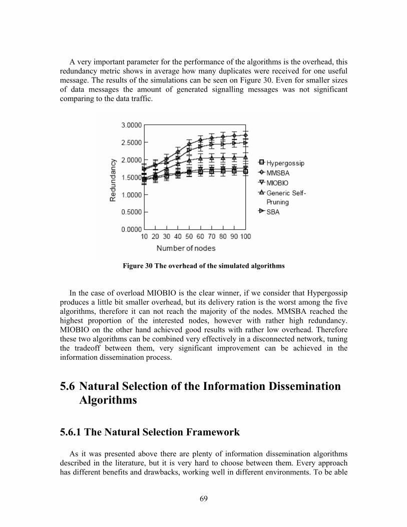
A very important parameter for the performance of the algorithms is the overhead, this
redundancy metric shows in average how many duplicates were received for one useful message. The results of the simulations can be seen on Figure 30. Even for smaller sizes of data messages the amount of generated signalling messages was not significant comparing to the data traffic.
Figure 30 The overhead of the simulated algorithms
In the case of overload MIOBIO is the clear winner, if we consider that Hypergossip produces a little bit smaller overhead, but its delivery ration is the worst among the five algorithms, therefore it can not reach the majority of the nodes. MMSBA reached the highest proportion of the interested nodes, however with rather high redundancy. MIOBIO on the other hand achieved good results with rather low overhead. Therefore these two algorithms can be combined very effectively in a disconnected network, tuning the tradeoff between them, very significant improvement can be achieved in the information dissemination process.
5.6 Natural Selection of the Information Dissemination Algorithms
5.6.1 The Natural Selection Framework
As it was presented above there are plenty of information dissemination algorithms described in the literature, but it is very hard to choose between them. Every approach has different benefits and drawbacks, working well in different environments. To be able
69
to choose we need precise models on mobility and traffic patterns. There are no such models and even if there were, the complexity of them would hinder their usability. Even worse, the environment is changing so rapidly that there is no hope for choosing a theoretically optimal algorithm.
Instead of extensive analytical modeling, one can choose an adaptive approach. This way the system “self-tunes” itself providing services with acceptable performance over a large set of possible environments. Every adaptive system needs some feedback to modify its behavior to increase performance. This is problematic when there is no model of the system. Instead of an analytically derived solution, the problem can be approached with a biologically inspired method, like natural selection. In this case the system has many algorithm individuals that compete with each other. The individuals with the highest fitness will reproduce faster than the less fit ones. The designer chooses the fitness function so that the species with good performance will get higher fitness scores. Evaluating the fitness of the algorithms using direct feedback has many difficulties. All the nodes that received the message should send some acknowledgment messages to the sender to indicate the success of transmission. This obviously increases the load on the network. More serious issue is that these feedback messages should be carefully coordinated to avoid collisions. If this is not solved then many acknowledgments get lost and the fitness evaluation will not work properly.
The fundamental problem of fitness estimation is that the receiver nodes have the information on the success of transmission while the sender nodes have the sender algorithm. The feedback approach solves this by propagating information back from the receivers to the senders. The key idea in this work is the reversal of this decision. Instead of trying to collect performance measurements at the sender and choosing the next generation of algorithms there, the sender attaches the code of the sender algorithm to every packet and delegates the decision to the receiver. This way every message carrying payload will also carry a genetic code essentially becoming a virtual seed. The receiver collects these messages from different nodes with the included algorithm descriptions. This way the receiver could guess which algorithms perform best as those are the algorithms whose code is seen in most messages. When the algorithm individual at the receiver node dies the node will choose the best algorithm based on his local measurements. If a message contains an obsolete payload then it is considered duplicate and a penalty could be accounted for the sender algorithm. This acts as an incentive to sender algorithms to send useful information only and do not “spam” the system.
With this approach an algorithm could reproduce only by successfully transmitting useful messages – virtual seeds. Still this is not enough to ensure the success of the system. Imagine an algorithm that sends out no messages at all. While this algorithm could not reproduce it still occupies a node and keeps it from sending messages. This can be solved by simply limiting the life of any algorithm individual with a timer. This way time becomes a limited resource for the competing algorithms and therefore it will have an implicit cost. Similar problem is when an algorithm continuously transmits messages making impossible for other nodes to send messages and reproduce. Again, costs can be assigned to message transmission by simply limiting the amount of messages that an algorithm is allowed to send. If this credit is depleted, the algorithm dies.
Therefore there are two limiting parameters of the information dissemination algorithms available in the network: the maximum number of
NAAA ,..,, 21
maxM
70
messages sent by an algorithm during its lifetime and a timer is set when the node starts using a new algorithm. So an algorithm dies, if
JmaxMM sent = or expires. J
For the mobile node a local fitness function is defined for every algorithm: thj
iii duplicatesjusefuljAj MMF ,,, −= , Ni ,..,1= (37)
where is the number of useful messages received by the node by the algorithm and is the number of duplicates received from the same algorithm on the same node, as the sender node attaches the code of the sender algorithm to every packet. Every time a mobile node needs to choose a new algorithm for disseminating its messages (because the last one died), it will choose on the basis of its fitness function, always the algorithm which has the highest fitness value in that moment will be chosen.
iusefuljM ,thj thi
iduplicatesjM ,
The rules outlined above concentrate on maximizing the outgoing useful traffic from a node. The applications running on the nodes are also interested in receiving useful messages; therefore algorithms should get some score for receiving messages. When a node receives a useful message it gives a score to the sender algorithm, but also a small fraction of this score to the algorithm at the receiving node for being polite and accepting useful messages. This way the cooperation level of the algorithms could be adjusted to examine the effect of the cooperation willingness on the overall properties of the system.
The fitness function needs to be modified if cooperation is introduced in the system, for the node the fitness function for the algorithm, which is currently running on the node, will be:
thj aA
aaaa receivejcoop
duplicatesjusefuljAj Mw
MMF ,,,,1
⋅+−= (38)
where is the number of useful messages the node received while the
algorithm was running on it, and
areceivejM ,thj aA
coopw1 is the cooperation bonus divisor, the ratio of the
bonus points obtained by sending/receiving a useful message. An important consequence of these rules is that there is no explicit fitness function. No
node in the system knows the fitness of a given algorithm at a given time. Every algorithm individual tries to “convince” the receivers of its usefulness but no node knows how many other nodes have chosen the same algorithm for reproduction.
This natural selection based framework was implemented in the above presented BIONETS simulator and the algorithms were implemented using a meta-protocol that is a generalization of the described algorithms so that all the algorithms recognize each others messages, however they may react as they see fit – no particular protocol sequence is mandatory. I have chosen the best performing algorithms based on the measurements introduced above, which were the MIOBIO and MMSBA, while APF was selected to check what will be the impact on natural selection if a too “aggressive” algorithm is also competing with the more complex and moderate algorithms.
71

5.6.2 Simulation Results
Two kinds of simulations were carried out with the BIONETS simulator. First the size of the data packets was changed, observing which combination of the information dissemination algorithms are more useful when transferring “small” or “big” packets. The second one was carried out to analyze the effect of cooperation on the performance of the algorithms. During these measurements the cooperation level of the algorithms was changed in the simulator, namely the proportion of scores, for sending and receiving a useful message.
By changing the data packets conclusions can be drawn on how to use the different information dissemination algorithms when the size of the data packets is changing. The data packet size was changed during the simulation in 5kbyte steps, the maximum size was 100kbyte. Finding a fair, and efficient awarding system is important, because this provides that always the most appropriate algorithm is selected for forwarding messages, resulting in optimal performance.
During the simulation – due to the high computing requirements – there were ten runs averaged and analyzed. Ten running in this case is enough to reduce any kind of error below the acceptable level.
5.6.2.1 Measurements with Changing Data Packet Size As mentioned before, in this kind of measurement the data packet size is changed,
from 1KByte to 100KByte in 5Kbyte steps. For each data size there were 10 runs averaged and plotted. At first, the performance of a system using MIOBIO and MMSBA forwarding algorithms is presented.
In Figure 31 the proportion of the received useful and duplicate bits can be seen (in Figure 31-35 on the horizontal axis the size of the data packets is shown in kilobytes.) As one can observe the combination of this two algorithms perform quite well. Despite the very slightly degrading performance these two algorithms perform exceptionally well when there is a need for large packet propagation. In Figure 32 the age of the data packets is shown in the entire system.
Recieved useful/duplicate bits (MIOBIO/MMSBA)
0
0,2
0,4
0,6
0,8
1
1,2
0 10 20 30 40 50 60 70 80 90 100
Figure 31 Received useful / duplicate number of bits for MIOBIO/ MMSBA competition
72

Average data age (MIOBIO/MMSBA)
0
500
1000
1500
2000
2500
0 10 20 30 40 50 60 70 80 90 100
Figure 32 Average Data Age for MIOBIO/MMSBA competition The average data age (averaged for the entire system) is highly increasing after the
packet size exceeds 50kbyte. The cause of the phenomena is that large packets “squeeze through” the system much slower than the small ones, because sending them requires more time and thus also more collisions happen.
In Figure 33 all the algorithms (APF, MIOBIO, MMSBA) compete. A sudden decrease is noticeable around 35kbyte packet size. This is because at this point the APF sends too many duplicate bits. APF generally performs quite well, but over a certain packet size it is not capable of “backing off” as well as in case of small packets.
Recieved useful/duplicate bits (MIOBIO/MMSBA/APF)
0
0,2
0,4
0,6
0,8
1
1,2
0 10 20 30 40 50 60 70 80 90 100
Figure 33 Received useful / duplicate number of bits for MIOBIO/ MMSBA/APF competition
When the effectiveness is dropping the average data age is increasing (Figure 34).
This again happens as the APF floods the system. The last simulation is when the APF competes against the MMSBA (Figure 35). The graph is very similar to Figure 33. This is
73

due the nature of APF. When APF is present in the system the graphs look all like Figure 33 and 35. Here, when sending small packets, the useful/duplicate ratio is very high, while for larger packets the “greedy” nature of APF worsens the overall throughput of the system.
Average data age (MMSBA/MIOBIO/APF)
0
500
1000
1500
2000
2500
0 10 20 30 40 50 60 70 80 90 100
Figure 34 Average Data Age for MIOBIO/MMSBA/APF competition
Recieved useful/duplicate bits (MMSBA/APF)
0
0,2
0,4
0,6
0,8
1
1,2
0 10 20 30 40 50 60 70 80 90 100
Figure 35 Received useful / duplicate number of bits for MMSBA/ APF competition
5.6.2.2 Measurements with different cooperation levels In this subsection the purpose of the measurements were to find out more about how to
encourage cooperation among the algorithms. The awarding system in the simulator was changed to gain better parameters. First the cooperation between APF and MMSBA is analyzed (Figure 36).
74

The cooperation bonus divisor is the ratio of the bonus points obtained by sending/receiving a useful message as introduced in (38). Knowing this, Figure 36 shows that when the reception of data packet is rewarded, then the entire system has better performance measures. In other words, the “greedy, spamming” algorithms such as flooding can be regulated this way. In this case for instance, a flood with an appropriately large back off period can survive, but a greedy one can not.
Sent useful per duplicate bits as the function of cooperation
Division, APF-MMSBA
0
0,1
0,2
0,3
0,4
0,5
0,6
0,7
0,8
1 11 21 31 41 51 61 71 81 91
Cooperation bonus divisor
Sent
use
ful/d
uplic
ate
[bit/
bit]
Figure 36 Sent useful/duplicate bits in function of the cooperation bonus divisor (APF/MMSBA)
In the next graph, the average data age rises, as the “mindless forwarding” is not
punished (Figure 37), as higher values on the horizontal axis indicate less motivation for cooperation.
Average data age as the function of cooperation
Division, APF-MMSBA
0
20
40
60
80
100
120
1 11 21 31 41 51 61 71 81 91
Cooperation bonus divisor
Aver
age
data
age
[sim
sec]
Figure 37 Average data age in function of the cooperation bonus divisor (APF/MMSBA)
Finally all the algorithms compete together in the system (Figure 38). The result is very similar to the one without the MIOBIO, which means by increasing the cooperation level between the nodes, the overall throughput of the system increases too.
75

Sent useful per duplicate bits as the function of cooperation
Division, APF-MIOBIO-MMSBA
0
0,1
0,2
0,3
0,4
0,5
0,6
0,7
0,8
0,9
1
0 10 20 30 40 50 60 70 80 90 100
Cooperation bonus divisor
Sen
t use
ful/d
uplic
ate
[bit/
bit]
Figure 38 Sent useful/duplicate bits in function of the cooperation bonus divisor (APF/MIOBIO/MMSBA)
When examining the average data age (Figure 39), we get very similar results to the
last case, by motivating the nodes to cooperate, the average data ages decreases, which will provide the users up-to-date information. It can also be observed, that the data age does not depend so much on the cooperation bonus divisor, as it depends on the data size. Thus it is possible to regulate data age with splitting up bigger packets into smaller ones.
Average data age as the function of cooperationDivision, APF-MIOBIO-MMSBA
0
20
40
60
80
100
120
0 10 20 30 40 50 60 70 80 90 100
Cooperation bonus divisor
Aver
age
data
age
[sim
sec]
Figure 39 Average data age in function of the cooperation bonus divisor (APF/MIOBIO/MMSBA)
76

5.7 Summary
Due to the frequent topology change one of the most important aspects of the self-managing MANETs is the effective spreading of information; it should be disseminated fast, before the period of validity expires. In Chapter 5 two novel information dissemination strategies (MIOBIO, Multi-Message SBA) for disconnected mobile networks are presented together with the outcome of a simulative study carried out to analyze their performance.
The most reliable algorithm is the MMSBA algorithm, followed by MIOBIO, Generic and SBA very close to each other. Hypergossiping was not able to reach large number of nodes, however it has a remarkably low overhead. Another interesting fact is that while the overhead values of Hypergossiping and MIOBIO are close, MIOBIO is the clear winner, because it can reach a much bigger proportion of nodes than Hypergossiping. The results clearly show that algorithms designed for network partitioning can achieve better reliability at the cost of some increased overhead.
Overall looking the two novel algorithms outperformed the existing algorithms created for disconnected mobile networks, therefore the total amount of the sent data can be reduced further, together with the delay experienced by the nodes, decreasing the unnecessary load of neighbouring nodes.
While there are a huge number of message forwarding algorithms described in the literature, the environment is changing so rapidly that there is no hope for choosing a theoretically optimal algorithm. Therefore I introduced a biologically inspired solution based on the phenomena of natural selection. The individuals with the highest fitness will reproduce faster than the less fit ones. The designer chooses the fitness function so that the species with good performance will get higher fitness scores. An important benefit is that there is no central fitness evaluation; every decision is made locally in the nodes, reducing the overhead generated by the performance feedback.
This natural selection based solution was implemented in the BIONETS simulator, together with the best performing algorithms (MIOBIO and MMSBA). During the performance evaluation the size of the data packets was changed and the level of cooperation between the nodes, to observe the effect on the performance of the algorithms. As it can be concluded APF is suitable only for an environment with smaller data packets, because of its greedy nature, while MIOBIO and MMSBA perform exceptionally well together when there is a need for large packet propagation. Introducing cooperation between nodes improved the overall parameters of the system like throughput and data age, also motivating greedy ones competing for survival to produce fewer duplicates, therefore spamming can be controlled with the rewarding system.
77
6 Conclusions
I presented general mobility management solutions, which can be utilized in the next generation mobile networks. The efficient network planning is crucial for the future systems, where the scalability problems and improving the network performance parameters can be a real challenge.
Since all the existing cellular networks use the zone-based scheme, that means the use of Location Areas, in practice; my first thesis addresses the optimization of such zone-based schemes to reduce the signalling cost in mobile networks. Most of the references related to the Location Area design are focused on how to determine the optimal numbers of cells for an LA or LA planning schemes are given for only a homogeneous mobility environment. In Thesis 1 a LA planning method is introduced first for a heterogeneous mobility environment, which means the inter-cell movement rate distribution is not near uniform, as it is assumed in the majority of LA planning schemes published earlier. Therefore the goal was to reduce the sum of the location update and paging cost. In this Thesis there was also presented a LA planning scheme for a near-uniform distribution case, where the final goal is the determination of optimum number of cells per LA for which the location update cost is minimum, with the paging cost as an inequality constraint function, which gives the novelty of this research, namely for both environments the LA structure can be optimized. In both cases a detailed cost structure is introduced and analyzed, serving like an evaluation framework for the LA forming algorithms.
For the heterogeneous scenario in the first thesis the performance evaluation of the LA forming algorithm (LAFA) and the cell regrouping algorithm (CEREAL) is given by a simulation tool, showing that compared with a reference algorithm chosen from the literature the LA forming technique reduces the location update cost by 40-60 percents. The regrouping algorithm performs well if we want to decrease the total cost of our system, it can reduce the total cost by 30-40%, sometimes over 50%.
The LA forming algorithm developed for the homogeneous scenario also contains two phases: a greedy algorithm (GREAL) is adopted which forms a basic partition of cells into LAs, and then a simulated annealing based algorithm (SABLAF) is applied for getting the final partition. Comparing them with the same reference algorithm, for the both mobility environments the SABLAF algorithm delivered the best performance, reducing the location update cost almost 50% more effective than the reference solution.
These solutions are effective on the first level of the network hierarchy, but the drafts do not address the realization of the hierarchical structure in detail during the network design. Therefore with these Location Area planning algorithms, we can obtain the optimal partition of cells for a given Access Router, which will represent a Location Area router.
A key issue is how to group these Access Routers on the next level of hierarchy, and on which level of hierarchy to implement the MAP functionalities, actually how many Access Routers should be beneath a MAP within a domain.
Therefore I presented a hierarchical network design algorithm (HIENDA) in Thesis 2, based on the structure given by the LA planning algorithm, aligned with a MAP allocation algorithm in Hierarchical Mobile IPv6 to optimize the mobility management in the Mobil IP networks (or generally another Proxy Agent Architecture used in micro-
78

mobility management). The main goal of HIENDA is to assign an optimal tree structure to a given source of Access Router handover rates. Therefore HIENDA considers the topology constraints, and takes the available mobility pattern and Access Router handover information as input, and finds a near optimal HMIP hierarchical structure for which the total signalling cost will be minimal.
A HMIP simulation environment was implemented integrating the cost functions and network designing schemes in order to extensively analyze and evaluate the capabilities of the hierarchical optimization technique, comparing them with other solutions. From the simulations results the conclusion could be drawn that the HIENDA is outperforming the other existing hierarchy forming solution in the terms of Location Update Cost, at the same time keeping the Packet Delivery Cost on a low level.
In Thesis 3 mobility management solutions are introduced for a non-traditional communication approach: my research interest was in developing novel information dissemination solutions for disconnected, autonomous networks, decreasing the signalling load occurring in epidemic routing. This required a highly innovative way of thinking and research, after network planning here the communication schemes of the nodes were designed for an opportunistic network lacking a fixed infrastructure. A simulator was used to evaluate the performance of different information dissemination algorithms and mobility models, presenting two novel information dissemination algorithms, the Multi-Message SBA (MMSBA) and the Modified IOBIO (MIOBIO), comparing them with the reference algorithms chosen from the literature which are the best available dissemination methods published earlier for a disconnected mobile environment: Generic Self-Pruning, SBA, Hypergossiping. The two novel algorithms outperformed the existing algorithms created for disconnected mobile networks; therefore the total amount of the sent data can be reduced further, together with the delay experienced by the nodes, decreasing the unnecessary load of neighbouring nodes.
Furthermore a novel bio-inspired framework is presented which utilizes natural selection for choosing the adequate information dissemination algorithm for different mobility environments in a self-managing MANET. As it can be concluded APF is suitable only for an environment with smaller data packets, because of its greedy nature, while MIOBIO and MMSBA perform exceptionally well together when there is a need for large packet propagation. Introducing cooperation between nodes improved the overall parameters of the system like throughput and data age, also motivating greedy ones competing for survival to produce fewer duplicates, therefore spamming can be controlled with the rewarding system.
79

List of Figures FIGURE 1 THE LOCATION AREA PLANNING PROBLEM ................................................................................... 12 FIGURE 2 THE REPRESENTATION OF THE MOBILE SYSTEM BY A GRAPH ......................................................... 17 FIGURE 3 JOINING THE TWO NODES (CELLS) INTO ONE SET (LA) ................................................................... 19 FIGURE 4 AN IMPLEMENTED MOBILE NETWORK IN THE SIMULATOR.............................................................. 22 FIGURE 5 AN EXAMPLE NETWORK FOR COMPARING TB-LAD AND LAFA.................................................... 23 FIGURE 6 THE LOCATION UPDATE COST IN RURAL ENVIRONMENT FOR THE TB-LAD AND THE LAFA
PARTITION............................................................................................................................................ 25 FIGURE 7 THE LOCATION UPDATE COST IN URBAN ENVIRONMENT FOR THE TB-LAD AND THE LAFA
PARTITION............................................................................................................................................ 25 FIGURE 8 THE AGGREGATED COST VERSUS THE VALUE OF PARAMETER K (RURAL) ...................................... 26 FIGURE 9 THE AGGREGATED COST VERSUS THE VALUE OF PARAMETER K (URBAN)...................................... 27 FIGURE 10 THE MANHATTAN CITY MODEL AND THE EUROPEAN CITY MODEL WITH MAIN ROADS IN BOLD... 28 FIGURE 11 THE LOCATION UPDATE COST FOR THE EUROPEAN CITY MODEL ................................................ 29 FIGURE 12 THE LOCATION UPDATE COST FOR THE MANHATTAN CITY MODEL............................................. 29 FIGURE 13 THE AGGREGATED COST FOR THE EUROPEAN CITY MODEL.......................................................... 30 FIGURE 14 THE AGGREGATED COST FOR THE MANHATTAN CITY MODEL ...................................................... 30 FIGURE 15 FLOWCHART OF SABLAF ........................................................................................................... 39 FIGURE 16 THE LOCATION UPDATE COST IN RURAL ENVIRONMENT ............................................................. 40 FIGURE 17 THE LOCATION UPDATE COST IN URBAN ENVIRONMENT............................................................. 41 FIGURE 18 A HIERARCHICAL MOBILE IPV6 NETWORK MAP OPTIMIZATION................................................ 45 FIGURE 19 AN EXAMPLE OF A HMIPV6 PROBABILITY TREE ......................................................................... 50 FIGURE 20 THE DESIGNED MOBILITY ENVIRONMENT..................................................................................... 53 FIGURE 21 THE LA STRUCTURE AFTER THE LAFA ALGORITHM ................................................................... 54 FIGURE 22 THE LA STRUCTURE AFTER THE CEREAL ALGORITHM .............................................................. 54 FIGURE 23 THE SECOND LEVEL OF THE HIERARCHY VIEWED FROM ABOVE ................................................... 55 FIGURE 24 THE THIRD LEVEL OF THE HIERARCHY VIEWED FROM ABOVE ...................................................... 56 FIGURE 25 THE FOURTH LEVEL OF THE HIERARCHY VIEWED FROM ABOVE ................................................... 56 FIGURE 26 THE LOCATION UPDATE COST FOR THE TWO HIERARCHICAL STRUCTURES ................................. 57 FIGURE 27 THE TOTAL SIGNALING COST FOR THE TWO HIERARCHICAL STRUCTURES................................... 58 FIGURE 28 GENERAL MODEL OF IOBIO ........................................................................................................ 64 FIGURE 29 DELIVERY RATIO OF THE SIMULATED ALGORITHMS..................................................................... 68 FIGURE 30 THE OVERHEAD OF THE SIMULATED ALGORITHMS....................................................................... 69 FIGURE 31 RECEIVED USEFUL / DUPLICATE NUMBER OF BITS FOR MIOBIO/ MMSBA COMPETITION........... 72 FIGURE 32 AVERAGE DATA AGE FOR MIOBIO/MMSBA COMPETITION ...................................................... 73 FIGURE 33 RECEIVED USEFUL / DUPLICATE NUMBER OF BITS FOR MIOBIO/ MMSBA/APF COMPETITION .. 73 FIGURE 34 AVERAGE DATA AGE FOR MIOBIO/MMSBA/APF COMPETITION.............................................. 74 FIGURE 35 RECEIVED USEFUL / DUPLICATE NUMBER OF BITS FOR MMSBA/ APF COMPETITION .................. 74 FIGURE 36 SENT USEFUL/DUPLICATE BITS IN FUNCTION OF THE COOPERATION BONUS DIVISOR
(APF/MMSBA) .................................................................................................................................. 75 FIGURE 37 AVERAGE DATA AGE IN FUNCTION OF THE COOPERATION BONUS DIVISOR (APF/MMSBA)........ 75 FIGURE 38 SENT USEFUL/DUPLICATE BITS IN FUNCTION OF THE COOPERATION BONUS DIVISOR
(APF/MIOBIO/MMSBA)................................................................................................................... 76 FIGURE 39 AVERAGE DATA AGE IN FUNCTION OF THE COOPERATION BONUS DIVISOR
(APF/MIOBIO/MMSBA)................................................................................................................... 76
80

List of Abbreviations APF Adaptive Periodic Flood AR Access Router BS Base Station CEREAL Cell Regrouping Algorithm CIP Cellular IP CN Correspondent Node GREAL Greedy Algorithm GSM Global System for Mobile Communications HA Home Agent HAWAII Handoff-aware Wireless Access Internet
Infrastructure HIENDA Hierarchical Network Design Algorithm HMIPv6 Hierarchical Mobile Internet Protocol version 6 IOBIO InfOrmation Dissemination Protocol for
BIOlogically Inspired autonomic Networks and Services
IP Internet Protocol IPv4 Internet Protocol version 4 IPv6 Internet Protocol version 6 LA Location Area LAFA Location Area Forming Algorithm LCoA On-link Care-of Address LM Location Management LU Location Updating MANET Mobile Ad Hoc Network MAP Mobility Anchor Point MAP Mobile Application Part MCS Mobile Communication System MIOBIO Modified InfOrmation Dissemination Protocol
for BIOlogically Inspired autonomic Networks and Services
MIPv6 Mobile Internet Protocol version 6 MMSBA Multi-Message Scalable Broadcast Algorithm MN Mobile Node MSC Mobile Switching Centre MT Mobile Terminal PA Paging Area PLMN Public Land Mobile Network QoS Quality-of-Service RA Routing Area
81

RAD Random Assessment Delay RCoA Regional Care-of Address RPGM Reference Point Group Mobility Model RPGMMDC Reference Point Group Mobility Model with
Dynamic Clustering SABLAF Simulated Annealing Based Location Area
Forming Algorithm SBA Scalable Broadcast Algorithm TB-LAD Traffic-Based Static Location Area Design TIMIP Terminal Independent Mobility for IP UC User Community URA UMTS Terrestrial Radio Access Network
Registration Area
82

References [1] B. L. Mark and Z. R. Zaidi, “Robust mobility tracking for cellular networks,” in Proc.
IEEE Int. Conf. Communications, vol. 1, New York, Apr.–May 2002, pp. 445–449. [2] P. G. Escalle, V. C. Giner, and J. M. Oltra, “Reducing location update and paging
costs in a PCS network,” IEEE Trans. Wireless Commun., vol. 1, pp. 200–209, Jan. 2002.
[3] A.Bar-Noy, I.Kessler, M.Sidi, "Mobile users: To update or not to update? ", Wireless Networks, vol1., no.2, pp 175-185, July 1995
[4] M. Mouly and M. B. Pautet, “The GSM system for mobile communication”, Telecom Publishing, France, June 1992
[5] I.F. Akyildiz, J. McNair, J. Ho, H. Uzunalioglu, and W. Wang, ”Mobility Management in Current and Future Communications Networks”, IEEE Network, July/August 1999
[6] 3GPP, Boston, MA, USA and London, UK, “3GPP TS 23.012 V5.0.0, 3rd Generation Partnership Project, Technical Specification Group Core Network, Location Management Procedures (Release 5), March 2001
[7] P.G. Escalle, V.C. Giner, and J.M. Oltra, “Reducing location update and paging costs in a pcs network”, Wireless Communications, IEEE Transactions on, 1(1):200–209, 2002.
[8] Yi-Bing Lin, “Reducing location update cost in a pcs network”, Networking, IEEE/ACM Transactions on, 5(1) 1997.
[9] P. S. Bhattacharjee, D. Saha and A. Mukherjee, “Intelligent paging strategies for third generation personal communication services networks,” Journal of Interconnection Networks, vol. 1, no. 3, pp. 153-171, Sep. 2000.
[10] S. Mishra and O. K. Tonguz, “New metric for analyzing multi-step paging schemes in mobile networks,” Proc. IEEE VTC’2001, vol. 4, pp. 2590-2594, 2001.
[11] Jun L.D., Ho C.D, “On Optimum Timer Value of Area and Timer–Based Location Registration Scheme”, IEEE Commun.Letters, vol. 5., pp.1106-1110
[12] Tsai J.T., Hsiao H.H., “Performance of Movement-Based Location Update and One-Step Paging in Wireless Networks with Sparsely Underlaid Microcells”, Proceedings of IEEE GLOBECOM, San Antonio, TX, pp. 642-647, Nov. 2001
[13] Li J., Kameda H., Li K., “Optimal Dynamic Mobility Management for PCS Networks”, IEEE/ACM Trans.Networking, vol.8, no.3, June 2000 , pp. 319-327
[14] B. Furht and M. Ilyas, “Wireless internet handbook - technologies, standards and applications”, 2003
[15] Casares-Giner V., Mataix-Oltra J., “Global Versus Distance-Based Local Mobility Tracking Strategies: A Unified Approach”, IEEE Trans.Veh.Technol., vol. 51, May 2002, pp. 472-485
[16] Ming-Hui J., Jorng-Tzong H.,Wu H. K., “Personal paging area design based on mobiles moving behaviours”, In Proc. of IEEE INFOCOM’ 01, vol. 1, pp. 21-30, Anchorage, Alaska, USA, April, 2001
[17] Yi-Bing Lin, “Reducing location update cost in a pcs network”, IEEE/ACM Transactions on Networking, 5(1) 1997
83

[18] Sen S. K., Bhattacharya A., Das S. K., “A selective location update strategy for pcs users”, ACM-Baltzer Journal of Wireless Networks, 5(5), pp. 313-326, October 1999
[19] Yang SR and Lin YB, “Performance Evaluation of Location Management in UMTS,” IEEE Trans.Vehicle Technology, Vol. 52, No. 6, Nov. 2003, pp. 1603 – 1615.
[20] Zhang X., Castellanos J., Campbelk A., “Design and performance of Mobile IP paging”, ACM Mobile Networks and Applications, special issue on modeling analysis and simulation of wireless and mobile systems, vol.7, no.2, Mar. 2002
[21] R. Thomas, H. Gilbert, and G. Mazziotto, “Influence of the moving of the mobile stations on the performance of a radio mobile cellular network”, In Proceedings 3rd Nordic Seminar, Copenhagen, Denmark, September 1998
[22] Chic-Lin I, Gregory P. Pollini, and Richard D. Gitlin, “Pcs mobility management using the reverse virtual call setup algorithm”, IEEE/ACM Transactions on Networking, ToN, 5(1):13-24, February 1997.
[23] C.U. Saraydar and C. Rose, “Location Area design using population and traffic data”, In Proceedings of Conference on Information Science and Systems, CISS 1998, pp 739-744, Prinston, NJ, USA, March, 1998
[24] P. R. Gondim, “Genetic algorithm and the location area partition problem in cellular networks”, In Proceeding of the IEEE 46th Vehicular Technology Conference, VTC’46, pages 1835-1838, 1996
[25] I. G. Tollis, “Optimal partitioning of cellular networks”, In IEEE International Conference on Communications, ICC’96, volume 3, pages 1377-1381, 1996
[26] Saraydar C. U., Kelly O., Rose C., “One-dimensional location area design, IEEE Trans. Veh. Technol.”, vol. 49, pp. 1626-1633, Sept. 2000
[27] Bhattacharje P. S., Saha D., & Mukherjee A., “An Approach for Location Area Planning in a Personal Communication Services Network (PCSN)”, IEEE Transactions on Wireless Communications, Vol. 3, No. 4, pp. 1176-1187, July, 2004
[28] E. Cayirci And I.F. Akyildiz, "Optimal Location Area Design to Minimize Registration Signalling Traffic in Wireless Systems", IEEE Transactions on Mobile Computing, Vol.2, No.1, January-March 2003
[29] Chiussi F.M., Khotimsky D.A., & Krishnan S., “Mobility Management in Third-Generation All-IP Networks”, IEEE Communications Magazine, vol.40, no.9, pp. 124-135, Sept. 2002.
[30] K. Nagel And M. Shreckenberg, "A cellular automaton model for freeway traffic", J. Phisique I, Vol. 2(12), pp. 2221-2229, 1992.
[31] Thomas R., Gilbert H., Mazziotto G., “Influence of the movement of the mobile station on the performance of a radio mobile cellular network”, in Proc. 3rd Nordic Seminar, Copenhagen, Denmark, Sept. 1988
[32] Kumar A., Umesh M. N., Jha R., “Mobility modeling of rush hour traffic for location area design in cellular networks”, in Proc. 3rd ACM Int. Workshop Wireless Mobile Multimedia, Boston, MA, pp. 48-54, 2000
[33] Bhattacharjee P. S., Saha D., Mukherjee A., “Heuristics for assignment of cells to switches in a PCSN: A comparative study”, in Proc. IEEE Int. Conf. Personal Communacation, Jaipur, India, Feb. 17-19, 1999, pp. 331-334
84
[34] Metropolis N., Rosenbluth A., Rosenbluth M., Teller A., Teller E., “Equation of State Calculations by Fast Computing Machines”, Journal of Chemistry and Physics, Vol. 21, pp. 1087-1092., 1953
[35] Kirkatrick S., Gelatt JR. C.D., Vecchi M.P., “Optimization by Simulated Annealing, Science 220”, pp. 671-680., 1983
[36] Taheri, J., Zomaya, A. Y., “A Simulated Annealing approach for mobile location management”, Computer Communications Volume 30, Issue 4, February 2007, pp. 714-730, ISSN:0140-3664
[37] W. Fritsche, F. Heissenhuber, “Mobility support for the Next Generation Internet”, White Paper, IPv6 Forum, 2000
[38] Johnson, D., Perkins, C., J. Arkko, “Mobility Support in IPv6”, RFC 3775, June 2004
[39] S. Deering, R. Hinden, “Internet Protocol, Version 6 (IPv6) Specification”, RFC 2460, December 1998
[40] R. Caceres, V. N. Padmanabhan, “Fast and Scalable Handoffs for Wireless Internetworks,” Proc. ACM Mobicom ’96, pp. 56-66, 1996
[41] C. Casteluccia, “Extending Mobile IP with Adaptive Individual Paging: A Performance Analysis,” Proc. IEEE Symp. Computer and Comm., pp. 113-118, 2000
[42] A. Valko, "Cellular IP: A New Approach to Internet Host Mobility," ACM SlGCOMM Comp. Commun. Rev., vol. 29, no. 1, pp. 50-65., Jan. 1999
[43] R. Ramjee et al., "HAWAII: A Domain-Based Approach for Supporting Mobility in Wide-area Wireless Networks," Proc. IEEE Int'l. Conf. Network Protocols. 1999.
[44] S. Das, A. Misra, P. Agrawal, and S. K. Das, „TeleMIP: telecommunications-enhanced mobile IP architecture for fast intradomain mobility,“ IEEE Pers. Commun., vol. 7, pp. 50-58, Aug. 2000
[45] A. Grilo, P. Estrela and M. Nunes, “Terminal Independent Mobility for IP (TIMIP)”, IEEE Communications Magazine, pp. 34-41, December 2001
[46] H. Soliman, C. Castelluccia, K. El Malki, L. Bellier, Hierarchical Mobile IPv6 Mobility Management (HMIPv6), RFC 4140, August 2005
[47] S. Pack, M. Nam, Y. Choi, “A Study On Optimal Hierarchy in Multi-Level Hierarchical Mobile IPv6 Networks”, Globecom 2004, pp 1290-1294, Nov. 2004.
[48] M. Mamei, A. Roli, and A. Zambonelli , “Emergence and Control of Macro-Spatial Structures in Perturbed Cellular Automata, and Implications for Pervasive Computing Systems,” IEEE Transactions on Systems, Man, and Cybernetics- Part A: Systems and Humans, Vol. 35, No. 3, pp. 337-348, May 2005
[49] F. Zambonelli, N. R. Jennings, and M. J.Wooldridge, “Developing multiagent systems: The Gaia methodology,” ACM Trans. Software Eng. Methodol., vol. 12, no. 3, pp. 417–470, 2003.
[50] C. Borcea, D. Iyer, P. Kang, A. Saxena, and L. Iftode, “Cooperative computing for distributed embedded systems,” in Proc. 22th Int. Conf. Distributed Comput. Syst., Vienna, Austria, pp. 227–237., Jul. 2002
[51] D. Estrin, D. Culler, K. Pister, and G. Sukjatme, “Connecting the physical world with pervasive networks,” IEEE Pervasive Comput., vol. 1, no. 1, pp. 59–69, Jan. 2002.
[52] F. Zambonelli, M.-P. Gleizes, M. Mamei, and R. Tolksdorf, “Spray computers: Frontiers of self-organization for pervasive computing,” in Proc. 14th
85

IEEEWorkshops Enabling Technol.: Infrastructures Collab. Enterprises, Modena, Italy, pp. 403–408., Jun. 2004
[53] J.Kephart and D. M. Chess, “The vision of autonomic computing,” IEEE Comput., vol. 36, no. 1, pp. 41–50, Jan. 2003.
[54] Basagni, S., Conti, M., Giordano, S., and Stojmenovic, “Mobile Ad Hoc Networking”, IEEE Press, John Wiley, 2004.
[55] Abolhasan, M., Wysocki, T., and Dutkiewicz, E., “A review of routing protocols for mobile ad hoc networks”, Elsevier Ad Hoc Networks 2, 1–22., Jan. 2004
[56] Chlamtac, I., Conti, M., and Liu, J., “Mobile ad hoc networking: imperatives and challenges. Elsevier Ad Hoc Networks”, 1, 13–64., Jul. 2003
[57] Grossglauser, M., and Tse, D., “Mobility increases the capacity of ad hoc wireless networks. ACM/IEEE Transactions on Networking”, 10, 4, 477–486., Aug. 2002
[58] Vahdat, A., and Becker, D., “Epidemic routing for partially connected ad hoc networks”, Technical Report CS-200006, Duke University, April 2000
[59] Larsen, T. O.-N., Clausen, T. H., Viennot, L., “Investigating data broadcast performance in mobile ad hoc networks”, Fifth International Symposium on Wireless Personal Multimedia Communications, 2002.
[60] Wu, J., and Dai, F., “Performance analysis of broadcast protocols in ad hoc networks based on self-pruning”, Wireless Communications and Networking Conference, Volume: 2, pp. 802- 807, 2004
[61] Williams, B., and Camp, T., “Comparison of broadcasting techniques for mobile ad hoc networks”, Proceedings of the 3rd ACM international symposium on Mobile ad hoc networking & computing, pp. 194 – 205, 2002.
[62] Chen, Y.-S., Ni, S.-Y., Tseng, Y.-C., and Sheu, J.-P., “The broadcast storm problem in a mobile ad hoc network”, Wirel. Netw. 8, 2/3 pp. 153-167 , 2002
[63] Chee Tseng, Y., and Yao Ni, S., “Adaptive approaches to relieving broadcast storms”, IEEE Transactions on Computers, Vol.52, No. 5, May 2003
[64] Khelil, A., Marrón, P. J., Becker, C., and Rothermel, K., “Hypergossiping: A generalized broadcast strategy for mobile ad hoc networks”, In Proceedings of the 2005 Conference on Communication in Distributed Systems (KiVS), February 2005.
[65] Lu, X., and Peng, W., “On the reduction of broadcast redundancy in mobile ad hoc networks”, In Proceedings of MOBIHOC, 2000
[66] Jie Wu, Fei Dai, “Broadcasting in ad hoc networks based on self-pruning”, In Proceedings of INFOCOM 2003, San Francisco, USA, April, 2003
[67] Tara Small, Zygmunt J. Haas, “The Shared Wireless Infostation Model - A New Ad Hoc Networking Paradigm (or Where there is a Whale, there is a Way)”, In Proc. IEEE MobiHoc '03, 2003
[68] Luciana Pelusi, Andrea Passarella, and Marco Conti, “Opportunistic Networking: Data Forwarding in Disconnected Mobile Ad hoc Networks”, IEEE Comm. Magazine, Vol. 44 Issue: 11, pp. 134-141, Nov 2006
[69] A. Chaintreau, P. Hui, J. Crowcroft, C. Diot, R. Gass, J. Scott, “Pocket Switched Networks: Real-world mobility and its consequences for opportunistic forwarding”, Technical Report UCAM-CL-TR-617, University of Cambridge, Computer Laboratory, February 2005.
86

[70] P. Hui, A. Chaintreau, J. Scott, R. Gass, J. Crowcroft, C. Diot, “Pocket Switched Networks and Human Mobility in Conference Environment”, in Proc. of ACM SIGCOMM ’05, Workshops, pp. 244-251, August 2005.
[71] X. Hong, M. Gerla, G. Pei, C.-C. Chiang, “A Group Mobility Model for Ad Hoc Wireless Networks”, In Proceedings of ACM/IEEE MSWiM'99, Seattle, WA, pp.53-60., Aug. 1999
[72] http://www.bionets.org [73] BIONETS Simulator online, http://bionets.hit.bme.hu [74] A. Varga, “The OMNet++ Discrete Event Simulation System”, In Proceedings of
the European Simulation Multiconference (ESM 2001), Prague, Czech Republic, June 6--9, 2001.
[75] “The OMNeT++ Discrete Event Simulation System,” http://www.omnetpp.org/, 2007.
[76] W. Drytkiewicz, S. Sroka, V. Handziski, A. Koepke, H. Karl, “A mobility framework for omnet++,” 3rd International OMNeT++ Workshop, January, 2003.
[77] H. K. et al., “A mobility framework for omnet++,” http://mobility-fw.sourceforge.net/, 2007
87

Publications
Book Chapters in English:
[B1] V. Simon, Á. Huszák, S. Szabó, S. Imre: „QoS Provision in IP Based Mobile Networks”, Lectures Notes in Computer Science, Published at Springer, Vol. 2790, ISBN 978-3-540-40788-1, pp. 1137-1140, 2004
[B2] Vilmos Simon, Sándor Imre: „Network Planning Algorithms for Optimizing Signalling Load in Mobile Networks”, Breakthrough Perspectives in Network and Data Communications Security, Design and Applications, Volume 1 of the Advances in Business Data Communications and Networking Series (ABDCN), IGI Global, edited by Indranil Bose, Chapter IX, pp. 149-163, 2008
[B3] Daniele Miorandi, Iacopo Carreras, Francesco De Pellegrini, Imrich Chlamtac, Vilmos Simon, Endre Varga: „Chemical Relaying Protocols”, in Bio-inspired Computing and Communication Networks, Eds. Y. Xiao and F. Hu, published by Auerbach Publications, Taylor & Francis Group, CRC, ISBN-10: 1420080326, ISBN-13: 978-1420080322, 2008 (to appear)
Journal Papers in English:
[J1] Vilmos Simon, Sándor Imre: ”Location Area Design Algorithms for Minimizing Signalling Costs in Mobile Networks”, International Journal of Business Data Communications and Networking (IJBDCN), IGI Global, Vol.3, No. 2, pp. 36-50, April-June 2007
[J2] Vilmos Simon, Sándor Imre: „A Simulated Annealing Based Location Area Optimization in Next Generation Mobile Networks”, Journal of Mobile Information Systems, IOS Press, Vol. 3, No. 3,4, pp 221-232, ISSN 1574-017X, 2007
[J3] Vilmos Simon, László Bokor, Sándor Imre: „A Hierarchical Network Design Solution for Mobile IPv6”, Journal of Mobile Multimedia (JMM), 2008
Journal Papers in Hungarian
[J4] Á. Huszák, T. Kiefer, V. Simon, G. L. Tilk, S. Imre, S. Szabó: “Handling of Mobility in IP based Networks”, Telecommunications, Vol. LVIII, No.4., 2003. pp. 4-13.
[J5] G. Péterfalvi, B. Pozsár, V. Simon, Á. Huszák, S. Imre: „Evolution of the Next Generation Mobile Networks”, Telecommunications, Vol. LX, No. 11., 2005. pp. 10-16.
88

Conference Papers with ISBN
[C1] V. Simon, Á. Huszák, S. Szabó: “Hierarchical Mobile IPv6 and Regional Registration Optimization”, 45th International Symposium Electronics in Marine, ELMAR2003, 16-18 June 2003, Zadar, Croatia, ISSN 1334-2630, pp. 292-296
[C2] V. Simon, S. Imre: “A Domain Forming Algorithm for Next Generation, IP Based Mobile Networks”, SoftCOM2004, October 10-13, 2004, Split, Dubrovnik (Croatia), Venice (Italy), Published at FESB-Split, ISBN 953-6114-69-0, pp. 289- 292
[C3] V. Simon, S. Imre: „Location Area Design Algorithms for Reducing Signalling Overhead in Mobile Networks, The 3rd International Conference on Advances in Mobile Multimedia- MoMM 2005, 19-21 September, Kuala Lumpur, Malaysia
[C4] Vilmos Simon, Tom Van Leeuwen, Gábor Péterfalvi, Sándor Imre, Ingrid Moerman: ” A Network Planning Tool for Location Area Forming in Next Generation Mobile Access Networks”, The 15th IST Mobile & Wireless Communications Summit 2006, 4-8 June 2006, Myconos, Greece
[C5] Vilmos Simon, Sándor Imre: " A Paging Cost Constrained Location Area Planning in Next Generation Mobile Networks”, The 4th International Conference on Advances in Mobile Multimedia- MoMM 2006, ISBN 3-85403-215-3, pp. 59- 70, Yogyakarta, Indonesia, December 4-6. 2006.
[C6] E. Varga, T. Csvórics, L. Bacsárdi, M. Bérces, V. Simon, S. Szabó: „Novel Information Dissemination Solutions in Biologically Inspired Networks”, The 9th International Conference on Telecommunications- ConTEL 2007, Zagreb, Croatia, June 13-15, 2007
[C7] László Bokor, Vilmos Simon, István Dudás, Sándor Imre: „Anycast Subnet Optimization for Efficient IPv6 Mobility Management”, IEEE GIIS 2007, ISBN 1-4244-1375-3, pp. 187-190, Marrakesh, Morocco, 2-6 July, 2007
[C8] L. Bacsárdi, M. Bérces, E. Varga, T. Csvórics, V. Simon, S. Szabó: „Strategies for Reducing Information Dissemination Overhead in Disconnected Networks”, The 16th IST Mobile and Wireless Communications Summit, ISBN 978-963- 8111-66-1, Budapest, Hungary, 1-5 July, 2007
[C9] V. Simon, L. Bacsárdi, M. Bérces, E. Varga, T. Csvorics, S. Szabó, S. Imre: „Overhead Reducing Information Dissemination Strategies for Opportunistic Communications”, IFIP/IEEE MWCN 2007, ISBN 978-1-4244-1719-3, pp.171- 75, Cork, Ireland, 19-21 September, 2007
89

[C10] Vilmos Simon, László Bacsárdi, Sándor Szabó, Daniele Miorandi: “BIONETS: a new vision of opportunistic networks”, IEEE WRECOM 2007, Rome, Italy, 1-2 October, 2007
[C11] Vilmos Simon, László Bokor, Sándor Imre: “Novel Network Design Algorithm for Optimizing Hierarchical Mobile IPv6”, The 5th International Conference on Advances in Mobile Multimedia- MoMM 2007, ISBN 978-3-85403-230-4, pp. 123-133, Jakarta, Indonesia, 3-5 December, 2007
[C12] Ahmad Al Hanbali, Mouhamad Ibrahim, Vilmos Simon, Endre Varga, Iacopo Carreras: „A Survey of Message Diffusion Protocols in Mobile Ad Hoc Networks”, in Proc. of Inter-Perf 2008, Athens, Greece, October 20-24, 2008 (to appear)
Conference Papers without ISBN
[C13] Simon Vilmos, Imre Sándor: „Optimalizációs algoritmusok a következő generációs mobil hálózatokban”, VMTDK, November 19-21, 2004, Senta, Serbia and Montenegro, language: Hungarian
[C14] Simon Vilmos, Imre Sándor: „Jelzéscsökkentő algoritmusok alkalmazása IP alapú mobil hálózatokban”, VMTDK, November 18-20, 2005, Subotica, Serbia and Montenegro, language: Hungarian
[C15] Simon Vilmos, Imre Sándor: „Location area tervezés Paging korláttal mobil hálózatokban”, VMTDK, November 17-19., 2006, Novi Sad, Serbia, language: Hungarian
[C16] Simon Vilmos, Imre Sándor: „Biológiai ihletésű algoritmusok alkalmazása mobil hálózatokban”, VMTDK, November 16-18, 2007, Novi Sad, Serbia, language: Hungarian
Research Project Reports
[P1] A. Burulitisz, T. Kiefer, Á. Huszák, V. Simon, G. Tilk, I. Dudás, G. Bilek, R. Milesz, S. Szabó, S. Imre: “QoS Provision in IP Micro Mobility Domains” poster presentation, High Speed Networking Laboratory Autumn Workshop, 25-26 November, 2002.
[P2] V. Simon, S. Imre, L. Pap: “QoS Provision in IP Based Mobile Networks” poster presentation, High Speed Networking Laboratory Autumn Workshop, 27-28 November, 2003.
[P3] V. Simon, S. Imre: “Optimization Algorithm in Next Generation Mobile Networks” poster presentation, High Speed Networking Laboratory Spring Workshop, 17-18 May, 2004.
90
[P4] S. Imre, S. Szabó, R. Schulcz, V. Simon, B. Rózsás, I. Bolya, S. Farkas, P. Fülöp, T. Szálka, L. Boecker, D. Velti: “Aspects of Heterogenous Mobile Systems” Inter-University Reseach Center for Telecommunications and Informatics, Project Report, June 2004. pp. 54-59.
[P5] Vilmos Simon, Gábor Péterfalvi, Balázs Pozsár, Sándor Imre, „Location Area Design Algorithms for Reducing Handover Signalling in Mobile Networks”, poster presentation, High Speed Networking Laboratory Spring Workshop, 23-24 May, 2005, Mátraháza, Hungary
[P6] V. Simon, Á. Huszák, P. Fülöp, T. Szálka, G. Bakonyi, A. Gaál, G. Péterfalvi, B. Pozsár, S. Imre, „Coexistence and Interworking Issues of Heterogeneous Mobile Networks”, Inter-University Reseach Center for Telecommunications and Informatics, poster presentation, 14. June, 2005
[P7] Vilmos Simon, Sándor Imre: „Location Area Design Algorithms for Minimizing Signalling Costs in Mobile Networks”, poster presentation, High Speed Networking Laboratory Spring Workshop, Balatonkenese, May 23-24, 2006
[P7] Vilmos Simon, „Improving QoS parameters in Mobil Multimedia Environment” Inter-University Research Center for Telecommunications and Informatics, oral presentation, June 16., 2006
[P8] Vilmos Simon: „Information dissemination algorithms and their evolution in mobile ad-hoc networks”, oral presentation, High Speed Networking Laboratory Spring Workshop, Balatonkenese, May 29-30, 2008
Student conferences
[SC1] Huszák Árpád, Kiefer Tamás, Simon Vilmos, Tilk Gergely: Mobilitás kezelés a következő generációs IP alapú mobil hálózatokban, HTE-BME diákkonferencia, 2002. május 10. language: Hungarian
[SC2] Huszák Árpád, Simon Vilmos: „Regionális regisztráció és Hierarchikus Mobil IPv6 optimalizálásának kérdései”, BME TDK konferencia, 2002. november 12., I. prize, language: Hungarian
[SC3] Huszák Árpád, Simon Vilmos: „Regionális regisztráció és Hierarchikus Mobil IPv6 optimalizálásának kérdései”, Országos TDK konferencia, 2003. április 17. language: Hungarian
[SC4] Simon Vilmos: “Hierarchikus Mobil IPv6 optimalizálás”, HTE-BME diákkonferencia, 2003. május 13. language: Hungarian
91

[SC5] Simon Vilmos: “Optimalizálási algoritmusok a következő generációs, IP alapú mobil hálózatokban”, HTE-BME diákkonferencia, 2004. május 18. language: Hungarian
92