MODEL BASED CONTROL DESIGN AND INTEGRATION OF AUTOMOTIVE CYBER-PHYSICAL

SYSTEMS

By

Di Shang

Thesis

Submitted to the Faculty of the

Graduate School of Vanderbilt University

in partial fulfillment of the requirements

for the degree of

MASTER OF SCIENCE

in

ELECTRICAL ENGINEERING

May, 2013

Nashville, Tennessee

Approved:

Professor Xenofon Koutsoukos

Professor Alan Peters

ACKNOWLEDGMENTS

I would like to acknowledge the support from General Motors. I would like to thank my research advisor, Dr.

Xenofon Koutsoukos, for providing me a lot of constructive advice and the opportunity to do research on the

vehicle platform. Also, I would like to be appreciated for the significantly help from two senior PhD work

fellow, Emeka Eyisi and Zhenkai Zhang. Finally, I feel very grateful to Dr. Peters for his advice on the thesis

writing.

ii

TABLE OF CONTENTS

Page

ACKNOWLEDGMENTS . . . . . . . . . . . . . . . . . . . . . . . . . . . . . . . . . . . . . . . ii

LIST OF TABLES . . . . . . . . . . . . . . . . . . . . . . . . . . . . . . . . . . . . . . . . . . . v

LIST OF FIGURES . . . . . . . . . . . . . . . . . . . . . . . . . . . . . . . . . . . . . . . . . . . vi

I INTRODUCTION . . . . . . . . . . . . . . . . . . . . . . . . . . . . . . . . . . . . . . . . . 1

I.1 Motivation . . . . . . . . . . . . . . . . . . . . . . . . . . . . . . . . . . . . . . . . . . . 1I.2 Challenge . . . . . . . . . . . . . . . . . . . . . . . . . . . . . . . . . . . . . . . . . . . 1I.3 Problem Statement . . . . . . . . . . . . . . . . . . . . . . . . . . . . . . . . . . . . . . . 2I.4 Contribution . . . . . . . . . . . . . . . . . . . . . . . . . . . . . . . . . . . . . . . . . . 3I.5 Organization of the thesis . . . . . . . . . . . . . . . . . . . . . . . . . . . . . . . . . . . 3

II BACKGROUND AND RELATED WORK . . . . . . . . . . . . . . . . . . . . . . . . . . . 5

II.1 Lane Keeping Control . . . . . . . . . . . . . . . . . . . . . . . . . . . . . . . . . . . . . 5II.1.1 Parameter Identification Self Turning Controller . . . . . . . . . . . . . . . . . . . 5

II.1.1.1 Self Tuning Controller Tuned by Dead Beat . . . . . . . . . . . . . . . . 5II.1.1.2 Self Tuning Controller Tuned by Pole Placement . . . . . . . . . . . . . 8

II.1.2 Self Turning Regulator . . . . . . . . . . . . . . . . . . . . . . . . . . . . . . . . 9II.2 Embedded System Modeling Language . . . . . . . . . . . . . . . . . . . . . . . . . . . . 11

III CONTROL DESIGN . . . . . . . . . . . . . . . . . . . . . . . . . . . . . . . . . . . . . . . 14

III.1 Vehicle Dynamic Linearized Model . . . . . . . . . . . . . . . . . . . . . . . . . . . . . . 14III.2 CCD Camera Model . . . . . . . . . . . . . . . . . . . . . . . . . . . . . . . . . . . . . . 15III.3 Lane Keeping Control Design . . . . . . . . . . . . . . . . . . . . . . . . . . . . . . . . . 16III.4 Lane Keeping Control Simulation . . . . . . . . . . . . . . . . . . . . . . . . . . . . . . . 17

III.4.1 Lane Keeping Control Curvy Road Simulation . . . . . . . . . . . . . . . . . . . . 18III.4.2 Lane Keeping Control Circle Road Simulation . . . . . . . . . . . . . . . . . . . . 18

IV LANE KEEPING CONTROL SOFTWARE IMPLEMENTATION AND SIMULATION . 21

IV.1 Lane Keeping Control Software Implementation . . . . . . . . . . . . . . . . . . . . . . . 21IV.2 Hardware In the loop Simulation . . . . . . . . . . . . . . . . . . . . . . . . . . . . . . . 23IV.3 Hardware in the Loop Simulation Platform . . . . . . . . . . . . . . . . . . . . . . . . . . 24IV.4 Lane Keeping Control HIL Simulation . . . . . . . . . . . . . . . . . . . . . . . . . . . . 25

V CPS CONTROL MODEL INTEGRATION . . . . . . . . . . . . . . . . . . . . . . . . . . . 27

V.1 Adaptive Cruise Controller . . . . . . . . . . . . . . . . . . . . . . . . . . . . . . . . . . 27V.2 Lane Keeping and Cruise Control Integration . . . . . . . . . . . . . . . . . . . . . . . . . 28

V.2.1 Simulink Simulation . . . . . . . . . . . . . . . . . . . . . . . . . . . . . . . . . 30V.2.1.1 Straight-Curve Track Without Supervisor Controller . . . . . . . . . . . 30V.2.1.2 Straight-Curve Track With Supervisor Controller . . . . . . . . . . . . . 31V.2.1.3 Circle Track Without Supervisor Controller . . . . . . . . . . . . . . . . 32V.2.1.4 Circle Track With Supervisor Controller . . . . . . . . . . . . . . . . . . 33

iii

V.2.2 HIL Simulation . . . . . . . . . . . . . . . . . . . . . . . . . . . . . . . . . . . . 35V.2.2.1 System Architecture . . . . . . . . . . . . . . . . . . . . . . . . . . . . 35V.2.2.2 Controller Software Implementation . . . . . . . . . . . . . . . . . . . . 36V.2.2.3 Simulation Result . . . . . . . . . . . . . . . . . . . . . . . . . . . . . 38

VI CONCLUSIONS AND FUTURE WORK . . . . . . . . . . . . . . . . . . . . . . . . . . . . 41

VI.1 Conclusion . . . . . . . . . . . . . . . . . . . . . . . . . . . . . . . . . . . . . . . . . . . 41VI.2 Future Work . . . . . . . . . . . . . . . . . . . . . . . . . . . . . . . . . . . . . . . . . . 41

BIBLIOGRAPHY . . . . . . . . . . . . . . . . . . . . . . . . . . . . . . . . . . . . . . . . . . . 42

iv

LIST OF TABLES

Table Page

III.1 Vehicle Dynamic Parameters . . . . . . . . . . . . . . . . . . . . . . . . . . . . . . . . 14

v

LIST OF FIGURES

Figure Page

I.1 CPS Design Layer [1] . . . . . . . . . . . . . . . . . . . . . . . . . . . . . . . . . . . . 2

II.1 Lane Keeping Control Sketch . . . . . . . . . . . . . . . . . . . . . . . . . . . . . . . . 5

II.2 ARMAX Model [2] . . . . . . . . . . . . . . . . . . . . . . . . . . . . . . . . . . . . . 6

II.3 ESMOL Design Flow [3] . . . . . . . . . . . . . . . . . . . . . . . . . . . . . . . . . . 13

III.1 CCD model Sketch . . . . . . . . . . . . . . . . . . . . . . . . . . . . . . . . . . . . . 15

III.2 Lane Keeping Control . . . . . . . . . . . . . . . . . . . . . . . . . . . . . . . . . . . . 16

III.3 Simulink Model Block . . . . . . . . . . . . . . . . . . . . . . . . . . . . . . . . . . . . 18

III.4 LKC Curve-Road Simulink Simulation Result . . . . . . . . . . . . . . . . . . . . . . . 19

III.5 Lane Keeping Stable Offset . . . . . . . . . . . . . . . . . . . . . . . . . . . . . . . . . 20

III.6 LKC Circle-Road Simulink Simulation Result . . . . . . . . . . . . . . . . . . . . . . . 20

IV.1 Logical Software Architecture of LKC Controller . . . . . . . . . . . . . . . . . . . . . 21

IV.2 LKC Controller Network Structure . . . . . . . . . . . . . . . . . . . . . . . . . . . . . 22

IV.3 LKC Controller Platform Deployment . . . . . . . . . . . . . . . . . . . . . . . . . . . 22

IV.4 Timing/Execution Model of Lane Keeping Controller. . . . . . . . . . . . . . . . . . . . 22

IV.5 HIL General Diagram . . . . . . . . . . . . . . . . . . . . . . . . . . . . . . . . . . . . 24

IV.6 LKC HIL Simulation Platform . . . . . . . . . . . . . . . . . . . . . . . . . . . . . . . 25

IV.7 Lane Keeping Control HIL Simulation Result . . . . . . . . . . . . . . . . . . . . . . . 26

V.1 Adaptive Cruise Controller Diagram . . . . . . . . . . . . . . . . . . . . . . . . . . . . 27

V.2 Adaptive Cruise Control Simulation Result . . . . . . . . . . . . . . . . . . . . . . . . . 28

V.3 Supervisor Controller . . . . . . . . . . . . . . . . . . . . . . . . . . . . . . . . . . . . 29

V.4 Integrated Control Simulink Model . . . . . . . . . . . . . . . . . . . . . . . . . . . . . 30

V.5 Straight-Curve Combined Track . . . . . . . . . . . . . . . . . . . . . . . . . . . . . . . 31

vi

V.6 Straight-Curve Road Simulation Without Supervisor Control . . . . . . . . . . . . . . . 32

V.7 Straight-Curve Road Simulation With Supervisor Control . . . . . . . . . . . . . . . . . 33

V.8 Circle Road Simulation Without Supervisor Control . . . . . . . . . . . . . . . . . . . . 34

V.9 Circle Road Simulation With Supervisor Control . . . . . . . . . . . . . . . . . . . . . . 35

V.10 Integrated Control Platform Structure . . . . . . . . . . . . . . . . . . . . . . . . . . . . 36

V.11 Logical Software Architecture of ACC And LKC Controller. . . . . . . . . . . . . . . . 36

V.12 Network/Platform Representation. . . . . . . . . . . . . . . . . . . . . . . . . . . . . . 37

V.13 Platform Deployment Aspect of Control Software. . . . . . . . . . . . . . . . . . . . . . 38

V.14 Timing/Execution Model of Integrated Control System. . . . . . . . . . . . . . . . . . . 39

V.15 Integrated Control HIL Simulation Result . . . . . . . . . . . . . . . . . . . . . . . . . . 40

vii

CHAPTER I

INTRODUCTION

I.1 Motivation

Cyber-Physical System (CPS) are complex systems because of the tight coupling and interactions between

the physical dynamic, computational dynamic and communication network. With the interaction between

the embedded computers, networks and physical processes, the Cyber and Physical levels of whole system

affect each other [4]. As an example of CPS, the recently automotive systems employ nearly 100 electronic

control units (ECU) for the computation of physical dynamic analysis and control. And most of these ECUs

control the safety-critical subsystem of vehicle, such as steering and breaking system, so a failure of the ECU

might lead serious safety problem [5][6]. The complexity of control system in ECUs is constrained by the

conflict between the functionality and ECU computation ability, the persisted effort for low production costs,

and tight time-to-market [7]. Due to the requirement and constrain of control software system, a reliable and

efficient approach for control software design become a dire need.

On the other hand, to achieve a global system objective, such as vehicle self-driving, individual control

systems are designed isolate then integrated with each other. During the control system integration, interac-

tions from both the Cyber and physical domains, which may not be accounted for during design can manifest

as a result of the composition of these components. Additionally, the independently design control appli-

cation might have objective with result in conflicts during operation. Due to the tight coupling in CPS, the

complex interaction within and between the Cyber and physical domains of CPS affects the overall behavior

of the integrated system and can result in unintended behaviors if not properly handled. Most integration con-

trol system problems are usually found in the final phase of the development cycle. And system correcting

costs effort highly because it involves the modification of specifications, requirements and design. Hence, a

systematic design, analysis and realistic testing of such system.

I.2 Challenge

The widely-known technique, model-based design approach (MBD)[8], is advantageous to solve the control

system integration problem. But a reasonable approach used to integrate control system components which

are generated from software and deployed on platform is still not clear. That makes the model integrating by

MBD challenging for the model interaction during the design often manifest when integration. Currently, to

make the system work, ad-hoc methods are usually used but this is not realistic especially when the system

complexity increase.

1

I.3 Problem Statement

In [1], it is presented the Cyber-Physical System is composed by three fundamental layers (Fig I.1). The three

layers are physical layer, the platform layer and the computation/communication layer. The physical layer

represents system components related to the physical dynamics which are usually described in continues time

by physical equations. Then the platform layer represents CPS components for communication network and

computation which interact with the physical layer through sensors and actuators. This thesis is based on a

Figure I.1: CPS Design Layer [1]

case of three CPS design layers. An automotive Cyber-Physical system is explored. Specifically, the physical

layer represents the vehicle physical components such as engine, steering, break or tires. The physical objects

are interconnected by physical components (e.g steering wheel) or Cyber-Physical objects (e.g. steer by wire).

The platform layer is composed by electrical control units as well as the network components on which ECUs

communicate with each other. The computation/communication layer includes software codes for control

application for vehicle, for example lane keeping control (LKC) and adaptive cruise control (ACC).

On the other hand, considering the model integration on CPS, the behavior emerging of vehicle control

include the coupling and interactions within and across the components in all three design layers. These

interactions and the effects of overall system behaviors are typically divided into two main categories:

1. Physical Interactions represent interactions that manifest as a result of composition of physical objects

as well as changes in their dynamics and environment. Examples of such interactions are effects of

changes in physical structure such as mass, suspension type, engine type etc. These interactions also

include changes in the environment such as changes in road geometry, curves, road grade, banking,

frictional surfaces etc.

2

2. Cyber Interactions represent interactions leaded by composition of Cyber components and variation in

both of network/platform and computation/communication layers. The changes might include variation

in network and computation component capacities and speed, deployment model, shared resources,

task allocation as well as timing specifications and scheduling etc.

In this thesis, it is assumed the physical layer components are defined by the CarSim vehicle dynamic model.

It is also assumed the network/platform is specified base on a defined set of computational nodes and commu-

nication network. The research problem address in this thesis is the design and integration of components in

the computation/communication layer of the vehicle, an automotive Cyber-Physical System. In detail, a lane

keeping controller for vehicle lateral dynamic is designed then integrated with the adaptive cruise controller

which is for vehicle longitudinal dynamic. Also, the integrated system behavior which is emerged from the

Cyber and Physical interactions is discussed.

I.4 Contribution

In this thesis, a model-based design and integration of control system is performed on an automotive Cyber-

Physical System. In detail, following the top-down model based design and integration method, a lane keep-

ing control (LKC) application which is used for vehicle lateral dynamic stability control is designed. Then

the LKC is integrated with an existing adaptive cruise controller (ACC) to form a vehicle integration control

system for the overall objective towards to autonomous driving. The approach, using well-defined models,

aims to evaluate and address the interaction from the Cyber and Physical domains that manifest as a result

of the integration. The Embedded System Modeling Language (ESMoL)[3] is chosen as the model based

design method. It streamlines control design with software modeling, code generation and deployment on

platform/network, providing detailed models for the various design layers in order to constrain the resulting

interactions. CarSim, a commercial vehicle dynamic simulation environment, is included for both for system

design and simulation which increases the efficient of system development. The evaluating results of control

design and integration are provided. For both the LKC system and integrated control system, Simulink simu-

lation and hardware in the loop simulation on a time-triggered experiment platform are performed. From the

evaluation result, it is shown the designed lane keeping controller can perform the desired control which is

preventing the vehicle drive off the road. Moreover, integrated control system coordinates the LKC and ACC

well in the situation when there is conflict between them.

I.5 Organization of the thesis

The chapters of thesis are organized as following. In Chapter 2, the background and related work about the

lane keeping control is discussed. And there is also a brief introduction for the ESMoL, the design flow of

3

model based control design. In Chapter 3, the theoretical design of the lane keeping controller is described

and the Simulink simulation result is shown and discussed. In Chapter 4, the software implementation of lane

keeping controller is presented as well as the LKC hardware in the loop simulation result. In Chapter 5, the

integration research of LKC and adaptive cruise controller (ACC) is discussed. The ACC is briefly reviewed

then a supervisor controller is designed. Also, simulation result of integrated control system is included. At

last, Chapter 6 summarizes the total result and provides further research direction.

4

CHAPTER II

BACKGROUND AND RELATED WORK

II.1 Lane Keeping Control

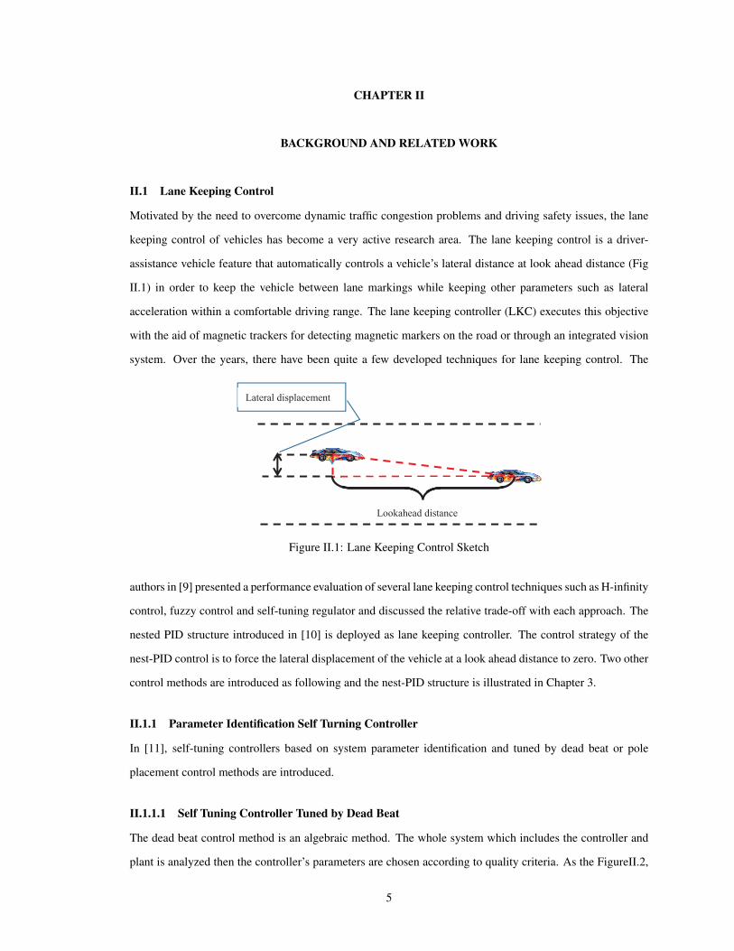
Motivated by the need to overcome dynamic traffic congestion problems and driving safety issues, the lane

keeping control of vehicles has become a very active research area. The lane keeping control is a driver-

assistance vehicle feature that automatically controls a vehicle’s lateral distance at look ahead distance (Fig

II.1) in order to keep the vehicle between lane markings while keeping other parameters such as lateral

acceleration within a comfortable driving range. The lane keeping controller (LKC) executes this objective

with the aid of magnetic trackers for detecting magnetic markers on the road or through an integrated vision

system. Over the years, there have been quite a few developed techniques for lane keeping control. The

Lateral displacement

Lookahead distance

Figure II.1: Lane Keeping Control Sketch

authors in [9] presented a performance evaluation of several lane keeping control techniques such as H-infinity

control, fuzzy control and self-tuning regulator and discussed the relative trade-off with each approach. The

nested PID structure introduced in [10] is deployed as lane keeping controller. The control strategy of the

nest-PID control is to force the lateral displacement of the vehicle at a look ahead distance to zero. Two other

control methods are introduced as following and the nest-PID structure is illustrated in Chapter 3.

II.1.1 Parameter Identification Self Turning Controller

In [11], self-tuning controllers based on system parameter identification and tuned by dead beat or pole

placement control methods are introduced.

II.1.1.1 Self Tuning Controller Tuned by Dead Beat

The dead beat control method is an algebraic method. The whole system which includes the controller and

plant is analyzed then the controller’s parameters are chosen according to quality criteria. As the FigureII.2,

5

+ +

+

+

Figure II.2: ARMAX Model [2]

the whole system is represented with several discrete transfer function blocks. The right part is the transfer

function for plant and error signal. And the left part is the function for controller which is composed by

functions for feedback signal and reference input signal. Several assumptions are made before the controller

design, they are: the plant can be represent as an ARMAX form and the plant has zero initial conditions.

From the ARMAX plant model, we have the equation:

A(z−1)y(k) = z−dB(z−1)u(k)+C(z−1)es(k) (II.1)

When es = v(k) = 0, and d = 0 from the controller a equation can be derived from the transfer function:

P(z−1)K(z−1)u(k) = R(z−1)w(k)−Q(z−1)y(k) (II.2)

Combine equation II.1 and II.2, the whole transfer function between input reference w(k) and plant output

y(k) is:

Gw(z) =Y (z)W (z)

=B(z−1)R(z−1)

A(z−1)K(z−1)P(z−1)+B(z−1)Q(z−1)(II.3)

From the transfer function, the tracking error can be derived as:

E(z−1) =W (z)−Y (z) = [1− B(z−1)R(z−1)

A(z−1)K(z−1)P(z−1)+B(z−1)Q(z−1)]W (z−1) (II.4)

In order to make sure small and zero order level tracking error in a finite number of control steps, the polyno-

mial of E(z−1) should be as simple as possible, such as not in the form of a fraction. If assume K(z−1) = 1,

then we have:

A(z−1)P(z−1)+B(z−1)Q(z−1) = 1

E(z−1) = [1−B(z−1)R(z−1)]W (z−1) (II.5)

6

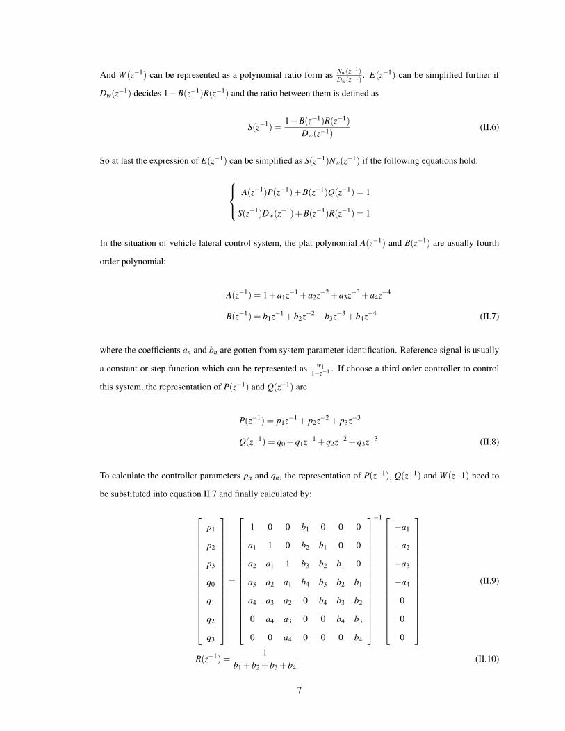
And W (z−1) can be represented as a polynomial ratio form as Nw(z−1)Dw(z−1)

. E(z−1) can be simplified further if

Dw(z−1) decides 1−B(z−1)R(z−1) and the ratio between them is defined as

S(z−1) =1−B(z−1)R(z−1)

Dw(z−1)(II.6)

So at last the expression of E(z−1) can be simplified as S(z−1)Nw(z−1) if the following equations hold:

A(z−1)P(z−1)+B(z−1)Q(z−1) = 1

S(z−1)Dw(z−1)+B(z−1)R(z−1) = 1

In the situation of vehicle lateral control system, the plat polynomial A(z−1) and B(z−1) are usually fourth

order polynomial:

A(z−1) = 1+a1z−1 +a2z−2 +a3z−3 +a4z−4

B(z−1) = b1z−1 +b2z−2 +b3z−3 +b4z−4 (II.7)

where the coefficients an and bn are gotten from system parameter identification. Reference signal is usually

a constant or step function which can be represented as w11−z−1 . If choose a third order controller to control

this system, the representation of P(z−1) and Q(z−1) are

P(z−1) = p1z−1 + p2z−2 + p3z−3

Q(z−1) = q0 +q1z−1 +q2z−2 +q3z−3 (II.8)

To calculate the controller parameters pn and qn, the representation of P(z−1), Q(z−1) and W (z−1) need to

be substituted into equation II.7 and finally calculated by:

p1

p2

p3

q0

q1

q2

q3

=

1 0 0 b1 0 0 0

a1 1 0 b2 b1 0 0

a2 a1 1 b3 b2 b1 0

a3 a2 a1 b4 b3 b2 b1

a4 a3 a2 0 b4 b3 b2

0 a4 a3 0 0 b4 b3

0 0 a4 0 0 0 b4

−1

−a1

−a2

−a3

−a4

0

0

0

(II.9)

R(z−1) =1

b1 +b2 +b3 +b4(II.10)

7

II.1.1.2 Self Tuning Controller Tuned by Pole Placement

The pole placement control tuning is another algebraic method. By set up suitable poles, the performance of

controller can be tuned for different plant model. The basic idea of pole placement tuning is introduced as

following.

A system with form shown by Figure II.2 is considered for the control design. Recall the equation II.4,

instead of setting the denominator as 1, it is set as a polynomial D(z−1) which is related to the desired poles:

A(z−1)P(z−1)+B(z−1)Q(z−1) = D(z−1) (II.11)

Substitute A(z−1)P(z−1) +B(z−1)Q(z−1) by D(z−1) in equation II.4 and still modify the reference signal

W (z) to the ratio form, the equation is changed to:

E(z−1) = [D(z−1)−B(z−1)R(z−1)

(A(z−1)K(z−1)P(z−1)+B(z−1)Q(z−1))]Nw(z−1)

Dw(z−1)(II.12)

In order to make the expression of E(z−1) simple, same as the dead-beat situation, it is still assumed Dw(z−1)

divides D(z−1)−B(z−1)R(z−1) and the ratio is S(z−1).

B(z−1)R(z−1)+Dw(z−1)S(z−1) = D(z−1) (II.13)

For a constant input, Dw(z−1) = 1− z−1. So to calculate the controller parameters, equation II.11 and II.13

show be solved together. For a four order vehicle plant, the finial equation for the controller parameter is:

q0

q1

q2

q3

q4

p1

p2

p3

=

b1 0 0 0 0 1 0 0

b2 b1 0 0 0 a1 −1 1 0

b3 b2 b1 0 0 a2 −a1 a1 −1 1

b4 b3 b2 b1 0 a3 −a−2 a2 −a1 a1 −1

0 b4 b3 b2 b1 a4 −a−3 a3 −a2 a2 −a1

0 0 b4 b3 b2 −a4 a4 −a−3 a3 −a2

0 0 0 b4 b3 0 −a4 a4 −a−3

0 0 0 0 b4 0 0 −a4

−1

d1 +1−a1

d2 +a1 −a2

d3 +a2 −a3

d4 +a3 −a4

d5 +a4

d6

d7

d8

(II.14)

Usually, D(z−1) is set with the poles of form s2 + 2ξ ωns+ω2n which we can define the dynamic by the

damping ratio (ξ ) and the natural frequency (ωn). After a group of ξ and ωn are defined, the continues poles

are calculated by s1,2 = −ξ ωn ±ωn√

ξ 2 −1. According to the relationship between poles of continuous

8

system and related discrete system zi = exp(siT0), the two poles of discrete system are:

z1 = eT0(−ξ ωn+ωn√

ξ 2−1), z2 = eT0(−ξ ωn−ωn√

ξ 2−1) (II.15)

Solve the parameters of D by D(z−1) = (z− z1)(z− z2) = 1+d1z−1 +d2z−2

d1 =−2exp(ξ ωnT0)cos(ωnT0√

1−ξ 2) ξ ≤ 1 (II.16)

d1 =−2exp(ξ ωnT0)cosh(ωnT0√

1+ξ 2) ξ > 1 (II.17)

d2 = exp(−2ξ ωnT0) (II.18)

II.1.2 Self Turning Regulator

An adaptive self-tuning regulator for lane keeping control is presented in [12]. The approach provides lane

keeping with robustness to unknown system parameters but the complexity of the approach makes it quite

challenging for an actual implementation on a digital platform.

In detail, before introduce the controller, several system coordinates transfer is introduced to make the

system controllable. From the system equation with uncertain systems:

x = f (x,u)+g(x,θ)u

y = h(x,θ)

where θ is the unknown parameter vector, u and y are the plant input and output respectively. It can be

transferred to the minimum phase and in observer canonical form:

ζ = Acζ +b(θ)µ +ψ(y,θ)

y =CcζAc =

0 1 0 ... 0

0 0 1 ... 0

... ... ... ... ...

0 0 0 ... 1

0 0 0 ... 0

,b =

0

...

bp

...

bn

,c =

[1 0 0 ... 0

]

Then a filter of following form is introduced:

ξ1

ξ2

...

˙xiρ−1

=

−λ1 1 0 ... 0

0 −λ2 1 ... 0

... ... ... ... ...

0 0 0 ... −λρ−1

ξ1

ξ2

...

ξρ−1

+

0

0

...

1

(II.19)

9

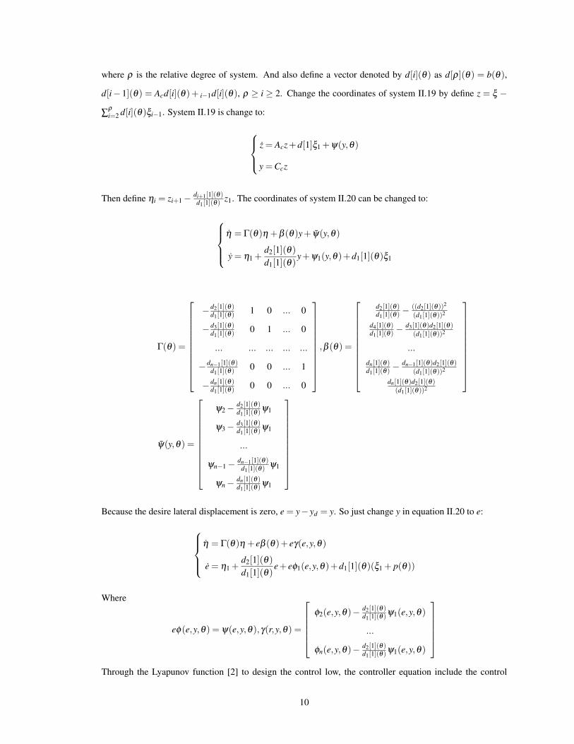
where ρ is the relative degree of system. And also define a vector denoted by d[i](θ) as d[ρ](θ) = b(θ),

d[i− 1](θ) = Acd[i](θ)+ i−1d[i](θ), ρ ≥ i ≥ 2. Change the coordinates of system II.19 by define z = ξ −

∑ρi=2 d[i](θ)ξi−1. System II.19 is change to:

z = Acz+d[1]ξ1 +ψ(y,θ)

y =Ccz

Then define ηi = zi+1 − di+1[1](θ)d1[1](θ)

z1. The coordinates of system II.20 can be changed to:

η = Γ(θ)η +β (θ)y+ ψ(y,θ)

y = η1 +d2[1](θ)d1[1](θ)

y+ψ1(y,θ)+d1[1](θ)ξ1

Γ(θ) =

− d2[1](θ)d1[1](θ)

1 0 ... 0

− d3[1](θ)d1[1](θ)

0 1 ... 0

... ... ... ... ...

− dn−1[1](θ)d1[1](θ)

0 0 ... 1

− dn[1](θ)d1[1](θ)

0 0 ... 0

,β (θ) =

d2[1](θ)d1[1](θ)

− ((d2[1](θ))2

(d1[1](θ))2

d4[1](θ)d1[1](θ)

− d3[1](θ)d2[1](θ)(d1[1](θ))2

...

dn[1](θ)d1[1](θ)

− dn−1[1](θ)d2[1](θ)(d1[1](θ))2

dn[1](θ)d2[1](θ)(d1[1](θ))2

ψ(y,θ) =

ψ2 − d2[1](θ)d1[1](θ)

ψ1

ψ3 − d3[1](θ)d1[1](θ)

ψ1

...

ψn−1 − dn−1[1](θ)d1[1](θ)

ψ1

ψn − dn[1](θ)d1[1](θ)

ψ1

Because the desire lateral displacement is zero, e = y− yd = y. So just change y in equation II.20 to e:

η = Γ(θ)η + eβ (θ)+ eγ(e,y,θ)

e = η1 +d2[1](θ)d1[1](θ)

e+ eϕ1(e,y,θ)+d1[1](θ)(ξ1 + p(θ))

Where

eϕ(e,y,θ) = ψ(e,y,θ),γ(r,y,θ) =

ϕ2(e,y,θ)− d2[1](θ)

d1[1](θ)ψ1(e,y,θ)

...

ϕn(e,y,θ)− d2[1](θ)d1[1](θ)

ψ1(e,y,θ)

Through the Lyapunov function [2] to design the control low, the controller equation include the control

10

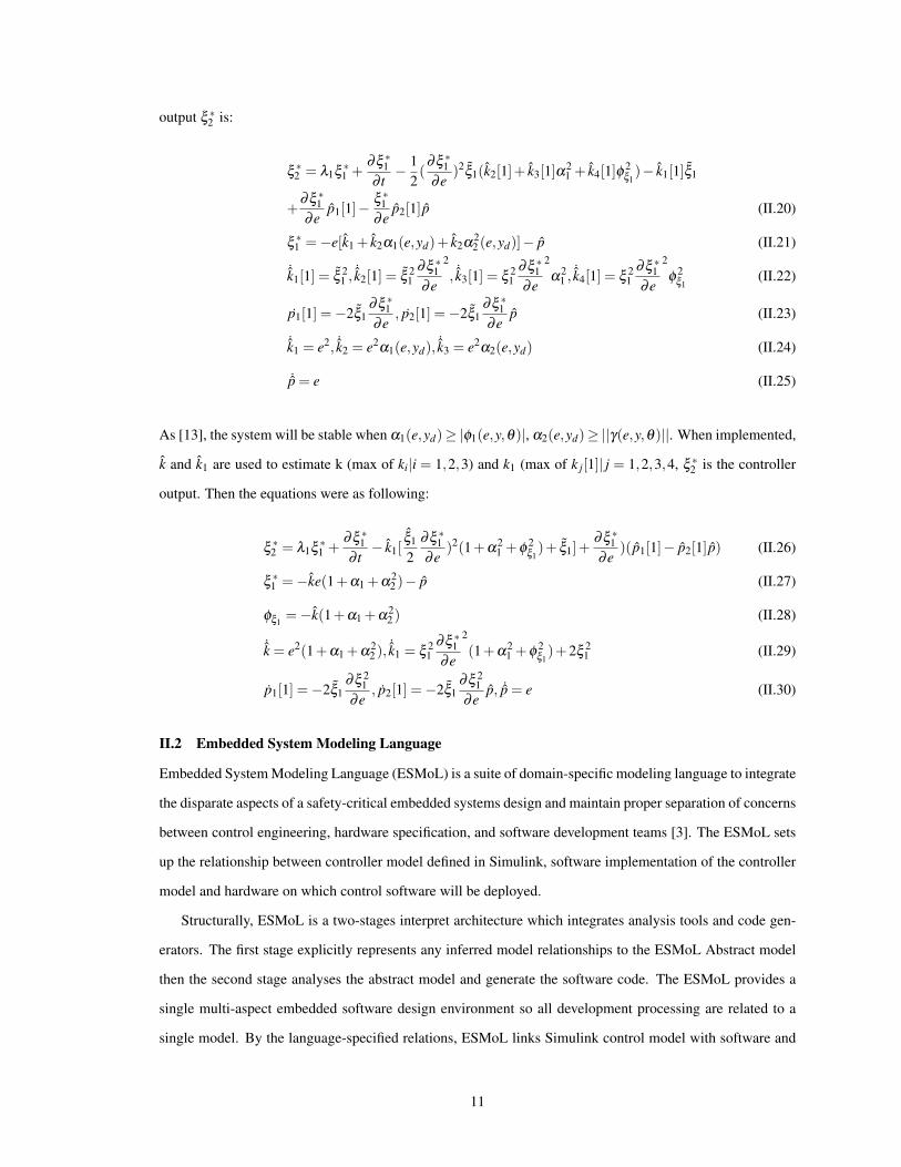
output ξ ∗2 is:

ξ ∗2 = λ1ξ ∗

1 +∂ξ ∗

1∂ t

− 12(

∂ξ ∗1

∂e)2ξ1(k2[1]+ k3[1]α2

1 + k4[1]ϕ 2ξ1)− k1[1]ξ1

+∂ξ ∗

1∂e

p1[1]−ξ ∗

1∂e

p2[1]p (II.20)

ξ ∗1 =−e[k1 + k2α1(e,yd)+ k2α2

2 (e,yd)]− p (II.21)

˙k1[1] = ξ 21 ,

˙k2[1] = ξ 21

∂ξ ∗1

∂e

2

, ˙k3[1] = ξ 21

∂ξ ∗1

∂e

2

α21 ,

˙k4[1] = ξ 21

∂ξ ∗1

∂e

2

ϕ 2ξ1

(II.22)

p1[1] =−2ξ1∂ξ ∗

1∂e

, p2[1] =−2ξ1∂ξ ∗

1∂e

p (II.23)

˙k1 = e2, ˙k2 = e2α1(e,yd),˙k3 = e2α2(e,yd) (II.24)

˙p = e (II.25)

As [13], the system will be stable when α1(e,yd)≥ |ϕ1(e,y,θ)|, α2(e,yd)≥ ||γ(e,y,θ)||. When implemented,

k and k1 are used to estimate k (max of ki|i = 1,2,3) and k1 (max of k j[1]| j = 1,2,3,4, ξ ∗2 is the controller

output. Then the equations were as following:

ξ ∗2 = λ1ξ ∗

1 +∂ξ ∗

1∂ t

− k1[ξ1

2∂ξ ∗

1∂e

)2(1+α21 +ϕ 2

ξ1)+ ξ1]+

∂ξ ∗1

∂e)(p1[1]− p2[1]p) (II.26)

ξ ∗1 =−ke(1+α1 +α2

2 )− p (II.27)

ϕξ1=−k(1+α1 +α2

2 ) (II.28)

˙k = e2(1+α1 +α22 ),

˙k1 = ξ 21

∂ξ ∗1

∂e

2

(1+α21 +ϕ 2

ξ1)+2ξ 2

1 (II.29)

p1[1] =−2ξ1∂ξ 2

1∂e

, p2[1] =−2ξ1∂ξ 2

1∂e

p, ˙p = e (II.30)

II.2 Embedded System Modeling Language

Embedded System Modeling Language (ESMoL) is a suite of domain-specific modeling language to integrate

the disparate aspects of a safety-critical embedded systems design and maintain proper separation of concerns

between control engineering, hardware specification, and software development teams [3]. The ESMoL sets

up the relationship between controller model defined in Simulink, software implementation of the controller

model and hardware on which control software will be deployed.

Structurally, ESMoL is a two-stages interpret architecture which integrates analysis tools and code gen-

erators. The first stage explicitly represents any inferred model relationships to the ESMoL Abstract model

then the second stage analyses the abstract model and generate the software code. The ESMoL provides a

single multi-aspect embedded software design environment so all development processing are related to a

single model. By the language-specified relations, ESMoL links Simulink control model with software and

11

hardware design concepts. Then in every ESMoL model, objects and parameters are included to describe

deployment of software components to hardware platforms. Moreover, ESMoL can shorten design cycles

because the analysis, simulation and deployment capabilities are integrated.

There are other tools have the similar partial functionality with ESMoL. For the code generation, Real-

Time Workshop in MATLAB Simulink, for example, is another automatic code generation tool. But it can

only transfer Simulink block to C function code and further development is desired to implement code on real

time platform. The TTPlan and similar toolbox developed by group from University of California, Berkeley

are known because of the time triggered scheduling functionality. For the platform specific simulation, there

are simulation tools such as Truetime, for network environment simulation, and System C. Compared with

the tools mentioned above, ESMoL is the first tool integrated all necessary capacities from model design to

real time software implementation.

Figure II.3 illustrates the ESMoL design flow which can be divided into 10 steps. A designed Simulink

controller model is imported automatically into the Generic Modeling Environment (GME) then changed to a

functional specification (Step 1). Software functions for controller model implementation are specified by the

imported model from Simulink (Step 2). Then, the hardware topology structure is defined as distributed ports

interconnected time triggered networks (Step 3). For Step 4, the deployment model is specified by generating

nodes for software components and communication ports for data message. By Step 5, timing model is set

by include timing parameter blocks to related software components and messages. Step 6 indicates a model

transformation from ESMoL model to the ESMoL Abstract model. All implied relationship are represented

by explicit relation objective in ESMoL. By Step 7, model interpreters transfer ESMoL Abstract model to

analysis specification then the scheduling problem is solved by the SchdeTool tool. For Step 8 and 9, another

interpreter transfers the analysis result from Step 7 back to ESMoL Abstract and ESMoL model. At last,

shown as Step 10, users can generate simulation code which can be deployed on desired platform.

12

Figure II.3: ESMOL Design Flow [3]

13

CHAPTER III

CONTROL DESIGN

In this Chapter, a lane keeping controller model is design in MATLAB/Simulink. A vehicle dynamic lin-

ear model is introduced first. Then nested PID controller structure as well as the controller parameter are

illustrated. The Simulink simulation results are presented at last.

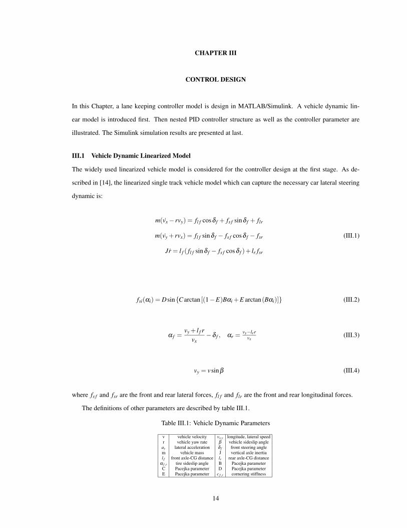
III.1 Vehicle Dynamic Linearized Model

The widely used linearized vehicle model is considered for the controller design at the first stage. As de-

scribed in [14], the linearized single track vehicle model which can capture the necessary car lateral steering

dynamic is:

m(vx − rvy) = fl f cosδ f + fs f sinδ f + flr

m(vy + rvx) = fl f sinδ f − fs f cosδ f − fsr (III.1)

Jr = l f ( fl f sinδ f − fs f cosδ f )+ lr fsr

fsi(αi) = Dsin{C arctan [(1−E)Bαi +E arctan(Bαi)]} (III.2)

α f =vy + l f r

vx−δ f , αr =

vy−lrrvx

(III.3)

vy = vsinβ (III.4)

where fs f and fsr are the front and rear lateral forces, fl f and flr are the front and rear longitudinal forces.

The definitions of other parameters are described by table III.1.

Table III.1: Vehicle Dynamic Parameters

v vehicle velocity vx,y longitude, lateral speedr vehicle yaw rate β vehicle sideslip angle

ay lateral acceleration δ f front steering anglem vehicle mass J vertical axle inertial f front axle-CG distance lr rear axle-CG distance

α f ,r tire sideslip angle B Pacejka parameterC Pacejka parameter D Pacejka parameterE Pacejka parameter c f ,r cornering stiffness

14

III.2 CCD Camera Model

In reality situation, the lateral displacement yl at a look head distance ls is measured by a CCD camera.

During the design process, the camera is modeled by the equation:

y = βv+ lsr+ vψ (III.5)

Where β , ρ , ψ , ls are the side slip angle, road curvature, yaw angle and look ahead distance respectively.

As showed by Figure III.1, the lateral displacement at ahead is calculated base on current displacement with

the effect of vehicle movement. The integration of βv+ vψ is the current displacement while the difference

between it with the displacement at head relates to the ls and the angle Ψerror. The Ψerror is an angle difference

between the vehicle yaw angle and the tangent direction of the curve. And it is calculated by r− vρ which

means the difference between the yaw rate the vehicle turn and yaw rate it is required to keep on the tangent

direction of the curve. To perform the lateral displacement calculation, an assumption is made that the curve

is a piece of straight line between the current displacement and yl measurement point. So it is required that

the radius of the curve should be much larger than the chosen look ahead distance value.

Current

Displacement

Assume to be a piece of straight line.

Tracking Path

Vehicle

Figure III.1: CCD model Sketch

The system III.2 is linearized by decoupling the longitudinal dynamics from lateral dynamics. The re-

duced linear system which contains the dynamic of system III.2 and CCD camera measurements (equation

III.5) is represented by the following linear vector system:

β

r

ψ

yl

=

a11 a12 0 0

a21 a22 0 0

0 1 0 0

v ls v 0

β

r

ψ

yl

+

b1

b2

0

0

δ f +

0

0

−v

−vls

ρ

15

The coefficients in equations are depend on v and uncertain physical parameters:

a11 =−c f + cr

mv, a12 =−1− c f l f −cr lr

mv2 ,

a21 =−c f l f − crlr

J, a22 =−

c f l2f +cr l2

rJv , (III.6)

b1 =c f

mv, b2 =

c f l fJ ,

where c f and cr are the front and rear tire cornering stiffness after the linear approximation of equation III.2.

The value of parameters are refereed from paper [10].

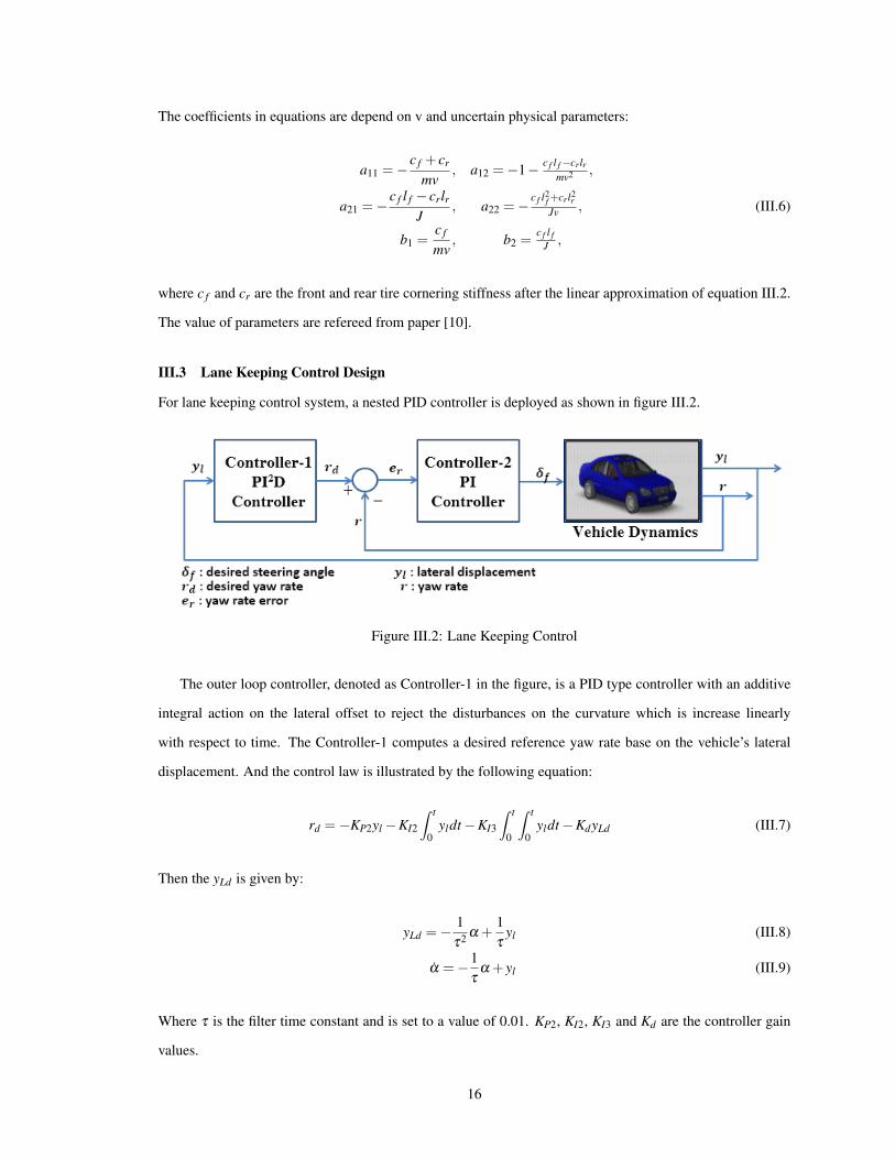
III.3 Lane Keeping Control Design

For lane keeping control system, a nested PID controller is deployed as shown in figure III.2.

Figure III.2: Lane Keeping Control

The outer loop controller, denoted as Controller-1 in the figure, is a PID type controller with an additive

integral action on the lateral offset to reject the disturbances on the curvature which is increase linearly

with respect to time. The Controller-1 computes a desired reference yaw rate base on the vehicle’s lateral

displacement. And the control law is illustrated by the following equation:

rd =−KP2yl −KI2

∫ t

0yldt −KI3

∫ t

0

∫ t

0yldt −KdyLd (III.7)

Then the yLd is given by:

yLd =− 1τ2 α +

1τ

yl (III.8)

α =−1τ

α + yl (III.9)

Where τ is the filter time constant and is set to a value of 0.01. KP2, KI2, KI3 and Kd are the controller gain

values.

16

The inner loop controller, denoted as Controller-2 in figure III.2, is a PI-type controller. It calculates the

steering angle value base on the error between the yaw rate and desired value output from Controller-1. The

control law is described as follows:

δ f =−KP1(r− rd)−KI1

∫ t

0(r− rd)dt (III.10)

On the aspect of parameters’ value, the values are first tuned with the vehicle linear model by the tuner

toolbox, then tuned to suit for the particular CarSim vehicle dynamic model. At last, the parameters are set

as shown:

KP1 = 12; KI1 = 10;

KP2 = 1.6; KI2 = 0.12; KI3 = 0.01;

Kd = 0.0005; τ = 0.01 (III.11)

III.4 Lane Keeping Control Simulation

Simulations of the lane keeping control is performed in the MATLAB Simulink to insure the correct of control

law.

The CarSim vehicle dynamic model is included as a represent of vehicle dynamic. CarSim is dynamic

simulation environment used to predict vehicle behavior. It provides an accurate, extensible, fast, stable and

cost effective solution for vehicle dynamic prediction [15]. With the extensibility, the CarSim model can

be included in MATLAB Simulink and simulated with the Simulink controller model. And it also supports

the real-time simulation with hardware in the loop using systems from most RT suppliers. A standard E-

class Sedan vehicle is used as the simulation car model. As presented by Figure III.3, there are a data type

conversion block and a rate transition block between the connection ports of CarSim model and controller

block. The reason of including the data type conversion is because the data type of controller and CarSim

model is not same. For the purpose of latter software implementation, all numeral data in the controller is

set to the fixed-point type (32 bits for word length and 16 bits for fraction length) while data type CarSim

model is floating number. On the other hand, the rate transfer block is include to perform up or down sample

between blocks for the sample rates of CarSim model and controller are 1ms and 10ms respectively. Inside

the controller block there are two subsystem for the CCD camera and the nested PID controller structure.

The simulation in two kinds of road environment is performed. The simulation results are illustrated and

discussed in the following section.

17

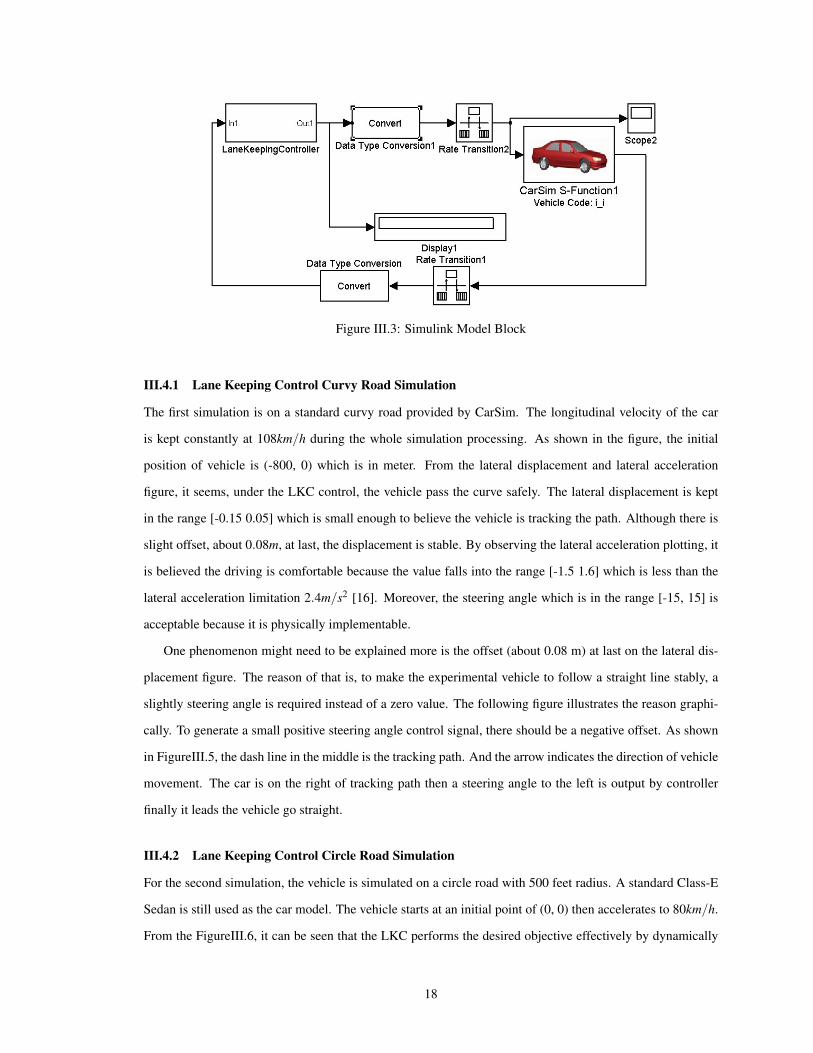
Figure III.3: Simulink Model Block

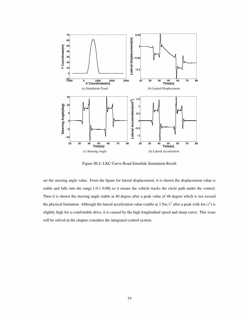
III.4.1 Lane Keeping Control Curvy Road Simulation

The first simulation is on a standard curvy road provided by CarSim. The longitudinal velocity of the car

is kept constantly at 108km/h during the whole simulation processing. As shown in the figure, the initial

position of vehicle is (-800, 0) which is in meter. From the lateral displacement and lateral acceleration

figure, it seems, under the LKC control, the vehicle pass the curve safely. The lateral displacement is kept

in the range [-0.15 0.05] which is small enough to believe the vehicle is tracking the path. Although there is

slight offset, about 0.08m, at last, the displacement is stable. By observing the lateral acceleration plotting, it

is believed the driving is comfortable because the value falls into the range [-1.5 1.6] which is less than the

lateral acceleration limitation 2.4m/s2 [16]. Moreover, the steering angle which is in the range [-15, 15] is

acceptable because it is physically implementable.

One phenomenon might need to be explained more is the offset (about 0.08 m) at last on the lateral dis-

placement figure. The reason of that is, to make the experimental vehicle to follow a straight line stably, a

slightly steering angle is required instead of a zero value. The following figure illustrates the reason graphi-

cally. To generate a small positive steering angle control signal, there should be a negative offset. As shown

in FigureIII.5, the dash line in the middle is the tracking path. And the arrow indicates the direction of vehicle

movement. The car is on the right of tracking path then a steering angle to the left is output by controller

finally it leads the vehicle go straight.

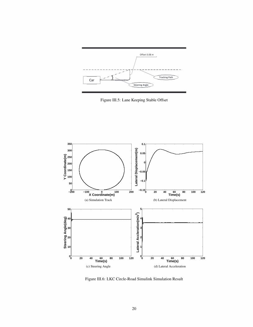
III.4.2 Lane Keeping Control Circle Road Simulation

For the second simulation, the vehicle is simulated on a circle road with 500 feet radius. A standard Class-E

Sedan is still used as the car model. The vehicle starts at an initial point of (0, 0) then accelerates to 80km/h.

From the FigureIII.6, it can be seen that the LKC performs the desired objective effectively by dynamically

18

−1000 0 1000 2000 3000−10

0

10

20

30

40

50

60

70

X Coordinate(m)

Y C

oord

inat

e(m

)

(a) Simulation Track

20 30 40 50 60 70 80

−0.1

−0.05

0

0.05

Time(s)

Late

ral D

ispl

acem

ent(

m)

(b) Lateral Displacement

20 30 40 50 60 70 80

−10

−5

0

5

10

15

Time(s)

Ste

erin

g A

ngle

(deg

)

(c) Steering Angle

20 30 40 50 60 70 80

−1

−0.5

0

0.5

1

1.5

Time(s)

Late

ral A

ccel

erat

ion(

m/s

2 )

(d) Lateral Acceleration

Figure III.4: LKC Curve-Road Simulink Simulation Result

set the steering angle value. From the figure for lateral displacement, it is shown the displacement value is

stable and falls into the range [-0.1 0.08] so it means the vehicle tracks the circle path under the control.

Then it is shown the steering angle stable at 40 degree after a peak value of 48 degree which is not exceed

the physical limitation. Although the lateral acceleration value (stable at 3.5m/s2 after a peak with 4m/s2) is

slightly high for a comfortable drive, it is caused by the high longitudinal speed and sharp curve. This issue

will be solved in the chapter considers the integrated control system.

19

Car

Offset 0.08 m

Tracking Path

Steering Angle

Figure III.5: Lane Keeping Stable Offset

−200 −100 0 100 2000

50

100

150

200

250

300

350

X Coordinate(m)

Y C

oord

inat

e(m

)

(a) Simulation Track

0 20 40 60 80 100 120−0.15

−0.1

−0.05

0

0.05

0.1

Time(s)

Late

ral D

ispl

acem

ent(

m)

(b) Lateral Displacement

0 20 40 60 80 100 1200

10

20

30

40

50

Time(s)

Ste

erin

g A

ng

le(d

eg)

(c) Steering Angle

0 20 40 60 80 100 1200

1

2

3

4

5

Time(s)

Lat

eral

Acc

lera

tio

n(m

/s2 )

(d) Lateral Acceleration

Figure III.6: LKC Circle-Road Simulink Simulation Result

20

CHAPTER IV

LANE KEEPING CONTROL SOFTWARE IMPLEMENTATION AND SIMULATION

In this chapter, the software implementation of the lane keeping control system is introduced. A hardware in

the loop simulation is performed then the result is discussed and compared with the Simulink result to show

the control effect introduced by the real time platform.

IV.1 Lane Keeping Control Software Implementation

In this section, the lane keeping controller software system is built following the ESMoL design flow which

is introduced in Chapter 2.

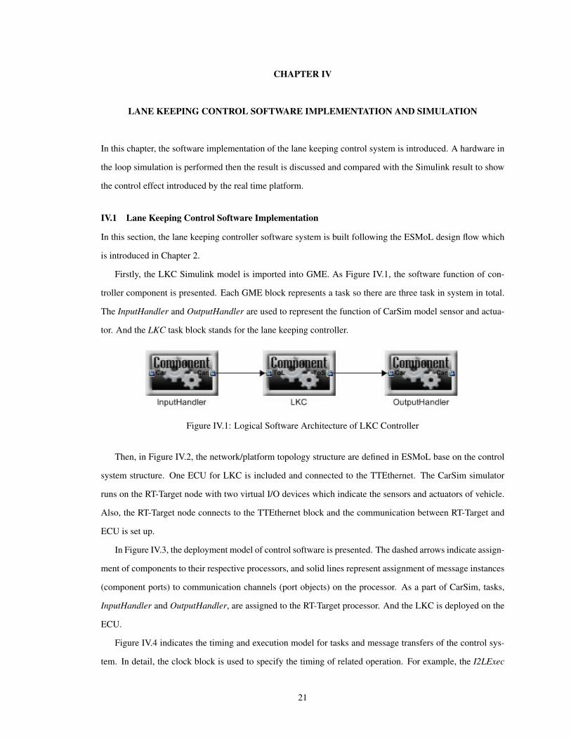
Firstly, the LKC Simulink model is imported into GME. As Figure IV.1, the software function of con-

troller component is presented. Each GME block represents a task so there are three task in system in total.

The InputHandler and OutputHandler are used to represent the function of CarSim model sensor and actua-

tor. And the LKC task block stands for the lane keeping controller.

Figure IV.1: Logical Software Architecture of LKC Controller

Then, in Figure IV.2, the network/platform topology structure are defined in ESMoL base on the control

system structure. One ECU for LKC is included and connected to the TTEthernet. The CarSim simulator

runs on the RT-Target node with two virtual I/O devices which indicate the sensors and actuators of vehicle.

Also, the RT-Target node connects to the TTEthernet block and the communication between RT-Target and

ECU is set up.

In Figure IV.3, the deployment model of control software is presented. The dashed arrows indicate assign-

ment of components to their respective processors, and solid lines represent assignment of message instances

(component ports) to communication channels (port objects) on the processor. As a part of CarSim, tasks,

InputHandler and OutputHandler, are assigned to the RT-Target processor. And the LKC is deployed on the

ECU.

Figure IV.4 indicates the timing and execution model for tasks and message transfers of the control sys-

tem. In detail, the clock block is used to specify the timing of related operation. For example, the I2LExec

21

Figure IV.2: LKC Controller Network Structure

Figure IV.3: LKC Controller Platform Deployment

block specifies the timing for message transfer from the InputHandler to the LKC. By setting the execution

period, desired offset and the worst case duration for every communication and the scheduler with TTEther-

net driver to take advantage of the synchronized time base all tasks can be executed according to the time-

triggered paradigm. As other example, the LKCExec block defines the execution period of LKC which is

10ms.

Figure IV.4: Timing/Execution Model of Lane Keeping Controller.

For the task scheduling, a heuristic algorithm base on the bottom-level of system task graph is used. The

22

longest path from any task to the end in the graph is represented as the bottom-level. Follow the technol-

ogy describe in [17], the message order is determined while the allocation of the tasks to the processors is

pre-defined. The algorithm orders the tasks as the bottom-level of its corresponding task graph vertex (in

descending order). By this method, all dependencies between tasks are insure before the task scheduling. For

the LKC control system, the critical path is InputHandler 7→ LKC 7→ OutputHandler.

After network/task scheduling, the schedule information is updated into the ESMoL and ESMoL Abstract

models automatically. The interpreter uses the updated ESMoL Abstract model to assemble all the codes for

compilation. Using the network scheduling result, a tool named as T T EBuild from TTTech generates the

binary configuration files for TTEthernet switch and C code configuration files for ECUs. C code files,

generated by Real Time Workshop, and T T EBuild with glue code files are assembled by ESMoL Stage 2

interpreter then makefiles are generated automatically. In in order to take advantage of the synchronized

time base of TTEthernet, all tasks are executed in RT-Linux kernel space. The compiled kernel modules are

deployed on ECUs.

IV.2 Hardware In the loop Simulation

The hardware in the loop simulation is a widely used technique during the real-time system development

and verification. By substituting the actually plant by dynamic mathematical representation, the embedded

software plant can be tested effectively. The electrical emulation of sensors and actuators are included in the

plant mathematical representation. The embedded system reads the value from each electrically emulated

sensor, then calculates the control output by the programmed control law code and implements the control

through the electrically emulated actuators. So a feedback loop is formed between the embedded software and

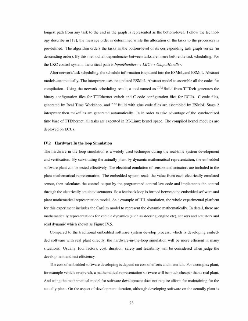
plant mathematical representation model. As a example of HIL simulation, the whole experimental platform

for this experiment includes the CarSim model to represent the dynamic mathematically. In detail, there are

mathematically representations for vehicle dynamics (such as steering, engine etc), sensors and actuators and

road dynamic which shown as Figure IV.5.

Compared to the traditional embedded software system develop process, which is developing embed-

ded software with real plant directly, the hardware-in-the-loop simulation will be more efficient in many

situations. Usually, four factors, cost, duration, safety and feasibility will be considered when judge the

development and test efficiency.

The cost of embedded software developing is depend on cost of efforts and materials. For a complex plant,

for example vehicle or aircraft, a mathematical representation software will be much cheaper than a real plant.

And using the mathematical model for software development does not require efforts for maintaining for the

actually plant. On the aspect of development duration, although developing software on the actually plant is

23

Embedded Software

Emulated Actuator

Emulated Sensor

Car Dynamic

Road Dynamic

CarSim model (plant mathematical representation)

Figure IV.5: HIL General Diagram

a more direct approach, but the problem caused by the plant might make the design lasts longer. Take the car

embedded software as an example, the designer cannot absolutely insure all components on the actual vehicle

perform the correctly mechanical function so a unknown component mis-function will caused problem which

cost long time to locate and fix. Considering the safety factor, a mathematically model is preferred than an

actually plant under some circumstances. A good example is an experiment to test the operation range of

plant during which a really plant might crash, be destroyed and then lead catastrophic consequence [18]. For

the feasibility, it is normal to explore the platform under situations which is not easy to achieve with real

plant. For example, to explore critical timings which means user actions are given with a short time interval.

IV.3 Hardware in the Loop Simulation Platform

A system structure for the TTEthernet-based hardware in the loop simulator is described by Figure IV.6. The

whole platform are divided into two layers: physical layer and platform layer.

The physical layer modeling the physical dynamic of the CPS system includes two components. The

design/visualization PC is used to compute CarSim vehicle dynamic during HIL simulation and the initial

control design and verification. On the other hand, the Target PC is a NI LabView Real-Time Target run-

ning NIs Real-Time Module which provides a complete solution for creating reliable, stand-alone real-time

systems [20]. During experiments, the vehicle dynamics modeled by CarSim is run on the Target PC. More-

over, the Target PC is integrated with a TTTech PCIe-XMC card which enables the seamless integration and

communication with ECUs on the Time-Triggered network supported by the TTEthernet switch [19].

The platform layer is composed by the TTEthernet switch and ECU. The TTEthernet Development Switch

has 8 ports with 100Mbps bandwidth. It supports 100 Base-TX Ethernet and also enables hard real-time

communication based on the TTEthernet protocol. The switch set up the communication between the ECU

and XMC card of Target PC and operates on the configuration defined by users.

24

Figure IV.6: LKC HIL Simulation Platform

The ECU is an IBX-530W-ATOM box with Intel Atom CPU and operated by Real-Time Linus system.

To enable the communication with other components in the TTEthernet network, each ECU is equipped a

TTEthernet Linux driver with related protocol. The controller software C code, generated from the design

process in ESMoL, is deployed and run on the ECU. Each software system component is executed in the

kernel space of running RT-Linux and follows the TTEthernet synchronized time.

IV.4 Lane Keeping Control HIL Simulation

A HIL simulation of the lane keeping controller is performed on the platform described before. A CarSim

curvy road is used as the road environment and Class-E Sedan vehicle model is chosen as the vehicle dynamic

model. The vehicle start at the position (-800, 0) then accelerate to 108km/h and always tracks the path. The

simulation result is shown by Figure IV.7. Two groups of data are illustrated on the figure. The solid black

line indicates the HIL simulation result. For comparison, the Simulink simulation result on the same curvy

road (Figure III.4) is referred and plotted by the dot red line.

By observing the plotting in black, it seems the embedded controller (control system on the ECU) can

still perform the acceptable control to achieve the lane keeping objective. It is shown the lateral displacement

value is stable and falls into the range [-0.12 0.08]. Also the steering angle value is between -15 deg and 15 deg

which is physical implementable and lateral acceleration value is smaller than the limitation of comfortable

driving. But by comparing the red line and black line, some conclusions can be made. Although the steering

angle and lateral acceleration values are almost same during the whole simulation, there is an observable

25

−1000 0 1000 2000 3000−10

0

10

20

30

40

50

60

70

X Coordinate(m)

Y C

oord

inat

e(m

)

(a) Simulation Track

20 30 40 50 60 70 80

-0.1

-0.05

0

0.05

Time(s)

Late

ral

Dis

pla

cem

en

t(m

)

(b) Lateral Displacement. Solid Line:Platform Resuilt.Dot Line: Simulink Result

20 30 40 50 60 70 80

-10

-5

0

5

10

15

Time(s)

Ste

eri

ng

An

gle

(deg

)

(c) Steering Angle. Solid Line:Platform Resuilt. DotLine: Simulink Result

20 30 40 50 60 70 80

-1

-0.5

0

0.5

1

1.5

Time(s)

Late

ral

Accele

rati

on

(m/s

2)

(d) Lateral Acceleration. Solid Line:Platform Resuilt.Dot Line: Simulink Result

Figure IV.7: Lane Keeping Control HIL Simulation Result

difference between the lateral displacement plotting of two experiments. Generally, the whole displacement

figure of platform (solid black line) is almost in the same shape with the Simulink figure (dot red line)

expect a positive offset. But in detail, comparing two figures at the time 27s, the platform figure keep same

while Simulink figure begins to decrease. Then this difference integrals and it causes the offset at last. This

phenomenon reveals the fact that the platform vehicle model reacts to the control slower than the Simulink

model. By reviewing the platform structure, it can be found that control delay and synchronous issues are

inevitable due to the switch network connection set up between controller and car model. From this result,

a conclusion can be made. It is that, addition to the traditional criteria such as stability, controllability and

robust ability to noise or vary input, the time delay robust of controllers will be an important factor for CPS

controller.

26

CHAPTER V

CPS CONTROL MODEL INTEGRATION

In this chapter, we present the integration of two control models on CPS system. The two controllers are the

lane keeping controller described in prior chapters and an adaptive cruise controller illustrated in [7]. Before

the introduction of controls integration issue, a briefly review of adaptive cruise controller is given. Then

controller integration theory is explored beginning with the controller conflict under the particular situation

and finishing at experimental result discussion and comparison. Hardware in the loop simulation is also

performed to discover the control effect introduce by the experimental platform.

V.1 Adaptive Cruise Controller

The adaptive cruise control (ACC) system is an active safety and driver-assistance vehicle feature that au-

tomatically controls a vehicle longitudinal velocity in a dynamic traffic environment. It controls the ACC-

equipped vehicle to maintain a certain distance, which is defined by desired time gap and current velocity,

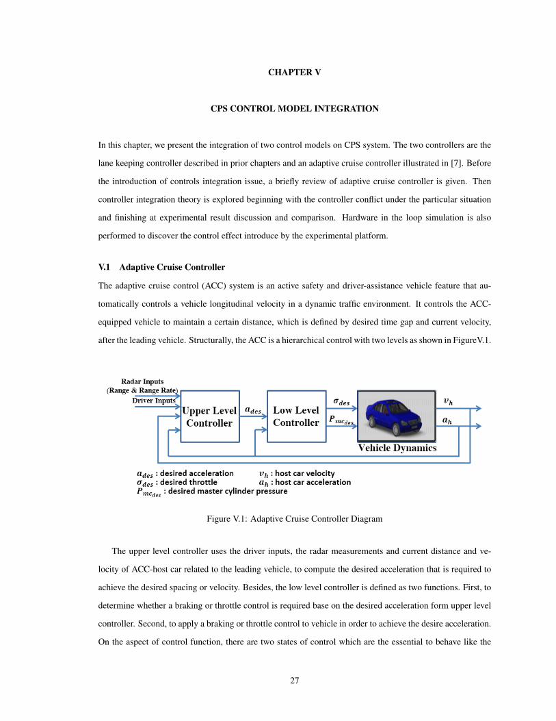
after the leading vehicle. Structurally, the ACC is a hierarchical control with two levels as shown in FigureV.1.

Figure V.1: Adaptive Cruise Controller Diagram

The upper level controller uses the driver inputs, the radar measurements and current distance and ve-

locity of ACC-host car related to the leading vehicle, to compute the desired acceleration that is required to

achieve the desired spacing or velocity. Besides, the low level controller is defined as two functions. First, to

determine whether a braking or throttle control is required base on the desired acceleration form upper level

controller. Second, to apply a braking or throttle control to vehicle in order to achieve the desire acceleration.

On the aspect of control function, there are two states of control which are the essential to behave like the

27

conventional cruise control system. The first one is when the leading car is detected by the radar, the ACC

control the velocity to maintain a pre-defined time gap between two cars. The second one is when the leading

car is absent, the ACC system control the velocity to maintain a driver set value. To explain the function more

clearly, an experiment scenario of past work is shown by FigureV.2 to explain the speed control of ACC.

0 20 40 60 80 100 1200

10

20

30

40

50

60

70

80

90

100

110

Time (s)

Vel

oci

ty (

Km

/h)

Host Velocity (Platform)Host Velocity (Simulink)Lead Velocity

(a) Vehicle Velocity

0 20 40 60 80 100 1200

10

20

30

40

50

60

70

80

90

100

110

Time (s)

Dis

tan

ce (

m)

Actual Distance (Platform)Actual Distance (Simulink)Desired Distance

(b) Distance

Figure V.2: Adaptive Cruise Control Simulation Result

In this experiment, two cars are set on a straight and flat road with an initial distance of 65 meters.

The initial speed values of the leading and following vehicle (ACC host vehicle) are 60 km/h and 65 km/h

respectively. The driver set cruise speed value is 80 km/h. At the beginning of the experiment, the following

car does not detect the leading car so it accelerates to the driver set velocity value (80 km/h). The controller

is in stage two mentioned above. Then, the leading car is detected and the following car breaks to reach the

same speed with the leading car in order to maintain the time gap. That is the stage one as described before.

After that, from about 40 second, the lead car began to accelerate so following car speeds up also until its

speed reach the driver set value again. At last, the leading car begin to break and following car then keep up

with the leading car.

V.2 Lane Keeping and Cruise Control Integration

In this section, we consider the integration of the lane keeping controller design in Chapter III and previously

described adaptive cruise controller. Before the integrated system design, the interaction and confliction

between integrated control components should be considered first. Although the two controllers modify

the behavior of two seemingly different dynamics of the vehicle, with the ACC controlling the longitudinal

dynamics while the LKC controls the lateral dynamics, there exists physical interactions between lateral and

longitudinal dynamics of the vehicle. Not only that, changes in the physical environment such as geometry of

28

vehicle path or road curvature highlights certain conflicts in the operation of the two distinctive controllers.

For example, the ACC on detecting a leading vehicle dynamically adjusts the speed of the ACC-equipped

vehicle to the lead vehicle’s speed. On a curved road, the ACC in an effort to track the leading vehicle, can

attain a vehicle speed that might be too fast, such that it can potentially obstruct the LKC’s ability to maintain

the desired lateral distance resulting in a conflict. This type of conflict can potentially result in undesired

and unintended behavior of the overall system. In order to address, these types of conflicts, we integrate a

supervisory controller whose main objective is to restrict the regions of operation of the integrated system in

a safe desirable manner.

Supervisor

Controller

ACC

Road Dynamic

On a curve?

User Set Speed

Figure V.3: Supervisor Controller

As the FigureV.3, the supervisory controller operates by dynamically determining the desired longitudinal

set speed of the ACC base on the perception of the current road geometry, specifically the road curvature. The

idea is that by restricting the allowable speed for the ACC base on the road curvature, the LKC can equally be

able to achieve its desired objective of maintaining a desired lateral distance. Hence, on a relatively straight

road, the ACC operates in its normal mode with the user set-speed and radar inputs but on a curvy road,

the supervisory controller modifies the user-set speed to a desired speed as the radius of curvature. The

underlying relationship between desired speed and road curvature is described by equation:

vx =√

ayMax ∗ρ (V.1)

Where vx, ayMax and ρ are the driver set velocity, maximum lateral acceleration and radius of the curvature

respectively.

Several groups of experiment simulation result are provided in the following part. Firstly, there are

experiments in Simulink. The effect of supervisor controller is discussed by comparing the results and it is

proved the including of supervisor controller is necessary to improve system performance. After that, the

second group of experiment involves the model-based software development of the integrated system with

the three controllers based on the controller software implementation and the deployment on the experimental

29

platform for a hardware-in-the-loop simulation.

V.2.1 Simulink Simulation

The simulation for the integrated control system in Simulink (Figure V.4) is performed first. Two CarSim

models are included to represent the leading and following vehicles. For controllers, all components for one

controller are included in the same Simulink block for code generation in the latter section.

Figure V.4: Integrated Control Simulink Model

V.2.1.1 Straight-Curve Track Without Supervisor Controller

For this simulation, the ACC and LKC are just combined together without the coordination of supervisor

controller. The selected test track is a dynamic path with a combination of straight paths and curved roads

with radii of 160m, 200m and 160m for the three curves as seen in FigureV.5. The desired time gap of the

ACC is set to 1.5s. The leading vehicle starts at an initial position of (0, 0) with an initial speed of 30 km/h

while the host vehicle, equipped with the integrated control system, starts at an initial position of (-800, 0)

with an initial speed of 80 km/h.

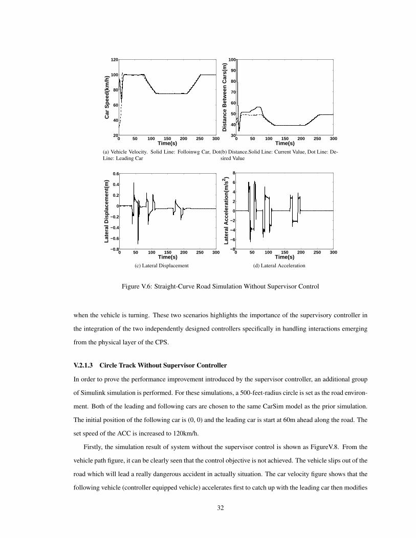
From FigureV.6, it can be seen that the ACC performs its desired objectives effectively by dynamically

tracking the leading vehicle’s speed as shown in FigureV.6a. While at same time maintaining a safe vehicle

distance as shown in FigureV.6b. On the other hand, the performance of the LKC is deteriorated due to the

resulting conflicts and interactions with the ACC. The lateral displacement, as shown in FigureV.6c, deviates

from the desired lane of the vehicle with a peak value of about -0.7 m. This amount of deviation can result

in potentially catastrophic consequence such as a collision with vehicle in other lane. Although, the curves

in the paths are very aggressive, the lateral acceleration exceeds 4m/s2 for the most part in the curved roads

which will lead the passenger feels uncomfortable. So it is necessary to improve the performance of lane

30

−2000 0 2000 4000 6000 8000−150

−100

−50

0

50

100

150

X Coordinate(m)

Y C

oord

inat

e(m

)

Figure V.5: Straight-Curve Combined Track

keeping control when cooperates with the adaptive cruise controller.

V.2.1.2 Straight-Curve Track With Supervisor Controller

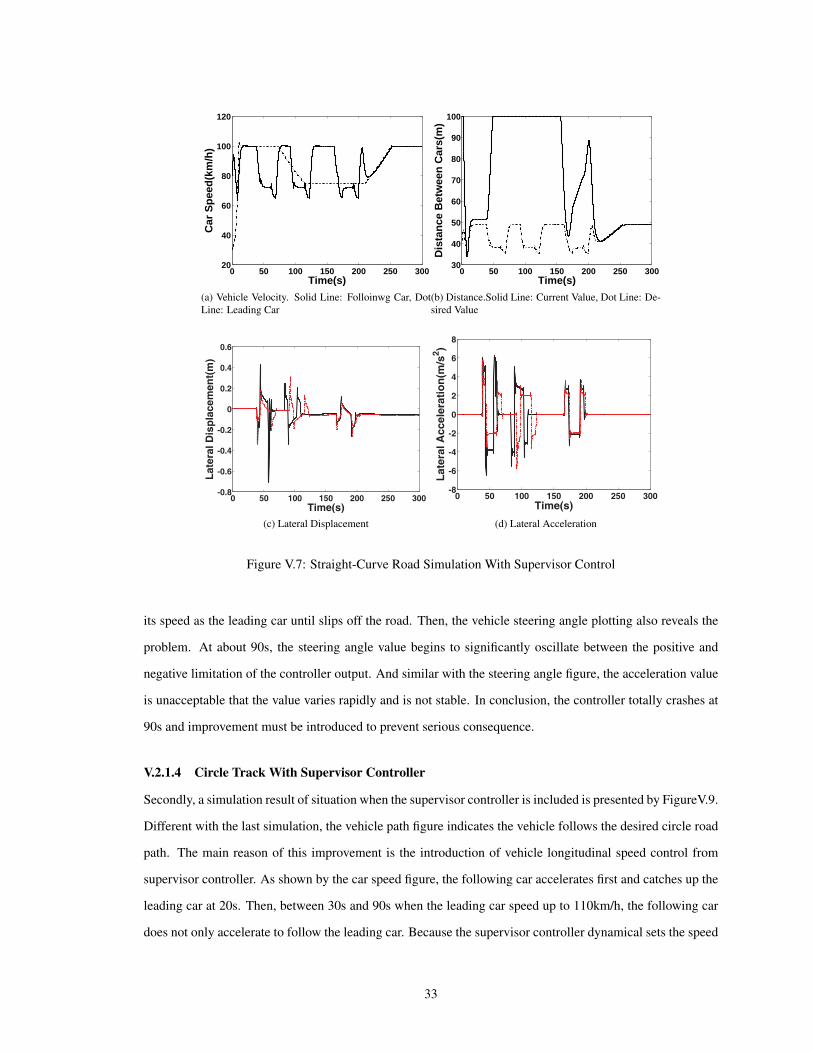
For this simulation, the ACC and LKC are integrated together with the coordination of supervisor controller.

The simulation result of the second experiment is shown by FigureV.7. Moreover, the lateral displacement and

lateral acceleration of first experiment are also plotted by the dot red line in order to compare. In the second

experiment, a supervisor controller is included to suit the longitudinal speed through the adaptive controller

base on the perceived road geometry/curvature. The specified controller, system parameters, chosen CarSim

vehicle model and road model are the same as in the previous scenario.

From FigureV.7a and b, it can be observed that the longitudinal speed of the following car is modified base

on the consideration on the road curve and the distance between two vehicles. For example at the time 30s,

85s and 160s, the following car breaks down because of the curve regardless that the distance it falls behind

the leading car is already larger than the desire value. After finish the turn, supervisor controller accelerates

the following vehicle to catch up the leading car. That is the situation occurs at 70s, 120s and 200s. From 40s

to 150s, the distance figure keep constantly at 100m which means the leading car is too far way to detect by

the radar. Figure V.7c and d compares the lateral performance of the system with and without a supervisory

controller. It can be seen in Figure V.7c that the lateral displacement for the case with a supervisory controller

is limited to a peak value about -0.34m as compared to -0.7m in the case without a supervisory controller.

Likewise, the lateral acceleration is also reduced in the aggressive curves as compared to the case without

the supervisory controller. As shown in the figure, the acceleration value decrease to 2m/s2 for most time

31

0 50 100 150 200 250 30020

40

60

80

100

120

Time(s)

Car

Sp

eed

(km

/h)

(a) Vehicle Velocity. Solid Line: Folloinwg Car, DotLine: Leading Car

0 50 100 150 200 250 30030

40

50

60

70

80

90

100

Time(s)

Dis

tan

ce B

etw

een

Car

s(m

)

(b) Distance.Solid Line: Current Value, Dot Line: De-sired Value

0 50 100 150 200 250 300−0.8

−0.6

−0.4

−0.2

0

0.2

0.4

0.6

Time(s)

Late

ral D

ispl

acem

ent(

m)

(c) Lateral Displacement

0 50 100 150 200 250 300−8

−6

−4

−2

0

2

4

6

8

Time(s)

Late

ral A

ccel

erat

ion(

m/s

2 )

(d) Lateral Acceleration

Figure V.6: Straight-Curve Road Simulation Without Supervisor Control

when the vehicle is turning. These two scenarios highlights the importance of the supervisory controller in

the integration of the two independently designed controllers specifically in handling interactions emerging

from the physical layer of the CPS.

V.2.1.3 Circle Track Without Supervisor Controller

In order to prove the performance improvement introduced by the supervisor controller, an additional group

of Simulink simulation is performed. For these simulations, a 500-feet-radius circle is set as the road environ-

ment. Both of the leading and following cars are chosen to the same CarSim model as the prior simulation.

The initial position of the following car is (0, 0) and the leading car is start at 60m ahead along the road. The

set speed of the ACC is increased to 120km/h.

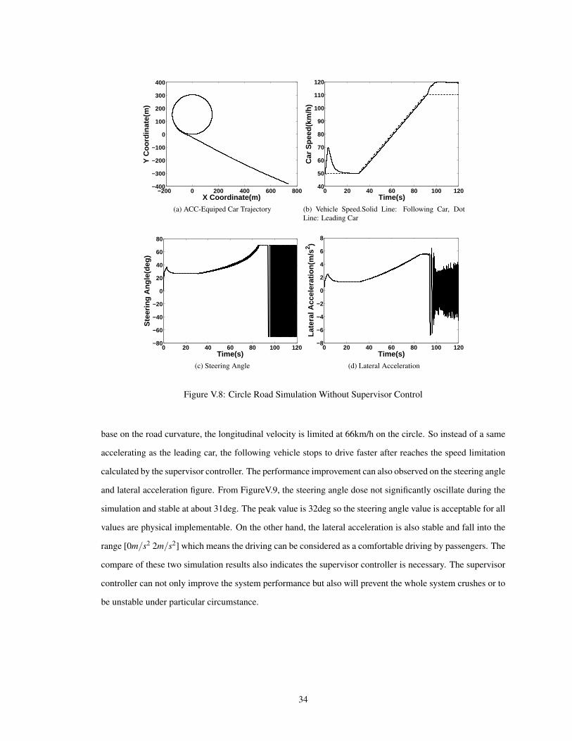
Firstly, the simulation result of system without the supervisor control is shown as FigureV.8. From the

vehicle path figure, it can be clearly seen that the control objective is not achieved. The vehicle slips out of the

road which will lead a really dangerous accident in actually situation. The car velocity figure shows that the

following vehicle (controller equipped vehicle) accelerates first to catch up with the leading car then modifies

32

0 50 100 150 200 250 30020

40

60

80

100

120

Time(s)

Car

Sp

eed

(km

/h)

(a) Vehicle Velocity. Solid Line: Folloinwg Car, DotLine: Leading Car

0 50 100 150 200 250 30030

40

50

60

70

80

90

100

Time(s)

Dis

tan

ce B

etw

een

Car

s(m

)

(b) Distance.Solid Line: Current Value, Dot Line: De-sired Value

0 50 100 150 200 250 300-0.8

-0.6

-0.4

-0.2

0

0.2

0.4

0.6

Time(s)

Late

ral

Dis

pla

cem

en

t(m

)

(c) Lateral Displacement

0 50 100 150 200 250 300-8

-6

-4

-2

0

2

4

6

8

Time(s)

Late

ral

Accele

rati

on

(m/s

2)

(d) Lateral Acceleration

Figure V.7: Straight-Curve Road Simulation With Supervisor Control

its speed as the leading car until slips off the road. Then, the vehicle steering angle plotting also reveals the

problem. At about 90s, the steering angle value begins to significantly oscillate between the positive and

negative limitation of the controller output. And similar with the steering angle figure, the acceleration value

is unacceptable that the value varies rapidly and is not stable. In conclusion, the controller totally crashes at

90s and improvement must be introduced to prevent serious consequence.

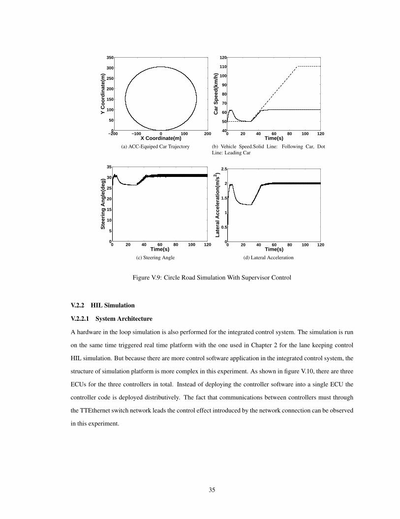
V.2.1.4 Circle Track With Supervisor Controller

Secondly, a simulation result of situation when the supervisor controller is included is presented by FigureV.9.

Different with the last simulation, the vehicle path figure indicates the vehicle follows the desired circle road

path. The main reason of this improvement is the introduction of vehicle longitudinal speed control from

supervisor controller. As shown by the car speed figure, the following car accelerates first and catches up the

leading car at 20s. Then, between 30s and 90s when the leading car speed up to 110km/h, the following car

does not only accelerate to follow the leading car. Because the supervisor controller dynamical sets the speed

33

−200 0 200 400 600 800−400

−300

−200

−100

0

100

200

300

400

X Coordinate(m)

Y C

oord

inat

e(m

)

(a) ACC-Equiped Car Trajectory

0 20 40 60 80 100 12040

50

60

70

80

90

100

110

120

Time(s)

Car

Sp

eed

(km

/h)

(b) Vehicle Speed.Solid Line: Following Car, DotLine: Leading Car

0 20 40 60 80 100 120−80

−60

−40

−20

0

20

40

60

80

Time(s)

Ste

erin

g A

ngle

(deg

)

(c) Steering Angle

0 20 40 60 80 100 120−8

−6

−4

−2

0

2

4

6

8

Time(s)

Late

ral A

ccel

erat

ion(

m/s

2 )

(d) Lateral Acceleration

Figure V.8: Circle Road Simulation Without Supervisor Control

base on the road curvature, the longitudinal velocity is limited at 66km/h on the circle. So instead of a same

accelerating as the leading car, the following vehicle stops to drive faster after reaches the speed limitation

calculated by the supervisor controller. The performance improvement can also observed on the steering angle

and lateral acceleration figure. From FigureV.9, the steering angle dose not significantly oscillate during the

simulation and stable at about 31deg. The peak value is 32deg so the steering angle value is acceptable for all

values are physical implementable. On the other hand, the lateral acceleration is also stable and fall into the

range [0m/s2 2m/s2] which means the driving can be considered as a comfortable driving by passengers. The

compare of these two simulation results also indicates the supervisor controller is necessary. The supervisor

controller can not only improve the system performance but also will prevent the whole system crushes or to

be unstable under particular circumstance.

34

−200 −100 0 100 2000

50

100

150

200

250

300

350

X Coordinate(m)

Y C

oord

inat

e(m

)

(a) ACC-Equiped Car Trajectory

0 20 40 60 80 100 12040

50

60

70

80

90

100

110

120

Time(s)

Car

Sp

eed

(km

/h)

(b) Vehicle Speed.Solid Line: Following Car, DotLine: Leading Car

0 20 40 60 80 100 1200

5

10

15

20

25

30

35

Time(s)

Ste

erin

g A

ng

le(d

eg)

(c) Steering Angle

0 20 40 60 80 100 1200

0.5

1

1.5

2

2.5

Time(s)

Lat

eral

Acc

eler

atio

n(m

/s2 )

(d) Lateral Acceleration

Figure V.9: Circle Road Simulation With Supervisor Control

V.2.2 HIL Simulation

V.2.2.1 System Architecture

A hardware in the loop simulation is also performed for the integrated control system. The simulation is run

on the same time triggered real time platform with the one used in Chapter 2 for the lane keeping control

HIL simulation. But because there are more control software application in the integrated control system, the

structure of simulation platform is more complex in this experiment. As shown in figure V.10, there are three

ECUs for the three controllers in total. Instead of deploying the controller software into a single ECU the

controller code is deployed distributively. The fact that communications between controllers must through

the TTEthernet switch network leads the control effect introduced by the network connection can be observed

in this experiment.

35

Design/Visualization PC

TTEthernet

Development Switch

(8 x 100Mbps)

Figure V.10: Integrated Control Platform Structure

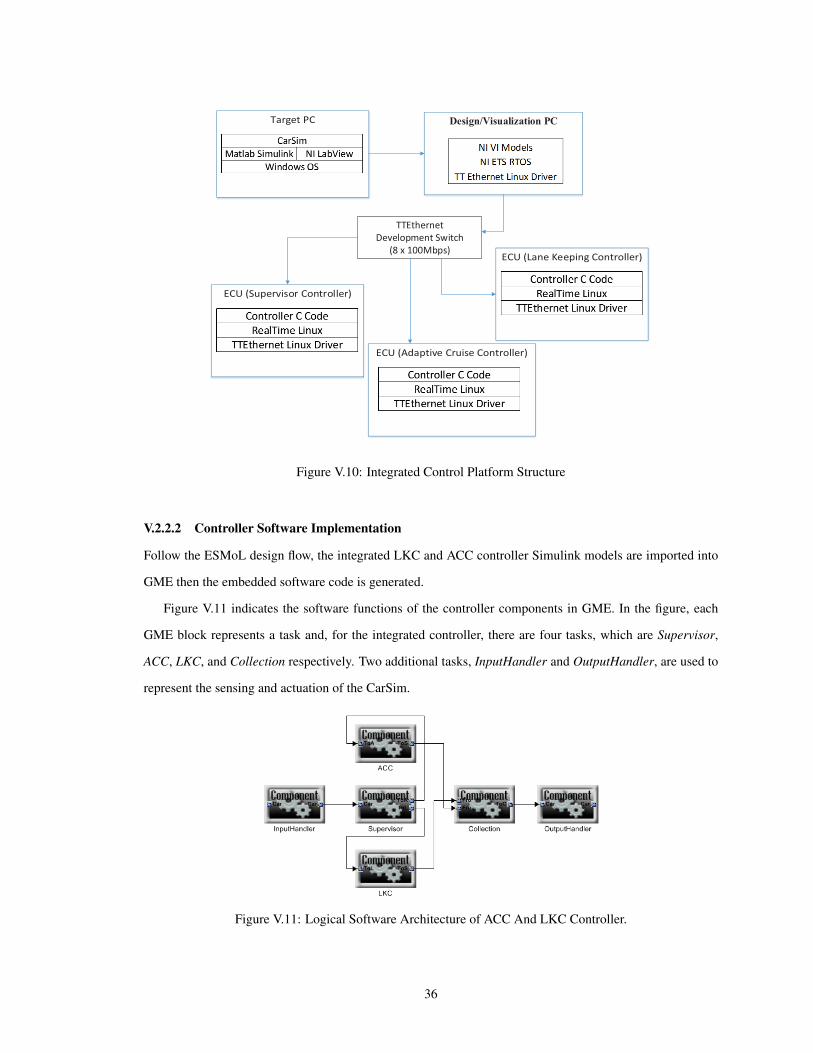
V.2.2.2 Controller Software Implementation

Follow the ESMoL design flow, the integrated LKC and ACC controller Simulink models are imported into

GME then the embedded software code is generated.

Figure V.11 indicates the software functions of the controller components in GME. In the figure, each

GME block represents a task and, for the integrated controller, there are four tasks, which are Supervisor,

ACC, LKC, and Collection respectively. Two additional tasks, InputHandler and OutputHandler, are used to

represent the sensing and actuation of the CarSim.

Figure V.11: Logical Software Architecture of ACC And LKC Controller.

36

In Figure V.12, the network/platform topology structure are modeled in the ESMoL. Three ECUs for

ACC, LKC and supervisor controller are specified as ECU1, ECU2 and ECU3. The RT-Target node is where

the CarSim simulator runs. Then two virtual I/O devices are included to represent the sensors and actuators

of vehicle. Specific parameters for TTEthernet need to be defined, such as hyperperiod, bandwidth, time slot

size, clock synchronization cycle, and synchronization precision. These specified parameters can be used to

generate the TTEthernet configuration script using an ESMoL interpreter.

Figure V.12: Network/Platform Representation.

In Figure V.13, the deployment model of control software is illustrated. Dashed arrows indicate assign-

ment of components to their respective processors, and solid lines represent assignment of message instances

(component ports) to communication channels (port objects) on the processor. Manually, the Supervisor and

Collection are deployed on ECU1, the ACC is deployed on ECU2 and LowLevelController and LKC are set

up on ECU3.

Figure V.14 illustrates the timing and execution model for tasks and message transfers of the control

system. The control system runs at a period of 10ms. Since a synchronized time base for communication

is provided by the TTEthernet , all the message transfers which are indicated by the timing block between

tasks are attached with TTExecInfo to indicate time-triggered communication. For instance, S2LExec is used

to specify the timing for the message transferring from Supervisor to LKC. The execution period, desired

offset and the worst case duration for every communication are set. Execution period is the hyper-period of

the TTEthernet configuration. And the desired offset is used to represent the initstart ns field of TT message

in the generated TTEthernet configuration script. Moreover, the worst case duration indicates the worst case

communication time of TTEthernet. The TTEthernet driver on each ECU has a scheduler to take advantage

of the synchronized time base, which can invoke the tasks according to a static schedule. Thus, all the tasks

37

Figure V.13: Platform Deployment Aspect of Control Software.

can be executed according to the time-triggered paradigm. The TTExecInfo is defined for each task by the

timing block connect to the particular task. For example, ACCExec block defines the execution period of ACC

is 10ms. Before scheduling, only the execution period and the task’s worst case execution time are necessary

to provide. All the period time is measured empirically.

For the task scheduling, the same heuristic algorithm is used as the one in Chapter 3. After network/task

scheduling, the same method is applied to generate codes then deploy on ECUs.

V.2.2.3 Simulation Result

The results of integrated control system hardware in the loop simulation is shown in Figure V.15. Observed

from Figure V.15a and b, the vehicle speed and distance are quite same compared to the simulation result in

Simulink (Figure V.7a and b). The vehicle still adjusts the speed base on the road curve and distance after the

leading car. But from Figure V.15c and d, difference between Simulink and Platform result can be observed

clearly. Taking a closer look at Figure V.15c, the black line enjoys the similar shape but a positive offset from

the red line. The offset is caused by the not synchronizing between components and network communication

delay introduced by platform. The same phenomenon is also shown in Figure IV.7b. Then, from Figure

V.15d, some oscillations on the black figure is illustrated which is also leaded by the synchronization and

delay issue.

38

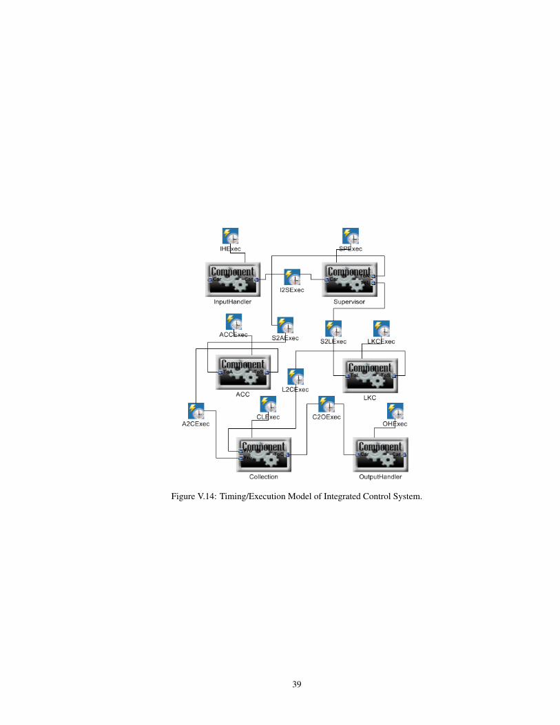
Figure V.14: Timing/Execution Model of Integrated Control System.

39

0 50 100 150 200 250 30020

40

60

80

100

120

Time(s)

Lo

ng

itu

din

al S

pee

d(k

m/h

)

(a) Vehicle Velocity. Solid Line: Folloinwg Car, DotLine: Leading Car

50 100 150 200 250 30030

40

50

60

70

80

90

100

Time(s)

Dis

tan

ce B

etw

een

Car

s(m

)

(b) Distance.Solid Line: Current Value, Dot Line: De-sired Value

0 50 100 150 200 250 300-0.4

-0.3

-0.2

-0.1

0

0.1

0.2

0.3

0.4

Time(s)

Late

ral

Dis

pla

cem

en

t(m

)

(c) Lateral Displacement

0 50 100 150 200 250 300-6

-4

-2

0

2

4

6

Time(s)

Late

ral

Accele

rati

on

(m/s

2)

(d) Lateral Acceleration

Figure V.15: Integrated Control HIL Simulation Result

40

CHAPTER VI

CONCLUSIONS AND FUTURE WORK

VI.1 Conclusion

This thesis presents model based design approach that facilitates the design and integration of time-triggered

automotive control system. The model based design in apply on the lane keeping controller design and the

integration between lane keeping control and adaptive cruise control. For the integration, the supervisor

controller is introduced to handle certain physical interactions such as the impact of road curvature on the

behavior of the two controller. The model design and integration of LKC and ACC is verified by the Simulink

and hardware in to loop simulation. And the simulation results are discussed and compared then the necessity

of supervisor controller is proved and the control effect introduced by simulation platform is illustrated.

VI.2 Future Work

In Chapter 5, the control model integration based on the model based design is illustrated. As an impor-

tant step of model integration, the analysis of interaction and conflict between controller models should be

performed at first but it is not included in the ESMoL. In order to achieve the automatically model based

controller integration, the automatic algorithm base on model conflict analysis and resolve should be consid-

ered in the future. To get the solution, the understanding of relationship between plants dynamic for each

control model is required which means the plant physical dynamic recognition technology might be worth to

consider.

41

BIBLIOGRAPHY

[1] J. Sztipanovits, X. Koutsoukos, G. Karsai, N. Kottenstette, P. Antsaklis, V. Gupta, B. Goodwine,J. Baras, and Shige Wang. Toward a science of cyber-physical system integration. Proc. of the IEEE,100(1):29 –44, jan. 2012.

[2] V. Bobal, J. Bohm, J. Fessl, and J. Machacek. Digital Self-tuning Controllers: Algorithms, Implemen-tation and Applications. Advanced Textbooks in Control and Signal Processing Series. Springer-VerlagLondon Limited, 2005.

[3] J. Porter, G. Hemingway, H. Nine, C. VanBuskirk, N. Kottenstette, G. Karsai, and J. Sztipanovits. Theesmol language and tools for high-confidence distributed control systems design. part 1: Language,framework, and analysis. Technical report, Sept. 2010.

[4] Edward A. Lee and Sanjit A. Seshia. Introduction to Embedded Systems - A Cyber-Physical SystemsApproach. Lee and Seshia, 1 edition, 2010.

[5] J. Mossinger. An insight into the hardware and software complexity of ecus in vehicles. Advancesin Computing and Information Technology, Communications in Computer and Information Science,198:99–106, 2011.

[6] J. Mossinger. Software in automotive systems. IEEE, 27(2):92 –94, march-april 2010.

[7] E. Eyisi, Z. Zhang, X. Koutsoukos, J. Porter, G. Karsai, and J. Sztipanovits. Model-based control designand integration of cyber-physical systems: An adaptive cruise control case study. Journal of ControlScience and Engineering, 2013.

[8] T. Stahl and M. Volter. Model-driven software development. John Wiley and Sons, 2006.

[9] Mariana S. Netto Salim Chaib and Said Mammar. H infinity, adaptive, pid and fuzzy control: com-parison of controllers for vehicle lane keeping. In 2004 IEEE intelligent Vehicles Symposium, pages139–144, Piscataway, NJ, USA, 2004. IEEE Press.

[10] Riccardo Marino, Stefano Scalzi, Giuseppe Orlando, and Mariana Netto. A nested pid steering con-trol for lane keeping in vision based autonomous vehicles. In Proceedings of the 2009 conference onAmerican Control Conference, ACC’09, pages 2885–2890, Piscataway, NJ, USA, 2009. IEEE Press.

[11] Jaromr Fessl Vladimr Bobl, Joseph Bhm and Jir Machcek. Digital Self-tuning Controllers: Algorithms,Implementation and Applications. Springer, 2005 edition edition, 2005.

[12] Said Mammar Mariana S. Netto. Lateral adaptive control for vehicle lane keeping. In Proceedings ofthe 2004 American Control Conference, pages 2693–2698, Piscataway, NJ, USA, 2004. IEEE Press.

[13] Riccardo Marino and Patrizio Tomei. Nonlinear Control Design: Geometric, Adaptive and Robust(Prentice Hall information, system sciences series). Prentice-Hall, 1995 edition edition, 1995.

[14] Dieter Kaesbauer Jurgen Ackermann, Andrew Bartlett. Robust Control: Systems With Uncertain Phys-ical Parameters. Springer-Verlag, 1993.

[15] Carsim. http://www.carsim.com/products/carsim/index.php.

[16] Ahmet Sami KILIN and Tamer BAYBURA. Determination of minimum horizontal curve radius usedin the design of transportation structures, depending on the limit value of comfort criterion lateral jerk.

[17] Oliver Sinnen. Task Scheduling for Parallel Systems. Wiley-Interscience, 2007.

[18] Kihong Park Jeongho Hwang Kyu Hoon Lee Kangwon Lee Soo-Jin Lee Tachun Hwang, Jihoon Rohand Young-Jam Kim. Development of hils systems for active brake control sysmtes. 2006.

[19] Ttethernet. http://www.tttech.com/en/products/ttethernet/.

[20] National instruments. http://www.ni.com/.

42