model based object ﬁnding in occluded cluttered environments

Model based object finding in

occluded cluttered environments

Peter Andersson

September 10, 2010

Master’s Thesis in Computing Science, 30 creditsSupervisor at CS-UmU: Per Lindstrom

Examiner: Fredrik Georgsson

Umea University

Department of Computing Science

SE-901 87 UMEA

SWEDEN

Abstract

The aim of the thesis is object finding in occluded and cluttered environment usingcomputer vision techniques and robot motion. Difficulties of the object finding are 1. findingobjects at hidden area and 2. finding unrecognized objects. For solving the difficulties, twomethods were developed, one is for finding objects in occluded cluttered environments usingmodel based object finding and the other to increase the robustness in object finding byidentifying known objects that are unidentified. The goal was to search occluded areas withthe bumblebee2 stereo camera to be able to identify all known objects in the environmentby removing all visible known objects To identify known objects SURF [9] was used andto be able to remove the identified objects their location first needed to be localized. Tolocalize the object‘s x and y coordinate the information from SURF [9] was used, and thedistance coordinate z is calculated using the depth image from the stereo camera. Themethod to identify objects the SURF [9] algorithm had missed to identify uses a methodto find unknown segments in the environment. By using a push motion on the segments tochange their angle it can remove possible light reflections and the object can be identified.The results of this research show that the method can find objects in occluded clutteredareas and it can also identified missed known objects.

Contents

1 Introduction 1

1.1 Background . . . . . . . . . . . . . . . . . . . . . . . . . . . . . . . . . . . . . 1

1.1.1 Tadokoro Lab . . . . . . . . . . . . . . . . . . . . . . . . . . . . . . . . 1

1.1.2 My project position in the lab . . . . . . . . . . . . . . . . . . . . . . 2

1.2 Sakigake Project . . . . . . . . . . . . . . . . . . . . . . . . . . . . . . . . . . 2

1.2.1 The Vision part of Sakigake project . . . . . . . . . . . . . . . . . . . 3

1.2.2 My part in the project . . . . . . . . . . . . . . . . . . . . . . . . . . . 5

1.3 Related Work . . . . . . . . . . . . . . . . . . . . . . . . . . . . . . . . . . . . 6

2 Unknown object finding and modeling 7

2.1 Finding unknown object . . . . . . . . . . . . . . . . . . . . . . . . . . . . . . 7

2.2 Handling unknown objects . . . . . . . . . . . . . . . . . . . . . . . . . . . . . 9

2.3 Modeling unknown objects . . . . . . . . . . . . . . . . . . . . . . . . . . . . 11

3 Model based object recognition in cluttered environment 15

3.1 Problem description . . . . . . . . . . . . . . . . . . . . . . . . . . . . . . . . 15

3.2 Method solution . . . . . . . . . . . . . . . . . . . . . . . . . . . . . . . . . . 16

3.3 Impact for real world applications . . . . . . . . . . . . . . . . . . . . . . . . 18

4 Fundamental techniques and Technical background 21

4.0.1 OpenCV . . . . . . . . . . . . . . . . . . . . . . . . . . . . . . . . . . . 21

4.0.2 SURF . . . . . . . . . . . . . . . . . . . . . . . . . . . . . . . . . . . . 23

4.0.3 Bumblebee2 BB2-08S2 . . . . . . . . . . . . . . . . . . . . . . . . . . . 25

4.0.4 Bresenham’s line algorithm . . . . . . . . . . . . . . . . . . . . . . . . 26

4.0.5 Grid map and depth image . . . . . . . . . . . . . . . . . . . . . . . . 26

4.0.6 Database XML . . . . . . . . . . . . . . . . . . . . . . . . . . . . . . . 27

4.0.7 Algorithm pseudo code . . . . . . . . . . . . . . . . . . . . . . . . . . 29

5 Results of multiple object finding 33

5.1 Evaluation of object finding . . . . . . . . . . . . . . . . . . . . . . . . . . . . 33

5.1.1 Evaluation of distance and rotation . . . . . . . . . . . . . . . . . . . . 33

5.1.2 Evaluation of multiple object finding . . . . . . . . . . . . . . . . . . . 35

iii

iv CONTENTS

5.2 Evaluating SURF robustness vs. speed . . . . . . . . . . . . . . . . . . . . . . 37

5.3 Evaluation of obstacle detection and improve localization by touch . . . . . . 38

5.4 Evaluating method of finding objects in hidden area . . . . . . . . . . . . . . 41

6 Conclusions 45

6.1 Limitations . . . . . . . . . . . . . . . . . . . . . . . . . . . . . . . . . . . . . 45

6.2 Future work . . . . . . . . . . . . . . . . . . . . . . . . . . . . . . . . . . . . . 45

7 Acknowledgments 47

References 49

A Source Code 51

List of Figures

2.1 3D point cloud segmentation: The first picture shows that if the objects are

separated it works just fine, but the second picture shows that if two objects

stand too close they will be labeled as one. . . . . . . . . . . . . . . . . . . . 8

2.2 Segmentation and the weighted links. . . . . . . . . . . . . . . . . . . . . . . . 8

2.3 Seperation Graph: The picture shows the weights maxima, we can also see a

separation between objects at 4 to 5. . . . . . . . . . . . . . . . . . . . . . . . 9

2.4 The algorithm for RRT-connect. . . . . . . . . . . . . . . . . . . . . . . . . . 11

2.5 Estimate the shape of the object. . . . . . . . . . . . . . . . . . . . . . . . . . 12

2.6 Noise filtering Result (a) range image, (b) threshold=0.2, (c) threshold=0.6,

(d) threshold=1.0. . . . . . . . . . . . . . . . . . . . . . . . . . . . . . . . . . 13

2.7 Result of object segmentation . . . . . . . . . . . . . . . . . . . . . . . . . . . 13

2.8 Result of 3D modeling . . . . . . . . . . . . . . . . . . . . . . . . . . . . . . . 13

3.1 Cluttered and occluded environment inside refrigerator: The Picture shows

us a real environment situation, and the white marking shows us the tea we

want to find but cannot because there are other objects in the way. . . . . . 16

3.2 Manipulator:The Picture shows the manipulator that is to be used for the

method. . . . . . . . . . . . . . . . . . . . . . . . . . . . . . . . . . . . . . . . 17

3.3 Bumblebee2 : The Picture shows the bumblebee2 stereo camera. . . . . . . . 17

3.4 Method flowchart: The flowchart shows in what order the method uses the

different methods to find all objects. . . . . . . . . . . . . . . . . . . . . . . . 18

4.1 Environment with all the components: 1 is the stereo camera. 2-6 are the

objects we are looking for and then we have 1 that is the human arm that is

removing objects from the environment . . . . . . . . . . . . . . . . . . . . . 22

4.2 Separate objects:The Figure shows the same two points found in both found

objects and the model. By moving all found points to the upper left corner of

the object and check if they are located in a 40x40-pixel box we can determen

if they belong to the same object. . . . . . . . . . . . . . . . . . . . . . . . . 24

v

vi LIST OF FIGURES

4.3 Descriptor: This figure shows what a descriptor point looks like [9]. The

descriptor is built up by 4x4 square sub-regions over the interest point(right).

The wavelet responses are computed for every square. Every field of the

descriptor is represented by the 2x2 square sub-divisions. These are the sums

dx, —dx—, dy, and —dy—, computed relatively to the orientation of the

grid (right). . . . . . . . . . . . . . . . . . . . . . . . . . . . . . . . . . . . . . 25

4.4 BB2 image: This is an image of the Bumblebee2 stereo camera. . . . . . . . . 26

4.5 Create a grid map: The left represents the values in the depth image with a

scale 1-5 and the right represents the grid map created from this values . . . 27

4.6 Depth image: The Depth Image shows what the image from the stereo camera

looks like. The green area is the segment that makes the grid map, seen in

Figure 4.7 . . . . . . . . . . . . . . . . . . . . . . . . . . . . . . . . . . . . . . 28

4.7 Grid map: The Grid Map shows the 2D representation of the segmented

part of the environment. The middle in the bottom of the image shows the

location of the camera, the red line the wall and obstacle points. The green

represents observed area, the red obstacle, the blue hidden area and the black

unobserved area. . . . . . . . . . . . . . . . . . . . . . . . . . . . . . . . . . . 28

5.1 Object one . . . . . . . . . . . . . . . . . . . . . . . . . . . . . . . . . . . . . 34

5.2 Object two: Object two is shown in a real situation and all the descriptor

points found in the environment is shown. . . . . . . . . . . . . . . . . . . . 34

5.3 SURF rotation and distant test graph: The Figure shows two graphs, both

graphs show the amount of found descriptor points on the y-axis, a) shows

the rotation on the x-axis and b) shows the distance from the camera. A

model is taken 100cm from the camera and in zero degrees. By moving and

rotating the object we can see the loss of descriptor points. . . . . . . . . . . 34

5.4 Objects in 210 and 300 degrees: The Figure shows how we find an object in

210 degree and degree angle and the matching points in the environment and

model. . . . . . . . . . . . . . . . . . . . . . . . . . . . . . . . . . . . . . . . . 36

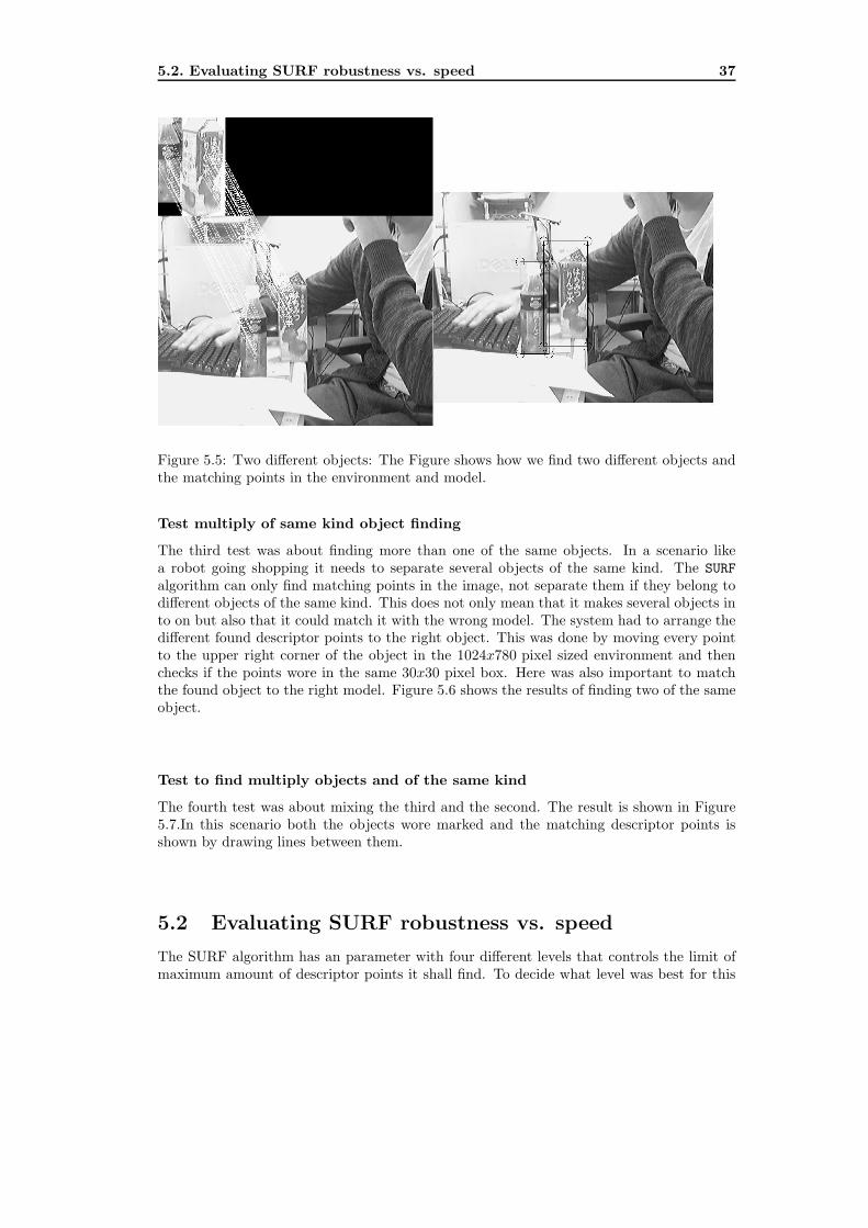
5.5 Two different objects: The Figure shows how we find two different objects

and the matching points in the environment and model. . . . . . . . . . . . . 37

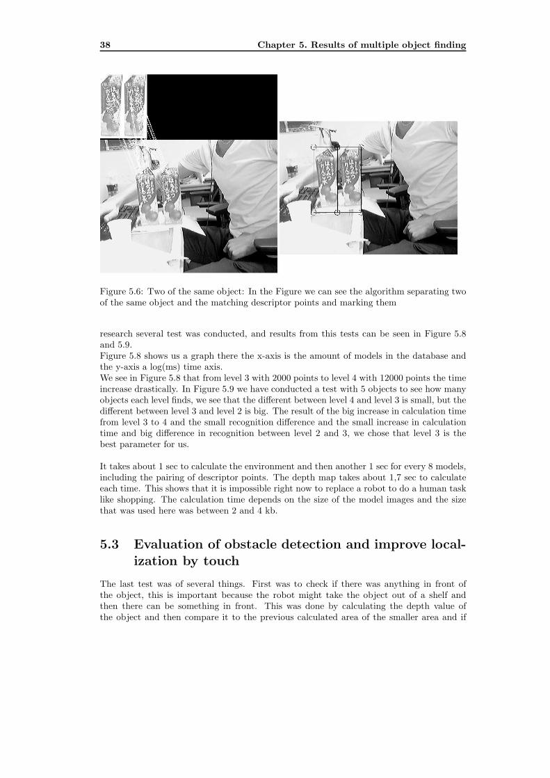
5.6 Two of the same object: In the Figure we can see the algorithm separating

two of the same object and the matching descriptor points and marking them 38

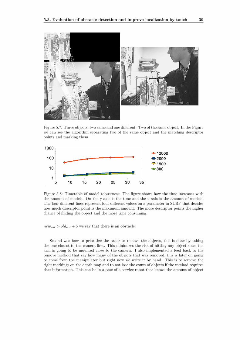
5.7 Three objects, two same and one different: Two of the same object: In the

Figure we can see the algorithm separating two of the same object and the

matching descriptor points and marking them . . . . . . . . . . . . . . . . . . 39

LIST OF FIGURES vii

5.8 Timetable of model robustness: The figure shows how the time increases

with the amount of models. On the y-axis is the time and the x-axis is the

amount of models. The four different lines represent four different values on a

parameter in SURF that decides how much descriptor point is the maximum

amount. The more descriptor points the higher chance of finding the object

and the more time consuming. . . . . . . . . . . . . . . . . . . . . . . . . . . 39

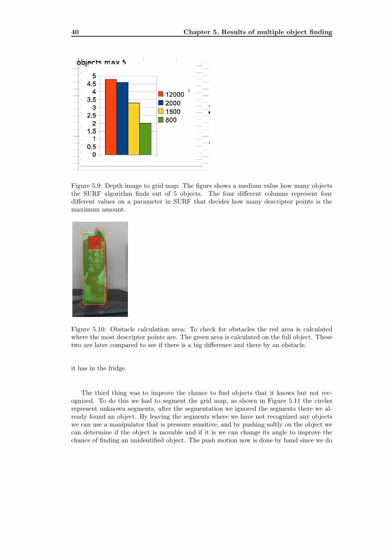
5.9 Depth image to grid map: The figure shows a medium value how many

objects the SURF algorithm finds out of 5 objects. The four different columns

represent four different values on a parameter in SURF that decides how many

descriptor points is the maximum amount. . . . . . . . . . . . . . . . . . . . . 40

5.10 Obstacle calculation area: To check for obstacles the red area is calculated

where the most descriptor points are. The green area is calculated on the full

object. These two are later compared to see if there is a big difference and

there by an obstacle. . . . . . . . . . . . . . . . . . . . . . . . . . . . . . . . 40

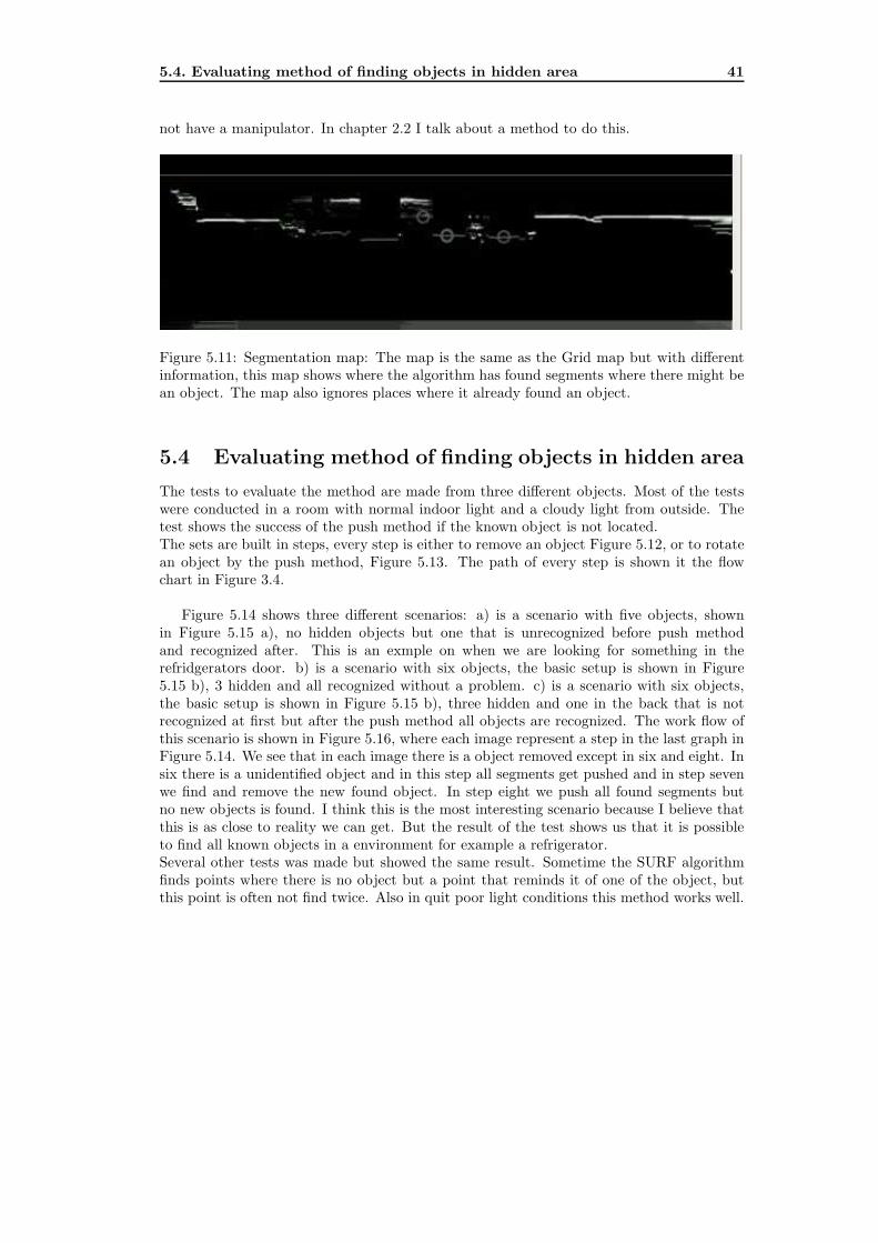
5.11 Segmentation map: The map is the same as the Grid map but with different

information, this map shows where the algorithm has found segments where

there might be an object. The map also ignores places where it already found

an object. . . . . . . . . . . . . . . . . . . . . . . . . . . . . . . . . . . . . . 41

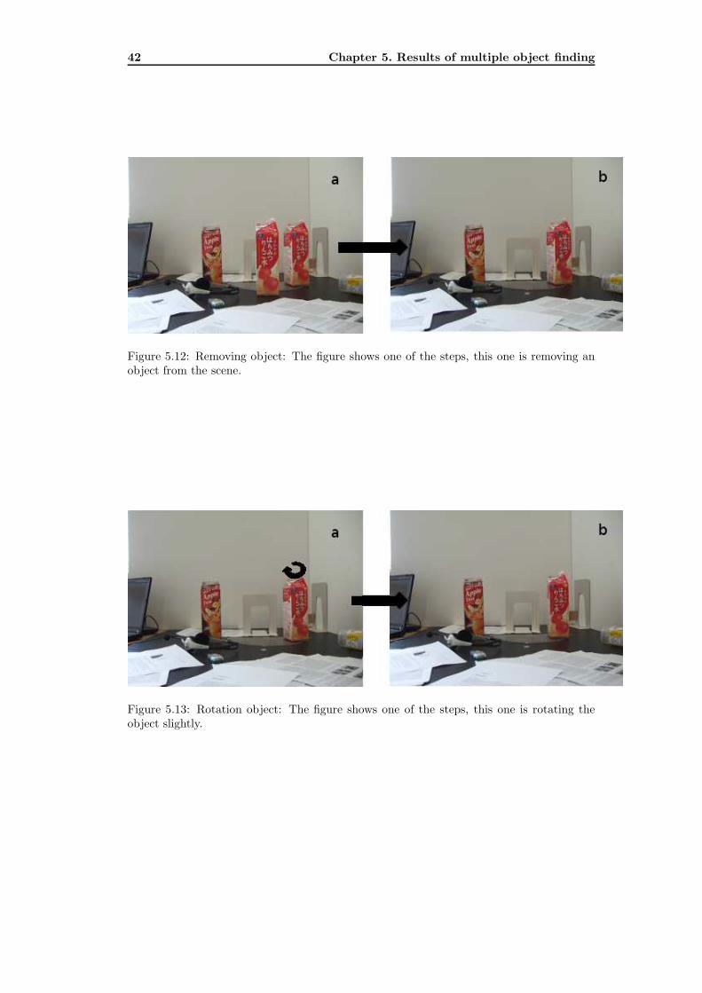
5.12 Removing object: The figure shows one of the steps, this one is removing an

object from the scene. . . . . . . . . . . . . . . . . . . . . . . . . . . . . . . . 42

5.13 Rotation object: The figure shows one of the steps, this one is rotating the

object slightly. . . . . . . . . . . . . . . . . . . . . . . . . . . . . . . . . . . . 42

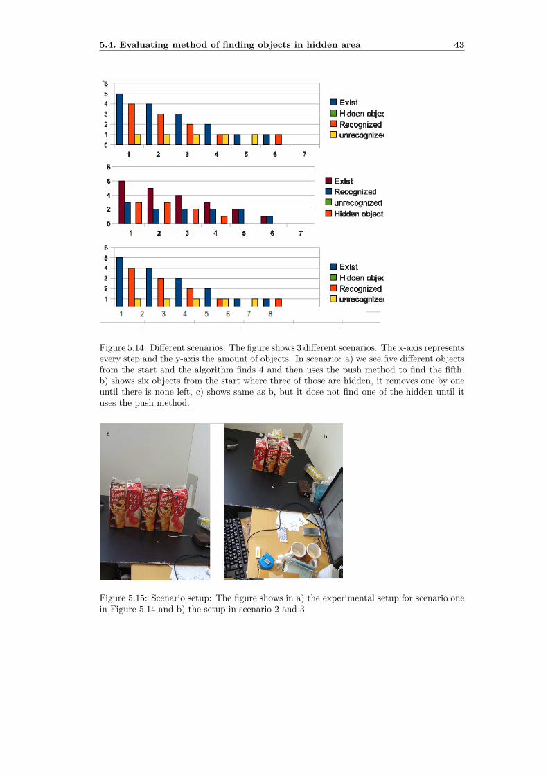
5.14 Different scenarios: The figure shows 3 different scenarios. The x-axis repre-

sents every step and the y-axis the amount of objects. In scenario: a) we see

five different objects from the start and the algorithm finds 4 and then uses

the push method to find the fifth, b) shows six objects from the start where

three of those are hidden, it removes one by one until there is none left, c)

shows same as b, but it dose not find one of the hidden until it uses the push

method. . . . . . . . . . . . . . . . . . . . . . . . . . . . . . . . . . . . . . . . 43

5.15 Scenario setup: The figure shows in a) the experimental setup for scenario

one in Figure 5.14 and b) the setup in scenario 2 and 3 . . . . . . . . . . . . 43

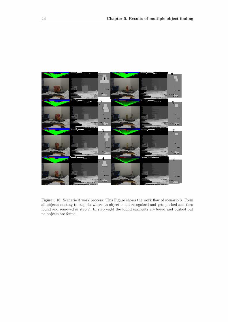
5.16 Scenario 3 work process: This Figure shows the work flow of scenario 3.

From all objects existing to step six where an object is not recognized and

gets pushed and then found and removed in step 7. In step eight the found

segments are found and pushed but no objects are found. . . . . . . . . . . . 44

viii LIST OF FIGURES

List of Tables

4.1 Bumblebee2 Specification . . . . . . . . . . . . . . . . . . . . . . . . . . . . . 25

5.1 The amount of matching descriptor points between the environment and an

object. The model of the object is taken at 100 cm. . . . . . . . . . . . . . . 35

5.2 The table shows the amount of descriptor points found when an object is

rotated both ways. After 30◦ rotation the object is hard to find. . . . . . . . 35

ix

x LIST OF TABLES

Chapter 1

Introduction

1.1 Background

Initially I want to explain a bit about where I do my thesis and my position in the laboratory.In Japan students start with their Master studies work when they start masters. They getassigned to a lab, a special area in their major and also a physical place with other studentsand professors in their field, and get a research topic that later will be their thesis.

1.1.1 Tadokoro Lab

The Tadokoro laboratory at Tohoku University is a robotic lab for safety, security andwelfare of life. The laboratory is divided in two parts: Safety & security and Welfare &Comfort.

The Safety & and Security part is mostly about the robots and their guiding, mappingand controlling systems. Mapping is to build 3D environment with help of 3D laser rangefinders and cameras. Guiding is to avoid obstacle and navigate with the help of the gener-ated maps. The Controlling systems are how to navigate the robot in different environments,like stairs, hills, slippery and to keep its balance.

The Welfare & Comfort part is about Compound eye systems and tactile feeling displays.Tactile feeling display is to be able to feel things that are located in another place or virtualmaterials in the computer. To be able to simulate feelings like pressure, roughness andfriction an ICPF tactile display are used. To feel things at a distant two things are neededone that can recognize the material and how the material is and one that tells your bodyhow it feels. If virtual materials and objects it to be felt only the hardware that sends toyour body is needed. The Compound eye system is a joined camera system that can handleup to and even over 100 cameras.

1

2 Chapter 1. Introduction

1.1.2 My project position in the lab

My position is different from the other students and also my background. I do not take anycourses or have the same background in robotics or touch as the other students. That’s whyI am working on a part of the project that no one else in the lab has any knowledge aboutand that is why I am working on it alone.

1.2 Sakigake Project

The project is to build a mobile robot that gathers environment information autonomouslyin the real world. This project can be compared to the DisneyTMcharacter Wall-e. Wall-eis a cleaner robot who is alone on the earth after the humans have left and all other robotshave malfunctioned. Wall-e wanders around cleaning the streets and finding objects thatare unknown to him. He sorts these objects with similar objects he found before and alsotries to find a use for the items. For example, once he found a light bulb and got it to workin a lamp.

This thesis is talking a lot about service robotics and how they are going to be a moreand more important role in our life, but before this can come to reality there are severaltasks that need to be mastered by the robots that yet are not. This chapter includes severalof these vision tasks and some methods to solve them. As stated before this thesis is aboutfinding known objects that are visible and hidden, but to be able to do that we need toknow the objects first. This chapter briefly talks about the entire process from identify-ing unknown objects and sorting them in the database to using that database to handlereal world tasks. Chapter 2 is about the work before identifying known objects from thedatabase or when new unknown objects are found and chapter 3 talks about my methodto handle the database and objects in the real world tasks. First of all the robot needsto identify areas where there is something, we take for granted that the robot already canidentify plain surface. The robot needs to decide if this object is in a reasonable size tohandle. After reaching the conclusion that there is something that is in a manageable size,the robot needs to make an accurate 3-D model of the found object. In this procedure therobot faces lots of problems. First it has do decide if it is going to look around the objector move it, this is to be able to see every side of the object. There is the problem of keepingtrack of the same object and its position during the modeling. If the robot is moving theobject, how should it move it? These tasks and some more problems will be explained inchapter 2. When the robot is trying to look for objects from the database it also has a lotof problems. One problem is light conditions, another is light reflections and a third is thatthe object can be partly hidden. This problem will be explained in my method in chapter3.

This project can be divided into two major parts:

– The Robot part

– The Vision part

The Robot part includes the robot’s motion and controlling. This report will not includethe robot part of the project.These are the major parts of the robot part:

1.2. Sakigake Project 3

– Movement of the robot

– Obstacle avoidance

– Terrain movement

– Map making

In the vision part there are four major tasks:

1. The first part is to identify objects that the robot knows about.

2. The second is to discover unknown objects

3. The third is to handle the object.

4. The fourth is to make models and categorize the new discovered items.

1.2.1 The Vision part of Sakigake project

This section is about the vision part of the Sakigake project, and the project’s differentparts will be explained briefly. The last part to find known objects is what this thesis isabout and will be explained later in chapter 3.

Identifying and removing known objects

The first part is about finding known objects and moving them out of the way so the robotcan concentrate on the unknown items it does not know anything about. This first partis also what this Thesis is about. In section 1.3 it will be discussed how other researchershave done similar things. There are many ways to identify known objects and this thesisexplains the method I have created, but this part of the report will give you a wider imageof object recognition. This will be more deeply explained in related work later on.

There are many ways to identify known objects and even more ways to make it morereliable.

– Feature point methods for finding objects - SURF SIFT

– Shape database methods

– Distant calculation methods = Stereo camera and range finders: laser and IR andUltra sound.

– Color histogram based methods

– Manipulator - use to slightly move the object to look at it from another angle toimprove recognition chance:

With a mix of these different methods we can both remove objects in the way of findingunknown object but also find specific objects we are looking for. For a fully functionalservice robot it is important to find objects we know, because most of the time when therobot preforms a task it will handle objects it already knows about.


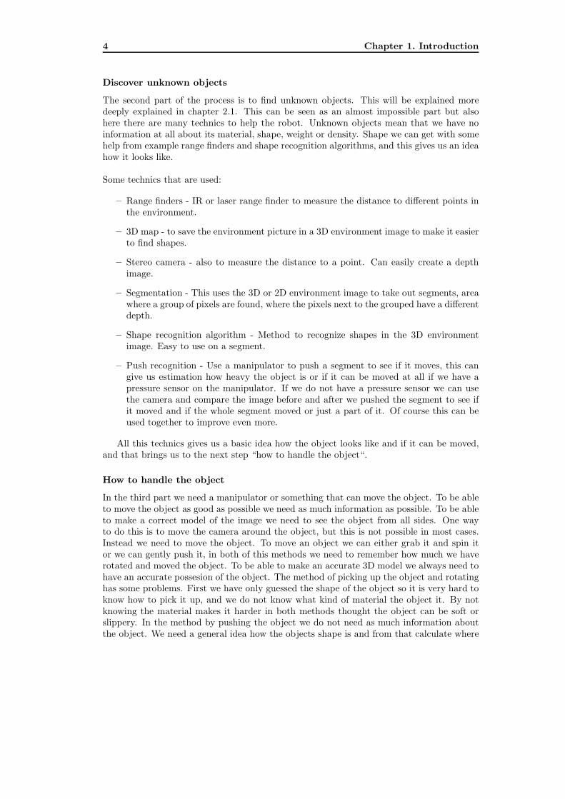
Discover unknown objects

The second part of the process is to find unknown objects. This will be explained moredeeply explained in chapter 2.1. This can be seen as an almost impossible part but alsohere there are many technics to help the robot. Unknown objects mean that we have noinformation at all about its material, shape, weight or density. Shape we can get with somehelp from example range finders and shape recognition algorithms, and this gives us an ideahow it looks like.

Some technics that are used:

– Range finders - IR or laser range finder to measure the distance to different points inthe environment.

– 3D map - to save the environment picture in a 3D environment image to make it easierto find shapes.

– Stereo camera - also to measure the distance to a point. Can easily create a depthimage.

– Segmentation - This uses the 3D or 2D environment image to take out segments, areawhere a group of pixels are found, where the pixels next to the grouped have a differentdepth.

– Shape recognition algorithm - Method to recognize shapes in the 3D environmentimage. Easy to use on a segment.

– Push recognition - Use a manipulator to push a segment to see if it moves, this cangive us estimation how heavy the object is or if it can be moved at all if we have apressure sensor on the manipulator. If we do not have a pressure sensor we can usethe camera and compare the image before and after we pushed the segment to see ifit moved and if the whole segment moved or just a part of it. Of course this can beused together to improve even more.

All this technics gives us a basic idea how the object looks like and if it can be moved,and that brings us to the next step “how to handle the object“.

How to handle the object

In the third part we need a manipulator or something that can move the object. To be ableto move the object as good as possible we need as much information as possible. To be ableto make a correct model of the image we need to see the object from all sides. One wayto do this is to move the camera around the object, but this is not possible in most cases.Instead we need to move the object. To move an object we can either grab it and spin itor we can gently push it, in both of this methods we need to remember how much we haverotated and moved the object. To be able to make an accurate 3D model we always need tohave an accurate possesion of the object. The method of picking up the object and rotatinghas some problems. First we have only guessed the shape of the object so it is very hard toknow how to pick it up, and we do not know what kind of material the object it. By notknowing the material makes it harder in both methods thought the object can be soft orslippery. In the method by pushing the object we do not need as much information aboutthe object. We need a general idea how the objects shape is and from that calculate where

1.2. Sakigake Project 5

the best point is to push. In this method we have the problem with the pushing, if we pushthe object we each time have a chance of losing the possession slightly. It is not certain theobject moves exactly as we predict after pushing it.

Make models and categorize

The last step to make a 3D model of an object is to capture its shape and the image of itssurface. To do this it is important to have the object alone and no other objects to close tothey can be mixed up as one object.

Here one method of modeling a segment described:

1. Get all the depth data of the segment

2. Get the surface image

3. Save information

4. Move the object slightly

5. Repeat from step one until the object have been rotated 360◦.

This is the method when you do not need any information about the object. It is possibleto change the push method to the grab and rotate, but like mentioned this is hard whenwe do not know how the object looks like. We can also move the camera around but thismight not be possible when there might be obstacles or a wall behind.

1.2.2 My part in the project

My part in the project was to identify known objects, remove them, look behind in the hid-den areas for other known objects, remove them and repeat this until there were no visibleknown objects in the environment. I was also supposed to identify areas that could be anobject.

The requirements were:

– This was supposed to be done with the minimum amount of information.

– Stereo camera

– SURF

– Find known objects

– Search hidden areas

– Find different kind of objects

– Find several of the same object


I chose to use a stereo camera to determine the distance to the object, the algorithmSURF [9] to locate known objects, a segmentation algorithm to identifying areas that couldbe an object and a 2D depth map to save information about different areas of the environ-ment.

The result of my research was a working prototype program that meet the requirementsand was able to save the coordinates of the found objects so a manipulator could removeor move them. By doing this the information in the environment could now decrease sounknown objects easier could be found. By implementing the segmentation part i also gotan idea where unknown items was located or unrecognized known objects, this made itpossible to implement the push method to increase the chance of finding known objects.

1.3 Related Work

To better understand the reason why this method is done this way this section will explainabout related researchers work and how their methods work. It will also relate to this paperand its method.

Previous in the report we was talking about different methods to identify objects andto make the methods more robust and reliably. In paper [8] Seungjin Lee and his collagesare talking about how to make a robust method for visual recognition and pose estimationof 3D objects in a noisy and visually not-so-friendly environment. In their method theyare using several different methods to find objects and there position. They are using lineand square algorithms to identify objects, SIFT to identify objects from a database withknown objects and a color algorithm to identify areas with the same color. They are alsousing a moving camera to take images from different positions to get a better robustnessand position estimation. They use the bumblebee stereo camera and the SIFT algorithm toestimate the position.

The next article is about increasing speed in object recognition [7]. They are using amethod called unified visual attention (UVAM) to calculate areas of interest where theybelieve unique objects are located and they are using the SIFT algorithm to search this ar-eas. This method is very fast because it does not need to calculate the entire environment,only the interesting areas from the UVAM. The UVAM consists of a combined stimulus-driven bottom-up attention and a goal-driven top-down attention to reduce execution timeof object recognition. Their conclusion is that this method increases the speed two timescompared to the speed without reduction in recognition accuracy.

In both the previous works we can see ways of finding object, color and shapes, butnone of these methods shows how to identify object that the algorithm missed. In thisresearch it is not prioritized on speed or robustness, the main effort is to find objects thatare not possible to find by just looking at an environment even if the camera is moved. Weconcentrate on the hidden areas behind the known objects. We are using the SURF [9]algorithm to recognize objects from our database and we are using a push method to movean unknown segment in the environment to change its angle to further improve the chanceof finding unrecognized known objects.

Chapter 2

Unknown object finding and

modeling

This chapter will more narrowly explain methods for finding, modeling and handling un-known objects. This is the part of the project before the real world tasks or when the robotdiscovers a new object. To have a service robot that needs as little maintenance or attentionas possible, it is important for the robot to be able to discover, remember and categorizeobjects without human help. To do this as clearly as possible this will be divided in threetasks in different subsections. The first is about finding an unknown object, the second isabout handling the found unknown object and the third is about how to make a 3D modelof the found object.

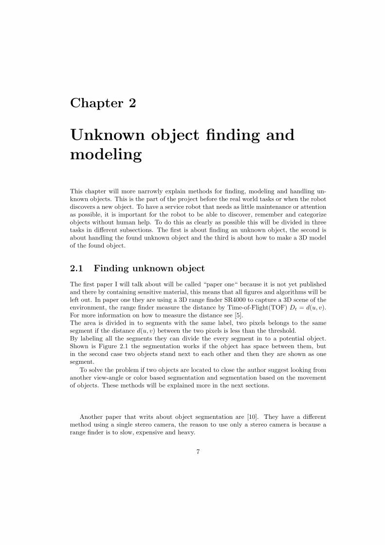
2.1 Finding unknown object

The first paper I will talk about will be called “paper one“ because it is not yet publishedand there by containing sensitive material, this means that all figures and algorithms will beleft out. In paper one they are using a 3D range finder SR4000 to capture a 3D scene of theenvironment, the range finder measure the distance by Time-of-Flight(TOF) Dt = d(u, v).For more information on how to measure the distance see [5].The area is divided in to segments with the same label, two pixels belongs to the samesegment if the distance d(u, v) between the two pixels is less than the threshold.By labeling all the segments they can divide the every segment in to a potential object.Shown is Figure 2.1 the segmentation works if the object has space between them, butin the second case two objects stand next to each other and then they are shown as onesegment.

To solve the problem if two objects are located to close the author suggest looking fromanother view-angle or color based segmentation and segmentation based on the movementof objects. These methods will be explained more in the next sections.

Another paper that writs about object segmentation are [10]. They have a differentmethod using a single stereo camera, the reason to use only a stereo camera is because arange finder is to slow, expensive and heavy.

7

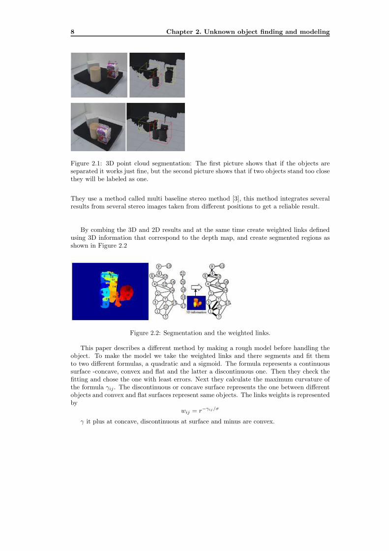
8 Chapter 2. Unknown object finding and modeling

Figure 2.1: 3D point cloud segmentation: The first picture shows that if the objects areseparated it works just fine, but the second picture shows that if two objects stand too closethey will be labeled as one.

They use a method called multi baseline stereo method [3], this method integrates severalresults from several stereo images taken from different positions to get a reliable result.

By combing the 3D and 2D results and at the same time create weighted links definedusing 3D information that correspond to the depth map, and create segmented regions asshown in Figure 2.2

Figure 2.2: Segmentation and the weighted links.

This paper describes a different method by making a rough model before handling theobject. To make the model we take the weighted links and there segments and fit themto two different formulas, a quadratic and a sigmoid. The formula represents a continuoussurface -concave, convex and flat and the latter a discontinuous one. Then they check thefitting and chose the one with least errors. Next they calculate the maximum curvature ofthe formula γij . The discontinuous or concave surface represents the one between differentobjects and convex and flat surfaces represent same objects. The links weights is representedby

wij = r−γij/σ

γ it plus at concave, discontinuous at surface and minus are convex.

2.2. Handling unknown objects 9

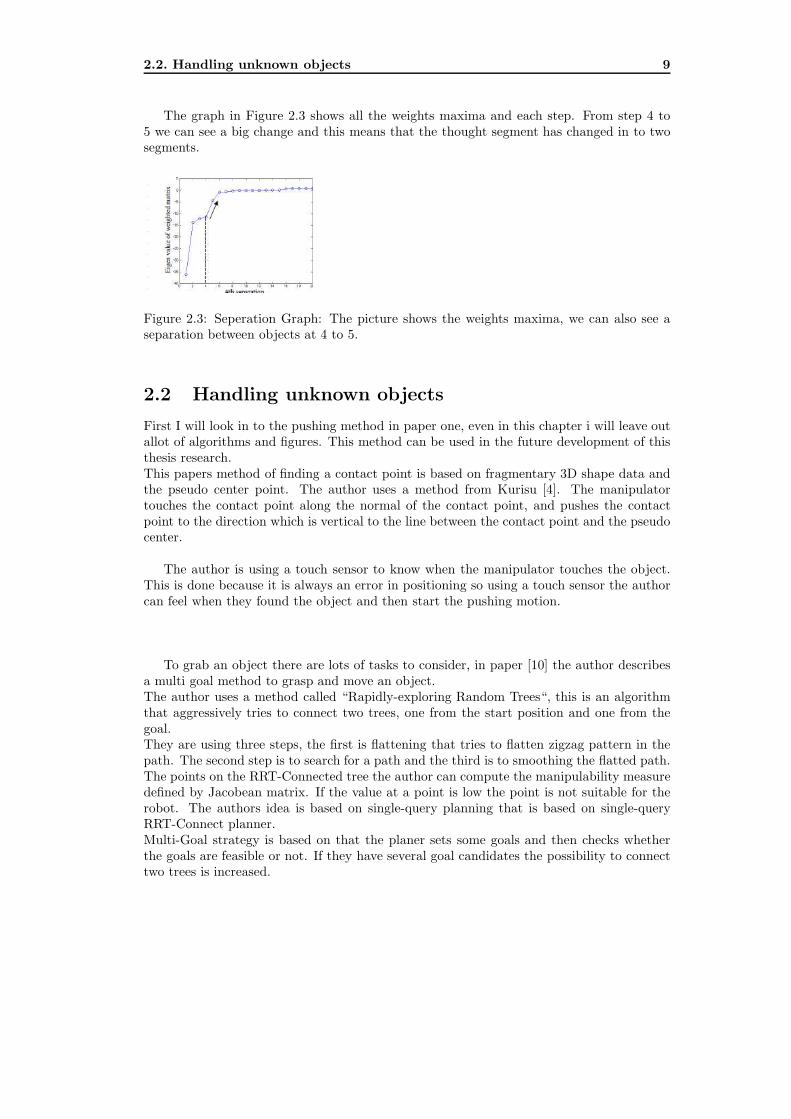
The graph in Figure 2.3 shows all the weights maxima and each step. From step 4 to5 we can see a big change and this means that the thought segment has changed in to twosegments.

Figure 2.3: Seperation Graph: The picture shows the weights maxima, we can also see aseparation between objects at 4 to 5.

2.2 Handling unknown objects

First I will look in to the pushing method in paper one, even in this chapter i will leave outallot of algorithms and figures. This method can be used in the future development of thisthesis research.This papers method of finding a contact point is based on fragmentary 3D shape data andthe pseudo center point. The author uses a method from Kurisu [4]. The manipulatortouches the contact point along the normal of the contact point, and pushes the contactpoint to the direction which is vertical to the line between the contact point and the pseudocenter.

The author is using a touch sensor to know when the manipulator touches the object.This is done because it is always an error in positioning so using a touch sensor the authorcan feel when they found the object and then start the pushing motion.

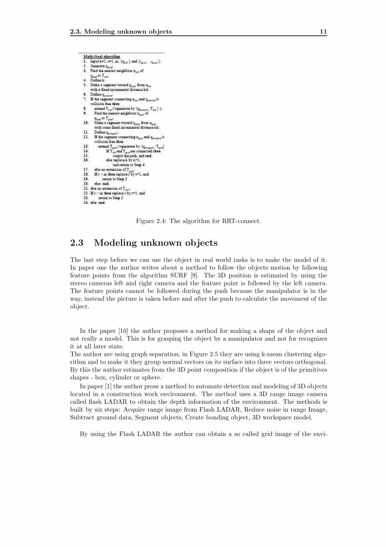
To grab an object there are lots of tasks to consider, in paper [10] the author describesa multi goal method to grasp and move an object.The author uses a method called “Rapidly-exploring Random Trees“, this is an algorithmthat aggressively tries to connect two trees, one from the start position and one from thegoal.They are using three steps, the first is flattening that tries to flatten zigzag pattern in thepath. The second step is to search for a path and the third is to smoothing the flatted path.The points on the RRT-Connected tree the author can compute the manipulability measuredefined by Jacobean matrix. If the value at a point is low the point is not suitable for therobot. The authors idea is based on single-query planning that is based on single-queryRRT-Connect planner.Multi-Goal strategy is based on that the planer sets some goals and then checks whetherthe goals are feasible or not. If they have several goal candidates the possibility to connecttwo trees is increased.


Two trees are generated , Tinit and Tgoal, by qinit and qgoal. The algorithm for Multi-Goal RRT-Connect is shown in Figure 2.4. They select qgoal> is based on the manipulabilitymeasure that is one of multi-criteria.The author suggests a new method for smoothing the zigzag path created by the Multi-GoalRRT-Connect, that is based on convolution technique in functional analysis. This techniqueis known that every continuous function can be approximate by a sequence of smooth(C-infinity) functions uniformly.For a link the zigzag function can be f(t), depending of time and the value is the link angle.The motion schedule is represented by the graph (t, f(t)). The support compact smoothfunction is:

g(t) = e1/t2−1),−1 < t < 1andg(t) = 0

If g(t)! = 0 they would like to approximate the function f(t). The function g(t) can becontrolled by a parameter d, such as gd = (1/cd)g(t/d). The number c is the integral g(t)normalized constant in the interval −1 < t < 1. The function is defined as:

fd(t) =

∫

∞

−∞

gd(t − x)f)x dx

This function is an approximation of the function f(t) with the control parameter d. Asa necessary condition to design the control parameter di at each point pi, we define it asdi = 1/2minti − ti1, ti2 − tifori = 1, ..., n, whereqi = (ti, f(ti))andpij = (tij , f(tij)). Thisonly changes the parameter di and are only executed around Di. Setting vmax > 0 andamax > 0, then the candidates of maximum acceleration are given at point t1, ....tn. Thenthey only check the value of

2fd

t2(t1), ...,

2fd

t2(tn)

, exceeds amax or not. If |2fd

t2 (t∗)| > amax, the time scale is corrected appropriately in theneighborhood of t∗.

2.3. Modeling unknown objects 11

Figure 2.4: The algorithm for RRT-connect.

2.3 Modeling unknown objects

The last step before we can use the object in real world tasks is to make the model of it.In paper one the author writes about a method to follow the objects motion by followingfeature points from the algorithm SURF [9]. The 3D position is estimated by using thestereo cameras left and right camera and the feature point is followed by the left camera.The feature points cannot be followed during the push because the manipulator is in theway, instead the picture is taken before and after the push to calculate the movement of theobject.

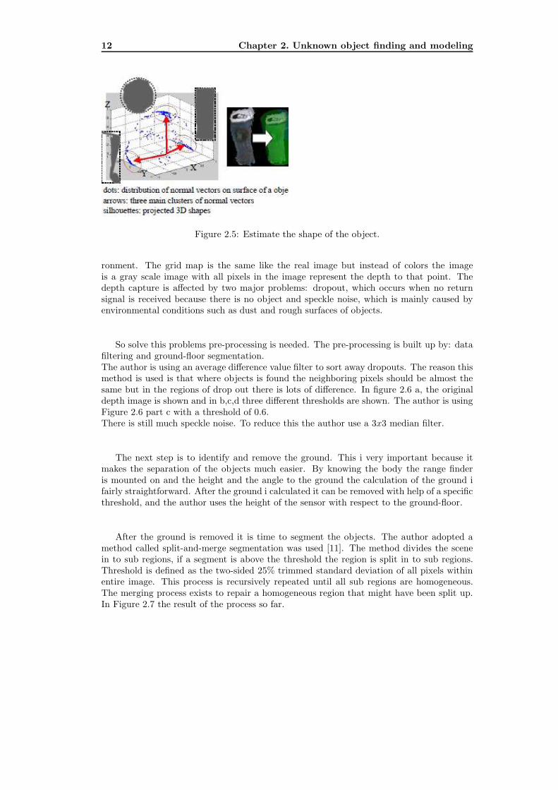
In the paper [10] the author proposes a method for making a shape of the object andnot really a model. This is for grasping the object by a manipulator and not for recognizesit at all later state.The author are using graph separation, in Figure 2.5 they are using k-mean clustering algo-rithm and to make it they group normal vectors on its surface into three vectors orthogonal.By this the author estimates from the 3D point composition if the object is of the primitivesshapes - box, cylinder or sphere.

In paper [1] the author prose a method to automate detection and modeling of 3D objectslocated in a construction work environment. The method uses a 3D range image cameracalled flash LADAR to obtain the depth information of the environment. The methods isbuilt by six steps: Acquire range image from Flash LADAR, Reduce noise in range Image,Subtract ground data, Segment objects, Create bonding object, 3D workspace model.

By using the Flash LADAR the author can obtain a so called grid image of the envi-


Figure 2.5: Estimate the shape of the object.

ronment. The grid map is the same like the real image but instead of colors the imageis a gray scale image with all pixels in the image represent the depth to that point. Thedepth capture is affected by two major problems: dropout, which occurs when no returnsignal is received because there is no object and speckle noise, which is mainly caused byenvironmental conditions such as dust and rough surfaces of objects.

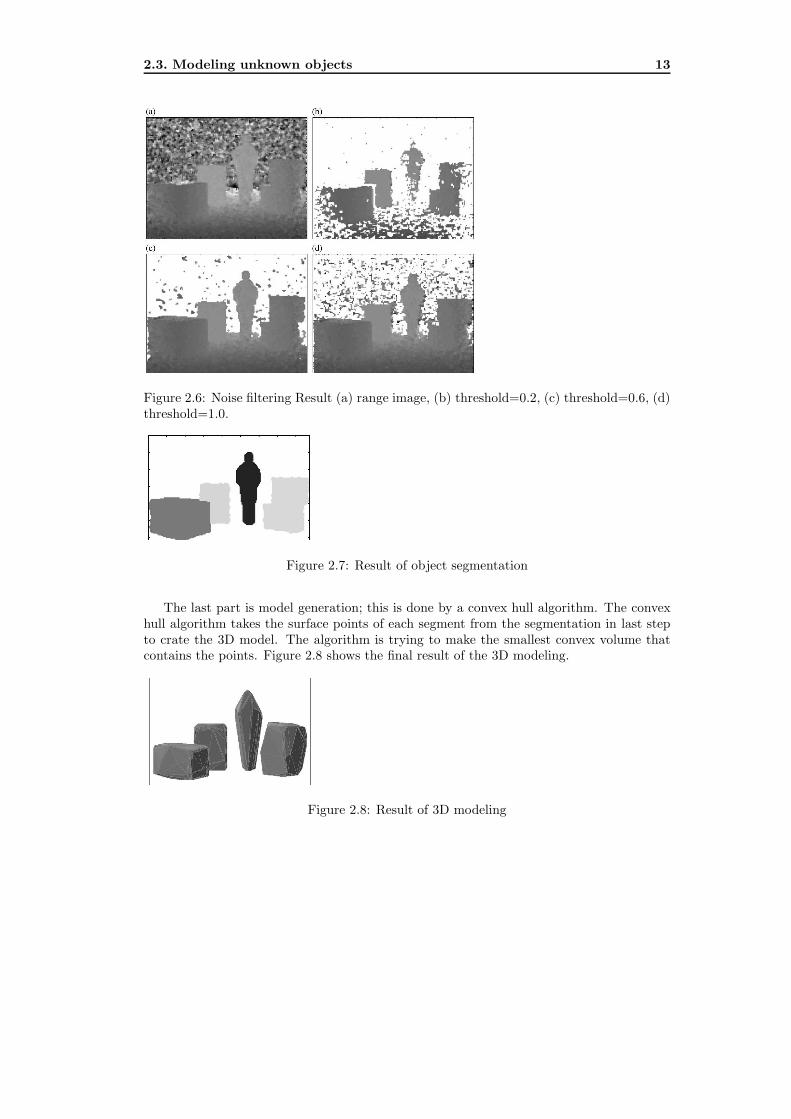
So solve this problems pre-processing is needed. The pre-processing is built up by: datafiltering and ground-floor segmentation.The author is using an average difference value filter to sort away dropouts. The reason thismethod is used is that where objects is found the neighboring pixels should be almost thesame but in the regions of drop out there is lots of difference. In figure 2.6 a, the originaldepth image is shown and in b,c,d three different thresholds are shown. The author is usingFigure 2.6 part c with a threshold of 0.6.There is still much speckle noise. To reduce this the author use a 3x3 median filter.

The next step is to identify and remove the ground. This i very important because itmakes the separation of the objects much easier. By knowing the body the range finderis mounted on and the height and the angle to the ground the calculation of the ground ifairly straightforward. After the ground i calculated it can be removed with help of a specificthreshold, and the author uses the height of the sensor with respect to the ground-floor.

After the ground is removed it is time to segment the objects. The author adopted amethod called split-and-merge segmentation was used [11]. The method divides the scenein to sub regions, if a segment is above the threshold the region is split in to sub regions.Threshold is defined as the two-sided 25% trimmed standard deviation of all pixels withinentire image. This process is recursively repeated until all sub regions are homogeneous.The merging process exists to repair a homogeneous region that might have been split up.In Figure 2.7 the result of the process so far.

2.3. Modeling unknown objects 13

Figure 2.6: Noise filtering Result (a) range image, (b) threshold=0.2, (c) threshold=0.6, (d)threshold=1.0.

Figure 2.7: Result of object segmentation

The last part is model generation; this is done by a convex hull algorithm. The convexhull algorithm takes the surface points of each segment from the segmentation in last stepto crate the 3D model. The algorithm is trying to make the smallest convex volume thatcontains the points. Figure 2.8 shows the final result of the 3D modeling.

Figure 2.8: Result of 3D modeling

Chapter 3

Model based object recognition

in cluttered environment

In past researches, lots of time and resources [?] have been put into computer vision andremarkable progress has been made. Even if all objects in cluttered environments are found,there are still a lot of problems to be solved. This chapter will explain a solution to someof this problems and a method to improve the recognition of objects in a real environmentthat did not get found.

3.1 Problem description

To find objects that are partly covered or completely hidden behind other objects makes ithard to identify the objects we are looking for, this we call hidden objects. To find hiddenobjects in occluded areas objects in the way need to be removed or slightly moved.

To remove identified objects we need to check so they are not partly covered and thereby completely free. We also need to decide what object to remove first if we have more thanone object to remove. This is especially needed when we are looking for an object in a shelfand cannot lift it straight up.

In addition computer vision has lots of other difficulties that have to be taken to accountwhen identifying objects. Working with model based recognition means that the model ofthe object and the same object in the environment has to look nearly the same. So if anobject in the environment has a different light condition, a reflection of a light or is damagedthe chances of making the match is harder. The more rotation it is on the object from itsoriginal pose also makes it harder to find. That is why we need a robust method to identifyknown objects.

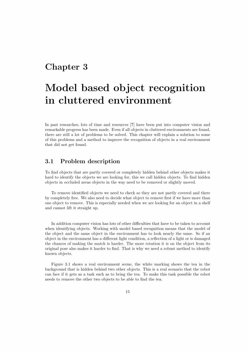
Figure 3.1 shows a real environment scene, the white marking shows the tea in thebackground that is hidden behind two other objects. This is a real scenario that the robotcan face if it gets as a task such as to bring the tea. To make this task possible the robotneeds to remove the other two objects to be able to find the tea.

15

16 Chapter 3. Model based object recognition in cluttered environment

Figure 3.1: Cluttered and occluded environment inside refrigerator: The Picture shows usa real environment situation, and the white marking shows us the tea we want to find butcannot because there are other objects in the way.

3.2 Method solution

To solve the problems stated before with the refrigerator and the tea as good as possible, Iproposed one solution using traditional computer vision methods and a robot motion. Hid-den areas are found from visual information, and unrecognized object can be found usingrobot motion and computer vision methods. In the rest of this section, I would like toexplain the details of the solution.

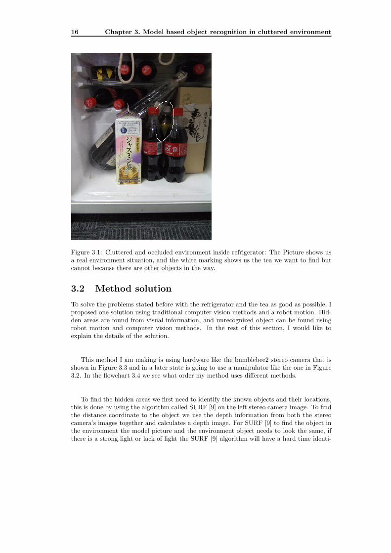
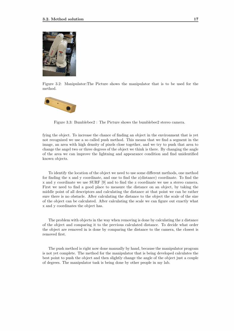
This method I am making is using hardware like the bumblebee2 stereo camera that isshown in Figure 3.3 and in a later state is going to use a manipulator like the one in Figure3.2. In the flowchart 3.4 we see what order my method uses different methods.

To find the hidden areas we first need to identify the known objects and their locations,this is done by using the algorithm called SURF [9] on the left stereo camera image. To findthe distance coordinate to the object we use the depth information from both the stereocamera’s images together and calculates a depth image. For SURF [9] to find the object inthe environment the model picture and the environment object needs to look the same, ifthere is a strong light or lack of light the SURF [9] algorithm will have a hard time identi-

3.2. Method solution 17

Figure 3.2: Manipulator:The Picture shows the manipulator that is to be used for themethod.

Figure 3.3: Bumblebee2 : The Picture shows the bumblebee2 stereo camera.

fying the object. To increase the chance of finding an object in the environment that is yetnot recognized we use a so called push method. This means that we find a segment in theimage, an area with high density of pixels close together, and we try to push that area tochange the angel two or three degrees of the object we think is there. By changing the angleof the area we can improve the lightning and appearance condition and find unidentifiedknown objects.

To identify the location of the object we need to use some different methods, one methodfor finding the x and y coordinate, and one to find the z(distance) coordinate. To find thex and y coordinate we use SURF [9] and to find the z coordinate we use a stereo camera.First we need to find a good place to measure the distance on an object, by taking themiddle point of all descriptors and calculating the distance at that point we can be rathersure there is no obstacle. After calculating the distance to the object the scale of the sizeof the object can be calculated. After calculating the scale we can figure out exactly whatx and y coordinates the object has.

The problem with objects in the way when removing is done by calculating the z distanceof the object and comparing it to the previous calculated distance. To decide what orderthe object are removed in is done by comparing the distance to the camera, the closest isremoved first.

The push method is right now done manually by hand, because the manipulator programis not yet complete. The method for the manipulator that is being developed calculates thebest point to push the object and then slightly change the angle of the object just a coupleof degrees. The manipulator task is being done by other people in my lab.


Figure 3.4: Method flowchart: The flowchart shows in what order the method uses thedifferent methods to find all objects.

3.3 Impact for real world applications

Service robots are coming more and more in to normal peoples home. Most it is in the formof vacuum cleaners and lawn molders. But in the near feature we will see robots in manydifferent shapes and with a wide range of functions. Service robots in our home might gettasks like getting the milk from the fridge, looking for the keys or look what is missing inthe kitchen before shopping. In all of this scenarios the robot needs to know many objectsto be able to find the on it is looking for or in the case with what is missing it needs of findall objects in the environment and say what is not there. It also needs to look behind andunder objects and search the hidden areas.

In the shopping scenario the robot gets a list with what it needs and after it checks thefridge what it got home and compare it to the list. After the comparison the robot can tella human what is missing, go shop it by itself or order it from the internet. In the scenariowith getting the milk it only needs to look in the fridge and move other grocery to find themilk, maybe we do not have any milk and it will add it to the shopping list. This can beused similar in different companies or in warehouses.

3.3. Impact for real world applications 19

In the rescue robotics field it is not so clear what we can use this algorithm for, we mightuse it to find dangerous materials or similar tasks, but the most important I think is to findhidden passage. If the robot is going from one place in the building to another the passagemay be blocked by a chair or a broken desk or something. To be able to find this path itneeds to remove the chair and look in the hidden area behind.

Chapter 4

Fundamental techniques and

Technical background

To be able to start I needed to learn the appropriate tools and methods for image recognition.The professor at Tohoku University gave me a book in OpenCV and some web pages on SURF.The first weeks was only to learn the C library OpenCV for real time image processing.

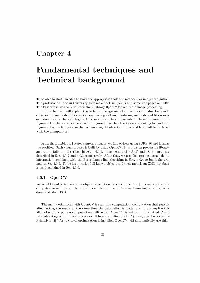
In this chapter I will explain the technical background of all technics and also the pseudocode for my methods. Information such as algorithms, hardware, methods and libraries isexplained in this chapter. Figure 4.1 shows us all the components in the environment: 1 inFigure 4.1 is the stereo camera, 2-6 in Figure 4.1 is the objects we are looking for and 7 inFigure 4.1 is the human arm that is removing the objects for now and later will be replacedwith the manipulator.

From the Bumblebee2 stereo camera‘s images, we find objects using SURF [9] and localizethe position. Such visual process is built by using OpenCV. It is a vision processing library,and the details are described in Sec. 4.0.1. The details of SURF and Depth map aredescribed in Sec. 4.0.2 and 4.0.3 respectively. After that, we use the stereo camera‘s depthinformation combined with the Bresenham’s line algorithm in Sec. 4.0.4 to build the gridmap in Sec 4.0.5. To be keep track of all known objects and their models an XML-databaseis used explained in Sec 4.0.6.

4.0.1 OpenCV

We used OpenCV to create an object recognition process. OpenCV [6] is an open sourcecomputer vision library. The library is written in C and C++ and runs under Linux, Win-dows and Mac OS X.

The main design goal with OpenCV is real time computation, computation that pursuitafter getting the result at the same time the calculation is made, and to accomplice thisallot of effort is put on computational efficiency. OpenCV is written in optimized C andtake advantage of multicore processors. If Intel’s architecture IPP ( Integrated PerformancePrimitives [2] ) for low-level optimization is installed OpenCV will automatically use this.

21

22 Chapter 4. Fundamental techniques and Technical background

Figure 4.1: Environment with all the components: 1 is the stereo camera. 2-6 are the objectswe are looking for and then we have 1 that is the human arm that is removing objects fromthe environment

Another goal with OpenCV is to provide a simple-to-use computer vision infrastructure.The OpenCV library contains over 500 functions in arias as:

– vision

– medical imaging

– security

– user interface

– camera calibration

– stereo vision

– robotics

This just some of the arias, but is regarding to the last once we choose to use OpenCV.OpenCV also contains algorithms for machine learning (MLL), this sub library is focusedon pattern recognition and clustering.

23

4.0.2 SURF

Seeded-Up Robust Features (SURF) [9] is a preferment scale- and rotation-invariant interestpoint detector and descriptor. It outperforms previously proposed schemes in terms of ro-bustness, distinctiveness and repeatability, and it also preforms better in computing speed.

To be able to understand SURF we first need to understand some of the parts it is builtfrom. The Hessian Matrix because it is good in accuracy. To be able to use the Hessian

Matrix in the optimal way we also use Integral Images which reduces the computationtime drastically.

The SURF algorithm is not by itself able to separate two identical objects found ina scene, it will only find matching points to the models. The method for separating twoobjects is shown in Figure 4.2, the figure shows the same two points found in both foundobjects and the model. By moving all found points to the upper left corner of the objectand check if they are located in a 40x40-pixel box we can determent if they belong to thesame object. By saving the amount of points found in the box with the matched model wecan compare the next found if it is a better match.

Integral Images

Integral images or summed area tables as they are also known as, is a 3D representationof an image. By placing an array of micro lenses in front of an image that looks differentdepending on the angel the lenses is being observed. They allow for fast computation of boxtype convolution filters. The Integral Images entry IP(x) is formed by a rectangular shapein the image I at location x = (x, y)⊤ and this rectangular region is formed by the originand x.

IP(x) =

i=0∑

i<x

j=0∑

j<y

I(i, j)

Once the Integral Image is computed, it takes three additions to calculate the sum ofthe intensities over any upright, rectangular area. The calculation time is independent ofthe size.

Hessian Matrix Based Interest Point

SURF is using Hessian Matrix to detect blob-like structures at locations where the deter-minant is maximum [9]. The scale selections are also relayed on the determinant. In animage I we take a pointx = (x,y), the matrix H(x, σ) in x at the scale σ is defined as follows

H(x, σ) =

[

Lxx(x/σ) Lxy(x, σ)Lxy(x, σ) Lyy(x, σ)

]

Lxx(x/σ) is the solution of the Gaussian second order derivative ∂2

∂x2 g(σ)with the imageI in point x, and similar for Lxy(x.σ) and Lyy(x.σ)

After the Gaussians are used because it is optimal for scale-spacing analysis. Theseapproximate second order Gaussian derivatives and can be evaluated at a very low com-putational cost using integral images. The calculation time therefore is independent of the


Figure 4.2: Separate objects:The Figure shows the same two points found in both foundobjects and the model. By moving all found points to the upper left corner of the objectand check if they are located in a 40x40-pixel box we can determen if they belong to thesame object.

filter size. A box filter 9x9 is an approximation of a Gaussian with σ = 1.2 and represent thelowest scale for computing blob response maps. To make is as fast and efficient as possiblethe weights applied to the rectangular regions are kept simple.

det(Happrox) = DxxDyy − (wDxy)2.

To balance the Hessians‘s determinant the relative weight w of the filter responses areused. This is needed for the energy conservation between the Gaussian kernels and theapproximated Gaussian kernels,

w =|Lxy(1.2)|F |Dyy(9)|F|Lyy(1.2)|F |Dxy(9)|F

= 0.912... ≃ 0.9,

where |x|F is the Frobenius norm. The weight changes depending on the scale, but inpractice this is a constant.

25

Descriptor

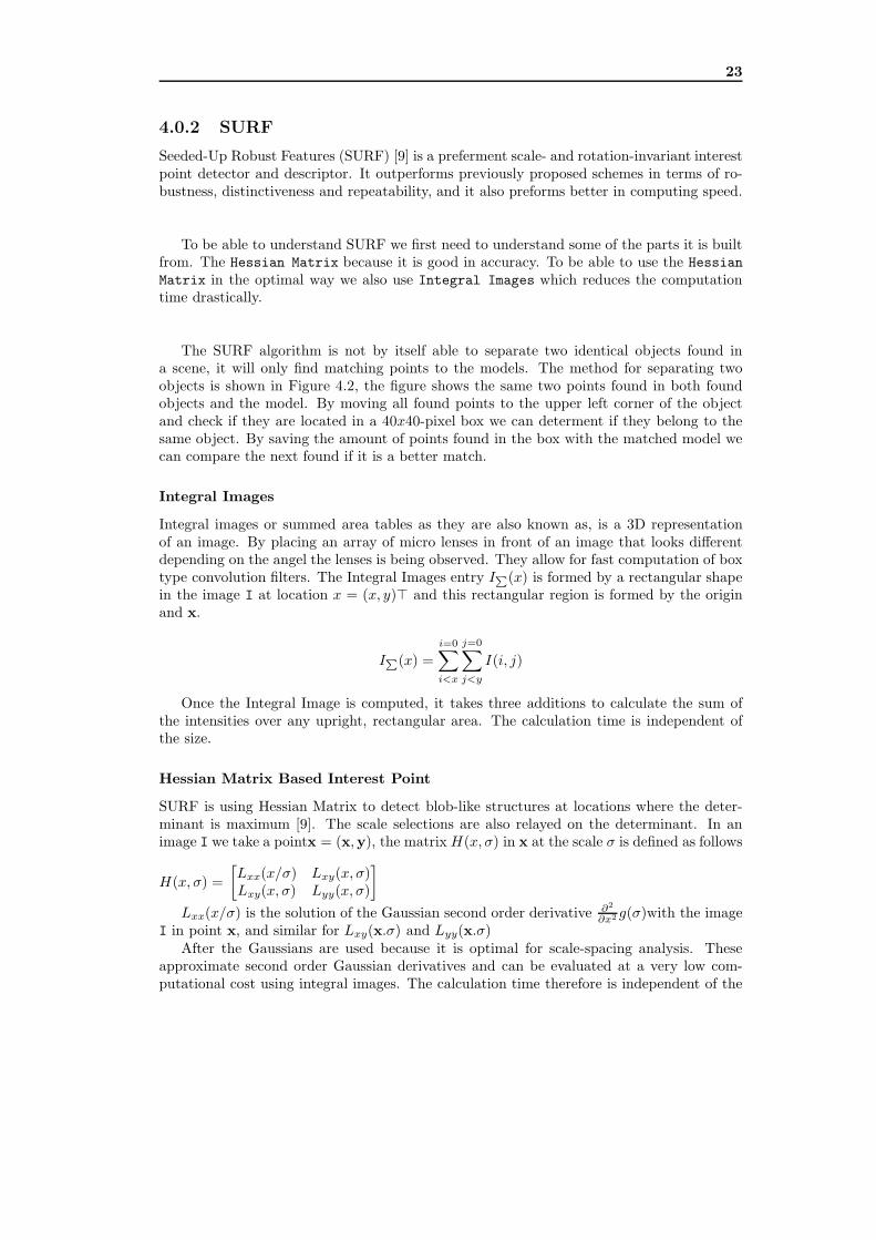
[9] A descriptor point is created by first creating a square region around the interest point,where it after is divided in to 4x4 square sub-regions, Figure 4.3. Every sub-region iscomputed with Haar wavelet responses at 5x5 regularly spaced sample points. A Gaussian( σ 3.3s) is applied to increase the robustness. After the wavelet for each sub-region issummed up to create the first set of entries in the feature vector. To get the polarityinformation of the intensity changes, the absolute values are also extracted. Each sub-region then have a four-dimensional descriptor vector v for its underlying intensity structurev = (Σd|x, Σdy , Σ|dx|, Σ|dy|).Concatenating this for all 4 × 4 sub-regions, this results in adescriptor vector of length 64. Invariance to contrast is achieved by turning the descriptorinto a unit vector.

Figure 4.3: Descriptor: This figure shows what a descriptor point looks like [9]. The de-scriptor is built up by 4x4 square sub-regions over the interest point(right). The waveletresponses are computed for every square. Every field of the descriptor is represented bythe 2x2 square sub-divisions. These are the sums dx, —dx—, dy, and —dy—, computedrelatively to the orientation of the grid (right).

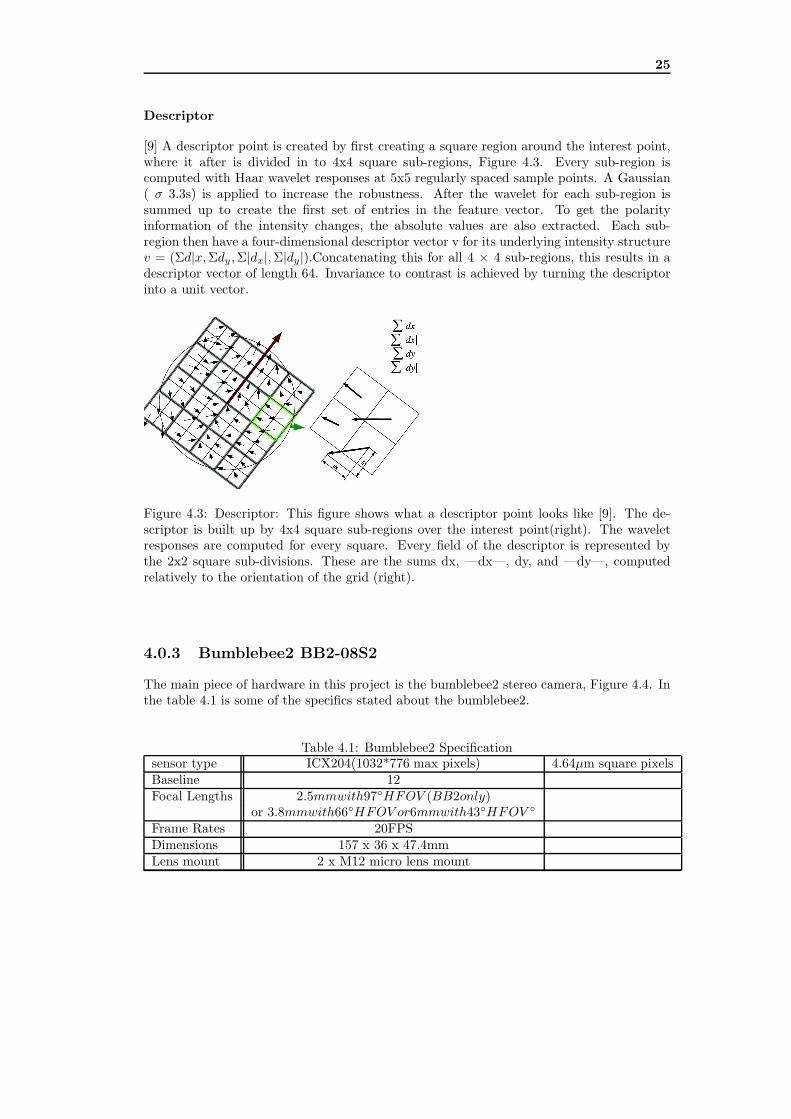
4.0.3 Bumblebee2 BB2-08S2

The main piece of hardware in this project is the bumblebee2 stereo camera, Figure 4.4. Inthe table 4.1 is some of the specifics stated about the bumblebee2.

Table 4.1: Bumblebee2 Specificationsensor type ICX204(1032*776 max pixels) 4.64µm square pixelsBaseline 12Focal Lengths 2.5mmwith97◦HFOV (BB2only)

or 3.8mmwith66◦HFOV or6mmwith43◦HFOV ◦

Frame Rates 20FPSDimensions 157 x 36 x 47.4mmLens mount 2 x M12 micro lens mount


Figure 4.4: BB2 image: This is an image of the Bumblebee2 stereo camera.

4.0.4 Bresenham’s line algorithm

Bresenham’s line algorithm is one of the most optimized algorithm to draw a line betweentwo points. I modified it so it continue to draw after the second point to the end of the gridmap, by doing this i mark the map as hidden area after the second point is passed.

function line(x0, x1, y0, y1)

boolean steep := abs(y1 - y0) > abs(x1 - x0)

if steep then

swap(x0, y0)

swap(x1, y1)

if x0 > x1 then

swap(x0, x1)

swap(y0, y1)

int deltax := x1 - x0

int deltay := abs(y1 - y0)

int error := deltax / 2

int ystep

int y := y0

if y0 < y1 then ystep := 1 else ystep := -1

for x from x0 to x1

if steep then plot(y,x) else plot(x,y)

error := error - deltay

if error < 0 then

y := y + ystep

error := error + deltax

4.0.5 Grid map and depth image

The Bumblebee2 stereo camera creates a depth image by taking two images and findingcorresponding pixels in the image from both cameras. The result of theis correspondingpixels is a grid map with (x,y,z)-coordinates for every point in the environment, the (x,y)-coordinate in the environment is the same as in the grid map and the z-coordinate is thevalue in that (x,y)-coordinate. This can be represented by a gray scale image with a rangefrom 0 to 254 and the higher value the closer to the camera.

27

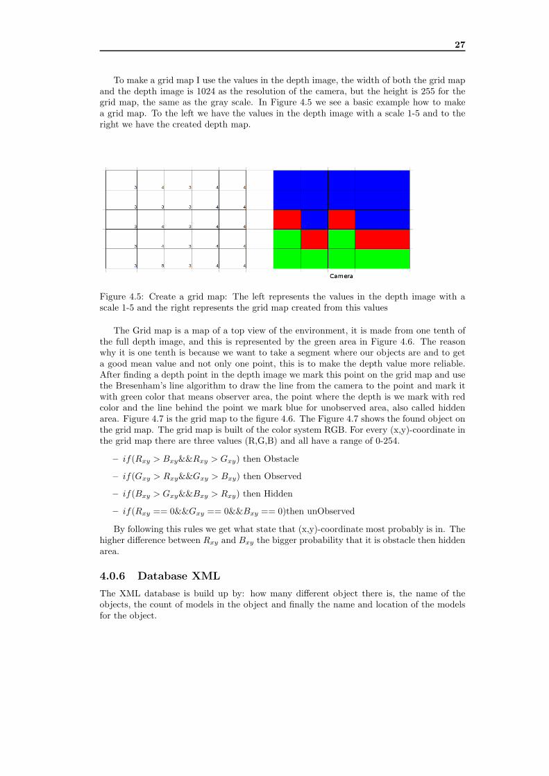
To make a grid map I use the values in the depth image, the width of both the grid mapand the depth image is 1024 as the resolution of the camera, but the height is 255 for thegrid map, the same as the gray scale. In Figure 4.5 we see a basic example how to makea grid map. To the left we have the values in the depth image with a scale 1-5 and to theright we have the created depth map.

Figure 4.5: Create a grid map: The left represents the values in the depth image with ascale 1-5 and the right represents the grid map created from this values

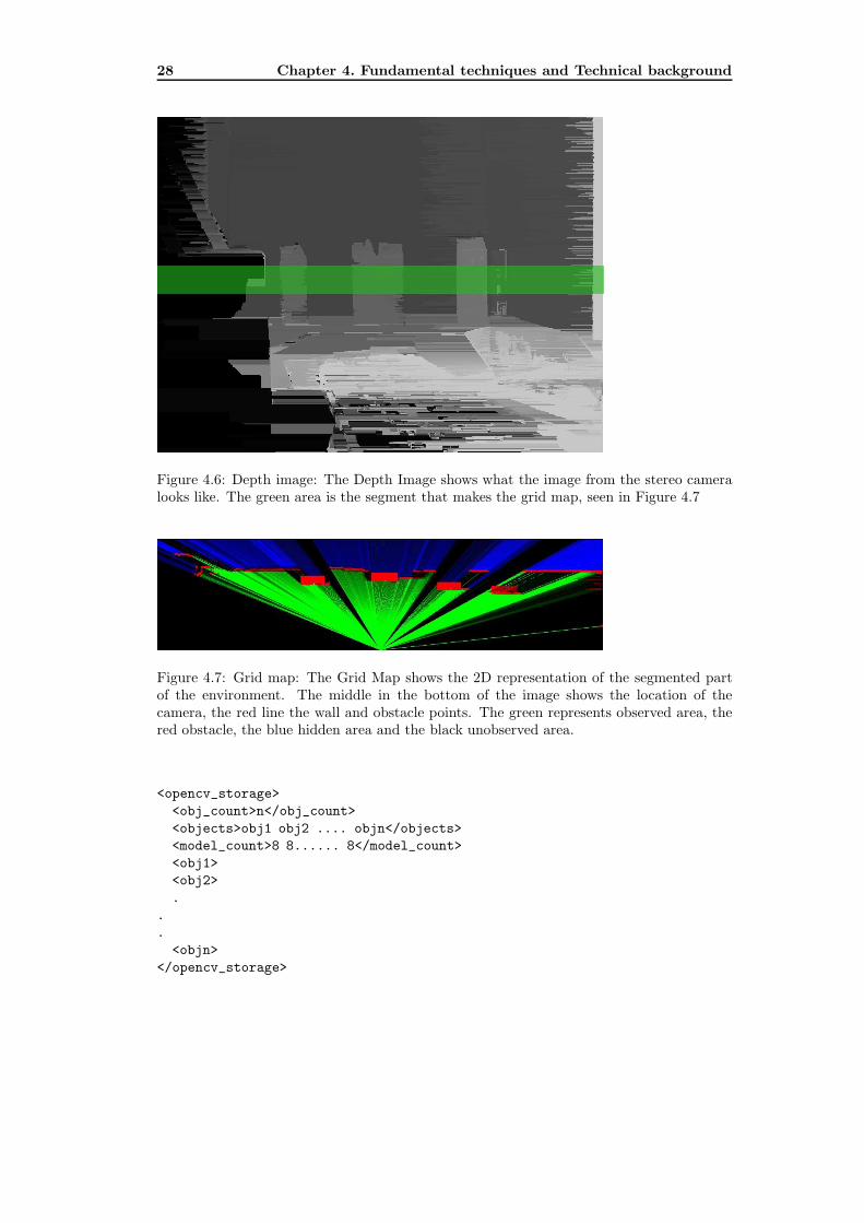
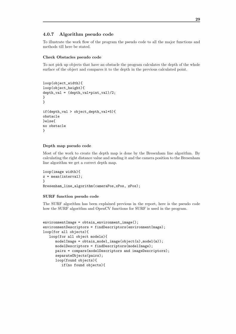
The Grid map is a map of a top view of the environment, it is made from one tenth ofthe full depth image, and this is represented by the green area in Figure 4.6. The reasonwhy it is one tenth is because we want to take a segment where our objects are and to geta good mean value and not only one point, this is to make the depth value more reliable.After finding a depth point in the depth image we mark this point on the grid map and usethe Bresenham’s line algorithm to draw the line from the camera to the point and mark itwith green color that means observer area, the point where the depth is we mark with redcolor and the line behind the point we mark blue for unobserved area, also called hiddenarea. Figure 4.7 is the grid map to the figure 4.6. The Figure 4.7 shows the found object onthe grid map. The grid map is built of the color system RGB. For every (x,y)-coordinate inthe grid map there are three values (R,G,B) and all have a range of 0-254.

– if(Rxy > Bxy&&Rxy > Gxy) then Obstacle

– if(Gxy > Rxy&&Gxy > Bxy) then Observed

– if(Bxy > Gxy&&Bxy > Rxy) then Hidden

– if(Rxy == 0&&Gxy == 0&&Bxy == 0)then unObserved

By following this rules we get what state that (x,y)-coordinate most probably is in. Thehigher difference between Rxy and Bxy the bigger probability that it is obstacle then hiddenarea.

4.0.6 Database XML

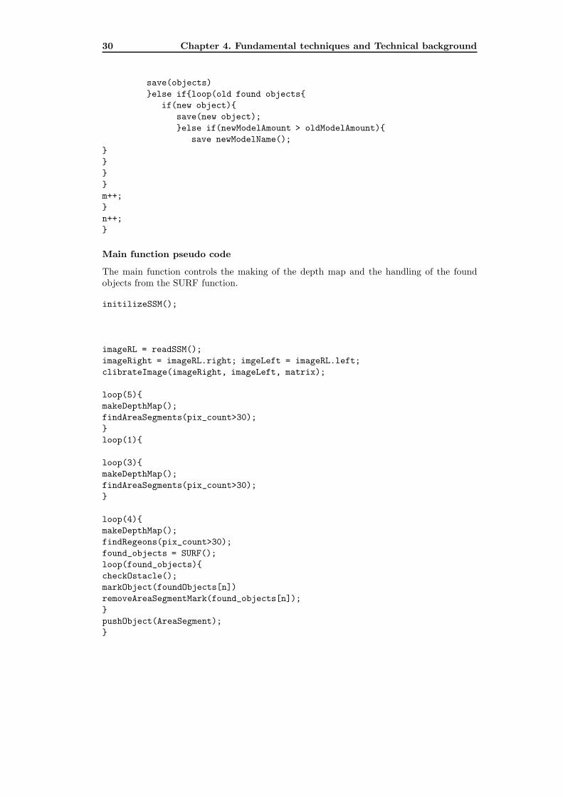
The XML database is build up by: how many different object there is, the name of theobjects, the count of models in the object and finally the name and location of the modelsfor the object.


Figure 4.6: Depth image: The Depth Image shows what the image from the stereo cameralooks like. The green area is the segment that makes the grid map, seen in Figure 4.7

Figure 4.7: Grid map: The Grid Map shows the 2D representation of the segmented partof the environment. The middle in the bottom of the image shows the location of thecamera, the red line the wall and obstacle points. The green represents observed area, thered obstacle, the blue hidden area and the black unobserved area.

<opencv_storage>

<obj_count>n</obj_count>

<objects>obj1 obj2 .... objn</objects>

<model_count>8 8...... 8</model_count>

<obj1>

<obj2>

.

.

.

<objn>

</opencv_storage>

29

4.0.7 Algorithm pseudo code

To illustrate the work flow of the program the pseudo code to all the major functions andmethods till here be stated.

Check Obstacles pseudo code

To not pick up objects that have an obstacle the program calculates the depth of the wholesurface of the object and compares it to the depth in the previous calculated point.

loop(object_width){

loop(object_height){

depth_val = (depth_val+pint_val)/2;

}

}

if(depth_val > object_depth_val+5){

obstacle

}else{

no obstacle

}

Depth map pseudo code

Most of the work to create the depth map is done by the Bresenham line algorithm. Bycalculating the right distance value and sending it and the camera position to the Bresenhamline algorithm we get a correct depth map.

loop(image width){

z = mean(interval);

}

Bresenham_line_algorithm(cameraPos,xPos, zPos);

SURF function pseudo code

The SURF algorithm has been explained previous in the report, here is the pseudo codehow the SURF algorithm and OpenCV functions for SURF is used in the program.

environmentImage = obtain_environment_image();

environmentDescriptors = findDescriptors(environmentImage);

loop(for all objects){

loop(for all object models){

modelImage = obtain_model_image(object(n),model(m));

modelDescriptors = findDescriptors(modelImage);

pairs = compare(modelDescriptors and imageDescriptors);

separateObjects(pairs);

loop(found objects){

if(no found objects){


save(objects)

}else if{loop(old found objects{

if(new object){

save(new object);

}else if(newModelAmount > oldModelAmount){

save newModelName();

}

}

}

}

m++;

}

n++;

}

Main function pseudo code

The main function controls the making of the depth map and the handling of the foundobjects from the SURF function.

initilizeSSM();

imageRL = readSSM();

imageRight = imageRL.right; imgeLeft = imageRL.left;

clibrateImage(imageRight, imageLeft, matrix);

loop(5){

makeDepthMap();

findAreaSegments(pix_count>30);

}

loop(1){

loop(3){

makeDepthMap();

findAreaSegments(pix_count>30);

}

loop(4){

makeDepthMap();

findRegeons(pix_count>30);

found_objects = SURF();

loop(found_objects){

checkOstacle();

markObject(foundObjects[n])

removeAreaSegmentMark(found_objects[n]);

}

pushObject(AreaSegment);

}

31

order = calculateRemoveOrder(objectsZPos);

loop(found_objects){

removeObject(found_objects[order[n]]);

}

}

Chapter 5

Results of multiple object

finding

The SURF algorithm and my method have been tested in multiple scenarios explained laterin this chapter, and the method has been tested in different light conditions such as daylight,evening, with extra background light and a dark environment with only indoor lights. Ithas clearly shown that the methods works and that it can find objects in hidden areas aswell as finding unrecognized known object by using the push method.

5.1 Evaluation of object finding

At first, I evaluated the SURF because the recognition result depends on the distance andangle between a camera and an object. It is necessary to clear the suitable experimentalcondition. I tested how it preforms when moving the object further away and closer to thecamera from its base position where the model was taken. I needed to test it by rotating itaround its own axis to find out when the object is no longer found.The algorithm also needs to be able to find multiple objects and multiple of the same objecttype.

5.1.1 Evaluation of distance and rotation

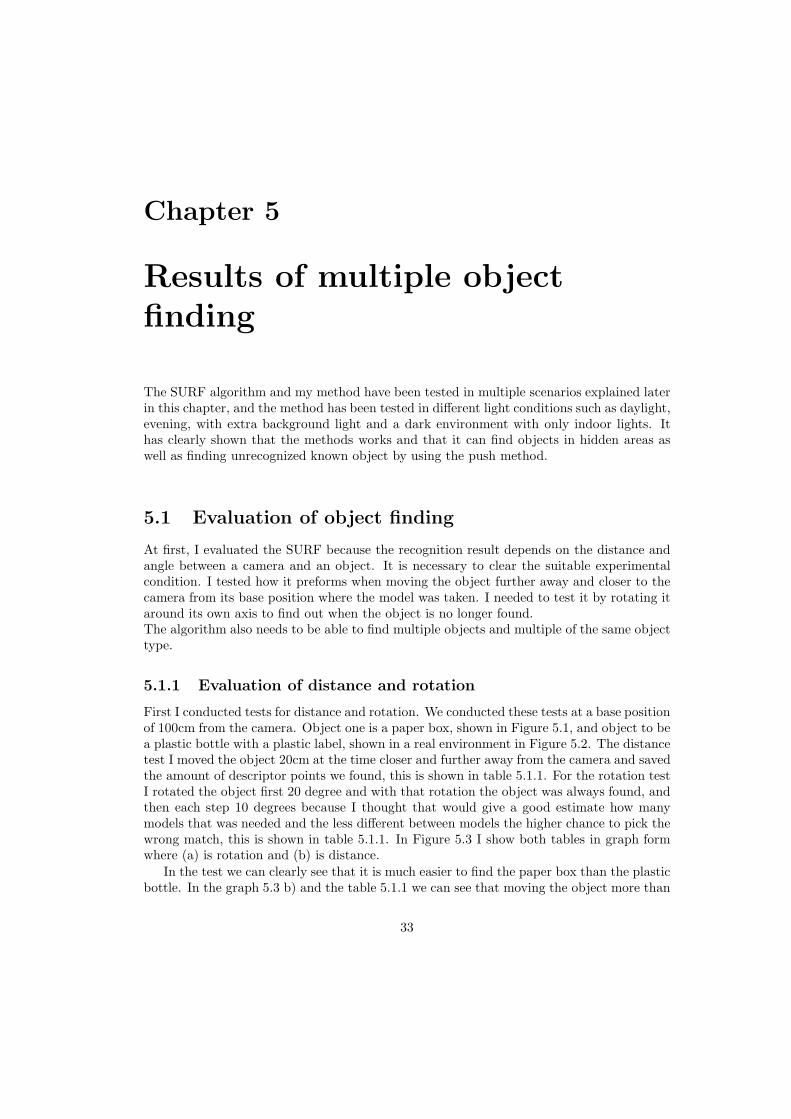
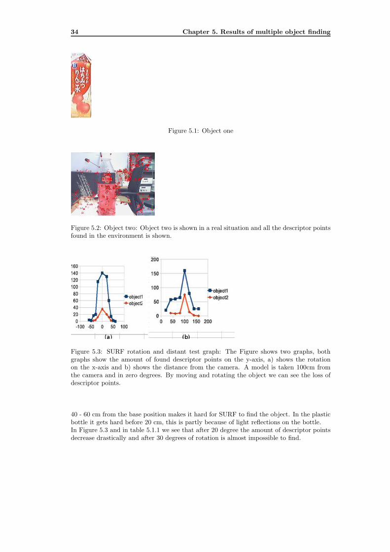
First I conducted tests for distance and rotation. We conducted these tests at a base positionof 100cm from the camera. Object one is a paper box, shown in Figure 5.1, and object to bea plastic bottle with a plastic label, shown in a real environment in Figure 5.2. The distancetest I moved the object 20cm at the time closer and further away from the camera and savedthe amount of descriptor points we found, this is shown in table 5.1.1. For the rotation testI rotated the object first 20 degree and with that rotation the object was always found, andthen each step 10 degrees because I thought that would give a good estimate how manymodels that was needed and the less different between models the higher chance to pick thewrong match, this is shown in table 5.1.1. In Figure 5.3 I show both tables in graph formwhere (a) is rotation and (b) is distance.

In the test we can clearly see that it is much easier to find the paper box than the plasticbottle. In the graph 5.3 b) and the table 5.1.1 we can see that moving the object more than

33

34 Chapter 5. Results of multiple object finding

Figure 5.1: Object one

Figure 5.2: Object two: Object two is shown in a real situation and all the descriptor pointsfound in the environment is shown.

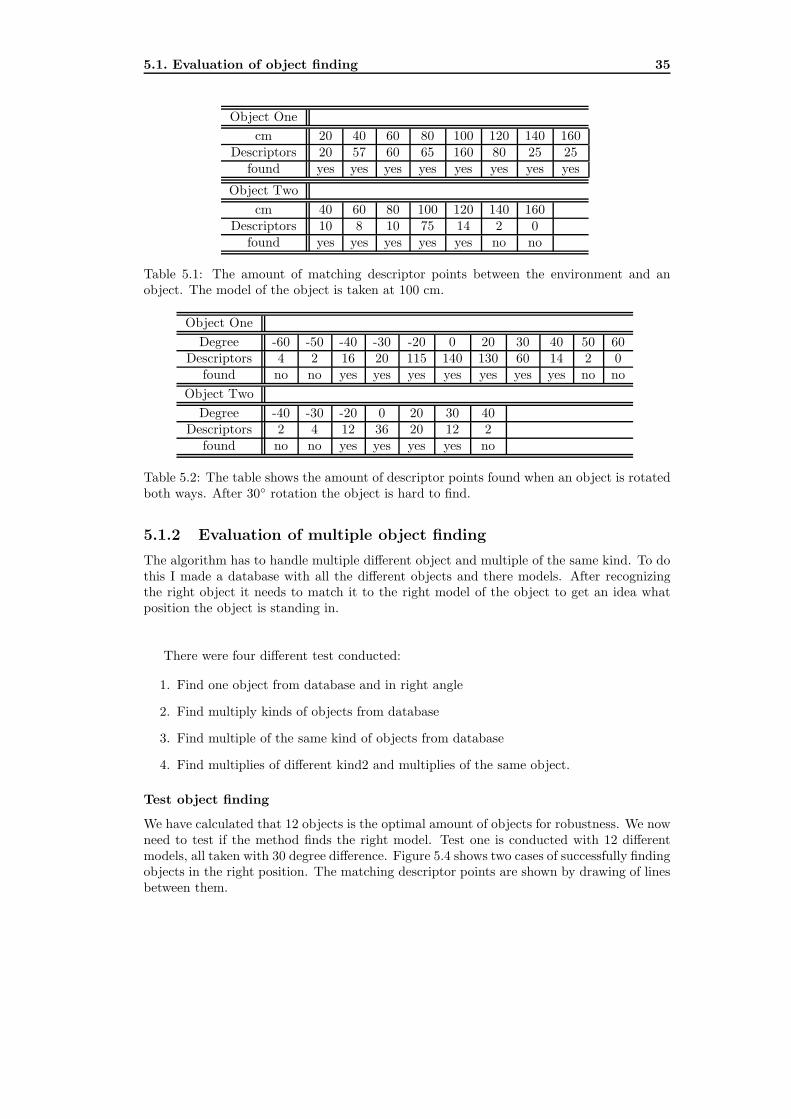
Figure 5.3: SURF rotation and distant test graph: The Figure shows two graphs, bothgraphs show the amount of found descriptor points on the y-axis, a) shows the rotationon the x-axis and b) shows the distance from the camera. A model is taken 100cm fromthe camera and in zero degrees. By moving and rotating the object we can see the loss ofdescriptor points.

40 - 60 cm from the base position makes it hard for SURF to find the object. In the plasticbottle it gets hard before 20 cm, this is partly because of light reflections on the bottle.In Figure 5.3 and in table 5.1.1 we see that after 20 degree the amount of descriptor pointsdecrease drastically and after 30 degrees of rotation is almost impossible to find.

5.1. Evaluation of object finding 35

Object One

cm 20 40 60 80 100 120 140 160Descriptors 20 57 60 65 160 80 25 25

found yes yes yes yes yes yes yes yes

Object Two

cm 40 60 80 100 120 140 160Descriptors 10 8 10 75 14 2 0

found yes yes yes yes yes no no

Table 5.1: The amount of matching descriptor points between the environment and anobject. The model of the object is taken at 100 cm.

Object One

Degree -60 -50 -40 -30 -20 0 20 30 40 50 60Descriptors 4 2 16 20 115 140 130 60 14 2 0

found no no yes yes yes yes yes yes yes no no

Object Two

Degree -40 -30 -20 0 20 30 40Descriptors 2 4 12 36 20 12 2

found no no yes yes yes yes no

Table 5.2: The table shows the amount of descriptor points found when an object is rotatedboth ways. After 30◦ rotation the object is hard to find.

5.1.2 Evaluation of multiple object finding

The algorithm has to handle multiple different object and multiple of the same kind. To dothis I made a database with all the different objects and there models. After recognizingthe right object it needs to match it to the right model of the object to get an idea whatposition the object is standing in.

There were four different test conducted:

1. Find one object from database and in right angle

2. Find multiply kinds of objects from database

3. Find multiple of the same kind of objects from database

4. Find multiplies of different kind2 and multiplies of the same object.

Test object finding

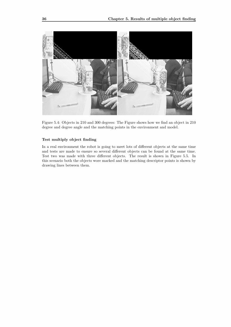
We have calculated that 12 objects is the optimal amount of objects for robustness. We nowneed to test if the method finds the right model. Test one is conducted with 12 differentmodels, all taken with 30 degree difference. Figure 5.4 shows two cases of successfully findingobjects in the right position. The matching descriptor points are shown by drawing of linesbetween them.


Figure 5.4: Objects in 210 and 300 degrees: The Figure shows how we find an object in 210degree and degree angle and the matching points in the environment and model.

Test multiply object finding

In a real environment the robot is going to meet lots of different objects at the same timeand tests are made to ensure so several different objects can be found at the same time.Test two was made with three different objects. The result is shown in Figure 5.5. Inthis scenario both the objects wore marked and the matching descriptor points is shown bydrawing lines between them.

5.2. Evaluating SURF robustness vs. speed 37

Figure 5.5: Two different objects: The Figure shows how we find two different objects andthe matching points in the environment and model.

Test multiply of same kind object finding

The third test was about finding more than one of the same objects. In a scenario likea robot going shopping it needs to separate several objects of the same kind. The SURF

algorithm can only find matching points in the image, not separate them if they belong todifferent objects of the same kind. This does not only mean that it makes several objects into on but also that it could match it with the wrong model. The system had to arrange thedifferent found descriptor points to the right object. This was done by moving every pointto the upper right corner of the object in the 1024x780 pixel sized environment and thenchecks if the points wore in the same 30x30 pixel box. Here was also important to matchthe found object to the right model. Figure 5.6 shows the results of finding two of the sameobject.

Test to find multiply objects and of the same kind

The fourth test was about mixing the third and the second. The result is shown in Figure5.7.In this scenario both the objects wore marked and the matching descriptor points isshown by drawing lines between them.

5.2 Evaluating SURF robustness vs. speed

The SURF algorithm has an parameter with four different levels that controls the limit ofmaximum amount of descriptor points it shall find. To decide what level was best for this


Figure 5.6: Two of the same object: In the Figure we can see the algorithm separating twoof the same object and the matching descriptor points and marking them

research several test was conducted, and results from this tests can be seen in Figure 5.8and 5.9.Figure 5.8 shows us a graph there the x-axis is the amount of models in the database andthe y-axis a log(ms) time axis.We see in Figure 5.8 that from level 3 with 2000 points to level 4 with 12000 points the timeincrease drastically. In Figure 5.9 we have conducted a test with 5 objects to see how manyobjects each level finds, we see that the different between level 4 and level 3 is small, but thedifferent between level 3 and level 2 is big. The result of the big increase in calculation timefrom level 3 to 4 and the small recognition difference and the small increase in calculationtime and big difference in recognition between level 2 and 3, we chose that level 3 is thebest parameter for us.

It takes about 1 sec to calculate the environment and then another 1 sec for every 8 models,including the pairing of descriptor points. The depth map takes about 1,7 sec to calculateeach time. This shows that it is impossible right now to replace a robot to do a human tasklike shopping. The calculation time depends on the size of the model images and the sizethat was used here was between 2 and 4 kb.

5.3 Evaluation of obstacle detection and improve local-

ization by touch

The last test was of several things. First was to check if there was anything in front ofthe object, this is important because the robot might take the object out of a shelf andthen there can be something in front. This was done by calculating the depth value ofthe object and then compare it to the previous calculated area of the smaller area and if

5.3. Evaluation of obstacle detection and improve localization by touch 39

Figure 5.7: Three objects, two same and one different: Two of the same object: In the Figurewe can see the algorithm separating two of the same object and the matching descriptorpoints and marking them

Figure 5.8: Timetable of model robustness: The figure shows how the time increases withthe amount of models. On the y-axis is the time and the x-axis is the amount of models.The four different lines represent four different values on a parameter in SURF that decideshow much descriptor point is the maximum amount. The more descriptor points the higherchance of finding the object and the more time consuming.

newval > oldval + 5 we say that there is an obstacle.

Second was how to prioritize the order to remove the objects, this is done by takingthe one closest to the camera first. This minimizes the risk of hitting any object since thearm is going to be mounted close to the camera. I also implemented a feed back to theremove method that say how many of the objects that was removed, this is later on goingto come from the manipulator but right now we write it by hand. This is to remove theright markings on the depth map and to not lose the count of objects if the method requiresthat information. This can be in a case of a service robot that knows the amount of object


Figure 5.9: Depth image to grid map: The figure shows a medium value how many objectsthe SURF algorithm finds out of 5 objects. The four different columns represent fourdifferent values on a parameter in SURF that decides how many descriptor points is themaximum amount.

Figure 5.10: Obstacle calculation area: To check for obstacles the red area is calculatedwhere the most descriptor points are. The green area is calculated on the full object. Thesetwo are later compared to see if there is a big difference and there by an obstacle.

it has in the fridge.

The third thing was to improve the chance to find objects that it knows but not rec-ognized. To do this we had to segment the grid map, as shown in Figure 5.11 the circlesrepresent unknown segments, after the segmentation we ignored the segments there we al-ready found an object. By leaving the segments where we have not recognized any objectswe can use a manipulator that is pressure sensitive, and by pushing softly on the object wecan determine if the object is movable and if it is we can change its angle to improve thechance of finding an unidentified object. The push motion now is done by hand since we do

5.4. Evaluating method of finding objects in hidden area 41

not have a manipulator. In chapter 2.2 I talk about a method to do this.

Figure 5.11: Segmentation map: The map is the same as the Grid map but with differentinformation, this map shows where the algorithm has found segments where there might bean object. The map also ignores places where it already found an object.

5.4 Evaluating method of finding objects in hidden area

The tests to evaluate the method are made from three different objects. Most of the testswere conducted in a room with normal indoor light and a cloudy light from outside. Thetest shows the success of the push method if the known object is not located.The sets are built in steps, every step is either to remove an object Figure 5.12, or to rotatean object by the push method, Figure 5.13. The path of every step is shown it the flowchart in Figure 3.4.

Figure 5.14 shows three different scenarios: a) is a scenario with five objects, shownin Figure 5.15 a), no hidden objects but one that is unrecognized before push methodand recognized after. This is an exmple on when we are looking for something in therefridgerators door. b) is a scenario with six objects, the basic setup is shown in Figure5.15 b), 3 hidden and all recognized without a problem. c) is a scenario with six objects,the basic setup is shown in Figure 5.15 b), three hidden and one in the back that is notrecognized at first but after the push method all objects are recognized. The work flow ofthis scenario is shown in Figure 5.16, where each image represent a step in the last graph inFigure 5.14. We see that in each image there is a object removed except in six and eight. Insix there is a unidentified object and in this step all segments get pushed and in step sevenwe find and remove the new found object. In step eight we push all found segments butno new objects is found. I think this is the most interesting scenario because I believe thatthis is as close to reality we can get. But the result of the test shows us that it is possibleto find all known objects in a environment for example a refrigerator.Several other tests was made but showed the same result. Sometime the SURF algorithmfinds points where there is no object but a point that reminds it of one of the object, butthis point is often not find twice. Also in quit poor light conditions this method works well.


Figure 5.12: Removing object: The figure shows one of the steps, this one is removing anobject from the scene.

Figure 5.13: Rotation object: The figure shows one of the steps, this one is rotating theobject slightly.

5.4. Evaluating method of finding objects in hidden area 43

Figure 5.14: Different scenarios: The figure shows 3 different scenarios. The x-axis representsevery step and the y-axis the amount of objects. In scenario: a) we see five different objectsfrom the start and the algorithm finds 4 and then uses the push method to find the fifth,b) shows six objects from the start where three of those are hidden, it removes one by oneuntil there is none left, c) shows same as b, but it dose not find one of the hidden until ituses the push method.

Figure 5.15: Scenario setup: The figure shows in a) the experimental setup for scenario onein Figure 5.14 and b) the setup in scenario 2 and 3


Figure 5.16: Scenario 3 work process: This Figure shows the work flow of scenario 3. Fromall objects existing to step six where an object is not recognized and gets pushed and thenfound and removed in step 7. In step eight the found segments are found and pushed butno objects are found.

Chapter 6

Conclusions

The method clearly shows that it can find multiply objects of the same kind and alsomultiply objects of different kind. It also show that it can find objects located in hiddenareas and detect obstacles.

6.1 Limitations

The algorithm does not support objects that stand different then the model, it can onlyhandle standing objects if the model is taken standing.

6.2 Future work

Future work is to implement the manipulator , to grab the object to be removed and toimplement the pushing motion.

45

46 Chapter 6. Conclusions

Chapter 7

Acknowledgments

First I like to thank professor Tadokoro to let me stay in his laboratory in Tohoku University.I also like to thank my internal mentor Ohno-Sensei, and my external supervisor at UmeAUniversity, Per LindstrA¶m. Finally I like to thank my mentor at Tohoku Univcersity,Hata-San.

47

48 Chapter 7. Acknowledgments

References

[1] Hyojoo Son , Changwan Kim , Kwangnam Choi . Rapid 3D object detection and mod-eling using range data from 3D range imaging camera for heavy equipment operation.

[2] Intel. Integrated Performance Primitives. http://software.intel.com/en-us/intel-ipp/(visited 2010-06-16).

[3] M. Okutomi and T. Kanade. A multiple-baseline stereo. In IEEE Transactions on

Pattern Analysis and Machine Intelligence, Vol. 15, No. 4, pages 53 – 363.

[4] Masamitsu Kurisu, Tsuneo Yoshikawa. Tracking control for an object in pushing op-eration. In I Journal of Robotic Systems, Volume 14 Issue 10, pages 729 –739.

[5] MESA Imaging AG. MESA Imaging AG. http://www.mesa-imaging.ch/index.php(visited 2010-06-16).

[6] OpenCV. OpenCV Home page. http://opencv.willowgarage.com/wiki/(visited 2010-06-16).

[7] Seungjin Lee, KwanhoKim,Joo-YoungKim,MinsuKim,Hoi-JunYoo. Familiarity basedunified visual attention model for fast and robust object recognition.

[8] Sukhan Lee, Seongsoo Lee, Jeihun Lee, Dongju Moon, Eunyoung Kim and JeonghyunSeo. Robust Recognition and Pose Estimation of 3D Objects Based on Evidence Fusionin a Sequence of Images.

[9] SURF. SURF Home page. http://www.vision.ee.ethz.ch/ surf/(visited 2010-06-16).

[10] Yutaka Hirano, Ken-ichi Kitahama, Shintaro Yoshizawa Toyota Motor Corporation.Image-based object recognition and dexterous hand/arm motion planning using rrts forgrasping in cluttered scene. Technical report, tec.toyota.co.jp, 1200, Mishuku, Susono,Shizuoka, 410-1193 JAPAN, 2005.

[11] Z. Lin, J. Jin, H. Talbot. Unseeded region growing for 3D image segmentation. In Proc.

VIP 2000, CRPIT, Sydney, 2000, pages 31 –37.

49

50 REFERENCES

Appendix A

Source Code

51

model based object ﬁnding in occluded cluttered environments

Documents