modelin nd ana lysis

8/22/2019 Modelin Nd Ana Lysis

http://slidepdf.com/reader/full/modelin-nd-ana-lysis 1/9

Modeling And Analysis of Simple Open Cycle Gas

Turbine Using Graph NetworksNaresh Yadav, I.A. Khan, and Sandeep Grover

Abstract —This paper presents a unified approach based graphtheory and system theory postulates for the modeling and analysisof Simple open cycle Gas turbine system. In the present paper, thesimple open cycle gas turbine system has been modeled up to its sub-system level and system variables have been identified to develop theprocess subgraphs. The theorems and algorithms of the graph theoryhave been used to represent behavioural properties of the system likerate of heat and work transfers rates, pressure drops and temperaturedrops in the involved processes of the system. The processes havebeen represented as edges of the process subgraphs and their limitsas the vertices of the process subgraphs. The system across variablesand through variables has been used to develop terminal equations of the process subgraphs of the system. The set of equations developedfor vertices and edges of network graph are used to solve the systemfor its process variables.

Keywords—Simple open cycle gas turbine, Graph theoretic ap-proach, process subgraphs, gas turbines system modeling, systemtheory

I. INTRODUCTION

V

arious efforts have been done in the past for developing

the mathematical model of the simple gas turbine sys-tems keeping into consideration the desired outcomes i.e. type

of applications, work outputs and the optimized conditions

for achieving maximum thermal efficiency and the component

efficiencies with in the system. Irrespective to the type of

application, during the modeling and analysis of simple cycle

gas turbines, the parameters related to system elements like

compressor, combustor and the turbines etc. are matched for

their peak performances to achieve their maximum efficiency

[1] in the integrated system. Therefore, these parameters are

interlinked for the attainment of objectives like high thermal

efficiency, low specific fuel consumption or high thrust [2] etc.

based on the type of applications.

It is worth to mention here that once the preliminary designconstraints like type of application, type of Turbo-machineries

to be used, operating conditions and the business objectives,

attention is focused on the thermodynamic evaluation [3]

of the gas turbine components and subsequently the aero-

thermal and mechanical design constraints [4] are resolved

for peaking thermal efficiency. New and advanced materials

are to be developed for matching better performance at high

firing temperatures. Therefore, the thermodynamic modeling

Naresh Yadav is Research scholar in Mechanical Engineering Departmentof Jamia Millia Islamia University, New Delhi, India (phone: 91-129-2242143,fax: 91-129-2242143; e-mail: nareshyadav5@ gmail.com).

Dr. I.A. Khan is Professor in Mechanical Engineering Department, Jamia

Millia Islamia University, New Delhi, India and Dr. Sandeep Grover is Profes-sor & Chairman in Mechanical Engineering Department, YMCA Universityof Science and Technology, Faridabad, India.

[5] of the simple gas turbine system is the most important

issue in the design of gas turbine systems. Since such devel-

opments encourage the researchers to achieve higher thermal

efficiencies within the realistic constraints [6], the advanced

gas turbine systems have been modeled and analyzed [7] for

power generation applications. The market leaders [8] and

the premier consultants [9]- [10] in the area of gas turbines

have provided an exhaustive database for the performanceevaluation of gas turbine systems including the effect of its

operating parameters on the gas turbine system performance.

Over the past few years, the simplicity in the algorithms

of interdisciplinary approaches have attracted the researchers

and scientists for system alternative representations and their

subsequent solutions for better understanding, user friendly

and precise decision making in the operating environment. The

interactive software [11] for Simple Cycle gas Turbine perfor-

mance for typical aircraft application has also been developed.

Various thermal system elements have been modeled [12]

using graph theoretic approach for thermodynamic evaluation

of thermal- hydraulic systems. Similarly, efforts have be done

for the formulation of several other engineering systems [13]and has been successfully implemented for the modeling and

analysis of some typical engineering systems [14] like truss

structures, gear trains etc.. The present work also aims at

implementation of system theory postulates and graph network

theory for formulation and analysis of simple open cycle gas

turbine system with validation through first law and second

law of thermodynamics.

II. WORKING OF SIMPLE OPEN CYCLE GAS

TURBINE

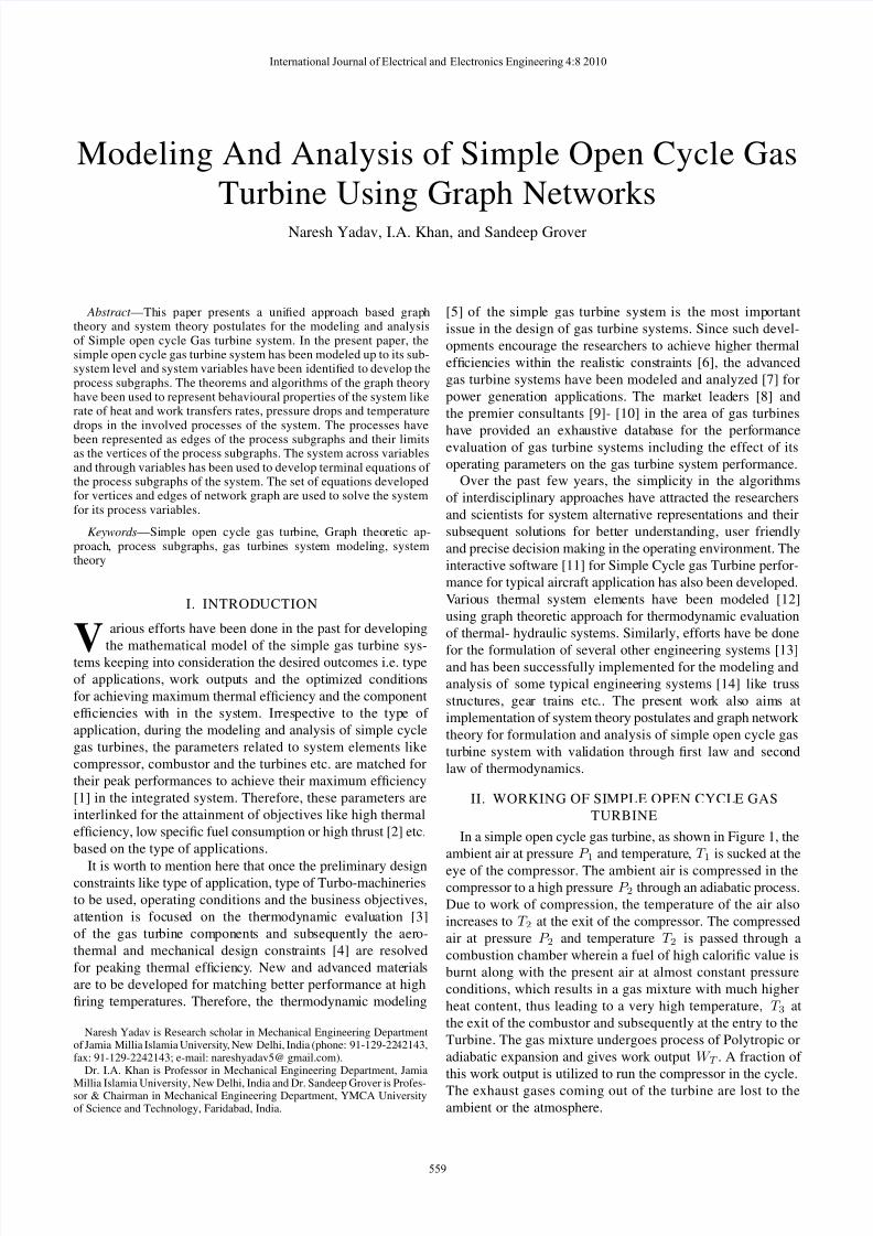
In a simple open cycle gas turbine, as shown in Figure 1, the

ambient air at pressure P 1 and temperature, T 1 is sucked at the

eye of the compressor. The ambient air is compressed in thecompressor to a high pressure P 2 through an adiabatic process.

Due to work of compression, the temperature of the air also

increases to T 2 at the exit of the compressor. The compressed

air at pressure P 2 and temperature T 2 is passed through a

combustion chamber wherein a fuel of high calorific value is

burnt along with the present air at almost constant pressure

conditions, which results in a gas mixture with much higher

heat content, thus leading to a very high temperature, T 3 at

the exit of the combustor and subsequently at the entry to the

Turbine. The gas mixture undergoes process of Polytropic or

adiabatic expansion and gives work output W T . A fraction of

this work output is utilized to run the compressor in the cycle.

The exhaust gases coming out of the turbine are lost to the

ambient or the atmosphere.

International Journal of Electrical and Electronics Engineering 4:8 2010

559



Fig. 1. Simple cycle gas turbine

Since, this is a direct heat loss, it is desirable to keep the

temperature and thus heat content of the exhaust of the turbine

to a minimum for efficient open cycle gas turbine system.

In open cycle gas turbine, for every stage of heat or work

transfer, various losses are also involved with in the system.

In actual open cycle gas turbine, the compression process inthe compressor and the expansion process in the turbine are

never ideal to be called as adiabatic processes but in fact are

better represented as polytropic. More work is to be done

on the compressor to drive it and a lesser work output is

achieved from the turbine as a result of polytropic expansion.

Similarly, in the combustor, the mixing of two streams i.e. hot

compressed air and gaseous fuel do not take place at constant

pressure. As a result of the above major accountable losses, the

thermal efficiency as well as specific work output is affected

significantly.

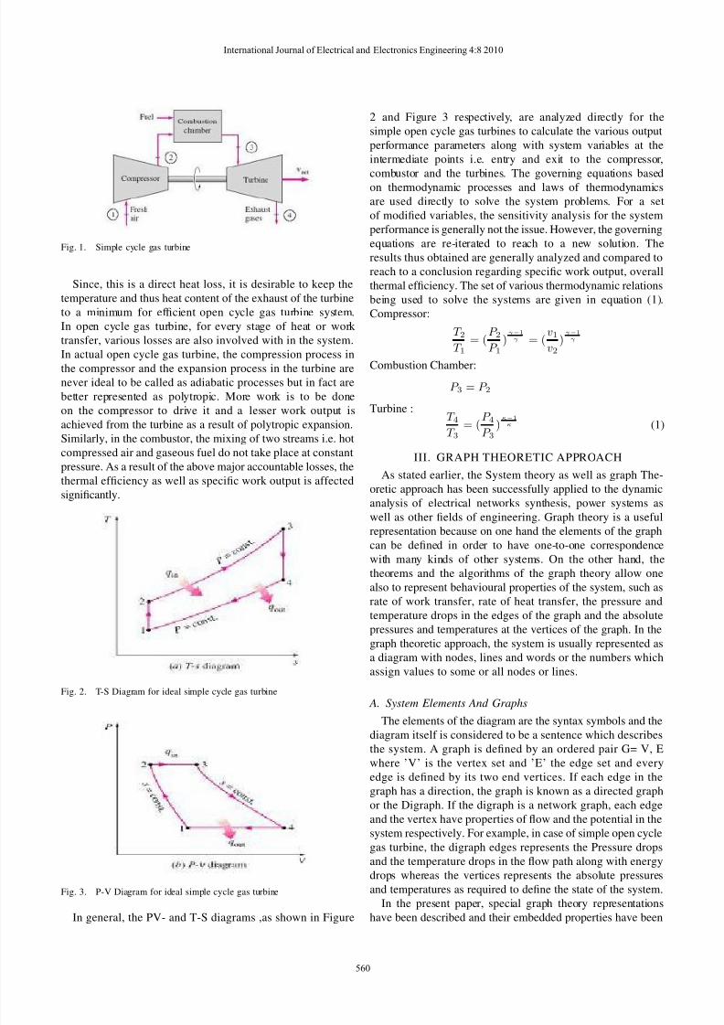
Fig. 2. T-S Diagram for ideal simple cycle gas turbine

Fig. 3. P-V Diagram for ideal simple cycle gas turbine

In general, the PV- and T-S diagrams ,as shown in Figure

2 and Figure 3 respectively, are analyzed directly for the

simple open cycle gas turbines to calculate the various output

performance parameters along with system variables at the

intermediate points i.e. entry and exit to the compressor,

combustor and the turbines. The governing equations based

on thermodynamic processes and laws of thermodynamics

are used directly to solve the system problems. For a set

of modified variables, the sensitivity analysis for the system

performance is generally not the issue. However, the governing

equations are re-iterated to reach to a new solution. The

results thus obtained are generally analyzed and compared to

reach to a conclusion regarding specific work output, overall

thermal efficiency. The set of various thermodynamic relations

being used to solve the systems are given in equation (1).

Compressor:

T 2

T 1= (P 2

P 1)γ−1

γ = (v1

v2)γ−1

γ

Combustion Chamber:

P 3 = P 2

Turbine :T 4

T 3= (P 4

P 3)κ−1κ (1)

III. GRAPH THEORETIC APPROACH

As stated earlier, the System theory as well as graph The-

oretic approach has been successfully applied to the dynamic

analysis of electrical networks synthesis, power systems as

well as other fields of engineering. Graph theory is a useful

representation because on one hand the elements of the graph

can be defined in order to have one-to-one correspondence

with many kinds of other systems. On the other hand, the

theorems and the algorithms of the graph theory allow one

also to represent behavioural properties of the system, such as

rate of work transfer, rate of heat transfer, the pressure and

temperature drops in the edges of the graph and the absolute

pressures and temperatures at the vertices of the graph. In the

graph theoretic approach, the system is usually represented as

a diagram with nodes, lines and words or the numbers which

assign values to some or all nodes or lines.

A. System Elements And Graphs

The elements of the diagram are the syntax symbols and thediagram itself is considered to be a sentence which describes

the system. A graph is defined by an ordered pair G= V, E

where ’V’ is the vertex set and ’E’ the edge set and every

edge is defined by its two end vertices. If each edge in the

graph has a direction, the graph is known as a directed graph

or the Digraph. If the digraph is a network graph, each edge

and the vertex have properties of flow and the potential in the

system respectively. For example, in case of simple open cycle

gas turbine, the digraph edges represents the Pressure drops

and the temperature drops in the flow path along with energy

drops whereas the vertices represents the absolute pressures

and temperatures as required to define the state of the system.

In the present paper, special graph theory representations

have been described and their embedded properties have been


560



used to model and analyze the Simple open cycle gas turbine.

Central to understanding these graphs are particular type of

graph called a tree. A tree is a connected graph with no circuits

or loops. The relation between the number of vertices ’v’ and

edges ’e’ of a tree are fixed as given by equation (2).

i.e.

e(T ) = v(T )− 1 (2)

and there is only one and only one path between any two

different vertices. A spanning tree is a subgraph of graph ’G’

witch is a tree and which includes all the vertices of ’G’ but

only a subset of the edges. The edges of the tree are called

branches, and the edges not in the spanning tree are called

chords.

B. Graph Representation Conventions

For convenience, this paper uses a line type attribute for the

representation of flow paths or the thermodynamic processes.A solid line has been represented for an edge with an unknown

value of the flow or the potential drops in terms or pressures

and temperatures. A dashed line is a chord which is an edge

not included in the spanning tree but forms the graph. When

a graph G is represented, it is possible to tell which edges

or the branches are incident at which nodes or the vertices

and what the orientations relative to the vertices are. The most

convenient way in which this incident information can be given

is in a matrix form. For a graph ’G’ with ’n’ vertices and ’b’

edges or branches, the complete incident matrix A = ahk is a

rectangular matrix of order ’n x b’ whose elements have the

values given by equation (3).

ahk =

⎧⎪⎪⎨⎪⎪⎩

1 if edge k is associated with vertex h andoriented away from vertex h

−1 if edge k is associated with vertex h andoriented towards vertex h

0 k is not associated with vertex h(3)

Any one row of the complete incident matrix can be ob-

tained by the algebraic manipulation of other rows, indicating

that the rows are not independent. Thus, by eliminating one

of the rows, the incident matrix is reduced to a reduced

incident matrix with rank as ’n-1’ and its size as ’n-1 x b’.

This reduced incident matrix is generally used to solve the

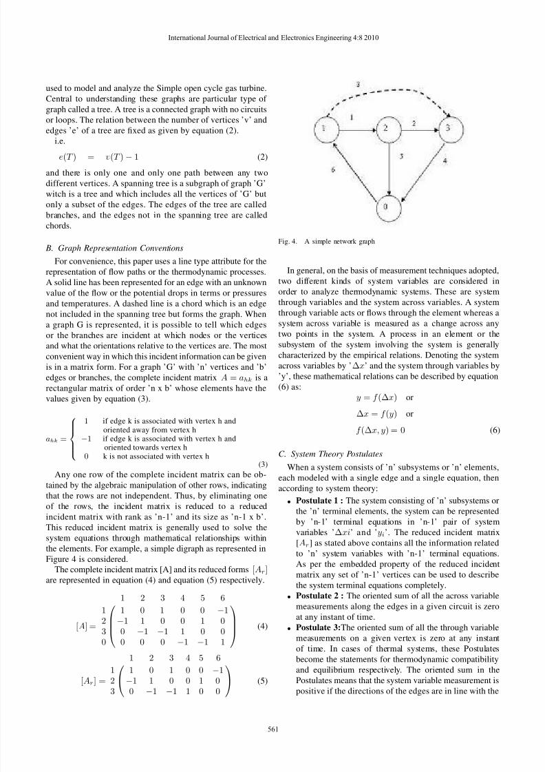
system equations through mathematical relationships withinthe elements. For example, a simple digraph as represented in

Figure 4 is considered.

The complete incident matrix [A] and its reduced forms [Ar]are represented in equation (4) and equation (5) respectively.

[A] =

⎛⎜⎜⎝

1 2 3 4 5 6

1 1 0 1 0 0 −12 −1 1 0 0 1 03 0 −1 −1 1 0 00 0 0 0 −1 −1 1

⎞⎟⎟⎠ (4)

[Ar] =⎛⎝

1 2 3 4 5 6

1 1 0 1 0 0 −12 −1 1 0 0 1 03 0 −1 −1 1 0 0

⎞⎠ (5)

Fig. 4. A simple network graph

In general, on the basis of measurement techniques adopted,two different kinds of system variables are considered in

order to analyze thermodynamic systems. These are system

through variables and the system across variables. A system

through variable acts or flows through the element whereas a

system across variable is measured as a change across any

two points in the system. A process in an element or the

subsystem of the system involving the system is generally

characterized by the empirical relations. Denoting the system

across variables by ’Δx’ and the system through variables by

’y’, these mathematical relations can be described by equation

(6) as:

y = f (Δx) or

Δx = f (y) or

f (Δx, y) = 0 (6)

C. System Theory Postulates

When a system consists of ’n’ subsystems or ’n’ elements,

each modeled with a single edge and a single equation, then

according to system theory:

• Postulate 1 : The system consisting of ’n’ subsystems or

the ’n’ terminal elements, the system can be represented

by ’n-1’ terminal equations in ’n-1’ pair of system

variables ’Δxi’ and ’yi’. The reduced incident matrix

[Ar] as stated above contains all the information relatedto ’n’ system variables with ’n-1’ terminal equations.

As per the embedded property of the reduced incident

matrix any set of ’n-1’ vertices can be used to describe

the system terminal equations completely.

• Postulate 2 : The oriented sum of all the across variable

measurements along the edges in a given circuit is zero

at any instant of time.

• Postulate 3:The oriented sum of all the through variable

measurements on a given vertex is zero at any instant

of time. In cases of thermal systems, these Postulates

become the statements for thermodynamic compatibility

and equilibrium respectively. The oriented sum in the

Postulates means that the system variable measurement is

positive if the directions of the edges are in line with the


561



conventions of the reduced incident matrix stated above.

According to Postulate 3, the vertex equations may be

stated by equation (7)as:

[Ar].[y] = 0 (7)

where notations have their usual meanings as mentioned

above. If ’x’ is a set of all system across variables mea-

sured at the vertices ’I’ relative to reference vertex then,

according to fundamental property of the reduced incident

matrix [Ar], the system across variable associated with

the edges of the graph ’G’ can be represented by equation

(8).

Δx = [Ar]T .[x] (8)

Then above equation can be considered as a statement of

the Postulate 2.

IV. METHODOLOGY

For such thermodynamic systems, the process graphs are

generally represented which define the behaviour of the ther-

modynamic system in respect of all kind of flows involved

in the process it is undergoing. The energy flows and energy

transformations can be represented in a unified manner along

with their interactions. This is achieved by modeling the

internal structure of the system as well as its sub-structure

(i.e. subsystems) using graph theory and the mathematical

relationships describing the behaviour of various elements of

the systems in terms of set of system measurable variables.

Following steps are generally followed for the analysis of such

systems:1) Identify the system variables for the simple open cycle

gas turbine which are sufficient to describe the physical

processes in the system.

2) In order to characterize such thermodynamic systems;

identify the subsystems or the elements up to the level

of the interaction stage with in the system. Develop the

terminal graphs which are self explanatory in terms of

system through and across variables.

3) Represent the energy transfers and energy transforma-

tions in the system elements in terms of their terminal

graphs with respect to the reference. Generally, in such

cases, the ambient conditions or the surrounding is

considered to be the reference for all kind of energytransfer rates.

4) Using linear graph theory, develop the associated ter-

minal graphs for the individual system through and

system across variables which may be termed as process

subgraphs for future reference.

5) verify the circuit Postulates and the vertex Postulates for

the associated terminal graphs i.e. process subgraphs.

Obtain the incident and reduced incidents matrices as

based on the principles linear graph theory.

6) Obtain the significant effects modeling related to work

and heat transfers i.e. WEMs (Work effect Models) and

EFMs (Energy Flow Models) in the system and at the

subsystem level, if any using the laws of thermodynam-

ics as applied to steady flow processes.

7) Obtain and solve the set of equations for the vertices

as well as on the edges of the process subgraphs

simultaneously for the set of unknown variables.

8) Calculate the dissipation along all the elements of the

simple open cycle gas turbine using governing equation

based on network theory.

9) The results thus obtained are to be verified using con-

ventional calculation procedures.

V. SIMPLE OPEN CYCLE GAS TURBINE

MODELING

A. System Variables

In case of a simple open cycle gas turbine, the three

main elements i.e. compressor, combustor and the turbine

connected in series along the flow constitute the system. Since

all the processes related to work and energy transfers are

associated with these elements only, hence these elements may

be considered to be the significant sub-systems of the system.

Even though, these sub-systems are connected to each other

with a set of insulated piping system which are responsible for

intermediate flow and energy transfers, yet in order to consider

the preliminary modeling stage their effect may be neglected

at present. While modeling the entire simple open cycle gas

turbine system in terms of system across variables and system

through variables responsible for complete description of the

system, it has summarily been analyzed that for the work

effect related to mass flow processes, the pressure of the

air flow represents itself the system across variable and the

volume or mass flow rate as the system through variable. While

for the energy flow processes in the system, the temperature

represents itself as the system across variable and the energy

flow rate as the system across variable with in the system.

The ambient or the surrounding is considered as reference for

calculating the changes in the across variable measurements

with in the system.

B. Terminal Elements of The System

While modeling the simple open cycle gas turbine system,

the system is represented into its elements and its terminals in

terms of rate of heat and work transfers over the sub-systems

and their terminals. In the present system, various terminals

have been represented across the different system elements

or the sub-systems and the directed edges have been shownfor energy transfer rates at various subsystems. The various

work and heat input rates with in the system are treated as

energy sources and sinks. The standard conventions have been

followed for the rate of heat and work transfers in the system

i.e. heat input to the system and work output from the system

as positive value while heat rejected from the system and

work done on the system as negative. In present system, since

work is to be done on the compressor and heat is rejected

to the surrounding or the ambient at the exit of the turbine,

hence these are negative while work output of the turbine

and heat input on account of fuel burning in the combustor

are considered to have positive values. In order to develop

the process subgraphs of the system, each element within the

system is replaced by its terminal graph


562



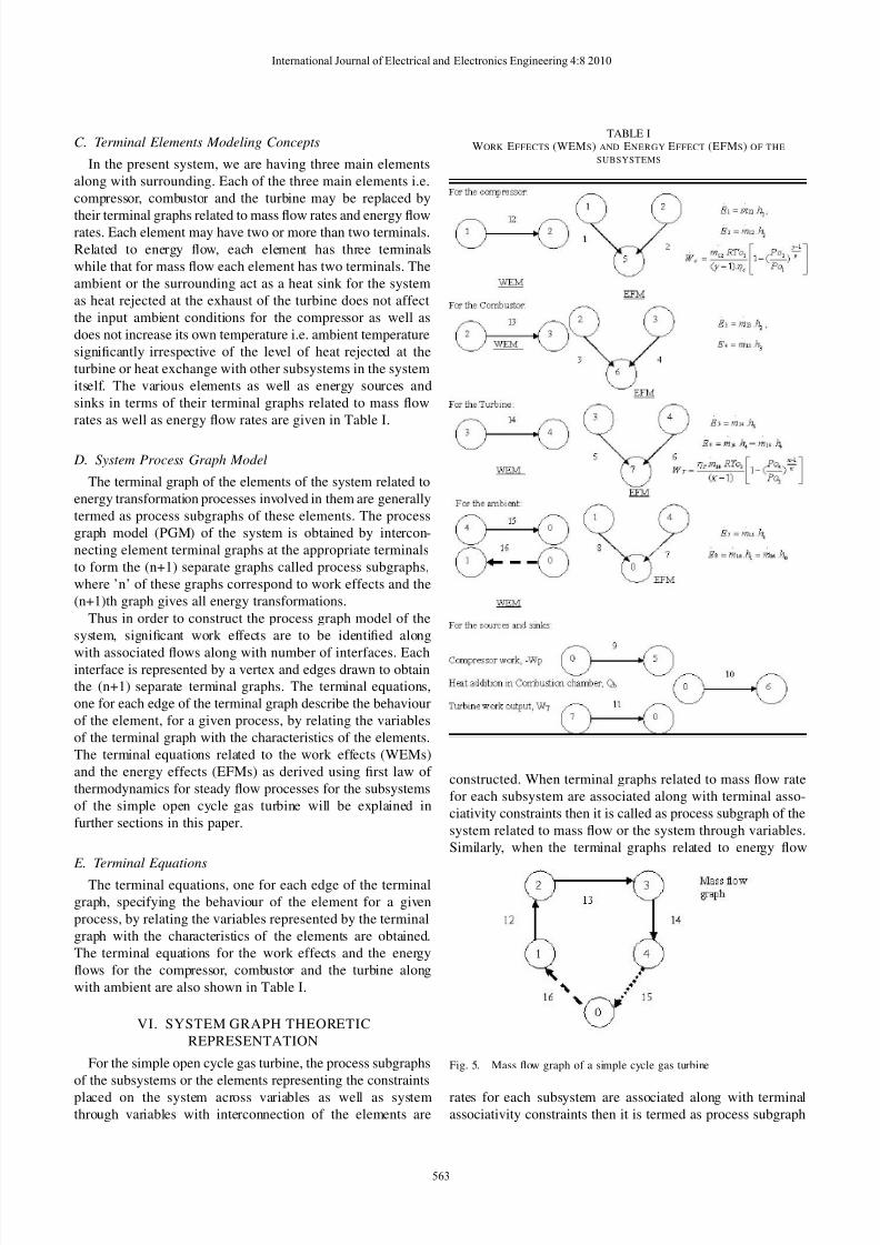
C. Terminal Elements Modeling Concepts

In the present system, we are having three main elements

along with surrounding. Each of the three main elements i.e.

compressor, combustor and the turbine may be replaced by

their terminal graphs related to mass flow rates and energy flowrates. Each element may have two or more than two terminals.

Related to energy flow, each element has three terminals

while that for mass flow each element has two terminals. The

ambient or the surrounding act as a heat sink for the system

as heat rejected at the exhaust of the turbine does not affect

the input ambient conditions for the compressor as well as

does not increase its own temperature i.e. ambient temperature

significantly irrespective of the level of heat rejected at the

turbine or heat exchange with other subsystems in the system

itself. The various elements as well as energy sources and

sinks in terms of their terminal graphs related to mass flow

rates as well as energy flow rates are given in Table I.

D. System Process Graph Model

The terminal graph of the elements of the system related to

energy transformation processes involved in them are generally

termed as process subgraphs of these elements. The process

graph model (PGM) of the system is obtained by intercon-

necting element terminal graphs at the appropriate terminals

to form the (n+1) separate graphs called process subgraphs,

where ’n’ of these graphs correspond to work effects and the

(n+1)th graph gives all energy transformations.

Thus in order to construct the process graph model of the

system, significant work effects are to be identified along

with associated flows along with number of interfaces. Eachinterface is represented by a vertex and edges drawn to obtain

the (n+1) separate terminal graphs. The terminal equations,

one for each edge of the terminal graph describe the behaviour

of the element, for a given process, by relating the variables

of the terminal graph with the characteristics of the elements.

The terminal equations related to the work effects (WEMs)

and the energy effects (EFMs) as derived using first law of

thermodynamics for steady flow processes for the subsystems

of the simple open cycle gas turbine will be explained in

further sections in this paper.

E. Terminal Equations

The terminal equations, one for each edge of the terminal

graph, specifying the behaviour of the element for a given

process, by relating the variables represented by the terminal

graph with the characteristics of the elements are obtained.

The terminal equations for the work effects and the energy

flows for the compressor, combustor and the turbine along

with ambient are also shown in Table I.

VI. SYSTEM GRAPH THEORETIC

REPRESENTATION

For the simple open cycle gas turbine, the process subgraphs

of the subsystems or the elements representing the constraints

placed on the system across variables as well as system

through variables with interconnection of the elements are

TABLE IWORK EFFECTS (WEMS) AND ENERGY EFFECT (EFMS) OF THE

SUBSYSTEMS

constructed. When terminal graphs related to mass flow rate

for each subsystem are associated along with terminal asso-

ciativity constraints then it is called as process subgraph of the

system related to mass flow or the system through variables.

Similarly, when the terminal graphs related to energy flow

Fig. 5. Mass flow graph of a simple cycle gas turbine

rates for each subsystem are associated along with terminal

associativity constraints then it is termed as process subgraph


563



of the system. In the present paper, the process subgraphs of

the simple open cycle gas turbine related to mass flow and

the energy flow are constructed using terminal flow graphs of

the subsystems given in Table I. The process flow graphs so

constructed for the simple open cycle gas turbine related to

mass flow and the energy flow rate are represented in Figure

5 and Figure 6 respectively.

Fig. 6. Energy flow graph of a simple cycle gas turbine

VII. SOLUTION

In reference to the number of equations required to solve

all the system across variables and system through variables,

the terminal equations associated with each element together

with the equation of the system as per the vertex Postulate and

the circuit Postulate are to be solved simultaneously. In order

to have a unique solution, the total number of independent

equations is to be equal to total number of variables in the

system. The stepwise solution of the simple open cycle gas

turbine through the establishment of relationship amongst

system theory, vertex postulate and the circuit postulates asbelow:

A. Developing The System Equations

In the case of Simple open cycle as turbine, it is worth

to mention that the emissions of the turbine are directly

discharges to the ambient atmosphere and the fresh air and

fuel are admitted to the Compressor and the Combustor re-

spectively. Since, the heat capacity of the ambient is generally

assumed to be very high as compared to other subsystems

in the cycle, the discharge of gas turbine to the ambient

effect the local temperature marginally and the intake of

the compressor takes place at the normal temperature of

the ambient irrespective of discharge temperature of the gas

turbine. Since, the cycle operates for a specified intake and

discharge volumes or masses of air and fuel, net mass transfer

to the system through its subsystems from the ambient and

vice-versa is taken as zero and the cycle is generally analyzed

for Steady Flow process assumptions. In the present case, from

the mass flow process graph, the corresponding Incident matrix

[A] is given by equation (9)as:

[A] =

⎛⎜⎜⎜⎜⎝

12 13 14 15 16

1 1 0 0 0 −12 −1 1 0 0 03 0 −1 1 0 04 0 0 −1 1 00 0 0 0 −1 1

⎞⎟⎟⎟⎟⎠

(9)

The corresponding reduced matrix [Ar] is obtained by elimi-

nating one of the row from the complete incident matrix [A].

Generally, the row for the ambient atmosphere is eliminated

to get the reduced incident matrix as the standard systems

through variables and across variables is known. Therefore,

the reduced Incident matrix [Ar] of the simple open cycle gas

turbine is given by equation (10)as:

[Ar] =

⎛⎜⎜⎝

12 13 14 15 16

1 1 0 0 0 −12 −1 1 0 0 03 0 −1 1 0 04 0 0 −1 1 0

⎞⎟⎟⎠ (10)

by multiplying the above reduced incident matrix [Ar] with a

vector of system through variable i.e. Mass flow rates through

the subsystems , we obtain the mathematical statement as

represented by equation (11) for the vertex postulates as:

⎛⎜⎜⎝

1 1 0 0 0 −12 −1 1 0 0 03 0 −1 1 0 04 0 0 −1 1 0

⎞⎟⎟⎠

⎛⎜⎜⎜⎜⎝

m12m13m14m15m16

⎞⎟⎟⎟⎟⎠

= 0 (11)

Since, for the mass flow process graph, the pressure, Poi,

is the system across variable measured at the vertices of the

system relative to the reference i.e. the ambient, then usingthe fundamental property of the reduced incident matrix as per

Vertex Postulate 2, the vector containing the pressure drops in

the subsystems is given by the equation (12) as:

⎛⎜⎜⎜⎜⎝

ΔPo12ΔPo13ΔPo14ΔPo15ΔPo16

⎞⎟⎟⎟⎟⎠

=

⎛⎜⎜⎜⎜⎝

1 −1 0 00 1 −1 00 0 1 −10 0 0 1−1 0 0 0

⎞⎟⎟⎟⎟⎠

⎛⎜⎜⎝Po1Po2Po3Po4

⎞⎟⎟⎠ (12)

Similarly, for the energy flow process graph, the incident

matrix , the reduced incident matrix and the corresponding

mathematical statement of the energy flow process graph as

per vertex postulate are given by equation (13), (14) and (15)

respectively.

[A] =

⎛⎜⎜⎜⎜⎜⎜⎝

1 2 3 4 5 6 7 8 9 10 11

1 1 0 0 0 0 0 0 1 0 0 02 0 1 1 0 0 0 0 0 0 0 03 0 0 0 1 1 0 0 0 0 0 04 0 0 0 0 0 1 1 0 0 0 05 −1 −1 0 0 0 0 0 0 −1 0 06 0 0 −1 −1 0 0 0 0 0 −1 0

7 0 0 0 0−

1−

1 0 0 0 0 10 0 0 0 0 0 0 −1 −1 1 1 −1

⎞⎟⎟⎟⎟⎟⎟⎠

(13)


564



[Ar] =

⎛⎜⎜⎜⎜⎝

1 2 3 4 5 6 7 8 9 10 11

1 1 0 0 0 0 0 0 1 0 0 02 0 1 1 0 0 0 0 0 0 0 03 0 0 0 1 1 0 0 0 0 0 04 0 0 0 0 0 1 1 0 0 0 0

5−

1−

1 0 0 0 0 0 0−

1 0 06 0 0 −1 −1 0 0 0 0 0 −1 07 0 0 0 0 −1 −1 0 0 0 0 1

⎞⎟⎟⎟⎟⎠

(14)

⎛⎜⎜⎜⎜⎝

1 2 3 4 5 6 7 8 9 10 11

1 1 0 0 0 0 0 0 1 0 0 02 0 1 1 0 0 0 0 0 0 0 03 0 0 0 1 1 0 0 0 0 0 04 0 0 0 0 0 1 1 0 0 0 05 −1 −1 0 0 0 0 0 0 −1 0 06 0 0 −1 −1 0 0 0 0 0 −1 07 0 0 0 0 −1 −1 0 0 0 0 1

⎞⎟⎟⎟⎟⎠

⎛⎜⎜⎜⎜⎜⎜⎜⎜⎜⎜⎝

E 1E 2E 3E 4E 5E 6E 7E 8E 9

˙E 10˙E 11

⎞⎟⎟⎟⎟⎟⎟⎟⎟⎟⎟⎠

= 0

(15)

as already done in case of pressure variable, the temperature

drops ΔToi ( i = 1,2,3,4,...11) associated with the edges

of the graph and may be expressed as a function of vertex

across variables T j , (j= 1,2,3,4,.....7) measured at each vertex

relative to the reference i.e. the ambient atmosphere (point O).

Therefore,the resultant equation (16) is represented as:

⎛⎜

⎜⎜⎜⎜⎜⎜⎜⎜⎜⎝

ΔTo1ΔTo2ΔTo3ΔTo4

ΔTo5ΔTo6ΔTo7ΔTo8ΔTo9

ΔTo10ΔTo11

⎞⎟

⎟⎟⎟⎟⎟⎟⎟⎟⎟⎠

=

⎛⎜

⎜⎜⎜⎜⎜⎜⎜⎜⎜⎝

1 0 0 0 −1 0 00 1 0 0 −1 0 00 1 0 0 0 −1 00 0 1 0 0 −1 0

0 0 1 0 0 0−

10 0 0 1 0 0 −10 0 0 1 0 0 01 0 0 0 0 0 00 0 0 0 −1 0 00 0 0 0 0 −1 00 0 0 0 0 0 1

⎞⎟

⎟⎟⎟⎟⎟⎟⎟⎟⎟⎠

⎛

⎜⎜⎜⎜⎝

To1To2

To3To4To5To6To7

⎞

⎟⎟⎟⎟⎠(16)

B. Application Of First Law Of Thermodynamics

The analysis through the first law of thermodynamics is

an energy accounting procedure in which the energy transfer

to and from the systems and the subsystems are taken into

account. In case of the simple open cycle gas turbine, the

flow of the air, air- fuel mixture or the hot gases as aresult of combustion are represented as steady flow processes.

Therefore, according to first law of thermodynamics applied to

to the steady flow energy states of each element in the system,

the equation (17) becomes

E 1 +Qinput = E 2 +W output (17)

where notations have their usual meaning with standard sign

conventions. i.e. the work output and the heat input rate as

positive and the work done on the system as well as the heat

rejection by the system as negative over the elements or the

subsystems of the system.

From the associated terminal graphs related to the energy

i.e. the Energy flow subgraph of the simple open cycle gas

turbine, reduced incident matrix is obtained. By applying the

vertex postulate to the energy flow process subgraph and

substituting the various rows representing energy rates on

the vertices along the mass flow through the subsystems of

the system into the equations containing energy transfer rates

with no mass transfers i.e. the energy transfer rates for the

Compressor input work, heat addition due to fuel burning in

the combustor and the net turbine output, we get the equation

(18) as

E 9 = −E 2 + E 8

˙E 10 = E 2 − E 4

˙E 11 = −E 4 + E 6 (18)

Representing the set of above equations in matrix form,

equation (19) can be written as

⎛⎝E 9

˙E 10˙E 11

⎞⎠ =

⎛⎝−1 0 0 11 −1 0 00 −1 1 0

⎞⎠

⎛⎜⎜⎝E 2E 4E 6E 8

⎞⎟⎟⎠ (19)

Since the flow of the air as well as the exhaust gases through

various components of the simple open cycle gas turbine is

assumed to be Steady type flow and the mass flow rate of

air is constant throughout the flow passage with no bleed i.e.

m12 = m13 = m14 = m15 = m16 = m. Therefore applying the

Steady flow Energy equation (SFEE) to various sub-systems

and substituting the terminal equations in the above equation,

we get equation (20) as

⎛⎝E 9

˙E 10˙E 11

⎞⎠ = [R].

⎛⎜⎜⎝m.ho1 −

m.R.To1(γ −1).ηc

[1− (Po2Po1

)γ−1

γ ]m.ho3

m.ho3 − (m.R.To3).ηT κ−1 [1− (Po4

Po3)κ−1κ ]

m.ho1

⎞⎟⎟⎠

(20)

where

[R] =

⎛⎝−1 0 0 11 −1 0 00 −1 1 0

⎞⎠

The above set of equations in matrix form gives the so-

lutions of the simple cycle gas turbine for various energy

transfer rates like compressor input work; heat addition to the

system through is element in the combustion chamber and

the net turbine work output. The application of the vertex

postulate leads to the same set of results as obtained by using

the conventional analysis. The similar calculations related to

overall thermal efficiency of the system may be carried out as

per standard procedures.

C. Application Of Second Law Of Thermodynamics

The first and second law of thermodynamics yields an

equation which specifies the upper bound of work output

,equation (21),as:


565



W u ≤ −

N j=1

mj.φj +

M i=1

mi.φi − Φ (21)

where M = Total number of inputs to the system

N = Total number of outputs in the system and the

dissipation in the system , equation (22), is given by

I = −W u −

N j=1

mj .φj +M i=1

mi.φi − Φ (22)

since for a steady flow process, φ is zero, hence we get

equation (23), equation (24) as

I = −W u −

N j=1

mj .φj +M i=1

mi.φi (23)

or

I = −W u −

N j=1

Φj +M i=1

Φi (24)

from the definition of exergy factor χ, the exergy Φ is

equal to χ.E . Furthermore, work output may be considered as

exergy output with exergy factor χ, equal to unity. Therefore,

in energy flow graph of the system, sources are used to model

all energy inputs and outputs. An edge representing a source

is drawn from a vertex to a datum vertex. For energy inputs,

this would imply that the through variable E i, i =1,2,3, .., N

will have a negative value. Therefore, above equation becomes

(equation (25))as

I = −

N +1j=1

χj .E j −

M i=1

χi.E i (25)

since the datum state is considered as dead state for the

system with exergy factor equal to zero, the across variables

associated with the sources are given as

Δχi = χi − χ0 = χi, for i= 1, 2, 3, 4,...... M;Δχj = χj − χ0 = χj, for j= 1, 2, 3, 4,...... N+1

by putting up the values of Δχi and Δχj , the dissipation

is given by equation (26) as

I = −

N +1j=1

Δχj .E j −M i=1

Δχi.E i (26)

Regrouping all the edges of the energy flow graph into three

categories i.e. M input edges, N+1 output edges and P process

graphs, we have equation (27) and equation (28) as

N +1j=1

Δχj .E j +M i=1

Δχi.E i +P

p=1

Δχ p.E p = 0 (27)

or

P p=1

Δχ p.E p = −

N +1j=1

Δχj .E j −M i=1

Δχi.E i (28)

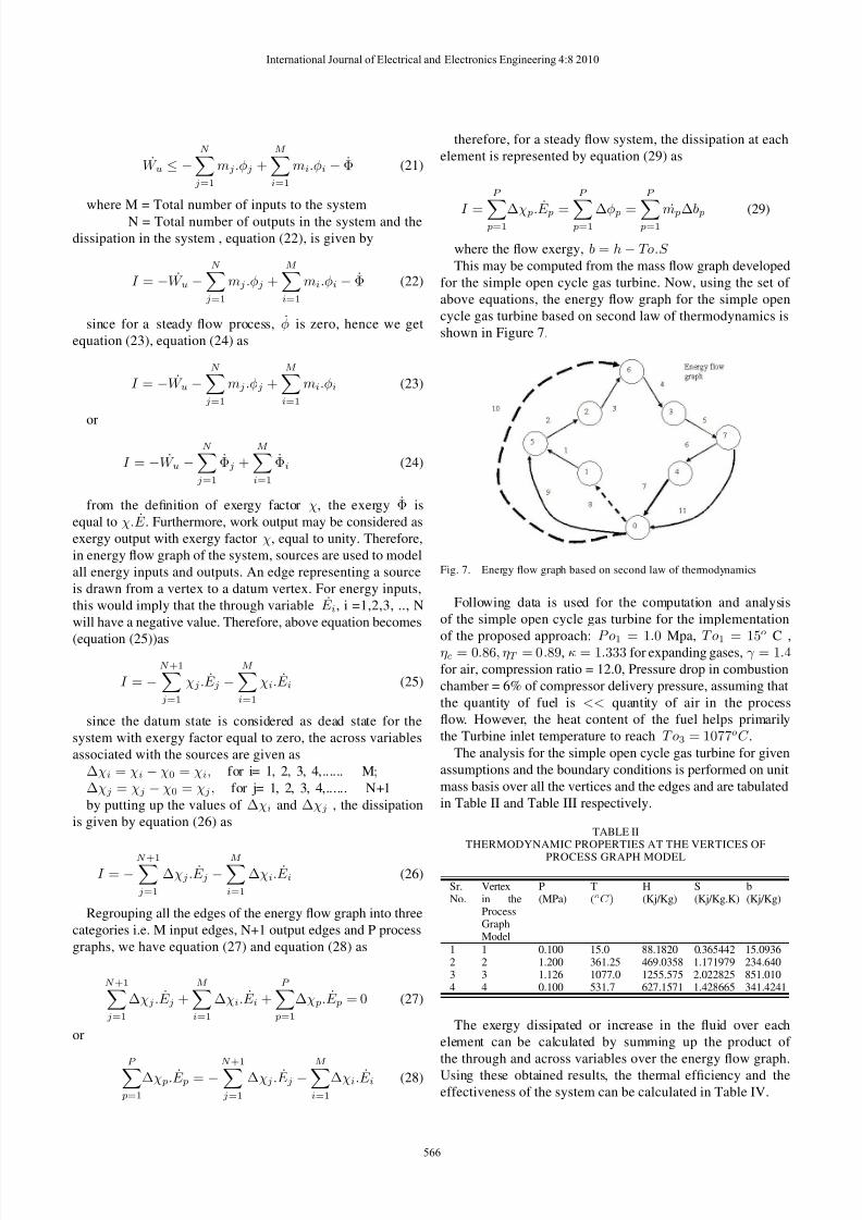
therefore, for a steady flow system, the dissipation at each

element is represented by equation (29) as

I =

P

p=1

Δχ p.˙E p =

P

p=1

Δφ p =

P

p=1m pΔb p (29)

where the flow exergy, b = h− To.S This may be computed from the mass flow graph developed

for the simple open cycle gas turbine. Now, using the set of

above equations, the energy flow graph for the simple open

cycle gas turbine based on second law of thermodynamics is

shown in Figure 7.

Fig. 7. Energy flow graph based on second law of thermodynamics

Following data is used for the computation and analysis

of the simple open cycle gas turbine for the implementation

of the proposed approach: Po1 = 1.0 Mpa, To1 = 15o

C ,ηc = 0.86, ηT = 0.89, κ = 1.333 for expanding gases, γ = 1.4for air, compression ratio = 12.0, Pressure drop in combustion

chamber = 6% of compressor delivery pressure, assuming that

the quantity of fuel is << quantity of air in the process

flow. However, the heat content of the fuel helps primarily

the Turbine inlet temperature to reach To3 = 1077oC .The analysis for the simple open cycle gas turbine for given

assumptions and the boundary conditions is performed on unit

mass basis over all the vertices and the edges and are tabulated

in Table II and Table III respectively.

TABLE IITHERMODYNAMIC PROPERTIES AT THE VERTICES OF

PROCESS GRAPH MODEL

Sr.No.

Vertexin theProcessGraphModel

P(MPa)

T(oC )

H(Kj/Kg)

S(Kj/Kg.K)

b(Kj/Kg)

1 1 0.100 15.0 88.1820 0.365442 15.09362 2 1.200 361.25 469.0358 1.171979 234.6403 3 1.126 1077.0 1255.575 2.022825 851.0104 4 0.100 531.7 627.1571 1.428665 341.4241

The exergy dissipated or increase in the fluid over each

element can be calculated by summing up the product of

the through and across variables over the energy flow graph.

Using these obtained results, the thermal efficiency and the

effectiveness of the system can be calculated in Table IV.


566



TABLE IIIEDGE-WISE FLOW EXERGY VARIATION

Sr.No.

Edges in theProcess GraphModel

M (Kg/Sec) Δb (Kj/Kg)

1 12 1.0 15.0936 - 234.640= -219.546

2 13 1.0 234.640 - 851.010= -616.370

3 14 1.0 851.010 - 341.4241= 509.5859

TABLE IVDISSIPATION AT INDIVIDUAL ELEMENTS

Sr.No.

Subsystem Δφ = −

pmpΔbp

1 Compressor -(1.0 x -219.546) = 219.5462 Combustion Chamber -(1.0 x -616.370) = 616.3703 Turbine -(1.0 x 509.5859) = -509.5859

VIII. CONCLUSION

In the present paper, the graph theoretic approach for

the modeling and analysis of simple open cycle gas turbine

has been presented. The concept of process graph models

representing the interconnections of the elements as well as

their behaviour have been developed for simple open cycle

gas turbine unit based on graph theory and system theory.

It is clear from the implementation method of the tech-

nique adopted that the modeling procedure involves sufficient

number of equations in terms of unknown variables which

can be used to get the unique solution of the system. The

System of equations has been solved using MATLAB for

the unknown governing variables. The relationships between

the vertex & circuit postulates of system theory and the

laws of thermodynamics have been adopted for the simple

open cycle gas turbine energy flow graphs and the exergy

analysis for the system. Since the results obtained by using

the present approach are similar to those obtained by using the

conventional techniques for such system and the approach is

quite sensitive to the affect of variation in the process variable

on the system behavior, the framework of such techniques can

be used further for further optimization of process parameters

of the simple cycle gas turbine systems.

REFERENCES

[1] Kurzke, J., Achieving maximum thermal efficiency with the Simple cycleGas Turbine 9th CEAS European Propulsion Forum: Virtual Engine- A Challenge for Integrated Computer Modelling, Roma, Italy, 15-17October, 2003

[2] Kurzke J., Gas Turbine cycle design Methodology: A comparison of parameter variation with Numerical Optimization ASME Journal of Engineering for Gas Turbine and Power, Volume 121, Pages 6-11, 1999

[3] Young J. B. and Wilcox R. C., Modeling the air cooled gas turbine:Part 1- General Thermodynamics ASME Journal of Turbomachinery,Volume 124, Pages 207 -213, 2002

[4] Silva V. V. R., Khatib W. and Fleming P. J., Performance optimizationof Gas Turbine engine Journal of Engineering Applications of ArtificialIntelligence, Volume 18, Pages 575-583, 2005

[5] Amann C. A., Applying Thermodynamics in search of superior engineefficiency ASME Journal of Engineering for Gas Turbine and Power,Volume 127, Pages 670-675, 2005

[6] Guha A., Performance and optimization of Gas Turbines with real gaseffects Proceedings of Institution of Mechanical Engineers, Volume 215Part A, Pages 507-512, 2001

[7] Yadav J. P. and Singh O., Thermodynamic analysis of air cooled simplegas/ steam combined cycle plant Proceedings of the Journal of Institutionof Engineers (INDIA), Volume 86, Pages 217-222, 2006

[8] Brooks F. J., GE gas Turbine performance characteristics GER-3567H,GE Power systems report, 2000

[9] Cohen H. , Rogers G. F. C. and Saravanamuttoo H. I. H., Gas Turbinetheory Fourth Edition, Longman Publishers, 1996

[10] Philip P. W. and Fletcher P., Gas Turbine performance SecondEdition, Blackwell Science, 2004

[11] Ghajar A. J., Delahoussaye R. D. and Nayak V. V., Development and implementation of Interactive/ Visual software for Simple Cycle gasTurbine Proceedings of American Society for Engineering EducationAnnual Conference and Exposition, 2005

[12] Chandrashekar M. and Wong F. C., Thermodynamic Systems Analysis- I: A Graph Theoretic approach Journal of Energy, Volume 7, Pages539-566, Number 6, 1982

[13] Shai O. and Preiss K., Graph theory representations of Engineeringsystems and their embedded knowledge Journal of Artificial Intelligencein Engineering, Volume 13, Pages 273-285, 1999

[14] Shai O. ,Titus N. and Ramani K., Combinatorial synthesis approach em-

ploying Graph networks Journal of Advanced Engineering Informatics,Volume 22, Pages 161-171, 2008


567

modelin nd ana lysis

Documents