modeling, analysis and simulation of robust control ...irphouse.com/ijee/ijeev4n2_9.pdf · scheme...
TRANSCRIPT

International Journal of Electrical Engineering. ISSN 0974-2158 Volume 4, Number 2 (2011), pp. 261-282 © International Research Publication House http://www.irphouse.com
Modeling, Analysis and Simulation of Robust Control Strategy on a 10kVA STATCOM for Reactive Power
Compensation
J.K. Moharana*, M. Sengupta and A. Sengupta
Department, of Electrical Engineering, Bengal Engineering and Science University, Shibpur,
Howrah-03, West Bengal, India. *Email: [email protected], [email protected]
Abstract
The STATCOM (STATic synchronous COMpensator) is being increasingly popular in power system applications. In general, reactive power compensation for power factor and stability of the grid system can be improved. A simple qd − transformation and steady state and transient analysis are achieved to characterize the open loop system. The small signal scheme in ∞H controller control the phase angle as well as modulation index of the switching pattern and with small perturbation of reference current (reactive current of load), the DC voltage nearly remains constant. The ∞H -controller design and implementation of the STATCOM is proposed without using independent control on DC-link voltage of the STATCOM. The ∞H -controller provides fast response of the STATCOM compensation of the reactive power and becoming the stable of the system. The pre-charge voltage of V600 on DC-link is chosen for tolerable transient variation of the relevant responses of the STATCOM. All responses are obtained trough MATLAB simulink tool box.
Index Terms: STATCOM, small signal model, ∞H controller
Introduction In recent years power systems have become very complex with interconnected long distance transmission lines. The interconnected grids tend to become unstable as the heavy loads vary dynamically in their magnitude and phase angle and hence power factor. Commissioning new transmission systems are extremely expensive and take

262 J.K. Moharana et al
considerable amount of time to build up. Therefore, in order to meet increasing power demands, utilities must rely on power export/import arrangements through the existing transmission systems. Power electronic devices are gaining popularity for applications in the field of power transmission and distribution systems. The reactive power (VAR) compensation and control have been recognized [1] as an efficient & economic means of increasing power system transmission capability and stability. The FACTS (Flexible AC Transmission Systems) devices, such as STATCOM has been introduced more recently which employs a VSI with a fixed dc link capacitor as a static replacement of the synchronous condenser. In a traditional synchronous condenser, the field current of the synchronous motor controls the amount of VAR absorbed/injected and in a similar way; the firing instant of the 3-phase inverter controls the VAR flow into or out of the STATCOM. Large numbers of capacitor banks or any other passive elements are no more required. Only a fixed set of capacitor provides the required VAR control, with a rapid control of bus voltage and improvement of utility power factor. It offers several advantages over conventional thyristorised converters [2] in terms of speed of response. The penalty paid for this improvement is in terms of introduction of some harmonics, which requires separate handling using active filtration techniques. Moran et al [3] have shown in details how the utilization of SPWM techniques reduces harmonic distortion. It has also been shown that an increase of modulation index reduces the size of the link reactor and stress on switches which are significant issues in practical implementation. The modeling and analysis of STATCOM steady state and dynamic performance with conventional control method have been studied by Schauder and Mehta [4]. In [5] the dynamic responses and steady state behavior of STATCOM with SVPWM has been studied and the advantages of introducing SVPWM inverter with higher values of MI are highlighted. It is also shown that a PI Controller designed on the basis of a linearized model [6-8] of the STATCOM achieves very good transient response. The large interconnected power system is called upon to work with different values of ''αthe angle between the grid voltage and the fundamental component of STATCOM output voltage. Also the modulation index (M.I) m of the inverter is to be varied over a wide range. The inherently nonlinear system also experiences plant parameter variation over a wide range. In this work it is shown that the PI Controller designed on the basis of the plant model, linearized about a nominal point cannot handle the plant parameter variation over the entire range. As a remedy the plant parameter variation is included as plant uncertainty and a controller based on ∞H -optimization is used. This gives significant improvement in plant response on variation of m and α . Starting with an established steady state open loop model of the STATCOM, the present paper goes on to develop closed loop models for investigating transient performance of the STATCOM. First, in Section II, general modeling of the STATCOM and study its open-loop responses. A small signal model is developed to establish the effect of the variation of the modulation index ''m and the phase angleα . Thereafter, a closed loop control scheme has been proposed with two types of controller design, so that dc link voltage may be kept unchanged. This scheme is both an extension and a significant improvement of the scheme suggested by Cho et al [6].

Modeling, Analysis and Simulation 263
Modeling of the STATCOM and Analysis Operating principle As is well known, the STATCOM is, in principle, a static (power electronic) replacement of the age-old synchronous condenser. Fig.1 (a) shows the schematic diagram of the STATCOM at PCC through coupling inductors. The fundamental phasor diagram of the STATCOM terminal voltage with the voltage at PCC for an inductive load as well as capacitive load in operation, neglecting the harmonic content in the STATCOM terminal voltage, are shown in Figs.1(b) and (c). Ideally, increasing the amplitude of the STATCOM terminal voltage oaV
r above the amplitude of the
utility voltage saVr
causes leading (capacitive) current caIr
to be injected into the
system at PCC. acaI _
r, the real component of caI
r, accounts for the losses in the
resistance of the inductor coil and the power electronic converter. Ideally, if the system losses can be minimized to zero, acaI _
r would become zero, and caI
r would be
leading at perfect quadrature. Then, oaVr
, which is lagging and greater than saVr
, would
also be in phase with saVr
. The STATCOM in such a case operates in capacitive mode (when the load is inductive)(as shown in Fig.1(b)). Similarly, the operation of the STATCOM can be explained to be inductive if the load is capacitive (as given in Fig.1(c)).
(a) (b) (c)
Figure 1: (a) Schematic diagram of STATCOM, (b) phasor diagram for inductive load operation and (c) phasor diagram for capacitive load operation. Modeling The modeling of the STATCOM, though well known, is reviewed in the lines below, for the sake of convenience. The modeling is carried out with the following assumptions:
1. All switches are ideal 2. The source voltages are balanced 3. sR represents the converter losses and the losses of the coupling inductor 4. The harmonic contents caused by switching action are negligible
The 3-phase stationary abc coordinate vectors with 1200 apart from each other

264 J.K. Moharana et al
are converted into αβ 2-phase stationary coordinates (which are in quadrature). The α axis is aligned with a axis and leading β axis and both converted into dq two-phase rotating coordinates. The Park’s abc to dq transformation matrix is given in (1)
⎥⎥
⎦
⎤
⎢⎢
⎣
⎡+−+−
=2/12/12/1
)3/2()3/2()()3/2()3/2()(
3
2πϖπϖϖπϖπϖϖ
tSintSintSintCostCostCos
K (1)
32
(
)3
2(
)(
32
,
⎥⎥⎥⎥⎥⎥
⎦
⎤
⎢⎢⎢⎢⎢⎢
⎣
⎡
⎥⎥⎥
⎦
⎤
⎢⎢⎢
⎣
⎡
+−
−−
−
==
παω
παω
αω
tSin
tSin
tSin
sV
scVsbVsaV
abcsV (2)
The actual proposed circuit is too complex to analyze as a whole, so that it is partitioned into several basic sub-circuits, as shown in Fig.1 (a). The 3-phase system voltage abcsV , lagging with the phase angle α to the STATCOM output voltage abcoV , and differential form of the STATCOM currents are defined in (2) and (3). where ,
ss RV ,,ϖ and sL have their usual connotations. The above voltages and currents are transformed into dq frame and given in (4) and (5)
( ) abcoVabcsVabccisRabccidt
dsL ,.,,, −+−= (3)
[ ]TCosSinsVqdosV 0, αα−= (4)
( ) oqsqcdscqscqs VViwLiRidtdL −+−−= (5a)
( ) odsdcdscqscds VViRiwLidtdL −+−= (5b)
The switching function S of the STATCOM can be defined as given in (6) and the modulation index, being constant for a programmed PWM, is given by (7). cm is the
modulation conversion index and 32 is the multiplying factor for transformation of
three phase stationary quantities to two phase dq rotating frame.
⎥⎥⎥⎥⎥⎥
⎦
⎤
⎢⎢⎢⎢⎢⎢
⎣
⎡
+
−=⎥⎥⎥
⎦
⎤
⎢⎢⎢
⎣
⎡=
)3
2(
)3
2(
)(
32
π
π
wtSin
wtSin
wtSin
mSSS
S c
c
b
a (6)
c
mdcv
peakoVmMI
3
2,=== (7)

Modeling, Analysis and Simulation 265
The STATCOM output voltages and dq transformation are given by, dcSvabcoV =. (8)
[ ] dcvT
cmqdooV 010, = (9)
The dc side current in the capacitor and its dq transformation may be written as, abcc
Tdc iSi ,= (10)
[ ]T
coicdicqicmdci ⎥⎦⎤
⎢⎣⎡= 010 (11)
The voltage and current related in the dc side is given by
dt
dvCi dc
dc = (12)
Now replacing (11) in (12) yields
cdcdc i
Cm
dtdv
= (13)
The complete mathematical model of the STATCOM in dq frame is obtained as given in (14)
⎥⎥⎥
⎦
⎤
⎢⎢⎢
⎣
⎡−+
⎥⎥⎥
⎦
⎤
⎢⎢⎢
⎣
⎡
⎥⎥⎥⎥⎥⎥⎥
⎦
⎤
⎢⎢⎢⎢⎢⎢⎢
⎣
⎡
−−
−−
=⎥⎥⎥
⎦
⎤
⎢⎢⎢
⎣
⎡
000
0
αα
CosSin
LV
vii
Cm
Lm
LR
w
wLR
vii
dtd
s
s
dc
cd
cq
c
s
c
s
s
s
s
dc
cd
cq
(14)
Steady State and transient Analysis The steady state equations of cqI , cdI , dcV , cP , cQ are given in (15-16) and their responses with the parameters given in Table 1, are shown in Fig.3 and Fig.4.
⎟⎟⎠
⎞⎜⎜⎝
⎛−=
=−=
αα
α
SinsRswL
CosM
sVdcV
cdIsR
SinsVcqI 0,
(15)
( )[ ]
( )α
α
22
2
212
2
SinsR
sVcQ
CossR
sVcP
=
−=
(16)

266 J.K. Moharana et al
Table 1
Sl.No Meaning Symbol Values 1 Fundamental Frequency 1f 50 Hz 2 Fundamental Angular Frequency 1ω 314 rad/sec 3 RMS line-to-line Voltage sV 415V 4 Effective coupling Resistance sR 1.0Ω 5 Coupling Inductance sL 5.44mH 6 DC link capacitor dcC 680 Fμ 7 Modulation Conversion Index
cm 0.98 to 1.22 8 Resistive load lR 23Ω 9 Inductive load lL mH60 , Ω06.2
The open loop steady state responses to a step change in phase angle α of the reactive component of STATCOM current, cqI , and the reactive VAR, cQ , of the STATCOM in capacitive mode of operation are shown in Figs.2.(a) and (b) respectively. The corresponding transient responses at 010−=α are given in Figs.3 (a) and (b) respectively.
(a) (b)
Figure 2: Steady state responses due to variation inα of STATCOM in capacitive mode: (a) Reactive component of STATCOM currents and (b) reactive power generated by STATCOM The steady states values of cqI and cQ vary with variation in phase angleα . These values (as shown in Figs.2 (a) and (b) respectively) are A72 and kVAR45.29− at
010−=α in capacitive mode of operation of STATCOM. The corresponding transient responses (Figs.3 (a) and (b)) in generating (capacitive) mode of operation of STATCOM have high transients seem to generate A72 and kVAR45.29− respectively after two and half power cycles. The high transient magnitude of cqi of

Modeling, Analysis and Simulation 267
the STATCOM unnecessarily increases the ratings of the STATCOM devices. The above calculations are on the basis of the mathematical model of the STATCOM. The practical STATCOM ratings will be limited by the choice of the switching devices (IGBT of SEMIKRON make of part no.SKM75GB123D) and the ripple current, the average current and the voltage rating of the DC link capacitor as also the current rating of the coupling inductor. The above values of the transient peak are actually out of range for the present set-up. Recalling the introduction in section, the STATCOM is a voltage source behind a reactance connected in shunt to the PCC. The system demands fast injection of current, both at fundamental and harmonic frequencies. The STATCOM voltage should be capable of fast variation in order to cater to system needs. States differently, the STATCOM voltage should be a function of the current ( *
cqi ) or reactive power ( *cq
) demanded by the power system. The most rudimentary control system structure required for this purpose is shown in Fig.4 (a). The control voltage, )(tvcontrol , is generated from a prior information of the series inductance, sL , and the phase and magnitude of the PCC voltage, )(tvs . If these are supplied to the reference generator,
(.)f , only once at the beginning of the operation, it constitutes an open-loop control system. Although the series inductance may not vary significantly, the PCC voltage,
)(tvs , will definitely under go considerable variation in phase and magnitude. Some of the internal variables of the STATCOM, e.g. the DC-link voltage may also vary which causes a variation in the gain K shown in Fig.4 (a). An open-loop control system will be unable to maintain the STATCOM current against the disturbances. This calls for closed-loop control of the STATCOM current, which is schematically shown in Fig.4 (b). The current or reactive power control (.)1f , is designed to obtain the desired closed- loop bandwidth.
(a) (b)
Figure 3: Transient responses to a step change of 010− in α of STATCOM in capacitive mode: (a) Reactive component of STATCOM current and (b) reactive power generated by STATCOM

268 J.K. Moharana et al
(a) (b)
Figure 4: Schematic of STATCOM: (a) With open-loop control and (b) with closed-loop control. Modeling of Load The LR − loads are connected at the PCC of the utility source in star connection. The
ba, and c three phase stationary coordinate of the load currents are converted into βα − of two phase stationary coordinate currents and then qd − of two phase
rotating co-ordinate currents. The simulations of the phase a load current with voltage at PCC, active and reactive components of the load currents and active and reactive power are shown in Fig.5. Fig.5(a) is shown the lagging power factor of 0.77 of a phase load current with respect to PPC a phase voltage. This lagging power factor can be compensated to unity power factor.Fig.5(b) is shown the d and q axis current of 11.5A and 7.2A of the above load respectively which can be used as reference values at the time of controlling d and q axis current of STATCOM. Fig.5(c) is shown the active and reactive power of KW6 and KVAR3 of the above load respectively.
(a) (b) (c)
Figure 5: (a) Grid phase a voltage and load phase a current, (b) active and reactive current of the load and (c) active and reactive power of the load Small Signal Scheme Modeling To know the dynamic characteristics of STATCOM system, the small signal analysis is to be done. For a given operating point, small signal equivalent circuit is derived based on the following assumption:

Modeling, Analysis and Simulation 269
i. The disturbance is small, ii. Hence, the second order terms (products of variations) are negligible, iii. The phase nominal value of angle α is small.
With the above assumptions the equations (9) and (11) can be rewritten as, dcv
cmdcV
cmdcv
cMdcV
cMtodvodV ˆˆˆˆ)(ˆ +++=+ (17)
cdic
McdIc
MdcidcI ˆˆ +=+ (18)
αα ˆˆ =Sin , 1cos =α and 00 =α (19) By using (5), (17), (18) and (19), and applying Laplace Transformation, we have,
⎥⎥⎥
⎦
⎤
⎢⎢⎢
⎣
⎡−−
=⎥⎥⎥
⎦
⎤
⎢⎢⎢
⎣
⎡
⎥⎥⎥
⎦
⎤
⎢⎢⎢
⎣
⎡
−+−
+
0)(ˆ
)(ˆ
ˆ
ˆˆ
0
0smV
sV
vii
sCMMRsLwL
wLRsL
cdc
s
dc
cd
cq
c
csss
sss α (20)
The important transfer functions of the states of the STATCOM in small signal model can be derived as
)()(ˆ
)(ˆ
sA
CswLdcV
sc
m
scqi= (21a)
)(
)22(
)(ˆ
)(ˆ
sAc
MCsRCssLsV
s
scqi ++−=
α (21b)
)(
)(
)(ˆ
)(ˆ
sA
ssRssLCdcV
sc
m
scdi +−= (22a)
)()(ˆ
)(ˆ
sA
CsswLdcV
s
scdi −=
α (22b)
)(
)(
)(ˆ
)(ˆ
sA
sRssLdcVc
M
sc
m
sdcv +−= (23a)
)()(ˆ
)(ˆ
sA
sLsVc
M
s
sdcv ϖ
α
−= (23b)
s
RMssLMsLsRCssCRsLssCLsA 2]2}2)(2{[2232)( +++++= ϖ (24)
Open loop responses The responses of the states cqi , cdi and dcv (as in (21-23)) are simulated in MATLAB using the parameters given in Table-1, with a variation of phase angle )(5ˆ tu−=α (in degree) and a change of modulation conversion index )(1.0ˆ tumc = . Fig.6 and Fig.7 show responses for a step change in modulation conversion index cm and phase angle

270 J.K. Moharana et al
α respectively in capacitive mode. It may be noted from the results that a change in cm has no steady state effect on the reactive component of STATCOM currents
(Fig.6 (a)) in capacitive mode. It however causes dcv to reduce by V35 in the steady state as shown in Fig.6 (b). However, due to a change inα by an amount given above, the STATCOM draws additional steady state reactive current of A37 (Fig.7 (a)) at steady state. Neither does, dcv , the DC-link voltage remain at its previous steady state value. It increases in magnitude (by V50 ) for a change in α (Fig.7 (b)). Hence the open loop dynamics suggest that it is required to have closed loop control of reactive component of STATCOM currents as well as DC-link voltage of STATCOM in order to reduce transient surges and to keep dcV constant.
(a) (b)
Figure 6: Transient response for change in cm in capacitive mode: (a) In cqi and (b)
dcv
(a) (b)
Figure 7: Transient response for change in α in capacitive mode: (a) In cqi and (b)
dcv Design of robust controller The state space model of STATCOM (14) is nonlinear in phase angleα . The models of the STATCOM in linear model are valid for small changes in α and cm about the nominal values. In any practical set-up the variables do vary beyond small ranges. Then the small signal models may be in adequate to represent the system behaviour. The controllers designed on the basis of these models may not give desired performance when applied to the original system. A way to overcome this problem is
Modeling, Analysis and Simulation 271
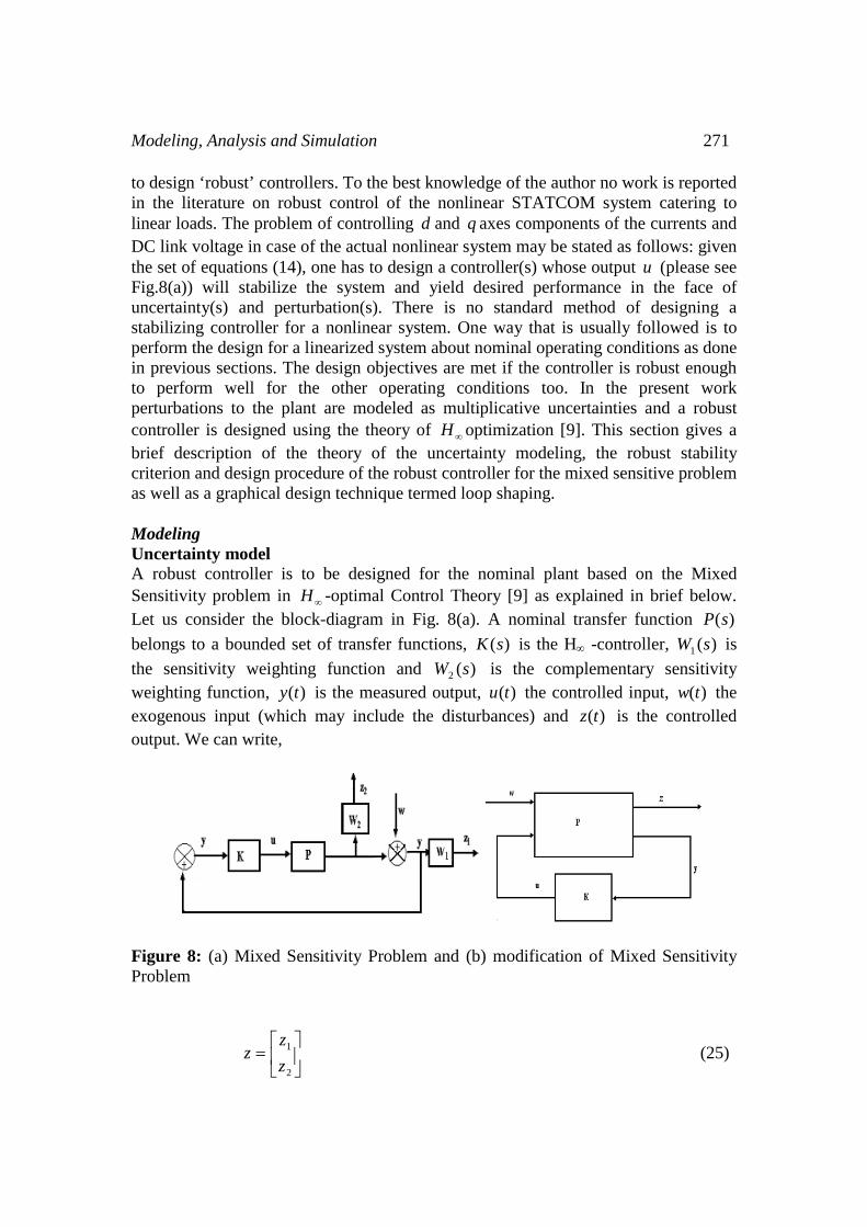
to design ‘robust’ controllers. To the best knowledge of the author no work is reported in the literature on robust control of the nonlinear STATCOM system catering to linear loads. The problem of controlling d and q axes components of the currents and DC link voltage in case of the actual nonlinear system may be stated as follows: given the set of equations (14), one has to design a controller(s) whose output u (please see Fig.8(a)) will stabilize the system and yield desired performance in the face of uncertainty(s) and perturbation(s). There is no standard method of designing a stabilizing controller for a nonlinear system. One way that is usually followed is to perform the design for a linearized system about nominal operating conditions as done in previous sections. The design objectives are met if the controller is robust enough to perform well for the other operating conditions too. In the present work perturbations to the plant are modeled as multiplicative uncertainties and a robust controller is designed using the theory of ∞H optimization [9]. This section gives a brief description of the theory of the uncertainty modeling, the robust stability criterion and design procedure of the robust controller for the mixed sensitive problem as well as a graphical design technique termed loop shaping. Modeling Uncertainty model A robust controller is to be designed for the nominal plant based on the Mixed Sensitivity problem in ∞H -optimal Control Theory [9] as explained in brief below. Let us consider the block-diagram in Fig. 8(a). A nominal transfer function )(sP belongs to a bounded set of transfer functions, )(sK is the H∞ -controller, )(1 sW is the sensitivity weighting function and )(2 sW is the complementary sensitivity weighting function, )(ty is the measured output, )(tu the controlled input, )(tw the exogenous input (which may include the disturbances) and )(tz is the controlled output. We can write,
Figure 8: (a) Mixed Sensitivity Problem and (b) modification of Mixed Sensitivity Problem
⎥⎦
⎤⎢⎣
⎡=
2
1
zz
z (25)

272 J.K. Moharana et al
The augmented plant is: ⎥⎥⎥
⎦
⎤
⎢⎢⎢
⎣
⎡=
PI
PW
PWW
G2
011
(26)
which relates: ⎥⎦⎤
⎢⎣⎡
⎥⎥
⎦
⎤
⎢⎢
⎣
⎡=
uw
Gy
zz
21
(27)
The block diagram of Fig.8(a) of the mixed sensitivity problem is modified to the general control problem as shown in Fig.8(b). The closed loop transfer function (Fig.8(a)) from w to z is denoted by )(sT . The control problem is to find a controller
)(sK such that The closed-loop system is internally stable The ∞-norm of the closed loop transfer function )(sT satisfies: γ<∞|||| T for some small 0>γ The perturbed transfer function, resulting from variations in operating conditions, can be expressed in the form of the ‘uncertainty set’ as shown in Fig.9 and given in ( ))(1)()(~
2 sWsPsP Δ+= (28) Here, Δ is a variable transfer function satisfying 1|||| <Δ ∞ . It may be recalled that the infinity norm ( )norm−∞ of a SISO transfer function is the least upper bound of its absolute value. This is also written as |)(|sup|||| ωωω jΔ=Δ and is the largest value of the gain on a Bode magnitude plot. The uncertainties, which are the variations of system operating conditions, are thus modeled through P~ in equation (2.46). In the multiplicative uncertainty model in equation (28), 2WΔ is the normalized plant perturbation away from 1. If 1|||| <Δ ∞ , then
Figure 9: Multiplicative perturbation model.
|)(||1)()(~
| 2 ωωω jW
jPjP
≤⎟⎟⎠
⎞⎜⎜⎝
⎛− for all ω (29)

Modeling, Analysis and Simulation 273
So, |)(| 2 ωjW provides the uncertainty profile. In the frequency plane it is the upper bound of all the normalized perturbed plant transfer functions away from 1. For the optimum case the weighting function can be determined as
)(
)()(~)(2 ω
ωωωjP
jPjPjW −= (30)
Robust stability and performance Let us consider )(sK some controller which is assumed to provide overall system stability if it provides internal stability for every plant in the uncertainty set. If L denotes the loop transfer function ( )PKL = , then the sensitivity function S is written
as L
S+
=1
1 (31) The complimentary sensitivity function or the input-output transfer
function is PK
PKST+
=−=1
1 (32)
For a multiplicative perturbation model, the robust stability condition is met if and
only if 1|||| 2 <∞TW . This implies that ,1|)(1
)()(| 2 <
+ ωωω
jLjLjW for all ω (33)
or, |)(1||)()(| ωωω jLjLj +<Δ , for allω , 1|||| <Δ ∞ (34) The nominal performance condition for an internally stable system is given as
1|||| 1 <∞SW , where 1W is a real-rational, stable, minimum phase transfer function (also called a weighting function). If )(sP is perturbed to ( ))(1)()(~
2 sWsPsP Δ+= and
S is perturbed to TW
SLW
S22 1)1(1
1~Δ+
=Δ++
= (35)
then the robust performance condition should therefore be [9]
1|||| 2 <∞TW and 1||1
||2
1 <Δ+ TW
SW, for all 1|||| <Δ (36)
Combining all the above, it can be shown that a necessary and sufficient condition for robust stability and performance is 1|||2||1||| <∞+ TWSW (37) This is the Mixed Sensitivity problem for controller design. Proposed control scheme Fig.10 is shown the proposed control strategy of small signal model of the STATCOM. ∞H -mixed sensitivity reduced order controller ( MSROCH −∞ ) (2.37) is applied at the reactive component of the STATCOM currents with reference reactive component of the load currents. The output of the controller generates a change in phase angle α and it can be converted to a change of modulation conversion index
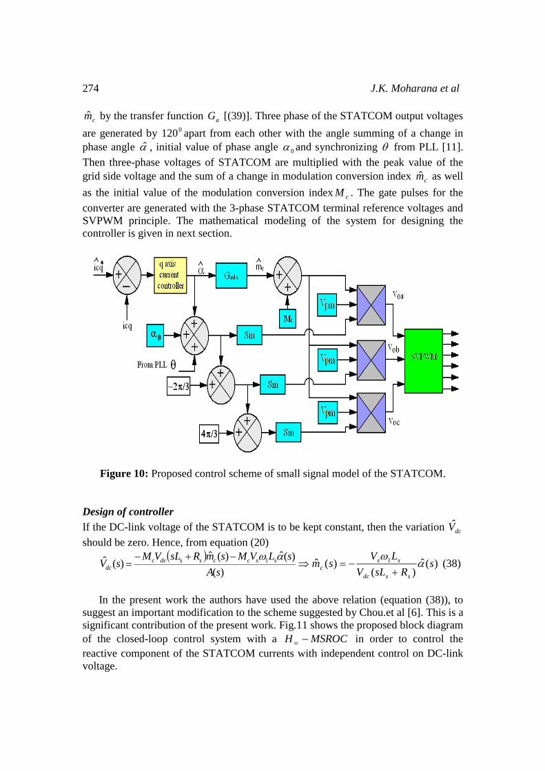
274 J.K. Moharana et al
cm by the transfer function aG [(39)]. Three phase of the STATCOM output voltages are generated by 0120 apart from each other with the angle summing of a change in phase angle α , initial value of phase angle 0α and synchronizing θ from PLL [11]. Then three-phase voltages of STATCOM are multiplied with the peak value of the grid side voltage and the sum of a change in modulation conversion index cm as well as the initial value of the modulation conversion index cM . The gate pulses for the converter are generated with the 3-phase STATCOM terminal reference voltages and SVPWM principle. The mathematical modeling of the system for designing the controller is given in next section.
Figure 10: Proposed control scheme of small signal model of the STATCOM. Design of controller If the DC-link voltage of the STATCOM is to be kept constant, then the variation dcV should be zero. Hence, from equation (20)
( )
)()(ˆ)(ˆ
)(ˆ 1
sAsLVMsmRsLVM
sV ssccssdccdc
αω−+−= )(ˆ
)()(ˆ 1 s
RsLVLV
smssdc
ssc α
ω+
−=⇒ (38)
In the present work the authors have used the above relation (equation (38)), to suggest an important modification to the scheme suggested by Chou.et al [6]. This is a significant contribution of the present work. Fig.11 shows the proposed block diagram of the closed-loop control system with a MSROCH −∞ in order to control the reactive component of the STATCOM currents with independent control on DC-link voltage.

Modeling, Analysis and Simulation 275
Figure 11: Block diagram of closed loop system with MSROCH −∞ . The forward path transfer function amG 2 is
⎟⎟⎠
⎞⎜⎜⎝
⎛⎟⎟⎠
⎞⎜⎜⎝
⎛+
−=)((
11
sACLV
RsLVLV
G dcsdc
ssdc
ssa
ωω (39)
In this section )(ˆ sI cq has been modeled as from (21) is
( )
)(ˆ)(
)(ˆ)(
)(ˆ 122
smsA
CLVs
sAMCRsCLV
sI cdcsdccdcsdcss
cqω
α +++−
= (40)
To achieve fast dynamic response without controlling the DC link voltage, then the variation of )(ˆ sVdc should be zero. By using equation (39), equation (40) may be modified to:
( )
)(ˆ))(()(
)(ˆ22
122
sRsLsA
CLVsA
MCRsCLVsI
ss
dcsscdcsdcsscq α
ω⎥⎦
⎤⎢⎣
⎡+
−++−
=
So that the nominal plat transfer function is,
( )
⎥⎦
⎤⎢⎣
⎡+
+++
−==))(()()(ˆ
)(ˆ)(
221
22
ss
dcsscdcsdcsscq
RsLsACLV
sAMCRsCLV
ssI
sPω
α (41)
The mixed sensitivity robust controller [9] is now designed for the nominal plant based on Mixed Sensitivity problem. The sensitivity weighting function )(1 sW is following basis: If the plant is )(sP and the loop transfer function (as mentioned earlier) is
ssKsPsL cω
== ))()()(( , and the sensitivity function is cs
ssSω+
=)( then the
weighting function )(1 sW for sensitivity )(sS is c
c
ss
sWξωω
++
=)(1 ,where ξ is the

276 J.K. Moharana et al
damping ratio. Here the nominal plant, )(sP is taken at (i) 98.0=cm at 00=α and the perturbed
plant, )(~ sP is taken at (ii) 22.1=cm and 00=α . The weighting function )(2 sW can
be determined as: )(~
)()(~)(2 sP
sPsPsW
−= (42)
The weighting function )(1 sW can be determined after choosing %5 over shoot,69.0=ξ and 8.409=
cω rad/sec and steady state error of 0.1 [9]. So )(1 sW will be
( ) ( )( )98.40
85.4092.01
+
+=
s
ssW (43).However, both weighting functions can be finalized in such
a way that both weighting functions obey 1|)(12||)(1
1| ≥−+− sWsW for all frequencies. Hence, by trial and error adjustment of pole and zero of the transfer function of the weighting functions, )(1 sW and )(2 sW will be
( )4.0
10)(1 +=
ssW (44) and ( )210
)(2 +
=s
ssW (45)
The Bode plots of |)(1
1| sW − and |)(12| sW− shown in Fig.12 indicate
1|)(12||)(1
1| ≥−+− sWsW at all frequencies. The weighting functions together with the nominal plant )(sP are used in the Robust Control Toolbox in MATLAB to yield the mixed sensitivity ∞H -Controller hK given in (46). The controller is of 5th order transfer function.
Figure 12: Bode plots of ( ) || 11 sW − and ( ) || 1
2 sW − for small signal model.
17182163134105
171521331047
104109.9102.1103.1106.4104.4108.7107.3103.4106.8)(×+×+×+×+×+×−×−×−×−×−
=sssss
sssssKh (46)
It may be noted that the small signal model of the STATCOM used here includes an improvement over existing work of Cho et al [6]. The design of the controller is another contribution of the author. The step response of the closed loop system is shown in Fig.13 (a) and the output
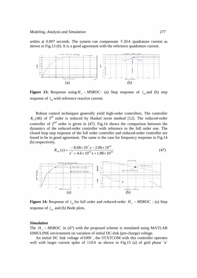
Modeling, Analysis and Simulation 277
settles at 0.007 seconds. The system can compensate A20m quadrature current as shown in Fig.13 (b). It is a good agreement with the reference quadrature current.
(a) (b)
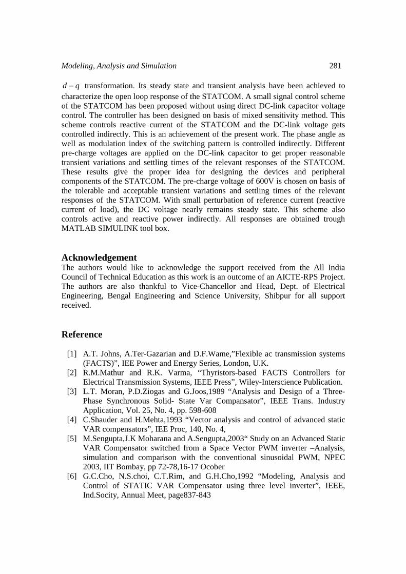
Figure 13: Response using MSROCH −∞ : (a) Step response of cqi and (b) step response of cqi with reference reactive current. Robust control techniques generally yield high-order controllers. The controller
hK (46) of 5th order is reduced by Hankel norm method [12]. The reduced-order controller of 2nd order is given in (47). Fig.14 shows the comparison between the dynamics of the reduced-order controller with reference to the full order one. The closed loop step response of the full order controller and reduced-order controller are found to be in good agreement. The same is the case for frequency response in Fig.14 (b) respectively.
10102
107
1088.1106.41006.21068.8)(×+×+×−×−
=ss
ssK hr (47)
(a) (b)
Figure 14: Response of cqi for full order and reduced-order MSROCH −∞ : (a) Step response of cqi and (b) Bode plots. Simulation The MSROCH −∞ in (47) with the proposed scheme is simulated using MATLAB SIMULINK environment on variation of initial DC-link (pre-charge) voltage. An initial DC link voltage of V100 , the STATCOM with this controller operates well with larger current spike of A110 as shown in Fig.15 (a) of grid phase ‘a’

278 J.K. Moharana et al
voltage with current .The power factor of the grid source with LR − load improves from 77.0 to unity in three power cycles over the open loop situation in Fig.5(a). The same dynamics of the STATCOM phase ‘a’ current is given in Fig.15 (b) with a current spike of A100 . The current surges in all cases are more than the acceptable limit as per the specifications of the STATCOM.
(a) (b)
Figure 15: Responses of small signal model of STATCOM with MSROCH −∞ at initial DC link voltage of V100 : (a) Grid phase ‘a’ voltage and current (b) Grid phase ‘a’ voltage and STATCOM phase ‘a’ current The same model is simulated with changing the initial DC link voltage of V550 . It is seen that with R-L load the power factor improves from 77.0 to unity after two cycles with a current spike of A45 as given in Fig.16 (a) (for grid phase ‘a’) on compared to Fig.5(a). Fig.16 (b) shows the dynamics of the STATCOM current with transient surge of A30 . Figs.16 (c) and (d) show the dynamics of d and q axes currents of the STATCOM and their transients ( A42 of active and A50− of reactive current) die out after two power cycles respectively .The active with reactive power generated by the STATCOM is shown in Fig.16 (e) and the transients ( kW18 of active power and kVAR20 of reactive power) die out in two power cycles as shown in Fig.16 (f). It is noted that the dynamics of the active currents of STATCOM is similar to the active power dynamics. Incase of reactive currents the dynamics is similar in nature but in phase opposition. The prototype STATCOM can not be designed taking the above transients of the relevant waveforms, since that will mean excessive surge current ratings of the solid-state devices (which are otherwise unnecessary with respect to steady state ratings) No separate voltage controller is needed for this model. The beauty of the model is that the voltage get controlled indirectly and come to steady state at V640 after surges of V970 respectively as shown in Fig.16(g). This is a contribution of the present work. It is noted that the system in case of this model is not so sluggish but the transient surges are not within reasonable limits.

Modeling, Analysis and Simulation 279
(a) (b) (c)
(d) (e) (f)
(g) (h) (i)
(j) (k) (l)
(m) (n)
Figure 16: Responses of small signal model of STATCOM with MSROCH −∞ at initial DC link voltage of V550 : (a) Grid phase ‘a’ voltage and current, (b) Grid

280 J.K. Moharana et al
phase ‘a’ voltage and STATCOM phase ‘a’ current, (c) Active and reactive components of STATCOM current, (d) Active and reactive components of STATCOM current (in expansion), (e) Active and reactive power generated by STATCOM, (f) Active and reactive power generated by STATCOM (in expansion), (g) DC link voltage of STATCOM, (h) DC link voltage of STATCOM (in expansion), (i) Variation of incremental of phase angle α , (j) Variation of incremental of modulation conversion index cm , (k) Grid phase ‘a’ voltage and STATCOM output phase ‘a’ voltage, (l) Grid phase ‘a’ voltage and STATCOM output phase ‘a’ voltage (in expansion), (m) Change of STATCOM reactive current due to change of reference current (load reactive current), (n) DC link voltage of STATCOM due to change of reference current (load reactive current) Figs.16 (i) and (j) show the corresponding dynamics of incremental phase angleα and modulation index cm respectively. Figs.16 (k) and (l) show the dynamics of the grid phase ‘a’ voltage with STATCOM output phase ‘a’ voltage and latter is greater with lagging very small angle than the former respectively. Application of small perturbation of reference reactive current as shown in Fig.16 (m) (reactive current of load), a very small change in DC link voltage is obtained. While the reference current returns to its original value the DC link voltage also returns to its steady state value as shown in Fig.16 (n). Again the same proposed model is simulated with an initial DC link voltage of
V600 .The relevant response is obtained with a lesser current spike of A20 and compensates after one power cycle as shown Fig.3.13 of the grid phase ‘a’ voltage and current. The peak and rms values of the grid current are the basis of the design and selection of the devices and the peripherals of STATCOM system.
Figure 17: Grid phase a voltage and current of small signal model of STATCOM with MSROCH −∞ at initial DC link voltage of V600 Conclusion The STATCOM (STATic synchronous COMpensator) has been modeled in a simple
Modeling, Analysis and Simulation 281
qd − transformation. Its steady state and transient analysis have been achieved to characterize the open loop response of the STATCOM. A small signal control scheme of the STATCOM has been proposed without using direct DC-link capacitor voltage control. The controller has been designed on basis of mixed sensitivity method. This scheme controls reactive current of the STATCOM and the DC-link voltage gets controlled indirectly. This is an achievement of the present work. The phase angle as well as modulation index of the switching pattern is controlled indirectly. Different pre-charge voltages are applied on the DC-link capacitor to get proper reasonable transient variations and settling times of the relevant responses of the STATCOM. These results give the proper idea for designing the devices and peripheral components of the STATCOM. The pre-charge voltage of 600V is chosen on basis of the tolerable and acceptable transient variations and settling times of the relevant responses of the STATCOM. With small perturbation of reference current (reactive current of load), the DC voltage nearly remains steady state. This scheme also controls active and reactive power indirectly. All responses are obtained trough MATLAB SIMULINK tool box. Acknowledgement The authors would like to acknowledge the support received from the All India Council of Technical Education as this work is an outcome of an AICTE-RPS Project. The authors are also thankful to Vice-Chancellor and Head, Dept. of Electrical Engineering, Bengal Engineering and Science University, Shibpur for all support received. Reference
[1] A.T. Johns, A.Ter-Gazarian and D.F.Wame,”Flexible ac transmission systems (FACTS)”, IEE Power and Energy Series, London, U.K.
[2] R.M.Mathur and R.K. Varma, “Thyristors-based FACTS Controllers for Electrical Transmission Systems, IEEE Press”, Wiley-Interscience Publication.
[3] L.T. Moran, P.D.Ziogas and G.Joos,1989 “Analysis and Design of a Three-Phase Synchronous Solid- State Var Compansator”, IEEE Trans. Industry Application, Vol. 25, No. 4, pp. 598-608
[4] C.Shauder and H.Mehta,1993 “Vector analysis and control of advanced static VAR compensators”, IEE Proc, 140, No. 4,
[5] M.Sengupta,J.K Moharana and A.Sengupta,2003“ Study on an Advanced Static VAR Compensator switched from a Space Vector PWM inverter –Analysis, simulation and comparison with the conventional sinusoidal PWM, NPEC 2003, IIT Bombay, pp 72-78,16-17 Ocober
[6] G.C.Cho, N.S.choi, C.T.Rim, and G.H.Cho,1992 “Modeling, Analysis and Control of STATIC VAR Compensator using three level inverter”, IEEE, Ind.Socity, Annual Meet, page837-843

282 J.K. Moharana et al
[7] G.C.Cho,N.S.choi,C.T.Rim,and G.H.Cho,1996 “Analysis and Controller Design of STATIC VAR Compensator Using Three-Level GTO Inverter”,IEEE,Transations on Power Electronics,Vol.11,No.1,page57-65,January
[8] A. Draou, M. Benghanem and A. Tahiri, 2001“Multilevel Converter and VAR Compensation”, Power Electronics Handbook”, pp.599-611, Academic Press
[9] K.Zhou and J.C.Doyle, 1997“Essentials of Robust Control” Prentice Hall [10] M.Sengupta,J.K Moharana and A.Sengupta,2003“ A Nonlinear Control
Modeling of A STATCOM for Reactive Power Compensation”NPSC 2004, IIT Madras, pp 72-78,16-17 Ocober
[11] V.Kaura and V.Blasko, 1997“Operation of a Phase Locked Loop System under Distorted Utility Conditions”,IEEE Transactions on Industry Applications, Vol.33, No.1, pp58-63
[12] Safonov, M.G., R.Y. Chiang, and D.J.N. Limebeer, 1990"Optimal Hankel Model Reduction for Nonminimal Systems," IEEE Trans. on Automat. Control, Vol. 35, No. 4, pp. 496-502.