modeling and analysis of continuous powder blending
TRANSCRIPT

8/13/2019 Modeling and Analysis of Continuous Powder Blending
http://slidepdf.com/reader/full/modeling-and-analysis-of-continuous-powder-blending 1/177
MODELING AND ANALYSIS OF CONTINUOUS POWDER BLENDING
by
YIJIE GAO
A Dissertation submitted to the
Graduate School-New Brunswick
Rutgers, The State University of New Jersey
in partial fulfillment of the requirements
for the degree of
Doctor of Philosophy
Graduate Program in Chemical & Biochemical Engineering
written under the direction of
Fernando J. Muzzio, Ph.D
Marianthi, G. Ierapetritou, Ph.D
and approved by
________________________
________________________
________________________
________________________
New Brunswick, New Jersey
OCTOBER, 2012

8/13/2019 Modeling and Analysis of Continuous Powder Blending
http://slidepdf.com/reader/full/modeling-and-analysis-of-continuous-powder-blending 2/177
ii
ABSTRACT OF THE DISSERTATION
MODELING AND ANALYSIS OF CONTINUOUS POWDER BLENDING
By YIJIE GAO
Dissertation Director:
Fernando J. Muzzio, Ph.D
Marianthi, G. Ierapetritou, Ph.D
The main focus of our research is to investigate continuous powder blending. The
unit operation of powder blending is widely used to reduce the heterogeneity degree of
product mixture in the manufacture of catalysts, cement, food, metal parts, and many other
industrial products. Currently in pharmaceutical industry, continuous powder blending has
received more attention as an efficient alternative to the traditional batch blending of
powders due to its ability in handling high-flux continuous tablet manufacturing.
Numerous previous approaches have been performed focusing on investigating the
applicability of continuous manufacturing system. However, the development of reliable
industrial system is limited by the inaccuracy of mixing index, the complicated effects of
operating conditions and the black-box characterization method, all of which result from
the lack of a theoretical model that can quantitatively characterize the whole continuous
powder mixing process. Therefore, the overall research objective of this work is to develop
8/13/2019 Modeling and Analysis of Continuous Powder Blending
http://slidepdf.com/reader/full/modeling-and-analysis-of-continuous-powder-blending 3/177
iii
a general standard method for quantitative process design and control. In this context, three
different specific aims are accomplished. We analyze and distinguish different
heterogeneity sources in the continuous blending process and develop a general model of
continuous blending. Fourier series is applied to characterize the axial blending component,
and a periodic section model is developed to capture the cross-sectional blending
component. Based on the modeling work, efficient design, control, and scale-up strategies
applicable for practical blending of pharmaceutical powders are determined. The
effectiveness of the methodology is demonstrated in particle blending simulations and
experiments using industrial mixing apparatuses to check its applicability and robustness
in pharmaceutical industrial use.
8/13/2019 Modeling and Analysis of Continuous Powder Blending
http://slidepdf.com/reader/full/modeling-and-analysis-of-continuous-powder-blending 4/177
iv
ACKNOWLEDGEMENTS
This work was supported by National Science Foundation Engineering Research Center on
Structured Organic Particulate Systems, through grant NSF-ECC 0540855, and
NSF-0504497. I would not have been able to complete this work without the guidance and
resources provided by both my advisors Marianthi G. Ierapetritou and Fernando J. Muzzio.
They are always responsible and supportive; teach me a lot not only on academic research
activities but also on many other aspects that I believe are very helpful in my future career.
I also would like to thank my committee members: Professor Rohit Ramachandran and
Professor Alberto Cuitino for their time, carefully reviewing my work, and providing
suggestions. I have had the pleasure to work with several following graduate students and
post-docs whom I would like to acknowledge for teaching me particular methods
providing helpful advice: Patricia Portillo, Fani Boukouvala, Bill Engisch, Juan Osorio,
Atul Dubey, and Aditya Vanarase. Further, I would like to acknowledge the Ierapetritou
group for the wonderful friendship we built together during my graduate career.
I want to thank my parents for their unconditional support during my graduate research.
Undoubtedly, I would not have been able to get this PhD degree without the support of my
wife Yuze Shang. Thank you.

8/13/2019 Modeling and Analysis of Continuous Powder Blending
http://slidepdf.com/reader/full/modeling-and-analysis-of-continuous-powder-blending 5/177

8/13/2019 Modeling and Analysis of Continuous Powder Blending
http://slidepdf.com/reader/full/modeling-and-analysis-of-continuous-powder-blending 6/177
vi
Cross-sectional blending analysis using periodic section modeling .................... 50
4.1 Material and method ........................................................................................... 50
4.2 Periodic section modeling................................................................................... 60
4.3 Verification ......................................................................................................... 63
4.4 Summary ............................................................................................................. 71
Chapter 5 ......................................................................................................................... 73
Blender design based on batch experience ............................................................ 73
5.1 Methodology ....................................................................................................... 73
5.2 Case studies......................................................................................................... 78
5.3 Summary ............................................................................................................. 97
Chapter 6 ....................................................................................................................... 100
Strategies on improving blending performance.................................................. 100
6.1 Optimizing continuous powder blending using factorial analysis .................... 100
6.2 Application of PLS and experimental validation.............................................. 113
6.3 Summary ........................................................................................................... 124
Chapter 7 ....................................................................................................................... 127
Scale-up of continuous powder blending............................................................. 127
7.1 Current limitations ............................................................................................ 127
7.2 Variance spectrum analysis............................................................................... 129
7.3 Methodology ..................................................................................................... 137
7.4 Scale-up of continuous blending components .................................................. 140
7.5 Summary ........................................................................................................... 152
Chapter 8 ....................................................................................................................... 154

8/13/2019 Modeling and Analysis of Continuous Powder Blending
http://slidepdf.com/reader/full/modeling-and-analysis-of-continuous-powder-blending 7/177
vii
Conclusions and future Perspectives.................................................................... 154
8.1 Summary ........................................................................................................... 154
8.2 Suggestion for future work ............................................................................... 156
Reference ....................................................................................................................... 157
CURRICULUM VITA ................................................................................................. 164
8/13/2019 Modeling and Analysis of Continuous Powder Blending
http://slidepdf.com/reader/full/modeling-and-analysis-of-continuous-powder-blending 8/177
viii
Lists of tables
Table 2.1 Operating conditions......................................................................................... 12
Table 2.2 Statistics of feed rate fluctuations of API at the investigated feed rates........... 14
Table 3.1 Validation of case study on the experimental data. .......................................... 48
Table 4.1 Physical and numerical parameters used in the DEM model. .......................... 52
Table 4.2 The number of initial loading particles for the periodic section....................... 56
Table 4.3 The feeding conditions for the corresponding continuous mixer. .................... 57
Table 5.1 Governing equations in the Hertz-Mindlin no slip contact model.................... 74
Table 6.1 Physical and numerical parameters used in the DEM model. ........................ 101
Table 6.2 Range of operation and geometry factors in this paper. ................................. 114
Table 7.1 Physical and numerical parameters used in the DEM model. ........................ 137
Table 7.2 The number of initial loading particles for both mixing cases. ...................... 139
8/13/2019 Modeling and Analysis of Continuous Powder Blending
http://slidepdf.com/reader/full/modeling-and-analysis-of-continuous-powder-blending 9/177
ix
List of illustrations
Figure 2.1 Side view of the studied continuous mixing system. ...................................... 11
Figure 2.2 Feed rate analysis of (a) API and (b) excipient. .............................................. 13
Figure 2.3 Calibration test on NIR method....................................................................... 15
Figure 2.4 (a) Data variability and (b) Model variability of RTD measurements. ........... 18
Figure 2.5 Experimental and fitted RTD curve in different operating conditions............ 24
Figure 2.6 Effects of operating conditions on (a) dispersion coefficient E and (b) axial
velocity v........................................................................................................................... 26
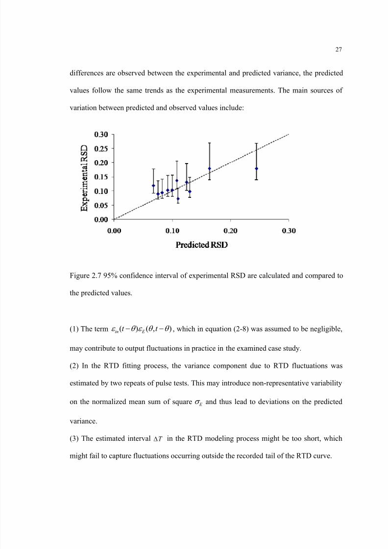
Figure 2.7 95% confidence interval of experimental RSD are calculated and compared to
the predicted values........................................................................................................... 27
Figure 2.8 Effects of operating conditions on the variance component due to feed rate
fluctuations........................................................................................................................ 28
Figure 2.9 Effects of operating conditions on the variance component due to incomplete
transverse mixing. ............................................................................................................. 29
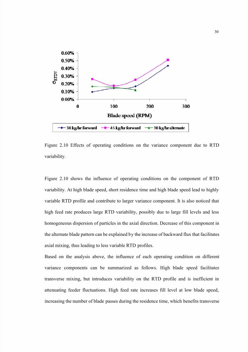
Figure 2.10 Effects of operating conditions on the variance component due to RTD
variability. ......................................................................................................................... 30
Figure 3.1 Signal fluctuation at sampling frequency may be distorted because of aliasing.
........................................................................................................................................... 37
Figure 3.2 The correction of the RTD using the Fourier series. ....................................... 40
Figure 3.3 Filtering ability of the Taylor Dispersion model with different Peclet numbers
from one to infinite. .......................................................................................................... 42
Figure 3.4 Summary of the case study.............................................................................. 45
8/13/2019 Modeling and Analysis of Continuous Powder Blending
http://slidepdf.com/reader/full/modeling-and-analysis-of-continuous-powder-blending 10/177
x
Figure 3.5 Filtering process using alternative RTDs. ....................................................... 47
Figure 4.1 Simulated geometry of the mixer composed of eight periodic sections.......... 53
Figure 4.2 Initial loading of batch mixing in periodic section.......................................... 55
Figure 4.3 Trajectory of one particle inside the periodic section. .................................... 60
Figure 4.4 RSD-t curves of batch mixing in periodic section of non-segregating particles.
........................................................................................................................................... 63
Figure 4.5 The fill level distribution along the mixing axis. ............................................ 65
Figure 4.6 RTD data and curve-fitting of 2, 4 and 6 constant-fill sections for
non-segregating partilcles. ................................................................................................ 66
Figure 4.7 Simulation and calculation of RSD-l curves in continuous mixing processes,
non-segregating particles. ................................................................................................. 67
Figure 4.8 RSD-t curves of batch mixing in periodic section filled by segregating particles.
........................................................................................................................................... 68
Figure 4.9 RTD of batch mixing in 2, 4 and 6 periodic sections for segregating partilcles.
........................................................................................................................................... 69
Figure 4.10 Simulation and calculation of RSD-l curves in continuous mixing processes,
segregating particles.......................................................................................................... 70
Figure 5.1 The rotating frame of reference. ...................................................................... 76
Figure 5.2 Case Study 1: geometries and rotating frame view of blade patterns. ............ 79
Figure 5.3 Velocity quiver plots of Case Study 1. ............................................................ 81
Figure 5.4 Fill level profiles along the axis of the simlated geometries in Case Study 1. 82
Figure 5.5 Fill level gradient in a continuous mixing simulation corresponding to the
cross-sectional PS mixing at 25% fill. .............................................................................. 84
8/13/2019 Modeling and Analysis of Continuous Powder Blending
http://slidepdf.com/reader/full/modeling-and-analysis-of-continuous-powder-blending 11/177
xi
Figure 5.6 RSD decay data and the fitted curves for Case Study 1. (a) 25% fill, (b) 50% fill.
........................................................................................................................................... 84
Figure 5.7 Case Study 2: geometries and rotating frame view of blade patterns. ............ 87
Figure 5.8 Velocity quiver plots of Case Study 2............................................................. 88
Figure 5.9 (a) Symmetric and (b) parallel blade pairs. ..................................................... 89
Figure 5.10 Fill level profiles along the axis of the simulated geometries in Case Study 2
for the regions enclosed by the red lines in Figure 5.8. .................................................... 90
Figure 5.11 RSD decay data and the fitted curves for Case Study 2. (a) 25%, (b) 50% fill.
........................................................................................................................................... 91
Figure 5.12 Case sutdy 3: geometries and rotating frame view of blade patterns. ........... 92
Figure 5.13 Velocity quiver plots of Case Study 3........................................................... 94
Figure 5.14 Fill level profiles along the axis of the simlated geometries in Case Study 3.
........................................................................................................................................... 95
Figure 5.15 RSD decay data and the fitted curves for Case Study 3. (a) 25%, (b) 50% fill.
........................................................................................................................................... 96
Figure 6.1 Simulated periodic section geometry. ........................................................... 102
Figure 6.2 Validation of periodic section modeling with more particles. ...................... 103
Figure 6.3 The control case: simulated, fitted, and normalized RTD and RSD-t curves for
different operating conditions. ........................................................................................ 104
Figure 6.4 Contours of normalized mean axial velocity vx’ in the design space of
operation. ........................................................................................................................ 106
Figure 6.5 Contours of normalized PS mixing rate k b’ in the design space of operation.
......................................................................................................................................... 107
8/13/2019 Modeling and Analysis of Continuous Powder Blending
http://slidepdf.com/reader/full/modeling-and-analysis-of-continuous-powder-blending 12/177
xii
Figure 6.6 Contours of continuous blending rate kc in the design space of operation. .. 108
Figure 6.7 Effect of (a) rotary speed, (b) blade angle, and (c) weir height on the mean axial
velocity v x, the control case............................................................................................. 109
Figure 6.8 Performance improvement strategy 1............................................................ 111
Figure 6.9 Performance improvement strategy 2............................................................ 112
Figure 6.10 Geometry of the periodic section. ............................................................... 113
Figure 6.11 Experimental setup. ..................................................................................... 116
Figure 6.12 NIR spectroscopy method. .......................................................................... 117
Figure 6.13 R 2 and Q 2 indices of the PLS regression from 1 to 3 principle components.
......................................................................................................................................... 118
Figure 6.14 The PLS weights w and c for the two components model. ......................... 119
Figure 6.15 PLS regression loading scores. The bars indicate 95% confidence intervals
based on jack-knifing...................................................................................................... 121
Figure 6.16 VIP of the predictor variables of the two-components PLS regression model.
......................................................................................................................................... 122
Figure 6.17 Summary of the experimental results. ......................................................... 123
Figure 7.1 Illustration of simulation designs. ................................................................. 138
Figure 7.2 Variance spectrum decay contours of non-segregating mixing cases. .......... 140
Figure 7.3 The initial and steady state profiles of variance spectrum of the non-segregating
mixing cases.................................................................................................................... 142
Figure 7.4 RSD-t decay curves measure at sampling size of 0.45 cm 3, non-segregating
mixing cases.................................................................................................................... 143

8/13/2019 Modeling and Analysis of Continuous Powder Blending
http://slidepdf.com/reader/full/modeling-and-analysis-of-continuous-powder-blending 13/177
xiii
Figure 7.5 Illustration of the constant-sample effect on the scaling up of powder mixing.
......................................................................................................................................... 144
Figure 7.6 Variance spectrum decay contours of cohesive segregating mixing cases. .. 146
Figure 7.7 The steady state profiles of variance spectrum of the cohesive segregating
mixing cases.................................................................................................................... 147
Figure 7.8 The snapshots of steady state mixture in the cohesive segregating mixing cases.
......................................................................................................................................... 148
Figure 7.9 RSD-t decay curves measure at sampling size of 0.45 cm 3, cohesive segregating
mixing cases.................................................................................................................... 149
Figure 7.10 Residence time distribution of all mixing cases. ......................................... 151
8/13/2019 Modeling and Analysis of Continuous Powder Blending
http://slidepdf.com/reader/full/modeling-and-analysis-of-continuous-powder-blending 14/177
1
Chapter 1
Introduction
1.1 Batch and continuous powder blending
Powder mixing is widely used in pharmaceutical, cement, food, and other industries in
which product mixtures need to satisfy typical performance criteria. In the pharmaceutical
processing, a homogenized powder mixture is required to produce tablets with minimum
variability, which is critical to meet strict regulatory constraints. This goal is usually
realized using batch mixing, which is an easily implemented process in which two or more
initially segregated materials are mixed, typically in a tumbling blender. Besides
traditional batch methods, continuous mixing has been studied in recent years as an
efficient alternative in high flux manufacturing (Marikh et al., 2006).
The role of continuous mixing is to reduce segregation of fluxes that are fed continuously
into the system. This process includes two parts (Pernenkil and Cooney, 2006): firstly, two
or more initially segregated components mix locally in the radial directions, which is
similar to batch mixing. Secondly, axial mixing smoothes out feed rate fluctuations so that
the requirement of uniform flowing streams can be met (Williams, 1976). Focusing on the
second part, earlier studies of continuous mixers involved the definition of variance
reduction ratio (VRR), which was first introduced (Beaudry, 1948; Danckwerts, 1953) as
the ratio of variances for the input and output material flow rates in fluid continuous mixing
systems. The case of perfect gas mixing was analyzed in a model of a single continuous
stirred tank (Danckwerts and Sellers, 1951), where feed rates with regular periodic
fluctuations and completely random fluctuations were investigated. In solid mixing, batch
8/13/2019 Modeling and Analysis of Continuous Powder Blending
http://slidepdf.com/reader/full/modeling-and-analysis-of-continuous-powder-blending 15/177
8/13/2019 Modeling and Analysis of Continuous Powder Blending
http://slidepdf.com/reader/full/modeling-and-analysis-of-continuous-powder-blending 16/177
3
fluidized particle movement, which makes this kind of mixer suitable in processing both
free-flowing and cohesive particles.
1.2 Residence time distribution (RTD)
In chemical engineering and related fields, the Residence Time Distribution (RTD) is
defined as the probability distribution of time that solid or fluid materials stay inside one or
more unit operations in a continuous flow system. It is a crucial index in understanding the
material flow profile, and is widely used in many industrial processes, such as the
continuous manufacturing of chemicals, plastics, polymers, food, catalysts, and
pharmaceutical products. In order to achieve satisfactory output from a specific unit
operation, raw materials are designed to stay inside the unit under specific operating
conditions for a specified period of time. This residence time information is usually
compared with the time necessary to complete the reaction or process within the same unit
operation. For example, in continuous powder mixing processes, powder is mixed in a
continuous mixer. The local mixing rate coupled with the time the powder stays inside the
mixer determines the unit performance. If the time required for local mixing is longer than
the actual residence time powder stays in the system, the process cannot provide a
complete mixture, and it fails its designed purpose (Gao et al., 2012). In other words, the
performance of any continuous unit operation is determined by the competition of the two
sub-processes: a batch process or reaction superimposed by an axial flow. Therefore, the
characterization of the RTD in different continuous unit operations is the first step in the
design, improvement, and scale-up of many manufacturing processes in the chemical
engineering industry.

8/13/2019 Modeling and Analysis of Continuous Powder Blending
http://slidepdf.com/reader/full/modeling-and-analysis-of-continuous-powder-blending 17/177
4
The research on the RTD in chemical engineering fields has focused on the influence of
operation conditions, materials, and the unit geometry on the RTD profile, the
improvement of measurement methods, and the improvement of predictive modeling on
different processes and units. Most studies investigated continuous unit operations by
using the RTD; few extended to the correlation between the RTD and the reaction or
process performance, which is usually case-sensitive. For example, a continuous polymer
foaming process was studied in an extruder (Larochette et al., 2009), where the thermal
decomposition rate of chemical blowing agent was compared with the RTD to investigate
the optimization of the foam density; a chemical-looping combustor was investigated in
both continuous and batch mode, in which the RTD was used to develop a model for
predicting the mass-based reaction rate constant for char conversion (Markström et al.,
2010); the production of polypropylene was characterized in a horizontal stirred bed
reaction by considering the RTDs of catalyst and polymer separately, which strongly
depend on the temporal catalyst activity (Dittrich and Mutsers, 2007); the emulsification
process in polymer mixing was studied in a twin-screw continuous extruder, where the
RTD and the morphology profile of the mixture was examined simultaneously in one pulse
test (Zhang et al., 2009); the Cr(VI) reduction in wastewater treatment was investigated in
an electrochemical tubular reactor by applying CFD and velocity profile, where the
performance was coupled with the axial flow rate (2010).
Modeling of continuous blending process has received significant attention in the literature
mainly through applications of residence time distribution (RTD) theory. These studies
were able to model the dispersion of particles along the direction of powder delivery
(Danckwerts, 1953). Efforts have been made using RTD as a measure for optimizing
8/13/2019 Modeling and Analysis of Continuous Powder Blending
http://slidepdf.com/reader/full/modeling-and-analysis-of-continuous-powder-blending 18/177
5
operating conditions in solid mixing in a rotary drum (Abouzeid et al., 1980; Abouzeid et
al., 1974) and in a convective continuous mixer (Marikh et al., 2008; Marikh et al., 2005).
Several RTD models were introduced characterizing the experimental RTD curves
(Nauman, 2008). Delay and dead volume models that linked PFR and CSTR units was
used for rotating kilns (McTait et al., 1998), single screw extruders (Yeh and Jaw, 1998)
and twin-screw continuous mixers (Ziegler and Aguilar, 2003); the dispersion model based
on Fokker-Planck equations with specified boundary conditions were used in rotary
calciners (Sudah et al., 2002a), fluidized beds (Harris et al., 2003a, b) and rotating kilns
(Sherritt et al., 2003); Markov chains (Harris et al., 2002b; Marikh et al., 2006); and a
compartment model (Portillo et al., 2008a) were developed which described granular
mixing using a network of interconnected cells based on possible flow patterns inside
different mixers.
Due to the wide scope of the RTD issue, every year a large number of papers have been
published using this conception in a host of disciplines. A previous review by Nauman
(2008) summarized the theoretical development history of the RTD since the beginning of
the last century, especially for continuous fluid systems. Some developments have
occurred since the previous review.
1.3 Challenges and outline of the dissertation
1.3.1 Lack of predictive model
Studies on continuous powder blending have been mainly focused on the influence of
operating conditions (feed rate, impeller speed etc.) and geometric designs (mixer size,
impeller types etc.) on the efficiency and throughput of mixers (Pernenkil and Cooney,
2006). One of the earliest studies on continuous mixing addressed the influence of different

8/13/2019 Modeling and Analysis of Continuous Powder Blending
http://slidepdf.com/reader/full/modeling-and-analysis-of-continuous-powder-blending 19/177
8/13/2019 Modeling and Analysis of Continuous Powder Blending
http://slidepdf.com/reader/full/modeling-and-analysis-of-continuous-powder-blending 20/177

8/13/2019 Modeling and Analysis of Continuous Powder Blending
http://slidepdf.com/reader/full/modeling-and-analysis-of-continuous-powder-blending 21/177
8/13/2019 Modeling and Analysis of Continuous Powder Blending
http://slidepdf.com/reader/full/modeling-and-analysis-of-continuous-powder-blending 22/177
9
are performed to determine the influence of the residence time distribution, cross-sectional
mixing performance, feeding characterization, operation and geometry, powder properties,
and the overall continuous mixing performance. This aim is discussed in Chapter 2
Specific Aim 2: Development of toolbox for continuous powder mixing process.
Based on the separated analysis of different variance sources, this research aims to develop
a general toolbox characterizing continuous powder mixing process. Decay models of
variance components through both axial and cross-sectional mixing are integrated.
Strategies regarding optimization of operations and geometry and scaling-up are
investigated by estimating the pros and cons of different factor on the two mixing
components. This aim is discussed in Chapters 3, 4.
Specific Aim 3: Practical application of the toolbox. This aim tests the developed
toolbox into practical continuous mixing processes such as in convective mixers and rotary
calciners for industrial purposes. Influence of operations, geometry and powder properties
on axial and cross-sectional mixing are separately considered and the overall mixing
performance is then estimated by the integration of the separately analyzed processes. In
addition, strategies developed in Specific Aim 2 will also be applied to improve the mixing
performance, and scale-up the studied apparatuses. This aim is discussed in Chapters 5 -7.
8/13/2019 Modeling and Analysis of Continuous Powder Blending
http://slidepdf.com/reader/full/modeling-and-analysis-of-continuous-powder-blending 23/177
8/13/2019 Modeling and Analysis of Continuous Powder Blending
http://slidepdf.com/reader/full/modeling-and-analysis-of-continuous-powder-blending 24/177
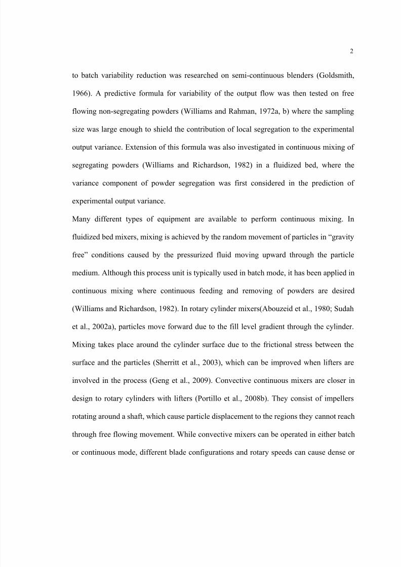
11
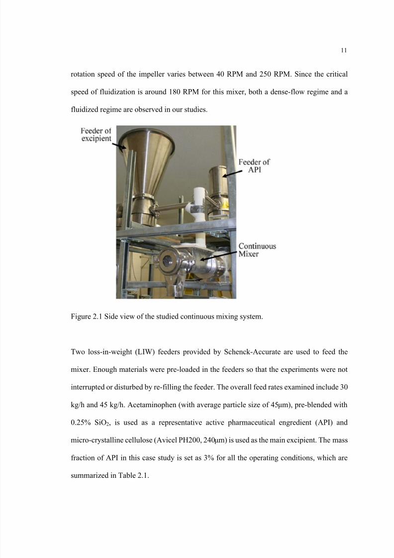
rotation speed of the impeller varies between 40 RPM and 250 RPM. Since the critical
speed of fluidization is around 180 RPM for this mixer, both a dense-flow regime and a
fluidized regime are observed in our studies.
Figure 2.1 Side view of the studied continuous mixing system.
Two loss-in-weight (LIW) feeders provided by Schenck-Accurate are used to feed the
mixer. Enough materials were pre-loaded in the feeders so that the experiments were not
interrupted or disturbed by re-filling the feeder. The overall feed rates examined include 30
kg/h and 45 kg/h. Acetaminophen (with average particle size of 45 μm), pre-blended with
0.25% SiO 2, is used as a representative active pharmaceutical engredient (API) and
micro-crystalline cellulose (Avicel PH200, 240 μm) is used as the main excipient. The mass
fraction of API in this case study is set as 3% for all the operating conditions, which are
summarized in Table 2.1.
8/13/2019 Modeling and Analysis of Continuous Powder Blending
http://slidepdf.com/reader/full/modeling-and-analysis-of-continuous-powder-blending 25/177
12
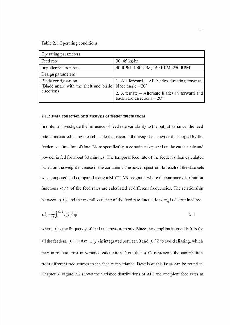
Table 2.1 Operating conditions.
Operating parameters
Feed rate 30, 45 kg/hr
Impeller rotation rate 40 RPM, 100 RPM, 160 RPM, 250 RPMDesign parameters
1. All forward – All blades directing forward, blade angle – 20°
Blade configuration(Blade angle with the shaft and bladedirection) 2. Alternate – Alternate blades in forward and
backward directions – 20°
2.1.2 Data collection and analysis of feeder fluctuations
In order to investigate the influence of feed rate variability to the output variance, the feed
rate is measured using a catch-scale that records the weight of powder discharged by the
feeder as a function of time. More specifically, a container is placed on the catch scale and
powder is fed for about 30 minutes. The temporal feed rate of the feeder is then calculated
based on the weight increase in the container. The power spectrum for each of the data sets
was computed and compared using a MATLAB program, where the variance distribution
functions ( ) s f of the feed rates are calculated at different frequencies. The relationship
between ( ) s f and the overall variance of the feed rate fluctuations 2inσ is determined by:
/ 22 2
0
1( )
2 s f
in s f df σ = ∫ 2-1
where s f is the frequency of feed rate measurements. Since the sampling interval is 0.1s for
all the feeders, 10 s f Hz = . ( ) s f is integrated between 0 and / 2 s f to avoid aliasing, which
may introduce error in variance calculation. Note that ( ) s f represents the contribution
from different frequencies to the feed rate variance. Details of this issue can be found in
Chapter 3. Figure 2.2 shows the variance distributions of API and excipient feed rates at

8/13/2019 Modeling and Analysis of Continuous Powder Blending
http://slidepdf.com/reader/full/modeling-and-analysis-of-continuous-powder-blending 26/177
13
different frequencies for the two feed rates studied. The peak of feed rate fluctuations of
API shifts from 0.16Hz to 0.24Hz when feed rate is increased. This indicates better feeding
conditions, since fluctuations at higher frequency are more easily filtered out by the mixer
(Weineköter and Reh, 1995). For the excipient, a sharp peak appears at 1.4 Hz at the lower
feed rate, whereas smaller peaks at higher frequencies (starts from 2.1 Hz) characterize the
higher feed rate. Notice that the lowest peak of feed rate fluctuations (peak at the lowest
frequency) always corresponds to rotating frequency of the feeding screw. The results in
Table 2.2 show that the feed rate of 45 kg/hr leads to smaller RSD of API concentration and
variance components at higher frequency domains. Since continuous mixer always
performs like a low-pass filter through which feeding fluctuations at higher frequencies are
easier to be attenuated (Gao et al., 2011b; Pernenkil and Cooney, 2006), these results
indicate better feeding performance at feed rate of 45 kg/hr.
Figure 2.2 Feed rate analysis of (a) API and (b) excipient.
8/13/2019 Modeling and Analysis of Continuous Powder Blending
http://slidepdf.com/reader/full/modeling-and-analysis-of-continuous-powder-blending 27/177
14
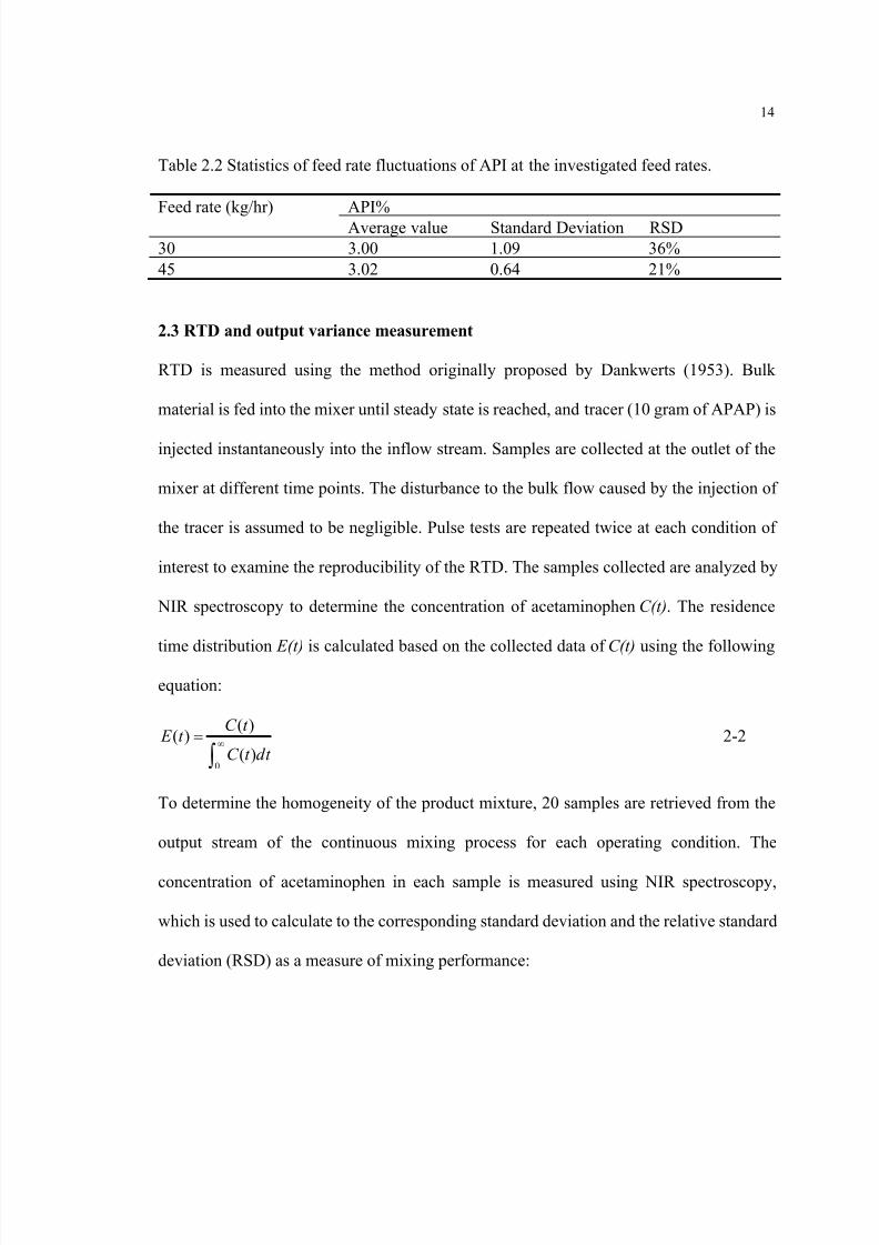
Table 2.2 Statistics of feed rate fluctuations of API at the investigated feed rates.
API%Feed rate (kg/hr)Average value Standard Deviation RSD
30 3.00 1.09 36%45 3.02 0.64 21%
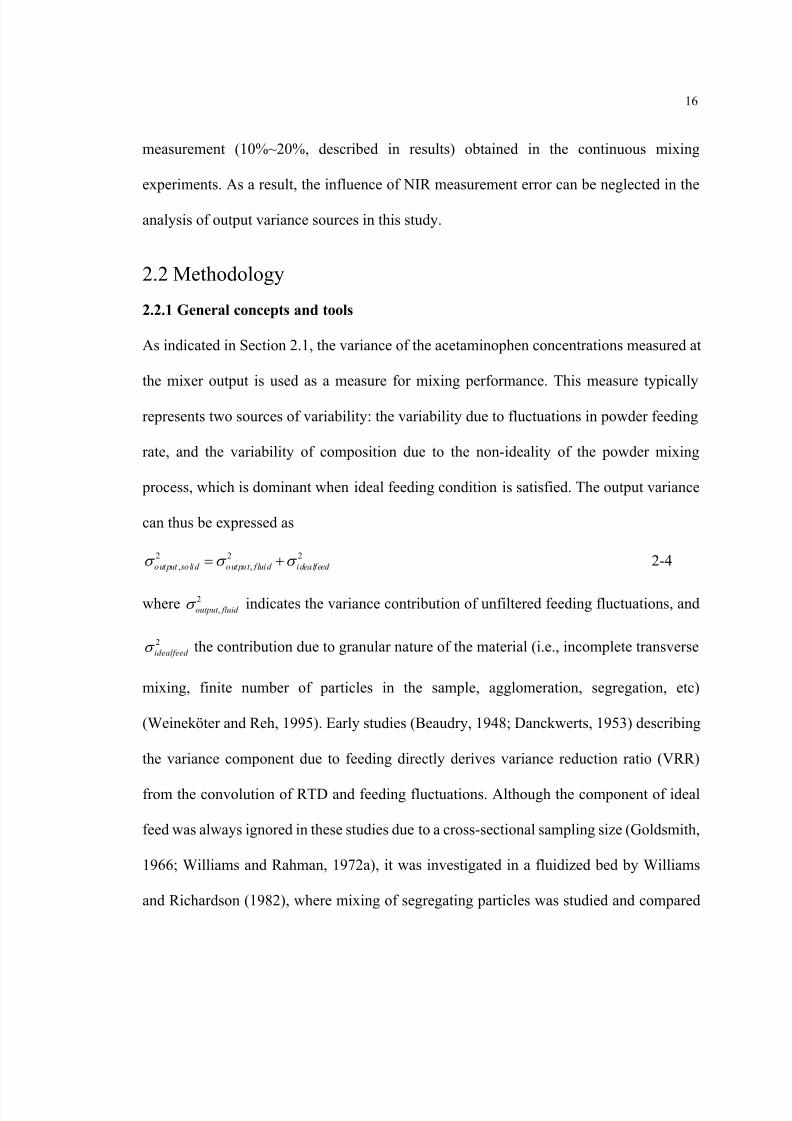
2.3 RTD and output variance measurement
RTD is measured using the method originally proposed by Dankwerts (1953). Bulk
material is fed into the mixer until steady state is reached, and tracer (10 gram of APAP) is
injected instantaneously into the inflow stream. Samples are collected at the outlet of the
mixer at different time points. The disturbance to the bulk flow caused by the injection of
the tracer is assumed to be negligible. Pulse tests are repeated twice at each condition of
interest to examine the reproducibility of the RTD. The samples collected are analyzed by
NIR spectroscopy to determine the concentration of acetaminophen C(t) . The residence
time distribution E(t) is calculated based on the collected data of C(t) using the followingequation:
0
( )( )
( )
C t E t
C t dt ∞=
∫ 2-2
To determine the homogeneity of the product mixture, 20 samples are retrieved from the
output stream of the continuous mixing process for each operating condition. The
concentration of acetaminophen in each sample is measured using NIR spectroscopy,
which is used to calculate to the corresponding standard deviation and the relative standard
deviation (RSD) as a measure of mixing performance:

8/13/2019 Modeling and Analysis of Continuous Powder Blending
http://slidepdf.com/reader/full/modeling-and-analysis-of-continuous-powder-blending 28/177
15
2
1( )Standard deviation
Average concentration 1
N
iC C RSD
C N σ
σ −
= = =−
∑ 2-3
where C is the average concentration of N samples and C i is the concentration of each
sample.
Figure 2.3 Calibration test on NIR method.
(a) Standard deviation (STDEV) (b) relative standard deviation (RSD) was measured at
API% of 2%~10% and 95% confidence intervals were estimated.
2.1.4 Analysis of NIR Method Error
In order to investigate the contribution of error in the NIR method to the output variance,
the following analysis is performed. Samples of 2%, 3%, 5% and 10% mass fraction of API
are prepared to study the measurement variability under the 3% API mass fraction
condition. Each sample is well mixed and measured ten times. The same sample is
re-agitated before the next measurement so that the scanned surface of the sample is
renewed. Standard deviation, RSD and 95% confidence interval are calculated. The results
are plotted in Figure 2.3, where the RSD from measurements is found to be around 1% in
the studied range of API%, which is insignificant compared to the output RSD
8/13/2019 Modeling and Analysis of Continuous Powder Blending
http://slidepdf.com/reader/full/modeling-and-analysis-of-continuous-powder-blending 29/177
16
measurement (10%~20%, described in results) obtained in the continuous mixing
experiments. As a result, the influence of NIR measurement error can be neglected in the
analysis of output variance sources in this study.
2.2 Methodology
2.2.1 General concepts and tools
As indicated in Section 2.1, the variance of the acetaminophen concentrations measured at
the mixer output is used as a measure for mixing performance. This measure typically
represents two sources of variability: the variability due to fluctuations in powder feeding
rate, and the variability of composition due to the non-ideality of the powder mixing
process, which is dominant when ideal feeding condition is satisfied. The output variance
can thus be expressed as
2 2 2, ,output so lid outpu t f luid idea lfeed σ σ σ = + 2-4
where 2,output fluid σ indicates the variance contribution of unfiltered feeding fluctuations, and
2idealfeed σ the contribution due to granular nature of the material (i.e., incomplete transverse
mixing, finite number of particles in the sample, agglomeration, segregation, etc)
(Weineköter and Reh, 1995). Early studies (Beaudry, 1948; Danckwerts, 1953) describing
the variance component due to feeding directly derives variance reduction ratio (VRR)
from the convolution of RTD and feeding fluctuations. Although the component of ideal
feed was always ignored in these studies due to a cross-sectional sampling size (Goldsmith,
1966; Williams and Rahman, 1972a), it was investigated in a fluidized bed by Williams
and Richardson (1982), where mixing of segregating particles was studied and compared

8/13/2019 Modeling and Analysis of Continuous Powder Blending
http://slidepdf.com/reader/full/modeling-and-analysis-of-continuous-powder-blending 30/177
17
with known or without feeding fluctuations. In our present work, this variance component
of ideal-feed is further decomposed as follows:
2 2 2idealfeed ITM RTDV σ σ σ = + 2-5
where the term 2σ ITM represents the variance component due to incomplete transverse
mixing (ITM), and the term 2σ RTDV represents the component due to RTD variability
(RTDV). Note that the sample size is supposed to be much smaller than the scale of
cross-sectional mixing to ensure that the term 2σ ITM
can be detected.
While traditional variance measurements can hardly provide information about the
different components of output variance, the characteristics of the RTD can reveal it. In
particular, the difference between experimental and model-predicted data, or the data
variability in a single RTD measurement is caused by incomplete transverse mixing, which
can be used as an indicator of transverse mixing (Figure 2.4a). Low data variability
indicates good transverse mixing and homogeneous API concentration in the cross-section
of outlet stream. Similarly, the difference between single and multiple model-fitted RTD
curves, or model variability in repeated RTD experiments indicates variance due to RTD
variability (Figure 2.4b). Small difference indicates good RTD reproducibility, which
leads to an insignificant output variance component 2σ RTDV , since little new axial
compositional heterogeneity generated in the system through superposition of RTD curves
with low variability. This issue was studied in Harris et al. (2002a) to validate a proposed
method of RTD measurement, where the first three moments of RTD were used in
comparison of repeated RTD measurements. It was also investigated in an earlier work
(Williams and Rahman, 1972a) in validating the ideal feed condition in a drum mixer.
Since quantification of both components correlates to the model fitting process of RTD, a
8/13/2019 Modeling and Analysis of Continuous Powder Blending
http://slidepdf.com/reader/full/modeling-and-analysis-of-continuous-powder-blending 31/177
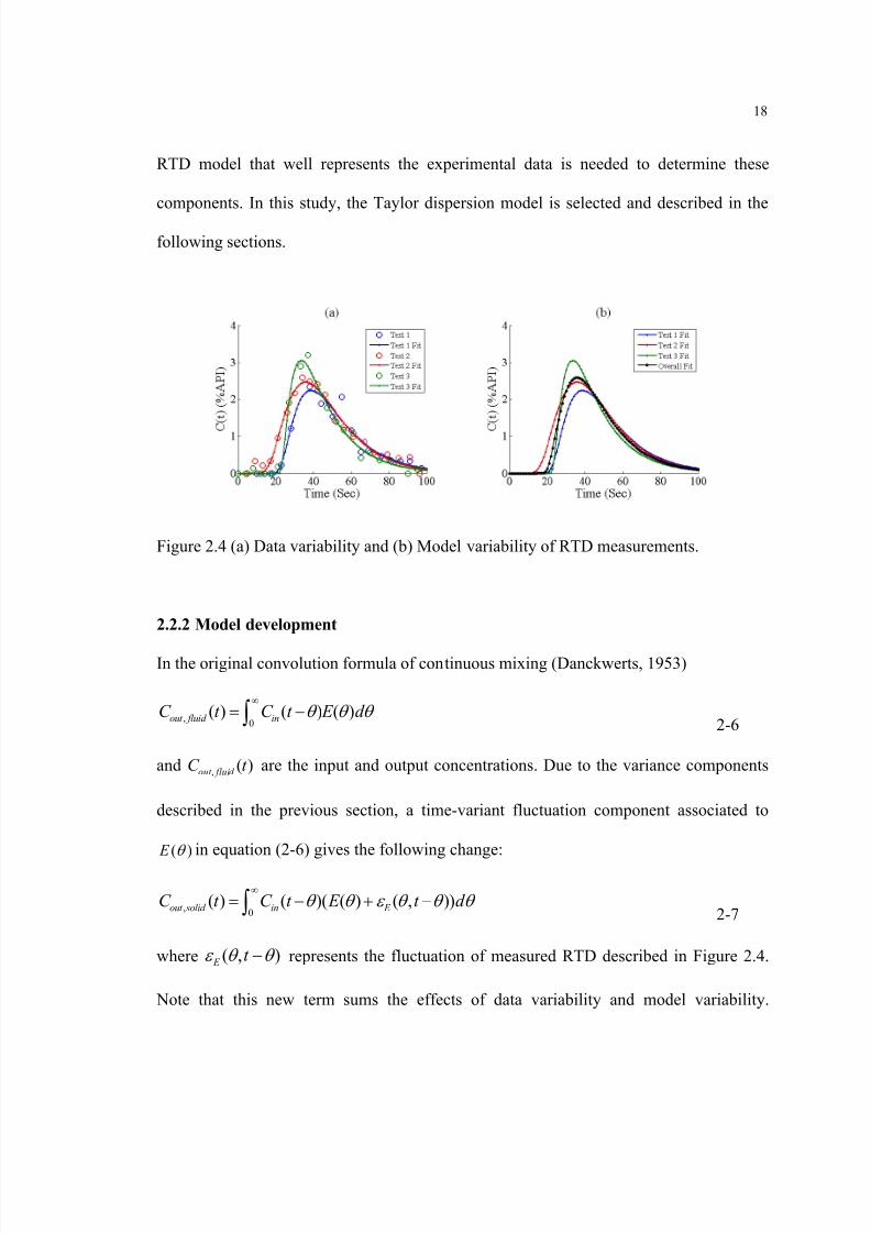
18
RTD model that well represents the experimental data is needed to determine these
components. In this study, the Taylor dispersion model is selected and described in the
following sections.
Figure 2.4 (a) Data variability and (b) Model variability of RTD measurements.
2.2.2 Model development
In the original convolution formula of continuous mixing (Danckwerts, 1953)
, 0( ) ( ) ( )out fluid inC t C t E d θ θ θ
∞= −∫ 2-6
and , ( )out fluid C t are the input and output concentrations. Due to the variance components
described in the previous section, a time-variant fluctuation component associated to
( ) E θ in equation (2-6) gives the following change:
, 0( ) ( )( ( ) ( , ))out solid in E C t C t E t d θ θ ε θ θ θ
∞= − + −∫ 2-7
where ( , ) E t ε θ θ − represents the fluctuation of measured RTD described in Figure 2.4.
Note that this new term sums the effects of data variability and model variability.

8/13/2019 Modeling and Analysis of Continuous Powder Blending
http://slidepdf.com/reader/full/modeling-and-analysis-of-continuous-powder-blending 32/177
19
Similarly, substituting ( )inC t θ − by the sum of mean and time-dependent fluctuation
( )in inC t ε θ + − , results in the following form:
, , 0( ) ( ) ( ( )) ( , )out solid out fluid in in E C t C t C t t d ε θ ε θ θ θ
∞= + + − −∫ 2-8
where , 0( ) ( ) ( )θ θ θ
∞= −∫out fluid inC t C t E d . Assuming that ( )in t ε is much smaller than inC :
, , 0( ) ( ) ( , )out solid out fluid in E C t C t C t d ε θ θ θ
∞≈ + −∫ 2-9
Since the variance componnets in the two components of equation (2-9) are independent,
the output variance of the concentration equals the sum of the variance components
contributed from each of them. Comparing equation (2-4) and (2-9), it is not difficult to
conclude that the ideal-feed variance component 2idealfeed σ comes from the integration of
RTD variability in E C ε .
2.2.3 Solution approach
In order to estimate the time-invariant RTD component E( θ ) discussed in the previous
section, as well as to understand the influence of operations on axial velocity and
dispersion, the Taylor dispersion model is considered as follows:
2
2
1C C C Peθ ξ ξ
∂ ∂ ∂+ =∂ ∂ ∂ 2-10
Equation (2-10) is the well-known one-dimensional Fokker-Planck equation that describes
time evolution of particle distribution in a continuous system (Risken, 1996). Detail of its
solution in different initial and boundary conditions can be found in (Levenspiel and Smith,
1957; Sherritt et al., 2003). One commonly used solution of equation (10), known as the
Taylor dispersion model, is obtained with open boundary conditions, which was described

8/13/2019 Modeling and Analysis of Continuous Powder Blending
http://slidepdf.com/reader/full/modeling-and-analysis-of-continuous-powder-blending 33/177
20
in Harris et al. (2003a, b) in characterizing the influence of axial gas and solid flux on axial
solid Peclet number in fluidized bed:
2( )1/ 20 4
1/ 2( , )(4 )
PeC PeC e
ξ θ θ ξ θ
πθ
− −
= 2-11
In equation (2-11) 0( )θ τ = −t t and z l ξ = are the dimensionless time and location in
continuous mixing process, where 0t represents the effect of time delay in RTD
measurement, τ is the mean residence time and l is the overall length of the mixer. 0C
denotes the amount of material injected in the pulse test. / Pe vl E = is the Peclet number,
where v and E represent the cross-section averaged axial velocity and the axial dispersion
coefficient of the system. When 1ξ = , equation (2-11) corresponds to the RTD of the
mixer.
The parameters Pe , 0C , τ and 0t in equation (2-11) are determined to minimize the
mean sum of square (MSS) error between predicted and experimentally determined values
of pulse test. This parameter set is defined as follows:
0 0[ , , , ] P Pe C t τ = 2-12
Fitted pulse test data can then be expressed as ( , )C t P . In particular, to evaluate the best
fitted curve for a single pulse test the follow error is minimized:
2 212
,1 1
[ ( , )] [ ( , )]min
n nij ij j ij ij
j ITM i i
C C t P C C t P MSS
n n= =
− −= =∑ ∑ 2-13
which represents the MSS error of data variability of RTD due to incomplete transverse
mixing. The overall MSS error of repeated RTD experiments is minimized when model
fitting of multiple pulse tests are performed:
8/13/2019 Modeling and Analysis of Continuous Powder Blending
http://slidepdf.com/reader/full/modeling-and-analysis-of-continuous-powder-blending 34/177
21
2 212
1 1 1 1
[ ( , )] [ ( , )]min
m n m nij ij ij ij
j i j i
C C t P C C t P MSS
mn mn= = = =
− −= =∑∑ ∑∑ 2-14
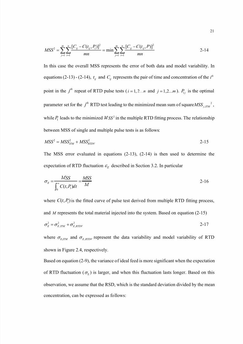
In this case the overall MSS represents the error of both data and model variability. In
equations (2-13) - (2-14), ijt and ijC represents the pair of time and concentration of the thi
point in the th j repeat of RTD pulse tests ( 1, 2...i n= and 1,2... j m= ). 1 j P is the optimal
parameter set for the th j RTD test leading to the minimized mean sum of square 2, j ITM MSS ,
while1
P leads to the minimized 2SS in the multiple RTD fitting process. The relationship
between MSS of single and multiple pulse tests is as follows:
2 2 2 ITM RTDV MSS MSS MSS = + 2-15
The MSS error evaluated in equations (2-13), (2-14) is then used to determine the
expectation of RTD fluctuation E ε described in Section 3.2. In particular
10( , )
σ ∞= =∫ E
SS MSS
C t P dt 2-16
where 1( , )C t P is the fitted curve of pulse test derived from multiple RTD fitting process,
and M represents the total material injected into the system. Based on equation (2-15)
2 2 2, ,σ σ σ = +
E E ITM E RTDV 2-17
where ,σ E ITM and ,σ E RTDV represent the data variability and model variability of RTD
shown in Figure 2.4, respectively.
Based on equation (2-9), the variance of ideal feed is more significant when the expectation
of RTD fluctuation ( σ E ) is larger, and when this fluctuation lasts longer. Based on this
observation, we assume that the RSD, which is the standard deviation divided by the mean
concentration, can be expressed as follows:
8/13/2019 Modeling and Analysis of Continuous Powder Blending
http://slidepdf.com/reader/full/modeling-and-analysis-of-continuous-powder-blending 35/177
22
σ = Δidealfeed E RSD k T 2-18
where k is a dimensionless coefficient describing the ratio between sum of RTD
fluctuations and the corresponding RSD. T Δ represents the time interval when the RTD
data were collected. In order to obtain reasonable T Δ , prolonged RTD measurements were
obtained for each operating condition so that all non-zero points can be recorded. Notice
that to guarantee this assumed relationship in equation (2-18), both RSD and E σ should be
determined by the sampling size. Using the experimental RTD and RSD obtained under
different operating conditions, k can be empirically estimated by applying linear
regression of the pairs idealfeed RSD and σ Δ E T . Then the variance components due to
incomplete transverse mixing and RTD variability can be derived based on the estimation
of k as follows:
,σ = Δ ITM E ITM RSD k T 2-19
,σ = Δ RTDV E RTDV RSD k T 2-20
Based on the estimation of the RSD components, the corresponding variance components
can then be conveniently derived using equation (2-3).
2.2.4 Methodology
Based on the theoretical work developed in the previous section, the following procedure
of the RTD modeling method can be established.
Step 1: Determine RTD from pulse tests, RSD at the outlet of continuous mixing process
( ,out solid RSD ) and feeding samples;
Step 2: Fit RTD using the Taylor dispersion model;

8/13/2019 Modeling and Analysis of Continuous Powder Blending
http://slidepdf.com/reader/full/modeling-and-analysis-of-continuous-powder-blending 36/177
23
Step 3: Apply the fitted RTD curve as well as the feeding samples to calculate the RSD
component of unfiltered feeding fluctuations,out fluid
RSD ;
Step 4: Determine idealfeed RSD based on ,out fluid RSD and ,out solid RSD ;
Step 5: Establish the correlation between idealfeed RSD and the form σ Δ E T which is obtained
in the RTD fitting process;
Step 6: Calculate ITM RSD and RTDV RSD and the corresponding variance components, then
analyze the effects of operations (feed rate, rotary speed, blade angle etc.) on each of them.
The analysis of step 6 can provide guidelines in order to improve the design and
performance of continuous mixing systems. In the next section the proposed procedure
was applied in a case study of continuous mixing in order to investigate the influence of
different operations to the mixing performance.
2.3 Experimental results and modeling
2.3.1 RTD fitting results
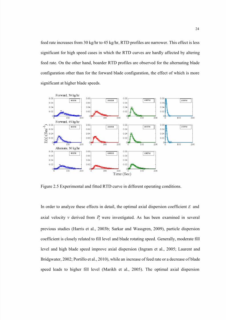
Figure 2.5 illustrates the influence of operating conditions and blade design on RTD
characteristics, as obtained experimentally for the materials considered. For each operating
condition, pulse tests were repeated twice so that the influence of RTD variability could be
included in the performance prediction. The Taylor Dispersion model and the non-linear
regression procedure described in Section 2.2 were applied in the RTD fitting process. The
curve in each plot corresponds to the best model fit using equation (2-14). It was observed
that RTD is more sensitive to blade speed than to feed rate and blade configuration. Lower
blade speeds and lower flow rate lead to larger mean residence time and wider RTD. When
8/13/2019 Modeling and Analysis of Continuous Powder Blending
http://slidepdf.com/reader/full/modeling-and-analysis-of-continuous-powder-blending 37/177
24
feed rate increases from 30 kg/hr to 45 kg/hr, RTD profiles are narrower. This effect is less
significant for high speed cases in which the RTD curves are hardly affected by altering
feed rate. On the other hand, boarder RTD profiles are observed for the alternating blade
configuration other than for the forward blade configuration, the effect of which is more
significant at higher blade speeds.
Figure 2.5 Experimental and fitted RTD curve in different operating conditions.
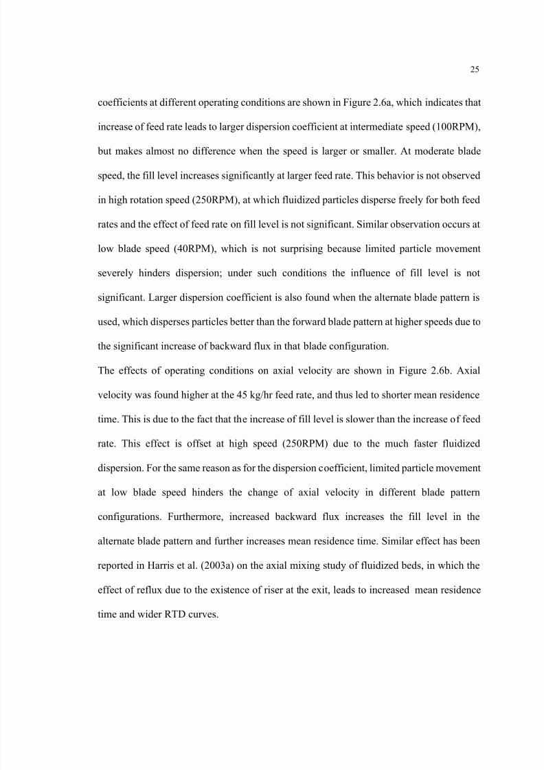
In order to analyze these effects in detail, the optimal axial dispersion coefficient E and
axial velocity v derived from 1 P were investigated. As has been examined in several
previous studies (Harris et al., 2003b; Sarkar and Wassgren, 2009), particle dispersion
coefficient is closely related to fill level and blade rotating speed. Generally, moderate fill
level and high blade speed improve axial dispersion (Ingram et al., 2005; Laurent and
Bridgwater, 2002; Portillo et al., 2010), while an increase of feed rate or a decrease of blade
speed leads to higher fill level (Marikh et al., 2005). The optimal axial dispersion
8/13/2019 Modeling and Analysis of Continuous Powder Blending
http://slidepdf.com/reader/full/modeling-and-analysis-of-continuous-powder-blending 38/177
25
coefficients at different operating conditions are shown in Figure 2.6a, which indicates that
increase of feed rate leads to larger dispersion coefficient at intermediate speed (100RPM),
but makes almost no difference when the speed is larger or smaller. At moderate blade
speed, the fill level increases significantly at larger feed rate. This behavior is not observed
in high rotation speed (250RPM), at which fluidized particles disperse freely for both feed
rates and the effect of feed rate on fill level is not significant. Similar observation occurs at
low blade speed (40RPM), which is not surprising because limited particle movement
severely hinders dispersion; under such conditions the influence of fill level is not
significant. Larger dispersion coefficient is also found when the alternate blade pattern is
used, which disperses particles better than the forward blade pattern at higher speeds due to
the significant increase of backward flux in that blade configuration.
The effects of operating conditions on axial velocity are shown in Figure 2.6b. Axial
velocity was found higher at the 45 kg/hr feed rate, and thus led to shorter mean residence
time. This is due to the fact that the increase of fill level is slower than the increase of feed
rate. This effect is offset at high speed (250RPM) due to the much faster fluidized
dispersion. For the same reason as for the dispersion coefficient, limited particle movement
at low blade speed hinders the change of axial velocity in different blade pattern
configurations. Furthermore, increased backward flux increases the fill level in the
alternate blade pattern and further increases mean residence time. Similar effect has been
reported in Harris et al. (2003a) on the axial mixing study of fluidized beds, in which the
effect of reflux due to the existence of riser at the exit, leads to increased mean residence
time and wider RTD curves.
8/13/2019 Modeling and Analysis of Continuous Powder Blending
http://slidepdf.com/reader/full/modeling-and-analysis-of-continuous-powder-blending 39/177
26
Figure 2.6 Effects of operating conditions on (a) dispersion coefficient E and (b) axial
velocity v.
2.3.2 Results and Discussion
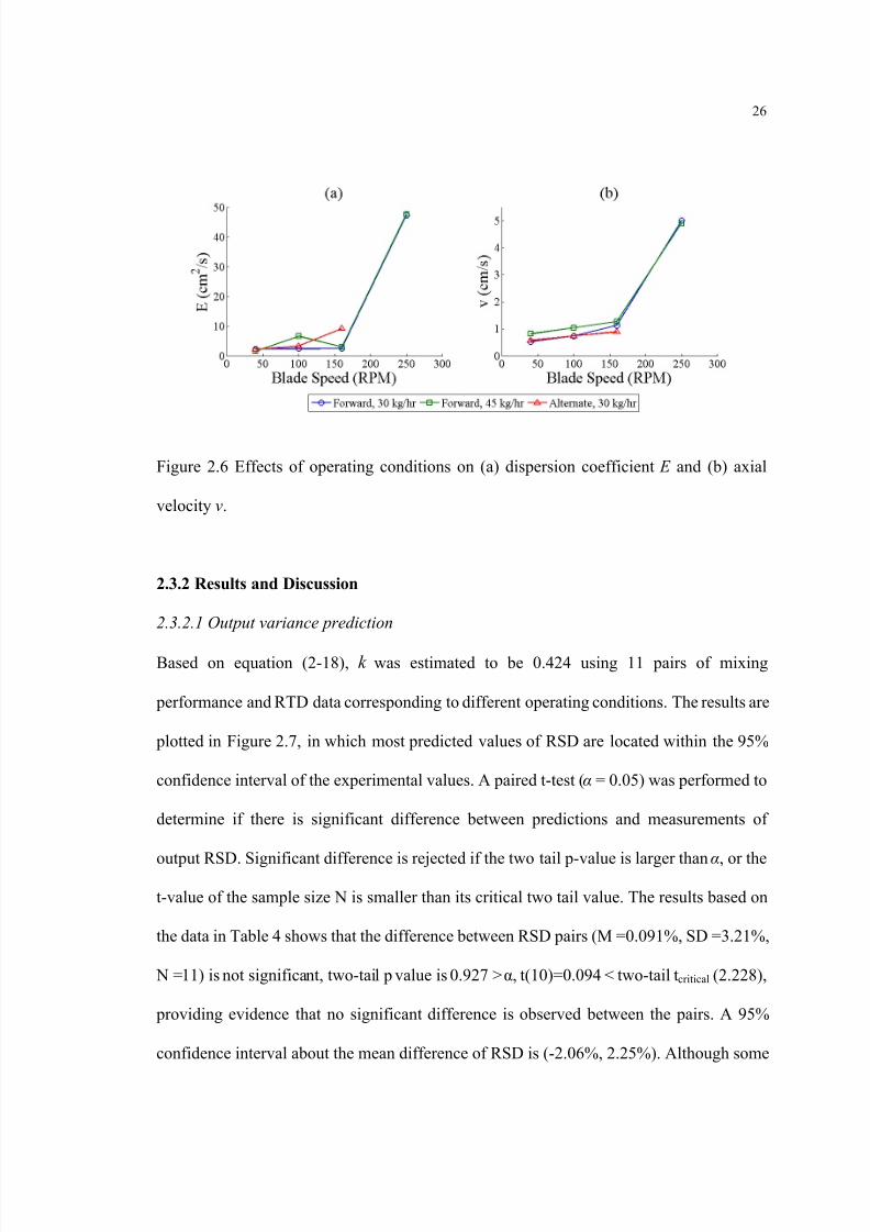
2.3.2.1 Output variance prediction
Based on equation (2-18), k was estimated to be 0.424 using 11 pairs of mixing
performance and RTD data corresponding to different operating conditions. The results are
plotted in Figure 2.7, in which most predicted values of RSD are located within the 95%
confidence interval of the experimental values. A paired t-test ( α = 0.05) was performed to
determine if there is significant difference between predictions and measurements of
output RSD. Significant difference is rejected if the two tail p-value is larger than α, or the
t-value of the sample size N is smaller than its critical two tail value. The results based on
the data in Table 4 shows that the difference between RSD pairs (M =0.091%, SD =3.21%,
N =11) is not significant, two-tail p value is 0.927 > α, t(10)=0.094 < two-tail t critical (2.228),
providing evidence that no significant difference is observed between the pairs. A 95%
confidence interval about the mean difference of RSD is (-2.06%, 2.25%). Although some
8/13/2019 Modeling and Analysis of Continuous Powder Blending
http://slidepdf.com/reader/full/modeling-and-analysis-of-continuous-powder-blending 40/177
27
differences are observed between the experimental and predicted variance, the predicted
values follow the same trends as the experimental measurements. The main sources of
variation between predicted and observed values include:
Figure 2.7 95% confidence interval of experimental RSD are calculated and compared to
the predicted values.
(1) The term ( ) ( , )ε θ ε θ θ − −in E t t , which in equation (2-8) was assumed to be negligible,
may contribute to output fluctuations in practice in the examined case study.
(2) In the RTD fitting process, the variance component due to RTD fluctuations was
estimated by two repeats of pulse tests. This may introduce non-representative variability
on the normalized mean sum of square E σ and thus lead to deviations on the predicted
variance.
(3) The estimated interval T Δ in the RTD modeling process might be too short, which
might fail to capture fluctuations occurring outside the recorded tail of the RTD curve.

8/13/2019 Modeling and Analysis of Continuous Powder Blending
http://slidepdf.com/reader/full/modeling-and-analysis-of-continuous-powder-blending 41/177

8/13/2019 Modeling and Analysis of Continuous Powder Blending
http://slidepdf.com/reader/full/modeling-and-analysis-of-continuous-powder-blending 42/177
29
Figure 2.9 Effects of operating conditions on the variance component due to incomplete
transverse mixing.
Ingram et al. (2005) found that the radial dispersion coefficient increased at high rotating
speed and moderate high fill level in rotating drums. In agreement with their previous
findings, faster decay of variance component due to incomplete transverse mixing is found
here at high blade speed in the studied convective mixer (Figure 2.9). It is also observed
that at low blade speed, high feed rate facilitates transverse mixing. This is due to the
significant increase of fill level under such conditions, which leads to larger number of
blade passes experienced by the powder and results in faster radial dispersion. Mixing is
also improved in the alternate blade configuration due to the effect of reflux discussed
above. Both effects are offset at high blade speed when the whole mixer is fluidized.
8/13/2019 Modeling and Analysis of Continuous Powder Blending
http://slidepdf.com/reader/full/modeling-and-analysis-of-continuous-powder-blending 43/177
30
Figure 2.10 Effects of operating conditions on the variance component due to RTD
variability.
Figure 2.10 shows the influence of operating conditions on the component of RTD
variability. At high blade speed, short residence time and high blade speed lead to highly
variable RTD profile and contribute to larger variance component. It is also noticed that
high feed rate produces large RTD variability, possibly due to large fill levels and less
homogeneous dispersion of particles in the axial direction. Decrease of this component in
the alternate blade pattern can be explained by the increase of backward flux that facilitates
axial mixing, thus leading to less variable RTD profiles.
Based on the analysis above, the influence of each operating condition on different
variance components can be summarized as follows. High blade speed facilitates
transverse mixing, but introduces variability on the RTD profile and is inefficient in
attenuating feeder fluctuations. High feed rate increases fill level at low blade speed,
increasing the number of blade passes during the residence time, which benefits transverse

8/13/2019 Modeling and Analysis of Continuous Powder Blending
http://slidepdf.com/reader/full/modeling-and-analysis-of-continuous-powder-blending 44/177
31
mixing while results in more RTD variability. Backward mixing produced by the alternate
blade pattern improves mixing due to the refluxing effect while leads to less variable RTD
profiles at moderate blade speed. In summary, the alternate blade pattern at moderate blade
speed generates the most efficient continuous mixing for the materials examined here,
while the effects of feed rate on transverse mixing and RTD variability offset each other for
the studied conditions, and thus is insignificant to the overall mixing performance.
2.4 Summary
In the present study, we have developed a method based on the experimental RTD for
prediction of the mixer performance in a continuous mixing system. Different sources of
output variance are separately examined using this method, which leads to better
understanding of the effects of operating conditions on each of the individual variance
component. Based on the established RTD-RSD correlation, the effects of two feed rates,
two blade configurations and four blade speeds are analyzed. The results show that
moderate RPM and alternate blade configuration facilitate mixing, while change of feed
rate shows no significant influence to the overall output variance. Since the developed
methodology is independent of operational conditions, sampling detection method, and
mixer type, it should be applicable as a general method to investigate continuous mixing
processes. Moreover, the developed variance separation method has an important
advantage in understanding the behavior of different variance sources, and thus provides
quantitative guidance in further studies in design and control of continuous mixer.

8/13/2019 Modeling and Analysis of Continuous Powder Blending
http://slidepdf.com/reader/full/modeling-and-analysis-of-continuous-powder-blending 45/177
8/13/2019 Modeling and Analysis of Continuous Powder Blending
http://slidepdf.com/reader/full/modeling-and-analysis-of-continuous-powder-blending 46/177
33
2
2 0
12 ( ) ( ) ( )out
fluid in
R r E E r d dr VRR
σ θ θ θ
σ
∞= = +∫ ∫ 3-1
2
( ) ( )( ) in in
in
t t r R r
δ δ σ
−= 3-2
( ) ( )in in inC t C t δ = + 3-3
where R(r) in equation (3-2) describes the autocorrelation coefficient or serial correlation
coefficient. ( )inC t , expressed as sum of the mean value inC and the fluctuation
part ( )in t δ in equation (3-3), is denoted as input feed rate. E(t) is the normalized residence
time distribution, derived from the measured residence time distribution C(t) using
equation (2-2).
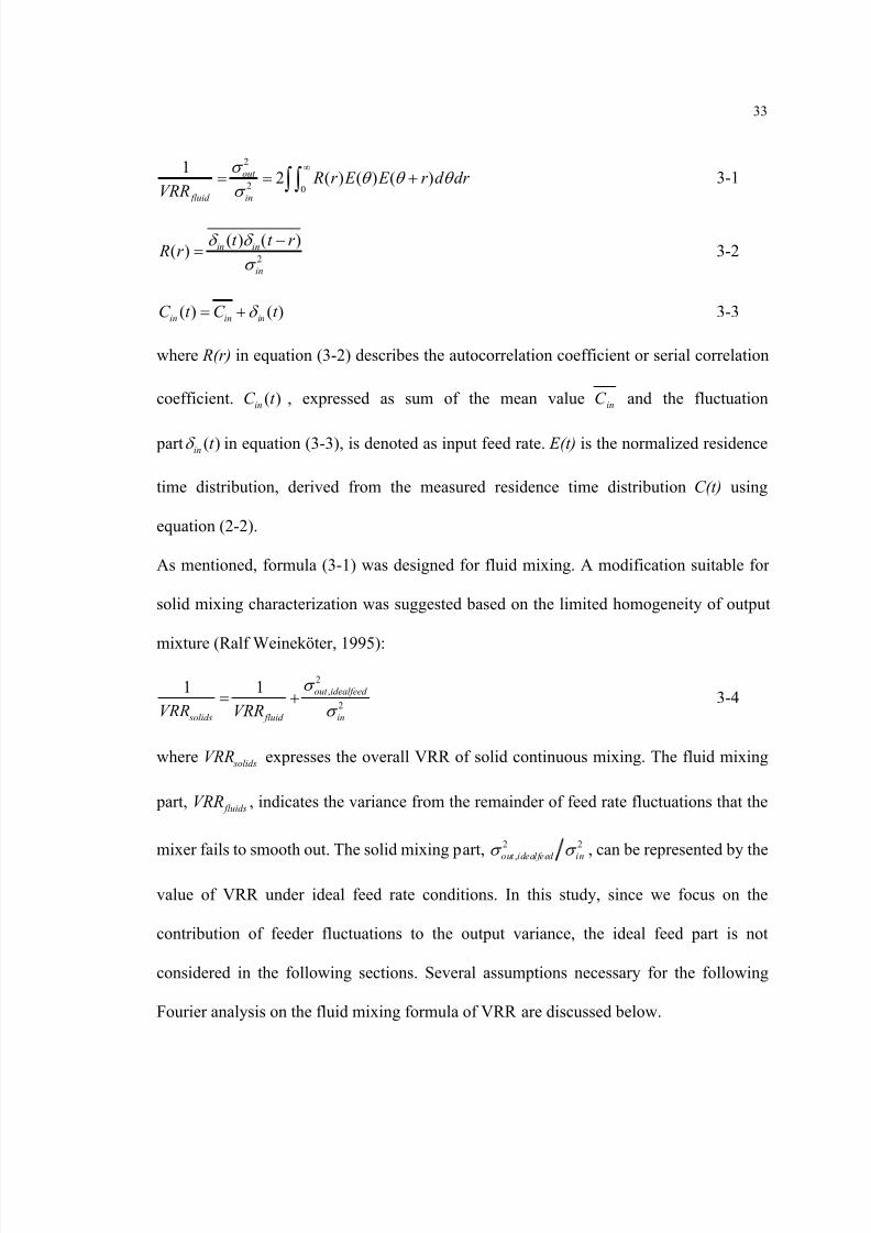
As mentioned, formula (3-1) was designed for fluid mixing. A modification suitable for
solid mixing characterization was suggested based on the limited homogeneity of output
mixture (Ralf Weineköter, 1995):2
,2
1 1 out idealfeed
solids fluid inVRR VRR
σ
σ = + 3-4
where solidsVRR expresses the overall VRR of solid continuous mixing. The fluid mixing
part, fluidsVRR , indicates the variance from the remainder of feed rate fluctuations that the
mixer fails to smooth out. The solid mixing part, 2 2,out idealfeed inσ σ , can be represented by the
value of VRR under ideal feed rate conditions. In this study, since we focus on the
contribution of feeder fluctuations to the output variance, the ideal feed part is not
considered in the following sections. Several assumptions necessary for the following
Fourier analysis on the fluid mixing formula of VRR are discussed below.
8/13/2019 Modeling and Analysis of Continuous Powder Blending
http://slidepdf.com/reader/full/modeling-and-analysis-of-continuous-powder-blending 47/177
34
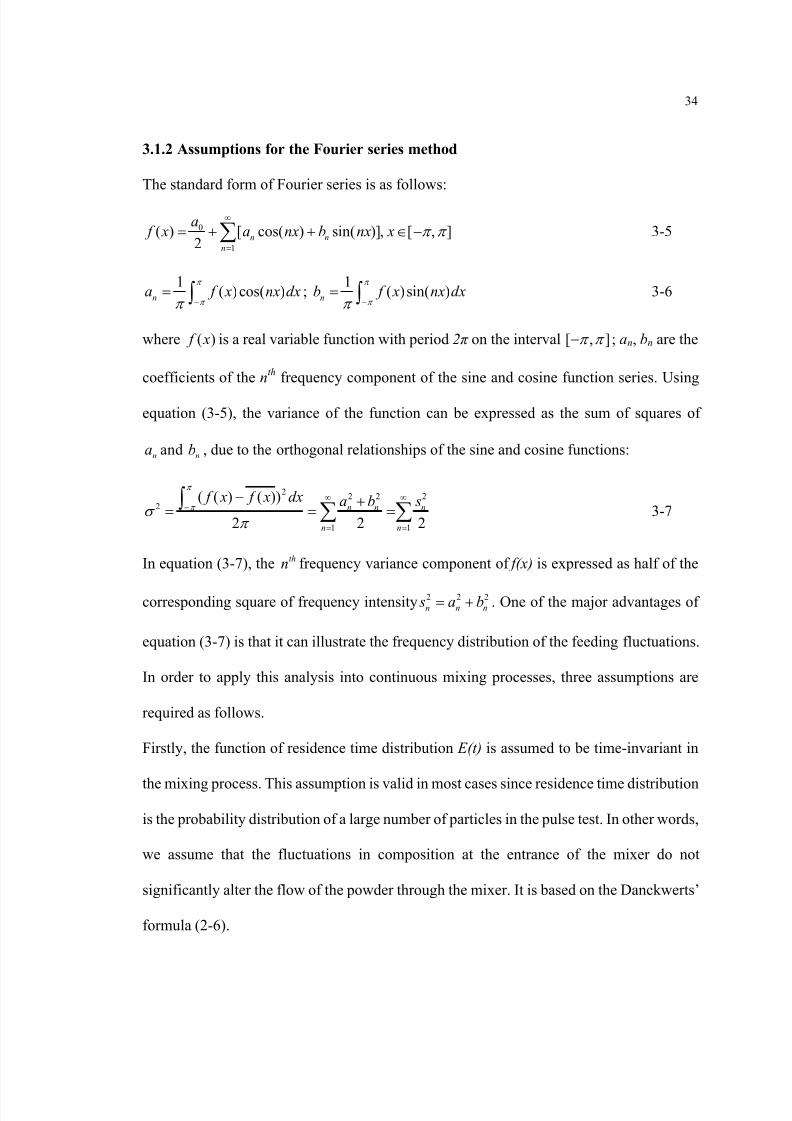
3.1.2 Assumptions for the Fourier series method
The standard form of Fourier series is as follows:
0
1
( ) [ cos( ) sin( )], [ , ]2 n n
n
a f x a nx b nx x π π
∞
== + + −∑ 3-5
1( ) cos( )na f x nx dx
π
π π −= ∫ ;
1( ) sin( )nb f x nx dx
π
π π −= ∫ 3-6
where ( ) f x is a real variable function with period 2π on the interval [ , ]π π − ; a n, bn are the
coefficients of the nth frequency component of the sine and cosine function series. Using
equation (3-5), the variance of the function can be expressed as the sum of squares of
na and nb , due to the orthogonal relationships of the sine and cosine functions:
2 2 2 22
1 1
( ( ) ( ))
2 2 2n n n
n n
f x f x dx a b sπ
π σ π
∞ ∞−
= =
− += = =∫ ∑ ∑ 3-7
In equation (3-7), the thn frequency variance component of f(x) is expressed as half of the
corresponding square of frequency intensity 2 2 2n n n s a b= + . One of the major advantages of
equation (3-7) is that it can illustrate the frequency distribution of the feeding fluctuations.
In order to apply this analysis into continuous mixing processes, three assumptions are
required as follows.
Firstly, the function of residence time distribution E(t) is assumed to be time-invariant in
the mixing process. This assumption is valid in most cases since residence time distribution
is the probability distribution of a large number of particles in the pulse test. In other words,
we assume that the fluctuations in composition at the entrance of the mixer do not
significantly alter the flow of the powder through the mixer. It is based on the Danckwerts’
formula (2-6).

8/13/2019 Modeling and Analysis of Continuous Powder Blending
http://slidepdf.com/reader/full/modeling-and-analysis-of-continuous-powder-blending 48/177
35
Due to the definition of Fourier series, the periodic function ( ) f x in equation (3-5) is
defined on the interval [ , ]π π −
; however, the definition domains for both ( )inC t and E(t)
are from zero to infinity while both feed rate fluctuations and RTD can only be recorded for
finite times in practice. Due to these limitations, another assumption is that the magnitude
of E(t) is negligible at the end of the RTD measurement. This makes sure that the recorded
values can be truncated and transformed onto the interval [ , ]π π − without missing
significant signal information. Exception to this assumption could occur when the mixer
has quasi-stagnant regions exchanging mass very slowly with the main flow. This issue is
discussed later in section 3.1.4.
The last assumption concerns the Dirichlet conditions that describe the sufficient condition
that guarantees existence and convergence of the Fourier series analysis. Based on this
assumption, finite coefficients na and nb in equation (3-6), together with the existence of
finite discontinuities, maxima and minima of points in f(x), are sufficient for Fourier series
convergence. The Dirichlet conditions should be satisfied on the involved feed rate
fluctuations, which guarantees that the reconstructed function based on the Fourier series
and the original function of feeder fluctuations are consistent with each other.
3.1.3 Application of Fourier series analysis
Based on equation (3-5), and the assumptions above, the continuous functions of feed rate
fluctuations ( )inC t and the residence time distribution ( ) E t in formula (2-6) were
transformed onto the interval [ , ]π π − , and substituted by the corresponding Fourier series.
The final output variance and VRR formula of Fourier series are as follows:
2 2 2 2 2 2 22 2
1 1
( )( )2 2
n n n n n nout
n n
a b A B s F π σ π
∞ ∞
= =
+ += =∑ ∑ 3-8
8/13/2019 Modeling and Analysis of Continuous Powder Blending
http://slidepdf.com/reader/full/modeling-and-analysis-of-continuous-powder-blending 49/177
36
2 2 2 2 2 2 2 22
1 12
2 2 2
1 1
( )( )1
( )
n n n n n nout n n
inn n n
n n
a b A B s F
VRR a b s
π π σ
σ
∞ ∞
= =∞ ∞
= =
+ += = =
+
∑ ∑
∑ ∑ 3-9
where na , nb are the Fourier series coefficients of the transformed feed rate ( )in f t at the
thn frequency component, and the square of the frequency intensity is denoted as
2 2 2n n n s a b= + ; similarly, n A , n B and 2 2 2
n n n F A B= + are the Fourier series coefficients and
the square of frequency intensity of the RTD function. Due to the expression of VRR in
equation (3-9), the filtering ability of the mixer is frequency dependent, expressed by the
term 2 2n F π . Notice that this filtering ability is not larger than one since amplification of
signal fluctuations is impossible in blending process. Comparison between equation (3-1)
and (3-9) indicates that the new VRR formula can clearly illustrate the contributions of
either feed rate fluctuations or RTD profiles to the output variance of the system, in
different frequency domains.
In order to utilize this new VRR formula in practice, we need to introduce the discrete
Fourier transform, as continuous records of feed rate and RTD signals with infinite
sampling frequency are not available. Moreover, since the scale of the Fourier coefficients
is discrete on the frequency domain and thus is proportional to the sample length, it is
difficult to compare variance distributions from feeding samples with different length. To
solve these problems, procedures are described as follows.
The expressions of discrete Fourier series are shown in equations (3-10) and (3-11), where
N is the number of signal points evenly sampled, and n x is the measured value of each
point and X k is the Fourier component of the k th frequency:
8/13/2019 Modeling and Analysis of Continuous Powder Blending
http://slidepdf.com/reader/full/modeling-and-analysis-of-continuous-powder-blending 50/177
37
21
0
2, 1, 2,... 1
i N kn N
k k k nn
X a ib x e k N N
π − −
== + = = −∑ 3-10
1 1
0 0
2 2 2 2cos ; sin
N N
k n k nn n
a x kn b x kn N N N N
π π − −
= =
= = −∑ ∑ 3-11
2/ 22
1 2
N n
n
sσ
=
= ∑ 3-12
In equation (3-12) the term 2n s has the same definition as that of the continuous form in
Appendix. By comparing equation (3-10) with the continuous case (3-5), it is found that N
is expressed as N =T in/Δt . Here T in denotes the length of feed rate sample, and Δt is the
sampling interval, which reciprocal of the sampling frequency.
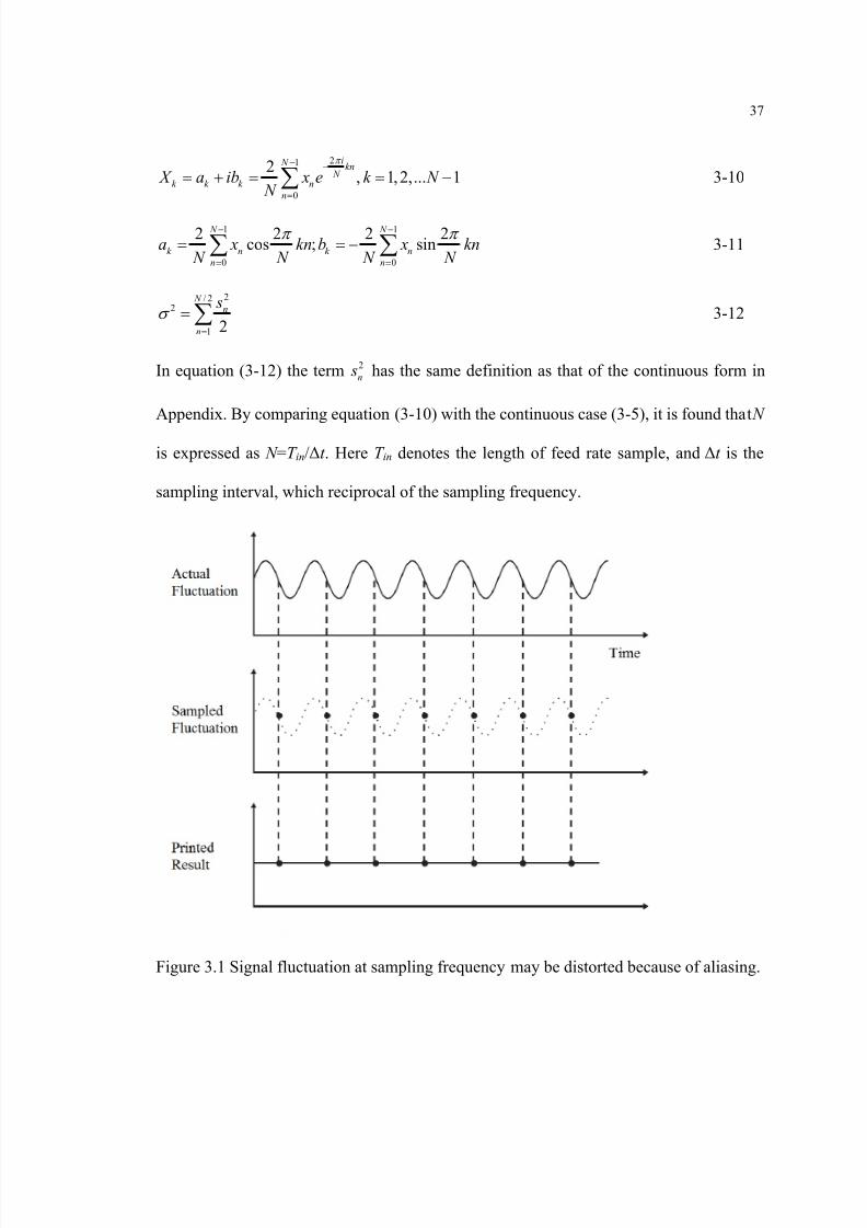
Figure 3.1 Signal fluctuation at sampling frequency may be distorted because of aliasing.
8/13/2019 Modeling and Analysis of Continuous Powder Blending
http://slidepdf.com/reader/full/modeling-and-analysis-of-continuous-powder-blending 51/177
38
One common problem caused by the discrete manner of the data collection is what is called
aliasing in the field of signal analysis, which describes the inaccuracy of fluctuation signal
measurement around the sampling frequency (Figure 3.1). To eliminate measurement error
caused by aliasing, the maximum frequency component we use in Fourier series is half of
the sampling frequency. For example, if the sampling time interval is 0.1s, the sampling
frequency is 10Hz, and the maximum frequency we can use in Fourier series calculation is
5Hz. Therefore, the 2 ~ 1 N N − components are dropped off in equation (3-12).
Equation (3-11) indicates that the magnitude of coefficients ak and bk is reciprocally
proportional to the number of sampling points N . Continuous integration formula instead
of sum of squares is thus necessary to avoid inconsistence caused by different N :
max 2/ 222 2
01
1 ( )( )
2 2
f N
n
s n f s f df f σ
=
Δ= ≈ Δ∑∫ 3-13
( ) n s s n f
f Δ =
Δ 3-14
In equation (3-14) we introduce the continuous form ( ) s f instead of the discrete variance
component series sn. Here Δ f =1/T in is the minimal frequency interval in the Fourier series,
and f max /2 denotes half of the frequency of sampling, corresponding to the N/2 component
of the variance intensity. Equation (3-14) represents the continuous variance intensity
distribution derived from the discrete series, and the scale of this distribution isindependent of how long the input flow is to be tested, or how many points are sampled on
the signal of feed rate.
Comparing equation (3-14) with the continuous formula of output variance or VRR in
(3-8), we define the ability of a continuous mixer to filter out feed rate fluctuations as Fe(f) :
( ) ( ) Fe f F f π = 3-15
8/13/2019 Modeling and Analysis of Continuous Powder Blending
http://slidepdf.com/reader/full/modeling-and-analysis-of-continuous-powder-blending 52/177
39
where ( ) n F n f F Δ = indicates that the magnitude of filtering ability is independent of the
number of sampling points. It should be noticed that the coefficient π in equation (3-15)
comes from the conversion of time scale from [0, ]int T to [ , ] x π π − . If this conversion
step is not applied, equation (3-15) is replaced by a general form where ) ( f F is now
directly from the Fourier series of ( ) E t :
2)(
)( inT f F f Fe = 3-16
Therefore, we derive the applicable form of output variance and VRR:
max22 2 2
0
1( ) ( )
2
f
out s f Fe f df σ = ∫ 3-17
max
max
2 2 220
22 2
0
( ) ( )1
( )
f
out f
in
s f Fe f df
VRR s f df
σ σ
= = ∫∫
3-18
where ( ) s f is the variance spectrum, and ( ) Fe f is the filtering ability of the mixer. It
becomes clear that for the input variance component 2( ) 2 s f f Δ at a small frequency
range [ 2 , 2] f f f f − Δ + Δ , a fraction of 21 ( ) Fe f − of that variance component will be
filtered out by the mixer. This formula shows its merit in clarifying the criterion for design
and selection of a mixer or a feeder in an integrated system. Examples of analysis of
( ) Fe f with different parameters and applications of equations (3-17) and (3-18) will be
discussed in detail below.
3.1.4 Correction of the RTD in Fourier series analysis
8/13/2019 Modeling and Analysis of Continuous Powder Blending
http://slidepdf.com/reader/full/modeling-and-analysis-of-continuous-powder-blending 53/177
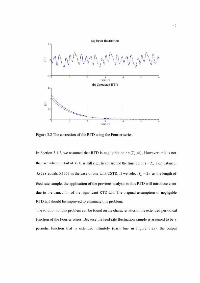
40
Figure 3.2 The correction of the RTD using the Fourier series.
In Section 3.1.2, we assumed that RTD is negligible on ( , )int T ∞ . However, this is not
the case when the tail of ( ) E t is still significant around the time point int T = . For instance,
(2 ) E τ equals 0.1353 in the case of one-tank CSTR. If we select 2inT τ = as the length of
feed rate sample, the application of the previous analysis to this RTD will introduce error
due to the truncation of the significant RTD tail. The original assumption of negligible
RTD tail should be improved to eliminate this problem.
The solution for this problem can be found on the characteristics of the extended periodical
function of the Fourier series. Because the feed rate fluctuation sample is assumed to be a
periodic function that is extended infinitely (dash line in Figure 3.2a), the output
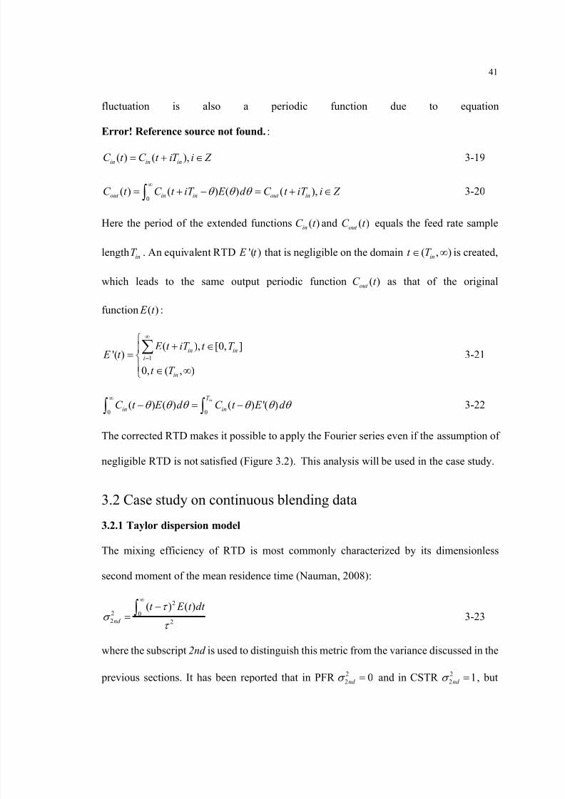
8/13/2019 Modeling and Analysis of Continuous Powder Blending
http://slidepdf.com/reader/full/modeling-and-analysis-of-continuous-powder-blending 54/177
41
fluctuation is also a periodic function due to equation
Error! Reference source not found. :
( ) ( ),in in inC t C t iT i Z = + 3-19
0( ) ( ) ( ) ( ),out in in out inC t C t iT E d C t iT i Z θ θ θ
∞= + − = + ∫ 3-20
Here the period of the extended functions ( )inC t and ( )out C t equals the feed rate sample
length inT . An equivalent RTD '( ) E t that is negligible on the domain ( , )int T ∞ is created,
which leads to the same output periodic function ( )out C t as that of the original
function ( ) E t :
1
( ), [0, ]'( )
0, ( , )
in ini
in
E t iT t T E t
t T
∞
=
+ =
∞
∑ 3-21
0 0( ) ( ) ( ) '( )
inT
in inC t E d C t E d θ θ θ θ θ θ ∞
− = −∫ ∫ 3-22
The corrected RTD makes it possible to apply the Fourier series even if the assumption of
negligible RTD is not satisfied (Figure 3.2). This analysis will be used in the case study.
3.2 Case study on continuous blending data
3.2.1 Taylor dispersion model
The mixing efficiency of RTD is most commonly characterized by its dimensionless
second moment of the mean residence time (Nauman, 2008):
2
2 02 2
( ) ( )nd
t E t dt τ σ
τ
∞−
= ∫ 3-23
where the subscript 2nd is used to distinguish this metric from the variance discussed in the
previous sections. It has been reported that in PFR 22 0nd σ = and in CSTR 2
2 1nd σ = , but

8/13/2019 Modeling and Analysis of Continuous Powder Blending
http://slidepdf.com/reader/full/modeling-and-analysis-of-continuous-powder-blending 55/177
42
little regarding the mixing efficiency has been discussed when the value of 22nd σ is between
zero and one. In this subsection, the filtering ability index developed in this work is used to
characterize the influence of parameters to the filtering ability of the Taylor dispersion
model (2-11).
Figure 3.3 Filtering ability of the Taylor Dispersion model with different Peclet numbers
from one to infinite.
In this model, the concentration ( 1, )C ξ θ = at the outlet of the continuous mixer is only a
function of θ , which can be normalized to deduce residence time distribution with only one
parameter Pe . The filtering ability Fe(f) of the RTD modeled by Taylor Dispersion model
are plotted in Figure 3.3, with different Pe . The plots indicate that better filtering ability of
the mixer occurs for smaller Pe due to lower and narrower ( ) Fe f curve. On the other
hand, the model acts more like a PFR when Pe is large, in which no smoothing takes place
in the mixer. ( ) Fe f equals one for all frequency components in PFR, while all other curve
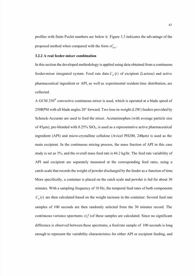
8/13/2019 Modeling and Analysis of Continuous Powder Blending
http://slidepdf.com/reader/full/modeling-and-analysis-of-continuous-powder-blending 56/177
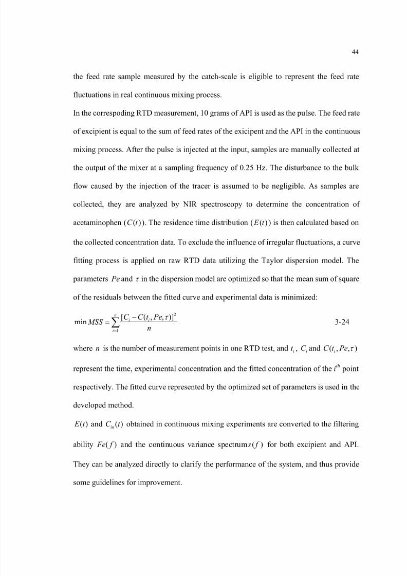
8/13/2019 Modeling and Analysis of Continuous Powder Blending
http://slidepdf.com/reader/full/modeling-and-analysis-of-continuous-powder-blending 57/177
44
the feed rate sample measured by the catch-scale is eligible to represent the feed rate
fluctuations in real continuous mixing process.
In the correspoding RTD measurement, 10 grams of API is used as the pulse. The feed rate
of excipient is equal to the sum of feed rates of the exicipent and the API in the continuous
mixing process. After the pulse is injected at the input, samples are manually collected at
the output of the mixer at a sampling frequency of 0.25 Hz. The disturbance to the bulk
flow caused by the injection of the tracer is assumed to be negligible. As samples are
collected, they are analyzed by NIR spectroscopy to determine the concentration of
acetaminophen ( ( )C t ). The residence time distribution ( ( ) E t ) is then calculated based on
the collected concentration data. To exclude the influence of irregular fluctuations, a curve
fitting process is applied on raw RTD data utilizing the Taylor dispersion model. The
parameters Pe and τ in the dispersion model are optimized so that the mean sum of square
of the residuals between the fitted curve and experimental data is minimized:
2
1
[ ( , , )]min
ni i
i
C C t Pe MSS
nτ
=
−= ∑ 3-24
where n is the number of measurement points in one RTD test, and it , iC and ( , , )iC t Pe τ
represent the time, experimental concentration and the fitted concentration of the ith point
respectively. The fitted curve represented by the optimized set of parameters is used in the
developed method.
( ) E t and ( )inC t obtained in continuous mixing experiments are converted to the filtering
ability ( ) Fe f and the continuous variance spectrum ( ) s f for both excipient and API.
They can be analyzed directly to clarify the performance of the system, and thus provide
some guidelines for improvement.

8/13/2019 Modeling and Analysis of Continuous Powder Blending
http://slidepdf.com/reader/full/modeling-and-analysis-of-continuous-powder-blending 58/177

8/13/2019 Modeling and Analysis of Continuous Powder Blending
http://slidepdf.com/reader/full/modeling-and-analysis-of-continuous-powder-blending 59/177
46
EPT in the figure) and API. The length of of the samples are 100 seconds, as described
above. By applying equation (2-6), the fluctuation of the output mass flow rate ( )out
C t can
be calculated (Figure 3.4b, c, solid lines). Notice that since the feed rate samples )(t C in
here are not feed rates in real conitnuous mixing experiments, the calculated ( )out C t are
estimations of the output flow rates. Complete validation of the prediction of ( )out C t can
be performed only when simutanuous measurements at input and output are available.
However, as the feed rate samples and the RTD measurements could represent the feeding
and filtering features of the process, the reliability of the unvalidated prediction of ( )out C t
is guaranteed.
Based on the feed rate samples and output flow rate predictions, a detailed variance
reduction profile is illustrated in the continous variance spectum ( ) s f in Figure 3.4e, f. It
can be observed that the output varince component is negligible at frequency larger than
0.25Hz in this case study. For both excipient and API, peaks of fluctuations are significant
at 0.05Hz in the input feed rate, while as much as 40% of the peaks survive through the
mixing process. In this perspective the system is not in its optimal set. Based on the profile
of ( ) s f and ( ) Fe f , either shifting the peaks of feeder fluctuations to a frequency higher
than 0.25Hz, or increasing the filtering ability below 0.1Hz or both improve the efficiency
of the system. For instance, the attenuation of the same excipient feed rate sample by
alternative RTDs, measured at 160 RPM and 40 RPM rotary speeds, are shown in Figure
3.5. The fitting parameters are 77.14= Pe , Sec17.29=τ , and 40.7= Pe , Sec17.52=τ ,
respectively. Compared with the 250 RPM case in Figure 3.4, it can be seen that better

8/13/2019 Modeling and Analysis of Continuous Powder Blending
http://slidepdf.com/reader/full/modeling-and-analysis-of-continuous-powder-blending 60/177
47
filtering occurs at the lower rotary speeds. The varaince peak of the feed rate sample at 0.05
Hz is almost completely attenuated due to the small values of ( ) Fe f at that frequency.
Figure 3.5 Filtering process using alternative RTDs.
(a) Fitted RTD curve at 160 RPM. (b) Fitted RTD curve at 40 RPM. (c) Filtering of
variance spectrum by the RTD at 160 RPM. (d) Filtering of variance spectrum by the RTD
at 40 RPM. The excipient feed rate sample in Figure 4 is used.
The input, output variance as well as the VRR can be calculated based on the integration of
variance spectrums in Figure 3.4e, f. These values can also be calculated based on the
traditional time domain method. Results using the two methods are consistent with each
other (Table 1), indicating the convergence of the variance spectrum or the assumption of
Dirichlet conditions in Section 2.2 is valid in this developed method.
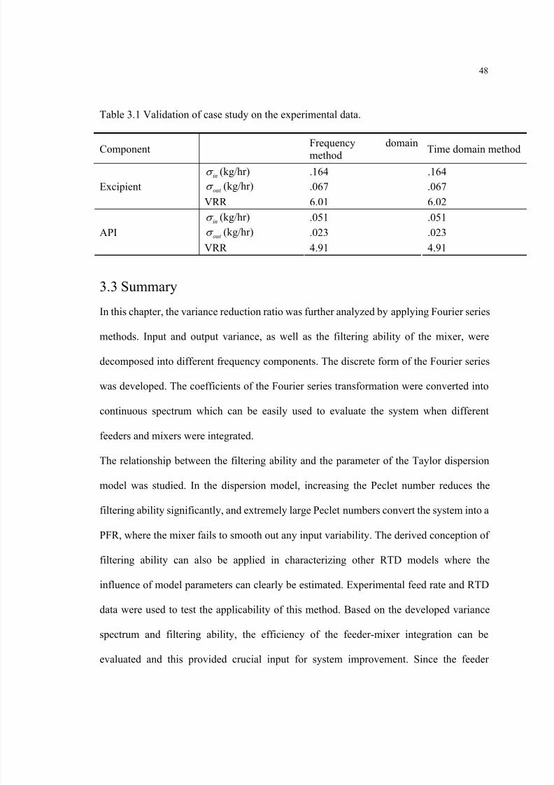
8/13/2019 Modeling and Analysis of Continuous Powder Blending
http://slidepdf.com/reader/full/modeling-and-analysis-of-continuous-powder-blending 61/177
48
Table 3.1 Validation of case study on the experimental data.
Component Frequency domainmethod Time domain method
inσ (kg/hr) .164 .164
out σ (kg/hr) .067 .067ExcipientVRR 6.01 6.02
inσ (kg/hr) .051 .051
out σ (kg/hr) .023 .023APIVRR 4.91 4.91
3.3 Summary
In this chapter, the variance reduction ratio was further analyzed by applying Fourier series
methods. Input and output variance, as well as the filtering ability of the mixer, were
decomposed into different frequency components. The discrete form of the Fourier series
was developed. The coefficients of the Fourier series transformation were converted into
continuous spectrum which can be easily used to evaluate the system when different
feeders and mixers were integrated.
The relationship between the filtering ability and the parameter of the Taylor dispersion
model was studied. In the dispersion model, increasing the Peclet number reduces the
filtering ability significantly, and extremely large Peclet numbers convert the system into a
PFR, where the mixer fails to smooth out any input variability. The derived conception of
filtering ability can also be applied in characterizing other RTD models where the
influence of model parameters can clearly be estimated. Experimental feed rate and RTD
data were used to test the applicability of this method. Based on the developed variance
spectrum and filtering ability, the efficiency of the feeder-mixer integration can be
evaluated and this provided crucial input for system improvement. Since the feeder

8/13/2019 Modeling and Analysis of Continuous Powder Blending
http://slidepdf.com/reader/full/modeling-and-analysis-of-continuous-powder-blending 62/177
49
fluctuations that cannot be filtered out are an essential contribution to the overall output
variance of the feeder-mixer system, this work provided a novel approach for improving
the design and quality control of continuous mixing system for industrial manufacturing.

8/13/2019 Modeling and Analysis of Continuous Powder Blending
http://slidepdf.com/reader/full/modeling-and-analysis-of-continuous-powder-blending 63/177
50
Chapter 4
Cross-sectional blending analysis using periodicsection modeling
To elucidate the cross-sectional blending performance of the continuous mixer, in this
chapter we assumes convective continuous blending as a combination of transverse
blending and axial movement. Moreover, it is assumed that the mixing process shares
similar characteristics as a batch mixing process within any transverse periodic section of
the mixer. The axial movement can be characterized by the residence time distribution of
the mixer. Thus, mixing along the axis of a continuous mixer composed of a series of
periodic sections can be estimated. Non-segregating and segregating particles are used to
test this idea. The rest of the chapter is organized as follows: the method, the description of
the DEM environment, and the simulation design are presented in Section 4.1. Section 4.2
illustrates the periodic section modeling. Results are discussed in Section 4.3, which shows
satisfactory prediction of both non-segregating and segregating continuous mixing
processes. We conclude with the applicability of the modeling in Section 4.4.
4.1 Material and method
4.1.1 Periodic section
As indicated in the last chapter, batch mixing inside one periodic section of a convective
continuous mixer is used to illustrate the continuous mixing process. The main
characteristic of the proposed periodic section is that each particle that exits through one
side of the periodic section reenters the section from the other side. This periodicity results
in the main advantage of this method in studying the flow pattern of the continuous mixer:
8/13/2019 Modeling and Analysis of Continuous Powder Blending
http://slidepdf.com/reader/full/modeling-and-analysis-of-continuous-powder-blending 64/177

8/13/2019 Modeling and Analysis of Continuous Powder Blending
http://slidepdf.com/reader/full/modeling-and-analysis-of-continuous-powder-blending 65/177

8/13/2019 Modeling and Analysis of Continuous Powder Blending
http://slidepdf.com/reader/full/modeling-and-analysis-of-continuous-powder-blending 66/177
53
representative of a non-segregating mixture, while the second case will result in
segregation, where the smaller, higher density type 2 particles will sink downward through
the gaps between the larger, lighter type 3 particles.
Figure 4.1 Simulated geometry of the mixer composed of eight periodic sections.
(a) Side view of the mixer, blades rotate counter-clockwise and push particles forward
along x axis, from the inlet to the outlet, (b) isometric view of one section, (c) side view of
one section with displayed dimensions.
To compare the similarity between batch-like mixing in the periodic section and the
corresponding continuous mixing in a full blender, simulations of both processes are
performed. In the current study, a convective continuous mixer composed of eight sections
8/13/2019 Modeling and Analysis of Continuous Powder Blending
http://slidepdf.com/reader/full/modeling-and-analysis-of-continuous-powder-blending 67/177
54
with the same geometry was considered. The mixing zone consists of a horizontal cylinder,
in which two opposing blades are located on the inner shaft at the middle of each section
(Figure 4.1). The detailed geometry of these sections is shown in Figure 4.1b, c. Blades are
oriented 40˚
at the cylinder axis to propel particles forward, as well as to mix particles in
the transverse directions. Particles are fed side-by-side continuously from the top of the
first section, and leave the mixer at the open end on the right side of the last section (Figure
4.1a). The left side of the mixer is closed to avoid material leakage. In steady state, feed
rate at the inlet should equals to the flow rate everywhere inside the mixer. As no weir is
used at the outlet of the mixer, no backward flux should be observed in the last several
sections. This indicates similar flow patterns (all forward) in the continuous mixing case,
and in the batch mixing case of the corresponding periodic section. Meanwhile, the
absence of weir could lead to much lower fill level in the last two or three sections than the
rest. As mixing efficiency depends significantly on fill level (Portillo et al., 2006; Sarkar
and Wassgren, 2009), the mixing efficiency in the last several sections should be different
from the rest. This will be considered in the development of the periodic section modeling
in Section 4.2.
The batch mixing in the corresponding periodic section also needs to be characterized.
Notice that the periodic section shares the same geometry with each single section of the
full mixer. Instead of feeding continuously at the top of the section, particles are initially
loaded side-by-side through the blade shaft (Figure 4.2). This insures that the main
compositional gradients at the beginning of the mixing process are in the same transverse
direction as the corresponding continuous process where different materials are fed in a
similar side-by-side style. The loaded fill level and component ratio in the periodic section
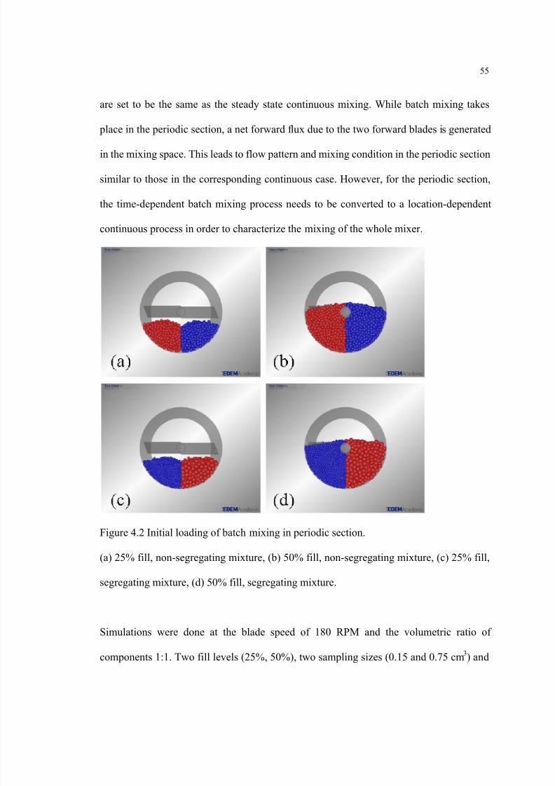
8/13/2019 Modeling and Analysis of Continuous Powder Blending
http://slidepdf.com/reader/full/modeling-and-analysis-of-continuous-powder-blending 68/177
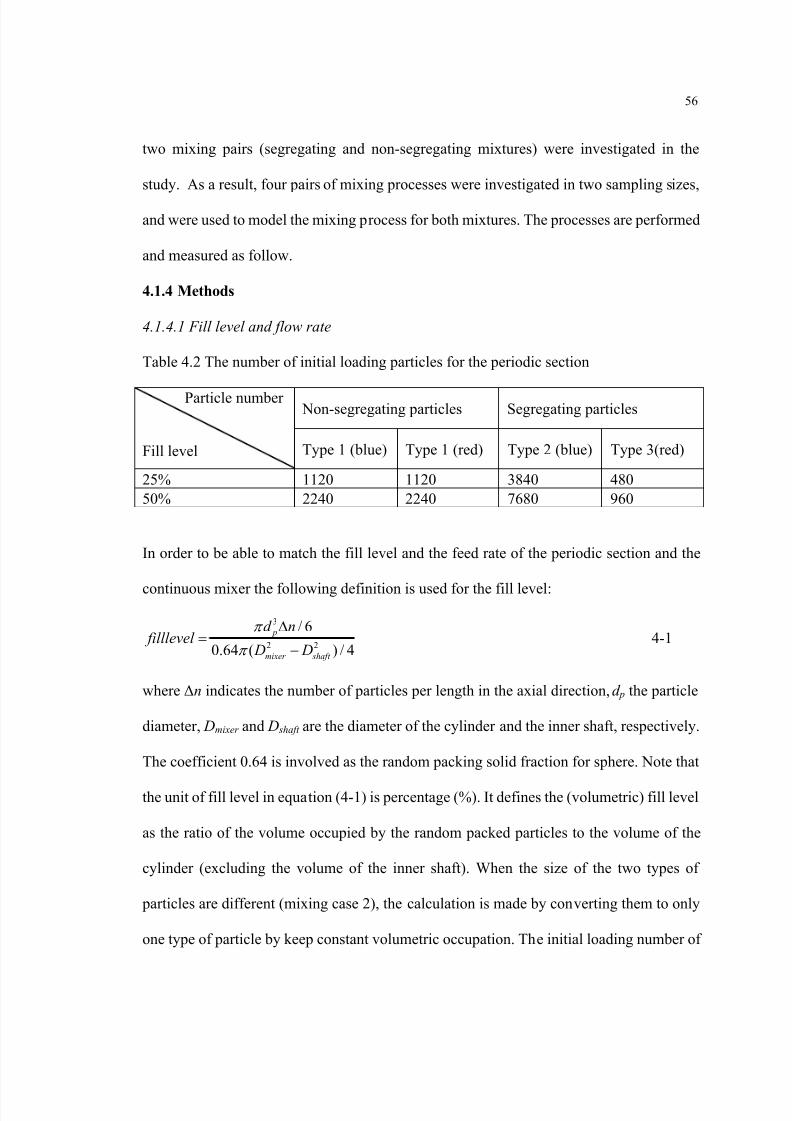
8/13/2019 Modeling and Analysis of Continuous Powder Blending
http://slidepdf.com/reader/full/modeling-and-analysis-of-continuous-powder-blending 69/177
56
two mixing pairs (segregating and non-segregating mixtures) were investigated in the
study. As a result, four pairs of mixing processes were investigated in two sampling sizes,
and were used to model the mixing process for both mixtures. The processes are performed
and measured as follow.
4.1.4 Methods
4.1.4.1 Fill level and flow rate
Table 4.2 The number of initial loading particles for the periodic section
Non-segregating particles Segregating particlesParticle number
Fill level Type 1 (blue) Type 1 (red) Type 2 (blue) Type 3(red)
25% 1120 1120 3840 48050% 2240 2240 7680 960
In order to be able to match the fill level and the feed rate of the periodic section and the
continuous mixer the following definition is used for the fill level:
3
2 2
/ 6
0.64 ( ) / 4 p
mixer shaft
d n filllevel
D D
π
π
Δ=
− 4-1
where Δn indicates the number of particles per length in the axial direction, d p the particle
diameter, Dmixer and D shaft are the diameter of the cylinder and the inner shaft, respectively.
The coefficient 0.64 is involved as the random packing solid fraction for sphere. Note that
the unit of fill level in equation (4-1) is percentage (%). It defines the (volumetric) fill level
as the ratio of the volume occupied by the random packed particles to the volume of the
cylinder (excluding the volume of the inner shaft). When the size of the two types of
particles are different (mixing case 2), the calculation is made by converting them to only
one type of particle by keep constant volumetric occupation. The initial loading number of
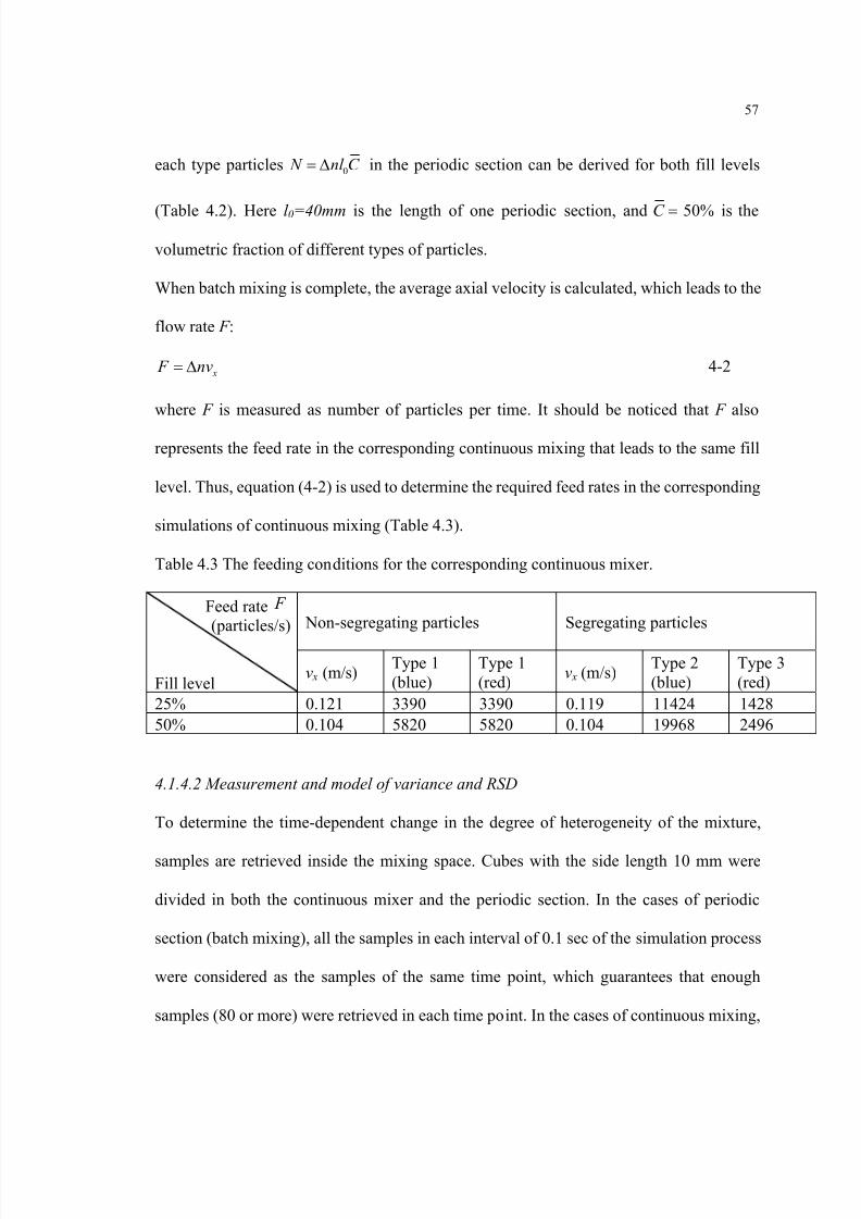
8/13/2019 Modeling and Analysis of Continuous Powder Blending
http://slidepdf.com/reader/full/modeling-and-analysis-of-continuous-powder-blending 70/177
57
each type particles 0 N nl C = Δ in the periodic section can be derived for both fill levels
(Table 4.2). Here l 0=40mm is the length of one periodic section, and 50%C = is the
volumetric fraction of different types of particles.
When batch mixing is complete, the average axial velocity is calculated, which leads to the
flow rate F :
x F nv= Δ 4-2
where F is measured as number of particles per time. It should be noticed that F also
represents the feed rate in the corresponding continuous mixing that leads to the same fill
level. Thus, equation (4-2) is used to determine the required feed rates in the corresponding
simulations of continuous mixing (Table 4.3).
Table 4.3 The feeding conditions for the corresponding continuous mixer.
Non-segregating particles Segregating particlesFeed rate F (particles/s)
Fill levelv x (m/s) Type 1
(blue)Type 1(red) v x (m/s) Type 2
(blue)Type 3(red)
25% 0.121 3390 3390 0.119 11424 142850% 0.104 5820 5820 0.104 19968 2496
4.1.4.2 Measurement and model of variance and RSD
To determine the time-dependent change in the degree of heterogeneity of the mixture,
samples are retrieved inside the mixing space. Cubes with the side length 10 mm were
divided in both the continuous mixer and the periodic section. In the cases of periodic
section (batch mixing), all the samples in each interval of 0.1 sec of the simulation process
were considered as the samples of the same time point, which guarantees that enough
samples (80 or more) were retrieved in each time point. In the cases of continuous mixing,
8/13/2019 Modeling and Analysis of Continuous Powder Blending
http://slidepdf.com/reader/full/modeling-and-analysis-of-continuous-powder-blending 71/177
58
the samples located in the same plane perpendicular to the x axis were regarded as the
samples in the same location. The time interval recorded is also 0.1 sec. In order to
investigate the influence of the sampling size, samples were selected based on the number
of particles inside each cube. Thus, for the non-segregating case (particle type 1), samples
with 7 or 35 particles were selected, respectively, corresponding to the number of particles
that can be randomly packed within the sampling sizes of 0.15 or 0.75 cm 3. For the
segregating case (particle type 2 and 3), since particle sizes are different, samples with
particles volumetrically equivalent to 23 and 118 particles type 2 were selected, to
represent different sampling sizes. It should be noticed that both sampling sizes are
relatively smaller than in practice, so that their influence on the value of RSD measurement
can be clearly distinguished.
After selecting the samples, the variance ( σ 2) and the relative standard deviation (RSD) of
the volumetric fraction in samples of each time point or location can be calculated and used
as a measure of the mixture heterogeneity.
In order to characterize the batch-like mixing process with fewer parameters, the variance
profile 2 ( )b t σ was modeled by the exponential decrease relationship shown below,
2 2 2 20( ) ( ) exp( )b SS SS bt k t σ σ σ σ = + − − 4-3
where 2 ( )b t σ , 2SS σ , 2
0σ are the variance in batch mixing of periodic section, the steady state
variance of the investigated sampling size, and the initial variance when particles are
totally segregated, respectively; and k b is the variance decay rate of the batch mixing
process. Note that similar relationships has been used in previous studies to model
V-blenders, bin blenders and other batch systems (Brone et al., 1998; Sudah et al., 2002b).
As 0.5C = , 20σ can be considered as equal to 0.25 using the following equation:
8/13/2019 Modeling and Analysis of Continuous Powder Blending
http://slidepdf.com/reader/full/modeling-and-analysis-of-continuous-powder-blending 72/177
59
20 (1 )C C σ = − 4-4
which leads to the initial RSD value of 1 by applying equation (2-2).
4.1.4.3 Measurement and model of RTD
In order to characterize particle movement of both the continuous mixer and the periodic
section the residence time distribution (RTD) is used in this work. Instead of using the
pulse test method by Danckwerts (1953) in the simulation of continuous mixing, RTD was
measured by considering the trajectory of particles inside the flow of the mixer, or the
periodic section. Figure 4.3 shows the trajectory of one particle in the direction of axial
movement in the periodic section. Since the blades in the periodic section are all forward,
unilateral movement can be observed for the studied particle. When it reaches the right side
of the section (40mm), it reappears at the other side (0 mm). Therefore, the time interval
between two transverses at one end of the space can be considered as one sample of the
RTD of a single periodic section. As a result, the RTD can be derived using the followingequation:
1
( ) ii
ii
n E t
n t =
=Δ∑ 4-5
where Δt the sampling time interval, and ni the number of samples in which the residence
time of each sample lies in ( t i, t i+Δt ). The RTD within sections of a whole continuous mixer
is measured in a similar way. However, in this case, one particle reaches the right side of
the sections will leave the system, instead of reappearing at the left side. To eliminate noise
from the measurements of RTD, around 6000 samples of particle trajectory were retrieved
for each RTD measurement. If the same flow rate and fill level are shared by sections in a
continuous mixer and the corresponding periodic section, the RTD within the continuous

8/13/2019 Modeling and Analysis of Continuous Powder Blending
http://slidepdf.com/reader/full/modeling-and-analysis-of-continuous-powder-blending 73/177
60
mixer can also be derived through the convolution of the RTD in one periodic section for
several times, which allows more efficient calculation.
Figure 4.3 Trajectory of one particle inside the periodic section.
To clarify the physical meaning of the statistical RTD obtained above, the Taylor
dispersion model (Section 2.2) is applied.
4.2 Periodic section modeling
As indicated in Section 4.1, the decrease of mixture heterogeneity is time-dependent in the
batch mixing process of the periodic section, while it is location-dependent in the
continuous mixing process. Meanwhile, we assume approximately a constant mixing
efficiency through the whole continuous mixer where the fill level is almost the same,
except for the last several sections. This indicates that in these first several constant-fill
8/13/2019 Modeling and Analysis of Continuous Powder Blending
http://slidepdf.com/reader/full/modeling-and-analysis-of-continuous-powder-blending 74/177
61
sections, the continuous mixing process of one cluster of particles depends only on the time
the cluster spends inside these sections. In other words, a continuous mixer with a series of
constant-fill sections can be considered as a batch mixer, which has the same fill and
mixing efficiency, and is operated for a time period equivalent to the RTD in the
continuous mixer. Thus, the present model should be designed to link the mixing efficiency
of these constant-fill sections, the RTD the clusters of particles stay within these sections,
and the heterogeneity decay curve along the continuous mixer. Since the batch mixing in
one periodic section should share the fill level and flow pattern with continuous mixing
within these constant-fill sections, we assume they share approximate the same mixing
efficiency. Based on this assumption, as well as the definitions of RTD and variance in the
previous section, the following empirical relationship is proposed:
2 2
0( ) ( ) ( , )c b t E t x dt σ σ
∞= ∫ 4-6
where 2 ( )c xσ is the variance at different locations x along the axis of a continuous mixer;
2 ( )b t σ is the variance decay of the batch mixing in the periodic section; and ( , ) E t x is the
RTD in the continuous mixer at location x. Notice that the sampling sizes of the
measurement of 2 ( )c xσ and 2 ( )b t σ should be the same.
Equation (4-6) is proposed based on the assumption that the variance at each transverse
plane in the continuous mixer is the average of the variance of the clusters of particles at
the same plane, which may have spent different residence time inside the mixer. Since in
most cases, the RTD in the convective continuous mixer is unimodal (single peak), the
average variance of these clusters of particles should be close to the variance of the cluster
8/13/2019 Modeling and Analysis of Continuous Powder Blending
http://slidepdf.com/reader/full/modeling-and-analysis-of-continuous-powder-blending 75/177
62
with the most particles, or the cluster that spends the mean residence time inside the mixer.
Based on this observation and equation (4-4), equation (4-6) can be re-written as follows:
2 2 2 20( ) ( ) exp( )c SS SS ck xσ σ σ σ = + − − 4-7
where 2SS σ , 2
0σ represent the same parameters as in equation (4-6), and k c is regarded the
variance decay rate along the axis of a continuous mixer, which is calculated as
/c b xk k v= 4-8
Equation (4-6) -(4-8) show the potential relationship between the batch mixing of a
periodic section and the corresponding continuous mixing, which shares the same fill level
with the periodic section. Considering the difficulty on realizing the periodic section
experimentally, equation (4-8) provides an alternative to estimate the value of k b in practice.
Since the variance decay and RTD data can be measured in the continuous mixing process,
we can achieve the values of k c and v x conveniently, and then the value of k b can be easily
calculated. On the other hand, since RSD is usually used as mixing index in practice, we
divide equations (4-4), (4-6) and (4-7) by square of the average concentration ( 2C ), and the
equations are converted to:
2 2 2 20( ) ( ) exp( )b SS SS b RSD t RSD RSD RSD k t = + − − 4-9
2 2
0( ) ( ) ( , )c b RSD x RSD t E t x dt
∞= ∫ 4-10
2 2 2 20( ) ( ) exp( )c SS SS c RSD x RSD RSD RSD k x= + − − 4-11
The simulation designs described in the previous section are used in the next section to
validate equations (4-9) -(4-11).
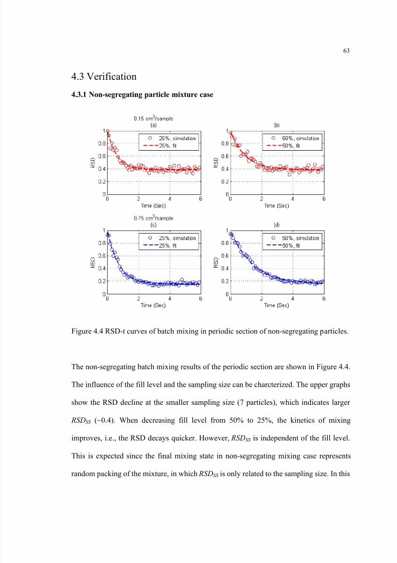
8/13/2019 Modeling and Analysis of Continuous Powder Blending
http://slidepdf.com/reader/full/modeling-and-analysis-of-continuous-powder-blending 76/177
8/13/2019 Modeling and Analysis of Continuous Powder Blending
http://slidepdf.com/reader/full/modeling-and-analysis-of-continuous-powder-blending 77/177

8/13/2019 Modeling and Analysis of Continuous Powder Blending
http://slidepdf.com/reader/full/modeling-and-analysis-of-continuous-powder-blending 78/177

8/13/2019 Modeling and Analysis of Continuous Powder Blending
http://slidepdf.com/reader/full/modeling-and-analysis-of-continuous-powder-blending 79/177
66
Figure 4.6 RTD data and curve-fitting of 2, 4 and 6 constant-fill sections for
non-segregating partilcles.
Figure 4.7 shows the simulated and calculated results of RSD decay in the case of
continuous mixing, for the first six constant-fill sections. By using equation (4-10), the
model fitted curves of both the batch mixing (RSD-t curve) in the periodic section and the
RTD were applied in predicting the RSD decay curve within the continuous mixer. It can
be seen that the calculated results could capture very well the simulated results for the
constant-fill sections (equation (4-11) leads to almost the same prediction). To compare the
RSD decay rate of different fills, the RSD values of 0.5 (for the sampling size of 0.15 cm 3)
and 0.25 (for 0.75 cm 3) were considered as the check points. It can be observed at 25% fill,

8/13/2019 Modeling and Analysis of Continuous Powder Blending
http://slidepdf.com/reader/full/modeling-and-analysis-of-continuous-powder-blending 80/177

8/13/2019 Modeling and Analysis of Continuous Powder Blending
http://slidepdf.com/reader/full/modeling-and-analysis-of-continuous-powder-blending 81/177
68
Figure 4.8 RSD-t curves of batch mixing in periodic section filled by segregating particles.
Figure 4.8 shows the batch mixing results for the segregating mixture. As illustrated in the
previous section for the non-segretating case, decreasing the fill level allows larger batch
mixing rate. However, the important aspect here is the fact that SS RSD are fill level
dependent, and in both fills should be higher than the case of random packing. This means
that the size and density ratio between the particles induces segregation that the mixer
cannot completely eliminate. SS RSD are larger at 25% fills in both sampling sizes,
indicating more segregation. This can be explained by the strength of blade disturbance on
the segregation. As the fraction of prepelled particles is smaller at low fill, the influence
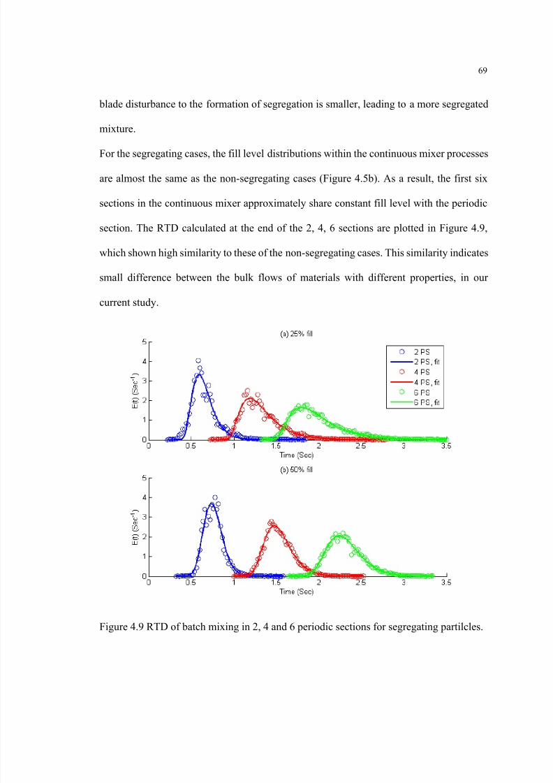
8/13/2019 Modeling and Analysis of Continuous Powder Blending
http://slidepdf.com/reader/full/modeling-and-analysis-of-continuous-powder-blending 82/177
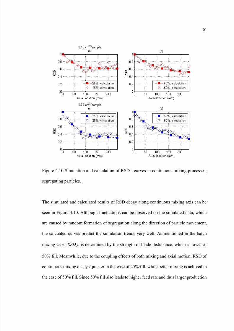
8/13/2019 Modeling and Analysis of Continuous Powder Blending
http://slidepdf.com/reader/full/modeling-and-analysis-of-continuous-powder-blending 83/177
70
Figure 4.10 Simulation and calculation of RSD-l curves in continuous mixing processes,
segregating particles.
The simulated and calculated results of RSD decay along continuous mixing axis can be
seen in Figure 4.10. Although fluctuations can be observed on the simulated data, which
are caused by random formation of segregation along the direction of particle movement,
the calcuated curves predict the simulation trends very well. As mentioned in the batch
mixing case, SS RSD is determined by the strength of blade distubance, which is lower at
50% fill. Meanwhile, due to the coupling effects of both mixing and axial motion, RSD of
continuous mixing decays quicker in the case of 25% fill, while better mixing is achived in
the case of 50% fill. Since 50% fill also leads to higher feed rate and thus larger production

8/13/2019 Modeling and Analysis of Continuous Powder Blending
http://slidepdf.com/reader/full/modeling-and-analysis-of-continuous-powder-blending 84/177

8/13/2019 Modeling and Analysis of Continuous Powder Blending
http://slidepdf.com/reader/full/modeling-and-analysis-of-continuous-powder-blending 85/177
72
decay can be calculated in separate subsections with different fills or mixing efficiencies.
The decreased variance calculated at the end of one subsection should be used as the initial
condition in the calculation of the next subsection. In other word, we can define a
multiplicative process for the variance decay, where in each subsection, variance goes
down by a factor ,exp( )i c i i F k x= − Δ . Here ,c ik represents the uniform variance decay rate
along axis x within subsection i, and i xΔ denotes the length of the subsection. This
requires involvement of mixing rates of the subsections at different fills, and the RTD
calculated separately for different subsections. This issue is worthy of investigation and
under consideration of future publication.
It should be emphasized that the periodic section modeling work indicates the similarity
between the continuous powder mixing and an equivalent batch mixing process. Therefore,
the knowledge developed in the field of batch mixing can be applied for the design and
optimization of continuous mixers. That means that designs and operations that improve
the performance of batch mixer can be conveniently used in the design of a continuous
mixer, provided that the axial motion of the materials is slow enough for the equivalent
batch mixing to be complete. Also due to the difficulties of experimentally performing
batch mixing of the periodic section, knowledge of the similarity between the mixing rate
of one periodic section and batch mixers with similar geometries can facilitate the practical
estimation of the mixing efficiency of a continuous process, and thus is worth considering.
This issue is discussed in the next chapter.
8/13/2019 Modeling and Analysis of Continuous Powder Blending
http://slidepdf.com/reader/full/modeling-and-analysis-of-continuous-powder-blending 86/177
73
Chapter 5
Blender design based on batch experience
To examine the similarity of blending between batch and periodic section, in this chapter
we use the Discrete Element Method (DEM) to investigate a family of simple geometries
consisting of a horizontal cylindrical section with periodic end walls, stirred by several
blades rotating around an axial shaft. Ideally, it would be desirable to have access to a
simple, experimentally realizable system that could be used to study cross-sectional
mixing in batch-like geometry in an effective manner. A simple geometry that is
experimentally realizable is a cylindrical section with solid end walls. However, the
presence of the end walls should be expected to affect the flow pattern, possibly leading to
very different mixing performance, potentially rendering the device useless as a validation
system. The rest of the chapter is organized as follows: the Discrete Element Method
(DEM), and the parametric space examined are described in Section 5.1; in Section 5.2 we
describe the results obtained, which show the effects of these designs on the mixing
performance. We summarize these effects and present the conclusions of this work in
Section 5.3.
5.1 Methodology
5.1.1 Discrete Element Method
Since the blending experiments in a cross section with periodic boundaries are difficult
(and perhaps impossible) to perform, we use the Discrete Element Method (DEM) as the
tool for examining the effect of blade patterns on flow and mixing for the configurations of
interest. Particles simulated are spheres, where the contact forces are calculated using the
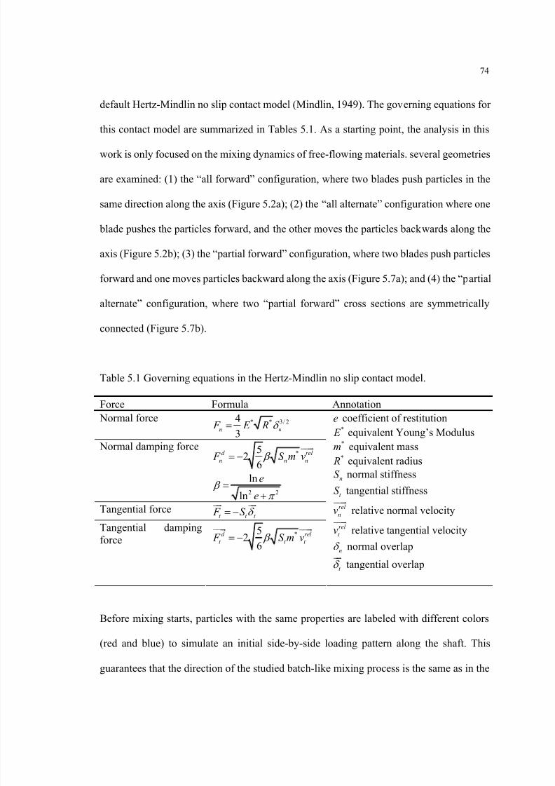
8/13/2019 Modeling and Analysis of Continuous Powder Blending
http://slidepdf.com/reader/full/modeling-and-analysis-of-continuous-powder-blending 87/177
74
default Hertz-Mindlin no slip contact model (Mindlin, 1949). The governing equations for
this contact model are summarized in Tables 5.1. As a starting point, the analysis in this
work is only focused on the mixing dynamics of free-flowing materials. several geometries
are examined: (1) the “all forward” configuration, where two blades push particles in the
same direction along the axis (Figure 5.2a); (2) the “all alternate” configuration where one
blade pushes the particles forward, and the other moves the particles backwards along the
axis (Figure 5.2b); (3) the “partial forward” configuration, where two blades push particles
forward and one moves particles backward along the axis (Figure 5.7a); and (4) the “partial
alternate” configuration, where two “partial forward” cross sections are symmetrically
connected (Figure 5.7b).
Table 5.1 Governing equations in the Hertz-Mindlin no slip contact model.
Force Formula Annotation Normal force * * 3/ 24
3n n F E R δ =
Normal damping force*5
26
d rel n n n F S m v β = −
2 2
ln
ln
e
e β
π =
+
Tangential forcet t t F S δ = −
Tangential dampingforce
*52
6
d rel t t t F S m v β = −
e coefficient of restitution* E equivalent Young’s Modulus*m equivalent mass* R equivalent radiusnS normal stiffness
t S tangential stiffnessrel nv relative normal velocityrel t v relative tangential velocity
nδ normal overlapt δ tangential overlap
Before mixing starts, particles with the same properties are labeled with different colors
(red and blue) to simulate an initial side-by-side loading pattern along the shaft. This
guarantees that the direction of the studied batch-like mixing process is the same as in the
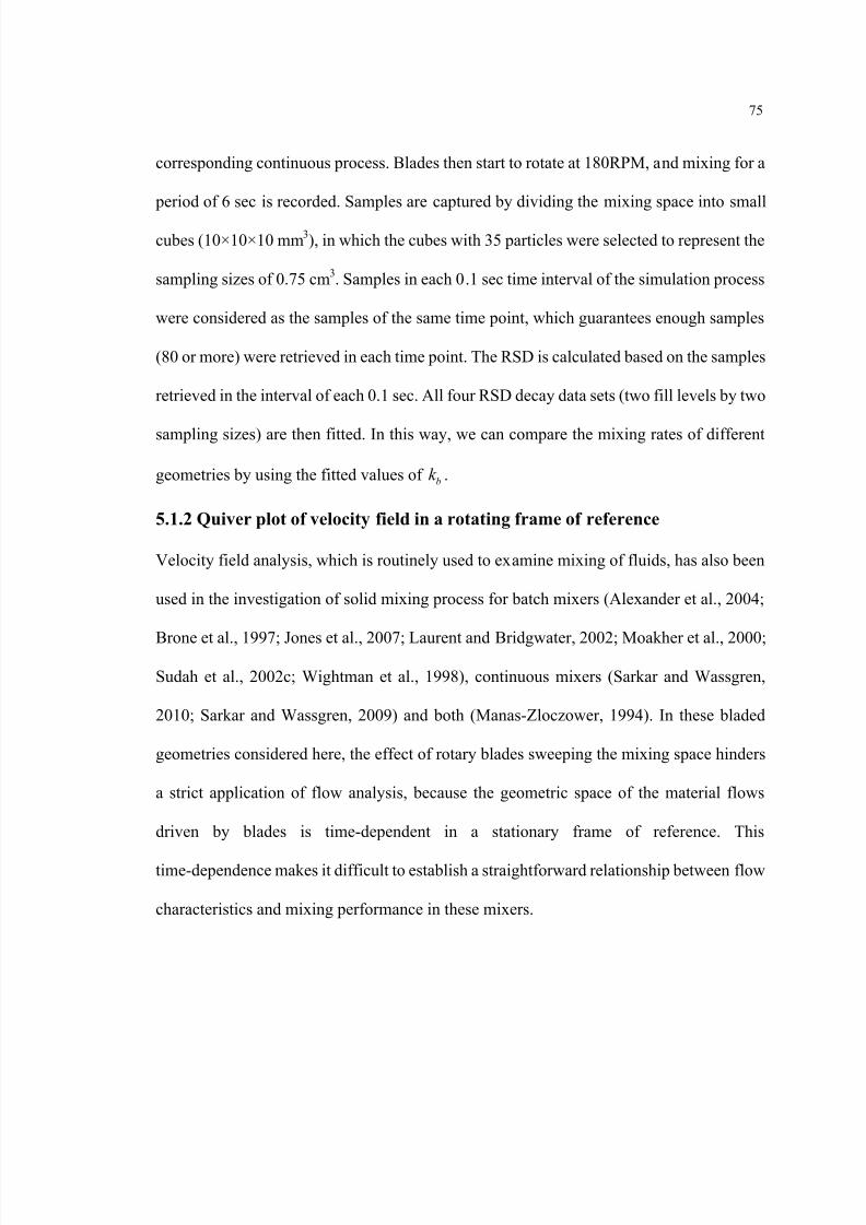
8/13/2019 Modeling and Analysis of Continuous Powder Blending
http://slidepdf.com/reader/full/modeling-and-analysis-of-continuous-powder-blending 88/177
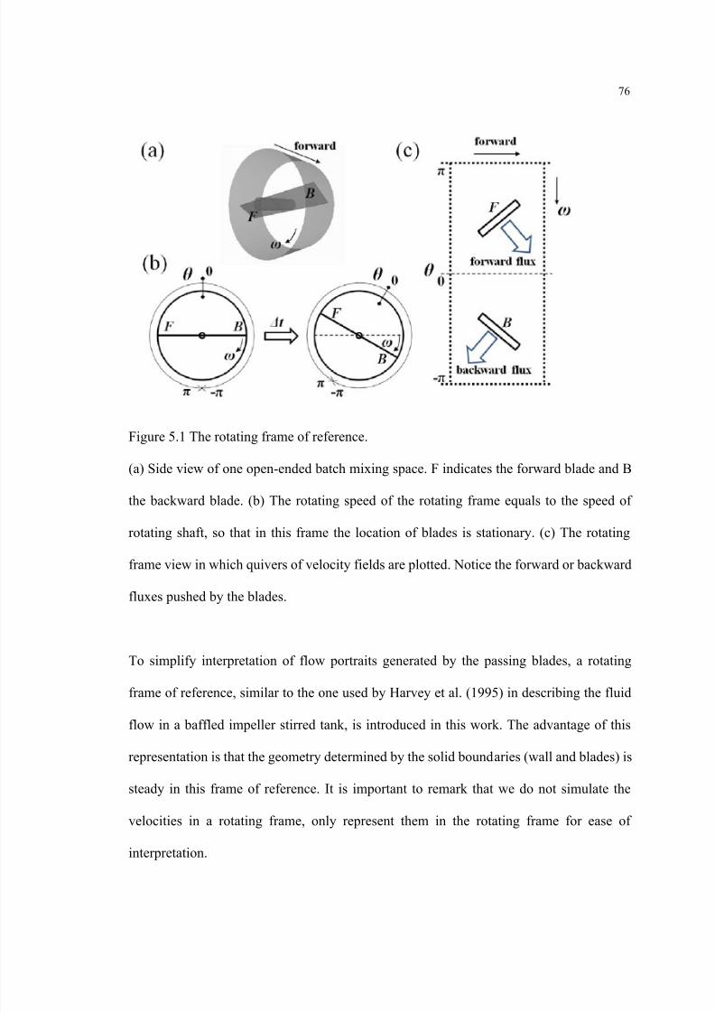
8/13/2019 Modeling and Analysis of Continuous Powder Blending
http://slidepdf.com/reader/full/modeling-and-analysis-of-continuous-powder-blending 89/177
76
Figure 5.1 The rotating frame of reference.
(a) Side view of one open-ended batch mixing space. F indicates the forward blade and B
the backward blade. (b) The rotating speed of the rotating frame equals to the speed of
rotating shaft, so that in this frame the location of blades is stationary. (c) The rotating
frame view in which quivers of velocity fields are plotted. Notice the forward or backward
fluxes pushed by the blades.
To simplify interpretation of flow portraits generated by the passing blades, a rotating
frame of reference, similar to the one used by Harvey et al. (1995) in describing the fluid
flow in a baffled impeller stirred tank, is introduced in this work. The advantage of this
representation is that the geometry determined by the solid boundaries (wall and blades) is
steady in this frame of reference. It is important to remark that we do not simulate the
velocities in a rotating frame, only represent them in the rotating frame for ease of
interpretation.
8/13/2019 Modeling and Analysis of Continuous Powder Blending
http://slidepdf.com/reader/full/modeling-and-analysis-of-continuous-powder-blending 90/177
77
The rotating frame is set to have the same rotational speed as the blades, so that the blade
locations are stationary in this new frame (see Figure 5.1b). Subsequently, quiver plots of
the velocity field in this frame are calculated as follow. At time t Δ after mixing starts, the
rotated angle 0θ of the reference frame is
0 t θ ω = Δ 5-1
where ω equals to the angular velocity of the rotating blades. For one particle with location
( , , ) y z and velocity components ( , , ) x y z v v v that are measured in a stationary rectangle
coordinate system, its location and velocity in the corresponding cylindrical coordinate
system are denoted as ( ', , )r xθ and '( , , )r xv v vθ , respectively. Here represents the
location of the particle in the axial direction, y the location in the side direction and z in
the vertical direction in the rectangle coordinate system; 'θ the angle in the tangent
direction, and r the location in the radial direction in the cylindrical coordinate system.
Based on these notations, the location of the same particle in the rotating frame of reference
can be denoted as ( , , )r xθ , in which
0'θ θ θ = − 5-2
where ( , )θ π π − represents the angle of the particle in the rotating frame, r and have
the same meaning as these in the cylindrical coordinate system.
In order to facilitate intuitive analysis, one more simplification is needed: we plot the
velocity field in angular-axial 2-D coordinates, using color to denote velocity magnitude
and arrow to denote velocity direction. Such 2-D plots are more easily interpreted than a
full 3-D representation of a vector field. To this end, we average velocities along the radial
coordinate; i.e., all particles within the same beam ( , ) xθ are considered to be at the same
8/13/2019 Modeling and Analysis of Continuous Powder Blending
http://slidepdf.com/reader/full/modeling-and-analysis-of-continuous-powder-blending 91/177
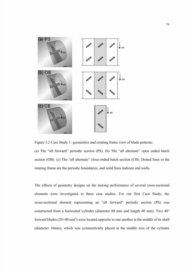
8/13/2019 Modeling and Analysis of Continuous Powder Blending
http://slidepdf.com/reader/full/modeling-and-analysis-of-continuous-powder-blending 92/177
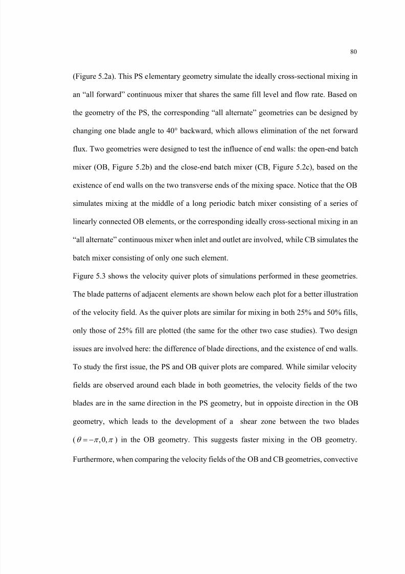
8/13/2019 Modeling and Analysis of Continuous Powder Blending
http://slidepdf.com/reader/full/modeling-and-analysis-of-continuous-powder-blending 93/177
80
(Figure 5.2a). This PS elementary geometry simulate the ideally cross-sectional mixing in
an “all forward” continuous mixer that shares the same fill level and flow rate. Based on
the geometry of the PS, the corresponding “all alternate” geometries can be designed by
changing one blade angle to 40° backward, which allows elimination of the net forward
flux. Two geometries were designed to test the influence of end walls: the open-end batch
mixer (OB, Figure 5.2b) and the close-end batch mixer (CB, Figure 5.2c), based on the
existence of end walls on the two transverse ends of the mixing space. Notice that the OB
simulates mixing at the middle of a long periodic batch mixer consisting of a series of
linearly connected OB elements, or the corresponding ideally cross-sectional mixing in an
“all alternate” continuous mixer when inlet and outlet are involved, while CB simulates the
batch mixer consisting of only one such element.
Figure 5.3 shows the velocity quiver plots of simulations performed in these geometries.
The blade patterns of adjacent elements are shown below each plot for a better illustration
of the velocity field. As the quiver plots are similar for mixing in both 25% and 50% fills,
only those of 25% fill are plotted (the same for the other two case studies). Two design
issues are involved here: the difference of blade directions, and the existence of end walls.
To study the first issue, the PS and OB quiver plots are compared. While similar velocity
fields are observed around each blade in both geometries, the velocity fields of the two
blades are in the same direction in the PS geometry, but in oppoiste direction in the OB
geometry, which leads to the development of a shear zone between the two blades
( ,0,θ π π = − ) in the OB geometry. This suggests faster mixing in the OB geometry.
Furthermore, when comparing the velocity fields of the OB and CB geometries, convective
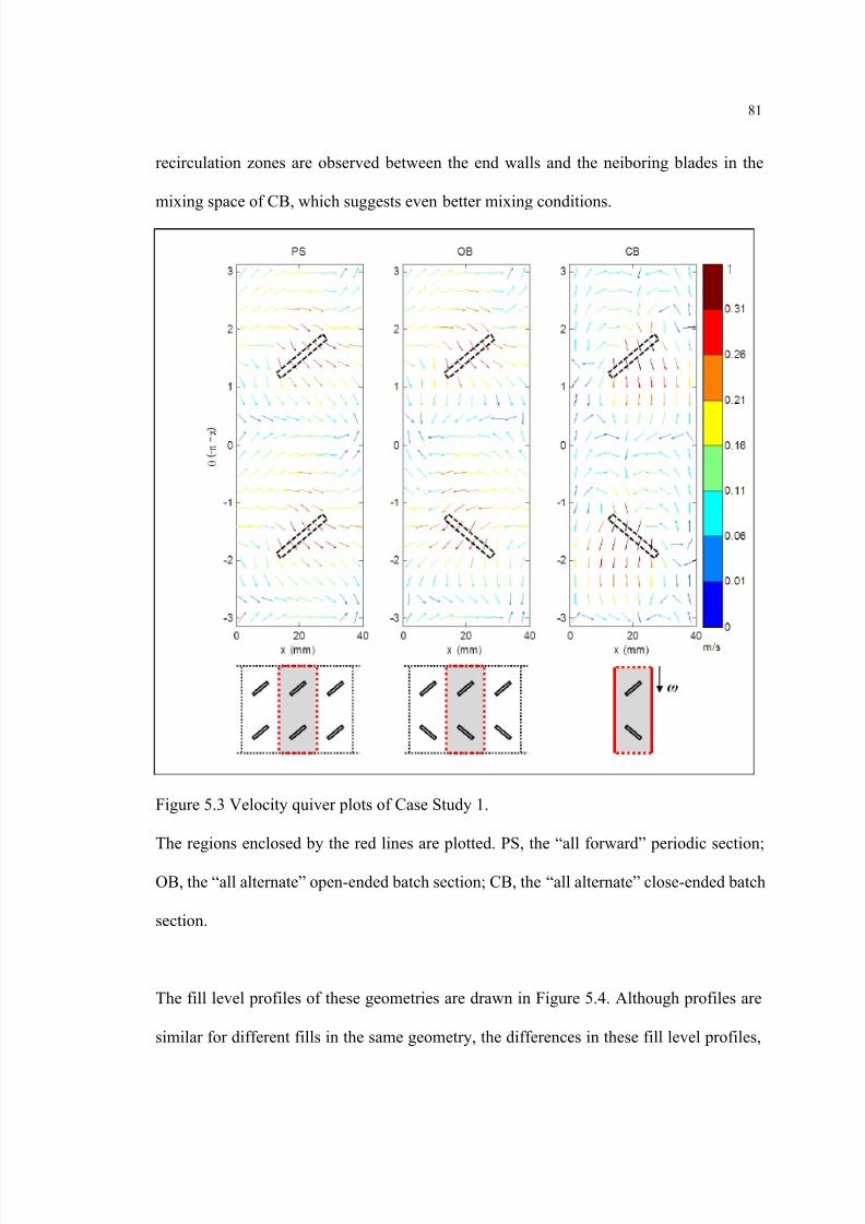
8/13/2019 Modeling and Analysis of Continuous Powder Blending
http://slidepdf.com/reader/full/modeling-and-analysis-of-continuous-powder-blending 94/177
81
recirculation zones are observed between the end walls and the neiboring blades in the
mixing space of CB, which suggests even better mixing conditions.
Figure 5.3 Velocity quiver plots of Case Study 1.
The regions enclosed by the red lines are plotted. PS, the “all forward” periodic section;
OB, the “all alternate” open-ended batch section; CB, the “all alternate” close-ended batch
section.
The fill level profiles of these geometries are drawn in Figure 5.4. Although profiles are
similar for different fills in the same geometry, the differences in these fill level profiles,
8/13/2019 Modeling and Analysis of Continuous Powder Blending
http://slidepdf.com/reader/full/modeling-and-analysis-of-continuous-powder-blending 95/177
82
increase from OB to PS to CB. The low fill at the middle of the mixing space is caused by
the blade motions in the same area: fill level decreases as blades continuously propel
particles away from the region of blades until conter-current fluxes due to the induced fill
level gradient are able to balance the effect of these convective motions.
Figure 5.4 Fill level profiles along the axis of the simlated geometries in Case Study 1.
The difference of the fill level profiles can be analyzed as follows. For the PS, the two
forward blades provide approximately twice the same forward fluxes in one revolution,
leading to a overlapped peak of fill level at 28 mm ahead of the blades, or 12 mm behind,
due to the periodicity of the space. This indicates that the peak of fill level due to single
blade motion should be 28 mm away from the blade. For the purpose of validation, a
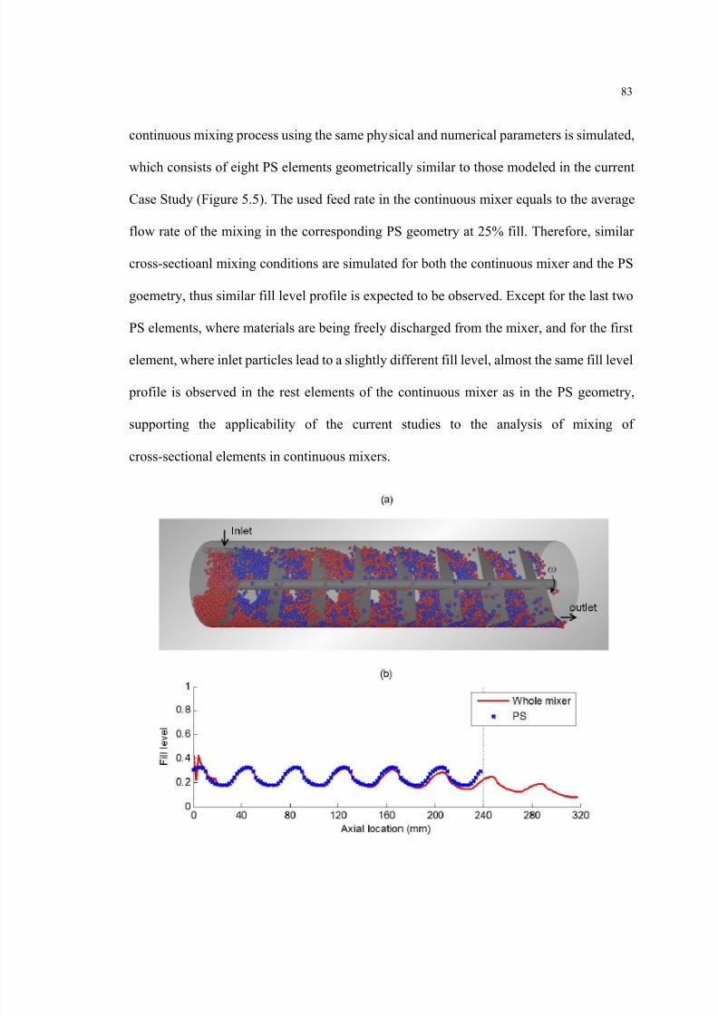
8/13/2019 Modeling and Analysis of Continuous Powder Blending
http://slidepdf.com/reader/full/modeling-and-analysis-of-continuous-powder-blending 96/177
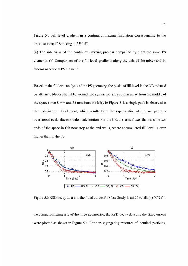
8/13/2019 Modeling and Analysis of Continuous Powder Blending
http://slidepdf.com/reader/full/modeling-and-analysis-of-continuous-powder-blending 97/177
84
Figure 5.5 Fill level gradient in a continuous mixing simulation corresponding to the
cross-sectional PS mixing at 25% fill.
(a) The side view of the continuous mixing process comprised by eight the same PS
elements. (b) Comparison of the fill level gradients along the axis of the mixer and in
thecross-sectional PS element.
Based on the fill level analysis of the PS geometry, the peaks of fill level in the OB induced
by alternate blades should be around two symmetric sites 28 mm away from the middle of
the space (or at 8 mm and 32 mm from the left). In Figure 5.4, a single peak is observed at
the ends in the OB element, which results from the superpostion of the two partially
overlapped peaks due to signle blade motion. For the CB, the same fluxes that pass the two
ends of the space in OB now stop at the end walls, where accumulated fill level is even
higher than in the PS.
Figure 5.6 RSD decay data and the fitted curves for Case Study 1. (a) 25% fill, (b) 50% fill.
To compare mixing rate of the three geometries, the RSD decay data and the fitted curves
were plotted as shown in Figure 5.6. For non-segregating mixtures of identical particles,
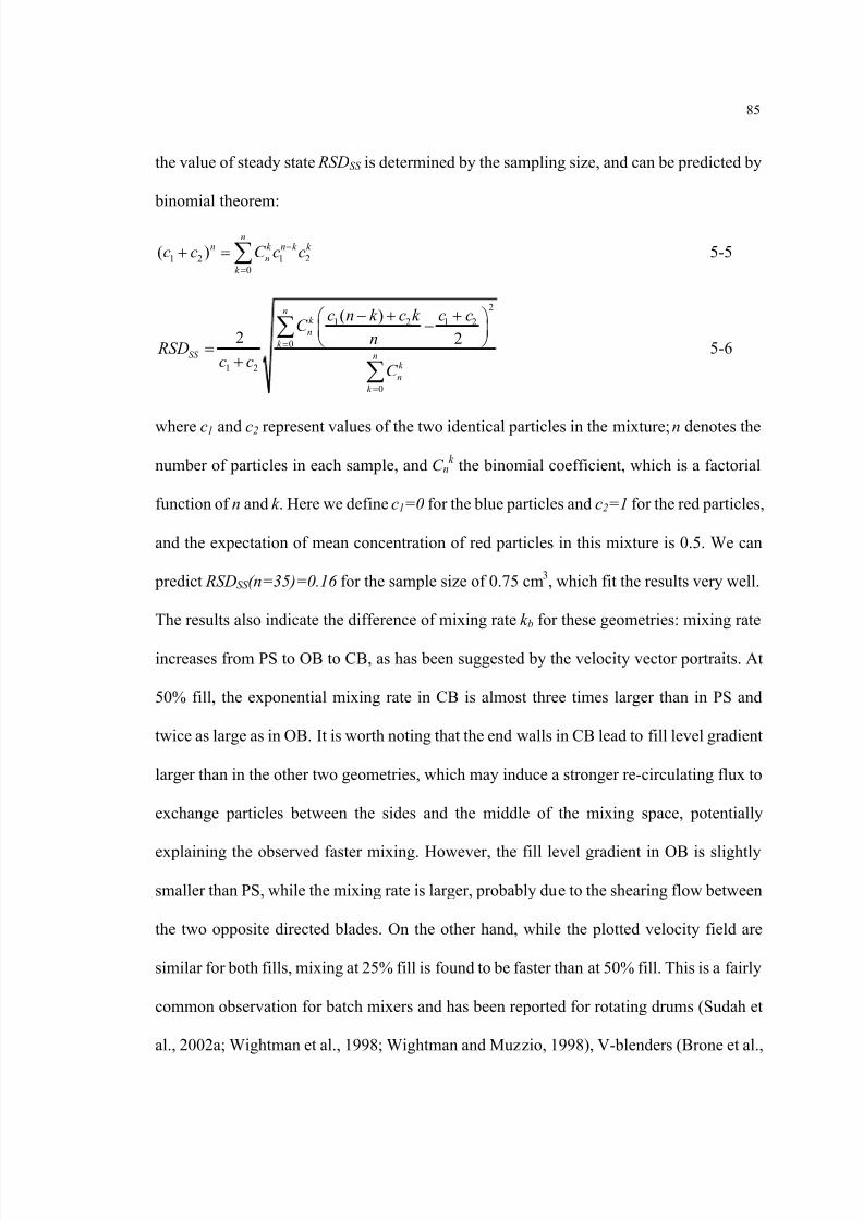
8/13/2019 Modeling and Analysis of Continuous Powder Blending
http://slidepdf.com/reader/full/modeling-and-analysis-of-continuous-powder-blending 98/177
85
the value of steady state RSDSS is determined by the sampling size, and can be predicted by
binomial theorem:
1 2 1 20
( )n
n k n k k n
k
c c C c c−
=+ =∑ 5-5
2
1 2 1 2
0
1 2
0
( )2 2
nk n
k SS n
k n
k
c n k c k c cC
n RSDc c C
=
=
− + + − =+
∑
∑ 5-6
where c1 and c2 represent values of the two identical particles in the mixture; n denotes the
number of particles in each sample, and C nk the binomial coefficient, which is a factorial
function of n and k . Here we define c1=0 for the blue particles and c2=1 for the red particles,
and the expectation of mean concentration of red particles in this mixture is 0.5. We can
predict RSDSS (n=35)=0.16 for the sample size of 0.75 cm 3, which fit the results very well.
The results also indicate the difference of mixing rate k b for these geometries: mixing rate
increases from PS to OB to CB, as has been suggested by the velocity vector portraits. At
50% fill, the exponential mixing rate in CB is almost three times larger than in PS and
twice as large as in OB. It is worth noting that the end walls in CB lead to fill level gradient
larger than in the other two geometries, which may induce a stronger re-circulating flux to
exchange particles between the sides and the middle of the mixing space, potentially
explaining the observed faster mixing. However, the fill level gradient in OB is slightly
smaller than PS, while the mixing rate is larger, probably due to the shearing flow between
the two opposite directed blades. On the other hand, while the plotted velocity field are
similar for both fills, mixing at 25% fill is found to be faster than at 50% fill. This is a fairly
common observation for batch mixers and has been reported for rotating drums (Sudah et
al., 2002a; Wightman et al., 1998; Wightman and Muzzio, 1998), V-blenders (Brone et al.,
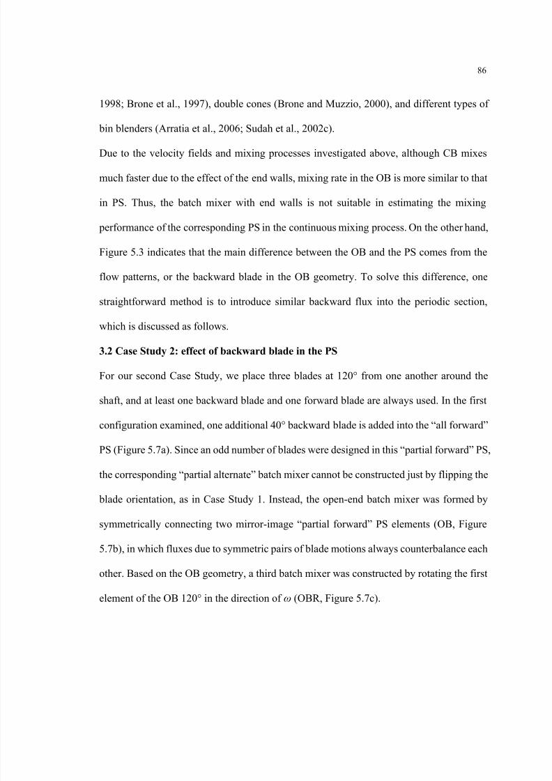
8/13/2019 Modeling and Analysis of Continuous Powder Blending
http://slidepdf.com/reader/full/modeling-and-analysis-of-continuous-powder-blending 99/177
86
1998; Brone et al., 1997), double cones (Brone and Muzzio, 2000), and different types of
bin blenders (Arratia et al., 2006; Sudah et al., 2002c).
Due to the velocity fields and mixing processes investigated above, although CB mixes
much faster due to the effect of the end walls, mixing rate in the OB is more similar to that
in PS. Thus, the batch mixer with end walls is not suitable in estimating the mixing
performance of the corresponding PS in the continuous mixing process. On the other hand,
Figure 5.3 indicates that the main difference between the OB and the PS comes from the
flow patterns, or the backward blade in the OB geometry. To solve this difference, one
straightforward method is to introduce similar backward flux into the periodic section,
which is discussed as follows.
3.2 Case Study 2: effect of backward blade in the PS
For our second Case Study, we place three blades at 120° from one another around the
shaft, and at least one backward blade and one forward blade are always used. In the first
configuration examined, one additional 40° backward blade is added into the “all forward”
PS (Figure 5.7a). Since an odd number of blades were designed in this “partial forward” PS,
the corresponding “partial alternate” batch mixer cannot be constructed just by flipping the
blade orientation, as in Case Study 1. Instead, the open-end batch mixer was formed by
symmetrically connecting two mirror-image “partial forward” PS elements (OB, Figure
5.7b), in which fluxes due to symmetric pairs of blade motions always counterbalance each
other. Based on the OB geometry, a third batch mixer was constructed by rotating the first
element of the OB 120° in the direction of ω (OBR, Figure 5.7c).

8/13/2019 Modeling and Analysis of Continuous Powder Blending
http://slidepdf.com/reader/full/modeling-and-analysis-of-continuous-powder-blending 100/177
87
Figure 5.7 Case Study 2: geometries and rotating frame view of blade patterns.
(a) The “partial forward” periodic section (PS). (b) The “partial alternate” open ended
batch section, with two PS elements symmetrically connected (OB). (c) The “partial
alternate” open-ended batch section, with the first PS element symmetrically connected,
and then rotated along the direction of ω for the angle 120° (OBR). Dotted lines in the
rotating frame are the periodic boundaries.
The velocity field representations of the three geometries examined in this Case Study are
plotted in Figure 5.8. Due to the motion of the backward blade, zigzag velocity fields
following the direction of the blades are found in all three geometries. This suggests

8/13/2019 Modeling and Analysis of Continuous Powder Blending
http://slidepdf.com/reader/full/modeling-and-analysis-of-continuous-powder-blending 101/177
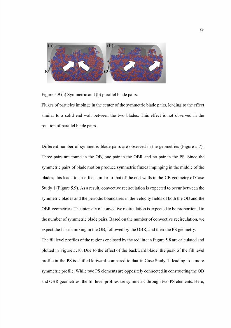
8/13/2019 Modeling and Analysis of Continuous Powder Blending
http://slidepdf.com/reader/full/modeling-and-analysis-of-continuous-powder-blending 102/177
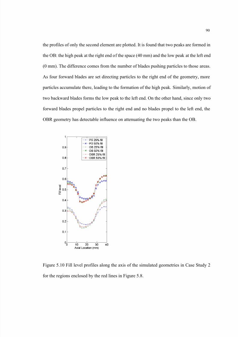
8/13/2019 Modeling and Analysis of Continuous Powder Blending
http://slidepdf.com/reader/full/modeling-and-analysis-of-continuous-powder-blending 103/177
90
the profiles of only the second element are plotted. It is found that two peaks are formed in
the OB: the high peak at the right end of the space (40 mm) and the low peak at the left end
(0 mm). The difference comes from the number of blades pushing particles to those areas.
As four forward blades are set directing particles to the right end of the geometry, more
particles accumulate there, leading to the formation of the high peak. Similarly, motion of
two backward blades forms the low peak to the left end. On the other hand, since only two
forward blades propel particles to the right end and no blades propel to the left end, the
OBR geometry has detectable influence on attenuating the two peaks than the OB.
Figure 5.10 Fill level profiles along the axis of the simulated geometries in Case Study 2
for the regions enclosed by the red lines in Figure 5.8.
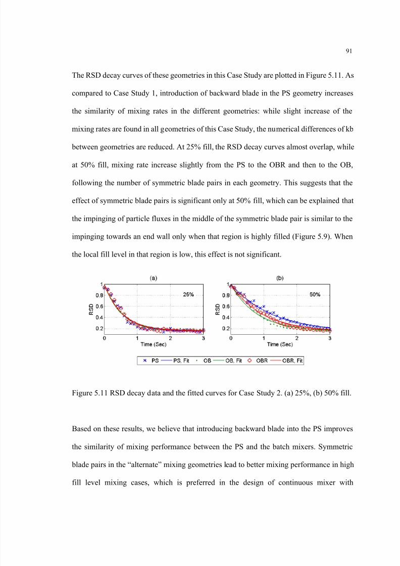
8/13/2019 Modeling and Analysis of Continuous Powder Blending
http://slidepdf.com/reader/full/modeling-and-analysis-of-continuous-powder-blending 104/177
91
The RSD decay curves of these geometries in this Case Study are plotted in Figure 5.11. As
compared to Case Study 1, introduction of backward blade in the PS geometry increases
the similarity of mixing rates in the different geometries: while slight increase of the
mixing rates are found in all geometries of this Case Study, the numerical differences of kb
between geometries are reduced. At 25% fill, the RSD decay curves almost overlap, while
at 50% fill, mixing rate increase slightly from the PS to the OBR and then to the OB,
following the number of symmetric blade pairs in each geometry. This suggests that the
effect of symmetric blade pairs is significant only at 50% fill, which can be explained that
the impinging of particle fluxes in the middle of the symmetric blade pair is similar to the
impinging towards an end wall only when that region is highly filled (Figure 5.9). When
the local fill level in that region is low, this effect is not significant.
Figure 5.11 RSD decay data and the fitted curves for Case Study 2. (a) 25%, (b) 50% fill.
Based on these results, we believe that introducing backward blade into the PS improves
the similarity of mixing performance between the PS and the batch mixers. Symmetric
blade pairs in the “alternate” mixing geometries lead to better mixing performance in high
fill level mixing cases, which is preferred in the design of continuous mixer with
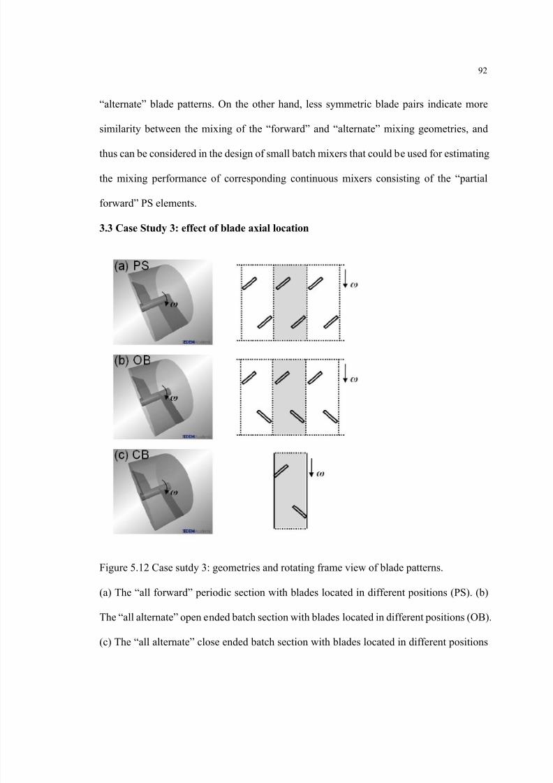
8/13/2019 Modeling and Analysis of Continuous Powder Blending
http://slidepdf.com/reader/full/modeling-and-analysis-of-continuous-powder-blending 105/177
92
“alternate” blade patterns. On the other hand, less symmetric blade pairs indicate more
similarity between the mixing of the “forward” and “alternate” mixing geometries, and
thus can be considered in the design of small batch mixers that could be used for estimating
the mixing performance of corresponding continuous mixers consisting of the “partial
forward” PS elements.
3.3 Case Study 3: effect of blade axial location
Figure 5.12 Case sutdy 3: geometries and rotating frame view of blade patterns.
(a) The “all forward” periodic section with blades located in different positions (PS). (b)
The “all alternate” open ended batch section with blades located in different positions (OB).
(c) The “all alternate” close ended batch section with blades located in different positions

8/13/2019 Modeling and Analysis of Continuous Powder Blending
http://slidepdf.com/reader/full/modeling-and-analysis-of-continuous-powder-blending 106/177
93
(CB). Dotted lines in the rotating frame are the periodic boundaries, and solid lines indicate
end walls.
Up to now, all the blades in all the geometries are always located in the middle of each
element. This leads to significant heterogeneity of fill level along the axis. The mixing rate
in these cases depends not only on the local fill level at the blade axial position, but also on
the exchange rate of materials between the blade area and the rest of the element along the
axis. When different fill level profiles are formed in these geometries, the exchange rates of
materials along the axis may not be the same, which is probably one reason leading to the
observed differences in mixing performance. To further examine this effect, the blades
were placed at different axial positions, the purpose of which is to form a more uniform fill
level profile for both the PS and other geometries. In this Case Study, the geometries of the
PS, the OB and the CB are very similar to those in the Case Study 1, except that the two
blades are located at different sites (at 10mm and 30mm along the axis of shaft, instead of
at 20mm in the middle of each cross-sectional element). The geometries and the rotating
frame view of blade patterns are shown in Figure 5.12.
The velocity fields in this Case Study are examined and plotted in Figure 5.13. While the
velocity fields of both the PS and the OB in this Case Study are similar to that in Case
Study 1, a convergence point at the center of the rotating frame is observed in the OB of the
current Case Study, instead of the shear region observed in Case Study 1. This suggests a
smaller mixing rate in the OB geometry in the current Case Study. Furthermore, in the
velocity field of the CB, the distance for the particles propelled by one blade to reach the
opposite end wall is longer (30 mm) compared to that of Case Study 1 (20 mm), which
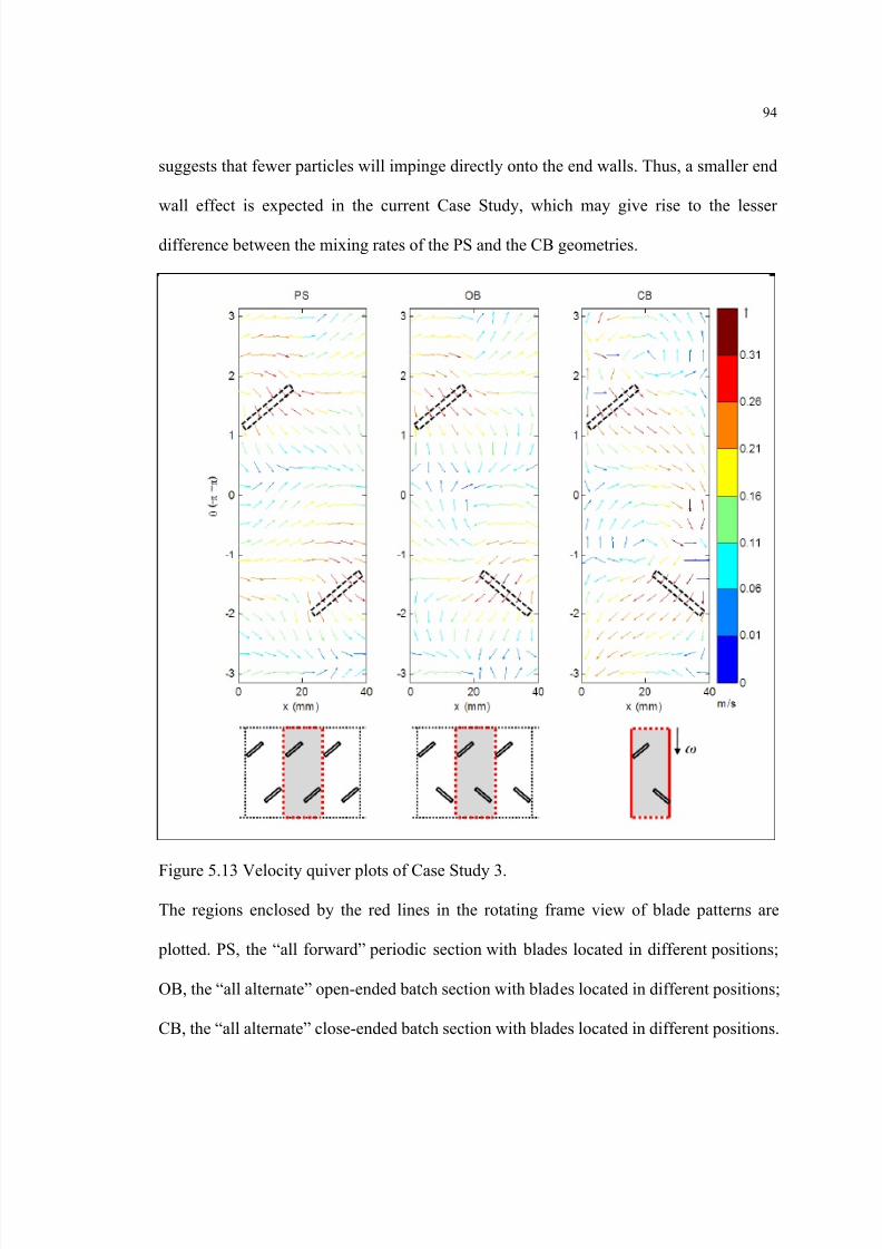
8/13/2019 Modeling and Analysis of Continuous Powder Blending
http://slidepdf.com/reader/full/modeling-and-analysis-of-continuous-powder-blending 107/177
94
suggests that fewer particles will impinge directly onto the end walls. Thus, a smaller end
wall effect is expected in the current Case Study, which may give rise to the lesser
difference between the mixing rates of the PS and the CB geometries.
Figure 5.13 Velocity quiver plots of Case Study 3.
The regions enclosed by the red lines in the rotating frame view of blade patterns are
plotted. PS, the “all forward” periodic section with blades located in different positions;
OB, the “all alternate” open-ended batch section with blades located in different positions;
CB, the “all alternate” close-ended batch section with blades located in different positions.
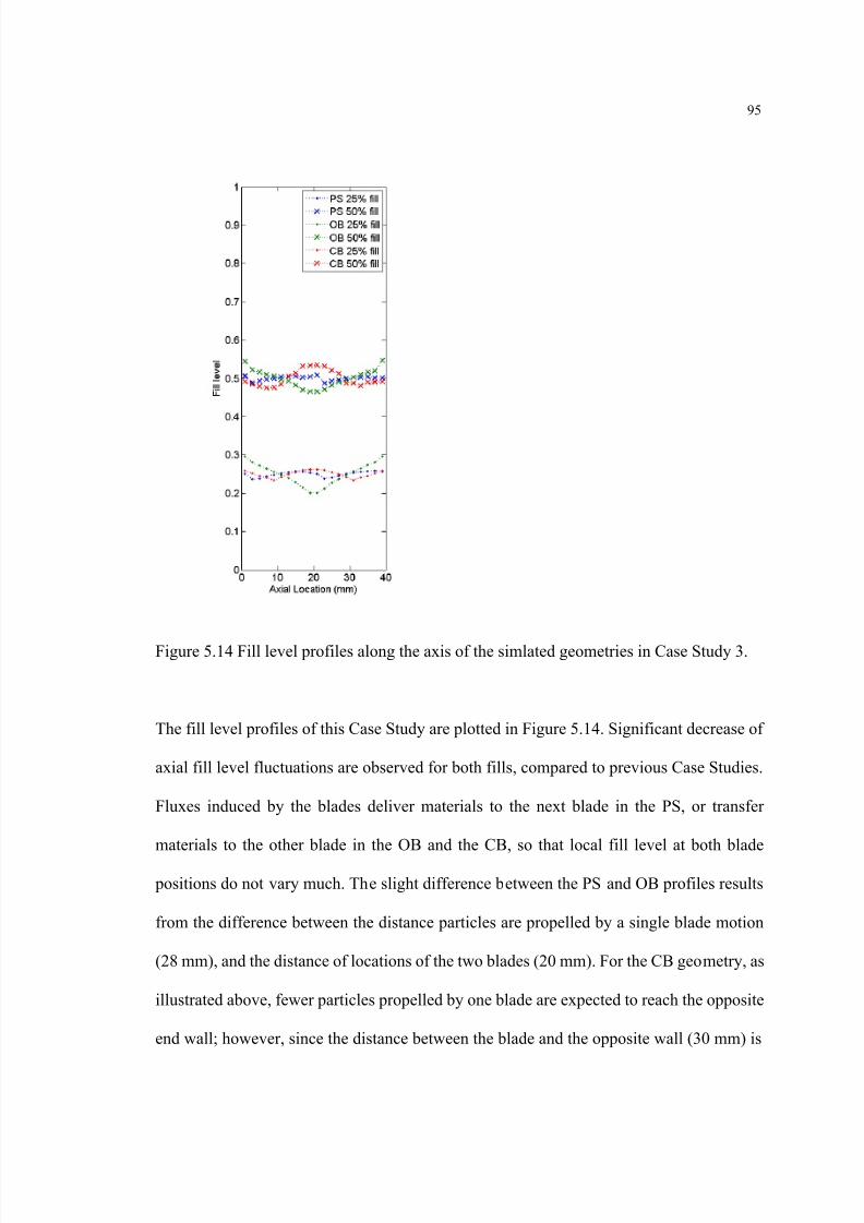
8/13/2019 Modeling and Analysis of Continuous Powder Blending
http://slidepdf.com/reader/full/modeling-and-analysis-of-continuous-powder-blending 108/177
95
Figure 5.14 Fill level profiles along the axis of the simlated geometries in Case Study 3.
The fill level profiles of this Case Study are plotted in Figure 5.14. Significant decrease of
axial fill level fluctuations are observed for both fills, compared to previous Case Studies.
Fluxes induced by the blades deliver materials to the next blade in the PS, or transfer
materials to the other blade in the OB and the CB, so that local fill level at both blade
positions do not vary much. The slight difference between the PS and OB profiles results
from the difference between the distance particles are propelled by a single blade motion
(28 mm), and the distance of locations of the two blades (20 mm). For the CB geometry, as
illustrated above, fewer particles propelled by one blade are expected to reach the opposite
end wall; however, since the distance between the blade and the opposite wall (30 mm) is
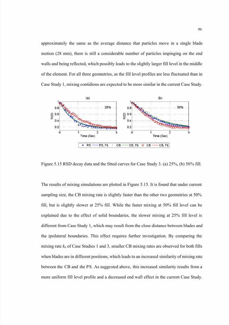
8/13/2019 Modeling and Analysis of Continuous Powder Blending
http://slidepdf.com/reader/full/modeling-and-analysis-of-continuous-powder-blending 109/177
96
approximately the same as the average distance that particles move in a single blade
motion (28 mm), there is still a considerable number of particles impinging on the end
walls and being reflected, which possibly leads to the slightly larger fill level in the middle
of the element. For all three geometries, as the fill level profiles are less fluctuated than in
Case Study 1, mixing contidions are expected to be more similar in the current Case Study.
Figure 5.15 RSD decay data and the fitted curves for Case Study 3. (a) 25%, (b) 50% fill.
The results of mixing simulations are plotted in Figure 5.15. It is found that under current
sampling size, the CB mixing rate is slightly faster than the other two geometries at 50%
fill, but is slightly slower at 25% fill. While the faster mixing at 50% fill level can be
explained due to the effect of solid boundaries, the slower mixing at 25% fill level is
different from Case Study 1, which may result from the close distance between blades andthe ipsilateral boundaries. This effect requires further investigation. By comparing the
mixing rate k b of Case Studies 1 and 3, smaller CB mixing rates are observed for both fills
when blades are in different positions, which leads to an increased similarity of mixing rate
between the CB and the PS. As suggested above, this increased similarity results from a
more uniform fill level profile and a decreased end wall effect in the current Case Study.
8/13/2019 Modeling and Analysis of Continuous Powder Blending
http://slidepdf.com/reader/full/modeling-and-analysis-of-continuous-powder-blending 110/177
97
On the other hand, RSD decay curves of the OB overlap with these of the PS for both fills.
This result shows satisfactory similarity, which suggests that besides the issues of end
walls and backward fluxes, keeping uniform fill level profile is also an important issue in
achieving similar mixing rates between different cross-sectional elements. Based on these
results, by constructing a batch mixer following the issues identified in the three case
studies, it is possible to estimate the cross-sectional mixing of a continuous mixing process
with similar geometries.
5.3 Summary
This work examines the cross-sectional mixing performance of several elemental
geometries in order to determine the effect of blade orientation, and characterize the impact
of circulation patterns in continuous powder mixers. An additional goal of the work
presented here is to determine whether a physically realizable batch mixer can be used to
study the cross-sectional component of the mixing process in a flow-through continuous
mixer. Two methods are used to perform these assessments. Two-dimensional quiver plots
of the velocity field, averaged in the radial directions, are used to examine qualitatively the
motion of particles in the various geometries. The mixing rate, which is represented by the
RSD logarithmic decay rate k b at a given fill level and sampling size, is used as the index to
compare mixing performance. In addition, fill level profiles are calculated to examine their
possible effects on mixing.
Several effects were readily apparent from the first case study, which examined three
elemental geometries with only two blades: (1) The orientation of the blades, and the
presence of solid walls, profoundly affected the motion patterns of particles in the
elemental geometry. (2) Backward-oriented blades created visible convective recirculation,
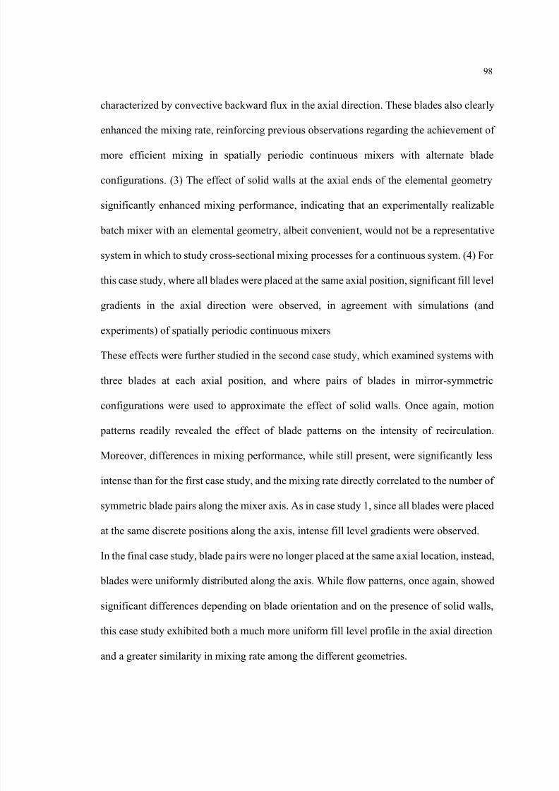
8/13/2019 Modeling and Analysis of Continuous Powder Blending
http://slidepdf.com/reader/full/modeling-and-analysis-of-continuous-powder-blending 111/177

8/13/2019 Modeling and Analysis of Continuous Powder Blending
http://slidepdf.com/reader/full/modeling-and-analysis-of-continuous-powder-blending 112/177

8/13/2019 Modeling and Analysis of Continuous Powder Blending
http://slidepdf.com/reader/full/modeling-and-analysis-of-continuous-powder-blending 113/177
100
Chapter 6
Strategies on improving blending performance
In this chapter, the previously developed periodic section modeling is used to determine
the influence of operating conditions on the performance of continuous blenders. The
influence on either the local mixing efficiency or the axial motion of the mixture is
separately considered. To understand the applicability of knowledge from successful
mixing cases, we focus on (1) a single blending geometry but four different mixing cases,
and examine in detail the performance similarity among these cases, and (2) multiply
geometry and operation factors on blending performance. The rest of the paper is
organized as follows: the simulations of different mixing cases using factorial analysis are
discussed in Section 6.1. The influence of multiple factors is investigated using the
Projection of Latent Structure (PLS) and validated experimentally in Section 6.2. The
summary are presented in 6.3.
6.1 Optimizing continuous powder blending using factorial analysis
6.1.1 Simulation and Methodology
Due to the difficulty involved in experimentally building a cross section with periodic
boundaries, we use the Discrete Element Method (DEM) as the tool for examining the
operations and mixing cases of interest. Detailed reviews of the DEM application can be
found in (Bertrand et al., 2005; Dubey et al., 2011). In this study, the software EDEM ®
from DEM Solutions is used to develop the desired geometries. The particles simulated are
spheres. The physical and numerical parameters used in this simulation are summarized in
Table 6.1. The approach has been used in our previous studies (Arratia et al., 2006; Gao et

8/13/2019 Modeling and Analysis of Continuous Powder Blending
http://slidepdf.com/reader/full/modeling-and-analysis-of-continuous-powder-blending 114/177
101
al., 2011a; Portillo et al., 2007), as well as in a number of previous efforts (Sarkar and
Wassgren, 2010; Zhou et al., 2004) and found to be able to accurately capture the dynamics
of mixing processes.
Table 6.1 Physical and numerical parameters used in the DEM model.
ValueParameterCase 1(Control)
Case 2(Lighter
particles)
Case 3(Larger
particles)
Case 4(Morecohesive
particles)Particle diameter (m) 3×10 -3 3×10 -3 4×10 -3 3×10 -3 Particle density (kg m -3) 1×10 3 0.2×10 3 1×10 3 1×10 3 Cohesion coefficient k (Jm -3)
F=kA F: Cohesive force A: Contact area
0 0 0 5×10 5
The cross-sectional element representing a periodic section (PS) was constructed from a
horizontal cylinder (diameter 80 mm and length 40 mm). Two 40° forward blades (20 mm
×40 mm) were located opposite to each other at different sites of the shaft (at 10 mm and 30
mm along the axis of the shaft) (Figure 6.1). This PS elementary geometry was tested in
previous chapters (Gao et al., 2011a), and was found that lead to more homogenous axial
fill level distribution and fewer dead spots. In this chapter, it is used to simulate the ideally
cross-sectional mixing in an “all forward” continuous mixer with the same fill level and
flow rate.
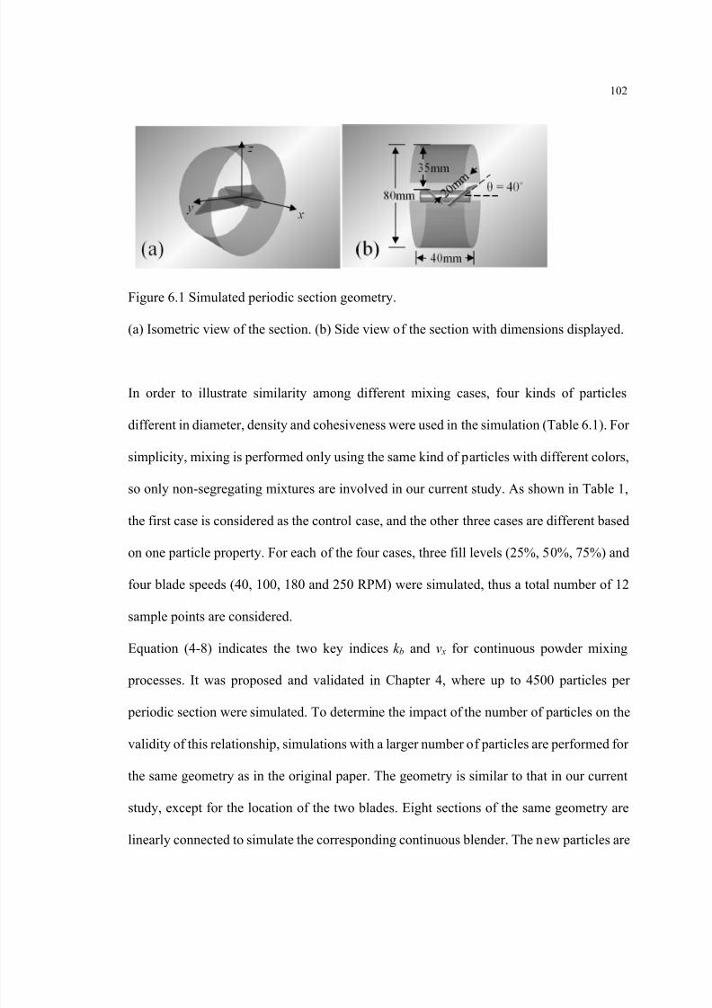
8/13/2019 Modeling and Analysis of Continuous Powder Blending
http://slidepdf.com/reader/full/modeling-and-analysis-of-continuous-powder-blending 115/177
102
Figure 6.1 Simulated periodic section geometry.
(a) Isometric view of the section. (b) Side view of the section with dimensions displayed.
In order to illustrate similarity among different mixing cases, four kinds of particles
different in diameter, density and cohesiveness were used in the simulation (Table 6.1). For
simplicity, mixing is performed only using the same kind of particles with different colors,
so only non-segregating mixtures are involved in our current study. As shown in Table 1,
the first case is considered as the control case, and the other three cases are different based
on one particle property. For each of the four cases, three fill levels (25%, 50%, 75%) and
four blade speeds (40, 100, 180 and 250 RPM) were simulated, thus a total number of 12
sample points are considered.
Equation (4-8) indicates the two key indices k b and v x for continuous powder mixing
processes. It was proposed and validated in Chapter 4, where up to 4500 particles per
periodic section were simulated. To determine the impact of the number of particles on the
validity of this relationship, simulations with a larger number of particles are performed for
the same geometry as in the original paper. The geometry is similar to that in our current
study, except for the location of the two blades. Eight sections of the same geometry are
linearly connected to simulate the corresponding continuous blender. The new particles are
8/13/2019 Modeling and Analysis of Continuous Powder Blending
http://slidepdf.com/reader/full/modeling-and-analysis-of-continuous-powder-blending 116/177
103
2 mm in diameter, which are 1.5 times smaller than the original ones. As a result, 7560
particles per periodic section are simulated representing a 25% fill level, and the
corresponding feed rate in the continuous blender is set as 11440 particles per second for
each component. A sampling size of 110 particles was used in the RSD calculations and the
results are plotted in Figure 2. While the fitted value of k b is 1.71 s -1, and RSDSS is 0.0930
under the sampling size of 110 particles, the mean axial velocity v x is 121 mm/s for both
simulations, leading to the predicted value of k b as 0.0141 mm -1. Figure 6.2b indicates the
validity the model when more particles are simulated. It should be noted that the prediction
was performed only in the first six sections (0 -240 mm) as fill level decreases dramatically
in the last two sections due to discharge effects.
Figure 6.2 Validation of periodic section modeling with more particles.
(a) Batch-like RSD decay data in periodic section. Dot line is the fitted curve. (b) RSD
decay data in the corresponding continuous blender. Solid line is the predicted decay curve
through the calculation of k c.
6.1.2 Factorial analysis results

8/13/2019 Modeling and Analysis of Continuous Powder Blending
http://slidepdf.com/reader/full/modeling-and-analysis-of-continuous-powder-blending 117/177
104
Figure 6.3 The control case: simulated, fitted, and normalized RTD and RSD-t curves for
different operating conditions.
Figure 6.3 summarizes the RTD and RSD-t curves of the control case. Using the data
derived from the particle-trajectory method and the cube-sample method, v x and k b are
determined using the least squares method. As shown in recent studies from our group
(Portillo et al., 2010; Vanarase and Muzzio, 2011), the mean residence time of continuous
blending is approximately anti-proportional to rotary speed of blades. Meanwhile, earlier
studies on batch blending (Brone et al., 1998; Brone and Muzzio, 2000) reveal the
8/13/2019 Modeling and Analysis of Continuous Powder Blending
http://slidepdf.com/reader/full/modeling-and-analysis-of-continuous-powder-blending 118/177
105
proportionality between batch mixing rate and rotation rate of blenders, indicating that a
similar relationship should exist between the mixing rate and blade speed in the periodic
section blending. To normalize the effects of blade speed on mixing and axial velocity,
RTD and RSD-t curves are replotted versus revolution (Figure 6.3, the second and fourth
columns), instead of versus time (Figure 6.3, the first and third columns). Results are
compared for different blade speeds and fill levels. In the normalized plots, mean residence
time and mixing process are independent of blade rotary speed, while both mixing and
axial delivery of particles are a little bit faster at low fill levels. The corresponding mean
axial velocity and mixing rate, normalized over rotary speed, are calculated as:
' / x xv v ω = 6-1
' /b bk k ω = 6-2
where ω is the blade speed measured as revolution per second. Notice that k b’ measures
mixing rate as RSD decay per revolution, and v x’ measures axial velocity as millimeters per
revolution. The influence of operating conditions on both indices for different mixing cases
is analyzed as follows.
Based on the above results, the influence of fill level and rotary speed on the normalized
mean axial velocity is plotted in Figure 6.4. It is noticed that the axial displacement during
each blade revolution increases with increasing rotary speed and decreasing fill level.
While the first three cases depict similar contour profiles, the more cohesive particle case is
found to be slightly different. Due to the cohesiveness in this case, the maximal value of
vx’ is not as large as in other cases, while the minimal value is found at a moderately low
blade speed (100 RPM) and large fill level (50% -75%). However, the overall trend in this
case is similar to the other three cases, thus is not affected by the different particle
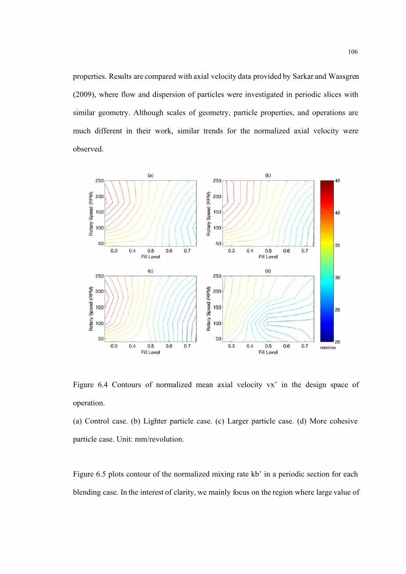
8/13/2019 Modeling and Analysis of Continuous Powder Blending
http://slidepdf.com/reader/full/modeling-and-analysis-of-continuous-powder-blending 119/177
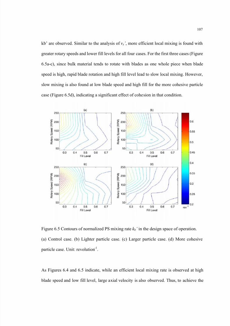
8/13/2019 Modeling and Analysis of Continuous Powder Blending
http://slidepdf.com/reader/full/modeling-and-analysis-of-continuous-powder-blending 120/177
107
kb’ are observed. Similar to the analysis of v x’ , more efficient local mixing is found with
greater rotary speeds and lower fill levels for all four cases. For the first three cases (Figure
6.5a-c), since bulk material tends to rotate with blades as one whole piece when blade
speed is high, rapid blade rotation and high fill level lead to slow local mixing. However,
slow mixing is also found at low blade speed and high fill for the more cohesive particle
case (Figure 6.5d), indicating a significant effect of cohesion in that condition.
Figure 6.5 Contours of normalized PS mixing rate k b’ in the design space of operation.
(a) Control case. (b) Lighter particle case. (c) Larger particle case. (d) More cohesive
particle case. Unit: revolution -1.
As Figures 6.4 and 6.5 indicate, while an efficient local mixing rate is observed at high
blade speed and low fill level, large axial velocity is also observed. Thus, to achieve the
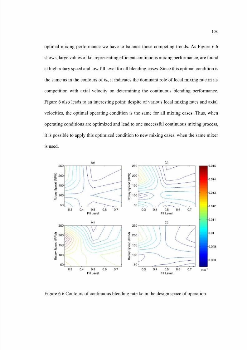
8/13/2019 Modeling and Analysis of Continuous Powder Blending
http://slidepdf.com/reader/full/modeling-and-analysis-of-continuous-powder-blending 121/177
108
optimal mixing performance we have to balance those competing trends. As Figure 6.6
shows, large values of kc, representing efficient continuous mixing performance, are found
at high rotary speed and low fill level for all blending cases. Since this optimal condition is
the same as in the contours of k b, it indicates the dominant role of local mixing rate in its
competition with axial velocity on determining the continuous blending performance.
Figure 6 also leads to an interesting point: despite of various local mixing rates and axial
velocities, the optimal operating condition is the same for all mixing cases. Thus, when
operating conditions are optimized and lead to one successful continuous mixing process,
it is possible to apply this optimized condition to new mixing cases, when the same mixer
is used.
Figure 6.6 Contours of continuous blending rate kc in the design space of operation.

8/13/2019 Modeling and Analysis of Continuous Powder Blending
http://slidepdf.com/reader/full/modeling-and-analysis-of-continuous-powder-blending 122/177
8/13/2019 Modeling and Analysis of Continuous Powder Blending
http://slidepdf.com/reader/full/modeling-and-analysis-of-continuous-powder-blending 123/177
110
To test the proposed approach for improving the mixing performance, the 25% fill
simulations of four blade speeds (40, 100, 180, and 250 RPM) were used as control cases.
To counterbalance the increase of axial velocity through the increase of blade speed, we
need operations that can decrease the axial forward flux. Our previous study (Gao et al.,
2011a) shows the effect of blade angle: axial velocity decreases with decreasing blade
angle. Another study (Vanarase and Muzzio, 2011) also indicates the effect of weir at the
discharge on hindering axial flow, which leads to a decrease of axial velocity. Based on
these studies, two strategies are proposed to improve the continuous blending performance:
(1) decreasing blade angle while increasing blade speed; (2) increasing weir height at the
end of the PS while increasing blade speed. The key to both strategies is to keep the axial
velocity constant through the increase of blade speed. For this purpose, additional
simulations were performed. Based on the case of 25% fill, 180 RPM simulation, the effect
of blade angle and weir height on the axial velocity were simulated, as plotted in Figure 6.7.
The corresponding fitted curves of these effects, as well as the effect of blade speed on
axial velocity, are determined. To find the corresponding blade angle and weir height that
keeps the axial velocity constant while increasing the blade speed, we assume the effects of
blade angle, blade speed and weir height on the axial velocity are independent from each
other and can be described as follows:
1 2 3( , , ) ( ) ( ) ( )ω θ η ω θ η = xv f f f 6-3
where ω is the rotary speed measured as RPM, θ is the blade angle and η=h/d the weir
height ratio ( h the height of the weir and d the diameter of the cylindrical mixing space).
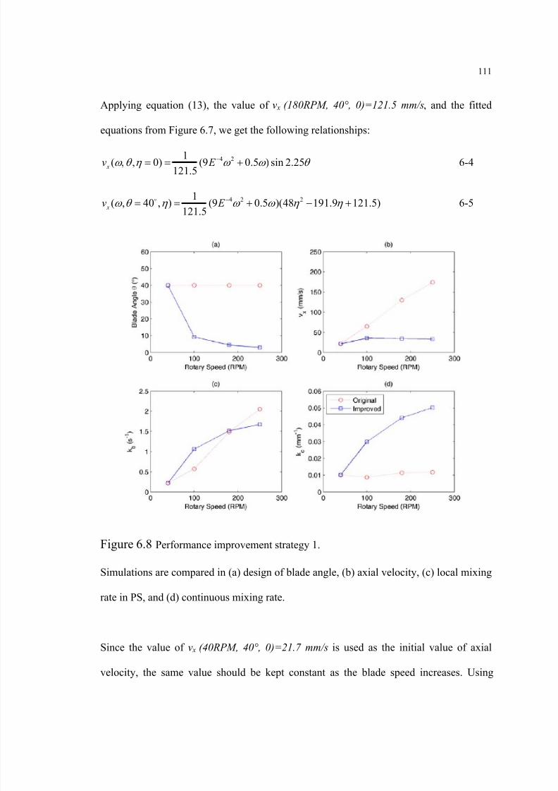
8/13/2019 Modeling and Analysis of Continuous Powder Blending
http://slidepdf.com/reader/full/modeling-and-analysis-of-continuous-powder-blending 124/177
111
Applying equation (13), the value of v x (180RPM, 40°, 0)=121.5 mm/s , and the fitted
equations from Figure 6.7, we get the following relationships:
4 21( , , 0) (9 0.5 ) sin 2.25
121.5ω θ η ω ω θ −= = +
xv E 6-4
4 2 21( , 40 , ) (9 0.5 )(48 191.9 121.5)
121.5ω θ η ω ω η η −= = + − +
xv E 6-5
Figure 6.8 Performance improvement strategy 1.
Simulations are compared in (a) design of blade angle, (b) axial velocity, (c) local mixing
rate in PS, and (d) continuous mixing rate.
Since the value of v x (40RPM, 40°, 0)=21.7 mm/s is used as the initial value of axial
velocity, the same value should be kept constant as the blade speed increases. Using

8/13/2019 Modeling and Analysis of Continuous Powder Blending
http://slidepdf.com/reader/full/modeling-and-analysis-of-continuous-powder-blending 125/177

8/13/2019 Modeling and Analysis of Continuous Powder Blending
http://slidepdf.com/reader/full/modeling-and-analysis-of-continuous-powder-blending 126/177
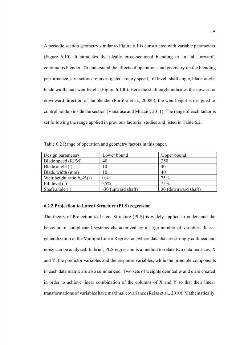
8/13/2019 Modeling and Analysis of Continuous Powder Blending
http://slidepdf.com/reader/full/modeling-and-analysis-of-continuous-powder-blending 127/177
114
A periodic section geometry similar to Figure 6.1 is constructed with variable parameters
(Figure 6.10). It simulates the ideally cross-sectional blending in an “all forward”
continuous blender. To understand the effects of operations and geometry on the blending
performance, six factors are investigated: rotary speed, fill level, shaft angle, blade angle,
blade width, and weir height (Figure 6.10b). Here the shaft angle indicates the upward or
downward direction of the blender (Portillo et al., 2008b); the weir height is designed to
control holdup inside the section (Vanarase and Muzzio, 2011). The range of each factor is
set following the range applied in previous factorial studies and listed in Table 6.2.
Table 6.2 Range of operation and geometry factors in this paper.
Design parameters Lower bound Upper boundBlade speed (RPM) 40 250Blade angle (
˚
) 10 40Blade width (mm) 10 40Weir height ratio hw /d (-) 0% 75%Fill level (-) 25% 75%Shaft angle (
˚
) -30 (upward shaft) 30 (downward shaft)
6.2.2 Projection to Latent Structure (PLS) regression
The theory of Projection to Latent Structure (PLS) is widely applied to understand the
behavior of complicated systems characterized by a large number of variables. It is a
generalization of the Multiple Linear Regression, where data that are strongly collinear and
noisy can be analyzed. In brief, PLS regression is a method to relate two data matrices, X
and Y, the predictor variables and the response variables, while the principle components
in each data matrix are also summarized. Two sets of weights denoted w and c are created
in order to achieve linear combination of the columns of X and Y so that their linear
transformations of variables have maximal covariance (Reiss et al., 2010). Mathematically,

8/13/2019 Modeling and Analysis of Continuous Powder Blending
http://slidepdf.com/reader/full/modeling-and-analysis-of-continuous-powder-blending 128/177
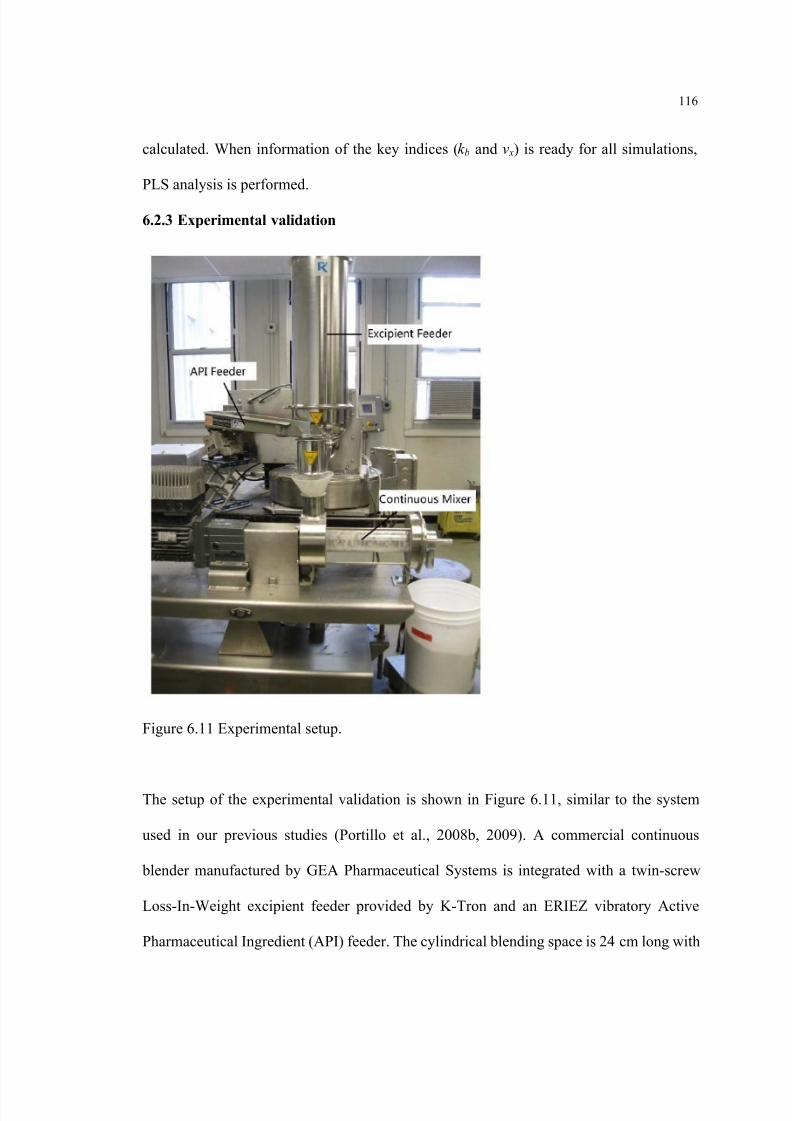
8/13/2019 Modeling and Analysis of Continuous Powder Blending
http://slidepdf.com/reader/full/modeling-and-analysis-of-continuous-powder-blending 129/177
116
calculated. When information of the key indices ( k b and v x) is ready for all simulations,
PLS analysis is performed.
6.2.3 Experimental validation
Figure 6.11 Experimental setup.
The setup of the experimental validation is shown in Figure 6.11, similar to the system
used in our previous studies (Portillo et al., 2008b, 2009). A commercial continuous
blender manufactured by GEA Pharmaceutical Systems is integrated with a twin-screw
Loss-In-Weight excipient feeder provided by K-Tron and an ERIEZ vibratory Active
Pharmaceutical Ingredient (API) feeder. The cylindrical blending space is 24 cm long with
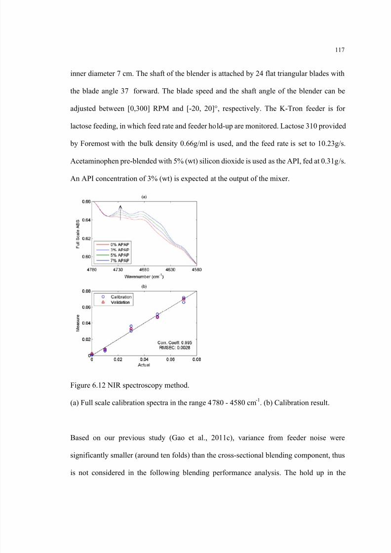
8/13/2019 Modeling and Analysis of Continuous Powder Blending
http://slidepdf.com/reader/full/modeling-and-analysis-of-continuous-powder-blending 130/177

8/13/2019 Modeling and Analysis of Continuous Powder Blending
http://slidepdf.com/reader/full/modeling-and-analysis-of-continuous-powder-blending 131/177
118
blender is calculated as the total mass in both feeders before blending begins minus the sum
of the powder remaining in the feeders and at the output when steady state is reached.
For each operating condition, ten vials of output samples are collected when steady state is
reached. Each vial contains approximate 1.5 cm 3 material. The API concentration in each
vial is determined by using NIR spectroscopy method (Gao et al., 2011c; Vanarase et al.,
2010). Lactose samples mixed with 0, 1, 3, 5, 7% (wt) pre-blended acetaminophen is
prepared for calibration. A Nicolet Antaris NIR spectrometer provided by Thermo Fisher is
used to acquire the absorbance spectra between the range 4000 cm -1 to 10000 cm -1 wave
numbers. Each calibration sample is scanned for four times with re-shake between adjacent
scans. Spectral data is collected using the software Omnic, and TQ Analyst is used to
develop the calibration model. Full scale absorbance between 4780 - 4580 cm -1 is used for
the spectral regression, and the software selects the range 4744.03 - 4705.46 cm -1 for the
calibration model (Figure 6.12a). The root mean square error of calibration (RMSEC) is
0.0028, indicating good fitting of the spectral data (Figure 6.12b). With this NIR method,
API concentration of the experimental samples can be determined, which are further
applied for the RSD calculation.
6.2.4 PLS regression results
Figure 6.13 R 2 and Q 2 indices of the PLS regression from 1 to 3 principle components.
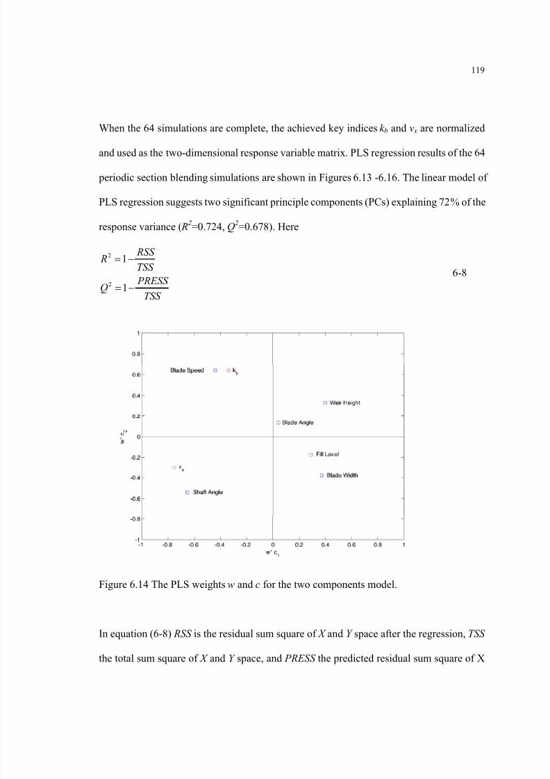
8/13/2019 Modeling and Analysis of Continuous Powder Blending
http://slidepdf.com/reader/full/modeling-and-analysis-of-continuous-powder-blending 132/177
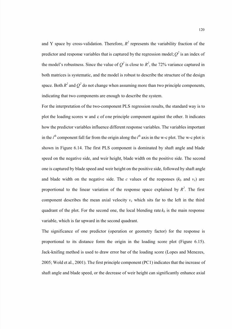
8/13/2019 Modeling and Analysis of Continuous Powder Blending
http://slidepdf.com/reader/full/modeling-and-analysis-of-continuous-powder-blending 133/177
120
and Y space by cross-validation. Therefore, R2 represents the variability fraction of the
predictor and response variables that is captured by the regression model; Q2 is an index of
the model’s robustness. Since the value of Q2 is close to R2, the 72% variance captured in
both matrices is systematic, and the model is robust to describe the structure of the design
space. Both R2 and Q2 do not change when assuming more than two principle components,
indicating that two components are enough to describe the system.
For the interpretation of the two-component PLS regression results, the standard way is to
plot the loading scores w and c of one principle component against the other. It indicates
how the predictor variables influence different response variables. The variables important
in the ith component fall far from the origin along the ith axis in the w-c plot. The w-c plot is
shown in Figure 6.14. The first PLS component is dominated by shaft angle and blade
speed on the negative side, and weir height, blade width on the positive side. The second
one is captured by blade speed and weir height on the positive side, followed by shaft angle
and blade width on the negative side. The c values of the responses ( k b and v x) are
proportional to the linear variation of the response space explained by R2. The first
component describes the mean axial velocity v x which sits far to the left in the third
quadrant of the plot. For the second one, the local blending rate k b is the main response
variable, which is far upward in the second quadrant.
The significance of one predictor (operation or geometry factor) for the response is
proportional to its distance form the origin in the loading score plot (Figure 6.15).
Jack-knifing method is used to draw error bar of the loading score (Lopes and Menezes,
2005; Wold et al., 2001). The first principle component (PC1) indicates that the increase of
shaft angle and blade speed, or the decrease of weir height can significantly enhance axial
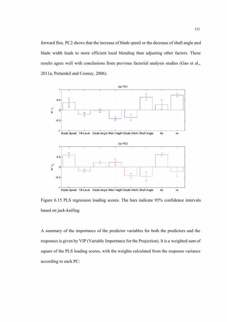
8/13/2019 Modeling and Analysis of Continuous Powder Blending
http://slidepdf.com/reader/full/modeling-and-analysis-of-continuous-powder-blending 134/177
121
forward flux. PC2 shows that the increase of blade speed or the decrease of shaft angle and
blade width leads to more efficient local blending than adjusting other factors. These
results agree well with conclusions from previous factorial analysis studies (Gao et al.,
2011a; Pernenkil and Cooney, 2006).
Figure 6.15 PLS regression loading scores. The bars indicate 95% confidence intervals
based on jack-knifing.
A summary of the importance of the predictor variables for both the predictors and the
responses is given by VIP (Variable Importance for the Projection). It is a weighted sum of
square of the PLS loading scores, with the weights calculated from the response variance
according to each PC:

8/13/2019 Modeling and Analysis of Continuous Powder Blending
http://slidepdf.com/reader/full/modeling-and-analysis-of-continuous-powder-blending 135/177
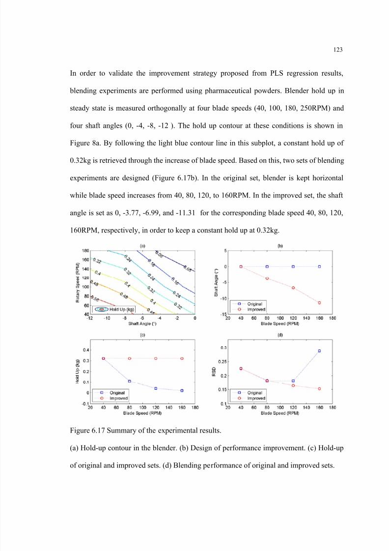
8/13/2019 Modeling and Analysis of Continuous Powder Blending
http://slidepdf.com/reader/full/modeling-and-analysis-of-continuous-powder-blending 136/177
8/13/2019 Modeling and Analysis of Continuous Powder Blending
http://slidepdf.com/reader/full/modeling-and-analysis-of-continuous-powder-blending 137/177
124
Blending performance of both experimental sets are measured and compared to show the
efficiency of the proposed strategy. As Figure 6.17c shows, hold up of the original set
decreases along the ascending blade speed, which leads to shorter residence time and thus
worse blending performance at large blade speed (Figure 6.17d). A similar profile has been
reported in our previous study (Vanarase and Muzzio, 2011). On the other hand, significant
performance improvement is observed at high blade speed in the improved set due to a
constant mean residence time. In this case, the number of blade passes that powder
experiences is simply proportional to the ascending blade speed. As expected, the RSD
decay curve is similar to batch systems, showing exponential decay profile against the
blade speed.
6.3 Summary
This chapter investigates the effect of operating conditions on two important parameters of
continuous blending: local mixing rate k b and axial velocity v x of powders. Factorial
analysis shows that, at high rotary speed and low fill level, particles move faster and reside
for a shorter time inside the mixer. Faster local mixing is observed in the same range of
operations. This competition between k b and v x leads to a trade-off on the overall
continuous blending performance even under the best operating conditions. Moreover, the
same optimal operating conditions are observed for different mixing cases, indicating that
these optimal conditions might be universal and could be applied in other cases using the
same mixer. The Projection to Latent Structure (PLS) regression analysis is further
introduced to clarify the complicate influence of various operation and geometry factors on
blending performance. Regression results show that shaft angle and blade speed are the
8/13/2019 Modeling and Analysis of Continuous Powder Blending
http://slidepdf.com/reader/full/modeling-and-analysis-of-continuous-powder-blending 138/177
125
most influential factors. Blade geometry and fill level show less impact in the investigated
range of factors. Based on these results, novel strategies are proposed as follows to
improve continuous blending performance. The key is to keep axial velocity constant when
increasing the blade speed. This guarantees the variance decay rate along the mixing axis is
proportional to the blade speed in continuous blending systems. To achieve this goal, blade
angle or weir height was altered along with the ascending blade speed in the factorial
analysis. Based on conclusions from the PLS regression, simultaneously changing shaft
angle and blade speed, which conveniently increases blending rate while keeps axial
velocity constant, is the most efficient strategy suggested for performance improvement.
Significant improvements on blending performance were observed in both simulations and
experimental validations using pharmaceutical powder. In sum, this work clarifies the
significance of various operation and geometry factors in the performance improvement of
continuous powder blending unit operation, and provides an efficient guidance on blender
design and operation control in practice.
Once more, it should be emphasized that all simulation cases in this chapter are
non-segregating. For segregating powders, the optimal operation does not only depend on
how fast mixing reaches steady state, but also on whether the steady state mixture can be
characterized as “well mixed”. Therefore, before designing continuous mixing system for
specific segregating case, batch mixing using a geometry and operation similar to one
periodic section of the corresponding continuous blender is recommended (Gao et al.,
2011a). If segregation is observed and leads to failure of mixing in the preliminary batch
case, it needs to be handled by altering operating conditions before the corresponding
continuous process is applied. As a result, previous studies on batch segregation such as

8/13/2019 Modeling and Analysis of Continuous Powder Blending
http://slidepdf.com/reader/full/modeling-and-analysis-of-continuous-powder-blending 139/177
8/13/2019 Modeling and Analysis of Continuous Powder Blending
http://slidepdf.com/reader/full/modeling-and-analysis-of-continuous-powder-blending 140/177
127
Chapter 7
Scale-up of continuous powder blending
In this chapter, the theoretical basis of scaling up continuous powder blending is
established. Firstly, variance spectrum analysis is introduced to illustrate the influence of
sampling size on the relationship between flow pattern similarity and mixing performance
similarity, which provides a theoretical means to analyze the scale-up of batch mixing
processes and the scale-up of the cross-sectional mixing in continuous mixing processes.
Secondly, the periodic section modeling proposed in the previous chapter (Gao et al., 2012)
is applied to characterize the cross-sectional blending component, which is considered as
the combination of a batch-like blending process and the axial motion of the powder along
the continuous mixer. The rest of the chapter is organized as follows. Current limitations
on scale-up is discussed in Section 7.1. In Sections 7.2 and 7.3, the variance spectrum,and
the simulation designs are introduced. Two methodologies to determine the variance
spectrum, the Fourier series and the Lomb Scargle Periodogram, are described. Conceptual
simulations with typical mixing cases of non-segregating and cohesive segregating
particles are then performed in Section 7.4 to show the applicability of the developed
scale-up strategy, followed by the conclusion in Section 7.5.
7.1 Current limitations
Previous work in the area of powder blending scale-up is based on the principle of
similarity proposed by Johnstone and Thring (1957). According to this principle, the
material flow patterns in two scales of mixing apparatuses are expected to be similar when
the dimensions, velocity fields, and force distributions of corresponding points are

8/13/2019 Modeling and Analysis of Continuous Powder Blending
http://slidepdf.com/reader/full/modeling-and-analysis-of-continuous-powder-blending 141/177
128
proportional to each other. Generally, dimensional analysis is applied to identify these
similarity criteria if the process governing equations are unknown, while dimensionless
forms are derived if the governing equations are available. Applying this principle, Wang
and Fan (1974) investigated the scaling up of tumbling mixers. Their results indicate that
the ratio of centrifugal force to the gravitational force, or the Froude number, can be used
as the main similarity criterion for the scale-up of a tumbling mixer. Based on
hydrodynamic similarity, Horio et al. (1986) developed a scale-up rule for fluidized beds
when the similarities in bubble coalescence, bubble splitting, and interstitial flow pattern
are satisfied. Surface velocity profiles in rotating cylinders were found to follow simple
scaling rules through the normalization of a one-dimensional motion equation with
constant acceleration (Alexander and Muzzio, 2005; Alexander et al., 2002).
Of the few studies concerning the scaling up of continuous powder mixing processes, most
efforts are spent on the characterization of the axial mixing component, namely, scaling up
of the RTD (residence time distribution). Based on dimensional analysis similar to the one
used in batch mode studies, Abouzeid et al. (1980) applied the characteristic time (the ratio
of dimensionless hold up and feed rate) as the main scale-up criterion for the RTD of
materials flowing in rotating drums. The dimensionless variance of the RTD, which is
defined as the second moment of the RTD function (Nauman, 2008), was approximately
calculated as a function of Peclet number using the Fokker-Planck dispersion model
(Risken, 1996). Similar analysis was performed in the polymer processing of a continuous
twin-screw extruder (Meijer and Elemans, 1988), on which the scale-up issues of geometry,
heat transfer, and power consumption were discussed. A more complex scaling
relationship for rotating drums was developed for particles without considering cohesion
8/13/2019 Modeling and Analysis of Continuous Powder Blending
http://slidepdf.com/reader/full/modeling-and-analysis-of-continuous-powder-blending 142/177
129
and only for cases where the effect of interstitial fluid is negligible (Ding et al., 2001). In
this study, parameters and variables were normalized using governing equations based on
the Eulerian approach, which assumes that the properties of the granular materials are a
continuous function of position (Johnson and Jackson, 1987; Savage and Hutter, 1989).
Despite the achievements described above, there are still two unresolved issues for
developing a quantitative scale-up strategy for continuous powder mixing processes.
Firstly, although it is generally believed that similar mixing performances can be achieved
in geometries of different scales when the principle of similarity is satisfied, theoretical
validation is not available yet. There is no doubt that we can get similar mixing when the
scale of mixing measurement, or the sampling size, is proportional to the scale of mixer
geometry. However, the key difficulty is that in most cases the sampling size applied for
mixing of different geometry scales is constant, as the size of samples is predetermined by
the size of the tablets, which is the final product of pharmaceutical manufacturing process.
This constant-sample effect on measuring the mixing performance is rarely considered in
previous scale-up studies. Secondly, few investigations focus on continuous powder
mixing compared to the well-studied batch mixing process. While it is well-known that the
continuous powder mixing process is a combination of axial and cross-sectional mixing
(Williams, 1976), quantitative modeling for both mixing components, especially for the
cross-sectional mixing, has not been well established. Thus, development of quantitative
scale-up strategies is difficult for the same process. We will discuss these issues in detail in
this chapter.
7.2 Variance spectrum analysis
7.2.1 Fourier analysis
8/13/2019 Modeling and Analysis of Continuous Powder Blending
http://slidepdf.com/reader/full/modeling-and-analysis-of-continuous-powder-blending 143/177
130
Variance spectrum is defined as the distribution of variance components in different
frequency domains, which can be obtained through the application of Fourier transform.
Shin and Fan (1978) used the application of discrete Fourier transform (DFT) to investigate
the characterization of random and ordered powder mixtures. While the amplitude of the
spectrum indicates the intensity of segregation at different frequency domains, the location
of the maximum spectrum component illustrates the scale of segregation intuitively (Poux
et al., 1991; Weineköter and Reh, 1995).
One-dimensional discrete Fourier series method has been discussed in Chapter 2. The
corresponding variance value σ 2(f s ) is calculated as the integration of the spectrum from
zero to half of the sampling frequency:
∫= 2/
0
22 )(21
)( s f
s df f s f σ 7-1
The variance spectrum is only determined by the structure of the mixture, while the
measured value of variance depends on the sampling frequency. Therefore, it can be
expected that: (i) mixtures with similar structures but different scales will share similar
variance spectra; (ii) mixing processes of different scales will share similar amounts of
decay within the variance spectra when the principle of similarity is satisfied; and (iii)
before the interaction of sampling frequency and variance spectrum decay is clarified, we
cannot claim that similar flow patterns always lead to similar variance decay when a
constant sampling size is used. Thus, the constant-sample effect of scaling up needs further
investigation.
By using the one-dimensional discrete Fourier transform (1D-DFT), Shin and Fan (1978)
theoretically confirmed the linear relationship between the decay of the spectrum and the
variance for mixing processes obeying the Fickian diffusion equation. However, this

8/13/2019 Modeling and Analysis of Continuous Powder Blending
http://slidepdf.com/reader/full/modeling-and-analysis-of-continuous-powder-blending 144/177
131
1D-DFT is not applicable in the study of practical powder mixing processes due to the
following reasons. First, almost all industrial processes of powder mixing are
three-dimensional, which cannot be characterized by one-dimensional Fourier analysis.
Secondly, the definition of Fourier analysis requires evenly distributed samples with equal
sampling sizes in a cube-shape space. This is usually not satisfied in practice, since most
powder mixing spaces are not cube-shaped, and the rotating motions of blades (convective
mixers) or mixing apparatuses (tumbling mixers) hinders the formation of evenly
distributed samples through mixing processes.
To overcome the first problem, the three-dimensional discrete Fourier transform (3D-DFT)
is introduced (Averbuch and Shkolnisky, 2003):
∑∑∑−
=
−
=
−
=
++−=+=
1
0
1
0
1
0
)(2
,,3,,,,,,2 N
l
N
m
N
n
kn jmhl N
i
nml k jhk jhk jh e x N
iba X π
7-2
3
2
,,22321
2
),,(),,()( f
X f k f j f h s f f f s s
k jh
Δ=ΔΔΔ==f 7-3
where l , m, n are the index of evenly sampled points within the three dimensions of the
space domain, and h, j, k are the index of frequency components in the corresponding
dimensions of the spatial-frequency domain. The overall variance measured at the
sampling frequency f s3 (the corresponding sampling size is 1/f s3 in unit of volume) can be
expressed as
∫∫∫≤++
= s f f f f
s df df df s f
23
321232
321
)(21
)( f σ 7-4
where ],0[,, 321 f N f f f Δ , and the limit 3f s /2 is applied to eliminate the effect of aliasing
(Gao et al., 2012). As indicated in equations (7-4), the 3D variance spectrum 2)(f s itself is

8/13/2019 Modeling and Analysis of Continuous Powder Blending
http://slidepdf.com/reader/full/modeling-and-analysis-of-continuous-powder-blending 145/177
132
a three-dimensional function. This makes it difficult to visualize the four-dimensional
profile 2),( t s f in the mixing process when we try to capture the spectrum decay as a
function of time. Therefore, it is necessary to convert the 3D variance spectrum to a 1D
spectrum by averaging the spectrum components with the same magnitude of frequency. In
this work, the variance spectrum values 2)(f s following equation (7-5) are considered to
share the same magnitude of frequency f :
f f f f 3321 =++ 7-5
The conversion of the variance spectrum is then expressed as follows:
∫∫∫∫∫∫
=++=++
=++ == f f f f
f f f f
f f f f dS s f wdS
dS s
f s3
2
3
3
2
2
321
321
321 )()(
1)(
)( f
f
7-6
∫= 2/
0
232 )()(21
)( s f
s df f w f s f σ 7-7
where w(f) is the weight of the averaged 1D variance spectrum s(f)2; dS indicates the
infinitesimal area on the plane indicated by equation (7-5) in the averaging process. By
using equation (7-6), the variance spectrum decay s(f,t) 2 can be visualized in a contour plot.
The second issue regarding the application of a Fourier transform is that the particles are
not evenly distributed. To overcome this problem, the Lomb-Scargle Periodogram is
introduced in the following subsection.
7.2.2 Lomb-Scargle Periodogram (LSP)
To characterize stellar cycles where the observation points are usually unevenly spaced,
Lomb-Scargle Periodogram was first proposed in the analysis of astronomical data in order
to detect periodic signals hidden in noise (Gilliland and Baliunas, 1987). The
Lomb-Scargle Periodogram is equivalent to a linear least-square fit of sine and cosine

8/13/2019 Modeling and Analysis of Continuous Powder Blending
http://slidepdf.com/reader/full/modeling-and-analysis-of-continuous-powder-blending 146/177
133
functions to the observed signal series, which is an alternative to the Fourier series in
estimating the profile of variance spectra (Babu and Stoica, 2010). For one-dimensional
unevenly sampled data ( t n xn), where tn indicates the location of sample xn, its linear
least-square fit of sine and cosine functions can be expressed as follows:
[ ]( ) cos sin cos sin f
a x t a t b t t t
bω ω ω ω
= + =
7-8
2
1
( ) [ ( )] N
n f nn
E x x t ω =
= −∑ 7-9
Notice that xn is also with mean of zero. To determine the value of E( ω )min for the best
fitting result, the following relationship should hold:
0 E E a b
∂ ∂= =∂ ∂ 7-10
and the difference of the least square fitting is calculated as follows:
2 min1
( ) [ ( )] ( ) N
nn
E X t E ω ω =
Δ = −∑ 7-11
Note that ( ) / E N ω Δ represents the variance component measured at frequency ω. Based
on Lomb and Scargle’s derivation (Lomb, 1976; Scargle, 1982), an estimation of the
variance spectrum s(f)2 can be expressed as follows:
2 2
1 12
2 2
1 1
cos ( ) sin ( )2( )
cos ( ) sin ( )
N N
n n n n
n n N N
n nn n
x t x t s f
f t t
ω τ ω τ
ω τ ω τ
= =
= =
− − = + ΩΔ − −
∑ ∑
∑ ∑ 7-12
1 1
1
sin21
tan2 cos2
N
nn N
nn
t
t
ω τ
ω ω
− =
=
=
∑
∑ 7-13

8/13/2019 Modeling and Analysis of Continuous Powder Blending
http://slidepdf.com/reader/full/modeling-and-analysis-of-continuous-powder-blending 147/177
134
where ω=2 π f is the angular frequency, and Ω represents the dimension of the variance
spectrum analysis (Hocke and Kämpfer, 2009). τ is a redundant parameter to simplify the
formula of the solution. The value of τ is chosen so that
1
cos ( )sin ( ) 0 N
n nn
t t ω τ ω τ =
− − =∑ 7-14
Equations (7-8) -(7-14) represents the generation of original formula of the Lomb-Scargle
Periodogram which is widely used in astronomical research. To apply this concept for the
analysis of powder mixing, two aspects of the mathematical formula should be modified to
account for a three-dimensional problem structure and an uneven sampling size
distribution. To achieve the first modification, all the scalar product ωtn in previous
equations are replaced by a dot product of two vectors ω · t n , where ω =2 π f (ω 1, ω 2, ω 3) is
the angular form of the three-dimensional spatial frequency, and tn (t n1, t n2, t n3) is the
three-dimensional location of the nth sample unevenly taken in the three-dimensional
mixture. The modified equations (7-15) and (7-16) for three-dimensional analysis are then
expressed as follows:
2 2
1 123 3
2 2
1 1
cos( ) sin( )2
( )cos ( ) sin ( )
N N
n nn n
N N
n n
x x s
f
θ θ
θ θ
= =
= =
− − = + Ω Δ − −
∑ ∑
∑ ∑
n n
n n
ω t ω tf
ω t ω t 7-15
1 1
1
sin 21
tan2 cos2
N
n N
n
θ − =
=
=
∑
∑
n
n
ω t
ω t 7-16
To achieve the second modification, the generalized Lomb-Scargle Periodogram (LSP)
(Zechmeister and Kürster, 2009) is applied in this chapter, which introduces the weight of

8/13/2019 Modeling and Analysis of Continuous Powder Blending
http://slidepdf.com/reader/full/modeling-and-analysis-of-continuous-powder-blending 148/177
135
samples in the calculation of variance spectrum. Equation (7-9) is thus modified as
follows:
2
1
( ) [ ( )] N
n n f nn
E w x x t ω =
= −∑ 7-17
where wn represents the weight of the nth sample of the three-dimensional mixture. When
unevensampling size distribution is present, which is the case in powder mixing, samples
with different sampling sizes are assigned different weights. For the samples with the
desired sampling size, we set wn=1; for the samples with sampling size far away from the
desired sampling size, we set wn=0. A simple linear weight distribution is used in this study.
The sample weight increases in a manner proportional to the sampling size until the desired
sampling size is reached, and then decreases in a similar manner. By introducing the
sample weight, the 3D formula of LSP are now expressed as follows:
2 2
1 123 3
2 2
1 1
cos( ) sin( )2( )
cos ( ) sin ( )
N N
n n n nn n
N N
n nn n
x w x w s
f w w
θ θ
θ θ
= =
= =
− − = + Ω Δ − −
∑ ∑∑ ∑
n n
n n
ω
t ω
tf
ω t ω t 7-18
1 1
1
sin 21
tan2 cos2
N
nn N
nn
w
wθ − =
=
=
∑
∑
n
n
ω t
ω t 7-19
which are the final formulas of LSP that are ready for characterizing the variance spectrum
decay in powder mixing processes. Ω3 represents the dimension of the 3D variance
spectrum, and Δ f the minimum detectable frequency under the current uneven sampling
condition.

8/13/2019 Modeling and Analysis of Continuous Powder Blending
http://slidepdf.com/reader/full/modeling-and-analysis-of-continuous-powder-blending 149/177
136
As mentioned before, the method of Lomb-Scargle Periodogram is an estimation of the
variance spectrum for the case where the standard Fourier analysis cannot be applied.
When fewer samples are retrieved, less information is available in the investigation of the
mixture structure, which leads to large deviation between the LSP and the real spectrum.
Previous studies on astronomical fields have investigated the statistical significance of the
spectrum obtained through the LSP method (Foster, 1995; Roberts, 1987; Stoica et al.,
2009). However, these works are mainly focused on the ability of the method in detecting
solar cycles, namely, how to distinguish single spectrum peaks from the original intensity
measurement with a noisy background. As the variance components in most of the
frequency domains are considered as white noise and are useless information, their role as
the spectrum distribution of variance is seldom referred. As a result, we only summarize a
few qualitative conclusions from these works that are useful for our study:
(i) When the mixture is ideally random, the variance spectrum of the mixture is the same
everywhere for both the DFT and the LSP method. In this case, the corresponding variance
measurement is proportional to the integration interval from zero to half of the sampling
frequency, thus being anti-proportional to the sampling size.
(ii) When the concentration in the mixture has a sinusoidal distribution, the variance
spectrum derived through DFT shows a sharp peak at the frequency of the sinusoid curve,
while its LSP estimation is a smear of the peak at the same frequency. The fewer samples
that are used in the LSP method, the more smears the peak looks like.
Examples of these characteristics of the LSP method are discussed within the results in
later sections.
8/13/2019 Modeling and Analysis of Continuous Powder Blending
http://slidepdf.com/reader/full/modeling-and-analysis-of-continuous-powder-blending 150/177
137
7.3 Methodology
Periodic section modeling is used in the study of scaling up continuous mixing processes.
The Discrete Element Method (DEM) is applied as the simulation environment for
examining the scaling up issue. In order to investigate the effects of different mixing
behaviors on the scale-up of continuous blending process, three kinds of particles with the
same diameters and densities were used in the simulations (Table 7.1). In the present study,
we investigate two case studies: in the first one a mixture consisting of only particles type 1
having different colors is considered whereas in the second case a mixture of particles type
2 and 3 are considered. The first case is representative of a non-segregating mixture, while
in the second case the two types of cohesive particles (types 2 and 3) will tend to
agglomerate with only the same type of particles, which results in segregation.
Table 7.1 Physical and numerical parameters used in the DEM model.
ValueParameterParticle 1 Particle 2 Particle 3
Cohesiveness No-Cohesive3
1 0k J m −= Self-cohesive withk
2 = 8 × 10 5 J m − 3
Self-cohesive withk
3 = 8 × 10 5 J m − 3
The simulation design is shown in Figure 7.1. Two periodic sections with geometries that
are similar in shape and scale are constructed within the DEM environment, while the
120mm-scale section has a size that is 1.5 fold larger than the 80mm-scale one in all
dimensions. Two fill levels (25%, 50%) were investigated for both geometries. In order to
understand the influence of the initial scale of segregation on the scaling up issue, two
loading patterns, the half loading and the quarter loading were tested. An overall 50:50
volumetric ratio of particles was loaded for all the simulations (Table 7.2). The empirical
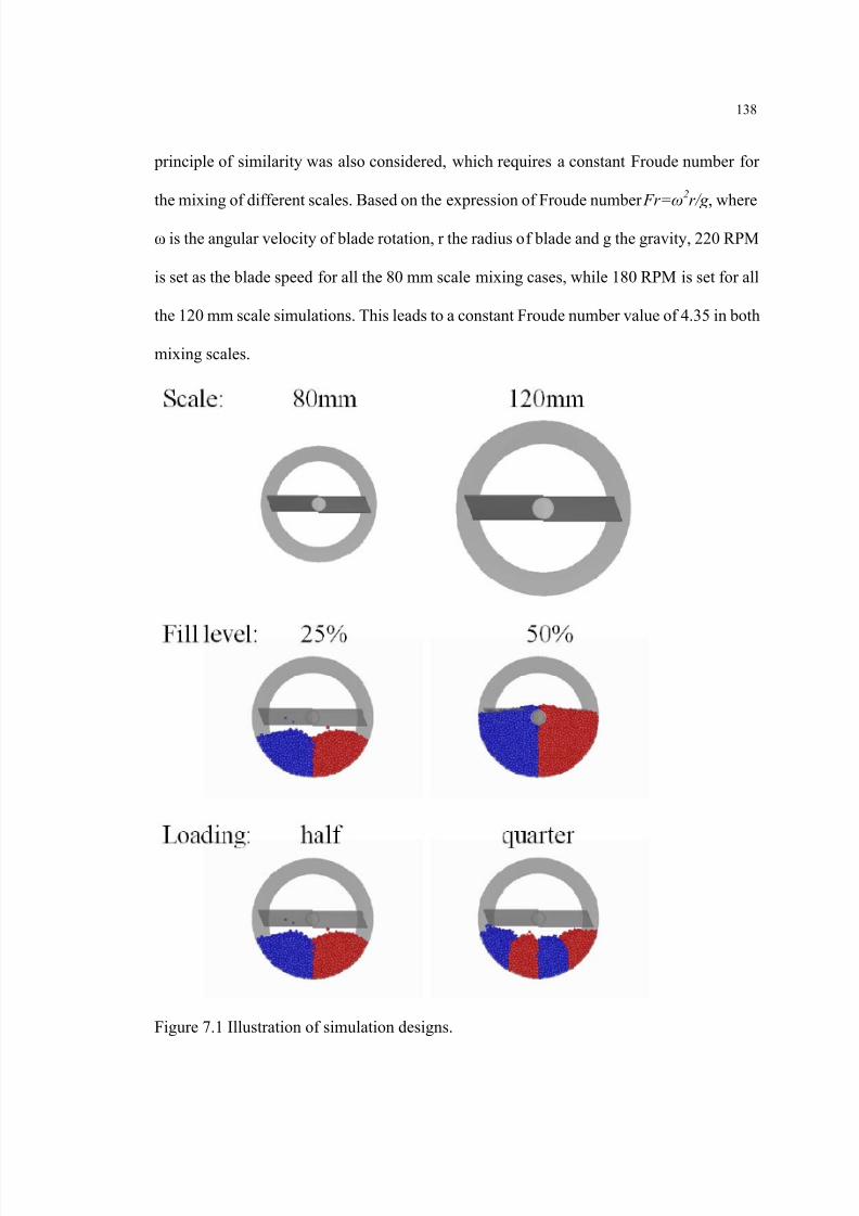
8/13/2019 Modeling and Analysis of Continuous Powder Blending
http://slidepdf.com/reader/full/modeling-and-analysis-of-continuous-powder-blending 151/177
138
principle of similarity was also considered, which requires a constant Froude number for
the mixing of different scales. Based on the expression of Froude number Fr= ω 2r/g , where
ω is the angular velocity of blade rotation, r the radius of blade and g the gravity, 220 RPM
is set as the blade speed for all the 80 mm scale mixing cases, while 180 RPM is set for all
the 120 mm scale simulations. This leads to a constant Froude number value of 4.35 in both
mixing scales.
Figure 7.1 Illustration of simulation designs.
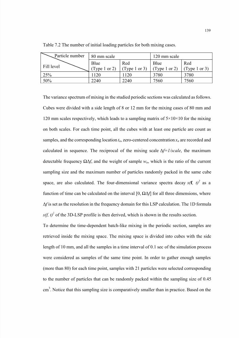
8/13/2019 Modeling and Analysis of Continuous Powder Blending
http://slidepdf.com/reader/full/modeling-and-analysis-of-continuous-powder-blending 152/177

8/13/2019 Modeling and Analysis of Continuous Powder Blending
http://slidepdf.com/reader/full/modeling-and-analysis-of-continuous-powder-blending 153/177
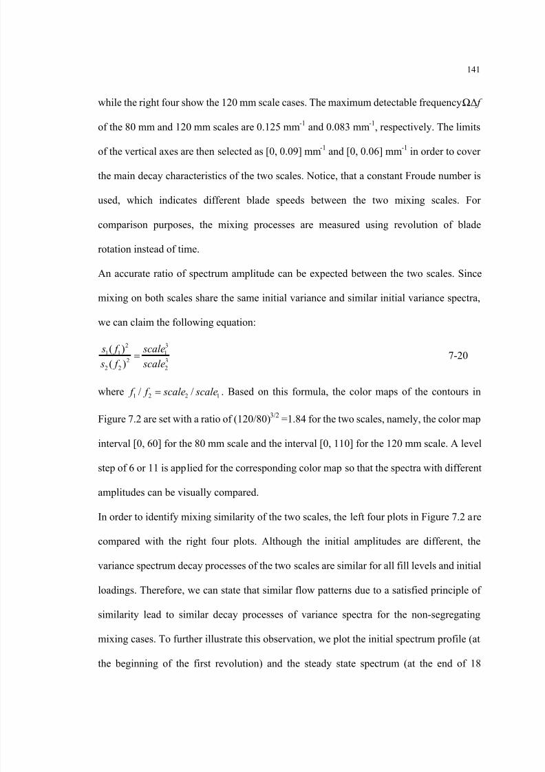
8/13/2019 Modeling and Analysis of Continuous Powder Blending
http://slidepdf.com/reader/full/modeling-and-analysis-of-continuous-powder-blending 154/177
141
while the right four show the 120 mm scale cases. The maximum detectable frequency ΩΔ f
of the 80 mm and 120 mm scales are 0.125 mm -1 and 0.083 mm -1, respectively. The limits
of the vertical axes are then selected as [0, 0.09] mm -1 and [0, 0.06] mm -1 in order to cover
the main decay characteristics of the two scales. Notice, that a constant Froude number is
used, which indicates different blade speeds between the two mixing scales. For
comparison purposes, the mixing processes are measured using revolution of blade
rotation instead of time.
An accurate ratio of spectrum amplitude can be expected between the two scales. Since
mixing on both scales share the same initial variance and similar initial variance spectra,
we can claim the following equation:
2 31 1 1
2 32 2 2
( )( )
s f scale s f scale
= 7-20
where 1 2 2 1/ / f f scale scale= . Based on this formula, the color maps of the contours in
Figure 7.2 are set with a ratio of (120/80) 3/2 =1.84 for the two scales, namely, the color map
interval [0, 60] for the 80 mm scale and the interval [0, 110] for the 120 mm scale. A level
step of 6 or 11 is applied for the corresponding color map so that the spectra with different
amplitudes can be visually compared.
In order to identify mixing similarity of the two scales, the left four plots in Figure 7.2 are
compared with the right four plots. Although the initial amplitudes are different, the
variance spectrum decay processes of the two scales are similar for all fill levels and initial
loadings. Therefore, we can state that similar flow patterns due to a satisfied principle of
similarity lead to similar decay processes of variance spectra for the non-segregating
mixing cases. To further illustrate this observation, we plot the initial spectrum profile (at
the beginning of the first revolution) and the steady state spectrum (at the end of 18
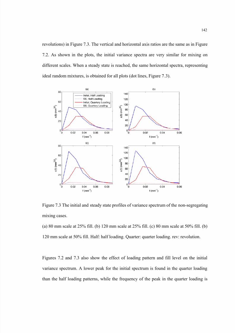
8/13/2019 Modeling and Analysis of Continuous Powder Blending
http://slidepdf.com/reader/full/modeling-and-analysis-of-continuous-powder-blending 155/177
142
revolutions) in Figure 7.3. The vertical and horizontal axis ratios are the same as in Figure
7.2. As shown in the plots, the initial variance spectra are very similar for mixing on
different scales. When a steady state is reached, the same horizontal spectra, representing
ideal random mixtures, is obtained for all plots (dot lines, Figure 7.3).
Figure 7.3 The initial and steady state profiles of variance spectrum of the non-segregating
mixing cases.
(a) 80 mm scale at 25% fill. (b) 120 mm scale at 25% fill. (c) 80 mm scale at 50% fill. (b)
120 mm scale at 50% fill. Half: half loading. Quarter: quarter loading. rev: revolution.
Figures 7.2 and 7.3 also show the effect of loading pattern and fill level on the initial
variance spectrum. A lower peak for the initial spectrum is found in the quarter loading
than the half loading patterns, while the frequency of the peak in the quarter loading is
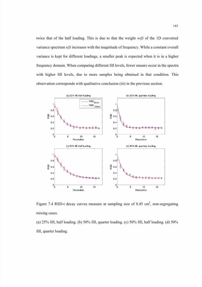
8/13/2019 Modeling and Analysis of Continuous Powder Blending
http://slidepdf.com/reader/full/modeling-and-analysis-of-continuous-powder-blending 156/177
143
twice that of the half loading. This is due to that the weight w(f) of the 1D converted
variance spectrum s(f) increases with the magnitude of frequency. While a constant overall
variance is kept for different loadings, a smaller peak is expected when it is in a higher
frequency domain. When comparing different fill levels, fewer smears occur in the spectra
with higher fill levels, due to more samples being obtained in that condition. This
observation corresponds with qualitative conclusion (iii) in the previous section.
Figure 7.4 RSD-t decay curves measure at sampling size of 0.45 cm 3, non-segregating
mixing cases.
(a) 25% fill, half loading. (b) 50% fill, quarter loading. (c) 50% fill, half loading. (d) 50%
fill, quarter loading.
8/13/2019 Modeling and Analysis of Continuous Powder Blending
http://slidepdf.com/reader/full/modeling-and-analysis-of-continuous-powder-blending 157/177
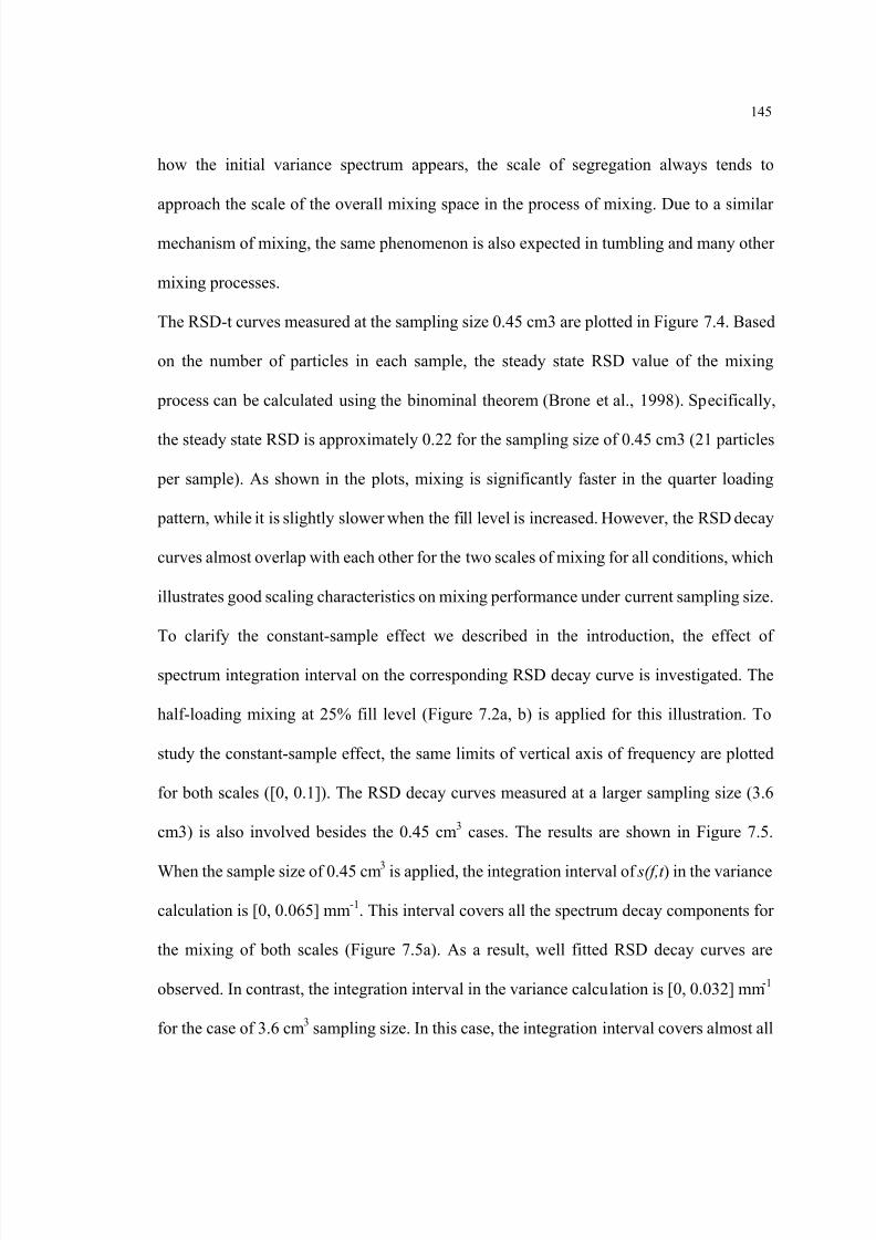
8/13/2019 Modeling and Analysis of Continuous Powder Blending
http://slidepdf.com/reader/full/modeling-and-analysis-of-continuous-powder-blending 158/177
145
how the initial variance spectrum appears, the scale of segregation always tends to
approach the scale of the overall mixing space in the process of mixing. Due to a similar
mechanism of mixing, the same phenomenon is also expected in tumbling and many other
mixing processes.
The RSD-t curves measured at the sampling size 0.45 cm3 are plotted in Figure 7.4. Based
on the number of particles in each sample, the steady state RSD value of the mixing
process can be calculated using the binominal theorem (Brone et al., 1998). Specifically,
the steady state RSD is approximately 0.22 for the sampling size of 0.45 cm3 (21 particles
per sample). As shown in the plots, mixing is significantly faster in the quarter loading
pattern, while it is slightly slower when the fill level is increased. However, the RSD decay
curves almost overlap with each other for the two scales of mixing for all conditions, which
illustrates good scaling characteristics on mixing performance under current sampling size.
To clarify the constant-sample effect we described in the introduction, the effect of
spectrum integration interval on the corresponding RSD decay curve is investigated. The
half-loading mixing at 25% fill level (Figure 7.2a, b) is applied for this illustration. To
study the constant-sample effect, the same limits of vertical axis of frequency are plotted
for both scales ([0, 0.1]). The RSD decay curves measured at a larger sampling size (3.6
cm3) is also involved besides the 0.45 cm 3 cases. The results are shown in Figure 7.5.
When the sample size of 0.45 cm 3 is applied, the integration interval of s(f,t ) in the variance
calculation is [0, 0.065] mm -1. This interval covers all the spectrum decay components for
the mixing of both scales (Figure 7.5a). As a result, well fitted RSD decay curves are
observed. In contrast, the integration interval in the variance calculation is [0, 0.032] mm -1
for the case of 3.6 cm 3 sampling size. In this case, the integration interval covers almost all

8/13/2019 Modeling and Analysis of Continuous Powder Blending
http://slidepdf.com/reader/full/modeling-and-analysis-of-continuous-powder-blending 159/177
146
the main decay components for the 120 mm scale mixing, while some components in
higher frequency domains are missed in the case of the 80 mm scale. This leads to different
fitted RSD decay curves (Figure 7.5b). Therefore, with the principle of similarity satisfied,
similar mixing performance can be achieved only when the sampling size is much smaller
than the scale of both mixing geometries.
Figure 7.6 Variance spectrum decay contours of cohesive segregating mixing cases.
The left four plots (a, c, e, g) show the 80 mm scale mixing cases. The right four plots (b, d,
f, h) show the 120 mm scale mixing cases. The same level step of color map is used for all
contours to show the spectrum profile of segregation when steady state is reached.
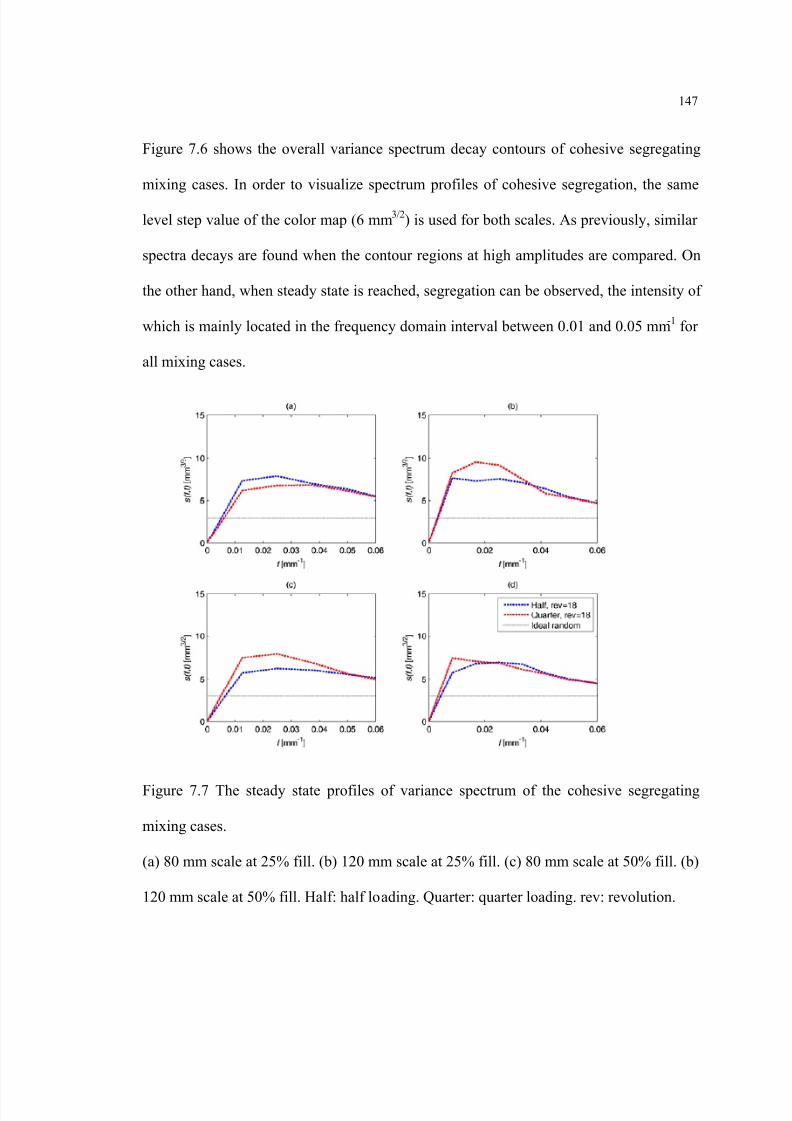
8/13/2019 Modeling and Analysis of Continuous Powder Blending
http://slidepdf.com/reader/full/modeling-and-analysis-of-continuous-powder-blending 160/177
147
Figure 7.6 shows the overall variance spectrum decay contours of cohesive segregating
mixing cases. In order to visualize spectrum profiles of cohesive segregation, the same
level step value of the color map (6 mm 3/2) is used for both scales. As previously, similar
spectra decays are found when the contour regions at high amplitudes are compared. On
the other hand, when steady state is reached, segregation can be observed, the intensity of
which is mainly located in the frequency domain interval between 0.01 and 0.05 mm -1 for
all mixing cases.
Figure 7.7 The steady state profiles of variance spectrum of the cohesive segregating
mixing cases.
(a) 80 mm scale at 25% fill. (b) 120 mm scale at 25% fill. (c) 80 mm scale at 50% fill. (b)
120 mm scale at 50% fill. Half: half loading. Quarter: quarter loading. rev: revolution.
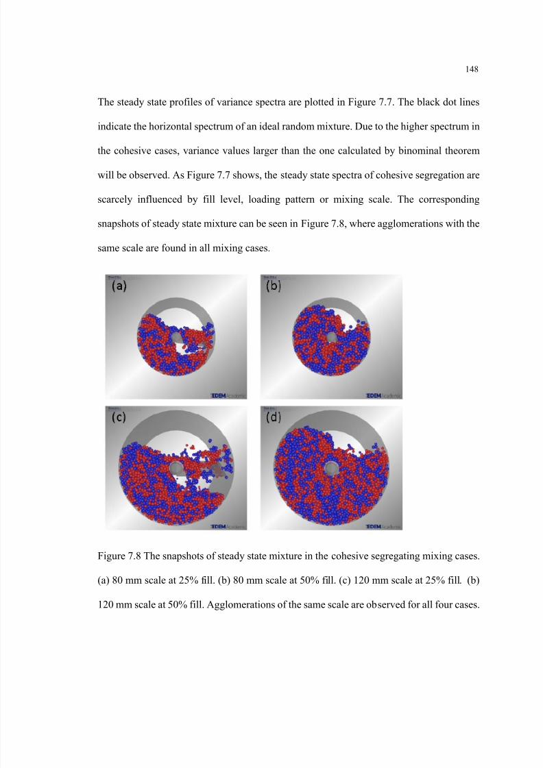
8/13/2019 Modeling and Analysis of Continuous Powder Blending
http://slidepdf.com/reader/full/modeling-and-analysis-of-continuous-powder-blending 161/177
148
The steady state profiles of variance spectra are plotted in Figure 7.7. The black dot lines
indicate the horizontal spectrum of an ideal random mixture. Due to the higher spectrum in
the cohesive cases, variance values larger than the one calculated by binominal theorem
will be observed. As Figure 7.7 shows, the steady state spectra of cohesive segregation are
scarcely influenced by fill level, loading pattern or mixing scale. The corresponding
snapshots of steady state mixture can be seen in Figure 7.8, where agglomerations with the
same scale are found in all mixing cases.
Figure 7.8 The snapshots of steady state mixture in the cohesive segregating mixing cases.
(a) 80 mm scale at 25% fill. (b) 80 mm scale at 50% fill. (c) 120 mm scale at 25% fill. (b)
120 mm scale at 50% fill. Agglomerations of the same scale are observed for all four cases.
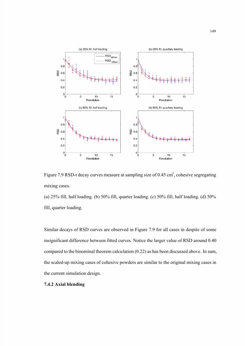
8/13/2019 Modeling and Analysis of Continuous Powder Blending
http://slidepdf.com/reader/full/modeling-and-analysis-of-continuous-powder-blending 162/177
149
Figure 7.9 RSD-t decay curves measure at sampling size of 0.45 cm 3, cohesive segregating
mixing cases.
(a) 25% fill, half loading. (b) 50% fill, quarter loading. (c) 50% fill, half loading. (d) 50%
fill, quarter loading.
Similar decays of RSD curves are observed in Figure 7.9 for all cases in despite of some
insignificant difference between fitted curves. Notice the larger value of RSD around 0.40
compared to the binominal theorem calculation (0.22) as has been discussed above. In sum,
the scaled-up mixing cases of cohesive powders are similar to the original mixing cases in
the current simulation design.
7.4.2 Axial blending

8/13/2019 Modeling and Analysis of Continuous Powder Blending
http://slidepdf.com/reader/full/modeling-and-analysis-of-continuous-powder-blending 163/177
150
The axial blending of the two cases is shown in Figures 7-10. The plots in this figure are
rescaled using the unit revolution instead of time for comparison purposes. Since the
residence time distribution does not depend on loading pattern, only the cases of half
loading are plotted. As illustrated, the RTD in non-segregating cases are similar for both
fill levels, indicating good scaling up characteristics of non-segregating particles on axial
mixing and motion. Larger RTDs of cohesive mixing is observed in the 80 mm scale
mixing, while RTDs in the 120 mm scale mixing cases are similar to those in the
non-segregating cases. Therefore, the effect of cohesion on the axial motion of particles is
significant only when the scale of mixing space is small, under which condition the
cohesive particles move much slower than the non-segregating particles. While the mean
residence time is slightly shorter at 25% fill in non-segregating mixing cases, particles stay
much longer in 80 mm scale mixing space in the cohesive cases, especially when the lower
fill level is used. It is worth to note that the axial velocity measured in 120 mm scale is
around 1.5 fold of that in the 80 mm scale due to the scale ratio of mixing space.
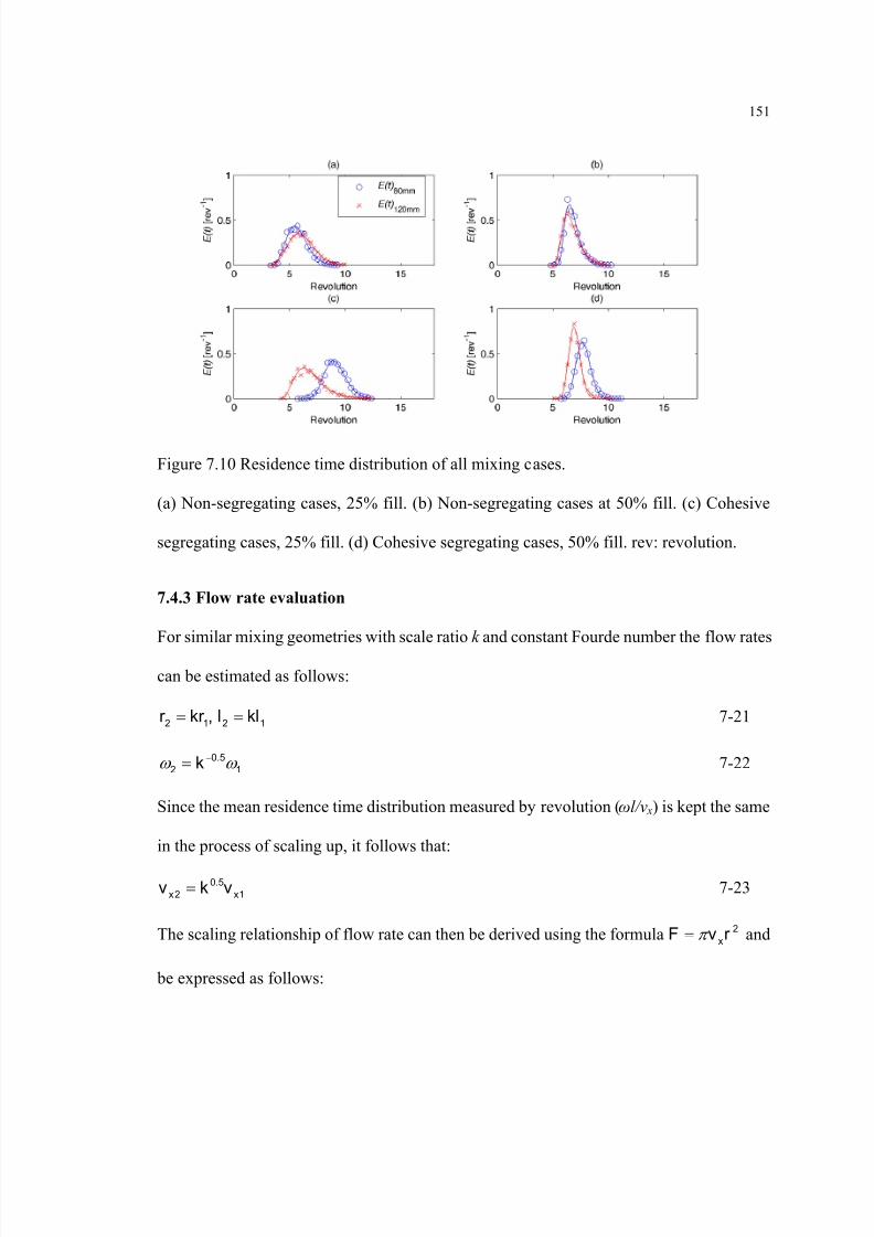
8/13/2019 Modeling and Analysis of Continuous Powder Blending
http://slidepdf.com/reader/full/modeling-and-analysis-of-continuous-powder-blending 164/177
151
Figure 7.10 Residence time distribution of all mixing cases.
(a) Non-segregating cases, 25% fill. (b) Non-segregating cases at 50% fill. (c) Cohesive
segregating cases, 25% fill. (d) Cohesive segregating cases, 50% fill. rev: revolution.
7.4.3 Flow rate evaluation
For similar mixing geometries with scale ratio k and constant Fourde number the flow rates
can be estimated as follows:
2 1 2 1,r kr l kl= = 7-21
0.52 1
kω ω −= 7-22
Since the mean residence time distribution measured by revolution ( ωl/v x) is kept the same
in the process of scaling up, it follows that:
0.52 1x x
v k v= 7-23
The scaling relationship of flow rate can then be derived using the formula 2x
F v r π = and
be expressed as follows:
8/13/2019 Modeling and Analysis of Continuous Powder Blending
http://slidepdf.com/reader/full/modeling-and-analysis-of-continuous-powder-blending 165/177
152
2.52 1
F k F= 7-24
Therefore, when a four-fold scaling up is applied on the mixing apparatus, the flow rate of
the larger continuous mixer is 32 fold of the original lab scale apparatus, which indicates a
tremendous increase in production rate for the continuous powder mixing system. This
shows the merit of using the model for continuous powder mixing on the scaling up
characteristics.
Similar analysis can be performed on the batch mixing systems, where the production rate
can be measured as 3b
F l k= where l 3 represent the batch volume and k b the mixing rate.
Since similar mixing rates, measured by the reciprocal of revolution ( /bk ω ), are achieved,
the scaling relationship of mixing rate is expressed as
0.52 1b b
k k k−= 7-25
As a result, a scaling up expression of production rate the same as equation (7-24) is
derived for the case of batch mixing, indicating the inherent coincidence of batch and
continuous mixing processes.
For the cohesive cases, equation (7-24) can be directly used for the scaling up of batch-like
powder mixing process, due to the scaling relationship observed in Section 7.4.1. However,
larger flow rate will be observed in the scaled-up continuous powder mixing process, due
to a relatively fast axial velocity in that case. This effect should be considered in the design
of scaling up strategy of cohesive mixing cases.
7.5 Summary
A new methodology based on the concept of variance spectrum has been developed for
studying the scale-up of powder mixing in continuous processes. The Lomb-Scargle

8/13/2019 Modeling and Analysis of Continuous Powder Blending
http://slidepdf.com/reader/full/modeling-and-analysis-of-continuous-powder-blending 166/177
153
Periodogram technique widely applied in astronomical studies has been used to estimate
the variance spectrum of unevenly distributed samples in powder mixing processes. The
periodic section modeling, proposed in our previous work (Gao et al., 2012), permits us to
consider the batch-like cross-sectional mixing and axial motion separately for the scale-up
of continuous powder mixing process. Such quantitative investigations are used to clarify
the effect of constant sampling size on mixing performance, and the effect of scaling up on
both cross-sectional and axial mixing within continuous mixing. For the non-segregating
mixing cases, similar scale-up characteristics are observed for both cross-sectional and
axial mixing in our simulation results. While a satisfying principle of similarity leads to
similar decay contours of variance spectra, a sampling size much smaller than the scales of
both apparatuses should be used to achieve similar mixing performance measurements.
When non-segregating materials are processed, a 2.5 fold increase in production rate is
obtainable for the scale-up of continuous powder mixing. However, in processes where
cohesive materials segregate due to a tendency to agglomerate, an even larger increase of
flow rate is expected. This results from the effect of cohesion on axial motion especially
when the scale of the mixing process is small. Our preliminary simulation results illustrate
that the proposed analysis can be used to achieve a successful scale-up strategy for
continuous powder mixing processes.
8/13/2019 Modeling and Analysis of Continuous Powder Blending
http://slidepdf.com/reader/full/modeling-and-analysis-of-continuous-powder-blending 167/177
154
Chapter 8
Conclusions and future Perspectives
8.1 Summary
In this dissertation, a novel predictive model is proposed first to provide strategies and
guidance on addressing design, scale-up, and improvement issues in continuous powder
blending process. The two main components of continuous blending are considered
separately. Fourier series is employed in clarifying the attenuation of feeding fluctuation in
the axial blending component. Feeding variance spectrum and blender filtering ability are
applied to describe the performance of the feeder blender integration, instead of the
fluctuation variance and the residence time distribution commonly used in conventional
investigations. An efficient estimation strategy is developed to improve the axial blending
when the integrated system is not in its optimal performance. By coupling the continuous
blending performance with the batch-like blending with a similar geometry, the periodic
section modeling is developed to capture the transitional status in the cross-sectional
blending component. The residence time distribution in the continuous blender is used to
predict the continuous blending performance from blending process in the periodic section.
For both segregating and non-segregating blending cases, designed simulations show
accurate predictions by using this model, and indicate that the mean residence time and the
batch-like blending rate in the periodic section are the key indices of the cross-sectional
blending component.
Due to recent development on powder feeding systems, variability on material flow was
significantly reduced in pharmaceutical manufacturing. The cross-sectional blending

8/13/2019 Modeling and Analysis of Continuous Powder Blending
http://slidepdf.com/reader/full/modeling-and-analysis-of-continuous-powder-blending 168/177
155
component is more significant affecting blending performance than the axial blending
component and is focused in this dissertation. In order to apply the knowledge of batch
blender in the design and improvement of continuous blender, performance similarity
between continuous and similar batch systems is investigated. We use Discrete Element
Method to investigate this issue. Mixing and flow of particles are examined in simple
geometries consisting of a cylindrical cross-section agitated by impellers. End walls and
symmetric blade pairs of the “alternate” blade patterns lead to faster mixing.
Non-symmetric elemental systems display both increased fill level uniformity and similar
mixing performance for both blade patterns. It demonstrates the need for caution when
attempting to use batch mixing information to estimate the cross-sectional mixing rate of
continuous powder mixers.
The effects of operation and geometry are examined on two key indices of continuous
blending: axial velocity and local mixing rate of the mixture. When the local mixing rate
improves at low fill level and high blade speed, particles also move faster in the axial
direction and reside for a shorter time inside the mixer. This trade-off between ascending
local mixing rate and descending residence time indicates a non-optimal overall blending
performance even when the best operating condition is applied. Strategies are performed to
further improve the blending performance, which are proposed by increasing the blade
speed while keeping a constant axial velocity. These strategies guarantee that the variance
decay rate along mixing axis is proportional to the blade speed in continuous blending
processes. Dramatic improvements are observed when these strategies are applied in both
simulations and experiments, which shows the merit of this work on design and
optimization of continuous powder blending process.

8/13/2019 Modeling and Analysis of Continuous Powder Blending
http://slidepdf.com/reader/full/modeling-and-analysis-of-continuous-powder-blending 169/177
8/13/2019 Modeling and Analysis of Continuous Powder Blending
http://slidepdf.com/reader/full/modeling-and-analysis-of-continuous-powder-blending 170/177
157
Reference
Abdi, H., 2010. Partial least squares regression and projection on latent structureregression (PLS Regression). Wiley Interdisciplinary Reviews: Computational Statistics 2,97-106.
Abouzeid, A.Z.M., Fuerstenau, D.W., Sastry, K.V., 1980. Transport behavior of particulate solids in rotary drums: scale-up of residence time distribution using the axialdispersion model. Powder Technology 27, 241-250.
Abouzeid, A.Z.M., Mika, T.S., Sastry, K.V., Fuerstenau, D.W., 1974. The influence ofoperating variables on the residence time distribution for material transport in a continuousrotary drum. Powder Technology 10, 273-288.
Alexander, A., Muzzio, F., 2005. Batch Size Increase in Dry Blending and Mixing,Pharmaceutical Process Scale-Up, Second Edition. Informa Healthcare, pp. 161-180.
Alexander, A., Shinbrot, T., Johnson, B., Muzzio, F.J., 2004. V-blender segregation patterns for free-flowing materials: effects of blender capacity and fill level. InternationalJournal of Pharmaceutics 269, 19-28.
Alexander, A., Shinbrot, T., Muzzio, F.J., 2002. Scaling surface velocities in rotatingcylinders as a function of vessel radius, rotation rate, and particle size. Powder Technology126, 174-190.
Arratia, P.E., Duong, N.-h., Muzzio, F.J., Godbole, P., Reynolds, S., 2006. A study of themixing and segregation mechanisms in the Bohle Tote blender via DEM simulations.Powder Technology 164, 50-57.
Averbuch, A., Shkolnisky, Y., 2003. 3D Fourier based discrete Radon transform. Appliedand Computational Harmonic Analysis 15, 33-69.
Babu, P., Stoica, P., 2010. Spectral analysis of nonuniformly sampled data - a review.Digital Signal Processing 20, 359-378.
Beaudry, J.P., 1948. Blender efficiency. Chemical Engineer 55, 112-113.
Bertrand, F., Leclaire, L.A., Levecque, G., 2005. DEM-based models for the mixing ofgranular materials. Chemical Engineering Science 60, 2517-2531.
Brone, D., Alexander, A., Muzzio, F.J., 1998. Quantitative characterization of mixing ofdry powders in V-blenders. AIChE Journal 44, 271-278.
Brone, D., Muzzio, F.J., 2000. Enhanced mixing in double-cone blenders. PowderTechnology 110, 179-189.

8/13/2019 Modeling and Analysis of Continuous Powder Blending
http://slidepdf.com/reader/full/modeling-and-analysis-of-continuous-powder-blending 171/177
158
Brone, D., Wightman, C., Connor, K., Alexander, A., Muzzio, F.J., Robinson, P., 1997.Using flow perturbations to enhance mixing of dry powders in V-blenders. PowderTechnology 91, 165-172.
Danckwerts, P.V., 1953. Continuous flow systems : Distribution of residence times.Chemical Engineering Science 2, 1-13.
Danckwerts, P.V., Sellers, S.M., 1951. The effect of hold up and mixing on a stream offluctuating composition. Industrial Chemist 27, 395.
Ding, Y.L., Forster, R.N., Seville, J.P.K., Parker, D.J., 2001. Scaling relationships forrotating drums. Chemical Engineering Science 56, 3737-3750.
Dittrich, C.J., Mutsers, S.M.P., 2007. On the residence time distribution in reactors with
non-uniform velocity profiles: The horizontal stirred bed reactor for polypropylene production. Chemical Engineering Science 62, 5777-5793.
Dubey, A., Sarkar, A., Ierapetritou, M., Wassgren, C.R., Muzzio, F.J., 2011.Computational Approaches for Studying the Granular Dynamics of Continuous BlendingProcesses, 1 – DEM Based Methods. Macromolecular Materials and Engineering 296,290-307.
Foster, G., 1995. The cleanest Fourier spectrum. ASTRONOMICAL JOURNAL 109,1889-1902.
Gao, Y., Ierapetritou, M., Muzzio, F., 2011a. Investigation on the effect of blade patternson continuous solid mixing performance. The Canadian Journal of Chemical Engineering89, 969-984.
Gao, Y., Ierapetritou, M., Muzzio, F., 2012. Periodic section modeling of convectivecontinuous powder mixing processes. AIChE Journal 58, 69-78.
Gao, Y., Muzzio, F., Ierapetritou, M., 2011b. Characterization of feeder effects oncontinuous solid mixing using fourier series analysis. AIChE Journal 57, 1144-1153.
Gao, Y., Vanarase, A., Muzzio, F., Ierapetritou, M., 2011c. Characterizing continuous powder mixing using residence time distribution. Chemical Engineering Science 66,
417-425.
Geng, F., Yuan, Z., Yan, Y., Luo, D., Wang, H., Li, B., Xu, D., 2009. Numerical simulationon mixing kinetics of slender particles in a rotary dryer. Powder Technology 193, 50-58.
Gilliland, R.L., Baliunas, S.L., 1987. Objective characterization of stellar activity cycles: I.Methods and solar cycle analyses, Astrophysical Journal, pp. 766-781.
Goldsmith, P.L., 1966. The Theoretical Performance of a Semi-Continuous BlendingSystem. The Statistician 16, 227-251.
8/13/2019 Modeling and Analysis of Continuous Powder Blending
http://slidepdf.com/reader/full/modeling-and-analysis-of-continuous-powder-blending 172/177
159
Harris, A.T., Davidson, J.F., Thorpe, R.B., 2002a. A novel method for measuring theresidence time distribution in short time scale particulate systems. Chemical EngineeringJournal 89, 127-142.
Harris, A.T., Davidson, J.F., Thorpe, R.B., 2003a. The influence of the riser exit on the particle residence time distribution in a circulating fluidised bed riser. ChemicalEngineering Science 58, 3669-3680.
Harris, A.T., Davidson, J.F., Thorpe, R.B., 2003b. Particle residence time distributions incirculating fluidised beds. Chemical Engineering Science 58, 2181-2202.
Harris, A.T., Thorpe, R.B., Davidson, J.F., 2002b. Stochastic modelling of the particleresidence time distribution in circulating fluidised bed risers. Chemical EngineeringScience 57, 4779-4796.
Harvey, A.D., Lee, C.K., Rogers, S.E., 1995. Steady-state modeling and experimentalmeasurement of a baffled impeller stirred tank. AIChE Journal 41, 2177-2186.
Harwood, C.F., Walanski, K., Luebcke, E., Swanstrom, C., 1975. The performance ofcontinuous mixers for dry powders. Powder Technology 11, 289-296.
Hobbs, D.M., Swanson, P.D., Muzzio, F.J., 1998. Numerical characterization of lowReynolds number flow in the Kenics static mixer. Chemical Engineering Science 53,1565-1584.
Hocke, K., Kämpfer, N., 2009. Gap filling and noise reduction of unevenly sampled data by means of the Lomb-Scargle periodogram. Atmospheric Chemistry and Physics 9,4197-4206.
Horio, M., Nonaka, A., Sawa, Y., Muchi, I., 1986. A new similarity rule for fluidized bedscale-up. AIChE Journal 32, 1466-1482.
Ingram, A., Seville, J.P.K., Parker, D.J., Fan, X., Forster, R.G., 2005. Axial and radialdispersion in rolling mode rotating drums. Powder Technology 158, 76-91.
Johnson, P.C., Jackson, R., 1987. Frictional–collisional constitutive relations for granularmaterials, with application to plane shearing. Journal of Fluid Mechanics 176, 67-93.
Johnstone, R.W., Thring, M.W., 1957. Pilot plants, models and scale-up methods inchemical engineering. MacGraw-Hill, New York.
Jones, J.R., Parker, D.J., Bridgwater, J., 2007. Axial mixing in a ploughshare mixer.Powder Technology 178, 73-86.
Larochette, M., Graebling, D., Nasri, D., Léonardi, F.d.r., 2009. Optimization of thePolymer Foam Process by the Residence Time Distribution Approach. Industrial &Engineering Chemistry Research 48, 4884-4891.
8/13/2019 Modeling and Analysis of Continuous Powder Blending
http://slidepdf.com/reader/full/modeling-and-analysis-of-continuous-powder-blending 173/177
160
Laurent, B.F.C., Bridgwater, J., 2002. Influence of agitator design on powder flow.Chemical Engineering Science 57, 3781-3793.
Levenspiel, O., Smith, W.K., 1957. Notes on the diffusion-type model for the longitudinalmixing of fluids in flow. Chemical Engineering Science 6, 227-235.
Lomb, N.R., 1976. Least-squares frequency analysis of unequally spaced data.Astrophysics and Space Science 39, 447-462.
Lopes, V.V., Menezes, J.C., 2005. Inferential sensor design in the presence of missing data:a case study. Chemometrics and Intelligent Laboratory Systems 78, 1-10.
Manas-Zloczower, I., 1994. Studies of mixing efficiency in batch and continuous mixers.Rubber chemistry and technology 67, 504-528.
Marikh, K., Berthiaux, H., Gatumel, C., Mizonov, V., Barantseva, E., 2008. Influence ofstirrer type on mixture homogeneity in continuous powder mixing: A model case and a
pharmaceutical case. Chemical Engineering Research and Design 86, 1027-1037.
Marikh, K., Berthiaux, H., Mizonov, V., Barantseva, E., 2005. Experimental study of thestirring conditions taking place in a pilot plant continuous mixer of particulate solids.Powder Technology 157, 138-143.
Marikh, K., Berthiaux, H., Mizonov, V., Barantseva, E., Ponomarev, D., 2006. FlowAnalysis and Markov Chain Modelling to Quantify the Agitation Effect in a ContinuousPowder Mixer. Chemical Engineering Research and Design 84, 1059-1074.
Markström, P., Berguerand, N., Lyngfelt, A., 2010. The application of a multistage-bedmodel for residence-time analysis in chemical-looping combustion of solid fuel. ChemicalEngineering Science 65, 5055-5066.
Martínez-Delgadillo, S.A., Mollinedo-Ponce, H., Mendoza-Escamilla, V., Barrera-Díaz,C., 2010. Residence time distribution and back-mixing in a tubular electrochemical reactoroperated with different inlet flow velocities, to remove Cr(VI) from wastewater. ChemicalEngineering Journal 165, 776-783.
McTait, G.E., Scott, D.M., Davidson, J.F., 1998. Residence time distribution of particles in
rotary kilns, in: Fan, L.-S., Knowlton, T.M. (Eds.), Fluidization, Durango, Colorado, pp.397-404.
Meijer, H.E.H., Elemans, P.H.M., 1988. The modeling of continuous mixers. Part I: Thecorotating twin-screw extruder, pp. 275-290.
Mindlin, R.D., 1949. Compliance of elastic bodies in contact. Journal of AppliedMechanics 71, 259-268.
8/13/2019 Modeling and Analysis of Continuous Powder Blending
http://slidepdf.com/reader/full/modeling-and-analysis-of-continuous-powder-blending 174/177
161
Moakher, M., Shinbrot, T., Muzzio, F.J., 2000. Experimentally validated computations offlow, mixing and segregation of non-cohesive grains in 3D tumbling blenders. PowderTechnology 109, 58-71.
Nauman, E.B., 2008. Residence Time Theory. Industrial & Engineering ChemistryResearch 47, 3752-3766.
Pernenkil, L., Cooney, C.L., 2006. A review on the continuous blending of powders.Chemical Engineering Science 61, 720-742.
Portillo, P., Muzzio, F., Ierapetritou, M., 2008a. Using Compartment Modeling toInvestigate Mixing Behavior of a Continuous Mixer. Journal of Pharmaceutical Innovation3, 161-174.
Portillo, P., Muzzio, F.J., Ierapetritou, M.G., 2007. Hybrid DEM-compartment modelingapproach for granular mixing. AIChE Journal 53, 119-128.
Portillo, P.M., Ierapetritou, M.G., Muzzio, F.J., 2008b. Characterization of continuousconvective powder mixing processes. Powder Technology 182, 368-378.
Portillo, P.M., Ierapetritou, M.G., Muzzio, F.J., 2009. Effects of rotation rate, mixing angle,and cohesion in two continuous powder mixers—A statistical approach. PowderTechnology 194, 217-227.
Portillo, P.M., Muzzio, F.J., Ierapetritou, M.G., Pantelides, W.M.a.C., 2006. Modeling anddesigning powder mixing processes utilizing compartment modeling, Computer AidedChemical Engineering. Elsevier, pp. 1039-1044.
Portillo, P.M., Vanarase, A.U., Ingram, A., Seville, J.K., Ierapetritou, M.G., Muzzio, F.J.,2010. Investigation of the effect of impeller rotation rate, powder flow rate, and cohesionon powder flow behavior in a continuous blender using PEPT. Chemical EngineeringScience 65, 5658-5668.
Poux, M., Fayolle, P., Bertrand, J., Bridoux, D., Bousquet, J., 1991. Powder mixing: Some practical rules applied to agitated systems. Powder Technology 68, 213-234.
Ralf Weineköter, L.R., 1995. Continuous Mixing of Fine Particles. Particle and Particle
Systems Characterization 12, 46-53.
Reiss, R., Wojsznis, W., Wojewodka, R., 2010. Partial least squares confidence intervalcalculation for industrial end-of-batch quality prediction. Chemometrics and IntelligentLaboratory Systems 100, 75-82.
Risken, H., 1996. The Fokker-Planck Equation: Methods of Solution and Applications, 2ed. Springer.
Roberts, D.H.L., J.; Dreher, J. W., 1987. Time Series Analysis with Clean - Part One -Derivation of a Spectrum. ASTRONOMICAL JOURNAL 93, 968 -989.
8/13/2019 Modeling and Analysis of Continuous Powder Blending
http://slidepdf.com/reader/full/modeling-and-analysis-of-continuous-powder-blending 175/177
162
Sarkar, A., Wassgren, C., 2010. Continuous blending of cohesive granular material.Chemical Engineering Science 65, 5687-5698.
Sarkar, A., Wassgren, C.R., 2009. Simulation of a continuous granular mixer: Effect ofoperating conditions on flow and mixing. Chemical Engineering Science 64, 2672-2682.
Savage, S.B., Hutter, K., 1989. The motion of a finite mass of granular material down arough incline. Journal of Fluid Mechanics 199, 177-215.
Scargle, J.D., 1982. Studies in astronomical time series analysis. II - Statistical aspects ofspectral analysis of unevenly spaced data. Astrophysical Journal 263, 835 -853.
Sherritt, R.G., Chaouki, J., Mehrotra, A.K., Behie, L.A., 2003. Axial dispersion in thethree-dimensional mixing of particles in a rotating drum reactor. Chemical Engineering
Science 58, 401-415.Shin, S.H., Fan, L.T., 1978. Characterization of solids mixtures by the discrete fouriertransform. Powder Technology 19, 137-146.
Stoica, P., Jian, L., Hao, H., 2009. Spectral Analysis of Nonuniformly Sampled Data: A New Approach Versus the Periodogram. Signal Processing, IEEE Transactions on 57,843-858.
Sudah, O.S., Chester, A.W., Kowalski, J.A., Beeckman, J.W., Muzzio, F.J., 2002a.Quantitative characterization of mixing processes in rotary calciners. Powder Technology126, 166-173.
Sudah, O.S., Coffin-Beach, D., Muzzio, F.J., 2002b. Effects of blender rotational speedand discharge on the homogeneity of cohesive and free-flowing mixtures. InternationalJournal of Pharmaceutics 247, 57-68.
Sudah, O.S., Coffin-Beach, D., Muzzio, F.J., 2002c. Quantitative characterization ofmixing of free-flowing granular material in tote (bin)-blenders. Powder Technology 126,191-200.
Vanarase, A.U., Alcalà, M., Jerez Rozo, J.I., Muzzio, F.J., Romañach, R.J., 2010.Real-time monitoring of drug concentration in a continuous powder mixing process using
NIR spectroscopy. Chemical Engineering Science 65, 5728-5733.
Vanarase, A.U., Muzzio, F.J., 2011. Effect of operating conditions and design parametersin a continuous powder mixer. Powder Technology 208, 26-36.
Wang, R.H., Fan, L.T., 1974. Methods for scaling-up tumbling. Chemical Engineering 81,88-94.
Weineköter, R., Reh, L., 1995. Continuous Mixing of Fine Particles. Particle and ParticleSystems Characterization 12, 46-53.

8/13/2019 Modeling and Analysis of Continuous Powder Blending
http://slidepdf.com/reader/full/modeling-and-analysis-of-continuous-powder-blending 176/177
163
Wightman, C., Moakher, M., Muzzio, F.J., Walton, O., 1998. Simulation of flow andmixing of particles in a rotating and rocking cylinder. AIChE Journal 44, 1266-1276.
Wightman, C., Muzzio, F.J., 1998. Mixing of granular material in a drum mixerundergoing rotational and rocking motions I. Uniform particles. Powder Technology 98,113-124.
Williams, J.C., 1976. Continuous mixing of solids. A review. Powder Technology 15,237-243.
Williams, J.C., Rahman, M.A., 1972a. Prediction of the performance of continuous mixersfor particulate solids using residence time distributions : Part II. Experimental. PowderTechnology 5, 307-316.
Williams, J.C., Rahman, M.A., 1972b. Prediction of the performance of continuous mixersfor particulate solids using residence time distributions Part I. Theoretical. PowderTechnology 5, 87-92.
Williams, J.C., Richardson, R., 1982. The continuous mixing of segregating particles.Powder Technology 33, 5-16.
Wold, S., Sjöström, M., Eriksson, L., 2001. PLS-regression: a basic tool of chemometrics.Chemometrics and Intelligent Laboratory Systems 58, 109-130.
Yeh, A.-I., Jaw, Y.-M., 1998. Modeling residence time distributions for single screwextrusion process. Journal of Food Engineering 35, 211-232.
Zalc, J.M., Szalai, E.S., Muzzio, F.J., Jaffer, S., 2002. Characterization of flow and mixingin an SMX static mixer. AIChE Journal 48, 427-436.
Zechmeister, M., Kürster, M., 2009. The generalised Lomb-Scargle periodogram, pp.577-584.
Zhang, C.-L., Feng, L.-F., Hoppe, S., Hu, G.-H., 2009. Residence time distribution: An oldconcept in chemical engineering and a new application in polymer processing. AIChEJournal 55, 279-283.
Zhou, Y.C., Yu, A.B., Stewart, R.L., Bridgwater, J., 2004. Microdynamic analysis of the particle flow in a cylindrical bladed mixer. Chemical Engineering Science 59, 1343-1364.
Ziegler, G.R., Aguilar, C.A., 2003. Residence time distribution in a co-rotating, twin-screwcontinuous mixer by the step change method. Journal of Food Engineering 59, 161-167.
8/13/2019 Modeling and Analysis of Continuous Powder Blending
http://slidepdf.com/reader/full/modeling-and-analysis-of-continuous-powder-blending 177/177
164
CURRICULUM VITA
YIJIE GAOChemical and Biochemical Engineering Department98 Brett Road, Piscataway, NJ 08854
Rutgers, The State University of New JerseyEmail: [email protected]
Education
2012 PhD Rutgers, The State University of New Jersey, Piscataway, NJ2007 BS Tsinghua University, Beijing, China
Peer-reviewed Journal Publications1. Gao, Y. , Ierapetritou, M., Muzzio, F., 2012. Periodic section modeling of convective
continuous powder mixing processes. AIChE Journal 58, 69-78.
2. Gao, Y. , Muzzio, F., Ierapetritou, M., 2011. Characterization of feeder effects oncontinuous solid mixing using fourier series analysis. AIChE Journal 57, 1144-1153.