modeling and analysis of reservoir response to stimulation...

MODELING AND ANALYSIS OF RESERVOIR RESPONSE TO

STIMULATION BY WATER INJECTION

A Thesis

by

JUN GE

Submitted to the Office of Graduate Studies of Texas A&M University

in partial fulfillment of the requirements for the degree of

MASTER OF SCIENCE

December 2009

Major Subject: Petroleum Engineering

MODELING AND ANALYSIS OF RESERVOIR RESPONSE TO

STIMULATION BY WATER INJECTION

A Thesis

by

JUN GE

Submitted to the Office of Graduate Studies of Texas A&M University

in partial fulfillment of the requirements for the degree of

MASTER OF SCIENCE

Approved by: Chair of Committee, Ahmad Ghassemi Committee Members, Stephen A. Holditch Benchun Duan Head of Department, Stephen A. Holditch

December 2009

Major Subject: Petroleum Engineering

iii

ABSTRACT

Modeling and Analysis of Reservoir Response to Stimulation by Water Injection.

(December 2009)

Jun Ge, B.S., China University of Geosciences;

M.S., Peking University

Chair of Advisory Committee: Dr. Ahmad Ghassemi

The distributions of pore pressure and stresses around a fracture are of interest in

conventional hydraulic fracturing operations, fracturing during water-flooding of

petroleum reservoirs, shale gas, and injection/extraction operations in a geothermal

reservoir. During the operations, the pore pressure will increase with fluid injection into

the fracture and leak off to surround the formation. The pore pressure increase will

induce the stress variations around the fracture surface. This can cause the slip of

weakness planes in the formation and cause the variation of the permeability in the

reservoir. Therefore, the investigation on the pore pressure and stress variations around a

hydraulic fracture in petroleum and geothermal reservoirs has practical applications.

The stress and pore pressure fields around a fracture are affected by: poroelastic,

thermoelastic phenomena as well as by fracture opening under the combined action of

applied pressure and in-situ stress.

In our study, we built up two models. One is a model (WFPSD model) of water-

flood induced fracturing from a single well in an infinite reservoir. WFPSD model

calculates the length of a water flood fracture and the extent of the cooled and flooded

iv

zones. The second model (FracJStim model) calculates the stress and pore pressure

distribution around a fracture of a given length under the action of applied internal

pressure and in-situ stresses as well as their variation due to cooling and pore pressure

changes. In our FracJStim model, the Structural Permeability Diagram is used to

estimate the required additional pore pressure to reactivate the joints in the rock

formations of the reservoir. By estimating the failed reservoir volume and comparing

with the actual stimulated reservoir volume, the enhanced reservoir permeability in the

stimulated zone can be estimated.

In our research, the traditional two dimensional hydraulic fracturing propagation

models are reviewed, the propagation and recession of a poroelastic PKN hydraulic

fracturing model are studied, and the pore pressure and stress distributions around a

hydraulically induced fracture are calculated and plotted at a specific time. The pore

pressure and stress distributions are used to estimate the failure potentials of the joints in

rock formations around the hydraulic fracture. The joint slips and rock failure result in

permeability change which can be calculated under certain conditions. As a case study

and verification step, the failure of rock mass around a hydraulic fracture for the

stimulation of Barnett Shale is considered.

With the simulations using our models, the pore pressure and poro-induced

stresses around a hydraulic fracture are elliptically distributed near the fracture. From the

case study on Barnett Shale, the required additional pore pressure is about 0.06 psi/ft.

With the given treatment pressure, the enhanced permeability after the stimulation of

hydraulic fracture is calculated and plotted. And the results can be verified by previous

work by Palmer, Moschovidis and Cameron in 2007.

v

DEDICATION

To my Family

vi

ACKNOWLEDGEMENTS

I would like to express my deep and sincere gratitude to my advisor, Dr. Ahmad

Ghassemi, for his support, guidance, encouragement and patience throughout the

completion of this research project. Dr. Ghassemi introduced me to the field of

Petroleum Rock Mechanics and provided me with the opportunity to learn and to do

research on the hydraulic fracture. I specially thank him for his patience and careful

review of this thesis. I would also like to thank Dr. Stephen A. Holditch and Dr.

Benchun Duan for kindly serving as committee members and reviewing this thesis.

I would like to thank my wife, Yu Zhong, for her support throughout the course

of my study. Thanks also go to my friends and colleagues in the finishing of my thesis

and the department faculty and staff for making my time at Texas A&M University a

great experience. I would especially like to thank my friends and colleagues including

Qingfeng Tao, Chakra Rawal, Jian Huang, Wenxu Xue, Dr. Zhengnan Zhang and Dr.

Xiaoxian Zhou. I really appreciate their help on my study.

Great appreciation goes to the Crisman Institute for support of this research. I

also want to extend my gratitude to Texas A&M University, DOE, for providing me

with financial assistance.

I thank God for empowering and guiding me throughout the completion of the

degree.

vii

TABLE OF CONTENTS

Page

1 INTRODUCTION ...................................................................................................... 1

1.1 Hydraulic Fracturing .......................................................................................... 1 1.2 Fracture Mechanics ............................................................................................ 3 1.3 Fracture Propagation Models ............................................................................. 5 1.4 Poroelasticity ..................................................................................................... 9 1.5 Problems Associated with Rock Mechanics .................................................... 10 1.6 Literature Review ............................................................................................ 12 1.7 Research Objectives ......................................................................................... 15 1.8 Sign Convention .............................................................................................. 15

2 POROELASTICITY AND THERMOELASTICITY .............................................. 16

2.1 Introduction ...................................................................................................... 16 2.2 Poroelastic Effects on Hydraulic Fracture ....................................................... 18 2.3 Results of Poroelastic PKN Model .................................................................. 19 2.4 Conclusions and Discussions ........................................................................... 23

3 PORE PRESSURE DISTRIBUTION AROUND HYDRAULIC FRACTURE ...... 24

3.1 Pore Pressure Geometry around a Fracture ..................................................... 26 3.2 Pore Pressure Distributions .............................................................................. 27 3.3 Case Study ....................................................................................................... 30 3.4 Conclusions ...................................................................................................... 35

4 STRESSES DISTRIBUTIONS AROUND HYDRAULIC FRACTURE ................ 36

4.1 Expressions for Stresses ................................................................................... 37 4.2 Poroelastic Stresses .......................................................................................... 39 4.3 Thermoelastic Stresses ..................................................................................... 43 4.4 Induced Stresses by Fracture Compression ..................................................... 45 4.5 Case Study ....................................................................................................... 49 4.6 Conclusions ...................................................................................................... 56

5 FAILURE POTENTIALS OF JOINTS AROUND HYDRAULIC FRACTURE ... 57

5.1 Structural Permeability Diagram ..................................................................... 58 5.2 Failure Potentials ............................................................................................. 65 5.3 Case Study for Barnett Shale ........................................................................... 69

viii

Page

5.4 Conclusions ...................................................................................................... 81 6 SUMMARY, CONCLUSIONS AND DISCUSSION ............................................ 83

6.1 Summary .......................................................................................................... 83 6.2 Conclusions ...................................................................................................... 84 6.3 Recommendations ............................................................................................ 85

NOMENCLATURE ........................................................................................................ 86

REFERENCES ................................................................................................................ 89

APPENDIX A .................................................................................................................. 95

APPENDIX B .................................................................................................................. 99

APPENDIX C ................................................................................................................ 110

APPENDIX D ................................................................................................................ 126

VITA .............................................................................................................................. 130

ix

LIST OF FIGURES

Page

Fig. 1.1 Hydraulic Fracturing Process .............................................................................. 3

Fig. 1.2 Geometry of Fracture Network (Modified from Warpinski and Teufel,1987) ..................................................................................................... 4

Fig. 1.3 Geometry of PKN Model. ................................................................................... 6

Fig. 1.4 Geometry of KGD Model. ................................................................................... 7

Fig. 1.5 Geometry of Penny-Shape or Radial Models...................................................... 8

Fig. 1.6 Mechanics of Poroelasicity. ............................................................................... 10

Fig. 1.7 Evolution of Flow System ................................................................................. 12

Fig. 2.1 Poroelastic Evolution Function ......................................................................... 20

Fig. 2.2 Variation of Fracture Pressure with Time ......................................................... 21

Fig. 2.3 Variation of Fracture Length with Time ........................................................... 21

Fig. 2.4 Variation of Fracture Maximum Width with Time. .......................................... 22

Fig. 3.1 Plan View of Two-winged Hydraulic Fracture ................................................. 28

Fig. 3.2 Pore Pressure Distribution around the Fracture................................................. 32

Fig. 3.3 Fracture Length and Major and Minor Axis of Cooled and Flooded zones as a Function of Time ............................................................................ 33

Fig. 3.4 Pore Pressure Distribution around Fracture in Barnett Shale (t=9 hours). .............................................................................................................. 34

Fig. 4.1 Stresses in Elliptical Coordinates System ......................................................... 39

Fig. 4.2 Temperature Distribution Surrounded the Fracture. ......................................... 45

Fig. 4.3 Stresses Variations due to Fracture Compression ............................................. 46

Fig. 4.4 Poro-Induced Stresses Distribution X Axis Direction....................................... 50

Fig. 4.5 Poro-Induced Stresses Distribution Y Axis Direction....................................... 51

x

Page

Fig. 4.6 Thermo-Induced Stresses Distribution X Axis Direction ................................. 51

Fig. 4.7 Thermo-Induced Stress Distribution Y Axis Direction. .................................... 52

Fig. 4.8 Induced Stresses Distribution by Fracture Compression in X Direction .......................................................................................................... 53

Fig. 4.9 Induced Stresses Distribution by Fracture Compression in Y Direction. ......................................................................................................... 54

Fig. 4.10 Induced Shear Stresses Distribution by Fracture Compression ........................ 54

Fig. 4.11 Effective Stresses Distribution around the Fracture (σ′x). ................................. 55

Fig. 4.12 Effective Stresses Distribution around the Fracture (σ′y) ................................. 55

Fig. 5.1 Structural Permeability Diagram for Cooper Basin (Nelson et al., 2007) ................................................................................................................ 60

Fig. 5.2 Structural Permeability Diagram for Cooper Basin (Our Program) .................. 60

Fig. 5.3 Structural Permeability Diagram for Otway Basin (Mildren et al., 2005) ................................................................................................................ 62

Fig. 5.4 Structural Permeability Diagram for Otway Basin (Our Program) ................... 62

Fig. 5.5 Structural Permeability Diagram for New Albany Shale (µ=0.6) ..................... 63



Fig. 5.8 Structural Permeability Diagram Showing the Orientations of Rock Joints That May be Reactivated during Fracture Stimulation Treatments at Treating Pressures in Barnett Shale .......................................... 65

Fig. 5.9 Joint Strikes in the Formation............................................................................ 68

Fig. 5.10 The Critical Pore Pressure for Joints. ............................................................... 69

Fig. 5.11 Critical Pore Pressure for Various Joints Orientations and Friction Angles .............................................................................................................. 71

Fig. 5.12 In Situ Stresses Profile away from the Central Fracture Face at Shut-in for the Case of Pnet=900 psi and K=1md. ................................................... 72

xi

Page

Fig. 5.13 In Situ Stresses Profile away from the Central Fracture Face at Shut-in for the Case of Pnet=902 psi and K=0.99md (Palmer et al., 2007). ............ 73

Fig. 5.14 Pore Pressure Distribution around the Fracture (for Barnett Shale) ................. 74

Fig. 5.15 Stress Distribution around the Fracture in X-Direction ................................... 75

Fig. 5.16 Stress Distribution around the Fracture in Y-Direction. .................................. 75

Fig. 5.17 Failure Potentials for One Set of Joints around Hydraulic Fracture (K=1md, Pnet=900 psi). ................................................................................... 76

Fig. 5.18 Trendlines for Failed Reservoir Volume (FRV=SRV) vs Net Fracture Pressure (Palmer et al., 2007). ......................................................................... 77

Fig. 5.19 Estimation Method for Failed Reservoir Volume (for Vertical Well). ............ 78

Fig. 5.20 Estimation Method for Failed Reservoir Volume (for Horizontal Well). ............................................................................................................... 79

Fig. 5.21 Estimated Failed Distance Normal to the Fracture Surface. ............................ 79

Fig. 5.22 Calculated Enhanced Permeability for Barnett Shale. ..................................... 80

Fig. 5.23 Enhanced Permeability During Injection to Match FRV for Lower Barnett Shale Fracture Treatments (Palmer et al., 2007). ............................... 80

Fig. 5.24 Failure Distance Normal to Centeral Fracture Face to Match FRV for Lower Barnett Shale Fracture Treatments (Palmer et al., 2007). .................... 81

xii

LIST OF TABLES

Page

Table 1.1 ....................Comparison between Traditional 2D Hydraulic Fracture Models 8

Table 2.1 ..........Input Parameters for Poroleastic PKN Model (Detournay et al., 1990) 19

Table 3.1 ........................Input Parameters for Simulations (Perkin & Gonzalez, 1985) 31

Table 3.2 ................................Input Parameters for Barnett Shale (Palmer et al. 2007) . 34

Table 4.1 ......Input Parameters for Simulations (Case from Perkin & Gonzalez, 1985) 48

Table 5.1 ..................................................................Parameters Used for Cooper Basin 61

Table 5.2 .................................................Otway Basin Data from Mildren et al. (2005) 61

1

1 INTRODUCTION

1.1 Hydraulic Fracturing

Hydraulic fracturing is a widely used stimulation technique to initiate a high

permeability conduit of gas in a low permeability reservoir. During the hydraulic

fracturing operation, a fluid is injected into a well at a pressure high enough to fracture

the formation. The process also can cause opening up of natural fractures already present

in the formation.

For the past 50 years, the technique of hydraulic fracturing has been widely used

in energy industry. One of the most important applications of this technique is the

stimulation of hydrocarbon wells for increasing oil and gas recovery (e.g., Veatch, 1983a,

1983b; Yew, 1997; Economides and Nolte, 2000). More than 70% of the gas wells and

50% of the oil wells in North America are stimulated using hydraulic fracturing (e.g.,

Valko and Economides 1995). Hydraulic fracturing can also be applied in the in situ

stress measurement (e.g., Haimson, 1978; Shin et al., 2001), and geothermal reservoir

stimulations (e.g., Murphy, 1983; Legarth, Huenges, and Zimmermann 2005; Nygren and

Ghassemi 2005).

Currently, the most important application of hydraulic fracturing technique is to

stimulate the low permeability gas reservoirs. As the economies of most nations in the

world continue to expand and the demand for energy continues to increase, more and

more unconventional oil and gas resources are being developed to meet the demands for

energy.

This thesis follows the style of SPE Journal.

2

Tight gas reservoirs, including tight gas sandstones (TG), gas shale (GS), and

coal-bed methane (CBM), are typical unconventional gas resources that are accumulated

in low-permeability geologic environments. In the 1970s, the United States government

defined a tight gas reservoir as a reservoir with an expected value of permeability to gas

flow of 0.1 md or less. Holditch (2006) defined a tight gas reservoir as “a reservoir that

cannot produce at economical rates nor recover economic volumes of natural gas unless

the well is stimulated by a larger hydraulic fracture treatment or produced by use of a

horizontal wellbore or multilateral wellbores.” Hydraulic fracturing is an efficient

technique to enhance productions from these low permeability reservoirs.

Another application of hydraulic fracturing is to stimulate geothermal production.

The production of geothermal energy from dry and low permeability reservoirs is

achieved by water circulation in natural and/or man-made fractures, and is often referred

to as enhanced or engineered geothermal systems (EGS) (MIT-Lead Report).

In hydraulic fracturing operations, the fracture fluid which is injected into the well

can be oil-based, water-based, or acid-based (Veatch, 1983a, 1983b). However, water

based hydraulic fracturing are the most common used and the least expensive. Slick-

water fracturing combines water with a friction-reducing chemical additive which allows

the water to be pumped at higher injection rates into the formation (Palisch et al., 2008).

The process of a hydraulic fracturing operation is shown in Fig.1.1 (Veatch,

1983a). It consists of blending special chemicals to make the appropriate fracturing fluid

and then pumping the blended fluid into the pay zone at high enough rates and pressures

to wedge and extend a fracture hydraulically (Gidley et al. 1989).

3

Fig.1.1 Hydraulic Fracturing Process

1.2 Fracture Mechanics

During the process of hydraulic fracturing, rock mechanics plays an important

role in governing the geometry of propagating fractures (Gidley et al., 1989). It is

important to understand the mechanisms of fluid-rock interaction in the hydraulic

fracturing. In real operations, fractures can be more complicated in Geometry, and we can

have complex fracturing and extremely complex fracturing in work (Fig.1.2). The long

axis of the fracture network or “fairway” is referred to as the hydraulic fracture “fairway

length” while the short axis is typically referred to as “fairway width” (Fisher et al.,

2004). The volume of this fairway or the stimulated volume can be estimated using the

rock mechanics methods for the hydraulic fractures. To do this, it is necessary to know

the pore pressure and stress distribution around the fracture or stimulated interval which

varies with the geometry of hydraulic fractures, and is affected by mechanical, thermal,

and chemical conditions of the surrounding host rock, especially the mechanical

properties.

4

Fig.1.2 Geometry of Fracture Network (Modified from Warpinski and Teufel, 1987)

According to previous studies (Gidley et al., 1989), some important factors that

have effects on fracture propagation include:

1) In situ stresses existing in rock: the local stress fields and variations in

stresses between adjacent formations are often though to dominate fracture

orientation and fracture growth. A hydraulic fracture will propagate

perpendicular to the minimum principal stress.

2) Relative bed thickness of formations in the vicinity of the fracture.

3) Mechanical rock properties: such properties as elastic modulus, Poisson’s

ratio, and toughness will affect the fracture propagation.

4) Fluid pressure gradients in the fracture.

5) Pore pressure distributions in the formation.

5

1.3 Fracture Propagation Models

Over the past 50 years, many models have been developed to study fracture

propagation, including two-dimensional (Perkins and Kern 1961; Geertsma and Klerk,

1969; Nordgren, 1972; Daneshy, 1973) and three dimensional models (Clifton in Gidley

et al., 1989). For my research, the traditional 2-D models of the fluid driven fracturing

process are reviewed.

1.3.1 PKN Model

Perkins and Kern (1961) developed equations to compute fracture length and

width for a fixed height. Later Nordgren (1972) improved their model by adding fluid

loss to the solution. The PKN model makes the assumption that the fracture has a

constant height and an elliptical cross section (Fig.1.3) in both the horizontal plane and

the vertical plane.

From the view of solid mechanics, the fracture height, hf, is independent of the

distance to which it has propagated away from the well. The problem is reduced to 2D by

using the plane strain assumption. For the PKN model, plane strain is considered in the

vertical direction, and the rock response in each vertical section along the x-direction is

assumed independent of its neighboring vertical planes. Plain strain implies that the

elastic deformations (strains) to open or close, or shear the fracture are fully concentrated

in the vertical planes sections perpendicular to the direction of fracture propagation.

6

Fig.1.3 Geometry of PKN Model

From the view of fluid mechanics, the fluid flow problem in the PKN model is

considered in one dimension in an elliptical channel. The fluid pressure, pf, is assumed

constant in each vertical cross section perpendicular to the direction of propagation.

1.3.2 KGD Model

The KGD model was developed by Khristianovic and Zheltov (1955) and

Geertsma and de Klerk (1969). In this model, the fracture deformation and propagation

are assumed to evolve in a situation of plane strain. The model also assumes that the fluid

flow and the fracture propagation are one dimension. The geometry of a traditional KGD

fracture propagation model is shown in Fig.1.4.

7

Fig.1.4 Geometry of KGD Model (Geertsma and de Klerk 1969)

The KGD model makes six assumptions: the fracture has an elliptical cross

section in the horizontal plane; each horizontal plane deforms independently; the fracture

height, hf , is constant; the fluid pressure in the propagation direction is determined by the

flow resistance in a narrow rectangular, vertical slit of variable width; the fluid does not

act on the entire fracture length; and the cross section in the vertical plane is rectangular

(fracture width is constant along its height) (Geertsma, 1969).

1.3.3 Penny-Shape or Radial Model

In the penny-shape or radial model, the fracture is assumed propagating within a

given plane and the geometry of the fracture is symmetrical with respect to the point at

which the fluid is injected (Fig.1.5). The study of the penny-shaped fracture in a dry rock

8

mass can be found in e.g., Abé et al. (1976). Abé et al. (1976) assumed a uniform

distribution of fluid pressure and constant fluid injection rate.

Fig.1.5 Geometry of Penny-Shape or Radial Model

1.3.4 Compare between 2D Models

Table.1.1 Comparison between Traditional 2D Hydraulic Fracture Models

Model Assumptions Shape Bottom Hole Pressure

Application

PKN Fixed Height Plain Strain

Elliptical Cross Section

Increasing with Time

More Appropriate When Length»Height

KGD Fixed Height Plain Strain

Rectangle Cross Section

Decreasing with Time

More Appropriate When Length«Height

Radial Uniform Distribution of Fluid Pressure, Constant Fluid Injection Rate

Circular Cross Section

Decreasing with Time

More Appropriate When It is Radial

9

The traditional 2D hydraulic fracturing models PKN, KGD, and Radial Model

can be compared as shown in Table.1.1. The mechanics of the traditional PKN and KGD

models and the analysis on sensitivity of some factors will be shown in the appendix A.

1.4 Poroelasticity

During the propagation of a hydraulic fracture, fluid loss into the permeable

formation causes the pore pressure increase in the reservoir, which in turn will cause

dilation of the rock around the fracture, and finally, reduce the width of the fracture. Rock

deformation also causes pore pressure to increase. The mechanism of poroelasticity will

be discussed in detail in Section 2.

The design of Hydraulic fracturing and the stress analysis must take into account

the influence of pore pressure increase caused by leak off. In addition, pore pressure

changes can cause stresses variations in the rock formation. The first detailed studies of

the coupling between the fluid pressure and solid stress fields were described by Biot

(1941). In poroelastic theory, the time dependent fluid flow is incorporated by combining

the fluid mass conservation with Darcy's law; the basic constitutive equations relate the

total stress to both the effective stress given by deformation of the rock matrix and the

pore pressure arising from the fluid. Biot’s theory of poroelasticity has been reformulated

by a number of investigators (e.g. Geertsma, 1957; Rice and Cleary, 1976). Fig.1.6 shows

the mechanics of poroelasticity.

10

Fig.1.6 Mechanics of Poroelasticity

The coupled poroelastic effects can be summarized as follows (Vandemme et.al,

1989):

(1) A volumetric expansion of the porous rock is induced by an increase of

the pore pressure;

(2) Pore pressure is increased from the application of a confining pressure if

the fluid is prevented from escaping (undrained condition), an increase of

the pore pressure results from the application of a confining pressure.

1.5 Problems Associated with Rock Mechanics

Fracturing by water injection is often used in both tight and permeable reservoirs.

In tight reservoirs fractures are usually induced intentionally to increase the injectivity. In

a permeable reservoir, fracturing may occur unintentionally if cold water is injected into a

relatively hot reservoir. For example, during water-flooding or other secondary or tertiary

recovery processes, fluids at temperatures typically cooler (70-80 ºF) than the in-situ

11

reservoir temperatures (200± ºF) are injected into a well. A region of cooled rock forms

around an injection well, and grows as additional fluid is injected. The rock within the

cooled region contracts and this leads to a decrease in stress concentration around the

injection well until the injection pressure minus the hoop stress exceeds the tensile

strength of the rock at a critical point on the well boundary and a fracture begins to

propagate to orient itself in the direction of maximum in-situ stress. Although the

increase in injectivity is favorable, the fracture may or may not have an adverse effect on

the sweep efficiency of the water drive in the case of petroleum, or inefficient heat

extraction in geothermal reservoirs, depending on the length, height and orientation of the

fracture. These fracture parameters can also be of critical importance for a successful

application of a tertiary recovery process, and development of geothermal reservoirs.

Fractures can develop considerable shear stress mechanically and the zone of

increased shear stress provides a mechanism for microseisms to accurately reflect the

length (and height) of the fracture as many microseisms should be induced in the zone as

the fracture propagates (Warpinski et al., 2001). These microseisms could be used to

estimate the stimulated reservoir volume and the enhanced permeability.

With the distributions of pore pressure and in situ stresses, and the properties of

reservoir rock mass, the failed reservoir volume and the enhanced permeability by the

stimulation after water injection could be estimated.

Therefore, to analyze these two estimations, two models are developed in our

work—the WFPSD model and the FracJStim model. The WFPSD model, which is

modeling the water-flood induced fracturing from a single well in an infinite reservoir, is

petroleum applications. The FracJStim model has a more general character and can be

12

used in the analysis of pore pressure and stress distributions around a hydraulic fracture,

and to assess the permeability enhancement around a hydraulic fracture when

appropriate.

In petroleum field operations, injection is at a BHP that is high enough to initiate

and extend a hydraulic fracture. The injected fluid then leaks off radically through a large

fracture face area. Because of the decreasing in horizontal in-situ rock stresses that result

from cold fluid injection, hydraulic fracturing pressures can be much lower than would be

expected for an ordinary low leak-off hydraulic fracturing treatment. If the injection

conditions are such that a hydraulic fracture is created, then the flow system will evolve

from an essentially circular geometry in the plan view to one characterized more nearly

as elliptical as shown in Fig.1.7.

Fig.1.7 Evolution of Flow System

1.6 Literature Review

Geertsma (1966) considered the potential of poroelastic effects for influencing

hydraulically-driven fracture propagation. Oil bearing rock is a two-phase system with

13

the potential for these effects. However, Geertsma concluded that these effects were to be

insignificant in practical situations. Cleary (1980) suggested that poroelastic effects can

be expressed as “back-stress”. Settari included poroelastic effects through a similar

approximation (Settari, 1980).

A poroelastic PKN hydraulic fracture model based on an explicit moving mesh

algorithm was set by Detournay (Detournay et al. 1990). The poroelastic effects, induced

by leak-off of the fracturing fluid, were treated in a manner consistent with the basic

assumptions of the PKN model. Their model was formulated in a moving coordinates

system and solved using an explicit finite difference technique.

Perkins and Gonzalez (1985) presented a semi-analytical model of a water-flood-

induced fracture emanating from a single well in an infinite reservoir. Their model has

two important features. First, the leak-off distribution is two-dimensional with the

pressure transient moving elliptically outward into the reservoir with respect to the

growing fracture. Second, the effect of thermo-elastic changes on reservoir rock stress

and therefore on fracture propagation pressure was incorporated. It was shown that

cooling of the reservoir rock following injection of cold water may cause fractures to

become very long. Koning (1985) presented an analytical model for waterflood-induced

fracture growth under the influence of poro- and thermoelastic changes in reservoir

stress. In his work, a model is presented in which the leak-off distribution in the reservoir

is allowed to range from 1-D perpendicular to 2-D radial with respect to the fracture. A

three dimensional calculation of poro-elastic changes in reservoir stress at the fracture

face is performed analytically for a quasi steady state pressure profile including elliptical

discontinuities in fluid mobility.

14

In our work, we use the formulation of Koning in the framework of Perking and

Gonzales approach to water-flood fracture propagation. The leak-off distribution in the

reservoir is allowed to range from 1-D perpendicular to 2D radial with respect to the

fracture. Also, an analytical calculation of the poroelastic stress changes at the fracture

face is presented. The stress change is induced by a quasi steady-state pressure profile

including elliptical discontinuities in fluid mobility. The calculations are performed in

two dimensions (plane strain) in elliptical coordinates.

We also include the effect of fracture pressurization in the model using the

solution for calculating the stresses distribution around a flat elliptic crack (Jaeger and

Cook, 1979). Also, the solution provided by Pollard and Segall (1987) is utilized to

improve the expressions for the calculation of the stress changes around an elliptic

fracture by including the effect of fracture pressurization.

A lot of work has been done on the joints slip in rock formations.

Jaeger and Cook (1979) gave the Mohr-Coulomb failure criterion for rock joints,

and calculated the shear stress and the normal stress on a joint surface using the principal

stresses.

Mildren et al. (2002) and Nelson et al. (2007) introduced the structural

permeability diagram technique to estimate the additional treating effective pressure

required to reactivate the existing joints in rock formations.

Palmer et al. (2007) used a method to estimate the enhanced permeability after

stimulation by hydraulic fracture in Barnett Shale. They pointed out that some data show

greater gas flow rate is correlated with a larger “failed reservoir volume”, and a higher

net fracturing pressure. They instigated the shear slip or failure along planes of weakness

15

by pore pressure increases during injection of fracturing fluid. By combing the

knowledge of in situ stress, and the strength for the planes of weakness, they predicted

failed distance from the central fracture plane. By matching the failed reservoir volume

with the volume of the microseismic cloud, they estimated the enhanced permeability by

stimulation after injection.

1.7 Research Objectives

The objectives of this study are:

1) To study the poroelasic effects on fracture propagation, as well as on the pore

pressure and stress distributions around a fracture. To investigate the pore

pressure and stresses distributions around a hydraulically induced fracture

based on previous works.

2) To study the shear slip or failure along planes of weakness by pore pressure

increases during injection of fracturing fluid.

3) To research the stimulated volume (rock failure) and the enhanced

permeability by hydraulic fracturing operations.

1.8 Sign Convention

Most published papers concerning poroelasticity consider tensile stress as positive.

However, in rock mechanics, compressive stresses are generally considered as positive

for the convenience of engineering use. In this thesis, in order to be consistent with the

rock mechanics literature, all equations are presented using the compression positive

convention. This sign convention is adopted for the remainder of this thesis unless

otherwise specified.

16

2 POROELASTICITY AND THERMOELASTICITY

2.1 Introduction

The effects of poroelasticity and thermoelasticity on fracture propagation, as well

as the pore pressure and stress distributions are considered in this study. For geothermal

reservoirs, these two factors are both significant, while for gas shale reservoirs, the

temperature of formation is not high and the effects of thermoelasticity are insignificant.

In this section, the effects of poroelasticity on fracture propagation are studied, and the

theory of thermoelasticity is introduced.

The theory of poroelasticity was introduced by Biot in 1941. The theory was

subsequently extended by Biot to include dynamics, anisotropy and nonlinear materials.

Rice and Cleary (1976) published a much more attractive presentation of theory through

the use of material parameters that are readily given a physical interpretation.

The theory of poroelasticity is an extension of the theory of elasticity and as such

inherits the same fundamental assumptions. It is assumed in the theory of elasticity that a

body is perfectly elastic and its material is homogeneous and continuously distributed

over its volume. Timoshenko and Goodier (1951) noted that very few bodies are

homogeneous at all scales. However, if the geometry of the structure is large compared to

the scale at which inhomogeneities are apparent then the theory can be a reasonable

approximation.

For the theory of poroelasticity to be a reasonable approximation, it is necessary

for the body to be large relative to a representative element of volume. In addition, it is

assumed that the body is composed of a porous, elastic, solid skeleton that is saturated

with a fluid. Both the pore fluid and the solid grains that compose the skeleton can be

17

assumed to have a linear compressibility, or can be assumed to be incompressible. Finally,

it is assumed that the fluid flow through the skeleton is governed by Darcy’s law, so that

the flow rate is directly proportional to the gradient of the pore pressure.

Rice and Cleary (1976) stated that the pore pressure, p, can be defined as “the

equilibrium pressure that must be exerted on a homogeneous reservoir of pore fluid

brought into contact with a material element so as to prevent any exchange of fluid

between it and the element”. They also propose that the term undrained deformation

applies to “stress alterations, Δσij, over a time scale that is too short to allow loss or gain

of pore fluid in an element by diffusive transport to or from neighboring elements”.

Conversely, the term drained deformation applies to stress alterations, Δσij, over a time

scale that is allow diffusive transport of pore fluid between elements to reach a steady

state condition.

There are some parameters that arise commonly when dealing with poroelastic

materials. In this section they will be defined.

First, the poroelastic constant, α, is independent of the fluid properties and is

defined as (Rice and Cleary, 1976):

3( ) 1(1 2 )(1 )

u

u s

KB K

ν ναν ν−

= = −− +

................................................. (2.1)

In which B is Skempton pore pressure coefficient, vu is undrained Poisson ratio, v

is drained Poisson ratio, K is drained bulk modulus of elasticity, and Ks bulk modulus of

solid phase. The range of poroelastic constant is 0 to 1, but most rocks fall in the range of

0.5 to 1 (Rice and Cleary, 1976).

The second parameter is poroelastic stress coefficient, usually expressed with

symbol η, and defined as (Detournay and Cheng, 1993):

18

(1 2 )2(1 )

νη αν

−=

− .................................................................................... (2.2)

The range of η is 0 to 0.5, and it is independent of the fluid properties.

The theory of thermoelasticity accounts for the effect of changes in temperature

on the stresses and displacements in a body (Jaeger, Cook and Zimmerman, 2007). The

thermoelasticity theory can be analogous to the theory of poroelasticity, with the

temperature playing a role similar to that of the pore pressure.

The coupled theory of thermo-poroelasticity was first developed by Palciauskas

and Domenico (1982), and later studied by other researchers (Zhang, 2004). In a fluid-

saturated porous rock, thermal loading can significantly alter the surrounding stress field

and the pore pressure field. Thermal loading induces volumetric deformation because of

thermal expansion/contraction of both the pore fluid and the rock solid. If the rock is

heated, expansion of the fluid can lead to a significant increase in pore pressure when the

pore space is confined. The tendency is reversed in the case of cooling. Therefore, the

time dependent poromechanical processes should be fully coupled to the transient

temperature field.

2.2 Poroelastic Effects on Hydraulic Fracture

Geertsma (1966) considered the potential of poroelastic effects for influencing

hydraulically-driven fracture propagation. Oil bearing rock is a two-phase system with

the potential for these effects. However, Geertsma concluded that these effects were to be

insignificant in practical situations. Cleary (1980) suggested that poroelastic effects can

be expressed as “back-stress”. Settari (1980) included poroelastic effects through a

similar approximation.

19

A poroelastic PKN hydraulic fracture model based on an explicit moving mesh

algorithm was described by Detournay (Detournay et al., 1990). The poroelastic effects,

induced by leak-off of the fracturing fluid, were treated in a manner consistent with the

basic assumptions of the PKN model. Their model was formulated in a moving

coordinates system and solved using an explicit finite difference technique.

In our work, we consider the frame work of Detournay (Detournay et al., 1990),

and a FORTRAN program is set to get the results for the effects from poroelasticity on

the fracture propagation. In our program, the input data are listed in Table.2.1.

Table 2.1 Input Parameters for Poroleastic PKN Model (Detournay et al., 1990) Power law constitutive constant (K): 5.6*10-7 MPa•s0.8 Power law fluid index (n): 0.8 Injection rate (Qo): 4*10-3 m3/s Poisson’s ratio (ν): 0.2 Shear Modulus (G): 1*104MPa Fracture Height (H): 10 m Leak-off coefficient (Cl): 6.3*10-5 m/s1/2 Interface pressure (λp): 1.7 MPa Poroelastic coefficient (η): 0.25 Diffusivity coefficient (c): 0.4 m2/s

2.3 Results of Poroelastic PKN Model

In our work, the numerical method is used to simulate a hydraulic fracturing

treatment in a permeable formation using a non-Newtonian fluid. The analysis is carried

out by first taking into consideration and then neglecting poroelastic effects. The basic

data used are shown in Table 2.1.

20

To compare with the results of previous work by Detournay et al., (1990), the

fracture is injected at the constant flow rate Q0 for 1000s, and then the well is shut in.

After the shut in of the well, the fracture pinching is analyzed without fluid flow back.

The poroleastic evolution function from our program is shown in Fig.2.1, which has great

agreement with the result given by Detournay et al., (1990). The fracture length, width

and the net fracturing pressure of the fracture are shown in Figs.2.2-2.4.

Fig.2.1 Poroelastic Evolution Function

21

Fig.2.2 Variation of Fracture Pressure with Time

Fig.2.3 Variation of Fracture Length with Time

22

Fig.2.4 Variation of Fracture Maximum Width with Time

From Fig.2.2 to Fig.2.4, the fracture pressure, length, and width are increasing

with time until the shut-in time, and then are decreasing. By comparing the variations of

fracture length, width, and pressure under the condition of poroelasticity and without

poroelasticity, it is easy to get conclusion that the fracture length and width are almost not

affected by poroelasticity, and fracture pressure is affected significantly.

To verify the results of this study, the plots are compared with the results from

Detournay et al. (1990), and the simulation of the net fracturing pressure, the fracture

length, and the fracture maximum width are close. The agreements between our work and

the results given by Detournay et al. (1990) give the validation of our work.

In our study, the sensitivity analyses of parameters are examined. The variations

of fracture length, width, and pressure with time under different shear Modulus, power

23

law constant, diffusivity coefficient are investigated. The detailed analysis can be found

in Appendix B.

2.4 Conclusions and Discussions

In this section, the impact of poroelastic effects on hydraulic fractures is reviewed,

and a poroelastic PKN model is examined. From the study, the effects of poroelasticity

on fracture propagation can be concluded as the following:

Poroelasticity causes a significant increase in fracturing pressure

The fracture length and width are unaffected;

From this study, it suggests that poroelastic effects can cause a significant

increase of the fracturing pressure, but have little influence on the geometry of the

fracture. This is direct consequence of assuming a constant leak-off coefficient. As

suggested by Detournay et.al (1990), for pressure dependent leak-off, the prediction of

both the geometry and the pressure will be different. Since the pressure response is under

strong influence of poroelasticity, ignoring poroelastic effects can lead to an erroneous

interpretation of the parameters such as minimum in situ stress, leak-off coefficient, when

determining of the state of the formation during an actual treatment.

24

3 PORE PRESSURE DISTRIBUTION AROUND HYDRAULIC FRACTURE

Pore pressure refers to the pressure in pores of a reservoir, usually the hydrostatic

pressure. During the water injection and hydraulic fracturing operations, the water

leaking off to the formation around fracture may increase the pore pressure in the

reservoir near fracture surface. The pore pressure variations will affect the stresses

distributions around the fracture and the affect the failure of rock mass in the reservoir.

Therefore, researches on the pore pressure distributions around a hydraulic fracture are of

interest.

If fluids at temperatures typically cooler than the in-situ reservoir temperatures

are injected into a well, a region of cooled rock forms around an injection well, and

grows as additional fluid is injected. The rock within the cooled region contracts and this

leads to a decrease in stress concentration around the injection well until the injection

pressure minus the hoop stress exceeds the tensile strength of the rock at a critical point

on the well boundary and a fracture begins to propagate and will orient itself in the

direction of maximum in-situ stress. As discussed in previous sections and shown in

Fig.1.6, the flow evolves into elliptical shape during the fracture propagates.

In our study, two models were developed. As introduced in previous sections, the

model WFPSD is a model of a water-flood induced fracture from a single well in an

infinite reservoir (Perkins and Gonzalez, 1985; Koning, 1985). The model is used to

calculate the length of a water flood fracture and the extent of the cooled and flooded

zones. The model allows the leak-off distribution in the formation to be two-dimensional

with the pressure transient moving elliptically outward into the reservoir with respect to

the growing fracture. The thermoelastic stresses are calculated by considering a cooled

25

region of fixed thickness and of elliptical cross section (details in next section). The

methodology of Perkins and Gonzalez (1985) is used for calculating the fracture lengths,

bottomhole pressures (BHP’s), and elliptical shapes of the flood front as the injection

process proceeds. However, in contrast to Perkins and Gonzalez (1985) and Koning

(1985) who gave only the calculation of poroelastic changes in reservoir stress at the

fracture face for a quasi steady-state pressure profile, our model allows the calculation of

the pore pressure and in situ stress changes at any point around the fracture caused by

thermoelasticity, poroelasticity, and fracture compression. The FracJStim model

calculates the stress and pore pressure distribution around a fracture of a given length

under the action of applied internal pressure and in situ stresses as well as their variation

due to cooling and pore pressure changes. It also calculates the failure potential around

the fracture to determine the zone of tensile and shear failure.

In petroleum field operations, injection often continues at a BHP that is high

enough to initiate and extend hydraulic fractures. The injected fluid leaks off radically

through the large fracture face area. Because of the decreasing in horizontal in-situ rock

stresses that result from cold fluid injection, hydraulic fracturing pressures can be lower

than would be expected for an ordinary low leak-off hydraulic fracturing treatment.







26


become very long compared to the fractures without cooling.

Koning (1985) presented an analytical model for waterflood-induced fracture

growth under the influence of poro- and thermoelastic changes in reservoir stress. He

assumed the fracture geometry from the traditional PKN fracture propagation model. By

considering the pore pressure and temperature effects on the stresses changes around a

hydraulic fracturing and on fracture propagation, an analytical model was also given for

the 3-D poroelastic and thermoelastic stress change at the fracture surface.

In our work, we use the formulation of Koning in the framework of Perking and



fracture. The pore pressure distributions during fracturing are calculated by using their

framework.

For the pore pressure distributions after hydraulic fracturing, the simplified

calculation is used from the Koning’s work.

3.1 Pore Pressure Geometry around a Fracture

From Muskat (1937), if water is injected into a line crack (representing a two-

wing, vertical hydraulic fracture), the flood front will progress outward, and its outer

boundary at any time can be described approximately as an ellipse that is confocal with

the line crack. Muskat (1937) deduced this by considering the flow from a finite line

source into an infinite reservoir, and using the theory of conjugate functions.

As Muskat (1937) studied in his work, the physical significance of the theory of

conjugate functions consists essentially in the observation that both the real and

27

imaginary parts of any analytic function of the complex variable z=x+iy, with the

physical application considering the flow from a finite line source into an infinite

reservoir, defined as:

1 ( )( ) cosh x iyf z p ic

ψ − += + = ......................................................... (3.1)

where c is a constant and p is the fluid pressure. Separating real and imaginary parts, it is

readily seen that:

cosh( )cos( )sinh( )sin( )

x c py c p

ψψ

==

......................................................................... (3.2)

So that:

2 2

2 2 2 2

2 2

2 2 2 2

1cosh ( ) sinh ( )

1co s( ) sin ( )

x yc p c p

x yc cψ ψ

+ =

− = ........................................................... (3.3)

The above equation (3.3) shows that the equipressure curves p=constant are the

confocal ellipses with foci at x c= ± .

3.2 Pore Pressure Distributions

From section 3.1, the pore pressure distribution geometry around a fracture could

be described approximately as an ellipse. As suggested by Perkins and Gonzalez (1985),

if the injected fluid is at a temperature different from the formation temperature, a region

of changed rock temperature with fairly sharply defined boundaries will progress outward

from the injection well but lag behind the flood front. The outer boundary of the region of

changed temperature also will be elliptical in its plan view and confocal with the line

crack (see Fig. 3.1).

28

With continued injection and fracture propagation, the pore pressure around the

fracture will change due to the effect of thermo-poroelasticity. Pore pressure within the

region of altered temperature (Cooled zone in Fig.3.1) will be changed by the contraction

of the formation rock and the expansion of surrounding rock. Pore pressure within the

waterflood region (Flooded zone in Fig.3.1) will be changed by the expansion or the

formation rock. In the three different regions, the pore pressure changes are calculated

separately. And the total pore pressure at any point around the fracture should be the

reservoir pressure plus the sum of all pore pressures induced.

Fig.3.1 Plan View of Two-winged Hydraulic Fracture.

Therefore, let’s consider any a point (x, y) around the fracture, we set in elliptical

coordinates:

x=Lf coshξ cosη .............................................................................. (3.4)

29

y=Lf sinhξ sinη ................................................................................ (3.5)

The pore pressure at any point around the fracture is changing with time and can be

given by (Koning, 1985):

P(ξ ,η ,t)=Pi+ ( )p ξ∆ ......................................................................... (3.6)

In which:

11

3.0( ) ln( )2 cosh sinh

q tpkh L L

κξπ λ ξ ξ

∆ =+

; ξ1≤ξ<ξ2 .......................... (3.7)

1 12 1

2

( ) ln( )2 cosh sinh

a bqp Pkh L L

ξπ λ ξ ξ

+∆ = + ∆

+; ξ0≤ξ<ξ1 ................ (3.8)

0 03 1 2

3

( ) ln( )2 cosh sinh

a bqp P Pkh L L

ξπ λ ξ ξ

+∆ = + ∆ + ∆

+; 0≤ξ<ξ0 ......... (3.9)

In which,

1

2

3

/ /

/

rw o

rw hot

rw cold

kkkkkk

λ µλ µλ µ

===

............................................................................ (3.10)

o f

kc

κφµ

= .................................................................................... (3.11)

where cf is the formation compressibility.

And

11 1

3ln( ) / (2 )w o rwtP i kk h

a b

................................................ (3.12)

1 12

0 0

ln( ) /(2 )hotw w rw

a bP i kk ha b

............................................ (3.13)

These equations are the elliptical pressure distributions in different zones

surrounding the fracture. In fact, it is better to calculate the pore pressure distribution at a

30

certain time t, so that we can see the difference of pore pressure in position. Therefore, at

every certain time t, we can get the distribution for the pore pressure around the fracture.

This will be shown in a case study (Fig. 3.2).

Considering the condition of pore pressure distribution after hydraulic fracturing,

Warpinski and Teufel (1987) gave the pressure transient profile. The pressure in an

infinite joint is approximately given by:

( , ) ( )( / )f f r fp y t p p p y y= − − .......................................................... (3.14)

where pf is the average pressure in hydraulic fracture over the entire treatment time and pr

is the original reservoir pore pressure.

And yf is the location of the fluid front which could be approximated given as

(Modified from Koning, 1985):

1.5ft

ktycφµ

= .................................................................................... (3.15)

3.3 Case Study

We used the parameters from Perkins and Gonzales (see Table3.1) to calculate the

pore pressure distributions around a hydraulic fracture.

Fig.3.2 shows the pore pressure distributions around a fracture during the fracture

propagation. And from the Fig. 3.2 (scale exaggerated in radial direction), it is easy to see

that the pore pressure distribution was about to be co-focal ellipses around the fracture,

and the pore pressure reaches its highest value at the fracture surface and decays to the

reservoir pore pressure in the far field (Fig. 3.2).

31

Table 3.1 Input Parameters for Simulations (Perkin and Gonzalez, 1985) Injection condition Depth to the center of the formation (D): 1524m Reservoir Thickness (h): 30.5m Water injection rate (Iw): 477m3/d Time (t): 5year Initial Reservoir temperature (TR): 65.6°C Bottomhole temp. of the injection water (Tw): 21.1°C Undisturbed reservoir fluid pressure (PR): 13.78MPa Reservoir Rock Properties Compressibility of mineral grains (cgr): 2.20E-05 (MPa)-1 Compressibility of fracture (cf): 4.080E-04(MPa)-1 Young's modulus (E): 13.8E+03MPa Relative perm. to water at residual oil saturation (krw) : 0.29 Residual oil saturation (Sor): 0.25 Initial water saturation (Swi): 0.20 Rock surface energy (U): 5.0E-02 kJ/m2 Linear coefficient of thermal expansion (β): 5.60E-06mm/ (mm*K) Poisson’s ratio (ν): 0.15 Density * Specific heat of mineral grains (ρgr*Cgr): 2347kJ/ (m3*K) Minimum in-situ, total horizontal earth stress ((σh)min): 24.1MPa Porosity (Φ): 0.25 (σH)max /(σh)min: 1.35 Reservoir permeability (k): 4.935E-14m2 Reservoir Fluid Properties Compressibility of oil (co): 1.5E-03 (MPa)-1 Compressibility of water (cw): 5.20E-04 (MPa)-1 Specific heat of oil (Co): 2.1kJ/(kg*K) Specific heat of water (Cw): 4.2kJ/(kg*K) Viscosity of oil at 65.6 °C (μo): 1.47E-09 MPa*s Viscos ity of water at 65.6 °C (μw): 4.30E-10 MPa*s Viscosity of water at 21.1°C (μw): 9.95E-10 MPa*s Density of oil (ρo): 881kg/m3 Density of water (ρw): 1000kg/m3

Fig.3.2 shows the contours of pore pressure around the fracture at injection time

t=100 days. At this time, the program based on Perkins and Gonzales shows the half-

fracture length, and by the method in this program, a contour plot of pore pressure is

shown in Fig.3.2 for t=100 days. The pattern of pore pressure distribution is elliptical as

one would expect. Note that half-fracture length is about 137 feet (41 m) at t=100 days.

32

The extent of the various invaded zones are also calculated, and the results show the

a0=148 ft; b0=57 ft for the cool region, a1=222 ft and b1=175 ft and for the water flooded

region (Fig.3.3).

Fig.3.2 Pore Pressure Distribution around the Fracture (t=100 days)

Fig.3.3 shows the fracture length and the major and minor axis of cooled and

flooded zone as a function of time. The major axis of cooled region is almost the same as

fracture length with time.

33

Fig. 3.3 Fracture Length and Major and Minor Axis of Cooled and Flooded Zones as a Function of Time

Another case is given in this study for the pore pressure distributions after

hydraulic fracturing. Table 3.2 is for the Barnett Shale, assuming the fracturing net

pressure in is 900 psi; the distribution of pore pressure around the hydraulic fracture is

plotted in Fig.3.4.

From the Fig.3.4, we can see that the pore pressure distribution is elliptically

decreasing from bottom-hole pressure at the fracture surface to the original reservoir pore

pressure at far field.

34

Fig.3.4 Pore Pressure Distribution around Fracture in Barnett Shale (t= 9 hours)

Table 3.2 Input Parameters for Barnett Shale (Palmer et al., 2007) In situ Stresses Depth (D): 8200 ft Min in situ stress (Sh): 5658 psi (= 0.69 psi/ft) Max in situ stress (SH): 6286 psi (Sh/SH = 0.9) Overburden (Sv): 8200 psi (= 1 psi/ft) Reservoir pressure (Po): 4100 psi (= 0.50 psi/ft) Barnett Shale properties Friction angle (Ф): 31 deg Cohesion (c): 100 psi Modulus (E): 3.00E6 psi Poisson’s ratio 0.25 Fracture Porosity (φ =

Ko = 0.03 mD; φo = 0.1%

Bulk compressibility (ct): 3.69E-06 (1/psi) Water viscosity at res. temp. 0.3 cp Injection permeability (K): Determined by matching the FRV trendlines Fracture Treatment Parameters Frac half height (Hf ): 200 ft Frac half length (Xf ): 1000 ft Pumping time (T): 9 hours Fracturing pressure (Pf): 100-900 Psi Fracturing rate (Q0): 70 bpm Fracture fluid volume (V): 800,000-1,000,000 gal

35

3.4 Conclusions

In this section, we have discussed the pore pressure distributions around a fracture

during the fracture propagation (fracture keeps growing). We also discussed the pore

pressure distributions around a hydraulic fracture after stimulation of water injection

(fracture stabilizes).

The WFPSD model for calculating the length of a water-flood induced fracture

from a single well in an infinite reservoir is developed. Similarly to Perkins and Gonzalez

(1985) and Koning (1985) the model allows the leak-off distribution in the formation to

be two-dimensional with the pressure transient moving elliptically outward into the

reservoir with respect to the growing fracture. The model calculates the length of a water

flood fracture and the extent of the cooled and flooded zones. The methodology of

Perkins and Gonzalez (1985) and Koning (1985) is used to calculate the fracture length,

bottom-hole pressures (BHP’s), and extent of the flood front as the injection process

proceeds. The pore pressure at any point around the fracture is calculated in this model.

The pore pressure distributions around a hydraulic fracture after stimulation by

water injection are also estimated and we will use this pore pressure distribution in the

later sections to determine the sliding of joints in the reservoir.

Furthermore, the pore pressure variations due to the existence of hydraulic

fracture will affect the in situ stresses around the fracture. This will be discussed in detail

in next section.

36

4 STRESSES DISTRIBUTIONS AROUND HYDRAULIC FRACTURE

In previous section, the pore pressure distributions around a hydraulic fracture are

discussed. In this section, the stresses distributions around a hydraulic fracture will be

examined at any point near the fracture surface.

Fracturing of water injection wells can occur either in tight or in permeable

reservoirs. In tight reservoirs fractures are usually induced intentionally to increase the

injectivity. In permeable reservoirs, fracturing may occur unintentionally if cold water is

injected into a relatively hot reservoir. During water-flooding or other secondary or

tertiary recovery processes, fluids at temperatures cooler than the in-situ reservoir

temperatures are injected into a well. A region of cooled rock forms around an injection

well, and grows as additional fluid is injected. The rock within the cooled region

contracts and this leads to a decrease in stress concentration around the injection well

until the injection pressure minus the hoop stress exceeds the tensile strength of the rock

at a critical point on the well boundary and a fracture begins to propagate to orient itself

in the direction of maximum in-situ stress. Although the increase in injectivity is

favorable, the fracture may have an adverse effect on the sweep efficiency of the water

drive in the case of waterflooding.

In our study, we developed WFPSD model and FracJStim model separately to

calculate the distributions of stresses around a propagation hydraulic fracture and a

stabilized fracture.




37





become very long.

Koning (1985) presented an analytical model for waterflood-induced fracture

growth under the influence of poro- and thermoelastic changes in reservoir stress. He

assumed the fracture geometry from the traditional PKN fracture propagation model. By

considering the pore pressure and temperature effects on the stresses changes around a

hydraulic fracturing and on fracture propagation, an analytical model was also given for

the 3-D poroelastic and thermoelastic stress change at the fracture surface.

In our model, we use the formulation of Koning in the framework of Perking and



fracture. Also, an analytical calculation of the poroelastic stress changes at the fracture

face is presented. The stress change is induced by a quasi steady-state pressure profile

including elliptical discontinuities in fluid mobility. The calculations are performed in

two dimensions (plane strain) in elliptical coordinates.

4.1 Expressions for Stresses

The stresses at any point around the fracture are mainly affected by the following

factors: pore pressure change, temperature change, and the presence of the fracture. The

latter was considered neither by Perkins and Gonzales nor by Koning. The stresses at any

point (x, y) surrounding the fracture are given by:

38

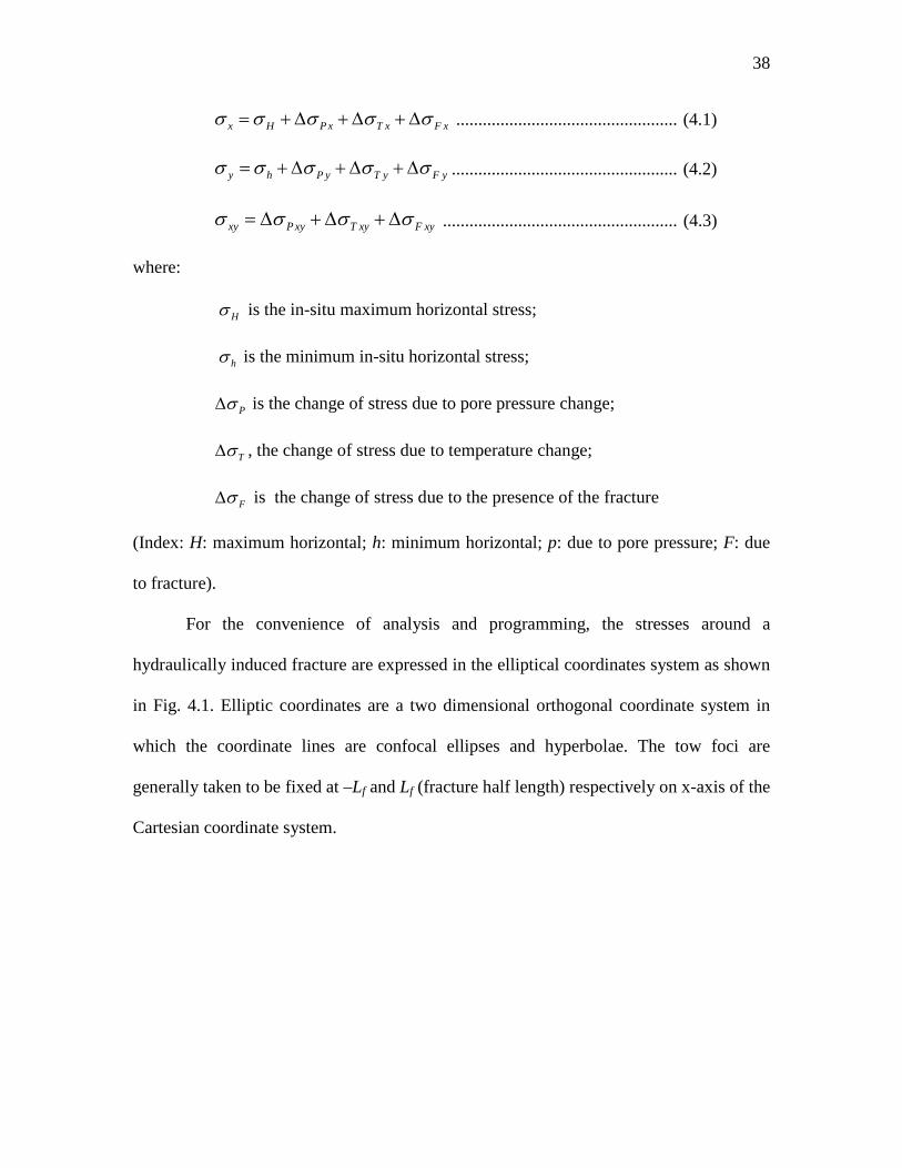
x H P x T x F xσ σ σ σ σ= + ∆ + ∆ + ∆ .................................................. (4.1)

y h P y T y F yσ σ σ σ σ= + ∆ + ∆ + ∆ ................................................... (4.2)

xy P xy T xy F xyσ σ σ σ= ∆ + ∆ + ∆ ..................................................... (4.3)

where:

Hσ is the in-situ maximum horizontal stress;

hσ is the minimum in-situ horizontal stress;

Pσ∆ is the change of stress due to pore pressure change;

Tσ∆ , the change of stress due to temperature change;

Fσ∆ is the change of stress due to the presence of the fracture

(Index: H: maximum horizontal; h: minimum horizontal; p: due to pore pressure; F: due

to fracture).

For the convenience of analysis and programming, the stresses around a

hydraulically induced fracture are expressed in the elliptical coordinates system as shown

in Fig. 4.1. Elliptic coordinates are a two dimensional orthogonal coordinate system in

which the coordinate lines are confocal ellipses and hyperbolae. The tow foci are

generally taken to be fixed at –Lf and Lf (fracture half length) respectively on x-axis of the

Cartesian coordinate system.

39

Fig.4.1 Stresses in Elliptical Coordinates System

In the following analysis for the induced stresses from pore pressure, temperature

variations and fracture compression are cited from relative references and all expressions

are converted into the same Cartesian coordinate system for the convenience of

calculations and programming.

4.2 Poroelastic Stresses

The stresses induced by the pore pressure variation around a hydraulic fracture

were given by Koning (1985). And the analytical fracture propagation model was

constructed by him with the following assumptions.

40

1) A vertical fracture confined to the pay zone with fixed height and the

geometry of PKN model extends laterally from a single well to an infinite

reservoir.

2) The fracture has an infinite conductivity and the fluid pressure along the

fracture length keeps constant.

3) The total leak-off rate equals to the constant injection rate.

4) The fracture propagates slow enough that the pressure distribution around the

fracture behaves as quasi steady state. And the transient pressure distribution

far away from the fracture moves radially outwards into the reservoir.

5) The fluid flow system can be separated into different elliptic zones as shown

in Fig.3.1.

With the assumptions the stresses at any point (ξ, η) in the pressure affected

region 0 ≤ ξ ≤ ξ2 surrounding the fracture is solving the poroelastic stress-strain relations

and are given by (Koning, 1985):

2 2( ) ( ) ( ) ( ) ( )

2 4 4

(1 ) 1 sinh 2 sin 2 ( )2 2

f fm m m m mp

L Lv pEJ g g gξ ξξ ξ η

ξ ησ ξ−∆ = Φ − Φ + Φ + ∆ ......... (4.4)

2 2( ) ( ) ( ) ( ) ( )

2 4 4

(1 ) 1 sinh 2 sin 2 ( )2 2

f fm m m m mp

L Lv pEJ g g gη ηη ξ η

ξ ησ ξ−∆ = Φ + Φ − Φ + ∆ ..... (4.5)

2 2( ) ( ) ( ) ( )

2 4 4

(1 ) 1 sin 2 sinh 22 2

f fm m m mp

L LvEJ g g gξη ξη ξ η

η ξσ−∆ = Φ − Φ − Φ ............................ (4.6)

The linear coefficient of pore pressure expansion J is used as:

(1 2 )3grcvJ

E−

= − ........................................................................... (4.7)

And where the superscript (m) is associated with the subregions:

41

1 2

0 1

0

1;2;

=3; 0

m ξ ξ ξξ ξ ξ

ξ ξ

= ≤ <= ≤ <

≤ <

.......................................................................... (4.8)

and:

2( ) ( ) 2 ( )

1 2( ) cosh 2 cos 2 (4 4 cosh 2 )2

fm m mLp A e Aξ

ξξ ξ ξ η ξ−Φ = − ∆ + + ..... (4.9)

2( ) ( ) 2 ( )

1 2cos 2 [ ( ) 4 4 cosh 2 ]2

fm m mLp A e Aξ

ηη η ξ ξ−Φ = ∆ − − .................. (4.10)

2( ) ( ) 2 ( )

1 2[ ( )]sin 2 [ 4 4 sinh 2 ]

4fm m mL p A e Aξ

ξηξη ξ

ξ−∂ ∆

Φ = + −∂

................. (4.11)

2( ) ( ) 2 ( )

1 2sin 2 [ ( ) 2 2 cosh 2 ]4

fm m mLp A e Aξ

η η ξ ξ−Φ = ∆ − − ..................... (4.12)

2 2( )

0

( ) 2 ( )1 2

[ ( )][ ( ) cosh 2 ] cos 2 [2 8

2 2 sinh 2 ]

f fm

m m

L L pp d

A e A

ξ

ξ

ξ

ξξ ξ ξ ηξ

ξ−

∂ ∆Φ = − ∆ + −

∂

− +

∫ ................... (4.13)

in which:

0

1 1 [ ( )][ ( ) cosh 2 ] ( )sinh 2 [cosh 2 1]2 4

[ ( )]2

w

m

pp d p

iph

ξ ξξ ξ ξ ξ ξ ξξ

ξξ π λ

∂ ∆∆ = ∆ − −

∂∂ ∆

= −∂

∫........ (4.14)

The pore pressure variations are given:

(1)1 2

(2)0 1

(3)0

2

( ) ( );

( );

( ); 00;

p ppp

ξ ξ ξ ξ ξ

ξ ξ ξ ξ

ξ ξ ξξ ξ

∆ = ∆ ≤ <

= ∆ ≤ <

= ∆ ≤ <= ≥

........................................................ (4.15)

and:

2(3)1

3

1[ ]32

w fi LA

hπ λ= ........................................................................... (4.16)

42

2(2) (3)1 1 0

2 3

1 1[ ]cos 232

w fi LA A h

hξ

π λ λ= + − ........................................... (4.17)

2(1) (2)1 1 1

1 2

1 1[ ]cos 232

w fi LA A h

hξ

π λ λ= + − .............................................. (4.18)

2

22(1)

21

1[ ]32

w fi LA e

hξ

π λ−= − ................................................................... (4.19)

1

22(2) (1)

2 21 2

1 1[ ]32

w fi LA A e

hξ

π λ λ−= + − ................................................... (4.20)

0

22(3) (2)

2 22 3

1 1[ ]32

w fi LA A e

hξ

π λ λ−= + − ................................................... (4.21)

While in the pressure unaffected region ξ≥ξ2, the stress changes:

2 2(0) (0) (0) (0)

2 4 4

(1 ) 1 sinh 2 sin 22 2

f fp

L LvEJ g g gξ ξξ ξ η

ξ ησ−∆ = Φ − Φ + Φ ........... (4.22)

2 2(0) (0) (0) (0)

2 4 4

(1 ) 1 sinh 2 sin 22 2

f fp

L LvEJ g g gη ηη ξ η

ξ ησ−∆ = Φ + Φ + Φ ........... (4.23)

2 2(0) (0) (0) (0)

2 4 4

(1 ) 1 sin 2 sinh 22 2

f fp

L LvEJ g g gξη ξη ξ η

η ξσ−∆ = Φ − Φ − Φ ........... (4.24)

where the superscript (0) stands for the region with zero pressure change.

And the constants are:

(0) (0) 2 (0) (0) 23 34 cos 2 ; 4 cos 2A e A eξ ξ

ξξ ηηη η− −Φ = Φ = − ..................... (4.25)

(0) (0) 2 (0) (0) 23 34 sin 2 ; 2 sin 2A e A eξ ξ

ξη ηη η− −Φ = Φ = − ..................... (4.26)

2(0) (0) 2 (0) (0) (1)

3 4 3 1 21

2 cos 2 ; cosh 232

w fi LA e A A A

hξ

ξ η ξπ λ

−Φ = − + = − ... (4.27)

22

(0)4 0

[ ( ) cosh 2 ]2

fLA p d

ξξ ξ ξ= − ∆∫ ....................................................... (4.28)

43

The listed equations above are in elliptical coordinates system, and Koning (1985)

gave transformation of the pore pressure induced stresses from elliptic coordinate system

into the x-y coordinates system by the following equations (Koning, 1985).

2

2

2

px p

py p

pxy p

g

g

g

ξ

η

ξη

σ σ

σ σ

σ σ

∆ = ∆

∆ = ∆

∆ = ∆

........................................................................... (4.29)

In which the metric tensor g is given:

2

(cosh 2 cos 2 )2

fLg ξ η= − .......................................................... (4.30)

In our work, we deduced the stresses transformation between these two coordinate

systems and the detailed deducing process can be found in Appendix C.

2

2

cos 2 sin 2 ( )sin

sin 2 ( )sinyy ηη ξη ξξ ηη

ηη ξη ξξ ηη

σ σ θ σ θ σ σ θ

σ σ θ σ σ θ

= + + +

= + + −.................... (C.17)

2sin 2 ( )sinxx ξξ ξη ξξ ηησ σ σ θ σ σ θ= − − − ................................ (C.18)

1( ( )sin 2 ) / cos 22xy yy xxξησ σ σ σ θ θ= − − ................................ (C.19)

In which θ is given by:

sinh sintancosh cos

y cx c

ξ ηθξ η

= = ........................................................ (C.8)

4.3 Thermoelastic Stresses

In this study, we considered the induced stresses by the variation of temperatures

around the fracture. The studies of thermoelastic stresses are most investigated in the

field of geothermal production (Ghassemi et al., 2005, 2006, and 2007). However, in

44

petroleum field, especially in gas shale reservoirs, due to the temperature difference

between injection fluids and reservoir fluids is small, the thermoelastic effects on stress

changes is less important than poroelastic stresses. Therefore, here it is assumed that the

temperature distribution around the fracture is uniform and elliptically distributed.

Therefore, not like the complexity of poroelastic stress changes surrounding the fracture,

the thermoelastic stress changes are simpler because the temperature distribution

surrounding the fracture is simply assumed to be elliptical and is only affected in the cool

region as we can see from Fig.4.2 (outside the cool region are all reservoir temperature,

uniform temperature distribution).

For a zone of uniform temperature change around the fracture, and assuming

plane strain, the interior thermo-elastic stresses perpendicular and parallel to the major

axes of the ellipse are given by the following equations (Perkinz and Gonzales, 1985).

0 01

0 0 0 0

0.9 2 0.7740

0 0 0

( / )(1 ) 11 ( / ) 1 ( / )

11/ 1 1.45( ) 0.35( ) 1 ( )2 2 2

T b aE T b a b a

bh hb b a

ν σβ

− ∆= + ∆ + +

+ + +

............... (4.31)

0 02

0 0 0 0

0.9 2 1.360

0 0 0

( / )(1 ) 11 ( / ) 1 ( / )

1/ 1 1.45( ) 0.35( ) 1 (1 )2 2

T b aE T b a b a

bh hb b a

ν σβ

− ∆= + ∆ + +

+ + + −

............... (4.32)

45

Fig.4.2 Temperature Distribution Surrounded the Fracture

Equations 4.31 and 4.32 are expressions for thermoelastic stress changes at any a

point (x, y) in the cool region and can be used in equations for calculations of changed in

situ stresses (see Equations 4.1-4.3). In this study, we have the expressions 1T Tyσ σ∆ = ∆

and 2T Txσ σ∆ = ∆ . Theses equations are expressed in X-Y coordinates, and don’t need to

be converted into elliptic coordinates.

4.4 Induced Stresses by Fracture Compression

In our work, the induced stresses by fracture compression are considered. On

many fracture treatments, a “stress shadow” effect is clearly seen in the mapping results

(Fisher et al., 2004). The compressive stress normal to the fracture faces is increased

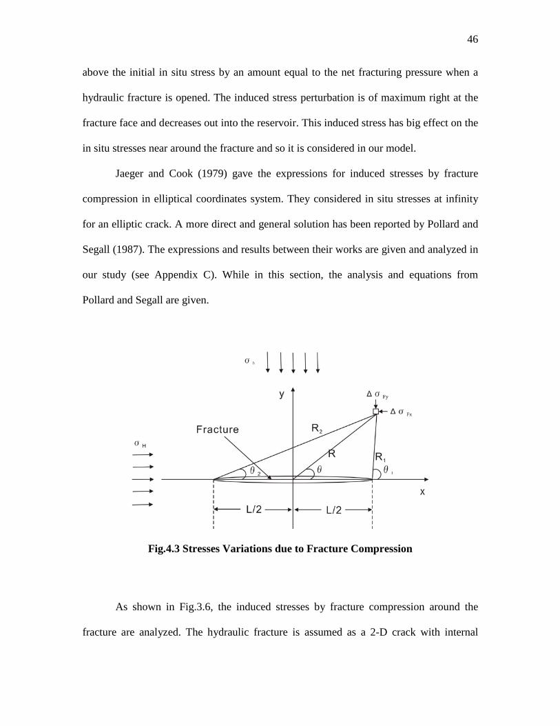
46

above the initial in situ stress by an amount equal to the net fracturing pressure when a

hydraulic fracture is opened. The induced stress perturbation is of maximum right at the

fracture face and decreases out into the reservoir. This induced stress has big effect on the

in situ stresses near around the fracture and so it is considered in our model.

Jaeger and Cook (1979) gave the expressions for induced stresses by fracture

compression in elliptical coordinates system. They considered in situ stresses at infinity

for an elliptic crack. A more direct and general solution has been reported by Pollard and

Segall (1987). The expressions and results between their works are given and analyzed in

our study (see Appendix C). While in this section, the analysis and equations from

Pollard and Segall are given.

Fig.4.3 Stresses Variations due to Fracture Compression

As shown in Fig.3.6, the induced stresses by fracture compression around the

fracture are analyzed. The hydraulic fracture is assumed as a 2-D crack with internal

47

pressure (here is the normal stress on the crack internal surface) original in situ stresses.

The expressions from Pollard and Segall (1987) are given in the following.

1 2 3

1 2 3

[ *cos( ) 1 ( / 2) sin sin 3 ]

[2 *sin( ) ( / 2) sin cos3 ]Fx I

II

Rr L RrRr L Rr

σ σ θ θ

σ θ θ

− −

− −

∆ = ∆ −Θ − − Θ

+∆ −Θ − Θ ....... (4.33)

1 2 3

2 3

[ *cos( ) 1 ( / 2) sin sin 3 ]

[( / 2) sin cos3 ]Fy I

II

Rr L Rr

L Rr

σ σ θ θ

σ θ

− −

−

∆ = ∆ −Θ − + Θ

+∆ Θ ....... (4.34)

1 2 3

2 3

[ *cos( ) 1 ( / 2) sin sin 3 ]

[( / 2) sin cos3 ]Fxy II

I

Rr L Rr

L Rr

σ σ θ θ

σ θ

− −

−

∆ = ∆ −Θ − − Θ

+∆ Θ ..... (4.35)

in which:

11 11

12 12

cI

cII

σ σ σ

σ σ σ

∆ = −

∆ = − ......................................................................... (4.36)

and 11cσ refers to the normal stress on the crack internal surface, and 12

cσ refers to the

shear stress on the crack internal. 11σ is the remote stress normal to the crack, 22σ is the

remote parallel stress, and 12σ is the remote shear stress. L is the fracture length, and the

geometric relations are given by the following equations: (as shown in the above figure

Fig.4.3)

2 2R x y= + , 1tan ( / )y xθ −= ...................................................... (4.37)

2 21 ( )

2LR y x= + − , 1

1 tan [ /( / 2)]y x Lθ −= − ............................. (4.38)

2 22 ( / 2)R y x L= + + , 1

2 tan [ /( / 2)]y x Lθ −= + ......................... (4.39)

1/ 21 2( )r R R= and 1 2( ) / 2θ θΘ = + ................................................ (4.40)

Negative values of θ, 1θ , and 2θ should be replaced by π+θ, π+ 1θ , and π+ 2θ respectively,

because these angles are in (0, π).

48

Table 4.1 Input Parameters for Simulations (Case from Perkin and Gonzalez, 1985) Injection condition Depth to the center of the formation (D): 1524m Reservoir Thickness (h): 30.5m Water injection rate (Iw): 477m3/d Time (t): 5year Initial Reservoir temperature (TR): 65.6°C Bottomhole temp. of the injection water (Tw): 21.1°C Undisturbed reservoir fluid pressure (PR): 13.78MPa Reservoir Rock Properties Compressibility of mineral grains (cgr): 2.20E-05 (MPa)-1 Compressibility of fracture (cf): 4.080E-04(MPa)-1 Young's modulus (E): 13.8E+03MPa Relative perm. to water at residual oil saturation (krw) : 0.29 Residual oil saturation (Sor): 0.25 Initial water saturation (Swi): 0.20 Rock surface energy (U): 5.0E-02 kJ/m2 Linear coefficient of thermal expansion (β): 5.60E-06mm/ (mm*K) Poisson’s ratio (ν): 0.15 Density * Specific heat of mineral grains (ρgr*Cgr): 2347kJ/ (m3*K) Minimum in-situ, total horizontal earth stress ((σh)min): 24.1MPa Porosity (Φ): 0.25 (σH)max /(σh)min: 1.35 Reservoir permeability (k): 4.935E-14m2 Reservoir Fluid Properties Compressibility of oil (co): 1.5E-03 (MPa)-1 Compressibility of water (cw): 5.20E-04 (MPa)-1 Specific heat of oil (Co): 2.1kJ/(kg*K) Specific heat of water (Cw): 4.2kJ/(kg*K) Viscosity of oil at 65.6 °C (μo): 1.47E-09 MPa*s Viscos ity of water at 65.6 °C (μw): 4.30E-10 MPa*s Viscosity of water at 21.1°C (μw): 9.95E-10 MPa*s Density of oil (ρo): 881kg/m3 Density of water (ρw): 1000kg/m3

49

4.5 Case Study

In previous sections, the stresses around a hydraulic fracture are analyzed. The

same case is used in this study as an example of the distribution of the stresses after 100

days of injection.

The poro-induced stresses distribution, thermo-induced stresses distribution and

induced stresses by fracture compression separately are calculated and plotted separately.

The parameters used for simulation in this case study are shown in Table.4.1.

The induced stresses by poroelasticity, thermoelasticity, and fracture compression

are considered. The equations for calculating the stress distributions around the crack in

Cartesian coordinates system are given by:

x H P x T x F xσ σ σ σ σ= + ∆ + ∆ + ∆ ................................................ (3.14)

y h P y T y F yσ σ σ σ σ= + ∆ + ∆ + ∆ ................................................. (3.15)

xy P xy T xy F xyσ σ σ σ= ∆ + ∆ + ∆ ................................................... (3.16)

With the current in situ stresses, the total principal stresses around the crack by

stresses transformation are given:

2 2 1/ 21

1 1( ) [ ( ) ]2 4x y x y xyσ σ σ σ σ σ= + + − + .................................. (4.41)

2 2 1/ 22

1 1( ) [ ( ) ]2 4x y x y xyσ σ σ σ σ σ= + − − + ..................................... (4.42)

And the maximum shear stresses distribution around a fracture can be given by:

1 21 ( )2

τ σ σ= − ............................................................................. (4.43)

Mean normal stress is given:

50

1 21 ( )2

σ σ σ= + ............................................................................. (4.44)

where Hσ is the in-situ maximum horizontal stress, hσ is the minimum in-situ horizontal

stress; Pσ∆ is the change of stress due to pore pressure change; Tσ∆ , the change of

stress due to temperature change; and Fσ∆ is the change of stress due to the presence of

the fracture ( index: H: maximum horizontal; h: minimum horizontal; p: due to pore

pressure; F: due to fracture). The interior thermo-elastic stresses perpendicular and

parallel to the major axes of the ellipse are given by Perkinz and Gonzales (1985.).

However, the induced poroelastic stresses are obtained as part of the current study.

Fig.4.4 Poro-Induced Stresses Distribution X Axis Direction (t=100 days)

51

Fig.4.5 Poro-Induced Stresses Distribution Y Axis Direction (t=100 days)

Fig.4.6 Thermo-Induced Stresses Distribution X Axis Direction (t=100 days)

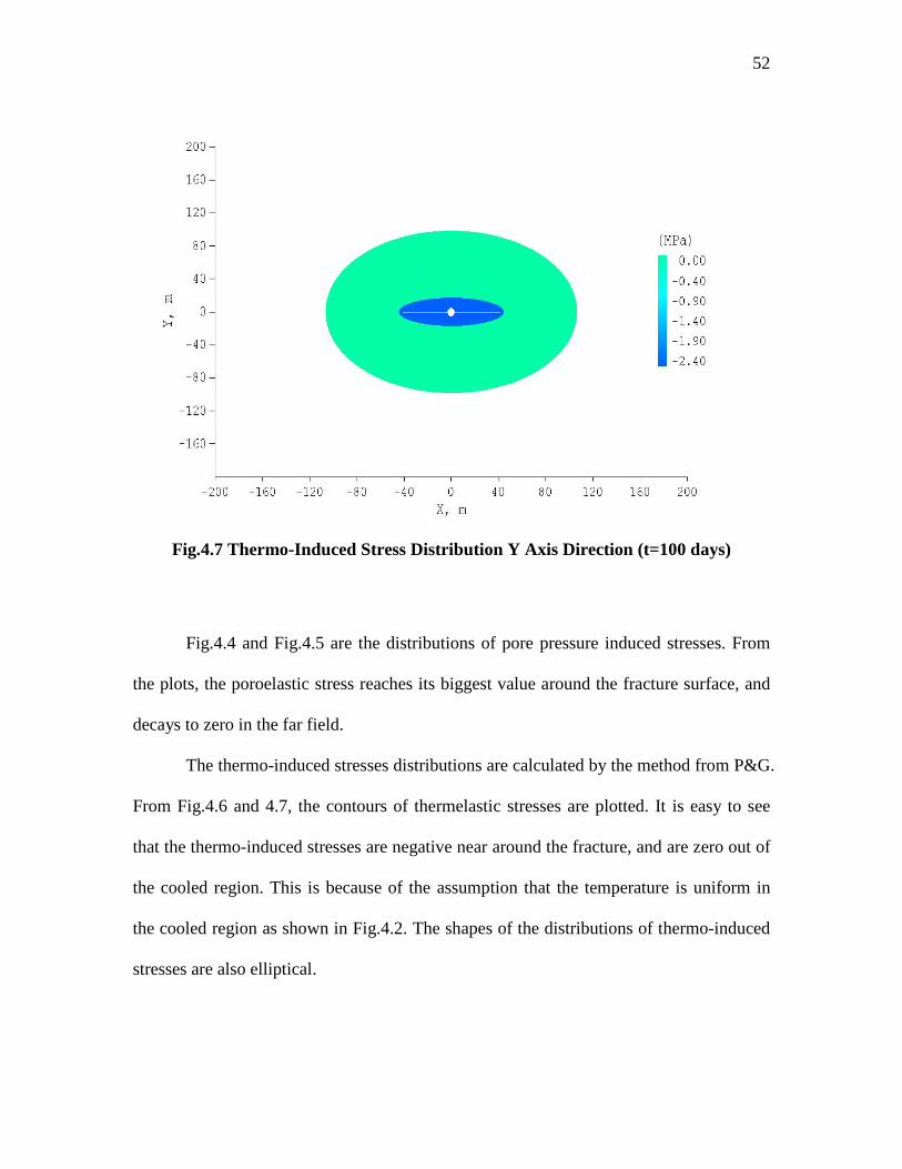
52

Fig.4.7 Thermo-Induced Stress Distribution Y Axis Direction (t=100 days)

Fig.4.4 and Fig.4.5 are the distributions of pore pressure induced stresses. From

the plots, the poroelastic stress reaches its biggest value around the fracture surface, and

decays to zero in the far field.

The thermo-induced stresses distributions are calculated by the method from P&G.

From Fig.4.6 and 4.7, the contours of thermelastic stresses are plotted. It is easy to see

that the thermo-induced stresses are negative near around the fracture, and are zero out of

the cooled region. This is because of the assumption that the temperature is uniform in

the cooled region as shown in Fig.4.2. The shapes of the distributions of thermo-induced

stresses are also elliptical.

53

According to the equations given by Pollard and Segall (1987), the induced

stresses by fracture compression are calculated and plotted for this case.

Fig.4.8, Fig.4.9 and Fig.4.10 are distributions of induced stresses by fracture

compression. From these figures, the induced stresses by fracture compression on x and y

axis have compressive values near fracture surface and negative values near the tips.

In Appendix C, the calculations and programming for fracture compression

induced stresses around a crack are described in detail.

Fig.4.8 Induced Stresses Distribution by Fracture Compression in X Direction

(t=100 days)

54

Fig.4.9 Induced Stresses Distribution by Fracture Compression in Y Direction

(t=100 days)

Fig.4.10 Induced Shear Stresses Distribution by Fracture Compression (t=100 days)

55

Fig.4.11 Effective Stresses Distribution around the Fracture (σ′x) (t=100 days)

Fig.4.12 Effective Stresses Distribution around the Fracture (σ′y) (t=100 days)

56

Then, according to equations 4.1-4.3, the effective stresses in X and Y directions

are calculated and plotted in Fig.4.11 and 4.12.

As shown in Fig.4.11 and Fig.4.12, the distributions of effective stresses around

near the fracture in X and Y directions have smaller values near the fracture tips.

4.6 Conclusions

In our study, we have developed a model (WFPSD model) for calculating the

length of a water-flood induced fracture from a single well in an infinite reservoir.

Similarly to Perkins and Gonzalez (1985) and Koning (1985) the model allows the leak-

off distribution in the formation to be two-dimensional with the pressure transient moving

elliptically outward into the reservoir with respect to the growing fracture. The model

calculates the length of a water flood fracture and the extent of the cooled and flooded

zones. The thermoelastic stresses are calculated by considering a cooled region of fixed

thickness and of elliptical cross section. The methodology of Perkins and Gonzalez

(1985) and Koning (1985) is used to calculate the fracture length, bottom-hole pressures

(BHP’s), and extent of the flood front as the injection process proceeds. Different from

previous work, in our WFPSD model, we also calculate the pore pressure distribution

around the fracture at any specific time. In addition, our model can calculate the stresses

variations at any point around the fracture caused by thermoelasticity, poroelasticity, and

fracture compression. The plots of stresses distributions at any specific time can be given

by our model. This model is useful for investigating the response of the rock mass to

stress variations resulting from pore pressure and temperature changes.

57

5 FAILURE POTENTIALS OF JOINTS AROUND HYDRAULIC FRACTURE

In previous sections, we have investigated the distributions of pore pressure and

stresses around a hydraulically induced fracture. In the following study, shear slip or

failure along planes of weakness caused by pore pressure increases during injection of

fluid is investigated. Knowledge of in situ stress, and strength for the planes of weakness,

is needed to predict potential failure area around the hydraulic fracture.

In this section, the pore pressure distribution after hydraulic fracturing is predicted,

and the failure of joints in the reservoir formation around a hydraulic fracture is studied

by constructing the Structural Permeability Diagram, by finding the critical pore pressure,

and by plotting the failure potential area around hydraulic fracture.

The structural permeability diagram is a technique that can be used to show the

additional pore pressure ΔP required to reactivate fabrics of different orientations

(Mildren et al. 2002; Nelson et al. 2007). With the structural permeability diagram, the

required minimum additional pore pressure is easy to find.

If the problem is simplified for certain sets of joints, the additional pore pressure

could be found with simple calculations. And for the formation with a certain set of joints

around a hydraulic fracture, the poroelastic changes of the in situ stresses are calculated,

as well as the induced stresses changes by fracture compression. the failure potential area

for the existing set of joints could be plotted near the fracture surface.

The failure of rock mass around the fracture is also studied to roughly predict the

failure distance from the central fracture surface. It may have significant impact on

permeability around a hydraulic fracture, and therefore on production. This in

conjunction with the microseismic cloud is used to estimate the stimulated volume and

58

the resulting rock mass permeability (Palmer et al., 2005; Palmer et al., 2007). The

injected permeability is greater than the virgin permeability, and this is interpreted as

enhanced permeability due to shear or tensile failure away from the central fracture plane.

In our model, the initial permeability and the fracturing geometry are given to simulate

the in situ stresses variations and predict the failure zone.

5.1 Structural Permeability Diagram

Knowing the pore pressure distributions, it can be applied to determine if the

joints in the reservoir around the fracture fail or not. And a structural permeability

diagram can be used to show the ΔP required to reactivate fabrics of different orientations

(Mildren et al., 2002; Nelson et al., 2007).

The structure permeability diagram is set up based on the dip angle δ and the

angle from north to the dip direction of the joints φ (clockwise positive). Here, the dip

angle refers to the angle between the joint plane and the horizontal plane; and the dip

direction is really vertical to the strike of the joint.

To get the structural permeability diagram, the direction cosines of the principal

stresses should be found first using the known dip angle and dip direction angle.

From Goodman (1989), the expressions for finding the direction cosines with dip

angle and δ and the dip direction angle φ:

cos(90 ) cos(90 )cos(90 ) sin(90 )sin(90 )

H

h

v

ddd

δ ϕδ ϕδ

= − × −= − × −= −

.............................................................. (5.1)

in which, dH, dh, and dv are direction cosines for the normal to a given weakness plane

with respect to the direction of the three stresses Hσ , hσ and vσ . The three principal

59

stresses and the direction cosines of the normal to the weakness plane with respect to the

principal stresses could then be decided by comparing the relative value between Hσ , hσ

and vσ .

The equations for calculation of normal and shear stresses on a plane were given

by Jaeger and Cook (1979) as the following:

2 2 21 2 3

2 2 2 2 2 2 2 2 21 2 3 2 3 1( ) ( ) ( )

n l m n

l m n m l n

σ σ σ σ

τ σ σ σ σ σ σ

= + +

= − + − + −........................ (5.2)

in which, l, m, and n are direction cosines for a given plane to the direction of the three

principal stresses.

Then, to investigate failure potentials of jointed rocks around a hydraulic fracture,

the Mohr-Coulomb failure criterion is used:

' tan 'ncτ σ φ= + .................................................................................. (5.3)

where τ is the shear stress on the joint plane, c (in some references given by τs) is the

shear strength or cohesive strength or cohesion of that joint, σn ' is the effective normal

stress on the joint and 'φ is the joint friction angle, and sometimes tan 'φ can be replaced

byµ , the coefficient of friction.

We set up our own program in the FracJStim model for plotting the structural

permeability diagram. In this section, we will compare some of our results with previous

works, and apply the structural permeability diagram to some gas shale reservoirs.

To verify the calculations, the model is first applied to the special case given by

Nelson et al. (2007) for the Cooper Basin stimulation experiment (Table.5.1). Fig.5.1

shows the structural permeability diagram for Cooper Basin from the work of Nelson et

al. (2007). Fig.5.2 shows the structural permeability diagram for Cooper Basin from our

60

program. Fig.5.1 and Fig.5.2 have good agreement except a 0.2 psi/ft difference on the

maximum effective treating pressure between them. This difference may be caused by

different calculation process or adjustments in the software used by Nelson et al. (2007).

Fig.5.1 Structural Permeability Diagram for Cooper Basin (Nelson et al., 2007)

Fig.5.2 Structural Permeability Diagram for Cooper Basin (Our Program)

61

Table 5.1 Parameters used for Cooper Basin (Nelson et al., 2007)

maxHσ (psi/ft) 1.85 E-W direction

minHσ (psi/ft) 0.84 N-S direction

Vσ (psi/ft) 0.95 Vertical

pP (psi/ft) 0.433

μ 0.6 Tensile negligible

H (ft) 9800

To further verify the results, we simulated the data of Otway Basin given by

Mildren et al., 2005 (Table 5.2). The structural permeability maps are shown in Fig.5.3

and Fig.5.4. Minor difference can be attributed to uncertainty in the input data used.

Fig.5.3 and Fig.5.4 show perfect agreement in plot shapes and values.

Table 5.2 Otway Basin Data from Mildren et al. (2005)

maxHσ (MPa/km) 37.1 156 º N

minHσ (MPa/km) 16.1 Normal to maxHσ

Vσ (MPa/km) 22.4 Vertical

pP (MPa/km) 9.8 μ 0.8 Tensile negligible H (km) 2.845

62

Fig.5.3 Structural Permeability Diagram for Otway Basin (Mildren et al., 2005)

Fig.5.4 Structural Permeability Diagram for Otway Basin (Our Program)

In the following, the application of structural permeability diagram on New

Albany Shale and Barnett Shale are given.

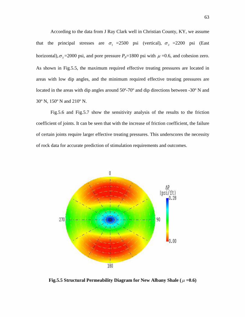
63

According to the data from J Ray Clark well in Christian County, KY, we assume

that the principal stresses are 1σ =2500 psi (vertical), 2σ =2200 psi (East

horizontal), 3σ =2000 psi, and pore pressure Pp=1800 psi with µ =0.6, and cohesion zero.

As shown in Fig.5.5, the maximum required effective treating pressures are located in

areas with low dip angles, and the minimum required effective treating pressures are

located in the areas with dip angles around 50º-70º and dip directions between -30º N and

30º N, 150º N and 210º N.

Fig.5.6 and Fig.5.7 show the sensitivity analysis of the results to the friction

coefficient of joints. It can be seen that with the increase of friction coefficient, the failure

of certain joints require larger effective treating pressures. This underscores the necessity

of rock data for accurate prediction of stimulation requirements and outcomes.

Fig.5.5 Structural Permeability Diagram for New Albany Shale (µ =0.6)

64



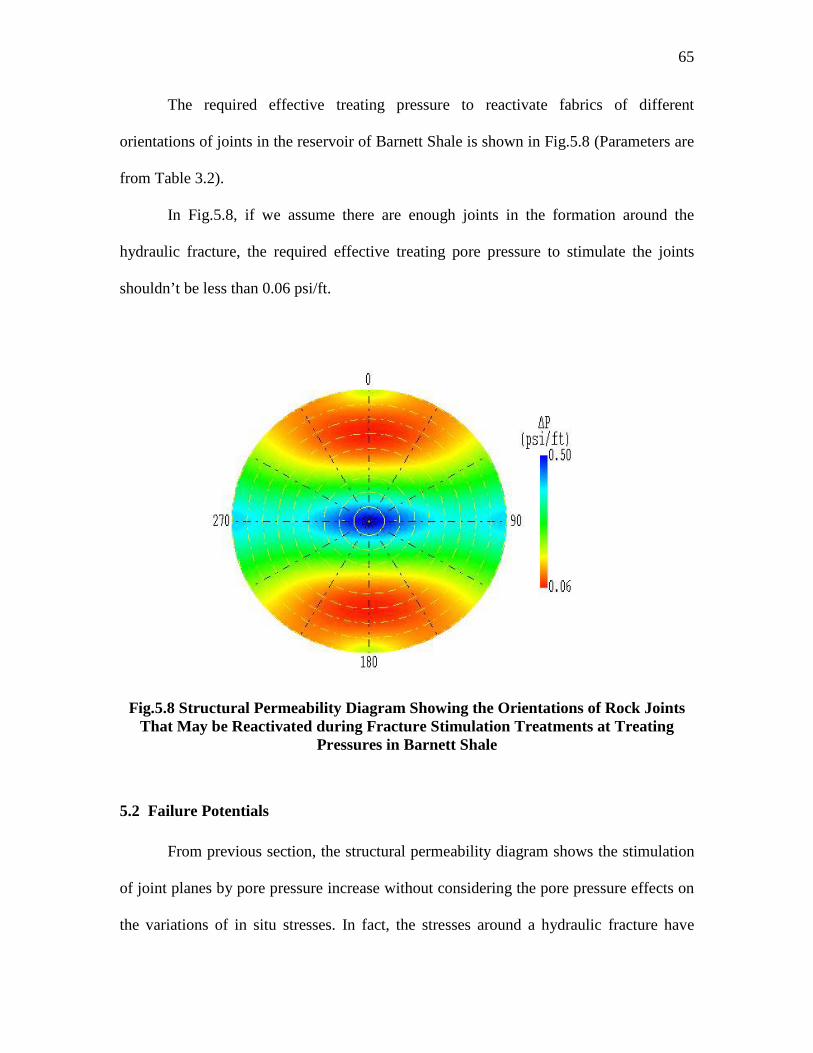
65

The required effective treating pressure to reactivate fabrics of different

orientations of joints in the reservoir of Barnett Shale is shown in Fig.5.8 (Parameters are

from Table 3.2).

In Fig.5.8, if we assume there are enough joints in the formation around the

hydraulic fracture, the required effective treating pore pressure to stimulate the joints

shouldn’t be less than 0.06 psi/ft.

Fig.5.8 Structural Permeability Diagram Showing the Orientations of Rock Joints That May be Reactivated during Fracture Stimulation Treatments at Treating

Pressures in Barnett Shale

5.2 Failure Potentials

From previous section, the structural permeability diagram shows the stimulation

of joint planes by pore pressure increase without considering the pore pressure effects on

the variations of in situ stresses. In fact, the stresses around a hydraulic fracture have

66

been changing with fracture propagation and pore pressure variation. Therefore, in the

following the failure potential of joints will be discussed with considering the stresses

variations.

The stresses at any point around the fracture are mainly affected by the following

factors: pore pressure change, temperature change, and the presence of the fracture. The

fracture compression induced stress was considered neither by Perkins and Gonzales nor

by Koning. In this study, as shown in section 4, we consider 2 dimensional stresses

distributions around the fracture by combing the effects from pore pressure, temperature,

and fracture compression.

In order to investigate the condition for sliding across joint planes, the effective

principal stresses are used by considering the effects of pore pressure. The 3D stresses

distributions can also be estimated by considering the induced stress in the vertical

direction, which can be the further work in the future.

In jointed rocks, the failure potentials should be analyzed by considering the

joints’ strike, dip and dip direction. Different joints can be theoretically expected for

different slip regimes. In a normal faulting regime, joints strike in the direction of SH

with dips in the direction of Sh. For the strike-slip faulting regime the fractures will

propagate in the vertical direction and strikes will generally bisect the SH and Sh direction

(Nygren and Ghassemi, 2005).

In this study, the joints are assumed to be vertical dips and the strikes of joints are

assumed to have an angle β with the minimum principal stress, so that we can use the two

dimensional stress distributions to estimate the failure potentials of joints.

67

Before determining the slip of joints, a failure criterion should be employed.

There are many failure criteria for the sliding of jointed rock masses. In our study, to

investigate failure potentials of jointed rocks around a hydraulic fracture, the Mohr-

Coulomb failure criterion is used as shown in Eqn.5.3.

If the joint orientation β is given by the angle between the joints’ orientation and

the minimum principal stress as shown in Fig.5.9, by assuming this angle the slip can be

determined. The normal stress and shear stress on the joints can be expressed in terms of

principal stresses (assume effective) using the following transformation equations (Jaeger

and Cook, 1979):

1 3 1 3' cos 22 2n

σ σ σ σσ β+ −= + ....................................................... (5.4)

1 3 sin 22

σ στ β−= ...................................................................... (5.5)

Then, the failure criterion for the planes of weakness or joints Eqn.5.3 can be

expressed in terms of principal stresses by applying the stress transformation equations in

Eqn.5.4 and 5.5. This yield:

( )

31 3

2( tan ')1 tan ' tan sin 2

sτ σ ϕσ σϕ β β+

− =−

............................................... (5.6)

68

Fig.5.9 Joint Strikes in the Formation

From the previous equations, the condition for failure along the joints is that the

left part is bigger than the right of the equation (Eqn.5.6). The potential for slip can then

be determined by defining Tf as:

( )

31 3

2( tan ')1 tan 'cot sin 2

sfT τ σ ϕσ σ

ϕ β β+

= − −−

........................................ (5.7)

When the value of Tf is larger than 0, joint slip will occur.

By considering the varied in situ stresses around the hydraulic fracture, the failure

potentials of joints in rock formations can be plotted.

For this two dimensional analysis, to compare with the structural permeability

diagram, the critical pore pressure to initiate slip for a joint is studied and shown in

Fig.5.10 (Nygren and Ghassemi, 2005).

69

Fig.5.10 The Critical Pore Pressure for Joints (Nygren and Ghassemi, 2005)

The additional pore pressure needed to activate the joints in Fig.5.9 can be

estimated by the following equation (Nygren and Ghassemi, 2005).

int 23 0

sin(90 )cos(90 )2 sin (90 )tan

jocp S β βσ β

φ − −

= + − −

......... (5.8)

in which: 0 1 3( ) / 2S σ σ= − .

5.3 Case Study for Barnett Shale

The model we set can be applied to check the stimulation of hydrocarbons after

hydraulic fracturing operations. In our study, a field case of Barnett Shale is investigated.

The hydraulic fracture in Barnett Shale is considered a stabilized fracture after

stimulation of water injection.

70

In the Barnett Shale, microseismic bursts are caused by shear failure on planes of

weakness well outside the central fracture plane (Palmer et al., 2007). Shear slip or

failure along planes of weakness is instigated by pore pressure increases during injection

of fracturing fluid.

As suggested by Palmer et al. (2007), during a fracture treatment, several things

occur synergistically in the reservoir:

From the central fracture, pressure is transmitted along natural fractures that

are open (or partially open), so that pore pressure increases during fracturing

operations;

The elevated pressure causes the variations of pore pressure and in situ

stresses shear or tensile failure, and enhances the permeability (especially if

several small tensile fractures coalesce into a large shear fracture);

The pressure is transmitted faster/further along the enhanced perm channels;

The enhanced permeability depends on the pressure transient, and the

pressure transient depends on the enhanced perm (i.e. they are coupled)

In tight gas reservoirs, the pore pressure is transmitted via natural fractures,

because the transmission via the matrix is too slow with very low permeability. Therefore,

Palmer et al. (2007) assumed there is a central fracture plane, oriented vertically, and that

this fracture plane is the source of the pressure transient that spreads out into the reservoir,

and induces shear or tensile failure.

Palmer et al. (2007) used the simplest slippage criterion - the linear friction law,

defined by the shear strength of the weak plane and by the coefficient of friction. In their

work, they have assumed for the Barnett Shale cohesion of 100 psi and friction angle of

71

31°. At the same time, they ignored the actual orientation of the weak planes, by

assuming there are enough planes in the preferred orientation for failure that these planes

dominate and govern the elliptical zone of failure.

In our study, we examined the method for critical pore pressure (Nygren and

Ghassemi, 2005); the slip map of joints for various joint orientations is plotted as the pore

pressure needed to reactivate the joints VS joint orientations. Fig.5.11 shows the critical

pore pressure gradient for various joint orientations and friction angles.

Fig.5.11 Critical Pore Pressure for Various Joints Orientations and Friction Angles

The stresses variations of Barnett Shale include the vertical stress in z direction by

considering the induced vertical stress as Eqn.5.9.

( )z v x y vσ σ σ σ= + ∆ + ∆ .................................................................... (5.9)

in which v is Poisson’s ratio and:

72

x P x T x F xσ σ σ σ∆ = ∆ + ∆ + ∆ ............................................................ (5.10)

y P y T y F yσ σ σ σ∆ = ∆ + ∆ + ∆ ........................................................... (5.11)

The induced stresses by thermoelasticity are neglected because the temperature

variations are relatively small in Barnett Shale. The in situ stresses profile away from the

central fracture face at shut in for the case of net pressure 900 psi and permeability 1md

with the parameters from Table.3.2 are plotted in Fig.5.12.

Fig.5.12 In Situ Stresses Profile away from the Central Fracture Face at Shut-in for the Case of Pnet=900 psi and K=1md

To verify the study, the in situ stresses profile away from the central fracture face

at shut in for the case of net pressure 902 psi and permeability 0.99 md with the

parameters from Table.3.2 are plotted in Fig.5.13 (Palmer et al., 2007). Through the

comparison between Fig.5.12 and Fig.5.13, we get the similar results and the validation

73

of our program.

Fig.5.13 In Situ Stresses Profile away from the Central Fracture Face at Shut-in for the Case of Pnet=902 psi and K=0.99md (Palmer et al., 2007)

Fig.5.14 shows us the pore pressure distribution around the fracture in Barnett

Shale at water flooding time t=9 hours. The maximum pore pressure lies around the

fracture surface, with a value of 6558 psi. The pore pressure is elliptically distributed

around the fracture surface and is decreasing from the central fracture to the reservoir

formation.

74

Fig.5.14 Pore Pressure Distribution around the Fracture (t=9 hours for Barnett Shale)

Fig.5.15 and Fig.5.16 are the stress distributions around the fracture in X and Y-

directions. The stresses variations are calculated by induced stresses from pore pressure

and fracture compression. With the parameters in Table 3.2 the stresses at any point

around the fracture could be estimated.

With stresses distributions, the slip of joints can be investigated. In our study,

different from what Palmer (Palmer et al., 2007) did, we used Mohr-Coulomb failure

criterion to determine the sliding of joints in rock formation around the hydraulically

induced fracture.

75

Fig.5.15 Stress Distribution around the Fracture in X-Direction

Fig.5.16 Stress Distribution around the Fracture in Y-Direction

76

As shown in the previous section, the failure criterion has been improved by

considering all of the three principal stresses. Using Eqn.5.7 and assuming the angle β is

given as π/4. The failure potentials of joints around the fracture can be plotted as Fig.

5.17.

Fig.5.17 Failure Potentials for One set of Joints around Hydraulic Fracture (K=1md, Pnet=900 Psi)

Fig.5.17 shows the failure potentials for fixed joints orientations. If we don’t

know the orientations of joints in the rock formations, the failed reservoir volume is not

easy to estimate. To simplify the calculation of failed reservoir volume and failed

77

distance, the failure of rock mass is investigated using Mohr-Coulomb criterion and

assuming the in situ stresses are fixed. Therefore, the rock mass will fail due to the pore

pressure increase after hydraulic stimulation.

The methodology of predicting the permeability in the failed region around a

fracture is based on the following trial and error procedure (Palmer et al., 2007):

1). An injection permeability K is guessed.

2). For a selected net fracture pressure (in the range 0 to 900 psi), the failed

reservoir volume is predicted.

3). K is varied until FRV matches the particular trendline of stimulated reservoir

volume (from induced seismcity) at the given net fracturing pressures.

In our study, the trendlines of the stimulated reservoir volume at given net

fracturing pressures are selected and read from the Palmer’s paper (Fig.5.18).

Fig.5.18 Trendlines for Failed Reservoir Volume (FRV=SRV) vs Net Fracture Pressure (Palmer et al., 2007)

78

From previous work, we know that the elliptically distributed pore pressure is

decreasing from the fracture surface to the far field (Muskat, 1937). The position of the

pore pressure contour small enough such that the joints will not slip marks the boundary

of the failure zone the treating pressure can create.

If we assume the failed distance is uniform along the fracture height, therefore,

we can estimate the failed reservoir volume as (Fig.5.19 and Fig.5.20):

d dFRV y x hπ= ................................................................................... (5.12)

Where yd is the failed distance, and xd is the failed distance in X direction, and h is

assumed equal to the fracture height Hf.

Fig.5.19 Estimation Method for Failed Reservoir Volume (for Vertical Well)

79

Fig.5.20 Estimation Method for Failed Reservoir Volume (for Horizontal Well)

Using the parameters for Barnett Shale in Table.3.2, the failed distance normal to

the fracture surface is plotted in Fig.5.21.

Fig.5.21 Estimated Failed Distance Normal to the Fracture Surface

80

Fig.5.22 Calculated Enhanced Permeability for Barnett Shale

Knowing the failed distance, the failed reservoir volume can be calculated from

equation 5.12. And by matching Fig.5.18 (Using data for a given net pressure from

Fig.5.18), the enhanced permeability with net pressure is plotted in Fig.5.23.

Fig.5.23 Enhanced Permeability during Injection to Match FRV for Lower Barnett Shale Fracture Treatments (Palmer et al., 2007)

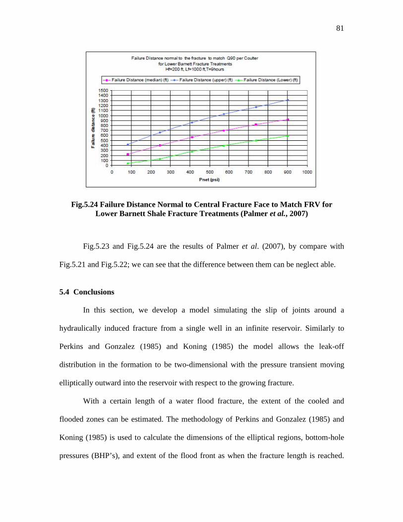
81

Fig.5.24 Failure Distance Normal to Central Fracture Face to Match FRV for Lower Barnett Shale Fracture Treatments (Palmer et al., 2007)

Fig.5.23 and Fig.5.24 are the results of Palmer et al. (2007), by compare with

Fig.5.21 and Fig.5.22; we can see that the difference between them can be neglect able.

5.4 Conclusions

In this section, we develop a model simulating the slip of joints around a

hydraulically induced fracture from a single well in an infinite reservoir. Similarly to

Perkins and Gonzalez (1985) and Koning (1985) the model allows the leak-off

distribution in the formation to be two-dimensional with the pressure transient moving

elliptically outward into the reservoir with respect to the growing fracture.

With a certain length of a water flood fracture, the extent of the cooled and

flooded zones can be estimated. The methodology of Perkins and Gonzalez (1985) and

Koning (1985) is used to calculate the dimensions of the elliptical regions, bottom-hole

pressures (BHP’s), and extent of the flood front as when the fracture length is reached.

82

The pore pressure and the stress changes at any point around the fracture caused by

poroelasticiy and fracture compression are also determined.

By using the Mohr-Coulomb failure criterion, we can estimate the slip of joints in

the formation around the fracture by considering the effects from pore pressure and

fracture compression. The structural permeability diagram is constructed to investigate

the required pore pressure to reactivate the joints around the hydraulic fracture. The

failure potential for a certain set of joints is studied with considering the variations of in

situ conditions. If given more assumptions, the failed reservoir volume can also be

estimated by this model, and if we know the actual failed reservoir volume, we can get

the enhanced permeability by the hydraulic fracture. Finally, with the data from Barnett

Shale, the model is verified.

This model can also be used in other types of petroleum reservoirs as well as

geothermal reservoirs.

83

6 SUMMARY, CONCLUSIONS AND DISCUSSION

6.1 Summary

In this research, the traditional two dimensional hydraulic fracturing propagation

models are reviewed, the propagation and recession of a poroelastic PKN hydraulic

fracturing model are studied, and the pore pressure and stresses distributions around a

hydraulically induced fracture are researched and plotted as figures.

In my study, the distributions of pore pressure and stresses around a fracture is of

interest in conventional hydraulic fracturing, fracturing during water-flooding of

petroleum reservoirs, and injection/extraction operation in a geothermal reservoir. The

stress and pore pressure fields are affected by: poroelastic, thermoelastic phenomena as

well as by fracture opening under the combined action of applied pressure and in-situ

stress. The development of two models is described in this study. One is a model of

water-flood induced fracture from a single well in an infinite reservoir (Perkins and

Gonzalez, 1985; Koning, 1985); it calculates the length of a water flood fracture and the

extent of the cooled and flooded zones. The model allows the leak-off distribution in the

formation to be two-dimensional with the pressure transient moving elliptically outward

into the reservoir with respect to the growing fracture. The thermoelastic stresses are

calculated by considering a cooled region of fixed thickness and of elliptical cross

section. The methodology of Perkins and Gonzalez (1985) is used for calculating the

fracture lengths, bottomhole pressures (BHP’s), and elliptical shapes of the flood front as

the injection process proceeds. However, in contrast to Perkins and Gonzalez (1985) and

Koning (1985) who gave only the calculation of poroelastic changes in reservoir stress at

the fracture face for a quasi steady-state pressure profile, the model allows calculation of

84

the pore pressure and in situ stress changes at any point around the fracture caused by

thermoelasticity, poroelasticity, and fracture compression. The second model calculates

the stress and pore pressure distribution around a fracture of a given length under the

action of applied internal pressure and in-situ stresses as well as their variation due to

cooling and pore pressure changes. It also calculates the failure potentials and slip map of

joints around the fracture to determine the zone of tensile and shear failure. This is of

interest in interpretation of micro-seismicity in hydraulic fracturing and in assessing

permeability variation around a stimulation zone.

6.2 Conclusions

The following conclusions are drawn from this study.

1. Poroelasticity can cause a significant increase in fracturing pressure, with little

effects on the fracture length and width during the fracture propagation and

recession process.

2. We develop a model for calculating the length of a water-flood induced fracture

from a single well in an infinite reservoir. Similarly to Perkins and Gonzalez

(1985) and Koning (1985) the model allows the leak-off distribution in the

formation to be two-dimensional with the pressure transient moving elliptically

outward into the reservoir with respect to the growing fracture. The model

calculates the length of a water flood fracture and the extent of the cooled and

flooded zones. The methodology of Perkins and Gonzalez (1985) and Koning

(1985) is used to calculate the fracture length, bottom-hole pressures (BHP’s),

and extent of the flood front as the injection process proceeds. We also calculate

85

the pore pressure and the stress changes at any point around the fracture caused

by thermoelasticity, poroelasticity and fracture compression.

3. By using the Mohr-Coulomb failure criterion, we can estimate the failure

potentials of joints and the critical pore pressure to activate joints, and if we

know the failed reservoir volume, we can get the enhanced permeability by the

stimulation of hydraulic fracturing operations. And this model can also be used in

other types of petroleum reservoirs.

6.3 Recommendations

In the future work, the pore pressure and stresses distributions around a hydraulic

fracture in P3D should be investigated.

More work should be focused on the applications for increasing the permeability

of unconventional gas reservoirs.

86

NOMENCLATURE

a0 and b0 = major and minor axis of cool region ellipse (L)

a1 and b1 = major and minor axis of water flood ellipse (L)

aR and bR = major and minor axis of the elliptical zone extending to the far-field (L)

A =drainage area (L2)

Cf = formation compressibility

Ct = system compressibility at initial reservoir conditions,

D = formation depth, (L)

E = Young’s modulus

G = shear modulus of rock formation

Gf =fluid pressure gradient

hf =fracture height, (L)

H =pay zone thickness, (L)

Hf =gross fracture height, (L)

i = time-step interval

ipf =the injection rate per zone

J =pseudosteady-state productivity index, dimensionless

k =formation permeability,

k/μ =permeability/viscosity ratio

K =cohesion modulus

Kc =critical stress-intensity factor

L =length, (L)

Lf =optimal fracture half-length, (L)

87

L(t)=fracture half-length at time t, (L)

p = pressure

p0 =pressure at the wellbore

pave = reservoir average pressure

pBHT = bottomhole treatment pressure

pf =fracture pressure

pi= initial pressure

p(0,t) =pressure at the wellbore at time t

p(X,t) =pressure at coordinate X at time t

Δp =pressure drop

Δp1= difference in pressure between water flood and far-field boundaries

Δp2= difference in pressure between cool front and water flood front

Δp3= difference in pressure between fracture surface and cool front

Δpf= difference in pressure between fracture surface and cool front

q =fracturing fluid flow rate

q0 =injection rate

q(0,t) =injection rate at the wellbore (x=0) at time t

re =reservoir drainage radius, (L)

rw =wellbore radius, (L)

Sw =water saturation

Swi =initial water saturation

t =time point during a fracture treatment

Tf =fracture temperature, ºF

88

Tpc =pseudocritical fracture temperature, ºF

Tpr =reduced temperature, ºF

V =volume, ft3

Vp =volume of proppant in pay, ft3

Vpf =volume of propped fracture, ft3

Vr =reservoir drainage volume, ft3

w =fracture width, ft

wj =level weighting factor

wkf =fracture conductivity, md-ft

wopt=optimal fracture width, ft

W(x,t) =width in elliptical fracture at time t at location X, ft

X =coordinate along direction of fracture propagation

Δσ =in-situ stress differential between the potential barrier and the payzone, psi

µg =gas viscosity, cp

ν =Poisson’s ratio

ρ =density of the fracturing fluid

σh =in-situ normal rock stress perpendicular to fracture face, psi

φ =porosity, %

89

REFERENCES

Abé, H., Mura, T., and Keer, L.M. 1976. Growth Rate of a Penny-Shaped Crack in

Hydraulic Fracturing of Rocks. J. Geophys. Res. 81. DOI:

10.1029/JB081i029p05335

Biot, M.A. 1941. General Theory of Three-Dimensional Consolidation. Journal of

Applied Physics 12 (2): 155-164.

Cleary, M.P. 1980. Comprehensive Design Formulae for Hydraulic Fracturing. Paper

presented at the SPE Annual Technical Conference and Exhibition, Dallas, Texas.

1980 Copyright 1980, American Institute of Mining, Metallurgical, and Petroleum

Engineers, Inc. 9259-MS.

Daneshy, A.A. 1973. On the Design of Vertical Hydraulic Fractures. SPE Journal of

Petroleum Technology 25 (1): 83-97. DOI: 10.2118/3654-pa

Detournay, E., Cheng, A.H.D., and Mclennan, J.D. 1990. A Poroelastic Pkn Hydraulic

Fracture Model Based on an Explicit Moving Mesh Algorithm. Journal of Energy

Resources Technology-Transactions of the Asme 112 (4): 224-230.

Economides, M.J. and Nolte, K.G. 2000. Reservoir Stimulation. Chichester, England ;

New York: Wiley. Original edition. ISBN 0471491926 (acid-free paper).

Geertsma, J. 1957. The Effect of Fluid Pressure Decline on Volumetric Changes of

Porous Rocks. Petroleum Transactions American Institute of Mining

Metallurgical and Petroleum Engineers 210: 331-340.

Geertsma, J. 1966. Problems of Rock Mechanics in Petroleum Production Engineering.

Paper presented at the Proc. 1st Cong. of the Intl. Soc. of Rock Mech., Lisbon

585-594.

90

Geertsma, J. and Klerk, F.d. 1969. A Rapid Method of Predicting Width and Extent of

Hydraulically Induced Fractures. SPE Journal of Petroleum Technology 21 (12):

1571-1581. DOI: 10.2118/2458-pa

Ghassemi, A. and Suresh Kumar, G. 2007. Changes in Fracture Aperture and Fluid

Pressure Due to Thermal Stress and Silica Dissolution/Precipitation Induced by

Heat Extraction from Subsurface Rocks. Geothermics 36 (2): 115-140.

Ghassemi, A., Tarasovs, S., and Cheng, A.H.-D. 2005. Integral Equation Solution of Heat

Extraction-Induced Thermal Stress in Enhanced Geothermal Reservoirs.

International Journal for Numerical and Analytical Methods in Geomechanics 29

(8): 829-844.

Ghassemi, A., Tarasovs, S., and Cheng, A.H.D. 2007. A 3-D Study of the Effects of

Thermomechanical Loads on Fracture Slip in Enhanced Geothermal Reservoirs.

International Journal of Rock Mechanics and Mining Sciences 44 (8): 1132-1148.

Ghassemi, A. and Zhang, Q. 2006. Porothermoelastic Analysis of the Response of a

Stationary Crack Using the Displacement Discontinuity Method. Journal of

Engineering Mechanics 132 (1): 26-33.

Jaeger, J.C. and Cook, N.G.W. 1979. Fundamentals of Rock Mechanics. Science

Paperbacks. London: Chapman and Hall. Original edition. ISBN 0412220105

(pbk.).

Jaeger, J.C., Cook, N.G.W., and Zimmerman, R.W. 2007. Fundamentals of Rock

Mechanics. Malden, MA: Blackwell Pub. Original edition. ISBN

9780632057597 (pbk. alk. paper).

91

Khristianovitch, S.A. and Zheltov, Y.P. 1955. Hydraulic Fracture of an Oil-Bearing Bed.

. Izvest. Akad. Nauk SSR, OTN 5: 3-41.

Koning, E.J.L. 1985. Fractured Water Injection Wells - Analytical Modelling of Fracture

Propagation. Society of Petroleum Engineers 14684-MS.

Legarth, B., Huenges, E., and Zimmermann, G. 2005. Hydraulic Fracturing in a

Sedimentary Geothermal Reservoir: Results and Implications. International

Journal of Rock Mechanics and Mining Sciences 42 (7-8): 1028-1041.

Maugis, D. 1992. Stresses and Displacements around Cracks and Elliptical Cavities:

Exact Solutions. Engineering Fracture Mechanics 43 (2): 217-255.

Murphy, H. 1983. Hot Dry Rock Reservoir Development and Testing in the USA. In

Mechanics of Elastic and Inelastic Solids 5, Hydraulic Fracturing and

Geothermal Energy, ed. Namet-Nasser, S., Abé, H., and Hirakawa, S., Boston:

Martinus Nijhoff Publishers.

Muskat, M. and Wyckoff, R.D. 1937. The Flow of Homogeneous Fluids through Porous

Media. International Series in Physics. New York: McGraw-Hill. Original edition.

ISBN.

Nordgren, R.P. 1972. Propagation of a Vertical Hydraulic Fracture. SPE Journal 12 (4):

306-314. DOI: 10.2118/3009-pa

Nygren, A. and Ghassemi, A. 2006. Poroelastic and Thermoelastic Effects of Injection

into a Geothermal Reservoir. Paper presented at the Golden Rocks 2006, The 41st

U.S. Symposium on Rock Mechanics (USRMS), Golden, CO. American Rock

Mechanics Association 06-1053.

92

Palciauskas, V.V. and Domenico, P.A. 1982. Characterization of Drained and Undrained

Response of Thermally Loaded Repository Rocks. Water Resour. Res. 18. DOI:

10.1029/WR018i002p00281

Palisch, T.T., Vincent, M.C., and Handren, P.J. 2008. Slickwater Fracturing – Food for

Thought. Paper presented at the SPE Annual Technical Conference and

Exhibition, Denver, CO, USA. Society of Petroleum Engineers 115766-MS.

Palmer, I.D., Moschovidis, Z.A., and Cameron, J.R. 2005. Coal Failure and

Consequences for Coalbed Methane Wells. Paper presented at the SPE Annual

Technical Conference and Exhibition, Dallas, TX. Society of Petroleum

Engineers 96872-MS.

Palmer, I.D., Moschovidis, Z.A., and Cameron, J.R. 2007. Modeling Shear Failure and

Stimulation of the Barnett Shale after Hydraulic Fracturing. Paper presented at the

SPE Hydraulic Fracturing Technology Conference, College Station, Texas,

U.S.A. Society of Petroleum Engineers 106113-MS.

Perkins, T.K. and Gonzalez, J.A. 1985. The Effect of Thermoelastic Stresses on Injection

Well Fracturing. SPE Journal 25 (1): 78-88. DOI: 10.2118/11332-pa

Perkins, T.K. and Kern, L.R. 1961. Widths of Hydraulic Fractures. SPE Journal of


Pollard, D.D. and Segall, P. 1987. Theoretical Displacements and Stresses near Fractures

Rock: With Applications to Faults, Joints, Veins, Dikes, and Solution Surfaces. In

Atkinson, B.K., ed., Fracture Mechanics of Rocks, New York: Academic Press.

93

Rice, J.R. and Cleary, M.P. 1976. Some Basic Stress Diffusion Solutions for Fluid-

Saturated Elastic Porous Media with Compressible Constituents. Rev. Geophys.

14. DOI: 10.1029/RG014i002p00227

Settari, A. 1980. Simulation of Hydraulic Fracturing Processes. SPE Journal 20 (6): 487-

500. DOI: 10.2118/7693-pa

Shin, K., Sugawara, K., and Okubo, S. 2001. Application of Weibull's Theory to

Estimating in Situ Maximum Stress [Sigma]H by Hydrofracturing. International

Journal of Rock Mechanics and Mining Sciences 38 (3): 413-420.

Sneddon, I.N. and Lowengrub, M. 1969. Crack Problems in the Classical Theory of

Elasticity. The Siam Series in Applied Mathematics. New York: Wiley. Original

edition. ISBN.

Timoshenko, S. and Goodier, J.N. 1951. Theory of Elasticity. Engineering Societies

Monographs. New York: McGraw-Hill. Original edition. ISBN.

Valkó, P. and Economides, M.J. 1995. Hydraulic Fracture Mechanics. Chichester ;

Toronto: Wiley. Original edition. ISBN 0471956643.

Veatch Jr., R.W. 1983a. Overview of Current Hydraulic Fracturing Design and Treatment

Technology--Part 1. SPE Journal of Petroleum Technology 35 (4): 677-687. DOI:

10.2118/10039-pa

Veatch Jr., R.W. 1983b. Overview of Current Hydraulic Fracturing Design and

Treatment Technology-Part 2. SPE Journal of Petroleum Technology 35 (5): 853-

864. DOI: 10.2118/11922-pa

94

Warpinski, N.R. and Branagan, P.T. 1989. Altered-Stress Fracturing. SPE Journal of


Warpinski, N.R. and Teufel, L.W. 1987. Influence of Geologic Discontinuities on

Hydraulic Fracture Propagation (Includes Associated Papers 17011 and 17074 ).

SPE Journal of Petroleum Technology 39 (2): 209-220. DOI: 10.2118/13224-pa

Warpinski, N.R., Wolhart, S.L., and Wright, C.A. 2001. Analysis and Prediction of

Microseismicity Induced by Hydraulic Fracturing. Paper presented at the SPE

Annual Technical Conference and Exhibition, New Orleans, Louisiana.

Copyright 2001, Society of Petroleum Engineers Inc. 71649-.

Yew, C.H. 1997. Mechanics of Hydraulic Fracturing. Houston, Tex.: Gulf Pub. Original

edition. ISBN 0884154742 (alk. paper).

95

APPENDIX A

MECHANICS OF TRADITIONAL 2D HYDRAULIC FRACTURE

PROPAGATION MODELS

The mechanics of traditional 2D hydraulic fracture propagation models are reviewed in

the following.

First, let’s come to the PKN model, the maximum width in the elliptical fracture

is given by Eqn.1.1 (from Perkins and Kern 1961).

( )( ) ( )

,

1 f f hX t

h pw

Gν σ− −

= ............................................................... (A.1)

where ν is the Poisson’s ratio, h the minimum in-situ rock stress perpendicular to the

fracture face, and G the shear modulus of the rock formation.

The term X is the coordinate along the direction of fracture propagation. The

pressure drop in the X direction is determined by the flow resistance in a narrow,

elliptical flow channel.

Hw

qxp

364 µπ−

=∂∆∂ ............................................................................... (A.2)

For the PKN model, the fluid pressure at the propagating edge falls off towards

the tip or leading edge. Thus for x = Lf, pf = h. This is based on the assumption that the

fracture resistance or toughness at the tip is zero. Note that for a crack created and opened

by a uniform internal pressure, the tip of the crack experiences infinite high tensile

stresses. However, in this model, the stress-concentration problem at the tip is ignored.

Nordgren (1972) wrote the continuity equation:

twh

xq f

∂∂

−=∂∂

4π ............................................................................. (A.3)

96

By using Eqn.A.1 to Eqn.A.3, we obtain a nonlinear partial-differential equation,

Eqn.A.4, in terms of w(X,t):

0-)-64(1 2

22

f

=∂∂

∂∂

tw

Xw

hG

µν ...................................................... (A.4)

Consider the following initial conditions for Eqn.A.4:

w(X, 0) = 0

w(X, t) = 0 for X ≥ L (t)

q (0, t) = q0 for a one-sided fracture

Or

q (0, t) = 0.5q0 for a two-sided fracture.

Finally, the shape of the fracture takes the form shown in Eqn.A.5.

( ) ( )25.0

10,,

−=

LXXwtXw ............................................................... (A.5)

And the fracture volume is given by Eqn.A.6.

( ) 1,05 0tq

LXtwLhV f =

−=

π .......................................................... (A.6)

For KGD model, the fluid pressure gradient in the propagation direction is

determined by Eqn. A.7.

dxtxwh

qpptxptpx

ff

),(112),(),0(

03

0 ∫=−=−µ

.......................... (A.7)

The equilibrium condition directed by applied mechanics is given by Eq. 4.59.

L

KdxxLtXp

h

L

22 ),(

022

+=−

∫ σπ ............................................................ (A.8)

97

where h is the in-situ rock stress, perpendicular to the fracture face. K is the cohesion

modulus.

Zheltov and Khristianovitch (1955) simplified the upper equations, which can be

used to calculate the pressure distribution approximately.

0pp f = ............................................................................................... (A.9)

for 0 < λ <L0 /L, and

0=fp .............................................................................................. (A.10)

for L0 /L < λ <1, where p is the fluid pressure. The λ= X/L is the dimensionless fracture

coordinate.

Then the condition of “wetted” fracture length can be calculated from Eq. 4.62.

This provides a good point to start the calculation, and this approximation is good enough

to prevent further refinements.

==

LpK

pLL

f

c

f

hσπλ2

sin00 ................................................................. (A.11)

The shape of the fracture in the horizontal plane is elliptical, with maximum width

at the wellbore that can be calculated using Eqn.A.12.

( ) ( ) ( )G

pLtw hf σν −−=

12,0 .................................................................... (A.12)

A good approximation to determine the fluid flow resistance in the fracture is

Eqn. A.13.

( )( ) ( ) 2

1200 3

3

147

,,00 −

−≈∫ λλλ

dtXwtw ................................................................. (A.13)

The fracture volume of one-sided fracture amounts can be calculated

approximately by Eqn. A.13.

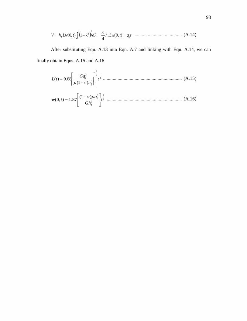
98

( ) tqtLwhdtLwhV ff 0

1

021

2 ),0(4

1),0( ==−= ∫πλλ ........................................ (A.14)

After substituting Eqn. A.13 into Eqn. A.7 and linking with Eqn. A.14, we can

finally obtain Eqns. A.15 and A.16

316

1

3

30

)1(68.0)( t

hGqtL

f

+=

νµ ................................................................. (A.15)

31

3

30 t)1(87.1),0(

+=

fGhqtw µν .............................................................. (A.16)

99

APPENDIX B

POROELASTIC PKN MODEL

B.1 Mechanics of Poroelastic PKN Model

As discussed in Section 2, the poroelasticity in hydraulic fracture is induced by

the leak-off of the fracturing fluid. The following will give the coupling mechanisms of

poroelasticity.

1) Balance of Fluid Momentum:

2

3 3

64

m ave

p q qx w w

µ π µπ

∂∆= − = −

∂ ................................................................. (B.1)

where:

Δp: net pressure in the fracture

q: average flow rate per unit height of fracture, which is Q0/hf

Q0: Injection Rate

wm: max width of the fracture in the cross section

wave: average width of the fracture

Hf: fracture height

µ: fluid viscosity

Note: the meaning of symbols in this thesis from now on will be shown in the

nomenclature later unless otherwise specified.

100

For a non-Newtonian fluid, the momentum equation for laminar flow of a power

law fluid in a fracture is approximated by the one-dimensional equation from lubrication

theory:

1

2 1

2 n

fn n

Kq qpx wψ

−

+

∂= −

∂.............................................................................. (B.2)

where:

3 24 122

5 12(2 1)2

nn

nn n

nnn

ψπ

++ Γ = ++ Γ

................................................ (B.3)

2) Local Fluid Mass Balance: (Continuity Equation)

0avewq ux t

∂∂+ + =

∂ ∂ .................................................................... (B.4)

For steady and incompressible flow, the volume flow rate into a control volume

must be equal to the volume flow rate out of the control volume, plus the volume leak-off

rate.

u: fluid leak-off velocity accounting for both walls

3) Leak-Off Equation:

( )2 lCu

t xτ=

− .................................................................................. (B.5)

Cl: leak-off coefficient

101

t: the lapse time since pumping starts

τ(x): the arrival time of fracture tip at location x.

4) Pressure-Width Relation: (without Poroelasticity)

( )14 4

fave m

v h pw w

Gπ π− ∆

= = ...................................................... (B.6)

If poroelasticity is considered: The average fracture width wave is composed of

two contributions, we and wp which reflect the existence of two different processes

(Cheng, 1990; Boone, 1990)

e pavew w w= + ........................................................................... (B.7)

in which the first component we is controlled by the net stress p=pf-σ0, while wp depends

on the net pressure Δp=pf-p0. The poroelastic processes that are taking place in the

permeability layer cause both we and wp to be time-dependent. However, the time-

dependednt contribution of we is typically overshadowed by that associated with wp

(Cheng, 1990). Hence it is approximated the net stress effect as being purely elastic

0( )ec fw M p σ= − .......................................................................... (B.8)

If the fluid pressure maintained constant, the time dependent width reduction wp

can be described as (Boone and Detournay, 1990)

2 ( *)pcw pM f tη= − ∆ .............................................................. (B.9)

where f(t*) is the evolution function which varies 0 and 1 approaches 0 and infinity,

respectively. The symbol t* denotes a dimensional fracture surface exposure time defined

as

102

[ ]2

4 ( )*

f

c t xt

hτ−

= ............................................................................. (B.10)

c is the diffusivity coefficient.

p

cCκφ

= ......................................................................................... (B.11)

Similarly, f (t*) is given by

0

4( *) ( )2 *

yf t erfc g y dytπ

∞ =

∫ .................................................... (B.12)

Where:

2( ) 1 42yg y y y= − + − .......................................................... (B.13)

The poroelastic contribution to the width change equation is derived on the

assumption that the fracture surface is directly exposed to a fracturing fluid of same

viscosity and compressibility as the reservoir fluid, and that the pore pressure difference

Δp between the fracture face and the far-field is a constant in time. The leak-off velocity

constituent with this set of assumption is given by (accounting for both walls)

( )2

( )pu

c t xκ

π τ∆

=−

...................................................................... (B.14)

The actual leak-off process, however, is described by equation (B.5) with the

leak-off coefficient Cl, a constant that takes into account difference in properties between

the fracturing and the reservoir fluid and the buildup of a filter cake on the fracture wall.

Assuming incompressibility of the fracturing fluid and ignoring the movement of the

fracturing/reservoir fluid interface, the leak-off equation (B.5) can equivalently be written

103

in terms of the difference pλ between the pressure at the fracturing/reservoir fluid

interface and the far-field pore pressure.

( )2

( )pu

c t x

κλ

π τ=

− ........................................................................ (B.15)

where:

lp

C cπλκ

= ................................................................................... (B.16)

Using equation (B.14) and (B.15), the expression for the width change in equation

(B.9) becomes

2 ( *)pp cw M f tηλ= − ...................................................................... (B.17)

Substituting equation (B.17) and (B.8) into (B.7) we get,

( )0c f Bw M p σ σ= − − ................................................................... (B.18)

where:

2 ( *)B p f tσ ηλ= ............................................................................. (B.19)

5) GLOBAL MASS BALANCE EQUATION

The fracture length, L is a function of time and not known a priori. The volume of

the fracture is equal to the volume of fluid pumped minus the cumulative leak-off

volume.

( ) ( ')

0 0 0 0

( , ) ( , ') ' ( ') 'L t L tL t

ow x t dx u x t dxdt q t dt+ =∫ ∫ ∫ ∫ ................................... (B.20)

104

where range 0 x L≤ ≤

/o o fq Q h= is the fluid injection rate per unit height of the fracture.

6) Initial and Boundary Condition

The system of equations are supplemented by the boundary conditions

(0, ) ( ); 0( ( ), ) 0, 0

oq t q t tp L t t t

= >= >

......................................................................... (B.21)

and the initial conditions

(0) 0 and (0,0) 0L p= = ............................................................... (B.22)

The mathematical model is required to predict the evolution of the fracture length

L(t), and fracturing pressure (0, ) (0, )f f op t p t σ= + ,as well as the field variables

( , ), ( , ), ( , ) an d ( , )q x t w x t p x t u x t .

B.2 Methodology

Finite difference method is used to solve the propagation and recession in this

poroealstic PKN hydraulic model (Detournay et al., 1990).

First, divide the fracture into n segments, that’s totally n+1 node along the fracture,

take x1=0 and Wn+1=0. On each node, a finite difference expression for the continuity

equation can be obtained. For nodes from 2 to n, central difference expression is applied,

while for the first node, forward difference expression is used. (No difference expression

needed for the last node because Wn+1=0).

With respect to time from tk to tk+1, use of integration formula gives a linear

tridiagonal system for Wi-1k, Wi

k and Wi+1k. Since Wi-1

k, Wik and Wi+1

k are known, by

105

solving the tridiagonal system, we can obtain width increment ΔWik of each node at time

tk+1, using standard numerical method. Thus the current width, length and volume of the

fracture can be calculated accordingly.

The tridiagonal system is given:

( )1

2 1

2

2 1 2 11 1

1 12 2

2 2 2 2 2 21 12

(2 2)( )4 ( )

( 1)( ) ( 1)( )( ) ( )

[( ) 2 () ( ) ]( )

4k

k pnkk ii

k pn k pnk kk i k ii i

k pn k pn k pnki i i

i k i

t pn wH wcon x

t pn w t pn ww wx x

t w w wx

HCl t tcon

π

τ τ+

+

+ +− +

− +

+ + ++ −

∆ +− ∆ + ∆

∆ + ∆ +∆ + ∆ ∆ ∆

∆= − − + ∆

− − − −

......... (B.23)

in which, the index i is from 2 to n.

2 1 1

2 1

H 2(2 2) (1 )4

pn pn pn

pn

Gconpn K vφ π + −

+= −+ −

................................................... (B.24)

Here we use pn in stead of the power law index n.

For node n=1,

[ ]2 1 2 11 1 1

2 2 2 21

(2 2)( ) 0 (2 2)( )

[( ) ( ) ]

k pn k k k pn ki i i i i

k pn k pni i

pn w w w pn w w

xQ w wcon

+ +− + +

+ ++

− + ∆ + ∆ + + ∆ ∆

= − .... (B.25)

Thus, for node 1 to node n along the fracture at time tk+1, we obtain:

[ ] [ ] [ ]1 1 [ ]k k ki i i i i i ib w a w c w d− +∆ + ∆ + ∆ = ................................................. (B.26)

In which, ai, bi, ci and di can be expressed from equation (B.23-B.25).

106

B.3 Programming

A FORTRAN program is used to simulate the propagation of a hydraulic fracture

with the effects from poroelasticity.

The flow chart of this program is shown in the following Fig.B.1.

Fig.B.1 Flow Chart of Poroleastic PKN Model

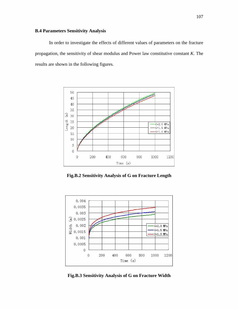
107

B.4 Parameters Sensitivity Analysis

In order to investigate the effects of different values of parameters on the fracture

propagation, the sensitivity of shear modulus and Power law constitutive constant K. The

results are shown in the following figures.

Fig.B.2 Sensitivity Analysis of G on Fracture Length

Fig.B.3 Sensitivity Analysis of G on Fracture Width

108

Fig.B.4 Sensitivity Analysis of G on Fracture Pressure

From the figures, we can see that the shear modulus has great effects on the

fracture propagation, especially on fracture width and pressure, and have fewer effects on

fracture length. The power law constitutive constant K has smaller effects on the fracture

propagation, and almost no effects on fracture length.

Fig.B.5 Sensitivity Analysis of K on Fracture Length

109

Fig.B.6 Sensitivity Analysis of K on Fracture Width

Fig.B.7 Sensitivity Analysis of K on Fracture Pressure

110

APPENDIX C

INDUCED STRESSES BY FRACTURE COMPRESSION

Stress field distributions around fracture are important in the conventional

hydraulic fracturing; fracturing during water-flooding of petroleum reservoirs. As we

know, the stresses around a fracture can be estimated from by adding four different parts:

in situ original stresses, poroelastic induced stresses; thermoelastic induced stresses and

induced stresses from fracture compression. In our former work, we have discussed the

poroelastic induced stresses and the thermoelastic induced stresses, and also include the

induced stresses by fracture compression in a comprehensive FORTRAN program. In

order to examine the importance of induced stresses by fracture compression, a separate

work has been done here. In this study, we reviewed several methods for the fracture

compression induced stresses, and compared them with some other work. A FORTRAN

program is used to get the contour plots for the distributions around fracture.

Since the fracture length is far greater than its width, we consider the fracture as a

line crack. A concise review of elastic theory with applications to geology is found in the

text by Jaeger and Cook (1979). The mathematical methods for crack theory are given in

the book by Sneddon and Lowengrub (1969). Jaeger and Cook (1979) gave the methods

for calculating the stresses changes around a flat elliptic crack. Pollard and Segall (1987)

also gave out the expressions for the calculations of stresses field around crack. Also,

another method for this problem is given by Norman R. Warpinski, and Paul T. Branagan

in 1989.

In this study, the improved expressions on the basis of Jaeger and Cook (1979) for

the calculation of the stress changes around an elliptic fracture due to the fracture are

111

given. The results from different methods can be compared with the work of D.Maugis

(1992). In this report, the method from Pollard and Segall is selected in our program to

calculate the effects of fracture pressurization. And the plots for special cases are given in

this report.

1) Expressions from Jaeger and Cook

Fig.C.1 Elliptical Coordinate System

As shown in figure.C.1, considering the flat elliptic crack 0 0ξ = , from J&C, for

uniaxial stress P2 at infinity inclined at β to the plane of the crack:

2 2cos 2 [(1 cos 2 )sinh 2 sin 2 sin 2 ]P Pξ ησ σ β α β ξ β η+ = + − − ...... (C.1)

112

22 2cos 2( )cosh 2 {(1 cos 2 )sinh 2 (cos 2 1)

cos 2 cosh 2 cos 2( ) cosh 2 sin 2 sin 2 }P Pξ ησ σ α η β ξ α β ξ η

β ξ η β ξ β η

− = − + − −

− + − − (C.2)

2

22

sin 2( )sinh 22

0.5 {sinh 2 sin 2 (cos 2 1)sin 2 (1 cos 2 )(cosh 2 1)}

P

P

ξηατ β η ξ

α ξ β ηη β ξ

= −

+ −+ − −

............................................ (C.3)

in which

1(cosh 2 cos 2 )α ξ η −= − ............................................................... (C.4)

In order to check the equations we used in program, I firstly simplified the

stresses on the axes Ox and Oy for the case2πβ = , and compared them with the plots in

J&C: And the following plots shown are:

Fig.C.2 Stresses on the X-Axis

113

Fig.C.3 Stresses on the Y-Axis

In the plots are shown the stresses xσ and yσ respectively, how could we get

these two values from ξσ and ησ ? We should use scale factors for the transform from

different coordinate systems. A transform factor we used in calculating the induced stress

by poro-thermo-elasticity for this is: 2

(cosh 2 cos 2 )2Lg ξ η= −

and: 2 *x g ξσ σ= ; 2y g ησ σ= ; 2 *xy g ξησ σ= ;

However, in this problem, this factor is not right.

114

In fact, for the special directions: 0η = and2πη = ; we get: 0ξησ =

So, stresses on the a-axis are: x ξσ σ= and y ησ σ=

And, stresses on the a-axis are: x ησ σ= and y ξσ σ=

And this conclusion is right through comparing with the plots compared with

what J&C got in their book (Fig.10.11.2, P268, 1979).

Then, the transformation factors in this problem are deduced in the following:

From J&C, we got the following equations:

22 ( 2 ) iyy xx xyi i e θ

ηη ξξ ξησ σ σ σ σ σ− + = − + ............................. (C.5)

yy xxξξ ηησ σ σ σ+ = + ................................................................. (C.6)

where:

2 cos 2 sin 2ie iθ θ θ= + ................................................................ (C.7)

sinh sintancosh cos

y cx c

ξ ηθξ η

= = ........................................................ (C.8)

Subtract equation C.5 from C.6:

22( ) ( 2 ) iyy xx yy xx xyi i e θ

ξξ ξησ σ σ σ σ σ σ− = + − − + ...................... (C.9)

So:

2 2 cos 2 cos 2

(2 )(cos 2 sin 2 )

( )( sin 2 )

yy xx yy xx

xy

yy xx

ii i

i

ξξ ξησ σ σ σ σ θ σ θ

σ θ θ

σ σ θ

− = + − +

− +

− −

.................. (C.10)

2 2 cos 2 cos 2

2 sin 2 2 cos 2 ( )( sin 2 )yy xx yy xx

xy xy yy xx

ii i

ξξ ξησ σ σ σ σ θ σ θ

σ θ σ θ σ σ θ

− = + − +

+ − − −..................... (C.11)

115

Therefore:

2 ( ) ( ) cos 2 2 sin 2yy xx yy xx xyξξσ σ σ σ σ θ σ θ= + − − + ........... (C.12)

2 ( ) sin 2 2 cos 2

1: ( )sin 2 cos 22

yy xx xy

yy xx xy

i i i

or

ηξ

ηξ

σ σ σ θ σ θ

σ σ σ θ σ θ

− = − − −

= − + ........................... (C.13)

We can also add C.5 to C.6, and get:

2 ( ) ( ) cos 2 2 sin 2yy xx yy xx xyηησ σ σ σ σ θ σ θ= + + − − ................. (C.14)

1 ( )sin 2 cos 22 yy xx xyηξσ σ σ θ σ θ= − + ...................................... (C.15)

Then, equation C.14 times cos 2θ and plus equation C.15 times 2 sin 2θ :

2 cos 2 2 sin 2 ( )cos 2yy xx ηη ξη ξξ ηησ σ σ θ σ θ σ σ θ− = + − + .............. (C.16)

The same process, we can get:

2

2

cos 2 sin 2 ( )sin

sin 2 ( )sinyy ηη ξη ξξ ηη

ηη ξη ξξ ηη

σ σ θ σ θ σ σ θ

σ σ θ σ σ θ

= + + +

= + + −.................... (C.17)

2sin 2 ( )sinxx ξξ ξη ξξ ηησ σ σ θ σ σ θ= − − − ................................ (C.18)

1( ( )sin 2 ) / cos 22xy yy xxξησ σ σ σ θ θ= − − ................................ (C.19)

We can put equations C.17 and C.18 into C.19 to get the expression for xyσ .

Then, we can get the total principal stresses around the crack by stresses

transformation:

116

2 2 1/ 21

1 1( ) [ ( ) ]2 4x y x y xyσ σ σ σ σ σ= + + − + ................................... (C.20)

2 2 1/ 22

1 1( ) [ ( ) ]2 4x y x y xyσ σ σ σ σ σ= + − − + ................................... (C.21)

And the maximum shear stresses distribution around a fracture can be given

by:

1 21 ( )2

τ σ σ= − ........................................................................... (C.22)

Mean normal stress is given:

1 21 ( )2

σ σ σ= + ........................................................................... (C.23)

These equations are checked in program and plots are given for comparison. Here

the maximum shear stress and mean normal stress for the case of uni-axial normal stress

p are given in the following:

Sign convention for the stresses: compressive as positive, and tensional as

negative, and pore pressure as positive.

The uni-axial tension stress (-1 MPa) at infinity perpendicular to the crack, using

these equations I plot the distributions of maximum shear stress, mean normal stress:

117

Fig.C.4 Maximum Shear Stress

Fig.C.5 Mean Normal Stress

118

In fact, after setting the same color scales, the figures we got from this program

are totally the same with what we got from the other methods such as the following

method.

2) Method from Pollard and Segall

Pollard and Segall (1987) have reported the general expressions for the stress field

about the crack.

Fig.C.6 Stresses Changes due to Fracture Compression

In order to compare with the expressions in Warpinski, I used the same 2-D crack

with the expressions from Pollard and Segall (1987), and transformed them into x-y

coordinates system:

1 2 322

1 2 3

[ *cos( ) 1 ( / 2) sin sin 3 ]

[2 *sin( ) ( / 2) sin cos3 ]xx I

II

Rr L RrRr L Rr

σ σ σ θ θ

σ θ θ

− −

− −

= + ∆ −Θ − − Θ

+∆ −Θ − Θ (C.24)

119

1 2 311

2 3

[ *cos( ) 1 ( / 2) sin sin 3 ]

[( / 2) sin cos3 ]yy I

II

Rr L Rr

L Rr

σ σ σ θ θ

σ θ

− −

−

= + ∆ −Θ − + Θ

+∆ Θ (C.25)

1 2 312

2 3

[ *cos( ) 1 ( / 2) sin sin 3 ]

[( / 2) sin cos3 ]xy II

I

Rr L Rr

L Rr

σ σ σ θ θ

σ θ

− −

−

= + ∆ −Θ − − Θ

+∆ Θ (C.26)

in which 11σ is the remote stress normal to the crack, 22σ is the remote parallel stress,

and 12σ is the remote shear stress. [ Iσ∆ , IIσ∆ ]=[( 11σ - 11cσ ),( 12σ - 12

cσ )] in which 11cσ

refers to the normal stress on the crack internal surface, and 12cσ refers to the shear stress

on the crack internal. L is the crack length, and the geometric relations are given by the

following equations: (as shown in the upper figure)

2 2R x y= + , 1tan ( / )y xθ −= ................................................... (C.27)

2 21 ( )

2LR y x= + − , 1

1 tan [ /( / 2)]y x Lθ −= − ........................... (C.28)

2 22 ( / 2)R y x L= + + , 1

2 tan [ /( / 2)]y x Lθ −= + ....................... (C.29)

1/ 21 2( )r R R= and 1 2( ) / 2θ θΘ = + .............................................. (C.30)

Negative values of θ, 1θ , and 2θ should be replaced by π+θ, π+ 1θ , and π+ 2θ

respectively, because these angles are in (0, π).

We should note that the stresses in equations C.24-C.26 are the total stress field

around the crack i.e., they include the in-situ stresses.

A special case is researched in this study; we use unit tension to test the results.

Given conditions for the upper equations:

120

11 1 MPaσ = − .......................................................................... (C.31)

22 12 12 11 0c c MPaσ σ σ σ= = = = ................................................ (C.32)

That means the condition only has unit normal remote stress on the crack without

other stresses and internal pressure.

The results of stresses distribution around the crack are given in the following

figures. Note that if the input data are changed, the program needs modified in order to

get right color scales.

Fig.C.7 Induced Stress around Crack ( xxσ∆ )

121

Fig.C.8 Induced Stress around Crack ( yyσ∆ )

Fig.C.9 Induced Stress around Crack ( xyσ∆ )

122

Fig.C.10 Total Stress around Crack ( xxσ )

Fig.C.11 Total Stress around Crack ( yyσ )

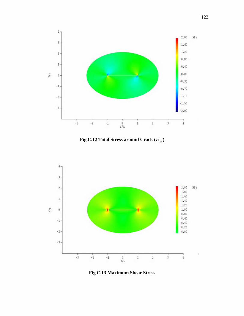
123

Fig.C.12 Total Stress around Crack ( xyσ )

Fig.C.13 Maximum Shear Stress

124

Fig.C.14 Mean Normal Stress

Fig.C.15 Maximum Principal Stress

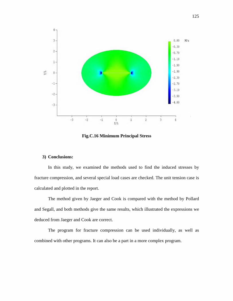
125

Fig.C.16 Minimum Principal Stress

3) Conclusions:

In this study, we examined the methods used to find the induced stresses by

fracture compression, and several special load cases are checked. The unit tension case is

calculated and plotted in the report.

The method given by Jaeger and Cook is compared with the method by Pollard

and Segall, and both methods give the same results, which illustrated the expressions we

deduced from Jaeger and Cook are correct.

The program for fracture compression can be used individually, as well as

combined with other programs. It can also be a part in a more complex program.

126

APPENDIX D

EQUATIONS USED FROM PERKINS AND KONG’S PAPER

1) Calculating Bottom hole Pressure:

1 2 3iwf R fP P P P P P= + ∆ + ∆ + ∆ + ∆ ....................................................... (D.1)

In which:

2t

1 22t

0.5 (Ln(K t/( c (0.5 r ))+0.80907) ( )1 0.5 (Ln(K t/( c (0.5 r ))+0.80907)

P Pφ µφ µ

× × × × × ×∆ = ∆

− × × × × × × ........ (D.2)

and

( , , )( , , ) iD DL

i wf

P P tP tP P

............................................................ (D.3)

and 2D tP =0.5 (Ln(K t/( c (0.5 r ))+0.80907)φ µ× × × × × ×

In which Pi is the initial reservoir pressure, and Pwf is the pressure at the inner

boundary, as shown in the plan view of Fig.3.1: the inner boundary is the hot/cold

boundary, and the outer boundary is the water/oil boundary.

So, here

1

1 2

( , , )( , , ) iD DL

i wf

P P t PP tP P P P

..................................... (D.4)

then,

2t

1 2 22t

0.5 (Ln(K t/( c (0.5 r ))+0.80907)/(1 ) ( )1 0.5 (Ln(K t/( c (0.5 r ))+0.80907)D DP P P P P

(D.5)

in which Ct is the total compressibility. The most reasonable value of r appears to be a1.

However, Kucuk and Brigham (1979.) did not mention a criterion for selection of r

127

except that it should be large enough; On the other hand, they also provided a different

expression for pressure that does not require r. namely:

1 (ln 2.19537)2wD DLP t ............................................................ (D.6)

in which:

6

2

3.6 10 oDL

t

k ttc L

......................................................................... (D.7)

1 67.2*10 wDo

qP Pk h

............................................................. (D.8)

As will be seen, the results from the previous Eqn. are closer to those of P&G.

This might be because ΔP1 in the latter equation is equal to the sum of ΔP1, ΔP2 and ΔP3,

so that the accuracy is less than the separated calculation.

ΔP2 and ΔP3 are calculated from the following equations:

1 12

0 0

ln( ) /(2 )w w rwa bP i kk ha b

................................................. (D.9)

0 03 ln( ) /(2 )w w rw

f

a bP i kk hL

.............................................. (D.10)

31/ 4

2 3 40.00074[ ](1 )

w w ff

i L EP

hµυ

∆ =−

..................................................... (D.11)

2) Calculating the semi-axes of the cool region and flooded zone:

iW Qt ...................................................................................... (D.12)

/( *(1 ))wt i or wiV W S S ...................................................... (D.13)

(1 ) (1 )

w w i

gr gr w w or o o o

C WVcC C S C S r

..................... (D.14)

128

2 22

41 2* /( * * ) 0.5* ( ) 4ff

VcF Vc h LL h

.......................... (D.15)

2 22

42 2* /( * * ) 0.5* ( ) 4wtwt f

f

VF V h LL h

....................... (D.16)

01*( 1 ) / 2

1fa L FF

.......................................................... (D.17)

01*( 1 ) / 2

1fb L FF

........................................................... (D.18)

11*( 2 ) / 2

2fa L FF

......................................................... (D.19)

11*( 2 ) / 2

2fb L FF

......................................................... (D.20)

3) Calculating Fracture Length:

1 1 22(1 ) f

UEPr

................................................................ (D.21)

in which:

1 iwf f=P -3 PP ................................................................................ (D.22)

1 min 1 1( )H T P ........................................................ (D.23)

in which 1T and 1P are calculated from the following equations:

0 01

0 0 0 0

0.9 2

0 0

0.7740

0

( / )(1 ) 1[ ]1 ( / ) 1 ( / )

1(1/{1 [1.45( ) 0.35( ) ]2 2 2

[1 ( ) ]})

T b aE T b a b a

h hb b

ba

ν σβ

− ∆= +

∆ + +

× + +

× +

.................................... (D.24)

129

0 01

0 0 0 0

0.9 2

0 0

1.360

0

( / )(1 ) 1[ ]1 ( / ) 1 ( / )

(1/{1 [1.45( ) 0.35( ) ]2 2

[1 (1 ) ]})

P b aEJ P b a b a

h hb b

ba

ν σ− ∆= +

∆ + +

× + +

× + −

................................. (D.25)

1 23grc

JE

.......................................................................... (D.26)

4) The Bisection method for finding Lf is as the following:

Over some interval the function is known to pass through zero because it changes

sign. Evaluate the function at the interval’s midpoint and examine its sign. Use the

midpoint to replace whichever limit that yields the same sign for F(x). After each

iteration, the bounds containing the root decrease by a factor of two. If after n iterations

the root is known to be within an interval of size n , then after the next iteration it will be

bracketed within an interval of size

1n = / 2n .................................................................................. (D.27)

Repeat the process until n is less than a small number such as 1.0E-06. The

corresponding value of x is the root of the function, i.e. the fracture length Lf.

For the problem at hand the function is F(x) =LHS-RHS. To find the root, select

Lf=X1 which makes F(x1)<0 while Lf=X2 which makes F(x2)>0. A root will be bracketed

in the interval (X1, X2). In this study, the assumed data are X1=0.6 and X2=1.0E04.

130

VITA

Name: Jun Ge Permanent Address: Harold Vance Department of Petroleum Engineering, 3116 TAMU, College Station, TX 77843-3116 Email Address: [email protected] Education: Chinese University of Geosciences, WuHan, HuBei, China B.S., Geology, June 2000 Peking University, Beijing, China M.S., Economic Geology, July 2003 Texas A&M University, College Station, Texas, USA M.S., Petroleum Engineering, December 2009 Affiliation: Society of Petroleum Engineers

modeling and analysis of reservoir response to stimulation...

Documents