modeling and design considerations for a micro-hydraulic
TRANSCRIPT

Modeling and Design Considerations for aMicro-Hydraulic Piezoelectric Power Generator
by
Onnik Yaglioglu
B.S. Mechanical EngineeringBogazici University, 1999
SA8KERMASSACHUSETTS INSTITUTE
OF TECHNOLOGY
OCT 2 5 2002
LIBRARIES
Submitted to the Department of Mechanical Engineering and theDepartment of Electrical Engineering and Computer Sciencein Partial Fulfillment of the Requirements for the Degrees of
Master of Science in Mechanical Engineering
and
Master of Science in Electrical Engineering and Computer Science
at theMASSACHUSETTS INSTITUTE OF TECHNOLOGY
February 2002
© 2002 Massachusetts Institute of Technology. All rights reserved.
SignatureofAuthor................................Department of Mechanical Engineering
January 15, 2002
C ertified b y ......... .. *.0 . ... ... .. ... ... .. ... ... .. ... ..Nesbitt W. Hagood, IV
Aa iate Professor of Aeronautics and AstronauticsThesis Supervisor
Certified by.....
Accepted by ..................
Alexander H. SlocumProfessor of Mechanical Engineering, MacVicar Faculty Fellow
Departmental Reader
.. ..of...6........... ..... ... ......Ain A. Sonin
fhifap4Dep n t Coy ttee on Graduate StudentsM/4K p nt*pfgg n Mechanical Engineering
Accepted by .................... ..-.............Arthur C. Smith
Chairman, Committee on Graduate StudentsDepartment of Electrical Engineering and Computer Science

F>
Modeling and Design Considerations for a
Micro-Hydraulic Piezoelectric Power Generator
by
Onnik Yaglioglu
Submitted to the Department of Mechanical Engineering and theDepartment of Electrical Engineering and Computer Science
on January 15, 2002, in partial fulfillment of therequirements for the degrees of
Master of Science in Mechanical Engineering
and
Master of Science in Electrical Engineering and Computer Science
Abstract
Piezoelectric Micro-Hydraulic Transducers are compact high power density transducers, whichcan function bi-directionally as actuators/micropumps and/or power generators. They are
designed to generate 0.5-1W power at frequencies of ~10-20kHz, resulting in high power densitiesapproaching 500W/kg. These devices are comprised of a main chamber, two actively controlled
valves, a low-pressure reservoir and a high-pressure reservoir. This thesis reports on modeling
and design considerations for Micro-Hydraulic Piezoelectric Power Generators. Since these
devices are complex fluid and structural systems, comprehensive simulation tools are needed
for effective design. Operation of each subcomponent of the device is highly coupled and every
design decision should be made with remaining components in mind. A system level simulationtool has been developed using Matlab/Simulink, by integrating models for different energydomains, namely fluids, structures, piezoelectrics and circuitry. The simulation architecture
allows for integration of the elastic equations of structural members into the dynamic simulations
as well as monitoring of important parameters such as chamber pressure, flowrate, and various
structural component deflections and stresses. Using the simulation, the operation of the system
is analyzed and important design considerations are evaluated. Fluidic oscillations within the
system are analyzed and an optimization procedure for the membrane structure within the main
chamber is presented. Parameter studies are performed for different piezoelectric materials,system compliances, and circuit topologies. Tradeoffs between operation conditions and theireffect on the performance are discussed. A design procedure is developed. Results indicate thatsystem efficiency is highly dependent on compliances within the device structure, the type of
piezoelectric material used and rectifier circuit topology.
Thesis Supervisor: Nesbitt W. Hagood, IVTitle: Associate Professor of Aeronautics and Astrtonautics
Departmental Reader: Alexander H. Slocum
Title: Professor of Mechancial Engineering, MacVicar Faculty Fellow
3


Acknowledgements
Special thanks goes to my family and my girlfriend. Without their support, this thesis could
not have been completed. I would like to thank to my family for their continuous support and
care. And, many thanks to my girlfriend for her patience and support.
Many thanks to Hagop Hachickian and Hachickian family for their continuous support and
help since the very first day I came to Boston.
I would like to thank my colleagues in the MHT group. Yu Hsuan Su, thanks very much for
your help and valuable insights you provided me. David Roberts, thanks for your guidance and
valuable discussions. And Jorge Carretero, thanks for your support throughout the completion
of this thesis.
I also would like to thank to Harry Callahan for his help in circuit modeling. Boston is
missing you and your guitar sound! Next time you come, we are definitely going to jam!
Finally, I would like to thank to Boston. It is such a great city to have fun and relax. I
don't know what I would do without the R&B and Jazz clubs. And, Cantab Lounge is always
going to be my favorite place.
This thesis is dedicated to my family.
This research work was sponsored by DARPA under Grant #DAAG55-98-1-0361 and by
ONR under Grant #N00014-97-1-0880.
5

.. . .,,. """ a . - - -0

Nomenclature
PHPR high pressure reservoir pressure
PLPR low pressure reservoir pressure
Pch main chamber pressure
APch main chamber pressure band
Pint-in inlet valve intermediate pressure
Pint-out outlet valve intermediate pressure
Qin inlet valve flow rate
Qout outlet valve flow rate
voin inlet valve opening
VOcat outlet valve opening
CS structural compliance of main chamber
Ceff effective compliance of the main chamber
Vo initial fluid volume of the main chamber
Of bulk modulus of working fluid
E Young modulus of Silicon
V Poissons ratio of silicon
p density of working fluid
Dch chamber diameter
Dpis piston diameter
Rvc valve cap radius
Wt tether width
Heh chamber height
7

Dp piezoelectric element diameter
LP piezoelectric element length
trop top support structure thickness
tbot bottom support structure thickness
tPis piston thickness
ttetop top tether thickness
ttebot bottom tether thickness
x~is piston deflection
Xte tether deflection
Xb bottom support structure deflection
AVtP volume swept by top support structure
AVPis volume swept by deflection of piston
A VP5 volume swept by bending of piston
AVe volume swept by tether bending
Fte force between piston and tethers
F, force on piezoelectric element
d 33 piezoelectric constant
D open circuit compliance of piezoelectric element
E closed circuit compliance of piezoelectric element
k33 coupling coefficient of piezoelectric element
keff effective coupling factor
V, voltage on piezoelectric element
I, current through piezoelectric element
V6 battery voltage
IA current through battery
QP charge on piezoelectric element
U-d depolarization stress of piezoelectric element
f operation frequency
7/ system efficiency
W generated power
8

Contents
1 Introduction
1.1 Microhydraulic Piezoelectric Transducers . . . .
1.2 Configuration and Operation . . . . . . . . . . .
1.3 Preliminary Design Considerations . . . . . . . .
1.4 Objective, Scope and Organization of the Thesis
2 Piezoelectric Power Generation and Circuitry
2.1 Introduction . . . . . . . . . . . . . . . . . . . . . . . . . . . . . . . . . . . . . . .
2.2 Previous Work . . . . . . . . . . . . . . . . . . . . . . . . . . . . . . . . . . . . .
2.3 Theoretical Background . . . . . . . . . . . . . . . . . . . . . . . . . . . . . . . .
2.4 Circuitry Considerations . . . . . . . . . . . . . . . . . . . . . . . . . . . . . . . .
2.4.1 M odeling . . . . . . . . . . . . . . . . . . . . . . . . . . . . . . . . . . . .
2.4.2 Simulation and Analysis . . . . . . . . . . . . . . . . . . . . . . . . . . . .
2.5 Other Circuits . . . . . . . . . . . . . . . . . . . . . . . . . . . . . . . . . . . . .
2.6 Piezoelectric Material Comparison . . . . . . . . . . . . . . . . . . . . . . . . . .
2.7 Conclusion . . . . . . . . . . . . . . . . . . . . . . . . . . . . . . . . . . . . . . .
3 Energy Harvesting Chamber and Preliminary Design Considerations
3.1 Configuration and Operation of the Energy Harvesting Chamber . . . . . . . . .
3.2 Modeling . . . . . . . . . . .. . ... . .. . .. . . . . . .. . . . . . . .. . . ..
3.2.1 Piezoelectric Cylinder . . . . . . . . . . . . . . . . . . . . . . . . . . . . .
3.2.2 Chamber Continuity . . . . . . . . . .. . .. . . .. . . . . .. . . . .. .
3.2.3 Fluid Model . . . . .. . . . . . . . . . . . . . . . . . . . . . . . . . . . ..
9
21
21
23
26
28
31
31
32
36
40
41
44
59
62
66
67
67
69
69
70
72

3.2.4 Circuitry . . . . . . . . . . . . . . . . . . . . . . . ... . . .
3.3 Working Fluid.... . . .....
3.4 Simulation and Analysis . . . . . . . . . . . . . . . . . . . . . . . .
3.4.1 Energy Harvesting Chamber and Full Bridge Rectifier . . .
3.4.2 Energy Harvesting Chamber and Full Bridge Rectifier with
tector Circuit . . . . . . . . . . . . . . . . . . . . . . . . . .
3.5 D iscussion . . . . . . . . . . . . . . . . . . . . . . . . . . . . . . . .
3.6 Summary and Conclusion . . . . . . . . . . . . . . . . . . . . . . .
4 Detailed Model of the Energy Harvesting Chamber
4.1 Analysis of a Simplified Chamber Structure . . . . . . . . . . . . .
4.2 Detailed Analysis of Structural Components . . . . . . . . . . . . .
4.2.1 Top Support Structure . . . . . . . . . . . . . . . . . . . . .
4.2.2 Bottom Support Structure . . . . . . . . . . . . . . . . . . .
4.2.3 Piston . . . . . . . . . . . . . . . . . . . . . . . . . . . . . .
4.2.4 Piston Tethers . . . . . . . . . . . . . . . . . . . . . . . . .
4.3 Simulation Architecture . . . . . . . . . . . . . . . . . . . . . . . .
4.4 Conclusion . . . . . . . . . . . . . . . . . . . . . . . . . . . . . . .
5 Further Design Considerations and Design Procedure
5.1 Further Design Considerations . . . . . . . . . . . . . . . . . . . .
5.1.1 Fluidic Oscillations . . . . . . . . . . . . . . . . . . . . . . .
5.1.2 Chamber filling and evacuation . . . . . . . . . . . . . . . .
5.1.3 Tether Structure Optimization . . . . . . . . . . . . . . . .
5.1.4 Operation Conditions and Trade-offs . . . . . . . . . . . . .
5.1.5 Bias Pressure . . . . . . . . . . . . . . . . . . . . . . . . . .
5.1.6 Scaling Issues . . . . . . . . . . . . . . . . . . . . . . . . . .
5.2 Design Procedure . . . . . . . . . . . . . . . . . . . . . . . . . . . .
5.2.1 Preliminary design decisions . . . . . . . . . . . . . ... . . .
5.2.2 Parameters imposed by active valve design . . . . . . . . .
5.2.3 Parameters imposed by fabrication process . . . . . . . . .
Voltage I
115
.115
.115
.122
.124
.129
.135
.138
.141
.. 141
.. 142
.. 143
10
. . . 77
. . . 77
. . . 78
. . . 79
De-
* . . 83
* . . 91
* . . 96
99
. . . 99
. . 102
. . . 102
* . . 104
* . . 106
* . . 107
* . . 110
* . . 114

5.2.4 Design Procedure.
5.3 Design Examples.....
5.3.1 Design Example 1
5.3.2 Design Example 2
5.4 Summary . . . . . . . . .
. . . . . . . . . . . . . . . . . . . . . . . . . . . . . .1 4 3
. . . . . . ... . . . . . . . . . . . . . . . . . . . . . . . 1 4 7
. . . . . . . . . . . . . . . . . . . . . . . . . . . . . . . 1 4 7
. . . . . . . . . . . . . . . . . . . . . . . . . . . . . . . 1 4 8
. . . . . . . . . . . . . . . . .. . . . . . . . . . . . . . . 1 5 7
6 Conclusions and Recommendations for Future Work 159
6.1 Sum m ary . . . . . . . . . . . . . . . . . . . . . . . . . . . . . . . . . . . . . . . . 159
6.2 Recommendations for Future Work . . . . . . . . . . . . . . . . . . . . . . . . . . 162
A Simulink Block Diagrams
B Matlab Files
C Maple Files
171
181
187
11


List of Figures
1-1 (a) Configuration of power generator (b) Configuration of actuator/ micopump.
The actuator/micropump configuration can also be operated with check valves
instead of active valves, which are necessary for power generator configuration. 22
1-2 Device layout for power generator configuration. Top and bottom packaging
pyrex layers not shown. . . . . . . . . . . . . . . . . . . . . . . . . . . . . . . . . 24
1-3 Generic operation duty cycle of the power generator. . . . . . . . . . . . . . . . . 25
1-4 (a) 5-layer device for subcomponent testing (b) Complete 9-layer device (c) SEM
of micromachined tethered piston structure [7]. . . . . . . . . . . . . . . . . . . . 27
1-5 Overall system architecture for the heel strike power generation configuration. 28
2-1 Graphic illustration of electromechanical energy conversion and definition of the
piezoelectric coupling factor k33 given in [18] (a) Conversion of energy from a
mechanical source to electrical work (b) Conversion of energy from an electrical
source to mechanical work. . . . . . . . . . . . . . . . . . . . . . . . . . . . . . . 38
2-2 Alternative idealized work cycles given in [8]. . . . . . . . . . . . . . . . . . . . . 39
2-3 Alternative circuits to rectify and store the electrical energy generated by the
piezoelectric elem ent. . . . . . . . . . . . . . . . . . . . . . . . . . . . . . . . . . 41
2-4 Simulation architecture used to simulate the piezoelectric element connected to
the full bridge rectifier. The force is imposed on the piezoelectric element. . . . 45
2-5 Time histories from the simulation of the piezoelectric element connected to the
full bridge rectifier for the case of imposed force. The generated power is IbVb. . 47
2-6 Force vs. deflection and voltage vs. charge plots of the piezoelectric element
compressed under the applied force for the case of full bridge rectifier. . . . . . . 48
13

2-7 Effect of battery voltage on power. . . . . . . . . . . . . . . . . . . . . . . . . . 49
2-8 Effect of bias force on the workcycle. . . . . . . . . . . . . . . . . . . . . . . . . . 50
2-9 General presentation of the work cycle of the piezoelectric element in terms of
stress, strain, electric field and charge density for the case of regular diode bridge. 52
2-10 Illustration of the effective coupling factor for the case of regular diode bridge. . 53
2-11 Time histories from the simulation of the piezoelectric element connected to the
full bridge rectifier and voltage detector circuit. The time intervals between the
dashed lines present the intevals where the switch(SCR) is in its "on" state. . . . 55
2-12 Force vs. deflection and voltage vs. charge plots of the piezoelctric element
compressed under the applied force for the case of full bridge rectifier and voltage
detector circuit. . . . . . . . . . . . . . . . . . . . . . . . . . . . . . . . . . . . . . 56
2-13 General presentation of the work cycle of the piezoelectric element in terms of
stress, strain, electric field and charge density for the case of the full bridge
rectifier and voltage detector circuit. . . . . . . . . . . . . . . . . . . . . . . . . . 57
2-14 Illustration of the effective coupling factor for the full bridge rectifier and voltage
detection circuit. . . . . . . . . . . . . . . . . . . . . . . . . . . . . . . . . . . . 58
2-15 Other alternative circuits for piezoelectric power generation. . . . . . . . . . . . . 59
2-16 Simulation results of the piezoelectric element shunted by a resistor for different
resistance values. . . . . . . . . . . . . . . . . . . . . . . . . . . . . . . . . . . . . 60
2-17 Comparison of resistive shunting(at optimum resistance) with full bridge rectifier
and full bridge rectifier with voltage detector. . . . . . . . . . . . . . . . . . . . . 61
2-18 Simulation results of the full bridge rectifier connected to a capacitor. . . . . . . 62
2-19 Force vs. deflection plot from the simulation of the full bridge rectifier with
additional inductor. . . . . . . . . . . . . . . . . . . . . . . . . . . . . . . . . . 63
2-20 Effective coupling factors of the diode bridge and the diode bridge with voltage
detector as a function of the couping coefficient.. . . . . . . . . . . . . . . . . . . 64
2-21 Piezoelectric Material Comparison: (a) Effective coupling factor (b) Energy density. 65
3-1 Energy harvesting chamber configuration. . . . . . . . . . . . . . . . . . . . . . . 68
3-2 Duty cycles of generic operation of the energy harvesting chamber. The valve
openings have the same duty cycle as the flowrates and are not shown here. . . . 68
14

3-3 Device schematics showing pressures at different locations. . . . . . . . . . . . . . 73
3-4 Valve orifice representation:(a) Valve cap geometry and fluid flow areas, (b) Rep-
resentation of flow through the valve as a flow contraction followed by a flow
expansion. . . . . . . . . . . . . . . . . . . . . . . . . . . . . . . . . . . . . . . . . 74
3-5 Look-Up tables used for flow loss contraction and expansion coefficients. The
loss coefficients are obtained from [51]. . . . . . . . . . . . . . . . . . . . . . . . . 75
3-6 Simulation architecture used in Simulink. . . . . . . . . . . . . . . . . . . . . . . 79
3-7 Simulation of the energy harvesting chamber attached to the full bridge rectifier
circuit.. . . . . . . . . . . . . . . . . . . . . . . . . . . . . . . . . . . . . . . . . . 80
3-8 Force vs. displacement curve of the piezoelectric element from the simulation of
the harvesting chamber attached to the full bridge rectifier. . . . . . . . . . . . . 82
3-9 Simulation of the energy harvesting chamber attached to the full bridge rectifier
and voltage detector circuit. The time intervals between the dashed lines present
the intervals where the switch(SCR) is in its "on" state. . . . . . . . . . . . . . . 84
3-10 Force vs. displacement curve of the piezoelectric element from the simulation of
the energy harvesting chamber attached to the full bridge rectifier and voltage
detector circuit. . . . . . . . . . . . . . . . . . . . . . . . . . . . . . . . . . . . . . 85
3-11 Time histories of the force and deflection of the piezolelectric element. . . . . . . 85
3-12 Force vs. displacement curve of the piezoelectric element and slopes at different
periods of operations. . . . . . . . . . . . . . . . . . . . . . . . . . . . . . . . . . 87
3-13 The effect of effective chamber compliance on force vs. deflection curve and
effective coupling factor. . . . . . . . . . . . . . . . . . . . . . . . . . . . . . . . . 90
3-14 Flowrate and frequency requirement for 0.5 W power requirement. . . . . . . . . 92
3-15 System efficiency as a function of the effective chamber compliance.. . . . . . . . 93
3-16 Required flowrates for 0.5 power generation. Comparison of different piezoelectric
elements and different circuitry. . . . . . . . . . . . . . . . . . . . . . . . . . . . 94
3-17 Required frequencies for the 0.5W power requirement. Comparison of different
piezoelectric materials and circuitry. Note that the required frequency in the
case of regular rectifier is independent of the chamber compliance. . . . . . . . . 95
15

3-18 Comparison of different piezoelectric materials and circuitry in terms of system
efficiency. . . . . . . . . . . . . . . . . . . . . . . . . . . . . . . . . . . . . . . . . 96
3-19 Maximum system efficiency(which corresponds to the case where the effective
compliance of the chamber is zero)as a function of the coupling coefficient. . . . 98
4-1 (a) Simplified chamber structure consisting of a fluid chamber with a compliant
wall (b) Deformation of the top plate and swept volume. . . . . . . . . . . . . . 100
4-2 Comparison of fluidic and structural compliances for a generic chamber structure
at different chamber diameters for fixed chamber height and top plate thickness. 101
4-3 (a) Schematic illustrating the dimensional parameters of the chamber, (b) defor-
mation of structural components and sign conventions, (c) free body diagrams
and sign conventions. Deflections are exaggerated . . . . . . . . . . . . . . . . . 103
4-4 Model of the bottom support structure: circular plate with a circular hole at its
center with guided boundary condition at inner radius b and clamped boundary
condition at outer radius a. . . . . . . . . . . . . . . . . . . . . . . . . . . . . . . 105
4-5 Model of the piston: circular plate with a circular hole at its center with guided
boundary condition at inner radius b and clamped boundary condition at outer
radius a. . . . . . . . . . . . . . . . . . . . . . . . . . . . . . . . . . . . . . . . . . 106
4-6 Model of the top tether: circular plate with a circular hole at its center with
guided boundary condition at inner radius b and clamped boundary condition
at outer radius a. . . . . . . . . . . . . . . . . . . . . . . . . . . . . . . . . . . . . 108
4-7 Simulation architecture used to integrate the elastic equations into system level
sim ulation.. . . . . . . . . . . . . . . . . . . . . . . . . . . . . . . . . . . . . 113
5-1 Helmholtz Resonator. . . . . . . . . . . . . . . . . . . . . . . . . . . . . . . . . . 116
5-2 Simulation of the chamber with constant overall compliance for different channel
geom etries . . . . . . . . . .. . . . . . . . . . . . . . . . . . . . . . . . . . . . . . 118
5-3 Comparison of flowrate time histories for different L/A ratios. . . . . . . . . . . 118
5-4 Simulation of the chamber attached to circuitry for different channel geometries. 119
5-5 Effect of L/A ratio on pressure band and generated power. . . .'. . . . . . . . . 120
5-6 Effect of valve opening on the pressure band in the chamber. . . . . . . . . . . . 123
16
5-7 Effect of operation frequency on the pressure band in the chamber. . . . . . . . . 123
5-8 (a) Schematic illustrating the hypotethical chamber (b) good tether design pro-
viding large piezoelectric element compression (c) poor tether design, either too
thin or large width, resulting in low chamber pressure and small piezoelectric
element compression (d) poor tether design, either very thick or small width,
resulting in large pressures but small piezoelectric element compression. . . . . . 125
5-9 (a) Piston deflection for different tether thicknesses and widths,(b) correspond-
ing pressures in the chamber (c) compliance of the chamber. The dashed line
corresponds to the hypotethical case where piston diameter is equal to chamber
diameter and there is perfect sealing. . . . . . . . . . . . . . . . . . . . . . . . . . 126
5-10 (a) Schetch illustrating tether deflection. (b),(c),and (d) show the stress com-
ponents on the bottom surface and deflected shape of the tether for 3 different
cases. (b) good tether design, (c) poor tether design where the tether is too com-
pliant, and (d) poor tether design where the tether is too stiff. . . . . . . . . . . 127
5-11 (a) SEM picture of micromachined piston structure [7](b)detailed view of the
tether and the fillet. . . . . . . . . . . . .. . . . . . . . . . . . . . . . . . . . . . . 128
5-12 Comparison of different piezoelectric materials in terms of required operation
frequency at different chamber diameters for a power requirement of 0.5W. . . . 131
5-13 Comparison of different piezoelectric materials in terms of required flowrate at
different chamber diameters for a power requirement of 0.5W. . . . . . . . . . . . 132
5-14 Comparison of different piezoelectric elements in terms of system efficiency for
different reservoir pressures and chamber diameters. . . . . . . . . . . . . . . . . 134
5-15 Required operation frequency and flowrate for different power requirements at
different chamber diameters (PHPR = 2MPa, piezoelectric material: PZN - PT ).135
5-16 Schematic illustrating the effect of bias pressure.(a) not biased case (b) biased case136
5-17 Effect of bias pressure on required frequency, flowrate and efficiency. . . . . . . . 137
5-18 Design procedure.. . . . . . . . . . . . . . . . . . . . . . . . . . . . . . . . . . . . 144
5-19 (a) System layout (b) System level simulation architecture (c) The chamber and
piezo block in the overall system architecture which was developed in Chapter 4. 146
5-20 Tether structure design. Piston deflection shown for different tether widths. . . 148
17

5-21 Simulation time histories of the design example 1 . . . . . . ... . . . . . . . . . . 150
5-22 Simulation time histories of the design example 1. . . . . . . . . . . . . . . . . . 151
5-23 Simulation time histories of the design example 1. . . . . . . . . . . . . . . . . . 152
5-24 Simulation time histories of the design example 2. . . . . . . . . . . . . . . . . . 154
5-25 Simulation time histories of the design example 2. . . . . . . . . . . . . . . . . . 155
5-26 Simulation time histories of the design example 2. . . . . . . . . . . . . . . . . . 156
A-1 Simulink model of the piezoelectric element. . . . . . . . . . . . . . . . . . . . . . 172
A-2 Simulink model of the diode bridge. . . . . . . . . . . . . . . . . . . . . . . . . . 173
A-3 Simulink model of the diode bridge attached to an inductor, voltage detector and
SCR(Silicon Controlled Rectifier). . . . . . . . . . . . . . . . . . . . . . . . . . . 174
A-4 Implementation of the voltage detector circuit. . . . . . . . . . . . . . . . . . . . 175
A-5 Simulink model of the full system including the chamber, piezoelectric element,
fluid models and circuitry. . . . . . . . . . . . . . . . . . . . . . . . . . . . . . . . 176
A-6 Simulink model of the main chamber and the piezoelctric element. . . . . . . . . 177
A-7 Simulink model of the inlet valve and fluid channel.. . . . . . . . . . . . . . . . . 178
A-8 Simulink model of the outlet valve and fluid channel. . . . . ... . . . . . . . . 179
B-1 Matlab code ised in Chapter 3 to calculate the required frequency, flowrate and
efficiency for different circuitry. . . . . . . . . . . . . . . . . . . . . . . . . . . . . 182
B-2 Matlab code used in Chapter 5 to calculate the required frequency, flowrate and
efficiency of the system attached to regular diode bridge for different reservoir
pressures and chamber diameters . . . . . . . . . . . . . . . . .... . . . . . . . 183
B-3 Matlab code used for tether optimization. . . . . . . . . . . . . . . . . . . . . . . 184
B-4 Matlab code used for writing system parameters into the workplace to be read
by the Simulink model for the system level simulation. . . . . . . . . . . . . . . . 185
18

List of Tables
2.1 Geometry and operation conditions used in simulation . . . . . . . . . . . . . . .
2.2 Comparison of circuitry in terms of energy density and effective coupling factor .
2.3 Properties of different piezoelectric materials . . . . . . . . . . . . . . . . . . . .
3.1 Comparison of different working fluids . . . . . . . . . . . . . . . . . . . . . . . .
3.2 The geometry and operation conditions used in the simulation . . . . . . . . . .
3.3 Summary and comparison of circuitry in terms of performance indices . . . . . .
5.1
5.2
5.3
Summary of preliminary design decisions applied to the design examples.
Summary of design and performance parameters of design example 1. .
Summary of design and performance parameters of design example 2. .
45
63
66
78
78
97
147
149
153
19

tQr

Chapter 1
Introduction
This chapter presents the configuration, operation and motivation of microhydraulic-piezoelectric
power generators. Preliminary design considerations are discussed. The objective, scope and
organization of the thesis are presented.
1.1 Microhydraulic Piezoelectric Transducers
Transducers are devices that convert physical energy from one form to another. Actuators
and power generators are examples of transducer devices. The performance and usefulness
of a transducer for most applications are highly dependent on two important characteristics:
compactness and power density, that is, power output of the transducer per its unit volume.
Conventional transducers, generally, not only tend to be heavy and bulky, but are also limited
in terms of power transduction capabilities because of their low bandwidths. For instance,
conventional hydraulic systems possess high single-stroke work, but their power densities are
greatly reduced by their large mass. Recent advances in active materials technology have
led to the development of many compact solid-state transducers. However, the power output
from these solid-state transducers is fairly limited for most macro applications. Although the
single-stroke work output of solid-state materials such as piezoelectric materials is relatively
small, such materials possess very high bandwidths, and as such, are capable of high power
output. However, since most applications do not require high frequency actuation, the high
bandwidth potential of piezoelectric materials is not fully utilized. Since a transducer's power
21

M=ValveeC Htrler
High Presure Inlet Main Chamber and Outlet Low PresureReservoire(HPI) Valve Piezoelectric Element Valve Reervoire(LPR)
Recificr
Power Out
(a)
ValveController
LOW Presure iniet Main Chamber and Outlet High PresireReservoire(UR) Valve Piezoelectric Element Valve Rsroire(HPR)
Eiechida
Power In
(b)
Figure 1-1: (a) Configuration of power generator (b) Configuration of actuator/ micopump.The actuator/micropump configuration can also be operated with check valves instead of activevalves, which are necessary for power generator configuration.
output is the product of its single stroke energy and its bandwidth, it is feasible to create high
performance transducers by combining high single-stroke force of a hydraulic system and high
frequency displacements of a piezoelectric element in a synergistic manner[1]. This concept
can be further exploited to create high performance transducers with very high power densities
by miniaturizing the transducer systems. The state-of-the-art micromachining (or MEMS)
technology has the potential to allow for the implementation of this concept at the micro scale.
Research and development of microfluidic devices has received a significant amount of inter-
est in the past years. The feasibility of micromachining many of the key building blocks (flow
channels, pumps, active/passive valves) of a micro-fluidic system including the integration of
solid-state materials such as piezoelectric materials to actuate valves has already been demon-
strated, and researchers are now striving to create complete microfluidic systems. However, the
microfluidic devices developed thus far mostly feature small flow conductance, limited stroke,
and low power density, and are mostly geared towards small flow/force applications such as
microdosing of fluids. An extensive literature review on microfluidic devices can be found in
22
[2].
A unique feature of piezoelectric microhydraulic transducers is their ability to operate as
both an actuator and a power generator, by merely reversing the direction of their operation. As
actuators, these transducers transform electrical energy input into mechanical/hydraulic energy
output, and as power generators, the transducers transform mechanical/hydraulic energy input
into electrical energy that can be stored in a battery or a capacitor. These high performance
transducers can significantly enhance the scope of micromachined transducers technology by
enabling many novel applications. When utilized as actuators, they are capable of extending
the usefulness of active material based structural actuation beyond small strain applications [1].
These actuators can also be useful in miniature robotics. As power generators, the transducers
can extract electrical energy from wasted mechanical energy sources such as vibrations of oper-
ating machinery, heel strike of human gait, wind, sound and function as disposable batteries for
numerous small electronic devices in both civilian and military applications. A literature survey
about piezoelectric power generation will be presented in Chapter 2. Detailed information and
comparisons of various transducers can be found in [2] where a feasibility analysis of Micro
Hydraulic Transducers has been performed.
1.2 Configuration and Operation
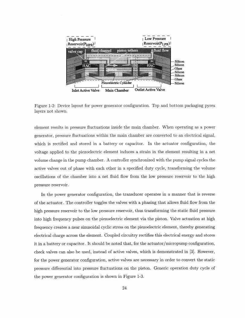
The concept of piezoelectric micro-hydraulic transducer (MHT) is schematically illustrated in
Figure 1-1 for actuator and power generator configurations. The transducers are comprised of
the following generic components: the main chamber which houses a piezoelectrically driven
tethered piston, two actively controlled valves, a low-pressure fluid reservoir (LPR), and a high-
pressure fluid reservoir (HPR). The power generator configuration requires rectification circuitry
to rectify and store the voltage generated by the piezoelectric element. The two active valves,
one operating between the HPR and the main chamber and the other one operating between
the main chamber and the LPR regulate the fluid flow into and out of the main chamber. The
piezoelectric element within the pump chamber serves as the main energy transducing element.
A detailed drawing of the device is shown in Figure 1-2.
When operating as an actuator/pump, the electrical signal applied to the piezoelectric
23
-. - --.------------------- -
High Pressure I Low PressureI Reservoir(PHpR)i i Reservoir(PLpR) I
SiliconSSilicon
Glass- Silicon
SiliconGlass
- ieoeecri~yider Silicon
Inlet Active Valve Main Chamber Outlet Active Valve
Figure 1-2: Device layout for power generator configuration. Top and bottom packaging pyrexlayers not shown.
element results in pressure fluctuations inside the main chamber. When operating as a power
generator, pressure fluctuations within the main chamber are converted to an electrical signal,
which is rectified and stored in a battery or capacitor. In the actuator configuration, the
voltage applied to the piezoelectric element induces a strain in the element resulting in a net
volume change in the pump chamber. A controller synchronized with the pump signal cycles the
active valves out of phase with each other in a specified duty cycle, transforming the volume
oscillations of the chamber into a net fluid flow from the low pressure reservoir to the high
pressure reservoir.
In the power generator configuration, the transducer operates in a manner that is reverse
of the actuator. The controller toggles the valves with a phasing that allows fluid flow from the
high pressure reservoir to the low pressure reservoir, thus transforming the static fluid pressure
into high frequency pulses on the piezoelectric element via the piston. Valve actuation at high
frequency creates a near sinusoidal cyclic stress on the piezoelectric element, thereby generating
electrical charge across the element. Coupled circuitry rectifies this electrical energy and stores
it in a battery or capacitor. It should be noted that, for the actuator/micropump configuration,
check valves can also be used, instead of active valves, which is demonstrated in [3]. However,
for the power generator configuration, active valves are necessary in order to convert the static
pressure differential into pressure fluctuations on the piston. Generic operation duty cycle of
the power generator configuration is shown in Figure 1-3.
24

(a) Chamber PreureP ---- - - -- - -- - -- -
- - - - -.-- - - - - ---- -- -
Pma
T2 T 3T/2 2T(b) Flowrate
-Inlet
-- Outlet
T2 T 3 T/2 2T
(c) Piston Deflection
T/2 T 3 T2 2T
Figure 1-3: Generic operation duty cycle of the power generator.
Active valves are comprised of a similar chamber/piston structure, called hydraulic ampli-
fication chamber (HAC), which incorporates a fluid enclosed in the volume between the piston
and the valve diaphragm, which effectively serves to amplify the small displacements of the
piezoelectric material into significantly larger displacements of the valve cap and effectively
transmits the high force actuation capability of the piezoelectric material. As the piston in the
active valve is displaced by the piezoelectric element, the pressure of the compressed fluid acts
to deform the smaller area valve membrane located at the top of the chamber. Deflection of the
rigid cap at the center of the valve membrane blocks fluid flow through the corresponding fluid
orifice. The utilization of the hydraulic amplification chamber also leads to minimization of the
actuator material, and thus helps in achieving high power densities. The ability to microma-
chine the device provides the scope to further miniaturize the system to micro scales, leading
to higher valve frequencies and therefore enhanced device power densities.
As shown in Figure 1-2, in each chamber, namely inlet HAC, main chamber (energy har-
vesting chamber) and outlet HAC, a piezoelectric element is sandwiched between the device
25

structure and a moveable piston plate. The piston plate is sufficiently thick for rigidity and
is tethered to the chamber wall through thin flexible diaphragms that extend radially from
the outer edges of the cylinder. The structure effectively constitutes a piston that can move
vertically up and down when a net force is applied to it.
The prototype MHT device consists of a 9-layer stack of pyrex and silicon micromachined
layers, as shown in Figure 1-2 and Figure 1-4. Sealing of the piston in the main chamber
is provided by annular tethers which are created through Deep Reactive Ion Etching (DRIE)
of a SOI wafer. The tether thickness (~10pm) is defined by the SOI device layer, and the
buried oxide acts as an etch stop. All glass layers are patterned by conventional diamond
core drilling. Piezoelectric cylinders are core drilled from piezoelectric substrate plates, onto
which a Ti-Pt-AuSn-Au multilayer film is sputter-deposited for eutectic bonding. The device
assembly is accomplished through anodic bonding of the glass layers to the silicon layers at
3000 C, a process which also enables the AuSn eutectic alloy to melt. Upon cooling, the alloy
solidifies, bonding the piezoelectric cylinders to the silicon layers. Detailed information about
the fabrication techniques developed for piezoelectric micro-hydraulic transducers can be found
in[3], [6], and [7].
1.3 Preliminary Design Considerations
The proposed MHT devices derive their enhanced performance from several inherent design
features. For efficient device operation, the compliances within the system, which result from
the deformations of the structural members like piston, tether and support structures, and com-
pression of the working fluid within the chambers should be minimum. This implies that the
chambers should have small volumes and the structural members should be as thick as possible.
This introduces trade-offs between fabrication limitations and design requirements. The type
of piezoelectric element also affects system efficiency since the coupling coefficient of the ele-
ment determines the electromechanical energy conversion work-cycle. For the power generator
configuration the rectifier circuit topology is another factor affecting system efficiency, since
it determines the electromechanical energy conversion work-cycle along with the piezoelectric
material.
26
)(b)
3 e etce tereer-
tether piston tte
(C)
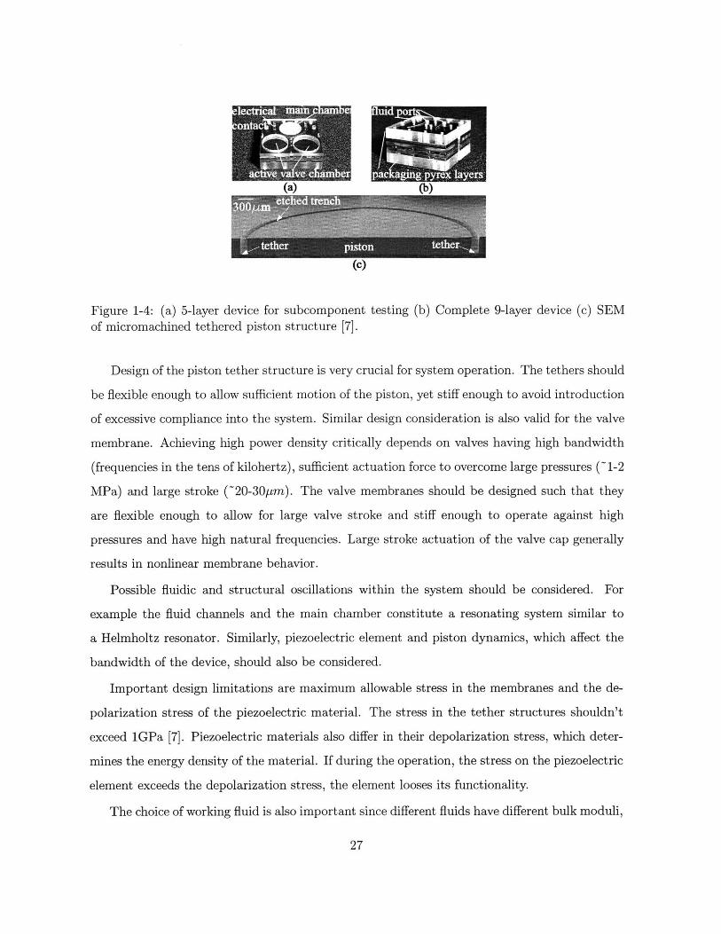
Figure 1-4: (a) 5-layer device for subcomponent testing (b) Complete 9-layer device (c) SEMof micromachined tethered piston structure [7].
Design of the piston tether structure is very crucial for system operation. The tethers should
be flexible enough to allow sufficient motion of the piston, yet stiff enough to avoid introduction
of excessive compliance into the system. Similar design consideration is also valid for the valve
membrane. Achieving high power density critically depends on valves having high bandwidth
(frequencies in the tens of kilohertz), sufficient actuation force to overcome large pressures (~1-2
MPa) and large stroke (~20-30Qm). The valve membranes should be designed such that they
are flexible enough to allow for large valve stroke and stiff enough to operate against high
pressures and have high natural frequencies. Large stroke actuation of the valve cap generally
results in nonlinear membrane behavior.
Possible fluidic and structural oscillations within the system should be considered. For
example the fluid channels and the main chamber constitute a resonating system similar to
a Helmholtz resonator. Similarly, piezoelectric element and piston dynamics, which affect the
bandwidth of the device, should also be considered.
Important design limitations are maximum allowable stress in the membranes and the de-
polarization stress of the piezoelectric material. The stress in the tether structures shouldn't
exceed 1GPa [7]. Piezoelectric materials also differ in their depolarization stress, which deter-
mines the energy density of the material. If during the operation, the stress on the piezoelectric
element exceeds the depolarization stress, the element looses its functionality.
The choice of working fluid is also important since different fluids have different bulk moduli,
27
Heel StrikeF - -- - - - - - - -- - - - - - - -r -- - - -I
Force Coupler - - Disp
- Heel Package
HPR L Miniature LPRL - Pump I L -
Pck Ph
Valve, Fluid & Chamber Valve, Fluid &
el Dynamics Pressure, Flow el DynamicsQ Q
SF, X P, I DV F1 Xvi -5 -- Chip Level
Hydraulic I Piston & I HydraulicAmplifier I Ithers Amplifier
- - - I I - -- I
F X KF X F~1~F F x
LPiezo Piezo Piezo
VP p I,
F - - - - - - - - - - - -
Drive Circuitry Harvesting Circuit Drive Circuitry ElectronicsL A _ - ------------ - I--
Scope ofthe thesis
Figure 1-5: Overall system architecture for the heel strike power generation configuration.
densities and viscosities.
1.4 Objective, Scope and Organization of the Thesis
Since these devices are complex, comprehensive simulation tools are needed for effective de-
sign. Operation of each subcomponent of the device is highly coupled and every design decision
should be made with remaining components in mind. The simulation tool should allow for the
monitoring of important parameters such as chamber pressure, flowrate, and various structural
component deflections and stresses. A system level simulation tool is needed which should be
developed by integration of different energy domains, namely fluids, structures, piezoelectric
material and circuitry. The challenges in modeling and simulation are: microscale fluid flow,
incorporation of membrane behavior into dynamic simulation, prediction of structural compli-
ances and incorporation of the elastic equations of the structural members into simulation.
The MHT group at MIT Active Material and Structures Laboratory(AMSL) has obtained
good experimental correlation for subcomponent models from tests on piezoelectrically driven
28

piston/tether structure, hydraulic amplification chamber structure and valve membrane [6],
flow tests through macro disc valves [4], and micropumps [3].
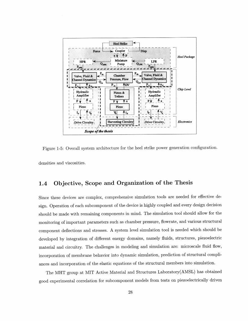
This thesis focuses on the modeling and design of piezoelectric microhydraulic transducers
used as power generators. The system architecture for a possible application, namely heel strike
power generation configuration is shown in Figure 1-5. The scope of the thesis is shown with
the dashed line in the system architecture. The heel package design will not be discussed. Also
design of the active valve structure will not discussed, which is detailed in [5]. Orifice models
developed in [4] are used for fluid flow through the valves.
The objectives of this thesis are:
- To develop a comprehensive system level model and simulation tool to analyze the main
chamber and the associated fluid channels and valves,
- To gain insight into system operation and understand the factors affecting the system
performance,
- Develop a design procedure, which should be complemented by the design of the active
valves.
The organization of the thesis is as follows: Chapter 2 presents an analysis of piezoelectric
power generation based on linear electromechanical energy conversion. Effect of circuitry and
piezoelectric material on energy density and effective coupling factor is discussed. Chapter 3
presents a simple model of the energy harvesting chamber, simulations with the coupled circuitry
and preliminary design considerations. The interaction of the main chamber and the circuitry is
discussed. The circuits presented in Chapter 2 and different piezoelectric materials are compared
in terms of flowrate and frequency requirements for a given pressure differential and power, and
in terms of system efficiency. Chapter 4 presents the detailed modelling of the energy harvesting
chamber and investigates the contribution of different structural components on the effective
compliance of the chamber. It also presents the simulation architecture used for integrating
elastic equations into system level simulation. Chapter 5 discusses further design considerations
for choosing chamber geometry with regard to operation conditions like maximum pressure,
operation frequency and flowrate. Parameter studies are performed and a design procedure
is developed. Chapter 6 summarizes important results and conclusions presented in previous
chapters and presents recommendations for future work.
29

C
C:

Chapter 2
Piezoelectric Power Generation and
Circuitry
This chapter presents an analysis of piezoelectric power generation based on linear electrome-
chanical energy conversion. Effect of circuitry and piezoelectric material on electromechanical
energy conversion and energy density is discussed.
2.1 Introduction
Piezoelectric materials are mostly used as sensors and actuators. Since they are capable of
electromechanical energy conversion and some have high coupling coefficients, which is an in-
dication of the efficiency of the electromechanical energy conversion, they can be also used as
power generators from ambient vibration or impact energy, and as structural vibration dampers.
The idea and the governing principles are the same for power generation and structural vibra-
tion damping, using piezoelectric elements and passive circuit elements. Damping of structural
vibrations with passive electrical circuit elements is discussed in [15] and [14]. This method
eliminates the need for viscoelastic materials or mechanical vibration absorbers attached to the
structure, or complex amplifiers which are required by the piezoelectric materials for active
structural control systems [15]. The coupling between mechanical and electrical domains pro-
vided by the piezoelectric effect allows the damping mechanism to be implemented as electrical
circuit elements rather than physical masses, springs and dampers. Most of the discussions
31

which are valid for the structural damping applications with piezoelectric elements are valid
for the power generation from ambient vibration or impact energy with piezoelectric elements.
In both cases, the purpose is to transfer as much energy from the mechanical to the electrical
domain. The transferred energy to the electrical domain can be either dissipated or stored.
If a piezoelectric element is shunted with a resistor or with a resistor and inductor network,
the converted electrical energy is basically dissipated. However, if the piezoelectric element is
connected to a rectifier circuit, a diode bridge for example, with a capacitor or battery, the
converted electrical energy can be stored.
2.2 Previous Work
Structural damping with piezoelectric elements shunted with a resistor and a resistor-inductor
network is analyzed in [15]. In the resistive shunting the electromechanical energy conversion
efficiency depends on the operation frequency, and the optimum frequency depends on the
resistance value. In other words, optimum efficiency is obtained when the impedance of the
piezoelectric element is equal to the impedance of the resistance. Shunting with a resistor
and inductor introduces an electrical resonance, which can be optimally tuned to structural
resonances for maximum vibration damping.
Linear shunting components such as resistive elements or resistive-inductive-capacitive cir-
cuits produce behavior analogous to that of viscoelastic damping materials and tuned proof-
mass dampers. Nonlinear piezoelectric shunting for structural damping using a piezoelectric
element attached to a diode bridge and a DC voltage is presented in [14]. The rectified DC shunt
performs less well in terms of energy conversion efficiency compared with the resistive shunt at
optimum frequency. However, unlike the resistive shunt, the rectified DC shunt is independent
of frequency and the transferred energy can be recovered depending on the implementation of
the DC voltage source.
Power generation characteristics of piezoelectric elements in response to impact loads are
investigated in [9], [10] and [11]. In the first two, a ball is dropped from a certain height onto a
piezoelectric plate vibrator. In the first one, the piezoelectric vibrator is shunted with a resistor
and the efficiency of transformation from mechanical to electrical energy in terms of initial
32

height and shunted resistance value is investigated. The efficiency is defined as the ratio of the
electrical energy dissipated in the resistor to the initial impact energy. The input mechanical
impact energy effects the efficiency due to nonlinearity in the vibrator and as expected there
is an optimum resistance value. They conclude that efficiency increases with decreasing input
impact energy, increasing mechanical quality factor Qm, increasing electromechanical coupling
coefficient k 2 and decreasing dielectric loss tan 6. They obtain a maximum efficiency of 52%.
The same authors of [9] investigate the power generation characteristics of the same sys-
tem attached to a diode bridge and capacitor instead of a resistor in [10]. In this case the
transformation efficiency is defined as the ratio of the impact energy to the energy stored in
the capacitor. As the capacitance of the capacitor increases, the electric charge increases be-
cause the duration of the oscillation becomes longer and the output voltage decreases. They
conclude that there exists an optimum capacitance value in terms of transformation efficiency.
They obtain a maximum efficiency of 35%. It should be noted that, if a force were imposed
on a piezoelectric element, the voltage on the capacitor would always increase until half of the
open circuit voltage which corresponds to the maximum stress on the piezoelectric element,
regardless of the capacitance of the capacitor. The value of the capacitance would change the
duration in which the maximum voltage is reached and the stored energy in the capacitor would
be proportional to its capacitance, since the maximum voltage is constant for a given maximum
stress. In the paper discussed above, the force on the piezoelectric element is not imposed, it
is determined depending on the impedances of the vibrator and the capacitor. In this case, the
impedance matching principle cannot be applied since the system is nonlinear because of the
diode bridge. No power density figures are reported in [9] and [10].
Piezoelectric power generation from thermal energy is presented in [20]. This paper discusses
an energy conversion system in which thermal energy is converted to high frequency, high voltage
electric a.c energy. The conversion system is composed of a thermal-acoustic natural heat engine
and a piezoelectric transduction system to convert the acoustic energy to electric energy.
Another system to convert acoustic energy to electric energy is presented in [35]. The
device is designed to convert waste acoustic energy, e.g. in automobile or airplane jet engines
to electrical energy in a predetermined frequency range. The system consists of a piezoelectric
bending element, means for mounting the piezoelectric bending element in an acoustic energy
33

path and a tuning means mounted on to the piezoelectric bending element to set the resonant
frequency of oscillation of the piezoelectric bending element within the predetermined frequency
range.
The idea of piezoelectric power generation from- the ocean waves is patented in [27]-[32]
by Ocean Power Technologies, Inc. The motivation in these studies is to utilize the enormous
amount of mechanical energy present in the oceans. [27] relates to the generation of electrical
power from waves on the surface of bodies of water, and particularly to the conversion of the
mechanical energy of such waves to electrical energy by means of piezoelectric materials. The
system consists of piezoelectric elements in the form of one or a laminate of sheets, each sheet
having an electrode on opposite surfaces thereof, a support means for maintaining the structure
in a preselected position within and below the surface of the water. In certain embodiments, the
elements are designed to enter into mechanical resonance in response to the passage of waves
thereover, increasing the mechanical coupling efficiency between the waves and the elements.
Similar approaches are presented in [28] and [30]. In [28], a float on a body of water is mechani-
cally coupled to a piezoelectric material member for causing alternate straining and de-straining
of the member in response to the up and down movement of the member in response to passing
waves, thereby causing the member to generate electric energy. The output impedance of the
float is matched to the input impedance of the member for increasing the energy transfer from
the float to the member. In [30], the system comprises a weighted member supported from a
piezoelectric element for applying a preselected strain to the element. In one embodiment, the
element is supported by a float floating on the surface of the water. In another embodiment,
the element is supported above the surface of the water and the weighted member, of negative
buoyancy, is immersed in the water. Means are provided for tuning the natural frequency of
the system to cause it to enter into mechanical resonance in response to passing waves. Similar
approaches are presented in [29], [31] and [32].
Some circuitry considerations for piezoelectric power generation are presented in [33] and
[26]. [33] presents a DC bias scheme for improved efficiency for applications including elec-
trostrictive materials, which have very weak piezoelectric characteristics. However, if a DC
bias is applied, the piezoelectric characteristics can be significantly increased. [26] presents an
alternative rectifier circuit, which includes an inductor, a SCR(silicon controlled rectifier) and
34

a voltage detection circuit in the conduction path between the piezoelectric element and the
storage element, a capacitor for example. The object is to optimize the transfer of the energy
produced by a piezoelectric transducer to a load. Another circuit designed for a wide variety
of applications is presented in [36].
Piezoelectric power generation for electronic wristwatch applications is presented in [23]-
[25]. [23] presents an electronic wristwatch having a piezoelectric generator in it. The generator
converts energy from mechanical to electrical energy to drive the electronic wristwatch. The
oscillation of a weight produces mechanical energy as it oscillates. A wheel train transmits
the mechanical energy to the generator by applying a torque to the generator. The generated
voltage is rectified with a diode bridge. Similar systems are presented in [24] and [25].
Piezoelectric power generation from wind energy is presented in [21] and [22]. The system
presented in [22] consists of a piezoelectric transducer mounted on a resilient blade which in
turn is mounted on an independently flexible support member. Fluid flow against the blade
causes bending stresses in the piezoelectric polymer which produces electric power.
Other piezoelectric power generation systems are presented in [34], [39], [38] and [37]. [34]
presents a piezoelectric fluidic-electric generator which consists of a piezoelectric bending ele-
ment, means for driving the piezoelectric bending element to oscillate with the energy of the
fluid stream, and electrodes connected to the piezoelectric element to conduct current generated
by the oscillatory motion of the piezoelectric element. [39] presents a system which consists of
a piezoelectric array which is mounted on one or more tires of a motor vehicle. As the vehicle
drives on the road, the tire is flexed during each revolution to distort the piezoelectric elements
and generate electricity.
Piezoelectric materials are also used in power electronics applications such as transformers.
Piezoelectric transformers are composite resonators made of two bonded piezoelectric parts.
The vibration of one part, excited by an input electric voltage, induces an output voltage
across the other part [40]. In other words, a piezoelectric transformer works by using the direct
and converse piezoelectric effects to acoustically transform power from one voltage and current
level to another [44]. Detailed information about the operational characteristics of piezoelectric
transformers can be found in [41] and [42].
Piezoelectric transformers have low-electric noise because they transmit power by mechan-
35

ical vibration. They can also operate efficiently at high frequencies, whereas conventional
electromagnetic transformers are not efficient at high frequencies because of core loss and cop-
per loss. Other advantages over the electromagnetic transformers can be stated as high voltage
isolation between primary and secondary, high frequency operation leading to reduction in the
filter capacitors and low weight and size [43]. Since piezoelectric transformers have much higher
power densities than electromagnetic transducers, they are very promising as power electronic
components for miniature and lightweight electrical equipment.
Fundamental limits on energy transfer of piezoelectric transformers are discussed in [44].
The discussion details similar considerations to those of the piezoelectric power generation con-
cept. One has to consider the work cycle of electromechanical energy conversion and associated
circuitry. Also the maximum electric field, the maximum surface charge density, the maximum
stress and the maximum strain of the piezoelectric element are important criteria to consider
when determining the limitations of power transfer in a piezoelectric transformer, as well as in
a piezoelectric power generation system.
2.3 Theoretical Background
The linear electromechanical energy conversion process with piezoelectric ceramics is by far the
easiest to handle, since the piezoelectric, dielectric and elastic constants can be applied directly
[8]. In linear analysis, the coefficients mentioned above are assumed to be constant during the
operation. The nonlinearity at high fields and hysteresis effects are ignored, i.e. the losses
due to nonlinear effects are not considered. It is also assumed that the operation frequency is
well below the lowest resonant frequency of the piezoelectric element, i.e. the operation can
be considered as quasi-static. The linear constitutive relationships for a general piezoelectric
element are:
D ET d E
(2.1)S_ d sE T
where D is a vector of electric displacements or charge density(charge/area), S is the vector
of material engineering strains, E is the vector of electrical field in the material(volts/meter),
36
T is the vector of material stresses (force/area), e is the matrix of dielectric constants, d
is the matrix of piezoelectric constants and s is the matrix of compliance coefficients of the
piezoelectric element. The superscripts ()T and ()E signify that the coefficients are measured
at constant stress and constant electric field respectively and the subscript ()t denotes the
matrix transpose. In this chapter, a specific case will be considered where the piezoelectric
element is subjected to compression parallel to the polarization of the element. It is assumed
that the lateral dimensions are small compared to the axial dimension, so that only the axial
stress T3 needs to be considered (T 1 =T2 ~ 0). Or, it can be assumed that, the element is free
to expand in lateral directions so that T3 is the only nonzero stress component. Under these
conditions, equation 2.1 reduces to
D3 Tf d33 E33 133E1(2.2)
S3 d33 s T3
where the first and second subscripts of the piezoelectric, dielectric and elastic constants
denote the orientation of the electric field and the stress respectively.
Quasi-static coupling factors, or coefficients, are very common and useful definitions for
piezoelectric energy conversion. The coupling coefficients are dimensionless and thus they pro-
vide a useful comparison between different piezoelectric materials independent of the specific
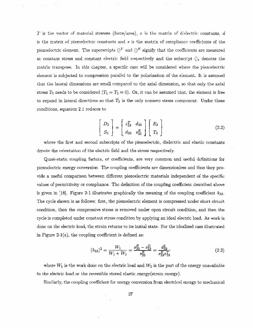
values of permittivity or compliance. The definition of the coupling coefficient described above
'is given in [18]. Figure 2-1 illustrates graphically the meaning of the coupling coefficient k3 3 .
The cycle shown is as follows: first, the piezoelectric element is compressed under short circuit
condition, then the compressive stress is removed under open circuit condition, and then the
cycle is completed under constant stress condition by applying an ideal electric load. As work is
done on the electric load, the strain returns to its initial state. For the idealized case illustrated
in Figure 2-1(a), the coupling coefficient is defined as:
(k33)2 _ W- _ s - s ET3 (2.3)W + W2 SE SnETV~l+ I 2 33 8333
where W1 is the work done on the electric load and W2 is the part of the energy unavailable
to the electric load or the reversible stored elastic energy(strain energy).
Similarly, the coupling coefficient for energy conversion from electrical energy to mechanical
37
W W2
- s3 SLOPE-S 3D SLOPEzE33
SLOPE=s 33 SLOPE =C33
(a) (b)
Figure 2-1: Graphic illustration of electromechanical energy conversion and definition of thepiezoelectric coupling factor k33 given in [18] (a) Conversion of energy from a mechanical sourceto electrical work (b) Conversion of energy from an electrical source to mechanical work.
energy can be derived using the idealized cycle illustrated in Figure 2-1(b). First, the element
is mechanically free when the electric source is connected. Then the element is blocked me-
chanically parallel to polarization before the electric source is disconnected. Then with E3 = 0
the mechanical block is removed and in its place a finite mechanical load is provided. For this
idealized cycle of work illustrated in Figure 2-1(b), the coupling coefficient is defined as:
W T_ s 3=0 d2(k33)2 _ 33 - 33 ._ 3(2.4)
W1 + W2 -6 TsEET
where W1 is the work done on the mechanical load and W2 is the part of the energy
unavailable to the mechanical load.
The idealized work cycles illustrated in Figure 2-1 correspond to the standard definition of
the piezoelectric coupling coefficient. Berlincourt proposes alternative work cycles of reversible
electromechanical energy conversion in [8]. These cycles are shown in Figure 2-2. The first
one, which is illustrated in Figure 2-2(a) corresponds to a case where the element is compressed
with the electric load not connected, i.e. under open circuit conditions, then the electric load
is connected with stress maintained, then the mechanical stress is reduced to zero with the
electric load again disconnected and finally the electric load is connected and the element
38
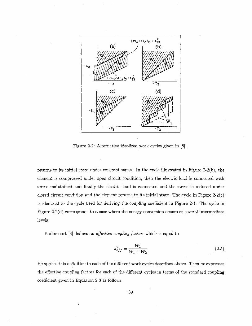
-3
4 JyT 3 1
Figure 2-2: Alternative idealized work cycles given in [8].
returns to its initial state under constant stress. In the cycle illustrated in Figure 2-2(b), the
element is compressed under open circuit condition, then the electric load is connected with
stress maintained and finally the electric load is connected and the stress is reduced under
closed circuit condition and the element returns to its initial state. The cycle in Figure 2-2(c)
is identical to the cycle used for deriving the coupling coefficient in Figure 2-1. The cycle in
Figure 2-2(d) corresponds to a case where the energy conversion occurs at several intermediate
levels.
Berlincourt [8] defines an effective coupling factor, which is equal to
2WT 1k2ff = (2.5)W1+ W2
He applies this definition to each of the different work cycles described above. Then he expresses
the effective coupling factors for each of the different cycles in terms of the standard coupling
coefficient given in Equation 2.3 as follows:
39
keff(a) = k33 2/(1 + k') (2.6)
keff(b) = k33 1 + k3 (2.7)
keff(c) = k33 (2.8)
keff(d) = k33 2/(n + k 3) (2.9)
where k33 is the standard coupling coefficient and n is the number of intermediate levels in
Figure 2-2(d). From equation 2.6 it is apparent that the coupling coefficient corresponding to
the first case in Figure 2-2 is greater than the standard coupling coefficient defined previously.
It is important to note that, the cycles described so far are idealized or hypothetical cycles.
The energy conversion process occurs with the mechanical and electrical energy sources con-
nected and disconnected at will. However, no explanation has been given in terms of how these
cycles can be achieved or approximated in a real application. In other words, the mechanical
and electrical infrastructures which would allow these cycles to occur are not discussed. In this
chapter, conversion from mechanical to electrical energy is considered, with emphasize on the
circuitry used which basically determines the work-cycle. In other words, the rectifying cir-
cuitry is the electrical infrastructure in the power generation process. In the following sections
two different circuit topologies will be analyzed in detail in terms of the effective coupling factor
and energy density.
2.4 Circuitry Considerations
Although in the literature different mechanisms for piezoelectric power generation has been
presented and some studies performed for piezoelectric material characterization for power
generation, no detailed analysis has been presented in terms of effective coupling factor, energy
density and piezoelectric material comparison with regard to circuitry. This section analyzes two
different circuits for rectifying and storing the electrical energy generated by the piezoelectric
element. These circuits constitute examples of nonlinear shunting of piezoelectric elements. The
first one is a regular full bridge rectifier with a battery attached to it. The second circuitry is the
same circuit proposed in [26] for piezoelectric power generation, which consists of a full bridge
40

(a) Full Bridge Rectifier
x k
r/N#' ~ '14 _'4 k
(b) Full Bridge Rectifier and Voltage Detector
F , . x
4
VP 1 +V.- T
Figure 2-3: Alternative circuits to rectify and store the electrical energy generated by the
piezoelectric element.
rectifier, an inductor, a silicon controlled rectifier (SCR), a voltage detector and a capacitor to
store the electrical energy. The circuits are shown in Figure 2-3.
2.4.1 Modeling
This section presents the modeling of the piezoelectric element and the circuitry. The models
are same for the two circuits under consideration except some small differences.
Piezoelectric Element
Linear piezoelectric constitutive relationships are assumed. The form of the constitutive equa-
tions used here is as follows:
. A d33~- -
S 333 -T T
= d3 631 (2.10)
L33 633 .
where D is the charge field, S is the strain, E is the electric field, and T is the stress. For a
cross-sectional area of A and length of Lp, the expressions for the deflection of the piezoelectric
element and the voltage across it become:
P L(D F +3 PXP = (S33FP+ 6p TP 633
(2.11)
41
F
PmcrwcC -~de

V, = TLP( F,- Q)(2.12)P 633 33
where xP is the deflection, Q, is the charge, F, is the force applied on the piezoelectric
cylinder, and V, is the voltage across the piezoelectric cylinder. And the current through the
piezoelectric element is given by:
dQ,I,= dt (2.13)
Diode Bridge
The model of the diode bridge rectifier is based on [52]. The governing equations can be
derived using Kirchoffs laws and diode equations. The notation in Figure 2-3 is used. Applying
Kirchoffs Current Law(KCL) in the junctions 1,2,3,and 4, we get:
I = i4 - i (2.14)
12 = il + i2
13 = i3 - i2
14 = -%3 - 74
The voltages across the diodes are given by:
vi = V-V2 (2.15)
V2 = V3-V2
V3 = V4-V3
V4 = V4-V
Applying Kirchoffs Voltage Law (KVL) around the loops corresponding to the cases where
V, > 0 and V1, <0 we get:
42
-V +v-14-+va = 0 for V >0
Vp+v2+Vb-V4 = 0 for V<0
(2.16)
For the case where V > 0, the currents flowing through diodes #1 and #3 are the same,
and for the case where V, < 0, the currents flowing through diodes #2 and #4 are the same.
Since all the diodes have the same constitutive relationship, we can write:
V - V2 = V4 - V
V4 -V 1 = V -- V2
for V > 0
for V > 0
(2.17)
Recognizing that V, = V1 - V3 ,V2 = 1 b, V4 = 0(ground) and using equation 2.17 we can write:
(2.18)2
14-VpV3 2
2
The voltage - current relationships (constitutive law) of the diodes are:
in = I[exp qv -rkT
in = 0
Vn > 0 (2.19)
V,1 < 0
where the subscript (), denotes the diode number, q = 1.60 x 10⁻¹ 9 (C) is the electron
charge, k = 1.38 x 10- 23(J/K) is the Boltzman constant and T is the temperature(T = 300K).
1 and 1 are diode properties. For CS57-04 diode (Collmer Semiconductor, Inc.), whose values
will be used throughout the thesis, they are measured to be: I = 10-6 and q = 17.25 [19].
43
Diode Bridge and Voltage Detection Circuit
For the diode bridge with the voltage detection circuit, the model is similar. The equations
2.14, 2.15, and 2.19 are valid. However because of the implementation of the voltage detection
circuit and SCR, the simulation architecture is different [53], which is shown in Appendix A.
The voltage detection circuit is not modeled. Only its function is implemented in Simulink.
The Kirchoffs Voltage Law can be written for this case using the notation in Figure 2-3 as:
-Vp+vl+v5+VcR+Vc+va = 0 for V,>0 (2.20)
Vp+V2+V5+VSCR+Vc+V4 = 0 for V<0
The voltage across the inductor is given by:
v tL (2.21)dt
And we can also write
VC =hI 2 (2.22)
2.4.2 Simulation and Analysis
Simulations are performed using Matlab/Simulink. The Simulink blocks and additional details
are given in the Appendix A. The Simulink architecture is shown in Figure 2-4. The piezoelectric
element block includes the constitutive relationships and the circuit block includes the equations
corresponding to the circuitry. The piezoelectric element is excited with an imposed force on
it. The geometry and operation conditions chosen for the simulation are shown in Table 2.1.
The imposed force is sinusoidal with an offset, namely it fluctuates between zero and the
force corresponding to the maximum applicable stress, which is the depolarization stress of the
piezoelectric element. In the case of PZN-4.5%PT, the depolarization stress is measured to
be around 1OMPa [19]. For the chosen piezoelectric cylinder diameter, the maximum force is
31.4N. Detailed comparison of different piezoelectric materials will be presented in section 2.6.
44
t

F
PiezoelectricElement XP
VP Ip p
Circuit
PowerOutpu
Figure 2-4: Simulation architecture used to simulate the piezoelectric element connected to thefull bridge rectifier. The force is imposed on the piezoelectric element.
Length of the piezoelectric element, Lp 1mm
Diameter of the piezoelectric element, DP 2mm
Operation frequency, f 20kHzMaximum force, Fp 31.4NOptimum battery voltage, Vb 90VPiezoelectric material PZN - 4.5%PT
Table 2.1: Geometry and operation conditions used in simulation
45

Full Bridge Rectifier
Simulation Simulation time histories are shown in Figure 2-5. The operation at steady state
can be summarized as follows: During the compression of the piezoelectric element the voltage
on it increases. If it reaches the battery voltage, current starts to flow through the battery and
in fact the piezoelectric element voltage is a little bit higher than the battery voltage during
this interval which causes the current to flow. The amount which the piezoelectric element
voltage exceeds the battery voltage during this interval depends on the diode properties and
other resistances in the system. When the force on the piezoelectric element begins decreasing,
the voltage decreases too and when it becomes less than the battery voltage current stops
flowing through the battery. As the force on the piezoelectric element keeps decreasing, the
voltage on the piezoelectric elements keep decreasing until it reaches the negative value of the
battery voltage. At this point, current begins to flow through the battery, now, however, from a
different branch of the diode bridge, namely through different diodes. Again during this interval
the voltage on the piezoelectric element exceeds the battery voltage a little bit (in this case it
is lower than the negative value of the battery voltage). When the force begins increasing, the
voltage begins increasing too and again no current flows through the battery. Throughout the
operation, the voltage on the piezoelectric element fluctuates between the negative and positive
values of the battery voltage.
In order to get insight into the energy conversion mechanism and to derive the governing
equations in the next section, it is worthwhile to look at the force vs. deflection and voltage vs.
charge plots of the piezoelectric element. These are plotted in Figure 2-6. The most important
observation is that there are two major regimes during the operation: Operation under open
circuit conditions, where the compliance of the piezoelectric element is small, i.e the piezoelectric
element is hard; and operation under closed circuit conditions, where the compliance of the
piezoelectric element is large, i.e the piezoelectric element is soft. The compliances in these
regimes are sD and sE for open circuit and closed circuit conditions respectively. The shaded
region in Figure 2-6 corresponds to the stored electrical energy in one cycle. The generated
power is then simply this energy times the operation frequency.
The battery voltage has an important effect on the performance. The simulation results
presented in Figure 2-5 and Figure 2-6 correspond to the optimum battery voltage (90V). The
46

(a) Applied Force
0.2 0.4 0.6 0.8 1 1.2 1.4
(b) Piezoelectric Element Deflection
0 0.2 0.4 0.6 0.8 1 1.2 1.4
(c) Voltage on Piezoelectric Element
7 7T- . -.. .-.. .-.. .-.. .-.. .-.. .- - --.. ... - - ....- ...- . -------- -
-- ---------
20'0 0.2 0.4 0.6 0.8 1 1.2 1.4
(d) Current through Battery(I)4 F
_ -Jg
3 . . . . . . . . . . . . . . . . .. ..., - .. . . m . m o . - o e m - 4 = - . . . . . . . . . . = . . . . . . . . -.. .=. .---.. ..................
................ .. ............
0 0.2 0.4 0.6 0.8 1 1.2 1.4
Time [10~ s]
Figure 2-5: Time- histories from the simulation of the piezoelectric element connected to thefull bridge rectifier for the case of imposed force. The generated power is IbVb.
47
4u
30
20
10
w --. - -.- N-- ---
0
0
-0.2
-0.4
-0.6-0.8
-1
120
60
-60
..... .. ------ I .... .. I ...... ...... ......I ......I.. ..-.. .- ....- ...------------------- -.. --.
- .. .. . . - . ... . .. -. ......-. ......-. ---- --- . .- . ..
Vb
I r-
n "
F-
-1
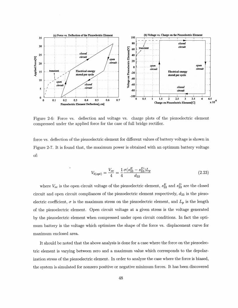
(a) Force vs. Deflection of the Piezoelectric Element (b) Voltage vs. Charge on the Piezoelectric Element35 100
80 closed3060 tranient ci
25- closed25 - . -.-.- -.-.-..- 40 -ciruit 4open:
S . 20 - -- --20020 -- - -- - -- --- :i d
cirdt cim*tA 15 - ransient . Electrical energy - - --- 2rstse .erc.le-2 Electrical energyStored per cycle stored per cycle
-p 8 -40 -1 0 -- - - - - - -.. . . -. . -. -
csclosed
5 -- --.... . - C&C dt . . . .--. . ... .... os-80 ci...t - --
01000 0.1 0-2 0.3 0.4 0.5 0.6 0.7 0 0.5 1 1.5 2 2.5 3 3.5 4 4.5
Piezoelectric Element Deflection[pjm] Charge on Piezoelectric Element[C] x 10
Figure 2-6: Force vs. deflection and voltage vs. charge plots of the piezoelectric element
compressed under the applied force for the case of full bridge rectifier.
force vs. deflection of the piezoelectric element for different values of battery voltage is shown in
Figure 2-7. It is found that, the maximum power is obtained with an optimum battery voltage
of:
Vb(opt) = Voc = 1 3(s3 (2.23)4 4 d33
where Voc is the open circuit voltage of the piezoelectric element, sE and sD are the closed
circuit and open circuit compliances of the piezoelectric element respectively, d33 is the piezo-
electric coefficient, o- is the maximum stress on the piezoelectric element, and Lp is the length
of the piezoelectric element. Open circuit voltage at a given stress is the voltage generated
by the piezoelectric element when compressed under open circuit conditions. In fact the opti-
mum battery is the voltage which optimizes the shape of the force vs. displacement curve for
maximum enclosed area.
It should be noted that the above analysis is done for a case where the force on the piezoelec-
tric element is varying between zero and a maximum value which corresponds to the depolar-
ization stress of the piezoelectric element. In order to analyze the case where the force is biased,
the system is simulated for nonzero positive or negative minimum forces. It has been discovered
48
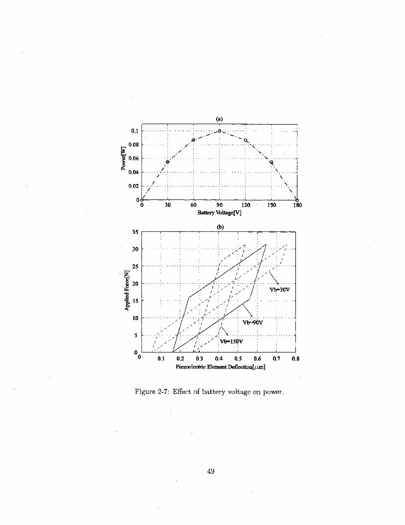
(a)
- ---- -- --- -. -. . -. .-. . -. . -. -. . -. -. -- -- -- - - - - - - -
-- - .-.- - - - -- - - - .- - -. -. - .- . --
- -.- .-.-.-.-.-.-.- - ,- - --- - - -
30 60 90 120Battery Voltage[V]
150 180
(b)
Vb=30V
Vb=150V
0.1 0.2 0.3 0.4 0.5 0.6Piezoelectric Element Deflection[gm]
0.7 0.8
Figure 2-7: Effect of battery voltage on power.
49
0.1
0.08
0.06
0.04
0.02
35
30 -
25 -
20 -r 2
S15 -
10 -
5
00
nmU O0

30
20
ELlo
.10
-20
-30
(a) Force vs. Deflection of the Piezoelectric Element
-AF-
.-.-.-.. .-
-. .. . . . . .-.. . . . . . . . . . . .. . .. . . . . . .
.A
... .. .. . .I .. .. .. . . . . . . . . . L . . . .. . . . J . . . . . ..
-0.75 -0.5 -0.25 0 0.25 0.5 0.75
Piezoelectric Element Deflection[pm]
Figure 2-8: Effect of bias force on the workcycle.
that the optimum battery voltage depends only on the stress band on the piezoelectric element,
namely on the difference of the maximum and minimum stresses on the piezoelectric element.
Figure 2-8 shows the workcycles for different applied forces which have the same peak to peak
values but different bias values. For each case the optimum battery voltage is the same since
the stress band resulting from each case is the same. Equation 2.23 can be rewritten as:
VAo-(st-stD)LpVb 4 ) i d3
(2.24)
where Aa is the stress band on the piezoelectric element.
Analysis In order to investigate the work cycle of the piezoelectric element, we can analyze
the stress vs. strain and electric field vs.charge density plots of the piezoelectric element in
detail. Important features of the work cycle is shown in Figure 2-9 which corresponds to the
optimum battery voltage case. It is important to not that, the dashed line, which corresponds
to the case in which the piezoelectric element would be compressed in closed circuit conditions,
passes through the middle of the stress vs. strain curve. We also know the slopes of the curve
50

in the two different regimes, namely open circuit and closed circuit regimes. Using simple
geometry, we can derive the coordinates of the corner points. From the voltage vs. charge
plot in Figure 2-6 we see that the voltage of the piezoelectric element fluctuates between the
positive and negative values of the battery voltage. Using constitutive relationships to calculate
the corresponding charge on the piezoelectric element at different states, we can get the electric
field vs. the charge density plot. These are shown in Figure 2-9.
The electrical energy stored (per piezoelectric element volume) in the battery in one cycle
for the case of optimum battery voltage, which is equal to the enclosed area by the stress vs.
strain or electric field vs charge density curve can obtained using simple geometry from Figure
2-9 as:
E=-( sgs)o3 (2.25)
where st and st are the closed circuit and open circuit compliances of the piezoelectric
element respectively and a- is the maximum stress on the piezoelectric element.
Then, the generated power by the piezoelectric element can be expressed as:
W = ( - st)aVPf (2.26)
where V is the volume of the piezoelectric element and f is the operation frequency. From the
above equation it can be seen that the power depends heavily on the stress on the piezoelectric
element. The most important limitation on piezoelectric power generation is the depolarization
stress. For stresses larger than this, piezoelectric element coefficients degrade and performance
decreases drastically. Each piezoelectric element has a different depolarization stress, which
constitute an important factor when determining their feasibility as power generators. Detailed
comparison of different piezoelectric elements will be presented in Section 2.6.
Effective coupling factor for an electromechanical energy conversion mechanism, in this case
a system which converts mechanical energy into electrical energy is defined as the ratio of the
mechanical work done on the system to the electrical energy stored in one cycle. This definition
is the same as the one used to derive the coupling coefficient. This is illustrated in Figure 2-10.
From the above definition we can write:
51

u,,,~- -.---------------------
2
O rmi-
0
(a) Stress vs. Strain
Au [sE K+SD]33P 2
(O'm. + ,,,)sg33
Strain (S) 2
(b)Electric Field vs. Charge Density
--------- - - - -- -- - -- ---
4 [SE,- S,33]4d 3
0
o -[s . 334d33
0 d,,(-. + 3 ,)
4 Charge Density (D)
d33(3a.+ od
4
Figure 2-9: General presentation of the work cycle of the piezoelectric element in terms of
stress, strain, electric field and charge density for the case of regular diode bridge.
52
-N
-~ -A
g csD331 UE33
u 2
SE3
z4- 1

u
6W
(T
W
2 2Strain (S)
Figure 2-10: Illustration of the effective coupling factor for the case of regular diode bridge.
k2 - (2.27)eff W1 + W2
Again using geometry, the effective coupling factor can be derived in terms of the piezoelec-
tric material compliances as:
k2 2(sE -8sD)kef f=33 +3s (2.28)
The definition of the coupling coefficient of a piezoelectric element was given in section 2.3.
Using equations 2.3 and 2.28, the effective coupling factor for the full bridge rectifier case can
be expressed in terms of the coupling coefficient as:
2k 2
k 2 = 3k 3 2(2.29)ff 33 +2
Full Bridge Rectifier and Voltage Detection Circuit
The operation of this circuit is as follows: The voltage detector circuit detects the voltage right
after the diode bridge (V2). Initially, the SCR is in "off" state. If V2 reaches its maximum and
begins decreasing, the voltage detector sends a current signal to SCR which turns it on. If the
detected voltage reaches zero, the voltage detector sends another signal to SCR which turns it
53
7

off.
Simulation The simulation architecture is the same as in Figure 2-4. The implementation
of the switching of the SCR and additional details of the Simulink model are presented in
Appendix A. Again, the force is imposed on the piezoelectric element. The geometry, operation
frequency and the piezoelectric material are the same as in the previous section. The time
histories resulting from the simulation are shown in Figure 2-11.
Again, in order to get insight into the energy conversion mechanism and to derive the
governing equations, it is worthwhile to look at the force vs. deflection and voltage vs. charge
plots for the piezoelectric element. These are plotted in Figure 2-12. We can see that there are
two basic operation regimes. The first one is operation under open circuit conditions, where the
compliance of the piezoelectric element is low, i.e the piezoelectric element is hard. The second
operation regime is defined with the almost flat lines in Figure 2-12. This regime corresponds
to the time intervals, where the switch (SCR) is on. In this regime, the piezoelectric material
behaves as a very soft material.
Since the SCR is initially closed, the piezoelectric element is first compressed under open
circuit conditions, until the applied force reaches its maximum and begins to decrease (period
1-2). In this period, the voltage on the piezoelectric element reaches the open circuit voltage
corresponding to the maximum stress applied on the element. Once the force begins to decrease,
the detected voltage, which is the rectified piezoelectric element voltage, begins to decrease too,
which causes the switch to turn on. After the switch turns on, the voltage decreases very fast
and the piezoelectric element is compressed with a very small effective stiffness. The switch
turns again off once the voltage reaches zero. During the period when the switch is on (2-3),
the piezoelectric element is squeezed until the point, as if it was being squeezed under the same
stress and closed circuit conditions. We can verify this by looking to the voltage vs. charge
plot. In state 3, the voltage on the piezoelectric element is zero and the force on it is almost
the maximum force. Of course, this rapid compression occurs in finite time and during this
time interval, the force decreases a little bit, which results in the almost flat region in force vs.
deflection plot. The shorter the "on" state, the flatter will be the line. It can be concluded
that, the performance of the system with this cycle depends highly on the time history of the
54

(a) Applied Force
- -. .-. . -. .
- -. .
-. .-.- -.-. . . -.
0.2 0.4
- --- -- - - --
- ------------
0.6 0.8 1 1.2 1.4
0-0.2
-0.4-0.6
-0.8
4
(b) Piezoelectric Element Deflection
-. . . . . . . ..------ .............. -----.......... ...........--I-- .. - -. - - - -------. . ............. ----
-. . ..~j................. . .
- -- ----- - ----------.--.. . . .-... . . . . . ............... . -.- ---1--.-- - -r
0 0.2 0.4 0.6 0.8 1 1.2 1.4
(c) Detected Voltage400 I
300 . ............. ..- - - - - - - - - - - - -
0-0 0.2 0.4 0.6 0.8 1 1.2 1.4
(d) Current through Inductor40
3 0 - - -.--.. .-. . --.. .-.. .-. .- - ----. . .. .- -.
20 - - - ..--..--.
10 -- -- --.... -..... . . .... .
n0 0.2 0.4 0.6 0.8 1 1.2 1.4
Time[10~4s]
Figure 2-11: Time histories from the simulation of the piezoelectric element connected to thefull bridge rectifier and voltage detector circuit. The time intervals between the dashed linespresent the intevals where the switch(SCR) is in its "on" state.
55
40
30-
20-
10*
0
r~q
S
- . I I Z!bl.
I

35
30
25
20
15
10
5
00
(a) Force vs. Deflection of the Piezoelectric Element
, , - - Full bridge rectifier- -- Rectifier and Voltage detector
Open C&cuit 3
- n switch . -.-.-. topen:
'--
-.. -. .-. .- ..;.-.. .-.-
switch
OP0.1 0.2 0.3 0.4 0.5 0.6
Piezoelectric Element Deflection[pm]
Figure 2-12: Force vs. deflection andcompressed under the applied force for
circuit.
(b) Voltage vs. Charge on the Piezoelectric Element
II00
0
0.7 0.8
- - - ull bridge rectifier
300 -...... Rectifier andVolage detector
witch200 -- - - - - -
opn Opi--
-100 -- - - . -open~
-200 --- - ch .rcz t
-300
0 1 2 3 4 5Charge on Piezoelectric Element[C]
voltage vs. charge plots of the piezoelctric elementthe case of full bridge rectifier and voltage detector
applied force.
Analysis After the observations done in the previous section, we can derive the equations
which determine the maximum strain and charge of the piezoelectric element, the energy stored
per cycle and the effective coupling factor. To keep the analysis more general, we again analyze
the work cycles in terms of stress vs. strain and electric field vs. charge density plots. Important
features of the idealized work cycles are shown in Figure 2-13. As mentioned earlier, there is a
finite time associated with the transition between states 2-3 and 4-1, where the force does not
remain at its maximum value. This time interval depends highly on the value of the inductor
used. In the simulation, an inductor of 20mH is used. It should be also mentioned that, the
capacitor has to be large enough to avoid saturation. The simulation results are very close to
the idealized cycles, which can be seen comparing Figure 2-12 and Figure 2-13. It should be also
mentioned that, the difference between these figures should be counted partly on a simulation
artifact. The switch operation and open circuit and closed circuit conditions are simulated
using very large and very small resistances respectively. It can be concluded that, the idealized
curves in Figure 2-13 are very good approximations to the actual work cycles.
56
6 7x 10
.- - - - - ;W-.. - - - r- - ---- --- -- I- - - - - - - .. - - 1, - . nft
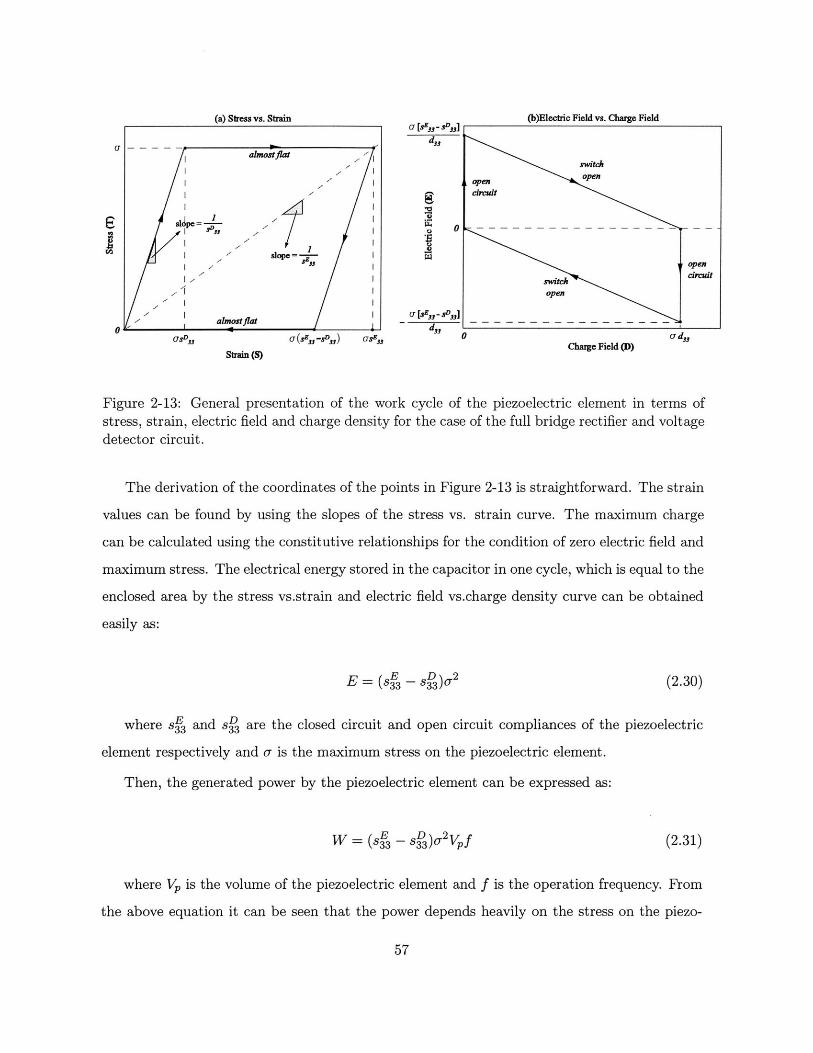
33abnosflat
open
I ope
t 6ircuit
a t- - -- --
1open
0sD.1 S (8) (sX -sD 33) "sg3 0Charge Field (D) u d3
Figure 2-13: General presentation of the work cycle of the piezoelectric element in terms ofstress, strain, electric field and charge density for the case of the full bridge rectifier and voltagedetector circuit.
The derivation of the coordinates of the points in Figure 2-13 is straightforward. The strain
values can be found by using the slopes of the stress vs. strain curve. The maximum charge
can be calculated using the constitutive relationships for the condition of zero electric field and
maximum stress. The electrical energy stored in the capacitor in one cycle, which is equal to the
enclosed area by the stress vs.strain and electric field vs.charge density curve can be obtained
easily as:
E = (s - sD)a2 (2.30)
where s E and sD are the closed circuit and open circuit compliances of the piezoelectric
element respectively and o- is the maximum stress on the piezoelectric element.
Then, the generated power by the piezoelectric element can be expressed as:
W (s33 33)0 s Pf (2.31)
where V is the volume of the piezoelectric element and f is the operation frequency. From
the above equation it can be seen that the power depends heavily on the stress on the piezo-
57
(a) Stress vs. Strain (b)Electric Field vs. Charge Field

U
eIW
2Cj
0
Strain (S)
Figure 2-14: Illustration of the effective coupling factor for the full bridge rectifier and voltage
detection circuit.
electric element. The power generated with this circuitry is four times bigger than the power
generated using the full bridge rectifier under the same conditions, namely same applied force
and frequency.
Using the definition in equation 2.27 and from Figure 2-14, the effective coupling factor can
be obtained as:
k 2 W 2(s_ - s) (232)
effw±W 24.32)e -W1 + W2 2s33-_S3
Using equations 2.3 and 2.32, we can express the effective coupling factor of the coupling
coefficient as:
2k2ff =2k3 (2.33)
It is very interesting to note that the diode bridge and the voltage detection circuit proposed
by Smalser in (26] result in the hypothetical electromechanical energy conversion work-cycle
proposed by Berlincourt [8]. This cycle is shown in Figure 2-2(a). The expression in equation
2.6 is identical to equation 2.33.
58

Figure 2-15: Other alternative circuits for piezoelectric power generation.
2.5 Other Circuits
This section discusses some other alternative circuits for piezoelectric power generation, shown
in Figure 2-15. The geometry, operation frequency and the piezoelectric material used for the
simulations are the same as in the previous section.
A much simpler circuit than the ones presented in previous sections is that involving just
a resistor. Resistive shunting of piezoelectric elements for structural damping is discussed in
[15]. The resistive shunting exhibits frequency dependent behavior and the converted electrical
energy is dissipated, not stored. Figure 2-16 shows the force vs. deflection and voltage vs.
charge plots from the simulation of the piezoelectric element shunted by a resistor. It can be
seen that, for relatively small resistance values, the piezoelectric element behaves close to the
closed circuit condition, whereas for large resistance values, it behaves close to the open circuit
condition. It should be noted that the simulations presented in Figure 2-16 are performed at a
certain frequency. If one were to keep the resistance constant and change the frequency, similar
behavior would be observed. Namely, at very large frequencies the behavior would be close to
open circuit behavior, whereas at very low frequencies, the behavior would be close to closed
59
(a) Resistive shunting (b) Full bridge rectifier with capacitor
F F
PowRer = IR
(c) Full bridge rectifier with battery and additional inductor
F
T .

(a) Force vs. Deflection of the PiezoelectricfElement35
25 --- - - - - i * -
~20 -
.2 5 ... .- ...
0 '
0 0.1 0.2 0.3 0.4 0.5 0.6 01 0.8 0.9Piezoelecbic Element Deflection~pm]
(b)Witage vs. Charge on the Piezoelectric Element7 int
150
Z 00
50
0
-50
-100
-150
-9nn
0 1 2 3 4Charge on Piezoelectric ElementEC]
Figure 2-16: Simulation results of the piezoelectric element shunted by a resistor for differentresistance values.
circuit behavior. Indeed, the maximum electromechanical energy conversion occurs when the
impedance of the load, which is the resistor, is matched to the impedance of the piezoelectric
element. In other words, for a given piezoelectric element and geometry, at any given resistance
value there exists an optimum frequency, or at any given frequency there exists an optimum
resistance value. The optimum resistance value is given as:
R ipt = 127r fCT(2.34)
where f is the operation frequency and CT is the capacitance of the piezoelectric element
under constant stress, which can be expressed as:
CT - eLALP
(2.35)
where el is the dielectric constant and A and Lp are the cross-sectional area and the length
of the piezoelectric element respectively.
Figure 2-17 compares the resistive shunting (for optimum resistance value) with the circuits
presented in previous sections. Resistive shunting performs better compared to the full bridge
rectifier in terms of electromechanical energy conversion. However, as mentioned earlier, the
60
- - - ...- ..- .-- - .- ..-- - ..- -. - - - -. ---. .-. .-- .- ..k ...
smkAR)
..... .... .. -. . -... .. --... .. R =--- -- -- --- -- --- -
5 6x.1
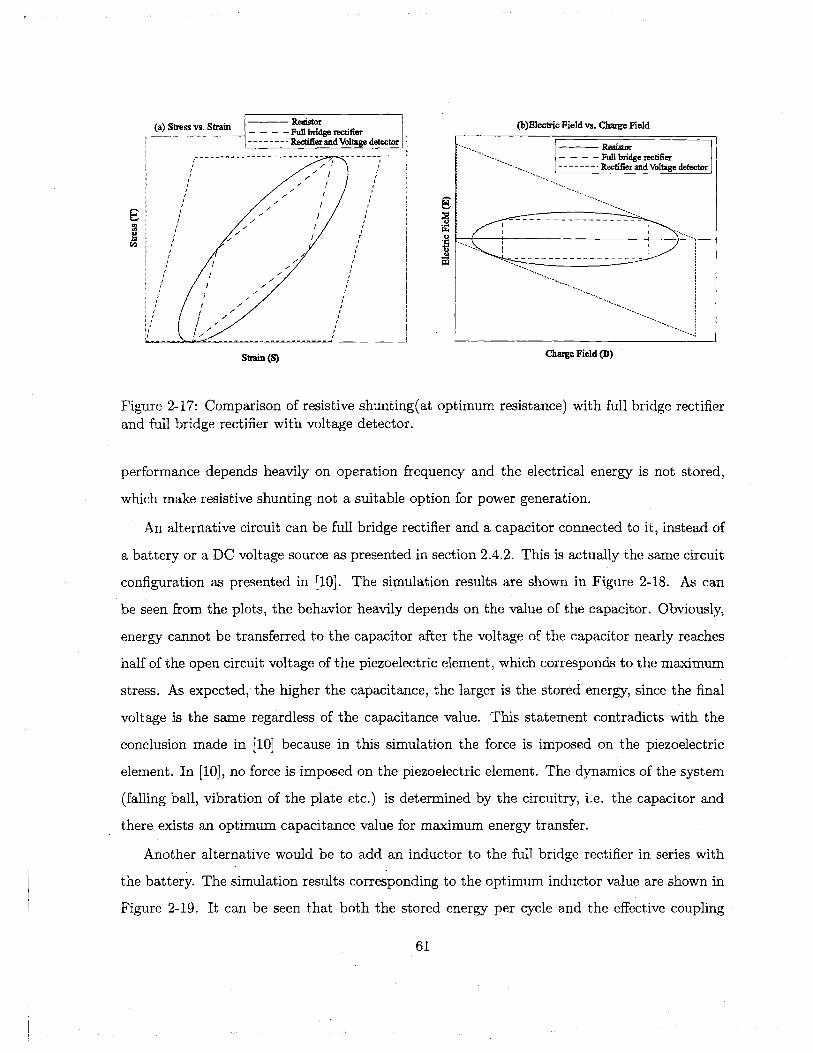
(a) Stress vs. Strain Resistorr _ - - -- F idge rectifier
-------- Rectifier and Voltage detector
---------------- ------ -
Strain (S)
Figure 2-17: Comparison of resistive shunting(atand full bridge rectifier with voltage detector.
Ooft
(b)Electric Field vs. Charge Field
-- - -Fullbridgerectifier-------Rectifier and oltage detector
Charge Field (D)
optimum resistance) with full bridge rectifier
performance depends heavily on operation frequency and the electrical energy is not stored,
which make resistive shunting not a suitable option for power generation.
An alternative circuit can be full bridge rectifier and a capacitor connected to it, instead of
a battery or a DC voltage source as presented in section 2.4.2. This is actually the same circuit
configuration as presented in [10]. The simulation results are shown in Figure 2-18. As can
be seen from the plots, the behavior heavily depends on the value of the capacitor. Obviously,
energy cannot be transferred to the capacitor after the voltage of the capacitor nearly reaches
half of the open circuit voltage of the piezoelectric element, which corresponds to the maximum
stress. As expected, the higher the capacitance, the larger is the stored energy, since the final
voltage is the same regardless of the capacitance value. This statement contradicts with the
conclusion made in [10] because in this simulation the force is imposed on the piezoelectric
element. In [10], no force is imposed on the piezoelectric element. The dynamics of the system
(falling ball, vibration of the plate etc.) is determined by the circuitry, i.e. the capacitor and
there exists an optimum capacitance value for maximum energy transfer.
Another alternative would be to add an inductor to the full bridge rectifier in series with
the battery. The simulation results corresponding to the optimum inductor value are shown in
Figure 2-19. It can be seen that both the stored energy per cycle and the effective coupling
61
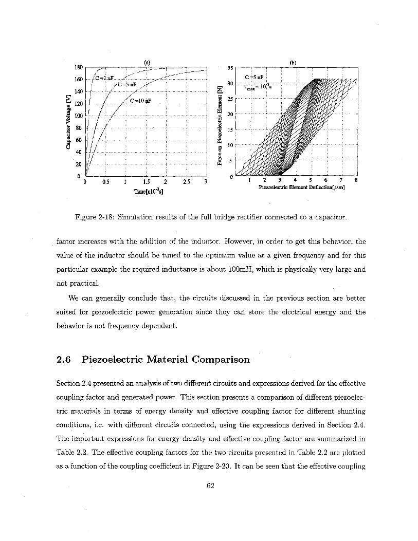
180 35
160 CC=10.C-5nFC=5 nF 30 -..... -......-.
140 -
2.C10tF....-. -.-.-.-2120 --
.100 / - -- =0-
~60 - -- - --75'
40
T0 .e[xl. .s] Piezoelecric Element.Deflection[jm]
Figure 2-18: Simulation results of the full bridge rectifier connected to a capacitor.
factor increases with the addition of the inductor. However, in order to get this behavior, the
value of the inductor should be tuned to the optimnum value at a given frequency and for this
particular example the required inductance is about lO0mH, which is physically very large and
not practical.
We can generally conclude that, the circuits discussed in the previous section are better
suited for piezoelectric power generation since they can store the electrical energy and the
behavior is not frequency dependent.
2.6 Piezoelectric Material Comparison
Section 2.4 presented an analysis of two different circuits and expressions derived for the effective
coupling factor and generated power. This section presents a comparison of different piezoelec-
tric materials in terms of energy density and effective coupling factor for different shunting
conditions, i.e. with different circuits connected, using the expressions derived in Section 2.4.
The important expressions for energy density and effective coupling factor are summarized in
Table 2.2. The effective coupling factors for the two circuits presented in Table 2.2 are plotted
as a function of the coupling coefficient in Figure 2-20. It can be seen that the effective coupling
62
(a) (b)

35
30
25
120
10
5
00 0.1 0.2 0.3 0.4 0.5 0.6 0.7
Piezoelectric Element Deflection[pm]
0.8 0.9
Figure 2-19: Force vs. deflection plot from the simulation of the full bridge rectifier withadditional inductor.
Rectifier Rectifier+Voltage Detector
Energy Density ED = ( - st)D ED = (s9E -SD2
2k 2 2k2Effective coupling factor k 2 33 k2 33
eff =k2 + 2 eff k23 + 1
Table 2.2: Comparison of circuitry in terms of energy density and effective coupling factor
factor for the case of the diode bridge is always smaller than the coupling coefficient whereas
the effective coupling factor for the case of the diode bridge with voltage detector is always
larger than the coupling coefficient. This can be also presented with the following inequality:
2k2 2k23 < k33< k 3 3
k23 + 2rk 3 +4(2.36)
which is valid since k33 < 1,
The energy density of a piezoelectric material, i.e. the maximum energy which can be
extracted from a piezoelectric element in one cycle is mostly limited by the depolarization stress
of the piezoelectric element, which means that if a stress higher than the depolarization stress
63
Full bridge rectifier and inductor-- -- Full bidgerectifier---- Rectifier and Vobzpg detsCimr
- - - ----- -- ---------I-----
------ ----- - -
-W
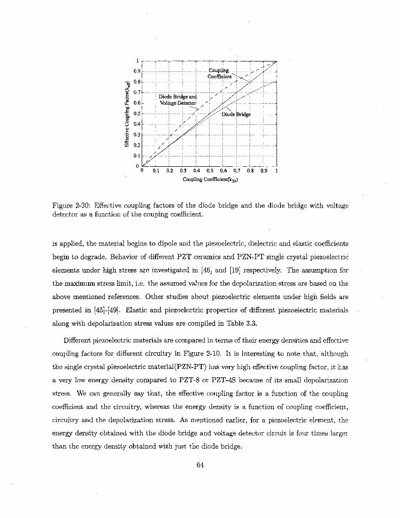
0.9 C... .. oupling . . - .uoefficient
- 0.8 -- - --.--
Diode Bridge andcd 0.6 -.--. Voltage Detector -
0 .5 - -..- ..- .. .... ..- B.. .... ....- . .--
o .3 ---. . . -Uj0.2 - - --ode.ndge
0 .1 - ....... ...-.. ...... ...- -.. .. ... ... ..
00 0.1 0.2 0.3 0.4 0.5 0.6 0.7 0.8 0.9 1
Coupling Coefficient(k 33)
Figure 2-20: Effective coupling factors of the diode bridge and the diode bridge with voltagedetector as a function of the couping coefficient.
is applied, the material begins to dipole and the piezoelectric, dielectric and elastic coefficients
begin to degrade. Behavior of different PZT ceramics and PZN-PT single crystal piezoelectric
elements under high stress are investigated in [46] and [19] respectively. The assumption for
the maximum stress limit, i.e. the assumed values for the depolarization stress are based on the
above mentioned references. Other studies about piezoelectric elements under high fields are
presented in [45]-[49]. Elastic and piezoelectric properties of different piezoelectric materials
along with depolarization stress values are compiled in Table 3.3.
Different piezoelectric materials are compared in terms of their energy densities and effective
coupling factors for different circuitry in Figure 2-10. It is interesting to note that, although
the single crystal piezoelectric material(PZN-PT) has very high effective coupling factor, it has
a very low energy density compared to PZT-8 or PZT-4S because of its small depolarization
stress. We can generally say that, the effective coupling factor is a function of the coupling
coefficient and the circuitry, whereas the energy density is a function of coupling coefficient,
circuitry and the depolarization stress. As mentioned earlier, for a piezoelectric element, the
energy density obtained with the diode bridge and voltage detector circuit is four times larger
than the energy density obtained with just the diode bridge.
64
*1
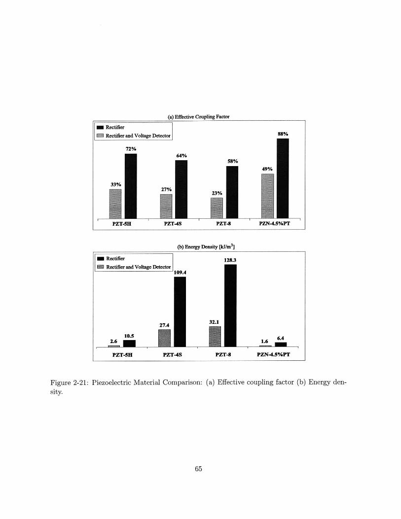
(a) Effective Coupling Factor
(b) Energy Density [kJ/m3]
Rectifier
Rectifier and Voltage Detector109.4
27.4
PZT-4S
1.6 6.
PZT-4SPZN-4.5%PT
10.5
PZT-5H
Figure 2-21: Piezoelectric Material Comparison: (a) Effective coupling factor (b) Energy den-
sity.
65
32.1
PZT-8
- Rectifier
MR Rectifier and Voltage Detector
72%64%
58%
33%
PZT-5H
129.3
88%
49%
PZN-4.5%PT
27%
PZT-4S PZT-8
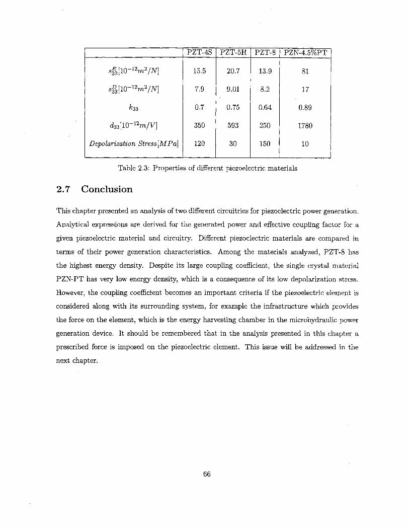
PZT-4S PZT-5H PZT-8 PZN-4.5%PT
st [1-1 2m 2 /N] 15.5 .20.7 13.9 81
s3[110 2 m 2 /N] 7.9 9.01 8.2 17
k33 0.7 0.75 0.64 0.89
d33 [101 2 m/V] 350 593 250 1780
Depolarization Stress[MPa] 120 30 150 10
Table 2.3: Properties of different piezoelectric materials
2.7 Conclusion
This chapter presented an analysis of two different circuitries for piezoelectric power generation.
Analytical expressions are derived for the generated power and effective coupling factor for a
given piezoelectric material and circuitry. Different piezoelectric materials are compared in
terms of their power generation characteristics. Among the materials analyzed, PZT-8 has
the highest energy density. Despite its large coupling coefficient, the single crystal material
PZN-PT has very low energy density, which is a consequence of its low depolarization stress.
However, the coupling coefficient becomes an important criteria if the piezoelectric element is
considered along with its surrounding system, for example the infrastructure which provides
the force on the element, which is the energy harvesting chamber in the microhydraulic power
generation device. It should be remembered that in the analysis presented in this chapter a
prescribed force is imposed on the piezoelectric element. This issue will be addressed in the
next chapter.
66

Chapter 3
Energy Harvesting Chamber and
Preliminary Design Considerations
This chapter presents a simple model of the energy harvesting chamber, simulations with the
coupled circuitry and preliminary design considerations. The interaction of the energy harvest-
ing chamber and the circuitry is discussed. The two circuits presented in Chapter 2 and different
piezoelectric materials are compared in terms of the flowrate and frequency requirements for a
given pressure differential and power, and in terms of system efficiency.
3.1 Configuration and Operation of the Energy Harvesting Cham-
ber
The Energy Harvesting Chamber consists of a fluid chamber, a piston and a piezoelectric
cylinder. The configuration of the energy harvesting chamber and its basic components are
shown in Figure 3-1.
The piston converts the pressure in the chamber to a force on the piezoelectric cylinder.
The inlet and outlet valves operate 1800 out of phase at high frequency and convert the static
pressure differential (PHPR -- LPR) into pressure fluctuations in the chamber. This results in
cyclic compression of the piezoelectric cylinder, which is coupled to the circuitry. The generic
operation and typical duty cycles are shown in Figure 3-2.
67

Chamber ceiling
D7
Outlet|valve HP
Working - -
fluid
Pistontethers
Bottom Plate
Figure 3-1: Energy harvesting chamber configuration.
Pmax
P.
Qave
xXmi
xM
(a) Chamber Pressure-- -------- ------- ---- --------
---- --------- -------------
T/2 T 3T/2 27
(b) Flowrate
- w otet
-- - - --- - ---- -\- - - - - -- -- - - - -- -
T/2 T 3 T/2 27
(c) Piston Deflection
- ----------- -------------- - -- - - - - - - -
T/2 T 3T/2 2T
Figure 3-2: Duty cycles of generic operation of the energy harvesting chamber. The valve
openings have the same duty cycle as the flowrates and are not shown here.
68
InletI valve
Piston '--
Piezoelectriccylinder
, __
In the chamber, the hydraulic energy is converted into mechanical energy, which is converted
into electrical energy in the piezoelectric element and then the electrical energy is stored in the
coupled circuitry. There is a strong coupling between the hydraulic/mechanical system and the
circuitry, in other words, the electrical circuit affects the behavior of the system dramatically,
an issue which should be analyzed in detail.
3.2 Modeling
In order to understand the interaction between the hydraulic, mechanical and electrical system,
a simple model of the energy harvesting chamber will be used to simulate a representative
system. The basic assumptions are:
- The effect of piston tethers on the motion of the piston is neglected perfect sealing between
the piston and the chamber walls is assumed
- An effective compliance, Ceff,is assigned for the chamber, which includes the combined
effect of the bending of the piston, chamber ceiling (top plate), bottom plate and piston tethers
as well as fluid compression inside the chamber. Ceff will be defined in section 3.2.2.
- Piston dynamics is neglected.
The detailed structural modeling and analysis of the compliance contributions of the struc-
tural members in the chamber will be presented in Chapter 4.
3.2.1 Piezoelectric Cylinder
The piezoelectric material is modeled using the same constitutive relationship given in Chapter
2, namely:
D d33S 8333 -T8T
= d33 D(3.1)L_ 33 33 ..
where D is the charge field, S is the displacement field (strain), E is the electric field, and T
is the stress. For a cross-sectional area of A and length of L, the expressions for the deflection
69
of the piezoelectric element and the voltage across it become:
x, = (s33FP + QP)(3.2)Ap 633
v =t d33 F -lQ) (3.3)V P (33 33
where x, is the deflection, Qp is the charge, Fp is the force applied on the piezoelectric
cylinder, and V, is the voltage across the piezoelectric cylinder. And the current through the
piezoelectric element is given by:
I= dQp (3.4)dt
3.2.2 Chamber Continuity
The chamber converts the hydraulic energy into mechanical energy via the piston, which applies
a force on the piezoelectric cylinder. In order to derive the expression for the chamber pressure,
continuity equation inside the chamber should be considered. Consider an initial fluid volume
inside the chamber. The time rate of the pressure change in the chamber is given by:
dP~h - I3f dV (3.5)dt V dt
where #f is the bulk modulus of the fluid, V0 is the initial volume of the fluid inside thedV
chamber and - is the volume change of the fluid. Sources of the volume change are:dt
- Net flowrate into the chamber
- Piston Movement
- Additional volume created inside the chamber by the deformation of the structural mem-
bers due to chamber pressure
Then, the time rate of the total volume change in the chamber can be expressed as:
dV Qin - Qout - As - dV(3.6)= dt ~dt
where x, is the displacement of the piston, which is equal to the deflection of the piezoelectric
cylinder, Api8 is the cross-sectional area of the piston, and V, is the total volume displaced by
70
the deformation of the structural members inside the chamber. The source of this additional
volume might be the deformation of the top and bottom plate of the chamber, deformation of
the piston tethers and deformation of the piston itself. The individual sources of the structural
compliance of the chamber will be analyzed in detail in Chapter 4.
Combining equations 3.5 and 3.6, we get:
dPeh _5 fdx dV= h- fQin -- QOUI; xPApi dS (3.7)dt VO dt dt
We can define the overall structural compliance as:
dVsCS= dVc (3.8)
From equations 3.7 and 3.8, we get the expression for the chamber pressure as:
dPch V.9 <'5s n dxpAh s +n - 6out Apis (3-9)
For simplicity, we can define an effective compliance for the chamber, which represents all
the compliance sources as:
Ce = (>+ cS)(3.10)
where the first and the second terms correspond to the fluidic compliance and structural
compliance respectively, which act like parallel capacitors in electrical circuit analogy.
We can rewrite 3.9 as follows:
dPeh 1 dx~d1 Qin - -Q d Apis (3.11)dt Ceff d
It is important to note that, in the above analysis the initial fluid volume inside the chamber,
V0, is assumed to be much larger than the volume displaced by the piston and the volume
displaced due to the deformation of the structural members inside the chamber. If the deflection
of the piston becomes comparable to the chamber height, the volume displaced by the piston
becomes comparable with the initial volume of the chamber, and that effect should be taken
into consideration, which will result in nonlinear behavior, i.e nonlinear compliance.
71

The generic duty cycle of the operation is shown in Figure 3-2. The average flowrate can
be calculated using the following relationship:
[T/2 fT
= /2 Qindt / 2 oUtd t
Qave T= = T/ T(3.12)
It is also important to note that:
T T/2
fTQindt = [ Qodt= 0 (3.13)
TIntegrating equation 3.11 from t = 0 to t = , using equation 3.12 and arranging terms,
2'we get the expression for the average flowrate as:
Qave = Apis(Xmax - Xmin)f + Cef f(Pmax - Pmin)f (3.14)
where Aprs is the cross-sectional area of the piston and f is the operation frequency. TheT
same expression can be obtained by integrating equation 3.11 from I = - to I = T. The first2
term in equation 3.14 corresponds to the flowrate required to move the piston and squeeze
the piezoelectric element. The second term corresponds to the flowrate required due to the
compliances in the chamber.
3.2.3 Fluid Model
The schematic of the device with pressures at different locations within the system is shown in
Figure 3-3 where Pit-in is the intermediate pressure at the exit of the inlet channel, and Pint-ost
is the intermediate pressure at the entrance to the outlet valve. Inlet and outlet channels have
the same geometry. Details of the Simulink architecture is given in the Appendix A.
Valve Orifice Flow Relations
Work by previous researches has shown that for small openings, poppet valves, such as the
valve cap in the active valves within the MHT systems, behave as long orifices in which the
effects of flow separation and subsequent re-attachement dominate the valve flow dynamics[5].
72

XjI X0ut
inlet ILain aoutletPr valve ,P habrp it- alve LP
cL LC
Figure 3-3: Device schematics showing pressures at different locations.
Qualitatively, the valve flow can be approximated by a simplified order-of-magnitude valve
model. The valve orifice may be characterized as a flow contraction followed by a flow expansion
as shown in Figure 3-4(a) and (b). An integral analysis gives a relationship for the combined
effect of the flow expansion and contraction. The loss coefficient (oifice is defined as the total
pressure drop AP = PHPR - Pint (for the inlet valve) over the dynamic pressure based on the
orifice local mean velocity (L = A)
(orifice 1 A2 I A 1 ) + ( A2 (3.15)
where the upstream, throat and downstream flow areas can be approximated as:
A2 = 27RvcHc (3.16)
AO = 27rRvczxc (3.17)
A1 = rRVC (3.18)
respectively, where He is the height of the radial flow channel above the valve membrane,
xVC is the valve cap distance from the valve stop structure and R'c is the radius of the valve
cap.
This approximation, however, is independent of the Reynolds number and therefore holds
only for Re> 10, 000, where the flow is in fully turbulent regime. In the MHT power generator,
Reynolds numbers are expected to fluctuate between approximately 10 and 20, 000 as the valves
73

Pch P ,Al HPR Pch
A 2 A0 -A 2 - AO -- A,
(a) (b)
Figure 3-4: Valve orifice representation:(a) Valve cap geometry and fluid flow areas, (b) Rep-
resentation of flow through the valve as a flow contraction followed by a flow expansion.
open and close. For this reason, correction factors obtained from experimental results need to
be employed to obtain better estimates of the loss coefficients for these low turbulence and
laminar flow regimes[4]. A loss coefficient for each of the contraction and expansion geometries,
(contraction and (exp ansion, respectively, is used to approximate the total loss coefficient through
the valve, as detailed in the following relation:
(orifice = (contraction(Re, A )+(expansion(Re (3.19)
where Reynolds number is defined as:
Re -Q (3.20)
Figure 3-5(a) plots (contraction as a function of Reynolds number and contraction area ratio
, and Figure 3-5(b) plots (exp ansion as a function of Reynolds number and the expansion
area ratio -l. As a result, the pressure-flow relation for the full valve orifice geometry can be
written as:
1 fQAP= P(*,ifice (3.21)
All subsequent fluid models discussed in this thesis incorporate these higher-order correction
factors to obtain an accurate estimation of the flow behavior. These flow models are based on
steady flow phenomenon and do not capture frequency dependent losses. For a specific value
of valve cap opening at a given time during the cycle, a relationship therefore exists for the
74
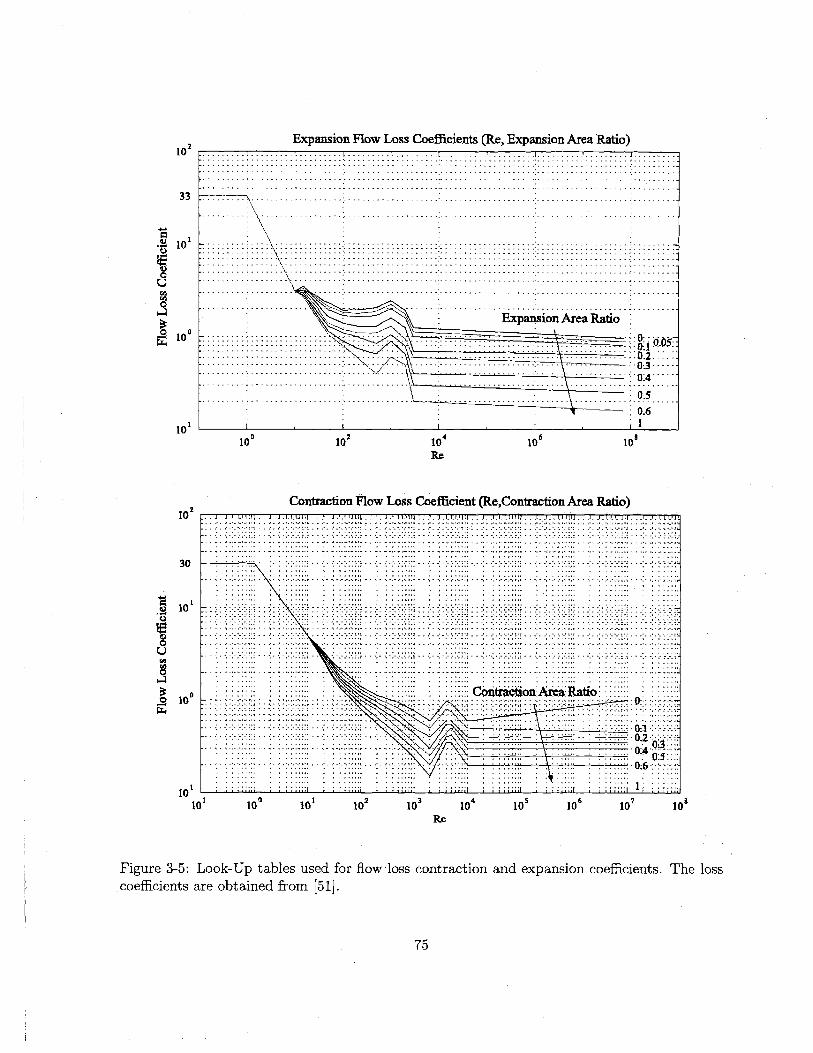
Expansion Flow Loss Coefficients (Re. Expansion Area Ratio)...... ...... .......
. . . . . . . . . . . . . . . . . . . . . . . . . . . . . : . . . . . . . . . . . . . . . .
. . . . . . . . . . . . . . . . . . . . . . . . . . . . . . . . . . . . . . . . . . . . . ... . . . . . . . . . . . . . . . . . . . . . . . . . . . . . . . . . . . . . . .. . . . . . . . . . .
. . . . . . . . . . . . . . . . . . . . . . . . . . . . . . . . . . . . . . . . . . . . . . . . . . . . . . . . . . . . . . . . . . . . . . . . . . . . . ... . . . . . . . . . . . . . . . . . . . . . . . . . . . . .
. . . . : . . . . . . . . . . . . . . . . . . . . - - - - - - - - - -
. . . . . . . . . . . . . . . . . . . . . ... . . . . . . . . . . . . . . . . . . . . . . . . . . . . . . . . . . . . . . . . . . . . . . . .
. . . . . . . . . . . . . . . . . . . . . . . . . . . . . . . . . . . . . . . . . . M . . . . . . . . .
. . . . . . . . . . . . . . . . . . . . . . . . . . . . . . . . . . .. I . . . . . . . . . . . . . . . . . . . . . . .
. . . . . . . . .. . . ... . . . .
. . . ... . . . . . .
. . . . . .. .. . . . . . . . .
. . . . . . . . . . . . . . . . . . . . . . . . . . . . . . . . . . . . . . . . . . . . . . . . . . . . . . . . . . . . . . . . . . . . . . . . . . . . . . . . . . . . . . . . . . . . . . . .
- - - - - - . . . . . . . . . . . . .. . . . . . . . . . . . . . I . . . . . . . . I .. . . . . . . . . . . . . . . . . . . . . . . . . . . . . . .
. . . . . . . . . . . . . . . . . . . . . . . . . . . ... . . . . . . . . . . . . . . . . . . . . . . . . . . . . ... . . . . . . . . . . . . . . . . . . . . . . . . . . . . .
. . . . . . . . . . . . . . . . . . . . . . . . . w . . . . . . . . . . . . . . . . . . . . . . . . . . . . . . . . . . . . . . . . . . . . . . . . . . . . . ..
. . . . . . . . . . I . . . . . . . . . . . . . .. . . . . . . . . . . . . . . . .. . . . . . . . . . q . . . . . . . . ... . . . . . . . . . . . . . . . . . ..
. . . . . . . . . . . . . . - - - - - - - . . . . . . . . . . . . . . . ... . . . . . . . . . . . . . . . . . . . .
Expansion Area Ratio...........
--- -------... ............. ...... OA.................... ... .......................................... ... ... :.- . - - - - ............... 0'2 -............................... ........... ......................... .. 0.3: ..... ................m ............ . ............ ... ... , -'0-4 '.............. .............................. ............... ..........
: 0.5................... ............... ..................... ....... ............0.6
10 0 10 2 10 4 10 6 10 a
Re
Contraction Flow Loss Coefficient (ReContraction Area Ratio)J. j -1-173LIj J- 3.1 t.ljuj 1. J.1.1.13111
%
. . . . . . . . . . . . . . . . .
. . . . . . . . . . . . . . . . . . . . . . . . . . . . . . . . . . . . . . . . . . . . . . . . . . . . . . . .
M I I . I
. . . . . . . . . . . . . . . . . . . . . . . . . . . . . . . . . . . . . . . . . . . . . . . . . . . . . . . . . .. . . d I -- - - - - - - - - -
r r r I I v r i t I I
. . ... . . . . . . . . . . . . . . . . . .
. . . . . . . . . . . . . . . . . . . . . . . . . . . . . . . . . . . . . . . .
'v I r r
I
I
I :d ...
. . . . . . . . . . . . . . . . .
P': Ratio:0
.. . . . . . . . . . . . . . . . . . .
0-.2
.1 1 P .1 1 1
L, L 0-.6
a I d -1 1 1
10 2
33
10
010
10
10 2
30
10,
10
10
10 10 10 10 2 10 3 10 4 10 S 10 6 10 7 10 a
Re
Figure 3-5: Look-Up tables used for flow -loss contraction and expansion coefficients. The losscoefficients are obtained from [511.
75

instantaneous fluid flow through the valve as a function of the pressure drop across the valve.
Equation 3.21 can be rewritten for inlet and outlet valves using the notation in Figure 3-3
as:
PHPR - Pn i t = Ri Qn Vi)Q (3.22)
Pn-otW- PLPR = Rot g(Qout, V out) Q2~ (3.23)
where Rn and Rout represent the flow resistances of the inlet and outlet valves, respectively,
which are functions of the flowrate and the corresponding valve opening at a given instant of
time.
Flow in the Channels
Due to the high Reynolds numbers, the flow in the channels is expected to be inertia dominated.
Furthermore, the compliance in the fluid channels is usually negligible due to the fact that the
channels are surrounded by rigid walls and their volume is much smaller than that of the
chamber. Under this assumptions the flow inside the channels is modeled as one dimensional
inviscid and incompressible flow. The pressure-flowrate relationship in this case is given as:
AP=I--t = -c) - (3.24)d Ac dt
where I is defined as the fluid inductance inside the channel, p is the fluid density and L
and Ac are the length and cross-sectional area of the fluid channel respectively. For the case of
inlet valve and outlet valve fluid channels, the pressure-flow relations can be written as:
Pint-in(t) - Pch(t) = d(c} cin (3.25)
AcN dto
Pch(t) - Pint-out(t) = (I c)cdQt (3.26)
For a long channel with small cross-sectional area, one can expect fluid inertial effects to
76
I
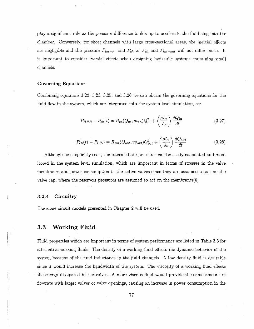
play a significant role as the pressure difference builds up to accelerate the fluid slug into the
chamber. Conversely, for short channels with large cross-sectional areas, the inertial effects
are negligible and the pressure Pint-ij and Pch or Pch and Pmt-,t will not differ much. It
is important to consider inertial effects when designing hydraulic systems containing small
channels.
Governing Equations
Combining equations 3.22, 3.23, 3.25, and 3.26 we can obtain the governing equations for the
fluid flow in the system, which are integrated into the system level simulation, as:
PHPR - Pch(t) = Rjn(Qn, vo 1n) Q + ( c)dti (3.27)
Ph(t) - PLPR = R,+ (pL> dQ (3.28)R~tQ~tvo~)QL KA) dt
Although not explicitly seen, the intermediate pressures can be easily calculated and mon-
itored in the system level simulation, which are important in terms of stresses in the valve
membranes and power consumption in the active valves since they are assumed to act on the
valve cap, where the reservoir pressures are assumed to act on the membranes[6].
3.2.4 Circuitry
The same circuit models presented in Chapter 2 will be used.
3.3 Working Fluid
Fluid properties which are important in terms of system performance are listed in Table 3.3 for
alternative working fluids. The density of a working fluid effects the dynamic behavior of the
system because of the fluid inductance in the fluid channels. A low density fluid is desirable
since it would increase the bandwidth of the system. The viscosity of a working fluid effects
the energy dissipated in the valves. A more viscous fluid would provide the same amount of
flowrate with larger valves or valve openings, causing an increase in power consumption in the
77

Density[kg/m3 Viscosity[Pa/s] Bulk Modulus[GPa]Water 1000 1.0e-3 2.24
Mercury 13,570 1.5e-3 25.0Silicone Oil 760 4.9e-4 2.0(degassed)
Table 3.1: Comparison of different working fluids
Length of the piezoelectric cylinder 1mmDiameter of the piezoelectric cylinder 2mm
Diameter of the piston 4.5mm
Effective chamber compliance (Ceff) 2 x 10- 18 [m 3 /Pa]
PHPR 2MPa
PLPR OMPaOperation Frequency 10kHz
Fluid channel length 1mmFluid channel cross-section 50pm x 100 pmPiezoelectric Material PZN-4.5%PT
Table 3.2: The geometry and operation conditions used in the simulation
valves. The bulk modulus effects the system compliance. Silicone oil is chosen as the working
fluid because of its low density, low viscosity and a bulk modulus comparable to that of water.
3.4 Simulation and Analysis
The equations presented in the previous section will be simulated using Simulink. The coupled
equations used to simulate the system are 3.2, 3.3, 3.4, 3.11, 3.27, 3.28 and equations for the
circuitry, which were given in Chapter 2.
The simulation architecture is shown in Figure 3-6. For the analysis in this chapter, a
representative system will be analyzed, for which the geometry and operation conditions are
presented in Table 3.2.
In the following analysis, the valve openings are imposed and reservoir pressures are as-
sumed to be constant. The valve size and opening are adjusted such that the pressure in the
energy harvesting chamber attains the high pressure reservoir pressure (PHPR) and low pressure
reservoir pressure (PLPR) as its maximum and minimum pressures respectively. In other words,
the pressure inside the chamber fluctuates between PHPR and PLPR. The valves operate 1800
out of phase.
78
A

Pch
Inlet gin gout Outlet PRLHPR Valve Valve
Chamber IVoi Continuity vO
x Fxp p
PiezoelectricElement
V Ip p
Circuit
PowerOutput
Figure 3-6: Simulation architecture used in Simulink.
3.4.1 Energy Harvesting Chamber and Full Bridge Rectifier
This section presents the simulation and analysis of the energy harvesting chamber attached to
the full bridge rectifier using the model presented in the previous section. The time histories
of the chamber pressure, flowrate and piston deflection, which is equal to the deflection of the
piezoelectric element, are shown in Figure 3-7.
In order to understand the interaction between the hydraulic/mechanical system and the
circuitry, and its implications on flowrate and frequency for a given power requirement, it is
worthwhile to investigate the plot of force on the piezoelectric element vs displacement of the
piezoelectric element. This is shown in Figure 3-8. It is interesting to note that the curve in
Figure 3-8 has the exact same shape of the force vs. displacement curve presented in Chapter
2 for the case of the imposed force on a piezoelectric cylinder attached to a diode bridge.
From this we can conclude that the force vs. displacement curve of a piezoelectric element
attached to the full bridge rectifier does not depend on the time history of the applied force.
So, the equations derived in Chapter 2 for the full bridge rectifier will be used here to derive
79

(a) Chamber Pressure
2.5 3 3.5 4 4.5 5
(b) Flowrate
2 2.5 3 3.5 4 4.5
(c) Piston Deflection
2.5 3 3.5Time [104s]
4 4.5
Figure 3-7: Simulation of the energy harvesting chambercircuit.
attached to the full bridge rectifier
80
.. . .. . .. .. .. . .. . .. .. . . . . . . . . .
. . . . . . . . . . . . . . . . ..... . . .. . .
- --..
2
1.5
1
0.5
0
0.4
0.3
0.2
0.1
0
miet-Outlet- - - . - -
-.. . .. . . . . . ... .. . . . .. . . . . . . ..... . . .
...........
. ....................... . . . ..
-- - -- - - - - - - - -______________
0
-0.2
5 -0.4
-0.6
-0.8
5
2 5
j
=i
I
-- - -- --- ----. ..-. .
.. . . . . . . -. .-. .-.-. .- .~
- - -
5
the governing equations for required frequency, flowrate and system efficiency.
For a given operation frequency and power requirement, the required cross-sectional area of
the piezoelectric element can be obtained from equation 2.25 as:
4WA= (3.29)
(s -- s )Dc2 Lpf
where W is the generated power, LP is the length of the piezoelectric cylinder and f is the
operation frequency. Since the maximum pressure in the chamber is PHPR, the cross-sectional
area of the piston should be equal to:
Apis = dA(3.30)PH PR
where 9d is the depolarization stress of the piezoelectric element. From the results derived
in Chapter 2, the total deflection of the piston/piezoelectric cylinder is given by:
AXp 2 OdLp(sE+%) (3.31)
Using equations 5.31, 3.29, 3.30, and 3.31, the required flowrate for a given power require-
ment and maximum chamber pressure can be derived as follows:
2(s4 + sg)WQ = E 43)P _ Cef f PHPRf (3.32)
(St - s3')PHPR
The first term in equation 3.32 corresponds to the flowrate which is required just to move
the piston. The second term corresponds to the additional flowrate required due to the chamber
compliance. If we consider the ideal case, where the chamber is not compliant, i.e Ceff = 0,
the minimum required flowrate is given by
2(se + sD)WQrmin 33 t- 33)PFR(3.33)s--8s )PH PR
In order to evaluate the performance of the energy harvesting chamber, we can define the
efficiency of the chamber as follows:
81
35
25 -I - - -2 2 rt-30 ----
. . . . ... .
2 5 --. .- - - -- -U.
20
~1 5- -- - - -. . . .. . . ..
5...........
10
0 0.1 0.2 0.3 0.4 0.5 0.6 0.7 0.8
Deflection of Piezoelectric Cylinder[pm]
Figure 3-8: Force vs. displacement curve of the piezoelectric element from the simulation ofthe harvesting chamber attached to the full bridge rectifier.
Electrical Power Out(3 Wc =Hydraulic Power In - QPHPR
In the extreme case, where the effective chamber compliance is zero, the efficiency has its
maximum value, which can be obtained from equations 3.32 and 3.34 as:
(S D - s ) k33 -1=3 = 3(335)
"m 72(st + sD) 4 - 2k23 (
It is interesting to note that the maximum efficiency of the chamber depends only on the
coupling coefficient of the piezoelectric material. This suggests that, regardless of the geometry
and operation conditions, the above expression puts an upper bound on the system efficiency,
which is only a function of the piezoelectric element chosen. It is important to note that the
above definition of the efficiency corresponds only to the energy harvesting chamber. If the
overall system is considered, the electrical power consumption in the active valves should be
taken into consideration.
82
3.4.2 Energy Harvesting Chamber and Full Bridge Rectifier with Voltage
Detector Circuit
This section presents the simulation and analysis of the Energy Harvesting Chamber attached to
the full bridge rectifier and voltage detector circuit. The geometry and the operation conditions
are the same as in the previous section. The time histories of the chamber pressure, flowrate
and piston deflection are shown in Figure 3-9.
It is interesting to note that there are sudden pressure drops inside the chamber and the
time histories of the chamber pressure and the piston deflection are quite different from the
time histories presented in the previous section. The most important observation is that during
the periods when the switch is on, the pressure decreases/increases suddenly because the fluid
cannot fill/evacuate the chamber immediately due to the fluid inertia of the fluid in the channels.
In order to understand the interaction between the hydraulic/mechanical system and the circuit,
and its implications on flowrate and frequency requirements for a given power, we can investigate
the force vs.displacement plot of the piezoelectric element which is shown in Figure 3-10.
In Figure 3-10, the force vs. displacement curve of the piezoelectric element for this case
is compared to the chamber attached to full bridge rectifier and to the case where the force is
imposed on the piezoelectric element attached to the regular diode bridge and voltage detector.
It is interesting to note that the new curve is much different than the imposed force case.
In the latter case, which was discussed in Chapter 2, during the interval when the switch is
on, the force is almost constant, and the portion of the curve corresponding to that period is
almost flat. However, for the chamber, during the interval when the switch is on, the piezo
becomes very soft, and the piston moves up or down very rapidly, which causes sudden pressure
drops/rises inside the chamber, as can be seen in Figure 3-9. In order to analyze the behavior
of the system, we can divide the time history into four periods, as shown in Figure 3-11.
In the periods 1-2 and 3-4 the piezoelectric element is open circuited, and the deflections
at the states 1 and 3 correspond to the deflection as if the material was short circuited and
the same force as in 1 and 3 was applied. In other words, F1 , F3 , x 1 , and x3 should satisfy the
following equations.
83

(a) Chamber Pressure
- ...*,. .. .......................-............. ...........-
- -. . -. . ..i ! ----- - -
I ...-
5S
5
5.5(b) Fowrate
5.5(c) Piston Deflection
6 6.5
6 6.5
7
7
4 4.5 5 5.5 6 6.5 7(d)Voltage Detected
5 5.5 6 6.5 7
Time [10 4 s]
Figure 3-9: Simulation of the energy harvesting chamber attached to the full bridge rectifierand voltage detector circuit. The time intervals between the dashed lines present the intervalswhere the switch(SCR) is in its "on" state.
84
1-
4 4.5
0.
0
Iret\ ) Outlet
./ - -- - -
I. 4.54
-0.3
0.4
-0.5
200,
100.
-............ ........... ......................
. . . I. ... . .I........... ............ II...... ..... I. . ... .I I { I
--- - - --.-. -. -4 4.5
0%
-. ....-. .-. .-. .- . .- .- .- . . -. -. .-. ..-
-. ..-. .- ..- ..- -. . -. .-. ..-
- --. . . - .- .- .- .- .-
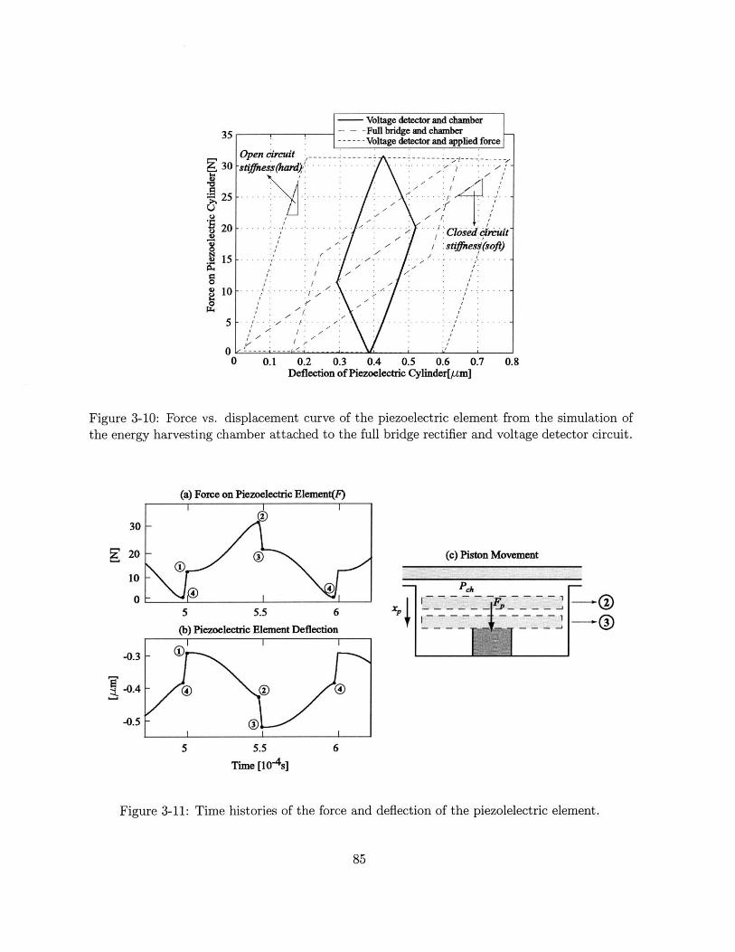
35
S30
25
20
15
100
5
00 0.1 0.2 0.3 0.4 0.5 0.6 0.7
Deflection of Piezoelectric Cylinder[Am]0.8
Figure 3-10: Force vs. displacement curve of the piezoelectric element from the simulation ofthe energy harvesting chamber attached to the full bridge rectifier and voltage detector circuit.
(a) Force on Piezoelectric Element(F)
5 5.5 6
(b) Piezoelectric Element Deflection
5 5.5
Time [10-4 s]
(c) Piston Movement
PC,x -- - -~
P - - -
_~IF- p- -
6
Figure 3-11: Time histories of the force and deflection of the piezolelectric element.
85
- Voltage detector and chamber-Full bridge and chamber- Voltage detector and applied force
Open circuit - ------.st.f..es..(hard)." ..... /.
Closed druitstiffiesd(soft)
. -
30
10
0
-0.3
-0.4
-0.5
- 4
- -7§J~ K-11 -~
i2 2
4
g20
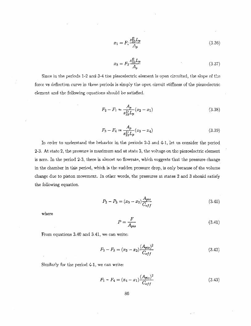
X1 = F A331, (3.36)
A,
Since in the periods 1-2 and 3-4 the piezoelectric element is open circuited, the slope of the
force vs deflection curve in these periods is simply the open circuit stiffness of the piezoelectric
element and the following equations should be satisfied.
F2 - F1 A,, ( -I) (3.38)s3LP
AF3 - F4 = , (x3 - X4 ) (3.39)
stL,
In order to understand the behavior in the periods 2-3 and 4-1, let us consider the period
2-3. At state 2, the pressure is maximum and at state 3, the voltage on the piezoelectric element
is zero. In the period 2-3, there is almost no flowrate, which suggests that the pressure change
in the chamber in this period, which is the sudden pressure drop, is only because of the volume
change due to piston movement. In other words, the pressures at states 2 and 3 should satisfy
the following equation.
A,P2 - P3 = (x3 - X2) A" (3.40)
Ceff
where
FP = AF-(3.41)
From equations 3.40 and 3.41, we can write:
F2 - F3 = (3 - X2)A )2(3.42)Cef f
Similarly for the period 4-1, we can write:
(Ai 8 )2 (.3F1 - F4 = (X4 - Xi) As 2(3.43)Cef f
86
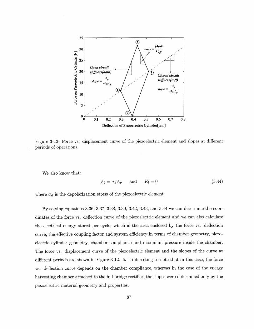
Opestio
@(Apis)2
slope =___
'n cir-uit
Cbs~ess(har) A - edcrciA stif
Slop,
edcircuit
ness(soft)
Al=SE 3jLp
0 0.1 0.2 0.3 0.4 0.5 0.6
Deflection of Piezoelectric Cylinder[gm]
Figure 3-12: Force vs. displacement curve of the piezoelectric element
periods of operations.
and slopes at different
We also know that:
F2 = UdAp and F4 = 0 (3.44)
where 0 -d is the depolarization stress of the piezoelectric element.
By solving equations 3.36, 3.37, 3.38, 3.39, 3.42, 3.43, and 3.44 we can determine the coor-
dinates of the force vs. deflection curve of the piezoelectric element and we can also calculate
the electrical energy stored per cycle, which is the area enclosed by the force vs. deflection
curve, the effective coupling factor and system efficiency in terms of chamber geometry, piezo-
electric cylinder geometry, chamber compliance and maximum pressure inside the chamber.
The force vs. displacement curve of the piezoelectric element and the slopes of the curve at
different periods are shown in Figure 3-12. It is interesting to note that in this case, the force
vs. deflection curve depends on the chamber compliance, whereas in the case of the energy
harvesting chamber attached to the full bridge rectifier, the slopes were determined only by the
piezoelectric material geometry and properties.
87
35
30-
25-
20-
15-
10-
U
U)
U)
0U)
5
00.7 0.8
- -
-
The coordinates of the force vs displacement curve are as follows:
O-d A 2 -L 2sE(SE - SD) O A 2Lp Ap(s - 8sD)(XI, Fi) pidAsLpS 33(S 33 - 3)3dAPAP(34 33(3)45Ce A A.s~( s-8D)'CE 8 L(2t- SD)\=CeffAp ± AfL+(2st - cfAp±A L(2s
O-dL 2(S E)2A 2 e5LASDa
(X2, F2) = (,dL 3 A).+adCffLPAp33 7-dA P (3.46)Cef f Ap + AP,,Lp ( 2s E - SD P
'd L1( sEs)2 A ~s+ O-Cef f LpApsS' O-dAp Lp~, s'+ OaCeff A(X3, F3) = 3 3 3(347)CeeAp + A% 8,Lp(2st - sD) 'Cej'jAp ± A%8L(2s D s?)
33-s SA3L+ f f5 LAp + sP s - 83
(X4 , F4 ) = ((dStA 8 Lp±JdCeffLpAp)(33 - S3)(348)CeffAp+A j8 Lp (2s - sD)
Using the coordinates of the points given in the above equations, electrical energy stored
per cycle can be calculated as:
F - -2LAp(st_ - 4S%1)(ApCef f + St AP,sLp)(ApCeff + sDA;sLP ([A% 3jL(2s - SD) + CeffAp] 2 (3.49)
From equation 5.31 we can write the expression for the flowrate as:
Qave = Ai 8(xs - x1) f + CeffPHPRf (3.50)
For a given power requirement W, we can determine the required frequency using:
W(3.51)
The required flowrate for a given power requirement can be derived from equations 3.45,
3.47, 3.49, 3.50, and 3.51 as:
W~s~e5PHR UOPPS3 2 33 31Qave -W CeffPkPR + a"LPAst(2t (3.52)
PHPR(CeffPH2 PR + ad A3)(StS3 - 3
WPHPRCeff[CeffPAPR + L 3 33)2d- 3s3-%) (Cef f +4LPR Ad 3) (CeffPPR ± c APS3
In the extreme case where the effective chamber compliance is zero, namely Ceff = 0, the
88

expression for the required flowrate simply reduces to
(2 -E-SD)W
QM ( P33 D33 (3.53)(8333 - 533PHP R
From the above expression we can get the maximum system efficiency using the definition
given in equation 3.34 as
(ES D -D k2
ch(max s33(-s ) 33 (354)c3max3)2s13+
kD23
where, as in the previous section, the maximum efficiency depends only on the coupling
coefficient of the piezoelectric material.
Figure 3-13 shows the force vs. deflection curve of the piezoelectric element for different
values of chamber compliance. It is interesting to note that, as the chamber compliance in-
creases, the curve approaches the curve for the case where the force is imposed. One might
think that having large compliance would have a positive effect on system performance, since
the area inside the curve, which is the electrical energy stored per cycle, increases with increas-
ing compliance. For a given power requirement lower frequencies and lower flowrates would be
required. However, as the compliance increases, the required flowrate increases dramatically
due to the second term in equation 3.50. This effect overwhelms the effect of decreased flowrate
due to lower frequency requirement and the maximum system efficiency occurs again for the
case where the chamber compliance is zero. The two extreme cases, namely Ceff = 0 and
Ceff = oo are shown in Figure 3-13 (b).
The effective coupling factor from mechanical to electrical energy was defined in Chapter 2
and the expressions were derived for different circuits for the imposed force case. For the case
of the energy harvesting chamber attached to the full bridge rectifier, the effective coupling
factor is the same as the one for the imposed force case since for the full bridge rectifier, the
force vs. displacement curve doesn't depend on the time history of the force on the piezoelectric
element. However, it was found that, the force vs. displacement curve for full bridge rectifier
and voltage detector depends on the time history of the force on the piezoelectric element, and
in this case the curve depends on the chamber compliance. The effective coupling factor was
defined in Chapter 2. From Figure 3-13 we can write:
89

(a) Effect of effective compliance
- Ce= 2 x18I
11
-e = C2x Ol
C 16
Cq~=2Xl-
0.1 0.2 0.3 0.4 0.5 0.6 0.7 0.8 0.9Deflection of Piezoelectric Cylinder[Am]
- Cff= 2x0~1'
(b) Energy Conversion Efficiency - - - Cf = 0' ''------- Cef = Oo
1IW 1 I
- 7
0 0.1 0.2 0.3 0.4 0.5 0.6 0.7 0.8 0.Deflection of Piezoelectric Cylinder[Am]
9
Figure 3-13: The effect of effective chamber compliance on force vs. deflection curve and
effective coupling factor.
90
35
30-
25-
20-
15
10
0.)
0
C.)
I -
I/
1 7
1 7/
j II 7
7
7
,
~7
/7
/- - / j
5
35
30
25
20
15
10
5
0
U
0N
4)
I I0 V0

k 2 W1
(eff W = W1 + W2 (3.55)
The effective coupling factor can be calculated using the coordinates of the force vs. de-
flection curve. For the case where the effective chamber compliance is infinity, the effective
coupling factor is:
00f= -Ik 2 2(st - $)3(3.56)Ce5 = f ef= 2sE D 3.3
33 33
for which case the electrical energy stored per cycle is:
E(ceffc) = ( t - SD)o-'ApLp (3.57)
which is the same amount of energy stored for the case of imposed force on piezoelectric
element with the same circuitry.
For the case where the effective chamber compliance is zero, the effective coupling factor
becomes:
Ceff = 0 -- + k' 3 = 3 33 - 2s) (3.58)eff- s - 2sD
for which case the electrical energy stored per cycle is:
E ~ ApLd(s 3- 333 333ECf=O) = E(28 )2 (3.59)(233 - 33)
3.5 Discussion
This section presents a comparison of circuitry and piezoelectric materials in terms of their effect
on important performance metrics such as flowrate, frequency and efficiency using the results
obtained in previous sections of this chapter. Let us consider the system analyzed in Section
3.4, for which the geometric parameters were given in Table 3.2. Now, however, the effective
chamber compliance will be varied and its effect on system performance will be investigated.
This could be accomplished, for example, by changing the thicknesses of the structural members
or by changing the chamber height. For a power requirement of 0.5W, the required frequency
91
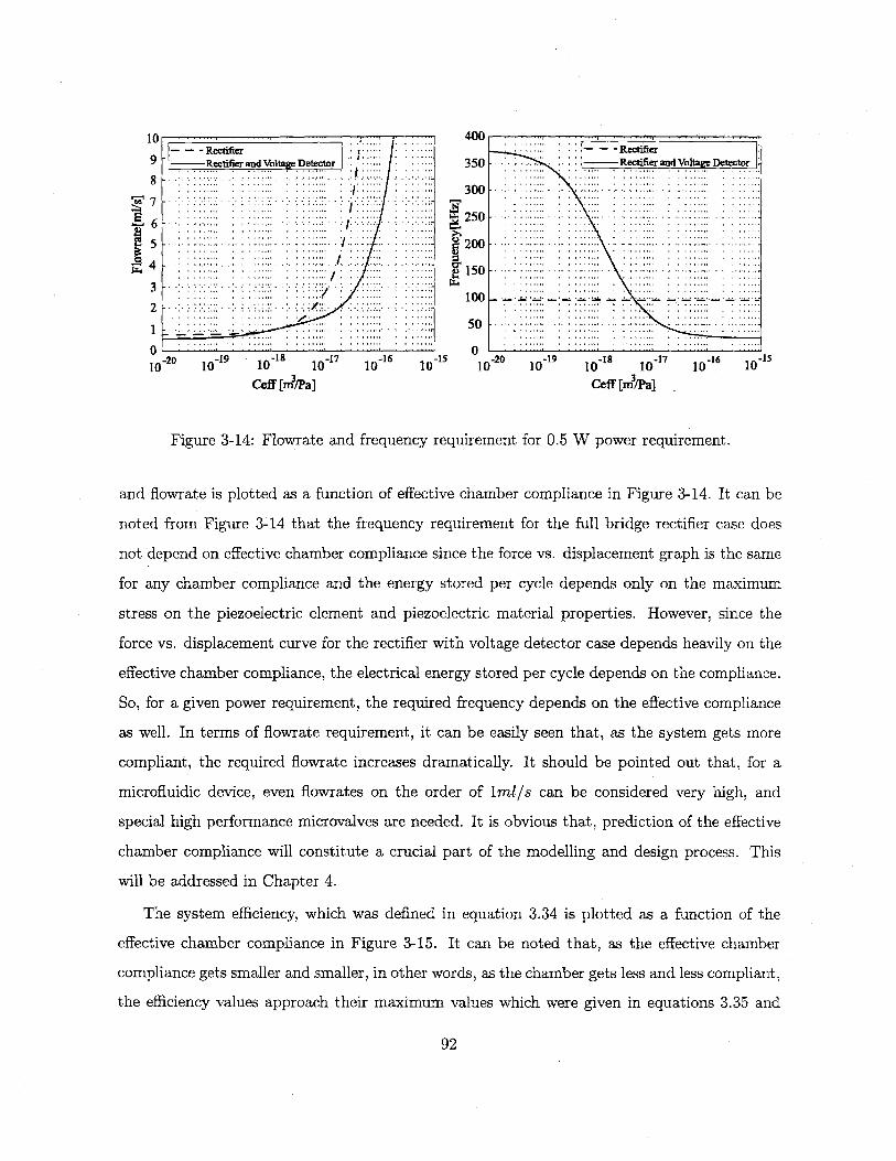
10 . - - - _-_- __-_- _- _- _ - -400 -
- - -Rectifier --- RectifierS Rectifier and Voltage Detector . :. 350 . Rectifier and Voltage Detector
8 . .. . . ...30. :00x-:
250 -
20 -19 -18 -17 -16 -15 -20 -19 -18 -17 16 -1510 10 10 10 10 10 10 10 10 10 10 10
Ceff [2 /Pa] Cefi' [2/Pa]
Figure 3-14: Flowrate and frequency requirement for 0.5 W power requirement.
and flowrate is plotted as a function of effective chamber compliance in Figure 3-14. It can be
noted from Figure 3-14 that the frequency requirement for the full bridge rectifier case does
not depend on effective chamber compliance since the force vs. displacement graph is the same
for any chamber compliance and the energy stored per cycle depends only on the maximum
stress on the piezoelectric element and piezoelectric material properties. However, since the
force vs. displacement curve for the rectifier with voltage detector case depends heavily on the
effective chamber compliance, the electrical energy stored per cycle depends on the compliance.
So, for a given power requirement, the required frequency depends on the effective compliance
as well. In terms of flowrate requirement, it can be easily seen that, as the system gets more
compliant, the required fiowrate increases dramatically. It should be pointed out that, for a
microfluidic device, even flowrates on the order of l/s can be considered very high, and
special high performance microvalves are needed. It is obvious that, prediction of the effective
chamber compliance will constitute a crucial part of the modelling and design process. This
will be addressed in Chapter 4.
The system efficiency, which was defined in equation 3.34 is plotted as a function of the
effective chamber compliance in Figure 3-15. It can be noted that, as the effective chamber
compliance gets smaller and smaller, in other words, as the chamber gets less and less compliant,
the efficiency values approach their maximum values which were given in equations 3.35 and
92
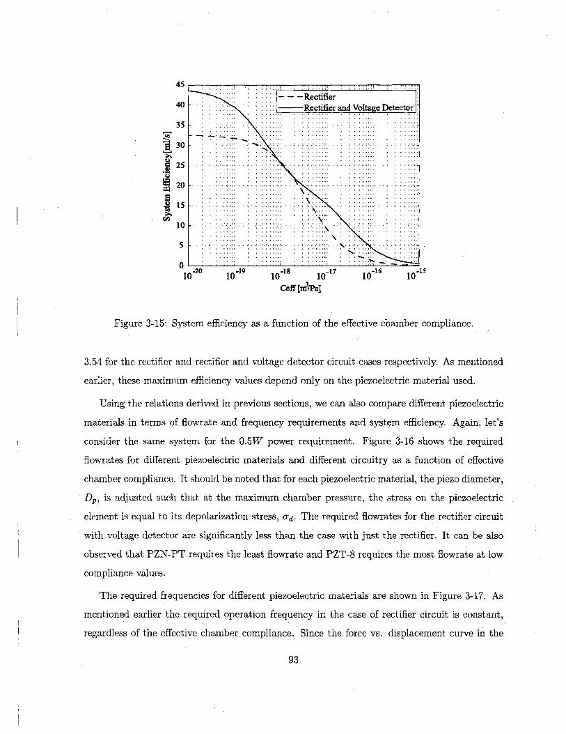
45
- - -Rectifier40 . ... :-Rectifier and Voltage Detector
35 -- - -
3 0 -- - --
-20-9-1-7-6-5
4)
.................... . .2....\w..
............ .............................
5 .................
-20 -19 -18 1116 1510 10 10 10 10 10
Ceff [nm/Pa]
Figure 3-15: System efficiency as a function of the effective chamber compliance.
3.54 for the rectifier and rectifier and voltage detector circuit cases respectively. As mentioned
earlier, these maximum efficiency values depend only on the piezoelectric material used.
Using the relations derived in previous sections, we can also compare different piezoelectric
materials in terms of flowrate and frequency requirements and system efficiency. Again, let's
consider the same system for the 0.5W power requirement. Figure 3-16 shows the required
flowrates for different piezoelectric materials and different circuitry as a function of effective
chamber compliance. It should be noted that for each piezoelectric material, the piezo diameter,
Dp, is adjusted such that at the maximum chamber pressure, the stress on the piezoelectric
element is equal to its depolarization stress, O-d. The required flowrates for the rectifier circuit
with voltage detector are significantly less than the case with just the rectifier. It can be also
observed that PZN-PT requires the least flowrate and PZT-8 requires the most flowrate at low
compliance values.
The required frequencies for different piezoelectric materials are shown in Figure 3-17. As
mentioned earlier the required operation frequency in the case of rectifier circuit is constant,
regardless of the effective chamber compliance. Since the force vs. displacement curve in the
93

(a) Rectifier (b) Rectifier with Voltage Detector10 . , n10
PZN-4.5%PT -.9. - -- . 9 -...-.-.--- -PZT-8 - - - -PZT-8
8 -.---------. PZT-4S 8 - ----------- PZT-4S- --- - - H- PZT-S1H
A6 65 -. ..... .. ..... . .... . ..
3 3
2---
-- -- -- 5---- --
0 . .7-7-7 7 -7.7.7 0-20 -1 9 -1 -17 -16 -15 1 -20 1 -19 1 -18 1 -17 -16 1 15110 10 0 1 110 10 ;~ 0 10-19 10 17 10 16
Ceff [rM/Pa] Ceff [m3,a]
Figure 3-16: Required flowrates for 0.5 power generation. Comparison of different piezoelectricelements and different circuitry.
case of the rectifier and voltage detection circuit depends heavily on the effective chamber
compliance, the required frequency for a certain power requirement depends on the effective
chamber compliance. Since the materials PZT-8 and PZT-4S have very high depolarization
stresses compared to PZT-5H and PZN-PT, the electrical energy stored per cycle for PZT-8
and PZT-4S is much larger, which means reduced frequency requirements for the same power
requirement. For example, although PZN-PT has the highest coupling coefficient(k 3 3 = 0.89)
among the piezoelectric materials discussed here, it requires higher operation frequencies due
to its low depolarization stress.
Figure 3-18 shows the system efficiency for different piezoelectric materials and circuitry. It
can be seen that, the chamber with the rectifier circuit and voltage detector is more efficient
than the case with the rectifier. As the effective compliance gets smaller and smaller, the
system efficiencies approach their maximum value, which are given by equations 3.35 and 3.54
for rectifier and rectifier with voltage detector cases respectively. As expected, PZN-PT is the
most efficient material due to its high coupling coefficient(ks3 = 0.89) and PZT-8 is the least
efficient material due to its low coupling coefficient(k 3 3 = 0.64). Although PZT-8 is the least
efficient one, it might be a better suited material since the system with PZN-PT has very high
94

Required Frequency for 0.5 W (rectifier and voltage detector)400-- - -
PZN-4.5%PT350-PZT-8
---.---- PZT-4S
300 PZT-5H* Required fequencies
with rectifier250 - - - - ---
200-PZso- f 179kHz
N; 150 .- -- -
98kHz100>::PZ-PTr
... PZT-R-f74kHz
50 ...... f=69kc z
0 - - --20 -19 -1 -17 -16 -15
10 10 10 10 10 10Ceff[n?/Pa]
Figure 3-17: Required frequencies for the 0.5W power requirement. Comparison of different
piezoelectric materials and circuitry. Note that the required frequency in the case of regular
rectifier is independent of the chamber compliance.
95

(a) Rectifier (b) Rectifier with Voltage Detector35 I ,...n;.r ia45 . . . . .
PZN-4.5%PT PZN-4.5%PT...PZu- -- PZT-8
30 -4- --------- PZT-4S ---------- PZT-4S- 35 ---- - PZT-H - 4..- - - - - - - -PZT-5.P2l- --- 5H
30....7>
- 20 S525.- .-
.1-15-2-0
N
1 -5 -V-10 ..-.A--....-.............. ......................... N
5 .. . . . ..~
0 -- 0L
-20 -19 -is .-17 -16 -15 -20 -19 ..is-1 -16 -1510 10 10 10 10 10 10 10 10 10 10 10
CefF [n1/Pa] Ceff [2 /Pal
Figure 3-18: Comparison of different piezoelectric materials and circuitry in terms of system
efficiency.
frequency requirements. The material selection process should address the design trade-offs
and should take the remaining components of the system, for example the active valves, into
consideration. One might choose to use PZN-PT which requires very high frequencies, but
this frequency can exceed the bandwidth of the active valves. This issue will be addressed in
Chapter 5.
One should remember that the analysis of the chamber attached to the rectifier and the
voltage detector presented in this chapter assumed that the impedances(inductances) of the
fluid channels are large enough such that there are sudden pressure drops inside the chamber
and the governing equations are derived assuming that in the time interval where the SCR is
in its "on" state, there is no net flowrate into the chamber.
3.6 Summary and Conclusion
This chapter presented a simple analysis of the energy harvesting chamber and a case study
using a simulation for a predetermined chamber geometry and operating conditions. The in-
teraction between the chamber and the circuitry has been investigated. Some of the important
performance metrics derived in the previous sections are summarized in Table 3.3.
96
I
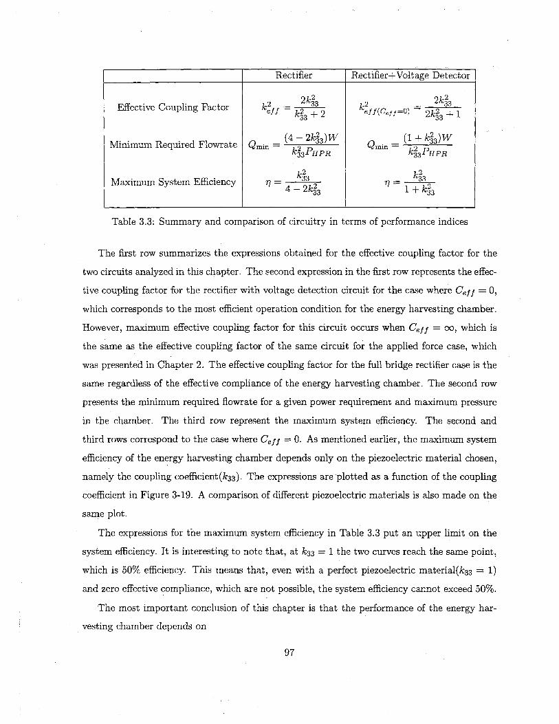
2k2 2k2Effective Coupling Factor ef2- k 3 3+ 2 kff(Ce3) 2k 3 ±1
(4 - 2k2 )2(1+ WMinimum Required Flowrate Qmin = (424 W (min1= k)
kkPH3PR 43PHPR
k2 k2Maximum System Efficiency3 = 3 1+k33
4 - 2k233 1+ k2
Table 3.3: Summary and comparison of circuitry in terms of performance indices
The first row summarizes the expressions obtained for the effective coupling factor for the
two circuits analyzed in this chapter. The second expression in the first row represents the effec-
tive coupling factor for the rectifier with voltage detection circuit for the case where Ceff = 0,
which corresponds to the most efficient operation condition for the energy harvesting chamber.
However, maximum effective coupling factor for this circuit occurs when Ceff = oo, which is
the same as the effective coupling factor of the same circuit for the applied force case, which
was presented in Chapter 2. The effective coupling factor for the full bridge rectifier case is the
same regardless of the effective compliance of the energy harvesting chamber. The second row
presents the minimum required flowrate for a given power requirement and maximum pressure
in the chamber. The third row represent the maximum system efficiency. The second and
third rows correspond to the case where Ceff = 0. As mentioned earlier, the maximum system
efficiency of the energy harvesting chamber depends only on the piezoelectric material chosen,
namely the coupling coefficient(k 3 3 ). The expressions are plotted as a function of the coupling
coefficient in Figure 3-19. A comparison of different piezoelectric materials is also made on the
same plot.
The expressions for the maximum system efficiency in Table 3.3 put an upper limit on the
system efficiency. It is interesting to note that, at k33 = 1 the two curves reach the same point,
which is 50% efficiency. This means that, even with a perfect piezoelectric material(k 3 3 = 1)
and zero effective compliance, which are not possible, the system efficiency cannot exceed 50%.
The most important conclusion of this chapter is that the performance of the energy har-
vesting chamber depends on
97
Rectifier Rectifier+Voltage Detector

50Rectifier
45---Rectifier+Voltage Detector]
... ...- - - .1-- - - -
25 ..-.. ..-....-... .-.
20
30~
0 0.1 0.2 0.3 0.4 0.5 0.6 0 7 0.8 0.9 1Coupling coefficient(kOg
zra2r-5 1 -i
Figure 3-19: Maximum system efficiency (which corresponds to the case where the effectivecompliance of the chamber is zero)as a function of the coupling coefficient.
- Rectification circuit topology
- 'Piezoelectric material (k33,0-d)
- Chamber compliance(Ceff)
Again it should be emphasized that the efficiency definition in this chapter corresponds only
to the energy harvesting chamber. The electrical power consumption in the active valves is not
considered.
98

Chapter 4
Detailed Model of the Energy
Harvesting Chamber
This chapter presents the detailed modelling of the energy harvesting chamber. In Chapter
3, an effective chamber compliance (Ceff) based on a typical MHT device was assumed to
be used in the simulation and the effect of compliance on system performance was analyzed.
This chapter investigates the contribution of different structural components on the effective
compliance of the chamber. It also presents the simulation architecture used for integrating
elastic equations into the system level simulation.
4.1 Analysis of a Simplified Chamber Structure
Consider a simple circular chamber structure consisting of a fluid chamber and rigid walls,
except the top portion of the chamber, as shown in Figure 4-1. The compliant portion can
be modeled as a clamped circular plate which deforms under the action of uniform pressure
underneath. For small deflections, the deformation of the top plate can be assumed to be linear
and can be analyzed using linear plate theory [50].
For a uniform pressure distribution P and a radius of a, the deflection of the top plate as a
function of the radial distance is given as:
w(r) = (a2 r2)2 (4.1)64D
99

,*,**,** 1 -gm-.---~- ~mrr~-~ - -. -
Compliant top plate
-1 t + k
rigid Dch=2a h "
rigid
(a)
rigid
a
A VS
(b)
Figure 4-1: (a) Simplified chamber structure consisting of a fluid chamber with a compliant
wall (b) Deformation of the top plate and swept volume.
where D is the flexural rigidity of the plate given by:
D = t 3
12(1 - V2)(4.2)
where E and v is the Young Modulus and Poisson ratio of the material respectively, and t is
the thickness of the plate. The additional volume created in the chamber due to the deformation
of the plate can be calculated by integrating equation 4.1 over the plate:
AV = aw(r)27rrdr = Pra6 (1 2)= w16Et
3
The structural compliance was defined in Chapter 3 as:
AVSAP (4.4)
which represents the volume change of the chamber due to structural deformations in re-
sponse to a change in chamber pressure. In this simple example, the top plate is the only
compliant structural member. Using equations 4.4 and 4.3, the structural compliance can be
calculated as:
CS = 7ra 6(1 -- V2)16Et
3
The effective chamber compliance can be obtained as:
(4.5)
100
(4.3)

-1510
.....- .-. .. .. - ----
10 Effecive Compliance
10.. ..
102~ 10.......
10
-19
1. 2 3 4 5 6 7 8 9 10
Dch[mm]
Figure 4-2: Comparison of fluidic and structural compiances for a generic chamber structureat different chamber diameters for fixed chamber height and top plate thickness.
0 ef ( arc)=(h + 7ra 6 (1- v)(46
where V0 is the initial fluid volume inside the chamber, /3g is the bulk modulus of the fluid
and h is the height of the chamber.
Consider a chamber with top plate thickness of 500gm and chamber height of 200gm.
Figure 4-2 shows a comparison of fluidic and structural compliances for different chamber
diameters. It can be seen that, for small chamber diameters, the compliance of the chamber
is dominated by the fluidic compliance, whereas at large chamber diameters the structural
compliance dominates. However, it should be noted that, if all the geometric parameters are
scaled the same amount, the ratio of the fluidic and structural compliances will remain the
same. This issue will be discussed further in Chapter 5.
101
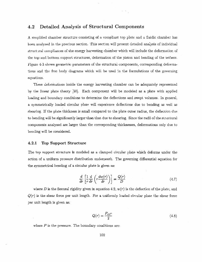
4.2 Detailed Analysis of Structural Components
A simplified chamber structure consisting of a compliant top plate and a fluidic chamber has
been analyzed in the previous section. This section will present detailed analysis of individual
structural compliances of the energy harvesting chamber which will include the deformation of
the top and bottom support structures, deformation of the piston and bending of the tethers.
Figure 4-3 shows geometric parameters of the structural components, corresponding deforma-
tions and the free body diagrams which will be used in the formulations of the governing
equations.
These deformations inside the energy harvesting chamber can be adequately represented
by the linear plate theory [50]. Each component will be modeled as a plate with applied
loading and boundary conditions to determine the deflections and swept volumes. In general,
a symmetrically loaded circular plate will experience deflections due to bending as well as
shearing. If the plate thickness is small compared to the plate outer radius, the deflection due
to bending will be significantly larger than that due to shearing. Since the radii of the structural
components analyzed are larger than the corresponding thicknesses, deformations only due to
bending will be considered.
4.2.1 Top Support Structure
The top support structure is modeled as a clamped circular plate which deforms under the
action of a uniform pressure distribution underneath. The governing differential equation for
the symmetrical bending of a circular plate is given as:
d 1id dw(r) _Q(r)(4)I[d(r (4.7)dr [rdr di 21 D
where D is the flexural rigidity given in equation 4.2, w(r) is the deflection of the plate, and
Q(r) is the shear force per unit length. For a uniformly loaded circular plate the shear force
per unit length is given as:
Q(r) hr (4.8)2
where P is the pressure. The boundary conditions are:
102
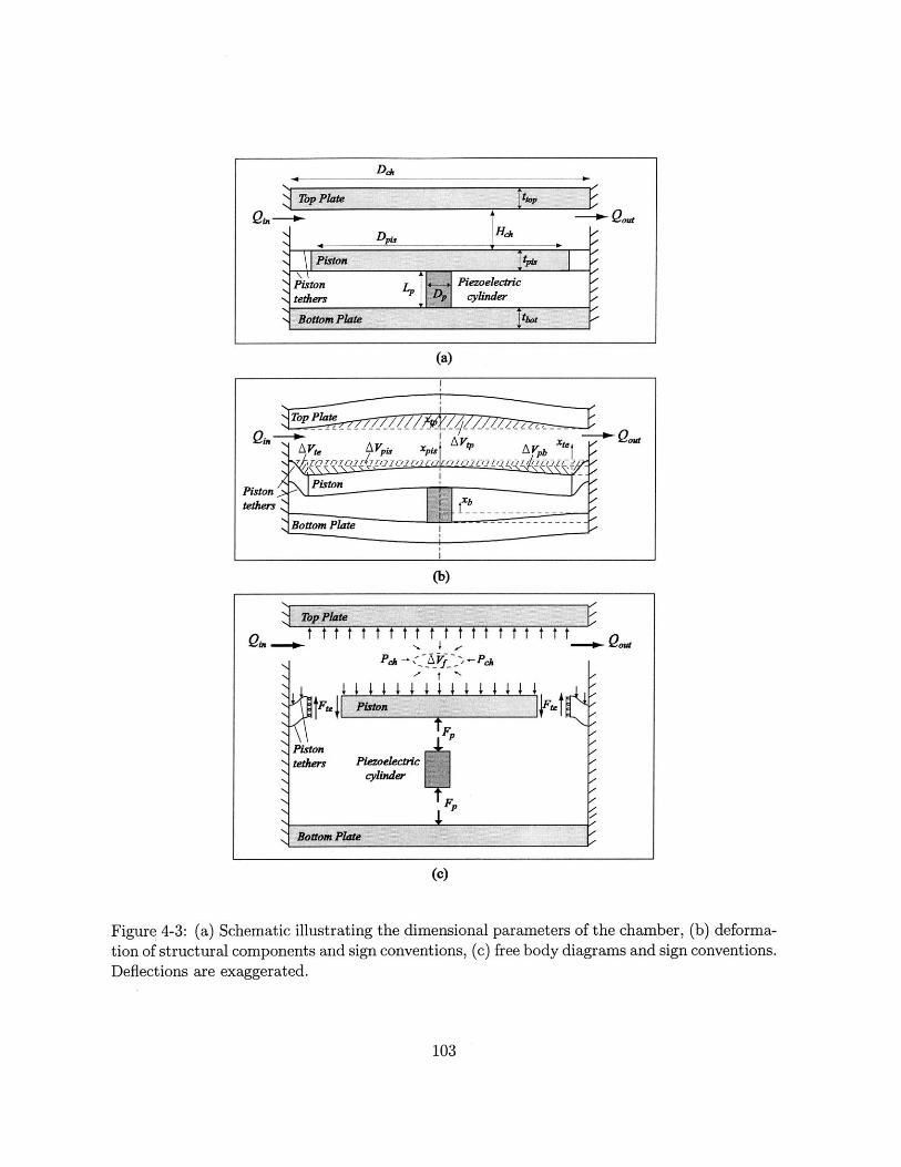
Dh
Top Plate 4z,
DpL H*
Pistonl
Piston Piezoelectric
tethers cylinder
Bottom Plate 41t
(a)
No-. Q Mt' A V ~ 'A' \
Piston ton
Bottom Plate -------------
(b)
IPPlate
- t t t I tP,
F& ulPstn
NNNNNNN
Pistontethers
I&AoPtte
(c)
t t t t t t t t t ti t t t-- V _-P
t
1F
Figure 4-3: (a) Schematic illustrating the dimensional parameters of the chamber, (b) deforma-tion of structural components and sign conventions, (c) free body diagrams and sign conventions.Deflections are exaggerated.
103
QMIt
lo,lollloo,
.ool
100,oo,
Piezoelectriccylinder
F
i 11111il I Ft.
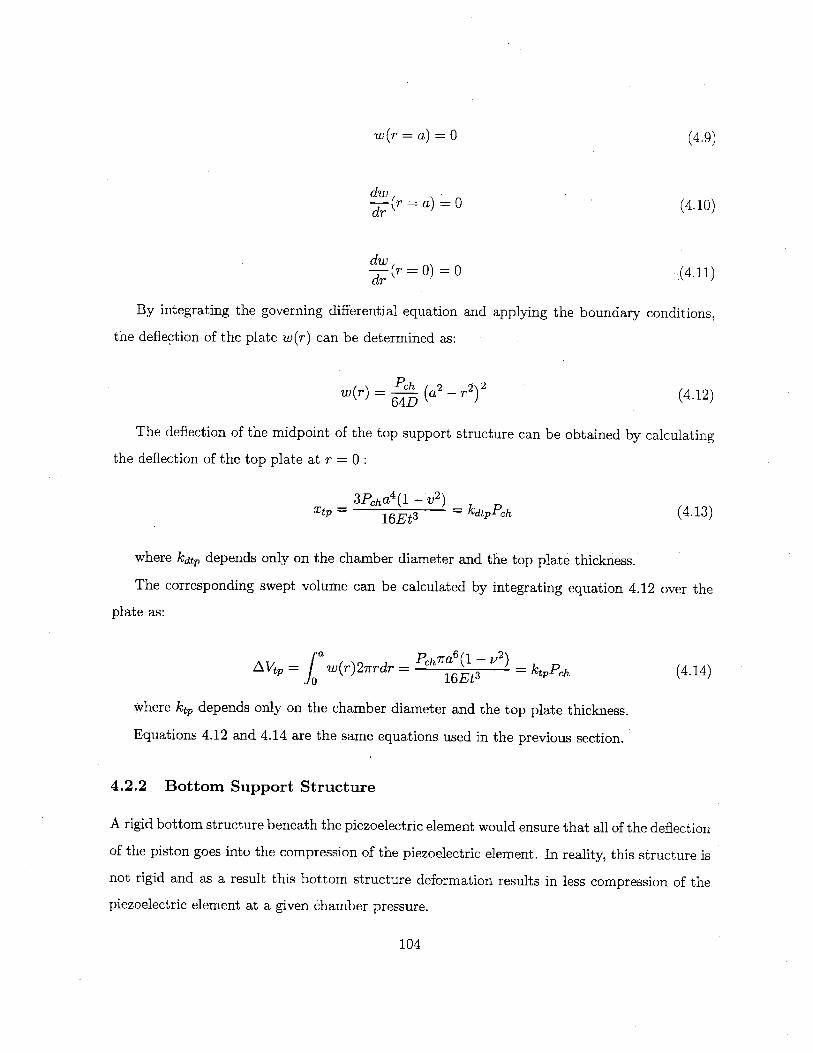
w(r = a) = 0 (4.9)
dw(r = a)-0 (4.10)
dwr = 0 (4.11)
By integrating the governing differential equation and applying the boundary conditions,
the deflection of the plate w(r) can be determined as:
P ) h 2 22w1(r) =' (a2 - 9)2(4.12)
The deflection of the midpoint of the top support structure can be obtained by calculating
the deflection of the top plate at r = 0:
3Pcha4 (1 - v2 )-tp -= 16Et3 = kdtPch (4.13)
where kdt, depends only on the chamber diameter and the top plate thickness.
The corresponding swept volume can be calculated by integrating equation 4.12 over the
plate as:
[a Pch7ra6(1 - v2 )
tP a w(r)27rrdr = h6Et3 =ktPch (4.14)
where ktp depends only on the chamber diameter and the top plate thickness.
Equations 4.12 and 4.14 are the same equations used in the previous section.
4.2.2 Bottom Support Structure
A rigid bottom structure beneath the piezoelectric element would ensure that all of the deflection
of the piston goes into the compression of the piezoelectric element. In reality, this structure is
not rigid and as a result this bottom structure deformation results in less compression of the
piezoelectric element at a given chamber pressure.
104

ar
b
FPiezo P w(r)
Clamped E,v
Figure 4-4: Model of the bottom support structure: circular plate with a circular hole at its
center with guided boundary condition at inner radius b and clamped boundary condition at
outer radius a.
The bottom support structure is modeled as a circular plate with a circular hole at the
center which is clamped at its outer radius (r = a) and guided at its inner radius (r = b),
shown in Figure 4-4. In this case the shear force per unit length is given as:
Q(r) = -27rr
(4.15)
where Fp is the force acting on the bottom support structure through the guided support in
the inner radius (r = b). The boundary conditions are:
(4.16)w(r = a) = 0
dw-(r = a) = 0
dr
dw(r = b) = 0
dr
(4.17)
(4.18)
The deflection of the bottom plate, Xb, can
applying the boundary conditions to obtain:
be calculated by integrating equation 4.7 and
Xb = kbFp (4.19)
105
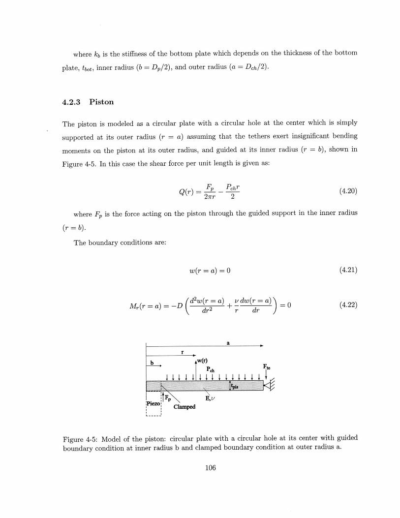
where kb is the stiffness of the bottom plate which depends on the thickness of the bottom
plate, tbot, inner radius (b = Dp/2), and outer radius (a = Deh/2).
4.2.3 Piston
The piston is modeled as a circular plate with a circular hole at the center which is simply
supported at its outer radius (r = a) assuming that the tethers exert insignificant bending
moments on the piston at its outer radius, and guided at its inner radius (r = b), shown in
Figure 4-5. In this case the shear force per unit length is given as:
Q(r) = F ch r27rr 2
(4.20)
where Fp is the force acting on the piston through the guided support in the inner radius
(r = b).
The boundary conditions are:
w(r = a) = 0 (4.21)
d2 w(r = a)M,(r = a) = -D ( r
v dw(r = a) 0r dr /
(4.22)
a
r
b W(r) t
,t $F\ E,,Piz|Clamped
Figure 4-5: Model of the piston: circular plate with a circular hole at its center with guided
boundary condition at inner radius b and clamped boundary condition at outer radius a.
106
dw(r = b) =0 (4.23)
dr
where M, denotes the bending moment per unit length along circumferential sections of the
plate. The deflection of the piston and the corresponding swept volume can be calculated by
integrating equation 4.7 and applying the boundary conditions to obtain:
Xpb = XjpiS - Xte = kp1F+ kp2Peh (4.24)
AV> = k F+ kp4Pch (4.25)
where k 1, kp2 , kp3,and kp4 depend on the thickness of the piston, tg,8 , inner radius (b =
D/2), and outer radius (a = Dpi/2). The dynamics of the piston can be represented using
the free body diagram in Figure 4-3 as:
Mris d = -ApisPcn + Fp - Fte = Fnet (4.26)dt2
4.2.4 Piston Tethers
In this section, tethers corresponding to a double layer piston structure will be analyzed which
consist of a top and bottom tether structure. In order to allow for flexibility in design, the
top and bottom tethers are defined to have different thicknesses (ttetoPt 6obot). The top tether
is modeled as a circular plate with a circular hole at the center which is clamped at its outer
radius and guided at its inner radius, shown in Figure 4-6. It experiences a concentrated force,
Ftetop, at its inner radius and a uniform pressure loading, Ph. The shear force per unit length
is given as:
Ftetop Pch(r 2 - b 2 )Q(r) = 2w r(4.27)27rr 2r
The boundary conditions are:
w(r = a) 0 (4.28)
107
IN
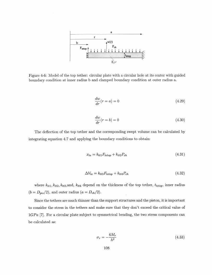
a
r
b w(r)F PcbFtetop II I
hetop
E,v
Figure 4-6: Model of the top tether: circular plate with a circular hole at its center with guidedboundary condition at inner radius b and clamped boundary condition at outer radius a.
dw-(r = a) = 0 (4.29)dr
dw-(r = b) = 0 (4.30)dr
The deflection of the top tether and the corresponding swept volume can be calculated by
integrating equation 4.7 and applying the boundary conditions to obtain:
Xte = kttiFtetop + ktt2Pch (4.31)
AVte = ktt3Ftetop + ktt4Pch (4.32)
where ktti, ktt2, ktt3,and, ktt 4 depend on the thickness of the top tether, ttetop, inner radius
(b = Dpi,/2), and outer radius (a = Deh/2).
Since the tethers are much thinner than the support structures and the piston, it is important
to consider the stress in the tethers and make sure that they don't exceed the critical value of
1GPa [7]. For a circular plate subject to symmetrical bending, the two stress components can
be calculated as:
6Mr- -h2 (4.33)
108

t =6M (4.34)
where Mr and Mt are the bending moment per unit length along the circumferential sections
of the plate and along the diametral section of the plate respectively, and h is the thickness of
the plate. The bending moments are obtained as:
(d2 w v dwNMr=- D + (4.35)
dr2 r dr
M -D 1 dw d 2
t ~r dr dr2
where D is the flexural rigidity of the plate. Using the equations 4.33, 4.34, 4.35, 4.36, the
stress components can be calculated after the governing plate equation 4.7 is integrated using
appropriate boundary conditions and the deflection of the plate, w, is determined. As will be
seen later in the next chapter, o-, is generally bigger than ot and the maximum stress occurs at
a = Dch/2. Then we can write the maximum stress in the top tether as:
6M,(r = Des/12) (-7(-max = Ott = -- 6 2 (4.37)tetop
which can be alternatively expressed as:
-tt = sttiFtetop + Stt2Pch (4.38)
where stti and Stt2 depend on the thickness of the top tether, tetop, inner radius (b =D,/2),
and outer radius (a = Dch/2).
The bottom tether is modeled in the same way as the top tether, except it experiences only
a concentrated force, Ftebot, at its inner radius and no pressure loading. The shear force per
unit length is:
Q(r) = 2irr (4.39)
The boundary conditions are the same as the boundary conditions for the top tether. The
109

deflection of the bottom tether, which is equal to the deflection of the top tether can be obtained
by integrating equation 4.7 and applying the boundary conditions to obtain:
Xte = ktbFtebot (4.40)
where kt 6 depends on the thickness of the bottom tether, ttebot, inner radius (b =Dpi,/2),
and outer radius (a = Dch/2).
Similarly, the stress in the bottom tether can be calculated as:
(tb = StbFtebot (4.41)
where SOt depends again on the thickness of the bottom tether, ttebot, inner radius (b =
Di,/2), and outer radius (a = Dch/2)
We can also write:
Fte = Ftetop + Ftebot (4.42)
which represents the force balance at the connection point of the tethers with the piston.
Detailed derivations of the elastic equations of the structural components are detailed in
Appendix C.
4.3 Simulation Architecture
This section will present the simulation architecture used for integrating the elastic equations
into the system level simulation.
Chamber Continuity
The continuity equation was derived in the previous chapter. In this section a more detailed
equation will be derived considering the volume displaced in the chamber due to deformations
of individual structural members. In the previous chapter, all the volume displaced by de-
formations was analyzed as a bulk value, namely AV, and was used to define the structural
compliance, C. Rewriting equation 3.5, we have:
110

dP~h _-/Of dV (4.43)dt V dt
where 1f is the bulk modulus of the fluid, V0 is the initial volume of the fluid inside thedV
chamber and -- is the rate of the volume change of the fluid. Sources of the volume changedt
are net flowrate into the chamber, piston movement and additional volume created inside the
chamber due to structural deformations. Considering these effects and integrating equation
4.43, we can write:
Pch = (Qin -- Qnt)dt + AVis + AVb + AVte - AV) (4.44)
where AVpi 8, AVpb, AVte, AVtp represent the swept volume due to the motion of the piston,
deformation of the piston, deformation of the top tether and deformation of the top support
structure respectively. The swept volume due to the motion of the piston is simply equal to:
V pis= xpisApis (4.45)
where Apis is the area of the piston. By arranging equation 4.44 we can obtain:
Pch = + CtP -(f(Qin - Qout)dt + xpisApis + AVpb + AVte (4.46)
where Ctp represents the structural compliance corresponding to the deformation of the top
support structure, which is given by equation 4.5.
Piezoelectric Cylinder
For a cross-sectional area of A, and length L,, the net deflection of the piezoelectric element
and the voltage across it can be expressed using linear constitutive relationships as:
Xb - = +(St3FP , T P(4.47)Ap 833
V = p( F- QP) (4.48)p 633 633
111
where Q, is the charge on the piezoelectric element.
Equations 4.13, 4.14, 4.19, 4.24, 4.25, 4.26, 4.31, 4.32, 4.38, 4.40, 4.41, 4.42, 4.44, 4.47, and4.48 (15eqns) can be solved for the 15 unknowns, namely V,,, t, AVp, AVte, AV2 , Xb, Xte,
Ffe, Fte-top, Fte-bot, ott, atb, Fp, Ph, and Fact in terms of Q,, pis, and Qnet where
Qnet = j(Qin - Qout)dt (4.49)
which tepresents the net fluid volume change inside the chamber due to the fluid flow into
and out of the chamber [52]. The elastic equations along with the chamber continuity equation
and piezoelectric element constitutive relationships are solved in Maple and the coefficients
(A 11, A1 2 ...) of the 15x3 matrix required by the simulation architecture, shown in Figure
4-7, is calculated. The coefficients are then processed in a Matlab code to generate the 15x3
matrix, which is fed to Simulink. The details are presented in Appendix B and Appendix C.
The Simulink blocks of the system model are presented in Appendix A.
The matrix equation solved in Simulink is as follows:
V A 11 A1 2 A 1 3
xtP A2 1 A2 2 A23
A Vt A31 A32 A33
AVte41 A42 A4 3
A Vb A5 1 A5 2 A5 3
Xb -A6 1 A 6 2 A6 3
Xte A71 A7 2 A73 Q .Fte = A81 A82 A8 3 XjS (4.50)
Fte-top A91 A9 2 A93 [ Qet
Fte-bot A10o A10 2 A103
Ott A11 1 A1 12 A11 3
cltb A1 21 A1 22 A1 23
Fp A1 31 A1 32 A1 33
Pch A141 A14 2 A14 3
Fnet A1 5 1 A15 2 A1 53
112

II
T_ QP
QM 1 + Qet
QOut P.-
Circuitry
- VP
10Xtp
1 AVtp0 AVt,
0 AVpb
N Xb
Xte
SFt.
SFtotop
SFt,-xot
at
0, Uth
F,
SPch
SF,,t PitoDynamics
Figure 4-7: Simulation architecture used to integrate the elastic equations into system levelsimulation.
113
15x3 Matrix

where the matrix coefficients are calculated using Maple.
The simulation architecture allows for integration of the elastic equations into the dynamic
simulations as well as for monitoring important parameters like deflections and swept volumes
of the individual structural components and stresses in the tethers.
4.4 Conclusion
This chapter presented detailed analysis of the energy harvesting chamber in terms of the
deformations of individual structural components. The deformations are analyzed using linear
plate theory. It is assumed that the deflections due to bending are significantly larger than
those due to shearing. A simulation architecture is presented to be included in the overall
system level simulation, which allows for inclusion of the elastic equations into the dynamic
simulation and allows for monitoring important parameters.
114

Chapter 5
Further Design Considerations and
Design Procedure
This chapter presents further design considerations in addition to those issues discussed in
Chapter 3. These are fluidic oscillations within the system, chamber filling and evacuation,
tether structure optimization and the effect of operation conditions and geometry on system
performance. At the end of the chapter, a design procedure along with two design examples
and simulation results will be presented. The system is analyzed only for the case where the
chamber is attached to the regular bridge.
5.1 Further Design Considerations
5.1.1 Fluidic Oscillations
Inertial effects should be considered when designing hydraulic systems containing small chan-
nels. In fact, in the MHT devices, the fluid channels and the main chamber constitute a
resonating system similar to a Helmholtz resonator, shown in Figure 5-1, which comprises a
fluid channel and a chamber with an effective compliance C. The natural frequency of the
Helmholtz resonator can be calculated by considering the free-body diagram of the fluid slug
within the channel. The equation of motion of the fluid slug can be written as:
115

chamber
F 1pressure R
P
CLAc
chamber
compliance
Figure 5-1: Helmholtz Resonator.
c c dt d' + PAC = 0 (5.1)
where P is the pressure inside the chamber which builds up as a result of the additional
fluid flow into the chamber, which can be expressed as:
P = Pc(5.2)C
Combining equations 5.1 and 5.2 we can obtain the governing equation for the Helmholtz
resonator as:
X + ( CL,) = 0 (5.3)
onator within the system depends on the channel geometry(-L-7 ratio), the compliance of the
AA,
chamber and the density of the working fluid. The chamber compliance here refers to the over-
all chamber, including the compression of the piezoelectric element. In Chapter 3, an effective
chamber compliance, Ceff, was defined which took only the structural deformations and fluid
compression into account, but not the compression of the piezoelectric element. In the context
of this discussion, it is convenient to define an overall chamber compliance, C, which includes
116

the structural deformations, fluid compression, and the deformation of the piezoelectric element.
The overall chamber compliance in this case can be defined as:
AVf_ fA(Qn - Qt)dtAPch APch
(5.5)
where AVf is the fluid volume change in the chamber due to the fluid flow. In fact, this
compliance is not a constant value in the actual power generator since the stiffness of the
piezoelectric element changes constantly (the stiffness flips between open-circuit and close-
circuit stiffnesses of the piezoelectric element) during the operation, as discussed in Chapter 2
and Chapter 3. In the following two subsections, the fluidic oscillations will be analyzed for two
cases. In the first case, a constant overall chamber compliance will be assumed for simplicity
and in order to get insight, and in the second case the actual system, i.e. the chamber attached
to the rectifier circuit will be analyzed in terms of fluidic oscillations.
Analysis with Constant Overall Chamber Compliance
Consider a chamber with constant overall chamber compliance, C - 10-[m3 /Pa], as defined in
equation 5.5. Figure 5-2 shows the simulation of the system for different chamber geometries, i.e.
for different LC/AC ratios. In the simulation, the operation conditions, valve size and openings
are adjusted such that the chamber pressure fluctuates between PHPR and PLPR for the case
where the inertial effects in the channels are negligible. These conditions are: PHPR = 2MPa,
PLPR = 0, f = 10kHz, R,, = 200pm, voj, = vOt = 20gm, and the working fluid is silicon-oil.
It can be see that there exists an optimum LC/AC value for which the difference between
the maximum and minimum pressures, i.e. the pressure band, APch, is maximum. This value
is approximately 25000(1/m). The pressure band is not very sensitive to LC/AC around the
optimum value, i.e. LC/AC = 24000 or Lh/AC = 26000 results pretty much in the same pressure
band. In fact, the optimum value of the LC/AC can be approximated using equation 5.4. Figure
5-3 shows the inlet flowrate time histories from the simulation. It can be seen that, the fluid
inductance in the channel causes the flow to lag, i.e. the flowrate reaches its maximum at a
later time compared to the case where the fluid inductance is negligible.
117
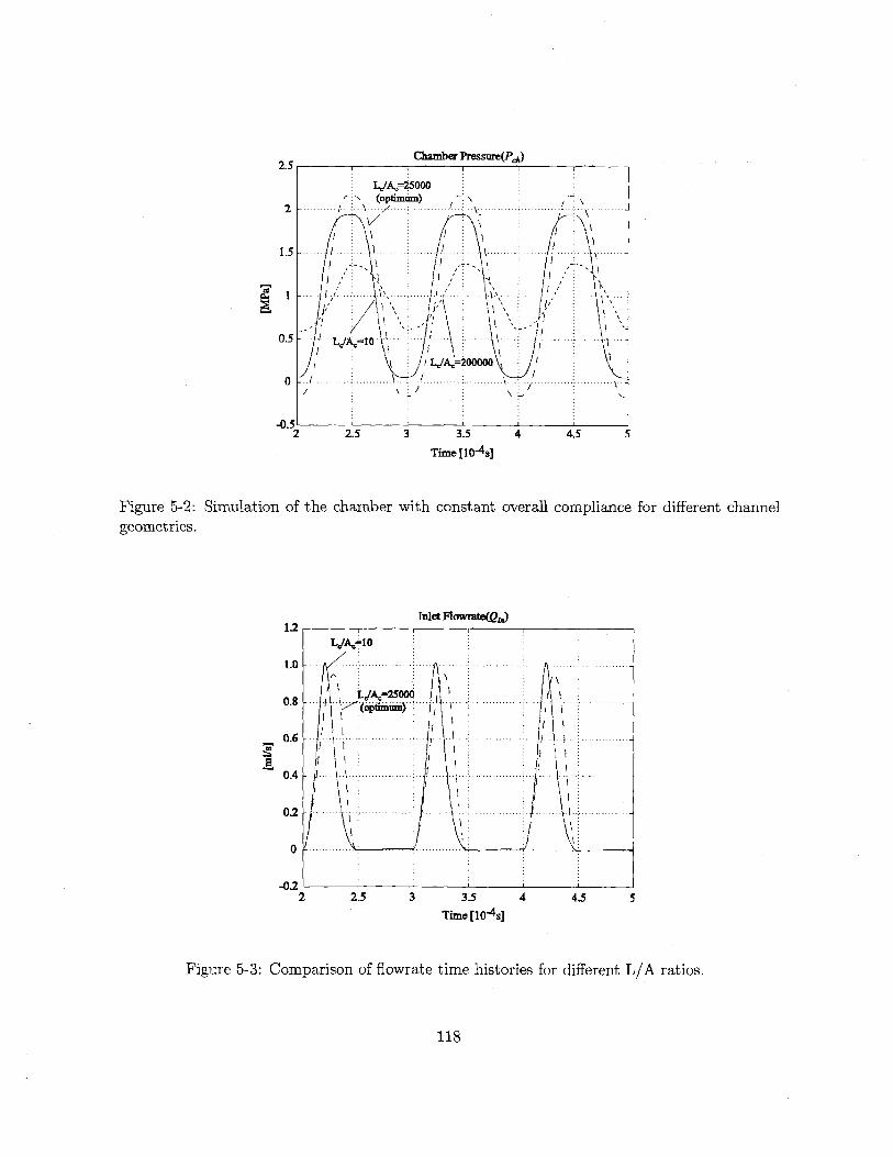
Chamber Pressure(PM)
L/A=25000(optimum) -
- - I -- --I
- . j.. ....... .
-j- - \
. . LJA. ..0 . I.-
ILIAk200000
\- . .-- \--............
2 2.5 i 3.5 4 4.5 5
Time [10-4s]
Figure 5-2: Simulation of the chamber with constant overall compliancegeometries.
12
1.0
0.8
0.6
0.4
02
0
-A2
Inlet Flowrate(QL,)
Le c10
LeA=25000
---- ----------.-....-
-...-.-.--
L-. . . . ... .. ---.-..--.....- ...--.... O.
......... ..............
for different channel
2 2.5 3 3.5 4 4.5 5Time [10-4 s]
Figure 5-3: Comparison of flowrate time histories for different L/A ratios.
118
2.5
2
1.5-
1
0.5
0
r-I
-V.Z

Chamber Pressure (Ph)
LA =25000
L/A I0 \ (o ptinum)2r
0.5
2 25 3 3.5 4 4.5 5
Time [104]
Figure 5-4: Simulation of the chamber attached to circuitry for different channel geometries.
Analysis of the chamber attached to circuitry
Consider the chamber geometry, effective compliance and operation conditions presented in
Table 3.2 of Chapter 3. Figure 5-4 shows the simulation of the same geometry for different
Lc/Ac ratios. Again, the valve size and opening is adjusted such that the chamber pressure
fluctuates between PHPRand PPafor the case where the inertial effects in the channels are
negligible. These conditions are: PHPR = 2MPa, PLPR = 0, f = 10kHz, R,,, = 200pim,
VOin= Mou = 20p~m, the working fluid is silicon-oil, and the battery voltage, V, is 90V, which
is optimized for a pressure band of 2MPa. Similar to the case where a constant overall chamber
compliance was assumed, there exists an optimum Lc/Ac value for which the difference between
the maximum and minimum pressures, i.e. the pressure band, APch, is maximum.
Figure 5-5 shows the effect of Lc/Ac ratio on pressure band and generated power. Through-
out the simulations the battery voltage was not changed. In fact, in a design, the battery
voltage should be determined according to the expected pressure band, which determines the
stress band on the piezoelectric element. For example, for the optimum Lc/Ac ratio, the pressure
band is 2.435MPa, which suggests a battery voltage of approximately 125V. If the simulation
is repeated with this value, the pressure band is now 2.472MPa, which is slightly different than
119

Pressure Band in the Chamber (APah) Power Generated (W)30.1 ---- r-- - _ _1 _7
resonant condition resonantrcondition2.8 -.-. 0.09
260.08 .. .. ..2.4 0.07
.quasstat -- -...-.--. 0.05 -quasistat.c -inertia dominatedinerta dominked
1.8 - -- - 0.04 -----
1 4 - - 0.02 -
1 00100.5 1 152 2.5 3 3.54 45 0 0.5 1 152 2.5 33.54 4.55
LI&, [IO5rr- 1J LIAC[1&5 n 1J
Figure 5-5: Effect of L/A ratio on pressure band and generated power.
the previous value, and the generated power is 0.1068W The slight change in the pressure band
suggests that the change in the battery voltage caused a small change in the overall chamber
compliance, because it basically determines the voltage level where the piezoelectric element
will change its stiffness, and therefore effects the time intervals in which the piezoelectric ele-
ment posses the different stiffnesses. The expression for the optimum battery voltage was given
in Chapter 2 as:
Vb = -~~s (5.6)4 d3
which can be written in terms of the pressure band in the chamber as:
1 APChA?is (st - (5)L)4 A4da
where A1,i and A, are the piston area and the cross-sectional area of the piezoelectric
cylinder respectively, and Aa- is the stress band on the piezoelectric element. It should be
noted that, when writing equation 5.7 the effect of tethers and piston dynamics is neglected. In
other words, static force balance between the piston and piezoelectric element is assumed and
the force applied by the tethers on the piston is neglected. This issue will be addressed later.
We can conclude that, for a given overall chamber compliance there exists an optimum
LC/AC ratio at a certain operation frequency, or similarly, there exists an optimum operation
120

frequency for a certain overall compliance and L/AC ratio. The fluidic oscillations should be
considered in any design procedure and the channels should be designed accordingly. This will
be addressed later in the discussion of the design procedure.
The overall chamber compliance was defined as the compliance of the chamber including
the compliances due to structural deformations and fluidic compliance, which is represented by
the effective compliance, Ceff, and the compliance due to the deflection of the piezoelectric
element. The compliance due to the deflection of the piezoelectric element can be calculated
considering the volume displaced by the piston due to the deflection of the element as a response
to the pressure change in the chamber:
Cp tts t A (APA A A% 8 (5.8)APeh APeh APeh k
where kp is the stiffness of the piezoelectric element, which can be expressed as:
kp 8=Ap (5.9)s33LP
where A, and Lp are the cross-sectional area and the length of the piezoelectric element
respectively, and 833 is the compliance coefficient of the element. As mentioned earlier, the
stiffness of the piezoelectric element changes constantly during the operation between the open
circuit and closed circuit stiffnesses, which should be calculated using st and s respectively.
Therefore the system is highly nonlinear and it is impossible to express the resonant frequency,
or the optimum L4/AC ratio analytically. However we can get a first order estimation of the
resonant frequency using one of the stiffnesses above. For example using the open circuit
compliance coefficient, sg, and from equations 5.4, 5.8, and 5.9 we obtain:
1 Ac 1 Ac 5.0fn =--D 2(5.10)2r Lp (Ceff + C) 27 LpV s LpA 2
where Ceff is the effective chamber compliance.
It is very important to note that in the simulations presented in this and the previous
121

sections (Figures 5-2 and 5-4), the pressure in the chamber overshot the reservoir pressures
(PHPR and PLPR) in the resonance conditions, which resulted in negative pressures, which
should be avoided because of cavitation. In the design procedure, the operation conditions
should be adjusted such that there won't be any cavitation. For example the system can be
biased, i.e. the reservoir pressures can be increased keeping the difference the same. Or, the
valve openings can be adjusted accordingly. The motivation for operating at resonance condition
is that the same pressure band can be achieved with smaller valve cap sizes or valve openings
compared to the case of negligible or very large fluid inductance in the channels, resulting in
reduced power consumption in the active valves.
5.1.2 Chamber filling and evacuation
In order to attain the desired pressure bands inside the chamber, it is important to design the
valve sizes, openings and the operation frequency accordingly. Consider the chamber attached
to the circuitry discussed in the previous section. Figure 5-6 shows the effect of valve opening on
pressure band in the chamber. A valve opening of 20pm provides perfect filling and subsequent
evacuation of the chamber in the required time interval and the chamber pressure fluctuates
between the reservoir pressures. A small valve opening of 51m results in poor(slow) filling
and evacuation, resulting in a reduced pressure band. A large valve opening of 50pm provides
very fast filling and evacuation, which causes the chamber pressure to retain its maximum
and minimum values for long time intervals. The latter results in the same power generated,
however it also results in more power consumption in the active valves due to the higher stroke.
A similar result would be obtained by keeping the valve opening the same, but increasing the
valve cap size. Again more power would be consumed in the active valves.
Figure 5-7 shows the effect of operation frequency on the pressure band in the chamber.
It can be seen that, for a fixed valve opening, different operation frequencies result in system
behaviors similar to the ones in Figure 5-6. At high frequency, there is not enough time for
the valve to fill and evacuate the chamber in the required time interval. Similarly, at low
frequency, there is more than enough time for the valves to fill and evacuate, which results in
similar behavior to the case of large valve opening. This implies that, the valve opening can
be reduced for reduced power consumption in the active valve and yet the same power can be
122
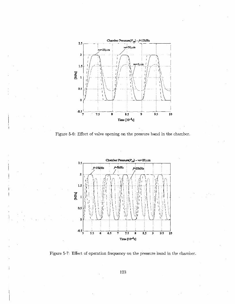
Chamber Pressure(P) -f=IOkHz2.5
2
1.5
0.5
0
-0.57 9 9.5 10
Figure 5-6: Effect of valve opening on the pressure band in the chamber.
Chamber Pressurr(Pa) - vo=20pmT I I 1 I I
10kHz Skzz f2kz
1 '-
'IIF. .. J
- --I
Ir 1
- )-
5.5 6 6.5 7 7.5 8
Time [10-4 s]
8.5 9 9.5 10
Figure 5-7: Effect of operation frequency on the pressure band in the chamber.
123
8 8.5
Time [U0-s]
vo-=-50pM:r20gm
1 r
--.-.--.--.-
- -. ...----.- .--. .
7.5
2.5
2
1.5
0.5
0
-0.5
generated as long as the pressure band in the chamber is kept at the desired level.
In the two cases analyzed above, the valve cap size could be analyzed instead of valve
opening, which would lead to the same conclusions. The combination of the valve size and the
valve opening define the overall valve resistance. We can conclude that, for a designed operation
frequency and pressure band, it is important to design the valve size and opening such that they
will provide just enough filling and evacuation of the chamber in the required time interval,
which is defined by the operation frequency, so that the chamber pressure fluctuates between the
reservoir pressures in the most economical way. As will be addressed later, the pressure band
is a very important design parameter, since the power generated is proportional to the square
of the stress band on the piezoelectric element. Additional design considerations concerning
the design of the valve size and opening is not within the scope of this thesis. The design
optimization of the active valves is detailed in [5].
5.1.3 Tether Structure Optimization
Design of the piston tether structure is very crucial for system operation. The tethers should
be flexible enough to allow sufficient motion of the piston, yet stiff enough to avoid introduction
of excessive compliance into the system. The tethers have to be designed to allow maximum
piezoelectric element compression for a given net fluid volume into the chamber, which occurs
basically at every cycle during system operation. To analyze the tether structure, consider a
simple hypothetical chamber which consists of a fluid chamber with rigid walls, a single layer
piston attached to the wall with a single tether providing sealing, and a piezoelectric element.
Figure 5-8 illustrates the hypothetical chamber and different tether designs. Figure 5-8(b)
illustrates a good tether design where the tethers allow large piezoelectric element compression.
Figure 5-8(c) illustrates a poor design where the tether is either too thin or the tether width,
t.,,, is very large (tw = [Dch - Dis]/2). This results in low pressure in the chamber and small
compression of the piezoelectric element since the compliance introduced by the tether is very
large. In other words, pressure doesn't built up inside the chamber because of the excessive
bending of the tether. Figure 5-8(d) illustrates another poor design where the tether is either
too thick or the tether width, t , is very small. In this case the pressure in the chamber is high
but the compression of the piezoelectric element is still very small since the very stiff tethers
124
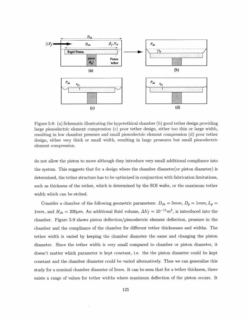
A Vf (3 1fvo
[Rigid Piston
atether
(a)
xPh
----- - --- ----
P4 XP
(c) (d)
Figure 5-8: (a) Schematic illustrating the hypotethical chamber (b) good tether design providinglarge piezoelectric element compression (c) poor tether design, either too thin or large width,resulting in low chamber pressure and small piezoelectric element compression (d) poor tetherdesign, either very thick or small width, resulting in large pressures but small piezoelectric
element compression.
do not allow the piston to move although they introduce very small additional compliance into
the system. This suggests that for a design where the chamber diameter(or piston diameter) is
determined, the tether structure has to be optimized in conjunction with fabrication limitations,
such as thickness of the tether, which is determined by the SOI wafer, or the maximum tether
width which can be etched.
Consider a chamber of the following geometric parameters: Deh = 5mm, Dp = 1mm, Lp=
1mm, and Heh = 200pm. An additional fluid volume, AVf = 10 1 1 M 3 , is introduced into the
chamber. Figure 5-9 shows piston deflection/piezoelectric element deflection, pressure in the
chamber and the compliance of the chamber for different tether thicknesses and widths. The
tether width is varied by keeping the chamber diameter the same and changing the piston
diameter. Since the tether width is very small compared to chamber or piston diameter, it
doesn't matter which parameter is kept constant, i.e. the the piston diameter could be kept
constant and the chamber diameter could be varied alternatively. Thus we can generalize this
study for a nominal chamber diameter of 5mm. It can be seen that for a tether thickness, there
exists a range of values for tether widths where maximum deflection of the piston occurs. It
125
MMMMMPM= - QIE;" --- - W - -- - - - - - -- - - - I -
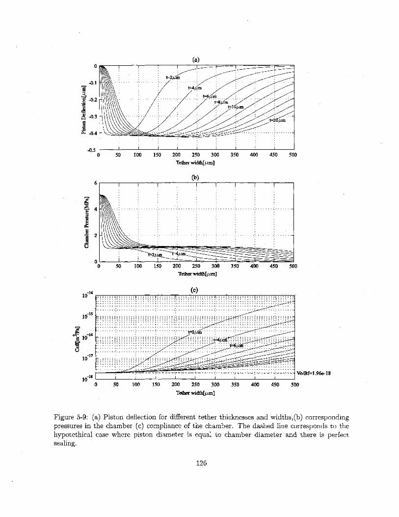
(a)0
==24
-02 - - - --- --- -. . -.-.-. .-
-04 -
-0.5
0 50 100 150 200 250 300 350 400 450 500
Tether width[pm]
(b)6
00 50 100 150 200 250 300 350 400 450 500
Tether width[pm]
-14 (C)
10(C
a10--
-1610- ----
- -- -- Vo/BF=V.96e.-18
100 50 100 150 200 250 300 350 400 450 500
Tether widih~tmi
Figure 5-9: (a) Piston deflection for different tether thicknesses and widths,(b) corresponding
pressures in the chamber (c) compliance of the chamber. The dashed line corresponds to thehypotethical case where piston diameter is equal to chamber diameter and there is perfectsealing.
126
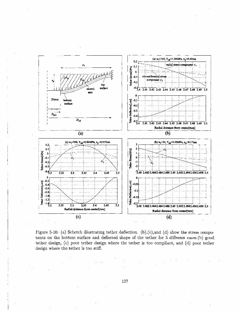
We
topneutra sufice
Piston bottomsurface
Dpi
Dch
(a)
(c) wt=300, Pg=0.84MPa, x,=0.315om
u 0
S 02- --
-0.3 - r-
-02 2.25 2.3 2.35 2.4 2 45 2
0
-0 .12 .- .... I .- ....- . - ..-.- . ...- ....- ..- .-.-- .. ....- .- . -. ---... -
-0 . ...... .....-- . -.. -.. ... -.- -.
-0 .6 - - --------- ... ---... .. -. . -.-..-.-.... .-.-
- 0 .3 - -- --.---.-...-.-...-.-.-...----.I . ... ..
-0.8
U-1222 2.25 2.3 2.35 2.4 2.45 2.
Radial distance from center~mm]5
(c)
(a) wf=100, Pch=l.O8MPa, x=0.42am
0.1 radialstmi cmponent UP
-0~ . .circu f6r nI= tstres ....... ....... ...component at
- 0 - . . .-- . .-- .- ... .. .. .... .. .. ---. . --.-... --
- 4 241 242 2.43 2.44 2.45 246 2.47 2.48 2.49 2.5
0
-0 -. ..- .... -. ---....--.-.......-- -.- - .-- - - . . -. - -- -- - - -----.. --- - --.
-0-5 --2.4 241 2.42 2.43 2.44 2.45 2.46 247 2.48 2.49 2.5
Radial distance from centerfmm]
(b)
--
3210
2:482 442 t62488249 %492 491492.48 22.48 2.4822.4842.4862-488249 2A922-4942.4962-498 2.5
..-. ... .... ..-.. -
-0.22.49 2.4S22.494 2.496 2499 2.49 2.492 2.494 2.496 2.499 2.5
Radial distance from center[mm]
(d)
Figure 5-10: (a) Schetch illustrating tether deflection. (b),(c),and (d) show the stress compo-nents on the bottom surface and deflected shape of the tether for 3 different cases.(b) goodtether design, (c) poor tether design where the tether is too compliant, and (d) poor tetherdesign where the tether is too stiff.
127
(b) w=20, P=339MPa, x=17nm
..... .. ....---- ... ..--- .. .. ... .I.. . .- .I- --- -- --........ .... ......... ... .......
.........
.5

(a)
(b)
Figure 5-11: (a) SEM picture of micromachined piston structure [7](b)detailed view of the
tether and the fillet.
can be also seen that for those values, the additional compliance introduced by the tethers is
negligible.
Figure 5-10 illustrates the stresses and deflected shapes of the tether with a thickness of
10pm for three different cases. Figure 5-10(b) illustrates a good design where the tether width
is optimized. Figure 5-10(c) illustrates a poor design where the tether width is very large and
therefore the pressure in the chamber and piston deflection are small. Figure 5-10(d) illustrates
another poor design where the tether width is small and therefore the tether is very stiff, which
results in small piston deflection even though the pressure built up in the chamber is high. It
can be also seen that the stresses in this case are very large compared to the previous two cases.
It should be noted that linear plate theory is used for this analysis which means that the
neutral axis coincides with the central axis of the tether. In general, in a well-designed tether
structure, the bottom surface of the tether experiences compressive stress near the chamber
wall and tensile stress near the piston, which is the case in Figure 5-10(b), and the maximum
stress occurs at the point where the tether is attached to the wall. The top surface experiences
stresses with opposite signs.
It is also very important to consider the effect of the fillet on the stress and to note that
the stresses calculated from the linear plate theory should be corrected using the proper stress
concentration factor. However the stresses calculated using linear theory give a reasonable
estimate and provide first order prediction about stresses during the design procedure. A
128
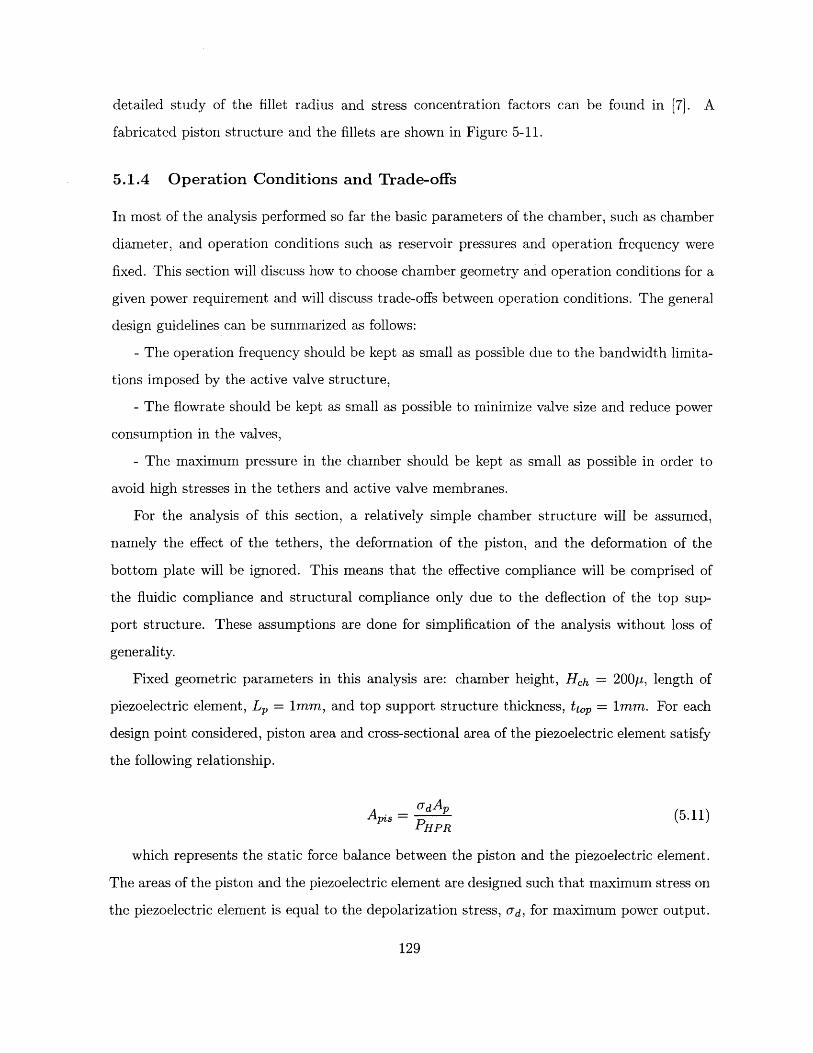
detailed study of the fillet radius and stress concentration factors can be found in [7]. A
fabricated piston structure and the fillets are shown in Figure 5-11.
5.1.4 Operation Conditions and Trade-offs
In most of the analysis performed so far the basic parameters of the chamber, such as chamber
diameter, and operation conditions such as reservoir pressures and operation frequency were
fixed. This section will discuss how to choose chamber geometry and operation conditions for a
given power requirement and will discuss trade-offs between operation conditions. The general
design guidelines can be summarized as follows:
- The operation frequency should be kept as small as possible due to the bandwidth limita-
tions imposed by the active valve structure,
- The flowrate should be kept as small as possible to minimize valve size and reduce power
consumption in the valves,
- The maximum pressure in the chamber should be kept as small as possible in order to
avoid high stresses in the tethers and active valve membranes.
For the analysis of this section, a relatively simple chamber structure will be assumed,
namely the effect of the tethers, the deformation of the piston, and the deformation of the
bottom plate will be ignored. This means that the effective compliance will be comprised of
the fluidic compliance and structural compliance only due to the deflection of the top sup-
port structure. These assumptions are done for simplification of the analysis without loss of
generality.
Fixed geometric parameters in this analysis are: chamber height, Hh = 200p, length of
piezoelectric element, LP = 1mm, and top support structure thickness, tt0,p = 1mm. For each
design point considered, piston area and cross-sectional area of the piezoelectric element satisfy
the following relationship.
Apis =UdAp (5.11)PH PR
which represents the static force balance between the piston and the piezoelectric element.
The areas of the piston and the piezoelectric element are designed such that maximum stress on
the piezoelectric element is equal to the depolarization stress, Od, for maximum power output.
129

It is assumed that the maximum and minimum pressures attained in the chamber are equal
to the high and low pressure reservoirs respectively, where PLPR is assumed to be zero for
simplicity.
Required operation frequency for a given power requirement
The required frequency in order to generate a certain amount of power, W, for the case of the
chamber attached to regular diode bridge is given by:
4Wf4W(5.12)(st - sff)a ApL~
where st and sQ are the closed circuit and open circuit compliances of the piezoelectric
element respectively. Figure 5-12 compares different piezoelectric materials in terms of required
frequency for a 0.5W power requirement at different chamber diameters and reservoir pressures.
It can be seen that, PZT - 4S and PZT - 8 require lower frequencies because of their very
high depolarization stress, even though they have smaller coupling coefficients compared to
PZT - 5H and PZN - PT. It should be noted that, the required frequency does not depend
on the chamber compliance, as can be seen from equation 5.12.
It is important to note that there is a trade-off between the maximum chamber pressure(PHPR)
and the operation frequency. For lower chamber pressures, higher operation frequencies are
needed. In fact, for a given piston diameter the required frequency is inversely proportional to
the reservoir pressure, as can be easily seen from equations 5.11 and 5.12. It can be also seen
that, for larger chamber diameters, the required operation frequency is smaller since for larger
chamber diameters, piezoelectric elements having larger diameter are used to satisfy equation
5.11, which results in lower frequency requirement due to the increased piezoelectric element
volume.
Required flowrate for a given power requirement
The required flowrate is given by the following equation, which was derived in Chapter 3:
2(sE + SD)WQ= 2+-CW ePHPRf(5.13)(S3t - sQ )PHPR
130
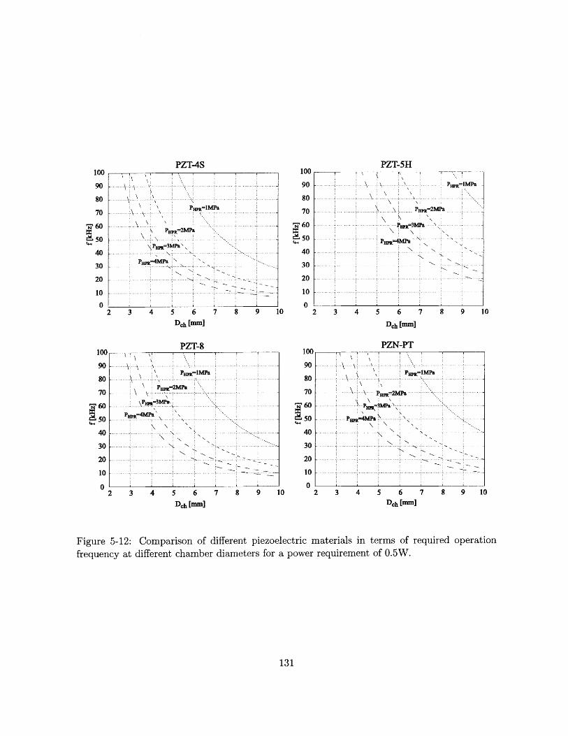
PZT-4S
PHPR=IMPa
NPEppJ-2MPa
PHpk7-APHP
2 3 4 5 6 7 8 9 1
Dch [mM]
PZT-8
10090
80
70
60
50
40
30
20
10
0
10~
90
80
70
60
150
40
30
20
10
n
PZT-5H
- \ PH lMP
- -\
P1qt7-t'38 '\
-............ ---- ...... ......----.-.-
- -~
- -
2 3 4 5 6 7 8 9 1
Dch [mm]
PZN-PT
2 3 4 5 6 7 8 9 10 2 3 4 5 6
Dch [mm] Dch [M]
0
Figure 5-12: Comparison of different piezoelectric materials in terms of required operation
frequency at different chamber diameters for a power requirement of 0.5W.
131
100
90
80
70
60
50
40
30
20
10
0
100
90
80
70
S60
50f4-1
40
30
20
10
I n
- \
Pa
\P Pa \~
- . . . K
IMPa
-.. .....
..-.. ......
PHPR=4
P a
..- . .
-
Pj -2N
- - -......
7 8 9 10
0
................. -
.......... -
...................
PZT-4S
3 4 5 6 7 8 9 10Dch [mm]
PZT-8
4.5
4
3.5
3
2.5
2
1.5
1
0.5
0
4.5
4
3.5
3
2.5
CY 2
1.5
1
0.5
0
PZT-5H4.5
4
3.5 ---
3 P
2.5
2 P-2MPa - -
1.5 PM 3MPa--- PR=M
1
0.5
02 3 4 5 6 7 8 9 10
Dch [m]
PZN-PT
4. .....5. ..... ..... ...
4
3.5
3
A 2.5
2
1.5
1
0.5
02 3 4 5 6 7 8 9 10
Dch [mm]
Figure 5-13: Comparison of different piezoelectric materials in terms of required flowrate at
different chamber diameters for a power requirement of 0.5W.
132
----- PR1MPa
-- P 23MPa-
- PHPR=4MPa -
....4....
----------PH =IMPa ---
HPR
P11P1 =3MPa -~-
- PW 4MPR - --
3 4 5 6 7 8 9 10
Dch [nM]
- - - -
- PK
P -k3MPa~
PHpR'MPa
-------- ---------------
.... ...... ........
where f is the required operation frequency corresponding to the power requirement at the
particular chamber diameter and reservoir pressure, as discussed in the previous subsection.
Figure 5-13 shows a comparison of different piezoelectric materials in terms of required flowrate
at different reservoir pressures and chamber diameters.
It can be seen that PZN - PT requires the least flowrates due to its high coupling co-
efficient, which translates into higher system efficiencies as discussed in Chapter 3. It can
be also noted that, for larger chamber diameters, higher flowrates are required. This can be
explained by considering equation 5.13. There are in fact two competing effects. For larger
chamber diameters, lower frequencies are needed, as shown in Figure 5-12, which suggest lower
flowrates. However, larger chamber diameters result in increased chamber compliance, which
is the dominating factor resulting in higher flowrates.
In this case, a trade-off exists between the required flowrate and maximum chamber pressure,
namely for lower chamber pressures, higher flowrates are required.
Efficiency
The efficiency of the system is given by:
W77 (5.14)
QPHPR
where the power consumption in the active valves is not considered. Figure 5-14 shows a
comparison of different piezoelectric elements in terms of system efficiency for different reservoir
pressures and chamber diameters. It can be seen that PZN - PT provides the most efficient
power generation due to its high coupling coefficient. For larger chamber diameters, the effi-
ciency is lower due to the fact that the flowrate is higher at larger chamber diameters, as shown
in Figure 5-13. It is also important to note that the efficiency decreases as the reservoir pressure
increases. This can be explained considering equations 5.11, 5.12 and 5.13. Combining these
equations we get:
2(s+ sg)W 4CffW(S = 3 +3(5.15)
3 3- st)PHP ± (s33 - s )adApisLp(
which is the explicit form of equation 5.13. Using equation 5.14 we get:
133

PZT-4S
............ ............. .. ......... ........ ........ ......... ................ ....... .......
.... .. ....... ... ..
................ ........ ............. ......
..................... ............ ........... ......... .
..... ............. -........ ......... ........... ...............................
........... ............... ------- ......................... 4 ............ ......Fl,, IMPR: PM-2MPa
............ . ...... ......... ...........--------------------
77- ............ ..
... 77 7
FMR =WP& Pml:-4MPa
3 4 5 6 9 10Dch Imml
PZT-8
PZT-5H
. . . .. . .. . . . . . . . .. . . . .. . . . . . .. . . . . . ... . . . .. . . .. . .. . . .. . . . .. . .. I .. . . . . .. . . -
. . . . . .. . . . . . . .. . . .. . . . . .. . . . . . .. ... . .. . . . . .. .. . . .. . . . .
. . . . .. . . . .. . . . .. .. . . . . . . . . . . . . . . .. . . .. . . . . . .. . . . .. . . . . .. . . . . .. . . . . . . ..
. . . . . .. . . . . . . . . . . .. . . . .. . . .. . . . . .. . . . . . . .. I . . .. . . . .. . . I',,-,,-,,,,,-
. . . .. . . . .. . . . . . . . .. . . . .. . . . . .. . . . . .. . . . . .. . . .. . . . ..I
. . . .. .. . . .. I . . . .. . . . .. . . I . .. . . . .. . . . . .. . . . .. . . . ... .. . . . . . .. . . . . .. . . . . .. . . . .. . . . .. . . . . . . . . . .. . . .
PHPR=4MPa..... .... .. ...... ........................PEPCIMPR:
PH PR---2M Pa ............ .... ... ......................... -
............ ...... ....................PIWX=z3
3 5 6 7 8 10Dcb ImIn]
PZN-PT
30
28
26,
24
r-m 22140IV 20pq
18
16
14
12
11 nlu
30
28
26
24
22
20
pq 18
16
14
12
.10,
Ju
28
26
24
22
20pq 18
16
14
12
L2
30
28
26
24
%-n 22 -
20 -pq19 -
16 -
14 -
12
10
..... ........... ...................... .......... ..... .. ..... ........ ....
.......................... ......................... .. .... . . . . . . .. . . . .. . .
... . . . . .. . . . . . . .. . . . . .. . . . . . .. . . .. . .. .. . . . .. . . . .. . . . . . .. . .. . . . .. . . . . . .... . .. . . . . . .. .
...... ..... .................. ....... .... . .. . . .. .. .. . .. . . . . . .. .
. . . .. .. . . . .. . . . .. .. ... . . . . .. .............................................
.......... ........................
PRne-IMPR:........ .. .......... ......... .......
PmR=2MPa...... ..... . ......... ........... ......................p
PEWR=4?APa---- -----------------
........... ................... ........... ....................... -
PRPR7lN2a ----------.............. ............ ....... :, . ............. ...................... ..........
.......... .................................. ........... ............ .......... -
PHP]r--2mft.......... ....... .......... -
b .. . .. . . . . . .. . . .. . . . . .. .. . . . . . .. . . . . .. . . .. . . . .. . . . . ... . . .I_
.......... .. .......Pm%=-4PO a ........... ....... .
.................. ........ ............ ........... r .........
................ .......... ...... ............. ........ ...........
. . . . .. . . . . . . . . .. . . . .. . . .. . . . . .. . . .. .. % . .. . . ..
3 4 5 6
Dch [mm]
10 5 6Dh [mm]
10
Figure 5-14: Comparison of different piezoelectric elements in terms of system efficiency fordifferent reservoir pressures and chamber diameters.
2 E D) -1(S33 + S33 + 4Cef f PHPR
(SE _ SD) (SE _ SD33 33 33 33) Crd Api, Lp
w - -QPHPR
(5.16)
from.which it can be easily seen that at a certain chamber diameter, the efficiency decreases
with increasing reservoir pressure. It is also possible to observe that efficiency does not depend
on the generated power.
134
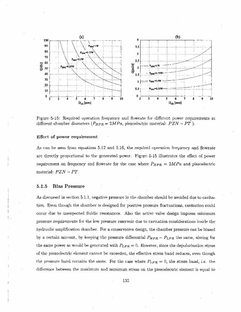
(a) 4(b)100 4
90 - ---- W -. 3.5 .--.
80 Pma=0. 7W 3
70 ..--..
Pn 2.5 ---, - , 0 - -- -- - ---- --
5 - --- -2 P P-1W
.2 .- -. .. -- - --
20 0.5 P......,....D......W
0 ___ _ _ __ __ __ _______0 i LLJ~2 3 4 5 6 7 8 9 10 2 3 4 5 6 7 8 9 10Dch [mm] Dch [mm]
Figure 5-15: Required operation frequency and flowrate for different power requirements atdifferent chamber diameters (PHPR = 2MPa, piezoelectric material: PZN - PT).
Effect of power requirement
As can be seen from equations 5.12 and 5.16, the required operation frequency and flowrate
are directly proportional to the generated power. Figure 5-15 illustrates the effect of power
requirement on frequency and flowrate for the case where PHPR = 2MPa and piezoelectric
material: PZN - PT.
5.1.5 Bias Pressure
As discussed in section 5.1.1, negative pressure in the chamber should be avoided due to cavita-
tion. Even though the chamber is designed for positive pressure fluctuations, cavitation could
occur due to unexpected fluidic resonances. Also the active valve design imposes minimum
pressure requirements for the low pressure reservoir due to cavitation considerations inside the
hydraulic amplification chamber. For a conservative design, the chamber pressure can be biased
by a certain amount, by keeping the pressure differential PHPR - PLPR the same, aiming for
the same power as would be generated with PLPR = 0. However, since the depolarization stress
of the piezoelectric element cannot be exceeded, the effective stress band reduces, even though
the pressure band remains the same. For the case where PLPR = 0, the stress band, i.e. the
difference between the maximum and minimum stress on the piezoelectric element is equal to
135
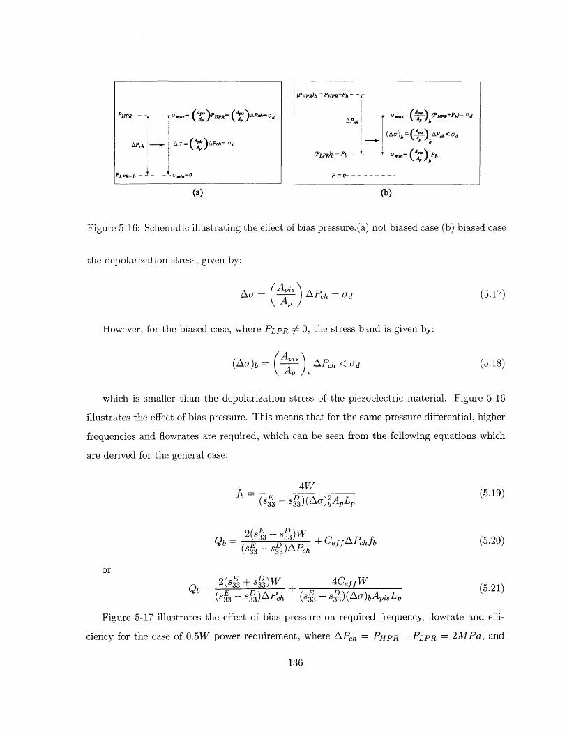
(a) (b)
Figure 5-16: Schematic illustrating the effect of bias pressure.(a) not biased case (b) biased case
the depolarization stress, given by:
AO- (Aps ) APch = 9d (5.17)Ap
However, for the biased case, where PLPR -# 0, the stress band is given by:
(AT) b - (AP ) APh < o-d (5.18)
which is smaller than the depolarization stress of the piezoelectric material. Figure 5-16
illustrates the effect of bias pressure. This means that for the same pressure differential, higher
frequencies and flowrates are required, which can be seen from the following equations which
are derived for the general case:
4WfA (SE SD (5.19)
(s3 -3 s(Ao) ApLp
2(s E + sD)WQb = 3 33 + C (5.20)
(S D3 )A hCef fAPchfb(33 -- s33)APeh
or
Qb (SE + s3) 4Ceff W (5.21)Q s3 s) APh+ (s - 33)(Ao)bA 8 LP (2
Figure 5-17 illustrates the effect of bias pressure on required frequency, flowrate and effi-
ciency for the case of 0.5W power requirement, where APeh = PHPR - PLPR = 2MPa, and
136
PHPR - ] - man HPR d
APa = A ( AP-n Ud
Pn=R - W=O
(HPR)b HPR- -
-9mar bHPR+Pbh GdAAP - b
LPR.)b Pb - -Mn bb-- b
P=O- -- -- -- ---
- - .. -;*O*AQM. '. -I ------- -- M-- - . I_ __-i

(a)
........................... ........ - ...................................Pb:= 0 Pl;=-: 0.6Nft:
.. ..... .. ...... .... .....
bp 0. PANPaPw- o.2MPa.
Alt OAM k .......................
............ ..........
................ ......... ........... ...... ............. ... pb-
........... ......
...........................
............................
Z--:) r
....... .................. ........... ................
P67 imps
Pb- 0.$NI[Pa
..............
PWc= OAMPa
4= OMWPa------------------
P6:= D
241p W= 0
.................... ... ..... .. .. ................... .................................
Pb- O-2hM 11 .... ............ .............
P = 0.4hft .............. ............. .....................
.. . . . . .. . . . .Py- 0.6?Aft
Pb- O.gAolPa.. . . . . . . . . .Pg- IMPa
.. . . . .. . . . . .. . .. . . . . . . . . . . . . . . . . . . . . . . . .
. . . . . . .. . . . . . . . . . .. . . . .. . . . . . ... . . . . . . . . . . .... . . . . . . . . . . .
. . . . . .. . . . . . . . . . . . . . . . . . . .
100
90 -
go-
70 -
60-
50-
4o.
30 -
2o-
10-
0 L2
I
5 6
Dch[mm]
10
22
20
18
16
14
12
lo
8
10
Figure 5-17: Effect of bias pressure on required frequency, flowrate and efficiency.
137
5 6 7 8 10Dch[mm]
3 4 5 6Dch[mm]

piezoelectric material is PZN - PT. It is important to note that the generated power is pro-
portional to the square of stress band and therefore the bias pressure should be kept as small
as possible. It can be easily shown that, for a given chamber diameter, the required frequency
for the biased case and for the case where PLPR = 0 are related by:
f APegh/ (APch(5.22)
A APch - Pb
where Pb is the bias pressure. It is assumed that in both cases the pressure differential in
the chamber is the same. Equation 5.22 implies that if the bias pressure is much smaller than
the pressure band in the chamber, its effect is negligible. However for typical MHT devices this
is not the case and the effect of bias pressure should be considered.
5.1.6 Scaling Issues
One of the many advantages of MEMS devices is their ability to operate at very high frequencies.
In other words, they allow operation with much larger bandwidth due to their high natural
frequencies. For linear systems, the scaling law for natural frequency can be obtained by
considering a very simple system consisting a cantilever beam and a proof mass attached to the
tip of the beam. The stiffness corresponding to the tip deflection of the beam in response to a
force applied to the tip can be obtained from beam theory:
EW H3k = 3 (5.23)
4L3
where E is the Youngs modulus, and W, H, and L are the width, the height and the length
of the beam respectively. The natural frequency of this system can be calculated by:
mWn k (5.24)
where m is the mass of the proof mass. If we define the scale factor, A, as the ratio of the
new scaled dimensions divided by the nominal, the dependence of the stiffness of the beam and
the mass of the proof mass on the system scale are:
k ~ A and M ~ A, (5.25)
138
where the scale dependence of the stiffness of the beam is obtained from equation 5.23.
The natural frequency of the system is then related to its size by:
A 1 =(5.26)
which can be generalized to any linear structure.
Similarly we can obtain the scaling laws for the power generator considering the dependence
of the natural frequency, required operation frequency and compliance of the system on system
scale. Consider the simple chamber structure described in Section 4.1, which consists of a fluid
chamber and a compliant top support structure. Here we assume that in the energy harvesting
chamber the top support structure is the only compliant structure, and the piston is rigid and
perfectly sealed to piston walls without tethers. The effective compliance for this case was
derived in Section 4.1 as:
VO 7rD'2 Hch 7TD6 (1 - V/2))
Ceff= -+ CS ch ± h (5.27)' 340f 1024Et 3(Oftop/
where Dch is the chamber diameter, Hch is the chamber height, and ttop is the thickness of
the top support structure. The dependence of the effective chamber compliance on the system
scale is then
Ceff A3 (5.28)
which suggests that as the system gets smaller, the compliance gets smaller. Lets consider
a case where PLPR = 0 and the effective chamber compliance is given by equation 5.27. For a
certain power requirement, the required operation frequency can be calculated as:
4Wf ) 2ApLp (5.29)
where (- is the stress band on the piezoelectric element, which is equal to the maximum stress
since PLPR = 0. As discussed earlier, in a design procedure, the chamber diameter and the
piezo diameter are chosen such that the maximum stress on the piezoelectric element is equal to
the depolarization stress of the piezoelectric element. If we assume that for any design scenario
139

this condition will be satisfied, then the dependence of the required frequency on system scale
can be obtained as:
freq ~ (5.30)
which suggests that as the system gets smaller, larger frequencies are required due to the
reduced piezoelectric element volume. The required flowrate is given by:
Q 92(stE+s )W(s- Sf3=PHPR + Ceff PHPRfreq (5.31)
3s 3 s)PHPR
From equations 5.28 and 5.30 we can obtain the dependence of the required fiowrate on the
system scale as:
Qr-~'A 0 (5.32)
which suggests that the required flowrate does not depend on the system scale. In smaller
scale, although the system compliance reduces, the required frequency increases in the same
amount which results in the same required flowrate. Since this results were derived for constant
PHPR and required power, W, the system efficiency does not depend on the system scale either,
which can be expressed as:
w=7Q~ A0
(5.33)PHPRQ
It should be noted that this analysis relies on the assumption that the active valves can
operate at very high frequencies and the valves and channels can provide the required flowrates
even when the system gets very small.
Consider a design case where the operation frequency is equal to the maximum bandwidth of
the device. If we make the system 10 times smaller and keep the required power and PHPR the
same, we will need 1000 times the frequency to generate the same power from the smaller device.
However we can increase the operation frequency only 10 times since the natural frequency is
inversely proportional to the system scale, which is expressed in equation 5.26. This implies
that we can extract only one percent of the required power from the small device. However
140

we can fit 1000 small devices inside the original volume, which means that we can generate
10 times the original power from the same volume. This suggests that the power density is
inversely proportional to the system scale, which can be expressed as:
1PD - 1 (5.34)
A
This suggests that, as the system gets smaller, the power density increases. Again, it should
be mentioned that, this analysis assumed that, in the smaller scale the valves and channels
can provide the required flowrate regardless of the system scale. However, it is expected that
viscous losses in the valves will begin to dominate beyond a certain scale and scaling further
down will not be more efficient. In order to perform this study, more detailed fluid models are
needed. Nevertheless, the above analysis provides a general understanding about the scaling of
the system.
5.2 Design Procedure
This section will present a design procedure for designing the microhydraulic piezoelectric power
generator. First, the design decisions made considering the issues discussed in previous sections
as well as those imposed by the active valve design and fabrication process will be presented.
Then, the design procedure will be described and two design examples will be presented along
with simulation results.
5.2.1 Preliminary design decisions
As discussed in Chapter 3, the working fluid is chosen to be silicone oil due to its low viscosity
and low density. It also has a comparable bulk modulus to that of water. Choice of piezoelectric
element is done considering the results in sections 5.1.4, 5.1.4, and 5.1.4. From Figure 5-12 it
can be seen that the piezoelectric material PZT - 5H has very high frequency requirements,
PZT - 4S, PZT - 8 have lower and very similar frequency requirements, and PZN - PT
has comparable frequency requirements to those of PZT - 4S and PZT - 8. If we examine
Figures 5-13 and 5-14, we can see that PZN - PT requires much lower flowrates and provides
much efficient power generation compared to other piezoelectric materials. In Chapter 2 it was
141

concluded that PZN - PT has the smallest energy density among the piezoelectric elements
considered, which is a result of its low depolarization stress. However due to its very high
coupling coefficient it provides very efficient electromechanical energy conversion and requires
the lowest flowrate for a given power requirement. It should be noted that, the implication of
the low energy density of PZN - PT is that, larger piezoelectric material volume is needed
compared to other piezoelectric materials for the same power output. However, the weight
of the piezoelectric element constitutes only a small fraction of the overall system weight and
the increased efficiency of PZN - PT due to its much higher coupling coefficient would still
overwhelm the effect of increased weight in terms of the overall system power density. The
chamber height is chosen to be 200pm. A preliminary study has shown that chamber heights
smaller than this could cause squeeze film damping effect inside the chamber and can result in
undesired losses. And, larger chamber heights would increase the chamber compliance, which
would decrease the efficiency of the system. The length of the piezoelectric element is chosen to
be 1mm. This parameter is basically determined considering the actuation in the active valves,
since all the piezoelectric cylinders within the system, namely the ones in the active valves and
the one in the energy harvesting chamber, have the same length because of the layered structure
of the device, which was explained in Chapter 1. Larger lengths would decrease the stiffness of
the piezoelectric elements inside the active valves, which reduces the actuation capability, and
smaller lengths could cause dielectric breakdown.
5.2.2 Parameters imposed by active valve design
The basic limitation of the active valves is their bandwidth. Current active valve designs
predict bandwidths in the order of 10 - 20kHz. Typical trade-offs in the active valve design
are stroke, bandwidth and force, which are detailed in [5]. Another important limitation is the
pressures that the active valves can work against, which basically imposes the maximum high
reservoir pressure possible. They can typically work against pressures of 2 - 3MPa. Also the
active valves impose a minimum pressure requirement due to cavitation considerations in the
hydraulic amplification chamber(HAC) within the active valve structure. In the design example
presented, the low pressure reservoir pressure, PHPR is chosen as 0.5MPa.
142
5.2.3 Parameters imposed by fabrication process
As briefly described in Chapter 1, the device consists of silicon and pyrex micromachined
layers. The thickness of the layers basically dictate the thicknesses of individual components.
For example, a double layer piston structure, which consist of two silicon layers bonded to each
other, will have a thickness of tpi8 = 80 0 Mm, which is the case in the design example. Since the
tethers are created through deep reactive ion etching(DRIE) of a SOI wafer, the tether thickness
is defined by the SOI layer. Also, the fillet radius control during the fabrication process imposes
some limitations on the tether width. For example narrow tethers would be very stiff due to the
relatively large fillet radius and the predictions of the linear theory used for the optimization
would not valid beyond a certain tether width. The top tether thickness, tetp, is chosen to
be 1Opm, whereas the bottom tether thickness is chosen to be thinner, namely, 5am, because
the bottom tether does not have any functionality and therefore it should be kept as thin as
possible so that it won't cause significant resistance to piston motion. The thicknesses of the
top and bottom support structures are determined by the number of layers used, including the
packaging layers on top and bottom portions of the device. As discussed in Chapter 3, the
compliance of the system is very important in terms of system performance and they should be
kept as small as possible. Therefore it is desirable to have very thick top and bottom support
structures. The effective thickness would also depend on the structure of the auxiliary system
in which the device is packaged. In the design examples, the top and bottom structures are
assumed to have the same thicknesses, namely ttp = tbot = 2.5mm, and they are assumed to
comprise of all silicon layers.
5.2.4 Design Procedure
Figure 5-18 presents a design procedure, which will be followed after the initial design decisions
are made using above considerations. The first part consists of analytical design calculations.
The pressure band in the chamber is dictated by the bias pressure, Pb, and high pressure reser-
voir pressure, PHFR. The piston diameter and piezo diameter are calculated using equations
5.11 and 5.19, and the battery voltage is calculated using equation 5.6.
These calculations are followed by the tether structure optimization, which determines the
optimum tether width, wt, for the given tether thicknesses and piston diameter. The designed
143

Calculate (D ratio depolarization stress, ad , and max. pressure, PHPR
Calculate the stress band, A a on the piezo bias pressure, Pb and PHPRanalytical I
calculations(quasistatic)
ICalculate D.. and D. power Requirement, W frequency,f, and length of piezo LP
-- -,.Calculate optimum battery voltage length of piezo LP
structuralmaximum allowable tether stressoptimization -Design tether width and thickness (silicon membrane strength test)
(quasistatic) i
microfabrication feasibility
__ (dynamic
(T effects)-- Determine optimum ratio for maximum pressure fluctuation
Determine valve cap size, Rc , and valve openings, vo;. and voout, active valve designsuch that chamber pressure fluctuates between PHPR and PLPR
Check the design for maximum allowable tether stress andpiezoelectric element stress(dynamic effects might be important)
Design fluid channels microfabrication feasibility
Figure 5-18: Design procedure.
144
simulation(dynamic)
layoutmask design I

tether width also determines the chamber diameter, Dch. The geometric parameters along with
the operation conditions are then fed to the system level-simulation. The simulation architecture
is shown 5-19 and the Simulink block diagrams are given in Appendix A.
First, simulations are performed to determine the optimum length to area ratio of the fluid
channels, using arbitrary valve resistance, i.e. arbitrary valve cap size or valve openings. It
is helpful to run these simulations with very small valve resistance, namely with very large
valve opening or very large valve cap, since the fluidic oscillations are much more pronounced
with lower valve resistances and it is easier to determine the optimum length to area ratio of
the channels. Then, the valve cap size and valve opening are designed such that the chamber
pressure fluctuates between reservoir pressures, namely between PHPR and PLPR. At this stage,
it is important to consider structural limitations, which might be imposed by the active valves.
For example, a large valve cap size requires a large membrane to allow sufficient valve motion,
however this may cause excessive stresses in the membrane. Or, a very large valve opening can
cause the same problem. Since the same effective valve resistance can be achieved with different
combinations of valve opening and valve cap size, coupled iterations may be necessary with the
active valve design procedure, which is not within the scope of this thesis. Detailed information
about the active valve design procedure can be found in [5].
Finally, the system is simulated, stresses in the tethers and on the piezoelectric element are
checked, and design iterations are performed if necessary. Although the valves are designed to
achieve the desired pressure band in the chamber, the stress band may be a little bit different
than expected. This can be explained by considering equation 5.11. This equation assumes
static force balance between the piezoelectric cylinder and the piston. Also, the effect of the
tether is neglected since the force exerted by the tethers on the piston is generally very small
compared to the force exerted by the piezo and force due to chamber pressure. As will be seen
in the design examples, the dynamics of the piston does not have a significant effect on system
performance and it is reasonable to assume quasi-static force balance. However, if the operation
frequency is much higher, the dynamics of the piston will be important and equation 5.11 will
not be valid. The design procedure presented above is followed by the layout and mask design
for the fabrication.
For the piston dynamics, a damping ratio of 5% is assumed, considering the piezoelectric
145
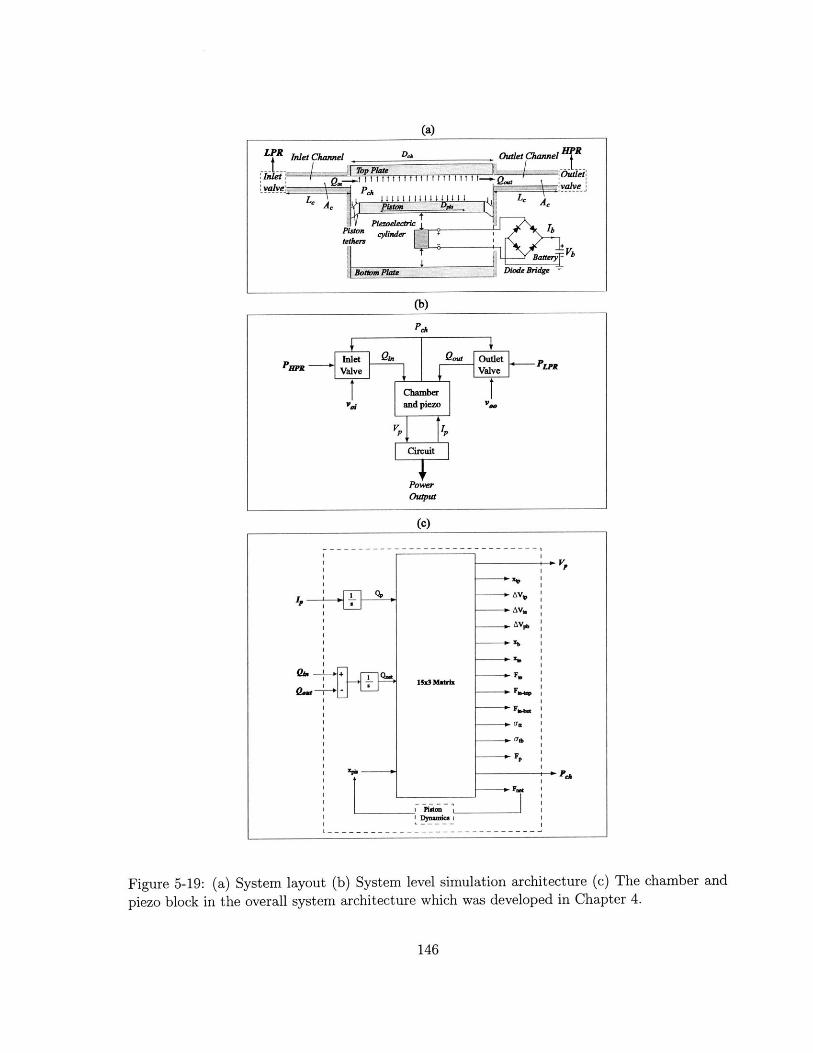
(a)
LPR Inlet Channel D _ _, Outef Channel _fR
valve' P -alvL Le A
oPlezoelectricil
tethers
lte Batery Vb
Bo" lateDiode Bridge
(b)
PBR Valve LValve PP
VIej nd jpiezo
Power
OWW
(c)
'P
-s
Vpf
151:3 matrix
F
p s
Inanw
Figure 5-19: (a) System layout (b) System level simulation architecture (c) The chamber and
piezo block in the overall system architecture which was developed in Chapter 4.
146
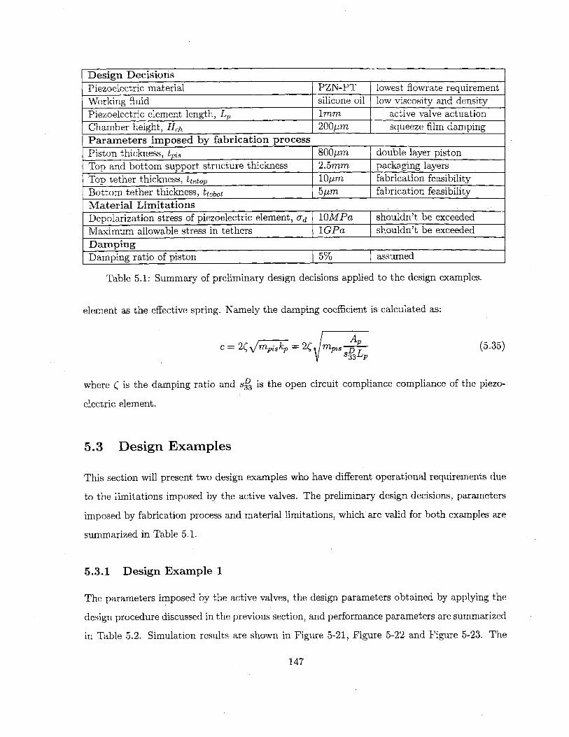
Design Decisions
Piezoelectric material PZN-PT lowest flowrate requirement
Working fluid silicone oil low viscosity and density
Piezoelectric element length, LP 1mm active valve actuationChamber height, H~h 200gim squeeze film damping
Parameters imposed by fabrication process
Piston thickness, t 800m double layer piston
Top and bottom support structure thickness 2.5mm packaging layers
Top tether thickness, ttetop 10Pm fabrication feasibility
Bottom tether thickness, tiebot 5ym fabrication feasibility
Material Limitations
Depolarization stress of piezoelectric element, O }1OMPa shouldn't be exceeded
Maximum allowable stress in tethers jGPa shouldn't be exceeded
Damping
Damping ratio of piston 5% assumed
Table 5.1: Summary of preliminary design decisions applied to the design examples.
element as the effective spring. Namely the damping coefficient is calculated as:
c=2(/mis kp =2C m iA (5.35)
where C is the damping ratio and sD is the open circuit compliance compliance of the piezo-
electric element.
5.3 Design Examples
This section will present two design examples who have different operational requirements due
to the limitations imposed by the active valves. The preliminary design decisions, parameters
imposed by fabrication process and material limitations, which are valid for both examples are
summarized in Table 5.1.
5.3.1 Design Example 1
The parameters imposed by the active valves, the design parameters obtained by applying the
design procedure discussed in the previous section, and performance parameters are summarized
in Table 5.2. Simulation results are shown in Figure 5-21, Figure 5-22 and Figure 5-23. The
147
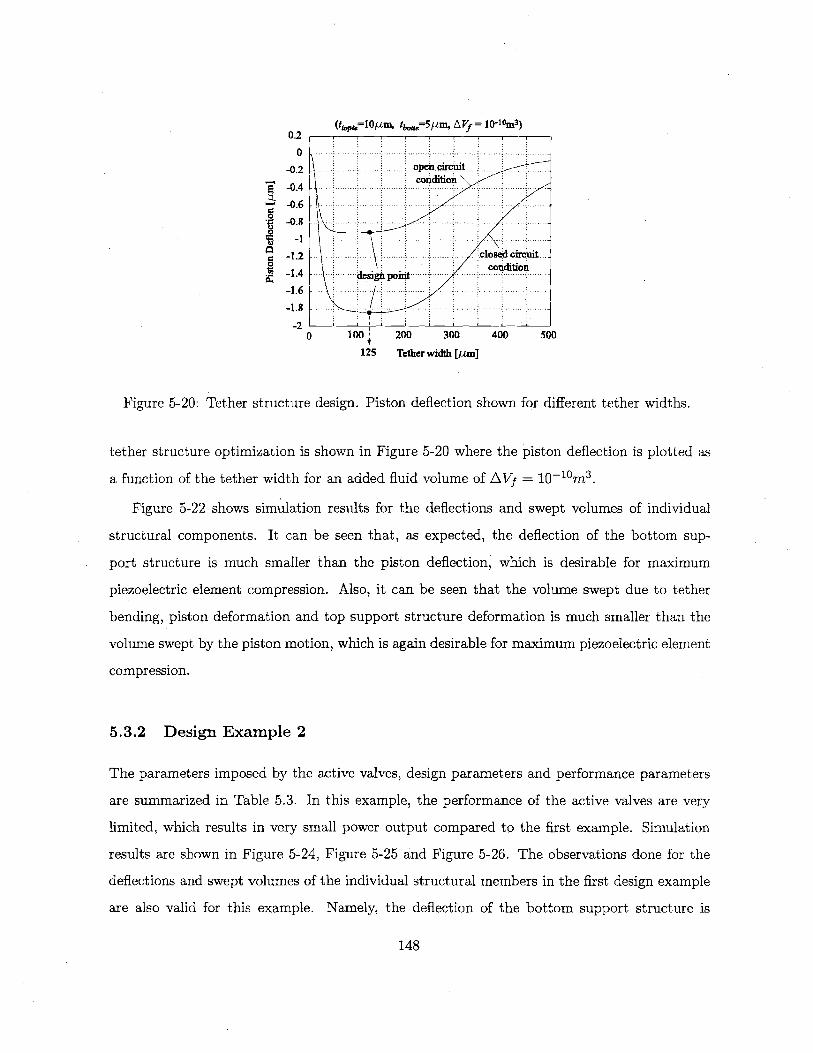
(tbp=10tm, t=5pM, AVfj= 10- 0m3)0.2
0 . .... .. ... .. .. .
-0.2 .. . open circuitcondition
rg -0 .4 ....- .... .. ..- ..... . .- .. .. .. .. ..-
-0.6 .- .-..
*-0.8--
6 -1
-1.2. closedcircuit.-. condition-1.4 . ....des ga n ..-.-
-1.6 ..
-1.8-
- -20 100 200 300 400 500
125 Tether width [gm]
Figure 5-20: Tether structure design. Piston deflection shown for different tether widths.
tether structure optimization is shown in Figure 5-20 where the piston deflection is plotted as
a function of the tether width for an added fluid volume of AVf = 1t 1 0 m 3 .
Figure 5-22 shows simulation results for the deflections and swept volumes of individual
structural components. It can be seen that, as expected, the deflection of the bottom sup-
port structure is much smaller than the piston deflection, which is desirable for maximum
piezoelectric element compression. Also, it can be seen that the volume swept due to tether
bending, piston deformation and top support structure deformation is much smaller than the
volume swept by the piston motion, which is again desirable for maximum piezoelectric element
compression.
5.3.2 Design Example 2
The parameters imposed by the active valves, design parameters and performance parameters
are summarized in Table 5.3. In this example, the performance of the active valves are very
limited, which results in very small power output compared to the first example. Simulation
results are shown in Figure 5-24, Figure 5-25 and Figure 5-26. The observations done for the
deflections and swept volumes of the individual structural members in the first design example
are also valid for this example. Namely, the deflection of the bottom support structure is
148

Power Requirement 0.25W Electrical power outputParameters imposed by active valve design
Operation frequency, f 20kHz bandwidth of active valves
Bias Pressure, P 0.5MPa cavitation in HAC chamberHigh Pressure. Reservoir Pressure, PHPR 3MPa membrane stress limitation
Important parameters resulting from operation conditionsPressure band in the chamber, APch 2.5MPa -Stress band on piezoelectric element, Ao- 8.33MPa -
Designed parameters
Piston Diameter, Dis 6.95mm
Piezoelectric cylinder diameter, Dp 3.8mm
Battery voltage, V6 74.9V
Tether width, Wt 125pm optimization
Chamber diameter, Dch 7.2mm
Fluid channel length to area ratio, La 5000m 1 same for inlet and outlet
Valve cap radius, R, 400pm same for inlet and outlet
Valve opening, voi, voot 24pm same for inlet and outlet
Performance parametersNet flowrate, Qnet 0.52ml/s -
Hydraulic power input 1.3W (PHPR - PLPR)Qnet
Efficiency, r I19.2% Electrical power outputHydraulic power input
Table 5.2: Summary of design and performance parameters of design example 1.
149

(a) Chamber Pressure(Phy)
---- --- -- .... . .
--- - - - - -- - - - --- - - - -
2 2.5 3 3.5
(c) Piston Deflection (xpb)
2 2.5 3 3.5
(e) Voltage on Piezoelectric Element (V,,)
- -- -- - ------ - --
....-.-.-.-.-.
-. .. .- . . -... -.. .
2.5 3Time [10-4]
3.5 4
2
1.5
0.5
442
10
5
0
0.5
-Vs01
(b) Flowrate(Q)
_Inl.t'1 I - - - Outlet
- 41
- - - --I
2.5 3 3.5
(d) Strs on piezoelectric elanent (a)
eam
4
t 2.5 3 3.5 4
(f) Gcnerated Power
2 2.5 3 3.5 4
Tne [10-4]
Figure 5-21: Simulation time histories of the design example 1.
150
3
-0.4
'F
-0.6
-0.8
100
50
0
-50
2
NetPower(W)
1). 1
Ann I
1
lu

0.04
0.03
S0.02
0.01
(a)Ttop support stucture deflection(x 4
. .. .....
02 2.5 3 3.5 4
(c) Tether Deflection(x4d
-.-.-.-.-.-.-.-...-.-.-.-.-.- -.-.- -
-- - ----- - --
2 2.5 3 3.5 4
(e) Top tether force(Fa,,)
1.5 [
nI-v2 2.5 3 3.5 4 2TunC [104sj
(b) Bottom support structure deflection(x )
0
-0.005-
-0.01 -- - - - -
-0.01-
2 2.5 3 3.5 4
(d) Force on piezoelectric eement(Fp)
(--m -r -- F-,- - - - - - - - -
N - - - - - -... ..... .......
2 2.5 3 3.5 4
(e) Bottom tether forme(Fww)
2.5 3 3.5Time [104g]
150
100
50
0
-0.1
Figure 5-22: Simulation time histories of the design example 1.
151
0
-0.5
-11
-1.5
2
0.5
-4

(a) Volume swept by top plate bending(AVq)
2 2.5 3 3.5 4
(c) Volume swept by piston bending(AVpb)
2.5 3 3.5 41
(e) Top tether stresa(u)
-2
(b) Volume swept by piston movement(A,,)
2 2.5 3 3.5 4
(f) Volume swept by tether bending(Vfr)Or
-0.5
-1.
-1.5
-2L2
-0.05
-0.1
-0.15
I2
2.5 3 3.5 4
2 1-- .533.5 - .ZI253.52 2.5 3 3.5 4 2 2.5 3 3.5 4
TM [1D 4. Tune [ji4o]
Figure 5-23: Simulation time histories of the design example 1.
152
6
4
P-
2
---
4
3
2
I
0
0
-012
-0.4
-0.6
-.. . . -. . -- ---- - - -
- -- --- - ---
00A 4
Iel
. . .
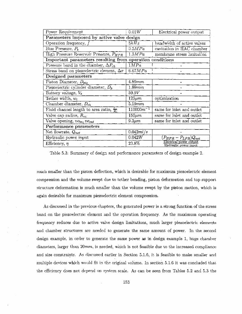
Power Requirement f0.01W j Electrical power outputParameters imposed by active valve design
Operation frequency, f 5kHz bandwidth of active valvesBias Pressure, Pb 0.5MPa cavitation in HAC chamber
High Pressure Reservoir Pressure, PHPR 1.5MPa membrane stress limitationImportant parameters resulting from operation conditions
Pressure band in the chamber, APch 1MPa __
Stress band on piezoelectric element, Au- 6.67MPc _
Designed parameters
Piston Diameter, Dpis 4.89mm -
Piezoelectric cylinder diameter, D, 1.89mm _
Battery voltage, Vb 59.9V -
Tether width, Wt 125pm optimization
Chamber diameter, Dch 5.19mm -
Fluid channel length to area ratio, 11000m same for inlet and outlet
Valve cap radius, Rt 150pm same for inlet and outlet
Valve opening, von, voost 9.3pm same for inlet and outletPerformance parameters
Net flowrate, Qnet 0.042ml/s -Hydraulic power input 0.042W (PHPR - PLPR)QnetEfficiencyr7 23.8% Electrical power output
Hydraulic power input
Table 5.3: Summary of design and performance parameters of design example 2.
much smaller than the piston deflection, which is desirable for maximum piezoelectric element
compression and the volume swept due to tether bending, piston deformation and top support
structure deformation is much smaller than the volume swept by the piston motion, which is
again desirable for maximum piezoelectric element compression.
As discussed in the previous chapters, the generated power is a strong function of the stress
band on the piezoelectric element and the operation frequency. As the maximum operating
frequency reduces due to active valve design limitations, much larger piezoelectric elements
and chamber structures are needed to generate the same amount of power. In the second
design example, in order to generate the same power as in design example 1, huge chamber
diameters, larger than 20mm, is needed, which is not feasible due to the increased compliance
and size constraints. As discussed earlier in Section 5.1.6, it is feasible to make smaller and
multiple devices which would fit in the original volume. In section 5.1.6 it was concluded that
the efficiency does not depend on system scale. As can be seen from Tables 5.2 and 5.3 the
153
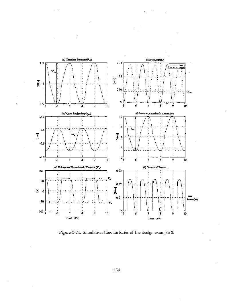
(a) Chamber Pressure(Ps,)
6 7 8
(c) Piston Deflection (Zx1 )
9
-11.65 6 7 8 9
(e) Voltage on PiezoelectricEElement(Vp)
6 7
Te [10-4]
I
0.15
0.1
0.05
0L0 5
10
8
4
0 2
0.03
0.02
0.01
08 9 10
6 7 8 9 F
(d) Ses onpezoelectuic element (a)
0
5 6 7 8 9 10
(f) Generated Power
5 6 7 8
Time [to-]
9 I
NetPower(*)
10
Figure 5-24: Simulation time histories of the design example 2.
154
1.5
ArLA
0 5
- -out et
--- -4 - - - --
-0.2
-0.4
-0.6- -- ---- --- -----
100
50
-50
-100,
-4
-- ---- -- - - ---- -
(b) Flowrale(Q)
-
,
-- - ... -... -... -. ..
r--
1t-
- - - - - - - --- -- - -- -- - - - -
- V

(a)Ttop support structure deflection(x*,) (b) Bottom support structure deflection(xb)-nAflll
-0.002
-0.003
6 7 8 9 iC
(c) Tether Deflecfion(ry)
20
10
05 6 7 8 9 1
(e) Top tether force(F ,,,)I.
6 7 8
T-Me [D4]9
-0.06
-0.08
-0 1
-0.12
-0.14
10
5 6 7 8 9
(d) Force on piezoelectric element(Fp)
6 7 8 9 1
(e) Bottom tether force(F ,)
.; --- - -- ------ - -. -.----- - --- ------- --- --
. 4 m - m s. m - o m e = . . . y . . .,. . m - a a 4 . . . . ...-
. . . . . .. .... m . o . m m . .. ...... ......o
b. . . . . . . . . . . . .
5 6 7 8r(1i-4s]
Figure 5-25: Simulation time histories of the design example 2.
155
0.005
0.004-
0.003
0.002-
0.0015
-0.4 r
-0.6
-0.8
-1
A4
0.2
0
-0.25
10
)
9 10
-UAR14' I p I
2 n I I I f I
- - - -. .- - - .- . . - .- . .-
-~~~ -.-.--.-.--.- --.- -
.. .. .... . - - - -. . - -.. . - -.-.-.-.
0
. ... . .. -. . . .. . .. .....
0
... .. .. .. -- -- -- --
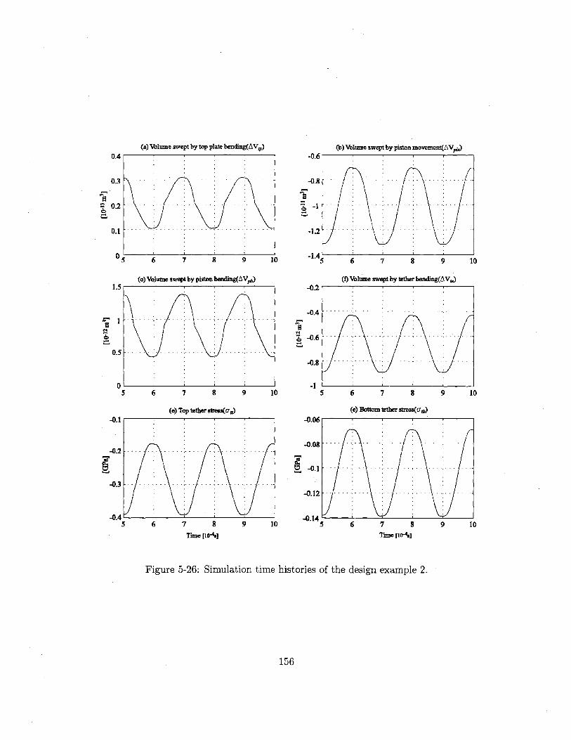
(b) Volume swept by piston movement(AVj,)
----- -- --- -- -- -
-0.6
-0.8
-1
1 -46 7 9 9 10 '5 6 7 8 9 10
(c)Volume swept by piston bending(AVp )-0.2
-0.4
-0.61
-0.8"
-15 6 7 8 9 10
(e) Top tether stress(ou)
r.4 1i-0.145 6 7 8 9 5
Tune [104s]
-0.06
(MVolume swept by tether bending(AV )
-- - -- ---- --
5 6 7 8 9
(e) Bottom tether stress(ut)
-0.08,
-0.12
6 7 8 9 10Tme po 4
.j
Figure 5-26: Simulation time histories of the design example 2.
156
0.4
0.3
0.2
0.1
0 5
1. 51
0
-0.1
-0.2
-0.3
3
(a) Volume swept by top plate bcnding(AV,,)
i
I
-1.21
- I I - . I
Ll
. .............. .. ---- --- --- - - - - --
I
0.5 [
I I
4
-. . ... . . . - - -.. .. . ... . ...-
- - - - -. .- .-. -
I A qA r-' A

second device, which is smaller than the first one, has higher efficiency. This is due to the fact
that in the example, only the chamber diameter and piezo diameter are smaller. The length
of the piezoelectric element, chamber height and structural thicknesses are kept constant. This
resulted in a stiffer chamber compared to the case where all the dimensions were reduced. The
explicit relationships and effect of geometric parameters on system scale can be seem in equation
5.27, which represents a simpler case than the actual chamber.
5.4 Summary
This chapter presented further design considerations and a design procedure along with two de-
sign examples. Fluidic oscillations within the system and conditions for sufficient chamber filling
and evacuation is analyzed. An optimization procedure for the tether structure is presented.
Trade-offs between operation conditions and their effect on the performance is discussed. Effect
of system scale on the performance is discussed. Effect of the fabrication process and the active
valves on the design is discussed.
157

GilVA~

Chapter 6
Conclusions and Recommendations
for Future Work
6.1 Summary
The objectives of this thesis were:
- To develop a comprehensive system level model and simulation tool to analyze the main
chamber and the associated fluid channels and valves of piezoelectric microhydraulic power
generation devices
- To gain insight into system operation and understand the factors affecting the syster
performance
- Develop a design procedure, which should be complemented by the design of the active
valves.
Chapter 1 presented the configuration, operation and motivation of ruicrohydraulic-piezoelectric
power generators. Primary challenges and preliminary design considerations is discussed.
Chapter 2 presented an analysis of piezoelectric power generation based on linear electrome-
chanical energy conversion. Effect of circuitry and piezoelectric material on energy density and
effective coupling factor is discussed. Models for two different circuit topologies are developed,
simulations are performed and analytical expressions are derived for the generated power and
effective coupling factor. Different piezoelectric materials are compared in terms of their en-
ergy densities and energy conversion efficiencies for different circuitry. It has been concluded
159

that, although the single crystal piezoelectric material(PZN-PT) has very high effective cou-
pling factor, it has a very low energy density compared to PZT-8 or PZT-4S because of its
small depolarization stress. Another important conclusion of this chapter is that, for a piezo-
electric element, the energy density obtained with the diode bridge and voltage detector circuit
is four times bigger than the energy density obtained with only the diode bridge. The effective
coupling factor is a function of the coupling coefficient and the circuitry, whereas the energy
density is a function of coupling coefficient, circuitry and the depolarization stress. Indeed, the
effective coupling factor becomes an important criteria if the piezoelectric element is considered
along with its surrounding system, for example the infrastructure which provides the force on
the element, which is the energy harvesting chamber in the microhydraulic power generation
device. It should be remembered that in the analysis presented in this chapter a prescribed
force is imposed on the piezoelectric element. This issue is addressed in Chapter 3.
Chapter 3 presented a simple model of the energy harvesting chamber, simulations with the
coupled circuitry and preliminary design considerations. The interaction of the energy harvest-
ing chamber and the circuitry is discussed. The two circuits presented in Chapter 2 and different
piezoelectric materials are compared in terms of the flowrate and frequency requirements for a
given pressure differential and power requirement, and in terms of system efficiency. Analytical
expressions are derived for the generated power, required flowrate, effective coupling factor and
system efficiency. The most important conclusion of this chapter is that the performance of the
energy harvesting chamber depends on
- Circuit topology
- Piezoelectric material(k 3 3 , ad)
- Chamber compliance(Ceff).
It is also concluded that, as k 3 3 approaches 1 and Ceff approaches 0, the system efficiency
for the two circuits analyzed approaches 50%. This means that, even with a perfect piezoelectric
material(k33 = 1) and zero effective chamber compliance, which are not possible, the system
efficiency cannot exceed 50%. It should be emphasized that the efficiency definition throughout
the thesis corresponds only to the energy harvesting chamber. The electrical power consumption
in the active valves is not considered.
Chapter 4 presented detailed modelling of the energy harvesting chamber. In Chapter 3,
160

an effective chamber compliance (Ceff) was assumed to be used in the simulation and in the
following analysis. This chapter investigated the contribution of different structural components
on the effective compliance of the chamber. Deformations of individual structural members are
calculated using linear plate theory. It is assumed that the deflections due to bending are
significantly larger than that due to shearing. A simulation architecture is presented to be
included in overall system level simulation, which allows for inclusion of the elastic equations
into dynamic simulation as well as monitoring important parameters.
Chapter 5 presented further design considerations in addition to the design issues discussed
in Chapter3. These were fluidic oscillations within the system, chamber filling and evacuation,
tether structure optimization, effect of operation conditions on system performance and trade-
offs, and scaling issues. The system is analyzed only for the case where the chamber is attached
to the regular bridge. A design procedure along with two design examples is presented. The
design decisions made considering the issues discussed in previous chapters as well as those
imposed by the active valve design and fabrication process is discussed. Simulation results
are shown. In Chapter 2 it was concluded that PZN - PT has the smallest energy density
among the piezoelectric elements considered, which is a result of its low depolarization stress.
However due to its very high coupling coefficient it provides very efficient electromechanical
energy conversion and requires lowest flowrate for a given power requirement. It should be
noted that, the implication of the low energy density of PZN - PT is that, larger piezoelectric
material volume is needed compared to other piezoelectric materials for the same power output.
However, the weight of the piezoelectric element constitutes only a small fraction of the overall
system weight and the increased efficiency of PZN - PT due to its much higher coupling
coefficient would still overwhelm the effect of increased weight in terms of the overall system
power density.
This thesis developed a framework to analyze piezoelectric microhydraulic power generators.
Insight into system operation is gained and important factors affecting system performance are
analyzed.
161

6.2 Recommendations for Future Work
Recommendations for future work in terms of modeling and design can be summarized in the
following subgroups:
Piezoelectric Element
The analysis presented in this thesis is based on linear electromechanical energy conversion.
More detailed analysis including nonlinear effects is required to obtain better predictions for
system performance. Also, piezoelectric element coefficients only in 3-3 direction is used since
the piezoelectric element is subjected to compression parallel to the polarization of the element
and assuming that the element is free to expand in lateral directions, so that T3 is the only
nonzero stress component. However, this is not the case since the piezoelectric cylinder is
bonded to the piston and bottom support structure. Finite element analysis is required to
calculate the effective coefficients in 3-3 direction, namely effective d3 3 , S t and s.
Fluid Structure Interaction
The system is analyzed for relatively low frequencies where the fluid channels were the only
components whose dynamic behavior was important for system performance. At higher fre-
quencies, the modal behavior of the piezoelectric element and the piston structure along with
the fluid contained in the chamber might be important (added mass effect of the fluid). De-
tailed finite element models are needed to investigate the fluid structure interaction within the
chamber.
Fluid model
In this thesis, a simple fluid model based on discharge coefficients taken from published data is
used. These models do not provide accurate estimation of the power consumption in the valves
since it is not possible to predict the force exerted on the valve cap and valve membrane by the
flow. Detailed CFD analysis can provide more insight into the fluid flow in the valve. This is
very important because of the complicated geometry of the valves.
162

Squeeze film damping
Squeeze film damping is a common problem in MEMS devices. Although not presented in this
thesis, a preliminary analysis has shown that, for the chamber height used in the design, squeeze
film effects are not important. However, for smaller devices, squeeze film damping can effect
system performance significantly. Detailed analytical models and/or finite element studies are
required to investigate this effect.
Scaling Study
As the system size gets smaller, the power density increases, however, only until a certain scale.
Beyond that scale, it is expected that viscous losses in the valves will begin to dominate and
scaling further down will not be more efficient. In order to perform this study, more detailed
fluid models are needed as mentioned earlier.
System level analysis
This thesis concentrated on the main chamber, also called the energy harvesting chamber, of the
piezoelectric microhydraulic power generators. System level simulations, including full active
valve structure, should be performed to obtained better predictions about system performance
and efficiency. However, it should be emphasized that, these simulations would provide realistic
predictions provided that good fluid models exist, as discussed above.
163

C.)

Bibliography
[1] N.W Hagood, D.C. Roberts, L. Saggere, K.S. Breuer, K.S.Chen, J.A. Carretero, H. Li,
R. Mlcak, S. Pulitzer, M. A. Schmidt, S. M. Spearing, Y.H.Su. "Micro Hydraulic Trans-
ducer Technology for Actuation and Power Generation". Proceedings of the SPIE Annual
International Symposium on Smart Structures and Materials, 7:680-688, 2000.
[2] Seward Webb Pulitzer III, "Feasibility Assesment and Design of Micro Hydraulic Solid-
State Transducers". SM Thesis, Masssachusetts Institute of Technology, 2001.
[3] H.Q. Li, D.C. Roberts, J.L. Steyn, K.T. Turner, J. A. Carretero, 0. Yaglioglu, Y.H.
SU, L. Saggere, N.W. Hagood, S.M. Spearing, M.A. Schmidt, R. Mlcak, K.S. Breuer. "A
High Frequency High Flow Rate Piezoelectrically Driven MEMS Micropump". Solid-State
Sensor and Actuator Workshop, pp. 69-72, 2000.
[4] J. A. Carretero. "Measurement and Modeling of the Flow Characteristics of Micro Disc
Valves". SM Thesis, Masssachusetts Institute of Technology, 2001.
[5] D. C Roberts, 0. Yaglioglu, J. Carretero, Y.H Su, L. Saggere, N.W. Hagood." Modeling,
Design, and Simulation of a Piezoelectrically Driven Microvalve for High Pressure, High
Frequency Applications, SPIE Proceedings, 4327:366-380, 2001
[6] D. C. Roberts. "Design, Modeling, Fabrication, and Testing of a Piezoelectric Microvalve
for High Pressure, High Frequency Hydraulic Applications". PhD Thesis, Masssachusetts
Institute of Technology, 2002.
165
[7] K. Turner, " An Evaluation of Critical Issues for Microhydraulic Transducers: Silicon Wafer
Bonding, Strength of Silicon on Insulator Membranes and Gold-Tin Solder Bonding" ,SM
Thesis, Masssachusetts Institute of Technology, 2001.
[8] D.A. Berlincourt. "Piezoelectric and Ferroelectric Energy Conversion".IEEE Transactions
on Sonics and Ultrasonics, S-15(2):89-97,1968.
[9] M. Umeda, K.Nakamura, S. Ueha. " Analysis of the Transformation of Mechanical Impact
Energy to Electric Energy Using Piezoelctric Vibrator".Jpn. Journal of Applied Physics,
35:3267-3273, 1996.
[10] M. Umeda, K.Nakamura, S. Ueha. "Energy Storage Characteristics of a Piezo-Generator
using Impact Induced Vibration ".Jpn. Journal of Applied Physics, 36:3146-3151, 1997.
[11] C. N. Xu, M. Akiyama, K. Nonaka, T. Watanabe. " Electrical Power Generation Charac-
teristics of PZT Piezoelectric Ceramics". IEEE Transactions on Ultrasonics, Ferroelectrics,
and Frequency Control, 45(4):1065-1070, 1998.
[12] M. Goldfarb, L. D. Jones." On the Efficiency of Electric Power Generation With Piezoelec-
tric Ceramic". Journal of Dynamic Systems, Measurement, and Control, Transactions of
ASME, 121:566-571, 1999
[13] P. G. Jones, S. P. Beeby, E. P. James, N. M. White."The Modelling of a Piezoelectric
Vibration Powered Generator for Microsystems. In Transducers '01, 2001
[14] D. J. Warkentin, N. W. Hagood. "Nonlinear Piezoelectric Shunting for Structural Damp-
ing". Proceedings of SPIE, 3041:747-757, 1997.
[15] N. W. Hagood, A. von Flotow. " Damping of Structural Vibrations with Piezolectric Ma-
terials and Passive Electrical Networks". Journal of Sound and Vibration, 146(2):243-268,
1991.
[16] N. W. Hagood, W. H. Chung, A. von Flotow. " Modelling of Piezoelectric Actuator Dynam-
ics for Active Structural Control". Journal of Intelligent Material Systems and Structures,
1(3):327-354, 1990.
166

[17] W. P. Mason. "An Electromechanical Representation of a Piezoelectric Crystal Used as a
Transducer". Proceedings of the Institute of Radio Engineers, 23(10):1252-1263, 1935.
[18] IEEE Std 176-1987 IEEE Standard on Piezoelectricicty, The Institute of Electrical and
Electronics Engineers. 1987
[19] Ching-Yu Lin. "Material Characterization and Modeling for Piezoelectric Actuation and
Power Generation under High Electromechanical Loading". PhD Thesis, Massachusetts
Institute of Technology, 2002
[20] J. M. Hall, W. E. Dillon, W. C. Nunnally. "Thermo-Acoustic-Piezoelectric Power Gen-
eration". Procedings of the 26th Intersociety Energy Conversion Engineering Conference-
IECEC'91, 2001.
[21] V. H. Schmidt. "Piezoelectric Energy Conversion in Windmills". Proceedings of IEEE:
Ultrasonic Symposium, 2:897-904, 1992.
[22] V. H. Schmidt. "Piezoelectric Wind Generator". United States Patent #4,536,674.August
20, 1985.
[23] S. Nagao. "Electronic Wristwatch With Generator". United States Patent #5,939,707.As-
signee: Seiko Epson Corporation, July 3, 1990.
[24] 0. Takahashi, Y. Hashimoto, E. Nagasaka, H. Miyazaki, T. Funasaka. "Piezolectric Power
Generator For a Portable Power Supply Unit and Portable Electronic Device Equipped
With Same ". United States Patent #5,751,091.Assignee: Seiko Epson Corporation, May
12, 1998.
[25] Y. Hashimoto, 0. Takahashi, H. Miyazaki, T. Funasaka, M. Furahata. "Power Genera-
tion Method and Power Generator Using a Piezoelctric Element and Electronic Device
Using The Power ". United States Patent #5,835,996.Assignee: Seiko Epson Corporation,
November 10, 1998.
[26] P. Smalser."Power Transfer of Piezoelectric Generated Energy". United States Patent
#5,703,474. Assignee: Ocean Power Technologies Inc., December 30, 1997.
167

[27] G. W. Taylor, J. R. Burns. "Power Generation From Waves Near the Surface of Bodies of
Water". United States Patent #4,404,490. September 13, 1983.
[28] J. R. Burns. "Ocean Wave Energy Conversion Using Piezoelectric Material Members".
nited States Patent #4,685,296. August 11, 1987.
[29] M. Y. Epstein, C. B. Carroll. "Piezoelectric Electric Energy Generator". United States
Patent #5,512,795. Assignee: Ocean Power Technologies, Inc., April 30, 1996.
[30] M. Y. Epstein. "Piezoelectric Generation of Electrical Power From Surface Waves on Bod-
ies of Water Using Suspended Weighted Members". United States Patent #5,578,889.
Assignee: Ocean Power Technologies, Inc., November 26, 1996.
[31] M. Y. Epstein, G. W. Taylor. "Water Craft Using Piezoelectric Materials". United States
Patent #5,621,264. Assignee: Ocean Power Technologies, Inc., April 15, 1997.
[32] C. B. Caroll. "Frequency Multiplying Piezoelectric Generators". United States Patent
#5,814,921. Assignee: Ocean Power Technologies, Inc., September 29, 1998.
[33] J. R. Burns. "DC Bias Scheme For Field Induced Piezoelectric Power Generators". United
States Patent #6,201,336. Assignee: Ocean Power Technologies, Inc., March 13, 2001.
[34] E. A. Kolm, H. H. Kolm. "Piezoelectric Fluid-Electric Generator". United States Patent
#4,387,318. Assignee: Piezo Electric Products, Inc., June 7, 1983.
[35] H. H. Kolm, E. A. Kolm. "Piezoelectric Acousto-Electric Generator". United States Patent
#4,467,236. Assignee: Piezo Electric Products, Inc., August 21, 1984.
[36] P. A. Todd, B. R. Walker. "Piezoelectric Circuit". United States Patent #5,065,067.
November 12, 1991.
[37] M. Kimura. "Piezo-Electricity Generation Device". United States Patent #5,801,475. As-
signee: Seiki Company, Ltd., September 1, 1998.
[38] S. Yamashita. "Portable Piezoelctric Electric Generation Device". United States Patent
#4,091,302. May 23, 1978.
168
[39] C. G. Triplett. "Vehicular Mounted Piezoelctric Generator". United States Patent
#4,504,761. March 12, 1985.
[40] E. Dieulesaint, D. Royer, D. Mazerolle, P. Nowak. "Piezoelectric Transformers". Electronic
Letters, 24(7):444-445, 1998.
[41] G. Ivensky, I. Zafrany, S. B. Yaakov. "Generic Operational Characteristics of Piezoeelctric
Transformers". Proceedings of IEEE: Power Electronics Specialists Conference, 3:1657-
1662, 2000.
[42] S. H. Lee, J. Hong, J.H. Yoo, G. S. Gong. " Characteristics of Piezoelectric Transformer
for Power Supply". Proceedings of IEEE: Ultrasonics Symposium, 1:971-975, 1998.
[43] J. Navas, T. Bove, J.A. Cobos, F. Nuno, K, brebol. "Miniaturised Battery Charger Using
Piezoielectric Transformers". Proceedings of IEEE: Applied Power Electronics Conference
and Exposition, 1:492-496, 2001.
[44] A. M. Flynn, S. R. Senders. "Fundamental Limits on Energy Transfer and Circuit Consid-
erations for Piezolectric Transformers" .Proceedings of Power Electronic Specialists Confer-
ence, IEEE Transactions, 2:1463-1471, 1998.
[45] S. E. Park, V. Vedula, M. J. Pan, W. S. Hackenbauer, P. Pertsch, T.Shrout. "Relaxor
Based Ferroelectric Single Crystals For Electromechanical Actuators". Proceedings of the
SPIE, 3324:136-144, 1998.
[46] Q. M. Zhang, J. Zhao, K. Uchino, J. Zheng. "Change of the Weak-Field Properties of
PB(ZrTi)03 Piezocermics With Compressive Uniaxial Stresses and Its Links to the Effect
of Dopants on the Stability of the Polarizations in the Materials". J. Mater. Res., 12(1):226-
234, 1997.
[47] V. D Kugel, Q. M. Zhang, B. Xu, Q. M. Wang, S. Chandran, L.E. Cross. "Behavior of
Piezoelectric Actuators under High Electric Field". Proceedings of the Tenth IEEE Inter-
national Symposium on Applications of Ferroelectrics, 2:655-658, 1996.
169

[48] J. Zhao, Q. M. Zhang. "Effect of Mechanical Stress on the Electromechanical Performance
of PZT and PMN-PT Ceramics". Proceedings of the Tenth IEEE International Symposium
on Applications of Ferroelectrics, 2:971-974, 1996.
[49] G. Yang, W. Ren, S.F. Liu, A. J. Masys, B. K. Mukherjee. "Effects of Uniaxial Stress
and DC Bias Field on the Piezoelectric, Dielectric, and Elastic Properties of Piezoelectric
Ceramics". Proceedings of IEEE: Ultrasonics Symposium, 2:1005-1008 ,2000.
[50] S. Timoshenko. "Theory of Plates and Shells". McGraw-Hill, NewYork, NY, 1940.
[51] I.E. Idelchik. "Handbook of Hydraulic Resistance", FL, 1994
[52] Y.H. Su. Personal communication. Massachusetts Institute of Technology, 2000
[53] V. Caliskan. Personal communication. Massachusetts Institute of Technology, 2001
170

Appendix A
Simulink Block Diagrams
This section presents the simulink models used in this thesis. Figure A-1 shows the model of
the piezoelectric element model used in Chapter 2 in order to simulate the case of applied force.
Later in the thesis, namely in Chapter 4 and Chapter 5, the piezoelectric element constitutive
equations are solved along with the elastic equations of the structural members of the main
chamber and incorporated into the simulation architecture with a 15x3 matrix, as described in
Chapter 4. Figures A-2 and A-3 present the simulink models of the regular diode bridge and the
diode bridge attached to the voltage detector, respectively, used throughout the thesis. Figure
A-4 presents the simulink blocks used to implement the function of the voltage detection circuit.
Figure A-5 shows the simulink architecture of the full system including the main chamber, fluid
models and circuitry, used in Chapter 5. Simulations in Chapter 3 are performed with a similar
model. Figures A-6, A-7 and A-8 present the simulink models for the main chamber presented
in Chapter 4 and the fluid models presented in Chapter 3. The circuit model used for the
simulations in Chapter 5, where the system is simulated only with regular diode bridge, is the
same as in Figure A-2.
Implementation of the voltage detector circuit and silicon controlled rectifier The
operation of the voltage detection circuit was described in Chapter 2. The function of the
voltage detector is implemented as follows: The voltage detector block in the Simulink model
sends a signal to the switch/resistor block which is either I or zero depending on the detected
voltage, V2. The logic is as follows:
171

< 0 and V2 > 0
> 0 and V2 > 0
signal=1 (switch on)
signal=0 (switch off)
< 0 and V2 < 0 signal=0 (switch
> 0 and V2 < 0 signal=0 (switch
The switch function is implemented with a resistor in the place of the SCR, whose value
depends on the signal. If the signal value is 1, the value of the resistor is very small and the
switch is in "on" state. If the signal value is 0, the value of the resistor is very large and the
switch is in "off" state. The following parameter values are used:
Large resistance: 10 6 Ohm, small resistance: 10-6Ohm, capacitance value: 10~ 7F, inductor
value: 20mH, m = 5, K = 107 , w = 5 x 10¹².
22
Force Disp0acemnentP, K
'u current 1-, chamrge Q Unear constitutive Voltagelaw for plezoelectrkms
Plazo diarge
Figure A-1: Simulink model of the piezoelectric element.
172
dV2
dt
if dV2
dtdV2
If ddtdV2
dt
off)
off)
- .1 UWAAMMUN 1! 11 M., I , - -. -

r 5 0 5 1 -1 0 0 - -1 0 0 11 0 V1 0 -1 1 0 V1 v i1 100 1
.5 -05 0 0 -1 1 Diode 1 0 -1 1 0K V2 L-1 0 0 1_ V2 y 12 _O 0 -1 -1_ 12x
Matrbx K Diode 2 K Prdc Power
Vp ainV3 Voltages y3 V 1 rrents 13Diode 3 lP
0 V4 v4 V 4Ground Diode 4 14
differential diode dioevoltages Equations currets
rzq
0Cz
CD
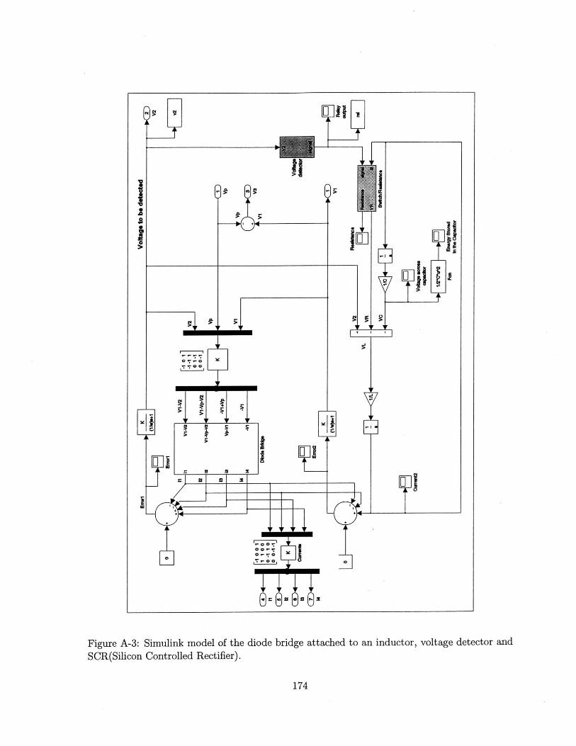
II
~I .1.
El ~
1~
IF IF-
0 **,
**C
mU ...*l
- I
~Ji
Figure A-3: Simulink model of the diode bridge attached to an inductor, voltage detector and
SCR(Silicon Controlled Rectifier).
174
I
I.212
&0
LM
I
I
5
6MM&M
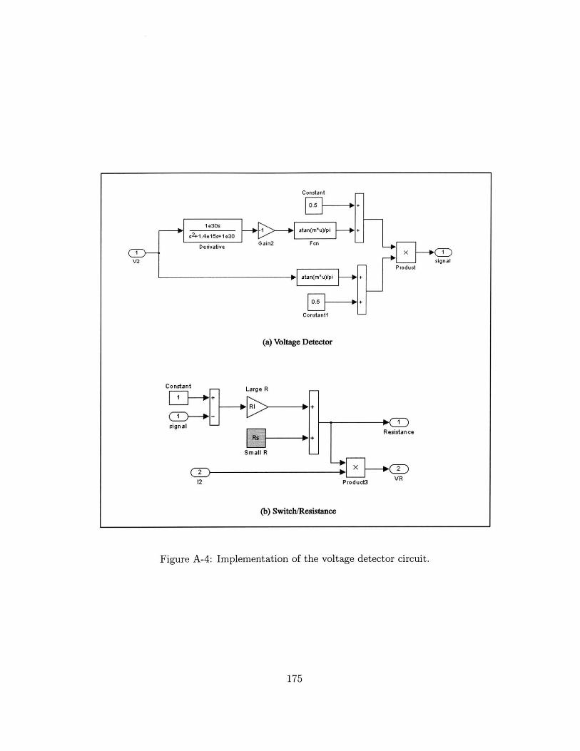
Constant
1 e3Oss2+1.4e15s+1 e30 1+
Derivative Gain2 FanC x C
V2 signalProduct
S atan(m'uypi --- +
Constant-
(a) Voltage Detector
Constant Large R
---- R +
CD- -signal -R esistan ce
Rs +
Small R
12 Product3
(b) Switch/Resistance
Figure A-4: Implementation of the voltage detector circuit.
175
=.% - -- ip- - I .. ---- -- - - - - - Z - - - - - -- - - --

0-in
Inlet valveand fluid channel
lp -In i-out
(DCl)
P(LPR)
vo-out0-out
Outlet valand fluid cha
Chamber andPiezoelectricElement
PLPR
va-out
OpeningP-ch
vennel
w. -
B- -d - - h - - - --Bokdiagram of the outlet valve opein
P-ch
Cp
lp
Power Vp
Power Circuit
0-out
PHPR - -
vo-In P-
Inlet ValveOpening
P(HPR)
vo-In
-0 P-ch
P-ch
0-in| 1
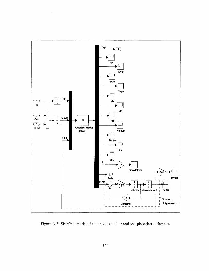
1D Oplp
-DI -netQ-in
0-out
x-pis
-* K -
Chamber Matrix(15x3)
VP 1
Figure A-6: Simulink model of the main chamber and the piezoelctric element.
177
xtp
DVtp
DVte
DVpb
xb
xte
Fte
Fte-top
Fte-bot
Sit
Stb
Fp hAp LIPiezo Stress
velocity dsplacemer
Damping
Apia ii
DVpis
t x-pis
PistonDynamics

x
0x
0.
x
Figure A-7: Simulink model of the inlet valve and fluid channel.
178

0
x -
0
le
Figure A-8: Simulink model of the outlet valve and fluid channel.
179
- - __, -0- - - -, i -I,-

00,C

Appendix B
Matlab Files
This section presents important Matlab codes used in the thesis.
Figure B-1presents the code used in Chapter 3 to calculate the required frequency, flowrate
and efficiency for different circuitry.
Figure B-2 presents the code used to calculate the required frequency, flowrate and efficiency
of the system attached to regular diode bridge for different reservoir pressures and chamber
diameters in Chapter 5.
Figure B-3 presents the Matlab code used in Chapter 5 for tether optimization. The elastic
equations and equations governing the chamber behavior are solved in Maple, which is presented
in Appendix C.
Figure B-4 presents the Matlab code used in Chapter 5 which writes the operational and
some of the geometric parameters into the Matlab workspace, which can be read by the Simulink
model for the system level simulation. Also, the 15x3 matrix required by the Simulink model
(Appendix A) is generated, whose coefficients are calculated by Maple, which is presented in
Appendix C.
181

% This code calculates the required frequency, flowrate and efficinecy for two different circuitries.& Effect of tethers is neglected and perfect sealing between the piston and the chamber walls is assumed.
clear all;
e PicZo properties (PZN-4 SPT)
s33R - ale-12 ; Closed circuit compliances33D - 17e-12 ; 1 Open circuit complianceSd - 1leg; I Depolarization stressPHPR . 2e6 ; High pressure reservoirW . 0.5 ; SPower requirement
t Dimensiona
Dpis . (4.Se-3); & Piston diameter(.chamber diameter since the effect of tethers is neglected)Apis - (Dpi&^2)pi/4; & Piston areaAp - Apia*PEPR/Sd; * Piezo area0p - sqrt (4eAp/pi); S Piezo diameterip - (le-3) ; & Piezo lengthVp - Ap*Lp ; & Piezo volume
% 'hamber atiffnes
Keff - lleis,2e15,3e15,4eiS,5els,Gels,7eiS,BelS,9elslel6,2ei6,3e16,4e16,Sel6,...Gel6,7el6,8e16,9el6,1e17,2e17,3e17,4e17,5e17,6ei7,7e17,8e17,9e17,lel,2e18....3e1,4elg, elS,6e15,7e10,aels,9ele,lelQ,2e19,3e19,4e19,5el9,6e19,7e19,Re19,9e19,1e20];
SRECTIFIER
energy stored per cycleEr - ((s33E-s33D)(Sd).^2.*Vp)./4;
% Required frequency [kHzl
fr - W./Er./1000;
& Required flowrate [ml/alOr - (2.a(s33E+a33D).aw./((s33E-a33D)aPEPR)+(PHPR.*fr.*1000./Keff)).le6 p
& Efficiencyeayer - (W./((Qr.e-e) .CPHPR)).l0O;
& RECTIFIER+VOLTACE DETECTOR
& Energy stored per cycle
es - -(s33D-33E).*Sd.^2.*Lp.Ap-(a33E.Lp.*Keff.Apis.^2+Ap).*(s33D.Lp.*Keff.*Apis.^2+Ap)./...
((Ap+2.s33E.*Lp.Keff.*Apis.^2-s33D.*Ip.*Keff.*Apisa.^2).^2);
Required frequency(kz]
fe - W./Es./1000 ;
& Required flowrate ml/sI
Os - (.(PHPE.^2.*s33E.eIc.*KeffCSd.^2.5Ap-s2D.*Lp.eKeff.Sd.2.*p) ....
(3.*s33R.*Lp.*Keff.*Sd.^2.*Ap.*PEPR.^2+s33H.-Lp.^2.*Kaff.^2. Bd.^4.*Ap.^2. s33D+PHPR.^4-PHPR.^2.*s33D.*Lp.*Kaff.*Sd.^2.*Ap)./...(PHPR.*(o33R.*Lp.*Kaff.*Sd.^2.*Ap+PHPR.^2).*(-s33D+s33R).*Ap.*Sd.^2.*Lp.*(PEPR.^2+o33D.*Lp.*Keff.*Sd.^ 2.*Ap).*Keff)).*le6;
* Efficiency
Boyne - ({s33E.*Lp.*Keff.*Sd.^2.-Ap+PHPR.^2).*(-a33D+s339). Ap.*Sd^2.*L.--(PliPR.^2+,23D.*Lp.*Keff.*Sd.^2.*Ap) 3Keff./. ..((PHPR.^2+2.ns33E.eLp.*Keff.OSd.^2.*Ap-s33D.Lp.Kaff.efd.'2.*Ap)....(3.*a33R.-Ip.-Keff.*Sd.^2.*Ap.*PHPR.^2+8233.*Lp.^2.*Keff ^2.*Sd.^4.-Ap.^2.*823D+PRPR.^4-PHPR.^2.-s23D.*Lp. Keff.*Sd.^2.*Ap)))*100;
Ceff-l./Keaff; Effective compliance
figure (i)hesemilogx(CeffQr,'b--,,Ceff,Os,'r-');set(h,'LineWidth',2)title('Study3')xlabel('Ceff[m^3/Pa] 'ylbel ('ilowrate [ml/si')legend('Rectifier','Rctifier+Voltage Detector')grid onaxis(Els-20 le-15 0 101)
figure (2)h.semilogx(Cefffr,'b--',Ceff,fs,'r-')p
set (h, 'LineWidth' ,2)xlabel ('aCeG f m^3/Pal ')
ylabel ('Frequency [kHzl')
grid on
figure (3)h-semilogx(Ceff,Eaysr,'b--',Ceff,Eayss,'r-');
set(h, 'LineWidth' ,2)xlabel('Ceff[m^3/Pa ')
ylabel('Systsm Efficiency[ml/sl')legend('Rectifier','Rectifier+Voltage Detector')grid on
Figure B-1: Matlab code ised in Chapter 3 to calculate the required frequency, flowrate and
efficiency for different circuitry.
182

1 This code calculates the required frequency, flowrate and efficiency ofI the system for different reservoir pressures and chamber diameters
clear alli
k Power requirement
W - 0.5 ; * Power ra
t Piezo properties(PZN-PT)
s33E - ale-12 'a closed cs33D = 17e-12 ; 4 Open ciSd = lOe6; ' Depolari
* Silicon material properties
v = 0.22, V PoissonsE - 165e9 &k Youngs s
t Silicon oil bulk modulus
Bf = 2e9 I 4 Fluid bu
* Operation condition: varying PHR
for PEPR - ls6:leE6;46;
* Geometric dimensions
n = 1:0.1:10y
Dch - le-3-n 'a Chamber
Hch - 200e-6 ; & ChamberAch -(Dch.^2)*pi/4: 'a ChamberAp - Ach.*PHPR./Sd; ' PiezoIP - le-3 ; ' Piezo 1htp - l-S : ' Top pl
t Calculation of compliances
Cs - (F6.*N.htp.3./(pi.*(l-v.^2) .(Dch./2).6)).^-l; a Top plecf - (Bf./(Ach.*ch)).^-l ; & FluidicCeff- Cs+Cf; 'a Effecti
1k Calculation of required frequency, flowrate and efficiency
f - 4.*w./((s33E-s33D).*Sd.^2.*Lp.*Ap); 4a Require
Q - 2.*(33E+s33D).*w./((s33E-s33D).PPR)+Ceff.*PHPR.*f, % Require
Eff - w./(Q.*PHPR); ' Efficie
]k Plotting results
figure (1)gridplot (Dch/le-3, f/le3)title('Required frequency vs. piston diameter')xlabel ('Dpis am] )ylabel('f[kHzl ')
hold on
figure (2)gridplot (Dch/le-3,0/le-5)title('Required flowrate vs. piston diameter')xlabel ('Dpis [m ')
ylabel ('Q ml/s' )
hold on
figure (3)gridplot (Dch/le-3 ,Eff100)title('Efficiency vs. piston diameter')xlabel ('Dpis (ml')ylabel('Eff [W]')
hold on
end
quirement
ircuit compliancercuit compliancezation stress
rationdulus
lk modulus
diameter
heightarea
rea
snghtte thickness
te compliancecompliance
vs compliance
d frequency
d flourate
ncy
Figure B-2: Matlab code used in Chapter 5 to calculate the required frequency, flowrate and
efficiency of the system attached to regular diode bridge for different reservoir pressures and
chamber diameters.
183

% Matlab code used in tether structure optimization. (Double layer piston)% The expressions for kxf, kxp, kvf, kvp, xpt, P, Fpt and Ceff are obtained using Maple.
clear all;
dVf - ic-10; t Input flow volume into the chamber
Dah - 7.2e-3; t Chamber diameterDp = 3.8e-3; t Piezo diameterLp - ic-3; t Piezo lengthAp = Dp^2*pi/4; k Piezo areaHch = 200e-6; t Chamber height
E - 165e9; t Youngs modulusv - 0.22; t Poisson ratioBf - 2e9; t Bulk moduluss33D = Se-12; t Open circuit compliance
a - Dch/2;kp Ap/s33D/Lp; t Piezo stiffnessVo = Hch*Dch^2*pi/4; t Initial volume of chamber
ttopte - ile-6;thotte - Se-6;
d - E*ttopte^3/(12*(l-v^2));do E*tbotte^3/(12*(-V^2));
for k- i1:2e3;
Dpis - (Dh)-k*0.0005e-3;
b = Dpis/2;Apis - Dpis^2*pi/4;
* Top tether
kxf = -1/16* (b4-2*b^2*a^2+4*b^2*a^2*log (a/b) 'log (b)+a^4 -4*a2*log (a)^2*b^2+4*a^2*log(a) *b2*log(b)) / (d*pi* (b2-a^2));kxp - -1/64* (3*b^6-7*b^4*a^2+4*b^4*log (b) *a^2+5*b^2*a^A4-4*b^4*a^2*log (a) -4*b^2*log(b) *a4+16*b^4*log (b) *a2*log (a/b) ...
-a^6+4*a^4*b'2*log(a) -16*a^2*log (a)^2*b^4+16*a^2*log (a) *b4*log (b) )/ (d* (b^2-a^2));
kvf - 1/64*pi' (16*b^4*log (b) *a'2*log (a/h)+16*a^2*log (a) *b^4*1g (b)+S*b^2*a'4-4*b4*log (b) *a^2+4*b^4*aA2*log (a)+4*b^2*...
log (b) *a^4-4*a^4*b^2*log (a) -16*a^2*log (a)^2*b^4 -a^6-7*b^4*a^2+3*b^6-16*a^4*log (a) *b'2*log (b) -*b^4*a'2*log (a/b) ...
+16*a^4*log (a)^2*b^2+8*a^4*b^2*log (a/b) -16*a^4*b^2*log(a/b) *log (a) ) / (d*pi* (b^2-a^2));kvp - 1/192*pi* (24*a^4*b^4*og (a/b)+24*a^4*b'4-22*b^6*a^2+a^8+7*b'8-48*a^4*b^4*og (a/b) *log (a) -4*a4*lg (a) *b^4*log (b) ...
+48*a^4*log (a)^2*b^4+48*b'6*a^2*log (a/b) *log (b)+4*b^6*aA2*log (a) *log (b) -48*b6*a^2*log(a)^2-24*b^6*a^2*log (a/b)-..-10*r^6*b^2)/(d*(b^2-a^2));
t Bottom tether
kxfb - 1/8*b^2*log(b) / (pi*ds) -1/8*b^2/ (pi*ds) +1/16* (-2*a^2*log (a)+a^2+2*b^2*log (b) -b2) *b^2/ (pi*ds* (a^2-b^2) )+1/4*b2*...a^2*log (a/b) *log (b) /(pi*ds*(a^2-b^2))+1/16*a^2*(a^2-2*b^2*log(b)-b^2-4*b^2*log(a)'2+2*b^2*log(a)+4*b^2*log(a)*...log(b) ) / (pi'ds* (a'2-b^2));
t Overall equations
xpis - -kxfb*(kxf*Apia-kxp)*dVf*Bf/(kxfb*Vo+kxfb*Bf*kvf*Apie-kxfb*Bf*kvp+kxf*Vo-kxf*Bfekvp+kxf*kp*kxfb*Vo-kxf*kp*kxfb* .Bf*kvp+kxf*Apis^2*Bf*kxfb+kxp*Bf*kvf+kxp*Btf*kvf*kp*kxfb-kxp*BfIkxfb*Apis);
P - Bf*dVf*(kxfb+kxf+kxf*kp*kxfb)/(kxfb*Vo+kxfb*Bf*kvf*Api-kxfb*Bf kvp+kxf*Vo-kxf*Bfekvp+kxf*kp*kxfb*Vo-kxf*kp*kxfb*Bf .*kvp+kxf*Apis^2*Bf*kxfb+kxp*Bft*kvf+kxp*Bf'kvf*kp*kxfb-kxp*Bf*kxfb*Apis);
Ceff - Vo/Bf+ (kxf b*kvf*Apis+kxp*kvf+kxp*kvf*kp*kxfb-kxfb*kvp-kxf*kvp-kxf*kp*kxfb*kp) / (kxfb+kxf+kxf*kp*kxfb);
xp(k) - xpis;Pch(k) - P;Comp(k) - Ceff;Dpion(k) - Dpis;
end
figure(2)subplot(3,1,1)plot ( (Dch-Dpisn) *le6/2,xp/le-6)
hold ontitle('Dah fixed,Dpis varied')ylabel ('Piston Deflection fuml ')
gridsubplot(3,1,2)plot ((Dch-Dpion) *1e6/2, Pch/le6)hold onylabel('rCamber Pressure[MPa]')gridsubplot (3 , 1, 3)semilogy ((Dch-Dpian) *1e6/2,Comp)hold onylabel ('Ceff [m3/Pal ')xlabel('tether width')grid
Figure B-3: Matlab code used for tether optimization.
184

I This code writes the system parameters to the Matlab workspace to be read by Simulink.S It also generates the 15x3 matrix used in Simulink, whose coefficients are calculated using Maple.
clear all,
& cluid Properties
rho - 760 % 9 fluid density [kg/m^3]pnu fluid - 0.65e-6; W viscosity [m^2/sacl;mufluid - rhoenu fluid; S viscosity [Pa/sec];
W Valve geometry
d_discin - 2*400e-6 p 5 inlet valve cap diameter[m];4_discout- d discin ; 1 outlet valve cap diameterms];
hi - 10cc-6;eta - 0.965 ;
4 Valve Channel Goeometry
lk - 5Se-7 p t Leakage [m]
La - 5000; V Channel lengthAc - 1; t Channel area
& Note: Since only L/A ratio is important in this study,* no exact channel geometry is defined, only the ratio is determined.
I Diode Properties for the rectifier circuit
T - 300;k - 1.38e-23;eta- -l.25/S;
q - 1.6e-19;In - le-6p
t Operation Conditions
voi - 24e-6 p V Inlet valve opening[m]
voo - 24e-6 ; t Oulet valve openingm]
Wn - 20000 ; Operation frequency[Hz]
Vb - 74.9; & Hattery Voltage [VI
PfPR - 306; S High Presure Reservoirs Pressure
PLPR - 0.5e6; S Low Presure Reservoire Pressure
I Expansion look-up table
Re - [0, 0.05,0.1,0.2,0.3,0.4,0.5,0.6,0.9] ;
Ce - [1,10,15,20,30,40,50,100,2e2,5e2,1e3,2e3,3e3,lelS] p
Te - [33,3.1,3.5,3.04,2.7,2.42,2.32,1.92,1.94,2.07,2.45,1.92,1.25,0.98;33,3.1,3.3,3.02,2.56,2.29,2.13,1.83,1.79,1.89,2.23,1.76,1.13,0.9;33,3.1,3.2,3,2.4,
2.15,1.95,1.7,1.6S,1.7,
2,1.
6,1,0.lp
33,3.1,3.2,2.8,2.2,1.85,1.65,1.4,1.3.1.3,1.6,1.25,0.7,0.64;33,3.1,3.1,2.6,2.,1.6,1.4,1.2,1.1,1-1,1.3,0.95,0.6,0.5;33
,3
.1,3
.0,2
.4,1.8,1.5,1.3,1.1,1.,l..S,1.05,0.8,0.4,0.
3 6
33,3.1,2.0,2.3,1.65,1.35,1.15,0.9,0.75,0.65,0.9,0.65,0.3,0.25;33,3.1,2.7,2.15,1.55,1.25,1.05,0.0,0.6,0.4,0.6,0.5,0.2,0.16;33,3.1,2.6,2,1.4,1.1,0.9,0.4,0.3,0.1,e-2,5e-2,2e-2,1.8e-2] p
* Contraction look-up table
Ro - [0,0.l,0.2,0.3,0.4,0.5,0.6,1 p
Cc - [1,10,20,30,40,50,1e2,2e2,5e2.1e3,2e3,4e3,5e3,1e4,lels] ;
Tc - [30,5,3.3,2.5,2.16,1.98,1.4,1.13,0.94,0.77,0.6,0.97,0.92,0.6,1;30,5,3.2,2.4,2,1.8,1.3,1.04,0.2,0.64,0.5,.,0.75,0.50,0.45;30,5,3.1,2.3,1.4,1.62,1.2,0.95,0.,0.5,0.4,0.6,0.6,0.4,0.430,5.,2.95,2.15,1.7,1.5,1.1,0.-5,0.6,0.44,0.30,0.55,055,0.3,0.35;30,5.,2.8,2.0,1.6,1.4,1,0.78,0.5,0.35,0.2S,0.45,0.5,0.3,0.3j30,5,2.7,1.8,1.46,1.3,0.9,0.65,0.42,0.3,0.2,0.4,0.42,0.25,0.25;30,5,2.6,1.7,1.35,1.2,0.8,0.56,0.35,0.24,0.15,0.35,0.35,0.20,0.20;30,5,2.6,1.7,1.20,0.8,0.6,0.40,0.15,0.01,0.05,0.15,0.15,0.10,0.10] p
0 Preparation of the matrix to be fed into Simulink
Thesisgileatrix; I Read in matrix values from Thesisfi4atrix.s
for 1-1:15for j-1:3
eval (['Amatrix(i,j) -A, nnmstr(i)num2str(j) 'p']),
and
Figure B-4: Matlab code used for writing system parameters into the workplace to be read bythe Simulink model for the system level simulation.
185

00C0

Appendix C
Maple Files
This section presents important Maple files used in the Thesis.
The first two codes are the Maple files used for tether optimization in Chapter 5. The first
one solves the elastic equations of the tether structures. The second one solves the governing
equation for the chamber behavior. The coefficients calculated are then fed to the Matlab code
used for tether optimization presented in Appendix B.
The third code solves the elastic equations of all the structural components within the
system along with the equations governing the chamber continuity and piezoelectric element
behavior. The equations are solved and the coefficients for the 15x3 matrix required by the
Simulink model architecture, which is described in Chapter 4, are calculated. These coefficients
are written in a Matlab m.file which are then read by another Matlab code (Appendix B) to
generate the 15x3 matrix. The assumptions and derivation of these equations are presented in
Chapter 4.
187

E This file solves the elastic equations corresponding to the tether structure.
Double layer piston is considered.It is assumed that everything except the tethers are rigid.
[ > restart;[ > Digita:=40:
Top tether
Define governing DE for bending of circular plate and shear force
Governing DE> eqn:='diff(1/r*diff(r*diff(w(r),r),r),r)=Q(r)/d':
F Shear force in terms of Pch(chamber pressure) and Fpt (force applied by the piston on the top tether)
L > Q (r) :=Fpt/ (2*Pi*r) - (1/2) *P* (r^2-b^2) /r:
Integrate the DE
F > Q1(r):=(int(Q(r)/d,r)+C1)*r:F > Q2(r):=(int(Q1(r),r)+C2)/r:E > v (r):=int (Q2 (r) ,r) +C3:
Apply BC's[ > BC1:-subs({r=a},w(r)).O:
E > BC2:=subs ({r=a}, dif f (w (r) , r) )=0
[ > BC3:=subs ((r=b), diff (w (r),r))=0:
E > Bet:=solve({BC1,BC2,BC3},{C1,C2,C3}):F > W(r) :=subs (Set,w(r))
Calculation of linear coefficients for deflection and swept volume
[ > kxf:=ubs((P=O,Fpt-1),subs({r.b},W(r))):[ > kxp e auba((P=1,Fpt=O},subS({rmb),W(r))):F > kvf g=subs((P=O,Fpt=),collect(siplify(int(2*pi*r*W(r) ,r=b..a)) ,(d,P))) :
F > kvp:=subs((P=1,Fpt=O},collect(sinplify(int(2*pi*r*W(r) ,r=b..a)) ,(d,P})):
Bottom tether
_' Define governing DE for bending of circular plate and shear force
Governing DE> eqn:='diff (1/r*diff (r*diff (w(r) ,r) ,r) ,r)=Q(r) /ds':
F Shear force in terms of Fpb (force applied by the piston on the bottom tether)L > Q (r) :=Fpb/ (2*Pi*r):
Integrate the DE
F > Q1(r):r=(int(Q(r)/ds.r)+C1)*r:
[> Q2(r):m(int(Q1(r),r)+C2)/r:
[ > w(r):mint(Q2(r),r)+C3:
Apply BC'sF > BC1:=subs ((r=a},w(r))=0:F > BC2±muba({rma},diff(w(r),r))=O:
F > BC3:=subs ((r=b},dif f (w(r),r))=0:F > Set:=solve({BC1,BC2,BC3},{C1,C2,C3)):F > W (r) :=subs (Set, w (r) ) :
Calculation of linear coeflicient for deflection
F > kxfb:maubm((P=O,Fpbsl),ub8({rmb),W(r))) :
188

-~ -- il~
189
- File: Compl.mwsThis file solves the overall equations governing the chamber behavior including piston deflection, swept volume, chamber pressure,force on piezo and fbrce on tethers.Also the effective compliance of the system is calculated. The elastic equations governing the tether behavior are calculated usinganother maple file.
L The results of both maple files are then fed to Matlab for tether structure optimization.E > restart;[ > Digits:=40:
9 Equations Governing top tether deflectionE > eanql:xpiawkxf*Fpt+kxp*P:E > eqn2:=dVt=kvf*Fpt+kvp*P:
Equation Governing bottom tether deflectionL > eqn3:=xpis=kxfb*Fpb:
Force Balance at piston-tether connectionL- > eqn4:-Fp=Fpt+Fpb:
Fluid Compliance
E > eqnS:=P=((dVf+dVt+xpis*Apia) / (Vo) ) *Bf:
Piston and Piezo
L > eqn6:=P*Apis+Fp+kp*xpis=O:
Solve equations for input dVf
[ aya:=olve({eqnl,eqn2,eqn3,eqn4,eqnS,eqn6),{xpis,Fp,dVt,P,Fpt,Fpb)):
[ > assign (sys) ;[ > Ceff:=collect(simplify( (dVf+xpia*Apia) /P) ,{Vo,Bf}) :

Fie: ThesSimComp.mmwWithin the simulink model, an 15 x 3 matrix is needed, which takes as inputs (Qp, Qnet, xpis) and solves for the outputs (Vp, xtp,DVtp, DVte, DVpb, xb, xte, Fte, Fte-top, Fte-bot, Stt, Stb, Fp, Pch, Fnet).This code calculates the coeficienta of this matrix.
[ > restart;[ > Digits:=40:
Governing Equations
Top support structureE EQN1 := x [tp]=k [dtp] *P [ch]:
E > RQN2 : - DV [tp] =k [tp] *P [chl:
Bottom Support Stucture[ > EQN3 := x[b] = k[b]*F[pl :
MisonS> EFQN 4 = x[pis] -x [te] =k [p1] *F[p] +k [p2] *P [ch]:
E > EQN5 := DV [pb =k [p3] *F [p +k [p4] *P [oh] :[ > XQN6 := F [net] =-A [pis] *P [ch] +F [p) -F [to]:
Piston TethersEQN7 := x[te]=k [ttl] *F [tetopl+k [tt2l *P [ch]:
[ > EQN8 = DV[tel=k[tt3]*F[tetop]+k[tt4]*P[ch]:[ > XQN9 := Str[tt]=a[ttl] *F [tetop]+8 [tt2] *P[ch]:
E > QN10 : [to] k [thl *F [tebot] :
[ > NQN11 := Str[tb] = [t]*F[tebot]:
L > EON12 : F[te]=F[tetop]+F[tebot]:
Chamber continuityE > ZQN13 := P[ch]=B[fl/V[ol*(Q[net]+x[pin]*A[pin]+DV[pb]+DV[tel -DV[tp]):
Piezoelectric Material[ Linear constituive relations.[ > EQN14 := x [b] -x [pis] = L [p] /A [p] * (sD [33] *F [p] +d [33] /eT [33] *Q [p]):[ > EQN15 V[p] = L[p]/A[pl*(d[33]/eT[33]*F[p]-1/eT[33]*Q[p] ):
Geometric and Material Parameters[ Geometric Parameters:[ > L[p]:=le-3: d[p]:w3.8e-3: A[p]:=(Pi*d[p]^2)/4:
[> d[pis]:=6.95e-3: w~t]:=125e-6:- d~ch]:=dl~pia]+2*w~t]: t[pis]:-=800e-6:.
I A [pia]:= (Pi*d [pis] ^2) /4:[ > t[tetop:=10-6: t[tebot]:=5-6:[ > t[bot] :=2500e-6: t[top] :=2500e-6:[ > H[ch] =200e-6.: V[o] :=Pi*(d[ch]^2/4)*H[ch]:
[ Material Parameters:> d[33] :=1780e-12± sD[33]:=17e-12: sE[33]:=81e-12: eT[33] :=d[33]^2/(aE[33]-sD[33]):> E[ai] :=16Se9: nu[sil:-0.22: B[f]:-2e9: rho[ai]:-2230: M[pis]:=rho[si]*A[pis]*t[pis]:
IN Calculate Linear Plate Coefficients
Is Top Support StructureCircular plate clambed at its outer radius(r=a).Positive deflection is upward.
[ > eqn:=' diff(1/r*diff(r*diff(Z(r),r),r),r)=Q(r)/DB':[ > Q(r):=P[ch]*r/2:
Page 1
190

> Q1(r):=(int(Q(r)/Ds,r)+C1)*r:[ > Q2(r):=(int(Q1(r),r)+C2)/r:
[ > wtp(r):=subs{{C2=0},int(Q2(r),r)+C3):[ > BC1:=subs({r=a),wtp(r))=
[ > BC2:-subs({r-a},diff(wtp(r),r))mO:[ > Bet:=solve((BC1,BC2},{C1,C3)):
[ > Wtp:=simplify(subs(Set,wtp(r))):[ > DVtp:=int(2*Pi*r*Wtp,r=O..a):
[ > Wtpo:=subs((r=O),Wtp) .[ > k[dtpl:=subs({P[ch]=1),Wtpo):[ > k[dtp] :=evalf(subs( {a=d[ah]/2, Dm=E[sil*t[top]^3/(12*(1-nu[sil^2))},k[dtpl)):
[ > k[tp]:=subs({P[ch]=1},DVtp)*:[ > k[tp] :evalf(subs{a=d[chJ/2, Da=nE[sil *t topV 3/(12*(1-nu[sil^2))},k[tp])):
Bottom Suport Structure[ Circular plate with a circular hole at the center which is clamped at its outer radius(r=a) and guided at its inner radius(r=b).Positive deflection is upward.
[ > eqn:=diff(1/rdiff(r*diff(Z(r),r),r),r)=Q(r)/Da':[ > Q(r):=-F[p]/2/Pi/r:[ > Q1(r):=(int(Q(r)/Ds,r) +C1)*r:
E > Q2(r):=(int(Q1(r),r)+C2)/r:[ > wb (r) :=int (Q2 (r) , r)+C3:E > BC1:=aubs({r=a},wb(r))=O:
[ > BC2:=aubs({r=a},diff(wb(r),r))=O:
E > BC3:=subs({r=b},diff(wb(r),r))=O :
[ > Set:=solve((BC1,BC2,BC3},{C1,C2,C3)):[ > Wb:=simplify(subs(Set, wb(r))):[ > k[bI :usimplify(subs({F[p] =1},aubm((rmb),Wb))) :
[ > k[bI :=evalf (subs ((a=d [h] /2, b=d[pl/2, Ds=[sil *t[bot] ^3/ (12* (1-nu [il ^2)) },k[b])):
PihtonCircular plate with a circular hole at the center which is simply supported at its outer radius(r=a) and guided at its inner
radius(r=b).Positive deflection is upward.
E > eqn:='diff (1/r*diff (r*diff (Z (r) ,r) ,r) ,r)=Q (r)/Da':E > Q(r):.F[pl/2/Pi/r-P[chl*r/2:E > Q1(r):=(int(Q(r)/Ds,r)+C1)*r:C > Q2(r):=(irnt(Q1(r),r)+C2)/r:[ > wp (r) :=int (Q2 (r) , r)+ C3 :
[ > BC1:=sub({rua}, wp(r))mO:E > BC2:=suba({r=a),diff(wp(r),r$2)+nu/r*diff(wp(r),r))=O:[ > BC3:=suba({rub},diff(wp(r),r))mO:E > Set:=aolve({BC1,BC2,BC3),(C1,C2,C3)) :[ > Wp:=simplify(subs(Set,wp(r))):[ > DVpb:=simplify(int(2*Pi*r*Wp,r=O. .a)):
[ > k[pll:usimplify(subs({P[ch]=O,F[pll},sub({rmb),Wp))) :[ > k [pl] :=evalf (subs ((aud [pis] /2, bud [p1/ 2, D=n t[ail *t [pial ̂ 3/ (12* (1-nu [il ̂ 2)),
nu=nu [siI ), k [pll ) :
[ > k [p2] :-simplify (subs ((P [ch]=1, F [p] =0}, subs ((rbWp)) ):> k [p2] :evalf (subs ({a-d [pisl /2, bud [p1/2, Da-E [i] *t [pis] A3/ (12* (1-nu [ai]A2)),
I nu=nu [oil ),k[p21)):[ > k[p3]:-=simplify(subs({P[ch]O,F[pl-1},DVpb)) :[ > k[p3] :=evalf (subs ({a=dEpis /2, b=d[pl/2, Ds=H [sil *t [pis] ^3/ (12* (1-nu [sil ^2)) ,
numnu[sil),k[p31)):
E > k[p4l:=simplify(subs((P[ch]=1,F[p]=O},DVpb)):> k [p4 :=evalf (subs ((aud [pis] /2, bad [p1/2, Ds=E [sil *t [pi] A^3/ (12* (1-nu [il A2)),
nu=nu[sil},k[p41)):2
Page 2
191

Drive Element TethersTop TetherAnnular plate clamped at outer radius (r=a) and guided at inner radius (r-b) with pressure applieddownward over tether and concentrated force applied upward at inner radius (r=b).
[ > eqn:='diff(1/r*diff(r*diff(Z(r),r),r),r)=Q(r)/Da':[ > Q (r) :=F [tetopi / (2*Pi*r) -P [chl] * (rA2-b^2) / (2*r):
[ > Q1(r):=(int(Q(r)/Ds,r)+C1)*r:[ > Q2(r):-(int(Q1(r),r)+C2)/r:[ > wtt(r):=int(Q2(r),r)+C3:F > BC1:=subs({r=a},wtt(r))=O:E > EC2:=subn( {r=a},diff(wtt(r),r))=O:[ BC3:=nubs({r-b},diff(wtt(r),r))=O:[ > Set:=aolve({BC1,BC2,BC3},(C1,C2,C3}) :[ > Wtt:=simplify(subs(Setwtt(r))):L > D/tt:=2implify(int2(2*Pi*r*Wtt,r=b..a)):[ > k[ttl] :m-implify(subs({P[ch]l0,F[tetop]=O),subsa({r-b},Wtt))):
> k[ttI]:=evalf0(ubs{{a=d[ch]/2, b=d[pi±]/2,I DanE[si]*tftetop]^3/(12*(1-nu[siI^2))),k[ttl])):E > k[tt2l :=nimplify(sub((P[chl-=1,F[tetop]=1},ubs((r=b),Wtt))):
L > k [tt2] :=eva1f (sub{((a=d [ch] /2, b=d[pis] /2,IDa=E [si] *t [tetoP] ̂ 3 /(12* (1-nu [SjA ^2) )), k[tt2 ) ) :
[ > k [tt3] :=aimplify (oub ({P [ch]=0, F[tatop]=l}, DVtt) ):> k [tt3] : evalf (gubs ({a-d[ch] /2, b=d [Piz]/2,
I Du=En[sil *t[tetop] 3/(12*l(-nu)[)i2)),k[tt3])):[ > k[tt4] :=mimplify(sub((P[chl=1,F[tetop]=O},(DVtt)() a t
> k [tt4] :=evalf (eub9({a=d[ch3 /2, b=d[pis] /2,l D =e [ila*t[tetop] ^3d/ (12*a (-nu[si ^a2) ) ), ktt4 )r):
[ > Stt:simplify(6* (Ds* (diff (Wtt,r$2)+nu/r*di ff(wtt,r)))/(h2)):E > a( [tt:=aimpli fy (ub({P[ch]=,Ftetop]=l),sub({rma},Stt))):
[> a [ttI] :=ev&If (nubn ({=d [ch3 /2, b=d [Pia]/2, Dn=E [oi]*t [tstop] ̂ 3/ (12* (1-nu [si] ̂ 2)) ,
I nu=nu [i, h=t[tetop(),Q[tt1))):[ > aB[tt2: = aimplify(subs(Pch 1,Ftetop]=)),Oubz({rma}, tt))):
L > [tt2]:=evalf(n ub (( a=d[ch /2, b=d [pin] /2, Dn=N [ail *t [tetop]^3/ (12* (1-nu [ni]^2)),nu=nu [il, h=t[tetop},a[tt2])):
Bottom TetherAnnular plate clamped at outer radius (r=a) and guided at inner radius (r=b)with concentrated force applied upward at inner radius (r=b).
E > egn:mldiff (l/r*diff (r*diff (z(r),r),r) ,r)=Q(r) /Dol:[ > Q (r) :=F [tebot] /(2*Pi*r) :[ > Q1 (r) := (int (Q (r) /D , r)+C1) *r:E > Q2 (r) := (int (Q1(r) ,r)+C2) /r:.[ > wth (r) : =int (02 (r) , r) +r3:[ > BC1:-=euba (r=a}, wth (r) ) =O:[ > BC2:=soubs {{rua},diff (wtb(r),r))mO-:[ > BC3:=ouba ({r=b}, dif f(wtb(r) ,r))=0:[ > Set :msolve ({BC1, BC2, BC3), (Cl, C2, C3)) :E > Wth:-=simplify (subs (But,wth (r))) :
E > k [tb] :=aimpli fy (suba ({F [tebot]=l}, subs ({r=b}, Wtb) )) :
[> k[tb]:-=ev&lf (xubz({&=d[ch]/2, b=d[pinl/2, Dgi=glsi]*tltebotl^3/(12*(l-nUlai]^,2)),1nu=nu[sil},k~tb])):
[ > Sth:-=oinplify(6*(Ds*(diff {Wth,r$2)+nu/r*diff (Wth,r))) /(h^2)) :
E > a [tb] :=aimpli fy (suba{{F [tebotl=l}, suba {{r=a),Sth) ) ):> a [tb]:-eva f (sub9 ({awd [ch] /2, bod [pia] /2, Ds= [Bi] * t[tebot] ̂ 3 /(12* (1-nu [ai] ^2)) ,
I nu=nu[ni], h=t~tebot1},5[tb])):
ESolve EquationsIn the Simulif model, the inputs to the matrix block are Qn. Onet and xpis. It is desired to solve for each of the output variables in
Page 3
192
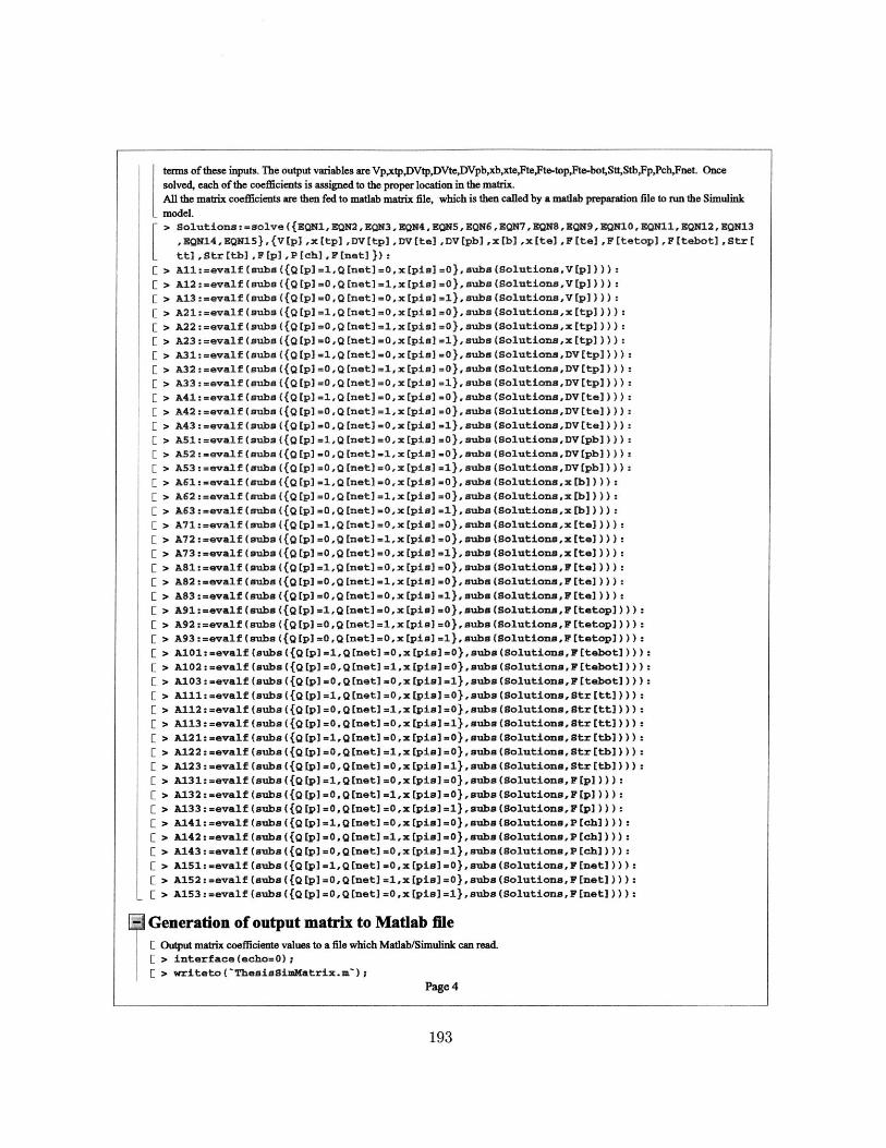
terms of these inputs. The output variables are VpxtpDVtpDVteDVpb xb,xte,FteFte-topFt -botSttStbFpPchFnet. Oncesolved, each of the coefficients is assigned to the proper location in the matrix.All the matrix coefficients are then fed to matlab matrix file, which is then called by a matlab preparation file to run the Simulinkmodel.> Solutions:=solve({EQN1,EQN2,EQN3, EQN4,EQN5,EQN6,EQN7,QN8S,EQN9,EQN10,EQN11,EQN12,EQN13
,NQN14, EQN15},{Vtp] ,x[tp] ,DV[tp] ,DV[te] ,DV[pbj ,x[b] ,x[te] ,F[te] ,F[tetop] ,F[tebot] ,Str[
tt],Str[tb],F[p],P[chlF[net]}):F > A11:=evalf(subs({Q[p]=1,Q[net]=,x[pis]=o),subs(Solutiona,V[p]))):
F > k12:.evalf(subs((Q[p]-0,Q[net]m1,x[pia]=0),subs(BolutionB,V[p1))):F > A13:=evalf(subs((Q[p]=O,Q[net]=,x[pia]1},ub(SolutionV [p]))):
[ > A21:=evalf(subs((Q[p]=1,Q[net]=o,x[pi]=O),subs(Solutiona,x[tpl))):F > A22:=evalf(subs({Q[p]=O,Q [net=l,x[pis=O},subs(olutions,x[tpl))):F > A23:=evalf(subs((Q[p]=O,Q[net]=O,x[pial=1),ubs(SolutionB,x[tp))):F > A31:=evalf(suba((Q[p]=1,o[net]mO,x[pis]-0),suba (8olutiona ,DV[tp]))):
F > A32:=evalf(suba((Q[p]=O,Q[net]s1,x[pia]=O), subs(olutions,DV[tp]))):E > A33:=evalf(muba((Q[p]=,Q[net]=,x[pia]=1},subs(olutiona,DV[tp]))):F > A41:=evalf(suba({Qlp]=1,Q[net]=,x[pie]=O},aubs(Solutions,DV[te]))) :
F > A42:=evalf(subs({Q[p]=,Q[net]=1,x[pie]=O},aubs(Solutiona,DV[te]))):F > A43:-evalf(subs({Q[p]=O,Q[net]=Ox[pislml), subs(Solutions,DV[te]))) :
F > A51:=evalf(subs((Q[p]=1,Q[net]=O,x[pis]=O},subs(Solutiona,DV[pb))):F > A52:-evalf(uuba{{Q[p]-O,Q[net -1,x[pi]-O},aub(olutiona,DV[pbl))):F > A53:=evalf(suba(fQ[p]=O,Q[net]=O,x[pia]=1),sub(olutions,DV[pb))):F > A61:mevalf(suba((Q[p]l1,Q[net]=O,x[pi]=}O),subs(olutions,x[b))):F > A62:=evalf(subs({Q[p]=O,Q[net]=1,x[pial=O),subs(Solutiona,x[b]))):F > A63:=evalf(sub({Q[p]=O,Q[net]=O,x[pial=1}aubs(Solution,x[b]))):E > A71:=evalf(suba((Q[p]=1,Q[net]=O,x[pis]=O),subs(Solutiona,x[te))):F > A72:=evalf(subs({Q[p]-O,Q[net]=1,x[pis]=O),subs(olutionn,x[te))):F > A73:=evalf(subs({Q[p]=O,Q[net]=O,x[pislul),subs(olutions,x[te]))):F > A81:=evalf(subs({Q[p]=1,Q[net]=O,x[pis]=O},subs(Solutions,F[te]))):F > A82:-=evalf(suba((Q[p]=O,Q[net]=1,x[pis]=}O), uba(Solutiona,F[te]))):F > kA3:=evalf(suba ((Q[p]=O,Q[net]=O,x[pi]=1}asub (olution,F[te)))):F > A91:mevalf(ubs ((Q[p]m1,Q[net]=O,x[pis]0O},ubs(SolutionzF[tetop]))):F > A92:=evalf(suba ((Q[p]=O,Q[net]=1,x[pia]=O),aub(golutions,F[tetop))):F > A93:=rvalf(suba({Q[p]=O,Q net]=,xpisl=1},aubs(Solution,F[tetop]))) :
F > A1O1:evalf(sub({Q[p-1,[net]-O,x[pi]=O},subs(olutions,F[tebot])))):F > A102:=evalf(suba({Q[p]=O,Q[net=1,x[pi]=O), tub(Solution,F[tebotj))):F > A103:mevalf(subs({Q[p]-.,Q [net]bO,x[pis]1},Subs(Solutions,F[tebot))):F > k111:=evalf(subs({Q[p]=1,Q[net]=O,x[pis]=O},subs(Solutions,tr[tt))):F > kl12:=evalf(suba({Q[p]=,Q[netl=,x[pis]=O},ubs(Solutionn,Str[tt]))) :
F > k113:-=evalf(suba({Q[p]=O,Q[net]=O,x[pia]=1},suba(solutions,str[tt))) :F > A121:evalf(sub({[p=1,Q[net]=O,x[pia]-0},ubs(olution,tr[tb]))):
F > A122:=evalf(suba({Q[p]=,Q[net]=,xtpis]=),subs(olution,tr[tb]))) :
F > A123:=evalf(subs({Q[p]=D,Q[net]=O,x[pi]=1}),sub(Solutiona,Str[tb]))):F > A131=evalf(suba({Q[p=1,Q[net]=O,x[pi]=O,ubs(Solutiona,P[p))) :
F > A132:-evalf(subsa({Q[pJ=0,O[netl1,x[pia]=O},subs(SolutionF[p))):F > A133:=evalf(subs({Q[p]=OQ[net]=O,x[pil=1},suba(Solution,F[pl))):F > A141:=evalf(suba({Q[p]=1,Q[net]=O,x[pis]=O},suba(Solution,P[ch] ))):F > k142:=evalf(suba({Q[p]=O,Q[net]m1,x[pis]=O},subS(Solution,P[Ch]))):F > A143:=evalf(suba({Q[p]=OQ[net]=O,x[pin]=l),aubs(olutiona,P[ch))) :F > A151:-evalf(subs({Q[p]m1,Q[net]-O,x[pi]O0},subs(olutiona,F[netl))) :
F > A152:=evalf(subs({Q[p]=,Q[net=1,x[pia]=O},ubs(Solution,F[netj))):F > A153=evalf(subs({Q[p]=O,Q[net]=O,x[pia]=1},ubs(Solution,F[neti))):
Generation of output matrix to Matlab fiej Output matrix coefficiente values to a file which Matlab/Simulink can read.F > interface(echo=O);F > writeto('ThesisSiwatrix.m');
Page 4
193
printf ('A1
printf(-A12
priritf(-A13
printf UA21
printf(-A22
printf ('A23
printf(-A31
printf (A.32
printf (A33
printf (A41
printf (-A42
printf(-A43
prirxtf(-AS1
printf(VAS2
printf(-AS3
printf(UAg1
printf UA62
printf (A63
printf(-A71
printf ('A72
printf(-A73
printf('A81
printf(-A82
printf ('A83
printf (A91
printf(-A92
printf(UA93
printf UA1O1
printf(UA102
printf(UA103
printf ('A11
printf ('A112
priutf(UA113
printf ('A12
printf(UA122
printf(UA123
printf (-A31
printf ('A32
printf(UA133
printf(UA14l
printf (-A42
printf (A143
printf (-A11
printf(UA152
printf(UA153
%+2. 08e;-,All);%+2.08e;-,A12);
%+2.O8e;-,A13);
%+2.08e;-,A21);
%+2.08e;-,A22);
%+2.O8e;-,A23);
%-.2. 08e; ,A31);-%+2.08e;',A32};
%+2.08e;-,A33);
%+2.O8e;V,A41);
%+2.08e;-,A42) ;%+2.08e;-,A43),
%+2.08e;X-AS1);-
%+2.08e;-,A52);
%+2.08e;-,A53);
%+2.08e;',A6l);
%+2.O8e;-,A62);
%+2.O8e;-,A63);
%+2.08e; ',A71) ;
%+2.O8e;',A71);
%+2.08e;-,A73);
%+2.08e;',A91);
%+2.08e;-,A82);
%+2.O8e;',A83);
%+2. 08e; -A91) ;
*%+2.08e;-,A92) ;
*%+2.08e;-,A13);
%+2.08e;-,A111);
%+2.08e;',A112);
%+2.O8e;-',A113);
%i2.08e;-,All1);
%+2.08e;>,A122);
%+2.08e;-,Al23);
%+2.08e;-,A131);
%+2.08e;>,A132);
%+2.0Se;-,A133);
%+2.O8e;-,A141);
%+2.08e;',A42);
%+2.O8e;',Al43);
%+2.O8e;',A151);
%.2.08e;',A152);
%+2.08e;',A153);
printf(-Ap =%+2.0Se;-,evalf(A[p]));
printf('Apis= 1%+2.8ef,evalf(A~pin]));
printf (MDpia= %-i2.O8e; ,evalf (M[pia]));
writeto(terminal);
Page 5
194