modeling and shaped based inversion for frequency …elmiller/laisr/pdfs/karbeyaz_phd.pdfmodeling...
TRANSCRIPT

Modeling and Shaped Based Inversion for Frequency
Domain Ultrasonic Monitoring of Cancer Treatment
A Thesis Presented
by
Basak Ulker Karbeyaz
to
The Department of Electrical and Computer Engineering
in partial fulfillment of the requirements
for the degree of
Doctor of Philosophy
in
Electrical Engineering
in the field of
Fields, Waves and Optics
Northeastern University
Boston, Massachusetts
September 2005

c© Copyright by Basak Ulker Karbeyaz
All Rights Reserved

NORTHEASTERN UNIVERSITY
Graduate School of Engineering
Thesis Title: Modeling and Shaped Based Inversion for Frequency Domain
Ultrasonic Monitoring of Cancer Treatment.
Author: Basak Ulker Karbeyaz.
Department: Electrical and Computer Engineering.
Approved for Thesis Requirements of the Doctor of Philosophy Degree
Thesis Advisor: Prof. Eric L. Miller Date
Thesis Reader: Prof. Robin Cleveland Date
Thesis Reader: Prof. Ronald A. Roy Date
Thesis Reader: Louis Poulo Date
Department Chair: Prof. Stephen McKnight Date
Director of the Graduate School Date
Copy Deposited in Library:
Reference Librarian Date
Abstract
High Intensity Focused Ultrasound (HIFU) is a cancer treatment technique
where high frequency sound waves (ultrasound) are used to necrose the cancerous
tissue. An important open issue is monitoring the progress of the treatment by
non-invasive imaging techniques. In this work, we propose the use of ultrasound-
based imaging techniques to characterize the geometric structure of the HIFU
lesion.
The computational size of the relevant 3D ultrasound problem renders im-
practical the use of nonlinear methods. Thus we relied on a linearized model,
the well-known first Born approximation, as the basis for determining both the
perturbations in the three acoustic parameters and the background properties
around which the linearization was performed. We demonstrated a novel method
for rapidly constructing the Born kernels for commercial-type transducer based
on a new semi-analytic expression for the impulse response of the cylindrical and
spherical transducers. We introduced a fast semi- analytical method based on
Stepanishen’s formulation (J.Acoust.Soc.Am, V.49, 1971B, 1627-1638) to com-
pute the acoustic field of these transducers in any physically realizable lossy
homogeneous medium. We demonstrated over two orders of magnitude speedup
compared to an optimized numerical routine and validated the accuracy of our
method with laboratory measurements with a tissue phantom.
To obtain quantitatively accurate reconstructions of the HIFU anomaly, one
could invert for the acoustic properties on a densely sampled grid of voxels.
However, the computational size of the problem makes traditional pixel based
inversion methods impractical. Hence, we exploited the fact that the treatment
results in ellipsoidal lesions in which sound speed and attenuation are altered
from their nominal values. We discussed shape-based methods under which we
need to estimate a small number of parameters to describe the geometry of the
lesion. The details of this nonlinear inversion method are provided and its per-
formance and robustness are demonstrated using both simulated and measured
broadband ultrasound backscatter data. Results are provided from data col-
lected using a commercial ultrasonic scanner, AN2300 of Analogic Corporation,
Peabody, MA, and a tissue phantom containing a HIFU-like lesion. [This work is
supported in part by CenSSIS (NSF Award No. EEC-9986821) and NSF Award
No. 0208548.]
ii

Acknowledgements
I am first and deeply grateful to my advisor, Prof. Eric L. Miller, for his guidance
and support over the period we have worked together. His ideas and enthusiasm
were the most valuable contributions to my thesis. I would also like to thank
to my co-advisor Prof. Robin Cleveland from Boston University who helped me
to fill the gaps in my ultrasound background. Without Prof. Cleveland’s help
and collaboration, the experimental part of this thesis would be incomplete. I
want to express my gratitude to Prof. Yaman Yener for giving me the courage
and opportunity to come to United States for my PhD study. I would like
to acknowledge the financial support through CenSSIS under the Engineering
Research Centers Program of the National Science Foundation. I also would like
to thank to Prof. Philip Serafim for his excellent teaching that helped me to
make peace with electromagnetic theory. I am grateful for technical assistance
provided by Dr. Yuan Jing, Dr. Emmanuel Bossy and Dr. Charles Thomas in
setting up the experiments. I also want to thank to my parents, who taught
me the value of hard-work, for their endless love and support. My gratitude
turns to my sister for her precious support and love. Finally, I will be always
grateful to my husband who has endlessly supported me over all these years for
his patience, love and ideas. His contribution to this dissertation is invaluable.
This thesis is dedicated to him.
iii
Contents
1 Introduction 1
1.1 Outline of the Thesis . . . . . . . . . . . . . . . . . . . . . . . . 15
2 Propagation of Ultrasound in Time Domain 16
2.1 Theory and Background . . . . . . . . . . . . . . . . . . . . . . 17
2.1.1 Jensen’s Formulation . . . . . . . . . . . . . . . . . . . . 18
2.1.2 Calibration Process: Obtaining the vpe signal . . . . . . . 21
2.2 Scattering from a flat-plate . . . . . . . . . . . . . . . . . . . . . 22
2.3 Scattering from a point target . . . . . . . . . . . . . . . . . . . 25
2.4 Scattering from arbitrary shaped weak scatterers: Born Approx-
imation . . . . . . . . . . . . . . . . . . . . . . . . . . . . . . . 28
2.5 Experiments . . . . . . . . . . . . . . . . . . . . . . . . . . . . . 29
2.6 Conclusion . . . . . . . . . . . . . . . . . . . . . . . . . . . . . . 33
3 Propagation of Ultrasound in the Frequency Domain 37
3.1 Derivation of the Scattered Field . . . . . . . . . . . . . . . . . 38
3.1.1 Acoustic Wave Equation . . . . . . . . . . . . . . . . . . 39
3.1.2 A Model for k2 . . . . . . . . . . . . . . . . . . . . . . . 40
iv
3.1.3 Born Approximation . . . . . . . . . . . . . . . . . . . . 45
3.2 Derivation of the Incident Field . . . . . . . . . . . . . . . . . . 47
3.3 Derivation of the Received Signal . . . . . . . . . . . . . . . . . 48
3.4 Derivation of the Spatial Transfer Function . . . . . . . . . . . . 50
3.4.1 On-axis case . . . . . . . . . . . . . . . . . . . . . . . . . 51
3.4.2 Off-axis case . . . . . . . . . . . . . . . . . . . . . . . . . 53
3.5 Wave Propagation Experiment . . . . . . . . . . . . . . . . . . . 56
3.6 Conclusion . . . . . . . . . . . . . . . . . . . . . . . . . . . . . . 62
4 Cylindrically Concave Transducers 64
4.1 Theory: Spatial Impulse Response . . . . . . . . . . . . . . . . . 65
4.2 Spatial Transfer Function for the Cylindrical Geometry . . . . . 66
4.3 Integral Calculation . . . . . . . . . . . . . . . . . . . . . . . . . 73
4.3.1 Case 1: Regions I and II 0 ≤ φp ≤ φt . . . . . . . . . . . 76
4.3.2 Case 2: Region III, φt < φp ≤ π − φt . . . . . . . . . . . 82
4.3.3 Case 3: Regions IV and V (π − φt) ≤ φp ≤ π . . . . . . 84
4.3.4 Case 4: On the z axis rp = 0 . . . . . . . . . . . . . . . . 89
4.3.5 Polynomial Approximation . . . . . . . . . . . . . . . . . 89
4.4 Results . . . . . . . . . . . . . . . . . . . . . . . . . . . . . . . . 92
4.4.1 Numerical Integration . . . . . . . . . . . . . . . . . . . 92
4.4.2 Experimental Comparison . . . . . . . . . . . . . . . . . 93
4.4.3 Numerical Comparison . . . . . . . . . . . . . . . . . . . 99
4.5 Conclusion . . . . . . . . . . . . . . . . . . . . . . . . . . . . . . 102
5 Shape Based Inversion 104
5.1 Mathematical Description and Background . . . . . . . . . . . . 105
v

5.1.1 Forward Model . . . . . . . . . . . . . . . . . . . . . . . 105
5.1.2 Ellipsoid Modeling . . . . . . . . . . . . . . . . . . . . . 108
5.1.3 Final Problem Statement . . . . . . . . . . . . . . . . . . 113
5.2 Inversion Approach . . . . . . . . . . . . . . . . . . . . . . . . . 115
5.3 Inversion Examples and Results . . . . . . . . . . . . . . . . . . 117
5.3.1 Numerical Experiments and Results . . . . . . . . . . . . 118
5.3.2 Error Analysis . . . . . . . . . . . . . . . . . . . . . . . . 125
5.3.3 Laboratory Experiment and Results . . . . . . . . . . . . 127
5.3.4 Simulation Grid and the Choice of Region of Interest . . 134
5.3.5 Results . . . . . . . . . . . . . . . . . . . . . . . . . . . . 138
5.4 Conclusion . . . . . . . . . . . . . . . . . . . . . . . . . . . . . . 143
6 Conclusion and Future Work 146
6.1 Objectives and Specific Aims . . . . . . . . . . . . . . . . . . . 146
6.2 Overview and Significance . . . . . . . . . . . . . . . . . . . . . 147
6.3 Preliminary Studies: A shape-based approach to the tomographic
Ultrasonic imaging problem . . . . . . . . . . . . . . . . . . . . 148
6.4 Future work: Design and Methods . . . . . . . . . . . . . . . . . 150
A Acoustic Field of the Cylindrically Concave Transducers 153
A.1 Case 1: Regions I and II 0 ≤ φp ≤ φt . . . . . . . . . . . . . . . 154
A.1.1 Region I: φmax < tanφp ≤ φt . . . . . . . . . . . . . . . . 154
A.1.2 Region II: tanφp ≤ φmax . . . . . . . . . . . . . . . . . . 155
A.2 Case 2: Region III, φt < φp ≤ π − φt . . . . . . . . . . . . . . . 156
A.3 Case 3: Regions IV and V π − φt ≤ φp ≤ π . . . . . . . . . . . 157
A.3.1 Region IV: tanφp < φmin . . . . . . . . . . . . . . . . . 157
vi

A.3.2 Region V: tanφp ≥ φmin . . . . . . . . . . . . . . . . . . 158
vii

List of Tables
3.1 Nominal acoustic properties of the Agar Phantom . . . . . . . . 61
5.1 Lower and upper limits for the geometric parameters of the ellipsoid120
5.2 Contrast and error values for the sound speed, attenuation and
density . . . . . . . . . . . . . . . . . . . . . . . . . . . . . . . . 121
5.3 Lower and upper limits for the geometric parameters of the ellipsoid142
5.4 Contrast and error values for the sound speed and attenuation . 143
viii

List of Figures
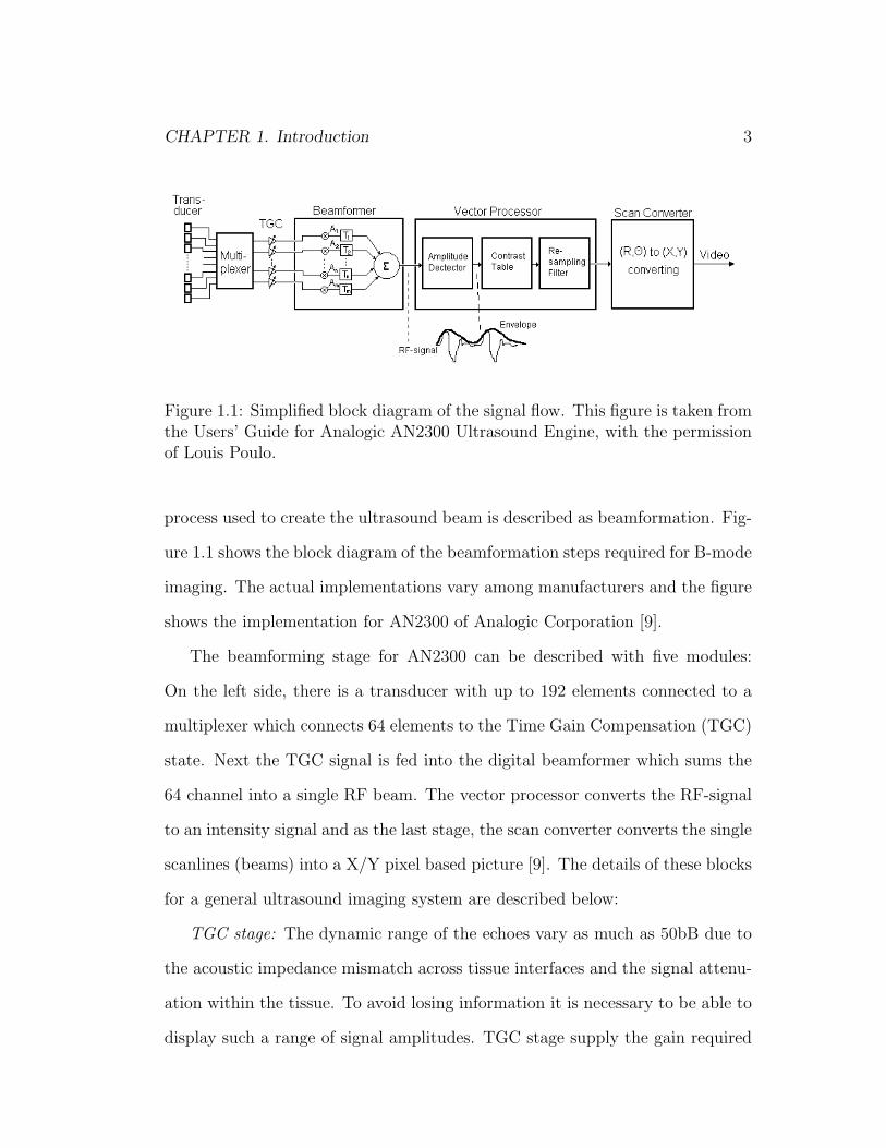
1.1 Simplified block diagram of the signal flow. This figure is taken
from the Users’ Guide for Analogic AN2300 Ultrasound Engine,
with the permission of Louis Poulo. . . . . . . . . . . . . . . . . 3
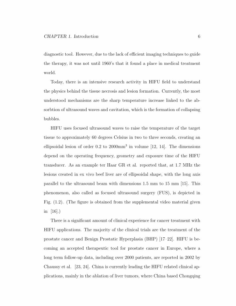
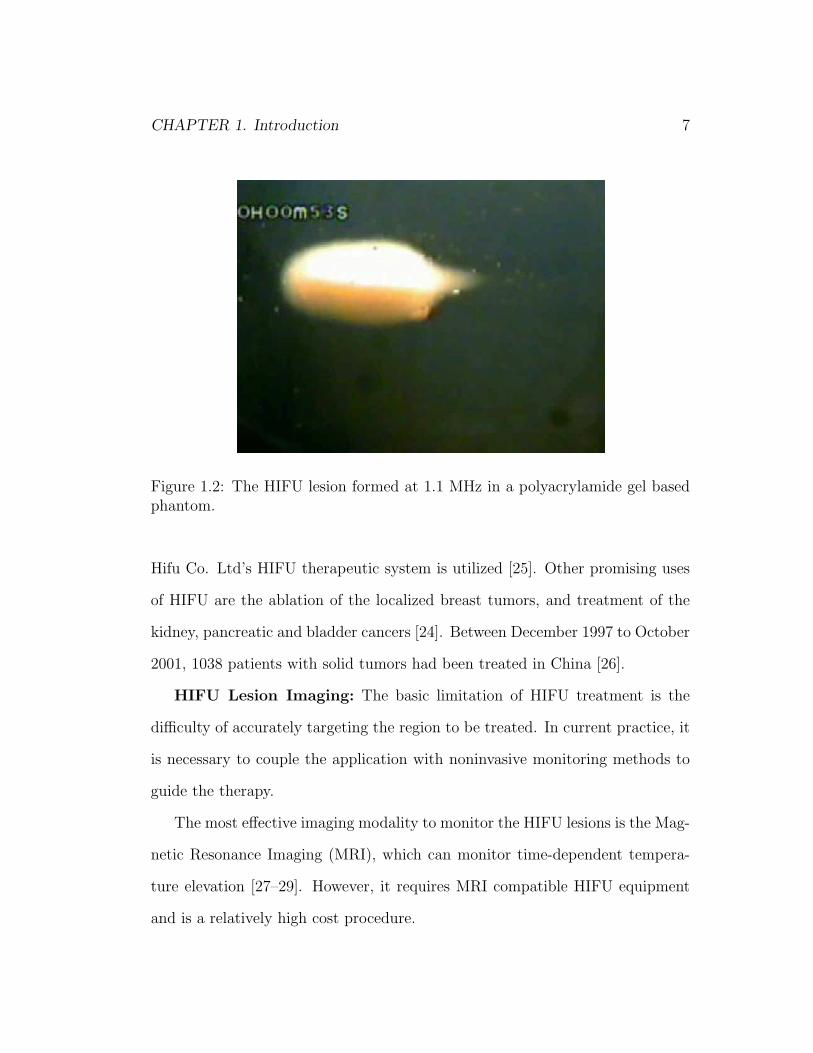
1.2 The HIFU lesion formed at 1.1 MHz in a polyacrylamide gel based
phantom. . . . . . . . . . . . . . . . . . . . . . . . . . . . . . . 7
2.1 Schematic showing the transducer/scatterer arrangement. . . . . 19
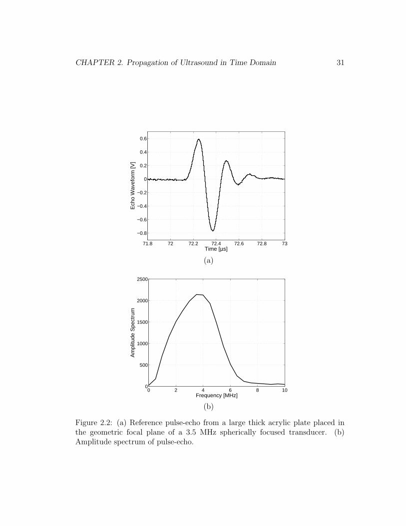
2.2 (a) Reference pulse-echo from a large thick acrylic plate placed
in the geometric focal plane of a 3.5 MHz spherically focused
transducer. (b) Amplitude spectrum of pulse-echo. . . . . . . . 31
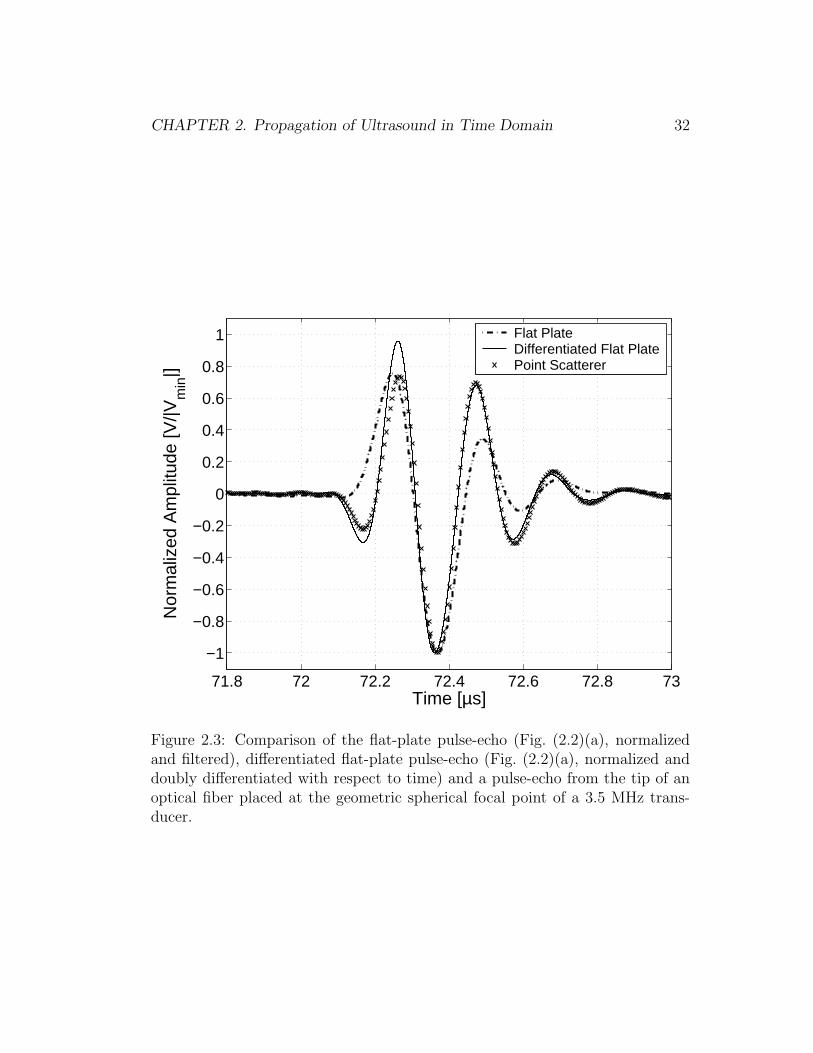
2.3 Comparison of the flat-plate pulse-echo (Fig. (2.2)(a), normalized
and filtered), differentiated flat-plate pulse-echo (Fig. (2.2)(a),
normalized and doubly differentiated with respect to time) and a
pulse-echo from the tip of an optical fiber placed at the geometric
spherical focal point of a 3.5 MHz transducer. . . . . . . . . . . 32
ix

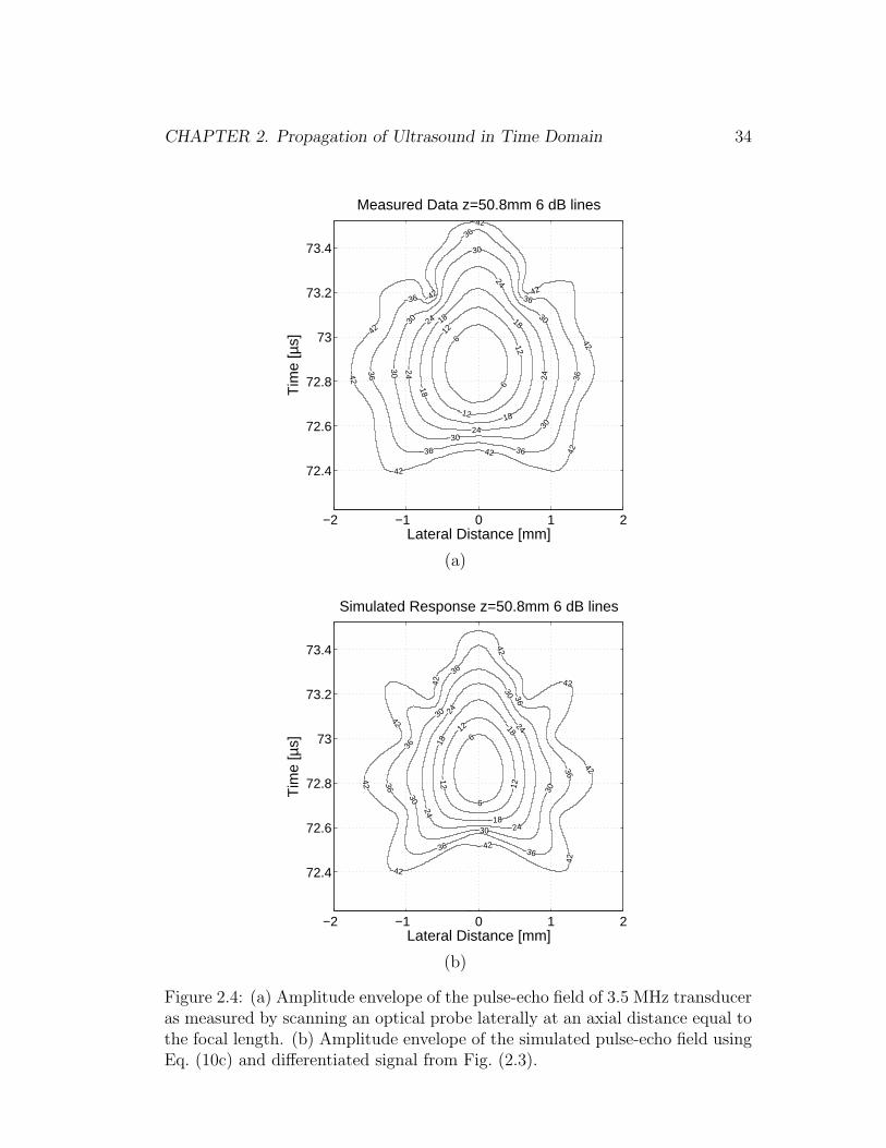
2.4 (a) Amplitude envelope of the pulse-echo field of 3.5 MHz trans-
ducer as measured by scanning an optical probe laterally at an
axial distance equal to the focal length. (b) Amplitude envelope
of the simulated pulse-echo field using Eq. (10c) and differentiated
signal from Fig. (2.3). . . . . . . . . . . . . . . . . . . . . . . . . 34
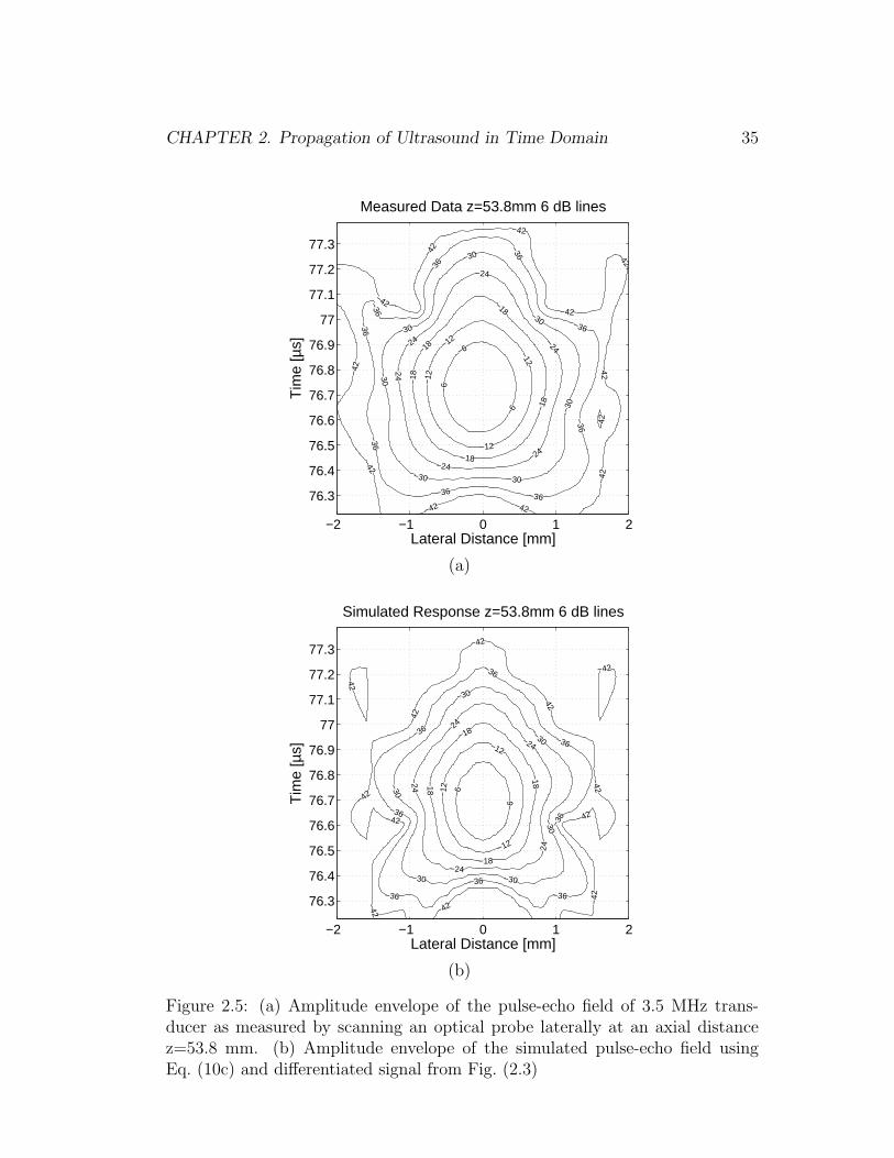
2.5 (a) Amplitude envelope of the pulse-echo field of 3.5 MHz trans-
ducer as measured by scanning an optical probe laterally at an
axial distance z=53.8 mm. (b) Amplitude envelope of the sim-
ulated pulse-echo field using Eq. (10c) and differentiated signal
from Fig. (2.3) . . . . . . . . . . . . . . . . . . . . . . . . . . . 35
3.1 Transmitter, receiver, and the scatterer location vectors. . . . . 49
3.2 Geometry of the problem.(On-axis case) . . . . . . . . . . . . . 52
3.3 Geometry of the problem.(Off-axis case) . . . . . . . . . . . . . 53
3.4 Data acquisition system and the water tank in Boston University. 57
3.5 Experimental setup with the transducers and the phantom. . . . 58
3.6 Predicted and measured waveforms after propagating through a
tissue mimicking phantom . . . . . . . . . . . . . . . . . . . . . 59
3.7 Beam plots of the predicted and measured waveforms. . . . . . . 60
4.1 The geometry of the transducer and the coordinate system. . . . 67
4.2 (a) The oscillations of the real part of the kernel in Eq.(4.5) at 5
MHz for P(0,10 mm,0)(b) The oscillations of the real part of the
kernel in Eq.(4.5) at 5 MHz for P(59 mm,8 mm,0) . . . . . . . . 69
4.3 Schematic showing the segmentation for φp . . . . . . . . . . . 70
4.4 The limit functions with monotonic decreasing φ dependency. . 77
x
4.5 The limiting functions with monotonic increasing φ dependency. 82
4.6 (a)Amplitude envelope of the simulated acoustic field on y axis
using the equations derived in Section 4.3 (b)Amplitude envelope
of the simulated acoustic field on y axis using Eq.(4.55) (c) Am-
plitude envelope of the measured ultrasound field of a 3.5 MHz
transducer. . . . . . . . . . . . . . . . . . . . . . . . . . . . . . 96
4.7 (a)Amplitude envelope of the simulated acoustic field on z axis
using the equations derived in Section 4.3 (b)Amplitude envelope
of the simulated acoustic field on z axis using Eq.(4.55) (c) Am-
plitude envelope of the measured ultrasound field of a 3.5 MHz
transducer. . . . . . . . . . . . . . . . . . . . . . . . . . . . . . 97
4.8 (a)Amplitude envelope of the simulated acoustic field on the x−z
plane using the equations derived in Section 4.3 (b)Amplitude
envelope of the simulated acoustic field on the x− z plane using
Eq.(4.55) (c) Amplitude envelope of the measured ultrasound field
of a 3.5 MHz transducer. . . . . . . . . . . . . . . . . . . . . . . 98
4.9 (a)Amplitude envelope of the simulated acoustic field on the x−y
plane using the equations derived in Section 4.3 (b)Amplitude
envelope of the simulated acoustic field on the x− y plane using
Eq.(4.55) (c) Amplitude envelope of the measured ultrasound field
of a 3.5 MHz transducer. . . . . . . . . . . . . . . . . . . . . . . 100
4.10 (a)Amplitude envelope of the simulated acoustic field on the x−y
plane for lossy medium using the equations derived in Section 4.3
(b)Amplitude envelope of the simulated acoustic field for lossy
medium on the x− y plane using Eq.(4.55) . . . . . . . . . . . . 101
xi

5.1 Decision function A(x) and its derivative . . . . . . . . . . . . . 111
5.2 The expected shapes are drawn with black lines on top of the
approximated ellipsoids. The contrasts of the ellipsoids are shown
with the color scales. As predicted from Fig. (5.1) the contrast
values gradually decay to zero. . . . . . . . . . . . . . . . . . . . 114
5.3 Experimental Setup . . . . . . . . . . . . . . . . . . . . . . . . . 118
5.4 Case 1: Inversion for similarly sized and shaped ellipsoids. . . . 122
5.5 Case 2: Inversion for concentric and overlapping ellipsoids. . . . 123
5.6 Case 3: Inversion for significantly different ellipsoids. . . . . . . 124
5.7 Common initial value for the simulations . . . . . . . . . . . . . 126
5.8 Distribution of volumetric and contrast errors . . . . . . . . . . 127
5.9 Linear array transducer . . . . . . . . . . . . . . . . . . . . . . . 128
5.10 Schematic of the locations of the transducers on the transducer
array . . . . . . . . . . . . . . . . . . . . . . . . . . . . . . . . . 129
5.11 Laboratory Experiment Settings . . . . . . . . . . . . . . . . . . 130
5.12 The real and the enhanced images of the BSA phantom. . . . . 132
5.13 A sample image of the BSA phantom with Analogic Engine ul-
trasound scanner (B-mode pre-scan converted). . . . . . . . . . 133
5.14 The data corresponding to the envelope of the signal from the
64th line of the image. . . . . . . . . . . . . . . . . . . . . . . . 133
5.15 Region of Interest in 3D . . . . . . . . . . . . . . . . . . . . . . 136
5.16 Region of Interest in 2D . . . . . . . . . . . . . . . . . . . . . . 137
5.17 Initial true ellipsoid distribution from different view angles . . . 139
5.18 True ellipsoid distribution from different view angles . . . . . . . 140
5.19 Experimental inversion result . . . . . . . . . . . . . . . . . . . 141
xii

Chapter 1
Introduction
Ultrasound imaging, also known as ultrasound scanning or sonography, is a
widespread noninvasive imaging modality using high frequency sound waves. It
is a low-cost real time diagnostic tool to monitor the abnormalities in the soft
tissues of the human body. With the proper setup of the ultrasound scanner,
the cross-sectional images of the internal organs, such as heart, liver, pancreas,
kidneys, and bladder can be obtained. In the medical area sonography is suc-
cessfully used for diagnostic and therapeutic applications such as: assessment
of fetus health, non-invasive detection and disintegration of kidney stones, and
diagnosis of osteoporosis.
The major advantage of ultrasound compared to the other imaging tech-
niques is the real-time imaging capability. It can show movement of internal
tissues and organs and, combined with the image processing tools, enables physi-
cians to monitor the blood flow in the body [1]. However compared to the other
tomographic techniques such as X-ray Computed Tomography and Magnetic
Resonance Imaging, ultrasound images have poor spatial resolution [1, 2]. Im-
ages are qualitative, do not give information about the physical nature of the
targets and are distorted by spatially varying transducer field. An increasing
1

CHAPTER 1. Introduction 2
number of researchers are working to develop new ultrasound imaging techniques
and transducer types to overcome this problem [1, 3–6].
Conventional diagnostic ultrasound scanners operate in pulse-echo mode
which is similar to the operation of a radar. The imaging process is initiated
when the ultrasound transducer, a piezoelectric element, is excited with a volt-
age spike. The transducer then emits a pressure wave in the form of longitudinal
mechanical vibration [7].
The acoustic wave propagating in the tissue gets reflected at the interfaces
between different acoustic impedances. Some of the reflected wave (echo) returns
to the transducer and is converted to an electrical signal.
The range of the echo signal is determined by the elapsed time, dt, from the
transducer emission to the arrival of the echo by assuming an average velocity
of sound in tissue:
Range = Vtissuedt
2(1.1)
where (Vtissue = 1540m/s) [7].
The strength of the pulse-echo mainly depends on two parameters: The
characteristic acoustic impedance across the interface, which is the product of
the mass density of the medium and the velocity of the ultrasound in that
medium, and the angle of incidence of the pressure wave at the tissue interface [7,
8].
The strength of the received echoes are usually displayed as increased bright-
ness in the display screen which is the B-mode (B for Brightness). The highly
reflecting bone surfaces would appear bright, and fluids that contain no scatter-
ers are dark.
Instrumentation for B-mode Imaging: The transmit and the receive
CHAPTER 1. Introduction 3
Figure 1.1: Simplified block diagram of the signal flow. This figure is taken fromthe Users’ Guide for Analogic AN2300 Ultrasound Engine, with the permissionof Louis Poulo.
process used to create the ultrasound beam is described as beamformation. Fig-
ure 1.1 shows the block diagram of the beamformation steps required for B-mode
imaging. The actual implementations vary among manufacturers and the figure
shows the implementation for AN2300 of Analogic Corporation [9].
The beamforming stage for AN2300 can be described with five modules:
On the left side, there is a transducer with up to 192 elements connected to a
multiplexer which connects 64 elements to the Time Gain Compensation (TGC)
state. Next the TGC signal is fed into the digital beamformer which sums the
64 channel into a single RF beam. The vector processor converts the RF-signal
to an intensity signal and as the last stage, the scan converter converts the single
scanlines (beams) into a X/Y pixel based picture [9]. The details of these blocks
for a general ultrasound imaging system are described below:
TGC stage: The dynamic range of the echoes vary as much as 50bB due to
the acoustic impedance mismatch across tissue interfaces and the signal attenu-
ation within the tissue. To avoid losing information it is necessary to be able to
display such a range of signal amplitudes. TGC stage supply the gain required

CHAPTER 1. Introduction 4
to compensate for these losses caused by the propagation of ultrasound in the
tissue [8].
Beamformer stage: The transmitted and received signals passing from the
array elements can be individually delayed in time. This step is implemented
electronically to steer and focus each of the sequence of acoustic pulses through
the plane or volume to be imaged.
The Huygens principle states that a wavefront can be decomposed into
a number of point sources, each being the center of an expanding spherical
wave [10]. In other words, any wavefront can be constructed from point sources.
This is the principle used to focus and steer the ultrasound beam to the desired
location in space. The signals that are sent to and received from the elements of
the aperture can be given individual time-delays to create the desired wavefront.
The beam steering can be achieved by either element selection or using a
phased array. Element selection is a low cost beam steering approach which
involves steering of the beam by selecting the center element. In this approach
one does not really change the orientation of the beam but rather change the
location of the origin. The beam will shift to a new location as the center of
the active element group is shifted to a new location. The beam steering can be
also be achieved by phased arrays using the appropriate time delays.
Vector Processing: After the beamformer stage, the received signals are
passed through several signal processing stages. The output of the beamformer
stage is a wide band RF signal. The signal is usually filtered to clean the out-
of-band noise contributions. A wide band image processing algorithm can also
be employed to reduce the impact of speckles. An envelope detection is imple-
mented in this stage to obtain the amplitude information [8].

CHAPTER 1. Introduction 5
Scan Converter: The image data is obtained on a polar coordinate grid for
commercial scanners and it is necessary to convert this image to one of the
standard TV image formats for easier viewing and recording. This stage is
known as the Scan Converter. The major function of the Scan conversion is
interpolation from a polar grid to a video pixel region.
As a summary, a typical ultrasound system uses a transducer made up of
a number of piezoelectric elements to transmit a sound pulse into the tissue.
Normally the same transducer is used to receive the reflected sound from the
scatterers within the body. This process is done in a sequential manner, steering
the emitted sound beam in turns along the lines in the region to be imaged.
The use of ultrasound for diagnostic purposes requires a strict limit to be
set on the applied power density (about 0.1 Watt/cm2) [11]. When used with
a higher intensity, a focused ultrasound beam can damage the tissue and create
lesions. Today, this destructive phenomenon is successfully used as a cancer
treatment technique known as High Intensity Focused Ultrasound (HIFU) ther-
apy [12].
High Intensity Focused Ultrasound: The observations on the destructive
ability of the high intensity ultrasound date back to the time of Paul Langevin.
During his tests with quartz plate transducers, he observed the death of small fish
which exposed to the beam of ultrasound. He also reported the pain felt in one’s
hand when immersed in a water tank insonated by high intensity ultrasound [13].
The idea of using ultrasound for therapeutic purposes is not new. The earliest
therapeutic ultrasound experiment on biological tissues was performed by Lynn
and Putnam (1942) where they necrosed brain tissue in animals using ultrasound
waves. This experiment was carried out even before the use of ultrasound as a
CHAPTER 1. Introduction 6
diagnostic tool. However, due to the lack of efficient imaging techniques to guide
the therapy, it was not until 1960’s that it found a place in medical treatment
world.
Today, there is an intensive research activity in HIFU field to understand
the physics behind the tissue necrosis and lesion formation. Currently, the most
understood mechanisms are the sharp temperature increase linked to the ab-
sorbtion of ultrasound waves and cavitation, which is the formation of collapsing
bubbles.
HIFU uses focused ultrasound waves to raise the temperature of the target
tissue to approximately 60 degrees Celsius in two to three seconds, creating an
ellipsoidal lesion of order 0.2 to 2000mm3 in volume [12, 14]. The dimensions
depend on the operating frequency, geometry and exposure time of the HIFU
transducer. As an example ter Haar GR et al. reported that, at 1.7 MHz the
lesions created in ex vivo beef liver are of ellipsoidal shape, with the long axis
parallel to the ultrasound beam with dimensions 1.5 mm to 15 mm [15]. This
phenomenon, also called as focused ultrasound surgery (FUS), is depicted in
Fig. (1.2). (The figure is obtained from the supplemental video material given
in [16].)
There is a significant amount of clinical experience for cancer treatment with
HIFU applications. The majority of the clinical trials are the treatment of the
prostate cancer and Benign Prostatic Hyperplasia (BHP) [17–22]. HIFU is be-
coming an accepted therapeutic tool for prostate cancer in Europe, where a
long term follow-up data, including over 2000 patients, are reported in 2002 by
Chaussy et al. [23, 24]. China is currently leading the HIFU related clinical ap-
plications, mainly in the ablation of liver tumors, where China based Chongqing
CHAPTER 1. Introduction 7
Figure 1.2: The HIFU lesion formed at 1.1 MHz in a polyacrylamide gel basedphantom.
Hifu Co. Ltd’s HIFU therapeutic system is utilized [25]. Other promising uses
of HIFU are the ablation of the localized breast tumors, and treatment of the
kidney, pancreatic and bladder cancers [24]. Between December 1997 to October
2001, 1038 patients with solid tumors had been treated in China [26].
HIFU Lesion Imaging: The basic limitation of HIFU treatment is the
difficulty of accurately targeting the region to be treated. In current practice, it
is necessary to couple the application with noninvasive monitoring methods to
guide the therapy.
The most effective imaging modality to monitor the HIFU lesions is the Mag-
netic Resonance Imaging (MRI), which can monitor time-dependent tempera-
ture elevation [27–29]. However, it requires MRI compatible HIFU equipment
and is a relatively high cost procedure.
CHAPTER 1. Introduction 8
Being inexpensive and commonly used in prostate imaging, B-scan ultra-
sound appears to be a good candidate to replace MRI. However, it has been
experimentally shown that the lesions does not yield a significant change in the
speckle pattern of a standard B-scan gray scale image, while limited informa-
tion can be extracted using data processing techniques [30]. These techniques
are based on signal energy [31], the non-linear properties of the microbubbles in
the lesion [32] and non-linear compounding [33].
Recent studies have shown that HIFU applications increase the stiffness of
the target area -up to ten times than the healthy tissue- making the lesions
detectable by imaging techniques that depict mechanical properties of the tissue
[34–36]. However this approach suffers from a possible non-uniqueness in the
inversion process [37].
We believe the imaging methods aimed to monitor the changes in the sound
speed and attenuation are the most promising modalities to replace MRI. It
has been reported that HIFU treatments affect both the sound speed and the
attenuation values of the tissue while forming lesions [38–43]. The change in
sound speed is less that 20 m/s (about 1%) and peaks at temperatures between
50◦-70◦ and then decreases with the further increase in the temperature. In most
cases the change is reported to be reversible. On the other hand the attenuation
coefficient significantly increases within the values ranging from 80% to 700%
and the change is irreversible [44].
The reversible characteristic of the sound speed makes the methods aimed to
monitor only the change in this parameter rather impractical. Recently Pernot
et al. [45] presented a very impressive in vitro result, where they estimate the
changes in the temperature from the sound speed measurements. However, the

CHAPTER 1. Introduction 9
lesion will not be visible once the tissue cools down.
The change in the attenuation is irreversible, hence the imaging methods
based on capturing the changes in the attenuation are more robust. Since the
attenuation in the necrosed tissue is much higher than that of a healthy tissue,
the tissue behind the HIFU lesion would appear slightly darker in standard B-
scan images. Processing the B-scan data Baker and Bamber [46] and Annad
and Kaczkowski [47] detected the changes in the ultrasound images behind the
lesion.
Although the common ultrasound wave propagation models depend on the
changes in the density of tissue, the link between density and HIFU lesions has
not yet been established.
Imaging methods that give the quantitative information about the changes in
the all three acoustic properties -attenuation, sound speed and density- should
dramatically improve lesion detection.
Inversion Methods: In this dissertation we propose an inversion method to
determine the spatial distribution of the sound speed, attenuation and density
of the HIFU lesions which uses the standard ultrasound scanners and HIFU
transducers.
Processing the data in this manner, reconstructing the acoustic parameters
from ultrasound measurements, is known as an inverse problem. Reconstruc-
tion problems have a wide range of applications in different disciplines including
acoustics. During the last few decades there has been an avalanche of publica-
tions on different aspects of the inverse problems. No attempt will be made to
present a comprehensive bibliography but the reader is referred to [48–53] for
the principal publications in this area.

CHAPTER 1. Introduction 10
The motive behind the presented inversion problem is to develop quantita-
tive, fully three dimensional ultrasonic imaging methods to determine the spatial
structure of the HIFU lesion. The traditional approach to this problem is to try
to reconstruct the voxelated versions of the sound speed, density and absorp-
tion images. What complicates this approach is the nominal wavelength of the
acoustic fields in tissue (0.3mm) coupled with the physical size of the region of
interest of the HIFU lesion (20mm), which implies that up to a one billion voxels
might be needed to describe the problem accurately.
Our approach to the problem is based on the specification of the parameters
describing the shape of the parameters. We assume the shape of the perturba-
tions are known ellipsoids- but the locations, sizes and orientations are unknown.
This method has been addressed in other fields and successfully used in tomo-
graphic imaging problems [54–56]. To completely characterize the changes in
one acoustic variable, we only need the location of the center, the lengths of the
three axes of the ellipsoid, three angles that orient the ellipsoid in space and the
contrast of the parameter. Thus rather than the millions of voxels defining each
of the three unknown acoustic parameters, we have only 3x10=30 quantities to
estimate from the measured data.
Forward Model: Extracting the quantitative information requires the use
of a well calibrated physical model directly within the processing algorithms.
In this study we examine in detail the acoustic wave behavior in human tissue
and present the equations that describe the propagation of ultrasound in a lossy,
dispersive medium.
A key to the implementation of the ultrasound propagation models is the

CHAPTER 1. Introduction 11
specification of the radiated field generated by the commercially available ul-
trasound transducers. Ultrasound measurements coupled with a computational
physical model of the ultrasonic transducer can be used to determine the spatial
maps of the attenuation, sound speed and density. The distribution of these
mechanical properties can be used to complement the images formed with tradi-
tional ultrasound data acquisition techniques that are based on delay and sum
beamforming.
Conventional ultrasound transducers used for medical diagnosis purposes are
generally the 1D array type transducers which consist of rectangular apertures
placed on either a flat or curved surface. Typically 1D arrays with 32 or more
elements that have natural focus in the elevation plane (either by curvature in
the element or by use of a lens) are used with electronic focusing along the lat-
eral dimension. Ideally, each element of the array can be excited individually to
obtain non-beam formed data. This allows us to collect full tomographic data
where single transmitter is used to probe the tissue and the response is mea-
sured by the full array or collection of elements of the array. Moreover, this type
of tomographic imaging would lead to innovative applications where the array
system can be optimized to classify certain targets based on the shape informa-
tion [57, 58]. To utilize the array transducers for applications beyond traditional
beam focusing and steering, it is necessary to have a precise knowledge of the
radiated fields generated by the cylindrically curved transducers. Once this field
is known, it can be applied to simulate the free diffraction field of the linear
arrays.
A number of different methods have been proposed to compute the ultra-
sonic transient fields. The spatial impulse response (SIR) approach provides
CHAPTER 1. Introduction 12
an effective method to predict the sound field of uniformly excited ultrasound
transducers. A through literature review of the applications of this method to
simulate the pressure fields of the arbitrarily shaped transducers is given in [59].
The impulse response of an ultrasound transducer is defined as the response
to a velocity impulse on the radiating surface of the transducer [60–62]. In the
time domain the SIR is convolved with the time derivative of the normal particle
velocity or the electromechanical response of the transducer to obtain the sound
pressure. For frequency domain applications, the simulated field is described
by the Fourier Transform of the spatial impulse response, that is the spatial
transfer function.
The frequency domain representation of the SIR for ultrasonic transducers
is trivial to state and the time domain response can be obtained via inverse
Fourier transform. However, the frequency domain representation of the re-
sponse presents a task that is too computationally demanding to compute in a
straightforward manner. For most of the cases the integral operator does not
have a closed form solution and has a highly oscillatory kernel. On the other
hand, time domain solutions are not sufficient to describe the behavior in tis-
sue like, frequency dependent lossy media. Due to this limitation, in general
frequency domain methods are preferred.
A number of powerful numerical methods are available to predict the spatial
transfer function of the linear arrays for lossless homogenous media. Wu and
Stepinski [59] proposed an efficient time domain method to compute the SIR for
linear arrays with cylindrically concave elements. In their method each element
is divided into a row of narrow strips which can be considered as planar rectangu-
lar transducers whose exact SIRs are available. However, two type of integrals,

CHAPTER 1. Introduction 13
the convolution and the summation over all the thin strips, should be effectively
done for each element. Moreover, their time-domain solution cannot be used to
simulate the behavior of the field in an attenuating medium. Frequency depen-
dent attenuation has a significant impact on ultrasound propagation in human
body and cannot be ignored. A time domain method which has applications
for attenuating media is the method proposed by Piwakowski and Sbai [63]. In
their method, the discrete representation array modelling (DREAM) procedure
is used to calculate the field radiated from arbitrary structured transducer ar-
rays. Their formulation can be applied to predict the acoustic fields in a power
law type attenuating medium. They presented the solution for the case where
the absorption increases linearly as a function of frequency. However to general-
ize this method, the velocity dispersion should be introduced and the relation for
the complex wave number that guarantees a causal solution should be known.
We seek a more flexible frequency domain method which can predict the spa-
tial response of a cylindrically radiator in any physically realizable lossy medium.
As discussed previously the expression for SIR for the frequency domain appli-
cations is difficult to evaluate in stable and efficient manner. The high frequency
content of the oscillatory kernel is typically handled with high sampling rates
which result in an unacceptable computation time.
Our approach to the problem is significantly different from the existing meth-
ods in the sense that we propose an analytical solution to the problem. The
method we propose in this dissertation complements the methods in the lit-
erature such that, with a new rapid integral formulation, the spatial transfer
response for cylindrical radiators for any type of lossy homogenous media is
obtained almost immediately and has a closed form expression. We follow the
CHAPTER 1. Introduction 14
approach of a relevant time domain work of Theumann et al. with the inspira-
tion of Arditi et al. [60, 64]. Theumann et al. worked with concave cylindrical
transducers and reduced the surface integral of the impulse response into a single
integral for which numerical methods are employed to obtain the result. The
philosophy of our approach is similar to that, but we propose an analytical so-
lution to the problem. The line integral kernels are expanded as a truncated
series of Legendre polynomials which could be integrated exactly term by term.
The resulting response is represented as summation of a few number of Bessel
functions.
Although, our main interest lies in the simulating the forward field from
clinically used phased array transducer, our initial efforts were concentrated on
the modeling of the forward field from spherically focused transducer in a lossy
medium [65]. The computations for this case is easier therefore allowed us to
focus on matching the computation model to the experimental data.
Objective of the Study: The aim in this study is to develop three dimen-
sional ultrasonic imaging methods to determine the spatial changes in all three
acoustic properties -attenuation, sound speed and density- of the HIFU lesion.
For this purpose:
• A well calibrated physical model describing the propagation and scattering
of ultrasound in human tissue should be developed. The effect of the
changes in the acoustic properties -sound speed, attenuation and density-
on the acoustic wave behavior should be described with the model.
• The forward model should be validated with experiments using clinically
used ultrasound transducers.
CHAPTER 1. Introduction 15
• Image reconstruction algorithms should be developed to observe the changes
in the sound speed, attenuation and density in HIFU lesions and the al-
gorithm should be tested with experimental measurements.
1.1 Outline of the Thesis
In this work after a short introduction on HIFU and existing lesion imaging
techniques (Chapter 1), a time domain model describing the propagation and
scattering of ultrasound in a homogeneous medium is given (Chapter 2). The
propagation of ultrasound waves in a dispersive, lossy medium is discussed in
Chapter 3 and a compact linear relation between the measured backscatter data
and the medium parameters (sound speed, attenuation and density) is presented.
In Chapter 4 a new method to compute the forward field from cylindrically
concave transducers is discussed. In Chapter 5 the inverse problem (obtaining
the shape of the HIFU lesion from ultrasonic measurements) is introduced and
the reconstructions with simulated and measured backscatter data are presented.
The thesis is concluded in Chapter 6 and the work that remains to be done in
this area is discussed.
Chapter 2
Propagation of Ultrasound in
Time Domain
Pulse-echo ultrasound imaging is a widespread non-invasive imaging modality
using acoustic waves. Although it is safe, widely available, easy to use, portable,
and provides real-time imaging, the resulting images are subjective and relative,
depend on the properties of the transducer used, and distorted by spatially
varying transducer field.
The physical basis for the problem of interest in this chapter is to calculate
the acoustic field scattered by a localized inhomogeneity embedded in a homoge-
neous background. We consider the case of the received signal for a monostatic
pulse-echo configuration although it is straightforward to generalize our results
to bi-static geometries.
In pulse-echo ultrasound imaging a single transducer is used to both trans-
mit an acoustic pulse and receive acoustic echoes. An electromechanical transfer
function is associated with the transducer for both the transmit process (convert-
ing the electrical excitation into an acoustic disturbance) and the receive process
(converting the acoustic disturbance into an electrical signal). To characterize
16
CHAPTER 2. Propagation of Ultrasound in Time Domain 17
the emitted and received acoustic pulse and to accomplish transducer calibra-
tion, the electromechanical response of the transducer must be determined.
In this chapter we present a time domain model which describes the propaga-
tion and scattering of ultrasound in homogeneous medium, under the assumption
of weak scattering. We provide a framework for calibration which consistently
integrates much of the previous literature in this area. We examine in detail the
case of a spherically focused transducer and prove that the electromechanical
response can also be measured by the use of a point target as well as a plate
reflector. We show both theoretically and experimentally that the scattered sig-
nal from a plate and point target are related by double differentiation in time.
In particular, we bring to attention to a possible misinterpretation of data taken
from a flat-plate when applied to scattering from a point target.
The chapter is organized as follows. The following section defines the inho-
mogeneous wave equation and explains the linearity assumptions made to obtain
a solvable equation. It also introduces the concept of calibration and gives the
necessary background to the reader. In Sections 2.2 and 2.3 the scattering of
sound from flat-plates and point targets is discussed. Section 2.4 combines the
ideas introduced in the previous sections and discusses the scattering of sound
in the framework of calibration and underlies the overlook in the literature. The
comparison of predicted and measured pressure fields are given in Section 2.5.
The chapter is concluded in Section 2.6.
2.1 Theory and Background
In this section we discuss the theory of scattering of sound and the relation be-
tween the electromechanical impulse response of a transducer and the measured

CHAPTER 2. Propagation of Ultrasound in Time Domain 18
back scattered signal from specific obstacles.
In his cited work Jensen [66] provided a computationally compact and useful
method for simulating the scattered field from arbitrary shaped weak scatterers.
For completeness of the dissertation the formulas and derivations in [66] will be
summarized here.
2.1.1 Jensen’s Formulation
Let V ′ be an inhomogeneity embedded in a homogeneous fluid medium of con-
stant sound speed co and density ρo. The linear wave equation for acoustic
pressure p(r, t) in time domain can be defined as [67]:
∇2p(r, t)− 1
c2o
∂2p(r, t)
∂t2=−24c(r)
c3o
∂2p(r, t)
∂t2+(
1
ρo
∇(4ρ(r))−4ρ(r)
ρ2o
∇(4ρ))·∇p(r, t)
(2.1)
where
• p is the acoustic pressure and depends on space, r, and time, t.
• 4c and 4ρ are the space dependent perturbations from the mean values
co and ρo :
ρ(r) = ρo +4ρ(r)
c(r) = co +4c(r)
The terms on the right hand side of Eq.(2.1) are the scattering terms (scat-
tering function) that vanish for a homogeneous medium. The scattered field is
calculated by integrating all the spherical waves emanating from the scattering
region V ′ using the time dependent Green’s function for unbounded space. Us-
ing r and r′ for source and scatterer (observation point) coordinates (Fig. (2.1))

CHAPTER 2. Propagation of Ultrasound in Time Domain 19
Figure 2.1: Schematic showing the transducer/scatterer arrangement.
and ignoring the second order term in the scattering function the scattered field
can be calculated as [68]:
ps(r, t) =
∫
V ′
∫
T
[−24c(r′)
c3o
∂2p(r′, t′)∂t2
]G(r, r′, t, t′) dt′ d3r′
+
∫
V ′
∫
T
[1
ρo
∇(4ρ(r′, t′)) · ∇ p(r′, t′)︸ ︷︷ ︸ps(r,t′)+pi(r,t′)
]G(r, r′, t, t′) dt′ d3r′(2.2)
where G(r, r′, t, t′) is the Green’s function for the Helmholtz equation in a ho-
mogeneous medium. In an unbounded three dimensional medium G(r, r′, t, t′)
is given by
G(r, r′, t, t′) =δ(t− t′ − |r − r′|/co)
4π|r − r′| (2.3)
The pressure field inside the scattering region V ′ can be defined as p(r, t′) =
ps(r, t′) + pi(r, t
′) where pi(r, t′) is the incident pressure field.
At first glance it might appear as if Eq.(2.2) is the solution we seek for the
scattered field, but we have written the integral equation for ps in terms of the
unknown total field. Eq.(2.2) is the Fredholm integral of the second kind and

CHAPTER 2. Propagation of Ultrasound in Time Domain 20
cannot be solved directly. The use of numerical methods, such as Finite Element
Method or Method of Moments are required to obtain a solution. To simplify the
equation, Born-Neumann approximation of the first kind is invoked. The con-
trast of the scatterer is assumed to be weak, and total field inside the scattering
region is approximated with the incident field [68, 69], p(r, t′) ∼= pi(r, t′).
Using the definition of the incident field and the spatial impulse response of
the transducer given in [60] and applying Born-Neumann expansion of the first
kind, Jensen [66] showed that it is possible to write Eq.(2.2) in a closed form
expression.
ps(r, t) = vpe(t) ∗t
∫
V ′fm(r′)× hpe(r, r
′, t)d3r′ (2.4)
where
vpe(t) =ρo
2Em(t) ∗t
∂v(t)
∂t
fm(r′) =∆ρ(r′)
ρo
− 2∆c(r′)co
hpe(r, r′, t) =
1
c2o
∂2Hpe(r, r′, t)
∂t2
Here vpe is the pulse echo wavelet which includes the transducer excitation and
the electromechanical impulse response, Em(t), during transmission and recep-
tion of the pulse; fm is the scattering function and stands for the inhomogeneities
in the medium; and hpe is the modified pulse echo impulse response that relates
the transducer geometry to the spatial length of the scattered field. Hpe is the
pulse-echo spatial impulse response obtained by Hpe = h(r, r′, t) ∗r′ h(r′, r, t).
Here h is the impulse response of the transducer which is calculated according
to [60]. The reader is referred to [66] for the full derivation of Eq.(2.4).
In case of a point scatterer fm is a Dirac impulse and Eq.(2.4) reduces to:
CHAPTER 2. Propagation of Ultrasound in Time Domain 21
ps(r, t) =1
c2o
∂2vpe(t)
∂t2∗r′ h(r, r′, t) ∗r′ h(r, r′, t) (2.5)
To characterize the scattered field the pulse echo vpe should be accurately
determined. In the next section the details of the calibration process, obtaining
the vpe signal, is explained.
2.1.2 Calibration Process: Obtaining the vpe signal
The common practice to calibrate a transducer is to place a large flat-plate in
the focal plane of a focusing transducer ([70–72]). A waveform measured under
these conditions, can, in principle, be used to aid in the removal or compensation
of transducer response and field effects on the measurement of tissue properties
([70–73]).
Following the notation in ([66]) the model for the scattering process, Eq.(2.2),
can also be summarized by the following equation:
υo(t) = υi(t) ∗t eT (t) ∗t hT (r, t) ∗t s(r, t) ∗t hR(r, t) ∗t eR(t) (2.6)
where υi(t) is the excitation voltage, eT (t) is the electromechanical response
that is the ratio of the derivative of the normal particle velocity with respect
to time relative to the transmit voltage, hT (r, t) is the transmit spatial impulse
response, hR(r, t) is the receive spatial impulse response of the transducer located
at position vector r, s(r, t) is a scattering term located at r which accounts for
perturbations or inhomogeneities in the medium that give rise to the scattered
signal, v0(t) is the output voltage from the transducer, eR(t) is the receive voltage
to force electromechanical response, and ∗t is convolution with respect to time.
CHAPTER 2. Propagation of Ultrasound in Time Domain 22
We define the round-trip pulse-echo electromechanical impulse response of
the transducer, epe(t) as:
epe(t) = υi(t) ∗t eT (t) ∗t eR(t) (2.7)
For the case where υi(t) is a very short electrical impulse (e.g., less than about
1/10th of the characteristic period of the transducer) epe will be proportional to
eT ∗t eR which is the true electromechanical impulse response of the transducer.
Equation (2.6) can now be written as
υo(t) = epe(t) ∗t hT (r, t) ∗t s(r, t) ∗t hR(r, t) (2.8)
where the remaining terms account for propagation and scattering. If one as-
sumes that the absorption of the medium (e.g. de-ionized and de-gassed water
in the low megahertz frequencies) is negligible then analytical expressions exist
for hT and hR for a spherically focused transducer ([60, 74]). The scattering
term s(r, t) depends on the target.
In this study we will discuss scattering from three different obstacles: a flat-
plate, a point target and an arbitrary shaped weak scatterer. The first two
cases will be presented for calibration and the third for imaging applications
that require such calibration.
2.2 Scattering from a flat-plate
In this section, we discuss the conditions under which the focal plane reflec-
tion from a flat-plate is a valid approximation of the electromechanical impulse

CHAPTER 2. Propagation of Ultrasound in Time Domain 23
response.
When the flat-plate is an ideal acoustic mirror, and placed at a distance
z from the transmitter, perpendicular to the beam axis, the receiver can be
considered as the mirror image of the transducer. Hence in pulse-echo imaging
of an acoustic mirror, the problem is the same as that of two identical transducers
separated by a distance 2z, as shown by Rhyne (1977), and Chen et al. (1994)
for both nonfocusing and focusing transducers.
In 1977 Rhyne derived a “radiation coupling” function for nonfocusing trans-
ducers where he calculated the reflection from a flat-plate. This result is the same
as the problem of finding diffraction loss, DF , between two identical transducers
at a distance 2z ([75, 76]). In both cases, this loss represents the reduction in
amplitude and change in phase when only a portion of a transmitted beam is
intercepted by a receiving transducer.
For a focusing aperture, Chen et al.([77]) showed that for the mirror placed
in the focal plane, the diffraction loss in the frequency domain is equal to
DF (z = 2F, f) = −{1− exp(jGp)[J0(Gp)− jJ1(Gp)]} (2.9a)
where the pressure focal gain is
Gp =πfa2
coF(2.9b)
in which f is frequency, co is the speed of sound in water, a is the aperture
radius, and F is the focal length. Chen et al. ([71]) found that this expression
has only a weak dependency of frequency. If the argument parameter Gp is large,
an asymptotic expression for Bessel functions of large arguments (Eq. 9.2.1 of
CHAPTER 2. Propagation of Ultrasound in Time Domain 24
[78]), can be used to approximate Eq.(2.9a) by
DF (z = 2F, f) ≈ −{1−√
2
πGp
exp
(jπ
4
)} = −{1− 1√
πGp
− j√πGp
} (2.10)
When Gp ≥ 16 the error of either the real or imaginary part of Eq.(2.10) com-
pared to Eq.(2.9a) is less than 0.042. Because the terms involving the square
root are small, the main contribution comes from the real part of Eq.(2.10). Both
Eq.(2.9a) and Eq.(2.10) vary extremely slowly with frequency over a transducer
bandwidth (e.g. 90% fractional bandwidth), so to a good approximation, the
frequency can be set equal to transducer center frequency, f = fc. Physically
the result of this small loss can be interpreted in terms of ray theory as a cone of
energy focused onto a plate and reflected back, almost but not quite perfectly,
along the same cone to the aperture of the transducer.
To use the transfer function defined in Eq.(2.10) in Eq.(2.7), we must account
for propagation delays to and from the plate and for the case where the plate
is not an ideal reflector. Then we can carry out an inverse Fourier transform
to obtain the time domain response. Given that a non-ideal mirror has a plane
wave pressure reflection coefficient,
RF =Z2 − Z1
Z2 + Z1
(2.11)
where Z2 is the specific acoustic impedance of the reflector and Z1, the char-
acteristic impedance of the fluid, then the three rightmost terms of Eq.(2.8)
CHAPTER 2. Propagation of Ultrasound in Time Domain 25
correspond to the following inverse Fourier transform:
hT (r, t) ∗t s(r, t) ∗t hR(r, t) = Real{=−1[DF (r, fc)RF exp (−j2πf(2F )/co) ]}
= RF [√
1/(πGp)− 1]δ(t− t2F ) (2.12)
From Eq.(2.12) we can see that the acoustic propagation and scattering from
plate at the focus of a transducer (that is, hT (r, t) ∗t s(r, t) ∗t hR(r, t)) is a scaled
impulse response delayed in time by t2F = 2F/co . Under these conditions, the
output voltage is an amplitude scaled delayed replica of the system response epe,
υo(t) ≈ RF [√
1/(πGp)− 1]epe(t− 2F/co) (2.13)
The round trip reference signal epe can be determined from the measured output
voltage signal, υo(t), and the scaling constant from Eq.(2.13).
2.3 Scattering from a point target
Often it is necessary to determine scattering from an ideal point scatterer rather
than a flat-plate. As an example, determining the spatial impulse response
(hT and hR) experimentally requires the use of a point scatterer. Moreover,
randomly positioned point scatterers form the basis of simulation models for
speckle and phantom-like objects that can be created from organized patterns
of point scatterers with assigned weighting [79]. In this section, we show how the
reflection from a point scatterer can be determined from a flat-plate response.
The starting point for a model of an ideal point scatterer is that of a rigid
(incompressible) sphere with a diameter much smaller than a wavelength, density

CHAPTER 2. Propagation of Ultrasound in Time Domain 26
ρ À ρo, and compressibility κ ¿ κo, where c = 1/√
ρκ and co = 1/√
ρoκo.
The scattering for this sphere known to be proportional to −k2 ([10]), where
k = ω/co, and a geometrical factor A. Since the inverse Fourier transform
theory of jω is ∂/∂t, −k2 corresponds to the transform (1/c2o)∂
2/∂t2. For this
type of target at the origin,
s(r, t) =A
c2o
∂2
∂t2∗t δ(t− |r|/co) (2.14a)
where A is a time-independent quantity that is given by (Eq.8.2.19, [10])
A =a3
3(1− 3
2cosθ) (2.14b)
where a is the radius of the scatterer and θ is the scattering angle. For direct
backscatter θ = π and A has the value
A =5a3
6. (2.14c)
Real transducers have a finite aperture and collect signals over a range of angles,
however, for 160 < θ < 200, which is appropriate for most ultrasound imaging
scenarios, the variation in A over the surface of the transducer is less than 5% and
the use of Eq.(2.14c) is appropriate. If this target is placed at the focal point,
then each of the spatial impulse responses in Eq.(2.6) reduces to an impulse
function centered at |r|/co [74],
hT (r, t) = hR(r, t) = `δ(t− |r|/co) (2.15a)

CHAPTER 2. Propagation of Ultrasound in Time Domain 27
where ([60], Eq. 7)
` = F
[1−
(1− a2
F 2
)1/2]
(2.15b)
Putting these results into Eq.(2.6) for a small spherical target at the focal point,
we find
υo(t) =A`2
c2o
∂2epe(t− 2|r|/co)
∂t2(2.15c)
therefore, the reflected signal from a point target will have the same shape as
the doubly differentiated reference waveform, epe(t) with the respect to time.
Although we derived this in terms of a rigid sphere target we note that other
targets smaller than a wavelength have a similar functional dependency in the
backscattered direction (θ = π) towards the transducer at distances greater than
a few wavelengths ([80, 81]). In particular, Nassiri and Hill [82] have shown that
back scatter from a disc is similar to that of a sphere, differing only in the
constant A. Both the sub-wavelength sphere and disc are practical realizations
of an ideal point target as viewed at moderate to large distances. Because of
the practical difficulties involved in realizing a point target, it may be difficult
to determine the constant A. An alternative approach to calibration described
by Hunt et al. [74] is to redefine the electromechanical response based on a
point target. Their electromechanical response would be the equivalent of epe
convolved with s for a point target from Eq.(2.6) and would include a double
differentiation with time. However, if A is not known it is not possible to apply
the calibration to the problem of quantitative imaging.

CHAPTER 2. Propagation of Ultrasound in Time Domain 28
2.4 Scattering from arbitrary shaped weak scat-
terers: Born Approximation
In the previous two sections we showed that the electromechanical impulse re-
sponse of a transducer can be measured using either a plate or a point target.
Once this reference signal is known, it can be applied to simulate the backscat-
tered field from arbitrary shaped targets through the Born approximation ([66]).
Equation 2.4(Equation (44) of ([66]) can be rearranged according to Eq.(2.7):
υo(r, t) = epe(t) ∗t [s(r′) ∗r∂2Hpe(r
′, r, t)∂t2
] (2.16)
in which r is the vector to a characteristic position of the transducer and r′
represents a vector to a point within the scatterer (Fig. (2.1)) and, as defined
by Jensen ([66]),
Hpe(r′, r, t) = h(r′, r, t) ∗t h(r, r′, t) (2.17)
is equivalent to hT ∗t hR in our Eq. (1). More explicitly, Eq.(2.16) is
υo(r, t) = epe(t) ∗t
[∫
V ′
[4ρ(r′)ρo
− 24c(r′)co
]1
c2o
∂2Hpe(r′, r, t)
∂t2d3r′
]
=1
c2o
∂2epe(t)
∂t2∗t
[∫
V ′
[4ρ(r′)ρo
− 24c(r′)co
]Hpe(r
′, r, t)d3r′](2.18)
where 4ρ and 4c are the perturbations in density and sound speed with respect
to background and V ′ is the scattering region.
In the case of a point scatterer Eq.(2.18) reduces to:
υo(r, t) =
[4ρ(r′)ρo
− 24c(r′)co
]1
c2o
∂2epe(t)
∂t2∗t h(r′, r, t) ∗t h(r, r′, t) (2.19)
CHAPTER 2. Propagation of Ultrasound in Time Domain 29
which is consistent with Eq.(2.5) (Jensen’s Eq. (50)). Specifically in the case
of a point scatterer placed at the focal point Eq.(2.19) reduces to the form of
Eq.(2.15c). This observation reveals a potential area of confusion with respect
to the results in [66], in which Eq.(2.19) is taken to be the response to a flat-plate
at the focal plane. More correctly, as indicated by the results in the previous
two sections of this paper, this flat-plate response is obtained by removing the
double time derivative.
In this work the overall outcome of the Born approximation derived by Jensen
([66]) is unchanged. However, we have used the twice time derivative of the plate
response in our simulations. The method of finding epe(t) described in Sections
2.2 and 2.3 can be applied directly to the more general case of scattering through
the Born approximation as given by Eq.(2.18).
2.5 Experiments
We carried out experiments to verify the fact that the scattered signal from
a plate and a small scatterer are related by double differentiation in time.
We used a spherically focused ultrasonic transducer, 3.5 MHz, 50.8 mm fo-
cal length, 12.8 mm radius (Model V380, Panameterics, Waltham, MA). This
strongly focusing transducer (F number 2 and Gp=24) was placed in a water
tank (0.8 m x 0.8 m x 1.5 m) that was filled with de-ionized de-gassed water at
approximately 21◦C. The transducer was operated in pulse-echo mode using a
pulse-receiver (UA 5052, Panametrics, Waltham, MA). The pulser-receiver ex-
cited the transducer with a short excitation signal that approximated a delta
function and the received echo was acquired on digital scope (LC 334a, LeCroy,

CHAPTER 2. Propagation of Ultrasound in Time Domain 30
Chestnut Ridge, NY) and transferred to a computer for later analysis. We in-
vestigated the reflections from two targets. The first was a 12.5 mm thick flat
acrylic plate acoustic mirror. The second target was from the cleaved end of an
optical fiber 110 microns in diameter point scatterer. Figure 2.2(a) shows the
reflected pulse measured from the front surface of the acrylic plate, υo(t). This
is the scaled pulse-echo impulse response, epe(t), according to Eq.(2.12). Here
Gp=24, so the diffraction correction factor is 0.885 and the reflection coefficient
at the water-acrylic interface is RF =0.348. Figure 2.3 compares three normal-
ized waveforms 1) the signal measured from the plate 2) the signal measured
from the optical fiber and 3) the doubly differentiated epe waveform obtained
from Eq.(2.8) (note this equation gives a sign inversion). We see that carrying
out the double-differentiation is crucial to obtaining good agreement between
predictions based on the impulse response of the transducer (epe) and the re-
ceived signal from a point scatterer. Without this operation neither the leading
negative half-cycle nor the details of the ringdown are captured correctly. This
result shows that the time-domain calibration function that is determined from
a flat-plate can be used to predict the waveform from a point scatterer at the
focus. Once this reference signal is known, it can be applied to simulate the
free diffraction field of the transducer or backscattering from other scattering
targets. We used Eq.(2.6) with the point scatterer characteristic, Eq.(2.13), and
the round trip spatial impulse response (Arditi et al.,1981) with 2 GHz sam-
pling frequency in time, to simulate the echoes scattered from a small point-like
target. To confirm our predictions, the optical fiber was mechanically scanned
through the tank and echo waveforms recorded at each location. Figure 2.4
shows the measured and predicted contour maps of the amplitude envelope of
CHAPTER 2. Propagation of Ultrasound in Time Domain 31
71.8 72 72.2 72.4 72.6 72.8 73
−0.8
−0.6
−0.4
−0.2
0
0.2
0.4
0.6E
cho
Wav
efor
m [V
]
Time [µs]
(a)
0 2 4 6 8 100
500
1000
1500
2000
2500
Am
plitu
de S
pect
rum
Frequency [MHz]
(b)
Figure 2.2: (a) Reference pulse-echo from a large thick acrylic plate placed inthe geometric focal plane of a 3.5 MHz spherically focused transducer. (b)Amplitude spectrum of pulse-echo.
CHAPTER 2. Propagation of Ultrasound in Time Domain 32
71.8 72 72.2 72.4 72.6 72.8 73
−1
−0.8
−0.6
−0.4
−0.2
0
0.2
0.4
0.6
0.8
1
Nor
mal
ized
Am
plitu
de [V
/|Vm
in|]
Time [µs]
Flat PlateDifferentiated Flat PlatePoint Scatterer
Figure 2.3: Comparison of the flat-plate pulse-echo (Fig. (2.2)(a), normalizedand filtered), differentiated flat-plate pulse-echo (Fig. (2.2)(a), normalized anddoubly differentiated with respect to time) and a pulse-echo from the tip of anoptical fiber placed at the geometric spherical focal point of a 3.5 MHz trans-ducer.

CHAPTER 2. Propagation of Ultrasound in Time Domain 33
the scattered fields for the case where the fiber was placed in the focal plane and
translated perpendicular to the acoustic beam axis. Figure 2.5 is a similar scan
but at an axial distance of 53.8 mm (about 3 mm or 10 wavelengths behind of
the focus). In both cases, there is a close agreement between the measured and
predicted scattered field. The slight differences are attributable to imperfections
in both the transducer as an ideal piston source, as determined by extensive hy-
drophone measurements, and the cleaved optical fiber as an isolated ideal point
target. The source transducer was found to have a mildly distorted, asymmetric
transmitted field when compared to simulations based on an ideal uniformly
weighted piston source. Pulse-echo simulations based on the point target wave-
form at the focal point gave slightly better agreement with measurements than
those shown here; however, we believe this result to be a consequence of the
imperfect realization of an ideal spherical scatterer by the cleaved optical fiber
which had it own unique response characteristic, as shown in Fig. (2.3). These
comparisons confirm that the plate-derived calibration waveform can be used to
predict the response of a scatterer anywhere in the field of the transducer.
2.6 Conclusion
We have shown, both theoretically and experimentally, that the pulse-echo im-
pulse response of a spherically focused transducer can be measured using either
a flat-plate or a point scatterer. The reflected waveforms in each case are not
identical but rather related by an operation of double differentiation. Because
of the difficulty of determining the precise geometry of practical realizations of
sub-wavelength point targets and, consequently, the calibration constant A, a
reflection from a flat-plate is recommended for determination of the reference
CHAPTER 2. Propagation of Ultrasound in Time Domain 34
−2 −1 0 1 2
72.4
72.6
72.8
73
73.2
73.4
Lateral Distance [mm]
Tim
e [µ
s]
Measured Data z=50.8mm 6 dB lines
−6
−6
−12
−12
−12
−18 −18
−18
−18
−24
−24
−24
−24
−24
−30
−30
−30
−30
−30
−30
−36
−36
−36
−36
−36−36
−36
−42
−42
−42
−42
−42
−42−42
−42
−42
(a)
−2 −1 0 1 2
72.4
72.6
72.8
73
73.2
73.4
Lateral Distance [mm]
Tim
e [µ
s]
Simulated Response z=50.8mm 6 dB lines
−6
−6
−12
−12
−12
−18
−18
−18
−24
−24
−24
−24
−30
−30
−30
−30
−30
−36
−36
−36
−36
−36−36
−36−42
−42
−42
−42
−42
−42
−42
−42
−42
(b)
Figure 2.4: (a) Amplitude envelope of the pulse-echo field of 3.5 MHz transduceras measured by scanning an optical probe laterally at an axial distance equal tothe focal length. (b) Amplitude envelope of the simulated pulse-echo field usingEq. (10c) and differentiated signal from Fig. (2.3).
CHAPTER 2. Propagation of Ultrasound in Time Domain 35
−2 −1 0 1 2
76.3
76.4
76.5
76.6
76.7
76.8
76.9
77
77.1
77.2
77.3
Lateral Distance [mm]
Tim
e [µ
s]
Measured Data z=53.8mm 6 dB lines
−6
−6
−6
−12
−12
−12
−12
−18
−18
−18
−18
−18
−24
−24
−24
−24
−24
−24
−30
−30
−30
−30
−30−30
−30−36
−36
−36
−36
−36
−36−36
−36
−36−42
−42
−42 −42
−42
−42
−42
−42
−42
−42
−42
−42
(a)
−2 −1 0 1 2
76.3
76.4
76.5
76.6
76.7
76.8
76.9
77
77.1
77.2
77.3
Lateral Distance [mm]
Tim
e [µ
s]
Simulated Response z=53.8mm 6 dB lines
−6
−6
−12
−12
−12
−18
−18
−18
−18
−24
−24
−24
−24
−24
−30
−30
−30
−30−30
−30
−36
−36
−36
−36
−36
−36
−36
−36
−42
−42
−42
−42
−42
−42
−42
−42
−42
−42
−42
−42
(b)
Figure 2.5: (a) Amplitude envelope of the pulse-echo field of 3.5 MHz trans-ducer as measured by scanning an optical probe laterally at an axial distancez=53.8 mm. (b) Amplitude envelope of the simulated pulse-echo field usingEq. (10c) and differentiated signal from Fig. (2.3)

CHAPTER 2. Propagation of Ultrasound in Time Domain 36
pulse. For values of focal gain greater than or equal to 16, the error in the
approximation (Eq.(2.10)), is less than five percent.
The formulation in Eq.(2.6) and the relation between the flat-plate and point
target echoes can be used to resolve differences among various calibration meth-
ods in the literature ([66, 70, 71, 74, 83, 84]) each of which can be used self-
consistently but may be in conflict with other methods. For example, Hunt et
al. [74] obtained a reference waveform from a point scatterer but their formula-
tion for the scatterer does not include the double differentiation of Eq.(2.15c).
Their waveform is used consistently to simulate speckle as a summation of ran-
dom point scatterers.
The time domain Born approximation of Jensen ([66]) in Eq.(2.18) includes
the double differentiation and shows that the echo signal from an inhomogeneous
medium can be obtained by convolving the point-scattered waveform with the
medium properties in agreement with Eq.’s (2.6) and (2.14a). If one wishes to
use the signal measured from a flat-plate for this Born model, it is necessary to
differentiate the reference signal twice with respect to time first. The wording
in Jensen ([66]) could be misinterpreted to mean that the flat-plate signal was
already differentiated.
In summary, the commonly used reference waveform from a flat-plate target
in the focal plane of a strongly focusing transducer (Gp ≥16) is appropriate to
determine epe(t) without distortion. This reference signal is useful for transducer
calibration and diffraction correction ([71, 72, 85, 86]). However, the waveform
must be used with care for other scattering targets.
In the next chapter the ideas that have been developed in this section will
be applied to the frequency domain.

Chapter 3
Propagation of Ultrasound in the
Frequency Domain
Propagation of ultrasound can accurately be predicted for a non-attenuating
medium e.g. water by using the methods derived in the previous chapter. In
Chapter 2 we presented a time domain model which describes the propagation
and scattering of ultrasound in a homogeneous medium. However, the behavior
of the field cannot be characterized for a lossy, attenuating medium.
Since the human tissue shows a dispersive ultrasound absorbtion, the fre-
quency dependent attenuation plays a prominent role in ultrasound imaging
applications. For most materials including biological tissues, the frequency de-
pendency of attenuation is characterized by a power-law relation: α(ω) = αo|ω|y,where αo and y (0 < n < 2) are the material-dependent parameters. For quanti-
tative ultrasound imaging, it is important to understand how the pressure field
behaves in such media. The apparent approach would be to carry the time do-
main models of Chapter 2 to the frequency domain and provide a mathematical
derivation of the acoustic Born model for a power law attenuating medium.
In this chapter, we first study the propagation of ultrasound waves in a
37
CHAPTER 3. Propagation of Ultrasound in the Frequency Domain 38
homogeneous, lossy medium. Next, we use the derived theory to obtain solutions
in the presence of weak inhomogeneities via Born approximation. We present a
compact linear relation between the measured backscatter data and the medium
parameters (sound speed, attenuation and density). We validate the proposed
model with experimental data.
This chapter is organized as follows. The first section defines the inhomo-
geneous wave equation in frequency domain, characterizes the background and
the scattering wave numbers and introduces the assumptions to obtain a linear
solvable equation. Section 3.2 presents the derivation of the incident field for
commercial spherical ultrasound transducers. Section 3.3 discusses the calcula-
tion of the measured backscatter signal in frequency domain and introduces a
compact relation between the medium parameters and the measured field. In
section 3.4 the spatial transfer function for spherically focused transducers is
formulated and a fast semi-analytical method is introduced to calculate the re-
sponse. The comparison of predicted and measured pressure fields for spherical
transducers is given in Section 3.5. The chapter is concluded in Section 3.6.
3.1 Derivation of the Scattered Field
In this section we introduce the linear time and frequency domain wave equations
which describes the propagation of ultrasound in a homogeneous medium. We
start with the equations derived in the previous chapter and extend them for
lossy, power law attenuating media.
The time domain equations derived in the previous chapter fails to charac-
terize the behavior of the acoustic field in a lossy, attenuating medium. Hence,
we derive the scattered field from an acoustic inhomogeneity of density, sound

CHAPTER 3. Propagation of Ultrasound in the Frequency Domain 39
speed and attenuation for a lossy medium and give brief details of the assump-
tions made to linearize the scattering problem.
3.1.1 Acoustic Wave Equation
For a fluid medium with space dependent sound speed and density, the linear
wave equation is defined as [81],(page 432):
∇ · ( 1
ρ(r)∇p(r, t))− 1
ρ(r)c(r)2
∂2p(r, t)
∂t2= 0 (3.1)
where r is a point in 3-space and t is the time variable. p(r, t) is the pressure
at r and t, ρ(r) is the density and c(r) is the speed of sound. After algebraic
manipulations this equation can be written as:
∇2p(r, t)−∇p(r, t) · ∇ ln ρ(r)− 1
c(r)2
∂2p(r, t)
∂t2= 0 (3.2)
The frequency domain wave equation is obtained by taking the Fourier trans-
form of the field with respect to the time at each position r. In this study the
representation form of the time harmonic relations is chosen as ejωt. Specifically
the instantaneous fields are related to their complex time harmonic forms by
p(r, t) = Re[p(r)ejωt]. With this definition the linear wave equation in frequency
domain is defined as:
∇2p(r, ω)−∇ ln ρ(r) · ∇p(r, ω) + k2(r, ω)p(r, ω) = 0 (3.3)
where ω is the angular frequency, p(r, ω) is the pressure at r and ω and k2(r, ω)
is the squared wavenumber at frequency ω and location r.
CHAPTER 3. Propagation of Ultrasound in the Frequency Domain 40
For a source distribution q(r, ω) located at r with frequency ω, the right hand
side of Eq.(3.3) is replaced by q(r, ω):
∇2p(r, ω)−∇ ln ρ(r) · ∇p(r, ω) + k2(r, ω)p(r, ω) = q(r, ω) (3.4)
3.1.2 A Model for k2
A key issue to model the wave behavior in frequency domain is the specification
of k2(r, ω). In non-attenuating media, k(r, ω) is a real-valued quantity equal to
ω/c(r). For a dispersive attenuating medium, a frequency dependent imaginary
component is introduced. The form of k(r, ω) to be used in that case is:
k =ω
c(r, ω)− jα(r, ω) (3.5)
where c(r, ω) is the dispersive speed of sound and α(r, ω) is the frequency de-
pendent attenuation coefficient.
Under the Born approximation, the scatterer is viewed as a small perturba-
tion to a homogenous background model, and the scattered field is expressed
linearly in terms of this perturbation. Hence we should linearize the problem
and define the changes is the three acoustic parameters, as a perturbation to
the known homogenous background.
Perturbation in Sound Speed and Attenuation
The first step to linearize the problem is to define the perturbations for the
sound speed and attenuation.
We assume the dispersive propagation velocity varies slightly from its mean

CHAPTER 3. Propagation of Ultrasound in the Frequency Domain 41
background value so that, it can be represented in the following form:
c(r, ω) = cb(r, ω) + cp(r, ω) (3.6a)
We linearize the above expression and for each component define dispersion as
perturbation to a slowly varying space dependent part:
c(r, ω) = cb(r) + cbd(r, ω) + cp(r) + cpd(r, ω) (3.6b)
where cb(r) is the slowly varying space dependent background speed, cp(r) is the
scatterer -perturbation- sound speed, cbd(r, ω) and cpd(r, ω) are the background
and perturbation dispersions respectively. If we normalize Eq.(3.6b) by a char-
acteristic sound speed co, which can be an average over space and frequency, we
obtain:
c(r, ω)
co
=cb(r)
co
+cbd(r, ω)
co
+cp(r)
co
+cpd(r, ω)
co
(3.7)
We assume weak spatial dependency for cb(r) and identify cb(r)/co as being the
order of unity that is cb(r)/co = O(1). Moreover we define:
cbd(r, ω)/co = O(ε) Background dispersion is small. The typical value is 0.01.
cp(r)/co = O(µ) Spatial variation is also small but different than the
size of dispersion. The typical value is 0.1.
cpd(r, ω)/co = O(µε) This term accounts for perturbation dispersion and
spatial variation will be smaller than the other two terms.
Repeating the same procedure for attenuation takes a little more thought.
The frequency dependency of attenuation will be represented with a power law
relation, which is appropriate for the tissue, hence the linearization employed in

CHAPTER 3. Propagation of Ultrasound in the Frequency Domain 42
Eq.(3.6b) cannot be applied. In other words, attenuation is inherently dispersive.
Hence, the terms like cb(r) or cp(r) will not appear in the derivation.
We again assume that the attenuation varies slightly from its mean value so
that:
α(r, ω) = αb(r, ω) + αp(r, ω) (3.8)
The form of attenuation for power law dependency is:
αb(r, ω) = αbo(ω
ωo
)n (3.9a)
αp(r, ω) = αpo(r)(ω
ωo
)n (3.9b)
where αbo is constant background attenuation and αpo(r) is space dependent per-
turbation value. For tissue like material the exponent is defined as: 0 < n < 2.
With this form Eq.(3.8) can be written as:
α(r, ω) = αbo(ω
ωo
)n + αpo(r)(ω
ωo
)n (3.10)
We substitute the sound speed and attenuation in Eq.(3.5) with their lin-
earized expressions (Eq.(3.7) and Eq.(3.8)), and ignore the space and frequency
dependency for simplicity of the notation, to obtain:
k =ω
cb + cbd + cp + cpd
− j(αb + αp) (3.11a)
We will work with this form of k and neglect the second order terms along the
CHAPTER 3. Propagation of Ultrasound in the Frequency Domain 43
way.
k =ω
cb
(1 +cbd
cb
+cp
cb
+cpd
cb
)−1 − j(αb + αp) (3.11b)
=ω
cb
(1− cbd
cb
− cp
cb
−»»»»:0O(µε) )− j(αb + αp) (3.11c)
We take the square of the both sides of Eq.(3.11c) and neglect the small disper-
sion terms:
k2 = (ω
cb
)2(1−
¶¶7O(ε)
cbd
cb
− cp
cb
)2 − j(2ω
cb
)(1−
¶¶7O(ε)
cbd
cb
− cp
cb
)(αb + αp)− j(αb + αp)2
= k2br
1− 2
cp
cb
− j2(1− cp
cb
)(αb + αp)
kbr
− j(αb + αp)
2
k2br
(3.12)
where kbr = ω/cb.
If we assume αb/kbr and αp/kbr are small then the terms with double under-
lining are second order. If we rearrange the terms in Eq.(3.12) and introduce
the space and frequency dependency:
k2 ≈ ω2
cb(r)2− j
2ωαb(r, ω)
cb(r)− cp(r)
[2ω2
cb(r)3
]− αp(r, ω)
[j
2ω
cb(r)
](3.13)
As described above, we assume weak spatial dependency for cb(r) and identify
cb(r)/co as being the order of unity, that is cb(r) ' co ' cb.
We can decompose k2 into a background k2b (ω) and a perturbation term
k2s(ω, r) where k2
s(ω, r) is a linear function of scattering parameters. That is we
write:
CHAPTER 3. Propagation of Ultrasound in the Frequency Domain 44
k2b (ω) =
ω2
c2b
− j2ωαb(ω)
cb
(3.14a)
k2s(r, ω) = cp(r)
[−2ω2
c3b
]+ αp(r, ω)
[−j
2ω
cb
](3.14b)
Perturbation in Density
In the previous part we showed that k2 term can be decomposed into background
and perturbation terms under the assumption that, the propagation velocity
and the attenuation vary slightly from their mean values. We now take our
assumptions one step further and assume the density varies slightly from its
mean value as well.
We define ρ(r) = ρb + ρp(r) where ρb is the constant, space independent,
background density and ρp(r) is the perturbation density, so that:
∇lnρ(r) = ∇ln(ρb + ρp(r)) = ∇ln(ρb(1 +ρp(r)
ρb
) = ∇ln(ρb) +∇ln(1 +ρp(r)
ρb
)
Define σ = ln(ρ(r)) = σb + σp(r, ω) then we can rewrite the wave equation
(Eq.(3.4)) in terms of σ as:
∇2p(r, ω)−∇σp(r).∇p(r, ω) + k2(r, ω)p(r, ω) = q(r, ω) (3.15)
where
σp(r) = ln(1 +ρp(r)
ρb
) (3.16a)
and for ρp(r)/ρb ¿ 1
∇σp(r) ≈ ∇ρp(r)
ρb
(3.16b)

CHAPTER 3. Propagation of Ultrasound in the Frequency Domain 45
We now decompose k2(r, ω) into k2b (ω) and k2
s(r, ω) and reorganize (Eq.(3.15))
as:
∇2p(r, ω) + k2b (ω)p(r, ω) = q(r, ω) +∇σp(r).∇p(r, ω)− k2
s(r, ω)p(r, ω) (3.17)
Equation Eq.(3.17) is the form of the wave equation that will be used in this
study.
3.1.3 Born Approximation
The scalar Helmholtz equation (Eq.(3.17)) cannot be solved directly for the
scattered field but a solution can be written in terms of the Green’s function [10].
The Green’s function for this case, G(r, r′, ω), is defined as the solution to the
background problem for a δ source located at position r′
∇2G(r, r′, ω) + k2bG(r, r′, ω) = −δ(r − r′) (3.18)
For the 3D case it is well known that
G(r, r′, ω) =exp{−jkb|r − r′|}
4π|r − r′|
where kb =√
k2b,R − jk2
b,I is implicitly a function of frequency and for which the
sign of the imaginary part is chosen to ensure that the Green’s function decays
as exponentially.
Based on the linearity of the scattering problem, we can use the Green’s
function to obtain p as the solution to the Lippman-Schwinger integral equation:
CHAPTER 3. Propagation of Ultrasound in the Frequency Domain 46
p(r, ω) = −∫
V ′G(r, r′, ω)q(r′, ω)d3r′
−∫
V ′G(r, r′, ω)(−k2
s(r′, ω) +∇σp(r
′).∇)p(r′, ω)d3r′ (3.19)
To simplify matters, we define the incident pressure field pb(r, ω) as the first
term on the right hand side of (Eq.(3.19)). The Born approximation is invoked
by replacing p with pb in the second term on the right hand side of (Eq.(3.19)).
Assuming the incident field is known and defining the scattered field as ps = p−pb
yields the Born model of interest in this work:
ps(r, ω) = +
∫
V ′G(r, r′, ω)k2
s(r′, ω)pb(r
′, ω)d3r′−∫
V ′G(r, r′, ω)∇σp(r
′).∇pb(r′, ω)d3r′.
(3.20)
The first term at the right hand side of the equation accounts for the perturba-
tions of the sound speed and the attenuation and is a linear function of these
quantities. On the other hand the second term, accounting for the density per-
turbation, has a gradient term. To simplify the second term on the right hand
side of Eq.(3.20) the Green’s theorem will be used. For simplicity r and ω
dependencies are dropped. By using the vector identities we can write:
∇.(σpG∇pb) = G∇pb.∇σp + σp∇pb.∇G + Gσp∇2pb (3.21)
Therefore the second term on the right hand side of (Eq.(3.20)) can be written

CHAPTER 3. Propagation of Ultrasound in the Frequency Domain 47
as:
∫
V ′G∇σp.∇pb d3r′ =
∫
V ′∇.(σpG∇pb)d
3r′−∫
V ′σp∇pb.∇Gd3r′−
∫
V ′Gσp∇2pbd
3r′
(3.22)
By Green’s theorem:
∫
V ′G∇σp.∇pb d3r′ =
∫
∂V ′σpG∇pbd
2r′−∫
V ′σp∇pb.∇Gd3r′−
∫
∂V ′Gσp[n.∇pb]d
2r′
(3.23)
The left hand side of Eq.(3.23) is a volume integral where integrand is a func-
tion of the gradient of the density perturbation. The right hand side of the
equation involves one volume and two surface integrals, all of which are the
linear functions of density. With the assumption of no scatterers on the bound-
ary (σp|∂V ′ = 0) the surface integrals vanish. As a result, the scattered field is
expressed as a linear function of the all the perturbation values:
ps(r, ω) =
∫
V ′{G(r, r′, ω)k2
s(r′, ω)pb(r
′, ω) + σp(r′)∇pb(r
′, ω).∇G(r, r′, ω)}d3r′.
(3.24)
3.2 Derivation of the Incident Field
The correct characterization of the incident field pb generated by commercially
available transducers is crucial for the solution of Eq.(3.24).
The incident field is generated by the transducer assuming no other sources
exist in the medium. For a focused transducer located at rs with surface area
CHAPTER 3. Propagation of Ultrasound in the Frequency Domain 48
S, the incident field is calculated with [60, 66, 87]:
pb(ω, r, kb, rs) =
∫
S
G(r, rs, rt, kb, ω)ρbυ(ω)d2rt (3.25)
where rt represents the vector traversing the transducer surface, and υ(ω) is the
Fourier transform of the particle velocity normal to the transducer surface.
Adapting the notation of the previous chapter, this equation can be written
as:
vb(ω, r, kb, rs) = eT (ω)
∫
S
G(r, rs, rt, kb, ω)d2rt (3.26)
where vb is the measured voltage, and eT (ω) is the Fourier transform of the
transmit electromechanical response of the transducer.
3.3 Derivation of the Received Signal
Having derived the major equations we now calculate the received signal for a
bi-static pulse-echo configuration [66]. The schematic showing the transmitter,
receiver, and the scatterer locations is given in Fig. (3.1).
We rewrite Eq.(3.20) and incident field pb in terms of the vectors defined in
Fig. (3.1):
ps(rto + rt, ω) =
∫
V ′G(rto + rt, r
′, ω)(k2
s(r′, ω)pb(r
′, rso, ω)d3r
′(3.27)
−∫
V ′∇σp(r
′).∇pb(r
′, rso, ω))d3r
′
pb(r′, rso, ω) = eT (ω)
∫
S
e−jk|r′−(rs+rso)|
4π|r′ − (rs + rso)|d2rs (3.28)
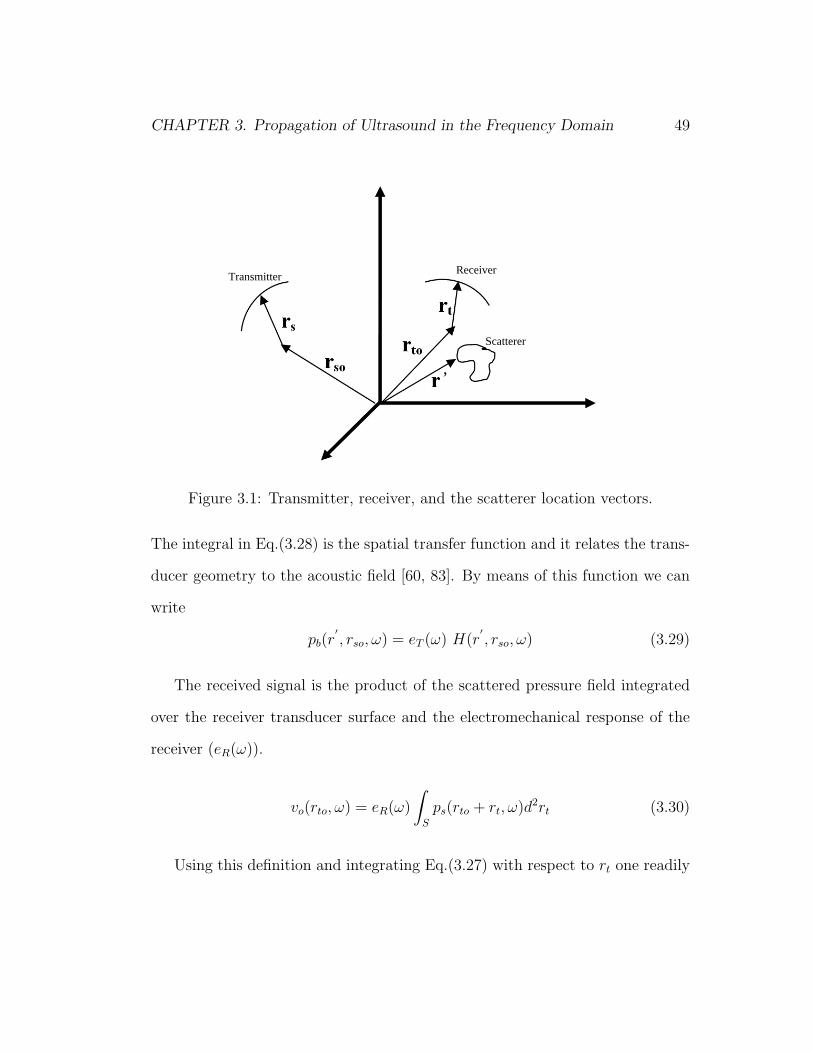
CHAPTER 3. Propagation of Ultrasound in the Frequency Domain 49
TransmitterReceiver
Scatterer
’
Figure 3.1: Transmitter, receiver, and the scatterer location vectors.
The integral in Eq.(3.28) is the spatial transfer function and it relates the trans-
ducer geometry to the acoustic field [60, 83]. By means of this function we can
write
pb(r′, rso, ω) = eT (ω) H(r
′, rso, ω) (3.29)
The received signal is the product of the scattered pressure field integrated
over the receiver transducer surface and the electromechanical response of the
receiver (eR(ω)).
vo(rto, ω) = eR(ω)
∫
S
ps(rto + rt, ω)d2rt (3.30)
Using this definition and integrating Eq.(3.27) with respect to rt one readily

CHAPTER 3. Propagation of Ultrasound in the Frequency Domain 50
obtains:
vo(rto, ω) = eT (ω)eR(ω)
∫
V ′H(rto, r
′, ω)k2
s(r′, ω)H(r
′, rso, ω)d3r
′(3.31)
−eT (ω)eR(ω)
∫
V ′H(rto, r
′, ω)∇σp(r
′).∇H(r
′, rso, ω)d3r
′
Finally using the Green’s theorem (Eq.(3.21)-Eq.(3.24))
vo(rto, ω) = epe
∫
V ′k2
s(r′, ω)H(rto, r
′, ω)H(r
′, rso, ω)d3r
′
+epe
∫
V ′σp(r
′)∇H(rto, r
′, ω).∇H(r
′, rso, ω))d3r
′(3.32)
The primary characteristic of Eq.(3.32), is that it provides a linear relation
between the real measured backscatter data and the medium parameters.
3.4 Derivation of the Spatial Transfer Function
Key to the implementation of the Born Model is the specification of the spatial
transfer function (H) of the commercially available transducers.
This section gives a detailed derivation of the semi-analytic expression for
the spatial transfer function of the spherically curved resonators in frequency
domain. The time domain formulation of Arditi et al. [60] will be applied to
frequency domain with the help of [87]. According to the definition of the spatial
transfer function we can write:
H(r, ω) =
∫
S
G(r, rt, ω)dS (3.33)
where S corresponds to the transducer surface, rt is the vector to a point within
CHAPTER 3. Propagation of Ultrasound in the Frequency Domain 51
the transducer, r is the observation point and G is the Green’s function.
The Green’s function in 3D for an unbounded media is known to be:
G(r, rt, ω) =e−jk|r−rt|
4π|r − rt| (3.34)
where k is the space invariant wave number.
A conventional approach might be to calculate this integral using numerical
integration techniques. For this type of problems numerical methods are not
attractive since the integral is highly oscillatory in rt.
The beauty of Arditi et al.’s time domain approach is converting the 2D
surface integral into a 1D line integral for which a closed form analytical solution
can be obtained. In frequency domain analytical solution does not exist but it
is convenient to apply numerical integration techniques to the resulting line
integral [87].
In our study we will use a different approach and project the integrand onto
the polynomial space and calculate the integral analytically.
3.4.1 On-axis case
To evaluate Eq.(3.33) Arditi defined three parameters ρ′, φ′ and dβ which are
shown in Fig. (3.2). R is the focal length of the transducer and O represents the
center of curvature. Following his approach and applying the Cosine theorem
on OPdS triangle one obtains:
H(rs, ω) =1
4π
∫
S
e−jkr′
r′dS (3.35a)
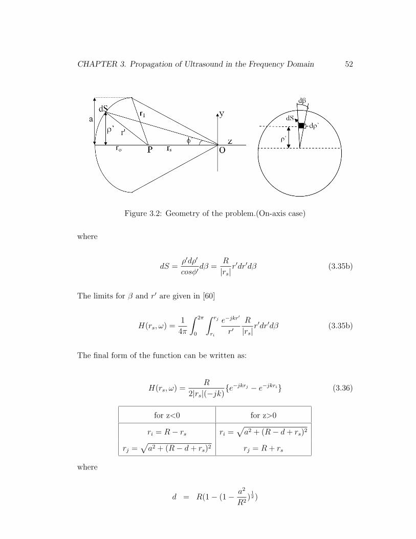
CHAPTER 3. Propagation of Ultrasound in the Frequency Domain 52
Figure 3.2: Geometry of the problem.(On-axis case)
where
dS =ρ′dρ′
cosφ′dβ =
R
|rs|r′dr′dβ (3.35b)
The limits for β and r′ are given in [60]
H(rs, ω) =1
4π
∫ 2π
0
∫ rj
ri
e−jkr′
r′R
|rs|r′dr′dβ (3.35b)
The final form of the function can be written as:
H(rs, ω) =R
2|rs|(−jk){e−jkrj − e−jkri} (3.36)
for z<0 for z>0
ri = R− rs ri =√
a2 + (R− d + rs)2
rj =√
a2 + (R− d + rs)2 rj = R + rs
where
d = R(1− (1− a2
R2)
12 )
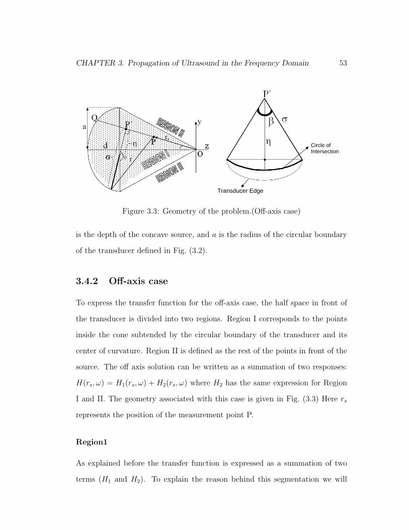
CHAPTER 3. Propagation of Ultrasound in the Frequency Domain 53
Circle ofIntersection
Transducer Edge
Figure 3.3: Geometry of the problem.(Off-axis case)
is the depth of the concave source, and a is the radius of the circular boundary
of the transducer defined in Fig. (3.2).
3.4.2 Off-axis case
To express the transfer function for the off-axis case, the half space in front of
the transducer is divided into two regions. Region I corresponds to the points
inside the cone subtended by the circular boundary of the transducer and its
center of curvature. Region II is defined as the rest of the points in front of the
source. The off axis solution can be written as a summation of two responses:
H(rs, ω) = H1(rs, ω) + H2(rs, ω) where H2 has the same expression for Region
I and II. The geometry associated with this case is given in Fig. (3.3) Here rs
represents the position of the measurement point P.
Region1
As explained before the transfer function is expressed as a summation of two
terms (H1 and H2). To explain the reason behind this segmentation we will

CHAPTER 3. Propagation of Ultrasound in the Frequency Domain 54
express the underlying physics in time domain. In time domain, the first part
represented by (H1) is the measured response before the first arrival of the signal
from the closest edge of the transducer. In other words, if the axial symmetry
around the line OPQ is considered, the on-axis derivation can be applied. In the
time interval between the arrivals from the edges, the axial symmetry no longer
exists which will be represented by H2. Mathematically speaking, H1 has the
same expression as the on-axis case.
Following the same approach as the on-axis derivation for frequency domain,
one may write the expression for H1 as:
H1(rs, ω) =R
2|rs|(−jk){e−jkrj − e−jkri} (3.37)
for z<0 for z>0
ri = R− |rs| ri =√
(a +√
r2sx + r2
sy)2 + M
rj =√
(a−√r2sx + r2
sy)2 + M rj = R + |rs|
M = (R− d + rsz)2
where
rs = rsxx + rsyy + rszz.
H2 has the same expression for both regions and will be defined in the next part.
Region2
For this region there is no axial symmetry and in the time domain, all the con-
tribution to the transfer function comes from the response between the arrivals
from the edges of the transducers. In the frequency domain this idea can be
expressed as follows:
CHAPTER 3. Propagation of Ultrasound in the Frequency Domain 55
From the definition of the impulse response one has:
H2(rs, ω) =1
4π
∫ r2
r1
∫ β(r′)
0
e−jkr′
r′R
rs
r′dβdr′ (3.38a)
H2(rs, ω) =R
4πrs
∫
r1
r2
e−jkr′β(rs, r′)dr′ (3.38b)
where
r1 = ((a− ry)2 + (R− d + rz)
2)1/2
r2 = ((a + ry)2 + (R− d + rz)
2)1/2
In this region β(rs, r′) is no longer a constant, which was 2π on the axis, but sub-
tends the arc length of points on the radiator equidistant from P. This angle and
the arc it subtends is shown in Fig. (3.3). The β(rs, r′) can be determined from
the intersection of the spherical transducer with a sphere of radius r′ centered
at P and defined as:
β(rs, r′) = 2cos−1
(η(r′)σ(r′)
)
η(r′) = R
{1− d
R
sinθ+
1
tanθ
(R2 + |rs|2 − (r′)2
2|rs|R)}
σ(r′) = R
{1−
(R2 + |rs|2 − (r′)2
2|rs|R)2
} 12
Equation (3.38b) can not be solved analytically but our observations revealed
that β is smooth in the [r1, r2] interval and can be approximated by up to 10th
CHAPTER 3. Propagation of Ultrasound in the Frequency Domain 56
order polynomials with 1.2% error bound. Specifically:
β(rs, r′) =
m=10∑m=0
am(r′)m; (3.39a)
H2(rs, ω) =R
4πrs
m=10∑m=0
am
∫
r1
r2
e−jkr′(r′)mdr′ (3.39b)
With this approximation H2(rs, ω) can be solved analytically.
At the Focus
The response at the focus of the transducer can be found by taking the Fourier
transform of the time domain impulse response. The impulse response at the
focus of the transducer is [60](eq. 12)
h(0, t) = dδ(t−R/c) (3.40)
taking the Fourier transform:
H(0, ω) = d exp{−jωR/c} = d exp{−jkR} (3.41)
3.5 Wave Propagation Experiment
A wave propagation experiment is performed to validate the Born model and the
spatial transfer function formulation of the spherically focused transducer. The
data acquisition system used in this experiment is located at Physical Acoustics
Laboratory at Boston University. The picture of the system with the water tank

CHAPTER 3. Propagation of Ultrasound in the Frequency Domain 57
Figure 3.4: Data acquisition system and the water tank in Boston University.
is given in Fig. (3.4). For this experiment Panametrics V380 PZT transducer
with 3.5 MHz nominal frequency, 50.8 mm focal length, and 12.8 mm radius is
used as the transmitter probe. This strongly focusing transducer (F number 2
and Gp=24) was placed in the water tank (0.8 m × 0.8 m × 1.5 m) that was
filled with de-ionized de-gassed water at approximately 21◦C. The transducer
was operated in transmit mode using a pulser-receiver (UA 5052, Panametrics,
Waltham, MA). The pulser-receiver excited the transducer with a short excita-
tion signal that approximated a delta function and the received echo was mea-
sured by PVDF Hydrophone with 0.1 mm radius. The data observed on digital
scope (LC 334a, LeCroy, Chestnut Ridge, NY) and transferred to a computer for
later analysis. The wave propagation through a 80 mm long cylindrical tissue
mimicking agar phantom with power law attenuation is measured. Figure 3.5
shows the experimental setup with the agar phantom and the transducers. The
nominal properties of the tissue mimicking phantom is given in Table 3.1 with

CHAPTER 3. Propagation of Ultrasound in the Frequency Domain 58
Figure 3.5: Experimental setup with the transducers and the phantom.
the real tissue properties for comparison.
To simulate the pressure fields, the electromechanical response of the trans-
ducer, eT (ω), should be obtained. For this purpose, a wave propagation ex-
periment was performed in water. The response at the focus of the spherical
transducer is measured with the PVDF hydrophone. Next, Eq.(3.29) is used
with a simplified Wiener filter and the Fourier transform of the measured water
data at the focal point (pf (ω)):
eT (ω) =pf (ω)H∗
f (ω)
|Hf (ω)|2 + q(3.42)
where Hf (ω) is the spatial transfer function at the focus, and q is the inverse of
the signal to noise ratio, and it was chosen to be 0.01max(|Hf (ω)|2) based on
the data measured at the focus.
Figure 3.6(a) shows the measured and predicted incident field for an off axis
measurement (x=-1.2 mm, y=-0.8 mm) where the receiver hydrophone is placed
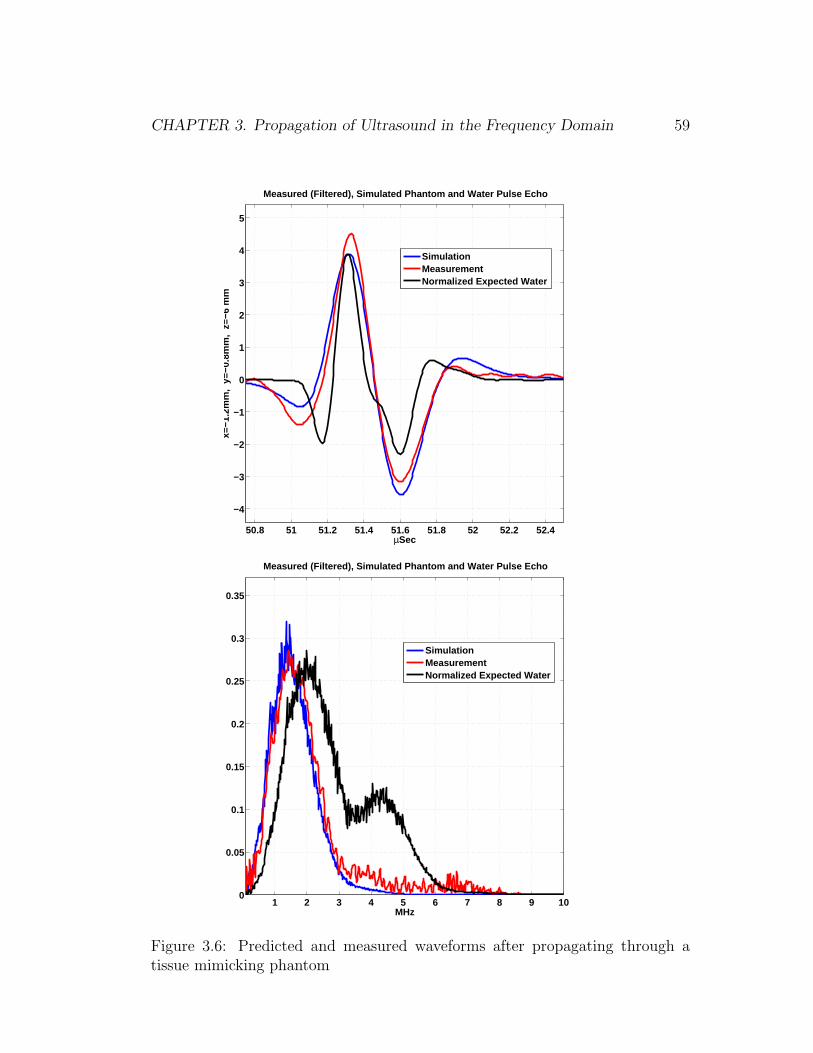
CHAPTER 3. Propagation of Ultrasound in the Frequency Domain 59
50.8 51 51.2 51.4 51.6 51.8 52 52.2 52.4
−4
−3
−2
−1
0
1
2
3
4
5
Measured (Filtered), Simulated Phantom and Water Pulse Echo
x=−1
.2m
m,
y=−0
.8m
m,
z=−6
mm
µSec
SimulationMeasurementNormalized Expected Water
1 2 3 4 5 6 7 8 9 100
0.05
0.1
0.15
0.2
0.25
0.3
0.35
Measured (Filtered), Simulated Phantom and Water Pulse Echo
MHz
SimulationMeasurementNormalized Expected Water
Figure 3.6: Predicted and measured waveforms after propagating through atissue mimicking phantom

CHAPTER 3. Propagation of Ultrasound in the Frequency Domain 60
−3 −2 −1 0 1 2 30.1
0.15
0.2
0.25
0.3
0.35
0.4
0.45
0.5Beam Plot for z=−6mm at 1.34 MHz
Lateral distance [mm]
MeasurementSimulation
−3 −2 −1 0 1 2 30.1
0.15
0.2
0.25
0.3
0.35
0.4
0.45
0.5Beam Plot for z=−20mm at 1.34 MHz
Lateral distance [mm]
MeasurementSimulation
Figure 3.7: Beam plots of the predicted and measured waveforms.
CHAPTER 3. Propagation of Ultrasound in the Frequency Domain 61
Table 3.1: Nominal acoustic properties of the Agar PhantomProperty Agar Phantom Human Tissue
Density (kg/m3) 1045 1000-1100Sound Speed (m/s) 1551 1450-1640Attenuation (Np/m/MHz) 10.17 4-17
at z=-6mm (see Fig. (3.5)) about 6 mm or 20 wavelengths behind the focus.
The transducer-receiver axial distance is 44.8 mm. Figure 3.6(b) shows the same
comparison in the frequency domain. To simulate the measured waveforms the
equations derived in the previous section for spatial transfer function of the
spherical transducer are used with the kb model derived in Section 3.1. Using
the approximate nominal values for the tissue mimicking phantom we were able
to get a very good agreement between the model and the experimental data.
The frequency dependency of attenuation is found with an optimization routine
and is characterized by a power of 1.2. Specifically the parameters used in the
simulations are:
k2b (ω) =
ω2
c2b
− j2ωαb(ω)
cb
(3.43a)
where
cb = 1545m/s (3.43b)
ρb = 1045m/s (3.43c)
αb = 54(ω
ωo
)1.2Np/m (3.43d)

CHAPTER 3. Propagation of Ultrasound in the Frequency Domain 62
where ωo is the mean angular frequency (2π3.5MHz) and 54 is obtained by:
12(3.5)1.2 hence for the attenuation instead of the nominal value,10.17, we used
12 and for sound speed we used 1545 m/s.
We also studied the effect of absorbtion on wave propagation and demon-
strated that the effect of attenuation cannot be ignored for tissue. The same
experiment is simulated using a wave number corresponding to lossless water.
The signals that would be measured in this case are plotted in Fig. (3.6)(a)-(b)
and significantly different from those measured and modeled from lossy tissue
phantom. The normalization constant used for water was 8.6.
For further validation of our model, we placed the PVDF hydrophone at
z=-6mm and z=-20mm and mechanically moved the receiver perpendicular to
the acoustic beam axis between -3mm and 3mm. We compared the maximums
of the absolute values of the frequency responses at 1.34 MHz. This particu-
lar frequency is chosen from 3.6(b) where the signals reach their peak values.
Figure 3.7(a)and(b) shows the comparison for z=-6mm and z=-20mm respec-
tively. We again have a very good agrement between the measurements and the
simulations.
3.6 Conclusion
In this chapter we concentrated on the development and validation of the fre-
quency domain Born model for medical ultrasound imaging applications.
There are no direct methods for solving the problem of wave propagation in
inhomogeneous medium. We therefore linearized our problem and defined the
inhomogeneities in the acoustic properties as perturbations to a homogenous,
lossy background model. The scattered acoustic wave is expressed linearly in

CHAPTER 3. Propagation of Ultrasound in the Frequency Domain 63
terms of the perturbations in sound speed, attenuation and density. Since our
ultimate interest lies in imaging the human tissue, the frequency dependency of
attenuation is characterized by a power-law relation.
We demonstrated a fast method to solve the incident field of spherically
curved radiators. The approach we proposed to obtain the spatial transfer func-
tion greatly improved the computation time of the Born kernel. To calculate the
incident field of the transducer at 225 observation points and 674 frequency val-
ues takes only 29 seconds with Matlab 6.5.0 on Pentium 4 machine with 3GHz
processor, and 1GByte memory.
We performed a validation experiment where we measured the wave propa-
gation through a tissue mimicking agar phantom with power law attenuation.
We simulated the measured field using the dispersive background wave num-
ber from Section 3.1 and equations from Section 3.2 and 3.4 that we derived
for the spherically focused radiators. The precise match between the measured
and simulated data support the validity of the methods developed in this dis-
sertation. We also observed the effect of absorbtion on ultrasound propagation.
Specifically, we showed the signals that would propagate in lossless water are
significantly different from those measured from lossy tissue mimicking phantom.
The next step will be the application of these methods to the inverse problem
area. The derived compact linear relation between the measured backscatter
data and the medium parameters will provide a basis for inversion.
To apply inversion algorithms to clinically obtained data, we would first need
a method to compute the pressure field of the clinically used phased arrays. The
experience we gained with focused transducers will help us simulate the forward
field from phased array transducers that will be presented in the next chapter.
Chapter 4
Cylindrically Concave
Transducers
Conventional ultrasound transducers used for medical diagnosis purposes are
generally of linear array type, consisting of linearly aligned rectangular apertures
with cylindrically curved surfaces which are focused in one direction. Typically
1D arrays that have natural focus in the elevation plane are used with electronic
focusing along the lateral dimension for beam forming applications. Ideally, each
element of the array can be excited individually to obtain non-beam formed data.
This type of applications allows us to collect full tomographic data where single
transmitter is used to probe the tissue and the response is measured by the
collection of the elements of the array. However, to utilize the array transducers
for applications beyond traditional beam focusing and steering, it is necessary
to have a precise knowledge of the radiated fields generated by the cylindrically
curved transducers.
In this chapter we introduce a fast semi-analytical frequency domain method
to compute the acoustic field of cylindrically concave transducers in a homoge-
nous medium by using the spatial impulse response approach. The method
64

CHAPTER 4. Cylindrically Concave Transducers 65
we propose complements the methods in the literature such that, with a new
rapid integral formulation, the pressure field due to cylindrical radiators for any
type of lossy or lossless media is obtained almost immediately and has a closed
form solution expressed with Bessel functions. The speed performance of the
semi-analytic technique is compared to an optimized numerical routine and the
method is validated with laboratory measurements.
This chapter is organized as follows. Section 4.1, briefly outlines the SIR
method and gives the equations that describe the pressure field produced by
time-harmonic excitations. In Section 4.2, we derive the integrals to compute
the spatial transfer function of the cylindrical radiators. In Section 4.3, we
introduce a semi-analytical method to compute those integrals. In Section 4.4,
we compare our method with numerical integration techniques and present a
comparison of predicted and measured pressure fields.
4.1 Theory: Spatial Impulse Response
For a homogenous fluid medium with a constant sound speed and density, the
acoustic field at frequency ω and position ~rp is calculated with the use of the
velocity potential Φ(~rp, ω) and imposing the appropriate boundary conditions
[61, 88]. For a uniform excitation, where the normal particle velocity υo on the
transducer surface is space invariant, i.e. υo(ω, ~rt) = υo(ω) where ~rt is the vector
traversing the transducer surface, the velocity potential can be expressed as:
Φ(~rp, ω) = υo(ω)
∫
S
e−jk| ~rp−~rt|
2π|~rp − ~rt|dS (4.1a)
= υo(ω)
∫
S
e−jkr
2πrdS = υo(ω)H(~rp, k) (4.1b)

CHAPTER 4. Cylindrically Concave Transducers 66
where k is the background wave number, r is the distance from the emitting
surface element dS to the observation point P as shown in Fig. (4.1) and H(~rp, k)
is the spatial transfer function of the transducer. IIn lossless dispersive media
k is a real valued quantity equal to ω/co(ω), where co(ω) is the speed of sound.
For a lossy medium, an imaginary component is introduced,
k(ω) =ω
co(ω)− jα(ω) (4.2)
where α(ω) is the frequency dependent attenuation coefficient.
The output voltage from the transducer at point ~rp is calculated from Eq.(4.1a)
as:
v(~rp, ω) = jωρoυo(ω)υi(ω)H(~rp, k) (4.3)
or
v(~rp, ω) = eT (ω)H(~rp, k) (4.4)
where ρo is the density, υi(ω) is the Fourier transform of the driving signal of the
transducer and eT (ω) is the density scaled electromechanical transfer function.
4.2 Spatial Transfer Function for the Cylindri-
cal Geometry
In this section the spatial transfer function of a concave rectangular transducer
will be calculated. The source S is a truncated cylinder with lateral dimensions
l × h and a radius R is given in Fig. (4.1). The focal point of the cylindrical
radiator is the origin of the cylindrical coordinates system, and the center of
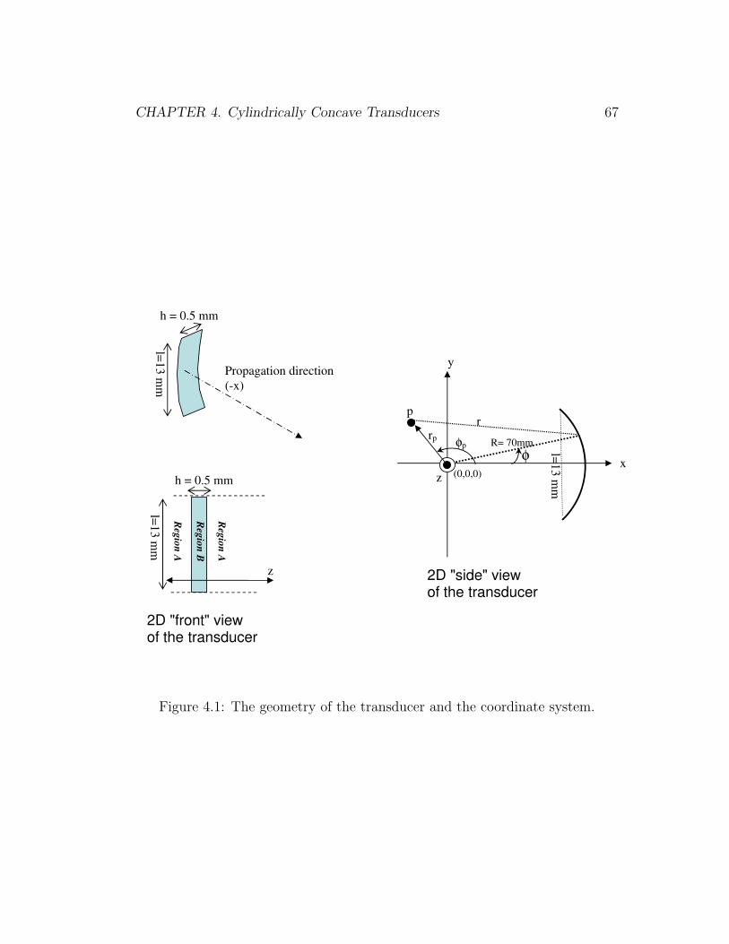
CHAPTER 4. Cylindrically Concave Transducers 67
Propagation direction
(-x)
h = 0.5 mm
l=13
mm
h = 0.5 mm
Reg
ion
A
2D "front" view
of the transducer
Reg
ion
B
Reg
ion
A
z l=
13
mm
x
y
φ φp
r
R= 70mm rp
p
z (0,0,0)
l=1
3 m
m
2D "side" view
of the transducer
Figure 4.1: The geometry of the transducer and the coordinate system.
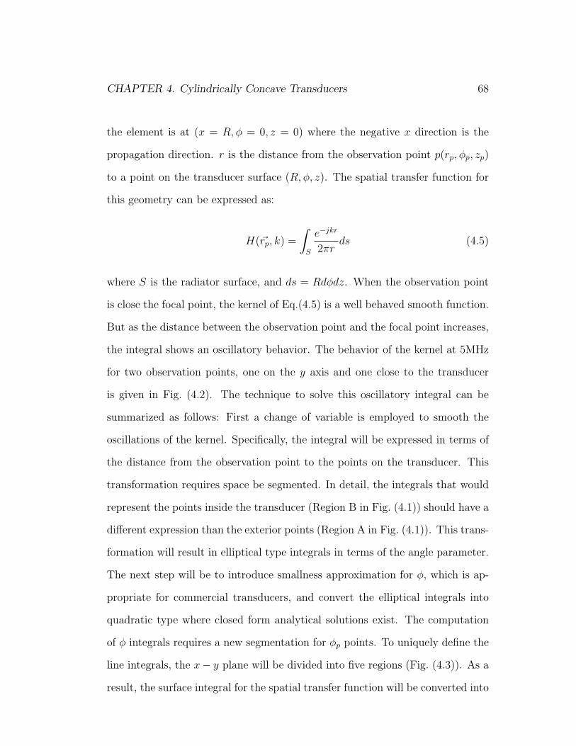
CHAPTER 4. Cylindrically Concave Transducers 68
the element is at (x = R, φ = 0, z = 0) where the negative x direction is the
propagation direction. r is the distance from the observation point p(rp, φp, zp)
to a point on the transducer surface (R, φ, z). The spatial transfer function for
this geometry can be expressed as:
H(~rp, k) =
∫
S
e−jkr
2πrds (4.5)
where S is the radiator surface, and ds = Rdφdz. When the observation point
is close the focal point, the kernel of Eq.(4.5) is a well behaved smooth function.
But as the distance between the observation point and the focal point increases,
the integral shows an oscillatory behavior. The behavior of the kernel at 5MHz
for two observation points, one on the y axis and one close to the transducer
is given in Fig. (4.2). The technique to solve this oscillatory integral can be
summarized as follows: First a change of variable is employed to smooth the
oscillations of the kernel. Specifically, the integral will be expressed in terms of
the distance from the observation point to the points on the transducer. This
transformation requires space be segmented. In detail, the integrals that would
represent the points inside the transducer (Region B in Fig. (4.1)) should have a
different expression than the exterior points (Region A in Fig. (4.1)). This trans-
formation will result in elliptical type integrals in terms of the angle parameter.
The next step will be to introduce smallness approximation for φ, which is ap-
propriate for commercial transducers, and convert the elliptical integrals into
quadratic type where closed form analytical solutions exist. The computation
of φ integrals requires a new segmentation for φp points. To uniquely define the
line integrals, the x− y plane will be divided into five regions (Fig. (4.3)). As a
result, the surface integral for the spatial transfer function will be converted into
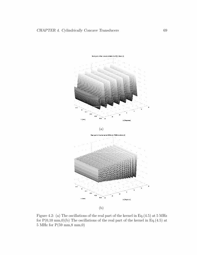
CHAPTER 4. Cylindrically Concave Transducers 69
(a)
(b)
Figure 4.2: (a) The oscillations of the real part of the kernel in Eq.(4.5) at 5 MHzfor P(0,10 mm,0)(b) The oscillations of the real part of the kernel in Eq.(4.5) at5 MHz for P(59 mm,8 mm,0)

CHAPTER 4. Cylindrically Concave Transducers 70
R
egio
n III
y
x
z (0,0,0)
Region II Region V
Region I Region IV
Figure 4.3: Schematic showing the segmentation for φp
line integrals. Having reduced the dimension of the integral, the line integral
kernels will be expanded as truncated series of Legendre polynomials which can
be integrated exactly term by term. The resulting spatial transfer function will
be represented as summation of a few number of Bessel functions. In this section
the initial steps of our algorithm is introduced. Mainly, Eq.(4.5) is presented in
terms of the distance parameter and segmentation for zp is discussed.
Using the cylindrical coordinates representation, the distance r in Eq.(4.5)
can be expressed as:
r2 = (rp cos(φp)−Rcos(φ))2 + (rp sin(φp)−Rsin(φ))2 + (zp − z)2
= M(φ) + (zp − z)2 (4.6)
where M(φ) = r2p + R2− 2rpR(cos(φ) cos(φp) + sin(φ) sin(φp)) contains all the φ

CHAPTER 4. Cylindrically Concave Transducers 71
dependent terms. Equation (4.5) can be written explicitly as:
H(~rp, k) =1
2π
∫ φmax
φmin
∫ h2
−h2
e−jk√
M(φ)+(zp−z)2
√M(φ) + (zp − z)2
Rdzdφ (4.7)
where φmax = arcsin( l2R
) and φmin = −φmax.
First, to simplify the integral, the element ds = Rdφdz will be expressed as
a function of r by eliminating the z dependence. Taking the derivative of the
both sides of the Eq.(4.6):
dz = − r
(zp − z)dr (4.8)
The sign of the element dz depends on the value of zp − z at the observation
point. The field point zp can have values between [−∞,∞] but the surface
point z is limited to the width of the transducer, h. Mathematically speaking,
(zp − z) =√
r2 −M(φ) for zp > z and −√
r2 −M(φ) for zp < z. Hence the
new surface element ds will be given as:
ds = ± r√r2 −M(φ)
Rdφdr (4.9)
and the correct sign will be determined from the observation point.
The surface S is now a function of r and φ, and the new integration limits
must be calculated. To express the new integrals, it is convenient to divide the
half space in front of the transducer into two regions. Due to the symmetry in
x−y and x−z planes of the radiator, the spatial impulse response is symmetric
with respect to z and y and the description of H(~rp, k) can be restricted to the
one quadrant of the y− z plane with zp ≥ 0 and y ≥ 0. The two regions will be
CHAPTER 4. Cylindrically Concave Transducers 72
defined as follows:
REGION A (zp ≥ h/2) If zp > h/2 (the maximum value of z), then (zp − z)
will always be positive and ds < 0. The integral limits for r can be found
by substituting the limiting values of z, (−h/2, h/2) in Eq.(4.6). Hence
the integral in Eq.(4.7) can be written in terms of r as:
R
2π
∫ φmax
φmin
∫ √M(φ)+(zp+h/2)2
√M(φ)+(zp−h/2)2
e−jkr
√r2 −M(φ)
drdφ (4.10)
REGION B (0 ≤ zp < h/2) If zp is smaller than the limiting value of z, the
integral should be decomposed into two parts for proper calculation.
• If−h2≤ z ≤ zp then (zp−z) ≥ 0 and ds < 0. Substituting the limiting
values of z, (−h/2, zp), in Eq.(4.6), the new integral is expressed as:
R
2π
∫ φmax
φmin
∫ √M(φ)+(zp+h
2)2
√M(φ)
e−jkr
√r2 −M(φ)
drdφ
• If zp ≤ z ≤ h2
then (zp − z) ≤ 0 and ds > 0. The limiting values for
z is (zp, h/2) and the new integral is given by:
R
2π
∫ φmax
φmin
∫ √M(φ)+(zp−h
2)2
√M(φ)
e−jkr
√r2 −M(φ)
drdφ
As a result, for this region the integral in terms of r can be expressed as:
R
2π
∫ φmax
φmin
[∫ √M(φ)+(zp+h
2)2
√M(φ)
E(r, φ)dr +
∫ √M(φ)+(zp−h
2)2
√M(φ)
E(r, φ)dr
]dφ
(4.11)

CHAPTER 4. Cylindrically Concave Transducers 73
where for the simplicity of the notation:
e−jkr
√r2 −M(φ)
= E(r, φ)
The type of the integrals that is introduced in this section can be summarized
in a compact form such as:
R
2π
∫ φmax
φmin
∫ F2(φ)
F1(φ)
E(r, φ)drdφ (4.12a)
where
F1(φ) =√
M(φ) + Azp (4.12b)
F2(φ) =√
M(φ) + Bzp (4.12c)
here Azp and Bzp represent the region specific constants defined by the zp value
of the observation point.
4.3 Integral Calculation
In the previous section the necessary integrals are derived to compute the spatial
transfer function of a cylindrical radiator and a compact form is introduced
which summarizes the formulae derived for two different regions. In this section,
the mathematical approximations to convert the surface integral presented in
Eq.(4.12a) into line integrals will be presented.
We were unable to find an analytical closed form solution for Eq.(4.12a).
Specifically, due to the r2 term in the denominator and the oscillatory expression
CHAPTER 4. Cylindrically Concave Transducers 74
e−jkr in the numerator, the exact integral with respect to r could not be obtained
analytically. Moreover, the integral is of elliptical type in terms of the angle
parameter. However, using the geometry information of the transducer, it is
possible to obtain a simpler expression for Eq.(4.12a) which would lead to a
closed form solution.
The geometry of the problem given in Fig. (4.1) -the placement of the trans-
ducer on the x axis- has a significant role in our method. Given the 2D side
view of the transducer in Fig. (4.1) one observes that the maximum value of φ
(or φmax) is arcsin( l2R
). For the most focusing type of transducers, like the one
we use in our experiments, the ratio of l/(2R) is small enough that cos(φ) can
be approximated with (1 − φ2/2) and sin(φ) can be replaced with φ. Specifi-
cally, the parameters that actually define the transducer used in this study are
R = 70 mm and l = 13 mm, hence arcsin( 13140
) ' 5◦. By means of this smallness
approximation, M(φ) will be described by:
M(φ) ≈ (r2p + R2 − 2rpRcos(φp))− (2rpRsin(φp))φ (4.13)
+(rpRcos(φp))φ2
The smallness approximation that is introduced on the way converts the
elliptical integral in Eq.(4.12a) into a quadratic type which has a closed form
solution. Since, the integral with respect to r cannot be obtained analytically,
we should change the order of integral in Eq.(4.12a) and attempt to calculate
the φ integral first. On the other hand, for the observation points on the z
axis (when rp = 0) the kernel will be independent of φ and this transformation
CHAPTER 4. Cylindrically Concave Transducers 75
cannot be employed. Therefore, the points on the z axis should be handled
separately.
In the next sections the mathematical details to reduce the type of integrals in
Eq.(4.12a) into line integrals will be presented where fast analytical integration
techniques can be applied to obtain a computationally efficient solution.
As discussed previously, the first step to obtain the line integrals will be to
employ the change of order of integration for r and φ. The algebraic details of
this alteration depend on the polar angle of the observation point. To uniquely
express the transfer function in terms of the angle parameter, the x− y plane is
divided into five regions as shown in Fig. (4.3). Region II and V correspond to
the points inside the cone subtended by the circular boundary of the transducer
and its center of curvature. Region III corresponds to the cone around the y
axis and Region I and IV are defined as the rest of the points in the first and
second quadrant.
Among all the regions, Region III requires a detailed explanation. The equa-
tions that would be derived are originated from Eq.(4.13) where (rpRcos(φp)) ap-
pears as a multiplication constant of φ2. For the points where cos(φp) = 0, such
as the ones on the y axis, the coefficient of this quadratic term is zero. Moreover,
for the observation points that are close to the y axis this term will be infinitesi-
mally small. Hence, the expansion employed below fails. For these points, which
are close to the y axis, cos(φ) will be approximated as unity and the last term
in Eq.(4.13) with the troublesome cos(φp) term is dropped. To minimize the er-
ror coming from this approximation, a threshold value should be chosen for the
polar angle which minimizes the effect of φ2 on the solution. Specifically the φp
value which satisfies the equation [(2rpRsin(φp)φmax) > 103(rpRcos(φp)φ2max)]
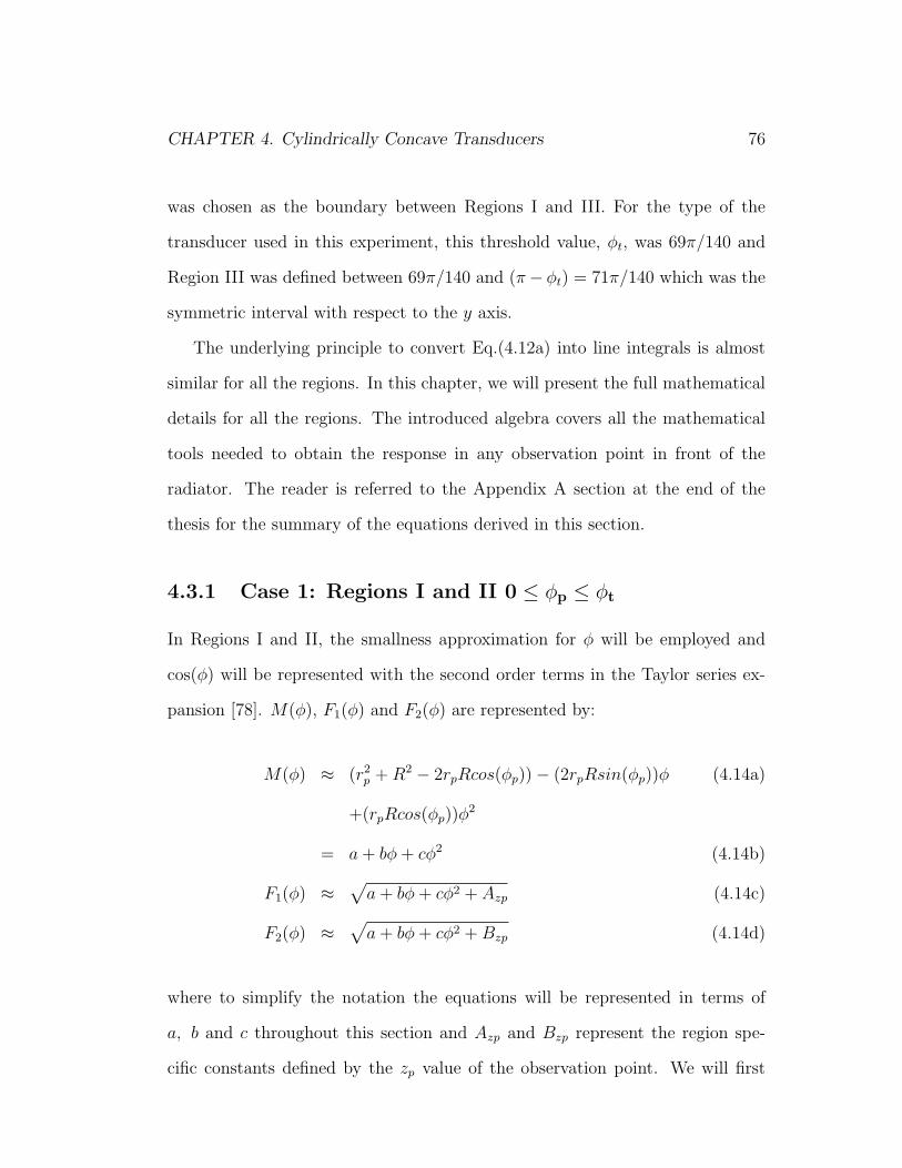
CHAPTER 4. Cylindrically Concave Transducers 76
was chosen as the boundary between Regions I and III. For the type of the
transducer used in this experiment, this threshold value, φt, was 69π/140 and
Region III was defined between 69π/140 and (π− φt) = 71π/140 which was the
symmetric interval with respect to the y axis.
The underlying principle to convert Eq.(4.12a) into line integrals is almost
similar for all the regions. In this chapter, we will present the full mathematical
details for all the regions. The introduced algebra covers all the mathematical
tools needed to obtain the response in any observation point in front of the
radiator. The reader is referred to the Appendix A section at the end of the
thesis for the summary of the equations derived in this section.
4.3.1 Case 1: Regions I and II 0 ≤ φp ≤ φt
In Regions I and II, the smallness approximation for φ will be employed and
cos(φ) will be represented with the second order terms in the Taylor series ex-
pansion [78]. M(φ), F1(φ) and F2(φ) are represented by:
M(φ) ≈ (r2p + R2 − 2rpRcos(φp))− (2rpRsin(φp))φ (4.14a)
+(rpRcos(φp))φ2
= a + bφ + cφ2 (4.14b)
F1(φ) ≈√
a + bφ + cφ2 + Azp (4.14c)
F2(φ) ≈√
a + bφ + cφ2 + Bzp (4.14d)
where to simplify the notation the equations will be represented in terms of
a, b and c throughout this section and Azp and Bzp represent the region spe-
cific constants defined by the zp value of the observation point. We will first

CHAPTER 4. Cylindrically Concave Transducers 77
φmax φmin
F1
F2
1
2
3
F2(φmin)
F1(φmin)
F2(φmax)
F1(φmax)
Figure 4.4: The limit functions with monotonic decreasing φ dependency.
introduce the solution for Region I, as it sets the basis for the other solutions.
The boundaries between the regions are described in terms of tan φp and the
reasoning behind this parameter will be explained in the next section.
Region I: φmax < tanφp ≤ φt
To reduce the order of the integral given in Eq.(4.12a) change of order of inte-
gration will be employed. The region of integration is shown in Fig. (4.4). To
facilitate the change of order it was necessary to divide the integral into three
pieces.
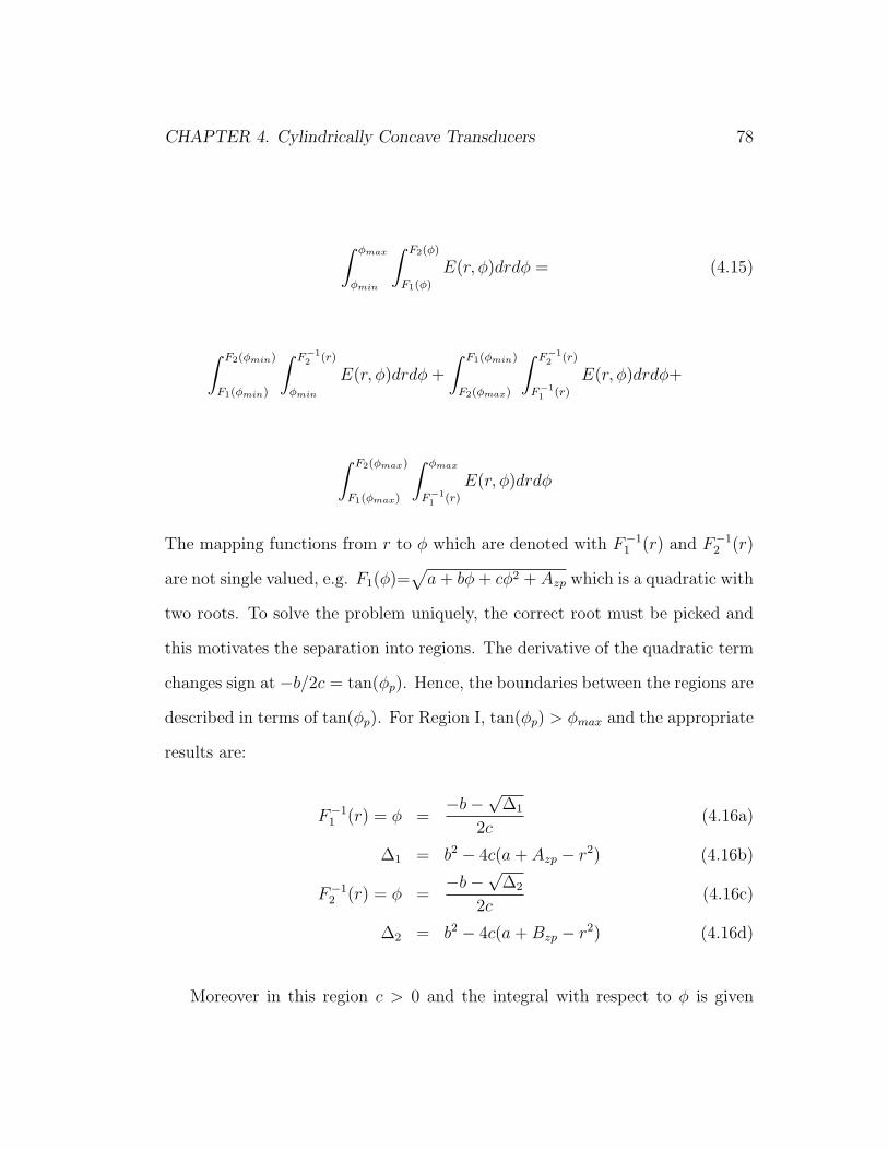
CHAPTER 4. Cylindrically Concave Transducers 78
∫ φmax
φmin
∫ F2(φ)
F1(φ)
E(r, φ)drdφ = (4.15)
∫ F2(φmin)
F1(φmin)
∫ F−12 (r)
φmin
E(r, φ)drdφ +
∫ F1(φmin)
F2(φmax)
∫ F−12 (r)
F−11 (r)
E(r, φ)drdφ+
∫ F2(φmax)
F1(φmax)
∫ φmax
F−11 (r)
E(r, φ)drdφ
The mapping functions from r to φ which are denoted with F−11 (r) and F−1
2 (r)
are not single valued, e.g. F1(φ)=√
a + bφ + cφ2 + Azp which is a quadratic with
two roots. To solve the problem uniquely, the correct root must be picked and
this motivates the separation into regions. The derivative of the quadratic term
changes sign at −b/2c = tan(φp). Hence, the boundaries between the regions are
described in terms of tan(φp). For Region I, tan(φp) > φmax and the appropriate
results are:
F−11 (r) = φ =
−b−√∆1
2c(4.16a)
∆1 = b2 − 4c(a + Azp − r2) (4.16b)
F−12 (r) = φ =
−b−√∆2
2c(4.16c)
∆2 = b2 − 4c(a + Bzp − r2) (4.16d)
Moreover in this region c > 0 and the integral with respect to φ is given
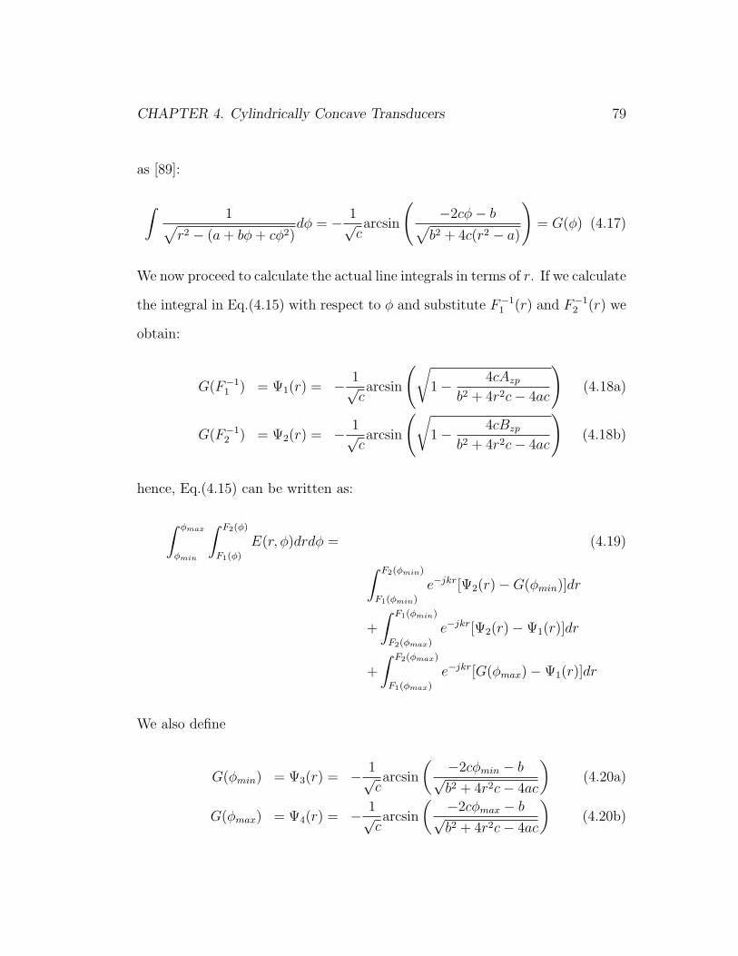
CHAPTER 4. Cylindrically Concave Transducers 79
as [89]:
∫1√
r2 − (a + bφ + cφ2)dφ = − 1√
carcsin
(−2cφ− b√
b2 + 4c(r2 − a)
)= G(φ) (4.17)
We now proceed to calculate the actual line integrals in terms of r. If we calculate
the integral in Eq.(4.15) with respect to φ and substitute F−11 (r) and F−1
2 (r) we
obtain:
G(F−11 ) = Ψ1(r) = − 1√
carcsin
(√1− 4cAzp
b2 + 4r2c− 4ac
)(4.18a)
G(F−12 ) = Ψ2(r) = − 1√
carcsin
(√1− 4cBzp
b2 + 4r2c− 4ac
)(4.18b)
hence, Eq.(4.15) can be written as:
∫ φmax
φmin
∫ F2(φ)
F1(φ)
E(r, φ)drdφ = (4.19)
∫ F2(φmin)
F1(φmin)
e−jkr[Ψ2(r)−G(φmin)]dr
+
∫ F1(φmin)
F2(φmax)
e−jkr[Ψ2(r)−Ψ1(r)]dr
+
∫ F2(φmax)
F1(φmax)
e−jkr[G(φmax)−Ψ1(r)]dr
We also define
G(φmin) = Ψ3(r) = − 1√carcsin
( −2cφmin − b√b2 + 4r2c− 4ac
)(4.20a)
G(φmax) = Ψ4(r) = − 1√carcsin
( −2cφmax − b√b2 + 4r2c− 4ac
)(4.20b)
CHAPTER 4. Cylindrically Concave Transducers 80
and present the transfer function in a compact form of four line integrals:
H =R
2π
∫ F1(φmin)
F1(φmax)e−jkr[−Ψ1(r)]dr +
∫ F2(φmin)
F2(φmax)e−jkr[Ψ2(r)]dr+
∫ F2(φmin)
F1(φmin)e−jkr[−Ψ3(r)]dr +
∫ F2(φmax)
F1(φmax)e−jkr[Ψ4(r)]dr
(4.21)
where
φmin = −arcsin(l/2R) (4.22)
φmax = arcsin(l/2R)
Region II: tanφp ≤ φmax
When tan(φp) is smaller than the limiting value of φ the inverse mapping func-
tions F−11 (r) and F−1
2 (r) change sign in the integral interval. Therefore the
integral in Eq.(4.12a) should be decomposed into two parts for unique represen-
tation.
∫ φmax
φmin
∫ F2(φ)
F1(φ)
E(r, φ)drdφ = H1 + H2 = (4.23)
∫ tan(φp)
φmin
∫ F2(φ)
F1(φ)
E(r, φ)drdφ +
∫ φmax
tan(φp)
∫ F2(φ)
F1(φ)
E(r, φ)drdφ
To obtain H1, the algorithm we used in Region I will be implemented. The limit
functions F1(φ) and F2(φ) are decreasing functions of φ and the inverses of the
functions are represented with the negative roots, hence the resulting integral

CHAPTER 4. Cylindrically Concave Transducers 81
has the similar form with the previous case and can be expressed as:
H1 =R
2π
∫ F1(φmin)
F1(φmax)e−jkr[−Ψ1(r)]dr +
∫ F2(φmin)
F2(φmax)e−jkr[Ψ2(r)]dr+
∫ F2(φmin)
F1(φmin)e−jkr[−Ψ3(r)]dr
(4.24)
where
φmin = −arcsin(l/2R) (4.25)
φmax = tan(φp)
The Ψ4(r) integral vanishes in this interval.
To calculate H2 the same path will be followed with minor modifications.
For this case M and r are the increasing functions of φ. The behavior of the
limiting functions with respect to φ is given in Fig. (4.5). As in Eq.(4.15), we
have to divide the integral into three parts for proper calculation.
The integral in Eq.(4.12a) will have the form:
∫ F2(φmin)
F1(φmin)
∫ F−11 (r)
φmin
E(r, φ)drdφ +
∫ F1(φmax)
F2(φmin)
∫ F−11 (r)
F−12 (r)
E(r, φ)drdφ+
∫ F2(φmax)
F1(φmax)
∫ φmax
F−12 (r)
E(r, φ)drdφ
After algebraic manipulations the resulting integral can be written as:
H2 =R
2π
∫ F1(φmax)
F1(φmin)e−jkr[−Ψ1(r)]dr +
∫ F2(φmax)
F2(φmin)e−jkr[Ψ2(r)]dr+
∫ F2(φmax)
F1(φmax)e−jkr[Ψ4(r)]dr
(4.26)

CHAPTER 4. Cylindrically Concave Transducers 82
φmin φmax
φφ
φ
φ
φ
φ
F1(φmin)
F1
F2
1
3
2 F2(φmin)
F2(φmax)
F1(φmax)
Figure 4.5: The limiting functions with monotonic increasing φ dependency.
where
φmin = tan(φp) (4.27)
φmax = arcsin(l/2R)
The Ψ3(r) integral vanishes in this interval.
4.3.2 Case 2: Region III, φt < φp ≤ π − φt
The equations we derived in the previous sections are originated from Eq.(4.17)
where we have 1/√
c or 1/√
rpRcos(φp) as a multiplication constant. Hence for
a zero rp or cos(φp) value, the derived equations will no longer be valid. As
discussed previously the first order approximation for cos(φ) will be employed

CHAPTER 4. Cylindrically Concave Transducers 83
in this region and the parameters that will be used for this case will be presented
with:
M(φ) ≈ (r2p + R2 − 2rpRcos(φp))− (2rpRsin(φp))φ (4.28a)
= a + bφ
F1(φ) ≈√
a + bφ + Azp (4.28b)
F2(φ) ≈√
a + bφ + Bzp (4.28c)
F−11 (r) =
r2 − a− Azp
b(4.28d)
F−12 (r) =
r2 − a−Bzp
b(4.28e)
In this region, M and r are decreasing functions of φ. The algorithm intro-
duced in the previous section can be applied to this case where we have:
∫ φmax
φmin
∫ F2(φ)
F1(φ)
E(r, φ)drdφ = (4.29)
∫ F2(φmin)
F1(φmin)
∫ F−12 (r)
φmin
E(r, φ)drdφ +
∫ F1(φmin)
F2(φmax)
∫ F−12 (r)
F−11 (r)
E(r, φ)drdφ+
∫ F2(φmax)
F1(φmax)
∫ φmax
F−11 (r)
E(r, φ)drdφ
Moreover for this region:
∫1√
r2 − (a + bφ)dφ =
2√
r2 − (a + bφ)
−b(4.30)

CHAPTER 4. Cylindrically Concave Transducers 84
We calculate the integral in Eq.(4.29) with respect to φ and substitute the limits
to obtain:
H =R
π(−b){ (4.31)
∫ F2(φmin)
F1(φmin)
e−jkr[√
Bzp −√
r2 − (a + bφmin)]dr
+
∫ F1(φmin)
F2(φmax)
e−jkr[√
Bzp −√
Azp]dr
+
∫ F2(φmax)
F1(φmax)
e−jkr[√
r2 − (a + bφmax)−√
Azp]dr }
with the definition of:
Ψ5(r) =√
r2 − (a + bφmin) (4.32a)
Ψ6(r) =√
r2 − (a + bφmax) (4.32b)
the spatial transfer function can be expressed in a compact form as:
H =R
π(−b)
∫ F2(φmin)
F2(φmax)e−jkr[
√Bzp]dr +
∫ F2(φmin)
F1(φmin)e−jkr[−Ψ5(r)]dr
+∫ F2(φmax)
F1(φmax)e−jkr[Ψ6(r)]dr +
∫ F1(φmin)
F1(φmax)e−jkr[−√
Azp]
(4.33)
where φmin and φmax are defined in Eq.(4.22).
4.3.3 Case 3: Regions IV and V (π − φt) ≤ φp ≤ π
The type of the integrals required to describe the transfer function of the points
in Region IV and V can be calculated using the algorithm we introduced in
Section 4.3.1. However, care must be taken since for these regions the integral of
the quadratic form has a different expression than Eq.(4.17). For this part cos(φ)

CHAPTER 4. Cylindrically Concave Transducers 85
will again be represented with the second order terms in series expansion [78]
and M(φ), F1(φ) and F2(φ) have the same forms in Section 4.3.1 as:
M(φ) ≈ (r2p + R2 − 2rpRcos(φp))− (2rpRsin(φp))φ (4.34a)
+(rpRcos(φp))φ2
= a + bφ + cφ2 (4.34b)
F1(φ) ≈√
a + bφ + cφ2 + Azp (4.34c)
F2(φ) ≈√
a + bφ + cφ2 + Bzp (4.34d)
Region IV: tanφp < φmin
In Region IV the limiting functions F1(φ) and F2(φ) are decreasing functions of
φ and the inverses of the limits should be computed with Eq.(4.16a)-(4.16d).
For this case cos(φ) < 0 and the integral of Eq.(4.12a) is represented by [89]:
∫1√
r2 − (a + bφ + cφ2)dφ =
1√−cln
(2√−c(r2 − a− bφ− cφ2)− 2cφ− b
)= G(φ)
(4.35)
To calculate the actual line integrals, we substitute F−11 (r) and F−1
2 (r) in Eq.(4.35)
to obtain:
G(F−11 ) = Ψ7(r) =
1√−cln
(2√−cAzp +
√b2 − 4c(a + Azp − r2)
)(4.36a)
G(F−12 ) = Ψ8(r) =
1√−cln
(2√−cBzp +
√b2 − 4c(a + Bzp − r2)
)(4.36b)
G(φmin) = Ψ9(r) =1√−c
ln
(2√−c(r2 − a− bφmin − cφ2
min)− 2cφmin − b
)
(4.36c)
CHAPTER 4. Cylindrically Concave Transducers 86
G(φmax) = Ψ10(r) =1√−c
ln(2√−c(r2 − a− bφmax − cφ2
max)− 2cφmax − b)
(4.36d)
The resulting equation is given as:
H =R
2π
∫ F1(φmin)
F1(φmax)e−jkr[−Ψ7(r)]dr +
∫ F2(φmin)
F2(φmax)e−jkr[Ψ8(r)]dr+
∫ F2(φmin)
F1(φmin)e−jkr[−Ψ9(r)]dr +
∫ F2(φmax)
F1(φmax)e−jkr[Ψ10(r)]dr
(4.37)
where
φmin = −arcsin(l/2R) (4.38a)
φmax = arcsin(l/2R) (4.38b)
Region V: tanφp ≥ φmin
When tan(φp) is larger than the smallest value of φ the integral should be de-
composed into two parts for proper calculation for the same reasons as in Sec-
tion 4.3.1.
∫ φmax
φmin
∫ F2(φ)
F1(φ)
E(r, φ)drdφ = H1 + H2 = (4.39)
∫ tan(φp)
φmin
∫ F2(φ)
F1(φ)
E(r, φ)drdφ +
∫ φmax
tan(φp)
∫ F2(φ)
F1(φ)
E(r, φ)drdφ
To find H2 the same algorithm with the previous section will be used. The
inverses of the functions are represented with the negative roots and the limits
are decreasing functions of φ hence the resulting integral has the similar form

CHAPTER 4. Cylindrically Concave Transducers 87
with the previous case and can be written as:
H2 =R
2π
∫ F1(φmin)
F1(φmax)e−jkr[−Ψ7(r)]dr +
∫ F2(φmin)
F2(φmax)e−jkr[Ψ8(r)]dr+
∫ F2(φmin)
F1(φmin)e−jkr[−Ψ9(r)]dr +
∫ F2(φmax)
F1(φmax)e−jkr[Ψ10(r)]dr
(4.40)
where
φmin = −tan(φp) (4.41a)
φmax = arcsin(l/2R) (4.41b)
To find H1 we rewrite Eq.(4.12a) in terms of a, b, and c
H1 =
∫ tan(φp)
φmin
∫ F2(φ)
F1(φ)
e−jkr
√r2 − (a + bφ + cφ2)
drdφ (4.42a)
and introduce a change of variable to write the integral in terms of the negative
φ to ensure the non-negativity of the logarithm function:
φ∗ = −φ (4.42b)
H1 =
∫ φmax
−tan(φp)
∫ F2(φ∗)
F1(φ∗)
e−jkr
√r2 − (a− bφ∗ + c(φ∗)2)
drdφ∗ (4.42c)
where
F ∗1 (φ∗) =
√(a− bφ∗ + c(φ∗)2 + Azp (4.42d)
F ∗2 (φ∗) =
√(a− bφ∗ + c(φ∗)2 + Bzp (4.42e)
With this new variable definition F ∗1 (φ) and F ∗
2 (φ) are decreasing functions of
φ and Eq.(4.40) can be used to find the final expression. In this region G(φ∗) is
CHAPTER 4. Cylindrically Concave Transducers 88
defined as:
G(φ∗) =1√−c
ln(2√−c(r2 − a + bφ∗ − c(φ∗)2)− 2cφ∗ + b
)(4.43)
and G(φmin) and G(φmax) are expressed as:
G(φmin) = Ψ11(r) =1√−c
ln
(2√−c(r2 − a + bφmin − cφ2
min)− 2cφmin + b
)
(4.44a)
G(φmax) = Ψ12(r) =1√−c
ln(2√−c(r2 − a + bφmax − cφ2
max)− 2cφmax + b)
(4.44b)
The final form of H1 is given as:
H1 =R
2π
∫ F ∗1 (φmin)
F ∗1 (φmax)e−jkr[−Ψ7(r)]dr +
∫ F ∗2 (φmin)
F ∗2 (φmax)e−jkr[Ψ8(r)]dr+
∫ F ∗2 (φmin)
F ∗1 (φmin)e−jkr[−Ψ11(r)]dr +
∫ F ∗2 (φmax)
F ∗1 (φmax)e−jkr[Ψ12(r)]dr
(4.45)
where
φmin = −tan(φp) (4.46a)
φmax = arcsin(l/2R) (4.46b)
The path that is followed to reduce the dimension of the integral in Eq.(4.12a)
can be summarized as follows: First a region is chosen where r was a monotonic
decreasing or increasing function of φ and change of order of integration was
employed to obtain a solvable integral in terms of φ. The new integration limits
are obtained and the integral is calculated with respect to φ which resulted with
line integrals of non-linear functions of r. For the observation point on the z
axis a different approach will be used as given below.
CHAPTER 4. Cylindrically Concave Transducers 89
4.3.4 Case 4: On the z axis rp = 0
For this case Eq.(4.12a) can be written as:
R
2π
∫ φmax
φmin
∫ F2
F1
e−jkr
√r2 −M
drdφ (4.47)
where M = R2 for rp = 0. The integrand is independent of φ and Eq.(4.47) can
be expressed as
Rφmax
π
∫ F2
F1
e−jkr
√r2 −R2
dr (4.48)
To remove the singularity caused by F1 = R, we employ integration by parts
and rewrite Eq.(4.48) as:
Rφmax
π
[e−jkrln(r +
√r2 −R2)|F2
F1−
∫ F2
F1
(−jk)e−jkrln(r +√
r2 −R2)dr
]
(4.49)
4.3.5 Polynomial Approximation
The compact expressions for the spatial transfer function of the cylindrical ra-
diator involve line integrals, some of which cannot be computed analytically.
The integrals with the nonlinear functions of r can be evaluated using a numer-
ical integration technique such as Gauss quadrature. The drawback of such a
time consuming implementation is for each different frequency value a separate
numerical integral routine must be used.
In this dissertation we introduced a faster approach. The above integrals
are further simplified using Legendre polynomials. The kernels of the line in-
tegrals are expanded as truncated series of Legendre polynomials which could
be integrated exactly term by term. The resulting spatial transfer function is

CHAPTER 4. Cylindrically Concave Transducers 90
represented as summation of a few number of Bessel functions.
The normalized Legendre polynomials P n(x) form a complete orthogonal
system over the interval [-1,1]. Mathematically speaking:
∫ 1
−1
P n(x)Pm(x) = δmn (4.50)
where δmn is the Kronecker delta. Any function f(x) defined in [-1,1] interval
may be expanded in terms of the normalized Legendre polynomials as:
f(x) =n=∞∑n=0
anP n(x) (4.51a)
and the coefficients an are obtained from:
an =
∫ 1
−1
P n(x)f(x)dx (4.51b)
If the function is smooth and well behaved, it can be represented with a truncated
series where the upper limit of Eq.(4.51a) is replaced with N .
Using the orthogonality of the Legendre polynomials, Bakhvalov and L .G.
Vasil’eva [90] showed that if the zeros of the Legendre polynomials (i.e. nodes of
the Gaussian-Legendre quadrature) are known, the coefficients of the truncated
Legendre series can be found without the need of an integration routine. In
other words Eq.(4.51b) can also be obtained from
an =N+1∑q=1
WqP n(λq)f(λq) (4.52)
where λq are the zeros of the Legendre polynomials and Wq are the weights of
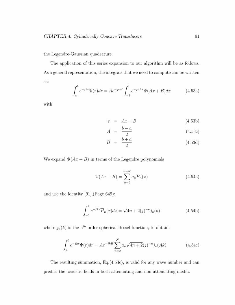
CHAPTER 4. Cylindrically Concave Transducers 91
the Legendre-Gaussian quadrature.
The application of this series expansion to our algorithm will be as follows.
As a general representation, the integrals that we need to compute can be written
as: ∫ b
a
e−jkrΨ(r)dr = Ae−jkB
∫ 1
−1
e−jkAxΨ(Ax + B)dx (4.53a)
with
r = Ax + B (4.53b)
A =b− a
2(4.53c)
B =b + a
2(4.53d)
We expand Ψ(Ax + B) in terms of the Legendre polynomials
Ψ(Ax + B) =n=N∑n=0
anP n(x) (4.54a)
and use the identity [91],(Page 649):
∫ 1
−1
e−jkxP n(x)dx =√
4n + 2(j)−njn(k) (4.54b)
where jn(k) is the nth order spherical Bessel function, to obtain:
∫ b
a
e−jkrΨ(r)dr = Ae−jkB
N∑n=0
an
√4n + 2(j)−njn(Ak) (4.54c)
The resulting summation, Eq.(4.54c), is valid for any wave number and can
predict the acoustic fields in both attenuating and non-attenuating media.

CHAPTER 4. Cylindrically Concave Transducers 92
4.4 Results
We carried out numerical and laboratory experiments to verify the method in-
troduced in this chapter. Using the formulas given in Section 4.3, the spatial
transfer function of the cylindrical transducer is calculated and compared with
the results of a numerical integration routine which computes Eq.(4.7) without
any approximations. The comparison results are validated with experimental
measurements.
4.4.1 Numerical Integration
A number of direct numerical integration techniques were applied to compute
Eq.(4.7). The Gauss-Legendre quadrature produced more accurate results in
less time than the other standard integration techniques such as trapezoidal
rule and Simpson’s rule.
The 2D numerical routine can be summarized with the following equation:
H =R
2π
N∑n=1
U∑u=1
wnwue−jk
√M(φn)+(zp−zu)2
√M(φn) + (zp − zu)2
(4.55)
where φn and zu denote the abscissas, and wn wu are the weights for φ and z
respectively. The number of terms are determined according to the maximum
frequency component of the signal. In this study 2π terms per minimum wave-
length is found to be sufficient for an accurate integral result. The number of
abscissas for z is computed by U = round(2πfmaxhco
) and the number of abscissas
for φ are: N = round(2RφmaxUh
). The routine is implemented in Matlab R14 on
a Pentium 4, 3GHz, 1GB RAM machine. The operating frequency of the trans-
ducer is 3.5MHz. To have a reasonable sized problem the maximum frequency

CHAPTER 4. Cylindrically Concave Transducers 93
of the signals is limited to 10MHz. For the transducer used in this study N=547
and U=21.
4.4.2 Experimental Comparison
A wave propagation experiment was performed to validate the spatial transfer
function formulation of the cylindrically concave transducer. For this exper-
iment, a curved 1-D array transducer (Model 8665, BK Medical, Wilmigton,
MA) consisting of 128 cylindrically curved elements was employed. The linear
array operated at 3.5 MHz and each radiator element had 70.0 mm focal length
with lateral dimensions 13 mm × 0.5 mm. The array was driven with the real
time ultrasound scanner of Analogic Corporation (AN2300). In this study the
wave propagation from a single element is measured. The array transducer was
placed in a water tank (0.8 m × 0.8 m × 1.5 m) that was filled with de-ionized
de-gassed water at approximately 21◦C. The single element radiator was oper-
ated in transmit mode using AN2300 where the system excited the transducer
with a short excitation signal that approximated a delta function and the re-
ceived echo was measured by a PVDF hydrophone with 0.1 mm radius. The data
were recorded on a digital scope (LC 334a, LeCroy, Chestnut Ridge, NY) and
transferred to a computer for later analysis. In this study, the wave propagation
in a lossless medium -in water- was investigated.
A number of experiments were performed to evaluate the performance of our
method. In this study, four comparison results are presented between measured
and simulated data. Figures 4.6 to 4.9 compare three normalized waveforms: (a)
the simulated response calculated with the method introduced in Section 4.3,
SIM1, (b) the simulated response computed with the numerical approach in

CHAPTER 4. Cylindrically Concave Transducers 94
Section 4.4.1 without any approximations, SIM2, and, (c) real measured data
in lossless medium. The error between the two simulated responses ((a) and
(b)) and the speed improvement in computation time are the most important
parameters to assess the performance of our method. The measures that will be
used to compare these two results are defined as follows:
Error% = 100‖SIM1 − SIM2‖2
‖SIM2‖2
(4.56a)
Speed Improvement Ratio =Total time required to compute SIM1
Total time required to compute SIM2
(4.56b)
To simulate the pressure fields, the density scaled electromechanical response
of the transducer, eT (ω), should be obtained. For this purpose, Eq.(4.4) is used
with a simplified Wiener filter [59] and the Fourier transform of the measured
data at the focal point (pf (ω)):
eT (ω) =pf (ω)H∗
f (ω)
|Hf (ω)|2 + q(4.57)
where Hf (ω) is the spatial transfer function at the focus, and q is the inverse of
the signal to noise ratio, and it was chosen to be 0.01max(|Hf (ω)|2) based on
the data measured at the focus.
When calculating the frequency domain signals, it must be taken into ac-
count that H has an oscillatory behavior and has some abrupt changes in time
domain. Equally sampled 512 frequency values between 0 to 10 MHz proved to
be adequate to simulate the signals. The time domain signals were obtained by
taking the inverse Fourier Transform of the signals acquired from Eq.(4.4). The
real valued wave number used in these simulations was equal to ω/co, where

CHAPTER 4. Cylindrically Concave Transducers 95
co = 1500m/s.
Figure 4.6 shows the acoustic field in Region III, on the y axis, for zp =
−2 mm. The measurements were obtained by scanning the PVDF hydrophone
vertically and recording waveforms at 19 equally spaced locations between -
1.8 mm to 1.8 mm. For this region, the error between two simulated responses
((a) and (b)) was found to be 0.07% and the speed improvement ratio 541. We
have a very close agreement with the measured data (c) and the slight differences
are attributable to the imperfections in the transducer as an ideal piston source,
and the low SNR due to the use of a single isolated element.
Figure 4.7 compares the propagation on the z axis. In this case, the PVDF
hydrophone was scanned laterally and 14 equally spaced measurements recorded
between -26 mm to 26 mm. The error between the two simulated responses
was 7.5x10⁻⁵% and the speed improvement ratio 1355. There was a very good
agreement between the measured and the predicted data.
In Figure 4.8 we investigate the off-axis propagation in Region II where a
similar scan with the previous case was performed. For this experiment the
observation points were 6mm behind the focus and parallel to the z axis. 19
equally spaced measurements were observed between -36 mm to 36 mm. The
error between two simulated responses and the speed improvement ratio were
obtained as 0.02% and 145 respectively. The decrease in the speed ratio is due to
the location of the observation points. This experiment shows the performance
of the algorithm for the observation points where two separate line integrals
should be calculated for φ dependency. There was again a very close agreement
with the measured data.
In Figure 4.9 the off-axis propagation in Regions I and II was investigated

CHAPTER 4. Cylindrically Concave Transducers 96
−30−30
−30
−30
−30
−30 −30 −30
−30 −30−25
−25
−25 −25
−25 −25
−25 −25 −25
−20 −20 −20
−20 −20−20
−15−15 −15
−15
−15−15−
15
−10−10
−10
−10−10
−10
−5 −5
−5−5
Simulated Response x=0mm z=−2mm 5 dB lines
Vertical Distance [mm]
Tim
e [µ
s]
−1 0 1
47.5
48
48.5
(a)
−30
−30 −30
−30
−30
−30 −30 −30
−30
−30−25 −25
−25 −25
−25
−25
−25−25 −25
−20 −20 −20
−20−20 −20
−15−15 −15
−15
−15−15
−15
−10−10
−10
−10−10
−10
−5
−5
−5−5
Simulated Response II x=0mm z=−2mm 5 dB lines
Vertical Distance [mm]
Tim
e [µ
s]
−1 0 1
47.5
48
48.5
(b)
−30
−30 −30−30
−30−30
−30 −30
−30 −30 −30
−25
−25
−25
−25
−25−25
−25 −25 −25
−20
−20 −20
−20 −20 −20
−15
−15 −15
−15 −15−15
−10
−10 −10
−10
−10−10
−10
−5
−5
−5
−5
Measured Response x=0mm z=−2mm 5 dB lines
Vertical Distance [mm]
Tim
e [µ
s]
−1 0 1
47.5
48
48.5
(c)
Figure 4.6: (a)Amplitude envelope of the simulated acoustic field on y axis usingthe equations derived in Section 4.3 (b)Amplitude envelope of the simulatedacoustic field on y axis using Eq.(4.55) (c) Amplitude envelope of the measuredultrasound field of a 3.5 MHz transducer.
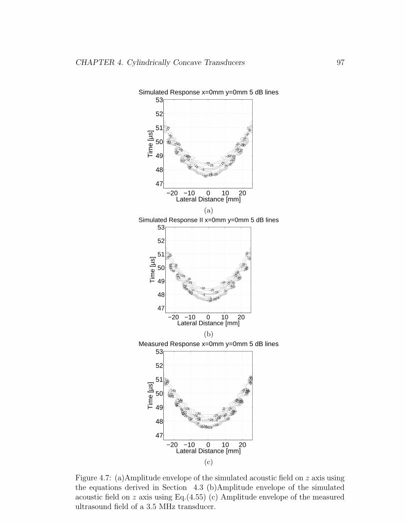
CHAPTER 4. Cylindrically Concave Transducers 97
−30 −30
−30
−30
−30
−30
−30
−30
−30
−30
−30
−30
−25 −25
−25 −25−25
−25
−25
−25
−25
−25
−25
−15 −15
−15 −15
−15
−15
−15 −15
−15
−5
−5
−5
−5
−5
−5
−5−5
Simulated Response x=0mm y=0mm 5 dB lines
Lateral Distance [mm]
Tim
e [µ
s]
−20 −10 0 10 2047
48
49
50
51
52
53
(a)
−30 −30
−30
−30
−30
−30
−30 −30
−30
−30
−30
−30
−25 −25
−25
−25
−25
−25
−25
−25
−25
−25
−25
−15 −1
5
−15
−15
−15 −15
−15
−15
−15
−5 −5
−5
−5
−5 −5
−5−5
Simulated Response II x=0mm y=0mm 5 dB lines
Lateral Distance [mm]
Tim
e [µ
s]
−20 −10 0 10 2047
48
49
50
51
52
53
(b)
−30 −30
−30
−30
−30
−30 −30
−30
−30
−30
−30
−25
−25
−25
−25
−25
−25
−25
−25−25 −2
5
−25
−25−25
−20
−20
−20
−20
−20 −20
−20−20 −20
−20
−20
−15
−15
−15
−15 −15
−15 −15
−15
−15
−15
−10
−10
−10
−10
−10
−10−10
−10
−5
−5
−5 −5
−5−5
Measured Response x=0mm y=0mm 5 dB lines
Lateral Distance [mm]
Tim
e [µ
s]
−20 −10 0 10 2047
48
49
50
51
52
53
(c)
Figure 4.7: (a)Amplitude envelope of the simulated acoustic field on z axis usingthe equations derived in Section 4.3 (b)Amplitude envelope of the simulatedacoustic field on z axis using Eq.(4.55) (c) Amplitude envelope of the measuredultrasound field of a 3.5 MHz transducer.

CHAPTER 4. Cylindrically Concave Transducers 98
−30 −30−30
−30 −
30
−30
−30 −30 −30−30−30
−30
−30
−30 −30
−30 −30
−30−30
−30
−30 −30
−15
−15
−15
−15
−15 −15
−15−15
−15
−15
−15−15
−15
−5
−5
−5−5
Simulated Response x=6mm y=0mm 5 dB lines
Lateral Distance [mm]
Tim
e [µ
s]
−20 0 20
44
46
48
50
52
(a)
−30 −30−30
−30
−30 −30
−30−30
−30 −3
0−
30
−30
−30−30
−30
−30
−30
−30
−30
−30
−30 −30
−15 −15
−15 −15
−15 −15
−15
−15
−15
−15−15 −15
−15
−5
−5
−5−5
Simulated Response II x=6mm y=0mm 5 dB lines
Lateral Distance [mm]
Tim
e [µ
s]
−20 0 20
44
46
48
50
52
(b)
−30
−30
−30 −3
0
−30
−30
−30
−30−30
−30−30
−30
−30
−30
−30
−30−30
−10
−10
−10
−10 −10−10
−10
Measured Response x=6mm y=0mm 5 dB lines
Lateral Distance [mm]
Tim
e [µ
s]
−20 0 20
44
46
48
50
52
(c)
Figure 4.8: (a)Amplitude envelope of the simulated acoustic field on the x − zplane using the equations derived in Section 4.3 (b)Amplitude envelope of thesimulated acoustic field on the x−z plane using Eq.(4.55) (c) Amplitude envelopeof the measured ultrasound field of a 3.5 MHz transducer.

CHAPTER 4. Cylindrically Concave Transducers 99
where the approximation for φ had the most significant effect on the results. For
this experiment the observation points were 6 mm behind the focus and parallel
to the y axis. 41 equally spaced measurements were observed between -4 mm to
4 mm. The error was found to be 0.12% and the speed improvement ratio 225
times. The effect of low SNR due to the use of single element can be visually
observed from Fig. (4.9) (c). The measured data is expected to be symmetric
around y=0.
4.4.3 Numerical Comparison
A numerical experiment was performed to assess the performance of our method
in lossy media. The same experiment with Figure 4.9 was simulated with a com-
plex wave number representing a power law attenuating medium. Specifically
the parameters used in this simulation were (Section 3.5):
k2(ω) =ω2
c2o
− j2ωαb(ω)
co
(4.58a)
where
co = 1500m/s (4.58b)
αb = 54(ω
ωo
)1.2Np/m (4.58c)
where ωo is the mean frequency (2π3.5MHz). The predicted responses obtained
with two different methods are given in Fig. (4.10). We have an excellent agree-
ment between two results. Quantitatively, the speed improvement ratio is ob-
tained as 225 times and the error between two simulations is 0.08%. These
comparisons confirm that the fast semi-analytical method we introduced in this
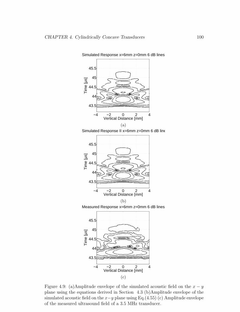
CHAPTER 4. Cylindrically Concave Transducers 100
−36
−36
−36 −36
−36
−36
−36
−36 −36−36
−36
−36
−36
−36−36
−30
−30 −30
−30
−30
−30 −30 −30
−30
−30 −30
−30 −30
−30
−30
−24
−24−24
−24
−24−24
−24
−24 −24 −24
−24−24
−18
−18 −18
−18
−18−18
−18
−18
−12 −12
−12
−6−6
Simulated Response x=6mm z=0mm 6 dB lines
Vertical Distance [mm]
Tim
e [µ
s]
−4 −2 0 2 4
43.5
44
44.5
45
45.5
(a)
−36
−36
−36 −36
−36
−36
−36
−36−36 −36
−36
−36
−36
−36−36
−30
−30 −30
−30
−30
−30 −30 −30
−30−30 −30
−30 −30
−30
−30
−24
−24−24
−24
−24−24
−24 −24 −24
−24−24
−18
−18 −18
−18
−18−18
−18
−18
−12
−12
−12
−6
−6
Simulated Response II x=6mm z=0mm 6 dB lines
Vertical Distance [mm]
Tim
e [µ
s]
−4 −2 0 2 4
43.5
44
44.5
45
45.5
(b)
−36
−36
−36
−36
−36
−36−36
−36
−36
−36
−36 −36 −36
−36−36 −36
−36−36
−30
−30
−30
−30−30
−30−30−30
−30
−30 −30 −30
−30
−30−30
−30
−24
−24
−24
−24
−24
−24
−24 −24 −24
−24−18
−18
−18
−18 −18 −18
−18
−12−12
−12
−12
−12−6 −6
−6
Measured Response x=6mm z=0mm 6 dB lines
Vertical Distance [mm]
Tim
e [µ
s]
−4 −2 0 2 4
43.5
44
44.5
45
45.5
(c)
Figure 4.9: (a)Amplitude envelope of the simulated acoustic field on the x − yplane using the equations derived in Section 4.3 (b)Amplitude envelope of thesimulated acoustic field on the x−y plane using Eq.(4.55) (c) Amplitude envelopeof the measured ultrasound field of a 3.5 MHz transducer.

CHAPTER 4. Cylindrically Concave Transducers 101
−4 −2 0 2 4
43.5
44
44.5
45
45.5
Vertical Distance [mm]
Tim
e [µ
s]
Simulated Response x=6mm z=0mm 6 dB lines
−6
−6−6−12
−12 −12
−12
−12−12
−18
−18
−18 −18 −18
−18
−18 −18 −18
−18 −18
−18−18
−24 −24 −24
−24−24−2
4−24
−24
−24 −24
−24
−24−24
−24−24
−24
−24−24
−30−30 −30
−30 −30 −30 −30
−30−30
−30−30
−30 −30
−30 −30 −30−30−30
−36 −36 −36−36−36
−36−36−36
(a)
−4 −2 0 2 4
43.5
44
44.5
45
45.5
Vertical Distance [mm]
Tim
e [µ
s]
Simulated Response II x=6mm z=0mm 6 dB lines
−6 −6
−6−12
−12 −12
−12
−12−12
−18
−18
−18 −18 −18
−18
−18 −18 −18
−18 −18
−18−18
−24 −24 −24
−24−24
−24
−24
−24−24 −24
−24
−24
−24
−24
−24
−24−24
−24−24
−30 −30 −30
−30 −30 −30
−30
−30
−30−30
−30
−30−30
−30 −30
−30 −30 −30−30−30
−36 −36−36−36−36
−36 −36−36
(b)
Figure 4.10: (a)Amplitude envelope of the simulated acoustic field on the x− yplane for lossy medium using the equations derived in Section 4.3 (b)Amplitudeenvelope of the simulated acoustic field for lossy medium on the x−y plane usingEq.(4.55)
CHAPTER 4. Cylindrically Concave Transducers 102
chapter can be used to predict the field of a cylindrically concave transducer for
any physically realisable lossy homogenous medium.
4.5 Conclusion
In this study, we introduced a fast method to compute the spatial transfer func-
tion of cylindrically concave transducers in lossless and attenuating medium.
For cylindrically focused transducers with low gain, we were able to use geomet-
rical information to transform the 2D surface integral from an elliptic type to a
parabolic type. The integrals could be evaluated by reducing the problem to a
1D line integral. The integrand was expressed as a truncated series of Legendre
polynomials, from which it was possible to evaluate the line integral as a sum of
spherical Bessel functions.
The form of the line integrals is such that the coefficients of the Legendre
polynomials depend only on geometry and not on frequency. They only need to
be calculated once and then the response at any frequency can be determined
by a summation where the number of terms does not depend on frequency. This
contrasts to direct integration approaches which need to employ finer discretiza-
tion for higher frequency components.
The method was compared to an optimized numerical method which evalu-
ated the surface integral directly. The speed of our algorithm depends on the
number of the line integrals that need to be evaluated for an observation point.
For the specific transducer that we used in our study, the speed improvement is
between 40 and 1400 and the maximum error between two simulations was found
to be 0.4%. Speed of evaluation is important because linear arrays employ 32 to
128 elements, each usually with a different phase and amplitude and potentially

CHAPTER 4. Cylindrically Concave Transducers 103
individual waveforms. Hence, the advantage of the method will be revealed for
array applications that requires the repeated computation of the time consum-
ing numerical routines. Moreover, our semi-analytical frequency domain method
can predict the spatial response of a cylindrical radiator in lossy medium simply
by adding an imaginary component to the wave number.
In summary, we present a powerful semi-analytical method which comple-
ments the numerical approaches in the current literature. The approach can
predict the acoustic field for a cylindrical concave transducer in attenuating
homogeneous media. The approach can be applied to determine the fields in
classical beam forming and also for applications such as tomography, that do
not employ delay and sum beamforming. The application of this model to pre-
dict the acoustic properties of the HIFU lesions will be explained in the next
chapter.

Chapter 5
Shape Based Inversion
In the previous chapters, the forward problem of finding the field measurements
from a given acoustic inhomogeneity of density, attenuation and sound speed is
formulated. In this chapter, the inverse problem of reconstructing the perturba-
tion parameters from field measurements will be analyzed and solved.
The motive behind the inversion problem -as explained previously in the
introduction- is to develop and validate quantitative, fully three dimensional
ultrasonic imaging methods to determine the spatial structure of the HIFU le-
sion. It has been reported that the treatment results in an ellipsoidal lesion in
which the acoustic properties of the tissue, sound speed and attenuation, are
significantly altered from their nominal values. An inversion method giving the
quantitative information about the tissue properties can, in principle, be used
to image the HIFU lesions. Complicating this approach is the fact that the
computational size of the most of the relevant 3D problems makes traditional
pixel based inversion methods impractical.
In this study we developed and implemented a shaped based inversion method
to image the HIFU lesions. Rather than trying to reconstruct the thousands of
104

CHAPTER 5. Shape Based Inversion 105
voxels defining the lesion, we concentrated on specifying the parameters de-
scribing the shape of the perturbation. We demonstrated that the shape based
inversion method can be employed for ultrasound data. The proposed method
is validated using simulated and measured broadband ultrasound backscatter
data.
This chapter is organized as follows: The first section introduces the shape
based inversion problem and describe the model and the formulae describing the
boundary of the ellipsoidal perturbations. In Section 5.2, we give the mathe-
matical details of the optimization routine and discuss the Jacobian calculation.
In Section 5.3 we present the inversion results with simulated and measured
backscattered data. The chapter is concluded in Section 5.4.
5.1 Mathematical Description and Background
5.1.1 Forward Model
To present the forward model, Eq.(3.24) from Chapter 3 is recalled in Eq.(5.1).
By replacing k2s with its mathematical equivalent, the scattered field can be
described by:
ps(r, ω) = −∫
V ′cp(r
′)G(r, r′, ω)
[2ω2
c3b
]pb(r
′, ω)d3r′
−∫
V ′αp(r, ω)G(r, r′, ω)
[j2ω
cb
]pb(r
′, ω)d3r′
+
∫
V ′σp(r
′)∇pb(r′, ω).∇G(r, r′, ω)d3r′ (5.1)
CHAPTER 5. Shape Based Inversion 106
This equation can be written in a more compact form
ps(r, ω) =
∫
V ′K1(r, r
′, ω)cp(r′)d3r′ +
∫
V ′K2(r, r
′, ω)αp(r′)d3r′ +
∫
V ′K3(r, r
′, ω)σp(r′)d3r′ (5.2)
where Ki, i = 1, 2, 3 depend only on the background properties. To represent
the forward model in terms of the experimental measurements Eq.(3.32) from
Chapter 3 will be used to obtain Ki.
For the imaging system of interest in this work we assume we have multiple
transmitters and receivers. For the case of NT transmitters and NR receivers
with NS frequency samples the measured data (y) can be written as a column
vector of size NT × NS × NR. Discretizing Eq.(5.2) at any position r′, the
scattered field can be written in a matrix-vector model of the form:
y =
[K1 K2 K3
]
f1
f2
f3
+ n = Kf + n (5.3)
where
• K is the matrix representation of the integral
• f1 is the column vector containing the voxel values of sound speed pertur-
bation, cp
• f2 is the column vector containing the voxel values of attenuation pertur-
bation, αp
CHAPTER 5. Shape Based Inversion 107
• f3 is the column vector containing the voxel values of density perturba-
tion, σp
• n is the additive sensor noise.
The ultimate goal is to restore the unknown medium parameters from measured
backscatter data. The traditional approach to this problem is to use linear inver-
sion methods, and try to reconstruct the voxelated versions of the sound speed,
density and absorption images. As discussed previously in the introduction
chapter, the nominal wavelength of the acoustic field in tissue is about 0.3mm
and the physical size of the region that we want to image is about 30mm which
implies an accurate discretization of the problem, 0.1 wavelengths, requires a
billion of voxels. The linear inversion problem is very ill-posed for this case due
to the enormous number of voxels defining each of the three unknown vectors
f1, f2, f3.
Our approach to the problem is based on the specification of the parameters
describing the shape of the perturbations. We assume the shape of the per-
turbations are known to be ellipsoids but the locations, sizes and orientations
are unknown. Specifically, the perturbations in Eq.(5.2), cp, αp, and σp, are
represented by ellipsoidal shapes.
To completely characterize the perturbation in one variable, we only need the
location of the center (xo, yo, zo), the lengths of the three axes of the ellipsoid
(l1, l2, l3), three angles (θ1, θ2, θ3) that orient the ellipsoid in space and (M)
contrast of the perturbation. Thus rather than the billion of voxels defining each
of the three unknown vectors, we have only 3 × 10=30 quantities to estimate
from the measured data. This approach is nonlinear but better posed.
CHAPTER 5. Shape Based Inversion 108
5.1.2 Ellipsoid Modeling
Exact Model of the Ellipsoid
In mathematical notation a perturbation ellipsoid can be defined with four ele-
ments:
• A length-3 vector, c, denoting the center of the ellipsoid, (xo, yo, zo).
• A diagonal matrix D = Diag(d) whose diagonal entries are the one over
the lengths of the semi-axes, (l1, l2, l3).
• An orthonormal matrix U whose three columns are the coordinates of the
semi-axes defined in therm of the Euler angles, (θ1, θ2, θ3).
• A constant M, defining the contrast of the object.
We begin by defining c, D, U :
c =
xo
yo
zo
(5.4)
D =
1/l1 0 0
0 1/l2 0
0 0 1/l3
(5.5)
U = U1(θ1)U2(θ2)U3(θ3) (5.6a)

CHAPTER 5. Shape Based Inversion 109
U =
cos(θ1) sin(θ1) 0
−sin(θ1) cos(θ1) 0
0 0 1
cos(θ2) 0 sin(θ2)
0 1 0
−sin(θ2) 0 cos(θ2)
cos(θ3) sin(θ3) 0
−sin(θ3) cos(θ3) 0
0 0 1
(5.6b)
A point r′ = [x′, y′, z′]T is determined to be on or in the ellipsoid if
||DUT (r′ − c)||22 ≤ 1 (5.7)
There are multiple ways to define the rotation matrix from Euler angles [92].
However, it has been reported that the representation of the U makes little
difference on the performance of the algorithm [56]. The representation type we
used here is referred as the ”x-convention” [56].
Having described the boundary of the anomaly, we define a support function
S(r′) which has value (1) on the ellipsoid and (0) outside. Mathematically S(r′)
will be represented as
S(r′) =
1 r′ ε ellipsoid
0 otherwise
(5.8)
Using the ellipsoid representation given above, we can use Eq.(5.7) to de-
termine if the centers of the voxels in the region of interest lies in or on the
ellipsoid. If the observation point is within the ellipsoid, S(r′) will be assigned
to 1. By means of this support function the perturbations will be defined as:
γ(r′) = MS(r′) (5.9)
CHAPTER 5. Shape Based Inversion 110
The support function that we chose to represent the anomalies, S(r′), is a
step function which gives discontinuity at the boundary of the ellipsoid. For the
performance of the optimization routine we should have a smooth approximation
for the boundary. Specifically, the key to any non-linear minimization technique
is to specify the Jacobian of the objective function with respect to the unknown
parameters. With such a representation, the Jacobian of the function should be
computed numerically which would increase the overall computation time of the
optimization routine. To obtain an analytical representation of the Jacobian we
should have a differentiable expression that maps the parameters describing the
shape to any point r′ in the region of interest.
To improve the performance of the optimization routine that will be used
in this study, we introduced a filter like decision function which approximates
a step function. Specifically, the decision function takes ||DUT (r′ − c)||22 as the
argument, produces zero output for the input values slightly larger than one
and provides a smooth transition from 1 to 0 at the boundary. The type of the
function used in this study will be introduced in the next section.
Approximate Model of the Ellipsoid: Sech
In this section we will introduce a differentiable expression to describe the bound-
ary of the ellipsoid. Specifically such an expression, which will be named as
decision function from now on, should satisfy these three properties:
The decision function
1. should be a function of r′ and ellipsoid parameters,
2. should have value 1 on and inside of the ellipsoid and 0 outside,

CHAPTER 5. Shape Based Inversion 111
−2 −1 0 1 20
0.2
0.4
0.6
0.8
1
1.2
1.4
1.6
1.8exp(sech(1.3x8))−1
0 0.5 1 1.5 2−8
−7
−6
−5
−4
−3
−2
−1
0∂[exp(sech(1.3x8))−1]/∂ x
Figure 5.1: Decision function A(x) and its derivative
3. should provide smooth transition from 1 to 0 at the boundary for differ-
entiability.
There are a number of functions which satisfies these properties. In this study
a function of sech is chosen as the decision function for the reasons that will be
explained below. We define the decision function, A(x), and the perturbations
as:
A(x) = exp(sech(1.3x8))− 1 (5.10a)
γ(r′) = exp(Msech(1.3||DUT (r′ − c)||162 ))− 1 (5.10b)
The decision function A(x), Eq.(5.10a), and its derivative are given in Fig. (5.1).
The function A(x), approximates a box and its derivative estimates an impulse
function. sech(1.3x8) is the main component of the decision function that
characterizes the shape of the box in Fig. (5.1). The coefficient 1.3 is chosen so
that without the scaling from the exponential function, the boundary value of
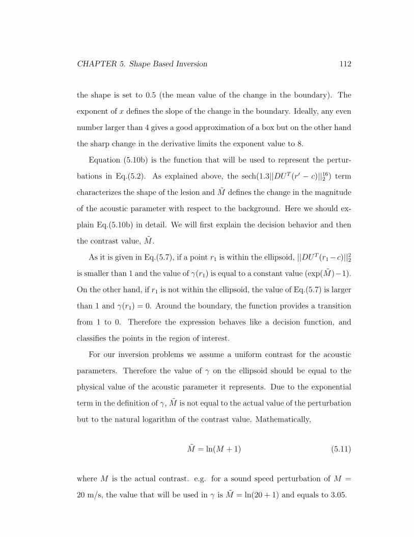
CHAPTER 5. Shape Based Inversion 112
the shape is set to 0.5 (the mean value of the change in the boundary). The
exponent of x defines the slope of the change in the boundary. Ideally, any even
number larger than 4 gives a good approximation of a box but on the other hand
the sharp change in the derivative limits the exponent value to 8.
Equation (5.10b) is the function that will be used to represent the pertur-
bations in Eq.(5.2). As explained above, the sech(1.3||DUT (r′ − c)||162 ) term
characterizes the shape of the lesion and M defines the change in the magnitude
of the acoustic parameter with respect to the background. Here we should ex-
plain Eq.(5.10b) in detail. We will first explain the decision behavior and then
the contrast value, M .
As it is given in Eq.(5.7), if a point r1 is within the ellipsoid, ||DUT (r1−c)||22is smaller than 1 and the value of γ(r1) is equal to a constant value (exp(M)−1).
On the other hand, if r1 is not within the ellipsoid, the value of Eq.(5.7) is larger
than 1 and γ(r1) = 0. Around the boundary, the function provides a transition
from 1 to 0. Therefore the expression behaves like a decision function, and
classifies the points in the region of interest.
For our inversion problems we assume a uniform contrast for the acoustic
parameters. Therefore the value of γ on the ellipsoid should be equal to the
physical value of the acoustic parameter it represents. Due to the exponential
term in the definition of γ, M is not equal to the actual value of the perturbation
but to the natural logarithm of the contrast value. Mathematically,
M = ln(M + 1) (5.11)
where M is the actual contrast. e.g. for a sound speed perturbation of M =
20 m/s, the value that will be used in γ is M = ln(20 + 1) and equals to 3.05.
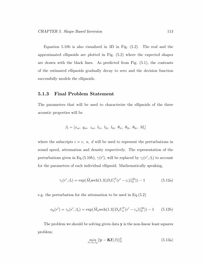
CHAPTER 5. Shape Based Inversion 113
Equation 5.10b is also visualized in 3D in Fig. (5.2). The real and the
approximated ellipsoids are plotted in Fig. (5.2) where the expected shapes
are drawn with the black lines. As predicted from Fig. (5.1), the contrasts
of the estimated ellipsoids gradually decay to zero and the decision function
successfully models the ellipsoids.
5.1.3 Final Problem Statement
The parameters that will be used to characterize the ellipsoids of the three
acoustic properties will be
βi = [xoi, yoi, zoi, l1i, l2i, l3i, θ1i, θ2i, θ3i, Mi]
where the subscripts i = c, a, d will be used to represent the perturbations in
sound speed, attenuation and density respectively. The representation of the
perturbations given in Eq.(5.10b), γ(r′), will be replaced by γi(r′, βi) to account
for the parameters of each individual ellipsoid. Mathematically speaking,
γi(r′, βi) = exp(Misech(1.3||DiU
Ti (r′ − ci)||16
2 ))− 1 (5.12a)
e.g. the perturbation for the attenuation to be used in Eq.(5.2)
αp(r′) = γa(r
′, βa) = exp(Masech(1.3||DaUTa (r′ − ca)||16
2 ))− 1 (5.12b)
The problem we should be solving given data y is the non-linear least squares
problem:
βc,βa,βd
min ||y −Kf(β)||22 (5.13a)

CHAPTER 5. Shape Based Inversion 114
Figure 5.2: The expected shapes are drawn with black lines on top of the ap-proximated ellipsoids. The contrasts of the ellipsoids are shown with the colorscales. As predicted from Fig. (5.1) the contrast values gradually decay to zero.

CHAPTER 5. Shape Based Inversion 115
β =
βc
βa
βd
(5.13b)
5.2 Inversion Approach
We propose to solve the minimization problem in Eq.(5.13a) using Gauss-Newton
method [93]. For this purpose, we first provide an initial guess for the ellipsoid
parameters (β0). Subsequent guesses (βk) for the parameter vectors are then
produced by the recurrence relation:
βk+1 = βk + αktk, 0 ≤ k ≤ kmax (5.14)
where αk is the sense optimal, kmax is the maximum number of iterations and
tk is the search direction and obtained from the solution of:
(JT J)tk = −JT ||y −Kf(βk)||2 (5.15)
Here J is the Jacobian and T is the transpose operator.
Jacobian Calculation
The Jacobian matrix will be obtained from the matrix multiplication defined in
Eq.(5.3).
∂y
∂µ= −
[K1 K2 K3
]
∂f1∂µ
∂f2∂µ
∂f3∂µ
(5.16)

CHAPTER 5. Shape Based Inversion 116
where µ is the unknown geometric parameter of the ellipsoid and as discussed
before, fis are the column vectors containing the voxel values of the perturba-
tions. To obtain Jacobian matrix, the derivatives of Eq.(5.12a) with respect to
the unknown ellipsoid parameters should be obtained. The mathematical details
are explained below.
Using the chain rule:
∂γi(r′, βi)
∂µ= −10.4Misech(1.3x8)tanh(1.3x8)x7exp(Misech(1.3x8))
∂x
∂µ(5.17a)
∂γi(r′, βi)
∂Mi
= sech(1.3x8)exp(Misech(1.3x8)) (5.17b)
where x = ||DiUTi (r − ci)||22. Using matrix algebra x can be written as:
x = (r′ − ci)T UiD
Ti DiU
Ti (r′ − ci)
The derivative of x with respect to the ellipsoid parameters can be obtained
with matrix calculus.
∂x
∂xoi, yoi, zoi
= 2∂(r′ − ci)
T
∂xoi, yoi, zoi
UiDTi DiU
Ti (r′ − ci) (5.18a)
where
∂(r′−ci)∂xoi
=
−1
0
0
∂(r′−ci)∂yoi
=
0
−1
0
∂(r′−ci)∂zoi
=
0
0
−1
(5.18b)
∂x
∂l1i, l2i, l3i
= 2(r′ − ci)T UiD
Ti
∂Di
∂l1i, l2i, l3i
UTi (r′ − ci) (5.19a)
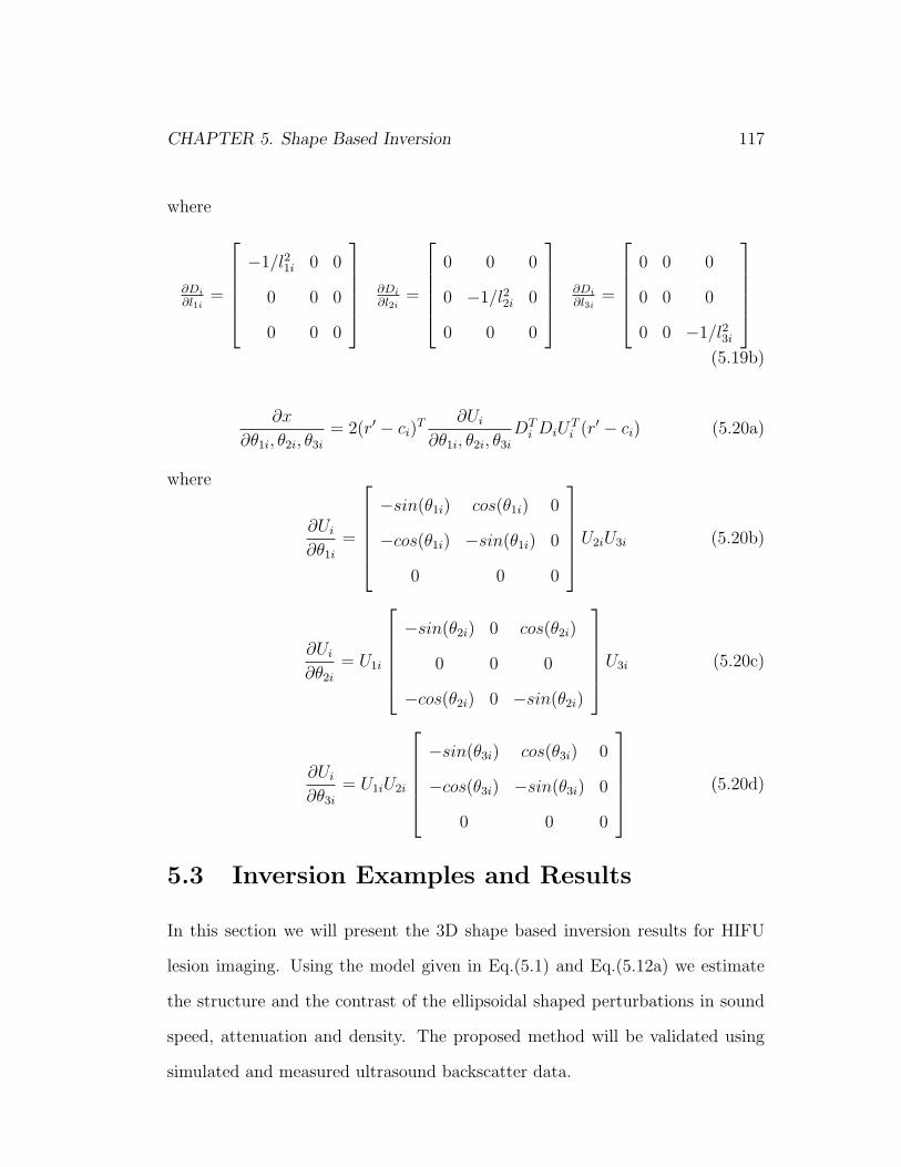
CHAPTER 5. Shape Based Inversion 117
where
∂Di
∂l1i=
−1/l21i 0 0
0 0 0
0 0 0
∂Di
∂l2i=
0 0 0
0 −1/l22i 0
0 0 0
∂Di
∂l3i=
0 0 0
0 0 0
0 0 −1/l23i
(5.19b)
∂x
∂θ1i, θ2i, θ3i
= 2(r′ − ci)T ∂Ui
∂θ1i, θ2i, θ3i
DTi DiU
Ti (r′ − ci) (5.20a)
where
∂Ui
∂θ1i
=
−sin(θ1i) cos(θ1i) 0
−cos(θ1i) −sin(θ1i) 0
0 0 0
U2iU3i (5.20b)
∂Ui
∂θ2i
= U1i
−sin(θ2i) 0 cos(θ2i)
0 0 0
−cos(θ2i) 0 −sin(θ2i)
U3i (5.20c)
∂Ui
∂θ3i
= U1iU2i
−sin(θ3i) cos(θ3i) 0
−cos(θ3i) −sin(θ3i) 0
0 0 0
(5.20d)
5.3 Inversion Examples and Results
In this section we will present the 3D shape based inversion results for HIFU
lesion imaging. Using the model given in Eq.(5.1) and Eq.(5.12a) we estimate
the structure and the contrast of the ellipsoidal shaped perturbations in sound
speed, attenuation and density. The proposed method will be validated using
simulated and measured ultrasound backscatter data.
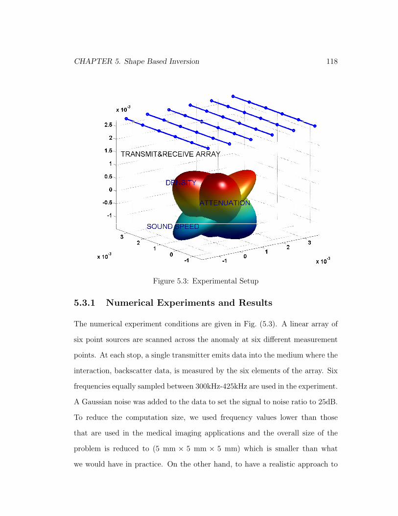
CHAPTER 5. Shape Based Inversion 118
Figure 5.3: Experimental Setup
5.3.1 Numerical Experiments and Results
The numerical experiment conditions are given in Fig. (5.3). A linear array of
six point sources are scanned across the anomaly at six different measurement
points. At each stop, a single transmitter emits data into the medium where the
interaction, backscatter data, is measured by the six elements of the array. Six
frequencies equally sampled between 300kHz-425kHz are used in the experiment.
A Gaussian noise was added to the data to set the signal to noise ratio to 25dB.
To reduce the computation size, we used frequency values lower than those
that are used in the medical imaging applications and the overall size of the
problem is reduced to (5 mm × 5 mm × 5 mm) which is smaller than what
we would have in practice. On the other hand, to have a realistic approach to

CHAPTER 5. Shape Based Inversion 119
the problem, we used the tissue mimicking dispersive model from Chapter 3 to
represent the background. The parameters used in the simulations are: cb =
1551m/s, ρb = 1045kg/m3, αb = 3.6(ω/ωo)1.2 where ωo = 2π350kHz. The
values of the contrasts for a realistic problem are chosen as explained below.
Total number of voxels in the region of interest is 4096 (16×16×16).
It has been confirmed with many publications that, the heating of tissue
affects both sound speed and attenuation [38–43]. The change in sound speed
is less that 20m/s about (1%) and in most cases reported to be reversible.
The attenuation coefficient has been measured to increase dramatically with
values ranging from 80%-700% which is still in the Born approximation range.
More precisely, for the Born approximation to be valid, the constraint on the
attenuation is defined as the smallness of αp/kb. Mathematically, as previously
discussed in Chapter 3, the nominal attenuation in human tissue is 35.6 Np/m
at 3.5 MHz. For the nominal sound speed of 1551 m/s and 700% perturbation in
attenuation, the ratio of αp/kb is 17x10−3. The change in the density is limited to
1% to validate the Born model of Chapter 3. Thus the bounds for the contrasts,
Mi, are chosen as:
• 0 m/s < Mc < 20 m/s
• 0 Np/m < Ma < 20 Np/m
• 0 kg/m3 < σp < 10 kg/m3, hence 0 < Md < 9.5x10⁻³
The inversion method described in Section 5.2 is implemented in Matlab where
the ”lsqnonlin” function with Gauss-Newton option is used. The geometric pa-
rameters and the contrasts of the ellipsoids, βi, are scaled to the same order

CHAPTER 5. Shape Based Inversion 120
Table 5.1: Lower and upper limits for the geometric parameters of the ellipsoidLower Limit Upper Limit
xo -2.5 mm 2.5 mmyo -2.5 mm 2.5 mmzo -2.5 mm 2.5 mml1 5x10⁻⁴ 2.5 mml2 5x10⁻⁴ 2.5 mml3 5x10⁻⁴ 2.5 mmθ1 0 2πθ2 0 πθ3 0 2π
(between 1 and 2) prior to the optimization routine to maximize the perfor-
mance. The bounds for the geometric parameters are given in Table 5.1. The
lower limits for the lengths of the semi axes is set to small number (different than
0) for proper solution. We set the lower and the upper bounds for the ”lsqnon-
lin” function to 1 and 2 respectively to ensure that the boundary of the ellipsoid
is in the region of interest and the contrasts are within the above defined limits.
Physically, in case of HIFU experiments we have prior knowledge of the rough
location and the approximate contrasts of the HIFU lesion. We basically use
this prior information and limit our search around the HIFU region.
A number of experiments are performed to assess the performance of the
inversion algorithm and to explore its ability to reconstruct the HIFU lesions.
In Fig. (5.4)-Fig. (5.6) we display the true ellipsoid distributions, the initial
guesses provided to our estimation method and the final result. For comparison
purposes, the true shapes are plotted with blue lines on the estimated ellipsoids.
Two measures are introduced to describe the error between real and simulated
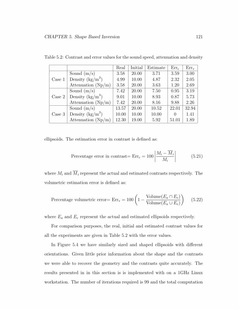
CHAPTER 5. Shape Based Inversion 121
Table 5.2: Contrast and error values for the sound speed, attenuation and density
Real Initial Estimate Errc Errv
Sound (m/s) 3.58 20.00 3.71 3.59 3.00
Case 1 Density (kg/m3) 4.99 10.00 4.87 2.32 2.05Attenuation (Np/m) 3.58 20.00 3.63 1.20 2.69Sound (m/s) 7.42 20.00 7.50 0.95 3.19
Case 2 Density (kg/m3) 9.01 10.00 8.93 0.87 5.73Attenuation (Np/m) 7.42 20.00 8.16 9.88 2.26Sound (m/s) 13.57 20.00 10.52 22.01 32.94
Case 3 Density (kg/m3) 10.00 10.00 10.00 0 1.41Attenuation (Np/m) 12.30 19.00 5.92 51.01 1.89
ellipsoids. The estimation error in contrast is defined as:
Percentage error in contrast= Errc = 100
∣∣∣∣Mi −M i
Mi
∣∣∣∣ (5.21)
where Mi and M i represent the actual and estimated contrasts respectively. The
volumetric estimation error is defined as:
Percentage volumetric error= Errv = 100
(1− Volume(Ea ∩ Ee)
Volume(Ea ∪ Ee)
)(5.22)
where Ea and Ee represent the actual and estimated ellipsoids respectively.
For comparison purposes, the real, initial and estimated contrast values for
all the experiments are given in Table 5.2 with the error values.
In Figure 5.4 we have similarly sized and shaped ellipsoids with different
orientations. Given little prior information about the shape and the contrasts
we were able to recover the geometry and the contrasts quite accurately. The
results presented in in this section is is implemented with on a 1GHz Linux
workstation. The number of iterations required is 99 and the total computation
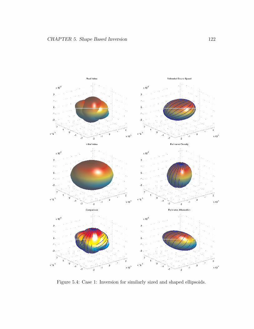
CHAPTER 5. Shape Based Inversion 122
Figure 5.4: Case 1: Inversion for similarly sized and shaped ellipsoids.
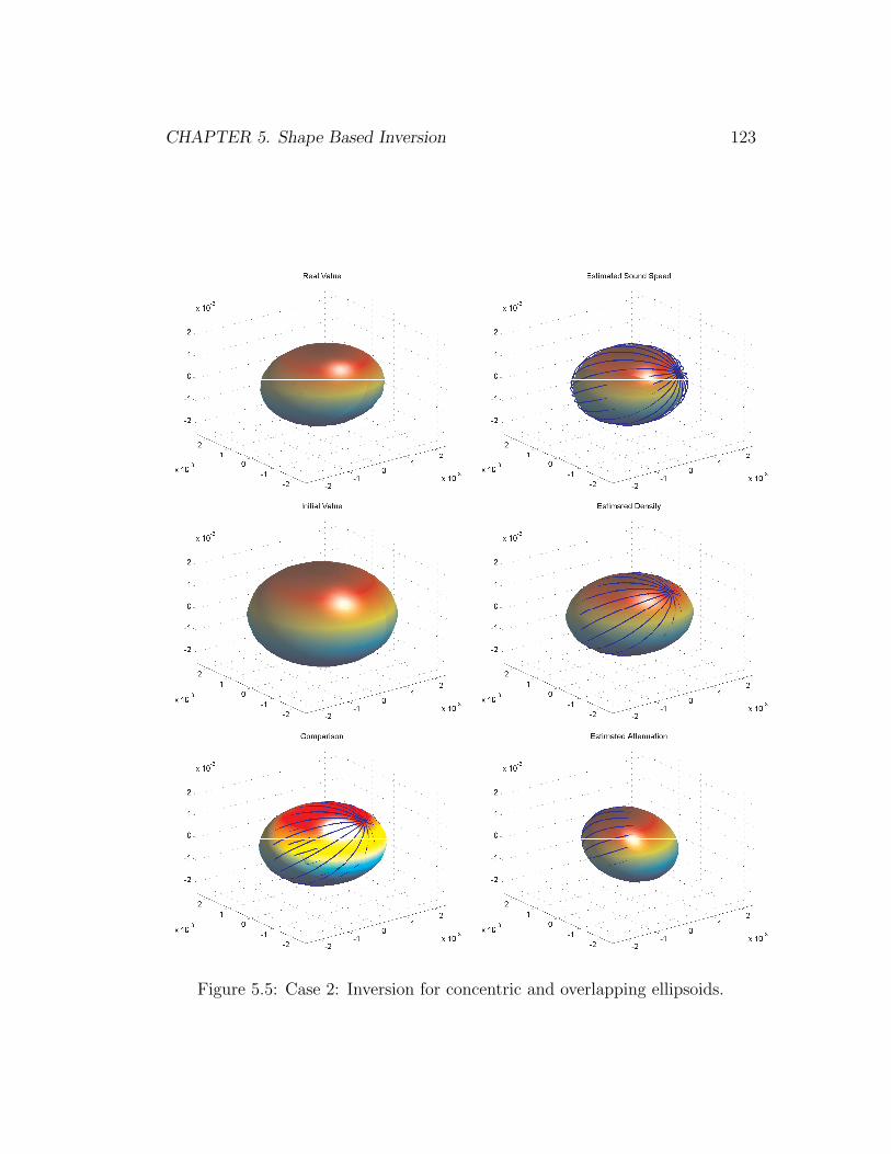
CHAPTER 5. Shape Based Inversion 123
Figure 5.5: Case 2: Inversion for concentric and overlapping ellipsoids.
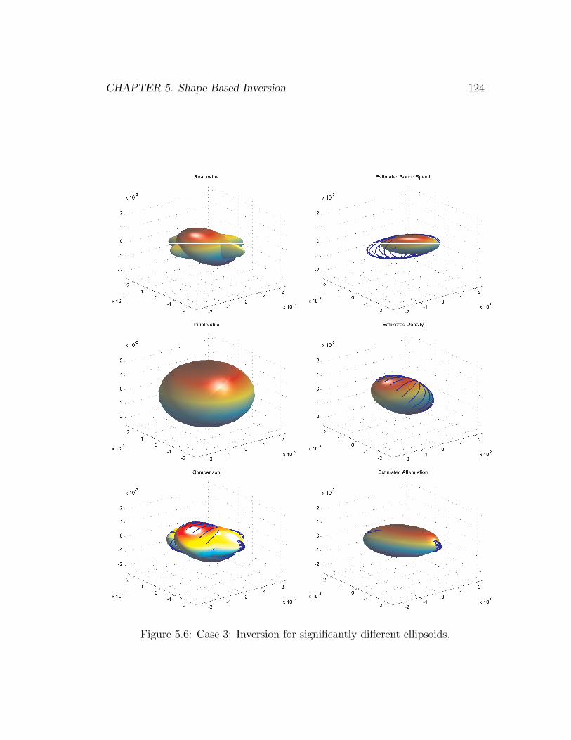
CHAPTER 5. Shape Based Inversion 124
Figure 5.6: Case 3: Inversion for significantly different ellipsoids.

CHAPTER 5. Shape Based Inversion 125
time is about 14 minutes.
In Figure 5.5 we examine a case in which we have three concentric, over-
lapping ellipsoids. This represents a lesion where the changes of the acoustic
properties confined into a single region of space. At first glance it appears as
if there is a single ellipsoid anomaly. However, we were able to classify three
distinct ellipsoids with our method. Although the initial estimates for the con-
trasts are considerably different than the real values, we obtained a very good
estimate for the contrasts and the geometries. The method we proposed to de-
fine the contrast of the object as a nonlinear parameter of the problem, greatly
improved the contrast detection. The number of iterations required is 98 and
the total computation time is about 14 minutes.
In the third case, Fig. (5.6), we study a scenario where we have three sig-
nificantly different ellipsoids. We again have a quite successful localization of
the perturbations. The slight differences are attributable to the dissimilar ori-
entation angles and the noise in the data. Our observations revealed that, the
rotation angles are the most difficult parameters to estimate for this type of
shape based inversion problems. The number of iterations required is 299 and
the total computation time is about 24 minutes. The same experiment is re-
peated with a noise level that sets the signal-to-noise to 40dB and a better
localization is obtained for the sound anomaly.
5.3.2 Error Analysis
A statistical error analysis was done to assess more thoroughly the performance
of the inversion method presented in this chapter. For this purpose, a Monte
Carlo simulation was performed in which we considered 140 estimation problems
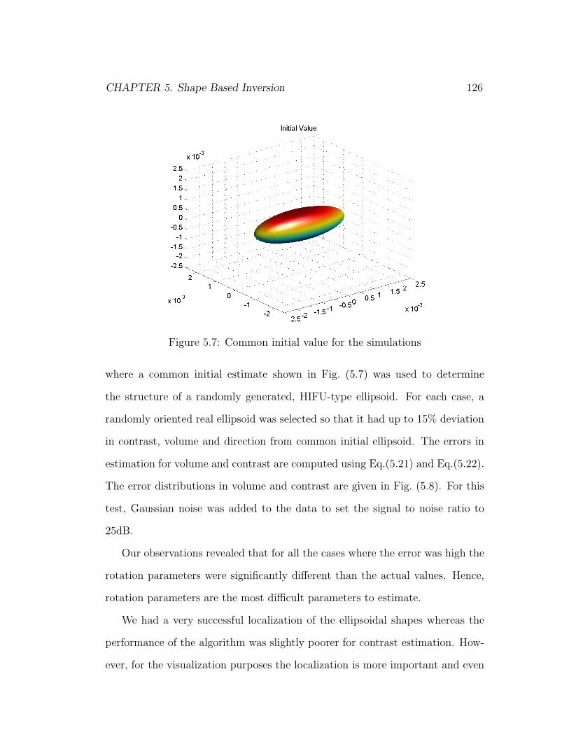
CHAPTER 5. Shape Based Inversion 126
Figure 5.7: Common initial value for the simulations
where a common initial estimate shown in Fig. (5.7) was used to determine
the structure of a randomly generated, HIFU-type ellipsoid. For each case, a
randomly oriented real ellipsoid was selected so that it had up to 15% deviation
in contrast, volume and direction from common initial ellipsoid. The errors in
estimation for volume and contrast are computed using Eq.(5.21) and Eq.(5.22).
The error distributions in volume and contrast are given in Fig. (5.8). For this
test, Gaussian noise was added to the data to set the signal to noise ratio to
25dB.
Our observations revealed that for all the cases where the error was high the
rotation parameters were significantly different than the actual values. Hence,
rotation parameters are the most difficult parameters to estimate.
We had a very successful localization of the ellipsoidal shapes whereas the
performance of the algorithm was slightly poorer for contrast estimation. How-
ever, for the visualization purposes the localization is more important and even

CHAPTER 5. Shape Based Inversion 127
0 2 4 6 8 10 12 14 16 18 200
5
10
15
20
25
30
35
40
45Distribution of Volumetric Error
Percentage Error
Num
ber
of C
ases
5 10 15 200
5
10
15
20
25
Distribution of Contast Error
Percentage Error
Num
ber
of C
ases
(a) (b)
Figure 5.8: Distribution of volumetric and contrast errors
the contrast errors were higher, in 75% of the studied cases the error was less
than or equal to 10%.
The results showed that, the method given in this chapter was largely suc-
cessful to estimate the randomly oriented ellipsoids.
5.3.3 Laboratory Experiment and Results
A laboratory experiment was performed to validate the inversion method de-
veloped in this chapter. The ideas presented in Section 5.1 were used with
data obtained from a single agar ellipsoid anomaly, which was volumetrically
homogenous, immersed into a homogenous lossy medium. The backscattering
measurements were obtained by a linear array transducer. The experiment and
the simulation details are presented in the following sections.
Linear Array Transducer
The linear array transducer that is introduced in Chapter 4 is used for a
backscattering experiment. The array (Model 8665, BK Medical, Wilmigton,
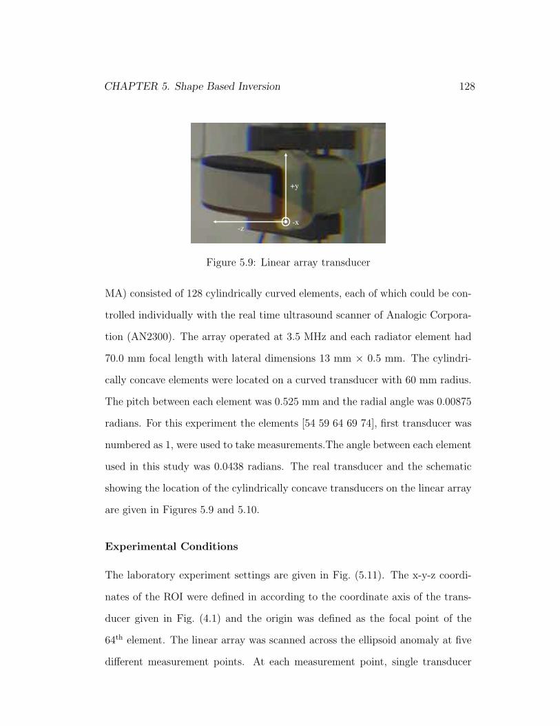
CHAPTER 5. Shape Based Inversion 128
+y
-x-z
Figure 5.9: Linear array transducer
MA) consisted of 128 cylindrically curved elements, each of which could be con-
trolled individually with the real time ultrasound scanner of Analogic Corpora-
tion (AN2300). The array operated at 3.5 MHz and each radiator element had
70.0 mm focal length with lateral dimensions 13 mm × 0.5 mm. The cylindri-
cally concave elements were located on a curved transducer with 60 mm radius.
The pitch between each element was 0.525 mm and the radial angle was 0.00875
radians. For this experiment the elements [54 59 64 69 74], first transducer was
numbered as 1, were used to take measurements.The angle between each element
used in this study was 0.0438 radians. The real transducer and the schematic
showing the location of the cylindrically concave transducers on the linear array
are given in Figures 5.9 and 5.10.
Experimental Conditions
The laboratory experiment settings are given in Fig. (5.11). The x-y-z coordi-
nates of the ROI were defined in according to the coordinate axis of the trans-
ducer given in Fig. (4.1) and the origin was defined as the focal point of the
64th element. The linear array was scanned across the ellipsoid anomaly at five
different measurement points. At each measurement point, single transducer
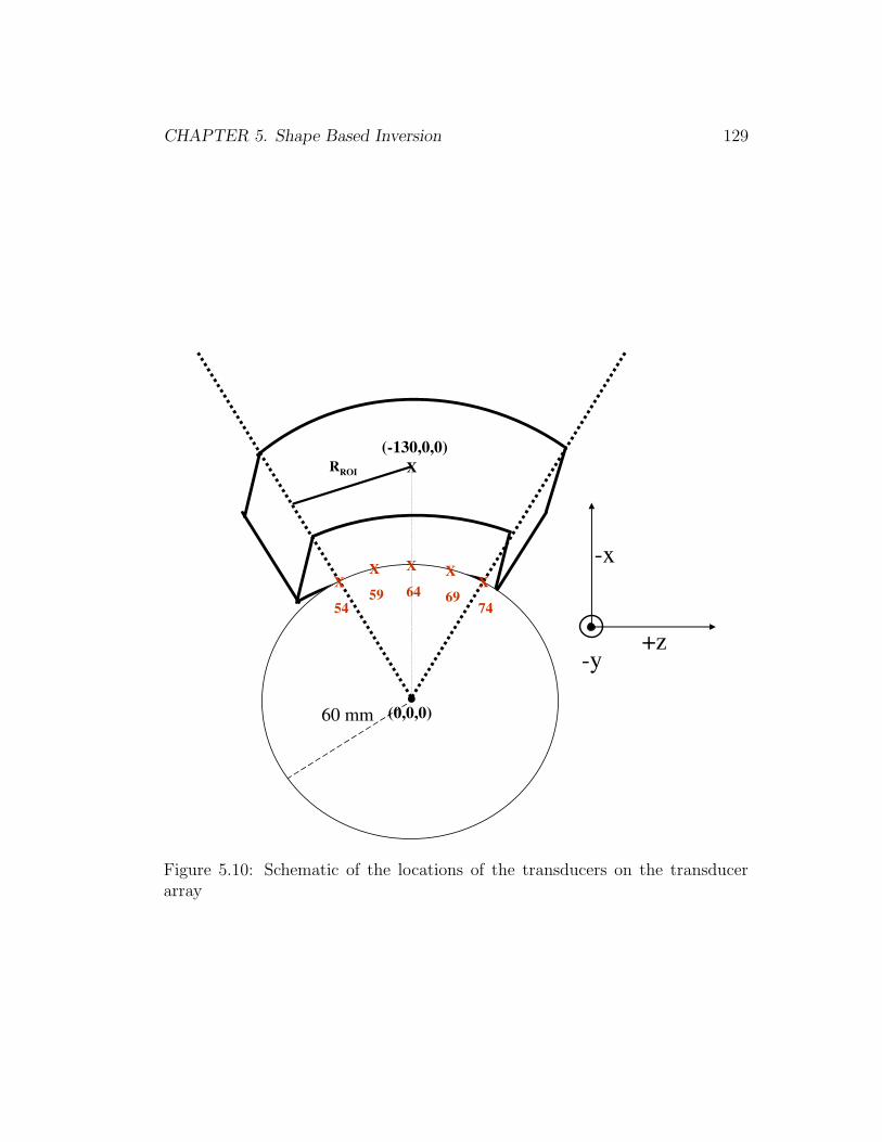
CHAPTER 5. Shape Based Inversion 129
•
60 mm
(-130,0,0)
X
(0,0,0)
RROI
X
54
X
59
X
64
X
69X
74
-x
-y+z
Figure 5.10: Schematic of the locations of the transducers on the transducerarray
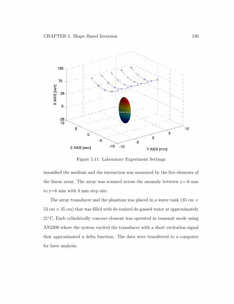
CHAPTER 5. Shape Based Inversion 130
Figure 5.11: Laboratory Experiment Settings
insonified the medium and the interaction was measured by the five elements of
the linear array. The array was scanned across the anomaly between y=-6 mm
to y=6 mm with 3 mm step size.
The array transducer and the phantom was placed in a water tank (35 cm ×53 cm × 35 cm) that was filled with de-ionized de-gassed water at approximately
21◦C. Each cylindrically concave element was operated in transmit mode using
AN2300 where the system excited the transducer with a short excitation signal
that approximated a delta function. The data were transferred to a computer
for later analysis.

CHAPTER 5. Shape Based Inversion 131
Phantom
An ellipsoidal shaped phantom (20 mm × 5 mm × 6 mm) is carved from an
Agar sample which had the nominal acoustic properties of cp = 1551m/s, ρp =
1045kg/m3, αp = 10.17Np/m/MHz. Our previous experience with this ma-
terial showed that, the actual parameters that should be used in the simula-
tions are: cp = 1545m/s, ρp = 1045kg/m3, αp = 54( ωωo
)1.2Np/m where ωo
is the mean angular frequency (2π3.5MHz) [94]. The ellipsoid was immersed
into an optically transparent, cylindrically shaped (radius: 32.5 mm, height:
125 mm), polyacrylamide hydrogel with 7% Bovine Serum Albumin (BSA) pro-
tein concentration. The acoustic properties of the background phantom were:
cb = 1540m/s, ρb = 1045kg/m3, αb = 1.5Np/m/MHz [95]. The polyacrylamide
hydrogel was used because it was optically transparent, and allowed visualizing
of the ellipsoidal anomaly. Moreover, the BSA phantom had the same density
with the Agar phantom which resulted in an experiment environment of which
there was a single ellipsoidal anomaly and altered sound speed and attenuation
values compared to the background. Therefore, this phantom configuration was
a very good approximation to what one would have in real HIFU practice. We
tried to place the ellipsoid so that it only had rotation with respect to the center
axis of the cylinder. The real and the enhanced images of the BSA phantom
are given in Fig. (5.12). A sample image (beamformed pre-scan converted) is
obtained with the Analogic engine when the transducer is aligned with the ellip-
soid (y=0 mm) is given in Fig. (5.13). The data corresponding to the envelope
of the signal from the 64th line of the image is given in Fig. (5.14).

CHAPTER 5. Shape Based Inversion 132
H= 125 mm
R=65 mm
(a)
(b)
Figure 5.12: The real and the enhanced images of the BSA phantom.

CHAPTER 5. Shape Based Inversion 133
20 40 60 80 100 120
100
200
300
400
500
600
700
800
Figure 5.13: A sample image of the BSA phantom with Analogic Engine ultra-sound scanner (B-mode pre-scan converted).
0 100 200 300 400 500 600 700 800 9000
50
100
150
200
250
300
Figure 5.14: The data corresponding to the envelope of the signal from the 64th
line of the image.
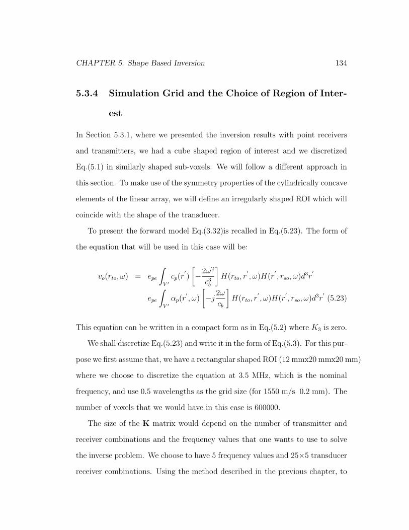
CHAPTER 5. Shape Based Inversion 134
5.3.4 Simulation Grid and the Choice of Region of Inter-
est
In Section 5.3.1, where we presented the inversion results with point receivers
and transmitters, we had a cube shaped region of interest and we discretized
Eq.(5.1) in similarly shaped sub-voxels. We will follow a different approach in
this section. To make use of the symmetry properties of the cylindrically concave
elements of the linear array, we will define an irregularly shaped ROI which will
coincide with the shape of the transducer.
To present the forward model Eq.(3.32)is recalled in Eq.(5.23). The form of
the equation that will be used in this case will be:
vo(rto, ω) = epe
∫
V ′cp(r
′)
[−2ω2
c3b
]H(rto, r
′, ω)H(r
′, rso, ω)d3r
′
epe
∫
V ′αp(r
′, ω)
[−j
2ω
cb
]H(rto, r
′, ω)H(r
′, rso, ω)d3r
′(5.23)
This equation can be written in a compact form as in Eq.(5.2) where K3 is zero.
We shall discretize Eq.(5.23) and write it in the form of Eq.(5.3). For this pur-
pose we first assume that, we have a rectangular shaped ROI (12 mmx20 mmx20 mm)
where we choose to discretize the equation at 3.5 MHz, which is the nominal
frequency, and use 0.5 wavelengths as the grid size (for 1550 m/s 0.2 mm). The
number of voxels that we would have in this case is 600000.
The size of the K matrix would depend on the number of transmitter and
receiver combinations and the frequency values that one wants to use to solve
the inverse problem. We choose to have 5 frequency values and 25×5 transducer
receiver combinations. Using the method described in the previous chapter, to

CHAPTER 5. Shape Based Inversion 135
compute the spatial transfer function for single frequency, location and trans-
mitter receiver combination takes approximately 0.01 seconds in Matlab R14.
Therefore, the total computation time for K matrix would be approximately
1042 hours. This direct approach is computationally very expensive and not
feasible. We have to use the symmetry properties of the transducer and reduce
the size of the computation domain. For this purpose we will first introduce the
sub-voxel approach.
To reduce the computation domain, the region of interest will be divided into
subcells (12 × 20 × 20 with 1mm side length) where the perturbation values
will be assumed constant in each sub-voxel. Mathematically speaking:
vo(rto, ω) = epecp
[−2ω2
c3b
] ∫
Vs
H(rto, r′, ω)H(r
′, rso, ω)d3r
′
epeαp(ω)
[−j
2ω
cb
] ∫
Vs
H(rto, r′, ω)H(r
′, rso, ω)d3r
′(5.24)
where Vs represents the sub-voxel. This approach would reduce the number of
voxels needed to represent the anomaly but the spatial transfer function should
be computed individually for each transducer for the complete ROI.
A fast method is introduced to compute the following integral:
∫
Vs
H(rto, r′, ω)H(r
′, rso, ω)d3r
′(5.25)
where the transfer function for single transducer is calculated and the reciprocity
of the cylindrically concave elements is used to find the response for the other
radiators. Specifically, for a homogeneous medium, the spatial transfer function
takes the absolute value of the distance between the transducer and the obser-
vation point as input. Therefore, the response computed for a transducer at a

CHAPTER 5. Shape Based Inversion 136
−20−10
010
20
−10
−5
0
5
10−15
−10
−5
0
5
10
15
x [mm]y [mm]
z [m
m]
Figure 5.15: Region of Interest in 3D
certain observation point will have the same expression for another transducer,
which has the same relative position with respect to that observation point. e.g.
The response computed at the focus of the 64th transducer can be used to obtain
the response at the focus of the 54th transducer, although the two transducers
are located at different positions in the ROI.
To implement this idea, a new ROI is defined. The ideas presented be-
fore (Eq.(5.23) and Eq.(5.24)) shall stay the same but applied to an irregularly
shaped grid. The shape of the ROI where discretization will be applied is given
in Figures (5.10) and (5.15). The location of the transducers with respect to the
ROI is given in Fig. (5.10).

CHAPTER 5. Shape Based Inversion 137
−15−10−5051015−25
−20
−15
−10
−5
0
5
10
15
20
25
74
69
64
z [m
m]
59
54
x [mm]
Figure 5.16: Region of Interest in 2D
The symmetry properties of the transducer and the reasons behind this shape
of ROI can be better understood from a 2D picture. A 2D slice of the ROI
which is defined in polar coordinates with the parameters (ra < r < rb, and,
−θa < θ < θa) is plotted in blue in Fig. (5.16). Now for the center transducer
(64) one computes the spatial transfer function at each pixel of a computation
grid which is twice the size of the original ROI (−2θa < θ < 2θa). This region is
shown in red in Fig. (5.16). For the center transducer one would use the spatial
transfer function values computed in the pixels corresponding to values between
(−θa < θ < θa) and for the transducer on the side (54) one would use the values

CHAPTER 5. Shape Based Inversion 138
computed at (0 < θ < 2θa). To make sure that the pixels overlap during this
process, the increment in the angle parameter is chosen as the angular pitch size
of the linear array. Moreover, due to the symmetry properties of the cylindrically
concave transducers one will only need to compute the values at the half of the
ROI, between (0 < θ < 2θa).
In each sub-voxel, the Gaussian quadrature approach is used to compute
Eq.(5.25). For this purpose the spatial transfer function of the center transducer
(64) is computed at the Gaussian nodes and stored with the Gaussian weights
and the volume of each sub-voxel. The stored values are recalled to create the
forward matrix that will be used in this study.
The parameters that is used in our simulation will be given here: 5 frequency
values equally sampled between 2.5MHz and 3MHz are used. The computation
grid was described with the parameters 0 ≤ y ≤ 12 mm, 118.6 ≤ r ≤ 141.36
and 0 ≤ θ ≤ 10(degrees). Total number of voxels was 4800 (12 × 20 × 20).
Total time to compute the spatial transfer response of the center transducer was
27.8 hours at 667MHz Unix workstation with 4 processors and 1GB Ram per
processor. Total computation time required to obtain the forward matrix for all
the transducers was 28.1 hours.
The calibration signal for this transducer is previously calculated in Chap-
ter 4 in Eq.(4.57) and, the epe signal is obtained with: epe = eT (ω)2.
5.3.5 Results
The first task to be done is to find the exact location of the ellipsoid with re-
spect to the transducer. Although maximum effort is used to place the ellipsoid

CHAPTER 5. Shape Based Inversion 139
Figure 5.17: Initial true ellipsoid distribution from different view angles
to align with the transducer, the location of the exact radiators in the trans-
ducer and the positioning errors (on the order of mm) cannot be controlled. In
Fig. (5.17) the ellipsoid, which is provided to the optimization routine as initial
guess to find the true ellipsoid, is displayed from different view angles.
In Fig. (5.18) the true ellipsoid, which is obtained from the optimization
routine is provided. The number of iterations required was 157. The minor
differences are attributable to the experimental errors as discussed before.
Next, the inversion method described in Section 5.2 is used to recover the
ellipsoid from a significantly different initial value. The bounds for the contrasts,
Mi, were chosen as:
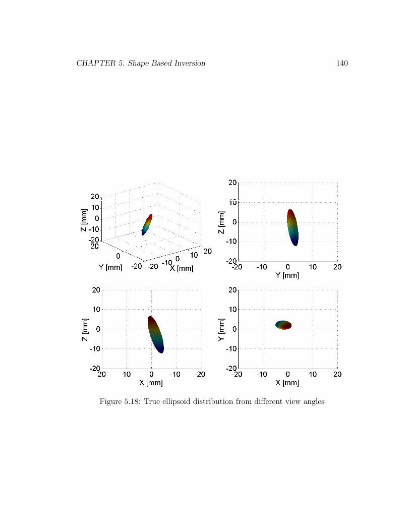
CHAPTER 5. Shape Based Inversion 140
Figure 5.18: True ellipsoid distribution from different view angles
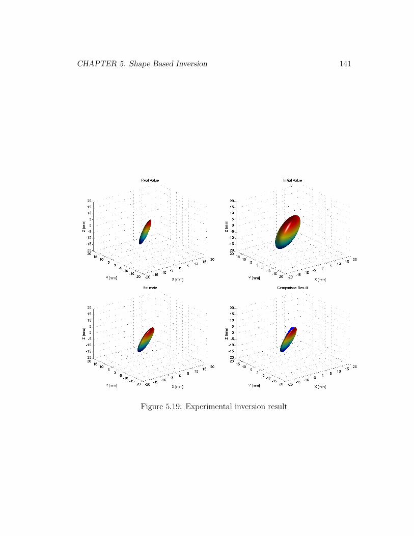
CHAPTER 5. Shape Based Inversion 141
Figure 5.19: Experimental inversion result
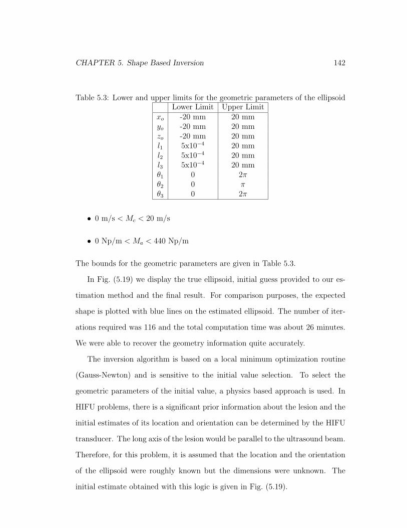
CHAPTER 5. Shape Based Inversion 142
Table 5.3: Lower and upper limits for the geometric parameters of the ellipsoidLower Limit Upper Limit
xo -20 mm 20 mmyo -20 mm 20 mmzo -20 mm 20 mml1 5x10⁻⁴ 20 mml2 5x10⁻⁴ 20 mml3 5x10⁻⁴ 20 mmθ1 0 2πθ2 0 πθ3 0 2π
• 0 m/s < Mc < 20 m/s
• 0 Np/m < Ma < 440 Np/m
The bounds for the geometric parameters are given in Table 5.3.
In Fig. (5.19) we display the true ellipsoid, initial guess provided to our es-
timation method and the final result. For comparison purposes, the expected
shape is plotted with blue lines on the estimated ellipsoid. The number of iter-
ations required was 116 and the total computation time was about 26 minutes.
We were able to recover the geometry information quite accurately.
The inversion algorithm is based on a local minimum optimization routine
(Gauss-Newton) and is sensitive to the initial value selection. To select the
geometric parameters of the initial value, a physics based approach is used. In
HIFU problems, there is a significant prior information about the lesion and the
initial estimates of its location and orientation can be determined by the HIFU
transducer. The long axis of the lesion would be parallel to the ultrasound beam.
Therefore, for this problem, it is assumed that the location and the orientation
of the ellipsoid were roughly known but the dimensions were unknown. The
initial estimate obtained with this logic is given in Fig. (5.19).
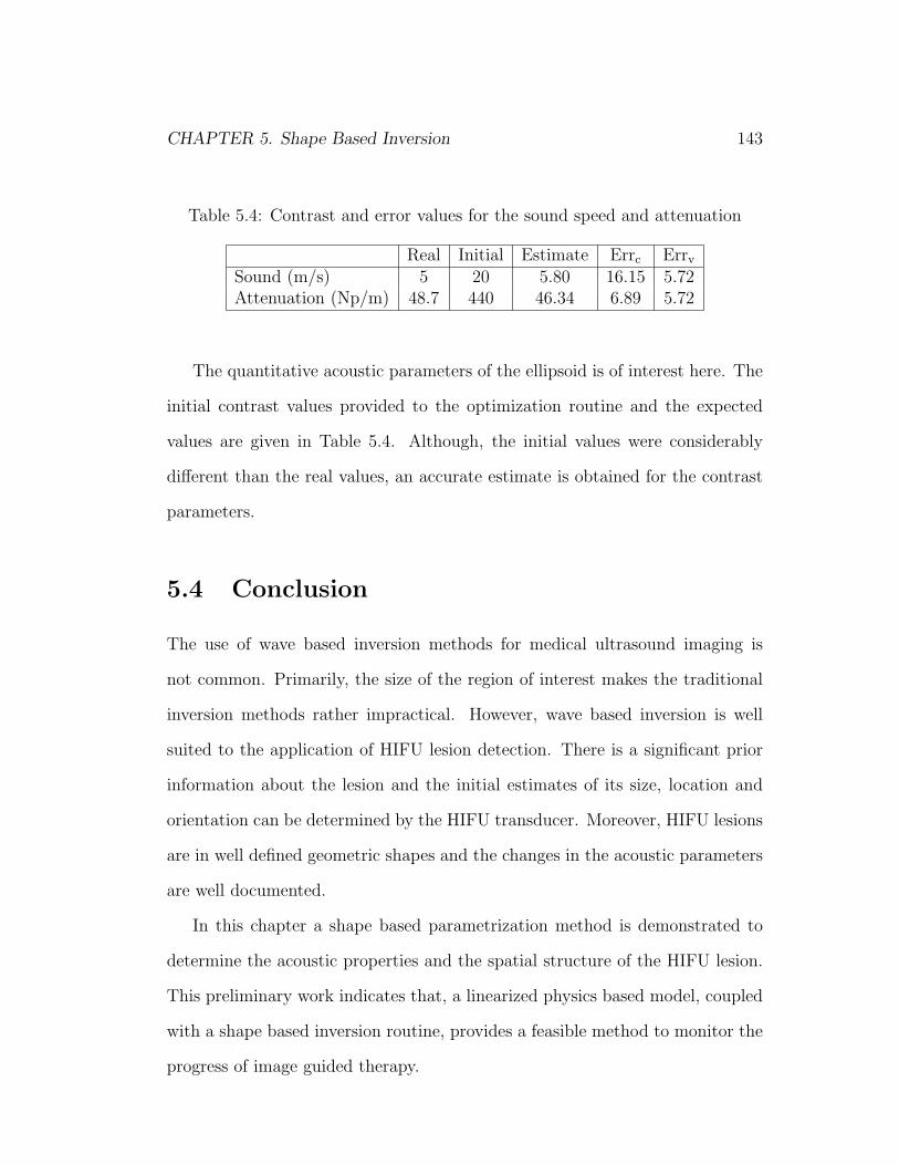
CHAPTER 5. Shape Based Inversion 143
Table 5.4: Contrast and error values for the sound speed and attenuation
Real Initial Estimate Errc Errv
Sound (m/s) 5 20 5.80 16.15 5.72Attenuation (Np/m) 48.7 440 46.34 6.89 5.72
The quantitative acoustic parameters of the ellipsoid is of interest here. The
initial contrast values provided to the optimization routine and the expected
values are given in Table 5.4. Although, the initial values were considerably
different than the real values, an accurate estimate is obtained for the contrast
parameters.
5.4 Conclusion
The use of wave based inversion methods for medical ultrasound imaging is
not common. Primarily, the size of the region of interest makes the traditional
inversion methods rather impractical. However, wave based inversion is well
suited to the application of HIFU lesion detection. There is a significant prior
information about the lesion and the initial estimates of its size, location and
orientation can be determined by the HIFU transducer. Moreover, HIFU lesions
are in well defined geometric shapes and the changes in the acoustic parameters
are well documented.
In this chapter a shape based parametrization method is demonstrated to
determine the acoustic properties and the spatial structure of the HIFU lesion.
This preliminary work indicates that, a linearized physics based model, coupled
with a shape based inversion routine, provides a feasible method to monitor the
progress of image guided therapy.

CHAPTER 5. Shape Based Inversion 144
We exploited the fact that, the treatment results in an ellipsoidal shaped
region and proposed a differentiable function to describe the boundary and the
contrast of the ellipsoid. The physical size of the region, in which the lesion re-
sides, results in the need to build and manipulate large matrices. We introduced
a reduced order method for synthesizing and manipulating these matrices.
Three numerical experiments were performed with point sources. Two cases
were presented where the ellipsoids describing the shapes were not identical,
and another case in which the spatial changes in the acoustic properties were
enclosed within a single ellipsoid. In all of the cases we were able to reconstruct
the geometry and the contrasts quite accurately. The results presented here were
obtained under 200 iterations using a Matlab implementation on a 1GHz Linux
workstation. The computation time was less than 25 minutes for all results.
A laboratory experiment was performed with a clinically used linear array
transducer. An ellipsoidal phantom was used which had perturbation in sound
speed and attenuation only and the spatial changes in the acoustic properties
were enclosed within a single ellipsoid. We were able to reconstruct the geometry
of the ellipsoid and the contrasts accurately. The results were obtained with
116 iterations using a Matlab implementation on a 667MHz workstation. The
computation time was 26 minutes.
The algorithms and the models presented in this chapter built a foundation
to expand these ideas to in-vitro and ex-vivo applications.
The method can be expanded to the specialization of the models to the
inhomogeneous ellipsoids and the characterization methods beyond ellipsoidal
shapes.

CHAPTER 5. Shape Based Inversion 145
The method assumes volumetrically homogenous shapes which can be ex-
tended to inhomogeneous ellipsoids [56]. The change in the contrast parameter
can be defined as a smooth function which is approximated with a low order
polynomial. In this case one will only need to determine a few number of addi-
tional parameters per ellipsoid depending on the order of the polynomial.
A more flexible shape based method to parameterize the structure of the
HIFU lesions might also be examined. Moving beyond the ellipsoidal struc-
tures might be required if the shape of the lesions cannot be adequately de-
scribed with the ellipsoids. It has been reported in the literature that, ”tadpole”
shaped lesions are observed for the cases where significant cavitational activity
is present.
Chapter 6
Conclusion and Future Work
6.1 Objectives and Specific Aims
The objective of this dissertation is the development and validation of quanti-
tative, fully three dimensional ultrasonic imaging methods to characterize the
location and the spatial structure of the High Intensity Focused Ultrasound
(HIFU) lesions.
Specific Aim #1 To develop a well calibrated physical forward model
that describes the propagation of ultrasound in human tissue. The forward
model should be sensitive to the changes in the acoustic properties, sound
speed, attenuation and density.
Specific Aim #2 To develop a geometry based inversion method for le-
sion identification.
Specific Aim #3 To validate the inversion algorithm using tissue-mimicking
phantoms with known perturbations in acoustic properties and determine
the accuracy of image reconstruction method.
146
CHAPTER 6. Conclusion and Future Work 147
6.2 Overview and Significance
In this study we focused on developing a geometry based characterization method
to monitor the HIFU lesions. A shape based inversion method which uses ul-
trasound backscatter data was proposed to determine the spatial distribution of
sound speed, attenuation and density of the lesions. Processing the data in this
manner, reconstructing the acoustic parameters from ultrasound measurements,
is known as inverse problem and the method we propose can be used for a wide
range of reconstruction problems. In this dissertation, we focused on cancer
treatment applications.
HIFU is a cancer treatment technique where high frequency sound waves
(ultrasound) are used to necrose the cancerous tissue without damaging the sur-
rounding healthy tissue. An important open issue in developing HIFU methods
for clinical use is monitoring the progress of the treatment by non-invasive imag-
ing techniques. In this work, we exploit the fact that the treatment results in
ellipsoidal (1-20 mm length) lesions in which the acoustic properties of the tissue
sound speed and attenuation - are altered from their nominal values.
Even under the assumption of a linearized scattering model such as that
provided by the Born approximation, the computational size of the most rele-
vant 3D problems makes traditional pixel based inversion methods impractical.
Hence in this work, we introduce a shape-based method under which we need
to estimate a small number of parameters to describe the 3D shape of the le-
sion. More specifically, we consider a number of options for shape estimation
depending on whether one is interested in a single physical unknown or multiple
quantities (sound speed, attenuation, and density) each of which may be altered
by the HIFU treatment.

CHAPTER 6. Conclusion and Future Work 148
The physical size of the region in which the lesion resides results in the need
to build and manipulate large matrices which define the underlying linearized
model. Thus, the second issue we propose to solve is the development of new,
reduced order methods for synthesizing and manipulating these matrices.
Significance:The use of wave based inversion methods for medical ultra-
sound imaging is not common. Primarily, the size of the region of interest
makes the traditional inversion methods rather impractical. However, wave
based inversion is well suited to the application of HIFU lesion detection. There
is a significant prior information about the lesion and the initial estimates of
its size, location and orientation can be determined by the HIFU transducer.
Moreover, HIFU lesions are in well defined geometric shapes and the changes in
the acoustic parameters are well documented.
6.3 Preliminary Studies: A shape-based approach
to the tomographic Ultrasonic imaging prob-
lem
Our initial efforts were focused on developing a time domain propagation model
that describes the scattering of ultrasound in homogenous medium. We pre-
sented a model which computes the acoustic field scattered by localized in-
homogeneities embedded into homogenous lossless background. Our efforts to
validate the forward method with laboratory measurements taken from a spher-
ically focused transducer, presented a need to develop a calibration method for
such transducers. We have shown, both theoretically and experimentally, that
CHAPTER 6. Conclusion and Future Work 149
the calibration signal for these type of radiators can be measured using either
a flat-plate or a point scatterer. The reflected waveforms in each case are not
identical but rather related by an operation of double differentiation.
Next, the ideas that have been developed for time domain propagation of ul-
trasound are applied to the frequency domain where we concentrated on the de-
velopment and validation of the frequency domain Born model for lossy medium.
We linearized our problem and defined the inhomogeneities in the acoustic prop-
erties as perturbations to a homogenous, lossy background model. The scattered
acoustic wave for such a medium is expressed linearly in terms of the pertur-
bations in sound speed, attenuation and density. The frequency dependency
of attenuation is characterized by a power-law relation. Moreover, we demon-
strated a fast method to solve the pressure field of spherically curved radiators
for frequency domain applications.
Our final aim should be to implement these ideas in medical imaging area
and the conventional ultrasound transducers used for medical imaging purposes
are generally of phased array type. Therefore, to apply our methods to more
realistic scenarios, we developed a method to simulate the forward field from
phased array transducers which have cylindrically concave elements.
We introduced a semi-analytic fast method which computes the forward field
from cylindrically concave transducers for any type of attenuating medium. We
compared our method to an optimized numerical integration routine which com-
putes this response numerically. The speed improvement is obtained as 40 to
1400. With our method, for the frequency domain applications where we need
to find the background field for a few frequency values, the response can be
obtained almost immediately.
CHAPTER 6. Conclusion and Future Work 150
Finally, we introduced a shape based inversion method which integrates the
methods that we developed so far. We demonstrated a shape based parame-
trization model to determine the acoustic properties and the spatial structure
of the HIFU lesion. We used the fact that, the treatment results in ellipsoidal
shaped lesions. We proposed a differentiable function to describe the boundary
and the contrast of the ellipsoid.
We performed three numerical experiments with point sources and one lab-
oratory experiment with the linear array transducer. In all of the cases we were
able to reconstruct the geometry and the contrasts quite accurately.
6.4 Future work: Design and Methods
The algorithms and the models presented in this dissertation built a founda-
tion to expand these ideas to in-vitro and ex-vivo applications. The work that
remains to be done in this area are the specialization of the models to the inho-
mogeneous background and expansion of the characterization methods beyond
ellipsoids.
Forward Problem:
Rytov-Model: In HIFU imaging experiments we are able to collect ultra-
sound data before the HIFU is used to create lesions in the tissue. Hence,
the problem we need to solve can be defined as a differential change esti-
mation in acoustic parameters. For this type of problems the Rytov model
is known to be more appropriate than the Born approximation. There-
fore, a new model can be introduced for the inverse problem in which the

CHAPTER 6. Conclusion and Future Work 151
change from Born approximation to Rytov model would require only the
use of different normalization for the data [96].
Inhomogeneous Background: The method that we developed in this
dissertation is valid for homogenous, lossy, power-law attenuating medium.
More complicated methods which are not using Born approximation can
be developed to handle tissue like inhomogeneous media. For many med-
ical applications, we are often interested in determining the propagation
of ultrasound waves due to tissue layers of fat and muscle. A closed form
expression for such media in terms of spherical harmonics is previously pre-
sented in [97]. This idea can be explored for our specific HIFU monitoring
problem.
Inverse Problem:
Inhomogeneous ellipsoids: The method we developed assumes volu-
metrically homogenous shapes which can be easily extended to inhomoge-
neous ellipsoids [56]. The change in the contrast parameter can be defined
as a smooth function which is approximated with a low order polynomial.
In this case one will only need to determine a few number of additional
parameters per ellipsoid depending on the order of the polynomial.
Non-ellipsoidal shapes: A more flexible shape based method to parame-
terize the structure of the HIFU lesions might also be examined. Moving
beyond the ellipsoidal structures might be required if the shape of the
lesions cannot be adequately described with the ellipsoids. It has been
reported in the literature that, ”tadpole” shaped lesions are observed for

CHAPTER 6. Conclusion and Future Work 152
the cases where significant cavitational activity is present.
Background Estimation: The application of the homogenous model to
invert anomalies embedded into inhomogeneous medium can be explored.
However, one should have a good estimate of the background parameters.
In ultrasound images we have speckles. Randomly positioned point scat-
terers can be used to model these speckles and the measurements obtained
before creating the lesions can be used to estimate the optimal background
parameter values.
Laboratory Experiments:
The experiments that we presented in this dissertation may be followed by
ex vivo studies. The imaging data can be collected on AN2300 ultrasound
engine (Analogic Corporation, Peabody MA) which gives an access to
unbeamformed RF data for inversion algorithms. Ex vivo studies can be
carried out using excised tissue samples. The background field can be
measured with backscattering experiments and compared to the predicted
waveforms obtained from our forward models. Next, individual HIFU
lesions can be created in the tissue to validate the reconstruction algorithm
that we presented in this study.
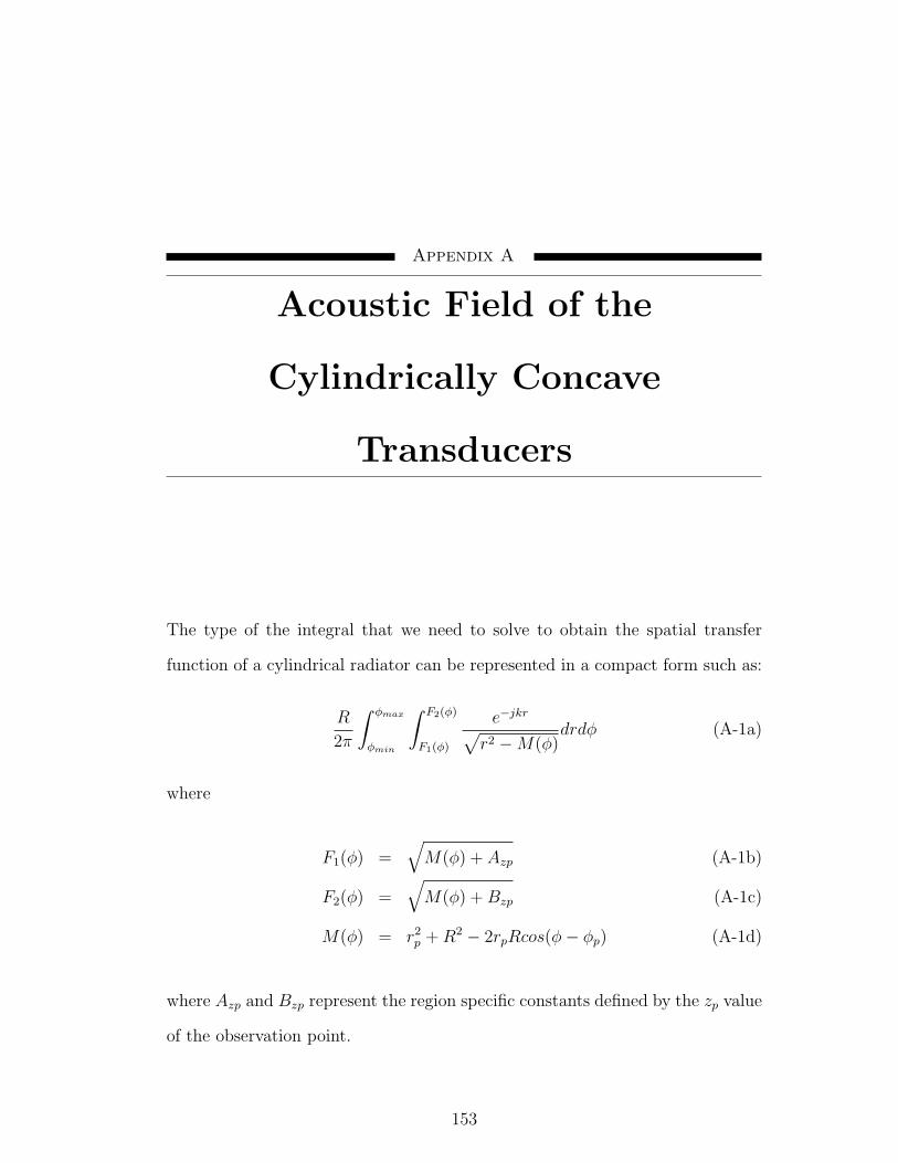
Appendix A
Acoustic Field of the
Cylindrically Concave
Transducers
The type of the integral that we need to solve to obtain the spatial transfer
function of a cylindrical radiator can be represented in a compact form such as:
R
2π
∫ φmax
φmin
∫ F2(φ)
F1(φ)
e−jkr
√r2 −M(φ)
drdφ (A-1a)
where
F1(φ) =√
M(φ) + Azp (A-1b)
F2(φ) =√
M(φ) + Bzp (A-1c)
M(φ) = r2p + R2 − 2rpRcos(φ− φp) (A-1d)
where Azp and Bzp represent the region specific constants defined by the zp value
of the observation point.
153

Appendix A. Acoustic Field of the Cylindrically Concave Transducers 154
A.1 Case 1: Regions I and II 0 ≤ φp ≤ φt
In this region M(φ), F1(φ) and F2(φ) are represented by:
M(φ) ≈ (r2p + R2 − 2rpRcos(φp))− (2rpRsin(φp))φ (A-2a)
+(rpRcos(φp))φ2 (A-2b)
= a + bφ + cφ2 (A-2c)
F1(φ) ≈√
a + bφ + cφ2 + Azp (A-2d)
F2(φ) ≈√
a + bφ + cφ2 + Bzp (A-2e)
A.1.1 Region I: φmax < tanφp ≤ φt
The expression for the spatial transfer function is given by:
H =R
2π
∫ F1(φmin)
F1(φmax)e−jkr[−Ψ1(r)]dr +
∫ F2(φmin)
F2(φmax)e−jkr[Ψ2(r)]dr+
∫ F2(φmin)
F1(φmin)e−jkr[−Ψ3(r)]dr +
∫ F2(φmax)
F1(φmax)e−jkr[Ψ4(r)]dr
(A-3)
where
Ψ1(r) = − 1√carcsin
(√1− 4cAzp
b2 + 4r2c− 4ac
)(A-4a)
Ψ2(r) = − 1√carcsin
(√1− 4cBzp
b2 + 4r2c− 4ac
)(A-4b)
Ψ3(r) = − 1√carcsin
( −2cφmin − b√b2 + 4r2c− 4ac
)(A-4c)
Ψ4(r) = − 1√carcsin
( −2cφmax − b√b2 + 4r2c− 4ac
)(A-4d)
φmin = −arcsin(l/R) (A-4e)
φmax = arcsin(l/R) (A-4f)

Appendix A. Acoustic Field of the Cylindrically Concave Transducers 155
A.1.2 Region II: tanφp ≤ φmax
The expression is given as the summation of the two responses:
∫ φmax
φmin
∫ F2(φ)
F1(φ)
drdφ = H1 + H2 (A-5)
H1 :
H1 =R
2π
∫ F1(φmin)
F1(φmax)e−jkr[−Ψ1(r)]dr +
∫ F2(φmin)
F2(φmax)e−jkr[Ψ2(r)]dr+
∫ F2(φmin)
F1(φmin)e−jkr[−Ψ3(r)]dr
(A-6)
where
φmin = −arcsin(l/R) (A-7a)
φmax = tan(φp) (A-7b)
The Ψ4(r) integral vanishes in this interval.
H2 :
H2 =R
2π
∫ F1(φmax)
F1(φmin)e−jkr[−Ψ1(r)]dr +
∫ F2(φmax)
F2(φmin)e−jkr[Ψ2(r)]dr+
∫ F2(φmax)
F1(φmax)e−jkr[Ψ4(r)]dr
(A-8)
where
φmin = tan(φp) (A-9a)
φmax = arcsin(l/R) (A-9b)
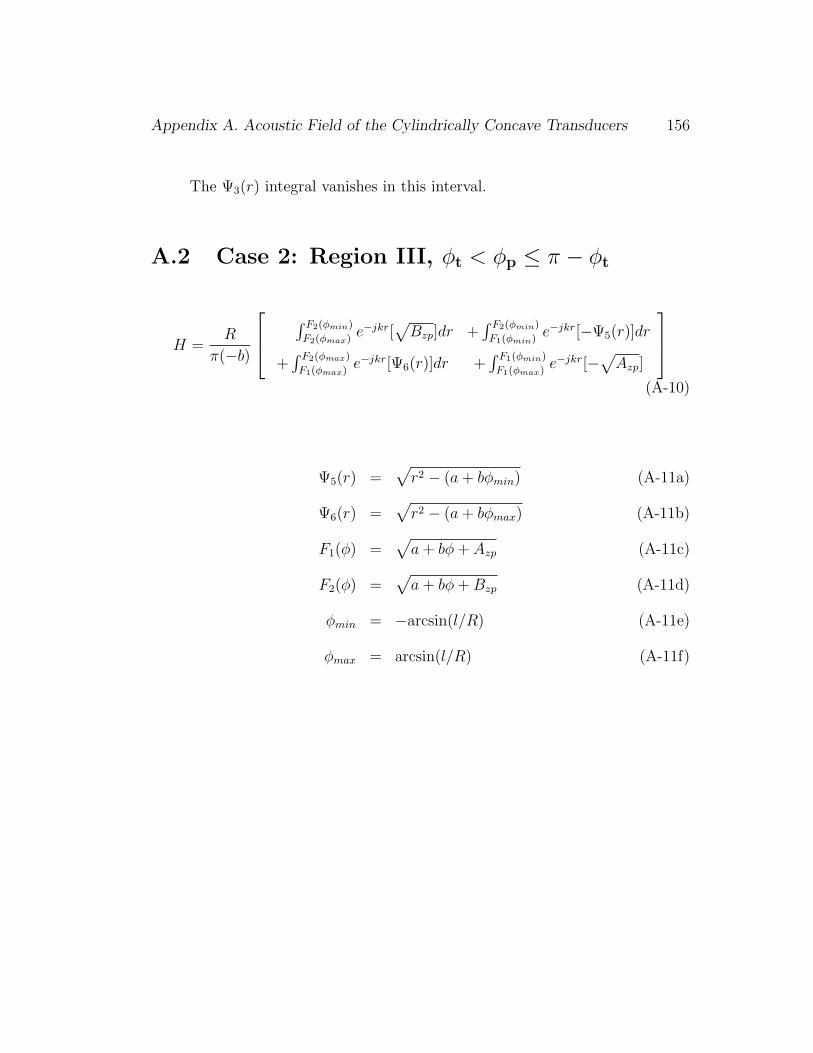
Appendix A. Acoustic Field of the Cylindrically Concave Transducers 156
The Ψ3(r) integral vanishes in this interval.
A.2 Case 2: Region III, φt < φp ≤ π − φt
H =R
π(−b)
∫ F2(φmin)
F2(φmax)e−jkr[
√Bzp]dr +
∫ F2(φmin)
F1(φmin)e−jkr[−Ψ5(r)]dr
+∫ F2(φmax)
F1(φmax)e−jkr[Ψ6(r)]dr +
∫ F1(φmin)
F1(φmax)e−jkr[−√
Azp]
(A-10)
Ψ5(r) =√
r2 − (a + bφmin) (A-11a)
Ψ6(r) =√
r2 − (a + bφmax) (A-11b)
F1(φ) =√
a + bφ + Azp (A-11c)
F2(φ) =√
a + bφ + Bzp (A-11d)
φmin = −arcsin(l/R) (A-11e)
φmax = arcsin(l/R) (A-11f)

Appendix A. Acoustic Field of the Cylindrically Concave Transducers 157
A.3 Case 3: Regions IV and V π − φt ≤ φp ≤ π
M(φ), F1(φ) and F2(φ) have the same forms in Section 4.3.1 as:
M(φ) ≈ (r2p + R2 − 2rpRcos(φp))− (2rpRsin(φp))φ (A-12a)
+(rpRcos(φp))φ2 (A-12b)
= a + bφ + cφ2 (A-12c)
F1(φ) ≈√
a + bφ + cφ2 + Azp (A-12d)
F2(φ) ≈√
a + bφ + cφ2 + Bzp (A-12e)
A.3.1 Region IV: tanφp < φmin
H =R
2π
∫ F1(φmin)
F1(φmax)e−jkr[−Ψ7(r)]dr +
∫ F2(φmin)
F2(φmax)e−jkr[Ψ8(r)]dr+
∫ F2(φmin)
F1(φmin)e−jkr[−Ψ9(r)]dr +
∫ F2(φmax)
F1(φmax)e−jkr[Ψ10(r)]dr
(A-13)
where
φmin = −arcsin(l/R) (A-14a)
φmax = arcsin(l/R) (A-14b)
Ψ7(r) =1√−c
ln
(2√−cAzp +
√b2 − 4c(a + Azp − r2)
)(A-14c)
Ψ8(r) =1√−c
ln
(2√−cBzp +
√b2 − 4c(a + Bzp − r2)
)(A-14d)
Ψ9(r) =1√−c
ln
(2√−c(r2 − a− bφmin − cφ2
min)− 2cφmin − b
)(A-14e)
Ψ10(r) =1√−c
ln(2√−c(r2 − a− bφmax − cφ2
max)− 2cφmax − b)
(A-14f)

Appendix A. Acoustic Field of the Cylindrically Concave Transducers 158
A.3.2 Region V: tanφp ≥ φmin
∫ φmax
φmin
∫ F2(φ)
F1(φ)
drdφ = H1 + H2 (A-15)
H1 :
H1 =R
2π
∫ F ∗1 (φmin)
F ∗1 (φmax)e−jkr[−Ψ7(r)]dr +
∫ F ∗2 (φmin)
F ∗2 (φmax)e−jkr[Ψ8(r)]dr+
∫ F ∗2 (φmin)
F ∗1 (φmin)e−jkr[−Ψ11(r)]dr +
∫ F ∗2 (φmax)
F ∗1 (φmax)e−jkr[Ψ12(r)]dr
(A-16)
F ∗1 (φ∗) =
√(a− bφ∗ + c(φ∗)2 + Azp (A-17a)
F ∗2 (φ∗) =
√(a− bφ∗ + c(φ∗)2 + Bzp (A-17b)
Ψ11(r) =1√−c
ln
(2√−c(r2 − a + bφmin − cφ2
min)− 2cφmin + b
)
(A-17c)
Ψ12(r) =1√−c
ln(2√−c(r2 − a + bφmax − cφ2
max)− 2cφmax + b)
(A-17d)
φmin = −tan(φp) (A-17e)
φmax = φmax (A-17f)

Appendix A. Acoustic Field of the Cylindrically Concave Transducers 159
H2 :
H2 =R
2π
∫ F1(φmin)
F1(φmax)e−jkr[−Ψ7(r)]dr +
∫ F2(φmin)
F2(φmax)e−jkr[Ψ8(r)]dr+
∫ F2(φmin)
F1(φmin)e−jkr[−Ψ9(r)]dr +
∫ F2(φmax)
F1(φmax)e−jkr[Ψ10(r)]dr
(A-18)
where
φmin = −tan(φp) (A-19a)
φmax = arcsin(l/R) (A-19b)

Bibliography
[1] Z. Cho, J. Jones, and M. Singh, Foundations of Medical Imaging. New
York: Wiley-Interscience, 1993.
[2] T. Taxt, A. Lundervold, J. Strand, and S. Holm, “Advances in medical
imaging,” 14th Intl Conference on Pattern Recognition (ICPR98), Brisbane,
Australia, August 1998.
[3] T. Misaridis and J. Jensen, “Use of modulated excitation signals in med-
ical ultrasound. part iii: high frame rate imaging,” IEEE Transactions on
Ultrasonics, Ferroelectrics and Frequency Control, vol. 52, pp. 208–219,
2005.
[4] J. Kirkhorn, S. Bjaerum, B. Olstad, K. Kristoffersen, and H. Torp, “A new
technique for improved spatial resolution in high frame rate color doppler
imaging,” IEEE Symposium on Ultrasonics, vol. 2, pp. 1947–1950, 2003.
[5] R. Carotenuto, G. Sabbi, and M. Pappalardo, “Spatial resolution enhance-
ment of ultrasound images using neural networks,” IEEE Transactions on
Ultrasonics, Ferroelectrics and Frequency Control, vol. 49, pp. 1039–1049,
2002.
160

BIBLIOGRAPHY 161
[6] D. Vray, T. Rastello, F. Schoofs, and P. Delachartre, “Improving the spa-
tial resolution of intravascular ultrasound imaging with synthetic aperture
fourier-based methods,” IEEE Symposium on Ultrasonics, vol. 2, pp. 1531–
1534, 1997.
[7] J. I. DiStasio, Ultrasonics as a Medical Diagnostic Tool. Noyes Data Cor-
poration, 1980.
[8] L. W. Goldman and J. B. Fowlkes, Medical CT and Ultrasound: Current
technology and Applications, Procedings of the 1995 summer school on
CT and US technology and Applications of the American Association of
Physicists in Medicine. Connecticut Collage New London, Connecticut,
1995.
[9] Users’ Guide for Analogic AN2300 Ultrasound Engine. Analogic Corpora-
tion, Peabody, MA, Sept. 2003.
[10] P. M. Morse and K. U. Ingard, Theoretical Acoustics. Princeton, N. J:
Princeton University Press, 1986.
[11] M. M. Hutter and D. W. Rattner, “Novel tissue destruction methods,”
Problems in General Surgery. Advances in Minimally Invasive Surgery,
vol. 18(1), pp. 26–32, 2001.
[12] G. T. Clement, “Perspectives in clinical uses of high-intensity focused ul-
trasound,” Ultrasonics, vol. 42, pp. 1087–1093, 2004.
[13] K. F. Graff, A History of Ultrasonics, in Physical Acoustics. Academic
Press, New York, 1982.

BIBLIOGRAPHY 162
[14] Z. Wang, J. Bai, L. Faqi, and et al., “Study of a ”biological focal region”
of high-intensity focused ultrasound,” Ultrasound in Medicine and Biology,
vol. 29, pp. 749–754, 2003.
[15] G. ter Haar, D. Sinnett, and I. Rivens, “High intensity focused ultrasound-a
surgical technique for the treatment of discrete liver tumors,” Phys. Med.
Biol., vol. 34, pp. 1743–1750, 1989.
[16] W. Chen, C. Lafon, T. J. Matula, S. Vaezy, and L. A. Crum, “Mechanisms
of lesion formation in high intensity focused ultrasound therapy,” Acoustic
Research Letters Online, vol. 4, pp. 41–46, 2003.
[17] L. Poissonnier, A. Gelet, J. Chapelon, and et al., “Results of transrectal
focused ultrasound for the treatment of localized prostate cancer (120 pa-
tients with psa < or + 10ng/ml),” Prog Urol., vol. 13, pp. 60–72, 2003.
[18] T. A. Gardner, A. Thomas, M. O. Koch, and et al., “Minimally invasive
treatment of benign prostatic hyperplasia with high intensity focused ul-
trasound using the sonablate [trademark] system: An updated report of
phase iii clinical studies conducted in the usa,” Proceedings of SPIE - The
International Society for Optical Engineering,, vol. v 4609, pp. 107–114,
2002.
[19] N. T. Sanghvi, J. Syrus, R. S. Foster, R. Bihrle, R. Casey, and T. Uchida,
“Noninvasive surgery of prostate tissue by high intensity focused ultra-
sound: An updated report,” Proceedings of SPIE, vol. 3907, pp. 194–200,
2000.
[20] S. Madersbacher, C. Kratzik, and M. Marberger, “Prostatic tissue ablation
BIBLIOGRAPHY 163
by transrectal high intensity focused ultrasound: histological impact and
clinical application,” Ultrasonics Sonochemistry, vol. 4, pp. 175–179, 1997.
[21] K. Nakamura, S. Baba, S. Saito, M. Tachibana, and M. Murai, “High-
intensity focused ultrasound energy for benign prostatic hyperplasia: clini-
cal response at 6 months to treatment using sonablate 200,,” J. Endourol.,
vol. 11, pp. 197–201, 1997.
[22] E. D. Mulligan, T. H. Lynch, D. Mulvin, D. Greene, J. M. Smith, and J. M.
Fitzpatrick, “High-intensity focused ultrasound in the treatment of benign
prostatic hyperplasia,,” Br. J. Urol., vol. 79, pp. 177–180, 1997.
[23] C. Chaussy, S. Thuroff, F. Lacoste, and A. Gelet, “Hifu and prostate can-
cer: The eurepean experience,” In proceedings of the 2nd International
Symposium on Therapeutic Ultrasound, 2002.
[24] J. Kennedy, G. T. Haar, and D. Cranstron, “High intensity focused ultra-
sound: Surgery of the future?,” The British Journal of Radilology, vol. 76,
pp. 590–599, 2003.
[25] F. Wu, W. Chen, J. Bai, Z. Zou, Z. Wang, H. Zhu, and Z.Wang, “Patho-
logical changes in human malignant carcinoma treated with high-intensity
focused ultrasound,,” Ultrasound Med. Biol., vol. 27, pp. 1099–1106 (, 2001.
[26] F. Wu, Z. Wang, W. Chen, and W. W. et al., “Extracorporeal high intensity
focused ultrasound ablation in the treatment of 1038 patients with solid
carcinomas in china: An overview,” Ultrasonics Sonochemistry, vol. 11,
pp. 149–154, 2004.

BIBLIOGRAPHY 164
[27] H. Cline, K. Hynynen, C. Hardy, R. Watkins, F. Schenck, and F. Jolesz,
“Mr temperature mapping of focused ultrasound surgery,,” Magn. Reson.
Med., vol. 31, pp. 628–636, 1994.
[28] N. McDannold, L. King, F. Jolesz, and K. Hynynen, “Usefulness of mr
imaging-derived thermometry and dosimetry in determining the thresh-
old for tissue damage induced by thermal surgery in rabbits,” Radiology,
vol. 216, pp. 517–523, 2000.
[29] K. Hynynen, O. Pomeroy, D. Smith, P. Huber, N. McDannold, and J. K.
et al., “Mr imaging-guided focused ultrasound surgery of fibroadenomas in
the breast: A feasibility study,” Radilology, vol. 219, pp. 176–185, 2001.
[30] S. Vaezy, X. Shi, R. Martin, and et al., “Real-time visualization of
high-intensity focused ultrasound treatment using ultrasound imaging,”
Ultrasound Med. Biol, vol. 27, pp. 33–42, 2001.
[31] R. Seip, J. Tavakkoli, R. Carlson, and et al., “High-intensity focused ultra-
sound (hifu) multiple lesion imaging: Comparison of detection algorithms
for real-time treatment control,” Proceedings of the IEEE Ultrasonics
Symposium, vol. 2, pp. 1427–1430, 2002.
[32] H. Yao, P. Phukpattaranont, and E. S. Ebbini, “Nonlinear imaging meth-
ods for characterization of hifu-induced lesions,” Proc. of SPIE – Thermal
Treatment of Tissue: Energy Delivery and Assessment II, vol. 4954,
pp. 183–191, 2003.
[33] H. Yao, P. Phukpattaranont, and E. Ebbini, “Enhanced lesion visualiza-
tion in image-guided noninvasive surgery with ultrasound phased arrays,”
BIBLIOGRAPHY 165
Proceedings of the 23rd Annual International Conference of the IEEE
Engineering in Medicine and Biology Society, vol. 3, pp. 2492–2495, 2001.
[34] F. Kallel, R. Stafford, R. Price, R. Righetti, J. Ophir, and J. D. Hazle, “The
feasibility of eleastographic visualization of hifu-induced thermal lesions in
soft tissues. image-guided high-intensity focused ultrasound,” Ultrasound
Med. Biol., vol. 25, pp. 641–647, 1999.
[35] N. R. Miller, J. C. Bamber, and P. M. Meaney, “Fundamental limitations
of noninvasive temperature imaging by means of ultrasound echo strain
estimation,” Ultrasound Med. Biol., vol. 28, pp. 1319–1333, 2002.
[36] K. Nightingale, M. S. Soo, and G. Grahey, “Acoustic radiation force impulse
imaging: In vivo demonstration of clinical feasibility,” Ultrasound Med.
Biol., vol. 28, pp. 227–235, 2002.
[37] P. E. Barbone and J. C. Bamber, “Quantitative elasticity imaging: What
can and what cannot be inferred from strain images,” Phys. Med. Biol.,
vol. 47, pp. 2147–2164, 2002.
[38] J. C. Bamber and C. R. Hill, “Ultrasonic attenuation and propagation speed
in mammalian tissues as a function of temperature,” Ultrasound Med. Biol.,
vol. 5, pp. 149–157, 1979.
[39] N. L. Bush, I. Rivens, G. R. ter Haar, and J. C. Bamber, “Acoustic prop-
erties of lesions generated with an ultrasound therapy system,” Ultrasound
Med. Biol., vol. 19, pp. 789–801, 1993.
[40] C. A. Damianou, N. T. Sanghvi, F. J. Fry, , and R. Maass-Moreno, “De-
pendence of ultrasonic attenuation and absorption in dog soft tissues on
BIBLIOGRAPHY 166
temperature and thermal dose,” J. Acoust. Soc. Am., vol. 102, pp. 628–
634, 1997.
[41] S. H. Bloch, M. R. Bailey, L. Crum, P. Kaczkowski, G. Keilman, and
P. Mourad, “Measurements of sound speed in excised tissue over tem-
perature expected under high-intensity focused ultrasound conditions,”
Proceedings of the joint meeting of the 16th ICA and the 135th Meeting of
the ASA, vol. 2, pp. 1065–1066, 1998.
[42] A. E. Worthington and M. D. Sherar, “Changes in ultrasound properties
of porcine kidney tissue during heating,” Ultrasound Med. Biol., vol. 27,
pp. 673–682, 2001.
[43] U. Techavipoo, T. Varghese, Q. Chen, T. A. Stiles, J. A. Zagzebski, and
G. R. Frank, “Temperature dependence of ultrasonic propagation speed and
attenuation in excised canine liver tissue measured using transmitted and
reflected pulses,” J. Acoust. Soc. Am., vol. 116, pp. 2859–2865, 2004.
[44] P. D. Tyreus and C. Diederich, “Two-dimensional acoustic attenuation
mapping of high-temperature interstitial ultrasound lesions,” Phys. Med.
Biol., vol. 49, pp. 533–546, 2004.
[45] M. Pernot, M. Tanter, J. Bercoff, K. Waters, and M. Fink, “Tempera-
ture estimation using ultrasonic spatial compound imaging,” IEEE UFFC,
vol. 51, pp. 606–615, 2004.
[46] L. A. S. Baker and J. C. Bamber, “Effect of dynamic receive focusing on
reflex transmission imaging (rti),” Proc. IEEE Ultrason. Symp., 2002.
BIBLIOGRAPHY 167
[47] A. Anand and P. J. Kaczkowski, “Monitoring formation of high intensity
focused ultrasound (hifu) induced lesions using backscattered ultrasound,”
Acoust. Res. Lett. Onlin, vol. 5, pp. 88–94, 2004.
[48] C. R. Vogel, “Computational methods for inverse problems,” Society of
Industrial and Applied Mathematics, 2002.
[49] F. Natterer and F. Wubbeling, “Mathematical methods in image recon-
struction,” SIAM, 2001.
[50] F. Aubry, M. Tanter, J. L. Thomas, and M. Fink, “Comparison between
time reversal and inverse filter focusing,” Acoustical Imaging, vol. 25,
pp. 01–108, 2000.
[51] G. Montaldo, M. Tanter, and M. Fink, “Real time inverse filter focusing
through iterative time reversal,” J. Acoust. Soc. Am., vol. 115, 2004.
[52] S. D. L. O. S. Haddadin and E. S. Ebbini, “Solution to the inverse scattering
problem using a modified distorted born iterative algorithm,” Proc. IEEE
Ultrason. Symp., 1995.
[53] O. S. Haddadin and E. Ebbini, “Imaging strongly scattering media using a
multiple frequency distorted born iterative method,” IEEE UFFC, vol. 45,
pp. 1485–1496, 1998.
[54] G. Boverman, M. K. Miled, and E. L. Miller, “Recent work in shape-based
methods for diffusive inverse problems,” Review of Scientific Instruments,
vol. 74, p. 2003, 2580-2582.
BIBLIOGRAPHY 168
[55] E. L. Miller, M. Cheney, M. K. Kilmer, G. Boverman, L. Ang, and D. Boas,
“Feature-enhancing methods for limited view tomographic imaging prob-
lems,” Subsurface Sensing Technologies and Applications, vol. 4, pp. 327–
353, 2003.
[56] M. Kilmer, E. L. Miller, A. Barbaro, and D. A. Boas, “3d shape-based
imaging for diffuse optical tomography,” Applied Optics Special Issue on
Topics in Biomedical Optics, vol. 42, pp. 3129–3144, 2003.
[57] P. C. Pedersen and L. Wan, “Optimization of pulse-echo array transducer
system for identification of specified targets,” Acoustical Imaging, vol. 26,
pp. 373–380, 2002.
[58] P. Pedersen and A. Nadkarni, “Optimization of an array based pulse-
echo system for identification of reflector geometry,” IEEE Symposium on
Ultrasonics, vol. 2, pp. 1050–1053, Aug 2004.
[59] P. Wu and T. Stepinski, “Spatial impulse response method for predicting
pulse-echo fields from a linear array with cylindrically concave surface,”
IEEE Transactions on Ultrasonics, Ferroelectrics, and Frequency Control,
vol. 46, pp. 1283–1299, 1999.
[60] M. Arditi, F. Foster, and J. Hunt, “Transient fields of concave annular
arrrays,” Ultrasonic Imaging, vol. 3, pp. 37–61, 1981.
[61] P. Stepanishen, “The time-dependent force and radiation impedance on a
piston in a rigid infinite planar baffle,” J.Acoust.Soc.Am., vol. 49, pp. 841–
849, 1971A.

BIBLIOGRAPHY 169
[62] P. R. Stepanishen, “Transient radiation from pistons in a infinite planar
baffle,” J.Acoust.Soc.Am, vol. 49, pp. 1627–1638, 1971B.
[63] B. Piwakowski and K. Sbai, “A new approach to calculate the field ra-
diated from arbitrarily structured transducer arrays,” IEEE Transactions
on Ultrasonics, Ferroelectrics and Frequency Control, vol. 46, pp. 422–440,
March 1999.
[64] J. F.Theumann, M.Arditi, J. J.Meister, and E.Jaques, “Acoustic fields of
concave cylindrical transducers,” J. Acoust. Soc. Amer., vol. 88, pp. 1160–
1169, 1990.
[65] T. L. Szabo, B. U. Karbeyaz, R. O. Cleveland, and E. L. Miller, “Determin-
ing the pulse-echo electromechanical characteristic of a transducer using flat
plates and point targets,” J. Acoust. Soc. Am., vol. 116, pp. 90–96, 2004.
[66] J. A. Jensen, “A model for the propagation and scattering of ultrasound in
tissue,” J. Acoust. Soc. Am., vol. 89, pp. 182–190, 1991.
[67] L. A. Chernov, Wave Propagation In Random Medium. Mcgraw-Hill, 1960.
[68] W. Chew, Waves and Fields in Inhomogenous Media. IEEE Press.
[69] M. Slaney and A. C. Kak, Principles of Computerized Imaging. IEEE Press,
1988.
[70] R. N. Carpenter and P. Stepanishen, “An improvement in the range reso-
lution of ultrasonic pulse echo systems by deconvolution,” J. Acoust. Soc.
Am, vol. 75, pp. 1084–1091, 1984.
BIBLIOGRAPHY 170
[71] X. Chen, D. Phillips, K. Schwarz, J. Mottley, and K. Parker, “The mea-
surement of backscatter coefficient from a broadband pulse-echo system: a
new formulation,” IEEE Trans. Ultrason. Ferroelectr. Freq. Control, vol. 44,
pp. 515–525, 1997.
[72] J. C. Machado and F. S. Foster, “Experimental validation of a diffraction
correction model for high frequency measurement of ultrasound backscatter
coefficients,” IEEE Ultrasonics Symp. Proc., pp. 1869–1872, 1998.
[73] J. M. Thijssen, “Spectroscopy and image texture analysis,” Ultrasound in
Medicine and Biology, vol. 26, pp. S41–S44, 2000.
[74] J. W. Hunt, M. Arditi, and F. Foster, “Ultrasound transducers for
pulse-echo medical imaging,” IEEE Trans Biomedical Engr, vol. BME-30,
pp. 453–481, 1983.
[75] H. Seki, A. Granato, and R. Truell, “Diffraction effects in the ultrasonic
field of a piston source and their importance in the accurate measurement
of attenuation,” J.Acoust. Soc. Am., vol. 28, pp. 230–238, 1956.
[76] P. H. Rogers and A. L. Buren, “An exact expression for the lommel diffrac-
tion correction integral,” J.Acoust. Soc. Am, vol. 55, pp. 724–728, 1974.
[77] X. Chen, K. Schwarz, and K. J.Parker, “Acoustic coupling from a focused
transducer to a flat plate and back to the transducer,” J. Acoust. Soc. Am.,
vol. 95, pp. 3049–3054, 1994.
[78] M. Abramowitz and I. A. Stegun, Handbook of Mathematical Functions
with Formulas, Graphs, and Mathematical Tables. New York: Dover, 9 ed.,
1964.

BIBLIOGRAPHY 171
[79] J. A. Jensen and P. Munk, eds., Computer phantoms for simulating
ultrasound B-mode and cfm images, (Boston, Massachusetts, USA), 23rd
Acoustical Imaging Symposium, 13-16 April 1997.
[80] J. W. S. Rayleigh, “Investigation of the disturbance produced by a spherical
obstacle on the waves of sound,” Proc. London Math. Soc., vol. 4, pp. 253–
283, 1872.
[81] A. D. Pierce, Acoustics. Woodbury, NY: Acoustical Society of America,
1989.
[82] D. K. Nassiri and C. R. Hill, “The use of angular acoustic scattering mea-
surements to estimate structural parameters of human and animal tissues,”
J. Acoust. Soc. Am, vol. 79, p. 2048:2054, 1986.
[83] E. Madsen, M. Insana, and J. A. Zagzebski, “Method of data reduction for
accurate determination of acoustic backscatter coefficients,” J. Acoust. Soc.
Am, vol. 76, pp. 913–923, 1984.
[84] S. L. Bridal, K. D. Wallace, R.L.Trousil, S. Wickline, and J. Miller, “Fre-
quency dependence of acoustic backscatter from 5 to 65 mhz (0.06<ka<4.0)
of polystyrene beads in agarose,” J. Acoust. Soc. Am, vol. 100, pp. 1841–
1848, 1996.
[85] R. A. Sigelmann. and J. Reid, “Analysis and measurement of ultrasonic
backscattering from an ensemble of scatterers excited by sine-wave bursts,”
J. Acoust. Soc. Am., vol. 53, pp. 1351–1355, 1973.
[86] J. M. Reid, “Self-reciprocity calibration of echo-ranging transducers,” J.
Acoust. Soc. Am., vol. 55, pp. 862–868, 1974.

BIBLIOGRAPHY 172
[87] E. L. Madsen, M. M. Goodsit, and J. A. Zagzebski, “Continous waves
generated by focused transducers,” J. Acoust. Soc. Am., vol. 70, pp. 1508–
1517, Nov. 1981.
[88] G. Tupholme, “Generation of acoustic pulses by baffled plane pistons,”
Mathematika, vol. 16, pp. 209–224, 1969.
[89] I. Gradshteyn and I. Ryzhik, Table of Integrals, Series, and Products. Aca-
demic Press, 2000.
[90] N. S. Bakhvalov and L. G. Vasil’eva, “Evaluation of the integrals of oscillat-
ing functions by interpolation at nodes of gaussian quadratures,” U.S.S.R.
Comput. Math. and Math. Phys., vol. 8, pp. 241–249, 1968.
[91] C. A. Balanis, Advanced Engineering Electromagnetics. John wiley & Sons,
1989.
[92] J. B. Kuipers, Quaternions and rotation sequences : a primer with
applications to orbits, aerospace, and virtual reality. Princeton, N.J. :
Princeton University Press, 1999.
[93] M. H. W. Philip E. Gill, Walter Murray, Practical optimization. New York
: Academic Press, 1981.
[94] B. U. Karbeyaz, E. L. Miller, R. O. Cleveland, and R. A. Roy, “Adaptive
linearized modeling and inversion for 3d tissue characterization,” J. Acoust.
Soc. Am., vol. 114, p. 2379, 2003.
BIBLIOGRAPHY 173
[95] C. Lafon, P. J. Kaczkowski, S. Vaezy, M. Noble, and O. A. Sapozh-
nikov, “Development and characterization of an innovative synthetic tissue-
mimicking material for high intensity focused ultrasound (hifu) exposures,”
IEEE Ultrasonics Symposium Proceedings, pp. 1295–1298, 2001.
[96] A. C. Kak and M. Slaney, Principles of Computerized Tomographic
Imaging. IEEE Press, 1988.
[97] J. Dey, Modeling and Analysis of Ultrasound Propagation in Layered
Medium. PhD thesis, Robotics Institute, Carnegie Mellon University, Pitts-
burgh, PA, August 1999.