modeling and validation of the baling process in the

MODELING AND VALIDATION OF THE BALING PROCESS IN THE COMPRESSION CHAMBER OF A LARGE SQUARE

BALER

A Thesis

Submitted to the College of Graduate Studies and Research

in Partial Fulfillment of the Requirement

for the Degree of

Doctor of philosophy

in the

Department of Agricultural and Bioresource Engineering

University of Saskatchewan

Saskatoon, Saskatchewan

By

Sadegh Afzalinia

March, 2005

Copyright 2005 Afzalinia, S.

COPYRIGHT

The author has agreed that the Library, University of Saskatchewan, may make

this thesis freely available for inspection. Moreover, the author has agreed that

permission for extensive copying of this thesis for scholarly purpose may be granted by

the professor or professors who supervised this thesis work recorded herein or, in their

absence, by the Head of Department or Dean of the college in which the thesis work was

done. It is understood that due recognition will be given to the author of this thesis and

to the University of Saskatchewan for any use of the material in this thesis. Copying or

publication or any use of the thesis for financial gain without approval by the University

of Saskatchewan and the author’s written permission is prohibited.

Request for permission to copy or to make any other use of the material in this

thesis in whole, or in part should be addressed to:

The Head,

Department of Agricultural and Bioresource Engineering,

University of Saskatchewan,

57 Campus Drive,

Saskatoon, SK,

CANADA S7N 5A9

ii

ABSTRACT

The pressure-density relationship and the pressure distribution inside the

compression chamber of a newly designed New Holland BB960 large square baler were

studied for the baling of alfalfa, whole green barley, barley straw, and wheat straw. An

analytical model was developed for the pressure distribution inside the compression

chamber of the large square baler in the x-, y-, and z-directions by assuming isotropic

linear elastic properties for forage materials. In order to validate this model, a tri-axial

sensor was designed and used to measure the forces inside the compression chamber

when whole green barley, barley straw, and wheat straw were baled. The experimental

results proved that the developed analytical model for each of the tested forage materials

had a good correlation with the experimental data with a reasonable coefficient of

determination (0.95) and standard error (20.0 kPa). Test data were also used to develop

an empirical model for the pressure distribution inside the compression chamber of the

baler for each of the tested forage materials using least square method in regression

analysis. These empirical models were simple equations which were only functions of

the distance from the full extension point of the plunger along the compression chamber

length.

Analytical and empirical models were also developed for the pressure-density

relationship of the baler for baling alfalfa and barley straw. Results showed that bale

density initially decreased with distance from the plunger, and then remained almost

constant up to the end of the compression chamber. The developed empirical model for

both alfalfa and barley straw was a combination of a quadratic and an exponential

equation. In order to validate the developed models, field tests were performed by

iii

baling alfalfa and barley straw of different moisture contents, flake sizes, and load

settings. The forces on the plunger arms were recorded by a data acquisition system. The

actual bale bulk density was calculated by measuring the bale dimensions and weight.

Results showed that both load setting and flake size had a significant effect on the

plunger force. The plunger force increased with increased load setting and flake size.

Comparing analytical and empirical models for bale density as a function of the pressure

on the plunger showed that the trend of variation of density with pressure in both models

was similar, but the rate of change was different. The variation rate of density with

pressure in the analytical model was higher than that of the empirical model. The

analytical model underestimated the bale density at low plunger pressures but showed

more accurate prediction at higher pressures, while the empirical model accurately

predicted the bale density at both low and high pressures.

Some crop properties such as coefficient of friction and modulus of elasticity

were determined for the development of the pressure distribution model. Results showed

that static coefficient of friction of alfalfa on a polished steel surface was a quadratic

function of material moisture content, while the relationship between the coefficient of

friction of barley straw on a polished steel surface and material moisture content was

best expressed by a linear equation. Results of this study also proved that modulus of

elasticity of alfalfa and barley straw was constant for the density range encountered in

the large square baler.

iv

Acknowledgments

I would first like to thank Allah who enabled me to complete this work. I would

like to express my great appreciation to my supervisor, Dr. Martin Roberge for his

effective guidance, support, and encouragement during this study. I would also like to

acknowledge the guidance and encouragement offered by the members of my advisory

committee Dr. W. Szyskowski, Dr. T. G. Crowe, Dr. L. G. Tabil, Jr, and Dr. C. P.

Maule and my external examiner Dr. B. Panneton. I would like to appreciate the

encouragement and help received from the faculty and staff of the department of

Agricultural and Bioresource Engineering, in particular the help extended by Wayne

Morley in instrumentation set up.

I would like to extend my sincerest appreciation to my family for their

encouragement and moral support during this study. This work would not have been

possible without the financial support of Agricultural Research and Education

Organization of Iran.

v

DEDICATION

This work is dedicated to my wife Mahnaz and my son Ehsan whose love and

encouragement have always been with me.

vi

TABLE OF CONTENTS COPYRIGHT i

ABSTRACT ii

ACKNOWLEDGEMENTS iv

DEDICATION v

TABLE OF CONTENTS vi

LIST OF TABLES x

LIST OF FIGURES xiii

LIST OF SYMBOLS xx

1. INTRODUCTION 1

1.1 Objectives 4

1.1.1 General Objective 4

1.1.2 Specific Objectives 4

2. LITERATURE REVIEW 5

2.1 Physical and Mechanical Properties 5

2.1.1 Friction, Adhesion, and Cohesion Coefficients 6

2.1.2 Particle Stiffness 11

2.1.3 Modulus of Elasticity and Poisson’s Ratio 11

2.2 Compression Characteristics 13

2.2.1 Pressure-Density Relationship 13

2.2.2 Pressure Distribution 21

2.2.3 Energy Requirement 24

2.3 Wafer Formation 25

vii

2.3.1 Moisture Content 25

2.3.2 Quality of Forage Materials 26

2.3.3 Particle Size 27

2.4 Studies Related to Baling Operation 27

2.5 Tri-axial Sensor Design 30

2.6 Summary 32

3. MATERIALS AND METHODS 35

3.1 Model Development 35

3.1.1 Pressure Distribution 35

3.1.1.1 Analytical Model 35

3.1.1.2 Empirical Model 50


3.1.2.1 Analytical Model 52

3.1.2.2 Empirical Model 53

3.2 Large Square Baler 54

3.3 Instrumentation Set up 60

3.3.1 Sensor Installation 60

3.3.2 Sensor Design 62

3.3.2.1 Uni-axial Sensor 62

3.3.2.2 Tri-axial Sensor 64

3.3.2.3 Sensor Calibration 72

3.4 Field Experiments 73

3.4.1 Pressure-Density for Alfalfa 74

3.4.2 Pressure-Density for Barley Straw 76

viii

3.4.3 Pressure Distribution Tests 79

3.5 Measurement of Crop Properties 83

3.5.1 Friction and Adhesion Coefficients 83

3.5.2 Modulus of Elasticity 87

4. RESULTS AND DISCUSSION 92

4.1 Model Development and Validation 92

4.1.1 Analytical Model for the Pressure Distribution 92

4.1.2 Validation of the Analytical Model 93

4.1.2.1 Barley Straw 95

4.1.2.2 Wheat Straw 100

4.1.2.3 Whole Green Barley 103

4.1.3 Validation of the Empirical Model 110

4.1.3.1 Barley Straw 111

4.1.3.2 Wheat Straw 113

4.1.3.3 Whole Green Barley 116

4.1.4 Comparison of Analytical and Empirical Models 118

4.1.5 Analytical Model for the Pressure-Density Relationship 120

4.1.6 Empirical Model for the Pressure-Density Relationship 123

4.1.7 Comparison of Analytical and Empirical Models 129

4.1.8 Field Tests 130

4.1.8.1 Baling Alfalfa 131

4.1.8.2 Baling Barley Straw 134

4.2 Sensor Design 138

4.2.1 Sensor Sensitivity 138

ix

4.2.2 Sensor Calibration 140

4.2.3 Sensor Performance in the Field 143

4.3 Measurement of Crop Properties 145

4.3.1 Friction and Adhesion Coefficients 145

4.3.2 Modulus of Elasticity 150

5. SUMMARY AND CONCLUSIONS 153

5.1 Summary 153

5.1.1 Analytical Model for the Pressure Distribution 153

5.1.2 Empirical Model for the Pressure Distribution 154

5.1.3 Comparison of Models of Pressure Distribution 156


5.1.5 Sensor Design 157

5.1.6 Crop Properties 158

5.2 Conclusions 159

5.3 Recommendations for Future Work 160

6. REFRENCES 162

APPENDIX A TABLES OF ANALYSIS OF VARIANCE 169

APPENDIX B FORCES APPLIED TO THE TRI-AXIAL SENSOR 172

x

LIST OF TABLES

Table 3.1 Dimensions of the EOR 72 Table 3.2 Raw data from pressure-density tests for alfalfa 78 Table 3.3 Raw data from pressure-density tests for barley straw 79 Table 3.4 A sample of data used to calculate the coefficient of friction 87 Table 3.5 A sample of data used to evaluate the variation of

modulus of elasticity with respect to bulk density 91

Table 4.1 Constants of the analytical model for the pressure distribution in the x-direction for different forage materials 94

Table 4.2 The coefficient of determination and the standard error

of the analytical model in the x-direction for different forage materials 96

Table 4.3 Estimated constants of the developed empirical models

for the pressure distribution in the x-direction for different forage materials 111

Table 4.4 Estimated constants of the developed models for pressure distribution in the y-direction for different

forage materials 111 Table 4.5 Values of the different terms of Eqs. 3.40 and 3.43 as

a function of distance form the full extension point of the plunger for barley straw 120

Table 4.6 Summary of validating of different models of pressure-density relationship with the data of baling alfalfa in the large square baler 125

Table 4.7 Estimated constants of the pressure-density model for alfalfa (Eq. 3.54) 126

Table 4.8 Summary of validating different models of pressure-density relationship with the data of baling barley straw in the large square baler 127

Table 4.9 Estimated constants of the pressure-density model for barley straw (Eq. 3.54) 128

xi

Table 4.10 Average plunger forces at different load settings for

alfalfa (α = 0.01) 132 Table 4.11 Average plunger forces at different flake sizes for alfalfa 132 Table 4.12 Average alfalfa bale densities at different load settings

(α = 0.01) 133 Table 4.13 Average alfalfa bale densities at different flake sizes 133 Table 4.14 The effect of the interaction between load setting and

flake size on the bale density for alfalfa 134 Table 4.15 Average plunger forces at different load settings for the

baling barley straw (α = 0.01) 135 Table 4.16 Average plunger forces at different flake sizes for the

baled barley straw 136 Table 4.17 The effect of the interaction between load setting and

flake size on the plunger force for barley straw 136 Table 4.18 Average barley straw bale densities at different load

settings 137 Table 4.19 Average barley straw bale densities at different flake sizes 137 Table 4.20 Cross sensitivities of the sensor resulting from uni-axial

calibration 140

Table 4.21 Estimated constants of the calibration equations of the sensor 141

Table 4.22 The coefficient of determination and the standard error of the sensor calibration equations 143

Table 4.23 Mean comparison of the static coefficient of friction of alfalfa on a polished steel surface at different moisture contents 146

Table 4.24 Adhesion coefficient of alfalfa on a polished steel surface

at different moisture contents 148

Table 4.25 Static coefficient of friction of barley straw on a polished steel surface at different moisture contents 149

xii

Table 4.26 Adhesion coefficient of barley straw on polished steel surface at different moisture contents 150

Table A.1 Analysis of variance of the data of the effect of flake size

and load setting on the alfalfa plunger load 169

Table A.2 Analysis of variance of data for the effect of the flake size and the load setting on alfalfa bale density 169

Table A.3 Analysis of variance of data of the effect of flake size and load setting on the plunger load for the baling barley straw 170

Table A.4 Analysis of variance of data of the effect of the moisture content on the coefficient of friction of alfalfa on a polished steel surface 170

Table A.5 Analysis of variance of data of the effect of the moisture content on the adhesion coefficient of alfalfa on a polished steel surface 170

Table A.6 Analysis of variance of data of the effect of the moisture content on the coefficient of friction of barley straw on a polished steel surface 171

Table A.7 Analysis of variance of data of the effect of moisture content on the adhesion coefficient of barley straw on a polished steel surface 171

xiii

LIST OF FIGURES Figure 2.1 Pressure-density relationships for barley straw at a

moisture content of 30% (wb) based on Bilanski’s model (Eq. 2.8) 16

Figure 3.1 Stress tensor on an element of an isotropic linear elastic

material 37 Figure 3.2 Normal stresses applied to an element of an isotropic linear elastic material 38

Figure 3.3 Side view of the compression chamber of a large

square baler 40 Figure 3.4 Top view of the compression chamber of a large

square baler 41 Figure 3.5 Stresses applied on the wedge part of an elastic material 42 Figure 3.6 Pressures applied on the wedge part of an element of

the bale 43 Figure 3.7 Applied forces to an element of the bale in the

compression chamber 45 Figure 3.8 New Holland BB960 large square baler 55 Figure 3.9 Cross-View of a CNH large square baler

(courtesy of CNH) 56 Figure 3.10 Packing the pre-compression chamber

(courtesy of CNH) 56 Figure 3.11 Filling the main compression chamber

(courtesy of CNH) 57 Figure 3.12 Sensors of the pre-compression chamber (New Holland

BB960 manual 2001) 58 Figure 3.13 The holding fingers situation right after feeding the

materials to the bale chamber (New Holland BB960 manual 2001) 59

Figure 3.14 Strain gages installed on the plunger arm 60

xiv

Figure 3.15 Arrangement of strain gages on the plunger arm and Wheatstone bridge(Vs and Vo are excitation and bridge output voltages, respectively) 61

Figure 3.16 Data acquisition and monitoring system 62 Figure 3.17 Assembled uni-axial sensor (height is 150 mm) 63 Figure 3.18 Load cell calibration using the Instron testing machine 64 Figure 3.19 Designed sensor without cover plates 65 Figure 3.20 Different pictures of the designed tri-axial sensor 65 Figure 3.21 Applied forces to the covering plates of the sensor

in the x-y plane 66 Figure 3.22 Applied forces to the covering plates of the sensor

in x-z plane 66 Figure 3.23 Forces transferred from covering plates to the

extended octagonal ring in different directions 67

Figure 3.24 Flexible and rigid sections of the extended octagonal ring (EOR) 67

Figure 3.25 Positions of the strain gages on the EOR to record

side forces 69

Figure 3.26 Stress nodes and strain gage locations in the extended octagonal ring. Bridge containing gages 1, 2, 3, and 4 is sensitive to Fx and the bridge containing gages 5, 6, 7, and 8 is sensitive to Fy 70

Figure 3.27 Sensor calibration using the Wykeham Farrance

shear box apparatus and a C-clamp 73

Figure 3.28 Displacement sensor used to measure the load cell Position 74

Figure 3.29 Baling pure alfalfa in Saskatchewan 75 Figure 3.30 Bale weight measurement 76

xv

Figure 3.31 Baling barley straw in Quebec 77 Figure 3.32 Load cell inside the bale in the x-direction 80 Figure 3.33 Load cell inside the bale in the z-direction 80 Figure 3.34 Load cell inside the bale in the y-direction 81 Figure 3.35 Force distribution along the compression chamber

length in the x-direction for alfalfa recorded by the uni-axial sensor at a moisture content of 15% wb (zero on the x-axis is the full extension point of plunger) 82

Figure 3.36 Tri-axial sensor inside the whole green barley bale 83 Figure 3.37 Schematic of a Wykeham Farrance shear box

(redrawn from Moysey and Hiltz 1985) 84 Figure 3.38 Measurement of the coefficient of friction using

Wykeham Farrances hear box 86 Figure 3.39 Coefficients of friction and the adhesion or cohesion

coefficients fromthe data of shear box 88

Figure 3.40 Two methods of calculating modulus of elasticity at one point of stress-strain curve 89

Figure 4.1 Experimental pressure distribution and the predicted pressure distribution based on the analytical model along the compression chamber length in the x- direction forbarley straw at a moisture content of 12.2% wb (zero on the x-axis is the full extension point of plunger) 96

Figure 4.2 The predicted and the experimental pressure distribution along the compression chamber length in the y-direction (vertical pressure) based on the analytical model for barley strawat a moisture content of 12.2% w.b. (zero on the x-axis is the full extension point of plunger) 98

xvi

Figure 4.3 Predicted pressure distribution along the compression chamber length in the z-direction (lateral pressure) based

on the analytical model for barley straw at a moisture content of 12.2% wb (zero on the x-axis is the full extension point of plunger) 99

Figure 4.4 Experimental pressure distribution and the predicted

pressure distribution based on the analytical model along the compression chamber length in the x-direction for wheat straw at a moisture content of 9.7% wb (zero on the x-axis is the full extension point of plunger) 101

Figure 4.5 Predicted and the experimental pressure distributions

along the compression chamber length in the y-direction (vertical pressure) based on the analytical model for wheat straw at a moisture content of 9.7% wb (zero on the x-axis is the full extension point of plunger) 102

Figure 4.6 Predicted pressure distribution along the compression

chamber length in the z-direction (lateral pressure) based on the analytical model for wheat straw at a moisture content of 9.7% wb (zero on the x-axis is the full extension point of plunger) 103

Figure 4.7 Experimental pressure distribution and the predicted

pressure distribution based on the analytical model along the compression chamber length in the x-direction for whole green barley at a moisture content of 51% wb (zero on the x-axis is the full extension point of plunger) 104

Figure 4.8 Predicted and the experimental pressure distributions

along the compression chamber length in the y-direction (vertical pressure) based on the analytical model for whole green barley at moisture content of 51% wb (zero on the x-axis is the full extension point of plunger) 106

xvii

Figure 4.9 Predicted pressure distribution along the compression chamber length in the z-direction (lateral pressure) based on the analytical model for whole green barley at a moisture content of 51% wb (zero on the x-axis is the full extension point of plunger) 107

Figure 4.10 The actual shape of the top wall of the compression chamber 109 Figure 4.11 Experimental and the predicted pressure distribution

based on the empirical model along the compression chamber length in the x- direction for barley straw at a moisture content of 12.2% wb (zero on the x-axis is the full extension point of plunger) 112

Figure 4.12 Experimental and predicted pressure distributions

Based on the empirical model along the compression chamber length in y-direction (vertical pressure) for barley straw at moisture content of 12.2% wb

(zero on the x-axis is the full extension point of plunger) 113

Figure 4.13 Experimental and the predicted pressure distributions

based on the empirical model along the compression chamber length in the x-direction for wheat straw at a moisture content of 9.7% wb (zero on the x-axis is the full extension point of plunger) 114


based on the empirical model along the compression chamber length in the y-direction (vertical pressure) for wheat straw at a moisture content of 9.7% wb (zero on the x-axis is the full extension point of plunger) 115


based on the empirical model along the compression chamber length in the x-direction for whole green barley at a moisture content of 51% wb (zero on the

xviii

x-axis is the full extension point of plunger) 116 Figure 4.16 Experimental and the predicted pressure distributions

based on the empirical model along the compression chamber length in the y-direction (vertical pressure) for whole green barley at moisture content of 51% wb (zero on the x-axis is the full extension point of plunger) 117

Figure 4.17 Variation of bale density along the compression

chamber length for alfalfa at a moisture content of 12.4% wb based on the analytical model of pressure- density (zero on the x-axis is the full extension point of plunger) 122

Figure 4. 18 Comparing the pressure-density relationship based on the

analytical model with the possible pressure-density relationship in reality 123

Figure 4.19 Experimental and the predicted densities vs. plunger

pressure in a large square baler for alfalfa at a moisture content of12.4% wb 126

Figure 4.20 Experimental and the predicted densities vs. plunger

pressure in a large square baler for barley straw at a moisture content of 8.7% wb 128

Figure 4.21 Predicted densities vs. the plunger pressure based

on the analytical and empirical models in a large square baler for alfalfa at 12.4% wb moisture content 130

Figure 4.22 Uni-axial horizontal calibration of the tri-axial sensor 139 Figure 4.23 Uni-axial vertical calibration of the tri-axial sensor 139 Figure 4.24 Predicted horizontal loads resulting from the

developed model in the tri-axial calibration vs. the applied horizontal loads 142

Figure 4.25 Predicted vertical loads resulting from the developed

model in the tri-axial calibration vs. the applied

xix

vertical loads 143 Figure 4.26 Experimental and the predicted coefficients of friction

of alfalfa on a polished steel surface vs. material moisture content 147

Figure 4.27 Variation of the apparent modulus of elasticity with bulk

density of alfalfa (E is modulus of elasticity and F is a function of Poisson’s ratio as defined in Eq. 3.61) 151

Figure 4.28 Variation of the apparent modulus of elasticity with bulk density of barley straw (E is modulus of elasticity and F is a function of Poisson’s ratio as defined in Eq. 3.61) 152

Figure B.1 Forces applied to the cover plates of the sensor 173 Figure B.2 Schematic of the sensor without cover plates 173 Figure B.3 Forces transferred from the covers to the hitch point of sensor 174 Figure B.4 Forces transferred from the hitch point to the center of braces 174 Figure B.5 Bending stresses applied to the ring section of the sensor. a)

a section of the flexible part (ring section) of the sensor; b) bending stress applied by Fx and Fy on the cross-section of the ring; and c) bending stress applied by Fz on the cross-section of the ring 175

xx

LIST OF SYMBOLS

a maximum height of compression chamber (cm)

A0 model coefficient

Ad adhesion coefficient (kPa)

AE average error

b maximum width of compression chamber (cm)

bi body force (N)

B0, B1, B2 model coefficients

c cut length (mm)

ci, cx, cy,c0 model coefficients

C model coefficient

d material property index

D sample diameter (in)

Da average depth of the converging section of baler (m)

D0 model coefficient

E modulus of elasticity (MPa)

E0 initial modulus of elasticity (MPa)

Er modulus of rupture (psi)

E(ε) modulus of elasticity as a function of strain (psi)

Fc portion of the plunger force resulting from the convergence of the bale

chamber side walls (N)

Fx load in the x-direction (N)

Fy load in the y-direction (N)

xxi

i, j, k x, y, z

k1, k2 model coefficients

K forage particle stiffness (MPa)

K0 initial bulk modulus

K1, K2 variables which are linear functions of material moisture content,

loading rate, and leaf content

l model coefficient

L compression chamber length (cm)

Lc length of the converging section of baler (m)

Ls sample length (m)

m model coefficient

Mw moisture content (% wb)

Mθ bending moment in ring section at angular position θ (N m)

n model coefficient

pr pressure ratio

P compression pressure (MPa)

Pb pressure at the base of compression chamber (MPa)

Pe pressure at the end of compression chamber (MPa)

Pmax maximum pressure in the compression chamber (MPa)

Pp pressure on the plunger (kPa)

Px pressure in x-direction at the distance x from the full extension point of

the plunger (kPa)

Py pressure in y-direction at the distance x from the full extension point of

the plunger (kPa)

xxii

Pz pressure in z-direction at the distance x from the full extension point of

the plunger (kPa)

q model coefficient

r compression ratio

R radius (m)

S tensile yield stress (kPa)

SE standard error (%)

t ring thickness (m)

V bale volume as a function of distance from the full extension point of

the plunger (m3)

V0 bale initial volume (m3)

Vx output of the horizontal force measurement bridge (v)

Vy output of the vertical force measurement bridge (v)

ΔV bale volume change (m3)

wc width of the converging section of baler (m)

wr ring width (m)

W/Aa cross-sectional area density (lb/in2)

Ws specific energy (MJ/t)

x distance from the full extension point of the plunger (cm)

y average lateral deflection of the hay (m)

ye experimental data

ey average of experimental data

yp predicted data

xxiii

α angle of the top wall of the compression chamber with respect to the x-axis (radians)

β angle of the side wall of the compression chamber with respect to the x-

axis (radians) δij Kronecker delta

γi bulk density (lb/in3)

γ0 initial bulk density (kg/m3)

γs material bulk density (kg/m3)

ε material strain (m/m)

εe material strain (in/in)

εθ strain at the angular position θ on the ring (m/m)

θ angle measured clockwise from the top of the ring (radians)

μ coefficient of friction

ν Poisson’s ratio

σ axial stress (psi)

σn normal stress (kPa)

τ shear stress (kPa)

1

CHAPTER 1

INTRODUCTION

Compressing forage materials into high-density packages is necessary to reduce

handling and storage costs and to facilitate the storage operation. Making such packages

requires a comprehensive understanding of the physical and the mechanical properties of

these materials and their mechanical behavior under pressure. It is also important to

know the pressure distribution within the compressed materials and the pressure-density

relationship for different forage materials, and to be able to quantify the effect of

material properties, machine characteristics, and operating conditions on this

relationship.

Baled forage material is the major type of forage material considered on the

commercial market. About 90% of produced forage material is baled by commercial

balers. Among the commercial balers, small rectangular balers have low field capacity

and produce small bales with low density in the range of 114 to 207 kg/m3 (Hunt 2001).

Round bales on the other hand have low density in the range of 100 to 170 kg/m3, and

have high transportation cost because of their cylindrical shape and low density (Hunt

2001, Culpin 1986, and Jenkins et al. 1985). Using a large square baler that produces

large, high-density rectangular bales could very well eliminate the aforementioned

problems. Therefore, to achieve accurate data for the bale compression chamber design

and optimization in a newly designed large square baler, it is necessary to study the

baling process which consists of: a) the relationship between the plunger pressure and

2

the bale density; b) the pressure distribution within the compression chamber in different

directions; and c) the effect of machine settings and forage material properties on the

baling process. In order to study the baling process, the first step is to measure the

physical and mechanical properties of the forage materials which are baled with this

baler. Accurate data of physical and mechanical properties of forage materials, such as

particle stiffness and coefficients of internal and external friction, are needed to estimate

the forces exerted on the bale and the compression chamber of the baler. These data are

also needed as input to the analytical and numerical models of the forage material

compaction process.

Applied forces on the forage material by the baler plunger are exerted on the bale

chamber during the baling process. In order to design and optimize the bale chamber

structure, comprehensive knowledge of these forces is necessary. Therefore, appropriate

sensor is needed to record these compressive forces in orthogonal directions. The tri-

axial sensor is a force transducer which is able to independently measure the forces in

three directions. Ideally, this sensor should measure the forces independently, but in

practice, there is always some cross sensitivities in this type of transducers because of

errors in machining, locating the strain nodes, and installation of the strain gages. It is

not possible to eliminate the cross sensitivity, but efforts must be made to reduce this

effect during the design, fabrication, and calibration process.

It is also very important to study the pressure-density relationship, stress

distribution along the bale, and the effect of different factors on the bale formation of

field-scale balers to achieve accurate data for the bale compression chamber design and

optimization.

3

In this project, a New Holland BB960 large square baler was used to bale alfalfa, whole

green barley, barley straw, and wheat straw. This baler produces bales with 1.2 m width,

0.9 m height, and an adjustable length of up to 2.5 m. In this baler, forage materials are

continuously picked up and fed into the baler using pick up system. A baffle plate

conducts forage materials towards the baler, and centering augers transfer the crop from

the ends of the pick up system into the packer. Double-tine packer fingers handle the

materials from the pick up system into the pre-compression chamber, and crop holding

fingers keep the forage materials in the pre-compression chamber, while still the stuffer

fork is inactive. When the pre-compression chamber is filled by the forage materials, the

stuffer system is activated by the pre-compression sensing mechanism. The top opening

of the pre-compression chamber is cleared by the holding fingers, while the preset

charge of forage materials are charged to the main compression chamber by the stuffer

fork at the same moment. The plunger pushes these materials to the main compression

chamber in its return stroke and compresses them against the partially formed bale in the

previous strokes. When the material flake is fed into the main bale chamber, the material

holding fingers return to their closed position. In this baler, top and side walls are

hinged; therefore, they can be inclined by the side density cylinder according to the

requested bale density. Top and side walls movement changes the bale outlet cross-

section, and therefore controls the bale density (New Holland BB960 manual 2001).

The structure of this thesis is intended to provide the reader with a detailed

description of previous works related to this research, theoretical analysis and

experiments that were conducted during this study, state and discuss the results obtained

from this research, summarize the findings of this study, and finally, to offer some

suggestions and recommendations regarding this particular baler.

4

1.1 OBJECTIVES

1.1.1 General Objective

The general objective of this research was to develop and validate a model

describing the baling operation process inside the compression chamber of a large

square baler using various crops and different mechanical settings.

1.1.2 Specific Objectives

In order to achieve the main objective of this research, the following are the

specific objectives:

a. to develop and validate an analytical model for the pressure distribution in the

compression chamber as a function of the crop properties, bale chamber

dimensions, and distance from the plunger along the compression chamber

length;

b. to develop and validate an empirical model for the pressure distribution in the

compression chamber as a function of distance from the plunger along the

compression chamber length;

c. to develop and validate analytical and empirical models describing the

relationship between plunger pressure and crop density; and

d. to evaluate the effects of flake size and load settings on the bale density and the

plunger force.

5

CHAPTER 2

LITERATURE REVIEW

There are many published papers in the area of the physical properties of forage

materials, their mechanical behavior when they are compressed, the pressure distribution

along the compression axis of the compressed materials, and the relationship between

applied pressure and material bulk density. In this review, efforts were made to gather

the most important part of the existing information regarding physical properties and

mechanical behavior of forage materials when they are compressed to high density.

Wafering is a process during which, loose forage material is concentrated into a high

density and compressed product. This compressed product is called a wafer. Most of the

previous research has been conducted on the wafering process using a cylindrical die;

however, this information can still be helpful to study the behavior of forage materials

during the baling operation because of the similarity between wafering with a die and

baling operations, which also incorporate wafering. Literature related to forage material

physical and mechanical properties, compression characteristics, wafer formation, baling

operation, tri-axial sensor design, and a summary of the review are topics covered in this

chapter.

2.1 Physical and Mechanical Properties

Without knowledge of physical and mechanical properties of agricultural

materials, an explanation of their behavior under compression is difficult. The following

6

sections provide a survey of previous studies and their findings about the coefficient of

friction, adhesion and cohesion coefficients, particle stiffness, the modulus of elasticity,

and Poisson’s ratio.

2.1.1 Friction, Adhesion, and Cohesion Coefficients

The maximum friction (limiting friction) force is the maximum force needed to

move a body which is subjected to a normal force against another body from rest. Once

the body starts to move, the friction force decreases compared to the maximum friction

force. This lower friction force is called sliding friction force. The ratio of the maximum

friction force to the corresponding normal force is called static coefficient of friction.

The ratio of the sliding friction force to the corresponding normal force is called sliding

or kinetic coefficient of friction. The coefficient of friction between two layers of the

same substance is called coefficient of internal friction, while the coefficient between

two different materials is called the coefficient of external friction.

The friction coefficient plays an important role in the compression of forage

materials. Applied pressure to the material during the baling process is directly affected

by the coefficient of friction; therefore, it can affect the energy requirement of the baling

process. The coefficient of friction depends on different parameters such as material

moisture content, the surface of the compression chamber wall, material type, particle

size, pressure, plant maturity, and position of the stem internode. Although, most

research work in the field of the coefficient of friction of agricultural materials were

related to grains, some literature was found regarding the static coefficient of friction of

forage materials.

7

Richter (1954) for instance, determined the static and sliding friction coefficients

for different forage materials. Coefficients of friction of chopped hay, chopped straw,

and corn and grass silages on a galvanized steel surface were measured. The static and

sliding coefficients of friction for chopped hay and straw were reported to range from

0.17 to 0.42 and 0.28 to 0.33, respectively. Based on these results, it was suggested that

values of 0.35 and 0.30 be used for the static and sliding coefficients of friction of the

chopped hay and straw, respectively. The range of 0.52 to 0.82 and 0.57 to 0.78 for the

static and sliding coefficients of friction regarding corn and grass silages were also

reported. It was also recommended that static and sliding coefficients of friction of 0.80

and 0.70 for corn and grass silages, respectively be used.

Bickert and Buelow (1966) determined the sliding coefficient of friction for

shelled corn on a steel and plywood surface, and barley on a steel surface. The

researchers reported that the sliding coefficient of friction was a linear function of

material moisture content. Snyder et al. (1967) studied the effect of normal pressure and

relative humidity on the sliding coefficient of friction of wheat grains on various metal

surfaces. The results of their study showed that normal pressure and relative humidity

had a small effect on the coefficient of friction. The value of the coefficient increased

with increasing relative humidity in the range of 25 to 85%.

Brubaker and Pos (1965) evaluated the effect of the type of material, the type of

surface, and the moisture content on the coefficient of friction of grains on structural

surfaces. Three types of materials (wheat, soybeans, and nylon spheres), three different

surfaces (Teflon, steel, and plywood), and four different moisture contents were

considered. They found that an increase of moisture content increased the static

coefficient of friction on all surfaces but Teflon. It was also reported that the moisture

8

content of plywood had a significant effect on frictional resistance on plywood.

Furthermore, Thompson and Ross (1983) reported that the coefficient of friction of

wheat grain on steel was affected by wheat moisture content. It was found that the

coefficient of friction increased with increasing moisture content from 8 to 20%, but at

24% moisture content, it decreased.

In another study, Lawton and Marchant (1980) designed and fabricated a shear

box to measure the coefficient of friction of agricultural seeds. The effect of the seed

moisture content on the coefficient of internal friction of wheat, barley, oats, tick beans,

and field beans was tested using the designed shear box. It was reported that material

moisture content had a significant effect on the coefficients of internal friction of all the

tested seeds; the coefficient increased with increasing moisture content. However, the

rate of increment was higher for the moisture ranging from 15 to 25% wet basis (wb).

Zhang et al. (1994) measured the coefficient of friction of wheat on corrugated

galvanized steel, smooth galvanized steel, and wheat using a direct shear box. Three

different levels of material moisture contents and four levels of normal pressures were

considered. Results showed that increasing the normal pressure in the range of 9.73 to

70.53 kPa with the moisture content ranging from 11.9 to 17.7% (wb) decreased the

coefficient of friction of wheat on a corrugated steel surface. It was also reported that

the coefficient of friction of wheat on a corrugated steel surface increased with

increasing moisture content.

Ling et al. (1997) determined the static and the kinetic coefficients of friction of

wood ash on a stainless steel surface, and evaluated the effect of ash moisture content

and the particle size on the coefficient of friction. Results of this study showed that both

the static and the kinetic coefficients of friction increased with increasing ash moisture

9

content and decreased with increasing ash particle size. Moysey and Hiltz (1985)

studied the effect of relative humidity and the method of filling the shear box on the

coefficient of internal friction of some chemical fertilizers. The angle of repose for the

tested fertilizers was also measured, and the results were compared with the coefficient

of internal friction. It was concluded that the filling method had a significant effect on

the coefficient of internal friction, while relative humidity had a small influence on the

coefficient. It was also observed that the angle of repose was smaller than the angle of

internal friction obtained using a direct shear box. Furthermore, it was found that the

coefficient of friction of the tested fertilizers on the common bin wall materials was

significantly higher than that of wheat on these materials.

Shinners et al. (1991) measured the friction coefficient of alfalfa on different

surfaces as affected by the surface type, moisture content, velocity, the normal pressure,

and the water lubrication rate. The moisture content was found to have a significant

effect on the coefficient of friction so that it was lower in the moisture range of 33 to

37% (wb) than the range of 73 to 77% (wb). In this study, the two highest coefficients of

friction (0.529 and 0.49) were obtained from polished steel and the glass coated steel

surfaces, respectively. The lowest coefficients (0.416, 0.402, and 0.375) were obtained

from polyethylene, iron oxide-coated steel, and Teflon coated steel, respectively.

Furthermore, the normal pressure and velocity in the tested range had no significant

effect on the friction coefficient, and the friction coefficient was reduced by the water

lubrication by an average of 67% for the all tested surfaces.

Ferrero et al. (1990) introduced the following analytical model for calculating the

coefficient of friction of straw from the die geometry, the wafer length, and the applied

pressure:

10

)ln()4/( PPLpD bsr −−=μ , (2.1)

where:

μ = coefficient of friction,

D = sample diameter (m),

pr = pressure ratio,

Ls = sample length (m),

Pb = pressure at the base of compression chamber (MPa) and

P = compression pressure (MPa).

A direct relationship between the coefficient of wall friction and the straw moisture

content was also found, while there was an inverse relationship between the straw

compressed density and the coefficient of wall friction.

Cohesion is the mutual attraction of particles of the same substance, while

adhesion is the attraction of dissimilar substances for each other. Mani et al. (2003)

measured the static coefficient of friction and the adhesion coefficient of corn stover

grind on a galvanized steel surface at different particle sizes and moisture contents. The

results showed that moisture content had a significant effect on the coefficient of friction

but adhesion was not affected by moisture content. Tabil and Sokhansanj (1997)

determined the cohesions of alfalfa grinds from low quality chop ground in a hammer

mill with two different screen sizes of 2.4 and 3.2 mm. They reported cohesions of 2.19

and 2.51 kPa for alfalfa ground using 3.2 and 2.4 mm screen sizes, respectively.

11

2.1.2 Particle Stiffness

Particle stiffness is the ability of particles to resist deformation within the linear

range. Bilanski et al. (1985) studied the mechanical behavior of alfalfa under

compression in a closed-end cylindrical die. They developed an analytical model for the

material bulk density in terms of the applied axial pressure and a constant coefficient

(K). They validated the derived model using their experimental data for alfalfa, and

found the value of 16.85 MPa for the model constant at a moisture content of 14% (wb).

They claimed that the model constant was particle stiffness; however, they did not prove

that. Mani et al. (2003) evaluated the effect of particle size and moisture content on the

particle stiffness of corn stover grind. The results showed that moisture content and

particle size had significant effect on the particle stiffness; particle stiffness increased

with increasing particle size and decreased with increasing moisture content.

2.1.3 Modulus of Elasticity and Poisson’s Ratio

Modulus of elasticity is defined as the slope of the linear part of the stress-strain

curve of engineering materials. For biological materials, the apparent modulus of

elasticity is used to explain the relationship between stress and strain. Apparent modulus

of elasticity is calculated based on two different definitions called the secant definition

and the tangent definition. In the secant definition, the apparent modulus is considered as

the ratio of stress to strain at a certain point, while the apparent modulus in tangent

method is defined as the slope of the stress-strain curve at a certain point on the curve

(Stroshine 2000). The modulus of elasticity of forage materials varies during the

compression process. The magnitude of this modulus mainly depends on the material

volumetric weight; however it is slightly affected by the material moisture content

12

(Sitkei 1986). Sitkei (1986) proposed the following equation for the variation of

Young’s modulus of forage materials during compression in terms of initial Young’s

modulus, initial bulk density, and material strain:

))1/(( 2200)( eeCEE εεγε −+= , (2.2)

where:

E(ε) = modulus of elasticity (psi),

E0 = initial modulus of elasticity (psi),

C = model coefficient,

γ0 = initial bulk density (lb/in3) and

εe = material strain (in/in).

Norris and Bilanski (1969) emphasized that the tensile modulus of elasticity for

the alfalfa stems was proportional to the stem bulk density and varied from 0.9 to 6.8

GPa (1.3 x 105 to 9.87 x 105 psi). These values are very high for forage materials and are

not reliable.

O’Dogherty (1989) cited the work of Osobov (1967) who suggested an

exponential equation for the modulus of elasticity as a function of bulk density in the

closed-end die in the following form:

[ ]nEE s /)(exp 00 γγ −= , (2.3)

where:

γs = material bulk density (kg/m3),

γ0 = initial bulk density (kg/m3),

E = modulus of elasticity (MPa),

E0 = initial modulus of elasticity (MPa) and

13

n = model coefficient.

O’Dogherty et al. (1995) studied the effect of plant maturity, position of the stem

internode, and stem moisture content on the physical and mechanical properties of wheat

straw. The results showed that the modulus of elasticity of wheat stems was affected by

plant maturity so that it increased with more advanced stage of plant maturity, whereas,

plant maturity had no significant effect on other stem physical properties. Elastic

modulus was also affected by the position of stem internode so that the fourth stem

internode (measured downward from the head) had the highest modulus of elasticity,

while the first stem internode had the least modulus of elasticity.

Poisson’s ratio is the absolute value of the ratio of the lateral strain over the axial

strain. Applied pressure to forage materials during the compression is also a function of

Poisson’s ratio. O’Dogherty (1989) cited the work of Mewes (1958 and 1959) who

reported that the maximum value of Poisson’s ratio for wheat straw was 0.5 at an

applied pressure of 177 kPa and it decreased to less than 0.1 by increasing applied

pressure up to 1.4 MPa.

2.2 Compression Characteristics

Previous studies related to the pressure-density relationship, pressure distribution

inside the compressed material, and energy requirement are reviewed in the next three

subsections.

2.2.1 Pressure-Density Relationship There is a direct relationship between the applied pressure and the forage material bulk

density during the compaction process. Most reported models for the pressure-density

14

relationship have either power law or exponential forms. Hundtoft and Buelow (1971)

studied the relationship between stress and strain during compression of bulk alfalfa.

The axial pressure was correlated to variables such as material moisture content, sample

size, and strain. They chopped the alfalfa with a length of 1/8 in. and compressed the

chopped material in a 3 in. diameter compression cylinder at a constant strain rate of 1

in/in-s. The equation of the axial pressure in terms of tested variables was given as:

)1.669.0(2 )36.1)(/032.0)(/124( wMweaww MAWMM +−++= εσ , (2.4)

where:

σ = axial pressure (psi),

Mw = wet basis moisture content ranging from 0.13 to 0.4 (decimal),

W/Aa = cross-sectional area density ranging from 1 to 3 (lb/in2) and

εe = bulk strain ranging from 0.2 to 4.0 (in/in).

The shortcoming of this model appears at low strain values. This model predicted

unreasonable values for axial stresses at low values of strain (Bilanski et al. 1985).

O’Dogherty and Wheeler (1984) introduced the following empirical models to

show the pressure-density relationship of barley straw compressed in a cylindrical die:

2000012.0 sP γ= for 150 < γs < 400 kg/m3 and (2.5)

[ ] 32.2)ln(00226.0ln 4 −= sP γ for γs > 400 kg/m3, (2.6)

where:

P = compression pressure (MPa) and

γs = material bulk density (kg/m3).

15

The density range encountered in balers is less than 400 kg/m3; therefore, Eq. 2.5 is

applicable to the pressure-density relationship in balers, but it has the same shortcoming

as Eq. 2.4.

Bilanski et al. (1985) studied the mechanical behavior of alfalfa under

compression in a closed-end cylindrical die. An analytical model was derived to express

the relationship between the applied axial pressure and the material bulk density by

assuming constant bulk modulus and then the derived model was validated with the

experimental data. The analytical model is given below:

)/(0maxmax )/()( KP

s e −=−− γγγγ , (2.7)

where:


γmax = maximum bulk density (kg/m3),



K = forage particle stiffness (MPa).

They estimated γmax and K from the experimental data for alfalfa in the pressure range of

0.0 to 39.3 MPa and validated the abovementioned model as follow:

)85.16/(0 )1405/()1405( Pe −=−− γγ . (2.8)

They also developed the following empirical model for the relationship between the

cohesive strength and the recovered density in compressed alfalfa:

CAS Bs −= 0

0γ , (2.9)

where:

S = tensile yield stress (kPa),

16

γs = material bulk density (kg/m3) and

A0, B0, C = model coefficients.

Figure 2.1 shows a typical pressure-density curve based on Bilanski’s model (Eq. 2.7).

This graph properly explains the mechanical behavior of forage materials under

compression. At the beginning of the compression process, forage materials resist

deformation under small pressures (density remains constant with increasing pressure),

but when pressure exceeds a certain amount, materials start to buckle. After that point,

density increases with increasing applied pressure until materials behave as

incompressible materials, and density remains constant from that point.

0

50

100

150

200

250

300

350

400

450

500

0 200 400 600 800 1000 1200 1400Pressure (kPa)

Den

sity

(kg/

m3 )

Figure 2.1 Pressure-density relationships for barley straw at a moisture content of 30% (wb) based on Bilanski’s model (Eq. 2.8).

17

Butler and McColly (1959) introduced the following empirical model to express

the compressed straw density as a function of the applied axial pressure:

)/ln( 21 kki σγ = , (2.10)

where:

γi = bulk density (lb/in3),

σ = applied axial pressure (psi) and

k1, k2 = model coefficients.

Bilanski et al. (1985) reported a power law equation for the pressure-density

relationship of the compressed straw. The equation had the following form:

msCP γ= , (2.11)

where:

P = compression pressure (MPa),


C, m = model coefficients.

Equations 2.11 and 2.12 were developed using a low loading rate; therefore, these

models are not applicable to the compression process at high loading rates. On the other

hand, initial conditions (P = 0 and γ = γ0) are not defined for Eq. 2.11. Therefore, these

models can predict material density for a certain range of applied pressure (Bilanski et

al. 1985).

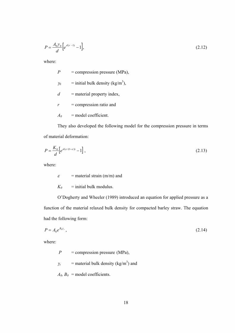
Faborode and O’Callaghan (1986) theoretically studied the compression process

of agricultural materials. They derived a new model for the compression pressure in

terms of compression ratio (r = γ/γ0) and the initial density:

18

[ ]1)1(00 −= −rded

AP

γ, (2.12)

where:



d = material property index,

r = compression ratio and

A0 = model coefficient.

They also developed the following model for the compression pressure in terms

of material deformation:

[ ]1))1/((0 −= −εεded

KP , (2.13)

where:

ε = material strain (m/m) and

K0 = initial bulk modulus.

O’Dogherty and Wheeler (1989) introduced an equation for applied pressure as a

function of the material relaxed bulk density for compacted barley straw. The equation

had the following form:

sBeAP γ00= , (2.14)

where:



A0, B0 = model coefficients.

19

O’Dogherty and Wheeler (1989) also reported the relationship between pressure,

moisture content, and the relaxed density of compressed wheat straw as given below:

[ ] )/ln(/)7()/1( / qPmPl nMs

w−=γ , (2.15)

where:



Mw = straw moisture content (% wb) and

l, m, n, q = model coefficients.

Ferrero et al. (1990) studied the pressure-density relationship of compressed

straw. They compressed chopped wheat and barley straw with maximum length of 40

mm and moisture contents ranging from 7 to 23 and 10 to 20%, respectively. The

pressure range of 20 to 100 MPa at a loading rate of 13 mm/s was applied to the

materials and the following empirical model was fitted to the experimental data:

)1)(( 000CP

s ePBA −−++= γγ , (2.16)

where:





Watts and Bilanski (1991) reported that the maximum stress in alfalfa wafers for

a certain deformation was a function of the material density in the form of:

[ ])(1log 021 γγ −−= sKKP (2.17)

20

where:



γ0 = initial bulk density (kg/m3) and

K1, K2 = variables which are linear functions of material moisture content,

loading rate, and leaf content.

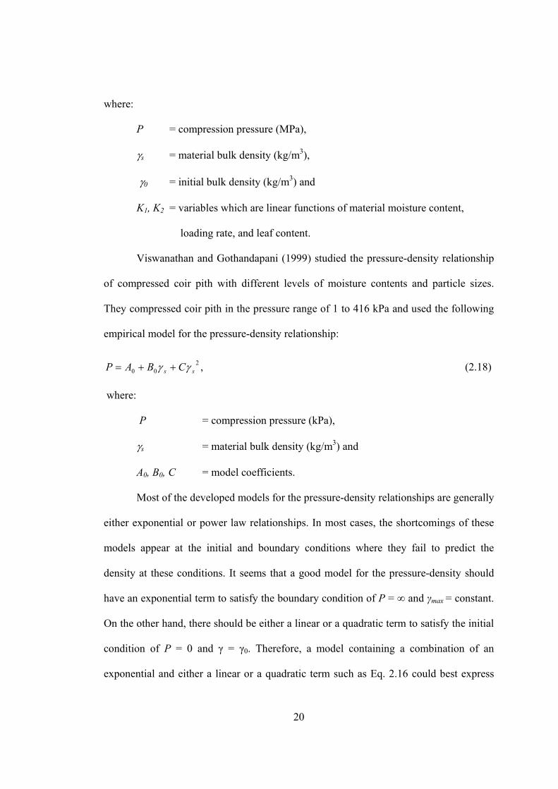
Viswanathan and Gothandapani (1999) studied the pressure-density relationship

of compressed coir pith with different levels of moisture contents and particle sizes.

They compressed coir pith in the pressure range of 1 to 416 kPa and used the following

empirical model for the pressure-density relationship:

200 ss CBAP γγ ++= , (2.18)

where:

P = compression pressure (kPa),



Most of the developed models for the pressure-density relationships are generally

either exponential or power law relationships. In most cases, the shortcomings of these

models appear at the initial and boundary conditions where they fail to predict the

density at these conditions. It seems that a good model for the pressure-density should

have an exponential term to satisfy the boundary condition of P = ∞ and γmax = constant.

On the other hand, there should be either a linear or a quadratic term to satisfy the initial

condition of P = 0 and γ = γ0. Therefore, a model containing a combination of an

exponential and either a linear or a quadratic term such as Eq. 2.16 could best express

21

the pressure-density relationship in compressed forage materials. It should also be noted

that all aforementioned models have been developed based on data obtained from

compressing forage materials in a closed-end cylindrical die. Thus, the models cannot be

exactly extended to the baling process.

2.2.2 Pressure Distribution

Sitkei (1986) introduced a model for the stress distribution inside the forage bale

at a distance x from the full extension point of the compressing plunger in terms of the

material properties and the compression chamber dimensions by assuming isotropic

linear elastic property for forage materials. The model had the form of:

⎥⎥⎦

⎤

⎢⎢⎣

⎡−+

−+−+=

∫ ∫= =

−−

−−−

L

sss

sss

a a

AAs

A

LxLA

sxLA

ssxLA

ex

dedeKe

eaBeABPPξ

ξ

ξ

ξ

ξαξαξαξξξξ

ξξαα

)/()/(

)/1/)(/()1)(/(

)/()/()/(

)(32)(2)(

, (2.19)

where:

[ ] )1/(/2/)2( ννμμα −++= baA ms , (2.20)

[ ])1/()/2(1(/)2( 2)2220 ννμνμααγ −+−+= baCB ms , (2.21)

342 /2/ αα ssss aBaBAK += , (2.22)

xa αξ −= , (2.23)

)2/(laam α−= , (2.24)

LaL αξ −= , (2.25)

Px = pressure in the x-direction at the distance x from the full extension

point of plunger (kPa),

Pe = pressure at the end of the compression chamber (kPa),

22

L = compression chamber length (cm),

x = distance from the full extension point of the plunger along the

compression chamber length (cm),

α = angle of top wall of compression chamber (radian),


μ = coefficient of friction between forage and compression chamber wall,

ν = Poisson’s ratio,

a = maximum height of compression chamber (cm),

b = maximum width of compression chamber (cm) and

C = model coefficient.

The shortcomings of this model were as follows:

a. it was derived for the bale chambers with only the top wall inclined, therefore it

could not be a general model for the pressure distribution,

b. in this model, pressure at the end of bale chamber was used as the boundary

condition to solve the governing differential equation which is difficult to

measure in practice and

c. there are some unnecessary terms in the model making it more complicated.

Faborode and O’Callaghan (1986) derived an equation to express the pressure

distribution in the compression die given by the following:

[ ] Rxprdx

reed

KP /)()1(0 1 μ−− −= , (2.26)

where:


point of plunger (MPa),

23

K0 = initial bulk modulus,

d = material property index,

r = compression ratio,

μ = coefficient of friction between die wall and forage materials,



pr = pressure ratio and

R = die radius (m).

Kepner et al. (1972) proposed the following equation to estimate the portion of

the plunger force which comes from the convergence of the bale chamber side walls:

μ)2( cca

c wLDyEF = , (2.27)

where:

Fc = portion of the plunger force resulting from the convergence of the bale

chamber side walls (N),

E = modulus of elasticity of the forage material (Pa),

y = average lateral deflection of the hay (m),

Da = average depth of the converging section of baler (m),

Lc = length of the converging section of baler (m),

wc = width of the converging section of baler (m) and

μ = coefficient of friction between the forage materials and chamber walls.

They emphasized that this equation covered only the side walls’ convergence force

rather than bottom wall friction force and the effect of the bottom wedges. Furthermore,

in the case of four-side convergence, the two Fc values should be considered.

24

Burrows et al. (1992) reported that in a high density baler, the compaction force

and the piston stroke had a parabolic relationship, when wheat straw with an initial

density of 92 kg/m3 was baled.

2.2.3 Energy Requirement

Reece (1967) designed a new wafering machine that continuously formed

wafers. The machine was tested by producing wafers from chopped alfalfa with 25%

moisture content, compression pressure of 13.81 MPa (2000 psi), and a holding time of

13 s. The results showed that the energy requirement for forming the wafer by this

machine with the abovementioned conditions was 3.23 Watt-h/kg (4.20 hp-h/t).

Hann and Harrison (1976) reported that in order to make wafers from alfalfa with

a cut length of 1.5 in. using a hydraulic wafering press, approximately 4.61 Watt-h/kg (6

hp-h per ton of dry hay) was required. Mohsenin and Zaske (1976) studied the

compaction of alfalfa hay and fresh alfalfa at different moisture contents and concluded

that the compaction energy required to achieve a certain bulk density for low moisture

hay was higher than that of the high moisture hay.

O’Dogherty and Wheeler (1984) reported the following equation to express the

relationship between the specific energy and the material relaxed bulk density of

compressed barley straw:

00.50525.0 −= ssW γ , (2.28)

where:

Ws = specific energy (MJ/t) and

γs = material bulk density (kg/m3).

25

Sitkei (1986) derived the following equation for the specific energy requirement

of compressed forage materials as a function of the applied pressure and material bulk

density:

maxmax /)/1(0

γγγ

γ∫ +=

s

PPdW ss , (2.29)

where:

Ws = specific energy,

Pmax = maximum pressure in the compression chamber,

γs = material bulk density,

γmax = maximum bulk density and

γ0 = initial bulk density.

Faborode and O’Callaghan (1986) reported that the specific energy of forage

materials increased during the compression process when the maximum applied pressure

increased. Freeland and Bledsoe (1988) compared seven different models of the large

round baler from the energy requirement viewpoint. They evaluated the effect of

chamber type and the operational procedures on the energy requirement of the balers.

The baler models with either fixed-geometry or variable-geometry chambers were

considered. They introduced a characteristic power curve for each of the balers, and

concluded that the fixed-geometry chamber needed more power to bale a certain amount

of materials compared to the variable-geometry chamber baler.

2.3 Wafer Formation

Wafer formation is affected by the physical characteristics of the materials that

are to be compressed such as crop moisture content, quality of forage materials, and

26

particle size. The following sections describe the effect of these parameters on wafer

formation.

2.3.1 Moisture Content

Pickard et al. (1961) studied the effect of the hay moisture content on the

pressure requirement of alfalfa wafers. Results of their research showed that at a

constant wafer density, the required pressure to form the wafer increased with increasing

alfalfa moisture content.

Rehkugler and Buchele (1967) evaluated the effect of moisture content of alfalfa

forage on the formation of wafers in a closed-end die. The results showed that wafer

density decreased with increased moisture content; therefore, concluded that to have a

high density wafer, moisture content of materials must be low.

Hall and Hall (1968) used a quadratic equation to express the wafer forming

stress at different die heating levels in terms of alfalfa moisture content in the form of:

2210 ww MBMBB ++=σ , (2.30)

where:

σ = required pressure (psi),

Mw = moisture content (% wb) and

B0, B1, B2 = model coefficients.

Srivastava et al. (1981) studied the effect of material moisture content on the

compression ratio, wafer density, and durability in the compaction of a mixture of alfalfa

and grass. They found that 11% (wb) was the optimum moisture content to get the

highest wafer density, durability, and the compression ratio. In another study, the range

27

of 10 to 20% (wb) was found to be the best moisture content of straw in order to produce

high durability wafers (O’Dogherty and Wheeler 1984).

2.3.2 Quality of Forage Materials

Pickard et al. (1961) studied the effect of the hay maturity on the pressure

requirement of alfalfa wafers. Results of their research showed that at a constant wafer

density, the required pressure to form the wafer increased with increasing alfalfa

maturity.

Reece (1966) studied the effect of alfalfa quality on the wafer durability. Wafer

formation was affected by the hay quality which was different for the hay coming from

the first and the second cuts. The hay from the second cut alfalfa resulted in a wafer with

a higher durability compared to the hay from the first cut due to its higher leaf-to-stem

ratio.

Rehkugler and Buchele (1967) evaluated the effect of the percentage of alfalfa

stem on the formation of wafers in a closed-end die. The experiments were performed on

both chopped and ground materials. The results showed that the high quantity of stem in

the material had an inverse effect on the formation of the wafer by decreasing protein

content as binding material. Grinding forage materials also decreased the expansion of

the wafer by changing the stem’s physical property.

2.3.3 Particle Size

O’Dogherty and Wheeler (1984) reported that durability of the straw wafer

decreased by chopping the material to be wafered. O’Dogherty and Gilbertson (1988)

conducted a study to establish a empirical relationship between the bulk density and the

cut length of wheat straw. Wheat straw was cut to a uniform length of 15 to 250 mm and

28

the samples were placed into a cylindrical container and a low pressure (100 Pa) was

applied to them. After measuring the bulk density of the samples at different cut lengths,

the following empirical model for the density-cut length relationship was developed:

[ ]1)/109.1(03412.0/17.98 ++= ccsγ , (2.31)

where:

γ s = material bulk density (kg/m3) and

c = cut length (mm).

2.4 Studies Related to Baling Operation

Corrie and Bull (1969) compared large rectangular hay bales with the

conventional bales at similar moisture content and density from the viewpoint of

heating, nutrient losses, and molding. The study showed that heating occurred in large

bales more than small ones at a certain dry matter density and moisture content, and it

was significantly affected by the dry matter bulk density, while nutrient losses were

higher in small bales compared to large bales. The results also indicated that decreasing

the dry matter density reduced the heating problem of the bales with a moisture content

of more than 25%, however this could not eliminate the risk of being contaminated with

mold. Meanwhile, the large rectangular bales provided a more efficient handling system

compared to the small ones.

Fairbanks et al. (1981) evaluated the effect of three types of baling machines on

the quality and the quantity of harvested hay. A small round baler, a big round baler, and

a mechanical stack maker were used in this study. The percentage of the crude fibre,

protein, and ash was measured as the quality factors immediately after baling and then

29

six months afterward. Results of this study revealed that there was no significant

difference between the quality of the fibres taken immediately after harvesting and those

taken after six months of storage; however, hay quality decreased with an increase in

precipitation.

Jenkins et al. (1985) used a large rectangular baler to collect and handle rice

straw, and compared its performance to that of a big round baler and the conventional

handling equipment. An economic comparison among the equipment was also

conducted. The results indicated that the large rectangular baler had the lowest handling

cost compared to the other available handling systems if the baler capacity was kept

high. Rain could easily penetrate the rectangular bales in an uncovered storage

condition, while rain penetration was limited to the outside surface in big round bales.

They concluded that, in contrast to the round bales, big rectangular bales must be stored

with cover.

Shinners et al. (1992) compared the performance of two small rectangular balers

with different feeding systems (side fed and bottom fed chamber) from the viewpoint of

the bale chamber and pick up losses. Results indicated 1.09 and 1.31% pick up losses for

the bottom and the side fed chambers, respectively. Therefore, the bottom-fed baler pick

up loss was 17% lower than that of the side fed chamber baler. Furthermore, they

reported 2.28 and 2.66% chamber losses for the bottom fed and the side fed chamber

baler, respectively (14% lower loss for the bottom fed chamber baler).

Coblentz et al. (1993) designed a new laboratory scale baler to make 10.3 by

10.8 by 13.4 cm wire-tied bales. The system was producing bales with densities of 150

to 800 kg/m3. The laboratory bale density was compared with that of the conventional

small-square alfalfa bales and a good correlation was found.

30

Shinners et al. (1996) compared the harvest and the storage losses of different

types of balers. Mid-size and small rectangular balers and the large round baler for the

harvesting losses comparison were considered. The pick up and the bale chamber losses

were compared for the considered balers. The results showed that the pick up losses of

the mid-size and the small rectangular and the large round baler were 0.7, 0.4, and 2.6%

of the total dry weight of the collected hay, respectively; therefore, the rectangular balers

had less pick up losses than the round balers. The bale chamber losses were 0.7, 1.6, and

1.6% of the total dry weight of the collected hay for the mid-size and the small

rectangular balers and the large round baler, respectively; therefore, the mid-size

rectangular baler had the least bale chamber loss.

2.5 Tri-axial Sensor Design

Forces applied to the forage material by the baler plunger are exerted on the bale

and bale chamber during the baling process. In order to model the pressure distribution

resulting from these forces, comprehensive knowledge of these forces is necessary.

Therefore, a tri-axial sensor is needed to record these compressive forces in three

directions. In this section, a review of studies related to sensor design is presented.

The tri-axial sensor is a force transducer which is able to measure the forces in

three directions independently using an extended octagonal ring (EOR). The EOR was

developed from the circular ring force transducer to give more stability to the transducer.

The idea of using the EOR in a measurement system was first introduced by Lowen et

al. (1951). Hoag and Yoerger (1975) derived analytical equations of stress distribution

for the simple and the extended ring transducers at different loading and boundary

conditions using the strain energy method. This study resulted in two equations

31

developed for the bending moment in the ring section of the extended ring which are

used for moment calculation in the ring section of the EOR as well. Thereafter,

modifications were brought to one of the Hoag and Yoerger’s equations by McLaughlin

(1996).

Godwin (1975) designed an extended octagonal ring transducer to measure the

soil reaction forces to the soil engaging tools in two directions and the moment in the

plane of these forces. A good linearity, small cross sensitivity, and hysteresis were

reported. Meanwhile, the practical sensitivities of the strain gages were much more than

the obtained values from the analytical equations. O’Dogherty (1975) fabricated a

transducer to determine the cutting and vertical forces of a sugar beet topping knife

using an extended octagonal ring. The results showed a good linearity, low hysteresis in

loading and unloading cycles, and cross sensitivities of 4.1 and 6.5% for the cutting and

the vertical forces, respectively in the calibration process of the transducer. Based on this

calculation, a modification to the coefficients of the formula which is used for the EOR

transducers was suggested; coefficients of 1.6 and 1.9 instead of 0.7 and 1.4 in the

equations of the vertical and the horizontal forces, respectively.

Godwin et al. (1993) designed a dynamometer using the EOR to measure the

exerted forces and moments on tillage tools. Two EOR in back-to-back form which their

longitudinal axes were making angles of 900 were used. The dynamometer using a tri-

axial loading method was calibrated and excellent linearity between the applied forces

and moments and the bridge output voltage was found. A small amount of hysteresis

effect between loading and unloading calibration curves, and cross sensitivity of less

than 4% was reported; however, in one case the reported cross sensitivity was 10.6%.

32

Gu et al. (1993) designed and built a transducer to measure the vertical and the

horizontal forces on the wheels of a quarter scaled model tractor using two EORs with

the stress nodes at positions of θ = ±45° and θ = 0°. The transducer was calibrated by

applying independent forces in two perpendicular directions, and a regression model for

each of the vertical and the horizontal primary sensitivities and the cross sensitivities

was developed. Cross sensitivities ranging from around zero to four percent were

reported.

O’Dogherty (1996) derived a formula to determine the ring thickness of the EOR

transducer using the data of the designed transducers by previous researchers. He

introduced a graphical procedure for the EOR design based on the geometrical

parameters of the ring. McLaughlin and co-workers (1998) designed and fabricated a

double extended octagonal ring (DEOR) drawbar transducer. They calibrated the

transducer using both uni-axial and tri-axial loading method. From the uni-axial loading

calibration, sensor cross sensitivities were assessed at 1.9 and 7.0% for the draft and the

vertical loading, respectively. From the tri-axial loading calibration, regression models

were derived to predict each of the draft, vertical, and side loads. The designed

transducer was also used to measure the draft, the vertical, and the side loads on the

drawbar of two secondary tillage tools and proved to be reliable in the field to measure

the drawbar forces.

2.6 Summary

Most of the information found in the literature about coefficients of friction was

related to the kinetic coefficient of friction rather than the static coefficient of friction.

Only one study was found about static coefficient of friction of some forage materials

33

(Richter 1954), but results of this research were not reliable because the moisture

content of materials has not been reported. Regarding other properties such as modulus

of elasticity and particle stiffness, information found in the literature were for materials

different from those used in this study. The results of crop properties from literature are

not directly extendable to this study; however, this information can help understand crop

behavior during the baling process. This information also gives an idea about methods of

measuring crop properties.

In the area of pressure-density relationships, more literature was found, however

all developed models were based on the data of compressing forage materials in a

closed-end cylindrical die. Although, these models cannot be directly extended to the

pressure-density relationship in balers, some of them (recently derived ones) give

information about the form of the pressure-density model in balers. They can also help

to determine the factors affecting this relationship.

The knowledge of pressure distribution along the axis of compression for

compressed forage materials, as expressed within the literature (Eqs. 2.19 and 2.26),

provides an idea about the pattern of pressure distribution in a large square baler and the

parameters affecting this pattern. Only two models (Sitkei1986 and Faborode and

O’Callaghan1986) were found in the literature regarding pressure distribution. One was

based on data released from compressing forage materials in a cylindrical die which is

not extendable to the pressure distribution in a bale chamber. The other one was an

analytical model which has been developed for a bale chamber by assuming an isotropic

linear elastic property for forage materials. The latter model had three shortcomings as

follows:

34

a. it was derived for bale chambers with only the top wall inclined, whereas in a

large square baler not only the top wall, but the side walls are also inclined;

b. in this model, the pressure at the end of bale chamber was used as the boundary

condition to solve the governing differential equation which is difficult to

measure in practice; and

c. there are some unnecessary terms in the model, making it more complicated.

The aforementioned shortcomings in previous studies justify distinct

experimental and theoretical studies on the pressure-density relationships and the

pressure distribution during the baling process.

35

CHAPTER 3

MATERIALS AND METHODS

In this chapter, model development, materials and methods used to carry out the

experiments, instrumentation set up, and field and laboratory tests are described.

3.1 Model Development

In this section, model development for the pressure distribution and pressure-

density relationship is explained. In each case, development of both analytical and

empirical models is covered.

3.1.1 Pressure Distribution

3.1.1.1 Analytical Model

The compositions and the properties of forage materials change continuously

during growth, maturity, and even after harvest because they are alive and biological

materials. These materials consist of solid and liquid components which make a very

complex construction whose mechanical behavior cannot be characterized by simple

equations and constants. The mechanical behavior of these materials varies with factors

such as loading rate, previous history of loading, material composition, and moisture

content. Therefore, most agricultural materials do not follow linearity in compression

tests even at small deformations. Because the load-deformation relationship in forage

materials depends on deformation rate, time also plays a role in this relationship. Thus,

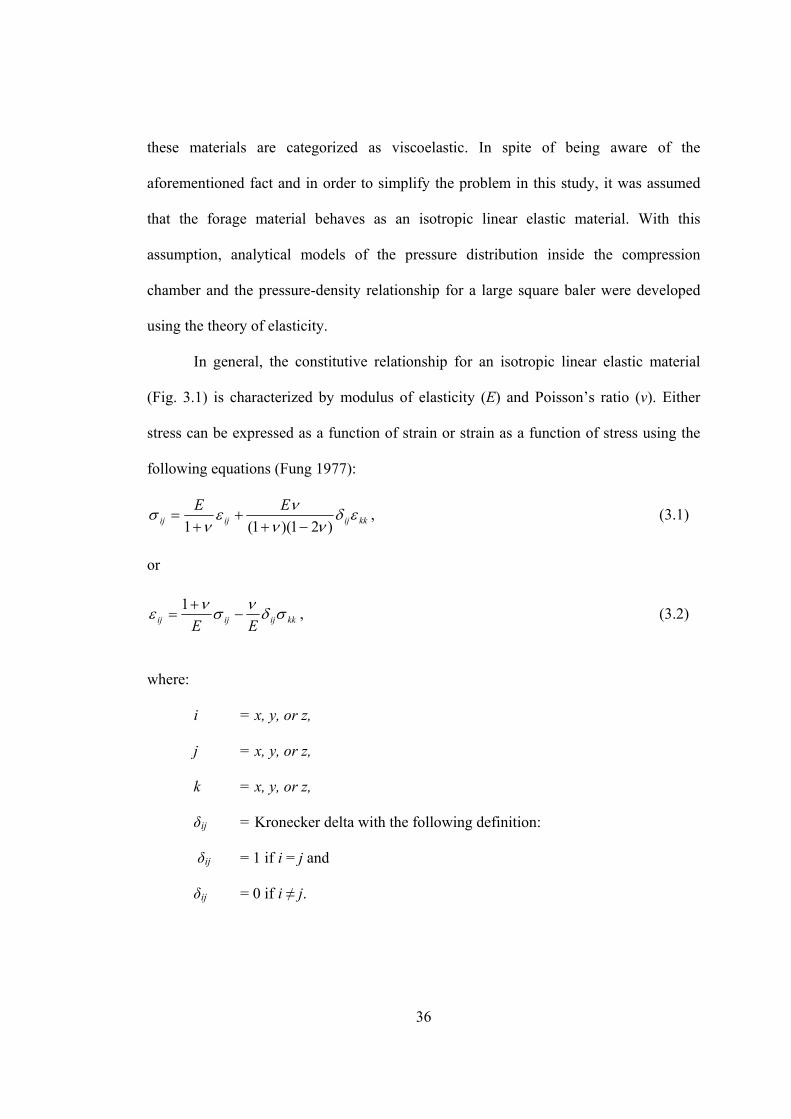
36

these materials are categorized as viscoelastic. In spite of being aware of the

aforementioned fact and in order to simplify the problem in this study, it was assumed

that the forage material behaves as an isotropic linear elastic material. With this

assumption, analytical models of the pressure distribution inside the compression

chamber and the pressure-density relationship for a large square baler were developed

using the theory of elasticity.

In general, the constitutive relationship for an isotropic linear elastic material

(Fig. 3.1) is characterized by modulus of elasticity (E) and Poisson’s ratio (ν). Either

stress can be expressed as a function of strain or strain as a function of stress using the

following equations (Fung 1977):

kkijijijEE εδ

νννε

νσ

)21)(1(1 −++

+= , (3.1)

or

kkijijij EEσδνσνε −

+=

1 , (3.2)

where:

i = x, y, or z,

j = x, y, or z,

k = x, y, or z,

δij = Kronecker delta with the following definition:

δij = 1 if i = j and

δij = 0 if i ≠ j.

37

Considering the normal stresses only and substituting σii = -Pi and εii = -εi where i = x, y,

and z (Fig. 3.2) the following equations can be derived between pressure and

compressive strain of an element of the bale in different directions:

( )[ ]zyxx PPPE

+−= νε 1 in x-direction, (3.3)

( )[ ]zxyy PPPE

+−= νε 1 in y-direction and (3.4)

( )[ ]yxzz PPPE

+−= νε 1 in z-direction. (3.5)

These relationships only valid for an isotropic linear elastic element.

y

x

z

σxx

σxy

σxzσzy

σzxσzz

σyy

σyxσyz

Figure 3.1 Stress tensor on an element of an isotropic linear elastic material.

38

y

x

z

Px = -σxx

Pz = -σzz

Py = -σyy

εx = -εxx

εz = -εzz

εy = -εyy

Figure 3.2 Normal stresses applied to an element of the bale inside the compression chamber.

From Eqs. 3.3, 3.4, and 3.5, εx, Py, and Pz can be calculated in terms of Px, εy, and εz as

follows:

( )ZYxx PE

εεν

νν

ννε +−

−−−+

=)1()1(

)21)(1( , (3.6)

( )ZYxyEPP νεενν

ν+

−+

−=

)1(1 2 and (3.7)

( )ZYxzEPP ενενν

ν+

−+

−=

)1(1 2 . (3.8)

Volume change of element is also stated in terms of either strains or stresses using the

following equation:

( )zyxzyx PPPEV

V++

−=++≅

Δ νεεε 21 . (3.9)

39

A general form of the equation of equilibrium for an isotropic linear elastic material is

given as follows:

0=+∂

∂i

ij bjσ

. (3.10)

Since body forces (bi) are assumed to be zero, the following equations result from Eq.

3.10:

0=∂∂

+∂

∂+

∂∂

zyxxzxyxx σσσ

, (3.11)

0=∂

∂+

∂

∂+

∂

∂

zyxyzyyxy σσσ

and (3.12)

0=∂∂

+∂

∂+

∂∂

zyxzzyzxz σσσ

. (3.13)

From Figures 3.3 and 3.4, ax and bx (variable height and width of compression chamber

as a function of the distance from the plunger) are defined using the following equations:

xaax α−= , (3.14)

xbbx β2−= , (3.15)

where:

a = maximum height of compression chamber (cm) and

b = maximum width of compression chamber (cm).

Furthermore, according to the geometry of the compression chamber, the following

assumptions can be made:

)(xax

yy εαε ==− and (3.16)

)(2 xb

xzz εβε ==− . (3.17)

40

Equations 3.16 and 3.17 state that the strains in the y- and z-directions are solely a

function of x. Therefore, based on Eqs. 3.6, 3.7, and 3.8, the strain in x-direction and the

pressures in y- and z-directions are also functions of x only if the variation of Px with

respect to y and z is zero. σyz is also assumed to be zero which is a reasonable

assumption. Therefore, the following equations result from Eqs. 3.11, 3.12, and 3.13:

0=∂∂

+∂

∂+

∂∂

zyxxzxyxx σσσ

, (3.18)

0=∂

∂

xxyσ

and (3.19)

0=∂∂

xxzσ

. (3.20)

Pp

y

dxxx

α

L

a x

Figure 3.3 Side view of the compression chamber of a large square baler.

41

β

z

x

b

b x

dx

Figure 3.4 Top view of the compression chamber of a large square baler.

Equations 3.19 and 3.20 show that σxy and σxz are only functions of y and z, so they do

not appear in the equation of equilibrium in the x-direction. Therefore, the stresses on

the wedge part of an element of elastic material resemble what are shown in Fig. 3.5.

Based on this free body diagram, the equations of equilibrium in the x- and y-directions

are as follows:

( ) 0cos

coscos

sintan =⎟⎠⎞

⎜⎝⎛ Δ

+Δ

−Δ+Δ xnnxxyx bxxbxxαατ

αασσασ and (3.21)

( ) 0cos

sincos

costan =⎟⎠⎞

⎜⎝⎛ Δ

−Δ

+Δ+Δ− xnnxxyy bxxbxxαατ

αασασσ . (3.22)

42

x

y

z

σyy(x)

σxy

y

x

σxx(x)

Δx

α σyy

σyx

σn

τnσxx

ασxy

xxxx

xx Δ∂∂

+σ

σ

Figure 3.5 Stresses applied on the wedge part of an elastic material.

From Eqs. 3.21 and 3.22, σn andτ n could be calculated as follows:

ασασασσ 2sincossin 22xyyxn ++= and (3.23)

ασασσ

τ 2cos2sin2 xy

yxn +⎟⎟

⎠

⎞⎜⎜⎝

⎛ −= . (3.24)

Comparing these stresses to pressures applied to an element of the bale in bale chamber

(Fig. 3.6), the following relationships could be found:

ασαασ 2sincossin 22xyyxnn PPP −+=−= and (3.25)

ασαμττ 2cos2sin2 xy

yxnnf

PPP −⎟⎟

⎠

⎞⎜⎜⎝

⎛ −==−= . (3.26)

43

σyx

τf = μPn

Py

Px

Pn

σxy

Figure 3.6 Pressures applied on the wedge part of an element of the bale.

Using Eqs. 3.25 and 3.26, σxy and Pn can be calculated in terms of μ, α, Px, and Py as

follow:

( ) ( )( ) ⎥

⎥⎦

⎤

⎢⎢⎣

⎡

−

−++=

ααμααμααμ

σ2cos2sin2

2sincos22sinsin2 22yx

xy

PP and (3.27)

( ) ( )( ) α

ααμααμααμ

αα

2sin2cos2sin2

2sincos22sinsin2

cossin22

22

⎥⎥⎦

⎤

⎢⎢⎣

⎡

−

−++−

+=

yx

yxn

PP

PPP

. (3.28)

Since in the large square baler, α is very small (α<<1rad) the following assumptions can

be made:

yn PP ≈ and (3.29)

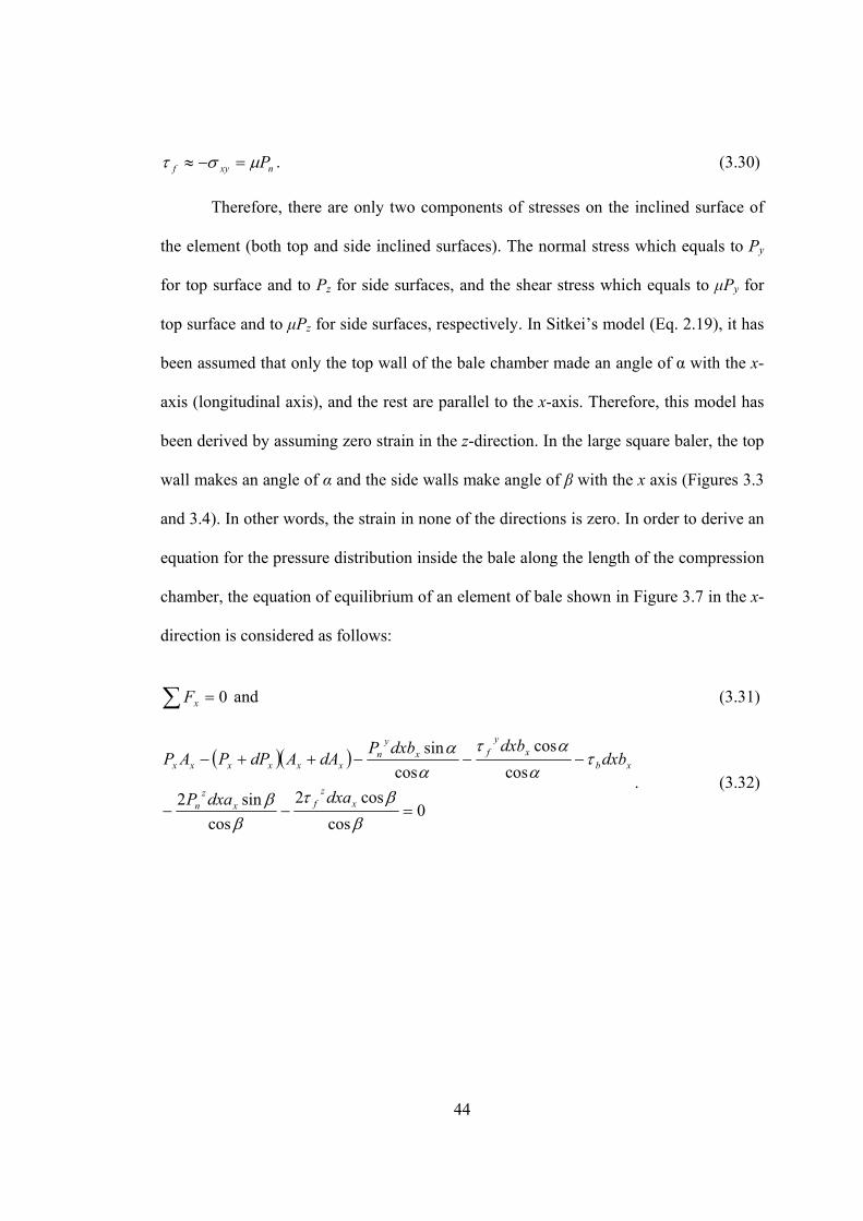
44

nxyf Pμστ =−≈ . (3.30)

Therefore, there are only two components of stresses on the inclined surface of

the element (both top and side inclined surfaces). The normal stress which equals to Py

for top surface and to Pz for side surfaces, and the shear stress which equals to μPy for

top surface and to μPz for side surfaces, respectively. In Sitkei’s model (Eq. 2.19), it has

been assumed that only the top wall of the bale chamber made an angle of α with the x-

axis (longitudinal axis), and the rest are parallel to the x-axis. Therefore, this model has

been derived by assuming zero strain in the z-direction. In the large square baler, the top

wall makes an angle of α and the side walls make angle of β with the x axis (Figures 3.3

and 3.4). In other words, the strain in none of the directions is zero. In order to derive an

equation for the pressure distribution inside the bale along the length of the compression

chamber, the equation of equilibrium of an element of bale shown in Figure 3.7 in the x-

direction is considered as follows:

0=∑ xF and (3.31)

( )( )

0cos

cos2cos

sin2cos

coscos

sin

=−−

−−−++−

ββτ

ββ

τα

ατα

α

xz

fxz

n

xbx

yfx

yn

xxxxxx

dxadxaP

dxbdxbdxbP

dAAdPPAP. (3.32)

45

x

y

z

Pybxdxτb

(Px+dPx)(Ax+dAx)

y

x

PxAx

dx

Pny = Py

τfy = μPn= μPyα

Figure 3.7 Applied forces to an element of the bale in the compression chamber.

Since α and β are small, the following assumptions can be made:

ααα == tansin ,

βββ == tansin ,

1coscos == βα ,

yy

n PP = ,

yy

n Pμτ = ,

zz

n PP = ,

zz

n Pμτ = and

yb Pμτ = .

46

By considering the above assumptions, Eq. 3.32 can be written as:

( ) ( ) ( ) 022 =++++ μβμα xzxyxx aPbP

dxAPd

. (3.33)

By inserting Py and Pz from Eqs. 3.7 and 3.8 into Eq. 3.33, the following equation is

obtained:

( ) ( ) ( )[ ]

( )( ) ( )( )[ ] 0221

221

2 =+++++−

+

+++−

+

yzxzyx

xxxxx

abE

abP

dxAPd

νεεμβνεεμαν

μβμανν

(3.34)

By inserting εy and εz from Eqs. 3.16 and 3.17 into Eq. 3.34, the following equation can

be written:

( ) ( ) ( )

( ) ( ) 022221

221

2 =⎥⎦

⎤⎢⎣

⎡⎟⎠⎞

⎜⎝⎛ +

++⎟

⎠⎞

⎜⎝⎛ +

+−

+

⎥⎦

⎤⎢⎣

⎡ ++

+−

+

xabbbaa

EA

baAP

dxAPd

xx

x

xx

xxxx

ναβμβνβαμαν

μβμανν

(3.35)

In order to simplify the problem, the mean values of Am, am, and bm are used instead of

variable values of Ax, ax, and bx according to the following definitions:

)2/(Laaa mx α−=≈ ,

)2/(2 Lbbb mx β−=≈ and

mmmx baAA =≈ . Therefore the following differential equation can be written for the pressure in the x-

direction:

47

0)1(

)2)((2)2)(2(

)(221

2 =⎥⎦

⎤⎢⎣

⎡−

+++++

+⎥⎦

⎤⎢⎣

⎡ ++

+−

+

xbaba

abaabbE

Pbadx

dP

mm

mm

xmm

x

νβανμββναμα

βμμαν

ν

(3.36)

In Sitkei’s model (Eq. 2.19), the modulus of elasticity (E) has been considered as a

function of the strain in y-direction, while the results of the experiments in this study

showed that E was constant for the density range encountered in the large square baler.

Therefore, a constant E was considered in this model. By reducing the constant

coefficients of the above differential equation to A and B using the following

relationships (Eqs. 3.38 and 3.39), the differential equation can be written in a simple

form of Eq. 3.37.

0=++ BxAPdxdP

xx , (3.37)

where:

⎥⎦

⎤⎢⎣

⎡ ++

+−

=mm ba

A )(221

βμμαν

ν , (3.38)

⎥⎦

⎤⎢⎣

⎡−

+++++=

)1()2)((2)2)(2(

2νβανμββναμα

mm

mm

babaabaabb

EB , (3.39)



L = compression chamber length (cm),



α = angle of top wall of compression chamber with respect to x-axis,

48

β = angle of side wall of compression chamber with respect to x-axis,

μ = coefficient of friction between forage and compression chamber wall,

ν = Poisson’s ratio,

a = maximum height of compression chamber (cm) and

b = maximum width of compression chamber (cm).

Equation 3.39 is a first order linear differential equation. The solution of this equation

with the boundary condition of Px = Pp at x = 0 (pressure on the plunger is Pp) could be

written as:

( )AxAxpx eAx

ABePP −− −−+= 12 . (3.40)

A and B as are expressed in Eqs. 3.38 and 3.39 are functions of compression chamber

geometry and forage material properties. In order to evaluate the effect of these

parameters (α, β, μ, υ, and cross-section area) on the constants A and B and consequently

on the pressure distribution, a compression chamber with a square cross-section is

assumed for simplification (a = b and am = bm). Therefore, A and B could be written as

follows:

( ) ( )βμαν

ν 241

++−

=ma

A , (3.41)

⎥⎦

⎤⎢⎣

⎡−

+++++=

)1()2)((2)2)(2(

2νβανμββναμα

maaEB

, (3.42)

According to Eqs. 3.41 and 3.42, A and B increase with increasing α, β, μ, and υ, while

they decrease with increasing cross-section area (a and am). Therefore, pressure in the x-

direction drops off faster with increasing wall angles, coefficient of friction, and

49

Poisson’s ratio, whereas with an increasing cross-section area it drops off more slowly.

If a compression chamber with no converged walls is considered (α = β = 0), constant B

will disappear and constant A will be only function of coefficient of friction, Poisson's

ratio, and chamber cross-section area. This shows that the second term of Eq. 3.40

comes from the walls convergence. Equation 3.40 expresses the pressure distribution

inside the compression chamber of a baler along the axis of compression (x-direction) as

a function of crop properties, bale dimensions, and the distance from the full extension

point of the plunger. Using Eqs. 3.7, 3.8, and 3.40, the following equations can be

derived for pressures in the y- and z-directions (Py and Pz):

( ) ( ) xab

abEeAxABePP AxAx

py ⎥⎦

⎤⎢⎣

⎡−

++⎥⎦

⎤⎢⎣⎡ −−+

−= −−

22 121

1 ννβα

νν and (3.43)

( ) ( ) xab

baEeAxABePP AxAx

pz ⎥⎦

⎤⎢⎣

⎡−+

+⎥⎦⎤

⎢⎣⎡ −−+

−= −−

22 121

1 νναβ

νν . (3.44)

According to Eqs. 3.43 and 3.44, on the plunger (x = 0) the following relationships exist

between pressures in the x-, y-, and z-directions (Pp is pressure in the x-direction at x =

0):

)0(11

)0()0( xpzy PPPP ⎟⎠⎞

⎜⎝⎛−

=⎟⎠⎞

⎜⎝⎛−

==ν

νν

ν . (3.45)

Therefore, the Poisson’s ratio (ν) can be calculated using Eq. 3.45 as follows:

)0()0()0(

)0()0()0(

xz

z

xy

y

PPP

PPP

+=

+=ν . (3.46)

The developed analytical model for pressure distribution in this study was validated

using collected data for barley straw, wheat straw, and whole green barley. The least-

50

square regression analysis method was used for model validation, and model constant

coefficients were estimated.

3.1.1.2 Empirical Model

The analytical model for the pressure distribution is a complicated model with

many parameters. These parameters which are related to the compression chamber

dimensions or forage material physical and mechanical properties have to be measured

prior to the modeling process. Measuring these parameters is usually a time-consuming

exercise (requires a lot of time) and is very expensive. So, in addition to the analytical

model, an empirical model was also introduced for the pressure distribution in the x- and

y-directions for the tested forage materials using the experimental data. According to the

pattern of the experimental data, an exponential model with unknown constants was

considered for each of the materials. The least square error in the regression analysis was

used to validate the model and estimate the model parameters. The general form of the

presented models was the same for the all tested forage materials, while the model

constants differed from material to material. The following is the general form of the

model in the x-direction for the tested forage materials:

xBx eAP 0

0−= , (3.47)

where:

Px = pressure in the x-direction as a function of distance from the full

extension point of the plunger (kPa),


compression chamber length (cm) and

A0, B0 = model coefficients.

51

Because the dug hole in the bale for the sensor was usually larger than the sensor

size, there was a gap between the sensor body and the top and side walls of the dug hole.

In practice, some of the forces applied in the y-direction have been consumed to fill this

gap. Since filling this gap takes some time, at the beginning of the force recording

process (near the plunger), the recorded forces in the y-direction were much lower than

the expected forces. However, the recorded forces at the end of the compression

chamber were much closer to the expected forces. Therefore, the values of forces

recorded in the y-direction were not reliable (especially near the plunger), however the

trend of force changing with distance from the plunger showed the force distribution

pattern inside the compression chamber in the y-direction. After converting the recorded

forces to pressure, the following exponential model was fitted to the experimental data

of barley straw, wheat straw, and whole green barley in the y-direction:

xDy CeP 0−= (3.48)

where:

Py = pressure in the y-direction at the distance x from the full extension



compression chamber length (cm) and

C, D0 = model coefficients.

The designed sensor was not able to record the forces in the z-direction (section 3.3.2.2);

therefore, there were no data available in the z-direction to model the pressure

distribution in this direction.

52

3.1.2 Pressure-Density Relationship

3.1.2.1 Analytical Model

It is also important to find a relationship between bale density and applied

pressure to the bale. Bale density changes during the baling process along the bale length

because of changing bale volume. Bale volume change is related to the pressures in

different directions given by Eq. 3.9. An analytical model can be derived by inserting Py

and Pz from Eqs. 3.7 and 3.8 into Eq. 3.9 as follows:

( )⎟⎠⎞

⎜⎝⎛ +

−+

−+

−=

Δzyxx

EPPEV

V εενν

νν11

221

0

. (3.49)

On the other hand, the relationship between volume change and density is expressed by:

xVV

VV

γγ 0

00

11 −=−=Δ , (3.50)

where:

ΔV = bale volume change (m3),

V0 = bale initial volume (m3),

V = bale volume as a function of distance from the full extension point of

the plunger (m3),

γx = bale density as a function of distance from the full extension point of

the plunger (kg/m3) and

γ0 = initial bale density (kg/m3).

By equating the right hand sides of Eqs. 3.49 and 3.50, and using Eqs. 3.16 and 3.17, the

following equation can be obtained:

53

( )( )( ) x

abab

EPx

x⎟⎠⎞

⎜⎝⎛ +

−−

+−

+−=−

βανν

ννν

γγ 2

121

1121

1 0 . (3.51)

After simplifying Eq. 3.51, the following model can be developed for the bale density as

a function of pressure, crop properties, and compression chamber dimensions:

( )( ) ( ) ( ) ( )[ ]xabEabPEab

Eab

xx βαννν

νγγ

2121110

+++−−−−

= . (3.52)

At the plunger (x = 0), Px is equal to Pp; therefore, γp which is the bale density in front of

the plunger is calculated from the following equation:

( )( ) ( )( ) p

p PEE

ννννγ

γ+−−−

−=

121110 . (3.53)

3.1.2.2 Empirical Model

Developing an empirical model for the relationship between the bale density and

plunger pressure in a large square baler was one of the objectives of this study. In order

to establish this model, the data of baling alfalfa and barley straw at different load

settings were used. In these tests, plunger forces were recorded by strain gages, and

densities were calculated by measuring bale dimensions and weight. Different models

have been introduced for the pressure-density relationship of forage materials, where

some of them were tested with the data of this experiment to find the best model for the

pressure-density relationship. The most promising model for the purpose of this study

was the model (Eq. 2.16) suggested by Ferrero et al. (1990). Thus, this model was

modified to show the best agreement with the experimental data of the relationship

between alfalfa and barley straw bale density and plunger pressure. Therefore, the

54

pressure-density relationship for the large square baler during the alfalfa and barley

straw baling process was best expressed with the following model:

)1)(( 02000

pPDpps eCPPBA −−+++= γγ , (3.54)

where:



Pp = compression pressure on the plunger (MPa) and

A0, B0, C, D0 = model coefficients.

Comparison of the analytical and empirical models for bale density as a function of

pressure on plunger, Pp, (Eqs. 3.52 and 3.53) shows that these models have completely

different general forms, however both models reveal that bale density has a direct

relationship with material initial density and plunger pressure.

3.2 Large Square Baler

In this project, a newly designed New Holland BB960 large square baler (Fig.

3.8) was used to bale alfalfa, whole green barley, barley straw, and wheat straw. This

baler produces bales with a width of 1.2 m, height of 0.9 m, and an adjustable length of

up to 2.5 m. A schematic of the large square baler and its components is shown in Figure

3.9. A large square baler has a two-stage feeding system (Figs. 3.10 and 3.11). After

being lifted by the pickup (1), the centering augers guide the crop to the packer

chamber throat opening, where it is swept into the pre-compression chamber by a

set of packer fingers (2) mounted on a triple throw crankshaft, giving the packer a

55

Figure 3.8 New Holland BB960 large square baler.

raking action that mixes the crop and ties the flake together as it feeds into the fixed-

volume pre-compression chamber (3). The holding fingers (4) retain the charge in the

chamber until the crop density reaches a predetermined level. At this point, the pre-

compression forks (5) engage to sweep the preformed flake into the bale chamber where

it is compressed by the plunger (6) into the compression chamber (7). Since one charge

makes one complete flake, bale density is always consistent throughout the bale with all

sides being well formed regardless of crop conditions or ground speed. This is

especially important when baling light swaths on rough ground. Conversely, balers

without pre-chambers must be driven at high speed to attempt to maintain flake content

and bale shape.

56

Pick-up (1)

Packer fingers (2)Pre-compression forks (5)

Pre-compression chamber (3)

Plunger (6)

Compression chamber (7)

Holding fingers (4)

Figure 3.9 Cross-view of a CNH large square baler (courtesy of CNH).

Figure 3.10 Packing the pre-compression chamber (courtesy of CNH).

Pick-up (1)

57

Figure 3.11 Filling the main compression chamber (courtesy of CNH).

The bale density control system in the large square baler could be used in three

different modes. The first mode is called the automatic bale density control mode. The

baler should work normally in this mode to produce bales with a uniform bale density

close to the pre-set density by the operator. In this study, the baler was operated in the

automatic mode, so only this mode is explained in this section. In this mode, the plunger

force sensor senses the force applied to the bale via the plunger, and a processor sets the

pressure in the bale density controlling system to adjust the bale density based on

plunger force. A density level is selected in this mode by an operator from the tractor

cab based on the crop type and moisture content. This mode can compensate for the

variation in the baling material conditions such as moisture content, so that the pressure

in the density cylinders changes to keep the plunger load and the bale density constant.

The available settings are 10, 20, 30, up to 100% of the maximum available plunger

force, and by changing the load setting; the side hydraulic cylinders adjust the applied

58

forces to the top and side walls in such a way that the baler applies a resistance equal to

the requested force to the plunger (New Holland BB960 Manual 2001).

There is also a pre-compression chamber that is located prior to the main

compression chamber so that the forage materials are compressed at an adjustable

pressure before entering the main chamber. The packer charges the forage materials

continuously into this chamber; when enough material is charged into the pre-

compression chamber and the pressure in the pre-compression chamber is exceeded

from the stuffer trip setting (this setting sets the size of the flake charged into the bale

chamber), the sensor paddles are pushed down (Fig. 3.12). At this time, the stuffer drive

is activated and the stuffer fork sends the material from the pre-compression chamber to

the bale chamber when the plunger is doing its compression stroke. At the same time,

the holding fingers open the top opening of the pre-compression chamber. Once the

material flake is charged to the bale chamber, the holding fingers return to their original

position (Fig. 3.13).

Figure 3.12 Sensors of the pre-compression chamber (New Holland BB960 Manual

2001).

59

Figure 3.13 The holding fingers situation right after feeding the materials to the bale

chamber (New Holland BB960 manual 2001).

There is a lever with ten positions to apply ten different pre-compression

pressure levels to the materials which is called the stuffer trip sensitivity lever. This

lever is connected to the pre-compression chamber sensor via a spring. Changing the

lever position changes the spring tension and consequently changes the sensor

sensitivity. The position of this lever determines the amount of materials fed to the bale

chamber (flake size) in such a way that increasing the spring tension increases the flake

size and decreasing the spring tension decreases the flake size. There are ten positions on

this lever (one to ten) to choose ten different flake sizes. Lower positions give thinner

flakes and higher positions give thicker flakes. Well-shaped dense bales should have a

flake with the thickness of 60 to 80 mm; however, flake size depends on the sensor

sensitivity.

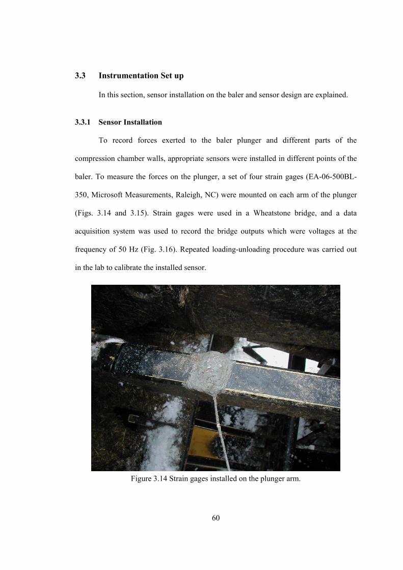
60

3.3 Instrumentation Set up

In this section, sensor installation on the baler and sensor design are explained.

3.3.1 Sensor Installation

To record forces exerted to the baler plunger and different parts of the

compression chamber walls, appropriate sensors were installed in different points of the

baler. To measure the forces on the plunger, a set of four strain gages (EA-06-500BL-

350, Microsoft Measurements, Raleigh, NC) were mounted on each arm of the plunger

(Figs. 3.14 and 3.15). Strain gages were used in a Wheatstone bridge, and a data

acquisition system was used to record the bridge outputs which were voltages at the

frequency of 50 Hz (Fig. 3.16). Repeated loading-unloading procedure was carried out

in the lab to calibrate the installed sensor.

Figure 3.14 Strain gages installed on the plunger arm.

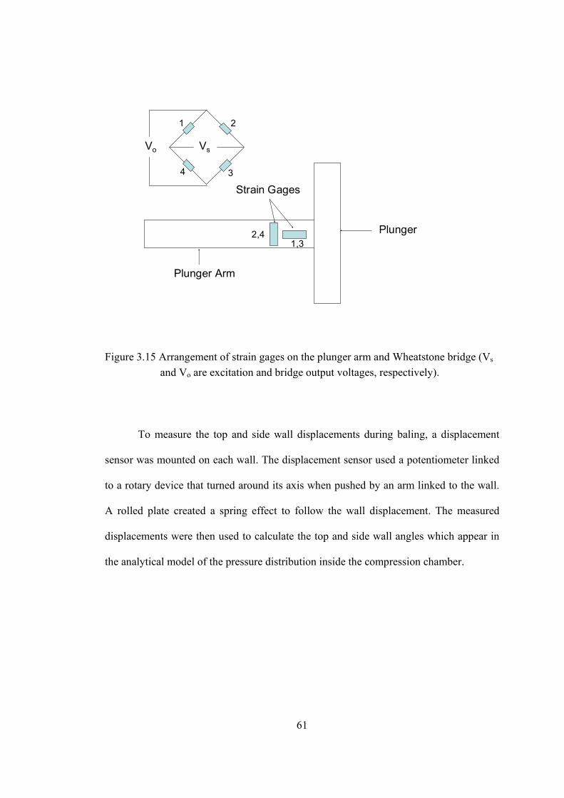
61

Plunger

Plunger Arm

Strain Gages

1,32,4

Vo Vs

1 2

34

Figure 3.15 Arrangement of strain gages on the plunger arm and Wheatstone bridge (Vs

and Vo are excitation and bridge output voltages, respectively).

To measure the top and side wall displacements during baling, a displacement

sensor was mounted on each wall. The displacement sensor used a potentiometer linked

to a rotary device that turned around its axis when pushed by an arm linked to the wall.

A rolled plate created a spring effect to follow the wall displacement. The measured

displacements were then used to calculate the top and side wall angles which appear in

the analytical model of the pressure distribution inside the compression chamber.

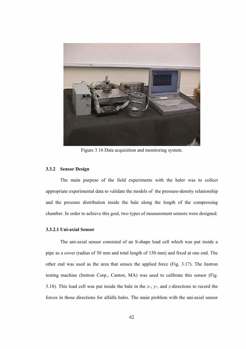
62

Figure 3.16 Data acquisition and monitoring system.

3.3.2 Sensor Design

The main purpose of the field experiments with the baler was to collect

appropriate experimental data to validate the models of the pressure-density relationship

and the pressure distribution inside the bale along the length of the compressing

chamber. In order to achieve this goal, two types of measurement sensors were designed.

3.3.2.1 Uni-axial Sensor

The uni-axial sensor consisted of an S-shape load cell which was put inside a

pipe as a cover (radius of 50 mm and total length of 150 mm) and fixed at one end. The

other end was used as the area that senses the applied force (Fig. 3.17). The Instron

testing machine (Instron Corp., Canton, MA) was used to calibrate this sensor (Fig.

3.18). This load cell was put inside the bale in the x-, y-, and z-directions to record the

forces in those directions for alfalfa bales. The main problem with the uni-axial sensor

63

was that it was not able to record the forces in three directions simultaneously. In

addition, because of the cylindrical shape of the sensor, the alignment with the

corresponding axis inside the bale chamber was difficult.

Figure 3.17 Assembled uni-axial sensor (height is 150 mm).

64

Figure 3.18 Load cell calibration using the Instron testing machine.

3.3.2.2 Tri-axial Sensor

A tri-axial sensor was designed using two extended octagonal ring (EOR) which

were put together as shown in Figure 3.19. The EOR was machined from aluminium

6061-T6 with yield strength of 275 MPa and Young’s modulus of 70 GPa. A cube of six

aluminum plates was used to cover the sensor and provide a suitable sensing area for the

applied forces at different directions (Fig. 3.20). Therefore, the outside dimensions of

the tri-axial sensor were: length of 210 mm, height of 160 mm, and width of 175 mm. z-

and y-direction views of the sensor and applied forces to the covering plates of sensor

are shown in Figures 3.21 and 3.22. The applied forces to the covering plates can be

transferred to each of the EOR used in this sensor. Therefore, three forces (Fx, Fy, and

Fz) and two moments (Mx and Mz) are applied to each EOR (Fig. 3.23). Since two

65

Figure 3.19 Designed sensor without cover plates (length of 163 mm, height of 110 mm, and width of 126mm).

Figure 3.20 Different pictures of the designed tri-axial sensor (length of 210 mm, height of 160 mm, and width of 175 mm for the sensor with cover).

66

R

FxFx

Fy

Fy

d

Y

X

Figure 3.21 Applied forces to the covering plates of the sensor in the x-y plane.

Fz

FxFx

Fz

Z

X

Figure 3.22 Applied forces to the covering plates of the sensor in the x-z plane.

67

Figure 3.23 Forces transferred from covering plates to the extended octagonal ring in different directions.

EORs have been used in this sensor, half of the applied forces to the covering plates in

each direction is applied to each EOR. The EOR consists of a rigid part and a flexible

part (Fig. 3.24). The flexible part which is the ring section of the EOR, is used as a

sensitive element to bending moment to measure the applied forces by installing strain

gages on. The horizontal and vertical forces (Fx and Fy) and Mz apply bending moment

at the ring section of the EOR; therefore, by installing strain gages at proper positions on

this element, these forces can be measured simultaneously and independently. The

bending moment at different angles of the ring section of this element is calculated from

the following equation using mechanics of materials:

θθπθ cos

2)sin2(

2RFRFM xy −−= , (3.55)

68

where:

R = radius of the ring section (m),

θ = angle, measured clockwise from the top of the ring (radians),

Mθ = bending moment in ring at angular position θ (N m) and

Fx, Fy = applied load in the x and y-directions (N).

Figure 3.24 Flexible and rigid sections of the extended octagonal ring (EOR).

In order to measure forces in different directions simultaneously and

independently with minimum cross sensitivities, proper positions of strain gages must be

determined using Eq. 3.55. For measuring Fy, the angle of the location of strain gage

must be selected in such a way that bending moment at that angle is only a function of

Fy. Therefore, the second term of Eq. 3.55 should be zero:

0cos2

=θRFx . (3.56)

69

From Eq. 3.56, θ is obtained to be 90°. So, strain gages should be installed at the angle of

90° clockwise from the top point of ring section to measure Fy without any side effects

from Fx and Fz. For Fx measurement, the first term of Eq. 3.56 should be zero; therefore:

0)sin2(2

=− θπ

RFy . (3.57)

From Eq. 3.57, θ is calculated to be 39.5°. So, strain gages should be installed at the

angle of 39.5° from the top point of the ring section to measure Fx without any side

effects from Fy and Fz. Strain gages installed at these two angles are not affected by Fz,

because Fz applies shear and torsion at those points which cannot be recorded by these

strain gages. In order to measure Fz, the strain gages must be installed on the side faces

of the ring section (Fig. 3.25).

Figure 3.25 Positions of the strain gages on the EOR to record side forces.

70

Based on the above analysis of the strain gage position, the stress nodes of the

EOR (Fig. 3.26) used in this sensor were selected at the positions of θ = ±39.50° and θ =

90° for axial and vertical force measurements, respectively. The radius of the ring

section of the EOR (R) was considered 25 mm, because it was the smallest required

Figure 3.26 Stress nodes and strain gage locations in the extended octagonal ring. Bridge containing gages 1, 2, 3, and 4 is sensitive to Fx and the bridge containing gages 5, 6, 7, and 8 is sensitive to Fy.

size of the ring for strain gage installation. A ring width of at least 38 mm was needed to

attach the horizontal force bracket to the EOR via four bolts. The ring center to center

distance (2L) was chosen to be 100 mm, and a distance of 50 mm was also required

between the two EORs. Based on these dimensions and a preliminary estimation of the

maximum plunger pressure, the maximum applied force to the sensor in the x-direction

was found to be about 9 kN. Therefore, the horizontal design load was considered to be

71

9 kN, and 56% of this load (5 kN) was selected as the vertical design load. According to

the abovementioned dimensions and design loads, the ring thickness was then

determined using Eq. 3.55 and the following equation from mechanics of materials:

( )2

216tEw

M

r

θθ

νε

−= , (3.58)

where:

wr, t = ring width and thickness (m),

εθ = strain at angular position θ on the ring (m/m),

Mθ = bending moment in the ring at the angular position θ (N m),

ν = Poisson’s ratio and

E = modulus of elasticity (Pa).

The maximum bending moment of the ring section was calculated using Eq. 3.55

then ring thickness was computed using Eq. 3.58. The allowable strain for aluminum

6061-T6 is 0.0039 m/m; therefore, based on this strain and the design loads, a ring

thickness of 6.5 mm was obtained for the EOR. Once the ring thickness was determined,

the ratio of the ring radius to the ring thickness (R/t) was calculated to make sure that the

condition for the thin ring was satisfied. The designed EOR dimensions are shown in

Table 3.1. A set of four strain gages were each installed at the positions of θ = ±39.5°

and θ = 90° on the ring section of the EORs. Each set of these strain gages formed a full

Wheatstone bridge so that there was one horizontal output and one vertical output for

each of the EORs (Fig. 3.26). Therefore, the force in the x-direction was calculated from

the sum of the horizontal outputs of the two EORs, and the force in the y-direction was

computed from the sum of the vertical outputs.

72

Table 3.1 Dimensions of the EOR.

Parameter Dimension (mm) t (ring thickness) 6.5

wr (ring width) 38

2L (ring center to center distance) 100

h 6

r (ring radius) 25

3.3.2.3 Sensor Calibration

The uni-axial loading calibration was performed by applying forces in the x- and

y-directions separately to determine the sensor vertical and horizontal primary,

secondary, and cross sensitivities. Three directional calibration was also carried out by

applying forces in the x-, y-, and z-directions to the sensor simultaneously. Independent

forces in the x- and y-directions were applied using the Wykeham Farrance shear box

apparatus and in the z-direction, force was applied by using a C-clamp. The applied

force in the z-direction was measured by locating a small load cell between the C-clamp

and the sensor wall (Figure 3.27). Four loading and three unloading points were

considered for the three directional calibrations.

A data acquisition system including a data logger (PPIO-AI8), a signal

conditioner (EXP16), a power supply, and a laptop were used to record the output of the

sensor at the frequency of 50 Hz. The data of the three directional calibration were used

to develop the multiple regression calibration equations to predict each of the forces in

the x- and y-directions. The primary, the secondary, and the cross sensitivities for each

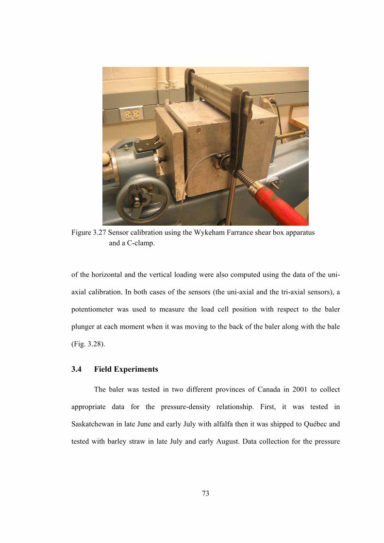
73

Figure 3.27 Sensor calibration using the Wykeham Farrance shear box apparatus

and a C-clamp.

of the horizontal and the vertical loading were also computed using the data of the uni-

axial calibration. In both cases of the sensors (the uni-axial and the tri-axial sensors), a

potentiometer was used to measure the load cell position with respect to the baler

plunger at each moment when it was moving to the back of the baler along with the bale

(Fig. 3.28).

3.4 Field Experiments

The baler was tested in two different provinces of Canada in 2001 to collect

appropriate data for the pressure-density relationship. First, it was tested in

Saskatchewan in late June and early July with alfalfa then it was shipped to Québec and

tested with barley straw in late July and early August. Data collection for the pressure

74

distribution model was performed in 2003 by baling whole green barley, barley straw,

and wheat straw.

Figure 3.28 Displacement sensor used to measure the load cell position.

3.4.1 Pressure-Density of Alfalfa

The farm considered in Saskatchewan was located in Clavet, a town about 30 km

southeast of Saskatoon. This field consisted of a quarter section (64 ha) of second year

pure alfalfa. The first cut was done in late June and early July, and completed in three

days. The effect of flake size and the load settings on the plunger force and the bale

density was evaluated on this field. The equipped large square baler was used to bale

alfalfa at 12.4% (wb) moisture content (Fig. 3.29). To determine the effect of flake size

and the load setting on the plunger force and bale density, three levels of flake sizes

(three positions of the sensitivity lever such as 3, 6, and 9 out of 10) and three levels of

load settings (50, 60, and 70% of the available maximum plunger force) were

75

considered. Baling was performed at the constant forward speed of 8 km/h. The forces

on the plunger arms were recorded by the data acquisition system. The average of the

peak forces resulting from the sum of the forces on the two plunger arms was considered

as the plunger force for each bale formation.

Figure 3.29 Baling pure alfalfa in Saskatchewan.

The actual bale bulk density was calculated by measuring the bale dimensions

and weight (Fig. 3.30). Table 3.2 shows a sample of the raw data taken in this test.

Moisture content of the material samples was determined using the ASAE standard

S358.2 DEC 98 for forage materials (ASAE 2001). A split plot experimental design with

three replications was established in the field to evaluate the effect of the main factor

(load setting) and the sub factor (flake size) on the plunger force and the bale density.

The SAS software (SAS Institute, Cary, NC) was used to analyze the data resulting from

this experiment, and the treatment mean comparison was carried out using Duncan’s

multiple range tests. Finally, efforts were made to fit one of the pressure-density models

which had been introduced in the literature to the data of the plunger pressures and the

corresponding bale densities. None of the models discussed in the section 2.2.1 fitted

76

sufficiently well to the experimental data of this test; therefore, a modified empirical

model was used to fit to the data of this experiment.

Figure 3.30 Bale weight measurement.

3.4.2 Pressure-Density of Barley Straw

In Québec, barley straw with 8.7% (wb) moisture content was baled in a 48 ha

farm. To determine the effect of flake size and the load setting on the plunger force and

bale density, three levels of flake sizes (three positions of the sensitivity lever like 3, 6,

and 9 out of 10) and four levels of the load settings (40, 60, 80, and 100% of the

available maximum plunger load) were considered (Fig. 3.31). Baling was performed at

the constant forward speed of 15 km/h. The forces on the plunger arms were recorded by

the data acquisition system. The average of the peak forces resulting from the sum of the

forces on the two plunger arms was considered as the plunger force for each bale

formation. The actual bale bulk density was calculated in the same manner as the alfalfa

in Saskatchewan. A sample of raw data taken in this test is shown in Table 3.3.

77

Figure 3.31 Baling barley straw in Quebec.

Moisture content of the material samples was determined using the ASAE

standard S358.2 DEC 98 for forage materials (ASAE 2001). The same experimental

design, the statistics software, and the mean comparison test, used in the previous test,

were also applied in this part of the study. At the end, an empirical model was fitted to

the data of this experiment.

78

Table 3.2 Raw data from pressure-density tests for alfalfa.

Load Setting (%) Flake size (lever position out

of 10)

Plunger Force (kN) Bale Density (kg/m3)

50 3/10 261.4 151.9 50 3/10 240.3 158.4 50 3/10 235.9 151.9 50 3/10 256.6 160.5 50 6/10 273.7 156.2 50 6/10 243.0 156.2 50 6/10 262.9 156.9 50 6/10 271.9 156.2 50 9/10 261.3 152.9 50 9/10 269.3 154.9 50 9/10 283.2 150.8 50 9/10 248.1 150.8 60 3/10 297.9 159.7 60 3/10 288.8 159.7 60 3/10 302.2 168.4 60 3/10 306.4 157.5 60 6/10 329.6 162.7 60 6/10 298.0 161.2 60 6/10 308.9 158.5 60 6/10 293.8 166.8 60 9/10 320.3 162.2 60 9/10 314.8 162.2 60 9/10 325.0 160.7 60 9/10 308.3 166.4 70 3/10 359.9 175.6 70 3/10 365.1 175.6 70 3/10 366.6 182.9 70 3/10 351.4 178.0 70 6/10 366.9 188.4 70 6/10 391.0 185.9 70 6/10 347.8 183.4 70 6/10 366.9 180.9 70 9/10 384.9 184.8 70 9/10 384.5 189.8 70 9/10 381.1 184.8 70 9/10 388.8 187.3

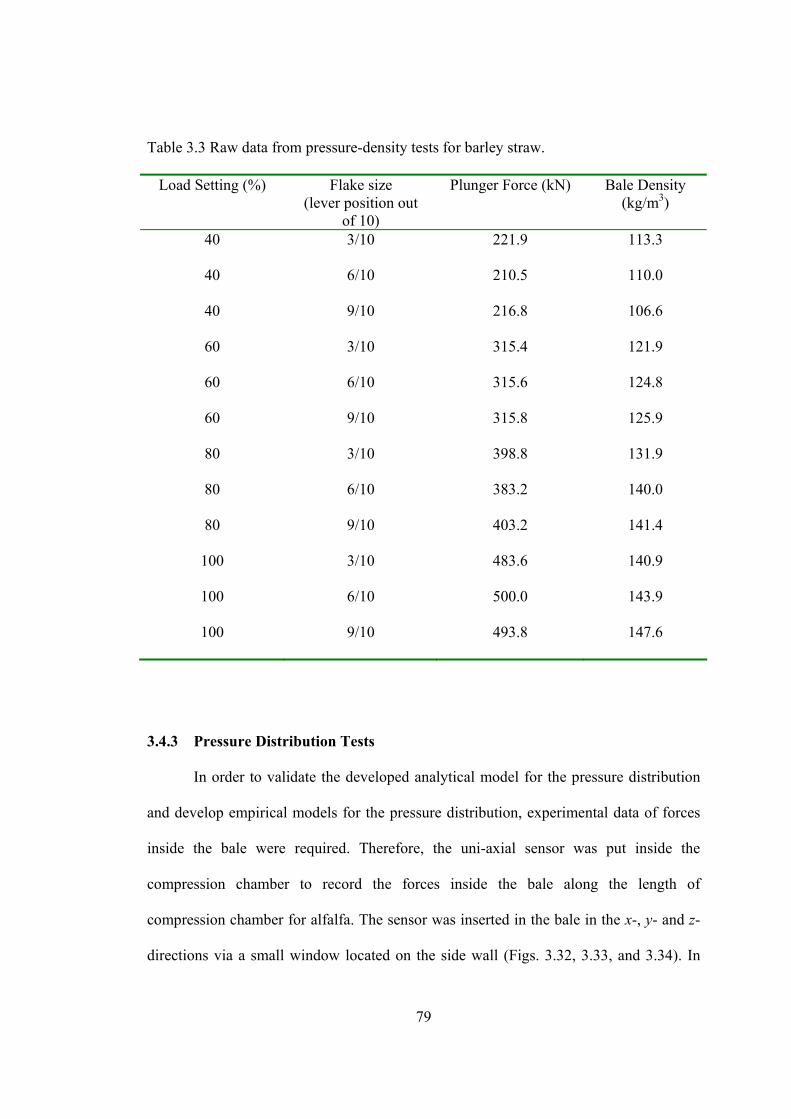
79

Table 3.3 Raw data from pressure-density tests for barley straw.

Load Setting (%) Flake size (lever position out

of 10)

Plunger Force (kN) Bale Density (kg/m3)

40 3/10 221.9 113.3

40 6/10 210.5 110.0

40 9/10 216.8 106.6

60 3/10 315.4 121.9

60 6/10 315.6 124.8

60 9/10 315.8 125.9

80 3/10 398.8 131.9

80 6/10 383.2 140.0

80 9/10 403.2 141.4

100 3/10 483.6 140.9

100 6/10 500.0 143.9

100 9/10 493.8 147.6

3.4.3 Pressure Distribution Tests

In order to validate the developed analytical model for the pressure distribution

and develop empirical models for the pressure distribution, experimental data of forces

inside the bale were required. Therefore, the uni-axial sensor was put inside the

compression chamber to record the forces inside the bale along the length of

compression chamber for alfalfa. The sensor was inserted in the bale in the x-, y- and z-

directions via a small window located on the side wall (Figs. 3.32, 3.33, and 3.34). In

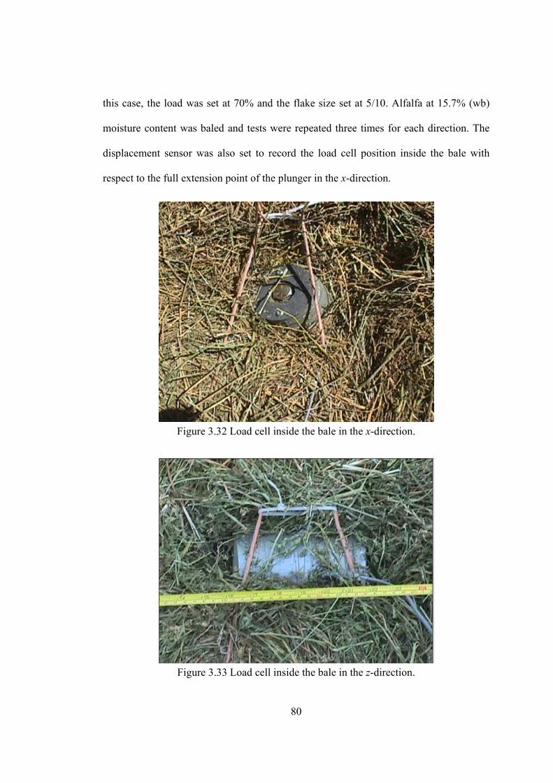
80

this case, the load was set at 70% and the flake size set at 5/10. Alfalfa at 15.7% (wb)

moisture content was baled and tests were repeated three times for each direction. The

displacement sensor was also set to record the load cell position inside the bale with

respect to the full extension point of the plunger in the x-direction.

Figure 3.32 Load cell inside the bale in the x-direction.

Figure 3.33 Load cell inside the bale in the z-direction.

81

Figure 3.34 Load cell inside the bale in the y-direction.

Forces recorded by the uni-axial sensor for alfalfa were compared with the

plunger forces measured by installing strain gages on the plunger arms in the pressure-

density tests (section 3.4.1). Results showed that forces recorded by the sensor in the x-

direction were twice as high as the forces measured by installing strain gages shown in

Table 3.2 (Fig. 3.35). This showed that the uni-axial sensor was not able to record

accurate data of force inside the compression chamber. Therefore, because of the

inaccuracy of forces obtained with the uni-axial sensor, a tri-axial sensor was designed

and used in the succeeding experiments.

The tri-axial sensor was used to measure the forces inside the bale in different

directions when whole green barley, barley straw, and wheat straw were baled. This

sensor was put inside the bale using a small window located on the bale chamber side

wall by drilling a hole at the bale cross-section center (Fig. 3.36). Whole green barley

was baled in August 2003 in Saskatoon with 51.0% of moisture content at the baling

82

speed of 8 km/h. The load and the flake size were set at 50% and 5/10, respectively.

Barley straw was baled in early September in Saskatoon at a 12.0% moisture content and

forward speed of 8 km/h. The load and the flake size settings were 60% and 5/10,

respectively. Wheat straw with 9.7% moisture content was baled in late September. The

0

100

200

300

400

500

600

700

800

900

1000

0 50 100 150 200 250 300Distance along the compression chamber (cm)

Forc

e in

X-d

irect

ion

(kN

)

Figure 3.35 Force distribution along the compression chamber length in the x- direction for alfalfa recorded by the uni-axial sensor at a moisture content of 15% wb and load setting of 70% (zero on the x-axis is the full extension point of plunger).

83

Figure 3.36 Tri-axial sensor inside the whole green barley bale.

load was set at 70% while the flake size setting and baling forward speed were the

same as the previous tests. Each treatment consisted of the force recording for a full

length of one bale, and each treatment was repeated three times for all cases. The same

data acquisition system, used in the sensor calibration, was utilized to record the output

of the sensor at the frequency of 50 Hz.

3.5 Measurement of Crop Properties

Measurement of some crop properties such as coefficients of friction, adhesion,

and modulus of elasticity are covered in this section.

3.5.1 Friction and Adhesion Coefficients

In this research, the coefficient of friction of selected forage materials on a

polished steel surface was measured in the laboratory using the Wykeham Farrance

84

shear box apparatus (Fig. 3.37). This apparatus consisted of a sample box for holding the

material samples, a force transducer to record the frictional force, two linear variable

differential transformers (LVDT) to measure the sample horizontal and vertical

displacements, a linkage to apply the normal force to the sample, and an electrical motor

to provide a relative motion for the variable half of the sample box with respect to its

fixed half. The coefficient of external friction was measured for alfalfa, barley straw,

wheat straw, and whole green barley on a polished steel surface. In the case of alfalfa

and barley straw, four levels of material moisture content were considered (12.0, 22.0,

31.0, and 42.2% (wb) for alfalfa and 12.2, 20.3, 32.9, 45.7 (wb) for barley straw), and

tests were carried out at five levels of normal pressures (200, 330, 500, 600, and 735

kPa).

Shearforce

Materialsample

Normalforce

LVDT(for vertical Displacement)

LVDT(for horizontal Displacement)

Forcetransducer

Figure 3.37 Schematic of the Wykeham Farrance shear box (redrawn from Moysey and Hiltz 1985).

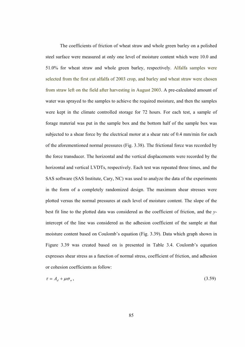
85

The coefficients of friction of wheat straw and whole green barley on a polished

steel surface were measured at only one level of moisture content which were 10.0 and

51.0% for wheat straw and whole green barley, respectively. Alfalfa samples were

selected from the first cut alfalfa of 2003 crop, and barley and wheat straw were chosen

from straw left on the field after harvesting in August 2003. A pre-calculated amount of

water was sprayed to the samples to achieve the required moisture, and then the samples

were kept in the climate controlled storage for 72 hours. For each test, a sample of

forage material was put in the sample box and the bottom half of the sample box was

subjected to a shear force by the electrical motor at a shear rate of 0.4 mm/min for each

of the aforementioned normal pressures (Fig. 3.38). The frictional force was recorded by

the force transducer. The horizontal and the vertical displacements were recorded by the

horizontal and vertical LVDTs, respectively. Each test was repeated three times, and the

SAS software (SAS Institute, Cary, NC) was used to analyze the data of the experiments

in the form of a completely randomized design. The maximum shear stresses were

plotted versus the normal pressures at each level of moisture content. The slope of the

best fit line to the plotted data was considered as the coefficient of friction, and the y-

intercept of the line was considered as the adhesion coefficient of the sample at that

moisture content based on Coulomb’s equation (Fig. 3.39). Data which graph shown in

Figure 3.39 was created based on is presented in Table 3.4. Coulomb’s equation

expresses shear stress as a function of normal stress, coefficient of friction, and adhesion

or cohesion coefficients as follow:

ndA μστ += , (3.59)

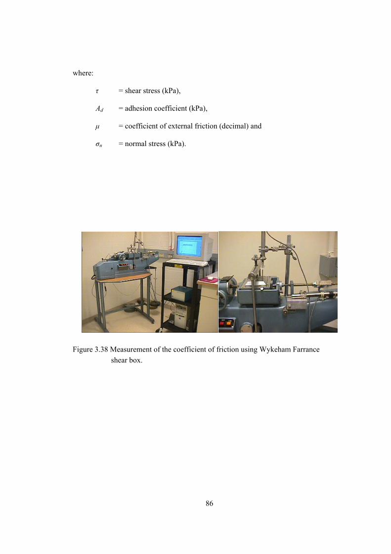
86

where:

τ = shear stress (kPa),

Ad = adhesion coefficient (kPa),

μ = coefficient of external friction (decimal) and

σn = normal stress (kPa).

Figure 3.38 Measurement of the coefficient of friction using Wykeham Farrance shear box.

87

Table 3.4. A sample of data used to calculate coefficient of friction.

Normal Stress (kPa) Shear Stress (kPa)

198.9 30.3

331.8 51.6

499.9 78.2

599.0 87.3

734.3 112.6

198.9 32.7

331.8 51.2

499.9 77.6

599.0 85.9

734.3 110.5

198.9 32.9

331.8 48.4

499.9 76.1

599.0 91.7

734.3 111.6

3.5.2 Modulus of Elasticity

The relationship between strain and stress in the proportional limit of the stress-strain

curve of the engineering materials could be explained using the modulus of elasticity, E,

which is the ratio of stress to strain (E = σ/ε). A single value of the modulus of elasticity

is considered for the stresses used in design calculations of most engineering materials,

because the stress-strain relationship is linear below the proportional limit for these

types of materials. For biological materials, the apparent modulus of elasticity is used to

explain the relationship between stress and strain. Apparent modulus of elasticity is

88

0

20

40

60

80

100

120

0 100 200 300 400 500 600 700 800Normal Stress (kPa)

Shea

r Str

ess

(kPa

)

Experimental data

Linear (Experimental data)

τ = 0.15σ+2.1

Figure 3.39 Coefficients of friction and the adhesion or cohesion coefficients from the data of shear box.

calculated based on two different definitions called the secant definition and the tangent

definition. In the secant definition, the apparent modulus is considered as theratio of

stress to strain at a certain point, while the apparent modulus in tangent method is

defined as the slope of the stress-strain curve at a certain point on the curve (Stroshine

2000). Figure 3.42 shows calculation of modulus of elasticity at point C using these two

methods. In the secant method, modulus of elasticity at point C is defined as the slope of

line AC, while in tangent method slope of line BD is considered as modulus of elasticity

at point C.

89

0

200

400

600

800

1000

1200

1400

0 0.2 0.4 0.6 0.8 1Strain (m/m)

Stre

ss (

kPa)

A

B C D

Figure 3.40 Two methods of calculating modulus of elasticity at one point of stress- strain curve.

In order to find a relationship between apparent modulus of elasticity and bulk

density of alfalfa and barley straw, the data of the tests performed for the particle

stiffness were used. When forage materials were compressed in a closed-end cylinder,

these materials were deformed only in the x-direction and strains in the y- and z-

directions were zero. Using Eq. 3.6 and setting strains in the y- and z-directions to zero,

the following relation will be found between stress and strain in the x-direction:

( ) xxx FEE εενν

νσ =−+

−=

)21(1)1( , (3.60)

where:

( ) )21(1)1(νν

ν−+

−=F . (3.61)

90

According to Eq. 3.60, when one of the aforementioned methods is used to calculate

modulus of elasticity, the obtained values (bulk modulus) are a combination of modulus

of elasticity and Poisson’s ratio. Because, Poisson’s ratio is a constant coefficient,

plotting the obtained values versus material bulk density can show the trend of variation

of modulus of elasticity with respect to material density.

The tangent method for the modulus calculation was used to calculate the

product of F (a function of Poisson’s ratio) and the modulus of elasticity (E). The stress-

strain curve was plotted for each of the tested materials. This curve consisted of three

parts: a) an elastic part, which started from the origin and continued up to the point with

50.00 kPa and 0.04 m/m of stress and strain, respectively. This part was very small

relative to the compacting part and could be ignored in the modulus calculation process;

b) a compacting part, which was the most dominant part of the stress-strain curve in the

compression process with an almost constant slope; and c) an incompressible part in

which strain remained constant with increasing stress. This part occurred at the high

stresses which are not encountered in the baling process; therefore this part was also

eliminated in the modulus calculation process. Thus, the compacting part of stress-strain

curve (part b) was considered and FE was calculated at each point of the curve using the

central difference approximation of the first derivative at that point. Therefore, this value

at each point was calculated from the ratio of the difference between the stresses of the

two points equidistant from that point (0.002 m/m from either side) to the difference

between their strains (Fig. 3.40). Density of the samples was calculated at each strain,

and the FE-γ curve was then plotted using the calculated FE values to find the trend of

variation of modulus of elasticity with respect to the material density. A sample of the

raw data taken in this test is shown in Table 3.5.

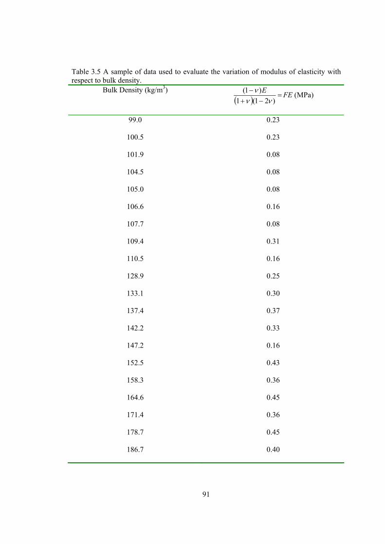
91

Table 3.5 A sample of data used to evaluate the variation of modulus of elasticity with respect to bulk density.

Bulk Density (kg/m3) ( ) =

−+−

)21(1)1(

ννν E FE (MPa)

99.0 0.23

100.5 0.23

101.9 0.08

104.5 0.08

105.0 0.08

106.6 0.16

107.7 0.08

109.4 0.31

110.5 0.16

128.9 0.25

133.1 0.30

137.4 0.37

142.2 0.33

147.2 0.16

152.5 0.43

158.3 0.36

164.6 0.45

171.4 0.36

178.7 0.45

186.7 0.40

92

CHAPTER 4

RESULTS AND DISCUSSION

In this chapter, results of model development and validation, sensor design, and

field and laboratory tests are discussed.

4.1 Model Development and Validation

In this section results of model development and validation for the pressure

distribution and pressure-density relationship are covered. In each case, results of both

analytical and empirical models are discussed.

4.1.1 Analytical Model for the Pressure Distribution

The analytical models for the pressure distribution in the x-, y-, and z-directions

were derived based on the theory of elasticity by assuming isotropic linear elastic

behavior for the forage materials (Eqs. 3.40, 3.43, and 3.44). In the literature, only one

model was found regarding the distribution of pressure inside the compression chamber

of balers (Sitkei’s model, Eq. 2.19). The developed model in this study (Eq. 3.40) has

three important advantages compared to Sitkei’s model (Eq. 2.19). The advantages are:

1. The new model (Eq. 3.40) is much simpler than Sitkei’s model (Eq. 2.19), has

fewer terms, and calculating the pressure using this model is much easier.

2. In the new model, the pressure on the plunger (Pp) has been used as the boundary

condition to solve the governing differential equation instead of the pressure at

93

the end of the bale chamber (Pe) which had been used in Sitkei’s model (Eq.

2.19). Measuring the pressure on the plunger is much easier than the pressure at

the end of the bale chamber; therefore, the boundary condition used in the new

model is much more accessible than that of Sitkei’s model (Eq. 2.19).

3. The new model is more general than Sitkei’s model (Eq. 2.19), because it is

applicable to all kinds of balers (including the balers with top and side walls

inclined), whereas Sitkei’s model (Eq. 2.19) is only applicable to the balers with

one pair of converging walls.

4.1.2 Validation of the Analytical Model

The analytical model (Eq. 3.40) was validated using the experimental data

collected for three different crops including barley straw, wheat straw, and whole green

barley. The least-square regression analysis method was used to validate the analytical

model in the x-direction (Eq. 3.40). In this method, υ, μ, and E were changed in order to

minimize the summation of the square difference between data resulting from the model

(Eq. 3.40) and the experimental data. Values of υ, μ, and E corresponding to the

minimum sum square error were considered as the estimated values for these

parameters. Values of 0.32, 0.38, and 0.40 were estimated for Poisson’s ratio of whole

green barley, wheat straw, and barley straw, respectively (Table 4.1). Sitkei (1986)

reported the range of 0.25 to 0.35 for Poisson’s ratio of forage materials for the pressure

range encountered in balers and the range of 0.35 to 0.45 for the pressure range

encountered in pelleting machines. Because the pressure in a large square baler is

usually higher than the pressure in smaller balers, the estimated values for Poisson’s

ratio of the tested materials are acceptable. For the modulus of elasticity, values of 10,

94

39, and 2.4 kPa were estimated from the analytical model validation for barley straw,

wheat straw, and whole green barley, respectively (Table 4.1). The estimated value of

the modulus of elasticity for barley straw was much lower than the measured value

(122.5 kPa). There were no measured values of modulus of elasticity for wheat straw

and whole green barley to compare the estimated values with. For the coefficient of

friction between forage materials and bale chamber walls, values of 0.55, 0.43, and 0.45

were estimated for whole green barley, wheat straw, and barley straw, respectively

(Table 4.1). These values were approximately three times as high as the coefficient of

friction of the same crops on polished steel surface measured in laboratory using shear

box at the similar moisture content. After observing these high values for coefficient of

Table 4.1 Constants of the analytical model for the pressure distribution in the x-direction for the different forage materials.

Material type α (rad) β (rad) E (kPa) μ ν Barley straw 0.09 0.13 10 0.45 0.40

Wheat straw 0.08 0.14 39 0.43 0.38

Whole green barley 0.07 0.12 2.4 0.55 0.32

friction, the surface of the compression chamber walls was inspected. It was observed

that the wall surface was covered by a rough layer of crop dry extract which increased

the coefficient of friction. In reality, after baling the first few bales (especially with the

higher moisture content), the wall surface will not be a polished steel surface anymore. It

will be a rough surface with a high coefficient of friction. Therefore, coefficients of

95

friction estimated from the analytical model are more realistic than the measured ones in

laboratory. The following are the results of model validation for barley straw, wheat

straw, and whole green barley.

4.1.2.1 Barley Straw

Pressure distribution inside the compression chamber of the baler in the x-

direction for barley straw at a load setting of 60% and the material moisture content of

12.2% (wb) is shown in Figure 4.1. Both the experimental data and the predicted

pressure values (based on Eq. 3.40) are presented in this figure. According to this plot,

the best fit between the experimental data and the predicted values was found at the

beginning of the compression chamber length close to the plunger and at the end of the

bale chamber length. The error of the pressure prediction on the plunger (x = 0) was very

low which proved that the model has accurately estimated the pressure on the baler

plunger. The standard error and the coefficient of determination of the regression

analysis in this case were 20.0 kPa and 0.95, respectively (Table 4.2).

96

0

50

100

150

200

250

300

350

400

0 100 200 300Distance along the compression chamber (cm)

Pres

sure

in X

-dire

ctio

n (k

Pa)

Experimental pressureAnalytically predicted pressure

Figure 4.1 Experimental pressure distribution and the predicted pressure distribution based on the analytical model along the compression chamber length in the x-direction for barley straw at a moisture content of 12.2% (wb) (zero on the x-axis is the full extension point of plunger).

Table 4.2 The coefficient of determination and the standard error of the analytical model in the x-direction for different forage materials.

Material type R2 Standard error (kPa)

Barley straw 0.95 20.0

Wheat straw 0.95 26.0

Whole green barley 0.96 18.4

97

According to Eq. 3.43, the vertical pressure (pressure in the y-direction) inside

the compression chamber of a large square baler at a certain distance from the plunger is

a function of the pressure in the x-direction, crop properties, and the compression

chamber dimensions. Therefore, the pressure distribution along the compression

chamber length in the y-direction (vertical pressure) for barley straw was obtained using

Eq. 3.43 and the data of the predicted horizontal pressures (Fig. 4.2). The pressure

distribution in the y-direction showed the same pattern as the pressure distribution in the

x-direction with the highest pressure near the plunger and the lowest pressure at the end

of the compression chamber. The maximum pressure in the y-direction for the barley

straw was about 65% of the maximum pressure in the x-direction. The experimental data

are also presented in Fig. 4.2. There was a significant difference between the

experimental and predicted pressures near the baler plunger, while at the end of

compression chamber these pressures were very close together. This showed that the

analytical model failed to accurately predict the pressure in the y-direction due to the

following potential reasons:

1. The analytical model in the x-direction was developed by assuming constant

value for Poisson’s ratio (υ). This value was estimated by validating the

analytical model in the x-direction and was used in the analytical model in the y-

direction to predict pressure in this direction. This estimated constant υ was an

average value of the actual variable Poisson’s ratio. In reality, υ probably has not

been constant along the compression process. This ratio has had its minimum

value (which has been smaller than the estimated value) at the beginning of

compression process (near the plunger) and has increased with increasing

distance from the plunger. Therefore, the maximum difference between the

98

experimental data and the predicted pressures was observed at the beginning of

the compression process and the minimum difference was observed at the end of

the compression chamber.

2. The experimental data have been much smaller than the expected pressures in the

y-direction due to the gap between the dug hole inside the bale and the sensor

body. Therefore, at the beginning of the baling process the difference between

the experimental data and the predicted pressures were very large, while after

filling the gap at the end of the compression chamber, the sensor was able to

record data close to the expected pressures.

0

50

100

150

200

250


Pres

sure

in Y

-dire

ctio

n (k

Pa)


Figure 4.2 The predicted and the experimental pressure distribution along the compression chamber length in the y-direction (vertical pressure) based on the analytical model for barley straw at a moisture content of 12.2% (wb) (zero on the x-axis is the full extension point of plunger).

99

Equation 3.42 expresses the pressure inside the compression chamber of a large

square baler in the z-direction (lateral pressure) in terms of the pressure in the x-

direction, dimensions of the compression chamber, and the properties of the baled crop.

This equation was used to plot the lateral pressure versus the distance from the full

extension point of the plunger along the compression chamber length for barley straw by

inserting in the predicted pressures in the x-direction into Eq. 3.44 (Fig. 4.3). The lateral

pressure distribution had the same pattern as the vertical pressure with the small

differences in the minimum pressures. The analytical model in the z-direction seemed to

have the same problem as the analytical model in the y-direction; however, there were

no experimental data available in this direction to which the predicted pressures could be

compared.

0

50

100

150

200

250

0 50 100 150 200 250Distance along the compression chamber (cm)

Pre

ssur

e in

Z-d

irect

ion

(kPa

)

Figure 4.3 Predicted pressure distribution along the compression chamber length in the

z-direction (lateral pressure) based on the analytical model for barley straw at a moisture content of 12.2% (wb) (zero on the x-axis is the full extension point of plunger).

100

4.1.2.2 Wheat Straw

Figure 4.4 shows the results of wheat straw compressed at a load setting of 70%

and material moisture content of 9.7% (wb). The analytical model (Eq. 3.40) predicted

the pressure on the baler plunger with an accuracy of 97.5%. The model showed a poor

accuracy for the pressure prediction at the compression chamber length range of 50 to

100 cm and for the end of the compression chamber length. The model predicted

negative values for the pressure at the distances larger than 190 cm; therefore, the model

was valid until 190 cm of the compression chamber length. The regression analysis of

the experimental and the predicted data of the pressure distribution in the case of wheat

straw presented a high coefficient of determination (0.95) and a low standard error (26

kPa) for the model fitness to the experimental data (Table 4.2).

101

-50

0

50

100

150

200

250

300

350

400

0 100 200 300

Distance along the compression chamber (cm)

Pres

sure

in X

-dire

ctio

n (k

Pa)

Experimental pressureEmpirically predicted pressure

Figure 4.4 Experimental pressure distribution and the predicted pressure distribution based on the analytical model along the compression chamber length in the x-direction for wheat straw at a moisture content of 9.7% (wb) (zero on the x-axis is the full extension point of plunger).

The pressure distribution in the y-direction inside the compression chamber of

the baler for wheat straw based on Eq. 3.43 is shown in Figure 4.5. This plot was

obtained by inserting in the predicted pressures in the x-direction into equation 3.41. The

maximum predicted vertical pressure for wheat straw was about 216 kPa which was

approximately 60% of the maximum pressure in the x-direction. The experimental data

are also presented in Figure 4.5. Similar to the results of the model validation in the y-

direction for barley straw, there was a significant difference between the experimental

data and the predicted pressures in the y-direction for wheat straw near the baler plunger,

while at the end of the compression chamber these pressures were very close together.

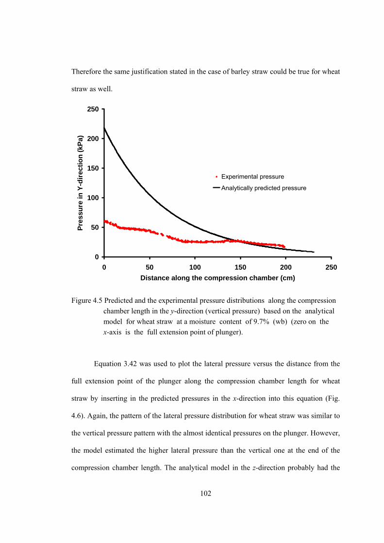
102

Therefore the same justification stated in the case of barley straw could be true for wheat

straw as well.

0

50

100

150

200

250


Pres

sure

in Y

-dire

ctio

n (k

Pa)

Experimental pressure

Analytically predicted pressure

Figure 4.5 Predicted and the experimental pressure distributions along the compression chamber length in the y-direction (vertical pressure) based on the analytical model for wheat straw at a moisture content of 9.7% (wb) (zero on the x-axis is the full extension point of plunger).

Equation 3.42 was used to plot the lateral pressure versus the distance from the

full extension point of the plunger along the compression chamber length for wheat

straw by inserting in the predicted pressures in the x-direction into this equation (Fig.

4.6). Again, the pattern of the lateral pressure distribution for wheat straw was similar to

the vertical pressure pattern with the almost identical pressures on the plunger. However,

the model estimated the higher lateral pressure than the vertical one at the end of the

compression chamber length. The analytical model in the z-direction probably had the

103

same problem as the analytical model in the y-direction; however, there were no

experimental data available in this direction to prove that.

0

50

100

150

200

250


Pres

sure

in Z

-dire

ctio

n (k

Pa)

Figure 4.6 Predicted pressure distribution along the compression chamber length in the z-direction (lateral pressure) based on the analytical model for wheat straw at a moisture content of 9.7% (wb) (zero on the x-axis is the full extension point of plunger).

4.1.2.3 Whole Green Barley

The experimental and the predicted pressure distribution in the x-direction based

on the developed analytical model for whole green barley at a load setting of 50% and

material moisture content of 51% (w.b.) is shown in Figure 4.7. The results of

comparing the predicted (based on Eq. 3.40) and the experimental pressures showed that

the predicted pressure by the analytical model on the plunger was 10% more than the

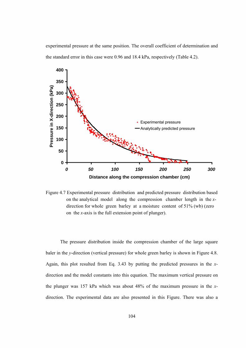
104

experimental pressure at the same position. The overall coefficient of determination and

the standard error in this case were 0.96 and 18.4 kPa, respectively (Table 4.2).

0

50

100

150

200

250

300

350

400


Pres

sure

in X

-dire

ctio

n (k

Pa)


Figure 4.7 Experimental pressure distribution and predicted pressure distribution based on the analytical model along the compression chamber length in the x- direction for whole green barley at a moisture content of 51% (wb) (zero on the x-axis is the full extension point of plunger).

The pressure distribution inside the compression chamber of the large square

baler in the y-direction (vertical pressure) for whole green barley is shown in Figure 4.8.

Again, this plot resulted from Eq. 3.43 by putting the predicted pressures in the x-

direction and the model constants into this equation. The maximum vertical pressure on

the plunger was 157 kPa which was about 48% of the maximum pressure in the x-

direction. The experimental data are also presented in this Figure. There was also a

105

significant discrepancy between the experimental data and the predicted pressures near

the baler plunger for whole green barley, but this discrepancy was much smaller

compared to the discrepancies in barley and wheat straw. This smaller difference

between the experimental data and the predicted pressures was most likely due to the

following reasons:

1. Whole green barley had the actual Poisson’s ratio closer to the estimated ratio.

On the other hand, the variation of Poisson’s ratio in whole green barley was

smaller than that of barley and wheat straw. Thus, the difference between the

experimental data and the predicted pressures was smaller compared to this

difference in barley and wheat straw.

2. The dug hole in the whole green barley bale had more uniform shape than the

other materials (barley and wheat straw) because of the higher moisture content

of green barley. Therefore, the gap between the sensor and the dug hole was

smaller for whole green barley and it took the forces less time to fill the gap. For

this reason the difference between the experimental and predicted pressures was

smaller than that of barley and wheat straw.

106

0

50

100

150

200

250


Pres

sure

in Y

-dire

ctio

n (k

Pa)


Figure 4.8 Predicted and the experimental pressure distributions along the compression chamber length in the y-direction (vertical pressure) based on the analytical model for whole green barley at moisture content of 51% (wb) (zero on the x-axis is the full extension point of plunger).

The pressure distribution in the z-direction (lateral pressure) for whole green

barley showed almost the same pattern as the vertical pressure distribution (Fig. 4.9). In

this particular case, the maximum lateral pressure on the plunger and the minimum one

at the end of the compression chamber length were almost identical to the vertical

maximum and minimum pressures, respectively. There were no experimental data

available in the z-direction in this case to compare the predicted pressures with.

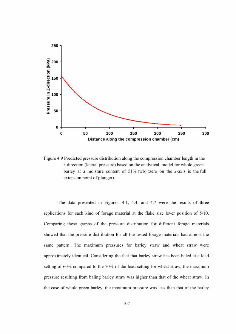
107

0

50

100

150

200

250


Pres

sure

in Z

-dire

ctio

n (k

Pa)

Figure 4.9 Predicted pressure distribution along the compression chamber length in the z-direction (lateral pressure) based on the analytical model for whole green barley at a moisture content of 51% (wb) (zero on the x-axis is the full extension point of plunger).

The data presented in Figures. 4.1, 4.4, and 4.7 were the results of three

replications for each kind of forage material at the flake size lever position of 5/10.

Comparing these graphs of the pressure distribution for different forage materials

showed that the pressure distribution for all the tested forage materials had almost the

same pattern. The maximum pressures for barley straw and wheat straw were

approximately identical. Considering the fact that barley straw has been baled at a load

setting of 60% compared to the 70% of the load setting for wheat straw, the maximum

pressure resulting from baling barley straw was higher than that of the wheat straw. In

the case of whole green barley, the maximum pressure was less than that of the barley

108

and wheat straw which was because of the lower load setting (50%) and Poisson’s ratio

(0.32).

The experimental pressures in all cases (for all forage materials) had their

maximum values on the plunger (x = 0) and then decreased exponentially with

increasing distance from the full extension point of the plunger up to about 60 cm from

the plunger. At this point (point “A”), the pressure started to increase due to reduction of

the cross-section area up to distance of about 95 cm from the plunger (Point “B”) and

again decreased. This problem occurred because of the presence of a bend in the

compression chamber walls (top and side walls) which increased the standard errors and

decreased the coefficients of determination of the models (Point “B” in Fig. 4.10). In

reality, the compression chamber walls make two different angles with the x-axis (a

larger angle for the part AB and a smaller angle for the part BC) while only one angle

was considered in model development for each wall for simplification.

Equations 3.43 and 3.44 which express the vertical and the lateral pressures in

terms of the pressure in the x-direction forage material properties, and the compression

chamber dimensions, consist of two parts. The first part is only a function of Poisson’s

ratio (ν) and the pressure in the x-direction, and is exactly identical in both equations.

The second part is a function of the distance from the full extension point of the plunger

(x), crop properties, and the compression chamber dimensions which vary from equation

to equation. For the maximum lateral and vertical pressures which take place on the

plunger, only the first part of the equation comes to play a role, because the distance

from the full extension point of the plunger is zero (x = 0). Therefore, the maximum

lateral and vertical pressures are solely functions of the maximum pressure in the x-

direction and Poisson’s ratio. Because the maximum pressure in the x-direction and the

109

Poisson’s ratio for each of the tested forage material were constant, the predicted

maximum vertical and the lateral pressures for each of the materials were the same but

they varied between crops tested. For the minimum pressures which occurred at the end

Plunger

Top wall

A B C

Figure 4.10 The actual shape of the top wall of the compression chamber.

of the compression chamber length, both parts of the equations play a role; therefore, the

minimum vertical and lateral pressures are not necessarily identical for a certain crop.

Comparing the maximum vertical and the lateral pressures for the different

materials showed that barley straw had the highest maximum lateral and vertical

pressures because of its largest Poisson’s ratio. Whole green barley had the lowest

maximum pressures because of its lowest Poisson’s ratio and lowest maximum pressure

in the x-direction.

110

4.1.3 Validation of the Empirical Model

The empirical models of the pressure distribution in the x- and y-directions for

different forage materials (Eqs. 3.47 and 3.48) were validated using the experimental

data of field tests. The least-square regression analysis was used for model validation,

and model constants were estimated for each of the tested crops (Tables 4.3 and 4.4).

The coefficient of determination and the standard error were also calculated for each case

as criteria of model fitness (Tables 4.3 and 4.4). A high coefficient of determination and

a low standard error of the model in the x-direction for all tested crops revealed that

there was a good correlation between the empirical model and the corresponding

experimental data in the x-direction. In contrast, coefficient of x for the model (-D0) in

the y-direction had a very low value which showed that the pressure distribution in this

direction was almost linear rather than exponential. The reason was probably inaccuracy

of the experimental data in the y-direction especially near the plunger. Therefore, there

was not a good correlation was not found between the empirical model and the

experimental data in the y-direction. The empirical models were validated using the data

collected for three different crops, namely barley straw, wheat straw, and whole green

barley. The following are the results of the empirical model validation for different

crops.

111

Table 4.3 Estimated constants of the developed empirical model (Eq. 3.47) for the pressure distribution in the x-direction for different forage materials.

Constant Barley straw Wheat straw Whole green barley

A0 370.81 410.31 326.47

B0 0.018 0.021 0.014

R2 0.96 0.97 0.96

Standard error 19.27 20.57 18.39

Table 4.4 Estimated constants of the developed model (Eq. 3.48) for pressure distribution in the y-direction for different forage materials.

Constant Barley straw Wheat straw Whole green barley C 61.2 59.2 113.3

D0 0.0083 0.0076 0.0077

R2 0.96 0.93 0.90

Standard error 3.1 2.6 8.2

4.1.3.1 Barley Straw

The pressure distribution inside the compression chamber of the large square

baler in the x-direction for barley straw based on the developed empirical model at a

load setting of 60% and moisture content of 12.2% (wb) is shown in Figure 4.11. Both

the experimental and the predicted pressures are presented in this figure. Based on the

graphs shown in this figure, the best fit between the experimental data and the predicted

pressures was found at the beginning of the compression chamber length close to the

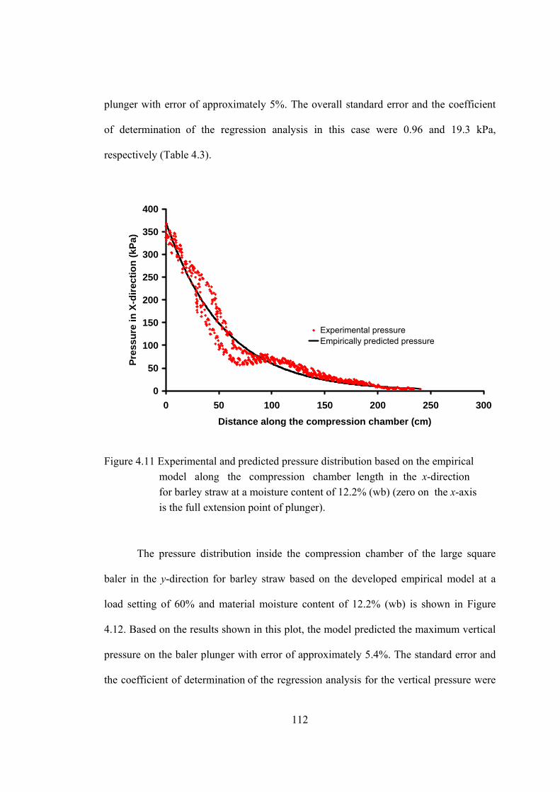
112

plunger with error of approximately 5%. The overall standard error and the coefficient

of determination of the regression analysis in this case were 0.96 and 19.3 kPa,

respectively (Table 4.3).

0

50

100

150

200

250

300

350

400


Pres

sure

in X

-dire

ctio

n (k

Pa)

Experimental pressure Empirically predicted pressure

Figure 4.11 Experimental and predicted pressure distribution based on the empirical model along the compression chamber length in the x-direction for barley straw at a moisture content of 12.2% (wb) (zero on the x-axis is the full extension point of plunger). The pressure distribution inside the compression chamber of the large square

baler in the y-direction for barley straw based on the developed empirical model at a

load setting of 60% and material moisture content of 12.2% (wb) is shown in Figure

4.12. Based on the results shown in this plot, the model predicted the maximum vertical

pressure on the baler plunger with error of approximately 5.4%. The standard error and

the coefficient of determination of the regression analysis for the vertical pressure were

113

3.1 kPa and 0.96, respectively (Table 4.4). The experimental data showed the trend of

the pressure distribution in the y-direction; however these data were much smaller than

the actual data (especially near the plunger).

0

10

20

30

40

50

60

70


Pres

sure

in Y

-dire

ctio

n (k

Pa)


Figure 4.12 Experimental and predicted pressure distribution based on the empirical

model along the compression chamber length in the y-direction (vertical pressure) for barley straw at a moisture content of 12.2% (wb) (zero on the x-axis is the full extension point of plunger). The same experimental data as in Figure 4.2 was used in this plot.

4.1.3.2 Wheat Straw

Figure 4.13 shows similar results for the wheat straw at a load setting of 70% and

material moisture content of 9.7% wb. The experimental and the predicted pressures

along the compression chamber length are presented in different colors to show the

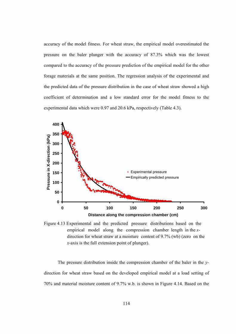
114

accuracy of the model fitness. For wheat straw, the empirical model overestimated the

pressure on the baler plunger with the accuracy of 87.3% which was the lowest

compared to the accuracy of the pressure prediction of the empirical model for the other

forage materials at the same position. The regression analysis of the experimental and

the predicted data of the pressure distribution in the case of wheat straw showed a high

coefficient of determination and a low standard error for the model fitness to the

experimental data which were 0.97 and 20.6 kPa, respectively (Table 4.3).

0

50

100

150

200

250

300

350

400


Pres

sure

in X

-dire

ctio

n (k

Pa)


Figure 4.13 Experimental and the predicted pressure distributions based on the

empirical model along the compression chamber length in the x- direction for wheat straw at a moisture content of 9.7% (wb) (zero on the x-axis is the full extension point of plunger). The pressure distribution inside the compression chamber of the baler in the y-

direction for wheat straw based on the developed empirical model at a load setting of

70% and material moisture content of 9.7% w.b. is shown in Figure 4.14. Based on the

115

results shown in this plot, the model predicted the maximum vertical pressure on the

baler plunger with error of approximately about 2.6%. The overall standard error and the

coefficient of determination of the regression analysis for the vertical pressure were 2.6

kPa and 0.93, respectively (Table 4.4). The experimental data showed the trend of the

pressure distribution in the y-direction; however the values of these data were not

reliable (especially near the plunger).

0

10

20

30

40

50

60

70


Pres

sure

in Y

-dire

ctio

n (k

Pa)


Figure 4.14 Experimental and the predicted pressure distributions based on the empirical model along the compression chamber length in the y- direction (vertical pressure) for wheat straw at moisture content of 9.7% (wb) (zero on the x-axis is the full extension point of plunger). The same experimental data as in Figure 4.5 was used in this plot.

116

4.1.3.3 Whole Green Barley

The experimental and the predicted pressure distribution in the x-direction based

on the developed empirical model for whole green barley at a load setting of 50% and

moisture content of 51% (wb) are presented in Figure 4.15. Results of the comparison of

predicted and experimental showed that the empirical model predicted the pressure on

the plunger with error of about 5%. The overall coefficient of determination and the

standard error in this case were 0.96 and 18.4 kPa, respectively (Table 4.3).

0

50

100

150

200

250

300

350

400


Pres

sure

in X

-dire

ctio

n (k

Pa)


Empirically predicted pressure

Figure 4.15 Experimental and the predicted pressure distribution based on the

empirical model along the compression chamber length in the x- direction for whole green barley at moisture content of 51% (wb) (zero on the x-axis is the full extension point of plunger).

The pressure distribution in the y-direction for whole green barley based on the

developed empirical model at a load setting of 50% and material moisture content of

117

51% (wb) is shown in Figure 4.16. Based on the results shown in this plot, the model

predicted the maximum vertical pressure on the baler plunger with error of

approximately about 17.9%. The overall standard error and the coefficient of

determination of the regression analysis for the vertical pressure were 8.2 kPa and 0.90,

respectively (Table 4.4). The experimental data showed the trend of the pressure

distribution in the y-direction; however these data were much lower than the actual data

(especially near the plunger) and were not reliable from the viewpoint of their values.

0

20

40

60

80

100

120

0 50 100 150 200 250 300Distance along the compression chambe (cm)

Pres

sure

in Y

-dire

ctio

n (k

Pa)


Empirically predicted pressure

Figure 4.16 Experimental and the predicted pressure distribution based on the empirical model along the compression chamber length in the y-direction (vertical pressure) for whole green barley at a moisture content of 51% (wb) (zero on the x-axis is the full extension point of plunger). The same experimental data as in Figure 4.2 was used in this plot.

118

4.1.4 Comparison of Analytical and Empirical Models

The analytical model for the pressure distribution was a complicated model and had

many parameters. These parameters which were related to the compression chamber

dimensions or forage material physical and mechanical properties have to be measured

prior to the modeling process. Measuring these parameters is usually a time-consuming

exercise and is very expensive. In contrast, the empirical models were simple equations

which were only functions of the distance from the full extension point of the plunger

along the compression chamber. Comparing the analytical and empirical models of the

pressure distribution in the x-direction (Eqs. 3.40 and 3.47) showed that the general form

of the empirical model was exactly the same as the first term of the analytical model.

Because the value of the first term of Eq. 3.40 was very large relative to that of the other

terms, especially for the distances less than 150 cm (Table 4.5), it was reasonable to

have the empirical model with the general form of the first term of Eq. 3.40. Coefficient

“A0” in this model is identical to the pressure on the plunger (Pp). Ideally, these two

coefficients (A0 in the empirical model and Pp in the analytical model) should be equal to

the experimental pressure on the plunger (maximum experimental pressure) but in

practice, there was some discrepancy between these coefficients depending on the model

accuracy. Results of model validation showed that the coefficient “A0” in the empirical

model for barley straw, wheat straw, and whole green barley were 370.8, 410.3, and

326.5 kPa, respectively (Table 4.3), while Pp in the analytical model was 350.0, 360.0,

and 325.0 kPa for barley straw, wheat straw, and whole green barley, respectively.

Comparing the results of the analytical and the empirical models in the x-

direction for barley straw revealed that the empirical model provided more accurate

pressure prediction with a larger coefficient of determination and a lower overall

119

standard error; however, the analytical model provided more accurate prediction of the

pressure on the plunger than the empirical model. Comparison of the results of the

analytical and the empirical models in the x-direction for baling wheat straw indicated

that the empirical model had more accurate overall prediction for the pressure along the

compression chamber, and had the larger coefficient of determination and the lower

overall standard error, while the analytical model provided more accurate prediction of

the pressure only on the plunger. For baling whole green barley, results showed that both

analytical and empirical models predicted the pressure distribution in the x-direction

with similar accuracy. Therefore, in order to estimate the pressure distribution of baling

whole green barley, either model could be used.

Comparing Eqs. 3.47 and 3.48 showed that the empirical model for the pressure

distribution in the x- and y-directions have the same general form with different model

constants. Comparing the analytical and empirical models for the pressure distribution in

the y-direction (Eqs. 3.43 and 3.48) revealed that the empirical model in the y-direction

had exactly the same general form as the first term of the analytical model in this

direction. Since the value of the first term of Eq. 3.43 was very large relative to that of

the other terms especially for the distances less than 150 cm (Table 4.5), the empirical

model was selected similar to the general form of the first term of Eq. 3.43. Coefficient

“C” in the empirical model was identical to the coefficient of the first term of the

analytical model.

120

Table 4.5 Values of the different terms of Eqs. 3.40 and 3.43 as a function of distance form the full extension point of the plunger for barley straw. Distance from the

plunger (cm)

First term of

Eq. 3.40 (kPa)

Rest of Eq.

3.40 (kPa)

First term of

Eq. 3.43 (kPa)

Rest of Eq.

3.43 (kPa)

0.0 356.0 0.0 237.3 0.0

15.0 275.6 -0.1 183.7 0.3

30.0 212.2 -0.3 141.5 0.5

45.0 164.9 -0.5 109.9 0.6

60.0 127.1 -0.9 84.7 0.7

75.0 97.8 -1.3 65.2 0.8

90.0 75.5 -1.8 50.4 0.8

105.0 56.9 -2.3 37.9 0.8

120.0 45.2 -2.8 30.1 0.8

135.0 35.2 -3.3 23.5 0.8

150.0 27.4 -3.8 18.2 0.8

165.0 21.1 -4.4 14.1 0.8

180.0 16.3 -4.9 10.9 0.7

195.0 12.6 -5.5 8.4 0.7

210.0 9.7 -6.1 6.5 0.6

225.0 8.2 -6.7 5.0 0.6

240.0 7.8 -7.3 3.9 0.5

4.1.5 Analytical Model for Pressure-Density Relationship

Alfalfa bale density versus distance from the full extension point of the plunger

along the compression chamber was plotted based on the analytical model of pressure-

density (Eq. 3.52). This graph shows that bale density decreases with distance of up to

50.0 cm, and then remains almost constant up to the end of the compression chamber

(Fig. 4.17), while in reality bale density should remain almost constant along the

121

compression chamber. This analytical model failed to accurately predict the bale

density along the compression chamber length due to the assumptions made in the

model development. This model was developed by assuming elastic behavior for

forage materials, while these materials were not elastic in reality. Therefore, the

unloading process in forage materials was not reversible. Figure 4.18 compares the

pressure-density relationship based on the analytical model with the possible pressure-

density relationship in reality. Point “A” is on the plunger; therefore the pressure and

density at this point are the maximum pressure and density in the baling process. Point

“B” is assumed to be a point at a distance x from the full extension point of the

plunger. According to the analytical model (Eq. 3.52), point “B” should be on the

pressure-density curve. Thus, the density at this point (γB) is much smaller than the

maximum density (γmax). In practice, point “B” will be probably somewhere at “C”

instead of being at “B” due to the inelastic property of forage materials. Point “C” has

a density close to the maximum density; therefore in reality density remains almost

constant along the compression chamber length. On the other hand, point “C” still has

the same pressure as point “B”; for this reason, the analytical model for the pressure

distribution which is based on the same assumptions as the analytical model for the

pressure-density relationship works well in the x-direction. Unfortunately, no

experimental data of the bale density along the compression chamber were available to

validate this analytical model. Figure 4.17 showed the bale density variation with

distance from the plunger when the bale was inside the bale chamber, so it cannot be

extended to the variation of the bale density after coming out of the compression

chamber. When the bale is out of the compression chamber, the tied twines keep a

constant pressure on the bale. This constant pressure can balance the bale density

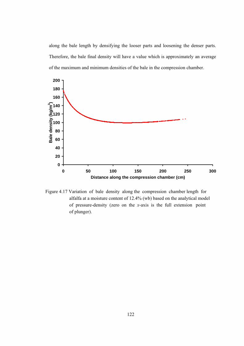
122

along the bale length by densifying the looser parts and loosening the denser parts.

Therefore, the bale final density will have a value which is approximately an average

of the maximum and minimum densities of the bale in the compression chamber.

0

20

40

60

80

100

120

140

160

180

200


Bal

e de

nsity

(kg/

m3 )

Figure 4.17 Variation of bale density along the compression chamber length for alfalfa at a moisture content of 12.4% (wb) based on the analytical model of pressure-density (zero on the x-axis is the full extension point of plunger).

123

0

100

200

300

400

500

600

0 50 100 150 200 250

Bale density (kg/m3)

Pres

sure

(kPa

)

B

C

APmax

PB

γmaxγB

Figure 4. 18 Comparing the pressure-density relationship based on the analytical

model with the possible pressure-density relationship in reality.

4.1.6 Empirical Model for Pressure-Density Relationship

Different models have been proposed for the pressure-density relationship of

forage materials in the literature. Some of these models including those proposed by

Ferrero et al. (1990), Viswanathan and Gothandapani (1999), Watts and Bilanski (1991),

Butler and McColly (1959), and Bilanski et al. (1985) were tested with the data of the

experimental tests to find the best model for the pressure-density relationship. The least-

square regression analysis method was used to validate each model with the

experimental data. In this method, model constant coefficients were changed in order to

minimize the summation of the square difference between data resulting from each of

124

the models and the experimental data. Then, the standard error and the average error

were calculated using the following equations (Figliola 2000):

( ) ( )[ ]n

yySE

n

iieip∑

=

−= 1

2

(4.1)

⎟⎟⎠

⎞⎜⎜⎝

⎛=

eySEAE 100

where:

SE = standard error,

yp = predicted data,

ye = experimental data,

AE = average error and

ey = average of the experimental data.

The model that had the minimum average error was selected as the best model. Results

of validation of these models using the experimental data of alfalfa are shown in Table

4.6. This table showed that the developed model for the pressure-density relationship in

this study (first model in the table) had the highest coefficient of determination and

lowest average error. The coefficient of determination and average error for this model

were 0.89 and 2.55%, respectively. This model was a modified version of model

proposed by Ferrero et al. (1990). Experimental data and predicted density for alfalfa

based on the proposed model (Eq. 3.54) versus plunger pressure are plotted in Figure

4.19. The standard error and the coefficient of determination for this model were 4.25

kg/m3 and 0.89, respectively (Table 4.6).

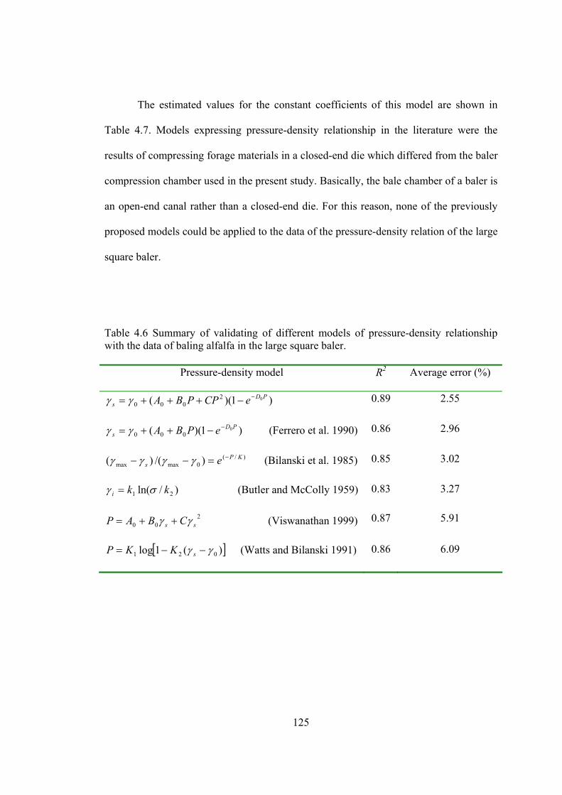
125

The estimated values for the constant coefficients of this model are shown in

Table 4.7. Models expressing pressure-density relationship in the literature were the

results of compressing forage materials in a closed-end die which differed from the baler

compression chamber used in the present study. Basically, the bale chamber of a baler is

an open-end canal rather than a closed-end die. For this reason, none of the previously

proposed models could be applied to the data of the pressure-density relation of the large

square baler.

Table 4.6 Summary of validating of different models of pressure-density relationship with the data of baling alfalfa in the large square baler.

Pressure-density model R2 Average error (%)

)1)(( 02000

PDs eCPPBA −−+++= γγ

0.89 2.55

)1)(( 0000

PDs ePBA −−++= γγ (Ferrero et al. 1990)

0.86 2.96

)/(0maxmax )/()( KP

s e −=−− γγγγ (Bilanski et al. 1985) 0.85 3.02

)/ln( 21 kki σγ = (Butler and McColly 1959) 0.83 3.27

200 ss CBAP γγ ++= (Viswanathan 1999) 0.87 5.91

[ ])(1log 021 γγ −−= sKKP (Watts and Bilanski 1991) 0.86 6.09

126

100

120

140

160

180

200

220

0.1 0.15 0.2 0.25 0.3 0.35 0.4Plunger pressure (MPa)

Bal

e de

nsity

(kg/

m3 )

Measured density

Empirically predicted dendity

Figure 4.19 Experimental and the predicted densities vs. plunger pressure in a large

square baler for alfalfa at a moisture content of 12.4% (wb). Table 4.7 Estimated constants of the pressure-density model for alfalfa (Eq. 3.54).

Constant Estimated values for alfalfa

γ0 80.00

A0 119.86

B0 -501.53

C 1306.62

D0 71.31

R2 0.89

Standard error 4.25

127

Models proposed by Ferrero et al. (1990), Viswanathan and Gothandapani

(1999), Watts and Bilanski (1991), Butler and McColly (1959), and Bilanski et al.

(1985) were also tested with the data of barley straw to find the best model for the

pressure-density relationship. Results of validation of these models using the

experimental data of barley straw are shown in Table 4.8. This table showed that the

developed model for the pressure-density relationship in this study (first model in the

table) had the highest coefficient of determination and lowest average error. The

coefficient of determination and average error for this model were 0.94 and 2.50%,

respectively. The experimental data and predicted densities for barley straw based on the

developed model (Eq. 3.54) versus the plunger pressure are plotted in Figure 4.20. The

estimated values for the constant coefficients of this model are shown in Table 4.9. The

standard error and the coefficient of determination of this model were 3.21 kg/m3 and

0.94, respectively (Table 4.9).

Table 4.8 Summary of validating different models of pressure-density relationship with the data of baling barley straw in the large square baler.

Pressure-density model R2 Average error (%)

)1)(( 0200

PDos eCPPBA −−+++= γγ

0.94 2.50

)/(0maxmax )/()( KP

s e −=−− γγγγ (Bilanski et al. 1985) 0.94 2.52

)/ln( 21 kki σγ = (Butler and McColly 1959) 0.94 2.55

)1)(( 0000

PDs ePBA −−++= γγ (Ferrero et al. 1990)

0.92 2.89

200 ss CBAP γγ ++= (Viswanathan 1999) 0.93 7.81

[ ])(1log 021 γγ −−= sKKP (Watts and Bilanski 1991) 0.92 8.00

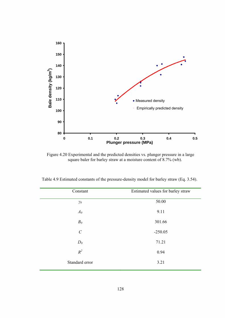
128

80

90

100

110

120

130

140

150

160

0 0.1 0.2 0.3 0.4 0.5Plunger pressure (MPa)

Bal

e de

nsity

(kg/

m3 )

Measured density

Empirically predicted density

Figure 4.20 Experimental and the predicted densities vs. plunger pressure in a large square baler for barley straw at a moisture content of 8.7% (wb).

Table 4.9 Estimated constants of the pressure-density model for barley straw (Eq. 3.54).

Constant Estimated values for barley straw

γ0 50.00

A0 9.11

B0 301.66

C -250.05

D0 71.21

R2 0.94

Standard error 3.21

129

4.1.7 Comparison of Analytical and Empirical Models

Comparison of the analytical and empirical models for bale density as a function

of pressure on the plunger, Pp, (Eqs. 3.53 and 3.54) showed that these models had

completely different general forms, but in both models bale density had a direct

relationship with the material initial density and plunger pressure. Figure 4.21 represents

the variation of the bale density of alfalfa with respect to the maximum pressure inside

the compression chamber (Pp) based on both analytical and empirical models. According

to these graphs, the trend of variation of density with pressure in both models is similar,

but their rate of changes is different. Variation rate of density with pressure in the

analytical model is higher than that of the empirical model. At low plunger pressures,

the analytical model underestimates the bale density but at the higher pressures its

prediction gets close to the real bale density. The cause of low accuracy in density

prediction based on the analytical model is probably the assumptions made in deriving

the analytical model. In the analytical model development, forage materials assumed to

behave as an isotropic linear elastic material which is not true in reality.

130

100

120

140

160

180

200

220

0.1 0.15 0.2 0.25 0.3 0.35 0.4Plunger pressure (MPa)

Bal

e de

nsity

(kg/

m3 )

Analytical modelEmpirical modelExperimental data

Figure 4.21 Experimental data and the predicted densities based on the analytical and empirical models vs. the plunger pressure in a large square baler for alfalfa at 12.4% (wb) moisture content.

4.1.8 Field Tests

Collected data from the experiments in both provinces (Saskatchewan and

Québec) in 2001 were analyzed using a split plot design in the SAS software (SAS

Institute, Cary, NC) except the evaluation of the flake size and load setting effect on the

barley straw bale density in Québec. For this study, insufficient data were collected to do

the statistical analysis. In this section, results of the effect of load setting and flake size

on the plunger force and bale density are discussed. Results are provided for baling

alfalfa and barley straw.

131

4.1.8.1 Baling Alfalfa

The analysis of variance of the data collected to test the effect of load setting and

flake size on the plunger force showed that both the load setting and flake size had a

significant effect on the plunger force (Table A.1). Means comparison analysis using the

Duncan’s multiple range test (DMRT) indicated that the difference between the plunger

forces at all the load settings was significant even at the significance level of 1% (Table

4.10). Means comparison analysis of the plunger forces at different flake sizes revealed

that at the significance level of 5%, the difference between all treatments was significant

(Table 4.11). However, at the significance level of 1% there was a considerable

difference only between the plunger force at flake size of 3/10 and the others (Table

4.11). The plunger force increased with increased percentage of the available maximum

plunger force on the load pre-setting control system and flake size. Although, the

plunger force was supposed to decrease with increasing flake size, results showed that

the plunger force increased with increasing flake size. This was probably due to the

increased flake size which increased the material rebounding after each plunger stroke.

A greater plunger force with the increasing load setting was expected; therefore, when

the load was set at 70% of the available maximum load, the plunger force reached its

maximum value.

132

Table 4.10 Average plunger forces at different load settings for alfalfa (α = 0.01).

Load setting Plunger force (kN) 50 255.6 a

60 305.5 b

70 372.3 c

a, b, c Averages with different letters were statistically different at 99% level.

Table 4.11 Average plunger forces at different flake sizes for alfalfa.

Flake size (plunger/stuffer ratio setting)

Plunger force (kN)

(α = 0.05) Plunger force (kN)

(α = 0.01) 3/10 299.7 a 299.7 a

6/10 313.6 b 313.6 b

9/10 320.1 c 320.1 b

a, b, c Averages with different letters were statistically different.

The results of the analysis of variance for the effect of load setting and flake

sizes on the alfalfa bale density are presented in Appendix A (Table A.2). These results

revealed that load setting, flake size, and their interaction had significant effect on the

alfalfa bale density at a significance level of 1%. The difference between all mean values

of the bale densities at different load settings at a significance level of 1% was

significant (Table 4.12). The mean comparison analysis of the bale density at different

flake sizes showed that at the significance level of 5%, the bale density at the flake size

of 3/10 was significantly different from bale densities at other flake sizes (Table 4.13).

However, at the confidence level of 99% only the difference between the bale densities

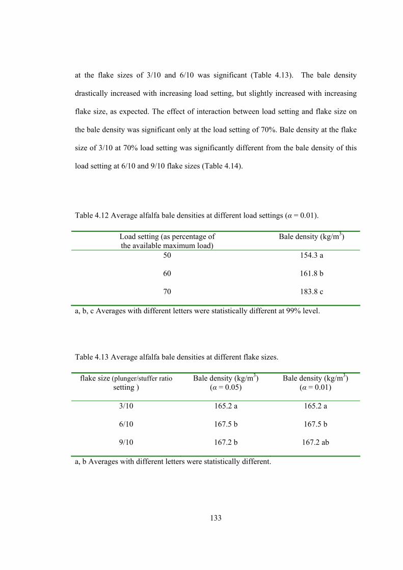
133

at the flake sizes of 3/10 and 6/10 was significant (Table 4.13). The bale density

drastically increased with increasing load setting, but slightly increased with increasing

flake size, as expected. The effect of interaction between load setting and flake size on

the bale density was significant only at the load setting of 70%. Bale density at the flake

size of 3/10 at 70% load setting was significantly different from the bale density of this

load setting at 6/10 and 9/10 flake sizes (Table 4.14).

Table 4.12 Average alfalfa bale densities at different load settings (α = 0.01).

Load setting (as percentage of the available maximum load)

Bale density (kg/m3)

50 154.3 a

60 161.8 b

70 183.8 c

a, b, c Averages with different letters were statistically different at 99% level.

Table 4.13 Average alfalfa bale densities at different flake sizes.

flake size (plunger/stuffer ratio setting )

Bale density (kg/m3) (α = 0.05)

Bale density (kg/m3) (α = 0.01)

3/10 165.2 a 165.2 a

6/10 167.5 b 167.5 b

9/10 167.2 b 167.2 ab

a, b Averages with different letters were statistically different.

134

Table 4.14 The effect of the interaction between load setting and flake size on the bale density for alfalfa.

Load setting (%) Flake size Bale density (kg/m3)

50 3/10 155.1 a

50 6/10 155.1 a

50 9/10 152.6 a

60 3/10 162.4 b

60 6/10 161.7 b

60 9/10 161.3 b

70 3/10 178.0 c

70 6/10 185.8 d

70 9/10 187.6 d

4.1.8.2 Baling Barley Straw

A summary of the analysis of variance of the data showing the effect of load

setting and flake size on the plunger load of the baler in the baling barley straw is

presented in the appendix A (Table A.3). Results showed that plunger load was

drastically affected by the load setting and interaction between load setting and flake

size at 1% significance level, while flake size had no significant effect on the plunger

load even at the significance level of 5%. Based on the mean comparison analysis, the

difference between plunger loads at diverse load settings was significant at the

significance level of 1%, therefore checking the difference between the treatments at the

significance level of 5% was not necessary (Table 4.15). This analysis, on the other

135

hand, showed no significant difference between the plunger load mean values at the

different flake sizes at the confidence level of 99% (Table 4.16). Whereas, means

comparison showed a significant difference between plunger loads at flake sizes of 6/10

and 9/10 at the confidence level of 95% (Table 4.16). As expected, a higher load setting

considerably increased the plunger load, while greater flake size slightly increased the

plunger load due to more relaxation of the larger flakes. The interaction between load

setting and flake size had a significant effect on the plunger force at all load settings but

60%. Results showed that at the highest level of load setting (100%) the medium flake

size required the maximum plunger force, while at the medium load settings (60 and

80%) the thickest and at the lowest load setting (40%) the thinnest flake size needed the

maximum plunger force (Table 4.17).

Table 4.15 Average plunger forces at different load settings for the baling barley straw (α = 0.01).

Load setting (percent of available maximum plunger force)

Plunger force (kN)

40 216.4 a

60 317.7 b

80 397.8 c

100 492.4 d

a, b, c, d Averages with different letters were statistically different at 99% level.

136

Table 4.16 Average plunger forces at different flake sizes for the baled barley straw.

flake size (plunger/stuffer ratio setting) Plunger force (kN)

(α = 0.05) Plunger force (kN)

(α = 0.01) 3/10 354.9 ab 354.9 a

6/10 354.0 b 354.0 a

9/10 359.3 a 359.3 a

a, b Averages with different letters had statistically significant difference. Table 4.17 The effect of the interaction between load setting and flake size on the plunger force for barley straw.

Load setting (%) Flake size Plunger force (kN)

40 3/10 221.9 a

40 6/10 210.5 ab

40 9/10 216.8 b

60 3/10 315.4 c

60 6/10 317.8 c

60 9/10 320.1 c

80 3/10 398.8 d

80 6/10 387.9 e

80 9/10 404.9 d

100 3/10 483.6 f

100 6/10 500.0 g

100 9/10 493.8 g

137

Average barley straw bale densities of the different treatments showed that the

bale density significantly increased with increasing load setting (Table 4.18). Flake size

had a slight effect on the barley straw bale density (Table 4.19); however, the number of

data available for the barley straw density was insufficient to perform a complete

statistical analysis. Results of flake size effect on the bale density in both tested

materials also showed that at the low load settings, bale density decreased with

increasing flake size (Table 3.2 and 3.3). This was probably because of more recovery

(rebound) of the thicker flakes at the lower plunger pressures.

Table 4.18 Average barley straw bale densities at different load settings.

Load setting (percent of

available maximum plunger force) Bale density (kg/m3)

40 109.9

60 124.1

80 137.7

100 144.1

Table 4.19 Average barley straw bale densities at different flake sizes.

Flake size (plunger/stuffer ratio setting) Bale density (kg/m3) 3/10 127.0

6/10 129.6

9/10 130.3

138

4.2 Sensor Design

Results of sensor sensitivity, sensor calibration, and sensor performance in the

field are discussed in this section.

4.2.1 Sensor Sensitivity

The sensor showed an excellent linearity under the uni-axial vertical and

horizontal loading calibration with no hysteresis in the unloading cycle (Figs. 4.22 and

4.223). Results of the primary, the secondary, and the cross sensitivities of the sensor for

each of the horizontal and the vertical loadings are shown in the Table 4.20. The

horizontal and vertical primary sensitivities of the sensor were 1479.7 and 1387.8

μVV-1kN-1, and cross sensitivities of four arm bridge outputs for the horizontal and the

vertical loadings were 0.64% and 2.85%, respectively. Godwin (1975) reported draft

and vertical cross sensitivities of 1.1 and 2.1%, respectively. McLaughlin et al. (1998)

found a cross sensitivity of 1.9 and 7.0% for the draft and the vertical loadings. Gu et al.

(1993) determined a range of 0 to 4% for the cross sensitivity. Therefore, the horizontal

cross sensitivity determined in this study was the lowest compared to those previously

reported, and the vertical cross sensitivity was found to be smaller than all reported

vertical sensitivities but what reported by Godwin (1975).

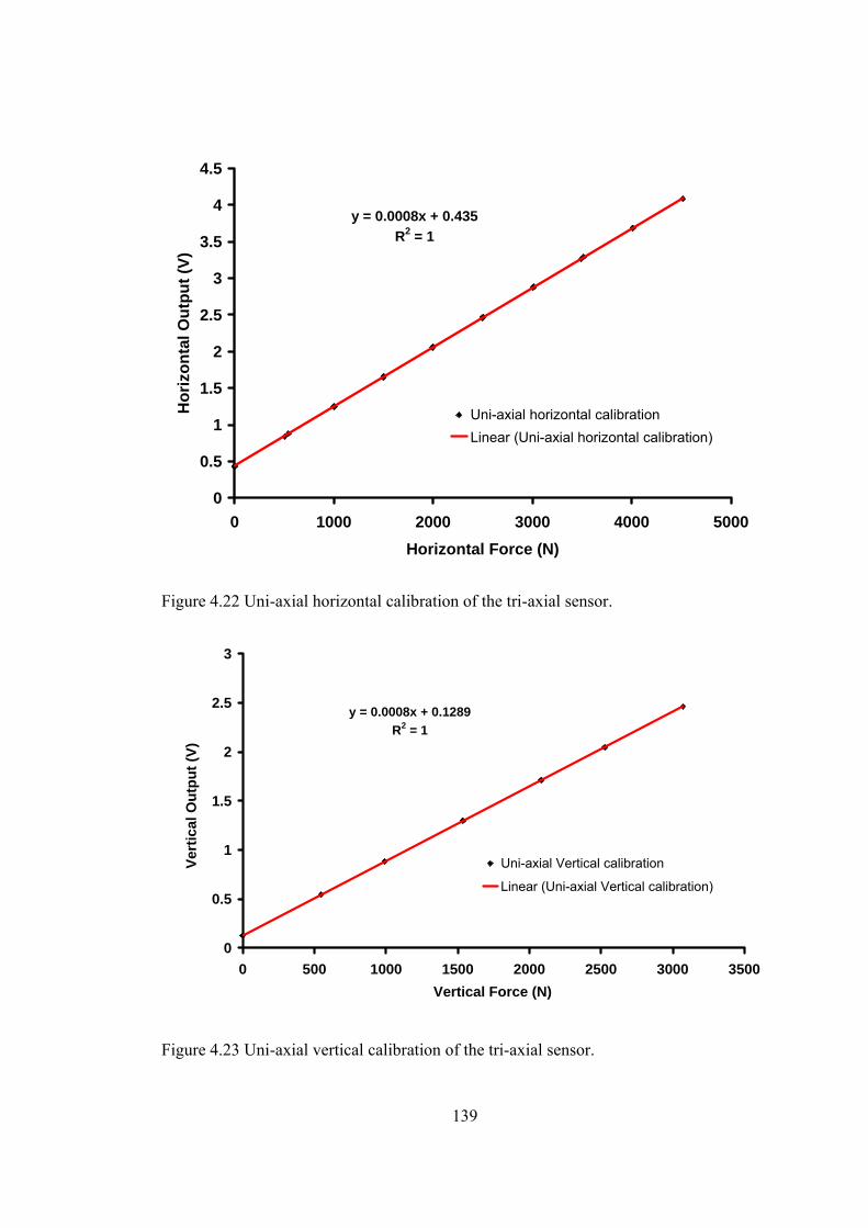
139

y = 0.0008x + 0.435R2 = 1

0

0.5

1

1.5

2

2.5

3

3.5

4

4.5

0 1000 2000 3000 4000 5000Horizontal Force (N)

Hor

izon

tal O

utpu

t (V)

Uni-axial horizontal calibrationLinear (Uni-axial horizontal calibration)

Figure 4.22 Uni-axial horizontal calibration of the tri-axial sensor.

y = 0.0008x + 0.1289R2 = 1

0

0.5

1

1.5

2

2.5

3

0 500 1000 1500 2000 2500 3000 3500Vertical Force (N)

Vert

ical

Out

put (

V)

Uni-axial Vertical calibration

Linear (Uni-axial Vertical calibration)

Figure 4.23 Uni-axial vertical calibration of the tri-axial sensor.

140

Table 4.20 Cross sensitivities of the sensor resulting from uni-axial calibration. Loading axis Primary sensitivity

(μVV-1kN-1) Secondary sensitivity

(μVV-1kN-1) Cross sensitivity (%) (Secondary/Primary)

x 1479.7 9.45 0.64

y 1387.8 39.55 2.85

4.2.2 Sensor Calibration

The tri-axial loading calibration data were used to develop the following

calibration equations for the forces in the x-direction (draft) and the y-direction (vertical

force) using multiple regression analysis.

0)( cVVcVcVcF yxiyzxxx +++= , (4.3)

0)( cVVcVcVcF yxixxyyy +++= , (4.4)

where:

Fx, Fy = forces in the x- and y-directions (N),

Vx, Vy = output of the horizontal and vertical force measurement bridges

(v) and

cx, cy, ci, c0 = model coefficients.

Least square method in multiple regression analysis was used to validate the developed

models and estimate the model constant coefficients (Table 4.21).

141

Table 4.21 Estimated constants of the calibration equations of the sensor

Model cx cy ci c0 Fx -1214.71 7.63 -13.91 -450.44

Fy -15.48 -1313.99 -0.53 -223.41

Results of the multiple regression models for Fx and Fy showed that the best

prediction model expressed the forces as a function of primary bridge output, secondary

bridge output, and the interaction between the primary and secondary outputs. The

predicted horizontal and vertical loads versus applied horizontal and vertical loads for

the tri-axial loading calibration are plotted in Figures 4.24 and 4.25, respectively. The

predicted forces were calculated using the abovementioned multiple regression models.

Figure 4.24 showed that the regression model for the force prediction in the x-direction

had successfully corrected the cross sensitivity effects from the forces in other directions

on the force measurement in this direction. The coefficient of determination and the

standard error in this case were 0.99 and 28.64 N, respectively (Table 4.22). The plot of

the predicted vertical forces versus applied vertical forces showed that the regression

model for the force in the y-direction had the ability to predict the applied forces to the

sensor in the y-direction (R2 = 0.99). However, the random error in this prediction was

higher than that of the model predicting force in the x-direction. The coefficient of

determination and the standard error for the force prediction in the y-direction were 0.99

and 86.5 N, respectively (Table 4.22).

Primary sensitivities of the EORs, calculated from the analytical equations and

the strain gage bridge theory, were 1122.4 and 848.8 μVV-1kN-1 for the horizontal and

142

vertical sensitivities, respectively. These calculated sensitivities were 75.9 and 61.2% of

the measured sensitivities (1479.7 and 1387.8 μVV-1kN-1). These results revealed that

the analytical equations used for the EOR design (Eqs. 3.54 and 3.57) underestimated

the stress at both positions (θ = ± 39.5° and θ = 90°) of the ring section of the EOR.

y = 0.9997x + 0.543R2 = 0.9997

-10

990

1990

2990

3990

4990

0 1000 2000 3000 4000 5000

Applied Fx (N)

Pred

icte

d F x

(N)

Predicted Fx vs. applied Fx

Linear (Predicted Fx vs. applied Fx)

Figure 4.24 Predicted horizontal loads resulting from the developed model in the tri- axial calibration vs. the applied horizontal loads.

143

y = 0.996x + 5.3286R2 = 0.996

-200

800

1800

2800

3800

0 500 1000 1500 2000 2500 3000 3500Applied Fy (N)

Pred

icte

d F y

(N)

Predicted Fy vs. applied Fy

Linear (Predicted Fy vs. applied Fy)

Figure 4.25 Predicted vertical loads resulting from the developed model in the tri-axial

calibration vs. the applied vertical loads.

Table 4.22 The coefficient of determination and the standard error of the sensor calibration equations.

Model R2 Standard error (kPa)

Fx 0.99 28.64

Fy 0.99 86.5

4.2.3 Sensor Performance in the Field

Placing the sensor inside the compression chamber of the baler and its alignment

inside the bale was the most difficult practical problem during the field tests. There was

no reference inside the compression chamber and the bale to use for sensor alignment;

144

therefore, sensor alignment was performed observationally. This has probably made

some misalignment for the sensor during the field tests which has caused some errors in

the recorded forces. Meanwhile, since the dug hole in the bale for sensor was usually

larger than the sensor size, there was a gap between the sensor body and the top and side

walls of the dug hole. In practice, some of the applied forces in the y- and z-directions

have been consumed to fill this gap. For this reason, recorded forces in the y-direction

were lower than the expected forces. Results of force measurement inside the

compression chamber in the x-direction were similar to the results obtained for the baler

plunger maximum force by installing strain gages on the plunger arms. The error for the

force measurement using the tri-axial sensor for barley straw was about 5%. However,

there was no reference to evaluate the obtained forces by the sensor in the y-direction;

results showed that the recorded forces were lower than the expected forces in this

direction. The reason was probably the gap between the walls of the sensor and dug hole

inside the bale. According to the theoretical analysis given in section 3.3.2.2, forces in

the z-direction could not be recorded by the strain gages mounted on this sensor.

Therefore, this sensor could only record the forces in the x- and y-directions. In practice,

some values were obtained for Fz as a function of the difference between forces in the x-

direction in two EORs, but the accuracy of this measurement was very low. In order to

make the sensor a perfect tri-axial force transducer, a set of stain gages must be mounted

on the side faces of the ring section of the EOR (Fig. 3.25) to be able to record Fz in

addition to Fx and Fy.

145

4.3 Measurement of Crop Properties

Results of measurement of some crop properties such as coefficient of friction,

adhesion coefficient, and modulus of elasticity are discussed in this section.

4.3.1 Friction and Adhesion Coefficients

Results of the analysis of variance of the effect of moisture content on the static

coefficient of friction of alfalfa on a polished steel surface showed that alfalfa moisture

content had a significant effect on the coefficient of friction at the confidence level of

99% (Table A.4). The coefficient of variation and the correlation coefficient in this case

were 6.1 and 0.95, respectively. The coefficient of friction increased with increasing

moisture content; however, the rate of the increment was larger for the higher moisture

contents than that of the lower ones (Table 4.23). This result was in good agreement

with the results reported for alfalfa and similar materials in the literature. Shinners et al.

(1991) reported that moisture content had a significant effect on the coefficient of

friction of alfalfa so that it was lower in the moisture range of 33 to 37% than the range

of 73 to 77%. Mani et al. (2003) presented that moisture content had a significant effect

on the coefficient of friction of corn stover grind. Ling et al. (1997) showed that both the

static and the kinetic coefficients of friction of wood ash increased with increasing ash

moisture content. At the confidence level of 95%, the difference between the

coefficients of friction at all moisture contents was significant, while at confidence level

of 99%, only difference between the coefficients at 12.0, 31.0, and 42.2% was

significant (Table 4.23). The coefficients of friction for alfalfa ranged from 0.15 to 0.26

for moisture contents of 12.0 to 42.2% (wb). Efforts were made to develop a

mathematical relationship between the coefficient of friction of alfalfa on a polished

146

steel surface and alfalfa moisture content. Therefore, the relationship between

coefficient of friction and moisture content for alfalfa was best expressed by the

following quadratic equation:

14.010107 425 +−×= −−ww MMμ , (4.5)

where:

μ = coefficient of friction and

Mw = moisture content % wb.

The experimental and predicted data of the coefficient of friction of alfalfa on a polished

steel surface versus moisture content is shown in Figure 4.26. The coefficient of

determination and the standard error of the model fitness were 0.95 and 0.01,

respectively.

Table 4.23 Mean comparison of the static coefficient of friction of alfalfa on a polished steel surface at different moisture contents.

Moisture content (%) Coefficient of friction (α = 0.05)

Coefficient of friction (α = 0.01)

12.0 0.15 a 0.15 a

22.0 0.17 b 0.17 ab

31.0 0.20 c 0.20 b

42.2 0.26 d 0.26 c

a, b, c, d Averages with different letters were statistically different. Each coefficient of friction represents average of fifteen samples.

147

0

0.05

0.1

0.15

0.2

0.25

0.3

0 5 10 15 20 25 30 35 40 45Moisture content (%wb)

Coe

ffici

ent o

f fric

tion

Experimental Coefficint of Friction

Poly. (Experimental Coefficint ofFriction)

μ = 7x10-5 Mw2-10-4 Mw+0.14

R2 = 0.95

Figure 4.26 Experimental and predicted coefficients of friction of alfalfa on a

polished steel surface vs. material moisture content. Although, the difference between the adhesion coefficients of alfalfa on a

polished steel surface at different levels of moisture content was considerable, the

analysis of variance of the effect of moisture content on the adhesion coefficient showed

no significant effect (A.5). This lack of effect could be partially due to a high coefficient

of variation between the data. However, Duncan’s multiple range mean comparison test

showed a significant difference between the adhesion coefficients at 12.0% and 42.2%

(wb) moisture contents at 95% of confidence level. The adhesion coefficient of alfalfa

on a polished steel surface increased with increasing moisture contents from 12.0 to

31.0% (wb) and then decreased at the moisture content of 42.2% (Table 4.24). The

lower adhesion coefficient at 42.2% moisture content could be related to the lubrication

of steel surface by water released from the moist materials under pressure. No literature

was found regarding adhesion coefficient of alfalfa to be able to compare the results

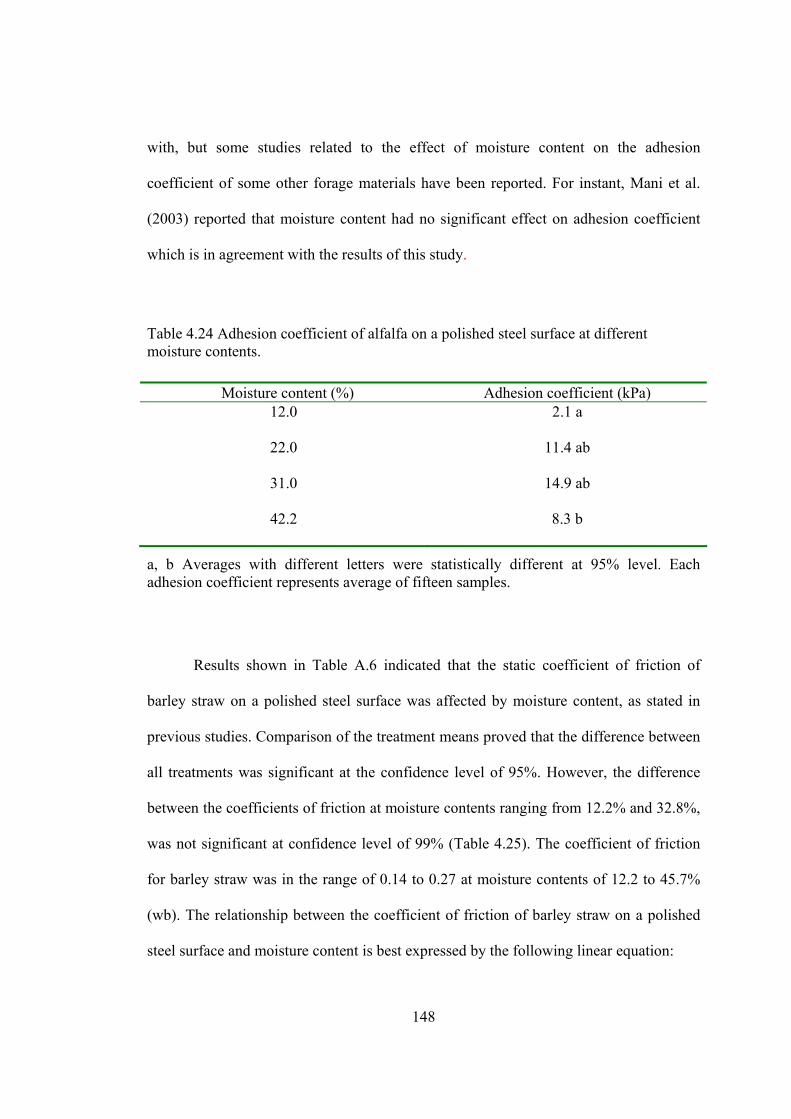
148

with, but some studies related to the effect of moisture content on the adhesion

coefficient of some other forage materials have been reported. For instant, Mani et al.

(2003) reported that moisture content had no significant effect on adhesion coefficient

which is in agreement with the results of this study.

Table 4.24 Adhesion coefficient of alfalfa on a polished steel surface at different moisture contents.

Moisture content (%) Adhesion coefficient (kPa) 12.0 2.1 a

22.0 11.4 ab

31.0 14.9 ab

42.2 8.3 b

a, b Averages with different letters were statistically different at 95% level. Each adhesion coefficient represents average of fifteen samples.

Results shown in Table A.6 indicated that the static coefficient of friction of

barley straw on a polished steel surface was affected by moisture content, as stated in

previous studies. Comparison of the treatment means proved that the difference between

all treatments was significant at the confidence level of 95%. However, the difference

between the coefficients of friction at moisture contents ranging from 12.2% and 32.8%,

was not significant at confidence level of 99% (Table 4.25). The coefficient of friction

for barley straw was in the range of 0.14 to 0.27 at moisture contents of 12.2 to 45.7%

(wb). The relationship between the coefficient of friction of barley straw on a polished

steel surface and moisture content is best expressed by the following linear equation:

149

1006.00037.0 += wMμ , (4.6)

where:

μ = coefficient of friction and

Mw = moisture content % wb.

The coefficient of determination and the standard error of the model were 0.93 and

0.013, respectively.

Table 4.25 Static coefficient of friction of barley straw on a polished steel surface at different moisture contents.

Moisture content (%) Coefficient of friction

(α = 0.05) Coefficient of friction

(α = 0.01) 12.2 0.14 a 0.14 a

20.3 0.18 b 0.18 ab

32.8 0.22 c 0.22 b

45.7 0.27 d 0.27 c

a, b, c, d Averages with different letters were statistically different. Each coefficient of friction represents average of fifteen samples.

The adhesion coefficient of barley straw on a polished steel surface was not

significantly affected by the material moisture content, while the difference between the

adhesion coefficients was considerable (Table A.7). However, Duncan’s multiple range

mean comparison test showed a significant difference between the adhesion coefficients

at moisture contents of 20.3% and 45.7% at the confidence level of 95% (Table 4.26).

Again the high coefficient of variation could be the reason for this lack of significant

difference. The coefficient increased with increasing moisture contents ranging from

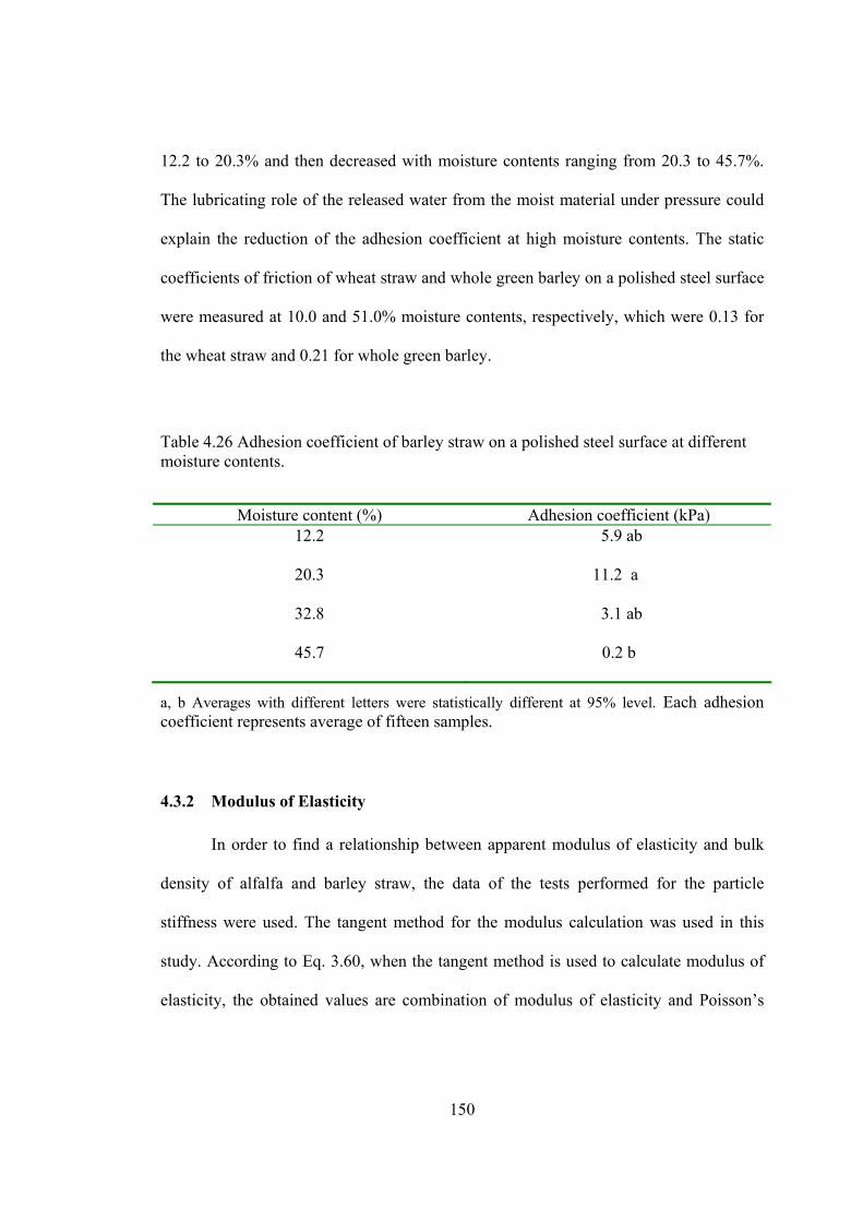
150

12.2 to 20.3% and then decreased with moisture contents ranging from 20.3 to 45.7%.

The lubricating role of the released water from the moist material under pressure could

explain the reduction of the adhesion coefficient at high moisture contents. The static

coefficients of friction of wheat straw and whole green barley on a polished steel surface

were measured at 10.0 and 51.0% moisture contents, respectively, which were 0.13 for

the wheat straw and 0.21 for whole green barley.

Table 4.26 Adhesion coefficient of barley straw on a polished steel surface at different moisture contents.

Moisture content (%) Adhesion coefficient (kPa)

12.2 5.9 ab

20.3 11.2 a

32.8 3.1 ab

45.7 0.2 b

a, b Averages with different letters were statistically different at 95% level. Each adhesion coefficient represents average of fifteen samples.

4.3.2 Modulus of Elasticity

In order to find a relationship between apparent modulus of elasticity and bulk

density of alfalfa and barley straw, the data of the tests performed for the particle

stiffness were used. The tangent method for the modulus calculation was used in this

study. According to Eq. 3.60, when the tangent method is used to calculate modulus of

elasticity, the obtained values are combination of modulus of elasticity and Poisson’s

151

ratio ( ( ) FEE=

−+−

)21(1)1(

ννν ). Since, Poisson’s ratio is a constant coefficient, plotting the

obtained values versus material bulk density can show the trend of variation of modulus

of elasticity with material bulk density. Therefore, calculated values for alfalfa and

barley straw were plotted versus material bulk density (FE-γ curve). Results for alfalfa

showed that the apparent modulus of elasticity remained constant as the density

increased from 100 kg/m3 to 220 kg/m3 (Fig. 4.27). Results for barley straw also showed

that the apparent modulus of elasticity remained constant as the density increased from

100 kg/m3 to 190 kg/m3 (Fig. 4.28). Therefore, the results of this study proved that

modulus of elasticity of alfalfa and barley straw was constant for the density range

encountered in the large square baler.

0

0.5

1

1.5

2

2.5

3

80 100 120 140 160 180 200 220 240Bulk density (kg/m3)

FE (M

Pa)

Figure 4.27 Variation of the apparent modulus of elasticity with bulk density of alfalfa (E is modulus of elasticity and F is a function of Poisson’s ratio as defined in Eq. 3.61).

152

0

0.5

1

1.5

2

2.5

3

80 100 120 140 160 180 200

Bulk density (kg/m3)

FE (M

Pa)

Figure 4.28 Variation of the apparent modulus of elasticity with the bulk density of barley straw (E is modulus of elasticity and F is a function of Poisson’s ratio as defined in Eq. 3.61).

153

CHAPTER 5

SUMMARY AND CONCLUSIONS

5.1 Summary

This section is intended to provide a summary of the most important results

achieved in this study.

5.1.1 Analytical Model for the Pressure Distribution

A new analytical model was developed for the pressure distribution inside the

compression chamber of a baler by assuming isotropic linear elastic behavior for forage

materials. Model development was performed according to the conditions of a large

square baler. The new conditions involved the constant modulus of elasticity instead of

the variable modulus of elasticity, and the inclined top and side walls instead of the

inclined top wall in Sitkei’s model (Eq. 2.19). The derived analytical model was found

to be simpler and more convenient than Sitkei’s model (Eq. 2.19). Results of the model

validation showed that the analytical model accurately predicted the pressure in the x-

direction, while the model was not accurate in the y- and z-directions. The overall

standard error and the coefficient of determination of the regression analysis were 20.0

kPa and 0.95, respectively.

For wheat straw, the analytical model predicted the pressure on the baler plunger

(maximum pressure) with the accuracy of 97.5%. The regression analysis of the

experimental and the predicted data of the pressure distribution for wheat straw revealed

154

a standard error and a coefficient of determination of 26 kPa and 0.95, respectively. The

overall standard error and coefficient of determination for whole green barley were 18.4

kPa and 0.96, respectively. Therefore, an acceptable correlation was found between the

experimental data and the derived analytical model for each of forage materials tested in

this study.

Comparing graphs of the pressure distribution of different forage materials based

on the derived analytical model indicated that the pressure distribution for all tested

forage materials had similar patterns. The maximum pressures for barley straw and

wheat straw were approximately identical. Considering the fact that barley straw had

been harvested at a lower load setting compared to the load setting for wheat straw

(barley straw baled at a load setting of 60% and wheat straw baled at a load setting of

70%), the maximum pressure resulting from the baling barley straw was higher than that

of wheat straw. The maximum pressure for whole green barley was inferior to those of

the barley and wheat straw which was explained by the lower load setting (50%) and

Poisson’s ratio (0.32).

5.1.2 Empirical Model for the Pressure Distribution

Data of the experimental tests were used to develop an exponential empirical

model for the pressure distribution inside the compression chamber of the baler for each

of the tested forage materials (barley straw, wheat straw, and whole green barley) using

regression analysis. These empirical models were simple equations which were only

functions of the distance from the full extension point of the plunger along the

compression chamber. These models had the identical general form for all forage

materials in each specific direction with different model constants. Based on the results

155

obtained for baling barley straw, the best correlation between the experimental data and

the predicted pressures was found at the beginning of the compression chamber length

close to the plunger (maximum pressure inside the bale chamber) with an error of

approximately 5%. The overall standard error and the coefficient of determination of the

regression analysis in this case for model in the x-direction were 19.3 kPa and 0.96,

respectively. For wheat straw, the empirical model overestimated the pressure in the x-

direction on the baler plunger with an accuracy of 87.3% which was the lowest

compared to the accuracy of the pressure prediction of the empirical model for the other

crops at the same position. The regression analysis of the experimental and the predicted

data of the pressure distribution in the x-direction for wheat straw presented a good

coefficient of determination and a low standard error for the model correlation to the

experimental data which were 0.97 and 20.6 kPa, respectively. Results of comparing the

predicted and experimental pressures showed that the empirical model predicted the

pressure on the plunger in the x-direction with the error of about 5% for whole green

barley. The overall coefficient of determination and the standard error were 0.96 and

18.4 kPa, respectively. Comparing the experimental and the predicted pressure

distribution in the x-direction revealed that the developed model for wheat straw

overestimated the maximum pressure on the baler plunger, whereas models for barley

straw and whole green barley estimated more accurate values for the maximum pressure

on the baler plunger. The empirical model in the y-direction was not accurate because of

the inaccurate experimental data.

156

5.1.3 Comparison of Models of Pressure Distribution

Comparing the results of the analytical and the empirical models in the x-

direction for barley straw revealed that the empirical model provided more accurate

pressure prediction with a larger coefficient of determination and a lower overall

standard error; however, the analytical model provided more accurate prediction of the

pressure on the plunger than the empirical model. Comparison of the results of the

analytical and the empirical models in the x-direction for baling wheat straw indicated

that the empirical model had more accurate overall prediction for the pressure along the

compression chamber, and had the larger coefficient of determination and the lower

overall standard error, while the analytical model provided more accurate prediction of

the pressure only on the plunger. For baling whole green barley, results showed that both

analytical and empirical models predicted the pressure distribution with similar

accuracy. Therefore, in order to estimate the pressure distribution of baling whole green

barley, either model could be used.

5.1.4 Pressure-Density Relationship

Analytical and empirical models were developed for the pressure-density

relationship of the baler for baling alfalfa and barley straw. Results of plotting the

analytical model versus distance from the plunger showed that bale density decreased

with distance up to 50 cm, and then remained almost constant up to end of compression

chamber. This model failed to accurately predict the bale density along the bale length

because of the assumption made in the model development. The developed empirical

model for both alfalfa and barley straw was a combination of a quadratic and an

exponential equation. In order to validate the developed models, field tests were

157

performed by baling alfalfa and barley straw. For alfalfa with 12.4% moisture content,

three flake sizes and three load settings were considered. Three levels of the flake sizes

and four levels of the load settings were considered for barley straw with 8.7% moisture

content. The forces on the plunger arms were recorded by a data acquisition system. The

actual bale bulk density was calculated by measuring the bale dimensions and weight.

Results showed that both load setting and flake size had a significant effect on the

plunger force and bale density. The plunger force and bale density increased with

increasing load setting and flake size.

Comparing analytical and empirical models for the bale density as a function of

pressure on the plunger showed that the trend of variation of density with pressure in

both models was similar, but the rate of change was different. The variation rate of

density with pressure in the analytical model was higher than that of the empirical

model. The analytical model underestimated the bale density at low plunger pressures

but showed more accurate prediction at higher pressures, while the empirical model

accurately predicted the bale density at low and high pressures.

5.1.5 Sensor Design

A tri-axial sensor was designed using an extended octagonal ring (EOR) and was

calibrated uni-axially and tri-axially. The sensor showed excellent linearity and low

cross sensitivities. Primary sensitivities of the EORs calculated from the analytical

equations and the strain gage bridge theory were 1122.4 and 848.8 μVV-1kN-1 for the

horizontal and the vertical sensitivities, respectively. These calculated sensitivities were

75.9 and 61.2% of the measured ones (1479.7 and 1387.8 μVV-1kN-1). Results revealed

that the analytical equations used for the EOR design (Eqs. 3.55 and 3.58)

158

underestimated the stress at the all positions (θ = ±39.5° and θ = 90°) of the ring section

of the EOR. Results of the force measurement inside the bale compression chamber in

the x-direction were close to the results obtained for the baler plunger maximum force

from installing strain gages on the plunger arms. For barley straw, the error for the force

measurement using the tri-axial sensor was approximately 5%. However, there was no

reference to evaluate the obtained forces by the sensor in the y-direction; results showed

that the recorded forces were lower than the expected forces in this direction. The reason

was probably the gap between the walls of the sensor and the dug hole inside the bale.

According to the theoretical analysis given in section 3.3.2.2, forces in the z-direction

could not be recorded by the strain gages mounted on this sensor. Therefore, this sensor

could only record the forces in the x- and y-directions.

5.1.6 Crop Properties

Results of the static coefficient of friction of different forage materials on the

polished steel surface showed that the moisture content of the forage materials had a

significant effect on the coefficient of external friction. The coefficient of external

friction increased with increasing crop moisture content for both alfalfa and barley

straw. The static coefficient of friction of alfalfa on a polished steel surface was a

quadratic function of material moisture content, while the relationship between the

coefficient of friction of barley straw on a polished steel surface and material moisture

content was best expressed by a linear equation. Results of variation of modulus of

elasticity with bulk density for both alfalfa and barley straw showed that the apparent

modulus of elasticity remained constant as bulk density increased in the density range

encountered in a large square baler.

159

5.2 Conclusions

This section is intended to list some of the most significant conclusions that can be

drawn from this research based on the addressed objectives. These conclusions are

outlined as follows:

1. Analytical models were developed for the pressure distribution inside the bale

along the compression chamber length in the x-, y-, and z-directions based on

theory of elasticity. The models were validated using experimental data in the x-

and y-directions collected for barley straw, wheat straw, and whole green barley.

The model in the x-direction was simpler and more convenient than Sitkei’s

model (Eq. 2.19) and showed a good correlation with the experimental data. The

analytical models did not work in the y- and z-directions because of either

inaccurate experimental data or inappropriate assumptions in model

development.

2. Empirical models were also developed for the pressure distribution in the x- and

y-direction for each of the tested forage materials using regression analysis. The

model accurately predicted the pressures in the x-direction, while it had a poor

accuracy in the y-direction.

3. Analytical and empirical models were developed for the pressure-density

relationship of large square baler for alfalfa and barley straw. The empirical

model had a good correlation with the experimental data, while the analytical

model showed an inaccurate prediction of density particularly at the low plunger

pressures.

160

4. Load setting and flake size had a significant effect on the plunger force and bale

density. The plunger force and bale density increased with increasing load setting

and flake size.

5. A tri-axial sensor was designed using EOR and was calibrated uni-axially and

tri-axially. The sensor showed excellent linearity and low cross sensitivities.

6. The static coefficient of friction of alfalfa on a polished steel surface was a

quadratic function of material moisture content, while the relationship between

the coefficient of friction of barley straw and moisture content was best

expressed by a linear equation.

5.3 Recommendations for Future Work

According to results and limitations of this study, the following recommendations can be

given to make the future studies more effective in this area:

1. This study was limited to the modeling of variation of the pressure distribution in

the x-, y-, and z-directions with respect to the x-direction. In other word, the

sensor was located at the center of the bale cross-section area; therefore, forces

were measured on the centerline of bale at different distances from plunger. In

order to have a comprehensive understanding of pressure patterns inside the

compression chamber, having the pressure variation in the y- and z-direction

(pressure variation from center to top and side walls) are also necessary.

Therefore, modeling of the variation of pressure in the y- and z-direction by

locating sensors at different positions from center to top and side walls could be

one of the objectives of the future studies.

2. The analytical models in the y- and z-directions were not validated in this study

because of lack of accurate experimental data in these directions. Therefore,

161

validating these models using accurate experimental data can be another aspect

of future work.

3. The analytical model for the pressure-density relationship was not validated in

this study, because of lack of experimental data. Therefore, validation of the

analytical model of pressure-density relationship by measuring the bale density

variation along the bale length can be performed in the future.

4. Since the field experiments in present study were performed at one level of

moisture content for each crop, evaluation of the effect of crop moisture content

on the pressure-density relationship and pressure distribution models can also be

considered in the future research.

162

REFERENCES

ASAE Standards, 47th Ed. 2001. S358.2-Moisture measurement-forage. 579. St. Joseph,

Mich. ASAE.

Bickert, W. G and F. H. Buelow. 1966. Kinetic coefficient of grains on surfaces.

Transactions of the ASAE 9(1):129-131, 134.

Bilanski, W. K., V. A. Graham and J. A. Hanusiak. 1985. Mechanics of bulk forage

deformation with application to wafering. Transactions of the ASAE 28(3): 697-

702.

Brubaker, J. E. and J. Pos. 1965. Determining static coefficients of friction of grains on

structural surfaces. Transactions of the ASAE 8(1):53-55.

Burrows, C. R., J. N. Reed, P. Hogan, S. P. Tomlinson and M. A. Neale. 1992.

Hydraulic flow division and ram synchronization in a high-density baler. Journal

of Agricultural Engineering Research 53(4): 273-287.

Butler, J, L. and H. F. McColly. 1959. Factors affecting the pelleting of hay.

Agricultural Engineering 40(8): 442-446.

Coblentz, W. K., J. O. Fritz and K. K. Bolsen. 1993. Baling system for making

laboratory-scale hay bales. Agronomy Journal 85: 962-965.

Corrie, W. J. and D. A. Bull. 1969. Investigations into the characteristics of large bales.

Journal of Agricultural Engineering Research 14(4): 323-331.

163

Culpin, C. 1986. Farm machinery, 11th ed. London, Britain. Collins Professional and

Technical Books.

Faborode, M. O. and J. R. O’Callaghan. 1986. Theoretical analysis of the compression

of fibrous agricultural materials. Journal of Agricultural Engineering Research

35(3): 175-191.

Fairbanks, G. E., S. C. Fransen and M. D. Schrock. 1981. Machine made stacks

compared with round bales. Transactions of the ASAE 24(2): 281-283, 287.

Ferrero, A., J. Horabik and M. Molenda. 1990. Density-pressure relationship in

compaction of straw. Canadian Agricultural Engineering 33(1): 107-111.

Figliola, R. S. and D. E. Beasley. 2000. Theory and design for mechanical

measurements, 3rd ed. New York, NY, the United States of America. John Wiley

and Sons, INC.

Freeland, R. S. and B. L. Bledsoe. 1988. Energy required to form large round hay bales-

effect of operational procedure and baler chamber type. Transaction of the ASAE

31(1): 63-67.

Fung, Y. C. 1977. A first course in continuum mechanics, 2nd ed. Englewood Cliffs,

New Jersey, the United States of America. Prentice-Hall, INC.

Godwin, R. J. 1975. An extended octagonal ring transducer for use in tillage studies.

Journal of Agricultural Engineering Research 20:347-352.

Godwin, R. J., A. J. Reynols, M. J. O’Dogherty, and A. A. Al-Ghazal. 1993. A triaxial

dynamometer for force and moment measurements on tillage implements.

Journal of Agricultural Engineering Research 55:189-205.

164

Godwin, R. J., P. S. G. Magalhaes, S. M. Miller, and R. K. Fry. 1985. Instrumentation

to study the force system and vertical dynamic behaviour of soil-engaging

implements. Journal of Agricultural Engineering Research 36:301-310.

Gu, Y., R. L. Kushwaha, and G. C. Zoerb. 1993. Cross sensitivity analysis of extended

octagonal ring transducer. Transactions of the ASAE 36(6):1967-1972.

Hall, G. E. and C. W. Hall. 1968. Heated-die wafer formation of alfalfa and

bermudagrass. Transactions of the ASAE 11(4): 578-581.

Hann, S. A. and H. P. Harrison. 1976. Friction in and energy required for extruding

alfalfa. Canadian Agricultural Engineering 18(1): 21-25.

Hoag, D. L., and R. R. Yoerger. 1975. Analysis and design of load rings. Transactions of

the ASAE 19:995-1000.

Hundtoft, E. B. and F. H. Buelow. 1971. An axial stress-strain relationship for bulk

alfalfa. Journal of Agricultural Engineering Research 16(1): 32-45.

Hunt, D. 2001. Farm power and machinery management, 10th ed. Ames, Iowa, the USA.

Iowa State University Press.

Jenkins, B. M., D. A. Toenjes, J. B. Dobie, and J. F. Arthur. 1985. Performance of large

balers for collecting rice straw. Transactions of the ASAE 28(2): 360-363.

Kepner, A. R., R. Bainer, and E. L. Barger. 1972. Principles of farm machinery, 2nd ed.

Westport, Connecticut, the United States of America. The AVI Publishing

Company, INC.

Lawton, P. J. and J. A. Marchant. 1980. Direct shear testing of seeds in bulk. Journal of

Agricultural Engineering Research 25: 189-201.

165

Ling, Q., J. H. Wilhoit, and C. A. Flood. 1997. Static and kinetic friction coefficients of

wood ash on stainless steel. ASAE Paper No. 976020. St. Joseph, Mich.: ASAE.

Lowen, E. G., E. R. Marshall, and M. C. Shaw. 1951. Electric strain gage tool

dynamometers. Proceedings of the Society of Experimental Stress Analysis 8(2):

1-16.

Mani, S., L. G. Tabil, S. Sokhansanj, and M. Roberge. 2003. Mechanical properties of

corn stover. CSAE Paper No. 036090. Montreal, Quebec: CSAE/SCGR.

McLaughlin, N. B. 1996. Correction of an error in equations for extended ring

transducers. Transactions of the ASAE 39(2):443-444.

McLaughlin, N. B., S. Tessier, and A. Guilbert. 1998. Improved double extended

octagonal ring drawbar transducer for 3-D measurement. Canadian Agricultural

Engineering 40:257-264.

Mewes, E. 1958. Zum verhalten von pressgutern in prestopfen (on the behaviour of

compressed matter in pressure chambers). Landtechnische Forshuny 8(6): 158-

164.

Mewes, E. 1959. Verdichtungsgesetzmassigkeiten nach presstop fversuchen

(compression relationships as a result of experiments in pressure chambers).

Landtechnische Forshuny 9(3): 67-76.

Mohsenin, N. and J. Zaske. 1976. Stress relaxation and energy requirement in

compaction of unconsolidated materials. Journal of Agricultural Engineering

Research 21: 193-205.

Moysey, E. B. and S. Hiltz. 1985. Friction properties of fertilizers. Canadian


166

New Holland. 2001. BB940, BB950, and BB960 Operator’s Manual. New Holland

North America Inc., New Holland, PA.

Norris, E. R. and W. K. Bilanski. 1969. Tensile properties of alfalfa stems. Canadian


Osobov, V. I. 1967. Theoretical principles of compressing fibrous plant materials.

Trudy Viskhom 55: 221-265.

O’Dogherty, M. J. 1975. A dynamometer to measure the forces on a sugar beet topping

knife. Journal of Agricultural Engineering Research 20:339-345.

O’Dogherty, M. J. 1996. The design of octagonal ring dynamometer. Journal of

Agricultural Engineering Research 63:9-18.

O’Dogherty, M. J. and J. A. Wheeler. 1984. Compression of straw to high densities in

closed cylindrical dies. Journal of Agricultural Engineering Research 29(1): 61-

72.

O’Dogherty, M. J. and H. G. Gilbertson. 1988. The relationship between bulk density

and median chop length of chopped wheat straw samples. Journal of

Agricultural Engineering Research 40(4): 245-257.

O’Dogherty, M. J. 1989. A review of the mechanical behavior of straw when

compressed to high densities. Journal of Agricultural Engineering Research

44(4): 241-265.

O’Dogherty, M. J., J. A. Huber, J. Dyson and C. J. Marshall. 1995. A study of physical

and mechanical properties of wheat straw. Journal of Agricultural Engineering

Research 62(2): 133-142.

167

Pickard, G. E., W. M. Roll and J. H. Ramser. 1961. Fundamental of hay wafering.

Transactions of the ASAE 4(1): 65-68.

Reece, F. N. 1966. Temperature, pressure, and time relationships in forming dense hay

wafers. Transactions of the ASAE 9(6): 749-751.

Reece, F. N. 1967. Power requirements for forming wafers in a closed-die process.


Rehkugler, G. E. and W. F. Buchele. 1967. Influence of stem in alfalfa forage on the

formation of wafers. Journal of Agricultural Engineering Research 12(4): 285-

292.

Richter, D. 1954. Friction coefficients of some agricultural materials. Agricultural

Engineering 35(6): 411-413.

Shinners, K. J., R. G. Koegel and L. L. Lehman. 1991. Friction coefficient of alfalfa.


Shinners, K. J., R. J. Straub and R. G. Koegel. 1992. Performance of two small

rectangular baler configurations. Applied Engineering in Agriculture 8(3): 309-

313.

Shinners, K. J., R. J. Straub, R. L. Huhnke and D. J. Undersander. 1996. Harvest and

storage losses associated with mid-size rectangular bales. Applied Engineering in

Agriculture 12(2): 167-173.

Sitkei, G. 1986. Mechanics of Agricultural Materials. Amsterdam, the Netherlands:

Elsevier.

Snyder, L. H., W. L. Roller, and G. E. Hall. 1967. Coefficients of kinetic friction of

wheat on various metal surfaces. Transactions of the ASAE 10(3):411-413,419.

168

Srivastava, A. C., W. K. Bilanski and V. A. Graham. 1981. Feasibility of producing

large-size hay wafers. Canadian Agricultural Engineering 23(2): 109-112.

Stroshine, R. 2000. Physical properties of agricultural materials and food products.

West Lafayette, Indiana, the USA.

Tabil, L. G., and S. Sokhansanj. 1997. Bulk properties of alfalfa grind in relation to its

compaction characteristics. Applied Engineering in Agriculture 13(4): 499-505.

Thompson, S. A., and I. J. Ross. 1983. Compressibility and frictional coefficients of

wheat. Transactions of the ASAE :1171-1176,1180.

Viswanathan, R. and L. Gothandapani. 1999. Pressure density relationship and stress

relaxation characteristics of coir pith. Journal of Agricultural Engineering

Research 73(3): 217-225.

Watts, K. C. and W. K. Bilanski. 1991. Stress relaxation of alfalfa under constant

displacement. Transactions of the ASAE 34(6): 2491-2498.

Zhang, Q., M. G. Britton, and R. J. Kieper. 1994. Interactions between wheat and a

corrugated steel surface. Transactions of the ASAE :951-956.

169

APPENDIX A

TABLES OF ANALYSIS OF VARIANCE

Table A.1 Analysis of variance of the data of the effect of flake size and load setting on the alfalfa plunger force.

Source DF SS MS F P R2 CV

Flake size 2 6487.6 3243.8 24.7 <0.0001 0.95 3.7 Load

setting 2 205830.5 102915.2 783.6 <0.0001

Interaction 4 687.7 171.9 1.31 0.27

Error 81 10638.8 131.3

Total 89 223644.6

Table A.2 Analysis of variance of data for the effect of the flake size and the load setting on alfalfa bale density.

Source DF SS MS F P R2 CV Flake size 2 96.7 48.4 5.6 0.005 0.95 1.8

Load setting 2 14124.7 7062.4 818.5 <0.0001

Interaction 4 472.5 118.1 13.7 <0.0001

Error 81 698.9 8.6

Total 89 15392.8

170

Table A.3 Analysis of variance of data of the effect of flake size and load setting on the plunger force for the baling barley straw.

Source DF SS MS F P R2 CV

Flake size 2 519.6 259.8 2.74 0.07 0.99 2.7 Load

setting 3 991904.9 330635.0 3489.6 <0.0001

Interaction 6 2636.2 439.4 4.64 0.0004

Error 84 7959.0 94.8

Total 95 1003019.7 Table A.4 Analysis of variance of data of the effect of the moisture content on the coefficient of friction of alfalfa on a polished steel surface.

Source DF Sum of squares

Mean square

F Value

Pr>F R2 Coefficient of variation

Model 3 0.0212 0.0071 49.8 <0.0001 0.95 6.1

Error 8 0.0011 0.0001

Corrected total

11

0.0223

Table A.5 Analysis of variance of data of the effect of the moisture content on the adhesion coefficient of alfalfa on a polished steel surface.


Mean square

F Value Pr>F R2 Coefficient of variation

Model 3 263.91 87.97 3.25 <0.081 0.55 56.61

Error 8 216.57 27.07

Corrected total

11

480.47

171

Table A.6 Analysis of variance of data of the effect of the moisture content on the coefficient of friction of barley straw on a polished steel surface.


Mean square


Model 3 0.0266 0.0089 38 <0.0001 0.93 7.5

Error 8 0.0019 0.0002

Corrected total

11

0.0285

Table A.7 Analysis of variance of data of the effect of moisture content on the adhesion coefficient of barley straw on a polished steel surface.


Mean square


Model 3 244.68 81.56 2.79 <0.11 0.51 114.09

Error 8 233.54 29.19

Corrected total

11

478.22

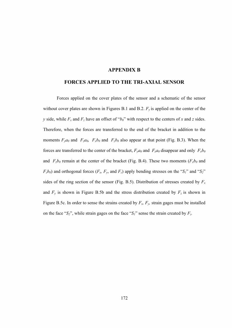
172

APPENDIX B

FORCES APPLIED TO THE TRI-AXIAL SENSOR

Forces applied on the cover plates of the sensor and a schematic of the sensor

without cover plates are shown in Figures B.1 and B.2. Fy is applied on the center of the

y side, while Fx and Fz have an offset of “b0” with respect to the centers of x and z sides.

Therefore, when the forces are transferred to the end of the bracket in addition to the

moments Fya0 and Fza0, Fxb0 and Fzb0 also appear at that point (Fig. B.3). When the

forces are transferred to the center of the bracket, Fya0 and Fza0 disappear and only Fxb0

and Fzb0 remain at the center of the bracket (Fig. B.4). These two moments (Fxb0 and

Fzb0) and orthogonal forces (Fx, Fy, and Fz) apply bending stresses on the “S1” and “S2”

sides of the ring section of the sensor (Fig. B.5). Distribution of stresses created by Fx

and Fy is shown in Figure B.5b and the stress distribution created by Fz is shown in

Figure B.5c. In order to sense the strains created by Fx, Fy, strain gages must be installed

on the face “S2”, while strain gages on the face “S1” sense the strain created by Fz.

173

y

x

z

Fx

Fz

Fy

b0

Cx

Cz

b0

Cy

2a0

Figure B.1 Forces applied to the cover plates of the sensor.

bracket

EOR

Center of bracketEnd of bracket

Figure B.2 Schematic of the sensor without cover plates.

174

Figure B.3 Forces transferred from the covers to the hitch point of sensor.

Figure B.4 Forces transferred from the hitch point to the center of braces.

175

S2

S1

t

w r

S2

S1

a)

b)

c)

Figure B.5 Bending stresses applied to the ring section of the sensor. a) a section of the

flexible part (ring section) of the sensor; b) bending stress applied by Fx and Fy on the cross-section of the ring; and c) bending stress applied by Fz on the cross-section of the ring.

modeling and validation of the baling process in the

Documents