modeling contractile mechanisms: huxley 1957 modelcga/myosim/campbell.pdf · 1 modeling contractile...
TRANSCRIPT
1
Modeling Contractile Mechanisms: Huxley 1957 Model
"With Slides Courtesy"Stuart Campbell, U Kentucky and "
J. Jeremy Rice"IBM T.J. Watson Research Center, P.O. Box 218,
Yorktown Heights, NY 10598 "[email protected]"
914-945-3728" ""
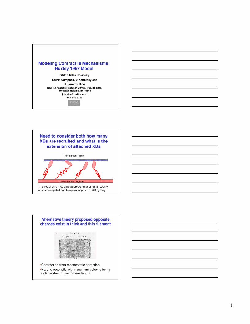
Need to consider both how many XBs are recruited and what is the
extension of attached XBs "
* This requires a modeling approach that simultaneously considers spatial and temporal aspects of XB cycling
Thin filament - actin
Thick filament - myosin
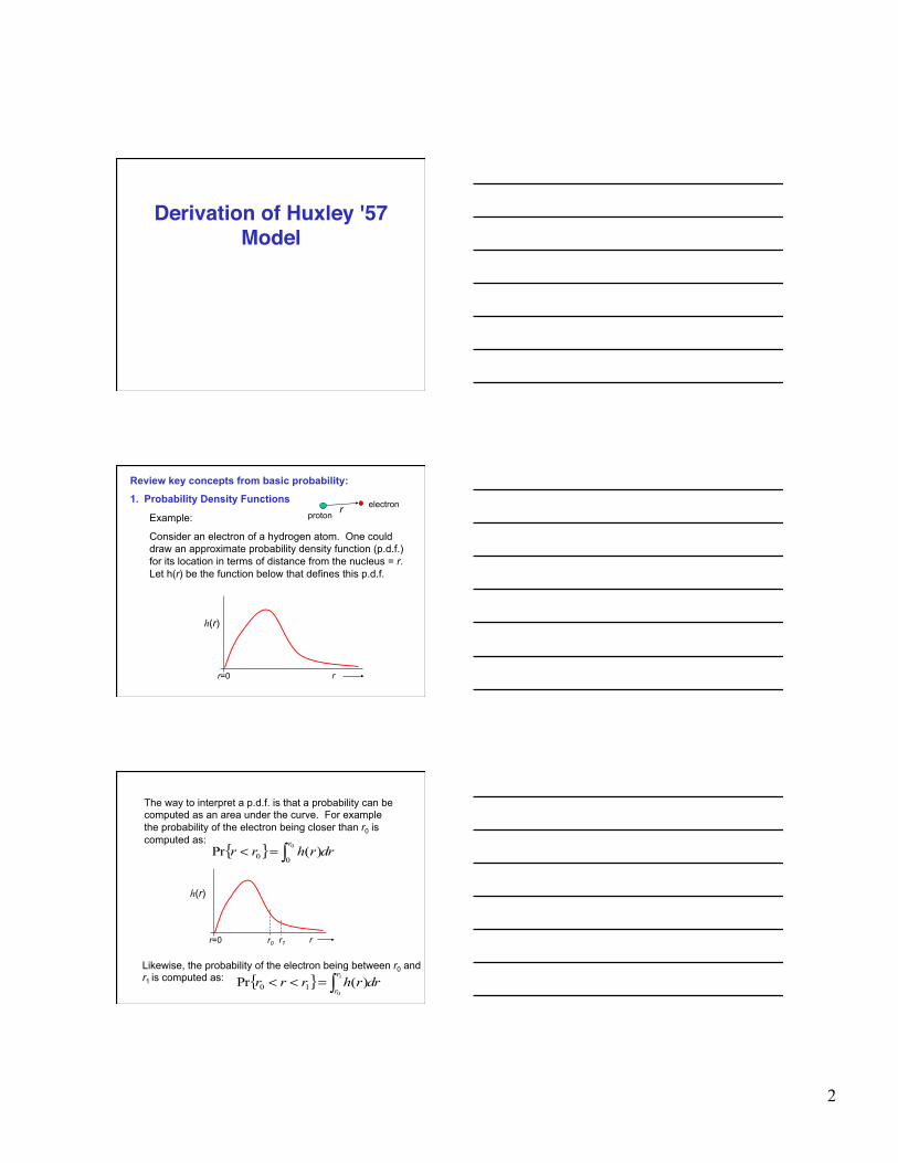
Alternative theory proposed opposite charges exist in thick and thin filament "
• Contraction from electrostatic attraction "• Hard to reconcile with maximum velocity being independent of sarcomere length "
2
Derivation of Huxley '57 Model"
Review key concepts from basic probability:
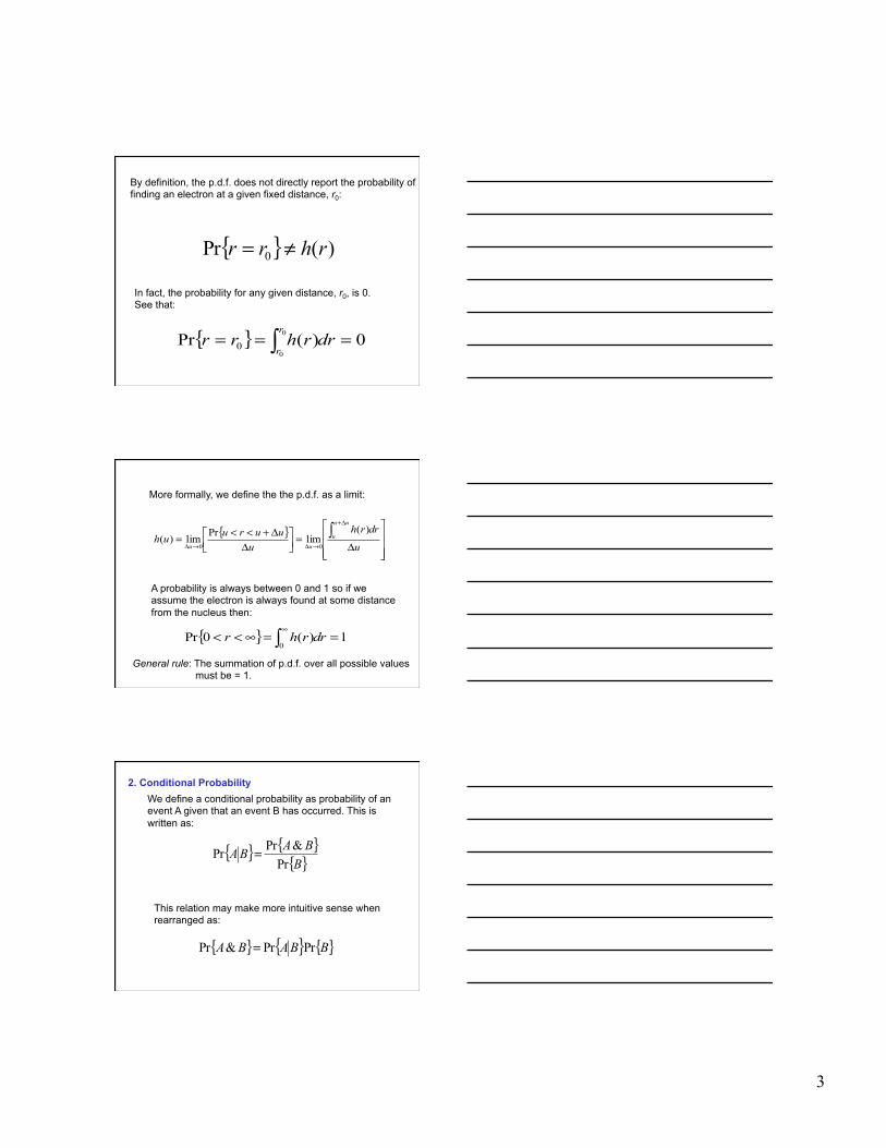
1. Probability Density Functions
Example:
Consider an electron of a hydrogen atom. One could draw an approximate probability density function (p.d.f.) for its location in terms of distance from the nucleus = r. Let h(r) be the function below that defines this p.d.f.
r proton
r=0 r
h(r)
electron
The way to interpret a p.d.f. is that a probability can be computed as an area under the curve. For example the probability of the electron being closer than r0 is computed as:
{ } drrhrrr
∫=< 0
00 )(Pr
r=0 r
h(r)
r0 r1
Likewise, the probability of the electron being between r0 and r1 is computed as: { } drrhrrr
r
r∫=<< 1
0
)(Pr 10
3
By definition, the p.d.f. does not directly report the probability of finding an electron at a given fixed distance, r0:
{ } )(Pr 0 rhrr ≠=
In fact, the probability for any given distance, r0, is 0. See that:
{ } 0)(Pr 0
00 === ∫ drrhrr
r
r
A probability is always between 0 and 1 so if we assume the electron is always found at some distance from the nucleus then:
More formally, we define the the p.d.f. as a limit:
{ }⎥⎥⎥
⎦
⎤
⎢⎢⎢
⎣
⎡
Δ=⎥⎦
⎤⎢⎣⎡
ΔΔ+<<= ∫
Δ+
→Δ→Δ u
drrh
uuuruuh
uu
uuu
)(limPrlim)(
00
{ } 1)(0Pr0
==∞<< ∫∞
drrhr
General rule: The summation of p.d.f. over all possible values must be = 1.
We define a conditional probability as probability of an event A given that an event B has occurred. This is written as:
{ } { } { }BBABA PrPr&Pr =
{ } { }{ }BBABA
Pr&PrPr =
This relation may make more intuitive sense when rearranged as:
2. Conditional Probability
4
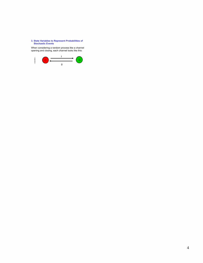
3. State Variables to Represent Probabilities of Stochastic Events
When considering a random process like a channel opening and closing, each channel looks like this:
C" O"f"
g"
For this channel, if we assume f = 1 s-1 and g = 2 s-1, then steady-state probability of the channel being open is computed as:
{ }31Pr =
+==
gffopenchannel
Of course, this does not mean the channel is 1/3 open because only states "closed" and "open" exist. However, if we were to average a large number of channel responses together, we would get something like this:
"Sample many runs and average to get better estimate of probability."
}
. .
.
0"1"
. .
Run 1
Run 2
Run n
.
0"
1"
1/3"
time"
So instead of tracking a each channel, we can define a state variable based system to capture the behavior of the whole population. When implemented this way, average behavior can calculated without averaging (and associated noise and computational cost).
C" O"f"
g"
{ }31Pr =
+===
gffopenchannel O state of Value
{ }32Pr =
+===
gfgclosedchannel C state of Value
5
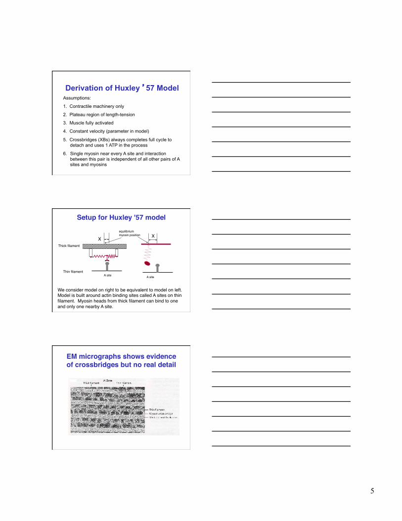
Derivation of Huxley ’57 Model Assumptions:
1. Contractile machinery only
2. Plateau region of length-tension
3. Muscle fully activated
4. Constant velocity (parameter in model)
5. Crossbridges (XBs) always completes full cycle to detach and uses 1 ATP in the process
6. Single myosin near every A site and interaction between this pair is independent of all other pairs of A sites and myosins
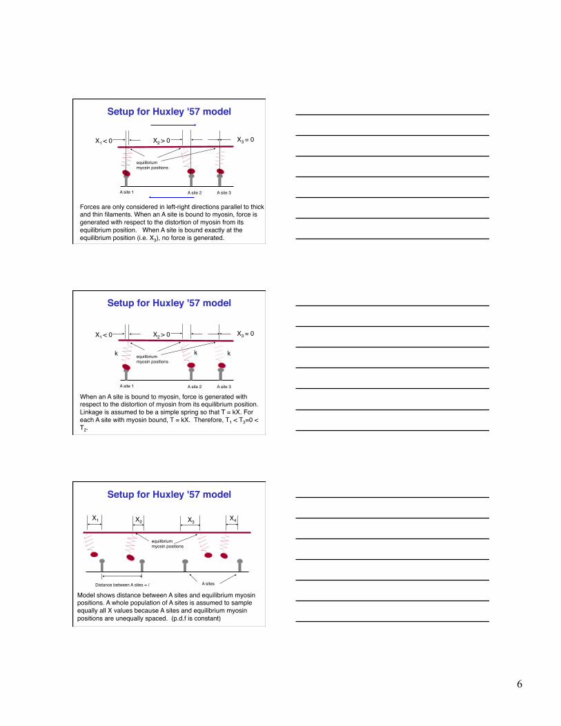
Setup for Huxley '57 model"
X"
We consider model on right to be equivalent to model on left. Model is built around actin binding sites called A sites on thin filament. Myosin heads from thick filament can bind to one and only one nearby A site."
A site"
equilibrium myosin position"
Thick filament"
Thin filament"A site"
X"
EM micrographs shows evidence of crossbridges but no real detail"
6
Setup for Huxley '57 model"
X1 < 0"
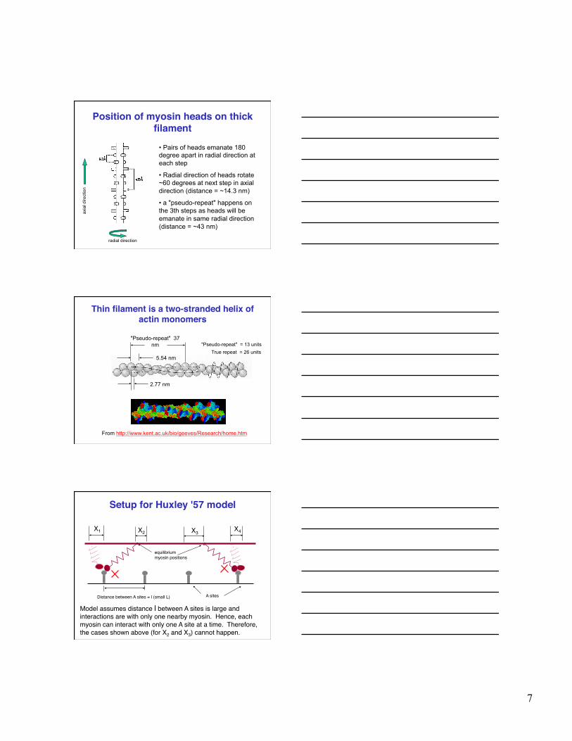
Forces are only considered in left-right directions parallel to thick and thin filaments. When an A site is bound to myosin, force is generated with respect to the distortion of myosin from its equilibrium position. When A site is bound exactly at the equilibrium position (i.e. X3), no force is generated. "
equilibrium myosin positions"
X2 > 0" X3 = 0"
A site 1" A site 2" A site 3"
Setup for Huxley '57 model"
X1 < 0"
When an A site is bound to myosin, force is generated with respect to the distortion of myosin from its equilibrium position. Linkage is assumed to be a simple spring so that T = kX. For each A site with myosin bound, T = kX. Therefore, T1 < T3=0 < T2. "
A site 1"
equilibrium myosin positions"
X2 > 0" X3 = 0"
A site 2" A site 3"
k k k
Setup for Huxley '57 model"
Distance between A sites = l
X1" X2" X3"X4"
Model shows distance between A sites and equilibrium myosin positions. A whole population of A sites is assumed to sample equally all X values because A sites and equilibrium myosin positions are unequally spaced. (p.d.f is constant)"
A sites"
equilibrium myosin positions"
7
Position of myosin heads on thick filament"
• Pairs of heads emanate 180 degree apart in radial direction at each step
• Radial direction of heads rotate ~60 degrees at next step in axial direction (distance = ~14.3 nm)
• a "pseudo-repeat" happens on the 3th steps as heads will be emanate in same radial direction (distance = ~43 nm)
axia
l dire
ctio
n
radial direction
Thin filament is a two-stranded helix of actin monomers"
From http://www.kent.ac.uk/bio/geeves/Research/home.htm
"Pseudo-repeat" = 13 units
5.54 nm
2.77 nm
"Pseudo-repeat" 37 nm
True repeat = 26 units
Setup for Huxley '57 model"
Distance between A sites = l (small L)"
X1" X2" X3"X4"
Model assumes distance l between A sites is large and interactions are with only one nearby myosin. Hence, each myosin can interact with only one A site at a time. Therefore, the cases shown above (for X2 and X3) cannot happen."
A sites"
equilibrium myosin positions"
8
Setup for Huxley '57 model"
X1"
The thick and thin filaments slide past each other at a constant velocity V. We assume that the motion results from combined action of many force generators acting across the whole muscle, so the sliding velocity is not affected by the local attachment or detachment events. Note: velocity is a parameter in the model."
equilibrium myosin positions"
X2" X3 "
Sliding in V > 0 direction (if thick filament fixed) "
"
Sliding in V < 0 direction (if thick filament fixed) "
Setup for Huxley '57 model"
X1"
As thick and thin filaments slide past each other at a constant velocity V, the relative position of A sites compared to equilibrium myosin positions changes. Therefore, when V>0, X1, X2 and X3 all get smaller (less positive or more negative) with time."
equilibrium myosin positions"
X2" X3 "
Sliding in V > 0 direction (if thick filament fixed) "
"
Sliding in V < 0 direction (if thick filament fixed) "
g2
g f
h
1
2
3
4
0 x
g1
f1
XB attach only in this range"
XB can detach at any distortion"
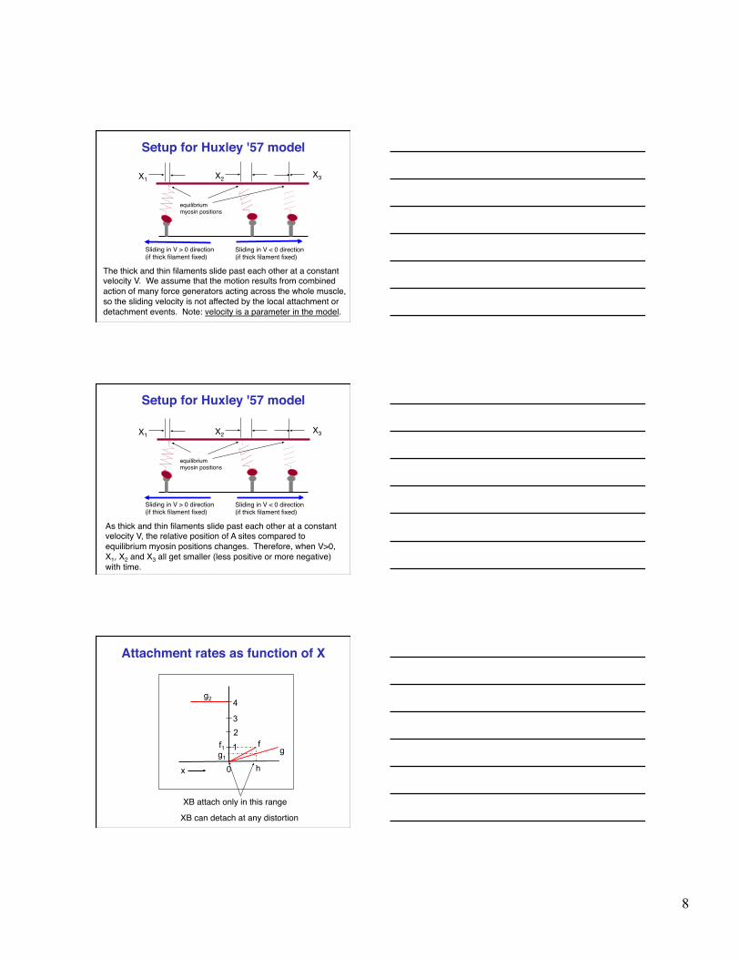
Attachment rates as function of X"

9
Attachment rates as function of X"
X < 0"
Attachment rate between A site and myosin are a function of the relative distance between the A site and equilibrium myosin position. In the model, f(X) is the function defined to control attachment. Function f(X) increases linearly from X=0 to X=h."
X = h/2"X = 0"
f(X)"
gf
h
123
4
0x
gf
h
123
4
0x
Detachment rates as function of X"
X1 < 0"
In the model, g(X) is the function defined to control detachment as a function of the relative distance between the A site and equilibrium myosin position. In the positive range, g(X) increases linearly from X=0. In the negative range, g(X) is large so that the negative distortion XBs ("draggers") detach quickly."
X > h"X = 0"
g(X)"
Let n(x,t) be a conditional probability describing the likelihood that an XB is attached given that the A site is at displacement x from the nearest XB equilibrium position.
To be more rigorous:
Conditional probability vertical bar means “given that”
⎥⎥⎥
⎦
⎤
⎢⎢⎢
⎣
⎡
⎪⎭
⎪⎬⎫
⎪⎩
⎪⎨⎧
Δ+=
→Δ xxtoxrangeinA
attachedXBhassiteA
Prlim)t,x(nx 0
10
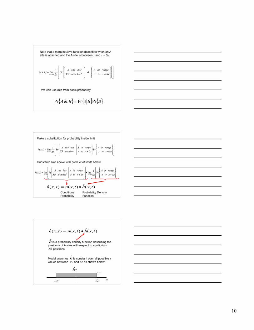
Note that a more intuitive function describes when an A site is attached and the A site is between x and x + Dx
We can use rule from basic probability
⎥⎥⎥
⎦
⎤
⎢⎢⎢
⎣
⎡
⎪⎭
⎪⎬⎫
⎪⎩
⎪⎨⎧
⎟⎟⎟
⎠
⎞
⎜⎜⎜
⎝
⎛
Δ+⎟⎟⎟
⎠
⎞
⎜⎜⎜
⎝
⎛
Δ=
→Δ xxtoxrangeinA
&attachedXB
hassiteAPr
xlim)t,x(nx
10
{ } { } { }BBABA PrPr&Pr =
⎥⎥⎥
⎦
⎤
⎢⎢⎢
⎣
⎡
⎪⎭
⎪⎬⎫
⎪⎩
⎪⎨⎧
Δ+⎪⎭
⎪⎬⎫
⎪⎩
⎪⎨⎧
Δ+Δ=
→Δ xxtoxrangeinA
xxtoxrangeinA
attachedXBhassiteA
xtxn
xPrPr1lim),(ˆ
0
⎥⎥⎥
⎦
⎤
⎢⎢⎢
⎣
⎡
⎪⎭
⎪⎬⎫
⎪⎩
⎪⎨⎧
Δ+Δ•
⎥⎥⎥
⎦
⎤
⎢⎢⎢
⎣
⎡
⎪⎭
⎪⎬⎫
⎪⎩
⎪⎨⎧
Δ+=
→Δ→Δ xxtoxrangeinA
xxxtoxrangeinA
attachedXBhassiteA
txnxx
Pr1limPrlim),(ˆ00
Make a substitution for probability inside limit
Substitute limit above with product of limits below
),(ˆ),(),(ˆ txhtxntxn •=Probability Density Function
Conditional Probability
),(ˆ),(),(ˆ txhtxntxn •=
is a probability density function describing the positions of A sites with respect to equilibrium XB positions
Model assumes is constant over all possible x values between -l/2 and l/2 as shown below:
l/2 -l/2
1/l
x
h
h
h
11
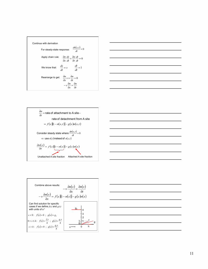
Continue with derivation
For steady-state response:
Apply chain rule:
We know that:
0=∂∂+
∂∂
dtdttn
dtdx
xn
( ) 0, =dttxdn
1=dtdt
vdtdx =
Rearrange to get: 0=∂∂+
∂∂
tnv
xn
tn
xnv
∂∂=
∂∂−
( ) ( ) ( )[ ] ( ) ( )xnxgxnxftxn −−=
∂∂ 1
( )
( ) ( )txnxndttxdn
,
0,
of instead use
wherestatesteady Consider
⇒
=
Unattached A site fraction Attached A site fraction
site A from detachment of rate
- site A to attachment of rate=∂∂tn
( ) ( )[ ] ( ) ( )txnxgtxnxf ,,1 −−=
Combine above results:
Can find solution for specific cases if we define f(x) and g(x) with units of s-1
( ) ( )txn
xxnv
∂∂=
∂∂−
( ) ( ) ( )[ ] ( ) ( )xnxgxnxfxxnv −−=
∂∂− 1
g2
g f
h
1
2
3
4
0 x
g1 f1
( ) ( ) 2;0:0 gxgxfx ==<
( ) ( )hxgxg
hxfxfhx 11 ;:0 ==≤<
( ) ( )hxgxgxfhx 1;0: ==>
12
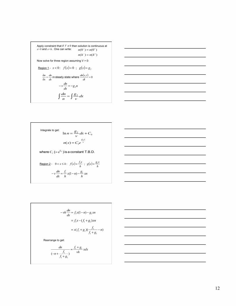
ngdxdnv 2−=−
∫∫ = dxvg
ndn 2
Apply constraint that if then solution is continuous at x=0 and x=h. One can write:
Now solve for three region assuming V > 0:
Region 1 -
)()()0()0(
+−
+−
==
hnhnnn
0≠V
( ) ( ) 2;0:0 gxgxfx ==<
( ) 0, ==∂∂
dttxdn
dxdn
xn wherestatesteady in
Integrate to get:
vxg
eCxn2
1)( =
T.B.D. constant a is )( where CoeC1 =
xnhgnx
hf
dxdnv 11 )1( −−=−
( ) ( )hxgxg
hxfxfhx 11 ;:0 ==≤<Region 2 -
02ln Cdxvgn +=
xngnxfdxdnvh 11 )1( −−=−
xngfxf )( 111 +−=
))((11
111 n
gffgfx −+
+=
Rearrange to get:
xdxvhgf
gffn
dn 11
11
1 )(
+=
++−
13
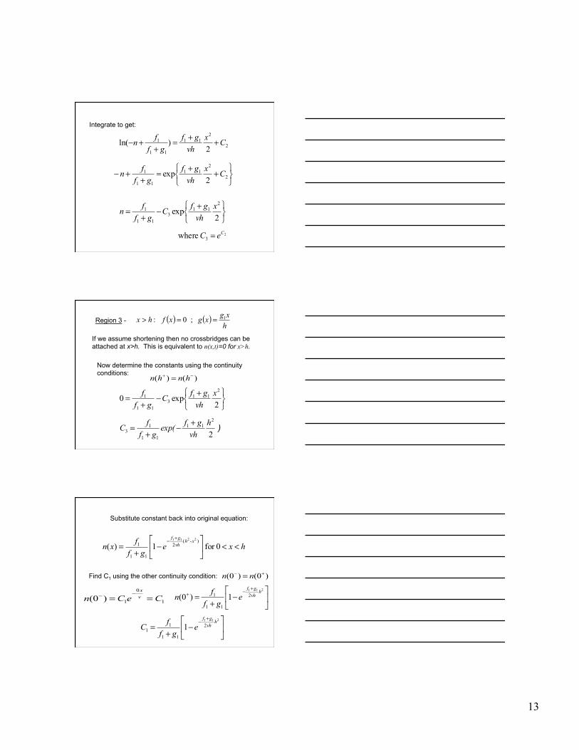
Integrate to get:
2
211
11
1
2)ln( Cx
vhgf
gffn ++=+
+−
⎭⎬⎫
⎩⎨⎧
++=+
+− 2
211
11
1
2exp Cx
vhgf
gffn
2
exp2
113
11
1
⎭⎬⎫
⎩⎨⎧ +−
+= x
vhgfC
gffn
23 where CeC =
( ) ( )hxgxgxfhx 1;0: ==>Region 3 -
If we assume shortening then no crossbridges can be attached at x>h. This is equivalent to n(x,t)=0 for x>h.
Now determine the constants using the continuity conditions:
)()( −+ = hnhn
2
exp02
113
11
1
⎭⎬⎫
⎩⎨⎧ +−
+= x
vhgfC
gff
) 2
211
11
13
hvhgfexp(
gffC +−+
=
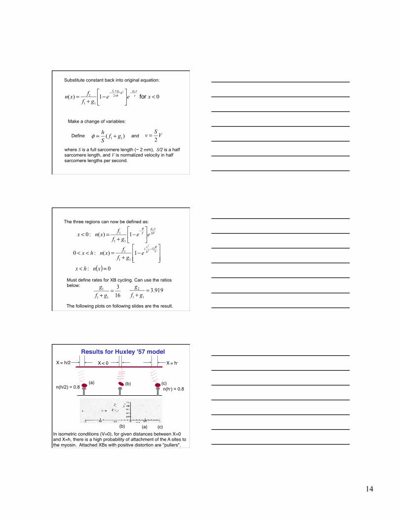
Substitute constant back into original equation:
)0()0( +− = nn
hxegffxn
xhvhgf
<<⎥⎦
⎤⎢⎣
⎡−
+=
+−0for 1)(
)-(2
11
12211
Find C1 using the other continuity condition:
1
0
1)0( CeCn vx
==−− ⎥
⎦
⎤⎢⎣
⎡−
+=
+−+211
2
11
1 1)0(h
vhgf
egffn
⎥⎦
⎤⎢⎣
⎡−
+=
+− 2112
11
11 1
hvhgf
egffC
14
Substitute constant back into original equation:
Define
where S is a full sarcomere length (~ 2 mm), S/2 is a half sarcomere length, and V is normalized velocity in half sarcomere lengths per second.
01)(2211
2
11
1 <⎥⎦
⎤⎢⎣
⎡−
+=
−+−xee
gffxn v
xghvhgf
for
Make a change of variables:
VSv2
=)( 11 gfSh +=φ and
The three regions can now be defined as:
Must define rates for XB cycling. Can use the ratios below:
( ) 0: =< xnhx
SVxg
V eegffxnx
2
1)(:011
1 ⎥⎦
⎤⎢⎣
⎡−
+=<
−φ
)
⎥⎥⎦
⎤
⎢⎢⎣
⎡−
+=<<
−Vh
x
egffxnhx
φ1(
11
1 2
2
1)(:0
The following plots on following slides are the result.
163
11
1 =+ gfg 919.3
11
2 =+ gfg
Results for Huxley '57 model"
In isometric conditions (V=0), for given distances between X=0 and X=h, there is a high probability of attachment of the A sites to the myosin. Attached XBs with positive distortion are "pullers"."
X < 0" X = h-"X = h/2"
(a)"
(c)"
(b)"
(a)"(b)"
(c)"n(h/2) = 0.8 n(h-) = 0.8
15
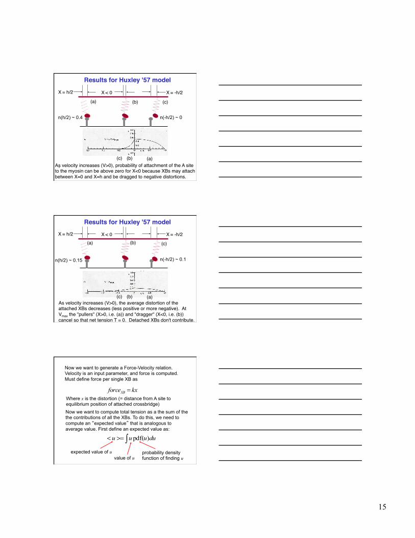
Results for Huxley '57 model"
."
X < 0" X = -h/2"X = h/2"
(a)"
(c)"
(b)"
(a)"(b)"
(c)"
As velocity increases (V>0), probability of attachment of the A site to the myosin can be above zero for X<0 because XBs may attach between X=0 and X=h and be dragged to negative distortions."
n(h/2) ~ 0.4 n(-h/2) ~ 0
Results for Huxley '57 model"
."
X < 0" X = -h/2"X = h/2"
(a)"
(c)"
(b)"
(a)"(b)"
(c)"
As velocity increases (V>0), the average distortion of the attached XBs decreases (less positive or more negative). At Vmax the "pullers" (X>0, i.e. (a)) and "dragger" (X<0, i.e. (b)) cancel so that net tension T = 0. Detached XBs don't contribute. "
n(-h/2) ~ 0.1 n(h/2) ~ 0.15
Now we want to generate a Force-Velocity relation. Velocity is an input parameter, and force is computed. Must define force per single XB as
Where x is the distortion (= distance from A site to equilibrium position of attached crossbridge) Now we want to compute total tension as a the sum of the the contributions of all the XBs. To do this, we need to compute an “expected value” that is analogous to average value. First define an expected value as:
expected value of u value of u
probability density function of finding u
kxforceXB =
∫>=< duuuu )pdf(

16
In our case, we want expected value of tension for all A sites, both attached and detached. We can write expected value as:
Force of attached A site
Attached A sites
True p.d.f. of all A site being at distance = x
[ ] dxxnxhxnkxTXB ∫∞
∞− ⎭⎬⎫
⎩⎨⎧ −•+>=< )(ˆ)(ˆ0)(ˆ
Detached A sites
[ ] dxxnxhxn∫∞
∞− ⎭⎬⎫
⎩⎨⎧ −+= )(ˆ)(ˆ)(ˆ1
Force of detached A site
)(ˆ)()(ˆ xhxnxn •=
A p.d.f. describing likelihood of A sites being distance x from the nearest equilibrium XB position
Model assumes is constant over all possible x values between -l/2 and l/2 as shown below:
l/2 -l/2
1/l
x
h
Conditional probability of an A site having an attached XB given its distance is x from the nearest equilibrium XB position
h
Recall these features of the model:
otherwiselxllxn
xn2/2/
;;
0/)(
)(ˆ<<−
⎩⎨⎧
=
Multiplying the terms produces:
dxxnkxTXB ∫∞
∞−>=< )(ˆ
dxxnlkxl
l∫−=2/
2/)(
Substitute for n(x) and integrate to get:
⎪⎭
⎪⎬⎫
⎪⎩
⎪⎨⎧
⎥⎥⎦
⎤
⎢⎢⎣
⎡⎟⎟⎠
⎞⎜⎜⎝
⎛ ++−−+
>=<−
φφ
φ VggfeV
lkh
gffT V
XB
2
2
112
11
1
211)1(1
2
Then substituting into expected value of force:
17
⎪⎭
⎪⎬⎫
⎪⎩
⎪⎨⎧
⎥⎥⎦
⎤
⎢⎢⎣
⎡⎟⎟⎠
⎞⎜⎜⎝
⎛ ++−−=><><=
−
φφ
φ VggfeV
TTTT V
XB
XB
2
2
11maxmax 2
11)1(1/
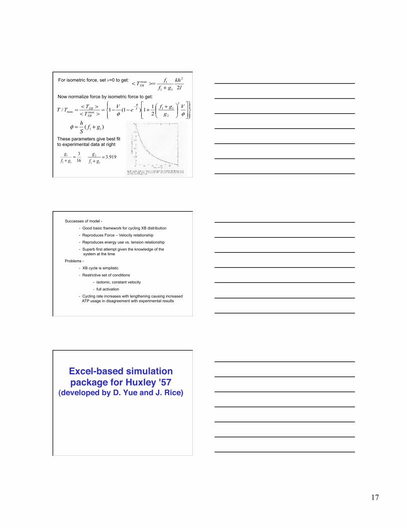
For isometric force, set v=0 to get: lkh
gffTXB 2
2
11
1max
+>=<
Now normalize force by isometric force to get:
)( 11 gfSh +=φ
163
11
1 =+ gfg 919.3
11
2 =+ gfg
These parameters give best fit to experimental data at right
Successes of model -
- Good basic framework for cycling XB distribution
- Reproduces Force – Velocity relationship
- Reproduces energy use vs. tension relationship
- Superb first attempt given the knowledge of the system at the time
Problems -
- XB cycle is simplistic
- Restrictive set of conditions
- isotonic, constant velocity
- full activation
- Cycling rate increases with lengthening causing increased ATP usage in disagreement with experimental results
Excel-based simulation package for Huxley '57
(developed by D. Yue and J. Rice)"
18
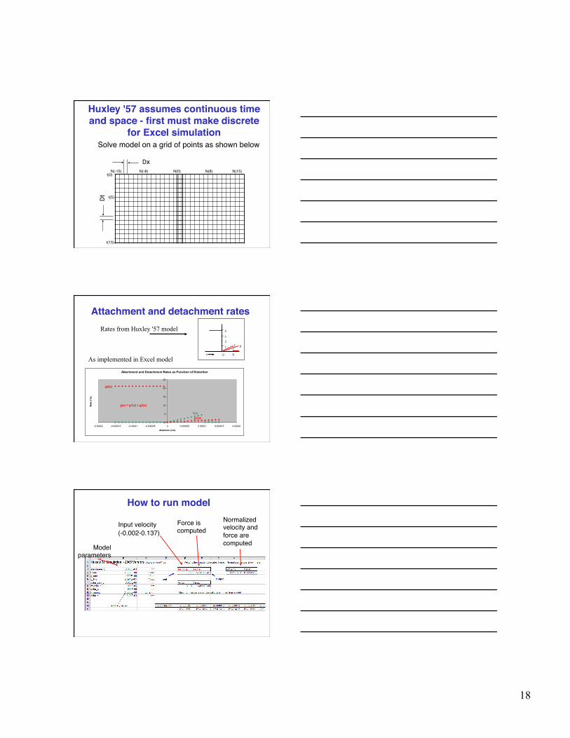
Huxley '57 assumes continuous time and space - first must make discrete
for Excel simulation"Solve model on a grid of points as shown below"
N(-15)" N(0)" N(15)"N(8)"N(-8)"
Dx"
Dt"
t(0)"
t(15)"
t(5)"
Attachment and detachment rates"
gf
h
123
4
0x
Rates from Huxley '57 model
As implemented in Excel model
Attachment and Detachment Rates as Function of Distortion
0
5
10
15
20
25
-0.00002 -0.000015 -0.00001 -0.000005 0 0.000005 0.00001 0.000015 0.00002
distortion (nm)
Rat
e (1
/s)
g(x) = g1(x) + g2(x)
f(x)
g2(x)
g1(x)
How to run model"
Model parameters"
Input velocity "(-0.002-0.137)"
Force is computed"
Normalized velocity and force are computed"
19
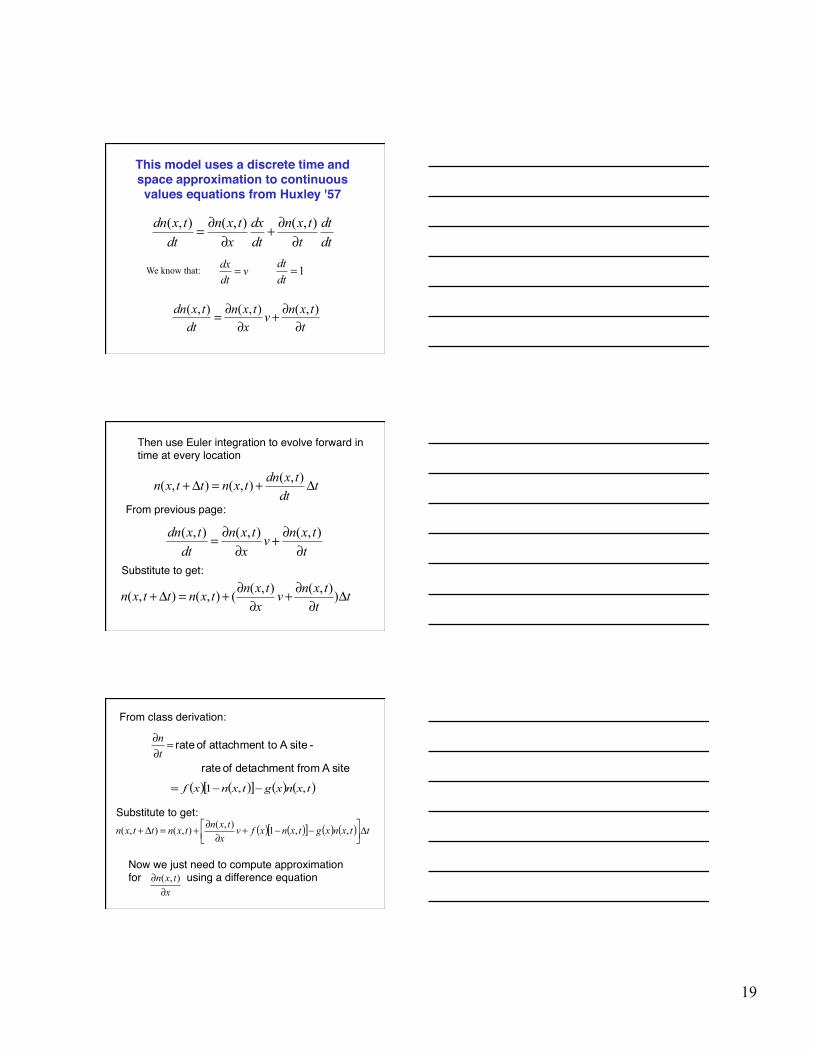
This model uses a discrete time and space approximation to continuous values equations from Huxley '57 "
We know that: 1=dtdt
vdtdx =
ttxnv
xtxn
dttxdn
∂∂+
∂∂= ),(),(),(
dtdt
ttxn
dtdx
xtxn
dttxdn
∂∂+
∂∂= ),(),(),(
From previous page:"
Then use Euler integration to evolve forward in time at every location"
tdttxdntxnttxn Δ+=Δ+ ),(),(),(
ttxnv
xtxn
dttxdn
∂∂+
∂∂= ),(),(),(
tttxnv
xtxntxnttxn Δ
∂∂+
∂∂+=Δ+ )),(),((),(),(
Substitute to get:"
site A from detachment of rate
- site A to attachment of rate=∂∂tn
( ) ( )[ ] ( ) ( )txnxgtxnxf ,,1 −−=
From class derivation:"
Substitute to get:"
Now we just need to compute approximation for using a difference equation"
xtxn
∂∂ ),(
( ) ( )[ ] ( ) ( ) ttxnxgtxnxfvxtxntxnttxn Δ⎥⎦
⎤⎢⎣⎡ −−+
∂∂+=Δ+ ,,1),(),(),(
20
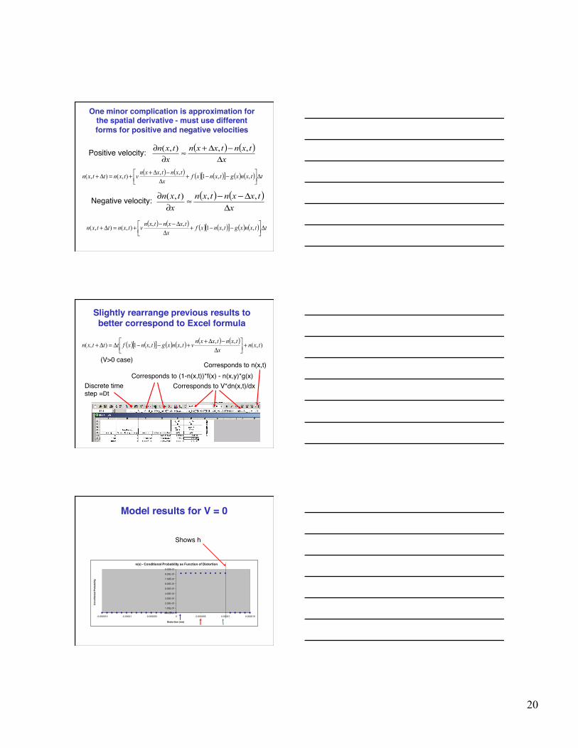
One minor complication is approximation for the spatial derivative - must use different forms for positive and negative velocities"
Positive velocity:" ( ) ( )x
txntxxnxtxn
Δ−Δ+≈
∂∂ ,,),(
Negative velocity:" ( ) ( )x
txxntxnxtxn
ΔΔ−−≈
∂∂ ,,),(
( ) ( ) ( ) ( )[ ] ( ) ( ) ttxnxgtxnxfx
txntxxnvtxnttxn Δ⎥⎦⎤
⎢⎣⎡ −−+
Δ−Δ++=Δ+ ,,1,,),(),(
( ) ( ) ( ) ( )[ ] ( ) ( ) ttxnxgtxnxfx
txxntxnvtxnttxn Δ⎥⎦⎤
⎢⎣⎡ −−+
ΔΔ−−+=Δ+ ,,1,,),(),(
Discrete time step =Dt"
Corresponds to (1-n(x,t))*f(x) - n(x,y)*g(x)"Corresponds to V*dn(x,t)/dx"
( ) ( )[ ] ( ) ( ) ( ) ( ) ),(,,,,1),( txnx
txntxxnvtxnxgtxnxftttxn +⎥⎦⎤
⎢⎣⎡
Δ−Δ++−−Δ=Δ+
Slightly rearrange previous results to better correspond to Excel formula"
Corresponds to n(x,t)"(V>0 case)"
n(x) - Conditional Probability as Function of Distortion
0.00E+00
1.00E-01
2.00E-01
3.00E-01
4.00E-01
5.00E-01
6.00E-01
7.00E-01
8.00E-01
9.00E-01
-0.000015 -0.00001 -0.000005 0 0.000005 0.00001 0.000015
Distortion (nm)
Con
ditio
nal P
roba
bilit
y
Model results for V = 0"
Shows h"
21
n(x) - Conditional Probability as Function of Distortion
0.00E+00
5.00E-02
1.00E-01
1.50E-01
2.00E-01
2.50E-01
3.00E-01
3.50E-01
4.00E-01
4.50E-01
5.00E-01
-0.000015 -0.00001 -0.000005 0 0.000005 0.00001 0.000015
Distortion (nm)
Con
ditio
nal P
roba
bilit
y
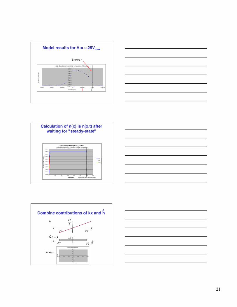
Model results for V = ~.25Vmax"
Shows h"
Calculation of n(x) is n(x,t) after waiting for "steady-state""
Calculation of sample n(X) values(See arrows on n(x) plot for sample locations)
0.00E+00
5.00E-02
1.00E-01
1.50E-01
2.00E-01
2.50E-01
3.00E-01
3.50E-01
4.00E-01
4.50E-01
5.00E-01
0 500 1000 1500 2000 2500 3000 3500
time (delta t)
Con
ditio
nal P
roba
bilit
y
N(1)
N(8)
N(15)
Data points taken at "steady state"
Combine contributions of kx and h "
> "
l/2 x
)(ˆ xh
-l/2
l/2 x -l/2
2kl
)(ˆ xhkx •
kx
1/l
k*x*h_hat as Function of Distortion
-0.6
-0.4
-0.2
0
0.2
0.4
0.6
-0.000015 -0.00001 -0.000005 0 0.000005 0.00001 0.000015
distortion (nm)
Fo
rce
/ cm
22
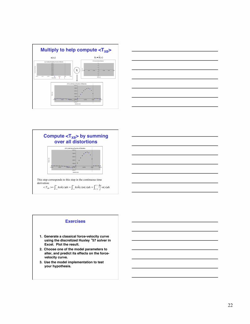
Multiply to help compute <TXB>"
X
k*x*h_hat as Function of Distortion
-0.6
-0.4
-0.2
0
0.2
0.4
0.6
-0.000015 -0.00001 -0.000005 0 0.000005 0.00001 0.000015
distortion (nm)
Fo
rce
/ cm
k*x*h_hat*n(x) as Function of Distortion
-2.50E-02
-5.00E-03
1.50E-02
3.50E-02
5.50E-02
7.50E-02
9.50E-02
-0.000015 -0.00001 -0.000005 0 0.000005 0.00001 0.000015
Distortion (nm)
Forc
e / c
m
n(x) - Conditional Probability as Function of Distortion
0.00E+00
5.00E-02
1.00E-01
1.50E-01
2.00E-01
2.50E-01
3.00E-01
3.50E-01
4.00E-01
4.50E-01
5.00E-01
-0.000015 -0.00001 -0.000005 0 0.000005 0.00001 0.000015
Distortion (nm)
Co
nd
itio
nal
Pro
bab
ility
)(ˆ xhkx •)x(n
Compute <TXB> by summing over all distortions"
k*x*h_hat*n(x) as Function of Distortion
-2.50E-02
-5.00E-03
1.50E-02
3.50E-02
5.50E-02
7.50E-02
9.50E-02
-0.000015 -0.00001 -0.000005 0 0.000005 0.00001 0.000015
Distortion (cm)
Fo
rce
/ cm
dxxnlkxdxxnxhkxdxxnkxT
l
lXB ∫∫∫ −
∞
∞−
∞
∞−==>=<
2/
2/)()()(ˆ)(ˆ
This step corresponds to this step in the continuous time derivation:
Exercises"
1. Generate a classical force-velocity curve using the discretized Huxley ‘57 solver in Excel. Plot the result."
2. Choose one of the model parameters to alter, and predict its effects on the force-velocity curve."
3. Use the model implementation to test your hypothesis."