modeling dynamics of post disaster recovery · modeling dynamics of post disaster recovery . a...
TRANSCRIPT

MODELING DYNAMICS OF POST DISASTER RECOVERY
A Dissertation
by
ALI NEJAT
Submitted to the Office of Graduate Studies of Texas A&M University
in partial fulfillment of the requirements for the degree of
DOCTOR OF PHILOSOPHY
August 2011
Major Subject: Civil Engineering

MODELING DYNAMICS OF POST DISASTER RECOVERY
A Dissertation
by
ALI NEJAT
Submitted to the Office of Graduate Studies of Texas A&M University
in partial fulfillment of the requirements for the degree of
DOCTOR OF PHILOSOPHY
Approved by:
Chair of Committee, Ivan Damnjanovic Committee Members, Stuart D. Anderson Kenneth F. Reinschmidt Sergiy Butenko
Arnold Vedlitz Head of Department, John Niedzwecki
August 2011
Major Subject: Civil Engineering
iii
ABSTRACT
Modeling Dynamics of Post Disaster Recovery. (August 2011)
Ali Nejat, B.S., Zanjan University, Zanjan, Iran;
M.S., Islamic Azad University, Tehran, Iran
Chair of Advisory Committee: Dr. Ivan Damnjanovic
Natural disasters result in loss of lives, damage to built facilities, and interruption of
businesses. The losses are not instantaneous, but rather continue to occur until the
community is restored to a functional socio-economic entity. Hence, it is essential that
policy makers recognize this dynamic aspect of the losses incurred and make realistic
plans to enhance recovery. However, this cannot take place without understanding how
homeowners react to recovery signals. These signals can come in different ways: from
policy makers showing their strong commitment to restore the community by providing
financial support and/or restoration of lifeline infrastructure; or from the neighbors
showing their willingness to reconstruct. The goal of this research is to develop a model
that can account for homeowners’ dynamic interactions in both organizational and
spatial domains. The spatial domain of interaction focuses on how homeowners process
signals from the environment, such as neighbors reconstructing and local agencies
restoring infrastructure, while the organizational domain of interaction focuses on how
agents process signals from other stakeholders that do not directly affect the
environment like insurers do. The hypothesis of this study is that these interactions

iv
significantly influence decisions to reconstruct and stay, or sell and leave. A multi-agent
framework is used to capture emergent behavior such as spatial patterns and formation
of clusters. The developed framework is illustrated and validated using experimental
data sets. The results from simulation model confirm that spatial and organizational
externalities play an important role in agents’ decision-making and can greatly impact
the recovery process. The results further highlight the significant impact of discount
factor and the accuracy of the signals on the percentage of reconstruction. Finally,
cluster formation was shown to be an emergent phenomenon during the recovery process
and spatial modeling technique demonstrated a significantly higher impact on formation
of clusters in comparison with experimental model and hybrid model.

v
DEDICATION
To my parents and my brother.

vi
ACKNOWLEDGMENTS
I would like to take this opportunity to acknowledge the excellent academic guidance
and financial assistance offered by Dr. Ivan Damnjanovic during my graduate studies at
Texas A&M University (TAMU). Without his guidance, this dissertation would have not
become a reality. Working with Dr. Damnjanovic was a wonderful experience in many
ways and I will never forget him in my life. I also sincerely appreciate the excellent
guidance and financial assistance offered by Dr. Stuart Anderson during my studies as a
PhD student and I am very grateful for all my research opportunities that were offered by
him. I would also want to extend my gratitude to Dr. Kenneth Reinschmidt for his
excellent guidance, support and feedbacks on various aspects of my studies including
this dissertation. I also sincerely appreciate the excellent guidance and support provided
by Dr. Butenko and Dr. Vedlitz on the different aspects of my doctoral research. In
general, I am very fortunate to have an extraordinary advisory committee with a wide
range of expertise that helped me view the challenges from multiple perspectives and
shape this dissertation in its current form.

vii
TABLE OF CONTENTS
Page
ABSTRACT ..................................................................................................................... iii
DEDICATION ................................................................................................................... v
ACKNOWLEDGMENTS .................................................................................................vi
TABLE OF CONTENTS ................................................................................................ vii
LIST OF FIGURES ............................................................................................................ x
LIST OF TABLES .......................................................................................................... xii
1. INTRODUCTION ........................................................................................................ 1 1.1. Problem Statement .............................................................................................. 1 1.2. Dissertation Goal ................................................................................................. 2 1.3. Scope ................................................................................................................... 3 1.4. Research Objectives ............................................................................................ 3
1.4.1. Micro-level Research Questions ............................................................. 4 1.4.2. Macro-level Research Question .............................................................. 6
1.5. Organization of the Dissertation.......................................................................... 7
2. LITERATURE REVIEW ............................................................................................. 9
2.1. Disaster Modeling ............................................................................................... 9
2.1.1. Loss Modeling ....................................................................................... 12 2.1.2. Recovery Modeling ............................................................................... 16
2.2. Research Problem .............................................................................................. 17
3. RESEARCH METHODOLOGY ............................................................................... 19
3.1. General Framework ........................................................................................... 19 3.2. Multi-Domain Interactions ................................................................................ 21
3.3. Experimental Setup ........................................................................................... 23 3.3.1. Spatial Interactions Experimental Setup ............................................... 23
3.3.2. Bargaining Situation Experimental Setup ............................................. 24 3.4. Summary ........................................................................................................... 25
viii
Page
4. MODELING SPATIAL INTERACTIONS ............................................................... 26 4.1. Introduction ....................................................................................................... 26 4.2. Theoretical Model ............................................................................................. 27
4.2.1. Signals and Uncertainty ........................................................................ 28 4.2.2. Game and Behavior ............................................................................... 34 4.2.3. Game Solution ....................................................................................... 36 4.2.4. MAS Integration .................................................................................... 38
4.3. Empirical Model ................................................................................................ 39 4.3.1. Experiment Design ................................................................................ 39
4.3.2. Model Formulation ................................................................................ 42 4.3.3. Parameter Estimation ............................................................................ 45 4.3.4. Experiment Results ............................................................................... 46 4.3.5. Discussion of the Results ...................................................................... 52 4.3.6. MAS Integration .................................................................................... 53
4.4. Summary ........................................................................................................... 54 4.5. Limitations ........................................................................................................ 55
5. MODELING ORGANIZATIONAL INTERACTIONS ............................................ 56
5.1. Introduction ....................................................................................................... 56 5.2. Theoretical Model ............................................................................................. 56
5.2.1. Background ........................................................................................... 56
5.2.2. Model Formulation ................................................................................ 58 5.2.3. Model Solution ...................................................................................... 60 5.2.4. MAS Integration .................................................................................... 63
5.3. Empirical Model ................................................................................................ 63 5.3.1. Experiment Design ................................................................................ 63 5.3.2. Model Formulation ................................................................................ 64 5.3.3. Model Fitting ......................................................................................... 65 5.3.4. Estimation Results ................................................................................. 80 5.3.5. MAS Integration .................................................................................... 80
5.3.6. Summary ............................................................................................... 81 5.4. Limitations and Future Work ............................................................................ 81
6. MULTIAGENT SYSTEM SIMULATION MODEL ................................................ 83
6.1. Introduction ....................................................................................................... 83 6.2. Multi Agent Systems ......................................................................................... 83 6.3. MAS-Model Structure and Specifications ........................................................ 85
6.3.1. “import-world” Module ......................................................................... 85 6.3.2. “setup-agent” Module ........................................................................... 92
ix
Page
6.3.3. “run” Module ......................................................................................... 94 6.3.4. “cluster” Module ................................................................................... 96
6.4. Model Validation ............................................................................................. 104 6.4.1. Sensitivity to Coefficient of Variation ................................................ 106 6.4.2. Sensitivity to Discount Factor ............................................................. 107 6.4.3. Theoretical Model versus Hybrid and Empirical Model ..................... 107
7. CONCLUSIONS AND FUTURE RECOMMENDATIONS .................................. 110
7.1. Conclusions ..................................................................................................... 110
7.2. Limitations ...................................................................................................... 112 7.3. Contributions ................................................................................................... 113
7.3.1. General Contributions ......................................................................... 113 7.3.2. Engineering Contributions .................................................................. 113
REFERENCES ............................................................................................................... 116
APPENDIX A ................................................................................................................ 125
APPENDIX B ................................................................................................................ 127
APPENDIX C ................................................................................................................ 129
APPENDIX D ................................................................................................................ 133
APPENDIX E ................................................................................................................. 135
APPENDIX F ................................................................................................................. 139
APPENDIX G ................................................................................................................ 142
APPENDIX H ................................................................................................................ 144
APPENDIX I .................................................................................................................. 147
VITA .............................................................................................................................. 148

x
LIST OF FIGURES
Page
Figure 2-1. Post-disaster recovery adapted from Chang and Miles (2004) ..................... 11
Figure 3-1. Research approach ......................................................................................... 20
Figure 3-2. Interactions in multi-domain environment .................................................... 22
Figure 4-1. The updating process of the theoretical model .............................................. 33
Figure 5-1. Extensive form of the bargaining game ......................................................... 61
Figure 5-2. The process of experimental model development ......................................... 66
Figure 5-3. Goodness of fit plots (ModelRisk Vose Software) ........................................ 70
Figure 5-4. Fitted distributions to the data (EasyFit Software) ........................................ 71
Figure 5-5. Model fit plots (R) ......................................................................................... 76
Figure 5-6. Model fit plots-Without outlier ..................................................................... 77
Figure 6-1. Area selection in Google Earth© .................................................................... 87
Figure 6-2. Aerial map with points .................................................................................. 88
Figure 6-3. Aerial map with points and polylines ............................................................ 89
Figure 6-4. Imported area in Netlogo framework ............................................................ 90
Figure 6-5. “import-world” pseudo code ......................................................................... 91
Figure 6-6. Characterized model in Netlogo .................................................................... 92
Figure 6-7. “setup-agent” pseudo code ............................................................................ 94
Figure 6-8. “run” pseudo code ......................................................................................... 96
Figure 6-9. DBSCAN pseudo code .................................................................................. 98
Figure 6-10. Clique pseudo code .................................................................................... 100
Figure 6-11. Case study – Kobe earthquake .................................................................. 101

xi
Page
Figure 6-12. Comparison of the two cluster-detection algorithms ................................. 102
Figure 6-13. Model sensitivity to discount factor and coefficient of variation .............. 106
Figure 6-14. Sensitivity analysis for different models ................................................... 108
Figure 7-1. Three pillars of a sustainable design ........................................................... 115

xii
LIST OF TABLES
Page
Table 2-1. Summary of more comprehensive loss models with their associated strengths and weaknesses adapted from Okuyama (2011) ............................. 15
Table 4-1. Experiment factorial design ............................................................................ 41
Table 4-2. SAS results from multinomial logistic regression-Model fit statistics ........... 49
Table 4-3. SAS results from multinomial logistic regression-Logistic procedure ........... 51
Table 5-1. List of the top 3 fitted distributions ................................................................ 69
Table 5-2. EasyFit statistical analysis result for fitted distributions (numbers in parentheses denote distribution ranking for each test) .................................... 72
Table 5-3. SAS results from multinomial logistic regression-Logistic procedure ........... 73
Table 5-4. R results from linear regression modeling for car-owner’s counter offer ...... 75
Table 5-5. R results from linear regression modeling for car-owner’s counter offer-without outlier ................................................................................................. 77
Table 5-6. Results from binomial logistic regression - R ................................................ 79
Table 6-1. Results from t test ......................................................................................... 104

1
1. INTRODUCTION
1.1. PROBLEM STATEMENT1
Pre-disaster planning is the key to effective recovery from natural catastrophes, such as
hurricanes, earthquakes, and tsunamis, or human-induced events such as acts of
terrorism or accidents. In anticipation of these high-impact low-probability events,
communities and their public and business decision-makers need policies, contingency
plans, procedures, and guidelines to implement recovery actions. Typically these actions
include evaluations of damage, removal of debris, and restoration of essential
infrastructure and services to then allow for a market-driven reconstruction of homes and
businesses.
In late summer of 2005, two major storms tested the ability of coastal
communities in the United States to achieve recovery goals. Hurricane Katrina, and a
few weeks later Hurricane Rita, exposed the flaws and deficiencies in the existing
policies, plans and budgets to meaningfully and quickly restore damaged infrastructure
and promote residential and business reconstruction. The scenes of damaged and
unserviceable buildings and even entire neighborhoods in New Orleans and other gulf
coast communities are constant reminders that the disaster is not over until the people
have returned, and the affected area has been restored to a functioning social, political
and economic entity.
This dissertation follows the style of Natural Hazards Review, ASCE.
2
Following the extensive media coverage, government agencies and the academic
community have initiated a number of studies to identify hazard-specific design
deficiencies, develop more effective emergency and evacuation plans, predict the extent
of structural damage, assess short-term recovery efforts, and model long-term economic
effects of market-driven reconstruction. However, very few studies, if any, have focused
on identifying the forces driving such long-term market-driven reconstruction.
1.2. DISSERTATION GOAL
The goal of this dissertation is to study how agents (i.e. homeowners) process signals
from spatial and organizational environment during long-term market-driven recovery.
A successful modeling effort requires capturing agents’ behavior as well as dynamics of
their interactions over extended period of time. Although there are research efforts on
modeling the recovery process, they fail to capture the complexity of interactions among
the agents in a multi-domain environment (i.e. spatial as well as organizational).
There are a number of beneficiaries of this research. Public officials can use the
developed models to evaluate recovery plans and strategically “seed” the reconstruction
efforts in areas that can maximize the speed of recovery. Transportation agencies can use
the model to evaluate effectiveness of restoration dynamics, while regulatory agencies
can use it to increase bargaining power of homeowners following the disaster.
3
1.3. SCOPE
The scope of this research is limited to modeling behavior of two key stakeholders:
homeowners, agents seeking to rebuild; and insurers, agents that maximize short-and
long-term utility. The scope indirectly includes public agencies as they control many
parallel parameters. Even though this assumption constrains the real life application of
the developed model, it allows for marginal assessment of the effects of spatial and
organizational externalities on the recovery process. Note that the models do not attempt
to fully explain a very complex post-disaster reconstruction process, nor heterogeneity in
homeowners’ behavior, but to provide a theoretical foundation for investigating the
emergent spatial phenomenon (i.e. clusters) and decision-making under uncertainty.
1.4. RESEARCH OBJECTIVES
This subsection presents research objectives formulated as research questions. The
research questions have been divided into two categories: 1) micro-level research
questions, and 2) macro-level research questions. The former category focuses on how
the agents interact in both spatial and organizational domain respectively, while the latter
category focuses on how such micro-level behaviors affect macro-level phenomena such
as spatial cluster formation.

4
1.4.1. Micro-level Research Questions
1.4.1.1. RQ1: How do the agents interact in the spatial domain?
The first micro-level objective of this research is solely focused on how agents make
decisions in a spatial environment. In other words, this question aims to capture how an
individual reconstruction decision-making is affected by its neighbors’ decision-making.
The solution to this question unveils the logic behind how agents’ update their beliefs
regarding the value of reconstruction given what they observe in the neighborhood.
Data Source: The dataset used to address this question comes from an
experimental study conducted in Fall 2010 in the department of Civil Engineering at
Texas A&M University. Study participants were the students of a junior-level civil
engineering course. The participants were faced with similar conditions as homeowners
in affected area would face after a disaster and were asked to choose among different
strategies.
Research Method: The methodology proposed for this research question is based
on a two-pronged approach. In the first theoretical approach, homeowners make
decisions based on their updated beliefs about their spatial surroundings. As
reconstruction unfolds, they update their beliefs accordingly. This process is captured
using Bayesian statistics. The outcome of the first approach is a closed-form theoretical
solution to the probability of reconstruction.
The goal in the second approach is to develop and estimate an empirical model
using previously defined datasets. The outcome of the second approach is a multinomial

5
logistic regression model to predict the probability of reconstruction. The reason behind
having two approaches is to cover the different aspects of spatial interactions
independently. In the first theoretical approach, the focus is only on the temporal aspect
of spatial interactions, which is solely based on assessment of how agents’ actions (i.e.
neighbors reconstruction actions), influence the dynamics of reconstruction-value in the
affected area. On the other hand, the second approach aims to capture broader effects
than just neighbors’ reconstruction decision. The empirical model is developed to
capture the confluence of different spatial parameters such as availability of
infrastructure.
Model Validation: The results from both models are tested for their capability of
delivering logically expected results.
1.4.1.2. RQ2: How do the agents interact in the organizational domain?
This research question aims to investigate how market conditions, government
regulation, and incentives affect the ability of homeowners to secure equitable treatment
when negotiating with large for-profit institutions such as insurers. In other words, the
objective is to investigate how agents’ risk attitudes affect their financial negotiations
with insurers. There is ample anecdotal evidence of price gouging and failure to pay
claims by some insurers after natural disasters. Indeed, it is not surprising for one party
to leverage a stronger bargaining position to take advantage of the reduced bargaining
strength of the other party (e.g. homeowners seeking to rebuild). Thus, in the second
6
proposed domain of interactions (organizational domain), the bargaining power of the
“stressed” agents is studied.
Data Source: The dataset used to address this research question is based on a
bargaining experiment that was conducted in Fall 2010 in the department of Civil
Engineering at Texas A&M University. Like in the previous experiment, study
participants were the students of a junior-level civil engineering course. The
experimental bargaining scenario mimicked what might happen after disaster between
homeowners and insurers. Participants were divided into two categories (homeowners
and insurers), and were asked to choose from the available options in respond to a
received offer.
Research Method: Much like the methodology used for RQ1, the proposed
approach to address this research question is two-fold: theoretical and empirical. In the
theoretical part, the bargaining problem is modeled based on the concepts of the
bargaining theory. In the empirical model, the approach to the bargaining problem is
based on analyzing the collected data from the experiment.
Model Validation: The results from both models are tested to check for their
capability of delivering logically expected results.
1.4.2. Macro-level Research Question
After separately investigating agents’ interaction in both spatial and organizational
domains, an integrative framework is designed to capture the effects of agents’ behavior
at a macro-level. This integrative framework is based on a multi-agent system (MAS)

7
simulation approach. There are a number of advantages associated with applications of
agent-based modeling technique, which make it a desirable approach to address the
macro-level research question. These benefits include: 1) the ability to tackle the
complexity of the research problem, 2) ability to capture the dynamics of the system
during the simulation period, and 3) ability to test different behavioral models.
1.4.2.1. RQ3: Does the spatial interaction of agents result in formation of clusters of
reconstructed properties?
The macro-level objective of this dissertation is to detect for any emergent phenomena
such as spatial cluster formation due to agents’ interactions. Spatial data suggest that
reconstruction, much like other neighborhood phenomena such as foreclosures, is
contagious and is nucleated first in small neighborhood areas.
Research Method: For this research question the methodology includes the
following steps: 1) developing a MAS model, 2) detecting spatial clusters in MAS model
using clustering algorithms, 3) hypothesis testing to determine the significance of the
results from the second step, and 4) contrasting the results from theoretical and empirical
spatial models to check for the factors that have the most significant influence on the
formation of clusters.
1.5. ORGANIZATION OF THE DISSERTATION
Section 2 outlines the existing literature on modeling disasters. The section starts with
introducing loss models and then proceeds to cover the literature on recovery models.
8
The section then continues to highlight the existing gap in the literature and is concluded
by an introduction on the approach to overcome the shortcomings.
Section 3 introduces the research methodology to address the objectives of this
dissertation. It starts with a discussion on the general framework and is further extended
to capture the multi-domain framework of interactions and experimental data sets
characteristics.
Section 4 covers the modeling procedure for the spatial domain of interactions. It
starts with a discussion on the theoretical model and its solution. To follow, the section
proceeds with the empirical model formulations and is continued by its associated
statistical analysis. To conclude, summary of findings is presented.
Section 5 captures the modeling of the organizational domain of interactions. It
begins with the theoretical model and proceeds to derive the solution. The section then
continues with an introduction on empirical model formulation, parameter estimation
and its associated statistical analysis. It then concludes by the summary of findings.
Section 6 extends on multi-domain MAS model. It starts with an introduction on
MAS models, and their specifications. To follow, the simulation setups are discussed
which are then followed by simulation results, research hypotheses, and testing methods.
The section ends with a discussion of the results, which is continued by summary of the
findings.
Finally, Section 7 outlines the summary of the dissertation, which is then
proceeded by the areas requiring future research.

9
2. LITERATURE REVIEW
This section outlines the existing literature on the broad subject of disaster modeling.
More specifically, the literature review is categorized into two typical modeling areas: 1)
loss modeling, and 2) recovery modeling. To conclude, the section captures the need and
the research problem listed as the objectives of this dissertation.
2.1. DISASTER MODELING
In the literature of disaster modeling, hazard is the incident of the physical occurrence
whereas disaster is the subsequent aftermath Okuyama and Chang (2004). The studies on
the impact of natural hazards on the socio-economic condition of affected areas gained
significant attention due to a series of disasters which took place during the mid 1990s
such as Northridge earthquake in 1994 and Great Hanshin (Kobe) earthquake in 1995
(Okuyama, 2007). These events followed by more recent catastrophes such as hurricane
Katrina in 2005 and hurricane Ike in 2008 highlight the vulnerability of the urban
infrastructure in modern cities and support the need for a better understanding of
multidimensional socio-economic impacts and the way the homeowners and public
sector respond.

10
Economic losses from both natural and anthropogenic disasters do not take place
instantly; rather they are accumulated over the time of recovery. This implies that to
assess the scale of losses, it does not suffice just to incorporate the initial losses. In other
words, the direct losses can trigger spillover effects which in turn can cause indirect
losses that are as significant, if not more, than the initial losses. In such settings, the
dynamics of post disaster recovery plays an important role. This is clearly shown in
Figure 2-1 where three different disaster cases are compared to each other (Chang and
Miles, 2004). It is assumed that in all the three cases the economy faces a significant
initial loss due to the occurrence of the disaster. In Case A, the reconstruction stimulus
has led the economic equilibrium to a curve which dominates the baseline. This indicates
future potential gains in the long run that will reimburse the initial losses. On the other
hand, Case C shows that the trend has come to equilibrium below the base line which
denotes that the reconstruction stimulus was not able to compensate the losses. In case
B, the economy has a short-term updrift before it converges to the baseline. Figure 2-1
illustrates how application of different policies during the recovery process can affect the
magnitude of the total losses.

11
Figure 2-1. Post-disaster recovery adapted from Chang and Miles (2004)
The economic impacts of natural disasters can be categorized into two major
categories, which are 1) direct losses, and 2) indirect losses. Differentiating between
these two terms has been a matter of controversy in the existing literature. While
Applied Technology Council (1991) and Heinz Center (2000) defined direct losses as
property damages and indirect losses as business disruptions, Albala-Bertrand (1993)
characterized indirect losses as a possibility rather than a reality, and Cochrane (2004)
classified indirect losses as those which are not directly caused by a disaster. Rose et al.
(1997), defined direct losses as those which incorporate property damage together with
its following interruptions to directly affected businesses, and indirect losses as those

12
which are associated with disruptions in businesses that are not directly influenced by a
disaster. Rose (2004) proposed the use of “higher-order effects” term as an alternative to
indirect effects to avoid the conflict with other economic modeling terminology
especially input-output (I/O) models. The term was intended to encompass both input-
output interdependencies and general equilibrium effects which can be attributed to price
changes in product markets.
Therefore direct losses can be classified as those that are attributed to the
damages and destructions to built environment, infrastructure, lifelines, and economic
sectors and inter-industry linkages. Indirect losses, on the other hand, represent losses
which are associated with the disturbances caused by the direct losses in economic
sectors that are not directly affected. This includes the imposed interruptions in
economic activities such as reductions in supply and demand. In other words, indirect
losses can be described as a byproduct of the direct losses. Models with a focus on
incorporating economic losses are represented as loss models whereas those which are
centered around integrating parameters that affect recovery time path are denoted as
recovery models. These two models are elaborated in the following subsections.
2.1.1. Loss Modeling
Loss models focus on capturing the initial losses rather than incorporating the dynamics
of a recovery process (Chang and Miles, 2004). There are a variety of classifications for
loss models in the literature. Brookshire et al. (1997) categorized direct loss estimation
methods into two categories which are: 1) loss estimation based on primary data such as
13
surveys in the affected areas, and 2) loss estimation founded on secondary data such as
insurance claims, and loans and highlighted their weak prognostic aptitude. Furthermore,
in the context of loss modeling, input-output (I/O) models are the most prevalent and
dominating modeling framework to capture the regional economic impacts and higher-
order effects of disasters (Rose 2004). I/O models are linear models which integrate the
sales and purchases in different segments of an affected economy. I/O models can
exhibit the interdependency of economic activities and economic sectors including
producers and/or consumer (Brookshire et al. 1997). This ability makes I/O models a
good candidate to study the domino effects caused by a disruption in an economic sector.
Furthermore, the simplicity of I/O models allows integrating engineering models to
estimate the higher-order effects of a disaster (Okuyama, 2007).
For example, Gordon and Richardson (1996), Gordon et al. (2004), Choe et al.
(2001), and Sohn et al. (2004) used the I/O modeling approach to study transportation
impacts, while Rose (1981), Rose et al. (1997), Rose and Benavides (1993, 1998)
applied this model to assess lifeline impacts. Furthermore Cochrane et al. (1997), and
Hewnigs and Mahindhara (1996) applied I/O models to capture the overall impacts of a
disaster whereas Rose et al. (1997), Cole (1998), and Rose and Benavides (1999) applied
I/O models to optimize recovery.

14
To overcome the limitations of I/O models such as their linear and rigid
structure, and lack of resource constraints (Okuyama, 2007), more complex models have
been developed by Boisvert (1992), Cochrane (1997), Davis and Salkin (1984).
In addition to traditional I/O models, econometric models are also used to capture
losses. The econometric models are statistically rigorous, data-intensive, and capable of
forecasting post-disaster conditions. Moreover, they fall short of differentiating between
direct and high-order impacts (Rose, 2004). The third alternative to I/O models is
Computable General Equilibrium (CGE) model. CGE models represent optimized
behavior of consumers and firms in response to price changes in a multi-market
framework (Rose 2004). These models can be seen through the works of Boisvert
(1992), Brookeshire and Mckee (1992), Rose and Guha (2004), and Rose and Liao
(2005). In contrast to I/O models, CGE models are non-linear, less rigid and capable of
incorporating supply constraints. In most CGE models, the basis is founded on an
extended I/O tables to account for separate institutional factors (Rose 2004). This
includes Social Accounting Matrices to represent the higher order effects (Cole 1995;
1998; 2004). A summary of these methods together with their strength and weakness
was summarized by Okuyama (2011) and is shown in Table 2-1.

15
Table 2-1. Summary of more comprehensive loss models with their associated strengths
and weaknesses adapted from Okuyama (2011)
Model Strengths Weaknesses
IO models
simple structure detailed inter-industry linkages wide range of analytical
techniques available easily modified and integrated
with other models
linear structure rigid coefficients no supply capacity constraint no response to price change overestimation of impact
SAM models
more detailed interdependency among activities, factors, and institutions
wide range of analytical techniques available
used widely for development studies
linear structure rigid coefficients no supply capacity constraint no response to price change data requirement overestimation of impact
CGE models
non-linear structure able to respond to price change able to cooperate with
substitution able to handle supply capacity
constraint
too flexible to handle changes
data requirement and calibration
optimization behavior under disaster
underestimation of impact
Econometric models
statistically rigorous stochastic estimate able to forecast over time
data requirement (time series and cross section)
total impact rather than direct and higher-order impacts distinguished
Although this subsection briefly outlined the most comprehensive methodologies
to estimate losses, there are additional studies aimed to capture the shortcomings of these
methodologies. These efforts include: 1) studies performed by Cole (1988, 1989) and
Okuyama et al. (2004) to capture the temporal aspect of recovery by introducing a
disrupted expenditure structure and sequential inter-industry model respectively, 2)

16
studies performed to incorporate the spatial impact of disasters such as an interregional
IO structure to assess higher order effect such as Okuyama (1999) and Sohn et al.
(2004), and 3) studies by Rose and Liao (2005), Tierney (1997), Okuyama et al. (1999)
to capture the behavioral changes due to disasters (Okuyama 2007).
2.1.2. Recovery Modeling
Despite the substantial literature on post-disaster loss modeling, only few studies (in
relative terms) have focused on the dynamics of recovery (Chang and Miles 2004). The
existing literature on modeling the recovery process can be grouped into five major
categories: 1) Studies with a focus on recovery as a temporal process: This includes
modeling temporal aspect of factory closure (Cole 1988 1989), interregional input-
output analysis (Okuyama et al. 2004), as well as recovery optimization by minimizing
economic losses (Rose et al. 1997), 2) Studies founded on a conceptual recovery
framework introduced by Haas et al. (1977) in which the recovery process was modeled
as a four-stage sequential incident. This study was followed by case studies by Hogg
(1980), Rubin and Popkin (1990), Rubin (1991), Berke et al. (1993), and Bolin (1993)
which extensively questioned this four-stage sequential approach to recovery, its
predictability, and argued that the order of the sequence can be different from what was
suggested by Haas et al. (1977). These subsequent studies characterized recovery as an
uncertain event affected by social disparities and decision-making, 3) Studies centered
around disparities in recovery, which were pursued by a two-pronged effort. The first
effort captured disparity in social classes among people (see Hewitt (1997), Blaikie

17
(1994)), where the second effort covered the recovery issues associated with disparities
in businesses (see Durkin (1984), Kroll et al. (1991) Tierney and Dalhamer (1998), and
Alesch and Holly (1998)), 4) Studies attempted to capture the effect of spatial externality
on different aspects of disaster recovery. Among those the spatial impact of lifeline
infrastructure was studied by Gordon et al. (1998), while Chang and Miles (2004)
proposed an object modeling technique to capture interactions between industry sectors
and community planning, and finally 5) Studies to determine the key performance
measures and indicators to capture the different aspects of the recovery process. These
include psychological or perceptional measures related to stress and frustration, to more
objective indicators such as regaining income, employment, household assets, and
household amenities (Bates 1982, 1993, 1994; Bolin and Bolton, 1983; Bolin and
Trainer, 1978; Peacock et al., 1987).
2.2. RESEARCH PROBLEM
While these efforts captured different aspects of the problem, an integrative spatial-
organizational agent-based model is still missing. An example of the existing literature
on modeling the recovery process through an agent-based approach is the model
presented by Chang and Miles (2004). Although the model is agent-based, the agents do
not exist spatially. Hence, this research aims to develop a theoretical link between the
existing efforts in modeling recovery with a focus on macro-level patterns and socio-
economic impact and those that are aimed at modeling micro-level behavior of
“stressed” agents. This integration will be conducted in a multi-agent system simulation

18
environment to capture the effects of time and the emergent system behavior. In other
words, the proposed model can capture 1) the behavior of homeowners in the presence
of spatial externality (being located among other homeowners), 2) the behavior of
homeowners while bargaining with high-marketing-power entities such as insurers under
stressed conditions and 3) the sensitivity of these two types of behaviors to a variety of
parameters such as availability of infrastructure, and market conditions.
19
3. RESEARCH METHODOLOGY
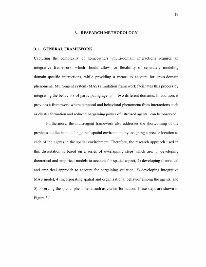
3.1. GENERAL FRAMEWORK
Capturing the complexity of homeowners’ multi-domain interactions requires an
integrative framework, which should allow for flexibility of separately modeling
domain-specific interactions, while providing a means to account for cross-domain
phenomena. Multi-agent system (MAS) simulation framework facilitates this process by
integrating the behaviors of participating agents in two different domains. In addition, it
provides a framework where temporal and behavioral phenomena from interactions such
as cluster formation and reduced bargaining power of “stressed agents” can be observed.
Furthermore, the multi-agent framework also addresses the shortcoming of the
previous studies in modeling a real spatial environment by assigning a precise location to
each of the agents in the spatial environment. Therefore, the research approach used in
this dissertation is based on a series of overlapping steps which are: 1) developing
theoretical and empirical models to account for spatial aspect, 2) developing theoretical
and empirical approach to account for bargaining situation, 3) developing integrative
MAS model, 4) incorporating spatial and organizational behavior among the agents, and
5) observing the spatial phenomena such as cluster formation. These steps are shown in
Figure 3-1.
20
Spatial Behavior Organizational Behavior
Theoretical Empirical Theoretical Empirical
SPATIAL DOMAIN
(neighbors)
ORGANIZATIONAL DOMAIN
(bargaining)
MULTI AGENT SYSTEM
PURE and HYBRID
BARGAINING
STRATEGIES
PURE and HYBRID
SPATIAL STRATEGIES
OBESERVE
EMERGENT
PHENOMENA
Figure 3-1. Research approach
As shown in the figure, for each of the spatial and organizational domains, two
types of models are defined; theoretical and empirical. Each of these models can be
separately chosen to model agents’ interactions. This is called a pure strategy. On the
other hand if agents’ interactions is believed to be a consequence of the confluence of
both models, one can assign different weights to each model and constitute a hybrid
model. The most important advantage of this feature is its ability to simulate a variety of
behaviors based on agents’ rationality and their different decision making parameters. In
spatial domain, one set of parameters captures the temporal aspect of spatial interactions
whereas the other set covers the situational aspect of this interaction. Similarly, in the
organizational domain, the first set of factors represents agents’ negotiation based on the
21
theoretical model while the other set of parameters capture a more realistic bargaining
behavior of agents and is based on the empirical model.
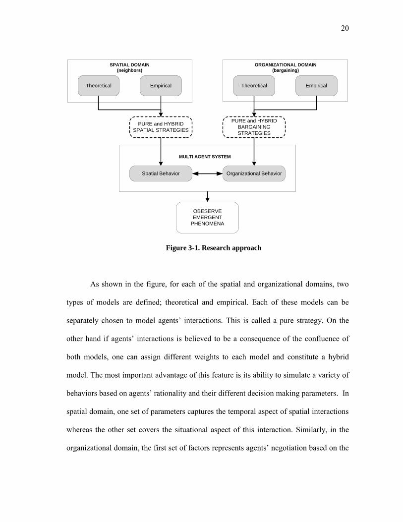
3.2. MULTI-DOMAIN INTERACTIONS
In this dissertation, the Multi-domain Multi-agent system (MD-MAS) model is illustrated
in Figure 3-2 as a 3-dimensional representation of the interaction domains. The two
interaction domains are: 1) spatial domain of interaction among the agents defined by
their spatial position (e.g. multi-layered networks of residential and commercial
properties, as well as different infrastructure systems including essential lifelines, such
as transportation, water, and electric power, and other more indirect yet still very
important systems such as schools, hospitals, and others); and 2) organizational domain
of interaction defining logical relationships among the stakeholders at the micro-social
level. As shown in the figure, the key micro-social organizational agents are
homeowners and insurers. While this list can be expanded to include other important
stakeholders, this research is guided by the principle of parsimony, in which the
complexity of model specification is determined by its predictive capability. In the MD-
MAS model, R represents a homeowner (homeowner), and I characterizes an insurer.
Following a disaster, homeowners decide about reconstruction of their property based on
the availability of resources coming from the insurer and/or the governing authorities,
while observing the actions of other homeowners.

22
Figure 3-2. Interactions in multi-domain environment
As shown in the figure, two major parameters drive homeowners’ actions
regarding reconstruction. The first is homeowners’ decision making structure which can
be either theoretical (based on agents rationality) or empirical and the second is
homeowners’ perception of environment. Both of these factors are dynamic. The
interaction starts at time zero when there is no reconstruction in the environment. Figure
3-2 shows the sequence of steps in the MD-MAS model. At Step 1, agents’ decision-
23
making structure is formed which leads to the corresponding actions in Step 2. Step 3
shows the effect of agents’ actions on the environment and vice versa. Finally, in Step 4,
the outcomes of these iterative interactions over time are discovered. These outcomes
can be divided into two categories, which are 1) rate of reconstruction, and 2) spatial
recovery patterns.
3.3. EXPERIMENTAL SETUP
As stated before, the empirical model formulation was based on the experiments. The
experiments in this dissertation were conducted in the form of surveys. Participants in
these surveys were chosen from a class of a CVEN junior level course in Zachry
Department of Civil Engineering, Texas A&M University. To preserve anonymity,
participants were asked to just communicate with the principal investigator through
emails. Proper care was taken to make sure that the identity of participants was kept
confidential and was not disclosed to any other participant. All the steps in the
experiments were taken by using emails between participants and principal investigator.
In other words where applicable, the principal investigator played the role of a proxy
between two interacting participants. Details regarding each of the experiments are
presented below.
3.3.1. Spatial Interactions Experimental Setup
In this experiment, the participants were asked to select a reconstruction strategy under
various overriding spatial and financial settings. Spatial configurations were governed by

24
the availability of infrastructure and the severity of damages. These configurations
resulted in 6 different scenarios. Financial viability of reconstruction was controlled by
the rate of availability of the funds and the cost of reconstruction. The available
reconstruction strategies were 1) reconstruct immediately, 2) wait for 6 months and
observe neighbors’ actions and decide accordingly and 3) take insurance money and buy
a housing alternative somewhere else in town. In this survey, 80 students participated.
Details regarding the survey together with instructions to participants are included in
Appendix A.
3.3.2. Bargaining Situation Experimental Setup
In this experiment, the students were divided into two groups and each group was
assigned a different role. The first group played the role of insurer while the second
participated as clients. Clients were supposed to maximize their claims while insurers
tended to minimize their losses. A total of 77 students participated in the experiment. Six
of the participants were assigned the role of insurer. Each of the insurers was responsible
for 10 to 12 clients. This was performed to differentiate the participants from each other
based on their attitude toward risk. Since insurers have the option of diversifying their
risk through multiple clients, they were assumed to be risk neutral. The clients on the
other hand, not having such an option, were assumed to be risk averse. Identity of clients
was kept confidential and transmission of information between the insurers and the
clients were managed through the proxy of the principal investigator.

25
3.4. SUMMARY
The objective of this section was to elaborate on the general framework of this
dissertation and explain the methodology to approach its goals. The following chapters
will sequentially complement this section by each focusing on a specific research
question.
Section 4, starts with the micro-level objectives of this dissertation by focusing
on the spatial domain and tackling agents interactions with each other. Furthermore,
Section 5 expands on the micro-level objectives by capturing the organizational domain
and addressing the interactions between homeowners and insurers. To continue, Section
6 elaborates on developing an integrative multi-domain agent based model that can
incorporate the outcomes from Section 4 and Section 5. This integrative model is used to
address the macro-level objective of this dissertation by looking for any emergent
phenomena such as formation of clusters. Finally Section 7 presents the summary of
findings and highlights the issues require future research.

26
4. MODELING SPATIAL INTERACTIONS
4.1. INTRODUCTION
This section presents the first micro-level objective of this dissertation by providing the
answer to the question: “How agents process the information from the neighborhood?”
The section starts with a presentation of a theoretical model in which the homeowners
are modeled as rational agents seeking to maximize their utility. This utility is assessed
in terms of homeowners’ gains/losses from the reconstruction. Based on this structure, at
each time step, the agents compute their expectation from two actions which are: 1) an
immediate reconstruction, and 2) waiting and making the decision in the next stage.
These expected values are directly influenced by the actions of neighboring homeowners
and eventually dominate agents reconstruction decisions.
To proceed, the section focuses on defining the waiting game among
homeowners and is extended to derive an equilibrium solution for the game each
homeowners “plays” with the other in the neighborhood. The section then continues with
introducing an empirical model which can account for a confluence of factors such as
homeowners financial status, intensity of damages in the area, and availability of
infrastructure. The empirical model is based on an experiment designed to establish
similar conditions to what agents would be facing following a disaster. The reason
behind developing the empirical model was to incorporate the situational aspect of
spatial interaction that the theoretical model does not consider. To conclude, the

27
summary of findings is presented which is then followed by the list of limitations of the
model and the need for future data collection and work.
4.2. THEORETICAL MODEL
Faced with property damage and partial or even complete destruction of neighborhoods,
the homeowners often question whether to rebuild the property immediately, or to wait
and collect more information about the future value of such an action. This new
information comes from signals from other homeowners in the immediate and extended
neighborhood as well as policy makers and community leaders. If there is observed
value in reconstruction (e.g. property values are restored as the community is being fully
rebuilt), a homeowner will rebuild as well; otherwise, he/she may wait until the next
time period to observe the value of reconstruction and then make the decision. In fact,
the choice of “do-now” versus “wait-and-see” has been extensively studied in multiple
applications where uncertainty is resolved sequentially.
Given that the value of neighboring reconstruction has a direct impact on the
future value of the yet-to-be reconstructed properties, it is essential for homeowners to
update their beliefs of the value of spending a substantial portion of their available
resources to reconstruct. This externality, the effect of decision making of a set of
property homeowners on the rest of the homeowners without considering their interests,
normally leads to a free-rider effect in which some homeowners prefer to wait and
observe the state of the world while some other homeowners rebuild. By doing this,
homeowners reduce the risk of reconstructing when the community has not recovered to

28
a functioning level. However, waiting may not always be the optimum strategy as
homeowners have limited resources for reconstruction that are decreasing as the they
wait to reconstruct and the benefits arising from the rebuilt properties are foregone. In
other words, waiting is costly and associated with various costs such as house rentals
which accumulates over the time and decrease financial flexibility of the homeowners in
regard to reconstruction.
The free-rider problem caused by externalities has been extensively studied by
economists. Groves and Ledyard (1977) presented a solution for optimizing the
allocation of public goods by formulating a specific allocation-taxation scheme, while
Porter (1995) studied its effect on the government’s decision making regarding oil and
gas leases. Also, Hendricks and Porter (1996) presented a Bayesian approach to capture
its effect on timing of exploratory drilling on wildcat tracts. Much like the theoretical
model introduced by Hendricks and Porter (1996), homeowners in this research are
assumed to have an updating-belief structure which is presented below.
4.2.1. Signals and Uncertainty
Assume that homeowner y makes the reconstruction decision in a neighborhood of N
homeowners. Homeowners’ future property values (e.g. homeowner 'sy ( yx ) and that of
the 1N neighbors , 1,..., 1ix X i N ), are assumed to be random variables from a
lognormal distribution with geometric mean exp( ) and precision (inverse of the
variance) . Therefore by transforming ix to iz where ln( ), 1,...,i iz x i N , it can be

29
concluded that iz would be a random draw from a normal distribution with mean and
precision . Without loss of generality, precision is normalized to 1. In this section,
the logarithms of homeowners’ future property values ( )iz are considered for the
purpose of mathematical derivation where 1,..., ~ ( ,1)Nz z N . It is assumed that
homeowner 'sy property value before damage is yv , reimbursements from insurer is yi ,
reconstruction cost is yc and the reconstruction period is limited to time T . Hence, the
net present value ( NPV ) of homeowner y ’s utility at time t can be expressed as:
( ( ), ) ( ) ln( / )t t
y y y yNPV U y t U y z v c i
(4-1)
where t represents the discount factor for time period t and ( )U y denotes homeowner
'sy utility from reconstruction. Homeowner y ’s belief about the mean of future
property values of all homeowners ( ) together with its neighbors’ beliefs about its
actual future property value ( )yz are updated through future market appraisal
information known as signals. For all homeowners, signals are considered to be
normally distributed with mean iz , and precision i where 1,...,i N .
Signals represent a belief about the future property values. Therefore,
homeowner y starts with its initial belief about the value of reconstruction in the
neighborhood. This initial belief can be updated based on the signals (i.e. revealed
property values from neighborhood). When the signals are observed, homeowner y
updates its belief about the mean of future property values in the neighborhood. This
further results in updating the belief of the other homeowners in the neighborhood about

30
yz . This process continues until homeowner y reconstructs, or decides to sell at its fair
market value or abandon the property and leave. Here, it is critical to understand how
signals coming from different agents (e.g. neighbors reconstructing their houses) affect
homeowners 'y s perception of the value of reconstruction ( )y ys z .
The belief-updating model used in this subsection is built upon previous studies
that have investigated sequential decision-making and information updating (e.g. the
“free-rider” problem, clock game, war of attrition, predator – prey waiting game, etc.).
More specifically, the model extends the Hendricks and Porter (1996) study on the effect
of timing on exploratory drilling, and develops a Bayesian value model to account for
new information and signals. The signals are revealed sequentially as homeowners
reconstruct ( )i is x . Following Bayes rule and ignoring prior beliefs, it can be shown
that homeowners’ belief about the mean of future property values in the neighborhood is
a random draw from a normal distribution with the following parameters:
1
1
[ (1 ) ]
N
i i i
i
s
(4-2)
1 (1 )
Ni
i i
(4-3)
The proof for Equations 4-2 and 4-3 are included in Appendix B. Additionally,
homeowners’ beliefs about , 1,..., (e.g. )i yz i N z conditional on the observed signals
from the neighborhood can be shown to be a random draw from a normal distribution
with the following parameters:

31
1y
y y
z
y
s
(4-4)
2( 1)
( 1) 1y
y
z
y
(4-5)
The proof for Equations 4-4 and 4-5 is included in Appendix C. Now if some
(e.g. h number) of the homeowners reconstruct, homeowners’ beliefs regarding the
mean of the future property values in the neighborhood ( ) will change respectively.
The new value will depend on: 1) number of homeowners that reconstructed and have a
revealed future value 1( ,..., )hz z ; and 2) the remainder of the signals ( )N h which,
ignoring prior beliefs (using a non-informative prior), is a normal random variable with
parameters shown in Equations 4-6 and 4-7 (Hendricks and Porter 1996). In these
equations z denotes the average revealed future property value and N represents the
total number of homeowners in the neighborhood.
1
1
[ (1 ) ]
N
i i ih i h
h
hz s
(4-6)
1 (1 )
Nh i
i h i
h
(4-7)
As shown in Equation 4-6, the new mean is a weighted mean of average revealed
future property values and the sum of the remaining signals from properties on which
reconstruction has not been started yet. Conditional on the signals and revealed property
values, the posterior distribution for beliefs about homeowner 'sy future property value
( )yz will be represented by a normal distribution with the parameters shown in

32
Equations 4-8 and 4-9 where y
h
z is the mean of homeowners’ beliefs about yz and y
h
z is
the precision of homeowners’ beliefs about yz given the new changes in the area.
1y
h
y yh
z
y
s
(4-8)
2( 1)
( 1) 1y
h
yh
z h
y
(4-9)
Therefore, homeowner y starts with its initial belief about the value of
reconstruction in the neighborhood. This initial belief is updated based on the signals
and revealed property values from neighboring property homeowners. When the signals
are observed, homeowner y updates its belief about the mean of the future property
values in the neighborhood. This will as well result in updating the belief of the other
homeowners in the neighborhood about yz . This process continues until homeowner y
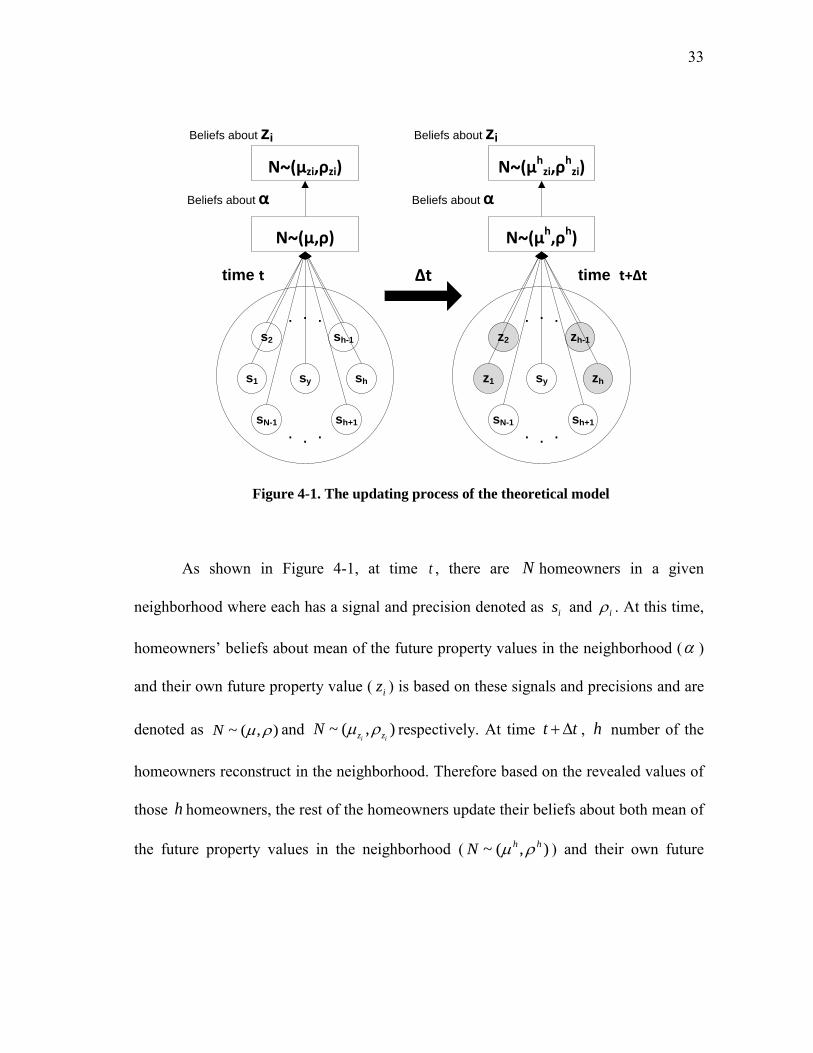
either reconstructs, or sticks to the do-nothing strategy and is shown in Figure 4-1.
33
sy
s2
s1
sN-1
sh-1
sh
sh+1
. . .
. ..
N~(µ,ρ)
Beliefs about α
sy
z2
z1
sN-1
zh-1
zh
sh+1
. . .
. ..
N~(µh,ρh)
Beliefs about α
N~(µzi,ρzi)
Beliefs about zi
N~(µhzi,ρ
hzi)
Beliefs about zi
Δttime t time t+Δt
Figure 4-1. The updating process of the theoretical model
As shown in Figure 4-1, at time t , there are N homeowners in a given
neighborhood where each has a signal and precision denoted as is and i . At this time,
homeowners’ beliefs about mean of the future property values in the neighborhood ( )
and their own future property value ( iz ) is based on these signals and precisions and are
denoted as ~ ( , )N and ~ ( , )i iz zN respectively. At time t t , h number of the
homeowners reconstruct in the neighborhood. Therefore based on the revealed values of
those h homeowners, the rest of the homeowners update their beliefs about both mean of
the future property values in the neighborhood ( ~ ( , )h hN ) and their own future

34
property value ( ~ ( , )z zi i
h hN ). This iterative process continues until everyone
reconstructs or wait till the last period.
4.2.2. Game and Behavior
In a multiagent setting, modeling human decision making becomes so complicated that it
is usually a norm to believe that agents opt for Nash equilibrium strategies (Nash 1950).
Nash equilibrium is the optimal solution of the game where neither of the players can
improve their payoffs by unilaterally changing their strategy. Based on this premise, a
game-theoretic model is developed to account for spatial interactions (e.g. the decision
to reconstruct depends also on the neighbors and their decisions). In other words, the
homeowners play a game with two strategies: wait, observe the signals, and reconstruct
only when there is a sufficient value to do so; or reconstruct immediately, without
waiting for the others. It is natural that homeowners with high value signals will select
immediate reconstruction, while the rest will prefer to wait until a positive net value is
secured.
However this wait-and-see strategy might not always be the optimal strategy due
to the financial constraints (e.g. cost of renting). In cases where the net value from
waiting exceeds that of immediate reconstruction, the game structure resembles war of
attrition in which a follower may end up with a higher payoff than a leader. To illustrate
the concept, a situation with only two neighbors (neighbor i and j ) is considered in
which ( ), and ( )t t represent the mean and precision of future property values at the
time of consideration (see Subsection 4.2.1). The logic behind a two-neighbor case

35
consideration is two-fold: 1) its simplicity, and 2) the fact that the behavioral analysis for
the multiple neighbor cases is not significantly different from the equilibrium solution
for the two-neighbor case (Hendricks and Porter 1996). The expected payoff from
immediate reconstruction for homeowner i considering no prior reconstruction can be
shown as:
[ | ( ), ( )] ( | ( ), ( )) ( )i iEVI i t t f z t t U i dz (4-10)
where [ , | ( ), ( )]EVI i t t t denotes the expected value from immediate reconstruction for
homeowner i at time t given the current state of information about future property
values in the neighborhood, ( | ( ), ( ))if z t t represents the normal probability density
function of iz with mean ( )
1
i i
i
t s
and precision
2( )( 1)
( )( 1) 1
i
i
t
t
, and iU represents
the gained utility for owner i at time t . On the other hand, if homeowner i waits and
observe its neighbor’s (homeowner j ) action, the state of information about the mean of
future property values in the neighborhood changes to a new normal distribution with the
following parameters (Hendricks and Porter 1996):
-1
-1
[ ( ) ( ) ( - (1 ) )]( )
[ ( ) (1 ) ]
j j j j
j
t t z st t
t
(4-11)
1( ) ( )
1 j
t t t
(4-12)
As shown in Equation 4-11, homeowner i ’s belief about ( )t t is a function
of homeowner j ’s property value which has not been revealed yet. It can be shown that
( )t t has a normal distribution with mean ( )t and precision 2(1 )t t j .

36
These derivations are shown in Appendix D. These derivations are used to compute the
expected payoff of waiting for homeowner i at time t which can be denoted as:
2[ | ( ), ( )] max[0, ( | , ( ))] ( ; ( ), ( ) ( ) (1 ))jEVW i t t EVI i t t f t t t d (4-13)
where [ | ( ), ( )]EVW i t t denotes the expected value from waiting for homeowner i at
time t given the current state of information about future property values in the
neighborhood, ( )t t and ( | ( ), ( ))EVI i t t t t denotes the expected value
from immediate reconstruction for homeowner i at time t t . In equation 4-13, the
expected payoff from waiting is assumed to be non-negative. This is attributed to the fact
that in this model no direct waiting costs are considered for waiting and the act of other
homeowners may hinder the homeowner reconstruction decision. Therefore as
mentioned in Equation 4-10, the expectation from immediate reconstruction for owner i
at time t is based on its belief about its future property value considering the present
information about the future property values in the neighborhood. In contrast, owner i
expectations from waiting depends on its gains from its updated information regarding
the future property values in the area. This updating process is based on assumption that
at time t t owner j reconstructs.
4.2.3. Game Solution
Based on these assumptions, the game between the homeowners (homeowners i and j )
can be defined as a war of attrition where homeowners have two pure strategies, 1)
starting the reconstruction, and 2) waiting for neighbors to reconstruct first and deciding

37
accordingly. In the case where pure strategies do not result in equilibrium or
homeowners are not determined about their reconstruction decisions, mixed strategies
can solve the problem.
Mixed strategies are formed by assigning probabilities to pure strategies. Mixed
strategies enable homeowners to randomly select between their pure strategies. For this
game, the mixed strategy equilibrium can be expressed by the probability of
reconstruction at each time period conditional on no prior reconstruction. The solution of
this game can be found using backward induction. In the last period (T ), homeowner i
will start reconstruction if reconstruction has a positive expected value
( ( | ( ), ( ) 0)EVI i T T . In period 1T , considering that no prior reconstruction has
occurred, homeowner i has two options. If it chooses to reconstruct then its expected
payoff of immediate reconstruction ( EPI ) would be the same as the last period. This is
shown in equation 4-14.
[ , ( 1), ( 1)] max[0, [ , ( 1), ( 1)]EPI i T T EVI i T T (4-14)
If homeowner i chooses to wait, its expected payoff from waiting ( )EPW
depends on the probability of its neighbor (homeowner j ) reconstructing ( ( | 1)jP R T ),
where jR denotes the action of reconstruction for homeowner j . Consequently
homeowner i ’s payoff can be shown as:
( | 1) [ , ( 1), ( 1)][ | ( 1), ( 1)]
(1 ( | 1)) max(0, ( | ( 1), ( 1)])
j
j
P R T EVW i T TEPW i T T
P R T EVI i T T
(4-15)
The first part of the formulation shown in Equation 4-15 indicates the state in
which homeowner j reconstructs and homeowner i updates its belief accordingly,

38
while the next part refers to the state in which homeowner j does not reconstruct and
homeowner i reconstructs if the payoff is positive. Homeowner i would be indifferent
between immediate reconstruction and waiting if the payoffs are the same. Equating
equations 4-14 and 4-15 leads to the equilibrium solution for the probability of
reconstruction at each time period:
(1 ) max[0, [ | ( 1), ( 1)]
( | 1)[ | ( 1), ( 1)] max[0, [ | ( 1), ( 1)]
j
EVI i T TP R T
EVW i T T EVI i T T
(4-16)
Considering no prior reconstruction, the same reasoning can be applied to other
reconstruction periods. Hence, the probability computed in Equation 4-16 is the mixed
strategy solution for the formulated game. This shows that if the payoff discrepancy
between waiting and immediate reconstruction is not substantial, an increase in the
probability of reconstruction will be expected. This can be attributed to signals with high
precisions. On the other hand, under low precision signals condition, an increase in level
of discounting will results in an increase in 1(1 ) / ratio and increase the probability
of reconstruction now.
4.2.4. MAS Integration
The result shown in Equation 4-16, indicates the mixed strategy equilibrium for
homeowners at each period. As previously stated, this equilibrium strategy is denoted in
the form of probability of reconstruction at each time considering no previous
reconstruction. To integrate the result in the MAS model, at each period the expected
value of instant reconstruction together with the expected value of waiting is computed
39
for each homeowner. This will result in probability of reconstruction for each
homeowner in that period. After computing this probability, a random number within the
range of zero to hundred is assigned to each homeowner. If the probability of
reconstruction for a given homeowner exceeds the value of the assigned random number
divided by hundred exceeds, the homeowner will reconstruct and otherwise the
homeowner will wait.
4.3. EMPIRICAL MODEL
This subsection presents an empirical model for making decisions regarding
reconstruction of properties. The empirical model is based on an experiment designed to
mimic a situation with conditions similar to real post-disaster conditions. The null
hypothesis in this part of the study was that homeowners’ decisions are not affected by
the following variables: 1) availability of infrastructure, 2) percent of damages in the
area, 3) homeowners’ financial capacity, 4) property value before disaster, and 5) the
value of a new housing alternative. These parameters were incorporated in the design of
the experiment.
4.3.1. Experiment Design
The first step in designing the experiment was to define a scenario. In this experiment, it
was assumed that a neighborhood with similar house plans and values was affected by a
hurricane. This has caused a significant damage in the neighborhood, forcing
homeowners to rent houses in other part of the town. At the same time homeowners need
40
to make decisions about reconstruction. Under these circumstances, each individual has
three reconstruction strategies: 1) to reconstruct immediately, 2) to wait six-months and
observe the reconstruction in the neighborhood, and 3) to take the insurance money and
buy a new housing alternative somewhere else in the town. Homeowners have no
information about whether their neighbors will reconstruct but can observe if they will,
by waiting. If a homeowner reconstructs right away and no one else reconstructs, there
would be a significant chance that the value of his/her property will be less than the cost
of reconstruction. In contrast, if they all reconstruct, there would be a high chance of
getting a property value much higher than the cost of repair. After defining the scenario,
the next step was to characterize the variables. These variables are assumed to drive
participants’ decision-makings and capture the different aspects of the initial hypothesis.
Variables defined for the experiment are as follow: 1) ratio of property values
before damage to the values of a new housing alternative ( 1r ) that defines the effect of
new alternative value by contrasting it to the original property value, 2) ratio of available
funds to required expenses ( 2r ) which denotes homeowners’ financial viability, 3) ratio
of property value before damage to its damaged value 3r that represents the influence of
level of property damage over reconstruction decisions, 4) percent of damages in the
neighborhood ( )pd , which is an ordinal variable and indicates the severity of damages
in the area with respective values of 0 for damage percentages below 50% and 1 for
damages more than 50%, and finally 5) availability of infrastructure in the area ( ai ) with
three possible values of 0, 1, and 2 where 0 corresponds to the case where there is no
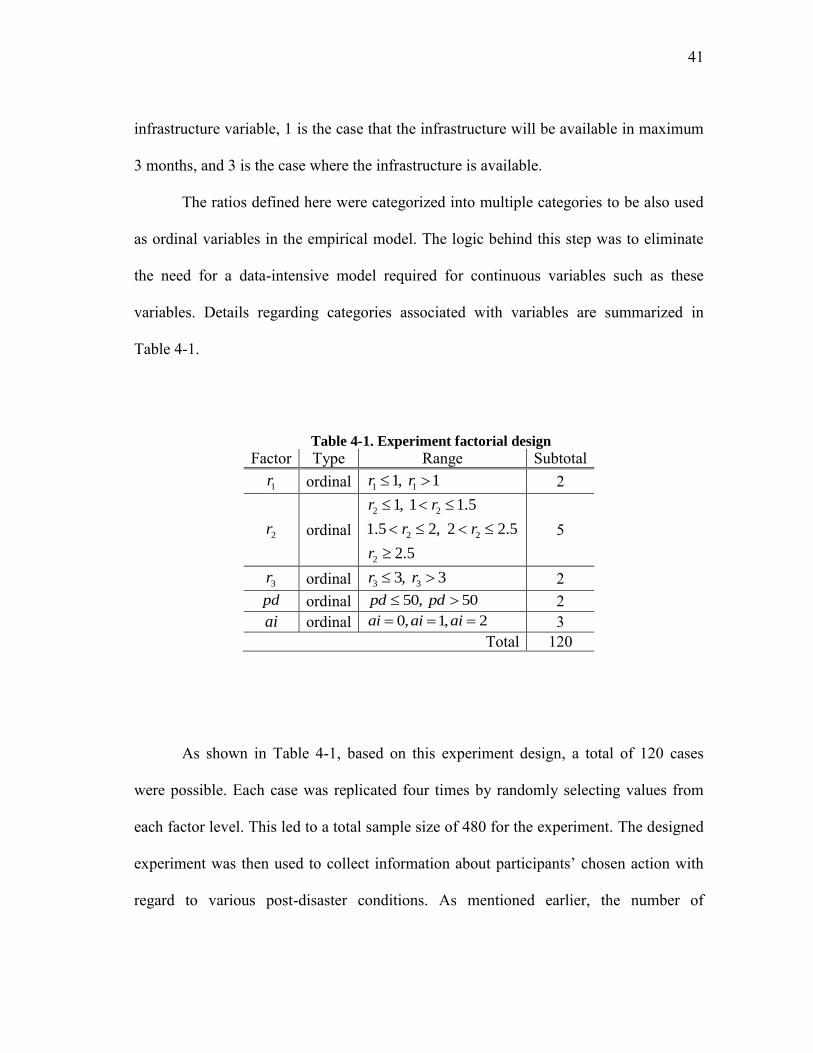
41
infrastructure variable, 1 is the case that the infrastructure will be available in maximum
3 months, and 3 is the case where the infrastructure is available.
The ratios defined here were categorized into multiple categories to be also used
as ordinal variables in the empirical model. The logic behind this step was to eliminate
the need for a data-intensive model required for continuous variables such as these
variables. Details regarding categories associated with variables are summarized in
Table 4-1.
Table 4-1. Experiment factorial design
Factor Type Range Subtotal
ordinal 1 11, 1r r 2
ordinal 2 2
2 2
2
1, 1 1.5
1.5 2, 2 2.5
2.5
r r
r r
r
5
ordinal 3 33, 3r r 2 pd ordinal 50, 50pd pd 2 ai ordinal 0, 1, 2ai ai ai 3
Total 120
As shown in Table 4-1, based on this experiment design, a total of 120 cases
were possible. Each case was replicated four times by randomly selecting values from
each factor level. This led to a total sample size of 480 for the experiment. The designed
experiment was then used to collect information about participants’ chosen action with
regard to various post-disaster conditions. As mentioned earlier, the number of
1r
2r
3r

42
participants in the survey was 80 and each participant was given 6 cases. A sample of
this survey together with its associated instructions is included in Appendix A.
4.3.2. Model Formulation
The collected data was used to structure a decision making model. To form the model,
logistic regression was used as the statistical modeling technique. Logistic regression is a
form of statistical modeling which relates a set of explanatory variables to a categorical
response variable. Response variables can either have two or more than two categories
and are called dichotomous or polytomous, respectively. In the case of this survey, the
response variable could take 3 different categories and as such is a polytomous variable.
Now depending on the type of the response variable, there are two ways to approach
logistic regression. If the response variable is ordinal, ordinal logistic regression
(proportional odds model or cumulative logistic regression) are used (McCullagh 1980)
whereas when the response variable in nominal, generalized logits (multinomial logistic
regression) is employed. In this survey the three different values for response variable
are 1) reconstruct immediately, 2) wait for 6 months, observe neighbors’ action and
decide accordingly, and 3) take insurance money and buy a housing alternative
somewhere else. Since the responses are nominal, generalized logits is pursued to
perform logistic regression. Generalized logit models are extended form of binary logit
models in which instead of having a single logit model, multiple logits are modeled.

43
4.3.2.1. Binary logit models
Binary logit models are a member of generalized linear models or GLMs which were
introduced by Nelder and Wedderburn (1972). Generalized linear models are
characterized by three components which are: 1) a random factor which represents the
probability distribution of the response variable; 2) a systematic component which
denotes a linear function of explanatory variables that are used as regressors; and 3) the
link which defines the functional relationship between the systematic component and the
expected value of the random component (Agresti 1990). Binary response Y with
outcomes 0 and 1 is a Bernoulli random variable with mean
( ) 1 ( 1) 0 ( 0) ( 1)E Y P Y P Y P Y . By denoting this probability as ( )x the
variance of Y would be:
2 2( ) ( ) [ ( )] ( )[1 ( )]VAR Y E Y E Y x x (4-17)
Now for the binary response variable, a linear probability model can be defined
as:
( ) ( )E Y x x (4-18)
The regression model shown in Equation 4-18 displays a major conceptual
shortcoming associated with linear probability model, which is the occurrence of
probabilities beyond the feasible range of 0 to 1. To address this defect, it would be more
beneficial if a logistic regression function is used, which is s-shape and has a monotonic
relationship with its regressor (Agresti 1990). This is shown in the following equation:
exp( )( )
1 exp( )
xx
x
(4-19)
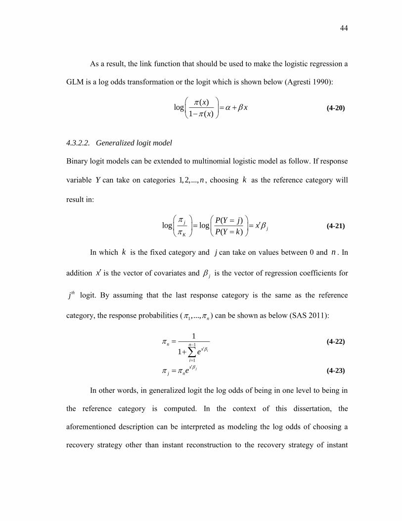
44
As a result, the link function that should be used to make the logistic regression a
GLM is a log odds transformation or the logit which is shown below (Agresti 1990):
( )log
1 ( )
xx
x
(4-20)
4.3.2.2. Generalized logit model
Binary logit models can be extended to multinomial logistic model as follow. If response
variable Y can take on categories 1,2,...,n , choosing k as the reference category will
result in:
( )log log
( )
j
j
K
P Y jx
P Y k
(4-21)
In which k is the fixed category and j can take on values between 0 and n . In
addition x is the vector of covariates and j is the vector of regression coefficients for
thj logit. By assuming that the last response category is the same as the reference
category, the response probabilities ( 1,..., n ) can be shown as below (SAS 2011):
1
1
1
1 i
n nx
i
e
(4-22)
jx
j ne
(4-23)
In other words, in generalized logit the log odds of being in one level to being in
the reference category is computed. In the context of this dissertation, the
aforementioned description can be interpreted as modeling the log odds of choosing a
recovery strategy other than instant reconstruction to the recovery strategy of instant

45
reconstruction. The vector of explanatory variables consists of 1 2 3, , , , and r r r pd ai and
the reconstruction strategy is the response (dependent) variable.
4.3.3. Parameter Estimation
Assuming N independent observations of the dependent variable, and multiple
observations for each fixed ix value, it can be concluded that ( ) ( )i i iE Y n x where
{1,..., }i I , and 1 ... In n N . Given that the joint probability mass function of 1Y to
IY would be proportional to the product of I binomial functions or simply the joint
conditional probability of the observations, therefore (Agresti 1990):
1 1
( )( ) [1 ( )] [1 ( )] exp log
1 ( )i i i i
I Iy n y n i
i i i i
i i i
xx x x y
x
(4-24)
and as a result the log- likelihood will be defined as:
( ) log 1 expi ij j i j ij
j i i j
L y x n x
(4-25)
The next step is to differentiate the log-likelihoods with respect to the vector of
and equal the results to zero. This will results in the following equations:
exp
1 exp
j ij
j
i ia i ia
i ia
j ij
j
xL
y x n x
x
(4-26)
which can be solved using Newton-Raphson method. There are several commercial
programs which perform these procedures among which SAS was used for the purpose
of this dissertation.
46
4.3.4. Experiment Results
The multinomial logistic regression model for this dissertation was approached through
the use of LOGISTIC procedure in SAS. This procedure is capable of forming
generalized logits which considering the type of response variable in this experiment,
qualifies it for implementation. This procedure has also the feature of incorporating
backward elimination technique in which insignificant covariates are eliminated from
the model one at a time. For the purpose of backward elimination, the significance level
was set to 95 percent. The detail results from regression analysis are included in
Appendix E.
Interpretation of the results from LOGISTIC procedure starts with model
information, model type, optimization technique, model convergence status and number
of observations. In this experiment, a generalized logit model with 480 observations and
3 nominal categories was studied. The optimization technique was based on Newton-
Raphson method. Model convergence was set to its default criterion ( 810 ). The model
convergence criterion denotes how well maximum likelihood procedure for parameter
estimation is converging. In addition, the reference category was selected to be the
immediate reconstruction strategy versus other reconstruction alternatives.
In each step of backward elimination procedure, model convergence status is
checked, then model fit statistics are reported for the model with and without covariates.
This is then followed by the results of hypothesis checking of model significance with
regard to its covariates. This iterative process continues until all the parameters
remaining in the model are statistically significant.

47
According to the results of this study, backward elimination process took 3 steps
to finalize the model during which two of the parameters were removed from the model.
These two predictors were 1r and 3r . Predictor
1r captured the effect of new housing
alternative and independent variable 3r was the effect of intensity of property damages
on reconstruction decisions.
The fit statistics for the model can be divided into two categories. The first is an
absolute fit statistic which in this study is McFadden’s pseudo R-squared and the second
is the relative fit statistics known as information criteria an includes AIC (Akaike
Information Criterion), SIC (Schwarz Information Criterion), and negative two times the
maximized log-likelihood ( max2log L ). These model fit statistics are defined below.
McFadden’s R-squared: The structure of McFadden’s pseudo 2r is similar to the
original R-squared with this fact that in original R-squared the variability of estimation
error to that of the data is compared whereas in McFadden’s the log-likelihood of
models with and without covariates are compared to each other. This likelihood ratio
indicates the level of improvement gained by the full model over the model without
covariates (Academic Technology Services 2011). This is shown below.
2 log ( )1
log ( )MF
L Fr
L I (4-27)
The results from regression analysis revealed a value of 0.203 for McFadden’s R-
squared. Although this value is substantially low compared to original and non-pseudo
R-squared but still shows a satisfactory level. Although Hosemer and Lemeshow (2000)
referred to the low McFadden’s R-squared values as being a norm, Shtatland et al.

48
(NSEUG) argued that the interpretation of the statistic is more important than the range
of its value. Following is the list of information criteria used for the model.
SIC/BIC (Schwarz/Bayesian Information Criterion): This information criterion is
comprised of two components as shown in equation 4-28. The first term corresponds to
maximized log-likelihood maxlog L whereas the next is the penalty term for overfitting in
which r is the number of categories for response variable, s is the number of covariates
in the model and if is the frequency value for thi observation.
maxSIC 2log ( 1)( 1) *log i
i
L r s f
(4-28)
AIC (Akaike Information Criterion) which like BIC is influenced by both
maximized log-likelihood and overfitting penalty and is shown in Equation 4-29.
maxAIC 2log 2 ( 1) ( 1)L r s (4-29)
During backward elimination these model fit statistics are computed for each
iteration. The summary of these values are shown in Table 4-2.
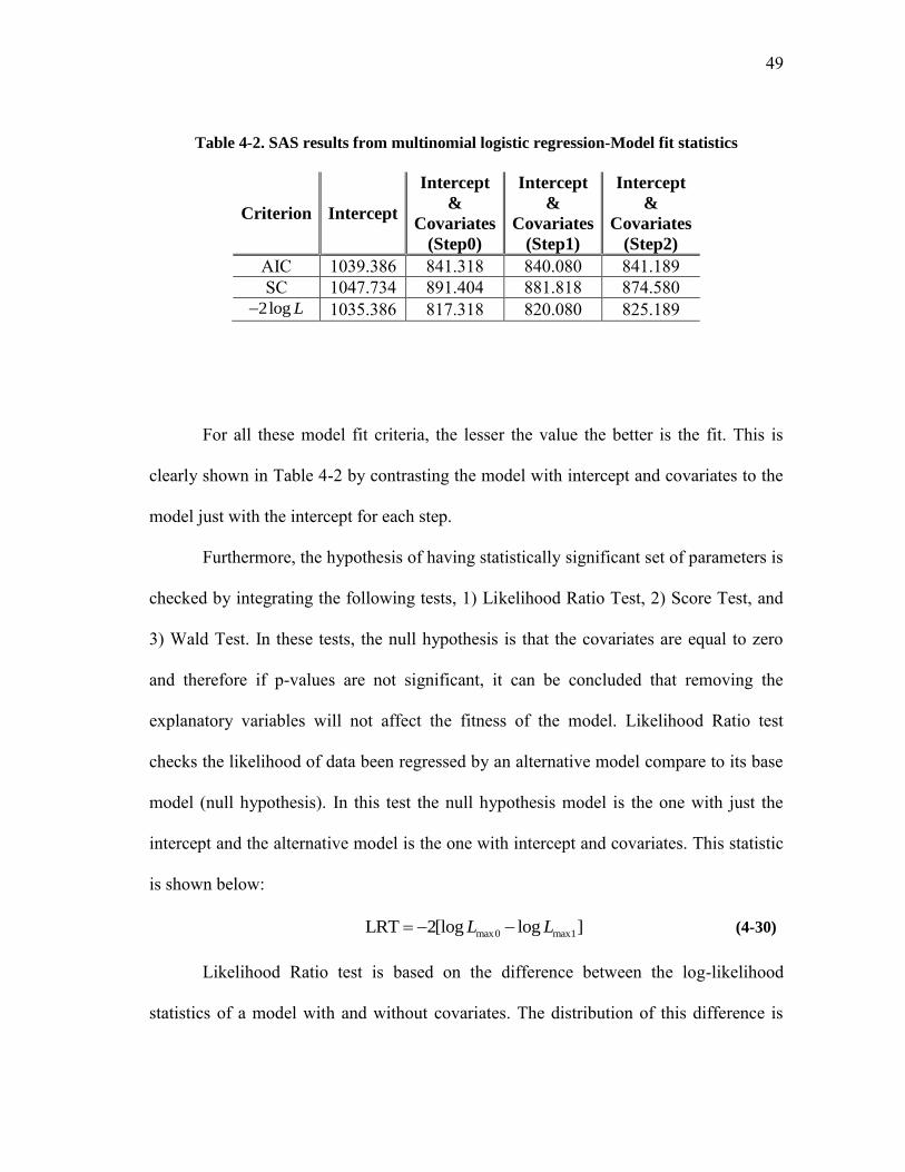
49
Table 4-2. SAS results from multinomial logistic regression-Model fit statistics
Criterion Intercept
Intercept
&
Covariates
(Step0)
Intercept
&
Covariates
(Step1)
Intercept
&
Covariates
(Step2)
AIC 1039.386 841.318 840.080 841.189 SC 1047.734 891.404 881.818 874.580
2log L 1035.386 817.318 820.080 825.189
For all these model fit criteria, the lesser the value the better is the fit. This is
clearly shown in Table 4-2 by contrasting the model with intercept and covariates to the
model just with the intercept for each step.
Furthermore, the hypothesis of having statistically significant set of parameters is
checked by integrating the following tests, 1) Likelihood Ratio Test, 2) Score Test, and
3) Wald Test. In these tests, the null hypothesis is that the covariates are equal to zero
and therefore if p-values are not significant, it can be concluded that removing the
explanatory variables will not affect the fitness of the model. Likelihood Ratio test
checks the likelihood of data been regressed by an alternative model compare to its base
model (null hypothesis). In this test the null hypothesis model is the one with just the
intercept and the alternative model is the one with intercept and covariates. This statistic
is shown below:
max0 max1LRT 2[log log ]L L (4-30)
Likelihood Ratio test is based on the difference between the log-likelihood
statistics of a model with and without covariates. The distribution of this difference is

50
chi-square with degrees of freedom equal to the difference in degrees of freedom of the
two models. On the other hand, Wald test examines whether a parameter is equal to a
certain value. Wald test statistic is shown below:
2
0ˆ( )
ˆvar( )WTS
(4-31)
In the context of this dissertation, this certain value is equal to zero and therefore
failing to reject the null hypothesis denotes that the parameter can be deleted from the
model. This is because an independent variable with a very small coefficient compare to
its standard error cannot have a significant effect on estimating the dependent variable.
Score test perform a similar action to Wald test. The test statistic is shown below which
takes a chi-square distribution under null hypothesis:
2
0
0
( )
( )
UST
I
(4-32)
In which log ( | )( )
L xU
,
2
2
log ( | )( )
L xI
, and null hypothesis is
0 0:H . According to the results, for all elimination steps, the p-values for these 3
tests were less than 0.001 for all elimination steps and as a result the null hypothesis of
having zero covariates was rejected.
To proceed, the analysis extends to cover the maximum likelihood estimates
from multinomial logistic regression using LOGISTIC procedure in SAS. These
estimates are shown in Table 4-3. The details regarding this model can be found in
Appendix E.

51
Table 4-3. SAS results from multinomial logistic regression-Logistic procedure
Parameter option DF Estimate St. Err Wald Chisq Pr>Chisq
Intercept 2 1 2.0172 0.6538 13.660 0.0002 Intercept 3 1 1.7657 0.7237 4.3092 0.0379
2r 2 1 -0.2456 0.1839 7.1375 0.0075
2r 3 1 -0.1363 0.2119 1.6557 0.1982 pd 2 1 1.1990 0.2826 18.0035 <0.0001 pd 3 1 2.7347 0.3342 66.9698 <0.0001 ai 2 1 -1.1070 0.1910 33.5981 <0.0001 ai 3 1 -2.1986 0.2248 95.6897 <0.0001
During backward elimination process since parameters 1r and 3r did not meet the
0.05 significance level, were removed from the model. Therefore it can be concluded
that for these parameters the null hypothesis cannot be rejected. This indicates that the
effect of a housing alternative and level of property damages on reconstruction decisions
was not significant.
As shown in Table 4-3, the parameter estimation results correspond to two sets of
equations labeled as 2 and 3 in Table 4-3 under column “ option”. These labels refer to
the categories defined for the response variable. Label 2 refer to the reconstruction
strategy of waiting for 6 months and observe neighbors’ action and decide accordingly
whereas label 3 refers to the strategy of getting insurance money and buy a housing
alternative somewhere else in the town. Regression results denote that both percent of
damage ( )pd and availability of infrastructure ( )ai are statistically significant across the
two models. Parameter 2r while significant in the first model, is not significant in the

52
second model in the presence of other parameters. The resulting equations are listed
below:
2
( 2)log 2.0172 0.2456* 1.1990* 1.1070*
( 1)
P opr pd ai
P op
(4-33)
2
( 3)log 1.7657 0.1363* 2.7347* 2.1986*
( 1)
P opr pd ai
P op
(4-34)
4.3.5. Discussion of the Results
Equation 4-33 indicates that for every one unit increase in availability of infrastructure
( )ai , the log of probability of waiting over probability of immediate reconstructing
(reference option or immediate reconstruction) is decreased by 1.1070. Similarly, a unit
increase in parameters pd and 2r will results in 1.1990 increase and 0.2456 decrease in
the log-odds of waiting (option 2) to immediate reconstruction (option 1).
The same logic can be used to interpret the results for Equation 4-34. Other
important conclusions are, 1) the more the 2r the less the probability of waiting or
leaving the area to immediate reconstruction. This means that if available funds exceed
expenses, it would be less likely for an individual to pursue a reconstruction strategy
other than the instant reconstruction, 2) the more the pd the more the likelihood of
waiting or leaving. This indicates that if the percent of damages in a neighborhood
increases, it would be more likely for an individual to opt for its second and third
reconstruction strategies rather than reconstructing right away, and finally 3) the more
the ai the less the odds of waiting or leaving to immediate reconstruction (option1).
This signifies the fact that if infrastructure is more accessible in a neighborhood,

53
individuals are more likely to stay and reconstruct rather than leave their property for
other reconstruction strategies. The regression results are included in Appendix E.
4.3.6. MAS Integration
The results shown in Equations 4-33 and 4-34 indicate the log odds of choosing an
alternative (waiting or leaving the area) to the reference category (reconstruct
immediately) based on the three different independent variables. These variables are the
ratio of available funds to the required expenses, the percent of damages in the area, and
the availability of infrastructure. To integrate the results in the MAS model, a series of
steps needs to be taken which are: 1) identifying the infrastructure in the area. In this
research the only infrastructure that was considered in the multi-agent system model was
transportation infrastructure; 2) assigning proper level of availability to the existing
infrastructure based on the defined empirical model. These availability levels are:
available status, available in three months status and not available status which are set
based on the distance of the given infrastructure from the source of disaster; 3) assigning
proper level of damage to each property based on its distance to the source of disaster.
This will results in calculation of percent of damages in the neighborhood in the MAS
model; 4) assigning financial resources and proper reconstruction cost to each
homeowner based on its property level of damage. This will lead to calculation of the
defined ratio ( 2r ) for each homeowner which denotes their financial flexibility. After
accomplishing all the previously mentioned steps, the probabilities associated with each
option for a homeowner can be computed using Equations 4-33, 4-34 and the fact that

54
the sum of the probabilities should add up to 1. After computing the probabilities, just
like the theoretical approach, a random number within the range of zero to hundred will
be assigned to each homeowner. For each home owner, If the random number lies within
the acceptable probability range of a strategy, that strategy will be the one that is
assumed to be pursued by the homeowner.
4.4. SUMMARY
The objective of this section was to define a framework which can account for modeling
agent’s spatial interactions. The section started with a theoretical behavioral model
which was solely focused on the neighboring aspect of homeowners’ interaction. The
result from the theoretical approach demonstrated that agents’ actions are influenced by
other agents in their surroundings. This conclusion was expressed as the probability of
reconstruction at each time step based on the state of the environment. Furthermore to
account for other factors, an experiment was designed and implemented with a goal of
using the data to develop an empirical model.
The results from the empirical model show that in a more realistic post-disaster
situation, the decision making of affected homeowners is significantly influenced by 3
variables: 1) severity of damages in the area which has a direct influence on choosing an
alternative to reconstruct immediately, 2) availability of infrastructure in the area which
in contrast to the previous parameter has a diverse effect on choosing an alternative to
immediate reconstruction, and finally 3) the financial viability of homeowners which

55
favors instant reconstruction. The next section proceeds to capture the next micro-level
research question, which is how agents interact in the organizational domain.
4.5. LIMITATIONS
Although the results from both theoretical and empirical models yielded rational results,
there were limitations associated with each modeling approach that might affect the
broad applicability of the results. These limitations are listed separately for each model.
In the theoretical model, the defined utility for homeowners had a limited number
of parameters in contrast to its complex structure in real conditions. Furthermore, other
influencing parameters such as availability of infrastructure were not included in the
model. In addition, the mixed strategy equilibrium for the probability of reconstruction
at each time step was based on the assumption that the interaction between homeowners
starts with a case where there are just two homeowners and this is not significantly
different from the results of a sub-game perfect equilibrium. On the other hand, in the
empirical model, the number of influencing variables were limited. in addition, due to
the insufficient number of participants for the experiment, all the variables were defined
as ordinal.
To overcome these limitations, the theoretical model should be extended to
account for multi-neighbor cases. On the other hand due to the fact that in the empirical
model, parameter estimation is based on maximum likelihood method, the more the data
the better is the model. Therefore to have a better predictor of real conditions, more data
is needed which requires a huge number of survey participants.

56
5. MODELING ORGANIZATIONAL INTERACTIONS
5.1. INTRODUCTION
The objective of this section is to address the second micro-level objective of this
dissertation - how individuals interact in the organizational domain while negotiating
with high-bargaining-power entities such as insurers. Much like the previous chapter,
this section is divided into two subsections. The objective of the first subsection is to
present a theoretical model of homeowner-insurer bargaining process, while the next
subsection is focused on comparing the results from theoretical model with the data from
an experimental study. The summary of findings is presented in the third subsection,
which is then followed by the assumptions and limitations in this section.
5.2. THEORETICAL MODEL
5.2.1. Background
Bargaining situations from a broad perspective occur when individuals or organizations
have a common interest in cooperation and conflicting interests in the form of
cooperation (Muthoo 2002). An example of these situations is the common-conflicting
set of interests with regard to division of a surplus between players.
Bargaining theory has been widely discussed in literature and applied to many
research domains. The motivation behind implementation of bargaining theory is to
capture the behavior of players in a game with mutual interests. Examples of bargaining

57
situations in different research areas include bribery and corruption (Basu et al. 1992;
Hindriks et al. 1999), wage negotiations (Gertler and Trigari 2009; Knabe 2009; Ellis
and Fender 1985; Grout 1984; McDonald and Solow 1981), marriage (Lundberg and
Pollak 1993; McElroy and Horney 1981; Manser and Brown 1980), coalition formation
(Psathas and Stryker 1965), conflict analysis (Anbarci et al. 2002), bid bargaining games
(Daniel et al. 1998), and war modeling (Reed 2003).
In the context of homeowner-insurer negotiations, the related studies include the
availability of equilibrium in competitive insurance markets by Rothschild and Stiglitz
(1976), the existence of equilibrium in reinsurance markets by Borch (1962), the effect
of risk aversion on bargaining by Kihlstrom and Roth (1982), the analysis of
monopolistic insurance markets by Stiglitz (1977), and the two-person insurance
negotiation by Schlesinger (1984).
The focus of this subsection is on the application of bargaining theory in post-
disaster negotiations; more specifically, to investigate the interactions between affected
homeowners on one side, and insurers on the other. This is a very important, yet often
overlooked aspect of the recovery process. There are numerous reported cases where
insurance settlement offers were much lower than estimated losses and claims.
Following Hurricane Katrina, National Public Radio (NPR) and Public Broadcasting
Service (PBS) have extensively reported on the problems homeowners have in settling
claims and obtaining insurance. A similar problem was reported by the Port of New
Orleans. Here, the bargaining power of the insurers is much greater than the bargaining

58
power of the homeowners. In such settings, “stressed” agents are often impatient and
willing to accept offers they might not otherwise have considered.
Therefore there is a need to model this process so that public agencies can react
correspondingly. In this section the goal is to address the same need using both
theoretical and empirical models. While theoretical model conceptually approaches the
problem, the empirical model reflects the results from the experiment.
5.2.2. Model Formulation
The bargaining model presented here is designed to capture the interaction between
players in the incidence of a disaster. In this settings, the two players are 1) insurer and
2) homeowner. In addition, it is assumed that the players are bargaining over the
difference between the maximum claim amount and no compensation.
Homeowners seek to maximize their claims while insurers try to minimize their
losses. Under this bargaining situation, one of the major driving factors is the available
strategies for both players. Each strategy will result in a payoff, which in bargaining
literature is divided into two categories. The first category is attributed to the payoffs
that are acquired while players are still in-play, negotiating to achieve an agreement and
is called an inside option. The other category is related to payoffs gained by players due
to quitting the game without reaching to an agreement (Muthoo 1999). In the theoretical
owner-insurer negotiation framework of this dissertation, while no specific inside option
was considered for players, the only available outside option was the payoff from
referring the case to court.

59
The model was designed in such a way that it can mimic a bargaining situation in
a case of a disaster. Following a disaster, bargaining starts between the affected
population and their insurers regarding the amount of compensation for the incurred
damage. Subsequent to the incidence, an insurer and homeowner start negotiating to
reach an agreement. The players are assumed to be rational players and therefore
maximizing their utilities.
The sequence of this bargaining game is as follows: The insurer starts the
negotiation by offering a claim amount to the homeowner. To respond, the homeowner
has three strategies: 1) accept the insurer’s offer, 2) reject and continue negotiation by
making a counteroffer, and 3) reject and take the case to the court in the next period. If
the homeowner chooses the first strategy the game is finished, if it prefers to take the
case to court both players will get their undiscounted court payoffs; and finally if the
homeowner opts for a counteroffer, the insurer has the option to either accept or reject
this counteroffer. In the next period, if the insurer accepts the offer, the game ends and if
he rejects, the case will be taken to court in which both players will get their court
payoffs. The homeowner’s court payoff is assumed to be a random draw from a uniform
distribution, (in this study distribution parameters are assumed to be 0.7a and 0.9b
) of the maximum claim amount which will be discounted by a common discount factor
(assumed to be 0.9 ) for each time step that an agreement is not achieved. For
simplicity the maximum claim amount is assumed to be 1. The discount factor is
incorporated in the model to account for the costly nature of waiting. Furthermore, both
players have a unique outside option, which is pursued by taking the case to court. It is

60
also assumed that the bargaining problem is a multi-period process, which will be
resolved in two-steps. In this model delay can be costly and in equilibrium condition, the
very first offer is accepted.
5.2.3. Model Solution
Since the bargaining problem in this research is a finite sequential process, the extensive
form of the game can be used to find the equilibrium strategy for the players. The
extensive form of the game is shown in Figure 5-1. In the extensive from, the game is
broken down into its feasible sets of strategies called subgames. The next step is to
check for Nash equlibria in each subgame. A Nash equilibrium is an optimal solution for
a game in terms of strategies for players, in which none of the players can improve their
payoffs by unilaterally changing their strategy. This process leads to finding the
subgame perfect Nash equilibria for the game. In the context of this dissertation, the goal
is to find an equilibrium offer in the insurer-homeowner negotiations. This equilibrium
strategy implies the amount of offer that should be made by insurer in the first period to
make the homeowner indifferent between accepting and rejecting and eventually
accepting the offer. The idea of subgame-perfect equilibrium for extensive-form games
was initiated by Selten (1978). A subgame perfect Nash equilibrium is a strategy which
leads to the Nash Equilibrium of every subgame of the original game. To compute
subgame perfect Nash equilibria, backward induction method is used. Backward
induction is an iterative process in which the optimal strategy is initially found for the
last period of the game and is subsequently used to find the optimal strategies for the

61
previous stages. This backward process continues until all players’ actions are being
determined. In this study the game in its extensive form (Figure 5-1), is a finite
sequential game in which the game starts with a first offer, continues with a possible
counteroffer and ends with acceptance or the court payoffs.
Figure 5-1. Extensive form of the bargaining game
Consider the backward induction process for the extended form of the game in
Figure 5-1, it is shown that in the 3rd period, if they do not reach the agreement

62
beforehand, both players will get their court payoffs ,I oC C . IC is insurer’s court payoff
whereas oC is homeowner’s court payoff. In this period the negotiation value has been
discounted twice, therefore 2
I oC C . Now by moving one step backward in period
2, there are two strategies available for the homeowner. The first is to reject insurer’s
offer (from the first period) and go to the court whereas the second is to reject the offer
and make a counteroffer. If homeowner chooses the first option the payoffs for insurer
and homeowner would be , oICC
respectively.
On the other hand if homeowner chooses to make a counteroffer the payoffs will
change to ,I IC C . This is due to the fact that the homeowner knows that if insurer
does not accept the offer, the case will be directed to court and insurer will get its court
payoff. Therefore homeowner will make its offer to be the same as insurer’s court
payoff. In addition, since in this period the negotiation value has been discounted once.
Proceeding with the backward process in period 1, there is a unique strategy for the
insurer to start the bargaining process.
Since insurer knows that in period 2, homeowner will opt for the second strategy
which is rejecting and making a counter offer (since the outcome of this strategy for the
homeowner is always higher than the outcome from directing the case to court), insurer
will make its offer to be the same as homeowner’s highest payoff in the 2nd period. As a
result insurer’s equilibrium strategy would be to offer IC for homeowner and keep
1 IC for himself. This strategy profile concludes the theoretical approach to solve

63
the bargaining game. The next subsection will approach the problem from an empirical
point of view to contrast the results to that of a theoretical approach.
5.2.4. MAS Integration
The result from the theoretical approach to capture the organizational behavior of
homeowners was presented as an equilibrium offer from insurer in the first period. The
structure of this equilibrium offer is very similar to the alternating offer bargaining
model by Rubinstein (1982). This equilibrium offer is based on three variables which
are: 1) discount factor, 2) maximum bargaining value, and 3) Insurer’s court payoff
wghich are initially defined for the model. Therefore integration of these results in the
MAS model requires entering the proper values for each variable and for each
homeowner in the model.
5.3. EMPIRICAL MODEL
5.3.1. Experiment Design
The empirical model studied in this dissertation is based on an experiment designed to
capture a similar situation to what occurs between insurer and homeowner following a
disaster. The experiment was designed to pose a situation that maybe more familiar to
the participants (i.e. undergraduate students). Among the possible options, a case of a car
accident seemed to be a good example due to its nature and the way the negotiations
between players take place. This is due to the fact that the strategies defined for both

64
parties are the same as those identified for the theoretical model. Therefore, the game
starts with insurer’s offer to car-owner. The car-owner can accept the offer, reject- go to
court, and reject-make a counter offer. The next step starts with insurer’s either
accepting or rejecting car-owner’s offer. Failing to reach an agreement in the second
period, will result in court payoffs for both parties. The details regarding the experiment
together with the instructions to participants are included in Appendix F. Results from
this experiment were used to formulate an empirical model to estimate more realistic
choices and compared to the theoretical model to check for similarities and
dissimilarities.
5.3.2. Model Formulation
Unlike the previous section, in the empirical model formulation there is no equilibrium
offer available for the insurer to start the negotiation. In other words, an empirical model
considers a payoff structure for players which is formed by incorporating their strategies
and the associated probabilities with each of the strategies. The objective of this
subsection is to estimate these strategies and probabilities by incorporating the data from
the experiment and test for several hypotheses related to the empirical model presented
below:
'
1 11 1 12 2 13( )+ ( ) ( ) Ob P b bC
P P
(5-1)
'
2 21 21 2 )( ) (1- )( Ob P C P b (5-2)
In equations above , {1,2}ib i is car-owner’s payoff in the thi period,
, {1,2}, {1,2,3}ijP i j is the probability of incurring event j at period i , OC is car-

65
owner’s court payoff, is the common discount factor for both of the players, '
1b is
insurer’s offer to the car-owner in the first period, and finally '
2b is the car-owner’s offer
in the second period. As shown in Equations 5-1 and 5-2, in the first period car-owner’s
expected payoff would be a combination of its payoffs from various game outcomes
with their associated probabilities.
There are three strategies available for the car-owner in this period, the first is to
pursue its court payoff which is the third term in Equation 5-1 ( /OC ), the next is to
reject insurer’s offer and make a counteroffer which corresponds to the second term of
the equation ( 2b ), and finally the last is to accept the insurer’s offer which corresponds
to the first term in the equation ( 1b ). Similarly in the second period the car-owner’s
expected payoff is a combination of its payoff from 1) court payoff due to insurer’s
rejection ( OC ), and 2) its own offer due to insurer’s acceptation of the offer ( 2b ) and
their associated probabilities.
5.3.3. Model Fitting
The subsequent step to model formulation is to estimate the parameters in Equations 5-1
and 5-2 by formulating and testing the hypotheses. The null hypotheses formed for this
purpose are as following: 1) insurer’s initial offer to homeowner ( 1b ) does not follow a
specific distribution, 2) car-owners’ decision following insurer’s initial offer is not
associated with the size of insurer’s initial offer. This hypothesis is to check whether
probabilities associated with homeowner’s response ( 11 12 13, , and P P P ) to insurer’s initial

66
offer ( 1b ) is significantly related to the size of the offer from insurer ( 1b ) , 3) car-
owner’s counter offer (2b ) is not associated with insurer’s initial offer ( 1b ), 4) insurer’s
decision to car-owner’s counteroffer is not related to the magnitude of the counteroffer (
2b ). The assumptions were statistically analyzed to check for validity and significance.
The whole process is shown in Figure 5-2.
1) insurer’s initial offer does not follow a specific
distributionData
Model Fitting Goodness of Fit Tests
HYPOTHESES
2) car-owner’s decision regarding insurer’s initial offer
is not associated with the size of insurer’s initial offer
3) car-owner’s counteroffer is not associated with the
size of insurer’s initial offer
4) insurer's decision regarding owner’s counteroffer is
not associated with the size of owner’s counteroffer
Figure 5-2. The process of experimental model development

67
5.3.3.1. Null Hypothesis 1: “Insurer’s initial offer does not follow a specific
distribution”
The null hypothesis is that the observed data from insurer’s offer are not random draws
from a specific distribution. A variety of methods can be used to fit distributions to data
and check for their statistical significance. These fitting procedures can either be
empirical (nonparametric) or parametric. Each of these methods has its own benefits and
drawbacks. Nonparametric models are usually easier to use but at the same time need
larger sample sizes. Parametric models are more complicated but are capable of
estimating parameters inside the feasible range and outside the observed data (Vose,
2008).
For the purpose of this dissertation since regression outcome is intended to be
directly used in the MAS model, the preference was given to a parametric regression. To
accomplish this, a wide range of possible distributions were checked for the observed
data through ModelRisk by Vose Software in which a total of 51 continuous univariate
distributions where fitted to data.
In this approach Maximum Likelihood Estimation (MLE) technique was used for
parameter estimation. The fitting results were rank ordered based on their information
criteria. Three information criteria were used to rank the fitted distributions. These
information criteria were: 1) SIC (Schwarz Information Criterion); 2) AIC (Akaike
Information Criterion); and 3) HQIC (Hanna-Quinn Information Criterion). Information
criteria were used as replacements for popular goodness of fit statistics such as Chi-
Square, Kolmogorov-Smirnoff, and Anderson-Darling. The reason is a set of drawbacks

68
associated with them such as, 1) they present the probability that data generated from the
fitted distribution has a goodness of fit statistic as low as the observed data instead of
providing a probability that observed data are necessarily random draws from the fitted
distribution, and 2) they cannot integrate censored, truncated, or binned data (Vose
2008).
For information criteria, the lower the values are the better the fit will be. The
other main benefit of using information criteria is that they penalize the model for
overfitting which is caused by additional parameters in the model to increase the
likelihood. The first two information criteria were described earlier in the chapter.
Similar to AIC and SIC, HQIC is also comprised of a separate component for the
maximized likelihood and a penalizing component for the number of parameters. This is
shown in Equation 5-3.
maxHQIC 2log 2ln[ln[ ]]L n k (5-3)
in which n is the number of observations, and k is the number of predictors. Among
these criteria SIC is the one with more penalizing power and AIC is the one with the
least (Vose 2008). The summary of fitting results rank ordered by their fitting statistics is
shown in Table 5-1. As shown in the table the best fit resulted from a Laplace
distribution with location parameter ( ) of 7000 and scale parameter ( b ) of 1044.7.

69
Table 5-1. List of the top 3 fitted distributions Distribution AIC SIC HQIC
Laplace -1186.853 -1182.504 -1184.127 Log-Laplace -1194.104 -1187.674 -1190.015
GLogistic -1195.233 -1188.803 -1191.144
Apart from model fit statistics, goodness of fit plots are also a good measure to
visually check the overall fit of a proposed model. Figure 5-3 shows these plots taken
from the output of ModelRisk software. The plots are 1) histogram of the observed data
versus PDF of the fitted distribution, 2) cumulative histogram of the observed data
versus CDF of the fitted model, 3) Q_Q plot or Quantile-Quantile plot which is a
probability plot that contrast two probability distributions (observed against fitted) by
plotting their quantiles against each other, and 4) P_P plot or Probability-Probability plot
which is a graphical representation of comparing two cumulative distributions (observed
against fitted) against each other. In the first two plots, the goodness of fit can be
visually checked by observing how the histograms of the observed data match the PDF
and CDF of the fitted distribution. In Q-Q and P_P plots, the goodness of fit can be
observed by checking how close the quantiles and cumulative distributions from
observed data match up with the same values for the fitted distribution. In an ideal case
the values should lie on the diagonal line shown in Figure 5-3.

70
a) PDF observed vs. fitted
b) CDF observed vs. fitted
c) P-P plot
d) Q_Q plot
Figure 5-3. Goodness of fit plots (ModelRisk Vose Software)

71
Since information criteria such as AIC do not provide test statistics, a similar
approach was performed in another commercial statistical software, EasyFit, in which
the Laplace distribution was contrasted to four major univariate distributions which were
Lognormal, Gamma, Normal and Weibull. The results from EasyFit statistical analysis
are shown in Figure 5-4 and Table 5-2. The results demonstrated that the Laplace
distribution fairly predicted the data, had the highest overall ranking, and as such
rejected the first null hypothesis that the data are not random draws from a specific
distribution.
Figure 5-4. Fitted distributions to the data (EasyFit Software)
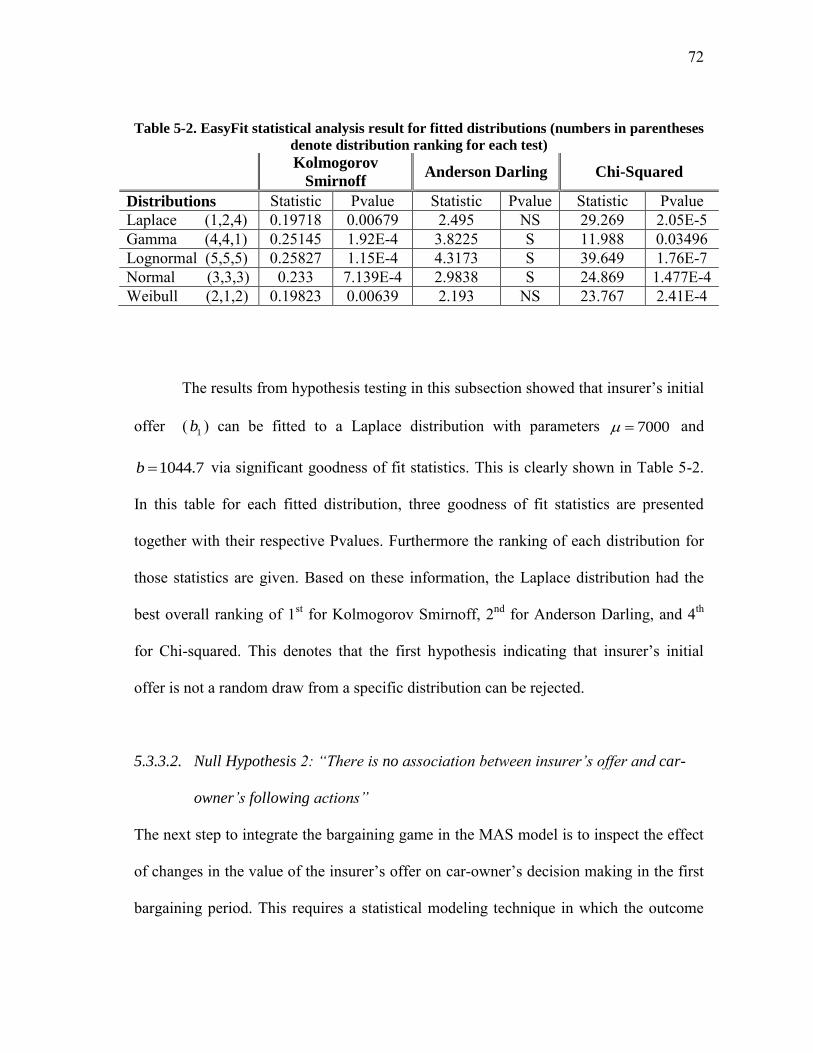
72
Table 5-2. EasyFit statistical analysis result for fitted distributions (numbers in parentheses
denote distribution ranking for each test)
Kolmogorov
Smirnoff Anderson Darling Chi-Squared
Distributions Statistic Pvalue Statistic Pvalue Statistic Pvalue Laplace (1,2,4) 0.19718 0.00679 2.495 NS 29.269 2.05E-5 Gamma (4,4,1) 0.25145 1.92E-4 3.8225 S 11.988 0.03496 Lognormal (5,5,5) 0.25827 1.15E-4 4.3173 S 39.649 1.76E-7 Normal (3,3,3) 0.233 7.139E-4 2.9838 S 24.869 1.477E-4 Weibull (2,1,2) 0.19823 0.00639 2.193 NS 23.767 2.41E-4
The results from hypothesis testing in this subsection showed that insurer’s initial
offer ( 1b ) can be fitted to a Laplace distribution with parameters 7000 and
1044.7b via significant goodness of fit statistics. This is clearly shown in Table 5-2.
In this table for each fitted distribution, three goodness of fit statistics are presented
together with their respective Pvalues. Furthermore the ranking of each distribution for
those statistics are given. Based on these information, the Laplace distribution had the
best overall ranking of 1st for Kolmogorov Smirnoff, 2nd for Anderson Darling, and 4th
for Chi-squared. This denotes that the first hypothesis indicating that insurer’s initial
offer is not a random draw from a specific distribution can be rejected.
5.3.3.2. Null Hypothesis 2: “There is no association between insurer’s offer and car-
owner’s following actions”
The next step to integrate the bargaining game in the MAS model is to inspect the effect
of changes in the value of the insurer’s offer on car-owner’s decision making in the first
bargaining period. This requires a statistical modeling technique in which the outcome

73
variable is categorical. In this phase of bargaining there are 3 available options for the
car-owner which are 1) accept the offer, 2) reject and make a counter offer, and 3) reject
and go to court. Since the response variable is nominal and has more than 2 categories,
multinomial logistic regression would be the proper modeling technique. The modeling
procedure is the same as the one described for spatial experiment. Results from SAS
statistical modeling software for multinomial regression is summarized in Table 5-3. The
details are included in Appendix G. Since no ordinal classification can be assigned to the
different levels of dependent variable, generalized logits is again employed for the
analysis. The reference category for analysis was set to car-owner’s last option which is
to accept the offer. The second option was set to be the owner’s counteroffer and finally
the third option is to refer the case to court.
Table 5-3. SAS results from multinomial logistic regression-Logistic procedure Parameter act DF Estimate St. Err Wald Chisq Pr>Chisq
Intercept 2 1 4.3344 0.6538 4.6156 0.0317 Intercept 3 1 3.5939 0.7237 2.1046 0.1469
Offer 2 1 -0.00068 0.00029 5.4247 0.0199 Offer 3 1 -0.00072 0.000365 3.8889 0.0486
The results from regression analysis indicates that the value of the offer in the
first period is statistically significant across the two models. The outcomes of this
logistic regression analysis can be shown in the following two equations:
121
11
log 4.3344 0.00068*P
bP
(5-4)

74
131
11
log 3.5939 0.00072*P
bP
(5-5)
Equation 5-4 indicates that for every one unit increase in insurer’s initial offer ( 1b ), the
log of probability of choosing the counteroffer strategy over probability of accepting the
offer (reference option) is decreased by 0.00068. Similarly in Equation 5-5, a unit
increase in insurer’s initial offer ( 1b ) will result in 0.00072 decrease in the log-odds of
choosing the court option instead of accepting the offer. Furthermore these equations
indicate that the more the offer is, the less would be the likelihood of preferring any
other options over accepting the offer. The results from multinomial logistic regression
in this part, contribute to finding the probability associated with owner’s different
strategies ( 11 12 13, , and PP P ) in Equation 5-1, in response to insurer’s initial offer ( 1b ).
5.3.3.3. Null Hypothesis 3: “Car-owner’s counter offer is not associated with insurer’s
offer in the first bargaining phase”
The third step was to check the hypothesis of not having an association between
insurer’s actions and car-owner’s counter-offer. The hypothesis is checked by fitting a
linear model to the data and check for the significance of the results.
There are four major criteria to be checked for a linear relationship between two
variables, these criteria are: 1) linearity, which is to check whether the predictor and the
response variable have a linear relationship. This can be checked by plotting the
residuals against fitted values and check whether the distribution of the points is
symmetrical along the horizontal line, 2) independence, which is to inspect whether

75
there is a correlation among residuals which can indicate that there is a potential for
model improvement. Independence can be checked by computing the autocorrelation
among the residuals, 3) homoscedasticity, which is to check for the homogeneity of the
variances and can be checked by inspecting the residual versus predicted values plot and
look for any heterogeneity, and 4) normality, which is to check whether the errors are
normally distributed in the model. Failing to demonstrate normally distributed errors in
the model can be a good indication of having an outlier. This significantly affects
parameter estimation, which in turn relies on minimizing the squared errors. This
phenomenon can be detected by drawing the normal probability plot of the residual and
check whether the points are randomly distributed along the diagonal line (Decision
Forecasting 2011).
The analysis of data for linear regression was performed in both R and SAS
programming environment. Table 5-4 summarizes the result from the original data in R.
The results from linear regression denotes a significant linear relationship between car-
owner’s counter offer and insurance initial offer and as a result the null hypothesis of not
having an association between these two parameters is rejected.
Table 5-4. R results from linear regression modeling for car-owner’s counter offer Parameter Estimate St. Err t value Pr>|t|
Intercept 2671.4749 814.7944 3.279 0.00343 Insurance-Offer 0.8449 0.1242 6.803 7.78e-07

76
In addition to Table 5-4, Figure 5-5 presents model’s goodness-of-fit plots. As
shown in the figure, there is a clear indication of having an outlier in the model. This can
be detected by observing: 1) the residuals are not normally distributed along the
horizontal line shown in the upper left side of the graph labeled as “Residuals vs Fitted”,
and 2) there is a point on “Residual vs Leverage” graph with a Cook’s distance higher
than 1, and 3) in the “Scale-Location” graph, there is a distinct trend in the distribution
of the points.
Figure 5-5. Model fit plots (R)

77
To address the problem the fifth observation was treated as an outlier and was
deleted from the data (as labeled in the graphs) and the new data was analyzed. The
goodness-of-fit plots are shown in Figure 5-6, while regression results are shown in
Table 5-5.
Figure 5-6. Model fit plots-Without outlier
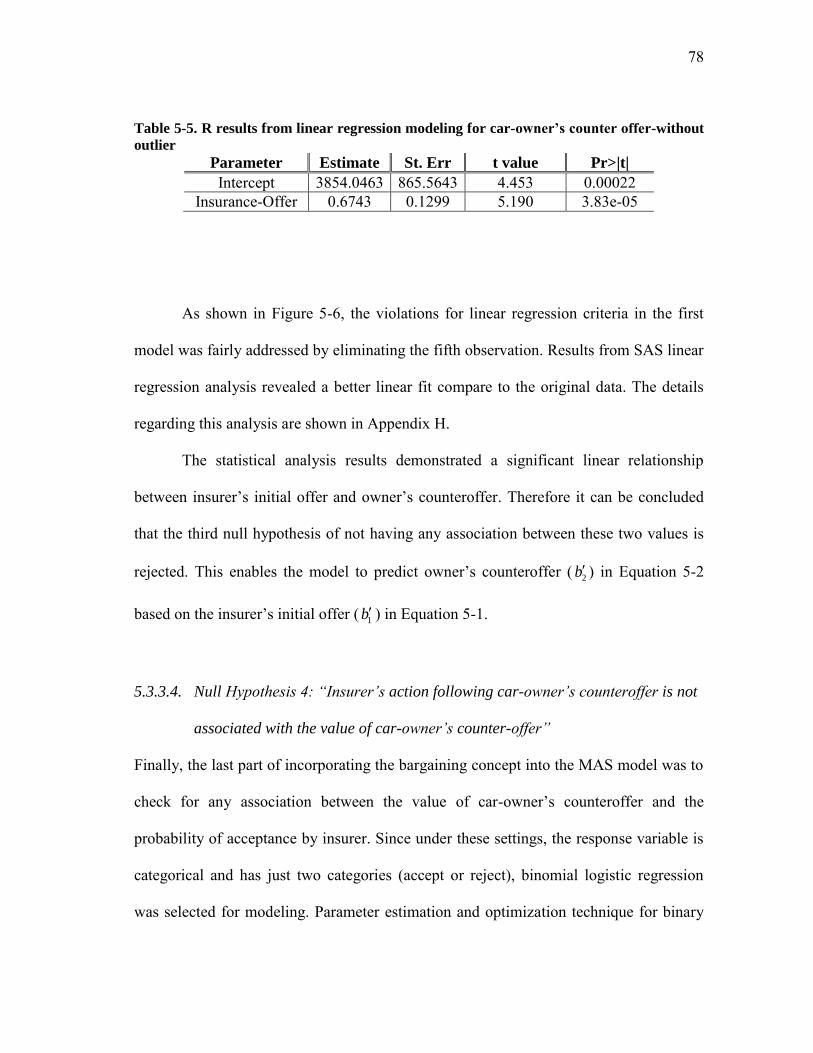
78
Table 5-5. R results from linear regression modeling for car-owner’s counter offer-without
outlier
Parameter Estimate St. Err t value Pr>|t|
Intercept 3854.0463 865.5643 4.453 0.00022 Insurance-Offer 0.6743 0.1299 5.190 3.83e-05
As shown in Figure 5-6, the violations for linear regression criteria in the first
model was fairly addressed by eliminating the fifth observation. Results from SAS linear
regression analysis revealed a better linear fit compare to the original data. The details
regarding this analysis are shown in Appendix H.
The statistical analysis results demonstrated a significant linear relationship
between insurer’s initial offer and owner’s counteroffer. Therefore it can be concluded
that the third null hypothesis of not having any association between these two values is
rejected. This enables the model to predict owner’s counteroffer ( 2b ) in Equation 5-2
based on the insurer’s initial offer ( 1b ) in Equation 5-1.
5.3.3.4. Null Hypothesis 4: “Insurer’s action following car-owner’s counteroffer is not
associated with the value of car-owner’s counter-offer”
Finally, the last part of incorporating the bargaining concept into the MAS model was to
check for any association between the value of car-owner’s counteroffer and the
probability of acceptance by insurer. Since under these settings, the response variable is
categorical and has just two categories (accept or reject), binomial logistic regression
was selected for modeling. Parameter estimation and optimization technique for binary

79
logit models were previously described in the Section 4. Table 5-6 shows the regression
results. The details regarding the regression results are included in Appendix I.
Table 5-6. Results from binomial logistic regression - R
Parameter Estimate St. Err Z Value Pr(>|Z|)
Intercept -1.565e+1 7.427 -2.107 0.0352 offer 1.99e-03 9.089e-04 2.190 0.0285
The outcome from logistic regression indicates a statistical significance for the
influence of car-owner’s counteroffer on insurer’s acceptance and hence the null
hypothesis of having no association between these parameters is rejected. The resulting
equation can be written as below:
212
21
log 15.65 1.99 03*( )1
Pe b
P
(5-6)
Equation 5-6 indicates that for every one unit increase in car-owner’s
counteroffer, the log of probability of rejection versus acceptance increases by 1.99*e-
03. Furthermore this shows that the more the counteroffer is the less would be the
likelihood of accepting the offer by the insurer. The results obtained here help predict the
probabilities regarding insurer’s accepting or rejecting owner’s counteroffer ( 21P ) in
Equation 5-2 and conclude the simulation of empirical bargaining procedure in the MAS
model.
80
5.3.4. Estimation Results
As previously mentioned, data from the experimental study was used for estimating
parameters of the empirical model (see Equations 5-1 and 5-2). These parameters
include insurer’s first offer (1b ), car-owner’s counter offer (
2b ) and probabilities
associated with each of the actions ( 11 12 13 21, , , and P P P P ). For the insurer’s first offer, the
statistical analysis showed that the hypothesis of having a model to significantly fit the
data is valid and the model is a Laplace distribution. Furthermore, the results from
multinomial regression analysis showed that the owner’s probability of accepting the
insurer offer, rejecting it, or making a counter offer is significantly associated with the
amount of insurer’s offer. In addition, the analysis indicated that the owner’s
counteroffer is a significant linear relation with the amount of insurer’s offer. Finally the
statistical analysis showed that the insurer’s reaction to owner’s counteroffer is
significantly associated with the amount of owner’s counteroffer. The generalized
bargaining model helps automate the empirical bargaining process in the MAS model
and reveals how agents would behave under various post disaster bargaining situations.
5.3.5. MAS Integration
To integrate the results in the MAS model the following steps should be taken: 1) to
code a program which can generate random variables from a Laplace distribution with
its given parameters, 2) calculate the probabilities associated with homeowners’ action
based on the value generated from the Laplace distribution using Equations 5-5 and 5-5,
3) calculate homeowner’s counter offer based on insurer’s initial offer using the results
81
shown in table 5-5, and finally 4) compute the probabilities associated with insurer’s
action in response to homeowner’s counter offer using Equation 5-6. Accomplishing
these steps leads to calculate the expected value of homeowners payoff in the first period
( 1b ) and concludes this subsection.
5.3.6. Summary
The objective of this section was to define a framework which can represent agents’
organizational behavior while negotiating with higher bargaining power entities such as
insurers. The section started with a theoretical model to present the optimal bargaining
solution under post disaster conditions. The second part of the section was focused on
capturing the same aspect of organizational interaction but from a more realistic point of
view. To accomplish this task, an experiment was designed to support building an
empirical model. Data collected from the experiment was used for parameter estimation
for the empirical model using various statistical analysis methods. The next section
introduces the multi agent framework and elaborates on how the models presented in
Sections 4 and 5 will be incorporated in such a framework.
5.4. LIMITATIONS AND FUTURE WORK
Similar to the previous chapter, there are a few assumptions and limitations associated
with this section which are: 1) simplifying the theoretical bargaining process in a 3-
period bargaining model; 2) using a common discount factor for both of the insurer and
homeowner in the theoretical model; 3) assuming no inside option and a unique outside

82
option for both of the players; 4) assuming certain court payoffs for both players; 5)
assuming a different hypothetical scenario for the empirical model, and 6) not having a
large number of participants for the empirical model.
Future work is needed to address the aforesaid limitations. The theoretical model
needs to integrate additional parameters including inside options or additional outside
options. This can include the outside option of selling properties to other entities with a
higher bargaining power rather than facing the insurer directly. Regarding the empirical
model, a large number of participants is required to address the need for the intensive
data requirement of model fitting due to the maximum likelihood method.

83
6. MULTIAGENT SYSTEM SIMULATION MODEL
6.1. INTRODUCTION
The objective of this section is to present a framework, which is capable of integrating
the proposed spatial and organizational models, and analyze the results. Due to the
complex nature of post-disaster recovery, this framework was based on previously
discussed Multi-dimension Multi Agent Systems (MD-MAS) model. This MAS model
selection allowed for simulating every single agent (homeowner) and their actions under
the governing conditions and assessing the outcomes of their mutual interactions. The
section starts with an introduction to MAS and extends to capture the structure of the
model and its specifications. To proceed, the section presents a case study that considers
both theoretical and empirical models to assess the recovery dynamics in the two-
pronged spatial-organizational domain. The result from the model is then checked for
sensitivity to different simulation set-up parameters. Finally the section ends with the
summary of key discoveries and directions for future research.
6.2. MULTI AGENT SYSTEMS
The Multi Agent Systems (MAS) approach is applied in many research domains that
require capturing dynamic interactions among multiple stakeholders. Examples of MAS
application covers a wide range of domains including land-use and land-cover change
(Parker et. al. 2003), epidemiology (Yergens et al. 2006), and traffic and transportation
84
in complex networks (Burmeister et al. 1997). The MAS results often reveal the hidden
behavior by accounting for temporal spatial interactions.
The MAS model is based on simulation of intelligent agents designed to achieve
a variety of goals. The agents may have common or conflicting goals and may interact
with other agents directly or indirectly (Bellifemine, 2007). Wooldridge and Jennings
(1995) classifies intelligent agents as being reactive, proactive, and social. Furthermore,
Padgham and Winikoff (2004) define an intelligent agent as an autonomous system
situated in an environment, which is reactive to the changes in the environment, pursues
its objectives determinedly while being flexible, recuperates from failures, and finally
interacts with other agents.
The MAS model features have led to their implementation in different research
areas such as modeling population dynamics based on economic status and cultural
identity (Benenson, 1998), spatial patterns of unemployment (Conley and Topa, 2002),
firms’ spatial competition (Collins and Sherstyuk, 2000), complexity in human-
environment interaction (An et al., 2005), land-use and land-cover change (Parker et. al,
2003), technology diffusion, resource use changes and policy analysis (Berger, 2001),
and residential land use patterns (Irwin and Bockstael, 2002).
This wide range of applications for MAS models shows its high potential in
handling the real-world complexities and as such qualifies it as an ideal candidate to
represent a framework for modeling interactions among the homeowners and other
agents during the post disaster recovery process.

85
6.3. MAS-MODEL STRUCTURE AND SPECIFICATIONS
In this section, the structure of the MAS model is presented in 4 sequential subsections.
The first subsection named as import-world module, elaborates on the multi-agent
framework chosen for the model and extends on how real world data was imported into
this framework. To illustrate the process, a neighborhood in College Station, Texas is
selected and is subsequently used to show model sensitivity to both theoretical and
empirical models, and initial parameters. The second subsection presents the details of
homeowners’ decision making structure for both spatial and organizational domains and
is named as agent-setup module. This is succeeded by the third subsection named as run
module, which controls the details regarding each run of the simulation by incorporating
the temporal and organizational aspect of recovery. Finally the last subsection illustrates
the methods used to capture emergent spatial phenomena such as formation of clusters
resulting from agents’ interactions and was described as cluster module.
6.3.1. “import-world” Module
The multi-agent framework chosen for this dissertation was Netlogo (Wilensky, 1999).
Netlogo started as StarlogoT in 1997 by Uri Wilensky and was named as Netlogo in
2002. Netlogo is a Java-based multi-domain multi-agent framework and has been used to
capture the complexity of a variety of topics in the literature. This include population
variation (BenDor et al. 2009), financial market (Dréau et al. 2009), green house effect
(Shultz 2009), infection and epidemic dynamics (Kleczkowski and Maharaj 2010) and
forest fire simulation (Niazi 2010).
86
One of the great advantages of multi-agent frameworks such as Netlogo is their
ability to model spatial aspects of the problem. This plays a crucial role in the context of
recovery dynamics where the recovery is significantly linked to the distribution of
agents’ location around the source of the disaster or its focal point. For the purpose of
this dissertation, the same feature was used to import the real conditions to the simulated
model.
There are two ways to import location data in Netlogo. In the first, the program
detects subjects based on their color. This makes it easier for programming but at the
same time impedes its applicability for the cases where there are a wide range of
gradient colors and the cases where a color is shared among different subjects. In
contrast to the first approach, the next method is based on using the GIS extension of the
program. This extension enables the model to import GIS data in two forms of data files,
which are ascii grid file and shape files. Ascii grid files include raster data whereas
shape files include vector data such as points, lines and polygons (Wilensky 1999). The
disadvantage regarding the second approach is its shortcoming in the types of imported
data. This shortcoming can be attributed to the fact that the software is incapable of
importing data from Google Earth© which is one of the most popular mapping software
and browser.
Programs such as Google Earth© provide users with universal GIS data.
However, this data cannot be saved as compatible formats with Netlogo. The outputs
from Google Earth© have another file format named as Keyhole Markup Language
(KML) which is the Extensible Markup Language (XML) form of the graphical data for

87
the use in maps and map browsers. To address this shortcoming, a KML to shape file
convertor (Zonum Solutions 2011) was used to convert data from KML extension to
shape files that are usable in Netlogo framework. This enabled the model to benefit from
the integrated features in Google Earth© such as pinpointing the targets and drawing
polylines and polygons. The steps taken to import geographical information in Netlogo
is described below for a selected neighborhood in College Station, Texas. Figure 6-1
shows this area.
Figure 6-1. Area selection in Google Earth©

88
After area selection, the next step was to pinpoint targets (homes) and draw the
polylines (streets) to import them as points and lines in the model. This step was
performed using Google Earth© features and is shown in Figure 6-2 and Figure 6-3.
a) aerial map
b) aerial map with points
Figure 6-2. Aerial map with points

89
Figure 6-3 displays the added polylines to the area in Google Earth© that
characterized the streets for model simulation.
Figure 6-3. Aerial map with points and polylines
After defining targets (homes) and polylines (streets), the next step was to import
the data in Netlogo modeling framework. The importing procedure was accomplished by
performing different subroutines and functions, list of which is shown in Figure 6-4
below. As shown in the figure, homes were detected as black dots whereas the streets or
other infrastructure were distinguished as black polylines.

90
Figure 6-4. Imported area in Netlogo framework
In this figure, subroutines, functions, and controllers for each module known as
programming components (PC) are presented. These programming components are
separately illustrated for each module in their corresponding subsection. For the import-
world module these components are listed in Figure 6-5.
91
SUB import-world import-drawing import-points import-paths detect-paths (as patches) clear-drawing END ------------------------------------------------------- FUNCTION import-drawing load(aerial-photo) END ------------------------------------------------------- FUNCTION import-points connect(points-database)
define j = 0 set i number of points in database while j <= i load(i) j = j + 1 END ------------------------------------------------------- FUNCTION import-paths connect(paths-database) define j = 0 set i number of points in database while j <= i load(i) j = j + 1
END ------------------------------------------------------- FUNCTION detect-path (as patches) ask patches if [intersect(patch,path)] = true [set patch as path] END
Figure 6-5. “import-world” pseudo code
After successfully importing the geographical data in Netlogo, The next step is to
identify each agent and assign its properties. This is the objective of the next subsection.

92
6.3.2. “setup-agent” Module
The goal of this simulation step is to setup homeowners’ decision-making structure and
characterize a hypothetical case of a disaster. This was followed by defining variables
that were previously introduced for both the theoretical and empirical models and was
accomplished through a series of actions, 1) define the source of disaster, 2) characterize
the points as homeowners by assigning them a decision-making structure for both
theoretical and empirical models, and 3) assign proper level of damage to both homes
and infrastructure based on their distance from the source of disaster. These are shown in
Figure 6-6.
Figure 6-6. Characterized model in Netlogo

93
Parameters modeled in Figure 6-6 are the same as those resulted from the data
used in spatial experiment in Section 4. According to the experiment results,
homeowners’ reconstruction decision is significantly associated with three variables
which are: 1) the ratio of available funds to reconstruction costs; 2) percent of damages
in the neighborhood which was categorized into two categories of below and over 50
percent of damages by using different icons; and 3) availability of infrastructure which
was classified in three groups of not available, available in three month and available, by
using different color codes.
Therefore the sequence of events in this subsection is as follow, initially the
disaster took place in the area and affected both homeowners and infrastructure.
Subsequent to this incident, homeowners are assigned a signal value, which is indicative
of their future property value if they reconstruct. The range of the signal value and its
precision together with homeowners’ initial property value and discount factor are
among the control simulation set-up parameters defined in this module.
At the same time, homeowners start bargaining with insurance companies to
secure funds for future reconstruction. This bargaining procedure is approached by both
theoretical and empirical models. This is then followed by defining neighborhood for
each homeowner. This allows for updating beliefs in homeowners regarding the mean of
property values in the neighborhood and their own future properly value. The parameter
denoting the radius of each homeowner’s neighborhood can also be set by the last
control parameter in this module. These steps are shown in Figure 6-7.

94
SUB setup-agent disaster setup-homeowner END ------------------------------------------------------- FUNCTION disaster damage(infrastructure) damage(homeowners) END ------------------------------------------------------- FUNCTION damage(i) if i=infrastructure [set category] if i=homeowners [set percent-damage] END ------------------------------------------------------- FUNCTION setup-homeowner assign(signal, precision) assign(insurance) assign(neighbor) assign-belief END ------------------------------------------------------- FUNCTION assign-belief set-belief(mean-future-property-values) set-belief(own-future-property-value) END
Figure 6-7. “setup-agent” pseudo code
After setting up the belief structure for homeowners, the next part is to simulate
their actions based on the existing conditions in the area. This is the objective of the next
subsection.
6.3.3. “run” Module
This module captures the temporal behavior of homeowners including the way they
update their beliefs at each time step during the recovery process. As previously
mentioned, two approaches were integrated in the model to capture the spatial and
organizational interactions of agents. In the theoretical-spatial model, homeowners’

95
behavior is based on the concepts of game theory and their mixed reconstruction
strategy, whereas in the empirical-spatial model this behavior is a function of
homeowners’ available funds versus cost of reconstruction, percent of damages in the
environment and availability of infrastructure. Similarly for the organizational domain,
the theoretical model is based on bargaining theory whereas the empirical model
captures the results from the experimental study. Agents’ decisions in each of these
approaches relies on their beliefs at the time of simulation which is updated in every
time step using this module.
Furthermore to generate hybrid models, a parameter was defined to assign
weights to each model. The sequence of events for each run of the model is as follows:
1) homeowners observe the current conditions in the area and update their beliefs
accordingly; and 2) homeowners calculate their probability of reconstruction based on
their updated beliefs and act respectively. This is shown in details in Figure 6-8.
96
SUB run Loop [ I = I + 1:I = total number of agents [stop] select agent:select neighbor -----------Reconstruction Strategy based on Experiment----------- Log(P(W)|P(R))=f(r2,pd,ai) Log(P(L)|P(R))=f’(r2,pd,ai) Calc-P(R) (Probability of Reconstruction) (EQUATION 4-33 & 4-34)
Calc-P(W) (Probability of Wait) (EQUATION 4-33 & 4-34)
Calc-P(L) (Probability of Leaving) (EQUATION 4-33 & 4-34) -----------Reconstruction Strategy based on Theory--------------
[Update-Belief agent(Signals Only)
if neighbor.reconstruct = true then
[Update-Belief agent](Signals & Real values) endif Calc-EVI (Immediate) Calc-EVW (Waiting) Calc-P(R) [reconstruct] [wait] (EQUATION 4-16) -----------Bargaining Strategy based on Theory-------------- Calc-Eq(offer) (SUBSECTION 5-2-3) -----------Bargaining Strategy based on Experiment-------------- Calc-b1 (expected payoff first round) (EQUATION 5-1)
Calc-b2 (expected payoff counteroffer) (EQUATION 5-2) T= T + 1 ] END
Figure 6-8. “run” pseudo code
6.3.4. “cluster” Module
The first three subsections addressed how the micro-level objectives of this dissertation
were incorporated in the multi-agent environment. The last subsection will focus on the
macro-level objective of this dissertation. Therefore, the objective of this subsection is to
create a feature in the multi-agent framework, which can detect any emergent
phenomena such as spatial cluster formation.
For the purpose of recovery pattern recognition, two clustering algorithms were
proposed: 1) Density Based Spatial Clustering of Applications with Noise (DBSCAN)

97
proposed by Ester et al. (1996); and 2) Clique algorithm. The results from both
algorithms were contrasted to each other to identify the best algorithm for the purpose of
this dissertation.
6.3.4.1. DBSCAN clustering algorithm
DBSCAN is one of the most frequent clustering algorithms cited in the literature with
the ranking of 22nd in the field of data mining (Microsoft 2010). In this algorithm, the
main idea behind detecting clusters is that for each point of a given cluster, the
neighborhood with a given radius must have at least a given number of members.
Therefore a cluster can be characterized by two key parameters: 1) Neighborhood, which
is the neighboring area within a given radius; and 2) Minimum points, which are the
minimum number of points that must exist within a cluster.
Based on these definitions, three classifications are illustrated founded on the
concept of points reachability, which are: 1) Directly Density Reachable, which is the
case where a point exists within the neighborhood of another point and that point
satisfies the minimum points criterion for clusters; 2) Density Reachable, in which a
point is not directly reachable by another point but is reachable through a set of
intermediate directly reachable points; and 3) Density Connected, which is the case
where two points are neither directly density reachable nor density reachable but are
density reachable to a single common point (Ester et al. 1996).
Now, according to these definitions, a cluster is a set of density-connected points
which is maximal with regard to density reachability. The pseudo code of this algorithm

98
is shown in Figure 6-9, in which D is the set of points, eps is the radius defining the
neighborhood, and MinPts is the minimum amount of points required to form a cluster
(Ester et al. 1996).
FUNCTION DBSCAN(D, eps, MinPts) C = 0 foreach point P in D if P.flagged = False set P as flagged
N = countNeighbors (P, eps) if size(N) < MinPts set P as NOISE else set C as New(cluster) checkCluster(P, N, C, eps, MinPts) END ------------------------------------------------------ FUNCTION checkCluster(P, N, C, eps, MinPts) cluster(C) = cluster(C) + P foreach point Q in N if Q.flagged = False set Q as visited M = countNeighbors(Q, eps) if sizeof(M) >= MinPts
set N = N + M if Q.ismemberofCluster = False cluster(C) = cluster(C) + Q END
Figure 6-9. DBSCAN pseudo code
6.3.4.2. Clique algorithm
The goal of clique algorithm is to find a set of complete sub-graphs within a graph that
satisfies a certain criterion. The clique algorithm was initiated by Luce and Perry (1949)
who used it in social networks and to find people who all know each other, and became
very popular afterwards.

99
In this algorithm, the research problem is modeled as a connected graph ( , )G V E
that consists of a set of vertices V and a set of unordered pairs, called edges E . Cliques
are any subsets of vertices T in G where any pair of vertices forms an edge in G . Then
the objective is to detect the maximum and maximal cliques. Maximal cliques are those
that cannot be extended by including any more adjacent vertices, while maximum
cliques are the ones with maximum number of vertices. For the purpose of this research,
the vertices represent the reconstructed homeowners and the edges denote the distance
between any pair of homeowners. In this subsection, the objective was not to detect
maximal or maximum cliques but to find the number of homeowners who were a part of
a clique with size of n , where n denotes the minimum number of homeowners. The
following pseudo code displays how this algorithm was integrated in the multi-agent
system. As shown in Figure 6-10, for every point in each sub-graph, the criteria of
forming a clique of size n are checked, and therefore the results are optimal by brute
force, in which all possible candidates for problem solutions are checked.

100
SUB clique dim D dim K(D)
D = set of homeowners foreach point P in D if P.reconstructed foreach point M in neighbor-radius point P if M.reconstructed create a link from P to M set K(P)=K(P)+M next next checkClique(P,K(P),no-clique) END ------------------------------------------------------
FUNCTION checkClique(P,K(P),no-clique) dim N foreach point N in K(P) foreach point L in K(N) if point L is a member of K(K(P)) set sum(N) = sum(N) + 1 next next foreach point D in K(P) if sum (D) >= no-clique set D member of Clique(P,K(P),no-clique) END
Figure 6-10. Clique pseudo code
6.3.4.3. Evaluation of cluster-detection algorithms
In this part, the objective is to contrast the aforementioned algorithms. To accomplish
this task the MAS model was used for a new case study. The case study was related to a
region affected by Kobe earthquake in Nagata area by Maki et al. (2007). The area was
imported in Netlogo by detecting the regions based on their colors. Figure 6-11 shows
the original and the imported maps converted to the grayscale format. Since in the
original photo the exact number of properties was not specified, in the simulated model
for each colored region, properties with equal distance from each other were
automatically created. The next step was to assign proper level of damage to each

101
homeowner. This was performed by the color coding on the original map in which red
showed major damage, yellow was moderate, blue indicated no damage, green was
slight damage, pink was burned out, and white showed no information.
a)original (Maki et al. 2007)
b)edited
c)imported in Netlogo
Figure 6-11. Case study – Kobe earthquake
Although the multi agent model developed here has its own simplifications, the
goal was to examine its ability to capture the major concepts. After defining the model,
both clustering algorithms were applied to the model. Figure 6-12 shows the results from
a single run of the model for the Kobe case study.

102
Figure 6-12. Comparison of the two cluster-detection algorithms
In this case study, the figures on the left are all identical and represent the initial
phase of the study. The black squares denote the properties that have been reconstructed.
The neighborhood defined for each property is shown by the drawn circle on the figure.
The case was tested for different scenarios in which the neighborhood radius was kept

103
the same and the minimum acceptable properties to form a cluster, was changed. This
number was changed from a minimum of three to a maximum of five.
In Figure 6-12, the second column shows the results from application of the
clique algorithm, whereas the third column shows the results for DBSCAN algorithm.
Although there exist similarities between the two methods, Clique algorithm being
optimal, shows a better coverage of properties that are believed to form a cluster
compared to the DBSCAN algorithm and, as such, was selected as the preferred cluster-
detection algorithm in this dissertation. This is clearly shown in Figures 6-12-b1 and 6-
12-b2.
6.3.4.4. Hypothesis testing
After selection of clique algorithm as the preferred cluster detection method for this
research, the algorithm was used for Kobe case study to examine the level of
significance of cluster formation in the model. This required developing a null
hypothesis for the model. The proposed null hypothesis would have to be a certain
percentage for cluster formation. Consequently performing the statistical procedure
shows whether the percentage of cluster formation is significant assuming the proposed
confidence level.
The hypothesis testing was formulated using a minimum rate of cluster-
formation. This minimum rate was set to be 50 percent of reconstructed properties.
Hence, accepting the alternate hypothesis would indicate that clustering in reconstruction

104
occurs more than 50 percent of the time. Assuming normality and unknown variance for
the population, a t-statistic was used for the test:
00 0 1 0 0 0 , 1: , : , ,
/n
XH H T t t
S n
(6-1)
where 0H is the null hypothesis,
1H is the alternative hypothesis, 0T is the test statistic,
and 0t is the rejection criterion. Since the t statistic is bigger than the rejection criterion,
the hypothesis of having a cluster formation equal to 50% is rejected and the alternative
hypothesis is accepted. This denotes that the rate of cluster formation is higher than
50%. Table 6-1 shows the results.
Table 6-1. Results from t test
t P-value Low
Interval
High
Interval
T test for 0.5 3.7438 2.375E-4 0.5452682 0.6460363
Based on the estimated p-values, it can be concluded having a level of cluster
formation higher than 50 percent is statistically significant base on a 95% confidence
level. Furthermore the confidence interval for the mean lies within the range of
[0.5452,0.646].
6.4. MODEL VALIDATION
Model validation in simulation models in general and social dynamics models in
particular is an inherently difficult task and a point of disagreement among the

105
researchers. The contradiction lies in the very essence of the modeling philosophy,
should models be the representative of the reality – as exists or built in future, or should
models be purpose-driven and focus on authenticity rather than statistical results
(Sterman, 2000). In this subsection, the goal is to pursue both approaches and strike the
balance between the parsimony and accuracy.
To examine the robustness of the model, a series of sensitivity analyses was
performed. These analyses started with the theoretical model by testing its reconstruction
sensitivity to a set of parameters, such as: 1) accuracy of signals through coefficient of
variation; and 2) economic parameters, such as discount factor. The base model was
assumed to have a discount factor of 0.9, coefficient of variation of 0.5, neighbor radius
of 4, initial value of $250K. Since discount factor and coefficient of variation were
separately defined just for the theoretical approach of the spatial model, the following
sensitivity analyses were performed for that specific part of the model.
To accomplish the task, two values were considered for each parameter. For
discount factor these values were 0.9 and 0.5, whereas for coefficient of variation these
values were 0.5 and 2. The logic behind these selections was that each represents an
extreme for that parameter. For example, the discount factor of 0.5 indicates a high
discounting which is in contrast to the discount factor of 0.9. On the other hand, the
coefficient of variation of 2 denotes a high level of variance, which is in contrast to the
coefficient of variation 0.5. The results from the simulation were depicted in Figure 6-
13. Explanation of the results is separately shown for each parameter.

106
Figure 6-13. Model sensitivity to discount factor and coefficient of variation
6.4.1. Sensitivity to Coefficient of Variation
The first feature of the model is its sensitivity to accuracy of signals through coefficient
of variation (CofV). As previously stated, a higher CofV indicates that the signal is a
poor indicator of the true future value or in other words, denotes a high variance
associated with the value.
The results show that given a fixed discount factor of 0.5, the reconstruction rate
decreases as the level of uncertainty for the signals increases. This is clearly shown for
the two sets of curves shown in Figure 6-13. The first two curves have a triangle marker
whereas the other two have a rectangle marker. This is due to the fact that homeowners
decide based on their observed signals from their surrounding neighbors. The accuracy
0.00%
10.00%
20.00%
30.00%
40.00%
50.00%
60.00%
70.00%
80.00%
90.00%
100.00%
0
0.0
2
0.0
4
0.0
6
0.0
8
0.1
0.1
2
0.1
4
0.1
6
0.1
8
0.2
0.2
2
0.2
4
0.2
6
0.2
8
0.3
0.3
2
0.3
4
0.3
6
0.3
8
0.4
0.4
2
0.4
4
0.4
6
0.4
8
0.5
DF=0.5-CofV=0.5
DF=0.5-CofV=2
DF=0.9-CofV=0.5
DF=0.9-CofV=2
Reconstruction Rate
Cu
mu
lati
ve D
istr
ibu
tio
n

107
of these signals is inversely proportional to their variance. Therefore with increasing
variance (uncertainty), owners become more hesitant in starting reconstruction and
prefer to wait and observe other neighbors’ action to guarantee a positive net value for
reconstruction.
6.4.2. Sensitivity to Discount Factor
The next characteristic of the model is its sensitivity to the level of discounting. The
results show that given a fixed CoV, reconstruction rate increases as discount factor
(DF) increases. This is again shown in for the two sets in Figure 6-13 displayed as full
lines and dash lines.
The reason behind this behavior is that discount rate is one of the driving
parameters in the process of decision making. Applying a high discount rate to the
present value calculations assigns more weight to the current payoffs compared to
payoffs anticipated in the future. Therefore one expects to observe an increase in the
number of reconstructing owners by increasing the discount rate and vice versa. It is
assumed that all the homeowners have the same discount rate.
6.4.3. Theoretical Model versus Hybrid and Empirical Model
The third sensitivity analysis was to contrast the different models to check for their
effect on the rate of reconstruction. These different models consist of, 1) Theoretical
model, 2) Empirical model, and 3) Hybrid model. For the hybrid model the assumption
108
was to consider an equal weight for both theoretical and empirical models. The results
from simulation is shown in Figure 6-14.
Figure 6-14. Sensitivity analysis for different models
For the purpose of simulation, a discount factor of 0.5 and a coefficient of
variation of 0.5 was considered for the model. The results shown in Figure 6-14, denotes
that the reconstruction rate in the empirical model has a very limited dispersion. This is
due to the fact that in the empirical model, reconstruction decisions is based on three
parameters which are: 1) ratio of available funds to reconstruction costs ( 2r ); and 2)
percent of damages in the neighborhood and availability of infrastructure. Among these
0.00%
10.00%
20.00%
30.00%
40.00%
50.00%
60.00%
70.00%
80.00%
90.00%
100.00%0
0.0
5
0.1
0.1
5
0.2
0.2
5
0.3
0.3
5
0.4
0.4
5
0.5
0.5
5
0.6
0.6
5
0.7
0.7
5
0.8
0.8
5
0.9
0.9
5 1
theoretical
empirical
hybrid
Rate of Reconstruction
Cu
mu
lati
ve P
rob
abili
ty

109
parameters, the availability of infrastructure does not change and as a result will not
contribute to the variability of the reconstruction rate. On the other hand 2r which is the
only parameter that is directly affected by the assumed discount factor, is not as
significant as the other two variables in the model. Therefore it is expected to have an
almost constant rate of reconstruction for the empirical model. The other important issue
shown in the figure is the substantially higher rate of reconstruction for empirical model
in contrast to the theoretical model. This result is attributed to the fact that in the
empirical model, the probability of reconstruction significantly increases by availability
of infrastructure and percent of damage in the area. In the model used for simulation,
almost half of the home owners have a damage level of less than 50 percent and are in
vicinity of either available infrastructure or semi-available infrastructure. These
parameters significantly contribute to the high rate of reconstruction in the empirical
model.
In addition, the hybrid model exhibits the characteristics of both empirical and
theoretical model. As shown in Figure 6-14, the level of dispersion has increased
compared to the empirical model which is due to including the equal weight for both
models. The rate of reconstruction is still higher than the theoretical model which is
inherited from the empirical model.
110
7. CONCLUSIONS AND FUTURE RECOMMENDATIONS
7.1. CONCLUSIONS
Modeling the dynamics of post-disaster recovery can play an important role in providing
public decision makers with analytical tools and methods to analyze policies that can
promote fast recovery of the affected areas. To restore the community on a level of a
functional socio-economic entity it is essential that policy makers and homeowners send
signals of strong commitment. Without this, the reconstruction is often sporadic as
spatial and information externalities dominate decisions to reconstruct and stay, or sell
the property and leave.
This dissertation presents a multi-domain behavioral model that captures the
homeowners’ behavior when spatial externalities are present. The multi-domain
considered for this model includes: 1) spatial domain of interaction in which the
behavior of homeowners while interacting with each other was presented; and 2)
organizational domain of interaction which analyzed the behavior of homeowners while
interacting with insurers to secure funding for reconstruction.
A two-pronged approach was utilized, capturing the spatial and organizational
externalities in this research. Regarding the spatial externality, the first approach was
based on a theoretical approach to the existence of spatial externality which led to the
free-rider problem. This results in the situation where homeowners may prefer to wait
and observe the neighbors’ actions rather than starting the reconstruction. As a result, the
homeowners were assumed to have two pure strategies, which are: 1) immediate

111
reconstruction; and 2) wait and observe the neighbors’ action and act accordingly.
Additionally from empirical approach this decision making is made based on a
confluence of parameters such as availability of infrastructure, percent of damage in the
area and financial flexibility of the homeowners. In this dissertation, the solution for
theoretical part was approached through a mixed strategy equilibrium, where
homeowners are indifferent between their strategies when the payoffs are the same. In
addition, the solution for the experimental method was addressed through logistic
regression modeling.
Regarding the organizational domain, the same set of approaches was applied to
the model. The first approach was to capture the characteristics of homeowners’
bargaining behavior in their interaction with insurers from a theoretical point of view,
whereas the next approach was to tackle this problem from an empirical perspective and
by running an experiment.
Based on the developed models, a multi-agent system simulation was developed
to integrate these models and depict the emergent behavior. In this multi-agent model,
homeowners were defined as intelligent agents with a belief structure which is updated
based on the signals from their neighbors.
The results from simulation model confirm that spatial and organizational
externalities play an important role in agents’ decision-making and can greatly impact
the recovery process. The results further highlight the significant impact of discount
factor and the accuracy of the signals on the percentage of reconstruction. Finally,
cluster formation was shown to be an emergent phenomenon during the recovery process

112
and spatial modeling technique demonstrated a significantly higher impact on formation
of clusters in comparison with experimental model and hybrid model.
The model assumed that reconstruction could peak out at less than 100 percent.
Therefore if the property-owners cannot secure a positive payoff from reconstruction,
they will not reconstruct but effectively leave the location eventually.
The issues deserving further attention are those which might have implications
for policy holders. These include setting constraints for availability of funding in regards
to reconstruction of residential units and transportation infrastructure, limiting the
number of insured homeowners, optimizing the methods of resource allocation,
incorporating the dynamics of the transportation infrastructure and others.
7.2. LIMITATIONS
As previously mentioned, this dissertation was intended to investigate the role of two
key intelligent agents in the dynamics of post-disaster recovery and to capture the overall
trend in post disaster reconstruction. While the number of affecting stakeholders could
be much more than what has been considered, this research followed the principle of
parsimony to clearly track the dynamics created in the system.
This model does not attempt to fully explain a very complex post-disaster
reconstruction process, nor to capture heterogeneity in owners’ behavior, but to provide
a theoretical foundation for investigating the phenomenon of spatial cluster formation
and decision-making under uncertainty.

113
It is also important to note that rezoning of the neighbors in abandoned areas and
the impacts of other influencing parameters such as location, density, public policy, and
others have not been considered in the model. Although the multi agent model
developed here has its own simplifications, which include lack of heterogeneity of the
agents, and availability of funds for reconstruction among others, it has an ability to
capture the broad trends.
7.3. CONTRIBUTIONS
7.3.1. General Contributions
The general contributions of this model are: 1) providing a platform to spatially model
the agents and investigate the resulting interactions; and 2) providing a platform with a
potential to observe the impact of public policies on dynamics of post disaster recovery.
7.3.2. Engineering Contributions
From the engineering viewpoint, the key contribution of this research is to provide a
framework which facilitates infrastructure-management in the context of natural hazards.
The capability of incorporating a variety of parameters in the MAS model developed for
this research allows for studying the impact of integrating different reconstruction and
resource allocation polices in the affected areas, which, in turn, will lead to optimizing
the available resources. This could be done in the model by capturing the process of
economic recovery in the community until a full socio-economic restoration is realized.

114
Economic recovery is a critical parameter facing communities affected by
disasters. The economic losses after disasters do not occur instantly but accumulate over
the duration of recovery. In other words, the immediate economic losses have a domino
effect on other sources of economic viability in a community.
For example, in Hurricane Katrina the economic losses other than those resulted
from immediate destructions were due to: 1) damages to industry by disruption in the oil
supply due to the destructions in oil refineries and platforms; 2) damages due to
disruption in commerce attributable to the destruction of highway infrastructure in the
Gulf Coast; 3) damages due to interruption in operation of US ports; and 4) damages due
to job losses and businesses (United States Department of Commerce, 2006). Similar
conditions were present for other natural disasters, such as the incurred economic losses
in Des Moines, Iowa due to the closure of the water treatment plant and disruption of
railroad traffic due to the damages to the flooded tracks; the economic losses suffered
due to the collapse of Oakland Bay Bridge, which included the disruptions created by the
destruction of major highway corridors; and the closure of local airport during the Loma
Prieta earthquake. Furthermore, loss of tourism was also among one of the major sources
for economic losses which were experienced in the affected communities, especially in
Sun Belt (FEMA 421, 1998).
Additionally, as shown in Figure 7-1, economic growth and recovery is among
the three pillars of a sustainable design of engineering structures (Adams 2006) and
together with public safety are the two driving factors for post disaster planning.
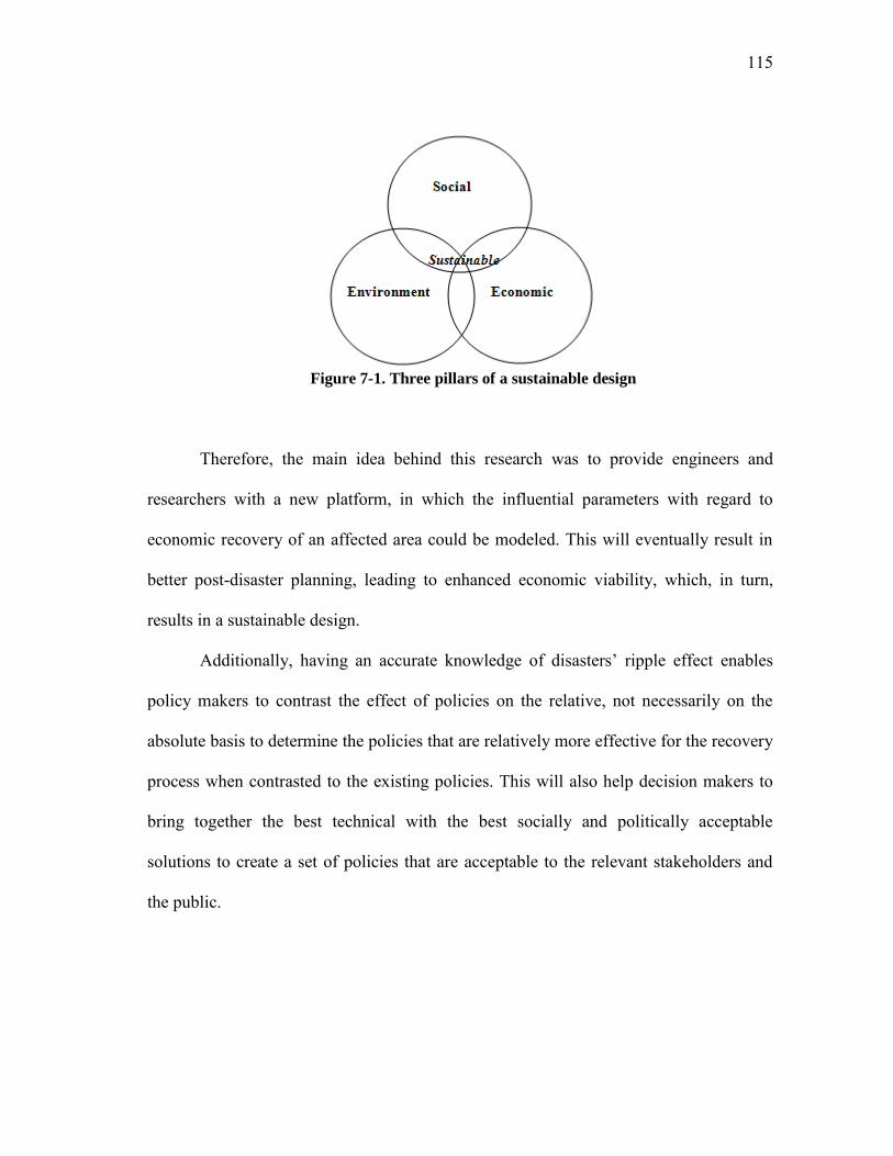
115
Figure 7-1. Three pillars of a sustainable design
Therefore, the main idea behind this research was to provide engineers and
researchers with a new platform, in which the influential parameters with regard to
economic recovery of an affected area could be modeled. This will eventually result in
better post-disaster planning, leading to enhanced economic viability, which, in turn,
results in a sustainable design.
Additionally, having an accurate knowledge of disasters’ ripple effect enables
policy makers to contrast the effect of policies on the relative, not necessarily on the
absolute basis to determine the policies that are relatively more effective for the recovery
process when contrasted to the existing policies. This will also help decision makers to
bring together the best technical with the best socially and politically acceptable
solutions to create a set of policies that are acceptable to the relevant stakeholders and
the public.

116
REFERENCES
Academic Technology Services (2011). Introduction to SAS. UCLA, Statistical Consulting Group. <http://www.ats.ucla.edu/stat/sas/notes2> (May 24, 2011).
Adams, W.M. (2006). The future of sustainability: re-thinking environment and
development in the twenty-first century. Report of the International Union for Conservation of Nature Renowned Thinkers Meeting, <http://cmsdata.iucn.org/downloads/iucn_future_of_sustanability.pdf> (May 23, 2010)
Agresti, A. (1990). Categorical data analysis. John Wiley & Sons, New York, NY. Albala-Bertrand, J.M. (1993). The political economy of large natural disasters: with
special reference to developing countries. Clarendon Press, Oxford, UK. Alesch, D. J. and Holly J. N. (1998). Small business failure, survival, and recovery:
lessons from January 1994 Northridge Earthquake. NEHRP Conference and Workshop on Research on the Northridge, California Earthquake, Richmond, CA
An, L., Linderman, M., Qi, J., Shortridge, A. and Liu, J. (2005). “Exploring complexity
in a human–environment system: An agent-based spatial model for multidisciplinary and multiscale integration.” Annals of the Association of
American Geographers, 95, 54–79. Anbarci, N., Skaperdas, S., and Syropoulos C. (2002). “Comparing bargaining solutions
in the shadow of conflict: How norms against threats can have real effects.” Journal
of Economic Theory, 106(1), 1-16. Applied Technology Council (1991). ATC-25: Seismic vulnerability and impact of
disruption on lifelines in the conterminous United States. Federal Emergency Management Agency, Applied Technology Council, Redwood City, CA.
Basu K., Bhattacharya S., and Mishra A. (1992). “Notes on bribery and the control of
corruption.” Journal of Public Economics, 48(3), 349-359. Bates, F. L. (1982). “Recovery, change and development: A longitudinal study of the
Guatemalan Earthquake.” University of Georgia, Department of Sociology, Athens, GA.
Bates, F. L., and Peacock , W. G. (1993). Living conditions, disasters and development.
University of Georgia Press, Athens, GA.
117
Bates, F. L., and Pelanda, C. (1994). “An ecological approach to disasters.” R.R. Dynes and K. J. Tierney (eds.), Disasters, collective behavior, and social organization. University of Delaware Press, Newark, 149-159.
Bellifemine, F., Caire G., and Greenwood D. (2007). Developing multi-agent systems
with JADE. John Wiley & Sons, New York. BenDor, T., Westervelt, J., Aurambout, J. & Meyer, W. (2009). “Simulating population
variation and movement within fragmented landscapes: An application to the gopher tortoise (Gopherus polyphemus).” Ecological Modeling, 220(6), 867-878.
Benenson, I. (1998). “Multi-agent simulations of residential dynamics in the city.”
Computers, Environment, and Urban Systems, 22 (1), 25-42. Berger, T. (2001). “Agent-based spatial models applied to agriculture: a simulation tool
for technology diffusion, resource use changes and policy analysis.” Agricultural
Economics, 25, 245–260. Berke, P. R., Kartez, J. and Wenger D. (1993). “Recovery after disaster: Achieving
sustainable development, mitigation and equity.” Disasters, 17(2), 93-109 Blaikie, P., Cannon, T., Davis, I., and Wisner B. (1994). At risk: natural hazards,
people’s vulnerability, and disasters. Routledge, New York. Boisvert, R. (1992). “Indirect losses from a catastrophic earthquake and local, regional,
and national interest.” Indirect economic consequences of a catastrophic
earthquake, National Earthquake Hazards Reduction Program, Federal Emergency Management Agency, Washington, DC, 207–265.
Bolin, R. C. (1993). Household and community recovery after earthquakes. Institute of
Behavioral Science, University of Colorado Boulder, CO. Bolin, R. C., and Bolton P. (1983). “Recovery in Nicaragua and the USA.” International
Journal of Mass Emergencies and Disasters, 1(1), 125-152. Bolin, R. C. and Trainer P. (1978). “Modes of family recovery following disaster: A
cross national study. ” E. Quarantelli (ed.), Disasters: Theory and research. Sage, Beverly Hills, CA, 1978, 234-247.
Boisvert, R. (1992). “Indirect losses from a catastrophic earthquake and local, regional,
and national interest.” in: “Indirect economic consequences of a catastrophic earthquake”, National Earthquake Hazards Reduction Program, Federal Emergency Management Agency, Washington, DC, 207–265.

118
Borch, K. H. (1962). “Equilibrium in a reinsurance market.” Econometrica, 30, 424-444. Brookshire, D. S., Chang, S. E., Cochrane, H., Olson, R. A., Rose, A. and Steenson, J.
(1997). “Direct and indirect economic losses from earthquake damage.”
Earthquake Spectra, 13(4), 683-701. Burmeister B., Haddadi, A., and Matylis, G. (1997). “Application of multi-agent systems
in traffic and transportation.” IEEE Proceedings on Software Engineering, 144(1), 51-60.
Chang, S. E. and Miles S. B. (2004). “The dynamics of recovery: A framework.” Y.
Okuyama and S. E. Chang (eds), Modeling the spatial economic impact of
disasters. Springer-Verlag, Berlin, 181-204. Cho, S., Gordon, P., Moore II, J.E., Richardson, H.W., Shinozuka, M. and Chang, S.E.
(2001). “Integrating transportation network and regional economic models to estimate the costs of a large urban earthquake.” Journal of Regional Science, 41, 39–65.
Cochrane, H.C., Chang, S.E. and Rose, A. (1997). “Indirect economic losses”,
Earthquake loss estimation methodology: HAZUS technical manual, National Institute of Building Sciences, Washington, DC.
Cochrane, H. C. (2004). “Indirect losses from natural disasters: Measurement and myth.”
Y. Okuyama and S.E. Chang (eds), Modeling spatial and economic impacts of
disasters. Springer, New York, NY, 37-52. Cole, S. (1995). “Lifelines and livelihood: A social accounting matrix approach to
calamity preparedness.” Journal of Contingencies and Crisis Management, 3, 1-11.
Cole, S. (1998). “Decision support for calamity preparedness: socioeconomic and
interregional impacts.” M. Shinozuka et al. (eds.), Engineering and
socioeconomic impacts of earthquakes: An analysis of electricity lifeline
disruptions in the new Madrid area. Multidisciplinary Center for Earthquake Engineering Research (MCEER), Buffalo, NY.
Cole, S. (2004). “Geo-hazards in social systems: An insurance matrix approach, Y.
Okuyama and S.E. Chang (eds), Modeling spatial and economic impacts of
disasters. Springer, New York, NY, 103-118. Collins, R. and Sherstyuk, K. (2000), “Spatial competition with three firms: an
experimental study.” Economic Inquiry, 38, 73–94.

119
Conley, T. G. and Topa, G. (2002), “Socio-economic distance and spatial patterns in unemployment.” Journal of Applied Econometrics, 17, 303–327.
Daniel, T. E., Seale, D. A., and Rapoport, A. (1998). “Strategic play and adaptive
learning in the sealed-bid bargaining mechanism.” Journal of Mathematical
Psychology, 42(2-3), 133-166. Davis, H.C. and E. L., Salkin (1984). “Alternative approaches to the estimation of
economic impacts resulting from supply constraints.” Annals of Regional
Science, 18, 25–34. Dréau, D., Stanimirov, D., Carmichael T., & Hadzikadic M. (2009). An agent-based
model of solid tumor progression. Paper presented at the 1st International Conference on Bioinformatics and Computational Biology, New Orleans, LA.
Durkin, M. E. (1984). The economic recovery of small businesses after earthquakes: the
Coalinga experience. International Conference on Natural Hazards Mitigation Research and Practice, New Delhi, India.
Ellis, C.J. and Fender, J. (1985). “Wage bargaining in a macroeconomic model with
rationing.” Quarterly Journal of Economics, 100, 625-650. Ester, M., Kriegel HP, Sander J., and Xu X. (1996). A density-based algorithm for
discovering clusters in large spatial databases with noise. Proceedings of 2nd International Conference on Knowledge Discovery and Data Mining (KDD-96), Portland, Oregon.
FEMA (1998). Planning for post-disaster recovery and reconstruction., Federal
Emergency Management Agency. <http://www.fema.gov/library/viewRecord.do?id=1558> (June 23, 2010)
Gertler, M., and Trigari A. (2009). “Unemployment fluctuations with staggered Nash
wage bargaining.” Journal of Political Economy, 117(1), 41-86. Gordon, P. and Richardson, H.W. (1996). The business interruption effects of the
Northridge earthquake. Lusk Center Research Institute, University of Southern California, Los Angeles, CA.
Gordon, P., Richardson, H.W. and Davis, B. (1998). “Transport-related impacts of the
Northridge earthquake.” Journal of Transportation and Statistics, 1, 22–36.
120
Gordon, P., Moore II, J.E., Richardson, H.W., Shinozuka, M., An, D. and Cho, S. (2004). “Earthquake disaster mitigation for urban transportation systems: an integrated methodology that builds on the Kobe and Northridge experiences.” Y. Okuyama and S.E. Chang (eds.), Modeling spatial and economic impacts of
disasters. Springer, New York, NY, 205–232. Grout, P. A. (1984). “Investment and wages in the absence of binding contracts: A Nash
bargaining approach.” Econometrica, 52, 449-460. Groves, T. and Ledyard, J. (1977). “Optimal allocation of public goods: a solution to the
Free Rider problem.” Econometrica, 45(4), 783-809. Haas, J. E., Kates, R. W. and Bowden M. (1977). Reconstruction following disaster.
MIT Press, Cambridge, MA. Heinz Center for Science, Economics and the Environment (2000). The hidden costs of
coastal hazards: implications for risk assessment and mitigation. Island Press, Washington, DC.
Hendricks, K. and Porter, R. (1996). “The timing and incidence of exploratory drilling
on offshore wildcat tracts.” The American Economic Review, 86(3), 388-407. Hewitt, K. (1997). Regions of risks: A geographical introduction to disasters. Addison
Wesley Longman Limited, Essex, UK. Hindriks, J., Keen, M., and Muthoo, A. (1999). “Corruption, extortion and evasion.”
Journal of Public Economics, 74(3), 395-430. Hogg, S. J. (1980). “Reconstruction following seismic disaster in Venzone, Friuli.”
Disasters, 4(2), 173-185. Irwin E. G., and Bockstael, N. E. (2002). “Interacting agents, spatial externalities and the
evolution of residential land use patterns.” Journal of Economic Geography,
2(1), 31-54. Kihlstrom, R. E. and Roth A. E. (1982). “Risk aversion and the negotiation of insurance
contracts.” Journal of Risk and Insurance, 49, 372-387. Kleczkowski, A., Maharaj, S. (2010). Stay at home, wash your hands: epidemic
dynamics with awareness of infection. Proceedings of Summer Computer Simulation Conference, Ottawa, Canada.
Knabe, A. (2009). “Implementing endogenous inside options in Nash wage bargaining
models.” Mathematical Social Sciences, 57(2), 161-176.

121
Kroll, C. A., Landis, J. D., Shen, Q., and Stryker, S. (1991). Economic impacts of Loma
Prieta earthquake: A focus on small businesses. Paper No: 91-187, University of California Transportation Center and the Center for Real Estate and Urban Economics, University of California at Berkeley, CA.
Luce, R. D., and Perry, A. D. (1949). "A method of matrix analysis of group structure"
Psychometrika, 14 (2), 95–116. Lundberg, S., and Pollak., R. A. (1993). “Separate spheres bargaining and the marriage
market.” Journal of Political Economy, 101(6), 988-1010. Maki, N., Kawakata, H., Yoshitomi, P. , Urakawa, V., Chan, K., Matsuura, H., Tatsumi,
K., Hara, T., Inokuchi, M., Higashida, M., Hayashi, H. and Kawata, Y. (2007). “Building an integrated database system of information on disaster hazard risk, and recovery process-cross-media database.” Annuals of Disaster, 50C, 63-67.
Manser, M., and Brown, M. (1980). “Marriage and household decision-making: A
bargaining analysis.” International Economic Review, 21, 31-44. McCullagh, P. (1980). “Regression models for ordinal data (with discussion).” Journal
of the Royal Statistical Society, series B, 42, 109-142. McDonald, I. and Solow, R. (1981). “Wage bargaining and employment.” American
Economic Review, 71, 896-908. McElroy, M. B., and Horney, M. J. (1981). “Nash-bargained household decisions:
toward a generalization of the theory of demand.” International Economic
Review, 22, 333-349. Microsoft Academic Search,
<http://academic.research.microsoft.com/CSDirectory/paper_category_7.htm> (June 23, 2010)
Muthoo, A. (1999). Bargaining theory with applications. Cambridge University Press,
Cambridge, UK. Nelder , J., and Wedderburn, R. W. M. (1972). “Generalized linear models.” Journal of
the Royal Statistical Society, series A, 135, 370-384. Niazi, M., Siddique, Q., Hussain, A., & Kolberg, M. (2010). Verification and validation
of an agent-based forest fire simulation model. Agent-directed simulation Symposium, Spring Simulation Conference, Orlando, FL.

122
Okuyama, Y. (2011). “Economic impacts of natural disasters: development issues and applications", <http://nexus-idrim.net/idrim09/Kyoto/Okuyama.pdf>, (May 10, 2010)
Okuyama, Y. (2007). “Economic modeling for disaster impact analysis: past, present,
and future.” Economic Systems Research, 19(2), 115-124. Okuyama, Y. and Chang, S.E. (2004). Modeling spatial and economic impacts of
disasters. Springer, New York, NY. Okuyama, Y., Hewings, G. J. D., and Sonis, M. (2000). Sequential inter-industry model
(SIM) and impact analysis: application for measuring economic impact of
unscheduled events. Paper presented at the 47th North American Meetings of the Regional Science Association International, Chicago, IL.
Padgham, L. and Winikoff, M. (2004). Developing intelligent agent systems. John Wiley
& Sons, UK. Parker, D. C., Manson, S. M., Janssen, M. A., Hoffman, M. J., and Deadman, P. (2003).
“Multi-agent systems for the simulation of land-use and land-cover change: a review.” Annals of the Association of American Geographers, 93(2), 314-337.
Peacock, W. G., Killian, C. D., and Bates, F. L. (1987). “The effects of disaster damage
and housing aid on household recovery following the 1976 Guatemalan earthquake.” International Journal of Mass Emergencies and Disasters, 5, 63-88.
Porter, R. H. (1995). “The role of information in U.S. offshore oil and gas lease
auction.” Econometrica, 63(1), 1-27. Psathas, G., and Stryker, S. (1965). “Bargaining behavior and orientations in coalition
formation.” Sociometry, 28(2), 124-144. Reed, W. (2003). “Information, power, and war.” American Political Science
Association, 94(4), 633-641. Rose, A. (1981). “Utility lifelines and economic activity in the context of earthquakes.”
J. Isenberg (ed.), Social and economic impacts of earthquake on utility lifelines. American Society of Civil Engineers, New York. NY, 107-120.
Rose, A. (2004). “Economic principles, issues, and research priorities in hazard loss
estimation.” Y. Okuyama and S.E. Chang (eds.), Modeling spatial and economic
impacts of disasters. Springer, New York, NY, 13–36

123
Rose, A. and Benavides, J. (1993). Inter-industry models for analyzing the economic
impacts of earthquakes and recovery policies. Report to National Center for Earthquake Engineering Research (NCEER), Department of Mineral Economics, The Pennsylvania State University, University Park, PA.
Rose, A. and Benavides, J. (1998). “Regional economic impacts.” M. Shinozuka, A.
Rose and R.T. Eguchi (eds.), Engineering and socioeconomic impacts of
earthquakes. Multidisciplinary Center for Earthquake Engineering Research (MCEER), Buffalo, NY, 95–123.
Rose, A. and Guha, G.S. (2004). “Computable general equilibrium modeling of electric
utility lifeline losses from earthquakes.” Y. Okuyama and S.E. Chang (eds.), Modeling spatial and economic impacts of disasters. Springer, New York, NY, 119–141.
Rose, A. and Liao, S.Y. (2005). “Modeling regional economic resilience to disasters: a
computable general equilibrium analysis of water service disruptions.” Journal of
Regional Science, 45, 75–112. Rose, A., Benavides, J., Chang, S.E., Szczesniak, P. and Lim, D. (1997). “The regional
economic impact of an earthquake: direct and indirect effects of electricity lifeline disruptions.” Journal of Regional Science, 37, 437–458.
Rothschild, M. and Stiglitz, J. E. (1976). “Equilibrium in competitive insurance markets:
an essay on the economics of imperfect information.” Quarterly Journal of
Economics, 90, 629-649. Rubin, C. B. and Popkin R. (1990). Disaster recovery after hurricane Hugo in South
Carolina. Final report to the National Science Foundation, George Washington University, Washington, DC.
Rubin, C. (1991). “Recovery from disaster.” T. E. Drabek and G. J. Hoetmer (eds.),
Emergency management: principles and practice for local government. International City Management Association, Washington, DC, 224-259.
Rubinstein, A. (1982). “Perfect equilibrium in a bargaining model.” Econometrica, 50,
97-109. Selten, R. (1975) “Reexamination of the perfectness concept for equilibrium points in
extensive games.” International Journal of Game Theory, 4, 25-55. Schlesinger, H. (1984). “Two-person insurance negotiation.” Insurance: Mathematics
and Economics, 3(3), 147-149.

124
Shultz, L. (2009). Understanding the greenhouse effect using a computer model. Master's thesis, University of Maine, Maine.
Sohn, J., Hewings, G.J.D., Kim, T.J., Lee, J.S. and Jang, S. G. (2004). “Analysis of
economic impacts of earthquake on transportation network.” Y. Okuyama and S.E. Chang (eds), Modeling spatial and economic impacts of disasters. Springer, New York, NY, 233–256.
Sterman, J. (2000). Business dynamics: systems thinking and modeling for a complex
world. McGraw Hill, New York, NY. Stokes, M.E., Davis, C.S., and Koch, G.G. (2000). Categorical data analysis using the
SAS system. SAS Institute Inc., Cary, NC. Stiglitz, J. E. (1977). “Monopoly, non-linear pricing and imperfect information: the
insurance market.” Review of Economic Studies, 44, 407-430. United States Department of Commerce (2010). Hurricane Katrina service assessment
report, <http://www.weather.gov/om/assessments/pdfs/Katrina.pdf. 2006> (03/03/2009)
Vose, D. (2008). Risk analysis: A quantitative guide. John Wiley & Sons, Chichester,
West Sussex, UK. Wilensky, U. (1999). NetLogo.< http://ccl.northwestern.edu/netlogo/>. Center for
Connected Learning and Computer-Based Modeling, Northwestern University, Evanston, IL.
Wilson, R. (1982). Earthquake vulnerability analysis for economic impact assessment.
Information Resources Management Office, Federal Emergency Management Agency, Washington, DC.
Wooldridge, M. and Jennings, N. R. (1995). “Intelligent agents: theory and practice.”
The knowledge Engineering Review, 10(2), 115-152. Yergens D., Hiner, J., Denzinger, J., and Noseworthy, T. (2006). Multi agent simulation
system for rapidly developing infectious disease models in developing countries. The 2nd International Workshop on Multi-Agent Systems for Medicine, Computational Biology and Bioinformatics as part of the 5th International Joint Conference on Autonomous Agents and Multi-agent Systems (AAMAS 2006), Future University, Hakodate, Japan.
Zonum Solutions, Online KML to SHP convertor
<http://www.zonums.com/online/kml2shp.php>, (March 10, 2011)

125
APPENDIX A
INSTRUCTION TO PLAYERS-SPATIAL SURVEY
Assume that you live in a neighborhood with similar house plans, and that your
neighborhood has been recently affected by a hurricane. Your property together with a
few number of properties in your neighborhood have been significantly damaged and not
suitable for living. As a result you as well as your neighbors are forced to rent houses in
another part of the town.
You are about to make a decision what to do. You have three options; 1) to
reconstruct your home immediately, 2) to wait six-months and see if any of your
neighbors have reconstructed or not and reconsider reconstruction based on your
observation, and finally 3) to take the insurance money and buy yourself a new house
somewhere else in the town.
You have no information about whether your neighbors will reconstruct or not but you
can observe if they will, by waiting. If you are to reconstruct right away and no one else
reconstructs there would be a significant chance that the value of your property will be
less than the cost of repair. In contrast if they all reconstruct there would be a high
chance of getting a property value much higher than your cost of repair.
Common Assumptions
Your neighborhood is the subdivision in which you are located
It would cost you $1,500 per month to rent a house

126
Specific Assumptions
No Specification Value*
1 Your property value before damage 2 Cost of a new property in other part of the town 3 Your savings/mortgages 4 Reimbursement from your insurance 5 Your property cost of repair 6 Your current (damaged) property value
*Computer generated data (all values are in thousand dollars)
Based on the specific assumptions described in Table 1 and the different
conditions showed in Table 2, pick an action from the following available options and
email it back:
Different Options:
1) Reconstruct your home immediately
2) Wait for 6 months and observe your neighbors’ actions and decide accordingly
3) Take the insurance money and buy yourself a house somewhere else in the town
Condition Availability of Infrastructure In your neighborhood
Percent of significantly damaged properties in your neighborhood
What would you do? (either 1,2, or 3)
1 Not Available Less Than 50% 2 Available Less Than 50% 3 Available in 3 months Less Than 50% 4 Not Available More Than 50% 5 Available More Than 50% 6 Available in 3 months More Than 50%

127
APPENDIX B
PROOF FOR EQUATIONS 4-2 AND 4-3
Proof: The proofs for Equations 4-2 and 4-3 are elaborated below through a series of
sequential steps. The proof starts with signal is and then integrates all the signals:
Given: ( ) ( , 1)
( | ) ( , )
i
i i i i
f z N
f s z N z
Assuming independency among variables: ( , ) ( ) ( | )i i i i if z s f z f s z
Marginal of is is proportional to: 2 21 1exp ( ) exp ( )
2 2i ix s x dx
Now expanding the equations will result in:
2 2 21 1exp ( ) exp (1 ) 2( )
2 2i i i i is x s x dx
Completing the square: 2
11
i ii
i
sx
2 2 2
2 2
1 1 1exp ( ) exp ( ( ) )
2 2 1
1 1exp (1 ) 2 ( ) ( )
2 1
i i i i
i
i i i i i
i
s s
x x s s dx
Taking the integral will result in (function of ):

128
2 2 2 2 21 1exp ( ( 2 ))
2 1i i i i i i
i
s s s
Assuming independency of signals conditional on results in following for all the
signals:
2
1 1
1exp 2
2 1 1
N Ni i i
i ii i
sK
This is proportional to:
1
1
1
1
1,
1
1
Ni i
Ni i i
Nii i
i i
s
N
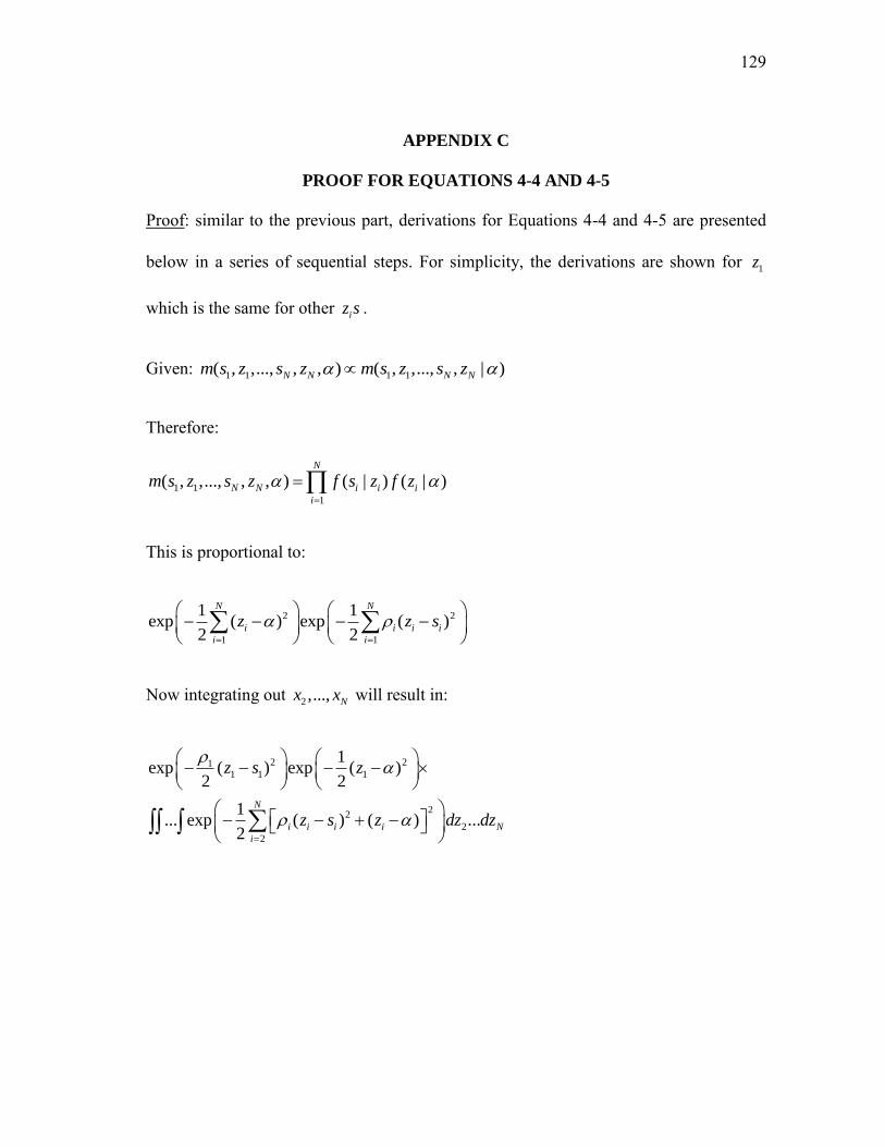
129
APPENDIX C
PROOF FOR EQUATIONS 4-4 AND 4-5
Proof: similar to the previous part, derivations for Equations 4-4 and 4-5 are presented
below in a series of sequential steps. For simplicity, the derivations are shown for 1z
which is the same for other iz s .
Given: 1 1 1 1( , ,..., , , ) ( , ,..., , | )N N N Nm s z s z m s z s z
Therefore:
1 1
1
( , ,..., , , ) ( | ) ( | )N
N N i i i
i
m s z s z f s z f z
This is proportional to:
2 2
1 1
1 1exp ( ) exp ( )
2 2
N N
i i i i
i i
z z s
Now integrating out 2 ,..., Nx x will result in:
2 211 1 1
22
2
2
1exp ( ) exp ( )
2 2
1... exp ( ) ( ) ...
2
N
i i i i N
i
z s z
z s z dz dz

130
This is proportional to:
2 2 211 1 1
2
2
2
1 1exp ( ) ( ) exp ( 1)
2 2 2
1... exp (1 ) 2 ( ) ...
2
N
i i i i i N
i
z s z N
z z s dz dz
This is now proportional to:
2 2 211 1 1
2
1
1 1exp ( ) ( ) exp ( 1)
2 2 2
( )1exp
2 1
Ni i
i i
z s z N
s
Now to integrate out :
2 2 2
1
2 2
21 1 1 1 1exp ( ) ( 1)
2 2 2 1 2 1
N Ni i
i ii i
sz N
This is proportional to:
2 2
1 1
2 2
* **
1 1 1exp( )exp ( [ ( ) 2 ( )
2 2 1 1
N Ni i
i ii i
sz N z
On the other hand derivation for part (*) of the bracket results in:
1
2 2 2 1 1
1 1 1* 1 (1 ) 1 1
1 1 1 1 1
N N Ni
i i ii i i
N
Similarly derivation for part (**) of the bracket results in:
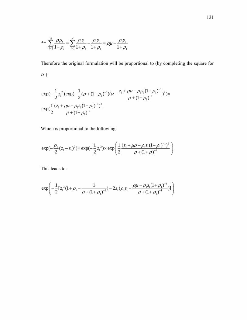
131
1 1 1 1
2 1 1 1
** 1 1 1 1
N Ni i i i
i ii i
s s s s
Therefore the original formulation will be proportional to (by completing the square for
):
12 1 21 1 1 1
1 1 1
1
1 2
1 1 1 1
1
1
(1 )1 1exp( )exp( ( (1 ) )( ) )
2 2 (1 )
( (1 ) )1exp(
2 (1 )
z sz
z s
Which is proportional to the following:
1 22 21 1 1 1 1
1 1 1 1
( (1 ) )1 1exp( ( ) ) exp( ) exp
2 2 2 (1 )
z sz s z
This leads to:
12 1 1 1
1 1 1 1 11 1
1 1
(1 )1 1exp [ (1 ) 2 ( )]
2 (1 ) (1 )
sz z s
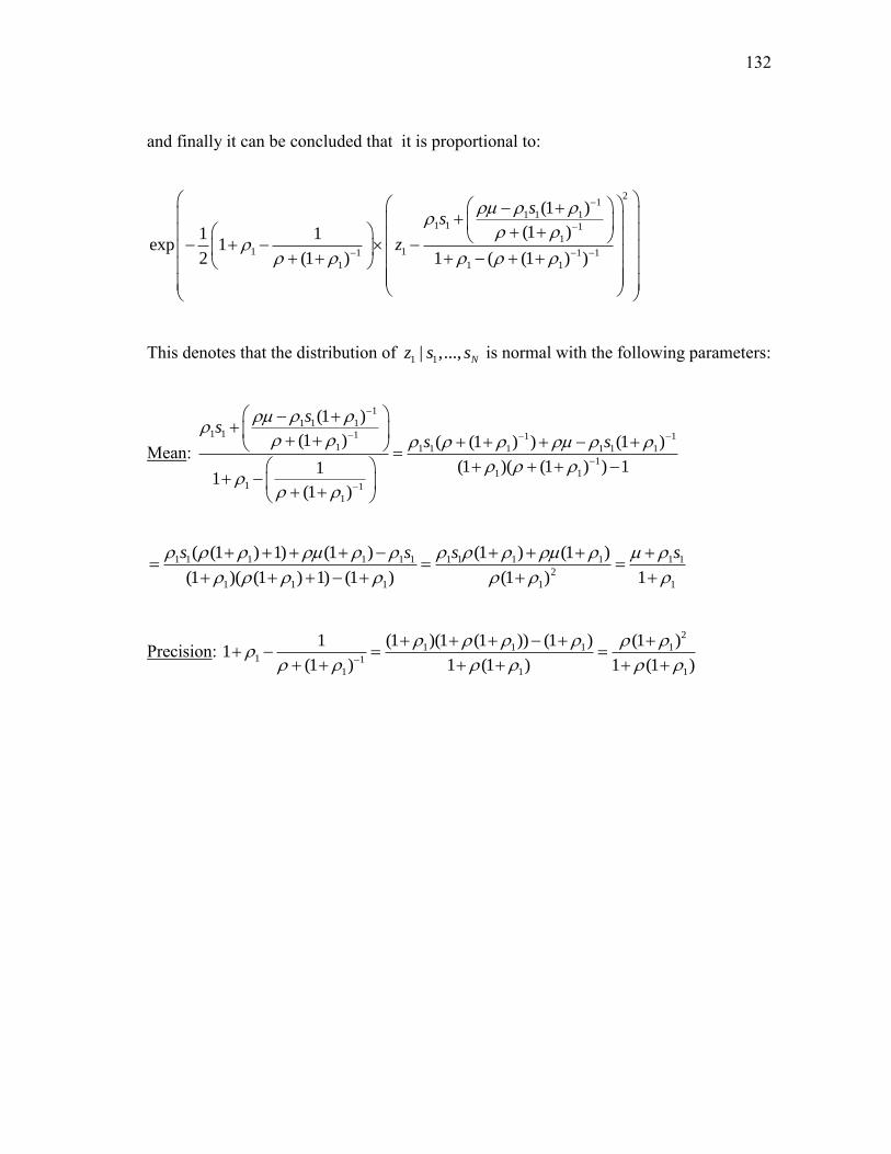
132
and finally it can be concluded that it is proportional to:
21
1 1 11 1 1
1
1 11 1 1
1 1 1
(1 )
(1 )1 1exp 1
2 (1 ) 1 ( (1 ) )
ss
z
This denotes that the distribution of 1 1| ,..., Nz s s is normal with the following parameters:
Mean:
1
1 1 11 1 1 1 1
1 1 1 1 1 1 1
1
1 1
1 1
1
(1 )
(1 ) ( (1 ) ) (1 )
(1 )( (1 ) ) 111
(1 )
ss
s s
1 1 1 1 1 1 1 1 1 1 1 1
2
1 1 1 1 1
( (1 ) 1) (1 ) (1 ) (1 )
(1 )( (1 ) 1) (1 ) (1 ) 1
s s s s
Precision:
2
1 1 1 11 1
1 1 1
(1 )(1 (1 )) (1 ) (1 )11
(1 ) 1 (1 ) 1 (1 )

133
APPENDIX D
PARAMETERS FOR ( )t t DISTRIBUTION
Calculating mean
Starting with the original formulation
-1
-1
[ ( ) ( ) ( (1 ) )]( )
[ ( ) (1 ) ]
j j j j
j
t t x st t
t
Calculating the expectation of ( )t t
-1
-1
( ) ( ) [ ] (1 )[ ( )]
( ) (1 )
j j j j
j
t t E x sE t t
t
Using Equation 4-4, will result in
1 -1
-1
( ) ( ) [( ( ) )(1 ) ] (1 )[ ( )]
(1 )
j j j j j j
j j
t t t s sE t t
Therefore
1
-1
[ ( ) ( ) ( )(1 ) ] [ ( ) ( )(1 ) ( )][ ( )] ( )
[ ( ) (1 ) ] [ ( )(1 ) 1]
j j
j j
t t t t t tE t t t
t t
Calculating Precision
Starting with the original formulation
-1
-1
[ ( ) ( ) ( (1 ) )]( )
[ ( ) (1 ) ]
j j j j
j
t t x st t
t
Calculating the variance for ( )t t
-1 2
-1Var[ ( )] Var [ ( ) (1 ) ] Var[ ]
( ) (1 )
j
j j
j
xt t t x
t
Following Equation 4-5
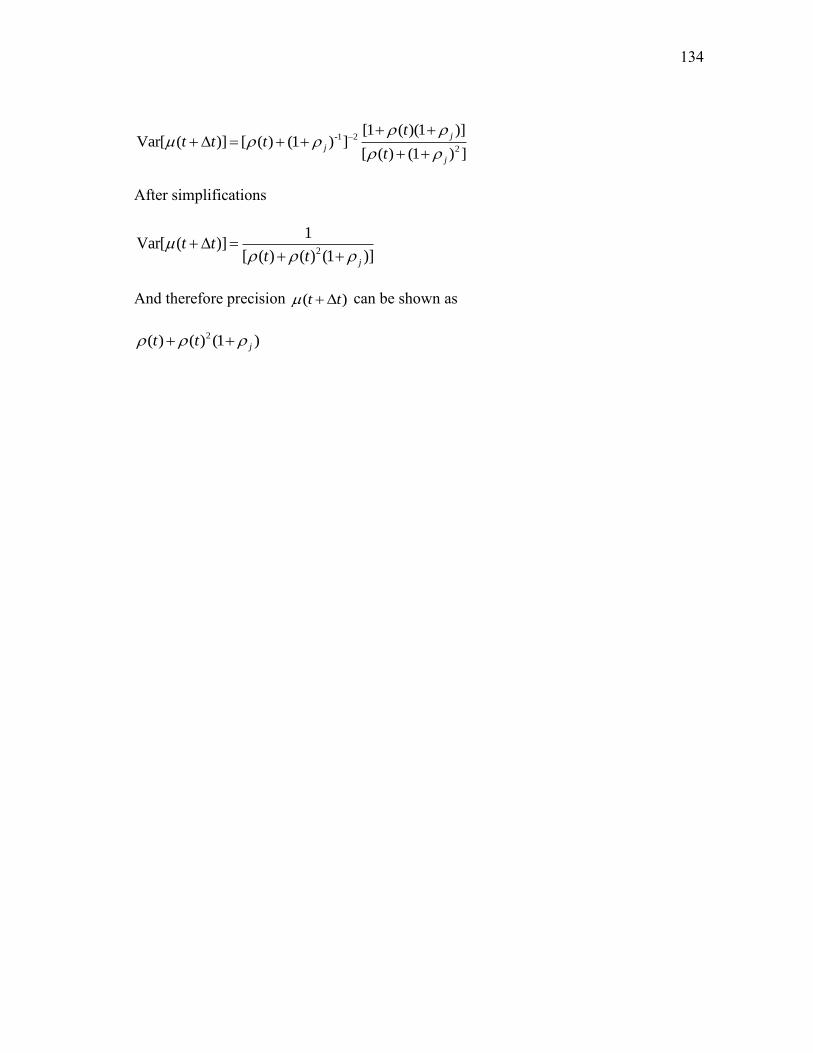
134
-1 2
2
[1 ( )(1 )]Var[ ( )] [ ( ) (1 ) ]
[ ( ) (1 ) ]
j
j
j
tt t t
t
After simplifications
2
1Var[ ( )]
[ ( ) ( ) (1 )]j
t tt t
And therefore precision ( )t t can be shown as
2( ) ( ) (1 )jt t
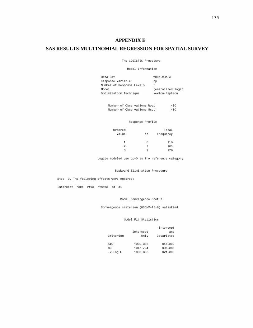
135
APPENDIX E
SAS RESULTS-MULTINOMIAL REGRESSION FOR SPATIAL SURVEY
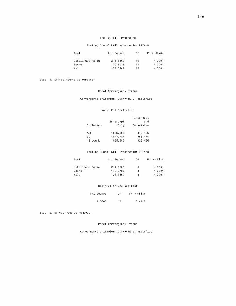
136

137

138

139
APPENDIX F
INSTRUCTIONS TO PLAYERS-ORGANIZATIONAL SURVEY
It is assumed that you as a car-owner have been involved in a car accident and your car
has been totaled. You know that your car did not worth more than $10,000. This value is
considered to be your Maximum Car Value or MCV. Now you are in the process of
negotiation with your insurance company to maximize your payoff. The insurer on the
other hand has an opposite goal which is to minimize its losses due to your claim. It is
believed that the negotiation starts with insurer’s offer to you. In these settings, you will
have three options to choose from which are: 1) accept the insurer’s offer, 2) reject and
continue negotiation by offering the insurer your own price, and 3) reject and pursue
your outside option which in this case will be the court. Similarly, the insurer has the
option of either accepting or rejecting your offer.
For simplicity it is assumed that the negotiation process will be performed in two
steps where step 1 is insurer’s offer to you and step 2 is your offer to insurer. If at the
end of the second step, no agreement is achieved, the case will be automatically referred
to the court. The court is assumed to be the “fair” arbitrator.
Assumptions
1) The outcome of the court for you would be a random draw from the three following
values: 0.7, 0.8, or 0.9 of the Current Value (CV) of your car.
2) Current Value (CV) of your car is the discounted value of your car for each step that
an agreement is not achieved. CV is computed by applying a discount factor of 0.9 for
each disagreement step.

140
3) You are supposed to pay a fixed cost of $500 for each step that the agreement is not
achieved for your commuting expenses or CE. The table below shows the process in
detail:
STEP 1:
Insurer Offers
Bargaining over MCV
Disagreement
You do not accept
the offer
STEP 2:
You Offer
Bargaining over CV= 0.9 * MCV
Disagreement
Insurance does not accept the
offer
COURT
Bargaining over
CV= 0.9*0.9 * MCV
Insurer You Insurer You Insurer You Insurer You Insurer You I(1)* O(1)* n/a -CE* I(2) O(2) n/a -CE*
I(3) I(4) I(5)
O(3) O(4) O(5)
*I(n)= Indicates insurer’s bargaining share in the nth round of the bargaining.
*O(n)= Indicates car-owner’s bargaining share in the nth round of the
bargaining. *CE= a fixed amount of $500 per every step that an agreement is not achieved.
Your Assigned Role
car-owner
Instructions
1) If you have been assigned the role of an car-owner then your insurer’s offer will be
emailed to you. The email then asks for your decision regarding the insurer offer. This
decision should either be 1) accept or 2) reject following your own offer, or 3) reject and
refer it to the court. After receiving your insurer’s offer please make your decision from
the options above and send it by email to me at: [email protected].
2) If you have been selected as an insurer, you are supposed to indicate your offers to
each of your customers (which are either 10 or 11) by completing the following table
and email it back to me at: [email protected]. Your offers will be received by your
clients and the results will be emailed back to you. If they did not accept your offer and

141
named their own offer, you are supposed to indicate whether you accept their offer or
prefer to go to the court.
Client
Number Your Offer
Client’s
Response Your Response
1 2 3 4 5 6 7 8 9 10 11 12
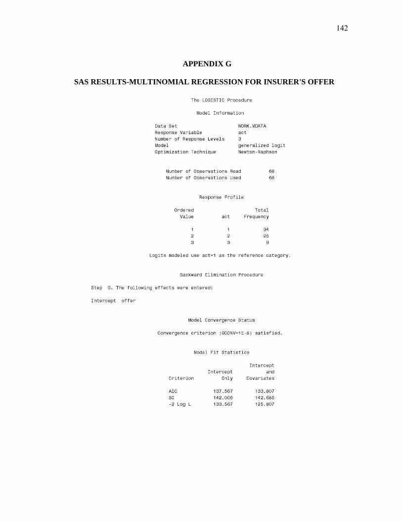
142
APPENDIX G
SAS RESULTS-MULTINOMIAL REGRESSION FOR INSURER'S OFFER

143

144
APPENDIX H
SAS RESULTS-LINEAR REGRESSION FOR OWNER'S COUNTEROFFER

145

146

147
APPENDIX I
R RESULTS-BINOMIAL REGRESSION FOR INSURER'S RESPONSE
148
VITA
Name: Ali Nejat Address: Zachry Department of Civil Engineering Texas A&M University 3136 TAMU
College Station, TX 77843-3136 Email Address: [email protected] Education: B.S., Civil Engineering, Zanjan University Zanjan, Iran, 2000
M.S., Civil Engineering, Islamic Azad University Tehran, Iran, 2003
Ph.D., Civil Engineering, Texas A&M University College Station, Texas, 2011