Article

Modeling Ecohydrological Processes and SpatialPatterns in the Upper Heihe Basin in China

Bing Gao 1, Yue Qin 2, Yuhan Wang 2, Dawen Yang 2,* and Yuanrun Zheng 3

Received: 29 September 2015; Accepted: 21 December 2015; Published: 25 December 2015Academic Editors: Ge Sun and James M. Vose

1 School of Water Resources and Environment, China University of Geosciences, Beijing 100083, China;gb03@cugb.edu.cn

2 State Key Laboratory of Hydroscience and Engineering, Department of Hydraulic Engineering,Tsinghua University, Beijing 100084, China; qiny13@mails.tsinghua.edu.cn (Y.Q.);wangyuha14@mails.tsinghua.edu.cn (Y.W.)

3 State Key Laboratory of Vegetation and Environmental Change, Institute of Botany,Chinese Academy of Sciences, Beijing 100093, China; zhengyr@ibcas.ac.cn

* Correspondence: yangdw@tsinghua.edu.cn; Tel.: +86-10-6279-6976; Fax: +86-10-6279-6971

Abstract: The Heihe River is the second largest inland basin in China; runoff in the upper reach greatlyaffects the socio-economic development in the downstream area. The relationship between spatialvegetation patterns and catchment hydrological processes in the upper Heihe basin has remainedunclear to date. In this study, a distributed ecohydrological model is developed to simulate thehydrological processes with vegetation dynamics in the upper Heihe basin. The model is validatedby hydrological observations at three locations and soil moisture observations at a watershed scale.Based on the simulated results, the basin water balance characteristics and their relationship withthe vegetation patterns are analyzed. The mean annual precipitation and runoff increase with theelevation in a similar pattern. Spatial patterns of the actual evapotranspiration is mainly controlledby the precipitation and air temperature. At the same time, vegetation distribution enhances thespatial variability of the actual evapotranspiration. The highest actual evapotranspiration is aroundelevations of 3000–3600 m, where shrub and alpine meadow are the two dominant vegetation types.The results show the mutual interaction between vegetation dynamics and hydrological processes.Alpine sparse vegetation and alpine meadow dominate the high-altitude regions, which contributemost to the river runoff, and forests and shrub contribute relatively small amounts of water yield.

Keywords: distributed ecohydrological model; vegetation dynamics; hydrological processes; waterbalance characteristics

1. Introduction

Vegetation, topography and climate variables interactively influence multi-scale ecohydrologicalprocesses in a large catchment. Vegetation patterns are a key factor affecting the water balance andcatchment water yield. Previous studies have demonstrated the impact of forest change on riverdischarge in China [1,2]. However, few studies have addressed the relationship between hydrologicalprocesses and vegetation patterns. In particular, the relationship between forest and water in theheadwater catchments of arid inland basins remains unclear [3]. In arid inland basins, the riverdischarge generated from the mountain regions greatly affects the socio-economic developmentand ecosystem sustainability of the downstream regions. Therefore, understanding the complexrelationship between spatial vegetation patterns and hydrological processes is important for integratedriver basin management. Hydrological observations and small-scale experiments provide limitedinformation for understanding the spatial patterns of ecohydrological processes in a large river basin [4].

Forests 2016, 7, 10; doi:10.3390/f7010010 www.mdpi.com/journal/forests

Forests 2016, 7, 10 2 of 21

Instead, a physically based distributed model that links ecohydrological processes across scales isneeded to analyze the spatial variability of hydrology with vegetation pattern.

In the past few decades, with global climate change and population growth, the water shortageand ecosystem degradation in many river basins have gained increasing concern worldwide.Meanwhile, changes in natural river runoff in the headwater catchments worldwide have been reportedin previous studies [5–11]. Because of the less direct influence of human activities in headwater areas,runoff changes are mainly caused by the mutual interactions among climate, vegetation and hydrology.Yang et al. [12] reported that climate contributions to river runoff showed a large spatial variationover China, and several studies attempted to attribute runoff change to the impacts of climate andvegetation changes [13–15]. However, vegetation is absent or simply parameterized in traditionalhydrological models [16]. It is relatively difficult to evaluate the influence of vegetation change onrunoff due to data availability and methodological limitations [17,18]. Therefore, it is important todevelop the ecohydrological models for understanding and predicting changes in the regional wateravailability under the changing environment.

Modeling hydrological processes at the catchment scale requires a flexible distributed schemeto represent the catchment topography, river network and vegetation patterns [19]. Previousstudies of distributed hydrological models focused on the representation of the heterogeneity ofcatchment landscape and physically based descriptions of hydrological processes, such as theSysteme Hydrologique Europeen (SHE) and the Variable Infiltration Capacity (VIC) model [20,21].Yang et al. [22,23] proposed the geomorphology-based hydrological model (GBHM) consideringsub-grid parameterization, which has been employed in macroscale studies [24,25] and mesoscalestudies [13,14,26,27]. To better simulate the hydrological changes in a catchment, it is necessary tocouple the vegetation pattern and vegetation dynamics in hydrological models [19]. Land surfacemodels, such as the second version of the Simple Biosphere model (SiB2) [28], have mainly focusedon the role of vegetation in the water-heat-carbon cycle. However, the catchment hydrology waspoorly represented in SiB2. Further research embedded the SiB2 into the GBHM and developeda distributed biosphere hydrological model called the Water and Energy Budget-Based DistributedHydrological Model (WEB-DHM) [29]. A comparative analysis of the WEB-DHM and GBHM hasbeen carried out and indicated that the WEB-DHM could be used to predict streamflow and conductthe water and energy flux estimations [30]. Several land surface models can simulate the cryosphereprocesses, such as the Community Land Model (CLM) [31]. However, they typically simplify thecatchment hydrological processes and cannot accurately simulate streamflow. Several studies attemptto develop physically based models to couple hydrological processes with ecological processes. Tagueand Band [32] developed the Regional Hydro-Ecologic Simulation System (RHESSys) to simulate bothhydrological processes and vegetation dynamics. However, in RHESSys, the frozen soil process is notconsidered and the soil temperature is estimated based on the average daily temperature. Manetaand Silverman [33] and Ivanov et al. [34] developed spatial distributed models to simulate the water,energy balance and vegetation dynamics. However, the frozen soil is not adequately considered, asthere are only two soil thermal layers in this model. Therefore, it is important to develop a distributedmodel that couples hydrological processes, cryosphere processes and vegetation dynamics.

There are several previous studies focusing on the hydrological modeling in the Heihe Riverbasin. Jia et al. [35] applied the water and energy transfer process (WEP) model to simulate and predictthe annual runoff changes due to climate and land use changes. Wang et al. [36] and Zhang et al. [37]applied heat and water coupling models to a small experimental catchment in the upper Heihe basin totest the model applicability in the high, cold mountainous area. Zhou et al. [38] chose several modulesfor the hydrological processes in cold regions and linked them to a catchment hydrological modelto improve the hydrological modeling capability in the cold mountainous area. Zang and Liu [39]applied the Soil and Water Assessment Tool (SWAT) in the Heihe basin to analyze the flow trends ofgreen and blue water. Yang et al. [19] developed a distributed scheme for ecohydrological modelingin the upper Heihe River. However, this scheme needs further coupling of vegetation dynamics into

Forests 2016, 7, 10 3 of 21

the hydrological simulation and improvement of the cryosphere hydrological processes. Because ofthe complexity of ecohydrological processes in the upper Heihe basin, further research to developa sophisticated ecohydrological model is still ongoing. A major research plan entitled “Integratedresearch on the ecohydrological processes of the Heihe basin” has been launched by the NationalNatural Science Foundation of China since 2010 [40]. One of the integrated research projects in thisresearch plan aims to develop a distributed ecohydrological model for the cold mountainous regionsof inland basins. With the help of the Heihe Watershed Allied Telemetry Experimental Research(HiWATER), which is a comprehensive ecohydrological experiment in this research plan [4], there arenew opportunities for ecohydrological model development in the Heihe basin.

The major objectives of this study are to (1) develop a distributed ecohydrological model bycoupling hydrological processes with vegetation dynamics and (2) analyze the relationship betweenthe water balance and vegetation patterns in the upper Heihe basin.

In the following sections, the features of the study area are presented, followed by the datadescriptions. The distributed ecohydrological model is then introduced. In the results and discussionsection, the model validation is presented, followed by the analysis of water balance characteristicsand the spatiotemporal variability of runoff. Finally, the catchment ecohydrological pattern is analyzedfrom the water balance and its relation to the vegetation distribution.

2. Study Area and Data Used

2.1. The Upper Heihe Basin

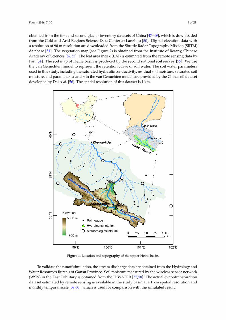
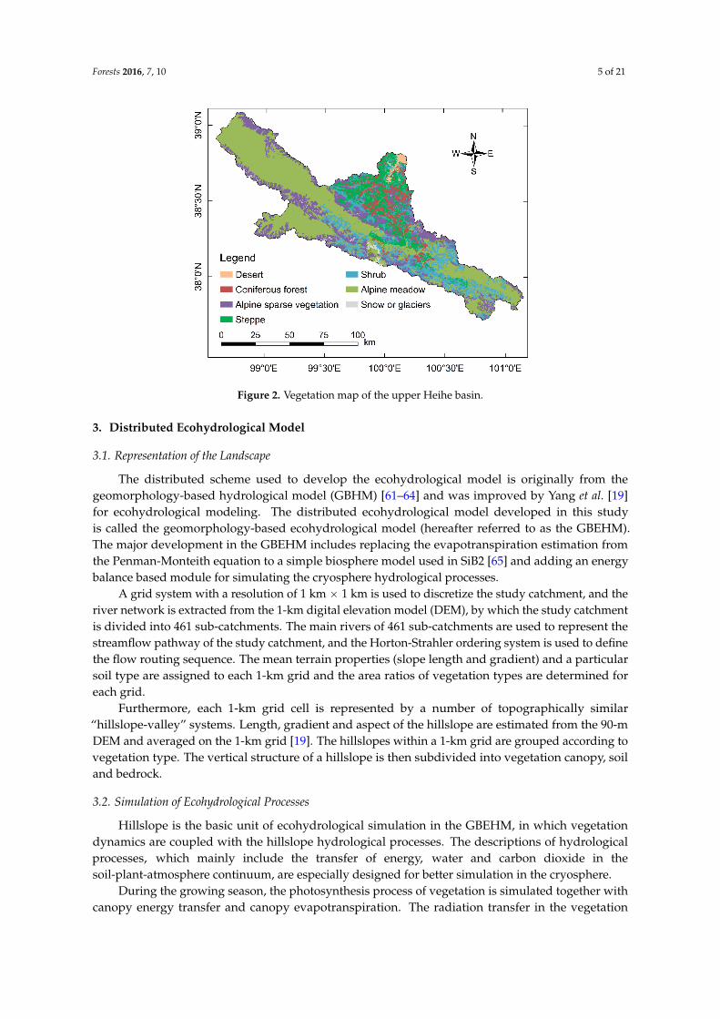
Heihe basin is the second largest inland basin in Northwest China. The upper reach of theHeihe River, which is gauged at the Yingluoxia hydrological station (see Figure 1), has a drainagearea of 10,005 km2. The upper Heihe basin generates nearly 70% of the total river runoff, whichsupplies agricultural irrigation and benefits the social economy development in the middle and lowerbasin [19,41]. There are two tributaries in the upper Heihe basin, namely, the West Tributary and EastTributary, both of which originate in the Qilian Mountains. The annual precipitation is between 200 mmand 700 mm with highly seasonal variability, and nearly 60% of the total annual rainfall is concentratedin summer from June to September. The upper Heihe basin has an elevation of 1700–5200 m, lowtemperature and relatively abundant vegetation types [41–44]. The major vegetation types includeconiferous forest (Picea crassifolia Kom.), shrub (Potentilla fruticosa Linn.), steppe (Stipa purpurea Griseb),alpine meadow (Kobresia pygmaea Clarke), alpine sparse vegetation (Saussurea medusa Maxim.), anddesert (Sympegma regelii Bunge) (see Figure 2).

2.2. Data Used in the Study

Two types of data are used in this study: the first type is the data used to build and run theecohydrological model, which include the geographic information and climatic forcing data, and thesecond type is the data used for model validation.

Meteorological observations are available at several stations within the study basin and itssurrounding areas, as shown in Figure 1. The data are acquired from the National MeteorologicalInformation Center affiliated with the China Meteorological Administration [45]. The observedmeteorological data include daily precipitation, temperature, sunshine hour, wind speed and relativehumidity. In this study, daily gridded precipitation is interpolated from the gauge data using themethod developed by Shen and Xiong [46]. Other forcing data are interpolated using the inversedistance method. The hourly temperature is estimated from the daily maximum and minimumtemperature using a sine curve. Hourly precipitation is estimated from the daily data according to theduration. Duration of precipitation within a day is determined by the precipitation amount estimatedfrom the regional historical records. The starting time of the precipitation in a day is decided randomlyand the hourly precipitation is specified using a normal distribution. The wind speed and relativehumidity are assumed uniform in a day. The location of glaciers and their areas and volumes are

Forests 2016, 7, 10 4 of 21

obtained from the first and second glacier inventory datasets of China [47–49], which is downloadedfrom the Cold and Arid Regions Science Data Center at Lanzhou [50]. Digital elevation data witha resolution of 90 m resolution are downloaded from the Shuttle Radar Topography Mission (SRTM)database [51]. The vegetation map (see Figure 2) is obtained from the Institute of Botany, ChineseAcademy of Sciences [52,53]. The leaf area index (LAI) is estimated from the remote sensing data byFan [54]. The soil map of Heihe basin is produced by the second national soil survey [55]. We usethe van Genuchten model to represent the retention curve of soil water. The soil water parametersused in this study, including the saturated hydraulic conductivity, residual soil moisture, saturated soilmoisture, and parameters α and n in the van Genuchten model, are provided by the China soil datasetdeveloped by Dai et al. [56]. The spatial resolution of this dataset is 1 km.

Forests 2016, 7, 10 4/21

elevation data with a resolution of 90 m resolution are downloaded from the Shuttle Radar

Topography Mission (SRTM) database [51]. The vegetation map (see Figure 2) is obtained from the

Institute of Botany, Chinese Academy of Sciences [52,53]. The leaf area index (LAI) is estimated from

the remote sensing data by Fan [54]. The soil map of Heihe basin is produced by the second national

soil survey [55]. We use the van Genuchten model to represent the retention curve of soil water. The

soil water parameters used in this study, including the saturated hydraulic conductivity, residual soil

moisture, saturated soil moisture, and parameters α and n in the van Genuchten model, are provided

by the China soil dataset developed by Dai et al. [56]. The spatial resolution of this dataset is 1 km.

Figure 1. Location and topography of the upper Heihe basin.

To validate the runoff simulation, the stream discharge data are obtained from the Hydrology

and Water Resources Bureau of Gansu Province. Soil moisture measured by the wireless sensor

network (WSN) in the East Tributary is obtained from the HiWATER [57,58]. The actual

evapotranspiration dataset estimated by remote sensing is available in the study basin at a 1 km

spatial resolution and monthly temporal scale [59,60], which is used for comparison with the

simulated result.

Figure 1. Location and topography of the upper Heihe basin.

To validate the runoff simulation, the stream discharge data are obtained from the Hydrology andWater Resources Bureau of Gansu Province. Soil moisture measured by the wireless sensor network(WSN) in the East Tributary is obtained from the HiWATER [57,58]. The actual evapotranspirationdataset estimated by remote sensing is available in the study basin at a 1 km spatial resolution andmonthly temporal scale [59,60], which is used for comparison with the simulated result.

Forests 2016, 7, 10 5 of 21Forests 2016, 7, 10 5/21

Figure 2. Vegetation map of the upper Heihe basin.

3. Distributed Ecohydrological Model

3.1. Representation of the Landscape

The distributed scheme used to develop the ecohydrological model is originally from the

geomorphology-based hydrological model (GBHM) [61–64] and was improved by Yang et al. [19] for

ecohydrological modeling. The distributed ecohydrological model developed in this study is called

the geomorphology-based ecohydrological model (hereafter referred to as the GBEHM). The major

development in the GBEHM includes replacing the evapotranspiration estimation from the Penman-

Monteith equation to a simple biosphere model used in SiB2 [65] and adding an energy balance based

module for simulating the cryosphere hydrological processes.

A grid system with a resolution of 1 km × 1 km is used to discretize the study catchment, and

the river network is extracted from the 1-km digital elevation model (DEM), by which the study

catchment is divided into 461 sub-catchments. The main rivers of 461 sub-catchments are used to

represent the streamflow pathway of the study catchment, and the Horton-Strahler ordering system

is used to define the flow routing sequence. The mean terrain properties (slope length and gradient)

and a particular soil type are assigned to each 1-km grid and the area ratios of vegetation types are

determined for each grid.

Furthermore, each 1-km grid cell is represented by a number of topographically similar

“hillslope-valley” systems. Length, gradient and aspect of the hillslope are estimated from the 90-m

DEM and averaged on the 1-km grid [19]. The hillslopes within a 1-km grid are grouped according

to vegetation type. The vertical structure of a hillslope is then subdivided into vegetation canopy, soil

and bedrock.

3.2. Simulation of Ecohydrological Processes

Hillslope is the basic unit of ecohydrological simulation in the GBEHM, in which vegetation

dynamics are coupled with the hillslope hydrological processes. The descriptions of hydrological

processes, which mainly include the transfer of energy, water and carbon dioxide in the soil-plant-

atmosphere continuum, are especially designed for better simulation in the cryosphere.

During the growing season, the photosynthesis process of vegetation is simulated together with

canopy energy transfer and canopy evapotranspiration. The radiation transfer in the vegetation

canopy layer includes interception, reflection, transmission and absorption and is described by the

same scheme in SiB2 [28,66]. The energy balance equation in the canopy layer is expressed as [28]

Figure 2. Vegetation map of the upper Heihe basin.

3. Distributed Ecohydrological Model

3.1. Representation of the Landscape

The distributed scheme used to develop the ecohydrological model is originally from thegeomorphology-based hydrological model (GBHM) [61–64] and was improved by Yang et al. [19]for ecohydrological modeling. The distributed ecohydrological model developed in this studyis called the geomorphology-based ecohydrological model (hereafter referred to as the GBEHM).The major development in the GBEHM includes replacing the evapotranspiration estimation fromthe Penman-Monteith equation to a simple biosphere model used in SiB2 [65] and adding an energybalance based module for simulating the cryosphere hydrological processes.

A grid system with a resolution of 1 km ˆ 1 km is used to discretize the study catchment, and theriver network is extracted from the 1-km digital elevation model (DEM), by which the study catchmentis divided into 461 sub-catchments. The main rivers of 461 sub-catchments are used to represent thestreamflow pathway of the study catchment, and the Horton-Strahler ordering system is used to definethe flow routing sequence. The mean terrain properties (slope length and gradient) and a particularsoil type are assigned to each 1-km grid and the area ratios of vegetation types are determined foreach grid.

Furthermore, each 1-km grid cell is represented by a number of topographically similar“hillslope-valley” systems. Length, gradient and aspect of the hillslope are estimated from the 90-mDEM and averaged on the 1-km grid [19]. The hillslopes within a 1-km grid are grouped according tovegetation type. The vertical structure of a hillslope is then subdivided into vegetation canopy, soiland bedrock.

3.2. Simulation of Ecohydrological Processes

Hillslope is the basic unit of ecohydrological simulation in the GBEHM, in which vegetationdynamics are coupled with the hillslope hydrological processes. The descriptions of hydrologicalprocesses, which mainly include the transfer of energy, water and carbon dioxide in thesoil-plant-atmosphere continuum, are especially designed for better simulation in the cryosphere.

During the growing season, the photosynthesis process of vegetation is simulated together withcanopy energy transfer and canopy evapotranspiration. The radiation transfer in the vegetation

Forests 2016, 7, 10 6 of 21

canopy layer includes interception, reflection, transmission and absorption and is described by thesame scheme in SiB2 [28,66]. The energy balance equation in the canopy layer is expressed as [28]

CBTc

Bt“ Rn ´ H ´ λE´ ξ (1)

where C is the effective heat capacity of the canopy (J¨m´2¨K´1), Tc is the canopy temperature (K),t is the time (s), Rn is the absorbed net radiation (W¨m´2), H is the sensible heat flux (W¨m´2), λ

is the latent heat of vaporization (J¨kg´1), E is the evapotranspiration rate (kg¨m´2¨ s´1), and ξ isthe energy transfer due to water phase change (W¨m´2), which is caused by the melting/freezingof the snow intercepted by the canopy. Thus, the energy budget is linked with water balance by theevapotranspiration component. The absorbed net radiation is calculated using the radiation transfermodel described by Sellers et al. [65]. The sensible heat flux of the canopy H is calculated as

H “ ρcpTc ´ Ta

rb(2)

where ρ is the air density (kg¨m´3), cp is the specific heat of air (J¨K´1¨kg´1), Tc is thecanopy temperature (K), Ta is the air temperature (K), and rb is the bulk canopy boundary layerresistance (s¨m´1).

The actual evapotranspiration rate of the vegetation layer is influenced by the leaf stomatalconductance, which is related to environmental properties, such as the canopy temperature, carbondioxide concentration and water vapor in the air. In this study, canopy conductance is estimated as [28]

gc “ mAc

Cshs p` bLT (3)

where gc is the canopy conductance (m¨ s´1), m and b are the empirical coefficients of vegetationtypes, Cs is the carbon dioxide partial pressure at the leaf surface (Pa), hs is the relative humidity,p is the atmospheric pressure (Pa), LT is the total leaf area index (m2¨m´2), and Ac is the canopyphotosynthesis rate (mol¨m´2¨ s´1) and is calculated as [67]

Ac “ An0Π (4)

Π “ FPAR{k (5)

where An0 is the net assimilation rate for the leaves at the top of the canopy (mol¨m´2¨ s´1), FPAR isthe fractional interception of photosynthetically active radiation, and k is the time-mean extinctioncoefficient for photosynthetically active radiation. The net assimilation rate of the leaf is calculated as

An “ A´ Rd (6)

where An is the leaf net assimilation rate (mol¨m´2¨ s´1), A is the leaf photosynthetic rate(mol¨m´2¨ s´1), and Rd is the leaf respiration rate (mol¨m´2¨ s´1). A and Rd are estimated by thefunctions of the maximum catalytic capacity of the photosynthetic enzyme (Vmax), canopy temperatureand other environmental factors [28,68,69]. Details about the calculation of gc, A and Rd were given bySellers et al. [28]. Based on the canopy conductance gc, the canopy transpiration rate is expressed as [28]

λEc “

„

e˚ pTcq ´ ea

1{gc ` 2rb

ρcp

γp1´Wcq (7)

where Ec is the canopy transpiration rate (kg¨m´2¨ s´1), e* is the saturation vapor pressure (Pa), ea

is the vapor pressure in the canopy (Pa), rb is the canopy boundary layer resistance (s¨m´1), ρ is thedensity of air (kg¨m´3), cp is the specific heat of air (J¨ kg´1¨K´1), and γ is the psychrometric constant

Forests 2016, 7, 10 7 of 21

(Pa¨K´1), Wc is the canopy wetness-snow cover fraction, and the other parameters are the same as inEquations (1) and (3). The soil evaporation rate Eg of the surface soil layer and the evaporation rate ofthe canopy interception Ei are calculated using the same methods in SiB2 [28]. Eg and Ei are added toEc as the total actual evapotranspiration over the hillslope unit.

In the non-growing season, ecohydrological simulation focuses on the cryosphere hydrologicalprocesses, which mainly include the snow melting process, soil freezing and thawing process, andglacier melting process. We use a similar scheme as in the Community Land Model version 4.0 (i.e.,CLM4.0) [31] to represent the heat transfer in snow and frozen soil:

cBTs

Bt“B

Bz

„

KTBTs

Bz

(8)

where c is the volumetric snow/soil heat capacity (J¨m´3¨K´1), Ts is the temperature (K) of thesnow/soil layers, z is the vertical depth of snow/soil (m), and KT is the thermal conductivity(W¨m´1¨K´1). Equation (8) solves the snow/soil temperature with the boundary condition as the heatflux into the top surface layer of the snow/soil and zero heat flux at the bottom of the soil column.The surface layer heat flux from the atmosphere is expressed as

h “ Sg ´ Lg ´ Hg ´ λEg (9)

where h is the upper boundary heat flux into the snow/soil layer (W¨m´2), Sg is the solar radiationabsorbed by the top layer (W¨m´2), Lg is the long-wave radiation absorbed by the ground (W¨m´2),Hg is the sensible heat flux from the ground (W¨m´2), and λEg is the latent heat flux from theground (W¨m´2).

After solving Equation (8), the soil or snow layer temperature is evaluated to determine whetherthe phase change will take place [31]. For the soil or snow layers, melting takes place under thecondition of

Ti ą T f and Wice ą 0. (10)

For the snow layers, freezing takes place under the condition of

Ti ă T f and Wliq ą 0 (11)

and for the soil layers, freezing takes place under the condition of

Ti ă T f and Wliq ą Wliq,max. (12)

In Equations (10)–(12), Ti is the temperature of the soil or snow layers (K), T f is the freezingtemperature of water (K), Wice is the mass of ice in the soil or snow layers (kg¨m´2), Wliq is the massof liquid water in soil or snow layers (kg¨m´2), and Wliq,max is the maximum mass of supercooledsoil water, which is the liquid water that coexists with the ice (kg¨m´2). The phase change rate isdetermined by the energy excess (or deficit) needed to change the temperature of soil or snow layers(Ti) to the freezing temperature (T f ). If the melting criteria in Equation (10) is met and energy excess isgreater than zero, then the ice mass is calculated by [31]

Wn`1ice “ Wn

ice ´Ui∆t

L f(13)

where Wn` 1ice is the ice mass after the phase change (kg¨m´2), Wn

ice is the ice mass before the phasechange (kg¨m´2), n + 1 and n refer to the time steps, Ui is the energy excess (W¨m´2), ∆t is the length

Forests 2016, 7, 10 8 of 21

of time step (s), and L f is the latent heat of ice fusion (J¨ kg´1). If the freezing criteria in Equations (11)or (12) is met and energy excess is less than zero, then the ice mass in the snow layers is adjusted by

Wn`1ice “ min

˜

Wnice `Wn

liq,Wnice ´

Ui∆tL f

¸

. (14)

The ice mass in the soil layers is adjusted by

Wn`1ice “

$

’

&

’

%

minpWnice `Wn

liq ´Wliq,max, Wnice ´

Ui∆tL f

q Wnice `Wn

liq ě Wliq,max

0 Wnice `Wn

liq ă Wliq,max

(15)

and the mass of liquid water is adjusted by

Wn`1liq “ Wn

liq `Wnice ´Wn`1

ice (16)

where Wn`1liq and Wn

liq are the mass of liquid water after and before the phase change (kg¨m´2),respectively, in Equations (14)–(16), and the other parameters are the same as in Equation (13).Moreover, glacier melting is simulated using the degree-day model [70,71].

The surface runoff is from the infiltration excess and saturation excess calculated by solvingRichards’ equation using an implicit finite difference method. The surface runoff flows through thehillslope into the stream via kinematic wave. The groundwater aquifer is treated as an individualstorage corresponding to each grid. The exchange between the groundwater and river water isconsidered as steady flow and calculated using Darcy’s law [64]. The runoff generated from the gridis the lateral inflow into the river of the sub-catchment. The flow routing in the river network of thewhole study catchment is solved using the kinematic wave approach:

$

’

’

&

’

’

%

BABt`BQBx

“ q

Q “S0

1{2

nr ¨ p2{3A5{3

(17)

where Q is the discharge (m3¨ s´1), t is the time (s), x is distance along the river (m), A is the area ofthe cross-section (m2), q is the lateral inflow to the river from the hillslope (m3¨ s´1), S0 is the slopeof the river bed, nr is the roughness of the river bed, and p is the wetting perimeter of cross-section(m). Equation (17) is solved using a nonlinear explicit finite difference method and Newton’s iterationscheme. The time step of the GBEHM model is one hour.

3.3. Model Calibration and Performance Evaluation Metrics

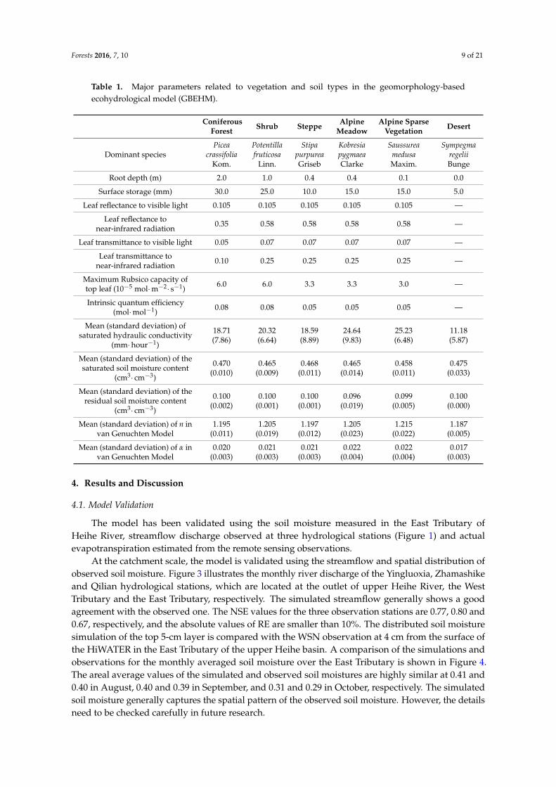
Most model parameters are estimated from field observations or remote sensing data, and somevegetation parameters are specified from previous studies [19]. The major parameters related tovegetation type are listed in Table 1. Considering the equilibration time for the hydrological statevariables (e.g., soil moisture, soil temperature, groundwater table), a warm-up run of the model in theperiod of 1999–2000 is used to update the model state variables. We perform our analysis in the periodfrom 2001 to 2012. The Nash-Sutcliffe efficiency (NSE) coefficient and relative error (RE) are used toevaluate the model performance.

Forests 2016, 7, 10 9 of 21

Table 1. Major parameters related to vegetation and soil types in the geomorphology-basedecohydrological model (GBEHM).

ConiferousForest Shrub Steppe Alpine

MeadowAlpine Sparse

Vegetation Desert

Dominant speciesPicea

crassifoliaKom.

Potentillafruticosa

Linn.

StipapurpureaGriseb

KobresiapygmaeaClarke

SaussureamedusaMaxim.

SympegmaregeliiBunge

Root depth (m) 2.0 1.0 0.4 0.4 0.1 0.0

Surface storage (mm) 30.0 25.0 10.0 15.0 15.0 5.0

Leaf reflectance to visible light 0.105 0.105 0.105 0.105 0.105 —

Leaf reflectance tonear-infrared radiation 0.35 0.58 0.58 0.58 0.58 —

Leaf transmittance to visible light 0.05 0.07 0.07 0.07 0.07 —

Leaf transmittance tonear-infrared radiation 0.10 0.25 0.25 0.25 0.25 —

Maximum Rubsico capacity oftop leaf (10´5 mol¨ m´2¨ s´1) 6.0 6.0 3.3 3.3 3.0 —

Intrinsic quantum efficiency(mol¨ mol´1) 0.08 0.08 0.05 0.05 0.05 —

Mean (standard deviation) ofsaturated hydraulic conductivity

(mm¨ hour´1)

18.71(7.86)

20.32(6.64)

18.59(8.89)

24.64(9.83)

25.23(6.48)

11.18(5.87)

Mean (standard deviation) of thesaturated soil moisture content

(cm3¨ cm´3)

0.470(0.010)

0.465(0.009)

0.468(0.011)

0.465(0.014)

0.458(0.011)

0.475(0.033)

Mean (standard deviation) of theresidual soil moisture content

(cm3¨ cm´3)

0.100(0.002)

0.100(0.001)

0.100(0.001)

0.096(0.019)

0.099(0.005)

0.100(0.000)

Mean (standard deviation) of n invan Genuchten Model

1.195(0.011)

1.205(0.019)

1.197(0.012)

1.205(0.023)

1.215(0.022)

1.187(0.005)

Mean (standard deviation) of α invan Genuchten Model

0.020(0.003)

0.021(0.003)

0.021(0.003)

0.022(0.004)

0.022(0.004)

0.017(0.003)

4. Results and Discussion

4.1. Model Validation

The model has been validated using the soil moisture measured in the East Tributary ofHeihe River, streamflow discharge observed at three hydrological stations (Figure 1) and actualevapotranspiration estimated from the remote sensing observations.

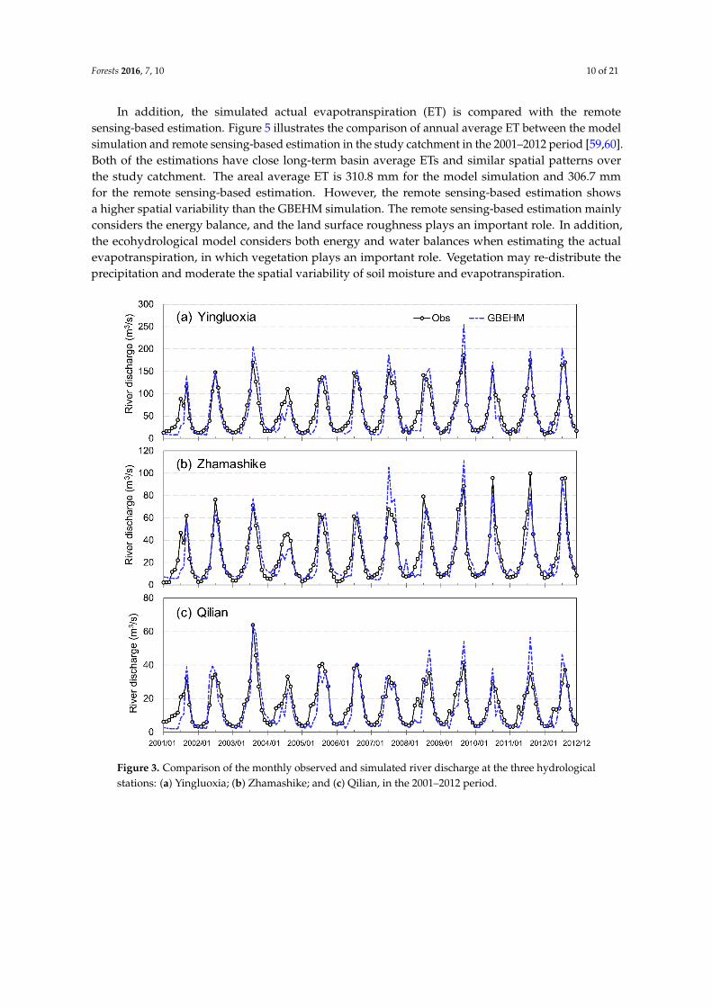
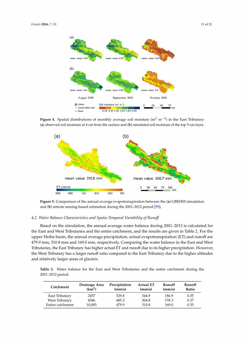
At the catchment scale, the model is validated using the streamflow and spatial distribution ofobserved soil moisture. Figure 3 illustrates the monthly river discharge of the Yingluoxia, Zhamashikeand Qilian hydrological stations, which are located at the outlet of upper Heihe River, the WestTributary and the East Tributary, respectively. The simulated streamflow generally shows a goodagreement with the observed one. The NSE values for the three observation stations are 0.77, 0.80 and0.67, respectively, and the absolute values of RE are smaller than 10%. The distributed soil moisturesimulation of the top 5-cm layer is compared with the WSN observation at 4 cm from the surface ofthe HiWATER in the East Tributary of the upper Heihe basin. A comparison of the simulations andobservations for the monthly averaged soil moisture over the East Tributary is shown in Figure 4.The areal average values of the simulated and observed soil moistures are highly similar at 0.41 and0.40 in August, 0.40 and 0.39 in September, and 0.31 and 0.29 in October, respectively. The simulatedsoil moisture generally captures the spatial pattern of the observed soil moisture. However, the detailsneed to be checked carefully in future research.

Forests 2016, 7, 10 10 of 21

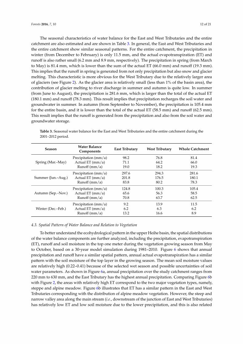
In addition, the simulated actual evapotranspiration (ET) is compared with the remotesensing-based estimation. Figure 5 illustrates the comparison of annual average ET between the modelsimulation and remote sensing-based estimation in the study catchment in the 2001–2012 period [59,60].Both of the estimations have close long-term basin average ETs and similar spatial patterns overthe study catchment. The areal average ET is 310.8 mm for the model simulation and 306.7 mmfor the remote sensing-based estimation. However, the remote sensing-based estimation showsa higher spatial variability than the GBEHM simulation. The remote sensing-based estimation mainlyconsiders the energy balance, and the land surface roughness plays an important role. In addition,the ecohydrological model considers both energy and water balances when estimating the actualevapotranspiration, in which vegetation plays an important role. Vegetation may re-distribute theprecipitation and moderate the spatial variability of soil moisture and evapotranspiration.Forests 2016, 7, 10 10/21

Figure 3. Comparison of the monthly observed and simulated river discharge at the three

hydrological stations: (a) Yingluoxia; (b) Zhamashike; and (c) Qilian, in the 2001–2012 period.

Figure 4. Spatial distributions of monthly average soil moisture (m3·m−3) in the East Tributary: (a)

observed soil moisture at 4 cm from the surface and (b) simulated soil moisture of the top 5-cm layer.

Figure 3. Comparison of the monthly observed and simulated river discharge at the three hydrologicalstations: (a) Yingluoxia; (b) Zhamashike; and (c) Qilian, in the 2001–2012 period.

Forests 2016, 7, 10 11 of 21

Forests 2016, 7, 10 10/21

Figure 3. Comparison of the monthly observed and simulated river discharge at the three

hydrological stations: (a) Yingluoxia; (b) Zhamashike; and (c) Qilian, in the 2001–2012 period.

Figure 4. Spatial distributions of monthly average soil moisture (m3·m−3) in the East Tributary: (a)

observed soil moisture at 4 cm from the surface and (b) simulated soil moisture of the top 5-cm layer. Figure 4. Spatial distributions of monthly average soil moisture (m3¨ m´3) in the East Tributary:(a) observed soil moisture at 4 cm from the surface and (b) simulated soil moisture of the top 5-cm layer.Forests 2016, 7, 10 11/21

Figure 5. Comparison of the annual average evapotranspiration between the (a) GBEHM simulation

and (b) remote sensing-based estimation during the 2001–2012 period [59].

4.2. Water Balance Characteristics and Spatio-Temporal Variability of Runoff

Based on the simulation, the annual average water balance during 2001–2012 is calculated for

the East and West Tributaries and the entire catchment, and the results are given in Table 2. For the

upper Heihe basin, the annual average precipitation, actual evapotranspiration (ET) and runoff are

479.9 mm, 310.8 mm and 169.0 mm, respectively. Comparing the water balance in the East and West

Tributaries, the East Tributary has higher actual ET and runoff due to its higher precipitation.

However, the West Tributary has a larger runoff ratio compared to the East Tributary due to the

higher altitudes and relatively larger areas of glaciers.

Table 2. Water balance for the East and West Tributaries and the entire catchment during the

2001–2012 period.

Catchment Drainage

Area (km2)

Precipitation

(mm/a)

Actual ET

(mm/a)

Runoff

(mm/a)

Runoff

Ratio

East Tributary 2457 529.8 344.9 186.9 0.35

West Tributary 4586 485.3 304.8 178.3 0.37

Entire catchment 10,005 479.9 310.8 169.0 0.35

The seasonal characteristics of water balance for the East and West Tributaries and the entire

catchment are also estimated and are shown in Table 3. In general, the East and West Tributaries and

the entire catchment show similar seasonal patterns. For the entire catchment, the precipitation in

winter (from December to February) is only 11.5 mm, and the actual evapotranspiration (ET) and

runoff is also rather small (6.2 mm and 8.9 mm, respectively). The precipitation in spring (from March

to May) is 81.4 mm, which is lower than the sum of the actual ET (66.0 mm) and runoff (19.3 mm).

This implies that the runoff in spring is generated from not only precipitation but also snow and

glacier melting. This characteristic is more obvious for the West Tributary due to the relatively larger

area of glaciers (see Figure 2). As the glacier area is relatively small (less than 1% of the basin area),

the contribution of glacier melting to river discharge in summer and autumn is quite low. In summer

(from June to August), the precipitation is 281.6 mm, which is larger than the total of the actual ET

(180.1 mm) and runoff (78.3 mm). This result implies that precipitation recharges the soil water and

groundwater in summer. In autumn (from September to November), the precipitation is 105.4 mm

for the entire basin, and it is lower than the total of the actual ET (58.5 mm) and runoff (62.5 mm).

This result implies that the runoff is generated from the precipitation and also from the soil water

and groundwater storage.

Figure 5. Comparison of the annual average evapotranspiration between the (a) GBEHM simulationand (b) remote sensing-based estimation during the 2001–2012 period [59].

4.2. Water Balance Characteristics and Spatio-Temporal Variability of Runoff

Based on the simulation, the annual average water balance during 2001–2012 is calculated forthe East and West Tributaries and the entire catchment, and the results are given in Table 2. For theupper Heihe basin, the annual average precipitation, actual evapotranspiration (ET) and runoff are479.9 mm, 310.8 mm and 169.0 mm, respectively. Comparing the water balance in the East and WestTributaries, the East Tributary has higher actual ET and runoff due to its higher precipitation. However,the West Tributary has a larger runoff ratio compared to the East Tributary due to the higher altitudesand relatively larger areas of glaciers.

Table 2. Water balance for the East and West Tributaries and the entire catchment during the2001–2012 period.

Catchment Drainage Area(km2)

Precipitation(mm/a)

Actual ET(mm/a)

Runoff(mm/a)

RunoffRatio

East Tributary 2457 529.8 344.9 186.9 0.35West Tributary 4586 485.3 304.8 178.3 0.37

Entire catchment 10,005 479.9 310.8 169.0 0.35

Forests 2016, 7, 10 12 of 21

The seasonal characteristics of water balance for the East and West Tributaries and the entirecatchment are also estimated and are shown in Table 3. In general, the East and West Tributaries andthe entire catchment show similar seasonal patterns. For the entire catchment, the precipitation inwinter (from December to February) is only 11.5 mm, and the actual evapotranspiration (ET) andrunoff is also rather small (6.2 mm and 8.9 mm, respectively). The precipitation in spring (from Marchto May) is 81.4 mm, which is lower than the sum of the actual ET (66.0 mm) and runoff (19.3 mm).This implies that the runoff in spring is generated from not only precipitation but also snow and glaciermelting. This characteristic is more obvious for the West Tributary due to the relatively larger areaof glaciers (see Figure 2). As the glacier area is relatively small (less than 1% of the basin area), thecontribution of glacier melting to river discharge in summer and autumn is quite low. In summer(from June to August), the precipitation is 281.6 mm, which is larger than the total of the actual ET(180.1 mm) and runoff (78.3 mm). This result implies that precipitation recharges the soil water andgroundwater in summer. In autumn (from September to November), the precipitation is 105.4 mmfor the entire basin, and it is lower than the total of the actual ET (58.5 mm) and runoff (62.5 mm).This result implies that the runoff is generated from the precipitation and also from the soil water andgroundwater storage.

Table 3. Seasonal water balance for the East and West Tributaries and the entire catchment during the2001–2012 period.

Season Water BalanceComponents East Tributary West Tributary Whole Catchment

Spring (Mar.–May)Precipitation (mm/a) 98.2 76.8 81.4

Actual ET (mm/a) 71.1 64.2 66.0Runoff (mm/a) 19.0 18.2 19.3

Summer (Jun.–Aug.)Precipitation (mm/a) 297.6 294.3 281.6

Actual ET (mm/a) 201.8 176.5 180.1Runoff (mm/a) 83.8 80.2 78.3

Autumn (Sep.–Nov.)Precipitation (mm/a) 124.8 100.3 105.4

Actual ET (mm/a) 65.6 56.3 58.5Runoff (mm/a) 70.8 63.7 62.5

Winter (Dec.–Feb.)Precipitation (mm/a) 9.2 13.9 11.5

Actual ET (mm/a) 6.2 6.3 6.2Runoff (mm/a) 13.2 16.6 8.9

4.3. Spatial Pattern of Water Balance and Relation to Vegetation

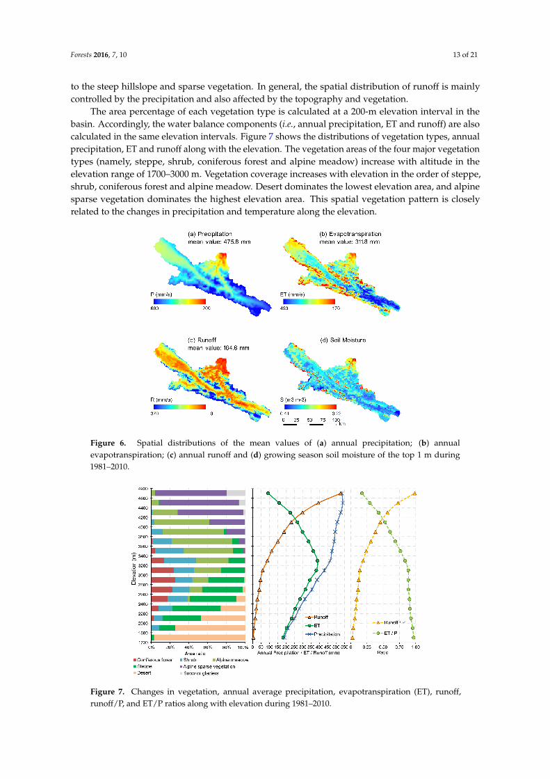
To better understand the ecohydrological pattern in the upper Heihe basin, the spatial distributionsof the water balance components are further analyzed, including the precipitation, evapotranspiration(ET), runoff and soil moisture in the top one meter during the vegetation growing season from Mayto October, based on a 30-year model simulation during 1981–2010. Figure 6 shows that annualprecipitation and runoff have a similar spatial pattern, annual actual evapotranspiration has a similarpattern with the soil moisture of the top layer in the growing season. The mean soil moisture valuesare relatively high (0.22–0.41) because of the selected wet season and possible uncertainties of soilwater parameters. As shown in Figure 6a, annual precipitation over the study catchment ranges from220 mm to 630 mm, and the East Tributary has the highest annual precipitation. Comparing Figure 6bwith Figure 2, the areas with relatively high ET correspond to the two major vegetation types, namely,steppe and alpine meadow. Figure 6b illustrates that ET has a similar pattern in the East and WestTributaries corresponding with the distribution of alpine meadow vegetation. However, the steep andnarrow valley area along the main stream (i.e., downstream of the junction of East and West Tributaries)has relatively low ET and low soil moisture due to the lower precipitation, and this is also related

Forests 2016, 7, 10 13 of 21

to the steep hillslope and sparse vegetation. In general, the spatial distribution of runoff is mainlycontrolled by the precipitation and also affected by the topography and vegetation.

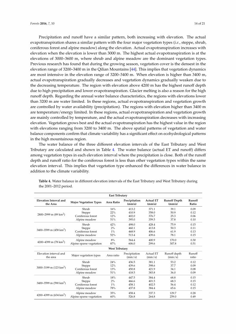
The area percentage of each vegetation type is calculated at a 200-m elevation interval in thebasin. Accordingly, the water balance components (i.e., annual precipitation, ET and runoff) are alsocalculated in the same elevation intervals. Figure 7 shows the distributions of vegetation types, annualprecipitation, ET and runoff along with the elevation. The vegetation areas of the four major vegetationtypes (namely, steppe, shrub, coniferous forest and alpine meadow) increase with altitude in theelevation range of 1700–3000 m. Vegetation coverage increases with elevation in the order of steppe,shrub, coniferous forest and alpine meadow. Desert dominates the lowest elevation area, and alpinesparse vegetation dominates the highest elevation area. This spatial vegetation pattern is closelyrelated to the changes in precipitation and temperature along the elevation.

Forests 2016, 7, 10 13/21

Figure 6. Spatial distributions of the mean values of (a) annual precipitation; (b) annual evapotranspiration;

(c) annual runoff and (d) growing season soil moisture of the top 1 m during 1981–2010.

Figure 7. Changes in vegetation, annual average precipitation, evapotranspiration (ET), runoff,

runoff/P, and ET/P ratios along with elevation during 1981–2010.

Precipitation and runoff have a similar pattern, both increasing with elevation. The actual

evapotranspiration shares a similar pattern with the four major vegetation types (i.e., steppe, shrub,

coniferous forest and alpine meadow) along the elevation. Actual evapotranspiration increases with

elevation when the elevation is lower than 3000 m. The highest actual evapotranspiration is at the

elevations of 3000–3600 m, where shrub and alpine meadow are the dominant vegetation types.

Previous research has found that during the growing season, vegetation cover is the densest in the

Figure 6. Spatial distributions of the mean values of (a) annual precipitation; (b) annualevapotranspiration; (c) annual runoff and (d) growing season soil moisture of the top 1 m during1981–2010.

Forests 2016, 7, 10 13/21

Figure 6. Spatial distributions of the mean values of (a) annual precipitation; (b) annual evapotranspiration;

(c) annual runoff and (d) growing season soil moisture of the top 1 m during 1981–2010.

Figure 7. Changes in vegetation, annual average precipitation, evapotranspiration (ET), runoff,

runoff/P, and ET/P ratios along with elevation during 1981–2010.

Precipitation and runoff have a similar pattern, both increasing with elevation. The actual

evapotranspiration shares a similar pattern with the four major vegetation types (i.e., steppe, shrub,

coniferous forest and alpine meadow) along the elevation. Actual evapotranspiration increases with

elevation when the elevation is lower than 3000 m. The highest actual evapotranspiration is at the

elevations of 3000–3600 m, where shrub and alpine meadow are the dominant vegetation types.

Previous research has found that during the growing season, vegetation cover is the densest in the

Figure 7. Changes in vegetation, annual average precipitation, evapotranspiration (ET), runoff,runoff/P, and ET/P ratios along with elevation during 1981–2010.

Forests 2016, 7, 10 14 of 21

Precipitation and runoff have a similar pattern, both increasing with elevation. The actualevapotranspiration shares a similar pattern with the four major vegetation types (i.e., steppe, shrub,coniferous forest and alpine meadow) along the elevation. Actual evapotranspiration increases withelevation when the elevation is lower than 3000 m. The highest actual evapotranspiration is at theelevations of 3000–3600 m, where shrub and alpine meadow are the dominant vegetation types.Previous research has found that during the growing season, vegetation cover is the densest in theelevation range of 3200–3400 m in the Qilian Mountains [44]. This implies that vegetation dynamicsare most intensive in the elevation range of 3200–3400 m. When elevation is higher than 3400 m,actual evapotranspiration gradually decreases and vegetation dynamics gradually weaken due tothe decreasing temperature. The region with elevation above 4200 m has the highest runoff depthdue to high precipitation and lower evapotranspiration. Glacier melting is also a reason for the highrunoff depth. Regarding the annual water balance characteristics, the regions with elevations lowerthan 3200 m are water limited. In these regions, actual evapotranspiration and vegetation growthare controlled by water availability (precipitation). The regions with elevation higher than 3400 mare temperature/energy limited. In these regions, actual evapotranspiration and vegetation growthare mainly controlled by temperature, and the actual evapotranspiration decreases with increasingelevation. Vegetation grows best and the actual evapotranspiration has the highest value in the regionwith elevations ranging from 3200 to 3400 m. The above spatial patterns of vegetation and waterbalance components confirm that climate variability has a significant effect on ecohydrological patternsin the high mountainous region.

The water balance of the three different elevation intervals of the East Tributary and WestTributary are calculated and shown in Table 4. The water balance (actual ET and runoff) differsamong vegetation types in each elevation interval where the precipitation is close. Both of the runoffdepth and runoff ratio for the coniferous forest is less than other vegetation types within the sameelevation interval. This implies that vegetation type enhanced the differences in water balance inaddition to the climate variability.

Table 4. Water balance in different elevation intervals of the East Tributary and West Tributary duringthe 2001–2012 period.

East Tributary

Elevation Interval andthe Area Major Vegetation Types Area Ratio Precipitation

(mm/a)Actual ET

(mm/a)Runoff Depth

(mm/a)RunoffRatio

2800–2999 m (89 km2)

Shrub 16% 413.2 371.1 39.1 0.09Steppe 22% 410.9 358.0 50.9 0.12

Coniferous forest 12% 402.0 376.7 25.3 0.06Alpine meadow 51% 395.0 359.5 37.8 0.10

3400–3599 m (458 km2)

Shrub 42% 498.0 428.4 75.9 0.15Steppe 2% 460.1 413.8 50.3 0.11

Coniferous forest 1% 468.9 406.6 61.9 0.13Alpine meadow 52% 513.4 439.6 78.1 0.15

4200–4399 m (78 km2)Alpine meadow 8% 564.4 400.9 170.0 0.30

Alpine sparse vegetation 87% 606.0 299.6 307.8 0.51

West Tributary

Elevation interval andthe area Major vegetation types Area ratio Precipitation

(mm/a)Actual ET(mm/a)

Runoff depth(mm/a)

Runoffratio

3000–3199 m (123 km2)

Shrub 24% 436.5 381.1 53.2 0.12Steppe 12% 439.6 398.6 37.7 0.09

Coniferous forest 13% 450.8 421.9 34.1 0.08Alpine meadow 51% 418.5 383.8 36.0 0.09

3400–3599 m (590 km2)

Shrub 18% 447.5 384.4 68.8 0.15Steppe 2% 466.6 401.5 68.3 0.15

Coniferous forest 1% 458.1 402.5 56.4 0.12Alpine meadow 78% 437.8 384.4 65.6 0.15

4200–4399 m (634 km2)Alpine meadow 35% 458.4 337.3 129.7 0.28

Alpine sparse vegetation 60% 526.8 264.8 259.0 0.49

Forests 2016, 7, 10 15 of 21

The water balance of the entire catchment for each vegetation type is also calculated and shownin Table 5, which is the result of the combined effects of climate and vegetation. Because the annualprecipitation increases with elevation and different vegetation types grow at different elevations, theannual precipitation of alpine meadow, alpine sparse vegetation and shrub are 488.5 mm, 547.3 mmand 495.9 mm, respectively, which are higher than those of coniferous forest (402.1 mm) and steppe(396.7 mm). The annual average actual evapotranspiration (ET) of coniferous forest, shrub, steppeand alpine meadow ranges from 331.5 mm to 355.0 mm, whereas the actual ET of alpine sparsevegetation is relatively lower (237.2 mm). Table 5 shows that the annual runoff depth varies fordifferent vegetation types. Alpine meadow and alpine sparse vegetation have higher annual runoff(147.8 mm and 310.1 mm, respectively) than forest and steppe (70.5 mm and 65.2 mm, respectively).The runoff ratios of the four major vegetation types, namely, steppe, shrub, coniferous forest andalpine meadow, range from 0.16 to 0.30, whereas alpine sparse vegetation has higher runoff ratio ofclose to 0.5 due to the high altitude. The water yield per unit area from different vegetation type isin order of alpine sparse vegetation, alpine meadow, shrub, coniferous forest and steppe. The topthree largest vegetation areas are covered by alpine meadow (with an area of 4549 km2), alpinesparse vegetation (with an area of 2009 km2) and shrub (with an area of 1652 km2), which are alsolocated in relatively high-elevation regions. The total runoff amount produced by the top three largestvegetation areas are 6.72 ˆ 108 m3/a (alpine meadow), 6.23 ˆ 108 m3/a (alpine sparse vegetation) and2.33 ˆ 108 m3/a (shrub) (see Table 5). The runoff amount produced by forests (with area of 561 km2)is 0.40 ˆ 108 m3/a. The coniferous forest has a small area (561 km2) and produces a small amount ofrunoff (0.40 ˆ 108 m3/a).

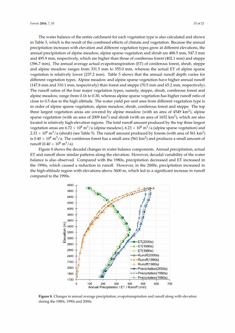
Figure 8 shows the decadal changes in water balance components. Annual precipitation, actualET and runoff show similar patterns along the elevation. However, decadal variability of the waterbalance is also observed. Compared with the 1980s, precipitation decreased and ET increased inthe 1990s, which caused a reduction in runoff. However, in the 2000s, precipitation increased inthe high-altitude region with elevations above 3600 m, which led to a significant increase in runoffcompared to the 1990s.

Forests 2016, 7, 10 15/21

The water balance of the entire catchment for each vegetation type is also calculated and shown

in Table 5, which is the result of the combined effects of climate and vegetation. Because the annual

precipitation increases with elevation and different vegetation types grow at different elevations, the

annual precipitation of alpine meadow, alpine sparse vegetation and shrub are 488.5 mm, 547.3 mm

and 495.9 mm, respectively, which are higher than those of coniferous forest (402.1 mm) and steppe

(396.7 mm). The annual average actual evapotranspiration (ET) of coniferous forest, shrub, steppe

and alpine meadow ranges from 331.5 mm to 355.0 mm, whereas the actual ET of alpine sparse

vegetation is relatively lower (237.2 mm). Table 5 shows that the annual runoff depth varies for

different vegetation types. Alpine meadow and alpine sparse vegetation have higher annual runoff

(147.8 mm and 310.1 mm, respectively) than forest and steppe (70.5 mm and 65.2 mm, respectively).

The runoff ratios of the four major vegetation types, namely, steppe, shrub, coniferous forest and

alpine meadow, range from 0.16 to 0.30, whereas alpine sparse vegetation has higher runoff ratio of

close to 0.5 due to the high altitude. The water yield per unit area from different vegetation type is in

order of alpine sparse vegetation, alpine meadow, shrub, coniferous forest and steppe. The top three

largest vegetation areas are covered by alpine meadow (with an area of 4549 km2), alpine sparse

vegetation (with an area of 2009 km2) and shrub (with an area of 1652 km2), which are also located in

relatively high-elevation regions. The total runoff amount produced by the top three largest

vegetation areas are 6.72 × 108 m3/a (alpine meadow), 6.23 × 108 m3/a (alpine sparse vegetation) and

2.33 × 108 m3/a (shrub) (see Table 5). The runoff amount produced by forests (with area of 561 km2) is

0.40 × 108 m3/a. The coniferous forest has a small area (561 km2) and produces a small amount of

runoff (0.40 × 108 m3/a).

Figure 8 shows the decadal changes in water balance components. Annual precipitation, actual

ET and runoff show similar patterns along the elevation. However, decadal variability of the water

balance is also observed. Compared with the 1980s, precipitation decreased and ET increased in the

1990s, which caused a reduction in runoff. However, in the 2000s, precipitation increased in the high-

altitude region with elevations above 3600 m, which led to a significant increase in runoff compared

to the 1990s.

Figure 8. Changes in annual average precipitation, evapotranspiration and runoff along with

elevation during the 1980s, 1990s and 2000s. Figure 8. Changes in annual average precipitation, evapotranspiration and runoff along with elevationduring the 1980s, 1990s and 2000s.

Forests 2016, 7, 10 16 of 21

Table 5. Water balance of the entire catchment for each vegetation type during the 2001–2012 period.

Vegetation Type and Area Covered byEach Type (km2)

Precipitation(mm/a)

Actual ET(mm/a)

Runoff Depth(mm/a)

RunoffRatio

Runoff Amount(108 m3/a)

Desert 91 253.1 238.0 15.1 0.06 0.01Shrub 1652 495.9 355.0 140.9 0.28 2.33Steppe 1063 396.7 331.5 65.2 0.16 0.69

Coniferous forest 561 402.1 331.6 70.5 0.18 0.40Alpine meadow 4549 488.5 348.7 147.8 0.30 6.72

Alpine sparse vegetation 2009 547.3 237.2 310.1 0.57 6.23Snow or glaciers 80 586.7 82.7 846.2 1.44 0.68

4.4. Comparison with Previous Studies in the Same and Similar Regions

In this study, the model simulation shows that the precipitation recharges soil water andgroundwater in the summer. This result is consistent with a previous study by Yang et al. [72] on theHeihe River. Using the hydrochemistry approach, it is found that the precipitation contributes onlyslightly to the total surface runoff, instead mainly recharging the sub-surface soil and groundwater.The interflow and groundwater flow dominate the total runoff. Additionally, Wang et al. [73] inferredthat as the air temperature has risen in the Heihe basin during the last 50 years, the active layer offrozen soil has increased in thickness. This may lead to the increase of both soil water storage andinterflow and thus change the contribution of each runoff component in the future.

Our study shows that forests contribute only a small amount of the water yield. In a previousstudy, He et al. [3] analyzed the water balance of a small experimental catchment (2.91 km2) in theupper Heihe basin and found that the forests contribute only 3.5% to the total runoff, which is similarto this study. This result is also supported by model simulations. For example, using the TopographyDriven Flux Exchange (FLEX-Topo) model, Gao et al. [74] report that forest hillslope generates onlya small amount of runoff in the upper Heihe basin. Qin et al. [75] analyze the water balance componentsof different landscapes in the upper Heihe basin using the VIC model and find that glaciers contribute3.57% of the total runoff and that the contribution of forests is also quite small (0.49%). This result alsoimplies that the barren regions contribute most of the total runoff (52.46%) and steppe contributes34.15% to the total runoff. This is in accordance with our results, as Qin et al. [75] consider the steppeand alpine meadow as the same vegetation type and consider regions in high elevation as barren.

Our study shows that the runoff ratio of coniferous forest has the lowest value (0.18) comparingwith other vegetation types except the desert in the upper Heihe River basin. This is similar to thefindings by Yaseef et al. [76], which shows that when precipitation larger than 300 mm ET accounts85% of precipitation for Aleppo pine forest in Southern Israel. Wang et al. [77] analyzed the annualwater balance of shrub at a station in the Inner Mongolian Highland Region with elevation of 1300 mand found that ET/P ratio is about 94%, which is higher than the results of the present study becauseof the differences of elevation and air temperature in the two study areas. Wang et al. [78] analyzed thewater balance of different vegetation in a small watershed in the Liupan Mountains, Northwest China,based on field measurements. They found that the evaporation rate (ratio of ET to precipitation) wasabout 60% for grassland, 93% for shrubs, and >95% for forest. This also shows that the forest has theleast water yield compared with other vegetation types in the Liupan Mountains.

5. Conclusions

A geomorphology-based ecohydrological model (GBEHM) is developed in the upper Heihebasin, and this model is validated using available observations, including soil moisture, streamflowdischarge, and actual evapotranspiration estimated from remote sensing. The catchment waterbalance characteristics and their spatial-temporal variability are analyzed based on the ecohydrologicalsimulation. The following conclusions can be drawn from the results of this study:

Forests 2016, 7, 10 17 of 21

(1) At the basin scale, the model provides a good simulation of streamflow discharge in the twotributaries and the entire catchment of the study area. It also captures the spatial pattern ofsoil moisture appropriately. In addition, the simulated actual evapotranspiration and remotesensing-based estimation have close long-term average values and similar spatial patterns overthe entire study catchment. The GBEHM may be useful for ecohydrological simulation andprediction in cold high-altitude regions.

(2) Analysis of the water balance characteristics shows that water balance characteristics are closelyrelated to the altitude and vegetation patterns in the study catchment. Regarding the annual waterbalance characteristics, the low-altitude regions with elevations below 3200 m are water limited.The actual annual evapotranspiration and vegetation distribution and growth are controlled bywater availability (precipitation). Seasonal analysis indicates that river runoffs are mainly insummer and autumn, and runoff in spring is generated from precipitation and snow melt.

(3) In the upper Heihe basin, the precipitation and runoff share a similar pattern, increasing withelevation. Actual evapotranspiration has a similar pattern with the four major vegetation types(i.e., steppe, shrub, coniferous forest and alpine meadow) along the elevation. The highest actualevapotranspiration is at the elevations of 3000–3600 m, where shrub and alpine meadow are thetwo dominant vegetation types. Precipitation controls the spatial pattern of annual runoff anddetermines the spatial pattern of vegetation together with the air temperature. Climate variabilityin the high mountainous region has a significant effect on ecohydrological patterns.

(4) At the same time, vegetation type enhanced the differences in annual runoff and actualevapotranspiration. In the same elevation interval with similar precipitation, differences inthe runoff depth (and the actual evapotranspiration) were caused mainly by the vegetation types.For the whole study area, the water yield per unit area from different vegetation types is in orderof alpine sparse vegetation, alpine meadow, shrub, coniferous forest and steppe. The three majorvegetation types, namely, alpine meadow (with an area of 4549 km2), alpine sparse vegetation(with an area of 2009 km2) and shrub (with an area of 1652 km2), located in relatively higherelevation contribute most of the river runoff.

Several limitations remain in the current study. The GBEHM simulates the vegetation dynamicswith the known leaf area index and other vegetation parameters. Further improvement of the modelshould include carbon partitioning to simulate the vegetation growth. The uncertainty of the modelparameters should be assessed to apply this model to other catchments.

Acknowledgments: This research was supported by the major plan of “Integrated Research on theEcohydrological Processes of the Heihe Basin” (Project Nos. 91225302, 91425303) funded by the National NaturalScience Foundation of China (NSFC).

Author Contributions: Dawen Yang conceived and designed the research. Yuanrun Zheng performed theclassification of vegetation types. Bing Gao performed the model programming and simulation. Yue Qin andYuhan Wang analyzed the simulated data. Yue Qin and Bing Gao took the lead in writing the manuscript.All authors contributed to the revision of the final manuscript.

Conflicts of Interest: The authors declare no conflict of interest.

References

1. Zhou, G.; Wei, X.; Luo, Y.; Zhang, M.; Li, Y.; Qiao, Y.; Liu, H.; Wang, C. Forest recovery and river discharge atthe regional scale of Guangdong Province, China. Water Resour. Res. 2010, 46, 5109–5115. [CrossRef]

2. Liu, W.; Wei, X.; Liu, S.; Liu, Y.; Fan, H.; Zhang, M.; Yin, J.; Zhan, M. How do climate and forest changesaffect long-term streamflow dynamics? A case study in the upper reach of Poyang River basin. Ecohydrology2015, 8, 46–57. [CrossRef]

3. He, Z.B.; Zhao, W.Z.; Liu, H.; Tang, Z.X. Effect of forest on annual water yield in the mountains of an aridinland river basin: A case study in the Pailugou catchment on northwestern China’s Qilian Mountains.Hydrol. Process. 2012, 26, 613–621. [CrossRef]

Forests 2016, 7, 10 18 of 21

4. Li, X.; Cheng, G.D.; Liu, S.M.; Xiao, Q.; Ma, M.G.; Jin, R.; Che, T.; Liu, Q.H.; Wang, W.Z.; Qi, Y.; et al. HeiheWatershed Allied Telemetry Experimental Research (HiWATER): Scientific Objectives and ExperimentalDesign. Bull. Am. Meteorol. Soc. 2013, 94, 1145–1160. [CrossRef]

5. Chang, H.J.; Jung, I.W. Spatial and temporal changes in runoff caused by climate change in a complex largeriver basin in Oregon. J. Hydrol. 2010, 388, 186–207. [CrossRef]

6. Belmont, P.; Gran, K.B.; Schottler, S.P.; Wilcock, P.R.; Day, S.S.; Jennings, C.; Lauer, J.W.; Viparelli, E.;Willenbring, J.K.; Engstrom, D.R.; et al. Large Shift in Source of Fine Sediment in the Upper Mississippi River.Environ. Sci. Technol. 2011, 45, 8804–8810. [CrossRef] [PubMed]

7. Taye, M.T.; Ntegeka, V.; Ogiramoi, N.P.; Willems, P. Assessment of climate change impact on hydrologicalextremes in two source regions of the Nile River Basin. Hydrol. Earth Syst. Sci. 2011, 15, 209–222. [CrossRef]

8. Zhou, D.G.; Huang, R.H. Response of water budget to recent climatic changes in the source region of theYellow River. Chin. Sci. Bull. 2012, 57, 2155–2162. [CrossRef]

9. Wu, L.; Long, T.Y.; Liu, X.; Guo, J.S. Impacts of climate and land-use changes on the migration of non-pointsource nitrogen and phosphorus during rainfall-runoff in the Jialing River Watershed, China. J. Hydrol.2012, 475, 26–41. [CrossRef]

10. Ficklin, D.L.; Stewart, I.T.; Maurer, E.P. Climate Change Impacts on Streamflow and Subbasin-ScaleHydrology in the Upper Colorado River Basin. PLoS ONE 2013, 8, e71297. [CrossRef] [PubMed]

11. Cuo, L.; Zhang, Y.X.; Gao, Y.H.; Hao, Z.C.; Cairang, L.S. The impacts of climate change and land cover/usetransition on the hydrology in the upper Yellow River Basin, China. J. Hydrol. 2013, 502, 37–52. [CrossRef]

12. Yang, H.B.; Qi, J.; Xu, X.Y.; Yang, D.W.; Lv, H.F. The regional variation in climate elasticity and climatecontribution to runoff across China. J. Hydrol. 2014, 517, 607–616. [CrossRef]

13. Ma, H.; Yang, D.W.; Tan, S.K.; Gao, B.; Hu, Q.F. Impact of climate variability and human activity onstreamflow decrease in the Miyun Reservoir catchment. J. Hydrol. 2010, 389, 317–324. [CrossRef]

14. Xu, X.Y.; Yang, H.B.; Yang, D.W.; Ma, H. Assessing the impacts of climate variability and human activities onannual runoff in the Luan River basin, China. Hydrol. Res. 2013, 44, 940–952. [CrossRef]

15. Tang, Y.; Tang, Q.; Tian, F.; Zhang, Z.; Liu, G. Responses of natural runoff to recent climatic variations in theYellow River basin, China. Hydrol. Earth Syst. Sci. 2013, 17, 4471–4480. [CrossRef]

16. Peel, M. Hydrology: Catchment vegetation and runoff. Prog. Phys. Geogr. 2009, 33, 837–844. [CrossRef]17. Samaniego, L.; Bardossy, A. Simulation of the impacts of land use/cover and climatic changes on the runoff

characteristics at the mesoscale. Ecol. Model. 2006, 196, 45–61. [CrossRef]18. Marshall, E.; Randhir, T.O. Spatial modeling of land cover change and watershed response using Markovian

cellular automata and simulation. Water Resour. Res. 2008, 44, W044234. [CrossRef]19. Yang, D.W.; Gao, B.; Jiao, Y.; Lei, H.M.; Zhang, Y.L.; Yang, H.B.; Cong, Z.T. A distributed scheme developed

for eco-hydrological modeling in the upper Heihe River. Sci. China Earth Sci. 2015, 58, 36–45. [CrossRef]20. Abbott, M.B.; Bathurst, J.C.; Cunge, J.A.; O’connell, P.E.; Rasmussen, J. An introduction to the European

Hydrological System—Systeme Hydrologique Europeen, “SHE”, 2: Structure of a physically-based,distributed modelling system. J. Hydrol. 1986, 87, 61–77. [CrossRef]

21. Liang, X.; Lettenmaier, D.P.; Wood, E.F. One-dimensional statistical dynamic representation of subgrid spatialvariability of precipitation in the two-layer variable infiltration capacity model. J. Geophys. Res. 1996, 101,21403–21422. [CrossRef]

22. Yang, D.W.; Koike, T.; Tanizawa, H. Application of a distributed hydrological model and weather radarobservations for flood management in the upper Tone River of Japan. Hydrol. Process. 2004, 18, 3119–3132.[CrossRef]

23. Yang, D.W.; Li, C.; Ni, G.H.; Hu, H.P. Application of a distributed hydrological model to the Yellow Riverbasin. Acta Geogr. Sin. 2004, 59, 143–154. (In Chinese)

24. Xu, J.J.; Yang, D.W.; Yi, Y.H.; Lei, Z.D.; Chen, J.; Yang, W.J. Spatial and temporal variation of runoff in theYangtze River basin during the past 40 years. Quat. Int. 2008, 186, 32–42. [CrossRef]

25. Cong, Z.T.; Yang, D.W.; Gao, B.; Yang, H.B.; Hu, H.P. Hydrological trend analysis in the Yellow River basinusing a distributed hydrological model. Water Resour. Res. 2009, 45, W00A13. [CrossRef]

26. Valeriano, O.; Koike, T.; Yang, K.; Yang, D.W. Optimal Dam Operation during Flood Season Usinga Distributed Hydrological Model and a Heuristic Algorithm. J. Hydrol. Eng. 2010, 15, 580–586. [CrossRef]

Forests 2016, 7, 10 19 of 21

27. Alam, Z.R.; Rahman, M.M.; Islam, A.S. Assessment of Climate Change Impact on the Meghna River Basinusing geomorphology based hydrological model (GBHM). In Proceedings of the ICWFM 2011—The 3rdInternational Conference on Water and Flood Management, Dhaka, Bangladesh, 8–10 January 2011.

28. Sellers, P.J.; Randall, D.A.; Collatz, G.J.; Berry, J.A.; Field, C.B.; Dazlich, D.A.; Zhang, C.; Collelo, G.D.;Bounoua, L. A Revised Land Surface Parameterization (SiB2) for Atmospheric GCMS. Part I: ModelFormulation. J. Clim. 1996, 9, 676–705. [CrossRef]

29. Wang, L.; Koike, T.; Yang, K.; Jackson, T.J.; Bindlish, R.; Yang, D.W. Development of a distributed biospherehydrological model and its evaluation with the Southern Great Plains Experiments (SGP97 and SGP99).J. Geophys. Res. 2009, 114. [CrossRef]

30. Wang, L.; Koike, T. Comparison of a distributed biosphere hydrological model with GBHM. Annu. J.Hydraul. Eng. 2009, 53, 103–108.

31. Oleson, K.W.; Lawrence, D.M.; Bonan, G.B.; Flanner, M.G.; Kluzek, E.; Lawrence, P.J.; Levis, S.; Swenson, S.C.;Thornton, P.E.; Dai, A.G.; et al. Technical Description of Version 4.0 of the Community Land Model (CLM), NCARTechnical Note; National Center for Atmospheric Research: Boulder, CO, USA, 2010; p. 257.

32. Tague, C.; Band, L. RHESSys: Regional Hydro-ecologic simulation system: An object-oriented approach tospatially distributed modeling of carbon, water and nutrient cycling. Earth Interact. 2004, 19, 1–42. [CrossRef]

33. Maneta, M.; Silverman, N. A spatially-distributed model to simulate water, energy and vegetation dynamicsusing information from regional climate models. Earth Interact. 2013, 17, 1–44. [CrossRef]

34. Ivanov, V.Y.; Bras, R.L.; Vivoni, E.R. Vegetation-Hydrology Dynamics in Complex Terrain of Semiarid Areas:I. A mechanistic Approach to Modeling Dynamic Feedbacks. Water Resour. Res. 2008, 44. [CrossRef]

35. Jia, Y.W.; Wang, H.; Yan, D.H. Distributed model of hydrological cycle system in Heihe River basin I Modeldevelopment and Verification. J. Hydraul. Eng. 2006, 37, 534–542. (In Chinese).

36. Wang, L.; Koike, T.; Yang, K.; Jin, R.; Li, H. Frozen soil parameterization in a distributed biospherehydrological model. Hydrol. Earth Syst. Sci. 2010, 14, 557–571. [CrossRef]

37. Zhang, Y.L.; Cheng, G.D.; Li, X.; Han, X.J.; Wang, L.; Li, H.Y.; Chang, X.L.; Flerchinger, G.N. Coupling ofa simultaneous heat and water model with a distributed hydrological model and evaluation of the combinedmodel in a cold region watershed. Hydrol. Process. 2013, 27, 3762–3776. [CrossRef]

38. Zhou, J.; Pomeroy, J.W.; Zhang, W.; Cheng, G.D.; Wang, G.X.; Chen, C. Simulating cold regions hydrologicalprocesses using a modular model in the west of China. J. Hydrol. 2014, 509, 13–24. [CrossRef]

39. Zang, C.F.; Liu, J.G. Trend analysis for the flows of green and blue water in the Heihe River basin,northwestern China. J. Hydrol. 2013, 502, 27–36. [CrossRef]

40. Cheng, G.; Li, X.; Zhao, W.; Xu, Z.; Feng, Q.; Xiao, S.; Xiao, H. Integrated study of thewater-ecosystem-economy in the Heihe River Basin. Natl. Sci. Rev. 2014, 1, 413–428. [CrossRef]

41. Chen, Y.; Zhang, D.; Sun, Y.; Liu, X.; Wang, N.; Savenije, H. Water demand management: A case study of theHeihe River Basin in China. Phys. Chem. Earth 2005, 30, 408–419. [CrossRef]

42. Herzschuh, U.; Kurschner, H.; Mischke, S. Temperature variability and vertical vegetation belt shifts duringthe last similar to ~50,000 yr in the Qilian Mountains (NE margin of the Tibetan Plateau, China). Quat. Res.2006, 66, 133–146. [CrossRef]

43. Wang, P.; Li, Z.Q.; Gao, W.Y. Rapid Shrinking of Glaciers in the Middle Qilian Mountain Region of NorthwestChina during the Last similar to 50 Years. J. Earth Sci. 2011, 22, 539–548. [CrossRef]

44. Deng, S.F.; Yang, T.B.; Zeng, B.; Zhu, X.F.; Xu, H.J. Vegetation cover variation in the Qilian Mountains and itsresponse to climate change in 2000–2011. J. Mt. Sci. 2013, 10, 1050–1062. [CrossRef]

45. National Meteorological Information Center, the China Meteorological Administration. Available online:http://cdc.nmic.cn (accessed on 24 December 2015).

46. Shen, Y.; Xiong, A. Validation and comparison of a new gauge-based precipitation analysis over mainlandChina. Int. J. Climatol. 2015. [CrossRef]

47. Wu, L.; Li, X. Dataset of the First Glacier Inventory in China; Cold and Arid Regions Science Data Center:Lanzhou, China, 2004.

48. Guo, W.; Liu, S.; Yao, X.; Xu, J.; Shangguan, D.; Wu, L.; Zhao, J.; Liu, Q.; Jiang, Z.; Wei, J.; et al. The SecondGlacier Inventory Dataset of China (Version 1.0); Cold and Arid Regions Science Data Center: Lanzhou,China, 2014.

Forests 2016, 7, 10 20 of 21

49. Wei, J.F.; Liu, S.Y.; Guo, W.Q.; Yao, X.J.; Xu, J.L.; Bao, W.J.; Jiang, Z.L. Surface-area changes of glaciers in theTibetan Plateau interior area since the 1970s using recent Landsat images and historical maps. Ann. Glaciol.2014, 55, 213–222. [CrossRef]

50. Cold and Arid Regions Science Data Center at Lanzhou. Available online: http://westdc.westgis.ac.cn(accessed on 24 December 2015).

51. Jarvis, A.; Reuter, H.I.; Nelson, A.; Guevara, E. Hole-filled seamless SRTM data (Version 4). InternationalCentre for Tropical Agriculture. 2008. Available online: http://srtm.csi.cgiar.org (accessed on 31 July 2015).

52. Hou, X. China Vegetation Map (1:1,000,000); Science Press: Beijing, China, 2001. (In Chinese)53. Zhou, J.H.; Zheng, Y.R. Vegetation Map of the Upper Heihe Basin V2.0; Heihe Plan Science Data Center: Lanzhou,

China, 2014.54. Fan, W. Heihe 1 km LAI Production; Heihe Plan Science Data Center: Lanzhou, China, 2014.55. Shi, X.; Yu, D.; Pan, X. A framework for the 1:1,000,000 soil database of China. In Proceedings of the 17th

World Congress of Soil Science, Bangkok, Thailand, 14–21 August 2002; pp. 1–5.56. Dai, Y.J.; Shangguan, W.; Duan, Q.Y.; Liu, B.Y.; Fu, S.H.; Niu, G. Development of a China Dataset of Soil

Hydraulic Parameters Using Pedotransfer Functions for Land Surface Modeling. J. Hydrometeorol. 2013, 14,869–887. [CrossRef]

57. Jin, R.; Li, X.; Yan, B.P.; Li, X.H.; Luo, W.M.; Ma, M.G.; Guo, J.W.; Kang, J.; Zhu, Z.L.; Zhao, S.J. A NestedEcohydrological Wireless Sensor Network for Capturing the Surface Heterogeneity in the Midstream Areasof the Heihe River Basin, China. IEEE Geosci. Remote Sens. Lett. 2014, 11, 2015–2019. [CrossRef]

58. Kang, J.; Jin, R.; Li, X.; Ma, M. HiWATER: WATERNET Observation Dataset in the Upper Reaches of the HeiheRiver Basin in 2013; Cold and Arid Regions Science Data Center: Lanzhou, China, 2014.

59. Wu, B.F. Monthly Evapotranspiration Datasets (2000–2012) with 1 km Spatial Resolution over the Heihe River Basin;Heihe Plan Science Data Center: Lanzhou, China, 2013.

60. Wu, B.F.; Yan, N.N.; Xiong, J.; Bastiaanssen, W.; Zhu, W.W.; Stein, A. Validation of ETWatch using fieldmeasurements at diverse landscapes: A case study in Hai Basin of China. J. Hydrol. 2012, 436, 67–80.[CrossRef]

61. Yang, D.W.; Herath, S.; Musiake, K. Development of a geomorphology-based hydrological model for largecatchments. Annu. J. Hydraul. Eng. 1998, 42, 169–174. [CrossRef]

62. Yang, D.W.; Herath, S.; Musiake, K. Comparison of different distributed hydrological models forcharacterization of catchment spatial variability. Hydrol. Process. 2000, 14, 403–416. [CrossRef]

63. Yang, D.W.; Herath, S.; Musiake, K. Spatial resolution sensitivity of catchment geomorphologic propertiesand the effect on hydrological simulation. Hydrol. Process. 2001, 15, 2085–2099. [CrossRef]

64. Yang, D.W.; Herath, S.; Musiake, K. A hillslope-based hydrological model using catchment area and widthfunctions. Hydrol. Sci. J. 2002, 47, 49–65. [CrossRef]

65. Sellers, P.J. Canopy reflectance, photosynthesis, and transpiration. Int. J. Remote Sens. 1985, 8, 1335–1372.[CrossRef]

66. Sellers, P.J.; Mintz, Y.; Sub, Y.C.; Dalcher, A. A Simple Biosphere Model (SiB) for Use within GeneralCirculation Models. J. Atmos. Sci. 1986, 43, 505–531. [CrossRef]

67. Sellers, P.J.; Berry, J.A.; Collatz, G.J.; Field, C.B.; Hall, F.G. Canopy reflectance, photosynthesis, andtranspiration Part III: Are analysis using improved leaf models and a new canopy integration scheme.Remote Sens. Environ. 1992, 42, 187–216. [CrossRef]

68. Collatz, G.J.; Ball, J.T.; Grivet, C.; Berry, J.A. Physiological and environmental regulation of stomatalconductance, photosynthesis and transpiration: A model that includes a laminar boundary layer.Agric. For. Meteorol. 1991, 54, 107–136. [CrossRef]

69. Collatz, G.J.; Ribas-Carbo, M.; Berry, J.A. Coupled Photosynthesis-Stomatal Conductance Model for leavesof C4 plants. Aust. J. Plant Physiol. 1992, 19, 519–538. [CrossRef]

70. Zhang, Y.; Liu, S.Y.; Ding, Y.J. Spatial Variation of Degree-day Factors on the Observed Glaciers in WesternChina. Acta Geogr. Sin. 2006, 61, 89–98. (In Chinese) [CrossRef]

71. Gao, X.; Ye, B.S.; Zhang, S.Q.; Qiao, C.J.; Zhang, X.W. Glacier runoff variation and its influence on riverrunoff during 1961–2006 in the Tarim River Basin, China. Sci. China Earth Sci. 2010, 53, 880–891. (In Chinese)[CrossRef]

Forests 2016, 7, 10 21 of 21

72. Yang, Y.; Xiao, H.; Wei, Y.; Zhao, L.; Zou, S.; Qiu, Y.; Yin, Z. Hydrological processes in the different landscapezones of alpine cold regions in the wet season, combining isotopic and hydrochemical tracers. Hydrol. Process.2012, 26, 1457–1466. [CrossRef]

73. Wang, Y.; Yang, D.; Lei, H.; Yang, H. Impact of cryosphere hydrological processes on the river runoff in theupper reaches of Heihe River. J. Hydraul. Eng. 2015, 46, 1064–1071. (In Chinese)

74. Gao, H.; Hrachowitz, M.; Fenicia, F.; Gharari, S.; Savenije, H. Testing the realism of a topography-drivenmodel (FLEX-Topo) in the nested catchments of the Upper Heihe, China. Hydrol. Earth Syst. Sci. 2014, 18,1895–1915. [CrossRef]

75. Qin, J.; Ding, Y.; Wu, J.; Gao, M.; Yi, S.; Zhao, C.; Ye, B.; Li, M.; Wang, S. Understanding the impact of mountainlandscapes on water balance in the upper Heihe River watershed in northwestern China. J. Arid Land 2013, 5,366–384. [CrossRef]

76. Yaseef, N.R.; Yakir, D.; Rotenberg, E.; Schiller, G.; Cohen, S. Ecohydrology of a semi-arid forest: Partitioningamong water balance components and its implications for predicted precipitation changes. Ecohydrology2009. [CrossRef]

77. Wang, X.; Ronny, B.; Li, X.; Kang, E. Water balance change for a re-vegetated xerophyte shrub area.Hydrol. Sci. J. 2004, 49, 283–295. [CrossRef]

78. Wang, Y.; Yu, P.; Xiong, W.; Shen, Z.; Guo, M.; Shi, Z.; Du, A.; Wang, L. Water-yield reduction afterafforestation and related processes in the semiarid Liupan Mountains, Northwest China. J. Am. WaterResour. Assoc. 2008, 44, 1086–1097. [CrossRef]

© 2015 by the authors; licensee MDPI, Basel, Switzerland. This article is an open accessarticle distributed under the terms and conditions of the Creative Commons by Attribution(CC-BY) license (http://creativecommons.org/licenses/by/4.0/).