MODELING EURASIAN WATERMILFOIL (MYRIOPHYLLUM SPICATUM) HABITAT

WITH GEOGRAPHIC INFORMATION SYSTEMS

By

Joby Michelle Prince

A Dissertation

Submitted to the Faculty of Mississippi State University

In Partial Fulfillment of the Requirements for the Degree of Doctor of Philosophy

in Agronomy in the Department of Plant and Soil Sciences

Mississippi State, Mississippi

April 2011

MODELING EURASIAN WATERMILFOIL (MYRIOPHYLLUM SPICATUM) HABITAT

WITH GEOGRAPHIC INFORMATION SYSTEMS

By

Joby Michelle Prince

Approved:

David R. Shaw Giles Distinguished Professor of Weed Science (Major Professor)

John D. Madsen Associate Extension/Research Professor of Weed Science (Major Professor and Director of Dissertation)

Justin H. Shows Assistant Professor of Statistics (Minor Professor)

Jane L. Harvill Associate Professor of Statistics (Committee Member)

Gary N. Ervin Associate Professor of Biological Sciences (Committee Member)

James L. Martin Professor (Committee Member)

Scott A. Samson Extension Professor (Committee Member)

William L. Kingery Professor of Agronomy Graduate Coordinator

George M. Hopper Interim Dean of the College of Agriculture and Life Sciences

Name: Joby Michelle Prince

Date of Degree: April 29, 2011

Institution: Mississippi State University

Major Field: Agronomy

Major Professors: David R. Shaw and John D. Madsen

Title of Study: MODELING EURASIAN WATERMILFOIL (MYRIOPHYLLUM SPICATUM) HABITAT WITH GEOGRAPHIC INFORMATION SYSTEMS

Pages in Study: 101

Candidate for Degree of Doctor of Philosophy

Eurasian watermilfoil (Myriophyllum spicatum) habitat was predicted at multiple

scales, including a lake, regional, and national level. This dissertation illustrates how

habitat can be predicted for M. spicatum using publically-available data for both

presence and environmental variables. Models were generated using statistical

procedures and quantative methods to determine where the greatest likelihood of

presence was located. For the single lake, presence and absence data were available,

but the larger-scale models used presence-only methods of prediction. These models

were paired with a Geographic Information System so that data could be visualized on a

map. For the selected lake, Pend Oreille (Idaho), spatial analysis using general linear

mixed models was used to show that depth and fetch could be used to predict habitat,

although differences were seen in their importance between the littoral and pelagic

zones. For the states of Minnesota and Wisconsin, Mahalanobis distance and maximum

entropy methods were used to demonstrate that available habitat will not always mean

presence of M. spicatum. The differing approaches to management in these states

illustrated how an aggressive public education campaign can limit spread of M.

spicatum, even when habitat is available. Bass habitat appeared to be the largest

predictor of M. spicatum in Minnesota, although this was due to the similar

environmental preferences by these species. Using maximum entropy, on a national

level, presence of M. spicatum appeared to be best predicted by annual precipitation.

Again, results showed that habitat is colonized as time permits, and not necessarily as

conditions permit.

ii

DEDICATION

I would like to dedicate this dissertation to my parents, Mack and Donna Prince.

God has blessed me beyond what I deserve, especially with my parents. I would not

have wanted them to be any different and they could not have been better. While I am

sure they would not call it a “sacrifice,” I know they have given much so that I could have

the opportunities I have had. It can not be easy to tell people that your thirty-something

daughter is “still in school”. I only hope that I have made my parents proud and that they

will look at what we have done and say it was worth the cost.

iii

ACKNOWLEDGEMENTS

I have been extremely fortunate to have been extended the opportunities in my

life. God has been generous in his blessings. Among these was the offer to come to

Mississippi State University and study under such esteemed scholars. Dr. David Shaw

has been patient with me as I have floundered with my research and questioned where

my life was going. He has been a trusted advisor and someone I have always admired

and felt fortunate to have been associated with. I am sure Dr. Shaw was relieved to

have Dr. John Madsen join him in his efforts to get me through school. Dr. Madsen is

“kind of a big deal”, and I am so grateful he puts out the crumbs for me to follow as I try

to understand what my research is showing. Dr. Jane Harvill has been missed dearly,

but she has been available to help me conquer all the statistics that I never learned in

school. Moreover, she has been a great friend and strong influence in my life. The

three of you have helped me grow up, even when I thought I was already grown.

I would also like to thank my other committee members, Dr. Justin Shows, Dr.

Gary Ervin, Dr. James Martin, and Dr. Scott Samson. I have been fortunate to also have

help from other faculty including Dr. Jeff Willers and Dr. Chris Brooks. Their expertise

has sometimes been the difference between success and failure. I would also mention

the support I have received from Dr. Ryan Wersal and Mr. John Cartwright. I feel the

most sympathy for John as he has endured me yelling at my computer and smacking my

desk in frustration. Finally, no one does this alone. I am so thankful for friends and

iv

family for being a shoulder to cry on, a voice of reason, and stick when I needed

prodding.

v

TABLE OF CONTENTS

DEDICATION .................................................................................................................... ii

ACKNOWLEDGEMENTS ................................................................................................. iii

LIST OF TABLES ............................................................................................................. vii

LIST OF FIGURES ........................................................................................................... ix

CHAPTER

1. INTRODUCTION ................................................................................................... 1

Theoretical Background ......................................................................................... 2 Technical Aspects of Model Function .................................................................... 4 Background for Conceptual Model ......................................................................... 5 Spatial Aspects of the Research Problem ............................................................. 7 Model Uncertainty .................................................................................................. 8 Project Objectives .................................................................................................. 9 Project Contribution ............................................................................................. 10 Literature Cited .................................................................................................... 11

2. LOCAL-SCALE MODEL: PEND OREILLE (IDAHO) ........................................... 16

Methods and Materials ........................................................................................ 17 Site Description........................................................................................ 17 Conceptual Model .................................................................................... 18 Model Data Preparation ........................................................................... 19

Data Analysis ...................................................................................................... 22 GIS Analysis ........................................................................................................ 23 Results ................................................................................................................ 23

Littoral ...................................................................................................... 24 Logistic Regression ...................................................................... 25 Binomial Regression with Overdispersion ................................... 26 Conditional Spatial GLMM ........................................................... 27 Marginal Spatial GLM .................................................................. 28 GIS Analysis ................................................................................ 29

Pelagic ..................................................................................................... 29 Logistic Regression ...................................................................... 29 Binomial Regression with Overdispersion ................................... 30 Random Effects ........................................................................... 30

vi

Marginal Spatial GLM .................................................................. 31 GIS Analysis ................................................................................ 31

Discussion ........................................................................................................... 31 Conclusions ......................................................................................................... 33 Literature Cited .................................................................................................... 34

3. REGIONAL-SCALE MODEL: MINNESOTA ........................................................ 57

Methods and Materials ........................................................................................ 59 Mahalanobis ............................................................................................ 60 Maxent ..................................................................................................... 61

Results ................................................................................................................ 62 Mahalanobis ............................................................................................ 62 Maxent ..................................................................................................... 62

Discussion ........................................................................................................... 64 Conclusion ........................................................................................................... 66 Literature Cited .................................................................................................... 68

4. NATIONAL-SCALE MODEL ................................................................................ 76

Materials and Methods ........................................................................................ 78 Results and Discussion ....................................................................................... 81 Conclusion ........................................................................................................... 85 Literature Cited .................................................................................................... 87

5. SUMMARY AND FUTURE RESEARCH ............................................................. 93

Positive Outcomes .............................................................................................. 95 Future Research .................................................................................................. 96 Literature Cited .................................................................................................... 98

APPENDIX

A. DATA DEFINITIONS FOR ALL CHAPTERS ....................................................... 99

vii

LIST OF TABLES

1.1 Factors influencing growth and morphology of Eurasian watermilfoil (Smith and Barko 1990). ........................................................................................ 15

2.1 Factors influencing growth and morphology of Eurasian watermilfoil (Smith

and Barko 1990). ........................................................................................ 44 2.2 Frequency table of presence of M. spicatum on Pend Oreille littoral zone. ........... 45

2.3 Results of logistic regression model for M. spicatum on Pend Oreille littoral

zone ............................................................................................................ 46

2.4 Measures of correlation from logistic regression model for M. spicatum on Pend Oreille littoral zone ............................................................................ 47

2.5 Results of binomial regression model with overdispersion for M. spicatum

on Pend Oreille littoral zone. ...................................................................... 48 2.6 Results of conditional spatial GLMM for M. spicatum on Pend Oreille littoral

zone. ........................................................................................................... 49 2.7 Results of marginal spatial GLM for M. spicatum on Pend Oreille littoral

zone. ........................................................................................................... 50 2.8 Frequency table of presence of M. spicatum on Pend Oreille pelagic zone. ......... 51

2.9 Results of logistic regression model for M. spicatum on Pend Oreille pelagic zone ............................................................................................... 52

2.10 Measures of correlation from logistic regression model for M. spicatum on

Pend Oreille pelagic zone. .......................................................................... 53 2.11 Results of binomial regression model with overdispersion for M. spicatum

on Pend Oreille pelagic zone. ..................................................................... 54 2.12 Results of random effects model for M. spicatum on Pend Oreille pelagic

zone. ........................................................................................................... 55 2.13 Results of marginal spatial GLM model for M. spicatum on Pend Oreille

pelagic zone. ............................................................................................. 56

viii

3.1 Validation results comparing presence (P) and absence (A) for field (observed) and predicted from Mahalanobis model for prediction of M. spicatum in Minnesota. .......................................................................... 74

3.2 Validation results comparing presence (P) and absence (A) for field

(observed) and predicted from Mahalanobis model for prediction of M. spicatum in Minnesota and Wisconsin. ................................................. 75

ix

LIST OF FIGURES

1.1 Example of a map algebra operation using addition (after Chrisman 2002). ......... 13 1.2 Conceptual model of proposed interactions between environmental

variables affecting Myriophyllum spicatum. ............................................... 14 2.1 Conceptual model of proposed interactions between environmental

variables affecting Myriophyllum spicatum. ............................................... 36 2.2 Separate analyses were conducted for the littoral and pelagic zones of

Pend Oreille Lake (Idaho) and outflowing river. ......................................... 37 2.3 Summary of probabilities for marginal spatial GLMM on the littoral zone for

two- and three-class ordinal categories (X-axis). Bar ranges run from the minimum to the maximum value for each ordinal category; values on the Y-axis reflect probability ....................................................... 38

2.4 Map of paired ordinal categories for two-class marginal spatial GLM for

Pend Oreille littoral zone. .......................................................................... 39 2.5 Predicted probabilities from marginal spatial GLM for Pend Oreille littoral

zone. ........................................................................................................... 40 2.6 Map of paired ordinal categories for two-class binomial regression with

overdispersion for Pend Oreille pelagic zone. ............................................ 41 2.7 Predicted probabilities from binomial regression with overdispersion for

Pend Oreille pelagic zone. .......................................................................... 42 2.8 True littoral zone for Pend Oreille lake with points predicted at greater than

or equal to 50% probability of being suitable M. spicatum habitat. ............. 43 3.1 Results of Mahalanobis analysis using 0.5 as the threshold for

presence/absence of M. spicatum in Minnesota. ....................................... 70 3.2 Results of Mahalanobis analysis using 0.5 as the threshold for

presence/absence of M. spicatum in Minnesota and Wisconsin. ............... 71 3.3 Receiver operating characteristic curve for maxent analysis of M. spicatum

in Minnesota. .............................................................................................. 72

x

3.4 Results of maxent analysis for prediction of M. spicatum in Minnesota................. 73 4.1 Receiver operating characteristic curve for maxent analysis of M. spicatum

in the United States. ................................................................................... 90 4.2 Maxent predictions for M. spicatum in the United States. Warmer colors

show areas with better predicted conditions. White dots show the presence locations. .................................................................................... 91

4.3 Distribution of M. spicatum records collected by Couch and Nelson (1985)

for 1980 ...................................................................................................... 92

1

CHAPTER 1

INTRODUCTION

The abiotic components of the environment necessary for survival constitute the

habitat requirements for a species (Gillenwater et al. 2006). Species habitat

requirements are described by habitat factors, which cover the most essential

characteristics of preferred habitats (Store and Jokimäki 2003). Geographic Information

Systems (GIS) are well suited for studies involving habitat modeling and delineation,

sometimes referred to as habitat suitability indexing (Gillenwater et al. 2006; Wang

1994). Geographic Information Systems also offer the advantage of being able to

overlay layers representing the spatial distribution of different environmental variables

related to habitat suitability and perform spatial operations on these layers (Gillenwater

et al. 2006).

The majority of previous work in habitat modeling, with and without the use of

GIS, focused on identifying and delineating potentially suitable habitats for desirable

species. Less focus has been given to using predictive modeling for species control or

proactive, preventative practices for nuisance species. Modeling such as this is

necessary to provide natural resource managers and policy makers with predictions of

the effects of a particular management practice (Valley et al. 2005). Morisette et al.

(2006) developed a nationwide habitat map for tamarisk (Tamarix spp.). The habitat

distribution map provided not only location information, but also helped guide

containment boundaries, identify priority areas for early detection and rapid response,

2

and monitor control strategies and cost-effectiveness in different states. Ecological

models can also be used as a forecasting tool to examine potential ecological impacts

and prioritize needs (Rotenberry et al. 2006), and to evaluate the expected effects of a

variety of landuse changes on a species or an ecological system (Romero-Calcerrada

and Luque 2006).

Theoretical Background

Development of ecological models provides a simple, direct method by which to

predict presence, absence, and spread of species in given environments. Levin (1992)

calls the understanding of patterns and process the “essence of science” while

acknowledging that complexity in nature forces modelers to make a trade-off between

detail and generalization. Romero-Calcerrada and Luque (2006) urged a “need to

develop indicators that simplify complexity in natural systems.” Simpler models are often

preferred to complex models because it is believed they have wider applicability and

represent better overall prediction of species presence. Levin (1992) noted that models

should contain “just enough” detail with the idea that the objective of the model build

should ultimately be to ask how much detail can be ignored. This approach is useful

because it limits the influence of peculiarities specific to a particular sample of species

data (Elith et al. 2002).

Store and Jokimäki (2003) identified four steps to habitat suitability modeling: 1)

constructing conceptual habitat suitability models; 2) producing the data needed for the

models; 3) evaluating a target area based on habitat factors; and 4) combining the

separate suitability indices. Empirical models in Store and Jokimäki (2003) were

constructed based on investigated relationships between abundance of species and

3

appropriate background variables. For species lacking objective, data-driven models,

habitat suitability models were based on expert knowledge of which factors determine

the habitat for a species and the relative importance of these variables. Suitability was

then determined by overlay analysis and cartographic modeling in a GIS using

standardized and weighted layers for those factors which expert knowledge or objective

models showed were foremost.

Several researchers (Baja et al. 2002; Carver 1991; Hall et al. 1992) reported

that the use of Boolean operators was too limiting because areas must fall into one of

two categories (suitable or unsuitable) when in reality, areas may be marginal in their

classification into one of these two areas – an attribute which is ignored by a strict

Boolean classification. Many felt that the use of fuzzy classification methods or

suitability indices was more representative of the continuous nature of environmental

variables (Baja et al. 2002; Carver 1991). Hall et al. (1992) contains a complete

discussion of the use of fuzzy classification versus Boolean classification.

Habitat suitability is often quantified by means of a suitability index or probability

(Store and Jokimäki 2003). A model may or may not encompass the additional step of

identifying areas which are not only suitable, but which have a higher probability of site

occupancy. This can, and probably should be, considered a separate research

question, using separate models to estimate presence and suitability. A species may

not act logically in that a species may not occupy the most suitable location for a variety

of reasons; thus an area may have a high species density but limited contribution to

long-term species persistence and vice versa (Elith et al. 2002).

In identifying those areas most likely to contain a species, it is often desirable to

weight each criterion and develop levels of suitability such as was done by Joerin et al.

(2001) and Wang (1994). It is important to note that weights can be either quantitative

4

or qualitative (Rohde et al. 2006). The consequence of qualitative weights is the impact

on available statistical options and this should be a consideration when choosing to

apply these types of weights.

Jensen et al. (1992) used GIS to predictively model dominant freshwater

macrophytes. The GIS was used to store the spatial data, query the database, and

employ Boolean logic to predict the spatial distribution of various aquatic macrophytes.

The authors found it necessary to obtain spatially registered biophysical information;

store the data using the appropriate GIS architecture; and specify and apply

environmental constraint criteria rules. The basic assumption was that aquatic

macrophytes would be present if all the environmental constraint criteria could be met. It

was concluded that the techniques used in this study could predict the location of

freshwater aquatic macrophytes and could also be used to predict where they would

occur in the future. Narumalani et al. (1997) came to the same conclusion when using

GIS to model aquatic macrophyte habitat.

Technical Aspects of Model Function

Overlay analysis using map algebra approaches have been used by other

researchers working in habitat suitability modeling (Store and Jokimäki 2003) and

related areas such as landuse planning (Millette et al. 1997). Map algebra is based on

simple mathematical principles. If each environmental constraint (or predictor variable in

statistical terms) is contained in an individual GIS layer, the intersection of those layers

identifies areas which satisfy multiple constraints. Whether the approach taken is a strict

Boolean approach (Joerin et al. 2001; Rohde et al. 2006; Romero-Calcerrada and Lunge

2006) or fuzzy classification (Baja et al. 2002; Carver 1991; Hall et al. 1992), there will

be areas which meet all or most criteria and those which do not meet any. The most

5

efficient way to identify these areas in a GIS is to perform these types of overlay

analyses.

Map algebra allows each raster cell (or vector grid cell) to be assigned a value

and any mathematical model can then be applied to those values. For example, two

layers can be “added” by adding cell values between layers for cells with corresponding

geographic space. With either a Boolean or fuzzy classification approach, 0’s and 1’s

can be utilized with multiplication operations to identify areas that are suitable and not

suitable. Cells are assigned values of 0 or 1, with 0 being unsuitable and 1 being

suitable. By multiplying the maps together, areas which meet both criteria return values

of 1, and cells which meet one or zero criteria return values of 0. In a fuzzy

classification system, layers can be added such that the overall magnitude of the output

represents the level of suitability (Fig. 1.1). Cell values in individual GIS layers or the

predictive output layer can be binned into ordinal categories to provide multiple levels of

suitability.

Layers can also be combined in a more complex manner using a relationship

developed through statistical procedures. Again, statistical procedures will differ

depending on choices made regarding classification of layers. Unless actual values are

used, categorical data analysis or nonparametric methods are more appropriate choices

for developing algorithms for overlay. Boolean approaches require the use of statistical

procedures designed for a 0/1 response variable.

Background for Conceptual Model

Currently Eurasian watermilfoil (Myriophyllum spicatum) is found in almost all fifty

states and is one of the most troublesome submerged aquatic plants in North America

6

(Madsen 1998; Smith and Barko 1990). Among those factors which most impact

presence of Eurasian watermilfoil, light availability, water movement, and sediment

dynamics appear to be the major driving mechanisms. A discussion of the relationship

between these factors is presented in Madsen et al. (2001).

Although many components of the aquatic environment influence presence, the

complex interrelationship between the various components requires careful selection of

model inputs to limit effects of multicollinearity between variables in the model. Smith

and Barko (1990) present a thorough list of these components in their review of Eurasian

watermilfoil ecology (Table 1.1).

Data on ecology of Eurasian watermilfoil are possibly of limited utility or may

force choices (if lack of alternatives is truly considered choice) regarding model

development in some instances. For example, it has been noted that the species is

typically most abundant in one to four meters of water, but will occur in up to 10 m of

water (Smith and Barko 1990). In a pure Boolean approach, an absolute limit may need

to be decided on an individual case basis. Light intensity is also related to the growth of

this species; however it has been found growing in a wide range of clarity and turbidity

(Smith and Barko 1990). Again, it could be virtually impossible to assign clear

demarcations between suitable and not suitable in this instance.

Store and Jokimäki (2003) advocated use of existing literature and expert

knowledge in model development. A conceptual model was developed based on

published scientific data (Madsen 1998; Madsen et al. 2001; Smith and Barko 1990, Fig.

1.2). The conceptual model acknowledges the influence only of elements of the

physical environment which are non-anthropogenic. Buchan and Padilla (2000) used

GIS and regression techniques to develop and test a model for predicting the likelihood

of Eurasian watermilfoil in lakes. They included factors such as presence of boat ramps,

7

type of boat launch, and proximity to highways and residences. They determined that

these factors were poorer predictors of milfoil presence than those which related to

species growth directly.

Spatial Aspects of the Research Problem

The landmark paper by Levin (1992) on scale and pattern in ecology addresses

the need for analyzing the problem on multiple scales. Levin proposes that variability

only has meaning relative to scale, and prediction must operate at the scale relevant to

the organism and process being examined. Many of the environmental factors thought

to contribute to the presence Eurasian watermilfoil vary across geography and also in

their importance between scales. The conceptual model (Fig. 1.2) shows an overview

of interactions without regard for which are more important at specific scales (i.e., local,

regional, national). Differences in importance among scales dictate which variables

should be considered for corresponding models. For example, at a local level,

fluctuations in mesoclimate and geology would likely not be significant because they

would not vary greatly enough to be of any use. However, variability in depth, Secchi

measurements, other species present, etc., is likely to be quite high and these variables

should be initially considered for predictor variables in a local-scale model. For a

national-scale model, temperature and climate should vary quite dramatically and would

likely contribute greatly to a model, whereas Secchi measurements would provide an

overabundance of data and detail which would only represent noise in a national scale

model.

Utilization of GIS and a spatial approach allows these variations to be better

visually represented in a model. The development of spatial statistics and the field of

8

landscape ecology serve as proof that many problems benefit from this method of

inspection, and make a clear case for multi-scale analysis of spatial problems in

predictive habitat modeling.

Model Uncertainty

Caswell (1976) suggests that the same model can and should be judged based

on its intended purpose. The author makes a distinction in what validity means for

models that predict outcomes versus models which recreate processes. Predictive

models are validated by 1) determining the domain over which the model applies, and 2)

attempting to refute the model to increase confidence. Duality of validity means that a

single model might be a valid predictor despite being scientifically refuted (i.e., provides

a good fit to the data but an illogical outcome).

Rykiel (1996) advocated a mechanistic approach to model evaluation as a

frequently-missed next step, citing evidence that understanding underlying relationships

is of crucial importance to resource managers who are often required to describe the

influence of changing land use activities on species. Natural variation is unlikely to be

fully-characterized by a model (Elith et al. 2002). As such, inaccuracy and imprecision of

ecological data place limits on model testability (Rykiel 1996). General linear models are

frequently used for habitat modeling, but relatively few publications exist in ecology

literature which discuss uncertainty in these models (Elith et al. 2002).

Despite the push by several researchers (Levin 1992; Romero-Calcerrada and

Luque 2006) to simplify ecological systems, Elith et al. (2002) argues that with general

linear models uncertainty is created by simplifying assumptions and abstractions of

ecological processes that must be made. Specific to GIS, layers are often interpolated,

9

creating uncertainty in the basedata which is propagated or compounded as the data are

summarized, classified, modeled, and interpolated. Errors can also exist with field data

due to sampling bias and observer error. Some of these represent systematic errors

which may not be detrimental to the model if the overall relationship is intact. Non-

systematic errors, particularly those in measurement and location can be hard to find

and are frequently not identified in the metadata accompanying a GIS layer. Finally,

spatio-temporal variability may not be fully captured by sampling protocols, which can

skew results. Acknowledging that their list was not exhaustive, after examining a

substantial number of potential error sources and their rectification, Regan et al. (2002)

concluded that a single method to address model uncertainty did not exist.

It appears that model uncertainty cannot be fully quantified or qualified and many

models may never be validated to levels acceptable for all purposes. A model must be

judged based on its intended use, simplifying assumptions, and applicable domain

without extension unless it can be shown that this extension is scientifically feasible and

logical.

Project Objectives

Objective 1: Develop a conceptual model and associated GIS framework for

Eurasian watermilfoil (Myriophyllum spicatum) habitat suitability.

Objective 2: Develop a local-scale model for M. spicatum presence in a single

lake.

Objective 3: Develop a regional-scale model for M. spicatum presence in a single

state.

Objective 4: Develop a national-scale model for M. spicatum presence.

10

Site location for the local-scale study was Pend Oreille Lake (Idaho). The

regional-scale studies were performed for the States of Minnesota and Wisconsin.

Chapters 2, 3, and 4 present the methods, results, and conclusions for the local,

regional, and national models, respectively. Chapter 5 serves as a summary and

presents future directions for this area of research.

Project Contribution

An understanding of the factors which allow invasive species such as Eurasian

watermilfoil to invade communities would improve the ability to eradicate these species.

Even if the goal is not eradication, providing some level of control would ease the

economic and ecological costs of Eurasian watermilfoil presence. As weed scientists,

ecologists, wildlife managers, and water quality professionals work to maintain

waterways, the GIS and GIS-modeling offers another tool in their arsenal. Predicting the

location and spread of these species will allow them to prioritize financial and manpower

resources, while simultaneously protecting many water resources.

11

Literature Cited

Baja, S., D. M. Chapman, and D. Dragovich. 2002. A conceptual model for defining and assessing land management units using a fuzzy modeling approach in GIS environment. Environ. Manage. 29:647-661.

Buchan, L. A. J. and D. K. Padilla. 2000. Predicting the likelihood of Eurasian

watermilfoil presence in lakes, a macrophyte monitoring tool. Ecol. Appl. 10:1442-1455.

Carver, S. J. 1991. Integrating multi-criteria evaluation with geographical information

systems. Int. J. Geogr. Inf. Syst. 5:321-339. Caswell, H. 1976. The Validation Problem. In Patten. B. (Ed.), Systems Analysis and

Simulation in Ecology, Academic Press, New York. pgs. 313-325. Chrisman, N. 2002. Exploring Geographic Information Systems. 2nd Edition. Wiley and

Sons, NY. 305 pp. Elith, J., M. A. Burgman, and H. M. Regan. 2002. Mapping epistemic uncertainties and

vague concepts in predictions of species distribution. Ecol. Model. 157:313-329. Gillenwater, D., T. Granata, and U. Zika. 2006. GIS-based modeling of spawning

habitat suitability for walleye in the Sandusky River, Ohio, and implications for dam removal and river restoration. Ecol. Eng. 28:311-323.

Hall, G. B., F. Wang, and Subaryono. 1992. Comparison of Boolean and fuzzy

classification methods in land suitability analysis by using geographical information systems. Environ. Plann. A. 24:497-516.

Jensen, J. R., S. Narumalani, O. Weatherbee, and K. S. Morris, Jr. 1992. Predictive

modeling of cattail and waterlily distribution in a South Carolina reservoir using GIS. Photogramm. Eng. Rem. S. 58:1561-1568.

Joerin, F, M. Theriault, and A. Musy. 2001. Using GIS and outranking multicriteria

analysis for land-use suitability assessment. Int. J. Geogr. Inf. Sci. 15:153-174. Levin, S. A. 1992. The problem of pattern and scale in ecology. Ecology 73:1943-

1967. Madsen, J. D. 1998. Predicting invasion success of Eurasian watermilfoil. J. Aquat.

Plant Manage. 36:28-32. Madsen, J. D., P. A. Chambers, W. F. James, E. W. Koch, and D. F. Westlake. 2001.

The interaction between water movement, sediment dynamics and submersed macrophytes. Hydrobiologia 444:71-84.

12

Millette, T. L., J. D. Sullivan, and J. K. Henderson. 1997. Evaluting forestland uses: a GIS-based model. J. Forest. 95:27-32.

Morisette, J. T., C. S. Jarnevich, A. Ullah, W. Cai, J. A. Pedelty, J. E. Gentle, T. J.

Stohlgren, and J. L. Schnase. 2006. A tamarisk habitat suitability map for the continental United States. Front. Ecol. Environ. 4:11-17.

Narumalani, S., J. R. Jensen, J D. Althausen, S. Burkhalter, and H. E. Mackey, Jr.

1997. Aquatic macrophyte modeling using GIS and logistic multiple regression. Photogramm. Eng. Rem. S. 63:41-49.

Regan, H. M., M. Colyvan, and M. A. Burgman. 2002. A taxonomy and treatment of

uncertainty for ecology and conservation biology. Ecol. Appl. 12:618-628. Rohde, S., M. Hostmann, A. Peter, and K. C. Ewald. 2006. Room for rivers: an

integrative search strategy for floodplain restoration. Landscape Urban Plan. 78:50-70.

Romero-Calcerrada, R. and S. Luque. 2006. Habitat quality assessment using weights-

of-evidence based GIS modeling: the case of Picoides tridactylus as species indicator of the biodiversity value of the Finnish forest. Ecol. Model. 196:62-76.

Rotenberry, J. T., K. L. Preston, and S. T. Knick. 2006. GIS-based niche modeling for

mapping species’ habitat. Ecology 87:1458-1464. Rykiel, E. J., Jr. 1996. Testing ecological models: the meaning of validation. Ecol.

Model. 90:229-244. Smith, C. S. and J. W. Barko. 1990. Ecology of Eurasian watermilfoil. J. Aquat. Plant

Manage. 28: 55-64. Store, R. and J. Jokimäki. 2003. A GIS-based multi-scale approach to habitat suitability

modeling. Ecol. Model. 169: 1-15. Valley, R. D., M. T. Drake, and C. S. Anderson. 2005. Evaluation of alternative

interpolation techniques for the mapping of remotely-sensed submersed vegetation abundance. Aquat. Bot. 81:13-25.

Wang, F. 1994. The use of artificial neural networks in a geographical information

system for agricultural land-suitability assessment. Environ. Plann. A. 26:265-284.

13

Figure 1.1. Example of a map algebra operation using addition (after Chrisman 2002).

F

igur

e 1.

2. C

once

ptua

l mod

el o

f pro

pose

d in

tera

ctio

ns b

etw

een

envi

ronm

enta

l var

iabl

es a

ffect

ing

Myr

ioph

yllu

m s

pica

tum

.

14

Tab

le 1

.1. F

acto

rs in

fluen

cing

gro

wth

and

mor

phol

ogy

of E

uras

ian

wat

erm

ilfoi

l (S

mith

and

Bar

ko 1

990)

. F

acto

r In

fluen

ce o

f Fac

tor

on W

ate

rmilf

oil G

row

th

Wat

er C

larit

y

1.

Low

wat

er c

lari

ty li

mits

wat

erm

ilfoi

l to

shal

low

roo

ting

dept

hs a

nd le

ads

to c

anop

y fo

rmat

ion.

2.

H

igh

wat

er c

lari

ty a

llow

s m

ilfoi

l gro

wth

at g

reat

er d

epth

s.

Tem

pera

ture

1.

P

lant

s ph

otos

ynth

esiz

e an

d gr

ow o

ver

a br

oad

tem

pera

ture

ran

ge (

ca. 1

5 to

35

C).

2.

M

axim

um g

row

th r

ates

occ

ur

at r

elat

ivel

y hi

gh w

ater

tem

pera

ture

s (c

a. 3

0-35

C).

3.

G

row

th is

lim

ited

in th

e sp

ring

once

the

wa

ter

tem

pera

ture

rea

ches

app

roxi

mat

ely

15

C.

In

orga

nic

Car

bon

1.

Pla

nts

gro

w b

est i

n re

lativ

ely

alka

line

lake

s.

2.

Pla

nts

can

gro

w in

lake

s of

low

alk

alin

ity,

but n

ot a

s vi

gor

ousl

y as

els

ewh

ere.

Min

eral

Nut

rient

s 1.

N

uisa

nce

gro

wth

s of

the

pla

nt a

re p

rimar

ily r

estr

icte

d to

mod

erat

ely

fert

ile la

kes,

or

fert

ile lo

catio

ns in

less

fe

rtile

lake

s.

2.

Upt

ake

of n

utrie

nts

from

sed

imen

ts b

y ro

ots

is a

ver

y im

por

tant

sou

rce

of m

iner

al n

utrie

nts,

par

ticul

arly

P

and

N.

3.

Maj

or c

atio

ns a

nd b

icar

bona

te a

re ta

ken

pred

omin

atel

y fr

om th

e w

ater

.

Sed

imen

t Te

xtur

e 1.

P

lant

s gr

ow

bes

t on

fine-

text

ured

inor

gani

c se

dim

ents

of

inte

rmed

iate

den

sity

, bec

ause

nut

rient

ava

ilabi

lity

appe

ars

to b

e gr

eate

st th

ere.

Wat

er M

ovem

ents

1.

V

eget

ativ

e sp

read

of p

lant

frag

men

ts is

aid

ed b

y w

ater

cur

rent

s.

2.

The

pla

nt d

oes

not u

sual

ly o

ccur

in h

igh

ene

rgy

envi

ronm

ents

.

Ice

Sco

ur

1.

Ice

scou

r m

ay e

xclu

de th

e pl

ant f

rom

sha

llow

are

as o

f la

kes

in c

old

clim

ates

.

Des

icca

tion

& F

reez

ing

1.

Des

icca

tion

dur

ing

draw

dow

n is

a v

iabl

e co

ntro

l mea

sure

par

ticul

arly

whe

n ac

com

pan

ied

by fr

eezi

ng

durin

g th

e w

inte

rtim

e.

15

16

CHAPTER 2

LOCAL-SCALE MODEL: PEND OREILLE (IDAHO)

The abiotic components of the environment necessary for survival constitute the

habitat requirements for a species (Gillenwater et al. 2006). Species habitat

requirements are described by habitat factors, which cover the most essential habitat

characteristics of preferred habitats (Store and Jokimäki 2003). Geographic Information

Systems (GIS) are well suited for studies involving habitat modeling and delineation,

sometimes referred to as habitat suitability indexing (Gillenwater et al. 2006).

Geographic Information Systems also offer the advantage of being able to overlay layers

representing the spatial distribution of different environmental variables related to habitat

suitability and perform spatial operations on these layers (Gillenwater et al. 2006).

Linking habitat models with GIS represents a powerful tool in natural resource

management and associated fields (Boyce et al. 2002).

Jensen and others (1992) and Narumalani and others (1997) used GIS to

predictively model dominant freshwater macrophytes. They assumed that aquatic

macrophytes would be present if all hypothesized environmental constraint criteria could

be met. They concluded that the GIS techniques used could predict the current location

of freshwater aquatic macrophytes.

The objective of this research is to develop a predictive model for Eurasian

watermilfoil (Myriophyllum spicatum L.) that estimates presence of this species in a

single lake ecosystem. M. spicatum is an invasive, aquatic weed, introduced into the

17

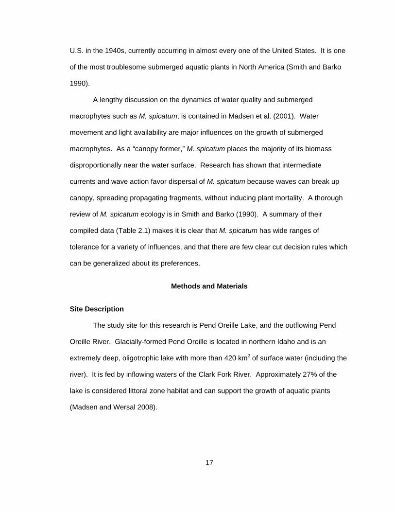
U.S. in the 1940s, currently occurring in almost every one of the United States. It is one

of the most troublesome submerged aquatic plants in North America (Smith and Barko

1990).

A lengthy discussion on the dynamics of water quality and submerged

macrophytes such as M. spicatum, is contained in Madsen et al. (2001). Water

movement and light availability are major influences on the growth of submerged

macrophytes. As a “canopy former,” M. spicatum places the majority of its biomass

disproportionally near the water surface. Research has shown that intermediate

currents and wave action favor dispersal of M. spicatum because waves can break up

canopy, spreading propagating fragments, without inducing plant mortality. A thorough

review of M. spicatum ecology is in Smith and Barko (1990). A summary of their

compiled data (Table 2.1) makes it is clear that M. spicatum has wide ranges of

tolerance for a variety of influences, and that there are few clear cut decision rules which

can be generalized about its preferences.

Methods and Materials

Site Description

The study site for this research is Pend Oreille Lake, and the outflowing Pend

Oreille River. Glacially-formed Pend Oreille is located in northern Idaho and is an

extremely deep, oligotrophic lake with more than 420 km2 of surface water (including the

river). It is fed by inflowing waters of the Clark Fork River. Approximately 27% of the

lake is considered littoral zone habitat and can support the growth of aquatic plants

(Madsen and Wersal 2008).

18

Conceptual Model

Based on published information, a conceptual model (Fig. 2.1) was built to show

proposed predictor variables and interactions between variables. The conceptual model

was used to focus data selection, but several proposed variables were not used because

the data do not exist, were not easy to collect, or would not vary significantly in value

across a single lake.

Major areas of mesoclimate and geology, labeled “indirect variables” in the

conceptual model, would not be considerably different on a single lake, but would be of

importance on a much larger scale, such as a national model. However, bathymetry/

topography would vary greatly in a single lake, and given the depths of Pend Oreille, are

of immense importance in the model.

“Direct and resource variables” are of more immediate importance on a single-

lake scale. However, for these are the variables, the risk of multicollinearity exists. For

example, fetch is calculated from wind data. Thus both variables essentially yield the

same information, and should not both be present as predictors in the same model.

Certainly light availability, considered the most controlling factor, can be inferred from a

variety of variables including depth and algal growth.

Some variables are simply not available. Many studies cite sediment nutrients as

an important predictive mechanism. However, the expense both in time and money to

collect sediment data often precludes its use for many studies. Unless a researcher

makes a significant effort to obtain data for the specific project, it is not likely that the

data can be found for use in a GIS or that the data will be sampled in accordance with

the requirements of the project. Additionally, while drawdown has been shown to be a

somewhat effective control, this method is associated more with reservoirs and

waterbodies with water-level-control structures, making this impractical for many studies.

19

Pend Oreille, however, is a lake with a water control structure and is drawn down each

winter. This affects the whole lake and thus would not be appropriate for a spatial

analysis because the measured value would not change across the lake.

Negative effects (Fig. 2.1) such as freezing are avoided by the timing and

location of the study. Information was recorded on native plant cover when the data set

was collected. Preliminary analysis indicated that plant cover was not useful for this

specific study, and thus was not included in further analysis.

Model Data Preparation

Spatial analysis using generalized linear models was conducted to estimate the

predictive probability for the presence of M. spicatum in Pend Oreille Lake and the

outflowing river. Predictor variables included water depth (hereafter depth), effective

fetch length (hereafter fetch), and distance from nearest M. spicatum population

(hereafter distance).

Data were split for separate analyses on Pend Oreille (Fig. 2.2). These areas

have been named “littoral” and “pelagic” to reflect perceived differences in zones. The

littoral zone contains the entire river and an upper portion of the lake where M. spicatum

was visibly present and water depth was shallow. This area represents a large area of

continous littoral zone. The majority of the lake is extremely deep and is thought to

prohibit M. spicatum colonization; thus, that area has been labeled as the pelagic zone.

Additionally, the littoral zone was grid-sampled, while the pelagic was not. It seems

unwise to perform a unified analysis on what are clearly different systems with different

sampling intensities, thus the division between zones for analyses. Hereafter, “littoral”

refers to the geographic area shown in Figure 2.2 unless otherwise stated.

20

All interpolations performed on predictor variable data were done using ordinary

kriging with ArcGIS Geostatistical Analyst1. In several studies designed to evaluate the

various interpolation methods for aquatic ecosystem variables (e.g., kriging, spline,

inverse distance weighted), kriging was generally regarded as the best option because it

produced the lowest mean square error (Bello-Pineda and Hernandez-Stefanoni 2007;

Valley et al. 2005). While this tool offers options for additional types of kriging, only

ordinary was applicable to the research problem because no a priori information

regarding the mean over the study area is required (Goovaerts 1997). Ordinary kriging

produces a linear prediction based on weighted averages and is intrinsically stationary

(i.e., assumes constant unknown mean and a semivariogram that is a function of

distance apart only) (Waller and Gotway 2004). The ArcGIS Geostatistical Analyst

contains options within ordinary kriging for anisotropy and specification of nugget. There

was no evidence that depth and fetch changed with direction, thus anisotropy was not

included. Further, in the areas investigated, due to the relative continuity of depth and

fetch, no nugget was necessary.

Water depth for the pelagic zone was interpolated from NOAA sounding data.

Bello-Pineda and Hernandez-Stefanoni (2007) noted that spherical models were found

to best fit the experimental semi-variograms and to best explain the spatial

autocorrelation present in the depth variable in their attempts to create a bathymetric

map, and preliminary data analysis showed that this was also the best option for depth

data from the NOAA sounding. Water depth for the littoral zone was collected in the field

and then interpolated. It was not possible to get one complete depth data set for the

entire study area.

1 ESRI, 380 New York Street, Redlands, CA 92373-8100

21

Fetch length was determined using methods outlined in the Shore Protection

Manual (USACE 1984). These methods were automated using Python scripts obtained

from USGS (Rohweder et al. 2008). Effective fetch gives a more representative

measure of how the wind governs the waves because it is a weighted distance of fetch

around a specified wind direction (Lehmann 1998). Effective fetch is calculated as

Σ cos Υ /Σ cos Υ ,

where = effective fetch, = distance to land, and Υ = deviation angle. Nine radials

are used in the calculations for this study. In this instance the specified wind direction

and speed were chosen to represent the dominant speed and direction such as was

done by Narumalani et al. (1997) over the growing season of M. spicatum in Pend

Oreille Lake.

Distance was used in two ways. First, distance was used as a Boolean variable

which identified if the point was within 500 m of an existing population. The maximum

separation of 500 m was chosen because it represented the smallest possible distance

which could be used with a 250-m grid. Second, distance was used as an absolute

variable measured from the closest observed M. spicatum presence point. Madsen and

Smith (1997) noted that M. spicatum, although capable of spread by stolon and

fragments, predominately (74%) propagated via stolon production, indicating a

significant chance for localized spread.

Presence/absence data were obtained by field surveys conducted in summer

2007 (Madsen and Wersal 2008). Presence/absence data were collected using a plant

rake with a point intercept sampling method developed by Madsen (1999).

Data were re-sampled to a 250-m point grid for analysis in SAS. This size was

selected to match the point intercept sampling size, and was necessary to perform

analysis within a unified framework. Re-sampling and grid generation were done with

(2.1)

22

Hawth’s Analysis Tools in ArcGIS (Beyer 2004). To increase computational speed, only

points where water depth was less than 10 m were considered for model use,

representing the limit of preferred depth for M. spicatum reported in literature (Smith and

Barko 1990) and the maximum depth observed during data collection (J. Madsen,

personal communication).

Data Analysis

A wide range of statistical options for analysis exist, but the choice is driven

primarily by known vs. unknown parameters, distribution, and model use. It is assumed

that the location of each observation is thought to influence the outcome, making the

problem inherently spatial. Tobler’s First Law of Geography (Tobler 1970) is often cited

in reference to spatial autocorrelation and postulates the level of correlation between

observations decreases with increasing distance. In traditional statistics it is assumed

that observations are independent and have normally distributed errors with mean zero

and constant variance. The independence assumption is violated when spatial data are

considered to be spatially autocorrelated. For this reason spatial statistical methods for

spatial data analysis are correct, in contrast to traditional methods. The challenge is

correctly modeling the spatial dependence so that it can be included in the analysis.

Initial models estimating the relationship between the presence of M. spicatum as

a linear function of depth, fetch, and distance were fit using SAS Procs LOGISTIC and

GLIMMIX2. From these models, residuals were computed. The residuals were then

used to determine an appropriate class of semivariogram models using Procs

VARIOGRAM and MEANS. Once it was determined a spherical semivariogram model

was fit best by the residual empirical semivariogram, Proc NLIN was used to obtain

parameter estimates for the semivariogram.

2 SAS Institute Inc., 100 SAS Campus Drive, Cary, NC 27513-2414

23

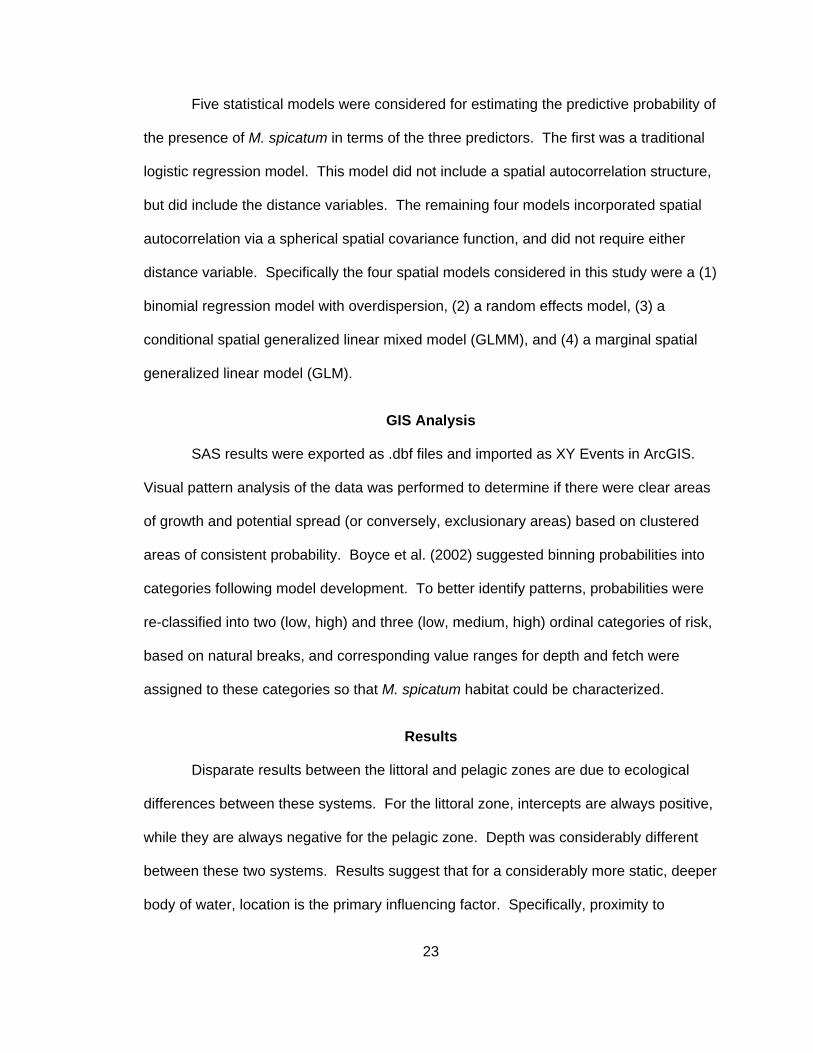
Five statistical models were considered for estimating the predictive probability of

the presence of M. spicatum in terms of the three predictors. The first was a traditional

logistic regression model. This model did not include a spatial autocorrelation structure,

but did include the distance variables. The remaining four models incorporated spatial

autocorrelation via a spherical spatial covariance function, and did not require either

distance variable. Specifically the four spatial models considered in this study were a (1)

binomial regression model with overdispersion, (2) a random effects model, (3) a

conditional spatial generalized linear mixed model (GLMM), and (4) a marginal spatial

generalized linear model (GLM).

GIS Analysis

SAS results were exported as .dbf files and imported as XY Events in ArcGIS.

Visual pattern analysis of the data was performed to determine if there were clear areas

of growth and potential spread (or conversely, exclusionary areas) based on clustered

areas of consistent probability. Boyce et al. (2002) suggested binning probabilities into

categories following model development. To better identify patterns, probabilities were

re-classified into two (low, high) and three (low, medium, high) ordinal categories of risk,

based on natural breaks, and corresponding value ranges for depth and fetch were

assigned to these categories so that M. spicatum habitat could be characterized.

Results

Disparate results between the littoral and pelagic zones are due to ecological

differences between these systems. For the littoral zone, intercepts are always positive,

while they are always negative for the pelagic zone. Depth was considerably different

between these two systems. Results suggest that for a considerably more static, deeper

body of water, location is the primary influencing factor. Specifically, proximity to

24

shoreline appears to increase probability of presence for M. spicatum. However, this is

more likely a proxy for indicating those areas with shallow littoral zone, and necessarily

proximity to shoreline per se.

Depth and fetch were highly significant in every model considered. Regardless

of zone, depth had negative coefficients in every model, while fetch had positive

coefficients for every model. The negative coefficient of depth indicates that the deeper

the water, the less likely an occurrence of Eurasian Watermilfoil. On the other hand, the

higher values of effective fetch indicated Eurasian Watermilfoil was more likely to occur.

All four of the spatial models had a lower predictive probability error variance than the

logistic regression model. However, the additional complexity of spatial models requires

advanced computing algorithms for covariate parameter estimation. For this study, this

additional complexity resulted in a lack of convergence in some cases. In the littoral

zone, modeling efforts were enhanced by the added complexity introduced by these

spatial models.

Model outputs indicate predictive probabilities for the presence of M. spicatum at

each point in the study area. A spatial view of these probabilities created in ArcGIS

illustrates areas where M. spicatum is likely to occur based on existing depth and fetch.

Littoral

Myriophyllum spicatum was present in 64% of the sample set and absent in 36%

(Table 2.2). Despite repeated attempts, several models would not converge. For some

models attempts were made to run models as bivariate with both depth and fetch, and

as univariate models with depth or fetch. Convergence was never achieved for the

random effects model (bivariate). While the univariate models for random effects did

converge, alone, neither could explain the response variable sufficiently. Interaction

between depth and fetch is likely present, and thus should not be used alone to model

25

response. The conditional spatial GLMM converged for both bivariate and univariate

models. However, a standard error could not be calculated for the range despite using

advanced techniques for estimating starting values and subsetting of data. Models for

which convergence was obtained include the traditional logistic regression, the binomial

regression model with overdispersion, and the marginal spatial GLM.

Logistic Regression

In this research problem, logistic models explain the trend in the probability of

occurrence of M. spicatum through the covariates depth and fetch. In this research

problem, response is binary (i.e., presence or absence), meaning that at any

particular location, the data have a Bernoulli distribution with probability of occurrence

, in lieu of a normal distribution, where , is also the mean of the

Bernoulli distribution. It is also the case that, at a particular location, the variance of the

process is , 1 .

The logistic regression model predicts the response variable without regard

to any spatial location. This is the only model that does not have a spatial component.

Our logistic model explains the trend in the probability of occurrence of M. spicatum, via

the logit function, through the covariates depth and fetch. More specifically, is

modeled with respect to depth , and fetch , by the relationship

log , , ,

, , ,

, , , , 1,2, … ,1343.

A stepwise selection procedure was used, with depth entering the model first,

and fetch second. The resulting fitted model was

1.9182 0.3893 , 0.000297 , , 1,2, … 1343.

(2.2)

(2.3)

26

The summary of the fit for this model indicates that intercept, depth, and fetch were

significant (Table 2.3). The Wald statistic reported represents the simplest and most

commonly used interval estimate for a fitted value in a logistic regression for the logit

function (Elith et al. 2002). Wald 2 values (167.7, 189.7, and 64.0, respectively)

indicate that the full model explains the response variable markedly better than a

random variable that does not depend on values of depth and fetch.

Measures of correlation indicate that the model did a reasonable job of correctly

assigning predicted probabilities (Table 2.4). More frequently than not (c = 0.78),

predicted probabilities were assigned by the model that corresponded to the

observations (i.e., in any matched [0, 1] pair, the higher probability was predicted for the

location with 1, and not 0).

Binomial Regression with Overdispersion

In the binomial regression model with overdispersion model, the trend in the

probability of occurrence of M. spicatum is modeled via the logit function through the

linear relationship between the covariates depth and fetch. The spatial component is

indirectly modeled through the overdispersion parameter. Overdisperion refers to the

situation whereby the data are more dispersed than is consistent with a standard mean-

variance relationship. The addition of overdispersion is an attempt to quantify the

inexactness of the mean-variance relationship (Schabenberger and Gotway 2005). The

inexactness is thought to be due to spatial influence on the data.

For each location, , the binomial regression model with overdispersion is

described as

, , ,

Var 1 ,

(2.4)

27

where represents the overdispersion parameter. The fitted model for binomial

regression with overdispersion was

, , , 1.9182 0.3893 0.000297 .

The overdispersion model was fitted using restricted maximum likelihood (Table

2.5). A value of 2 > 1 indicates the presence of overdispersion. The large estimate of

the overdispersion parameter of 1.8701 in this analysis indicates that the data likely is

overdispersed. Thus the variability is not fully described by the predictors selected. It is

possible this is due to underlying spatial variability. The inclusion of the overdispersion

parameter should be an improvement over a traditional logistic model because there is

clearly unexplained variability that needs to be accounted for, even if its cause is not

identified.

Conditional Spatial GLMM

Spatial dependence can be explained partially or wholly by the proximity of

environmental predictor variables. Randomness inherent in depth and fetch due to

interpolation is accounted for through the normality assumption on the term , having

spatial covariance structure, . Any remaining spatial dependence can be due

to underlying biotic processes or unobservable variables (Miller and Franklin 2006). The

conditional approach models the unobserved spatial process through the use of random

effects within the mean function and models the conditional mean and variance as a

function of both fixed covariate effects and these random effects resulting from the

unobserved spatial process. Variance is dependent on the mean with consideration for

overdispersion. The data are conditionally independent and spatial dependence is

addressed by a Gaussian random field (Schabenberger and Gotway 2005).

The conditional spatial GLMM is described as

(2.5)

28

| ~ Bernoulli µ s , independent

logit

Var |

~ 0, .

The fitted model for conditional spatial GLMM was

logit 9.1117 1.7061 0.001016 .

For this model, spatial autocorrelation was modeled using the spherical model given by

1 ,

0, otherwise.,

The spherical covariance function specifically modeled the spatial dependency in the

data, partially due to kriging values of fetch and depth. The results of fitting this model

indicate that intercept, depth, and fetch are all significant (Table 2.6). The fitted

covariance structure was

~ 0, 81.5731 1.0534 .

Marginal Spatial GLM

The marginal spatial GLM incorporates a term which helps to describe the

inexactness or random behavior in depth and fetch due to interpolation. The marginal

spatial GLM differs from the conditional model in that the marginal mean is modeled as a

function of unknown fixed, non-random parameters (i.e., 0, 1). It gives the same

inference as a conditional model, but with differing interpretation (Schabenberger and

Gotway 2005). The marginal spatial GLM is described as

E

logit

Var .

(2.6)

(2.10)

(2.8)

(2.7)

(2.9)

29

The results of fitting this model indicate that intercept, depth, and fetch are all significant

(Table 2.7). The fitted model was

logit 1.9182 0.3893 0.000297 .

GIS Analysis

Ordinal categories illustrated a clear trend (Fig. 2.3) with respect to depth and

fetch. In general, probabilities were negatively related to depth and positively related to

fetch. For many model outputs, in the 3-class system, high depth/high fetch was not

always present. Predicted probabilities, when mapped, showed a clear increase with

depth (Figs. 2.4, 2.5).

Pelagic

Myriophyllum spicatum was present in 9% of the sample set and absent in 91%

(Table 2.8). Despite repeated attempts and robust methods for estimating starting

parameter values, the conditional spatial GLM for the pelagic zone did not converge.

Logistic Regression

The logistic regression model predicts the response variable without regard

for any spatial dependency. is modeled with respect to depth , and fetch , by

Equation Set 2.2, with one exception: in the pelagic analysis, 1,2, … ,930.

As with the littoral analysis, a stepwise selection procedure was used, with depth

entering the model first, and fetch second. The resulting fitted model was

0.8995 0.3599 , 0.000179 , .

The summary of the fit for this model indicates that intercept, depth, and fetch were

significant (Table 2.9). Wald 2 values (5.3, 28.5, and 12.1, respectively) indicate that

the full model explains the response variable markedly better than a random variable

that does not depend on values of depth and fetch.

(2.12)

(2.11)

30

Measures of correlation indicate that the model did a reasonable job of correctly

assigning predicted probabilities (Table 2.10). More frequently than not (c = 0.73),

predicted probabilities were assigned by the model that corresponded to actual real-

world observations (i.e., in any matched [0, 1] pair, the higher probability was predicted

for the location with 1, and not 0).

Binomial Regression with Overdispersion

The binomial regression model with overdispersion was performed using

Equation Set 2.4. As with the littoral analysis, the overdispersion model was fitted using

maximum likelihood (Table 2.11). The fitted model was

, , , 0.8995 0.3599 0.000179 .

The overdispersion parameter of 1.0320 in this analysis is likely not significantly greater

than 1, and thus overdispersion may not be occurring. In this event, there would be no

need to include this more complex model over the logistic regression model.

Random Effects

The random effects model is a standard bivariate binomial regression model that

incorporates random effects to model the spatial dependence. The random effects

model is described by

| ~ Bernoulli µ s , independent

logit

Var Z s | s σ µ

~ 0,

The results of fitting this model indicate that intercept, depth, and fetch are

significant (Table 2.12). The fitted model was

logit 8.1978 1.2530 0.000680 .

(2.14)

(2.13)

(2.15)

31

Marginal Spatial GLM

The marginal spatial GLM is described by Equation Set 2.10. The results of

fitting this model indicate that intercept, depth, and fetch are significant (Table 2.13).

The fitted model was

logit 1.3255 0.2329 0.000112

GIS Analysis

Ordinal categories produced mixed results, and were deemed not valuable to

data analysis. In general, probabilities were disparate and no clear patterns could be

detected for any of the models with regard to both the two- and three-class systems. For

many model outputs, the range of values was so small that graphs were of limited utility

for illustration purposes, and thus they are not included. Predicted probabilities were

low, except in the shallowest areas (Figs. 2.6, 2.7). When higher probabilities (> 0.50)

were compared with the true, measured, littoral zone from Pend Oreille (Fig. 2.8) it

appears that even when light, which is traditionally the most limiting factor, is available,

depth and fetch will still control the ability of M. spicatum to establish.

Discussion

Multiple justifications can be made about which model is “best”. It is improper to

report traditionally-interpreted metrics like R2 because R2 is best interpreted in the

context of linear models with independent errors – both naïve assumptions in our

context. Consequently, it’s not clearcut to compare a single reported value for each

model and say which one is “best”.

In this instance the most-defensible position is that the simplest model is best.

This theory is called “Occam’s Razor” or the “Principle of Parsimony.” Rules of

parsimony dictate that when two or more models are competitive, then the simplest

(2.16)

32

model should be used. Romero-Calcerrada and Luque (2006) reported that simpler

models were preferred for their wider applicability and better overall prediction of species

presence. Therefore the added complexity of a robust spatial model for the pelagic zone

is not warranted, and the basic logistic model will suffice. For the littoral zone, the

selection would be the overdispersion model. It did prove to be superior to the logistic

regression, and when compared to the competing, more complex spatial models, it is the

simplest choice.

The alternative argument is that it is irresponsible to recommend a model which

knowingly omits information about a system, regardless of simplicity. The more explicit

spatial models take into account variation due to location which is ignored in the logistic

model. There is variability accounted for in the random effects model and conditional

spatial GLMM due to random effects in the predictors. In this instance, added

computational time and complexity are worth the added effort to produce a more

“complete” model.

The amount of zeros (absence) in a dataset influences the failure rate for models

relying on fixed effects. It is possible in this study, given the high percentage of zeros in

the pelagic zone, that these models were limited in their usefulness from the onset, and

might yield significantly different results in a study with a large percentage of presence

points.

By definition a true pelagic zone would not contain aquatic plants. It is possible

that trying to model presence in this habitat would not be possible in practice because

the data create a situation for which a realistic model would never converge. Due to the

lack of continuous true littoral zone, the model is never able to completely close around

the pelagic zone.

33

Conclusions

Based on the results seen in this study, robust spatial models are more useful in

modeling smaller, shallower, more dynamic systems. Depth and fetch were useful in

predicting the presence of M. spicatum, but were not as significant in more robust

models for the pelagic zone. In these systems, location only has more explanatory

ability than spatial covariance structures. The littoral zone showed a clear trend of more

frequent presence in low depth, high fetch areas. These trends were not as clear for the

pelagic zone. However, the coefficients for the pelagic zone models indicate that the

same trend should occur.

34

Literature Cited

Bello-Pineda, J. and J. L. Hernandez-Stefanoni. 2007. Comparing the performance of two spatial interpolation methods for creating a digital bathymetric model of the Yucatan submerged platform. Pan-Amer. J. Aquat. Sci. 2:247-254.

Beyer, H. L. 2004. Hawth's Analysis Tools for ArcGIS. Available at

http://www.spatialecology.com/htools. Boyce, M. S., P. R. Vernier, S. E. Nielsen, and F. K. A. Schmiegelow. 2002. Evaluating

resource selection functions. Ecol. Model. 157:281-300. Elith, J., M. A. Burgman, and H. M. Regan. 2002. Mapping epistemic uncertainties and

vague concepts in predictions of species distribution. Ecol. Model. 157:313-329. Gillenwater, D., T. Granata, and U. Zika. 2006. GIS-based modeling of spawning

habitat suitability for walleye in the Sandusky River, Ohio, and implications for dam removal and river restoration. Ecol. Eng. 28:311-323.

Goovaerts, P. 1997. Geostatistics for Natural Resource Evaluation. Oxford University

Press, NY. Jensen, J. R., S. Narumalani, O. Weatherbee, and K. S. Morris, Jr. 1992. Predictive

modeling of cattail and waterlily distribution in a South Carolina reservoir using GIS. Photogrammetric Eng. Remote Sens. 58:1561-1568.

Lehmann, A. 1998. GIS modeling of submerged macrophyte distribution using

generalized additive models. Plant Ecol. 139:113-124. Madsen, J. D. 1999. Point and line intercept methods for aquatic plant management.

APCRP Technical Notes Collection (TN APCRP-MI-02), U.S. Army Engineer Research and Development Center, Vicksburg, MS. 16 pp.

Madsen, J. D., P. A. Chambers, W. F. James, E. W. Koch, and D. F. Westlake. 2001.

The interaction between water movement, sediment dynamics and submersed macrophytes. Hydrobiologia 444:71-84.

Madsen, J. D. and D. H. Smith. 1997. Vegetative spread of Eurasian watermilfoil

colonies. J. Aquat. Plant Manage. 35:63-68. Madsen, J. D., and R. M. Wersal. 2008. Assessment of Eurasian watermilfoil

(Myriophyllum spicatum L.) Populations in Lake Pend Oreille, Idaho for 2007. Mississippi State University, Geosystems Research Institute Report 5028.

Miller, J. and J. Franklin. 2006. Explicitly incorporating spatial dependence in predictive

vegetation models in the form of explanatory variables: a Mojave Desert case study. J. Geograph. Syst. 8:411-435.

35

Narumalani, S., J. R. Jensen, J D. Althausen, S. Burkhalter, and H. E. Mackey, Jr. 1997. Aquatic macrophyte modeling using GIS and logistic multiple regression. Photogrammetric Eng. Remote Sens. 63:41-49.

Rohweder, J., J. T. Rogala, B. L. Johnson, D. Anderson, S. Clark, F. Chamberlin, and K.

Runyon. 2008. Application of wind fetch and wave models for habitat rehabilitation and enhancement projects. U.S. Geological Survey Open-file Report 2008-1200, 43p.

Romero-Calcerrada, R. and S. Luque. 2006. Habitat quality assessment using weights-

of-evidence based GIS modeling: the case of Picoides tridactylus as species indicator of the biodiversity value of the Finnish forest. Ecol. Model. 196:62-76.

Schabenberger, O. and C. A. Gotway. 2005. Statistical Methods for Spatial Data

Analysis. Chapman & Hall/CRC Press, Boca Raton, FL. 488 pp. Smith, C. S. and J. W. Barko. 1990. Ecology of Eurasian watermilfoil. J. Aquat. Plant

Manage. 28: 55-64. Store, R. and J. Jokimäki. 2003. A GIS-based multi-scale approach to habitat suitability

modeling. Ecol. Modeling 169: 1-15. Tobler, W. R. 1970. A computer movie simulating urban growth in the Detroit region.

Econ. Geogr. 46:234-240. United States Army Corps of Engineers [USACE]. 1984. Shore Protection Manual.

Coastal Engineering Research Center, Fort Belvoir, VA. Valley, R. D., M. T. Drake, and C. S. Anderson. 2005. Evaluation of alternative

interpolation techniques for the mapping of remotely-sensed submersed vegetation abundance. Aquat. Bot. 81:13-25.

Waller, L. A. and C. A. Gotway. 2004. Applied Spatial Statistics for Public Health Data.

John Wiley and Sons, Hoboken, NJ. 494 pp.

Fig

ure

2.1.

Con

cept

ual m

odel

of p

ropo

sed

inte

ract

ions

bet

wee

n en

viro

nmen

tal v

aria

bles

affe

ctin

g M

yrio

phyl

lum

spi

catu

m.

36

Fig

ure

2.2.

Sep

arat

e an

alys

es w

ere

cond

ucte

d fo

r th

e lit

tora

l an

d pe

lagi

c zo

nes

of P

end

Ore

ille

Lake

(Id

aho

) an

d ou

tflow

ing

river

.

37

38

0

0.1

0.2

0.3

0.4

0.5

0.6

0.7

0.8

0.9

1

Low Dep

th, 

Low Fetch

Low Dep

th, 

High Fetch

High Dep

th, 

Low Fetch

High Dep

th, 

High Fetch

Probabilty

0

0.1

0.2

0.3

0.4

0.5

0.6

0.7

0.8

0.9

1

Low Dep

th, 

Low Fetch

Low Dep

th, 

Med

 Fetch

Low Dep

th, 

High Fetch

Med

 Dep

th, 

Low Fetch

Med

 Dep

th, 

Med

 Fetch

Med

 Dep

th, 

High Fetch

High Dep

th, 

Low Fetch

High Dep

th, 

Med

 Fetch

Probability

Figure 2.3. Summary of probabilities for marginal spatial GLMM on the littoral zone

for two- and three-class ordinal categories (X-axis). Bar ranges run from the minimum to the maximum value for each ordinal category; values on the Y-axis reflect probability.

F

igur

e 2.

4. M

ap o

f pa

ired

ordi

nal c

ateg

orie

s fo

r tw

o-cl

ass

mar

gina

l spa

tial G

LM f

or P

end

Ore

ille

litto

ral z

one.

39

Fig

ure

2.5.

Pre

dict

ed p

roba

bilit

ies

from

mar

gina

l spa

tial G

LM fo

r P

end

Ore

ille

litto

ral z

one.

40

F

igur

e 2.

6. M

ap o

f pa

ired

ordi

nal

cate

gorie

s fo

r tw

o-cl

ass

bino

mia

l re

gres

sion

with

ove

rdis

pers

ion

for

Pen

d O

reill

e pe

lagi

c zo

ne.

41

Fig

ure

2.7.

Pre

dict

ed p

roba

bilit

ies

from

bin

omia

l reg

ress

ion

with

ove

rdis

pers

ion

for

Pen

d O

reill

e pe

lagi

c zo

ne.

42

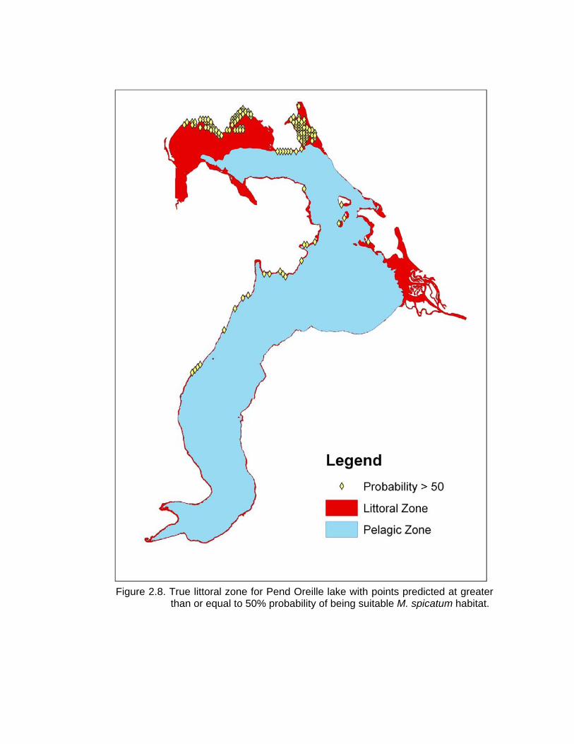
Figure 2.8. True littoral zone for Pend Oreille lake with points predicted at greater than or equal to 50% probability of being suitable M. spicatum habitat.

Tab

le 2

.1. F

acto

rs in

fluen

cing

gro

wth

and

mor

phol

ogy

of E

uras

ian

wat

erm

ilfoi

l (S

mith

and

Bar

ko 1

990)

. F

acto

r In

fluen

ce o

f Fac

tor

on W

ate

rmilf

oil G

row

th

Wat

er C

larit

y

1. L

ow w

ater

cla

rity

lim

its w

ater

milf

oil t

o sh

allo

w r

ootin

g de

pths

and

lead

s to

can

opy

form

atio

n.

2. H

igh

wat

er c

larit

y al

low

s m

ilfoi

l gro

wth

at g

reat

er d

epth

s.

T

empe

ratu

re

1. P

lant

s ph

otos

ynth

esiz

e an

d gr

ow o

ver

a br

oad

tem

pera

ture

ran

ge (

ca. 1

5 to

35

C).

2.

Max

imum

gro

wth

rat

es o

ccu

r at

rel

ativ

ely

high

wat

er te

mpe

ratu

res

(ca.

30-

35 C

).

3. G

row

th is

lim

ited

in th

e sp

ring

once

the

wa

ter

tem

pera

ture

rea

ches

app

roxi

mat

ely

15

C.

Inor

gani

c C

arbo

n 1.

Pla

nts

gro

w b

est i

n re

lativ

ely

alka

line

lake

s.

2. P

lant

s ca

n gr

ow

in la

kes

of lo

w a

lkal

inity

, bu

t not

as

vig

orou

sly

as e

lsew

her

e.

Min

eral

Nut

rient

s 1.

Nui

sanc

e gr

ow

ths

of th

e pl

ant

are

prim

arily

res

tric

ted

to m

oder

atel

y fe

rtile

lake

s, o

r fe

rtile

loca

tions

in le

ss

fert

ile la

kes.

2.

Upt

ake

of n

utrie

nts

from

sed

imen

ts b

y ro

ots

is a

ver

y im

por

tant

sou

rce

of m

iner

al n

utrie

nts,

par

ticul

arly

P a

nd

N.

3. M

ajor

cat

ions

and

bic

arbo

nate

are

take

n pr

edom

inat

ely

from

the

wat

er.

Sed

imen

t Te

xtur

e 1.

Pla

nts

gro

w b

est o

n fin

e-te

xtur

ed in

orga

nic

sedi

men

ts o

f in

term

edia

te d

ensi

ty, b

ecau

se n

utrie

nt a

vaila

bilit

y ap

pear

s to

be

grea

test

ther

e.

Wat

er M

ovem

ents

1.

Veg

etat

ive

spre

ad o

f pla

nt fr

agm

ents

is a

ided

by

wat

er c

urre

nts.

2.

The

pla

nt d

oes

not u

sual

ly o

ccur

in h

igh

ene

rgy

envi

ronm

ents

.

Ice

Sco

ur

1. Ic

e sc

our

may

exc

lude

the

plan

t fro

m s

hallo

w a

reas

of

lake

s in

col

d cl

imat

es.

Des

icca

tion

& F

reez

ing

1. D

esic

catio

n d

urin

g dr

awdo

wn

is a

via

ble

cont

rol m

easu

re p

artic

ular

ly w

hen

acco

mp

anie

d by

free

zing

dur

ing

the

win

tert

ime

.

44

45

Table 2.2. Frequency table of presence of M. spicatum on Pend Oreille littoral zone.

M. spicatum Status Frequency Percent

Absent (0)

488

36.34

Present (1) 855 63.66

46

Table 2.3. Results of logistic regression model for M. spicatum on Pend Oreille littoral zone.

Parameter Degrees of

Freedom

Estimate Standard

Error

Wald 2 p-value

Intercept (0) 1 1.9182 0.1481 167.7057 < 0.0001

Depth (1) 1 -0.3893 0.0283 189.6671 < 0.0001

Fetch (2) 1 0.000297 0.000037 64.0487 < 0.0001

47

Table 2.4. Measures of correlation from logistic regression model for M. spicatum on Pend Oreille littoral zone.

Percent Concordant 77.5 Somers’ D 0.555

Percent Discordant 22.0 Gamma 0.558

Percent Tied 0.5 a 0.257

Pairs 417,240 c 0.778

48

Table 2.5. Results of binomial regression model with overdispersion for M. spicatum on Pend Oreille littoral zone.

Parameter Estimate Standard

Error

t p-value

Intercept (0) 1.9182 0.2026 9.47 < 0.0001

Depth (1) -0.3893 0.03866 -10.07 < 0.0001

Fetch (2) 0.000297 0.000051 5.85 < 0.0001

Overdispersion (2) 1.8701

49

Table 2.6. Results of conditional spatial GLMM for M. spicatum on Pend Oreille littoral zone.

Parameter Estimate Standard

Error

t p-value

Intercept (0) 9.1117 0.6105 14.92 < 0.0001

Depth (1) -1.7061 0.1064 -16.04 < 0.0001

Fetch (2) 0.001016 0.000132 7.72 < 0.0001

Variance (s2) 81.5731 3.2593

Residual (2) 0.000417 0.000046

Range (m) 1.0534 .

50

Table 2.7. Results of marginal spatial GLM for M. spicatum on Pend Oreille littoral zone.

Parameter Estimate Standard Error t p-value

Intercept (0) 1.9182 0.2026 9.47 < 0.0001

Depth (1) -0.3893 0.03866 -

10.07

< 0.0001

Fetch (2) 0.000297 0.000051 5.85 < 0.0001

Variance (02) 1.8699 0.07228

Residual (12) 0.000187 0.002598

Range (m) . .

51

Table 2.8. Frequency table of presence of M. spicatum on Pend Oreille pelagic zone.

M. spicatum Status Frequency Percent

Absent (0) 843 90.65

Present (1) 87 9.35

52

Table 2.9. Results of logistic regression model for M. spicatum on Pend Oreille pelagic

zone. Parameter Degrees

of

Freedom

Estimate Standard

Error

Wald 2 p-value

Intercept (0) 1 -0.8995 0.3923 5.2561 0.0219

Depth (1) 1 -0.3599 0.0674 28.5205 < 0.0001

Fetch (2) 1 0.000179 0.000052 12.0954 0.0005

53

Table 2.10. Measures of correlation from logistic regression model for M. spicatum on Pend Oreille pelagic zone.

Percent Concordant 72.1 Somers’ D 0.451

Percent Discordant 27.1 Gamma 0.455

Percent Tied 0.8 a 0.077

Pairs 73,341 c 0.725

54

Table 2.11. Results of binomial regression model with overdispersion for M. spicatum on Pend Oreille pelagic zone.

Parameter Estimate Standard

Error

t p-value

Intercept (0) -0.8995 0.3986 -2.26 0.0243

Depth (1) -0.3599 0.06846 -5.26 < 0.0001

Fetch (2) 0.000179 0.000052 3.42 0.0006

Overdispersion (2) 1.0320

55

Table 2.12. Results of random effects model for M. spicatum on Pend Oreille pelagic zone.

Parameter Estimate Standard Error t p-value

Intercept (0) -8.1978 1.2516 -6.55 < 0.0001

Depth (1) -1.2530 0.2097 -5.97 < 0.0001

Fetch (2) 0.000680 0.000166 4.10 < 0.0001

Variance (s2) 2.82 x 10-6 .

Residual (2) 76.3477 3.5646

56

Table 2.13. Results of marginal spatial GLM model for M. spicatum on Pend Oreille pelagic zone.

Parameter Estimate Standard Error t p-value

Intercept (0) -1.3255 0.4874 -2.72 0.0067

Depth (1) -0.2329 0.07844 -2.97 0.0031

Fetch (2) 0.000112 0.000069 1.63 0.1030

Variance (02) 0.6775 0.05145

Residual (12) 0.2514 0.5866

Range (m) 999.56 153.10

57

CHAPTER 3

REGIONAL-SCALE MODEL: MINNESOTA

Development of ecological models provides a simple, direct method by which to

predict presence, absence, and spread of species in given environments. Models can

be used to highlight areas of concern with regard to invasive species such as Eurasian

watermilfoil (Myriophyllum spicatum L.) because they can indicate areas susceptible to

future invasion (Buchan and Padilla 2000). Roley and Newman (2008) reported that up

to 4,700 lakes in Minnesota are uninfested but susceptible to invasion by M. spicatum.

Invasions are often found providentially by state agencies or private citizens (Roley and

Newman 2008). Thus a mechanism for directing scouting efforts could allow for better

cataloging of current populations of this and other invasive species, which can mean

better chances at early detection and eradication.

One method that can be used in modeling habitat is Mahalanobis distance.

Mahalanobis distance is a dimensionless measure of the distance in multivariate space

from the ideal ecological niche (Calenge et al. 2008; Knick and Rotenberry 1998). A

special case of Mahalanobis distance can be used in a set of “presence only” methods

for predictive habitat modeling. The majority of species data available tends to be

presence only (Zaniewski et al. 2002). This is particularly true of invasive species as

many data collection efforts are focused on detection. These data are often recorded

without planned sampling schemes so that absences cannot be inferred (Elith et al.

58

2006). Regardless, Elith et al. (2006) reported that in many instances it was possible to

achieve valid results using some presence-only methods.

In a maximum entropy analysis (hereafter “maxent”), areas without values are

not automatically considered absences, which reduces bias from inclusion of false

absences (Elith et al. 2006; Phillips et al. 2006). Maxent utilizes maximum entropy to

make predictions from incomplete data, which in invasive species work could be

unsampled areas. It can be used to estimate species distribution by finding the

probability distribution that is closest to uniform (i.e., “maximum entropy”) for a study

area under a specified set of environmental constraints (Phillips et al. 2006). The

maxent statistic weights each variable by a different constant where the value of each

weight corresponds to the importance or the magnitude of the variable to the system’s

entropy. The probability distribution is estimated by iteratively altering one weight at a

time to maximize the likelihood of the occurrence dataset. To avoid overfitting, the

estimated distribution is constrained so that the average value for a given predictor is

close to the empirical average rather than equal to it (Hernandez et al. 2006). In

comparison studies, maxent outperformed other accepted quantitative methods for

ecological modeling (Hernandez et al. 2006; Phillips et al. 2006).

An advantage of Mahalanobis, however, is that it assumes a species will

distribute itself optimally within the available habitat. This method is thus ideal for spatial

studies involving GIS because it partially accounts for the influences of spatial

autocorrelation, interaction between variables, and covariance (Knick and Rotenberry

1998).

In general, most models assume that species distribution is a function of

environmental conditions (Guisan and Zimmerman 2000). Some research (Cheruvelil

and Soranno 2008) has reported that anthropogenic landscape features may outweigh

59

natural landscape influence in importance. In a study focusing specifically on detection

of M. spicatum in Minnesota lakes, Roley and Newman (2008) found only physical

habitat variables to be of significance despite including variables to serve as surrogates

for human vectoring (i.e., boat ramps).

Cheruvelil and Soranno (2008) examined the ability of lake and landscape

features to predict various metrics of macrophyte cover. They used combinations of

variables including road density and lake hydrology, among other factors, in their

determination that anthropogenic landscape features may outweigh natural landscape

influence in importance. Conversely, Buchan and Padilla (2000) reported that

anthropogenic variables were poorer predictors of M. spicatum presence. Both papers

point to exceptions, however, that can explain these divergent conclusions. Cheruvelil

and Soranno (2008) note that growth form affected variable selection, noting specifically

that M. spicatum cover required the most complex model. Buchan and Padilla (2000)

follow up their conclusions by stating that statistical significance of predictor variables

may not equate to ecological significance. Thus anthropogenic variables may or may

not be of use in a model, but intuitively are included because invasion ecology indicates

these are key influences.

Methods and Materials

The states of Minnesota and Wisconsin were divided into a 500 m grid using

ArcGIS3 and Hawth’s Tools (Beyer 2004). Non-water areas were removed from the

sample. Data for analysis were obtained from the Minnesota Department of Natural

Resources Data Deli4 and researchers at the University of Minnesota (Roley and

3 ESRI, 380 New York Street, Redlands, CA 92373-8100 4http://deli.dnr.state.mn.us/index.html.

60

Newman 2008). These included Secchi depth, total alkalinity, Carlson’s Trophic State

Index, lake size, distance from lake access (i.e., boat launch), distance from road,

distance from reported bass habitat, and M. spicatum presence. Data were weighted for

analysis using flow accumulation rates obtained from the National Hydrography Dataset

Plus5.

Mahalanobis

A Mahalanobis analysis was performed on the dataset using the Mahalanobis

extension (Jenness 2003) for ArcView 3.x6. All variables were included in the analysis.

The Mahalanobis extension calculates distance using the following equation (Jenness

2003)

D ,

where x = vector of data, m = vector of mean values of x, C-1 = inverse covariance matrix

of x, and T indicates transpose.

D2 is approximately x2k-1. It is only exactly if all x are N(,). P-values for a 2

distribution with k-1 degrees of freedom (where k = the number of predictor variables)

were derived Mahalanobis distances and re-classed using cut-off values of 0.5 (Fig 3.1)

and 0.4. The value of 0.5 is a standard choice, and 0.4 was selected because this was

the natural break in the data. Values greater than or equal to 0.5 and 0.4, respectively,

were considered presence when the data were re-classified, with values less than these

thresholds considered absence. Re-classed output was compared to known values of

presence and absence for validation. Validation included calculating Cohen’s kappa,

specificity, and sensitivity (Hirzel et al. 2006).

5 Horizon Systems Corporation, P.O. Box 5084, Herndon, VA 20170 6 ESRI, 380 New York Street, Redlands, CA 92373-8100

(3.1)

61

The Mahalanobis methods were repeated using combined data from Wisconsin

and Minnesota. Data for Wisconsin were obtained from the Wisconsin Department of

Natural Resources7 and USGS Nonidigenous Aquatic Species database8. These

included the same variables used for the Minnesota study.

Maxent

The maxent statistic (q was calculated using the Maxent software9. Only the

state of Minnesota was considered. Maxent is defined by the following equation (Phillips

and Dudik 2008)

q xZ

exp ∑ λ f x ,

where for each , 1, … , represents the weight, is the jth feature at x, x is

presence and Z is a normalizing constant forcing the sum of the entropy components to

one.

In addition to maps of predicted suitability, the Maxent software produces a

receiver operating characteristic (ROC) curve, information regarding the relative

contribution of each variables, jackknife tests of variable importance, and response

curves. From a GIS standpoint, the map provides a useful tool in the production of a

spatially-referenced continuous variable ranging from 0 to1 where higher values indicate

higher relative suitability (Gibson et al. 2007). These values can be thresholded and

binned into any number of ordinal categories for further analysis.

7http://dnr.wi.gov/ 8 http://nas.er.usgs.gov/ 9 http://www.cs.princeton.edu/~schapire/maxent/

(3.2)

62

Results

Mahalanobis

The Kappa statistic () measures the proportion of agreement between

Mahalanobis predicted and the field observed presence and absence values, removing

that part of agreement that is due to chance (Feuerman and Miller 2005). Despite

repeated modifications to variable combinations, the results of for Minnesota alone

were below acceptable thresholds (typically 0.7 in literature). The highest obtained

was 0.1, which would not be considered a success under any circumstances.

Calculated specificity and sensitivity were 0.75 and 0.55, respectively (Table 3.1). This

indicates that there is high probability of correctly identifying an absence, but only a

marginally better than random chance of correctly identifying a presence. Feuerman and

Miller (2005) have shown that when both specificity and sensitivity are less than 0.875, it

is not possible to obtain a of 0.75 or greater (which indicates good to excellent

agreement between model and observations).

The combined data for Minnesota and Wisconsin produced a of 0.54, with

specificity and sensitivity of 0.94 and 0.54, respectively (Fig. 3.2, Table 3.2). Again,

was below the standard threshold albeit substantially improved from the Minnesota

alone analysis. Specificity and sensitivity values again indicate a high probability of

correctly identifying an absence, but only a marginally better than random chance of

correctly identifying a presence.

Maxent

An analysis based on maxent resulted in a highly predictive model for Minnesota.

The ROC curve (Fig. 3.3) showed an area under the curve (AUC) of 0.968. AUC

represents the probability that a randomly chosen presence site will be ranked more

63

suitable than a randomly chosen absence site (Phillips and Dudik 2008) and values >

0.9 are considered to be highly accurate (Manel et al. 2001).

The most useful variable in terms of explanatory power was bass habitat (45%)

followed by Carlson’s TSI (28%). Lake access was shown to be least useful (0.6%),

which confirms what has been shown in other studies (Buchan and Padilla 2000; Roley

and Newman 2008) with regard to anthropogenic contributions to presence. Spatially it

appears the most suitable areas are clustered near the major metropolitan area of

Minneapolis-St. Paul (Fig. 3.4).

A causal link may not exist between bass and M. spicatum, but empirically bass

habitat would be an excellent predictor of M. spicatum presence. Both species prefer

lakes dominated by a shallow littoral zone with abundant aquatic plant habitat. It is no

secret on popular fishing press and natural resource agency websites that bass and M.

spicatum are often co-located. This is particularly problematic because it creates friction

between groups wishing to eliminate the threat posed by this invasive weed and bass

fishing enthusiasts who equate M. spicatum mats with quality fishing. Guntersville Lake

(Alabama) is a legendary bass fishing lake, largely due to its much-touted M. spicatum

(Felsher 2007; Russow 2010). In other areas of the country many comments are made

about how the bass fishing was better when M. spicatum was more prevalent

(Anonymous 2002; Knapp 2004) or how the introduction of M. spicatum has been a

positive step for the bass fishing community (Vick 2003). This problem is exacerbated

by the disturbance (and subsequent fragmentation) caused by fishermen and their boats

and also by the purposeful introduction of M. spicatum to a waterbody in the hopes of

creating more bass habitat. Frequently the information given on forums does little to

discourage spread and introduction. It is not difficult to find comments on forums

(http://www.HotSpotOutdoors.com, accessed Jun 16, 2010) such as “Milfoil creates

64

awesome fish habitat while clearing up the water at the same time” and “I think people

know what milfoil and zebra mussels are, but do we really know the true effects they can

have -- both positive and negative? I know of the potential positive effects, and I have

'heard' of the potential negative effects.” These comments illustrate that there is a

definite culture that not only identifies bass habitat with M. spicatum, but encourages the

growth of one species to support the other.

Discussion

Despite its prominence in ecology research, utility of Cohen’s is under some

debate. A significant number of absences have been recorded for Minnesota. While the

modeling methods used in these analyses do not rely on these data, the validation did

utilize these figures. Therefore it seems fair to acknowledge potential limitations of these

metrics.

Manel et al. (2001) reviewed published ecological literature and determined that

many studies make no effort to evaluate the results, and when results are evaluated,

performance metrics are potentially biased by the number of presence samples included

in development of the model. Their findings indicated that specificity and sensitivity were

influenced by prevalence, but that was not. Vaughn and Ormerod (2005) raised

concerns about regarding the definition of “chance” and then pointed to specificity and

sensitivity as better alternatives which are “independent of prevalence”. However,

McPherson et al. (2004) reported that changes in prevalence affected all three metrics.

Changes in prevalence affected , with deviations from optimum prevalence resulting in

bias with low prevalence decreasing values and high prevalence increasing values.

Higher prevalence also led to better sensitivity but poorer specificity. McPherson et al.

(2004) cautioned that these biases made kappa inappropriate for comparisons between

65

models performed in varying regions of on varying species, stating that this issue had

not been addressed by current (at that time) ecological literature.

In contrast, ROC curves are thought to be uninfluenced by prevalence

(McPherson et al. 2004; Manel et al. 2001). Manel et al. (2001) reported that was a

more robust indicator of model performance, but they detected no prevalence bias in

their analysis.

The dataset used in this analysis was considered to have sufficient sample points

with more than reasonable spatial distribution. Although results from a Mahalanobis

analysis may not be reasonably validated by chosen metrics, results from a maxent

analysis indicate that a model can be formed for this dataset that is not influenced by

prevalence bias because maxent analysis do not require absence data. Further, given

the size and breadth of input data it is not likely the results are influenced by a “detection

bias” which can sometimes be the case, particularly with invasive species.

Based on results from the Mahalanobis analysis, it appears possible the

fundamental niche for M. spicatum is much larger than the realized niche. Roley and

Newman (2008) reported that over 4,700 waterbodies were susceptible but not infested

with M. spicatum. It is possible with more time that M. spicatum will spread to these

areas if conditions are favorable. Roley and Newman (2008) also reported that

infestations appeared to spread out from the point of initial introduction, with lakes

closest to the initial invasion more likely to be positive for M. spicatum. This could be

further support that proliferation in Minnesota is a function of time, and not a funcation of

the natural characteristics of the waterbodies themselves precluding infestation by M.

spicatum.

Additionally, the State of Minnesota’s Department of Natural Resources has an

active education campaign to prevent and limit spread of milfoil. These efforts include

66

billboards, radio and television advertising, public service announcements, printed

materials, press releases, media contacts, newspaper ads, staffing at sports shows and

other major events, educational displays and exhibits, informational signs at public water

accesses, presentations to the public, and training all designed to increase awareness

and limit introductions of M. spicatum. Surveys to quantify effectiveness indicate that

these efforts are producing the desired results with 97% of boaters in one survey

indicating they were aware of the State’s invasive species laws, and 99% indicating the

campaign had led them to action (Invasive Species Program 2010).

Unrelated to niche mechanics, this educational campaign could be artificially

limiting the species’ ability to spread, and would probably not be captured by the model

input variables. Management strategies employed as a result of early detection and

prevention campaigns could also limit M. spicatum’s ability to spread into some areas

that are suitable habitat from a modeling standpoint.

The inclusion of Wisconsin in a second, combined Mahalanobis method was

done to test which explanation was more likely. Wisconsin was selected more for its

characteristics, not all of which are a function of its proximity to Minnesota. Wisconsin

has a comparable environment; however, Wisconsin has had populations for M.

spicatum for a much longer period of time. The earliest populations of M. spicatum in

Wisconsin are from the late 1960’s (Buchan and Padilla 2000), while the earliest

population in Minnesota is from the late 1980’s (Roley and Newman 2008). Wisconsin

has also not had the aggressive education campaign of Minnesota.

Conclusion

From these results it may be concluded that (1) Mahalanobis is an inappropriate

choice for modeling M. spicatum habitat, or (2) that the metrics used to evaluate the

Mahalanobis model were inappropriate. Cohen’s values indicate that the calculated

67

model would have no accuracy for predicting habitat. Perhaps this is due to bias from

prevalence, which has been shown to be troublesome for Cohen’s , specificity, and

sensitivity in previous research. Alternatively, and more likely, the Mahalanobis model

could indicate that Eurasian watermilfoil may occupy only a small proportion of the

habitat available in Minnesota. This conclusion is supported by results of the combined

analysis of Minnesota and Wisconsin and results from the Mahalanobis analysis, in

addition to other literature (Roley and Newman 2008).

Results of the maxent analysis indicate that M. spicatum habitat is correctly

characterized by the maxent model or that M. spicatum has not reached all potential

habitats due to some limiting factor, possibly time. Myriophyllum spicatum habitat is

influenced primarily by bass habitat and trophic status. While it is true that M. spicatum

does provide cover for bass, the coincidence in finding M. spicatum and bass is likely

due to their favoring of similar conditions. Both prefer the shallow areas of highly

productive lakes with similarly mesotrophic conditions.

Lack of M. spicatum spread into the fundamental niche may be a simple function

of time for dispersal but it is not possible with current data to validate this hypothesis.

Any data available would likely state the year M. spicatum was found, which may or may

not be a valid indicator of when M. spicatum appeared given the aforementioned

providential nature of species’ discovery.

Based on the results seen from the joint analysis of Minnesota and Wisconsin, it

appears the most likely scenario is that M. spicatum has not reached its maximum

habitat potential in Minnesota, and in agreement with the findings of Roley and Newman

(2008) will continue to find suitable habitat in Minnesota when allowed to spread to new

areas.

68

Literature Cited

Anonymous. 2002. Red hot Guntersville hosts Citgo Bassmasters. Available at: http://www.kansasangler.com. Accessed Jun 16, 2010.

Beyer, H. L. 2004. Hawth's Analysis Tools for ArcGIS. Available at

http://www.spatialecology.com/htools. Buchan, L. A. J. and D. K. Padilla. 2000. Predicting the likelihood of Eurasian

watermilfoil presence in lakes, a macrophyte monitoring tool. Ecol. Appl. 10:1442-1455.

Calenge, C., G. Darmon, M. Basille, A. Loison, and J. M. Jullien. 2008. The factorial

decomposition of the Mahalanobis distances in habitat selection studies. Ecology 89:555-566.

Cheruvelil, K. S. and P. A. Soranno. 2008. Relationships between lake macrophyte

cover and lake and landscape features. Aquat. Bot. 88:219-227. Elith, J., C. H. Graham, R. P. Anderson, M. Dudik, S. Ferrier, A. Guisan, R. J. Hijmans,

F. Huettmann, J. R. Leathwick, A. Lehmann, J. Li, L. G. Lohmann, B. A. Loiselle, G. Manion, C. Moritz, M. Nakamura, Y. Nakazawa, J. McC. Overton, A. T. Peterson, S. J. Phillips, K. Richardson, R. Scachetti-Pereira, R. E. Schapire, J. Soberón, S. Williams, M. S. Wisz, and N. E. Zimmermann. 2006. Novel methods improve prediction of species’ distributions from occurrence data. Ecography 29:129-151.

Felsher, J. N. 2007. Arkansas’ top lunker lakes. Available at:

http://www.arkansassportsmanmag.com. Accessed Jun 16, 2010. Feuerman, M. and A. R. Miller. 2005. The kappa statistic as a function of sensitivity and

specificity. Int. J. Math. Educ. Sci. Tech. 36:517-527. Gibson, L., B. Barnett, and A. Burbidge. 2007. Dealing with uncertain absences in

habitat modeling: a case study of a rare ground-dwelling parrot. Diversity Distrib. 13:704-713.

Guisan, A. and N. E. Zimmermann. 2000. Predictive habitat distribution models in

ecology. Ecol. Model. 135:147-186. Hernandez, P. A., C. H. Graham, L. L. Master, and D. L. Albert. 2006. The effect of

sample size and species characteristics on performance of different species distribution modeling methods. Ecography 29:773-785.

Hirzel, A. H., G. Le Lay, V. Helfer, C. Randin, and A. Guisan. 2006. Evaluating the

ability of habitat suitability models to predict species presences. Ecol. Model. 199:142-152.

69

Invasive Species Program. 2010. Invasive Species of Aquatic Plants and Wild Animals in Minnesota: Annual Report for 2009. Minnesota Department of Natural Resources, St. Paul, MN. 142 pp.

Jenness, J. 2003. Mahalanobis distances (mahalanobis.avx) extension for ArcView 3.x,

Jenness Enterprises. Available at: http://www.jennessent.com/arcview/ mahalanobis.htm.

Knapp, J. 2004. Bonus largemouths of Upper Chesapeake Bay. Available at: http://www.midatlanticgameandfish.com. Accessed Jun 16, 2010.

Knick, S. T. and J. T. Rotenberry. 1998. Limitations to mapping habitat use areas in

changing landscapes using the Mahalanobis distance statistic. J. Agric. Biol. Environ. Stat. 3:311-322.

Manel, S., H. C. Williams, and S. J. Ormerod. 2001. Evaluating presence-absence

models in ecology: the need to account for prevalence. J. Appl. Ecol. 38:921-931. McPherson, J. M., W. Jetz, and D. J. Rogers. 2004. The effects of species’ range sizes

on the accuracy of distribution models: ecological phenomenon or statistical artefact? J. Appl. Ecol. 41:811-823.

Phillips, S. J., R. P. Anderson, and R. E. Schapire. 2006. Maximum entropy modeling

of species geographic distributions. Ecol. Model. 190:231-259. Phillips, S. J. and M. Dudik. 2008. Modeling of species distributions with Maxent: new

extensions and a comprehensive evaluation. Ecography 31:161-175. Roley, S. S. and R. M. Newman. 2008. Predicting Eurasian watermilfoil invasions in

Minnesota. Lake Reserv. Manage. 24:361-369. Russow, R. 2010. Beating the crowd. Available at: http://sports.espn.go.com.

Accessed Jun 16, 2010. Vaughn, I. P. and S. J. Ormerod. 2005. The continuing challenges of testing species

distribution models. J. Appl. Ecol. 42:720-730. Vick, N. 2003. Metro-area largemouths. Available at:

http://www.minnesotasportsmanmag.com. Accessed Jun 16, 2010. Zaniewski, A. E., A. Lehmann, and J. McC. Overton. 2002. Predicting special spatial

distributions using presence-only data: a case study of native New Zealand ferns. Ecol. Model. 157:261-280.

70

Figure 3.1. Results of Mahalanobis analysis using 0.5 as the threshold for

presence/absence of M. spicatum in Minnesota.

Fig

ure

3.2.

Res

ults

of

Mah

alan

obis

ana

lysi

s us

ing

0.5

as t

he t

hres

hold

for

pres

ence

/abs

ence

of

M.

spic

atum

in M

inne

sota

and

Wis

cons

in.

71

F

igur

e 3.

3. R

ecei

ver

oper

atin

g ch

arac

teris

tic c

urve

for

ma

xent

ana

lysi

s of

M. s

pica

tum

in M

inne

sota

.

72

73

Figure 3.4. Results of maxent analysis for prediction of M. spicatum in Minnesota.

74

Table 3.1. Validation results comparing presence (P) and absence (A) for field (observed) and predicted from Mahalanobis model for prediction of M. spicatum in Minnesota.

Field

P A

Mahalanobis P 244 1478

A 81 1842

75

Table 3.2. Validation results comparing presence (P) and absence (A) for field (observed) and predicted from Mahalanobis model for prediction of M. spicatum in Minnesota and Wisconsin.

Field

P A

Mahalanobis P 558 474

A 172 2846

76

CHAPTER 4

NATIONAL-SCALE MODEL

Previous work in habitat modeling predominately focuses on identifying and

delineating potentially suitable habitats for desirable species. Less focus has been given

to using predictive modeling for species control or proactive, preventative practices for

troublesome species, although interest in this area is increasing. Modeling of this sort

could be especially useful for economically important invasive pest species (Peterson et

al. 2003). Managers and researchers may find many benefits in large-scale solutions for

identifying habitat that are neither labor intensive nor prohibitively time-consuming

(Dettmers and Bart 1999) as these solutions may provide not only location information,

but also help guide containment boundaries, identify priority areas for early detection

and rapid response, and monitor control strategies and cost-effectiveness in different

states. Large-scale national models could also be used to guide higher-resolution

models for smaller extents (Morisette et al. 2006).

Morisette and others (2006) developed a nationwide habitat map for tamarisk

(Tamarix spp.). Environmental layers used were those which covered large areas,

including the land-cover component from NASA’s MODIS instrument. Hirzel and Le Lay

(2008) reported that land cover data have the most diverse influence on ecological

niche, but were quick to add these data may not be well suited for ecological purposes

because they are designed for a different purpose and suffer from poor spatial accuracy,

77

precluding their use in fine-scaled modeling. However a national model is not likely to

be at the level of scale where slight locational accuracy is an issue.

Climate variables are also thought to drive species distribution, particularly at

large extents. Climate is thought to affect plants in particular because, unlike animals,

they cannot avoid adverse climates by sheltering or migrating (Hirzel and Le Lay 2008).

Neilsen et al. (2008) constructed both national and regional models for the invasive

ornamental, Heracleum mantegazzianum. Climate was shown to be significant in the

national model for explaining distribution. Certainly the preponderance of studies on

species range changes in response to climate change indicates that climate is a large

driver in habitat determination.

Thuiller et al. (2004) assessed the influence of land cover and climate on species

distribution in Europe. They concluded that climate was the major driver for both

species distribution and land cover. However they also found that land cover inclusion

improved the explanatory power of their models despite this. In larger-scale models, this

effect was negligible unless the climate variables had poor predictive power. This was

possibly due to correlation between climate and land cover, with exceptions occurring in

specific classes where land cover was not as influenced by climatic conditions (i.e.,

inland water and arable land).

Many considerations go into developing a national-scale model covering a large

geographic extent and requiring a large volume of data. In previous studies (Peterson et

al. 2003) it has been noted that processing time was a bottleneck in model runs for

predicting potential invasive distributions of plant species. Morisette and others (2006)

produced their national map at a scale of 1 km, which was felt to be the resolution that fit

both the available data and the practical constraints of computation.

78

Morisette et al. (2006) collected data for their tamarisk model from 45 disparate

databases and additional geospatial information that was found via web search. In other

studies (Peterson et al. 2003), another shortcoming of collecting data on-line was related

to the availability of herbarium records and other forms of presence data in digital form

on the web. This is applicable to many studies on invasive species, as the majority of

available data is frequently presence-only and often comes from herbarium records.

The objective of this study is to develop a national model for the predicted habitat

of Eurasian watermilfoil (Myriophyllum spicatum L.), an invasive, aquatic weed. This

non-native weed was introduced into the U.S. in the 1940s, with the earliest herbarium

records coming from Washington D.C. (1942), Arizona (1945), California (1948), Ohio

(1949) (Couch and Nelson 1985). Myriophyllum spicatum currently occurs in almost

every state, but some areas have more pronounced problems with this weed.

Methods and Materials

Each county in the United States was described by a set of predictor variables.

These variables included those which were thought to vary across broad areas and

influence suitability of habitat. Variables were hardiness zones, land cover, average

precipitation, and percent water. All data were collected from publicly available sources

of GIS data. Hardiness zones were obtained from the USDA (Cathey 1990). Land

cover data was downloaded from the USGS National Land Cover Database (Homer et

al. 2004). Precipitation data represented 30-yr average monthly precipitation and was

compiled by the PRISM climate group at Oregon State University (PRISM climate group,

2006). Data on the percentage of water surface per county (hereafter “percent water”)

were acquired from NOAA (Anonymous, 1999). Presence data were collected using

several publicly available web databases. These included the Invasive Plant Atlas of

79

New England (IPANE)10, the Invasive Plant Atlas of the Midsouth (IPAMS)11, USGS

Nonindigenous Aquatic Species (NAS) database12, and USDA Plants database13.

Presence data also came from unpublished field surveys.

Data were compiled in ArcGIS14 so that each county had a value for each

variable. These data were joined to county centroids so that (x,y) coordinates could be

determined for input into maxent, which requires a latitude, longitude pair for each

presence entry. Although a county-level analysis is not ideal, compiling data from

various states showed a range of data assembly level, with many states reporting data

on a county-level only. Thus a “lowest useable unit” of county was adopted for analysis.

The maxent statistic (q was calculated using the Maxent software15. Only the

state of Minnesota was considered. Maxent is defined by the following equation (Phillips

and Dudik 2008)

q xZ

exp ∑ λ f x ,

where for each , 1, … , represents the weight, is the jth feature at x, x is

presence and Z is a normalizing constant forcing the sum of the entropy components to

one. Maxent allows for both categorical and continuous predictor variables. In the

analysis hardiness zones and landcover are used as categorical, while precipitation and

percent water are continuous variables.

10 IPANE, http://nbii-nin.ciesin.columbia.edu/ipane 11 IPAMS, http://www.gri.msstate.edu/ipams/ 12 USGS NAS database, http://nas.er.usgs.gov 13 USDA PLANTS database, http://plants.usda.gov 14 ESRI, 380 New York Street, Redlands, CA 92373-8100 15 http://www.cs.princeton.edu/~schapire/maxent/

(4.1)

80

In addition to maps of predicted suitability, the Maxent software produces a

receiver operating characteristic (ROC) curve, information regarding the relative

contribution of each variables, jackknife tests of variable importance, and response

curves. From a GIS standpoint, the map provides a useful tool in the production of a

spatially-referenced continuous variable ranging from 0 to1 where higher values indicate

higher relative suitability (Gibson et al. 2007). Another benefit is that these values can

be thresholded and binned into any number of ordinal categories for further analysis.

Maxent utilizes maximum entropy to make predictions from incomplete data. It

can be used to estimate species distribution by finding the probability distribution that is

closest to uniform (i.e., “maximum entropy”) for a study area under a specified set of

environmental constraints (Phillips et al. 2006). The maxent statistic weights each

variable by a different constant where the value of each weight corresponds to the

importance or the magnitude of the variable to the system’s entropy. The probability

distribution is estimated by iteratively altering one weight at a time to maximize the

likelihood of the occurrence dataset. To avoid overfitting, the estimated distribution is

constrained so that the average value for a given predictor is close to the empirical

average rather than equal to it (Hernandez et al. 2006). In comparison studies, maxent

outperformed other accepted quantitative methods for ecological modeling (Hernandez

et al. 2006; Phillips et al. 2006). A major advantage of maxent over many popular

methods is that areas without values are not automatically considered absences, which

reduces bias from inclusion of false absences (Elith et al. 2006; Phillips et al. 2006).

Graham et al. (2007) concluded that maxent experienced no decline in performance due

to errors in spatial accuracy when compared with other model techniques, also making it

an appropriate choice for this study since data were not collected specifically for the

81

purpose of this study and it has been argued that landcover data suffered from spatial

inaccuracy (Hirzel and Le Lay 2008).

Results and Discussion

The maxent analysis resulted in a highly predictive model. Maxent was run with

different combinations of the selected variables until the highest area under the curve

(AUC) for the ROC curve could be obtained. A ROC curve is plotted by placing all

sensitivity values on the y-axis against their equivalent (1-specificity) values on the x-

axis (Miller 2005). The AUC statistic represents the probability that a randomly chosen

presence site will be ranked more suitable than a randomly chosen absence site (Phillips

and Dudik 2008). AUC is a measure of overall accuracy and is independent of

prevalence, making it well-suited for studies on vegetation modeling (Miller 2005). The

model which produced the best ROC curve included all 4 variables. The ROC curve

(Fig. 4.1) showed an area under the curve (AUC) of 0.792. AUC values > 0.7 indicate

useful application (Manel et al. 2001), thus the model was considered to be good. The

AUC of 0.792 indicates a reasonable likelihood of correctly predicting habitat.

The most useful variable in terms of explanatory power was precipitation (43%)

followed by percent water (30%). Hardiness zone was shown to be least useful (10%).

Jackknife analysis showed that land cover appears to have the most information by

itself. Percent water was the variable with the most information not contained in the

other variables.

It is hypothesized that hardiness zones were considered the least useful because

the information that goes into the development of a hardiness zone is likely correlated

with data already in the model. These zones are based on, among other things, rainfall,

temperature, and day length (Cathey 1990), indicating that the precipitation data may

have been adequate to describe the model without hardiness zones. It may also be that

82

hardiness zones are developed with additional data that are uninformative for M.

spicatum distribution at this scale. It is possible percent water has the most explanatory

power of a single variable solely since as an aquatic species, M. spicatum has greater

likelihood of occurrence in areas where there is more available habitat (suitable or

otherwise).

The geological processes which formed most lakes created lake districts, or

groupings of lakes (Wetzel 2001). Soranno et al. (1999) found that annual climate was

an important driver for synchrony – a measure of the degree to which lakes in a district

behave similarly over time – in lake districts. This could explain why when precipitation

is considered as the most useful explanatory variable, the resultant maxent output map

appears to show clustering of probabilities within areas of high lake density (i.e., lake

districts). Additionally, if it can be accepted that humans are the primary vector for M.

spicatum as many authors suggest, the proximity of lakes in the district likely increases

the number of chances for introductions from one lake to the next. Johnstone et al.

(1985) reported that boaters had low probability of moving between lakes beyond 125

km apart, and around 0.25 probability of moving between lakes in a district. They

concluded that boats provided a viable mechanism for interlake transport of plant

fragments.

Neilsen et al. (2008) found that human population density was a driving force

behind distribution of H. mantegazzianum. Although not considered in this study, the

areas for which lower relative probabilities were determined are also areas for which

populations are known to be limited (i.e., the Western U.S.). This could be an additional

explanatory variable for consideration in future studies. Again, if humans can be

considered a primary vector, the more populated areas pose more chances for

introductions and increased likelihood of lake utilization.

83

Low probabilities in the areas for which density of lakes is smaller and

populations are lower may also be explained by the arid nature of these areas.

Chambers (1994) noticed a relationship between mean annual dew point temperature

and M. spicatum range. Since by their nature aquatic plants must remain wet to remain

viable, in an arid environment, fragments may have a harder time surviving transport on

boat trailers, considered to be the primary means by which humans spread this weed.

Additionally, with less dense distributions of lakes, the distance between lakes is greater,

limiting the movement between lakes and increasing the time available for desiccation of

plant fragments on boat trailers.

Specific to the model results, it is important not to equate availability with use

(Dettmers and Bart 1999), as these are not the same thing for a species. Chambers

(1994) reported no instance of M. spicatum in the Prairie Provinces of Canada despite

no environmental constraint on its establishment. With few populations near these

provinces, it was assumed that geographic restraints were likely one of the biggest

mechanisms preventing presence of M. spicatum, with the nearest documented

occurrence of M. spicatum over 300 km away. Additionally, depending on a state or

county’s protocols, M. spicatum may be aggressively managed, thus limiting its

occurrence, despite high probability of habitat suitability. In Minnesota for example,

Roley and Newman (2008) reported that over 4,700 waterbodies were susceptible but

not infested with M. spicatum. This may be attributable to the State of Minnesota’s

Department of Natural Resources (MN DNR), which has an active education campaign

to prevent and limit spread of M. spicatum. Multiple outlets are utilized by MN DNR in

this endeavor including media outlets and other traditional forms of education and

outreach all designed to increase awareness and limit introductions of M. spicatum.

Ninety-seven percent of boaters in one survey conducted by MN DNR indicated they

84

were aware of the State’s invasive species laws, and 99% indicated the campaign had

led them to action (Invasive Species Program 2010).

Zaniewski et al. (2002) concluded that presence-only models were more likely to

predict the fundamental niche, unless absences or even “pseudo” absences could be

included. Phillips et al. (2006) stated that to the extent the model accurately predicts the

fundamental niche, however, the projection to geographic space will represent the

species’ potential distribution. Even without absence data, concurrence with prior

studies (Couch and Nelson 1985, Fig. 4.3) indicates that these results may accurately

portray the fundamental niche, and thus the potential distribution of M. spicatum.

It should also be acknowledged several challenges are associated with use of

presence-only data, specifically when the researcher is not the collector. Elith and

others (2006) evaluated the capacity of presence-only data to predict species’

distribution. They concluded that these data were useful for modeling distribution and

that methods such as maxent were effective in these endeavors. Ideally presence and

absence data would be used to create the model, particularly for a weed species that is

as ubiquitous as M. spicatum. Unfortunately, data sources like IPANE log presence

almost exclusively. The only way to obtain absence data would be to purposefully collect

it, but this also presents many challenges. Because the analysis is done on a county

level, it would be impossible to survey an entire county and guarantee absence. It wouls

also be impossible to determine if this is truly absence or simply suitable area which has

not been colonized by M. spicatum. Many states for which data are missing, Mississippi

for example, do not have a severe enough problem with M. spicatum to warrant

statewide surveys. Collecting these data would be prohibitive in terms of both cost and

time.

85

Further, utilizing “volunteer” type databases such as IPANE introduces unknown

sampling bias into the input data (Elith et al. 2006; Zaniewski et al. 2002). Often the

data in these databases are collected without a sampling scheme, which can create data

clustering in areas that are more accessible. Inputs in this case tended to be clustered

in parts of the country where M. spicatum is problematic. Dependency on previously

collected databases did limit the available inputs to the model, although it would be just

as easy to argue that the prevalence is higher and the frequency greater in these areas

because of the duration of M. spicatum in these areas, allowing for much more

established populations.

Conclusion

While there are many considerations for presence-only models, the use of

maxent overcomes many of the limitations these models present. Given the nature of

data available on invasive species from public databases, it is more common to see

these types of analysis. While it could be argued that more reliable results for a species’

potential distribution can be obtained when absence data are added, these studies are

less feasible for large area models, particularly for ubiquitous invasive weed species like

M. spicatum.

Invasive plants are known for their opportunistic traits. A large percentage of the

U.S., particular in the Eastern half, appears to be available to M. spicatum, should it find

an opportunity for introduction. Maxent produced a reasonable county-level national

model of M. spicatum habitat based on land cover, precipitation, hardiness zone and

percentage of water. Results indicated that percent water largely influences the

probability of suitable habitat. Presence may be dictated by lake density, human

population density, and dew point as reasonable justification can be made for each and

all. These results closely resembled an introduction and spread pattern for M. spicatum,

86

perhaps indicating that habitat is colonized as time permits, and not necessarily as

conditions permit.

87

Literature Cited

Anonymous. 1999. Land Use / Land Cover Data (1990 Census - Urban Area Enhanced). Coastal Assessment and Data Synthesis (CA&DS) System. National Coastal Assessments (NCA) Branch, Special Projects Office (SP), National Ocean Service (NOS), National Oceanic and Atmospheric Administration (NOAA). Silver Spring, MD.

Cathey, H. M. 1990. USDA Plant Hardiness Zone Map. USDA Miscellaneous

Publication No. 1475. U.S. National Arboretum, Agricultural Research Service, U.S. Department of Agriculture, Washington, DC.

Chambers, P. A. 1994. Submersed macrophytes in the Canadian prairies: Dealing with

home-grown problems. Lake Reserv Manage 10:5-8. Couch, R. and E. Nelson. 1985. Myriophyllum spicatum in North America. Proceedings

of the First International Symposium on Watermilfoil (Myriophyllum spicatum) and Related Haloragaceae Species. July 23-24, 1985, Vancouver, B. C.

Dettmers, R. and J. Bart. 1999. A GIS modeling method applied to predicting forest

songbird habitat. Ecol. Appl. 9:152-163. Elith, J., C. H. Graham, R. P. Anderson, M. Dudik, S. Ferrier, A. Guisan, R. J. Hijmans,

F. Huettmann, J. R. Leathwick, A. Lehmann, J. Li, L. G. Lohmann, B. A. Loiselle, G. Manion, C. Moritz, M. Nakamura, Y. Nakazawa, J. McC. Overton, A. T. Peterson, S. J. Phillips, K. Richardson, R. Scachetti-Pereira, R. E. Schapire, J. Soberón, S. Williams, M. S. Wisz, and N. E. Zimmermann. 2006. Novel methods improve prediction of species’ distributions from occurrence data. Ecography 29:129-151.

Gibson, L., B. Barnett, and A. Burbidge. 2007. Dealing with uncertain absences in

habitat modeling: a case study of a rare ground-dwelling parrot. Diversity Distrib. 13:704-713.

Graham, C. H., J. Elith, R. J. Hijmans, A. Guisan, A. T. Peterson, B. A. Loiselle, and the

Nceas Predicting Species Distributions Working Group. 2008. The influence of spatial errors in species occurrence data used in distribution models. J. Appl. Ecol. 45:239-247.

Hernandez, P. A., C. H. Graham, L. L. Master, and D. L. Albert. 2006. The effect of

sample size and species characteristics on performance of different species distribution modeling methods. Ecography 29:773-785.

Hirzel, A. H. and G. Le Lay. 2008. Habitat suitability modeling and niche theory. J.

Appl. Ecol. 45:1372-1381. Homer, C., C. Huang, L. Yang, B. Wylie, and M. Coan. 2004. Development of a 2001

National Landcover Database for the United States. Photogrammetric Engineering and Remote Sensing, Vol. 70, No. 7, July 2004, pp. 829-840.

88

Invasive Species Program. 2010. Invasive Species of Aquatic Plants and Wild Animals

in Minnesota: Annual Report for 2009. Minnesota Department of Natural Resources, St. Paul, MN. 142 pp.

Johnstone, I. M., B. T. Coffey, and C. Howard-Williams. 1985. The role of recreational

boat traffic in the interlake dispersal of macrophytes: a New Zealand case study. J. Environ. Manage. 20:263-279.

Manel, S., H. C. Williams, and S. J. Ormerod. 2001. Evaluating presence-absence

models in ecology: the need to account for prevalence. J. Appl. Ecol. 38:921-931. Miller, J. 2005. Incorporating spatial dependence in predictive vegetation models:

residual interpolation methods. The Professional Geographer. 57:169-184. Morisette, J. T., C. S. Jarnevich, A. Ullah, W. Cai, J. A. Pedelty, J. E. Gentle, T. J.

Stohlgren, and J. L. Schnase. 2006. A tamarisk habitat suitability map for the continental United States. Front. Ecol. Environ. 4:11-17.

Neilsen, C. P. Hartvig, and J. Kollmann. 2008. Predicting the distribution of the invasive

alien Heracleum mantegazzianum at two different spatial scales. Diversity Distrib. 14:307-317.

Peterson, A. T., M. Papes, and D. A. Kluza. 2003. Predicting the potential invasive

distributions of four alien plant species in North America. Weed Sci. 51:863-868. Phillips, S. J. and M. Dudik. 2008. Modeling of species distributions with Maxent: new

extensions and a comprehensive evaluation. Ecography 31:161-175. Phillips, S. J., R. P. Anderson, and R. E. Schapire. 2006. Maximum entropy modeling

of species geographic distributions. Ecol. Model. 190:231-259.

PRISM climate group. 2006. United States Average Monthly or Annual Precipitation, 1971 – 2000. The PRISM Climate Group at Oregon State University, Corvallis, OR.

Roley, S. S. and R. M. Newman. 2008. Predicting Eurasian watermilfoil invasions in

Minnesota. Lake Reserv. Manage. 24:361-369. Soranno, P. A., K. E. Webster, J. L. Riera, T. K. Kratz, J. S. Baron, P. A. Bukaveckas, G.

W. Kling, D .S. White, N. Caine, R. C. Lathrop, and P. R. Leavitt. 1999. Spatial variation among lakes within landscapes: Ecological organization along lake chains. Ecosystems 2:395-410.

Thuiller, W., M. B. Araújo, and S. Lavorel. Do we need land-cover data to model species

distributions in Europe? J. Biogeogr. 31:353-361. Wetzel, R. G. 2001. Limnology. 3rd Edition. Academic Press, San Diego, CA. 1006 pp.

89

Zaniewski, A. E., A. Lehmann, and J. McC. Overton. 2002. Predicting special spatial distributions using presence-only data: a case study of native New Zealand ferns. Ecol. Model. 157:261-280.

Fig

ure

4.1.

Rec

eive

r op

erat

ing

char

acte

ristic

cur

ve fo

r m

axe

nt a

naly

sis

of M

. spi

catu

m in

the

Uni

ted

Sta

tes.

90

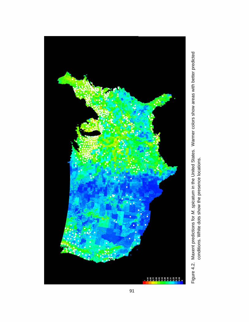
Fig

ure

4.2.

Max

ent p

red

ictio

ns fo

r M

. spi

catu

m in

the

Uni

ted

Sta

tes.

War

mer

col

ors

show

are

as w

ith b

ette

r pr

edic

ted

cond

ition

s. W

hite

dot

s sh

ow th

e pr

esen

ce lo

catio

ns.

91

4.3.

Dis

trib

utio

n of

M. s

pica

tum

rec

ords

col

lect

ed b

y C

ouch

and

Nel

son

(198

5) f

or 1

980.

92

93

CHAPTER 5

SUMMARY AND FUTURE RESEARCH

In their review paper, Guisan and Thuiller (2005) determined the earliest known

example of modeling species was published in 1924 to predict the spread of cactus

species in Australia. Computer-based modeling approaches for species distribution

began in the mid-1970s, but it was not until the early 1990s when publications on

predictive modeling of species distribution increased sharply (Guisan and Thuiller 2005).

The area of predictive modeling in ecology and related fields continues to grow with new

methods taken from other fields. These methods are then incorporated into a broader

suite of tools which can be used to address issues related to invasive species.

For stakeholders and decision makers dealing with Eurasian watermilfoil

(Myriopyllum spicatum L.), models can help direct limited financial and personnel

resources aimed at prevention or containment. As pressure from tightening budgets at

funding sources trickles down to front-line managers such as government agencies,

water management districts, and university research programs, a targeted approach to

invasion prevention will be key.

Using models can present a set of challenges. Many decisions, frequently

subjective, go into building a model. Use of presence and/or absence data is frequently

dictated by extent of the area of interest, economic considerations for data collection and

processing, and the abundance of the species of interest. Methods exist for modeling

94

under both approaches and research supports positive outcomes for both

presence/absence and presence-only modeling. When dealing with large areas, such

as a national model, presence-only modeling is the most convenient option. Particular to

invasive species, most available data is presence-only, so choices are dictated almost a

priori by available data. Maxent is a very appealing option for presence-only modeling

because it doesn’t complicate a model by assuming unknown (i.e., unsurveyed or

sampled) areas are absences. This assumption can be crucial when modeling invasive

species.

Another decision which can not be ignored is the choice of scale. Levin (1992)

posed that variability has meaning relative only to scale of observation. He added that it

was more important to capture how a system changes across scales in lieu of trying to

determine the correct scale. By using a three-scale approach in this study, it has been

possible to use a variety of predictor variables to characterize M. spicatum habitat at

different levels of observation. Given what is known about introduction, spread, and

transport of Eurasian watermilfoil, it makes sense to examine all three scales in order to

determine how spread is influenced: 1) in a single lake where stem elongation and

fragments account for the majority of spread; 2) on a regional scale where spread is

largely to due to transport among lakes by anthropogenic mechanisms; and 3) on a

national scale where broader issues of climate and landcover influence habitat

availability against the pressures from local and regional factors.

A comparison across scales of results from maximum entropy (hereafter

“maxent”) analysis yields AUCs of 0.771, 0.953, 0.968, and 0.792 for littoral, pelagic,

Minnesota, and National models, respectively. It appears then, that the most useful

scale is a regional-level model. Levin (1992) indicates that by increasing our scaling unit

(i.e., going from local to regional) a model moves from “unpredictable, unrepeatable

95

individual cases” to a model which is more generalized, trading detail for predictability.

This does not appear to extend to the case of the National model, for which the AUC

decreases. It may be possible, however, that the AUC for the National model could be

improved by increasing the number of samples. For a fixed number of predictor

variables, increasing the sample size would increase ability to estimate coefficients,

potentially increasing the AUC for this model.

The value of 0.953 for the pelagic seems extremely high and can likely be

explained by the fact that for the largest part of the pelagic zone, predictions of absence

or low probability are correct. Given the depths of the pelagic zone, intuitively M.

spicatum would not be expected and thus if the model predicted the entire zone to be

void of M. spicatum, the error rate for false positives would not be sufficiently high.

Positive Outcomes

Despite a fairly ubiquitous distribution, it is encouraging to see that when a

concerted effort is made, Eurasian watermilfoil can successfully be prevented from

overtaking habitat. M. spicatum spread appears to be largely time dependent, less than

habitat dependent. When comparing the status of Eurasian watermilfoil in Wisconsin

with Minnesota, it is possible to see the difference 20 years can make in establishment

of Eurasian watermilfoil as a nuisance species. The experience of Minnesota proves

that public education can be effective at limiting the spread of this invasive species.

Even more promising is that this was true even when habitat was deemed suitable. For

states where M. spicatum is still a non-nuisance species, this is extremely valuable, as

these states can begin to think about approaches that can be undertaken to help

ameliorate risks of widespread establishment and implement these measures early.

96

Public awareness and education programs, in addition to limiting spread, could

provide added benefits to “volunteer” type databases such as IPANE16 and IPAMS17. A

more informed citizenry is resource that would be a boon to data collection and

identification of invasives such as Eurasian watermilfoil. The economic and practical

feasibilities of collecting both presence and absence data at large scales creates a need

to focus on methods for presence-only prediction, and increases the dependency on

these types of databases. While maybe not ideal, a sufficient amount of research

supports the idea that presence-only data can be effectively used to predict habitat for

many species. The development of methods specific to presence-only models will likely

escalate, and public awareness of invasives can only benefit this type of work. A more

informed citizenry is also much more likely to be supportive of control and prevention

methods for Eurasian watermilfoil; something front-line managers can also appreciate.

Future Research

Macrophytes have traditionally been neglected in many water quality models

including the most commonly used models such as WASP18 and QUAL2K19 (Park et al.

2003). Park and others (2003) were able to develop a non-GIS based, more “traditional”

water quality model which also included the effect of macrophytes on environmental

features such as dissolved oxygen and nutrient cycling. Another model, MILFO20,

models vegetative growth, but not location, of Eurasian watermilfoil based on

16 IPANE, http://nbii-nin.ciesin.columbia.edu/ipane 17 IPAMS, http://www.gri.msstate.edu/ipams/ 18 Water Analysis Simulation Program, U.S. Environmental Protection Agency, Washington,

D.C., http://www.epa.gov 19 U.S. Environmental Protection Agency, Washington, D.C., http://www.epa.gov 20 U.S. Army Corps of Engineers, Washington, D.C., http://www.usace.army.mil

97

environment. Jensen and others (1992) were able to incorporate features such as fetch

to determine not only presence, but density and spread of aquatic macrophytes. These

successes represent pieces of a total modeling approach to Eurasian watermilfoil

management. A logical next step is to incorporate existing mathematical-based water

quality models into a GIS-based habitat suitability model for M. spicatum. A real world

model requires the user to have pre-existing data which show the conditions present.

Ideally it is desirable to link GIS-based habitat models for Eurasian watermilfoil with

other existing water quality models so that this need not be the case.

Ultimately, incorporation of these models allows the user not only to predict

probability of occurrence but also spread in response to user specified changes in

environment variables. There is already considerable research underway about how

climate change will affect the range of many species, including invasives.

Incorporation with water quality models would further allow the user to generate

scenarios with simulated changes in water quality upstream or downstream, and also

run models without measured field data on water quality. Not that it should be

advocated, but it would be entirely possible for the user to run whole simulations from

start to finish without leaving the desk.

Dependence on modeling will only increase as new methods and novel

approaches are developed. Good science and a push for validation will help to ensure

that modeling remains of value.

98

Literature Cited

Guisan, A. and W. Thiller. 2005. Predicting species distribution: offering more than simple habitat models. Ecol. Lett. 8:993-1009.

Jensen, J. R., S. Narumalani, O. Weatherbee, and K. S. Morris, Jr. 1992. Predictive

modeling of cattail and waterlily distribution in a South Carolina reservoir using GIS. Photogrammetric Eng. Remote Sens. 58:1561-1568.

Levin, S. A. 1992. The problem of pattern and scale in ecology. Ecology 73:1943-

1967. Park, S. S., Y. Na, and C. G. Uchrin. 2003. An oxygen equivalent model for water

quality dynamics in a macrophyte dominated river. Ecol. Modeling. 168:1-12.

99

APPENDIX A

DATA DEFINITIONS FOR ALL CHAPTERS

Dat

a D

ata

type

S

ourc

e N

umbe

r of

re

cord

s D

escr

iptio

n

Cha

pter

2

Fie

ld S

urve

y –

Pel

agic

sh

apef

ile

Dr.

Joh

n M

adse

n 1,

071

Dat

a fr

om g

ener

al 2

007

field

sur

vey

on P

end

Ore

ille,

con

tain

s pr

esen

ce a

bsen

ce d

ata

for

Myr

ioph

yllu

m s

pica

tum

F

ield

Sur

vey

- Li

ttora

l sh

apef

ile

Dr.

Joh

n M

adse

n 60

6D

ata

from

gen

eral

200

7 fie

ld s

urve

y on

Pen

d O

reill

e, c

onta

ins

pres

ence

abs

ence

dat

a fo

r M

. sp

icat

um

Bou

ndar

y sh

apef

ile

Dr.

Joh

n M

adse

n 1

Bou

ndar

y fo

r re

sear

ch a

rea

Tru

e Li

ttora

l Z

one

shap

efile

D

r. J

ohn

Mad

sen

1B

ound

ary

for

the

true

litto

ral z

one

(as

oppo

sed

to

the

port

ion

of t

he s

tudy

tha

t w

as c

lass

ified

as

litto

ral f

or a

naly

sis

purp

oses

) S

ound

ing

im

age

NO

AA

a N

/AIm

age

of N

OA

A s

ound

ing

data

col

lect

ed o

ver

Pen

d O

reill

e la

ke

Win

d ta

ble

US

Na

vy

101,

201

Dat

a fr

om U

S N

avy

buo

y on

Pen

d O

reill

e co

ntai

ned

win

d sp

eed

and

vect

or fo

r 20

07

Dep

th

shap

efile

D

r. J

ohn

Mad

sen

1,34

3D

ata

colle

cted

with

a d

epth

fin

ding

dur

ing

a 20

07

field

sur

vey

on P

end

Ore

ille

Cha

pter

3

Fie

ld S

urve

y sh

apef

ile

Sar

ah R

oley

3,

446

Dat

a co

llect

ed o

n pr

esen

ce a

nd a

bsen

ce o

f M

. sp

icat

um,

tota

l alk

alin

ity,

Sec

chi d

epth

, an

d la

ke

size

F

ield

Sur

vey

shap

efile

M

N D

NR

19

9S

uppl

emen

t dat

a on

pre

senc

e of

M. s

pica

tum

M

N b

ased

ata

shap

efile

M

N D

NR

B

ound

ary

dat

a fo

r co

untie

s, la

kes,

and

sta

te,

as

wel

l as

road

net

wor

k, a

nd b

oat

acce

ss s

ites

Flo

w

accu

mul

atio

n (3

0m)

imag

e N

HD

+b

N/A

F

low

acc

umul

atio

n ra

tes

for

MN

and

WI

Bas

s ha

bita

t da

ta fo

r M

N

tabl

e U

nive

rsity

of

MN

19

,966

Dat

a fr

om a

fis

herie

s su

rvey

whe

re b

ass

are

iden

tifie

d

100

WI b

ased

ata

shap

efile

W

I DN

Rc

B

ound

ary

dat

a fo

r co

untie

s, la

kes,

and

sta

te, a

s w

ell a

s ro

ad n

etw

ork,

and

boa

t ac

cess

site

s F

ield

Sur

vey

shap

efile

U

SG

S N

AS

d

730

Dat

a on

pre

senc

e of

M. s

pica

tum

B

ass

habi

tat

data

for

WI

shap

efile

W

I D

NR

4,

385

Del

inea

tion

of w

ater

s cl

assi

fied

as b

ass

habi

tat

for

the

stat

e C

hapt

er 4

H

ardi

ness

zon

es

imag

e U

SD

Ae

N/A

H

ardi

ness

zon

es f

or t

he U

S

Land

cov

er

(30m

) im

age

US

GS

N

/A

Land

cov

er c

lass

es f

rom

the

Nat

iona

l Lan

d C

over

da

taba

se

Pre

cipi

tatio

n ta

ble

PR

ISM

Clim

ate

grou

p 21

,812

,625

30-y

r av

era

ge m

onth

ly p

reci

pita

tion

Per

cent

wat

er

tabl

e N

OA

A

3,14

1P

erce

nt w

ater

by

coun

ty

Nat

iona

l ba

seda

ta

shap

efile

E

SR

If

Bou

ndar

ies

for

stat

es, c

ount

ies,

lake

s an

d riv

ers

Fie

ld s

urve

y ta

ble

IPA

NE

, IP

AM

Sg ,

US

GS

, US

DA

2,

563

Pre

senc

e da

ta f

rom

pub

licly

ava

ilabl

e so

urce

s co

nden

sed

into

one

tabl

e a N

atio

nal O

cean

ic a

nd A

tmos

pher

ic A

dmin

istr

atio

n

b Nat

iona

l Hyd

rogr

aphy

Dat

aset

Plu

s

c Dep

artm

ent o

f Nat

ural

Res

ourc

es

d US

Geo

logi

c S

urve

y N

oni

ndig

enou

s A

quat

ic S

peci

es

e US

Dep

artm

ent o

f Agr

icul

ture

f Env

ironm

enta

l Sys

tem

s R

esea

rch

Inst

itute

g Inva

sive

Pla

nt A

tlas

of N

ew E

ngla

nd,

Inva

sive

Pla

nt A

tlas

of th

e M

id-S

outh

101