1

Modeling Hypoxia in the Chesapeake Bay: Ensemble Estimation Using a

Bayesian Hierarchical Model

1Craig A. Stow and 2Donald Scavia

1NOAA Great Lakes Environmental Research Laboratory, Ann Arbor, MI 48105, 734-741-2268,

734-741-2055 (fax), craig.stow@noaa.gov, Corresponding author

2School of Natural Resources & Environment, University of Michigan, Ann Arbor, Michigan

48109-1115, 734-615-4860, scavia@umich.edu

Final Version – January 7, 2008

Journal of Marine Systems

2

Abstract

Quantifying parameter and prediction uncertainty in a rigorous framework can be an important

component of model skill assessment. Generally, models with lower uncertainty will be more

useful for prediction and inference than models with higher uncertainty. Ensemble estimation,

an idea with deep roots in the Bayesian literature, can be useful to reduce model uncertainty. It

is based on the idea that simultaneously estimating common or similar parameters among models

can result in more precise estimates. We demonstrate this approach using the Streeter-Phelps

dissolved oxygen sag model fit to 29 years of data from Chesapeake Bay. Chesapeake Bay has a

long history of bottom water hypoxia and several models are being used to assist management

decision-making in this system. The Bayesian framework is particularly useful in a decision

context because it can combine both expert-judgment and rigorous parameter estimation to yield

model forecasts and a probabilistic estimate of the forecast uncertainty.

Keywords: Chesapeake Bay, hypoxia, Streeter-Phelps, Bayesian, hierarchical model, uncertainty

3

1. Introduction

Bottom-water hypoxia (dissolved oxygen ≤ 2 mg l-1) has become common in many coastal

marine ecosystems (Diaz 2001), causing stresses in some estuarine species (Eby et al. 2005,

Craig and Crowder 2005). Hypoxia is generally attributed to eutrophication induced by

excessive nutrients, though other sources may contribute to oxygen demand (Mallin et al. 2006).

Low oxygen conditions were first reported in Chesapeake Bay in the 1930s (Newcombe and

Horne 1938, Officer et al. 1984). Though hypoxia may have been an intermittent natural

phenomenon, sediment core analyses indicate that the frequency and extent of Chesapeake Bay

hypoxia increased with European settlement in the watershed and the consequent land cover

changes (Cooper and Brush 1991, Cooper 1995).

Reducing the severity of Chesapeake Bay hypoxia is an important restoration goal, and

several water quality models have been used to help decision-makers estimate the pollutant load

decreases needed to attain the desired improvements. The complexity of these models has

ranged from a three-dimensional dynamic model (Cerco and Cole 1993) to simpler statistical

relationships (Hagy et al. 2004). The range of modeling approaches used in Chesapeake Bay

reflects an ongoing debate among water quality modelers regarding the relative utility of

complex vs. simple models (Borsuk et al. 2001), each with characteristic advantages and

disadvantages. If we understand the important system processes and can express them

mathematically, then process-based models should provide reliable predictions of system

behavior. Alternatively, statistical models help quantify predictive uncertainty; however,

statistical models rarely have an explicit mechanistic basis, reducing their confidence for use in

predictions outside the bounds of past observation.

4

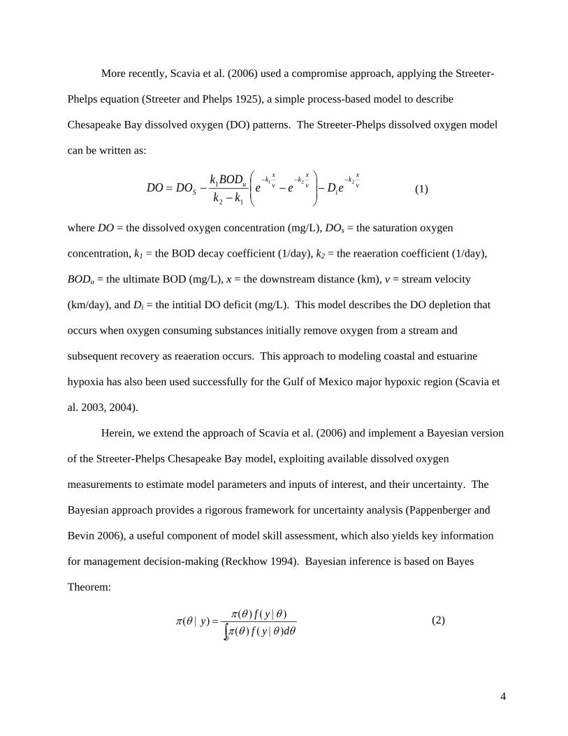
More recently, Scavia et al. (2006) used a compromise approach, applying the Streeter-

Phelps equation (Streeter and Phelps 1925), a simple process-based model to describe

Chesapeake Bay dissolved oxygen (DO) patterns. The Streeter-Phelps dissolved oxygen model

can be written as:

vxk

ivxk

vxku

S eDeekk

BODkDODO 221

12

1 −−−−

−

−−= (1)

where DO = the dissolved oxygen concentration (mg/L), DOs = the saturation oxygen

concentration, k1 = the BOD decay coefficient (1/day), k2 = the reaeration coefficient (1/day),

BODu = the ultimate BOD (mg/L), x = the downstream distance (km), v = stream velocity

(km/day), and Di = the intitial DO deficit (mg/L). This model describes the DO depletion that

occurs when oxygen consuming substances initially remove oxygen from a stream and

subsequent recovery as reaeration occurs. This approach to modeling coastal and estuarine

hypoxia has also been used successfully for the Gulf of Mexico major hypoxic region (Scavia et

al. 2003, 2004).

Herein, we extend the approach of Scavia et al. (2006) and implement a Bayesian version

of the Streeter-Phelps Chesapeake Bay model, exploiting available dissolved oxygen

measurements to estimate model parameters and inputs of interest, and their uncertainty. The

Bayesian approach provides a rigorous framework for uncertainty analysis (Pappenberger and

Bevin 2006), a useful component of model skill assessment, which also yields key information

for management decision-making (Reckhow 1994). Bayesian inference is based on Bayes

Theorem:

∫ )|()()|()(

=)|(θ

θθθπθθπθπ

dyfyfy (2)

5

where π(θ | y) is the posterior probability of θ (the probability of the model parameter or input

vector, θ, after observing the data, y), π(θ) is the prior probability of θ , (the probability of θ

before observing y), and f (y | θ) is the likelihood function, which incorporates the statistical

relationships as well as the mechanistic or process relationships among the predictor and

response variables. In many modeling applications π(θ) is a set of fixed values (probability

distributions with a probability mass of one on a particular value for each θ ), often based on

precedent, experience, or tabulated literature values (Bowie et al. 1985).

Scavia et al. (2006) used fixed a priori values for the model parameters based on a

combination of available information and expert judgment. While Scavia et al. (2004, 2006)

used Monte Carlo analysis to characterize prediction variance due to uncertainty in one of the

model parameters, v, Bayes theorem provides a rigorous framework to simultaneously relax

more of the fixed model inputs and incorporate uncertainty in these values by expressing them as

probability distributions. Higher uncertainty is expressed by choosing a large variance for the

prior distribution, while more certain values can be represented with a smaller prior variance

(with a fixed point value being the extreme case of absolute certainty). If there is little prior

information available about a particular input value, then a non-informative (also called vague or

diffuse) prior distribution can be used. A non-informative prior generally has a very large

variance and minimally influences the posterior distribution of θ . The posterior distribution,

π(θ | y), is a weighted combination of the information conveyed by the prior distribution and the

likelihood function (i.e. the combined model and data). Thus, if the data contain a lot of

information about the value of θ (as conveyed via the likelihood function) even a prior

distribution with a small variance may have only a modest influence on the posterior distribution.

6

Using Bayes theorem there is no distinction between model parameters and other

unknown model inputs such as unobserved initial conditions, missing values of state variables, or

external inputs. Any unknown quantity can be estimated if the combination of the prior

distribution and likelihood function provide sufficient information. In the Streeter-Phelps

equation k1, k2 , and v would typically be considered the model parameters, which could be

estimated from data, while DOs, DOi, and BODu are measured boundary conditions, initiation

conditions, and observed inputs, respectively . However, with sufficient data for DO and x, any

of these parameters and/or inputs can be estimated and, in fact, the mathematical structure of the

Streeter-Phelps equation makes it possible to estimate all of them simultaneously, although

extreme correlation can impose numerical difficulties when estimating some parameter/input

combinations.

An important difference between Bayesian methods and most parameter estimation

approaches is that Bayesian inference emphasizes using the entire posterior distribution of

parameter values, not just a single set of optimal values. This feature can be particularly

important when the posterior distribution is asymmetric with optimal values that are different

from the mean values (Stow et al. 2006), or when the model response surface is nonlinear.

Predictions for unobserved or future ys (denoted y~) are assessed over the entire posterior

parameter distribution as:

θθπθθπθ

dyyfyy )|()|~(),|~( ∫= (3)

which is referred to as the predictive distribution. Equation 3 indicates that, future y values are

predicted by considering all probable combinations of the parameter vector θ, which translates

into a mapping of the distribution of θ to a distribution of y~. The predictive distribution

incorporates prediction uncertainty resulting from uncertainty in all estimated model inputs,

7

including their covariance, as well as the model error term and uncertainty in the model error

variance.

2. Methods

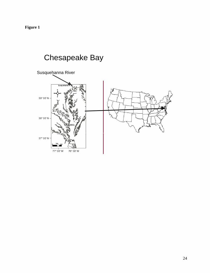
Scavia et al. (2006) used the Streeter-Phelps model to calculate summer steady-state sub-

pycnocline oxygen concentration profiles along the main stem of the Chesapeake Bay (Figure 1)

for each year from 1950-2003. Because the Chesapeake Bay is vertically stratified with surface

waters flowing seaward and bottom waters flowing landward, they estimated sub-pycnocline

oxygen demand as a point source of organic matter, proportional to Susquehanna River nitrogen

load, at the southern end of the mid-Bay region (ca. 220 km from the Susquehanna River mouth).

While physical and biological processes relating external nitrogen loading to hypoxia are

actually quite complex, the model’s ability to reproduce the observed interannual variability in

both profiles and hypoxic volume, and the fact that the model calculates a theoretical profile at

steady state (as opposed to via detailed temporal dynamics), help justify their use of the

simplifying assumptions.

DO profiles of data were computed from interpolated observations that populated a

regular grid with dimensions, first at 1-m resolution in the vertical and then at 1-km in the

horizontal across constant depths (Hagy et al. 2004). From this grid, we produced down-estuary

profiles for 137 values along the ~220 km transect for each of the 36 years from 1950 – 2003

that we used in our analysis.

Historically, the practical implementation of Bayesian methods was limited because most

non-linear process-based models result in mathematical forms that are analytically intractable

when incorporated into Bayes theorem. Thus, numerical estimation was required which made

8

applications using models of more than a few dimensions impractical because of the extensive

computer time needed. However, the advent of fast, cheap, and widely available desktop

computing has fostered development of algorithms that make numerical estimation for Bayesian

approaches feasible (Gelfand and Smith 1990). These Markov Chain Monte Carlo (MCMC)

algorithms begin with user-provided start values and after a sufficient “burn in” period converge

in distribution to the posterior. Once converged, they effectively provide a representative,

proportional, random sample from the posterior distribution. The resultant sample can then be

used to precisely estimate any function of the posterior distribution by plugging the sampled

values into the function. To implement our model, we used WinBUGS, a free, downloadable

MCMC software designed for Bayesian applications (Gilks et al. 1994). All of our inference is

based on samples of 1,000 taken from the posterior distribution after a sufficient “burn-in” to

ensure the MCMC algorithm had converged.

To incorporate the Streeter-Phelps model (equation 1) into Bayes theorem (equation 2),

we added an error term, ε, to the model and assumed ε to be normally distributed with zero mean

and variance of σ2. This assumption is consistent with nonlinear regression methods based on

least-squares or maximum-likelihood optimization approaches (Bates and Watts 1988).

Additionally, Scavia et al. (2006) incorporated a term, F, to estimate the fraction of surface

organic carbon production that settles below the pycnocline. With the inclusion of an additive

error term, ε, equation 1 becomes:

ε+−

−

−××

−=−−−

vxk

ivxk

vxku

S eDeekkBODFk

DODO 221

12

1 (4).

If ε is assumed to be independent and normally distributed with mean = 0, and variance = σ2 then

equation 4 is incorporated into the following likelihood function:

9

−

+

−

−××

+−−−−

=∏ 2

2

12

1

2

137

1 2exp

21

221

σπσ

vxk

ivxk

vxku

Sh

h

hhh

eDeekkBODFkDODO

(5)

where h denotes each of the observed DO estimates along the transect and σ2 is a parameter that

can be estimated from the data. Equation 5 denotes the likelihood function for any single year;

for all g = 1-29 years of available data the likelihood function is:

−

+

−

−××

+−−−−

= =∏∏ 2

2

12

1

2

29

1

137

1 2exp

21

221

σπσ

vx

k

iv

xk

vx

kuSgh

g h

ghghgh

eDeekkBODFkDODO

(6).

Scavia et al. (2006) held DOs, k1, and F constant across years at fixed values of 5 mg l-1, 0.09

day-1, and 0.85, respectively. The vertical flux parameter, k2, was estimated using a salt-and-

water-balance box model, adapted from Hagy et al. (2004), and applied to Chesapeake Bay by

Hagy (2002). The resulting values that varied along the transect, were used for all years.

Additionally, they used fixed a priori estimates of BODu and Di, for each year. BODu and Di

were derived from the Susquehanna load and observed values at the model origin, respectively.

In subsequent analyses, they used v as a calibration term and varied it among years to improve

the model fit.

To demonstrate the utility of Bayesian approaches we start with the inputs used by Scavia

et al. (2006) and systematically relax some of the fixed a priori assumptions, using the available

data to estimate these inputs via Bayes Theorem. We impose a hierarchical structure on the

10

model, allowing selected inputs to differ by year, with the assumption that the yearly estimates

arise from a common normal distribution (Borsuk et al. 2001). The mean and variance of this

“parent” normal distribution each require a prior distribution. We first allow k1 to differ by year

and estimate posterior distributions for all 29 years. Then we do the same for DOs and estimate

posterior distributions for each of the 29 years. Scavia et al. (2006) used fixed Di values that

differed across years; similarly we estimate Di for all 29 years allowing it to differ by year. In

each of these three demonstrations we use non-informative priors for the estimated model inputs.

That is, we chose priors with large variance so that the posterior parameter distributions would

effectively be determined by the data, not by our a priori beliefs about plausible parameter

values. For a fourth demonstration we simultaneously estimate k1, DOs, and Di, allowing each of

them to differ by year, again using non-informative priors for all of them. Finally, because

estimating k1, DOs and Di, simultaneously, results in unrealistic estimates for DOs, we use a

semi-informative prior distribution for DOs (normal with mean = 5.0 and standard deviation =

0.167). This semi-informative prior places a loose a priori constraint on DOs values, allowing

the data to influence them, but keeping them in a physically plausible range. In all instances we

use a non-informative prior distribution for model error variance σ2.

3. Results

3.1 - k1, DOs, and Di independently estimated

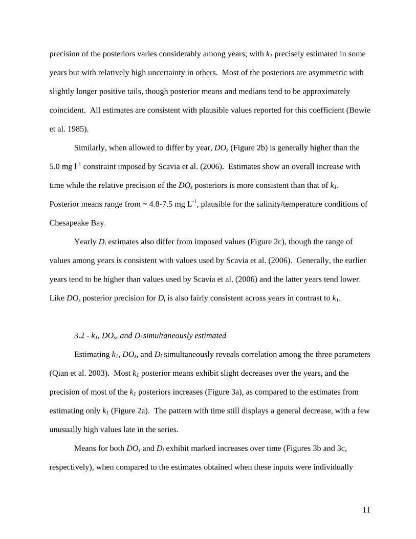
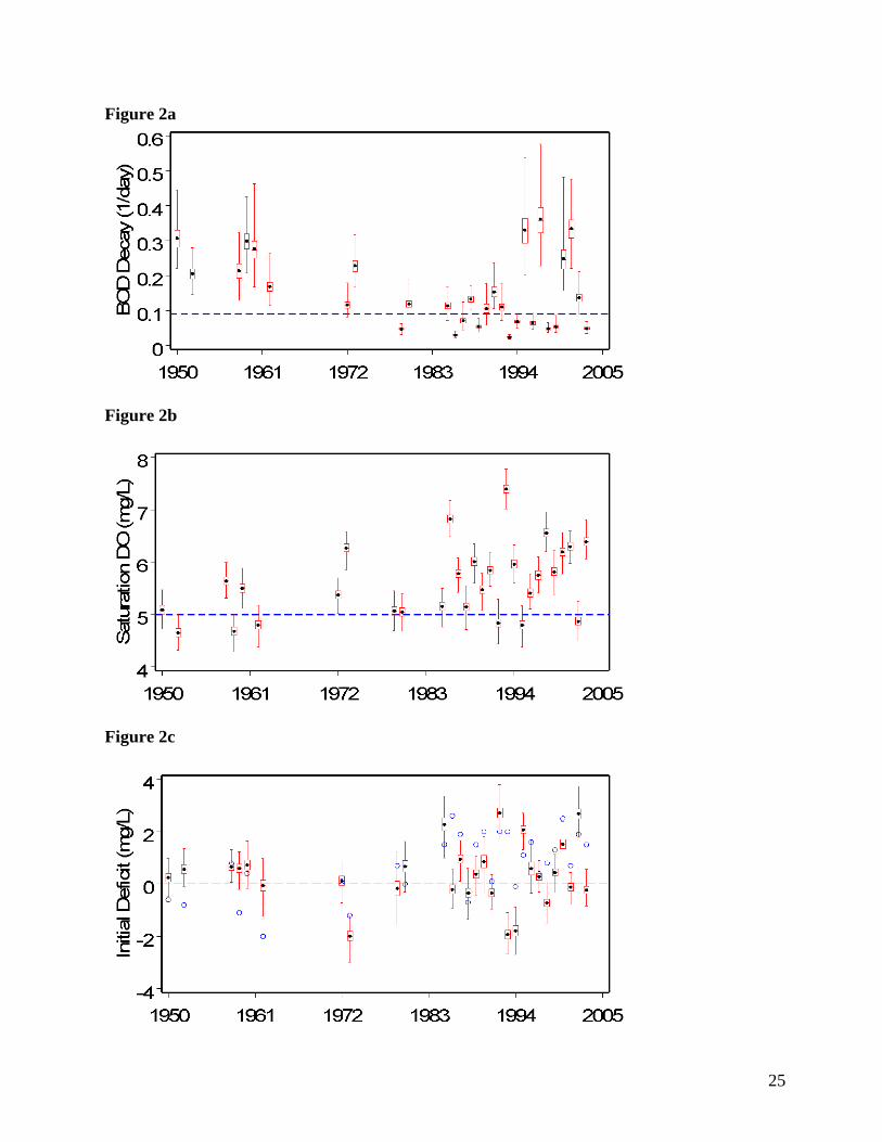
When k1 is estimated as a free parameter (Figure 2a), most yearly k1 values differ from

the 0.09 value used by Scavia et al. (2006), though they vary about 0.09. Generally, k1 decreases

through time and the posterior precision (variance-1) increases; however, four years late in the

series (1995, 1999, 2000, 2001) assume larger values with wider posterior distributions. The

11

precision of the posteriors varies considerably among years; with k1 precisely estimated in some

years but with relatively high uncertainty in others. Most of the posteriors are asymmetric with

slightly longer positive tails, though posterior means and medians tend to be approximately

coincident. All estimates are consistent with plausible values reported for this coefficient (Bowie

et al. 1985).

Similarly, when allowed to differ by year, DOs (Figure 2b) is generally higher than the

5.0 mg l-1 constraint imposed by Scavia et al. (2006). Estimates show an overall increase with

time while the relative precision of the DOs posteriors is more consistent than that of k1.

Posterior means range from ~ 4.8-7.5 mg L-1, plausible for the salinity/temperature conditions of

Chesapeake Bay.

Yearly Di estimates also differ from imposed values (Figure 2c), though the range of

values among years is consistent with values used by Scavia et al. (2006). Generally, the earlier

years tend to be higher than values used by Scavia et al. (2006) and the latter years tend lower.

Like DOs posterior precision for Di is also fairly consistent across years in contrast to k1.

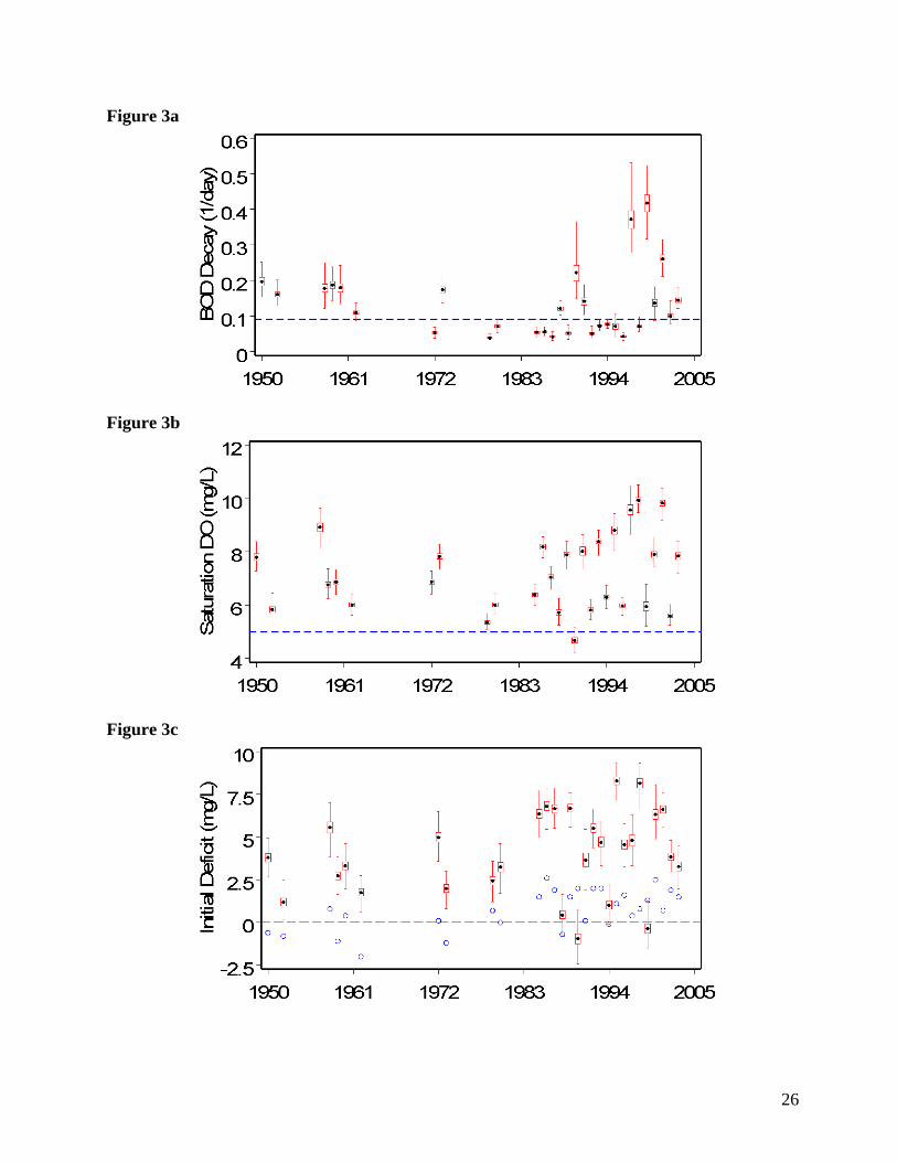
3.2 - k1, DOs, and Di simultaneously estimated

Estimating k1, DOs, and Di simultaneously reveals correlation among the three parameters

(Qian et al. 2003). Most k1 posterior means exhibit slight decreases over the years, and the

precision of most of the k1 posteriors increases (Figure 3a), as compared to the estimates from

estimating only k1 (Figure 2a). The pattern with time still displays a general decrease, with a few

unusually high values late in the series.

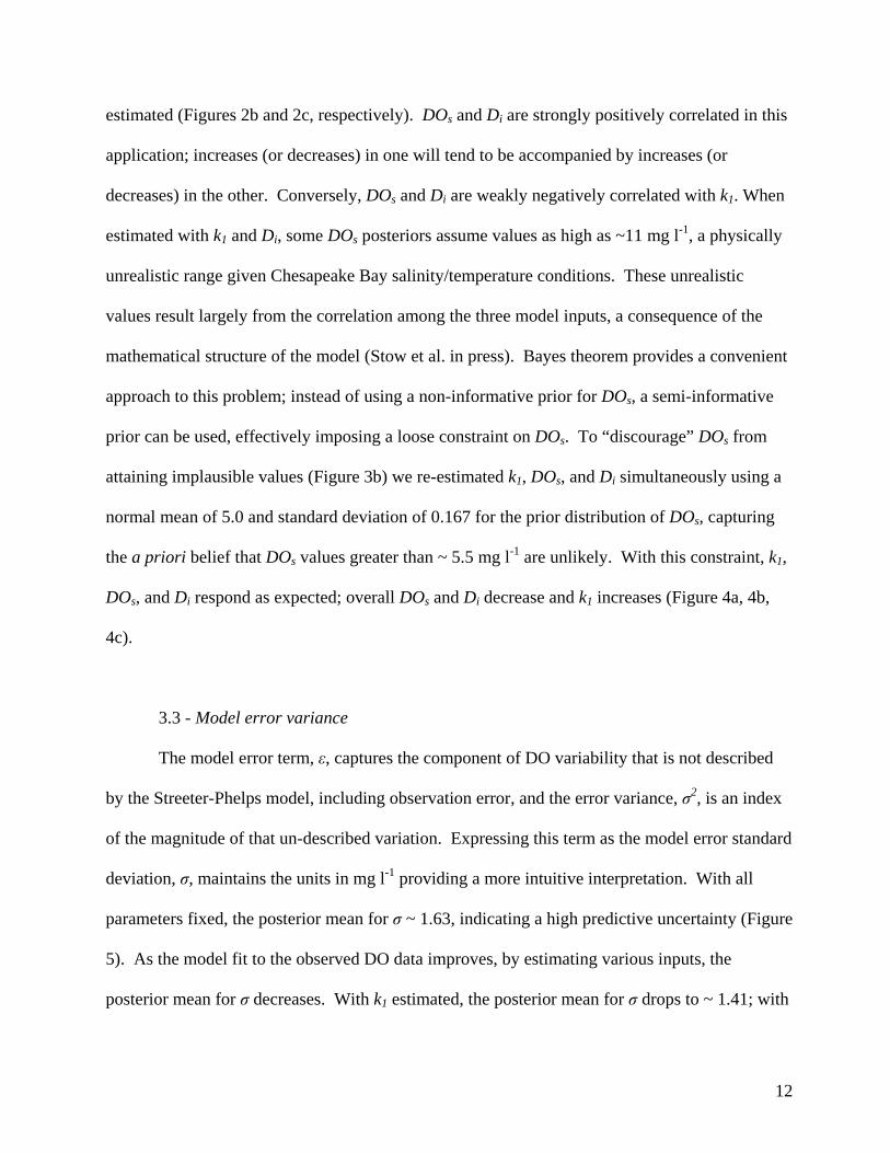
Means for both DOs and Di exhibit marked increases over time (Figures 3b and 3c,

respectively), when compared to the estimates obtained when these inputs were individually

12

estimated (Figures 2b and 2c, respectively). DOs and Di are strongly positively correlated in this

application; increases (or decreases) in one will tend to be accompanied by increases (or

decreases) in the other. Conversely, DOs and Di are weakly negatively correlated with k1. When

estimated with k1 and Di, some DOs posteriors assume values as high as ~11 mg l-1, a physically

unrealistic range given Chesapeake Bay salinity/temperature conditions. These unrealistic

values result largely from the correlation among the three model inputs, a consequence of the

mathematical structure of the model (Stow et al. in press). Bayes theorem provides a convenient

approach to this problem; instead of using a non-informative prior for DOs, a semi-informative

prior can be used, effectively imposing a loose constraint on DOs. To “discourage” DOs from

attaining implausible values (Figure 3b) we re-estimated k1, DOs, and Di simultaneously using a

normal mean of 5.0 and standard deviation of 0.167 for the prior distribution of DOs, capturing

the a priori belief that DOs values greater than ~ 5.5 mg l-1 are unlikely. With this constraint, k1,

DOs, and Di respond as expected; overall DOs and Di decrease and k1 increases (Figure 4a, 4b,

4c).

3.3 - Model error variance

The model error term, ε, captures the component of DO variability that is not described

by the Streeter-Phelps model, including observation error, and the error variance, σ2, is an index

of the magnitude of that un-described variation. Expressing this term as the model error standard

deviation, σ, maintains the units in mg l-1 providing a more intuitive interpretation. With all

parameters fixed, the posterior mean for σ ~ 1.63, indicating a high predictive uncertainty (Figure

5). As the model fit to the observed DO data improves, by estimating various inputs, the

posterior mean for σ decreases. With k1 estimated, the posterior mean for σ drops to ~ 1.41; with

13

DOs estimated, the posterior mean drops to ~ 1.34; and with Di estimated, the posterior mean is ~

1.48. However, the biggest decrease is realized when all three inputs are estimated. In that case,

the posterior mean for σ declines to ~ 0.73. When the semi-informative prior is imposed on DOs,

the posterior mean for σ rebounds slightly to ~ 0.93.

Predictive uncertainty arises from a combination of the input uncertainty and the model

error variance. Generally, predictive uncertainty decreases as more inputs are estimated and the

model error variance declines; however this decline in the model error variance is partially offset

by the accompanying input uncertainty that arises when inputs are estimated rather than fixed.

Figure 6 compares model mean predictions and corresponding 95% predictive intervals from the

model with fixed parameters and the model with the semi-informative prior for DOs for four

representative years. In all cases the predictive interval width is greatly reduced when inputs are

estimated instead of fixed, reflecting the decreasing model error variance (Figure 5).

Additionally, the mean predictions track the observed values better with estimated inputs

because different values of k1 and DOs were estimated for each year instead of using one value

chosen to work acceptably well among all years.

4. Discussion

Ensemble estimation is based on the premise that, when multiple response variables share

common or similar parameters, simultaneous estimation of these parameters yields more precise

inference (Congdon 2001), a result of “borrowing strength from the ensemble” (Morris 1983).

This idea has deep roots in the Bayesian literature (Box and Draper 1965, Efron and Morris

1972, 1973a) and underlies Empirical Bayes approaches (Efron and Morris 1973b, 1975) as well

14

as their closely-related, current incarnation as hierarchical/multilevel models (Gelman and Hill

2007, Qian and Shen 2007).

This approach represents a compromise. On one hand, a model developed using data

from multiple years will probably be less accurate for a specific year, because the model

represents the average of the years. On the other hand, a model based only on year-specific data

will have a larger uncertainty because of the smaller year-specific sample size. Hierarchical

models provide a rigorous methodology to systematically combine information from several

sources and appropriately weight the group-specific or year-specific information depending on

the degree of similarity to other groups in the data set.

In our application we somewhat arbitrarily chose three model parameters k1, DOs, and Di

to estimate as ensembles (within a hierarchical structure), differing by year but arising from a

common parent distribution, while σ2 was modeled to have the same value for all years. Many

other combinations are possible, for example σ2 could also be allowed to differ by year with (or

without) a common parent distribution, or any of the model parameters could be estimated by

assuming they are the same across years, differ by year but have a common hierarchical

structure, or are independent from year to year (no hierarchical structure). However, allowing all

the estimated parameters to independently differ by year, without a hierarchical structure, is

equivalent to estimating each year separately and confers none of the benefit of ensemble

estimation. Our intent in this presentation was largely to illustrate the methodological approach;

we are continuing to experiment with the model by systematically altering the underlying

assumptions and estimating different parameter sets. In our eventual application of this model

we intend to examine differences in some of the parameters that have occurred through time,

such as F and BODu Most of the parameter time-trajectories presented herein (Figures 2-4)

15

reveal an increase in variance occurring in the mid-1980s, consistent with previous work that has

suggested important changes in the estuary occurred at approximately that time (Hagy et al.

2004, Kemp et al. 2005). These changes may indicate important ecosystem processes that have

changed over time and provide clues for more effective management. Additionally, this model

provides a basis to estimate the effect of future BOD reductions and the corresponding

probabilities of attaining management goals (Borsuk et al. 2002). Future model improvements

will also include incorporation of a lognormal model error to bound DO predictions at zero. The

Bayesian approach can facilitate many different model error forms and other alternatives to a

normal error structure may be considered as well.

Bayesian methods are sometimes criticized because they require subjective user-provided

prior information. Berger and Berry (1988) countered this criticism, demonstrating that

statistical inference is inherently subjective, often rather subtly. The use of expert judgment-

based a priori fixed values for model parameters is common and well-accepted in

environmental/ecological modeling, yet it is highly subjective. Our presentation reveals that

Bayesian approaches allow reduced subjectivity by using imprecise a priori information thus,

letting the observations more strongly influence inference. The semi-informative normal prior

we used for DOs with mean = 5.0 and standard deviation = 0.167 is consistent with the a priori

belief that there is only a one percent chance that DOs values fall outside the 4.5 – 5.5 mg l-1

range, yet many of the final estimates were outside the range (Figure 2-4). This result illustrates

that even with a relatively tight a priori constraint Bayesian methods can permit the data to be

influential.

While Bayesian methods are sometimes criticized for subjectivity, empirical modeling is

occasionally disparaged as “simple curve fitting” because the model is largely determined by

16

observed data. Our results demonstrate that the Bayesian framework facilitates a combined

modeling approach, allowing the simultaneous use of a priori fixed parameter values, semi-

informative prior distributions, and non-informative priors. Thus, Bayesian modeling further

facilitates the compromise modeling philosophy advocated by Scavia et al (2006).

17

Acknowledgements

We thank Jim Hagy for use of his estimates of nutrient loads and oxygen profiles. This paper is

GLERL contribution number 1453.

18

References

Bates, D. M. and D. G. Watts. 1988. Nonlinear Regression Analysis & Its Applications. John

Wiley & Sons. NY.

Berger, J. O., and D. A. Berry. 1988. Statistical-Analysis and the Illusion of Objectivity.

American Scientist, 76:159-165.

Borsuk, M. E., C. A. Stow, and K. H. Reckhow. 2002. Predicting the frequency of water quality

standard violations: A probabilistic approach for TMDL development. Environmental

Science & Technology, 36: 2109-2115.

Borsuk, M.E., D. Higdon, C.A. Stow, and K.H. Reckhow. 2001. A Bayesian hierarchical model

to predict benthic oxygen demand from organic matter loading in estuaries and coastal zones.

Ecological Modelling, 143: 165-181.

Bowie, G. L., W. B. Mills, D. B. Porcella, C. L. Campbell, J. R. Pagenkopf, G. L. Rupp, K. M.

Johnson, P. W. H. Chan, S. A. Gherini, and C. E. Chamberlin. 1985. Rates, constants, and

kinetic formulations in surface water quality modeling. EPA/600/3-85/040, U.S.

Environmental Protection Agency, Washington DC.

Box, G. E. P., and N. R. Draper. 1965. The Bayesian estimation of common parameters from

several responses. Biometrika, 52:355-365.

Cerco. C.F., and T.M. Cole. 1993. Three-dimensional eutrophication model of Chesapeake Bay.

Journal of Environmental Engineering 119:1006-1025.

Congdon, P. 2001. Bayesian Statistical Modelling. John Wiley & Sons, LTD. NY.

Cooper, S.R. 1995. Chesapeake Bay watershed historical land-use impact on water quality and

diatom communities. Ecological Applications, 5: 703-723.

19

Cooper, S.R., and G.S. Brush. 1991. Long-term history of Chesapeake Bay anoxia. Science, 254:

992-996.

Craig, J.K., and L.B. Crowder. 2005. Hypoxia-induced habitat shifts and energetic consequences

in Atlantic croaker and brown shrimp on the Gulf of Mexico shelf. Marine Ecology Progress

Series, 294: 79-94.

Diaz, R.J. 2001. Overview of hypoxia around the world. Journal of Environmental Quality, 30:

275-281.

Eby, L.A., L.B. Crowder, and C.M. McClellan.2005. Habitat degradation from intermittent

hypoxia: impacts on demersal fishes. Marine Ecology Progress Series, 291: 249-261.

Efron, B., and C. Morris. 1972. Empirical Bayes on vector observations:An extension of Stein's

method. Biometrika, 59:335-347.

Efron, B., and C. Morris. 1973. Combining possibly related estimation problems. Journal of the

Royal Statistical Society Series B, 35:379-402.

Efron, B., and C. Morris. 1973. Stein's estimation rule and its competitors - an empirical Bayes

approach. Journal of the American Statistical Association, 68:117-130.

Efron, B., and C. Morris. 1975. Data analysis using Stein's estimator and its generalizations.

Journal of the American Statistical Association, 70:311-319.

Gelfand, A.E., and A.F.M. Smith. 1990. Sampling based approaches to calculating marginal

densities. Journal of the American Statistical Association, 85: 398-409.

Gelman, A., and J. Hill. 2007. Data Analysis Using Regression and Multilevel/Hierarchical

Models, Cambridge University Press. NY.

20

Gilks, W.R., A. Thomas, and D.J. Spiegelhalter. 1994. A language and program for complex

Bayesian modelling. The Statistician, 43: 169-177.

Hagy, J. D., W.R. Boynton, C.W. Keefe, and K.V. Wood. 2004. Hypoxia in Chesapeake Bay,

1950–2001: Long-term Change in Relation to Nutrient Loading and River Flow. Estuaries,

27: 634–658.

Kemp, W. M., W. R. Boynton, J. E. Adolf, D. F. Boesch, W. C. Boicourt, G. Brush, J. C.

Cornwell, T. R. Fisher, P. M. Glibert, J. D. Hagy, L. W. Harding, E. D. Houde, D. G.

Kimmel, W. D. Miller, R. I. E. Newell, M. R. Roman, E. M. Smith, and J. C. Stevenson.

2005. Eutrophication of Chesapeake Bay: historical trends and ecological interactions.

Marine Ecology-Progress Series, 303:1-29.

Mallin, M.A., V.L. Johnson, S.H. Ensign, and T. A. MacPherson. 2006. Factors contributing to

hypoxia in rivers, lakes and streams. Limnology & Oceanography, 51 (1, part 2): 690-701.

Morris, C. N. 1983. Parametric empirical Bayes Inference: Theory and applications. Journal of

the American Statistical Association, 78:47-55.

Newcombe, C.L., and W.A. Horne. 1938. Oxygen-poor waters of the Chesapeake Bay. Science,

88: 80-81.

Officer, C.B., R.B. Biggs, J.L. Taft, L.E. Cronin, M.A. Tyler, W.R. Boynton. 1984. Chesapeake

Bay anoxia: Origin, development, and significance. Science, 223: 22-27.

Pappenberger, F., and K. J. Beven. 2006. Ignorance is bliss: Or seven reasons not to use

uncertainty analysis. Water Resources Research, 42: WO5302,

doi:10.1029/2005WR004820.

Qian, S. S., C. A. Stow, and M. E. Borsuk. 2003. On Monte Carlo methods for Bayesian

inference. Ecological Modelling, 159: 269-277.

21

Qian, S. S, and Z. Shen. 2007. Ecological applications of multilevel analysis of variance.

Ecology, 88: 2489-2495.

Reckhow, K.H. 1994. Importance of scientific uncertainty in decision-making. Environmental

Management, 18: 161-166.

Scavia, D., D. Justic, and V. J. Bierman, Jr. 2004. Reducing hypoxia in the Gulf of Mexico:

Advice from three models. Estuaries 27:419–425.

Scavia, D., N. N. Rabalais, R. E. Turner, D. Justic, and W. Wiseman Jr. 2003. Predicting the

response of Gulf of Mexico Hypoxia to variations in Mississippi River Nitrogen Load.

Limnology and Oceanography 48:951–956.

Scavia, D.,E.L.A. Kelly, and J.D. Hagy. 2006. A simple model for forecasting the effects of

nitrogen loads on Chesapeake Bay hypoxia. Estuaries and Coasts, 29: 674-684.

Stow, C.A., K.H. Reckhow, and S.S. Qian. 2006. A Bayesian approach to retransformation bias

in transformed regression. Ecology, 87: 1472-1477.

Stow, C.A., K.H. Reckhow, S.S. Qian, E.C. Lamon, G.B. Arhonditsis, M.E. Boruk and D. Seo.

Evaluating water quality model uncertainty for adaptive TMDL implementation. Journal of

the American Water Resources Association. 43: 1499-1507.

Streeter H.W. and E.B. Phelps. 1925. A Study in the Pollution and Natural Purification of the

Ohio River, III Factors Concerning the Phenomena of Oxidation and Reaeration. US Public

Health Service, Public Health Bulletin No. 146, Feb 1925 Reprinted by US PHEW, PHA

1958.

22

Figure Captions

Figure 1

Location map of Chesapeake Bay

Figure 2

Posterior distribution samples for each of the 29 years of available data for k1 (a), DOs (b), and Di

(c), with k1, DOs, and Di independently estimated. Horizontal dashed blue lines indicate fixed

values used by Scavia et al. (2006) for k1 and DOs; blue circles indicate values used by Scavia et

al. (2006) for Di. Dotted horizontal line at zero on Di plots included for visual reference. Box

and whisker icons depict posterior sample mean (black dot), median (horizontal red line in box),

interquartile range (box), and extreme values (whiskers).

Figure 3

Posterior distribution samples for each of the 29 years of available data for k1 (a), DOs (b), and Di

(c), with k1, DOs, and Di jointly estimated. Horizontal dashed blue lines indicate fixed values

used by Scavia et al. (2006) for k1 and DOs; blue circles indicate values used by Scavia et al.

(2006) for Di. Dotted horizontal line at zero on Di plots included for visual reference. Box and

whisker icons depict posterior sample mean (black dot), median (horizontal red line in box),

interquartile range (box), and extreme values (whiskers).

Figure 4

Posterior distribution samples for each of the 29 years of available data for k1 (a), DOs (b), and Di

(c), with k1, DOs, and Di jointly estimated and semi-informative prior distribution for DOs.

Horizontal dashed blue lines indicate fixed values used by Scavia et al. (2006) for k1 and DOs;

23

blue circles indicate values used by Scavia et al. (2006) for Di. Dotted horizontal line at zero on

Di plots included for visual reference. Box and whisker icons depict posterior sample mean

(black dot), median (horizontal red line in box), interquartile range (box), and extreme values

(whiskers).

Figure 5

Posterior distribution sample representing model error standard deviation (σ) with fixed inputs

fixed used by Scavia et al. (2006), only k1 estimated, only DOs estimated, only Di estimated, k1,

DOs, and Di simultaneously estimated with non-informative priors, and k1, DOs, and Di estimated

with semi-informative prior for DOs.

Figure 6

Model predictions and observations (blue line) for representative years. The red dotted lines are

the mean prediction and bounds of the 95% predictive interval from the model with fixed inputs.

The solid dark lines are the mean prediction and bounds of the 95% predictive interval from the

model with k1, DOs and Di estimated, and a semi-informative prior on DOs. The dashed line

depicts predictions from the model used by Scavia et al. (2006).

24

Figure 1

Chesapeake Bay

Susquehanna River

25

Figure 2a

Figure 2b

Figure 2c

26

Figure 3a

Figure 3b

Figure 3c

27

Figure 4a

Figure 4b

Figure 4c

28

Figure 5

0.5

0.75

1

1.25

1.5

1.75

Model E

rror

Sta

ndard

Devi

atio

n

EverythingFixed

DecayCoefficient

DOSaturation

InitialDeficit

EverythingEstimated

InformativePrior

29

1950

-202468

10

0 50 100 150 200 250

Km

Dis

sove

d O

xyge

n (m

g/l)

Figure 6

1997

-5

0

5

10

0 50 100 150 200 250

Km

Dis

solv

ed

Oxy

gen

(mg/

l)

2003

-6-4-202468

10

0 50 100 150 200 250

Km

Dis

solv

ed

Oxy

gen

(mg/

l)

1973

-5

0

5

10

0 50 100 150 200 250

Km

Dis

solv

ed

Oxy

gen

(mg/

l)