modeling inflation using a non-equilibrium equation … · using a non-equilibrium equation of...

JPL Publication 13-14

Modeling Inflation Using a Non-Equilibrium Equation of Exchange Robert G. Chamberlain

National Aeronautics and Space Administration Jet Propulsion Laboratory California Institute of Technology Pasadena, California

December 2013

https://ntrs.nasa.gov/search.jsp?R=20140011391 2018-08-02T21:30:48+00:00Z

This paper was prepared for the International Conference on Economic Modeling (EcoMod2014) in Bali, Indonesia, 16–18 July 2014. The conference is sponsored by the EcoMod Network, www.ecomod.net, 351 Pleasant Street #357, Northampton, MA 01060, USA.

The research described here was carried out by the Athena development team at the Jet Propulsion Laboratory, California Institute of Technology, 4800 Oak Grove Drive, Pasadena, CA 91109-8099, and is sponsored by the U.S. Army TRADOC G2 Intelligence Support Activity and the National Aeronautics and Space Administration.

Reference herein to any specific commercial product, process, or service by trade name, trademark, manufacturer, or otherwise, does not constitute or imply its endorsement by the United States Government or the Jet Propulsion Laboratory, California Institute of Technology.

© 2014 California Institute of Technology. Government sponsorship acknowledged.

http://www.ecomod.net/

MODELING INFLATION

Abstract Inflation is a change in the prices of goods that takes place without changes in the actual

values of those goods.

The Equation of Exchange, formulated clearly in a seminal paper by Irving Fisher in 1911, establishes an equilibrium relationship between the price index P (also known as “inflation”), the economy’s aggregate output Q (also known as “the real gross domestic product”), the amount of money available for spending M (also known as “the money supply”), and the rate at which money is reused V (also known as “the velocity of circulation of money”).

This paper offers first a qualitative discussion of what can cause these factors to change and how those causes might be controlled, then develops a quantitative model of inflation based on a non-equilibrium version of the Equation of Exchange.

Causal relationships are different from equations in that the effects of changes in the causal variables take time to play out—often significant amounts of time. In the model described here, wages track prices, but only after a distributed lag. Prices change whenever the money supply, aggregate output, or the velocity of circulation of money change, but only after a distributed lag. Similarly, the money supply depends on the supplies of domestic and foreign money, which depend on the monetary base and a variety of foreign transactions, respectively. The spreading of delays mitigates the shocks of sudden changes to important inputs, but the most important aspect of this model is that delays, which often have dramatic consequences in dynamic systems, are explicitly incorporated.

i

MODELING INFLATION

Table of Contents Preface ...................................................................................................................................................................... iv 1 Preliminaries ................................................................................................................................................... 1

1.1 Inflation ..................................................................................................................................................... 1 1.2 Real vs. Nominal Prices ....................................................................................................................... 1 1.3 Market “Baskets” ................................................................................................................................... 2 1.4 Index Values ............................................................................................................................................ 2 1.5 Escalation vs. Inflation ........................................................................................................................ 2 1.6 The Word “dollar” and the “$” Symbol .......................................................................................... 3 1.7 Exchange Rates and Inflation Conversions ................................................................................. 3 1.8 Currency Black Markets ...................................................................................................................... 4 1.9 “Normal” Inflation ................................................................................................................................. 4

2 The Equation of Exchange .......................................................................................................................... 6 2.1 The Money Supply, M ........................................................................................................................... 7

2.1.1 What Can Cause the Money Supply to Change? ................................................................ 8 2.1.2 Dual Currencies / Dollarization .............................................................................................. 8

2.2 Aggregate Output, Q ............................................................................................................................. 9 2.2.1 What Can Cause Aggregate Output to Change? ................................................................. 9

2.3 The Velocity of Circulation of Money, V ..................................................................................... 10 2.3.1 What Can Cause the Velocity of Circulation of Money to Change? ......................... 11

3 Causes and Control of Inflation ............................................................................................................. 12 3.1 Industrialization ................................................................................................................................. 12 3.2 Investments in Productive Infrastructure ................................................................................ 12 3.3 Technology ............................................................................................................................................ 12

3.3.1 Productivity .................................................................................................................................. 12 3.4 Advertising ............................................................................................................................................ 14 3.5 Changes in the Money Supply ........................................................................................................ 14

3.5.1 Manipulation of the Domestic Money Supply ................................................................. 15 3.5.2 Foreign Money ............................................................................................................................ 16

3.5.2.1 Remittances ................................................................................................................................................................. 16 3.5.2.2 Domestic and Foreign Investments .................................................................................................................... 16 3.5.2.3 Net Foreign Aid .......................................................................................................................................................... 17 3.5.2.4 Tourism ......................................................................................................................................................................... 17 3.5.2.5 Exports and Imports ................................................................................................................................................. 17

3.6 Demographics ...................................................................................................................................... 17 4 A Model: Causal Relationships with Distributed Lags .................................................................. 18

4.1 Modeling Context ............................................................................................................................... 18 4.2 Causal Relationships ......................................................................................................................... 19

4.2.1 Generic Updating Equation .................................................................................................... 21 4.2.2 Monetary Base ............................................................................................................................ 21 4.2.3 Domestic Money ......................................................................................................................... 21 4.2.4 Foreign Money ............................................................................................................................ 22 4.2.5 Money Supply .............................................................................................................................. 22

ii

MODELING INFLATION

4.2.6 Equation of Exchange ............................................................................................................... 23 4.2.7 Wage Index ................................................................................................................................... 24

5 Research Opportunities ........................................................................................................................... 25 5.1 Technological Change and Escalation in Prices & Wages ................................................... 25 5.2 Endogenous Investments and Interest Rates .......................................................................... 25 5.3 Long-Run Inflation ............................................................................................................................. 26

6 Appendix: Distributing Delayed Effects ............................................................................................. 27 6.1 The Causal Relationship .................................................................................................................. 27 6.2 Time T in the Past............................................................................................................................... 28 6.3 Time t, the Present ............................................................................................................................. 28 6.4 Bottom Line .......................................................................................................................................... 29

7 Appendix: Central Bank Operations .................................................................................................... 30 7.1 Monetary Policy .................................................................................................................................. 30 7.2 Derivation of the Money Multiplier ............................................................................................. 30

References ............................................................................................................................................................ 33 List of Figures Figure 1. Athena’s Modeling Areas .............................................................................................................. 18 Figure 2. Athena’s Economics Model .......................................................................................................... 19 Figure 3. Causal Relationships Leading to Inflation ............................................................................. 20 Figure 4. Distributed Lag ................................................................................................................................. 28

iii

MODELING INFLATION

Preface The primary purpose of this paper is to document some modeling ideas that may be of

use to other professional modelers of macroeconomic systems.

To make this material accessible to less-specialized modelers and to other analysts who may not be economists, Section 1 discusses terminology and a variety of topics: the distinctions between real & nominal prices and between escalation & inflation, the use of the word “dollar” and the “$” symbol, base years and index values, market “baskets”, foreign exchange rates and inflation conversions, currency black markets, and “normal” inflation.

Economists and others already familiar with this material may wish to skim this first section, looking for unfamiliar usages. Warning: The author’s attempt to use plain language, and his engineering background, may make this paper harder for academic economists to read. As they are not the primary target audience, customary verbal shortcuts and some customary choices of symbols have been intentionally avoided. Thus forewarned, however, these readers should have little difficulty.

The theoretical foundation for the model is the Equation of Exchange, which is derived and elaborated upon in Section 2. On that theoretical basis, the causes of inflation and actions that might be taken to control it are discussed in Section 3. Finally, a model of the effects of changes in causal variables is presented in Section 4. After a brief mention of a couple of research opportunities, appendices discuss central bank operations and some technical details with regard to the spreading of lagged effects of changes in causal variables over spans of time.

iv

MODELING INFLATION

1 Preliminaries 1.1 Inflation

From an economic point of view, inflation is a change in the prices of goods that takes place without changes in the actual values of those goods. Wages will track inflation, but only after a distributed lag,1 so inflation causes wage earners to experience changes in purchasing power. Inflation changes the purchasing power of stores of money (savings, loans, bonds, etc.) even more than wages, as these do not track inflation. Most of the money from foreign sources (remittances, foreign investments, tourism, foreign aid, exports/imports) tends to maintain its purchasing power because exchange rates adjust to inflation very rapidly. Even so, some foreign money takes a while to make its way into the money supply.

When the inflation rate is negative, the condition is often called “deflation”. For simplicity, however, this paper uses the term “inflation”, regardless of its sign. Deflation is, after all, rather rare and usually short-lived.

1.2 Real vs. Nominal Prices From a physical scientist’s point of view, economists use a very strange measuring rod:

money. Due to inflation, money keeps changing its value. To deal with this awkward fact, economists have introduced what they call “real” values, which are the dollar values as of a particular point in time, called the base year.2 “Real prices”, for example, might be expressed in “2014 dollars”.

Economists then refer to the prices that are actually seen in the market, which have been subjected to inflation, as “nominal” prices. Nominal prices are expressed in “current dollars”, “inflated dollars”, “nominal dollars”, or just “dollars”. Sometimes the phrases “in real terms” or “in nominal terms” are used instead of qualifying the noun “dollar”. When qualifiers are used in text—and often when they are not—the $ symbol itself is usually not qualified. An extraordinarily careful writer might subscript the dollar sign symbol itself to indicate the base year for a real price, as in $2014, but that degree of precision is rare.3

1 By a distributed lag, I mean a delay that is spread out over time; for example, some people’s wages might lag inflation by a mere month due to a very aggressive cost of living clause in their contracts; others’ wages might lag by a year or more. 2 That “point” is sometimes a year long, but when they are being careful and precise, economists specify whether they mean the start of the year, the end of the year, or some other specific time. Location also affects the value of money, but that nuance is usually described as a regionally dependent difference in the cost of living rather than as a difference in the inflated value of the dollar because the term inflation is applied to an entire economy, which generally is understood to mean that it is a countrywide phenomenon. Furthermore, differences in regional costs of living are likely to be due to differences in regional supply and demand curves, rather than to regional differences in the value of the dollar. 3 When I want it to be very clear that I am referring to nominal dollars, I often use $t , but I don’t recall seeing anyone else use that convention. Using an actual number for the year, as in the text above, might be mistaken for a dollar amount and may not be a good idea.

1

MODELING INFLATION

1.3 Market “Baskets” The terms “prices” and “wages” are rather vague because they refer to the prices of

many different items and the wages of many different kinds of workers. Imagine a market basket containing a little bit of each of the goods and services that make up the gross domestic product (GDP), with the ratios of their amounts matching the ratios that are actually exchanged throughout the country. Suppose that the actual amounts are just enough so that the basket is worth $1 in the base year.

There are many ways such baskets could be defined. In addition to a “GDP basket”, a “CPI basket”4 would contain a mix of goods and services in the ratios that are purchased by consumers and a “worker basket” would contain a mix of workers in the ratios that are employed in the country. In each case, the actual amounts would be just enough so that the basket is worth $1 in the base year.

Macroeconomic models seldom, if ever, deal with the price or quantity of a single, closely defined good or service. A metals sector, for example, would be made up of iron, nickel, copper, etc. In a higher-resolution model, an iron sector would be made up of pig iron, steel, etc., and so on. As a result, it is customary to price all subsets of goods and services in such models at $base year1/unit, and the unit is a basket of goods and services in that subset, with ratios as are seen in the market, and sized so that $base year1 is its base price. A consequence of this practice is that economists usually talk about quantities in dollars, rather than in tonnes or liters or any other unit familiar to physicists and chemists.

1.4 Index Values It is often easier to understand the meaning of a number that is changing by dividing its

current value by its value in the base year. That quotient is called an index value; by definition, its value in the base year is exactly 1.0.

If we are considering the price of a “basket” of goods and services as defined in the previous section, we see that such prices are also index values. Thus, the price of the hypothetical GDP basket is the “price index” and the price of the hypothetical worker basket is the “wage index”.

Dealing with price and wage indices avoids, or at least puts off, talking about specific prices and wages in terms of $/unit, $/tonne, and even $/work-year.

1.5 Escalation vs. Inflation Inflation is further complicated by the fact that many of the causes of inflation act not

on goods as a whole, but on individual goods and services. The term “escalation” is used for changes in the price of an individual good or service.

“Inflation” refers to the average change in prices of a defined basket of goods and services. For example, the CPI is based on a consumer-relevant collection defined, in the

4 CPI = consumer price index

2

MODELING INFLATION

United States, by the U.S. Bureau of Labor Statistics,5 while the GDP deflator is based on all of the goods and services used to define the GDP. These averages are weighted by the quantity sold of each good or service as defined for the basket.6

Thus, as we have seen in our own personal experiences, the inflation rate can be highly positive even while the prices of some individual items, such as computer memory, are dropping rapidly. If improvements in technology drive down the prices of enough items, inflation can become deflation.

1.6 The Word “Dollar” and the “$” Symbol Because we want the analysis to be applicable in many regions of the world, we need to

choose a generic word and symbol to represent the value of a fixed amount of money. I have chosen the word dollar and the associated symbol $ for the convenience of American readers, but that was not an arbitrary decision because doing so is a common practice among those studying international economics.

The $ symbol is usually interpreted to mean the United States dollar, or USD, but it does not have to be interpreted as such. Input data and computed numbers would be different, of course, but there would be no change in the model if dollar and the $ were interpreted to mean euros or Japanese yen or Indian rupees.

1.7 Exchange Rates and Inflation Conversions When converting from other currencies to $ and to and from the base year, there are

several issues to consider:

• What currency—dinars, say, represented by d—is associated with base case data

• The exchange rate between d and $ in the base year

• Inflation indices for d and $ may be based on different base years

• The two currencies, d and $, generally experience different inflation rates

5 Actually, they define several indices, for different classes of consumers. See, for example, http://research.stlouisfed.org/fred2/categories/9 (accessed 3/21/13 2:44 p.m. PDT). Economists consider that when a good or service has been exchanged that it has been "consumed" by a "consumer"; actually using it up is not required. 6 A further complication is that these quantities are changed from time to time (by the agency that owns the definition) in an attempt to keep pace with changes in overall consumption and supply patterns so that the indices are more meaningfully compared with current wages. The unstated presumption is that if anyone wants to compare index values at different times, they will be sophisticated enough to make the corrections—which the agencies generally do publish.

3

http://research.stlouisfed.org/fred2/categories/9

MODELING INFLATION

1.8 Currency Black Markets There will be a black market in foreign currency when enough of these conditions are

met:7

• There is an official exchange rate, and it is pegged at a level that does not reflect the true market value of the domestic currency.

• The government makes it difficult or illegal for its citizens to own much or any foreign currency.

• Exchanges are taxed in one or both directions.

• The black market currency is counterfeit.

• The black market currency was acquired illegally and must be laundered before use.

• The domestic currency has a high inflation rate but the foreign currency does not (is “hard” or “stable”).

• There is a lack of confidence among the populace in the value of the domestic currency. This can be a result of economic sanctions imposed from outside the country.

In a currency black market, the price of the foreign currency is higher than it would be at the official exchange rate. There would therefore be very few exchanges at the official rate because the amount of foreign currency available at the official rate is limited.

In fact, the amount of the foreign currency available at the official rate can be expected to be negligibly small. Suppose 1 dollar is exchanged for 1 euro at the official rate of 1 dollar/euro and 5 dollars are exchanged for 1 euro at the black market rate of 5 dollars/euro. Now suppose you have 100 euros. You can exchange them for 500 dollars on the black market. Now, you can take that 500 dollars to the official market and exchange them for 500 euros (if there are any euros there). Next, you’ll take that 500 euros and exchange them for 2,500 dollars on the black market, and so on. Very soon, there will be no euros available at the official rate. If you want euros, you’ll have to go to the black market and exchange 500 dollars to get 100 of them. The official rate is theoretically better, but the euro drawer is empty. Thus, all euros will be removed from the official exchange market and either held in reserve, used for certain transactions, or sold on the black market for 5 dollars each, at the black market rate of 5 dollars/euro.

Bottom line: When there is a black market in currency, the correct exchange rate to use is the (black) market rate, not the official one.

1.9 “Normal” Inflation It occurred to me that there must be some sort of “normal” long-term inflation rate.

Centuries ago, a penny a day was an unskilled worker’s wage. In my own memory, 60 years

7 Sources: http://en.wikipedia.org/wiki/Black_market#Currency accessed 6/5/13 4:10 p.m. PDT and http://www.investopedia.com/articles/investing/031213/currency-trading-black-market.asp accessed 6/5/13 4:15 p.m. PDT.

4

http://en.wikipedia.org/wiki/Black_market%23Currency

http://www.investopedia.com/articles/investing/031213/currency-trading-black-market.asp

MODELING INFLATION

ago, 10 cents could buy a comic book and 1 dollar could buy a haircut or a seat in a double-feature movie. Prices seem to go up—a lot and persistently—over the long term.

Is this a real phenomenon? If so, what are the causes? To get ahead of the story (see Section 2), nothing in the Equation of Exchange, on which the model described in this paper is based, has an obvious long-term secular effect.

One long-term secular force is investment that exceeds depreciation. This can be expected to increase aggregate output, so unless the money supply times the velocity of circulation of money increases at the same rate or faster, one would expect deflation over the long run, not inflation.

Is there a reason to expect the money supply to increase faster on average in the long run than aggregate output does? According to John Ledyard,8 economists would probably not agree that there is a “natural rate of inflation”, but they probably would agree that long-run inflation is a function of central bank policy and money supply (as well as expectations). Some economists, he says, argue that a small positive rate is good for real growth. He pointed out that this would accommodate the expansion in investment mentioned in the previous paragraph.9

Furthermore, improvements in technology can be expected to eventually increase the velocity of circulation of money until no further increases matter.

Clearly, however, long-run inflation is not a universal phenomenon. In the poorest parts of the world, an unskilled worker's wage is still only about a dollar a day.10

Bottom line: We can expect that central bank policies, investments, and improvements in technology will cause long-run increases in both the money supply and the velocity of circulation of money such that their product will exceed the rate of growth of aggregate output with the end result that there will usually be a small, long-run positive inflation rate.

The model described here does not address this issue, nor does it include an estimate of the effect of the phenomenon.11

8 John Ledyard, Alan and Lenabelle Davis Professor of Economics and Social Sciences at the California Institute of Technology, personal communication, 7/17/13. 9 I find myself wondering if causality goes in the other direction. Perhaps long-term real growth creates a need for larger rates of increase in the money supply, thereby causing a small positive long-term inflation rate. 10 Even so, a dollar is 100 times as big as a penny, so this may not be a good counterargument. 11 However, we do use this observation to provide default historical values of the variables needed at the start of the simulation by assuming that rates of change were constant as far back as needed. Backwards extrapolation then generally produces numbers that approach zero asymptotically instead of numbers that go embarrassingly negative.

5

MODELING INFLATION

2 The Equation of Exchange Irving Fisher, who wrote the seminal reference [Fisher 1911] on the Equation of

Exchange, developed the equation directly as follows.12 First, note that the money spent on a single transaction must equal the per-unit price paid times the amount sold. Combine all the transactions in a year, recognizing that the same money will be used over and over, and we come up with one of the usual forms of the Equation of Exchange:13

𝑀 ∗ 𝑉 = 𝑃 ∗ 𝑄.

Bromley summarized this by pointing out that the left side is total spending on the GDP, the right side is the value of the GDP, and these have to be equal to each other.

Fisher took about 32 pages to explain the terms in this equation. Let’s see if we can do it in half a page.

Let’s start with Q. Consider a “GDP basket”, as defined in Section 1.3, containing a little bit of each of the goods and services that make up the GDP. The number of those GDP baskets that are exchanged in one time unit is the quantity, Q.

Next, P. The price of one GDP basket in the base year is one dollar; that is: $base year1/GDP basket. But we want to express the price in nominal terms, so we must multiply it by the amount of inflation since the base year. Since the price in the base year is $base year1, the price in year t must be numerically equal to the amount of inflation expressed as a multiplier. Thus, the symbol P can mean either the price of GDP baskets, expressed in $t/GDP basket or it can be used to represent the inflation index, expressed in $t/$base year.

M is the total amount of money available for use and is called “the money supply”.

V is called “the velocity of circulation of money” and is the number of times the average dollar in circulation changes hands during a year. The reciprocal of this is sort of the mean time a dollar stays in a wallet.14

Since we are currently interested primarily in the price level, we will use the form:15

12 See [Fisher 1911], chapters II and III, and [Bromley 2013], page 142. 13 A vertically centered asterisk is used throughout this paper to signify multiplication. 14 Of course, most money seldom sees an actual wallet, so this statement should be taken rather loosely. 15 Caveat: Referring to the use of the money supply for policy making, the Board of Governors of the U.S. Federal Reserve System said, at http://www.federalreserve.gov/faqs/money_12845.htm (accessed 2/19/13 at 5:15 p.m. PST):

Over recent decades, however, the relationships between various measures of the money supply and variables such as GDP growth and inflation in the United States have been quite unstable. As a result, the importance of the money supply as a guide for the conduct of monetary policy in the United States has diminished over time. The Federal Open Market Committee, the monetary policymaking body of the Federal Reserve System, still regularly reviews money supply data in conducting monetary policy, but money supply figures are just part of a wide array of financial and economic data that policymakers review.

That said, it may be noted that while this statement applies to the current situation in the United States, the Equation of Exchange was popular among economists in the United States for a long period until recently.

6

http://www.federalreserve.gov/faqs/money_12845.htm

MODELING INFLATION

𝑃 =𝑀 ∗ 𝑉𝑄

.

The remaining subsections discuss each of the factors in more detail.

It is tempting to determine the inflation rate by taking the derivative of the above equation with respect to time and doing a little algebra to get the inflation rate, expressed as a dimensionless fraction per time, (dP/P)/dt.16 Doing so, however, would be very misleading because the Equation of Exchange describes a causal relationship that takes time to happen.17 Changes in any of the causal variables will eventually result in corresponding changes in the output variable if nothing interferes with the process.

Thus, the inflation rate must be computed directly from changes in the value of the price index P over an interval of time Δ𝑡:

𝐼𝑛𝑓𝑙𝑎𝑡𝑖𝑜𝑛 𝑅𝑎𝑡𝑒𝑡 = 𝑃𝑡 − 𝑃𝑡−∆𝑡

∆𝑡𝑃𝑡−∆𝑡� .

2.1 The Money Supply, M The money supply is the amount of money that is easily available for transactions. It is

important to note that this goes far beyond the currency that has been stamped and printed, as discussed below.

Since U.S. markets currently use a lot of highly sophisticated systems to facilitate trade, current U.S. experience may be less relevant to countries undergoing stability and recovery operations than earlier U.S. experience. It should probably also be pointed out that many economists, when applying “the quantity theory of money” treat both Q and V as constants, thereby assuming away much of the usefulness of the Equation of Exchange. It is possible Q and V constitute major parts of what “The Fed” had in mind when they said they now use “a wide array of financial and economic data”. 16 A Wikipedia author at http://en.wikipedia.org/wiki/Equation_of_exchange (accessed 3/21/13 3:33 p.m. PDT) and at http://en.wikipedia.org/wiki/Quantity_theory_of_money (accessed 4/8/13 3:04 p.m. PDT) fell into this trap—and temporarily pulled me along with him. (Lesson: Be wary of Wikipedia, useful though it is.) When you consider the time-consuming process by which a small amount of currency becomes a larger amount of money, which is discussed in Section 7.2, it becomes obvious that time derivatives would be misleading. 17 [Bromley 2013] points out that the Equation of Exchange is an equilibrium equation, not a dynamic one. He says (paraphrased from pp. 143–4) that when M changes, V changes in the opposite direction for a few months, then V springs back, pulling Q along about 6 months to a year later. Eighteen months to 3 years after the change in M, P catches up. While P is catching up, Q may stop moving or even appear to move backwards compared to the rest. Eventually, (in about 3 years), the only effect of a change in M is a change in P; V, Q, real wages, and the real interest rate are all at about the same level as before. Note, however (now not paraphrasing Bromley), saying that real wages do not change is equivalent to saying that nominal wages will eventually reflect the eventual change in the price level, P, that results from a change in the money supply.

7

http://en.wikipedia.org/wiki/Equation_of_exchange

http://en.wikipedia.org/wiki/Quantity_theory_of_money

MODELING INFLATION

2.1.1 What Can Cause the Money Supply to Change?

The actual cash—banknotes and coins—in circulation is an important part of the money supply. Thus, four of the factors that affect the money supply are:

• Domestic currency in circulation

• Bank reserves of currency

• Consumer reserves of currency

• Foreign currency in circulation

Actual cash, while very important, is only a small part of the total money supply. Only a portion of the cash that is deposited in a bank is kept in the bank for immediate withdrawal by depositors (that is, “held in reserve”). The rest is loaned out and is again available for transactions. When the loaned money is spent, most of it is eventually again deposited in a bank. Most of these deposits are also available for loans. This process is repeated over and over; the multiplicative effect is theoretically limited only by the reciprocal of the fraction of the reserves that are held by the banks and by the recipients of the loans. This is discussed further in Section 7.2. Thus, two very important factors that affect the money supply are the reserves held by banks and by private citizens.

Consumer deposits are not a bank’s only source of money. Another important source, which creates money out of thin air, so to speak, is open market operations of the central bank. These consist of buying or selling government bonds to banks, thereby creating or using portions of the banks’ reserves that exist only as entries on the books of the central bank.

Changes in any of these will change the amount of money that is readily available for transactions—that is, the money supply. This topic will be addressed again, more explicitly (that is, with equations), in Section 3.5.

2.1.2 Dual Currencies / Dollarization

Either all foreign money must be exchanged for domestic currency, in which case foreign money has no effect on the money supply; or the economy will be dollarized, in which case “foreign currency [is circulated] in parallel to or instead of the domestic currency. … The term is not only applied to usage of the United States dollar, but generally to the use of any foreign currency as the national currency.”18

In the real world, especially in the countries in which we are particularly interested, prohibition of the use of foreign currency is unlikely to be successful.19 Those transactions that take place free of government control will use whichever currency is acceptable to both parties to the transaction. Each party would prefer to spend the weaker currency and

18 The quote is from http://en.wikipedia.org/wiki/Dollarization (accessed 6/25/13 11:08 am PDT), which has an extensive discussion of this topic. 19 If, however, it were to be successful, incoming foreign money can be expected to have a positive effect on demand, which would lead to increased productive output. With no change in the money supply or the velocity of circulation of money, the expected result would be deflation.

8

http://en.wikipedia.org/wiki/Dollarization

MODELING INFLATION

receive the stronger one; the choice will depend upon the relative bargaining power of the participants.

Consequently, this model assumes the economy is unofficially or semi-officially dollarized: That is, foreign money entering the country increases the money supply even though it may not be legal tender.20 Foreign currency is valued at its exchange rate (see Section 1.7). We will not consider official (a.k.a. de jure or full) dollarization, in which the country has abandoned its domestic currency and adopted the foreign currency as its sole legal tender.

Although we will treat foreign money as part of the money supply, we will track it separately from the domestic money and it will have its own velocity of circulation. See Section 3.5.

For simplicity, no other effects of dollarization will be modeled.

Since foreign currency will be exchanged at the true market rate (that is, at the black market rate, if the official exchange rate is not allowed to float), neither the price level nor aggregate production will be affected by the mere fact that two (or more) kinds of currency are in circulation.

2.2 Aggregate Output, Q It seems fairly obvious that if the supply of goods is increasing at the same rate as the

money supply, and all of the goods are sold, the price level should not change. Indeed, if nothing else changes, that is what the Equation of Exchange predicts. But better than that, it tells what to expect if there is a change in the production rate even if other things are also changing.

Changes in the production rate for any particular product are easy to visualize. By aggregate output, however, we are referring to the production of everything in the economy that contributes to the GDP.

The variable Q is the number of GDP baskets produced per year.

2.2.1 What Can Cause Aggregate Output to Change?

If the economy is running at economic equilibrium, aggregate output is determined by intersections of the supply and demand curves for the products that make up the aggregate GDP product. Thus, aggregate output will change if:

• Demand curves change. Among the things that can affect a demand curve are:

• Number of consumers. More consumers move all demand curves to the right.

• Wages, when compared to the price level. Wage increases move the demand curves to the right. Wage decreases move it to the left.

• Prices are determined by the intersection of the supply and demand curves, so changes in price do not affect the demand curve itself. Rather, the equilibrium price is the end result of a presumably convergent dynamic process involving changes in

20 Legal tender is currency that a creditor must accept by law.

9

MODELING INFLATION

supply (along the supply curve) due to changes in price and changes in demand (along the demand curve) due to changes in price.

• Fashions are unlikely to have an effect on aggregate prices or quantities, though effects can be quite dramatic in regard to individual products or services.

If there is unsatisfied demand and factories are running at capacity, aggregate output will be affected by:

• Production infrastructure—that is, increases or decreases in production capacity. These can be caused by new construction, by changes in desired levels of operations and/or maintenance, and by intentional destruction of capacity.

If there is unsatisfied demand due to a labor shortage, aggregate output will be affected by:

• Available labor force. In a sophisticated model, this might be differentiated by job classification. The number of people in the labor force should also be affected by the ratio of the wage index and the price level.

• Labor turbulence. There will always be some people who are technically unemployed, but are actually between jobs.

• Worker and job location imbalance, or geographic unemployment. Some people, perhaps as a consequence of being forcibly dislocated from their homes, live too far from available jobs.

Technological change can affect aggregate output by changes in:

• Productivity of the factors of production (see Section 3.3.1)

• Preferences among ingredients used in production

Technological advancements can be expected to cause improvements in aggregate output, which tends to reduce inflation, but they can have other effects as well, some of which may increase inflation. In particular, they can have direct effects on the money supply and the velocity of circulation of money. In an economy changing from an agricultural emphasis to an industrial one, money is not only created by the central bank and by investment banks’ and consumers’ reserve policies, but by technology, due to increased use of credit. Furthermore, a dollar has a higher velocity of circulation when it can be transmitted electronically.

2.3 The Velocity of Circulation of Money, V By definition, the velocity of circulation of money21 is the average rate at which a typical

dollar bill is repeatedly used in transactions. It is the reciprocal of the average amount of time that a typical bill stays in the wallet.22 The different kinds of money that make up the

21 This phrase is frequently shortened to “the velocity of money”, but the shortened phrase is even more confusing than the longer one, which I have used throughout this paper, though I have used “velocity” for short a few times, when context makes the meaning clear. 22 As pointed out earlier, the “dollar” no longer has to be represented even by an actual piece of paper, and the “wallet” can be an electronically accessible account.

10

MODELING INFLATION

money supply (see Section 2.1) vary in liquidity, so they (the different kinds of money) must have rather different values for velocity. In fact, the cutoff as to which kinds of investments are included when computing the money supply is based on this concern.23

In many models, the velocity of circulation of money is assumed to be constant, which is probably a satisfactory assumption over short periods in a stable economy—but a stable economy cannot be assumed to be the case in our context.

2.3.1 What Can Cause the Velocity of Circulation of Money to Change?

The factors that drive the velocity are highly subjective, and might be susceptible to information operations. Bromley24 mentions that people will tend to get rid of money faster (i.e., the velocity of circulation of money will be higher) if:

• Increasing inflation makes tomorrow’s money worth even less than today’s.

• There is an increasing interest rate on non-money investments (such as houses).

• Wages are increasing or there is a decreasing popular desire to hold wealth as money, perhaps due to decreased confidence in the government.25

I have thought of four technology-based phenomena that can cause changes in the velocity of circulation of money:

• Shifts in the relative amounts of the different kinds of money used. Use of checks in preference to cash, for example, might increase the average velocity because fewer trips to the bank would be needed. Use of a larger fraction of foreign currency in a dual-currency economy might decrease the average velocity because highly inflationary domestic currencies tend to be treated as “hot potatoes”.

• Improvements in information technology, or increases in the use thereof, would increase the velocity due to reduction in the time needed to clear checks.

• Increased use of automatic teller machines, debit cards, or credit cards reduces withdrawal times.

• Increased use of electronic transfer of funds reduces transaction times from days to minutes.

23 Discussions of the Equation of Exchange sometimes point out that the 𝑃 ∗ 𝑄 term can be thought of in a disaggregated form as a sum of 𝑃𝑖 ∗ 𝑄𝑖 , where i ranges over all transactions in the economy. Irving Fisher [Fisher 2011] pointed out that the 𝑀 ∗ 𝑉 term can be thought of as an aggregation of 𝑀𝑗 ∗ 𝑉𝑗 terms, where j ranges over different kinds of money, each with its own velocity. Fisher’s illustration in his Chapter III considers only currency and bank deposits. This observation is used in this paper to deal with dual currencies in Section 3.5. 24 See [Bromley 2013], page 143. 25 For what it’s worth, according to http://en.wikipedia.org/wiki/Equation_of_exchange (accessed 3/21/13 3:33 p.m. PDT), economists Alfred Marshall, A.C. Pigou, and John Maynard Keynes, of Cambridge University, argued that V should be equal to the average consumer’s nominal wage divided by the average consumer’s cash reserve. Thus, a change in either the average wage or that average cash reserve that is due to less-than-usually-settled conditions or high inflation would lead to a change in the velocity of circulation of money. Assuming that they are correct would allow a modeler to make V an endogenous variable—which I have not done.

11

http://en.wikipedia.org/wiki/Equation_of_exchange

MODELING INFLATION

3 Causes and Control of Inflation As discussed in Section 2, we can use the Equation of Exchange to compute the amount

of inflation relative to a base case if we know the changes in the money supply, aggregate output, and the velocity of circulation of money, but the modeling challenge is to determine what in the real world causes changes in those variables.

3.1 Industrialization Industrialization expresses itself largely as massive changes in production capacity.

Industrialization refers to the introduction or adaptation of industrial methods of production and manufacturing, and is usually associated with significant social changes, as well as with changes in production capacity.

To properly assess the consequences of industrialization, those social changes must also be modeled, as they will have significant indirect effects on the economy.

3.2 Investments in Productive Infrastructure Building more production capacity, even at a lesser scale than would be required to

justify the label “industrialization” will tend to reduce inflation unless there are corresponding changes in the money supply. On the other hand, if there is no latent demand, additional capacity may have no effect on the amount of aggregate output.

Decreases in production, whether due to direct or collateral damage or other reasons, will tend to increase inflation.

3.3 Technology Improvements in technology can lead to changes in the productivity of the factors of

production and to reductions in the per-output-unit amounts of ingredients required.26

Changes in what technologies are used in the country can also lead to changes in the velocity of circulation of money.

3.3.1 Productivity

The discussion that follows is about productivity, not production. The Q in the Equation of Exchange depends on the amount of production (that is, aggregate output), which depends on, but is not the same as, productivity.

Productivity is expressed in a CGE (computable general equilibrium) model by so-called “production functions”. For example, the Cobb-Douglas production function often used to describe the production of goods has this form:27

26 Since labor is invariably one of the factors of production that is needed, improvements in technology will generally lead to increased wages, though possibly fewer jobs. 27 In this equation, taken from the Athena CGE model, the subscript g is for the goods sector of the CGE model, while p is for the populace sector, which supplies the labor factor of production. Academic economists usually refer to the populace sector as the households sector, a term I have avoided on the politically correct grounds that it sounds vaguely “too Western”. I’m not at all sure that was a good idea, but it seemed good at the time. I

12

MODELING INFLATION

𝑄𝑆𝑔 = 𝐴𝑔 ∗ 𝑄𝐷𝑔𝑔𝑓𝑔𝑔 ∗ 𝑄𝐷𝑝𝑔𝑓𝑝𝑔.

The parameter Ag carries the information as to how much of the ingredients are needed to produce each goods basket. The parameters fgg and fpg describe how the ingredients are economically traded for each other as their prices vary.

The use of improved production technology would increase Ag, thereby decreasing QDgg and QDpg, the amounts of goods and labor respectively, needed to produce any amount of supplied output, QSg; and would change the values of fgg and fpg, as well.28 It would be quite difficult to find new values of these parameters directly—they are usually calibrated by gathering SAM29 data for a country that uses the appropriate technology—though changes that simply cut all ingredients by x% would imply simply increasing Ag by x%.

If a Leontief production function is assumed to describe the production technology, the changes are even more obvious.30 A Leontief production function for goods can be written in this form:

𝑄𝐷𝑔𝑔 = 𝐴𝑔𝑔 ∗ 𝑄𝑆𝑔, 𝑄𝐷𝑝𝑔 = 𝐴𝑝𝑔 ∗ 𝑄𝑆𝑔.

Richard Stone [Stone 1962] pointed out that changes in ingredient requirements can be represented by multiplying the rows of the Leontief matrix by numbers that are larger or smaller than 1.0, while changes in technology can be represented by multiplying the columns of the Leontief matrix by numbers that are larger or smaller than 1.0.

Improved production technology should improve productivity, which would tend to reduce prices. It is also likely to change the demand for labor, which could lead to increased unemployment—but it might not; I’d be inclined to trust the CGE model’s synthesis of the combined effects of those contradictory trends more than my intuition.

Some kinds of improved technology, such as the introduction of ATMs,31 would increase the velocity of circulation of money, which would tend to increase the inflation rate.

Some kinds of improved technology, such as online banking or increased use of credit cards, might increase the money supply and perhaps the velocity of circulation of money, both of which would tend to increase the inflation rate.

considered changing the usage for this paper alone, but decided I’d rather confuse a few professors who can more easily sort it out than any of my customers who might read this paper. Besides, populace truly is a more precise term than households for that which supplies consumers and workers. 28 The following discussion also applies to the use of technology that is less productive, replacing increasing by decreasing as appropriate. 29 SAM is an acronym for “social accounting matrix”, a format for organizing most of the high-level data that describes the economics of a country. When filled with data describing the annual value flow rates between sectors in an economy, they are used to calibrate the model parameters of a CGE model. 30 For this reason, and because there is little opportunity for substitution at high levels of aggregation, we plan to change the production function used for the goods sector in the Athena CGE from a Cobb-Douglas formulation to a Leontief formulation in a later version. 31 ATM = automatic teller machines

13

MODELING INFLATION

It is difficult to make explicit generic mathematical statements as to the contributions of technological change to the velocity of circulation of money and the money supply. Each case will have to be considered on its own.

3.4 Advertising Ultimately, consumer demand is constrained by the consumers’ total income.

Advertising can change how that demand is distributed among available products. The effects on the economy of changes in relative demand could be significant, as some sectors are much more labor-intensive and others may be much more capital-intensive.

Advertising can change consumers’ relative propensities to hoard, to invest, and to spend money.

3.5 Changes in the Money Supply Since we have assumed there are two kinds of currency in circulation,32 the product

𝑀 ∗ 𝑉 in the Equation of Exchange is actually the sum 𝑀 ∗ 𝑉 = 𝐷𝑀 ∗ 𝑉𝐷𝑀 + 𝐹𝑀 ∗ 𝑉𝐹𝑀, where we distinguish between the circulation velocities of domestic money (DM) and foreign money (FM). For simplicity, let’s assume that foreign currency circulates only a fraction 𝜆 as fast as domestic money does. Then, the sum becomes 𝑀 ∗ 𝑉 = 𝐷𝑀 ∗ 𝑉𝐷𝑀 + 𝜆 ∗ 𝐹𝑀 ∗ 𝑉𝐷𝑀. But now we don’t need to subscript the velocity. So, let’s use V for VDM (as before) and let

𝑀 = 𝐷𝑀 + 𝜆 ∗ 𝐹𝑀, where 𝜆 = the ratio of the velocities of circulation of foreign currency and domestic currency. Then, we can use the Equation of Exchange without further change.33

The money supply at time t, Mt, thus consists of the two parts, domestic and foreign, according to:

𝑀𝑡 = 𝐷𝑀𝑡 + 𝜆 ∗ 𝐹𝑀𝑡, where Mt = the money supply at time t, which is all of the money in the country that is easily spent,

as defined and discussed in Section 2.1.

DMt = the domestic money supply at time t, the portion of the money supply that is based on the local currency. Both M and DM are expressed in terms of nominal34 domestic $. See Section 3.5.1 for a discussion of how this might be manipulated.

32 See Section 2.1.2. To deal with more than one foreign currency in circulation, the approach taken here could easily be extended by subscripting λ and FM—at the cost of increased complexity. It would also be possible to consider more than one kind of domestic money—funds in checking accounts are more liquid (that is, they have a higher velocity of circulation) than funds in savings accounts, for example, but the complexity and the data collection burden would grow faster than the insight gained, so we will stick to two kinds of currency (domestic and foreign). 33 However, note that if V changes but VFM does not, the value of 𝜆 must be adjusted accordingly.

14

MODELING INFLATION

FMt = the amount of foreign money in circulation in the country at time t, and is discussed below and in Section 3.5.2.

Note that the money supply is obtained by multiplying the domestic monetary base by the much-larger-than-one money multiplier (see Section 7.2), but foreign currency is multiplied by the smaller-than-one velocity fraction, so injections of foreign currency will have much less effect on inflation than changes in domestic currency.35

3.5.1 Manipulation of the Domestic Money Supply

Warning: There is a strong U.S./Western bias in the discussions of central bank tactics in the Wikipedia articles on which the following discussion is based. Those articles often make an implicit or explicit assumption that the environment is the U.S. economy.36

The central bank sets the country’s monetary policy, attempting to maintain maximum employment, stable prices, and moderate long-term interest rates.37 The hands-on tactics they have available to achieve these goals are very limited.

Three variables can be affected: r, the investment bank reserve ratio; h, the fraction of currency that people keep on hand; and MB, the monetary base. An intermediate variable known as the money multiplier, m, is computed from r and h by a formula derived in the appendix (Section 7.2):

𝑚 =1

𝑟 + ℎ − 𝑟 ∗ ℎ .

Then the domestic money supply DM is computed from m and MB: 𝐷𝑀 = 𝑚 ∗𝑀𝐵.

The process that generates the money multiplier takes time to be realized, so the domestic money supply tracks the monetary base, but with a lag, as described in Section 4.2.5.

34 Recall from Section 1.2 that money that is “expressed in nominal terms” is what actually changes hands in a transaction. 35 Foreign currency is not multiplied by the money multiplier on the assumption that banks do not use their stocks of foreign currency in the money multiplier process described in Section 7.2. Consequently, foreign money and foreign currency are synonyms. If we were to use the alternate assumption that banks do use their stocks of foreign currency as a basis for loans, the two phrases would not be synonymous and the equation would be 𝑀𝑡 = 𝐷𝑀𝑡 + 𝜆 ∗ 𝑚𝑓 ∗ 𝐹𝐶𝑡 , where mf is the money multiplier for foreign currency, FCt. 36 That said, all banking addresses common needs. For example, Islamic banking that is consistent with the principles of sharia law is subject to at least some of the same needs and forces as Western banking. E.g., charging interest is considered to be sinful, but an investment bank can still exist and make a profit while helping someone buy a house without charging interest by buying the house, then reselling it at a higher price, accepting payments over time for the purchase. (http://en.wikipedia.org/wiki/Islamic_banking accessed 3/25/13 3:40 p.m. PDT.) The end result is essentially the same as having the buyer pay back an interest-bearing loan with the house held as collateral. 37 From http://www.federalreserve.gov/faqs/money_12848.htm accessed 3/27/13 4:45 p.m. PDT.

15

http://en.wikipedia.org/wiki/Islamic_banking

http://www.federalreserve.gov/faqs/money_12848.htm

MODELING INFLATION

3.5.2 Foreign Money

Foreign money, FM, comes from many sources:

• REM = net remittances, the money sent home by expatriates, discussed in Section 3.5.2.1

• NFI = net foreign investment, discussed in Section 3.5.2.2

• FA = net foreign aid, discussed in Section 3.5.2.3

• TOUR = net tourism, the money spent by foreign tourists, discussed in Section 3.5.2.4

• EXP = exports, discussed in Section 3.5.2.5

• IMP = imports, which are also discussed in Section 3.5.2.5

3.5.2.1 Remittances

Remittances increase the money supply without necessarily changing aggregate output or velocity. This tends to increase inflation. Hence, while having a positive short-term effect on the economy due to increased demand, remittances could have negative long-term effects. The rather extreme illustration that comes to mind is the effect on Spain of the sixteenth century influx of gold from the New World. Had that gold been used to improve Spain’s productive infrastructure instead of being wasted on luxurious consumption, often of imported goods, history might have been quite different. To the extent that remittances increase the populace’s wealth to the point that they are able to increase their savings and, hence, investment in infrastructure, remittances can tend to decrease inflation. To the extent that increases in wealth increase the velocity of circulation of money, remittances can also increase velocity, which would increase inflation.

When domestic prices go up due to inflation (relative to the countries from which the remittances are coming), remittances become more valuable because foreign currency exchanges for more domestic dollars.

3.5.2.2 Domestic and Foreign Investments

Net foreign investment increases the money supply, which tends to increase the inflation rate. When domestic prices go up due to inflation, it is easier for foreigners to invest, and harder for domestic investors because the stores of money they have are worth less.

Both domestic and foreign investment generally increase production capability, which tends to decrease the inflation rate. Such investments may be in technology with higher productivity than is currently in use, which also tends to decrease the inflation rate.

To the extent that investments result in increased production capacity, increases in aggregate output can be expected, which will mitigate or even reverse the effect of the influx of foreign currency. Furthermore, construction of production capacity usually requires domestic labor, which reduces unemployment, which increases worker income and, hence, consumer demand, which increases the GDP immediately, even before the new production capacity comes on line.

16

MODELING INFLATION

3.5.2.3 Net Foreign Aid

To the extent that foreign aid consists of cash payments, it increases the money supply directly. If that increase is not counterbalanced by large enough increases in aggregate output, inflation can be expected.

3.5.2.4 Tourism

In poor countries, remittances often provide a significant flow of foreign currency into the economy. Tourists can provide a second large flow.

There really are two major groups of tourists, internal and external. From the point of view of economics, internal tourism is just consumers buying from the goods and services sector, which appears to be how tourism is currently tracked. External tourism is when people come from outside the country and spend money on the goods and services sector then leave, which is in essence exporting the goods and services they bought. In many economies (Egypt, Jordan, Thailand, etc.) tourism is a huge part of the economy. When data sources treat all tourism as internal, it misleadingly looks like a trade imbalance.38

The TOUR variables in the equation for the money supply refer to external tourism only.

3.5.2.5 Exports and Imports

Exported goods and services bring money into the country and increase both Q and the GDP; imports send money out of the country.

When nominal prices change due to inflation, unless exchange rates are set by government fiat, they will reflect not only those changes, but changes in the value of the foreign currencies as well. Hence, all foreign money can be evaluated by using the exchange rate.

As discussed in Section 1.8, if there is a black market in currency, the appropriate exchange rates to use are the market rates, even if there are official rates that are different.

Economically motivated actions by foreign actors could change export quantities up or down, but the immediate effects would go away when the foreign operations stop. Long-term consequences, such as changes in what farmers choose to grow, might persist. But would these really be long-term changes, or would the affected citizens simply resume what they had been doing before the intervention?

3.6 Demographics Demographic changes such as immigration and emigration can change the money

supply as people bring money with them, take money with them, or send remittances home. Even movement between neighborhoods can change both the labor supply and consumer demand, thereby changing production levels.

As a consequence of moving away from their jobs, displaced persons can have a significant amount of geographic unemployment.

38 Source: Mr. Robert E. Crowson of the U.S. Army TRADOC G2 Intelligence Support Activity, personal communication, April 2013.

17

MODELING INFLATION

4 A Model: Causal Relationships with Distributed Lags 4.1 Modeling Context

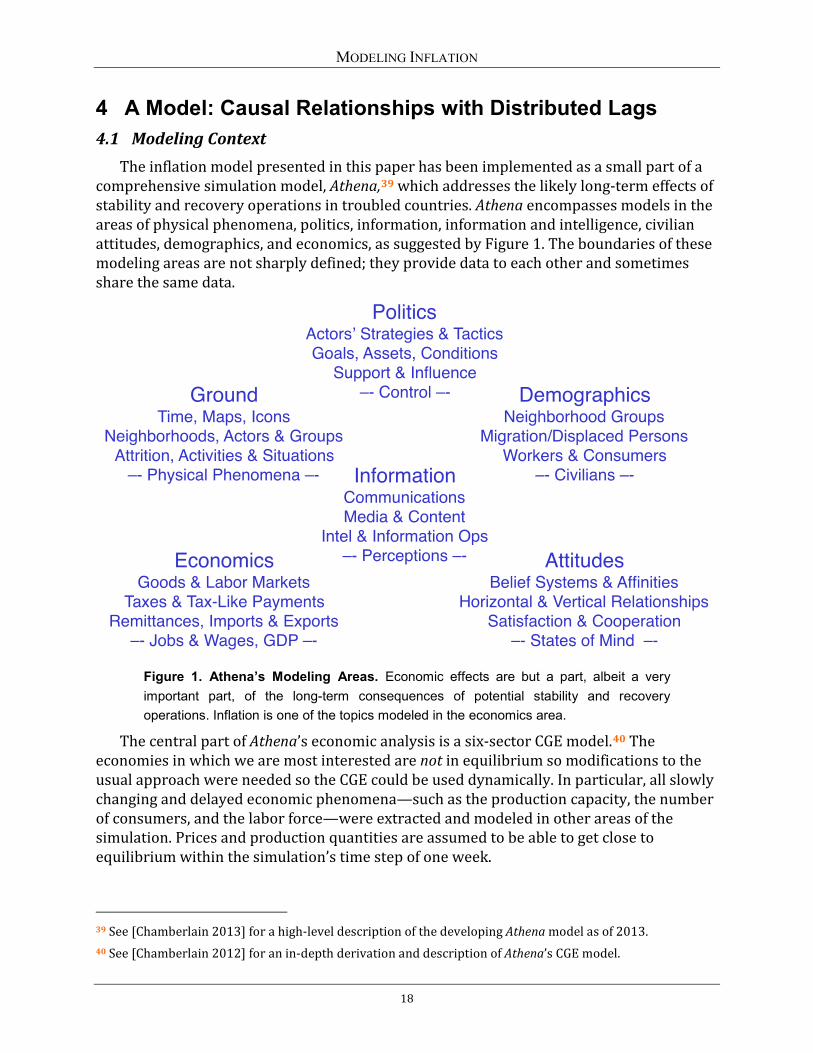
The inflation model presented in this paper has been implemented as a small part of a comprehensive simulation model, Athena,39 which addresses the likely long-term effects of stability and recovery operations in troubled countries. Athena encompasses models in the areas of physical phenomena, politics, information, information and intelligence, civilian attitudes, demographics, and economics, as suggested by Figure 1. The boundaries of these modeling areas are not sharply defined; they provide data to each other and sometimes share the same data.

Figure 1. Athena’s Modeling Areas. Economic effects are but a part, albeit a very important part, of the long-term consequences of potential stability and recovery operations. Inflation is one of the topics modeled in the economics area.

The central part of Athena’s economic analysis is a six-sector CGE model.40 The economies in which we are most interested are not in equilibrium so modifications to the usual approach were needed so the CGE could be used dynamically. In particular, all slowly changing and delayed economic phenomena—such as the production capacity, the number of consumers, and the labor force—were extracted and modeled in other areas of the simulation. Prices and production quantities are assumed to be able to get close to equilibrium within the simulation’s time step of one week.

39 See [Chamberlain 2013] for a high-level description of the developing Athena model as of 2013. 40 See [Chamberlain 2012] for an in-depth derivation and description of Athena’s CGE model.

18

MODELING INFLATION

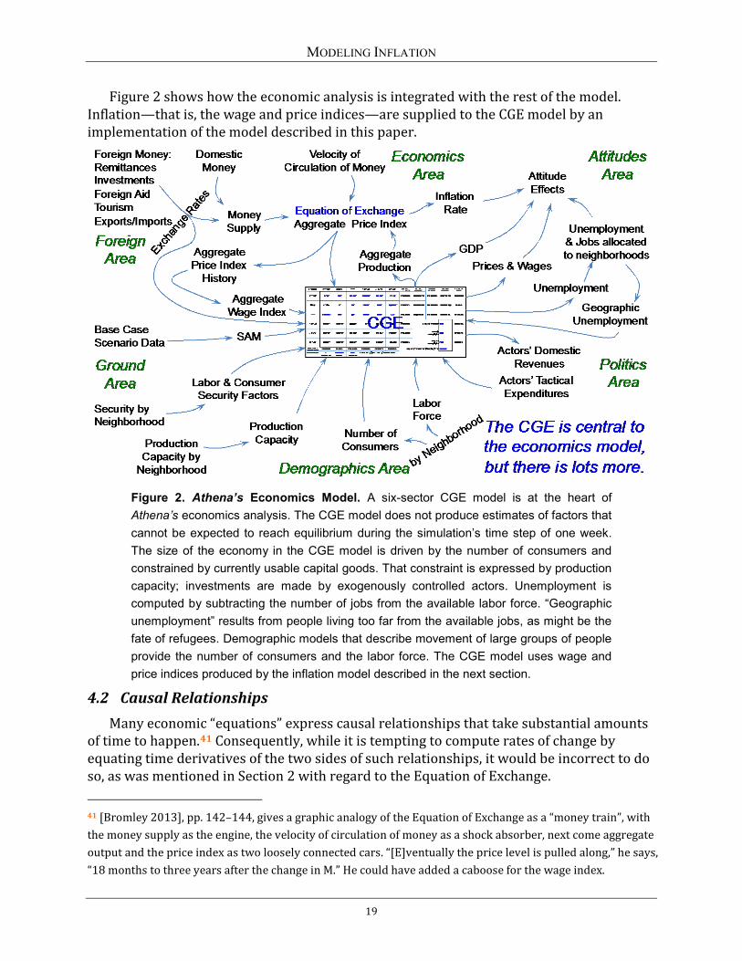
Figure 2 shows how the economic analysis is integrated with the rest of the model. Inflation—that is, the wage and price indices—are supplied to the CGE model by an implementation of the model described in this paper.

Figure 2. Athena’s Economics Model. A six-sector CGE model is at the heart of Athena’s economics analysis. The CGE model does not produce estimates of factors that cannot be expected to reach equilibrium during the simulation’s time step of one week. The size of the economy in the CGE model is driven by the number of consumers and constrained by currently usable capital goods. That constraint is expressed by production capacity; investments are made by exogenously controlled actors. Unemployment is computed by subtracting the number of jobs from the available labor force. “Geographic unemployment” results from people living too far from the available jobs, as might be the fate of refugees. Demographic models that describe movement of large groups of people provide the number of consumers and the labor force. The CGE model uses wage and price indices produced by the inflation model described in the next section.

4.2 Causal Relationships Many economic “equations” express causal relationships that take substantial amounts

of time to happen.41 Consequently, while it is tempting to compute rates of change by equating time derivatives of the two sides of such relationships, it would be incorrect to do so, as was mentioned in Section 2 with regard to the Equation of Exchange.

41 [Bromley 2013], pp. 142–144, gives a graphic analogy of the Equation of Exchange as a “money train”, with the money supply as the engine, the velocity of circulation of money as a shock absorber, next come aggregate output and the price index as two loosely connected cars. “[E]ventually the price level is pulled along,” he says, “18 months to three years after the change in M.” He could have added a caboose for the wage index.

19

MODELING INFLATION

To avoid the temptation and to emphasize this fact, I have eschewed the use of the equals sign, “=”, in favor of a simple arrow, “←”. Thus, the expression 𝐸 ← 𝑓(𝐶, … ,𝐷) means that the effect variable E is related to the causal variables 𝐶, … ,𝐷 by the function 𝑓(𝐶, … ,𝐷).

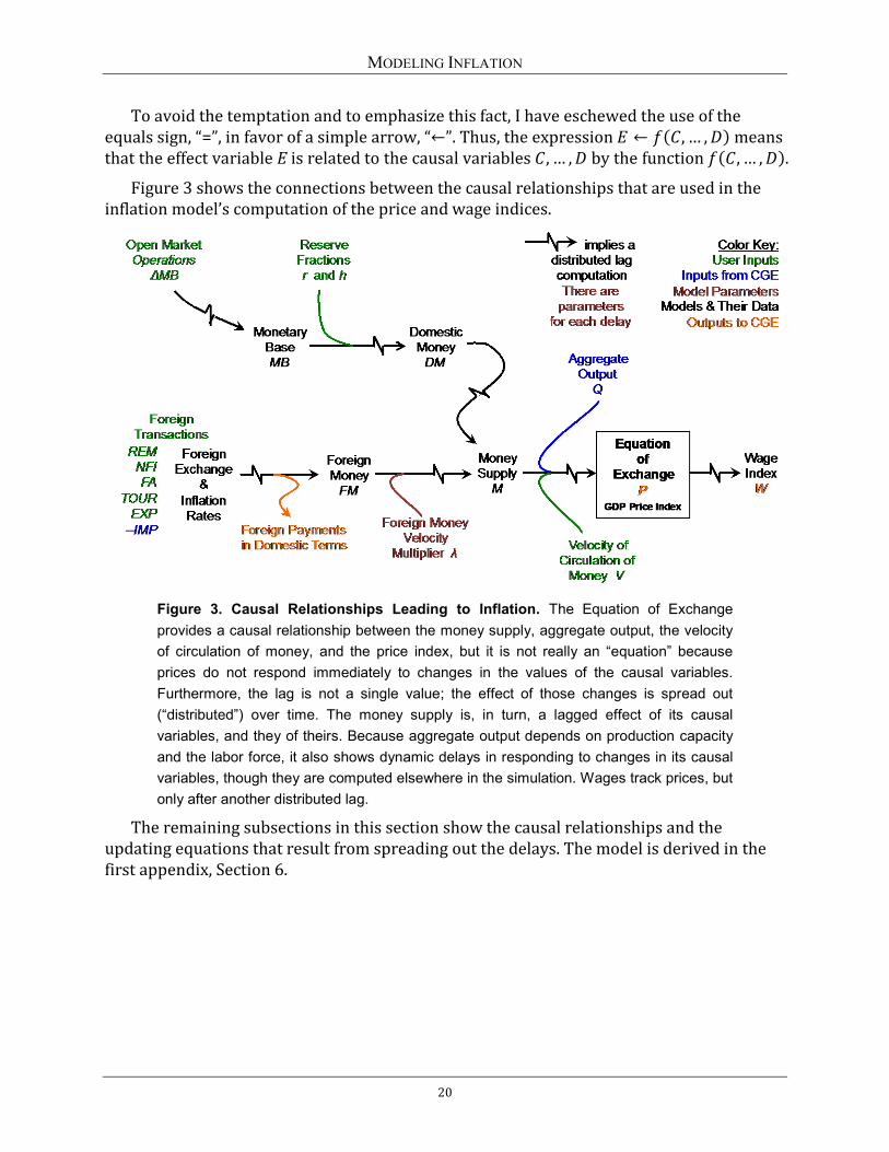
Figure 3 shows the connections between the causal relationships that are used in the inflation model’s computation of the price and wage indices.

Figure 3. Causal Relationships Leading to Inflation. The Equation of Exchange provides a causal relationship between the money supply, aggregate output, the velocity of circulation of money, and the price index, but it is not really an “equation” because prices do not respond immediately to changes in the values of the causal variables. Furthermore, the lag is not a single value; the effect of those changes is spread out (“distributed”) over time. The money supply is, in turn, a lagged effect of its causal variables, and they of theirs. Because aggregate output depends on production capacity and the labor force, it also shows dynamic delays in responding to changes in its causal variables, though they are computed elsewhere in the simulation. Wages track prices, but only after another distributed lag.

The remaining subsections in this section show the causal relationships and the updating equations that result from spreading out the delays. The model is derived in the first appendix, Section 6.

20

MODELING INFLATION

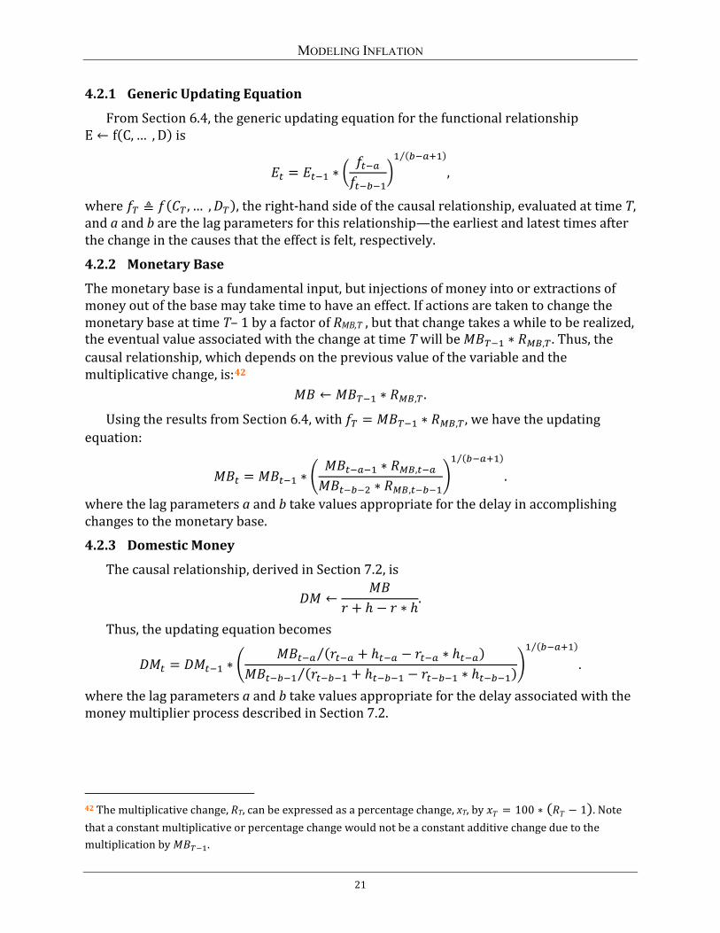
4.2.1 Generic Updating Equation

From Section 6.4, the generic updating equation for the functional relationship E ← f(C, … , D) is

𝐸𝑡 = 𝐸𝑡−1 ∗ �𝑓𝑡−𝑎𝑓𝑡−𝑏−1

�1 (𝑏−𝑎+1)⁄

,

where 𝑓𝑇 ≜ 𝑓(𝐶𝑇 , … ,𝐷𝑇), the right-hand side of the causal relationship, evaluated at time T, and a and b are the lag parameters for this relationship—the earliest and latest times after the change in the causes that the effect is felt, respectively.

4.2.2 Monetary Base

The monetary base is a fundamental input, but injections of money into or extractions of money out of the base may take time to have an effect. If actions are taken to change the monetary base at time T– 1 by a factor of RMB,T , but that change takes a while to be realized, the eventual value associated with the change at time T will be 𝑀𝐵𝑇−1 ∗ 𝑅𝑀𝐵,𝑇. Thus, the causal relationship, which depends on the previous value of the variable and the multiplicative change, is:42

𝑀𝐵 ← 𝑀𝐵𝑇−1 ∗ 𝑅𝑀𝐵,𝑇.

Using the results from Section 6.4, with 𝑓𝑇 = 𝑀𝐵𝑇−1 ∗ 𝑅𝑀𝐵,𝑇, we have the updating equation:

𝑀𝐵𝑡 = 𝑀𝐵𝑡−1 ∗ �𝑀𝐵𝑡−𝑎−1 ∗ 𝑅𝑀𝐵,𝑡−𝑎

𝑀𝐵𝑡−𝑏−2 ∗ 𝑅𝑀𝐵,𝑡−𝑏−1�1 (𝑏−𝑎+1)⁄

.

where the lag parameters a and b take values appropriate for the delay in accomplishing changes to the monetary base.

4.2.3 Domestic Money

The causal relationship, derived in Section 7.2, is

𝐷𝑀 ←𝑀𝐵

𝑟 + ℎ − 𝑟 ∗ ℎ.

Thus, the updating equation becomes

𝐷𝑀𝑡 = 𝐷𝑀𝑡−1 ∗ �𝑀𝐵𝑡−𝑎 (𝑟𝑡−𝑎 + ℎ𝑡−𝑎 − 𝑟𝑡−𝑎 ∗ ℎ𝑡−𝑎)⁄

𝑀𝐵𝑡−𝑏−1 (𝑟𝑡−𝑏−1 + ℎ𝑡−𝑏−1 − 𝑟𝑡−𝑏−1 ∗ ℎ𝑡−𝑏−1)⁄ �1 (𝑏−𝑎+1)⁄

.

where the lag parameters a and b take values appropriate for the delay associated with the money multiplier process described in Section 7.2.

42 The multiplicative change, RT, can be expressed as a percentage change, xT, by 𝑥𝑇 = 100 ∗ (𝑅𝑇 − 1). Note that a constant multiplicative or percentage change would not be a constant additive change due to the multiplication by 𝑀𝐵𝑇−1.

21

MODELING INFLATION

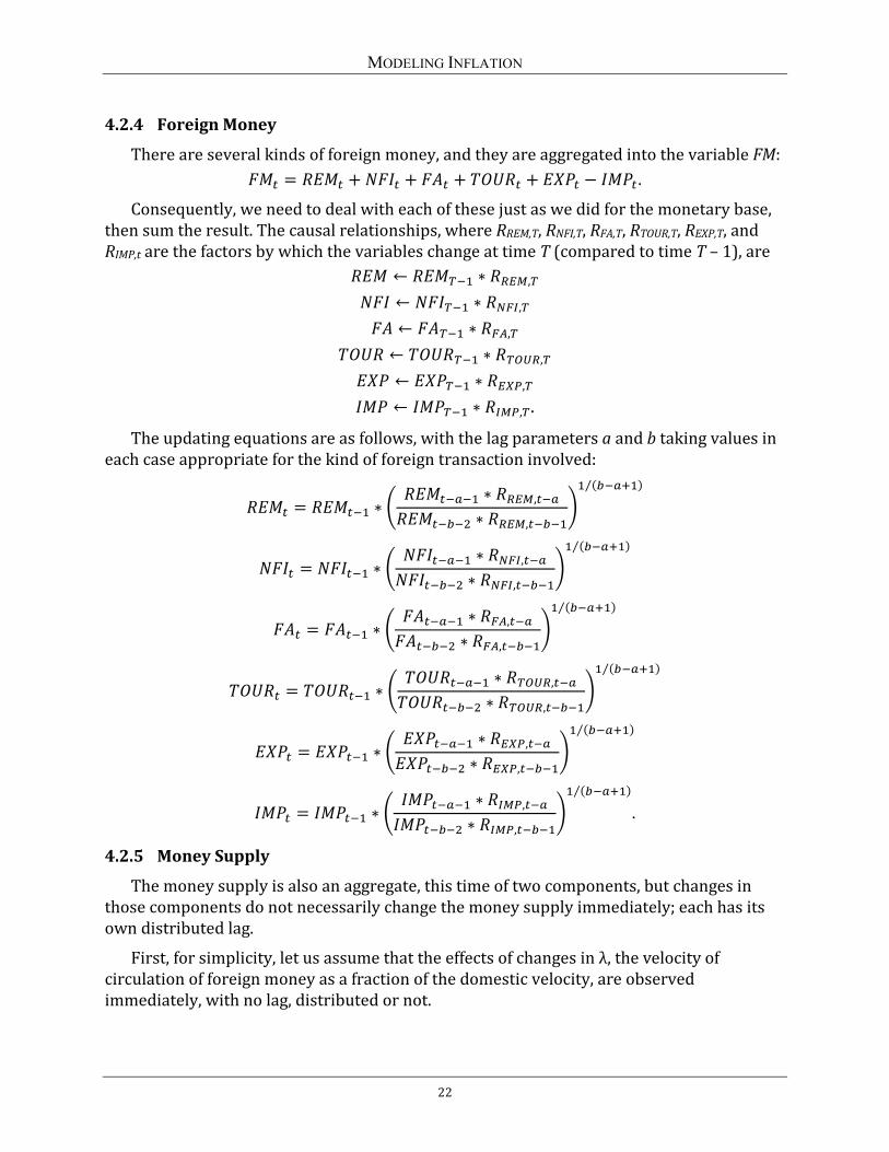
4.2.4 Foreign Money

There are several kinds of foreign money, and they are aggregated into the variable FM: 𝐹𝑀𝑡 = 𝑅𝐸𝑀𝑡 + 𝑁𝐹𝐼𝑡 + 𝐹𝐴𝑡 + 𝑇𝑂𝑈𝑅𝑡 + 𝐸𝑋𝑃𝑡 − 𝐼𝑀𝑃𝑡 .

Consequently, we need to deal with each of these just as we did for the monetary base, then sum the result. The causal relationships, where RREM,T, RNFI,T, RFA,T, RTOUR,T, REXP,T, and RIMP,t are the factors by which the variables change at time T (compared to time T – 1), are

𝑅𝐸𝑀 ← 𝑅𝐸𝑀𝑇−1 ∗ 𝑅𝑅𝐸𝑀,𝑇 𝑁𝐹𝐼 ← 𝑁𝐹𝐼𝑇−1 ∗ 𝑅𝑁𝐹𝐼,𝑇 𝐹𝐴 ← 𝐹𝐴𝑇−1 ∗ 𝑅𝐹𝐴,𝑇

𝑇𝑂𝑈𝑅 ← 𝑇𝑂𝑈𝑅𝑇−1 ∗ 𝑅𝑇𝑂𝑈𝑅,𝑇 𝐸𝑋𝑃 ← 𝐸𝑋𝑃𝑇−1 ∗ 𝑅𝐸𝑋𝑃,𝑇 𝐼𝑀𝑃 ← 𝐼𝑀𝑃𝑇−1 ∗ 𝑅𝐼𝑀𝑃,𝑇.

The updating equations are as follows, with the lag parameters a and b taking values in each case appropriate for the kind of foreign transaction involved:

𝑅𝐸𝑀𝑡 = 𝑅𝐸𝑀𝑡−1 ∗ �𝑅𝐸𝑀𝑡−𝑎−1 ∗ 𝑅𝑅𝐸𝑀,𝑡−𝑎

𝑅𝐸𝑀𝑡−𝑏−2 ∗ 𝑅𝑅𝐸𝑀,𝑡−𝑏−1�1 (𝑏−𝑎+1)⁄

𝑁𝐹𝐼𝑡 = 𝑁𝐹𝐼𝑡−1 ∗ �𝑁𝐹𝐼𝑡−𝑎−1 ∗ 𝑅𝑁𝐹𝐼,𝑡−𝑎𝑁𝐹𝐼𝑡−𝑏−2 ∗ 𝑅𝑁𝐹𝐼,𝑡−𝑏−1

�1 (𝑏−𝑎+1)⁄

𝐹𝐴𝑡 = 𝐹𝐴𝑡−1 ∗ �𝐹𝐴𝑡−𝑎−1 ∗ 𝑅𝐹𝐴,𝑡−𝑎

𝐹𝐴𝑡−𝑏−2 ∗ 𝑅𝐹𝐴,𝑡−𝑏−1�1 (𝑏−𝑎+1)⁄

𝑇𝑂𝑈𝑅𝑡 = 𝑇𝑂𝑈𝑅𝑡−1 ∗ �𝑇𝑂𝑈𝑅𝑡−𝑎−1 ∗ 𝑅𝑇𝑂𝑈𝑅,𝑡−𝑎

𝑇𝑂𝑈𝑅𝑡−𝑏−2 ∗ 𝑅𝑇𝑂𝑈𝑅,𝑡−𝑏−1�1 (𝑏−𝑎+1)⁄

𝐸𝑋𝑃𝑡 = 𝐸𝑋𝑃𝑡−1 ∗ �𝐸𝑋𝑃𝑡−𝑎−1 ∗ 𝑅𝐸𝑋𝑃,𝑡−𝑎

𝐸𝑋𝑃𝑡−𝑏−2 ∗ 𝑅𝐸𝑋𝑃,𝑡−𝑏−1�1 (𝑏−𝑎+1)⁄

𝐼𝑀𝑃𝑡 = 𝐼𝑀𝑃𝑡−1 ∗ �𝐼𝑀𝑃𝑡−𝑎−1 ∗ 𝑅𝐼𝑀𝑃,𝑡−𝑎

𝐼𝑀𝑃𝑡−𝑏−2 ∗ 𝑅𝐼𝑀𝑃,𝑡−𝑏−1�1 (𝑏−𝑎+1)⁄

.

4.2.5 Money Supply

The money supply is also an aggregate, this time of two components, but changes in those components do not necessarily change the money supply immediately; each has its own distributed lag.

First, for simplicity, let us assume that the effects of changes in λ, the velocity of circulation of foreign money as a fraction of the domestic velocity, are observed immediately, with no lag, distributed or not.

22

MODELING INFLATION

Now we have a complication. We need to distinguish between the amounts of domestic and foreign money that there is at some time t and the amount that has gone through its delay period and is contributing to the money supply. We are already denoting the first of these amounts by DMt and FMt. To avoid introducing new letters, let’s use a prime for the amounts that have worked their way into the money supply: DM’t and FM’t.

Then, the equation to compute the money supply is 𝑀𝑡 = 𝐷𝑀′𝑡 + 𝜆𝑡 ∗ 𝐹𝑀′𝑡.

The causal relationships for the two kinds of money are: 𝐷𝑀′ ← 𝐷𝑀𝑇−1 ∗ 𝑅𝐷𝑀,𝑇 , where we have to compute 𝑅𝐷𝑀,𝑇 = 𝐷𝑀𝑇 𝐷𝑀𝑇−1⁄ 𝐹𝑀′ ← 𝐹𝑀𝑇−1 ∗ 𝑅𝐹𝑀,𝑇 , where we have to compute 𝑅𝐹𝑀,𝑇 = 𝐹𝑀𝑇 𝐹𝑀𝑇−1⁄ .

But these expressions can be simplified to 𝐷𝑀′ ← 𝐷𝑀𝑇 𝐹𝑀′ ← 𝐹𝑀𝑇 .

Finally, by using the results from Section 6.4, we have the updating equations:

𝐷𝑀′𝑡 = 𝐷𝑀′𝑡−1 ∗ �𝐷𝑀𝑡−𝑎

𝐷𝑀𝑡−𝑏−1�1 (𝑏−𝑎+1)⁄

𝐹𝑀′𝑡 = 𝐹𝑀′𝑡−1 ∗ �𝐹𝑀𝑡−𝑎

𝐹𝑀𝑡−𝑏−1�1 (𝑏−𝑎+1)⁄

.

and the lag parameters a and b take values appropriate for the delays associated with changes in the amounts of domestic or foreign monies becoming part of the money supply.

To repeat, the equation to compute the money supply is43 𝑀𝑡 = 𝐷𝑀′𝑡 + 𝜆𝑡 ∗ 𝐹𝑀′𝑡.

4.2.6 Equation of Exchange

The casual relationship usually known as the Equation of Exchange fits the generic model derived in Section 6 very nicely:

𝑃 ←𝑀 ∗ 𝑉𝑄

.

Thus, 𝑓𝑇 becomes 𝑀𝑇 ∗ 𝑉𝑇 𝑄𝑇⁄ and the updating equation becomes

𝑃𝑡 = 𝑃𝑡−1 ∗ �𝑀𝑡−𝑎 ∗ 𝑉𝑡−𝑎 𝑄𝑡−𝑎⁄

𝑀𝑡−𝑏−1 ∗ 𝑉𝑡−𝑏−1 𝑄𝑡−𝑏−1⁄ �1 (𝑏−𝑎+1)⁄

.

43 It may not be unreasonable to assume that both delays are negligible. In that case, the updating equation for the money supply would be much simpler, as it can skip the complication involving DM’t and FM’t . Specifically, that simpler equation would be: 𝑀𝑡 = 𝐷𝑀𝑡 + 𝜆 ∗ 𝐹𝑀𝑡 .

23

MODELING INFLATION

4.2.7 Wage Index

Saying that wages track prices well, but with a distributed lag, means that a given multiplicative change in the price index P will eventually lead to the same multiplicative change in the wage index W. That is,

𝑊 ← 𝑃𝑇 ∗ 𝑅𝑃,𝑇 .

But we know that 𝑅𝑃,𝑇 = 𝑃𝑇 𝑃𝑇−1⁄ , by definition. Consequently, using the results of Section 6.4, the updating equation is

𝑊𝑡 = 𝑊𝑡−1 ∗ �𝑃𝑡−𝑎𝑃𝑡−𝑏−1

�1 (𝑏−𝑎+1)⁄

.

24

MODELING INFLATION

5 Research Opportunities Our implementation of this inflation model interfaces with a very simple CGE model,

with a single sector for aggregate production, a single sector that provides aggregate labor, and exogenous investors in capital. Most elaborations of the inflation model would need to be supported by a more sophisticated CGE.

5.1 Technological Change and Escalation in Prices & Wages Our CGE model has a sector for aggregated output, but is not resolved in finer detail. By

interfacing with a CGE model with higher resolution in the production sectors, it would be possible to estimate not just overall inflation, but escalation of the prices of the products of all of the production sectors modeled.

One of the major benefits of a CGE model with more production sectors would be that models of technological change would be easier to construct and validate and could be more accurate.

Our simple CGE model also has only a single sector that provides labor. Increasing the number of sectors to represent this area would not only provide a distinction between the wage/salary levels of different kinds of workers, but also permit study of how those levels change separately as technology and demographics evolve over time.

5.2 Endogenous Investments and Interest Rates In contrast to most CGE model implementations, it was appropriate in our context to

make the actors who make investment decisions exogenous. One consequence was that the usual trades between hiring labor and investing in capital, a study of which led to the original work by Cobb and Douglas [Cobb-Douglas 1928], are outside the scope of this paper.44

That said, investors should be an integral endogenous part in many, perhaps most, applications of the work described here. Introducing an investment bank sector into the CGE model would result in the creation of a loanable funds market; the “price” in this market is the interest rate.

The investment bank’s investments would be represented by expenditures in the CGE model and by routine inputs to models of production infrastructure. It would accept savings from other sectors and make investments in the infrastructure associated with those other sectors. Routine investments could be calibrated by assuming decisions are made to optimize a Cobb-Douglas utility function, the end result of which is the same as assuming a constant vector of budget fractions.

If the model deals with savings and investments, it must track not just the flows of value that constitute the CGE model, but savings balances, interest payments, and use of those amounts when making financial decisions. Savings and debt must be accounted for in every sector.

44 The Cobb-Douglas function has applications beyond its use as the production function in the labor-capital trade. Our CGE model, for example, uses a Cobb-Douglas utility function for consumers’ choices.

25

MODELING INFLATION

The financial entities that make up the sectors in the CGE model will mitigate the consequences of changes in prices by shifting their demand from product to product as described by their production and utility functions and by drawing upon their savings. But those stores of money are limited, and the limits will be encountered sooner by the less wealthy among them. This distribution of wealth should not be ignored; using average values would give misleading results. It may be possible to use a Gini curve to address this issue.45

5.3 Long-Run Inflation As discussed in Section 1.9, it seems that there tends to be a small, long-run normal rate

of inflation. There is no agreement whether this phenomenon even exists, much less how it operates or how it can be estimated.

45 See [Lawler 2010].

26

MODELING INFLATION

6 Appendix: Distributing Delayed Effects 6.1 The Causal Relationship

Let us start with a causal relationship,46 𝐸 ← 𝑓(𝐶, … ,𝐷),

which says that given the values of a set of causal variables (C, …, D) at some particular time, such as T, the value of the effect variable E will eventually take on the value of the function evaluated at time T.

This relationship would be an equation if changes in the causal variables had immediate consequences on the value of the effect. Instead, we assume that those consequences play out, after a delay, over an interval.

Intuition and experience say that effects should be realized according to a function that has a most likely value and a more-or-less bell-shaped curve, which might be described by a gamma distribution or some similar function. Plots of the resultant cumulative values of the effect variable versus time would exhibit S-curves. However, not only do we not understand the details of the phenomena well enough to reliably estimate the parameters of such a function, but the phenomena are chaotic enough that it is unlikely that an S-curve would be any more realistic on the average than a Z-curve, which connects a starting time and an ending time with a straight line. When a Z-curve is applied in successive time steps, it becomes a staircase, as may be seen in Figure 4. We assume that the rate of change is the same at each step, so the risers on this staircase actually follow an exponential curve instead of a straight line.47,48

46 These relationships are usually called "equations" and written with an equals sign instead of an arrow. An arrow is used here instead to make it clear that the value of the variable on the left of the arrow would eventually become equal to the value of the expression on the right. Just how this is modeled is the essence of this appendix. 47 If the graph were drawn on semi-log graph paper, with a logarithmic scale on the y-axis, the line would be straight. 48 Whether the steps are the same height as of their predecessors or the same multiple of them is surely within our zone of ignorance as to their true locations—either way of interpolating keeps the main features: there is a delay and it is spread out in time. However, an algorithm to generate artificial historical data to reduce the user’s data collection burden uses this model to extrapolate into the past. Constant size steps can extrapolate to negative values, giving values that do not pass the “laugh test”. Extrapolating with constant multipliers between steps follow a negative exponential curve, which stays positive.

27

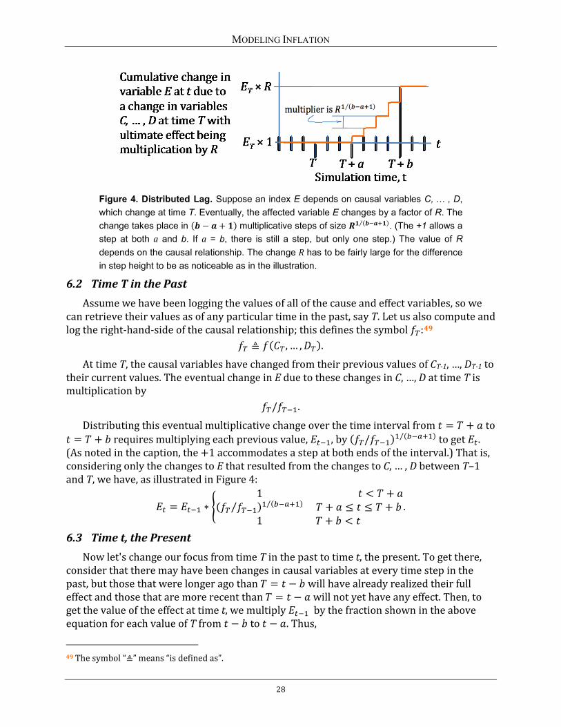
MODELING INFLATION

Figure 4. Distributed Lag. Suppose an index E depends on causal variables C, … , D, which change at time T. Eventually, the affected variable E changes by a factor of R. The change takes place in (𝒃 − 𝒂 + 𝟏) multiplicative steps of size 𝑹𝟏 (𝒃−𝒂+𝟏)⁄ . (The +1 allows a step at both a and b. If a = b, there is still a step, but only one step.) The value of R depends on the causal relationship. The change R has to be fairly large for the difference in step height to be as noticeable as in the illustration.

6.2 Time T in the Past Assume we have been logging the values of all of the cause and effect variables, so we

can retrieve their values as of any particular time in the past, say T. Let us also compute and log the right-hand-side of the causal relationship; this defines the symbol 𝑓𝑇:49

𝑓𝑇 ≜ 𝑓(𝐶𝑇 , … ,𝐷𝑇).

At time T, the causal variables have changed from their previous values of CT-1, …, DT-1 to their current values. The eventual change in E due to these changes in C, …, D at time T is multiplication by

𝑓𝑇/𝑓𝑇−1.

Distributing this eventual multiplicative change over the time interval from 𝑡 = 𝑇 + 𝑎 to 𝑡 = 𝑇 + 𝑏 requires multiplying each previous value, 𝐸𝑡−1, by (𝑓𝑇/𝑓𝑇−1)1 (𝑏−𝑎+1)⁄ to get 𝐸𝑡. (As noted in the caption, the +1 accommodates a step at both ends of the interval.) That is, considering only the changes to E that resulted from the changes to C, … , D between T–1 and T, we have, as illustrated in Figure 4:

𝐸𝑡 = 𝐸𝑡−1 ∗ �1 𝑡 < 𝑇 + 𝑎

(𝑓𝑇 𝑓𝑇−1⁄ )1 (𝑏−𝑎+1)⁄ 𝑇 + 𝑎 ≤ 𝑡 ≤ 𝑇 + 𝑏1 𝑇 + 𝑏 < 𝑡

.

6.3 Time t, the Present Now let's change our focus from time T in the past to time t, the present. To get there,

consider that there may have been changes in causal variables at every time step in the past, but those that were longer ago than 𝑇 = 𝑡 − 𝑏 will have already realized their full effect and those that are more recent than 𝑇 = 𝑡 − 𝑎 will not yet have any effect. Then, to get the value of the effect at time t, we multiply 𝐸𝑡−1 by the fraction shown in the above equation for each value of T from 𝑡 − 𝑏 to 𝑡 − 𝑎. Thus,

49 The symbol “≜” means “is defined as”.

28

MODELING INFLATION

𝐸𝑡 = 𝐸𝑡−1 ∗� (𝑓𝑇 𝑓𝑇−1⁄ )1 (𝑏−𝑎+1)⁄𝑡−𝑎

𝑇=𝑡−𝑏.

If there are time steps during which the causal variables did not change, the ratio 𝑓𝑇 𝑓𝑇−1⁄ for those time steps is 1.0, so there is no need to omit them from the product over T.

Noting that the exponent can be taken outside the summation, this can be written out more explicitly as

𝐸𝑡 = 𝐸𝑡−1 ∗ �𝑓𝑡−𝑏𝑓𝑡−𝑏−1

∗𝑓𝑡−𝑏+1𝑓𝑡−𝑏

∗𝑓𝑡−𝑏+2𝑓𝑡−𝑏+1

∗ … ∗𝑓𝑡−𝑎−1𝑓𝑡−𝑎−2

∗𝑓𝑡−𝑎𝑓𝑡−𝑎−1

�1 (𝑏−𝑎+1)⁄

.

6.4 Bottom Line But now we notice that there is a huge amount of cancelation,50 so the equation

telescopes down to

𝐸𝑡 = 𝐸𝑡−1 ∗ �𝑓𝑡−𝑎𝑓𝑡−𝑏−1

�1 (𝑏−𝑎+1)⁄

,

where 𝑓𝑇 ≜ 𝑓(𝐶𝑇 , … ,𝐷𝑇), the right-hand side of the causal relationship, evaluated at time T, and a and b are the lag parameters for this relationship.

50 If we had used an S-curve for the delay distribution function, the cancelation would not have occurred because the exponent would not have factored out of the product. Instead of each term in the brackets making an equal contribution to the product, each would have been weighted by the S-curve.

29

MODELING INFLATION

7 Appendix: Central Bank Operations

7.1 Monetary Policy To maintain their reserves at required levels, banks borrow money from the central

bank and from each other. The central bank, however, is in a special position—using open market operations, it can buy or sell government bonds to banks, using portions of the banks’ reserves that exist only as entries on the books of the central bank; these operations increase or decrease the monetary base. Selling bonds increases the national debt; buying them decreases it. If the central bank is constrained by a debt limit, its ability to increase the monetary base may be constrained.

To stimulate the export of domestic goods, the central bank may be able to change the foreign exchange rates of its currency by using a tactic that only it has available:51 devaluation of the currency. Devaluation of the currency is a tactic designed to attract foreign money. It can only be used when exchange rates are fixed by government policy, rather than allowed to float in response to market conditions. (Pegging exchange rates is unlikely to be successful in the real world. See the discussion of currency black markets in Section 1.8.)

Runaway inflation caused by excessive amounts of currency in circulation is sometimes addressed by reissuance of currency, which is intended to reestablish control of the money supply; the smaller amount of newly issued domestic currency presumably has a higher, more stable value than the old, which is especially likely if a large amount of counterfeit currency is in circulation.

Both devaluation and reissuance are outside the scope of this paper.

7.2 Derivation of the Money Multiplier The only three variables that might be affected by central bank decisions are:

C = the amount of domestic currency in circulation outside of bank vaults.52

r = the actual investment bank reserve ratio, which is the fraction of deposits that is held in reserve—that is, not loaned back out. This fraction is presumably at least as large as the reserve requirement set by the central bank.

51 Source: http://www.newyorkfed.org/aboutthefed/fedpoint/fed38.html accessed 3/20/13 5:27 p.m. PDT. 52 The published values (in the United States) include what is circulating (and in vaults) in foreign countries, which theoretically should be omitted in our context. But when we are considering troubled countries, the amount of their domestic currency circulating in foreign countries must surely be negligible. Of more concern is how much counterfeit currency is in circulation, an amount that may be difficult to estimate. If it is not ignored, the counterfeit currency in circulation must be included in the money supply, but if it can be assumed that banks will not accept counterfeit currency, it should not be subjected to the money multiplier. These nuances are not included in the model described here.

30

http://www.newyorkfed.org/aboutthefed/fedpoint/fed38.html

MODELING INFLATION

h = the fraction of the currency people don’t spend that they keep on hand (that is, in repositories that are not used as a source for loans). They deposit the rest into demand accounts at a bank (that is, into D, which is defined below).

The central bank does not have control of either r or h, but since both are heavily dependent upon expectations, the bank can affect them by the content and manner of public statements.

There are a few other relevant variables:

DM = the domestic money supply, the value of everything (except foreign currency) that can be spent as if it were money.

MB = the monetary base, which consists of the currency in circulation plus the currency held in reserve in investment banks.

m = the money multiplier, which describes how much larger the domestic money supply is than the monetary base.

D = the amount of demand deposits in investment banks.

R = the amount of currency held in reserve by investment banks.

H = the amount of currency people keep on hand (that is, in repositories that are not used as a source for loans). This includes the amount of currency that people keep in their wallets and under the mattress. Note that H can be thought of as the part of C that is held out; that is, 𝐻 = ℎ ∗ 𝐶.

The process that I have referred to elsewhere as the “money multiplier process” is as follows. People put a fraction h of the currency they don’t spend into savings and cash on hand (that is, into H) and deposit the rest into demand accounts at a bank (that is, into D). The bank puts a fraction r of what it gets into its reserves (that is, into R) and loans the rest to other people. The people who receive the loans spend it all, but the people they pay put a fraction h into H and the rest into D, and the cycle repeats ad infinitum.

Thus, suppose people start with an amount of currency equal to C. At the first step of the process, 𝐻 = ℎ ∗ 𝐶 and 𝐷 = (1 − ℎ) ∗ 𝐶, then 𝑅 = 𝑟 ∗ 𝐷 = 𝑟 ∗ (1 − ℎ) ∗ 𝐶. The bank then lends (1 − 𝑟) ∗ (1 − ℎ) ∗ 𝐶.

At the next step, without loss of generality,53 people spend all of the money from the loans and the people they pay put a fraction h of that into H, etc., so that H increases by ℎ ∗ (1 − 𝑟) ∗ (1 − ℎ) ∗ 𝐶; D increases by (1 − 𝑟) ∗ (1 − ℎ)2 ∗ 𝐶; and R increases by 𝑟 ∗ (1 − 𝑟) ∗ (1 − ℎ)2 ∗ 𝐶, and the bank lends another (1 − 𝑟)2 ∗ (1 − ℎ)2 ∗ 𝐶.

After this process has gone on forever, we have

𝐻 = [ℎ + ℎ(1 − 𝑟)(1 − ℎ) + ℎ(1 − 𝑟)2(1− ℎ)2 + ℎ(1 − 𝑟)3(1 − ℎ)3 + ⋯ ] ∗ 𝐶

53 To the extent that the loan recipients don’t spend all of the proceeds of the loan, but save some, that amount is included with the fraction h, which is saved by the people they pay.

31

MODELING INFLATION

𝐷 = [(1 − ℎ) + (1 − 𝑟)(1 − ℎ)2 + (1 − 𝑟)2(1− ℎ)3 + (1 − 𝑟)3(1 − ℎ)4 + ⋯ ] ∗ 𝐶

𝑅 = [(1 − 𝑟)(1− ℎ) + (1 − 𝑟)2(1 − ℎ)2 + (1 − 𝑟)3(1 − ℎ)3 + (1 − 𝑟)4(1− ℎ)4 + ⋯ ] ∗ 𝐶 amount of currency

avail. for the next loan= (1 − 𝑟)(1− ℎ) ∗ 𝐶, (1 − 𝑟)2(1− ℎ)2 ∗ 𝐶, (1− 𝑟)3(1 − ℎ)3 ∗ 𝐶, …

The total amount of currency that has been subjected to this process is MB, the monetary base. If we assume the process has been running long enough, the end state can be obtained by summing each of these infinite series.54

Thus, identifying x in footnote 54 with (1 − 𝑟)(1 − ℎ) and Y with the infinite series 𝑥 + 𝑥2 + 𝑥3 + ⋯, we have 𝐻 = ℎ ∗ [1 + 𝑌] ∗ 𝑀𝐵. Then, using 𝑌 = 𝑥 (1 − 𝑥)⁄ and substituting back in 𝑥 = (1 − 𝑟) ∗ (1 − ℎ), we get

𝐻 = ℎ ∗ �1 +𝑥

1 − 𝑥� ∗ 𝑀𝐵 = ℎ ∗

1 − 𝑥 + 𝑥1 − 𝑥

∗ 𝑀𝐵 =ℎ ∗ 𝑀𝐵1 − 𝑥

=ℎ ∗ 𝑀𝐵

1 − (1 − 𝑟) ∗ (1 − ℎ) ,

and finally,

𝐻 =ℎ ∗ 𝑀𝐵

𝑟 + ℎ − 𝑟 ∗ ℎ .

Similarly, but skipping most of the algebra, from 𝐷 = (1 − ℎ) ∗ (1 + 𝑌) ∗ 𝑀𝐵, we get

𝐷 =(1 − ℎ) ∗ 𝑀𝐵𝑟 + ℎ − 𝑟 ∗ ℎ

.

Similarly, from 𝑅 = 𝑟 ∗ (1 − ℎ) ∗ (1 + 𝑌) ∗ 𝑀𝐵, we get

𝑅 =𝑟 ∗ (1 − ℎ) ∗ 𝑀𝐵𝑟 + ℎ − 𝑟 ∗ ℎ

.

Then, the money multiplier, m, is

𝑚 =𝐷𝑀𝑀𝐵

=𝐻 + 𝐷𝑀𝐵

=1

1 − (1 − 𝑟) ∗ (1 − ℎ) =1

𝑟 + ℎ − 𝑟 ∗ ℎ ,

and the domestic portion of the money supply, DM, is given by

𝐷𝑀 =𝑀𝐵

𝑟 + ℎ − 𝑟 ∗ ℎ .

54 Using 𝑥 = (1 − 𝑟)(1 − ℎ), all of the series can be written so they contain the form 𝑥 + 𝑥2 + 𝑥3 + ⋯, which we can call Y. Note that 𝑌 = 𝑥 + 𝑥2 + 𝑥3 + ⋯ may be written 𝑌 = 𝑥 ∗ (1 + 𝑌) , which is easily solved to give 𝑌 = 𝑥 (1 − 𝑥)⁄ , which is the sum of the infinite series. Since the series converges, “long enough” means “when it has gone on until the residual is negligible”. When the closed form formula for Y is inserted into the equations, solution is then straightforward, as is shown in the next paragraph.

32

MODELING INFLATION

References [Bromley 2013] Ray Bromley. Options and Outcomes: The Basic Ideas of Macroeconomics,

Fall 2006 Edition. Available online, copy downloaded on 2/19/13 from http://www.myecnclass.com.

[Chamberlain 2012] Robert G. Chamberlain, William H. Duquette, Brian J. Kahovec. Athena’s Computable General Equilibrium Model, JPL Publication 12-18, Jet Propulsion Laboratory, 4800 Oak Grove Drive, Pasadena, CA 91109-8099. December 2012.

[Chamberlain 2013] Robert G. Chamberlain and William H. Duquette, Athena in 2013 and Beyond, JPL Publication 13-9, Jet Propulsion Laboratory, 4800 Oak Grove Drive, Pasadena, CA 91109-8099. May 2013.

[Cobb-Douglas 1928] Charles W. Cobb and Paul H. Douglas, “A Theory of Production” in The American Economic Review, Vol. 18, No. 1, pp. 139–165. 1928.

[Fisher 1911] Irving Fisher, assisted by Harry G. Brown. The Purchasing Power of Money, its Determination and Relation to Credit, Interest and Crises (New York: Macmillan, copyright 1911). New and Revised Edition published 1922. 541 pp. Copy downloaded on 2/14/13 from http://oll.libertyfund.org/?option=com_staticxt&staticfile=show.php%3Ftitle=1165&Itemid=27.

[Lawler 2010] Rebecca Lawler, “Wage Distributions and Survival: Modeling Techniques for use in Stability Operations”, SURF 2010 Final Report, Jet Propulsion Laboratory, 4800 Oak Grove Drive, Pasadena, CA 91109-8099, 24 August 2010.

[Stone 1962] Richard Stone and Alan Brown, A Computable Model of Economic Growth, The M.I.T. Press, Massachusetts Institute of Technology, Cambridge, Massachusetts. 1962.

33

http://www.myecnclass.com/

http://oll.libertyfund.org/?option=com_staticxt&staticfile=show.php%3Ftitle=1165&Itemid=27

http://oll.libertyfund.org/?option=com_staticxt&staticfile=show.php%3Ftitle=1165&Itemid=27

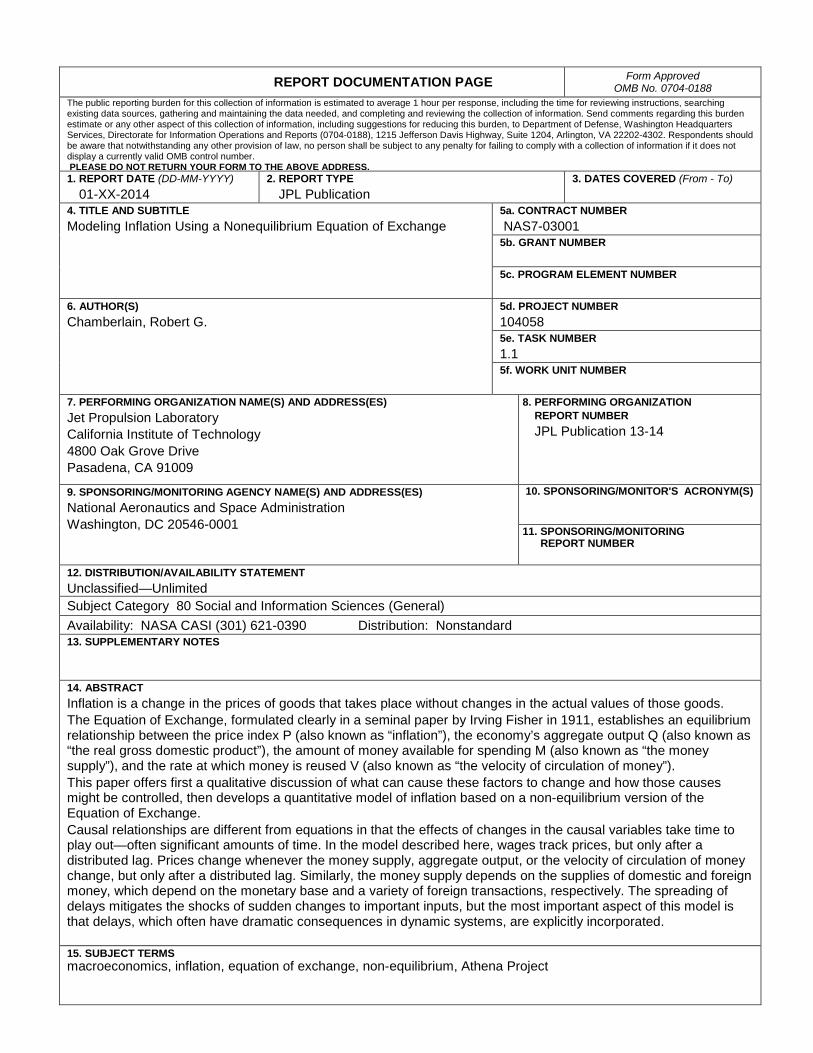
REPORT DOCUMENTATION PAGE Form Approved OMB No. 0704-0188

The public reporting burden for this collection of information is estimated to average 1 hour per response, including the time for reviewing instructions, searching existing data sources, gathering and maintaining the data needed, and completing and reviewing the collection of information. Send comments regarding this burden estimate or any other aspect of this collection of information, including suggestions for reducing this burden, to Department of Defense, Washington Headquarters Services, Directorate for Information Operations and Reports (0704-0188), 1215 Jefferson Davis Highway, Suite 1204, Arlington, VA 22202-4302. Respondents should be aware that notwithstanding any other provision of law, no person shall be subject to any penalty for failing to comply with a collection of information if it does not display a currently valid OMB control number. PLEASE DO NOT RETURN YOUR FORM TO THE ABOVE ADDRESS. 1. REPORT DATE (DD-MM-YYYY) 01-XX-2014

2. REPORT TYPE JPL Publication

3. DATES COVERED (From - To)

4. TITLE AND SUBTITLE Modeling Inflation Using a Nonequilibrium Equation of Exchange

5a. CONTRACT NUMBER NAS7-03001 5b. GRANT NUMBER 5c. PROGRAM ELEMENT NUMBER

6. AUTHOR(S) Chamberlain, Robert G.

5d. PROJECT NUMBER 104058 5e. TASK NUMBER 1.1 5f. WORK UNIT NUMBER

7. PERFORMING ORGANIZATION NAME(S) AND ADDRESS(ES) Jet Propulsion Laboratory California Institute of Technology 4800 Oak Grove Drive Pasadena, CA 91009

8. PERFORMING ORGANIZATION REPORT NUMBER JPL Publication 13-14

9. SPONSORING/MONITORING AGENCY NAME(S) AND ADDRESS(ES) National Aeronautics and Space Administration Washington, DC 20546-0001

10. SPONSORING/MONITOR'S ACRONYM(S)

11. SPONSORING/MONITORING REPORT NUMBER

12. DISTRIBUTION/AVAILABILITY STATEMENT Unclassified—Unlimited Subject Category 80 Social and Information Sciences (General)

Availability: NASA CASI (301) 621-0390 Distribution: Nonstandard 13. SUPPLEMENTARY NOTES

14. ABSTRACT Inflation is a change in the prices of goods that takes place without changes in the actual values of those goods. The Equation of Exchange, formulated clearly in a seminal paper by Irving Fisher in 1911, establishes an equilibrium relationship between the price index P (also known as “inflation”), the economy’s aggregate output Q (also known as “the real gross domestic product”), the amount of money available for spending M (also known as “the money supply”), and the rate at which money is reused V (also known as “the velocity of circulation of money”). This paper offers first a qualitative discussion of what can cause these factors to change and how those causes might be controlled, then develops a quantitative model of inflation based on a non-equilibrium version of the Equation of Exchange. Causal relationships are different from equations in that the effects of changes in the causal variables take time to play out—often significant amounts of time. In the model described here, wages track prices, but only after a distributed lag. Prices change whenever the money supply, aggregate output, or the velocity of circulation of money change, but only after a distributed lag. Similarly, the money supply depends on the supplies of domestic and foreign money, which depend on the monetary base and a variety of foreign transactions, respectively. The spreading of delays mitigates the shocks of sudden changes to important inputs, but the most important aspect of this model is that delays, which often have dramatic consequences in dynamic systems, are explicitly incorporated. 15. SUBJECT TERMS macroeconomics, inflation, equation of exchange, non-equilibrium, Athena Project

modeling inflation using a non-equilibrium equation … · using a non-equilibrium equation of...

Documents