the stress equilibrium equation - phoenix analysis & … · · 2012-10-12the stress...
TRANSCRIPT
Plane Stress and Plane StrainMAE 323: Chapter 4
2011 Alex Grishin 1MAE 323 Chapter 4
The Stress Equilibrium Equation
•As we mentioned in Chapter 2, using the Galerkin formulation and a choice
of shape functions, we can derive a discretized form of most differential
equations.
•In Structural Mechanics, the governing differential equation will most often
be the stress equilibrium equation. We will therefore derive the two
dimensional version of it here (see course handouts for the three
dimensional version)
•The version we will show is quite standard and was first offered by Cauchy
in 1823 by considering the pressure that exists on a plane of arbitrary
orientation within a differential element of material (a continuum). In this
paper, Cauchy first introduced the notion of a stress tensor.*
*Cauchy was actually not the first person to derive an equilibrium expression for the elastic continuum. This
honor usually goes to Navier (1821), but his method was based on a molecular theory of isotropic solids which
wasn’t quite correct. For a fascinating account, see:
S. P. Timoshenko, History of Strength of Materials. Dover, 1983.

Plane Stress and Plane StrainMAE 323: Chapter 4
2011 Alex Grishin 2MAE 323 Chapter 4
The Stress Equilibrium Equation
The stress tensor and surface traction
x
y
∆L
n
nx
ny
F
Tx
Ty
•The static equilibrium on a
“infinitesimal wedge” may be
found by considering the
pressure on an arbitrary plane
•The external pressure may be
thought of as the component of
traction normal to the plane
•The traction is defined by:
T
0
( )limA A∆ →
∆=∆
FT
Where A is the surface area of the plane*,
F is an arbitrary external force acting
normal to the plane
*in our case, this is just ∆L x 1=∆L
T1
S1
T2
S2
1
2

Plane Stress and Plane StrainMAE 323: Chapter 4
2011 Alex Grishin 3MAE 323 Chapter 4
The Stress Equilibrium Equation
The stress tensor and surface traction
x
y
∆L
n
nx
ny
F
Tx
Ty T
S
T1
S1
T2
S2
1
2
•In the most general sense, any arbitrary
continuously varying force, F on a surface
may be split into a component normal (the
pressure) and tangential to the surface
•In Cauchy’s analysis, this is done on all
three sides of the wedge: the inclined side
and the two sides of the wedge parallel to
the x and y-axes, which for the time being
are numbered 1 and 2
•In what follows, we will assume that the
force, F acts normal to the surface (simply
for clarity), so that S is zero

Plane Stress and Plane StrainMAE 323: Chapter 4
2011 Alex Grishin 4MAE 323 Chapter 4
The Stress Equilibrium Equation
The stress tensor and surface traction
x
y
∆L
n
nx
ny
F
Tx
Ty T
T1
S1
T2
S2
1
2
xF∑2 1
2 1
cos sin 0
cos sinx
x
T L T L S L
T T S
θ θθ θ
∆ − ∆ − ∆ == +
yF∑1 2
1 2
sin cos 0
sin cosy
y
T L T L S L
T T S
θ θθ θ
∆ − ∆ − ∆ =
= +
Plane Stress and Plane StrainMAE 323: Chapter 4
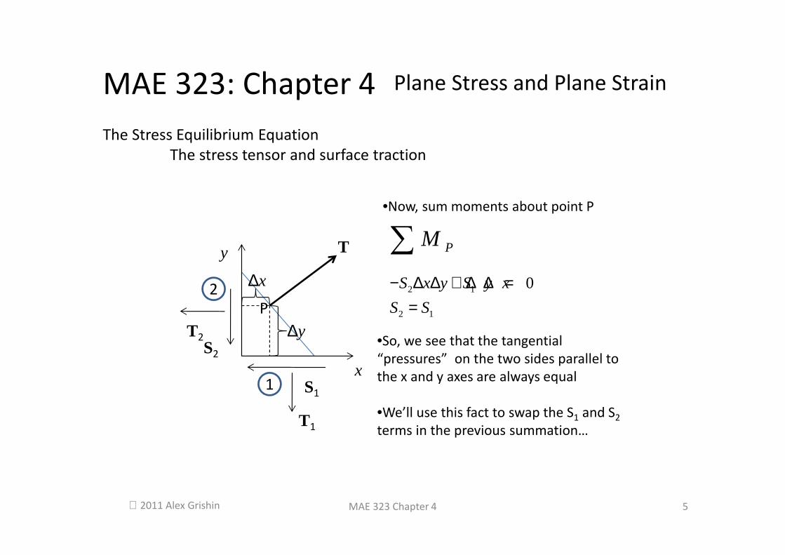
2011 Alex Grishin 5MAE 323 Chapter 4
The Stress Equilibrium Equation
The stress tensor and surface traction
x
y
T1
S1
T2
S2
1
2
PM∑•Now, sum moments about point P
T
P
∆y
∆x2 1
2 1
0S x y S y x
S S
− ∆ ∆ + ∆ ∆ ==
•So, we see that the tangential
“pressures” on the two sides parallel to
the x and y axes are always equal
•We’ll use this fact to swap the S1 and S2
terms in the previous summation…

Plane Stress and Plane StrainMAE 323: Chapter 4
2011 Alex Grishin 6MAE 323 Chapter 4
The Stress Equilibrium Equation
The stress tensor and surface traction
x
y
∆L
n
nx
ny
F
Tx
Ty T
T1
S1
T2
S2
1
2
2 2x x yT T n S n= +
•Now, we know that
cos
sinx
y
n
n
θθ
==
1 1y y xT T n S n= +
•So the traction equilibria may
expressed as (after swapping the
S2 and S1 terms):
•Or, as a matrix equation*:
2 2
1 1
x x
y y
T nT S
T nS T
=
(1)

Plane Stress and Plane StrainMAE 323: Chapter 4
2011 Alex Grishin 7MAE 323 Chapter 4
The Stress Equilibrium Equation
The stress tensor and surface traction
•The matrix of normal and tangential pressures is known as the Cauchy or
infinitesimal stress tensor. It’s two-dimensional form is shown below. It gets
this name because it is only valid for small increments of stress and
corresponding strain
2 2
1 1
xx xy
yx yy
T S
S T
σ σσ σ
=
•The preceding derivation could have been done in three dimensions following
the same procedure, but on a plane cut through a 3D infinitesimal cube (a
tetrahedron)…
•As we saw in slide 5: xy yxσ σ= So, the matrix is also symmetric

Plane Stress and Plane StrainMAE 323: Chapter 4
2011 Alex Grishin 8MAE 323 Chapter 4
The Stress Equilibrium Equation
The stress tensor and surface traction
•A diagram like the one below could be used to follow the same procedure as
was done in 2D, but in all three dimensions, yielding the full 3 x 3 Cauchy
stress tensor
x
y
Tx
Ty
3
1
z
T
Tz2
xx xy xz
yx yy yz
zx zy zz
σ σ σσ σ σσ σ σ
=
σ
xy yx
yz zy
xz zx
σ σσ σσ σ
=
=
=

Plane Stress and Plane StrainMAE 323: Chapter 4
2011 Alex Grishin 9MAE 323 Chapter 4
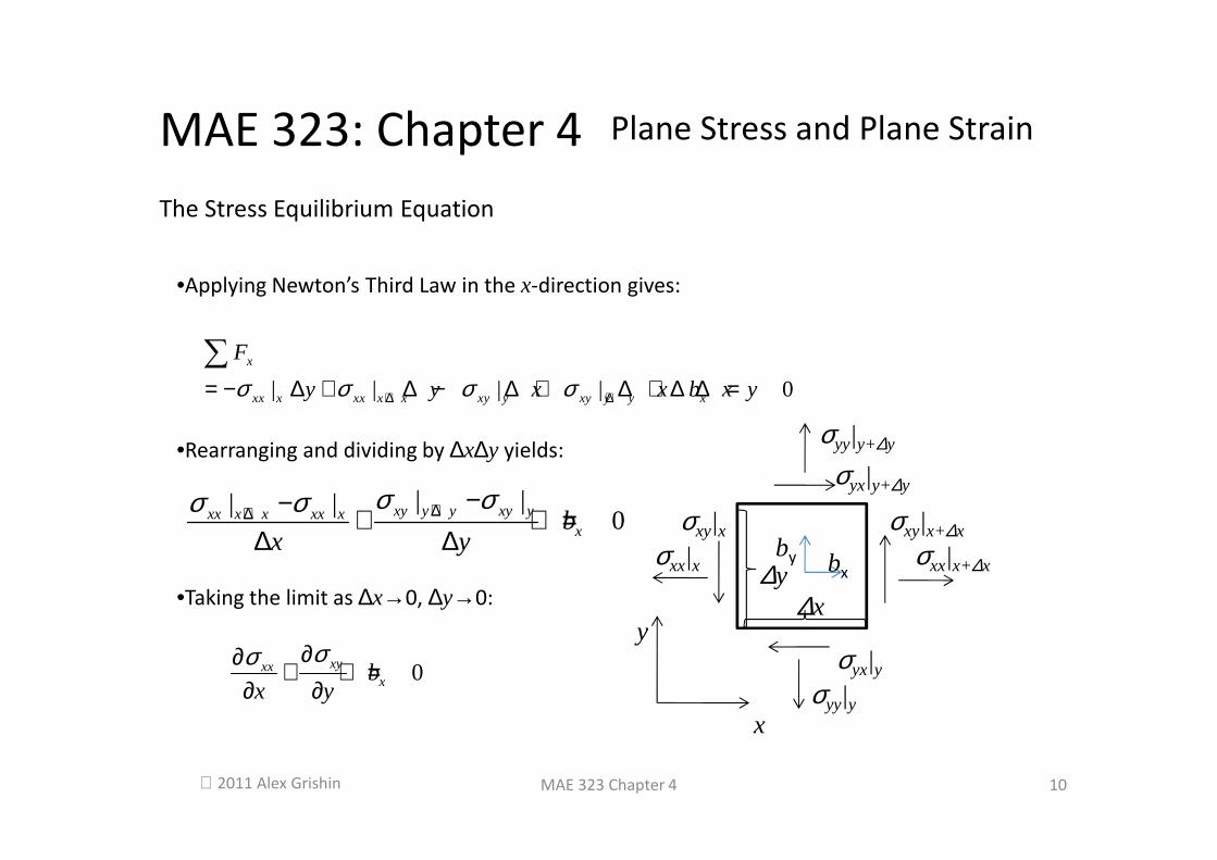
The Stress Equilibrium Equation
•Next,we’d like to derive the stress equilibrium differential equation itself,
which forms the basis for most structural problems.
x
y
σxx|x+∆x
σxy|x+∆x
σyx|y+∆y
σyy|y+∆y
σxx|x
σxy|x
σyy|y
σyx|y
∆x
∆ybx
by
•Again, we’ll work just in
two dimensions to keep
things simple. This
time, we’ll use an
infinitesimal element
with all four sides as
shown
•Here, b is a body force
per unit volume
Plane Stress and Plane StrainMAE 323: Chapter 4
2011 Alex Grishin 10MAE 323 Chapter 4
The Stress Equilibrium Equation
•Applying Newton’s Third Law in the x-direction gives:
x
y
σxx|x+∆x
σxy|x+∆x
σyx|y+∆y
σyy|y+∆y
σxx|x
σxy|x
σyy|y
σyx|y
∆x∆y bx
by
| | | | 0x
xx x xx x x xy y xy y y x
F
y y x x b x yσ σ σ σ+∆ +∆= − ∆ + ∆ − ∆ + ∆ + ∆ ∆ =∑
•Rearranging and dividing by ∆x∆y yields:
| || |0xy y y xy yxx x x xx x
xbx y
σ σσ σ +∆+∆ −− + + =∆ ∆
•Taking the limit as ∆x→0, ∆y→0:
0xyxxxb
x y
σσ ∂∂ + + =∂ ∂

Plane Stress and Plane StrainMAE 323: Chapter 4
2011 Alex Grishin 11MAE 323 Chapter 4
The Stress Equilibrium Equation
•Similarly, repeating the previous three steps in the y-direction yields:
•And, once again, even though we won’t go thru the steps, we will simply point
out that the full three dimensional equations can be obtained in a similar
manner, considering a three-dimensional cube element instead of a square.
Without showing the derivation, the equations are:
0
0
0
xyxx xzx
yx yy yzy
zyzx zzz
bx y z
bx y z
bx y z
σσ σ
σ σ σ
σσ σ
∂∂ ∂+ + + =∂ ∂ ∂
∂ ∂ ∂+ + + =
∂ ∂ ∂∂∂ ∂+ + + =
∂ ∂ ∂
0yy xyyb
y x
σ σ∂ ∂+ + =
∂ ∂

Plane Stress and Plane StrainMAE 323: Chapter 4
2011 Alex Grishin 12MAE 323 Chapter 4
The Stress Equilibrium Equation
•Regardless of spatial dimension, the stress equilibrium can be written
compactly in indicial notation as:
•Where, as usual, the Einstein summation convention implies summation over
repeated indices and the comma in the subscript means “derivitative with
respect to the coordinate variable implied by the index following the comma”
, 0ij j ibσ + =

Plane Stress and Plane StrainMAE 323: Chapter 4
2011 Alex Grishin 13MAE 323 Chapter 4
Small Strains
•The stress equilibrium equations derived previously give us only half the
picture. To fully solve for the response of a bounded continuum (a structure),
we need a way to relate stresses and forces to strains and displacements,
respectively. So, before we look at that, we will introduce the common notion
of small, or infinitesimal strains
•From the work we’ve already done, we know that in a structural problem, we
relate forces to displacements through Hooke’s Law (remember it kept coming
back again and again). Further, we saw that in reduced continuum solutions,
we had solutions over elements (in two dimensions) of the form:
1
1
( , ) ( , )
( , ) ( , )
n
i ii
n
i ii
u f x y N x y u
v g x y N x y v
=
=
= =
= =
∑
∑

Plane Stress and Plane StrainMAE 323: Chapter 4
2011 Alex Grishin 14MAE 323 Chapter 4
Small Strains
•Just as the displacement field is the natural counterpart to the external forces
in a structure, the strain field is the natural counterpart to the stress field in a
structure. So, in two spatial dimensions, we can expect four strain
components (three independent ones due to the symmetry in slide 7)
•We will designate the strain tensor as εεεε.
xx xy
yx yy
ε εε ε
=
ε
And, in three dimensions:
xx xy xz
yx yy yz
zx zy zz
ε ε εε ε εε ε ε
=
ε

Plane Stress and Plane StrainMAE 323: Chapter 4
2011 Alex Grishin 15MAE 323 Chapter 4
Small Strains
•Although it’s a little difficult to convey graphically, an infinitesimal element
undergoing nonzero εxx,εyy, and εyz represents a small perturbation from an
equilibrium configuration (the dashed square), such that the actual lengths, ∆xand ∆y don’t change. With this in mind, the strain components are defined as:
x
y
,, |x yu v,, |x x yu v +∆
,, |x y yu v +∆ ,, |x x y yu v +∆ +∆
θy
θx
, ,
0
| |lim x x y x y
xxx
u u u
x xε +∆
∆ →
− ∂= = ∆ ∂
, ,
0
| |lim x y y x y
yyy
v v v
y yε +∆
∆ →
− ∂= = ∆ ∂
, ,
0
| |lim tanx x y x y
x xx
v vv
x xθ θ+∆
∆ →
− ∂ = = ≈ ∂ ∆

Plane Stress and Plane StrainMAE 323: Chapter 4
2011 Alex Grishin 16MAE 323 Chapter 4
Small Strains
And finally:
x
y
,, |x yu v,, |x x yu v +∆
,, |x y yu v +∆ ,, |x x y yu v +∆ +∆
θy
θx
, ,
0
| |lim tanx y y x y
y yy
u uu
y yθ θ+∆
∆ →
− ∂ = = ≈ ∂ ∆
•The engineering shear strain is given by:
xy
u v
y xγ ∂ ∂= +
∂ ∂
•The tensor shear strain is ½ the
engineering shear strain:
1
2xy
u v
y xε ∂ ∂ = + ∂ ∂
Plane Stress and Plane StrainMAE 323: Chapter 4
2011 Alex Grishin 17MAE 323 Chapter 4
Small Strains
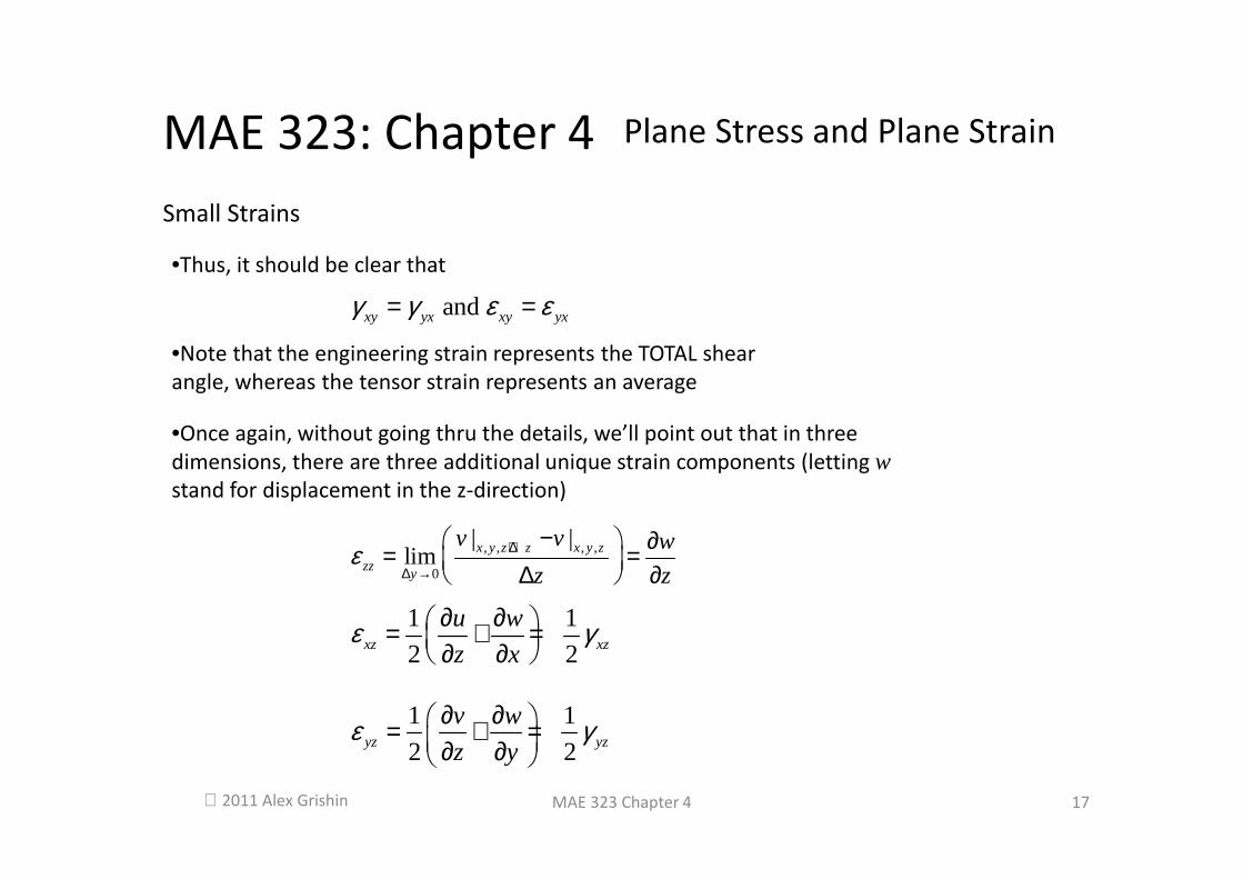
•Thus, it should be clear that
•Once again, without going thru the details, we’ll point out that in three
dimensions, there are three additional unique strain components (letting wstand for displacement in the z-direction)
andxy yx xy yxγ γ ε ε= =
, , , ,
0
| |lim x y z z x y z
zzy
v v w
z zε +∆
∆ →
− ∂= = ∆ ∂
1 1
2 2yz yz
v w
z yε γ∂ ∂ = + = ∂ ∂
1 1
2 2xz xz
u w
z xε γ∂ ∂ = + = ∂ ∂
•Note that the engineering strain represents the TOTAL shear
angle, whereas the tensor strain represents an average

Plane Stress and Plane StrainMAE 323: Chapter 4
2011 Alex Grishin 18MAE 323 Chapter 4
Generalized Hooke’s Law
•As we mentioned earlier, in order to fully solve the response of a bounded
continuum to an external load, we need a constitutive relation between the
stress and strain components. This is understood as a property of the
continuum (different materials will respond differently over the same bounded
continuum under a given loading regime)
•So, we’re looking for something of the form σσσσ=Cεεεε, where C plays the role of K
in Hooke’s law
•Unfortunately, a thorough discussion of this mathematical object is beyond
the scope of this course*. However, we’ll hit the introductory highlights. We’ll
begin by noting that in its most general form, C is a fourth rank tensor, and in
indicial notation, the relation between stress and strain is given by:
*We suggest the interested student begin by looking up “Hooke’s
Law” in Wikipedia, for a pretty good introduction
ij ijkl klCσ ε= (2a)
Plane Stress and Plane StrainMAE 323: Chapter 4
2011 Alex Grishin 19MAE 323 Chapter 4
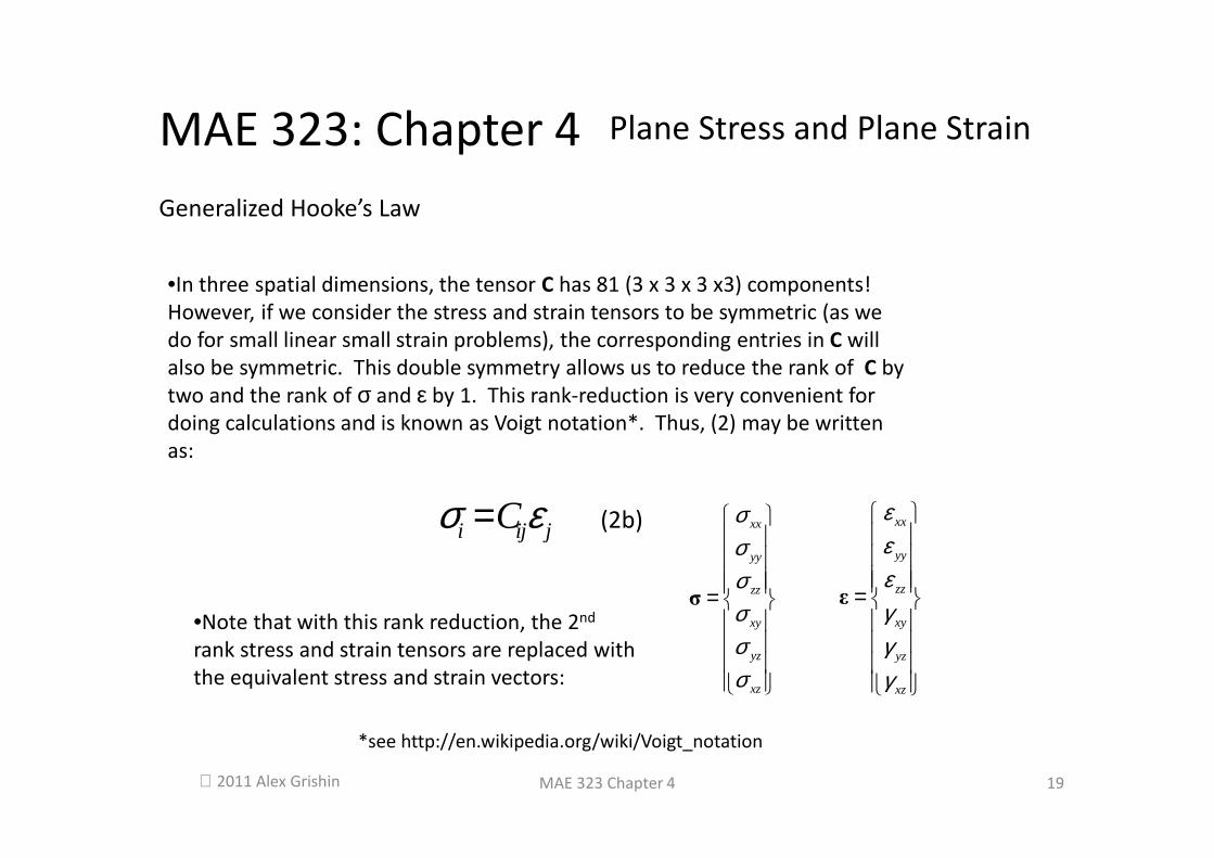
Generalized Hooke’s Law
•In three spatial dimensions, the tensor C has 81 (3 x 3 x 3 x3) components!
However, if we consider the stress and strain tensors to be symmetric (as we
do for small linear small strain problems), the corresponding entries in C will
also be symmetric. This double symmetry allows us to reduce the rank of C by
two and the rank of σ and ε by 1. This rank-reduction is very convenient for
doing calculations and is known as Voigt notation*. Thus, (2) may be written
as:
*see http://en.wikipedia.org/wiki/Voigt_notation
i ij jCσ ε=
•Note that with this rank reduction, the 2nd
rank stress and strain tensors are replaced with
the equivalent stress and strain vectors:
xx
yy
zz
xy
yz
xz
σσσσσσ
=
σ
xx
yy
zz
xy
yz
xz
εεεγγγ
=
ε
(2b)
Plane Stress and Plane StrainMAE 323: Chapter 4
2011 Alex Grishin 20MAE 323 Chapter 4
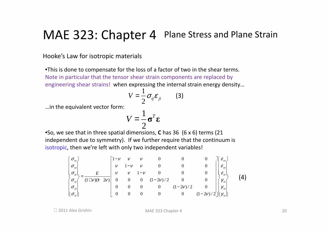
Hooke’s Law for isotropic materials
•This is done to compensate for the loss of a factor of two in the shear terms.
Note in particular that the tensor shear strain components are replaced by
engineering shear strains! when expressing the internal strain energy density…
…in the equivalent vector form:
1
2 ij jiV σ ε=
1
2TV = σ ε
•So, we see that in three spatial dimensions, C has 36 (6 x 6) terms (21
independent due to symmetry). If we further require that the continuum is
isotropic, then we’re left with only two independent variables!
1 0 0 0
1 0 0 0
1 0 0 0
0 0 0 (1 2 ) / 2 0 0(1 )(1 2 )
0 0 0 0 (1 2 ) / 2 0
0 0 0 0 0 (1 2 ) / 2
xxxx
yyyy
zzzz
xyxy
yzyz
xzzz
E
εσ ν ν νεσ ν ν νεσ ν ν νγσ νν νγσ νγσ ν
− − − = −+ −
−
−
(4)
(3)

Plane Stress and Plane StrainMAE 323: Chapter 4
2011 Alex Grishin 21MAE 323 Chapter 4
Hooke’s Law for isotropic materials
•So, equation (4) gives us the constitutive relation for an isotropic material in
three dimensions, such that C in equation (2b) is:
1 0 0 0
1 0 0 0
1 0 0 0
0 0 0 (1 2 ) / 2 0 0(1 )(1 2 )
0 0 0 0 (1 2 ) / 2 0
0 0 0 0 0 (1 2 ) / 2
E
ν ν νν ν νν ν ν
νν νν
ν
− − −
= −+ − −
−
C
•If we had some other type of material (perhaps orthotropic, or transversely
isotropic for example), we would simply replace C with the appropriate
constitutive relation. Any other material will have more non-zero terms and
more independent variables. The minimum number of independent (scalar)
material properties for a continuum in at least two spatial dimensions is two.
•We have given equation (4) in a particular form, where E is the Elastic
Modulus and ν is Poisson’s Ratio

Plane Stress and Plane StrainMAE 323: Chapter 4
2011 Alex Grishin 22MAE 323 Chapter 4
The Elastic Modulus and Poisson’s Ratio
•The elastic modulus, E (also known as Young’s Modulus) measures the
material’s tensile strain under a uniform tensile stress., while Poisson’s Ratio
gives a measure of how much the material contracts in a direction transverse to
the uniform tensile stress (this is known as Poisson’s Effect). This may be seen by
taking the inverse of equation (4):
1 0 0 0
1 0 0 0
1 0 0 01
0 0 0 2(1 ) 0 0
0 0 0 0 2(1 ) 0
0 0 0 0 0 2(1 )
xxxx
yyyy
zzzz
xyxy
yzyz
xzzz
E
σε ν νσε ν νσε ν νσγ νσγ νσγ ν
− − − − − − = +
+
+
•Now, apply a uniaxial stress, { }0 0 0 0 0T
xxσ=σ
1 0 0 0
1 0 0 0 0
1 0 0 0 010 0 0 2(1 ) 0 0 0
0 0 0 0 2(1 ) 0 0
0 0 0 0 0 2(1 ) 0
xx xx
yy
zz
xy
yz
zz
E
ε ν ν σε ν νε ν νγ νγ νγ ν
− − − − − − = + +
+
(5)

Plane Stress and Plane StrainMAE 323: Chapter 4
2011 Alex Grishin 23MAE 323 Chapter 4
The Elastic Modulus and Poisson’s Ratio
•This results in the equations: 1xx xx
yy xx
zz xx
E
E
E
ε σ
νε σ
νε σ
=
= −
= −
(6a)
(6b)
(6c)
•The fundamental linear relationship between stress and strain is embodied in
(6a), and we may in fact define the elastic modulus E under a uniaxial stress, σxx
from (6a) as:xx
xx
Eσε
=
•Furthermore, (6b) and (6c) state that there are two transverse components of
compressive strain (the sign of the strain is opposite that of the stress) resulting
from the uniaxial stress field. And, if we substitute σxx=Eεxx into (6b) and (6c) to
solve for ν, we obtain:
yy zz
xx xx
ε ενε ε
= − = −
(7)
(8)

Plane Stress and Plane StrainMAE 323: Chapter 4
2011 Alex Grishin 24MAE 323 Chapter 4
The Elastic Modulus and Poisson’s Ratio
•In other words, Poisson’s ratio may be thought of as a ratio of transverse to axial
strain (or contraction) under a uniaxial stress as shown in the figure below. It is
worth repeating: This a material property. Different materials will exhibit
different ratios of contraction under a given tensile load (the values may even be
negative or zero, but they must never exceed 0.5, in which case the material is
perfectly incompressible) :
xxε
yyε
zzεxxσ
x
y
z
xxσ

Plane Stress and Plane StrainMAE 323: Chapter 4
2011 Alex Grishin 25MAE 323 Chapter 4
Plane Stress
•When analyzing bounded continua in two spatial dimensions, one can make
one of two assumptions. The first one is that all stress components in the third
dimension (let’s call it z) are zero. In other words:
•We plug this assumption into (4) :
0zz xz yzσ σ σ= = =
1 0 0 0
1 0 0 0
1 0 0 0 010 0 0 2(1 ) 0 0
0 0 0 0 2(1 ) 0 0
0 0 0 0 0 2(1 ) 0
xx xx
yy yy
zz
xy xy
yz
zz
E
ε ν ν σε ν ν σε ν νγ ν σγ νγ ν
− − − − − − = + +
+
to yield:
1
2(1 )
xx xx yy
yy xx yy
xy xy
E
ε σ νσε νσ σγ ν σ
− = − + +
( )zz xx yyE
νε σ σ= − +
and:
(9) (10)
These
components
are zero

Plane Stress and Plane StrainMAE 323: Chapter 4
2011 Alex Grishin 26MAE 323 Chapter 4
Plane Stress
•Note that separation of the z-component strain reaction (due purely to
Poisson’s Effect) in (10) is integral to the plane stress assumption. We omit it
from the constitutive relation and apply it as a bookkeeping exercise after
calculating the in-plane reactions
•Re-writing (10) as a matrix equation:
1 01
1 0
0 0 2(1 )
xx xx
yy yy
xy xy
E
ε ν σε ν σγ ν σ
− = − +
2
1 0
1 01
0 0 (1 ) / 2
xx xx
yy yy
xy xy
Eσ ν εσ ν ε
νσ ν γ
= − −
•And, after inversion (using Mathematica):
(12)
And remember our bookkeeping:
( )zz xx yyE
νε σ σ= − +
(11)
Plane Stress and Plane StrainMAE 323: Chapter 4
2011 Alex Grishin 27MAE 323 Chapter 4
Plane Stress
•Note that inverting a truncated version of (5) did NOT yield a corresponding
truncated version of (4)! This is very important and distinguishes plane stress
from plane strain from a purely mathematical standpoint.
•The assumptions of plane stress are an approximation. In real structures, the out-
of-plane (z) strain would in fact be accompanied by a corresponding out-of-plane
stress as required by (4). However, the approximation is good under certain
circumstances which we will discuss later

Plane Stress and Plane StrainMAE 323: Chapter 4
2011 Alex Grishin 28MAE 323 Chapter 4
Plane Strain
•The other 2D assumption we could make is that all the strain components in the
z-direction are zero:
0zz xz yzε ε ε= = =
•This is a different kind of assumption because it can be explicitly enforced (it may
be stated as a boundary condition on the LHS of the governing differential
equation), whereas the plane stress assumption arises from an observed
approximation due to the absence of loads, gradients, and boundary conditions in
the z-direction.
•Simply plug the above assumptions into (4):
1 0 0 0
1 0 0 0
1 0 0 0 0
0 0 0 (1 2 ) / 2 0 0(1 )(1 2 )
0 0 0 0 (1 2 ) / 2 0 0
0 0 0 0 0 (1 2 ) / 2 0
xx xx
yy yy
zz
xy xy
yz
zz
E
σ ν ν ν εσ ν ν ν εσ ν ν νσ ν γν νσ νσ ν
− − − = −+ − −
−

Plane Stress and Plane StrainMAE 323: Chapter 4
2011 Alex Grishin 29MAE 323 Chapter 4
Plane Strain
1 01
1 0(1 )(1 2 )
0 0 (1 2 ) / 2
xx xx
yy yy
yx xy
σ ν ν εσ ν ν ε
ν νσ ν γ
− = − + − −
•This yields:
•And:
( )(1 )(1 2 )zz xx yy
Eνσ ε εν ν
= ++ −
Where we again remove the out-of-plane reaction purely due to Poisson’s Effect
and calculate it separately.
•As we mentioned before, this condition can be explicitly enforced in a structure.
Specifically, If we fix the z-displacements at the extreme z-locations (the “ends” of
the structure) and ensure no load gradients in the z-direction, then the plane
strain assumption should hold at locations far from the ends.
(13)

Plane Stress and Plane StrainMAE 323: Chapter 4
2011 Alex Grishin 30MAE 323 Chapter 4
Plane Strain (axisymmetric version)
•The planar axisymmetric formulation is another planar stress/strain formulation,
but we do not include it as a separate category because it is actually equivalent to
the plane strain formulation in cylindrical coordinates (all properties of plane strain
hold equally true of axisymmetric elements). Switching to a cylindrical reference
frame does introduce some interesting differences, however.
…all that is required to convert the
plane strain formulation to an
axisymmetric one is replace the y-
coordinate with the cylindrical z,
the x-coordinate with r, and z
coordinate with θ . This produces
a 4 x 4 constitutive matrix and 4 x 1
stress/strain vector:
( )(1 )(1 2 ) rr zz
Eθθ
νσ ε εν ν
= ++ −
θ
r
z

Plane Stress and Plane StrainMAE 323: Chapter 4
2011 Alex Grishin 31MAE 323 Chapter 4
Plane Strain (axisymmetric version)
( )(1 )(1 2 ) rr zz
Eθθ
νσ ε εν ν
= ++ −
θ
r
z
( )( )
1 0
1 0
1 01 1 2
0 0 0 1/ 2
r r
z z
rz rz
Eθ θ
σ εν ν νσ εν ν νσ εν ν νν νσ γν
− − =
−+ − −