modeling natural human hand motion for grasp animation
TRANSCRIPT

IN DEGREE PROJECT MATHEMATICS,SECOND CYCLE, 30 CREDITS
, STOCKHOLM SWEDEN 2017
Modeling Natural Human Hand Motion for Grasp Animation
JOHANNES JEPPSSON
KTH ROYAL INSTITUTE OF TECHNOLOGYSCHOOL OF ENGINEERING SCIENCES


Modeling Natural Human Hand Motion for Grasp Animation
JOHANNES JEPPSSON
Degree Projects in Mathematical Statistics (30 ECTS credits) Degree Programme in Applied and Computational Mathematics (120 credits) KTH Royal Institute of Technology year 2017 Supervisor at Gleechi: 'DQ�6RQJSupervisor at KTH: Timo Koski Examiner at KTH: Timo Koski

TRITA-MAT-E 2017:53 ISRN-KTH/MAT/E--17/53--SE
Royal Institute of Technology School of Engineering Sciences KTH SCI SE-100 44 Stockholm, Sweden URL: www.kth.se/sci

Abstract
This report was carried out at Gleechi, a Swedish start-up company workingwith implementing hand use in Virtual Reality. The thesis presents handmodels used to generate natural looking grasping motions. One model weremade for each of the thirty-three different grasp types in Feix’s The GRASPTaxonomy.
Each model is based on functional principal components analysis whichwas performed on data containing recorded joint angles of grasping motionsfrom real subjects. Prior to functional principal components analysis, dy-namic time warping was performed on the recorded joint angles in order toput them on the same length and make them suitable for statistical analysis.The last step of the analysis was to project the data onto the functionalprincipal components and train Gaussian mixture models on the weights ob-tained. New grasping motions could be generated by sampling weights fromthe Gaussian mixture models and attaching them to the functional principalcomponents.
The generated grasps were in general satisfying, but all of the thirty-threegrasps were not distinguishable from each other. This was most likely causedby the fact that each degree of freedom was modelled in isolation from eachother, so that no correlation between them was included in the model.


Modellering av Naturliga Handrörelser förGreppanimationer
Johannes Jeppsson
Abstract
Denna rapport utfördes på Gleechi, ett svenskt start-up företag som job-bar med att implementera handrörelser i Virtual Reality. Uppsatsen presen-terar statistiska modeller för att generera handrörelser som utför olika typerav grepp och som ser naturliga ut. En modell skapades för alla trettiotregrepptyp i Feixs The GRASP Taxonomy.
Varje modell bygger på funktionell principalkomponentsanalys som utför-des på data innehållande inspelade vinklar från fingerleder från personer somutförde olika grepp på föremål. Innan funktional principalkomponentanalysutfördes så genomfördes dynamic time warping på datan för att få de inspe-lade greppen på samma längd och göra den lämplig för statistisk analys. Detsista steget i analysen var att projicera ned datan på principalkomponenter-na och träna Gaussian mixture models på vikterna som erhölls. Nya greppkunde då genereras genom att dra vikter från Gaussian mixture models ochskapa linjärkombinationer med de funktionella principalkomponenterna.
De genererade greppen var generellt sett tillfredställande, men alla tret-tiotre grepptyper var inte särskiljbara från varandra. Detta berodde medstörsta sannolikhet på att varje frihetsgrad modellerades isolerat från deandra så att ingen korrelation mellan dem var inkluderad i modellen.
ii


Acknowledgements
I would like to thank Timo Koski for his mathematical insight, his ability tocalm me down when I was sure everything was doomed, and his entertainingstories.
I would like to thank Gabriel Isheden for sharing his exceptional abilityof analyzing problems and for his kindness of taking me under his wings.
I would like to thank Sixten Matz for his fantastic ideas and clearsight.I would like to thank Henriette Matz for being such a fantastic support
and team player.Finally I would like to thank Gleechi for their hospitality.
Stockholm, July 2017
Johannes Jeppsson
iii

iv

Contents
1 Introduction 11.1 Background . . . . . . . . . . . . . . . . . . . . . . . . . . . . 11.2 Related Work . . . . . . . . . . . . . . . . . . . . . . . . . . . 21.3 Outline . . . . . . . . . . . . . . . . . . . . . . . . . . . . . . 7
Abbrevations 9
2 Model 112.1 Choice of model . . . . . . . . . . . . . . . . . . . . . . . . . . 112.2 Description of model . . . . . . . . . . . . . . . . . . . . . . . 12
3 Theory 133.1 Dynamic Time Warping for One-dimensional Sequences . . . 133.2 Dynamic Time Warping for Multivariate Sequences . . . . . . 143.3 Principal Components Analysis . . . . . . . . . . . . . . . . . 143.4 Functional Principal Components Analysis . . . . . . . . . . . 15
4 Method 174.1 Implementation . . . . . . . . . . . . . . . . . . . . . . . . . . 174.2 Classification . . . . . . . . . . . . . . . . . . . . . . . . . . . 21
5 Results 235.1 Result of implemented techniques . . . . . . . . . . . . . . . . 235.2 Generating grasps . . . . . . . . . . . . . . . . . . . . . . . . . 315.3 Classification . . . . . . . . . . . . . . . . . . . . . . . . . . . 36
6 Summary 41
A Generated grasps 43
v

vi

Chapter 1
Introduction
This degree project aims to use a data-driven approach to generate naturallooking hand motions in the process of reaching to grasp objects in thecontext of Virtual Reality applications.
Realistic hand grasp animation is an important aspect for an immersiveVirtual Reality experience, as grasping objects is one of the most importantways humans interact with the world. This report focuses on the generationof the hand and finger motions in the process of grasping objects, but notthe process of establishing a realistic grip on the object. This degree projectwas carried out at Gleechi; a Swedish start-up company producing softwarefor realistic hand interaction in real-time; http://www.gleechi.com.
The task of this project was to use a data-driven technique for generatingnatural looking human hand motion in the context of grasping objects inorder to investigate if this could be a viable approach for future use.
1.1 Background
Humans are very good at perceiving details in hand gestures, e.g. Jörg etal. found in [18] that hand and finger motion is important for conveying theintended meaning of a scenario. Being able to produce accurate and realistichand motions is therefore important for increasing the feeling of presence inusing Virtual Reality.
Generating realistic hand motions in Virtual Reality is however a difficulttask. And there are several obstacles connected with generating accurate andrealistic hand movements.
1.1.1 High Degree of Freedom
The human hand itself is a very complex organ that consists of twenty-seven bones with interlinking joints. Any mechanical model attempting torepresent the hand with its dynamic properties is bound to be complex.
1

Animating hand motion is thus a very difficult task since there are a highnumber of interdependent degrees of freedom to be controlled for.
The fact that the hand has many degrees of freedom must be taken intoaccount in the data collection process, i.e. the more dimensions that aretaken into account, the more data needs to be collected to account for theextra dimensions.
1.1.2 Naturalness
Generating hand motions that look realistic to humans pose another demandon the generation process. Movements that for some reason are perceived asartificial will get in the way of the Virtual Reality experience. In continuoususe, it might also be necessary for movements performing a similar task toexhibit some variation, in order to not look artificial. Naturalness is thebenchmark of generated motions, but it is also the hardest to pinpoint.
1.1.3 Data driven
There are hand models that use databases as starting points and search themfor similar motions that might be configured for the task at hand. However,the aim of this thesis is to produce a model that can sample data withoutusing a database. This means that a probabilistic distribution that reflectshand motions must be estimated.
1.1.4 Real-time generation
It is the goal of Gleechi to obtain a model that is able to sample new motionsin real-time. This puts an upper bound on how complicated the model canbe in terms of computer power. Since the task of this thesis is exploratory inits nature, this aspect is not of immediate importance. But when choosinga model it should be considered whether it is possible to make real-timesimulations eventually.
1.1.5 Non-linearity
Hand motions are intrinsically non-linear, and thus a model for generatinghand motions should preferably also be able to generate non-linear motions.
1.2 Related Work
There have been several different approaches on how to go about gener-ating natural-looking hand motions in Virtual Reality. The most promi-nent methods, which have been considered in this thesis, can be categorized
2

into techniques based on principal component analysis (PCA), Gaussian pro-cess latent variable machines (GPLVMs) and restricted Boltzmann machines(RBMs) respectively.
1.2.1 Grasp taxonomies
An important aspect of analyzing grasping of objects has been the effort ofcreating grasp taxonomies, such as the Cutkosky grasp taxonomy [2]. Forinstance Feix et al. in has provided a list in [32] of thirty-three differentgrasps, when only considering the hand and not the object shape and size.Figure 1.1 below contains images of the thirty-three grasp types of the Feixtaxonomy. Taxonomies are considering the final hand posture when a grip isestablished, but by that virtue they are also important for how reaching tograsp motions differ. Taxonomies provide the foundation for differentiatingbetween grasp types.
3

Figure 1.1: The thirty-three grasp types of the Feix grasp taxonomy.
4

1.2.2 PCA based approaches
PCA based techniques arise mainly from the effort to tackle the many degreesof freedoms in the hand.
In [3], Santello et al. explored the idea of lack of individuation in fingermovements. They asked five right-handed subjects to grasp each of fifty-seven imaginary objects five times. They recorded the final posture of thehand with fifteen degrees of freedom and then performed discriminant analy-sis, regression analysis, and principal components analysis. They found thatthe first two principal components accounted for more than eigthy percentof the variance in hand shapes.
A follow up study on Santello et al. [3] was later performed by Dai et al.[26]. They performed PCA and found that eighty-three percent of the vari-ance was captured by the first three principal components. After this theyperformed functional principal components analysis on the projected dataand found that the first two functional components accounted for aboutninety-five percent of variation in the grasping motion. The subjects per-formed fifteen different grasps from the Cutkosky grasp taxonomy, and theysuggest four different groups of motion based on k-means-clustering.
Ciocarlie et al. [9] used the first two principal components for graspsynthesis of four different hand models. In order to find a conforming grasp,they formulated an energy function that described the distance of previouslyselected contact points on the hand model to the object. The energy functionwas then minimized using Simulated Annealing. As a feasibility test, theytook the grasp found by minimizing the energy function and use inversekinematics to find an arm position. If an arm position was found withoutany collision, the configuration was chosen. Using the first two principalcomponents, the resulting grasp did not always conform to the surface ofthe object. In those cases they closed each finger until it fully enclosed theobject.
Amor et al. [13] collected a wide range of possible hand shapes, onwhich they then performed PCA to achieve low-dimensional grasp space. Todiscriminate to hand positions that are anatomically feasible, they learnta Gaussian Mixture Model (GMM) on the PCA space. The number ofGaussians used in the GMM was chosen using the Bayesian InformationCriterion. To synthesize new grasps, they stipulated a grasp metric basedon the distance of the sensors to the object, an estimate of the stability ofthe grasp, and a penalty value. To find a suitable grasp they minimizedthe metric using Dynamic Hill Climbing technique. The grasp found wasaccepted if it also satisfied that the probability of the grasp was above acertain threshold, according to the GMM.
Zhao et al. [27] divided a grasping hand motion into reaching, closingand manipulating phases. They obtained grip-dependent probabilistic mo-tion models for closing motion. Training data was labeled with the type of
5

grasp used (e.g. pinch grasp) and the final database included motion cap-ture data from hands grasping ten different objects using ten different gripmodes. To process the data, dynamic time warping was used to warp thegeometric and temporal training data respectively into comparable time se-ries of equal length. FPCA was then applied to the warped time series toobtain a low-dimensional, parametric representation for closing motion. Fur-thermore, they learn a joint probability distribution to model the correlationbetween the geometric and timing variations. The prior distributions weremodeled using a Gaussian mixture model. The parametric representationand the joint probability distribution define a generative model for closing-phase motion synthesis. Synthesizing new motion was done by sampling thejoint probability distribution and inserting the samples into the parametricrepresentation. For synthesizing the reaching motion motion, they searchedfor a similar motion from the database and confined it to the first frame ofthe closing motion using smoothing techniques.
In [31] Du et al. extended FPCA by scaling, a method they call SFPCA.They applied FPCA on weighted data, where the weights were found suchthat they minimized the error in Euclidean joint space.
1.2.3 RBMs
RBMs are a form of neural networks that have been used extensively inmodeling locomotion.
In [11] Taylor et al. introduced the Conditional Restricted BoltzmannMachine (CRBM) to model different styles of human motion. The CRBM isa two-layer neural network that extends the Restricted Boltzmann Machine(RBM) by taking into consideration the temporal aspect of the data. Thisis done by also taking as input the previous n configurations, making theinput have autoregressive connections. In their experiment they included theprevious three time steps. The model was then trained by a method calledcontrastive divergence. The trained CRBM is a probability density modelof sequences, thus the CRBM can be used to synthesize new motions byinitializing with the first n time steps. Sampling from the joint distributionwas done by performing alternating Gibbs sampling. The resulting modelwas able to model different styles of motion that were present in the trainingdata. To generate a motion of a specific style, the model was initialized withthe first n time steps of that style, e.g. jogging or walking.
In [17] Taylor and Hinton presented an extension to the CRBM, called theFactored CRBM. The factored CRBM aims to improves the ability to blendmotion styles or to transition smoothly between them, and it also lowers thecomputational load from O(N3
) to O(N2). For purposes of comparison, they
also used a two-layer CRBM which successfully models ten different stylesof walking. The factored CRBM was also able to model the ten differentmotion styles, as well as blending and transitioning between styles.
6

In [19] Taylor et al. presented another extension to CRBM that in-cludes latent style variables, which they call Implicit Mixture of CRBMs(imCRBM). imCRBMs can be trained unsupervised, in which case the modeldetects atomic motion primitives in the data.
Chiu and Marsella [20] made use of the property of stacking RBMs.They introduced a hierarchical factored conditional Restricted BoltzmannMachine (HFCRBM) which consisted of two layers. The first layer is arestricted CRBM which extract patterns of the motion and the second layeris an FCRBM. By this structure they are able to generate motion styles aswell as blending of styles with better performance than a single FCRBM.
In [21] Chiu and Marsella modified the HFCRBM by stacking an FCRBMon top of a CRBM. The modified HFCRBM was used to generate a gesturemotion from speech.
1.2.4 GPLVMs
GPLVMs is a dimensionality reduction technique that generalizes PCA torepresent the data with Gaussian Processes, this provides for non-linear map-ping from the latent space to the data space [5]. GPLVMs has been used tomodel human poses in [6].
In [8] Wang et al. introduced Gaussian Process Dynamical Models (GPDMs),which extend GPLVMs with an autoregressive component which allows tomodel the temporal aspect. Wang et al. later used GPDMs with style-specific factors to model human locomotion of different styles in [12] and[14].
Chiu et al. generated gestures based on speech labels in [29] with the useof GPDMs. In their approach, each point in the reduced space correspondsto a motion frame in the observed space; to generate gestures, they sampleda trajectory in the reduced space and mapped it back to the observed space.In particular they interpolated trajectories to generate smooth transitionsbetween gestures connected to different speech labels.
1.3 Outline
In chapter two, the choice of model is presented, specifically in section 2.2 themodel for generating hand motions is described. In chapter three, the theo-retical background for dynamic time warping, principal component analysisand functional principal component analysis is presented. In chapter four,the methodology of the analysis is discussed. In chapter five, the results ofthe analysis are presented.
7

8

Abbrevations
DoF Degree of freedom
DTW Dynamic time warping
FPCA Functional principal component analysis
FPCs Functional principal components
GMM Gaussian mixture model
LOOCV Leave-one-out cross-validation
PCA Principal component analysis
PCs Principal components
9

10

Chapter 2
Model
In this chapter, the choice of using a model based on FPCA is argued for onthe basis of the literature study. Next, the general outline of the model ispresented.
2.1 Choice of model
The main reason a model based on GPLVMs was not chosen is that they onlyprovide a mapping from latent space to observed space, and no mapping inthe opposite direction. While this is what is desired in generation of grasps,it is not suitable for classification purposes; i.e. given an observed grasp,find the mapping to latent space.
CRBMs have the advantage that all DoFs come to use, so that no di-mension reduction is needed. However, CRBMs studied in the literaturereview are not deterministic in the sense that they are not guaranteed tostay within the type they are initialized in. This makes CRBMs problematicfor generating grasps of specific types.
FPCA does not show the obstacles presented for GPLVMs or CRBMsabove which is why it is the chosen methods of this thesis.
With respect to the obstacles for generating hand motions presented inthe previous chapter, FPCA is a good candidate. First, FPCs are able todescribe non-linear motions. Second, only the FPCs are needed to be keptin the computer memory, so real-time generation is most likely possible.Third, it is a data driven approach which fits into the objectives of Gleechi.Finally, in order to handle the high amount of DoFs, FPCA has been appliedindividually to each DoF. This approach is obviously a simplification of thehand motions since correlation between joint angles are not accounted for bythis approach.
11

2.2 Description of model
In order to apply FPCA, the first step was to divide the data by grasp type,and within each grasp type divide the data by DoF, so that FPCA could beapplied to each DoF separately. The second step was to get the data on thesame length; for this purpose DTW was applied to all grasps within a grasptype. DTW resulted in two datasets; one containing the warped motions,and the other containing the time warping functions.
Next, FPCA was applied to each DoF for each grasp type. Each DoF,✓i
(t), describes a one-dimensional angle in a finger joint, and the change overtime in the angle could thus be modeled by a linear combination of the meanmotion and the FPCs as
✓i
(t) = pi,0(t) + ↵
i,1pi,1(t) + · · ·+ ↵i,k
pi,k
(t) (2.1)= p
T
i
(t)↵i
, (2.2)
where p
i
(t) contains the FPCs and of which pi,0(t) represents the mean
function.Then FPCA was performed on the time warping functions, ⌧
i
(t), as well.Temporal variations could be modeled similarly as
⌧i
(t) = qi,0(t) + �
i,1qi,1(t) + · · ·+ �i,l
qi,l
(t) (2.3)= q
T
i
(t)�i
, (2.4)
where q
i
(t) contains the FPCs and of which qi,0(t) represents the mean
function.In the analysis, two FPCs was used for joint angles and one FPC was
used for time warping functions, hence k was set to 2 and l was set to 1.The end result was one model for each grasp type of Feix’s grasp tax-
onomy, thirty-three models in total. A parametric model for generatingmotions for each grasp type was obtained by
⇥(t) =
0
B@p
T
1
�q
T
1 (t)�1
�↵1
...p
T
16
�q
T
16(t)�16
�↵16
1
CA , (2.5)
where variations of the grasp type were obtained by providing differentweights, ↵
i
and �
i
.The last step of the model was to train GMMs to be able to estimate
the weights ↵
i
and �
i
. This was done by projecting the recorded grasps inthe data onto the FPCs and train the GMMs on the projected weights. OneGMM was trained for DoF.
For generating new grasps, estimate weights, ˆ
↵
i
and ˆ
�
i
, were sampledfrom the GMMs and inserted into the parametric model 2.5.
12

Chapter 3
Theory
In this section, the theory of DTW and FPCA, which are central to themodel, will be briefly explained.
3.1 Dynamic Time Warping for One-dimensionalSequences
DTW [1, 24] is a technique for measuring similarity between two temporal se-quences. The intuition is that the sequences are aligned by locally stretchingand shrinking until they are as similar as possible.
In its basic form, DTW takes two sequences, {xi
}Mi=1 and {y
j
}Nj=1, and
finds a new set of indices {mk
}Lk=1 and {n
k
}Lk=1 of same length L such that
LX
l=1
d(xml , ynl), (3.1)
is minimized for some distance function d(·, ·) (e.g. Euclidean distance).The two sequences {x
mk}Lk=1 and {y
nk}Lk=1 are referred to as the warped se-
quences, and the indices {mk
}Lk=1 and {n
k
}Lk=1 are referred to as the warping
paths.The warping paths must satisfy the following conditions
1. 1 mk
M , 1 nk
N
2. m1 = n1 = 1 and mL
= M , nL
= N ,
3. (mk+1 �m
k
, nk+1 � n
k
) = (0, 1), (1, 0) or (1, 1).
The first condition assures that the warping paths are defined on the sameinterval as the original sequences. The second condition assures that theboundary conditions are honored, i.e. the warped sequences have the samestarting and ending point as the original sequences. The third and finalcondition assures that at least one of the warping paths are increasing all
13

the time in order to avoid that the warping paths result only in repeatingthe indices that produce the smallest distance.
Let us reformulate DTW slightly to link it to the multivariate case. Letx 2 RM and y 2 RN represent the sequences to align. Finding the warpingpaths is equivalent to finding matrices W
x
2 RM⇥L and W
y
2 RN⇥L withcolumns containing only zeros except for a single one such that the conditionsabove are fulfilled and
d(xWx
, yW
y
) (3.2)
is minimized.
3.2 Dynamic Time Warping for Multivariate Se-quences
In the multivariate case, the multivariate sequences to be aligned can berepresented by matrices. Let us also allow for there to be N different se-quences to align. For an informative approach to multivariate DTW [25] canbe consulted.
Let the original sequences be represented by a set of d-dimensional ma-trices {X
i
}Ni=1, Xi
2 Rd⇥ni , where ni
represents the length of matrix X
i
.As in the one-dimensional case the objective is to find a set of matrices{W
k
}Nk=1, with columns containing only zeros except for a single one such
that
NX
i=1
NX
j=1
d(Xi
W
i
, X
j
W
j
), (3.3)
is minimized. The warped sequences are represented by the set {Xk
W
k
}Nk=1
which consists of d-dimensional matrices of equal length L. The warpingpaths are represented by the set {W
k
}Nk=1.
3.3 Principal Components Analysis
Principal components analysis (PCA) is a technique that converts a set ofobservations into a set of linearly uncorrelated variables. PCA is commonlyused for dimensional reduction.
Given N observations of a d-dimensional variable represented in a matrixX 2 RN⇥d, PCA finds the orthogonal basis in Rd, where each basis vector,in descending order, explains as much variance as possible in the sampleddata X.
What PCA does in particular is to find the eigenvectors of the samplecovariance matrix 1
N
X
T
X (assuming that X has zero mean). The largest
14

eigenvalue corresponds to the basis vector that explains the most variancein the collected data. Thus choosing any subset of the eigenvectors corre-sponding to the largest eigenvalues is going to span a subspace of Rd thatexplains the most variance possible in X for that amount of basis vectors.
3.4 Functional Principal Components Analysis
Function principal component analysis (FPCA) is a generalization of PCAin the Hilbert space L2(T ). Any of [34, 30, 28] can be consulted, where thelast gives a very good explanation of the more general case.
Let L2(T ) be a Hilbert space of square integrable functions with respectto Lebesgue measure dt on an interval T = [a, b], a < b. The inner producton L2(T ) is defined as
hf, gi =Z
T
f(t)g(t)dt. (3.4)
Further, each element f 2 L2(T ) has a continuous mean function µ(t) =
E[f(t)], and a continuous covariance function Kf
(s, t) = Cov(f(s), f(t)).For an arbitrary random variable X 2 L2(T ), define Z as
Z(t) = X(t)� µ(t). (3.5)Since Z is square integrable, has zero mean, is defined over a closed andbounded interval and has a continuous covariance function, the Karhunen-Loève theorem implies that Z has the representation
Z(t) =1X
r=1
⇠r
�r
(t), (3.6)
where {�r
}1r=1 is an orthonormal basis of L2(T ) and ⇠
r
= hZ,�r
i.Further, the orthonormal basis {�
r
}1r=1 are the eigenfunctions of the
linear operator TKZ formed by the covariance kernel of Z, defined as
TKZf =
ZCov(Z(s), Z(·))f(t)dt (3.7)
= hKZ
(s, ·), fi. (3.8)
That is to say that TKZ admits eigenfunctions �
r
2 L2(T ) satisfying
TKZ�r
= �r
�r
(s). (3.9)Using (3.5) and (3.6) gives a representation of X expressed in the basis
{�r
}1r=1 as
X(t) = µ(t) +1X
r=1
⇠r
�r
(t). (3.10)
15

Here �r
is referred to as the r:th FPC. The coefficients {⇠r
}1r=1 in (3.10)
minimize the expression
kX � µ�1X
r=1
⇠r
�r
(t)k. (3.11)
Assuming that the eigenvalues {�r
}1r=1 are expressed in non-increasing
order, X can be readily approximated by
X(t) ⇡ µ(t) +
pX
r=1
⇠r
�r
(t), (3.12)
for some finite p 2 N.FPCA is a useful technique to obtain a small dimension space which
captures much of the variability in the data. The first FPC accounts forthe most variation, while the second FPC accounts for the largest variationorthogonal to the first FPC, and so on. Much of the variation in the datacan be captured by only using a few FPCs as in (3.12).
16

Chapter 4
Method
In this chapter, the procedure in each step of the method is described inmore detail. First, the treatment of data is described, then how the timewarping was performed followed by the application of FPCA and PCA tothe treated data, and lastly how the classification was performed.
4.1 Implementation
The purpose of the analysis was to create generative models for natural handmotion as described in chapter two.
In order to accomplish this goal, the data was grouped by grasp typesafter which DTW was performed. Next, FPCA was performed on the datawithin each grasp type. Lastly one GMM was trained on the FPC weightsfor each DoF. In order to generate motions, weights could be sampled fromthe GMMs.
An alternative approach was tested where additionally PCA was per-formed in each time step after DTW. FPCA was then performed on thePCA weights instead. One GMM was trained on the FPC weights for eachdegree of freedom as in the first approach. This second approach reduces theDoFs and the computational load, but in turn it also contains less informa-tion than the first model and was expected to be less accurate.
Finally, a classification approach was taken to compare the models’ abil-ity to distinguish between different grasp types. The classification was doneby simply calculating the the L2-distance between a grasp and its projec-tion in each model. The grasp was considered to belong to the type whichaccounts for the lowest distance. For comparison, a similar classificationapproach was taken where PCA was performed on the last frame and theEuclidean distance was calculated of the last frame instead.
17
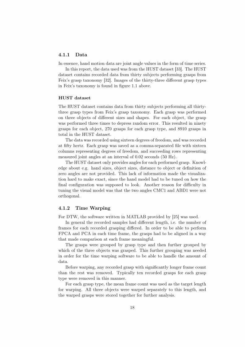
4.1.1 Data
In essence, hand motion data are joint angle values in the form of time series.In this report, the data used was from the HUST dataset [33]. The HUST
dataset contains recorded data from thirty subjects performing grasps fromFeix’s grasp taxonomy [32]. Images of the thirty-three different grasp typesin Feix’s taxonomy is found in figure 1.1 above.
HUST dataset
The HUST dataset contains data from thirty subjects performing all thirty-three grasp types from Feix’s grasp taxonomy. Each grasp was performedon three objects of different sizes and shapes. For each object, the graspwas performed three times to depress random error. This resulted in ninetygrasps for each object, 270 grasps for each grasp type, and 8910 grasps intotal in the HUST dataset.
The data was recorded using sixteen degrees of freedom, and was recordedat fifty hertz. Each grasp was saved as a comma-separated file with sixteencolumns representing degrees of freedom, and succeeding rows representingmeasured joint angles at an interval of 0.02 seconds (50 Hz).
The HUST dataset only provides angles for each performed grasp. Knowl-edge about e.g. hand sizes, object sizes, distance to object or definition ofzero angles are not provided. This lack of information made the visualiza-tion hard to make exact, since the hand model had to be tuned on how thefinal configuration was supposed to look. Another reason for difficulty intuning the visual model was that the two angles CMC1 and ABD1 were notorthogonal.
4.1.2 Time Warping
For DTW, the software written in MATLAB provided by [25] was used.In general the recorded samples had different length, i.e. the number of
frames for each recorded grasping differed. In order to be able to performFPCA and PCA in each time frame, the grasps had to be aligned in a waythat made comparison at each frame meaningful.
The grasps were grouped by grasp type and then further grouped bywhich of the three objects was grasped. This further grouping was neededin order for the time warping software to be able to handle the amount ofdata.
Before warping, any recorded grasp with significantly longer frame countthan the rest was removed. Typically ten recorded grasps for each grasptype were removed in this manner.
For each grasp type, the mean frame count was used as the target lengthfor warping. All three objects were warped separately to this length, andthe warped grasps were stored together for further analysis.
18

no. joint1 CMC12 ABD13 MCP14 IP15 MCP26 PIP27 DIP28 MCP39 PIP310 DIP311 MCP412 PIP413 DIP414 MCP515 PIP516 DIP5
Figure 4.1: Description of the sixteen DoFs used in the HUST dataset. Thenumbering of joints (e.g. PIP4) is referring to the corresponding finger; 1 =thumb, 2 = index finger, 3 = middle finger, 4 = ring finger, 5 = little finger.
The DTW procedure resulted in the warped grasps as well as their warp-ing paths, where the latter were mappings between warped frames and orig-inal frames. Thus statistical analysis could be carried out on the warpedgrasps as well as the warping paths separately.
4.1.3 FPCA implementation
From DTW, a collection of warped grasps of the same length for each grasptype was provided. To get data which was suitable for FPCA, the warpeddata was divided by DoF. So in each grasp type, the data was divided intosixteen datasets, each one describing realizations of one degree of freedom.
FPCA was performed separately on each DoF. This means that for eachgrasp type, FPCA was performed sixteen times, once for each DoF. Thefirst two FPCs were used for each DoF. For FPCA, the R package fda.uscprovided by [23] was used.
FPCA on Warping Paths
FPCA was also carried out on the warping paths of each grasp type. Forthis analysis only one FPC was used since it preserved one hundred percentof the variation. Thus each warping path could be represented by the linearcombination of the mean function and the first FPC of its grasp type.
19

FPCA with preceding PCA
An alternative approach was attempted, wherein FPCA was preceded byPCA. The purpose of this approach was to further reduce the dimensionalityof the data, resulting in less variables to control for.
After DTW, PCA was performed in each successive frame. The firstPCs of every frame were concatenated together in chronological order, andthe same thing was done to the second PCs and so on. The purpose ofthis procedure was to create a time dependent function of how the graspchanged over time with lower dimensionality. FPCA was then applicable tothe weights of the concatenated PCs.
Given a discrete measurement of a grasp in T time frames, g = {gt
}Tt=1,
gt
2 R16, the first step was to carry out PCA in each time frame, t, so that
gt
⇡dX
i=1
↵i,t
p
i,t
, (4.1)
where p
i,t
is the i :th PC at frame t, d is the number of PCs and ↵i,t
is theprojection of g
t
onto p
i,t
(assuming that p
i,t
is chosen so that kpi,t
k2 = 1).The next step was to concatenate each PC’s projections as ↵
i
= {↵i,t
}Tt=1
to get the evolution of the projections over time. Then ↵i
was approximatedas a continuous function and FPCA was performed on it, so that
↵i
(⌧) ⇡kX
j=1
�i,j
f
i,j
(⌧), (4.2)
where f
i,j
is the j :th FPC for ↵i
, k is the number of FPCs and �i,j
is theprojection of ↵
i
onto f
i,j
(assuming that kfi,j
kL2 = 1).
In summary, combining (4.1) and (4.2) gives
gt
⇡dX
i=1
⇣ kX
j=1
�i,j
f
i,j
⌘(t) p
i,t
. (4.3)
4.1.4 GMMs
From FPCA, each DoF of the warped grasp could be approximately repre-sented by the mean function and a linear combination of FPCs. For eachDoF, two FPCs were used and hence two weights were needed for represen-tation. The way in which new grasps was generated was through samplingFPC weights from GMMs.
In order to train GMMs for this purpose, all grasps was projected on theFPCs of their own grasp type in order to obtain their FPC weights. For eachDoF, the set of all two-tuples containing the two weights for a projected DoFwere used to train a two dimensional GMM with two components. Whenthe GMMs were trained, weights could be sampled from them.
20
To generate new grasps, weights were sampled from the GMMs and usedto make linear combinations of FPCs as described in (2.5).
For training GMMs, the R package mixtools provided by [15] was used.In this package, the expectation-maximization (EM) algorithm is used tofind the parameters for normal distributions contained in the GMMs.
4.1.5 Visualization
For visualizing grasping motions, the page http://www.mymodelrobot.appspot.com/ was used [35]. To use this site a model had to be defined, which wasprovided by Gleechi. Grasping motions could then be visualized by providingcomma separated files with angles of each joint defined in the model.
4.2 Classification
For evaluating how well each model was at representing its specific type ofgrasp, a classification scheme was performed in which all unwarped graspwere fed into each model to determine how well that model was able torepresent the grasp.
When a grasp was fed to the model, the first step was to warp the grasp tothe warped time of the model. The warping was done by the mean functionobtained from FPCA on warping paths.
Next, the warped grasp was projected on the FPCs and the L2 distancewas calculated between the warped grasp, g, and its projection,
kg �kX
i=1
hg,fk
ifk
kL2 , (4.4)
where f
k
is the k:th FPC of the model.For comparison, a classification based on PCA of the last frame of each
grasp type was performed. Similarly to the first approach, the Euclideandistance between the last frame of each grasp and its projection was calcu-lated.
21

22

Chapter 5
Results
In this chapter the results of the analysis are presented and discussed.In the first section the results of each individual implemented technique
is presented, then in the next section the results from generating grasps arepresented, finally the results of the classification is presented.
5.1 Result of implemented techniques
In this section, the result of each implemented technique is presented. Anoverlook of time warping and GMM training can be found in table 5.1 below,of which the details will be further discussed in the following sections.
23

Object Target frames Warping EM-algorithm1 Large Diameter 432 Small Diameter 41 linear3 Medium Wrap 424 Adducted Thumb 40 linear5 Light Tool 386 Prismatic 4 Finger 427 Prismatic 3 Finger 448 Prismatic 2 Finger 409 Palmar Pinch 32 Fail on DoF 1310 Power Disk 47 linear11 Power Sphere 43 linear12 Precision Disk 4413 Precision Sphere 4114 Tripod 3915 Fixed Hook 3716 Lateral 37 linear17 Index Finger Extension 4018 Extension Type 3919 Distal Type 5420 Writing Tripod 39 linear21 Tripod Variation 44 linear22 Parallel Extension 34 Fail on DoF 9, 10, 1323 Adduction Grip 4224 Tip Pinch 3625 Lateral Tripod 3826 Sphere 4 Finger 4227 Quadpod 4128 Sphere 3 Finger 4629 Stick 41 linear30 Palmar 3731 Ring 39 Fail on dof 10, 13, 15, 1632 Ventral 3733 Inferrior Pincer 40 Fail on dof 10, 13, 14, 15
Table 5.1: Summary of warping and GMM training for each model. In thecolumn Warping it is stated if linear warping had to be used as described insection 5.1.1. In the column EM-algorithm it is stated if problems occurredwhen training the GMMs due to EM-algorithm diverging as described insection 5.1.4.
24

5.1.1 Time warping
Time warping was performed on each grasp type with target length set tothe mean frame length of data of that grasp type.
The warping was not always satisfactory for all grasps. This manifesteditself as a repetition of a single time frame in the warped grasp, as can beseen in fig 5.1. Any grasp that was warped in this manner was removed. Theamount of unsatisfactory warps was typically one or two for each object.
Figure 5.1: Example from time warping of medium wrap. The left subfigureshows a histogram of sample lengths before warping. The right subfigureshows warping paths, where two paths can be seen to be stationary in longintervals. In this example all warping paths are defined between frame zeroand forty-two
In eight cases out of thirty-three, the warping software failed altogetherand was unable to produce results. In these cases, a simpler form of warpingwas used instead, where the warping paths were linear. An example ofthis can be seen in fig 5.2. The models in which linear warping had to beused were small diameter, adducted thumb, power disk, power sphere, lateral,writing tripod, tripod variation and stick.
25
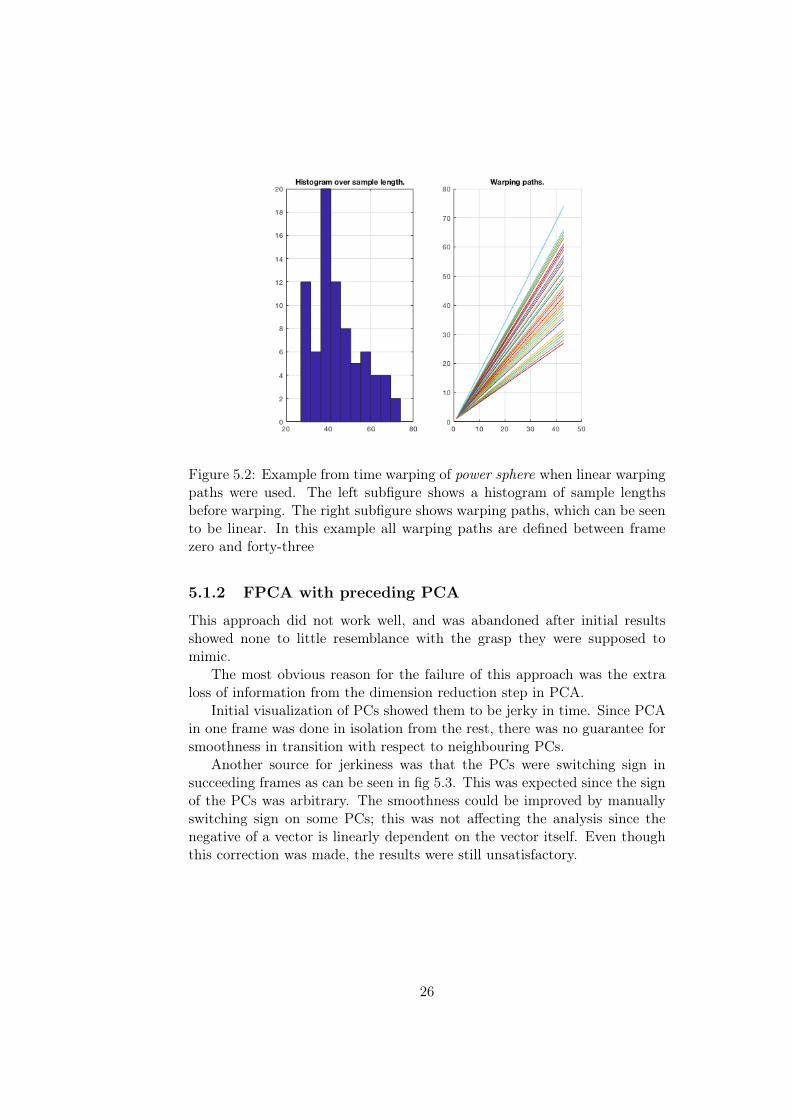
Figure 5.2: Example from time warping of power sphere when linear warpingpaths were used. The left subfigure shows a histogram of sample lengthsbefore warping. The right subfigure shows warping paths, which can be seento be linear. In this example all warping paths are defined between framezero and forty-three
5.1.2 FPCA with preceding PCA
This approach did not work well, and was abandoned after initial resultsshowed none to little resemblance with the grasp they were supposed tomimic.
The most obvious reason for the failure of this approach was the extraloss of information from the dimension reduction step in PCA.
Initial visualization of PCs showed them to be jerky in time. Since PCAin one frame was done in isolation from the rest, there was no guarantee forsmoothness in transition with respect to neighbouring PCs.
Another source for jerkiness was that the PCs were switching sign insucceeding frames as can be seen in fig 5.3. This was expected since the signof the PCs was arbitrary. The smoothness could be improved by manuallyswitching sign on some PCs; this was not affecting the analysis since thenegative of a vector is linearly dependent on the vector itself. Even thoughthis correction was made, the results were still unsatisfactory.
26

Figure 5.3: Projections reveal sign changes in principal components at suc-cessive frames.
5.1.3 FPCA
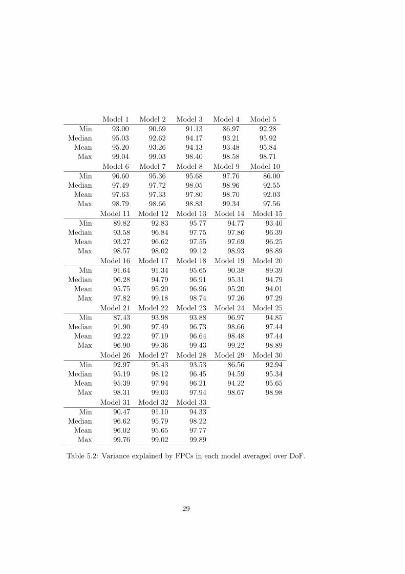
Considering all analyses, FPCA with two FPCs was able to explain between86.00 and 99.89 percent of the variance in the data, with a mean at 95.90percent. Thus the FPCs was successful in spanning a large subspace of thedata and consequently had the capacity of making good approximations ofjoint angles. This means that successful grasp generation was most likelynot severely restricted by FPCs’ inability to reproduce certain grasp config-urations lying outside FPC-space.
Variance explained by FPCs is presented in more detail in table 5.2 below.An example of FPCA visualization together with data is presented in
fig 5.4. And an example of data expressed as linear combination of FPCs ispresented in fig 5.5. In these figures it can be seen that FPCs gives reasonablygood approximations of the curves.
27

0 10 20 30 40
0.0
0.5
1.0
frames
radians
Figure 5.4: Example of samples of an angle and result of FPCA. Samplesare in grey and mean function added to FPCs are in red.
0 10 20 30 40
0.0
0.2
0.4
0.6
frames
radians
Figure 5.5: Example of a sample and its projection on FPCs. Sample is ingrey and its projection is in red.
28
Model 1 Model 2 Model 3 Model 4 Model 5Min 93.00 90.69 91.13 86.97 92.28
Median 95.03 92.62 94.17 93.21 95.92Mean 95.20 93.26 94.13 93.48 95.84Max 99.04 99.03 98.40 98.58 98.71
Model 6 Model 7 Model 8 Model 9 Model 10Min 96.60 95.36 95.68 97.76 86.00
Median 97.49 97.72 98.05 98.96 92.55Mean 97.63 97.33 97.80 98.70 92.03Max 98.79 98.66 98.83 99.34 97.56
Model 11 Model 12 Model 13 Model 14 Model 15Min 89.82 92.83 95.77 94.77 93.40
Median 93.58 96.84 97.75 97.86 96.39Mean 93.27 96.62 97.55 97.69 96.25Max 98.57 98.02 99.12 98.93 98.89
Model 16 Model 17 Model 18 Model 19 Model 20Min 91.64 91.34 95.65 90.38 89.39
Median 96.28 94.79 96.91 95.31 94.79Mean 95.75 95.20 96.96 95.20 94.01Max 97.82 99.18 98.74 97.26 97.29
Model 21 Model 22 Model 23 Model 24 Model 25Min 87.43 93.98 93.88 96.97 94.85
Median 91.90 97.49 96.73 98.66 97.44Mean 92.22 97.19 96.64 98.48 97.44Max 96.90 99.36 99.43 99.22 98.89
Model 26 Model 27 Model 28 Model 29 Model 30Min 92.97 95.43 93.53 86.56 92.94
Median 95.19 98.12 96.45 94.59 95.34Mean 95.39 97.94 96.21 94.22 95.65Max 98.31 99.03 97.94 98.67 98.98
Model 31 Model 32 Model 33Min 90.47 91.10 94.33
Median 96.62 95.79 98.22Mean 96.02 95.65 97.77Max 99.76 99.02 99.89
Table 5.2: Variance explained by FPCs in each model averaged over DoF.
29

5.1.4 GMMs
Finding proper parameters for GMMs was in some cases unsuccessful, due tothe EM-algorithm diverging. In these cases a single two-dimensional Gaus-sian distribution was used instead, with parameters sample mean and samplecovariance. The cases in which the EM-algorithm failed can be seen in table5.1.
An example of how the probability distributions obtained for GMMscould look is presented in fig 5.6.
-3 -2 -1 0 1 2 3
-3-1
01
23
-0.6 -0.2 0.2 0.6
-0.6
-0.2
0.2
0.6
-0.5 0.0 0.5-0.5
0.0
0.5
-3 -2 -1 0 1 2 3
-3-1
12
3-2 -1 0 1 2
-2-1
01
2
-2 -1 0 1 2
-2-1
01
2
-1.0 -0.5 0.0 0.5 1.0
-1.0
-0.5
0.0
0.5
1.0
-2 -1 0 1 2-2
-10
12
-2 -1 0 1 2
-2-1
01
2
-0.5 0.0 0.5
-0.5
0.0
0.5
-4 -2 0 2 4
-4-2
02
4
-2 -1 0 1 2
-2-1
01
2
-1.0
0.0
1.0
-4-2
02
4
-3-1
01
23
-3-2
-10
12
3
Figure 5.6: Example of probability distribution of GMMs. This plot showsprobability distribution function level curves of GMMs for grasp type writingtripod. First DoF is shown in top left corner and following DoFs proceedsfrom left to right.
The probability distributions had means centered at zero. Weights setto zero corresponded to linear combinations of FPCs consisting only of themean function.
From inspection of the probability distributions, it could be seen thatthe range of values likely to be obtained from the GMMs were relativelylarge, which indicated some variation in the training data and consequentlyvariation in the generated weights.
Since the variance of weight values were relatively large, the FPCs werethus significant in the linear combinations for generated grasps; contrary to
30

weights being very small and generated grasps being mostly governed by themean functions.
One likely source for this variation is that hand sizes and shapes differ,producing different sets of angles for the same task. Since the data setcontains data from thirty different subjects, it is very likely that some setsof angles acted in unison in this way. Taking angle values from significantlydifferent hand shapes might also produce incorrect hand configurations forthe task to some degree.
In light of this, the absence of correlation between DoFs in the modelwas likely to have an effect on the generated data.
5.2 Generating grasps
The grasps generated by the models were in general similar to the grasp typesthey were supposed to mimic; they were able to capture distinct features.However, more subtle features were not captured. For example, this was thecase for grasps that are only distinguished by how many fingers are in contactwith the object, e.g. grasp types prismatic 4 finger, prismatic 3 finger andprismatic 2 finger. For comparison, appendix A contains images of the lastframe of generated grasps next to grasps from the training data of each type.
In general, there were two issues with the grasps generated by the models.First, fingers did not move in unison, resulting in configurations where theywere not equally bent. Second, in many cases generated grasps looked similarto generated grasps of other types, which made it hard to identify the specificgrasp. The second issue is most likely a consequence of the first since fingersnot moving in unison made some distinguishable features disappear. Thiswas for example the case for grasp types prismatic 4 finger, prismatic 3 fingerand prismatic 2 finger mentioned above.
As was mentioned earlier, it is important to note that the space rep-resented by joint angles are not in one-to-one correlation with the handconfiguration space when considering many subjects. This is due to differ-ences in hand shapes and sizes, i.e. when two individuals perform the sametype of grasp, the joint angles are not guaranteed to be the same. Thus itwas not expected that joint angles alone could sufficiently describe a handconfiguration. In light of this, the fact that each DoF was modeled sepa-rately is most likely an important factor for the fingers not moving in unisonand for many grasp types being indistinguishable. This means that corre-lation between DoFs was not included in the model, and in extension thatindividual-specific variations were not accounted for.
In table 5.3, the mean L2-distances between grasps and its projectionsare presented. In each row, the values have been divided by the framelength of the model to facilitate comparison between rows. This table givesan indication of how well the different models were performing. In twenty-
31

eight cases the model had its lowest mean distance for its own grasp type.In fourteen cases the grasp type had its lowest mean distance for its ownmodel. And in twelve cases it happened simultaneously that the model hadits lowest mean distance for its own grasp type and that the grasp type hadits lowest mean distance for its own model. Worth noting is that nine grasptypes had their lowest mean distance for model nine, palmar pinch, whilesixteen models were not the minimum mean distance of any grasp type.
These observations indicate that the set of models does not amount toa very good distinction between grasps. From visual inspection, there wereseveral groups of grasps that were hard to discern from one another. Onesuch group of grasps that was not easily distinguishable from one anotherconsists of grasp types adducted thumb, light tool and fixed hook. Anothergroup consists of types prismatic 4 finger, prismatic 3 finger. prismatic 2finger and writing tripod. A third group consists of grasp types precisiondisk, precision sphere and tripod.
32

Gra
spty
pe
Mod
el1
23
45
67
89
1011
1213
1415
1617
1819
2021
2223
2425
2627
2829
3031
3233
17.
3411
.62
11.1
612
.33
13.8
89.
739.
7211
.02
12.8
114
.54
10.3
09.
2610
.65
10.7
912
.90
14.1
012
.67
9.96
8.23
12.3
712
.37
12.0
79.
5111
.38
10.6
99.
3710
.86
8.87
18.4
013
.46
10.3
415
.92
10.0
52
12.2
211
.80
11.5
914
.01
14.5
216
.93
16.8
218
.84
20.9
814
.50
12.8
113
.82
18.3
017
.80
13.4
619
.31
14.3
714
.67
12.1
617
.49
17.0
818
.01
14.0
319
.21
17.5
812
.65
18.9
211
.59
17.0
313
.52
14.8
615
.19
15.0
73
11.7
711
.95
10.3
012
.90
12.9
615
.46
15.6
316
.90
18.4
814
.64
12.6
212
.31
16.7
215
.87
12.2
617
.09
13.4
313
.31
12.0
515
.83
15.6
716
.76
12.5
017
.29
15.7
811
.64
17.2
110
.79
15.9
412
.64
13.9
314
.22
13.8
24
11.0
111
.49
10.2
910
.02
11.6
214
.35
14.9
415
.68
17.4
314
.86
12.4
111
.55
15.6
514
.86
10.6
616
.07
12.5
012
.30
10.8
414
.97
14.6
715
.96
11.1
316
.15
14.5
811
.19
15.9
210
.15
14.4
911
.55
13.6
613
.02
13.1
85
13.0
213
.39
12.2
616
.13
8.91
15.2
716
.04
16.0
116
.62
13.8
514
.24
11.6
116
.68
14.9
79.
5318
.48
13.0
414
.09
10.5
118
.37
18.9
816
.89
10.3
816
.71
14.9
510
.59
16.8
310
.32
11.9
711
.50
14.6
411
.66
13.1
96
9.20
12.3
410
.37
13.8
810
.77
6.00
6.32
6.75
7.60
14.3
312
.34
7.08
6.76
6.77
10.3
310
.48
10.1
58.
167.
699.
9811
.11
9.77
7.45
7.11
7.04
7.84
6.70
7.77
13.7
311
.19
10.0
612
.32
9.04
79.
5513
.07
11.2
413
.60
12.1
96.
796.
497.
088.
6015
.07
12.4
47.
777.
527.
2911
.39
10.7
811
.33
8.49
8.17
9.96
10.8
110
.34
8.15
7.80
7.51
8.66
7.33
8.36
14.6
212
.46
10.3
813
.09
9.57
810
.89
14.8
412
.62
15.2
312
.88
7.16
7.04
6.99
8.81
16.4
314
.16
8.47
7.86
7.48
12.5
011
.06
12.1
79.
039.
0010
.93
11.8
111
.25
8.69
7.86
7.66
9.42
7.56
9.04
15.0
314
.28
11.6
913
.49
10.8
59
8.04
12.7
011
.42
13.7
911
.82
5.55
6.05
5.91
5.22
14.4
011
.03
6.00
5.46
5.64
11.4
610
.93
11.1
97.
566.
5810
.83
11.2
57.
396.
235.
476.
017.
235.
477.
5216
.63
12.6
18.
0214
.41
6.77
1015
.75
15.1
214
.43
22.2
814
.03
20.9
921
.17
23.0
624
.25
10.7
014
.14
15.6
522
.77
21.5
513
.64
25.1
616
.59
19.4
811
.51
23.5
524
.63
23.0
814
.64
23.6
721
.56
12.8
523
.42
13.5
916
.22
14.5
816
.85
15.6
715
.53
119.
6911
.33
10.6
313
.57
13.2
312
.81
12.5
714
.51
16.5
812
.76
9.59
10.8
413
.82
13.9
412
.63
15.8
012
.77
12.3
29.
0514
.56
14.6
015
.61
11.4
514
.82
13.6
89.
9114
.30
9.46
17.5
413
.03
11.5
115
.40
11.4
512
8.44
12.3
310
.95
14.6
412
.37
6.98
7.26
7.85
8.32
12.9
910
.12
6.16
7.03
7.37
11.6
812
.45
11.0
28.
766.
9311
.27
12.2
89.
977.
247.
917.
677.
137.
207.
4116
.94
12.8
39.
0614
.45
7.90
138.
5812
.62
10.9
014
.26
11.8
95.
886.
106.
516.
8913
.77
10.9
65.
965.
516.
1611
.29
11.0
810
.38
7.80
7.19
9.86
10.8
59.
027.
016.
346.
527.
485.
707.
6615
.91
12.0
09.
0713
.70
8.03
149.
9413
.78
11.8
614
.94
11.8
96.
496.
646.
657.
7515
.04
12.8
67.
416.
726.
3211
.58
10.3
010
.84
8.18
8.00
9.91
11.1
610
.18
7.57
7.06
6.90
8.47
6.47
8.22
14.0
913
.03
10.8
512
.30
9.74
1512
.64
12.9
711
.78
13.3
49.
6115
.69
16.2
816
.70
18.0
714
.04
13.8
512
.19
17.3
215
.79
9.19
18.0
912
.86
13.7
310
.43
17.3
417
.14
17.7
610
.72
17.5
715
.17
11.2
017
.41
10.8
112
.46
10.5
914
.73
11.7
513
.36
1613
.04
14.3
312
.23
14.8
712
.08
8.87
8.87
8.88
10.8
917
.26
16.6
19.
599.
378.
7611
.49
8.89
10.6
48.
8611
.43
10.8
511
.17
14.2
19.
679.
178.
6910
.95
8.94
10.5
511
.85
11.4
413
.26
11.1
012
.99
1712
.99
15.4
014
.36
16.1
414
.39
14.0
914
.24
14.7
616
.19
15.3
514
.14
11.7
815
.00
14.2
013
.72
16.9
39.
2912
.32
11.1
716
.43
15.7
015
.90
11.7
015
.72
13.9
011
.82
15.4
011
.51
15.2
614
.04
16.0
611
.47
14.8
618
10.5
913
.91
12.3
313
.16
13.3
69.
469.
619.
9610
.96
16.5
313
.83
9.39
9.87
9.55
12.6
912
.46
11.5
78.
109.
9611
.84
11.0
111
.45
9.28
10.0
29.
7410
.27
10.0
39.
7915
.77
12.4
211
.59
13.5
011
.39
1911
.08
14.4
812
.79
16.7
712
.21
10.3
710
.68
11.4
212
.43
15.1
113
.74
10.2
310
.97
10.8
812
.13
15.2
813
.20
11.7
17.
9114
.71
15.5
113
.46
10.1
611
.61
11.3
210
.04
10.8
99.
6415
.39
13.8
011
.87
14.2
010
.68
2012
.44
14.8
112
.51
15.1
713
.44
9.32
9.03
9.66
11.7
716
.97
15.4
69.
829.
789.
6012
.57
11.7
311
.98
9.44
10.9
19.
8910
.30
13.7
010
.38
9.99
9.29
11.0
89.
5610
.69
13.8
612
.69
13.6
112
.39
13.4
121
14.0
716
.69
14.2
816
.11
15.1
511
.33
11.0
211
.83
14.4
518
.40
16.8
911
.56
11.9
911
.89
14.4
014
.31
13.2
810
.86
11.9
512
.08
10.9
715
.42
11.8
512
.04
11.3
612
.81
11.8
612
.41
15.6
414
.48
15.4
514
.06
15.5
522
9.14
16.4
815
.63
14.3
416
.87
9.20
9.54
9.26
8.25
18.1
912
.68
8.26
8.09
8.53
15.9
615
.68
13.9
67.
197.
2014
.16
11.4
15.
567.
728.
449.
1110
.30
8.58
10.1
423
.93
17.1
49.
2118
.78
8.47
239.
4812
.44
10.9
712
.78
10.6
58.
568.
969.
099.
9713
.86
11.4
58.
079.
158.
7010
.51
11.4
210
.88
8.87
7.57
11.3
511
.69
11.1
57.
089.
348.
588.
608.
998.
2513
.83
11.5
410
.44
12.0
39.
2524
9.17
13.2
411
.40
14.3
112
.07
6.07
6.43
6.43
6.73
15.3
012
.48
6.80
6.25
6.37
11.6
310
.86
11.4
97.
947.
6110
.74
11.2
29.
247.
206.
056.
808.
206.
198.
3415
.95
12.6
79.
0814
.25
8.24
2510
.12
13.5
011
.49
13.9
011
.79
6.68
6.50
6.53
8.13
15.2
513
.15
7.46
7.13
6.67
11.0
89.
6410
.27
7.89
8.33
9.04
9.96
10.5
57.
647.
016.
408.
586.
678.
4613
.06
12.1
011
.36
11.2
110
.48
2610
.18
12.4
911
.11
16.6
111
.37
10.1
410
.48
11.8
412
.22
12.4
511
.48
8.62
11.1
510
.78
11.2
414
.96
12.4
811
.76
8.04
14.5
616
.24
13.5
89.
1912
.20
11.2
07.
6511
.33
7.96
15.3
312
.87
11.2
613
.92
9.83
279.
1912
.75
10.9
214
.53
11.4
95.
946.
046.
447.
0714
.08
12.0
56.
495.
896.
1210
.89
10.6
510
.37
7.94
7.39
9.62
10.9
09.
727.
226.
496.
467.
655.
647.
5614
.31
11.8
79.
9312
.51
8.87
2811
.42
13.3
611
.87
16.9
111
.83
11.5
611
.81
12.7
613
.52
14.5
413
.44
9.96
12.5
011
.82
11.9
115
.83
12.9
111
.97
9.45
15.3
916
.48
14.2
010
.36
13.3
012
.27
9.35
12.5
78.
5014
.86
13.4
612
.63
13.4
311
.54
2914
.49
14.9
513
.74
16.5
011
.81
15.1
915
.54
15.6
617
.30
16.7
016
.95
13.0
017
.04
15.3
511
.84
18.1
513
.41
13.2
912
.85
17.5
816
.66
17.3
012
.07
16.7
715
.13
12.5
717
.17
11.7
411
.59
12.5
616
.57
11.7
415
.82
3013
.28
13.1
712
.17
14.0
611
.68
15.9
416
.29
16.8
318
.23
14.6
914
.31
12.7
517
.34
16.0
511
.04
17.3
212
.85
13.3
111
.85
16.8
416
.25
17.6
211
.38
17.3
815
.33
12.1
817
.55
11.6
312
.98
10.4
015
.09
12.1
714
.25
318.
9313
.24
12.5
315
.85
15.3
99.
599.
4610
.01
10.4
815
.32
10.6
18.
178.
929.
6214
.57
15.2
215
.78
9.93
7.87
13.8
713
.86
10.2
08.
959.
579.
639.
089.
249.
1122
.07
14.9
26.
7719
.37
7.05
3213
.00
14.8
514
.03
14.9
812
.12
14.7
315
.19
15.4
716
.52
15.7
914
.87
12.2
116
.36
14.8
811
.89
17.7
210
.53
12.4
811
.10
17.2
615
.87
15.8
110
.89
16.4
214
.62
11.5
516
.72
11.1
812
.11
12.5
916
.44
9.67
15.2
333
8.09
12.5
311
.75
15.7
313
.83
7.69
7.89
8.14
7.79
14.1
710
.15
6.59
6.95
7.45
13.3
013
.94
14.5
48.
876.
6112
.83
13.0
68.
727.
227.
377.
887.
437.
137.
8620
.71
14.4
96.
0318
.31
5.08
Tabl
e5.
3:Ta
ble
show
ing
mea
nof
L2-d
ista
nces
ofgr
asp
type
san
dit
spr
ojec
tion
s.T
heva
lues
was
mul
tipl
ied
bya
fact
orof
hund
red
and
divi
ded
bym
odel
fram
ele
ngth
,100·kg�proj igk/
Ti
for
the
purp
oses
ofea
sier
read
ing
and
com
paris
onbe
twee
nce
llsre
spec
tive
ly.
Row
srep
rese
ntst
atis
tica
lmod
elan
dco
lum
nsre
pres
entg
rasp
type
.T
hece
llde
fined
bye.
g.ro
wfiv
e,co
lum
nfo
ursh
ows
the
mea
nL2
dist
ance
whe
nal
lgra
sps
ofty
pefo
urw
asfe
din
toth
em
odel
crea
ted
for
gras
pty
pefiv
e.C
ompa
ring
this
colu
mn
wit
hth
ece
llde
fined
byro
wfo
ur,c
olum
nfiv
esh
ows
that
the
clas
sific
atio
nis
not
sym
met
ric.
The
low
est
valu
efo
rea
chst
atis
tica
lmod
elha
sbe
enhi
ghlig
hted
.T
helo
wes
tva
lue
for
each
gras
pty
peha
sbe
enfr
amed
.
33

5.2.1 Temporal comparison
Disregarding how well the grasp type was captured by the model, the tem-poral aspect was in general well captured in the models. There was no signif-icant issues in this aspect, like e.g. fluctuations or jerkiness. The generatedgrasps lacked a little bit in smoothness compared to the training data.
Two grasp types have been selected for illustrating temporal comparison.The first case, which is shown in table 5.4, shows grasp type index finger
extension, in which the grasp type was successfully modelled. This case fitswell in the overall description above, since there is a distinctive feature whichwas well captured, namely the extended index finger.
The other case, which is shown in table 5.5, shows grasp type lateraltripod, in which the grasp type was not successfully modelled. This casegives an example of how small variations in bending between fingers was notwell captured.
Data sample Generated sample
1
2
3
4
34

5
6
7
Table 5.4: Temporal comparison between data sample and generated sampleof grasp type index finger extension. In this comparison it can be seen thatthe generated sample did well in capturing the distinct feature of the grasp.
Data sample Generated sample
1
2
35

3
4
5
6
7
Table 5.5: Temporal comparison between data sample and generated sampleof grasp type lateral tripod. In this comparison it can be seen that thegenerated grasp failed to capture the variations in bending between fingers.
5.3 Classification
In this section the results of the two classification approaches using FPCAand last frame PCA are presented.
36

5.3.1 FPCA
Using the models for classification was not successful. For some grasp types,grasps were more often classified outside their own type than not. It washowever expected that the classification would perform badly for two reasons.First, in the classification procedure, all DoFs were weighted equally, so thatthe overall hand posture was considered for classification. This approachwas clearly not proficient at identifying distinctive features of each grasp.Second, the FPCA-based classification used the whole temporal movementof the hand, but grasp types are identified by the final configuration onlyand much of the initial movement was similar for all the grasps. Thus theidentifying posture was a smaller part of the movement. The confusionmatrix for classification is presented in table 5.6 below.
The worst case was grasp type stick, which was only correctly classifiedsix times. The most successful case was grasp parallel extension, with two-hundred and fifteen correctly classified grasps. These results are reasonablewhen comparing to the other grasps; parallel extension is very distinct inthe sense that there are no other grasps in which almost all fingers are fullyextended, thus creating a big difference in terms of joint angles. Grasp typestick on the other hand has a similar configuration to many other grasptypes, e.g. light tool and fixed hook.
As in table 5.3, some models are overrepresented in classification, mostprominently model nine, palmar pinch, which nine grasp types were mostoften classified as. There were however less grasp types more often classifiedoutside their own model in the confusion matrix compared to how manygrasp types had their lowest mean distance outside their own model.
In general, the confusion matrix in table 5.6 shows a similar pattern asin table 5.3 above. Grasp types classified in models correspond in generalto grasp types having low mean L2-distances in that model compared toothers. This is expected since the the L2-distance between grasps and theirprojections was used in both cases. Numbers were not divided by framelength in the confusion matrix as in table 5.3.
37

Grasp
type
Model
12
34
56
78
910
1112
1314
1516
1718
1920
2122
2324
2526
2728
2930
3132
331
15524
87
02
61
00
572
10
01
02
31
00
70
10
02
20
00
02
361
145
00
00
00
50
00
00
00
01
00
00
00
02
00
00
03
218
8112
30
00
07
100
00
01
00
01
10
01
00
00
22
00
04
26
1163
00
01
00
20
00
60
00
00
00
10
00
00
01
00
05
02
49
1400
00
117
30
00
535
00
191
30
182
116
025
3823
05
06
80
00
027
267
20
16
99
01
01
70
00
15
61
50
01
00
17
40
00
03
204
10
00
10
01
01
01
10
00
00
10
10
00
08
25
47
38
2053
13
10
09
61
31
74
50
24
210
20
80
04
09
268
132
1588
6081
1836
959
8394
319
912
6521
329
52113
5635
9343
83
222
3710
00
00
00
00
0120
01
00
00
00
00
00
00
00
00
01
00
011
416
130
00
00
03
611
00
00
00
10
00
00
01
03
00
00
012
40
00
23
00
03
243
113
00
10
12
00
05
015
35
00
00
113
20
00
06
22
10
022
554
00
00
00
10
11
11
162
01
00
014
40
30
18
1118
10
05
1348
013
11
613
70
52
140
207
01
03
015
132
3582
480
51
029
70
00
1334
023
304
70
130
111
06
5960
03
016
00
01
11
00
00
10
00
046
01
02
00
10
00
00
21
00
017
01
10
00
00
00
00
00
00
1661
00
50
00
00
00
41
019
018
712
610
16
512
21
32
22
831
1995
640
802
177
110
112
1014
311
019
12
10
11
10
03
10
02
01
00
260
10
00
02
11
20
00
120
02
33
00
01
00
10
01
02
02
027
190
00
00
00
13
01
021
01
41
00
00
00
00
00
00
00
03
100
00
00
00
21
00
022
21
24
15
126
60
24
54
00
449
414
19215
21
21
12
01
34
123
40
14
39
68
60
54
66
58
48
16
20
644
25
17
610
07
024
44
1111
728
2718
250
225
2920
431
019
1827
181
1569
304
174
136
83
525
42
19
27
2626
31
05
233
549
819
1055
520
2710
874
203
126
09
026
1022
1410
410
41
131
4041
01
51
22
100
00
50
0121
451
32
10
027
20
00
123
148
00
012
3021
011
13
610
20
42
97
630
21
00
028
05
72
10
10
00
53
00
20
03
81
00
00
010
160
10
00
029
00
00
10
00
00
00
00
00
00
00
00
00
00
00
60
00
030
013
86
51
20
019
60
00
147
05
26
50
40
11
07
14102
01
031
02
00
00
01
02
80
00
01
00
10
10
02
00
03
00
1560
5332
14
25
10
00
01
00
02
16
301
41
00
20
00
01
461
0171
033
60
61
510
96
82
129
65
28
01
171
00
1513
111
08
47
570
149
Table5.6:
Confusion
matrix
forFP
CA
.
38
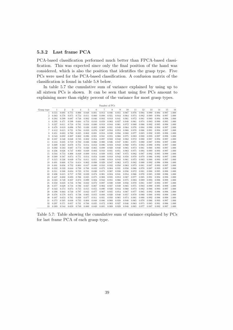
5.3.2 Last frame PCA
PCA-based classification performed much better than FPCA-based classi-fication. This was expected since only the final position of the hand wasconsidered, which is also the position that identifies the grasp type. FivePCs were used for the PCA-based classification. A confusion matrix of theclassification is found in table 5.8 below.
In table 5.7 the cumulative sum of variance explained by using up toall sixteen PCs is shown. It can be seen that using five PCs amount toexplaining more than eighty percent of the variance for most grasp types.
Number of PCs
Grasp type 1 2 3 4 5 6 7 8 9 10 11 12 13 14 15 161 0.555 0.695 0.755 0.806 0.848 0.881 0.912 0.936 0.955 0.967 0.976 0.984 0.990 0.994 0.997 1.0002 0.363 0.576 0.675 0.754 0.811 0.860 0.898 0.921 0.944 0.964 0.974 0.982 0.989 0.994 0.997 1.0003 0.384 0.599 0.687 0.748 0.802 0.846 0.883 0.918 0.941 0.961 0.972 0.981 0.989 0.994 0.998 1.0004 0.295 0.471 0.598 0.684 0.753 0.810 0.859 0.903 0.927 0.948 0.961 0.974 0.983 0.990 0.995 1.0005 0.327 0.611 0.718 0.781 0.834 0.880 0.918 0.944 0.961 0.972 0.980 0.986 0.992 0.995 0.998 1.0006 0.478 0.619 0.696 0.765 0.830 0.882 0.908 0.931 0.949 0.964 0.976 0.984 0.990 0.994 0.997 1.0007 0.412 0.615 0.721 0.784 0.833 0.876 0.907 0.934 0.953 0.968 0.978 0.986 0.991 0.994 0.997 1.0008 0.451 0.683 0.760 0.825 0.862 0.891 0.918 0.938 0.956 0.968 0.977 0.985 0.992 0.995 0.998 1.0009 0.543 0.692 0.807 0.862 0.896 0.921 0.941 0.955 0.966 0.975 0.983 0.988 0.993 0.997 0.998 1.000
10 0.337 0.540 0.648 0.735 0.802 0.854 0.897 0.922 0.942 0.962 0.972 0.980 0.987 0.994 0.997 1.00011 0.444 0.635 0.719 0.782 0.826 0.866 0.900 0.926 0.947 0.961 0.971 0.980 0.987 0.993 0.997 1.00012 0.309 0.562 0.678 0.751 0.814 0.853 0.890 0.923 0.942 0.960 0.974 0.982 0.990 0.994 0.997 1.00013 0.392 0.583 0.687 0.773 0.826 0.865 0.899 0.928 0.948 0.965 0.973 0.981 0.988 0.993 0.997 1.00014 0.436 0.626 0.747 0.803 0.849 0.883 0.910 0.931 0.951 0.963 0.975 0.984 0.989 0.993 0.997 1.00015 0.504 0.753 0.806 0.849 0.889 0.914 0.939 0.955 0.967 0.975 0.982 0.987 0.992 0.995 0.999 1.00016 0.389 0.567 0.674 0.751 0.814 0.854 0.889 0.918 0.942 0.958 0.970 0.979 0.986 0.992 0.997 1.00017 0.315 0.536 0.649 0.754 0.811 0.851 0.890 0.918 0.943 0.961 0.973 0.983 0.988 0.993 0.997 1.00018 0.491 0.668 0.754 0.814 0.862 0.898 0.929 0.947 0.962 0.972 0.982 0.988 0.992 0.996 0.998 1.00019 0.401 0.656 0.752 0.804 0.847 0.880 0.910 0.932 0.950 0.963 0.973 0.981 0.987 0.993 0.997 1.00020 0.332 0.533 0.644 0.730 0.788 0.832 0.872 0.904 0.931 0.950 0.966 0.978 0.987 0.993 0.997 1.00021 0.311 0.508 0.634 0.723 0.781 0.830 0.875 0.907 0.938 0.956 0.972 0.981 0.988 0.995 0.998 1.00022 0.496 0.615 0.717 0.789 0.839 0.874 0.901 0.924 0.941 0.954 0.966 0.976 0.985 0.990 0.996 1.00023 0.427 0.602 0.693 0.766 0.825 0.875 0.908 0.935 0.953 0.967 0.977 0.985 0.991 0.994 0.998 1.00024 0.583 0.749 0.837 0.873 0.899 0.924 0.943 0.955 0.966 0.975 0.983 0.989 0.993 0.996 0.999 1.00025 0.350 0.623 0.716 0.786 0.832 0.872 0.897 0.920 0.939 0.956 0.970 0.981 0.987 0.993 0.997 1.00026 0.377 0.629 0.716 0.786 0.827 0.867 0.902 0.927 0.949 0.965 0.975 0.983 0.990 0.995 0.998 1.00027 0.343 0.574 0.674 0.755 0.815 0.855 0.890 0.920 0.944 0.960 0.973 0.982 0.988 0.993 0.997 1.00028 0.398 0.663 0.740 0.797 0.842 0.877 0.907 0.935 0.954 0.967 0.977 0.985 0.992 0.996 0.998 1.00029 0.376 0.579 0.671 0.738 0.805 0.855 0.888 0.920 0.940 0.957 0.970 0.980 0.988 0.993 0.998 1.00030 0.487 0.653 0.761 0.830 0.877 0.911 0.931 0.950 0.965 0.974 0.981 0.988 0.992 0.996 0.998 1.00031 0.272 0.505 0.648 0.735 0.804 0.848 0.886 0.908 0.928 0.948 0.965 0.978 0.986 0.993 0.997 1.00032 0.297 0.571 0.657 0.731 0.788 0.835 0.872 0.903 0.927 0.946 0.963 0.975 0.985 0.991 0.996 1.00033 0.389 0.544 0.659 0.749 0.800 0.849 0.885 0.909 0.929 0.948 0.965 0.977 0.987 0.992 0.997 1.000
Table 5.7: Table showing the cumulative sum of variance explained by PCsfor last frame PCA of each grasp type.
39

Grasp
type
Model
12
34
56
78
910
1112
1314
1516
1718
1920
2122
2324
2526
2728
2930
3132
331
19124
200
00
12
00
00
01
50
03
10
20
00
06
00
00
00
02
12148
282
25
91
00
20
00
02
07
40
110
25
01
02
00
00
03
1142
1663
50
10
00
00
00
011
01
41
00
12
00
00
02
00
04
11
7168
270
00
00
00
00
390
04
11
00
30
00
00
02
00
05
00
115
1450
00
10
00
00
3615
00
00
00
81
00
00
108
03
06
82
00
0159
140
03
90
52
11
03
160
00
21
03
50
08
00
07
10
00
04
17318
82
20
02
00
02
02
50
03
011
70
014
00
08
01
00
00
2139
80
00
020
00
01
1015
20
215
211
016
00
00
09
30
00
01
00
1350
00
02
00
00
260
20
047
20
10
00
20
2010
00
00
02
50
0202
58
111
00
01
00
00
00
07
01
05
00
011
21
00
019
73
58
13414
110
00
00
00
00
13
017
170
02
00
012
02
00
04
20
013
20139
110
00
01
00
00
00
047
00
02
00
013
00
00
09
20
06
2234
1340
00
00
00
00
00
030
80
04
00
014
00
10
08
114
30
00
0158
00
04
282
40
10
233
09
01
00
015
00
044
300
00
00
00
00
1535
00
00
00
00
00
00
110
00
016
00
20
170
01
10
00
00
1196
05
03
30
31
00
00
010
02
317
00
00
00
00
00
00
00
00
2280
40
00
00
00
00
00
012
018
54
310
10
10
30
00
00
36
0144
115
1511
95
20
05
11
20
019
03
41
110
215
100
10
323
11
39
903
40
814
112
77
07
10
820
11
02
00
02
20
00
02
06
08
8110
370
114
340
85
01
00
021
81
10
00
11
80
00
00
00
027
19
1450
113
50
114
06
00
022
00
00
00
30
00
00
00
00
019
00
0225
00
00
00
00
00
023
00
04
85
104
00
30
22
45
02
21
10
1733
102
03
45
00
024
00
10
00
03
450
00
02
00
01
172
00
8136
00
01
06
40
1025
00
40
03
416
130
00
024
02
02
2021
100
22
1090
02
23
02
026
30
00
03
00
012
2924
280
00
03
00
20
00
0129
32
06
00
027
100
00
06
248
34
32
62
00
00
50
10
00
218
13713
00
00
028
17
12
10
1810
00
31
221
20
01
20
30
00
314
16142
01
00
029
10
20
20
00
00
00
02
27
04
019
10
23
11
00
1650
034
030
00
68
00
00
00
20
00
715
00
20
00
00
00
00
1205
00
031
00
20
00
00
120
00
00
00
00
90
00
010
00
00
00
1480
6932
00
00
00
00
10
00
00
00
160
12
10
08
30
00
120
0196
033
00
00
00
00
170
00
00
00
00
120
00
08
00
00
00
560
155
Table5.8:
Confusion
matrix
forlast
frame
PC
Aclassification
usingfive
PC
s.R
ows
representthe
typeP
CA
was
performed
on,columns
representgrasp
typefed
intothe
model.
40

Chapter 6
Summary
In this report a statistical approach was taken to generate natural lookinggrasp motions in a Virtual Reality context.
Training was made on data from the thirty-three grasp types of Feix’sgrasp taxonomy, and one model was built for each grasp type. The data con-sisted of recordings of sixteen joint angles measured at fifty hertz. Graspingmotions of thirty subjects were included in the data.
Each model was created by first applying DTW to the data, then FPCAwas conducted, and finally GMMs were trained in order to be able to generategrasps. In every model, each DoF was modeled separately.
The models were in general good at capturing distinctive features of grasptypes, but failed to capture more subtle features. The failing manifesteditself as an inability to produce finger movements moving in uniform. Thismade grasp types with subtle differences hard to distinguish and made graspsdefined by how many fingers were in contact with the object in many casesincorrect.
The underlying reason for failure to capture subtle features was likelydue to the fact that hand sizes and shapes differ, producing different setsof angles for the same task between subjects. Since FPCA resulted in amean 95.9 percent explained of the variability in the data, successful graspgeneration was most likely not restricted by FPCs’ inability to reproducecertain grasp configurations lying outside FPC-space. Instead, the fact thateach DoF was modelled separately was most likely the reason for failed graspgeneration. Since each DoF was modeled in isolation, no correlation betweenDoFs was included in the models, thus differences in hand shapes and sizeswere not accounted for.
For future models, some correlation between DoFs should be includedin the model to be able to generate fingers moving in unison and generatesatisfying grasps for grasps types with subtle differences from each other.
A classification scheme was conducted where L2-distances was calculatedbetween a grasp and its projection on the FPCs in each model. For com-
41
parison the Euclidean distance between the last frame of a grasp and itsprojection on the first five PCs of each model was conducted. The PCA-based scheme clearly outperformed the FPCA-based scheme, which did notperform well.
It was however not surprising that the classification based on FPCA didnot work well for two reasons. First, all DoFs were weighted equally, thusthe overall hand posture was considered for classification instead of weighingthe distinctive DoFs more than the less distinctive DoFs. Second, the wholetemporal movement of the hand was included in the FPCs, but grasp typesare identified by the final position only, and much of the initial movementswere similar for many grasps. Thus the identifying posture was a smallerpart of the movement.
To remedy this failure, a future classification based on FPCA could bene-fit from using larger weights on DoFs important for the grasp type. Anotherimprovement could be to use the final posture for classification, which wasshown in the PCA-based classification to be a more favorable approach.
42

Appendix A
Generated grasps
Grasp type Data sample Generated sample
1 Large diameter
2 Small diameter
3 Medium wrap
4 Adducted thumb
43

5 Light tool
6 Prismatic 4 finger
7 Prismatic 3 finger
8 Prismatic 2 finger
9 Palmar pinch
10 Power disk
44

11 Power sphere
12 Precision disk
13 Precision sphere
14 Tripod
15 Fixed hook
16 Lateral
45

17 Index fingerextension
18 Extension type
19 Distal type
20 Writing tripod
21 Tripod variation
22 Parallel extension
23 Adduction grip
46
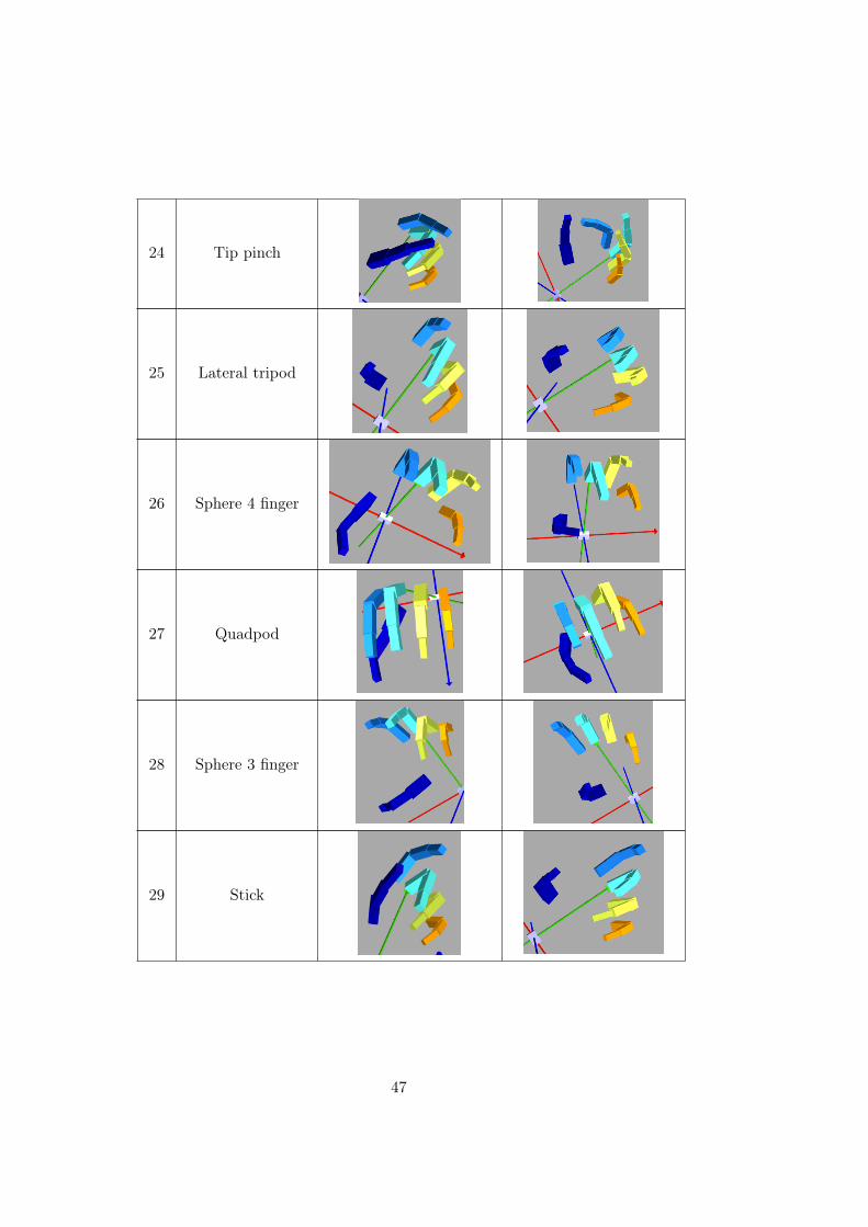
24 Tip pinch
25 Lateral tripod
26 Sphere 4 finger
27 Quadpod
28 Sphere 3 finger
29 Stick
47

30 Palmar 4 finger
31 Ring
32 Ventral
33 Inferior pincer
Table A.1: Comparison of training data and generated samples. Middlecolumn contains images of the last frame of training data. Rightmost columncontains images of the last frame of generated grasps.
48

Bibliography
[1] Hiroaki Sakoe and Seibi Chiba. “Dynamic programming algorithmoptimization for spoken word recognition”. In: IEEE transactions onacoustics, speech, and signal processing 26.1 (1978), pp. 43–49.
[2] M. R. Cutkosky. “On grasp choice, grasp models, and the design ofhands for manufacturing tasks”. In: Robotics and Automation, IEEETransactions on 5.3 (1989), pp. 269–279.
[3] Marco Santello, Martha Flanders, and John F. Soechting. “PosturalHand Synergies for Tool Use”. In: The Journal of Neuroscience 18.23(Dec. 1998), pp. 10105–10115. url: http://www.jneurosci.org/content/18/23/10105.abstract.
[4] N. Somia et al. “The Initiation and Sequence of Digital Joint Motion”.In: Journal of Hand Surgery 23.6 (1998), pp. 792–795.
[5] Neil Lawrence. “Gaussian Process Latent Variable Models for Visuali-sation of High Dimensional Data”. In: In NIPS. 2003, p. 2004.
[6] Keith Grochow et al. “Style-based inverse kinematics”. In: ACM trans-actions on graphics (TOG). Vol. 23. 3. ACM. 2004, pp. 522–531.
[7] Raquel Urtasun et al. “Priors for people tracking from small trainingsets”. In: Computer Vision, 2005. ICCV 2005. Tenth IEEE Interna-tional Conference on. Vol. 1. IEEE. 2005, pp. 403–410.
[8] Jack Wang, Aaron Hertzmann, and David M Blei. “Gaussian processdynamical models”. In: Advances in neural information processing sys-tems. 2006, pp. 1441–1448.
[9] Matei Ciocarlie, Corey Goldfeder, and Peter Allen. “Dexterous Grasp-ing via Eigengrasps: A Low-Dimensional Approach to a High-ComplexityProblem”. In: (2007). url: http://www.coreygoldfeder.com/papers/RSS07.pdf.
[10] Ying Li, Jiaxin L. Fu, and Nancy S. Pollard. “Data-Driven GraspSynthesis Using Shape Matching and Task-Based Pruning.” In: IEEETrans. Vis. Comput. Graph. 13.4 (2007), pp. 732–747. url: http ://dblp.uni-trier.de/db/journals/tvcg/tvcg13.html#LiFP07.
49
[11] Graham W. Taylor, Geoffrey E. Hinton, and Sam T. Roweis. “Model-ing Human Motion Using Binary Latent Variables.” In: NIPS. Ed. byBernhard Schölkopf, John C. Platt, and Thomas Hofmann. MIT Press,2007, pp. 1345–1352. isbn: 0-262-19568-2. url: http://dblp.uni-trier.de/db/conf/nips/nips2006.html#TaylorHR06.
[12] Jack M. Wang, David J. Fleet, and Aaron Hertzmann. “MultifactorGaussian Process Models for Style-content Separation”. In: Proceedingsof the 24th International Conference on Machine Learning. ICML ’07.Corvalis, Oregon, USA: ACM, 2007, pp. 975–982. isbn: 978-1-59593-793-3.
[13] Heni B. Amor et al. “Grasp synthesis from low-dimensional probabilis-tic grasp models”. In: Computer Animation and Virtual Worlds 19.3-4(2008), pp. 445–454. issn: 1546-427X. url: http://dx.doi.org/10.1002/cav.252.
[14] Jack M Wang, David J Fleet, and Aaron Hertzmann. “Gaussian processdynamical models for human motion”. In: IEEE transactions on patternanalysis and machine intelligence 30.2 (2008), pp. 283–298.
[15] Tatiana Benaglia et al. “mixtools: An R Package for Analyzing FiniteMixture Models”. In: Journal of Statistical Software 32.6 (2009), pp. 1–29. url: http://www.jstatsoft.org/v32/i06/.
[16] Trevor Hastie, Robert Tibshirani, and Jerome Friedman. The Elementsof Statistical Learning. Data Mining, Inference, and Prediction. SecondEdition. Springer-Verlag New York, 2009.
[17] Graham W. Taylor and Geoffrey E. Hinton. “Factored Conditional Re-stricted Boltzmann Machines for Modeling Motion Style”. In: Proceed-ings of the 26th Annual International Conference on Machine Learn-ing. ICML ’09. Montreal, Quebec, Canada: ACM, 2009, pp. 1025–1032. isbn: 978-1-60558-516-1. url: http://dx.doi.org/10.1145/1553374.1553505.
[18] Sophie Jörg, Jessica Hodgins, and Carol O’Sullivan. “The Perceptionof Finger Motions”. In: Proceedings of the 7th Symposium on AppliedPerception in Graphics and Visualization. APGV ’10. Los Angeles,California: ACM, 2010, pp. 129–133. isbn: 978-1-4503-0248-7.
[19] Graham W. Taylor et al. “Dynamical binary latent variable modelsfor 3D human pose tracking.” In: CVPR. IEEE Computer Society,2010, pp. 631–638. isbn: 978-1-4244-6984-0. url: http://dblp.uni-trier.de/db/conf/cvpr/cvpr2010.html#TaylorSFH10.
[20] Chung-Cheng Chiu and Stacy C. Marsella. “A style controller for gen-erating virtual human behaviors”. In: The Tenth International Confer-ence on Autonomous Agents and Multiagent Systems. Taipei, Taiwan,May 2011.
50

[21] Chung-Cheng Chiu and Stacy C. Marsella. “How to train your avatar:A data driven approach to gesture generation”. In: The 11th Interna-tional Conference on Intelligent Virtual Agents (IVA 2011). Reykavik,Iceland, Sept. 2011.
[22] Henning Hamer et al. “Data-driven animation of hand-object interac-tions.” In: FG. IEEE, 2011, pp. 360–367. url: http://dblp.uni-trier.de/db/conf/fgr/fg2011.html#HamerGUG11.
[23] Manuel Febrero-Bande and Manuel Oviedo de la Fuente. “StatisticalComputing in Functional Data Analysis: The R Package fda.usc”. In:Journal of Statistical Software 51.4 (2012), pp. 1–28. url: http://www.jstatsoft.org/v51/i04/.
[24] Jeremy Kun. Dynamic Time Warping for Sequence Comparison. https://jeremykun.com/2012/07/25/dynamic-time-warping/. Blog. 2012.
[25] Feng Zhou and Fernando De la Torre Frade. “Generalized Time Warp-ing for Multi-modal Alignment of Human Motion”. In: IEEE Con-ference on Computer Vision and Pattern Recognition (CVPR). June2012.
[26] Wei Dai, Yu Sun, and Xiaoning Qian. “Functional analysis of graspingmotion.” In: IEEE, 2013, pp. 3507–3513.
[27] Wenping Zhao et al. “Robust realtime physics-based motion control forhuman grasping.” In: ACM Trans. Graph. 32.6 (2013), 207:1–207:12.url: http://dblp.uni-trier.de/db/journals/tog/tog32.html#ZhaoZMC13.
[28] Jeng-Min Chiou, Yu-Ting Chen, and Ya-Fang Yang. “Multivariate func-tional principal component analysis: A normalization approach”. In:Statistica Sinica (2014), pp. 1571–1596.
[29] Chung-Cheng Chiu and Stacy C. Marsella. “Gesture Generation withLow-Dimensional Embeddings”. In: Proceedings of the 13th Interna-tional Conference on Autonomous Agents and Multiagent Systems.Paris, France, May 2014, pp. 781–788.
[30] Honglang Wang. Functional Principal Component Analysis. [Online;accessed 18-August-2017]. 2014. url: https://honglangwang.wordpress.com/2014/12/20/functional-principal-component-analysis/.
[31] Han Du et al. “Scaled Functional Principal Component Analysis forHuman Motion Synthesis”. In: Proceedings of the 9th InternationalConference on Motion in Games. MIG ’16. Burlingame, California:ACM, 2016, pp. 139–144. isbn: 978-1-4503-4592-7.
[32] T. Feix et al. “The GRASP Taxonomy of Human Grasp Types”. In:Human-Machine Systems, IEEE Transactions on 46.1 (2016), pp. 66–77.
51
[33] Ming-Jin Liu et al. “Biomechanical characteristics of hand coordina-tion in grasping activities of daily living”. In: PloS one 11.1 (2016),e0146193.
[34] Wikipedia. Functional principal component analysis — Wikipedia, TheFree Encyclopedia. [Online; accessed 18-August-2017]. 2017. url: https://en.wikipedia.org/w/index.php?title=Functional_principal_component_analysis&oldid=783422668.
[35] Igor Zubrycki and Grzegorz Granosik. “Fundamentals of Robotics withMyModelRobot”. In: (). url: http://www.mymodelrobot.appspot.com/.
52


TRITA -MAT-E 2017:53ISRN -KTH/MAT/E--17/53--SE
www.kth.se