IT 17 002

Examensarbete 30 hpJanuari 2017

Modeling of drug effect in general closed-loop anesthesia

Sander Cox

Institutionen för informationsteknologiDepartment of Information Technology

Teknisk- naturvetenskaplig fakultet UTH-enheten Besöksadress: Ångströmlaboratoriet Lägerhyddsvägen 1 Hus 4, Plan 0 Postadress: Box 536 751 21 Uppsala Telefon: 018 – 471 30 03 Telefax: 018 – 471 30 00 Hemsida: http://www.teknat.uu.se/student

Abstract

Modeling of drug effect in general closed-loopanesthesia

Sander Cox

In medicine, anesthesia is achieved by administering two interacting drugs. Nowadays,the Depth of Anesthesia can be expressed by the Bispectral Index Scale, which ismeasured by an EEG. In order to make automatic closed-loop anesthesia possiblewith the benefits of 1) relieving the anesthesiologist from the hard task ofadministering optimal drug doses, 2) achieving more consistent drug effects by meansof individualization, and 3) reducing side effects because of the achieved reducedoverall drug administration, estimating accurate models of the effect of drug doses onthe Depth of Anesthesia is essential.

The model used was a minimally parametrized PharmacoKinetic-PharmacoDynamicWiener model. The parameters of the model were estimated using an ExtendedKalman Filter, whose parameters were tuned manually. The model and filter weretested on new data from both the University of Porto and the University of Brescia.The unit of the reference data set from Porto was unknown, so in order to use thescale-dependent model an educated guess was made to convert the other data sets toa reasonable scale. Furthermore, the data from Brescia was incomplete, which couldonly partly be remediated. Similar tracking performances were obtained when usingthe new data sets compared to the reference data, however, either relatively constantestimates, or different parameter estimates for similar conditions, were typicallyobtained. This questions the validity of the model used and if the parameters foundcan be trusted. Therefore, the replication of the procedure on other complete data,and the comparison with the application of other models on the studied data, issubject for future research.

Tryckt av: Reprocentralen ITCIT 17 002Examinator: Mats DanielsÄmnesgranskare: Marcus BjörkHandledare: Alexander Medvedev

Contents

1 Introduction 3

2 Medical background: anesthesia 4

3 Theoretical background 4

3.1 Modelling of dynamical systems . . . . . . . . . . . . . . . . . . . . . . . . 43.1.1 Models . . . . . . . . . . . . . . . . . . . . . . . . . . . . . . . . . 43.1.2 Signals in models . . . . . . . . . . . . . . . . . . . . . . . . . . . . 53.1.3 State and state-space models . . . . . . . . . . . . . . . . . . . . . 63.1.4 Stationary points and linearization . . . . . . . . . . . . . . . . . . 73.1.5 Disturbances . . . . . . . . . . . . . . . . . . . . . . . . . . . . . . 83.1.6 Transfer functions . . . . . . . . . . . . . . . . . . . . . . . . . . . 93.1.7 PID controller . . . . . . . . . . . . . . . . . . . . . . . . . . . . . 12

3.2 Pharmacokinetics and pharmarcodynamics . . . . . . . . . . . . . . . . . 133.2.1 Wiener models . . . . . . . . . . . . . . . . . . . . . . . . . . . . . 15

3.3 The Kalman filter . . . . . . . . . . . . . . . . . . . . . . . . . . . . . . . 163.4 The extended Kalman filter . . . . . . . . . . . . . . . . . . . . . . . . . . 18

4 Used model of effect of drug concentrations on BIS 21

4.1 General properties . . . . . . . . . . . . . . . . . . . . . . . . . . . . . . . 214.2 The model in detail . . . . . . . . . . . . . . . . . . . . . . . . . . . . . . . 21

4.2.1 Linear block . . . . . . . . . . . . . . . . . . . . . . . . . . . . . . . 224.2.2 Nonlinear block . . . . . . . . . . . . . . . . . . . . . . . . . . . . . 224.2.3 State-space model . . . . . . . . . . . . . . . . . . . . . . . . . . . 234.2.4 Assigned values to parameters . . . . . . . . . . . . . . . . . . . . 25

5 Testing the model on data 25

5.1 Available data . . . . . . . . . . . . . . . . . . . . . . . . . . . . . . . . . 255.2 A typical run on the old data: marsh pat1 . . . . . . . . . . . . . . . . . . 265.3 Testing on new data from Porto: Bis 1 . . . . . . . . . . . . . . . . . . . . 29

5.3.1 Attempt to prevent the occurrence of complex values with constraints 305.3.2 Attempt with tuning . . . . . . . . . . . . . . . . . . . . . . . . . . 345.3.3 Scaling . . . . . . . . . . . . . . . . . . . . . . . . . . . . . . . . . 36

5.4 Testing on data from Brescia: PZ41 1 . . . . . . . . . . . . . . . . . . . . 365.5 Units . . . . . . . . . . . . . . . . . . . . . . . . . . . . . . . . . . . . . . . 36

5.5.1 Calculating recommended doses . . . . . . . . . . . . . . . . . . . . 375.6 Running with conversion to assumed unit . . . . . . . . . . . . . . . . . . 39

5.6.1 60Bis 1 (converted to mg/h) . . . . . . . . . . . . . . . . . . . . . 395.6.2 Bis1 (converted to mg/h) and tuned . . . . . . . . . . . . . . . . . 435.6.3 3600PAZ41new tuned and with right sampling interval . . . . . . . 46

6 Conclusion and future work 50

2

1 Introduction

Problem

In medicine, anesthetic drugs are administered in order to induce reversible loss of sen-sation and facilitate surgery. Since the depth of anesthesia (DoA) can be nowadaysmeasured from electroencephalogram (EEG) of the patient using so-called bispectral in-dex (BIS), automatic closed-loop anesthesia has become feasible. Apart from relievingthe anesthesiologists from the routine task of adjusting the flow of anesthetic drugs toachieve a desired level of DoA, closed-loop anesthesia holds promise for more consistentdrug effect because of treatment individualization and less side effects due to a reductionof the overall administered drug dose during the surgery. Systematic design of feedbackcontrol needs an accurate description of the drug concentration in, and its actual effecton the patient.

The point of departure was the article Online Nonlinear Identification of the Effectof Drugs in Anaesthesia Using a Minimal Parameterization and BIS Measurements [9],which is part of the PhD thesis of Dr. Margarida Silva. In this paper, a simpler model(than the commonly used compartment models) for anesthesia, modeling the effect of twointeracting drugs on the DoA in the patient under surgery, is proposed. This minimallyparametrized pharmacokinetic-pharmacodynamic (PKPD) model and the accompanyingMatlab source code with the method are available and are used to model patient datafrom two clinical setups. The data were collected at the University of Brescia (Italy)and University of Porto (Portugal).

Goal

The aim is to mathematically model the effect of the hypnotic/amnestic agent propo-fol, and the analgesic drug remifentanil, that are intravenously administered in manualgeneral anesthesia. The effect of the drugs is measured by BIS. The initial values andparameters of the model are estimated from the data. A method for parameter estima-tion in nonlinear statespace models, in particular the extended Kalman filter (EKF) isdiscussed. The EKF is the method used in the provided Matlab source code and willbe applied to the available data sets from Brescia and Porto. So, a given estimationmethod is applied to (new) data. The algorithm and method do not have to be signifi-cantly changed, but the parameters of the EKF need tuning to the specific characteristicsof the new clinical setup. An analysis of the parameter estimates and comparison of themodeling quality of the different settings is performed.

The following sections will cover the medical background, the theoretical groundsfor the model, the extended Kalman filter algorithm, the model used and the clinicalproperties of the data, before the results of applying the modeling approach to data fromthe different clinical setups are discussed.

3

2 Medical background: anesthesia

In medicine, anesthesia is usually achieved by administering both a analgesic and ahypnotic drug. The former suppressing pain and the latter reducing consciousness. Inour case the analgesic drug is propofol and the hypnotic drug is remifentanil.

The so called “depth of anesthesia” (DoA) is measured by the so called BispectralIndex Scale (BIS), which is obtained by an electroencephalogram (EEG). The BIS-measure is a percentage, ranging from 0 to 100%. At 100% the patient is completelyawake and at 0% the patient is dead. It is important that the index is kept betweencertain values: a value that is too low results in unnecessary drug use, a longer recoveryperiod for the patient and possibly severe side effects caused by an overdose. A valuethat is too high may cause a patient to regain consciousness or to not be totally painfree. The ideal DoA is between 40% and 60%. Having this in mind, the advantages ofautomatizing this procedure becomes apparent.

As described in Margardia M. Silva’s PhD thesis [7] anesthesia usually consists ofthree phases: 1) the induction phase, in which relatively high drug doses are given undera short period of time in order to quickly get the patient in a state ready for surgery, 2)a maintenance phase, in which this state is reinforced with relatively small drug doses,and 3) a recovery phase, in which the administration of the anesthetic drugs is ceasedand sometimes a “counter drug” is given to neutralize the effect of these drugs if recoveryseems to take too much time. The optimal start dose is given as a bolus injection andis usually estimated using individual patient properties such as weight and sex.

3 Theoretical background

3.1 Modelling of dynamical systems

For this section that covers a general theoretical background Modeling of dynamic sys-tems by Lennart Ljung and Torkel Glad [4] was used.

3.1.1 Models

The point of modeling is to make it possible to study and understand parts of realityand link observations to patterns. A system is an object or collection of objects whoseproperties are of interest to study. For this system, research questions are formulated. Alot of these questions can be answered by experimentation, but in other cases this is notpossible, either because it is too expensive, too dangerous, or simply because the systemdoes not exist (yet). In those situations it is necessary to make a model of the systemin order to answer the research questions. A model is a tool to making it possible toanswer the research questions without having to do an experiment in “the real world”,for example on patients. Instead, experiments can be done on the model itself.

A distinction is made between mental models, verbal models, physical models andlastly mathematical models, which is the one this project is about. In mathematicalmodels the relations between the quantities of the systems are typically described in the

4

form of differential equations. The mathematical model can be used to predict how thesystem would behave, either analytically, i.e. by analyzing the equations, or by meansof simulation, i.e. a numerical experiment.

Even though simulation is safe and cheap, the quality of the model has to be goodenough to be able to make accurate predictions, and answer the research questions.Apart from black box approaches, two different disciplines are at play when it comes toconstructing mathematical models. The first one is the domain of expertise, i.e. the reallife application area, for example anesthetics, and the second one is the knowledge ofhow to translate this domain knowledge into a valid mathematical model. The expertknowledge in our case is for example the known effects of propofol and remifentanil,their interaction properties, what dosages are commonly used, and so on. It is importantto realize that every model has a limited domain of validity: the model is only able tomake reliable predictions or claims under certain conditions. Because of these limitationsmodels and simulations cannot totally replace experimentation.

Mathematical models can be divided into different categories based on the followingproperties:

• Deterministic (the same input always gives the same output) orStochastic (there is an element of randomness).

• Dynamic (the variables of the system also depend on previous signals) orStatic (the variables of the system only depend on current signals)

• Continuous time (time continuous signals) orDiscrete time (measurements at specific time points, a.k.a. sampling)

A visual representation where the different logical units of a system are represented byblocks and where the interactions between the units are denoted by arrows between theblocks, is called a block diagram. Compartment models, i.e. models used for pharma-cokinetics and -dynamics (section 3.2), make use of block diagrams.

3.1.2 Signals in models

Mathematical models often have both system parameters, which belong to the system,and design parameters, which belong to the method (e.g. a Kalman filter). It dependson the view of the researcher what parameters are of main interest, for example whichones are set to fixed values and which ones are estimated. A possible goal of simulatinga model is to determine the best design parameters of a specific method on a specificsystem, or to estimate certain system parameters with (optimized) design parameters 1.

The signals that the system produces are called the outputs and are sometimes ofmain interest. Other times, estimating parameters is of more interest.

External signals influence other signals in the model but are not influenced them-selves. If these external signals can be controlled, they are called input signals and

1Marcus Bjork

5

are denoted with ui(t). If the external signals cannot be controlled, they are calleddisturbance signals.

Because of the ubiquity of computers in modern day research, essentially all signalsare received, registered and processed digitally, which implies that the signals need to besampled, i.e. measured or processed at specific times. If the time between consecutivemeasurements is fixed (i.e. the sampling is done uniformly) so that tk = kT , then T iscalled the sampling interval and 2π/T (in radians per second) the sampling frequency.

3.1.3 State and state-space models

For a dynamical model, the input values at a certain time step are not enough to calculatethe output: for discrete models we also need to take the inputs at previous time stepsinto account, and for continuous models the derivatives. The state of the system at timet0 is the vector with the values of all internal variables (i.e. the variables that are neededto completely describe the system’s state) at time step t0. With these state variablesand the current input, the output at the next time step can be calculated iteratively.The values of intermediate time steps or derivatives are stored in the state vector. Amodel using its state vector for these calculations is called a state-space model.

A common way of writing a dynamical model is as a system of first-order differentialequations with state variables (x1(t) ,..., xn(t)). Written out, the system then becomes:

x1(t) = f1(x1(t), ..., xn(t), u1(t), ...., um(t))

x2(t) = f2(x1(t), ..., xn(t), u1(t), ...., um(t))...

xn(t) = fn(x1(t), ..., xn(t), u1(t), ...., um(t))

in vector notation: x(t) = f(x(t), u(t)),

which has n internal variables and m input variables.

The outputs can then be calculated by the internal variables and inputs:

y1(t) = h1(x1(t), ..., xn(t), u1(t), ...., um(t))

y2(t) = h2(x1(t), ..., xn(t), u1(t), ...., um(t))

...

yn(t) = hn(x1(t), ..., xn(t), u1(t), ...., um(t))

in vector notation: y(t) = h(x(t), u(t)).

So in general the relations are as follows:

x(t) = f(x(t), u(t))

y(t) = h(x(t), u(t)) ,(1)

which is a nonlinear state-space model.

6

If f(x, u) and h(x, u) are linear functions of x and u, i.e. if:

f(x, u) = Ax+Bu

h(x, u) = Cx+Du(2)

the model is called linear.

3.1.4 Stationary points and linearization

A solution x(t), for t ≥ t0, to the state model in (1) for a specific input function u(t)and initial conditions x0 (at t = t0) is called a trajectory.

In some situations, the input u(t) is constant: u(t) ≡ u0. The solution(s) (if thereexist any) to

x(t) = f(x(t), u0) = 0

are denoted x∗i (where i is just a numbering) and are called stationary solutions and

(x∗0, u0), (x∗1, u0), ... are called stationary points. The intuition behind it is that if x = 0,

there is no change and the system will stay in the same state as the initial state: thetrajectory is just a constant. The output of the system will then also be constant. Iftrajectories that start close to the stationary point eventually end up in the stationarypoint, this point is called asymptotically stable. If all trajectories converge to this sta-tionary point eventually, it is called globally asymptotically stable.

Say there is an asymptotically stable stationary solution x0 for an input u0. Then x0 isdependent on u0 and therefore also the stationary output y0 is:

y0 = h(x0(u0), u0) = g(u0)

This expression describes the stationary relationship between the constant input andcorresponding stationary output. For a linear system, the time it takes for the outputto get close to its new stationary output y1 after changing u0 to u1 is called the timeconstant.

A nonlinear system can be linearized in the neighborhood of stationary solutions. Forthe stationary point (x0, y0), the system then becomes:

∆x(t) = A∆x(t) +B∆u(t)

∆y(t) = C∆x(t) +D∆u(t)

Where ∆x(t) = x(t) − x0, ∆u(t) = u(t) − u0, ∆y(t) = y(t) − y0 and where A and B

are the Jacobians of f(x, u) (with respect to x and u respectively) and C and D are the

7

jacobians of h(x, u) (with respect to x and u respectively), evaluated at (x0, u0). It isimportant to keep in mind that the linearization is only useful for points close to thestationary point, and that it is usually unclear how accurate this linear approximationactually is, although the error can be estimated. Therefore conclusions based on this ap-proximation should be taken with care and should take the estimated error into account.

3.1.5 Disturbances

As explained in 3.1.2, disturbance signals are external signals that cannot be controlled.Yet these can have an significant impact on the behavior of the system, and thereforethey are important to consider. It matters if the disturbance signals are known, and inthat case whether they can be separately measured, or unknown.

An example of a measurable disturbance signal is that of a model of a solar-heatedhouse, where the solar intensity (disturbance signal) together with a pump velocity (inputsignal) is used to model the storage temperature (output). Essentially, the input signaland disturbance signal are treated the same in the model, which leads to the followingalterations of the equations in (1) presented in section 3.1.3.

x(t) = f(x(t), u(t), e(t))

y(t) = h(x(t), u(t), e(t))

A challenge is to describe this disturbance signal in a suitable way in order to be able toincorporate it in the model. However, an advantage is that a model can be built for thedisturbance signal, separate from the dynamic model and based on direct measurements.

An example of a nonmeasurable disturbance signal is that of a model of the motionof an airplane. The forces of the air that are exerted on the plane depend not only onrudder and flap movements (inputs), but also on the wind (disturbance signal). A majordifference with the previous example is that the disturbance signals are barely separatelymeasurable: they can typically only be observed indirectly, through their effect on othermeasurable variables. Therefore it follows that the modeling of the disturbance signalcannot be done separately.

The more common case is when the disturbance signal is completely unknown. Thedisturbance signal is then usually added to the output signal in the following way:

y(t) = z(t) + e(t)

where z(t) is the undisturbed signal and:

x(t) = f(x(t), u(t))

z(t) = h(x(t), u(t))

The problem of describing the disturbance signal in a suitable way remains, but e(t) isnow not directly measurable. Input and output signals must be used to infer e(t).

8

3.1.6 Transfer functions

This subsection is based on “Feedback systems: an introduction for scientists and engi-neers” [6] and [4].

A transfer function is a compact description of the input/output relation for a linearsystem (as described in equation (2)). It is the main tool for implementing this focus oninput/output characteristics and makes it possible to understand the overall behavior ofthe system. The strength of the transfer function is that it provides a very convenientrepresentation in manipulating and analyzing complex linear feedback systems. Thetransfer function is the Laplace transform of the output divided by the Laplace transformof the input, as explained below. 2

Consider the linear system:

x = Ax+Bu

y = Cx+Du(3)

The Laplace transform of the state equation equals 3:

sX(s)− xt=0 = AX(s) +B U(s)

If the initial state is chosen as xt=0 = 0, this reduces to:

X(s) = (sI −A)−1B U(s)

The Laplace transform of the output equation gives:

Y (s) = CX(s) +DU(s)

⇔

Y (s) = C(sI −A)−1B U(s) +DU(s)

⇔

Y (s) = (C(sI −A)−1B +D)U(s)

The Laplace transformation of (3) then gives:

X(s) = (sI −A)−1B U(s)

Y (s) = (C(sI −A)−1B +D)U(s)

(4)

2“Feedback systems” has the approach that the transfer function represents the response of the system

to an exponential input : u = ezt (where z is a complex number: s = σ + iω). This can be appropriate

since many signals can be represented as exponentials, a sum of exponentials or by a linear combination

of those. However, for this project no such assumptions about u(t) are made.3following http://www.egr.msu.edu/classes/me851/jchoi/lecture/Lect 4.pdf based on [1]

9

The transfer function from u to y is then the map from the input to the output:

Gyu(s) = C(sI−A)−1B+D (5)

This mapping can be written as:

Y(s) = Gyu(s)U(s) (6)

An important property of the transfer function is that it is invariant to changes ofthe coordinates in the state space.

A transfer function is determined in the following way. Consider the linear SISO system(see section 3.2.1 for more details):

dny

dtn+ a1

dn−1

y

dtn−1+ ...+ any = b0

dmu

dtm+ b1

dm−1

u

dtm−1+ ...+ bmu (7)

where u and y as usual are input and output, respectively. Since the system is linearand differentiation in the time domain corresponds to multiplication by s of the Laplacetransform, (7) can be written as:

(sn + a1sn−1 + ...+ an)Y (s) = (b0s

m + b1sm−1 + ...+ bm)U(s) (8)

This is abbreviated as:

a(s)Y (s) = b(s)U(s)

where a(s) is the characteristic polynomial of the ordinary differential equation. Thisgives:

Y (s) =b(s)

a(s)U(s)

and therefore the transfer function is:

G(s) =b(s)

a(s)(9)

The order of G(s) is the order of the denominator polynomial a(s). If the degree ofthe polynomial b(s) is less than or equal to the degree of a(s) then the model is calledproper. If the degree of b(s) is strictly less than the degree of a(s), the model is calledstrictly proper. [3]

For a state space system with transfer function (9), the roots of the polynomiala(s) are called the poles of the system and the roots of b(s) the zeros. The polescorrespond to different resonances with different dampings (modes). These modes are

10

then excited to different degrees for different inputs.4 A zero blocks the transmissionof the corresponding input signals (because Y (s) = G(s)U(s) = b(s)

a(s)U(s) assuming that

a(s) �= 0).Some characteristics of the transfer function, like the gain and the location of the

poles and zeros, determine the system completely.The zero frequency gain (or static gain) is the magnitude of the transfer function at

s = 0 and represents the ratio of the steady-state value of the output with respect to astep input. The system (7), assuming a constant input u0 and output y0, then becomesany0 = bmu0 which leads to the transfer function G(0) = bm

anConsider now the transfer function G(s) = C(sI − A)−1

B + D. Its poles are theeigenvalues of A in the state space model, because these points are where the character-istic polynomial λ(s) = det(sI−A) equals 0 and hence sI−A is noninvertible (singular).Hence the poles of a state space system only depend on matrix A.

Zeros are the complex numbers s such that U(s) can give output 0. Applying thisproperty to the Laplace transformations of equation (3) yields:

sX(s) = AX(s) +B U(s)

0 = C X(s) +DU(s)(10)

which can be written as:

�A− sI B

C D

� �X(s)U(s)

�= 0

The zeros are the values s such that

�A− sI B

C D

�

loses rank, which implies that a system where the matrix B or C is square and full rankdoes not have zeros. In practice this means that a system has no zeros if every state canbe controlled independently or if the full state is measured.

A block diagram (section 3.1.1) of a system can be used to derive a transfer function fora larger part of the system by composing the transfer functions of the different blockswith block diagram algebra. Two transfer functions that are in series:

u G1 G2 y

Figure 1: Two transfer functions in series

have as transfer function G = G2G1

4Marcus Bjork

11

Two transfer functions that are in parallel:

u

G1

G2

Σ y

Figure 2: Two transfer functions in parallel

have transfer function G = G1 +G2

The feedback connection:

u Σ e G1

−G2

y

Figure 3: Two transfer functions in a feedback connection

has a combined transfer function G = G11+G1G2

. This follows from:

y = G1e = G1(u−G2y) ⇔ (1 +G1G2)y = G1u ⇔ y = G11+G1G2

u

The general idea is that the transfer functions of these simple combinations can be thebuilding blocks of more complex systems and in their turn can used to derive morecomplex transfer functions.

3.1.7 PID controller

A PID controller has a proportional, integral and derivative part. The goal of the con-troller is to minimize the error between the current measured quantity and the referencesignal. For this, it uses the course of this error through time, the error function e(t),and combines at every time step the current error and the integral and derivative of theerror function to produce the output (which typically is connected to some action). Thesignificance of the different parts is set by the different gains, Kp, Ki and Kd respectively.One or more gains can be 0, usually not the proportional part, resulting in a P, PI orPD controller, depending on what parts are remaining. Figure 4 visualizes this process.

12

error

kp

ki�

kdddt

Σ controller output

Figure 4: Schematic representation of a PID controller

It can be understood as that the proportional part takes into account the error of thepresent, the integral part the error of the past and the derivative part the error of thefuture. The output of the PID controller is mathematically expressed as:

u(t) = kpe(t) + ki

� t

0e(τ)dτ + kd

de(t)

dt

3.2 Pharmacokinetics and pharmarcodynamics

For this part “Concepts in clinical pharmacokinetics” [2] was used. Pharmacokinetics(PK) is the study of the time course of drug absorption, distribution, metabolism, andexcretion, i.e. how drug concentrations behave in different parts of the human body. Theeffect of a drug is usually related to its concentration at the site of action (i.e. the partof the body where it should have its effect) and therefore concentration measurementsin these parts are useful. However, measuring drug concentrations at these sites is notpractical and is therefore done indirectly, most often by measuring drug concentrationsin blood plasma. An important assumption is that the concentrations in blood plasmaare directly (and proportionally) related to the concentrations in the site of action. Thisproperty is called kinetic homogeneity.

Pharmacodynamics (PD) is about the relation between the drug concentration atthe site of action and the resulting effect. It is assumed that the concentration at thesite of action is the main factor that determines the intensity of the effect, but other(cellular biological) factors can also have an impact. The effectiveness of a drug, thedrug potency, can be expressed in terms of the 50% effective concentration or EC50,which is the concentration that is needed to reach half of the maximum effect, Emax, ofthe drug. A lower EC50 indicates a more potent drug. It should be noted that EC50

does not indicate other characteristics, such as the duration of the effect. An importantphenomenon that should be dealt with is that the effect of some drugs can decrease overtime: the patients develops a tolerance for the drug. Using the EC50 in a Hill functionis a common way to model pharmacodynamics (see section 4.2.2).

The relationship between PK and PD is illustrated in figure 5:

13

Drugadministration

Drug at siteof action

Drug effectsPharmaco-

kinetics

Pharmaco-

dynamics

Figure 5: Pharmacokinetics and Pharmacodynamics

The monitoring of drug concentrations has as its goal to keep a drug concentration withinits therapeutic range: above a concentration that has an effect and below a concentrationthat is (possibly) toxic. The boundaries of the therapeutic range are usually expressedas a unit of mass per volume. Of course these boundaries are drug dependent and thereis a variability in drug response between patients. Apart from patient dependent factorsalso drug interactions can play a role in the concentrations in the blood plasma. Thetask of a clinician is to select a drug, determine its dose, administer it, measure thepatient’s response and the concentration of the drug in the blood plasma and adjust thedose and administration accordingly.

The behavior of drugs in the human body is very complex and therefore simplifi-cations are needed. Commonly compartmental models are used, where a compartmentrepresents a collection of organs/tissues that roughly behave as a unit. In some casesone compartment suffices, treating the whole human body as a unit, with one input (theadministration of the drug) and one output (the breaking down of the drug). In othercases a two-compartment model is needed, representing the human body with as a cen-tral unit (the blood stream and highly perfused organs) that interacts with peripheralunit (e.g. fat and muscle tissue and cerebrospinal fluid). Administration and eliminationtakes place in the central unit. The interaction between compartments is described withrates. Usually it is assumed that the elimination rate is constant. A compartment modelthat has more than two compartments is called a multi-compartment model.

An example of a multi-compartment model is the very common PK model shown infigure 6.

14

Compartment 1 Effect compartment

Compartment 2

Compartment 3

infusion rate

clearance

Figure 6: Common multi-compartment model for PK (of propofol and remifentanil).

Instead of just treating the human body as a single unit on which drugs have adirect effect, or as a central unit and a peripheral unit, it is modeled by a compartmentthat has an inflow and outflow of the drug and that is interacting with three othercompartments, of which one is the effect compartment. The effect compartment is theunit that represents the site of action.

3.2.1 Wiener models

Pharmacokinetics and pharmacodynamics are sometimes also modeled with a Wienermodel. The basic structure of a Wiener model is shown in figure 7. As in the case witha compartment model, a Wiener model can be written as a number of linear differentialequations, but without the physical interpretation. Also, the pharmacodynamic partcontains a nonlinearity, that in the Wiener model is represented by the nonlinear block.5

Linear blockG

Nonlinear blockf(z)

u(t) y(t)z

Figure 7: Single input single output (SISO) Wiener model

An input signal u(t) is forwarded to the linear block which outputs a signal z that isforwarded to the nonlinear block giving y(t). The above model is a single input, singleoutput model, but it can be expanded to a multiple input, single output (MISO) model(or even a multiple input, multiple output model if that is desired). In a MISO Wienermodel the linear block consists of multiple units, as shown in figure 8.

5Marcus Bjork

15

Linear block unitG1

z1

Linear block unitGn

u1(t)

un(t) zn

CNonlinear block

f(z)y(t)z

Figure 8: Multiple input single output (MISO) Wiener model

The input signals u1(t), . . . , un(t) are forwarded to their corresponding linear blockunits. These units output the signals z1, . . . , zn respectively, which will be combinedinto one signal: z = C(z1, . . . , zn). The function C can for example be a weighted sumof the signals z1, . . . , zn. The signal z is then the input for the nonlinear block that inits turn outputs y(t).

3.3 The Kalman filter

The Kalman filter is an iterative mathematical method that is used for both online andoffline state estimation. It combines a prediction (estimate) with measurements andaverages them, depending on the estimated error in the prediction and the estimatederror of the measurements in a particular way, producing an updated estimate. Hence,the Kalman filter is usable in models with noise. The Kalman filter is the best linearfilter and gives an optimal combination of previous estimates and measurements [5].Since the data will be sampled, the Kalman filter will be explained for the discrete timecase.

Essentially, at every iteration the Kalman gain, current estimate and the new un-certainty in the estimate are calculated 6. The following equation gives an intuitiveexplanation of the process:

Estimate(t) = Estimate(t−1) +KalmanGain (Measurements− Estimate(t−1)) (11)

The Kalman gain is a measure for assigning more weight to the estimate or to themeasurements. If the error in the estimate is bigger, the measurements should have moreimpact, if the error in the measurements is bigger, the estimate should, as achieved by:

KalmanGain =�estimate

�estimate + �measurements(12)

6Special Topics - The Kalman Filter (7 of 55) The Multi-Dimension Model 1

https://www.youtube.com/watch?v=-cD7WkbAIL0

16

We can visualize the role of the Kalman filter in the diagram in figure 9 .

Πx(t)

KF

u(t) y(t)

v(t)

x(t+ 1)

e(t)

Figure 9: Schematic representation of the Kalman filter

It shows that there is a process Π with a state x, which changes with time t: Πx(t). Thisprocess produces at a specific time t, for giving inputs u(t), and distorted by the processerror v(t), an output y(t). The Kalman filter KF uses the input plus the output ofthe process distorted by measurement noise e(t) and estimates the state of the dynamicsystem at time t : x(t). It can be seen as the Kalman filter gradually filtering out theuncertainty of the process and the noise of the measurement. That is why it is called afilter.

In equation form the model becomes:

x(t+ 1) = Ax(t) +Bu(t) + v(t) (13)

y(t) = Cx(t) + e(t) (14)

where x(t+1) is the new state vector, x(t) the current, y(t) the output, u(t) is the inputvector, v(t) process noise and e(t) measurement noise. A, B and C are matrices (recallthe linear model of section 3.1.3, D is set to zero).

The dynamical system starts with initial values x(0) = x0. The process error v(t)and measurement error e(t) have an expected value of 0:

17

E{v(t)} = 0

E{e(t)} = 0

and covariance matrices R1 and R2, respectively. The difference between the estimateand real state can be proven to have an expected value of 0:

E{x− x} = 0

The covariance matrix of the error of the estimate is called P (t) and is estimatedwith the matrix A and the covariance matrix of the process error R1 by:

P (t) = ATP (t− 1) A+R1 (15)

This covariance matrix is then used together with the covariance matrix of the measure-ment error (R2) to get to the Kalman gain (K):

K(t) = P (t) CT�CP (t)CT +R2

�−1(16)

If the variance of the estimation error (P (t)) is small compared to the variance of themeasurement error (R2), which means that (assuming a bias of 0) the estimate is closeto the true value, the value of K is small. On the other hand, if P (t) is big comparedto R2, it means the estimate is not so close to the true value and we want to adjust theestimate more crudely, which is reflected in a bigger value for K. The estimate of thenext state is then as follows:

x(t+ 1) = Ax(t) +Bu(t) +K(t)�Cx(t)− y(t)

�(17)

where Cx(t)− y(t) = y(t)− y(t) is the difference between the estimated output and themeasured output, which, depending on K, is given more or less weight for the estimateof x(t+ 1). After this, P (t) is updated with:

P (t) = (I −KC)P (t) (18)

and is used for the next iteration.

3.4 The extended Kalman filter

The extended Kalman filter is used in situations where the system is nonlinear. Thefunctions of the state vector f and the functions of the input vector h could be anydifferentiable functions:

x(t+ 1) = f(x(t), u(t)) + v(t) (19)

y(t) = h(x(t)) + e(t) (20)

18

In the linear case, the Kalman filter has been proven to gradually improve the stateestimate until stationary conditions are reached. In the extended Kalman filter thereis no such guarantee, but we assume that if we repeatedly linearize the system aroundthe current working point and use the standard Kalman filter, this would be good enough.

Torsten Soderstrom [10](p 245) initially uses the equations:

x(t+ 1) = f(t, x(t)) + g(t, x(t))v(t) (21)

y(t) = h(t, x(t)) + e(t) (22)

As T. Soderstrom remarks, this equation can be extended with an input signal u(t):

x(t+ 1) = f(t, x(t), u(t)) + g(t, x(t))v(t) (23)

We now want to locally approximate the system with a linearization, or more pre-cisely: compute the filter gain by linearizing the nonlinear model. We therefore substitutef , g and h with an expansion of a first order (i.e. linear) Taylor series around estimatesof x(t). For f and g this is around the most recent estimate: x(t|t). For h this is aroundthe predicted state: x(t|t − 1), because the measurement y(t) has to be compared withits predicted value to obtain a correction term to the filter. [10](p 246)

f(t, x(t) ≈ f(t, x(t|t)) + F (t)(x(t)− x(t|t))g(t, x(t) ≈ G(t)

h(t, x(t)) ≈ h(t, x(t|t− 1) +H(t)(x(t)− x(t|t− 1)) ,

where:

F (t) =∂f(t, x)

∂x|x=x(t|t)

G(t) = g(t, x)|x=x(t|t)

H(t) =∂h(t, x)

∂x|x=x(t|t−1)

In words, this means that f is approximated by evaluating f at the estimate x andadding the difference between the true x and the estimate multiplied by a Jacobi ma-trix. The smaller the difference, the smaller the effect. Note that f and h are nonlinearfunctions that need to be linearized by their respective Jacobi matrices, while the noisev(t) is a linear function of g, so it can be estimated by just plugging in the estimated x

in the function g.

This gives rise to the following linear system:

19

x(t+ 1) = F (t)x(t) +G(t)v(t) + u

y(t) = H(t)x(t) + e(t) + w(t)

u(t) = f(t, x(t|t)− F (t)x(t|t)w(t) = h(t, x(t|t− 1))−H(t)x(t|t− 1)

(24)

In words, u is the linearization error of F and w(t) the linearization error of H. Thenext state is then approximated by the previous state multiplied by a Jacobi matrix,plus the process error, plus the linearization error. The output y(t) is then described interms of a current state multiplied by a Jacobi matrix and two additional terms: themeasure error and the linearization error. Note that u(t) has nothing to do with u(t)(the input vector). The resemblance is just a matter of notation.

By applying the Kalman filter, the following formulas are obtained:

Using

x(t|t) = x(t|t− 1) +K(t)�y(t)−H(t)x(t|t− 1)− w(t)

�

andw(t) = h(t, x(t|t− 1))−H(t)x(t|t− 1)

we get:

x(t|t) = x(t|t− 1) +K(t)�y(t)− h(t, x(t|t− 1))

�(25)

(Comp. simple Kalman (17): x(t+ 1) = Ax(t) +Bu(t) +K(t)[Cx(t)− y(t)])

x(t+ 1|t) = F(t) x(t|t) + u(t) = f(t, x(t|t),u(t)) (26)

(Note the inclusion of the input u(t))

K(t) = P(t|t− 1) HT(t)�H(t)P(t|t− 1)]HT(t) +R2(t)

�−1(27)

(Compare simple Kalman (16): K(t) = P (t) CT [C P (t) CT +R2]−1)

P(t|t) = P(t|t− 1) − K(t) H(t) P(t|t− 1) (28)

(Compare simple Kalman (18): P (t) = (I −K C) P (t))

P(t+ 1|t) = F(t) P(t|t) FT(t) +G(t) R1 GT(t) (29)

(Compare simple Kalman (15): P (t) = ATP (t− 1) A+R1)

20

4 Used model of effect of drug concentrations on BIS

4.1 General properties

M.M. Silva et al. [9] use a dynamical, stochastic, discrete time model with input signals(see section 3.1.1) for the anesthesia of a patient:

x(t+ 1) = f(t, x(t), u(t)) + g(t, x(t))v(t)

(equation 23 repeated for convenience)

A linear function for the input is used, which turns the above equation into:

x(t+ 1) = f(t, x(t)) +Bu(t) + g(t, x(t))v(t) (30)

The estimate of x(t+ 1) then becomes:

x(t+ 1|t) = f(t, x(t|t)) +Bu(t) (31)

Note that these above two equations are special cases of the equations (23) and (26)which is a consequence of the choice for a linear function for the input signal. The inputsignal is not (necessarily) constant.

The input u(t) are the infusion rates of the administered drugs propofol and remifen-tanil. The output value y(t) is the measured BIS. The disturbance signals (which areunknown) consist of the noise in the process (the process error: v(t)) and the noise inthe measurement (measurement error: e(t)) (see 3.3 and 3.4). Input and output signalsmust be used to infer the measurement noise (recall 3.1.5).

4.2 The model in detail

The following MISO Wiener model is used:

Linear block unitG1

xprope (t, θ)

Linear block unitG2

rprop

rremi x

remie (t, θ)

CNonlinear block

f(z)y(t)z

Figure 10: Multiple input single output (MISO) Wiener model

21

There are two input signals, the infusion rates of both drugs, and one output signal, theBIS value.

4.2.1 Linear block

The linear block units are:

Xprope (s,α) =

k1k2k3α3

(s+ k1α)(s+ k2α)(s+ k3α)R

prop(s) (32)

Xremie (s, η) =

l1l2l3η3

(s+ l1η)(s+ l2η)(s+ l3η)R

remi(s) (33)

where Xprope (s,α) is the Laplace transform of the output from the model linear dynamic

part for propofol xprope (s,α) and Rprop(s) is the Laplace transform of the input signal

rprop(s), which is the concentration of the administered drug. And similarly for remifen-tanil. The parameters k1, k2, k3, l1, l2, and l3 are set to fixed values. This means thepole locations −k1α, −k2α and −k3α of (32) and −l1η, −l2η and −l3η of (33) dependrespectively on α and η, which are chosen as the unknown parameters.

4.2.2 Nonlinear block

In the article, the input for the nonlinear block is defined as the weighted sum

z(t) = Uremi(t, η) +mUprop(t,α) (34)

where

Uprop(t,α) =xprope (t,α)

ECprop50

(35)

Uremi(t, η) =xremie (t, η)

ECremi50

(36)

and where xremie (t) and x

prope (t) are the effect concentrations, which are normalized with

respect to their concentration at half the maximal effect (ECremi50 and EC

prop50 ). These

normalization constants are fixed and specific to a drug (see section 3.2 for drug potency).

The following equation for the output of the nonlinear block was derived from thegeneralized Hill equation:

y(t) =y0

(1 + (Uremi(t, η) +mUprop(t,α))γ(37)

Here y(t) is the BIS-estimate at time t and y0 is the initial BIS-value (i.e. the valuecorresponding to the normal awake condition, before the administration of the drugs).In addition to α and η, m and γ are the parameters chosen to be unknown.

22

4.2.3 State-space model

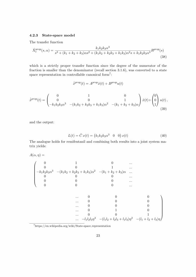
The transfer function

Xprope (s,α) =

k1k2k3α3

s3 + (k1 + k2 + k3)αs2 + (k1k2 + k2k3 + k1k3)α2s+ k1k2k3α3R

prop(s)

(38)

which is a strictly proper transfer function since the degree of the numerator of thefraction is smaller than the denominator (recall section 3.1.6), was converted to a statespace representation in controllable canonical form7:

˙xprop(t) = Aprop

x(t) +Bprop

u(t)

˙xprop(t) =

0 1 00 0 1

−k1k2k3α3 −(k1k2 + k2k3 + k1k3)α2 −(k1 + k2 + k3)α

x(t)+

001

u(t) ,

(39)

and the output:

L(t) = C x(t) =�k1k2k3α

3 0 0�x(t) (40)

The analogue holds for remifentanil and combining both results into a joint system ma-trix yields:

A(α, η) =

0 1 0 ...

0 0 1 ...

−k1k2k3α3 −(k1k2 + k2k3 + k1k3)α2 −(k1 + k2 + k3)α ...

0 0 0 ...

0 0 0 ...

0 0 0 ...

... 0 0 0

... 0 0 0

... 0 0 0

... 0 1 0

... 0 0 1

... −l1l2l3η3 −(l1l2 + l2l3 + l1l3)η2 −(l1 + l2 + l3)η

7https://en.wikipedia.org/wiki/State-space representation

23

andC

� =�k1k2k3α

3 0 0 l1l2l3η3 0 0

�

By taking into account (34), (35) and (36) and choosing another ordering of the elementsin the state vector, the vector used in the article is obtained:

C(θ) =�0 0 m

k1k2k3α3

ECprop50

0 0 l1l2l3η3

ECremi50

�

wherez(t) = C(θ)x(t)

Since we have two input signals, Bprop has to be composed with the corresponding matrixfor remifentanil. Another choice of ordering then leads to the matrix used in the article:

B =

�1 0 0 0 0 00 0 0 1 0 0

�T

B has to be multiplied with u(t), which contains the infusion rates, which is called r(t)in the article and which contains both the rate of propfol and remifentanil:

r(t) =�rprop(t) r

remi(t)�T

The above gives the continuous-time representation:

˙x(t) = A(α, η) x(t) +B r(t)

z(t) = C(θ)x(t)(41)

Because of the dimensions of the matrices A, B and r(t), ˙x is a column vector with 6entries, the first three related to the linear part of propofol, the last three of remifentanil.In order to be able to use the discrete time EKF, the model in 41 is discretized.

From 4.2.1 and 4.2.2 it follows that the model has four system parameters that are tobe estimated:

θ =�α η m γ

�T

The state space of the discretized model is augmented with these four parameters, whichleads to the following ten state variables:

ˆx =�xprop1 xprop2 xprop3 xremi1 xremi2 xremi3 α η m γ

�T

(remember that m = 1 + β)

24

4.2.4 Assigned values to parameters

The following parameters have been assigned the following values:

• k1 and l1 are set to 1

• k2 and l2 are set to 2

• k3 and l3 are set to 3

• y0 is set to 97.7 due to monitor restrictions.

The parameters k1, k2, k3, l1, l2 and l3 are determined over a large database of patientdata. Also EC

prop50 and EC

remi50 are set to fixed values, but these values are not made

explicit in [9] nor is their unit mentioned. This unit inconclusiveness gives rise to prob-lems if these values are to be used on different data sets with different units. It is notmentioned in [9] to what database these parameters were set. Instead, a reference ismade to [8] but it is not mentioned there either.

5 Testing the model on data

5.1 Available data

The data was provided by the universities of Brescia and Porto. The set-up of Portomade use of a PID controller (recall 3.1.7) while in the case of Brescia the drugs wereadministered manually by an anesthesiologist monitoring the patient (so also in closed-loop). Porto used a sample time of 5 s; Brescia used 1 s. Each file corresponds to aspecific surgery of a patient and has (at least) three sets of numbers: the BIS-values, theinfusion rates for propofol and the infusion rates for remifentanil. The available files were:

Brescia (sample time 1 s)

• PZ41 1.mat

– The infusion rate of the drugs are in ml/h and the volumes are in ml. Thedrug concentrations are 20mg/ml for propofol and 10µg/ml for remifentanil.

• PAZ41new.mat (a slightly corrected file of PZ41 1, see section 5.4)

– The infusion rates of the drugs are in mg/s for propofol and µg/s for remifen-tanil. The drug concentrations are 20mg/ml for propofol and 10µg/ml forremifentanil.

Porto (sample time 5 s)

• marsh pat1.mat through marsh pat7.mat (part of BIS Urology, old files)

– The infusion rate units are unknown

25

• schnider pat1.mat through schnider pat7.mat (part of BIS Urology, old files)

– The infusion rate units are unknown

• Bis 1.mat and Bis 2.mat (new files)

– The infusion rates of the drugs are in mg/min

• data HA 1.mat through data HA 5.mat (for cross checking in section 5.5.1)

– The infusion rates of the drugs are in mg/min

The model and implementation will be tested on PAZ41new and Bis 1.

5.2 A typical run on the old data: marsh pat1

In order to gain understanding of the process, the program with the implementationof the EKF that was provided was first run on data that it was said to work on forthe chosen parameters at section 4.2.4. This data was marsh pat1. Here the otherparameters were:

• P0 = diag�1002 102 12 1002 102 12 102 102 1002 1002

�

• R1 = diag�102 102 0.12 102 102 0.12 102 102 302 302

�

• R2 = 1010

• ECprop50 = 80

• ECremi50 = 65

Figure 11 plots the infusion rates of propofol and remifentanil at every time step (aspresent in the data).

Figure 12 plots for every data point of infusion rates the output of the linear blockunit of both propofol and remifentanil, normalized with their respective half effect “con-centrations” (EC50). This plot gives an indication of their respective contributions. Theamplitude of the output of each linear block is in the same range as the amplitude ofits input, because its static gain is one. Therefore, the output of each block should be,just as its input, in the vicinity of the corresponding half effect concentration (EC50),because a much lower value would have no effect and a much higher value would indi-cate an overdose. In other words: it should be inside its therapeutic range (recall section3.2). It follows that the output of both linear block units, normalized by the respectiveEC50s, should roughly have an order of 1, to which the shown graph complies. Thesample interval is 5 seconds.

Figure 13 plots the estimates of the unknown model parameters at every time step.All parameter estimates clearly change over time.

26

0 60 120 180 240 300 360

Time (min)

0

500

1000

1500

2000

2500D

rug r

ate

[m

L/h

] propofol

remifentanil

Figure 11: The infusion rates of propofol and remifentanil from marsh pat1 plottedagainst time.

0 500 1000 1500 2000 2500 3000 3500 4000 4500 5000

time step

0

0.2

0.4

0.6

0.8

1

1.2

1.4

1.6

1.8

Am

plit

ude

Figure 12: Outputs of the linear block of propofol (red) and remifentanil (blue) for everydata point of marsh pat1. The sample interval is 5 seconds.

Figure 14 plots the estimated BIS-value with the measured BIS-value at every timestep. It can be seen that the estimated values follow the measured values, but do soquite roughly: the graph of the real BIS-values show bigger variations than the graphof the estimated values. This is the desired outcome. The curve of the BIS-estimatesshould show the underlying BIS-values, without being distorted by the measurementnoise. So one wants the estimated BIS-values to follow the measurements, but not tooclosely: ideally the error shall not be correlated.

In order to be able to better evaluate the results, another was created where thedifference between measured and estimated bis-value was plotted, which will be includedin the following sections.

27

0 60 120 180 240 300 360

Time (min)

0

0.5

1

1.5

!

"(t)#(t)m(t)$(t)

Figure 13: Estimates of the different parameters plotted against time (marsh pat1)

0 60 120 180 240 300 360

Time (min)

20

30

40

50

60

70

80

90

100

Ou

tpu

t

meas. BIS

est. BIS

Figure 14: The BIS-values (magenta dashed line) and BIS-estimates (blue line) ofmarsh pat1 plotted against time.

28

5.3 Testing on new data from Porto: Bis 1

The program was run on new data from Porto, which was Bis 1. Here the other param-eters were:

• P0 = diag�10000 102 12 1002 102 12 102 102 1002 1002

�

• R1 = diag�100 102 0.12 102 102 0.12 102 102 400 302

�

• R2 = 2 · 109

• ECprop50 = 50

• ECremi50 = 30

A problem that occurred was that the program returned complex values. This wasindicated by Matlab but could also be suspected by the appearance of the first figure(figure 15), which is symptomatic for the emergence of complex values 8:

-0.1 0 0.1 0.2 0.3 0.4 0.5 0.6 0.7 0.8

time step

-1

-0.5

0

0.5

1

1.5

Am

plit

ude

!10-4

Figure 15: Outputs of the linear block of Propofol (red) and Remifentanil (blue) forevery data point of Bis1 giving rise to the suspicion that values had turned complex.

Matlab’s debugger led to the iteration in the end fase of the execution where sud-denly the calculation of the matrix H turned into a matrix with complex values. Moreexactly, when calling the function to calculate the jacobi matrix, all the entries suddenlybecame complex9. A suggestion 10 was to manually convert accidentally obtained com-plex vectors into real ones. The imaginary parts were very close to zero so the idea wasthat it would not make a difference when ignored. This did not work in the end, sinceeven though H (see section 3.4) is forced to be real valued, the vector with all ten stateestimates xtt happens to become complex valued anyway.

8according to Alexander Medvedev

9From now on using tf = isreal(H) as a break point

10by Alexander Medvedev

29

The following part of the bigger expression that is used to calculate the state esti-mates

(x9 k2 k3 x37 x3 /C50prop + I2 I3 x8 x6 /C50remi)

x10

with its parameters plugged in:

(6x9 x37 x3 / 50 + 6x8 x6 / 30)

x10 (42)

turns complex. This happens when the base of the expression turns negative (a negativenumber to a rational power turns complex). The base can only become negative ifthe first terms gets negative and has bigger absolute value than the second (positive)term or if the second term gets negative and has a bigger absolute value than the first(positive) term, or if both terms are negative. It was discovered that x3, x7 and x8 arepositive throughout the running of the program, x9 turns negative in an iteration afterthe change to complex values, and most interestingly x6 gets negative long before thechange to complex values and alternates between negative and positive values throughoutthe running of the program.

By inspecting the different state values during run time it was discovered that morex-values attain negative values from very early on, Only x3, x7 and x8 were positivethroughout the running. Surprisingly, this does not give rise to problems before the endphase, where the complex numbers originated.

The reason why some x-values become negative, could lie in the settings of the EKF(treated in section 5.3.2) or in the scaling of the data (treated in section 5.3.3). Beforegoing into these topics, it is investigated if the problem can be solved with constraints.

5.3.1 Attempt to prevent the occurrence of complex values with constraints

Positivity constraint

The first approach is to put a constraint in the program that the state estimates cannever be negative. This was done by altering the assignment of the state values from

x1=x(1);

to

x1= max(0, x(1));.

and similarly for x2 through x10. Even though this measure prevented negative valuesand the first figure does not show behavior of complex values anymore, it resulted alsoin the warning

Warning: Matrix is singular to working precision.

which points to problems with inverting the matrix in the equation of determining theKalman gain in equation (27). The implementation used the Matlab function inv() and

30

0 2 4 6 8 10 12

time step

0

1

2

3

4

Am

plit

ude

!10-6

Figure 16: Outputs of the linear block of Propofol (red) and Remifentanil (blue) for thefirst twelve data point of Bis1 with a positivity constraint.

a suggestion 11 was to use the function pinv() (pseudo inverse) instead. The use of thepseudo inverse in combination with the positivity constraint resulted in the followingerror message:

Error using svd

Input to SVD must not contain NaN or Inf.

Error in pinv (line 18) [U,S,V] = svd(A,’econ’);

Apart from the singularity warning, the first figure (figure 16) also looks very differ-ent: instead of having two heavily oscillating graphs as in figure 12, it shows two smoothmonotonically increasing curves and only plots the first 12 time steps. Furthermore, allthe parameters seem to have been constant during these time steps as shown in figure17. And finally, the output of the filter is not visible anymore in figure 18. Zoomingin revealed that the bis-estimates were only plotted during the first minute, complyingwith twelve time steps with a sample time of five seconds.

The reason for these observations is that an entry of the state vector (x1) turns neg-ative in iteration 12 and is then (by the constraint) set to zero. In following calculationsthis entry causes divisions by zero, resulting in NaN-entries. Subsequent calculationswith these NaN-entries result in more NaN-entries. This explains the thrown warningand the incomplete graphs: a matrix with NaN entries cannot be inverted and a NaNas an output cannot be plotted.

11by Marcus Bjork

31

0

Time (min)

0

0.5

1

1.5!

"(t)#(t)m(t)$(t)

Figure 17: Parameter estimates for data points of the first 12 time steps of Bis1 with apositivity constraint. All parameters seem to have been constant throughout these timesteps.

0 60 120 180

Time (min)

30

40

50

60

70

80

90

100

Outp

ut

meas. BIS

est. BIS

Figure 18: The BIS-values (magenta dashed line) of Bis1 with a positivity constraintplotted against time. The BIS-estimates (blue line) have vanished because the valueswere NaNs that were not plotted by Matlab. Only a blue dot in the upperleft cornercan be observed.

32

0 500 1000 1500 2000 25000

0.5

1

1.5

Am

plit

ude

0 500 1000 1500 2000 2500

time step

0

2

4

6

8

Am

plit

ude

!10-3

Figure 19: Outputs of the linear block of propofol (red) and remifentanil (blue) for everydata point of Bis1 with absolute value constraint. The sample interval is 5 seconds.

Absolute value

Another constraint on the state estimates that was tried was the absolute value. Thisresulted in no warnings about complex values, nor warning about singular matrices.The figures of the parameter estimates, BIS-measurements and -estimates, and infusionrates had no detectable strange behavior, but in the figure of linear block contributions(figure 19) the curve of remifentanil (blue) has become very small (compare figure 12).Also, the plot in figure 20 of the difference between measured and estimated BIS valuesshowed a discrepancy indicating that the filter is maybe not working properly.

In this case using the pseudo inverse did not result in error messages, but did notchange the figures either.

33

0 20 40 60 80 100 120 140 160 180 200

time (min)

-30

-25

-20

-15

-10

-5

0

5

10

15

y!y

Figure 20: The difference between the measured and estimated BIS values (y − y) forBis1 with absolute value constraint.

5.3.2 Attempt with tuning

The extended Kalman filter needs to be tuned in order to give satisfying results. Thetuning parameters are P0, R1 and R2. P0 is the initial estimate of the covariancematrix. R1 corresponds to the process noise and R2 to the measurement noise, whichsays something about how much one relies on the model or on the data. R1 is a vectorwith values corresponding to the uncertainty of every state; R2 is a scalar. The ratiobetween R2 and a state’s entry in R1 will determine how fast this state will change andconsequently whether the estimate y follows the measurements poorly, smoothly or tooclosely. To some degree one should be able to affect a state individually with tuning.

The idea was that different settings of the filter might also solve the problem ofarising negative x-values and thereby prevent the emergence of complex values.

Since the imaginary values appear so late, it is probably not helpful to alter thematrix with initial values p0, since its effect decreases over time.

The way the new estimate is calculated:

xt+1 = xt +Kt(y(t)− y(t))

points to the conclusion that a too big number is subtracted and that therefore theKalman gain is too strong. This is probably a consequence of that the variance of thenoise of the measurements is bigger than expected. In order to reduce the effect, the

34

initial values of R2 can be increased in equation (27) (repeated for convenience):

K(t) = P (t|t− 1) HT (t)�H(t)P (t|t− 1)]HT (t) +R2(t)

�−1

First it was attempted to remediate the occurrence of negative concentrations byaltering R2. Significantly increasing or decreasing this value had no positive effect.Hereafter, a more directed approach was taken in the form of altering the entry in thediagonal R1 matrix corresponding to the x-values that turned negative. Special attentionwas given to x6 since that was the variable in the exponential expression (42) that turnednegative first.

Tuning the different entries in R1 only managed to delay the emergence of complexnumbers, so altering R1 and R2 did not eliminate the problem of arising complex values.Also, negative values appeared frequently when the program was run on marsh pat1 sothis property does not appear to be of crucial importance.

Another approach was to take a closer look at the data that was fed into the program(Bis 1). With inspection, nothing anomalous could be found: the data showed an overall“smooth” behavior: there were no outliers among the data points. The values for thepropofol concentrations were generally between 2 and 4, apart from the start dose, a fewpoints where it was around 20, or sections where it was 0. But those points were notclose to the point where complex values arose and moreover they were already occurringearly on. However, comparing figure 21 to figure 11 reveals a discrepancy: the plots ofpropopfol and remifentanil in figure 21 are not on the same scale, indicating there couldbe an issue with scaling.

0 60 120 180

Time (min)

0

50

100

150

200

Dru

g r

ate

[m

L/h

]

propofol

remifentanil

Figure 21: The infusion rates of propfol and remifentanil from Bis 1 plotted againsttime.

35

5.3.3 Scaling

The next step was to take a look at the data (marsh pat1 etc.) to which the algorithmwas tuned. Inspecting this it showed there was a big difference in scale between the twodata sets, the second having numbers in the range of multiple hundreds. This raises thequestion what units are used in the different data sets. It was tried to scale the datapoints from (Bis 1) into to the range of the data points from marsh pat1. Roughlythis meant multiplying the propofol concentrations by 100 and the remifentanil concen-trations by 1000. This indeed prevented the occurrence of complex numbers: neitherMatlab threw a warning, nor did the program stop at the conditional break point. Moreinformation about the exact use of units is needed to convert the numbers more precisely.In the paper the unit mg/ml was used, but the graphs carry the description ml/h. Theunit question will be treated in section 5.5.

5.4 Testing on data from Brescia: PZ41 1

Inspection of the PZ41 1 data showed that it does not fit the structure of an inductionphase and maintenance phase (as explained in section 2). The two data files of PZ41 1that were inspected were Pompe.Propofol that contained infusion rates in ml/h andPompe.Vol prop that contained volumes in ml. The first one showed a very steadybehavior: the infusion rate is around 20 ml/h most of the time: from just after the startto almost the end of the data set. Then, after a short transition, it is 10 for a period oftime and then practically turns to zero. The second data file showed a steadily increasingnumber from 0 to 29. This data probably corresponds to the accumulated administereddrug volume. The numbers seem to increase at a very steady pace, being in accordancewith the former data. Throughout the data there are no outliers, so there do not seemto be an initial doses and there are no intermittent infusions.

This oddity was reported to the responsible person in Brescia and it turned outthere was an error with the program that took care of the measurements: it did notsave the drug infusions from the bolus mode (only from the maintenance mode). A new,reconstructed data set (PAZ41new) was received where the initial bolus was calculatedwith help of the volume data. However, no intermittent doses were present and themaintenance dose was of a different order of magnitude in comparison to the old dataset.

5.5 Units

It turned out that the data was collected from three different hospitals with three differ-ent protocols and therefore different units. Information about the used units has beenreceived from Brescia, but only a vague guess for the used units in the old Porto datawas received. In order to determine in what unit the BIS Urology files are delivered,the approach was to, for the respective drugs, look up the recommended bolus doses(used in the induction phase) per kilogram body weight and their units, and with the

36

help of the patient information, in particular the patient’s weight, calculate the actualrecommended initial dose. Since these numbers are quite standard, the data should re-semble the calculated recommended initial dose. This recommended dose is converted todifferent units and these are compared to the induction doses of the data, in an attemptto infer if the unit is volume (ml) per time unit, or mass (mg or µg) per time unit andwhether the time unit is second, minute or hour. In case of volume per time unit, eventhe concentration is needed (mg/ml or µg/ml) to make conversion between mass andvolume possible.

5.5.1 Calculating recommended doses

Table 1 shows the found information with respect to the recommended propofol dosages.

Table 1: Recommended propofol dosages. “IVP q10sec” means “intravenous push everyten seconds” and “ASA III/IV” are categories by the American Society of Anesthesiology.

Induction<55 years: 40 mg IVP q10sec until onset (2-2.5 mg/kg)>55 years or debilitated or ASA III/IV: 20 mg IVP q10sec until onset (1-1.5 mg/kg)Maintenance<55 years old: 0.1-0.2 mg/kg/min IV>55 years old or debilitated or ASA III/IV: 0.05-0.1 mg/kg/min IV

http://reference.medscape.com/drug/diprivan-propofol-343100

InductionLess than 55 years: Anesthetic Induction: 40 mg IV every 10 seconds until inductiononset. Total dose required is 2 to 2.5 mg/kg with a maximum of 250 mg.Less than 55 years: Maintenance of Anesthesia: IV infusion: 100 to 200 mcg/kg/min.Maximum dose 20,000 mcg/min. Maximum dose 10,000 mcg/min.Intermittent bolus: 20 to 50 mg as needed.

https://www.drugs.com/dosage/propofol.html

The patient statistics comprise five fields: a number for the patient’s sex, the age, theweight, the height and a fifth number of which the meaning was unclear. Patient number1 of the marsh study (marsh pat1) had the numbers 1.0, 43.0, 63.0, 170.0, 51.72,which means they is under 55 years of age. This would mean that the induction onset issomewhere between 126 and 157.5 mg with an initial dosage of 240 mg/min. The rateduring maintenance would then be 6.3 - 12.6 mg/min.

37

Table 2: Values for different dose types per data set

Induction phase dose Maintenance doses Intermittent dosesmarsh pat1 (prop vel) 555.5556 (long) 166.9444 - 78.5833 585.5278 - 2318.2

Bis 1 (up) 179.1117 (short) 7.9783 - 1.4783 12.8017 - 22.1750PZ41 1 (Pompe.Propofol) ? 22.10000 20.1000 none

PAZ41new (prop) 3.3330 0.1228 - 0.1006 nonedata HA 1 200-188.32 (very short) 19.3667 - 2.1000 21.2967

The Swedish medical products agency12 has similar recommendations for Propofol, onlyhaving a slightly lower bound for both induction phase and maintenance phase andslightly higher for intermittent doses:

induction: 20-40 mg every tenth second until 1.5-2.5 mg/kgmaintenance: 4-12 mg/kg/hintermittent: 25-50 mg.

The recommended induction dose of 120-240 mg/min and maintenance dose of 3.15/6.3-12.6 mg/min were converted to different units. The values of PAZ41new, PZ41 1, BIS 1and dataHA 1 all fit the recommendations when converted to their stated units. How-ever, the numbers of marsh pat1 do not comply with the recommendations. The value555 would fit best in the range of 360-720 ml/h (with a concentration of 20 mg/ml) forthe induction phase, but then values of 78-166 are much too high for the recommended9.45/18.9-37.8 ml/h for maintenance. If the unit would be ml/h for a concentration of10 mg/ml then 555 would be significantly less than the recommended range of 720-1440ml/h and values of 78-166 would be significantly more than 18.9/37.8-75.6. It has to beconcluded that the proportion between induction and maintenance dose does not followthe recommendations. The maintenance dose should be about one twentieth of the in-duction dose for this patient’s weight. This proportion varies somewhat according to thepatient’s weight, but even for heavier patients the induction and maintenance doses aretoo close to each other. All seven marsh pat files showed the same pattern. Maybe thishas something to do with the nature of the surgery, but this information can probablynot be retrieved anymore and Margarida M. Silva recommended not to rely on this data.Therefore it is decided to use it only for illustrative purposes.

The patient of the Brescia data has the following statistics:Sex: 1, Age: 28, Weight: 90, Height: 190, Ts: 1

which would imply that the total induction onset is somewhere between 180 and 225mg with an initial dose of 240 mg/min. The maintenance dosage should then be 9-18mg/min.

12Lakemedelsverket

38

Since the data from Brescia is, according to personal communication, received in ml/h,conversion to mg/ml requires to know the used concentrations. However, there is con-fusing information about the used concentrations. Personal communication stated thatthe concentrations were 20mg/ml for Propofol and 10µg/ml for Remifentanil, but inthe data file, the statistics read ConcProp: 20 and concRemi: 50.

Because of the lack of information about BIS Urology, it is decided not to use those filesfor calibrating the program or determining the used unit. The most likely scenario atthis point is that the program is calibrated for input in mg/h (according to MargaridaSilva), that there is something significantly abnormal about the BIS Urology files andthat the label of the y-axis of the graph plotting the drugs doses, stating the unit isml/h is a typo.

5.6 Running with conversion to assumed unit

Converting the data of PAZ41new (multiplying by 3600) and Bis 1 (multiplying by 60)to mg/h does not result in any complex numbers. And below follows the analysis ofthese rescaled data sets.

5.6.1 60Bis 1 (converted to mg/h)

The parameters R1, R2, P0, ECprop50 , EC

remi50 were initially as in section 5.3. Running

the program on the converted data with these parameters led to figures 22-25.The blue curve in figure 22 shows that the normalized linear output of remifentanil istoo small (it is not roughly of order 1 as explained in section 5.2). This will be dealtwith in the next section (section 5.6.2).

Figure 23 shows the parameter estimates. Unlike figure 13, not all four parame-ter estimates vary (a lot): at least one seems to have been constant. Changing thecorresponding entries in R1 did not resolve this problem.

The curve of the BIS-estimates in figure 24 follows the BIS-measurements too closely,which means it does not show the underlying structure of the BIS-measurements but isinfluenced too much by the measurement noise. This can also been inferred from figure25, where the error between the estimates and measurements are too close to zero. In anattempt to make the estimate less influenced by the measurement noise, the covariancematrices of the process error (R1) and measurement error (R2) as well as the initialcovariance matrix of the error of the estimate (P0) were changed. The biggest impactseemed to result from changing R2 from 2 · 108 to 2 · 1011.

A peculiar finding was that two different sets of values for P0 produced similarlysmooth estimates, as shown in figure 26 and figure 27, but resulted in very differentestimations of m: if P0 is as in (43), m is estimated around 0.6 (figure 28) and if P0 is asin (44), m is estimated around 1 (figure 29). (R2 = 2 · 1011 and R1, EC

prop50 , and EC

prop50

as before.)

39

P0 = diag�106 104 102 106 104 102 104 104 106 105

�(43)

P0 = diag�104 102 100 104 102 100 102 102 104 103

�(44)

So, given a fixed scaling, it apparently is possible to find different parameter estimateswith different settings of the EKF. It is therefore unclear how to determine if a solutionis valid.

0 500 1000 1500 2000 2500

time step

0

0.5

1

1.5

Am

plit

ude

Figure 22: Outputs of the linear block of propofol (red) and remifentanil (blue) for everydata point of Bis1 converted to mg/h. The blue line is close to zero. The sample intervalis 5 seconds.

0 60 120 180

Time (min)

0

0.5

1

1.5

!

"(t)#(t)m(t)$(t)

Figure 23: Parameter estimates for every data point of Bis1 converted to mg/h.

40

0 60 120 180

Time (min)

30

40

50

60

70

80

90

100

Outp

ut

meas. BIS

est. BIS

Figure 24: The BIS-values (magenta dashed line) of Bis1 converted to mg/h plottedagainst time. The BIS-measurements are mostly covered by the BIS estimates.

0 20 40 60 80 100 120 140 160 180 200

time

-15

-10

-5

0

5

10

15

20

25

y!y

Figure 25: The difference between the measured and estimated BIS values (y − y) forBis1 converted to mg/h.

41

0 60 120 180

Time (min)

30

40

50

60

70

80

90

100

Outp

ut

meas. BIS

est. BIS

Figure 26: The BIS-values (magenta dashed line) and BIS-estimates (blue line) of Bis1converted to mg/h plotted against time with P0 as in equation (43)

.

0 60 120 180

Time (min)

20

30

40

50

60

70

80

90

100

Outp

ut

meas. BIS

est. BIS

Figure 27: The BIS-values (magenta dashed line) and BIS-estimates (blue line) of Bis1converted to mg/h plotted against time with P0 as in equation (44).

42

0 60 120 180

Time (min)

0

0.5

1

1.5

!

"(t)#(t)m(t)$(t)

Figure 28: Parameter estimates for every data point of Bis1 converted to mg/h whereP0 is as in equation (43).

0 60 120 180

Time (min)

0

0.5

1

1.5

!

"(t)#(t)m(t)$(t)

Figure 29: Parameter estimates for every data point of Bis1 converted to mg/h whereP0 is as in equation (44).

5.6.2 Bis1 (converted to mg/h) and tuned

In order to get the normalized linear output of both propofol and remifentanil aroundorder 1 (as explained in section 5.2), the half effect concentrations were changed. Thisled to the following parameters:

43

• P0 = diag�104 102 100 104 102 100 102 102 104 103

�

• R1 = diag�1 104 0.12 102 102 0.12 200 102 302 302

�

• R2 = 2 · 1011

• ECprop50 = 50

• ECremi50 = 1

Figure 30 shows that the normalized linear output in general is in the desired rangefor both drugs, except for the very beginning of the surgery, where it is rather high forpropofol. However, this might be acceptable for the induction phase where typicallyhigh dosages are administered. Figure 31 shows the parameter estimates. Again, not allfour seem to vary as much as in figure 13. Changing the corresponding entries in R1 didnot resolve this problem.

Figure 32 shows the BIS-measurements and -estimates. Except for the beginning,the estimates follow the measurements smoothly, indicating a good estimate. This isin compliance with figure 33 that shows the difference between the measurements andestimates: the difference is restricted, indicating the estimates are not far off, but atthe same time not too small, indicating the estimates are not influenced too much bymeasurement noise. More tuning of P0 or using the values of P0 in [9]13 did not improvethe approximation in the beginning.

0 500 1000 1500 2000 2500

time step

0

0.5

1

1.5

2

2.5

3

3.5

4

Am

plit

ude

Figure 30: Outputs of the normalized linear block of propofol (red) and remifentanil(blue) for every data point of Bis1 converted to mg/h.

13P0 = diag�100

210

212

1002

102

12

102

102

102

102�

44

0 60 120 180

Time (min)

0

0.5

1

1.5

!

"(t)#(t)m(t)$(t)

Figure 31: Parameter estimates for every data point of Bis1 converted to mg/h

0 20 40 60 80 100 120 140 160 180 200

Time (min)

20

30

40

50

60

70

80

90

100

meas. BIS

est. BIS

Figure 32: The BIS-values (magenta dashed line) and BIS-estimates (blue line) of Bis1converted to mg/h plotted against time.

45

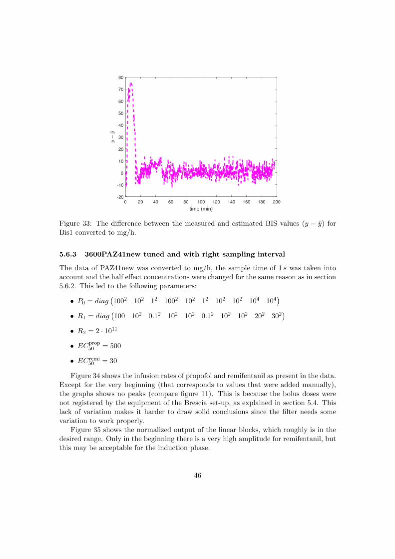
0 20 40 60 80 100 120 140 160 180 200

time (min)

-20

-10

0

10

20

30

40

50

60

70

80

y!y

Figure 33: The difference between the measured and estimated BIS values (y − y) forBis1 converted to mg/h.

5.6.3 3600PAZ41new tuned and with right sampling interval

The data of PAZ41new was converted to mg/h, the sample time of 1 s was taken intoaccount and the half effect concentrations were changed for the same reason as in section5.6.2. This led to the following parameters:

• P0 = diag�1002 102 12 1002 102 12 102 102 104 104

�

• R1 = diag�100 102 0.12 102 102 0.12 102 102 202 302

�

• R2 = 2 · 1011

• ECprop50 = 500

• ECremi50 = 30

Figure 34 shows the infusion rates of propofol and remifentanil as present in the data.Except for the very beginning (that corresponds to values that were added manually),the graphs shows no peaks (compare figure 11). This is because the bolus doses werenot registered by the equipment of the Brescia set-up, as explained in section 5.4. Thislack of variation makes it harder to draw solid conclusions since the filter needs somevariation to work properly.

Figure 35 shows the normalized output of the linear blocks, which roughly is in thedesired range. Only in the beginning there is a very high amplitude for remifentanil, butthis may be acceptable for the induction phase.

46

An important and worrying observation is that the parameter estimates of α andη in figure 36 are flipped compared to the estimates for the Bis1 data in figure 31.This is unexpected since one expects all patients to comply to the same model, andthat parameters only differ slightly between patients. The situation where parameterestimates develop significantly differently between patients is not in line with this. Also,not all four parameters seem to vary as much as in figure 13: some seem to be roughlyconstant. Changing the corresponding entries in R1 did not resolve this problem.

Figure 37 shows the BIS-measurements and -estimates. Just as the BIS-estimates forthe Bis1 data in figure 32, it shows a poor approximation in the beginning of the processand this could not be resolved by more tuning of P0 or using the recommended entriesfor P0 in [9]. However, whereas the curve in figure 32 displays a smooth development, thecurve in figure 37 displays a more sharp-cornered irregular pattern, indicating that theseestimates are influenced more severely by measurement noise. This is in compliancewith figure 38 that shows that the difference between the measurements and estimatesis quite small (and smaller than for Bis1 in figure 33). Maybe more tuning of R1 will beable to improve the approximation, but this result was the best result obtained withinthe scope of this project.

0 60

Time (min)

0

0.5

1

1.5

2

2.5

3

Dru

g r

ate

[m

L/h

]

!104

propofol

remifentanil

Figure 34: The infusion rate of propofol and remifentanil from PAZ41new (converted tomg/h and tuned) plotted against time.

47

0 500 1000 1500 2000 2500 3000 3500 4000 4500

time step

0

2

4

6

8

10

12

14

16

18

Am

plit

ude

Figure 35: Normalized outputs of the linear block of propofol (red) and remifentanil(blue) for every data point of PAZ41new (converted to mg/h and tuned). The sampletime is 1 s

0 60

Time (min)

0

0.5

1

1.5

!

"(t)#(t)m(t)$(t)

Figure 36: Parameter estimates of PAZ41new (converted to mg/h and tuned) plottedagainst time.

48

0 60

Time (min)

0

10

20

30

40

50

60

70

80

90

100O

utp

ut

meas. BIS

est. BIS

Figure 37: The BIS-values (magenta dashed line) and BIS-estimates (blue solid line) ofPAZ41new (converted to mg/h and tuned) plotted against time.

0 10 20 30 40 50 60 70 80

time (min)

-10

0

10

20

30

40

50

60

70

y!y

Figure 38: The difference between the measured and estimated BIS values (y − y) forPAZ41new (converted to mg/h and tuned).

49

6 Conclusion and future work

The uncertainty about the used unit in the BIS Urology files caused a lot of trouble andthis uncertainty could not be resolved using international dosage standards. Therefore,eventually an educated guess was made about the unit in which the data of Brescia andPorto should be provided to the program. In addition, with trial and error, the EC50swere set to values that produced a sensible scale in the normalized output of the linearblock. This guessing of the right scaling of the data and the right values for the halfeffect concentrations made it harder to draw reliable conclusions.

The EKF was tuned by varying the initial covariance matrix P0, and the covariancematrices of the process noise and measurement noise (R1 and R2 respectively). Atbest, this resulted in fairly good BIS-estimations, but at the same time in parameterestimates that were constants over time. Addressing this issue by directly changing thecorresponding entries in R1 did not result in more varying parameter estimates. Thestate space entries related to the linear part of propofol and remifentanil (i.e. the firstsix entries) did not seem to play a role at all and changing a parameter entry in R1 didnot straightforwardly affect the estimate of the corresponding parameter. This is not inaccordance with general properties of tuning (as treated in section 5.3.2) and this findingquestions how useful further tuning of R1 is, and also how adequate the used model isor how adequate the set parameters are.

Another worrying finding was that different settings of the EKF, while resulting incomparable tracking performances, could lead to different parameter estimates. Thisraises the question what solution is correct and how to determine this. Assuming thescaling of the data is somewhat accurate, this points out the limitations of the usedmodel: apparently it is not able to produce a unique solution for the used data. Also,the finding that parameter estimates could differ significantly between patients, ques-tions the used model. Maybe the parameter estimates could be quite different betweenpatients, but reasonably they should be in the same order of magnitude and should playa comparable role in the model. Flipped parameters as described in 5.6.3 do not complywith this. Another finding that questions the used model was that altering P0 did notmanage to improve the approximation in the beginning of the process. A different modelmay therefore be more adequate.

Another difficulty was that the data of Brescia did not include bolus dosages. Thishas a negative implication on the validity of the results, because one needs to have somevariation in the input for the algorithm to produce reliable estimates. This is because ifthe input signals are constant, then the output signal will also become constant, whichmakes it impossible to learn about the dynamics of the system.

Since the results question the validity of the used model, future work should include:the replication of the procedure on other data, the replication on data from Brescia thatdoes include all administered bolus doses, and the comparison with the application ofother models (e.g. compartment models) on the studied data.

The long term goal is to make automatic closed-loop anesthesia possible with thebenefits of relieving the anesthesiologist from the hard task of administering optimal

50

drug doses, achieving more consistent drug effects by means of individualization, andreducing side effects because of the achieved reduced overall drug administration.

References

[1] Panos J Antsaklis and Anthony N Michel. A linear systems primer. Birkhauser,Boston, 2007.

[2] Joseph T. DiPiro, William J. Spruill, William E. Wade, Robert A. Blouin, andJane M. Pruemer. Concepts in clinical pharmacokinetics. American Society ofHealth-System Pharmacists, 2005.

[3] Graham C Goodwin, Stefan F Graebe, and Mario E Salgado. Control system design.Prentice Hall, 2001.

[4] Lennart Ljung and Torkel Glad;. Modeling of Dynamic Systems. Prentice Hallinformation and system sciences series, 1994.

[5] Peter S. Maybeck. Stochastic models, estimation, and control, vol-ume 141 of Mathematics in Science and Engineering, chapter 1. 1979.http://www.cs.unc.edu/∼ welch/kalman/media/pdf/maybeck ch1.pdf.

[6] Richard M Murray and Karl Johan Astrom. Feedback systems: an introduction forscientists and engineers. Princeton University Press, 2008.

[7] Margarida M. Silva. Nonlinear Modeling and Feedback Control of Drug Delivery inAnesthesia. Uppsala: Acta Universitatis Upsaliensis, 2014.

[8] M.M. Silva, T. Mendonca, and T. Wigren. Nonlinear identification of the hu-man response to anaesthesia by the use of bis measurements. Dept. Infor-mation Technology, Uppsala University, Uppsala, Sweden, Tech. Rep. 2010-008,http://www.it.uu.se/research/publications/reports/2010-008/2010-008-nc.pdf.

[9] M.M. Silva, T. Mendonca, and T. Wigren. Online nonlinear identification of theeffect of drugs in anaesthesia using a minimal parameterization and bis measure-ments. Proc. American Control Conference (ACC), Baltimore, MD, USA, pages4379–4384, June 30 - July 2, 2010.

[10] T. Soderstrom. Discrete-time Stochastic Systems: estimation and control. Springer-Verlag London Limited, 2002.

51