modeling of hydraulic systems - maplesoft.com · hydraulics library tutorial ... is not a standard...
TRANSCRIPT

Modeling of Hydraulic Systems
Tutorial for the Hydraulics Library
®

Hydraulics Library Tutorial
The software described in this document is furnished only under license, and may be used or copied only
in accordance with the terms of such license. Nothing contained in this document should be construed to
imply the granting of a license to make, use, or sell any of the software described herein. The information
in this document is subject to change without notice, and should not be construed to imply any
representation or commitment by the author.
This document may not be reproduced in whole or in part without the prior written consent of the author.
MapleSim, Maple, and Maplesoft are trademarks of Waterloo Maple Inc.
Modelica® is a registered trademark of the Modelica Association.
PneuLib, HyLib, Pneumatics Library and Hydraulics Library are registered trademarks of Modelon AB.
Other product or brand names are trademarks or registered trademarks of their respective holders.
Hydraulics Library Manual and Tutorial
2013-09-04
© 1997 – 2013 Modelon AB. All rights reserved.
Modelon AB
IDEON Science Park
SE-223 70 LUND
Sweden
E-mail: [email protected]
URL: http://www.modelon.com/
Phone: +46 46 286 2200
Fax: +46 46 286 2201
Maplesoft
615 Kumpf Drive
Waterloo, ON, N2V 1K8
Canada
E-mail: [email protected] URL: http://www.maplesoft.com/
Phone: +1-519-747-2373
Fax: +1-519-747-5284

“Everything should be made as simple as possible,
but not simpler.”
Albert Einstein

Preface
Modeling the static and dynamic response of hydraulic drives has been a research topic for a number a
decades. In the fifties a number of models for analog computers have been developed and published. The
restrictions of the analog computers limited the size of the models. Often they were linearized about an
operating point and could therefore not predict the response of the system for large deviations from that
operating point.
In the seventies digital computers became available and were used to model and simulate hydraulic
systems. In the beginning only small models with few states were used because no simulation software
was available. For each modeling task a new program had to be written in a programming language, e. g.
ALGOL or FORTRAN. Later the first simulation languages, e. g. CSMP, were used. Because of the lack
of reusable models these studies were very time consuming.
During that time a lot of research was done to develop mathematical models, i. e. to find mathematical
equations that describe the response of a hydraulic component. This work, today’s powerful digital
computers and high level simulation languages enable us to quickly model and simulate even complex
hydraulic circuits and study them before any hardware has been build.
This tutorial gives an overview about both modeling complex hydraulic systems and modeling typical
components. For a number of components it lists several mathematical models and compares them. But it
is not a standard text book on hydraulics because it doesn’t explain the operation of these components.
This tutorial gives general remarks and examples of modeling hydraulic systems in chapter 2. In chapter 3
a number of component models is given. The reference section gives the details of the model
implementation in the Hydraulics Library (formerly HyLib) in the Modelica language version 3.1.

TABLE OF CONTENTS
Hydraulics Library Tutorial 2
PREFACE 4
1 BASIC PRINCIPLES 0
2 SYSTEM MODELS 2
2.1 Hydraulic Drive 9
2.2 Hydrostatic Transmission (Closed Circuit) 10
2.3 Hydrostatic Transmission (Open Circuit) 11
2.4 Hydrostatic Transmission (Secondary Control) 12
2.5 Including mechanical parts 13
2.6 Semi-empirical models 14
2.7 Using Modelica's advanced features 15
3 COMPONENT MODELS 17
3.1 Hydraulic fluids 17 3.1.1 Compressibility 17 3.1.2 Viscosity 22 3.1.3 Inductance 25
3.2 Pumps 27 3.2.1 Theoretical Displacement, Power Flow of an Ideal Pump 27 3.2.2 Efficiency 27 3.2.3 Modeling the Losses 28 3.2.4 Physically Motivated Models 29 3.2.5 Abstract Mathematical Models 31 3.2.6 Models for Time Domain Simulation 33 3.2.7 Effects of Reduced Intake Pressure 35
3.3 Motors 38
3.4 Cylinders 40 3.4.1 Seal friction 40 3.4.2 Leakage 44 3.4.3 Fluid Compressibility and Housing Compliance 44 3.4.4 What happens if there is no flow but the rod is pulled out? 44
3.5 Restrictions 46 3.5.1 Calculating Laminar Flow 47 3.5.2 Calculating Discharge Coefficient Cd For Turbulent Flow Through Orifices 50 3.5.3 Calculating Loss Coefficients or K-Factors 53 3.5.4 Cavitation 57 3.5.5 Metering Edges of Valves 58 3.5.6 Library Models for Orifices 58 3.5.7 Library Models for Metering Orifices of Valves 65
3.6 Spool Valves 66 3.6.1 Servo and Proportional Valves 66 3.6.2 Directional Control Valves 69
3.7 Flow and Pressure Control Valves 71
3.8 Long Lines 75 3.8.1 Steady State Pressure Loss in Lines 75 3.8.2 Modeling the Dynamics of Long Lines 77 3.8.3 Examples using Model LongLine and LongLine_u_air 80
3.9 Accumulators 85
3.10 Filters and Coolers 85
REFERENCES 86
INDEX 94


0 1 Basic Principles
1 Basic Principles
There are several ways to model a hydraulic system. Which is appropriate depends on the purpose of the
simulation study. A model can be very small and linear to gain insight in the typical response of a system,
e. g. stability or sensitivity to parameter changes. Or it can be very elaborate and consist of a lot of
nonlinearities to predict the response of a particular machine and a particular load cycle.
Modeling a dynamic system is an engineering task and that means there are some guidelines but no fixed
rules that will guarantee success, if followed, or lead to failure, if ignored. The main point is that a good
model helps to get the work done, to answer the questions that were the reason it was made.
Unfortunately it is not possible to say in advance which the answers to the questions are.
One reasonable approach is to start modeling “the heart of the system” assuming ideal boundary
conditions. In case of a hydraulic control system this may be the inner loop consisting of a servovalve and
a cylinder. Pressure supply, auxiliary valves and instrumentation can be modelled as ideal. The first
simulation runs will show the influence of the valve characteristics, the internal leakage of the cylinder or
the response of the external load. At this point more detailed information is usually needed about the key
components which leads to questions to the manufacturer or own measurements. If the response of this
small system is fully understood, more detailed models can be used for the auxiliary components. For
instance the ideal pressure supply can be replaced by a model of a pump driven by an electric motor and a
pressure valve. The model of the pump can include the torque and volumetric losses and the valve model
can include leakage and saturation.
If stability problems occur it is always useful to look at the linearized system. While building the model
one should therefore try to find out which component influences which eigenvalues, e. g. associate the
very lightly damped mode with a pressure valve or the large time constant with the volume at the main
pump.
The model should be as simple as possible but not simpler. It should describe the physical phenomena
even if the used parameters are always somewhat wrong. This means that it always makes sense to model
leakage even if it is small because it adds almost always damping to the system. And real systems are
very often better damped than their models. It depends on the system and the experience of the analyst
whether it is better to use “global” models of the components or “local” when modeling a system. For
example a global model of a pump includes the reduction of output flow if the input pressure is too low
while the smaller local model doesn’t describe this effect. If the system works properly the pump’s inlet
pressure is always high enough and the global model is not necessary. If on the other hand the inlet
pressure is too low the local model is not a valid representation of the system and leads to wrong results.
1 Basic Principles 1
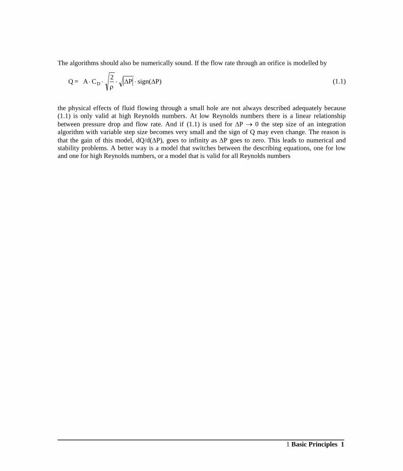
The algorithms should also be numerically sound. If the flow rate through an orifice is modelled by
P)sign( P 2
C A = Q D
(1.1)
the physical effects of fluid flowing through a small hole are not always described adequately because
(1.1) is only valid at high Reynolds numbers. At low Reynolds numbers there is a linear relationship
between pressure drop and flow rate. And if (1.1) is used for P 0 the step size of an integration
algorithm with variable step size becomes very small and the sign of Q may even change. The reason is
that the gain of this model, dQ/d(P), goes to infinity as P goes to zero. This leads to numerical and
stability problems. A better way is a model that switches between the describing equations, one for low
and one for high Reynolds numbers, or a model that is valid for all Reynolds numbers

2 2 System Models
2 System Models
The conceptive easiest way to model a hydraulic system is to identify all important components, e. g.
pump, valves, orifices, cylinders, motors, etc. connect their models according to the circuit diagram and
place a lumped volume at each node, the connection of two or more components. This leads to a set of
differential equations where the through variable, flow rate, can be easily calculated from the known state
variables, i. e. the across variables, which are the pressures in the volumes (nodal analysis).
The laminar resistance is a typical example. The flow rate Q through that component is calculated by:
) P-(P G = Q BA (2.1)
where G is the conductance, PA is the pressure at port A and PB is the pressure at port B. The flow rate is
positive, Q > 0, if PA > PB. The through variable of this model is the mass flow rate Q = m_flow which
is identical for the input and the output port. The across variables are the pressures PA and PB, which are
usually different.
The library icons show the symbol of the component, the abbreviation and names the ports if necessary,
the object diagram includes the across and through variables and the positive flow direction.
Figure 2.1 Diagram of laminar resistance.
In a lumped volume the flow rate is integrated with respect to time to calculate the pressure. The
describing differential equation is:
Q(t) V
=dt
dP
(2.2)
with the bulk modulus , the volume V and the flow rate Q(t). Both and V can be constants or depend
on other system variables. The across variable is again the pressure P, the through variable the flow rate
m_flow. In the library oil filled components are symbolized by the red background of the drawing, e. g.
the model OilVolume or ChamberA.

2 System Models 3
Figure 2.2 Icon of lumped volume, library model OilVolume
The direct connection of two lumped volumes leads usually to problems. If you look at the resulting
system from a modeling point it is a poor model because there is always a resistance between two real
energy storage devices (and this is not included in the model). In the electrical world this could be the
resistance of the wire between two capacitors, in the hydraulic world the resistance of the connecting
hose. System theory says that such a system is not completely controllable and observable, i. e. not a
minimal realisation. Mathematicians say that the resulting differential equations form a higher index
system that cannot be solved by the usual integration algorithms. However, when looking at such a
system an engineer would simply eliminate one state (differential equation of a lumped volume) and add
the amount of oil of that state to the other state. This can be done automatically by an appropriate
algorithm that is implemented in MapleSim. It is then possible to connect lumped volumes directly to one
another and this feature is used in the Hydraulics library.
For the proposed modeling approach the system in Figure 2.3 gives an example. It has a pump as flow
source with a relief valve, a 4 port control valve, a hydraulic motor and a tank.

4 2 System Models
Figure 2.3 Example system
In most cases it is best to model a pump as a flow source because almost all pumps used for oil hydraulics
displace the fluid with pistons, gears or vanes. This means they produce a flow rate while the pressure
builds up according to the resistances the oil has to pass on its way to the tank. In this example the flow
rate of the pump is constant, i. e. Qpump = 10-3 m3/s. In the library SI units are used. This has the
advantage that no conversions are needed during calculations. On the other hand the approach can lead to
numerical problems because some of the numbers of the resulting set of equations are very big (e. g.
pressure: 107 Pa) while others are very small (e. g. conductance: 10
-12 m
3/(s Pa) ).
In the model the tank has always a constant pressure regardless of the amount of oil coming in. In this
example the preload pressure is 0 Pa (against the atmosphere).
The pressure relief valve can be described by a (static) relationship of the pressure differential between
the inlet port and the outlet port and the resulting flow through the valve. In most cases this simple model
is sufficient because the speed of response of a relief valve is usually many times faster than that of the
driven load. A more detailed model can be derived from measurements of the input-output response
(Viersma 1980) or by modeling all parts of the valve, like spool, springs, orifices (Merritt 1967).
Unfortunately the necessary parameters for these dynamic models are not easily available.
A simple model of the control valve uses orifices to describe the resistances the oil has to pass depending
on the position of the lever. A simple model of the hydraulic motor describes the torque at the shaft as a
function of the pressure at the two ports and the motor displacement, DMotor.
2
(t) P- (t)P D= (t) BA
Motor
(2.3)
2 System Models 5
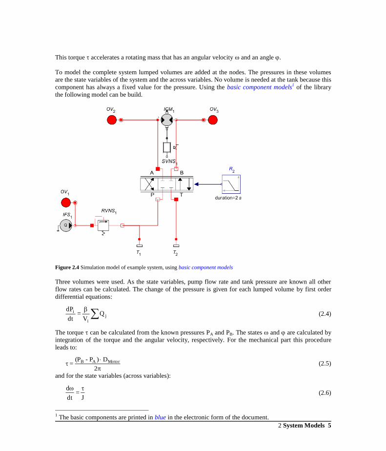
This torque accelerates a rotating mass that has an angular velocity and an angle .
To model the complete system lumped volumes are added at the nodes. The pressures in these volumes
are the state variables of the system and the across variables. No volume is needed at the tank because this
component has always a fixed value for the pressure. Using the basic component models1 of the library
the following model can be build.
Figure 2.4 Simulation model of example system, using basic component models
Three volumes were used. As the state variables, pump flow rate and tank pressure are known all other
flow rates can be calculated. The change of the pressure is given for each lumped volume by first order
differential equations:
ji
i QV
=td
Pd (2.4)
The torque can be calculated from the known pressures PA and PB. The states and are calculated by
integration of the torque and the angular velocity, respectively. For the mechanical part this procedure
leads to:
2
D ) P- (P = MotorAB (2.5)
and for the state variables (across variables):
J
=td
d (2.6)
1 The basic components are printed in blue in the electronic form of the document.

6 2 System Models
=td
d (2.7)
The placement of volumes at the nodes can be justified by the fact that there is very often a considerable
amount of oil in the fittings and hoses between the components. The compliance of this oil and the
housings can lead to lightly damped oscillations.
But while this manual placement of lumped volumes makes sense from a modeling point of view there
are at least two drawbacks. In a typical hydraulic circuit diagram these volumes don’t appear and
therefore a number of engineers don’t like them to be in the object diagram of the simulation model.
Some component models already have a lumped volume included, e. g. the cylinder models. And if the
placement of lumped volumes can be done automatically by the simulation program the modeller
shouldn’t be required to do so. In the main windows of the Hydraulics library almost all component
models have therefore already added these volumes at the hydraulic ports. And if applicable the inertia of
the moving parts is also included. Figure 2.5 shows the object diagram of the main motor model. It is
composed of the ideal motor, laminar resistances to model the leakage and the rotor to describe the inertia
of the motor shaft and the coupled load.
Figure 2.5 Object diagram of main motor model ConMot
Using the main models the object diagram looks very similar to a hydraulic circuit diagram; the user
doesn’t have to place lumped volumes at the nodes.

2 System Models 7
Figure 2.6 Simulation model of example system using main models
The amount of oil at a port becomes a parameter in the parameter window of the model.
Figure 2.7 Parameter window of ConMot, model of a constant displacement motor

8 2 System Models
Sometimes however these volumes become very small and their time constants are negligible compared
with the rest of the system dynamics. In this case the basic models can be used without the volumes and a
numerical solution of the resulting equations can be used.
Besides the lumped volume there is a second energy storage element in hydrostatic systems: The
inductance of an oil column. This storage element is equivalent to the inertia of a mass in translational
mechanics. Usually it is not necessary to include this effect in a system model. However if there are high
frequency excitations or long lines the effect of the inductance of the oil column cannot always be
neglected.
Hydraulic systems are usually build to drive mechanical loads, e. g. propel a vehicle or move a mass.
When modeling a system it is necessary to model these mechanical parts too. And detailed models of
hydraulic components often require the modeling of the inertia of moving parts, e. g. spools or pistons.
Simple mechanical models with one degree of freedom are therefore needed.
The easiest way to model a translational mechanical system with one degree of freedom is to identify all
components that have a mass, regard them as rigid and connect them with compliant components, e. g.
springs or dampers. This leads to a set of differential equations where the through variable, force F, can
be easily calculated from the known state variables, i. e. the across variables, which can be the positions s
and velocities, v = d s/d t, of the masses. It is important to use the same coordinate system throughout the
model! The icons of the mechanical models show therefore a small arrow: All arrows must point to the
same direction!
2 System Models 9
As with lumped volumes the direct connection of two masses leads to a singular problem. It is necessary
to have one compliant component in between, e. g. a spring. However the mechanical libraries in the
Modelica standard library and MapleSim are set up such that a rigid connection between two masses can
be dealt with.
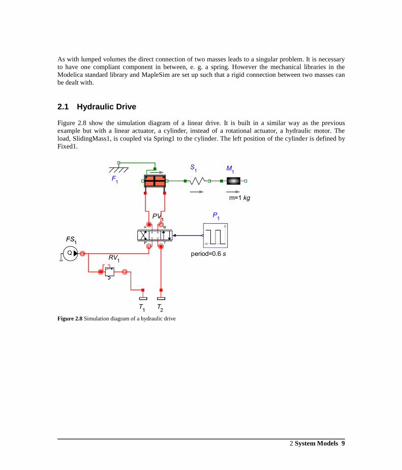
2.1 Hydraulic Drive
Figure 2.8 show the simulation diagram of a linear drive. It is built in a similar way as the previous
example but with a linear actuator, a cylinder, instead of a rotational actuator, a hydraulic motor. The
load, SlidingMass1, is coupled via Spring1 to the cylinder. The left position of the cylinder is defined by
Fixed1.
Figure 2.8 Simulation diagram of a hydraulic drive

10 2 System Models
2.2 Hydrostatic Transmission (Closed Circuit)
Figure 2.9 show the simulation model of a hydrostatic transmission. This kind of drive is used for small
wheel loaders or fork lift trucks. There are many studies on the dynamic response of these drives (e. g.
Knight et al. 1972, Hahmann 1973, Svoboda 1979, Wochnik and Frank 1993, Lennevi 1995, Sannelius
1999).
The necessary power is delivered by a diesel engine, symbolized by the rectangle. This engine drives the
main pump and a charge pump. The main pump is a variable displacement pump that can produce an oil
flow in both directions, depending on the command signal. The main pump is connected to the wheel
motor which has a constant displacement. This kind of circuit is called “closed circuit” because the pump
output flow is sent directly to the hydraulic motor and then returned in a continuous motion back to the
pump. The charge pump is needed to maintain a minimum pressure in the return line from the motor to
the pump, i. e. replenish the oil that has left the circuit as leakage. The pressure in the return line is limited
by the relief valve. There are two more relief valves to limit the pressure in the high pressure line.
Figure 2.9 Object diagram of a closed circuit hydrostatic transmission
This system shows the importance of “global” component models. If for example the diameter of the
check valves is too small or the charge pressure is too low the pressure in the return line will drop below
atmospheric pressure at high speed. If the reduction of output flow and the limit of the pressure to the
vapour pressure were not modelled the simulation would show negative pressure values in the return line.
To use this hydrostatic transmission a controller is necessary to give input signals to the Diesel engine and
the main pump. In the past different concepts have been used. The simplest way was to give the operator

2.2 Hydrostatic Transmission (Closed Circuit) 11
two levers to change both signal manually. Another machine used an open loop strategy to command the
swash angle of the main pump and the engine speed as a function of commanded speed. An important
feature of the controller was overload detection and deswashing of the pump to prevent the Diesel engine
from stalling if the required torque was too high. Newer concepts use nonlinear decoupling controllers
that are realized electronically (Wochnik and Frank 1993, Lennevi 1995).
2.3 Hydrostatic Transmission (Open Circuit)
The hydrostatic transmission in Sect. 2.1 is a closed circuit system. The drive in Figure 2.10 is an open
circuit system because the oil flows from the motor into the tank and not to the pump. This kind of circuit
is used if the pump delivers oil to several actuators including double-acting cylinders with differential
area because then the return flow differs from the pump flow. This is a common situation for excavators
which have cylinders with differential area for the boom, arm and bucket and motors for the swing and
propel.
Figure 2.10 Simulation diagram for hydraulic drive with counterbalance valve
When using a motor in an open circuit a counterbalance valve is needed to decelerate the load. Figure
2.10 show the circuit. If the pump pressure is high enough the counterbalance valve is wide open and the
oil flows from the pump to the motor, through the counterbalance valve to the tank. If the pump pressure
is about the atmospheric pressure the spring in the counterbalance valve moves the spool to the left and
12 2 System Models
the valve is closed. If the motor is rotating there will be a pressure build up at motor port B which leads to
a torque that decelerates the motor. The vehicle stops.
These systems tend to be oscillatory when decelerating the motor. In that operating condition the needed
pump power is small (the pressure is low) and it is therefore not necessary to model the Diesel engine and
the pump in detail. A constant flow source is used instead. The check valve is used to provide more
damping of the system. The intention is to close the valve fast, and open it slowly.
The external torque to the motor can be used to analyse different operating conditions, e. g. model an
uphill or downhill slope. The model is very well suited to look at the sensitivity to parameter changes, e.
g. the effect of a reduction of the internal or external leakage of the motor or a change of the amount of oil
in the lumped volumes. A detailed study of this kind of drive system was done by Kraft (1996).
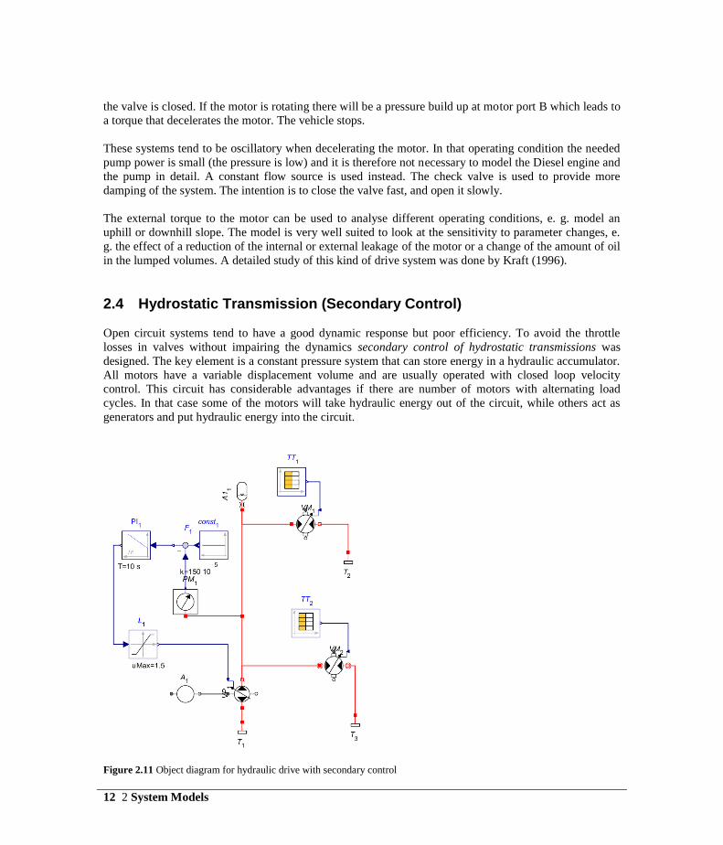
2.4 Hydrostatic Transmission (Secondary Control)
Open circuit systems tend to have a good dynamic response but poor efficiency. To avoid the throttle
losses in valves without impairing the dynamics secondary control of hydrostatic transmissions was
designed. The key element is a constant pressure system that can store energy in a hydraulic accumulator.
All motors have a variable displacement volume and are usually operated with closed loop velocity
control. This circuit has considerable advantages if there are number of motors with alternating load
cycles. In that case some of the motors will take hydraulic energy out of the circuit, while others act as
generators and put hydraulic energy into the circuit.
Figure 2.11 Object diagram for hydraulic drive with secondary control
2.6 Semi-empirical models 13
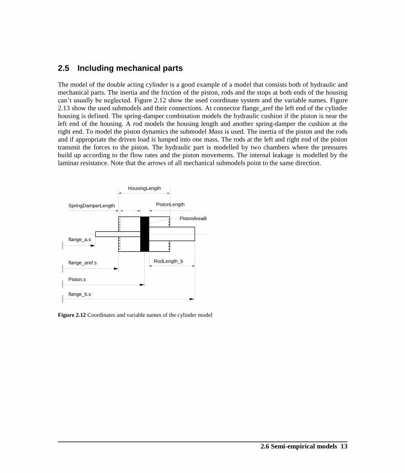
2.5 Including mechanical parts
The model of the double acting cylinder is a good example of a model that consists both of hydraulic and
mechanical parts. The inertia and the friction of the piston, rods and the stops at both ends of the housing
can’t usually be neglected. Figure 2.12 show the used coordinate system and the variable names. Figure
2.13 show the used submodels and their connections. At connector flange_aref the left end of the cylinder
housing is defined. The spring-damper combination models the hydraulic cushion if the piston is near the
left end of the housing. A rod models the housing length and another spring-damper the cushion at the
right end. To model the piston dynamics the submodel Mass is used. The inertia of the piston and the rods
and if appropriate the driven load is lumped into one mass. The rods at the left and right end of the piston
transmit the forces to the piston. The hydraulic part is modelled by two chambers where the pressures
build up according to the flow rates and the piston movements. The internal leakage is modelled by the
laminar resistance. Note that the arrows of all mechanical submodels point to the same direction.
Figure 2.12 Coordinates and variable names of the cylinder model
flange_aref.s
Piston.s
flange_a.s
flange_b.s
PistonLength
HousingLength
SpringDamperLength
RodLength_b
PistonAreaB
14 2 System Models
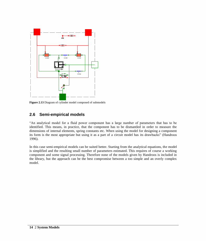
Figure 2.13 Diagram of cylinder model composed of submodels
2.6 Semi-empirical models
“An analytical model for a fluid power component has a large number of parameters that has to be
identified. This means, in practice, that the component has to be dismantled in order to measure the
dimensions of internal elements, spring constants etc. When using the model for designing a component
its form is the most appropriate but using it as a part of a circuit model has its drawbacks” (Handroos
1996).
In this case semi-empirical models can be suited better. Starting from the analytical equations, the model
is simplified and the resulting small number of parameters estimated. This requires of course a working
component and some signal processing. Therefore none of the models given by Handroos is included in
the library, but the approach can be the best compromise between a too simple and an overly complex
model.
2.6 Semi-empirical models 15
2.7 Using Modelica's advanced features
The library is set up in such a way that for typical hydraulic systems Modelica's advanced features are
best used. Sometimes however the modeller may wish to override these default settings.
State selection is automatically done by MapleSim and is usually not a critical point for hydraulic
systems. The lumped volumes in the Hydraulics library have therefore the default setting
stateSelect=StateSelect.default with the exception of the models from the package Volumes that are
deliberately chosen by the user (OilVolume, OilVolume2, VolumeConst, VolumeTemp). They have the
next higher priority (stateSelect=StateSelect.prefer). This ensures that the index reduction algorithm
selects these volumes as states and thus keeps their attributes, like initial conditions. The default setting
for all volumes can be overridden by the modifier stateSelect=StateSelect.xxx where xxx is one of (never,
avoid, default, prefer, always).
Selecting initial conditions is easy for most hydraulic systems because typically it is best to start with a
system at rest, i.e. all pressures are equal to zero. Then appropriate control signals drive the system to the
operating point of interest. Another way is to set some initial conditions to the desired values and have
MapleSim calculate all other required variables, e. g. Chamber(port_A(p(start=1e5, fixed=true))).
Modelica uses SI units for all models. That has the advantage that the user doesn't have to convert units
when writing models, e. g. l/min to m³/s or bar to Pa. The numerical range of variables becomes very big
however. Pressures can reach up to 108 Pa while conductance may be in the range of 10
-12 m
3/(s*Pa). To
ease the burden on the numerical integrator the attribute nominal has been introduced in the Modelica
language. It enables automatic scaling of variables. In the Hydraulics library a value of p_nominal=1e6 is
used in the definition of the oil pressure p(nominal=p_nominal). This constant is defined under package
Hydraulics.
For additional information about state selection, initialisation and scaling see the MapleSim manual and
on-line help and the Modelica manuals.


3.1 Hydraulic fluids 17
3 Component Models
This chapter gives mathematical models of the most important components of hydraulic systems, e. g.
pumps, motors, valves etc. For a number of components there is more than one model and a discussion
which model is appropriate.
3.1 Hydraulic fluids
In a hydraulic system the fluid is needed to transport energy. As a string can only transmit a tensile force
a technical fluid can only transmit positive pressure. In the library this effect is described in the
component models, e. g. the pump stops delivering fluid if the intake pressure is too low. All components
based on TwoPortComp limit the internally used pressure at a port to the vapour pressure. Only very pure
fluids can transmit negative pressure. Experimental results show values of 25 MPa for water (Briggs
1950).
3.1.1 Compressibility
There are several properties of a fluid that may need modeling. Most important for hydraulic control
systems is the spring effect of a liquid leading, together with the mass of mechanical parts, to a resonance
that very often is the chief limitation to dynamic performance. The stiffness of the fluid spring is
characterized by the bulk modulus . Hayward (1970) gives several definitions of the bulk modulus and
some simple formulas for the bulk modulus of water, mercury and mineral oil that is free from entrained
air.
Effect of Wall Thickness
The effective bulk modulus depends on the fluid bulk modulus and the bulk modulus of the container
due to mechanical compliance. Equation 3.1 shows the effect of the wall thickness (Theissen 1983).
WE
1
1
St
e
(3.1)
with: e effective bulk modulus,
fluid bulk modulus,
ESt Young‘s modulus of elasticity for metal.
W is given for thick walled steel tubes by:
18 3 Component Models
( ) ( ) ( )
( )
(3.2)
with: Do outside diameter,
Di inside diameter,
Poisson‘s ratio, 0.3 for steel.
For thin walled tubes with a wall thickness S and S/Do < 0.1 this equation can be simplified to:
S
DW i (3.3)
with: Di inside diameter,
S wall thickness.
For rubber hoses Martin (1981) gives an empirical formula that works well up to P = 0.5 Pmax:
( ) ( )( ) (
) (3.4)
with: D internal diameter in m,
Pmax maximum allowable working pressure in MPa.
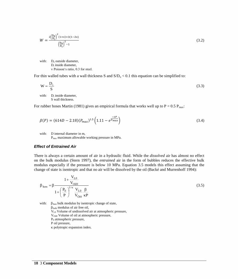
Effect of Entrained Air
There is always a certain amount of air in a hydraulic fluid. While the dissolved air has almost no effect
on the bulk modulus (Stern 1997), the entrained air in the form of bubbles reduces the effective bulk
modulus especially if the pressure is below 10 MPa. Equation 3.5 models this effect assuming that the
change of state is isentropic and that no air will be dissolved by the oil (Backé and Murrenhoff 1994):
PV
V
P
P1
V
V1
0Öl
0L
/1
0
0Oil
0L
Isen
(3.5)
with: Isen bulk modulus by isentropic change of state,
bulk modulus of air free oil,
VL0 Volume of undissolved air at atmospheric pressure,
VOil0 Volume of oil at atmospheric pressure,
P0 atmospheric pressure,
P oil pressure,
polytropic expansion index.

3.1 Hydraulic fluids 19
Figure 3.1 Bulk modulus as a function of entrained air
Bowns et al. (1973) showed that when a greater amount of dissolved air is in the hydraulic fluid at start up
of a system this air will be completely released quite rapidly. They measured a time of two hours or less
for all test cases. There are however no models that describe the rate of solution of air bubbles under
(varying) pressure (Hayward 1962).
Effective Bulk Modulus
The value of the bulk modulus depends on the fluid, the pressure, the entrained air, the container and the
temperature. The low values of the bulk modulus at low pressure lead to low corner frequencies of
hydraulic motors and may cause stability problems. It is therefore important to model this effect if the
working pressure is below 10 MPa. As the housings of hydraulic components aren‘t infinitely stiff their
compliance has to be included in the calculations. To simplify modeling an effective bulk modulus has
been defined as (Backé and Murrenhoff 1994, Martin 1995):
V
P V =e
. (3.6)
It can be measured by setting the component under pressure and recording the pressure drop P while
letting a small amount of oil, V, out of the component. Figure 3.2 shows the measured bulk modulus of
oil at 20 and 50 °C and the effective bulk modulus of oil in a high pressure hose, a tube or a housing
(Zimmermann 1985).
0 2 4 6 10MPa
0
0.2
0.4
0.6
0.8
1
0
0.2
0.4
0.6
0.8
1
Pressure
0.010.001
= 0.1Vair
Voil
is
enoil

20 3 Component Models
Figure 3.2 Effective bulk modulus as a function of pressure
As the effective bulk modulus depends on a number of parameters it should be measured with the actual
component. Kürten (1993) and Manring (1997) describe suitable procedures. If this is not possible
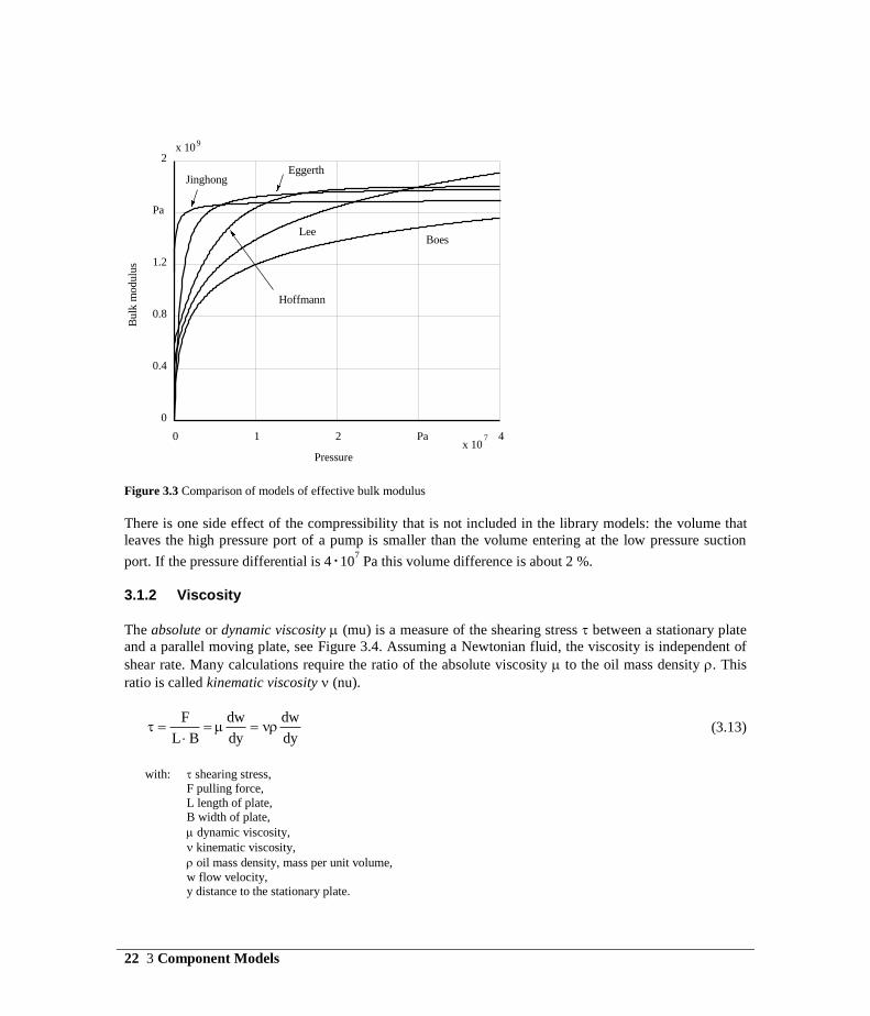
numbers from literature can be used. Four different models are shown in Figure 3.3. The biggest
difference between the models is the behaviour at low pressure. Those of Eggerth and Boes have a bulk
modulus of almost zero while Lee‘s has a value that is approximately 19 % and Hoffmann‘s 33 % of the
maximal value. Eggerth‘s model also includes the effect of the oil temperature.
Boes’s Model
1
P
P99log5.0)P(
ref
e (3.7)
with: = 1.2 . 10
9 Pa,
Pref = 107 Pa.
Hoffmann’s Model
( ) [ ( )] (3.8)
with: P in Pa,
Pmax = 1.8 . 10
9 Pa,
0 0.5 1 1.5 2 3x 10
7
0
0.5
1
1.5
2.5x 10⁹
Pa
Pa
Pressure
Eff
ecti
ve
bulk
modulu
s
tube & housing
high pressure hose
o measurement
20 °C
50 °C
3.1 Hydraulic fluids 21
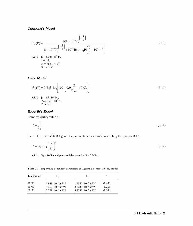
Jinghong's Model
P10)Pc1(R10)P101(
)P101()P(
51
5
11
5
11
5
e (3.9)
with: = 1.701 . 10
9 Pa,
= 1.4,
c1 = -9.307 . 10
-6,
R = 4 . 10
-5.
Lee’s Model
0.03
P
P0.9100log0.5)P(
maxe (3.10)
with: = 1.8 . 10
9 Pa,
Pmax = 2.8 . 10
7 Pa,
P in Pa.
Eggerth’s Model
Compressibility value c:
e
1c
(3.11)
For oil HLP 36 Table 3.1 gives the parameters for a model according to equation 3.12
021
P
PCCc (3.12)
with: P0 = 106 Pa and pressure P between 0 < P < 5 MPa.
Table 3.1 Temperature dependent parameters of Eggerth’s compressibility model
Temperature
C1
C2
20 °C
4.943 . 10-10 m²/N
1.9540 . 10-10 m²/N
-1.480
50 °C 5.469 . 10-10 m²/N 3.2785
. 10-10 m²/N -1.258
90 °C 5.762 . 10-10 m²/N 4.7750
. 10-10 m²/N -1.100
22 3 Component Models
Figure 3.3 Comparison of models of effective bulk modulus
There is one side effect of the compressibility that is not included in the library models: the volume that
leaves the high pressure port of a pump is smaller than the volume entering at the low pressure suction
port. If the pressure differential is 4 . 10
7 Pa this volume difference is about 2 %.
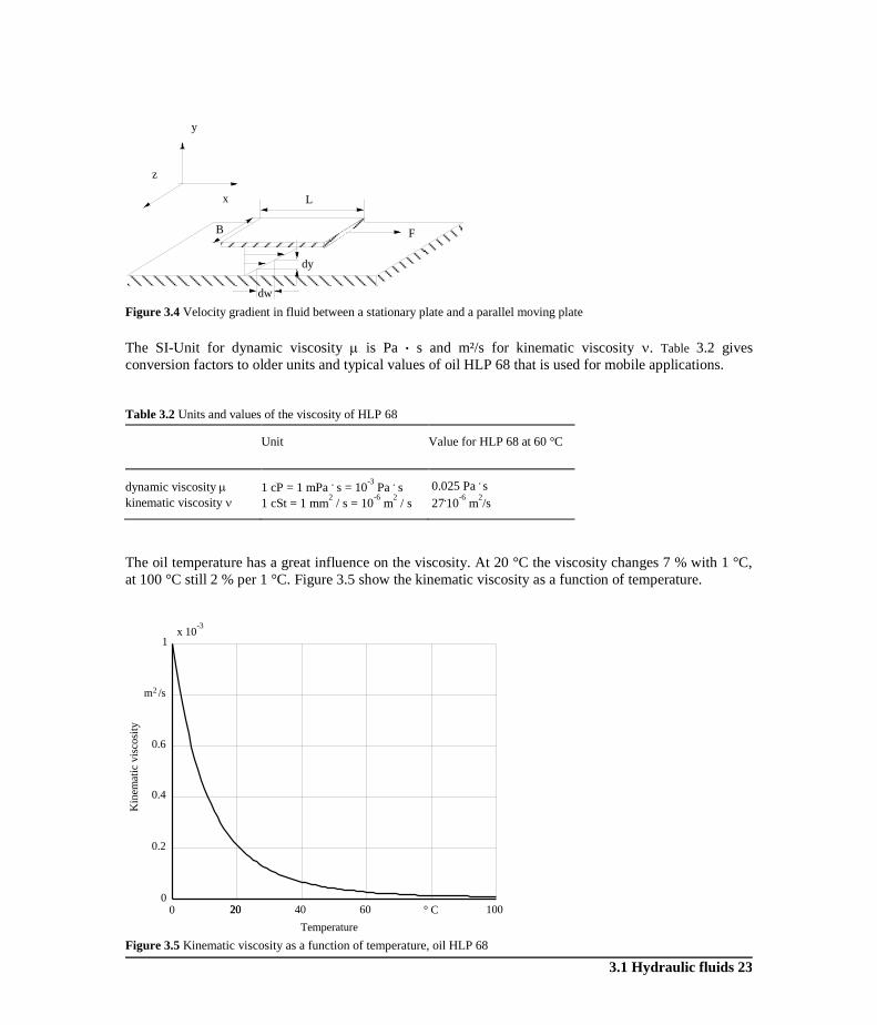
3.1.2 Viscosity
The absolute or dynamic viscosity (mu) is a measure of the shearing stress between a stationary plate
and a parallel moving plate, see Figure 3.4. Assuming a Newtonian fluid, the viscosity is independent of
shear rate. Many calculations require the ratio of the absolute viscosity to the oil mass density . This
ratio is called kinematic viscosity (nu).
dy
dw
dy
dw
BL
F
(3.13)
with: shearing stress,
F pulling force,
L length of plate,
B width of plate,
dynamic viscosity,
kinematic viscosity,
oil mass density, mass per unit volume,
w flow velocity,
y distance to the stationary plate.
x 109
0 1 2 Pa 4x 10
7
0
0.4
0.8
1.2
Pa
2
Pressure
Bulk
modulu
s
Hoffmann
Eggerth
LeeBoes
Jinghong
3.1 Hydraulic fluids 23
Figure 3.4 Velocity gradient in fluid between a stationary plate and a parallel moving plate
The SI-Unit for dynamic viscosity is Pa . s and m²/s for kinematic viscosity . Table 3.2 gives
conversion factors to older units and typical values of oil HLP 68 that is used for mobile applications.
Table 3.2 Units and values of the viscosity of HLP 68
Unit
Value for HLP 68 at 60 °C
dynamic viscosity
1 cP = 1 mPa . s = 10
-3 Pa
. s
0.025 Pa
. s
kinematic viscosity
1 cSt = 1 mm2 / s = 10
-6 m
2 / s 27
.10
-6 m
2/s
The oil temperature has a great influence on the viscosity. At 20 °C the viscosity changes 7 % with 1 °C,
at 100 °C still 2 % per 1 °C. Figure 3.5 show the kinematic viscosity as a function of temperature.
Figure 3.5 Kinematic viscosity as a function of temperature, oil HLP 68
x
y
z
B
L
dy
dw
F
0 20 40 60 1000
0.2
0.4
0.6
1x 10
-3
° C
Temperature
Kin
emat
ic v
isco
sity
m /s2
20
24 3 Component Models
If the kinematic viscosity is plotted as a function of temperature, with the absolute temperature in K on
the x-axis in a logarithmic scale, and the term ln(ln(on the y-axis, straight lines result (see e.g.
DIN 51 563). The slope of the straight lines is given by:
)Tln()Tln(
WWm
12
21
(3.14)
with: Wi = ln(ln(i +0.8 )),
i Value of kinematic viscosity in mm²/s at temperature Ti,
Ti temperature in K.
The kinematic viscosity at an arbitrary temperature Tx can be calculated by:
( ( ) ( )) (3.15)
At very low temperatures the viscosity changes drastically and equation 3.15 is no longer valid. Another
important parameter is the pressure. The viscosity increases with increasing pressure. This is very
important for hydrostatic bearings because the load capacity goes up when the load increases. This effect
can be described by:
P
0e)P( (3.16)
with: 0 viscosity at atmospheric pressure,
viscosity-pressure-coefficient.
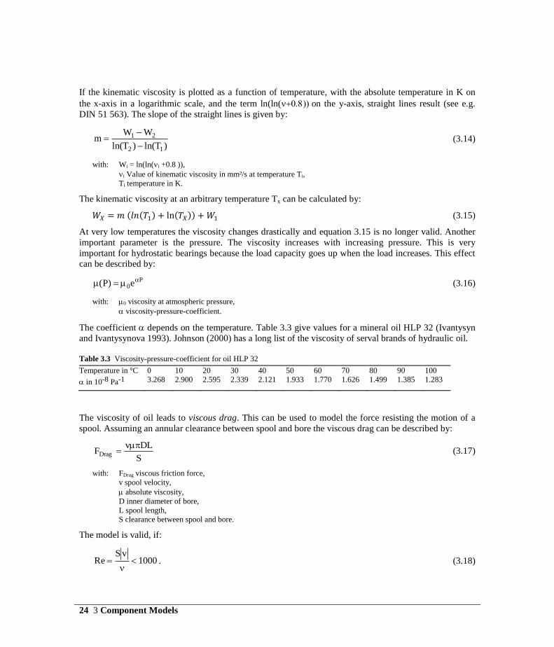
The coefficient depends on the temperature. Table 3.3 give values for a mineral oil HLP 32 (Ivantysyn
and Ivantysynova 1993). Johnson (2000) has a long list of the viscosity of serval brands of hydraulic oil.
Table 3.3 Viscosity-pressure-coefficient for oil HLP 32 Temperature in °C 0 10 20 30 40 50 60 70 80 90 100
in 10-8 Pa-1
3.268 2.900 2.595 2.339 2.121 1.933 1.770 1.626 1.499 1.385 1.283
The viscosity of oil leads to viscous drag. This can be used to model the force resisting the motion of a
spool. Assuming an annular clearance between spool and bore the viscous drag can be described by:
S
DLvFDrag
(3.17)
with: FDrag viscous friction force,
v spool velocity,
absolute viscosity,
D inner diameter of bore,
L spool length,
S clearance between spool and bore.
The model is valid, if:
1000vS
Re
. (3.18)
3.1 Hydraulic fluids 25
3.1.3 Inductance
Newton‘s second law gives the force F to accelerate a mass m:
td
vdmamF . (3.19)
Equation 3.19 is analogous to the expression for voltage drop u across an inductance:
td
idLu . (3.20)
By analogy the inductance Lth of a fluid is defined as:
dt
dQ
PL th
. (3.21)
Assuming a one-dimensional flow, where all fluid particles have identical velocities at any instance of
time, and a tube length l, an interior area A and a fluid density and combining equation 3.19 and 3.21
leads to the theoretical inductance Lth:
A
td
Qd
PL th
l
. (3.22)
The inductance plays an important role for high frequency changes, e. g. switching of fast valves. When
modeling typical valves it is not necessary to include the inductance in the model (Ramdén 1999).
If oil has to pass through a small hole or slot into a larger container the measured inductance Lre is higher
than calculated by equation 3.21. For sharp-edged holes with 0.5 mm < D < 1 mm, 1 < l/D < 20 Tsung
(1991) found:
Dthre e
D554.1LL
ll
(3.23)
with: D inner diameter,
l length.
Lau et al. (1995) and Johnston (2002) give formulas to calculate the inductance of the oil column in
orifices in the freuqency domain.
To derive the theoretical inductance a uniform velocity profile was assumed. But the velocity profile for
stationary laminar flow is not uniform but parabolic (Doebelin 1972), given by:
2
maxR
r1w)r(w (3.24)
with: R inner radius.
26 3 Component Models
The mean velocity wmean for this velocity profile is given by:
maxmean w2
1w . (3.25)
The kinetic energy is:
2mean
2kin wR
3
4E . (3.26)
The inductance therefore has an (upper) value of:
A3
4Lmax
l . (3.27)
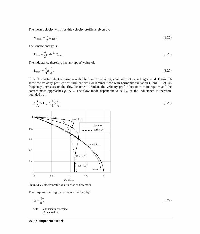
If the flow is turbulent or laminar with a harmonic excitation, equation 3.24 is no longer valid. Figure 3.6
show the velocity profiles for turbulent flow or laminar flow with harmonic excitation (Ham 1982). As
frequency increases or the flow becomes turbulent the velocity profile becomes more square and the
correct mass approaches . A
. l. The flow mode dependent value Lre of the inductance is therefore
bounded by:
A3
4L
Are
ll (3.28)
Figure 3.6 Velocity profile as a function of flow mode
The frequency in Figure 3.6 is normalized by:
2R
8 (3.29)
with: kinematic viscosity,
R tube radius.
0
0.2
0.4
0.6
1
0 0.5 1 1.5 2
r/R
Re = 105
laminar
turbulent
w / wmean
0
0.2
0.4
0.6
1
0 0.5 1 1.5 2
r/R
Re = 105
laminar
turbulent
w / wmean
3.2 Pumps 27
3.2 Pumps
Pumps are needed to convert mechanical energy into hydraulic energy and vice versa. There are two
different types: Turbine pumps, impeller pumps and propeller pumps which are rarely found in hydraulic
power systems. Most power systems require positive displacement pumps. At high pressures, piston
pumps are often preferred to gear or vane pumps. These pumps should be modelled as flow sources
because they displace the fluid with pistons, vanes or gears. This means they produce a flow while the
pressure at the outlet port builds up according to the resistance the oil has to pass on its way to the tank.
3.2.1 Theoretical Displacement, Power Flow of an Ideal Pump
For an ideal pump there is only one equation to describe the input torque and the delivered flow rate Q,
respectively:
2
PDPump (3.30)
with: required input torque,
DPump volumetric displacement,
P pump differential pressure.
nDQ Pump (3.31)
with: Q flow rate,
DPump volumetric displacement,
n shaft speed in rpm.
The theoretical displacement DPump of a gear or piston pump is given by its displacement volume per
revolution. Sometimes the displacement is given in volume / rad. For mobile systems typical values vary
from 12.10-6
m3 for small gear pumps up to 160.10
-6 m
3 for piston pumps.
3.2.2 Efficiency
In all real pumps there is a flow from the high pressure port to the low pressure port called internal or
cross-port leakage. There is also an external leakage from each pump chamber past the pistons to the case
drain. For swash plate-type axial piston pumps the external leakage is usually smaller than the internal
leakage.
The internal and external leakage reduces the theoretical flow rate. This reduction is described by the
volumetric efficiency, vol:
theovolport QQ . (3.32)
Due to friction there are mechanical losses in a pump. They result from bearings, seals and friction at
rotating parts. Due to these losses the input torque must be higher than the theoretical values. The torque
loss is described by the torque efficiency, tor:
tor
pump
2
PD
. (3.33)
28 3 Component Models
The over-all efficiency is defined as the ratio of actual hydraulic horsepower output to the mechanical
horsepower supplied. The over-all efficiency is the product of volumetric and torque efficiencies:
torvol (3.34)
A comparison of the efficiencies of piston, gear and vanes pumps as a function of viscosity, pressure and
speed is given by Yeaple (1990).
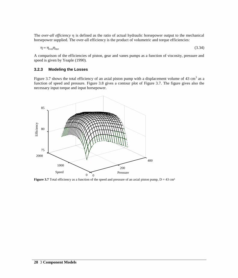
3.2.3 Modeling the Losses
Figure 3.7 shows the total efficiency of an axial piston pump with a displacement volume of 43 cm3 as a
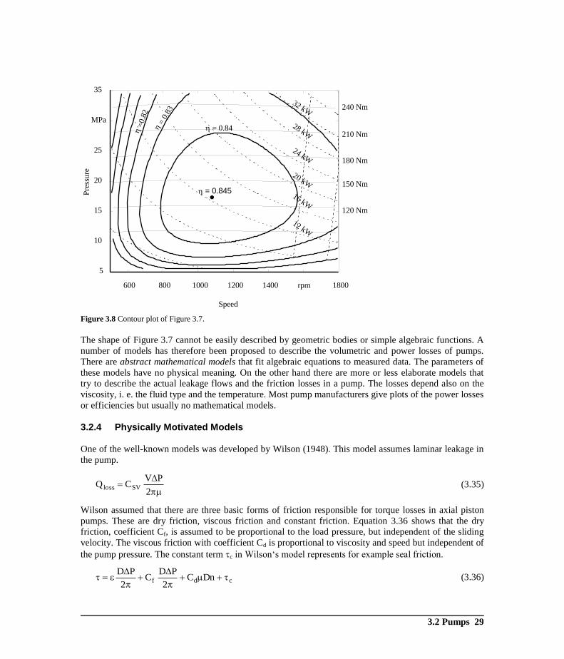
function of speed and pressure. Figure 3.8 gives a contour plot of Figure 3.7. The figure gives also the
necessary input torque and input horsepower.
Figure 3.7 Total efficiency as a function of the speed and pressure of an axial piston pump, D = 43 cm³
0
200
400
0
1000
2000
75
80
85
Speed Pressure
Eff
icie
ncy
3.2 Pumps 29
Figure 3.8 Contour plot of Figure 3.7.
The shape of Figure 3.7 cannot be easily described by geometric bodies or simple algebraic functions. A
number of models has therefore been proposed to describe the volumetric and power losses of pumps.
There are abstract mathematical models that fit algebraic equations to measured data. The parameters of
these models have no physical meaning. On the other hand there are more or less elaborate models that
try to describe the actual leakage flows and the friction losses in a pump. The losses depend also on the
viscosity, i. e. the fluid type and the temperature. Most pump manufacturers give plots of the power losses
or efficiencies but usually no mathematical models.
3.2.4 Physically Motivated Models
One of the well-known models was developed by Wilson (1948). This model assumes laminar leakage in
the pump.
2
PVCQ SVloss (3.35)
Wilson assumed that there are three basic forms of friction responsible for torque losses in axial piston
pumps. These are dry friction, viscous friction and constant friction. Equation 3.36 shows that the dry
friction, coefficient Cf, is assumed to be proportional to the load pressure, but independent of the sliding
velocity. The viscous friction with coefficient Cd is proportional to viscosity and speed but independent of
the pump pressure. The constant term c in Wilson‘s model represents for example seal friction.
cdf DnC2
PDC
2
PD
(3.36)
600 800 1000 1200 1400 rpm 1800
5
10
15
20
25
MPa
35P
ress
ure
=
0.8
2
= 0
.83
= 0.84
32 kW
28 kW
24 kW
20 kW
16 kW
12 kW
240 Nm
210 Nm
180 Nm
150 Nm
120 Nm
Speed
= 0.845
30 3 Component Models
For a gerotor motor with a displacement volume of D = 80.46 cm³ Conrad et al. (1993) give the following
coefficients:
Csv = 5.6148e-7
Cpv = 9.4792e-2
Cvv = 6.3688e2
Mc = 5.7898e0
Schlösser (1968) also used physical reasoning to model the losses in a pump:
STSVloss QQPBPAQ (3.37)
with: thSVSV D2
PCQ
and 3
2
thSTST
2
DP2CQ
.
The torque losses are given by:
cTvp2
loss FEDPC . (3.38)
with:
2
PDC th
PVp ,
2
DC th
VVv , 3
5
th2
TVT2
D
2C
, 0.constC .
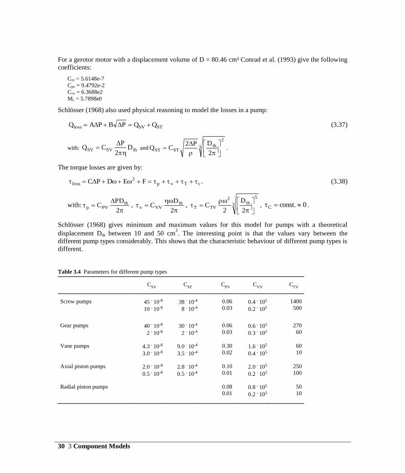
Schlösser (1968) gives minimum and maximum values for this model for pumps with a theoretical
displacement Dth between 10 and 50 cm3. The interesting point is that the values vary between the
different pump types considerably. This shows that the characteristic behaviour of different pump types is
different.
Table 3.4 Parameters for different pump types
CSV
CST
CPV
CVV
CTV
Screw pumps
45 . 10-8
10 . 10-8
38 . 10-4
8 . 10-4
0.06
0.03
0.4 . 105
0.2 . 105
1400
500
Gear pumps
40
. 10-8
2 . 10-8
30 . 10-4
2 . 10-4
0.06
0.03 0.6
. 105
0.3 . 105
270
60
Vane pumps 4.3 . 10-8
3.0 . 10-8
9.0 . 10-4
3.5 . 10-4
0.30
0.02 1.6
. 105
0.4 . 105
60
10
Axial piston pumps 2.0 . 10-8
0.5 . 10-8
2.8 . 10-4
0.5 . 10-4
0.10
0.01 2.0
. 105
0.2 . 105
250
100
Radial piston pumps 0.08
0.01 0.8
. 105
0.2 . 105
50
10
3.2 Pumps 31
For pumps the overall efficiency is given by:
TV2
VVPV
STSV
CCC1
CC1
(3.39)
with the non dimensional numbers and :
forceschydrostati
forcesviscous
P
, (3.40)
forceschydrostati
forcesinertial
P22
V3 th
. (3.41)
For motors the overall efficiency is given by:
STSV
TV2
VVPV
CC1
CCC1. (3.42)
3.2.5 Abstract Mathematical Models
To describe the efficiency of a pump, abstract mathematical models can also be used. These models are
not derived by describing the actual reasons of the losses, e. g. speed depending friction or pressure
depending leakage, but by fitting the coefficients of a given equation to measured data. Often two
equations are used. One to compute the mechanical power loss PLmech and the other for the volumetric
power loss PLvol. The equation may look like this (Ivantysyn and Ivantysynova 1993)
222272625
2242322
2212019
22181716
2151413
2121110
22987
2654
2321Lvol
P]n)AAA(
n)AAA(AAA[
P]n)AAA(
n)AAA(
AAA[n)AAA(
n)AAA(AAAP
(3.43)
with: angle of the swash plate,
n speed of rotation,
P pressure.
For axial piston pumps it often suffices to use only the linear dependency of the speed n and the angle .
To model the torque losses an equivalent polynomial is needed. Another type of equation is:
( ) ∑ [ ][
][ ]. (3.44)

32 3 Component Models
The number of terms used is given by l. Suitable values range from 3 to 10 where higher values usually
give better models. Heumann (1987) proposed the following model for variable displacement swash plate
type pumps:
Delivered flow rate Q in l/min:
n/hPcPnchPnc+hnc=Q q4q32
2q1q , (3.45)
required input horsepower P in kW:
Pn c +h P n c +h n c = 3p2p1p P (3.46)
with: n in 1/min,
P in MPa,
h = Deff / Dmax,
Deff
effective displacement volume of variable displacement pump,
Dmax
maximum displacement volume.
Parameters for variable displacement swash plate type pumps, equation 3.46, are given in Table 3.5.
Table 3.5 Parameters for Heumann’s model for axial piston pumps
D [cm3]
C1q
C2q
C3q
C4q
C1p
C2p
C3p
2.0e+2
1.7538e-1
-9.35e-6
-1.898e-4
-1.13e+1
2.098e-3
2.91390e-3
6.240e-5
5.0e+2 4.2953e-1 -2.85e-5 -4.653e-4 -1.50e+1 3.752e-3 6.81720e-3 3.252e-4
8.0e+2 7.2818e-1 -3.75e-5 -7.853e-4 -1.92e+2 7.917e-3 1.12033e-2 6.715e-4
5.0e+1 4.8429e-2 -2.30e-8 -6.476e-5 -1.30e+1 1.880e-4 7.27800e-4 6.730e-5
1.0e+2 1.0044e-1 -1.80e-8 -2.140e-4 -1.30e+2 2.890e-4 1.48260e-3 1.291e-4
5.0e+1 4.8603e-2 -2.08e-7 -7.582e-5 -2.0000 9.030e-4 7.61700e-4 1.260e-5
6.3e+1 7.1395e-2 -6.65e-7 -9.490e-5 -2.47e+1 1.314e-3 1.17300e-3 3.540e-5
1.0e+2
1.0413e-1 -1.21e-7 -1.226e-4 -1.37e+1 2.757e-3 1.57730e-3 9.110e-5
The model for gear pumps is given by:
n / P c + P c + P n c +n c = Q 4q3q2q1q , (3.47)
P n c +n c = 2p1p P . (3.48)
Parameters for gear pumps, equations 3.47 and 3.48 , are given in Table 3.6.
Table 3.6 Parameters for Heumann’s model for gear pumps
D [cm3]
C1q
C2q
C3q
C4q
C1p
C2p
1.25
1.302e-3
-2.00e-7
-2.920e-2
-1.5000
5.80e-5
2.44e-5
2.00 1.981e-3 -5.70e-6 -1.200e-3 -7.56e+1 1.08e-4 3.54e-5
3.20 3.009e-3 -1.59e-5 -1.040e-2 -1.90e+1 9.80e-5 5.48e-5
5.00 4.745e-3 -1.17e-5 -4.310e-2 -1.26e+1 1.31e-4 8.33e-5
8.00 8.020e-3 -1.78e-5 -1.001e-1 -8.2000 2.79e-4 1.401e-4
1.25e+1 1.1826e-2 -1.20e-6 -1.090e-1 -1.570e+1 2.27e-4 2.307e-4
2.00e+1 1.8192e-2 -2.93e-5 -1.430e-1 -5.510e+1 3.80e-4 3.501e-4
3.20e+1 3.0196e-2 -5.45e-5 -2.272e-1 -1.231e+2 1.068e-3 5.296e-4
5.00e+1 4.5972e-2 -1.84e-4 -2.726e-1 -6.920e+1 7.540e-4 8.961e-4
8.00e+1
7.0201e-2 -1.50e-5 -8.500e-1 -6.000e+1 2.389e-3 1.266e-3
3.2 Pumps 33
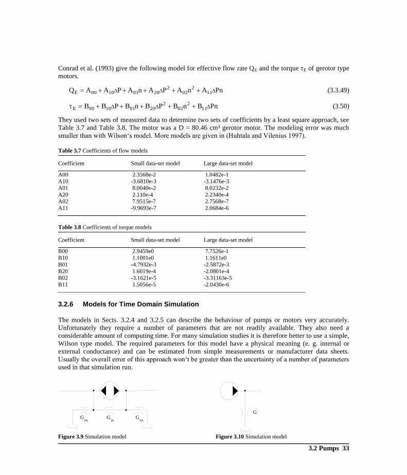
Conrad et al. (1993) give the following model for effective flow rate QE and the torque E of gerotor type
motors.
PnAnAPAnAPAAQ 112
022
20011000E (3.3.49)
PnBnBPBnBPBB 112
022
20011000E (3.50)
They used two sets of measured data to determine two sets of coefficients by a least square approach, see
Table 3.7 and Table 3.8. The motor was a D = 80.46 cm³ gerotor motor. The modeling error was much
smaller than with Wilson‘s model. More models are given in (Huhtala and Vilenius 1997).
Table 3.7 Coefficients of flow models
Coefficient
Small data-set model
Large data-set model
A00 2.3568e-2 1.0482e-1
A10 -3.6810e-3 -3.1476e-3
A01 8.0040e-2 8.0232e-2
A20 2.110e-4 2.2340e-4
A02 7.9515e-7 2.7568e-7
A11
-9.9693e-7 2.0684e-6
Table 3.8 Coefficients of torque models
Coefficient
Small data-set model
Large data-set model
B00 2.9459e0 7.7526e-1
B10 1.1001e0 1.1611e0
B01 -4.7932e-3 -2.5872e-3
B20 1.6019e-4 -2.0801e-4
B02 -3.1621e-5 -3.31163e-5
B11
1.5056e-5 -2.0430e-6
3.2.6 Models for Time Domain Simulation
The models in Sects. 3.2.4 and 3.2.5 can describe the behaviour of pumps or motors very accurately.
Unfortunately they require a number of parameters that are not readily available. They also need a
considerable amount of computing time. For many simulation studies it is therefore better to use a simple,
Wilson type model. The required parameters for this model have a physical meaning (e. g. internal or
external conductance) and can be estimated from simple measurements or manufacturer data sheets.
Usually the overall error of this approach won‘t be greater than the uncertainty of a number of parameters
used in that simulation run.
Figure 3.9 Simulation model Figure 3.10 Simulation model
Gin
Gex
Gex
G
34 3 Component Models
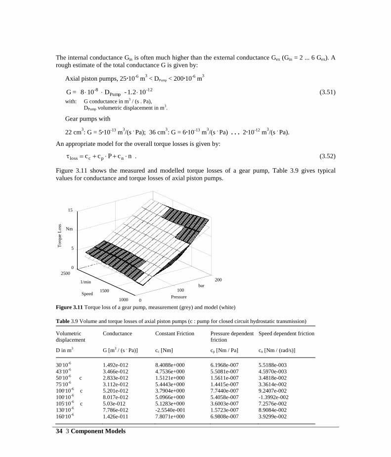
The internal conductance Gin is often much higher than the external conductance Gex (Gin = 2 ... 6 Gex). A
rough estimate of the total conductance G is given by:
Axial piston pumps, 25.10-6
m3 < DPump < 200.10
-6 m
3
-12Pump
-8 101.2- D108 = G (3.51)
with: G conductance in m3 / (s . Pa),
DPump volumetric displacement in m3.
Gear pumps with
22 cm3: G = 5.10
-13 m
3/(s
. Pa); 36 cm
3: G = 6.10
-13 m
3/(s
. Pa) . . . 2.10
-12 m
3/(s
. Pa).
An appropriate model for the overall torque losses is given by:
ncPcc npcloss . (3.52)
Figure 3.11 shows the measured and modelled torque losses of a gear pump, Table 3.9 gives typical
values for conductance and torque losses of axial piston pumps.
Figure 3.11 Torque loss of a gear pump, measurement (grey) and model (white)
Table 3.9 Volume and torque losses of axial piston pumps (c : pump for closed circuit hydrostatic transmission)
Volumetric
displacement
D in m3
Conductance
G [m3 / (s
. Pa)]
Constant Friction
cc [Nm]
Pressure dependent
friction
cp [Nm / Pa]
Speed dependent friction
cn [Nm / (rad/s)]
30.10
-6
1.492e-012
8.4088e+000
6.1968e-007
5.5188e-003
43.10
-6 3.466e-012 4.7536e+000 5.5081e-007 4.5970e-003
50.10
-6 c 2.833e-012 1.5121e+000 1.5611e-007 3.4818e-002
75.10
-6 3.112e-012 5.4443e+000 1.4415e-007 3.3614e-002
100.10
-6 c 5.201e-012 3.7904e+000 7.7440e-007 9.2407e-002
100.10
-6 8.017e-012 5.0966e+000 5.4058e-007 -1.3992e-002
105.10
-6 c 5.03e-012 5.1283e+000 3.6003e-007 7.2576e-002
130.10
-6 7.786e-012 -2.5540e-001 1.5723e-007 8.9084e-002
160.10
-6 1.426e-011
7.8071e+000 6.9808e-007 3.9299e-002
0
100
200
1000
1500
1/min
2500
0
5
Nm
15
SpeedPressure
Torq
ue
Loss
bar

3.2 Pumps 35
Table 3.10 Volume and torque losses of gear pumps
Volumetric
displacement
D in m3
Conductance
G [m3 / (s
. Pa)]
Constant friction
cc [Nm]
Pressure dependent
friction
cp [Nm / Pa]
Speed dependent
friction
cn [Nm / (rad/s)]
28.10
-6
5.069e-013
6.6740e-001
5.9123e-007
3.4449e-003
3.2.7 Effects of Reduced Intake Pressure
The input pressure of a pump can fall below atmospheric pressure because there are hydraulic losses,
occurring in suction pipe, pipe bends and filter. This leads to a decrease of the output flow. Typical
allowed values of the inlet pressure are between 15 and 50 kPa below atmospheric pressure. Too low
values of the input pressure should be avoided because a decrease of input pressure reduces the
mechanical efficiency of the pump. If the input pressure is too low, cavitation will occur which can
destroy the pump. Cavitation can be heard (strong noise) and felt (vigorous pulsations).
Most manufacturers specify a minimum pressure at the inlet port but they don‘t usually provide curves of
the relation between flow and inlet pressure. Some manufacturers specify a maximum pressure at the inlet
port of the pump. If the pressure is higher than a specified value, which is usually the atmospheric
pressure, the pump delivers a higher output flow. Maximum values of the input pressure are between 0.15
and 0.3 MPa.
For a model of a pump it is necessary to model the decrease of delivered flow when the input pressure
decreases especially when the input pressure goes towards the vapour pressure of the fluid. Otherwise the
model would output a flow while the input pressure, e. g. the pressure in a lumped volume, is at the
vapour pressure and no fluid can flow into the pump. There are several references for the reduction of
flow rate as a function of input pressure. Zalka and Látrányi (1971) give measurements for gear pumps,
Hibi et al. (1977) for axial piston pumps, Schulz (1979) gives a formula for piston pumps and Yeaple
(1990) shows calculations to predict cavitations.
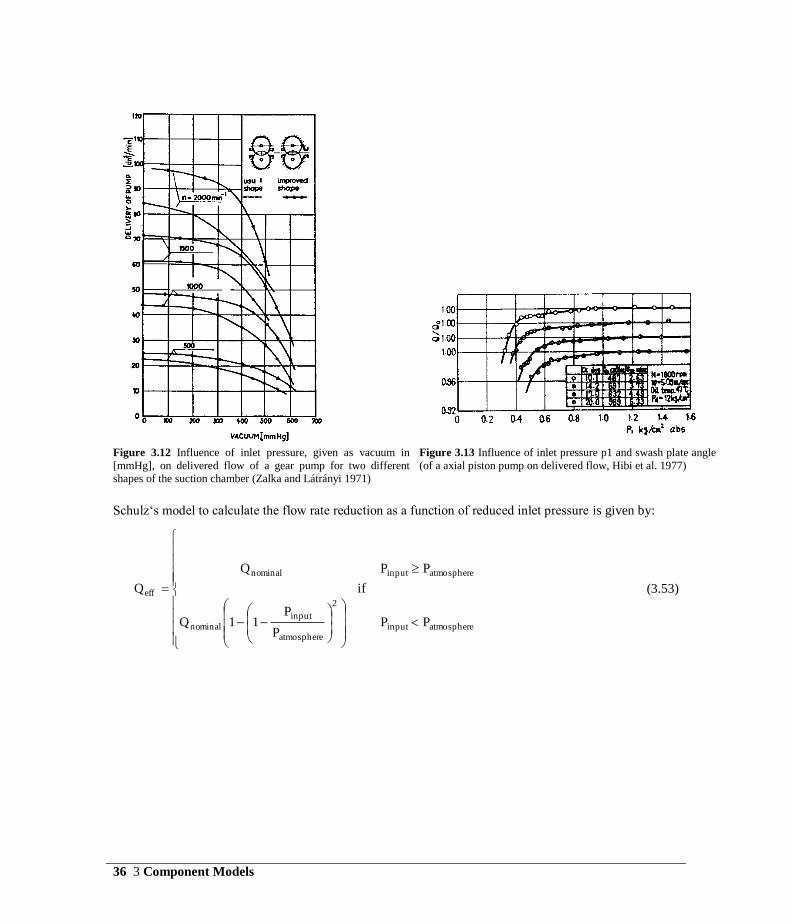
36 3 Component Models
Figure 3.12 Influence of inlet pressure, given as vacuum in
[mmHg], on delivered flow of a gear pump for two different
shapes of the suction chamber (Zalka and Látrányi 1971)
Figure 3.13 Influence of inlet pressure p1 and swash plate angle
(of a axial piston pump on delivered flow, Hibi et al. 1977)
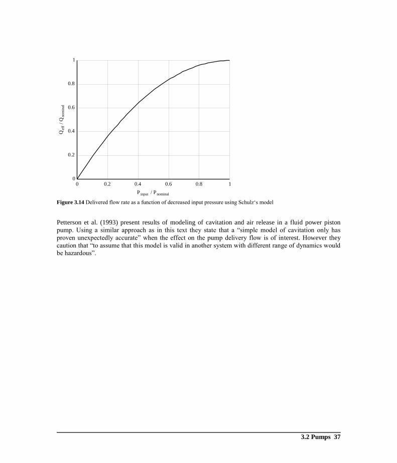
Schulz‘s model to calculate the flow rate reduction as a function of reduced inlet pressure is given by:
atmosphereinput
2
atmosphere
input
alminno
atmosphereinputalminno
eff
PPP
P11Q
if
PPQ
Q (3.53)
3.2 Pumps 37
Figure 3.14 Delivered flow rate as a function of decreased input pressure using Schulz‘s model
Petterson et al. (1993) present results of modeling of cavitation and air release in a fluid power piston
pump. Using a similar approach as in this text they state that a “simple model of cavitation only has
proven unexpectedly accurate” when the effect on the pump delivery flow is of interest. However they
caution that “to assume that this model is valid in another system with different range of dynamics would
be hazardous”.
0 0.2 0.4 0.6 0.8 10
0.2
0.4
0.6
0.8
1
P input nominal/ P
Qef
fnom
inal
/ Q
38 3 Component Models
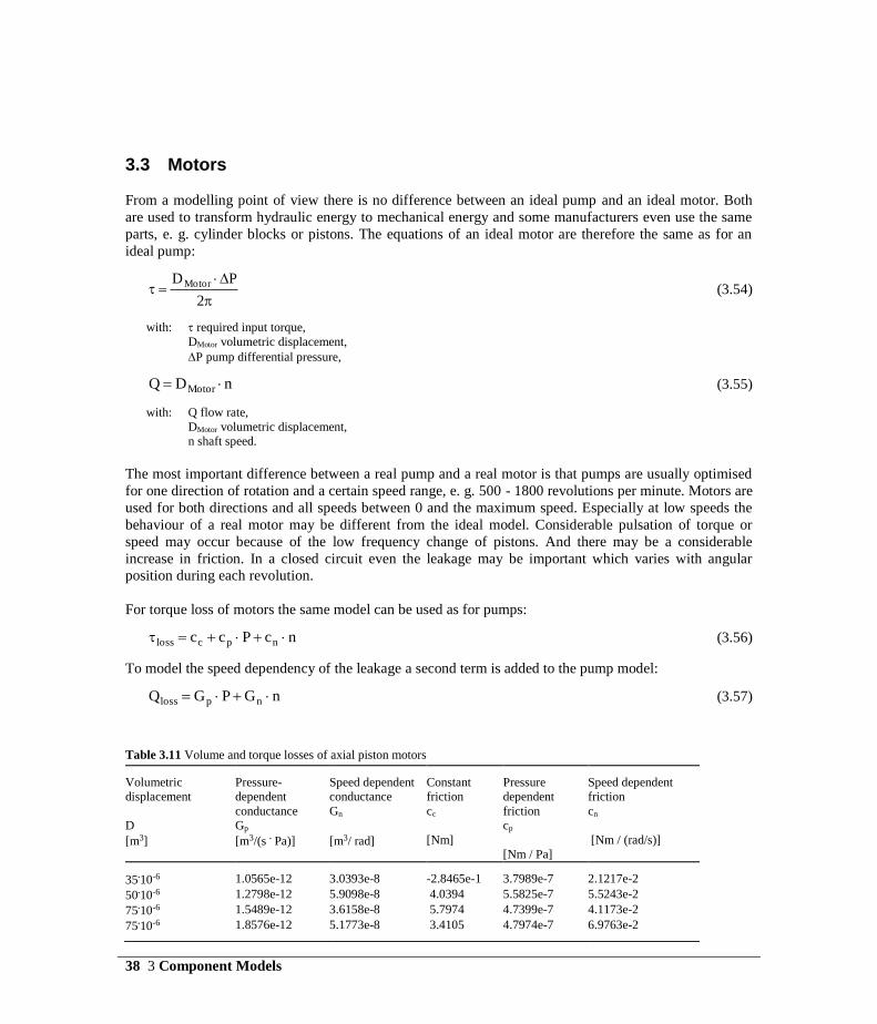
3.3 Motors
From a modelling point of view there is no difference between an ideal pump and an ideal motor. Both
are used to transform hydraulic energy to mechanical energy and some manufacturers even use the same
parts, e. g. cylinder blocks or pistons. The equations of an ideal motor are therefore the same as for an
ideal pump:
2
PDMotor (3.54)
with: required input torque,
DMotor volumetric displacement,
P pump differential pressure,
nDQ Motor (3.55)
with: Q flow rate,
DMotor volumetric displacement,
n shaft speed.
The most important difference between a real pump and a real motor is that pumps are usually optimised
for one direction of rotation and a certain speed range, e. g. 500 - 1800 revolutions per minute. Motors are
used for both directions and all speeds between 0 and the maximum speed. Especially at low speeds the
behaviour of a real motor may be different from the ideal model. Considerable pulsation of torque or
speed may occur because of the low frequency change of pistons. And there may be a considerable
increase in friction. In a closed circuit even the leakage may be important which varies with angular
position during each revolution.
For torque loss of motors the same model can be used as for pumps:
ncPcc npcloss (3.56)
To model the speed dependency of the leakage a second term is added to the pump model:
nGPGQ nploss (3.57)
Table 3.11 Volume and torque losses of axial piston motors
Volumetric
displacement
D
[m3]
Pressure-
dependent
conductance
Gp
[m3/(s . Pa)]
Speed dependent
conductance
Gn
[m3/ rad]
Constant
friction
cc
[Nm]
Pressure
dependent
friction
cp
[Nm / Pa]
Speed dependent
friction
cn
[Nm / (rad/s)]
35.10-6
1.0565e-12
3.0393e-8
-2.8465e-1
3.7989e-7
2.1217e-2
50.10-6 1.2798e-12 5.9098e-8 4.0394 5.5825e-7 5.5243e-2
75.10-6 1.5489e-12 3.6158e-8 5.7974 4.7399e-7 4.1173e-2
75.10-6 1.8576e-12
5.1773e-8 3.4105 4.7974e-7 6.9763e-2
3.2 Pumps 39
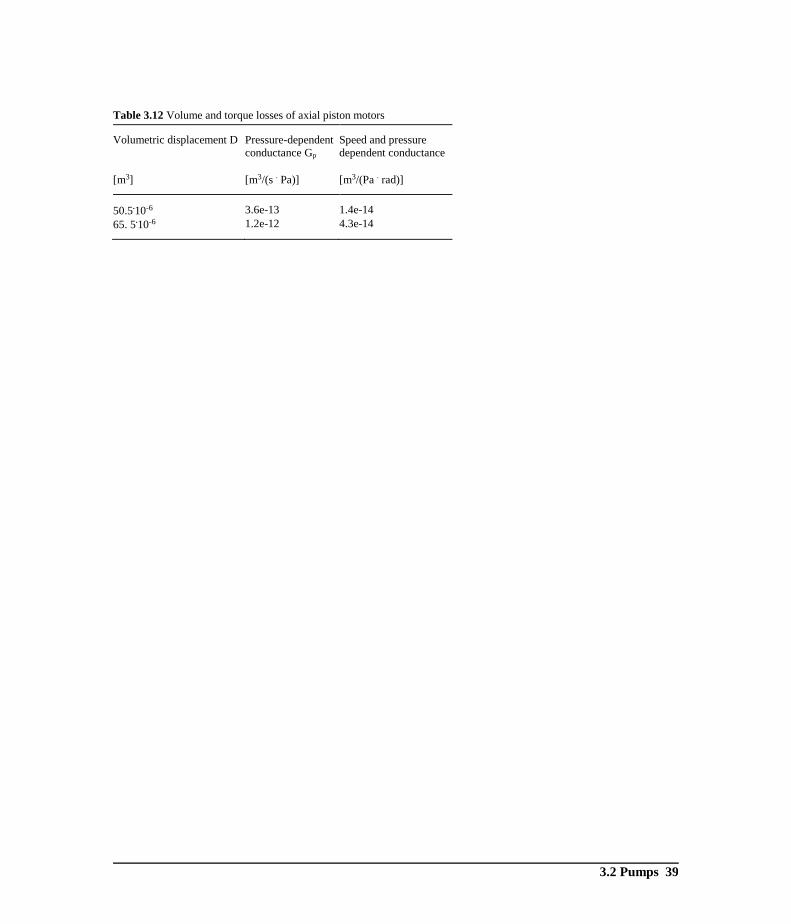
Table 3.12 Volume and torque losses of axial piston motors
Volumetric displacement D
[m3]
Pressure-dependent
conductance Gp
[m3/(s . Pa)]
Speed and pressure
dependent conductance
[m3/(Pa . rad)]
50.5.10-6
3.6e-13
1.4e-14
65. 5.10-6
1.2e-12 4.3e-14

40 3 Component Models
3.4 Cylinders
The function of the cylinder in hydraulic systems is to convert the hydraulic energy supplied by the pump
into useful work. The model of an ideal, mass less, single-acting, single ended cylinder is given by:
Balance of forces:
APF (3.58)
with: F force,
P pressure in cylinder chamber,
A piston area.
Continuity:
td
xdAQ (3.59)
with: Q flow rate,
x position,
dx / dt velocity.
Figure 3.15 Ideal cylinder
However there are more effects that may need modeling:
Seal friction
Leakage
Fluid compressibility and housing compliance
Pulling rod force
3.4.1 Seal friction
There are many different designs of seals to get a good compromise between friction and leakage. Yeaple
(1990) gives an example of a piston rod where the friction force could be reduced from 230 lb to 16 lb
while the leakage increased from 0.4 g/1000 cycles to 11 g/1000 cycles. He also quotes a rule of thumb
that “friction losses in hydraulic piston and rod seals represent an energy loss of less than 5 %” and shows
that these 5 % sum up to 7 million barrels of fuel oil a year in the United States alone.
FP
Ax
Q

3.4 Cylinders 41
Armstrong-Hélouvry (1991) gives the following definitions:
Static Friction (Stiction) The torque (force) necessary to initiate motion from rest. It is often greater than the kinetic friction.
Kinetic friction (Coulomb friction, Dynamic friction)
A friction component that is independent of the magnitude of the velocity.
Viscous Friction A friction component that is proportional to velocity and, in particular, goes to zero at zero velocity.
Break-Away The transition from rest (static friction) to motion (kinetic friction).
Break-Away Force (Torque)
The amount of force (torque) required to overcome static friction.
Stribeck Friction or the Stribeck Effect A friction phenomenon that arises from the use of fluid lubrication and gives rise to decreasing friction
with increasing velocity at low velocity.
Negative Viscous Friction Decreasing friction with increasing velocity. Stribeck friction is an example of negative viscous friction.
When modeling a cylinder the characteristic of the seal friction must be known. For control or servo
systems it is important whether the static friction (stiction) is negligible and the speed dependent friction
dominates, which means a linear relation between pressure and rod force, or if the high static seal friction
gives rise to slip-stick effects at low speeds.
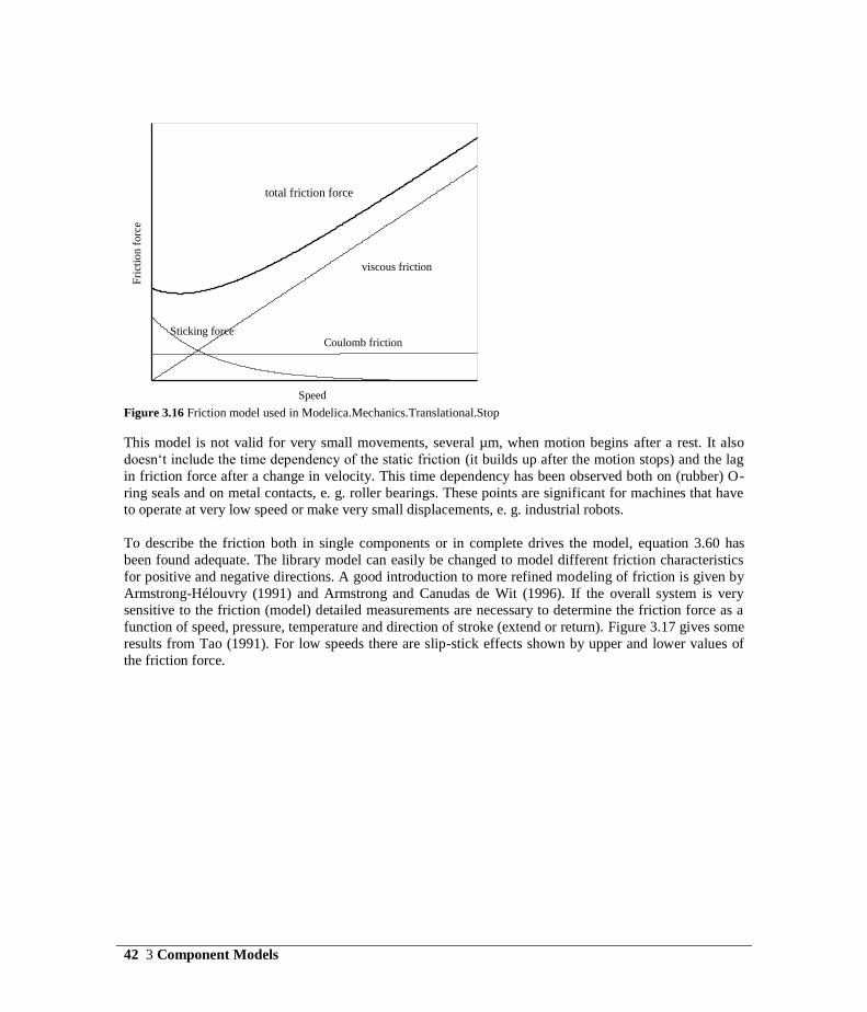
Friction as a function of speed can be modelled with the model Stop in the Modelica standard library, see
Figure 3.16. This model uses the following equation (Tustin 1947):
[ | |] ( ) (3.60)
with: Ffric total friction force,
fprop coefficient of viscous, speed proportional friction,
v velocity,
FCoulomb speed independent, constant Coulomb friction force,
FStribeck force modeling Stribeck effect,
fexp coefficient of decay for Stribeck force.
42 3 Component Models
Figure 3.16 Friction model used in Modelica.Mechanics.Translational.Stop
This model is not valid for very small movements, several µm, when motion begins after a rest. It also
doesn‘t include the time dependency of the static friction (it builds up after the motion stops) and the lag
in friction force after a change in velocity. This time dependency has been observed both on (rubber) O-
ring seals and on metal contacts, e. g. roller bearings. These points are significant for machines that have
to operate at very low speed or make very small displacements, e. g. industrial robots.
To describe the friction both in single components or in complete drives the model, equation 3.60 has
been found adequate. The library model can easily be changed to model different friction characteristics
for positive and negative directions. A good introduction to more refined modeling of friction is given by
Armstrong-Hélouvry (1991) and Armstrong and Canudas de Wit (1996). If the overall system is very
sensitive to the friction (model) detailed measurements are necessary to determine the friction force as a
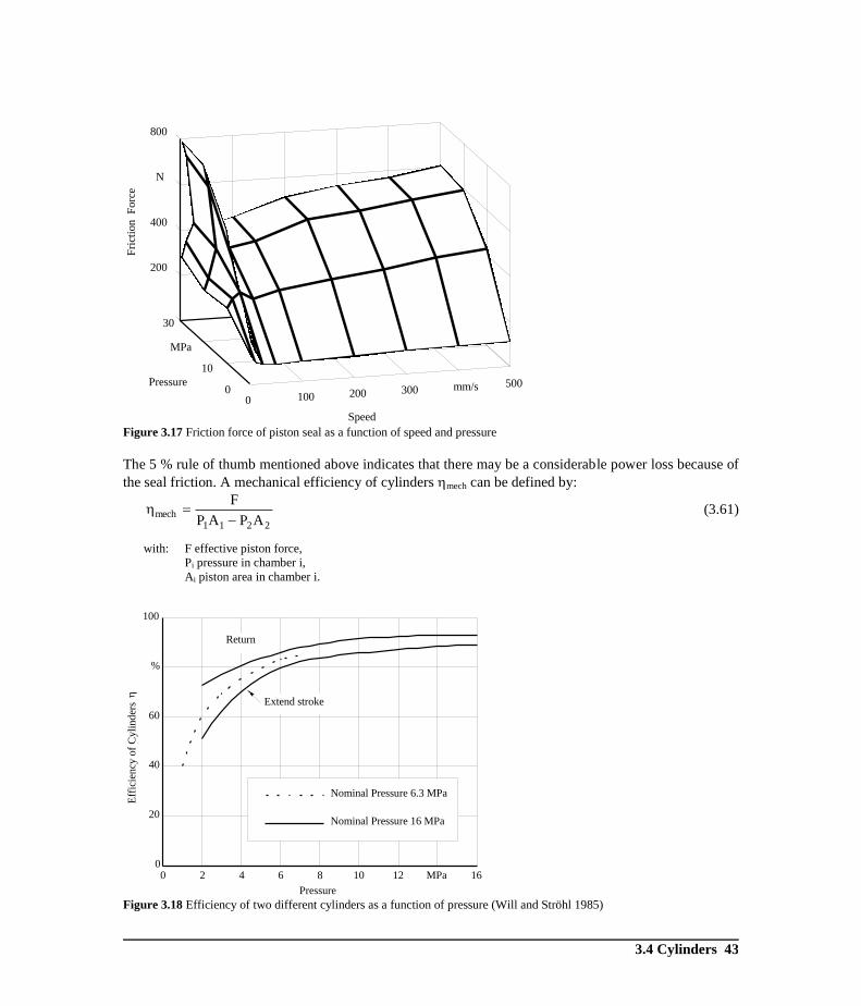
function of speed, pressure, temperature and direction of stroke (extend or return). Figure 3.17 gives some
results from Tao (1991). For low speeds there are slip-stick effects shown by upper and lower values of
the friction force.
Speed
Fri
ctio
n f
orc
e
total friction force
Coulomb friction
Sticking force
viscous friction
3.4 Cylinders 43
Figure 3.17 Friction force of piston seal as a function of speed and pressure
The 5 % rule of thumb mentioned above indicates that there may be a considerable power loss because of
the seal friction. A mechanical efficiency of cylinders mech can be defined by:
2211
mechAPAP
F
(3.61)
with: F effective piston force,
Pi pressure in chamber i,
Ai piston area in chamber i.
Figure 3.18 Efficiency of two different cylinders as a function of pressure (Will and Ströhl 1985)
0 100 200 300 mm/s 5000
10
MPa
30
200
400
N
800
Speed
Pressure
Fri
ctio
n F
orc
e
0 2 4 6 8 10 12 160
20
40
60
100
MPa
%
Pressure
Eff
icie
ncy
of
Cyli
nder
s
Return
Extend stroke
Nominal Pressure 6.3 MPa
Nominal Pressure 16 MPa

44 3 Component Models
3.4.2 Leakage
Some leakage is necessary to assure seal lubrication. In most cases the leakage doesn‘t affect the system
behaviour considerably and there is no need to model it. As the leakage flow is always small it can be
modelled as laminar flow described by a laminar resistance.
3.4.3 Fluid Compressibility and Housing Compliance
The oil in the cylinder chamber is compressible and the housing is not infinitely stiff. Both effects are
modelled by the effective bulk modulus eff. In the cylinder chamber model Hoffmann‘s model is used.
3.4.4 What happens if there is no flow but the rod is pulled out?
To describe the pressure build up in one cylinder chamber the following differential equation is used:
dt
)t(dxA)t(Q
)t(xA
)p(
td
Pd eff (3.62)
with: P pressure in cylinder chamber,
eff effective bulk modulus of oil, pressure dependent,
A piston area,
x position,
Q flow rate into chamber,
dx / dt velocity.
If there is no flow, Q(t) = 0, and an external force moves the piston in Figure 3.15 to the left, dx/dt
becomes smaller than 0, and pressure builds up, dP/dt > 0. If the force moves the piston to the right,
however, dx/dt becomes greater than 0 and pressure decreases. But as no negative pressure exists in
technical fluids, equation 3.59 is then no longer valid. The pressure remains at a constant value that is
given for pure fluids by the vapour pressure. For mineral oil Fassbender (1993) measured a minimum
absolute pressure of 25 mbar while the vapour pressure is 0.03 mbar.
Figure 3.19 shows the measured pressure as a function of piston displacement when a rather compliant
cylinder is used and the seal permits some air to enter the cylinder camber. The pressure falls from
atmospheric pressure (0.1 MPa) to about 0.01 MPa. Figure 3.20 shows the pressure as a function of the
relative increase in chamber volume. Even a modest increase in volume of 0.5 % is enough for the
pressure to fall to the minimum value, this value doesn‘t change significantly if the volume is further
expanded.

3.4 Cylinders 45
Figure 3.19 Measured pressure and piston displacement as function of time
Figure 3.20 Pressure as a function of increased volume
To describe these effects there is a limiter in the library submodel OilVolume. It limits the value of the
effective bulk modulus to eff(P=0 Pa).
0 0.1 0.2 0.3 0.4 0.5 0.6 0.8
0
0.02
0.04
0.06
0.08
0.12
s
MPa
Time
Pre
ssure
(ab
solu
te)
0
1
2
3
4
6
mm
Disp
lacemen
t
Displacement
Pressure
0 1 2 3 50
0.02
0.04
0.06
0.08
0.12
%
MPa
Volume change
Pre
ssure
46 3 Component Models
3.5 Restrictions
While pumps, motors and cylinders are needed to transform mechanical energy to hydraulic energy and
vice versa other components are needed to transport, filter and cool the oil or control the flow. When
modeling the dynamic response of a system the resistance of these components has to be considered. The
dc resistance R is the ratio of pressure drop P, across variable, to volume flow rate Q, through variable:
constQ
constPQ
PR
(3.63)
The inverse of the resistance is the conductance G:
R
1G . (3.64)
When modeling flow in a hydraulic system there are two extreme cases:
1. constR , (3.65)
which leads to:
P~PR
1Q . (3.66)
The linearity between pressure drop and flow characterises laminar flow.
2. )Q,P(RR , (3.67)
which leads to:
P~Q . (3.68)
The “square root” dependency characterises turbulent flow.
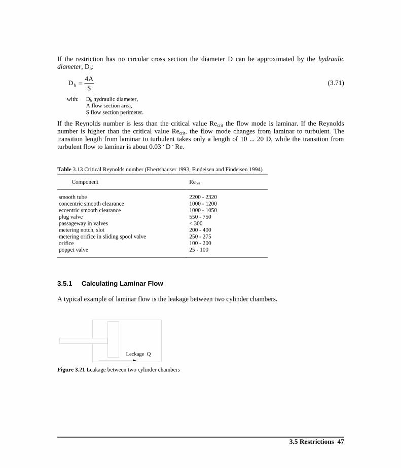
A typical example of laminar flow is the leakage between the ports of a spool valve, an example of
turbulent flow the flow through a sharp edged orifice. For a number of (technical) restrictions the flow is
not exactly laminar or turbulent but best described by:
1n5.0;P~Q n . (3.69)
The flow mode depends on the restriction, the flow velocity and the kinematic viscosity of the fluid and is
characterized by the Reynolds number Re:
Du
Re (3.70)
with: u flow velocity,
D diameter,
kinematic viscosity.
3.5 Restrictions 47
If the restriction has no circular cross section the diameter D can be approximated by the hydraulic
diameter, Dh:
S
A4Dh (3.71)
with: Dh hydraulic diameter,
A flow section area,
S flow section perimeter.
If the Reynolds number is less than the critical value Recrit the flow mode is laminar. If the Reynolds
number is higher than the critical value Recrit, the flow mode changes from laminar to turbulent. The
transition length from laminar to turbulent takes only a length of 10 ... 20 D, while the transition from
turbulent flow to laminar is about 0.03 . D
. Re.
Table 3.13 Critical Reynolds number (Ebertshäuser 1993, Findeisen and Findeisen 1994)
Component
Recrit
smooth tube
2200 - 2320
concentric smooth clearance 1000 - 1200
eccentric smooth clearance 1000 - 1050
plug valve 550 - 750
passageway in valves < 300
metering notch, slot 200 - 400
metering orifice in sliding spool valve 250 - 275
orifice 100 - 200
poppet valve 25 - 100
3.5.1 Calculating Laminar Flow
A typical example of laminar flow is the leakage between two cylinder chambers.
Figure 3.21 Leakage between two cylinder chambers
Leckage Q
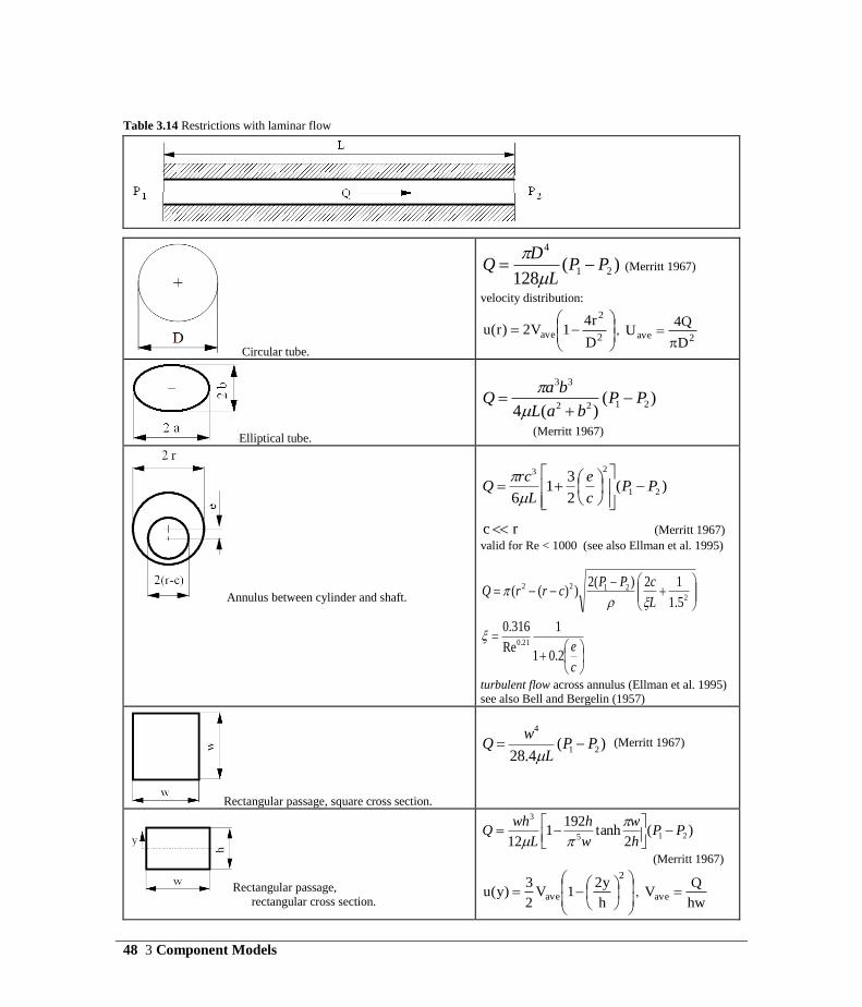
48 3 Component Models
Table 3.14 Restrictions with laminar flow
Circular tube.
)(128
21
4
PPL
DQ
(Merritt 1967)
velocity distribution:
2
2
aveD
r41V2)r(u ,
2aveD
Q4U
Elliptical tube.
)()(4
2122
33
PPbaL
baQ
(Merritt 1967)
Annulus between cylinder and shaft.
)(2
31
621
23
PPc
e
L
rcQ
rc (Merritt 1967)
valid for Re < 1000 (see also Ellman et al. 1995)
c
e
L
cPPcrrQ
2.01
1
Re
316.0
5.1
12)(2))((
21.0
2
2122
turbulent flow across annulus (Ellman et al. 1995)
see also Bell and Bergelin (1957)
Rectangular passage, square cross section.
)(4.28
21
4
PPL
wQ
(Merritt 1967)
Rectangular passage,
rectangular cross section.
)(2
tanh192
112
215
3
PPh
w
w
h
L
whQ
(Merritt 1967)
2
aveh
y21V
2
3)y(u ,
hw
QVave

3.5 Restrictions 49
)(12
21
3
PPL
whQ
(Merritt 1967)
Rectangular passage, two parallel plates,rectangular
cross section with w >> h
.
)(5.155
21
4
PPL
sQ
(Merritt 1967)
Triangular passage, right angle triangle cross
section
)(185
21
4
PPL
sQ
(Merritt 1967)
Triangular passage, equilateral triangle cross
section.
Table 3.15 More restrictions with laminar flow
)(9
221
0
3
0 PPdh
hdQ
b
b
bd
Q2Re (Müller 1978)
Ball in perfect cylindrical bore, centric.
)(135
2)2(3621
0
2
0PP
dhhQ
b
bd
Q2Re (Müller 1978)
Ball in perfect cylindrical bore, maximum
eccentricity
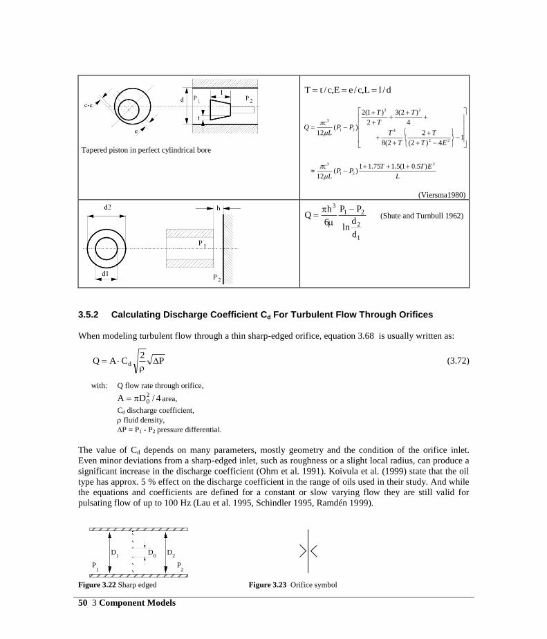
50 3 Component Models
Tapered piston in perfect cylindrical bore
d/lL,c/eE,c/tT
L
ETTPP
L
c
ET
T
T
T
T
T
T
PPL
cQ
2
21
3
22
4
22
21
3
)5.01(5.175.11)(
12
14)2(
2
2(8
4
)2(3
2
)1(2
)(12
(Viersma1980)
1
2
213
d
dln
PP
6
hQ
(Shute and Turnbull 1962)
3.5.2 Calculating Discharge Coefficient Cd For Turbulent Flow Through Orifices
When modeling turbulent flow through a thin sharp-edged orifice, equation 3.68 is usually written as:
P2
CAQ d
(3.72)
with: Q flow rate through orifice,
4/DA 20 area,
Cd discharge coefficient,
fluid density,
P = P1 - P2 pressure differential.
The value of Cd depends on many parameters, mostly geometry and the condition of the orifice inlet.
Even minor deviations from a sharp-edged inlet, such as roughness or a slight local radius, can produce a
significant increase in the discharge coefficient (Ohrn et al. 1991). Koivula et al. (1999) state that the oil
type has approx. 5 % effect on the discharge coefficient in the range of oils used in their study. And while
the equations and coefficients are defined for a constant or slow varying flow they are still valid for
pulsating flow of up to 100 Hz (Lau et al. 1995, Schindler 1995, Ramdén 1999).
Figure 3.22 Sharp edged Figure 3.23 Orifice symbol
DD1 0
D2
1P
2P
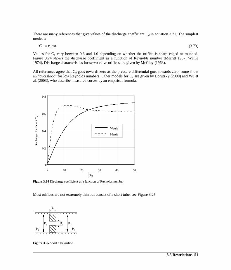
3.5 Restrictions 51
There are many references that give values of the discharge coefficient Cd in equation 3.71. The simplest
model is
.constCd (3.73)
Values for Cd vary between 0.6 and 1.0 depending on whether the orifice is sharp edged or rounded.
Figure 3.24 shows the discharge coefficient as a function of Reynolds number (Merritt 1967, Weule
1974). Discharge characteristics for servo valve orifices are given by McCloy (1968).
All references agree that Cd goes towards zero as the pressure differential goes towards zero, some show
an “overshoot” for low Reynolds numbers. Other models for Cd are given by Borutzky (2000) and Wu et
al. (2003), who describe measured curves by an empirical formula.
Figure 3.24 Discharge coefficient as a function of Reynolds number
Most orifices are not extremely thin but consist of a short tube, see Figure 3.25.
Figure 3.25 Short tube orifice
0 10 20 30 40 50
0
0.2
0.4
0.6
0.8
Re
Weule
Merrit
Dis
char
ge
Coef
fici
ent
Cd
DD1 0
D2
1P
2P
L
A*
L
A*
L
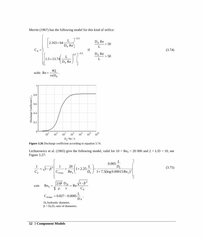
52 3 Component Models
Merritt (1967) has the following model for this kind of orifice:
50L
ReD
50L
ReD
if
ReD
L74.135.1
ReD
L64163.2
C
0
0
5,05.0
0
5,0
0
d
(3.74)
with: 0D
Q4Re
.
Figure 3.26 Discharge coefficient according to equation 3.74.
Lichtarowicz et al. (1965) give the following model, valid for 10 < Reh < 20 000 and 2 < L/D < 10, see
Figure 3.27:
2
max
4
)Re00015.0(log5.71
005.0
25.21Re
2011
1
h
h
hhDd
D
L
D
L
CC (3.75)
with:
d
4H
hC
1Re
DP2Re
h
maxdD
L0085.0827.0C ,
Dh hydraulic diameter,
= D0/D1 ratio of diameters.
10 10 10 10 10 10 10-2 0 2 4 6 8 10
0
0.2
0.4
0.6
1
0.8
Dis
char
ge
Coef
fici
ent
Cd
D Re / L0
.
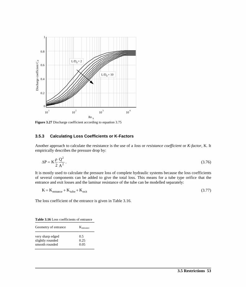
3.5 Restrictions 53
Figure 3.27 Discharge coefficient according to equation 3.75
3.5.3 Calculating Loss Coefficients or K-Factors
Another approach to calculate the resistance is the use of a loss or resistance coefficient or K-factor, K. It
empirically describes the pressure drop by:
2
2
A
Q
2KP
. (3.76)
It is mostly used to calculate the pressure loss of complete hydraulic systems because the loss coefficients
of several components can be added to give the total loss. This means for a tube type orifice that the
entrance and exit losses and the laminar resistance of the tube can be modelled separately:
exittubeentrance KKKK (3.77)
The loss coefficient of the entrance is given in Table 3.16.
Table 3.16 Loss coefficients of entrance
Geometry of entrance
Kentrance
very sharp edged
0.5
slightly rounded 0.25
smooth rounded 0.05
0
0.2
0.4
0.6
1
1 2 3 410 10 10 10
0.8
Re h
Dis
char
ge
coef
fici
ent
Cd L/D = 2
0
L/D = 100

54 3 Component Models
The loss coefficient of the exit is always 1.0, regardless whether it is sharp edged or rounded. Several
references give values of the loss coefficient of orifices and experimental data. Winckler (1967) cites
equations from Schaller ( 3.78) and Chaimowitch (3.79) to calculate K:
4.1DRe
L64
Re
64K
0
(3.78)
with: 2300Dw
Re 00
,
L/D0 > 1,
0.5 < D0 < 4 mm,
D0/D2 0.5.
This equation models the entrance resistance with 0.4 and the exit resistance with 1.0. Winckler mentions
that other references state an entrance resistance of 0.5 if all edges are sharp. If the edges are slightly
rounded this reduces to 0.25 and goes down to 0.06 if the edges are rounded with an radius R/D = 0.06:
2
22
20
21
20
1 D
D1
D
D15.0
ReD
L64K
(3.79)
with: 2300Dv
Re 00
,
L/D0 > 2.
For orifices as in Figure 2.1 Winckler (1967) gives experimental and calculated data for a model given by
equation 3.91.
Table 3.17 Experimental and calculated data for orifices (Winckler 1967) L D0 D1 D2 K1
measured
K2
measured
K1
Eq. (3.78)
K2
Eq. (3.78)
K1
Eq. (3.79)
K2
Eq. (3.79)
1
0.345
8
2.5
250
1.6
250
1.4
185
1.47
1
0.514 8 2.5 270 1.3 190 1.4 125 1.42
Will (1968) distinguishes between short restrictions with L/D0 1.2, (3.80) and Figure 3.28, and long
restrictions, (3.85) and Figure 3.30. The difference is that for a short restriction the narrowest area of the
flow path, A*, lies behind the restriction, while it is within the restriction for a long restriction.
Figure 3.28 Flow through short restriction
A*
L
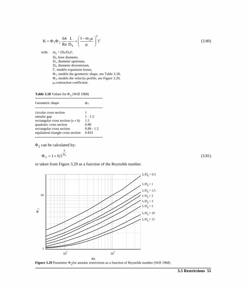
3.5 Restrictions 55
2
2
h21
m1
D
L
Re
64K (3.80)
with: m2 = (D0/D2)²,
D0, bore diameter,
D1, diameter upstream,
D2, diameter downstream,
models expansion losses,
1, models the geometric shape, see Table 3.18,
2, models the velocity profile, see Figure 3.29,
contraction coefficient.
Table 3.18 Values for 1 (Will 1968)
Geometric shape
1
circular cross section
1
annular gap 1 - 1.5
rectangular cross section (a » b) 1.5
quadratic cross section 0.89
rectangular cross section 0.89 - 1.5
equilateral triangle cross section
0.833
2 can be calculated by:
hD
L
2 5,01 (3.81)
or taken from Figure 3.29 as a function of the Reynolds number.
Figure 3.29 Parameter 2for annular restrictions as a function of Reynolds number (Will 1968)
102
103
1
10
Re
2
L/D = 10
L/D = 10
L/D = 0.50
L/D = 1,50
L/D = 20
L/D = 30
L/D = 50
0
L/D = 150
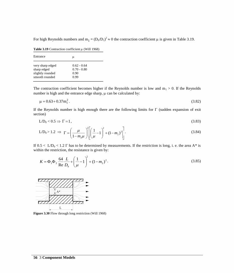
56 3 Component Models
For high Reynolds numbers and m1 = (D0/D1)2 0 the contraction coefficient is given in Table 3.19.
Table 3.19 Contraction coefficient (Will 1968)
Entrance
very sharp edged
0.62 - 0.64
sharp edged 0.70 - 0.80
slightly rounded 0.90
smooth rounded
0.99
The contraction coefficient becomes higher if the Reynolds number is low and m1 > 0. If the Reynolds
number is high and the entrance edge sharp, can be calculated by:
21m37.063.0 . (3.82)
If the Reynolds number is high enough there are the following limits for (sudden expansion of exit
section)
L/D0 < 0.5 1 , (3.83)
L/D0 > 1.2
2
2
22
2
)1(11
1m
m
. (3.84)
If 0.5 < L/D0 < 1.2 has to be determined by measurements. If the restriction is long, i. e. the area A* is
within the restriction, the resistance is given by:
2
2
2
21 )1(11
Re
64m
D
LK
h
. (3.85)
Figure 3.30 Flow through long restriction (Will 1968)
A*
L
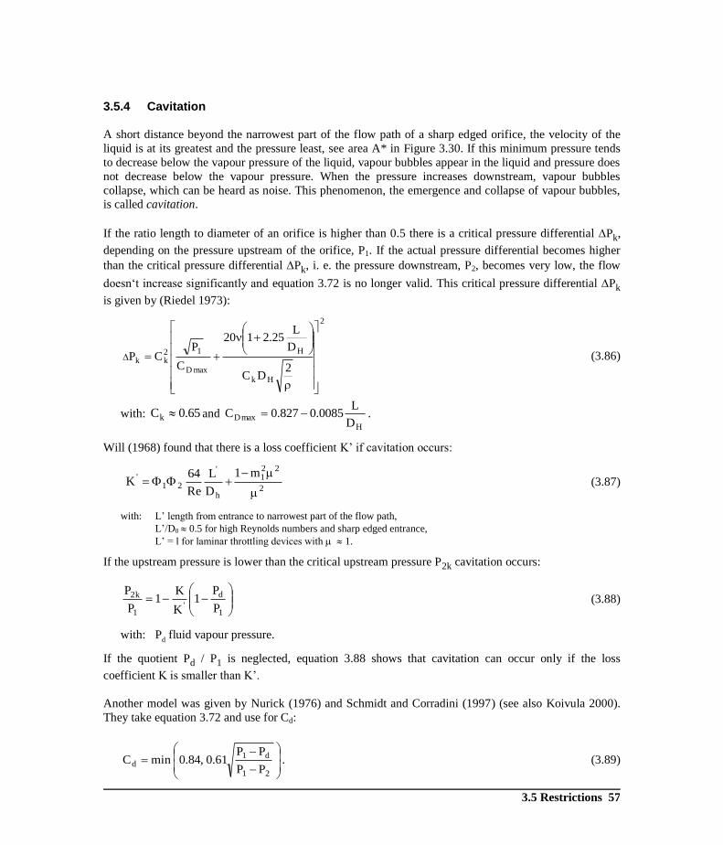
3.5 Restrictions 57
3.5.4 Cavitation
A short distance beyond the narrowest part of the flow path of a sharp edged orifice, the velocity of the
liquid is at its greatest and the pressure least, see area A* in Figure 3.30. If this minimum pressure tends
to decrease below the vapour pressure of the liquid, vapour bubbles appear in the liquid and pressure does
not decrease below the vapour pressure. When the pressure increases downstream, vapour bubbles
collapse, which can be heard as noise. This phenomenon, the emergence and collapse of vapour bubbles,
is called cavitation.
If the ratio length to diameter of an orifice is higher than 0.5 there is a critical pressure differential Pk,
depending on the pressure upstream of the orifice, P1. If the actual pressure differential becomes higher
than the critical pressure differential Pk, i. e. the pressure downstream, P2, becomes very low, the flow
doesn‘t increase significantly and equation 3.72 is no longer valid. This critical pressure differential Pk
is given by (Riedel 1973):
2
Hk
H
maxD
12kk
2DC
D
L25.2120
C
PCP
(3.86)
with: 65.0Ck and H
maxDD
L0085.0827.0C .
Will (1968) found that there is a loss coefficient K’ if cavitation occurs:
2
221
h
'
21' m1
D
L
Re
64K
(3.87)
with: L’ length from entrance to narrowest part of the flow path,
L’/D0 0.5 for high Reynolds numbers and sharp edged entrance,
L’ = l for laminar throttling devices with 1.
If the upstream pressure is lower than the critical upstream pressure P2k cavitation occurs:
1
d
'1
k2
P
P1
K
K1
P
P (3.88)
with: Pd fluid vapour pressure.
If the quotient Pd / P1 is neglected, equation 3.88 shows that cavitation can occur only if the loss
coefficient K is smaller than K’.
Another model was given by Nurick (1976) and Schmidt and Corradini (1997) (see also Koivula 2000).
They take equation 3.72 and use for Cd:
21
d1d
PP
PP61.0,84.0minC . (3.89)

58 3 Component Models
3.5.5 Metering Edges of Valves
There are several models for the metering edges of valves. One uses the equation for a sharp edged
circular orifice and varies the diameter of this orifice according to the position of the valve spool, i. e. the
opened area of the valve and the orifice are the same. Another way is to measure the spool position,
pressure drop and flow rate of the valve and use a look up table for the simulation. This method is the
most accurate but requires an already existing valve and a lot of effort. The first method is usually good
enough if the parameters of similar valves are known. Other models usually need a lot of parameters that
are unknown when designing a system. A detailed study is presented by Borghi et al. (2005).
Figure 3.31 Spool valve Figure 3.32 Symbol
3.5.6 Library Models for Orifices
When modeling turbulent flow through an orifice, equation 3.72 is usually used in the literature. If the
pressure drop across the orifice becomes very low, however, and the Reynolds number is 200 or less even
the flow through a sharp edged orifice becomes laminar. And equation 3.72 is not only a poor model for
laminar flow but leads to severe numerical problems as the following example shows.
Figure 3.33 Example for orifice model
The flow rate Q in Figure 3.33 is modelled by:
P2
CAQ d
(3.72)
with: 21 PPP .
The “gain” of the orifice, i. e. dQ / d(P), is given by:
po
dd
P2
2CA
Pd
P2
CAd
Pd
dQ
(3.90)
with: po
P pressure drop evaluated at the operating point.
x P1
P2
spool
P1
P2
x
D/2
QVol , P
1 1Vol , P
2 2
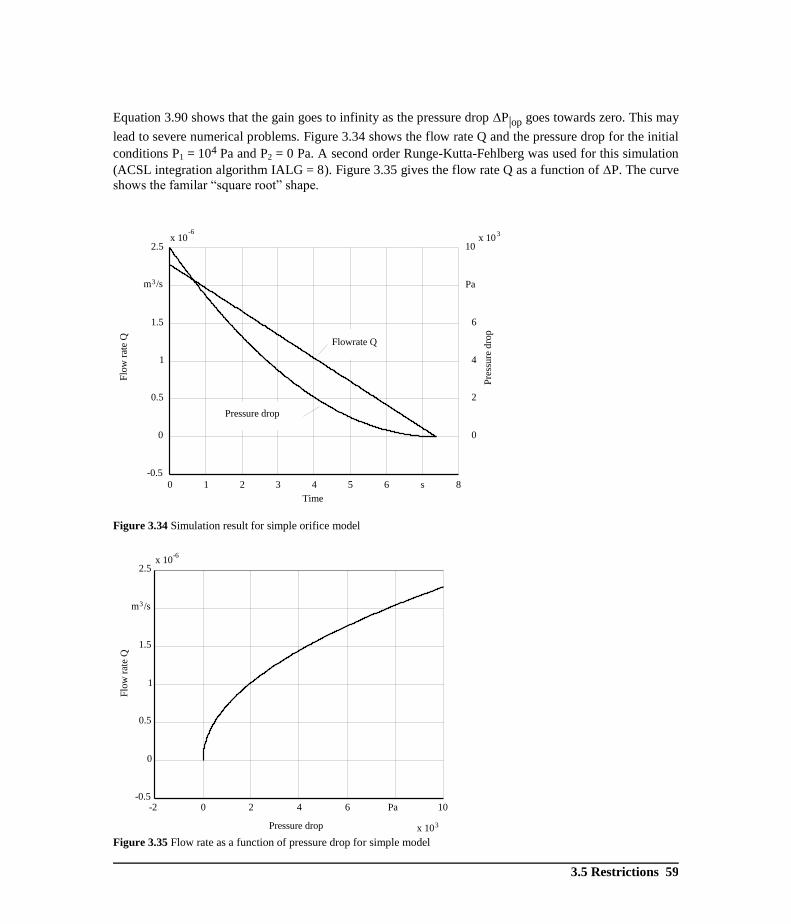
3.5 Restrictions 59
Equation 3.90 shows that the gain goes to infinity as the pressure drop P|op goes towards zero. This may
lead to severe numerical problems. Figure 3.34 shows the flow rate Q and the pressure drop for the initial
conditions P1 = 104 Pa and P2 = 0 Pa. A second order Runge-Kutta-Fehlberg was used for this simulation
(ACSL integration algorithm IALG = 8). Figure 3.35 gives the flow rate Q as a function of P. The curve
shows the familar “square root” shape.
Figure 3.34 Simulation result for simple orifice model
Figure 3.35 Flow rate as a function of pressure drop for simple model
0 1 2 3 4 5 6 8
-0.5
0
0.5
1
1.5
2.5x 10
-6
s
Time
Flo
w r
ate
Q
0
2
4
6
10x 10
3
Pa
Pre
ssure
dro
p
Flowrate Q
Pressure drop
m /s3
einfaches blendenmodell ble
-2 0 2 4 6 10
x 103
-0.5
0
0.5
1
1.5
2.5x 10
-6
Pa
Pressure drop
Flo
w r
ate
Q
m /s3

60 3 Component Models
The simulation result and the flow rate as a function of pressure drop show the expected results. Pressure
differential and flow rate go to zero with increasing time. The problem with this simple model shows
Figure 3.36. When the pressure differential approaches zero the step size of the variable step integration
algorithm becomes very small and the number of integration steps per unit time increases dramatically.
This means that it is not possible to use a stop time of the simulation that is much greater than the time at
which the pressure drop approaches zero because the needed computing time is too long. Generally
speaking this orifice model works only if the pressure drop is higher than zero or if an integration method
with a fixed step size is used.
Figure 3.36 Number of integration steps per unit time. Huge increase at t = 7,39 s
Figure 3.37 show the time response after the pressure drop has become negative for the first time. It is a
limit cycle around the origin caused by the infinite gain at P = 0.
0 1 2 3 4 5 6 810
10
10
10
0
1
2
3
s
Time
Num
ber
of
step
s
einfaches blendenmodell ble
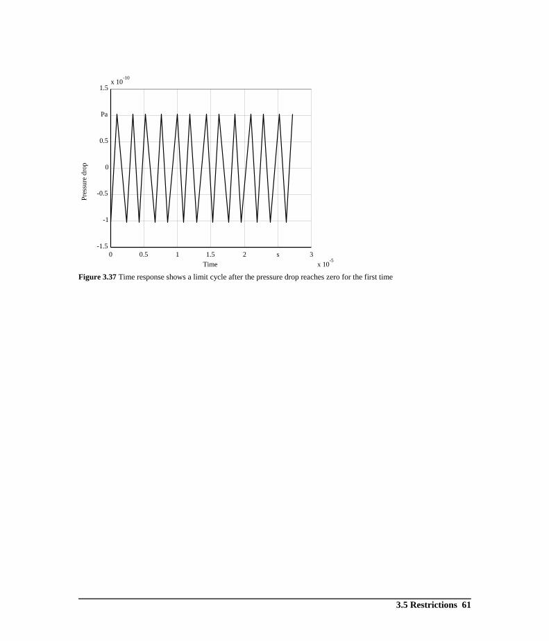
3.5 Restrictions 61
Figure 3.37 Time response shows a limit cycle after the pressure drop reaches zero for the first time
x 10-5
0 0.5 1 1.5 2 3
-1.5
-1
-0.5
0
0.5
1.5x 10
-10
s
Pa
Time
Pre
ssure
dro
p
einfaches blendenmodell ble

62 3 Component Models
In the library the model Orifice uses the following equations to describe laminar/turbulent flow through
fixed restrictions:
21 K
Re
KK (3.91)
and
2
2
A2
QKP
(3.92)
This equation was used in the German national standard TGL 38188 to describe the resistance
characteristic of fixed hydraulic resistors. The coefficient K1 determines the response at low Reynolds
numbers when laminar flow exists:
Re
KKlim 1
0Re
, (3.93)
which leads to:
PK2
DQlim
1
3
0Re
(3.94)
for an annular restriction. K1 depends on the type of restriction. For tubes with a circular cross section K1
is given by:
D
L64K1 . (3.95)
For high Reynolds numbers, i. e. turbulent flow, K1/Re goes toward zero and K2 determines K:
2Re
KKlim
. (3.96)
The flow rate Q as a function of P is given by:
2
2
Re K
P2
4
DQlim
(3.97)
The relation between Cd, the discharge coefficient of equation 3.72 and K2 is given by:
2
d
2C
1K . (3.98)
The gain dQ / d P for (3.92) is given by:
PKD8K2
D
Pd
dQ
22222
1
3
(3.99)
and for the limit P 0 follows:
1K2
D
Pd
dQlim
3
0PΔ
. (3.100)
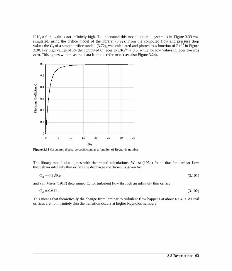
3.5 Restrictions 63
If K1 0 the gain is not infinitely high. To understand this model better, a system as in Figure 3.33 was
simulated, using the orifice model of the library, (3.92). From the computed flow and pressure drop
values the Cd of a simple orifice model, (3.72), was calculated and plotted as a function of Re0.5
in Figure
3.38. For high values of Re the computed Cd goes to 1/K20.5
= 0.6, while for low values Cd goes towards
zero. This agrees with measured data from the references (see also Figure 3.24).
Figure 3.38 Calculated discharge coefficient as a function of Reynolds number
The library model also agrees with theoretical calculations. Wuest (1954) found that for laminar flow
through an infinitely thin orifice the discharge coefficient is given by:
Re2.0Cd (3.101)
and van Mises (1917) determined Cd for turbulent flow through an infinitely thin orifice:
611.0Cd . (3.102)
This means that theoretically the change from laminar to turbulent flow happens at about Re 9. As real
orifices are not infinitely thin the transition occurs at higher Reynolds numbers.
blendenmodell ble zeta = k1/Re + k2
0 5 10 15 20 25 30 35
0
0.1
0.2
0.3
0.4
0.5
0.6
Re
Dis
char
ge
Coef
fici
ent
Cd

64 3 Component Models
The model OriPoly is not based on physical reasons but tries to avoid the numerical problems of the
simple model in (3.72) by an empirical polynomial approximation around P 0 (Ellman and Piché
1996):
trtrtr
tr
trturb
PP0)P(signP
P3
P
P
D4
ReA3
when
PP)P(signP2
AC
)P(Q (3.103)
where the transition pressure difference Ptr occurs at:
2
turb
22tr
trDC8
Re9P
(3.104)
This corresponds to a Reynolds number of 3/2 Retr. The Reynolds number is defined proportional to the
orifice diameter D:
A
DQRe (3.105)
with: Q flow rate,
A orifice cross section area,
Retr transition Reynolds number,
Cturb orifice coefficient,
D orifice diameter.
To use this model the transition Reynolds number Retr has to be chosen. From that the transition pressure
Ptr can be calculated.
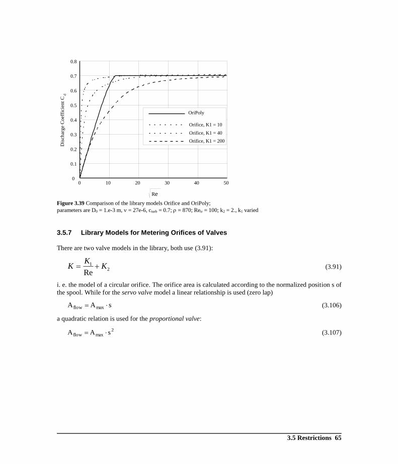
3.5 Restrictions 65
Figure 3.39 Comparison of the library models Orifice and OriPoly;
parameters are D0 = 1.e-3 m, = 27e-6, cturb = 0.7; = 870; Retr = 100; k2 = 2., k1 varied
3.5.7 Library Models for Metering Orifices of Valves
There are two valve models in the library, both use (3.91):
21
ReK
KK (3.91)
i. e. the model of a circular orifice. The orifice area is calculated according to the normalized position s of
the spool. While for the servo valve model a linear relationship is used (zero lap)
sAA maxflow (3.106)
a quadratic relation is used for the proportional valve:
2
maxflow sAA (3.107)
0 10 20 30 40 500
0.1
0.2
0.3
0.4
0.5
0.6
0.7
0.8
OriPoly
Orifice, K1 = 10
Orifice, K1 = 40
Orifice, K1 = 200
Re
Dis
char
ge
Coef
fici
ent
Cd
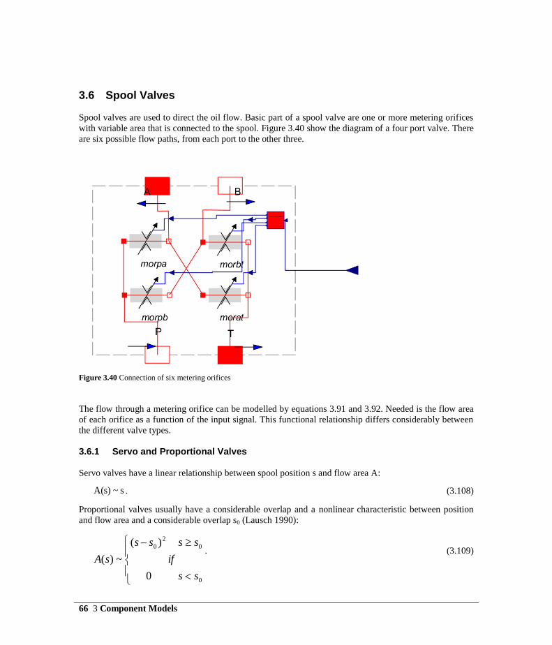
66 3 Component Models
3.6 Spool Valves
Spool valves are used to direct the oil flow. Basic part of a spool valve are one or more metering orifices
with variable area that is connected to the spool. Figure 3.40 show the diagram of a four port valve. There
are six possible flow paths, from each port to the other three.
Figure 3.40 Connection of six metering orifices
The flow through a metering orifice can be modelled by equations 3.91 and 3.92. Needed is the flow area
of each orifice as a function of the input signal. This functional relationship differs considerably between
the different valve types.
3.6.1 Servo and Proportional Valves
Servo valves have a linear relationship between spool position s and flow area A:
s~)s(A . (3.108)
Proportional valves usually have a considerable overlap and a nonlinear characteristic between position
and flow area and a considerable overlap s0 (Lausch 1990):
0
0
2
0
0
)(
~)(
ss
ss
if
ss
sA
. (3.109)
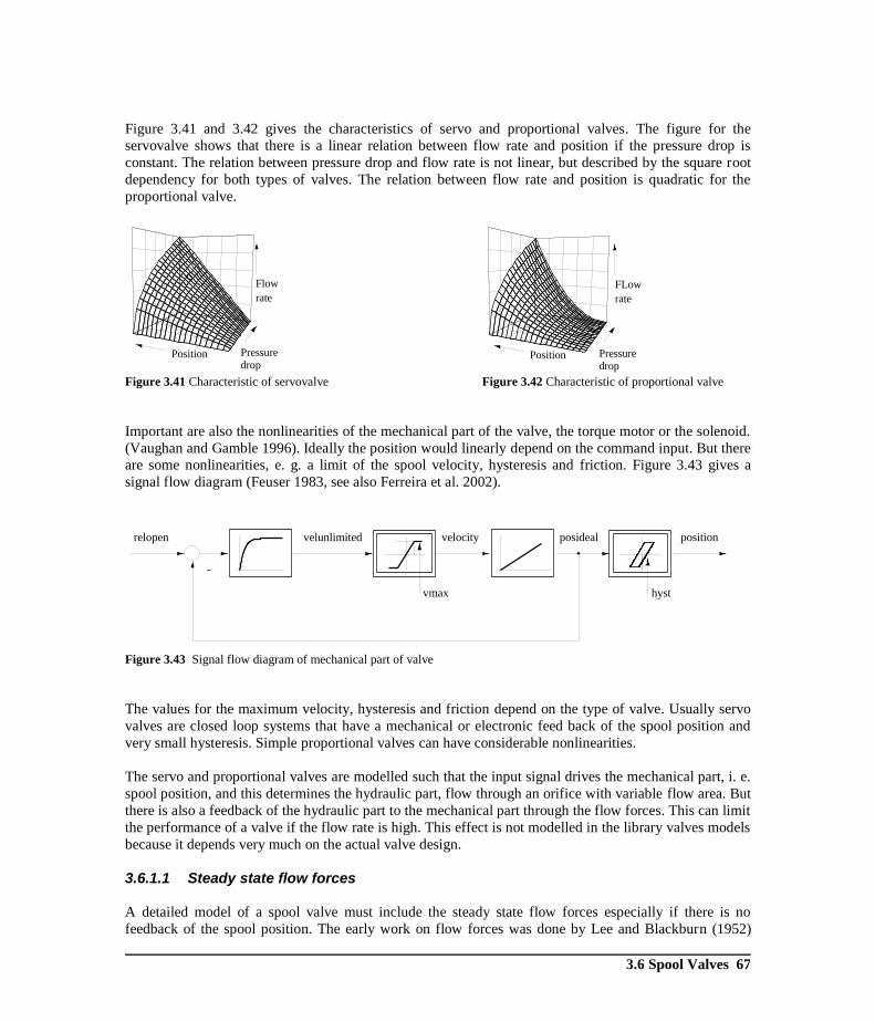
3.6 Spool Valves 67
Figure 3.41 and 3.42 gives the characteristics of servo and proportional valves. The figure for the
servovalve shows that there is a linear relation between flow rate and position if the pressure drop is
constant. The relation between pressure drop and flow rate is not linear, but described by the square root
dependency for both types of valves. The relation between flow rate and position is quadratic for the
proportional valve.
Figure 3.41 Characteristic of servovalve Figure 3.42 Characteristic of proportional valve
Important are also the nonlinearities of the mechanical part of the valve, the torque motor or the solenoid.
(Vaughan and Gamble 1996). Ideally the position would linearly depend on the command input. But there
are some nonlinearities, e. g. a limit of the spool velocity, hysteresis and friction. Figure 3.43 gives a
signal flow diagram (Feuser 1983, see also Ferreira et al. 2002).
Figure 3.43 Signal flow diagram of mechanical part of valve
The values for the maximum velocity, hysteresis and friction depend on the type of valve. Usually servo
valves are closed loop systems that have a mechanical or electronic feed back of the spool position and
very small hysteresis. Simple proportional valves can have considerable nonlinearities.
The servo and proportional valves are modelled such that the input signal drives the mechanical part, i. e.
spool position, and this determines the hydraulic part, flow through an orifice with variable flow area. But
there is also a feedback of the hydraulic part to the mechanical part through the flow forces. This can limit
the performance of a valve if the flow rate is high. This effect is not modelled in the library valves models
because it depends very much on the actual valve design.
3.6.1.1 Steady state flow forces
A detailed model of a spool valve must include the steady state flow forces especially if there is no
feedback of the spool position. The early work on flow forces was done by Lee and Blackburn (1952)
Pressure drop
Flow
rate
Position Pressure drop
FLow
rate
Position
-
relopen velunlimited velocity posideal position
vmax hyst

68 3 Component Models
who also give a plot of the jet angle as a function of spool position. Nikolaus (1971) gives a formula for
that plot. A survey on flow through spool valves is given by Chapple et al. (1999).
Figure 3.44 Flow through a spool valve
1
2
ax cosA
QF (3.110)
with: Fax flow force,
mass density,
A flow area,
s position of spool, s = 0+ => valve opens,
r radial clearance.
1 jet angle.
0s934.0
if
0s34.0
r
s69.2
59.1
cos 1
(3.111)
Another formula for the jet angle 1 is given by Merritt (1967):
111
111
sin2/)2/tan(logcos)2/(1
cos2/)tan(logsin)2/(1
e
e
r
v
C
x (3.112)
with: xv spool position,
Cr radial clearance.
Feigel (1992) gives approximations for different valve types.
One metering orifice: PQ077,0Fax . (3.113)
Two metering orifices: PQ077,0Fax . (3.114)
Four metering orifices: PQ109,0Fax (3.115)
with: Fax axial force on the spool in N,
Q flow rate in l/min,
P pressure differential in bar.
2
1
P0
s
Fax L
control volume

3.6 Spool Valves 69
3.6.1.2 Dynamic Flow Forces
In addition to the steady state flow forces there are dynamic flow forces if the flow rate changes. They are
caused by the inertia of the moving oil column.
dt
)t(QdLF dyn,ax (3.116)
The effect of the dynamic flow forces is small, the magnitude is about the same as the viscous friction
forces (Backé 1962). This force is therefore usually not included in a spool valve model.
3.6.2 Directional Control Valves
While servo and proportional valves have an analog input and metering orifices that can be opened
gradually, directional control valves are switching valves that in steady state are either completely open or
completely closed. Their command signals are therfore binary signals, “on” or “off”. Depending on the
construction there may be one or two command signals: one if the valve has two stable states and two if
the valve has three stable states.
Figure 3.45 Icon of 4 port - 3 way and 4 port - 2 way directional control valves
The flow through one metering orifice can be modelled by (3.91) and (3.92). The diameter of each orifice
as a function of the spool position is given by a piece wise defined linear function. This consists of
segments where the flow is blocked, i.e. the diameter of the metering orifice set to a small value
describing leakage. There are segments where the valve is completely opened, i.e. the diameter is set to a
(maximum) value that is computed from the nominal pressure drop across one metering orifice and the
flow rate. For example, the maximum diameter for the flow path from P to B is given by dmaxPB:
dpnom2
kqnomareamax 2
PBPB

70 3 Component Models
PBPBmax
areamax2d
These segments are connected by straight lines to have a smooth transition when the spool moves from
one position to another. In contrast to servo valves this “dynamic phase” is often not relevant for the
analysis and the operation of the circuit. Typically, there is also no information from the valve
manufacturer. In the library the spool dynamics is described by a first order system whose time constant
can be set for the opening and closing operation separately.
More important than the spool dynamics are the flow paths that are opened or closed during the transition
between the stable positions. Even if the stable positions are identical (identical valve symbol) the
connections during the shifting of the spool may differ.
Figure 3.46 Icon and internal connections of a 4 port 3 way directional control valve (DCV_4_3_B)
When the pump pressure and the flow rate is high, the unbalanced forces and flow forces acting on the
spool are higher than the force generated by the solenoid and the valve is partially closed. The effect can
be modelled by the equations given above. However, the required detailed information is often not
available and therefore the two parameters P_max and coeff_P are used to describe the valve behaviour.
P_max specifies the maximum hydraulic power in W where the valve is still completely open and
coeff_P is a reduction coefficient to adjust the model to the manufacturer's data. When the specified
hydraulic power is exceeded, a warning is printed in the log window (Mode Simulation / Simulation /
Show Log).
1 => diameter is given by dmax + dleak (completely open)
0 => diameter is given by dleak (leakage only)

3.7 Flow and Pressure Control Valves 71
3.7 Flow and Pressure Control Valves There are two types of control valves. One can be described as shutoff valves, e. g. check valves. They are
either wide open or completely shut, having a minimum or maximum resistance. The transition from one
state to the other is fast. Usually it suffices to describe only the static input-output relationship based on
the pressure at the input and output port, because the speed of response of the valves is many times faster
than the response of the overall system. A check valve is a typical example of this kind of shutoff valve.
Figure 3.47 Check valve
The valve is considered open if the pressure at A, PA, is higher than the pressure at B, PB, plus a preload
pressure given by the spring force, called popen. If the valve is open oil flows from port A through the
orifice and the laminar resistance. If the valve is closed there is only the leakage through the laminar
resistance. Figure 3.48 show the flow rate as a function of pressure drop for the library model
CheckValveTwo.
Figure 3.48 Flow as a function of pressure drop
model CheckValveTwo, popen = 0.2 Mpa, diameter = 0.001 m, k1 = 10, k2 =2
There is a number of check valves who‘s response can be characterized by this model. But there are also
valves that have a definite transition state between completely closed and wide open. They can be
modelled by the library model CheckValve.
A
Ch2 ; popen 0.2 MPa; diameter 0.001 m, k1 10; k2 2
-2 -1 0 1 3-1
0
1
2
4
x 10-5
MPa
Pressure drop
Flo
w r
ate
popen
valve open
leakage
m /s3
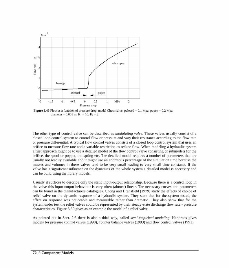
72 3 Component Models
Figure 3.49 Flow as a function of pressure drop, model Checkvalve, pclosed = 0.1 Mpa, popen = 0.2 Mpa,
diameter = 0.001 m, K1 = 10, K2 = 2
The other type of control valve can be described as modulating valve. These valves usually consist of a
closed loop control system to control flow or pressure and vary their resistance according to the flow rate
or pressure differential. A typical flow control valves consists of a closed loop control system that uses an
orifice to measure flow rate and a variable restriction to reduce flow. When modeling a hydraulic system
a first approach might be to use a detailed model of the flow control valve consisting of submodels for the
orifice, the spool or poppet, the spring etc. The detailed model requires a number of parameters that are
usually not readily available and it might use an enormous percentage of the simulation time because the
masses and volumes in these valves tend to be very small leading to very small time constants. If the
valve has a significant influence on the dynamics of the whole system a detailed model is necessary and
can be build using the library models.
Usually it suffices to describe only the static input-output relationship. Because there is a control loop in
the valve this input-output behaviour is very often (almost) linear. The necessary curves and parameters
can be found in the manufacturers catalogues. Chong and Dransfield (1979) study the effects of choice of
relief valve on the dynamic response of a hydraulic system. They state that for the system tested, the
effect on response was noticeable and measurable rather than dramatic. They also show that for the
system under test the relief valves could be represented by their steady-state discharge flow rate - pressure
characteristics. Figure 3.50 gives as an example the model of a relief valve.
As pointed out in Sect. 2.6 there is also a third way, called semi-empirical modeling. Handroos gives
models for pressure control valves (1990), counter balance valves (1993) and flow control valves (1991).
Chk pclosed 0.1MPa; popen 0.2 MPa;
diameter 0.001 m; K1 = 10; K2 = 2
-2 -1.5 -1 -0.5 0 0.5 1 2-1
0
1
2
4
x 10-5
MPa
Pressure drop
Flo
w r
ate
popenpclosed
leakage
valve open
m /s3

3.7 Flow and Pressure Control Valves 73
Figure 3.50 Flow rate as a function of pressure for a relief valve, ReliefValve, pclosed = 19 MPa, popen = 20.5 MPa,
Gleak = 1.111e-12, Gopen = 1.666e-9
If the pressure differential is below a certain value, pclosed, there is only leakage. This leakage can be
small but can also be considerably for bigger valves. The manufacturers’ data sheets usually give some
numbers. If the valve is working the resistance of the valve depends on the pressure differential. The
resistance is decreasing with increasing pressure differential. If the pressure differential is too high the
valve is wide open and its resistance is constant.
Sometimes it is necessary to make a detailed model of a valve. This has to include the inertia of the
moving parts, the oil volumes under pressure and the restrictions. Table 3.20 gives some models for
restrictions that are neither spools nor orifices.
Table 3.20 Models of different valve types
Disk Valve
xr2Ax
2/rxwhenAA px
2p rA r4Lw
2
x
p
A
A2.03.1K
(Lyon 1982)
Rel ; pclosed 19 MPa, popen 20.5;
GLeak 1.111e-012; BOpen 1.666e-009
18.5 19 19.5 20 20.5 21 21.5 22.50
1
2
3
4
6x 10
-3
MPa
Pressure differential
Flo
w r
ate
popenpclosed
working rage
popen GOpen
m /s3

74 3 Component Models
x = 0 => valve closed
Simple Ball Valve
xr5.1Ax
r3.1r when valid is Ax
2p rA
r4Lw
2
x
p
A
A15.05.0K
(Lyon 1982)
2
11 D
h14.0
D
h8.065.2K
25.0D/h1.0 1
(Chaimowitsch 1961)
x = 0 => valve closed
Needle Valve
2tanx
2tanxr2A 22
x , 0xwhen0Ax
2tanxr22Lw ,
2
x
p
A
A15.05.0K
K is valid from Ax = 10 to Ax = 100 % of entry area, Ap.
(Lyon 1982)
Poppet valve
2
11 D
h14.0
D
h8.065.2K
25.0D/h1.0 1
1.0D/b 1m
(Chaimowitsch 1961)
see also (Bergada and Watton 2004)

3.8 Long Lines 75
3.8 Long Lines
In most hydraulic control systems the lines are short and are of reasonably large diameter to keep fluid
flow velocities to a low value. In these situations it is usually reasonable to ignore line resistance as
negligible relative to, for example, control valve resistance, line capacitance as negligible relative to, for
example, actuator capacitance, and fluid inertia as a very minor dynamic effect relative to the inertia of
the actuator and load. Alternatively, line resistance can be lumped with valve resistance and possibly with
actuator inlet resistance, and line capacitance with actuator or other adjacent components’ capacitance(s).
There may be cases however where it is desirable to include some or all of a line‘s R, C and L effects in a
dynamic model. The situation could arise:
if the lines are long,
if the lines are of small bore,
if the system is being driven in a highly dynamic mode.” (Dransfield 1981).
As Dransfield states the simplest line model is not to model it explicitly but adding only the line volume
to the volume of the components connected by that line. The next step can be to model the oil
compressibility by a lumped volume. This is acceptable if the length l of the line is shorter than
maxf10
al (3.117)
with: a speed of sound,
fmax highest frequency of interest.
If the highest frequency of interest leads to a length that is shorter than given by equation 3.117 or if the
pressure drop across the line is important a detailed line model has to be used.
3.8.1 Steady State Pressure Loss in Lines
To model the pressure drop the friction factor f (3.118) is used. This number depends on the Reynolds
number and, if the flow is turbulent, on the internal smoothness of the pipe.
Lu
DP2f
2
(3.118)
with: f friction factor,
P pressure differential,
D inside diameter,
u (mean) velocity,
mass density of fluid,
L pipe length.
The library model RigidLine models the losses for Reynolds numbers from 0 to 105 and uses the laws of
Hagen-Poiseuille and Blasius from Table 3.21. The transition from laminar to turbulent flow is modelled
as instantaneous; a dynamic model is given by Schindler (1995). In the library models there is no check
whether the condition for smooth pipes is fulfilled.
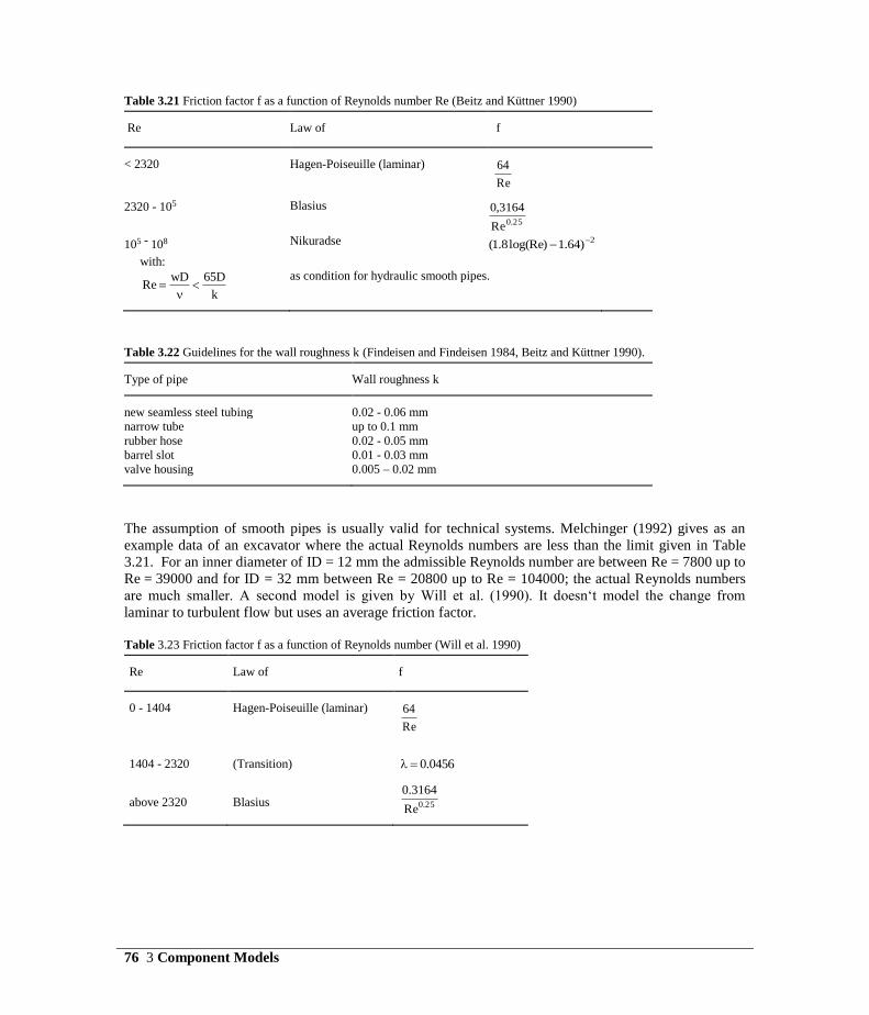
76 3 Component Models
Table 3.21 Friction factor f as a function of Reynolds number Re (Beitz and Küttner 1990)
Re
Law of
f
< 2320
Hagen-Poiseuille (laminar)
Re
64
2320 - 105 Blasius
25.0Re
3164,0
105 - 108 Nikuradse 2)64.1log(Re)8.1(
with:
k
D65wDRe
as condition for hydraulic smooth pipes.
Table 3.22 Guidelines for the wall roughness k (Findeisen and Findeisen 1984, Beitz and Küttner 1990).
Type of pipe
Wall roughness k
new seamless steel tubing
0.02 - 0.06 mm
narrow tube up to 0.1 mm
rubber hose 0.02 - 0.05 mm
barrel slot 0.01 - 0.03 mm
valve housing 0.005 – 0.02 mm
The assumption of smooth pipes is usually valid for technical systems. Melchinger (1992) gives as an
example data of an excavator where the actual Reynolds numbers are less than the limit given in Table
3.21. For an inner diameter of ID = 12 mm the admissible Reynolds number are between Re = 7800 up to
Re = 39000 and for ID = 32 mm between Re = 20800 up to Re = 104000; the actual Reynolds numbers
are much smaller. A second model is given by Will et al. (1990). It doesn‘t model the change from
laminar to turbulent flow but uses an average friction factor.
Table 3.23 Friction factor f as a function of Reynolds number (Will et al. 1990)
Re
Law of
f
0 - 1404
Hagen-Poiseuille (laminar)
Re
64
1404 - 2320 (Transition) 0456.0
above 2320
Blasius 25.0Re
3164.0
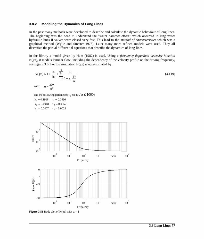
3.8 Long Lines 77
3.8.2 Modeling the Dynamics of Long Lines
In the past many methods were developed to describe and calculate the dynamic behaviour of long lines.
The beginning was the need to understand the “water hammer effect” which occurred in long water
hydraulic lines if valves were closed very fast. This lead to the method of characteristics which was a
graphical method (Wylie and Streeter 1978). Later many more refined models were used. They all
discretize the partial differential equations that describe the dynamics of long lines.
In the library a model given by Ham (1982) is used. Using a frequency dependent viscosity function
N(j), it models laminar flow, including the dependency of the velocity profile on the driving frequency,
see Figure 3.6. For the simulation N(j) is approximated by:
3
1ii
i
j1
k
j1)j(N (3.119)
with: 2D
32
and the following parameters ki for / 1000 :
0024.00407.0k
0352.00948.0k
2496.01918.0k
33
22
11
Figure 3.51 Bode plot of N(j) with = 1
-90
0
Phas
e N
(j
)
10 10 10 10 rad/s 10
100
102
|N(j
w)|
101
-45
10 10 10 10 rad/s 10
-2 -1 0 1 3
-2 -1 0 1 3
Frequency
Frequency
°
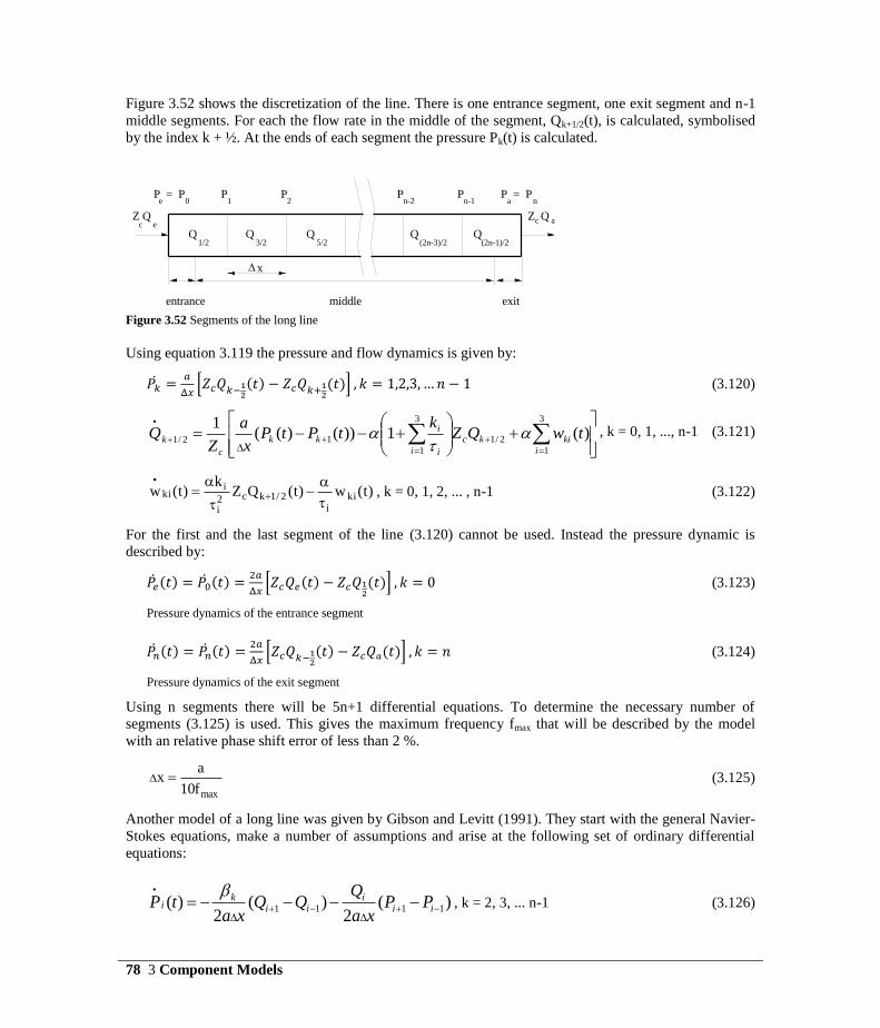
78 3 Component Models
Figure 3.52 shows the discretization of the line. There is one entrance segment, one exit segment and n-1
middle segments. For each the flow rate in the middle of the segment, Qk+1/2(t), is calculated, symbolised
by the index k + ½. At the ends of each segment the pressure Pk(t) is calculated.
Figure 3.52 Segments of the long line
Using equation 3.119 the pressure and flow dynamics is given by:
[
( ) ( )] (3.120)
3
1
2/1
3
1
12/1)(1))()((
1
i
kikc
i i
ikk
c
ktwQZ
ktPtP
x
a
ZQ
, k = 0, 1, ..., n-1 (3.121)
)t(w)t(QZk
)t(w kii
2/1kc2i
iki
, k = 0, 1, 2, ... , n-1 (3.122)
For the first and the last segment of the line (3.120) cannot be used. Instead the pressure dynamic is
described by:
( ) ( )
[ ( )
( )] (3.123)
Pressure dynamics of the entrance segment
( ) ( )
[
( ) ( )] (3.124)
Pressure dynamics of the exit segment
Using n segments there will be 5n+1 differential equations. To determine the necessary number of
segments (3.125) is used. This gives the maximum frequency fmax that will be described by the model
with an relative phase shift error of less than 2 %.
maxf10
ax (3.125)
Another model of a long line was given by Gibson and Levitt (1991). They start with the general Navier-
Stokes equations, make a number of assumptions and arise at the following set of ordinary differential
equations:
)(2
)(2
)( 1111
iii
iik
i PPxa
QQQ
xatP
, k = 2, 3, ... n-1 (3.126)
P = Pe 0
P = Pa n
P1
P2
Pn-1
Pn-2
Q1/2
Q3/2
Q5/2
Q(2n-3)/2
Q
Z Qc e
Z Qc a
entrance exitmiddle
x
(2n-1)/2
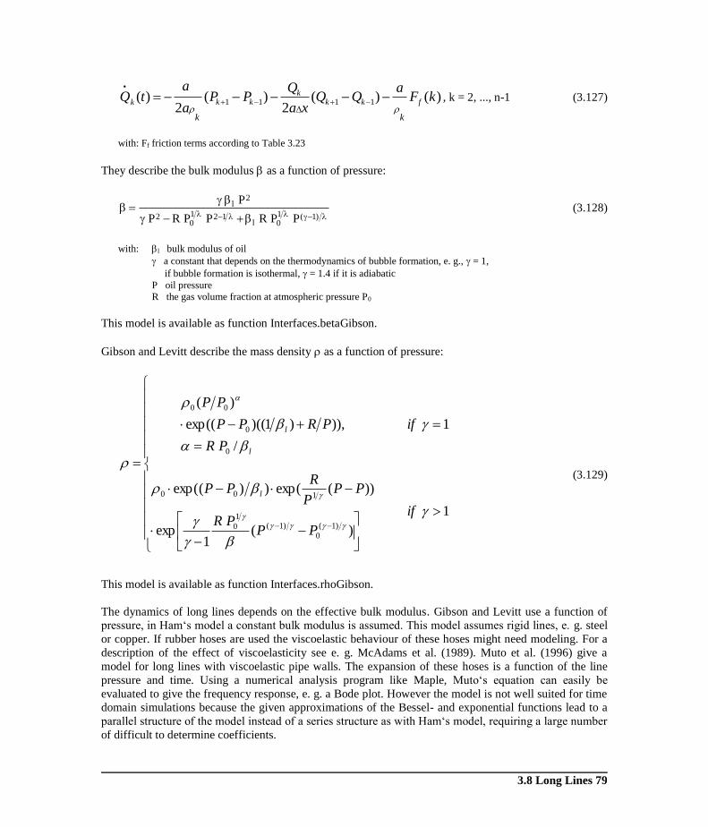
3.8 Long Lines 79
)()(2
)(2
)( 1111 kFa
QQxa
QPP
a
atQ fkk
kkkk
kk
, k = 2, ..., n-1 (3.127)
with: Ff friction terms according to Table 3.23
They describe the bulk modulus as a function of pressure:
)1(10l
1210
2
2l
PPRPPRP
P (3.128)
with: l bulk modulus of oil
a constant that depends on the thermodynamics of bubble formation, e. g., = 1,
if bubble formation is isothermal, = 1.4 if it is adiabatic
P oil pressure
R the gas volume fraction at atmospheric pressure P0
This model is available as function Interfaces.betaGibson.
Gibson and Levitt describe the mass density as a function of pressure:
1
)(1
exp
))(exp())(exp(
1
/
)),)1)((exp((
)(
)1(
0
)1(1
0
100
0
0
00
if
PPPR
PPP
RPP
if
PR
PRPP
PP
l
l
l
(3.129)
This model is available as function Interfaces.rhoGibson.
The dynamics of long lines depends on the effective bulk modulus. Gibson and Levitt use a function of
pressure, in Ham‘s model a constant bulk modulus is assumed. This model assumes rigid lines, e. g. steel
or copper. If rubber hoses are used the viscoelastic behaviour of these hoses might need modeling. For a
description of the effect of viscoelasticity see e. g. McAdams et al. (1989). Muto et al. (1996) give a
model for long lines with viscoelastic pipe walls. The expansion of these hoses is a function of the line
pressure and time. Using a numerical analysis program like Maple, Muto‘s equation can easily be
evaluated to give the frequency response, e. g. a Bode plot. However the model is not well suited for time
domain simulations because the given approximations of the Bessel- and exponential functions lead to a
parallel structure of the model instead of a series structure as with Ham‘s model, requiring a large number
of difficult to determine coefficients.

80 3 Component Models
Table 3.24 Effective bulk modulus and speed of sound (Viersma 1980)
Steel tube
Di = 12.5 mm;
Do = 16 mm
High pressure hose
Di = 12.5 mm
nominal pressure
effective
a
effective
a
50
90
130
225
bar
bar
bar
bar
14600 bar
15100 bar
15700 bar
18900 bar
1270 m/s
1296 m/s
1320 m/s
1450 m/s
5000 bar
5370 bar
5680 bar
746 m/s
772 m/s
795 m/s
Table 3.25 Speed of sound of different hoses(Wacker 1985)
Hose type
pressure range
Speed of sound
3 TE
( textile braid)
20 - 100 bar
700 m/s
2 STT
(two-wire braid)
10 - 170 bar 975 m/s
4 SP
(four light spiral wire)
20 - 170 bar 1025 m/s
= 34 mm²/s; oil temperature 50 °C
3.8.3 Examples using Model LongLine and LongLine_u_air
The model LongLine assumes laminar flow, i. e. Reynolds numbers below 2320. Figure 3.53 shows the
pressure drop as a function of flow rate for the steady state. The pressure started at zero, was increased up
to 6.104 Pa by opening a valve and then reduced to zero again. The hysteresis results from the necessary
force, i. e. pressure drop, to accelerate the oil. The model RigidLine that computes only the resistance of
the line shows no hysteresis but a jump when the critical Reynolds number is exceeded.
Table 3.26 Frequencies for example in Figure 3.54.
Number of segments n
Frequency fmax
4
17 Hz
9 38 Hz
39 163 Hz

3.8 Long Lines 81
Figure 3.53 Pressure drop as a function of flow rate for models LongLine and RigidLine
The model LongLine or LongLine_u_air is used when the dynamic response of hydraulic lines has to be
included in the model. To validate the models data from the literature was used. The first test is an
example from Ham (1982) that consists of a pipe with diameter of 13 mm and a length of 31.98 m
terminated by a laminar resistance. For three different numbers of segments, 4, 9 and 39, the frequency
response was computed and is shown in Figure 3.52 to Figure 3.54. The top figures show the response of
the model LongLine and the analytical solution, the bottom figures the response of the model
LongLine_u_air for different values of the parameters R and .
Figure 3.54 Magnitude plots of |p1 / p0| for the analytical solution and model LongLine with 4 segments (top) and model
LongLine_u_air with 4 segments for different values of R and
daten aus lolkenn1.mat Simulationsdauer 120 s
element length = 3.198 m; dia = 0.03 m;
nu = 0.000027 m**3/s; rho = 865 kg/m**3
x 10-3
Flo
w ra
te
0 2 4 6 8 12
x 104
0
0.5
1
2
Pa
Pressure drop
LongLine
RigidLine
m /s3
0 50 100 150 200 250
0
2
4
6
8
10
gai
n LongLine
0 50 100 150 200 250
0
2
4
6
8
10
gai
n
frequency (Hz)
analytical
R = 0; gamma = 1 R = 0.05; gamma = 1 R = 0.05; gamma = 1.4R = 0; gamma = 1.4

82 3 Component Models
Figure 3.55 Magnitude plots of |p1 / p0| for the analytical solution and model LongLine with 9 segments (top) and model
LongLine_u_air with 9 segments for different values of R and
Figure 3.56 Magnitude plots of |p1 / p0| for the analytical solution and model LongLine with 39 segments (top) and model
LongLine_u_air with 39 segments for different values of R and
The results for R = 0, = 1.0 and R = 0, = 1.4 are almost identical for this set-up. In general the simpler
model LongLine_u_air needs less computing time than the model LongLine. It doesn't describe the
frequency dependent friction but can account for unsolved air. The greatest differences occur therefore for
0 50 100 150 200 250
0
2
4
6
8
10gai
n
0 50 100 150 200 250
0
2
4
6
8
10
gai
n
frequency (Hz)
R = 0; gamma = 1 R = 0.05; gamma = 1 R = 0.05; gamma = 1.4R = 0; gamma = 1.4
LongLine
analytical
LongLine
analytical
R = 0; gamma = 1 R = 0.05; gamma = 1 R = 0.05; gamma = 1.4R = 0; gamma = 1.4
0 50 100 150 200 250
0
2
4
6
8
10
gai
n
0 50 100 150 200 250
0
2
4
6
8
10
gai
n
frequency (Hz)
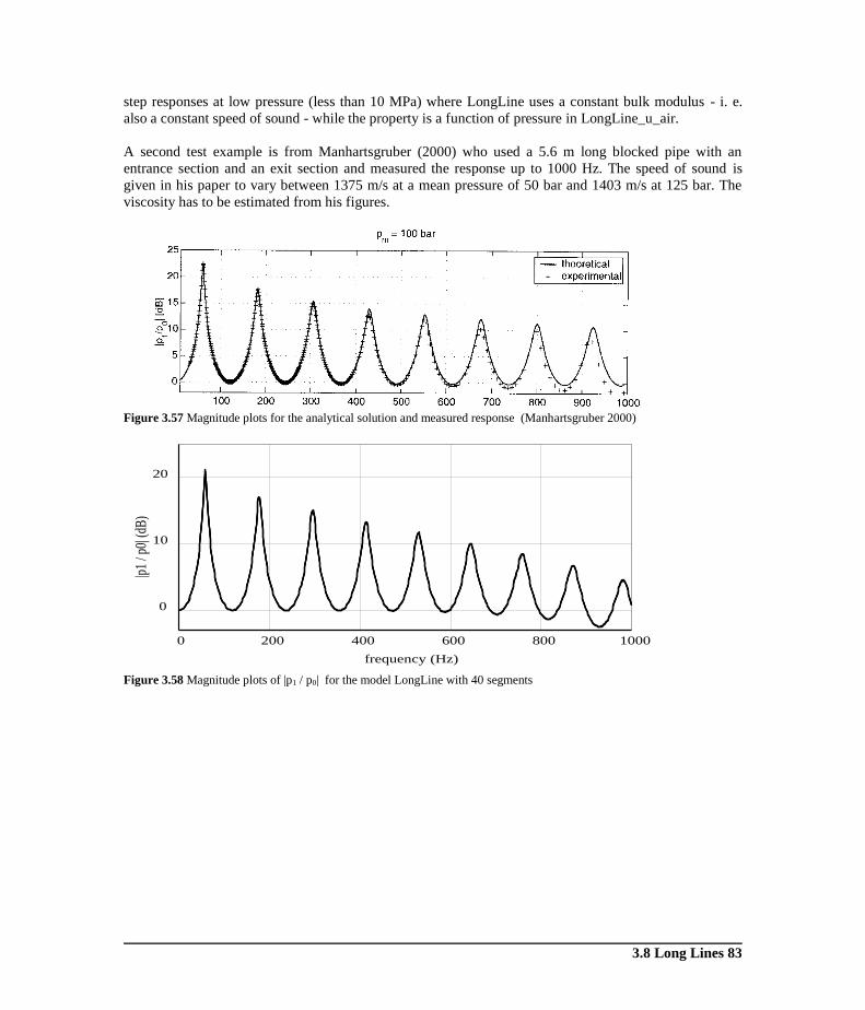
3.8 Long Lines 83
step responses at low pressure (less than 10 MPa) where LongLine uses a constant bulk modulus - i. e.
also a constant speed of sound - while the property is a function of pressure in LongLine_u_air.
A second test example is from Manhartsgruber (2000) who used a 5.6 m long blocked pipe with an
entrance section and an exit section and measured the response up to 1000 Hz. The speed of sound is
given in his paper to vary between 1375 m/s at a mean pressure of 50 bar and 1403 m/s at 125 bar. The
viscosity has to be estimated from his figures.
Figure 3.57 Magnitude plots for the analytical solution and measured response (Manhartsgruber 2000)
Figure 3.58 Magnitude plots of |p1 / p0| for the model LongLine with 40 segments
0
10
20
0 200 400 600 800 1000
frequency (Hz)
|p1
/ p0|
(dB
)
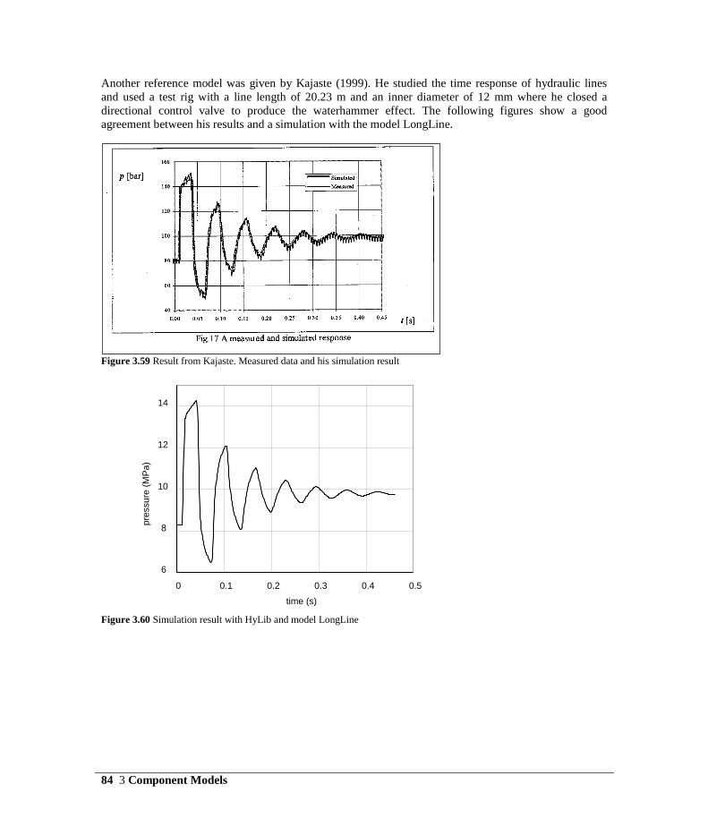
84 3 Component Models
Another reference model was given by Kajaste (1999). He studied the time response of hydraulic lines
and used a test rig with a line length of 20.23 m and an inner diameter of 12 mm where he closed a
directional control valve to produce the waterhammer effect. The following figures show a good
agreement between his results and a simulation with the model LongLine.
Figure 3.59 Result from Kajaste. Measured data and his simulation result
Figure 3.60 Simulation result with HyLib and model LongLine
0 0.1 0.2 0.3 0.4 0.5
6
8
10
12
14
time (s)
pre
ssu
re (
MP
a)
Kajaste 1 - LongLine

References 85
3.9 Accumulators
There are different types of accumulators. The so called spring accumulators store energy by
compressing a metal spring. More often a volume of gas, mostly nitrogen, is used to store the energy.
These hydro-pneumatic accumulators are used to either reduce the pressure and flow fluctuations or to
supplement a pump in a circuit, where the load cycle requires maximum power over a short period of time
only, e. g. a system with secondary control, see Sect. 2.4. The design of accumulators differs depending
on the task.
If an accumulator is used in a hydraulic circuit, it is usually necessary to model it because the compliance
of the accumulator spring, i. e. the gas volume, is much smaller than the compliance of the oil spring. The
accumulator reduces the effective bulk modulus of the system.
3.10 Filters and Coolers
Filters are used to keep the fluid clean. When modeling the system dynamics there are two points that
may need consideration. There is always a certain amount of fluid in the filter and a filter has a resistance.
The oil in the filter can be modelled by a lumped volume or added to a lumped volume that describes the
lines connected to the filter. The resistance of a filter is usually small and doesn‘t influence the dynamics
of the complete system.
If it is necessary to model the losses data from the manufacturer or measurements are needed because
there are only few theoretical models mentioned in the literature. There are references to losses in flow
normal to plane screens (Cornell 1958, Chaimowitch 1961) but they can‘t be used to model the losses of a
filter. Fritsche (1984) made measurements with one particular type of filter and used the following
polynomial:
3
3
2
210Re
1a
Re
1a
Re
1aaK
(3.130)
with a0 = 0.591 . 101
a1 = -0.305 . 102
a2 = 0.255 . 104
a3 = 0.997 . 104
To calculate the Reynolds number Re the diameter of the fitting, 16 mm, was used.
Coolers are needed to control the temperature of the fluid and there are the same problems as with filters
when modeling them. There are some theoretical models (Anon. 1974) but when modeling a particular
component measurements are needed. Fritsche (1984) used the same model as for filters and found the
following coefficients:
a0 = 0.681 . 101
a1 = -0.274 . 103
a2 = 0.930 . 104
a3 = 0.543 . 103
86 References
References
Anon. (1974) VDI-Wärmeatlas. VDI-Verlag: Düsseldorf
Armstrong-Hélouvry, B. (1991) Control of Machines with Friction. Kluwer Academic Publishers, Boston
Armstrong B., Canudas de Wit C. (1996): Friction Modeling and Compensation. The Control Handbook,
edited by W.S.Levine, CRC Press, pp. 1369-1382.
Backé, W. (1962) Über die dynamische Stabilität hydraulischer Steuerungen unter Berücksichtigung der
Strömungskräfte. Thesis RWTH Aachen
Backé, W., Murrenhoff, H. (1994) Grundlagen der Ölhydraulik. RWTH Aachen

References 87
Beater, P. (1999) Entwurf hydraulischer Maschinen – Modellbildung, Stabilitätsanalyse und Simulation
hydrostatischer Antriebe und Steuerungen. Springer Berlin Heidelberg New York.
Beater, P. Object-oriented Modeling and Simulation of Hydraulic Drives. Simulation News Europe. SNE
22, 1998. S.11 - 13.
Beitz W. , Küttner K.-H. Herausgeber (1990) Dubbel - Taschenbuch für den Maschinenbau. Springer,
Berlin Heidelberg New York.
Bell, J., Bergelin, O., P., (1957) Flow Through Annular Orifices. Transactions of the ASME. 79:593 - 601
Bergada, J. M., Watton, J. (2004) A direct solution for flowrate and force along a cone-seated poppet
valve for laminar flow conditions. Proceedings of the Institution of Mechanical Engineers / Journal
of systems and control engineering. 218:197-210
Boes, C. (1995) Hydraulische Achsantriebe im digitalen Regelkreis. Ph.D. Thesis, RWTH Aachen
Borghi, M., Milani, M., Paoluzzi, R. (2005) Influence of the notch shape and number of notches on the
metering characteristics of hydraulic spool valves. International Journal of Fluid Power 6(2):5-18
Borutzky, W., Barnard, B.,Thoma, J. U. (2000) Describing bond graph models of hydraulic components
in Modelica. Mathematics and Computers in Simulation. 53:381-387
Bowns, D., E., Edge, K., Worton-Griffiths, J. (1993) The Effect of Air in the Fluid on the Operating
Characteristics of a Hydrostatic Transmission. 3rd International Fluid Power Symposium, Turin,
May 1973. pp A1 - 1:15
Briggs, L. J. (1950) Limiting Negative Pressure of Water. Journal of Applied Physics 21:721- 722
Chaimowitsch, E. M. (1961) Ölhydraulik. Grundlagen und Anwendung. VEB Verlag Technik Berlin.
Chapple, P., Grahl-Madsen, M., Lie, T. (1999) Flow Through Spool Valves - CFD and a Link to the Past.
Int Workshop on Computer Software for Design of Fluid Power Systems. Trondheim 99
Chong, F. K. and Dransfield, P. (1979) The Effect of Choice on Relief Valve on the Response of a Hy-
draulic Control System. Proc. Conference on Control Engineering, Melbourne, pp 65 - 69
Conrad, F., Sorensen, P., M., Trostmann, E. (1990) On the Modelling of Flow- and Torque-loss in Hydro-
static Machines. 9th int Symp Fluid Power, Cambridge, 1990. pp. 3 - 17
Conrad F., Trostmann E., Zhang M (1993) Experimental identification and modelling of flow and torque
losses in gerotor hydraulic motors. Proceedings of the 2nd
JHPS International Symposium on Fluid
Power Tokyo, 677 - 682
Cornell, W. (1958) Losses in flow normal to plane screens. Transaction ASME 80, 1958, Nr. 4
Doebelin E. O. (1972) System Dynamics: Modeling and Response. Charles E. Merrill Publishing Compa-
ny. Columbus/Ohio
Dransfield, P. (1981) Hydraulic Control Systems - Design and Analysis of Their Dynamics. Springer,
Berlin Heidelberg New York.
Ebertshäuser, H. (1993)Formelsammlung. o+p Konstruktionsjahrbuch 1993/94. Mainz: Vereinigte
Fachverlage GmbH.
Eggerth, S. (1980) Beitrag zur Messung von Volumenströmen viskoser Flüssigkeiten in Druckleitungen.
Ph.D. thesis Technische Universität Dresden.
Ellman, A., Koskinen, Vilenius (1995) Through Flow in Short Annulus of Fine Clearance. ASME Inter-
national Mechnical Engineering Congress and Exposition, San Francisco, p 813 - 821

88 References
Ellman, A., Piché, P. A. (1996) A Modified Orifice Flow Formula for Numerical Simulation. ASME
International Mechanical Engineering Congress and Exposition. Atlanta, USA
Elmqvist, H., Cellier, F. E., Otter, M. (1993) Object-oriented Modeling of Hybrid Systems. ESS‘93,
European Simulation Symposium, Delft, The Netherlands
Fassbender, A. (1993) Saugdrosselung - der Einfluß von Druckmedium und Temperatur. Ölhydraulik und
Pneumatik 37:702 - 707
Feigel, H.-J. (1992) Strömungskraftkompensation in direktgesteuerten elektrohydraulischen
Stetigventilen. Ph.D. Thesis RWTH Aachen.
Fensvig, A. T; Nielsen, T. H., Ovesen, T. B. (1975) On the Dynamics of Rubber Bag Accumulators -
Analytical and Experimental Modeling. 4th
International BHRA Fluid Power Symposium. Shef-
field.
Ferreira, J. A.., Gomes de Almeida, F., Quintas, M. R. (2002) Semi-empirical model for a hydraulic ser-
vo-solenoid valve. Institution of Mechanical Engineers. Journal of systems and control engineer-
ing. 216 (3): 237-248
Feuser, A. (1983) Ein Beitrag zur Auslegung ventilgesteuerter Vorschubantriebe im Lageregelkreis.
Ph.D. Thesis, Universität Erlangen-Nürnberg.
Findeisen, D., Findeisen, F. (1994) Ölhydraulik. Springer, Berlin Heidelberg New York
Fritzsche, M. (1984) Ölleitungsdimensionierung. FVA Frankfurt
Gibson, A., O., Levitt, J., A., (1991) Modeling and simulation of fluid flow in pipes and hoses. The 3rd
triennial international symposium on fluid control, measurement, and visualization. FLUCO-
ME'91. August 28-31, 1991, San Francisco, California. 67-75
Götz, W. (1983) Hydraulik in Theorie und Praxis. Robert Bosch GmbH. Stuttgart
Hahmann, W. (1973) Das dynamische Verhalten hydrostatischer Antriebe mit Servopumpe und ihr
Einsatz in Regelkreisen. Ph.D. thesis TH Aachen
Ham, A. A. (1982) On the Dynamics of Hydraulic Lines supplying Servosystems. Ph.D. Thesis Tech-
nische Hogeschool Delft
Handroos, H. M., Vilenius, M. J. The Utilization of Experimental Data in Modelling Hydraulic Single
Stage Pressure Control Valves. ASME Journal of Dynamic Systems, Measurement and Control,
Vol 112, Number 3, Setember 1990, pp. 482 – 488
Handroos H; Halme J; Vilenius. Steady-state and Dynamic Properties of Counter Balance Valves.
3. Scandinavian International Conference on Fluid Power Linköping. 1993
Handroos H; Vilenius M. The influence of Semi-Empirical Control Valve Model Parameter Accuracy on
Simulated Hydraulic System Responses. Transactions ASME Journal of Dynamic Systems, Meas-
urement Control 1992
Handroos H; Vilenius M J. Flexible Semi-Empirical Models for Hydraulic Flow Control Valves Transac-
tions of the ASME Journal of Mechanical Design 1991
Handroos M; Keskinen E K; Vilenius M.Effect of design parameters on vibrational behaviour of a coun-
ter balance valve equipped hydraulic crane. Proc of the 2nd JHPS Int Symposium on Fluid Power
Toky 1993
Handroos, H., Halme, H. (1996) Semi-empirical model for a counter balance valve. The Third JHPS In-
ternational Conference on Fluid Power, Yokohama, Japan, 4-6 Nov, 1996

References 89
Hayward, A., T., J. (1962) How Air Bubbles Affect the Compressibility of Hydraulic Oil. Hydraulic
Power Transmission, No. 90, 384-388
Hayward, A. T. J. (1970) How to Estimate the Bulk Modulus of Hydraulic Fluids. Hydraulic Pneumatic
Power (1)
Heumann, H. (1987) Ermittlung von Kennwerten hydrostatischer Geräte unter Berücksichtigung ihrer
Verwendbarkeit bei der rechnergestützten Projektierung und Konstruktion hydraulischer Systeme.
7. Fachtagung Hydraulik und Pneumatik. Dresden.
Hibi, A., Ibuki,T., Ichikawa, T., Yokote, H. (1977) Suction Performance of Axial Piston Pumps. Bulletin
of the JSME 20(139):79-84, 827:833
Hoffmann, W. (1981) Dynamisches Verhalten hydraulischer Systeme, automatischer Modellaufbau und
digitale Simulation. Ph.D. thesis RWTH Aachen
Huhtala K., Karen J. K., Vilenius M. J. (1995) Semi-emperical modelling of losses in components of
hydrostatic transmission systems. Proceedings of the 8th
Bath International Fluid Power Workshop
237-253
Huhtala, K., Vilenius, M. (1997) Comparison of Steady-State Models of Hydraulic pumps. 5th Scandina-
vian Int Conf on Fluid Power, Linköping, 1997. pp. 139 - 156
Ivantysyn, J. , Ivantysynova M. (1993) Hydrostatische Pumpen und Motoren. Vogel, Würzburg.
Ivantysyn, J., Ivantysynova, M. (2001) Hydrostatic pumps and motors : principles, design, performance,
modelling, analysis, control and testing. 1. Engl. ed. Akademia Books International. New Delhi.
Jinghong, Y., Zhaoneng, C., Yuanzhang, L. (1994) The Variation of Oil Effective Bulk Modulus With
Pressure in Hydraulic Systems. Transaction of the ASME. Journal of Dynamic Systems, Meas-
urement, and Control, 116:144 -150
Johnson, J. J. (2000) Designer's Handbook for Electrohydraulics, IDAS Engineering, East Troy, WI, USA
Johnston, D., N. (2002) Prediction of hydraulic inductance. Proceeding of the IMECE 2002, ASME Inter-
national Mechanical Engineering Congress & Exposition, Nov. 17-22, 2002, New Orleans, Louisi-
ana, pp 85-92
Kajaste, J. (1999) Pipeline models for large-scale fluid power systems, analysis and validation.The Sixth
Scandinavian International Conference on Fluid Power, SICFP'99, May 1999, Tampere, Finland.
pp 529 - 543
Kallies, H.-E. (1968) Über das Leistungsverhalten von Prallplattenventilen. Ph.D. Thesis. TU Berlin
Knight, G. C.; McCallion, H.; Dudley, B. R. (1972) Connection capacitance effects in hydrostatic trans-
mission systems and their prediction by mathematical model. Proc Instn Mech Engrs 186:661
Koivula, T., Ellman, A., Vilenius, M. (1999) The Effect of Oil Type on Flow and Cavitation Properties in
orifices and annular clearances. Workshop on Power Transmission & Motion Control 1999. Bath.
p. 151 - 165
Koivula, T. (2000) On Cavitation in Fluid Power.1st FPNI-PhD Symposium, Hamburg 2000,
pp. 371 - 382
Korkmaz, F. (1982) Hydrospeicher als Energiespeicher. Springer, Berlin Heidelberg New York
Kraft, W. (1996) Experimentelle und analytische Untersuchungen hydrostatischer Fahrantriebe am
Beispiel eines Radbaggers. Ph. D. Thesis. RWTH Aachen.
90 References
Kürten, T. (1993) Modellbildung, Simulation und digitale Regelung hydraulischer Antriebe mit
elektrohydraulischen Schaltventilen. Ph.D. Thesis Universität -GH- Duisburg. Duisburg:
F. Seidelt.
Lallement J. (1989) Hydropneumatic Accumulators. Second Bath International Fluid Power Workshop
43-57
Lausch, H. (1990) Digitale Regelung hydraulischer Antriebe mittels pulsbreitenmoduliert angesteuerter
Proportionalventile. Ph.D. Thesis. Universität -GH- Duisburg.VDI-Fortschrittsbericht 213, Reihe
8. Düsseldorf. VDI-Verlag.
Lau, K. K., Edge, K. A., Johnston, D. N. (1995) Impedance characteristics of hydraulic orifices. ImechE
Vol 209, p 241 – 253
Lee, S., Y., Blackburn, J., F., (1952) Contributions to Hydraulic Control 1 Steady-State Axial Forces on
Control-Valve Pistons. Transactions of the ASME. 74:1005 - 1111
Lee, K. I. (1977) Dynamisches Verhalten der Steuerkette Servoventil - Motor- Last. Ph.D. thesis
RWTH Aachen.
Lennevi, J. (1995) Hydrostatic Transmission Control. Desing Methodology for Vehicular Drivetrain Ap-
plications. Ph. D. Thesis Linköping University, Sweden
Leonhard, W. (1985) Control of Electrical Drives. Springer, Berlin Heidelberg New York
Lichtarowicz A., Duggins, R. K., Markland, E. (1965) Discharge Coefficients for Incompressible Non-
Cavitating Flow Through Long Orifices. J. Mech. Eng. Sc. Nr. 2:210 - 219
Lyon, J. L. (1982) Lyon‘s Valve Designer‘s Handbook. Van Nostrand Reinhold Company, New York
Mäkinen, J., Ellman, A., Piché, R (1997) Dynamic Simulations of Flexible Hydraulic-Driven Multibody
Systems using Finite Strain Beam Theory. Proc. 5th
International Conference on Fluid Power, Lin-
köping 2:119-134
Manhartsgruber, B. (2000) Experimental validation of mathematical models of hydraulic pipelines with
high-frequency excitation. Bath Workshop on Power Transmission and Motion Control (PTMC
2000), Bath, 2000. 29-41
Manring, N. D. (1997) The Effective Fluid Bulk-Modulus Within a Hydrostatic Transmission. Transac-
tions of the ASME Journal of Dynamic Systems, Measurement, and Control. 119:462-466
Martin, H. R. (1981) Effects of Pipes and Hoses on Hydraulic Circuit Noise and Performance. 37th
Nat.
Fluid Power Conference, Chicago, 35:71 - 76
Martin, H. (1995) The Design of Hydraulic Components and Systems. Ellis Horwood, London
McAdams, J. P., Manuel, W. S., Hall, H. E. (1989) Comparison of Response-Time Tests with Computer
Simulations for Control Hoses in Subsea Production Service. Proc. 21st Annual Offshore Technol-
ogy Conf., Houston. Texas. Paper OTC 5917:367-376
McCloy, D. (1968) Discharge Characteristics of Servo Valve Orifices. Fluid Power International Confer-
ence, Olympia, 43-50
Melchinger, U. (1992) Simulation der Arbeitsbewegungen und Antriebssysteme von Hydraulikbaggern.
VDI-Fortschrittsbericht 212. Reihe 1. Düsseldorf: VDI-Verlag.
Merritt, H. E. (1967) Hydraulic Control Systems. New York: John Wiley & Sons
References 91
van Mises, R. (1917) Berechnung von Ausfluß- und Überfallzahlen.Z. Ver. Deutsch. Ing, 61:447-452,
465-474, 493-498
Müller, H. (1978) Die Kugel als Kolben hydrostatischer Maschinen. Ph.D. Thesis Technische Universität
Braunschweig
Muto, T., Yamada, H., Kato, H. (1996) A Fast and Convenient Method for Simulating Transient Re-
sponse of Fluid Lines with Viscoelastic Pipe Walls. 12. Aaechener Fluidtechnisches Kolloquium.
RWTH Aachen
Nikolaus, H. (1971) Stationäres und dynamisches Verhalten von hydraulischen
Zeiwegestromregelventilen. Habilitationsschrift Universität Karlsruhe.
Nikolaus, H. (1981) Hydrospeicher als hydraulische Batterie für hydrostatische Getriebe. Ölhydraulik und
Pneumatik. 25:p 563 - 566.
Nurick, W., H. (1976) Orifice Cavitation and Its Effect on Spray Mixing. Transactions of the ASME
Journal of Fluids Engineering. 98:681 - 687
Nykänen, T., H., A., Esqué, S., Ellman, A., U. (2000) Comparison of different fluid models. Bath Work-
shop on Power Transmission and Motion Control (PTMC 2000), Bath, 2000, 101-110
Ohrn, T., R., Senser,D., W., Lefebvre, A., H. (1991) Geometrical Effects on Discharge Coefficients for
Plain-orifice Atomizers. Atomization and Sprays. 1:137 - 153
Otis, D. R., (1974) New Developments in Predicting and Modifying Performance of Hydraulic Accumu-
lators National Conference on Fluid Power, Chicago, Vol. 28, 30th
ann mtg. 473 - 489
Pettersson M, Weddfelt K; Palmber J-O (1993) Modelling and Measurement of Cavitation and Air Re-
lease in a Fluid Power Piston Pump. Proc. 3rd
Scandinavian International Conference on Fluid
Power. Linköping, Sweden
Ramdén C, (1999) Experimental Methods in Valve Characterisitic Assesment. Ph. D. thesis Linköping
University, Sweden.
Riedel, H.-P. (1973) Untersuchung von Kavitationserscheinungen an hydraulischen Widerständen.
Ph.D. thesis RWTH Aachen.
Rotthäuser, S.; Finke, T. (1990) Hydrospeicher als lineares Übertragungselement ölhydraulik und
pneumatik 34:348
Rotthäuser, S. (1993) Verfahren zur Untersuchung hydro-pneumatischer Speicher.Ph.D. thesis RWTH
Aachen
Rupprecht, K.-R. (1988) Hydrospeicher - Experimentelle und analytische Untersuchungen zur
Energiespeicherung. Ph.D. Thesis RWTH Aachen.
Schindler, D. (1995) Numerische und experimentelle Untersuchungen über pulsierende Strömungen in
Rohren und Ventilen als Grundlage für die Entwicklung energieeffizienter Schalttechniken in der
Ölhydraulik. Ph.D. thesis Johannes Kepler Universität Linz.
Schlösser, W. M. (1968) Über den Gesamtwirkungsgrad von Verdrängerpumpen. Ölhydraulik und Pneu-
matik 12:415 - 420.
Schlösser W. (1961) Mathematical model for displacement pumps and motors.Hydraulic power transmis-
sion 252 - 257, 269-328
Schmidt, D., P., Corradini, M., L. (1997) Analytical Prediction of the Exit Flow of Cavitating Orifices.
Atomization and Sprays. 7:603 - 616

92 References
Schulz, R. (1979) Berechnung des dynamischen Verhaltens hydraulischer Antriebe großer Leistung für
Umformmaschinen. Ph.D. Thesis. RWTH Aachen
Shute, N. A., Turnbull D. E. (1962) The minimum power loss of hydrostatic slipper bearings.Brit. Hy-
dromech. Research. Ass. (B.H.R.A) Special Paper SP 721 (April (1962)
Stern, H. (1997) On the Bulk Modulus of Hydraulic Fluids in the Presence of Dissolved Gas. FPST-
Vol.4/DSC-Vol 63. Fluid Power Systems and Technology, Collected Papers, ASME. pp. 113 - 123
Stern, H. (2000) The role of dissolved and nascent air in oil-hydraulic systems. Fluid Power Systems &
Technology 2000, McLain Editor, pp. 91 - 98
Svoboda, J. (1979) Analogue and Digital Modelling in the Design of a hydraulic vehicular transmission.
Proc Instn Mech Engrs 193:277
Tao J. (1991) Untersuchung der physikalischen Vorgänge im Dichtspalt und des Reibverhaltens von
Hydraulik-Stangendichtungen. Ph.D. Thesis. RWTH Aachen.
Theißen, H. (1983) Die Berücksichtigung instationärer Rohrströmung bei der Simulation hydraulischer
Anlagen. Ph.D. thesis RWTH Aachen.
Tsung T.-T. (1991) Analytische und experimentelle Untersuchungen zur Bestimmung der hydraulischen
Induktivität von Schlitzen und Bohrungen. Ph.D, thesis RWTH Aachen.
Tustin, A. (1947) The effects of Backlash and of Speed-Dependent Friction on the Stability of Closed-
Cylce Control Systems. IEE-Journal, vol 94, part 2A, p. 143 - 151
Vaughan, N., D., Gamble, J., B. (1996) The Modeling and Simulation of a Proportional Solenoid Valve.
Transactions of the ASME. 118:120 - 125
Viersma, T. J. (1980) Analysis, Synthesis and Design of Hydraulic Servosystems and Pipelines. Amster-
dam: Elsevier Scientific Publishing Company.
Wacker, K. (1985) Flüssigkeitsschall in Rohrleitungssystemen mit kleinem Durchmesser. Ölhydraulik
und Pneumatik 29:818 - 825 and 908 - 915
Wacker, K. (1987) Bestimmung der akustischen Impedanz von Drosselventilen. Ölhydraulik und
Pneumatik 31:227 - 233
Weule, H. (1974) Eine Durchflußgleichung für den laminar-turbulenten Strömungsbereich. Ölhydraulik
und Pneumatik 18:57 - 67
Will, D. (1968) Der Einfluß der Öltemperatur auf das Durchflußverhalten von Drosselventilen unter
besonderer Berücksichtigung der Kavitation. Ph.D. thesis. Technische Universität Dresden.
Will, D. et al. (1990) Modellierung und Berechnung hydraulischer Elemente und Anlagen. 9.Aachener
Fluidtechnisches Kolloquium, RWTH Aachen
Will, D., Stöhl, H. (1985) Einführung in die Hydraulik und Pneumatik.VEB Verlag Technik, Berlin
Wilson, W. E. (1946) Rotary-Pump Theory. Trans of the ASME 68, pp 371
Winckler, R. (1967) Die Zylinderspaltdrossel als variabler Widerstand in elektrohydraulischen
Regelgeräten. Ph.D. thesis, Technische Universität Berlin
Wochnik, J. and Frank, P. M. (1993) Dieselhydraulischer Antrieb. VDI Berichte 1026. pp 113 - 124. VDI
Verlag, Düsseldorf
Wu, D., Burton, R., Schoenau, G. (2003) An empirical discharge coefficient model for orifice flow. Inter-
national Journal of Fluid Power. 3(3)13-18

References 93
Wuest, W. (1954) Strömung durch Schlitz- und Lochblenden bei kleinen Reynolds-Zahlen. Ingenieur-
Archiv 22:357 - 367
Wylie, E. B., Streeter, V. L. (1978) Fluid Transients. McGraw Hill, New York
Zimmermann, H. L. (1985) Untersuchung des statischen und dynamischen Verhaltens vorgesteuerter
Druckminderventile. Ph.D. thesis RWTH Aachen.
Yeaple, F. (1990) Fluid Power Design Handbook. Marcel Dekker, Inc. New York and Basel
Zalka, A. Látrányi, J. (1971) Suction Capability and Cavitation of Gear Pumps. Second Fluid Power
Symposium, Organised by the British Hydromechanics Research Association, BHRA. Guildford
UK
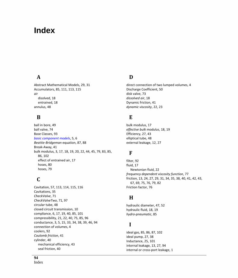
94
Index
Index
A
Abstract Mathematical Models, 29, 31 Accumulators, 85, 111, 113, 115 air
disolved, 18 entrained, 18
annulus, 48
B
ball in bore, 49 ball valve, 74 Base Classes, 93 basic component models, 5, 6 Beattie-Bridgeman equation, 87, 88 Break-Away, 41 bulk modulus, 3, 17, 18, 19, 20, 22, 44, 45, 79, 83, 85,
86, 102 effect of entrained air, 17 hoses, 80 hoses, 79
C
Cavitation, 57, 113, 114, 115, 116 Cavitations, 35 CheckValve, 71 CheckValveTwo, 71, 97 circular tube, 48 closed circuit transmission, 10 compliance, 6, 17, 19, 40, 85, 101 compressibility, 21, 22, 40, 75, 85, 96 conductance, 3, 5, 15, 33, 34, 38, 39, 46, 94 connection of volumes, 4 coolers, 92 Coulomb friction, 41 cylinder, 40
mechanical efficiency, 43 seal friction, 40
D
direct connection of two lumped volumes, 4 Discharge Coefficient, 50 disk valve, 73 dissolved air, 18 Dynamic friction, 41 dynamic viscosity, 22, 23
E
bulk modulus, 17 effective bulk modulus, 18, 19 Efficiency, 27, 43 elliptical tube, 48 external leakage, 12, 27
F
filter, 92 fluid, 17
Newtonian fluid, 22 frequency dependent viscosity function, 77 friction, 13, 24, 27, 29, 31, 34, 35, 38, 40, 41, 42, 43,
67, 69, 75, 76, 79, 82 Friction factor, 76
H
hydraulic diameter, 47, 52 hydraulic fluid, 18, 19 hydro-pneumatic, 85
I
ideal gas, 85, 86, 87, 102 ideal pump, 27, 38 Inductance, 25, 101 internal leakage, 13, 27, 94 internal or cross-port leakage, 1
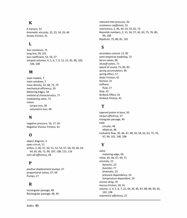
Index 95
K
K-Factors, 53 kinematic viscosity, 22, 23, 24, 26, 46 kinetic friction, 41
L
line resistance, 75 long line, 78, 101 loss coefficient, 53, 54, 57 lumped volumes, 4, 5, 6, 7, 9, 12, 15, 95, 98, 105,
106, 108
M
main models, 7 main windows, 7 mass density, 22, 68, 75, 79 mechanical efficiency, 35 Metering Edges, 58 method of characteristics, 77 modulating valve, 72 motor
torque loss, 38 volumetric loss, 38
N
negative pressure, 10, 17, 44 Negative Viscous Friction, 41
O
object diagram, 3 open circuit, 11 orifice, 2, 46, 47, 50, 51, 52, 53, 57, 58, 59, 60, 63,
64, 65, 66, 72, 99, 107, 108, 115, 116 over-all efficiency, 28
P
positive displacement pumps, 27 proportional valves, 67, 69 Pumps, 27
R
rectangular passage, 48 Rectangular passage, 48, 49
reduced inlet pressure, 36 resistance coefficient, 53 restrictions, 5, 46, 49, 54, 55, 62, 73 Reynolds numbers, 2, 51, 56, 57, 62, 63, 75, 76, 80,
99, 108 RigidLine, 75, 80, 81, 101
S
secondary control, 12, 85 semi-empirical modeling, 72 Servo valves, 66 shutoff valves, 71 speed of sound, 75, 80, 83 spring accumulators, 85 spring effect, 17 Static Friction, 41 Stiction, 41 stiffness
fluid, 17 Stop, 41 Stribeck Effect, 41 Stribeck friction, 41
T
tapered piston in bore, 50 torque efficiency, 27 triangular passage, 49 tube
circular, 48 elliptical, 48
turbulent flow, 26, 46, 47, 48, 50, 58, 62, 63, 75, 76, 97, 99, 101, 106, 108
V
valve metering edge, 58
Valve, 65, 66, 67, 69, 71 viscosity, 22
dynamic, 23 function, 77 kinematic, 22 pressure dependency, 24 temperature dependent, 24
viscous drag, 24 viscous friction, 29, 41 volume, 3, 4, 5, 6, 7, 22, 44, 45, 85, 87, 88, 89, 90, 92,
102, 108 volumetric efficiency, 27

96
Index