modeling & simulation of dynamic systems
DESCRIPTION
Modeling & Simulation of Dynamic Systems. Lecture-7 Block Diagram & Signal Flow Graph Representation of Control Systems. Dr. Imtiaz Hussain email: [email protected] URL : http://imtiazhussainkalwar.weebly.com/. Introduction. - PowerPoint PPT PresentationTRANSCRIPT

Modeling & Simulation of Dynamic Systems
Dr. Imtiaz Hussainemail: [email protected]
URL :http://imtiazhussainkalwar.weebly.com/
Lecture-7Block Diagram & Signal Flow Graph Representation
of Control Systems
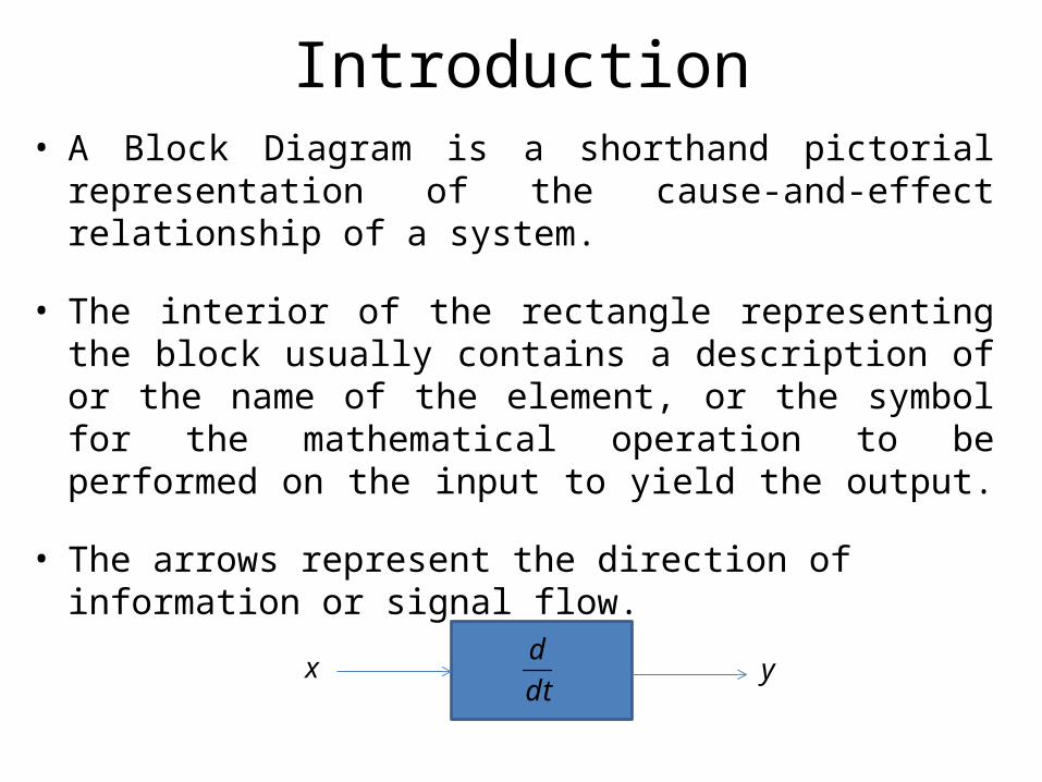
Introduction• A Block Diagram is a shorthand pictorial representation of
the cause-and-effect relationship of a system.
• The interior of the rectangle representing the block usually contains a description of or the name of the element, or the symbol for the mathematical operation to be performed on the input to yield the output.
• The arrows represent the direction of information or signal flow.
dt
dx y
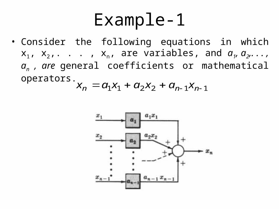
Example-1• Consider the following equations in which x1, x2,. . . , xn, are
variables, and a1, a2,. . . , an , are general coefficients or mathematical operators.
112211 nnn xaxaxax
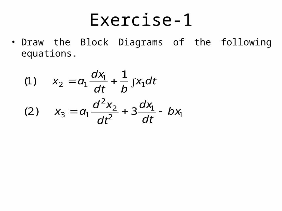
Exercise-1• Draw the Block Diagrams of the following equations.
11
22
2
13
11
12
32
11
bxdt
dx
dt
xdax
dtxbdt
dxax
)(
)(
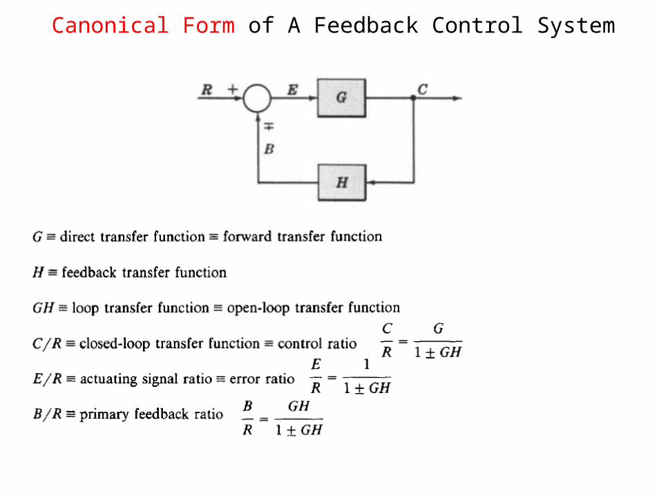
Canonical Form of A Feedback Control System
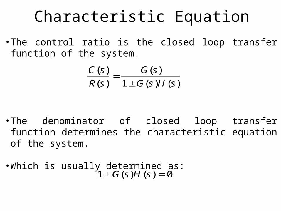
Characteristic Equation• The control ratio is the closed loop transfer function of the system.
• The denominator of closed loop transfer function determines the characteristic equation of the system.
• Which is usually determined as:
)()()(
)()(
sHsG
sG
sR
sC
1
01 )()( sHsG
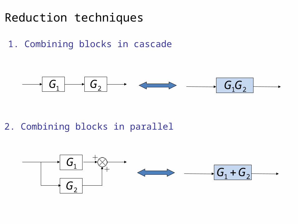
Reduction techniques
2G1G 21GG
1. Combining blocks in cascade
1G
2G21 GG
2. Combining blocks in parallel

Reduction techniques
3. Moving a summing point behind a block
G G
G
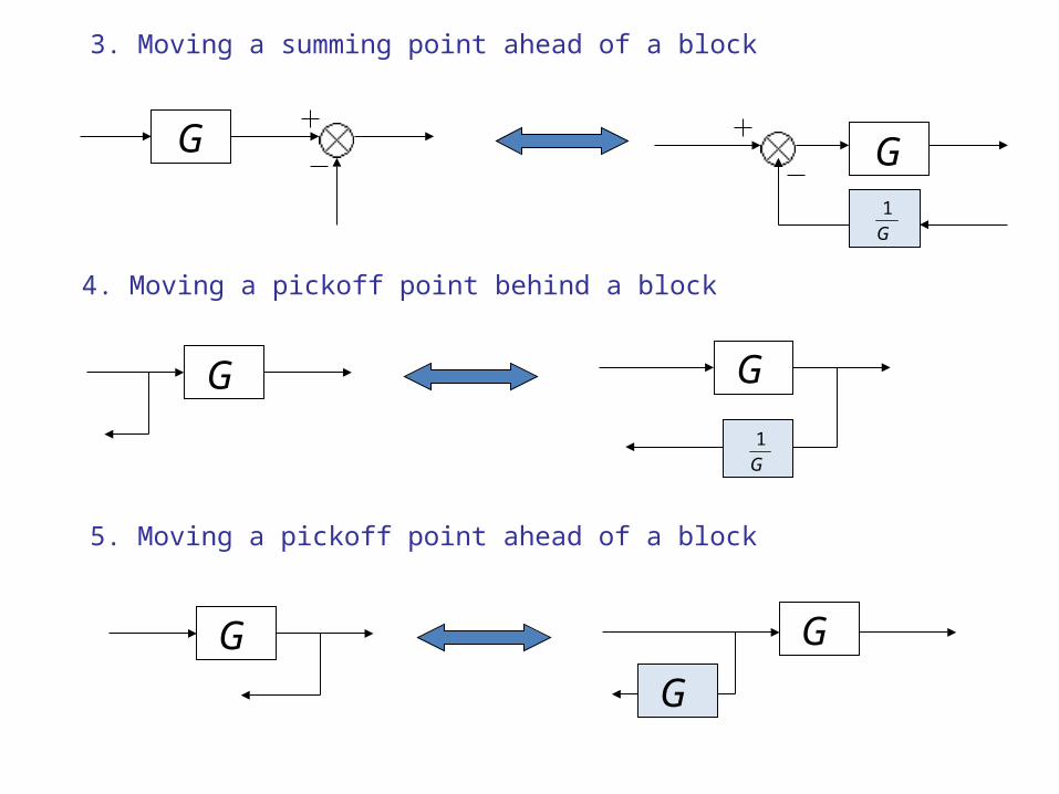
5. Moving a pickoff point ahead of a block
G G
G G
G
1
G
3. Moving a summing point ahead of a block
G G
G
1
4. Moving a pickoff point behind a block
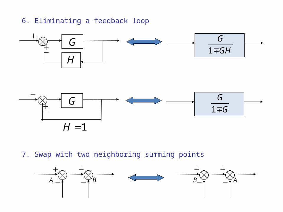
6. Eliminating a feedback loop
G
HGH
G
1
7. Swap with two neighboring summing points
A B AB
G
1H
G
G
1

Example-2• For the system represented by the following block diagram
determine:1. Open loop transfer function2. Feed Forward Transfer function3. control ratio4. feedback ratio5. error ratio6. closed loop transfer function7. characteristic equation 8. closed loop poles and zeros if K=10.
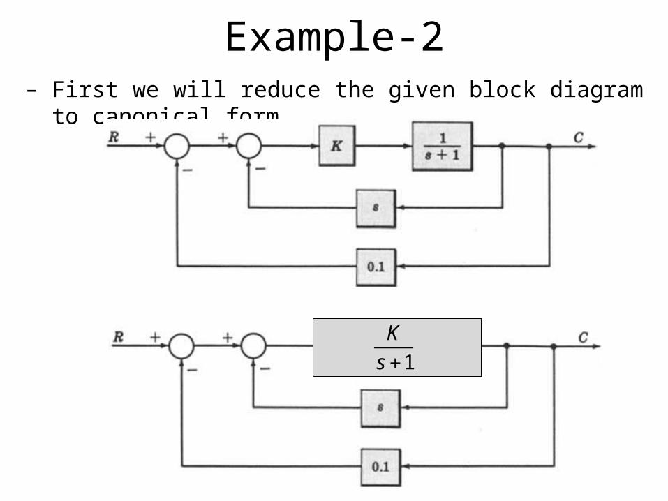
Example-2– First we will reduce the given block diagram to canonical form
1sK
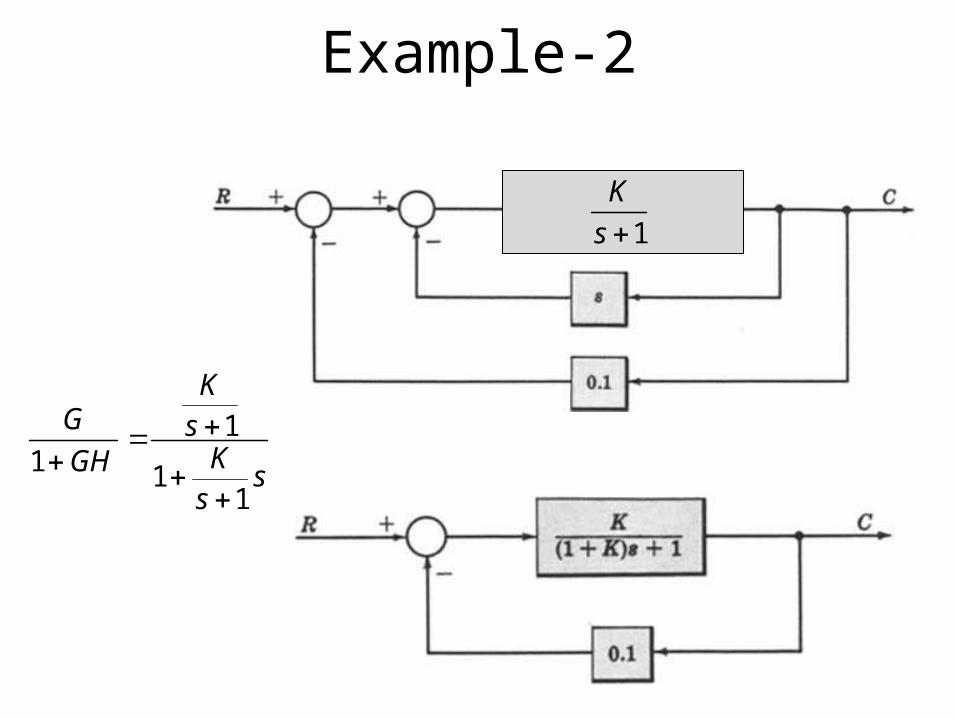
Example-2
1sK
ss
Ks
K
GH
G
11
11
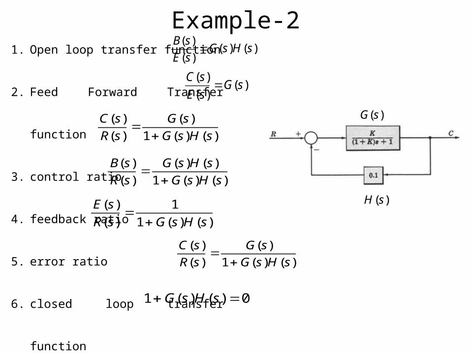
Example-21. Open loop transfer function
2. Feed Forward Transfer function
3. control ratio
4. feedback ratio
5. error ratio
6. closed loop transfer function
7. characteristic equation
8. closed loop poles and zeros if K=10.
)()()()(
sHsGsE
sB
)()()(
sGsE
sC
)()()(
)()(
sHsG
sG
sR
sC
1
)()()()(
)()(
sHsG
sHsG
sR
sB
1
)()()()(
sHsGsR
sE
1
1
)()()(
)()(
sHsG
sG
sR
sC
1
01 )()( sHsG
)(sG
)(sH
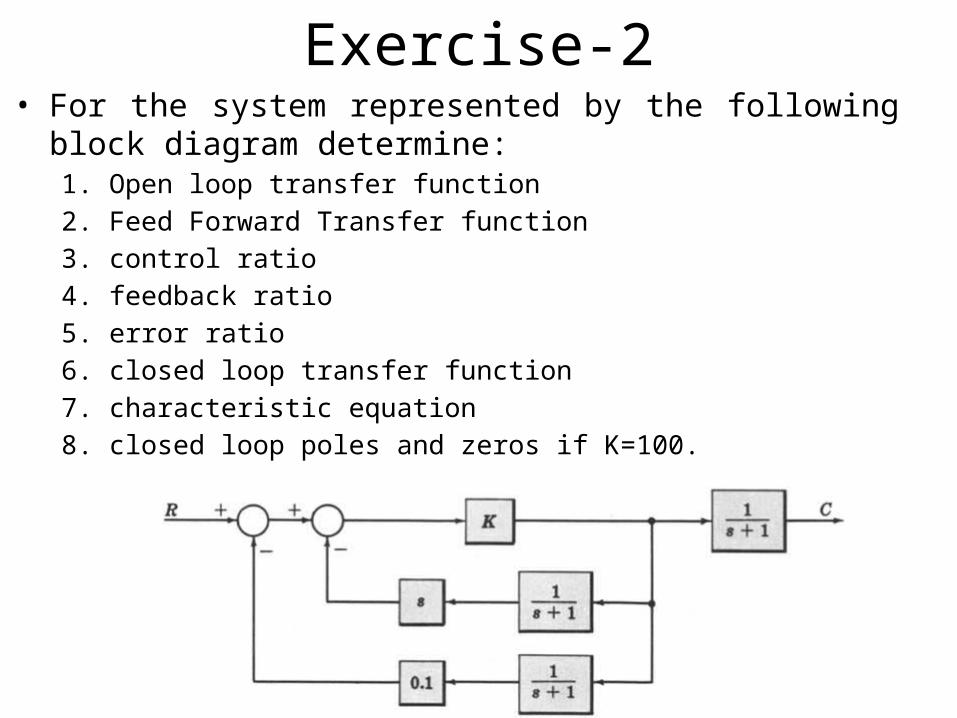
Exercise-2• For the system represented by the following block diagram
determine:1. Open loop transfer function2. Feed Forward Transfer function3. control ratio4. feedback ratio5. error ratio6. closed loop transfer function7. characteristic equation 8. closed loop poles and zeros if K=100.

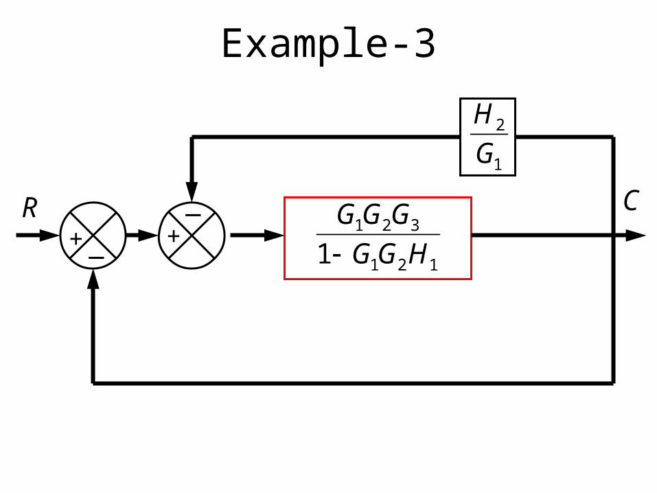
Example-3
R_+
_+
1G 2G 3G
1H
2H
+ +
C
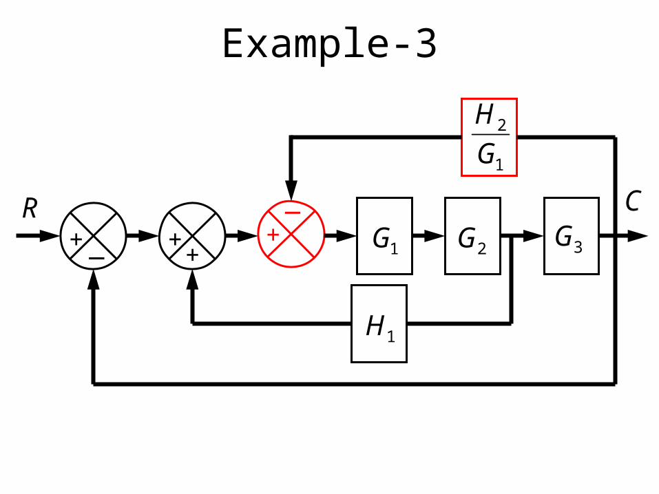
Example-3
R_+
_+
1G 2G 3G
1H
1
2
G
H
+ +
C
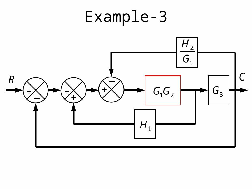
Example-3
R_+
_+
21GG 3G
1H
1
2
G
H
+ +
C
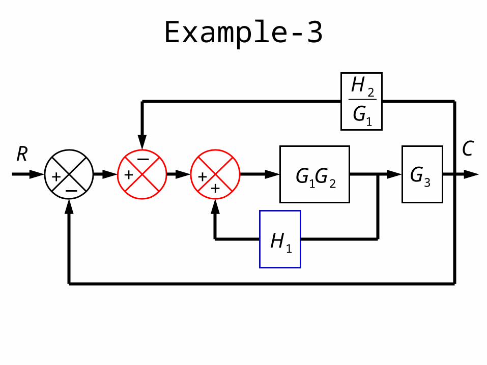
Example-3
R_+
_+
21GG 3G
1H
1
2
G
H
+ +
C
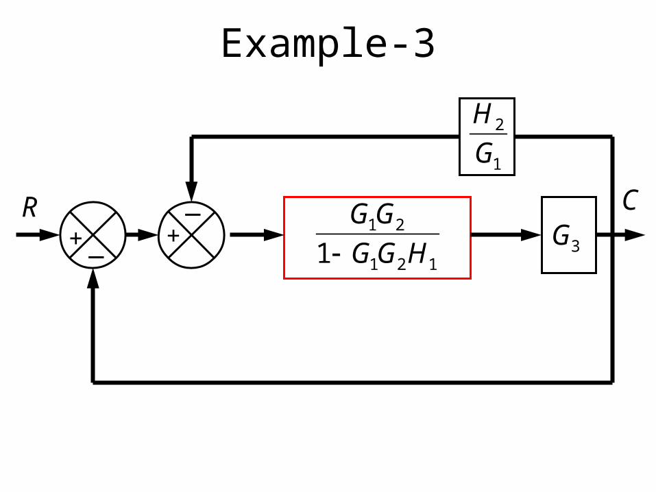
Example-3
R_+
_+
121
21
1 HGG
GG
3G
1
2
G
H
C
Example-3
R_+
_+
121
321
1 HGG
GGG
1
2
G
H
C
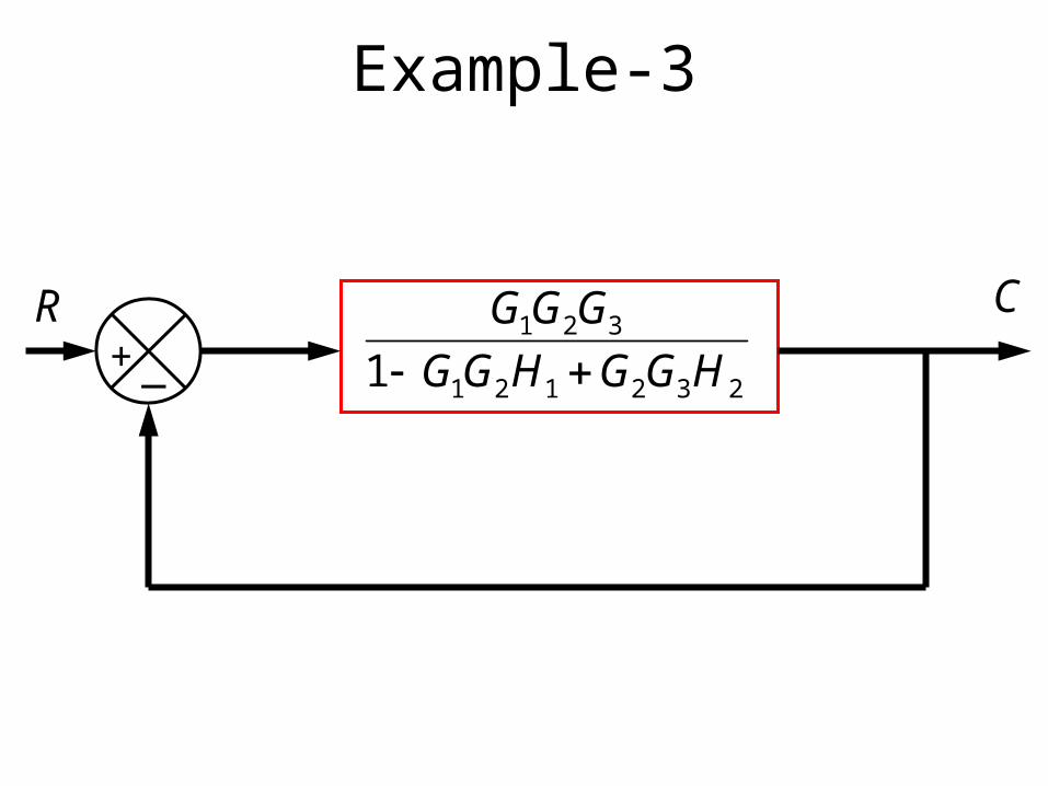
Example-3
R_+
232121
321
1 HGGHGG
GGG
C
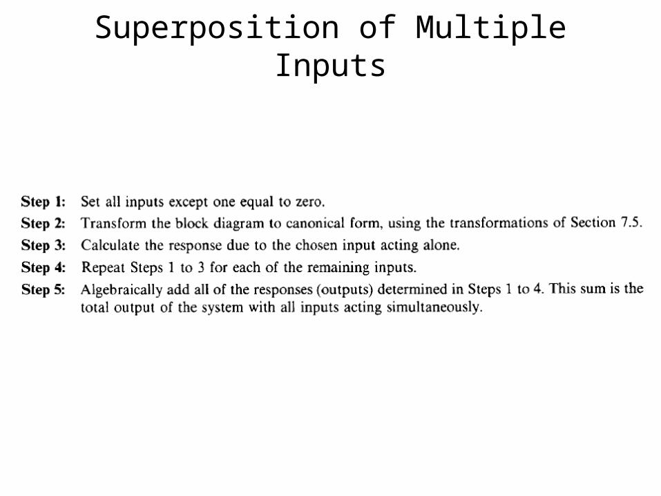
Superposition of Multiple Inputs
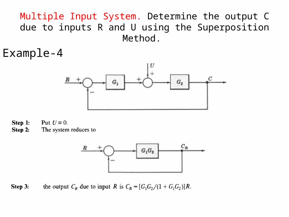
Multiple Input System. Determine the output C due to inputs R and U using the Superposition Method.
Example-4
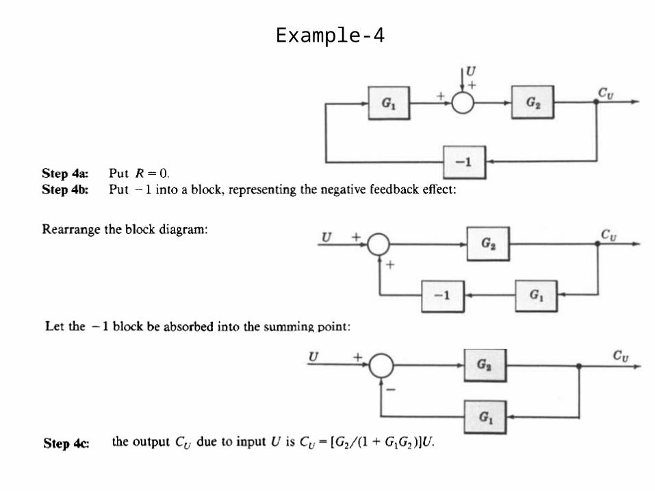
Example-4
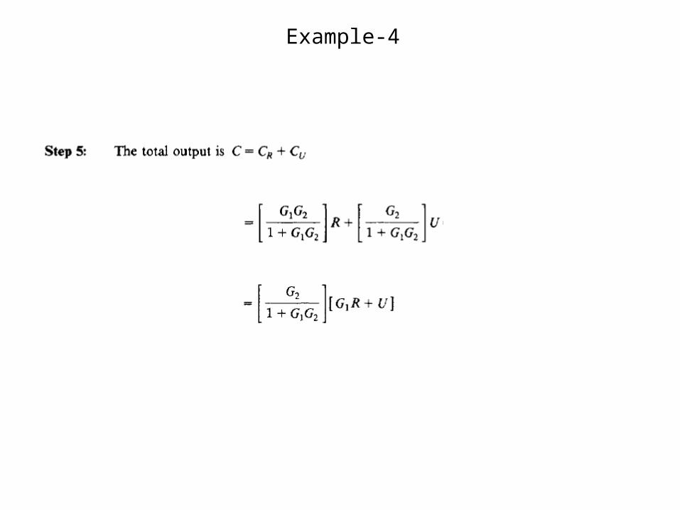
Example-4
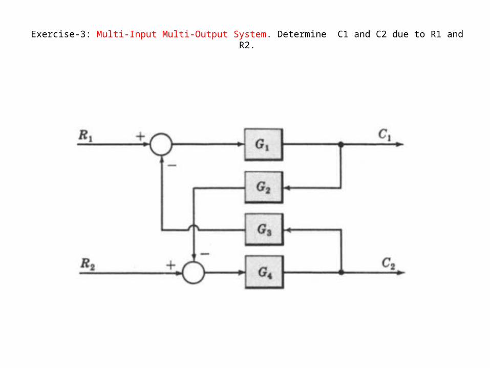
Exercise-3: Multi-Input Multi-Output System. Determine C1 and C2 due to R1 and R2.
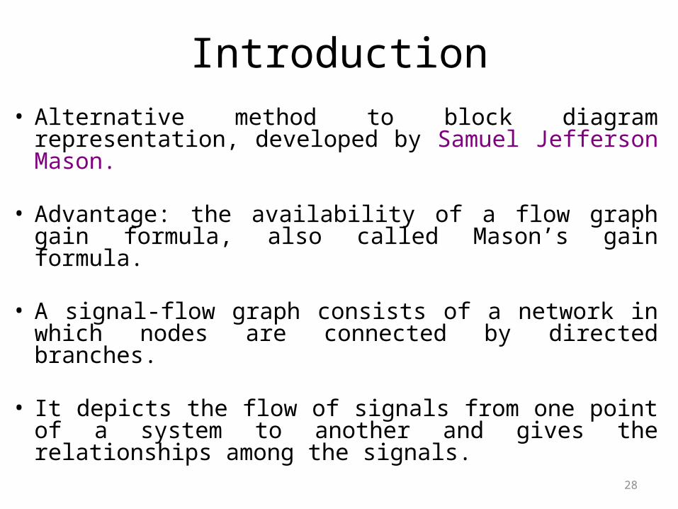
Introduction
28
• Alternative method to block diagram representation, developed by Samuel Jefferson Mason.
• Advantage: the availability of a flow graph gain formula, also called Mason’s gain formula.
• A signal-flow graph consists of a network in which nodes are connected by directed branches.
• It depicts the flow of signals from one point of a system to another and gives the relationships among the signals.
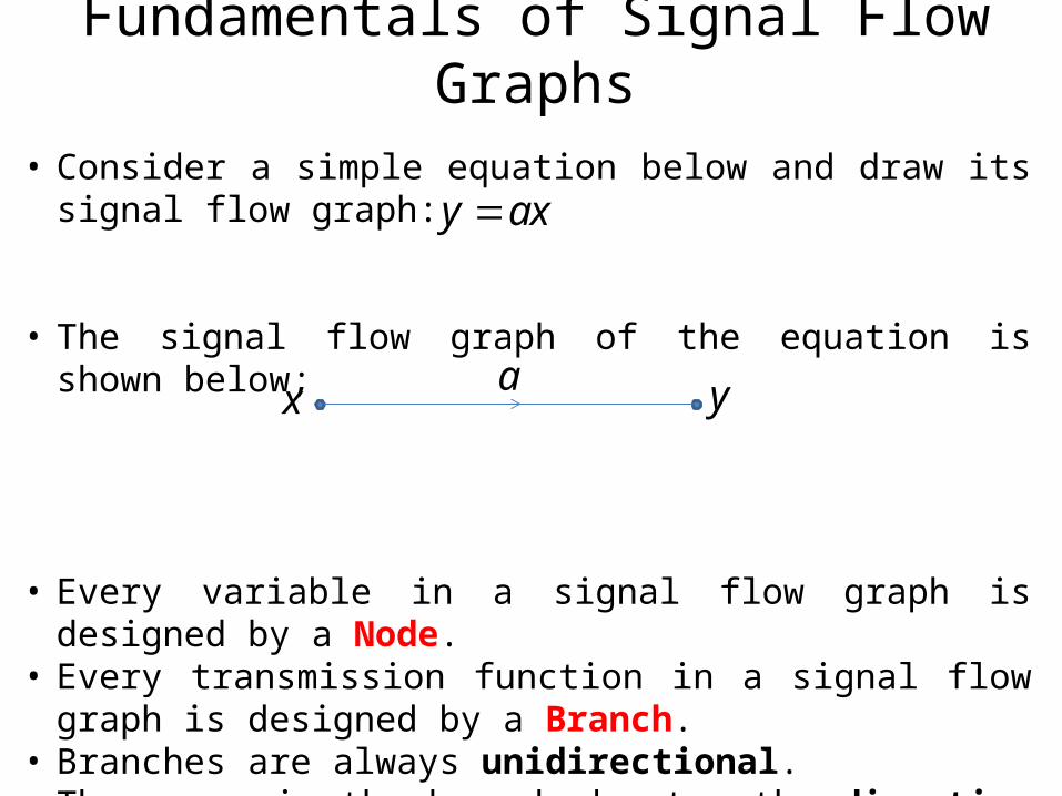
Fundamentals of Signal Flow Graphs
• Consider a simple equation below and draw its signal flow graph:
• The signal flow graph of the equation is shown below;
• Every variable in a signal flow graph is designed by a Node.• Every transmission function in a signal flow graph is designed by a
Branch. • Branches are always unidirectional.• The arrow in the branch denotes the direction of the signal flow.
axy
x ya
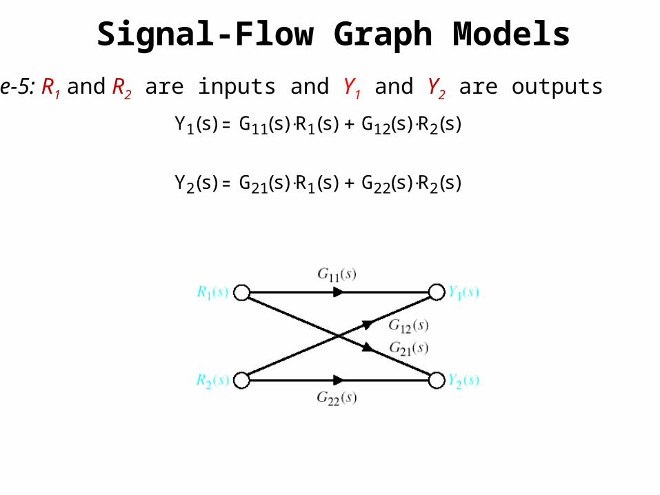
Signal-Flow Graph Models
Y1 s( ) G11 s( ) R1 s( ) G12 s( ) R2 s( )
Y2 s( ) G21 s( ) R1 s( ) G22 s( ) R2 s( )
Example-5: R1 and R2 are inputs and Y1 and Y2 are outputs
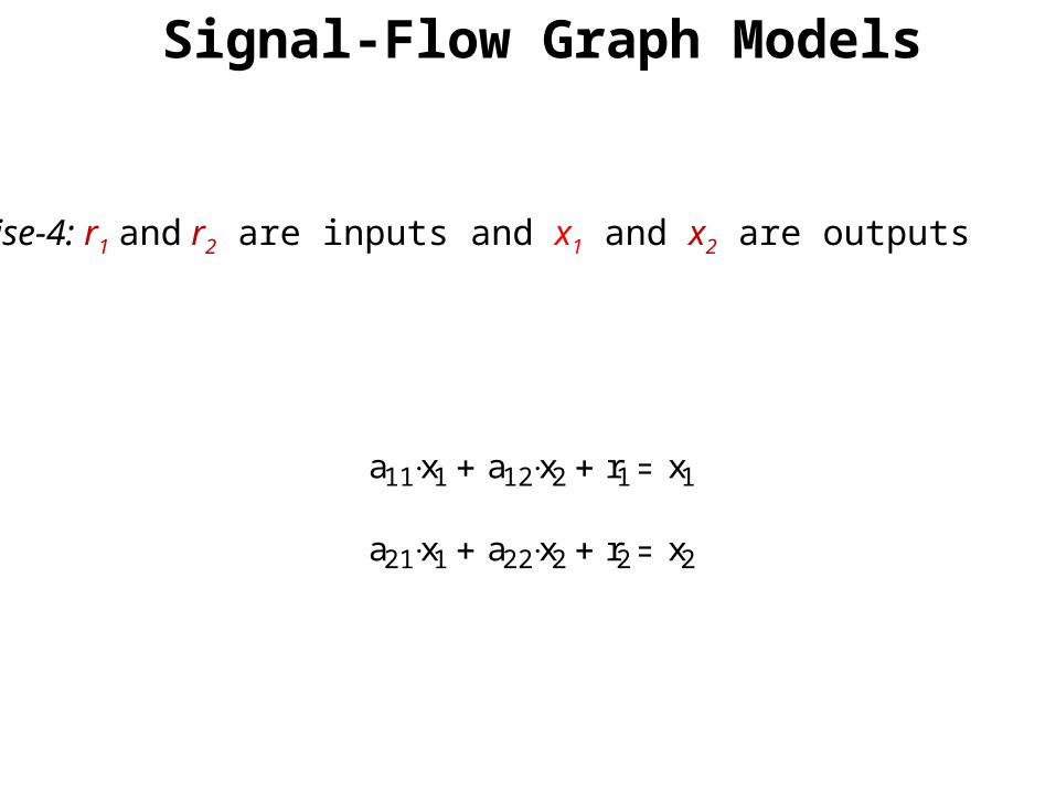
Signal-Flow Graph Models
a11 x1 a12 x2 r1 x1
a21 x1 a22 x2 r2 x2
Exercise-4: r1 and r2 are inputs and x1 and x2 are outputs
Signal-Flow Graph Models
34
203
312
2101
hxx
gxfxx
exdxx
cxbxaxx
b
x4x3x2x1
x0 h
f
g
e
d
c
a
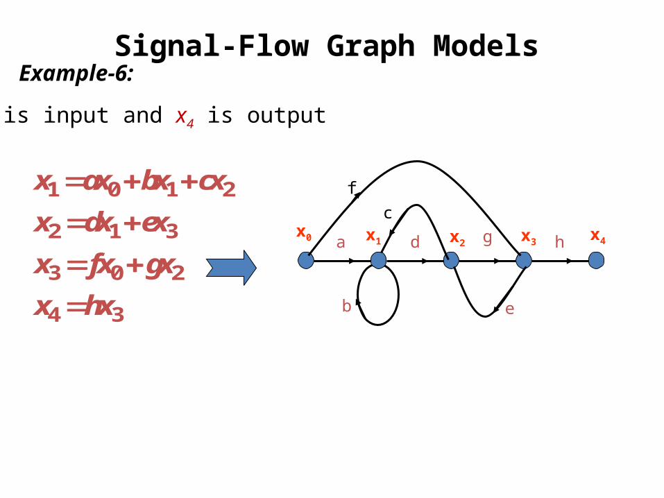
xo is input and x4 is output
Example-6:
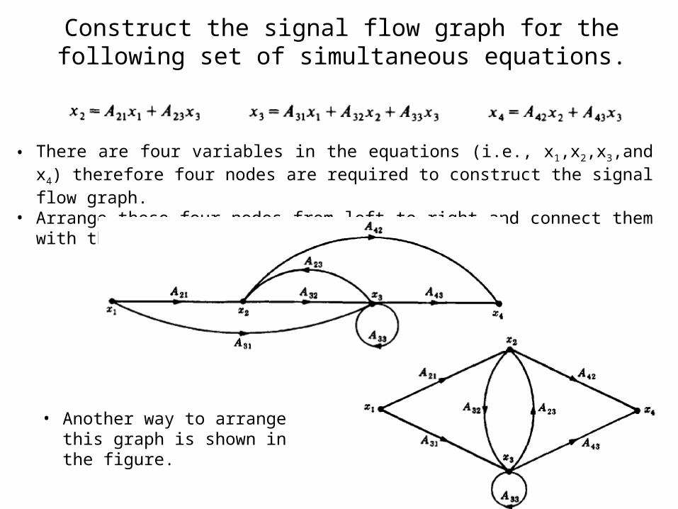
Construct the signal flow graph for the following set of simultaneous equations.
• There are four variables in the equations (i.e., x1,x2,x3,and x4) therefore four nodes are required to construct the signal flow graph.
• Arrange these four nodes from left to right and connect them with the associated branches.
• Another way to arrange this graph is shown in the figure.
Terminologies
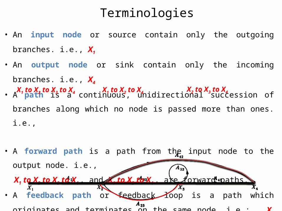
• An input node or source contain only the outgoing branches. i.e., X1
• An output node or sink contain only the incoming branches. i.e., X4
• A path is a continuous, unidirectional succession of branches along which no
node is passed more than ones. i.e.,
• A forward path is a path from the input node to the output node. i.e.,
X1 to X2 to X3 to X4 , and X1 to X2 to X4 , are forward paths.
• A feedback path or feedback loop is a path which originates and terminates on
the same node. i.e.; X2 to X3 and back to X2 is a feedback path.
X1 to X2 to X3 to X4 X1 to X2 to X4 X2 to X3 to X4
Terminologies
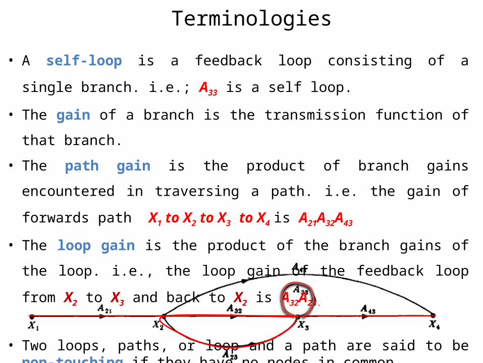
• A self-loop is a feedback loop consisting of a single branch. i.e.; A33 is a self
loop.
• The gain of a branch is the transmission function of that branch.
• The path gain is the product of branch gains encountered in traversing a path.
i.e. the gain of forwards path X1 to X2 to X3 to X4 is A21A32A43
• The loop gain is the product of the branch gains of the loop. i.e., the loop gain
of the feedback loop from X2 to X3 and back to X2 is A32A23.
• Two loops, paths, or loop and a path are said to be non-touching if they have no nodes in common.
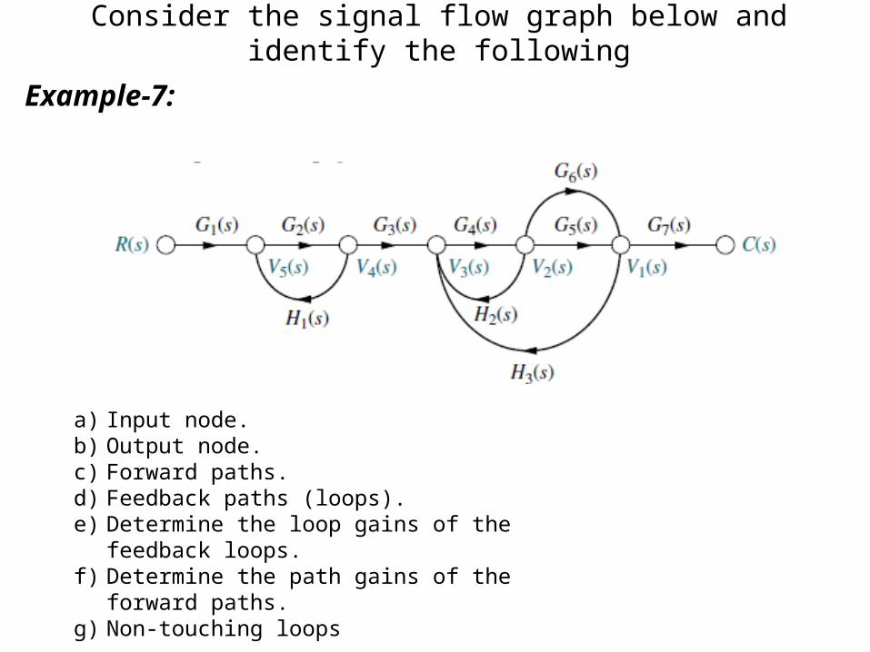
Consider the signal flow graph below and identify the following
a) Input node.b) Output node.c) Forward paths.d) Feedback paths (loops).e) Determine the loop gains of the feedback loops.f) Determine the path gains of the forward paths.g) Non-touching loops
Example-7:
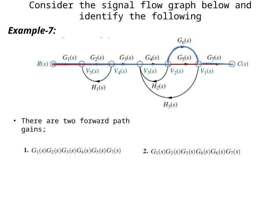
Consider the signal flow graph below and identify the following
• There are two forward path gains;
Example-7:
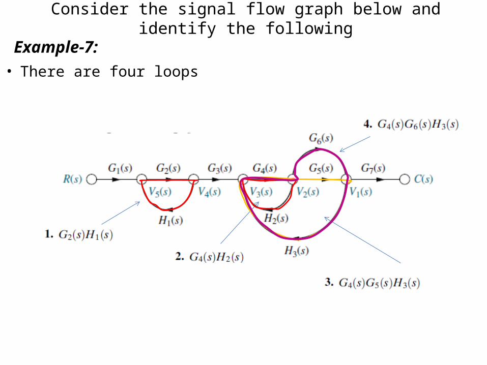
Consider the signal flow graph below and identify the following
• There are four loops
Example-7:
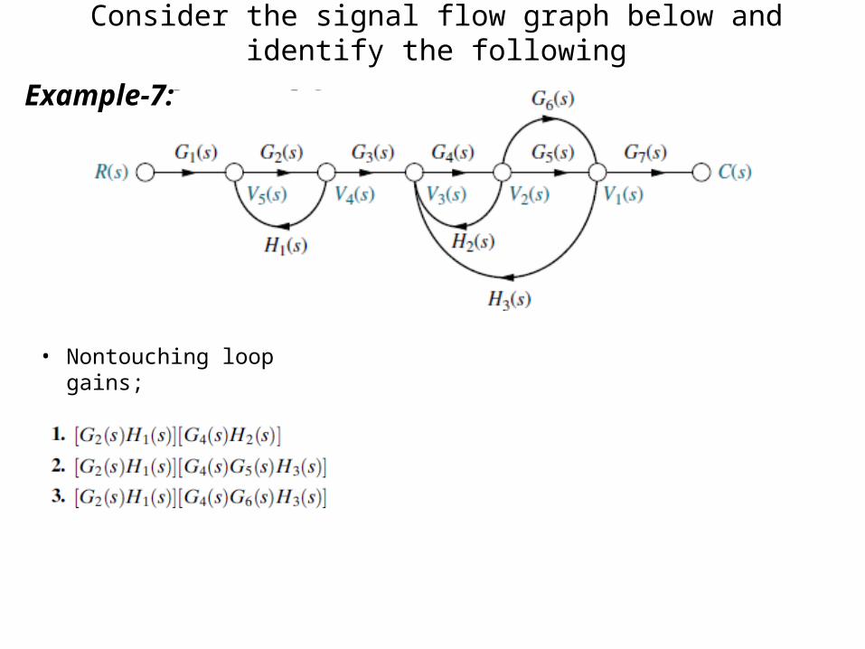
Consider the signal flow graph below and identify the following
• Nontouching loop gains;
Example-7:
Mason’s Rule (Mason, 1953)
• The block diagram reduction technique requires successive
application of fundamental relationships in order to arrive at the
system transfer function.
• On the other hand, Mason’s rule for reducing a signal-flow graph
to a single transfer function requires the application of one
formula.
• The formula was derived by S. J. Mason when he related the
signal-flow graph to the simultaneous equations that can be
written from the graph.
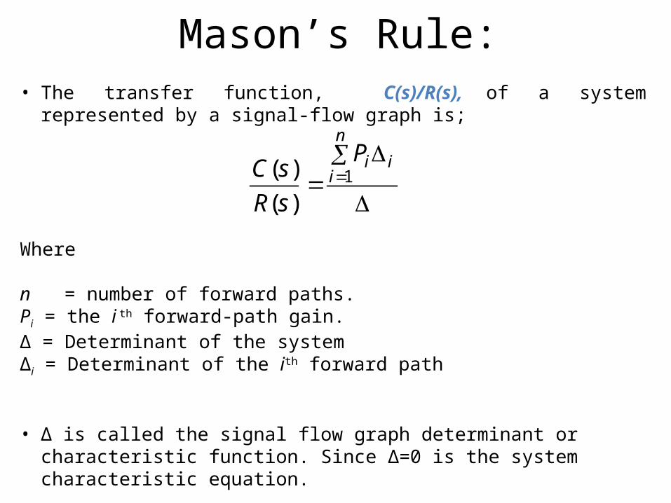
Mason’s Rule:• The transfer function, C(s)/R(s), of a system represented by a signal-flow graph
is;
Where
n = number of forward paths.Pi = the i th forward-path gain.∆ = Determinant of the system∆i = Determinant of the ith forward path
• ∆ is called the signal flow graph determinant or characteristic function. Since ∆=0 is the system characteristic equation.
n
iiiP
sR
sC 1
)()(
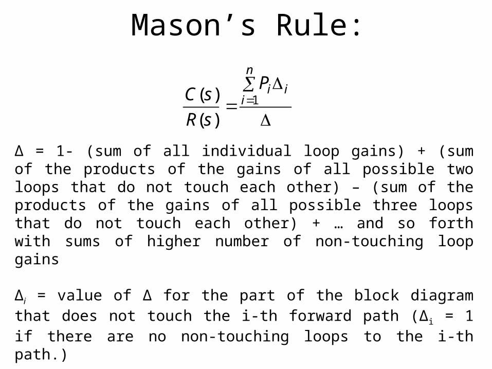
Mason’s Rule:
∆ = 1- (sum of all individual loop gains) + (sum of the products of the gains of all possible two loops that do not touch each other) – (sum of the products of the gains of all possible three loops that do not touch each other) + … and so forth with sums of higher number of non-touching loop gains
∆i = value of Δ for the part of the block diagram that does not touch the i-th forward path (Δi = 1 if there are no non-touching loops to the i-th path.)
n
iiiP
sR
sC 1
)()(
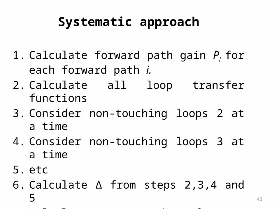
Systematic approach
1. Calculate forward path gain Pi for each forward path i.
2. Calculate all loop transfer functions3. Consider non-touching loops 2 at a time4. Consider non-touching loops 3 at a time5. etc6. Calculate Δ from steps 2,3,4 and 57. Calculate Δi as portion of Δ not touching forward
path i
43
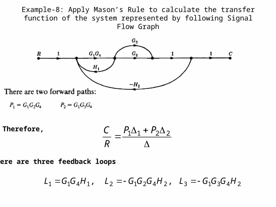
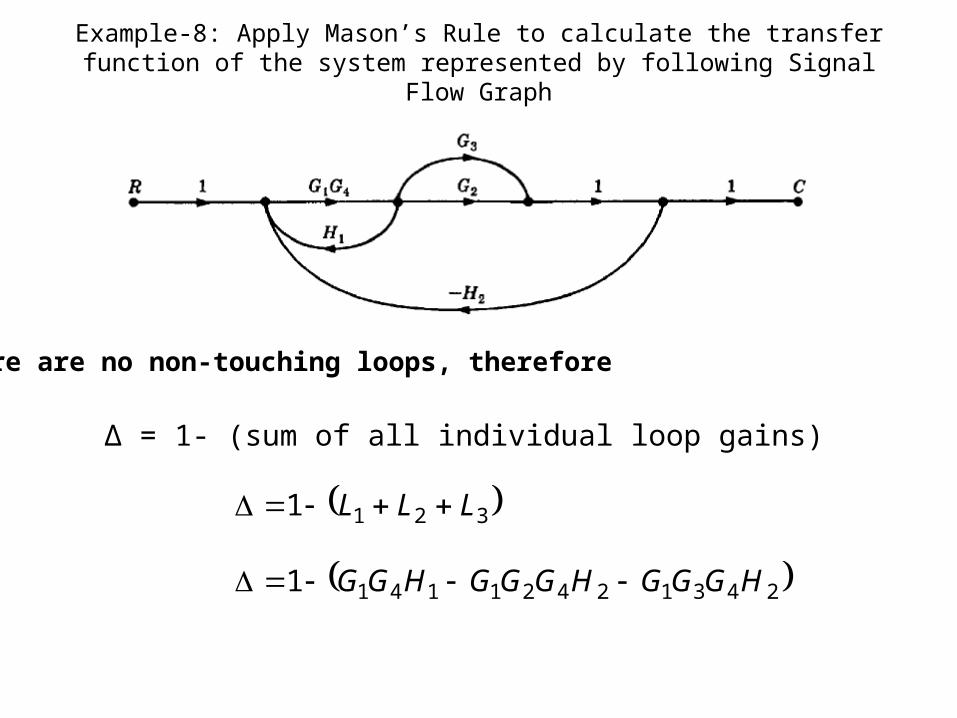
Example-8: Apply Mason’s Rule to calculate the transfer function of the system represented by following Signal Flow Graph
2211 PP
R
CTherefore,
24313242121411 HGGGLHGGGLHGGL ,,
There are three feedback loops
Example-8: Apply Mason’s Rule to calculate the transfer function of the system represented by following Signal Flow Graph
∆ = 1- (sum of all individual loop gains)
There are no non-touching loops, therefore
3211 LLL
243124211411 HGGGHGGGHGG
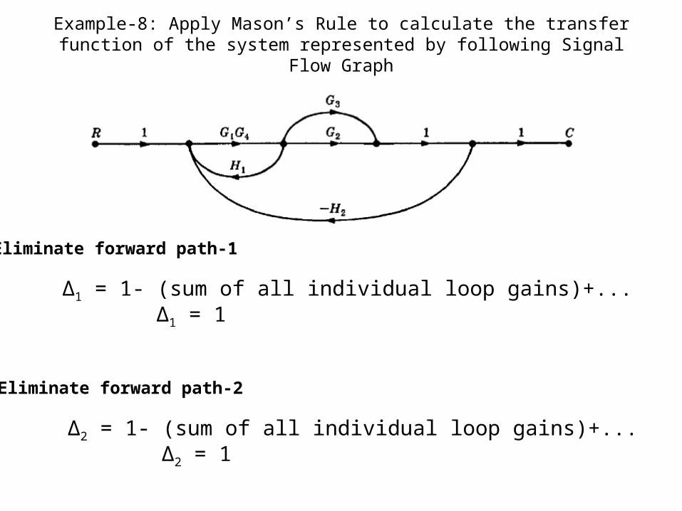
Example-8: Apply Mason’s Rule to calculate the transfer function of the system represented by following Signal Flow Graph
∆1 = 1- (sum of all individual loop gains)+...
Eliminate forward path-1
∆1 = 1
∆2 = 1- (sum of all individual loop gains)+...
Eliminate forward path-2
∆2 = 1
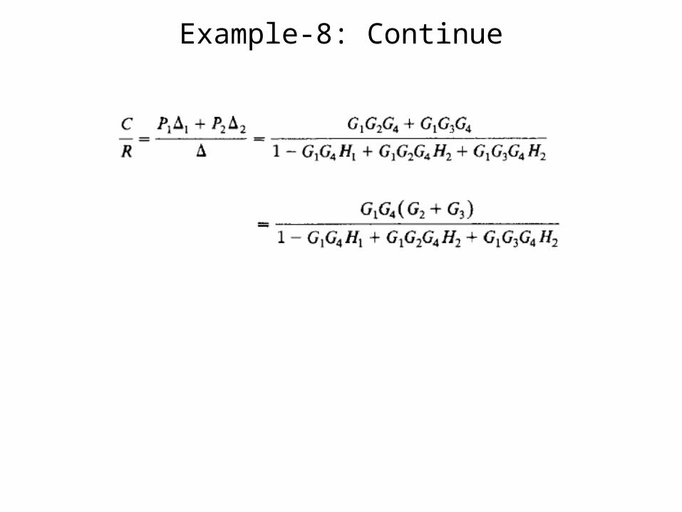
Example-8: Continue
48
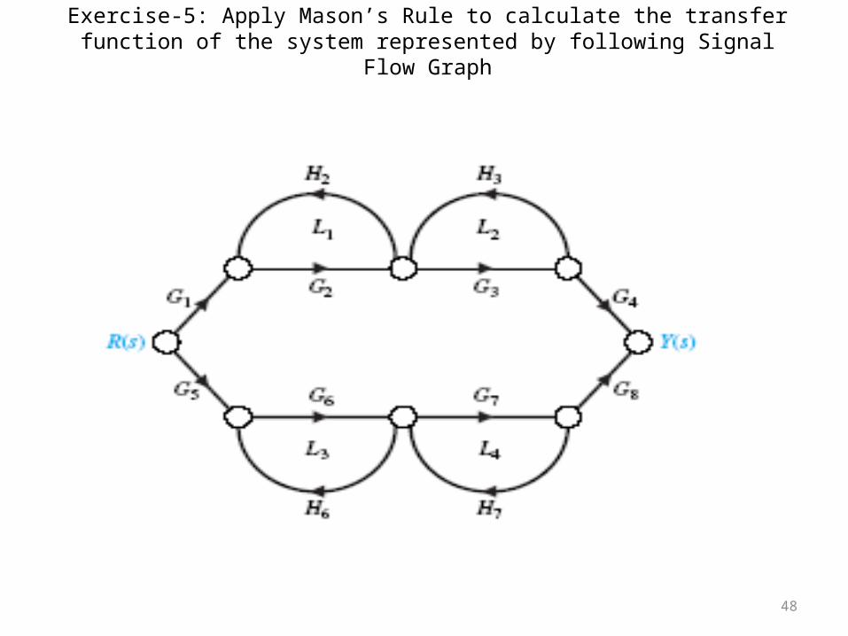
Exercise-5: Apply Mason’s Rule to calculate the transfer function of the system represented by following Signal Flow Graph
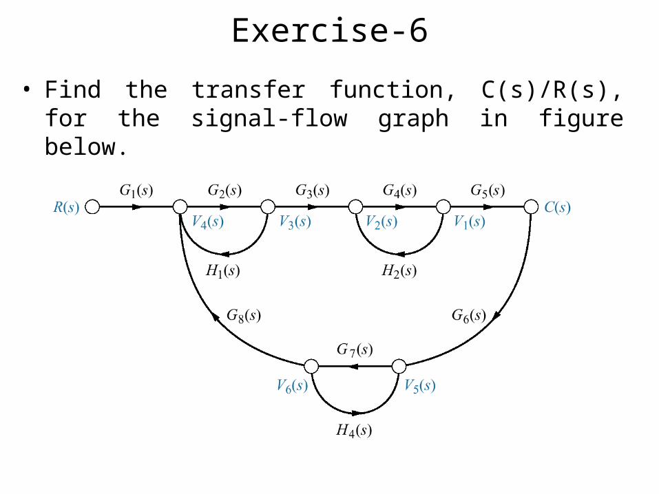
Exercise-6
• Find the transfer function, C(s)/R(s), for the signal-flow graph in figure below.
G1 G4G3
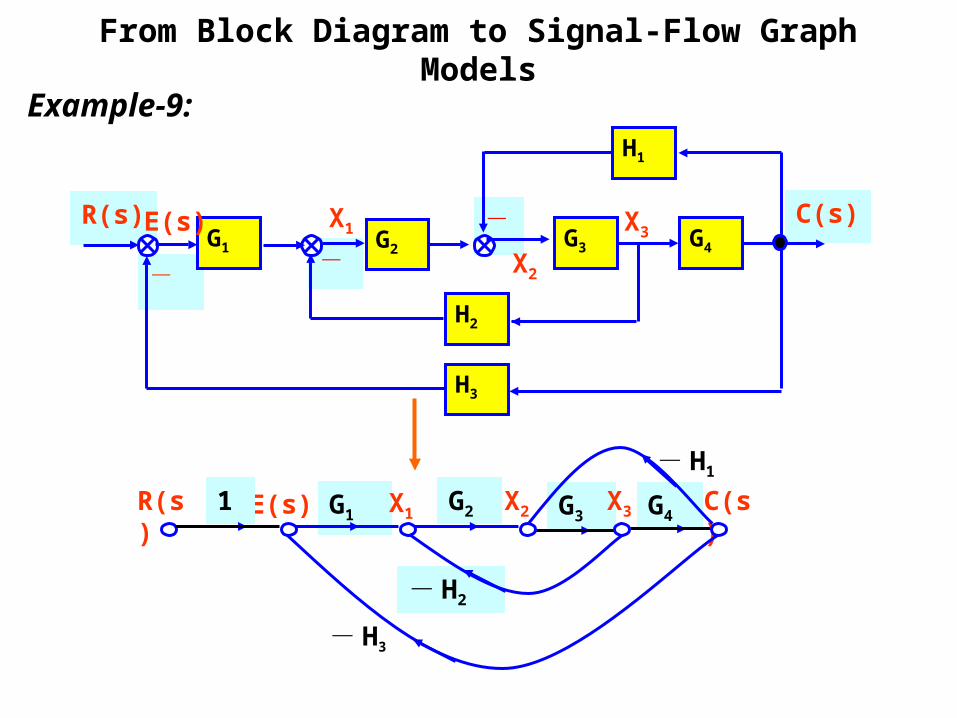
From Block Diagram to Signal-Flow Graph Models
--
-
C(s)R(s)G1 G2
H2
H1
G4G3
H3
E(s) X1
X2
X3
R(s) C(s)
- H2
- H1
- H3
X1 X2 X3E(s)1 G2
Example-9:
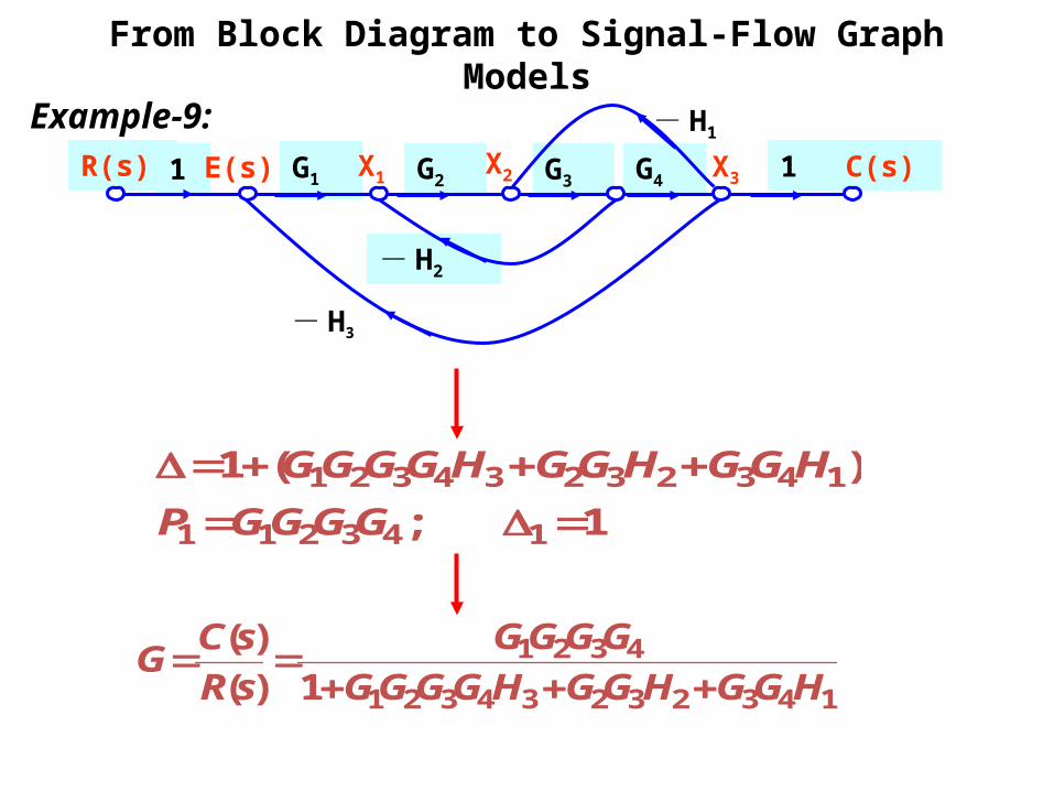
1;
)(1
143211
14323234321
GGGGP
HGGHGGHGGGG
14323234321
4321
1)(
)(
HGGHGGHGGGG
GGGG
sR
sCG
R(s)
- H2
1G4G3G2G11 C(s)
- H1
- H3
X1 X2 X3E(s)
From Block Diagram to Signal-Flow Graph ModelsExample-9:
G1
G2
+-
+
-
-
-
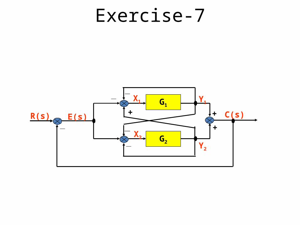
+ C(s)R(s) E(s)
Y2
Y1X1
X2
-
Exercise-7
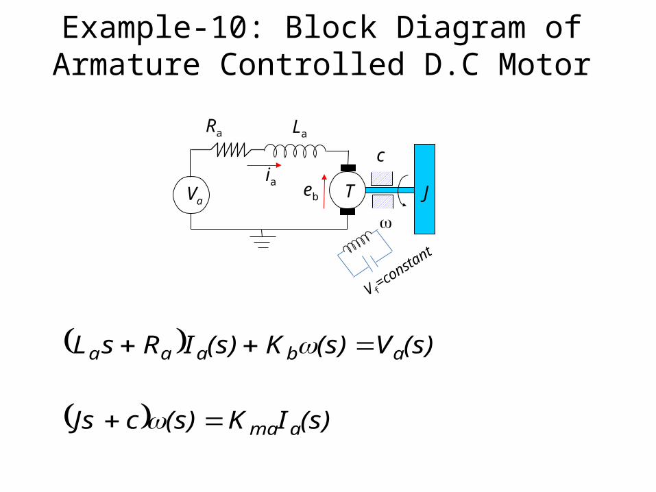
Example-10: Block Diagram of Armature Controlled D.C Motor
Va
iaT
Ra La
J
c
eb
V f=constant
(s)IK(s)cJs
(s)V(s)K(s)IRsL
ama
abaaa
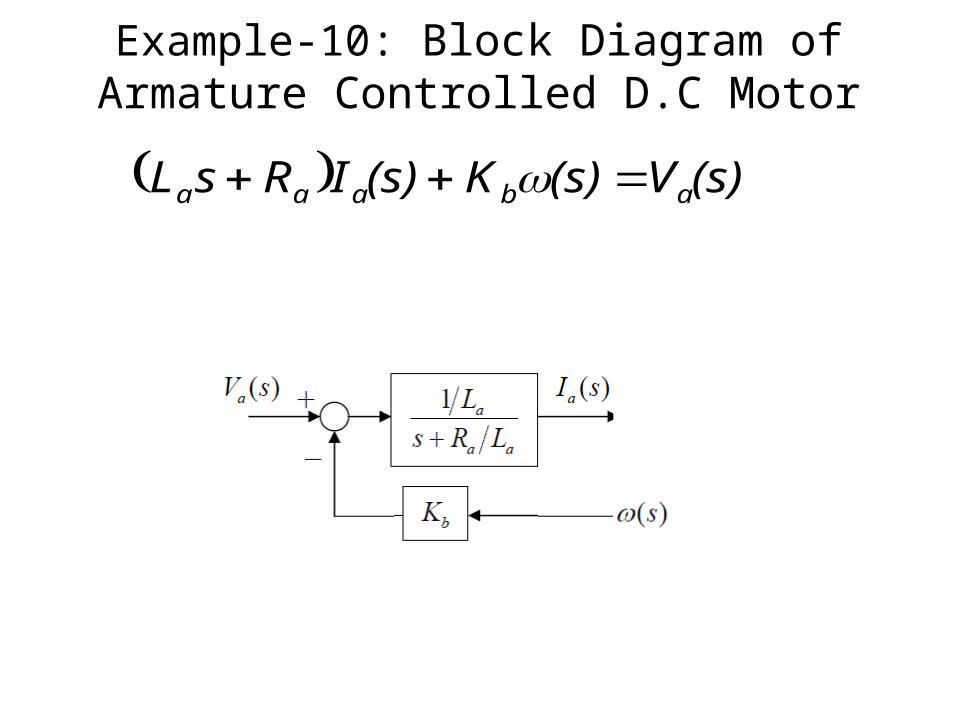
Example-10: Block Diagram of Armature Controlled D.C Motor
(s)V(s)K(s)IRsL abaaa
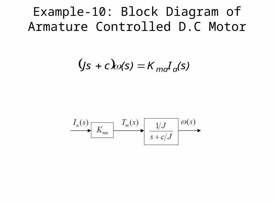
Example-10: Block Diagram of Armature Controlled D.C Motor
(s)IK(s)cJs ama
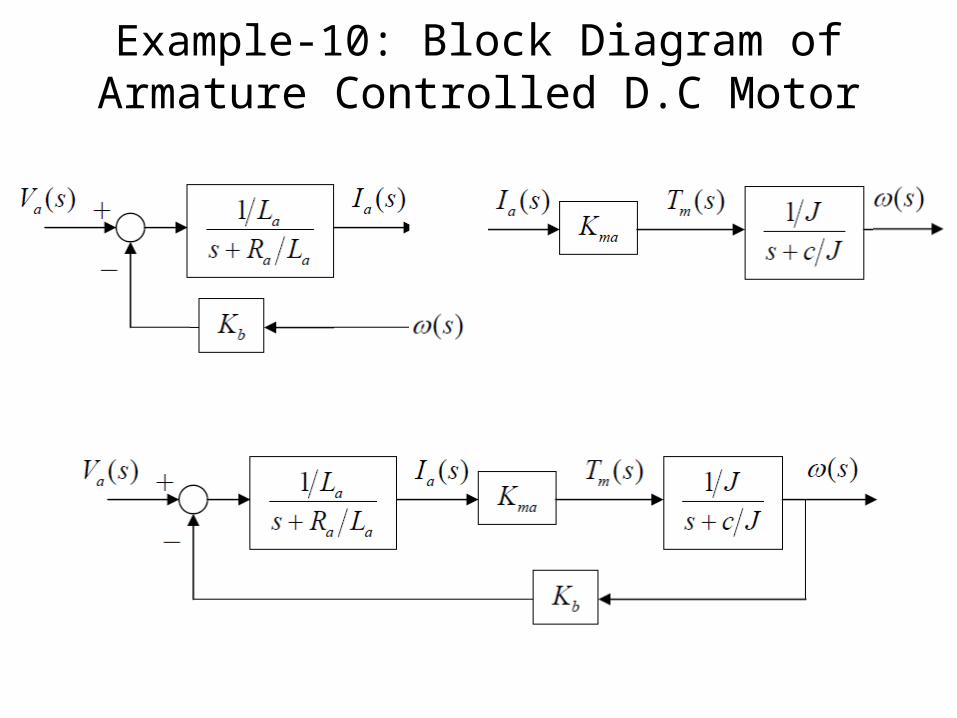
Example-10: Block Diagram of Armature Controlled D.C Motor
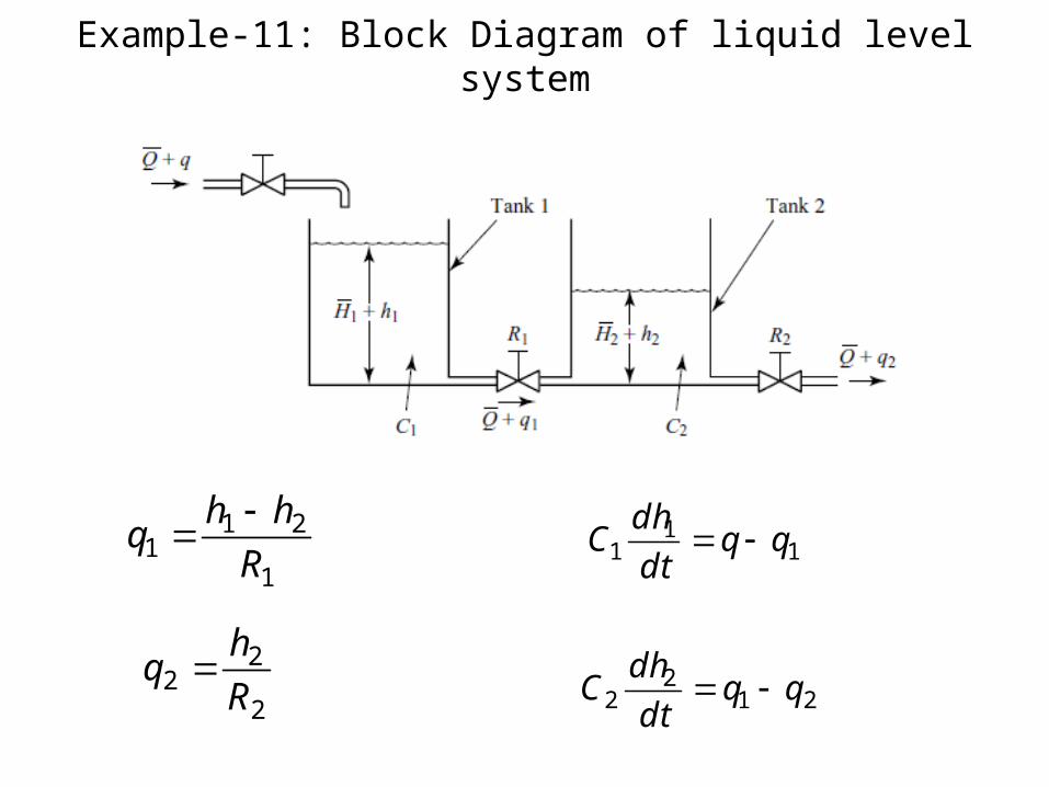
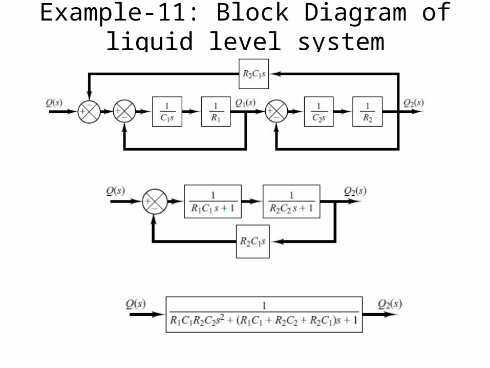
Example-11: Block Diagram of liquid level system
11
1 qqdt
dhC
1
211 R
hhq
212
2 qqdt
dhC
2
22 R
hq

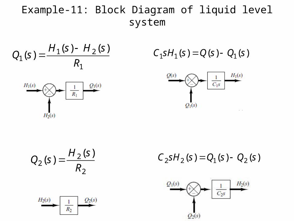
Example-11: Block Diagram of liquid level system
)()()( sQsQssHC 111 1
211 R
sHsHsQ
)()()(
2
22 R
sHsQ
)()( )()()( sQsQssHC 2122
11
1 qqdt
dhC
1
211 R
hhq
212
2 qqdt
dhC 2
22 R
hq
L
L
L
L
Example-11: Block Diagram of liquid level system
)()()( sQsQssHC 111 1
211 R
sHsHsQ
)()()(
2
22 R
sHsQ
)()( )()()( sQsQssHC 2122
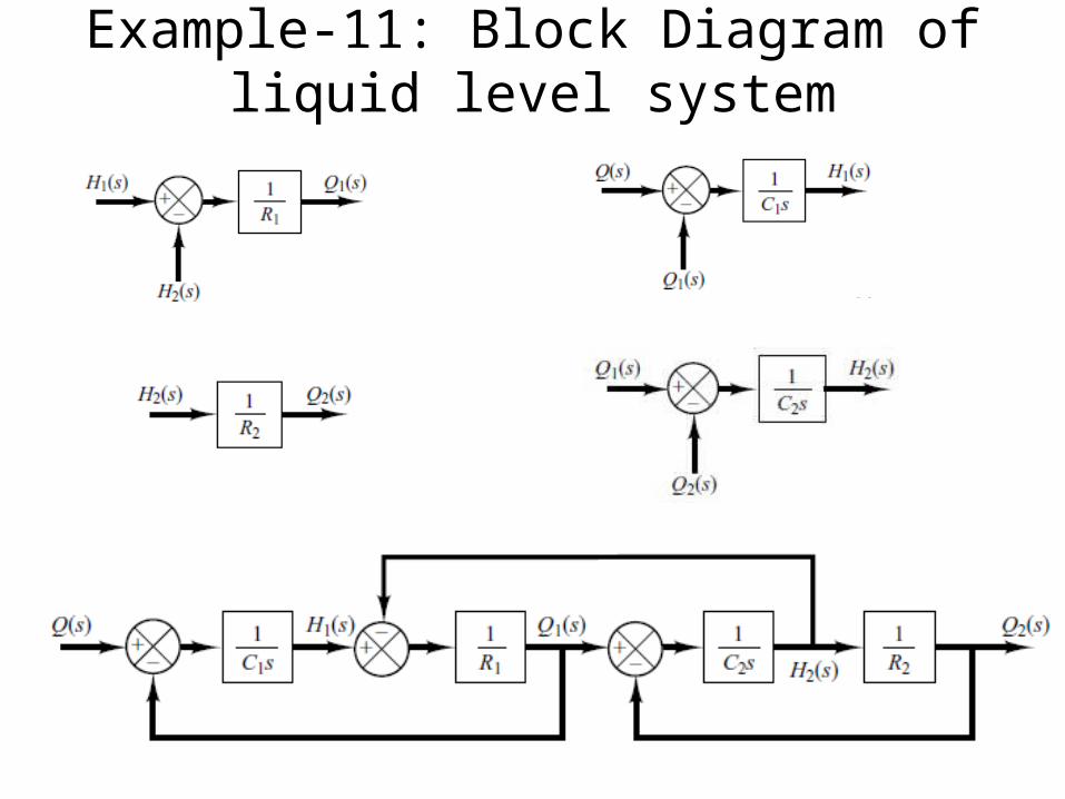
Example-11: Block Diagram of liquid level system
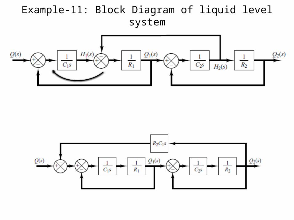
Example-11: Block Diagram of liquid level system
Example-11: Block Diagram of liquid level system

END OF LECTURE-7To download This Lecture Visit :http://imtiazhussainkalwar.weebly.com