modeling techniques and control strategies for inverter ... · universitätsverlag der tu berlin...
TRANSCRIPT

Universitätsverlag der TU Berlin
Aris Gkountaras
Modeling Techniques and Control Strategies for Inverter Dominated Microgrids
Elektrische Energietechnik an der TU Berlin Band 2


Aris GkountarasModeling Techniques and Control Strategies
for Inverter Dominated Microgrids

Die Schriftenreihe Elektrische Energietechnik an der TU Berlin wirdherausgegeben von:Prof. Dr. Sibylle Dieckerhoff,Prof. Dr. Julia Kowal,Prof. Dr. Ronald Plath,Prof. Dr. Uwe Schäfer

Elektrische Energietechnik an der TU Berlin | 2
Aris Gkountaras
Modeling Techniques and Control Strategiesfor Inverter Dominated Microgrids
Universitätsverlag der TU Berlin

Bibliografische Information der Deutschen NationalbibliothekDie Deutsche Nationalbibliothek verzeichnet diese Publikation inder Deutschen Nationalbibliografie; detaillierte bibliografischeDaten sind im Internet über http://dnb.dnb.de abrufbar.
Universitätsverlag der TU Berlin, 2017http://verlag.tu-berlin.de
Fasanenstr. 88, 10623 BerlinTel.: +49 (0)30 314 76131 / Fax: -76133E-Mail: [email protected]
Zugl.: Berlin, Techn. Univ., Diss., 2016Gutachter: Prof. Dr.-Ing. Sibylle DieckerhoffGutachter: Prof. Dr.-Ing. Friedrich W. FuchsGutachter: Prof. Dr. Nikos HatziargyriouGutachter: Dr.-Ing. Tevfik SeziDie Arbeit wurde am 21. März 2016 an der Fakultät IV unter Vorsitzvon Prof. Dr.-Ing. Clemens Gühmann erfolgreich verteidigt.
Diese Veröffentlichung – ausgenommen Zitate und Abbildungen –ist unter der CC-Lizenz CC BY lizenziert.Lizenzvertrag: Creative Commons Namensnennung 4.0http://creativecommons.org/licenses/by/4.0
Umschlagfoto:Ted Eytan | https://www.flickr.com/photos/taedc/12311698465/CC BY-SA| https://creativecommons.org/licenses/by-sa/2.0/
Druck: Meta Systems Publishing & Printservices GmbH, WustermarkSatz/Layout: Aris Gkountaras
ISBN 978-3-7983-2872-3 (print)ISBN 978-3-7983-2873-0 (online)
ISSN 2367-3761 (print)ISSN 2367-377X (online)
Zugleich online veröffentlicht auf dem institutionellen Repositoriumder Technischen Universität Berlin:DOI 10.14279/depositonce-5520http://dx.doi.org/10.14279/depositonce-5520

Contents1 Introduction 9
2 Stability and power sharing fundamentals 142.1 Grid stability principles . . . . . . . . . . . . . . . . . . . . . . . 142.2 Power sharing in microgrids . . . . . . . . . . . . . . . . . . . . . 17
2.2.1 Derivation of droop control . . . . . . . . . . . . . . . . . 192.2.2 Line impedance determination . . . . . . . . . . . . . . . 222.2.3 Small signal stability analysis . . . . . . . . . . . . . . . . 24
3 Generator modeling and control 303.1 Diesel generator . . . . . . . . . . . . . . . . . . . . . . . . . . . 30
3.1.1 Electrical and mechanical part . . . . . . . . . . . . . . . 303.1.2 Controller design . . . . . . . . . . . . . . . . . . . . . . . 35
3.2 Grid inverter . . . . . . . . . . . . . . . . . . . . . . . . . . . . . 383.2.1 Grid feeding inverter . . . . . . . . . . . . . . . . . . . . . 463.2.2 Grid forming inverter in standalone mode . . . . . . . . . 543.2.3 Grid forming inverter in parallel mode . . . . . . . . . . . 563.2.4 Limiting signals in cascaded control structures . . . . . . 58
3.3 Battery pack . . . . . . . . . . . . . . . . . . . . . . . . . . . . . 613.3.1 Battery cell . . . . . . . . . . . . . . . . . . . . . . . . . . 613.3.2 Battery pack with DC/DC converter . . . . . . . . . . . . 64
3.4 Modeling towards real time simulation . . . . . . . . . . . . . . . 69
4 Black start and synchronisation techniques 734.1 Black start of hybrid microgrid . . . . . . . . . . . . . . . . . . . 734.2 Synchronisation of grid forming inverter . . . . . . . . . . . . . . 76
4.2.1 Control structure modification . . . . . . . . . . . . . . . 774.2.2 Implementation . . . . . . . . . . . . . . . . . . . . . . . . 794.2.3 Synchronisation of a 2nd grid forming inverter . . . . . . . 81
4.3 Conclusions of black start and synchronisation techniques . . . . 84
5 Load sharing considerations 855.1 Modular implementation of droop control . . . . . . . . . . . . . 855.2 Transient load sharing . . . . . . . . . . . . . . . . . . . . . . . . 89
5.2.1 Influence of grid impedance on transient load sharing . . . 965.2.2 Oscillations due to transient load sharing . . . . . . . . . 98
5.3 SoC-Adaptive droop control . . . . . . . . . . . . . . . . . . . . 1015.3.1 Concept presentation and implementation . . . . . . . . . 102
5

Contents
5.3.2 Case studies . . . . . . . . . . . . . . . . . . . . . . . . . 1035.3.3 Evaluation and further development of proposed algorithm 108
5.4 Load sharing conclusions . . . . . . . . . . . . . . . . . . . . . . 109
6 Short circuit strategy 1106.1 Protection means . . . . . . . . . . . . . . . . . . . . . . . . . . 1116.2 Grid forming inverter . . . . . . . . . . . . . . . . . . . . . . . . 112
6.2.1 Current limiting methods . . . . . . . . . . . . . . . . . . 1136.2.2 Theoretical fault models . . . . . . . . . . . . . . . . . . . 1196.2.3 Evaluation of current limiting methods . . . . . . . . . . . 1206.2.4 DC and AC components rating . . . . . . . . . . . . . . . 127
6.3 Grid feeding inverter . . . . . . . . . . . . . . . . . . . . . . . . 1286.3.1 Grid code requirements . . . . . . . . . . . . . . . . . . . 1296.3.2 Realization of reactive current injection . . . . . . . . . . 1306.3.3 Evaluation of reactive current injection . . . . . . . . . . . 1326.3.4 Mixed current injection (MCI) principle . . . . . . . . . . 134
6.4 Validation of proposed strategy . . . . . . . . . . . . . . . . . . . 1386.4.1 Operation with synchronous generator . . . . . . . . . . . 1406.4.2 Operation without synchronous generator . . . . . . . . . 141
6.5 Short circuit strategy conclusions . . . . . . . . . . . . . . . . . . 144
7 Conclusions 1457.1 Contributions to state of the art . . . . . . . . . . . . . . . . . . 1457.2 Further research points . . . . . . . . . . . . . . . . . . . . . . . 146
Bibliography 147
List of Figures 157
List of Tables 160
Appendices 161
A Appendix 163A.1 Distributed generators parameters . . . . . . . . . . . . . . . . . 163A.2 Phase locked loop (PLL) implementation . . . . . . . . . . . . . 166
A.2.1 PLL Controller Design . . . . . . . . . . . . . . . . . . . . 167A.3 Real time simulation test scenarios parameters . . . . . . . . . . 168
A.3.1 Black start and synchronization test scenarios . . . . . . . 168A.3.2 Load sharing considerations test scenarios . . . . . . . . . 168A.3.3 Short circuit strategy test scenarios . . . . . . . . . . . . . 169
6

Abstract
The character of modern power systems is changing rapidly and inverters are tak-ing over a considerable part of the energy generation. A future purely inverter-based grid could be a viable solution, if its technical feasibility can be firstvalidated. The focus of this work lies on inverter dominated microgrids, whichare also mentioned as ’hybrid’ in several instances throughout the thesis. Hy-brid, as far as the energy input of each generator is concerned. Conventionalfossil fuel based distributed generators are connected in parallel to renewableenergy sources as well as battery systems. This co-existence of different genera-tor types serves as a means of accelerating the grid integration of inverter-basedgenerators. The main contributions of this work comprise of: The analysis ofdetailed models and control structures of grid inverters, synchronous generatorsand battery packs. The utilization of these models to formulate modular controlstrategies for the distributed generators of medium voltage microgrids and eval-uate their performance in real time simulation test scenarios. The first controlstrategy involves the development of a synchronization technique for grid form-ing inverters. Secondly, achieving load sharing among distributed generatorsemploying conventional droop control is analyzed. Furthermore, the problem oftransient load sharing between grid forming units with different time constantsis addressed. The transient response of the microgrid upon a load step change isoptimized with a developed control modification for grid forming inverters. Thenegative effect of transient load sharing is in this way minimized, in parallel withevaluating the case of more than one inverters working in parallel. Moreover, acontrol algorithm is introduced that incorporates the grid secondary control toprimary control. In this way, load sharing is influenced by the state of chargeof battery packs and a certain level of grid autonomy can be achieved. Finally,the developed microgrid structures are tested in fault conditions: A short circuitstrategy is developed for grid forming and feeding inverters. The main guide-line for the short circuit strategy is that the fault isolation should be basedon traditional protection means. Therefore the developed control modificationsshould not be based on communication between generators and maximizing theshort circuit current is the main objective. For grid forming units, various cur-rent limiting methods are compared in standalone and parallel operation. Itscomponents overrating and the parallel operation with a synchronous generatorare investigated. For the grid feeding inverters, the reactive current injectionstrategy is optimized through the proposed mixed current injection with theobjective of maximizing its fault current contribution.
7

Kurzfassung
Die Struktur der modernen Energieversorgung hat sich in den letzten Jahrzehn-ten massiv geändert. Dezentrale Generatoren, die auf Wechselrichtern basieren,übernehmen einen großen Teil der Energieerzeugung. Ein ausschließlich wechsel-richterbasiertes Netz wäre ein realistischer Ansatz, wenn seine technische Mach-barkeit verifiziert werden könnte. Der Fokus dieser Arbeit liegt auf wechselrich-terdominierten Inselnetzen, welche auch als ’hybride’ Netze bezeichnet werden,da die primäre Energieversorgung von konventionellen Kraftstoffen und erneu-erbaren Energien kommt. Die Untersuchung der Koexistenz von unterschiedli-chen dezentralen Generatoren kann die Integration von erneuerbaren Energienbeschleunigen. Die wichtigste Beiträge dieser Arbeit sind: Die Analyse von Mo-dellen und Regelstrukturen von Netzwechselrichtern, Synchrongeneratoren undBatterieanlagen. Die entwickelten Modelle werden verwendet, um Regelstrate-gien für dezentrale Generatoren in Mittelspannungsinselnetzen zu formulieren.Ihre Funktionsweise wird mittels Echtzeitsimulation validiert. Die erste Strategieist eine Synchronisationsmethode für netzbildende Wechselrichter. Zweitens wirddie Leistungsaufteilung in Mittelspannungsinselnetzen mittels Droop Regelunganalysiert. Weiterhin erfolgt die Untersuchung der transienten Lastaufteilungzwischen netzbildenden Einheiten mit unterschiedlichen Zeitkonstanten. Die dy-namische Reaktion eines Inselnetzes wird durch eine Regelungsmodifikation fürdie netzbildenden Wechselrichter optimiert. Dadurch werden die Oszillationenwährend der transienten Lastaufteilung minimiert. Beim Betrieb mehrerer par-alleler Wechselrichter wird der Einfluss der Netzimpedanz auf die transienteLastaufteilung analysiert. Die dritte entworfene Regelstrategie umfasst die In-tegration der Sekundärregelung in die Primärregelung. Der Ladezustand vonBatterien wird mit der Lastaufteilung gekoppelt, um die Autonomie des Netzeszu stärken. Abschließend wird eine Kurzschlussstrategie für netzbildende undnetzspeisende Wechselrichter entwickelt. Die grundlegende Richtlinie ist, dassdie Fehlerisolation auf traditionellen Schutzmaßnahmen basieren sollte. Ziel derStrategie ist die Maximierung des Kurzschlussstromes. Als zusätzliche Rand-bedingung soll keine Kommunikation zwischen Generatoren stattfinden. Ver-schiedene Strombegrenzungsmethoden für netzbildende Wechselrichter werdenim Einzel- und Parallelbetrieb mit einem Synchrongenerator verglichen. Für dennetzspeisenden Wechselrichter wird die Blindstromeinspeisung mit dem vorge-stellten Prinzip der gemischten Stromeinspeisung optimiert, um den Betrag desFehlerstroms zu maximieren.
8

1 Introduction
The german term ’Energiewende’ is becoming more and more international overthe years. This term could be briefly translated as the transition of electri-cal energy production from conventional fossil fuel based electrical generationmeans to more environmental friendly and therefore sustainable solutions, suchas renewable energy sources. Most of such regenerative sources are interfacedto the grid through inverters. Upon connecting more and more of such invert-ers, conventional power plants should be disconnected, or operated for less hoursduring the day. These conventional power plants are based mostly on electricallyexcited synchronous generators that possess enormous rotating masses. Thesemasses are coupled with the grid frequency and are exploited in favor of gridstability. By disconnecting such generators, and integrating to the grid robustinverter-based generators a significant amount of technical challenges arise. Oneof the key challenges is grid operational planning. This is an inherent problem ofthe integration of volatile energy sources that deliver stochastically their energyinput to the grid. This energy generation should be ideally coordinated withload demand. However, generation and load planning is not the focus of thisthesis. The focus lies mainly on a shorter time range, namely on the transientresponse of inverter dominated grids after a disturbance. The goal is to demon-strate that power electronics based generators can cooperate smoothly with eachother and with conventional synchronous generators.More specifically, this work concentrates on the investigation of transient oper-ational issues of medium voltage hybrid microgrids. The term microgrid is firstintroduced in [1] and describes ”a cluster of loads and microsources operatingas a single controllable system that provides both power and heat to its localarea”. In this work heat interchanges between microgrid components are notconsidered, and only power flow between generators and loads is investigated.The term hybrid refers to the hybrid energy sources included in the investiga-tions [2], [3], which combine renewable energy based sources with conventionalfossil fuel based distributed generators. To balance excessive power generationfrom the renewable energy sources, storage means are required. Only battery-based solutions are here investigated, whereas also thermal storage could also bean economically viable solution. In the case of microgrids, the inverters shouldtake over most of the grid supporting functions that normally conventional gen-erators possess. It is typical for the majority of standalone real microgrids toassign the role of grid forming units to diesel generators [3]. The focus of thisthesis lies on shifting the role of grid support to inverter-interfaced units. Itwas first shown in [4], more than four decades ago, that voltage source inverters
9

1 Introduction
can work on grid forming mode, namely produce and stabilize a three phasemicrogrid of variable voltage and frequency. Working on a similar direction,in this thesis the priority is set to the detailed control structure of distributedgenerators that are responsible for grid control. In conventional grids, controlis applied in various time scales, such as primary, secondary and tertiary con-trol [5], [6]. This hierarchical structure is organized as follows: Primary controlis the inner control structure of each distributed generator, ensuring stable gridoperation in steady state and transients. The objective of secondary controlis to restore frequency to its nominal operating point. In emerging microgridstructures secondary control for voltage is also introduced [6]. Tertiary controlis applied to regulate power flows within different grid interconnections, such ase.g. two interconnected microgrids. The contributions of this work are locatedonly in the area of primary and secondary control.There are two main concepts for the control objectives of any grid interfacedinverter [5]. The first one, the grid feeding mode, is when the main objectiveis to control the DC-link voltage at its input. In this way, the energy balanceof the DC-link remains intact, and the full amount of power that reaches theDC-link is tried to be ’fed’ to the grid. In modern power systems, all renewableenergy sources are interfaced to the grid through a grid feeding inverter. Underthe principle of maximum power point tracking (MPPT), the power electroniccomponents that connect the renewable energy sources to the grid should max-imize their power output, independent of other loads or generators conditions.The second one, is the grid forming mode, when the inverter controls the outputvoltage and frequency, trying to ’form’ an autonomous grid. In this case, theenergy flow coming out from the DC-part of the inverter is determined throughthe grid demands. In case of power excess, e.g. when the regenerative sourcesare feeding-in their rated power and the load is relatively low, the grid forminginverter should feed this excess energy to its storage element. On the otherhand, if there is a lack of energy, e.g. the regenerative sources are not feedingany power to the grid and simultaneously there is an increased load demand,the storage element of the grid forming inverter should cover the load needs.Load sharing between grid forming units is a significant aspect of any grid struc-ture. In this work, despite the fact that microgrids are considered a new andalternative grid topology, a conventional control scheme is utilized to achieveload sharing, namely droop control. Droop control has been successfully thebackbone of modern power systems and the means of achieving load sharingwithout any communication means between synchronous generators since theintroduction of the first AC grids. Its operation has been thoroughly analyzedfor conventional synchronous generators [7]. In this work, the same concept thatapplies for conventional generators is implemented for grid forming inverters.The suitability of droop control is further investigated for the parallel operationof grid forming inverters with synchronous generators.
10

Thesis structure
The thesis is organized as follows:
• Chapter 2 starts with the fundamentals of grid stability and power sharing.Grid stiffness and the various power sharing concepts for microgrids arebriefly explained. Furthermore, the derivation of droop control is analyzedand its suitability for medium voltage microgrids is investigated.• In chapter 3 the core of this work is presented, the distributed genera-tors models and control structures. An electrically excited synchronousgenerator operating as a controlled diesel generator is firstly introduced.The grid inverters follow, in their both possible configurations, namely ingrid feeding or grid forming mode. Their control structure is formed andthe respective controllers are designed, identifying their appropriate con-trol plants. The model of a battery-based distributed generator is furtheranalyzed, which comprises of battery cells as well as a DC/DC converterfor controlling the output DC voltage. Finally, the transition to real timesimulation is explained, accompanied with the necessary modifications tothe models previously explained.• In chapter 4, the first control strategy of this work is introduced, which isa straight forward synchronization scheme for grid forming inverters. Thiscontrol scheme enables any grid forming inverter to connect smoothly to anexisting grid, without the presence of any unwanted transient effects. Theblack start of a medium voltage microgrid once with the synchronous gen-erator working as the master generator, and once the grid forming inverteris also documented to demonstrate the superiority of inverter-interfacedgrid forming units.• In chapter 5, load sharing between grid forming units is investigated. Thenecessary derivations for implementing droop control for grid forming in-verters are documented. The problem of transient load sharing betweengrid forming units with different time constants is introduced. A controlstrategy is then developed, which successfully broadens the spectrum ofany possible step load change that the microgrid can withstand. Tran-sient load sharing with more than one grid forming inverters in parallel isfurther analyzed. Furthermore, a new control algorithm for battery basedgrid forming inverters is proposed, which couples the state of charge (SoC)of battery packs with the selection of setpoints for droop control. The in-troduced control algorithm is called SoC-Adaptive droop control, since thesetpoints of droop control of the grid forming inverter are ’adapted’ accord-ing to the SoC level of the battery pack in the DC part of the distributedgenerator. In this way, the autonomy of the grid is increased, since SoC-Adaptive droop control is a means of secondary control, and is incorporatedin primary control without any communication means between generators.• The last contribution of this work is the formulation of a short circuit strat-
11

1 Introduction
egy for the inverter-interfaced distributed generators, explained in chapter6. Starting from the grid forming inverters, several current limiting meth-ods are presented and analyzed. The two most promising are implementedin real time simulation scenarios, to compare their robustness in standaloneoperation, as well as their stability in parallel operation with a synchronousgenerator. Furthermore, overrating grid forming inverter’s components isinvestigated in test scenarios that involve complex microgrid topologies.As far as the grid feeding inverters are concerned, the state of the art forfault-ride-through (FRT) in stiff grids is first presented. Then, the reactivecurrent injection strategy is further analyzed in the case of medium voltagemicrogrids and implemented in test scenarios. The limits of this strategyare identified, and a control modification is proposed, namely the principleof mixed current injection, with the clear objective of maximizing the faultcurrent.• The last chapter is devoted to summarizing the main points of this work aswell as discussing further research points that can be developed from theresults of this thesis.
The main attributes of the operating strategies proposed in this thesis can beobserved in Fig. 1.1. In this figure the major contributions of this work areclassified based on three factors: (i) their investigation focus, (ii) the requiredmodeling depth for the power electronic components and (iii) the time scale ofinterest.
Time ms sec min
Inve
stig
atio
n fo
cus
Optimizing power flow
Stability
Average models
PE m
odel
ing
dept
h
Switching models Synchronization
(Transient) load sharing
SoC-Adaptive droop control
Short circuitstrategy
Fig. 1.1: Classification of proposed operational strategies
The modeling depth of power electronic components is directly coupled withthe time scale of interest. Starting from the short circuit strategy, switchingmodels for the power electronic components are needed since the investigationsare focused at a time frame of as low as a few milliseconds. Stable operation aswell as the maximization of the fault current are the objectives of the strategy.Moving on the synchronization technique for grid forming inverters, stabilityshould be also in this case validated in a short time focus, since connecting agenerator to the grid is considered a transient disturbance. The problematic oftransient load sharing between grid forming units with different time constants,which expands up to a time frame of a few seconds, is further investigated. The
12

investigation focus lies on both ensuring that the grid remains stable after sucha severe disturbance, as well as maintaining power sharing among generators.Therefore, the power flow is also in this case considered. Finally, the SoC-Adaptive droop control is located in a different time and investigation focus. Inthat case, average models of power electronics components or even ideal voltageand current sources could be deployed, since the objective is to optimize thepower flow in the area of secondary control, from tens of seconds up to severalminutes of operation. In this work, real time simulation is selected to validate theproposed models and control strategies. With this selection a degree of freedomis obtained as far as modeling is concerned, since the simulation duration ofcomplex models is further reduced with the use of a powerful real time simulator.Furthermore, the developed models can be deployed for hardware in the loop(HIL) applications, where hardware demonstrators can be connected in parallelwith simulation models, to accelerate model prototyping [8], [9].
13

2 Stability and power sharingfundamentals
The theoretical investigations in this chapter focus on the vital foundation ofany type of electrical network, its grid forming units. Similar to mainland grids,also in the case of microgrids for reliability issues more than one grid formingunits should be at all times present. The interactions of such ideal grid form-ing units working in parallel are evaluated in this section. Ideal means at thispoint that the inner electrical, mechanical, or control delays are neglected, andthese units can regulate the voltage and frequency in their output with no re-strictions. The conditions for power sharing as well as voltage and frequencystability are investigated. The coupling of grid forming units is based on droopcontrol which is first theoretically derived and its limitations for the implemen-tation in medium voltage microgrids are investigated. Before analyzing howeverthe fundamentals of power sharing, it is necessary to comment on the terms gridstability and stiffness, which characterize any type of grid. Grid feeding unitsare in this chapter omitted and are considered as a part of the overall load ofthe microgrid.
2.1 Grid stability principles
The decisive criterion for any operating strategy developed for modern powersystems is grid stability. Power system stability is defined in [10] as ”the propertyof a power system to remain in a state of operating equilibrium under normaloperating conditions and to regain an acceptable state of equilibrium after be-ing subjected to a disturbance”. In the following section two important pointsderiving from the definition of stability of a power system are further discussed,namely how can stability be validated, and what type of disturbances can beemployed for this validation.System stability is analyzed in order to verify the feasibility of the strategies pro-posed in this work. Throughout this thesis stability is validated through two dif-ferent methods depending on the modeling detail of grid components: (i) In thischapter, where only ideal distributed generators are considered, system stabilityis verified through small signal stability analysis. The physical coupling betweengenerators is analytically calculated and system stability around an operating
14

2.1 Grid stability principles
point is validated by analyzing the behavior of the eigenvalues of the charac-teristic matrix of the system. Stability analysis of an equilibrium can be alsoinvestigated through the identification of a Lyapunov function, in other wordsproving Lyapunov stability. An alternative would be applying mathematicaltheorems to the characteristic matrices of the sytem, such as the Routh-Hurwitzcriterion for linear time-invariant (LTI) systems [11]. (ii) On the other hand,when detailed modeling of the grid components is required, analytical deriva-tions of stability can become cumbersome. In that case, real time simulationscenarios are prepared, which include in-depth models of distributed generators.The modeling techniques in the direction of real time simulation are found inchapter 3.As far as the power system disturbances are concerned, the disturbance type isdependent on the time focus of each investigation. In the case of small signalstability analysis small disturbances are applied in all system variables for theanalysis of the system eigenvalues. In the real time simulation scenarios thatfollow in the next chapters the disturbances have various attributes as far astime scale and intensity are concerned: starting from the synchronization of aunit and a (step) load change, to more severe disturbances such as grid faults.An attribute directly linked to the transient response of a system and thereforestability is grid stiffness, which is further analyzed in the next section.
Grid stiffness
Grid stiffness in general is defined as the capability of the grid to preserve itsvoltage and frequency stability during and after the presence of a disturbance.More specifically, stiffness at a certain grid point is determined traditionally inpower systems through short circuit power: the power that flows through thatgrid node in case of a short circuit. Considering a distributed energy generatorto be connected to a grid, the term "short circuit ratio" at its point of commoncoupling (PCC) is further introduced. The short circuit ratio is defined as theshort circuit power that flows to the PCC, divided by the rated power of thegenerator. The two decisive factors for the calculation of the short circuit powerat a certain PCC are (i) the grid impedance connecting the PCC to the rest ofthe grid and (ii) the characteristics and limitations of the existing grid compo-nents. Fig. 2.1 shows distributed energy resources (DER) connected to two gridconfigurations with different stiffness.Fig. 2.1a shows the integration of a distributed generator to a voltage bus whichis connected through a reactance to an ideal voltage source. That could be thecase of a high voltage grid with the distributed energy resource, typically coupledthrough a step-up transformer to the medium or low voltage level. The idealvoltage source represents a grid feeder as a standard representation used forpower system stability studies. The short circuit power in such a configurationcan be calculated if the connecting terminals of the feeder are short-circuited.The lower the value of the grid reactance Xg the higher the amount of short
15

2 Stability and power sharing fundamentals
Xg
DER
(a) a stiff grid
R12L12
DER3
DER2 DER1
(b) a weak grid
Fig. 2.1: Typical network examples
circuit current reaching the terminals of the feeder. Typical stiff grids are con-sidered with a short circuit ratio of more than 5 [10]. In such electrical networksthe distributed generator to be connected does not have a major influence ongrid stability. On the other hand, the grid structure shown in Fig. 2.1b possessesdifferent attributes. That would normally be a case of a radial grid in medium orlow voltage level. An alternative to the radial configuration is the meshed struc-ture, where the distributed generators are connected with distribution lines notonly to the loads but also to each other. In this way, grid reliability increases,since in case of a line malfunction, the faulted line can be disconnected and themajority of the loads remain unaffected from this separation. In Fig. 2.1b thedistribution line that closes the ring of the three distributed generators is dashedto demonstrate the variant of a meshed configuration. Meshed structures arehowever not common in distribution grids up to 100kV, since 85 % of the dis-tribution grid level is radial, realized as open-ring formations [12]. Both radialand meshed configurations are considered in this work to demonstrate that thecontrol strategies proposed are independent of the grid topology.There are a few attributes that classify this network as a weak grid. First of all,there is no feeder present. There is no ideal voltage source that can guaranteevoltage and frequency stability as well as a high short circuit power. This micro-grid is based only on distributed generators that typically have low short circuitpower. Furthermore, the grid impedances are no more inductive with low values,such as Xg, but high impedances with an ohmic and an inductive part, Rij andLij respectively, where i, j denote the generators connected through the line.This leads to a severe change as far as power sharing and therefore frequency andvoltage control are considered. In summary, in such a grid structure, generatorsbehavior and response are strongly interconnected and a transient disturbanceaffects all grid participants. Therefore, such a microgrid is considered a worstcase scenario for the control challenges of distributed generators which shouldtake over the majority of grid supporting functions.
16

2.2 Power sharing in microgrids
2.2 Power sharing in microgrids
After the introduction of the concept of grid stiffness, the goal of power sharingamong multiple generators should be further analyzed. In any modern powersystem the presence of multiple generators is required for reliability issues. Toensure proper system operation and controllability, the load of the grid shouldbe equally distributed among the generators . This load distribution is namedpower sharing and is a vital concept of any electrical grid.
Power sharing definition Power sharing is defined as the operating steadystate point where the active and reactive power output of all generators presentin the grid are being governed by the following equations:
P1
x1= P2
x2= P3
x3= ... = Pi
xi(2.1)
Q1
y1= Q2
y2= Q3
y3= ... = Qi
yi(2.2)
where: 1,2,3...i is the number of generators connected, Pi, Qi is the active andreactive power output of each generator respectively and xi, yi design factorsthat rule power sharing. In case that a proportional power sharing is desired, thedesign factors are selected equal to the rated power of each generator, namelyxi = yi = Si.
In case power sharing fails, it is certain that the grid will be led to instability,since the limitations of the generators will cause severe transient disturbances.Primary control is typically responsible for achieving power sharing, as the firstlevel of control of each distributed generator. There are various concepts toachieve proportional power sharing, that can be classified in three different vari-ants, as shown in figures 2.2 & 2.3, (i) Droop control, (ii) central control andthe (iii) master-slave principle. In the case of droop control, only local mea-surements are needed to achieve power sharing. Local measurements meansthat each generator has a controller that requires only parameters measured atits point of common coupling (PCC). In Fig. 2.2 the implementation of droopcontrol for the case of three generators of a radial microgrid is shown. For sim-plification purposes the load is considered central, the droop control concepthowever would achieve sufficient results also for the case of distributed loads.The index i = 1...3 stands for each generator, V & I are the voltage and cur-rent at the output of each generator (single or three-phase) and V ∗ & δ∗ arethe voltage amplitude and angle references that each generator should apply atits output to achieve proportional power sharing. With dashed lines additionalmeasured signals required for each local controller are depicted, such as for thecase of synchronous generators, their rotational speed.
17

2 Stability and power sharing fundamentals
I1
V1
Local controller DER1
V1 * δ1
*
I2
V2
Local controller DER2
V2 * δ2
*
I3
V3
Local controller DER3
V3 * δ3
*
Fig. 2.2: Power sharing achieved through droop control
Both alternatives to droop control are based on rapid information exchangebetween generators [13–16]. The first one considers flat hierarchy between gen-erators. All measurements are processed through a central controller unit thatcalculates and delivers the required setpoints for each generator. Voltage andcurrent measurements for the load, VL and IL respectively, might be also neededfor power sharing optimization purposes, but are not a prerequisite, thereforedrawn with dashed lines in Fig. 2.3a. The inner local controllers of each gen-erator are omitted in Fig. 2.3. Typical industry products for microgrids arecentral controllers that receive and react upon local measurements at variousgrid feeders [17–19].The other alternative for power sharing is not based on flat hierarchy betweengenerators. One generator is assigned as the master unit and receives the ma-jority of the measured signals. This master unit calculates the references forall generators of the microgrid and sends the respective commands to the slaveunits, see Fig. 2.3b. The implementation principle can change, depending onthe grid topology as well as the attributes of the distributed generators. Theslave units can operate in both grid feeding and grid forming mode.A proper comparison of the performance of the three control concepts exceedsthe focus of this work. Droop control is chosen for the first control level of thegrid forming units and the reason is twofold:
• Reliability: Droop control is the only primary control concept that canoperate without any means of robust communication. This provides a sig-nificant advantage in comparison with both alternatives which in communi-cation failure can no longer ensure grid stability. Communication of slowerdynamics is only required in the case of droop control for the secondary
18

2.2 Power sharing in microgrids
I1V1
DER1
V1 * δ1
*
DER2
V2 * δ2
*
ILVL
I2V2
Centralcontroller
I1...3V1...3 VL IL
I3V3
DER3
V3 * δ3
*
(a) with a central controller
DER2
V2 * δ2
*
ILVL
I2V2
Master
I2V2 VL IL
I1
V1
DER1
V1 * δ1
*
Slave
I3
V3
DER1
V3 * δ3
*
Slave
(b) with the master-slave principle
Fig. 2.3: Power sharing through communication
and tertiary level of control. If this communication fails grid stability isfurther maintained, as long as the power reserves of the generators allowit.• Smoother integration of inverter-dominated grids: A priority in this work isto compare inverter-based with conventional distributed generators and ac-celerate their integration. Therefore, it needs to be validated that inverter-based distributed generators can overtake all grid services that synchronousgenerators have provided with conventional means for more than a fewdecades [10]. Droop control is a fundamental attribute of modern powersystems and therefore choosing it for the primary control of grid forminginverters will not alter the rest of the traditional grid structure.
2.2.1 Derivation of droop control
Droop control has been successfully implemented not only for synchronous gen-erators in modern power systems but also for inverter-based grids, [20], [21]. Thefollowing section focuses on the derivation of droop control, starting from powercalculation between two bus bars, A and B with a distribution line in-between,as shown in Fig. 2.4. The objective of this section is to demonstrate the inherentconnection between active power, P to frequency, f and reactive power, Q tovoltage, V . This interconnection can be exploited to achieve load sharing be-
19

2 Stability and power sharing fundamentals
tween distributed generators only with the help of local measurements at theirPCC.
V2 -δV1 0
SI -φ Z θΑ Β
Fig. 2.4: Voltage bus bars with a distribution line
The complex apparent power for the single phase system of Fig. 2.4 is as fol-lowing calculated:
S = P + jQ= V1 · I∗ = V1( V1− V2
Z)∗ = V1(V1−V2 · ejδ
Ze−jθ ) = V12
Zejθ− V1V2
Zej(θ+δ)
(2.3)The real and imaginary part of equation (2.3) can be extracted, providing theexpressions for active and reactive power calculation.
P = V12
Z cosθ− V1V2Z cos(θ+ δ)
Q= V12
Z sinθ− V1V2Z sin(θ+ δ)
(2.4)
Bearing in mind that the distribution line has the following parameters:
Zejθ =R+ jX (2.5)
The equations (2.4) are transformed to:
P = V1R2+X2 [R · (V1−V2 cosδ) + X ·V2 sinδ]
Q= V1R2+X2 [−R ·V2 sinδ+ X(V1−V2 cosδ)]
(2.6)
Trying to solve equations (2.6) for voltage and angle, which are the main vari-ables to be tuned from the control algorithm, one obtains:
V2 sinδ = XP−RQV1
V1−V2 cosδ = RP+XQV1
(2.7)
20

2.2 Power sharing in microgrids
Concluding from equations (2.7) it can be clearly noted that Vi and δ, volt-age amplitude and angle respectively, are both coupled with active and reactivepower, and further assumptions should be made in order to decouple the param-eters of the system. The first assumption is that the distribution line betweenthe voltage buses is predominantly inductive. That is the case of high voltagelines, where conventional generators are commonly connected. In this perspec-tive, the resistance can be neglected for further calculations. In our case, wheremedium voltage lines are considered, the line impedance attributes are furtherinvestigated in the next section. For completing the calculations, the conven-tional assumption of high voltage lines is considered. The inductive character ofthe lines results also in the simplification of the trigonometric functions of Eq.2.7 since the voltage angle is relatively small.
X >>R sinδ ≈ δ cosδ ≈ 1 (2.8)
Based on these assumptions, equations (2.7) can be simplified to the followingform:
δ = XPV1V2
V1−V2 = XQV1
(2.9)
At this point, it can be observed that the voltage angle is coupled only with activepower, and the difference of the voltage amplitude defines the reactive power flowthrough the line. Equations (2.9) can be therefore further exploited to form thefirst level of control of each conventional synchronous generator in modern powersystems, namely primary control. Primary control typically involves only thecoupling of active power with voltage angle and therefore frequency. However,in the case of microgrids, it is advantageous to couple also reactive power withvoltage amplitude to optimize reactive power sharing. By introducing frequencyand voltage amplitude deviation and coupling them with active and reactivepower respectively, the following equation can be formed:
ω−ω0 =−kp(P −P0)V1−V0 =−kq(Q−Q0)
(2.10)
Active power is therefore ’drooped’ from the angular frequency deviation, andreactive power is drooped from the voltage deviation, with the so-called droopgains, kp and kq respectively. To perform this action a nominal point is consid-ered, where at the nominal angular frequency and voltage amplitude, ω0 and V0,the generator should provide a set of setpoints for the power, namely P0 & Q0.Droop control is typically graphically depicted, as shown in Fig. 2.5. The maxi-mum angular frequency deviation, ∆ω voltage amplitude deviation ∆V , as wellas the maximum reactive power provision from each generator, ∆Q are furtherdiscussed in the following chapters. For simplicity reasons, in the next sectionsin the graphical representation of droop control, the angular frequency ω is re-placed by frequency f . The transient response of any system of droop controlled
21

2 Stability and power sharing fundamentals
ω0+Δω
Angular frequency
Active power (pu)
ω0
1P0
ω0-Δω
(a) P/ω
V0+ΔV
Voltage amplitude
Reactive power
V0
ΔQQ0
V0-ΔV
ΔQ
(b) Q/V
Fig. 2.5: Theoretical droop characteristics
generators can be tuned by adjusting the droop control gains, depending on thedynamics of the investigated grid structure. Before selecting appropriate droopgains however, the assumption of inductive lines is further investigated in thenext section for the case of medium voltage microgrids.
2.2.2 Line impedance determination
For the derivation of the fundamental equations of droop control, given in Eq.2.10, it has been assumed that the connecting path between both voltage busesis mainly inductive. In this section the line impedance ratio is more preciselycalculated for the case of medium voltage microgrids. The two voltage buses ofFig. 2.4 are for this investigation replaced by a microgrid with two distributedgenerators working in parallel. The generators are considered ideal and are mod-eled as voltage sources that are connected through distribution lines to a centralload. The lines have an ohmic and inductive impedance part, as shown in Fig.2.6 with Ri, Li. A step up transformer is also included in this analysis, depictedonly with its leakage inductance LT i. The range of parameters used in this sec-
R1
DER1
L1
LT1
R2 L2
DER2
LT2
Fig. 2.6: Typical microgrid with two generators
tion are summarized in Table 2.1. The focus lies on calculating the impedanceratio of such a generic microgrid, and not identifying a worst case scenario, since
22

2.2 Power sharing in microgrids
a flexibility on the microgrid topology for the investigations of the next chaptersis desired. For simplification purposes, the rated power of the distributed gen-erators is considered equal. It is assumed that the generator connecting voltage
Variable ValueGenerator voltage (kV ) [ 0.69−3.3 ]
Generator rated power (MVA) [ 1−10 ]Transformer short-circuit impedance (pu) 0.05
Line cable inductance (mH per km) [ 0.296−0.363 ]Line cable resistance (Ω per km) [ 0.0467−0.09 ]
Table 2.1: System parameters range
increases in a linear manner with the rated power. The inductance and resistorrange is defined by 1kV and 10kV cable datasheets [22], [23]. The inductance re-mains almost constant with decreasing voltage, the resistance however increasesits value with lower voltages. The upper limit corresponds to the 1kV cable.
05
10
0
5
101
2
3
4
Line length (km)Rated power (MVA)
X/R
Rat
io
Fig. 2.7: Variation of line impedance
It can be observed from Fig. 2.7 that the impedance ratio is always higherthan 1, but not high enough so that the resistive part can be neglected. Inlow voltage grids, the impedance would be mainly resistive, causing problemsin the effectiveness of the implementation of droop control [24], [25]. Alterna-tive droop control concepts have been already introduced for resistive networks,which couple different variables depending on the impedance, or try to estimatethe grid impedance [25,26]. Another alternative solution proposes using a phaseangle droop characteristic for the active power sharing [27]. However, in thatcase, higher droop gains are required, that in turn affect the system stabilityand require also a supplementary control loop to overcome this problem. Fur-thermore, it has been already shown in [28] that with decreased impedance ratioand therefore more resistive grid impedances, the poles of a system of droop
23

2 Stability and power sharing fundamentals
controlled ideal generators connected in the same voltage bus are shifted closerto, or into the right half-plane, causing instability. To get a further insight onthe system dynamics, a small signal stability analysis is performed to evaluatethe suitability of droop control in medium voltage microgrids and the allowedrange of droop gains.
2.2.3 Small signal stability analysis
Small signal stability analysis can be a useful method to analyze the behavior ofa system for small disturbances around a steady state point. It has already beena powerful tool to analyze the parallel transient behavior of synchronous ma-chines in the past [7] and recently transfered to the stability analysis of droopcontrolled inverters [29]. Similar to [29], small signal stability analysis for amedium voltage standalone microgrid is performed, to derive necessary conclu-sions on the selection of droop characteristics for both control loops, active powerto frequency P/f and reactive power to voltageQ/V . When implementing droopcharacteristics, selecting appropriate droop gains is a criterion that determinesthe transient response of the system. To identify stable and non stable regions,small signal analysis of a two ideal generators system is performed. Startingfrom the typical droop equations, as defined in Eq. 2.10, and for simplificationpurposes selecting zero setpoint for the active and reactive power:
ω = ω0−kpP (2.11)
V = V0−kqQ (2.12)
where ω and ω0 are the actual and the nominal angular frequency respectivelyand V and V0 are the actual and nominal voltage amplitude respectively. A lowpass filter is introduced for the measurement of active and reactive power, tointroduce a form of virtual inertia to the inverter. In this way, the inverter-baseddistributed generator will not react to each instantaneous change of P and Q.The low pass filter equations, Eq. 2.13 & 2.14 are given with the help of theLaplace transformation:
Pmeas(s) = ωfs+ωf
P (s) (2.13)
Qmeas(s) = ωfs+ωf
Q(s) (2.14)
where ωf is the corner frequency of the low pass filter, selected identical for bothP and Q. The Laplace transformation is selected for the calculation of the lowpass filter to ease the derivative calculation performed in the next equations.Considering small disturbances around the steady state and integrating the lowpass filter for power measurement, equations (2.11) and (2.12) can be linearized:
24

2.2 Power sharing in microgrids
∆ω(s) =− kpωf
s+ωf∆P (s)
∆V (s) =− kqωf
s+ωf∆Q(s)
(2.15)
and in the time domain the following equations are obtained:
∆ :ω =−ωf∆ω−kpωf∆P
∆:V =−ωf∆V −kqωf∆Q
(2.16)
The voltage vector at the connecting terminals of each generator is further de-fined through Fig. 2.8 and Eq. 2.17 & 2.18. Linearizing Eq. (2.18) for δ, the
V
δ
vx
vy
Fig. 2.8: Voltage vector coefficients
−→V i = vxi+ jvyi (2.17)
where i denotes generator numbering,in our case i= 1, 2
vx = V cos(δ)vy = V sin(δ)δ = arctan(vy
vx)
(2.18)
angular position of the voltage V:
∆δ = ∂δ∂vx
∆vx+ ∂δ∂vy
∆vy (2.19)
Due to Eq. (2.18), Eq. (2.19) can be transformed to:
∆δ =− vy
vx2+vy
2 ∆vx+ vx
vx2+vy
2 ∆vy (2.20)
Since∆ω = ∆
:δ (2.21)
the following equation can be deduced based on (2.20) and (2.21)
∆ω =− vy
vx2+vy
2 ∆ :vx+ vx
vx2+vy
2 ∆ :vy (2.22)
Linearizing once more, now the equation (2.17) transforms to
∆V = vx√vx
2+vy2∆vx+ vy√
vx2+vy
2∆vy (2.23)
and it follows that its derivative can be directly calculated:
∆:V = vx√
vx2+vy
2∆ :vx+ vy√
vx2+vy
2∆ :vy (2.24)
25

2 Stability and power sharing fundamentals
Solving the system of the above equations for the derivatives of the voltagecoefficients and angle, one obtains:
∆ :vx = ny
mxny−mynx∆ω+ mynxωf
mxny−myny∆vx+ mynyωf
mxny−mynx∆vy+ kqmyωf
mxny−mynx∆Q (2.25)
∆ :vy = nx
mynx−mxny∆ω+ mxnxωf
mynx−mxny∆vx+ mxnyωf
mynx−mxny∆vy+ kqmxωf
mynx−mxny∆Q (2.26)
bearing in mind that:
mx =− vy
vx2+vy
2 my = vx
vx2+vy
2 nx = vx√vx
2+vy2
ny = vy√vx
2+vy2 (2.27)
Using equations (2.16), (2.25), & (2.26) the state space equations of the systemcan be derived, which describe the behavior of each generator in case of smalldisturbances around a steady state point.
∆ :ω
∆ :vxi
∆ :vyi
= [Mi]
∆ω
∆vxi
∆vyi
+ [Ci] ∆Pi
∆Qi
(2.28)
where the auxiliary matrices Mi and Ci are defined as follows:
[Mi
]=
−ωf 0 0ny
mxny−mynx
mynxωf
mxny−myny
mynyωf
mxny−mynx
nx
mynx−mxny
mxnxωf
mynx−mxny
mxnyωf
mynx−mxny
(2.29)
[Ci
]=
−kpωf 0
0 kqmyωf
mxny−mynx
0 kqmxωf
mynx−mxny
(2.30)
By deriving the nodal admittance matrix equation and combining it with thestate space equations (2.28) the characteristic matrix A of the system can befound. In Eq. 2.31 the definition of the characteristic matrix of a scalar systemis given: [
∆:X]
= [A] [∆X] (2.31)
In our investigations, X = [ ∆ω, ∆vxi, ∆vyi ], as already given in Eq. 2.28.A parameter sweep can now be performed, to investigate the stability of the
26

2.2 Power sharing in microgrids
eigenvalues of the characteristic matrix. Considering the system of the twogenerators in Fig. 2.9, the nodal admittances matrix can be obtained. Theangle of the first generator is chosen equal to zero to minimize the variablesinvolved in the calculation.
R1
V1 0
L1
Rl
Ll
R2L2
V2 δ2
I1 I2
Fig. 2.9: Two ideal generators feeding a load
where:Z1 =R1 + jωL1 , Z2 =R2 + jωL2 , Zl =Rl + jωLl (2.32)
represent the impedances of the distribution lines and the load, δ2 the voltageangle of the second generator, V1, V2 and I1, I2 the voltage and current am-plitudes of both generators respectively. The following equation, Eq. (2.33)gives the admittance matrix of the system, calculated from the line and loadimpedances.
I1
I2
=
Zl+Z2(Zl+Z1)(Zl+Z2)−Z2
l− Zl
(Zl+Z1)(Zl+Z2)−Z2l
− Zl
(Zl+Z1)(Zl+Z2)−Z2l
Zl+Z1(Zl+Z1)(Zl+Z2)−Z2
l
V1
V2
(2.33)
or, in its compact form:[I] = [Y ][V ] (2.34)
Defining vector coefficients for the current similar to the voltage (Eq. 2.17 &2.18), the active and reactive power can be calculated:
Pi = vxiixi+vyiiyi, , Qi = vxiiyi−vyiixi (2.35)
Considering small disturbances from a steady state point, Eq. 2.35 can betransformed to:
[∆S] = [I][∆vi] + [Vi][∆I] (2.36)
Substituting in (2.28), the transfer matrix A of the system is can be fully de-
27

2 Stability and power sharing fundamentals
scribed, where Ks is an auxiliary matrix consisting only from ones and zeros.
[A] = ([Ms] + [Cs]([Is] + [Vs][Ys])[Ks]) (2.37)
The index s introduced in Eq. 2.37 denotes system, since the angle, voltageand power expressions for each generator are now merged in a single matrixthat describes the full system of two generators. By finding the eigenvalues ofthe matrix A, we can derive the necessary conclusions for the stability of oursystem in small deviations from the steady state. In Table 2.2 the steady stateparameters of a specific operation point are given. The linearization takes placearound this system operating point:
Variable ValueVoltage V1 (V ) 2685 + 0iVoltage V2 (V ) 2651 + 205i
Impedance Z1 (Ω) 0.01 + 0.0165iImpedance Z2 (Ω) 0.01 + 0.0165i
Variable ValueCurrent I1 (A) 265.5−78.95iCurrent I2 (A) 261.9 + 37.8i
Impedance Zl (Ω) 5 + 0.5i
Table 2.2: Steady state parameters
The operation point is selected arbitrarily, whereas a selection of a differentsteady state point should not influence the results of the small signal stabilityanalysis [29]. A 3.3 kV system is considered. The eigenvalues of the charac-teristic matrix are plotted for a different set of droop gains and lengths of thedistribution lines connecting both generators. In this way, the stability of thesystem upon implementing droop control can be verified and the limitations, asfar as droop gains are concerned, can be derived. These limitations can be usedin the next chapters where more complex microgrids are formed.
-40 -30 -20 -10 0 10-30
-20
-10
0
10
20
30
Real part
Imag
inar
y pa
rt
kp upper limit 2Hz/MW
increasing kp
Fig. 2.10: Root locus for kp sweep
-20 -15 -10 -5 0 5 10-20
-10
0
10
20
Real part
Imag
inar
y pa
rt
kq upper limit 300V/MVar
Fig. 2.11: Root locus for kq sweep
Observing Fig. 2.10 and 2.11 useful conclusions can be drawn on the selection ofappropriate droop gains for our system. In Fig. 2.10 a parameter sweep of the
28

2.2 Power sharing in microgrids
droop gain for the P/f characteristic is performed, for three different distributionline lengths, L= [1, 5, 10] km between the generators and the eigenvalues of thesystem are drawn. The system matrix given in Eq. 2.37 has 6 eigenvalues, only4 of them are depicted in Fig. 2.10 since the other two have negligible values.The different colors stand for different eigenvalue of the matrix. Important forour observations are the eigenvalues that have a positive real part, which couldlead to system instability. In Fig. 2.11 only two eigenvalues are shown, which byincreasing kq penetrate the right real positive part of the root locus. From theintersection of the eigenvalues with the imaginary axis, the upper limits for kpand kq can be obtained respectively. It is shown that the system matrix eigen-values experience a different change depending on droop gains and line lengths.It can be observed that for longer distribution lines the limits for droop gainsthat ensure stable operation increase. In other words, it is demonstrated that forshorter lines, the generators coupling increases and smaller droop gains are re-quired to achieve same stability performance. This line lengths conclusion is alsoverified with a poles-zeros stability consideration in [30]. Figures 2.10 & 2.11 arenot employed to calculate suitable droop gains that can deliver the most stabletransient response of the system, yet identify the allowed regions of droop gainsthat can be employed in a system. Furthermore, the two-generators-system usedin this section does not cover the whole spectrum of possible microgrid configu-rations. However, when the system is expanding with longer distribution lines,the limitations for the droop gains derived from the small signal stability anal-ysis also expand. Therefore, the two generators system is considered from thisperspective a worst case scenario.The small signal stability analysis demonstrated that even in the case of mediumvoltage lines, conventional droop control can deliver a stable response. There-fore, it is selected as the first level of control for the grid forming units andresponsible for ensuring load sharing. Its performance will be evaluated in thereal time simulation scenarios of the next chapters.
29

3 Generator modeling and control
The generators are an essential part of the microgrid. Their modeling require-ments for investigations in system-level, as well as the analysis of their controlstructure is the focus of this chapter. A detailed overview is given about thetwo most common type of generators:
• Synchronous generator based distributed generators: A model of an elec-trically excited synchronous generator is in detail presented and analyzed.This model can be employed to represent the characteristics of a dieselgenerator, which prevail in real microgrids, such as islanded grids.• Inverter-based distributed generators: The focus of this work lies on theinterfacing element of these generators to the grid, namely the inverter. Aclassification is performed according to its control objective to grid feedingand grid forming mode of operation. The DC part of the inverter is furthermodeled in detail in the case of grid forming mode of operation with abattery pack.
3.1 Diesel generator
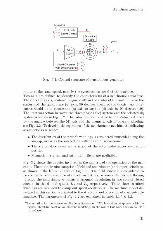
The diesel generator is modeled as an electrically excited synchronous generator,as shown in Fig. 3.1. There are two control loops present: The automatic voltageregulator (AVR) and the speed governor. Both control loops apply the droopcharacteristics explained in Eq. 2.10 for active and reactive power, where Qg isthe reactive power measured at the output of the generator and Pset the droopcontrol setpoint.
3.1.1 Electrical and mechanical part
There are several methods of modeling an electrically excited synchronous gen-erator depending on the analysis depth required for the investigations. Thesynchronous generator consists of two main components: the armature and fieldwindings. The field winding is supplied with direct current to produce a mag-netic field which induces alternating voltages in the armature windings. Whenthree-phase currents flow through the armature winding, a magnetic field inthe air-gap rotating at synchronous speed will be created. The field winding isplaced in the rotor of the machine. To acquire steady torque both fields must
30
3.1 Diesel generator
AVR with Droop Control
Vf
ωm
Tm
ExcitationSystem
ig Vg
PCC
Vg*
Qg (ig ,Vg )
Vg
Prime Mover
ωm*Speed Governor
with Droop Control Pset
Fig. 3.1: Control structure of synchronous generator
rotate at the same speed, namely the synchronous speed of the machine.Two axes are defined to identify the characteristics of a synchronous machine.The direct (d) axis, centered magnetically in the center of the north pole of thestator and the quadrature (q) axis, 90 degrees ahead of the d-axis. An alter-native would be to choose the (q) axis to lag the (d) axis by 90 degrees [10].The interconnection between the three-phase (abc) system and the selected dqsystem is shown in Fig. 3.2. The rotor position relative to the stator is definedby the angle θ between the (d) axis and the magnetic axis of phase α winding,see Fig. 3.2. To develop the equations of the synchronous machine the followingassumptions are made:
• The distribution of the stator’s windings is considered sinusoidal along theair-gap, as far as the interaction with the rotor is concerned.• The stator slots cause no variation of the rotor inductances with rotorposition.• Magnetic hysteresis and saturation effects are negligible.
Fig. 3.2 shows the circuits involved in the analysis of the operation of the ma-chine. The rotor circuits comprise of field and amortisseur (or damper) windings,as shown in the left sub-figure of Fig. 3.2. The field winding is considered tobe connected with a source of direct current, Ifd whereas the current flowingthrough the amortisseur windings is assumed circulating in two sets of closedcircuits in the d- and q-axis, Ikd and Ikq respectively. These short-circuitedwindings are intended to damp out speed oscillations. The machine model de-veloped in this section is oriented to the structure and operation of a salient-polemachine. The parameters of Fig. 3.2 are explained in Table 3.1 1 & 3.2.
1The notation for the voltage amplitude in this section, ”E”, is used, in compliance with thetypical literature notation on machine modeling. In the rest of this work the symbol ”V ”is preferred.
31

3 Generator modeling and control
b
a
c
Ea
ΨaIa
Ib
IcEc
Ψc
Ψb
Eb
Axis of phase a
θ
d-axis
q-axis
Rotation
IfdEfd
ωe
Fig. 3.2: Coupling of dq and abc equivalent circuits
The core of the machine model is the dq-circuit based on the Lad reciprocal pusystem [10], [31] as shown in Fig. 3.3. In this system, the base current in anyrotor circuit is defined as the current which induces in each phase 1 pu voltageinduced by the mutual inductance Lad [10]. This circuit represents the electricalcharacteristics of the machine.
Rfd
Lfd
Lad
LlΨq ωe
dtEd
id
dΨd
R1d
L1d1dad
lRs
Efd R2q
L2qLaq
LlΨd ωe
dtEq
iq
dΨq
R1q
L1q
lRs
Fig. 3.3: DQ equivalent circuit
Variable Description
Edq Induced terminal voltageΨdq Flux linkagefd Field winding
kd & kq d− & q−axis amortisseur circuitk 1,2... n; n=no. of amortisseur circuitsωe Rotor angular velocity
Table 3.1: Machine parameters in dq & description
The pu base units are summarized in Table A.1. An important observation oncalculating impedances in pu values is that inductances and reactances are thesame when calculated in pu. In the described model, time is also in pu, whichaffects all integrators in the model. The dq equivalent circuit parameters given
32

3.1 Diesel generator
Variable Description
Ll & Rs Self inductance & resistance of stator windingLadq DQ components of mutual inductance between stator & rotor windings
L1dq , L2dq Self inductances of DQ amortisseur circuitsLfd & Rfd Self inductance & resistance of rotor circuit
Ldq DQ-axis synchronous reactance
Table 3.2: DQ equivalent parameters
in Table 3.2, which are also called fundamental or basic parameters, cannotbe directly measured from the machine terminals. Instead, it is common tolist in the datasheet the operational parameters of the machine, which can beobtained through a variety of experimental methods, such as open-circuit (OC)and short-circuit (SC) tests. The operational parameters, given in Table 3.3are in pu and similar expressions apply also for the q-axis. The coupling of the
Variable Description
T′
d0 D-axis OC transient time constantT
′
d D-axis SC transient time constantT
′′
d0 D-axis OC sub-transient time constantT
′′
d D-axis SC sub-transient time constant
Table 3.3: Datasheet parameters required
fundamental machine parameters, such as the rotor and stator inductances andresistors, with the operational parameters is based on interconnecting the statorand rotor circuits with the incremental values of terminal quantities, as shownin Fig. 3.4. More specifically, by examining the machine response under smallperturbations (this is denoted through the suffix ∆) the operational parameterscan be derived.Introducing G(s), the stator to field transfer function and Ldq, the operationald- and q-axis inductance, Figure 3.4 can be quantified in Eq. 3.1 & 3.2.
∆Ψd(s) =G(s)∆Efd(s)−Ld∆id(s) (3.1)
∆Ψq(s) =−Lq∆iq(s) (3.2)
where s is the Laplace operator. For the d-axis equivalent, the analytical ex-pression for Ld(s) can be calculated from the left part of Fig. 3.3 and Eq. 3.1and written in factored form in Eq. 3.3. The analytical mathematical derivationcan be found in [10].
Ld(s) = Ld1 + (T4 +T5)s+T4T6s
2
1 + (T1 +T2)s+T1T3s2 ≈ Ld(1 + sT
′
d)(1 + sT′′
d )(1 + sT
′d0)(1 + sT
′′d0) (3.3)
33

3 Generator modeling and control
Δid D-axis
networkΔEfd
+
-ΔΨd
+
-
Δiq Q-axis
networkΔΨq
+
-
Fig. 3.4: d- and q-axis networks identifying terminal quantities
where:
T′
d0 = T1 = Lad+LfdRfd
T′′
d0 = T3 = 1R1d
(L1d+ LadLfdLad+Lfd
)
T′
d = T4 = 1Rfd
(Lfd+ LadLlLad+Ll
)
T′′
d = T6 = 1R1d
(L1d+ LadLlLfdLadLl +LadLfd+LfdLl
)
Lad = Ld−Ll
(3.4)
Similar expressions apply also for the q-axis equivalent circuit. The parametersthat appear in Eq. 3.4 are named in Table 3.3 and can be directly obtained fromthe machine datasheet. The missing parameters of Table 3.2 can be calculatedsolving the 5x5 system of Eq. 3.4.The developed model in the dq rotating reference frame has to be able to connectwith all other models in a three-phase system. Therefore, a controlled currentsource is developed as shown in Fig. 3.5]. The inherent problem of this inter-connection scheme is that no inductive component can be directly connected atits output. This can be easily bypassed by using a large resistive component inparallel with the inductive element.
IgPCC
Vg
abc
dq Idq
θe
abc
dqEdq
θe
Fig. 3.5: DQ model connection
θeωmp
ωe
Dqequivalent
circuit
Vf , from AVR Te 1
J( Tm – Te )
Swing equation
Tm ,from SpG
Fig. 3.6: Model of the mechanical part
34

3.1 Diesel generator
The electrical torque Te, seen as an output of the dq equivalent circuit in Fig.3.6, is directly calculated in the dq equivalent circuit as given in the followingequation:
Te = Ψdiq−Ψqid (3.5)
In Fig. 3.6 the SpG stands for speed governor.
3.1.2 Controller design
Both control loops of the diesel generator are shown in Fig. 3.7 and 3.82. Allparameters are in pu with the base units given in Table A.1. For the auto-matic voltage regulator (AVR) a simplified mathematical model of the AC5Abrushless excitation system based model, as defined in [32], is implemented.The simplifications are performed due to the modeling focus of the synchronousgenerator [33]:
• The load compensator and power factor controller terms are not imple-mented since a reactive power/voltage droop characteristic is selected toinvestigate the reactive power flow among distributed generators. Propor-tional reactive power sharing cannot be achieved when these two terms arepresent.• Over/under excitation & Volts per Hertz limiters are not implemented,since they are activated only under steady state operation which exceedsthe time focus of this work.
Both exciter and prime mover of the generator are not modeled deeper than alow pass filter with an appropriate time constant. The focus of the investigationsin this work are directed to the grid coupling between different distributed gen-erators. Thus, a detailed modeling approach of a diesel turbine or the excitationcircuit would not provide a better insight of the machine transient response.Droop characteristics are implemented for both control loops, as theoreticallyanalyzed in chapter 2. More specifically for the speed governor, the droop char-acteristic is implemented as a setpoint for the mechanical torque in pu, T ∗
m whichis identical to the setpoint for active power, as both of them are in pu as ex-plained in [10] & [31].The output voltage reference, V ∗
g as well as the angular velocity reference ω∗m
are selected equal to 1 pu.
2For each control structure shown in this work, for each sum of signals the plus sign isconsidered as standard input sign and not depicted in the control diagram.
35

3 Generator modeling and control
-
- Exciter Emulation
Vf
Qg (ig ,Vg)
Vg
kq
Vg*
Fig. 3.7: AVR
--
Prime mover Emulation
kp
Tm
ωm
- Tm*
ωm*
Fig. 3.8: Speed governor
AVR design The controller parameters of the AVR are calculated based onpole placement. Similar to [34] and [35], the machine/exciter system can berepresented by first order models. The control plant and the PID controller canbe emulated with the following transfer functions:
GAV R(s) = 1(1 + sTg,oc)(1 + sTe)
, GC(s) = kds2 +kps+ki
s(3.6)
where: Tg,oc is the generator open circuit time constant, Te the exciter opencircuit time constant and kd, kp, ki the derivative, proportional and integralgains of the controller. Regarding pole placement, a certain amount of trial anderror can be involved during design validation, since the direct placement of theclosed loop poles gives rise to zeros of the transfer function that might affect thetransient response of the system. The characteristic equation of the closed loopsystem is expressed as:
GAV R(s)GC(s) =−1 (3.7)
Although it’s a third order system, by placing the third pole on the far leftreal axis the system response can be approximated with a second order system’sresponse. In this way, choosing a minimum response overshoot and setting thesettling time equal with the open circuit time constant of the machine, thecontroller gains are obtained.
Speed governor design Similar to AVR, a PID controller is also realized for thespeed governor [36]. Direct pole placement for the controller gains is once moreselected as the most appropriate tuning method. Emulating the machine/dieselturbine system with the following transfer function:
GSG(s) = 1(1 + sTg,m)(1 + sTt)
(3.8)
where Tg,m is the starting time of the machine which is based on the moment ofinertia J :
Tg,m = 2H = 2(12J(ω
p)2 1Sbase
) (3.9)
36

3.1 Diesel generator
with H being the inertia constant of the machine which can be physically inter-preted by:
H = stored energy at rated speed in MWs
MV A rating(3.10)
and Tt the diesel turbine time constant. The characteristic equation of the closedloop system is once more obtained, and the gains of the PID controller are oncemore calculated based on pole placement.
Validation of controllers The controllers designed in the previous paragraphsare verified in operation with a medium voltage salient pole machine [37]. Adetailed list of the synchronous generators parameters are given in Table A.3 &A.4 and the corresponding controller parameters in Table A.5. The Bode plotsof the open loop transfer function of the control plant with the PID controllerare drawn, to evaluate the frequency response of the selected controller gains.
0
50
100
Mag
nitu
de (d
B)
10−3 10−2 10−1 100 101 102−135
−90
−45
Pha
se (d
eg)
Bode Diagram
Frequency (Hz)
Fig. 3.9: Bode plot of AVR con-troller
−50
0
50
100
Mag
nitu
de (d
B)
10−3 10−2 10−1 100 101 102−180
−135
−90
−45
Pha
se (d
eg)
Bode Diagram
Frequency (Hz)
Fig. 3.10: Bode plot of SpG con-troller
The Bode plots in Fig. 3.9 & 3.10 can aid to the direct calculation of the phasemargin of the control loop. The crossing point of the magnitude bode plot withthe 0dB axis (@ 20 for the AVR and @ 8Hz for the SpG) is required for thephase margin calculation. Noting at this crossing point the difference betweenthe phase bode plot and the 180 phase limit delivers the controller margin.An adequate phase margin of 90 and 50 for the AVR and the speed governorrespectively delivers a transient stable response of the control plant in both cases(phase margin > 30 [38], [39]).
The root locus of the system is also plotted to further examine the stability ofthe system. The far left placed pole can be observed from Fig. 3.11 & 3.12. Itis also shown that all poles and the root locus curves connecting poles and zerosremain in the left plane. At this point it should be noted that both controllersare working in parallel and in the controller design explained in this section their
37

3 Generator modeling and control
-12 -10 -8 -6 -4 -2 0 2-2
-1.5
-1
-0.5
0
0.5
1
1.5
2Root Locus
Real Axis (seconds-1)
Imag
inar
y A
xis
(sec
onds
-1) Far left
placed pole
Fig. 3.11: Root locus of AVR controller
-160 -140 -120 -100 -80 -60 -40 -20 0 20-40
-30
-20
-10
0
10
20
30
40Root Locus
Real Axis (seconds-1)
Imag
inar
y A
xis
(sec
onds
-1) Far left
placed pole
Fig. 3.12: Root locus of SpG controller
interconnection is not considered. That could lead to small deviations, as far asthe transient response of the generator is concerned, in the selected overshootsand settling time of the closed control loops of the machine.
3.2 Grid inverter
A generic model of an inverter connected to the rest of the microgrid through aLC(L) filter at its output is the next component to be modeled. This converteris the interfacing element of any inverter-based distributed generator with thegrid and is in detail analyzed. Since grid studies is the focus of this work, thecontrol algorithm governing the inverter is the model core and losses calculationor the analysis of the switching process of the semiconductors are neglected.Transformation methods for three-phase systems are implemented, derived fromthe equivalent ones for modeling synchronous machines [40]. The synchronousrotating reference frame (SRRF), also called the dq0 coordinates system, is se-lected as appropriate control base for our algorithms as an industry standardmethod. Alternatives can be found, such as the αβγ stationary reference frameor the abc natural reference frame. The natural reference frame could be ameaningful alternative if unsymmetrical faults are considered [41]. In that case,an alternative would be the implementation of separate controllers in the syn-chronous rotating or stationary reference frame, for controlling the symmetricalcomponents of voltage and currents [42]. A control concept in synchronous ro-tating frame in combination with symmetrical components analysis has beensuccessfully implemented for the case of two parallel inverters in unsymmetricalloading conditions in [13]. The following figure presents a vectorial representa-tion of the abc to dq transformation, where X could be any three phase system,such as voltage, current, flux linkages, etc. The Xγ, X0 components of thetransformations calculated in Eq. 3.11 & 3.12 are identical and only relevant fornon- symmetrical systems and are not further mentioned in this work. In Fig.3.13 and Eq. 3.11 & 3.12 ω is the rotating angular velocity of the coordinatessystem, θ0 is the angle between D- and a-axis of the system, and θ = ωt+ θ0the full angle of the new DQ rotating reference frame. These transformations
38

3.2Gridinverter
Xa
Xb
Xc
ω
XdXq
θο
Fig. 3.13:abc&dqvectors
Xα
Xβ
Xγ
=
2
3−1
3−1
3
01√3−1√3
1
3
1
3
1
3
Xa
Xb
Xc
(3.11)
Xd
Xq
X0
=
cos(θ) sin(θ) 0
−sin(θ)cos(θ)0
0 0 1
Xα
Xβ
Xγ
(3.12)
canbequiteusefulforcontrolalgorithms,wheresignalscanbeeasilycontrolledinotherreferenceframesthanthenaturalreferenceframe. Toelaboratethisconvenienceathree-phasesymmetricalvoltagesystemisshowninallthreeco-ordinationsystemsbelow. AsseeninFig.3.14c,thed-andq-componentofthesinusoidalvoltageareDCquantitiesinsteadystate,sincetheyarerotatingwiththeangularfrequencyofthesystemω
0 0.005 0.01 0.015 0.02
−1
−0.5
0
0.5
1
Time[s]
Voltage,Vabc[pu]
Va
Vb
Vc
,andPIcontrollerscanbeemployedtogovernthem.
(a)in
0 0.005 0.01 0.015 0.02
−1
−0.5
0
0.5
1
Time[s]
Voltage,Vαβ[pu]
Vα
Vβ
abc (b)in
0 0.005 0.01 0.015 0.02
−1
−0.5
0
0.5
1
Time[s]
Voltage,Vdq[pu]
Vd
Vq
αβ (c)indq
Fig.3.14:Transformationofathree-phasevoltage
InvertertopologyThetopologiesselectedforthegridinverterareshowninFig.3.15.Theleftone,inFig.3.15aisthestandard2-leveltopologywithaca-pacitorfedDC-linkasinput.Therightone,inFig.3.15b,isthe3-levelNeutralPointClamped(NPC)topologywithacapacitorfedDC-linkasinput.InFig.3.15theinverterisportrayedwithIGBT-diodesemiconductors,asmostappro-priatecandidatesforlow/mediumvoltageandhighpowerapplications.PulseWidthModulation(PWM)isimplementedasastandardmodulationtechniqueforgridinverters.
39

3 Generator modeling and control
-
+
VDC Vinv
(a) 2-level
-
+
VDC Vinv
(b) NPC
Fig. 3.15: Grid inverter topologies
The main difference between topologies is the output voltage, as shown in Fig.3.16. The phase to DC-link middle point voltage at the output of the invertertogether with the sinusoidal reference voltage are depicted.
0.205 0.21 0.215
−0.4
−0.2
0
0.2
0.4
0.6
Time [s]
Vol
tage
, Vin
v [*V
DC
]
(a) 2-level
0.205 0.21 0.215
−0.4
−0.2
0
0.2
0.4
0.6
Time [s]
Vol
tage
, Vin
v [*V
DC
]
(b) NPC
Fig. 3.16: Output phase voltage
The inherent advantage of the NPC topology is that, as a three-level topology,the output phase voltage depending on the switching pattern can get threedifferent values (+VDC2 , 0, −VDC2 ), whereas at the 2-level inverter only two
(+VDC2 , −VDC2 ). By having more voltage levels the form of a sinusoidal signalis approached, minimizing the need for an output filter. These two topologiesare selected to demonstrate the independence of the topology for the controlalgorithms and grid studies performed in this work. Furthermore, the topologyselection is additionally based on the voltage and power level of the inverter-interfaced distributed generator.
40

3.2 Grid inverter
Mathematical model of inverter with LCL filter The mathematical model ofa single-phase inverter connected through a LCL filter is depicted in Fig. 3.17.The resistors present in Fig. 3.17 are the equivalent series resistances (ESR) ofthe filter inductors and are in the order of 0.005 pu, which is quite reasonablefor medium voltage, high power inductors [43]. The equations of the system areformed, where:
Vi : inverter output voltageVg : grid voltage
L1, R1 : converter side L & R
Cf : filter capacitorVC : filter capacitor voltage
L2, R2 : grid side L & R
R1
Vi
L1 R2L2
-
Cf
+
i1 i2
iC
VC
-
+
Vg
Fig. 3.17: Inverter model with LCL filter
di1dt
=−R1
L1i1−
VcL1
+ ViL1
(3.13)
dVcdt
=− 1Cf
(i1− i2) (3.14)
di2dt
=−R2
L2i2 + Vc
L2− VgL2
(3.15)
To describe the inverter output voltage, switching functions are introduced [44],defined in the following equations with the variable p. In the case of a 2-levelconverter, which is shown in Fig. 3.15a, the switching function for a single legof the inverter is equal to 1 when the upper switch is closed and 0 when thelower switch is closed. Similar to equations 3.11 & 3.12, equation 3.16 showstheir transformation to the synchronous rotating reference frame.
[pdq
]=
cos(θ) cos(θ− 2π
3 ) cos(θ+ 2π3 )
sin(θ) sin(θ− 2π3 ) sin(θ+ 2π
3 )
pa
pb
pc
(3.16)
With the use of switching functions, the voltage at the output of the convertercan be calculated from the available DC-link voltage:
Vinv(t) = pdqVDC(t)
2 (3.17)
We conclude to the following state space equations of the mathematical modelof the inverter by combining equations (3.13) – (3.17) and transforming them to
41

3 Generator modeling and control
the dq coordinates:
d
dt
Vcd
Vcq
i1d
i1q
i2d
i2q
=
0 ω1
Cf
0 −1
Cf
0
−ω 0 01
Cf
0 −1
Cf
−1
L10 −
R1
L1ω 0 0
0 −1
L1−ω −
R1
L10 0
1L2
0 0 0 −R2
L2ω
01
L20 0 −ω −
R2
L2
Vcd
Vcq
i1d
i1q
i2d
i2q
+
0 0
0 0
0 0
0 0
−1
L20
0 −1
L2
[
Vgd
Vgq
]+
0 0
0 0VDC
L10
0VDC
L1
0 0
0 0
[
pd
pq
](3.18)
The impact of the dq transformation is seen in Eq. 3.18 with the coupling termsbetween the d and q components of voltage and current. In case a transformerconnects the inverter to the grid, its leakage inductance can be added to L2. Thedamping resistor in series with the filter capacitor is neglected for the formulationof the above equations.
DC-link capacitance sizing The selection of the DC-link capacitance is basedon the maximum permissible voltage ripple. Assuming linear increase of thevariation of the output power ∆Pmax during one switching period Ts [45] & [46],the maximum energy ∆W to be transferred through the DC-link during oneswitching period can be calculated:
∆W ≈ ∆PmaxTs2 (3.19)
This energy deviation can be however also calculated from the energy that canbe stored in the capacitor:
∆W ≈ CDCVDC∆VDC (3.20)
where VDC and ∆VDC are the DC-link voltage and voltage ripple respectively.Taken into consideration that the maximum power in case of distributed gener-ators is the rated power, namely ∆Pmax = Pn, Eq. 3.19 & 3.20 can be combinedinto:
CDC = PnTs2VDC∆VDC
(3.21)
It is however acknowledged that Eq. 3.21 results in significantly lower capaci-tance values from those realistically selected [45] & [46]. This calculation schemedoes not take into consideration the DC-link voltage control dynamics, whichhave a significant impact on the stability of the DC-link. To obtain a reason-ably stable response even in the case of grid faults, it is common to oversize thecapacitance derived from this calculation. In [45], a multiple of the switchingperiod is used for this calculation to improve the selection. In this work thepermissible allowed DC-link voltage ripple is selected quite low ∆VDC = 1−2 %,since a stable response of the inverter during grid faults is also a focus. Furtherinvestigations on the proper selection of the capacitance should include calcu-
42

3.2 Grid inverter
lation of the capacitor current and choosing appropriate capacitors to ensurethat enough power cycles are guaranteed. Since system cost reduction is notthe priority of this work, but the investigations in system level with realisticcomponents, the selection of DC-link capacitance is not further investigated.
LC(L) Filter Design For the development of operational strategies for gridinverters in the next chapters, different control objectives, voltage and powerlevels are involved. Therefore, a generic algorithm is developed for the design ofthe inverter grid filter that can be easily scaled based on the inverter’s differentattributes. The algorithm has four main steps:
• Calculate the required inverter-side filter inductor based on a pre-definedmaximum allowable current ripple• If it is the case of a LCL filter, the grid-side inductor is designed as afraction of the inverter-side inductor.• The capacitance is selected through the choice of the filter’s resonancefrequency.• A passive damping resistor is selected based on a desired damping factor.
The design process followed in this work starts from the calculation of the cur-rent ripple at the output of the inverter. The inductor equivalent series resis-tance is for this calculation neglected and the grid voltage, or in our case, thevoltage across the capacitor is considered constant through a switching event.For this calculation, the capacitor’s influence to the ripple current is consideredminimal, since it is also designed to dampen the higher order harmonics, andthe inverter-side inductor filters the biggest harmonic proportion of the current.The derivation of the current ripple calculation is performed according to [47].The worst case current ripple is obtained during the zero crossing of the phasevoltage, see Fig. 3.18.
- VDC
Δirir
3n
VDC3n
t1 t2
Fig. 3.18: Current ripple by phase voltage zero crossing
43

3 Generator modeling and control
Both curves are drawn based on the assumption that the grid voltage is constantduring one switching period and the phase voltage drops across the inverter-sidefilter inductance. From this figure the following equation can be obtained:
∆ir = VDCt13nLf
, where t1 = t2 =√
3mmax
8fs(3.22)
In Eq. 3.22, mmax = 1.15 is the maximum modulation factor for the case ofspace vector PWM, or PWM with third harmonic injection, and n = 1 or 2 inthe case of 2-level or 3-level inverters respectively. From Eq. 3.22, by settinga maximum permissible current ripple, ∆ir = 15...25 % of the nominal current,the required minimum inverter-side filter inductance can be chosen [43]. Thesecond step of the design process is to select the filter resonance frequency (ff ).A guidance rule is given in Eq. 3.23. An alternative would be to design thecapacitor based on its reactive power requirements, as a proportion of the ratedpower of the inverter [48].
10 ·fg < ff <fs10 (3.23)
where fg is the grid nominal frequency (in our case, 50 Hz) and fs the se-lected switching frequency for the semiconductors. This equation can be how-ever successfully followed only in low voltage applications, where the switchingfrequency lies in the area of fs> 5kHz. In medium voltage applications compro-mises should be found, where the switching frequency can obtain values lowerthan 1kHz. In this case the resonance frequency can reach values down toff = 250Hz [43]. Since different factors are involved in this selection, designingan LC(L) filter should be performed in an iterative manner, taking into consid-eration grid code requirements for the output current [49] or voltage [50] har-monics. In this work, the optimization of the LCL filter is not the investigationfocus. The priority is set to realistically model inverter-based medium voltagesystems. The filter resonance frequency is set in the range of fs = 450...550Hz,depending on the switching frequency of the inverter. After selecting the de-sired resonance frequency, the filter capacitance value can be calculated fromEq. 3.24.
ωf = 1√LfCf
⇒ Cf = 1ω2fLf
(3.24)
where Lf could be, in the case of a LC filter a single inductor, or in the case of aLCL filter the parallel connection of both inductors, Lf = L1L2
L1 +L2, as depicted
in Fig. 3.17. The selection of the grid-side inductor in the case of a LCL filteris performed typically as a fraction of the inverter-side inductor. The grid-sideinductor L2 is normally smaller than the inverter-side inductor L1, since it doesnot have to dampen the whole harmonic current spectrum directly at the inverteroutput and is considered a less cost-driving component than the inverter-sidefilter inductor. Typical values for L2 are in the area of L2 = 0.1...0.25L1 [43].The last filter component is required to dampen unstable transient dynamics
44

3.2 Grid inverter
triggered by disturbances or sudden variation of the inverter operating point.The proper damping of these dynamics is achieved through the insertion of pas-sive elements to the filter structure. Although active damping methods canbe found in the literature [51], the method of passive damping is further fol-lowed in this work. In this method, a resistor is placed in series with the shuntcapacitor. To select the value of the passive damping resistor, the damping fac-tor ζp should be introduced. Integrating the resistor, Rd in the circuit of Fig.3.17, the dynamics of the filter should be analyzed [43]. The inverter’s forward
self-admittance, Y1(s) = I1(s)Vi(s)
and the forward trans-admittance Y2 = I2(s)Vi(s)
aretherefore formulated:
Y1(s) = 1L1
s2 + RdL2s+ 1
L2Cfs(s2 + 2ζpωfs+ω2
f ) , Y2(s) = RdL1L2
s+ RdCfs
s(s2 + 2ζpωfs+ω2f ) (3.25)
where ωf is the filter resonance angular frequency and ζp = Rd2
√√√√CfLf
the dominant
damping factor. These two factors define the dynamic response of the system,as shown from the denominators of Eq. 3.25. Once the reactive components ofthe filter are selected, the damping resistor can be directly calculated from thedesired damping factor. A variation of the damping factor in the range of ζp =0.21...0.37 was performed in [43]. The value of ζp = 0.3 delivered an acceptablecompromise between damping and attenuation, and is further selected in thiswork.As far as the filter type is concerned, the control objective of the inverter couldhave been a selection criterion. It has been demonstrated in chapter 2 that droopcontrol for grid forming units is based on inductive distribution lines. That hasbeen verified with the calculation of the stability margins of the eigenvalues of atwo-generators system. These margins increase with increased impedance pathbetween them, as shown in Fig. 2.10 & 2.11. Therefore, it would be reasonableto select for grid forming inverters a filter type that increases the output gridimpedance, e.g. an LCL filter. However, that would not be a realistic approach.Grid forming units connect storage elements to the grid which should be typicallyable to work in both grid forming and feeding mode. Therefore, the inverterfilter should be independent of the control mode of the inverter. In this work, tovalidate that the control strategies proposed are fully operational independentof the filter type, a differentiation on the filter selection is performed dependingon the inverter voltage. For inverters that are connected at 1kV a LCL filteris chosen, whereas for inverters connected at 3.3kV a LC filter is implemented.At this point it should be mentioned that all inverters are connected to thegrid through a step-up transformer, therefore its leakage inductance serves in allcases as an increased output grid impedance. The filter parameters dependingon the voltage and power level can be found in Table A.6.
45

3 Generator modeling and control
3.2.1 Grid feeding inverter
In modern power systems, all renewable energy based distributed generatorsthat work with the principle of Maximum Power Point Tracking (MPPT) areequipped with a grid feeding inverter. The concept of MPPT is to extract thehighest amount of energy from the input source, which could be the case of asolar cell or a wind turbine. The main objective of the grid feeding operationalmode is to deliver to the grid the full amount of energy that reaches the DC-link of the inverter. Furthermore, depending on the grid frequency and voltage,grid supporting functions, such as active power / frequency droop and reactivecurrent / voltage droop are also implemented. The explanation of this cascadedcontrol mode starts from the inner fundamental control plant of the inverter andleads to the upper grid-related control functions.
~= i1
Vg
Current Controller in SRRF
VDCPWM
Vg i1
VDC
Vg
VDC*
Vg*Iq
*
Id*
Grid supporting functions
DC-Link Voltage
ControllerI (pu)
0
PCC
Inputsource
Imax
Ps* (V, f ) fg
*
Ps* (V, f )
L1
Cf
Fig. 3.19: Overall control structure of a grid feeding distributed generator
3.2.1.1 Mathematical model of inverter control plant
For the derivation of the control structure of Fig. 3.19, the mathematical modelof the inverter control plant in steady state operating conditions is first obtained.Starting from the inner current controller and assuming that the DC-link voltageis constant, one can obtain the equations of the model with the use of Eq. 3.13,3.17 and Eq. 3.18:
L1di1ddt
= L1ωi1q−R1i1d+Vid−VCd (3.26)
L1di1qdt
=−L1ωi1d−R1i1q +Viq −VCq (3.27)
The voltage across the filter capacitor, VC , can be accounted as a disturbancefor the faster inner current controller and can be fed forward along with the
46

3.2 Grid inverter
coupling terms due to the transformation to the synchronous rotating referenceframe (SRRF). VC does not need to be directly measured, but estimated fromVg, i1 and Ltr, the transformer’s leakage inductance and calculated in Laplacedomain:
VC(s) = Ltri1(s)s+Vg(s)1−LtrCfs2 (3.28)
The equations Eq. 3.26 and Eq. 3.27 can be graphically depicted in the followingfigure, Fig. 3.20, where Gc(s) = kpcs+kic
sis the PI controller for the d- and q-
axis.
I1d*
I1d
-GC(s)
-
VCd
Vid*
PWMVid
Lω
I1q*
-GC(s) Viq
*PWM
Viq
I1q
Lω
-
VCq
- L1s+R1
1 I1d
L1s+R1
1 I1q
Lω
Lω
-Fig. 3.20: Control block diagram of the grid feeding inverter
The current controller is connected to the control plant though the inverter, asseen in Fig. 3.20. To calculate the transfer function of the system, the couplingand feed-forward terms are neglected, as well as the inverter and transforma-tion calculations, which are considered ideal components. Defining appropriatecontroller gains, the closed-loop transfer function can be represented by a firstorder linear system:
Idq(s)I∗dq(s)
= 1Tis+ 1 (3.29)
The appropriate gains for the PI controller are given by:
kpc = L1
Ti, kic = R1
Ti(3.30)
where Ti is the time constant of the closed-loop system, identical for each axis.This time constant is a designer’ choice, and it should be quite small for a fastcontrol response, but the bandwidth ( 2π
2Ti) should also be at least ten times
smaller than the switching frequency of the inverter (expressed in rad/sec) [52],
47

3 Generator modeling and control
[53]. This bandwidth requirement ensures that the inverter can be neglectedduring the formulation of the transfer function of the current controller. Typicalvalues for Ti are in the range of 0.5−5 ms [54].Since in this work medium voltage applications are considered and the switchingfrequency is selected between 2 and 2.5 kHz, see Table A.6, the bandwidthrequirement is not met. Therefore, the alternative of the technical optimum(or modulus optimum) criterion is applied [55], [56]. In this case, the controlplant of the inductor and resistor in series of the filter is identified with theaddition of the delay due to the switching frequency of the inverter. It shouldbe noted that also for the case of technical optimum a dominant pole shouldbe present [56], which in our case is the first order system of the inductor andresistor in series, TRL = L1
R1with a gain of KRL = 1
R1. The PWM block of
figure 3.20 is replaced by GPWM = KPWM
Tss+ 1 , where KPWM is the inverter voltagegain, and Ts the time constant due to the switching frequency and the restof processing delays, typically selected equal to Ts = 1.5Tsf , with Tsf the timeconstant of the switching frequency. The transfer function of the closed loopsystem can then be calculated as follows:
Gcc = 1TRLTs
KpcKPWMKRLs2 + TRL
KpcKPWMKRLs+ 1
(3.31)
Identifying the damping factor D of the second order system and setting it equalto D =
√2/2 for a critically damped system [55], the current controller can be
fully calculated:
kpc = TRL2TsKPWMKRL
, kic = kpc
TRL(3.32)
The initial objective of replacing the closed current control loop with a firstorder system has been obtained with this method too. Since TRL >> Ts, thefirst order system of the current control loop is obtained by:
Gcc = 12Tss+ 1 (3.33)
The DC-link controller is built as an outer loop, resulting in a cascaded controlstructure, shown in Fig. 3.21. Starting from the energy stored in the DC-linkcapacitor CDC :
Ec = 12CDCV
2DC (3.34)
The time derivative of this energy should lead to the power balance equationof the DC-link. Defining the power coming from the input source Pin, and the
48

3.2 Grid inverter
power delivered to the grid as Pout:
12CDC
d
dtV 2DC = Pin−Pout (3.35)
Similar to the current control loop, a linear system is the objective of the DC-link controller. Therefore, the DC-link voltage VDC is substituted with a controlvariable u. For the practical implementation of this controller, the reference andmeasured voltage will be squared and then substracted to obtain the input errorof the PI controller, ε(t). Neglecting the filter resistor R1 as it is responsible forless than 1% of the transferred power, the instantaneous power delivered to thegrid calculated in dq coordinates is Pout = 3
2VCdId+
>
0VCqIq, while the power input
source is considered a disturbance, δ(t) [52]. The q-component of the voltageVCq is zero since the selected axis for the dq transformation is aligned with theaxis of phase a, and VCd
is therefore equal to the voltage amplitude, VC :
12CDC
d
dtu= δ(t)− 3
2 VCId (3.36)
The transfer function of the system is derived, taking also into consideration theD-axis current reference I∗
d as control variable, and the transfer function of theunderlaying current controller:
GDC(s) = u(s)Id(s)
=− 3VCCDC
1s
12Tss+ 1 (3.37)
The transfer function has one pole in the origin, and symmetrical optimumcriteria can be applied to design the PI controllers. Defining once more a PIcontroller with a transfer function of:
GPIDC(s) = kpv(1 + 1
Tvs) (3.38)
The symmetrical optimum criterion is based on designing the amplitude andphase plot of the open loop transfer function being symmetrical about thecrossover frequency [56], [57]& [58]. The gain of the controllers are then givenby [55]:
kpv = CDC4αTs
, Tv = 4Ts (3.39)
where α= 2.4 is selected to result in a critically damped second order system, andthe time constant of the voltage controller is increased because of the samplingdelay of the measured DC-link voltage. It can be observed that the amplitudeof the output voltage is eliminated from Eq. 3.39, since the controller is de-signed in pu. Several alternatives can be found for designing the PI controllerof the DC-link voltage, including the principle of the Internal Model Control(IMC) [52]. The IMC method has the objective of subtracting the control plant
49

3 Generator modeling and control
from the closed loop transfer function and selecting then an appropriate con-troller bandwidth based on the application.The overall control structure of the controller is given in Fig. 3.21.
VDC*
I1q*(Vg )
VCd
dqabc
δg
abcdq
δg
I1
-
I1d
I1q
ωL1
--
VDC
-
( )2
VgVCdq
VCq
ωL1
ampl
itude
lim
itatio
n
I1Eq. 3.28
-- ( )2
PLL VCδg
abcdq
δg
VC
Fig. 3.21: Cascaded control structure of grid feeding inverter
The phase locked loop (PLL) which is needed to acquire the grid voltage angle,δg is based on input/output power balance equations, or phase balance methodas described in [59]. An alternative would be the standard DQ- control struc-ture, where the Q-component of the voltage is controlled to zero to produce thesystem frequency [60]. More on the implementation of the PLL can be found inAppendix A.
3.2.1.2 Dynamic grid supporting functions
There are several codes and norms that have been issued for grid feeding in-verters connected to stiff grids for the provision of grid support during tran-sients [61], [62]. In a microgrid, which is classified as a weak grid prone to sta-bility disturbances, the grid supporting functions are of fundamental importancefor stable operation. In Fig. 3.22 & 3.23, typical droop curves for supportinggrid voltage and frequency are depicted. The limits for the reactive current (orpower) injection are taken from [61] and for active power/frequency dependencefrom [62]. These functions are formed by taking into consideration the inductivecharacter of a stiff grid.
The grid supporting functions influence the operation of the grid feeding inverterand the controller of the input power source. The grid feeding inverter is respon-sible for the power balance of the DC-link and can also control separately thereactive current reference, depending on the grid voltage. It is however not re-sponsible for the input power to the DC-link. Therefore, if over/under-frequencyoccurs, the controller of the input power source should intervene to prohibit rise
50

3.2 Grid inverter
Voltage drop (pu)
Reactive current (pu)
Deadband
0.1-0.1-0.5
-1
0.2-0.2
Fig. 3.22: Reactive current/voltage
Frequency (Hz)
Active power (pu)
49.5
0.12
50.5
Deadband
49.8 50.2
-0.12
Fig. 3.23: Active power/frequency
of the DC-link voltage. It should be also explained why in the case of voltagedeviations the grid feeding inverter obtains a direct current reference, whereas inthe case of frequency deviations the inverter obtains a power reference. Power isdirectly coupled with voltage, therefore in the case of voltage deviations apply-ing a power reference would not meaningful, since the voltage varies. Frequencydeviations are not however coupled with power amplitude, therefore it is rea-sonable to give to the inverter a power reference in that case. In Fig. 3.22, theso-called ’k-factor’ can be identified as the proportionality factor between reac-tive current reference and voltage drop, which is in this case equal to 2. In [63]the impact of different values of this k-factor on the stability of a relatively stiffgrid is investigated. Further discussions on reactive current injection are givenin chapter 6, where the dynamic response in fault case is analyzed, and the curveof Fig. 3.22 is optimized for medium voltage microgrids.
3.2.1.3 Static grid supporting functions
The supporting functions explained in the previous section refer to abnormalstates, where the grid voltage or frequency experience deviations from theirnominal values. Further requirements however exist, which demand power set-points from renewable energy based generators during normal operation. Theseare called static grid supporting functions, with the most typical one being con-trolling the power factor at the PCC of the grid feeding inverter. The gridoperator can define a reference point for the reactive power, Q∗
g or directly forthe power factor, e.g. cosφ = 0.95. In this case, the control structure of Fig.3.19 should be modified with an additional PI controller for the calculation ofthe new reactive current reference, I∗
q . In Fig. 3.24 the Q∗g variant is depicted.
The PI controller dynamics should be carefully designed, so that unwanted tran-sient effects can be avoided. These dynamics should be at least 10 times slower
51

3 Generator modeling and control
Vg
Vg*
Iq*
Fig. 3.22&
Fig. 3.23
Ps* (V, f )
fg*
static
dynamic
Iq*
Iq*
Vg , fg
within limits
PIcontroller -
Qg
Qg*
Fig. 3.24: Static support of grid feeding inverter
than the dynamics of the DC-link PI controller to avoid operational states wherethe two outer PI controllers are working against each other. The active and re-active power the generator feeds to the grid Pg & Qg, can be calculated fromthe grid voltage, Vg and the output current.
3.2.1.4 Grid feeding inverter controller verification
Although the focus of this work is in system level, the dynamics of each compo-nent were also tested in standalone mode to verify the selected design process.In this paragraph the dynamics of the grid feeding inverter are validated througha step response applied to its closed control loop.
Step Response
Time (milliseconds)
Am
plitu
de
0 10 20 30 40 50 600
0.2
0.4
0.6
0.8
1
1.2 Sn=3, 4, 5 MVA
Fig. 3.25: Grid feeding inverter controller verification
The outer control reference to which the step input is applied is the DC-linkvoltage controller. The grid impedance or grid voltage dynamics are neglectedfor this theoretical investigation. The closed control loop consists of the cas-caded DC-link voltage controller and inner current controller with their controlplants accordingly. It is demonstrated in Fig. 3.25 that the cascaded controldelivers a robust performance towards the step disturbance. The selected rated
52

3.2 Grid inverter
powers ofSn=3,4,5MV Acorrespond to grid feeding inverter models used inthe investigations of the following chapters. The inverter, filter and controllerparameters can be found in Table A.6. Analyzing Fig. 3.25, an overshoot ofalmost10%is observed, which can be explained through the DC-link controllerdesign. The DC-link voltage is an essential stability element for the grid feedinginverter. The DC-link controller time constant derived from symmetrical opti-mum criteria was reduced to allow this overshoot. It is selected in this way toenable fast tracking of the voltage reference upon load changes or faults.
3.2.1.5 Grid feeding inverter in PQ control
In case the input source of the distributed generator is able to control the DC-link voltage, a variation of the grid feeding control can be applied, in this worknamed PQ control. The outer DC-link voltage control is replaced by the directcalculation of the d- and q-axis component of the current reference:
Pset=3
2VCdId
∗+0
VCqIq
Qset=−3
2VCdIq
∗+0
VCqId
(3.40)
As previously explained, the q-component of the voltage is zero due to the axisalliance of the angle produced from the PLL, identical to the axis of phase a.The overall control structure is depicted in Fig. 3.26. The setpoints for active
~
= i1
Vg
Current Controller in SRRF
Vg
PWM
Vg i1
Iq*
Id* Eq. 3.28 I(pu)
0
PCC
Inputsource
Imax
L1
Cf
Eq. 3.40
&δg
Pset , Qset
i1
Fig. 3.26: Control structure of grid feeding inverter in PQ control
and reactive power,PsetandQsetrespectively, can be given from the utility gridoperator, or can vary depending on the incoming energy of the input source.Fuel cells, batteries and flywheels would be ideal candidates for this controlmode, since they can regulate their output power. This operational mode isquite useful for grid supporting strategies, because of the flexibility it offersdepending on grid demands, and not necessarily in the incoming energy as inthe case of renewable energy sources.
53

3 Generator modeling and control
3.2.2 Grid forming inverter in standalone mode
The topology of the grid forming inverter, depicted in Fig. 3.27, is quite similarto the one of the grid feeding inverter. A LCL filter is selected in this case,together with a step-up transformer for the grid connection. The grid forminginverter requires a DC input source that provides the energy required from thegrid. The case when the DC power capacity cannot fulfill the grid demands isnot considered in this work. In such a scenario, the grid forming inverter shoulddisconnect from the grid to avoid internal damage of its DC source. If the gridforming inverter is the only grid forming unit in that case, then load sheddingshould be performed. The input source controls also the DC-link voltage ofthe system. The objective of the inverter’s control algorithm is to regulate theamplitude voltage and frequency at its output and provide the necessary activeand reactive power to the rest of the microgrid. A cascaded control structure ishere implemented [64].
~= i1
VC
PCC
Inputsource
L1
Cf
i2 L2
Current Controller in SRRF
PWM
i1
Iq*
Id* Voltage Controller
in SRRF + current limitation method
δ* i2 VCVC
VCd*=1 pu
VCq*=0
f *= 50 Hz
Fig. 3.27: Overall control structure of grid forming standalone inverter
The mathematical model of the inner current controller was in detail explainedin section 3.2.1. The control variation is located at the outer voltage controlloop. The main objective of this loop is to regulate the voltage at the output ofthe inverter VC across the filter capacitor Cf . The dynamics of this control loopare governed by equations 3.14 and in dq frame 3.18, once more documentedhere:
CfdVCd
dt= CfωVCq + i1d− i2d (3.41)
CfdVCq
dt=−CfωVCd
+ i1q− i2q (3.42)
If the dynamics of the inner current controller are also taken into consideration,Fig. 3.28 is obtained. The control plant of the grid forming inverter is depicted,where Ti = 2Ts, as previously explained. From equations 3.41 & 3.27 and Fig.3.28, the PI controller for the voltage loop can be designed. A direct selection
54

3.2 Grid inverter
-VCdI1d
* I1d
-
Cf s1
Cf ω
-
Cf s1 VCq
-Cf ω
I1q* I1q
I2d
I2q
Ti s+11
Ti s+11
Fig. 3.28: Voltage control plant of the grid feeding inverter
of the phase margin of the open loop is selected as design process [54]. Let
GPIV(s) = kpv
s+ z
s(3.43)
be the transfer function of the PI controller for the voltage loop. The open loopgain can then be calculated as:
l(s) = kpv
2TsCf( s+ z
s+ 2T−1s
) 1s2 (3.44)
Defining the gain crossover frequency ωc =√zT−1
s , and selecting a phase mar-
gin of δm = sin−1 (1−2Tsz1 + 2Tsz
) = 53 , the PI controller gain can be calculated ask = Cfωc. This direct selection of the phase margin equal to 53 is similar tothe implementation of the symmetrical optimum criterion [54]. The advantageof this method is that the phase margin can be further tuned, in cases wherethe symmetrical optimum criterion does not achieve satisfactory results. Theproposed cascaded control structure is depicted in Fig. 3.29. Similar to section3.2.1, decoupling terms for the voltage are present, as well as feed-forward termsof system outputs, here the load current. The feed-forward term of the currentcan be multiplied with a factor ranging from F = 0.5...0.8 to minimize the effectof a severe disturbance in the slower outer voltage loop [64]. Different combina-tions for the DQ components of the voltage reference V ∗
Cdqexist, the one followed
in this work is selecting V ∗Cd
= VC = 1 pu and V ∗Cq
= 0 [54].
55

3 Generator modeling and control
VCd
dqabc
abcdq
I1
-
I1d
I1q
ωL1
--
VCq
ωL1
curr
ent l
imita
tion-
I2d
abcdq
-
VCdωCf
-
ωCf
-
VC
VCqδ*
abcdq δ*
I2
I2q
I1d*
I1q*
VCd*= 1 pu
δ*
VCq*= 0
δ* 2πf *
I2q
Fig. 3.29: Cascaded control structure of grid forming standalone inverter
3.2.3 Grid forming inverter in parallel mode
In parallel mode of operation more than one grid forming units are workingin parallel to share the grid load. In this case, droop control is implementedto achieve proportional power sharing among the distributed generators, as ex-plained in chapter 2. The inner voltage and current controllers in SRRF remainthe same as with the standalone mode of operation. The outer references for the
~= i1
VC
PCC
Inputsource
L1
Cf
i2 L2
Current Controller in SRRF
PWM
i1
Iq*
Id* PQ Calculation
and Droop Control
VC i2
Voltage Controller in SRRF + current limitation method
V*f *
Vd*
Vq*=0
δ*
δ* i2 VCVC
Fig. 3.30: Overall control structure of grid forming inverter in parallel mode
voltage and transformation angle change, as shown in Fig. 3.31. An interestingcomponent of the implementation of droop control is the selection of the cut-offfrequency of the low pass filter applied after the calculation of active and reac-tive power. According to [25] and [29], a designated range for this frequency isfLPF = 5−10Hz. In chapter 2 this range is proven to provide stable operation.The allowed region for the droop gains kp , kq for medium voltage, high powergrid forming units was investigated in chapter 2. The selection of the appropri-ate droop gains and power setpoints, Pset, Qset depends on the configuration of
56

3.2 Grid inverter
P
Q
-
Qset
-kp
kq
VC
I2
Pset
P, Q Calculation
δ*
VCd*
VCq*=0
V*
2πf *
Fig. 3.31: Droop control implementation for grid forming inverter
each microgrid and will be further discussed in chapters 5 & 6.In parallel operation of a great number of grid forming inverters, system costreduction is always an issue. To reduce these hardware costs (in expense ofincreasing programming complexity however), the measurement points can beminimized. Similar to the estimation of the capacitor voltage from the gridvoltage and converter current, given in Eq. 3.28, the output current I2 can bealso estimated. The grid voltage Vg and converter current are measured, andaccording to Fig. 3.17 the following equation is formed:
I2(s) = I1(s)Cf (L2 +Ltr)s2 +R2Cfs+ 1−
Vg(s)CfsCf (L2 +Ltr)s2 +R2Cfs+ 1 (3.45)
where R2 is the resistance of the grid side inductor, as previously explained.The required measurements for the overall control structure are I2 and Vg, incase the components values are known with adequate precision. Since thesekind of estimations are sensitive to noise disturbances and parameters change,it is typical in hardware setups to implement more complex state observerswith variable error feedback, such as in [65]. The capacitor’s voltage VC hasto be measured for the synchronization of the grid forming inverter in paralleloperation.
Grid forming controller validation Similar to the grid feeding inverter, thedynamic of the grid forming inverter is tested through a 1 pu step response ofits closed control loop. The closed control loop includes the inner current andvoltage controller, as well as their control plants, namely the time constants ofthe LCL filter. For the investigations performed in this work, the power andvoltage level of the grid forming inverter vary depending on the test scenario,as depicted in Fig. 3.32. Therefore the performance of the developed controller,in combination with the designed filter parameters is evaluated for a spectrumof the rated power, Sn. The figure depicts the step response of the closed loopsystem of the control structure of the grid forming inverter in standalone mode.The outer power calculation and droop control loop is neglected, since the dy-
57

3 Generator modeling and control
Step Response
Time (seconds)
Am
plitu
de
0 0.005 0.01 0.015 0.02 0.025 0.030
0.2
0.4
0.6
0.8
1
1.2
1.4
Sn=1….6 MVA
Fig. 3.32: Grid forming inverter controller verification
namics of droop control are of a higher order and do not influence the responseof the grid forming inverter. The step response refers to the input referenceof the two-loop closed system, which in this case would be the voltage ampli-tude across the filter capacitor. The dynamics of the control loop do not showany over-transients and the transient response becomes slower by increasing therated power. It can be observed that the grid forming inverter manages to con-trol its output voltage in all cases in less than two grid periods. The theoreticalstep response of the ideal closed control loop is not taking into considerationthe dynamics of the input power source, the DC-link of the inverter as well asthe grid load. The dynamics of the DC-part could introduce a further delay,depending on the ability of the DC power source to provide the necessary powerthat the grid load demands.
3.2.4 Limiting signals in cascaded control structures
To prevent component malfunction or even destruction, limitation should be em-ployed in strategic positions of the cascaded control structure. This is typicallyperformed by signal saturation, where the variables are limited to a predefinedzone. Due to the presence of PI controllers in the cascaded control structurespreviously explained, an antiwind-up scheme is implemented to prevent the PIcontrollers integrators to augment the error. Wind up is a well known phe-nomenon that degrades PI controller’s performance, with several schemes al-ready developed to minimize its effects [66].
58

3.2 Grid inverter
3.2.4.1 Design of Anti-windup Loop
Anti-windup or back calculation [53] is a common practice in the implementationof PI controllers. Starting from Fig. 3.33, the basic equations that govern thePI controller can be formulated.
-ki
kp
kAW
-
u*(t) y(t)
u(t)
e(t) y(t)
Fig. 3.33: Anti-windup structure
y(t) = kpe(t) +∫kie(t) (3.46)
definingI(t) =
∫e(t) (3.47)
and extracting ki from the integration as a time invariant factor, one obtains:
y(t) = kpe(t) +kiI(t) (3.48)
To avoid integrator windup, the error to be integrated, e(t) should be modifiedso that the outcome of the integration, I(t), could remain stable once the outputy(t) is saturated. Defining the modified error as e(t), the saturated output y(t)can be calculated then as:
y(t) = kpe(t) +kiI(t) (3.49)
The modified error that the integrator should receive as input can then be cal-culated by subtracting Eq. 3.46 from Eq. 3.49:
e(t) = 1kp
[y(t)−y(t) +kpe(t)] = e(t) + 1kp
[y(t)−y(t)] (3.50)
The modified error contains the original error and the difference that the inte-grator produces because of the saturated value. The anti-windup gain can becalculated as in Eq. 3.50 and realized in Fig. 3.33, with kAW = 1
kp[52]. The
selected anti-windup gains for each inverter case are given in Table A.6.
59

3 Generator modeling and control
3.2.4.2 PWM-voltage limitation
To avoid over-modulation, the voltage references routed to PWM are limited.The limits can be set according to the modulation technique used and the degreeof freedom that the grid filter provides. Typical values range from 1 to 1.15 pu,depending on the modulation method used, namely sinusoidal-triangle or spacevector/injection of third harmonic modulation . The voltage vector can belimited with a control element shown in Fig. 3.34, which extends the previouslyshown control structures.
dqabc
δ*
Vd
Vq
Vd
Vq
Vdsat
Vqsat
PWM Current controller
Fig. 3.34: Reference voltage amplitude limitation
3.2.4.3 Current limiting methods
The current limiting element in the inverter’s controller structure serves as themain protection mechanism for all power electronic components. There are twomain approaches for the implementation of a current limiting method in thecascaded controller structure in SRRF:
• current reference saturation: It has been demonstrated in the previoussections that all grid inverters are equipped with an inner current controller.This current limiting method saturates the current reference at the inputof this controller. The reference value can be limited either direct at its d-and q-components, or through the amplitude of the current. An alternativefor the current amplitude limiting would be to set saturated values for eachcurrent component, as soon as the current exceeds a threshold value.• transient virtual impedance: In this approach the controller’s reference sig-nals are not saturated. An artificial impedance is built from the measuredvoltage and current at the output of the inverter, successfully limiting theinverter current as soon as a threshold value is reached.
The different current limiting concepts are further analyzed and compared forthe case of grid forming inverters in standalone and parallel operation in chapter6.
60

3.3 Battery pack
3.3 Battery pack
Batteries play a crucial role in the smooth grid integration of renewable energysince they can transform chemical to electrical energy and consequently storeit. This is a significant benefit towards balancing electrical energy productionand consumption. In this work, only secondary batteries that can be chargedand discharged providing several operational cycles are taken into consideration[67].
3.3.1 Battery cell
The structure of a battery cell is shown in Fig. 3.35 discharging to an ohmicload [68], [69]. Two subcells are the main components, which are inside anelectrolyte and isolated through a separator, so that internal short circuit canbe avoided. The respective chemical equations are also included in Fig. 3.35.Further explanations to the chemical reactions as well as the proper selectionon anode and cathode materials can be found in [68]. The main characteristic
Ar ne- + Ao
AnodeElectrolyte Separator
CathodeKo ne-+ Kr
Anions current
Cations current
ne- IRload
Fig. 3.35: Battery cell structure
of any battery cell is the direct dependence of the voltage at its output, namelythe open circuit voltage (VOC) to the state of charge (SoC) of the battery cell.This dependence is documented in the Nernst equation that directly relatesthe voltage potential of a battery half-cell to the concentration of the reactantsused [68]. Since the direct calculation of the open circuit voltage depends on thereaction coefficients, it is common to experimentally obtain its characteristics.Based on these measurements, this relation can be expressed as a curve andvaries for each battery type and also for the charging and discharging process.
61

3 Generator modeling and control
The focus of our work is not to examine this discharging and charging curve ofa specific battery type, but to develop a model that can receive and implementthese curves. Since for most battery types the charging and discharging curvespossess similar characteristics, in order to decrease the complexity of the modelit is decided to simulate the battery model with an universal SoC-output voltagecurve. An exemplary curve of a lithium-ion battery [70] is shown in Fig. 3.36,where Cb is the nominal battery capacity. It can be observed that when theSoC drops below 10%, the voltage experiences a significant drop. This voltagedrop defines the operational limit of the battery cell, the lowest SoC that canbe tolerated during deep discharging.
0 0.2 0.4 0.6 0.8 12.5
3
3.5
4
SoC [Ah/Cb]
VO
C [V
]
Fig. 3.36: State of charge vs open circuit voltage
3.3.1.1 Dynamic behavior of a battery cell
The dynamic behavior of a battery cell under load is determined mainly throughthree different mechanisms, named in electrochemistry over-potentials, η.
• First of all, the conductance of the electrolyte as well as of the battery leadsand electrodes can be represented as an ohmic element, mostly describedas Re, the inner resistance of the battery cell.• The transition between the conduction of ions and electrons in the activematerial, as shown in Fig. 3.35, is not ideal and produces charge transferlosses. These can be represented as a parallel RC element, Rct and Cdl. Thecharge transfer resistance, Rct depends on the geomentry of the battery celland the current exchange density. The capacitive element appears due tothe rise of charge carriers with positive and negative charge at the interfacelayer of the active material. Due to the double charge characteristic, thecapacitive element is called double layer capacitor Cdl.• The last loss mechanism can be found in the Nernst equation, where thegalvanic potential is calculated directly from the concentration gradientsand the consequent diffusion processes of the ions in the electrolyte [68].
62

3.3 Battery pack
These losses are called diffusion overvoltages and their exact effect on thedynamical behavior can be found through measurement of the dynamicbattery impedance. The diffusion losses can be accurately representedthrough an additional parallel RC element, called Warburg impedance [71].
The battery equivalent circuit with the passive elements that reproduce its elec-trochemical dynamical model is depicted in Fig. 3.37, where VBAT is the outputvoltage of the battery cell. The passive components of the battery equivalent
VOC VBAT
+
-
Re
Rct
Cdl
RW
CW
Fig. 3.37: Equivalent circuit of battery cell
circuit are parametrized through the method of electrochemical impedance spec-troscopy (EIS). In the method of EIS a small ac current flows through the deviceunder investigation and its voltage response is measured by calculating the deviceimpedance for a wide frequency range. In [71] the impedance of a Li-ion batterycell is measured and used to calculate the passive components of the equiva-lent circuit. The measurement is performed for SoC = 50% and surroundingtemperature T = 25C and is depicted together with the calculated impedancemodel in Fig. 3.38. The impedance spectroscopy takes place for a frequencyrage of 2.1m Hz to 21.7 Hz, with 21.7 Hz being the point where the impedancespectrum cuts the real axis. In the following section the interpretation of themeasured impedance is analyzed, which is then deployed for the derivation of theparameters of the equivalent circuit. The four decisive points for the derivationof the parameters are depicted, along with the frequency at which they appear.
• The Warburg impedance as well as the diffusion (charge transfer) losses arenegligible for higher frequencies [68]. Therefore, the section point of theimpedance with the real axis at f1 = 21.7 Hz represents the inner batteryresistance Re = 50mΩ.• Towards the end of the first semicircle, at f3≈ 21.7mHz, the charge transferresistance Rct can be calculated. At that point the only active resistancesare Rct and Re, and their sum, read from Fig. 3.38 is around 130 mΩ. SoRct ≈ 80mΩ.• To calculate the double layer capacitance its impedance, in parallel with
63

3 Generator modeling and control
0.05 0.075 0.1 0.125 0.150
0.01
0.02
0.03
0.04
0.05
Re (Zb)
-Im (Z
b)
MeasuredCalculated
f2 @ 350 mHz
f1 @ 21.7 Hzf3 @ 21.7 mHz
f4 @ 2.1 mHz
Fig. 3.38: Impedances comparison
the charge transfer resistance, is required:
Zct//dl = Rct1 +ω2R2
ctC2dl
− j ω2R2ctC
2dl
1 +ω2R2ctC
2dl
(3.51)
At f2 = 350mHz the semicircle caused by the parallel impedance of chargetransfer resistance and double layer capacitance reaches its maximum, andthe real and imaginary parts of the equation 3.51 are equal [68]. Therefore:
1RctCdl
= 2π ·350mHz ⇒ Cdl = 5.7F (3.52)
• The Warburg impedance dominates in the lower frequencies region betweenf3 and f4 [71]. The Warbung capacitance CW is calculated from the lowestfrequency point and the Warbung resistance, RW from curve fitting of thedesired impedance to the measured value [69], as seen in Fig. 3.38:
CW = 2.2kF , RW = 54mΩ (3.53)
The dynamic impedance of a battery cell can lightly variate depending onthe state of charge [71]. For dynamic impedance models that are valid for awider SoC-range the integration of non-linear passive elements has been pro-posed [72].
3.3.2 Battery pack with DC/DC converter
In the previous section the detailed modelling technique of a battery cell waspresented. A single cell however cannot be connected to the rest of the microgrid.Depending on the desired voltage and power level, several battery cell stringsshould be connected. To reduce model complexity, in our work it is assumedthat, when forming a battery pack, the single battery cell model remains and
64

3.3 Battery pack
the voltage is calculated from the current SoC and multiplied with the numberof cells in series. In case of more cell strings in parallel, the charge capacity ofa single cell is consequently multiplied and added to the model.An overview of several estimation methods of the battery SoC is given in [68]. Astraight-forward method is measuring the output cell current i and integratingit to obtain the battery charge, Q:
Q=∫idt (3.54)
and setting an initial SoC value (SoC0) the instantaneous state of charge canbe estimated:
SoC(t) = SoC0−∫idt
Cb(3.55)
where Cb is the nominal battery capacity, measured in Ah.A grid inverter is needed to connect the battery pack to any AC microgrid. Con-necting directly the battery pack to the DC-link of the inverter could be prob-lematic, since the battery output voltage can experience a severe drop in lowerSoCs. The DC-link voltage should be over-dimensioned, so that the battery-based distributed generator could stay connected when operating in lower SoCs.An alternative would be to connect intermediately a DC/DC converter to boostthe voltage to the required level. Despite the fact that the full bridge DC/DCconverter could be an attractive solution for this application, since its voltageinput limits can reach quite low values [69], the half bridge was selected to re-alistically minimize switches number and losses. The complete configurationof the DC/DC converter with its control structure and the implementation ofthe battery cell model is depicted in Fig. 3.39, where np is the number of cellsconnected in series.
iL VDCnp
DC-link voltage controller
VDC
VDC*
Current controller
iL*
PWM
(Ah)
(V)SoC
estimationVOC
Cb
Fig. 3.39: Battery pack model with DC/DC converter
65

3 Generator modeling and control
3.3.2.1 DC/DC converter model
The control structure shown in Fig. 3.39 is a cascaded control structure witha faster inner current control loop and an outer voltage control loop. A singlevoltage control loop is not considered in this work, since it induces an unsta-ble dynamic behavior of the current. In that case, the system is constitutednon minimum-phase, as it is shown in [73] for an ideal boost converter. Analternative to this control structure would be to develop two control structuresand depending on the operation mode of the half-bridge, as boost or buck con-verter, to switch between these structures [74]. This control method was notfollowed in this work, since the mode transition between control loops can in-duce unwanted transient behavior as well as increasing the model complexity.The simplified battery model with the half-bridge topology is depicted in Fig.3.40 to ease the deviation of the differential equations that govern its operation,where RB = Re +Rct +RW . The capacitances of the two parallel branches areneglected, since their time constants are negligible for the operation of the ro-bust DC/DC converter. The inverter is replaced with a resistor, RL, since the
iLRB
VOC
LB CB Vout RL
T1
T2
Fig. 3.40: Halfbridge converter with simplified battery model
direction of the power flow does not have an effect in the formulation of thestate space equations. A more appropriate representation of the inverter wouldbe with a controlled current source. However, since a steady state operationpoint and not the transient response is considered, the simplified resistor modelcan be utilized. The state variables of the system are identified as the currentthat flows through the inductor at the input of the half-bridge, and the DC-linkvoltage at its output. The equations that govern these state variables when theupper switch T1 is conducting can be formulated, where each switch is modeledthrough its on-state resistance Ron:
LBdiLdt
= VOC− iL(RB +Ron)−Vout (3.56)
CBdVoutdt
= iL−VoutRL
(3.57)
66

3.3 Battery pack
and when the lower switch T2 is conducting respectively:
LBdiLdt
= VOC− iL(RB +Ron) (3.58)
CBdVoutdt
=−VoutRL
(3.59)
The on-state resistance of a semiconductor can be calculated with any giventechnical semiconductor datasheet. In our case medium voltage, higher powerIGBTs are selected. The on-state resistance is then calculated at T = 125C,for IGBT modules with a maximum collector-emitter voltage, VCE = 3.3kV andmaximum continuous DC collector current IC = 200A in the range of Ron ≈10mΩ [75]. The state space equations 3.56-3.59 can be written in a more compactform, if we define the control variable u equal to 1 when T1 is conducting and 0when T2 is conducting, RT =RB +Ron, and x1,x2 = Vout, iL:
:x1 = 1
CB(ux2−
x1
RL) (3.60)
:x2 = 1
LB(VOC−RTx2−ux1) (3.61)
Setting the derivatives of the state variables equal to zero in Eq. 3.60&3.61 theequilibrium point of the system can be found. Solving for the control variablein the steady state point, us:
us = VOC2x1s
±
√√√√√(VOC
2x1s
)2− RTRL
(3.62)
From Eq.3.62 a condition can be formulated in order the control variable us tobe a real number, when the output voltage obtains its minimum value, x1 = VOC :
RLmin ≥ 4RT (3.63)
It has been shown in [69] that, to overcome this limitation, a different topol-ogy for the DC/DC converter could have been selected, such as the full bridgecircuit. However, RLmin results in a multiple of the maximum power that thebattery can provide and is an unrealistic loading condition for our investiga-tions. Therefore, despite this limitation the half-bridge is further considered forthe DC/DC converter topology of the battery pack.
67

3 Generator modeling and control
3.3.2.2 Controller design
Instead of implementing the usual cascaded PI-controllers structure [74] for thehalf-bridge, a linearized inner proportional controller is used for the current anda standard PI-controller for the outer voltage loop. The input-output feedbacklinearization is selected, with the relative degree of the transfer function δ = 1being smaller than the system order n = 2 [76]. The relative degree δ is equalto 1, since the control variable of the system u appears at the first derivativefunction of the state variable, as given in Eq. 3.61. A PT1-element can beselected for the desired performance of the linearized current control loop:
y(s) = sxs+ sx
r(s) (3.64)
with r, y the reference and output of the current loop respectively, and sx > 0 adesign variable. By integrating Eq. 3.64 into 3.61 the state feedback term thatcorresponds to the proportional current controller can be found:
u=−LBx1
(sxr− sxx2−VOCLB
+ RTLB
x2) (3.65)
Using Eq. 3.65 and Eq. 3.60&3.61, the transfer function of the inner currentcontrol loop and therefore the control plant for the outer voltage control loopcan be found:
GiL(s) =−(s+ 2RT
LB− VOCLBx2s
)
CBx1s
LBx2ssx
(s+ sx)s+ x2s
CBx21s
(VOC−RTx2s) + 1CBRL
(3.66)
where x1s = V ∗out, the reference for the output voltage, and x2s = r are the de-
sired equilibrium points of the system. Pole placement can be successfully im-plemented for the voltage control loop [69,77]. Starting from defining a transferfunction for the voltage controller:
Kx1(s) = kx1
(s+β1)(s+β0)s(s+α1) (3.67)
This form for the voltage controller is selected so that the poles of the transferfunction of 3.66 can be directly eliminated through the zeros of the controller.In combination with the pole cancellation, an additional pole and gain factoris needed to enhance the stability of the closed looop system. The controller’spole, α1 is placed in the far left plane of the real axis, as seen from Fig. 3.41b,to shift the crossing point of the root locus curves of the open loop system tothe far left plane of the real axis. To ensure that a minimum-phase system isobtained, despite the presence of zeros in the right plane of the real axis, the
68

3.4 Modeling towards real time simulation
derivative of the open loop transfer function in the system equilibrium can beof assistance. More specifically, the equilibrium of the system is chosen at thecrossing point of the root locus curves, where the derivative of the open looptranfer function becomes zero [76]:
d(GiL(s) ·Kx1(s))ds
= 0 , ⇒ kx1 = LBx2ssxCBx1s
(3.68)
Solving Eq. 3.68 the last controller parameter kx1 can be found. All batterymodel and controller parameters are listed in Appendix A, in Table A.8.
0 0.1 0.2 0.3 0.4 0.5 0.60
0.2
0.4
0.6
0.8
1
Step Response
Time (seconds)
Am
plitu
de
(a) step response of closed loop
−600 −400 −200 0 200 400 600−300
−200
−100
0
100
200
300Root locus
Re (seconds−1)
Im (s
econ
ds−1
)
(b) root locus of open loop
Fig. 3.41: DC/DC converter controller validationA small overshoot is observed in the step response of the closed control loopshown in Fig. 3.41a. It is however in an acceptable region and lines along withthe guideline followed also for the design of the DC-link voltage controller of thegrid feeding inverter, namely to achieve fast response of the DC-link control unitin case of transients.
3.4 Modeling towards real time simulation
The previously explained theoretical models are implemented for real time sim-ulation scenarios of different hybrid microgrids configurations. To prepare realtime simulation models, a few design rules are explained in the following sec-tions.
Discretization principles For any type of simulation of a model based onan electrical system, the differential equations governing the system should besolved. Starting from the following generic differential equation:
dx
dt= f(x,u) (3.69)
69

3 Generator modeling and control
where u is the input variable and x is the output variable. The notation canbe simplified, setting f [x(tk),u(tk)] = f [(x(k)),u(k)] [78]. By integrating thedifferential equation 3.69, the following equation is obtained:
x(k) = x(k−1) +∫ kh
(k−1)hf dt (3.70)
where h is the sampling time of the discretization method. As most appropriatemethod the Tustin method or also known as trapezoidal integration method isselected:
x(k) = x(k−1) + h
2 [f(k)−f(k−1)] (3.71)
In the following table useful functions based on the continuous Laplace operator,s are transformed with the help of the Tustin method and the discrete z-operator:It is highly recommended to discretize each function used in any model intended
Ideal integrator, 1s
h
2z+ 1z−1
1st order system, 1Ts+ 1
h(z+ 1)z(2T +h) +h−2T
Table 3.4: Exemplary discretized functions
for real time simulation to minimize modeling complexity.
PWM sampling implementation The expressions stated in Table 3.4 can beuseful when in a simulation environment different sample times are present.This is the case when a controller is working with specific sampling intervalstrying to regulate a 2- or 3- level, 3-phase inverter. A quite popular solutionis the asymmetrical regular sampling, or double-edge modulation. With thissampling technique, the reference signal is compared with the carrier signal onlywhen the carrier signal reaches its edges, that means, twice in each switchingperiod. The benefits of asymmetrical regular sampling based PWM can bebriefly summarized:
• Compared to natural sampling based PWM, regular sampling results insymmetrical modulation [79]. For higher switching fs to fundamental fre-quency f ratios(fs
f>≈ 10), regular sampling can not only suppress the
third, fourth and fifth lower sidebands of the carrier, but overall improvethe frequency spectrum of the output pulse width modulated signal.• The digital implementation of regular sampling can be not only signifi-cantly convenient for modern microprocessor based control platforms [80],but also for simulation purposes. First of all, the simulation models repre-sent the system under investigation more precisely with a realistic sampling
70

3.4 Modeling towards real time simulation
method, since regular sampling is state of the art in PWM implementa-tions. Second and most important, the complexity of the simulation modelis significantly reduced. With double-edge modulation all measurementsignals are sampled at a slower rate than the sample time in which thesimulation solver works to discretize and solve the differential equationsof the system. In this way, all data coupled with the inverter’s controllerchange their values in a slower rate than the solver sample time and de-crease the amount of data the solver has to manage during one ’solving’interval.
Combining asymmetrical regular sampling with one sixth third harmonic injec-tion a PWM scheme with high dc-link voltage utilization, superior harmonicperformance [43] [54] and equivalent results with space vector modulation canbe obtained [81].
Employing a commercially available real time simulator Parallel to the pre-viously mentioned modeling aspects, when working with a commercially avail-able real time simulator a few additional features can be exploited. In thiswork the OP5600 real time simulator from the company Opal-RT R© is used.This simulator provides extensive model libraries designed for real time simu-lation. More specifically, an intermediate model between average value basedmodels of semiconductors, which retain the average voltage dynamics neglectingthe PWM process and consequently harmonics [54], and ideal switching mod-els that neglect losses can be found. These intermediate models together withoverlapping discretization solvers simulate switching events with high accuracyby approximating between values obtained at each sample time to produce thecorrect voltage and current waveform [82]. In this way the ideal switching pro-cess of semiconductors is combined with the higher sample times needed for gridstudies.
mabc
VDC Vabc
(a) switching
Vabc=mabcVDC
2
VDC IDC Iabc
(b) intermediate [83], [84]
Vabc=mabcVDC
2
1-mabc 2
Iabc
Iabc
1+mabc 2 Iabc
VDC 2
VDC 2
1-mabc
(c) average [54]
Fig. 3.42: Modeling variants of 3-phase inverters
In Fig. 3.42 the modeling variants of an inverter are depicted, where mabc andmabc is the input and output of PWM respectively. That means thatmabc are thesinusoidal control signals that are led to the modulator and mabc the generated
71

3 Generator modeling and control
pulses respectively. The DC-link current in the intermediate inverter model canbe calculated from the power balance equation [85]:
IDC = (Va−Vb)Ia− (Vb−Vc)IcVDC
(3.72)
where Vi, Ii with i= a,b,c are the phase voltage and current respectively at theoutput of the inverter. In that model, the halfbridge of the inverter is replaced byan ideal voltage source that directly amplifies the output of the modulator. Thevoltage at the output of the inverter remains pulsed. On the other hand, in theaverage model no switching takes place and the semiconductors are neglected,producing an ideal sinusoidal voltage at the output of the inverter.
72

4 Black start and synchronisationtechniques
After preparing the models of the main microgrid components, the next stepis to form various microgrid configurations and investigate the problems thatrise during their operation. Our investigations are targeted solely to standalonemicrogrids that have no interconnection with a stiff grid. That could be the caseof remote islands which should rely only on autonomous power solutions. Oncethe microgrid topology is selected, a start-up process as well as consequentlyindividual synchronisation processes for each generator should take place. Toverify the proposed synchronisation techniques the system stability is supervised.When we are referring to stable operation of paralleled generators, it means thatall generators are in synchronism, or colloquially in step [10]. The focus of ourinvestigations are the grid forming units, such as the diesel generator and thegrid forming inverter in parallel mode. These units carry the main duty ofstabilizing the microgrid despite transient effects.
4.1 Black start of hybrid microgrid
One crucial operational issue is booting up a microgrid, the black start as thisstart-up process is also called [86]. At least one grid forming unit is neededduring all operational modes of any grid. In conventional stiff grid structures,black start is defined as the ability to boot up the system without importingexternal power. In this way, also in microgrids, black start means that the mi-crogrid has the ability to start operating on its own, without external support.Communication between generators is essential during the black start process:not only if more than one generators are involved to generate the connectingsequence, as well as to control the loads to be connected [87]. Sequencing algo-rithms based on multi-agent deployment can be implemented, which receive andevaluate load demands and generator’s operation status to coordinate the start-up procedure [88]. The black start of a microgrid can be divided in two differentcases: One is the first time start-up process of a microgrid for its operational ’de-but’. Secondly, re-energizing the grid after the occurrence of a fault. Althoughthe goal is the same, different principles gain importance for each case. The gridforming unit that receives the first order to start its booting process is called
73

4 Black start and synchronisation techniques
master generator [89]. The generic criteria for the appointment of a grid unit asthe master unit in a black start process can be summarized as following [90]:
• Short start-up time for fast restoration of microgrid.• Self starting with self powered auxiliary systems.• Should be able to handle the heavy inrush load current at the starting ofre-energizing process due to prior de-energized conditions of the loads.
Whereas the second and third criteria are applicable for both black start cases,a short start-up time and fast restoration is only valid in case a fault has previ-ously occured. In case of hybrid microgrids a diesel generator is present, whichis characterized by its slower turning-on process compared to inverter-interfaceddistributed generators. It is common for the diesel generator to overtake theblack start process as a master generator and the inverters to follow [89]. Bat-tery based distributed generators can also be employed as master generators [91]to re-energize the microgrid faster in case of a fault. A renewable energy sourcecan be also theoretically appointed as the first component of the black startprocess. The control mode of its grid inverter should switch to grid formingmode and this operational mode can remain so as long as the input energysource is enough to stabilize the intermediate DC-link [90]. The appointment ofthe master generator depends mainly on its rated power, so that a significantnumber of loads can be connected to the grid as soon as possible. In the caseof re-energizing, all loads should be initially disconnected and remain so untilsteady state is reached, and all inverters could switch to grid forming mode toaccelerate the connection of all microgrid loads [92].The benefits of the existence of robust grid forming units in a microgrid canbe also utilized for the re-energization of an interconnected mainland grid. Thevolatile microgrid can be first booted up to support sensitive and emergencyloads, with the interconnection of a stiffer grid to follow [93], [94]. The restora-tion of a more complex grid is typically performed through booting-up severalsub-systems working in parallel to minimize the re-energizing process [95]. Inthat case, provided that storage systems are available in the grid structure, theirgrid forming mode of operation can significantly reduce the required black starttime of a sub-system. Despite the obvious advantages of fast-tracking grid form-ing units, the coordination of only the generators is not sufficient for a smoothre-energizing process. A restoration chain of command between generators andloads is also crucial for the black-start process but exceeds the focus of thiswork.
Black start test scenario
In the following section the test scenario of an exemplary black start of a mediumvoltage hybrid microgrid is carried out, with the microgrid topology depictedin Fig. 4.1. The diesel generator is first appointed as master generator andsecondly the grid forming inverter overtakes the start- up process. This test
74

4.1 Black start of hybrid microgrid
scenario should document the time constants difference of rotating and non-rotating distributed generators. The parameters for the diesel generator that areused in this test scenario can be found in [37], with a few indicating parametersalready given in Table A.3. The grid forming inverter is sized equally to thediesel generator (Sn = 6.75 MVA) to ease drawing conclusions on their behavior.The detailed inverter parameters are given in Table A.6. From that table, it isevident that the filter losses for this power level are no longer viable and amore reasonable solution would be to split the power to several inverters inparallel. However, in this scenario, the focus is on the fundamental differencein the transient response of the grid forming units, which is independent of theLC(L) filter output of the inverter. Therefore, the unrealistic filter losses ofthe inverter are neglected. The current limitation for the inverter is selected atIlim = 1.1 pu. The droop gains for active and reactive power are within limits, asgiven in chapter 2. They are however selected lower than their upper limits, toenable a smooth parallel operation of the distributed generators. The higher thedroop gains, the lower the stability margin of the system, causing oscillationsduring transient states. The DC-link of the inverter is modeled as an ideal DCvoltage source, since in this time range of a few hundred milliseconds up to a fewseconds, the modeling focus lies on the grid part and the interactions betweengenerators. The test scenario proceeds as following: The master generator is
=~
Grid forming inverter
Synchronous Generator
11/3.3 kV
Fig. 4.1: Microgrid configuration for black start scenario
initially booted to reach its steady state voltage and frequency values. Then,once an equilibrium is reached, a step load change that equals 50 % of thenominal load of the generator takes place. Once the system reaches its newsteady state point, a second step load change occurs, so that in the end ofthe test scenario the generator’s current reaches its nominal value. At thispoint it should be once more noted that both mechanical parts and excitationsystem of the synchronous generator are considered in the model ideal and theirsignificant start-up times are not further considered. The test scenario considersan ideal operation of them without supporting elements typically present for gasturbine units and large diesel aggregates, such as start-up frequency convertersfor the excitation systems. If the start-up times of these components were alsoconsidered, the start-up process would exceed the range of a few minutes. In Fig.4.2 the results of both test scenarios are shown. The first significant observation
75

4 Black start and synchronisation techniques
0 20 40 600
0.2
0.4
0.6
0.8
1
Time [s]
[pu]
Voltage magnitudeCurrent magnitudeFrequency
(a) with diesel generator
0 0.5 1 1.50
0.2
0.4
0.6
0.8
1
1.2
1.4
Time [s]
Voltage&
Current[pu]
0 0.5 1 1.50.95
0.96
0.97
0.98
0.99
1
1.01
1.02
1.03
1.04
1.05
Frequency[pu]
Voltage magnitudeCurrent magnitudeFrequency
(b) with grid forming inverter
Fig. 4.2: Black start test scenario
is the time scale in both processes. Starting from Fig. 4.2a, it is apparent thatthe synchronous generator reaches its equilibrium after each transient processafter more than fifteen seconds. This is to be expected, since the generator’sinertia is responsible for the suppression of any instantaneous speed variation.Observing Fig. 4.2b on the other hand, it is evident that, since the inverterdoes not poses any mechanical inertia, it can follow any transient change in amatter of tens of milliseconds. The transient response of the inverter is mainlyaffected from the time constants of the low pass filters used in for active andreactive power measurement in droop control. Comparing also both figures,the difference in the frequency drop can be documented, where the invertercan control the output frequency in a quite narrow range around the nominalfrequency. The steady state frequency drop is due to the implementation of thedroop characteristic. Lastly, in Fig. 4.2a, during the initial start-up process, thegenerator is not left open-circuited, but has a small output load. This is dueto the modeling interconnection technique used (3.5), which contains a currentsource as main component that cannot be left open-circuited.In the following sections the synchronisation of grid forming units is analyzed,once the black start process is successfully completed. The synchronisationprocess of a grid feeding inverter is omitted, since it is well developed in thestate of the art. The typical method includes charging the DC-link of the inverterwith resistors and bypassing them after the DC-link has reached its referencevalue [13].
4.2 Synchronisation of grid forming inverter
The synchronisation technique for the grid forming inverter is similar to theone that modern synchronous generators employ to connect to the grid. Morespecifically, the following measures should be taken prior to synchronisation [96],[97]:
76

4.2 Synchronisation of grid forming inverter
• The produced electrical frequency of the generator is equal to the one of thegrid. That means that the generator’s rotating speed should be adjustedto match the grid frequency.• Synchronous generator and grid have the same phase sequence. That couldarise a problem right after the generator’s installation and during the firstgrid synchronisation attempt.• Output voltage magnitude of the generator matches the grid voltage. Ifthe magnitudes don’t match, the generator will be connected and work inover-excited or under-excited mode, depending on which voltage is higher.• Not only the magnitude but also the voltage phase angle should match, thiscan be supervised by observing the zero crossing points of both voltages.
If not all four synchronizing conditions are met, equal load sharing cannot beachieved and a transient process will occur that will lead to a massive reactivepower circulation between generator and grid. In the past light bulbs wereemployed to observe the phase difference between connecting points. They werelater replaced by synchroscopes, and in modern power systems by controllersthat overtake and perform the synchronisation process automatically.
4.2.1 Control structure modification
The control structure proposed in this work is based on the synchronisationcriteria that apply for synchronous generators and were listed above [98] & [99].Alternatives can be found, where a grid forming inverter is connected in gridfeeding mode and its control structure is changed afterwards to grid formingmode [100]. The control structure of the grid forming inverter working in parallelwith other grid forming units (as depicted in Fig.3.30 & 3.31) is modified for thesynchronisation. In Fig. 3.30 it is shown that the inverter control’s objectiveis to control the voltage across the filter capacitor. That could work ideally ifthe grid forming inverter works in standalone mode, or is the master generatorin parallel mode. Once however it is required to connect to an already up-and-running microgrid, the grid voltage is required. Therefore, a phase-locked-loop(PLL) is employed to facilitate the synchronisation. As shown in Fig. 4.3 thegrid voltage Vg is measured for the synchronisation. The objective is to controlthe output voltage of the inverter right after the transformer Vi to match the gridvoltage, so that a smooth synchronisation can take place. Prior to the connectionof the inverter to the grid, the output current i2 is zero and the output voltageis equal to the capacitor voltage, Vi = VC . Therefore, controlling the capacitorvoltage to match the grid voltage results in a synchronization process withouttransient phenomena.
77

4 Black start and synchronisation techniques
~= i1
VC
PCC
Inputsource
L1
Cf
i2 L2
Current Controller in SRRF
PWM
i1
Iq*
Id* PQ Calculation
and Droop Control
VC i2
Voltage Controller in SRRF + current limitation method
V*f *
Vd*
Vq*=0
δ*
δ* i2 VCVC
VgVi
Vi
Vg
sync
Fig. 4.3: Modifications for synchronisation
The sequence criteria are followed. Frequency, voltage and angle should besynchronized as shown in Fig. 4.4 with the use of a PLL for the frequency andtwo PI controllers for the voltage amplitude and angle. Then, the restoration
Frequency synchronization
P
Q
-
Qset
-kp
kq
VC
I2
Pset
P, Q Calculation
δ*
VCd*
VCq*=0
V*
2πf *
PLLVg 2πfg
cf
PLL Vgθg
PLL Viθi-
P0
cA
Q0
cV
Vg
Vi
-
Angle synchronization
Voltage magnitude synchronization
f *restoration
Pset restoration
Qset restoration
Fig. 4.4: Controller modification
process for the desired frequency, active and reactive power setpoints is smoothlyinitiated with ramps that have tf , tA and tv duration respectively. The rampduration depends on the desired synchronization duration and varies in the testscenarios that follow. The reactive power and frequency desired setpoints areinitiated with the same firing pulses cf and cv. Then, the setpoint for the activepower is initiated with the pulse cA so that the system can reach its steady statepoint and both generators can share the load. The objectives of this controlscheme is to avoid frequency and voltage drops during the synchronisation, andcirculating reactive current between the grid forming units.
78

4.2 Synchronisation of grid forming inverter
4.2.2 Implementation
The control sequence explained in the previous section is implemented in a realtime simulation test scenario of the exemplary microgrid of Fig. 4.1. The dis-tributed generators are once more designed with the same rated power, Si = 6.75MVA with the rest model parameters given in Table A.10. In this configura-tion the grid forming inverter is directly coupled at the same voltage bus barwith the synchronous generator to demonstrate a worst case scenario, where theconnecting impedance between both generators is practically negligible. Theactive and reactive power output of each distributed generator in the follow-ing figures are scaled with their rated power, Si. From Fig. 4.5a the goal ofthe synchronisation process can be observed. Before connecting the inverter att= 40 seconds the diesel generator has been booted and it delivers active powerclose to its nominal one. Once the synchronisation of the grid forming inverteris completed, after t = 90 seconds, the load is effectively shared between bothgenerators and the microgrid has reached a new steady state point. At Fig. 4.5b
40 60 80 100
0
0.2
0.4
0.6
0.8
1
Time [s]
Synchronous generatorGrid forming inverter
(a) Active power P/Si in pu
40 50 60 70 80 90 100
0.994
0.996
0.998
1
1.002
Time [s]
SG: !m
Inverter: fPLL
40 40.5 410.9964
0.9965
0.9966
0.9967
0.9968
0.9969
(b) Frequency related parameters (pu)
40 60 80 100−0.05
0
0.05
0.1
Time [s]
Synchronous generatorGrid forming inverter
(c) Reactive power , Q/Si in pu
40 60 80 1000.96
0.97
0.98
0.99
1
1.01
1.02
1.03
1.04
Time [s]
(d) PCC voltage amplitude in pu
Fig. 4.5: Grid forming inverter synchronisation
the rotational speed of the synchronous generator and the frequency measuredby the PLL at the output of the grid forming inverter are depicted. The droopgains are selected relative small, therefore the frequency deviations are also min-imal. Despite that, the ramps shown in Fig. 4.4 can be vividly observed in the
79

4 Black start and synchronisation techniques
frequency curve. During t = 40 and t = 60 seconds the frequency and reactivepower setpoints ramps are active. Then, during t = 60 and t = 80 seconds theramp for the active power setpoint is active. From Fig. 4.5d the stiffness of themicrogrid can be evaluated.It has been briefly explained in section 2.1 that in weak grids the generatorsare strongly interconnected. In this case, the coupling can be explained by thevoltage response of the microgrid. Since the two generators are connected in thesame voltage bus, the grid impedance from each generator to the load, as wellas between both generators is minimal, and an over-voltage of almost 0.02 pu isdemonstrated. Despite the fact that the distributed generators are connected inthe same voltage bus, the reactive power flowing into the microgrid is not fullyshared by the two generators. This is due to the impedance of the transformerof the grid forming inverter, that produces a deviation of almost 0.01 pu. InFig. 4.5c the impact of harmonics on the microgrid can also be observed. Beforethe connection of the inverter the measured reactive power of the synchronousgenerator does not show an harmonic content, and as soon as the inverter isconnected, a small (∼ 1%) ripple is evident. This harmonic content for bothgenerators is to be expected and lies in an acceptable region. Regarding thenew steady state point, a few interesting points can be observed from Fig. 4.5b& 4.5d. The frequency is close to 1, since the nominal setpoint for both gen-erators is Pset = 0.5 pu and the voltage drops lower than 1 pu since a reactivepower/voltage droop characteristic with Qset = 0 is employed.
Synchronization at low loading conditions
To generalize the real time simulation results of the previous section, a secondtest scenario is prepared, where the central load is halved. Furthermore, theimpact of selecting a higher gain for the P/f droop characteristic is also demon-strated with a faded line in the frequency response (see Fig. 4.6b). The activepower output of each generator is in this case also halved, and the results ofthe synchronisation process are similar to the previous case of nominal load.The inverter is once more connected at t = 40 sec and the setpoints ramps areactivated subsequently. A difference that can be noticed is that in this case theactive power output is not strongly affected from the activation of the frequencyand reactive power setpoint restoration ramps. Due to the presence of lowerload, the frequency deviation in this point is also minimal and therefore theactive power sharing is not altered during the setpoint restoration. Observingthe zoomed frequency in the synchronisation moment, it is also shown that theoscillation of the rotational speed of the generator is not affected from the dif-ferent loading conditions and its amplitude remains in an acceptably low region(< 0.001 pu). Increasing the P/f droop gain by 50% the amplitude of the oscilla-tion is almost doubled, but remain in safe operating regions (≈ 0.001 pu). Oncethe synchronisation is completed, the steady state frequency deviation followsthe selected droop characteristic with an increased droop gain. An interesting
80

4.2 Synchronisation of grid forming inverter
40 60 80 100−0.1
0
0.1
0.2
0.3
0.4
0.5
0.6
0.7
0.8
Time [s]
Synchronous generatorGrid forming inverter
(a) Active power P/Si in pu
40 60 80 1000.996
0.997
0.998
0.999
1
1.001
1.002
1.003
1.004
Time [s]
SG: !m
Inverter: fPLL
40 40.2 40.4 40.6 40.8 41 41.20.9992
0.9994
0.9996
0.9998
1
1.0002
1.0004
Time [s]
(b) Frequency related parameters (pu)
40 60 80 100−0.05
0
0.05
Time [s]
Synchronous generatorGrid forming inverter
(c) Reactive power , Q/Si in pu
40 60 80 1000.96
0.97
0.98
0.99
1
1.01
1.02
1.03
1.04
Time [s]
(d) PCC voltage amplitude in pu
Fig. 4.6: Grid forming inverter synchronisation at lower loading conditions
point regarding the reactive power sharing is the synchronisation moment, uponwhich a peak is documented. The observed peak however (< 0.02 pu) does notpose a threat for the stability of the system. The over-voltage at the commonvoltage bus is also in this case minimized, since a lower power flow shift takesplace.
4.2.3 Synchronisation of a 2nd grid forming inverter
A point worth to be documented is also the synchronisation of a second gridforming inverter in such a hybrid microgrid. The same control structure shownin Fig. 4.4 is once more applied for an additional inverter connected to themicrogrid of Fig. 4.1. This test scenario follows the synchronisation processof the 1st inverter, and the second inverter is synchronized as soon as the firsttwo generators reach their steady state, at t= 100 seconds. The duration of thesynchronisation ramps tf , tA and tv are chosen in this case smaller, to acceleratethe inverter connection. This could be quite useful in case of grid restorationafter a fault, where the faster response capabilities of an inverter should be fullyexploited. The rated power of the 2nd grid forming inverter is selected equal tothe other distributed generators, namely Sn = 6.75 MVA and the rest of the
81

4 Black start and synchronisation techniques
=~
Synchronous Generator
11/3.3 kV
Rl2 Ll2
=~
2nd Grid forming inverter
1st Grid forming inverter
3.3/11 kV
Fig. 4.7: Connection of a 2nd inverter to the microgrid of Fig. 4.1
model parameters are given in Table A.10. As it can be observed from Fig.
95 100 105 110 115 120 125 130
0
0.1
0.2
0.3
0.4
0.5
Time [s]
Synchronous generator1st grid forming inverter2nd grid forming inverter
(a) Active power P/Si in pu
95 100 105 110 115 120 125 1300.9998
0.9999
1
1.0001
1.0002
1.0003
1.0004
1.0005
Time [s]
SG: !m
1st inverter: fPLL1
2nd inverter: fPLL2
(b) Frequency related parameters (pu)
95 100 105 110 115 120 125 130−0.05
0
0.05
0.1
Time [s]
Synchronous generator1st grid forming inverter2nd grid forming inverter
(c) Reactive power Q/Si in pu
95 100 105 110 115 120 125 1300.98
0.985
0.99
0.995
1
1.005
1.01
1.015
1.02
Time [s]
(d) PCC voltage amplitude in pu
Fig. 4.8: 2nd grid forming inverter synchronisation
4.8a, the second inverter connects faster to the microgrid, compared to the firstone. The diesel generator reacts also in this case quite slowly, depending on itsmechanical inertia, and takes a certain amount of time to reach the new steadystate point. The inverters however are able to synchronize faster, without pro-ducing any unwanted transient effects. That could be quite useful in the case ofre-energizing a grid after a black out, where all available generators should sta-bilize the grid as soon as possible. The duration of the restoration ramps in thistest scenario is significantly shortened, and that can be also first confirmed fromFig. 4.8c. The reactive power setpoint ramp produces the linear increase in the
82

4.2 Synchronisation of grid forming inverter
output power of the 2nd grid forming inverter. The voltage, depicted in Fig. 4.8dis directly affected from this restoration method. A voltage amplitude increaseis documented, measured at the PCC of the first two distributed generators.This is to be expected, since both initial generators reduce their reactive poweroutput and a new steady state point in the reactive power sharing is achieved.Observing this steady state point for the reactive power sharing, the inherentdisadvantage of the Q/V droop characteristic is demonstrated. The three dis-tributed generators are not connected to the same voltage bus and the voltageamplitude deviations measured at the output of each generator depend on theload location and the length of the distribution lines of the grid. Since thesedeviations are unequal, the reactive power flowing through the microgrid is notfully shared among the generators, and the 2nd grid forming inverter providesthe grid with excessive reactive power. The reactive power sharing problem isnot further investigated in this work. Communication based methods have beenproposed that utilize measurements from all distributed generators, to facilitateaccurate reactive power sharing. These communication methods can be inte-grated in the primary [101] or in the secondary [102] control scheme of eachdistributed generator. An alternative to communication based methods wouldbe the traditional local compensation method that prevails in modern power sys-tems. In Fig. 4.8b the parameters related with the transient frequency responseof the microgrid are shown. In this figure it is evident that the 2nd grid form-ing inverter, through its frequency reference successfully pulls up the two othergenerators. It is also shown that the frequency reference of the 1st grid forminginverter manages to follow faster the frequency reference of the 2nd grid forminginverter. The synchronous generator, with its behavior documented through itsrotational speed, synchronizes with the other two generators shortly after the2nd synchronisation process takes place.
83

4 Black start and synchronisation techniques
4.3 Conclusions of black start and synchronisationtechniques
In this chapter the first practical issues that rise with the deployment of micro-grids are addressed. First, the black start sequence, as far as the generators areconcerned, is explained. Then, the benefit of assigning a grid forming inverteras a master generator is demonstrated by comparing its fast booting up processto the equivalent of a synchronous generator. Furthermore, a synchronisationmethod for grid forming inverters is introduced that achieves smooth and fullycontrolled grid connection. Reactive power exchange between generators duringthe synchronisation is avoided and frequency and voltage show a stable transi-tion with minimal deviations from their steady state points. The flexibility ofgrid forming inverters during their grid connection is verified with the synchro-nisation of an additional grid forming inverter. Through real time simulationresults it is demonstrated that the grid forming inverters can not only re-energizefaster a microgrid after a fault, but also speed up the response of conventionalsynchronous generators working in parallel.
84

5 Load sharing considerations
A decisive issue to any modern power system is controlling the power flow be-tween the grid components that generate and consume electrical energy. Similarto stiff grids, also in microgrids it is crucial to supervise this power flow and itcould be more problematic since the available energy is strictly limited due tothe decreased number of generators. To facilitate the power flow from the gen-eration points to the consumption points, load sharing between the distributedgenerators should be achieved. The approach selected in this work to realizeload sharing is based on droop control, as theoretically explained in chapter 2.This chapter is focused on the problems that arise during the parallel operationof grid forming units, as far as load sharing is concerned.
5.1 Modular implementation of droop control
Typical droop curves for conventional synchronous generators are shown in Fig.5.1a. As explained in chapter 2, the active power is ’drooped’ from the frequency,so that all generators can respond equally upon load changes, building up ’arti-ficial’ means of communication. The droop curve is characterized through threeparameters, such as the active power setpoint Pset, the nominal frequency f0and the maximum allowed frequency drop ∆f . A similar curve is also built upfor the reactive power/voltage coupling. Despite the fact that medium voltagemicrogrids with a complex and not purely inductive impedance path are con-sidered, this Q/V droop characteristic is also implemented to improve reactivepower sharing between generators.The main difference between the two generic droop characteristics is that, sinceconventional generators and not bidirectional generators are still considered, theP/f droop curve lies only at the first operational quadrant, since power cannotbe absorbed. The Q/V droop curve on the other hand reaches also to the secondquadrant, since reactive power can be absorbed and produced from conventionalsynchronous generators. It is obvious that if two or more generators are workingin parallel and have the same power rating, they will share equally the load ifidentical droop curves are applied. Once the power rating becomes unequal,the droop curves should be modified so that the generators can share the loadproportionally to their rated power. Proportional power sharing is desired inorder to ensure stable operation. Larger, stiffer generators should overtake a
85

5 Load sharing considerations
f0+Δf
Frequency (Hz)
Active power (pu)
f0-Δf
f0
1Pset
(a) P/f
V0+ΔV
Voltage (V)
Reactive power (pu)
V0
-ΔQ Qset=0
V0-ΔV
ΔQ
(b) Q/V
Fig. 5.1: Generic droop characteristics
bigger portion of the load compared to smaller weaker generators, which aremore prone to disturbances.
The droop gains kP , kQ are defined through the maximum frequency & power orvoltage & reactive power deviation, as given in Eq. 5.1 and graphically depictedin Fig. 5.1.
kPi = 2π ·∆f∆P , kQi = ∆V
∆Q (5.1)
The maximum values for the droop gains that ensure stable operation in genericmedium voltage microgrids with short distribution lines have been given in Fig.2.10 & 2.11. As already seen in chapter 4, the droop gains are selected at least10 times smaller than the actual limitations derived in chapter 2. The reason istwofold:
• First, since the grid forming units in this work have different attributes andcharacteristics, smooth transient response is always desired. Larger droopgains would force the generators to synchronize faster, producing frequencyand voltage transients.• In parallel, it is also demonstrated that, since droop gains are relativelysmall, the steady state frequency and voltage deviation of such a micro-grid is minimal. If there are no directly-coupled rotating machines as loadsconnected to the microgrid, the need for secondary control can be ques-tioned. In this direction leads also the development of the SoC-Adaptivedroop control, introduced in section 5.3, which aims at grid autonomy andas much as possible communication-free operation. In other words, thesecondary control could be implemented not with the focus of frequencyrestoration, but only for optimizing the power flow in the microgrid in awider time scale.
Introducing microgrids as abstract elements of power systems that will changeradically the way the grid is structured is not a leading guideline in this work.
86

5.1 Modular implementation of droop control
The priority is set to the practical problems that occur when incorporatingmicrogrids in the philosophy of the modern grid principles. Therefore, also inthe case of droop control, it was selected to design droop control of inverterssimilar to the one of synchronous generators and not modify the droop controlimplementation of synchronous generators for microgrid applications. A step inthe opposite direction would be to generate the setpoint for the speed governorthrough power calculation, similar to the case of the grid forming inverter [103].The generator speed governor of Fig. 3.8 remains intact and the droop gainsand setpoints of inverters as firstly shown in the general droop characteristics ofFig. 2.5 are calculated.An additional feature of the strategies proposed in this work is modularity. Theimplementation of droop control should be flexible, so that the integration ofcomponents with different rated power, voltage level and characteristics in themicrogrid could be accelerated. In equation 5.2 the desired droop gains andsetpoints are given so that two distributed generators working in parallel canshare any load proportionally to their rated power, Si.
kP1
kP2
= S2
S1,
Pset1Pset2
= S1
S2(5.2)
The proportionality that connects droop gains and setpoints with the ratedpower can be derived from the nature of droop characteristics. In a typicaldroop curve provided in Fig. 5.1, to obtain proportional power distribution aproportional frequency deviation among the generators should be built. Thisdeviation is directly dependent on the droop gains and setpoints selected. Thedesired frequency deviation is calculated as shown in Eq. 5.3:
∆P1
S1= ∆P2
S2& ∆f1 = ∆f2 (5.3)
Combining Eq. 5.1 & 5.3 the reverse proportionality that governs the droopgains in the first part of Eq. 5.2 can be explained. Similar equations apply alsofor the reactive power/voltage characteristic.
Different droop characteristics
Different droop characteristics can be applied depending on the nature of thedistributed generator that supplies the grid forming inverter. Such an exampleis the case of batteries as prime energy source of the grid inverter. In this case,the distributed generator could absorb or deliver active power to the grid, andthe droop curve can vary for battery- or diesel-based generators, as shown inFig. 5.2a.
87

5 Load sharing considerations
f0+Δf
Frequency (Hz)
Active power (pu)
f0-Δf
f0
1PsetDG-1
DieselGenerator
Battery
PsetBAT
(a) Typical droop curve
Frequency (Hz)
Active power (pu)
f0
1PsetDG-1
DieselGenerator
Battery
PsetBAT
f0+Δf2
f0-Δf2
f0+Δf1
f0-Δf1
(b) Droop curve with dead zone
Fig. 5.2: Droop characteristics for different generators
Batteries are prone to reduced life cycles if not charged and discharged optimally.Therefore, the implementation of a droop characteristic as in Fig. 5.2a wouldlead to constant change in the power output of the battery depending on theactual grid load. In Fig. 5.2b an alternative droop curve is shown. In thiscase, the droop control is implemented with a frequency supervision unit. If thefrequency is close to its nominal value, the battery should not provide or absorbactive power to the grid. This alternative droop curve is highly recommendablefor hybrid microgrids, since it should be avoided to charge the battery fromthe diesel generator and the battery should be active only in near the limitsoperation [104], [105], [106]. The frequency supervision should take place insteady state mode and not during transient processes, to ensure stable operationand not constant switching between control modes. Waiting for the systemto reach a frequency equilibrium is highly important since non-stiff grids withfew or none inertia-based generators can experience rapid frequency changes.Since operational planning in a wider time scale is not the focus of this work,the alternative droop curves are not further considered in the following testscenarios.Observing Fig. 5.2b one can reach the conclusion that this mode of operation issimilar to grid feeding mode with P/f droop characteristic, as depicted in Fig.3.23. The difference however lies on the primary response of the inverter in thesetwo control modes. In grid forming mode the inverter has an active part in loadsharing and reacts in a robust way to any grid disturbance. In grid feeding modethe inverter supports the grid in case of over- or under-frequencies in a similarway. However, this support is inherently slower than grid forming control, sinceit relies on the primary response of the grid forming units. Therefore, it is not tobe doubted that a grid forming unit, even with a dead zone, is more grid-friendlythan grid feeding operation with grid supporting functions.
88

5.2 Transient load sharing
5.2 Transient load sharing
A real time simulation test scenario is formulated to demonstrate the implemen-tation of droop control in hybrid microgrids, with generators working in parallelwith different rated power. The hybrid microgrid of Fig. 4.1 is once more con-sidered. Since all grid components connected at the same bus bar, a minimalchange in the state of any component of the common bus will rapidly affect allgrid participants. Identical P/f droop curves are applied in both generators todemonstrate successful load sharing after the step load change. The rated powerof the grid forming inverter in this case is selected at SGFo = 2MVA and therest model parameters for this test scenario are given in Table A.11. The ratedpower of the grid forming inverter is selected quite lower than the one of thediesel generator to demonstrate:
• The implementation of droop control for generators with different ratedpower, where upon a load change, the generators should overtake a portionof the load depending on their power capacity.• The impact that this lower rated power has on the transient stability ofthe two-generators weak microgrid.
In Fig. 5.3 & 5.4 the transient response of the two-generators system of Fig. 4.1upon the load step change at t= 80 sec is depicted. Previous to the load changethe system has been successfully booted-up and reached a steady state whereboth generators share equally the initial load.
78 80 82 84 86 88 900.4
0.5
0.6
0.7
0.8
0.9
1
Time [s]
Synchronous generatorGrid forming inverter
(a) Active power P/Si in pu
80 82 84 860.99
0.995
1
1.005
Time [s]
SG: !mInverter f $
PLL frequencySG: !m (standalone)
(b) Frequency related parameters inpu
Fig. 5.3: Load sharing upon a step load change (i)
The active power output of each generator is scaled to each generator’s ratedpower, as shown in Fig. 5.3a. In this way, the proportionality of load sharingcan be easily observed, since in steady state each generator should provide equalamount of active power in proportion to its rated power. The first observationis that once the system reaches its new steady state, at t= 90 seconds both gen-erators provide the same amount of active power. The proportionality of load
89

5 Load sharing considerations
sharing is therefore demonstrated. The focus lies in-between the two steadystate points. In t = 80− 90 seconds the grid forming inverter overtakes almostthe whole amount of the newly introduced load. The duration of this transientperiod is determined mainly from the inertia of the synchronous generator, asshown in Fig. 5.3b. An inverter based generator, as long as the power inputsource can provide the required amount of power, can in a matter of millisecondsset its output current and frequency to the desired values. The diesel generatoron the other hand, due to its inertia experiences a significant drop in its rotat-ing speed, which in turn influences the output frequency. Until the synchronousgenerator can set the new desired frequency, the parallel inverter overtakes thewhole amount of load. This transient state will be further on called ’transientload sharing’ [103]. In the test scenario depicted in this section, since the intro-duced load is comparable to the rated power of the grid forming inverter, rightafter the step change, the inverter provides almost its full capacity, until thediesel generator slowly provides the active power assigned to its rated power.The test scenario is once more repeated without the presence of the grid forminginverter. The synchronous generator is working in standalone mode and the stepchange is decreased so that the generator receives equal load in both cases. Theresponse of the mechanical speed of the generator is shown in Fig. 5.3b and thevoltage response in Fig. 5.4b. In this way it is compared if the microgrid showsa better frequency and voltage response with the presence of the grid forminginverter. To verify that the step load change is proportional in both cases, it canbe observed that the mechanical speed of the generator before and after the stepload change is identical. The voltage steady state point is not identical in bothcases because the inverter introduces a further voltage drop due to the leakangeinductance of its transformer.
78 80 82 84 86 88 90−0.05
0
0.05
0.1
Time [s]
Synchronous generatorGrid forming inverter
(a) Reactive power Q/Si in pu
78 80 82 84 86 88 90
0.93
0.94
0.95
0.96
0.97
0.98
0.99
1
1.01
Time [s]
SG in parallel with inverterSG standalone
(b) Voltage amplitude in pu
Fig. 5.4: Load sharing upon a step load change (ii)
The reactive power sharing, seen in Fig. 5.4a, is not proportional to the ratedpower, since the connecting impedance of each generator is not equal. The in-verter has the additional leakage inductance of its transformer, that requires theinjection of reactive power. The diesel generator however does not contribute to
90

5.2 Transient load sharing
this reactive power demand providing less than 0.02 pu of its rated power. Asalready mentioned, the focus of this work is only primary grid control withoutimplementing secondary control as it would be normally the case. Thereforeboth voltage and frequency in steady state have deviations from their nominalreferences. The amplitude of the common PCC voltage is depicted in Fig. 5.4b.A voltage drop is observed which reaches almost 0.04 pu. From this minimalvoltage drop the direct advantage of the selected control algorithm for the gridforming inverter is demonstrated. Although the step load change power is almost0.15 pu of the installed generators power capacity, the voltage drop is even lowerthan 0.05 pu. This is due to the robust reaction of the grid forming inverter,that supports the grid with its fast characteristics.The observation of the frequency and voltage response with and without the gridforming inverter leads to significant conclusions. The frequency and voltage dropin the case of the standalone synchronous generator are almost 3 and 2 timesrespectively higher than the parallel mode. Therefore, although transient loadsharing results in unequal transient load sharing between grid forming units, itachieves better transient response upon a disturbance.This optimal response is the reason why none other alternatives have been inves-tigated for the control structure of the grid forming inverter. The most commonalternative is ’emulating’ the behavior of a synchronous generator with the in-verter’s control. Popular concepts in this direction are the VIrtual SynchronousMAchine (VISMA) [107], the Synchronverter concept [108] and the principle ofintegral droop control [109] with the main objective of creating virtual inertia forthe grid forming inverter. It is highly accepted that inertia has played a signif-icant role over the past century in the stability of any power system. However,with the evolution of state of the art and the introduction of new components,the character of power systems can be altered and improved, by utilizing thebenefits of each component. Therefore, it is our objective to take advantageof the rapid response of a grid forming inverter in case of step load changes, orshort circuits and not artificially turn it to a slower and less vigorous component.Moreover, the lack of short circuit current provision of the inverter, its inherentdisadvantage compared to a synchronous generator, cannot be solved with theseconcepts. It is also demonstrated in [110] that when in parallel with synchronousgenerators, the grid forming control concept presented in chapter 3 results in abetter frequency & voltage response in case of a step load change, com-pared with the synchronverter control concept. Therefore, the guideline for thiswork is to fully utilize the benefits of employing such a grid forming inverter toa hybrid microgrid, while ensuring grid voltage and frequency stability.
Impact of droop gains on transient load sharing
Transient load sharing is dependent on the different time constants of grid form-ing units. It is also dependent on the P/f droop characteristic selected. Thisimpact is demonstrated in this section by repeating the previous test scenario
91

5 Load sharing considerations
with a modified kp value, the P/f droop gain. Since the focus of transient loadsharing is not reactive power sharing, the Q/V droop gain kq is kept constantthroughout this test. The value of the parameter kp in the previous test scenariowas 0.05 Hz/MW (as given in Table A.11) and is modified from a minimum ofkp = 0.012 Hz/MW to a maximum of kp = 0.12 Hz/MW for the synchronousgenerator, with the droop gain for the grid forming inverter being altered re-spectively to maintain proportional power sharing. The initial kp was selectedas an optimum value to achieve transient load sharing of short duration andno subsynchronous oscillations. The limits for this parameter regarding systemstability are further explained in this section.By drastically decreasing the droop gain it is expected that the transient loadsharing will deteriorate. Decreasing a droop gain inherently leads to the ’relax-ation’ of the interconnection between generators. Therefore, after a disturbancethe transient response will be prolonged and in our case the unequal power shar-ing between the two generators will be extended. This is verified from Fig. 5.5a,where the new steady state is not reached within 10 seconds after the load stepchange. Furthermore, oscillations rise up right after the disturbance. The droopgain has been decreased beyond realistic limits and the generators coupling isno longer viable for stable operation. On the other hand, one would expect
80 85 900.4
0.5
0.6
0.7
0.8
0.9
1
Time [s]
Activepow
erP=S
i[pu]
Synchronous generatorGrid forming inverter
80 85 900.4
0.5
0.6
0.7
0.8
0.9
1
Time [s]
Activepow
erP=S
i[pu]
Synchronous generatorGrid forming inverter
80 85 90
−0.04
−0.02
0
0.02
0.04
0.06
0.08
0.1
0.12
0.14
Time [s]
Reactivepow
erQ=S
i[pu]
Synchronous generatorGrid forming inverter
(a) with kp = 0.012 Hz/MW
80 85 90
−0.04
−0.02
0
0.02
0.04
0.06
0.08
0.1
0.12
0.14
Time [s]
Reactivepow
erQ=S
i[pu]
Synchronous generatorGrid forming inverter
(b) with kp = 0.12 Hz/MW
Fig. 5.5: Impact of droop gain selection on transient load sharing
92

5.2 Transient load sharing
that increasing the droop gain might lead to transient load sharing of reducedduration. The peak active power is indeed reduced, compared to Fig. 5.3a, butthe duration of the transient phenomenon is not reduced. Furthermore, dur-ing transient load sharing, at t = 82 seconds, the output active power of thegrid forming inverter drops lower than the synchronous generator’s output. Afurther low frequency oscillation is therefore introduced, which is not a desiredphenomenon for the system. Increasing the droop gain beyond that point wouldonly lead to increased low frequency oscillations and not to optimized transientresponse.In summary, it has been demonstrated that droop gains influence the inten-sity of transient load sharing. Severe oscillations occur if the droop gains arestrongly reduced and on the other hand further increasing them can deterioratethe transient response of the grid forming units.
Non-linear transient load sharing
The first scenario is repeated to examine the robustness of droop controlleddistributed generators in the presence of non-linear loads. The passive load isreplaced by an ohmic load connected through a 3-phase diode bridge to thecommon bus bar of the two generators, as shown in Fig. 5.6. The power ofthe non-linear load is selected close to the initial step load change, to ease thecomparison between both cases. In Fig. 5.7 the transient response of the two-
=~
Grid forming inverter
Synchronous Generator
11/1 kV
Fig. 5.6: Hybrid microgrid with non linear load
generators system of Fig. 5.6 is depicted. The step change of the non-linearload introduces a significal amount of harmonics, as it can be observed in Fig.5.7c & 5.7d. It is also evident from Fig. 5.7a that the synchronous generator isloaded with more harmonics than the grid forming inverter which has a fastercurrent control loop that can minimize the influence of the harmonics close tothe grid frequency induced from the diode bridge. In Fig. 5.7b the frequencycharacteristic of each generator is depicted, with both of them remaining unaf-fected from the non-linearities, opposite to the PLL frequency, which appearswith a ripple. The PCC voltage along with the current that the non-linear loadabsorbs are shown in Fig. 5.7e & 5.7f. The PCC voltage is distorted, since there
93

5 Load sharing considerations
78 80 82 84 86 88 900.4
0.5
0.6
0.7
0.8
0.9
1
Time [s]
Synchronous generatorGrid forming inverter
(a) Active power P/Si
(pu)
79 80 81 82 83 84 850.995
0.996
0.997
0.998
0.999
1
1.001
Time [s]
SG: !mInverter: f $
PLL frequency
(b) Frequency related pa-rameters (pu)
78 80 82 84 86 88 90−0.1
−0.05
0
0.05
0.1
0.15
0.2
Time [s]
Synchronous generatorGrid forming inverter
(c) Reactive power Q/Si
(pu)
78 80 82 84 86 88 900.94
0.95
0.96
0.97
0.98
0.99
1
Time [s]
(d) Voltage amplitude(pu)
79.995 80 80.005 80.01 80.015−0.25
−0.2
−0.15
−0.1
−0.05
0
0.05
0.1
0.15
0.2
Time [s]
(e) Non-linear load cur-rent (pu)
79.98 79.99 80 80.01 80.02−1
−0.5
0
0.5
1
Time [s]
(f) 3phase bus voltage (pu)
Fig. 5.7: Load sharing upon a step change of a non linear load
is no filter connecting the non-linear load to the rest of the microgrid. The baseunit for the load current shown in Fig. 5.7e is chosen to be the base current ofthe synchronous generator.
Transient load sharing induced by a grid feeding unit
In all previous test scenarios the load has been modeled as a passive impedanceconnected directly to the microgrid, or through a three phase diode bridge. Todemonstrate that transient load sharing occurs independent of the type of load,a grid feeding inverter is connected to the microgrid, as shown in Fig. 5.8. The
=~
Synchronous Generator
11/1 kV
Rl2 Ll2
=~
Grid feeding inverter
Grid forming inverter
3.3/11 kV
Fig. 5.8: Hybrid microgrid with grid forming and feeding inverter
grid feeding inverter is operated in PQ mode with an ideal DC voltage sourceat its input. Its rated power is selected at SGFe = 5MVA and at t= 80 secondsa step change occurs in its active power reference, from 0 to 0.24 pu 3. All
3The positive setpoint corresponds to power injection from the grid feeding inverter to themicrogrid.
94

5.2 Transient load sharing
further parameters are given in Table A.12. The step change is selected in that
80 82 84 86 88 90−0.1
0
0.1
0.2
0.3
0.4
0.5
0.6
0.7
0.8
Time [s]
Synchronous generatorGrid forming inverterGrid feeding inverter
(a) Active power P/Si in pu
79 80 81 82 83 84 850.998
0.999
1
1.001
1.002
1.003
Time [s]
Synchronous generator !m
Grid forming inverter f $
PLL frequency
(b) Frequency in pu
80 82 84 86 88 90−0.05
0
0.05
0.1
Time [s]
Synchronous generatorGrid forming inverterGrid feeding inverter
(c) Reactive power Q/Si in pu
78 80 82 84 86 88 900.98
0.985
0.99
0.995
1
1.005
1.01
1.015
1.02
Time [s]
(d) Voltage amplitude in pu
Fig. 5.9: Transient load sharing caused by grid feeding inverter
range to induce a disturbance similar to the step load change of the previoussections. As soon as the step change occurs, both grid forming units shouldreduce their output, since the grid feeding inverter is injecting power to the gridand overtakes a part of the load. The grid feeding inverter can be also consid-ered as a ’negative’ load. The grid forming inverter reacts once more faster thanthe synchronous generator, reducing rapidly its output active power. A reversetransient load sharing is observed in Fig. 5.9a with the synchronous generatorfollowing the step change with a delay of a few seconds. The frequency of themicrogrid is rising, since the load that corresponds to each generator is reduced.The power shift that the grid feeding inverter induces results in two negativeeffects, namely voltage rise of the common bus and reactive power exchangebetween the grid forming units. For almost 4 seconds (80-84 seconds) the twogrid forming units exchange reactive power, which is an unwanted transient phe-nomenon. However, this is expected in case of severe transient disturbances suchas step load changes. This reactive power exchange could be further reducedby increasing the gain for the reactive power/voltage droop characteristic onthe expense of higher voltage sensitivity during transients. The consequencesof altering the droop gain to the system has already been demonstrated for theactive power/frequency droop characteristic and are not further investigated forthe complementary droop curve.
95

5 Load sharing considerations
Comparing the results of this subsection (Figs. 5.9a, 5.9b and 5.9d) with theresults of the first step load change (Figs. 5.3a, 5.3b and 5.4b) the character-ization of the grid feeding inverter as a negative load can be justified. It isdemonstrated that active power, frequency and voltage show an almost reversetransient response, identical to load disconnection.
5.2.1 Influence of grid impedance on transient load sharing
In the case of more than one grid forming inverters working in parallel with asynchronous generator the question rises: which unit experiences the most se-vere transient loading conditions. A hybrid microgrid is once more formed toinvestigate the effect that the inverter’s rated power has on the transient loadsharing. The microgrid is depicted in Fig. 5.11a. Three distributed generatorsare present, all connected to the same voltage bus. The inverters are connectedas in the previous scenarios through a step-up transformer to the rest of themicrogrid. The DC-link of each inverter is once more modeled with an idealvoltage source, since its dynamics do not influence the inverter’s response aftera step load change. The rated power for the first grid forming inverter (GFoI1)
90 95 100 105 1100.2
0.4
0.6
0.8
1
Time [s]
Diesel generator
GFoI1
GFoI2
89.9 90 90.1 90.2 90.3 90.40.2
0.4
0.6
0.8
1
(a) Active power P/Si in pu
90 91 92 93 940.999
0.9995
1
1.0005
1.001
Time [s]
SG: !mGFoI1: f
$
GFoI2: f$
PLL frequency
(b) Frequency related pa-rameters in pu
90 92 94 96 98-0.2
-0.1
0
0.1
0.2
0.3
Time [s]
Diesel generator
GFoI1
GFoI2
89.95 90 90.05 90.1 90.15 90.2 90.25-0.2
-0.1
0
0.1
0.2
(c) Reactive power Q/Si in pu
90 92 94 96 98 100
0.9
0.92
0.94
0.96
0.98
1
1.02
Time [s]
89.95 90 90.05
0.9
0.92
0.94
0.96
0.98
1
1.02
(d) Voltage amplitude in pu
Fig. 5.10: Transient load sharing results
96

5.2 Transient load sharing
and the second grid forming inverter (GFoI2) are selected at SGFo1 = 2MVAand SGFo2 = 6.75MVA respectively. The droop gains for all three distributedgenerators are given in Tables A.10 & A.11 and the power of the load step changeis equal to Pload = 5 MW. It would be expected that the inverter with the lowerrated power experiences the most severe transient load sharing. However, thisis not the case as seen in Fig. 5.10a. The inverter with the higher rated power,GFoI2, namely 6.75 MVA, overtakes the majority of the load for the first gridperiods (∼ 80 ms) after the load change. The two grid forming inverters synchro-nize faster than the diesel generator that follows afterwards. The frequency dropis minimal (less than 0.0015 pu) and the mechanical speed of the synchronousgenerator recovers within 15 seconds after the step load change. Reactive powerexchange between generators with a duration of almost two grid periods is ob-served in Fig. 5.10c. As mentioned in the previous test scenario, this short-timepower exchange cannot be avoided in such cases of severe transient disturbances.Although the step load change equals to almost 30 % of the installed generatorscapacity, the induced voltage drop is less than 10 %, as shown in Fig. 5.10d. Theinfluence that the grid forming inverters have on the stiffness of the microgridcan be validated through this minimal voltage decline.Due to the absence of inertia, the inverters compared to the synchronous gen-erator are working as ideal droop-controlled voltage sources and their modelscould be simplified and idealized as in Fig. 5.11b. The most influencing factorfor the load sharing between ideal sources is their grid connecting impedance.The grid impedance in our case is mainly inductive, since it includes leakageinductance of transformers, and an additional inductance as part of an LCLfilter, if present. The ohmic part of the impedances can be neglected, since itamounts to less than 2% of the inductive part.Choosing as base quantities the parameters of the synchronous generator, it canbe calculated that the connecting impedances of the grid forming inverters havea ratio of Z1/Z2 ≈ 8.9. It has been shown in Fig. 2.10 & 2.11 that by increas-
=~
GFoI2
Diesel Generator
11/3.3 kV
=~
GFoI1
11/1 kV
(a) Full scale microgrid
GFoI1
Diesel Generator
Z1
GFoI2Z2
(b) Idealized depiction of microgrid
Fig. 5.11: Hybrid microgrids for transient load sharing considerations
ing the length of a distribution line connecting two droop-controlled generators,the stability margin for the droop gains increases. In other words, paralleled
97

5 Load sharing considerations
generators working ’closer’ to each other have an increased coupling and requirelower droop gains. The line length can be interpreted as the grid connectingimpedance of each generator: The smaller the grid impedance, the bigger theinterconnection between grid components. That is also valid for the case of tran-sient load sharing. The second grid forming inverter has the shortest electricalconnection (grid connecting impedance) to the central load and experiences themost severe transient load sharing.An option to solve this unequal transient load sharing among inverters would beto design a virtual impedance that creates artificial voltage drops and matchesthe grid impedances. However, in this way not only the reactive power sharingis deteriorated, as well as equal impedances can never be obtained due to thefact that the loads are also distributed and not central, as in the real time sim-ulation test scenario above. The guideline should be to make sure that the gridimpedances of such grid forming inverters working in parallel do not have greatdeviations that could shortly overload one of the distributed generators. De-signing components depending on other grid participants should be avoided. Itis an important reliability factor of any power system the ability to design eachgrid component independent of the co-existence of other grid components.
5.2.2 Oscillations due to transient load sharing
Analyzing the results from the previous sections, a rational questions rises: canthe transient load sharing be problematic for inverter-based distributed gener-ators? In case of severe step load changes, the inverter cannot provide all thenecessary power due to the activation of the current limitation component. Itshould be further investigated if the current limiting component during transientload sharing results in system instability.
5.2.2.1 Activation of current limitation
In the following section, three severe step load changes in the system of Fig. 4.1occur to activate the current limitation of the grid forming inverter. The currentlimiting method selected for this test scenario is the amplitude limitation andwill be further analyzed and compared with other current limiting methods inchapter 6. The rated power of the grid forming inverter is selected at Sinv =2MVA. The step load changes are P = 2, 2.25 and 2.5 MW. In the followingfigures with increased load power the line fading increases.
The first observation is that the inverter’s current is in all three cases limitedto the pre-selected value of 1.1 pu and the inverter’s components are effectivelyprotected from over-currents. As the power of the step load change increases,the inverter remains in its limited value longer, as shown in Fig. 5.12b and theintensity of the oscillations increases, as seen in Fig. 5.12a. The active power,depicted in 5.12a, appears as ’clipped’ since the current is shortly limited and
98

5.2 Transient load sharing
80 80.5 81 81.5 820.4
0.5
0.6
0.7
0.8
0.9
1
1.1
Time [s]
Synchronous generatorGrid forming inverter
(a) Active power P/Si in pu
80 80.5 81 81.50.4
0.5
0.6
0.7
0.8
0.9
1
1.1
Time [s]
Inverter reference currentInverter measured current
(b) Inverter-side current in pu
80 80.2 80.4 80.6 80.8 81
−0.2
−0.1
0
0.1
0.2
0.3
Time [s]
Synchronous generatorGrid forming inverter
(c) Reactive power Q/Si in pu
80 80.2 80.4 80.6 80.8 81
0.84
0.86
0.88
0.9
0.92
0.94
0.96
0.98
1
Time [s]
(d) PCC voltage amplitude in pu
Fig. 5.12: Transient load sharing with current limiting
the active power cannot be further increased. Since the current amplitude islimited to 1.1 pu, and the reactive power that the grid forming inverter deliversto the grid is close to 0.15 pu, the active power does not reach the maximumvalue of 1.1 pu. The reactive power exchange between generators deteriorateswith increased load change, as shown in Fig. 5.12c. The synchronous generatoris forced to compensate the inability of the inverter to provide excess reactivepower. A similar deterioration can be observed in the voltage response of thesystem. Although right after the step load change the inverter manages to delivera minimal voltage drop, when the current limitation is activated the voltage dropicreases, as shown in Fig. 5.12d.In this test scenario, if the step load change exceeds the value of P = 4 MW ,the system becomes unstable.
5.2.2.2 Frequency reference switching
A control method is proposed in this work to minimize the instabilities thatoccur during severe step load changes. When the current limitation of the in-verter is activated, the grid frequency instead of the frequency setpoint fromdroop control is used as a reference. The implementation concept is shown inFig. 5.13. As soon as the current crosses over a designated threshold value, Ith,
99

5 Load sharing considerations
the frequency reference calculated changes to the one measured from the PLL.This modification is applied only for the parallel operation of the grid forming
Idsat
Iqsat
Id*
Iq*
ω *
Idq*
limitation
Idq*
Vd*
Vq*
Voltagecontroller
Currentcontroller
δ* δ*
>Ith
Droopcontrol
ωgPLL
Fig. 5.13: Frequency reference switching concept
inverter with a synchronous generator. In standalone mode, the transient loadsharing does not appear, since the inverter is the only grid forming unit of themicrogrid.In this way the two generators are eased to synchronize faster, since the frequencyreference for the inverter is decoupled from the inactive voltage controller andtries to follow the grid frequency imposed from the diesel generator. Fig. 5.14shows the results of the implementation, compared to the operation withoutthe proposed control method. The threshold value Ith in this test scenario isselected equal to 1 pu. The step load change is P = 3 MW and with faded linesare shown the results without frequency reference switching. It has to be men-tioned that such a severe load change of almost 40% of the power capacity ofall grid generators is rare and resembles an unrealistic case scenario. It is shownthat with the implementation of frequency reference switching for the same stepchange the current remains for a shorter period of time in the limited value, andthe oscillations significantly decrease in amplitude and duration. Observing Fig.5.14c, the effect that the oscillations have on the frequency measured by theinverter’s PLL can be analyzed. The PLL frequency is not directly coupled withthe inverter’s voltage controller behavior, and linking the frequency reference toit minimizes the inability of the inverter to control its output voltage during ac-tive current limitation. It can be seen however that the oscillations remain evenwith the implementation of frequency reference switching. Instabilities duringsevere load changes can in a similar manner occur during the parallel operationof synchronous generators, according to the voltage angle-active power stabilitycurve [10].An alternative to the proposed frequency switching method could be the imple-mentation of a mixed virtual impedance to improve transient load sharing, asin [103]. However, the maximum current amplitude is in that case equal to 1.5pu and not close to the rated value and, since the virtual impedance is ratedfor the worst case scenario, an increased voltage drop is produced. In the casethe limit is close to the rated current, e.g. 1.1 pu, the activation of a transientimpedance could lead to instabilities, since the gap between limiter’s activation
100

5.3 SoC-Adaptive droop control
80 81 82 830.4
0.5
0.6
0.7
0.8
0.9
1
1.1
Time [s]
Synchronous generatorGrid forming inverter
(a) Active power P/Si in pu
80 81 82 830.4
0.5
0.6
0.7
0.8
0.9
1
1.1
Time [s]
Inverter reference currentInverter measured current
(b) Inverter-side current in pu
80 81 82 830.985
0.99
0.995
1
1.005
1.01
Time [s]
SG: !mInverter: f $
PLL frequency
(c) Frequency (pu)
80 81 82 83 840.75
0.8
0.85
0.9
0.95
1
Time [s]
(d) PCC voltage amplitude in pu
Fig. 5.14: Improving transient load sharing
and maximum allowed current is minimal. Therefore, the only possible alter-native is the current amplitude limitation equipped with a frequency switchingcontrol concept. The aforementioned transient virtual impedance is further com-pared with the current amplitude limitation in the case of severe faults cases inchapter 6.
5.3 SoC-Adaptive droop control
The focus in the previous sections was the transient response of different hybridmicrogrid configurations after a disturbance. That could be the synchronisa-tion of a generator, or a load change, realized in its worst possible form, asa step change. It has been demonstrated in all above cases that both voltageand frequency show a stable response. All previous investigations have beendealing only with each generator’s individual control structure and the identi-cal primary control structure which was realized through droop characteristics.Looking however one step further in the time axis, the secondary control [111]is responsible for restoring the microgrid voltage and frequency to their nominalvalues in a time span of 10-15 minutes [44], so that there are no large deviationsfor the consumers. For the voltage the boundaries are typically ± 10% [112] and
101

5 Load sharing considerations
for the frequency is for islanded grids normally lower than ± 1% [113]. The sec-ondary control requires communication means between generators, since it altersthe individual droop control of each generator, to influence the steady state loadsharing according to energy market or cost requirements. Communication re-quirements can easily expand the affordable and technical feasible region whenconsidering complex grid configurations, with dispersed generation units thatalso depend on weather prognosis and do not possess the characteristics of largepower plants. The overall hierarchical control structure of power systems withprimary, secondary, and tertiary control is based on the characteristics of ’out-dated’ large power plants.As far as communication is concerned, approaches exist that integrate rapidcommunication between generators for the implementation of not only secondarycontrol, as well as primary control [114]. The grid integration of battery systemsis linked with generators communication and short-term balancing of energy con-sumption and generation. In microgrids, communication agents could be utilizedto rapidly enhance the power distribution exploiting storage availability [115].The overall concept of smart grids is, if one may say, based on the evolution ofcommunication means, and the rapid information interchange between genera-tors. These concepts however do tend to deviate from realistic approaches thatare also economically affordable. In this work the focus lies on providing reli-able and as far as possible autonomous solutions for practically implementablehybrid microgrids. In this section more specifically, the communication meanswithin a hybrid microgrid are minimized, incorporating secondary within pri-mary control, only based on local measurements of each generator. This couldbe a very useful approach in case communication fails, comparable to design-ing the distribution lines of a power system taking into consideration the ’N-1criterion’ [116]: any type of grid should be fully operable in case one of itsdistribution lines displays a fault in its functionality.
5.3.1 Concept presentation and implementation
The concept of SoC-Adaptive droop control is to manipulate the active power/frequency(P/f) droop setpoints depending on the state of charge (SoC) of the battery packconnected at the input of the grid forming inverter [117]. Optimizing droop con-trol on the basis of the information of the SoC batteries has been presentedin [118]. A comparable approach has been introduced for a multi terminal DC-grid coupled system in [119] but cannot be applied for an islanded AC-microgridwith frequency supervision. In [120] the battery SoC is also used to modify droopcontrol, but this modification is limited to the optimization of frequency regu-lation and the assessment of its stability.The idea is quite straight forward: The grid forming inverter that connects thebattery, or the battery with a renewable energy source, to the grid adjusts itssetpoints based on the SoC of the battery connected to the DC-link, as shown inFig. 5.15a. In other words, the droop setpoints of any distributed generator are
102

5.3 SoC-Adaptive droop control
’adapted’ based on the state of charge of its battery pack. The second idea ofthis algorithm, shown in Fig. 5.15b, is to switch to a variation of PQ grid feedingmode, when grid conditions and SoC level favor it. By grid conditions the gridfrequency is implied. The limit ∆f is selected arbitrarily at ±0.015Hz. Whenboth frequency and SoC is within limits, a controller is activated, that allowsthe active power setpoint to be brought to 1 or -1, depending on the conditions.The power output is still altered through droop control and grid forming mode.
SoC (%)908060402010
Pset (pu)
Pi
Sbase
Pi
2Sbase
(a) Pset coupled with SoC
- 0-Pout
1
-1
SoC > 80% & fg < (50-Δf )
If (1) OR (2) are true
Pset
SoCfg
(1)
(2)
Fig. 5.15a
SoC < 20% & fg > (50+Δf )
(b) Implementation
Fig. 5.15: SoC-adaptive droop control concept
An alternative would be to switch the whole control mode in PQ grid feedingmode, with Pout = 1/−1 and Qout = 0. In this way however, in case of a fault theinverter should switch back to grid forming mode to support the grid with non-fixed PQ setpoints. Therefore, the variation of PQ-grid feeding mode throughP/f droop setpoint modification is introduced.
5.3.2 Case studies
Test scenarios are conducted to analyze the performance of the proposed SoC-Adaptive droop control. The main parameters of the test scenarios are givenin Fig. 5.16 & 5.20 and the models presented in chapter 3 are utilized. Theindividual parameters of the synchronous generator as well as the grid invertersare given in Table A.3 & A.6 respectively. One full day profile for the renewableenergy based generators is scaled to 240 seconds of real time simulation, and thebattery capacity is also scaled respectively. As previously already mentioned,cost considerations are not included in this work, so minimizing the batterycapacity is not the focus of this algorithm. The microgrid is considered in asteady state point when the test scenarios start. The load is selected at adifferent level for the microgrids with central or local storage in order to activateall operating regions of the proposed algorithm. The battery capacity is not thefocus of this investigation and differentiates between the two scenarios so that theoperating regions of the algorithm could be activated. Two different scenariosare performed for two microgrid topologies, based on local and central storage
103

5 Load sharing considerations
respectively. In the first microgrid, shown in Fig. 5.16 the battery packs aredistributed and located in the DC-link of each renewable energy source. Theaim of this selection is not to compare the microgrid topologies as far as storageposition is concerned, but to evaluate the performance of the proposed controlalgorithm in various grid topologies. Furthermore, as mentioned in chapter 1, thetime focus exceeds the time constants of power electronic components as wellas the DC-link voltage dynamics of inverter-interfaced generators. The inputsources that resemble renewable energy sources are modeled as ideal currentsources following a generation profile. Average value based models for the powerelectronic converters can be utilized in these scenarios.
5.3.2.1 Decentralized storage
The evaluation of the proposed strategy starts from a grid topology based ondecentralized storage means. The meshed grid of Fig. 5.16 includes batterypacks in the DC-link of each distributed generator with a renewable energysource as input. That would be the ideal grid-friendly structure, where eachgenerator is working in a grid forming mode, actively supporting the grid uponeach load change. It has been demonstrated in the first load sharing test sce-nario (subsection 5.2), that grid forming inverters are grid-friendly generatorsthat control their output voltage and frequency and react faster and more effi-cient that synchronous generators. Therefore, it is reasonable to consider thatboth grid inverters of Fig. 5.16 are working in grid forming mode. The initialP/f droop setpoints and gains are selected as explained in Section 5.1, so thatthe distributed generators share the grid load according to their rated power.The droop gains remain unaffected during the implementation of SoC-Adaptivedroop control.
SynchronousGenerator
=~
=~
PV Park
(3 MVA)
3.3/11 kV 11/3.3 kV
(6.75 MVA)
Wind Turbine(5 MVA)
Battery Pack
(5 MW)==
Battery Pack
(3 MW)
==
Fig. 5.16: Hybrid microgrid with decentralized storage
Arbitrary profiles for the renewable energy sources are selected for this scenario,as shown in Fig. 5.17. The wind turbine (WT) profile is different for each sce-nario to activate charging and discharging control modes of the battery packconnected in parallel to its DC-link. The PV profile remains constant and thecapacity of the battery connected in parallel is over-sized. In this way, the
104

5.3 SoC-Adaptive droop control
performance of only one generator applying SoC-adaptive droop control can beevaluated. In a more realistic test scenario the combination of control responsesof multiple generators applying SoC-Adaptive droop control could be further in-vestigated. In Fig. 5.18 the operation of the algorithm is shown for a case where
100 150 200 250 3000
0.2
0.4
0.6
0.8
1
Time [s]
Cur
rent
I i/I n [pu]
WTPV
(a) For activation of deep discharging
100 150 200 250 3000
0.2
0.4
0.6
0.8
1
Time [s]
Cur
rent
I i/I n [pu]
WTPV
(b) For activation of deep charging
Fig. 5.17: RES profiles used for algorithm evaluation
the battery of the WT is almost empty. Despite the fact that the PV providesalmost its rated power, as it can be seen from Fig. 5.18c, the SoC of its batterypack remains within the boundaries 40−60% because its capacity is oversized.The fact that SoC-Adaptive droop control is not activated for the PV park canbe deduced also from Fig. 5.18a, where the diesel generator shares during thewhole real time simulation scenario the load proportionally with the PV park.The significant points for the algorithm are highlighted in Fig. 5.18c with verti-cal dashed lines, to better comprehend the algorithm steps. At point (1) the SoC
(1) (2) (3)
(a) Active power in pu (b) Frequency in Hz (c) SoC in %
Fig. 5.18: Microgrid with local storage: Charging scenario
of the wind turbine battery goes below 40 %, forcing the wind-battery-systemto feed the grid with less active power. That is the case of minimal incomingenergy from the wind turbine to the DC-link of its grid forming inverter. Thedroop setpoint is reduced and, as seen in Fig. 5.18a, the wind turbine is nolonger sharing the load with the other distributed generators. At point (2) theSoC reaches a value below 20% with an output active power of less than 0.1 pu.At that point, the modified grid forming mode starts, where the battery tries
105

5 Load sharing considerations
to be charged from the grid, if the grid frequency is in an allowed region. Thatcontinues until point (3), when the frequency reaches its upper limit (50+0.015Hz). Within the region between operation points (2) & (3), the grid form-ing inverter connecting the wind-turbine-battery system starts to absorb energyfrom the rest of the microgrid to charge its battery pack. That implies that,because the load is relatively small and the frequency is in the allowed region,the diesel generator and the photovoltaic park increase their output power tofeed the battery of the wind turbine. In this way, power is shifted from onebattery pack to another, since the grid conditions allow it. That could prove asa useful tool against load and energy shedding, since the batteries of the grid arealways self-balancing their SoC. Moreover, the practice of increasing the outputpower of the diesel generator in lower loads could significantly improve its fuelefficiency [121], therefore reducing the total costs.In Fig. 5.19c the reverse case is examined, where due to the excess of windenergy, the distributed generator based on the wind-turbine-battery system in-creases its output power to the microgrid. Once more, all generators start fromidentical setpoints and share the load equally, depending on their rated power,and deviations can only be seen in the wind turbine based system, which expe-riences the radical change in its battery SoC. The wind-turbine-battery systemis allowed to increase its output power only because, as seen from Fig. 5.19b,the frequency is within the permissible region (50−0.015 Hz). As soon as thefrequency reaches its lower limit for the deactivation of the SoC-Adaptive droopcontrol, around t = 210 seconds, the P/f droop control setpoint begins its de-creasing course, so that the load can in the end be again equally shared by allgenerators.
(a) Active power in pu (b) Frequency in Hz (c) SoC in %
Fig. 5.19: Microgrid with local storage: Discharging scenario
An interesting observation from Fig. 5.18a & Fig. 5.19a is that, once the windturbine changes rapidly its delivered power, the photovoltaic park follows fasterthan the synchronous generator. This is due to time scaling necessary for thetest scenarios. The inertia of the diesel generator remains quite high, thereforeit cannot follow precisely the changes in the frequency and active power in a fewseconds.
106
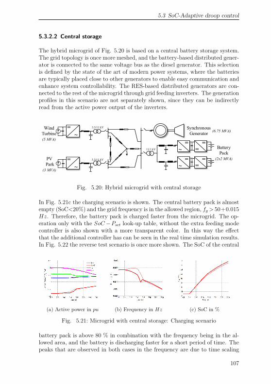
5.3 SoC-Adaptive droop control
5.3.2.2 Central storage
The hybrid microgrid of Fig. 5.20 is based on a central battery storage system.The grid topology is once more meshed, and the battery-based distributed gener-ator is connected to the same voltage bus as the diesel generator. This selectionis defined by the state of the art of modern power systems, where the batteriesare typically placed close to other generators to enable easy communication andenhance system controllability. The RES-based distributed generators are con-nected to the rest of the microgrid through grid feeding inverters. The generationprofiles in this scenario are not separately shown, since they can be indirectlyread from the active power output of the inverters.
SynchronousGenerator
=~
Wind Turbine(5 MVA)
=~ Battery
Pack(2x2 MVA)
==
=~
PV Park
(3 MVA)
3.3/11 kV
3.3/11 kV
11/1 kV
=~ =
=
(6.75 MVA)
Fig. 5.20: Hybrid microgrid with central storage
In Fig. 5.21c the charging scenario is shown. The central battery pack is almostempty (SoC<20%) and the grid frequency is in the allowed region, fg > 50+0.015Hz. Therefore, the battery pack is charged faster from the microgrid. The op-eration only with the SoC−Pset look-up table, without the extra feeding modecontroller is also shown with a more transparent color. In this way the effectthat the additional controller has can be seen in the real time simulation results.In Fig. 5.22 the reverse test scenario is once more shown. The SoC of the central
(a) Active power in pu (b) Frequency in Hz (c) SoC in %
Fig. 5.21: Microgrid with central storage: Charging scenario
battery pack is above 80 % in combination with the frequency being in the al-lowed area, and the battery is discharging faster for a short period of time. Thepeaks that are observed in both cases in the frequency are due to time scaling
107

5 Load sharing considerations
and would not appear if the test scenario would be conducted in real time basis.The impact of this algorithm on the frequency can be observed in Fig. 5.22b.
(a) Active power in pu (b) Frequency in Hz (c) SoC in %
Fig. 5.22: Microgrid with central storage: Discharging scenario
At t= 80 seconds, the proposed algorithm starts to discharge the battery faster,bringing the frequency closer to its tolerance band of 50± 0.015 Hz. That isa further advantage of the proposed algorithm. In case of over- (or under-)frequency, provided that there is also a need (or excess) of energy from the bat-teries, the frequency is brought back closer to its nominal value. In other words,the frequency state is exploited as a communication means for more reliablepower distribution.
5.3.3 Evaluation and further development of proposedalgorithm
The structure of nowadays grids moves towards increased used of communica-tion. Secondary and tertiary control are prevailing and electrical energy marketdefines the long-term power flow. However, with the penetration of renew-able energy sources storage is needed and should be integrated to the existinggrid. With the increased penetration of storage means the market characteris-tics should evolve and secondary control becomes more and more complicated.To overcome this problem, a basic algorithm is proposed which does not relyon communication. With the use of SoC-Adaptive droop control the autonomyof the grid is increased, since each distributed generator is supporting the gridand self-adjusting its power flow. The inherent drawbacks of the algorithm areevident:
• Dimensioning the capacity of battery systems: The guideline for the designshould be grid reliability. Therefore, each battery pack should be designedaccording to all other storage means present in the grid, so that the loadcan be efficiently distributed.• Long-term planning of power distribution: Constraints should be furtherintroduced to facilitate the long-term successful implementation of the al-gorithm in a well-defined microgrid concerning load forecast and generationcapacity.
108

5.4 Load sharing conclusions
• The proposed algorithm cannot be combined with a secondary grid control.This strategy is based on droop setpoints planning according also to gridfrequency deviations. As soon as these deviations disappear, or the iden-tical setpoints for all generators are altered, the algorithm can no longerserve its purpose.
Furthermore, the algorithm should be further investigated in combination withefficient battery charging and discharging methods. The strategy proposed inthis section can be characterized as a grid-friendly control algorithm. For costreduction, the factors that reduce battery lifetime and durability should also betaken into consideration.
5.4 Load sharing conclusions
In this chapter different aspects of load sharing in microgrids with various type ofdistributed generators are analyzed. The fundamentals of implementing droopcontrol for grid forming units with various rated powers in parallel are presented.The problematic of transient load sharing between synchronous generators andgrid forming inverters is further introduced. The influence that droop gains,load type and grid impedance have on the severity of transient load sharing isinvestigated. To overcome the instabilities that may occur during severe tran-sient load sharing cases the concept of frequency switching is proposed. In thisway, the grid forming inverter follows the transient response of the synchronousgenerator when its current is limited. Finally, a grid-friendly algorithm for gridforming units that connect battery packs is proposed to support the autonomyof distribution generation. Through this algorithm, each distributed genera-tor self-adjusts the power exchange with the microgrid, based on the measuredfrequency deviation and the state of charge of its battery pack.
109

6 Short circuit strategy
In the previous chapters the focus was on synchronization concepts and loadsharing considerations which are all not classified as severe transient phenomena.The most challenging point for the smooth operation of any electrical grid isdealing with faults. The goal of this chapter is twofold:
• to document the transient response of medium voltage microgrids duringand after faults.• to introduce the necessary control modifications for each distributed gen-erator to support the microgrid during these severe transients.
These control modifications are classified as a short circuit strategy. The at-tributes and objectives of this strategy follow these guidelines:
• It has become evident in this work that the focus is the inverter-basedgenerators, as main components of (hybrid) microgrids. We have seen thatthe inverters in grid-forming or grid-feeding mode can follow the controlreferences and adapt the behavior that any grid operator demands, whichis a basic advantage in their employment in any power systems. Their ma-jor disadvantage however is their inherent disability to produce overcurrentneeded for fault detection and isolation. A basic attribute of the developedshort circuit strategy is that it is based on the traditional over-current pro-tection scheme. Therefore, the short circuit current should be maximizedand inverter’s oversizing is investigated.• Autonomy: In this work no solutions are considered based on communica-tion. As in chapter 2 explained, there are several industry products that arebased on central controllers. This is unavoidable for optimal energy plan-ning and operational management, since different parameters and states ofgenerators are needed. In this work, similar to chapter 5, the worst-casescenario is considered, when communication is not available or possible.Moreover, to react upon a fault, a robust solution should be independentof communication delays that could be up to a few grid periods.• Modularity: Since the strategy is not based on a central controller, thegrid topology can be expanded or reduced and that should not alter theindividual controller of each inverter-interfaced distributed generator.
110

6.1 Protection means
6.1 Protection means
Before looking into details the control structure of each distributed generator,a short presentation of the protection means that prevail in modern power sys-tems should be performed. The protection means are based on the detection ofover-current and isolating the distribution lines involved in the fault. Typicalovercurrent-tripping time characteristics for line circuit breakers, are shown inFig. 6.1 ( [122]). The four different types (A,B,C,D) depend on the applicationconditions of the breaker and overloading demands. The different characteris-tics also aid in the realization of selective protection and assisting a rapid faultdetection [122]. The form of the characteristic remains the same, independent
10
Tripping time, tt
Min
utes
Seco
nds
0.010.050.10.515
30
1
5
20
6040
Multiple of the rated current In
1 1.5 2 3 4 5 6 7 8 10
ABCD
1.13 In
Fig. 6.1: Typical tripping characteristics of circuit breakers
of whether the protection device is based on a fuse, a circuit breaker or relay.These characteristics do always include also a tolerance band, that eases theimplementation and tuning of each protection means based on the electrical in-stallation that needs to be protected. The limits of these tolerance bands arethe case of e.g. conventional tripping and non-tripping current for line circuitbreakers. Observing Fig. 6.1, it is obvious that difficulties rise in the installationof protection means if inverter-based distributed generators dominate a grid. Itis common practice to up-rate the inverter in order to provide maximum supportin fault cases, but the uprating is far from enough to cover the values shownin Fig. 6.1. For grid feeding inverters it is standard to oversize up to 1.5 to 2pu [123], [16], [124] and for grid forming units up to 3-5 pu [16] [125]. Otherapproaches refer to uprating the inverter to 2 pu independent of the applica-tion [126], [127], [128]. Therefore, it is evident that the protection means shouldget more intelligent, to successfully deal with faults in inverter-dominated grids.Such an intelligent approach would be rapid communication schemes that des-
111

6 Short circuit strategy
ignate relays hierarchy for selective protection, to optimize the time needed toidentify fault location [129]. Another approach for inverter-dominated grids is tointegrate an extra storage system that could provide, for a short period of time,over-currents needed for the fault detection [124], [130]. Selecting and designinga ultra-capacitor based storage system designated for providing fault current inisolated microgrids can be found in [131].The problematic of developing a short circuit strategy for islanded grids thatcannot supply the necessary over-currents has existed before the development ofgrid inverters. A typical example is isolated on-board grids of ships. In that case,the problem of distinguishing between overloading conditions and faults has ap-peared, since the diesel generators forming the grid might not provide in all casessufficient short circuit current. A solution towards utilizing the measured gridadmittance during the fault instead of over-currents has been proposed in [132].However, this approach has limited applicability in inverter-dominated grids,since the measurement is prone to disturbances, and moreover it also requires aspecific amount of over-currents from the generators to facilitate the admittancemeasurement.The focus of this short circuit strategy is the control structure of the inverter-based distributed generator and how should they react upon the appearanceof a fault. As previously mentioned, no approaches are investigated which arebased in communication. That could be the case of a master-slave principle,where grid forming inverters working in parallel are properly synchronized andbuild up a frequency-dependent fraction of the fault current [133]. Since theover-current provision of inverter-based distributed generators is limited, thelimits between overloading conditions and fault conditions tend to disappear.Therefore, in such inverter-dominated microgrids, overloading conditions shouldbe avoided. That would be the case of higher inrush currents of transformers ordirectly-coupled motors with no power electronic interface. The control modifi-cations introduced in this chapter focus only on the generators of the microgrid.A necessary expansion of the proposed strategy is to design the tolerances forprotection means and loads accordingly.
6.2 Grid forming inverter
The focus of the short circuit strategy for the grid forming inverter is the cur-rent limiting method implemented to protect all inverter’s components. Thewidely implemented cascaded control structure in SRRF presented in chapter 3is the only control structure implemented in this work. The cascaded multi-loopcontrol structure offers the inherent possibility to insert a current reference lim-itation between voltage and current control level. This is the main advantage ofthe grid forming control based on the multi-loop method, opposed to a simplesingle-loop voltage control. In single loop grid forming structures, the voltagereference should be rapidly reduced to effectively limit the current. That could
112
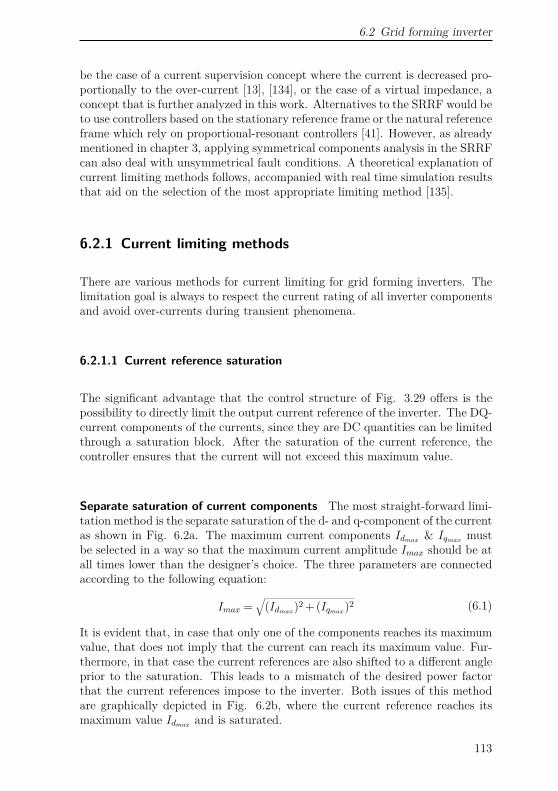
6.2 Grid forming inverter
be the case of a current supervision concept where the current is decreased pro-portionally to the over-current [13], [134], or the case of a virtual impedance, aconcept that is further analyzed in this work. Alternatives to the SRRF would beto use controllers based on the stationary reference frame or the natural referenceframe which rely on proportional-resonant controllers [41]. However, as alreadymentioned in chapter 3, applying symmetrical components analysis in the SRRFcan also deal with unsymmetrical fault conditions. A theoretical explanation ofcurrent limiting methods follows, accompanied with real time simulation resultsthat aid on the selection of the most appropriate limiting method [135].
6.2.1 Current limiting methods
There are various methods for current limiting for grid forming inverters. Thelimitation goal is always to respect the current rating of all inverter componentsand avoid over-currents during transient phenomena.
6.2.1.1 Current reference saturation
The significant advantage that the control structure of Fig. 3.29 offers is thepossibility to directly limit the output current reference of the inverter. The DQ-current components of the currents, since they are DC quantities can be limitedthrough a saturation block. After the saturation of the current reference, thecontroller ensures that the current will not exceed this maximum value.
Separate saturation of current components The most straight-forward limi-tation method is the separate saturation of the d- and q-component of the currentas shown in Fig. 6.2a. The maximum current components Idmax & Iqmax mustbe selected in a way so that the maximum current amplitude Imax should be atall times lower than the designer’s choice. The three parameters are connectedaccording to the following equation:
Imax =√
(Idmax)2 + (Iqmax)2 (6.1)
It is evident that, in case that only one of the components reaches its maximumvalue, that does not imply that the current can reach its maximum value. Fur-thermore, in that case the current references are also shifted to a different angleprior to the saturation. This leads to a mismatch of the desired power factorthat the current references impose to the inverter. Both issues of this methodare graphically depicted in Fig. 6.2b, where the current reference reaches itsmaximum value Idmax and is saturated.
113

6 Short circuit strategy
Iq*
Id*
Current controller
Voltage controller
(a) Separate saturation
Iq
Id
Idsat
Iqsat
Id*
Iq*
Iqmax
Idmax
(b) Saturation mismatch
Fig. 6.2: Current components separate limitation
Current amplitude saturation To fully exploit the current rating of the in-verter’s components, it is desired to develop a method that can limit the cur-rent amplitude to the designer’s choice. In this way, the two negative aspectsexplained in the previous paragraph can be tackled. The current reference am-plitude |I∗
dq| and the vector angle δdq that results from the DQ-components isrequired for this method:
|I∗dq|=
√(I∗d)2 + (I∗
q )2 (6.2)
δdq = tan−1(I∗q
I∗d
)(6.3)
The amplitude is then directly limited and the angle is needed for the calculationof the saturated values of each current component, as shown in Fig. 6.3a.
Idsat
Iqsat
Id*
Iq*
Eq. 6.2&
Eq. 6.3
Eq. 6.4&
Eq. 6.5
Idq*
δdq
Idqsat
(a) Implementation
Current controller
Voltage controller
Iq
Id
Idsat
Iqsat
Id*
Iq*
(b) Vector amplitude saturation
Fig. 6.3: Current amplitude saturation
where:Isatd = cos(δdq) · Isatdq (6.4)
Isatq = sin(δdq) · Isatdq (6.5)
An alternative approach for the implementation of Fig. 6.3a is setting a satu-rated value once the limitation is activated. The current amplitude is calculatedand compared with its maximum value. As soon as the limitation is reached,the reference switches to fixed values. The saturated values for each component
114

6.2 Grid forming inverter
Current controller
Iq*
Id*
Voltage controller(Id
*)2 +(Iq*)2
Idsat
Iqsat
(a) Under normal operation
Current controller
Iq*
Id*
Voltage controller(Id
*)2 +(Iq*)2
Idsat
Iqsat
(b) with current limitation activated
Fig. 6.4: Current limitation through saturated values
are given in Eq. 6.6.
Isatd = I∗d√
(I∗d)2 + (I∗
q )2Imax , Isatq =
I∗q√
(I∗d)2 + (I∗
q )2Imax (6.6)
This approach of setting saturated values as soon as a limit is reached is com-mon for controllers in the stationary reference frame or the natural referenceframe [136], [137] and [127]. In that case the current reference is not a DCquantity and the standard saturation method cannot be implemented. Thedisadvantage of this method is that switching between signals can lead to insta-bilities when operating near the boundaries. That means that it is possible toswitch back and forth between values during the transient state, that could leadto system instability. This can be identified as controller state ’latching’ andcould be dealt with trip and reset logic signals that supervise the transition [41].Since in this work all control structures are implemented in the synchronous ro-tating reference frame, the direct amplitude saturation of Fig. 6.3 is preferred.
6.2.1.2 Transient virtual impedance
A substitute to the saturation of the current reference would be the implemen-tation of a transient virtual impedance. The concept of virtual impedance is amethod of creating an artificial impedance at the output of an inverter throughits controller. In other words, it is a way of forcing the inverter’s controller toadjust its references as if an additional impedance was present in the circuit.The manipulation of the measured current and (or) voltage is required to builtup this virtual impedance.The virtual impedance principle is well known for optimizing the grid connect-ing impedance of an inverter, to ease reactive power sharing, or facilitate droopcontrol in ohmic low voltage grids [138], [139]. This fixed virtual impedanceimplementation will be further named steady state virtual impedance, since itis independent of the grid load. Virtual impedance can however be exploitedto achieve current limitation in case of overloads, named in this case transientvirtual impedance. The transient virtual impedance is mostly implemented as
115

6 Short circuit strategy
a series element in the circuit [140], [141], [142], alternatives however do existthat implement the impedance in parallel with the LCL filter capacitor [143]. Inthis work the virtual impedance in series is only considered, as it will be shownthat it provides the faster response to a fault. A simplified form of virtualimpedance principle is found also in [144]. There, in case an over-current is de-tected, the actual current is multiplied with a scalable gain, in order to limit itsvalue in the safe operational region and the inverter does not sense the presenceof overload or fault. In case of steady state virtual impedance selecting a properimpedance ratio is carefully performed, depending on the grid topology and thedesired load sharing. Most of the steady state virtual impedances are inductive,due to the derivation of droop control which is based on high voltage inductivegrids. In the case of transient virtual impedance however, it is a complicatedmatter on how to properly design the impedance ratio. One way of selectingthe impedance ratio is by evaluating the system stability around an equilibriumpoint. Instability can be produced due to the digital implementation of virtualimpedances, for example through the sampling delay of the inverter’s processingunit. It has been demonstrated that, if all practical implementations of a mixedvirtual impedance are taken into consideration, increasing the inductive part ofthe impedance decreases the stability margin near the equilibrium point [145].In this work the focus lies on implementing a pure resistive transient virtualimpedance.The goal of the current limitation is to limit the inverter’s current, i1 as shownin Fig. 6.6a. It would therefore be expected to place the transient virtualimpedance in the loop between inverter and filter capacitor. It can be howevershown that it is more reasonable to select the grid current i2 and to place thevirtual impedance after the capacitor. The reason is twofold. First, the invertercurrent is not sinusoidal and has a high frequency ripple which can be filteredout, introducing however a time-delay due to the filtering method. Secondly,for the transient virtual impedance it is of high importance to act rapidly andlimit the current as soon as possible. It can be shown that the transfer functionGcu = I2
I1shows a low pass filter behavior, and the outer current reacts to the
transient effect faster. The transfer function output to input current, Gcu iscalculated in Eq. 6.7, treating the grid part as a disturbance to the behaviorof the filter, and incorporating also Rd, the resistor used for passive dampingof the LC filter resonance. All variables can be identified in Fig. 6.6a, similarto the theoretical model of the grid interface of an inverter with LCL filter, aspreviously shown in Fig. 3.17.
Gcu = I2(s)I1(s) = RdCfs+ 1
L2Cfs2 + (R2 +Rd)Cfs+ 1 (6.7)
It can be seen from Fig. 6.5 that the behavior of Gcu is similar to a low pass fil-ter. Therefore the output current i2 is chosen to build up the virtual impedance.Instabilities when selecting the inner inverter current for the realization of tran-
116

6.2 Grid forming inverter
−30
−20
−10
0
10
Mag
nitu
de (d
B)
102 103 104 105−90
−45
0
Pha
se (d
eg)
Frequency (rad/s)
(a) Bode plot
0 0.5 1 1.5 2 2.5 30
0.2
0.4
0.6
0.8
1
1.2
1.4
Time (milliseconds)
Am
plitu
de
(b) Step response
Fig. 6.5: Steady state and dynamic response of Gcu
sient virtual impedances have also been documented in [103]. The transientvirtual impedance can be calculated as shown in Fig. 6.6b.
R1 L1 R2L2
Cf
i1 i2
iC
-
+
Vg
Rv
Rd
Vi
(a) Circuit integration
I2
Rv
Rvmax
Ith Imax
(b) Non-linearity of virtual impedance
Fig. 6.6: Representation of transient virtual impedance
The implementation of the virtual impedance is depicted in Fig. 6.7. The imple-
Vd*
Voltage controller
-I2dRv( ) I2
0
If > IthI2
0
Vq*
- I2qRv( ) I2
Fig. 6.7: Implementation of transient virtual impedance
mentation reveals the main disadvantage of the transient virtual impedance, theswitching between states. Since it is not desired to have a virtual impedance ac-
117

6 Short circuit strategy
tive during normal operation, a non-linear transient impedance is formed, whichis activated as soon as the current exceeds the limit Ith, as shown in Fig. 6.6b.The linear increase of the virtual resistor depending on the current amplitudehas a further impact on the voltage and current coupling. Following Ohm’s law,in the case of a resistor there is a linear relation between voltage and current.Introducing such a non-linearity alters this relation, as explained in the followingequations:
Rv = VRv
I2Rv = αI2 (6.8)
where VRv is the amplitude of the virtual voltage drop across the virtual resistor,I2 the amplitude of the outer current and α is the linear relation of the virtualresistor and the current amplitude, when the current exceeds its threshold value.Combining both equations shown in Eq. 6.8, the following equation is obtained:
VRv = aI22 (6.9)
It is therefore concluded that introducing the non-linear virtual resistor withlinear dependence on the current a quadratic relation between voltage and cur-rent is formed. This calculation does not take into consideration the delays thatare introduced through the voltage and current controller of the inverter thatrealize the transient non-linear virtual resistor.For the calculation of Rvmax the worst case scenario is needed. This is chosenas the case where the fault occurs directly at the output of the grid forminginverter, at its PCC. In this way the grid impedance is minimum and the max-imum current should be provided from the inverter.
~
= i1
VC
i2
PCC
L1
Cf
L2
(a) Fault location for worst-case
Cf
R1 i1 i2
+
-
Vc Ltr
RvmaxL1 R2L2
LVi
(b) Single-phase equivalent
Fig. 6.8: Circuits for calculating Rvmax
The damping resistor Rd is omitted for the calculation as shown in Fig. 6.8since its value is insignificant compared to the rest of the circuit elements. Themaximum virtual resistor, Rvmax is then given by the following equation.
Rvmax =√√√√∆V 2
I2max
− (ω(L2 +Ltr))2−R2 (6.10)
where ∆V is the voltage drop that should be artificially built to resemble thevirtual resistor. In this work it is selected equal to 0.95 pu, leaving an operationalmargin for the voltage during fault.
118

6.2 Grid forming inverter
6.2.2 Theoretical fault models
To better understand the transient behavior of the grid forming inverter, theo-retical fault models are derived. These models can be used to conduct stabilityanalysis of more complex grid structures. From the single-phase control rep-resentation of the grid forming inverter depicted in Fig. 6.9, simplified faultmodels can be calculated [137]. The dotted lines in Fig. 6.9 indicate the cur-
VC
VC*
-GV(s)
I2
FI1
*I1
-GC(s)
-VC
I2
Inverter +LC Filter
Vi*
PWMVi
-
Lf s+Rf
1
Cf s1
Fig. 6.9: Single-phase control representation with current limiting
rent limiting methods of current reference saturation or virtual impedance. Thetransfer functions of the voltage and current PI controllers are GV (s) & GC(s)respectively and F is the feed-forward factor for the output current. Analyzingthe control structure of Fig. 6.9 the following equivalent structures can be ob-tained. During normal operation, the grid forming inverter can be represented as
G0(s)VC*
Z0(s) I2
VC
(a) with virtual impedance
Gcl(s)I1sat*
I2
VCCf
(b) with current reference saturation
Fig. 6.10: Inverter simplified fault model
a controlled voltage source behind an impedance, quite similar to the representa-tion of a synchronous generator in power system stability studies [10]. However,when the current limitation is active, the grid forming inverter can no longercontrol the output voltage and behaves like a controlled current source behindthe filter capacitor. Fig. 6.10 shows the respective equivalent circuits. Equa-tions 6.11-6.13 provide the necessary calculations to reach these simplifications.
119

6 Short circuit strategy
G0(s) = GV (s)GC(s)sCf [GC(s)− (Rf + sLf )] +GV (s)GC(s) (6.11)
Gcl(s) = GC(s)GC(s)− (Rf + sLf ) (6.12)
Z0(s) = GC(s)[F −RvGV (s)−1] + (Rf + sLf )sCf [GC(s)− (Rf + sLf )] +GV (s)GC(s) (6.13)
It is shown that the inverter transforms into a current source when the currentreference saturation is activated. In the case of virtual impedance however, theinverter is able to control its output voltage similar to normal operation. Inother words, the voltage controller remains active during the fault. The inverterstill operates as a voltage source with a modified grid-interfacing impedance.This could be a great advantage as far as stability investigations are concerned,since:
• the grid voltage is maintaned under control even in fault case.• non-linearities introduced due to the current limiting method and the trans-formation to current source can be eliminated.• systems based on more than one inverters can be easier analyzed, since eachconverter operates still as a voltage source with a defined output voltageand impedance, opposed to current source operation.
The equations 6.11-6.13 and therefore the theoretical fault models derived fromthem do not include the practical implementation issues coupled with the virtualresistor. First, the transient nature that includes a switching event is not takeninto consideration. Secondly, the non-linear relation between transient virtualimpedance and output current, Rv(I2) could not be included in the calculations,since it would complicate the simplified equivalent circuits. The impact of thesetwo important implementation elements of the virtual resistor on the systemresponse is discussed in the following sections.
6.2.3 Evaluation of current limiting methods
The previously described control methods are compared in real time simulationscenarios. The two main scenarios needed for the performance evaluation in-clude fault response in standalone and parallel operation. The fault is simulatedas a three phase symmetrical fault that lasts 10 grid periods. The fault detec-tion and clearance is not part of these investigations, however the selected faultduration represents a worst-case scenario of the time needed from typical pro-tection means to isolate a distribution line fault. In standalone operation, thegrid forming inverter is the only grid forming unit in the microgrid. Therefore,the dynamic and stable response of the inverter to a fault is the main compar-ison criterion. Parallel operation means that more than one grid forming units
120

6.2 Grid forming inverter
are working in parallel. In our investigations, the parallel operation of a gridforming inverter with a synchronous generator is chosen as a realistic scenario.The transient response of the microgrid, as far as voltage and frequency stabilityare concerned, is the main investigation aspect.For the real time simulation scenarios that follow the vector amplitude satura-tion (limitation) is compared with the introduced transient virtual impedance.The alternative current reference saturation methods are not further consideredsince:
• The separate saturation does not fully utilize the current rating of theinverter.• Setting saturated values requires further implementation complexity andintroduces switching between different references that can cause unwantedtransient effects.
6.2.3.1 Standalone operation
The current limiting methods are compared based on their transient robustness,with the following criteria:
• fast provision of over-current• stable current limitation during fault• exiting limitation state with minimum transient effect
In standalone operation the frequency response could also be a tool to evaluatethe current limiting methods. However, the frequency control is realized throughthe transformation angle for the SRRF and it is not directly affected from thesaturation of the PI controllers. Therefore, the controllability of the frequencycannot really be exploited as a comparison criterion.The rated power for the grid forming inverter for both standalone and paralleloperation is selected at Sinv = 2MVA. However, the current rating of the in-verter is selected in this case equal to Imax = 3 pu. In this way, an overcurrentprovision can be ensured to aid in fault detection and isolation. In the follow-ing figures (V AL) stands for vector amplitude limitation and (V I) for virtualimpedance. In Fig. 6.11a the amplitude of the converter current, I1 is shownfor standalone operation since this is the current that should be limited. De-spite the fact that the vector amplitude limiting method appears to react fasterthan the virtual impedance method, the latter produces smoother transitions,especially while exiting the current limitation. The results for both limitingmethods seem quite similar as far as the converter current amplitude and hencethe protection of inverter components is concerned. To obtain a more detailedinsight, the amplitude of the voltage across the filter capacitor is depicted inFig. 6.11b. It can be observed that the virtual impedance method, since itprovides a smoother and slower response than the vector amplitude limitationshows no over-voltages while exiting the fault, but produces a higher voltage
121

6 Short circuit strategy
2 2.05 2.1 2.15 2.2
1
1.5
2
2.5
3
Time [s]
I1[pu]
VALVI
(a) Converter current amplitude
2 2.1 2.2 2.30
0.2
0.4
0.6
0.8
1
Time [s]
VC[pu]
VALVI
(b) Capacitor voltage amplitude
Fig. 6.11: Fault response of grid forming inverter in standalone operation
drop upon the fault activation. The conclusion from the standalone operation isthat both methods can achieve satisfactory results with the virtual impedancemethod producing a more stable current response with the expense of excessivevoltage drop compared to vector amplitude limitation.
6.2.3.2 Parallel operation with synchronous generator
Since the focus of this work are hybrid microgrids, the parallel operation ofthe grid forming inverter with the synchronous generator is also a fundamentaltest scenario for performance evaluation. The circuit shown in Fig. 6.12 andthe parameters for the synchronous generator given in Table A.3 are used forthis test scenario. This topology represents a worst-case scenario, since thegrid impedance connecting the two grid forming units is minimal. We haveseen in chapter 2 that the stability margins, as far as system eigenvalues areconsidered, increase with increasing lengths of the distribution lines between gridforming units. The worst case scenario for the fault location which minimizesthe grid impedance is also in this case considered. The fault is located at thecommon voltage bus of the two generators. The fault duration and impedanceare identical to the test-scenarios for the standalone operation. In the followingfigures, GForm stands for grid forming inverter and SG stands for synchronousgenerator. The current depicted, IGen denotes the synchronous generator outputcurrent and the converter current. The test scenario of the parallel operationis performed once for the case of vector amplitude limitation (V AL) and isrepeated for the case of virtual impedance limitation (V I).
122

6.2 Grid forming inverter
~
=
PCC
Fig. 6.12: Topology for parallel operation
The first observation from Fig. 6.13 is that the current limitation is in both casessuccessful and the inverter provides the selected maximum 3 pu overcurrent.The synchronous generator on the other hand is able to provide a significantlyhigher amount of overcurrent reaching almost 6.5 pu. Oscillations occur, whichis to be expected due to the rotational speed swings of the generator. Thetransient phenomenon after the fault is cleared lasts in both cases almost 2seconds. Comparing Fig. 6.13a & Fig. 6.13b it is observed that with thevirtual impedance method the current reaches faster its maximum limit. Thisbehavior deviates from the results obtained for the standalone operation. Sincethe inverter in this scenario is not the only grid forming unit in the microgrid,the transient response is affected by the oscillating response of the synchronousgenerator. The deviation from the maximum value of the current in the case
40 40.5 410
1
2
3
4
5
6
7
Time [s]
IGen[pu]
SGGForm
(a) with vector amplitude limitation
40 40.5 410
1
2
3
4
5
6
7
Time [s]
IGen[pu]
SGGForm
(b) with virtual impedance
Fig. 6.13: Generator current amplitude during parallel operation
of vector amplitude limitation is less than 0.1 pu and it is elliminated aftera few grid periods. Therefore, this deviation is not considered as a significantcomparison criterion. The main difference however between both methods occurswhen the virtual impedance is deactivated. At about t= 40.9 seconds the current
123

6 Short circuit strategy
reaches the selected threshold value, Ith = 1.1 pu, and the virtual impedance isswitched off. To further examine the impact of this transient effect, the voltageof each distributed generator VGen is shown in Fig. 6.14.
40 40.5 41 41.5 420
0.2
0.4
0.6
0.8
1
Time [s]
VGen[pu]
PCC voltageCapacitor voltage
(a) with vector amplitude limitation
40 40.5 41 41.5 420
0.2
0.4
0.6
0.8
1
Time [s]VGen[pu]
PCC voltageCapacitor voltage
(b) with virtual impedance
Fig. 6.14: Generator voltage amplitude during parallel operation
The output voltage of the synchronous generator is the PCC voltage, whereas thefilter capacitor voltage is chosen for the inverter, to directly show the influence ofthe voltage control loop. There are no overvoltages present applying the vectoramplitude limitation method and a steady state point is reached smoothly. Onthe other hand, an over-voltage is visible for the transient virtual impedancemethod. The reason is two-fold:
• First, the non-linearity of the virtual resistor. The linear dependence of thevirtual resistor on the output current, does not consider the existence ofother generators working in parallel. The interactions of the inverter withother generators cause a deviation on the interconnection of the actualinverter current I2 with the non-linear virtual resistor as shown in Fig.6.15. It is to be expected that in the region of the current between Ith
(pu)I2
Rv
Rvmax
ImaxIth
Effect of other generators
Fig. 6.15: Mismatch of virtual impedance calculation
- Imax the grid impedance, which is in series with the virtual resistor,has a non-negligible value and causes deviations from the pre-calculated
124

6.2Gridforminginverter
lineardependenceofcurrentamplitudeandtransientnon-linearvirtualresistor.Sincecalculatingtheactualgridimpedanceaswellastheloadsharingbetweengeneratorsinrealtimeandadjustingthenon-linearityofthevirtualresistoruponthemposesseveredifficulties,onlythelineardependenceisconsideredinthiswork.Uponfaultclearance,theinverter’scontrollerdoesnotcooperateideallywiththevirtualresistorsincetheoscillationsofthesynchronousgeneratordirectlyaffecttheloadthattheinvertershouldtakeoverandover-voltagesareproduced.
•
40 40.5 41 41.50.985
0.99
0.995
1
1.005
1.01
1.015
1.02
1.025
Time[s]
SG: ωm
GForm: f
Droop
fPLL
Thedeactivationofthevirtualimpedance.Sincethevirtualresistancede-pendsonthecurrentamplitudeandnotoneachd-orq-componentofthecurrent,thedeactivationofthevoltagedropoftheq-componentproducesthisjumpofthevoltage.Anoptimizationtoeliminatethisjumpwouldbetotransformthevirtualresistorfromcurrentamplitudetocurrentcompo-nentdependent,butthatwouldleadtonotutilizingthefullcapabilityoftheinverter,whichisbasedonthecurrentamplitude.
Tocompletethecomparison,thefrequency-relatedparametersofthehybridmicrogridaredepictedinFig.6.16.Themechanicalrotationalspeedofthesyn-chronousgeneratorisshown,alongwiththedroopcontrolreferenceforthegridforminginverter.ThegridfrequencyatthecommonvoltagebusdetectedwithaPLLisalsoincludedinthefiguretovalidatethatthesystemstartsandreturnstothesamesteadystatepoint.ThemeasuredPLLfrequencyduringthefaultistobediscarded,sincethevoltageislessthan0.01puandthemeasurementisthereforeunreliable.
40 40.5 41 41.50.985
0.99
0.995
1
1.005
1.01
1.015
1.02
1.025
Time[s]
SG: ωm
GForm: f
Droop
fPLL
(a)withvectoramplitudelimitation (b)withvirtualimpedance
Fig.6.16:Frequency-relatedparametersduringparalleloperation
Aspreviouslystated,frequencyswingsoccurwhichareduetotheinertiaoftherotorofthedieselgenerator.Ontheotherhand,thefrequencyreferenceofthegridforminginvertertriestopullupthefrequencytoareferencecloseto1pu.Sincethevoltagedropsandthecurrentincreases,theoutputpowerremainswithinnormaloperationlimitsandthereforethefrequencyreferenceisclosetoitsnominalvalue.Inthisoperationthedroopcurvesareselectedidenticalfor
125

6 Short circuit strategy
both diesel generator and grid forming inverter with Pset = 0.5 pu. It is shownin Fig. 6.16a that the frequency reference during the fault is higher than thenominal frequency. That means that the inverter, despite the fact that it de-livers Imax = 3 pu, the active power output is less than 0.5 pu. This is due tothe grid impedance that the inverter ’sees’ as a load. This impedance is mainlyinductive, since the filter and transformer inductive impedance are a few ordershigher than the fault resistance chosen to be Rfault = 1mΩ. The frequency re-sponse of the grid forming inverter during the fault is in both limiting methodsalmost identical. Comparing closely Fig. 6.16a & 6.16b it is observed that theover-speed of the generator after the fault is slightly higher, and also at t= 40.9seconds, the deactivation of the virtual impedance is once more evident.Therefore, in parallel operation with the synchronous generator the vector am-plitude limiting method achieves better performance than the virtual impedancelimiting method. The virtual impedance is introduced as an intelligent solutionto overcome the non-linearities that are introduced with the limiting methodsbased on current reference saturation. However, the practical problems that arisewith its implementation, and the effect that the unpredictable grid impedancehas on the system behavior lead to the selection of the vector amplitude lim-iting method as the method that performs quite well in both test-scenariosdocumented in this section.
6.2.3.3 Parallel operation with no current over-rating
The last test scenario to evaluate current limiting methods for grid forminginverters is the case when the inverter is not over-sized and the current limitationis close to its nominal value, Imax = 1.1pu. In this case the synchronous generatoris the dominant grid forming unit in the microgrid, with the grid forming inverterplaying a secondary role in the over-current provision. The implementation ofthe transient non-linear virtual impedance is practically not feasible, since Imaxand Ith have the same value. If the virtual resistor was implemented, uponits activation a significant jump on the voltage would appear, since the virtualimpedance would not be non-linear, but fixed to its maximum value, Rvmax. Theperformance of the current vector amplitude limitation is shown in the followingfigures, to demonstrate stable parallel operation with the sychronous generator,even in the case of no over-current provision from the inverter. It can be seenfrom Fig. 6.17a that the transient effect of the short-circuit forces the inverterto remain longer with its current limitation activated. This is due to the factthat the synchronous generator cannot instantly return to its prior fault loadingconditions and during that period the inverter takes over the excess load. Thiseffect can be clearly observed in the output voltage, see Fig. 6.17b. As longas the current limitation of the inverter is active, the voltage is lower than thenominal value. Comparing Fig. 6.14a with Fig. 6.17b, it can be seen thatwithout over-current provision from the inverter, the voltage restoration showsworse transient behavior. Similar to the output voltage, the decisive parameters
126

6.2Gridforminginverter
40 40.5 410
1
2
3
4
5
6
7
Time[s]
SGGForm
(a)CurrentIGenin
40 40.5 41 41.5 420
0.2
0.4
0.6
0.8
1
Time[s]
PCC voltageCapacitor voltage
pu (b)VoltageVGenin
40 40.5 41 41.50.985
0.99
0.995
1
1.005
1.01
1.015
1.02
1.025
Time[s]
SG: ωm
GForm: f
Droop
fPLL
pu (c)Frequencyinpu
Fig. 6.17:Paralleloperationwithnoover-rating
forthefrequencyresponseinFig.6.17ciscomparedwiththecorrespondingresultsinFig.6.16a.Asamaindifference,inFig.6.17calowerover-speedforthesynchronousgeneratorcanbeidentified.Here,theinfluenceoftheinverteronthegridfrequency,namelytryingto’pullitup’closetoitsnominalvalueissmaller,sinceitcontributeswithaquitesmallerfaultcurrent. Therefore,thesynchronousgeneratorisnotinfluencedbythepresenceoftheinverteranditsover-speedisreduced.Thishoweverdoesnotleadtofasterfrequencyrestoration,sinceinbothcasesthefaultrecovery,asfarasthefrequencyisconcerned,lastsupto1.5seconds. ThePLLresponseseemstobeslowerinthecaseofnooverrating,butthisdependsalsoonthevoltagebeingmeasured,whichhasnotreacheditssteadystateyetandcanhaveanegativeimpactonthefrequencymeasurement.Concludingtheseinvestigations,itcanbeseenfromtheresultsthatthevectoramplitudelimitationmethodcanachievepromisingresultsinallcases,whereasthevirtualimpedancemethodhasweakpointsthatarisefromitspracticalimplementation.
6.2.4 DCandACcomponentsrating
Theratingofthecomponentsofeachdistributedgeneratorisasignificantel-ementoftheproposedshortcircuitstrategy. Therefore,itisproposedtodis-tinguishbetweeninverterandACpartrating,andDCpartandinputenergysourcerating. Thecurrentlimitingmethodfortheinverterwasexplainedintheprevioussection.ToproceedwiththeratingselectiontheDCpowersourceshouldbedefined.Inthischapterabatterypackisconsidered,usingthemodelproposedinchapter3.InFig.6.18thedistributedgeneratorbasedonthebat-terypackisshown.TwonewcomponentsareintroducedinadditiontoFig.3.39andFig.3.30toensurethestableoperationwithdifferentratingfortheDCandACpartsofthedistributedgenerator.First,thesaturationofthecurrentreferencefortheD-component.ThegridforminginvertercannotdemandinthiswaymoreactivepowerthanwhattheDC-partcandeliver.Secondly,afurthercurrentlimita-
127

6 Short circuit strategy
~
=iL
VDC
+-
Battery Cells
np
DC-link voltage controller
VDCCurrent
controller
iL
PWM
(Ah)
(V)
SoC Estimation
VOC
C
VDC*
i1
VC
PCC
L1
Cf
i2 L2
Current controller in SRRF
PWM
i1
Iq*
Id*
PQ calculation and droop
control
VC i2
*Voltage
controller in SRRF
V*f *
Vd*
Vq*
δ*
δ* i2 VCVC
I (pu)
0
Imax
Idmax
-Idmax
iILmax
-ILmax
Fig. 6.18: Distributed generator based on a battery pack
tion is introduced for the current reference for the DC/DC converter to limit theoutput current of the battery. The two limits, Idmax, ILmax are selected equal(in pu) so that the power flow to/from the DC-link can remain intact. It willbe demonstrated in the next section that for the case of grid feeding invertersthese limits are different, depending on the grid voltage. For the grid forminginverter however that is not the case, since the inverter is considered a load forthe input source and the input DC current is adjusted dynamically based onthe inverter output current. Since the battery pack, or any other energy powersource that could be the input of the grid forming inverter, typically costs signif-icantly more than the AC-part of the distributed generator, it is reasonable toselect Imax > Idmax. This selection is performed not only for cost reduction, aswell as for technical considerations and advantages. First of all, there should bea protection margin between the two values to overcome transient effects thatmight occur. Second, since the goal of the short circuit strategy is to maximizethe fault current, oversizing only the grid forming inverter could lead to increas-ing the available reactive power to be provided. This is further investigated inthe next sections, where the grid feeding inverter is also considered to contributeto the fault current.
6.3 Grid feeding inverter
The control objective for the grid feeding inverter during fault is quite morestraight-forward than the grid forming inverter. That is because grid feedinginverters prevail in mainland ’stiff’ grids (see Fig. 2.1a) and grid codes andguidelines have been introduced that govern their behavior. In the case of gridforming inverters however, which are not thought to operate in parallel with thestiff grid but to build a weak microgrid (see Fig. 2.1b), the operational guidelinesare currently developed. In this work, as explained in the previous section, the
128

6.3 Grid feeding inverter
grid forming inverter is able to provide a certain amount of over-current. That ishowever insufficient for building-up the over-currents that are needed for typicalprotection means, as seen in Fig. 6.1. Therefore, also the grid feeding invertersshould aid in this direction, stay connected during faults and provide up to theirrated current in all cases. In this section, starting from the traditional grid coderequirements for grid feeding inverters, their suitability is investigated in thecase of hybrid microgrids and guidelines are also in this case derived.
6.3.1 Grid code requirements
The grid code requirements for static grid support from grid feeding inverterswere shortly mentioned in chapter 3. The reactive current injection more specif-ically was shown in Fig. 3.22. The case of grid over-voltages and consequentlyreactive current absorption is not considered in this work, since the focus is faultcases which cause significant voltage drops. Analyzing once more Fig. 3.22, it isevident that the grid feeding inverter should remain grid-connected and inject 1pu reactive current. The questions that rise are time-related: how long shouldthe inverter remain grid connected and how fast should the reactive currentinjection be realized.
Fault duration For the maximum fault duration fault-ride-through character-istics have been included in the grid codes [61] and a typical curve is shownbelow in Fig. 6.19. Analyzing Fig. 6.19, the guideline is that the inverter
Time (s)
Voltage(pu)
Δt1=150ms
1
0.05
Δt2=up to 1.5 sec
disconnection is allowed
Fig. 6.19: Fault-ride-through characteristic
should stay connected at least for 150 ms as soon as the fault occurs with amaximum voltage drop of 95%. In other cases the maximum voltage drop canreach up to 1 pu. The voltage restoration follows, and if the restoration lastsmore than 1.5 seconds the inverter is allowed to disconnect. This characteristicwas mainly developed for stiff grids. In our case, since the microgrid stiffnessis quite lower, the voltage restoration time limit should be eliminated and theinverter should remain at all times connected.
129

6 Short circuit strategy
Robustness of reactive current injection Robustness is defined in this para-graph as how fast and accurate should the reactive current injection (RCI) takeplace. In Fig. 6.20 & Table 6.1 the tolerance bands as defined in the gridcode [146] are depicted.
Iq*
Reactive current (pu)
Iq*+a IN
Iq*-b IN
tr ts Time (ms)
Fig. 6.20: RCI tolerance bands
Tolerance band characteristics Value
Upper limit, α (pu) 0.2Lower limit, β (pu) 0.1
Maximum response time, tr (ms) 30Maximum settling time, ts (ms) 60
Table 6.1: RCI parameters
It is worth to be noted that a transient period for the reactive current injectionis tolerated both in duration and settling time, as well as amplitude mismatches.The settling time is defined as the time period from when the reactive currentinserts until it stays within the pre-determined amplitude tolerance band. Analternative grid code, [61] suggest a faster maximum settling time ts of 40 ms.
6.3.2 Realization of reactive current injection
To fulfill the grid code requirements of injecting up to 1 pu reactive power,several methods can be utilized [147]:
• Curtailment of the DC power injected to the DC-link.• A means of flexible active transmission system (FACTS) like the staticcompensator (STATCOM) can be connected in parallel with the grid feed-ing inverter. The topology of STATCOM is identical to the grid feedinginverter, with the difference that there is not input power source on theDC-side. In this way, the inverter can freely generate or absorb reactivepower up to 1 pu.• The grid feeding inverter can be oversized to meet the grid requirements.• Energy storage systems (ESS) can be deployed to store the incoming DCpower. In this way the grid feeding inverter can operate as a STATCOM,providing (or absorbing) reactive power to (or from) the grid.
130

6.3 Grid feeding inverter
In this work providing additional equipment to overcome a fault is not consid-ered a realistic option. Either oversizing the grid feeding inverter, or reducingthe input power can achieve similar results with significantly lower costs. Therealization of the active power curtailment depends on the topology and char-acteristics of the energy source of the grid feeding inverter. For grid feedinginverter in PQ mode, a simple change in the PQ setpoints that are fed intothe inverter’s controllers, see Fig. 3.26, can rapidly change the active power fedto the DC-link and inject the required 1 pu reactive current. For grid feedinginverters connecting renewable energy sources (RES), the realization is morecomplicated.For wind turbines, taking advantage of the inertia of the wind turbine can helpdisposing the excess active power. The unnecessary active power can producean accelerating torque for the turbine, removing the incoming current to theDC-link [148]. It was demonstrated in [149] that this process for a back-to-backfrequency converter connecting a permanent magnet synchronous machine tothe grid can be realized within up to 10 switching periods of the stator sideconverter. The over-speeding control method was selected to realize the acceler-ation of the wind turbine, rapidly modifying the speed control of the converter.It has been also demonstrated in [150] that this method of accelerating the windturbine during a fault can be also applied in doubly fed induction generator(DFIG) based wind turbines where the frequency converter is in the rotor cir-cuit, with the stator being directly coupled with the grid.For photovoltaic plants, a similar strategy can be deployed in the componentthat performs maximum power point tracking (MPPT). In a two-stage system,where a DC/DC converter is in charge of MPPT, a voltage close to the open-circuit voltage should be rapidly set, so that the active power output can becurtailed. In one-stage systems, where the grid feeding inverter controlling theDC-link voltage automatically sets the solar module voltage, the system can beconsidered as self-protected. As soon as a reactive current reference is set, theDC-link voltage starts to increase, and in turn reduces the power the modulesgenerate [151].Therefore, the worst case for grid feeding inverters is the case of wind turbineswhere a delay of up to 10 switching periods of the stator-side converter is re-quired to realize the active power curtailment. The vector amplitude limitingmethod is selected for the cascaded control structure, since it has shown promis-ing results in the case of grid forming inverters. The RES-emulator shown inFig. 6.21 generates the reference for the current that reaches the DC-link and,in case a voltage drop is detected, minimizes this DC-current with a delay often switching periods of the stator-side converter of a wind turbine e.g. 5ms.In this way, the dynamics of the DC-link are realistically modeled during fault.An alternative would be to include a detailed model of the RES-side converter,but that would increase the model complexity without providing any additionalinformation about the behavior of the system. The reactive current reference,I∗q is chosen according to the ENTSOE-E draft network code (Fig. 3.22).
131

6 Short circuit strategy
~= i1
Vg
Current Controller in SRRF
VDCPWM
Vg i1
VDC
Vg
VDC*
Vg*Iq
*
Id*
Calculation of Iq
*
DC-Link Voltage
ControllerI (pu)
0
PCC
Imax
L1
Cf
Ireduce
Emulator of RES
IinIin
0
Ireduce
Fig. 6.21: Grid feeding inverter modeling for fault investigations
6.3.3 Evaluation of reactive current injection
The choice of reactive current as means of grid support by renewable-energybased distributed generators is twofold:
• The main disadvantage of renewable energy is its stochastic energy provi-sion. Therefore it is a safe option to set only reactive current as injectionreference in case of a fault, since a grid inverter can provide at any timeany amount of reactive power as long as its DC-link voltage is properlymanaged. Special care should be given for unsymmetrical faults where thecurrent reference for the current injection should be included in positiveand negative sequence components [152]. The protection means work withcurrent amplitude, therefore it is irrelevant if this current is reactive oractive, the priority is to have the maximum amplitude.• High voltage grids are mainly inductive. In this case, the fault impedanceconsists of the distribution line and transformer inductive impedance whichrequires reactive power.
In case of medium voltage grids however, the impedance ratio is variable. Asalready shown in chapter 2 and more specifically in Fig. 2.7, the impedance hasa XR
ratio of ~1 - 4. That means that both active and reactive power are neededduring fault. In order to further evaluate the impact of the reactive currentinjection principle in medium voltage microgrids, the active and reactive powerflow in the microgrid should be thoroughly analyzed for various fault impedances.The circuit shown in Fig. 6.22 is formed for this purpose. This topology depictsthe steady state representation of inverter-based generators working in parallel assoon as a fault occurs. Although the focus of this work is hybrid microgrids, thesynchronous generator is considered in this scenario disconnected to demonstratea worst-case scenario. It is to be compared, if the amplitude of the fault current
132

6.3 Grid feeding inverter
is higher with or without the presence of the grid feeding units realizing reactivecurrent injection. Steady state conditions are considered, since the power flowbetween generators is the focus, and not the transition during and after the fault.In Fig. 6.22 Ri, Li are resistance and inductance of the distribution lines and
=~Grid feeding
inverters(1x3 & 1x5 MVA)
=~ Grid forming
inverters(2x2 MVA)=
~
3.3/11 kV 11/1 kV
=~
R1L1L2R2
L3
R3
RSC
ISC
Fig. 6.22: Topology for RCI evaluation
Rsc, Isc fault resistance and current. The parameters used for the simulationof this microgrid are found in Table A.13. The rated power of the grid feedingunits is selected double from the grid forming units. It is reasonable to proceedin this way, since (i) the challenge of integrating renewable energy sources is tominimize the energy storage requirements and (ii) the cost of storage systems isreasonably higher than renewable energy sources [3]. The energy storage meansin our case, a battery pack, is connected through the grid forming inverters.The DC-link dynamics are neglected in this scenario, since only steady statecalculations are needed.The test scenario conditions and guidelines for each distributed generator aresummarized once more:
• The grid feeding inverters are supposed to deliver only reactive currentaccording to the RCI principle.• As soon as the current limitation of the grid forming inverter is activated,the outer voltage controller is effectively deactivated, converting the gener-ator into a current source, as shown in Fig. 6.10b. This modeling approachis valid as long as the grid load is larger than the inverter rating, which isalways the case in a fault scenario.
The current limitation for the grid forming inverter maximum current, the D-component of the current and the battery output current are selected Imax = 3pu and Idmax = ILmax = 1.1 pu respectively. The pu representation is basedon the parameters of Table A.13. The DC-part of the grid forming inverter-based distributed generator is therefore rated for only the nominal current, andonly the inverter is over-sized. The grid feeding inverter is providing its ratedreactive current, equal to 1 pu according to the grid codes requirements. Thefault impedance is modeled as a pure resistance with a parameter sweep from 1mΩ to 1 Ω. The length of the distribution line in series supplying the fault is keptconstant, L3 = 1 km. In Fig. 6.23, with dashed lines the corresponding resultsare shown also for the case that the grid feeding inverter (GFeed) is disconnected.
133

6 Short circuit strategy
10-3 10-2 10-1 1002
2.5
3
3.5
4
4.5
5
Fault resistance RSC [Ohm]
Shor
t circ
uit c
urre
nt a
mpl
itude
I SC [p
u]
A: L1 = 3km, L2 = 1km
B: L1 = 1km, L2 = 3km
Case A without GFeedCase B without GFeed
Fig. 6.23: Fault resistance sweep
The short circuit current amplitude is normalized to the sum of the rated currentof the grid forming inverters, to ease reading the figure. For lower impedances,the excessive current from the grid feeding inverters is absorbed through the grid,whereas when the impedance gets more ohmic the short circuit current drops.After the value of RSC = 80mΩ and 200mΩ for case A and B respectively, it is nolonger useful to keep the grid feeding inverters connected, since it mainly over-loads the grid forming inverters. It is evident that a reactive power exchangetakes place between the inverter-interfaced distributed generators. When thegrid impedance becomes ohmic, most of the reactive power injected from thegrid feeding inverters is absorbed through the grid forming inverters. Closeto RSC = 1Ω the grid forming inverter exits the current limitation since theexcessive reactive current is no longer needed. It can be further deduced that ifthe fault is located closer to the grid feeding inverters the fault current increases.This is due to the fact that when L2 increases, the grid forming inverters hasto provide active power towards the grid feeding inverters to compensate theline losses, not contributing to the fault. Based on these results, to increase theshort circuit current capability of any system comprised of grid forming and gridfeeding inverters for a variety of fault impedances, Idmax & ILmax are increasedfrom 1.1 to 2 pu.
6.3.4 Mixed current injection (MCI) principle
As shown in the previous section, the implementation of the reactive currentprinciple does not maximize in all cases the fault current. Due to the non-inductive characteristic of the distribution lines, even in fault impedances aslow as RSC = 80mΩ reactive power exchange between the distributed generatorstakes place. This reactive power exchange leads to excessive losses, and most
134

6.3 Grid feeding inverter
importantly reduces the fault current. With reduced current, fault detectionand isolation could become impossible for the grid protection mechanism.
6.3.4.1 Interpretation of measured grid voltage
The main guideline for the development of the short circuit strategy is its depen-dence only on local measurements and no means of communication. To identifythe severity of the fault, the measured grid voltage at the point of commoncoupling of the grid feeding inverter is used. Similar to the reactive currentinjection principle of Fig. 3.22, depending on the grid voltage the grid feedinginverter should inject a certain amount of current to support the fault. In Fig.6.24 the distributed energy resource (DER) depicts the distributed generatorthat is connected through the grid feeding inverter, Rl & Ll the distribution lineimpedance, and RSC the fault resistance. A controlled voltage source is also de-
LlRll
PCC
LlRll RSC
PCC
DER DER
Fig. 6.24: Formulation of fault impedance
picted in the figure, to represent the grid forming units (synchronous generatoror grid forming inverter) that are connected through the fault and also supplya fraction of the short circuit current. It is drawn with a dashed line, since itsposition and grid connection cannot be exactly known. Their fault contributioncannot be measured or estimated, therefore the grid voltage at the PCC of thegrid feeding inverter can vary depending on the overall short circuit current. Ob-serving Fig. 6.24, the coupling between grid voltage of the grid feeding inverter(voltage at PCC) and the fault impedance can be derived:
• Independent of the short circuit impedance, the fault impedance will alwayshave an ohmic characteristic due to the medium voltage distribution lineattributes.• If the fault impedance is relatively small or the fault is located closer tothe PCC the resulting voltage drop will be lower. On the other hand, ifthe fault impedance is relatively large, or the fault is located away fromthe PCC, the voltage drop becomes higher.
Therefore, measuring the voltage at the point of common coupling of the gridfeeding inverter can give a useful insight on the grid current requirements duringthe fault. At this point it should be noted that the voltage also depends on thegrid topology and the short circuit current provision of other generators, but theconcept remains the same.
135

6 Short circuit strategy
6.3.4.2 Calculation of MCI limits
The last subsection explained that the injected current should be directly linkedto the measured PCC voltage. To develop such a fault current-grid voltage dia-gram, the maximum DC input current to the DC-link of the inverter dependingon the output voltage should be first calculated. The cause of this limitationfor the DC current is that the DC-link voltage is constant but the inverter’soutput voltage strongly depends on the grid voltage. If this is not taken intoconsideration, the power balance equation of the DC link, Eq. 3.35 will lead toa voltage increase, since the input current cannot be absorbed from the inverter.The input DC current can be regulated from the DC-link chopper or directlyfrom the renewable energy source side converter. To calculate the input DCcurrent limits of the grid feeding inverter the single phase representation of Fig.6.26 is formed.
0 0.1 0.2 0.3 0.40
0.2
0.4
0.6
0.8
1
Output voltage, [pu]
Max DC current,
[pu]
PVWT
Fig. 6.25: Maximum DC cur-rent
L1I1Ltr
-
Cf
+
I2
IC
VC VgVi
Fig. 6.26: Circuit forIinmax calculation
The calculation is performed in two main steps: First the maximum permis-sible voltage amplitude at the inverter output is calculated from the followingequations:
Vi=jωL1I1+VC
VC=jωL2I2+Vg
I1=IC+I2
IC=jωCfVC
(6.14)
The equations of 6.14 are almost identical with Eq. 3.13 - 3.15. The losses of theparasitic resistors of the inductors, as well as the damping resistor are neglected.The current in Eq. 6.14 is set to the maximum inverter current, in the case of gridfeeding inverters toI2max =1pu. Furthermore, it is considered that the outputcurrent is in phase with the grid voltage, namely that the inverter is feeding
136

6.3 Grid feeding inverter
the grid only with active power. For this calculation the principles of mixed orreactive current injection is discarded, and normal steady state operation withlower grid voltage is considered. Since all elements of Eq. 6.14 are known, theinverter’s output voltage can be found, and subsequently the maximum inputDC current from Eq. 6.15:
Iinmax = 3VirmsI1rms
VDC(6.15)
Implementing these equations for both grid feeding inverters of Fig. 6.29 thecurve of Fig. 6.25 can be calculated. In this curve the maximum permissibleinput current for the inverter is formed in dependence of its output voltage.No big differences are observed during the two grid feeding inverters with thedifferent rated power. This is due to the fact that the filter characteristics are alsoadjusted depending on the rated power of the inverter. This maximum currentcan now be utilized to form the MCI curve that should govern the behavior ofthe grid feeding inverters during the fault.
6.3.4.3 Development of MCI diagram
After identifying the current limits due to inverter’s rating, the MCI curve canbe developed as shown in Fig. 6.27. This current should be ’mixed’, composed ofboth active and reactive component. As previously mentioned, the grid voltageis utilized to identify the severity of the fault. Pure reactive current injectionis deployed only in severe faults and by decreasing voltage drop active currentis also injected. The limit after which the inverter should further provide onlyactive current is selected at Vg = 0.2 pu where, as it can be read from Fig.6.25, the inverter can provide Iinmax = 0.2 pu maximum DC input current. Thisoperation point is selected identical for both photovoltaic park and wind turbine,since their difference in Fig. 6.25 is negligible. As previously mentioned, MCIis a current injection principle that follows the mixed impedance of distributionlines. In Fig. 6.27, Iin refers to the input current to the DC-link, as depicted inFig. 6.21. Fig. 6.27 can be classified as a modified PQ diagram for grid feedinginverters in fault cases. The drawbacks of this method is twofold:
• the RES-based generator can provide mixed current only when their inputsource allows them to. In case of insufficient DC current, an inner line ofthe diagram of Fig. 6.27 should be followed. This is however not a severedrawback, since the amount of In required is minimal by severe faults, asproven in the last subsection, see Fig. 6.25.• As previously mentioned in Section 6.1, overloading conditions should notbe allowed in inverter-based microgrids. Introducing the principle of mixedcurrent injection, highly inductive loads that cause grid voltage drops mightpose a threat for the stability of the system. When connecting such loads,or in the case of higher inrush or motor magnetizing currents a grid voltage
137

6 Short circuit strategy
Iin
IQ
1 Vg in pu
1
0.05
0.2
0.2
1
Fig. 6.27: MCI principle
Iin
IQ
1
To overcome the measured grid voltage transient
(1) (2) (3)
(1)
(2)
(3)
Fig. 6.28: MCI step-by-step process
drop would appear. If this voltage drop is not severe enough, the grid feed-ing inverters continue to provide the active power previous to the fault, asshown in Fig. 6.27. In that case the grid forming units overtake the pro-vision of excess reactive power. To overcome this problem, grid guidelinesfor the allowed inrush currents should be formulated for all grid loads.• The MCI principle could be quite sensitive to the transients of the measuredgrid voltage. Therefore the process of reaching the setpoint of the MCI-diagram is explained in Fig. 6.28. Depending on the grid voltage drop,first the DC-link incoming current is reduced. Reactive current injectionis then activated, followed by the final adjustment of the setpoint as soonas the grid voltage reaches a stable, with tolerances, value.
The MCI process should be quantified depending on the rated power of the gridfeeding inverter and the microgrid topology. The priorities are the maximizationof the fault current as well as the protection of the power electronic componentsof the grid feeding inverter. An implementation example of the method as wellas a comparison between both injection principles (RCI & MCI) follows.
6.4 Validation of proposed strategy
Real time simulation test scenarios are formulated to validate the performance ofthe proposed control modifications for the inverter-based distributed generators.The assumptions for the development and evaluation of the proposed strategyare once more here summarized:
• Symmetrical faults are only considered. It is well known that the faultsmajority are unsymmetrical. In this work an effort is made so that thebasics of a short circuit strategy are formulated, which can be furtherexpanded to successfully face any type of fault.
138

6.4 Validation of proposed strategy
• Loads are disconnected as soon as the voltage drop appears. The reality isquite more complicated: Households and other types of loads, such as streetlights, are not inverter-interfaced to the grid and would remain connected incase of not so severe voltage drops. Another case would be industrial loadswith power electronic interface that could sense the grid voltage, and assoon as a drop appears, the loads can be disconnected. In our investigationssevere faults are considered, where the voltage drop is significant, andeven if the loads remained connected, the majority of the current wouldflow to the fault location and not the loads, since the fault impedance issignificantly lower.• Fault detection and isolation are not the focus of this work. Thereforeselectivity and setting the protection means accordingly is not included.
The proposed control strategy is validated in the hybrid microgrid of Fig. 6.29.Four distributed generators are present with a meshed structure interconnectingthem. As previously mentioned, a meshed structure is not typical for mediumvoltage grids, but it could represent a grid structure of a real island, where forreliability reasons a meshed structure is proposed. The voltage and rated powerlevel of each generator is also shown in Fig. 6.29.
SynchronousGenerator
=~
Wind Turbine(5 MVA)
=~ Battery
Pack(2x2 MVA)
==
=~
PV Park
(3 MVA)
3.3/11 kV
3.3/11 kV
11/1 kV
=~ =
=
(6.75 MVA)
Fig. 6.29: Hybrid microgrid for validation of short circuit strategy
Similar to the previous chapters, the generators parameters can be found inTables A.3 & A.6. Test scenarios with and without the synchronous generatorare performed to investigate respectively: The co-existence of rotational andnon-rotational distributed generators in fault conditions and the capability ofinverter-based generators to overcome the fault and supply over-current. Theresponse of the synchronous generator in the first few periods right after thefault, the so called sub-transient period is the focus of this work. The controlstructure shown in Section 3.1.2 is not altered for the development of the shortcircuit strategy. The fault location is selected in the middle of the distributionline that connects the two RES-based distributed generators. Other alternativeswould be directly at the output of the grid feeding inverters or the commonvoltage bus of the grid forming units. However, these alternatives would notprovide any useful insights for the evaluation of the short circuit strategy. If thefault was located directly at the output of a grid feeding unit, the MCI principle
139

6Shortcircuitstrategy
wouldproduceapurereactivecurrentsetpointsincethegridvoltagewouldbeminimal.Ontheotherhand,ifthefaultwaslocatedatthecommonvoltagebusofthegridformingunits,theMCIprinciplewouldbestronglyfavored,sincethefaultimpedanceforthegridfeedingunitswouldbemainlyohmic.Furthermore,theresultsofsuchatestscenario,concerningvoltageandfrequencystability,werealsodocumentedintheevaluationofcurrentlimitingmethodsbetweengridformingunitsinparallelintheprevioussection.Therefore,thefaultlocationiskeptconstantandresemblesalsoaworstcasescenariowitharealisticvaryingfaultimpedance.
6.4.1 Operationwithsynchronousgenerator
Thefirsttestscenarioincludesthedieselgeneratortodocumentwhatoccurswhentwodifferentgridformingunitsareinvolvedinthefault.Inthiscase,thefaultcurrentisscaledwiththenominalcurrentofthedieselgeneratorandthefaultresistanceisRSC=1mΩ
100 100.1 100.2 100.30
1
2
3
4
5
6
7
8
Time[s]
SGBATWTPVFault
.Sincethefaultresistanceinthisscenarioisminimal,acomparisonbetweentheinjectionprinciplesisnotnecessary,sincethegridvoltageislowerthan0.05puandthegridfeedinginvertersinjectonlyreactivepower. AsshowninFig. 6.30a,inlessthantwogridperiodsthe
(a)Currentin
100 100.1 100.20.96
0.98
1
1.02
1.04
1.06
Time[s]
BATWTPV
pu (b)Voltagein
100 100.5 101 101.5
0.995
1
1.005
1.01
Time[s]
SG: ωm
BAT: fDroop
fPLL
pu (c)Frequencypu
Fig.6.30:Realtimesimulationresultswithdieselgenerator
inverter-basedgeneratorsprovidetheirmaximumcurrent,supportingthefault.TheIdmaxsaturationcomponentcausestheadditionaltransienteffectobservedinthecurrentofthegridforminginverterjustafewmsafterthefaultoccurs.Theabsolutevalueofthefaultcurrentisalmostequallysuppliedbythedieselgeneratorandtheinverter-basedgenerators. TheRESmanagetodeliverthereactivecurrentreferencealmostwithin30milliseconds,fullymeetingthegridrequirementsexplainedinFig.6.20withnoover-currentsandunwantedtran-sients.TheDC-linkvoltageofallthreeinverters(onlythebehaviorofonegridforminginverterisshownsincetheiroperationisidentical)isshowninFig.6.30b.TheapparentcontroldifferencecanbededucedfromtheresponseoftheDC-linkvoltage:Thegridforminginverterexperiencesavoltagedropduetotheexcessload.Previouslytothefault,duetothepresenceofthesynchronous
140

6.4 Validation of proposed strategy
generator and the current provision of the grid feeding inverters the batterypack is charged. The fault is therefore ’sensed’ as an excessive load for the gridforming inverter. The grid feeding inverters on the other hand show a voltageincrease due to the implementation of the mixed current injection strategy. Aspreviously mentioned, the delay of four switching periods of the input converteris responsible for the small voltage increase, but it remains within the allowedboundaries.The frequency response in Fig. 6.30c is formed by the different characteristics ofeach grid forming unit. A drop occurs in the rotational speed of the synchronousgenerator, whereas the frequency reference for the inverter sets a value close toits nominal one. The measured PLL frequency is shown, but cannot be fullyreliable, since in faulty conditions the voltage to be measured is under 0.05 pu.Despite the overshoot of the rotational speed of the diesel generator, both gridforming units manage to synchronize afterwards, reaching a steady state. It isworth to be mentioned that if the fault duration is increased beyond realisticlimits, frequency instabilities can occur. However, the 10 grid periods durationselected in this work is considered a realistic worst-case scenario.
6.4.2 Operation without synchronous generator
On a more demanding scenario, the synchronous generator is disconnected, andthe inverter-based generators are responsible for providing over-current. Thefault resistance is once more sweeped to investigate the performance of the MCIprinciple.
RSC = 1mΩ Same conditions with previous test scenario are applied, and alsoin this test scenario the grid voltage is under the limit of 0.05 pu, and onlyreactive current is injected from the grid feeding inverters. Fig. 6.31a depictsthe amount of current that each generator provides to the fault. The faultcurrent is scaled once more to the nominal current of the diesel generator tocompare it with the first test scenario. All three inverters manage to effectivelycontrol their output current. An important remark should be pointed out at thispoint. Observing the beginning of the fault, it can be clearly seen that the faultcurrent is not the sum of the other three distributed generators. This is dueto the fact that the current of each inverter-based generator is measured beforethe LC filter, directly at the output of the inverter. This location is selectedto demonstrate that the current is effectively limited and the power electronicscomponents are at all times protected. The impact of each LC(L) filter is thereason for the mismatch of the currents shown in Fig. 6.31a. The DC-linkvoltage shown in Fig. 6.31b verifies the previous analysis. First, the DC-linkvoltage of the grid forming inverter experiences in this case an increase insteadof a decrease shown in the previous test scenario. This is due to the fact thatsince the diesel generator is not present in this scenario but the load is constant,
141

6 Short circuit strategy
100 100.1 100.2 100.30
0.5
1
1.5
2
2.5
3
3.5
4
Time [s]
BATWTPVFault
(a) Current in pu
100 100.1 100.2 100.3
0.85
0.9
0.95
1
1.05
1.1
Time [s]
BATWTPV
(b) Voltage in pu
100 100.5 101 101.5
0.99
0.992
0.994
0.996
0.998
1
Time [s]
BAT: fDroop
fPLL
(c) Frequency in pu
Fig. 6.31: Real time simulation results without diesel generator
the battery pack is discharged prior to the fault. As soon as the fault occurs,the grid voltage drops and the excessive DC-current injected to the DC-link isno longer needed. The DC-link voltage of the grid feeding inverter experiencesalso a small drop right after the initial voltage jump due to the delay of theRES emulator. This voltage drop is minimal and after a few periods the voltagestabilizes. Increasing the fault duration showed that the DC-link voltage returnseventually to the nominal value. The frequency response is quite similar to theprevious test scenario and since the oscillations of the diesel generator are notpresent, a smoother transient phenomenon is documented.
RSC = 0.5Ω An increased fault resistance is selected in this scenario, to demon-strate the advantages of MCI. Both current injection principles are implemented,to compare their effectiveness. Instead of increasing the fault resistance, the faultlocation could have been altered and selected further away from the grid feed-ing inverters. The frequency response is not shown in this test-scenario, as itshows similar behavior to Fig. 6.31c. Comparing figures 6.32a & 6.32b, thefirst observation is that the fault current in the case of mixed current injec-tion is significantly increased. As previously explained, this is due to the ohmiccharacter of the overall fault impedance that the grid feeding inverter senses.Furthermore, after the fault is isolated, a transient effect causes the inverterscurrents to exceed their safety limits. In that case, the power electronic com-ponents would have been destroyed. On the other hand, in the case of MCIthe inverters currents remain within limits. An oscillating behavior is howeverobserved in the currents of the grid feeding inverter. The DC-link voltage shouldbe also examined to justify the existence of both transient phenomena. Figure6.33 aids in the clarification of the response of the inverter-interfaced distributedgenerators.
142

6.4 Validation of proposed strategy
99.95 100 100.05 100.1 100.15 100.2 100.25 100.30
0.5
1
1.5
2
2.5
3
3.5
4
4.5
Time [s]
BATWTPVFault
(a) with RCI
99.95 100 100.05 100.1 100.15 100.2 100.25 100.30
0.5
1
1.5
2
2.5
3
3.5
4
4.5
Time [s]
BATWTPVFault
(b) with MCI
Fig. 6.32: Current amplitude in pu with RSC = 0.5 Ω
In the case of RCI the DC-link voltage collapses. The maximum reactive currentcannot be delivered to the grid since the fault impedance is ohmic and the gridforming inverter cannot absorb it. Furthermore, a certain amount of activepower should be delivered to compensate for distribution line, transformer andfilter losses. This active power cannot be delivered in this case from the gridforming inverter, and the power balance of the DC-link collapses.
100 100.1 100.2 100.3 100.4
0.4
0.5
0.6
0.7
0.8
0.9
1
1.1
Time [s]
BATWTPV
(a) with RCI
100 100.05 100.1 100.15 100.2 100.25 100.3
0.85
0.9
0.95
1
1.05
1.1
1.15
Time [s]
BATWTPV
(b) with MCI
Fig. 6.33: DC-link voltage in pu with RSC = 0.5 Ω
On the other hand, in the case of MCI the DC-link voltage experiences anoscillating behavior. This is due to the DC-link dynamics and partly due to thecapacitance selected, which is quite small compared to the rated power of thegenerator. Increasing the DC-link capacitor could reduce but not fully eliminatethe transient. The oscillating behavior is also caused from the setpoint imposingof the MCI principle. This setpoint selection is elaborated thoroughly in Fig.6.35.
143

6 Short circuit strategy
100 100.05 100.1 100.15 100.2 100.25 100.30
0.2
0.4
0.6
0.8
1
1.2
Time [s]
Vg=0.1 pu
Fig. 6.34: Grid voltage amplitude in pu
Iin
IQ
1 Vg=0.1 pu
10.05
0.5
Fig. 6.35: Calculating MCI setpoint
As soon as the fault occurs, the voltage drop appears and the incoming currentto the DC-link is reduced, according to Fig. 6.28. As soon as the output voltagestabilizes to Vg = 0.1 pu as shown in Fig. 6.34 the reactive current injection hasstarted and the setpoint of IQ = 0.5 pu, Iin = 0.05 pu is formulated. The gridvoltage tolerance band is selected in this case ± 0.01 pu and the MCI setpointcalculation lasts 40 ms, which, as previously analyzed, is depending on the gridvoltage response. Over-voltages occur upon the isolation of the fault, which isto be expected due to the severity of the fault and the ’short’ electrical distancesbetween generators and fault location. The over-voltage reaches up to 1.2 pu ofthe nominal value.
6.5 Short circuit strategy conclusions
In this chapter the fault response of different distributed generators is analyzedand documented. The optimal current limiting method for grid forming invert-ers for both standalone and parallel operation is proposed. The selection of thelimiting method is based on both theoretical fault analysis and real time simula-tion results. The required modeling depth for grid feeding inverters during faultconditions is further described. The principle of reactive current injection is pre-sented, and its suitability for medium voltage hybrid microgrids is investigated.Based on the theoretical analysis of the parallel operation of inverter-interfaceddistributed generators with limited short circuit current capability the RCI prin-ciple is optimized. A mixed current injection (MCI) principle is proposed withthe clear objective of maximizing the fault current. Real time simulation resultsvalidate the effectiveness of the proposed method.
144

7 Conclusions
In the previous chapters several technical problems of inverter dominated micro-grids were analyzed. In order to provide solutions for these problems, modelingtechniques in the direction of real time simulation were developed. The focus ofthe investigations was mainly the inverter-interfaced distributed generators andtheir interactions after a transient grid disturbance.
7.1 Contributions to state of the art
As a base of this work, the detailed models of various distributed generatorshave been in depth analyzed. These models were associated with several controlstrategies for medium voltage microgrids with a wide time focus. The black startprocess with different grid forming units has been simulated and documentedand the synchronization process of a droop-controlled grid forming inverter to amicrogrid was thoroughly analyzed. A control algorithm was proposed to enablesmooth synchronisation with no transients as far as voltage and frequency areconcerned. Furthermore, the problem of transient load sharing was investigatedand the concept of frequency reference switching was proposed. The impactof droop gains, load types and grid impedance on the transient load sharinghas been demonstrated. The oscillations that microgrids with different gridforming units experience after severe load steps were successfully minimized.Moreover, the principle of SoC-Adaptive droop control was proposed, a means toincrease the autonomy of any microgrid, incorporating secondary control withinprimary control. Real time simulations of hybrid microgrids with central anddistributed storage means have verified the suitability of the proposed algorithm.Finally, a short circuit strategy for the inverter-based distributed generators wasdeveloped. Objectives of the short circuit strategy were the maximization of thefault current, as well as the stable parallel operation of grid forming units. Twodifferent current limiting methods have been proposed and compared for thegrid forming inverter. Their performance has been investigated in standalonescenarios as well as in a parallel operation with the synchronous generator.For the grid feeding units, the principle of mixed current injection has beenintroduced. The proposed concept is based on the traditional reactive currentinjection that dominates in the case of stiff grids. The measured output gridvoltage is linked with the active and reactive power setpoint that the invertershould inject to the grid in fault case. Various real time simulation scenarios
145

7 Conclusions
validate the capability of the grid inverters in fault case to provide over-currentas well as preserve the voltage and frequency stability during and after thefault.
7.2 Further research points
Despite that several operational aspects of inverter-dominated microgrids havebeen in depth analyzed, further research points for the expansion of the proposedcontrol strategies can be identified:
• The parallel operation of grid forming units with different time constantshas been thoroughly investigated in this work. However, the control struc-ture of the grid forming inverter should be further expanded with a symmet-rical components analysis to face unsymmetrical loads or faults. Further-more, it remains to be investigated if the problematic of transient load shar-ing is deteriorated in the presence of severe unsymmetrical load changes.• Optimizing SoC-Adaptive droop control and combining it with battery-friendly setpoints. That could be charging strategies such as the constantcurrent or constant voltage control methods [153] that increase the lifetimeexpectancy of battery cells.• The short circuit strategy proposed in this work should be further expandedto cover also the case of unsymmetrical faults. For grid forming units, theproposed principle of transient virtual impedance could be implementedin a different reference frame and compared with the traditional controlstructure in SRRF. In that case a symmetrical components analysis isrequired for grid feeding inverters. In order to maximize its short circuitcurrent contribution, the principle of MCI should be combined with positiveor negative sequence current injection, which has been already developedfor the case of reactive current injection [154], [155].• To calculate precisely fault currents and tune respectively the protectionmeasures, not only generators should be in detail modeled. In-depth anal-ysis of further grid components such as loads and transformers should beincluded in future investigations of transient response of such microgrids.In the case of loads, instead of the typical constant impedance modeling,an alternative would be the ZIP model [156]. In that case each load ismodeled with an impedance, a current source and a power source in par-allel. As far as transformers are concerned, saturation effects could bealso investigated, integrating also iterative processes to directly define thetransformer saturation curve, similar to [157].
146

Bibliography
[1] R. Lasseter, “Microgrids,” in Power Engineering Society Winter Meeting, 2002. IEEE,vol. 1, pp. 305–308 vol.1, 2002.
[2] C. Colson, M. Nehrir, R. Sharma, and B. Asghari, “Improving sustainability of hybridenergy systems part i: Incorporating battery round-trip efficiency and operational costfactors,” Sustainable Energy, IEEE Transactions on, vol. 5, pp. 37–45, Jan 2014.
[3] D. Prull, Design and Integration of an Isolated Microgrid with a High Penetration ofRenewable Generation. PhD thesis, University of California Berkeley, 2008.
[4] K. Schemionnek, Zur Erzeugung einphasiger sowie dreiphasiger symmetrierbarer Kon-stantspannungssysteme variabler Frequenz durch selbstgeführte Wechselrichter. PhD the-sis, TU Berlin, 1973. (in German).
[5] J. Rocabert, A. Luna, F. Blaabjerg, and P. Rodriguez, “Control of power converters inac microgrids,” Power Electronics, IEEE Transactions on, vol. 27, pp. 4734–4749, Nov2012.
[6] J. Guerrero, M. Chandorkar, T. Lee, and P. Loh, “Advanced control architectures forintelligent microgrids part i: Decentralized and hierarchical control,” Industrial Elec-tronics, IEEE Transactions on, vol. 60, pp. 1254–1262, April 2013.
[7] J. Uudrill, “Dynamic stability calculations for an arbitrary number of intercon-nected synchronous machines,” Power Apparatus and Systems, IEEE Transactions on,vol. PAS-87, pp. 835–844, March 1968.
[8] H. Li, M. Steurer, K. Shi, S. Woodruff, and D. Zhang, “Development of a unified design,test, and research platform for wind energy systems based on hardware-in-the-loop real-time simulation,” Industrial Electronics, IEEE Transactions on, vol. 53, pp. 1144–1151,June 2006.
[9] B. Lu, X. Wu, H. Figueroa, and A. Monti, “A low-cost real-time hardware-in-the-looptesting approach of power electronics controls,” Industrial Electronics, IEEE Transac-tions on, vol. 54, pp. 919–931, April 2007.
[10] P. Kundur, Power System Stability and Control. McGraw-Hill, 1994.
[11] J. Schiffer, Stability and Power Sharing in Microgrids. PhD thesis, Technische Univer-sität Berlin, 2015.
[12] J. Büchner, J. Katzfey, O. Flörcken, A. Moser, and M. Uslar, “Abschlussbericht zumforschungsprojekt nr. 44/12 ’moderne verteilernetze für deutschland’,” tech. rep., Studieim Auftrag des Bundesministeriums für Wirtschaft und Energie (BMWi), 2014. (inGerman).
[13] T. Völker, Regelung unsymmetrisch belasteter Inselnetze durch unabhängige Wechsel-richter im Parallelbetrieb. PhD thesis, Universität Bremen, 2009. (in German).
147

Bibliography
[14] M. Prodanovic, T. Green, and H. Mansir, “A survey of control methods for three-phaseinverters in parallel connection,” in Power Electronics and Variable Speed Drives, 2000.Eighth International Conference on (IEE Conf. Publ. No. 475), pp. 472–477, 2000.
[15] T. Caldognetto and P. Tenti, “Microgrids operation based on master - slave cooperativecontrol,” Emerging and Selected Topics in Power Electronics, IEEE Journal of, vol. 2,pp. 1081–1088, Dec 2014.
[16] J. Peas Lopes, C. Moreira, and A. Madureira, “Defining control strategies for microgridsislanded operation,” Power Systems, IEEE Transactions on, vol. 21, pp. 916–924, May2006.
[17] Siemens AG, Product Brochure: Spectrum Power - Advanced Microgrid ManagementSystem.
[18] ABB Power Generation, Product Brochure: MGC600 - Renewable Microgrid Controller.
[19] GE - Digital Energy Sector, Product Brochure: Grid IQ - Microgrid Control System.
[20] M. Chandorkar, D. Divan, and R. Adapa, “Control of parallel connected inverters instandalone ac supply systems,” Industry Applications, IEEE Transactions on, vol. 29,pp. 136–143, Jan 1993.
[21] A. Tuladhar, K. Jin, T. Unger, and K. Mauch, “Parallel operation of single phase invertermodules with no control interconnections,” in Applied Power Electronics Conferenceand Exposition, 1997. APEC ’97 Conference Proceedings 1997., Twelfth Annual, vol. 1,pp. 94–100 vol.1, Feb 1997.
[22] Brugg Cables, GKN4-LeiterNS-Polymerkabel Datasheet, 2013. (in German).
[23] Prysmian cables and systems, VPE-Kabel mit Cu-Leiter N2XS2 Datasheet, 2007. (inGerman).
[24] A. Engler and N. Soultanis, “Droop control in lv-grids,” in Future Power Systems, 2005International Conference on, pp. 6 pp.–6, Nov 2005.
[25] J. Guerrero, J. Matas, L. G. de Vicuna, M. Castilla, and J. Miret, “Decentralizedcontrol for parallel operation of distributed generation inverters using resistive outputimpedance,” Industrial Electronics, IEEE Transactions on, vol. 54, pp. 994–1004, April2007.
[26] K. De Brabandere, B. Bolsens, J. Van den Keybus, A. Woyte, J. Driesen, R. Belmans,and K. Leuven, “A voltage and frequency droop control method for parallel inverters,”in Power Electronics Specialists Conference, 2004. PESC 04. 2004 IEEE 35th Annual,vol. 4, pp. 2501–2507 Vol.4, 2004.
[27] R. Majumder, B. Chaudhuri, A. Ghosh, R. Majumder, G. Ledwich, and F. Zare, “Im-provement of stability and load sharing in an autonomous microgrid using supplementarydroop control loop,” Power Systems, IEEE Transactions on, vol. 25, pp. 796–808, May2010.
[28] O. Osika, Stability of Micro-Grids and Inverter-dominated Grids with High Share ofDecentralized Sources. PhD thesis, Universität Kassel, 2005.
[29] E. Coelho, P. Cortizo, and P. Garcia, “Small-signal stability for parallel-connected in-verters in stand-alone ac supply systems,” Industry Applications, IEEE Transactionson, vol. 38, pp. 533–542, Mar 2002.
[30] M. Jostock, Stabilität wechselrichtergeführter Inselnetze. PhD thesis, Universität Lux-embourg, 2013. (in German).
148

Bibliography
[31] I. Boldea, Synchronous Generators. Taylor & Francis, 2006.
[32] IEEE Power Engineering Society, IEEE Std. 421.5: Recomended Practice for ExcitationSystem Models for Power System Stability Studies, 2005.
[33] Basler Electric Company Ltd., Mathematical per-unit model of the DECS-200 excitationsystem, 2001.
[34] A. Godhwani and M. Basler, “A digital excitation control system for use on brushlessexcited synchronous generators,” Energy Conversion, IEEE Transactions on, vol. 11,pp. 616–620, Sep 1996.
[35] Z.-L. Gaing, “A particle swarm optimization approach for optimum design of pid con-troller in avr system,” Energy Conversion, IEEE Transactions on, vol. 19, pp. 384–391,June 2004.
[36] R. Best, D. Morrow, D. McGowan, and P. Crossley, “Synchronous islanded operation ofa diesel generator,” Power Systems, IEEE Transactions on, vol. 22, pp. 2170–2176, Nov2007.
[37] Converteam Ltd, Standard Alpha SGT 100 Datasheet, 2007.
[38] J. Lunze, Systemtheoretische Grundlagen, Analyse und Entwurf einschleifiger Regelun-gen. Springer-Verlag Berlin Heidelberg, 2008. (in German).
[39] P. Orlowski, Praktische Regeltechnik. Springer-Verlag Berlin Heidelberg, 2007. (in Ger-man).
[40] W. Duesterhoeft, M. W. Schulz, and E. Clarke, “Determination of instantaneous currentsand voltages by means of alpha, beta, and zero components,” American Institute ofElectrical Engineers, Transactions of the, vol. 70, pp. 1248–1255, July 1951.
[41] N. Bottrell and T. Green, “Comparison of current-limiting strategies during fault ride-through of inverters to prevent latch-up and wind-up,” Power Electronics, IEEE Trans-actions on, vol. 29, pp. 3786–3797, July 2014.
[42] S. Pokharel, S. Brahma, and S. Ranade, “Modeling and simulation of three phase inverterfor fault study of microgrids,” in North American Power Symposium (NAPS), 2012,pp. 1–6, Sept 2012.
[43] A. Rockhill, M. Liserre, R. Teodorescu, and P. Rodriguez, “Grid-filter design for amultimegawatt medium-voltage voltage-source inverter,” Industrial Electronics, IEEETransactions on, vol. 58, pp. 1205–1217, April 2011.
[44] R. Teodorescu, M. Liserre, and P. Rodriguez, Grid converters for photovoltaic and windpower systems. Wiley Ltd, 2011.
[45] L. Malesani, L. Rossetto, P. Tenti, and P. Tomasin, “Ac/dc/ac pwm converter withreduced energy storage in the dc link,” Industry Applications, IEEE Transactions on,vol. 31, pp. 287–292, Mar 1995.
[46] M. Winkelnkemper, Reduzierung von Zwischenkreiskapazitäten in Frequenzumrichternfür Niederspannungsantriebe. PhD thesis, FG Leistungselektronik, Technische Univer-sität Berlin, 2005. (in German).
[47] F. Jenni and D. Wüest, Steuerverfahren für selbstgeführte Stromrichter. vdf Hochschul-verlag an der ETH Zürich, 1995. (in German).
149

Bibliography
[48] M. Liserre, F. Blaabjerg, and S. Hansen, “Design and control of an lcl-filter-based three-phase active rectifier,” Industry Applications, IEEE Transactions on, vol. 41, pp. 1281–1291, Sept 2005.
[49] K. Jalili and S. Bernet, “Design of lcl filters of active-front-end two-level voltage-sourceconverters,” Industrial Electronics, IEEE Transactions on, vol. 56, pp. 1674–1689, May2009.
[50] R. Meyer and A. Mertens, “Design and optimization of lcl filters for grid-connectedconverters,” in Power Electronics and Motion Control Conference (EPE/PEMC), 201215th International, pp. LS7a.1–1–LS7a.1–6, Sept 2012.
[51] I. Gabe, V. Montagner, and H. Pinheiro, “Design and implementation of a robust currentcontroller for vsi connected to the grid through an lcl filter,” Power Electronics, IEEETransactions on, vol. 24, pp. 1444–1452, June 2009.
[52] R. Ottersten, On Control of Back-to-Back Converters and Sensorless Induction MachineDrives. PhD thesis, Chalmers University of Technology, Sweden, 2003.
[53] L. Harnefors and H.-P. Nee, “Model-based current control of ac machines using theinternal model control method,” Industry Applications, IEEE Transactions on, vol. 34,pp. 133–141, Jan 1998.
[54] A. Yazdani and R. Iravani, Voltage-Source Converters in Power Systems - Modeling,Control, and Applications. Wiley, 2010.
[55] V. Blasko and V. Kaura, “A new mathematical model and control of a three-phase ac-dcvoltage source converter,” Power Electronics, IEEE Transactions on, vol. 12, pp. 116–123, Jan 1997.
[56] H. Lutz and W. Wendt, Taschenbuch der Regelungstechnik. Europa Lehrmittel Verlag,harri deutsch ed., 2014. (in German).
[57] S. Preitl and R.-E. Precup, “Points of view in controller design by means of extendedsymmetrical optimum method,” in IFAC Control Systems Design, Bratislava, 2003.
[58] C. Kessler, Das Symmetrische Optimum. Zeitschrift Regelungstechnik, 1958. (in Ger-man).
[59] T. Sezi, “Fast and accurate measurement of power system frequency,” in Power andEnergy Society General Meeting, 2010 IEEE, pp. 1–7, July 2010.
[60] A. Timbus, M. Liserre, R. Teodorescu, and F. Blaabjerg, “Synchronization methodsfor three phase distributed power generation systems - an overview and evaluation,” inPower Electronics Specialists Conference, 2005. PESC ’05. IEEE 36th, pp. 2474–2481,June 2005.
[61] ENTSO-E, Draft Network Code for Requirements for Grid Connection applicable to allGenerators, January 2012.
[62] BDEW, Technische Richtlinie Erzeugungsanlagen am Mittelspannungsnetz, Juni 2008.(in German).
[63] B. Weise, “Impact of k-factor and active current reduction during fault-ride-through ofgenerating units connected via voltage-sourced converters on power system stability,”Renewable Power Generation, IET, vol. 9, no. 1, pp. 25–36, 2015.
[64] N. Pogaku, M. Prodanovic, and T. Green, “Modeling, analysis and testing of autonomousoperation of an inverter-based microgrid,” Power Electronics, IEEE Transactions on,vol. 22, pp. 613–625, March 2007.
150

Bibliography
[65] E. Bueno, F. Espinosa, F. Rodriguez, J. Urefia, and S. Cobreces, “Current control ofvoltage source converters connected to the grid through an lcl-filter,” in Power Electron-ics Specialists Conference, 2004. PESC 04. 2004 IEEE 35th Annual, vol. 1, pp. 68–73Vol.1, June 2004.
[66] H.-B. Shin, “New antiwindup pi controller for variable-speed motor drives,” IndustrialElectronics, IEEE Transactions on, vol. 45, pp. 445–450, Jun 1998.
[67] C. Hamann and W. Vielstich, Elektrochemie, 4. Auflage. Wiley-VCH Verlag, 2005. (inGerman).
[68] A. Jossen and W. Weydanz, Moderne Akkumulatoren richtig einsetzen. Inge ReichardtVerlag, 2006. (in German).
[69] P. K. P. Ferraz, “Regelung und echtzseitsimulation einer batteriegestuetzen photo-voltaikanlage am mittelspannungsnetz,” Master’s thesis, FG Leistungselektronik, TUBerlin, 2013. (in German).
[70] Saft, Rechargeable Lithium-ion battery VL 34480 Datasheet, February 2009.
[71] S. Buller, M. Thele, R. De Doncker, and E. Karden, “Impedance-based simulation mod-els of supercapacitors and li-ion batteries for power electronic applications,” IndustryApplications, IEEE Transactions on, vol. 41, pp. 742–747, May 2005.
[72] D. Vladikova, “The techique of the differential impedance analysis, part i: Basics of theimpedance spectroscopy,” in Advanced Techniques for Energy Sources Investigation andTesting, Sofia, Bulgaria, 2004.
[73] H. Sira-Ramirez and R. Silva-Ortigoza, Control Design Techniques in Power ElectronicsDevices. Springer-Verlag London, 2006.
[74] A. Haruni, A. Gargoom, M. Haque, and M. Negnevitsky, “Dynamic operation and con-trol of a hybrid wind-diesel stand alone power systems,” in Applied Power ElectronicsConference and Exposition (APEC), 2010 Twenty-Fifth Annual IEEE, pp. 162–169, Feb2010.
[75] Infineon, FF200R33KF2C IGBT-Module Datasheet, March 2013.
[76] J. Adamy, Nichtlineare Regelungen. Spri, 2009. (in German).
[77] V. Öz, Modellierung und Echtzeitsimulation eines Batteriesytems für autonomePhotovoltaik-Anlagen. Bachelor’s thesis, FG Leistungselektronik TU Berlin, 2013. (inGerman).
[78] F. Haugen, Discrete-time signals and systems. TechTeach, February 2005. freewaredocument - available from http://techteach.no.
[79] S. Bowes, “New sinusoidal pulsewidth-modulated invertor,” Electrical Engineers, Pro-ceedings of the Institution of, vol. 122, pp. 1279–1285, November 1975.
[80] S. Bowes and M. Mount, “Microprocessor control of pwm inverters,” Electric PowerApplications, IEE Proceedings B, vol. 128, pp. 293–305, November 1981.
[81] J. Sun and H. Grotstollen, “Optimized space vector modulation and regular-sampledpwm: a reexamination,” in Industry Applications Conference, 1996. Thirty-First IASAnnual Meeting, IAS ’96., Conference Record of the 1996 IEEE, vol. 2, pp. 956–963vol.2, Oct 1996.
151

Bibliography
[82] C. Dufour and J. Belanger, “Discrete time compensation of switching events for accuratereal-time simulation of power systems,” in Industrial Electronics Society, 2001. IECON’01. The 27th Annual Conference of the IEEE, vol. 2, pp. 1533–1538 vol.2, 2001.
[83] Mask of Universal Bridge Model. Matlab Simulink Simpower Systems Library, Math-works S.A.
[84] Mask of 2-level Time-Stamp-Bridge Model. RT-Lab Library, Opal-RT.
[85] Help manual of Universal Bridge Model. Matlab Simulink Simpower Systems Library,Mathworks S.A.
[86] S. Chowdhury, S. P. Chowdhury, and P. Crossley, Microgrids and active distributionnetworks. The Institution of Engineering and Technology, 2009.
[87] S. Chakraborty, M. G. Simoes, and W. E. Kramer., eds., Power Electronics for Renew-able and Distributed Energy Systems. Springer-Verlag London, 2013.
[88] N. Cai, X. Xu, and J. Mitra, “A hierarchical multi-agent control scheme for a blackstart-capable microgrid,” in Power and Energy Society General Meeting, 2011 IEEE,pp. 1–7, July 2011.
[89] J. Dang and R. Harley, “Islanded microgrids black start procedures with wind powerintegration,” in Power and Energy Society General Meeting (PES), 2013 IEEE, pp. 1–5,July 2013.
[90] S. Thale and V. Agarwal, “A smart control strategy for the black start of a micro-grid based on pv and other auxiliary sources under islanded condition,” in PhotovoltaicSpecialists Conference (PVSC), 2011 37th IEEE, pp. 002454–002459, June 2011.
[91] D. Dong, P. Wang, W. Qin, and X. Han, “Investigation of a microgrid with vanadiumredox flow battery storages as a black start source for power system restoration,” inIndustrial Electronics and Applications (ICIEA), 2014 IEEE 9th Conference on, pp. 140–145, June 2014.
[92] J. Peas Lopes, C. Moreira, A. Madureira, F. Resende, X. Wu, N. Jayawarna, Y. Zhang,N. Jenkins, F. Kanellos, and N. Hatziargyriou, “Control strategies for microgrids emer-gency operation,” in Future Power Systems, 2005 International Conference on, pp. 6pp.–6, Nov 2005.
[93] C. Moreira, F. Resende, and J. Peas Lopes, “Using low voltage microgrids for servicerestoration,” Power Systems, IEEE Transactions on, vol. 22, pp. 395–403, Feb 2007.
[94] J. Li, J. Su, X. Yang, and T. Zhao, “Study on microgrid operation control andblack start,” in Electric Utility Deregulation and Restructuring and Power Technolo-gies (DRPT), 2011 4th International Conference on, pp. 1652–1655, July 2011.
[95] J. Ancona, “A framework for power system restoration following a major power failure,”Power Systems, IEEE Transactions on, vol. 10, pp. 1480–1485, Aug 1995.
[96] J. Machowski, W. J. Bialek, and R. J. Bumby, Power System Dynamics: Stability andControl. John Wiley & Sons, 2008.
[97] T. Croft, P. F. Hartwell, and I. W. Summers, American Electrician’s Handbook. McGraw-Hill, 2002.
[98] A. Gkountaras, S. Dieckerhoff, and T. Sezi, “Real time simulation and stability evalua-tion of a medium voltage hybrid microgrid,” in Power Electronics, Machines and Drives(PEMD 2014), 7th IET International Conference on, pp. 1–6, April 2014.
152

Bibliography
[99] C.-T. Lee, R.-P. Jiang, and P.-T. Cheng, “A grid synchronization method for droop-controlled distributed energy resource converters,” Industry Applications, IEEE Trans-actions on, vol. 49, pp. 954–962, March 2013.
[100] L. Sahoo, N. Thakur, K. Rai, P. Sensarma, R. Jha, P. Mohanty, A. Sharma, A. Srinidhi,and A. Chaurey, “Synchronization and operation of parallel inverters using droop con-trol,” in Power Electronics and ECCE Asia (ICPE ECCE), 2011 IEEE 8th InternationalConference on, pp. 2406–2412, May 2011.
[101] P. Zhang, R. Li, J. Shi, and X. He, “An improved reactive power control strategyfor inverters in microgrids,” in Industrial Electronics (ISIE), 2013 IEEE InternationalSymposium on, pp. 1–6, May 2013.
[102] A. Micallef, M. Apap, C. Staines, and J. Guerrero Zapata, “Secondary control for re-active power sharing and voltage amplitude restoration in droop-controlled islandedmicrogrids,” in Power Electronics for Distributed Generation Systems (PEDG), 20123rd IEEE International Symposium on, pp. 492–498, June 2012.
[103] A. Paquette, Power Quality and Inverter-Generator Interactions in Microgrids. PhDthesis, Georgia Institute of Technology, May 2014.
[104] Q. Fu, L. Montoya, A. Solanki, A. Nasiri, V. Bhavaraju, T. Abdallah, and D. Yu,“Microgrid generation capacity design with renewables and energy storage addressingpower quality and surety,” Smart Grid, IEEE Transactions on, vol. 3, pp. 2019–2027,Dec 2012.
[105] L. Guo, X. Fu, X. Li, and C. Wang, “Coordinated control of battery storage systemand diesel generators in ac island microgrid,” in Power Electronics and Motion ControlConference (IPEMC), 2012 7th International, vol. 1, pp. 112–117, June 2012.
[106] J.-H. Jeon, J.-Y. Kim, S.-K. Kim, and J.-M. Kim, “Unified compensation control ofa hybrid energy storage system for enhancing power quality and operation efficiencyin a diesel and wind-turbine based stand-alone microgrid,” in Power Electronics forDistributed Generation Systems (PEDG), 2012 3rd IEEE International Symposium on,pp. 264–270, June 2012.
[107] H.-P. Beck and R. Hesse, “Virtual synchronous machine,” in Electrical Power Qualityand Utilisation, 2007. EPQU 2007. 9th International Conference on, pp. 1–6, Oct 2007.
[108] Q.-C. Zhong and G. Weiss, “Synchronverters: Inverters that mimic synchronous gen-erators,” Industrial Electronics, IEEE Transactions on, vol. 58, pp. 1259–1267, April2011.
[109] M. Dewadasa, A. Ghosh, and G. Ledwich, “Dynamic response of distributed generatorsin a hybrid microgrid,” in Power and Energy Society General Meeting, 2011 IEEE,pp. 1–8, July 2011.
[110] A. Paquette, M. Reno, R. Harley, and D. Divan, “Transient load sharing between invert-ers and synchronous generators in islanded microgrids,” in Energy Conversion Congressand Exposition (ECCE), 2012 IEEE, pp. 2735–2742, Sept 2012.
[111] J. Guerrero, J. Vasquez, J. Matas, L. de Vicuna, and M. Castilla, “Hierarchical controlof droop-controlled ac and dc microgrids: A general approach toward standardization,”Industrial Electronics, IEEE Transactions on, vol. 58, pp. 158–172, Jan 2011.
[112] IEEE Power Engineering Society, IEEE Std. 1547.2: Interconnecting Distributed Re-sources with Electric Power Systems, 2008.
153

Bibliography
[113] IEEE Power Engineering Society, IEEE Std. 1547.4: Design, Operation and Integrationof Distributed Resource Island Systems with Electric Power Systems, 2011.
[114] J. Liang, T. Green, G. Weiss, and Q.-C. Zhong, “Hybrid control of multiple inverters inan island-mode distribution system,” in Power Electronics Specialist Conference, 2003.PESC ’03. 2003 IEEE 34th Annual, vol. 1, pp. 61–66 vol.1, June 2003.
[115] C. Colson and M. Nehrir, “Comprehensive real-time microgrid power management andcontrol with distributed agents,” Smart Grid, IEEE Transactions on, vol. 4, pp. 617–627,March 2013.
[116] H. Ren, I. Dobson, and B. Carreras, “Long-term effect of the n-1 criterion on cascadingline outages in an evolving power transmission grid,” Power Systems, IEEE Transactionson, vol. 23, pp. 1217–1225, Aug 2008.
[117] A. Gkountaras, S. Dieckerhoff, and T. Sezi, “Performance analysis of hybrid microgridsapplying soc-adaptive droop control,” in Power Electronics and Applications (EPE’14-ECCE Europe), 2014 16th European Conference on, pp. 1–10, Aug 2014.
[118] T. Dragicevic, J. Guerrero, J. Vasquez, and D. Skrlec, “Supervisory control of anadaptive-droop regulated dc microgrid with battery management capability,” PowerElectronics, IEEE Transactions on, vol. 29, pp. 695–706, Feb 2014.
[119] C. Gavriluta, I. Candela, A. Luna, J. Rocabert, and P. Rodriguez, “Adaptive droopfor primary control in mtdc networks with energy storage,” in Power Electronics andApplications (EPE), 2013 15th European Conference on, pp. 1–9, Sept 2013.
[120] I. Serban, R. Teodorescu, and C. Marinescu, “Energy storage systems impact on theshort-term frequency stability of distributed autonomous microgrids, an analysis usingaggregate models,” Renewable Power Generation, IET, vol. 7, pp. 531–539, Sept 2013.
[121] F. Katiraei and C. Abbey, “Diesel plant sizing and performance analysis of a remotewind-diesel microgrid,” in Power Engineering Society General Meeting, 2007. IEEE,pp. 1–8, June 2007.
[122] G. Pistora, Berechnung von Kurzschlussströmen und Spannungsfällen. VDE Verlag,2004. (in German).
[123] S. Wall, “Performance of inverter interfaced distributed generation,” in Transmissionand Distribution Conference and Exposition, 2001 IEEE/PES, vol. 2, pp. 945–950 vol.2,2001.
[124] N. Jayawarna, N. Jenkins, M. Barnes, M. Lorentzou, S. Papthanassiou, and N. Hatzi-agyriou, “Safety analysis of a microgrid,” in Future Power Systems, 2005 InternationalConference on, pp. 7 pp.–7, Nov 2005.
[125] R. Mallwitz, “Leistungselektronik zur wandlung photovoltaisch gewonnener energie,” inInternationaler ETG-Kongress, VDE-Verlag Berlin, November 2013. (in German).
[126] M. Brucoli, T. Green, and J. McDonald, “Modelling and analysis of fault behaviour ofinverter microgrids to aid future fault detection,” in System of Systems Engineering,2007. SoSE ’07. IEEE International Conference on, pp. 1–6, April 2007.
[127] D. V. Tu and S. Chaitusaney, “Impacts of inverter-based distributed generation controlmodes on short-circuit currents in distribution systems,” in Industrial Electronics andApplications (ICIEA), 2012 7th IEEE Conference on, pp. 1645–1650, July 2012.
[128] J. Keller and B. Kroposki, Understanding Fault Characteristics of Inverter-Based Dis-tributed Energy Resources, Technical Report NREL/TP-550-46698 2010.
154

Bibliography
[129] T. Ustun, C. Ozansoy, and A. Ustun, “Fault current coefficient and time delay assign-ment for microgrid protection system with central protection unit,” Power Systems,IEEE Transactions on, vol. 28, pp. 598–606, May 2013.
[130] N. Jayawarna, M. Barnes, C. Jones, and N. Jenkins, “Operating microgrid energy storagecontrol during network faults,” in System of Systems Engineering, 2007. SoSE ’07. IEEEInternational Conference on, pp. 1–7, April 2007.
[131] N. Hatziargyriou, ed., Microgrids Architectures and Control. Wiley IEEE Press, 2014.
[132] W. Planitz, Beiträge zur Erkennung elektrischer Fehler in Inselnetzen mit kleinemKurzschluss-Strom und variabler Betriebsfrequenz. Fortschritt-Berichte VDI, 1992. (inGerman).
[133] S. Chiang, C.-H. Lin, and C. Yen, “Current limitation control technique for paralleloperation of ups inverters,” in Power Electronics Specialists Conference, 2004. PESC04. 2004 IEEE 35th Annual, vol. 3, pp. 1922–1926 Vol.3, June 2004.
[134] M. Hauck, Bildung eines dreiphasigen Inselnetzes durch unabhängige Wechselrichter imParallelbetrieb. PhD thesis, Universität Fridericiana Karlsruhe, 2002. (in German).
[135] A. Gkountaras, S. Dieckerhoff, and T. Sezi, “Evaluation of current limiting methods forgrid forming inverters in medium voltage microgrids,” in Energy Conversion Congressand Exposition (ECCE), 2015 IEEE, Sept 2015.
[136] M. Marwali and A. Keyhani, “Control of distributed generation systems-part i: Voltagesand currents control,” Power Electronics, IEEE Transactions on, vol. 19, pp. 1541–1550,Nov 2004.
[137] C. Plet, M. Brucoli, J. McDonald, and T. Green, “Fault models of inverter-interfaceddistributed generators: Experimental verification and application to fault analysis,” inPower and Energy Society General Meeting, 2011 IEEE, pp. 1–8, July 2011.
[138] Y. W. Li and C.-N. Kao, “An accurate power control strategy for power-electronics-interfaced distributed generation units operating in a low-voltage multibus microgrid,”Power Electronics, IEEE Transactions on, vol. 24, pp. 2977–2988, Dec 2009.
[139] W. Yao, M. Chen, J. Matas, J. Guerrero, and Z. ming Qian, “Design and analysis ofthe droop control method for parallel inverters considering the impact of the compleximpedance on the power sharing,” Industrial Electronics, IEEE Transactions on, vol. 58,pp. 576–588, Feb 2011.
[140] D. Vilathgamuwa, P. C. Loh, and Y. Li, “Protection of microgrids during utility voltagesags,” Industrial Electronics, IEEE Transactions on, vol. 53, pp. 1427–1436, Oct 2006.
[141] F. Salha, F. Colas, and X. Guillaud, “Virtual resistance principle for the overcurrentprotection of pwm voltage source inverter,” in Innovative Smart Grid Technologies Con-ference Europe (ISGT Europe), 2010 IEEE PES, pp. 1–6, Oct 2010.
[142] A. Paquette and D. Divan, “Virtual impedance current limiting for inverters in mi-crogrids with synchronous generators,” Industry Applications, IEEE Transactions on,vol. 51, pp. 1630–1638, March 2015.
[143] C. Plet and T. Green, “A method of voltage limiting and distortion avoidance for is-landed inverter-fed networks under fault,” in Power Electronics and Applications (EPE2011), Proceedings of the 2011-14th European Conference on, pp. 1–8, Aug 2011.
[144] M. Moon and R. Johnson, “Dsp control of ups inverter with over-current limit usingdroop method,” in Power Electronics Specialists Conference, 1999. PESC 99. 30th An-nual IEEE, vol. 1, pp. 552–557 vol.1, Aug 1999.
155

Bibliography
[145] R. Reibsch, Entwicklung und Untersuchung von Kurzschlussstrategien für netzbildendeWechselrichter. Diplom thesis, Fachgebiet Leistungselektronik, TU Berlin, April 2014.(in German).
[146] Bundesverband der Energie und Wasserwirtschaft, Verordnung zu Systemdienstleistun-gen durch Windenergieanlagen (SDLWindV), May 2009. (in German).
[147] S. Grunau and F. W. Fuchs, “Effect of wind-energy power injection into weak grids,” inEWEA - European Wind Energy Association Conference, 2012.
[148] S. Alepuz, A. Calle, S. Busquets-Monge, S. Kouro, and B. Wu, “Use of stored energy inpmsg rotor inertia for low-voltage ride-through in back-to-back npc converter-based windpower systems,” Industrial Electronics, IEEE Transactions on, vol. 60, pp. 1787–1796,May 2013.
[149] H. Nadobny, “Entwicklung und untersuchung von netzstützenden strategien für wind-kraftanlagen mit vollumrichter,” Master’s thesis, FG Leistungselektronik, TU Berlin,2014. (in German).
[150] L. Yang, Z. Xu, J. Ostergaard, Z. Y. Dong, and K. P. Wong, “Advanced control strat-egy of dfig wind turbines for power system fault ride through,” Power Systems, IEEETransactions on, vol. 27, pp. 713–722, May 2012.
[151] M. Mirhosseini, J. Pou, and V. Agelidis, “Single-stage inverter-based grid-connectedphotovoltaic power plant with ride-through capability over different types of grid faults,”in Industrial Electronics Society, IECON 2013 - 39th Annual Conference of the IEEE,pp. 8008–8013, Nov 2013.
[152] C.-T. Lee, C.-W. Hsu, and P.-T. Cheng, “A low-voltage ride-through technique forgrid-connected converters of distributed energy resources,” Industry Applications, IEEETransactions on, vol. 47, pp. 1821–1832, July 2011.
[153] T. Palanisamy, “Charging techniques for a universal lead-acid battery charger,” in PowerSources Symposium, 1990., Proceedings of the 34th International, pp. 72–76, Jun 1990.
[154] H. chih Chen, C. tse Lee, P. tai Cheng, R. Teodorescu, F. Blaabjerg, and S. Bhat-tacharya, “A flexible low-voltage ride-through operation for the distributed generationconverters,” in Power Electronics and Drive Systems (PEDS), 2013 IEEE 10th Inter-national Conference on, pp. 1354–1359, April 2013.
[155] L. Hadjidemetriou, E. Kyriakides, and F. Blaabjerg, “A grid side converter currentcontroller for accurate current injection under normal and fault ride through operation,”in Industrial Electronics Society, IECON 2013 - 39th Annual Conference of the IEEE,pp. 1454–1459, Nov 2013.
[156] K. Hatipoglu, I. Fidan, and G. Radman, “Investigating effect of voltage changes onstatic zip load model in a microgrid environment,” in North American Power Symposium(NAPS), 2012, pp. 1–5, Sept 2012.
[157] L. Landgraf, Modellierung von Verteiltransformatoren für Leistungselektronikanwendun-gen. Bachelor’s thesis, FG Leistungselektronik TU Berlin, 2013. (in German).
156

List of Figures1.1 Classification of proposed operational strategies . . . . . . . . . 122.1 Typical network examples . . . . . . . . . . . . . . . . . . . . . 162.2 Power sharing achieved through droop control . . . . . . . . . . 182.3 Power sharing through communication . . . . . . . . . . . . . . 192.4 Voltage bus bars with a distribution line . . . . . . . . . . . . . 202.5 Theoretical droop characteristics . . . . . . . . . . . . . . . . . 222.6 Typical microgrid with two generators . . . . . . . . . . . . . . 222.7 Variation of line impedance . . . . . . . . . . . . . . . . . . . . 232.8 Voltage vector coefficients . . . . . . . . . . . . . . . . . . . . . 252.9 Two ideal generators feeding a load . . . . . . . . . . . . . . . . 272.10 Root locus for kp sweep . . . . . . . . . . . . . . . . . . . . . . . 282.11 Root locus for kq sweep . . . . . . . . . . . . . . . . . . . . . . . 283.1 Control structure of synchronous generator . . . . . . . . . . . . 313.2 Coupling of dq and abc equivalent circuits . . . . . . . . . . . . 323.3 DQ equivalent circuit . . . . . . . . . . . . . . . . . . . . . . . . 323.4 d- and q-axis networks identifying terminal quantities . . . . . . 343.5 DQ model connection . . . . . . . . . . . . . . . . . . . . . . . . 343.6 Model of the mechanical part . . . . . . . . . . . . . . . . . . . 343.7 AVR . . . . . . . . . . . . . . . . . . . . . . . . . . . . . . . . . 363.8 Speed governor . . . . . . . . . . . . . . . . . . . . . . . . . . . 363.9 Bode plot of AVR controller . . . . . . . . . . . . . . . . . . . . 373.10 Bode plot of SpG controller . . . . . . . . . . . . . . . . . . . . 373.11 Root locus of AVR controller . . . . . . . . . . . . . . . . . . . . 383.12 Root locus of SpG controller . . . . . . . . . . . . . . . . . . . . 383.13 abc & dq vectors . . . . . . . . . . . . . . . . . . . . . . . . . . 393.14 Transformation of a three-phase voltage . . . . . . . . . . . . . . 393.15 Grid inverter topologies . . . . . . . . . . . . . . . . . . . . . . 403.16 Output phase voltage . . . . . . . . . . . . . . . . . . . . . . . . 403.17 Inverter model with LCL filter . . . . . . . . . . . . . . . . . . . 413.18 Current ripple by phase voltage zero crossing . . . . . . . . . . . 433.19 Overall control structure of a grid feeding distributed generator 463.20 Control block diagram of the grid feeding inverter . . . . . . . . 473.21 Cascaded control structure of grid feeding inverter . . . . . . . . 503.22 Reactive current/voltage . . . . . . . . . . . . . . . . . . . . . . 513.23 Active power/frequency . . . . . . . . . . . . . . . . . . . . . . . 513.24 Static support of grid feeding inverter . . . . . . . . . . . . . . . 523.25 Grid feeding inverter controller verification . . . . . . . . . . . . 52
157

List of Figures
3.26 Control structure of grid feeding inverter in PQ control . . . . . 533.27 Overall control structure of grid forming standalone inverter . . 543.28 Voltage control plant of the grid feeding inverter . . . . . . . . . 553.29 Cascaded control structure of grid forming standalone inverter . 563.30 Overall control structure of grid forming inverter in parallel mode 563.31 Droop control implementation for grid forming inverter . . . . . 573.32 Grid forming inverter controller verification . . . . . . . . . . . . 583.33 Anti-windup structure . . . . . . . . . . . . . . . . . . . . . . . 593.34 Reference voltage amplitude limitation . . . . . . . . . . . . . . 603.35 Battery cell structure . . . . . . . . . . . . . . . . . . . . . . . . 613.36 State of charge vs open circuit voltage . . . . . . . . . . . . . . 623.37 Equivalent circuit of battery cell . . . . . . . . . . . . . . . . . . 633.38 Impedances comparison . . . . . . . . . . . . . . . . . . . . . . 643.39 Battery pack model with DC/DC converter . . . . . . . . . . . 653.40 Halfbridge converter with simplified battery model . . . . . . . . 663.41 DC/DC converter controller validation . . . . . . . . . . . . . . 693.42 Modeling variants of 3-phase inverters . . . . . . . . . . . . . . . 714.1 Microgrid configuration for black start scenario . . . . . . . . . 754.2 Black start test scenario . . . . . . . . . . . . . . . . . . . . . . 764.3 Modifications for synchronisation . . . . . . . . . . . . . . . . . 784.4 Controller modification . . . . . . . . . . . . . . . . . . . . . . . 784.5 Grid forming inverter synchronisation . . . . . . . . . . . . . . . 794.6 Grid forming inverter synchronisation at lower loading conditions 814.7 Connection of a 2nd inverter to the microgrid of Fig. 4.1 . . . . 824.8 2nd grid forming inverter synchronisation . . . . . . . . . . . . . 825.1 Generic droop characteristics . . . . . . . . . . . . . . . . . . . . 865.2 Droop characteristics for different generators . . . . . . . . . . . 885.3 Load sharing upon a step load change (i) . . . . . . . . . . . . . 895.4 Load sharing upon a step load change (ii) . . . . . . . . . . . . 905.5 Impact of droop gain selection on transient load sharing . . . . . 925.6 Hybrid microgrid with non linear load . . . . . . . . . . . . . . 935.7 Load sharing upon a step change of a non linear load . . . . . . 945.8 Hybrid microgrid with grid forming and feeding inverter . . . . 945.9 Transient load sharing caused by grid feeding inverter . . . . . . 955.10 Transient load sharing results . . . . . . . . . . . . . . . . . . . 965.11 Hybrid microgrids for transient load sharing considerations . . . 975.12 Transient load sharing with current limiting . . . . . . . . . . . 995.13 Frequency reference switching concept . . . . . . . . . . . . . . 1005.14 Improving transient load sharing . . . . . . . . . . . . . . . . . 1015.15 SoC-adaptive droop control concept . . . . . . . . . . . . . . . . 1035.16 Hybrid microgrid with decentralized storage . . . . . . . . . . . 1045.17 RES profiles used for algorithm evaluation . . . . . . . . . . . . 1055.18 Microgrid with local storage: Charging scenario . . . . . . . . . 1055.19 Microgrid with local storage: Discharging scenario . . . . . . . . 1065.20 Hybrid microgrid with central storage . . . . . . . . . . . . . . . 107
158

List of Figures
5.21 Microgrid with central storage: Charging scenario . . . . . . . . 1075.22 Microgrid with central storage: Discharging scenario . . . . . . . 1086.1 Typical tripping characteristics of circuit breakers . . . . . . . . 1116.2 Current components separate limitation . . . . . . . . . . . . . . 1146.3 Current amplitude saturation . . . . . . . . . . . . . . . . . . . 1146.4 Current limitation through saturated values . . . . . . . . . . . 1156.5 Steady state and dynamic response of Gcu . . . . . . . . . . . . 1176.6 Representation of transient virtual impedance . . . . . . . . . . 1176.7 Implementation of transient virtual impedance . . . . . . . . . . 1176.8 Circuits for calculating Rvmax . . . . . . . . . . . . . . . . . . . . 1186.9 Single-phase control representation with current limiting . . . . 1196.10 Inverter simplified fault model . . . . . . . . . . . . . . . . . . . 1196.11 Fault response of grid forming inverter in standalone operation . 1226.12 Topology for parallel operation . . . . . . . . . . . . . . . . . . 1236.13 Generator current amplitude during parallel operation . . . . . . 1236.14 Generator voltage amplitude during parallel operation . . . . . . 1246.15 Mismatch of virtual impedance calculation . . . . . . . . . . . . 1246.16 Frequency-related parameters during parallel operation . . . . . 1256.17 Parallel operation with no over-rating . . . . . . . . . . . . . . . 1276.18 Distributed generator based on a battery pack . . . . . . . . . . 1286.19 Fault-ride-through characteristic . . . . . . . . . . . . . . . . . . 1296.20 RCI tolerance bands . . . . . . . . . . . . . . . . . . . . . . . . 1306.21 Grid feeding inverter modeling for fault investigations . . . . . . 1326.22 Topology for RCI evaluation . . . . . . . . . . . . . . . . . . . . 1336.23 Fault resistance sweep . . . . . . . . . . . . . . . . . . . . . . . 1346.24 Formulation of fault impedance . . . . . . . . . . . . . . . . . . 1356.25 Maximum DC current . . . . . . . . . . . . . . . . . . . . . . . 1366.26 Circuit for Iinmax calculation . . . . . . . . . . . . . . . . . . . . 1366.27 MCI principle . . . . . . . . . . . . . . . . . . . . . . . . . . . . 1386.28 MCI step-by-step process . . . . . . . . . . . . . . . . . . . . . . 1386.29 Hybrid microgrid for validation of short circuit strategy . . . . . 1396.30 Real time simulation results with diesel generator . . . . . . . . 1406.31 Real time simulation results without diesel generator . . . . . . 1426.32 Current amplitude in pu with RSC = 0.5 Ω . . . . . . . . . . . . 1436.33 DC-link voltage in pu with RSC = 0.5 Ω . . . . . . . . . . . . . 1436.34 Grid voltage amplitude in pu . . . . . . . . . . . . . . . . . . . . 1446.35 Calculating MCI setpoint . . . . . . . . . . . . . . . . . . . . . . 144A.1 PLL methods . . . . . . . . . . . . . . . . . . . . . . . . . . . . 167
159

List of Tables2.1 System parameters range . . . . . . . . . . . . . . . . . . . . . . 232.2 Steady state parameters . . . . . . . . . . . . . . . . . . . . . . 283.1 Machine parameters in dq & description . . . . . . . . . . . . . 323.2 DQ equivalent parameters . . . . . . . . . . . . . . . . . . . . . 333.3 Datasheet parameters required . . . . . . . . . . . . . . . . . . . 333.4 Exemplary discretized functions . . . . . . . . . . . . . . . . . . 706.1 RCI parameters . . . . . . . . . . . . . . . . . . . . . . . . . . . 130A.1 Base units for pu system . . . . . . . . . . . . . . . . . . . . . . 163A.2 Alpha SGT100 Parameters (i) . . . . . . . . . . . . . . . . . . 164A.3 Alpha SGT100 Parameters (ii) . . . . . . . . . . . . . . . . . . 164A.4 DQ parameters of the machine . . . . . . . . . . . . . . . . . . . 164A.5 Synchronous generator controller parameters . . . . . . . . . . . 165A.6 Grid inverter parameters (i) . . . . . . . . . . . . . . . . . . . . 165A.7 Grid inverter parameters (ii) . . . . . . . . . . . . . . . . . . . . 166A.8 2 MW Battery pack and DC/DC controller parameters . . . . . 166A.9 Model parameters for synchronization test scenarios (i) . . . . . 168A.10 Model parameters for synchronization test scenarios (ii) . . . . . 168A.11 Load sharing parameters for first test scenario . . . . . . . . . . 169A.12 Load sharing parameters for third test scenario . . . . . . . . . 169A.13 Simulation parameters for the circuit of Fig. 6.22 . . . . . . . . 169

Appendices


A Appendix
This appendix contains most of the parameters used in the real time simulationtest scenarios presented in the previous chapters. The parameters are organizedbased on each generator.
A.1 Distributed generators parameters
The pu parameters of the synchronous generator model are given in the followingtable:
Variable Description
Esbase (V ) Peak value of rated line-to-neutral voltageIsbase (A) Peak value of rated line currentSsbase (V A) Rated apparent power, Ssbase = 3EsbaseIsbase
2fbase (Hz) Rated electrical frequencyωbase (rad/sec) Electrical angular velocity
tbase (sec) Base time quantity, tbase = 1ωbase
; ddt
= 1ωbase
d
dt
p Pole pairs
Table A.1: Base units for pu system
Solving the system of Eq. 3.4 the rest of the DQ parameters needed to completethe machine model can be obtained in Table A.4.Table A.5 provides the parameters of the two controllers governing the behaviorof the synchronous generator, as presented in chapter 3. Their structure can befound in Fig. 3.8 & 3.7. The selection of the upper limits was done accordinglyto the provided detailed machine datasheet, as well as guidelines from [10] & [31].

A Appendix
Variable Value
Rated power, Ssbase (kV A) 6750Phase-to-phase rms voltage, Vsbase (kV ) 11Phase voltage amplitude, Esbase (V ) 8980Current amplitude, Isbase (A) 500Electrical frequency, fbase (Hz) 50Pole pairs, p 2Nominal speed, nn (rev/min) 1500Over-speed, nmax (rev/min) 1800Base impedance, Zb (Ω) 17.93Synchronous reactance, D-axis Xd (pu) 2.773Synchronous reactance, Q-axis Xq (pu) 1.392Stator winding leakage reactance, Xl (pu) 0.108Stator winding DC resistance, Rs (pu) 0.00833
Table A.2: Alpha SGT100 Parameters (i)
Variable Value
Field winding DC resistance, Rf (Ω) 0.204D-axis OC transient time constant, T ′
d0 = Tg,oc (sec) 4.31D-axis SC transient time constant, T ′
d (sec) 0.503D-axis OC sub-transient time constant, T ′′
d0 (sec) 0.059D-axis SC sub-transient time constant, T ′′
d (sec) 0.04Q-axis OC sub-transient time constant, T ′′
q0 (sec) 0.188Q-axis SC sub-transient time constant, T ′′
q (sec) 0.042Armature DC time constant, Ta (sec) 0.120Full load torque, Tm (kNm) 35.26Rotor inertia, J (kgm2) 254Exciter time constant, Te (sec) 0.1Machine starting time, Tg,m (sec) 0.92Diesel turbine time constant, Tt (sec) 0.62
Table A.3: Alpha SGT100 Parameters (ii)
Variable Value
Self inductance of rotor winding , Lf (pu) 0.234D-component of mutual inductance , Lad (pu) 2.65Q-component of mutual inductance , Laq (pu) 1.28D-component of self inductance of amortisseur circuit , L1d (pu) 0.223Q-component of self inductance of amortisseur circuit , L1q (pu) 0.234Resistance of amortisseur circuit , R1 (pu) 0.0028
Table A.4: DQ parameters of the machine
164

A.1 Distributed generators parameters
Speed governor
Proportional gain, kp 24.5Integral gain, ki 18.5Derivative gain, kd 6.51Lower limit, SpGlow pu 0Upper limit, SpGup pu 1.1
Automatic voltage regulator
Proportional gain, kp 40.58Integral gain, ki 18.25Derivative gain, kd 2.75Lower limit, AV Rlow pu 0Upper limit, AV Rup pu 2.5
Table A.5: Synchronous generator controller parameters
Table A.6 & Table A.7 obtain all parameters for the grid inverter models usedin the chapters of this work. The output voltage PI controller refers to the gridforming mode, whereas the DC-link voltage controller refers to grid feeding modeof operation. The inner current controller remains the same for both cases.
Rated power, Sn (MVA) 1 2
Inverter topology 2-LevelGrid voltage, Vg (kV ) 1DC-link voltage, VDC (kV ) 1.7Switching frequency, fs (kHz) 2.5DC-link capacitance, CDC (mF ) 3.5 4.8LC(L) filter converter inductance, L1 (mH) 1 0.86Inductor equivalent series resistance, RL (mΩ) 3.3 1.7LC(L) filter capacitance, Cf (mF ) 0.42 0.506LC(L) filter grid inductance, L2 (mH) 0.31 0.26Passive damping resistor, Rd (Ω) 0.205 0.142Transformer leakage inductance, Ltr (mH) 0.15 0.079Proportional gain of current PI controller, kpc 1.3 0.75Integral gain of current PI controller, kic 0.39 0.38Proportional gain of output voltage PI controller, kpv 0.14 0.1693Integral gain of output voltage PI controller, kiv 0.79 0.95Proportional gain of DC-link voltage PI controller, kpDC 0.35 0.49Integral gain of DC-link voltage PI controller, kiDC 5.9 8.1Antiwind-up gain for output voltage PI controller, AWv 0.06 0.08Antiwind-up gain for current PI controller, AWc 0.007 0.009
Table A.6: Grid inverter parameters (i)
165

A Appendix
Rated power, Sn (MVA) 3 4 5 6 6.75
Inverter topology 3-Level (NPC)Grid voltage, Vg (kV ) 3.3DC-link voltage, VDC (kV ) 5.5Switching frequency, fs (kHz) 2DC-link capacitance, CDC (mF ) 5 5.4 5.6 5.9 6.2LC(L) filter converter inductance, L1 (mH) 1.11 0.81 0.64 0.55 0.48Inductor equivalent series resistance, RL (mΩ) 1.1 0.8 0.66 0.55 0.48LC(L) filter capacitance, Cf (mF ) 0.09 0.12 0.16 0.19 0.21Passive damping resistor, Rd (Ω) 0.7 0.55 0.41 0.32 0.27Transformer leakage inductance, Ltr (mH) 0.57 0.44 0.35 0.28 0.257Proportional gain of current PI controller, kpc 1.4 1.3 0.8 0.85 0.5Integral gain of current PI controller, kic 1.41 1.31 0.79 0.85 0.5Proportional gain of output voltage PI controller, kpv 0.031 0.04 0.052 0.06 0.079Integral gain of output voltage PI controller, kiv 3.51 4.6 5.8 7 7.9Proportional gain of DC-link voltage PI controller, kpDC 0.15 0.17 0.18 0.183 0.19Integral gain of DC-link voltage PI controller, kiDC 2.57 2.8 2.9 3.8 3.99Antiwind-up gain for output voltage PI controller, AWv 0.095 0.11 0.126 0.15 0.17Antiwind-up gain for current PI controller, AWc 0.011 0.0124 0.014 0.016 0.017
Table A.7: Grid inverter parameters (ii)
The last detailed model of a generator is the battery pack with the dc/dc con-verter at its output. Its parameters are given in the following table:
Variable Value
Inner resistance, Re (mΩ) 50Charge transfer resistance, Rct (mΩ) 80Double layer capacitance, Cdl (F ) 5.7Warburg resistance, RW (mΩ) 54Warburg capacitance, CW (kF ) 2.2DC/DC converter inductance, LB (mH) 0.33DC-link capacitance, CB (mF ) 6.8
Variable Value
Switching frequency, fDC/DC (kHz) 1.5Open-circuit voltage, VOC (kV ) 1500Design variable for current loop, sx 0.62Desired system pole, α1 500Voltage controller 1st zero, β1 24.7Voltage controller 2nd zero, β0 7.27Controller gain, kx1 2.65
Table A.8: 2 MW Battery pack and DC/DC controller parameters
A.2 Phase locked loop (PLL) implementation
As briefly mentioned in chapter 3, the phase balance method modified from [59],shown in Fig. A.1b was followed in this work. The typical method of controllingthe q-component of the voltage to extract the voltage angle is also depicted inFig. A.1a, [60].Observing Fig. A.1b and Eq. 3.16, it can be seen that the phase balance methodis identical to controlling the d-component of the voltage.
166

A.2 Phase locked loop (PLL) implementation
abc
δ
Vg dqvq
ω
(a) Controlling the q-component
Vg
cos(x)
2/3
ωref
2π/3
cos(x)-
2π/3
cos(x)
(b) Phase balance method
Fig. A.1: PLL methods
A.2.1 PLL Controller Design
Q-component based The transfer function of the closed loop of the PLL de-picted in Fig. A.1a can be easily calculated in Eq. A.1. In the same equationthe standard transfer function with a zero is also shown, to derive the necessaryrelations for the PLL controllers.
Hs =kps+ kp
Ti
s2 +kps+ kpTi
⇔ G(s) = 2ζωns+ω2n
s2 + 2ζωns+ω2n
(A.1)
where kp, Ti are the PLL PI controller parameters, ζ, ωn is the damping factorand corner frequency of the second order system. Choosing an appropriatesettling time and overshoot for the system, the controller parameters can bederived.
Phase balance method Designing the PI controller of the PLL based on thephase balance method, a straight-forward guideline from [59] is followed. Toachieve fast convergence and no overshooting, as well as simple hardware im-plementation, the controller parameters are given by the following equations:
c= 2πM
, kp = 0.5c
, ki = 0.1c (A.2)
where kp, ki are the controller parameters andM is the typical number of samplesper measurement cycle, M = 64.
167

A Appendix
A.3 Real time simulation test scenarios parameters
A.3.1 Black start and synchronization test scenarios
Table A.10 provides the necessary model parameters for the synchronizationscenarios performed in chapter 4. All three distributed generators in these sce-narios have the same rated power, therefore identical droop gains. Only the2nd grid forming inverter connects through a distribution line to the rest of themicrogrid. For the synchronization algorithm for the grid forming inverter, thevalues for the pulses imply the time point that the pulse is applied, whereasfor the restoration ramps their duration. The restoration ramps are applied assoon as the corresponding pulse has been applied.
Variable Value
P/f droop gain, kp (Hz/MW ) 0.04Q/V droop gain, kq (pu/MV ar) 0.052nd inverter line length , l2 (km) 10Line resistance, Rl2 (Ω) 0.5Line inductance, Ll2 (mH) 2.96
Table A.9: Model parameters for synchronization test scenarios (i)
1st inverter 2nd inverter
Qset pulse, cv @ t= (sec) 40.05 100.01f∗ pulse, cf @ t= (sec) 40.05 100.01Pset pulse , cA @ t= (sec) 60 100.05Qset restoration ramp, tv (sec) 20 1f∗ restoration ramp, tf (sec) 20 1Pset restoration ramp, tA (sec) 20 5
Table A.10: Model parameters for synchronization test scenarios (ii)
A.3.2 Load sharing considerations test scenarios
Table A.11 provides the necessary model parameters for the first load sharinginvestigations test scenario.The introduced parameters for the simulation test scenario that involves tran-sient load sharing under the presence of a grid feeding unit are given in thefollowing table.
168

A.3 Real time simulation test scenarios parameters
Variable Value
Initial microgrid central load , Pinit (MW ) 3.95Step load change , Pstep (MW ) 1.2Inverter current limitation, Ilim (pu) 1.1Diesel generator P/f droop gain, kpDG
(Hz/MW ) 0.05Diesel generator Q/V droop gain, kqDG
(pu/MV ar) 0.07Inverter P/f droop gain, kpinv (Hz/MW ) 0.17Inverter Q/V droop gain, kqinv (pu/MV ar) 0.23
Table A.11: Load sharing parameters for first test scenario
Variable Value
Initial microgrid central load , Pinit (MW ) 6Rated power of Grid feeding inverter , SGF eed
(MVA) 5Distribution line length, lGF eed
(km) 5Line resistance, Rl2 (Ω) 0.25Line inductance, Ll2 (mH) 1.48Step change for power reference of Grid feeding inverter Pstep (pu) 0.24
Table A.12: Load sharing parameters for third test scenario
A.3.3 Short circuit strategy test scenarios
Grid forming inverters Grid feeding inverters
Rated power S (MVA) 2x2 1x3 & 1x5Grid-connecting voltage VP CC (kV ) 1 3.3Transformer leakage inductance Xtr (pu) 0.05Line cable inductance (mH per km) 0.3Line cable resistance (Ω per km) 0.06
Table A.13: Simulation parameters for the circuit of Fig. 6.22
169

Mod
elin
g Te
chni
ques
and
Con
trol
Str
ateg
ies f
or In
vert
er D
omin
ated
Mic
rogr
ids
Universitätsverlag der TU Berlin
Universitätsverlag der TU Berlin
ISBN 978-3-7983-2872-3 (print)ISBN 978-3-7983-2873-0 (online)
Elektrische Energietechnik an der TU Berlin Band 2
The character of modern power systems is changing rapidly and inverters are taking over a con-siderable part of the energy generation. A future purely inverter-based grid could be a viable solution, if its technical feasibility can be first validated. The focus of this work lies on inverter dominated microgrids, which are also mentioned as ‚hybrid‘ in several instances throughout the thesis. Hybrid, as far as the energy input of each generator is concerned. Conventional fossil fuel based generators are connected in parallel to renewable energy sources as well as battery systems. The main contributions of this work comprise of: The analysis of detailed mo-dels and control structures of grid inverters, synchronous generators and battery packs and the utilization of these models to formulate control strategies for distributed generators. The deve-loped strategies accomplish objectives in a wide time scale, from maintaining stability during faults and synchronization transients as well as optimizing load flow through communication-free distributed control.
Aris
Gko
unta
ras
2
Modeling Techniques and Control Strategies for Inverter Dominated Microgrids
9 783798 328723I S B N 9 7 8 - 3 - 7 9 8 3 - 2 8 7 2 - 3 http://verlag.tu-berlin.de
Aris Gkountaras
Modeling Techniques and Control Strategies for Inverter Dominated Microgrids
Umschlag_Ted Eytan.indd 1 10.01.2017 14:57:23