modelling athletic training and performance: a hybrid ... · a hybrid artificial neural network...
TRANSCRIPT

Modelling Athletic Training and Performance: A Hybrid Artificial Neural Network Ensemble Approach By
Tania Churchill July 2014
A thesis submitted in partial fulfilment of the requirements of the Degree of Doctor of Philosophy in Information Sciences and Engineering at the University of
Canberra, Australian Capital Territory, Australia.

iii
TABLE OF CONTENTS LIST OF FIGURES ............................................................................................................................. IX
LIST OF TABLES ............................................................................................................................. XIII
ABSTRACT ...................................................................................................................................... XV
FORM B ........................................................................................................................................ XVII
CERTIFICATE OF AUTHORSHIP OF THESIS .................................................................................... XVII
ACKNOWLEDGEMENTS ................................................................................................................. XIX
CHAPTER 1 - INTRODUCTION .......................................................................................................... 1
1.1. Objectives ..................................................................................................................................... 2
1.2. The Problem ................................................................................................................................. 3
1.3. Quantification of Training Load .................................................................................................... 4
1.4. Systems Modelling ........................................................................................................................ 7
1.5. Machine Learning for Modelling .................................................................................................. 8
1.6. Summary ....................................................................................................................................... 9
1.7. Thesis Outline ............................................................................................................................... 9
CHAPTER 2 – RESEARCH MOTIVATION: SPORTS SCIENCE ............................................................. 13
2.1. Introduction ................................................................................................................................ 13
2.2. Characteristics of Road Race Cycling .......................................................................................... 13
2.3. Training Principles ...................................................................................................................... 14
2.4. Energy Systems ........................................................................................................................... 18
2.5. Physiological Response to Training ............................................................................................ 20
2.6. Detraining ................................................................................................................................... 20
2.7. Fatigue ........................................................................................................................................ 21
2.8. Over-reaching and Overtraining ................................................................................................. 23
2.9. Taper ........................................................................................................................................... 24
2.10. Heart Rate Variability ............................................................................................................. 26
2.11. Performance ........................................................................................................................... 27
2.12. Summary ................................................................................................................................. 29
CHAPTER 3 – A SURVEY OF SYSTEMS MODELLING RESEARCH ...................................................... 33
3.1. Impulse-Response Models .......................................................................................................... 34

iv
3.1.1. Limitations of Impulse-Response Models........................................................................... 39
3.1.2. Performance Manager ............................................................................................................ 42
3.1.3. Summary of Impulse-Response Models ................................................................................. 43
3.2. Alternative Modelling Approaches ............................................................................................. 44
3.2.1. Dynamic Meta-Model ......................................................................................................... 45
3.2.2. SimBEA ................................................................................................................................ 47
3.2.3. Artificial Neural Networks .................................................................................................. 48
3.3. Limitations of Current Modelling Approaches ........................................................................... 50
3.4. Quantification of Training Load .................................................................................................. 51
3.4.1. Rating of Perceived Exertion .............................................................................................. 52
3.4.2. EPOC ................................................................................................................................... 53
3.4.3. Using Power to Quantify Training Load .............................................................................. 54
3.4.4. Summary of Load Quantification Methods ........................................................................ 57
3.5. Quantification of Performance ................................................................................................... 58
3.6. Summary ..................................................................................................................................... 60
CHAPTER 4 – KNOWLEDGE DISCOVERY FOR SPORTING PERFORMANCE ..................................... 63
4.1. Research Problem ....................................................................................................................... 63
4.2. Research Design .......................................................................................................................... 64
4.3. Data ............................................................................................................................................ 65
4.4. The Data Mining Process ............................................................................................................ 67
4.5. Statistical Models........................................................................................................................ 68
4.5.1. Regression .......................................................................................................................... 68
4.5.2. ARIMA ................................................................................................................................. 69
4.5.3. Gaussian Process ................................................................................................................ 70
4.6. Machine Learning ....................................................................................................................... 71
4.6.1. Pattern Mining .................................................................................................................... 71
4.6.2. Artificial Neural Networks .................................................................................................. 74
4.6.3. Genetic Algorithms ............................................................................................................. 80
4.6.4. Other Approaches ............................................................................................................... 81
4.6.5. Hybrid Models .................................................................................................................... 81

v
4.6.6. Evaluation of Machine Learning Models ............................................................................ 82
4.7. Summary and Proposed Model .................................................................................................. 83
CHAPTER 5 – CORRELATION OF TRAINING LOAD AND HEART RATE VARIABILITY INDICES .......... 87
5.1. Heart Rate Variability ................................................................................................................. 87
5.2. Training Load Quantification ...................................................................................................... 89
5.3. Using Power to Quantify Training Load ...................................................................................... 89
5.4. Modelling .................................................................................................................................... 90
5.4.1. Data..................................................................................................................................... 90
5.4.2. Orthostatic Test .................................................................................................................. 91
5.4.3. HRV Analysis ....................................................................................................................... 91
5.4.4. Training Load ...................................................................................................................... 91
5.4.5. Data Analysis ....................................................................................................................... 92
5.5. Results ........................................................................................................................................ 93
5.6. Discussion of Results .................................................................................................................. 93
5.7. Summary ..................................................................................................................................... 95
CHAPTER 6 – CORRELATION OF NOVEL TRAINING LOAD AND PERFORMANCE METRICS IN ELITE CYCLISTS ....................................................................................................................................................... 97
6.1. Training Load and Performance ................................................................................................. 97
6.2. Modelling .................................................................................................................................. 101
6.2.1. Training Load .................................................................................................................... 101
6.2.2. Quantifying Performance ................................................................................................. 101
6.3. Orthostatic Test ........................................................................................................................ 102
6.3.1. HRV Analysis ..................................................................................................................... 103
6.3.2. Data Pre-processing .......................................................................................................... 103
6.3.3. Multiple Linear Regression Modelling .............................................................................. 104
6.4. Results ...................................................................................................................................... 105
6.5. Discussion and Analysis ............................................................................................................ 105
6.6. Summary ................................................................................................................................... 110
CHAPTER 7 - IDENTIFYING TAPER SHAPE AND ITS EFFECT ON PERFORMANCE .......................... 111
7.1. The Taper .................................................................................................................................. 111
7.2. Modelling the Taper ................................................................................................................. 113

vi
7.2.1. Quantifying Training Load ................................................................................................ 113
7.2.2. Quantifying Performance ................................................................................................. 114
7.2.3. Symbolic Aggregate Approximation ................................................................................. 115
7.2.4. Taper Shapes .................................................................................................................... 116
7.2.5. Data Pre-Processing .......................................................................................................... 120
7.2.6. Statistical Analysis ............................................................................................................. 121
7.3. Results ...................................................................................................................................... 121
7.4. Discussion and Analysis ............................................................................................................ 123
7.5. Summary ................................................................................................................................... 126
CHAPTER 8 – HANNEM: A HYBRID ANN ENSEMBLE FOR SYSTEMS MODELLING ........................ 127
8.1. Introduction .............................................................................................................................. 127
8.1.1. The SimBEA Model ........................................................................................................... 128
8.1.2. Artificial Neural Networks ................................................................................................ 132
8.1.3. Learning From Small Datasets .......................................................................................... 134
8.1.4. Linear Models - ARIMA ..................................................................................................... 135
8.1.5. Hybrid Models .................................................................................................................. 137
8.1.6. Proposed HANNEM Model ............................................................................................... 139
8.2. Method ..................................................................................................................................... 142
8.2.1. Subjects ............................................................................................................................. 142
8.2.2. Quantifying Training Load ................................................................................................ 142
8.2.3. Quantifying Performance ................................................................................................. 143
8.2.4. Additional Parameters ...................................................................................................... 144
8.2.5. Data Pre-processing .......................................................................................................... 145
8.2.6. Model Fitting .................................................................................................................... 145
8.2.7. Evaluation ......................................................................................................................... 149
8.3. Results ...................................................................................................................................... 149
8.3.1. Identifying Sub-Maximal Performances: Cluster Analysis ................................................ 149
8.3.2. Performance Time Series .................................................................................................. 152
8.3.3. Individual Model Performance ......................................................................................... 154
8.3.4. ANN Model Input .............................................................................................................. 157

vii
8.3.5. ANN Model Performance Prior to Bootstrapping ............................................................ 159
8.3.6. Bootstrap and Noise ......................................................................................................... 159
8.3.7. HANNEM Performance ..................................................................................................... 161
8.4. Discussion ................................................................................................................................. 165
8.4.1. SimBEA Performance ........................................................................................................ 167
8.4.2. ARIMA ............................................................................................................................... 168
8.4.3. Least Squares Multiple Linear Regression ........................................................................ 169
8.4.4. Bootstrap and Noise ......................................................................................................... 170
8.4.5. Component ANN Topology ............................................................................................... 171
8.4.6. Hybrid Models .................................................................................................................. 172
8.4.7. ANN Ensemble .................................................................................................................. 174
8.4.8. Testing Methodology ........................................................................................................ 175
8.4.9. Combining the Component ANNs .................................................................................... 175
8.5. Summary ................................................................................................................................... 178
CHAPTER 9 – VALIDATION OF HANNEM ...................................................................................... 181
9.1. Introduction .............................................................................................................................. 181
9.1.1. Neural Network Ensembles .............................................................................................. 182
9.1.2. Combining Component Output ........................................................................................ 184
9.1.3. Choosing the Number of Component Networks .............................................................. 184
9.1.4. Training of Component ANNs ........................................................................................... 185
9.1.5. Creating Diversity in Component ANNs ............................................................................ 186
9.2. Method ..................................................................................................................................... 187
9.2.1. Data Generation ............................................................................................................... 187
9.2.2. Network Architecture and Parameters ............................................................................ 190
9.2.3. Overtraining Factor ........................................................................................................... 190
9.2.4. Combining Component Output ........................................................................................ 191
9.2.5. Confusion Matrix .............................................................................................................. 191
9.2.6. Calculating Variance ......................................................................................................... 191
9.2.7. Algorithm for Conducting Experiments ............................................................................ 192
9.3. Results ...................................................................................................................................... 193

viii
9.3.1. Experiment 1 ..................................................................................................................... 193
9.3.2. Experiment 2 ..................................................................................................................... 194
9.3.3. Effect of Dataset Size - Comparison of Experiment 1 and 2 ............................................. 196
9.3.4. Variance ............................................................................................................................ 196
9.3.5. Number of Networks ........................................................................................................ 198
9.4. Discussion ................................................................................................................................. 201
9.5. Summary ................................................................................................................................... 204
CHAPTER 10 – CONCLUSION AND FUTURE WORK ...................................................................... 207
APPENDIX A – LIST OF PUBLICATIONS ......................................................................................... 219
APPENDIX B - GLOSSARY .............................................................................................................. 221
APPENDIX C – ALGORITHM USED IN HANNEM ........................................................................... 223
APPENDIX D – EXPERIMENT 1-2 .................................................................................................. 225
REFERENCE LIST ........................................................................................................................... 229

ix
LIST OF FIGURES Figure 1-1. Modelling the relationship between training and performance. The athlete is to some extent a “black box”, as the underlying physiological responses to training are not completely understood. Training has the biggest impact on performance, but other factors such as recovery and nutrition also play a role. .................................................................................................................................................... 4 Figure 2-1. An estimate of the proportion of energy the aerobic and anaerobic energy systems contribute during selected periods of maximal exercise. Values taken from Table II in Gastin (2001). .... 19 Figure 2-2. A demonstration of the pattern of load for the most common types of taper. Adapted from Figure 1 in Mujika & Padilla (2003)............................................................................................................. 25 Figure 2-3. Factors affecting performance, classified into 6 major groups.Adapted from Powers & Howley, 2008. ............................................................................................................................................. 28 Figure 3-1. The figure demonstrates the curves for fitness and fatigue resulting from a single training session. The performance curve represents the balance between the fitness and fatigue curves. For this figure the variables were set to: K1 = 1, K2 = 2, r1 = 45 days, r2 = 15 days. ................................................ 36 Figure 3-2. The figure demonstrates the curves for fitness and fatigue resulting from a single training session. The performance curve represents the balance between the fitness and fatigue curves. For this figure the variables were set to: K1 = 1, K3 = 0.0148, τ1 = 40 days, τ 2 = 9 days, τ3 = 7 days, p* = 10. ....... 38 Figure 3-3. Flow chart showing the basic structure of the PerPot model.The load rate is split into two potentials – the strain potential and the response potential. The flow out of the strain and response potential reservoirs into the performance potential reservoir is regulated by the delays DS and DR. Figure adapted from Perl, Dauscher & Hawlitzky (2003). .......................................................................... 46 Figure 4-1. This figure shows the components of the proposed system. Inputs to the model are on the left and model outputs on the right. The model inputs shaded in yellow are designed to be adaptable and extensible, and will be dependent on the data available from an individual athlete. Examples of supporting data that might be useful include RPE values from training sessions, HR data, recovery data such as sleep duration and quality, results from lifestyle stress questionnaires (e.g. Profile of Mood States), and results from any regularly undertaken sport specific standardised testing. .......................... 64 Figure 4-2. Predetermined breakpoints are used to break the feature space into equiprobable regions. Each data point is mapped to the symbol of the region it falls in. ............................................................. 73 Figure 4-3. This figure shows the architecture of a neural network with 3 layers – an input layer, an output layer, and one hidden layer. Each of the nodes is interconnected, and weights express the relative importance of each node input. .................................................................................................... 75 Figure 5-1 (a) Values over time of PTRIMP after wavelet transform. (b) Values over time of RI after wavelet transform. (c) Semblance. White corresponds to a semblance of +1 (high positive correlation), 50% grey to a semblance of 0, and black to a semblance of -1 (high negative correlation). ..................... 94 Figure 6-1. Comparison of the area under the MMP curve between an athlete’s personal best, and a Performance A. ......................................................................................................................................... 102 Figure 6-2 3d graph showing relationship of performance to PTRIMP(3) and RI. The yellow balls represent the location of each observation in 3d space. The surface is fitted using additive regression,

x
allowing the nonlinearity of the relationships to be demonstrated. The lines indicate the residuals (red for negative, green for positive). .............................................................................................................. 109 Figure 6-3. Fitted performances compared to actual performances, sorted by fitted performance. Actual performances have been separated into 3 groups – low, high and moderate performances. ............... 109 Figure 7-1. Comparison of the area under the MMP curve between an athlete’s personal best, and a Performance A. ......................................................................................................................................... 114 Figure 7-2. Predetermined breakpoints are used to break the feature space into equiprobable regions. Each data point is mapped to the symbol of the region it falls in. ........................................................... 116 Figure 7-3. Low taper shapes contain the above combinations of low to medium training loads. ......... 117 Figure 7-4. Low tail taper shapes consist of a high training load on days one and/or two, and low to medium loads on day three. ..................................................................................................................... 118 Figure 7-5. High taper shapes included tapers with a high training load on days one and/or two, and a high load on day three. ............................................................................................................................. 119 Figure 7-6.High tail taper shapes contained low to medium training loads on days one and two, and a high load on day three. ............................................................................................................................. 120 Figure 7-7. Plot of mean performance for each subject, grouped by category. Error bars show 95% confidence intervals. This plot shows the variation between subjects in their reaction to different taper shapes. ...................................................................................................................................................... 122 Figure 8-1. SimBEA models the decline in performance once training ceases. The blue bar represents a training impulse, and the red bars the performance estimate of the model. After the initial supercompensation effect triggered by the training impulse, performance declines to pre-training levels. .................................................................................................................................................................. 128 Figure 8-2. The response of the SimBEA model to a constant training load (blue bars). After an initial increase, performance (red bars) plateaus. When the training load ceases on day 11, there is a supercompensation effect as fatigue from the preceding training load is dissipated. ............................ 129 Figure 8-3. SimBEA places an upper limit on the fitness benefit that can result from a training impulse. As the training load is increased by a factor of 3 on day 4, performance (red bars) declines due to an increase in the fatigue impulse while the fitness impulse, which has hit the upper limit on adaptation, remains constant. ..................................................................................................................................... 130 Figure 8-4. Schematic showing the flow of signals through an ANN. Adapted from Han and Kamber (2006). ....................................................................................................................................................... 133 Figure 8-5. A schematic diagram of the component models of HANNEM, showing model inputs and outputs. A SimBEA model and either an ARIMA or linear regression model were fitted. The performance predictions from SimBEA and the linear model, along with a rolling average of PTRIMP (training load) were used as inputs into an ensemble of ANN models, after the technique of bagging and adding jitter or noise to the data was applied. The performance prediction of HANNEM is the mean of the component ANN predictions........................................................................................................................................ 141 Figure 8-6. Diagram of ANN architecture. In this example there are 3 input units, a hidden layer with 3 units, and 1 output unit. ........................................................................................................................... 148

xi
Figure 8-7. Cluster analysis on the variables performance and average speed for Subject C. Cluster 4 shows a group of performances with high average speed and low performance – indicating a submaximal effort. ................................................................................................................................... 150 Figure 8-8. Cluster analysis on the variables average power and average speed for Subject C. Cluster 1 shows a group of performances with high average speed and low average power – indicating a submaximal effort. ................................................................................................................................... 151 Figure 8-9. Raw performance time series for Subject A – no significant trend apparent. ....................... 152 Figure 8-10. The performance time series for Subject A after a differencing of 1 was applied .............. 153 Figure 8-11. Raw performance time series for Subject B showing downward trend. ............................. 153 Figure 8-12. De-trended performance time series for Subject B (differencing of 1 applied). ................. 153 Figure 8-13. Raw performance time series for Subject C showing downward trend. ............................. 154 Figure 8-14. De-trended performance time series for Subject C (differencing of 1 applied). ................. 154 Figure 8-15. SimBEA v Performance for Subject A. A weak non-linear relationship is apparent. ............ 156 Figure 8-16. SimBEA v Performance for Subject B. R2 = 0.32 ................................................................... 156 Figure 8-17. SimBEA v Performance for Subject C. A weak nonlinear relationship is apparent. ............ 156 Figure 8-18. Bivariate fit of Performance by ARIMA for Subject A. R2 = 0.72. ......................................... 156 Figure 8-19. Bivariate fit of Performance by ARIMA for Subject B. R2 = 0.53. ......................................... 156 Figure 8-20. Bivariate fit of Performance by MLR prediction. R2 = 0.54. ................................................. 157 Figure 8-21. Subject A ANN model inputs. ............................................................................................... 157 Figure 8-22. Subject B ANN model inputs. ............................................................................................... 158 Figure 8-23. Subject C ANN model inputs. Note the greater variability in performance for Subject C. .. 158 Figure 8-24. Performance series for Subject A ......................................................................................... 160 Figure 8-25. Performance series after bootstrapping and adding jitter for Subject A. ............................ 160 Figure 8-26. Performance series for Subject B ......................................................................................... 160 Figure 8-27. Performance series after bootstrapping and adding jitter for Subject B ............................. 160 Figure 8-28. Performance series for Subject C ......................................................................................... 160 Figure 8-29. Performance series after bootstrapping and adding jitter for Subject C. ............................ 160 Figure 8-30. Ensemble predicted performance compared to actual performance for Subject A. ........... 162 Figure 8-31. Ensemble predicted performance versus actual performance for Subject A. R2 = 0.78 ...... 162 Figure 8-32. Ensemble predicted performance compared to actual performance for Subject B. ........... 163 Figure 8-33. Ensemble predicted performance versus actual performance for Subject B. R2 = 0.62. ..... 163 Figure 8-34. Ensemble predicted performance compared to actual performance for Subject C. ........... 164 Figure 8-35. Ensemble predicted performance versus actual performance for Subject C. R2 = 0.51. ..... 164 Figure 9-1. Visualisation of the data function. A sample training set of 150 points belonging to one of two classes is visualised here. The error rate is 0% for this visualisation. ............................................... 189 Figure 9-2. The problem of correctly identifying the underlying pattern in the dataset becomes more difficult with sparse data. This visualisation shows 30 points in the training set, as used in Experiment 2. The error rate is 0% for this visualisation. ................................................................................................ 189 Figure 9-3. Visualisation of training dataset with 50% data errors. Points with an erroneous class label are shown in blue. .................................................................................................................................... 189

xii
Figure 9-4. Experiment 1: Performance of EarlyExit and OverTrained ensembles by number of networks and error rate. The decline in performance with increasing data error rates is relatively steady, until the 50% error rate. ......................................................................................................................................... 194 Figure 9-5. Experiment 2: EarlyExit and OverTrained ensembles by number of networks and error rate. The performance of both ensembles is much poorer on data with a 40% error rate than it was for the larger dataset in Experiment 1. ................................................................................................................ 195 Figure 9-6. Experiment 1: Comparison of the difference in the variance of EarlyExit and OverTrained ensemble models by error rate. The x axis shows the number of networks included in the ensemble (from 20 – 50 for this chart). If the difference is above 0, the OverTrained ensemble has greater variance than the EarlyExit ensemble, and conversely if the difference is below 0 the EarlyExit ensemble has the greater variance. The OverTrained ensembles have higher variance for error rates from 10% to 30%. 197 Figure 9-7. Experiment 2: Comparison of the difference in the variance of EarlyExit and OverTrained ensemble models by error rate. The x axis shows the number of networks included in the ensemble (from 20 – 50 for this chart). If the difference is above 0, the OverTrained ensemble has greater variance than the EarlyExit ensemble, and conversely if the difference is below 0 the EarlyExit ensemble has the greater variance. The OverTrained ensembles have higher variance for error rates from 10% to 40%. 198 Figure 9-8. Experiment 1: EarlyExit and OverTrained variance by number of networks in the ensemble (6-99 shown) and data error rate. The graph shows that the level of variance among component networks in an ensemble drops in a predictable exponential decay curve as the number of networks in the ensemble increases. It can also be seen that the variance for the EarlyExit ensemble shows more variation between the different error levels than that of the OverTrained ensembles. ......................... 199 Figure 9-9. Experiment 2: EarlyExit and OverTrained variance by number of networks in the ensemble (6-99 shown) and data error rate. The graph shows that the level of variance among component networks in an ensemble drops in a predictable exponential decay curve as the number of networks in the ensemble increases. ................................................................................................................................. 200 Figure D-1. Comparison of performance of EarlyExit and OverTrained ensemble models by error rate. 227

xiii
LIST OF TABLES Table 4.1. Summary of modelling techniques ............................................................................................ 86 Table 6.1. Characteristics of PTRIMP(3) and RI for records paired with a performance. N = 25. All parameters are recorded in arbitrary units (a.u) ..................................................................................... 105 Table 7.1 Mean and standard deviation (SD) of performance grouped by taper shape for each subject. .................................................................................................................................................................. 122 Table 8.1. Definition of parameters for the SimBEA model. .................................................................... 132 Table 8.2. Training load parameters. ........................................................................................................ 142 Table 8.3. The input parameters for component ANN models by subject. .............................................. 146 Table 8.4. The level of noise applied to bootstrapped sample by variable and dataset. ......................... 147 Table 8.5. Performance of the individual models. ................................................................................... 155 Table 8.6. Performance of an ANN model on test sample (using k-fold cross-validation). ..................... 159 Table 8.7. Improvement of ANN model when bootstrapping and jitter are performed. ........................ 161 Table 8.8. Performance of ANN ensemble predictions for each subject using leave on out testing. ...... 161 Table 9.1. The algorithm used for Experiment 1 and 2. ........................................................................... 192 Table 9.2. Experiment 1: Mean performance of OverTrained and EarlyExit ensembles, across ensemble sizes of 1 to 99, by data error rates. Significance testing used paired samples methodology. ............... 193 Table 9.3. Experiment 2: Mean performance of OverTrained and EarlyExit ensembles, across ensemble sizes of 1 to 99, by data error rates. Significance testing used paired samples methodology. ............... 195 Table 9.4. Experiment 1: mean variance for OverTrained and EarlyExit ensembles across ensemble sizes of 5-99, by error rate. ............................................................................................................................... 196 Table 9.5. Experiment 2: mean variance for OverTrained and EarlyExit ensembles across ensemble sizes of 5-99, by error rate. ............................................................................................................................... 197 Table C.1. Algorithm used to generate and validate an ensemble of ANN model. .................................. 223
xv
ABSTRACT How an athlete trains is the most influential factor in the myriad of variables which determine
performance in endurance sports. The questions that face all coaches and athletes is how
should I train in order to: a) produce peak performance; and b) produce a peak when desired?
The aim of this research was to develop a model which enables the accurate prediction of
cycling performance using field derived training and racing data. A number of techniques were
developed to pre-process raw sensor data; a novel training load quantification technique
(PTRIMP) was developed to encapsulate duration and intensity of training load in one metric;
the shape of training microcycles was analysed using a data mining approach whereby the time
series of PTRIMP was transformed into a symbolic representation; Heart Rate Variability (HRV)
indices were calculated from daily orthostatic tests; and a performance quantification
technique allowing performance to be calculated from power data obtained from any race /
training session where the athlete makes a 100% effort was developed. This data allowed a
model to be created that can assist an athlete in manipulating training load and consequently
manage fatigue levels, such that they arrive at a competition in a state from which a high
performance is likely, and a low performance is unlikely.
Artificial Neural Networks (ANN) were the key modelling technique used to model the
relationship between training and performance. A hybrid ANN ensemble model – named
HANNEM - was developed. To avoid overfitting of the model, the regularisation technique of
bagging and adding noise to each bag was used. A combination model was created by using the
output from a linear statistical model as an input for the neural network model, resulting in
improved model accuracy. In the final modelling step, an ensemble of neural network models
was created, resulting in an improvement of predictive performance over a single model.
Model fit was evaluated using leave-one-out testing. Three datasets consisting of longitudinal
training and racing power data obtained from three elite cyclists were used to validate the
model (R2 = 0.51, 0.64 and 0.78). These moderate to strong results are in a similar range to
those reported in other modelling studies. ANN models on noisy, sparse datasets are prone to

xvi
overfitting. A series of experiments were performed on synthetic data to investigate overfitting
issues and validate the use of a bagged ensemble of ANNs on such datasets. Interestingly,
deliberately overtrained individual ANNs resulted in improved ensemble performance for
synthetic datasets with low to moderate data error rates. The novel modelling approach
employed overcame the difficulties associated with using field-derived model inputs, which will
allow the model to be implemented in the real world environment of professional sport. The
model is a practical tool for the planning of training to maximise competition performance.

xix
ACKNOWLEDGEMENTS I would like to thank my supervisor, Professor Dharmendra Sharma. His advice, support, and
unwavering belief in this research have been invaluable, and I am deeply grateful to him. I
would also like to thank the other members of my thesis committee, Dr Bala Balachandran and
Dr Graham Williams for the generous sharing of their time and expertise.
I owe a deep debt of gratitude to Mr Robert Cox for sharing his detailed and insightful
knowledge of a wide range of machine learning topics, and also his practical assistance with
neural network related issues. Thank you to Dr Alex Antic for editorial and mathematical
assistance.
I am thankful to my family to all the support they have provided me. A heartfelt thank you to
my sister Ruth, who went above and beyond to proofread every word of this thesis. Thanks to
the ferret, who was The Wolf of theses.
Thank you to all who have supported Project Silly Hat. This thesis could not have been
completed without each and every one of you.

1
CHAPTER 1 - INTRODUCTION Performance in endurance sports is determined by a myriad of factors - from physiological and
psychological parameters to technological and environmental factors. Extensive research effort
has gone into attempting to understand the factors that influence performance and the
relationship between them. The consensus is that by understanding the factors that influence
performance they can be manipulated to produce peak performances when desired.
From the 1970’s onwards, numerous studies have focused on modelling physiological
responses to training input using linear mathematical concepts (Banister, Calvert, Savage, &
Bach, 1975; Banister, Carter, & Zarkadas, 1999; Busso, 2003; Busso, Carasso, & Lacour, 1991).
Unfortunately, however, linear modelling approaches are not likely to be the most appropriate
choice for such studies. There is common agreement among researchers that an appropriate
model for modelling responses to training needs to consider the complexity and non-linear
nature of athletic performance and its response to training (Ganter, Witte, & Edelmann-Nusser,
2011).
There are currently a number of software tools available on the market (CyclingPeaks WKO+,
RaceDay Performance PredictorTM), which calculate an arbitrary measure of training load to
model training and performance. This approach follows on from the TRIMP (training impulse)
method proposed by Bannister and Calvert (Banister & Calvert, 1980).
Some more recent researchers have looked at using nonlinear methods - namely neural
networks - to model training response relationships (Hohmann, Edelmann-Nusses, &
Hennerberg, 2001). The results from this early work is promising, with neural network models
outperforming conventional linear models. However, these techniques have not yet been used
to model training response relationships in cycling.
Performance modelling for cycling presents a number of unique challenges. These include:

2
• Difficulty in objectively assessing performance. Performance in road racing involves
many different facets, including a strategic component. The rider with the highest
average power, for example, is not necessarily the winner of the race (Martin et al.,
2001).
• Difficulty in objectively quantifying training load. Cyclists undergo many different types
of training sessions, with varying intensities and durations. Interval sessions have
varying work to rest ratios, and varying numbers of repeats. These factors affect how
fatiguing the training is, but do not indicate how training load, fatigue and fitness should
be modelled.
For the purposes of this research, an elite athlete was defined as an athlete who has
participated in a World Championship, World Cup, Olympic Games or Commonwealth Games in
the last 12 months.
Studying the training and performance of elite athletes involves specific challenges. By
definition, elite athletes are rare. Thus investigations inevitably involve dealing with few
subjects and low statistical power. Due to the unique requirements of studying elite athletes,
researchers in this area have little interest in generalising results to wider, non-elite populations
(Sands, 2008).
This review will look at the significant research that has been conducted in modelling training
input and performance output in the sports domain, and will examine the potential role of
computer science techniques in solving some of the identified issues in performance modelling.
1.1. Objectives This thesis presents and evaluates a novel hybrid neural network ensemble model called Hybrid
Artificial Neural Network Ensemble Model (HANNEM). HANNEM has been developed during

3
this period of study to provide a system that will enable cycling coaches and athletes to
manipulate training loads to prepare cyclists for peak performances in competitions.
The proposed model relies on the development of techniques to quantify training and racing
data collected from elite cyclists in the field. Training and performance datasets are inevitably
small in this domain. The HANNEM approach has the ability to extract patterns from the small,
noisy and incomplete datasets that are typical of the domain. The ultimate aim of this research
is to develop a model that predicts real world performance from data obtained in the field with
sufficient accuracy to allow the model to be used as a tool to provide decision support when
developing a training plan.
In summary, the objectives of this thesis are to:
• Develop techniques to quantify training load from data collected by elite cyclists in the
field;
• Develop techniques to quantify performance from field-derived data;
• Develop a model to predict real world cycling performance, using quantified training as
an input; and
• Achieve sufficient model accuracy to enable the model to function as a decision support
tool for cycling coaches and athletes to plan the manipulation of training loads to
prepare cyclists for peak performances in competitions.
1.2. The Problem In 1996, Banister, Morton and Fitz-Clarke wrote:
“...there is no formal training theory developed for exercise such as [one to identify] the type,
quantity or pattern of a training stimulus necessary to produce a prescribed measured effect
and the field remains empirical and fallible.”

4
This topic has received significant research attention; however the situation remains much the
same today. The development of a model that will model the relationship between training and
performance such that performance output can be predicted from training input and other
known and measurable factors still remains as a “holy grail” of exercise physiology research.
Figure 1-1 provides a schematic of the components of the problem.
Figure 1-1. Modelling the relationship between training and performance. The athlete is to some extent a “black box”, as the underlying physiological responses to training are not completely understood. Training has the biggest impact on performance, but other factors such as recovery and nutrition also play a role.
1.3. Quantification of Training Load When athletes train they apply a series of stimuli which alters their physiological status. The
body’s adaptations are moderated by the volume, intensity and duration of the stimuli (Bompa
& Carrera, 2005). Exercise physiologists have long sought to measure the training stimulus of
athletes so that the relationship between training and adaptation, and training and
performance can be examined. Training load can be thought of as the encapsulation of the
frequency, intensity and volume of training.
In order to model training input and performance output, training load must be quantified in
some way so it can be used as a systems model input. There has been great difficulty in finding

5
a way to effectively quantify training load using a single term (Foster et al., 2001). Taha and
Thomas (2003) suggest that the parameters of intensity, frequency and duration need to be
taken into account.
Training-induced adaptations are specific to the type of training stimulus applied. Busso and
Thomas (2006) conclude that the specificity of the activity also needs to be considered, possibly
by multifactorial models that don’t simplify training loads into a single variable. This approach
would, however, increase model complexity significantly.
It is proposed that to accurately reflect the physiological load of training, the quantification
approach needs to consider:
• Volume (duration/distance); and • Intensity.
Considerations which would be of possible benefit include the pattern of load (higher weights
for rapid accelerations or at the end of sustained high intensity) and the specificity of training.
As part of this research project, a load quantification method will be developed that will
consider volume (duration/distance) and intensity. The possibility of including pattern of load
and specificity in the method will also be considered.
There are a number of different measurements that can be used to gain a picture of exercise
intensity. The most commonly used for cycling are heart rate and power data.
Heart rate data
The body adjusts heart rate (HR) so that cardiac output is sufficient to deliver adequate blood,
oxygen and nutrients to working muscles. As such, heart rate is an indicator of physiological
load, and has been traditionally used at the basis for load quantification methods (e.g. Banister,
1991).

6
The occurrence of cardiac drift (the continuous increase in heart rate that usually occurs during
prolonged moderate-intensity exercise (Jeukendrup, 2002)) is a common criticism of using HR
to measure training load (e.g. (Skiba, 2008). There is a delay between changes in exercise
intensity and the corresponding changes in heart rate. Heart rate is also affected by factors
unrelated to exercise intensity, including the nervous system and variables such as hydration,
temperature and caffeine.
Power data
Power is a direct reflection of exercise intensity, while heart rate is a physiological response to
the exercise intensity (Jeukendrup, 2002). Some of the newer load quantification techniques
developed use power as the input, rather than the traditional heart rate.
Power is the amount of energy generated per unit of time. In cycling it is the amount of energy
transferred to the pedals (in watts) per second. SRM power monitors (Schoberer Rad
Messtechnik, Jülich, Germany) are commonly used to measure power in cycling. The SRM
system provides reliable measurements of power (Gardner et al., 2004), as well as
measurements of cadence, speed and distance.
The SRM system is a crank-based device, which measures the deformation of the crankset
when torque is applied, by the use of strain gauges. The measured torque and cadence values
are digitised, and sent to a microcomputer mounted on the handlebars. The microcomputer
calculates the power using the average torque over each complete pedal revolution, and the
cadence (Vogt et al., 2006).
Power output is a direct reflection of exercise intensity, and is not influenced by other variables
in the way that heart rate is. This makes power data a good candidate to be used as the basis
for training load quantification techniques. Training Stress Score (Coggan, n.d.(a)) and BikeScore
(Skiba, 2007) are two widely used techniques which use power data.

7
1.4. Systems Modelling
Researchers who have wished to predict athletic performance have commonly used systems
modelling approaches (e.g. Banister, 1991). Load quantification techniques have been a
fundamental aspect of systems modelling approaches. These approaches attempt to predict an
output (in this case performance) from input(s) (most commonly training load).
Systems theory creates a mathematical model as an abstraction of a dynamic process. The
system has at least one input, and one output, which are related by a mathematical
representation called a transfer function (Busso & Thomas, 2006).
Banister (1991) proposed a systems model to describe the relationship between training and
performance. He argues that conceptually, repeated training bouts contribute to two factors -
fitness and fatigue. At any point in time, this relationship can be expressed as the formula:
Performance = Fitness – Fatigue. This type of model is commonly referred to as an impulse-
response model. Various authors (e.g. Busso, 2003; Coggan, n.d .(c); Bruckner, 2006) have
subsequently added different adaptations to the original impulse-response model proposed by
Banister.
The impulse-response models generally suffer from a number of limitations. A systems model
inevitably requires some level of simplification of the underlying complex system being
modelled. Busso and Thomas (2006) argue that the impulse-response models are overly
simplified. In addition, the models have not been linked to underlying physiological processes
(Taha & Thomas, 2003). A number of researchers have also criticised the inability of the models
to accurately predict future performance (Taha & Thomas, 2003; Busso & Thomas, 2006).
Some of the impulse-response models (e.g. Bannister, 1991; Busso, 2003; Coggan (n.d. (c))
assume that a greater amount of training leads to better performance. Previous studies have
reported that the impact of training loads on performance has an upper threshold, beyond

8
which training doesn’t elicit further adaptations (Fry et al., 1992; Morton, 1997 cited in Hellard
et al., 2006).
The impulse-response models of Banister (1991), Busso (2003), Bruckner (2006), and to a lesser
extent Coggan (n.d. (c)) all rely on frequent performance measure to provide input to the
models. Frequent performance tests are often not practical for elite athletes during the
competition season. In fact the majority of the studies conducted on these models have been
on either untrained subjects, or trained but not elite athletes.
The identified problems with the existing impulse-response models limit their usefulness in
predicting performance for elite athletes. Accurately predicting performance from training
remains an unsolved challenge; one of the holy grails of sport science.
1.5. Machine Learning for Modelling The nature of the problem of modelling complex systems (such as biological systems,
ecosystems, or in this case an athlete ‘ecosystem’) requires an approach where the essential
features of the complex problem are modelled such that system behaviour can be modelled,
even under noisy conditions. A paradigm shift has occurred in the modelling to training
responses, as it has become clear that biological adaptation is a complex and non-linear
dynamical system (Ganter, Witte & Edelmann-Nusser, 2011). Researchers have moved away
from the use of linear concepts towards individual non-linear process-oriented concepts
(Pfeiffer & Hohmann, 2011).
Machine learning offers a range of non-linear modelling tools. The non-linear modelling
techniques of artificial neural networks (ANNs) have been suggested as potentially appropriate
for use in modelling the relationship between training and performance (Hellard et al., 2006).
Neural networks are flexible, adaptive learning systems that can find patterns in observed data
enabling the development of nonlinear systems models that can make reliable predictions
(Samarasinghe, 2006).

9
ANNs have been used to model training and performance in swimming by Edelmann-Nusser,
Hohmann, Henneberg (2002). Pfeiffer and Hohmann (2011) used the same dataset to repeat
the findings. Despite the encouraging results reported in both studies, due to the very small
dataset used to train the neural network, the resultant network is likely to be overtrained (refer
to Chapter 4 for further details on ANNs and overtraining).
1.6. Summary A workable model for predicting athletic performance needs to be based on simplified
abstractions of the underlying complex physiological structures. An important question is to
decide just how much of the underlying structure should be incorporated into the model (Taha
& Thomas, 2003). A balance needs to be struck between complexity of the model and ease of
use.
Busso and Thomas (2006) concluded that existing models developed to predict athletic
performance are not accurate enough to be used by a particular athlete to monitor their
training. We wish to arrive at a model that offers the greatest accuracy for the least cost. The
cost of the model includes both computational costs as well as the amount of effort required by
the athlete in order to utilise the model. It is proposed that by using machine learning
techniques in the modelling process, a more robust model can be developed – one that can
overcome some of the identified limitations in the existing models.
1.7. Thesis Outline The remainder of this thesis is organised as follows:
Chapter 2 introduces further background material by introducing important sport science
concepts that underlie the principles of training and performance. These principles form the
foundation for the modelling work that is the focus of this thesis. A critical discussion identifies

10
gaps in the current sport science knowledge which impact the modelling of training and
performance.
Chapter 3 lays out the important criteria for effective modelling of training and performance. It
introduces the primary modelling approaches that been have used to model the training
performance relationship, and evaluates the approaches in light of the criteria developed.
Chapter 4 considers the longstanding problem of using knowledge discovery techniques to
improve elite sporting performance. It identifies the issues surrounding the use of knowledge
discovery techniques in this domain with a view towards developing a methodology for the
generation of an improved prediction model for the training and performance domain.
Chapter 5 discusses the development and initial validation of a novel training load
quantification technique called PTRIMP (Power TRaining IMPulse), which allows training load to
be quantified from field-derived data. Chapter 5 first appeared as a published paper (refer to
Appendix A for a list of publications).
Chapter 6 details the development of a novel performance quantification technique that is
practical for use by elite road cyclists. A case study is presented which investigates the
relationship between PTRIMP, an indicator of fatigue, and the performance metric developed.
Chapter 6 first appeared as a published paper.
Chapter 7 describes the practical application of PTRIMP and the novel performance
quantification technique to the problem of identifying the optimal shape of a taper for an
athlete prior to a competition. This investigation determines whether the quantification
techniques developed provide information accurate enough to be used as the basis of a model
which can provide relevant feedback on the optimal design of training programs. Chapter 7 first
appeared as a published paper.
Chapter 8 describes the development and validation of HANNEM on datasets collected from
three elite road cyclists. The modelling techniques discussed in Chapters 3 and 4 are extended

11
and combined, and the novel techniques for quantifying training and performance detailed in
Chapters 5 and 6 are utilised. This chapter discusses the results obtained and their implications
for the aim of modelling real world training and performance data of elite road cyclists.
Chapter 9 addresses the issues of validating the HANNEM model and describes a set of
experiments designed to answer questions raised over the issues associated with using ANNs to
model small noisy datasets. It investigates the effects of ensembles on overfitting issues, and
also investigates the question of determining the optimal size of an ensemble.
Chapter 10 discusses the contribution of this thesis, identifies the limitations of the work
presented and identifies opportunities for future work.
Finally, the appendices list further details. Appendix A provides a list of publications that have
been published to date from the thesis. Appendix B contains a glossary of terms used in this
work. Appendix C details the algorithm used in HANNEM to generate and validate an ensemble
of ANN models. Appendix D provides a detailed visualisation of the results of the experiments
conducted in Chapter 9.
13
CHAPTER 2 – RESEARCH MOTIVATION: SPORTS SCIENCE 2.1. Introduction
This chapter provides an introduction to training principles as they relate to preparing for
international road cycling competitions. Coaches and exercise physiologists attempt to design
training programs that apply the optimal training stimulus - allowing an athlete to achieve peak
performance for targeted competitions. Existing knowledge in some key areas of the science of
training is incomplete, resulting in coaches and exercise physiologist relying on anecdotal
evidence and trial and error to some extent when attempting to design a training program.
These areas will be highlighted in this survey of current research.
The primary aim of this chapter is to draw together existing knowledge about the underlying
physiological processes governing athletic response to training and link these processes to
commonly accepted training principles. This is done with a view towards developing a novel
machine learning model that describes the relationship between training and performance in
cyclists. We begin with identifying the characteristics of road race cycling, before introducing
the principles of athletic training. The energy systems used to power movement are discussed,
before turning to the physiological responses of the body to training. Finally, the components of
athletic performance are decomposed and discussed. The gaps in existing knowledge of the
science of training are identified in the context of developing a model of training and
performance.
2.2. Characteristics of Road Race Cycling
Road cycling competitions offer a complex array of challenges to cyclists. Road cycling can be
broadly classified as an endurance sport, with professional cyclists cycling approximately 30,000
to 35,000km each year in training and competition (Lucia, 2001). Male professional cyclists may
14
race between approximately 80 and 100 days in a year (Cycling Quotient, 2010), while female
professional cyclists may race between approximately 30 and 70 days in a year. These races
vary from numerous 1-day races, several 1-week tour races, and for the men, one or two 3-
week tour races (i.e. Giro d'Italia, Tour de France and Vuelta a Espana) (Lucia, 2001).
Four main stage or race types are possible; flat stages (usually ridden at high speeds with a
large group of riders (peloton), often having a sprint finish), individual time trials (often from 40
to 60km on generally flat terrain), hilly stages (involving one or more significant climbs), and
criteriums (short, fast races conducted on a short, largely flat circuit). Typical stages may have
durations of approximately 1-5 hours (Faria, Parker & Faria, 2005).
Different terrain places differing demands on cyclists. Flat races often involve sprints and surges
at a high intensity (to maintain position, and respond to attacks) interspersed with periods at a
lower intensity while a rider drafts (sits in the slipstream) of other riders. The climbs in hilly
races require the ability to sustain constant submaximal power outputs for extended periods of
time. The stochastic nature of cycling requires road cyclists to possess exceptional aerobic and
anaerobic capabilities (Ebert et al., 2005).
In addition to terrain variations, road cycling competitions include many uncontrollable
variables, such as: weather conditions; altitude; wind direction; and team tactics (Lucia, 2001).
These variables will all affect an athlete’s performance and as such will have an impact on the
development of a model developed to predict performance from training load. The variables
which impact performance are further discussed in Section 2.11 Performance.
2.3. Training Principles Athletes prepare to meet the demands of competition by performing structured and focused
training designed to mimic the demands of competition. The end goal of such training is to
optimise athletic performance.

15
The human body has extensive mechanisms designed to enable it to maintain relatively stable
internal physiological conditions, or homeostasis. When physiological conditions are disturbed,
the body reacts in an attempt to preserve homeostasis. If the disturbance continues (as in the
case of training), the body adapts its functions to a higher level (Whyte, 2006). Performance
gains are possible only if the athlete observes this sequence:
Increasing stimulus (load) adaptation performance improvement (Bompa & Haff, 2009)
In order for adaptation to occur, appropriate recovery periods need to be scheduled. If the
training stimulus is excessive, or recovery is inadequate, the athlete will be unable to adapt and
maladaptation will occur. This results in decreased performance (Bompa & Haff, 2009).
Superior adaptation leads to improved performance. The goal therefore is to progressively and
systematically increase the training stimulus (by manipulating the intensity, volume and
frequency of training), while scheduling in appropriate recovery (Bompa & Haff, 2009).
The effect of training can be classified into three broad categories, each occurring on a different
timescale. The immediate training effect occurs during and immediately after a training session.
It is characterised by increased fatigue, and elevations of heart rate and blood pressure, as well
as depletion of muscle glycogen (Bompa & Haff, 2009).
The positive training benefits of a training session become apparent after the fatigue of the
previous stage dissipates; adaptation can then occur, accompanied by improved performance
(Bompa & Haff, 2009). The onset of this delayed training effect depends on the size of the
training stimulus - the larger the stimulus of a session, the longer it takes for the resultant
fatigue to dissipate and performance gains to be realised (Häkkinen et al., 1989).
The cumulative training effect is the long term performance benefit that occurs as the result of
training. The effects of long-term endurance training include major adaptations in skeletal
muscle, such as increases in mitochondrial content and respiratory capacity of the muscle

16
fibres. Such adaptations in the muscle have beneficial metabolic consequences, such as a
slower utilisation of muscle glycogen and blood glucose, a greater reliance on fat oxidation, and
a higher lactate threshold. These adaptations underlie the performance improvements that an
athlete realises after undergoing appropriate endurance training (Holloszy & Coyle, 1984).
Training overload needs to be combined with an appropriate period of recovery. Fatigue
induced by training results in a perturbation of homeostasis, combined with a reduction in
functional capacity. If recovery between training sessions is sufficient, the body dissipates
fatigue and replaces energy stores, allowing the body to rebound into a state of
supercompensation (Bompa & Haff, 2009).
The rate of recovery follows a curvilinear pattern. 70% of recovery occurs in the first third of
the recovery process, while 20% occurs in the second third, and the remaining 10% in the final
curve (Bompa & Carrera, 2005). The total duration of the recovery process varies according to
the type and intensity of training (Bompa & Haff, 2009).
The recovery period, including the supercompensation phase, from a single training session
generally takes about 24 hours (Bompa & Haff, 2009). Disturbances to homeostasis may remain
for up to seven days post-exercise, however (Kreider, 1998).
The duration of the recovery curve is affected by such variables as:
• Age - in general, the supercompensation phase takes longer in athletes younger than 18
years of age, while athletes older than 25 require more recovery time (Whyte, 2006);
• Gender - Males exhibit faster recovery rates than females (Bompa & Carrera, 2005); and
• Previous training - Well-trained athletes tend to recover at a faster rate than un-trained
athletes (Bompa & Carrera, 2005).

17
The process of adaption has a number of features which are of importance in understanding
the training process. These are: overload, adaptation, accommodation, reversibility, specificity
and individualisation.
Overload The overload principle states that training adaptation takes place only if the magnitude of the training load is above the habitual level. Accommodation The principle of accommodation states that the response of a biological object to a constant stimulus decreases over time (Zatsiorsky & Kraemer, 2006). If a training load is applied at a constant level, adaption occurs initially, before stagnation and a plateau follows (Bompa & Haff, 2009). Reversibility Adaptations made to training begin to return to pretraining levels when training ceases (Frontera, 2007). Specificity Specific adaptations are made to the demands placed on the body. The training an athlete undergoes needs to be specific to the demands they will encounter in competition. Individualisation Individuals will respond differently to the same training session (McArdle, Katch & Katch, 2005).
Coaches and athletes prepare training programs to carefully apply the optimum amount of
training overload. Training load is a key concept, fundamental in both prescribing training and
in monitoring performed training. Training load can be thought of as the combination of the
frequency, intensity and volume of training.
Frequency refers to how often training is performed - i.e. the number of training sessions per day or per week. Intensity refers to the level of exertion during a training session. It can be quantified by power output or work performed per unit of time. Volume refers to the duration of a training session. Intensity and duration tend to be inversely related - long training sessions are necessarily conducted at a lower intensity than sessions of short duration where high intensity can be maintained.
In creating a training program, coaches manipulate the variables of frequency, intensity and
volume, in an attempt to provide the optimum training stimulus. A training program also needs
to be constructed in such a way as to trigger adaptations specific to the demands the athlete

18
will face in competition. An awareness of the various energy systems that are used to power
movement is the foundation for creating stimuli to trigger specific adaptations.
2.4. Energy Systems
The body needs energy in order to survive and perform work. Adenosine triphosphate (ATP) is
the building block providing the energy for muscular activity. ATP stores within the body are
limited, contributing little to the total supply of energy. As the total store of ATP is sufficient to
maintain muscular activity for only a few seconds, this energy source must be regenerated by
either aerobic or anaerobic phosphorylation if exercise is to continue.
When the cardio-respiratory system is able to deliver sufficient oxygen to the exercising
muscles, aerobic production of ATP occurs within the mitochondria. Through a series of
chemical reactions, glycogen and fatty acids are broken down in the presence of oxygen
producing molecules of ATP as an end result.
In addition to the aerobic mechanisms for producing ATP, a number of anaerobic pathways
exist. With increasing exercise intensity, sufficient oxygen can no longer be delivered by the
cardio-respiratory system to the mitochondria of the exercising muscle and thus aerobic energy
production fails to meet energy needs.
The primary fuel for anaerobic ATP production is glucose, stored as glycogen in the muscles
and the liver. The first anaerobic pathway involves a process referred to as the glycolytic
system, where glycogen is broken down into lactate during muscle contraction producing a
small number of ATP molecules.
The ATP-CP system provides a second pathway for anaerobic ATP production. Creatine
phosphate (CP) is a high-energy phosphagen that acts as an immediate substrate for ATP
synthesis. Stores of CP, however, are very limited - enough to sustain maybe 10-15 seconds of

19
exercise (National Academy of Sports Medicine, 2009). The ATP-CP system is the predominant
energy system for maximal activities lasting up to 15 seconds (Brown, Miller & Eason, 2006).
The anaerobic energy pathways provide a rapid means of producing energy - however only
limited amounts of energy can be produced. The aerobic pathways, on the other hand, are
more complex and are significantly slower to produce energy. They can, however, provide
practically limitless supplies of energy.
Figure 2-1. An estimate of the proportion of energy the aerobic and anaerobic energy systems contribute during selected periods of maximal exercise. Values taken from Table II in Gastin (2001).
The use of each energy system occurs on a continuum, with all three systems constantly
supplying energy. The duration and intensity of the exercise being performed will determine
which of the three systems is predominant at any one time. Refer to Figure 2-1 for a chart
showing the estimated proportion of energy supplied by the aerobic and anaerobic energy
systems during maximal exercise for time durations between 10 and 240 seconds.
0
20
40
60
80
100
10 15 20 30 45 60 75 90 120 180 240
% E
nerg
y Co
ntrib
utio
n
Duration of Exhaustive Exercise (sec)
Estimate of Energy System Contribution During Selected Periods of Maximal Exercise
% Anaerobic
% Aerobic

20
2.5. Physiological Response to Training
Endurance training induces a number of adaptations in previously untrained individuals. These
adaptations increase the ability of the athlete to perform prolonged strenuous exercise.
Cardiovascular adaptations include: improved peak oxygen update (V02max); increased blood
volume; and decreased heart rate during exercise of the same intensity. Muscular changes
include: greater muscle glycogen storage; increased capillary density of working muscles; and
increased mitochondrial density (Kubukeli, Noakes & Dennis, 2002; Bompa & Haff, 2009). The
major consequences of these adaptations are a slower utilisation of muscle glycogen and blood
glucose, a greater reliance on fat oxidation, and reduced lactate production for a given exercise
intensity (Holloszy & Coyle, 1984).
Sprint training also induces specific adaptations. It raises the activity of glycolytic or related
enzymes, thus improving anaerobic energy production. In addition, lactate transport capacity is
enhanced, expediting lactate clearance rates (Kubukeli, Noakes & Dennis, 2002).
2.6. Detraining The principle of reversibility means that when training ceases the adaptations the body has
made to training begin to quickly reverse. This partial or complete loss of training-induced
adaptations when training load provides insufficient stimulus is referred to as detraining
(Mujika & Padilla, 2000 (a)).
Short term detraining (less than 4 weeks of an insufficient training stimulus) results in a rapid
decline in maximal oxygen uptake (V02max) and blood volume in highly trained athletes. Heart
rate during exercise increases, but this is not sufficient to prevent maximal cardiac output being
reduced as a result of the lower stroke volume. Ventilatory efficiency is also reduced (Mujika &
Padilla, 2000 (a); Mujika & Padilla, 2003).

21
Glycogen storage levels are rapidly reduced as the result of short term detraining. Muscle
capillary density may decrease in as little as 2-3 weeks of insufficient training. Reduced
mitochondrial density and a decline in oxidative enzyme activities result in a reduction of
aerobic mitochondrial production of ATP. Higher reliance is placed on carbohydrates as a fuel
source. Blood lactate concentration increases at submaximal exercise intensities, reflecting the
greater contribution of anaerobic pathways to energy supply (Mujika & Padilla, 2000 (a); Mujika
& Padilla, 2003).
Following longer term detraining (greater than 4 weeks) muscle fibre changes begin to occur.
Oxidative muscle fibre proportion is decreased in endurance athletes. Force production decline
relatively slowly, and usually remains above sedentary values for long periods (Mujika & Padilla,
2000 (b)).
The changes brought about by detraining outlined above result in a general loss of
cardiorespiratory fitness, metabolic efficiency and muscle respiratory capacity. Endurance
performance becomes increasingly impaired the longer the period of inactivity. These negative
effects can be limited or avoided by employing reduced training strategies. By maintaining
training intensity, a moderate reduction in frequency and marked reduction of training volume
can occur while still limiting detraining (Mujika & Padilla, 2000 (b); Mujika & Padilla, 2003).
2.7. Fatigue
Fatigue can be defined as the inability to maintain a power output or force during repeated
muscle contractions (Powers & Howley, 2008). Gaining a more precise understanding of the
factors underpinning both fatigue and cycling performance may help to determine which
training adaptations have the biggest impact on performance, and how best to structure
training to maximise these adaptations (Noakes, 2000). In addition, an understanding of the

22
characteristics of fatigue - particularly its time course - underpins any model of training and
performance.
There is conjecture amongst the scientific community about the exact cause of fatigue. Fatigue
is a complex phenomenon, influenced by events occurring in both the periphery and the central
nervous system (Meeusen, Watson & Dvorak, 2006). Numerous theories and models to explain
the cause of fatigue have been proposed, but still no precise explanation exists (Noakes, 2000).
Such models include the following:
• Cardiovascular / anaerobic; • Energy supply / energy depletion; • Neuromuscular fatigue; • Muscle trauma; • Biomechanical; • Thermoregulatory; • Psychological / motivational; and • Central governor (Abbiss & Laursen, 2005).
The central governor model of fatigue, proposed by Lambert, St Claire Gibson & Noakes (2005)
is a complex systems model of fatigue that has triggered extensive debate among exercise
physiologists (e.g. Weir et al. (2006). In this model, exercise performance is continuously
manipulated as the interactions of numerous physiological systems are monitored via feed-
forward and feedback loops.
The central governor model hypothesises that a central governor in the brain controls pacing
strategies such that physiological systems are not pushed to catastrophic failure. The endpoint
of the exercise bout acts as an anchor point, and the athlete's prior experience with similar
sessions serves as a template for subconscious setting of exercise intensity (Lambert, St Clair
Gibson & Noakes, 2005).

23
2.8. Over-reaching and Overtraining
As we have discussed, in order for performance gains to be realised an athlete needs to apply a
training stimulus which overloads the body, disturbing homeostasis and causing fatigue. With
adequate recovery, the fatigue dissipates and the body adapts to a higher level of functioning.
The balance between the training stimulus and recovery is crucial in this process.
Endurance athletes commonly undergo high training loads with limited recovery for periods of
time throughout the season. Chronic maladaptations can occur as a result of this imbalance
between training load and recovery, along with a disruption in internal homeostasis. This leads
to major declines in performance, with possible symptoms associated with fatigue and mood
disturbance (Halson, 2003).
The terms 'overreaching' and 'overtraining' are commonly used in reference to chronic
maladaptations. Overreaching can be defined as a short-term decrement in performance
capacity which occurs as a result of an imbalance between training load and recovery. The
performance decrement may or may not be accompanied by related physiological and
psychological symptoms of disturbance. Restoration of performance capacity may take from
several days to several weeks (Kreider, 1998).
Overtraining is further along the continuum from overreaching - the imbalance between
training load and recovery has been of sufficient magnitude and duration to cause a long-term
decrement in performance, from which restoration of performance may take several weeks or
months (Kreider, 1998). Other life stressors, such as sleep loss, environmental stressors (heat,
cold, altitude) or social, occupational, nutritional or travel stress may combine with training
stress to trigger maladaptation (Meeusen et al., 2006).
Studies have shown that an inverted parabolic relationship exists between training load and
performance (Busso, 2003). Since the target area for optimal training is small, both
undertraining and overtraining are a common problem for athletes (Kreider, 1998). The
24
quantity of training stimuli which results in either performance enhancement or overreaching/
overtraining is currently unknown (Halson, 2003). Approaches (such a performance modelling)
have been developed in an attempt to ascertain for an individual athlete the optimal level of
training load to trigger performance improvements, but no such approaches are without
limitations. This will be discussed further in Chapter Three.
2.9. Taper
The taper can be defined as a period of reduced training prior to a competition, undertaken
with the aim of achieving peak performance at the desired time (Thomas, Mujika & Busso,
2009). The aim of the taper is to reduce accumulated training-induced fatigue, while retaining
or further enhancing physical fitness (Bosquet, Montpetit, Arvisais & Mujika, 2007). It is of
paramount importance in the preparation of athletes for competitions (Pyne, Mujika & Reilly,
2009; Mujika, 2009).
The effectiveness of a taper as reported in the literature varies, however the improvement in
performance is usually in the range of 0.5%-6%. A realistic goal for performance improvement
as the result of a taper is about 3% (Mujika & Padilla, 2003). In competitive athletes such
modest improvements are important. A worthwhile improvement for top-ranked athletes is
estimated to be in the range of 0.5%-3.0% for events such as endurance cycling (Hopkins,
Hawley & Burke, 1999).
Uncertainty exists about the optimal design of a taper (Mujika & Padilla, 2003). Coaches often
rely on a trial-and-error approach - which inevitably leaves ample possibility for error (Mujika,
2009). The key elements to manipulate in determining an optimal taper include; the magnitude
of reduction in training volume; training intensity; duration of the taper, and; the pattern of the
taper (Pyne, Mujika & Reilly, 2009).
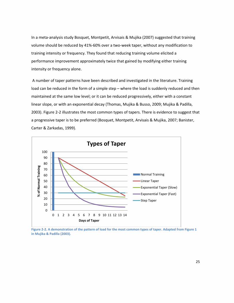
25
In a meta-analysis study Bosquet, Montpetit, Arvisais & Mujika (2007) suggested that training
volume should be reduced by 41%-60% over a two-week taper, without any modification to
training intensity or frequency. They found that reducing training volume elicited a
performance improvement approximately twice that gained by modifying either training
intensity or frequency alone.
A number of taper patterns have been described and investigated in the literature. Training
load can be reduced in the form of a simple step – where the load is suddenly reduced and then
maintained at the same low level; or it can be reduced progressively, either with a constant
linear slope, or with an exponential decay (Thomas, Mujika & Busso, 2009; Mujika & Padilla,
2003). Figure 2-2 illustrates the most common types of tapers. There is evidence to suggest that
a progressive taper is to be preferred (Bosquet, Montpetit, Arvisais & Mujika, 2007; Banister,
Carter & Zarkadas, 1999).
Figure 2-2. A demonstration of the pattern of load for the most common types of taper. Adapted from Figure 1 in Mujika & Padilla (2003).
0
10
20
30
40
50
60
70
80
90
100
0 1 2 3 4 5 6 7 8 9 10 11 12 13 14
% o
f Nor
mal
Tra
inin
g
Days of Taper
Types of Taper
Normal Training
Linear Taper
Exponential Taper (Slow)
Exponential Taper (Fast)
Step Taper
26
Little research has been done on more complicated taper patterns. One such study looked at
the effect of a two-phase taper. This model study found that the last 3 days of the taper were
optimised with a 20% to 30% increase in training load. In the modelled response, such a two-
phase approach allowed for additional fitness adaptations to be made in the final 3 days,
without compromising the removal of fatigue. The magnitude of the performance gain is
questionable (1%), however, over the optimal linear taper (Thomas, Mujika & Busso, 2009).
Much of the literature provides generalised guidelines on designing an optimal taper. It must be
noted, however, that individual responses to training vary. Not all athletes respond equally to
the training undertaken during a taper, and tapering strategies must be individualised (Mujika,
2009). Individual profiles of training adaptation and the time course of de-training need to be
considered in determining optimal taper duration (Mujika & Padilla, 2003).
Research into whether the effects of a taper vary between males and females is inconclusive.
Mujika (2009) concluded that there is no evidence to suggest that tapering programs should be
varied on the basis of gender, or that a gender effect exists concerning the adaptations and
taper effects on performance.
A model which accurately relates training load to performance should be able to provide
individualised guidance on the optimal type and shape of taper for an athlete. Chapter Seven
looks at the effect of the shape of a taper on performance.
2.10. Heart Rate Variability
Heart Rate Variability (HRV) has been proposed as a tool for monitoring training-related fatigue
in athletes (Earnest et al., 2004; Atlaoui et al., 2007). By monitoring fatigue levels, it is hoped
that fatigue can be managed such that both undertraining and overtraining can be avoided.
Heart rate (HR) is not constant – rather it fluctuates from beat to beat. HRV refers to the
variation of the beat-to-beat interval, measured as the time between beats.
27
Electrocardiographs (ECGs) and some types of heart rate monitors are capable of measuring the
time points (in milliseconds) between beats.
HRV is a function of the synergistic action between the two branches of the autonomic nervous
system (the parasympathetic nervous system (PNS) and the sympathetic nervous system (SNS)),
which act in balance to maintain cardiovascular variables in an optimal range during changing
external or internal conditions (Earnest et al., 2004). Activity in the SNS elevates heart rate
while the PNS has the opposite effect (Atlaoui et al., 2007). Measuring the beat-to-beat interval
during an orthostatic test is a reliable method of assessing HRV in athletes (Wisbey &
Montgomery n.d.).
Fatigue alters the balance between the PNS and SNS. Theoretically, the autonomic imbalances
observed in fatigued or overtrained athletes should be discernible from HRV indices, and there
is some evidence to suggest this is the case (Baumert et al., 2006; Earnest et al., 2004).
It is hypothesised that HRV could be included as a proxy for tracking fatigue in a model relating
training to performance. Chapter Five investigates this hypothesis by analysing a dataset from
an elite cyclist to identify whether there is a correlation between training load and heart rate
variability indices.
2.11. Performance
The concept of performance in road cycling must be examined in order to establish a workable
definition to underpin this research. Performance in cycling is affected by numerous factors.
Such factors can be classified into six major groups;
• Diet • Central Nervous System (CNS) function • Strength / skill • Environment

28
• Energy production • Equipment
(refer to Figure 2-3 for a schematic of the factors affecting performance).
Figure 2-3. Factors affecting performance, classified into 6 major groups.Adapted from Powers & Howley, 2008.
Coaches and exercise physiologists require the effects of physiological variables on
performance to be isolated, in order to determine whether a particular training regime has
triggered an observed variation in performance. The presence of so many confounding
variables, however, makes this difficult to achieve.
Performance testing is commonly performed in a lab, where the environment can be controlled
to a large extent. There are a number of issues with this approach - firstly the priority for elite
Performance
Diet- Carbohydrate- Water intake CNS Function
- Arousal- Motivation
Strength/ Skill- Pacing
- Body type- Frontal surface area
- Muscle fibre type- DraftingEnvironment
- Altitude- Heat
- Humidity- Terrain- Wind
Energy ProductionAnaerobic sources
- [CP]- Glycolysis
Aerobic sources- V02 max
- Cardiac output- 02 delivery
- 02 extraction- Mitochondria
Equipment- Aerodynamics
- Weight

29
athletes is competition, and lab testing is rarely a practical option for athletes to fit in among
their training, travel and race commitments. Secondly, the relationship between performance
in tests and performance in events has been questioned (e.g. Hopkins, Hawley & Burke, 1999),
and how a change in performance in a test translates to performance change in a competition
remains uncertain.
Quantifying cycling performance in competitions presents a number of unique challenges.
Cycling competitions are highly variable in terms of terrain, distance and environmental
conditions, meaning that time to completion is generally of no use as a performance measure.
Measuring the power a cyclist outputs has become a relatively common practice. In cycling,
power is the amount of energy transferred to the pedals (in watts) per second. Power is a direct
reflection of exercise intensity, and thus is a possible candidate for use in quantifying
performance.
Power is highly stochastic, however, and varies according to the terrain. A study by Ebert et al.
(2005) examined the power profiles of top 20 finishers in Women's World Cup races, and
compared the profiles of flat versus hilly races. They found that the terrain significantly
influenced the power output profile, with hilly races requiring the ability to sustain constant
submaximal power outputs for long durations while climbing. Flat races, on the other hand,
often involve sprints and surges at a high intensity to maintain position and respond to attacks.
Chapter Six addresses these difficulties, and proposes a novel method for quantifying
performance in road cycling competitions.
2.12. Summary
Much is known about the underlying physiological processes governing the human body’s
response to training, yet much also remains unclear. A set of training principles are commonly
accepted by exercise physiologists, and such knowledge underpins the creation of training

30
programs for athletes. One key principle is that increasing the training stimulus (or load) results
in adaptation of the body, leading to an improvement in performance. Training load can be
thought of as a combination of frequency, intensity and volume of training, and these variables
are manipulated in the creation of training programs with the aim of applying the optimal
stimulus at any one time.
Application of a training stimulus leads to fatigue. The precise mechanisms governing fatigue
remain unclear. Appropriate recovery, however, must be included in a training program to
allow recovery from training induced fatigue, so that the body rebounds into a state of
supercompensation. An imbalance between the training stimulus and recovery can lead to
states of overreaching and overtraining, both of which result in performance decrements. HRV
is a potential tool for tracking fatigue and recovery in athletes.
Fuel is supplied to working muscles through three energy pathways; the aerobic system, the
anaerobic ATP-CP system and the anaerobic glycolytic system. An understanding of the energy
systems, in combination with an understanding of the physiological responses to training, is
used to design workouts to target specific adaptations in an athlete to prepare them for the
specific demands that will be met in competition. These adaptations to training begin to
reverse when the training stimulus is insufficient. A model of training and performance needs
to adequately reflect the time course for both gaining and losing some of the most important
physiological adaptations to training.
In the final phase of preparation for a competition, athletes commonly undertake a taper to
improve performance by reducing accumulated training-induced fatigue, while retaining or
enhancing fitness. Uncertainty still exists about the optimal design of a taper, and in addition,
taper advice must consider individual responses to training.
Road cycling performance is a concept which underpins this research. Performance in this
context is a complex concept, influenced by numerous factors; it is also particularly difficult to
quantify. Exercise physiologists wish to isolate the physiological components of performance so

31
that the effects a particular training regime has on performance can be determined. In the lab,
confounding affects can be controlled to a large extent – however lab testing is frequently not
practical. Nor has the relationship between performance changes in exercise tests in the lab
and performance changes in competition been reliably established. Field testing is more
practical, but also suffers from limited control over confounding factors.
Power output (measured in watts) is a direct measure of the performed by a cyclist, and as such
is commonly used in exercise load measures. Both training load quantification and performance
quantification techniques need to accurately reflect the physiological load of a particular ride.
Terrain significantly influences a power output profile, and so thought needs to be given to a
method of accounting for these differences in quantification techniques.
This chapter has identified a number of major unresolved questions which must be answered
by this research in order to develop a novel neural network model that describes the
relationship between training and performance in cyclists; the ultimate aim of this research.
These questions include:
• How can we quantify training load to accurately reflect the physiological load of rides
conducted over differing terrain? • How can we quantify performance in competitions - to close a feedback loop on the
efficacy of a training program - without requiring impractical lab testing? • How can we determine the optimal training stimulus for a given individual for any point
in their training regime? • How can we determine the time course of fatigue for a given individual for a specified
training stimulus, and by extension, the optimal amount of recovery required?

33
CHAPTER 3 – A SURVEY OF SYSTEMS MODELLING RESEARCH
This chapter introduces the primary modelling approaches that have been used to predict
performance from training load. In Chapter Two, we identified some criteria as important for
developing a useful model to describe the relationship between training and performance in
cyclists. Some of the criteria are specific to the domain of road cycling; however many of the
models examined have been developed and tested against less complex scenarios – for
example swimming, where time and distance are good measures of both training and
performance, or in situations where training and performance testing are both completed in
the lab. These criteria are still a useful starting point for evaluating the modelling approaches
introduced in this chapter. The criteria are as follows:
• A modelling approach needs to incorporate a technique to accurately measure the
physiological load of training - taking into account differing terrain, pattern of load and
duration of training sessions.
• A performance quantification technique needs to minimise confounding factors (e.g. for
cycling, confounding factors include terrain, competition type and team tactics) in order
to accurately reflect performance levels.
• The model needs to have the ability to determine the optimal training stimulus for an
individual athlete at any one time.
• The model needs to be able to determine the time course of fatigue for an individual
athlete given: a current training status; and a training stimulus at time t. By extension,
the model needs to determine the optimal amount of recovery required.

34
Models of training and performance in the literature can be classified as belonging to three
broad categories: impulse-response models; antagonistic models, and machine learning
models. We will begin by considering the key models in each of the three categories.
Systems modelling has been a popular approach in the attempt to model the relationship
between training and performance. Impulse-response models are the dominant form of
systems model used in this domain, and the key impulse-response models that have been
proposed will be discussed first. Antagonistic models are an evolution of the impulse-response
models. These models and the promising results that have been reported from some of these
approaches will be presented. Machine learning techniques (such as neural networks) have
recently been used with some reported success.
The primary aim for this chapter is to identify the most promising of the existing models, and
discuss their advantages and limitations. This will be done with a view towards the
development of a novel model to describe the relationship between training and performance
in cyclists with sufficient accuracy to enable it to be used as a tool in planning training
programmes.
3.1. Impulse-Response Models
Banister and co-workers (1975) proposed that the relationship between training and
performance could be conceptualised by the idea that repeated training bouts contribute to
two factors - fitness and fatigue. At any point in time, this relationship can be expressed by the
following equation: = −
( 3-1 )
This underlying concept gives rise to what are commonly termed the impulse-response models.

35
Banister (1991) firstly quantified training using a training impulse or TRIMP (further details of
this quantification technique are provided in Section 3.4 - Quantification of Training Load). He
considered that a proportion of the training impulse at time t (w(t)) defined a fitness impulse
(p(t)) and a fatigue impulse (f(t)). The proportion of fitness to fatigue gained from a training
impulse is not equal, and will also vary between individuals. The TRIMP is therefore weighted
by multipliers k1 and k2 (initially k1 = 1 for fitness and k2 = 2 for fatigue). Between training
bouts, fitness and fatigue both decline. This is modelled by an exponential decay equation.
Fitness and fatigue decay at different rates, and rates again vary between individuals. This is
modelled by relative decay time constants. Equation ( 3-2 ) shows the complete formula in the
form presented by Morton, Fitz-Clarke and Banister (1990). Banister (1991) defines the decay
constant for fitness ( ) initially as 45 days and fatigue ( ) as 15 days. Refer to
Figure 3-1 for a graphical example of the fitness and fatigue curves that result from a single
training impulse. The performance curve is the difference between the fitness and fatigue
elements of Equation ( 3-2 ). ( ) = [ ( − ) ⁄ + ( )] − [ℎ( − ) ⁄ + ( )]
( 3-2 )
where ( ) and ℎ( ) are arbitrary fitness and fatigue response levels, respectively, at the end
of day and is the intervening period between the current day’s training and that previously
undertaken.
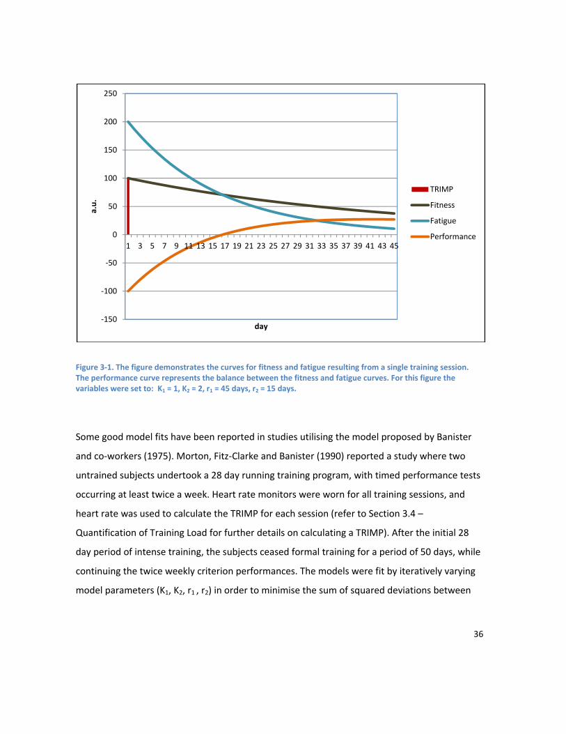
36
Figure 3-1. The figure demonstrates the curves for fitness and fatigue resulting from a single training session. The performance curve represents the balance between the fitness and fatigue curves. For this figure the variables were set to: K1 = 1, K2 = 2, r1 = 45 days, r2 = 15 days.
Some good model fits have been reported in studies utilising the model proposed by Banister
and co-workers (1975). Morton, Fitz-Clarke and Banister (1990) reported a study where two
untrained subjects undertook a 28 day running training program, with timed performance tests
occurring at least twice a week. Heart rate monitors were worn for all training sessions, and
heart rate was used to calculate the TRIMP for each session (refer to Section 3.4 –
Quantification of Training Load for further details on calculating a TRIMP). After the initial 28
day period of intense training, the subjects ceased formal training for a period of 50 days, while
continuing the twice weekly criterion performances. The models were fit by iteratively varying
model parameters (K1, K2, r1 , r2) in order to minimise the sum of squared deviations between
-150
-100
-50
0
50
100
150
200
250
1 3 5 7 9 11 13 15 17 19 21 23 25 27 29 31 33 35 37 39 41 43 45
a.u.
day
TRIMP
Fitness
Fatigue
Performance
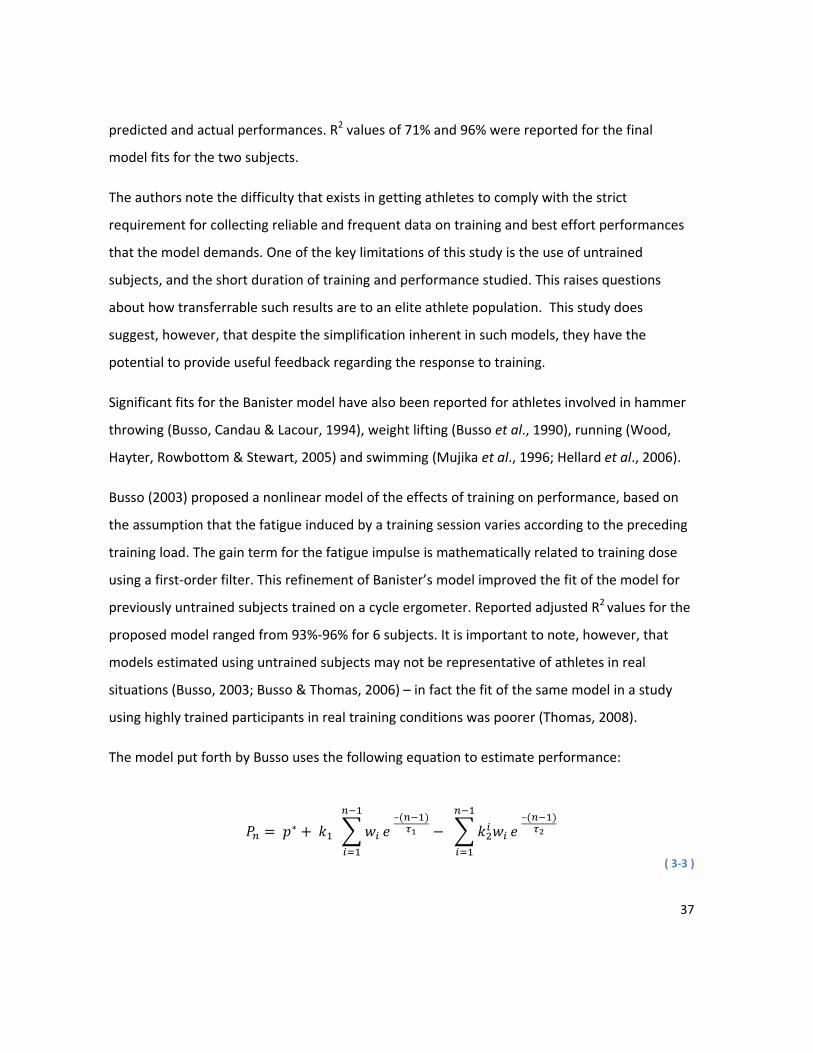
37
predicted and actual performances. R2 values of 71% and 96% were reported for the final
model fits for the two subjects.
The authors note the difficulty that exists in getting athletes to comply with the strict
requirement for collecting reliable and frequent data on training and best effort performances
that the model demands. One of the key limitations of this study is the use of untrained
subjects, and the short duration of training and performance studied. This raises questions
about how transferrable such results are to an elite athlete population. This study does
suggest, however, that despite the simplification inherent in such models, they have the
potential to provide useful feedback regarding the response to training.
Significant fits for the Banister model have also been reported for athletes involved in hammer
throwing (Busso, Candau & Lacour, 1994), weight lifting (Busso et al., 1990), running (Wood,
Hayter, Rowbottom & Stewart, 2005) and swimming (Mujika et al., 1996; Hellard et al., 2006).
Busso (2003) proposed a nonlinear model of the effects of training on performance, based on
the assumption that the fatigue induced by a training session varies according to the preceding
training load. The gain term for the fatigue impulse is mathematically related to training dose
using a first-order filter. This refinement of Banister’s model improved the fit of the model for
previously untrained subjects trained on a cycle ergometer. Reported adjusted R2 values for the
proposed model ranged from 93%-96% for 6 subjects. It is important to note, however, that
models estimated using untrained subjects may not be representative of athletes in real
situations (Busso, 2003; Busso & Thomas, 2006) – in fact the fit of the same model in a study
using highly trained participants in real training conditions was poorer (Thomas, 2008).
The model put forth by Busso uses the following equation to estimate performance:
= ∗ + –( ) − –( )
( 3-3 )

38
The value of the gain term k2 at day i is estimated using the following equation: = w e ( )
( 3-4 )
Pn is the estimation of performance on day n from successive training loads wi with i varying
from 1 to n - 1. p* represents the initial performance level of the athlete. k1 and k3 are gain
terms which adjust the magnitude of fatigue relative to fitness. The two time constants τ1 and
τ2 represent the number of days over which fitness and fatigue impulses decay, respectively. τ3
is also a time constant. Refer to Figure 3-2 for a graphical example of the fitness and fatigue
curves that result from a single training impulse.
Figure 3-2. The figure demonstrates the curves for fitness and fatigue resulting from a single training session. The performance curve represents the balance between the fitness and fatigue curves. For this figure the variables were set to: K1 = 1, K3 = 0.0148, τ1 = 40 days, τ 2 = 9 days, τ3 = 7 days, p* = 10.
-40
-20
0
20
40
60
80
100
120
140
160
1 3 5 7 9 11 13 15 17 19 21 23 25 27 29 31 33 35 37 39 41 43 45
a.u.
day
Training
Performance
Fitness
Fatigue

39
Model parameters are determined by fitting the model performances to actual performances
by the least square method, which minimises the residual sum of squares for f(n).
( ) = ∗∗ − ∗ + –( ) − –( )
( 3-5 )
Where pn** = actual performance on day n.
3.1.1. Limitations of Impulse-Response Models Hellard et al. (2006) demonstrated that the four parameter Banister model suffers from ill-
conditioning problems; problems which are likely to affect the accuracy of parameter
estimates. Hellard suggests that the following issues contributed to the ill-conditioning:
• Small sample size. With one performance data point being obtained weekly (at most) sample size is an important consideration. The more model parameters that need to be estimated, the larger the sample size required.
• The model parameters are not independent. Inter-dependent parameters mean that several sets of parameters can provide the ‘best’ solution for a given dataset.
• Misspecification of the model. The model assumes that subsequent performances are independent, and that parameter estimates stay stable over time. Both assumptions are unlikely to be correct. (Hellard et al., 2006)
Impulse-response models typically require frequent performance measures to enable
estimation of model parameters. Hellard et al. (2006) suggests that greater than 60
observations would be required for estimation of a four parameter Banister model. Frequent
testing is impractical for elite athletes (Borrensen & Lambert, 2009; Hellard et al., 2006); even if
weekly testing were feasible, it would still take in excess of a year to capture an appropriately
sized dataset.
The behaviour of the impulse-response models deviates in a number of areas from known
physiological responses to training. Biological adaptation is a complex non-linear problem
(Edelmann-Nusser et al., 2002). Busso (2003) suggests that the relationship between daily

40
amounts of training and performance might be best described as a parabolic relationship.
Traditional impulse-response models are based on linear mathematical equations. Although
Busso’s (2003) model is non-linear in that the relationship between training and performance is
dependent upon previous training loads, all impulse-response models assume that a greater
amount of training leads to a better performance. In fact, the positive relationship between
training load and performance has an upper limit, beyond which further training doesn’t result
in performance gains (Morton, 1997). The authors of a recent modelling study (Mujika, Busso &
Geyssant, 2012) report that their findings indicate the possible existence of a training stimulus
threshold, beyond which intensity would be the main factor in the production of a training
effect. Further to this, the impulse-response model is unable to model the long-term
decrement of performance capacity (overtraining) which is the result of an imbalance between
training and/or lifestyle stress and recovery (Bruckner & Wilhelm, 2008).
The impulse-response models are abstractions; they don’t assume a relationship to underlying
fitness and fatigue processes. Attempts to link the model to underlying processes have had
limited success (Taha & Thomas, 2003). It is important to note, however, that knowledge is
currently limited concerning the effects of training on each of the potential physiological
“markers” that have been identified (Borresen & Lambert, 2009).
Similarly, Bruckner (2006) argues that although impulse-response models model a rise in the
fitness impulse immediately after a training session, the underlying physiological processes
being modelled can take up to 72 hours to adapt. In the Banister model, the immediate
increase in fitness is overshadowed by the concurrent immediate rise in fatigue. The
adjustment mechanism of the Banister model appears to differ from what is known about the
underlying physiological process. Taha & Thomas (2003) report that the model-based estimated
time course of changes in fitness and performance differs from the results observed from
experimental observations.
Reported performance of impulse-response models has been extremely varied, both between
studies and between subjects in the same study. Mujika et al. (1996) in a study looking at the

41
effect of training on swimming performance found that the model explained between 45% and
85% of the variations in actual performance.
Hellard et al. (2005) found that training variables explained only 36% of variation in the
performance of Olympic swimmers. Thomas, Mujika and Busso (2008) report a fit of between
45% and 63% between modelled and actual performances of eight elite swimmers.
The smallest worthwhile improvement for top-level athletes in the individual sport of road
cycling time trials is in the order of approximately 0.6% (Paton & Hopkins, 2006). Paton and
Hopkins (2006) concluded that drafting in road races precludes estimation of the smallest
worthwhile change in performance for this event. Nevertheless, it is likely that small changes in
performance could have a significant effect on the outcome of elite competition. It is thus
essential that models are able to predict performance with only small margins of error
(Borresen & Lambert, 2009).
Busso and Thomas (2006) provide the strongest criticism of impulse-response models, arguing
that the simplifications made in abstracting complex physiological processes into a small
number of entities mean that the accuracy of prediction will suffer greatly. They conclude that
such modelling processes would barely be compatible with the accuracy required to make such
tools useful in designing training programs.
Despite the valid concerns raised by some researchers about the accuracy of impulse-response
modelling and by extension their predictive ability, software programs based on these models
(such as TrainingPeaks WKO+ and RaceDay) are popular with both recreational and elite cyclists
and coaches, who use them in monitoring and developing training plans.

42
3.1.2. Performance Manager
Andy Coggan developed the Performance Manager concept to attempt to overcome some of
the limitations with the impulse-response model. His work is now included in the popular
software package TrainingPeaks WKO+.
The Performance Manager is based on the observation that performance is generally greatest
when training is first progressively increased to a high level, to build fitness, and then tapered
to eliminate residual fatigue. The model eliminates the gain factors k1 and k2 which are used to
convert the impulse into separate fitness and fatigue impulses. This makes the model simpler
by removing the difficulty of establishing appropriate values for the gain factors. It does,
however, mean that the resultant fitness and fatigue components are relative indicators of
changes in performance ability, rather than absolute predictors. It also allows the substitution
of simpler exponentially-weighted moving averages for the fitness and fatigue components
(Coggan, n.d. (c)).
The Performance Manager consists of the following components:
• Training Stress Score (TSS). This is a cycling-specific load quantification technique which
uses power as the measure of cycling intensity. It provides a way of measuring training
load, and is used as the input for the other components of the Performance Manager.
• Chronic Training Load (CTL). This is equivalent to the fitness part of the performance =
fitness - fatigue equation. It provides a measure of chronic training load by calculating
an exponentially-weighted moving average of daily TSS values. The default time
constant is set to 42 days. The use of TSS as the load quantification measure means that
both volume and intensity of training are taken into consideration (Coggan, 2006).
• Acute Training Load (ATL). ATL is equivalent to fatigue in the impulse-response model. It
provides a measure of acute training load by calculating an exponentially-weighted

43
moving average of daily TSS values. The default time constant is set to 7 days (Coggan,
2006).
• Training Stress Balance (TSB) is the difference between CTL and ATL. It serves a similar
purpose to the output of the impulse-response model (i.e. a performance predictor),
however, as the gain factors have been eliminated from the model it is better viewed as
an indicator of the freshness of the athlete - or how well they have adapted to their
recent training load (Coggan, n.d. (c)).
The Performance Manager model has not been validated by any scientific studies.
Consequently the fit of the model to actual performances has not been reported. As with the
impulse – response models, the Performance Manager doesn’t consider the specificity of the
training.
The Performance Manager has two time constant parameters which determine the duration of
the fitness and fatigue impulses. These parameters are set by trial and error. Banister (1991)
suggested that the parameters for the impulse-response model need to be reset every 60-90
days. There is no mechanism within the Performance Manager for recalibrating parameters as
the athlete’s fitness changes over time.
Although removing the gain factors and setting the remaining two model parameters by trial
and error reduces the requirements for frequent performance tests, the Performance Manager
still requires regular performance testing in order to calibrate TSS.
3.1.3. Summary of Impulse-Response Models In order to create a workable model, simplified abstractions need to be made of the underlying
complex structures. Determining just how much of the underlying structure should be
incorporated into models of the relationship between training and performance is, however, a
difficult question (Taha & Thomas, 2003). A balance needs to be struck between complexity and

44
ease of use - to arrive at a model that derives the greatest accuracy in predicting performance
for the least computation cost. Busso and Thomas (2006) argue that the strong simplifications
made by the impulse-response models seem to be barely compatible with the accuracy
required for designing a training program. They further concluded that in order for systems
modelling techniques to be of practical use for coaches developing training programs, new
modelling strategies should be considered along with mechanisms for the consideration of the
specificity of the training activity.
Existing models have three key limitations:
1. The input for the impulse-response models discussed is training load. None of the training load quantification methods used in the literature accurately describe physiological load for the different types of sessions a cyclist commonly undertakes. Training load quantification algorithms will be discussed in Section 3.4 Quantification of Training Load. Simplification of the model input (training load) into a single variable is likely to negatively affect model accuracy (Taha & Thomas, 2003; Busso & Thomas, 2006).
2. To estimate model parameters regular performance tests are required; this is not practical for professional cyclists. Banister (1991) found that the constants for the model will only serve for a period from 60 to 90 days before the process of iterative modelling and resetting the model constants needs to be repeated. The requirement to regularly reset model constants also reduces the amount of data available for modelling.
3. The inability of the models to accurately predict future performance (Taha & Thomas, 2003; Busso & Thomas, 2006).
3.2. Alternative Modelling Approaches Some researchers consider that deterministic, linear models based on group statistics are
inadequate for understanding and explaining complex systems - such as the training process
(Perl, 2004). A shift in approach to modelling training and performance has occurred; away
from linear cause-effect oriented models, and towards individual models that allow for complex
non-linear interactions between observations (Pfeiffer, 2008; Balague & Torrents, 2005). Such
45
approaches include a dynamic meta-model named PerPot, an antagonistic model named
SimBEA, and the machine learning technique of artificial neural networks.
3.2.1. Dynamic Meta-Model
Perl (2001) describes a Performance-Potential-Metamodel (or PerPot). This model simulates
the interaction between training load and performance using a state – event framework with
adaptive delays.
Hellard et al. (2006) highlighted the conceptual richness of this model, as it accurately models
some principles of training which the impulse-response models fail to account for. It models the
collapse in performance following overreaching or overtraining, as well as the reduction in
performance that occurs during detraining. It also models the law of diminishing returns as it
applies to increasing the training load of well-trained athletes.
The PerPot model is based on the principle of antagonism – the same basic principle underlying
the impulse-response model. In the PerPot model a response potential fulfils a similar role to
the fitness impulse, while the strain potential is similar to the fatigue impulse of the impulse-
response model. Hence each load impulse (training load input) feeds the strain potential and
the response potential. The strain and response potentials in turn influence the performance
potential. The response potential raises the performance potential (incorporating a delay
controlled by the response flow parameter - this is equivalent to the fitness decay constant).
The strain potential reduces the performance potential (incorporating a delay controlled by the
strain flow parameter which is equivalent to the fatigue decay constant). The strain potential is
stored in a reservoir with a finite capacity - if the reservoir is overloaded an overflow is
produced, which further reduces the performance potential. Figure 3-3 shows a flow chart
describing the structure of the PerPot model.

46
Figure 3-3. Flow chart showing the basic structure of the PerPot model.The load rate is split into two potentials – the strain potential and the response potential. The flow out of the strain and response potential reservoirs into the performance potential reservoir is regulated by the delays DS and DR. Figure adapted from Perl, Dauscher & Hawlitzky (2003).
Pfeiffer and Schrot (2009) obtained an excellent model fit for performance using a PerPot
model. The study involved collecting heart rate and power data from two professional road
cyclists and one mountain biker in a five month study. TRIMPs were calculated from the heart
rate data collected during training and used as the input for the PerPot model. Performance
was tested three times per week using cycle ergometer tests. The reported Intraclass
Correlation Coefficient (ICC) values for modelled and real performances ranged from 0.61 to
0.86 for the three athletes.
Ganter, Witte and Edelmann-Nusser (2006) reported a wide range of model fits with R2 values
of between 13.4% – 92.8% using the PerPot model. The study collected training and
performance data from ten athletes during eight weeks of cycling training, using heart rate data

47
to record TRIMPs from training and the mean power output during 30s maximal effort exercise
tests to measure performance. The range in model fit reported could be due to issues with the
reliability of the performance test protocol chosen. Nevertheless, the large variation in
modelling results between athletes in this and other studies raises questions about the internal
integrity of the modelling.
The PerPot model has a number of limitations. Bruckner (2006) notes that the model does not
accurately model short-term supercompensation effects. After exposure to a single training
dose, the model shows a delayed decrease in performance, followed by a return to the initial
level of performance – with no supercompensation. PerPot models also show a time lag
between a training impulse and the resultant fatigue effect (Bruckner & Wilhelm, 2008). This
delay is not reflected in the underlying physiological processes. As with the linear mathematical
models, PerPot also requires frequent performance testing to enable estimation of parameters.
3.2.2. SimBEA
In 2006, Bruckner proposed an antagonistic model called SimBEA. The mathematical
implementation of SimBEA is based on the PerPot model. In addition, it attempts to realistically
model the physiological processes that PerPot does not; namely the supercompensation effect -
the performance decline associated with overtraining as well as detraining (Bruckner &
Wilhelm, 2008).
A maximum adaption rate parameter controls the ‘ceiling’ for training load beyond which
maladaptation and a decline in performance consistent with overtraining occurs. A minimum
training load parameter determines the minimum training impulse below which detraining
occurs. Model parameters are determined by varying them iteratively and optimising the fit of
actual performance to modelled performance (Bruckner & Wilhelm, 2008).

48
The SimBEA model was evaluated in a two phase longitudinal case study undertaken by
Bruckner and Wilhelm (2008), using training and performance data from a runner. In phase one
of the study, six weeks of daily performance and training data was collected. In the second
phase of the study, data from 68 weeks of training and 25 performances were collected. During
the 68 weeks the athlete trained as normal and could choose when to schedule performances,
thus resulting in a more realistic dataset.
Training load was measured using a TRIMP calculated by multiplying a fifteen-point rate of
perceived exertion (RPE) by the duration of the training session. Performance was measured by
recording the heart rate during a submaximal effort. The average heart rate for this standard
endurance test was taken as the performance.
The first phase of the study showed a good fit between predicted and actual performances. The
reported ICC for this phase was 0.86. The second phase of the study saw a moderate fit, with an
ICC value of 0.65. It is worth noting that phase two used a data collection protocol which is
more realistic for collecting data from elite athletes, and still achieved a moderate fit. These
results, while promising, are from a single case study and the SimBEA model requires further
research before definitive conclusions can be drawn.
3.2.3. Artificial Neural Networks
Neural networks are flexible, adaptive learning systems that can find patterns in observed data,
enabling the development of nonlinear systems models which can make reliable predictions
(Samarasinghe, 2006). The non-linear modelling techniques of neural networks have been
suggested as potentially appropriate for use in modelling the relationship between training and
performance (Hellard et al., 2006).
Silva et al. (2007) used neural network technology to create models of swimming performance.
They concluded that this approach was valid for resolving complex problems such as

49
performance modelling. In order to achieve good results, however, neural networks, in
common with other machine learning techniques, require large volumes of data in order to
converge on an accurate model. Large datasets are unlikely to be obtainable in this domain.
Neural networks are prone to overfitting, particularly with small, noisy datasets such as
frequently occur in the training and performance domain. Overfitting occurs when the model
identifies the noise in the dataset, rather than the underlying relationship in the data.
Overfitting is a known limitation when using neural networks with small datasets.
Neural networks have been used to model the competitive performances of an elite swimmer,
on the basis of training data (Hohmann, Edelmann-Nusses & Hennerberg, 2001). The study
concluded that neural networks are excellent tools to model and even predict competitive
performances on the basis of training data. The precision of the neural network prediction was
much higher than that achieved by a conventional regression analysis. The authors identified
two key advantages of using neural networks. The approach is robust in handling issues with
input data - such as noise; and the neural network can model nonlinear transformation of the
relationship between training and performance i.e. as the athlete’s fitness changes over time.
In the Hohmann study (Hohmann, Edelmann-Nusses & Hennerberg, 2001) a very small dataset
(only 19 records) was used in the modelling. Recognising the overfitting problems neural
networks experience in modelling with very small datasets, the researchers used data from a
different swimmer to pre-train the network. This method resulted in a surprisingly small
prediction error (0.04%), however doubts remain with the methodology employed in the study.
Much evidence exists that training responses are highly individual (Avalos et al., 2003; Busso,
2003; Millet et al., 2002).
Haar (2012) used neural networks to model a small dataset (24 performances) obtained from
three highly-trained triathletes. He concluded that ANNs were particularly suitable models for
the prediction of athletic performance from training, however there are also doubts about the
methodology employed in this study, as it appears not to have addressed issues with

50
overfitting, nor did it provide details of the architecture of the ANN used, or the validation
process used.
Hellard et al., (2006) criticises neural networks for being a “black box”, with a limited ability to
explicitly identify causal relationships. This makes it difficult to interpret the results obtained. It
is, however, perhaps unreasonable to expect a model to elucidate the extremely complex
underlying structures governing the response to training.
3.3. Limitations of Current Modelling Approaches
A number of models have been developed in an attempt to quantify the relationship between
training and performance. Modelling this relationship as a systems model with training load as
the input and performance as the output is an attractive concept – however many of these
models have only moderate accuracy (Borresen & Lambert, 2009). The inevitable simplifications
of the underlying physiological processes inherent in these models - particularly the reduction
of model inputs into a single number representing training load – have been suggested as the
likely cause of such model’s poor predictive performance (Busso & Thomas, 2006). The impulse-
response models (and their successors, such as SimBEA and PerPot) are limited in their
practicality in the real world, due to their requirement for frequent performance tests in order
to estimate model parameters.
The impulse-response models fail to model the key physiological processes of
supercompensation and overtraining (Bruckner & Wilhelm, 2008). The PerPot model does
capture the system collapse effect of overtraining, however it’s modelling of the
supercompensation effect has been criticised for its lack of physiological accuracy (Bruckner &
Wilhelm, 2008).
Neural network models have the advantage of being able to adapt as the relationship between
training and performance changes over time. They are also flexible modelling systems, allowing

51
more than one input. Datasets in this domain are inevitably small however, and neural
networks typically require large datasets to train the model (Jobson et al., 2009). Neural
networks remain a promising tool for modelling training and performance, however techniques
to avoid overtraining need to be utilised or developed.
3.4. Quantification of Training Load
All the models we have discussed have used training load as a model input. Training load must
be quantified in some way, but how should this be done? The frequency, duration and intensity
of training all contribute to the nature and magnitude of the training effect (Borresen &
Lambert, 2009) and so all need to be considered in a quantification technique (Taha & Thomas,
2003). There has been great difficulty in finding a way to effectively quantify training load using
a single term (Foster et al., 2001).
Banister’s TRIMP was introduced in Section 3.1. A TRIMP is derived from multiplying the
duration of training by the relative training intensity (measured by heart rate). A multiplying
factor is applied in order to weight higher heart rate (HR) ratios proportionally higher.
= (min) × −− ×
( 3-6 )
where HRex is mean HR during the session, HRrest is the athlete’s resting HR, and
HRmax is the athlete’s maximal HR, and y is a multiplying factor defined as follows: ( ) = 0.64 . ( ) = 0.86 .
( 3-7 )
where x equals delta HR ratio during exercise.
52
Taha and Thomas (2003) describe calculating a TRIMP using currently accepted methods of
measuring heart rate intensity. An absolute measure of percentage of maximum heart rate is
used, while Banister used the Karvonen method of heart rate reserve.
TRIMPs have been successfully used to model the relationship between training and
performance in many studies (e.g. Banister et al., 1999; Millet et al., 2002; Ganter, Witte &
Edelmann-Nusser, 2006). TRIMPs are a relatively easy measure to calculate, and require only
heart rate monitors, which are readily available and moderately priced. They are a useful
integrative measure of training load for cyclists (Faria et al., 2005). TRIMPs also have the
advantage of being able to be calculated across most sports and training activities, for example
running and cycling. They are not an appropriate load quantification method for strength
training, however, as heart rate only measures the cardiovascular load of exercise.
Heart rate is a poor method of evaluating very high intensity exercise (Foster et al., 2001). It is
likely that long duration, low intensity incorrectly provides a TRIMP score higher than that
obtained from high intensity exercise of shorter duration (Hayes & Quinn, 2009; Rusko et al.,
2004).
Heart rate is affected by many factors; which impacts on its reliability as a measure of training
load. Factors which can affect heart rate include temperature, hydration, sleep, overtraining
and caffeine (Jeukendrup, 2002, p. 67). There are claims that the variability of heart rate
impacts on the validity of quantification methods based on heart rate (Skiba, 2008).
3.4.1. Rating of Perceived Exertion
Foster et al. (2001) proposed a method of quantitating training using a rating of perceived
exertion (RPE). The RPE method involves getting athletes to rate their exertion for a session on
Borg’s RPE scale - a scale of 1 to 10 (Borg, 1985, cited in Foster et al., 2001). The 2001 study

53
suggested that a TRIMP obtained from RPE (duration x RPE) was highly correlated with a
modified TRIMP calculated from heart rate zones.
RPE has been used as the input of a systems model to study training and performance in an
elite sprinter. The authors concluded that the resultant model was a potentially powerful tool
for assessing the effects of training on athletic performance (Suzuki et al., 2006). Bruckner and
Wilhelm (2008) also used RPE successfully when they validated their SimBEA model using
training data from a runner.
Some advantages of using RPE as a load quantification technique are: it can be used across
many different exercise modalities, including strength training; it requires no equipment; and it
is simple to calculate. The disadvantages of this approach include: it is a subjective measure; it
relies on individual’s memory of the session; differences in rating exist between individuals; and
some intra-subject variation exists.
3.4.2. EPOC EPOC (excess post-exercise oxygen consumption) is a measure of the oxygen consumed in
excess of resting requirements during recovery from exercise. Measured in litres or ml/kg, it
reflects exercise induced disturbance of the body’s homeostasis, and the resultant recovery
demand (Wisbey, 2006).
EPOC increases with higher intensity and / or increased duration of exercise (“Indirect EPOC
Predication Method Based On Heart Rate Measurement,” 2007). EPOC can thus be used as a
measure of training load. It has been suggested that EPOC reflects the cumulative response of
the body to the entire training session (Jobson et al., 2009).
It is only possible to measure EPOC in the lab, by analysing respiratory gases. Firstbeat
Technologies, however, have developed software to predict EPOC (EPOCpred) based on the
inter-beat (RR) interval heart rate data.

54
In order to make a prediction of EPOC a known maximal heart rate and VO2 max (the maximal
oxygen update) for the user is required. The heart rate and heart rate variability (HRV)
measurements during exercise are used to predict respiratory rate and VO2. Predicted
respiratory rate, and VO2 are then used in conjunction with heart rate to predict EPOC (B.
Wisbey, personal communication, June 26, 2006).
Two key advantages of predicted EPOC are: it has a significant correlation with laboratory
measured EPOC (Rusko et al., 2003), and thus good physiological accuracy; and it is suited to
measuring the physiological load of high intensity exercise. The validation of predicted EPOC
against measured EPOC has, however, only been tested for short durations of exercise.
EPOC is more affected by training intensity than volume (Rusko et al., 2004). EPOC is therefore
only a useful measure for monitoring training response to short, intense training sessions
(Wisbey, 2006). Using EPOC to measure the training load of long endurance exercise will not
accurately reflect the physiological load and the recovery time needed from such a session. In
addition, the predicted EPOC for a session is the peak EPOCpred reached. This means that
repeated efforts with a long recovery will not result in an increased EPOCpred (Wisbey, 2006).
Other disadvantages of using predicted EPOC as a load quantification technique include: the
calculation is complicated and requires proprietary software and hardware; and it is based on
heart rate, which as previously discussed can be affected by a variety of factors.
3.4.3. Using Power to Quantify Training Load
Power is the amount of energy generated per unit of time. In cycling, it is the amount of energy
transferred to the pedals (in watts) per second. SRM power monitors are commonly used to
measure power in cycling. They provide reliable measurements of power (Gardner et al., 2004),
as well as measurements of cadence, speed and distance.
Power is a direct reflection of exercise intensity as opposed to heart rate, which is a response to
the exercise intensity (Jeukendrup, 2002). Heart rate is affected by external factors, and also

55
experiences a delay in responding to changes in exercise factors. As a direct reflection of work
output, power is not affected by these limitations.
Power has good potential to be used as the basis for quantifying training load. It does have
some practical limitations however. Power based load metrics can only be used in sports where
power can be easily measured (i.e. cycling). Training load from cross training or strength work
can’t be measured. Power monitors are also still not in widespread use, due mainly to their
relatively high cost – and for athletes with multiple bikes (training, racing and time trial bikes)
there is as yet no easy way to switch power monitors between bikes.
In order to use power data as a training load metric, it needs to be pre-processed in some way.
Taking the mean power of a session is a common summary statistic. Power output is highly
variable however, so the mean doesn’t necessarily accurately reflect the physiological demands
of a session.
In an attempt to come up with a better summary of physiological load than mean power,
Coggan (2003, 2006) proposed the concept of normalised power. Normalised power is an
estimate of the constant power that an athlete could have maintained for the same
physiological load.
Normalised Power Normalised power is calculated by:
1. Smoothing the power data by applying a 30 second rolling average filter. This is to
account for the fact that physiological responses to changes in exercise are not
instantaneous, but follow a characteristic time course. 30 seconds was chosen as the
typical half life of many physiological responses (e.g. heart rate, VO2) (Coggan, 2003).
2. Raise the smoothed data to the 4th power. This takes into account the non-linear nature
of physiological responses (Coggan & Edwards, 2006), by giving more weighting to
higher power values.

56
3. Average the values obtained in step 2.
4. Take the 4th root of the average to give normalised power (Coggan & Edwards, 2006).
Normalised power is then used in the calculation for a load quantification technique called
Training Stress Score (TSS).
Training Stress Score Training Stress Score was proposed by Coggan in 2003 as a load quantification method using
power. An intensity factor (IF) is used to normalise TSS to functional threshold power (or the
power that can be maintained in a 60 minute time trial). This allows for easier comparison of
TSS between athletes. The formulas for calculating TSS are included below:
= ℎ ℎ
( 3-8 ) = (ℎ) × × 100 ( 3-9 )
TSS has a number of advantages: it is based on power, which is a direct measurement of
training stimulus (work rate), rather than a response to the stimulus (such as heart rate); it is
relatively simple to calculate (Coggan, n.d (a)); and by using normalised power as the basis for
the calculation, TSS applies increased loading for high intensities, which is in keeping with
physiological principles.
I argue that TSS places too much emphasis on training duration when quantifying load, and not
enough on intensity. For example, when an athlete is coasting downhill, and applying zero force
to the pedals, TSS still accumulates.
The model has not been validated by any scientific studies (Coggan, n.d (a)). A similar algorithm
(BikeScore), however, has received some initial support from a study which demonstrated the
usefulness of the algorithm as an input function for systems-based performance modelling.
Using the load quantification technique it was possible to accurately model performance (Skiba,
2007).

57
3.4.4. Summary of Load Quantification Methods
The load quantification methods we have examined - TRIMPs, RPE, EPOC and TSS - all suffer
from drawbacks in physiological accuracy and / or practicality. TSS is widely used by cyclists and
has a number of advantages. The key criticism of TSS is that it places too great an emphasis on
duration, and consequently too little on intensity.
For the greatest physiological accuracy, a load quantification technique would be multifactorial
and include the specificity of the activity, as well as the pattern of load. None of the current
load quantification techniques consider these aspects.
Pattern of load is a consideration which impacts on physiological cost. Accelerating to a given
speed requires greater power application- and hence comes at a greater physiological cost-
than maintaining a given speed. Similarly, maintaining the same power at the end of an interval
comes at greater physiological cost than maintaining that power at the beginning of an interval.
The power output of a cyclist is a direct reflection of exercise intensity. Heart rate responds to
the exercise intensity. The load quantification algorithms using power weight a certain power
output the same whether it occurs at the start of a session, when an athlete is fresh, or at the
end when they are fatigued. The occurrence of cardiac drift (the continuous increase in heart
rate that usually occurs during prolonged moderate-intensity exercise (Jeukendrup, 2002, p.
66)) is cited as a criticism of using HR to measure training load (e.g. Skiba, 2008). Maintaining
the same power at the end of an effort comes at greater physiological cost than maintaining
that power at the beginning of an effort – we suggest that HR more accurately models the
physiological cost in this situation than power.
Multifactorial techniques which consider specificity, or include HR data as well as power data
while potentially increasing the physiological accuracy of load quantification techniques, do
come at the cost of increased complexity in both data collection and model construction. This

58
compromise between accuracy and usability will need to be considered in the development of a
new load quantification technique for this research.
3.5. Quantification of Performance
Training load is the key input for the models we have discussed, and the other critical
component is the output: performance. The exact components which constitute the concept of
performance are sport-specific. Many of the modelling studies we have discussed have
concentrated on sports such as swimming, where performance is logically quantified as a
function of time, or have used standardised lab testing, usually on a cycle ergometer, to define
performance. We will review the current approaches that have been used for quantifying
performance, and discuss their applicability for cycling.
Numerous studies (Thomas, Mujika & Busso, 2008; Mujika et al., 1996; Avalos et al., 2005) have
used a method where performances are converted into a percentage of personal best
performances. A similar approach in cycling would require the athlete to complete a regular
performance test. As discussed, this is generally not practical.
Morton et al. (1990) used a criterion point scale to quantify performance. The equation for the
curve of athletic performance records over time is:
= + − ( 3-10 )
where y is the time or distance recorded for an athletic performance, L is the perfect
performance (e.g. world record), a is an amplitude factor that is positive for running events and
negative for jumping or throwing events, and b is a time parameter - the difference between L
and the performance of any able-bodied individual (Morton et al., 1990). Road cycling, with its
59
variety of terrain and the impact of drafting and team tactics, does not have an easily definable
concept of perfect performance, however.
A conceptually similar technique called Mercier Scoring is commonly used to compare track
and field athletes. The Mercier Scoring Tables are the result of a statistical comparison of all
performance in Athletics. A linear fit is applied to the weighted average of the 5th, 10th, 20th,
50th and 100th World-ranked performances in each event over the past 4 years. Performances
from more recent years are given a higher weighting. McGregor (2007) used this performance
quantification technique in applying a Banister-type model to the training and racing data of a
1500m runner.
Hellard et al. (2006) examined the effect of different performance quantification techniques on
the modelling process using a Banister model. Performance was modelled using a logarithm
transformation, expressed as a percentage of the world record, as well as the criterion points
scale proposed by Morton et al. (1990). These methods resulted in a less reliable model
compared to the one obtained when performance was quantified as a percentage of the best
performance achieved by the athlete in the course of the study period.
An athlete’s best performances are likely to occur during an actual competition where training
induced fatigue was minimised by tapering prior to the event. Ignoring this data eliminates a
particularly important component of the training – performance relationship. One study which
quantified performance from actual competition data was done by Millet et al. (2002), who
used a subjective rating technique to measure performance in triathlon competitions. The
validity of this method is questioned by Taha and Thomas (2003) due to its subjective nature. It
does however, highlight the difficulty of establishing an accurate method of testing and
quantifying performance, which is practical enough to implement in the real world of elite
athletes.
It is clear from this review that there is currently no acceptable method for quantifying
performance for road cyclists in the field. Such a method would need to: reflect the

60
physiological component of performance; minimise the impact of external factors such as
terrain, drafting and team tactics; and be practical for elite cyclists to implement in terms of
data collection.
3.6. Summary
We have discussed the methods available to quantify training load, and their limitations. A
training load quantification method needs to:
• Reflect training intensity in accordance with known physiological principles; • Provide a physiologically accurate balance between the loading of duration and
intensity; • Provide consistent results independent of external factors; and • Be practical and robust in terms of data collection and processing.
All of the current methods of quantifying training load reflect a compromise in one or more of
the above areas.
We have discussed the methods available to quantify performance, and their limitations. A
performance quantification method needs to:
• Provide an accurate representation of the physiological component of performance; • Minimise the impact of external factors such as terrain, drafting and team tactics; and • Be practical and robust in terms of data collection in the field.
Again, all of the current methods of quantifying performance reflect a compromise in one or
more of the above areas.
The methods available to model the relationship between training and performance have also
been discussed. Such models need to:
• Accurately reflect known physiological effects, such as overtraining, detraining and supercompensation;

61
• Operate with very small datasets; • Operate with a practically achievable number and type of performance tests; and • Have good predictive performance.
As above, all of the current methods discussed require a compromise in one or more of the
requirements.
It is clear that in order to develop a system that will enable cycling coaches and athletes to
manipulate training loads to prepare cyclists for peak performances in competitions, a new load
quantification technique, a new performance quantification technique, and a new or adapted
modelling approach will all need to be developed.
The next chapter, Chapter Four, will investigate computational modelling approaches and
assess them for suitability for modelling athletic training and performance.

63
CHAPTER 4 – KNOWLEDGE DISCOVERY FOR SPORTING PERFORMANCE
In recent years there has been rapid growth in the use of data mining techniques to discover
knowledge from datasets from a broad range of industries and domains. As data has become
more extensive and pervasive, new techniques have been developed to “mine” information
from these sources. Problems in sport science have much in common with the problems
encountered in other domains, yet they also have some distinctive characteristics which have
not been extensively addressed by existing techniques.
This chapter considers the longstanding problem of knowledge discovery to improve elite
sporting performance. The primary aim is to draw together previous modelling work performed
on similar problems with a view towards developing a methodology for the generation of a
better prediction model for the training and performance domain. We begin with introducing
the research problem, and discussing the nature of the data collected. The research design
employed in this study is described. The field of data mining is introduced along with a brief
introduction to a data mining process commonly employed. Various modelling techniques from
both the statistical and machine learning domain are introduced, and their potential
applicability discussed. It is not the intention of this study to describe all modelling techniques
but rather to concentrate on the concepts and techniques that are relevant to the research
problem.
4.1. Research Problem
The aim of this research is to develop a model that will describe the relationship between
training and performance such that performance output can be predicted from training input
and other known and measurable factors. The model developed needs to be adaptable and

64
extensible, such that it can adapt to changes or additions to the input data. Figure 4-1 shows a
high-level overview of the components of the proposed model.
Figure 4-1. This figure shows the components of the proposed system. Inputs to the model are on the left and model outputs on the right. The model inputs shaded in yellow are designed to be adaptable and extensible, and will be dependent on the data available from an individual athlete. Examples of supporting data that might be useful include RPE values from training sessions, HR data, recovery data such as sleep duration and quality, results from lifestyle stress questionnaires (e.g. Profile of Mood States), and results from any regularly undertaken sport specific standardised testing.
4.2. Research Design
This research employs a naturalistic approach, using data from athletes’ normal training and
competition performance, rather than a research-driven manipulation of the variables being
studied. While this approach has limitations, it allows the research to be conducted on
professional cyclists; who are unlikely to consent to participation in experimental trials (Barnett
et al., 2010). A time-series design has been used, involving observation of training and racing
over time. This design allows both the short term and long term effects of training on
performance to be observed over extended periods.

65
An ideographic approach has been followed. This approach studies each athlete as a separate
entity, consequent to the premise that responses to training are individual (as discussed in
Chapter 2). The end result is a sequence of successive training data points, generally measured
daily, and a sequence of performance data points which are irregularly spaced. The main
limitation of study designs which use a case study approach with single or small numbers of
participants is difficulty in generalising the findings to a wider population (Kinugasa, 2013).
Barnett et al. (2010) points out the benefits of such naturalistic, idiographic studies, stating that
they can potentially provide highly practical and individual information to coaches and athletes
on the relationship between training and performance. Further, such a research design is
ethically and personally acceptable to professional athletes due to its undisruptive nature.
4.3. Data
Daily training and racing data were captured for several professional cyclists over the course of
a season or several seasons. For each training or racing session, the raw sensor data captured
was converted into a single unit measurement of training load, using a novel algorithm which
will be introduced in Chapter 5. In addition, for races a single unit measurement of the
performance was calculated using a novel algorithm which will be introduced in Chapter 6.
One athlete also performed an orthostatic test each morning over the period studied, enabling
the athlete’s level of fatigue to be estimated using HRV algorithms. This algorithm will be
introduced in Chapter 5.
In Chapter Two, we learnt that the relationship between training load and performance is likely
to be an inverted parabola (Busso, 2003). Biological adaptation is a complex non-linear
problem, as the adaptation of a biological system leads to changes within the system itself
(Edelmann-Nusser, Hohmann & Henneberg, 2002). In other words, inputs into the system lead
not only to adaptations, but also to changes in the adaptive behaviour itself.

66
In a linear system, the magnitude of the system output (y) is related to the input (x) by a simple
equation in the form of y = mx + b where m = the slope of the line and b = the intercept. The
behaviour of a linear system can be fully understood and predicted (Goldberger, 1999).
In contrast, small changes of the input variable can have dramatic and unanticipated effects in
nonlinear systems. For example, a simple equation that describes a parabola might be: y = ax(1-
x). Depending on the value of a, this equation can generate steady states, regular oscillations or
highly unstable behaviour. A nonlinear system cannot be understood by examining its
components individually. Such a reductionist approach fails to consider the interaction between
the individual components (Goldberger, 1999).
Data can be considered deterministic if it is possible to fully predict an outcome from a given set
of inputs (assuming the underlying relationship is known). In practice, however, most data
contains noise (Rabunal & Dorado, 2006). There are a number of potential sources of noise in
the training and performance datasets. These include artificial spikes in the SRM sensor data;
slight drifts in the sensor readings due to ambient temperature changes during a ride; external
factors not considered by the system such as nutrition and sleep; and the simplifications that
need to be made of the underlying physiological processes in order to estimate training load.
The ability of a modelling technique to deal with noisy data thus needs to be considered.
A limited volume of data is inevitable in this domain. Training data accumulates with one data
point per day, per athlete. Performances occur at most every week. The underlying relationship
between training and performance changes over time so larger datasets consisting of years of
data may have reduced accuracy for time periods where the underlying relationship is
changing, or is different to that of the majority of the dataset. Missing data is also an issue –
human error, equipment malfunction, changes of bikes and difficulties associated with frequent
travelling can all result in missing data.

67
4.4. The Data Mining Process
Data mining can be defined as the “process of discovering meaningful new correlations,
patterns and trends by sifting through large amounts of data... Data mining employs pattern
recognition technologies as well as statistical and mathematical techniques” (Gartner, 2012).
A widely used methodology for undertaking data mining projects is the CRoss-Industry Standard
Process for Data Mining (CRISP-DM). CRISP-DM involves six interrelated phases:
• Business Understanding – identifying the problem and developing an understanding of
the business objectives for the project;
• Data Understanding – Developing an understanding of the data including how to
source it, and identifying data quality issues. This phase involves performing an initial
exploration of the data;
• Data Preparation – Clean and pre-process the data to prepare it for modelling;
• Modelling – Select, apply and tune various modelling techniques;
• Evaluation – Assess the performance of the models, and how well they achieve project
objectives; and
• Deployment – Deliver the results of the data mining project to the client / end user.
(Muehlen & Su, 2012)
The choice of a particular modelling technique or algorithm to apply for a particular situation
depends on the nature of the problem and the properties of the dataset. It is often difficult to
choose the right technique for a particular situation. Typically a number of models are trialled,
and the most accurate result is selected. A number of potential models will be considered in the
following sections.

68
4.5. Statistical Models
The use of statistical and mathematical models is well established within the field of sport
science. Statistical models tend not to require large datasets to be effective, however they do
tend to rely on prior knowledge of the form of the relationship between variables, and also
tend to require the dataset to meet certain conditions, such as normality and serial
independence. Regression and ARIMA (autoregressive integrated moving average) models are
two techniques that are routinely employed.
4.5.1. Regression
A popular, well-understood statistical technique used to model a relationship between a set of
input variables and an output variable is multiple regression. Regression attempts to find the
line of best fit for the given data. Few authors have used multiple regression in modelling the
relationship between training and performance (Hellard et al., 2006), however Mujika et al.
(1996) used stepwise regression to model training load and performance, and reported a close
match with the Banister model. Hellard et al. (2006) suggests multiple linear regression as a
viable alternative to the Banister model, and found improved statistical accuracy in estimated
parameters and modelled performances using this technique.
Hellard et al. (2006) proposes transforming each training variable by a quadratic (or higher-
order) function, in order to model the potentially parabolic relationship between training load
and performance. The relationship between training and performance, however, is unlikely to
be as simplistic as a parabola, and such modelling is not easily able to account for the change in
the relationship between training and performance over time.
Jobson et al. (2009) suggest applying mixed linear models for repeated measures data, such as
that collected by Busso (2003). Mixed models allow a model of popular behaviour to be

69
constructed, rather than creating an individual model for each subject. Parameters of the
model are varied to take into account intra-individual variability (Avalos et al., 2003). Avalos et
al. (2003) reported moderate model performances using a mixed model with swimmers with an
average R2 of 37.7% and a range of 15.1% to 65.5%. Yeh (2007) states, however, that mixed
linear models are usually unreliable. The exact value of model parameters typically need to be
estimated from the data set, which is difficult as the assumption of normality may be violated in
small data sets (Yeh, 2007).
The relationship between training and performance is likely to be too complex to be modelled
most effectively by regression approaches alone. They may, however, offer some benefits when
combined with more complex non-linear modelling approaches.
4.5.2. ARIMA Training and performance time series have a temporal aspect. Sequential performances are not
likely to be independent – indeed it is likely that previous performances contain important
information that can be used to predict subsequent performances.
Autoregressive integrated moving average (ARIMA) models are a popular linear model for time
series forecasting. In an ARIMA model, the future value of a variable is assumed to be a linear
function of several past observations, plus random errors.
Stationarity is a necessary condition for building useful ARIMA models. A time series displaying
a trend or heteroscedasticity requires preprocessing techniques such as differencing and power
transformation to remove the trend and stabilise the variance (Zhang, 2003).
One key advantage for the domain of training adaptation is that the ARIMA technique does not
require large amounts of data. It also takes into account the time ordered nature of the data.
The major limitation of ARIMA models is the pre-assumed linear form of the model. We know
that biological adaptation is a complex non-linear problem.

70
As we have discussed, the relationship between training and performance cannot be described
by a linear equation. Therefore multiple regression, mixed linear models and ARIMA models on
their own, are unlikely to be the most effective approach in describing this relationship. They
do, however, have a potential place as components in a hybrid model that includes other non-
linear techniques.
4.5.3. Gaussian Process
A central challenge in modelling time-series data is determining a model that can capture the
nonlinear nature of the data, while avoiding overfitting. Gaussian process models are nonlinear
regression models that can obtain relatively good results with only small training data sets
(Ruano, 2005). Gaussian process models account for the fact that input data contains noise. The
default assumption is that the noise has a Gaussian distribution (Schwaighofer et al., 2007).
Gaussian process modelling works by considering a family of functions that could potentially
model the system in question. This collection of functions reflects a prior belief about the
nature of the system. This prior belief is then updated in the light of new information (i.e. the
observed data). Principles of statistical inference are used to identify the most likely posterior
function – the function that most likely describes the true relationship of the system, in the
light of both prior assumptions and the observed data (Schwaighofer et al., 2007).
Gaussian process models have a number of advantages. One key advantage is that unlike ANNs,
they perform well with comparatively small data sets. They are robust models, requiring
relatively few tuning parameters. They also provide an estimate of the uncertainty in the model
predictions. This uncertainty estimate is provided for each input point on which the prediction
is made (Ruano, 2005).
These advantages do come with some costs, however. Gaussian process models are
computationally expensive. This is likely to be less of an issue when modelling with small data
sets. Lack of transparency is another limitation. They are ‘black box’ models, and don’t provide
any information about the nature of the relationships of the underlying system (Ruano, 2005).

71
Gaussian process models also tend not to be as adept at modelling complex relationships as
machine learning models.
To the author’s knowledge, Gaussian process models have not been applied to the domain of
sports training and performance modelling. Some authors have used Gaussian process models
successfully for modelling biological processes – e.g Zhou et al. (2010) who reported that a
Gaussian process model was superior to both an ANN and a Support Vector Machine (SVM)
model in the modelling of peptides.
4.6. Machine Learning
In recent years there has been rapid growth in the successful use of machine learning
techniques for knowledge discovery applications in a diverse range of problem domains such as
economics, medicine and government. These flexible and powerful techniques are ideally
suited to dealing with large volumes of data where little is known about the underlying
relationships between data elements. The following sections will introduce some algorithms
which are potentially applicable to the problem of modelling the relationship between training
and performance.
4.6.1. Pattern Mining
Sequential pattern discovery has emerged as an important research topic in knowledge
discovery (Ruan, Xu & Pan, 2005). It is a technique that aims to discover correlations between
events through their order of appearance (Cohen, Adams & Berthold, 2010). These
subsequences of frequently occurring ordered events can be thought of as patterns.
Training data is essentially a time series as it consists of a sequence of ordered values that
change with time. Time series can be transformed (or symbolised) into curves or shapes. For
example, the shapes made by a series of training might be described as up, sharp up, sharp

72
down, down. Training series that follow a similar pattern can be identified and grouped
together.
Searching for patterns in real-valued data is difficult (McGovern et al., 2011). Discretising or
symbolising the time series is a technique that is used to reduce the dimensionality of real-
valued time series data to enable pattern discovery. Many high level representations of time
series have been proposed (Lin et al., 2007).
A number of time series representations have been introduced, including the Discrete Fourier
Transform (DFT) (Faloutsos et al., 1994) and Discrete Wavelet Transform (DWT) (Chan & Fu,
2002). These real-numbered transformations are limited in the algorithms that can be applied
to them. A method of discretising time series data into symbolic strings has been proposed by
Lin et al. (2003), called Symbolic Aggregate approXimation, or SAX. Data that has been
discretised can utilise a number of existing data mining algorithms, such as Markov models and
decision trees (Lin et al., 2007).
SAX allows a time-series of arbitrary length n to be reduced to a string of arbitrary length w. The
alphabet size used is also an arbitrary integer (Lin et al., 2003). The process involves firstly
normalising the time series to have a mean of zero and a standard deviation of one. A series of
breakpoints are identified that divide a Gaussian distribution up into n number of equiprobable
regions. These breakpoints are used to map each data point into symbols, such that a data
point lower than the smallest breakpoint will be mapped to the symbol ‘a’; a point greater than
or equal to the smallest breakpoint but smaller than the next breakpoint will be mapped to ‘b’
and so on (refer to Figure 4-2).

73
Figure 4-2. Predetermined breakpoints are used to break the feature space into equiprobable regions. Each data point is mapped to the symbol of the region it falls in.
Pham, Le and Dang (2010) propose an improvement to SAX, called adaptive Symbolic Aggregate
approXimation (aSAX), which uses an adaptive vector of breakpoints, determined by a
preprocessing phase using a k-means clustering algorithm. This technique enables appropriate
breakpoints to be set for non-Gaussian distributions. Lin et al. (2007) claim, however, that the
correctness of the SAX algorithm remains when the Gaussian assumption is violated and only a
slight drop in efficiency is observed.
Constructing a training program is really about choosing the optimal combination and
sequencing of training patterns, made up of individual training sessions. These patterns exist on
different timescales. In training periodisation literature these cycles on different timescales are
sometimes referred to as microcycles, mesocycles and macrocycles. Through techniques such
as SAX, it is possible that frequent patterns in training and performance data can be identified
and isolated, leading to an improved understanding of which patterns or combination of
patterns have been successful with an individual athlete.
0
3
6
9
1 2 3 4 5 6 7 8 9 10
ValueB
C
A

74
4.6.2. Artificial Neural Networks In Chapter Three, we introduced artificial neural networks (ANN) as a modelling tool that has
been used by some researchers to model the relationship between training and performance.
In this section further details will be provided on the implementation details and characteristics
of ANNs.
Artificial neural networks are non-linear statistical data modelling tools. They can be used to
model complex relationships between inputs and outputs or to find patterns in data. They
involve a network of simple processing elements (neurons or nodes) which communicate by
sending signals to each other over a large number of weighted connections.
A neural network consists of a set of interconnected nodes (or neurons). Each input variable
corresponds to a node at the first or input later. Each variable to be predicted corresponds to a
node at the final or output layer. One or more hidden layers, consisting of nodes connected
between the input and output layers, are frequently included in a neural network architecture.
Refer to Figure 4-3 for an example of a neural network with two nodes in the input layer, a
hidden layer with 3 modes and an output layer with a single node.
Weights express the strength, or relative importance of each node input. A neural network
“learns” by a process of repeated adjustments to these weights (Negnevitsky, 2002).

75
Figure 4-3. This figure shows the architecture of a neural network with 3 layers – an input layer, an output layer, and one hidden layer. Each of the nodes is interconnected, and weights express the relative importance of each node input.
Nodes include an activation or transfer function that controls the type of relationship that the
neural network can model. Sigmoid functions are the most popular activation functions – they
behave linearly around 0 (when weights are small) and non-linearly around the limits. This
means that both linear and non-linear phenomena can be modelled (Tuffery, 2011).
There are various types of neural network models. A multilayer perceptron is the archetypal
neural network. This network is made up of several layers, as described earlier – an input layer,
one or more hidden layers, and an output layer. Each node in a level is connected to the set of
nodes in the previous layer. This type of network is particularly suitable for the discovery of
complex non-linear relationships.
Neural networks can be used to create adaptive systems - a system that can change its
behaviour according to changes in the information that flows through the network. The main
advantage of neural networks is their excellent predictive performance. They are more useful

76
where the structure of relationships in the data is not clear (Tuffery, 2011). The ANN algorithm
enables complex relationships between inputs and outputs to be captured (Shmueli, Patel &
Bruce, 2008). Neural networks can also take into account complex interactions between
variables, as each input variable is automatically assigned a weight as part of the learning
process (Tuffery, 2011). Techniques such as linear regression do not have the ability to deal
with such complexities in the data.
Neural networks are effective in the presence of multicollinearity (De Veaux & Ungar, 1994)
while the hidden nodes of the network exploit the contribution of each predictor (Ingrassia &
Morlini, 2005). This is an important benefit in a domain where sources of information are
limited, and system inputs are likely to be highly correlated. Neural networks are also non-
parametric; they don’t assume that variables adhere to a particular probability distribution
(Tuffery, 2011).
The error of a neural network model can be expressed in terms of the bias squared plus the
variance. The bias is the measure of a model's ability to generalise to an unseen test set after
the model has been trained on the training sample. The variance can be characterised at a
measure of the extent to which the same predictions would have been obtained from a model
trained on a different training sample (Sharkey, 1996).
To achieve a model that performs well a balance needs to be struck between the conflicting
requirements of small variance and small bias. Attempts to reduce the bias (by fitting the model
more closely to the training sample) are likely to result in higher variance, while decreasing the
variance (reducing the closeness of fit to the training sample) usually results in increased bias
(Sharkey, 1996).
There are three main drawbacks of the neural network approach that are relevant in the
current domain. Firstly, neural networks can be described as “black boxes”; the outcome is
predicted while the cause and effect relationship between inputs and outputs is not identified.
This is a valid approach where a system is too complex to fully understand, although prediction

77
of behaviour is possible (Rabunal & Dorado, 2006). It means, however, that the system output
cannot be validated by relating the model to what is known about the underlying physiological
processes. Nor can examination of the model, in this domain, add to our understanding of the
mechanics of the relationship between training and performance.
To alleviate this “black box” limitation to some extent, it is possible, as some researchers have
done (such as Perl, Dauscher & Hawlitzky, 2003) to generate synthetic data to check the
system’s performance against expected physiological behaviour.
The second limitation of ANNs is that of extrapolation. Although ANNs are capable of making
predictions based on generalisations made from a given set of data, extrapolations are likely to
be unreliable. If the network has been trained upon data within a certain range, its predictions
outside of this range may be completely invalid (Shmueli, Patel & Bruce, 2008). It is also
important to realise that convergence towards a global solution is not always achieved. Neural
networks can get trapped in local minima, and fail to find the global best solution.
The final limitation presents the most serious problem in the application of neural networks to
this domain. The flexibility in modelling offered by an ANN comes at a cost: it relies heavily on
having a large amount of data for training of the model. ANNs perform poorly when data is
insufficient (Shmueli, Patel & Bruce, 2008).
Learning from small data sets is fundamentally difficult. Estimating the underlying probability
distribution of the observations is problematic, and models constructed are prone to overfitting
(Yeh, 2007). An overfitted model fits the data used for model building well, but has poor
generalisation ability for new data (Zhang, 2003). Small data sets also cause problems in
estimating the exact relationship between the inputs and outputs (Li & Liu, 2009).
How much data is enough? A common rule of thumb for the minimum size of data sets is to
double the number of connections between neurons in the ANN (Edelmann-Nusser, Hohmann
& Hennebarg, 2002). Definitions of what constitutes a ‘small’ data set vary between authors.
Tsai and Li (2008) defines a training set as large enough if it provides enough information to

78
enable stable learning accuracy. Modelling a complex, noisy or unstable system generally
requires more samples than a simple, stable system. In this domain minimum datasets of 25 or
so and upward are likely.
One approach proposed in recent years to alleviate some of the problems associated with
modelling small data sets is to generate some virtual data to increase the completeness of the
data set (Li and Liu, 2009; Tsai & Li, 2008).
A statistical resampling technique called bootstrapping is particularly useful for small datasets
(Sharkey, 1996). Bootstrapping involves sampling, with replacement, from the training set. The
limitation of traditional bootstrapping is that no new information is added in the process, so
some of the issues of a small dataset remain (Zhang, 2007).
One strategy that can be used in conjunction with bootstrapping to prevent overfitting is the
regularisation technique of jittering. Jittering consists of adding artificial noise to bootstrapped
data, thus supplementing the training sample with additional artificially created data which is
similar to, but different from, the original data. This typically smoothes the dataset, assisting
the neural network to learn the true underlying pattern, rather than overfitting to the
idiosyncrasies of the sample data (Zhang, 2007). Zur, Jiang and Metz (2004), found that adding
additional data samples with jitter to a small dataset prior to training can increase the
performance of ANNs.
One of the major developments occurring in neural networks is ensemble modelling.
Ensembles combine the output of several individual models. Combining different models can
result in an improvement of predictive performance over that of an individual model (Peronne
& Cooper, 1992; Sharkey, 1996; Zhang, 2007). The smoothing property of the ensemble method
can remove overfitting (Perrone, 1992).
Ensembles formed of models which are quite different (e.g. trained with different data) tend to
be most effective. Creating different training datasets can be achieved by a number of different
techniques, for example: bootstrapping; using different data sources; or different pre-

79
processing techniques (Sharkey, 1996). Bagging is a term frequently used to refer to the
technique of training an ensemble of models on a number of different - although overlapping -
datasets created using bootstrapping (Tuffery, 2011). Such techniques are particularly useful
where there is a shortage of data (Sharkey, 1996).
As discussed previously, the error of a model can be expressed in terms of the bias squared plus
the variance. In the context of evaluating an ensemble of nets, the bias term refers to the
measure of the extent to which the ensemble output differs from the target function, while the
variance measures the extent to which the individual members of the ensemble disagree
(Sharkey, 1996). Ensemble techniques can reduce the variance, but not the bias, of a model;
improving the model generalisation (Tuffery, 2011). An effective approach, therefore, is to
create a set of nets with high variance, but low bias - as the variance component will be
removed when combining the models (Sharkey, 1996).
To create models with high variance (i.e. models which disagree in their predictions) the
model's learning needs to be disrupted in some way. This can be achieved by varying the
learning sample, or by using the same sample but varying the learning parameters (Tuffery,
2011). The consensus emerging from the field is that it is by varying the training data in some
way, models with high variance are more likely to be achieved (Sharkey, 1996).
There is no established methodology for choosing the most appropriate size of an ensemble, as
it is dependent on the number of distinct models that can be created from the dataset
(Perrone, 1992). Tuffery (2011) considers that about 10 models are sufficient. Zhang (2007)
found that an ensemble size of 5 or 10 appeared to be a reasonable choice for a time series
forecasting problem, achieving significant performance gains over a single model, while still
keeping computational effort low.
Once an ensemble of models has been created, an effective way of combining the outputs must
be found. Simple averaging and weighted averaging are two possible techniques (Sharkey,
1996). A type of weighted averaging called boosting – a technique which is commonly applied

80
to ensembles of decision trees - involves modifying the training set of each model iteratively, to
counter errors made in the previous iteration’s model. These modifications generally include a
technique to overweight or increase the importance of those observations which were
modelled poorly (Tuffery, 2011). Boosting tends to improve model accuracy over a simple
ensemble or bagging, but is prone to overfitting, particularly with noisy data (Han & Kamber,
2006). Simple averaging has been shown to be effective and efficient approach (e.g. Zhang,
2003).
Zhang (2007) proposes a neural ensemble model based on the idea of adding jitter to the input
data, and forming several different training sets with the noisy data. The jittered ensemble
method is based on the concept that for each data point many possible discrete observations
could have been made. Creating multiple jittered instantiations for each data point can be
viewed as multiple alternate realisations of the underlying data generation process (Zhang,
2007).
A single neural network model - such as that used in the training and performance modelling
literature - is likely to result in overfitting problems when used on the smaller datasets gathered
in this research. Techniques such as bagging, and applying jitter to the bagged samples should
reduce the impact of overfitting, thus allowing access to the benefits of ANNs; particularly their
ability to model complex relationships and handle complex interactions between variables. It is
clear from this review that the development of new algorithms and techniques should be
considered, including the use of other models in conjunction with ANN models (creating a
hybrid model) as well as refinements of the ANN algorithm.
4.6.3. Genetic Algorithms
Genetic algorithms aim to reproduce the mechanisms of natural selection. The most
appropriate rules for the solution to a prediction or classification problem are selected, and

81
after crossing and mutating, are transmitted to a child generation. The process is repeated for a
number of generations until a sufficiently predictive model is obtained (Tuffery, 2011).
Genetic algorithms are particularly useful for solving optimisation problems. The creation of
athlete’s training programs can be thought of as an optimisation problem. Genetic algorithms
have not been used in this domain to the author’s knowledge, although they are widely used
for solving optimisation problems such as timetabling. Used in combination with pattern mining
techniques, genetic algorithms could assist in developing optimal training sub-sequences.
4.6.4. Other Approaches
Other machine learning approaches that are potentially applicable to modelling the relationship
between training and performance include Decision Trees and Support Vector Machines.
Although there are subtle variations between the different types of machine learning
algorithms, the basic process of learning from training data is the same – which means that the
results from any individual dataset are usually similar.
4.6.5. Hybrid Models
Hybrid models apply a number of different modelling methods to the same data. They can
make a synthesis of the results, or use the output from one model as the input for a second.
These approaches can potentially combine the best parts of each model, using each model’s
unique features to capture different patterns in the data. It is nearly always possible to build a
more robust and more precise model in this manner (Tuffery, 2011).
There is a body of research into the use of combination models for time series forecasting.
Some researchers have found that predictive performance improves with the use of combined
82
models over that of single time series models (e.g. Zhang 2003, Zhang & Qi, 2005), while other
researchers have shown a hybrid model can underperform its constituent model performances
(Taskaya-Temizel & Casey, 2005).
Hybrid models alleviate to some extent the difficulty of finding the single best performing
model for an individual dataset. In theory the combination of a statistical model and a machine
learning model could combine the effectiveness of statistical models on relatively small
datasets, with the ability of machine learning models to capture complex data patterns.
4.6.6. Evaluation of Machine Learning Models
Machine learning models all involve training the model on representative sample of the
dataset; the models learn from this training sample. In order to evaluate the performance of a
model, the model is tested against new, unseen data. A dataset is commonly partitioned into a
number of subsets, usually a training and a testing set. The testing set of previously unseen
data is used to predict the unbiased performance of the model.
There are different techniques for partitioning a dataset. The most common technique is called
holdout sampling - the dataset is simply divided randomly into two unequal subsets (commonly
70% training and 30% testing). This technique is not suitable for very small datasets, however,
where the size of the training dataset will simply become too small for effective training.
K-folds cross-validation is more suitable for small datasets as it uses all the available data for
both training and testing. In this technique data is randomly partitioned into k subsamples. In
an iterative process, a model is created where one subsample is used for testing, and the rest
are used for training, until all subsets have been used as the testing set. The performance of
each of the models is averaged, to give an estimate on how the model might perform on new
observations.

83
Leave-one-out cross-validation (also called jack-knifing) is a form of k-folds cross validation
where k is equal to the number of observations in the dataset. In an iterative process a model is
created using one randomly chosen data point as the testing set and the rest of the dataset as
the training set, until all data points have been used as the testing point once. Leave-one-out
cross-validation is effective for very small datasets.
4.7. Summary and Proposed Model
Data mining and machine learning techniques have become increasingly important fields for
the discovery of knowledge from datasets in a wide range of domains. The problems and
datasets involved in the sport science domain have some distinctive characteristics. Training
and performance datasets for individual athletes are inevitably small in size and noisy. The
relationship between training and performance is highly individual, so aggregating data
between individuals is not likely to be useful.
This chapter presented selected statistical and machine learning techniques that have been, or
have the potential to be, used in sport science knowledge discovery projects. Table 4.1 shows
summaries of the techniques that have been described. Historically, statistical and
mathematical techniques have been used by sport science researchers. Statistical techniques
are able to handle relatively small datasets. They tend, however, to be sensitive to noise and
they require assumptions to be made beforehand about the form of the relationship in the
data. Statistical techniques also tend to be limited in their ability to model highly complex
relationships in data.
More recently, machine learning techniques have been successfully applied to problems in a
wide variety of domains. Such techniques have not been widely used in the sport science
domain as yet. Machine learning techniques tend to be flexible and are generally able to model
highly complex data relationships. No assumptions need to be made about the form of the data

84
prior to modelling. They do, however, require large amounts of data to achieve such flexibility,
and are prone to overfitting in the absence of adequate data. Techniques such as bagging can
be used to reduce the impact of overfitting issues.
The literature shows that the majority of models used for the prediction of performance have
been mathematical and statistical techniques. A smaller number of researchers have looked at
using machine learning techniques, namely ANNs, but there is little evidence of the
development of new techniques and algorithms to overcome the current data issues. It is well
known that datasets in the training and performance domain are highly complex however little
attention has been paid to the issues of size and noise in the data. In fact there is limited
research from any domain into the use of machine learning techniques on small datasets. Work
such as that of Li, Chen and Lin (2003) and Li et al. (2005, 2009), has focused on generating
virtual data in order to create a larger dataset, however this is problematic where little is
known about the properties of the underlying population from which the sample is taken. It is
therefore desirable to have a method that can alleviate issues with data quality and extract
data points that contain higher information content from noisy and incomplete datasets.
Combinations of techniques and models have great potential to be used in predicting
performance from training data. Multiple techniques can be used to combine the best features
from statistical and machine learning approaches, and improve the robustness of models
created on small noisy datasets.
The work of this thesis extends current sport science and data mining research through the
development of a model called HANNEM (Hybrid Artificial Neural Network Ensemble Model).
HANNEM is a hybrid model, combining a statistical model with neural network ensemble
technology. It combines a linear statistical modelling technique to capture linear patterns in the
data; with the SimBEA model developed by Bruckner (2006) to capture important domain
knowledge regarding the physiological processes underlying training and its impact on
performance; and an ANN model to capture non-linear patterns in the data as well as complex
interactions between variables. To reduce overfitting and increase the generalisability of the

85
model the technique of bagging is used, with noise or jitter added to the bags, and an ensemble
of ANNs is trained on these slightly different bags of data. Overall the goal of HANNEM is to
model the relationship between training and performance with a view towards obtaining
sufficient accuracy in predicting performance to permit the model to be used for optimisation
of training programs.
Technique Comments Regression - Can’t model complex non-linear phenomena
- Is sensitive to collinearity issues - Can handle relatively small datasets
ARIMA - Popular model for time series forecasting
- Stationarity is a necessary condition - Can handle relatively small datasets - Describes linear relationships only
Gaussian Process - Nonlinear regression model
- Considers family of functions that potentially model the system in question
- Can handle relatively small datasets - Provide estimate of uncertainty in predictions - Black box
SAX - Identifies patterns in time series data
ANN - Models non-linear phenomena and complex interactions between variables
- Can handle noisy data - Can be trapped in local minima - Black box - Requires large amounts of data to avoid overfitting
Genetic Algorithms - Solves optimisation problems
- Uses mutation to avoid premature convergence towards local optima

86
Decision Trees - Creates rules which are easy for users to understand - Variables can be collinear - The model selects the most appropriate variables - Relatively unaffected by extreme values - Models non-linear phenomena - Greedy algorithm detecting local not global optima at each step - Requires large amounts of data to avoid overfitting
Support Vector Machines - Models non-linear phenomena- Black box - Requires large amounts of data to avoid overfitting
Hybrid Models - Can potentially combine the best parts of a number of models - Is nearly always possible to create a more robust and precise hybrid
model than the best single model - Alleviates difficulty in choosing best single model
Table 4.1. Summary of modelling techniques

87
CHAPTER 5 – CORRELATION OF TRAINING LOAD AND HEART RATE VARIABILITY INDICES Over the years researchers have grappled with finding a way to effectively quantify training
load using a single term. Training load is primarily a function of the intensity of a session and its
volume (duration or distance), yet difficulties remain in determining the appropriate relative
weightings between these two variables. A training load quantification technique must be
practical and easy to obtain as part of an athlete’s normal training routine.
The current chapter discusses the development of a novel training load quantification
technique called PTRIMP (Power TRaining IMPulse). PTRIMP has been developed to provide a
physiologically consistent weighting of intensity and fatigue. The raw data for the measurement
is obtained from power data captured during training rides.
The relationship between PTRIMP and heart rate variability indices (indicative of fatigue) is also
investigated. The study aims to determine whether PTRIMP as observed in the field correlates
with fatigue measures in a manner consistent with known physiological responses to training.
In this way the internal coherence of the PTRIMP algorithm can be evaluated.
5.1. Heart Rate Variability
Heart rate variability has been proposed as a tool for monitoring training-related fatigue in
athletes (Earnest et al., 2004; Atlaoui et al., 2007). HRV is a function of the synergistic action
between the two branches of the autonomic nervous system (the parasympathetic nervous
system (PNS) and the sympathetic nervous system (SNS)). They act in balance through neural,
mechanical, humoral and other physiological mechanisms to maintain cardiovascular variables
in an optimal range during changing external or internal conditions (Earnest et al., 2004).

88
Activity in the SNS increases heart rate, constricts blood vessels, decreases gastrointestinal
motility and constricts sphincters, while activity in the PNS has the opposite effect (Atlaoui et
al., 2007). Heart rate (HR) is not constant – rather it fluctuates from beat to beat. HRV refers to
the variation of the beat-to-beat interval, measured as the time between beats.
Electrocardiographs (ECGs) and some types of heart rate monitors are capable of measuring the
time points in milliseconds between beats. Measuring the beat-to-beat interval during an
orthostatic test is a reliable method of assessing HRV in athletes. An orthostatic test involves
being supine, then standing up. It is effective as it combines information on parasympathetic
tone during the supine portion of the test, where the PNS is dominant, with the interaction of
the SNS upon standing (Wisbey & Montgomery, n.d.). While standing, heart rate is increased
and cardiac contractility and vascular tone are decreased by a decrease in PNS activity and an
increase in SNS activity (Atlaoui et al., 2007).
Fatigue alters the balance between the PNS and SNS. There are suggestions of two types of
overtraining – one characterised by SNS dominance, and the other by PNS dominance
(Lehmann et al., 1996; Atlaoui et al., 2007). Theoretically, the autonomic imbalances observed
in fatigued or overtrained athletes should be discernible in HRV indices, and there is some
evidence to suggest this is the case (Baumert et al., 2006; Earnest et al., 2004).
Earnest et al. (2004) found little correlation between HRV and exercise volume of professional
cyclists during Stages 1-9 of the Tour of Spain. A strong inverse correlation, however, was
observed between HRV and exercise volume and intensity in stages 10-15. If in fact training-
induced fatigue is detectable using HRV indices, a correlation should exist between training
load and a Recovery Index (RI) derived from HRV. In this study, we examine the HRV response,
and compare it to the training load of a female professional road cyclist during normal training
and racing over a period of 250 days.

89
5.2. Training Load Quantification
There has been great difficulty in finding a way to effectively quantify training load using a
single term (Foster et al., 2001). A number of different measurements have been used by
researchers to estimate exercise intensity. Two of the most appropriate for cycling are heart
rate and power data. Banister proposed a quantifying training load using a unit of training
termed a TRIMP (TRaining IMPulse) (Banister, 1991). A TRIMP is derived from multiplying the
duration of training by the relative training intensity (measured by heart rate). A multiplying
factor is applied in order to weight higher heart rate (HR) ratios proportionally higher.
Heart rate is a poor method of evaluating very high intensity exercise (Foster et al., 2001).
Although TRIMPs can be calculated for a range of sports, they are not an appropriate load
quantification method for strength training, as heart rate only measures the cardiovascular load
of exercise.
Heart rate is affected by many factors, which impacts on its reliability as a measure of load.
Factors which can affect heart rate include temperature, hydration, sleep, overtraining and
caffeine (Jeukendrup, 2002). There are claims that the variability of heart rate impacts on the
validity of quantification methods based on heart rate (Skiba, 2008).
5.3. Using Power to Quantify Training Load
Power is the amount of energy generated per unit of time. In cycling, it is the amount of energy
transferred to the pedals (in watts) per second. SRM power monitors are commonly used to
measure power in cycling. The SRM system provides reliable measurements of power (Gardner
et al., 2004), as well as measurements of cadence, speed and distance.
Power is a direct reflection of exercise intensity- whereas heart rate is a response to the
exercise intensity (Jeukendrup, 2002). Heart rate is affected by external factors, and also

90
experiences a delay in responding to changes in exercise factors. As a direct reflection of work
output, power is not affected by these limitations.
Power has potential as the basis for quantifying training load, but in order to be useful, the
power data needs to be analysed correctly. Taking the mean power of a session is a common
summary statistic. Power output is highly variable, however, so the mean doesn’t necessarily
accurately reflect the physiological demands of a session.
Training Stress Score (TSS) was proposed by Coggan in 2003 as a load quantification method
using power. An intensity factor (IF) is used to normalise the TSS to functional threshold power
(or the power that can be maintained in a 60 minute time trial). This allows for easier
comparison of TSS between athletes.
The relationship between intensity and physiological load is an exponential curve. We propose
that, along with TRIMPS, TSS places too much emphasis on the duration of a session, while not
weighting high intensity training enough.
The load quantification technique we have named PTRIMP (Power TRaining IMPulse) was
developed in an attempt to overcome this limitation, and better reflect the physiological cost of
high intensity efforts.
5.4. Modelling
5.4.1. Data
A female professional cyclist provided sensor data from training and racing, as well as sensor
data from a daily orthostatic test over a 250 day period. This period includes the European
racing season, as well as a break from training over the Christmas period, and subsequent early
season training. The following subsections provide details of the methodology used to collect
the data.

91
5.4.2. Orthostatic Test
The subject completed an orthostatic test each morning upon first arising. Wearing a Polar
CS600 heart rate monitor (Polar Electro Oy), set to record R-R intervals, the subject lay down in
a quiet place for 3 minutes. Recording started after the HR settled. At the three minute mark,
the subject raised themselves into a standing position, and recording continued for a further 2
minutes. The HR data was then downloaded, and transmitted for analysis.
5.4.3. HRV Analysis
Custom-built software (HRV Athlete, FitSense Australia) was used to analyse the HR file of R-R
intervals (recorded in milliseconds). The software uses a Fast Fourier Transform (FFT) and a
power spectral density analysis to decompose the signal into its sinusoidal components,
allowing plotting of the power of each component as a function of its frequency. Power was
broken down into two frequency bands – low frequency (LF, 0.04 to 0.15 Hz) and high
frequency (HF, 0.15 to 0.4 Hz) (Wisbey & Montgomery, n.d). Parasympathetic activity is
considered responsible for HF, and both parasympathetic and sympathetic outflows are
considered to determine LF (Aubert et al., 2003). The LF/HF ratio thus gives an indication of the
status of the autonomic nervous system. The LFHF data was smoothed, and then standardised
using a z-score to give a Recovery Index (RI).
5.4.4. Training Load
A professional model SRM power monitor (SRM, Julich, Welldorf, Germany) was fitted to the
subject’s road and time trial bikes. Data from all rides (training and racing) was captured. Data
was imported into MATLAB 2007b (Mathworks Inc., Boston, MA) for the calculation of PTRIMP.

92
A record of the Maximal Mean Power (MMPs), or the highest mean power achieved by the
athlete for a defined duration, was kept for 5s, 30s, and 4mins. An MMP was updated at the
completion of a ride when a new personal best was achieved. The following steps were taken to
calculate PTRIMP. The power data was first smoothed by taking 3 rolling averages, of 5s, 30s
and 4mins durations. Each of the smoothed points was then given a weight, which was
calculated by dividing the point by the athlete’s Maximal Mean Power (MMP) for that duration
and expressing the result as a percentage. The function form of PTRIMP(s), where s = 5, 30 or
240 seconds, is a 4th degree polynomial of this percentage (Xi) (refer to Equation ( 5-1 )). Each
PTRIMP(s) is then added together to determine PTRIMP (refer to Equation ( 5-2 )).
PTRIMP(s) = (−9.615 − 008) + (2.263 − 005) − (0.0004612) + (0.01615) − 0.01119 ( 5-1 )
PTRIMP = PTRIMP(5 ) + PTRIMP(30 ) + PTRIMP(240 )1,000 ( 5-2 )
5.4.5. Data Analysis
Coggan (n.d. (c)) suggests using a time constant of 7 days to model the time course of training
induced fatigue. PTRIMP data was thus smoothed over 7 days using an exponential moving
average.
RI data had some missing days, for instance when the athlete was travelling, or when
equipment failed. A linear interpolation was applied, where at most two consecutive days of
data was missing. Data was missing for an extended period (21 and 12 days) at two points in
the dataset. Values from this period were removed from analysis.
Wavelet-based semblance analysis allows two datasets to be compared on the basis of their
phase, as a function of frequency. It is suitable for use with non-stationary data, unlike many
other statistical correlation measures (Cooper & Cowan, 2008). This type of analysis is

93
appropriate for describing the relationship between physiological time series, where describing
the entire dataset with a single number is an oversimplification. Datasets might be uncorrelated
on short timescales due to noise, while being strongly correlated in larger timescales. The
cyclical nature of training programs means it is also possible that a correlation exists during
some phases of training, and not others.
The wavelet-based semblance analysis was calculated using Matlab source code developed by
Cooper (referred to in Cooper & Cowan, 2008). A time scale of 30 days was found to give the
best resolution.
5.5. Results
RI and PTRIMP datasets were strongly negatively correlated on larger time scales of 30 days and
above. In smaller scales, there appeared to be small cycles of positive correlation interspersed
with negative correlation. The first 40 days were moderately positively correlated (Figure 5-1
(c)).
5.6. Discussion of Results
The hours of training [mean ± standard deviation (SD)] completed over the 250 days studied
was 1.5hrs ± 1.3. Average power output was 134 watts ± 34. PTRIMP values were 11.8a.u
(arbitrary values) ± 13.
The semblance analysis showed a high negative correlation between PTRIMP and RI over much
of the dataset. This is in accordance with the physiological principles underlying the values –
when training levels over the last 7 days have been high, it is expected that fatigue is high, and
thus the RI is low. Although additional work with more subjects is required, this data indicates

94
that higher training loads as measured by PTRIMP are associated with higher fatigue levels as
measured by the RI.
At smaller time scales, (around 7 days) it becomes apparent that regular periods of positive
correlation are interspersed with periods of negative correlation. One possible explanation for
this phenomenon is that there is a delay between increased training and the onset of long-term
fatigue. Halson (2002) found that it took between 3-7 days of intensified training before
overreaching developed.
It is suggested that future investigations looking at whether the periods of positive correlation
occur during a particular stage of a training microcycle could provide more insight into this
phenomenon. From these results, it is as yet unclear whether HRV data provides useful
indications of fatigue at the micro level – or during a normal 7 day microcycle of training.
The first 40 days of the dataset show a moderate positive correlation. This is likely to be a result
of both the PTRIMP and the RI calculations being more unstable in this period; both calculations
rely on a body of previous data to individualise the scores. Thus PTRIMP may appear higher in
this period (Figure 5-1(a)), as multiple new MMP records were set during this time.
Figure 5-1 (a) Values over time of PTRIMP after wavelet transform. (b) Values over time of RI after wavelet transform. (c) Semblance. White corresponds to a semblance of +1 (high positive correlation), 50% grey to a semblance of 0, and black to a semblance of -1 (high negative correlation).
7.336 7.3365 7.337 7.3375 7.338
x 105
102030
PTRIMP
7.336 7.3365 7.337 7.3375 7.338
x 105
0
50
100
Recovery Index (RI)
Semblance
Sca
le (
days
)
Day20 40 60 80 100 120 140 160 180 200
10
20
30
a
b
c

95
5.7. Summary This section documented the development of the PTRIMP algorithm for the quantification of
training load. The PTRIMP algorithm was developed to accurately reflect the physiological cost
of high intensity efforts. The algorithm reflects the exponential relationship between intensity
and work performed as well as considering the interaction between intensity and the duration
of efforts performed within a training session.
In a novel application wave based semblance analysis was used to compare training load
(PTRIMP) with a fatigue indicator (RI) on the basis of their phase as a function of frequency.
PTRIMP and RI were strongly negatively correlated on time scales of 30 days or above, showing
that high training levels (over the previous 7 days) where linked to high fatigue levels. These
results were expected, and provide evidence to support the claims for the physiological
accuracy of the PTRIMP algorithm. This work also provides support for suggestions that heart
rate variability (HRV) indices may be useful in predicting fatigue in athletes, allowing training to
be adjusted to reduce the risk of injury / sickness / overtraining.

97
CHAPTER 6 – CORRELATION OF NOVEL TRAINING LOAD AND PERFORMANCE METRICS IN ELITE CYCLISTS
Researchers have used many different techniques to quantify performance in the training and
performance modelling literature. Many approaches require the athlete to undertake regular
performance tests: something that is not practical for elite athletes. Other performance
quantification techniques rely on time or other performance measures which are inappropriate
for road cycling. A key point of difference for this research is that no change in routine or
additional work was required in order for athletes to achieve compliance with data collection
requirements.
This chapter considers the development of a novel performance metric that is practical for use
by elite road cyclists. The performance quantification technique developed is based on the
understanding that performance in a road race is determined by one or more critical periods, of
differing durations, during a race.
A case study is presented in this chapter which investigates the relationships between PTRIMP -
the novel training load quantification technique developed in Chapter Five; an indicator of
fatigue (RI); and the novel performance metric developed. This is done with a view to
ascertaining whether the dataset collected (and the techniques developed for quantifying
training load and performance) have the potential to be used in the modelling and prediction of
performance with sufficient accuracy for the model to be used as a tool in optimising training
programs.
6.1. Training Load and Performance
Athletes and coaches seek to optimise athletic performance for key competitions by maximising
fitness and minimising fatigue. An understanding of the relationship between training and
performance is required to achieve this. From the 1970’s onwards, numerous studies have

98
focused on modelling physiological responses to training input using linear mathematical
concepts in an attempt to better understand the training - performance relationship (Banister
et al., 1975; Banister, Carter, & Zarkadas, 1999; Busso, 2003; Busso, Carasso, & Lacour, 1991).
These impulse-response models require frequent performance testing to enable estimation of
model parameters. Hellard et al. (2006) suggests that greater than 60 observations would be
required for the estimation of a four parameter Banister model. Such frequent testing,
however, is generally not feasible due to the pressures of competition, travel and training
placed on elite cyclists.
A technique to simulate the interaction between training load and performance using a state –
event model with adaptive delays has been developed (referred to as the PerPot model) by Perl
(2001). Further details on the implementation of the PerPot model are included in Chapter
Three. Pfeiffer and Schrot (2009) obtained an excellent model fit for performance using a
PerPot model. As with the linear mathematical models, however, this type of model requires
frequent performance testing to enable estimation of parameters.
Other nonlinear methods to model training-response relationships have encountered practical
limitations. Neural networks can effectively model training and performance (Hohmann,
Edelmann-Nusses, and Hennerberg 2001) but similar to other artificial intelligence techniques
require large volumes of data in order to converge on an accurate model. A limited volume of
data is inevitable in this domain. Training data generally accumulates with one data point per
day, per athlete. Performances occur, at most, every week.
We propose using multiple linear regression to create a model for the relationship between
training and performance. It is suggested that a realistic number of observations (approximately
20) would be required for such a model (Soper, 2009). This type of model can also take into
account possible interactions between input variables (Sen & Shrivastava, 1990).
In order to model training load and performance, techniques to quantify these variables must
be utilised. Chapter 5 introduced the novel training load quantification technique called

99
PTRIMP. Training load alone does not provide a complete picture of likely fatigue levels,
however, as other factors such as sleep will affect the fatigue levels of an athlete. HRV has
been proposed as a tool for monitoring training-related fatigue in athletes (Earnest et al., 2004;
Atlaoui et al., 2007).
Heart rate (HR) is not constant – rather it fluctuates from beat to beat. HRV refers to the
variation of the beat-to-beat interval, measured as the time between beats.
Electrocardiographs (ECGs) and some types of heart rate monitors are capable of measuring the
time points in milliseconds between beats. HRV is a function of the synergistic action between
the two branches of the autonomic nervous system (the parasympathetic nervous system (PNS)
and the sympathetic nervous system (SNS)), which act in balance to maintain cardiovascular
variables in an optimal range during changing external or internal conditions (Earnest et al.,
2004). Activity in the SNS elevates heart rate while the PNS has the opposite effect (Atlaoui et
al., 2007). Measuring the beat-to-beat interval during an orthostatic test is a reliable method of
assessing HRV in athletes (Wisbey & Montgomery n.d.) (refer to Chapter 5 for further details on
conducting an orthostatic test).
Fatigue alters the balance between the PNS and SNS. Theoretically, the autonomic imbalances
observed in fatigued or overtrained athletes should be discernible from HRV indices, and there
is some evidence to suggest this is indeed the case (Baumert et al., 2006; Earnest et al., 2004).
We propose that adding HRV indices of fatigue, which reflect other stressors such as illness and
lack of sleep, will increase the fit of the model.
The final input needed to build up the model we propose is performance – and a technique for
quantifying performance is required. Numerous studies (Thomas, Mujika & Busso, 2008; Mujika
et al., 1996; Avalos et al., 2005) have used a method where performances are converted into a
percentage of personal best performances. A similar approach in cycling would require the
athlete to complete a regular performance test. As discussed, this is generally not practical.
Other researchers (such as Morton et al., 1990) use methods where an individual’s
performance is compared to a ‘perfect performance’ such as a world record performance.
100
Hellard et al. (2006) found these techniques to be unreliable, and in addition they are
problematic when it comes to road cycling as an easily definable perfect performance does not
exist in this context.
Quod, Martin, Martin and Laursen (2010) examined the maximal power produced by
experienced cyclists for durations of 60-600s during a series of mass start cycle races. They
found that these maximal powers were similar to the power produced over the same durations
in laboratory testing, and conclude that field Maximal Mean Power (MMP) analysis may provide
coaches with a useful tool for the quantification of changes in road cycling performance
capacity. They note, however, that is it unlikely that a rider will give a maximal effort across
each of the durations examined in a single race.
The results of a road race are typically determined by one or more critical periods during the
race. The cyclist who can produce the greatest maximal effort for these race-specific critical
time periods is potentially the winner (Quod, Martin, Martin & Laursen, 2010). MMP analysis
intends to capture the output of a cyclist during these critical periods.
A technique which enables performance data to be collected from training and racing data
greatly increases the volume of usable data available to a researcher. We propose such a
technique, which builds on the concept of MMP analysis. The proposed technique identifies the
shape of an athlete’s Maximal Mean Power (MMP) curve of personal bests over a range of
durations. The area under the personal best MMP curve is then compared to the area under
the curve for the MMP curve from an individual performance.
The aims of the present study were to use a novel training load quantification method (PTRIMP)
and HRV indices (RI) as predictors in a multiple regression model to predict cycling performance
calculated using a novel algorithm. PTRIMP, RI and performance are all calculated from field
derived training and racing data.

101
6.2. Modelling
A professional female cyclist provided data for the study over a 250 day period. This period
included the European racing season, as well as a break from training over the Christmas
period, and subsequent early season training.
6.2.1. Training Load
An SRM power monitor (professional model, SRM, Julich, Welldorf, Germany) was fitted to the
subject’s road and time trial bikes over the data collection period. Power data from all rides
(training and racing) was captured at 1Hz. In accordance with operator instructions, the SRM
was zeroed prior to the start of each session. Data was imported into MATLAB 2007b
(Mathworks Inc., Boston, MA) for the calculation of PTRIMP. PTRIMP was calculated as per the
method outlined in Chapter 5. A record of MMPs for 5s, 30s, and 4mins achieved by the athlete
was kept, and updated when a new personal best was achieved. TSS was calculated using
MATLAB, according to the method presented by Coggan (n.d. (a)).
6.2.2. Quantifying Performance
The athlete kept a training diary where a subjective rating of the percentage of effort expended
for each session was recorded. This was used to identify races and training sessions where a
100% effort (‘I gave everything I had’) was made.
The durations for which MMP were recorded were at regular intervals from 5s to 20min. These
durations are chosen to represent a spectrum of energy system contributions. For durations of
up to approximately 10 seconds, energy is predominantly supplied by the anaerobic alactic
system. From around 10 seconds to approximately 60 seconds, energy is predominantly
supplied by the anaerobic lactic system. Beyond this, the contribution of the aerobic energy
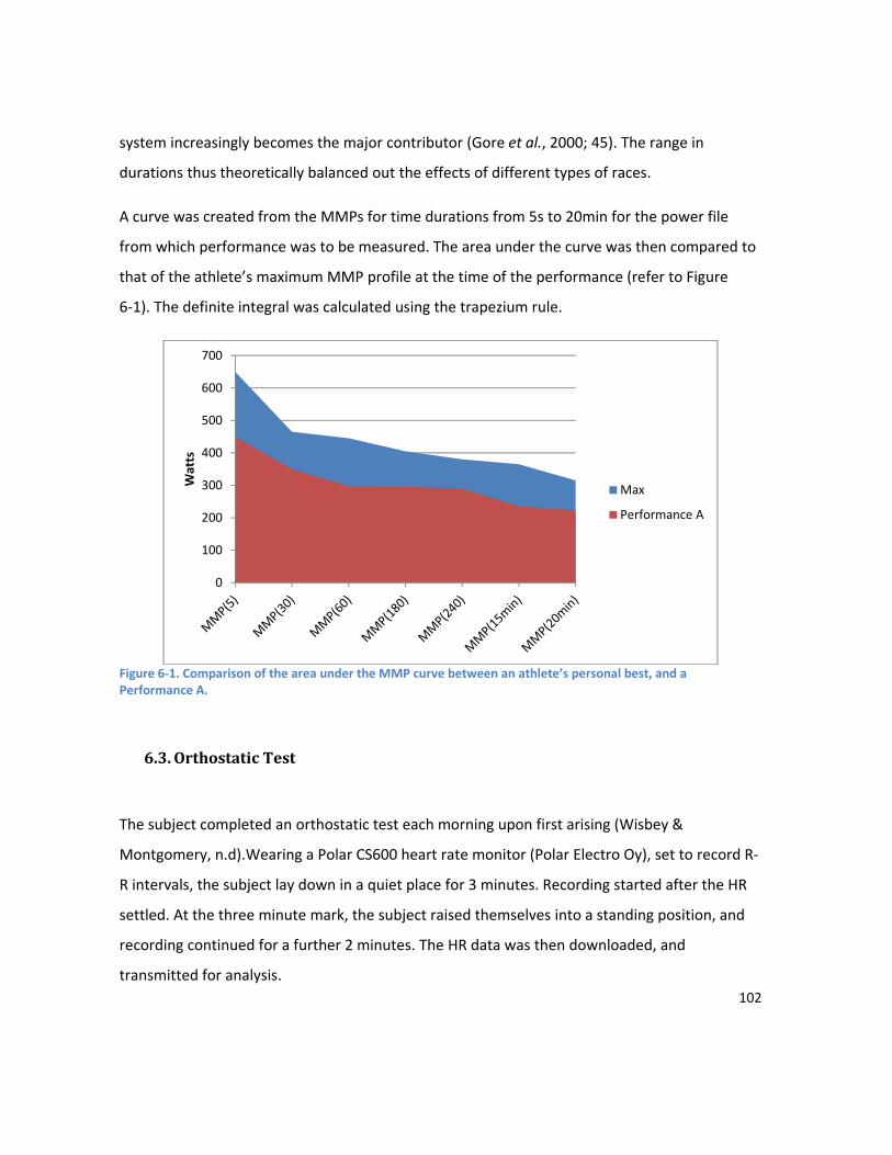
102
system increasingly becomes the major contributor (Gore et al., 2000; 45). The range in
durations thus theoretically balanced out the effects of different types of races.
A curve was created from the MMPs for time durations from 5s to 20min for the power file
from which performance was to be measured. The area under the curve was then compared to
that of the athlete’s maximum MMP profile at the time of the performance (refer to Figure
6-1). The definite integral was calculated using the trapezium rule.
Figure 6-1. Comparison of the area under the MMP curve between an athlete’s personal best, and a Performance A.
6.3. Orthostatic Test
The subject completed an orthostatic test each morning upon first arising (Wisbey &
Montgomery, n.d).Wearing a Polar CS600 heart rate monitor (Polar Electro Oy), set to record R-
R intervals, the subject lay down in a quiet place for 3 minutes. Recording started after the HR
settled. At the three minute mark, the subject raised themselves into a standing position, and
recording continued for a further 2 minutes. The HR data was then downloaded, and
transmitted for analysis.
0
100
200
300
400
500
600
700
Wat
ts
Max
Performance A

103
6.3.1. HRV Analysis
Custom-built software (HRV Athlete, FitSense Australia) was used to analyse the HR file and
calculate the RI for each day as per the method outlined in Chapter 5.
6.3.2. Data Pre-processing
PTRIMP data was smoothed over 3, 7, 14 and 30 days using a rolling average. Missing values for
PTRIMP and RI (caused by equipment failure etc.) were interpolated. A linear interpolation was
used for RI. Missing PTRIMP values were interpolated by using HR data captured on the same
day. A HR TRIMP was calculated using the equation:
= (min) × ( 6-1 )
where T = time in minutes, HRex = average HR for the session and HRmax = the athlete’s
maximum HR. HR TRIMP values were then standardised by calculating z-scores. The following
equation was then solved for PTRIMP:
= − ( 6-2 )
where t = HR TRIMP z-score, μ = mean of PTRIMP sample and σ = SD of PTRIMP sample.
Scatterplots indicated that the relationship between PTRIMP smoothed over 3 days (PTRIMP(3))
and performance is non-linear (inverted parabola). The data was transformed using the natural
log of Performance to improve the linear relationship. A constant was added to Performance so
that all values were positive prior to transformation. As performance is measured in arbitrary
units (a.u), it was judged no information was lost in this process.
The dataset contained outliers. Trials showed that one outlier with very poor performance was
artificially inflating the fit of the model. This worst performance was capped at -155,000(a.u).

104
Successive data points were treated as independent, as in most cases the performance
measurements are separated in time.
6.3.3. Multiple Linear Regression Modelling
Mean and standard deviation (SD) were calculated for all variables. For log transformed data
the mean was back-transformed (emean) and SD is presented as a coefficient of variation
(100(eSD - 1). The Shapiro-Wilk normality test was performed to verify the normality of the
distribution as both z-scores and linear regression techniques assume normality. Pearson’s
product-moment correlation coefficient was used to determine the association between
variables. The Breusch-Pagan test was used to test for heteroskedasticy of residuals. A Durbin-
Watson test was used to test for autocorrelation in the residuals.
Correlation analysis was performed to give an initial indication of whether PTRIMP data
smoothed over 3, 7, 14 or 30 days was likely to have the strongest influence on performance.
From this analysis, PTRIMP(3) and RI were selected as the variables showing the highest
correlation with performance. PTRIMP(3) and RI were not found to be significantly correlated.
A multiple linear regression model was created using linear least squares to minimise the
residual sum of squares. The adjusted coefficient of determination (R2) was calculated. A
process of data exploration was followed to find the best model. The outcome of this process
was the inclusion of interaction terms between RI and PTRIMP(3) and a quadratic term for
PTRIMP(3) increased the fit of the model.
A k-means cluster analysis was performed on the performance data to derive three clusters
(interpreted as low, moderate and high performance). Models were fitted using the R Statistical
Package Version 2.6.1 (The R Development Core) and the package Rcmdr (version 1.3-15).
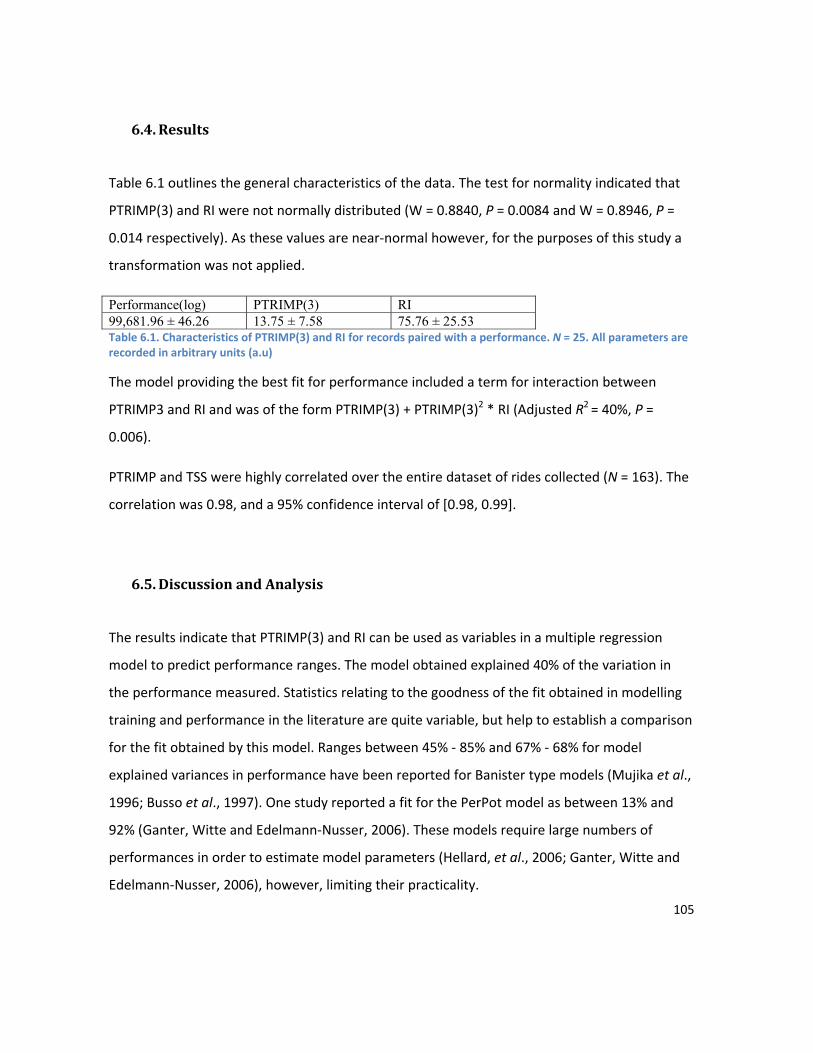
105
6.4. Results
Table 6.1 outlines the general characteristics of the data. The test for normality indicated that
PTRIMP(3) and RI were not normally distributed (W = 0.8840, P = 0.0084 and W = 0.8946, P =
0.014 respectively). As these values are near-normal however, for the purposes of this study a
transformation was not applied.
Performance(log) PTRIMP(3) RI 99,681.96 ± 46.26 13.75 ± 7.58 75.76 ± 25.53 Table 6.1. Characteristics of PTRIMP(3) and RI for records paired with a performance. N = 25. All parameters are recorded in arbitrary units (a.u)
The model providing the best fit for performance included a term for interaction between
PTRIMP3 and RI and was of the form PTRIMP(3) + PTRIMP(3)2 * RI (Adjusted R2 = 40%, P =
0.006).
PTRIMP and TSS were highly correlated over the entire dataset of rides collected (N = 163). The
correlation was 0.98, and a 95% confidence interval of [0.98, 0.99].
6.5. Discussion and Analysis
The results indicate that PTRIMP(3) and RI can be used as variables in a multiple regression
model to predict performance ranges. The model obtained explained 40% of the variation in
the performance measured. Statistics relating to the goodness of the fit obtained in modelling
training and performance in the literature are quite variable, but help to establish a comparison
for the fit obtained by this model. Ranges between 45% - 85% and 67% - 68% for model
explained variances in performance have been reported for Banister type models (Mujika et al.,
1996; Busso et al., 1997). One study reported a fit for the PerPot model as between 13% and
92% (Ganter, Witte and Edelmann-Nusser, 2006). These models require large numbers of
performances in order to estimate model parameters (Hellard, et al., 2006; Ganter, Witte and
Edelmann-Nusser, 2006), however, limiting their practicality.

106
Comparatively few researchers have investigated the relationship between training and
performance outside of the laboratory setting. Performance testing in the laboratory attempts
to control for as many lurking variables as possible. Factors such as nutrition, hydration,
temperature, and pacing strategies have not been controlled in this research using real-world
performances. As such, the fit of this model is not expected to be as good as those reported for
studies using performances measured by frequent laboratory testing. The aim of this study,
however, is to use field-derived data to develop a model which can be used as a practical tool
by athletes and coaches.
The significant explanatory power of the model suggests that the methodology used to
calculate performance has potential to be used in real world modelling. The non-linear
relationship between PTRIMP and RI (refer to Figure 6-2) indicates that for peak performance,
an athlete should be fresh, but not too fresh. This is in accordance with common tapering
strategies. Figure 6-3 demonstrates the effectiveness of the model in correctly distinguishing
between low and high performances. There is some cross-over between low and medium and
medium and high performances, however.
The fit of the model was significantly improved by adding RI as an explanatory variable. HRV
indices capture more information about an athlete’s state of fatigue than training load alone.
HRV is affected by other factors such as sleep, life stress and illness (Fletcher, 2007; Wisbey &
Montgomery, n.d.). The addition of the quadratic term for PTRIMP(3) improved the fit of the
model due to the non-linear relationship between training and performance.
Two findings of this study were not in accordance with the literature. We found that PTRIMP
smoothed with rolling average over 3 days showed the highest correlation with performance.
The values for the time course of fatigue parameter (an input into the Banister model) have
been reported as 15 days (Morton et al., 1990) and 12.4 days (Mujika et al., 1996). Coggan (n.d.
(c)) suggests using a time constant of 7 days to model the time course of training induced
fatigue. The findings in the present study suggest a shorter time frame for the time course of
fatigue than has been generally reported in the literature.

107
Banister (1991) proposed that the relationship between training and performance could be
conceptualised by Equation Error! Reference source not found.. A variant of this concept was
tested for significance in the model, by introducing a variable obtained by subtracting
PTRIMP(7) (representing fatigue) from PTRIMP(30) (representing fitness). The time courses
chosen to represent fitness and fatigue were as suggested by Coggan (n.d. (c)). The resultant fit
was poor.
These findings appear to be interrelated. The correlation between performance and training
load decreased as the number of days PTRIMP was averaged over increased. This is most likely
related to the algorithm used for quantifying performance. Performance was calculated relative
to the athlete’s best performance at that time. As the athlete became fitter, the level required
to achieve a ‘good’ performance also rose, thus decreasing the impact of ‘fitness’ (dependent
on long term training) and increasing the impact of ‘fatigue’ (induced by short term training).
It is suggested that further work be conducted in a number of areas. The hypothesis that the
algorithm used to quantify performance reduced the impact of long term training on the model
can be tested by constructing another model. By adjusting the performance algorithm to be
relative to the best performance achieved by the athlete over the entire course of the study,
the correlation between long term training and performance can be examined.
The relationship between training and performance is complex, non-linear, and changes over
time. The variation over time was not captured in the present model. Use of this data with a
dynamic systems model (PerPot for example) may provide a better fit. Machine learning
techniques are typically suitable for modelling complex non-linear behaviour, and should be
considered for use in this domain.
PTRIMP is highly correlated with TSS. PTRIMP does have an advantage over TSS in achieving a
more physiologically accurate relationship between the relative weighting of duration and
intensity. TSS and PTRIMP both calculate load additively, however TSS has ride duration (T) as a

108
multiplicative constant (refer to Equations ( 6-3 ) and ( 6-4 )). TSS thus places more emphasis on
training duration at the expense of intensity compared to PTRIMP.
≈ × ( )
( 6-3 )
≈ ( )
( 6-4 )
where T = total duration time
t = time measure interval
Prt = raw power at time t
f, g = functions
n = number of observations
τ = number of rolling average intervals
For example consider the following two training rides:
Ride t1 t2 …tn Duration (T) 1 200w 0 0 1hr 2 200w 0 0 2hr TSS for ride 2 will be greater than TSS for ride 1. PTRIMP, however, calculates the two rides as
equal, which is an accurate reflection of the actual physiological work load.
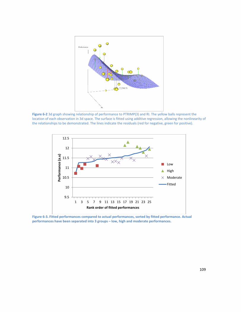
109
Figure 6-2 3d graph showing relationship of performance to PTRIMP(3) and RI. The yellow balls represent the location of each observation in 3d space. The surface is fitted using additive regression, allowing the nonlinearity of the relationships to be demonstrated. The lines indicate the residuals (red for negative, green for positive).
Figure 6-3. Fitted performances compared to actual performances, sorted by fitted performance. Actual performances have been separated into 3 groups – low, high and moderate performances.
9.5
10
10.5
11
11.5
12
12.5
1 3 5 7 9 11 13 15 17 19 21 23 25
Perf
orm
ance
(a.u
)
Rank order of fitted performances
Low
High
Moderate
Fitted

110
6.6. Summary
This chapter describes the development of a novel performance metric. The performance
metric is founded on the understanding that performance in a road race is determined by one
or more critical periods. These critical periods require maximal power outputs over varying
durations. The performance metric developed allows performance to be estimated from data
collected in real world races. The chapter further describes a model which enables the
prediction of performance (quantified using the novel algorithm developed) from an athlete’s
training and HRV indices. The model provides athletes with target ranges for training load and
fatigue levels to increase the likelihood of a high performance. The use of field-derived inputs
makes this model a practical tool for the planning of a taper to maximise competition
performance.
This research is an initial case study, and additional work with a larger sample size is required.
The results indicate, however, that the novel techniques developed to quantify training load
and performance have the potential provide the basis for models of sufficient accuracy to
enable their use as a tool in optimising training programs. It is suggested that other, non-linear
modelling techniques, such as dynamic systems models or machine learning techniques, be
considered to optimise modelling performance.

111
CHAPTER 7 - IDENTIFYING TAPER SHAPE AND ITS EFFECT ON PERFORMANCE Athletes and coaches manipulate training load with the aim of achieving the physical state most
conducive to optimal performance at the desired time for key competitions. Part of the
manipulation of training load involves the reduction of training for a short period prior to a
competition - this is known as a taper.
This chapter considers the practical application of the novel performance metric PTRIMP and
the novel performance quantification technique (detailed in Chapters 4, 5 and 6) to the
problem of identifying the optimal taper for an athlete. Two datasets obtained from two female
elite cyclists are modelled to determine each athlete's optimal taper shape. The aim of this
investigation was to firstly identify the effect the shape of a taper has on an elite cyclists’
performance, and secondly, to determine if individual differences in optimal taper shape exist
between athletes. Furthermore a model which demonstrates that taper shape has a significant
effect on performance provides validation of the PTRIMP and performance metrics. It also
provides confirmation that such information can be the basis of models accurate enough to be
able to provide relevant feedback on the optimal design of training programs.
7.1. The Taper
The taper can be defined as a period of reduced training prior to a competition, undertaken
with the aim of achieving peak performance at the desired time (Thomas, Mujika & Busso,
2009). It is of paramount importance in the preparation of athletes for competitions (Pyne,
Mujika & Reilly, 2009).
The effectiveness of a taper as reported in the literature varies, however the improvement in
performance is usually in the range of 0.5% - 6%. A realistic goal for performance improvement

112
as the result of a taper is about 3% (Mujika & Padilla, 2003). In competitive athletes such
modest improvements are important. A worthwhile improvement for top-ranked athletes is
estimated to be in the range of 0.5% - 3.0% for events such as endurance cycling (Hopkins,
Hawley & Burke, 1999).
The aim of the taper is to reduce accumulated training-induced fatigue, while retaining or
further enhancing physical fitness (Bosquet, Montpetit, Arvisais & Mujika, 2007). The key
elements to manipulate in determining an optimal taper include; the magnitude of reduction in
training volume; training intensity; duration of the taper; and the pattern of the taper (Pyne,
Mujika & Reilly, 2009).
Uncertainty exists about the optimal design of a taper (Mujika & Padilla, 2003). In a meta-
analysis study Bosquet, Montpetit, Arvisais & Mujika (2007) suggested that training volume
should be reduced by 41% - 60% over a two-week taper, without any modification to training
intensity or frequency. They found that reducing training volume elicited a performance
improvement approximately twice that gained by modifying either training intensity or
frequency.
A number of taper patterns have been described and investigated in the literature. Training
load can be reduced in the form of a simple step – where the load is suddenly reduced and then
maintained at the same low level; or it can be reduced progressively, either with a constant
linear slope, or with an exponential decay (Thomas, Mujika & Busso, 2009; Mujika & Padilla,
2003). There is evidence to suggest that a progressive taper is to be preferred (Bosquet,
Montpetit, Arvisais & Mujika, 2007; Banister, Carter & Zarkadas, 1999).
Little research has been done on more complicated taper patterns. One such study looked at
the effect of a two-phase taper. This model study found that the last 3 days of the taper were
optimised with a 20% to 30% increase in training load. In the modelled response such a two-
phase approach allowed for additional fitness adaptations to be made in the final 3 days,
without compromising the removal of fatigue. The magnitude of the performance gain is

113
marginal (0.01%), however, compared to the optimal linear taper (Thomas, Mujika & Busso,
2009).
Much of the literature provides generalised guidelines on designing an optimal taper. It must be
noted, however, that individual responses to training vary. Not all athletes respond equally to
the training undertaken during a taper, and tapering strategies must be individualised (Mujika,
2009). Individual profiles of training adaptation and the time course of de-training need to be
considered in determining optimal taper duration (Mujika & Padilla, 2003). The positive
performance results of the two-phase taper in modelling work done by Thomas, Mujika and
Busso (2009) suggests that further investigation into optimal taper shapes is warranted.
The purpose of this study was to provide validation of the PTRIMP and performance metrics by
investigating the effect of the shape of a taper on elite cyclists’ performance, and determining if
individual differences in optimal taper shape exist between athletes. We aim to investigate
these aspects from a novel angle – through symbolisation of taper time series information and
subsequent relation of the taper shape to performance.
7.2. Modelling the Taper Two female elite cyclists provided data for the study over a period of 250 and 870 days
respectively. An SRM power monitor (professional model, Schoeberer Rad Messtechnik,
Germany) was fitted to each subject’s bike(s) over the data collection period. Power data from
all rides (training and racing) was captured at 1Hz. In accordance with operator instructions, the
SRM was zeroed prior to the start of each session. SRM data files were imported into a custom-
built program for the calculation of training load (PTRIMP) and performance.
7.2.1. Quantifying Training Load
PTRIMP was calculated as per the method described in Chapter Five (refer to Equations ( 5-1 )
and ( 5-2 )). A record of MMPs for 5s, 30s, and 4mins achieved by the athlete was kept, and
updated when a new personal best was achieved.

114
7.2.2. Quantifying Performance
Each athlete kept a training diary, which was used to identify races. Performances were
included in the dataset when training data existed for the three days prior to the performance.
Twenty-six performances were identified for Subject A, and 22 for Subject B.
A curve was created from the MMPs for time durations from 5s to 20min for the power file
from which performance was calculated. The area under the curve was then compared to that
of the athlete’s maximum MMP profile at the time of the performance (refer to Figure 7-1). The
definite integral was calculated using the trapezium rule.
Figure 7-1. Comparison of the area under the MMP curve between an athlete’s personal best, and a Performance A.
The durations for which MMP were recorded were at regular intervals from 5s to 20min. These
durations were chosen to represent a spectrum of energy system contributions. For durations
of up to approximately 10 seconds, energy is predominantly supplied by the anaerobic alactic
system. From around 10 seconds to approximately 60 seconds, energy is predominantly
supplied by the anaerobic lactic system. Beyond this, the contribution of the aerobic energy
0
100
200
300
400
500
600
700
Wat
ts
Max
Performance A

115
system increasingly becomes the major contributor (Gore, 2000). The range in durations thus
theoretically balanced out the effects of different types of races.
7.2.3. Symbolic Aggregate Approximation
Symbolic Aggregate approXimation (SAX) allows a time-series of arbitrary length n to be
reduced to a string of arbitrary length w. The alphabet size used is also an arbitrary integer (Lin,
Keogh, Lonardi & Chiu, 2003). The process involves firstly normalising the time-series to have a
mean of zero and a standard deviation of one. A series of breakpoints are identified that divide
a Gaussian distribution up into n number of equiprobable regions. These breakpoints are used
to map each data point into symbols, such that a data point lower than the smallest breakpoint
will be mapped to the symbol ‘a’, a point greater than or equal to the smallest breakpoint but
smaller than the next breakpoint will be mapped to ‘b’ and so on (refer to Figure 7-2).
A time series consisting of the three days training load (PTRIMP) in the lead up to a
performance was created. The Matlab code of Lin, Keogh, Lonardi and Chiu (2002 & 2003) was
used to discretise the time series of PTRIMP data. The code was customised in two areas. A
change was made such that normalisation of the time series was performed based on the entire
series, rather than just on the current ‘window’ of data. The code which performs numerosity
reduction was also removed. A window size of three days and an alphabet size of three were
used. An alphabet size of three was selected as a good compromise enabling the creation of a
usable number of patterns whilst maintaining reasonable statistical power.
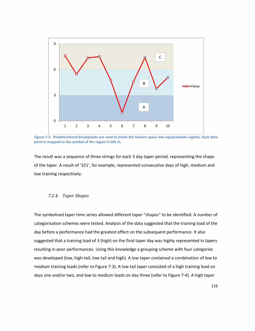
116
Figure 7-2. Predetermined breakpoints are used to break the feature space into equiprobable regions. Each data point is mapped to the symbol of the region it falls in.
The result was a sequence of three strings for each 3 day taper period, representing the shape
of the taper. A result of ‘321’, for example, represented consecutive days of high, medium and
low training respectively.
7.2.4. Taper Shapes
The symbolised taper time series allowed different taper “shapes” to be identified. A number of
categorisation schemes were tested. Analysis of the data suggested that the training load of the
day before a performance had the greatest effect on the subsequent performance. It also
suggested that a training load of 3 (high) on the final taper day was highly represented in tapers
resulting in poor performances. Using this knowledge a grouping scheme with four categories
was developed (low, high-tail, low-tail and high). A low taper contained a combination of low to
medium training loads (refer to Figure 7-3). A low tail taper consisted of a high training load on
days one and/or two, and low to medium loads on day three (refer to Figure 7-4). A high taper
0
3
6
9
1 2 3 4 5 6 7 8 9 10
ValueB
C
A
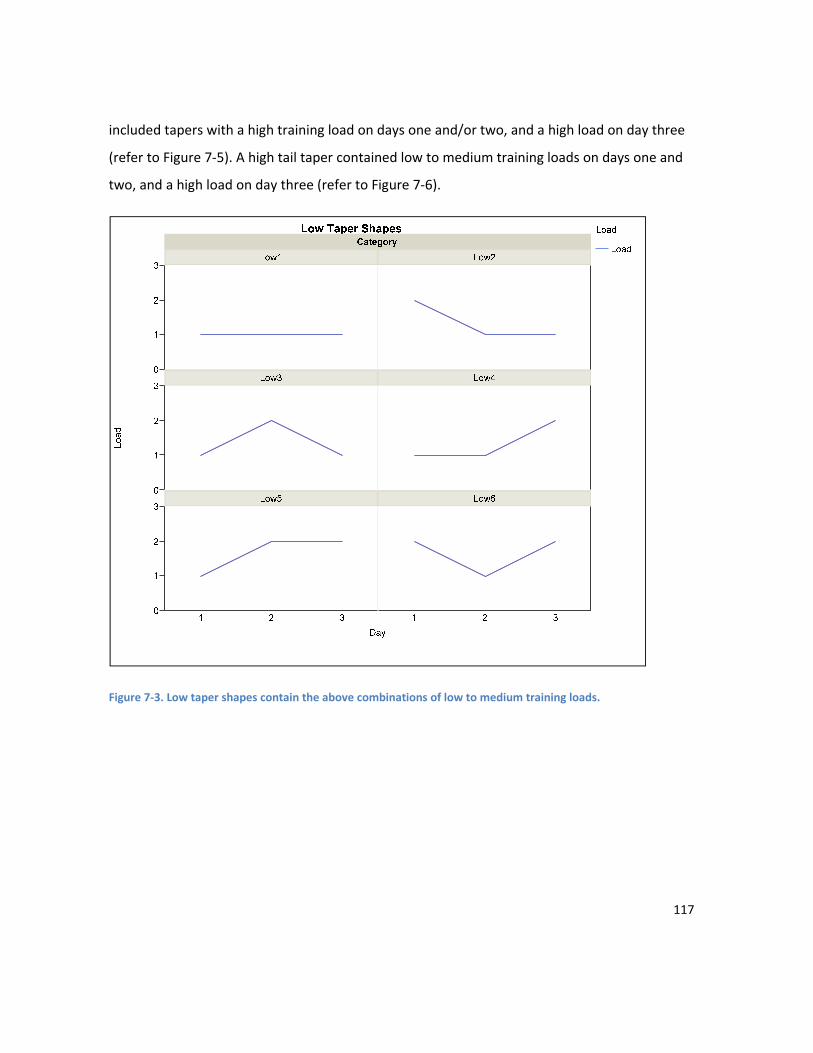
117
included tapers with a high training load on days one and/or two, and a high load on day three
(refer to Figure 7-5). A high tail taper contained low to medium training loads on days one and
two, and a high load on day three (refer to Figure 7-6).
Figure 7-3. Low taper shapes contain the above combinations of low to medium training loads.

118
Figure 7-4. Low tail taper shapes consist of a high training load on days one and/or two, and low to medium loads on day three.
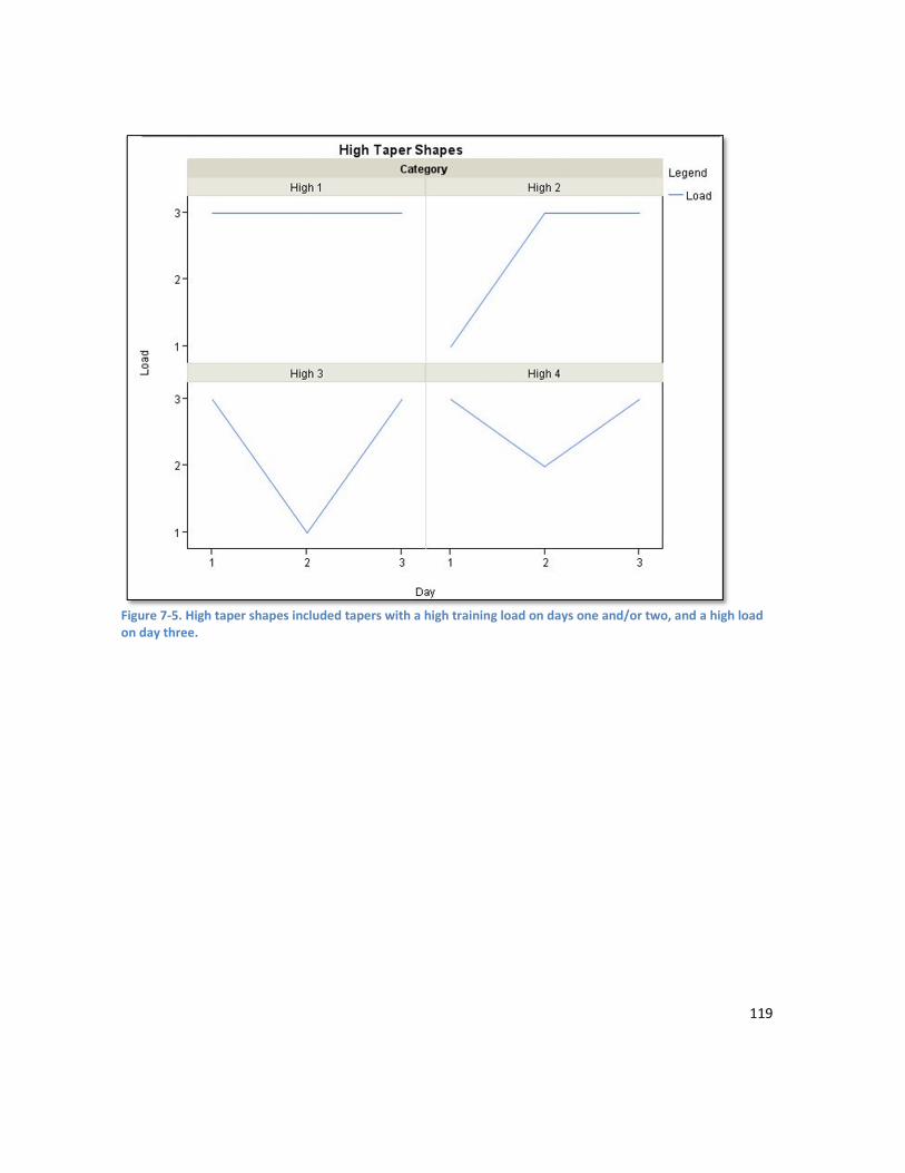
119
Figure 7-5. High taper shapes included tapers with a high training load on days one and/or two, and a high load on day three.

120
Figure 7-6.High tail taper shapes contained low to medium training loads on days one and two, and a high load on day three.
7.2.5. Data Pre-Processing
SRM files occasionally include short durations of spurious power readings. Such spurious data
points were identified and removed. The Performance dataset for one subject contained an
outlier. This (worst) performance was capped at -155,000(au).
The Performance data was transformed by taking the natural log of Performance. A constant
was added to Performance so that all values were positive prior to transformation. As
performance is measured in arbitrary values (au), it was judged no information was lost in this
process.

121
7.2.6. Statistical Analysis
The Shapiro-Wilk normality test was performed to verify the normality of the distribution. A
two-way analysis of variance (ANOVA) confirmed that a significant interaction effect between
subject and taper shape was present. Subsequently, the difference between the taper shapes
was compared using a one-way analysis of variance (ANOVA). The scale proposed by Cohen
(1988) was used for interpretation: the magnitude of the difference was considered either
small (0.2), moderate (0.5), or large (0.8).The statistical power for the effect size was
determined to indicate the probability of correctly rejecting a false null hypothesis. Statistics
were calculated using the R Statistical Package Version 2.6.1 (The R Development Core) and the
package Rcmdr (version 1.3-15).
7.3. Results Statistically significant differences were observed in the mean of performances grouped by
taper shape between subjects (for raw data refer to Table 7.1). The main effect of taper shape
on performance was significant for both Subject A (F(3, 22) = 4.2, p < 0.05, MSE = 0.5) and
Subject B (F(3,18) = 3.9, p < 0.05, MSE = 0.3). The effect of each taper group on performance
showed considerable variation between subjects (refer to Figure 7-7).
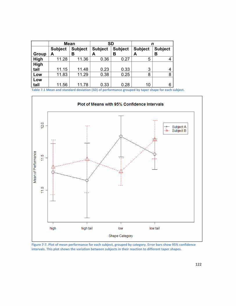
122
Mean SD n
Group Subject A
Subject B
Subject A
Subject B
Subject A
Subject B
High 11.28 11.36 0.36 0.27 5 4 High tail 11.15 11.48 0.23 0.33 3 4 Low 11.83 11.29 0.38 0.25 8 8 Low tail 11.56 11.78 0.33 0.28 10 6
Table 7.1 Mean and standard deviation (SD) of performance grouped by taper shape for each subject.
Figure 7-7. Plot of mean performance for each subject, grouped by category. Error bars show 95% confidence intervals. This plot shows the variation between subjects in their reaction to different taper shapes.

123
The most effective taper for Subject A was a “low” taper, where combinations of low to
medium training days were performed. The least effective taper was a “high tail” taper,
where low to medium training was performed in days one and two, and a high training
load was undertaken on day three. Using Cohen’s scale (Cohen, 1988) the effect size
between the “low” and the “high tail” taper was classified as large. The statistical power
was 97.5% (5% error level). When expressed as a percentage, this was a 6.1%
improvement in performance.
The most effective taper for Subject B was a “low tail” where a high training load was
undertaken on days one and/or two, and a low training load undertaken on day three. The
least effective taper for Subject B was the “low” taper. Using Cohen’s scale (Cohen, 1988)
the effect size between the “low tail” and the “low” taper was classified as large. The
statistical power was 92.4% (5% error level). When expressed as a percentage, this was a
4.4% improvement in performance.
7.4. Discussion and Analysis The results show considerable variance between individuals in their response to a taper. A
two-way ANOVA showed that the interaction effects between taper shape and subject was
significant. Combining the results of both subjects was considered inappropriate, even
though the subjects for this study were reasonably homogenous – both female elite
cyclists. Tapering advice in the literature is frequently generalised across genders, between
different sports, and between trained athletes and elite athletes. These results suggest
that specific tapering advice cannot be provided using a generalist model.
The “low” taper shape was associated with the highest mean performance for Subject A,
and the lowest mean performance for Subject B. The optimal taper may be influenced by
the intensity and volume of the training preceding the taper. Those who train harder and
longer may require a longer taper to enable them to recover, while those with less training
require a shorter taper to minimise loss of fitness (Kubukeli, Noakes, & Dennis, 2002). One

124
possible explanation for the variance in taper effect observed is that Subject A tended to
carry more fatigue into the final 3 days of training, due to a higher training load in the
preceding training cycle. Thus, a low training load in the taper allowed for more effective
dissipation of fatigue, resulting in higher performance.
The most effective taper shape for Subject B was the “low tail” shape. If Subject B went
into the final 3 days with relatively low levels of fatigue, higher training loads would not
have the negative effect on overall fatigue that they would for Subject A. Thomas, Mujika
and Busso (2009) suggest that a moderate increase in training load in the final 3 days of a
taper can allow adaptations to training to occur without compromising fatigue
minimisation.
The most effective taper shape for Subject A represented a 6.1% improvement, while that
of Subject B represented a 4.4% improvement. Paton & Hopkins (2006) estimate that the
smallest worthwhile improvement for top-level athletes in the individual sport of road
cycling time trials is in the order of approximately 0.6%. They concluded, however, that
drafting in road races precludes estimation of the smallest worthwhile change in
performance for this event. Nevertheless, it is likely that small improvements in
performance, as observed in this study, could have a significant effect on the outcome of
elite competition.
The experimental design did not consider the training load prior to the final 3 days of taper
before a performance. The study reported in Chapter 6 suggested that training load over
the 3 days before a performance had the highest correlation with performance. The
current research could be extended by modelling the training load in the 4-11 days prior to
the 3-day period studied. Such an extension could potentially determine whether the level
of training-induced fatigue brought into the taper period affects the optimal shape of the
taper, as hypothesised.

125
The training load quantification method (PTRIMP) aggregates the volume and intensity of
training. This means it is not possible to distinguish the specific influence of training
intensity during the taper. The model we have developed can determine the optimal shape
of training load within a taper, but cannot provide guidance on the optimal balance
between training duration and intensity during the taper. There is general agreement in
the literature that intensity should be maintained in the taper (e.g Mujika & Padilla, 2003;
Pyne, Mujika & Reilly, 2009; Bosquet, Montpetit, Arvisais & Mujika, 2007), and this is the
general practice followed by the subjects.
In this study, crisp boundaries were used in determining the breakpoints in the
symbolisation process. Crisp boundaries result in some loss of data, as two similar training
load values positioned either side of a boundary will be treated as different categories
although the actual difference in values is small. Removing crisp boundaries in favour of
fuzzy boundaries would remove this potential issue.
This research studied the effect of different taper shapes on performance in actual
competitions. Few studies have used data from real world training and performance data.
The relationship between performance in tests and performance in events was questioned
by Hopkins, Hawley & Burke (1999), and how a change in performance in a test translates
to performance change in a competition remains uncertain.
Performance tests in competition are affected by external factors, such as climatic
conditions, tactics, drafting, terrain and varying competition types (time trials, hilly road
races, flat road races and criteriums are all race types included in this study’s dataset).
Such factors are either not applicable, or can be controlled for, in a lab situation. The fact
that the effect size of the different taper shape treatments is significant for both subjects,
however, indicates that the model developed is robust.
The use of field-derived model inputs makes this model a practical tool for the planning of
a taper to maximise competition performance. The relatively minimal data collection
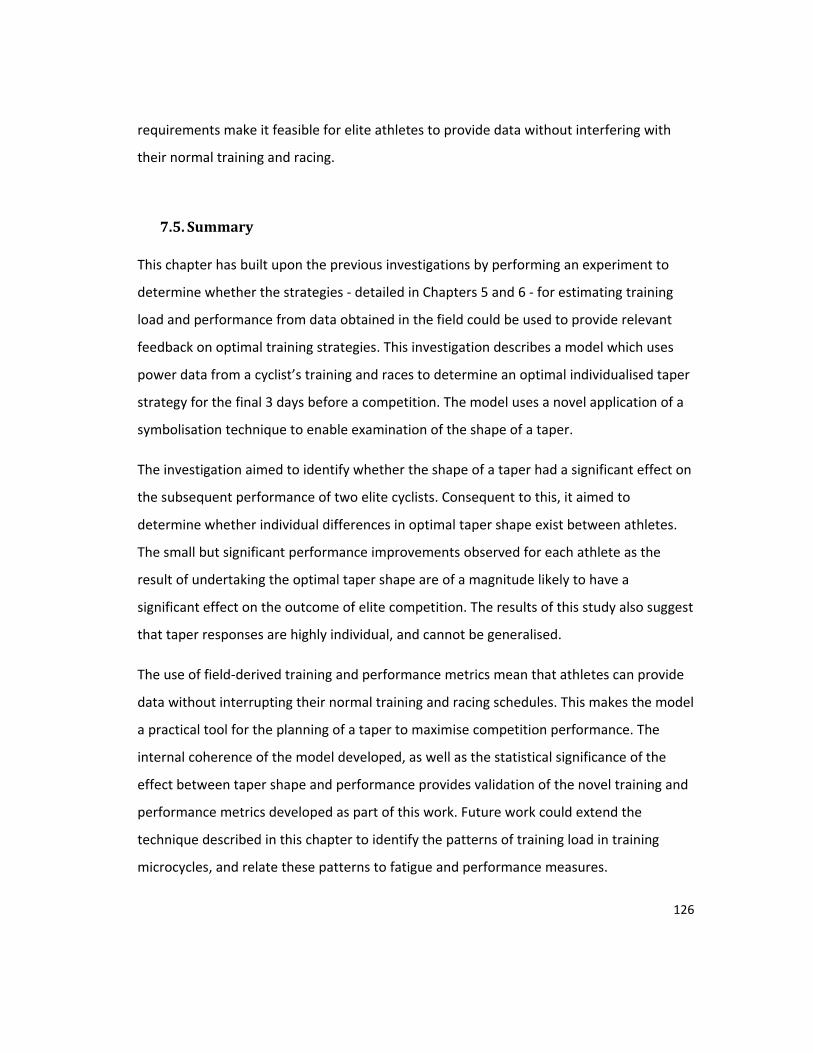
126
requirements make it feasible for elite athletes to provide data without interfering with
their normal training and racing.
7.5. Summary This chapter has built upon the previous investigations by performing an experiment to
determine whether the strategies - detailed in Chapters 5 and 6 - for estimating training
load and performance from data obtained in the field could be used to provide relevant
feedback on optimal training strategies. This investigation describes a model which uses
power data from a cyclist’s training and races to determine an optimal individualised taper
strategy for the final 3 days before a competition. The model uses a novel application of a
symbolisation technique to enable examination of the shape of a taper.
The investigation aimed to identify whether the shape of a taper had a significant effect on
the subsequent performance of two elite cyclists. Consequent to this, it aimed to
determine whether individual differences in optimal taper shape exist between athletes.
The small but significant performance improvements observed for each athlete as the
result of undertaking the optimal taper shape are of a magnitude likely to have a
significant effect on the outcome of elite competition. The results of this study also suggest
that taper responses are highly individual, and cannot be generalised.
The use of field-derived training and performance metrics mean that athletes can provide
data without interrupting their normal training and racing schedules. This makes the model
a practical tool for the planning of a taper to maximise competition performance. The
internal coherence of the model developed, as well as the statistical significance of the
effect between taper shape and performance provides validation of the novel training and
performance metrics developed as part of this work. Future work could extend the
technique described in this chapter to identify the patterns of training load in training
microcycles, and relate these patterns to fatigue and performance measures.

127
CHAPTER 8 – HANNEM: A HYBRID ANN ENSEMBLE FOR SYSTEMS MODELLING
8.1. Introduction This chapter brings together the load quantification algorithm (PTRIMP) research
described in Chapter 5 and the performance quantification algorithm research described
in Chapter 6, by creating a model to describe the relationship between training and
performance for elite road cyclists. The physiological processes underlying an athlete’s
response to training (as described in Chapter 2) form the theoretical underpinning for
this chapter. The modelling techniques discussed in Chapters 3 and 4 are combined and
extended.
A novel hybrid artificial neural network ensemble model (HANNEM) is developed in this
chapter. The model overcomes issues in the domain concerning: limited amounts of
noisy and often incomplete data; ambiguity as to the form of the patterns present in the
data; and practical concerns limiting the number of independent parameters available
for modelling. HANNEM combines the SimBEA model (Bruckner, 2006) - an evolution of
the impulse-response models described in Chapter3, which brings valuable information
regarding physiological responses such as supercompensation, accommodation and
reversibility - with linear and nonlinear modelling techniques. In the proposed HANNEM
model, a linear model identifies the linear patterns in the data, while a neural network
model captures the nonlinear patterns in the data.
This investigation tests HANNEM using three datasets consisting of longitudinal training
and racing power data, collected from three elite road cyclists. The results of these tests
are presented along with a discussion of the effectiveness of the model.

128
8.1.1. The SimBEA Model
SimBEA is conceptualised as an evolution of the traditional impulse-response model.
The model incorporates three important training principles; adaptation and
supercompensation; accommodation; and reversibility. A given training impulse causes
an immediate performance decrement due to the effect of fatigue, followed by a
delayed increase in performance as the result of an increase in fitness. SimBEA thus
models the supercompensation curve (refer to Chapter 2 - Training Principles for a
discussion on the theory of supercompensation). Figure 8-1 shows how the model
behaves in response to a single training impulse - captured as the blue bar. The resulting
performance estimate of the model (the red bar) initially decreases in response to the
training impulse that occurs on day 2, then rebounds by day 4. This behaviour is
consistent with what is known about the supercompensation curve.
The SimBEA model also behaves in accordance with the training principle of reversibility.
Figure 8-1 demonstrates that the adaptations made to training gradually return to pre-
training levels once training ceases. As no further training stimulus is applied after day 2,
once the initial supercompensation effect triggered by this stimulus dissipates
performance gradually declines.
Figure 8-1. SimBEA models the decline in performance once training ceases. The blue bar represents a training impulse, and the red bars the performance estimate of the model. After the initial supercompensation effect triggered by the training impulse, performance declines to pre-training levels.
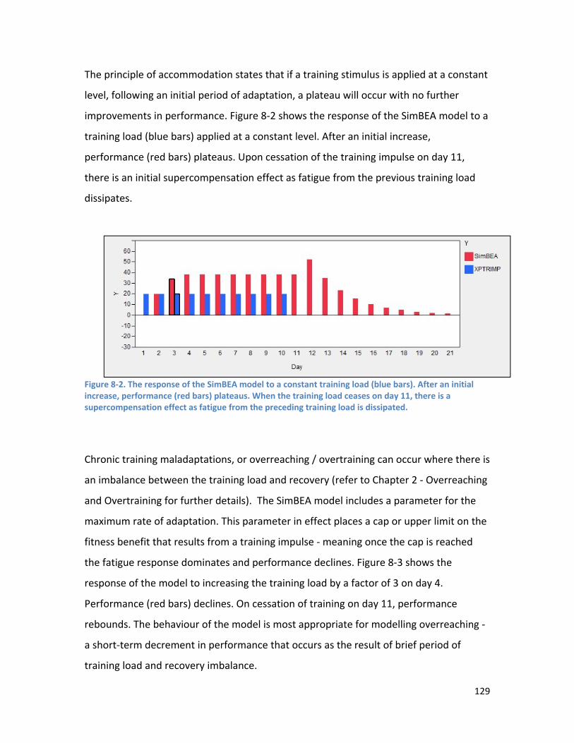
129
The principle of accommodation states that if a training stimulus is applied at a constant
level, following an initial period of adaptation, a plateau will occur with no further
improvements in performance. Figure 8-2 shows the response of the SimBEA model to a
training load (blue bars) applied at a constant level. After an initial increase,
performance (red bars) plateaus. Upon cessation of the training impulse on day 11,
there is an initial supercompensation effect as fatigue from the previous training load
dissipates.
Figure 8-2. The response of the SimBEA model to a constant training load (blue bars). After an initial increase, performance (red bars) plateaus. When the training load ceases on day 11, there is a supercompensation effect as fatigue from the preceding training load is dissipated.
Chronic training maladaptations, or overreaching / overtraining can occur where there is
an imbalance between the training load and recovery (refer to Chapter 2 - Overreaching
and Overtraining for further details). The SimBEA model includes a parameter for the
maximum rate of adaptation. This parameter in effect places a cap or upper limit on the
fitness benefit that results from a training impulse - meaning once the cap is reached
the fatigue response dominates and performance declines. Figure 8-3 shows the
response of the model to increasing the training load by a factor of 3 on day 4.
Performance (red bars) declines. On cessation of training on day 11, performance
rebounds. The behaviour of the model is most appropriate for modelling overreaching -
a short-term decrement in performance that occurs as the result of brief period of
training load and recovery imbalance.
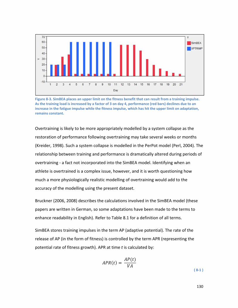
130
Figure 8-3. SimBEA places an upper limit on the fitness benefit that can result from a training impulse. As the training load is increased by a factor of 3 on day 4, performance (red bars) declines due to an increase in the fatigue impulse while the fitness impulse, which has hit the upper limit on adaptation, remains constant.
Overtraining is likely to be more appropriately modelled by a system collapse as the
restoration of performance following overtraining may take several weeks or months
(Kreider, 1998). Such a system collapse is modelled in the PerPot model (Perl, 2004). The
relationship between training and performance is dramatically altered during periods of
overtraining - a fact not incorporated into the SimBEA model. Identifying when an
athlete is overtrained is a complex issue, however, and it is worth questioning how
much a more physiologically realistic modelling of overtraining would add to the
accuracy of the modelling using the present dataset.
Bruckner (2006, 2008) describes the calculations involved in the SimBEA model (these
papers are written in German, so some adaptations have been made to the terms to
enhance readability in English). Refer to Table 8.1 for a definition of all terms.
SimBEA stores training impulses in the term AP (adaptive potential). The rate of the
release of AP (in the form of fitness) is controlled by the term APR (representing the
potential rate of fitness growth). APR at time t is calculated by:
( ) = ( )
( 8-1 )

131
where VA is a delay parameter which controls the rate of release of AP. AP is calculated
by the following formula: ( + ∆ ) = ( ) + ( ) − ( ) ( 8-2 )
where L(t) is the training load from the previous time increment (the previous day in this
case). The complete model is represented by Equation ( 8-3 ): ( + ∆ ) = ( ) − × ( ) + ( × × min( ( ), )) − ( 8-3 )
where p = performance, t = time t, AF = adjustment factor, BF = fatigue factor, AR =
atrophy rate, and APR = potential rate of growth.
The SimBEA model contains four parameters; an adjustment factor (AF), a fatigue factor
(BF), a delay (VA) and an atrophy rate (AR). Adjustment of these parameters allows the
model to be optimised for each individual athlete.
Term Definition
Adjustment Factor (AF) AF determines the proportion of the fitness gain generated by a given training impulse.
Fatigue Factor (BF)
The parameter BF determines the proportion of fatigue generated by a given training impulse.
Delay (VA) As discussed previously, a given training impulse results in an immediate increase in fatigue, and a delayed increase in fitness as the recovery or adaptation process operates. The fitness component of training impulses is stored, until release, in what the SimBEA model terms the adaptive potential (AP). The delay parameter controls the release rate of the current stock of adaptive potential.
Atrophy Rate (AR) As discussed previously, the principle of reversibility states that upon cessation or reduction in training, performance will gradually diminish. The parameter AR is the term in the SimBEA model which is responsible for controlling the rate of atrophy of

132
performance.
Model Fitting The four parameters of the model are varied iteratively to determine the values resulting in the best fit for an individual dataset. The model is thus adjusted to suit the individual characteristics of each athlete in their response to training.
Table 8.1. Definition of parameters for the SimBEA model.
8.1.2. Artificial Neural Networks Artificial Neural Networks (ANN) are modelling tools well suited to modelling complex
nonlinear and linear relationships whose exact form is unknown; modelling the
relationship between training and performance is just such a problem. Refer to Chapter
4 for a detailed overview of the characteristics of ANNs.
Multilayer Perceptrons (MLP) are the most common form of ANNs. They are particularly
suitable for complex non-linear models (Tuffery, 2011). MLPs are made up of several
layers: the input unit(s), the output units(s) and one or more hidden levels. Each unit at
a layer is connected to the set of units of the preceding layer. Each unit j receives
incoming signals from either the input variables or from every unit i in the previous
layer. There is a weight (Wi,j - initially set randomly), associated with each connection
between units. The incoming signal (Nj) to the unit j is the weighted sum of all the
incoming signals (Equation ( 8-4 )).
= ,
( 8-4 )
Nj passes through an activation function (xi) to produce the output signal (yj) of the unit
j. A sigmoid function is the most popular activation function. It behaves linearly around
the value of 0 (when weights are small) and non-linearly at the limits. Refer to
Figure 8-4 for a diagram depicting the flow of signals through an ANN.
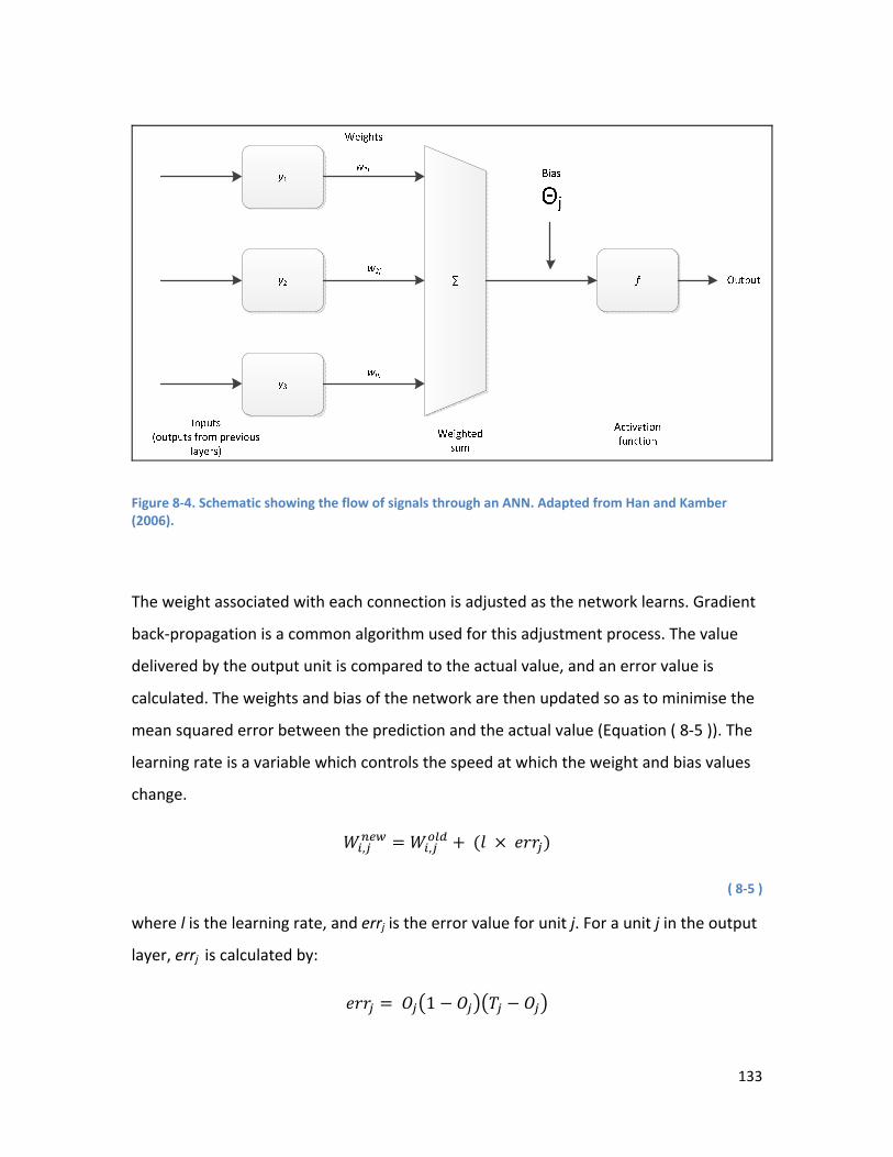
133
Figure 8-4. Schematic showing the flow of signals through an ANN. Adapted from Han and Kamber (2006).
The weight associated with each connection is adjusted as the network learns. Gradient
back-propagation is a common algorithm used for this adjustment process. The value
delivered by the output unit is compared to the actual value, and an error value is
calculated. The weights and bias of the network are then updated so as to minimise the
mean squared error between the prediction and the actual value (Equation ( 8-5 )). The
learning rate is a variable which controls the speed at which the weight and bias values
change.
, = , + ( × )
( 8-5 )
where l is the learning rate, and errj is the error value for unit j. For a unit j in the output
layer, errj is calculated by: = 1 − −

134
( 8-6 )
where Oj is the actual output of unit j and Tj is the known target value of the given
training tuple. The error of a hidden layer unit j is:
= 1 − ,
( 8-7 )
where wj,k is the weight of the connection from unit j to a unit k in the next higher layer,
and errk is the error of unit k (Han & Kamber, 2006).
Researchers in the training modelling space have reported favourable results in the use
of ANNs to model swimming performance (Edelmann-Nusser, Hohmann & Hennerberg,
2002; Hohmann, Edelmann-Nusser & Hennerberg, 2001; Silva et al., 2007). The research
in this domain has, however, failed to properly address the overfitting issues involved
with modelling small datasets using ANNs. Hohmann, Edelmann-Nusser and Hennerberg
(2001) used data from a different athlete to pre-train their network, however the
individual nature of the response to training makes this approach unlikely to be
successful in all but exceptional cases.
8.1.3. Learning From Small Datasets
Learning from small data sets is fundamentally difficult; small data sets make models
prone to overfitting, and increase the difficulty in discovering the exact relationship
between input(s) and output (Yeh, 2007). High-noise, non-stationary time series
increase the modelling difficulty even further. There are an infinite number of models
which would fit the training data well in such situations, but few which generalise well
(Giles, Lawrence & Tsoi, 2001).
In Chapter 4, the technique of bootstrapping (sampling with replacement) was
introduced as a means of creating artificial data. Better performance can be achieved
135
when ANNs, as unstable predictors, are redundantly combined using an ensemble of
models. This ensemble technique improves generalisation ability (Sharkey, 1996), and is
particularly useful when learning from a small data set. Bagging is a related technique,
referring to the construction of a family of models on n bootstrap samples (Tuffery,
2011). The process of resampling with replacement increases the independence of the
training sets, and hence the independence of the models, leading to improved ensemble
results (Raviv & Intrator, 1996). Bagging produces predictions that are more robust to
noisy data, and the technique has been proven to always have improved predictions
over a single predictor (Han & Kamber, 2006).
Some researchers (Raviv & Intrator, 1996; Zur, Jiang & Metz, 2004; Zhang, 2007) have
proposed ensembles of neural networks with noise or jitter added to the bagged
training sets. Training with noise causes the data to appear smoother to the neural
networks, improving the model’s ability to learn the true underlying pattern of the data
and avoid overfitting (Zhang, 2007). The smoothed bagged approach means that larger
datasets with greater independence are created, simulating the true noise in the data
(Raviv & Intrator, 1996). An observed dataset can be thought of as a single instantiation
of an infinite number of datasets which could have been realised from the underlying
process. The particular instantiation depends on the noise values at each point, or any
other random shocks (Zhang, 2007).
There are no established principles reported in the literature for choosing the
appropriate level of noise. The most effective level of noise is likely to be dependent on
the individual dataset, and its inherent noise levels (Zhang, 2007).
8.1.4. Linear Models - ARIMA
Autoregressive integrated moving average (ARIMA) models are used for prediction of
non-stationary time series where linearity between variables is assumed (Gomes et al.,

136
2006). ARIMA models are linear in that predictions of future values are constrained to
hold a linear relationship to past observations (Zhang, 2003). They are widely used in
forecasting social, economic, engineering, foreign exchange and stock problems
(Khashei, Bijari & Raissi Ardali, 2009).
The model formulation actually consists of three sub-models: the autoregressive (AR),
the integrated (I), and the moving average (MA). ARIMA models require that the time
series is stationary. A stationary time series does not show a trend; its mean and the
autocorrelation structure are constant over time. Differencing is a commonly applied
technique to remove a trend in the data (Zhang, 2003). The integrated component of
the ARIMA model aims to render the data series stationary, while the MA and AR
components aim to address the stochastic elements (Reddy, 2011).
ARIMA models are expressed as ARIMA (p,q,d) where p is the order of the AR
component, q is the order of the MA component, and d is the differencing number
applied. The AR model captures the past behaviour of the system, expressing the
residuals at the current time as a linear function of p past residuals. The MA model is a
special type of low-pass filter, which captures the transient shocks or perturbations of
the system with a linear function of q past white noise errors (Reddy, 2011).
The AR component or ARIMA (p,0,0) method is represented as: = + ∅ + ∅ + ⋯ + ∅ +
( 8-8 )
where p is the number of the autoregressive terms, Yt is the forecast output, Yt-p is the observation at time t-p, and ∅1, ∅2,..., ∅p is a finite set of parameters determined by
linear regression. ∅0 is the intercept and et is the error associated with the regression.
The MA component, or ARIMA(0,0,q) is represented as: = − ∅ − ∅ − ⋯ − ∅ +
( 8-9 )

137
where q is the number of the moving average terms, ∅1, ∅2,..., ∅q are the finite weights
and μ is the mean of the series.
An ARIMA (p,0,q) model has the form: = + ∅ + ∅ + ⋯ + ∅ + − − − ⋯ − +
( 8-10 )
An ARIMA (p,d,q) model is an ARIMA (p,0,q) model as per Equation ( 8-10 ), performed
on a time series that has been differenced d times.
ARIMA models can provide accurate forecasting over short periods of time. They are
easy to implement, requiring no further information than the time series to be
modelled. They do, however, require large amounts of historical data in order to yield
desired results (Khashei, Bijari, Raissi Ardali, 2009). In the literature it is estimated that
to be effective ARIMA models require at least 50 - or preferably greater than 100 - data
points(Khashei, Bijari, Raissi Ardali, 2009; Tseng, Yu & Tzeng, 2002; Reddy, 2011).
Although ARIMA models have been used extensively in a variety of domains, only one
athletic performance modelling study to date has applied an ARIMA model to a
performance dataset. Ferger (2008) fit an ARIMA model to the performance dataset
gained for a single subject in a lab study. The fit reported was moderate, with an
Intraclass Correlation Coefficient (ICC) of 0.47. It is important to note, however, that the
unrealistic conditions of data collection and the short (90 days) duration of the dataset
are likely to result in enhanced performance of the model to what would be obtained
under realistic conditions.
8.1.5. Hybrid Models It is nearly always possible to build a more robust and precise model by combining a
number of different models. The prediction obtained from the first model can be used
as an independent variable in the second model (Tuffery, 2011). The idea of the
138
combined model is to use each model’s unique capabilities to capture different patterns
in the data (Zhang, 2003).
Zhang (2003) notes that it is difficult for modellers to choose the right modelling
technique for each unique situation. Modellers generally perform testing with a
selection of the models which are most likely to fit their needs, and then choose the one
that returns the best result. The final model selected is not necessarily the best for
future predictive performance. Many studies suggest that by combining several models,
forecasting performance can be improved over that of an individual model (e.g.
Makridakis & Hibon, 2000; Khashei, Bijari & Raissi Ardali, 2009). This obviates to some
extent the requirement to find the single best model (Zhang, 2003).
As noted in Chapter 4, real world time series are rarely purely linear or nonlinear,
frequently containing both linear and nonlinear patterns (Zhang, 2003). As it is difficult
to identify the nature of all the patterns in a dataset from a real-life problem, hybrid
methodologies that have both linear and nonlinear modelling capabilities can be an
effective modelling technique (Khasei & Bijari, 2010).
Hybrid ARIMA –ANN models have been used to model time series from a number of
applied problem areas (Diaz-Robles et al., 2008). In such hybrids, the ARIMA model
deals with the non-stationary linear component and the neural network deals with non-
linear patterns in the data thus improving forecasting performance (Taskaya-Temizel &
Casey, 2005). Zhang (2003) found that a hybrid ARIMA and neural network model
resulted in improved forecasting accuracy compared to that achieved by either model in
isolation.
Hybrid ARIMA-ANN models are generally constructed sequentially, by first applying an
ARIMA model to the time series, and then using the residuals from the ARIMA model as
the input for the ANN model (e.g. Zhang, 2003; Diaz-Robles et al., 2008). It is typically
assumed that the residuals of a linear component will include valid non-linear patterns
that can be modelled using a neural network (Zhang, 2003; Zhang & Qi, 2005). This

139
assumption that the relationship between the linear and non-linear components is
additive may not, however, be a valid assumption (Taskaya-Temizel & Casey, 2005).
8.1.6. Proposed HANNEM Model HANNEM has been designed and developed to overcome some of the limitations
inherent in modelling small, noisy datasets, and to take advantage of the robustness and
increased generalisation ability offered by new techniques such as the use of hybrid
models, ensembles of models, and data processing techniques such as bagging. It has
been designed to work with training and performance data collected from the field, and
quantified using the novel techniques already outlined in this thesis. The proposed
HANNEM approach incorporates the following components (refer to Figure 8-5 for a
schematic of the components):
1. PTRIMP: input used to provide a summary of the athlete’s training load.
2. Performance: the HANNEM output.
3. Cluster analysis: used in a novel technique to identify and eliminate races where
the athlete did not give 100% effort for strategic reasons.
4. Bruckner’s (2006) SimBEA model: the prediction from a SimBEA model is used as
a model input.
5. Linear statistical models: a model input used to model the linear patterns in the
data. An ARIMA model was used for two datasets, and least squares multiple
linear regression for the third dataset.
6. An ensemble of ANNs which take as inputs the performance predications from a
SimBEA model and the linear model as well as a summary of the recent training
load (PTRIMP), to capture the nonlinear patterns in the data.

140
7. Data preprocessing: use of the technique of bagging and the addition of noise or
jitter to the bagged training sets in order to create diversity within the ensemble
component ANNs.
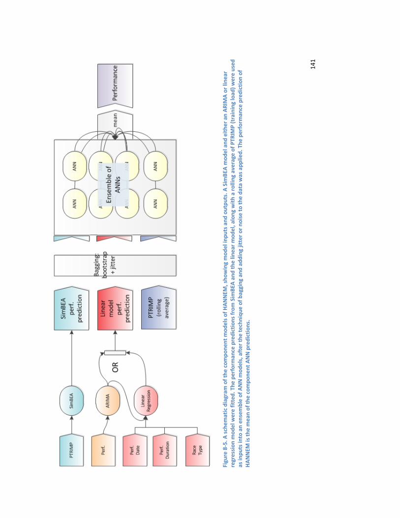
141
Figu
re 8
-5. A
sche
mat
ic d
iagr
am o
f the
com
pone
nt m
odel
s of H
ANN
EM, s
how
ing
mod
el in
puts
and
out
puts
. A S
imBE
A m
odel
and
eith
er a
n AR
IMA
or li
near
re
gres
sion
mod
el w
ere
fitte
d. T
he p
erfo
rman
ce p
redi
ctio
ns fr
om S
imBE
A an
d th
e lin
ear m
odel
, alo
ng w
ith a
rolli
ng a
vera
ge o
f PTR
IMP
(tra
inin
g lo
ad) w
ere
used
as
inpu
ts in
to a
n en
sem
ble
of A
NN
mod
els,
aft
er th
e te
chni
que
of b
aggi
ng a
nd a
ddin
g jit
ter o
r noi
se to
the
data
was
app
lied.
The
per
form
ance
pre
dict
ion
of
HAN
NEM
is th
e m
ean
of th
e co
mpo
nent
AN
N p
redi
ctio
ns.

142
8.2. Method
8.2.1. Subjects
Two female and one male professional road cyclists provided data for the study over a
period of 250, 870 and 1107 days for subjects B, A and C, respectively. An SRM power
monitor (professional model, Schoeberer Rad Messtechnik, Germany) was fitted to each
subject’s bike(s) over the data collection period. Power data from all rides (training and
racing) was captured at 1Hz. In accordance with operator instructions, the SRM was
zeroed prior to the start of each session. SRM data files were imported into a custom-
built program for the calculation of training load (PTRIMP) and performance.
8.2.2. Quantifying Training Load
Table 8.2 describes the parameters that were derived to quantify training load.
Variable Description PTRIMP Measure of training load, calculated as outlined in Chapter 5. Chronic Training Load (CTL)
CTL provides a measure of training load over a longer time period by calculating an exponentially-weighted moving average of daily training load (PTRIMP) values. A time constant of 30 days has been used here.
Acute Training Load (ATL)
ATL provides a measure of short-term training load by calculating an exponentially-weighted moving average of daily training load (PTRIMP) values. A time constant of 5 days has been used here.
ATL3 Calculated as per ATL, but using a time constant of 3 days. Training Stress Balance (TSB)
The difference between CTL and ATL. It conceptually represents the difference between 'fitness' and 'fatigue' and as such is used a performance indicator.
Table 8.2. Training load parameters.

143
8.2.3. Quantifying Performance
The SRM download software (released by SRM to enable athletes to download data files
from the device to their computer) enables the user to associate ride notes with each
file. These notes, as well as the training diary kept by one athlete, were used to identify
races. A performance measure (calculated as using the custom built program outlined in
Chapter 7, Modelling the Taper) was calculated for each identified race. Performances
were included in the dataset when training data existed for the three days prior to the
performance.
The dataset for Subject C contained numerous stage races (multi-day races). It was
noted that performance was highly variable within a stage race. It is common that not
all stages within a stage race will be ridden with a maximal effort. Some stages may
involve conserving energy for strategic reasons. Strategies to conserve energy can
involve drafting, or riding in other rider’s slipstream to reduce drag and thus save
energy. In order to identify which races involved a maximal effort, and which races
involved conserving energy for strategic reasons, cluster analysis was used. The k-means
cluster algorithm (JMP version 8 Cluster platform, SAS Institute, Cary, NC) was used to
create 8 clusters on the variables performance and average speed. A further 8 clusters
were also created on the variables average power and average speed (8 clusters were
found to create the most cohesive groupings). Performances that were included in the
high average speed and low performance or low average power clusters were identified
as races in which energy was conserved rather than being maximal performances.
Twenty eight performances were identified for Subject A, twenty three for Subject B,
and one hundred and forty two for Subject C. It is important to note that although
performances are a time series, they occur at irregular intervals.

144
8.2.4. Additional Parameters
A number of additional parameters were derived and considered for inclusion in
HANNEM. The following subsections provide details of these parameters.
Symbolic Aggregate Approximation
A time series consisting of the three days training load (PTRIMP) in the lead up to a
performance was created. The Symbolic Aggregate approXimation (SAX) technique
outlined in Chapter 7 (Modelling the Taper) was used to symbolise the time series of
PTRIMP data. A window size of three days and an alphabet size of three were the
settings used.
Taper Shapes
Chapter 7 (Section 2) outlined a grouping scheme consisting of four categories (low,
high-tail, low-tail and high). These categories were again used for this study.
Orthostatic Test and HRV Analysis
The dataset for Subject A contains HRV data obtained from a daily orthostatic test.
Details of the orthostatic test protocol and the resultant HRV analysis are contained in
Chapter 5 (Modelling of the data). The variable Pnn50 was standardised (using a z-
score) and included in the data set for Subject A. Pnn50 is the percentage of successive
R-R interval differences larger than 50ms. It was calculated using custom-built software
(HRV Athlete, FitSense Australia).
Race Type
The type of race from which a performance derived was determined, and categorised
into one of three categories; road race, tour or criterium. Road race was the category
used for single day races which were not criteriums. Criteriums are races held on a short
circuit course, involving numerous laps. Multi-day stages races were categorised as tour.

145
8.2.5. Data Pre-processing
SRM files occasionally include short durations of spurious power readings caused by
sensor interference. Such spurious data points were identified and removed. Each
athlete’s dataset of performances was analysed for outliers. One outlier was identified
for Subject A – as it was an early performance recorded before sufficient data had been
captured to enable stabilisation of MMPs, the decision was made to cap this
performance at -20,000 arbitrary units (au).
The performance time series of all subjects showed a significant downward trend. This
was due to the nature of the performance measure. Performances were calculated in
comparison to the athlete’s best performance to date. It takes some time before the
database of personal bests for an athlete becomes stable. The trend in the performance
series obscured the underlying performance data, and was thus pre-processed to
remove the trend. Differencing of order 1 was used.
8.2.6. Model Fitting
This section describes the fitting process for the models which make up HANNEM:
SimBEA, ARIMA or least squares multiple regression and an ensemble of ANNs.
SimBEA
JMP version 8 (SAS Institute, Cary, NC) was used to calculate and fit the SimBEA model
as set forth by Bruckner (2006, 2008). Refer to Equation ( 8-3 ) for the equation used.
The nonlinear platform in JMP was used to fit the model parameters, by minimising the
residual sum of squares error. For Subject A and B, the model was fit to the entire
dataset. For Subject C, whose dataset spanned 4 years, the model was fit to each year
separately.
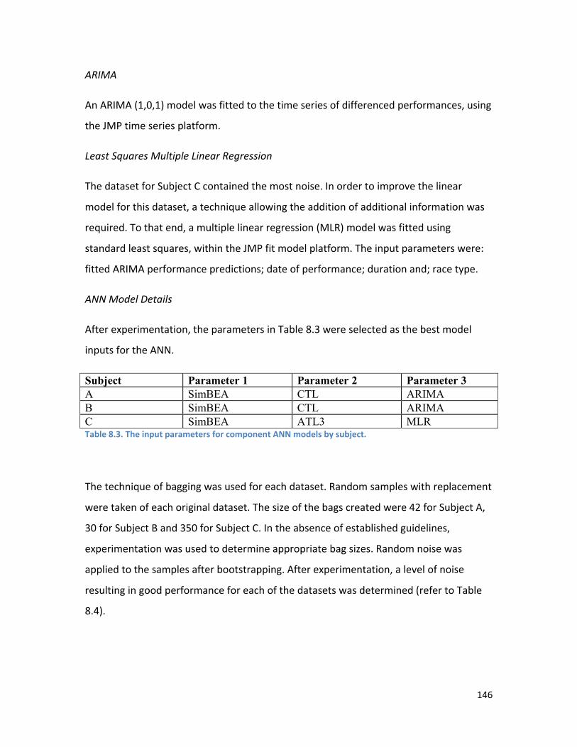
146
ARIMA
An ARIMA (1,0,1) model was fitted to the time series of differenced performances, using
the JMP time series platform.
Least Squares Multiple Linear Regression
The dataset for Subject C contained the most noise. In order to improve the linear
model for this dataset, a technique allowing the addition of additional information was
required. To that end, a multiple linear regression (MLR) model was fitted using
standard least squares, within the JMP fit model platform. The input parameters were:
fitted ARIMA performance predictions; date of performance; duration and; race type.
ANN Model Details
After experimentation, the parameters in Table 8.3 were selected as the best model
inputs for the ANN.
Subject Parameter 1 Parameter 2 Parameter 3 A SimBEA CTL ARIMA B SimBEA CTL ARIMA C SimBEA ATL3 MLR Table 8.3. The input parameters for component ANN models by subject.
The technique of bagging was used for each dataset. Random samples with replacement
were taken of each original dataset. The size of the bags created were 42 for Subject A,
30 for Subject B and 350 for Subject C. In the absence of established guidelines,
experimentation was used to determine appropriate bag sizes. Random noise was
applied to the samples after bootstrapping. After experimentation, a level of noise
resulting in good performance for each of the datasets was determined (refer to Table
8.4).
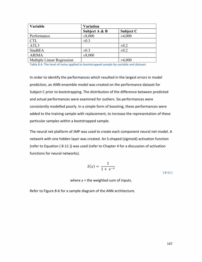
147
Variable Variation Subject A & B Subject C
Performance ±8,000 ±4,000 CTL ±0.3 ATL3 ±0.2 SimBEA ±0.3 ±0.2 ARIMA ±8,000 Multiple Linear Regression ±4,000 Table 8.4. The level of noise applied to bootstrapped sample by variable and dataset.
In order to identify the performances which resulted in the largest errors in model
prediction, an ANN ensemble model was created on the performance dataset for
Subject C prior to bootstrapping. The distribution of the difference between predicted
and actual performances were examined for outliers. Six performances were
consistently modelled poorly. In a simple form of boosting, these performances were
added to the training sample with replacement, to increase the representation of these
particular samples within a bootstrapped sample.
The neural net platform of JMP was used to create each component neural net model. A
network with one hidden layer was created. An S-shaped (sigmoid) activation function
(refer to Equation ( 8-11 )) was used (refer to Chapter 4 for a discussion of activation
functions for neural networks).
( ) = 11 + ( 8-11 )
where x = the weighted sum of inputs.
Refer to Figure 8-6 for a sample diagram of the ANN architecture.

148
Figure 8-6. Diagram of ANN architecture. In this example there are 3 input units, a hidden layer with 3 units, and 1 output unit.
K-fold crossvalidation (with 5 groups) was used to judge model performance.
An ensemble of 8 neural networks was created. A script was used to automate the
process within the JMP software (refer to Appendix C, Table C.1 for a listing of the
algorithm used). Each individual neural network was trained on a training dataset with
the addition of bootstrapped samples with random noise injected. Each model was thus
trained on a slightly different training sample. N iterations were performed of the
ensemble building process (where n = number of performances in the dataset minus 1).
For each iteration, 1 performance was excluded from the training samples to enable
ensemble performance to be validated using leave-one-out testing.
A sequence of fits was applied for each individual ANN model in order to determine the
optimal ANN configuration. The number of hidden nodes was varied from 2 to 5, and
the learning rate varied from 0.001 to 0.04. Learning rates typically have a value
between 0.0 and 1.0 (Han & Kamber, 2006); rates in the range of 0.001 to 0.04 were
found to be most effective with this data. The hidden node and learning rate
parameters which resulted in the best performed model (judged by R2 values for the fit
of the trained model to the test partition created using k-fold cross-validation) was
selected, and the resulting formula for the model was saved.
The predictions of each individual model were combined using a simple average. The
averaged predicted performance was then compared to the actual performance.
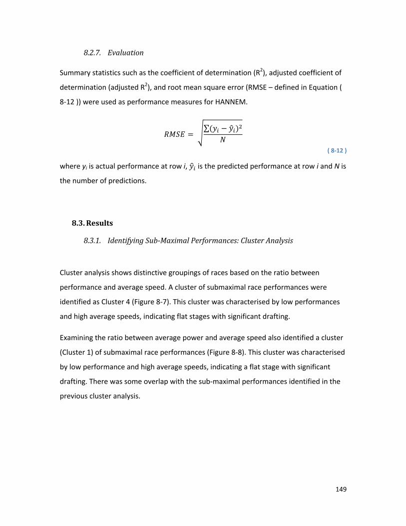
149
8.2.7. Evaluation Summary statistics such as the coefficient of determination (R2), adjusted coefficient of
determination (adjusted R2), and root mean square error (RMSE – defined in Equation (
8-12 )) were used as performance measures for HANNEM.
= ∑( − )
( 8-12 )
where yi is actual performance at row i, is the predicted performance at row i and N is
the number of predictions.
8.3. Results
8.3.1. Identifying Sub-Maximal Performances: Cluster Analysis
Cluster analysis shows distinctive groupings of races based on the ratio between
performance and average speed. A cluster of submaximal race performances were
identified as Cluster 4 (Figure 8-7). This cluster was characterised by low performances
and high average speeds, indicating flat stages with significant drafting.
Examining the ratio between average power and average speed also identified a cluster
(Cluster 1) of submaximal race performances (Figure 8-8). This cluster was characterised
by low performance and high average speeds, indicating a flat stage with significant
drafting. There was some overlap with the sub-maximal performances identified in the
previous cluster analysis.

150
Figure 8-7. Cluster analysis on the variables performance and average speed for Subject C. Cluster 4 shows a group of performances with high average speed and low performance – indicating a submaximal effort.

151
Figure 8-8. Cluster analysis on the variables average power and average speed for Subject C. Cluster 1 shows a group of performances with high average speed and low average power – indicating a submaximal effort.

152
8.3.2. Performance Time Series Subject A
The performance time series for Subject A does not show a significant trend (Figure 8-9).
Figure 8-10 shows the time series after a differencing of 1 was applied.
Subject B
The raw performance time series for Subject B shows a downward trend (Figure 8-11).
Figure 8-12 shows the time series after a differencing of 1 was applied to remove the
trend.
Subject C
The raw performance time series for Subject C shows a downward trend (Figure 8-13).
The high variability in this time series is also apparent. Figure 8-14 shows the time series
after a differencing of 1 was applied to remove the trend.
Figure 8-9. Raw performance time series for Subject A – no significant trend apparent.

153
Figure 8-10. The performance time series for Subject A after a differencing of 1 was applied
Figure 8-11. Raw performance time series for Subject B showing downward trend.
Figure 8-12. De-trended performance time series for Subject B (differencing of 1 applied).

154
Figure 8-13. Raw performance time series for Subject C showing downward trend.
Figure 8-14. De-trended performance time series for Subject C (differencing of 1 applied).
8.3.3. Individual Model Performance
The performance of the SimBEA model alone was poor for each subject’s dataset. The
relationship between predicted and actual performance for Subject A and C was
nonlinear, while for Subject B a weak linear relationship was apparent (refer to Table
8.5, Figure 8-15, Figure 8-16, Figure 8-17).
The ARIMA model had a stronger fit for each subject (Table 8.5, Figure 8-18, Figure
8-19). The fit of the ARIMA model for Subject C was still poor however, so a MLR model
was created. The MLR model showed a substantial improvement over the ARIMA model
(Table 8.5, Figure 8-20).

155
Model details Model performance (R 2) Type Model Input Subject A Subject B Subject C SimBEA PTRIMP Weak non-
linear 0.32 Weak non-
linear ARIMA (1,0,1) Performance (differenced) 0.72 0.53 0.43 MLR ARIMA predictions,
Performance Data, Duration, Race Type
0.54
Table 8.5. Performance of the individual models.
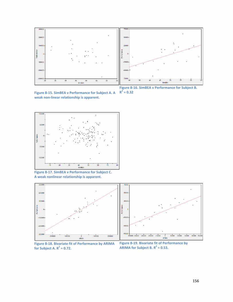
156
Figure 8-15. SimBEA v Performance for Subject A. A weak non-linear relationship is apparent.
Figure 8-16. SimBEA v Performance for Subject B. R2 = 0.32
Figure 8-17. SimBEA v Performance for Subject C. A weak nonlinear relationship is apparent.
Figure 8-18. Bivariate fit of Performance by ARIMA for Subject A. R2 = 0.72.
Figure 8-19. Bivariate fit of Performance by ARIMA for Subject B. R2 = 0.53.

157
Figure 8-20. Bivariate fit of Performance by MLR prediction. R2 = 0.54.
8.3.4. ANN Model Input
The inputs for each of the subject’s ANN models are graphed in Figure 8-21, Figure 8-22
and Figure 8-23. It can be seen that each of the inputs pick up different parts of the
overall pattern of performance. Slightly different parameters were found to be most
effective for Subject C compared to the other two subjects.
Figure 8-21. Subject A ANN model inputs.

158
Figure 8-22. Subject B ANN model inputs.
Figure 8-23. Subject C ANN model inputs. Note the greater variability in performance for Subject C.

159
8.3.5. ANN Model Performance Prior to Bootstrapping
The subjects’ ANN model performances are summarised in Table 8.6. Each ANN model
was generated three times, and the results reported. As neural networks are unstable
estimators, reporting only the results from a single run could lead to misleadingly good
or poor results. The performance of the ANN models for Subject B showed the greatest
variability.
Model details Performance (R2) Model parameters Hidden
nodes Overfit penalty
Subject A Subject B Subject C
SimBEA, CTL, ARIMA
5 0.016 – 0.001 0.87-0.90* 3-5 0.001 -0.004 0.43-
0.64*
SimBEA, ATL(3), MLR
3 0.001 0.54-0.57*
Table 8.6. Performance of an ANN model on test sample (using k-fold cross-validation).
* Range of model performance over 3 runs.
8.3.6. Bootstrap and Noise
Section 8.2.6 Model Fitting detailed the steps taken in pre-processing the datasets to
bootstrap the data and add random noise. The stepped effect created in the
performance series by the bootstrapping with the addition of random noise is illustrated
by Figure 8-24 - Figure 8-29.
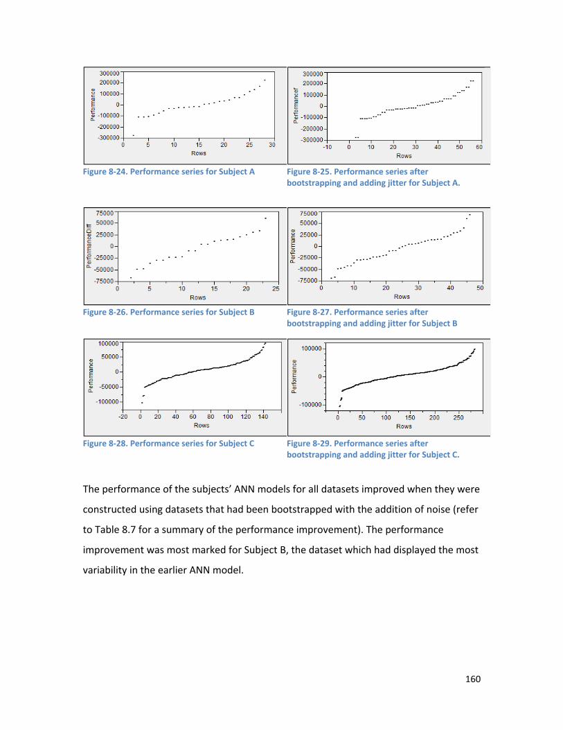
160
Figure 8-24. Performance series for Subject A
Figure 8-25. Performance series after bootstrapping and adding jitter for Subject A.
Figure 8-26. Performance series for Subject B Figure 8-27. Performance series after bootstrapping and adding jitter for Subject B
Figure 8-28. Performance series for Subject C Figure 8-29. Performance series after bootstrapping and adding jitter for Subject C.
The performance of the subjects’ ANN models for all datasets improved when they were
constructed using datasets that had been bootstrapped with the addition of noise (refer
to Table 8.7 for a summary of the performance improvement). The performance
improvement was most marked for Subject B, the dataset which had displayed the most
variability in the earlier ANN model.

161
Model parameters Subject
Hidden Nodes
Overfit penalty
Performance (R2) Bootstrap Improvement
(R2) Min Max
SimBEA, CTL, ARIMA
A 5 0.001 – 0.004 0.97 0.98
0.09
B 4-5 0.002-0.004 0.94 0.96 0.42SimBEA, ATL(3), MLR C 3,5 0.004-0.002 0.61 0.63 0.07
Table 8.7. Improvement of ANN model when bootstrapping and jitter are performed.
8.3.7. HANNEM Performance For Subjects B and C, the ANN ensemble performed better than the best single network.
For Subject A, the best single network performed substantially better than the
ensemble. In all cases, the ensemble performed substantially better than the worst
single network (Table 8.8). The predicted performance tracks very closely to actual
performance for Subject A and B (Figure 8-30 to Figure 8-33). The accuracy of the
performance predictions is more variable for Subject C, but still tracks actual
performance quite closely (Figure 8-34 and Figure 8-35).
Ensemble Average Best Single Network Worst Single Network
Subject R2 R2 Adjusted RMSE R2
R2 Adjusted RMSE R2
R2 Adjusted RMSE
A 0.78 0.77 48690 0.90 0.90 32478 0.48 0.46 74824
B 0.62 0.60 19999 0.56 0.53 21512 0.27 0.24 27570
C 0.51 0.51 23824 0.49 0.48 24403 0.38 0.38 26776
Table 8.8. Performance of ANN ensemble predictions for each subject using leave on out testing.

162
Figure 8-30. Ensemble predicted performance compared to actual performance for Subject A.
Figure 8-31. Ensemble predicted performance versus actual performance for Subject A. R2 = 0.78
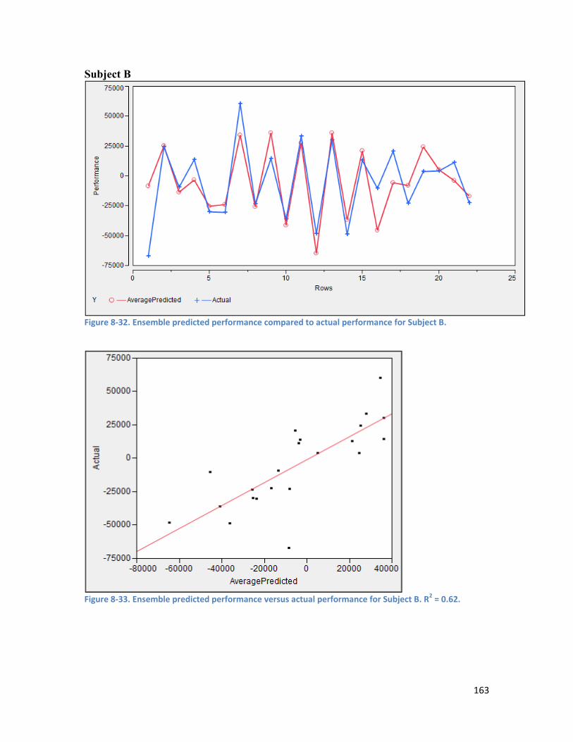
163
Subject B
Figure 8-32. Ensemble predicted performance compared to actual performance for Subject B.
Figure 8-33. Ensemble predicted performance versus actual performance for Subject B. R2 = 0.62.

164
Subject C
Figure 8-34. Ensemble predicted performance compared to actual performance for Subject C.
Figure 8-35. Ensemble predicted performance versus actual performance for Subject C. R2 = 0.51.
165
8.4. Discussion The performance quantification technique used for this research has been described in
detail in Chapter 6. Briefly, performance is compared to an athlete's personal best
maximal mean power (MMP) over a range of time durations. A record of an athlete's
best MMP is kept for each time duration, and updated whenever a new personal best is
achieved.
The personal bests of the athletes tended to improve over the duration of the data
collection, resulting in the performance datasets exhibiting downward trends over time
(refer to Figure 8-9, Figure 8-11 and Figure 8-13). These trends are functions of the data
collection process, and were removed in the preprocessing phase by differencing.
The intent of this research is to design a performance modelling process which is
practical in the real world of elite road cycling. As such, precise maximal mean power
curves obtained from recent specific testing will frequently be unavailable, and so a
database of MMPs needs to be built up over time. The models created will become
increasingly accurate as the recorded MMPs become closer to the real MMP of the
athlete.
An alternative option would be to calculate an absolute performance value by using the
peak performance (for each duration) from the entire dataset as the performance
benchmark. This approach could provide interesting additional information about the
variation of performance over time, however in order to understand the relationship
between training load and performance, performance needs to be calibrated to an
athlete’s capabilities at that time. Using absolute performance would distort the
relationship between training and performance in the early parts of the dataset, as what
were - at the time - good performances for an athlete, would become poor
performances in comparison to their later achievements.

166
Conversely, there may be a future need to develop a mechanism to reduce the MMP
values, to cater for example to masters athletes whose maximal capabilities may be
declining. This mechanism is not currently included in the modelling process.
Establishing a performance dataset for an athlete using real world training and racing
data relies on being able to identify those sessions where the athlete made a maximal
effort. For Athletes A and B, a training diary was available which recorded the athlete’s
perception of effort for each session (e.g. ‘I gave everything I had’). This information was
not available for Subject C.
All races were initially assigned as performances for Subject C. In initial modelling, the
models constructed for only single day races performed well, while those constructed
for only multi-day stage races performed extremely poorly. This was likely due to the
tactical nature of multi-day stage races. Depending on a cyclist’s role within a team,
certain stages are likely to be completed with the goal of conserving energy for later,
tactically crucial, stages. For example, climbing specialists often attempt to conserve
energy during flat stages which are predicted to end in a bunch sprint. They can do this
by drafting – riding in the slipstream of other riders. Stages with power files which show
a low average power output, and a high average speed, are indicative of such flat stages
where drafting is occurring and a 100% effort is not made. To identify such stages,
cluster analysis was performed on the variables performance and average speed, and
average power and average speed (refer to Figure 8-7 and Figure 8-8). The identified
performances were excluded from the study, substantially reducing the noise of the
performance time series. This novel technique has the potential to increase the range of
datasets that can be used for modelling, because additional information on the level of
effort put in to each session is frequently not available.
The dataset for Subject C showed highly variable performances. To improve the
performance of the model with the extreme performance values, a simple form of
boosting was used. An ANN model was fitted to the dataset to identify the
performances that resulted in the largest modelling errors. These performances were
167
re-sampled and added back to the dataset, thus increasing their influence within the
dataset.
Boosting is a technique that is often used in modelling with decision trees. Boosting
concentrates on data points that are difficult to model. The boosting algorithm involves
an iterative process where a model is applied successively to different versions of the
initial training sample – these samples are modified to place greater weight on the
observations which were incorrectly modelled in the preceding iteration. A variant of
boosting called ‘arcing’ (short for ‘adaptive resampling and combining’) draws a training
sample with replacement in each iteration (i.e. bootstrapping) with a greater probability
of drawing the observations that were incorrectly modelled in the preceding iteration
(Tuffery, 2011). The simple boosting technique employed in this research was
conceptually similar to the arcing technique. Future research might automate what was
here a manual process by employing the arcing algorithm.
8.4.1. SimBEA Performance The fitted SimBEA model on its own had a poor fit with the performance series for each
athlete. The relationship between SimBEA and performance for Subject B was linear,
with an R2 value of 32%. The relationship between SimBEA and performance for Subject
A and C was weak and appeared to be non-linear.
Bruckner and Wilhelm (2008) note that the SimBEA model had lower accuracy when it
was fitted to a dataset of 68 weeks, compared to a dataset of 6 weeks, although they
report an intraclass correlation coefficient (ICC) of 0.65 over 68 weeks which is still a
moderate fit. Bruckner recommends that the calibration of the model be reviewed
periodically to adjust the parameters as necessary, and therefore improve model
accuracy. Calvert, Banister, Savage & Bach (1975) applied an impulse response model to
the training and performance data of a swimmer. They found that the optimal
parameters for the model varied slightly for each season.
168
The SimBEA model was fitted to the entire performance dataset for subjects A and B
(consisting of 1 and 2 seasons of racing, respectively). These datasets did not contain
enough performances to enable refitting of the model parameters for smaller time
frames. The performance dataset for Subject C contained data from 4 seasons. Enough
performances were contained within each season to refit the model parameters for
each season.
Although the fits obtained with the SimBEA model were poor, including the SimBEA
predicted performance as a parameter in an ANN model improved the model
performance. It is concluded that the domain knowledge which is embedded within the
SimBEA model, including information regarding physiological phenomena such as
supercompensation and reversibility, added valuable information to the final ANN
model.
8.4.2. ARIMA A central task of fitting an ARIMA model is determining the model order. It is common
to fit all plausible models, and choose on the basis of their performance (Venerables &
Ripley, 2002). An ARIMA (1,0,1) model proved to have the best fit for these datasets.
The performance of the ARIMA models ranged from poor to good. The fit for subject A
was R2 = 72%; for Subject B, R2 = 53%; and the fit for Subject C was poor, with R2 = 43%.
These results are similar to those reported by Ferger (2008), who fitted an ARIMA (0,0,0)
model to a performance time series. Ferger reported a model fit of ICC = 0.47.
It is important to note that the performance datasets are not evenly spaced in time. This
has the effect of reducing the stability of the autocorrelation structure within the
dataset. A performance is much more likely to be affected by the previous performance
if it occurred the day before, rather than weeks before. This is most relevant to the
ARIMA model for Subject C, whose dataset contained the highest proportion of multi-
day stage races, and in fact the model for this dataset resulted in the poorest fit. In this

169
research, the function of the ARIMA model is to model the linear patterns contained in
the performance dataset. As such, close model fits are not expected from the ARIMA
models alone.
8.4.3. Least Squares Multiple Linear Regression As discussed, the ARIMA model for the performance dataset of Subject C had the
poorest fit. Multiple linear regression was identified as an alternative linear modelling
technique that would be less affected by the varying time scales of the performance
time series, as well as allow further information to be added to the model. The inputs
which resulted in the best performing MLR model were: ARIMA performance
predictions, date of performance, taper shape and race type.
The fact that the date of performance was a valid predictor suggests that successive
performances are not independent, and this was confirmed during the ARIMA modelling
process. The race type variable was also found to be a significant predictor in the
multiple regression model. As discussed previously, performance within a multi-day
stage race (categorised as ‘tour’) displayed some unique characteristics compared to
single day races (‘road race’), most noticeably higher variation. Criteriums, raced over
short circuits, are characterised by repeated short high-powered efforts. Distinctive
power profiles are created by different race types - for example the repeated high-
powered efforts of short duration which characterise criteriums and the long iso-
powered efforts of time trials. This can also be observed with different types of terrain –
flat races tend to be characterised by large sections of low power output, with relatively
brief high power efforts for the intermediate sprint points, bunch positioning and the
final sprint. Hilly races tend to be characterised by threshold power outputs for
relatively long durations while climbing, and then very low power outputs for the
descents. The performance algorithm was developed to work with a range of race types
and terrain, and the resulting characteristics of their power files. There are inevitable
simplifications involved, however, in designing an algorithm to calculate one number to

170
represent an entire performance. The multiple linear regression model showed that
tours tended to have lower performances compared to criterium and single-day races,
as would be expected due to the increased levels of fatigue experienced during a tour.
Similarly, performance duration was found to have an effect, with longer durations
resulting in slightly higher performances. Longer sessions are likely to provide more
opportunities for generating high MMP values over the range of time durations
recorded – 5 seconds to 20 minutes.
Linear regression is not a technique that has been commonly applied to the problem of
modelling training and performance, due to the established non-linear nature of the
problem. As with the ARIMA model, the intent is to model the linear patterns in the
dataset. The fit of the model was R2 = 54%, an improvement over the fit of the ARIMA
model alone for this dataset (R2 = 43%).
8.4.4. Bootstrap and Noise
No established guidelines exist in the literature for determining the appropriate amount
of bootstrapping and the appropriate level of noise to apply to a dataset to order to
achieve the most effective results. The optimum values were determined by
experimentation, and varied according to the dataset.
In each case, performance was improved when an ANN model was applied to a bag of
bootstrapped and jittered dataset rather than an original dataset. The small level of
performance improvement achieved (in R2 values) ranged from an improvement of 7%
for Subject C, 9% for Subject A, and 42% for Subject B. The amount of improvement is
likely to be related to the size of the original dataset – Subject B had the smallest
dataset and Subject C the largest. The problems of overfitting and subsequent poor
performance on the validation sample is more severe in small datasets, and thus
techniques to reduce overfitting such as bootstrapping and adding noise are likely to be
more effective. This is consistent with Zhang (2007), who found that no significant

171
difference in performance was observed in bootstrapping and adding jitter with
datasets of over 100 samples.
Zhang (2007) states that the bootstrapping and jitter process causes the data to appear
smoother to a neural network. The visualisations of each performance series before and
after the process (refer to Figure 8-25, Figure 8-27 & Figure 8-29) show that the data
became more ‘stepped’ - with small clusters of values around each original value -
rather than a true smoothing affect. Some papers – for example Yeh (2007) – suggest
expanding the range of the dataset when creating artificial data to supplement small
datasets. The difficulty lies in concomitantly expanding the range of the input
parameters appropriately, when the underlying relationship between the model input
and the output is unknown. I argue that it is better to add slight noise to bootstrapped
data rather than expanding the range of parameters to create a smoothed dataset and
risk distorting the underlying relationships present in the original dataset.
8.4.5. Component ANN Topology
Determining the topology of an ANN requires a trade off between model complexity and
the amount of data provided. The greater the number of nodes (in the hidden layer as
well as in the input layer), the more data is required. Edelmann-Nusser, Hohmann &
Henneberg (2002) used the rule of thumb that the minimum number of observations
required is about double the number of connections between nodes. In this research,
three model inputs proved to be the optimal number, and the best parameters for
inclusion in the model were selected after experimentation. The optimal number of
hidden nodes was selected by fitting a sequence of models with the number of hidden
nodes varying from 2 to 5.

172
8.4.6. Hybrid Models
The addition of the performance prediction from the SimBEA model as an input to the
ANN model significantly improved the performance of the ANN model. The hybrid
SimBEA-ANN model performed better than either model performed alone. Although
the performance of the SimBEA model alone was poor, it appears that the domain
knowledge embedded in the model provided additional information to the ANN model
compared to using training load alone as an input.
A key limitation of the SimBEA model (used in isolation) is its lack of flexibility. It only
accepts a single input - training load. Research indicates that the impulse response
models (e.g. the Banister and Busso models, and also SimBEA) perform well in
controlled conditions, such as in lab experiments, where the noise in the dataset is likely
to be much less of an issue. Such models have frequently performed less well in real
world conditions. In the current research, the modelling technique needs to be able to
deal with noisy data. In these situations, adding further information to the model in the
form of additional parameters is generally required to achieve adequate model
performance.
The performance of the hybrid model (a combination of SimBEA, ARIMA and ANN
models, or a combination of SimBEA, ARIMA, MLR and ANN models) was better than the
performance of any single model for each of the datasets. The improvements for
Subjects B and C, however, were slight. Zhang (2003) found that a hybrid ARIMA- ANN
model performed better than either model alone. It is hypothesised that the slight
improvement recorded for Subject B was likely due to the small size of the dataset,
making overfitting with an ANN model inevitable unless further techniques were applied
to reduce this. An overfitted model would explain the relatively poor performance of
the model on the validation sample. The dataset for Subject C was much larger, and
overfitting is not likely to have been much of a problem. It is likely that the ANN in this
173
case had difficulty in modelling the extremes of performance seen in this dataset, and
consistently underestimated both poor performances and good performances.
The literature around using hybrid ARIMA and ANN models contends that the ARIMA
model models the linear patterns in the dataset, and the ANN model models the non-
linear patterns (e.g. Zhang, 2003; Khashei & Bijari, 2010; Hippert, Pedreira, & Souza,
2000). Some practitioners use the residuals from the ARIMA model as the input to the
ANN model (e.g. Zhang, 2003; Khashei & Bijari, 2010). Hippert, Pedreira, & Souza (2000)
successfully composed a hybrid model using the predictions from an ARIMA model
rather than the residuals as the input to an ANN model.
Modelling the residuals from an ARMIA model assumes that the relationship between
the linear and non-linear components of a dataset is additive (Taskaya-Temizel & Casey,
2005). The validity of this assumption has not been established. Initial trials of using
ARIMA residuals as an input into the ANN model resulted in extremely poorly
performing models. The approach followed in this research was therefore to use the
predictions from the ARIMA models as an input – and this resulted in better performing
ANN models.
Choosing the appropriate input parameters for an ANN model can be difficult,
particularly if parameters are correlated. One technique commonly used to reduce the
number of inputs while still retaining vital information from the all parameters is to use
Principle Components Analysis (PCA) or factor analysis. PCA uses an orthogonal
transformation to convert a number of potentially correlated variables into a generally
reduced set of linearly uncorrelated variables. The trials in this research of using PCA to
reduce two or three different correlated parameters into one value resulted in poorer
model performance compared to including the three best parameters in the ANN
model. The hybrid MLR-ANN model used for Subject C allowed valuable information
from additional parameters to be derived, and combined into a single input - the MLR
prediction. In this manner the use of the MLR model as an input to the ANN model

174
performed a similar function to PCA, but resulted in significantly better model
performance.
8.4.7. ANN Ensemble
The literature offers no definitive suggestions for choosing the optimal number of
models to include in an ensemble. Zhang (2007) found that between 5 and 10 models
offered a reasonable compromise between parsimony and modelling accuracy. Tuffery
(2011) suggests using around 10 models. Perrone & Cooper (1992) found that ensemble
performance ceased to improve after inclusion of more than 6 to 8 component ANNs,
pointing out that the number of distinct local minima in functional space is quite small.
In this research experimental trials showed that an ensemble of 8 models performed
better with these datasets than an ensemble of 5 models, while the improvement using
10 models was minimal, and it was judged to be not worth the extra computational
expense.
The use of bootstrapping and jitter in generating the training sets for each of the
component ANN models meant that each model was trained on slightly different data.
Sharkey (1996) considers that varying the data on which a set of ANNs is trained is more
likely to create an effective ensemble, and Zhang (2007) found this to be the case
experimentally. Raviv and Intrator (1996) found that noisy bootstrapping performed
best in conjunction with ensemble averaging. The noise helped to push different
component models to different local minima, producing a more independent ensemble
(Raviv and Intrator, 1996). Networks which have fallen into different local minima will
have difficulty in modelling different areas of feature space, and thus their error terms
will not be strongly correlated (Perrone & Cooper, 1992).

175
8.4.8. Testing Methodology
For small datasets holdout validation is not feasible, as partitioning an already small
dataset into training and testing sets reduces the available training information. Instead,
jacknifing or leave-one-out validation was used for testing the performance of the
ensemble in this research. This is where one data point at a time is removed from the
dataset before the model is constructed on the remaining data points. The model
output was tested on the removed data point, before repeating for each data point in
the dataset. Jacknifing is not commonly used in neural network training, due to the large
computational overhead (Perrone & Cooper, 1992), but it is an appropriate technique
for small datasets.
8.4.9. Combining the Component ANNs
Some authors (e.g. Sharkey, 1996; Zhou, Wu & Tang, 2002) have found that selecting
ANNs for inclusion in an ensemble, rather than including all, results in better
performance. Zhou, Wu & Tang (2002) used genetic algorithms to select the most
appropriate ANNs. Perrone and Cooper (1992) created a large number of component
models then used a heuristic selection method to select the ANNs with the least errors.
The presence of collinearity between the errors made by component ANNs can be an
indicator that averaging may not be the most effective method of combining ensemble
output – however if the majority of the components are correct averaging will perform
well (Sharkey, 1996). Zhang (2007) found that averaging component outputs was a
simple and effective technique. Simple averaging was used in this research, however
future research could investigate whether model performance could be improved by
implementing a model selection algorithm.
For Subjects B and C, the ensemble performed better than the best single network. For
Subject A, the best single network performed substantially better than the ensemble. In

176
all cases, the ensemble performed substantially better than the worst single network.
This is to be expected, as an ensemble works as a smoothing operator over the
predictions of the individual ANN models.
HANNEM explained 77% of the variance of performance for Subject A. 60% of the
variance was explained for Subject B, and 51% for Subject C. Bruckner (2006) points out
that his SimBEA model can predict performance direction or trends rather than absolute
performance. The performance quantification technique developed in this research uses
arbitrary units as its unit of measurement. This is a function of the fact that for road
cycling, there is no performance standard against which an individual performance can
be measured. There is no time, distance or average power that can be used as a
standard; unlike sports such as swimming, running and many track cycling events. This
means that performance measurements cannot be converted back into concrete units
like time, distance or watts. For this reason, the focus of the final model developed in
this research does not aim to predict absolute performance (which would be
meaningless) - rather it aims to predict the direction and rate of performance trends.
The large amount of data needed for both the impulse-response models and particularly
the neural network models has always been a significant problem affecting the practical
usefulness of training and performance models. Athletes and coaches wish to receive
feedback from such a model as soon as possible, rather than waiting while a dataset of
sufficient size is gathered. Overtraining is a particular issue when using neural networks
to model small datasets. The smallest dataset in this research contained just 30
performances; yet achieved a good level of generalisation to the validation data (using
jackknife validation). This result supports the use of the techniques implemented to
reduce overfitting; namely bootstrapping (bagging), adding noise, and the use of an
ensemble of ANNs.
At the other end of the spectrum there is a potential issue with having data that extends
over a long time period. The largest dataset in this research included data from 4
seasons. The relationship between training and performance changes over time, and
177
including data from such large time horizons in the training sample might reduce the
accuracy of the modelling for the most recent data. One potential avenue of
investigation for dealing with this issue is to use boosting to increase the weight or
relative importance of the most recent data points compared to older data points.
A useful model needs be able to be used to calculate predicted performance given a
proposed training load structure (Pfeiffer & Hohmann, 2011). Busso and Thomas (2006)
caution that the quality of model predictions are likely to suffer greatly from the
simplifications made in aggregating training load into a single number, as well as the
simplifications inherent in modelling complex physiological processes in a small number
of entities. To be useful in the real world, the model needs to be as parsimonious as
possible, require as few inputs as possible, while maintaining high levels of accuracy in
performance prediction.
An important consideration is to determine how far in time the model can predict
performance and retain an appropriate level of accuracy. Bruckner (2006) found that
prediction accuracy dropped significantly for time horizons longer than one week. The
data used in the Bruckner study contained evenly spaced performance data, which
makes investigating prediction accuracy over different time frames a straightforward
process.
The time horizon over which performance predictions maintain accuracy is related to
the stability of model parameters over time. If the perfect model was developed - one
that accurately captured the underlying relationship between training and performance,
then performance predictions would remain accurate for any time horizon until the
underlying relationship changes. The question of how far in time predictions can remain
accurate is therefore to some extent dependent on the stability of the training-
performance relationship in an individual athlete.
One relatively simple way to potentially improve model performance would be to trial
additional inputs to the model. The inputs for the models developed in this research are
based on information derived from a single sensor – the power monitor on the subject’s

178
bike. This was done to ensure that the requirements for subjects participating in this
research were as minimal as possible.
Lamberts, Swart, Noakes & Lambert (2011) believe that the combination of an objective
data source (measurement of power) , a subjective data source (for example a rating of
perceived exertion) and alterations in the functioning of the autonomic nervous system
(HRV for example) shows advantages over interpreting a single variable in creating a
performance test. Similarly, a subjective measurement of training load (e.g. RPE) could
bring important information to the model, and information that is less highly correlated
than the power sensor derived variables. RPE would also assist in determining which
races involved sub-maximal efforts and thus should not be included as performances.
The model developed was designed to function without requiring regular performance
testing, unlike many of the impulse-response models. Further work to examine the long-
term reliability of the performance metric could use submaximal testing protocols, such
as the one proposed by Lamberts, Swart, Noakes & Lambert (2011), as an method of
verifying observed performance trends. An appropriate sub-maximal performance
testing protocol also has the potential to reduce the amount of data an athlete requires
before a realistic optimal performance profile is developed – which is essential before a
workable model can be developed.
The current model assumes that poor performances are functions of the training leading
in to the performance, rather than a decline due to aging for example. Further work
could be done on developing a technique to identify situations where the optimal
performance profile of an athlete needs to be reduced.
8.5. Summary This chapter outlined the development of a hybrid linear artificial neural network
ensemble model to model the relationship between training and performance. Training
load was quantified using the PTRIMP algorithm (described in Chapter 5) and
179
performance was quantified using the technique described in Chapter 6. The SimBEA
model developed by Bruckner (2006) was used to capture important domain knowledge
regarding the physiological process underlying training and its impact on performance. A
linear model (either an ARIMA or Multiple Linear Regression model) was created to
model the linear patterns in the data. A neural network model, which took as inputs the
performance predictions from the SimBEA model and the linear model, as well as a
summary of recent training load, was employed to capture the nonlinear patterns in the
data. The performance of the hybrid model (a combination of SimBEA, ARIMA and ANN
models, or a combination of SimBEA, ARIMA, MLR and ANN models) was better than the
performance of any single model for each of the datasets.
The small datasets inherent in the elite sport domain mean that overfitting with a neural
network model is a potential problem. To reduce overfitting and increase the
generalisability of the model the techniques of bootstrapping, adding noise or jitter to
the dataset, and training an ensemble of models on slightly different datasets (bagging)
were used.
Three datasets containing power data captured from the training and racing of three
elite athletes were used to test the performance of the model on real world datasets.
Moderate to good fits were obtained for the model predictions using jacknife validation
(R2 = 77%; R2 = 60% and; R2 = 51% for Subjects A, B and C respectively).
One of the key questions surrounding these results is whether the level of accuracy
reported is sufficient to enable the model to be used as a training planning tool for elite
athletes. Measurement of performance in road cycling cannot be absolute, only relative
to an individual’s previously recorded capabilities. The aim of the model is to correctly
identify the direction and rate of performance trends, rather than predict an exact
performance level.

181
CHAPTER 9 – VALIDATION OF HANNEM 9.1. Introduction
The development and testing of HANNEM - the model developed in this work to
describe the relationship between training and performance in elite cyclists – was
described in Chapter 8. HANNEM uses an ensemble of neural networks to generate the
final model output. Ensembles are a popular method of increasing the performance and
robustness of single ANN models; however questions remain about how they should be
constructed. In addition, their use with very small datasets has not received much
attention in the research literature.
Learning with very small datasets is a fundamentally difficult problem. If a dataset is
noisy as well as small - as is the case with the training and performance datasets
detailed in this work - the difficulty is compounded as the number of data points
reflecting the underlying relationship is reduced even further. The ability of a model,
trained on such data, to generalise to new data can be questioned. A validation dataset
that is also necessarily small compounds this problem, meaning it may not be possible
to estimate the true generalisation ability of the model with sufficient accuracy. The
question of how, therefore, to validate a model developed with a very small dataset
arises.
This chapter details a set of experiments designed to test key points of the HANNEM
modelling methodology and to address the identified risks of small noisy datasets. A
number of datasets with known characteristics were generated for these experiments.
In particular, the relationship between overfitting individual networks and ensemble
generalisation performance will be investigated, along with the impact of noisy data and
dataset size. The investigations in this chapter aim to answer the following questions:
Does an ensemble mitigate overfitting issues with small datasets? Can overtraining
improve performance of an ANN ensemble? How many ANNs should form an
ensemble?

182
9.1.1. Neural Network Ensembles
Neural networks are unstable classifiers (Tuffery, 2011). In general ANNs have many
local minima and frequently fail to converge to the global optimum solution. Combining
the output of several ANNs into an ensemble has a smoothing, stabilising affect (Carney
& Cunningham, 1999). Each component model has errors, but they are combined in
such a way as to minimise the effect of the errors of individual nets (Sharkey, 1996).
Perrone and Cooper (2003) show that the existence of differing local minima in
component nets actually benefits the ensemble. Ensemble techniques can yield
dramatic improvements in performance compared to single ANNs (Carney &
Cunningham, 1999).
The error of a predictor such as an ANN ensemble can be expressed in terms of the bias
squared plus the variance1. The bias and variance of a predictor can be estimated when
the predictor is trained on different random data samples taken from the entire set. The
bias can be characterised as a measure of the predictor’s ability to generalise to new
data - it corresponds to the performance of the ensemble on the validation set. Variance
can be characterised as the extent to which the predictions vary according to the
particular sample the predictor was trained on. A well-performing estimator has both
low bias and low variance, but these two elements have conflicting requirements and
thus involve some element of tradeoff (Sharkey, 1996).
The general principle for creating good ensembles is to include diverse models. Diverse
models disagree in their predictions and thus have high variance (Tuffery, 2011;
1 An ANN constructs a function f(x;D) based on a particular dataset (D) with training set (x1, y1),...,(xn,yn). The mean squared error (MSE) of f may be written [( ( ; ) − [ | ]) ] where ED is the expectation with respect to the training set D, and [ | ] is the target function. This equation can be decomposed into bias and variance components which gives us, = ( [( ( ; ) − [ | ]) ]) (bias)
+ ( ; ) − ( ; ) (variance)

183
Kuncheva & Whitaker, 2003). Ensemble members that exhibit high variance should also
display a low correlation of errors (Sharkey, 1996). The usual effect of combining the
output of ensemble members is to reduce the variance in the final estimator. Good
ensemble members therefore need to be both accurate (low bias) and diverse (high
variance) (Granitto, Verdes & Ceccatto, 2005). Component members exhibiting low bias
and high variance can be combined to produce an ensemble estimator with low bias and
low variance.
Several measures of diversity have been suggested for estimating the diversity of
classifiers – including ANNs. There are, however, few accepted formal definitions of
diversity to date (Fu et al., 2013). Kuncheva and Whitaker (2003) give a good review of a
number of methods - they found that the ten methods investigated tended to be highly
correlated with each other. There appears to be no widely accepted best method for
measuring diversity in ensembles (Melville & Mooney, 2005), and much of the literature
is concerned with techniques for measuring diversity in regression estimators. This
research will use Kohavi-Wolpert variance (Kohavi & Wolpert, 1996) in the modified
form outlined by Kuncheva and Whitaker (2003).
Creating a diverse ensemble can be done in a number of ways; by varying the training
data, using differing network architecture, or conducting training using differing
algorithms. Perhaps the most popular approach to the creation of a diverse set of ANNs
is bagging, a technique which varies the training data. In bagging a training set (t) of size
n is perturbed by randomly sampling from t with replacement until a bag with n data
points is created. The bag may thus contain repeated data points and may exclude some
points from the original set. On average, 63.2% of the data points from the original set
will be contained in each bag, with the remainder consisting of duplicates, some of
which will appear multiple times (Melville & Mooney, 2005). Each ensemble member is
trained on a different bag, and the variations in the training sets create diverse
estimators.

184
Bagging is particularly useful for reversing the lack of robustness of unstable classifiers
such as ANNs. Some of the effectiveness of bagging may be due to the fact that any
outliers in the initial sample will only be included in some bags - thus reducing their
effect on predictions (Tuffery, 2011). Bagging is particularly useful where there is a
shortage of data (Sharkey, 1996), however, with small training datasets there is a limit
to the amount of diversity that can be created using this method (Melville & Mooney,
2005).
9.1.2. Combining Component Output
Once a set of nets has been created, a way of combining their outputs must be found
(Sharkey, 1996). Taking a simple average, as was done in HANNEM, is a popular
approach for combining the output of predictors. Majority voting is a simple and
popular strategy for combining the output of classifiers. It is a strategy where each
component classifier votes for a category, and the category with the largest number of
votes is taken as the ensemble prediction (Hansen & Salamon, 1990). More complex
schemes have been proposed, such as ranking the output of each component model
(e.g. Perrone & Cooper, 1993) and slight improvements have been reported. This
investigation, however, utilised the simple and computationally efficient technique of
majority voting.
9.1.3. Choosing the Number of Component Networks There is no established technique or rule of thumb in the literature for selecting an
optimal number of component networks. Some recommendations range from 5 (Zhang,
2007) to 40 (Raviv & Intrator, 1996). Perrone and Cooper (1993) suggest that choosing
the number of models included in the ensemble in dependent on the number of distinct
models that can be created from the dataset. This implies that smaller ensembles are
appropriate for smaller datasets. This investigation examined the performance of
differing numbers of component networks in an ensemble, from 1 to 99 networks. Each

185
of these ensemble sizes were tested on two different dataset sizes, to investigate the
effect the size of the training set has on the optimal number of networks.
9.1.4. Training of Component ANNs Deciding when to stop training is an important consideration in creating an ANN model.
Early exit techniques are widely used and include simple techniques for stopping
training of a neural network when certain criteria are met. This is done with the aim of
avoiding overtraining and increasing generalisation ability of the network. Early exit
techniques are among the most popular for optimising ANN generalisation
performance, particularly for ensemble learning (Carney & Cunningham, 1999). Carney
and Cunningham (1999) argue that early-stopping is particularly suitable for bagged
ensembles. Caruana, Lawrence, & Giles (2001) note that early-stopping is critical for all
nets, not only those prone to overfitting (for example due to over-large nets or small
datasets).
The basic concept of early-exit techniques is to terminate neural networking training as
soon as some estimate of generalisation error begins to rise. The generalisation error is
generally calculated against a validation set, commonly using cross-validation or hold-
out validation techniques (Carney & Cunningham, 1999).
Early exit techniques aim to avoid overtraining of the network. Overtraining or
overfitting of a network is considered to have happened when a link or relationship
between input and output variables that appears in the training sample – and as such is
learned by the model - does not occur in the wider population (Tuffery, 2011).
Overtraining is occurring when the performance of a model on a training set continues
to improve but the generalisation performance on unseen data (the validation set)
begins to fall. The overtrained network conforms accurately to the individual quirks in
the training set which prevents it from generalising to unseen data which does not
contain the same individual quirks.

186
Neural networks are widely recognised as prone to overtraining. Overtraining can occur
when datasets are small, or when the number of hidden nodes is too high. The general
consensus is that it is important to avoid overtraining and early exit techniques are
common for this reason. Common wisdom states that machine learning techniques,
such as neural networks, (which are prone to overtraining) should be avoided for
modelling with small databases for this reason (e.g. Tuffery, 2011).
9.1.5. Creating Diversity in Component ANNs Advice in the literature on techniques for producing diverse ANN estimators generally
suggests varying one or more of the following: the initial random weights; the topology;
the algorithm employed; or the data. We have discussed how training each ensemble
member on slightly different sets of data (using the technique of bagging) creates
diversity, and can lessen the deleterious effects of noise and outliers in the original
dataset.
Sharkey (1996) notes that it makes sense to take steps to reduce the bias of individual
ensemble members (i.e. by taking more account of the training data) since the increased
variance that results will be removed by combining ensemble member outputs. Early
exit training increases the generalisation capacity of individual networks to unseen data
– in other words it reduces the account that model takes of the training data.
Conversely, overtraining generally decreases an individual network's ability to generalise
to new data by taking more account of the training data. Thus it is proposed that
overtraining component ANNs may result in a decrease in the overall bias of an
ensemble, and the resulting increase in variance will be removed by the smoothing
affect of the ensemble; giving a net effect of a performance increase.
It is proposed that the concerns of overfitting individual neural network models when
datasets are very small - and the consequent compromising of the model’s ability to
generalise to new data - are obviated by the generation of diverse ensemble

187
components (using the technique of bagging) and the subsequent regularising effect of
ensemble combining. In fact, it is proposed that in many cases deliberately overtraining
ensemble members will increase diversity and thus the eventual performance of the
ensemble. The following sections outline an investigation to determine whether
creating an ensemble of ANNs mitigates any overfitting issues with small datasets, and
in fact whether deliberate overtraining can improve ANN ensemble performance.
Finally, the optimal number of component nets in an ensemble is investigated in
relation to the size and level of error in training datasets.
9.2. Method Experiments were conducted on two different dataset sizes. These experiments will be
referred to as Experiment 1 and Experiment 2. The experiments were designed to test
the questions mentioned in the introduction, namely: Does an ensemble mitigate
overfitting issues with small datasets? Can overtraining improve performance of an ANN
ensemble? How many ANNs should be in an ensemble?
9.2.1. Data Generation
The function used to generate the training and validation datasets is depicted in
Equation ( 9-1 ). This function was chosen because it exhibited visual similarities to the
expected inverted parabolic shape (and complexity) of the relationship between training
and performance (Busso, 2003). Refer to Figure 9-1 for a visualisation of the function. = 0.2 1 + (7 ) + 0.65 ( 9-1 )
Datasets of 300 (Experiment 1) and 60 (Experiment 2) data points were generated, and
then divided into equal partitions of training and testing sets. Figure 9-1 shows a
visualisation of the dataset generated for Experiment 1, and Figure 9-2 shows a

188
visualisation of the dataset for Experiment 2. The datasets were divided into two classes
(represented by the red and green dots in the figures) that are separated by the
function generated with Equation ( 9-1 ). A validation set of 1,000 data points was
generated in each experiment. Each component ANN in an ensemble was trained using
a bag of data (randomly selected from the training partition with replacement). For
Experiment 1, bags contained 150 data points, and for Experiment 2, 30 data points.
Each dataset was created with a specified level of error, between 10% and 50%. Refer to
Figure 9-3 for a visualisation of a dataset with 50% error. The points shown in blue in the
graphs represent data points that are erroneous or incorrectly labelled. It can be seen
that the high level of error in the dataset obscures the underlying function of the
dataset. The ability of the model to accurately assess the correct class of a given point is
represented by the error rate of the model.
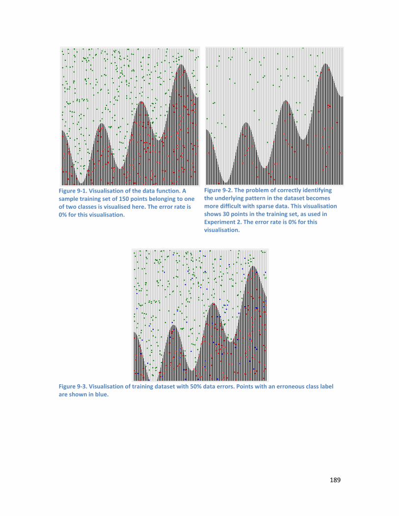
189
Figure 9-1. Visualisation of the data function. A sample training set of 150 points belonging to one of two classes is visualised here. The error rate is 0% for this visualisation.
Figure 9-2. The problem of correctly identifying the underlying pattern in the dataset becomes more difficult with sparse data. This visualisation shows 30 points in the training set, as used in Experiment 2. The error rate is 0% for this visualisation.
Figure 9-3. Visualisation of training dataset with 50% data errors. Points with an erroneous class label are shown in blue.

190
9.2.2. Network Architecture and Parameters
A multilayer perceptron (MLP) with 1 hidden layer was the ANN used. The MLP
incorporated self training logic. The number of nodes in the hidden layer, the optimal
number of training epochs and the training constant were all determined by the self
training algorithm using a trial and error approach. An early exit rule was used, whereby
training ends provided that either:
a) A prescribed minimum number of epochs has elapsed (300 in this case) and the
last peak in testing accuracy was within a given percentage of the start of the run
(45% in this case); or
b) The prescribed minimum number of epochs has elapsed and the last peak in
testing accuracy was more than a given number of epochs previously (2,000 in
this case).
The number of nodes was given an upper limit of 1 input node, 9 hidden layer nodes,
and 1 output layer node. Tuffery (2011) suggests that the optimal number of hidden
layer nodes lies between and 2n, where n equals the number of input nodes, but
reports that some authors suggest extending this to 3n. An upper limit of 9 hidden layer
nodes was chosen as a value that follows these suggested rules of thumb plus allows a
margin.
9.2.3. Overtraining Factor
The OverTrained ensemble members were trained for n epochs where n = optimal
number of training epochs, multiplied by the overtraining factor. The overtraining factor
was set to 10 for these experiments. This factor was chosen to ensure a significant level
of overtraining was achieved.

191
9.2.4. Combining Component Output
Majority voting was employed. The ensemble made a decision if ( ) component
models agreed, otherwise no decision was made.
9.2.5. Confusion Matrix
A confusion matrix was calculated for each ensemble to evaluate its prediction
performance. The confusion matrix contained the rates of True Positives, False Positives,
True Negatives and False Negatives.
The True Positive rate of the classifier was estimated as:
=
The False Positive rate of a classifier was estimated as:
=
9.2.6. Calculating Variance Kohavi and Wolpert (1996) gave an expression for the variability of a predicted class
label y for data point x. Kuncheva and Whitaker (2003) used this general idea and
adapted it for binary class labels and a correct or incorrect decision (oracle output) as
shown in Equation ( 9-2 ).
− ( = | ) − ( = | )
( 9-2 )
Averaged over the whole set of networks, Equation ( 9-3) was used to derive Kohavi-
Wolpert variance.

192
= 12 1 − ∑ ( = 1| )=1 2 − ∑ ( = 0| )=1 2
( 9-3)
Where n = the number of networks in the ensemble.
9.2.7. Algorithm for Conducting Experiments
Table 9.1 describes the algorithm used to conduct the experiments.
For networks 1 to 99
Generate a dataset (with specified data function, data distribution and error rate)
Partition into two equal datasets: a training and a testing dataset
For i = 0 to i < numNetworks
Create a bag of data of size (sizeData) by sampling with replacement
Partition into two equal datasets: a training and a testing dataset
Determine the optimal number of nodes, epochs and training constant by varying these
parameters iteratively.
Train an early stopping network using the optimal number of nodes, epochs and training
constant.
Train an overtrained network using the optimal number of nodes, the optimal number of
epochs * overtraining factor, and the optimal training constant.
Generate a confusion matrix for both the early stopping network and the overtrained
network.
End for loop
Perform majority voting for each ensemble member for early stopping networks. Generate a
confusion matrix.
Perform majority voting for each ensemble member for overtrained networks. Generate a
confusion matrix.
End for loop
Table 9.1. The algorithm used for Experiment 1 and 2.

193
9.3. Results
The performance of the overtrained and early exit ensembles with varying error rates
and ensemble sizes were assessed using two criteria: the percentage of correct
classifications (performance), and the variance of the ensemble components.
9.3.1. Experiment 1 The mean performance for OverTrained and EarlyExit ensembles was calculated over
the range of ensemble sizes tested, for each data error rate. OverTrained Ensembles
performed better than EarlyExit ensembles for data error rates of 10, 30 and 40%.
EarlyExit ensembles performed slightly better for data error rates of 20 and better for
data error rates of 50%. All differences in means between the performance of EarlyExit
and OverTrained ensembles were statistically significant (p = 0.05). Refer to Table 9.2 for
a comparison of the means of the performance of OverTrained and EarlyExit ensembles,
and to Figure 9-4 for a visualisation of the performance of each type of ensemble by
number of networks and error rate.
Data Error Rate
OverTrained Mean –Performance
EarlyExit Mean -Performance
Mean Difference - Performance
Significance (2-tailed)
10 88.52929 88.04747 0.481818 .00020 87.76667 87.99899 -0.23232 .00030 86.00909 83.41818 2.590909 .00040 83.89293 83.13838 0.754545 .01150 43.19091 52.61414 -9.42323 .000
Table 9.2. Experiment 1: Mean performance of OverTrained and EarlyExit ensembles, across ensemble sizes of 1 to 99, by data error rates. Significance testing used paired samples methodology.
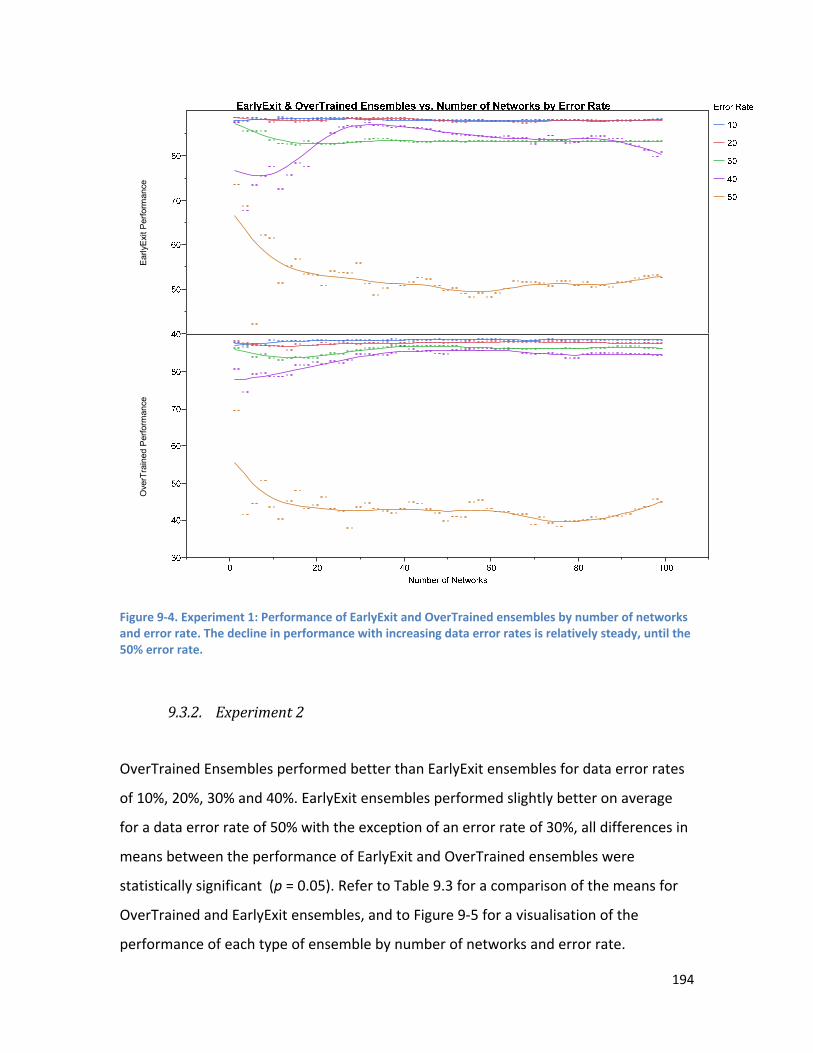
194
Figure 9-4. Experiment 1: Performance of EarlyExit and OverTrained ensembles by number of networks and error rate. The decline in performance with increasing data error rates is relatively steady, until the 50% error rate.
9.3.2. Experiment 2
OverTrained Ensembles performed better than EarlyExit ensembles for data error rates
of 10%, 20%, 30% and 40%. EarlyExit ensembles performed slightly better on average
for a data error rate of 50% with the exception of an error rate of 30%, all differences in
means between the performance of EarlyExit and OverTrained ensembles were
statistically significant (p = 0.05). Refer to Table 9.3 for a comparison of the means for
OverTrained and EarlyExit ensembles, and to Figure 9-5 for a visualisation of the
performance of each type of ensemble by number of networks and error rate.
Ear
lyE
xit P
erfo
rman
ceO
verT
rain
ed P
erfo
rman
ce
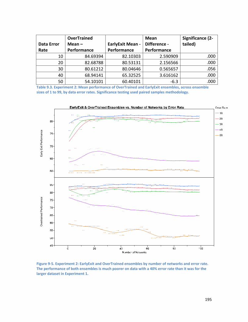
195
Data Error Rate
OverTrained Mean – Performance
EarlyExit Mean - Performance
Mean Difference - Performance
Significance (2-tailed)
10 84.69394 82.10303 2.590909 .00020 82.68788 80.53131 2.156566 .00030 80.61212 80.04646 0.565657 .05640 68.94141 65.32525 3.616162 .00050 54.10101 60.40101 -6.3 .000
Table 9.3. Experiment 2: Mean performance of OverTrained and EarlyExit ensembles, across ensemble sizes of 1 to 99, by data error rates. Significance testing used paired samples methodology.
Figure 9-5. Experiment 2: EarlyExit and OverTrained ensembles by number of networks and error rate. The performance of both ensembles is much poorer on data with a 40% error rate than it was for the larger dataset in Experiment 1.
Ear
ly E
xit P
erfo
rman
ceO
vert
rain
ed P
erfo
rman
ce

196
9.3.3. Effect of Dataset Size - Comparison of Experiment 1 and 2
EarlyExit ensembles performed better in both experiments when the error rate was
50%, and when the error rate was 20% in Experiment 1. In all other levels of data error -
OverTrained ensembles were better performed in both experiments. Refer to Appendix
D, Figure D-1 for a detailed visualisation allowing a comparison to be made of the
performance of EarlyExit and OverTrainined ensemble models, for both experiments.
9.3.4. Variance
Experiment 1
OverTrained ensembles had the highest mean variance for error rates of 10%, 20% and
30%. EarlyExit ensembles had the highest variance for error rates of 40% and 50%. The
difference in means between EarlyExit and OverTrained ensembles were statistically
significant (p = 0.05) for each of the error rate levels. Refer to Table 9.4 for a comparison
of the means of variance for the OverTrained and EarlyExit ensembles by data error
rate. Figure 9-6 shows a comparison of the difference in the variance of EarlyExit and
OverTrained ensemble models by error rate. The OverTrained ensembles had higher
variance for error rates from 10% to 30%.
Data Error Rate (%)
OverTrained Mean – variance
EarlyExit Mean - variance
Mean Diff - variance
Significance (2-tailed)
10 0.001692 0.001671 2.1E-05 .000 20 0.001815 0.001726 8.96E-05 .000 30 0.001792 0.001435 0.000357 .000 40 0.001756 0.002465 -0.00071 .000 50 0.001808 0.002119 -0.00031 .000
Table 9.4. Experiment 1: mean variance for OverTrained and EarlyExit ensembles across ensemble sizes of 5-99, by error rate.

197
Experiment 2
OverTrained ensembles had the highest mean variance for error rates of 10%, 20% and
30% and 40%. EarlyExit ensembles had the highest variance for error rates of 50%. The
difference in means between EarlyExit and OverTrained ensembles were statistically
significant at the θ = 0.05 level for each of the error rate levels. Refer to Table 9.5 for a
comparison of the means of variance for OverTrained and EarlyExit ensembles by data
error rate. Refer to Figure 9-7 for a visualisation of the difference in the variance of
EarlyExit and OverTrained ensemble models by error rate. It can be seen the
OverTrained ensembles have higher variance for error rates from 10% to 40%.
Error Rate (%) OverTrained Mean EarlyExit Mean Mean Diff
Significance (2-tailed)
10 0.001174 0.000916 0.000258 .000 20 0.000981 0.000494 0.000487 .000 30 0.001174 0.000916 0.000258 .000 40 0.000705 0.000294 0.000411 .000 50 0.000795 0.001102 -0.00031 .0099
Table 9.5. Experiment 2: mean variance for OverTrained and EarlyExit ensembles across ensemble sizes of 5-99, by error rate.
Figure 9-6. Experiment 1: Comparison of the difference in the variance of EarlyExit and OverTrained ensemble models by error rate. The x axis shows the number of networks included in the ensemble (from 20 – 50 for this chart). If the difference is above 0, the OverTrained ensemble has greater variance than the EarlyExit ensemble, and conversely if the difference is below 0 the EarlyExit ensemble has the greater variance. The OverTrained ensembles have higher variance for error rates from 10% to 30%.

198
Figure 9-7. Experiment 2: Comparison of the difference in the variance of EarlyExit and OverTrained ensemble models by error rate. The x axis shows the number of networks included in the ensemble (from 20 – 50 for this chart). If the difference is above 0, the OverTrained ensemble has greater variance than the EarlyExit ensemble, and conversely if the difference is below 0 the EarlyExit ensemble has the greater variance. The OverTrained ensembles have higher variance for error rates from 10% to 40%.
OverTrained ensembles tend to out-perform EarlyExit ensembles for low to medium
(10% – 40%) rates of data error. This behaviour is consistent across the differing sizes of
training dataset for Experiment 1 and 2 (150 and 30 training data points respectively).
The level of variance in an ensemble tracks with its overall performance. OverTrained
ensembles tended to have higher variance for low to medium (10% – 40%) rates of data
error.
9.3.5. Number of Networks
It can be seen from Figure 9-4 that the optimal number of networks for peak
performance for each combination of data error rates and type of ensemble
(OverTraining and EarlyExit) is highly variable. In general for lower to moderate data
error rates (10% - 40%) ensembles with number of networks in the range of 20-40
appear to be a good trade-off between model parsimony and performance. The level of
variance among component networks in an ensemble drops in a predictable exponential
decay curve as the number of networks in the ensemble increases (refer to Figure 9-8
and Figure 9-9). Ensembles consisting of networks in the range of 20 to 40 appear to
offer the best compromise between bias (or how correct the predictions of the
ensemble are) and variance (the level of disagreement among ensemble members) and
model parsimony.

199
Figu
re 9
-8. E
xper
imen
t 1: E
arly
Exit
and
Ove
rTra
ined
var
ianc
e by
num
ber o
f net
wor
ks in
the
ense
mbl
e (6
-99
show
n) a
nd d
ata
erro
r rat
e. T
he g
raph
show
s tha
t th
e le
vel o
f var
ianc
e am
ong
com
pone
nt n
etw
orks
in a
n en
sem
ble
drop
s in
a pr
edic
tabl
e ex
pone
ntia
l dec
ay cu
rve
as th
e nu
mbe
r of n
etw
orks
in th
e en
sem
ble
incr
ease
s. It
can
als
o be
seen
that
the
varia
nce
for t
he E
arly
Exit
ense
mbl
e sh
ows m
ore
varia
tion
betw
een
the
diffe
rent
err
or le
vels
than
that
of t
he O
verT
rain
ed
ense
mbl
es.

200
Figu
re 9
-9. E
xper
imen
t 2: E
arly
Exit
and
Ove
rTra
ined
var
ianc
e by
num
ber o
f net
wor
ks in
the
ense
mbl
e (6
-99
show
n) a
nd d
ata
erro
r rat
e. T
he g
raph
show
s tha
t th
e le
vel o
f var
ianc
e am
ong
com
pone
nt n
etw
orks
in a
n en
sem
ble
drop
s in
a pr
edic
tabl
e ex
pone
ntia
l dec
ay cu
rve
as th
e nu
mbe
r of n
etw
orks
in th
e en
sem
ble
incr
ease
s.
201
9.4. Discussion
For both datasets sizes tested (150 and 30 data points) the ensembles consisting of
overtrained nets tended to perform slightly better for data error rates from 10% to 40%.
The ensembles consisting of nets which were trained using the EarlyExit algorithm
performed substantially better with high data error rates of 50%.
These findings suggest that the regularisation effect of combining the output of an
ensemble of models does indeed remove the deleterious effects of overtraining under
most data conditions. For high levels of noise in the data, nets trained using an early exit
strategy were the most effective. Variance among nets is likely to be high with noisy
datasets, due to the different bags of data containing different outliers. In this case
reducing the bias of the estimators by taking less account of the data (achieved by the
early exit training algorithm) is likely to be the most effective way of increasing
ensemble performance. This idea is lent support by Krogh (1996), who found that when
there are large amounts of noise in the training data it is unnecessary to increase the
diversity of component networks.
For both dataset sizes tested, ensembles where the component nets were overtrained
had the highest mean variance for error rates of 10%, 20% and 30%. For error rates of
40% with the larger dataset (Experiment 1), the early exit ensemble had greater
variance; while with the smaller dataset (Experiment 2), the overtrained ensemble had
greater variance. Early Exit ensembles had the highest mean variance for error rates of
50% for both dataset sizes.
These findings indicate that when date error levels are low to moderate, overtraining
component networks does indeed increase their diversity. This is in accordance with
Carney and Cunningham (1999), who believe that overtraining the networks in an
ensemble generates more variance. It appears that the effect of overtraining on
variance was slightly more pronounced with the smaller dataset (Experiment 2). In both
experiments the overtraining was achieved by multiplying the optimal number of
training epochs by an overtraining factor of 10. The level of overfitting achieved by the
202
net trained in this manner, however, would vary slightly according to the size of the
dataset. The level of overfitting achieved for the smaller dataset is likely to be greater.
We have seen that the increase in variance for these low to moderate levels of error in
the data was accompanied by an increase in ensemble performance, indicating that bias
was not unduly increased by the overtraining. Grannitto, Verdes and Ceccato (2005)
agree that some controlled degree of overtraining in component networks improves
ensemble performance.
It is interesting to note that when noise in the dataset is high, overtraining the
component nets actually reduces the diversity. This is surprising, as it was expected that
overtraining would continue to increase variance for datasets with high levels of error in
the data, along with the bias.
The mean performance of the EarlyExit ensembles for the smaller dataset (Experiment
2) and a 50% data error rate is 60%. This stands out as anomalous. Given that the level
of error in the dataset is known to be 50%, a performance above this level is suggestive
of overfitting. The mean performance for OverTrained ensembles for this experiment
was 54%, which is more realistic. It thus appears that deliberately overtraining
component nets trained on a very small, very noisy dataset actually reduced the level of
overfitting in the resultant ensemble compared to an ensemble whose component nets
weren’t deliberately overtrained. It is widely accepted that the estimation of error used
to determine when to stop training in an early-exit network can fluctuate during training
in the presence of noise in the data (Carney & Cunningham, 1999). It is therefore likely
that there may have been more variation in the early exit point chosen by the self
training algorithm when trained on datasets with high noise levels.
The EarlyExit ensemble for the larger dataset and a data error level of 50% didn’t appear
to suffer from the same overfitting issues, with a realistic mean performance of 52.6%.
The OverTrained ensembles performed poorly on this experiment, with a mean
performance of 43%. Again, it is unexpected that overtrained ensembles had a lower
mean variance for this experiment than that of the early exit ensembles. Interestingly,
203
however, the overtrained ensembles have higher variances than the early exit
ensembles towards the larger end (from around 40 onwards) of ensemble sizes tested.
It is important to note, in these discussions of overfitting, that overfitting is not
necessarily a global phenomenon. Overfitting can vary significantly in different regions
of input space (Caruana, Lawrence, & Giles, 2001). This effect is particularly noticeable
with sparse data, with the sparse regions tending to suffer from overfitting before the
more populous regions. Figure 9-2 demonstrates that with 30 data points, some regions
are more sparsely populated than others. The training and performance datasets used
throughout this research have sparse data, and as such it is likely that the component
nets of the HANNEM model contained some regions of input space that were
overtrained. The findings of this investigation show that the regularisation effect of
combining the outputs of an ensemble mitigates the adverse effects of overtraining.
Performance was highly variable across different ensemble sizes, particularly with low
numbers of ensemble members. This is to be expected with unstable predictors.
Ensembles with around 20 to 40 networks appeared to perform the best, particularly
with low to moderate data error rates. Slightly larger ensemble sizes appear to be
optimal with the higher levels of error in the data. The diversity of component nets
drops rapidly from 1 to around 20 component nets. The inflection point for the variance
curves occurs around 20 to 40 net mark – the same region where performance tends to
be greatest.
Findings on the optimal number of component networks in an ensemble have been
variable in the literature. Carney and Cunningham (1999) found that there was little to
be gained by using more than 30 networks and improvements seemed to level out at
about 100 networks. Raviv and Intrator (1996) found that a 40-net ensemble gave
superior results to a 5-net ensemble. Zhang (2007) suggests that ensemble sizes of 5 to
10 are a reasonable balance between ensemble performance and computational
efficiency. Tuffery (2011) considers that about 10 models is sufficient. Perrone and
Cooper (1993) suggest that the optimal number of models for an ensemble is

204
dependent on the number of distinct models that can be created from the dataset. The
results from these experiments suggest that the optimal number of networks doesn’t
vary largely with variations in the size of the dataset, and the level of noise in the data.
The results do suggest, however, that highly noisy datasets benefit from a slightly larger
number of component models. This finding suggests that the HANNEM model could be
improved by increasing the number of component ANNs to between 20 and 40.
9.5. Summary
This chapter is concerned with investigating the use of neural network ensemble models
on very small datasets, and indentifying the subsequent generalisation ability of such
models. This novel investigation examined the relationship between overfitting
individual networks and ensemble generalisation performance, as well as the effect of
different levels of noise in the data, and the inter-relationship of these variables with
the size of the dataset.
The results show that using a bootstrapped ensemble of ANNs mitigates the affect of
overtraining component nets, and in fact for low to moderate levels of noise in the data
an overtraining strategy increases model diversity and provides performance benefits.
The results also suggest that early exit rules become unstable in situations of high data
error and very small datasets. It may be useful in these situations to increase the
minimum number of epochs performed.
Although the HANNEM model did not use deliberately overtrained component nets,
with sparse data it is likely that some regions of input space would be overtrained and
other regions undertrained. The findings of this study show that the regularisation effect
of an ensemble means that the ability of the ensemble to generalise to new data is not
adversely affected.

205
The findings suggest that the HANNEM model could be improved by increasing the
number of component nets. It was shown that the optimal number of nets increases
slightly for datasets with large rates of error. Although the rate of error in the three case
study datasets used to validate the HANNEM model is unknown, given the performance
of the models reported in Chapter 8, it is likely that the rate of error ranges from around
30% - 48% (it is a reasonable assumption that the variance of performance unexplained
by HANNEM is largely due to noise in the data). Estimating the level of variance in the
ensemble provides a technique that gives an insight into the number of distinct models
that can be created from a dataset, and can be used in establishing an appropriate
number of component models for a particular dataset.

207
CHAPTER 10 – CONCLUSION AND FUTURE WORK
Researchers have been working on the problem of how to model athletic training and
performance for at least the last 30 years. A model that enables prediction of
performance and hence offers a practical solution to the problem of how to optimise
training for an individual athlete has remained the "holy grail" of sport science. Early
approaches used statistical and mathematical techniques, in conjunction with a systems
modelling approach. As machine learning techniques continue to be developed, some
researchers have experimented with applying these techniques to the problem.
Machine learning techniques, however, are dependent on the quality of the data
available. Athletic training and performance datasets are usually incomplete, noisy, and
very small. In addition, training load is only one of a myriad of factors which affects
performance.
The work reported in this thesis began with the development of a novel training load
quantification technique called PTRIMP. Researchers have found great difficulty in
finding a way to effectively quantify training load using a single term. I propose that two
commonly used approaches - TRIMPS and TSS - place too much emphasis on the
duration of a session, while not weighting high intensity training enough. PTRIMP was
developed to address this limitation, and to more accurately reflect the physiological
cost of high intensity efforts.
The first investigation undertaken in this thesis was a case study to examine the
relationship between PTRIMP and a Recovery Index derived from HRV data. The aim of
this investigation was to provide validation of the PTRIMP algorithm, by determining
whether PTRIMP tracked with the fatigue measure in a manner consistent with known
physiological responses to training. Wavelet-based semblance analysis, in a technique
developed by Cooper and Cowan (2007), was used to compare the PTRIMP and the RI
dataseries on the basis of their phase, as a function of frequency.
208
The results of this investigation showed that PTRIMP and Recovery Index were strongly
negatively correlated on larger time scales of 30 days or above. This is in accordance
with known physiological responses to training; when training levels over the past seven
days have been high, it is expected that fatigue levels would be high, and thus the RI
should be low. At smaller time scales of around seven days, regular periods of moderate
to strong positive correlation were interspersed with periods of moderate to strong
negative correlation. It was hypothesised that this phenomenon may have been due to
the delay that is known to exist between increased training and the onset of long-term
fatigue. This investigation provided evidence that the novel training load quantification
technique developed (PTRIMP) performed as expected in a real world situations -
tracking with a marker of fatigue in a physiologically realistic manner.
The focus of this work next turned to developing a method of quantifying performance
for road cyclists. Many researchers have used a method whereby performances from a
standardised exercise test are converted into a percentage of the subject's personal
best performance for that test. This approach requires subjects to complete regular
performance tests. A key point of difference in this research is that it required no
change in routine or additional work in order to achieve compliance with the
requirements of data collection. This becomes vital when working with elite athletes for
whom their performance is their livelihood. It was therefore necessary to develop a
technique for quantifying performance that works with field-derived data.
An athlete's best performances are likely to occur during an actual competition as
training induced fatigue will have been minimised by a taper. Field-derived performance
metrics for some sports - such as swimming, or to a lesser extent sprinting - are
relatively easily developed because performance is a function of time (over a certain
distance) and conditions are relatively stable between competitions. Time cannot be
used as a proxy for performance in road cycling, however, due to the variation in
distances, terrain, environmental conditions, drafting and tactics which are integral to
road cycling races.

209
The results of a cycling road race are typically determined by one or more critical
periods during the race. At its simplest, to improve performance the athlete needs to
increase the amount of power they can generate for these critical periods - the
durations of which will be specific to the race. By recording Maximal Mean Powers over
a range of durations, the power outputs during these critical periods can be captured.
MMP profiles can then theoretically be used to track performance improvements.
The proposed performance quantification technique generates a MMP profile for each
athlete, recording their best output to date over regular intervals from 5s to 20min.
These durations represent a spectrum of energy system contributions; from primarily
anaerobic to primarily aerobic systems. A second MMP profile, created with the same
durations from 5s to 20min, is generated from the race for which performance is to be
calculated. The area under the curve of each of the MMP profiles is then calculated, and
the difference between the MMP curve for the performance and the MMP curve for the
athlete's best output to date is taken as performance.
The second investigation undertaken in this work examined the correlation of PTRIMP,
RI and the novel performance metric developed. PTRIMP data was smoothed over a
number of time windows (3, 7, 14 and 30 days). Correlation analysis indicated that
PTRIMP data smoothed over 3 days (PTRIMP(3)) was most strongly correlated to
performance. A multiple linear regression model with PTRIMP(3) and RI as inputs, and
performance as the output was fitted using linear least squares to minimise the residual
sum of squares. The inclusion of an interaction term between PTRIMP(3) and RI, as well
as a quadratic tern for PTRIMP(3) provided the best fit. The fit for the model was weak,
explaining only 40% of the variation in performance measured. The explanatory power
of the model did, however, suggest that there is a non-linear positive relationship
between training load as measured by PTRIMP, and performance, as quantified by the
proposed technique.
The third investigation undertaken in this work built upon the previous investigations by
taking the novel training load and performance quantification techniques developed,

210
and performing an experiment to determine whether this information could be used to
provide relevant feedback on optimal training strategies. This investigation focused on
the taper period – the period of reduced training undertaken prior to a competition.
The aim of a taper is to reduce accumulated fatigue caused by training, while
maintaining or enhancing fitness. The optimal design of a taper is still unknown, and in
any case is likely to be specific to an individual athlete in accordance with the principle
of specificity. The three key elements that can be manipulated in designing a taper are
the magnitude of the reduction in training volume, the intensity of the training
completed during the taper, and the pattern of the taper. This investigation focused on
the pattern of the taper.
A number of simple taper patterns have been investigated by researchers. Existing
evidence suggests that a progressive reduction in training load (using either a constant
linear slope or an exponential decay) is to be preferred over reductions in the form of a
simple step – where training load is suddenly reduced and then maintained at the same
level. Little work has been done on more complex patterns, although some early
modelling work by Thomas, Mujika and Busso (2009) suggests that such work could be
beneficial. Few studies have used data from real world training and performance data.
As the relationship between performance in tests and performance in events is
questionable, such real world modelling can potentially provide very valuable
information.
Modelling an athlete’s response to training gives the opportunity to examine the impact
of taper shape on performance. The aim of this investigation was to firstly identify the
effect the shape of a taper has on an elite cyclists’ performance; and secondly, to
determine if individual differences in optimal taper shape exist between athletes.
The datasets used for this investigation consisted of power data from the training and
racing of two female elite cyclists over a period of 250 and 870 days. PTRIMP and
performance were calculated as per the previous investigations.

211
It was necessary to find a pre-processing technique to enable an understanding and
subsequent classification of the shape of the training load in the final three days of a
taper. In a novel application, Symbolic Aggregate approXimation (SAX) was used to
discretise the taper time-series (the training load or PTRIMP for the three days prior to a
competition) to a symbolic representation using an alphabet size of three. The
discretisation resulted in a sequence of three strings for each three day taper period,
with the string representing that shape of the taper. A string of ‘321’, for example,
represented a taper that started with a high training load on day p-3, then a medium
load on day p-2 and a low training load on day p-1 (where p = the day of the performance
or competition).The strings of taper shapes were grouped into four categories to
describe their shape (low, high-tail, low-tail and high). Analysis showed that the main
effect of taper shape on performance was statistically significant for both athletes a 5%
level of significance. Considerable variance existed between individuals and their
response to a particular taper shape. The interaction effects between taper shape and
subject were statistically significant.
These results suggest that tapering advice, which in the literature is frequently
generalised across genders, between different sports, and between athletes of differing
levels of training, cannot be usefully provided using a generalist model.
The effect size of the different taper shape treatments was statistically significant for
both subjects. The evidence that training load has a predictable and significant effect on
performance provides validation for the integrity of the techniques used to quantify
training and performance.
The most effective taper shape for each athlete represented a 6.1% and 4.4%
improvement respectively, compared with the least effective taper shape. While
drafting and team tactics preclude the estimation of the smallest worthwhile
improvement in road cycling, Paton and Hopkins (2006) estimate that the smallest
worthwhile improvement for top-level athletes in individual road cycling time trials is
approximately 0.6%. It is therefore likely that the small improvements in performance

212
observed in this investigation as the result of employing an optimal taper shape could
have a significant effect on the outcome of elite road races. These findings point to the
usefulness of modelling training and performance and the ability of such models to
provide practical feedback for athletes and coaches to assist them in the planning of
training programs. The relatively minimal data collection requirements for this study -
made possible by the development of the novel training load and performance
quantification techniques which require only the provision of power data from all
training rides and performances – make it feasible for elite athletes to provide data
without interfering with their normal training and racing schedules.
The investigations already described set up the foundation and framework for the
development of a model to describe the relationship between training and performance
for elite road cyclists. The fourth investigation in this work described the development
of a novel hybrid artificial network ensemble model (HANNEM).
For HANNEM to be effective, it needed to overcome a number of limitations in the data
associated with the training and performance domain, namely limited amounts of noisy
and incomplete data. Data collected from elite athletes needs to make minimal changes
to their normal training and racing routines, and this limits the number of independent
parameters available for modelling.
The modelling relies on collecting data on performances that represent maximal efforts
– it is thus crucial to be able to identify such sessions. A training diary recording the
athlete’s perception of effort for each session can be useful here, but is not always
available. A novel technique was therefore developed to identify races where, due to
tactical (or other) considerations, 100% effort was not made by the athlete. Power files
which show a low average power output, and a high average speed are indicative of flat
stages in a multi-day stage race where drafting is occurring and 100% effort is not made.
Cluster analysis was performed on the variables performance and average speed, and
average power and average speed. Clusters with high speed and low performance or
power were identified as stages not involving 100% effort, and excluded from the
213
dataset. This substantially reduced the noise of the performance dataset. This novel
technique increases the range of datasets that can be used for modelling.
HANNEM combined three key modelling elements: a SimBEA model (Bruckner, 2006); a
linear model (either an ARIMA or multiple linear regression model); and an ensemble of
artificial neural networks. PTRIMP was used as the model input and performance was
the output.
The SimBEA model developed by Bruckner (2006) was used to capture important
domain knowledge about the underlying physiological processes governing the response
to training, and their impact on performance. A linear model was incorporated to model
the linear patterns in the data. A neural network model, taking as inputs a summary of
recent training load quantified using the PTRIMP algorithm, as well as the performance
predictions from the SimBEA model and the linear model, was used to capture the
nonlinear patterns in the data. The performance of the hybrid model (a combination of
SimBEA, ARIMA and ANN models, or a combination of SimBEA, ARIMA, MLR and ANN
models) was better than the performance of any single model for each of the datasets.
The use of neural networks with small, noisy datasets is potentially problematic. Neural
networks created on such datasets are prone to overfitting issues, resulting in models
with poor generalisation abilities. To reduce overfitting problems, the techniques of
bagging, and adding noise or jitter to each bag was used. An ensemble of ANNs were
trained on the bagged sets, which all varied slightly.
Three datasets captured from the training and racing of three elite road cyclists were
used to test the performance of HANNEM. Moderate to good fits were obtained for the
HANNEM predictions using jacknife validation (R2 = 78%; R2 = 60% and; R2 = 51% for
Subjects A, B and C respectively).
These results are in contrast to the fits obtained for an impulse-response model alone.
Fits for SimBEA (described by Bruckner, 2006) were poor – an R2 of 32% for Subject B,

214
and weak not linear relationships between actual performance and predicted
performance for Subjects A and C.
A key question when evaluating these results is whether the level of accuracy reported
is such that HANNEM can be used as a training planning tool for coaches and elite
athletes. The results from Chapter 7 indicate that the techniques developed throughout
this research are indeed able to determine appropriate taper strategies that result in
worthwhile levels of performance improvement. Measurement of performance in road
cycling cannot be absolute but rather is made up of a number of critical moments.
Performance is best measured relative to an individual’s previously recorded capabilities
during critical moments. The aim of HANNEM is to correctly identify the direction and
rate of change in performance trends, rather than predict an exact performance level,
and this it achieved.
The sparse datasets used in the modelling make it likely that some regions of input
space would be overtrained by component ANN models, and other regions
undertrained. The final investigation of this work addressed this issue of potential
overfitting and resultant lack of generalisation with small noisy datasets. The
investigation aimed to determine whether creating an ensemble of ANNs mitigates the
effect of overfitting with small and potentially noisy datasets, and in fact whether
deliberate overtraining can actually improve the performance of an ensemble of ANNs.
The optimal number of component ANNs in an ensemble was also investigated in
relation to the size and level of noise in training datasets.
The results showed that by combining a diverse collection of ANN models (created using
bagging) into an ensemble, the smoothing effect of the ensemble removed any adverse
effects of overtraining on individual nets. In fact, for low to moderate levels of noise in
the data, a strategy of overtraining was shown to increase the diversity of the
component models and consequently provide performance benefits to the ensemble.
The findings suggest that HANNEM is not likely to be compromised in its ability to

215
generalise to new data due to overtrained regions in the sparse dataset - as a result of
the regularisation effect of the ANN ensemble.
The investigation showed the optimal size of the ensemble was variable, as you would
expect with unstable estimators. Twenty to forty nets tended to be a good range for an
ensemble, with the optimal number of nets increasing slightly for datasets with large
rates of error. These findings suggested that HANNEM could be improved by increasing
the number of component nets in the ensemble to between 20 and 40 nets. The
findings also suggest that estimation of the level of variance in the ensemble for
differing ensemble sizes can give insight into the number of distinct models that can be
created from a particular dataset. Examining variance and performance over a range of
ensemble sizes, and choosing a number of nets somewhere around the point of
inflection in the level of variance was shown to be an effective strategy.
In summary, the results (as shown in Chapter 8) showed that the application of
HANNEM in predicting performance in elite cyclists is promising. The method presented
in this thesis provides the basis for real world performance prediction using data
obtained in the field. The model has been designed to:
1. Provide a technique for quantifying training load in a physiologically accurate
manner from power data file collected in the field.
2. Quantify performance from race power data collected in the field, using the
insight that performance in a race consists of maximal performance in a number
of critical moments in the race.
3. Provide a technique for symbolising taper shape and subsequently identifying
the optimal taper shape for an athlete.
4. Identify and eliminate races or stages where the athlete did not give 100% effort
for strategic reasons.

216
5. Incorporate Bruckner’s (2006) SimBEA model to capture domain knowledge
about the physiological processed underlying training and performance.
6. Construct linear statistical models to model the linear patterns in the data and
take advantage of the strengths of such statistical models.
7. Estimate performance using an ensemble of ANNs to capture the nonlinear
patterns in the data, using as inputs the performance predications from the
SimBEA model and the linear model as well as a summary of the recent training
load (PTRIMP).
8. Use the technique of bagging and the addition of noise or jitter to the bagged
training sets in order to create diversity in the component ANNs. These
techniques are particularly appropriate for small, noisy datasets.
A coach or elite athlete may be able to use the HANNEM model to:
• Identify the direction and rate of change in performance trends;
• Identify the optimal shape of the taper;
• Present the model with proposed changes in training load (in the form of
estimated PTRIMP values) and observe the resultant estimated change in
performance; and
• Ultimately use the above information to provide decision support when
developing a training plan to enable the athlete to deliver optimal performance
at the desired time.
The research conducted in this thesis advances current training and performance
modelling techniques to allow prediction of road cycling performance training and
racing data collected from the field. New techniques were developed to allow the
field-derived data to be quantified for modelling. Modelling techniques have been

217
developed to extract patterns from these small, noisy and incomplete datasets, and
build robust prediction models with sufficient accuracy to be used in assisting the
planning of training. The new approach shows great promise for assisting elite
athletes and coaches in planning and monitoring training, and shows potential for
both future research and commercialisation. The approach also provides a modelling
framework that can potentially be utilised in other domains where datasets are
small, noisy and incomplete.
The research conducted has raised a number of issues worthy of further research.
The major future extensions to this work which have been identified include the
following:
1. Add more component ANNs to the ensemble of ANNs used in HANNEM. The
investigation reported in Chapter 9 suggested that 20-40 nets might be
appropriate. Creating a test harness to trial a range of nets sizes, and then
examining the resultant estimated performance and variance should allow
the optimal ensemble size to be estimated.
2. Investigate the effect of deliberate overtraining on component ANNs in
HANNEM. The investigations reported in this work indicate that early
stopping algorithms may become unstable with very high levels of error exist
in the dataset. The evidence suggests that overtrained ensembles perform
better than early exit ensembles when data error levels are low to moderate.
3. Investigations (undertaken by the author and a collaborator) are currently
underway into a new type of neural network architecture and training
algorithm, which is designed to reduce the adverse impact of regions of
sparse data and unsupported data points on modelling. The network,
nicknamed SANATY, uses mapping in input space to identify the k nearest
neighbours who are best placed to provide a prediction for any unseen new
data point. An intelligent arbiter then takes the input from the nearest
neighbours and uses fusion techniques to synthesis the final prediction.

218
SANATY has the potential to be of use for all datasets that suffer from
regions of sparse data.
4. Develop an automated tool which uses a technique such as genetic
algorithms to solve the optimisation problem of sequencing training loads.
5. HANNEM has the potential to be useful in identifying abnormal patterns in
performance. These abnormal patterns could be the result of illness or
doping. HANNEM establishes a relationship between training and
performance, and when this relationship becomes disrupted, it indicates that
a variable unaccounted for by the model warrants identification and
investigation.

219
APPENDIX A – LIST OF PUBLICATIONS This appendix displays the list of refereed publications that have been achieved to date
from the thesis work.
Churchill, T., Sharma, D., Balachandran, B., (2010). Identifying Taper Shape and its effect on Performance. Proceedings of the 9th Conference of Mathematics in Sport (Darwin, 2010).
Churchill, T., Sharma, D., Balachandran, B., (2009).Correlation of training load and heart rate variability indices in elite cyclists. Proceedings of the 2nd International Conference Mathematics in Sport (Groningen, 2009).
Churchill, T., Sharma, D., Balachandran, B., (2009). Correlation of novel training load and performance metrics in elite cyclists. Proceedings of the 7th International Symposium for the International Association on Computer Science in Sport (Canberra, 2009).
Churchill, T., Sharma, D., Balachandran, B., (2008). AI modelling of the relationship between training and performance in athletes. Proceedings of the 8th Conference of Mathematics in Sport (Tweed Heads, 2008).

221
APPENDIX B - GLOSSARY
Term Definition ANN Artificial Neural Network ARIMA Autoregressive Integrated Moving Average ATL Acute Training Load CTL Chronic Training Load HR Heart rate HRV Heart Rate Variability ICC Intraclass Correlation Coefficient MMP Maximum Mean Power PNS Parasympathetic Nervous System PTRIMP Power Training Impulse RI Recovery Index RPE Rate of Perceived Exertion RR interval The interval between successive R waves SAX Symbolic Aggregate approXimation SimBEA An impulse-response model SNS Sympathetic Nervous System SRM Schoberer Rad Messtechnik. Device to measure power output of cyclistsSVM Support Vector Machine TSB Training Stress Balance

223
APPENDIX C – ALGORITHM USED IN HANNEM The algorithm used in HANNEM to generate and validate an ensemble of ANN models. For i = 0; i < numberOfRows; i++ {
Go to Row(i); Exclude; For(i = 0; i<8; i++) {
CreateBagOfData(sampleSize); AddNoise(); With bag
Neural Net( Y(:Performance), X(:SimBEA, :LinearModelPrediction, :TrainingLoad), CrossValidation("K-Fold", 5), SequenceOfFits ( OverfitPenalty(Vary from 0.001 to 0.04), HiddenNodes(Vary from 2 to 5) )
) Save Formula for best performing model
}
Average prediction of component nets for excluded row Table C.1. Algorithm used to generate and validate an ensemble of ANN model.
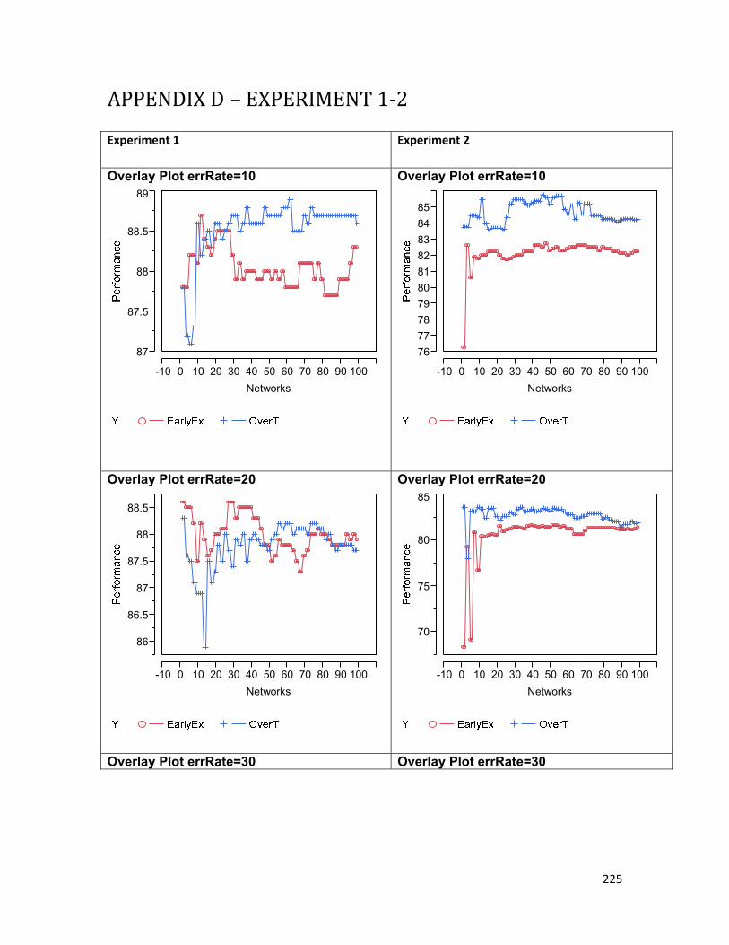
225
APPENDIX D – EXPERIMENT 1-2 Experiment 1 Experiment 2
Overlay Plot errRate=10
Overlay Plot errRate=10
Overlay Plot errRate=20
Overlay Plot errRate=20
Overlay Plot errRate=30 Overlay Plot errRate=30
87
87.5
88
88.5
89
-10 0 10 20 30 40 50 60 70 80 90 100
Networks
76
77
78
79
80
81
82
83
84
85
-10 0 10 20 30 40 50 60 70 80 90 100
Networks
86
86.5
87
87.5
88
88.5
-10 0 10 20 30 40 50 60 70 80 90 100
Networks
70
75
80
85
-10 0 10 20 30 40 50 60 70 80 90 100
Networks
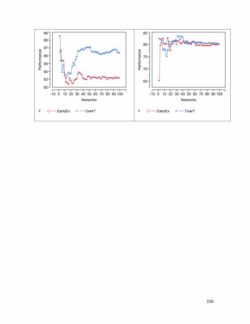
226
82
83
84
85
86
87
88
89
-10 0 10 20 30 40 50 60 70 80 90 100
Networks
65
70
75
80
85
-10 0 10 20 30 40 50 60 70 80 90 100
Networks
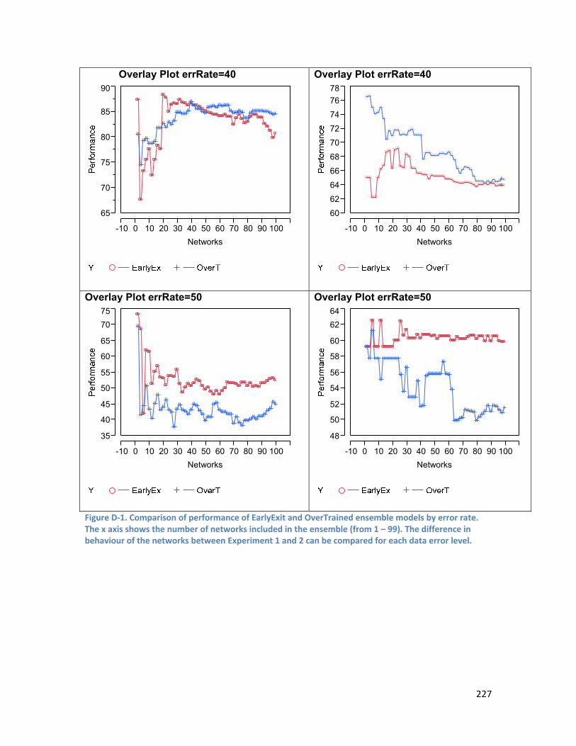
227
Overlay Plot errRate=40
Overlay Plot errRate=40
Overlay Plot errRate=50
Overlay Plot errRate=50
Figure D-1. Comparison of performance of EarlyExit and OverTrained ensemble models by error rate. The x axis shows the number of networks included in the ensemble (from 1 – 99). The difference in behaviour of the networks between Experiment 1 and 2 can be compared for each data error level.
65
70
75
80
85
90
-10 0 10 20 30 40 50 60 70 80 90 100
Networks
60
62
64
66
68
70
72
74
76
78
-10 0 10 20 30 40 50 60 70 80 90 100
Networks
35
40
45
50
55
60
65
70
75
-10 0 10 20 30 40 50 60 70 80 90 100
Networks
48
50
52
54
56
58
60
62
64
-10 0 10 20 30 40 50 60 70 80 90 100
Networks

229
REFERENCE LIST Abbiss, C. R., & Laursen, P. B. (2005). Models to explain fatigue during prolonged endurance
cycling. Sports medicine, 35(10), 865–898. Atlaoui, D., Pichot, V., Lacoste, L., Barale, F., Lacour, J. R., & Chatard, J. C. (2007). Heart Rate
Variability, Training Variation and Performance in Elite Swimmers. Int J Sports Med, 28(5), 394-400.
Aubert, A. E., Seps, B., & Beckers, F. (2003). Heart rate variability in athletes. Sports Medicine, 33(12), 889.
Avalos, M., Hellard, P., & Chatard, J. C. (2003). Modeling the training-performance relationship using a mixed model in elite swimmers. Med Sci Sports Exerc, 35(5), 838-46.
Avalos, Marta , Hellard, Phillipe, Millet, Gregoire, Lacoste, Lucien, Barale, Frederic, & Chatard, Jean-Claude. (2005). Modeling the Residual Effects and Threshold Saturation of Training: A Case Study of Olympic Swimmers. The Journal of Strength and Conditioning Research, 19(1), 67-75.
Balagué, N., & Torrents, C. (2005). Thinking before computing: changing approaches in sports performance. International Journal of Computer Science in Sport, 4(1), 5-13.
Banister, E. W. (1991). Modeling Elite Athletic Performance. In Physiological Testing of the High Performance Athlete. Champaign: Human Kinetics Books (pp. 403-424).
Banister, E. W., & Calvert, T. W. (1980). Planning for future performance: implications for long term training. Canadian journal of applied sport sciences. Journal canadien des sciences appliquées au sport, 5(3), 170-6.
Banister, E. W., Calvert, T. W., Savage, M. V., & Bach, T. (1975). A systems model of training for athletic performance. Aust. J. Sports Med, 7, 57-61.
Banister, E. W., Carter, J. B., & Zarkadas, P. C. (1999). Training theory and taper: validation in triathlon athletes. European Journal of Applied Physiology and Occupational Physiology, 79(2), 182-191.
Banister, E. W., Morton, R. H., & Fitz-Clarke, J. R. (1996). Clinical dose-response effects of exercise. The physiology and patophysiology of exercise tolerance. New York, London: Plenum, 297–09.
Barnett, A., Cerin, E., Reaburn, P., & Hooper, S. (2010). The effects of training on performance and performance-related states in individual elite athletes: A dynamic approach. Journal of sports sciences, 1.
Baumert, M., Brechtel, L., Lock, J., Hermsdorf, M., Wolff, R., Baier, V., & Voss, A. (2006). Heart Rate Variability, Blood Pressure Variability, and Baroreflex Sensitivity in Overtrained Athletes. Clinical Journal of Sport Medicine, 16(5), 412.
Bompa, T. O., & Haff, G. (2009). Periodization: Theory and Methodology of Training. Human Kinetics.
Bompa, T., & Carrera, M. (2005). Periodization training for sports. Human Kinetics. Borresen, J., & Lambert, M. I. (2009). The Quantification of Training Load, the Training
Response and the Effect on Performance. Sports Medicine, 39(9), 779–795. Bosquet, L., Montpetit, J., Arvisais, D., & Mujika, I. (2007). Effects of tapering on performance:
a meta-analysis. Medicine & Science in Sports & Exercise, 39(8), 1358. Brown, S. P., Miller, W. C., & Ph.D, J. M. E. (2006). Exercise Physiology: Basis of Human
Movement in Health and Disease. Lippincott Williams & Wilkins. Bruckner, J. (2006). Training im leistungssport: Modellierung und simulation von
adaptationsprozessen. Christian-Albrechts-Universität, Kiel. Brückner, J., & Wilhelm, A. (2008). Modellierung und simulation von adaptationsprozessen. E-
Journal Bewegung und Training, 2(2008), 51-65.

230
Busso, T. (2003). Variable dose-response relationship between exercise training and performance. Med Sci Sports Exerc, 35(7), 1188–1195.
Busso, T., & Thomas, L. (2006). Using Mathematical Modeling in Training Planning. International Journal of Sports Physiology and Performance, 1, 400-405.
Busso, T., Candau, R., & Lacour, J. R. (1994). Fatigue and fitness modelled from the effects of training on performance. European journal of applied physiology and occupational physiology, 69(1), 50–54.
Busso, T., Carasso, C., & Lacour, J. R. (1991). Adequacy of a systems structure in the modeling of training effects on performance. J Appl Physiol, 71(5), 2044-2049. Retrieved June 28, 2007, from http://jap.physiology.org/cgi/content/abstract/71/5/2044
Busso, T., Denis, C., Bonnefoy, R., Geyssant, A., & Lacour, J. R. (1997). Modeling of adaptations to physical training by using a recursive least squares algorithm. Journal of Applied Physiology, 82(5), 1685-1693.
Busso, T., Häkkinen, K., Pakarinen, A., Carasso, C., Lacour, J. R., Komi, P. V., & Kauhanen, H. (1990). A systems model of training responses and its relationship to hormonal responses in elite weight-lifters. European Journal of Applied Physiology, 61(1), 48–54.
Banister, E. W., Calvert, T. W., Savage, M. V., & Bach, T. (1975). A systems model of training for athletic performance. Aust. J. Sports Med, 7, 57–61.
Carney, J. G., & Cunningham, P. (1999). Tuning diversity in bagged neural network ensembles. Trinity College Dublin Technical Report TCD-CS-1999-44. Retrieved from http://citeseerx.ist.psu.edu/viewdoc/download?doi=10.1.1.43.101&rep=rep1&type=pdf
Caruana, R., Lawrence, S., & Giles, L. (2001). Overfitting in neural nets: Backpropagation, conjugate gradient, and early stopping. Advances in neural information processing systems, 402–408.
Chan, K. P., & Fu, A. W. (2002). Efficient time series matching by wavelets. In Data Engineering, 1999. Proceedings., 15th International Conference on (pp. 126–133).
Churchill, T., Sharma, D., Balachandran, B., (2009). Correlation of novel training load and performance metrics in elite cyclists. Proceedings of the 7th International Symposium for the International Association on Computer Science in Sport (Canberra, 2009).
Coggan, (n.d (a)). Quantifying training load. Retrieved June 17, 2007, from http://www.cyclecoach.com/andycoggantrainingload/
Coggan, (n.d (b)). Training and racing using a power meter: an introduction. Retrieved April 18, 2007, from http://www2.cyclingpeakssoftware.com/PowerTrainingChapter.pdf
Coggan, A (n.d. (c)). The scientific inspiration for the performance manager . Retrieved May 30, 2007, from http://www.cyclingpeakssoftware.com/power411/performancemanagerscience.asp
Coggan, A, (2006). The Performance Manager. Presented at the USA Cycling Summit. Retrieved on May 30, 2007, from http://www.cyclingpeakssoftware.com/pmc_summit.pdf
Coggan, A. (2003). Training and racing using a power meter: an introduction. Retrieved from http://www2.cyclingpeakssoftware.com/PowerTrainingChapter.pdf
Coggan, A., & Edwards, L., (2006). Making sense out of apparent chaos: analyzing on the bike power data. In: The Science of Cycling: Transforming research into practical applications for athletes and coaches. Highlighted symposium, American College of Sports Medicine 53rd Annual Meeting. May 31, 2006.
Cohen, J., (1988). Statistical power analysis for the behavioral sciences. Lawrence Erlbaum Associates, Hillsdale.
Cohen, P. R., Adams, N., & Berthold, M. R. (2010). Advances in Intelligent Data Analysis IX: 9th International Symposium, IDA 2010, Tucson, AZ, USA, May 19-21, 2010, Proceedings. Springer.
Cooper, G. R. J., & Cowan, D. R. (2008). Comparing time series using wavelet-based semblance analysis. Computer Geosciences., 34(2), 95-102.

231
Cycling Quotient., (2010) . Retrieved October 15, 2010, from http://www.cqranking.com De Veaux, R. D., & Ungar, L. H. (1994). Multicollinearity: A tale of two nonparametric
regressions. Lecture notes in statistics. Springer verlag, New York, 393–393. Díaz-Robles, L. A., Ortega, J. C., Fu, J. S., Reed, G. D., Chow, J. C., Watson, J. G., & Moncada-
Herrera, J. A. (2008). A hybrid ARIMA and artificial neural networks model to forecast particulate matter in urban areas: The case of Temuco, Chile. Atmospheric Environment, 42(35), 8331–8340. doi:10.1016/j.atmosenv.2008.07.020
Earnest, C. P., Jurca, R., Church, T. S., Chicharro, J. L., Hoyos, J., & Lucia, A. (2004). Relation between physical exertion and heart rate variability characteristics in professional cyclists during the Tour of Spain. British Journal of Sports Medicine, 38(5), 568-575. doi:10.1136/bjsm.2003.005140
Ebert, T. R., Martin, D. T., McDonald, W., Victor, J., Plummer, J., & Withers, R. T. (2005). Power output during women’s World Cup road cycle racing. European Journal of Applied Physiology, 95(5), 529–536.
Edelmann-Nusser, J., Hohmann, A., & Henneberg, B. (2002). Modeling and prediction of competitive performance in swimming upon neural networks. European Journal of Sport Science, 2(2), 1–10.
Faloutsos, C., Ranganathan, M., & Manolopoulos, Y. (1994). Fast subsequence matching in time-series databases. ACM SIGMOD Record, 23(2), 419–429.
Faria, E. W., Parker, D. L., & Faria, I. E. (2005). The science of cycling: physiology and training-part 1. Sports Medicine, 35(4), 285–312.
Ferger, K. (2010). Dynamik individueller Anpassungsprozesse. Sportwissenschaft, 40(1), 9–18. Fletcher, E., (2007). Heart Rate Variability (HRV), Recovery Index (RI) and Heart Rate
Variability Index (HRVI): Accurate tools for assessing psychological stress, physiological workload and recovery in athletes. Retrieved 26 August, 2009 from www.fletchersportscience.co.uk/uploads/img47de4f1a7067b1.pdf
Foster, C., Florhaug, J. A., Franklin, J., Gottschall, L., Hrovatin, L. A., Parker, S., Doleshal, P., Dodge, C. (2001). A new approach to monitoring exercise training. J. Strength Cond. Res, 15(1), 109-115.
Frontera, W. R. (2007). Clinical sports medicine: medical management and rehabilitation. Elsevier Health Sciences.
Fry, R. W., Morton, A. R., & Keast, D. (1992). Periodisation of training stress--a review. Canadian Journal of Sport Sciences = Journal Canadien Des Sciences Du Sport, 17(3), 234–40. doi:1325264
Fu, B., Wang, Z., Pan, R., Xu, G., & Dolog, P. (2013). An Integrated Pruning Criterion for Ensemble Learning Based on Classification Accuracy and Diversity. In 7th International Conference on Knowledge Management in Organizations: Service and Cloud Computing (pp. 47–58). Retrieved from http://link.springer.com/chapter/10.1007/978-3-642-30867-3_5
Ganter, N., Witte, K., & Edelmann-Nusser, J. (2006). Performance prediction in cycling using antagonistic models. Internation Journal of Computer Science in Sport, 5(2), 56.
Ganter, Witte, K., & Edelmann-Nusser, J. (2011). The development of cycling performance during the training program: an analysis using dynamical systems theory. International Journal of Computer Science in Sport, 10(1).
Gardner, A. S., Stephens, S., Martin, D. T., Lawton, E., Lee, H., Jenkins, D. (2004). Accuracy of SRM and power tap power monitoring systems for bicycling. Medicine and science in sports and exercise, 36(7), 1252-8.
Gartner (2012), Data Mining | Gartner. (n.d.). Gartner IT glossary. Retrieved 20 February 2013, from http://www.gartner.com/it-glossary/data-mining/
Gastin P.B., (2001). Energy system interaction and relative contribution during maximal exercise. Sports Medicine, 31(10), 725–741.

232
Giles, C. L., Lawrence, S., & Tsoi, A. C. (2001). Noisy time series prediction using recurrent neural networks and grammatical inference. Machine Learning, 44(1), 161–183.
Goldberger, A. L. (1999). Nonlinear dynamics, fractals, and chaos theory: Implications for neuroautonomic heart rate control in health and disease. The Autonomic Nervous System. Geneva: World Health Organization.
Gomes, G. S. S., Maia, A. L. S., Ludermir, T. B., De AT de Carvalho, F., & Araujo, A. F. (2006). Hybrid model with dynamic architecture for forecasting time series. In Neural Networks, 2006. IJCNN’06. International Joint Conference on (pp. 3742–3747). Retrieved on April 4, 2013, from http://ieeexplore.ieee.org/xpls/abs_all.jsp?arnumber=1716613
Gore, C. J. (Ed.). (2000). Physiological Tests for Elite Athletes. Champaign: Human Kinetics. Granitto, P. M., Verdes, P. F., & Ceccatto, H. A. (2005). Neural network ensembles: evaluation
of aggregation algorithms. Artificial Intelligence, 163(2), 139–162. doi:10.1016/j.artint.2004.09.006
Haar, B. (2012). Analyse und Prognose von Trainingswirkungen: multivariate Zeitreihenanalyse mit künstlichen neuronalen Netzen. Retrieved from http://elib.uni-stuttgart.de/opus/volltexte/2012/6906/
Häkkinen, K., Keskinen, K. L., Alen, M., Komi, P. V., & Kauhanen, H. (1989). Serum hormone concentrations during prolonged training in elite endurance-trained and strength-trained athletes. Europe an journal of applied physiology and occupational physiology, 59(3), 233–238.
Halson, S. L. (2003). Performance, metabolic and hormonal alterations during overreaching. Retrieved October 15, 2010, from http://eprints.qut.edu.au/15790/
Halson, S. L., Bridge, M. W., Meeusen, R., Busschaert, B., Gleeson, M., Jones, D. A., & Jeukendrup, A. E. (2002). Time course of performance changes and fatigue markers during intensified training in trained cyclists. Journal of applied physiology, 93(3), 947-956.
Han, J., & Kamber, M. (2006). Data Mining: Concepts and Techniques (2nd Edition.). Amsterdam: Morgan Kaufmann Publishers.
Hansen, L. K., & Salamon, P. (1990). Neural network ensembles. Pattern Analysis and Machine Intelligence, IEEE Transactions on, 12(10), 993–1001.
Hayes, P. R., & Quinn, M. D. (2009). A mathematical model for quantifying training. European journal of applied physiology, 106(6), 839–847.
Hellard, P., Avalos, M., Lacoste, L., Barale, F., Chatard, J. C., Millet, G. P. (2006). Assessing the limitations of the Banister model in monitoring training. Journal of Sports Sciences, 24(5), 509-520.
Hellard, P., Avalos, M., Millet, G., Lacoste, L., Barale, F., & Chatard, J. C. (2005). Modeling the Residual Effects and Threshold Saturation of Training: A Case Study of Olympic Swimmers. The Journal of Strength and Conditioning Research, 19(1), 67-75.
Hippert, H. S., Pedreira, C. E., & Souza, R. C. (2000). Combining neural networks and ARIMA models for hourly temperature forecast. IJCNN 2000, Proceedings of the IEEE-INNS-ENNS International Joint Conference on Neural Networks, 2000 (Vol. 4, pp. 414–419 vol.4). Presented at the IJCNN 2000, Proceedings of the IEEE-INNS-ENNS International Joint Conference on Neural Networks, 2000, IEEE. doi:10.1109/IJCNN.2000.860807
Hohmann, A., Edelmann-Nusser, Juergen, & Hennegerg, B. (2000). A Nonlinear approach to the analysis & modeling of training & adaptation in swimming. Retrieved June 26, 2007, from http://coachesinfo.com/article/index.php?id=152&style=printable
Hohmann, A., Edelmann-Nusses, J., & Hennerberg, B. (2001). Modeling and prognosis of competitive performance in elite swimming. XIX International Symposium on Biomechanics in Sports, June 20-27, San Francisco, USA, 54-57.
Holloszy, J. O., & Coyle, E. F. (1984). Adaptations of skeletal muscle to endurance exercise and their metabolic consequences. Journal of applied physiology, 56(4), 831.

233
Hopkins, W. G., Hawley, J. A., & Burke, L. M. (1999). Design and analysis of research on sport performance enhancement. Medicine and Science in Sports and Exercise, 31(3), 472-485.
Indirect EPOC predication method based on heart rate measurement. (2007). Retrieved June 24, 2007, from http://www.firstbeattechnologies.com/files/EPOC_white_paper.pdf
Ingrassia, S., & Morlini, I. (2005). Neural network modeling for small datasets. Technometrics, 47(3), 297–311.
Jeukendrup, A. (2002). High-Performance Cycling. Champaign: Human Kinetics. Jeukendrup, A. E. (2002). Time course of performance changes and fatigue markers during
intensified training in trained cyclists. Journal of applied physiology, 93(3), 947. Jobson, S. A., Passfield, L., Atkinson, G., Barton, G., & Scarf, P., (2009). The analysis and
utilization of cycling training data. Sports Medicine, 39, 833-844. Khashei, M., & Bijari, M. (2010). An artificial neural network (p, d, q) model for timeseries
forecasting. Expert Systems with Applications, 37(1), 479–489. doi:10.1016/j.eswa.2009.05.044
Khashei, M., Bijari, M., & Raissi Ardali, G. A. (2009). Improvement of Auto-Regressive Integrated Moving Average models using Fuzzy logic and Artificial Neural Networks (ANNs). Neurocomputing, 72(4–6), 956–967. doi:10.1016/j.neucom.2008.04.017
Kinugasa, T. (2013). The Application of Single-Case Research Designs to Study Elite Athletes’ Conditioning: An Update. Journal of Applied Sport Psychology, 25(1), 157–166. doi:10.1080/10413200.2012.709578
Kohavi, R., & Wolpert, D. H. (1996). Bias plus variance decomposition for zero-one loss functions. In Machine learning-international workshop then conference- (pp. 275–283). Retrieved March 31, 2013, from http://ai.stanford.edu/~ronnyk/biasVar.pdf
Kreider, R. B. (1998). Overtraining in sport. Human Kinetics. Krogh, P. S. A. (1996). Learning with ensembles: How over-fitting can be useful. In Proceedings
of the 1995 conference (Vol. 8, p. 190). Kubukeli, Z. N., Noakes, T. D., & Dennis, S. C. (2002). Training techniques to improve
endurance exercise performances. Sports Medicine (Auckland, N.Z.), 32(8), 489-509. Kuncheva, L. I., & Whitaker, C. J. (2003). Measures of diversity in classifier ensembles and their
relationship with the ensemble accuracy. Machine learning, 51(2), 181–207. Lambert, E. V., St Clair Gibson, A., & Noakes, T. D. (2005). Complex systems model of fatigue:
integrative homoeostatic control of peripheral physiological systems during exercise in humans. British Journal of Sports Medicine, 39:, 52 -62. doi:10.1136/bjsm.2003.011247
Lamberts, R. P., Swart, J., Noakes, T. D., & Lambert, M. I. (2011). A novel submaximal cycle test to monitor fatigue and predict cycling performance. British Journal of Sports Medicine, 45(10), 797–804. doi:10.1136/bjsm.2009.061325
Lehmann, M., Foster, N., Heinz, J., Keul. 1996. Overtraining in distance runners. In Encyclopedia of sports medicine and exercise physiology. New York: Garland. (Project cancelled by Garland – draft available online). Retrieved March, 25, 2008 at www.sportsci.org/encyc/drafts/Running_dist_overtrain.doc
Li, D. C., & Liu, C. W. (2009). A neural network weight determination model designed uniquely for small data set learning. Expert Systems with Applications, 36(6), 9853–9858.
Li, D. C., & Yeh, C. W. (2008). A non-parametric learning algorithm for small manufacturing data sets. Expert Systems with Applications, 34(1), 391–398.
Li, D. C., Chen, L. S., & Lin, Y. S. (2003). Using functional virtual population as assistance to learn scheduling knowledge in dynamic manufacturing environments. International Journal of Production Research, 41(17), 4011–4024.
Li, D. C., Fang, Y. H., Lai, Y. Y., & Hu, S. C. (2009). Utilization of virtual samples to facilitate cancer identification for DNA microarray data in the early stages of an investigation. Information Sciences, 179(16), 2740–2753.

234
Li, D. C., Wu, C., & Chang, F. M. (2005). Using data-fuzzification technology in small data set learning to improve FMS scheduling accuracy. The International Journal of Advanced Manufacturing Technology, 27(3), 321–328.
Lin, J., Keogh, E., Lonardi, S., & Chiu, B. (2003). A symbolic representation of time series, with implications for streaming algorithms. In Proceedings of the 8th ACM SIGMOD workshop on Research issues in data mining and knowledge discovery (pp. 2-11). San Diego, California: ACM. doi:10.1145/882082.882086
Lin, J., Keogh, E., Lonardi, S., Lankford, J. P., & Nystrom, D. M. (2004). Visually mining and monitoring massive time series. In Proceedings of the tenth ACM SIGKDD international conference on Knowledge discovery and data mining.
Lin, J., Keogh, E., Patel, P. & Lonardi, S., (2002). Finding motifs in time series. In proceedings of the 2nd Workshop on Temporal Data Mining, at the 8th ACM SIGKDD International Conference on Knowledge Discovery and Data Mining. Edmonton, Alberta, Canada.
Lin, J., Keogh, E., Wei, L., & Lonardi, S. (2007). Experiencing SAX: a novel symbolic representation of time series. Data Mining and Knowledge Discovery, 15(2), 107–144.
Lucia, A., Hoyos, J., & Chicharro, J. L. (2001). Physiology of professional road cycling. Sports Medicine, 31(5), 325–337.
Makridakis, S., & Hibon, M. (2000). The M3-Competition: results, conclusions and implications. International Journal of Forecasting, 16(4), 451–476.
Martin, D. T., McLean, B., Trewin, C., Lee, H., Victor, J., Hahn, A. G. (2001). Physiological characteristics of nationally competitive female road cyclists and demands of competition. Sports Med, 31(7), 469-477.
McArdle, W. D., Katch, F. I., & Katch, V. L. (2005). Essentials of exercise physiology (p. 753). Baltimore: Lippincott Williams & Wilkins.
McGovern, A., Rosendahl, D. H., Brown, R. A., & Droegemeier, K. K. (2011). Identifying predictive multi-dimensional time series motifs: an application to severe weather prediction. Data Mining and Knowledge Discovery, 22(1-2), 232-258.
McGregor, S. (2007). An Impulse-Response Model using Pace and Duration Correlates to Performance of a 1500 m Olympic Finalist. Retrieved on February 21, 2008, from http://www.acsm-msse.org/pt/re/msse/fulltext.00005768-200705001-01597.htm;jsessionid=H8nJGfF8nxCnrJGwNG3KmMzQvWqdfnJ2QvwSm7wRJLQSN2pvTTzQ!-1428189930!181195629!8091!-1?index=1&database=ppvovft&results=1&count=10&searchid=3&nav=search
Meeusen, R., Duclos, M., Gleeson, M., Rietjens, G., Steinacker, J., & Urhausen, A. (2006). Prevention, diagnosis and treatment of the overtraining syndrome. European Journal of sport science, 6(1), 1–14.
Meeusen, R., Watson, P., & Dvorak, J. (2006). The brain and fatigue: New opportunities for nutritional interventions? Journal of Sports Sciences, 24(7), 773–782.
Melville, P., & Mooney, R. J. (2005). Creating diversity in ensembles using artificial data. Information Fusion, 6(1), 99–111. doi:10.1016/j.inffus.2004.04.001
Millet, G. P., Candau, R. B., Barbier, B., Busso, T., Rouillon, J. D., & Chatard, J. C. (2002). Modelling the Transfers of Training Effects on Performance in Elite Triathletes. International Journal of Sports Medicine, 23(1), 55-63.
Morton, R. H. (1997). Modelling training and overtraining. Journal of Sports Sciences, 15(3), 335-340. doi:10.1080/026404197367344
Morton, R., Fitz-Clarke, J., & Banister, E. (1990). Modeling human performance in running. Journal of applied physiology, 69(3), 1171–1177.
Muehlen, M. zur, & Su, J. (2012). Business Process Management Workshops: BPM 2010 International Workshops and Education Track, Hoboken, NJ, USA, September 13-15, 2010, Revised Selected Papers. Springer.
Mujika, I. (2009). Tapering and Peaking for Optimal Performance. Human Kinetics.

235
Mujika, I., Busso, T., & Geyssant, A. (2012). Modelling the effects of training in competitive swimming. In Biomechanics and Medicine in Swimming VII (Vol. 7, p. 221). Retrieved April 24, 2013 from http://books.google.com.au/books?hl=en&lr=&id=Giei2dGgTvkC&oi=fnd&pg=PA221&ots=AwCTPfiKNL&sig=GpqPD-YLwhSSuYSVdVzmXxxDKic
Mujika, I., & Padilla, S. (2000)(a). Detraining: loss of training-induced physiological and performance adaptations. Part I: short term insufficient training stimulus. Sports Medicine, 30(2), 79–87.
Mujika, I., & Padilla, S. (2003). Physiological and performance consequences of training cessation in athletes: detraining. Rehabilitation of sports injuries: scientific basis, 117.
Mujika, I., & Padilla, S. (2003). Scientific bases for precompetition tapering strategies. Medicine & Science in Sports & Exercise, 35(7), 1182.
Mujika, I., Busso, T., Lacoste, L., Barale, F., Geyssant, A., & Chatard, J. C. (1996). Modeled responses to training and taper in competitive swimmers. Medicine in Science and Sports Exercise, 28(2), 251–258.
National Academy of Sports Medicine, (2009). NASM Essentials of Sports Performance Training. Lippincott Williams & Wilkins.
Negnevitsky, M. (2002). Artificial Intelligence A Guide to Intelligent Systems. Harlow: Addison-Wesley.
Noakes, T. D. (2000). Physiological models to understand exercise fatigue and the adaptations that predict or enhance athletic performance. Scandinavian Journal of Medicine & Science in Sports, 10(3), 123–145.
Noakes, T. D., St Clair Gibson, A., & Lambert, E. V. (2005). From catastrophe to complexity: a novel model of integrative central neural regulation of effort and fatigue during exercise in humans: summary and conclusions. British Journal of Sports Medicine, 39:, 120 -124. doi:10.1136/bjsm.2003.010330
Paton, C. D., & Hopkins, W. G. (2006). Variation in performance of elite cyclists from race to race. European Journal of Sport Science, 6(01), 25–31.
Perl, J. (2001). PerPot: A metamodel for simulation of load performance interaction. European Journal of Sport Science, 1 (2), 1-13.
Perl, J. (2004). Modelling dynamic systems basic aspects and application to performance analysis. International Journal of Computer Science in Sport, 3(2), 19–28.
Perl, J. (2004). PerPot-a meta-model and software tool for analysis and optimisation of load-performance-interaction. International Journal of Performance Analysis in Sport, 4(2), 61–73.
Perl, J., Dauscher, P., & Hawlitzky, M. (2003). On the long term behaviour of the performance-potential-metamodel PerPot. International Journal on Computer Science in Sport. Retrieved May 22, 2007, from http://www.informatik.uni-mainz.de/dycon/Full2003__Perl_Dauscher_Hawlitzky.pdf
Perrone, M. P., & Cooper, L. (1993). When networks disagree: Ensemble methods for hybrid neural networks. DTIC Document.
Pfeiffer, M. (2008). Modeling the Relationship between Training and Performance-A Comparison of Two Antagonistic Concepts. International Journal of Computer Science in Sport, 7.
Perrone, M., Cooper, L., (1992). When networks disagree: Ensemble methods for hybrid neural networks. DTIC Document.
Pfeiffer, M., & Hohmann, A. (2011). Applications of neural networks in training science. Human Movement Science, In Press, Corrected Proof. doi:16/j.humov.2010.11.004
Pfeiffer, M., & Schrot, C. (2009). Simulated analysis of the relationship between training and performance in cycling. In Proceedings of the 14th annual congress of the European College of Sports Science (p. 230). Oslo, Norway.

236
Pham, N., Le, Q., & Dang, T. (2010). HOT aSAX: A Novel Adaptive Symbolic Representation for Time Series Discords Discovery. Intelligent Information and Database Systems, 113–121.
Powers, S. K., & Howley, E. T. (2008). Exercise Physiology: Theory and Application to Fitness and Performance. McGraw-Hill Higher Education.
Pyne, D. B., Mujika, I., & Reilly, T. (2009). Peaking for optimal performance: Research limitations and future directions. Journal of Sports Sciences, 27(3), 195-202.
Quod, M. J., Martin, D. T., Martin, J. C., & Laursen, P. B. (2010). The Power Profile Predicts Road Cycling MMP. International Journal of Sports Medicine, 31(06), 397–401. doi:10.1055/s-0030-1247528
Rabunal, J. R., & Dorado, J. (2006). Artificial Neural Networks in Real-life Applications. Idea Group Inc.
Raviv, Y., & Intrator, N. (1996). Bootstrapping with noise: An effective regularization technique. Connection Science, 8(3-4), 355–372.
Reddy, T. A. (2011). Applied Data Analysis and Modeling for Energy Engineers and Scientists. Springer.
Ruan, D., Li, T. R., Xu, Y., & Pan, W. (2005). Sequential pattern mining. Intelligent Data Mining-Techniques and Applications, Heidelberg, Springer.
Ruano, A. E., & Engineers, I. O. E. (2005). Intelligent control systems using computational intelligence techniques. IET.
Rusko, H. K., Pulkkinen, A., Saalasti, S., Hynynen, E., & Kettunen, J. (2003). Pre-prediction of epoc: a tool for monitoring fatigue accumulation during exercise? 50th Annual Meeting of the American College of Sports Medicine, San Francisco, California, USA, May, 28-31.
Rusko, H., Pulkkinen, A., Martinmaki, K., Saalasti, S., & Kettunen, J. (2004). Influence of Increased Duration or Intensity on Training Load as evaluated by EPOC and TRIMPS. Medicine & Science in Sports & Exercise, 36(5), S144.
Samarasinghe, S. (2006). Neural Networks for Applied Sciences and Engineering : From Fundamentals to Complex Pattern Recognition. CRC Press.
Sands, W. A. (2008). Measurement issues with elite athletes. Sports Technology, 1(2-3), 101-104. doi:10.1002/jst.17
Schwaighofer, A., Schroeter, T., Mika, S., Laub, J., Ter Laak, A., Sülzle, D., Ganzer, U., Heinrich, N., Müller, K. R. (2007). Accurate solubility prediction with error bars for electrolytes: A machine learning approach. J. Chem. Inf. Model, 47(2), 407–424.
Sen, A. K., & Srivastava, M. S. (1990). Regression analysis: theory, methods and applications. Springer, New York.
Sharkey, A. (1996). On combining artificial neural nets. Connection Science, 8(3-4), 299–314. Shmueli, G., Patel, N. R., & Bruce, P. C. (2008). Data Mining for Business Intelligence:
Concepts, Techniques, and Applications in Microsoft Office Excel with Xlminer. Wiley India Pvt. Ltd.
Silva, A. J., Costa, A. M., Oliveira, P. M., Reis, V. M., Saavedra, J., Perl, J., Rouboa, A., Marinho, D. A. (2007). The use of neural network technology to model swimming performance. Journal of Sports Science and Medicine, 6, 117-125.
Skiba, P. (2008). Analysis of power output and training stress in cyclists. Retrieved February 18, 2008, from http://www.physfarm.com/Analysis%20of%20Power%20Output%20and%20Training%20Stress%20in%20Cyclists-%20BikeScore.pdf.
Skiba, P. (2007). Evaluation of a Novel Training Metric in Trained Cyclists. Medicine & Science in Sports & Exercise, 39(5), s448.
Soper, D. (2009). The free statistics calculators website. Online Software. Retrieved 26 August 2009 from http://www.danielsoper.com/statcalc/.

237
Suzuki, S., Sato, T., Maeda, A., & Takahashi, Y. (2006). Program design based on a mathematical model using rating of perceived exertion for an elite Japanese sprinter: a case study. Journal of Strength & Conditioning Research, 20(1), 36-42.
Taha, T., & Thomas, S. G. (2003). Systems modelling of the relationship between training and performance. Sports Medicine, 33(14), 1061-1073.
Taskaya-Temizel, T., & Casey, M. C. (2005). A comparative study of autoregressive neural network hybrids. Neural Networks, 18(5–6), 781–789. doi:10.1016/j.neunet.2005.06.003
The Performance Manager. (2006). Retrieved May 29, 2007, from http://www.cyclingpeakssoftware.com/pmc_summit.pdf
Thomas, L., Mujika, I., & Busso, T. (2008). A model study of optimal training reduction during pre-event taper in elite swimmers. Journal of Sports Sciences, 26(6), 643.
Thomas, L., Mujika, I., & Busso, T. (2009). Computer Simulations Assessing the Potential Performance Benefit of a Final Increase in Training During Pre-Event Taper. The Journal of Strength & Conditioning Research, 23(6), 1729.
Tsai, T.-I., & Li, D.-C. (2008). Utilize bootstrap in small data set learning for pilot run modeling of manufacturing systems. Expert Systems with Applications, 35(3), 1293-1300. doi:10.1016/j.eswa.2007.08.043
Tseng, F. M., Yu, H. C., & Tzeng, G. H. (2002). Combining neural network model with seasonal time series ARIMA model. Technological Forecasting and Social Change, 69(1), 71–87.
Tuffery, S. (2011). Data Mining and Statistics for Decision Making. John Wiley and Sons. Venables, W. N., & Ripley, B. D. (2002). Modern applied statistics with S. Springer verlag. Vogt, S., Heinrich, L., Schumacher, Y. O., Blum, A., Roecker, K., Dickhuth, H., Schmid, A.
(2006). Power output during stage racing in professional road cycling. Medicine and science in sports and exercise, 38(1), 147-51.
Weir, J. P., Beck, T. W., Cramer, J. T., & Housh, T. J. (2006). Is fatigue all in your head? A critical review of the central governor model. British Journal of Sports Medicine, 40(7), 573–586. doi:10.1136/bjsm.2005.023028
Whyte, G. (2006). The physiology of training. Elsevier Health Sciences. Wisbey, B. (2006). EPOC – Quantify Your Training Load? Triathlon & Multisport Magazine,
9(8). Wisbey, B., Mongomery, P., (n.d). Using heart rate variability to help your athletic performance.
Retrieved February 20, 2009 from http://www.transitionzone.com.au/content/physiology/Monitoring%20fatigue%20with%20HRV.pdf
Wood, R. E., Hayter, S., Rowbottom, D., & Stewart, I. (2005). Applying a mathematical model to training adaptation in a distance runner. European Journal of Applied Physiology, 94(3), 310–316.
Yeh, C. W. (2007). Using the Trend and Potency Approach to Forecast under a Dynamic and Changeable Environment. National Cheng Kung University.
Zatsiorsky, V. M., & Kraemer, W. J. (2006). Science and practice of strength training. Human Kinetics Publishers.
Zhang, G. P. (2003). Time series forecasting using a hybrid ARIMA and neural network model. Neurocomputing, 50, 159-175. doi:10.1016/S0925-2312(01)00702-0
Zhang, G. P., & Qi, M. (2005). Neural network forecasting for seasonal and trend time series. European Journal of Operational Research, 160(2), 501–514. doi:10.1016/j.ejor.2003.08.037
Zhang, G.P., (2007). A neural network ensemble method with jittered training data for time series forecasting. Information Sciences, 177(23), 5329-5346. doi:10.1016/j.ins.2007.06.015
Zhou, P., Chen, X., Wu, Y., & Shang, Z. (2010). Gaussian process: an alternative approach for QSAM modeling of peptides. Amino acids, 38(1), 199–212.
Zhou, Z., Wu, J., & Tang, W. (2002). Ensembling neural networks: Many could be better than all. Artificial Intelligence, 137(1–2), 239–263. doi:10.1016/S0004-3702(02)00190-X

238
Zur, R., Jiang, Y., & Metz, C., (2004). Comparison of two methods of adding jitter to artificial neural network training. International Congress Series, 1268, 886-889. doi:10.1016/j.ics.2004.03.238