modelling economy-wide effects of future productivity
TRANSCRIPT

Modelling Economy-wide Effects of Future
Automotive AssistanceProductivity Commission
Research Report
May 2008

© COMMONWEALTH OF AUSTRALIA 2008
ISBN 978-1-74037-255-8
This work is subject to copyright. Apart from any use as permitted under the Copyright Act 1968, the work may be reproduced in whole or in part for study or training purposes, subject to the inclusion of an acknowledgment of the source. Reproduction for commercial use or sale requires prior written permission from the Attorney-General’s Department. Requests and inquiries concerning reproduction and rights should be addressed to the Commonwealth Copyright Administration, Attorney-General’s Department, Robert Garran Offices, National Circuit, Canberra ACT 2600.
This publication is available in hard copy or PDF format from the Productivity Commission website at www.pc.gov.au. If you require part or all of this publication in a different format, please contact Media and Publications (see below).
Publications Inquiries: Media and Publications Productivity Commission Locked Bag 2 Collins Street East Melbourne VIC 8003
Tel: (03) 9653 2244 Fax: (03) 9653 2303 Email: [email protected]
General Inquiries: Tel: (03) 9653 2100 or (02) 6240 3200
An appropriate citation for this paper is:
Productivity Commission 2008, Modelling Economy-wide Effects of Future Automotive Assistance, Melbourne.
The Productivity Commission
The Productivity Commission, is the Australian Government’s independent research and advisory body on a range of economic, social and environmental issues affecting the welfare of Australians. Its role, expressed most simply, is to help governments make better policies, in the long term interest of the Australian community.
The Commission’s independence is underpinned by an Act of Parliament. Its processes and outputs are open to public scrutiny and are driven by consideration for the wellbeing of the community as a whole.
Information on the Productivity Commission, its publications and its current work program can be found on the World Wide Web at www.pc.gov.au or by contacting Media and Publications on (03) 9653 2244.

FOREWORD III
Foreword
Assistance to the automotive industry, while exceeding that for most other Australian industries, has been greatly reduced over the past two decades. Following a public inquiry by the Productivity Commission in 2002, assistance is scheduled to be further reduced to align more closely with the manufacturing norm by 2015.
On 14 February 2008, the Australian Government commissioned a review of the current assistance program by a panel headed by the former Premier of Victoria, the Hon. Steve Bracks. The panel is to report by the end of July 2008. When announcing the review, it was foreshadowed that the Government would separately request the Productivity Commission to undertake modelling of economy-wide effects of future assistance options. This study responds to that request.
Models can capture many, but not all, of the economy-wide ramifications of changes in industry assistance. Moreover, as policy changes become smaller, models may be too blunt to rank nuanced options. Accordingly, the Commission has complemented its modelling with analysis of other factors which potentially bear on the outcomes.
The Commission’s modelling indicates that there would be economy-wide benefits from reductions in assistance to the automotive sector, particularly for tariffs, and that the benefits would be larger under the program currently in place than options entailing lesser reductions. In the Commission’s assessment, these conclusions are not materially affected by consideration of influences not captured directly by the model.
In preparing its study, the Commission had early meetings with Mr Bracks and the Review Secretariat. Three modelling experts refereed the modelling, with ‘work-in progress’ discussed at a technical workshop attended by them, as well as by members of the secretariat and other officials. The Commission is grateful to all for their cooperation and input. Gary Banks AO Chairman
30 May 2008


CONTENTS V
Contents
Foreword III
Abbreviations IX
Overview XIII
1 Background and approach to the study 1 1.1 Introduction 1 1.2 The Bracks Review and the Commission’s study 4 1.3 Background to the current assistance regime 4 1.4 The Commission’s approach to this study 8
2 Current assistance to the industry 11 2.1 Tariff assistance 11 2.2 Budgetary assistance 14 2.3 Other policies 19
3 Modelling the assistance scenarios 23 3.1 The choice of a model 23 3.2 Key features of the MMRF model 25 3.3 Implementing shocks to the model 39 3.4 Key outputs 42
4 The modelling 45 4.1 Main mechanisms at work 45 4.2 Reference case results 48 4.3 Results for option scenarios and sensitivity tests 55
5 The modelling in perspective 63 5.1 What do the model simulations indicate? 63 5.2 How robust are the model specifications and key parameters? 65 5.3 Accounting for ‘exogenous’ considerations 74

VI CONTENTS
5.4 Summing up the economy-wide effects 80
APPENDICES
A Study request A.1
B Referee comments — summary B.1 B.1 The model B.1 B.2 Features of the model B.2 B.3 Implementing shocks B.7
C Supporting tables C.1
D Database modifications D.1 D.1 Updating the base year D.1 D.2 Disaggregating the automotive industry D.5 D.3 Incorporating ACIS D.9
E Additional simulation results E.1 Reference cases E.1 Review options E.4 Sensitivity analyses E.9
References R.1
BOXES
1.1 The Australian motor vehicle and parts industry: some facts and figures 2 2.1 Policies that assist the Australian automotive industry 12 2.2 Some tariff concepts 14 2.3 Estimating assistance to the car and components sectors 15 2.4 How ACIS credits are distributed 18 2.5 Levels of assistance provided by other policy measures 20 3.1 Export demand elasticities and terms of trade effects 28 3.2 Modelling ACIS — a subsidy for what? 34 3.3 Considerations in designing the GCIF 35 3.4 Possible effects of the Green Car Innovation Fund 36 3.5 Measuring changes in economic welfare in the MMRF model 43
CONTENTS VII
4.1 The differing effect of tariffs and subsidies 46 5.1 Modelling some possible effects of economies of scale 68 5.2 Comparison with previous modelling results 70 5.3 Some issues in seeking to devise an ‘optimal’ tariff 71 5.4 Some possible effects of prospective PTAs 73
FIGURES
1.1 Production, imports and exports of cars in Australia, 1982–2007 3 2.1 Allocation of ACIS funding, 2007 17 3.1 Industry structure in MMRF 31 3.2 Australia’s terms of trade and the nominal exchange rate 42 D.1 Stages in updating an MMRF database to 2005-06 D.2
TABLES
2.1 Preferential and MFN tariff rates, automotive industry, 2005 13 3.1 State sectoral shares of value-added 31 3.2 Tariff rates implied in the MMRF database 32 3.3 Sectoral distribution of headline MFN tariff rates 33 3.4 ACIS funding by jurisdiction 33 3.5 List of scenarios for modelling automotive assistance 39 3.6 Percentage change in trade-weighted average tariff rate 40 4.1 Reference case results — economy-wide 49 4.2 Reference case results — automotive industry 53 4.3 Reference case results — by jurisdiction 55 4.4 Option scenario results — economy-wide 56 4.5 Sensitivity simulation results — economy-wide 60 4.6 Productivity simulation results — economy-wide 62 4.7 Productivity simulation results — automotive industry 62 5.1 Australian PMV production and exports, by producer, 2006 67 C.1 Preferential tariff rates by HS8 code subtitle C.2 C.2 Domestic-Import substitution elasticities in MMRF C.7 C.3 Estimated first-round budgetary impacts of policy options C.9 D.1 Concordance — 2001-02 ABS national input–output and MMRF
industries D.3

VIII CONTENTS
D.2 Concordance — IOPC–HS D.7 D.3 Share of total ACIS funding by sector D.10 E.1 Simulation results — automotive industry, Victoria E.1 E.2 Simulation results — automotive industry, South Australia E.2 E.3 Simulation results — component manufacturing industry E.3 E.4 Simulation results — automotive industry E.4 E.5 Simulation results — by jurisdiction E.5 E.6 Simulation results — automotive industry, Victoria E.6 E.7 Simulation results — automotive industry, South Australia E.7 E.8 Simulation results — component manufacturing industry E.8 E.9 Simulation results — automotive industry E.9 Table E.10 Simulation results — by jurisdiction E.10

ABBREVIATIONS IX
Abbreviations
Abbreviations ABS Australian Bureau of Statistics
ACIS Automotive Competitiveness and Investment Scheme
ANZSIC Australian and New Zealand Standard Industrial Classification
ASEAN Association of Southeast Asian Nations
ATO Australian Taxation Office
AutoCRC The Cooperative Research Centre for Advanced Automotive Technology
CoPS Centre of Policy Studies
ERA Effective rate of assistance
ETS Emissions Trading Scheme
FAPM Federation of Automotive Product Manufacturers
FCAI Federal Chamber of Automotive Industries
f.o.b. Free on board
GCIF Green Car Innovation Fund
GDP Gross Domestic Product
GE General Equilibrium
GNE Gross National Expenditure
GSP Gross State Product
HS Harmonised System
IAC Industries Assistance Commission
IC Industry Commission
ICA Institute of Chartered Accountants in Australia
IOIG Input–Output Industry Group

X ABBREVIATIONS
IOPC Input–Output Product Classification
MFN Most-Favoured-Nation
MMRF Monash Multi-Regional Forecasting
MVP Motor vehicle and parts
OBPR Office of Best Practice Regulation
PC Productivity Commission
PMV Passenger motor vehicle
PTA Preferential trade agreement
R&D Research and Development
SIC Strategic Investment Coordination
TCF Textile, clothing and footwear
WTO World Trade Organization

OVERVIEW


OVERVIEW XIII
Overview
The Commission was asked by the Government to undertake modelling of the economy-wide effects of assistance options and scenarios identified by the current Bracks Review of Australia’s automotive industry. The options cover a number of combinations of tariffs and levels of assistance provided under the Automotive Competitiveness and Investment Scheme (ACIS).
Assessing economy-wide effects of any policy intervention requires identification and summation of all the costs and benefits that flow from it. For instance, changes in industry assistance alter the economic returns from different activities. This induces changes in the pattern of resource allocation across the economy (requiring adjustments by labour and capital), as well as levels of investment and, through various mechanisms, productivity. These changes in turn affect industry output, exports and imports, prices (including the ‘terms of trade’) and, hence, national production and income.
Policy role of modelling
No model can replicate the economy and all its complex interactions. But economy-wide general equilibrium (GE) models can capture many of these effects in a stylised way. They trace through the impacts of changes in prices brought about by changes in assistance policies across the economy, capturing so-called ‘allocative’ efficiency impacts, changes in use of labour and of capital, and consequent terms of trade effects. These models can also provide a disaggregated picture of the economy, simulating potential changes in the size of particular industries (including the assisted industry) and levels of regional activity.
By giving an indication of the magnitude of resource impacts, GE models have played an important role in most previous reviews of assistance to the automotive and other industries in Australia. Particularly when assistance levels were very high, GE models exposed the substantial ‘export tax’ effect of industry assistance and the potential for large income gains from reducing that assistance and allowing labour and capital to move to higher-valued uses in the Australian economy. They also exposed the substantial transfers from consumers and taxpayers to assisted industries.

XIV MODELLING AUTOMOTIVE ASSISTANCE
But GE modelling becomes less insightful the smaller the policy ‘shock’. This is because the resource impacts correspondingly diminish and can be confounded by ‘noise’ from the model’s many simplifying assumptions. While remaining valuable for understanding the impacts of policy change, in such circumstances GE models may be too blunt to rank nuanced policy options.
Moreover, many potentially important effects of changes in assistance regimes are not directly estimated by these models. For example, policy-related innovation and ‘spillover’ effects, as well as technological change and costs of adjustment, are not captured. While such effects can be incorporated (for example, as a productivity shock to the model), estimating their magnitude requires separate analysis.
This means that although modelling can make an important contribution, it must be complemented by additional analysis of ‘exogenous’ factors to enable a complete assessment of the economy-wide effects of assistance options.
The modelling task in context
The automotive industry has long received government assistance significantly above levels afforded other Australian industries (box 1). The general tariff rate for passenger motor vehicles and components, which was reduced to 10 per cent in 2005, remains at least twice the rate applying since 1996 to most other manufacturing activities (excluding the textiles, clothing and footwear sector, the subject of a parallel review). Budgetary assistance also remains substantial (primarily through the ACIS program, providing around $0.5 billion in duty credits per year), representing about one-third of direct financial assistance to the manufacturing sector.
In its 2002 inquiry into the industry, the Commission recommended that the tariff be reduced to the norm for the manufacturing sector of 5 per cent in 2010, cushioned by an extension of the ACIS program to 2010. It was considered that further, yet still gradual, exposure to competitive pressures would encourage the industry to continue to enhance its competitiveness. Indeed, the anticipated benefits of increased competition in driving workplace and other efficiencies played a greater role than modelled resource effects in the Commission’s recommendations. The recommended program also provided the industry with the decade of policy certainty that it sought, to facilitate investment. (Reinforcing this objective, the Commission made no recommendations to modify other assistance schemes pending the phase down of tariffs and ACIS.)
While the Government of the day agreed that the tariff would be reduced to 5 per cent in 2010, ACIS funding was substantially increased and its duration

OVERVIEW XV
extended beyond what had been recommended. In doing this, the Government reaffirmed its primary objective of easing the industry’s continued transition to a more competitive, low assistance environment. And, while endorsing the need for policy certainty domestically, a further inquiry by the Commission in 2008 was foreshadowed, to determine whether changes in legislated tariff reductions might be warranted in the light of economic conditions at that time.
Box 1 The Australian automotive industry receives a range of
assistance The Commission estimates that the automotive industry received around $1.1 billion in support in 2006-07, from three sources:
• a tariff of 10 per cent on imported passenger vehicles and related components (except those subject to preferential tariffs under bilateral trade agreements), which is scheduled to fall to 5 per cent in 2010 and remain at that level until (at least) 2015
• a tariff of 5 per cent on light commercial and 4WD vehicles and related components
• the Automotive Competitiveness and Investment Scheme (ACIS) which provides around $0.5 billion a year and which will provide more than $4 billion in subsidies (provided as import credits) between 2006 and 2015.
Additional support is provided by:
• virtually prohibitive tariffs of $12 000 per imported second-hand vehicle (other than for specialist use)
• fringe benefits tax provisions which favour fleet sales (local cars account for around three-quarters of the fleet market) and the luxury car sales tax which primarily affects imported vehicles
• government purchasing preferences for vehicles manufactured or imported by local vehicle producers.
The industry also has access to a range of support measures generally available to business, such as R&D grants and tax concessions (the automotive industry accounts for about one-third of all such assistance), TRADEX (which refunds tariff duty paid on inputs for exported products), and funding for specific ‘strategic’ investments via the Strategic Investment Coordination program. It also receives support from State Governments via payroll tax concessions, grants and low interest loans.
In addition, the industry has received ad hoc financial support from State Governments and the Australian Government. The latter recently announced a Green Car Innovation Fund which is to deliver support of $500 million over the period 2011 to 2015.

XVI MODELLING AUTOMOTIVE ASSISTANCE
The Review Panel’s options
The Bracks Review has a broad remit, in part reflecting concerns about a number of pressures on the industry, including recent exchange rate appreciation, an acceleration of the longer-term shift in preferences away from larger ‘family’ vehicles, as well as increased imports from the United States and Thailand resulting from preferential trade agreements with those countries.
The policy options that the Commission was requested to model include various changes to the mix, nature and level of assistance provided through tariffs and ACIS, but not other forms of assistance (table 1). The Review Panel also sought modelling of a scenario in which the Australian dollar achieved parity with the US dollar.
Table 1 The policy options modelled Tariff remains at 10% Tariff 5% as scheduled Tariff reduced to 0%
ACIS stays at Stage 2 Option 5 (current assistance regime)
Options 2 & 3 (ACIS modelled as credits
and grants)
Not modelled
ACIS to Stage 3 Option 4 Option 1 Not modelled
ACIS discontinued as scheduled
Option 6 Reference case 1 (policy as scheduled)
Option 7
Some technical considerations
To model these options, the Commission used the model known as MMRF (developed by the Centre of Policy Studies at Monash University). This model provides a decomposition of impacts by State and Territory (box 2). In ‘comparative-static’ mode, the model provides a ‘snapshot’ of policy impacts in the ‘long run’ — when the economy has fully adjusted.
The model database was updated with the most recent official data, with the automotive industry being disaggregated into car assembly and components manufacture.

OVERVIEW XVII
Box 2 The MMRF model provides a regional perspective The MMRF model is a well-documented model with a proven track record. It was most recently used by the Commission in its study Potential Benefits of the National Reform Agenda (PC 2006). The model was updated with the most recent available information about the economy (to 2005-06) and disaggregated further to identify separately car assemblers and component manufacturers.
Unlike single-industry or sectoral models, the MMRF model is designed to capture the economy-wide impacts of policy changes by representing the Australian economy as a combination of the economies (and industries) of all States and Territories. Consequently, it allows analysis of the effects of policy at the jurisdiction and industry levels. This is especially useful given the concentration of the industry in Victoria and South Australia.
A comparative-static version of MMRF was used, which means that simulation results do not relate to a particular year, and particular adjustment paths cannot be inferred. While a time dimension may be insightful in some applications, a comparative-static model was preferred for this study because it captures the long-term implications of changing industry policy, while avoiding the need to formulate long-range (and often contentious) forecasts about the economy and automotive industry for a ‘base case’ scenario.
Also, as requested by the Review Panel, the newly-announced Green Car Innovation Fund (GCIF) was incorporated in all simulations as part of the model ‘database’ policy environment. This was done by treating it as an additional production subsidy to the industry, though it remains unclear whether the GCIF will generate additional vehicle production. If it simply compensated vehicle producers for replacing existing vehicle models with production of hybrid and other green vehicles or features that are less commercially viable, there would be a productivity loss and no net expansion in output.
The modelling results are broadly as anticipated
In line with the long-standing incremental approach to assistance reductions for this industry, the various options being modelled involve relatively small policy-induced price changes to an industry accounting for less than 1 per cent of GDP. Relative to the economy, the estimated net impacts appear small. For example, the ‘reference case’ scenario R1, which models the scheduled reduction in the tariff to 5 per cent in 2010 and removal of ACIS by 2015, yields a 0.06 per cent gain in annual national output and a 0.06 per cent increase in the community’s ‘economic welfare’ (as measured by real adjusted GNE). Nevertheless, these small percentages equate to around $600 million and $500 million respectively. Furthermore, they would accrue

XVIII MODELLING AUTOMOTIVE ASSISTANCE
each year in perpetuity, and would be sizeable in present value terms. (Table 2 provides a sample of results.)
Table 2 Benefits from tariff cuts dominate ACIS cuts, but a commodity-induced appreciation dominates both
Tariff: to 5% to 5% 10% to 0 to 5% ACIS: to 0 Stage 2 to 0 to 0 Stage 3 Other settings: ‘Commodity
boom’
National aggregates Real adjusted GNE ($ million) 517 496 23 1458 11 677 Real GDP ($ million) 598 568 31 1677 13 715 Exports (% change) 0.40 0.32 0.08 0.97 -2.94 Imports (% change) 0.27 0.26 0.01 0.75 2.27
Sectoral aggregates (% change) Agriculture 0.07 0.05 0.02 0.14 -1.56 Mining 0.36 0.26 0.10 0.81 14.47 Food processing 0.09 0.07 0.03 0.21 -3.01 Manufacturing -0.12 -0.07 -0.05 -0.22 -3.99 Services 0.05 0.05 0.00 0.15 0.82
Automotive assembly (% change) Output -4.60 -2.93 -1.68 -8.52 -11.18 Employment -5.47 -3.50 -1.99 -10.14 -13.07 Exports -2.86 1.14 -3.97 0.97 -28.74
Components (% change) Output -1.37 -1.16 -0.22 -3.12 -3.72 Employment -1.78 -1.53 -0.24 -4.13 -6.57 Exports 4.12 4.43 -0.30 11.77 -25.68
Indeed, the modelling consistently indicates that further reductions in automotive assistance, particularly tariffs, could be expected to yield net economy-wide benefits. The larger the reduction, the larger the gain to the wider community and economy.
• Moreover, the projected net benefits mask the much larger gains to Australian car buyers and taxpayers. In addition to around $1 billion in tariffs they pay on car imports, more than $1 billion is redistributed each year to the automotive industry (a majority of which is foreign owned).
• The automotive industry is projected to contract as a result of reductions in assistance (more so for car assembly than component manufacture), but this reduction is more than offset by expansion of activity in the services and mining sectors. As a result, there are projected (small) declines in aggregate economic activity in South Australia, and to a lesser extent in Victoria, but increases in Western Australia and Queensland. Nonetheless, output per person in all States

OVERVIEW XIX
and Territories is estimated to increase.
• The modelling also suggests that reducing tariffs is significantly more beneficial to the community than reducing ACIS. As well as different levels of assistance currently provided by tariffs and subsidies, this reflects the additional impost tariffs place on the purchase price of cars compared with direct budgetary support (which instead places the funding burden on taxpayers, typically in a less distorting manner than tariffs). That said, the model does not capture the complexity of the tax system in Australia and likely underestimates the benefits of reducing the tax burden and, hence, the benefits from reducing ACIS.
Of course, the simulations are sensitive to the many assumptions underlying the model and, as noted earlier, must be considered in conjunction with a range of other potentially important impacts. A number of ‘sensitivity’ scenarios were modelled to test the robustness of the results. These involved different model ‘closures’ and different key parameters, but none significantly affected the estimates or the qualitative differences across simulations.
The assumed export demand elasticities are of particular relevance for the current exercise. The Commission used an export demand elasticity of 10 (that is, a 1 per cent decrease in the price of Australia’s commodity exports leads to a 10 per cent increase in the quantity demanded). Essentially, this means that additional exports can only be sold with a (small) decrease in their price, leading to a deterioration in the terms of trade. Sensitivity analysis undertaken with an export demand elasticity of 5 still showed net benefits from assistance reductions, though negligible. Of course, if sufficiently low elasticities were assumed, the projected fall in the terms of trade driven by higher export volumes following a tariff reduction could outweigh the projected gains from reallocating resources, reducing national income. However, such low elasticities are generally regarded as implausible, given that Australia’s exports comprise a small share of world trade.
Moreover, relatively low elasticities often are used in GE models to proxy the impact of frictions in the economy not captured in the model, and so do not necessarily represent a considered assessment of the actual degree of market power in trade. At any rate, even if Australian exporters of some commodities do possess market power, maintaining protection of the automotive industry would be a very blunt and relatively costly way of exploiting it (box 3).

XX MODELLING AUTOMOTIVE ASSISTANCE
Box 3 Export elasticities and terms of trade effects The theoretical proposition that small tariffs may add to national income by taxing foreigners has sometimes been invoked in reviews of tariff policy. However, because of the informational requirements and risk of retaliation by trading partners, it has rarely become a practical policy rationale.
At issue is whether Australia has the degree of market power in world markets required to achieve this result (whether indirectly through protection of the automotive industry or by directly taxing or restricting key exports such as iron ore, wheat and wool). The weight of evidence is that even for these commodities, in the longer term, Australian industries are more likely ‘price takers’ than ‘price makers’. For example, despite many in-depth reviews, there is scant evidence that the single export desk for wheat was able to capture price premiums in world markets by exploiting market power.
Even if exporters had market power in world markets, the efficient response would be to tax exports of the commodities in question directly, taking into account developments in international markets. Relying on indirect linkages between the automotive industry (or any other import-competing industry) and resources used in the export sector would be a haphazard and risky approach.
Accounting for exogenous effects
As noted at the outset, while GE modelling is the most useful tool available, it can shed light on only a subset of the economy-wide ramifications of changes in industry assistance. Other considerations must also be accounted for.
• One is adjustment costs. Some workers will lose their jobs as assistance is reduced and owners of capital may also suffer losses if the value of plant and equipment falls. (Though losses incurred by foreign owners do not diminish Australian wealth.) In the Commission’s assessment, however, adjustment costs would be mitigated by the current buoyant economic conditions and the likelihood that manufacturers and their employees have already adjusted, at least in part, to the previously scheduled reductions in industry assistance. However, adjustment may be ‘lumpy’ rather than incremental, with job losses concentrated in locations where firms close. Even in such cases, it would make more sense to facilitate workers to adjust rather than incur the ongoing costs of supporting additional activity that would otherwise be unprofitable. On the Commission’s reckoning, each job currently ‘saved’ in the industry requires around $300 000 in support each year from the Australian community.
• Second, automotive assistance policies, if carefully targeted, might generate spillover benefits to the economy which could be forfeited if assistance were reduced. But tariffs and ACIS mainly cause the industry to be larger than

OVERVIEW XXI
otherwise, and are not targeted at developing skills or supporting types of research and development that would generate significant benefits outside the industry itself.
– Assisted ‘green car’ production is unlikely to lead either to innovation spillovers or lower greenhouse emissions. The GCIF will likely encourage some buyers to switch from taxed, more efficiently produced imported hybrid and fuel-efficient vehicles to subsidised, higher cost, locally-produced ones — without markedly increasing ‘green car’ sales overall. Moreover, with an Emissions Trading Scheme in prospect, policies that directly encourage or prescribe production and use of particular emission reduction technologies are not needed and may be counterproductive.
• The model does not capture economies of scale, the presence of which could mean that a relatively small reduction in assistance triggers the closure of some firms because their unit costs rise as sales fall. On the other hand, economies of scale can assist lower-cost firms which are able to capture some of the sales from plants that close (for example, in the car fleet market). From this perspective, industry protection may encourage industry fragmentation, rather than drive efficient integration and achievement of scale economies. In addition, firms with economies of scale in other industries, by reducing their costs as output expands, could benefit more from reductions in automotive assistance than estimated by the model.
• Also not modelled are impacts on productivity that might flow from increased competitive pressures on the industry. In its 2002 inquiry, the Commission observed the potential for large efficiency gains from further workplace flexibility within enterprises, and it is probable that many of these gains remain untapped. The key is cooperation at the workplace level to facilitate operational improvements, but relaxing previously-announced assistance reductions could reduce the impetus for agreement.
– A number of other sources of cost savings have not been modelled. Adhering to an agreed program of reductions in assistance may reduce future lobbying by industries to gain or retain assistance, and the costs that this entails. Cost savings could also come from reducing program compliance and administrative burdens on firms and government.
Related considerations
As noted earlier, the Review Panel sought modelling of a scenario in which the Australian dollar achieved parity with the US dollar. Simulating this within a GE model is problematic — instead the Commission modelled a terms of trade improvement to show possible effects of higher export commodity prices generated

XXII MODELLING AUTOMOTIVE ASSISTANCE
by a continued ‘minerals boom’. Not surprisingly, as shown in table 2, the resultant large real appreciation swamps the effects of reductions in industry assistance, causing the automotive industry, along with other manufacturing industries, to contract relative to mining and the non-traded (services) sector.
That said, delaying scheduled assistance reductions would impede scarce resources from flowing to their highest-valued uses in the economy, reducing the scope for Australia to benefit from rising world commodity prices. Moreover, sheltering one industry from these pressures would place greater adjustment burdens on other industries.
Other market developments, such as changing consumer preferences and the negotiation of preferential trade agreements, have not been modelled, but are unlikely to overturn the projected benefits of assistance reductions either. For example, consumer preferences change in all markets and businesses that pick such trends succeed. Indeed, it is plausible that government policies (including the relatively higher tariff for passenger motor vehicles compared with SUVs and government purchasing preferences) have skewed production towards larger ‘family’ cars, blunting the incentive for the industry to respond to changes in buyer preferences. The promised inducement for the production of hybrid and other green car models and features poses similar risks.
Summing up the economy-wide effects
In the Commission’s assessment, modelling of the various assistance options, in conjunction with these broader considerations, suggests that economy-wide gains are greater under the current assistance reduction program. Reducing tariffs to 5 per cent by 2010 and removing ACIS by 2015 can be expected to have a positive pay off. By comparison, the options that would prolong higher assistance for this industry would be likely to impose costs on the community as a whole.

BACKGROUND AND APPROACH TO THE STUDY
1
1 Background and approach to the study
1.1 Introduction
Concentrated in Victoria and South Australia, the Australian motor vehicles and parts (MVP) industry (box 1.1) includes three foreign-owned vehicle assemblers and around 200 component producers. It accounts for approximately 0.6 per cent of Australia’s gross value added and employment, with exports totalling around $5 billion, or some 40 per cent of its production. Several hundred specialised tooling and service providers are also linked to the industry’s supply chain.
This study disaggregates the MVP industry into car assembly, car component manufacturing, and production of other vehicles and related components. The ‘automotive industry’ is defined as the cars and components sectors only, and is the focus of this study. It accounts for around 75 per cent of the value added of the MVP industry.
Although automotive assistance has been wound down over the past 25 years, the automotive industry continues to command much higher levels of assistance than most other Australian industries. For example, tariffs on imported cars and components are generally at 10 per cent — double or more than those applying to most other imports — and the industry obtains substantial budgetary assistance from the Australian Government. The resultant assistance to the industry is estimated to have amounted to some $1.13 billion in 2006-07, equivalent to around $23 500 per automotive worker (chapter 2). The industry also receives ad hoc assistance from State Governments, and benefits from other measures such as government purchasing preferences (detailed in chapter 2).
In recent years, the industry has faced heightened competitive pressures from imports, which have been attributed to four main sources, namely:
• the 35 per cent appreciation of the Australian dollar (in trade-weighted terms) since 2002 which, while reducing the price of imported intermediate inputs used in vehicle production, has also made imported vehicles cheaper for Australian consumers

2 MODELLING AUTOMOTIVE ASSISTANCE
Box 1.1 The Australian motor vehicle and parts industry:
some facts and figures • There are three vehicle producers — Holden, Ford and Toyota — all of which are
subsidiaries of major overseas producers. They produce four passenger vehicle models (and derivatives of those models) at three plants in Melbourne and Adelaide, augmenting this range with vehicles sourced from affiliates overseas.
• More than 200 firms produce automotive components for use as both original equipment in new vehicles and for the replacement market. While many of these firms are located in Melbourne and Adelaide, significant component production also occurs in Sydney and in a number of major regional centres. There are also several hundred, mainly small, firms around Australia producing replacement components and accessories exclusively for the ‘aftermarket’.
• Numerous small firms provide specialised tooling to vehicle and component producers. Most of these are located in Victoria, with the remainder in New South Wales and South Australia (ABS 2005g). Vehicle and component producers also have some in-house tooling capacity, but this is mainly used for maintenance and repair.
• Several firms provide specialist automotive engineering, design, testing and customising services, although much of this activity is undertaken in-house by vehicle and component producers.
• Employment is around 68 000, including some 23 000 in vehicle assembly. The industry accounts for around 6 per cent of both value added and employment in the manufacturing sector and around 0.6 per cent of value added and employment in the economy as a whole (ABS 2007a). It is of greater significance to the South Australian and Victorian economies, and to particular cities and regions within them.
• The local vehicle market has been growing steadily over the past decade. However, much of this growth has been for smaller passenger and all-terrain/four-wheel-drive vehicles that, apart from sales of the Ford Territory, are currently imported.
• Most locally-produced vehicles are large models, with three-quarters of domestic sales made to fleet customers, of which 25 per cent are government purchases (Bracks 2008a). Domestic demand for large vehicles has stagnated in recent years, contributing to a decline in the industry’s share of the local passenger vehicle market from around 70 per cent in the early nineties to 25 per cent in 2006 (DIISR 2006).
• The industry has largely offset the impact of this fall in market share by increasing exports. Exports, which now account for more than 40 per cent of production compared with less than 9 per cent in the early 1990s, were valued at around $5 billion in 2007. Major export markets include the Middle East, the United States, New Zealand and Korea.
• a further shift in consumer preferences from the large cars produced domestically, towards imported smaller and more fuel efficient cars, in the context of a substantial increase in the real price of oil (which more than doubled

BACKGROUND AND APPROACH TO THE STUDY
3
over the five years from 2001-02).
• the effects of a reduction in automotive tariffs, from 15 to 10 per cent, in 2005
• tariff preferences for automotive imports from Thailand and the United States, provided under preferential trade agreements (PTAs) that commenced in 2005.
Vehicle imports have increased more sharply over the last five years. Although total domestic sales have also increased over this period and automotive exports have continued to grow, local production has fallen significantly from its peak in 2003 (figure 1.1).
Figure 1.1 Production, imports and exports of cars in Australia, 1982–2007
0
100
200
300
400
500
1983 1985 1987 1989 1991 1993 1995 1997 1999 2001 2003 2005 2007
000s
Production Imports Exports
Data sources: DIISR (1999, 2006); FCAI (2008a).
These developments have added to pressures for rationalisation within the industry, which in turn have been reflected in some recent plant closures. Most notably, in March 2008 Mitsubishi ceased manufacturing operations in Adelaide, following lacklustre sales of its 380 model, and Ford has foreshadowed the closure of its Geelong engine plant from 2010. The components sector has also struggled against pressures such as escalating prices for raw materials, which have caused a number of businesses to cease production (Bracks 2008a).
Such developments have brought calls for a pause to legislated reductions in tariffs, which are currently scheduled to fall to 5 per cent in 2010, or for further increases in other forms of assistance.

4 MODELLING AUTOMOTIVE ASSISTANCE
1.2 The Bracks Review and the Commission’s study
On 14 February 2008, the Australian Government commissioned a review of the automotive industry by a panel headed by the former Premier of Victoria, the Honourable Steve Bracks. The Bracks Review is to assess the challenges and opportunities currently facing the automotive industry, and to make recommendations on government policies and assistance arrangements for the industry in the years ahead.
In announcing the review, the Minister for Innovation, Industry, Science and Research charged the review with the task of ‘laying down a new set of principles to make the industry sustainable into the future’ and ensuring ‘that government programs [for the industry] are effective and efficient’. The review is also intended to ‘particularly consider the impact of global concern about climate change on the industry and the impact of changing consumer vehicle preferences’ (Carr 2008c). The panel is scheduled to report by the end of July 2008.
When announcing the review, the Minister foreshadowed that: The Government will separately request the Productivity Commission to undertake modelling on economy-wide effects of future assistance options. The Commission’s modelling will be released publicly to inform the panel’s examination of the industry, public debate, and the Government’s deliberations in this area. (Carr 2008c)
The Commission subsequently received a letter from the Assistant Treasurer, on 14 April 2008, formally requesting that it undertake this study (appendix A).
Whereas the Bracks Review has been requested to work with the automotive industry ‘to overcome barriers to success and … take advantage of new opportunities’ (Carr 2008c), the emphasis of the Commission’s task is to focus on the economy-wide effects of future assistance options for the industry. Taking an economy-wide approach involves gauging the effects of the various policy options on all parts of the economy — including firms and workers in other industries as well as consumers and taxpayers. It also requires consideration of impacts across different parts of Australia.
1.3 Background to the current assistance regime
In the past, the automotive industry has received extremely high levels of assistance, delivered predominantly through tariffs, import quotas, local content schemes and similar protective arrangements. A series of inquiries by the Commission’s predecessor bodies, dating from the 1970s (IAC 1974, 1981; IC 1990, 1997), found that the industry was one of Australia’s most highly assisted. Indeed, when the

BACKGROUND AND APPROACH TO THE STUDY
5
industry’s ‘effective rate of assistance’ (ERA) peaked in the mid-1980s, it was almost six times higher than the average rate for manufacturing industries.1
The Commission’s inquiries revealed that behind these protective walls had grown a fragmented, inward-looking and uncompetitive industry. The arrangements were found to be imposing high costs on consumers and on other industries, and modelling confirmed that the distortions in the allocation of resources across the economy were creating net costs for Australia overall.
As noted earlier, Australian governments have significantly reduced automotive assistance since the mid-1980s. Assistance has also been recalibrated, with less emphasis on import protection and more on budgetary support, including for adjustment and innovation.
Over this period, the automotive industry has undergone a major rationalisation and transformation. In its most recent inquiry into automotive assistance, conducted in 2002, the Commission reported that domestic vehicle assemblers and component producers had become more specialised, adopted more innovative and efficient production practices, lifted quality standards, undertaken greater product innovation, adopted more flexible and productive work practices, and become more export-oriented. Although the industry still had some significant weaknesses (especially in relation to workplace relations), the Commission found that the industry’s efficiency and competitiveness had improved considerably.
While reforms to the industry’s assistance were found to have played a strong role in these improvements, they were also facilitated by macro- and micro-economic reform generally (including more flexible industrial relations and lower infrastructure costs) and other economic developments (including a significant depreciation in the exchange rate from the early 1980s).
Modelling and ‘exogenous’ considerations in the Commission’s 2002 policy assessment
The principal task of the Commission’s 2002 inquiry was to advise the Government on assistance for the automotive industry beyond 2005, when key elements of the previous assistance arrangements were due to terminate.
1 The ERA is a measure of net assistance to an industry divided by the industry’s value added (see
chapter 2 for further details). The ERA for the motor vehicle and parts industry peaked at almost 140 per cent in 1984-85, when the average ERA for the manufacturing sector was 23.4 per cent (PC 2000). Today, the ERA for the automotive industry is around 15 per cent, (see chapter 2) compared to 4.5 per cent for the manufacturing sector overall (PC 2008a).

6 MODELLING AUTOMOTIVE ASSISTANCE
In contrast to its approach in earlier inquiries, which were conducted when automotive assistance was much higher, the Commission noted that making assessments about appropriate assistance arrangements for the years after 2005 was more complicated.
The previously high levels of automotive assistance had led to significant distortions in resource allocation across the economy. Hence, reducing assistance offered the prospect of a significant net gain to the community from a better allocation of resources — an outcome reflected in quantitative modelling undertaken at the time. These so called ‘static resource allocation’ gains were judged, in those earlier reviews, to greatly outweigh the accompanying adjustment costs — particularly given the opportunity for the industry to mitigate adjustment pressures through improvements in productivity and quality.
But with assistance to the industry to be much lower by 2005, the Commission found in its 2002 inquiry that the allocative gains likely to ensue from further reductions in government support would be commensurately smaller. Indeed, the quantitative modelling undertaken for the inquiry suggested that the gains could even be outweighed for a period by consequent small, but adverse, shifts in the ‘terms of trade’ (the price of Australia’s exports relative to its imports).
With the static resource allocation effects becoming smaller and, it appeared, largely offset by terms of trade effects, the Commission indicated that policy judgements depended more than previously on considerations that were not directly captured in quantitative modelling. These ‘exogenous’ considerations, such as potential productivity gains, industry-specific market failures and adjustment costs, had always been part of the policy calculus; they now assumed greater significance in formulating future assistance policy.
Among the key exogenous issues raised in favour of assistance were that process and skills development in the automotive sector generated ‘spillover’ benefits, and that assistance was necessary to ensure that local automotive producers were able to capture globally mobile capital, ahead of rivals in other countries. However, the Commission did not find such spillover and ‘investment competition’ arguments for greater assistance compelling. Among other things, it found that generally-available measures such as an Research and Development (R&D) tax concession, which could be accessed by all industries, were the preferable means of realising any such benefits.
Nor did the Commission see merit in arguments by industry participants that changes in assistance to the Australian automotive industry should be made contingent on reforms in overseas markets. It noted, among other things, that such a policy would effectively sideline the range of domestic considerations that are

BACKGROUND AND APPROACH TO THE STUDY
7
relevant to Australia’s decision on whether to further reduce automotive tariffs (such as costs to consumers and other businesses), and could greatly delay the benefits of further reform.
On the question of whether assistance should be linked to currency movements, the Commission concurred with the view put by the Federation of Automotive Product Manufacturers that:
To argue that the tariff should be reduced when the dollar is down is to suggest that it should be increased when the Australian dollar is strong. This would not be good policy and would create enormous uncertainty for the future. (PC 2002, p. 151)
On the other hand, the Commission did see a number of exogenous matters as enhancing the case for continuing with reductions in automotive assistance. These included the scope for such reductions to induce further improvements in the industry’s productivity, as earlier reforms had achieved. There were also risks that halting reform may indicate that the government was susceptible to industry lobbying for preferment, encouraging the diversion of entrepreneurial effort away from more productive activities. The Commission was also cognisant of the substantial and ongoing costs to car buyers, taxpayers and other Australian businesses entailed in assistance to the automotive sector.
The Commission’s 2002 recommendations and the Government’s response
Recognising the desire of the automotive industry for policy clarity and certainty and the benefits they would bring, the Commission’s recommendations covered the decade from 2005 to 2015. Its key recommendations were that:
• after the scheduled decline in automotive tariffs to 10 per cent in 2005, they should remain at that level until 2010, when they should be reduced to 5 per cent
• the Automotive Competitiveness and Investment Scheme (ACIS) be extended, largely in its prevailing form, as a transitional mechanism until the end of 2010.
Although there were reservations about the effects of ACIS, the Commission supported an extension of the scheme until 2010 on the basis that it would help ease the industry’s transition to the lower tariff environment it had recommended. Similarly, the Commission expressed concerns about some other forms of assistance to the industry, such as government purchasing preferences, but held back from recommending reforms to these areas in the transitional period to 2015, during which automotive tariffs were to fall to 5 per cent.

8 MODELLING AUTOMOTIVE ASSISTANCE
While recognising that adoption of its recommendations would generate further pressures for rationalisation within the industry, the Commission indicated that they had been designed to minimise the potential for disruptive change in the industry. It noted, however, that diverse pressures for adjustment would remain, and that any pronounced or regionally concentrated adjustment could warrant specific measures to assist affected employees or regions.
The Australian Government announced a new assistance package for the automotive industry in December 2002. The package mirrored the Commission’s recommendations regarding tariffs, but entailed an increase in the quantum of assistance provided under ACIS and extended the scheme until 2015. In announcing the new arrangements, the Government stated:
The new look package goes far beyond what was recommended by the Productivity Commission Review, adding an extra 50% or $1.4 billion over the 10 year continuation of the scheme. … Similar to its predecessor, the post-2005 Automotive Competitiveness and Investment Scheme will be a transitional scheme that will encourage competitive investments by firms in the automotive industry in order to achieve sustainable growth. (Macfarlane 2002)
1.4 The Commission’s approach to this study
Whereas the Commission’s 2002 review of automotive assistance was a full public inquiry, entailing the release of a draft ‘position’ paper and providing extensive scope for public consultation and the testing of ideas and arguments, this present commissioned study is a more limited exercise. As outlined earlier, the Commission has been tasked with modelling the economy-wide effects of assistance options and scenarios outlined by the Bracks Review of the automotive industry. However, the purpose of the study is not only to inform the Review’s examination of the industry, but also to help inform the public discussion and the Government’s deliberations (Carr 2008c).
The model used in this report is a version of the Monash Multi-Regional Forecasting model, a general equilibrium model based on the one used in the Commission’s report on the Potential Benefits of the National Reform Agenda (PC 2006) and subsequently released publicly. It includes a detailed representation of the automotive industry at the State/Territory level, and provides an indication of how policy changes affect different parts of the Australian economy. For this report, the model has been disaggregated to identify vehicle assemblers and component manufacturers separately. Thus, in measuring how each jurisdiction’s economy and the national economy adapt to the modelled scenarios, the model reflects the influence of:
BACKGROUND AND APPROACH TO THE STUDY
9
• differences in the size and structure of each jurisdiction’s economy
• the relationship between various parts of the automotive industry and other parts of the economy.
The model is used to simulate different policy scenarios detailed in chapter 3. The scenarios include, but are not limited to, the options indicated in the request from the Assistant Treasurer (appendix A). The options include various changes to the mix, nature and level of assistance provided through tariffs and ACIS. Importantly, they exclude changes to other government policies benefitting the automotive industry such as the tariff on second-hand vehicles, government purchasing preferences, and generally available measures such as TRADEX and the 125 per cent tax concession for expenditure on R&D (see chapter 2).
While shedding light on a number of issues relevant for considering future assistance for the automotive industry, economic modelling also has limitations. Accordingly, as in the 2002 inquiry, this study has examined the sensitivity of parameters and features of the model used, and has sought to take into account key exogenous factors that influence the effects of assistance policies and/or the merits of those policies, together with its primary modelling assessments.
The Commission’s modelling approach and some preliminary results were reviewed by a panel of expert modellers at a work-in-progress technical workshop, held on 28 April 2008. Participants included three referees, as well as representatives of the Automotive Review Secretariat, the Australian Government Treasury, and the Department of Innovation, Industry, Science and Research. A summary of the referee comments and a description of how those comments have been incorporated into the modelling are set out in appendix B.
Where relevant, the Commission has also drawn on findings from its earlier reviews and modelling exercises, together with information provided in the Bracks background and discussion papers.

CURRENT ASSISTANCE
11
2 Current assistance to the industry
To be able to model the effects of changes in assistance, a detailed understanding of how assistance arrangements operate is required. In this chapter, the current arrangements — how they are implemented and the levels of support — are outlined. The focus is on those measures that are explicitly referred to in the task requested of the Commission (appendix A), namely:
• tariffs
• two budgetary measures — the Automotive Competitiveness and Investment Scheme (ACIS) and the proposed Green Car Innovation Fund (GCIF).
Other policies that assist the automotive industry in Australia (box 2.1) are also outlined briefly, but were not modelled in this study.
2.1 Tariff assistance
A 10 per cent Most-Favoured-Nation (MFN) tariff currently applies to most imports of new cars and related automotive components into Australia.1 Under current plans, this rate is due to fall to 5 per cent on 1 January 2010. (This will equate to the general tariff rate that, since 1996, has already applied to most other manufactured imports.) Currently, a 5 per cent tariff is applied to light commercial and 4WD vehicles and related components. This is not scheduled to change.
Tariffs lower than the MFN rate apply to imports from some countries under preferential trade agreements (PTAs). Australia has entered into four bilateral trade agreements — with New Zealand, Singapore, the United States and Thailand — and several other concessional arrangements are in place.2 Although tariffs still apply to some automotive imports from these countries (but not to those from New Zealand, 1 The MFN rate applies to imports from all World Trade Organization (WTO) member countries
for which no preferential agreement exists. The MFN rate varies from zero to 10 per cent, depending on the product involved.
2 For example, Canada and Australia grant each other preferential tariffs on a limited range of products under the Canada–Australia Trade Agreement, which was established in 1960 and amended in 1973 (DFAT 2007). Australia also has preferential agreements under Generalised System of Preferences arrangements, as well as with countries of the South Pacific and Papua New Guinea.

12 MODELLING AUTOMOTIVE ASSISTANCE
Papua New Guinea and Singapore), they are typically less than the MFN rate (table 2.1).3
Box 2.1 Policies that assist the Australian automotive industry The automotive industry in Australia benefits from a range of policy measures, in addition to tariffs and ACIS (and, by 2011, the GCIF).
Industry-specific initiatives • Tariff of $12 000 on imports of second-hand vehicles (other than for specialist use),
which effectively precludes competition from this source.
• Purchasing preferences (of some governments and statutory bodies) for vehicles manufactured or imported by local vehicle producers. These effectively provide a subsidy to companies with a local presence.
• The fringe benefits tax concession on private use of company cars, which is seen as especially important to local manufacturers, given their reliance on fleet sales.
• Ad hoc support by State/Territory and Australian Governments, such as through payroll tax concessions, grants and low-interest loans, often to attract new investment, to prevent a threatened plant closure or to provide support for adjustment following a closure.
• AutoCRC (the Cooperative Research Centre for Advanced Automotive Technology). Created in December 2005, it is partly funded by the Australian Government, and involves nine car assemblers and component manufacturers, two State Governments and ten research institutions. It aims to deliver ‘smarter, safer, cleaner manufacturing and vehicle technologies’.
General policies • The Export Market Development Grants Scheme, which provides taxable grants to
reimburse up to 50 per cent of designated export promotion expenses (focusing on small and medium enterprises).
• TRADEX, which provides upfront exemptions from customs duty and GST on imported goods that are intended for direct export or are used in the manufacture of exported goods.
• R&D grants and tax concessions — including the 125 per cent R&D concession, the Premium 175 per cent tax concession, and the R&D tax offset (which is available to companies with an annual turnover of less than $5 million).
Sources: AutoCRC (2008); PC (2002, 2008a).
3 Australia is also currently considering or negotiating PTAs with India, Korea, Indonesia,
Malaysia, China, Japan, ASEAN (Association of Southeast Asian Nations) and the Gulf Cooperation Council (Bahrain, Kuwait, Oman, Qatar, Saudi Arabia and the United Arab Emirates). On 27 May 2008, the Australian Government announced that it had concluded PTA negotiations with Chile. The agreement is expected to be formally signed in late July 2008 and take effect on 1 January 2009 (Crean 2008).

CURRENT ASSISTANCE
13
Given these PTAs, the actual nominal tariff on automotive products — as represented by a trade-weighted average (box 2.2) — is lower than 10 per cent. Preferential arrangements may not necessarily reduce the level of assistance provided to the Australian industry, however, particularly if they result in so-called ‘trade diversion’ rather than ‘trade creation’ (box 2.3).
Table 2.1 Preferential and MFN tariff rates, automotive industry, 2005 Country Carsa Components Others
No. of tariff lines 24 84 100
Canada Minimum (%) 0 0 0
Maximum (%) 0 10 10
MFN Minimum (%) 5 0 0
Maximum (%) 10 10 10
Minimum (%) 0 0 0New Zealand, Papua New Guinea, Singapore Maximum (%) 0 0 0
Thailand Minimum (%) 5 0 0
Maximum (%) 10 10 10
United States Minimum (%) 5 0 0
Maximum (%) 10 10 10a ‘Cars’, ‘components’ and ‘others’ are the sectors as defined in the process of disaggregating the MMRF database (chapter 3). Australia does not import all automotive products from each country listed.
Source: Appendix C.
The net assistance provided to an industry can be measured by the net subsidy equivalent and effective rate of assistance, which account for the effects of all forms of assistance on the prices of an industry’s outputs, as well as the effects of assistance on the prices of an industry’s inputs (box 2.3). Effective rates provide an indication of the extent to which assistance allows an industry to attract and hold economic resources. Industries with relatively high effective rates of assistance are more likely, as a result of their assistance, to be able to attract resources away from those with lower rates (PC 2008a).
In 2006-07, the estimated effective rates of assistance due to tariffs alone were 4.2 per cent for car assemblers and 8.8 per cent for components manufacturers.

14 MODELLING AUTOMOTIVE ASSISTANCE
Box 2.2 Some tariff concepts Ad valorem tariffs are applied as a percentage of the ‘free on board’ value of the imported good (such as 10 per cent).
Specific tariffs are applied as a given dollar amount per unit of the imported good to which they are applied (such as $12 000 per car). A specific tariff on a good can be converted to an ad valorem equivalent by dividing the tariff revenue by the value of the imports concerned.
Trade-weighted average tariffs account for the fact that different tariff rates apply to:
• different goods produced by an industry
• goods imported from different countries.
They are calculated as the weighted sum of each import from each country, that is:
w
i
i
j
jij
i
i
j
j
ijij tM
tM =× ∑∑∑∑
= == = 1 11 1
)100
(
where Mij represents the value of imports M of product j from partner country i, and tij is the tariff rate applied to those imports. Thus, for example, a high tariff rate receives a low weight if few of the goods to which it is applied are actually imported.
Sources: Appendix D; PC (2008a).
2.2 Budgetary assistance
In addition to tariff protection, various forms of budgetary assistance are available to the automotive industry. Some of these are specific to it, while others are also available to other industries (box 2.1; PC 2007b, 2008a). Of those that target the automotive industry, ACIS and the recently-announced GCIF are briefly examined below, to provide an understanding of the approach taken to incorporating these measures in the modelling.
The Automotive Competitiveness and Investment Scheme
ACIS was introduced in 2001 as a transitional measure to help the automotive industry adjust to lower tariffs and to increased international competition, containing some elements of the earlier Export Facilitation Scheme and Duty Free Allowance (PC 2002). As noted in chapter 1, the transitional nature of the program was re-emphasised by the (then) Australian Government when it announced changes to assistance arrangements following the Commission’s 2002 inquiry.

CURRENT ASSISTANCE
15
Box 2.3 Estimating assistance to the car and components sectors Broadly speaking, effective rates of assistance (ERAs) are calculated as the net assistance provided to an industry divided by the industry’s unassisted value-added. The Commission publishes assistance estimates for a range of industries, including motor vehicles and parts (MVP), annually in its Trade & Assistance Review publication.
For 2006-07, the MVP industry was estimated to have received a net subsidy equivalent of $1.26 billion from the tariff and budgetary measures covered in the estimates. The accompanying ERA was 12.2 per cent (PC 2008a). For this study, the Commission has disaggregated these estimates into separate estimates for cars and components (and ‘others’), in line with the scope of the automotive assistance arrangements being modelled.
Tariffs and tariff preferences The estimates of tariff assistance are derived in part by assuming that MFN rates approximate the ‘price wedge’ created by tariffs. The estimates abstract from the effects of tariff concessions provided under preferential trade agreements (PTAs).
The tariff concessions provided under PTAs need not result in any significant impact on prices in the domestic market and, thus, on assistance provided by the general (MFN) tariff regime. This would be the case if automotive producers in the partner country effectively ‘pocketed’ the tariff concession, rather than reduced their prices below the prevailing (tariff-inflated) price of rival vehicles made elsewhere. For example, automotive imports from Thailand have grown significantly since the Thailand-Australia PTA took effect in 2005 (although it is understood that many of these are in the ‘other’ vehicles and components category that are outside the focus of the current study). While an empirical matter, in the car segment it appears plausible that the main effect of the agreement has been to induce a switch in the source of some imports, rather than induce significant reductions in the price of those imports. To the extent that this is so, the MFN rate would remain the most appropriate measure of the ‘price wedge’ created by automotive tariffs and these related concessions.
However, to the extent that concessions provided by PTAs result in a reduction in the prices of cars and related components in the Australian market, assistance to the automotive industry’s outputs will be lower than that implied by the MFN rate. Equally though, to the extent that the price of components is lower, the penalties (or negative assistance) on car assemblers’ inputs will also be lower than implied by the MFN rate. In these circumstances, use of the MFN rate could result in some overstatement of assistance to the components sector, and either some overstatement or understatement of assistance to assemblers, depending on trade patterns with the PTA partner countries and which automotive products have been subject to price reductions (and their relative magnitudes).
On the other hand, to the extent that PTAs afford Australian automotive producers preferential market access in partner countries, effective assistance to the Australian industry could be increased. In effect, Australian producers would obtain the benefit of assistance provided by a partner country’s general automotive tariff regime for exports to that market. The actual assistance effects would depend on the extent of trade between partner countries and the margin of preference afforded by the PTA.

16 MODELLING AUTOMOTIVE ASSISTANCE
Box 2.3 (continued)
Budgetary and other assistance
As well as general tariff assistance, the estimates for the automotive industry cover support provided through ACIS, TRADEX, Export Market Development Grants, the R&D offset and tax concessions, the AutoCRC and some other, minor, items. The estimates omit assistance from several other sources, including State Government budgetary assistance and the potentially substantial assistance afforded by government purchasing preferences and the $12 000 duty on imported second-hand vehicles.
Disaggregation procedure
The assistance estimates for MVP were disaggregated as follows:
• production, materials and value added estimates for cars and components were derived using material usage and value added shares from the modelling database
• ACIS shares from the modelling database were used to disaggregate ACIS between cars and components
• for non-ACIS budgetary assistance, given limited information about the industry incidence of these programs, production shares, as derived from the modelling database were used to allocate this assistance between cars and components
• tariff assistance estimates, as published in Trade & Assistance Review, were disaggregated according to the average tariff levels on inputs and outputs that are faced by both cars and component producers.
Assistance estimates for the combined automotive industry, 2006-07 Cars Components Automotive
Net Subsidy Equivalent $m $m $m Tariffs 148.0 373.3 521.3 ACIS 357.0 180.0 537.0 Other budgetary assistance 33.5 36.4 69.9Total 538.5 589.7 1128.2 Effective Rate of Assistance % % %
Tariffs 4.2 8.8 6.7 ACIS 10.1 4.3 6.9 Other budgetary assistance 0.9 0.9 0.9Total 15.2 13.9 14.5
The estimated total net subsidy equivalent for the automotive industry of $1.13 billion is equivalent to $23 500 per worker, based on employment levels of 48 000 (based on employment data classified by ANZSIC codes drawn from ABS 2007a).

CURRENT ASSISTANCE
17
ACIS support is delivered through import duty credits funded by tariff revenue,4 and has been designed in three stages.
• Stage 1 (1 January 2001 to 31 December 2005). Funding included capped credits totalling $2 billion, as well as uncapped credits.
• Stage 2 (1 January 2006 to 31 December 2010). Funding includes capped credits totalling $2 billion. Uncapped credits continue unchanged.
• Stage 3 (scheduled to begin on 1 January 2011 and end on 31 December 2015). Total capped credits worth $1 billion, with annual funding to decline progressively over the period. Uncapped credits will continue unchanged. (AusIndustry 2008a)
The nature of the scheme means that the level of capped ACIS funding falls as tariffs fall.
ACIS credits are issued quarterly to registered motor vehicle assemblers, automotive component producers, automotive machine tool and tooling producers, and automotive service providers (figure 2.1; box 2.4).
Figure 2.1 Allocation of ACIS funding, 2007
0.3% Service providers1.5% Tool producers
39.2% Component producers
59% Vehicle producers
Data source: AusIndustry, unpublished data.
Credits are tradeable and can be sold to any firm (in any industry) that has an interest in importing the eligible goods. Revenue from selling credits can be used
4 Credits are used to discharge customs duty paid on ‘eligible automotive products’ which include
motor vehicles under Harmonised System (HS) subheadings 8702, 8703 and 8704 and any components or machinery that are used specifically in producing them (Customs Tariff Act 1995 (Cwlth), Schedule 4, Item 41E).

18 MODELLING AUTOMOTIVE ASSISTANCE
for a range of purposes, including research and development (R&D), investment, export market development and training (PC 2002). In practice, credits are traded at a small discount. The Commission noted in its last automotive inquiry (PC 2002), for example, that many component producers sold their credits to vehicle importers at a price of around 95 to 98 cents in the dollar.
Box 2.4 How ACIS credits are distributed Uncapped credits are distributed exclusively to car assemblers and are tied to production levels, according to the formula: PMVPMVuncapped tPACIS ××= 15.0 , where
PPMV is the ex-factory value of car production and tPMV is the tariff rate on cars.
Capped credits are shared by all producer classes. A multi-step modulation process is used to ensure expenditure does not exceed the allocation. The first step distributes 55 per cent of credits to car assemblers and 45 per cent to the rest of the supply chain. Subsequent steps involve modulating the amounts within the two groups according to various rules (including that no individual assembler can receive credits exceeding 5 per cent of its value of production).
The capped entitlements of car assemblers are calculated as follows.
1. Production credits are equal to 10 per cent of the value of production of motor vehicles multiplied by the car tariff rate plus 25 per cent of the value of production of engines and engine components multiplied by the car tariff rate.
2. Investment credits are equal to: (a) 10 per cent of the value of investment in approved plant and equipment used to
produce motor vehicles, engines or engine components (b) 25 per cent of the value of investment in approved plant and equipment in
relation to the production of automotive components (other than engines and engine components), automotive machine tooling or automotive services
(c) 45 per cent of the value of investment in R&D for third parties in relation to production of automotive components (other than engines and engine components), automotive machine tooling or automotive services.
Automotive component producers, automotive machine tool and tooling producers and automotive service providers are entitled to:
1. 25 per cent of the value of investment in approved plant and equipment
2. 45 per cent of the value of investment in approved R&D.
Sources: AusIndustry (2008a, b).
Because some ACIS expenditure is allocated on an uncapped basis, it is possible for outlays to exceed tariff revenue. This could be the case if, for example, new PTAs, which reduced tariff revenue, were put in place while ACIS was still operating. If this occurred, the Government could either discontinue ACIS payments or distribute

CURRENT ASSISTANCE
19
the uncapped amounts as grants from budgetary funding sources other than tariff revenue.
The Commission (PC 2008a) estimated the total level of ACIS funding to be $537 million in 2006-07. Assuming capped funding is distributed evenly over the five years of Stage 2, some $400 million of capped credits and $137 million in uncapped credits were allocated.
In 2006-07, the effective rate of assistance due to ACIS alone is estimated to be 10.1 per cent for car assemblers and 4.3 per cent for components manufacturers. (Combined with the assistance provided by tariffs, the estimated effective rate of assistance provided to the sectors was 14.1 and 13.1 per cent respectively.)
The Green Car Innovation Fund
The GCIF is due to start in 2011 and operate for five years. As proposed, it will involve the Australian Government investing one dollar for every three dollars invested by the industry, up to a value of $500 million, thereby aiming to generate $2 billion worth of R&D investment in green cars. In its 2008-09 Budget, the Australian Government allocated $100 million of expenditure to the Fund for the 2011-12 financial year (Australian Government 2008b).
The Government has indicated that funding will be open to various technologies, and will not be allocated entirely to one vehicle model, company or technology (Australian Government 2008b; Carr 2008a). Because the Bracks Review has been asked to make recommendations on the most effective way to deliver funding under the GCIF, more specific details about the Fund are unavailable.
The Australian Government has also pledged to ‘purchase hybrid or other value-for-money, environmentally-friendly vehicles’ if produced in Australia (Carr 2008a). The combined funding and purchasing commitments appear directed at achieving both environmental and industry-development objectives. According to the Australian Government, for example, the GCIF:
… will encourage the development and manufacture of low-emission vehicles in Australia, promoting innovation and sustainability in the Australian automotive industry. (Australian Government 2008b, p. 22)
2.3 Other policies
As noted above (box 2.1), the automotive industry benefits from a range of industry-specific and general policies and initiatives, in addition to those outlined in

20 MODELLING AUTOMOTIVE ASSISTANCE
sections 2.1 and 2.2. Although the level of assistance that these policies provide cannot easily be quantified, some of them appear to afford substantial levels of additional assistance (box 2.5).
Box 2.5 Levels of assistance provided by other policy measures It is not possible to quantify the assistance provided through some policies that affect the automotive industry, such as the prohibitive tariff on second-hand vehicles and government purchasing preferences. What follows is evidence of the value of assistance provided by some of the other measures outlined in box 2.1. Industry-specific measures
• Funding of the AutoCRC includes $38.4 million from the Australian Government, $17.1 million from industry and $12.5 million from universities and State Governments over seven years.
• The Australian Treasury (2007) estimated that about $1.5 billion worth of claims for fringe benefits tax concessions on company cars were made in 2006-07. Domestic car producers — which rely largely on fleet sales — could benefit from this concession to the extent that it encourages the purchase of company cars.
• Over the years, substantial direct government expenditure has been allocated to ad hoc assistance measures. In May 2006, for example, the Australian Government announced that it would provide $52.5 million to fund the design, engineering and manufacture of the next generation Ford Falcon and Territory vehicles in Victoria, and the design and engineering of a Ford light commercial vehicle. In October that year, the Australian Government announced it would provide $6.7 million over four years (matched by the Victorian and South Australian Governments) to General Motors Holden, to introduce safety and fuel management improvements and to reduce greenhouse gas emissions on Commodores.
General policies
• In 2006-07, $1.6 million was provided to the industry through the Export Markets Development Grants Scheme, while TRADEX provided $46.9 million of assistance to exporting industries using motor vehicles and parts.
• In 2006-07, $25.5 million worth of assistance was provided to the automotive industry through R&D grants and tax concessions. Of this, $15.5 million was under the 125 per cent concession, $7.5 million under the Premium 175 per cent tax concession, and $2.5 million under the R&D tax offset. (A ‘clawback’ mechanism is in place to ensure that R&D that attracts ACIS (or other government income) does not also attract a tax concession above 100 per cent.)
Sources: Australian Treasury (2007); AutoCRC (2008); Howard (2006); Macfarlane (2006); PC (2002, 2008a); Toyota (2008).

CURRENT ASSISTANCE
21
In other cases, such as with the luxury car tax,5 the effect on domestic producers is more ambiguous. However, given that this tax applies to vehicles with a GST-inclusive value above $57 123, it is more likely to be imposed on imported than on domestically-produced vehicles. On balance, therefore, it is plausible that it provides some additional assistance to domestic producers.
Some of the industry-specific and general policy measures potentially overlap or interact. For example, producers could seek to offset the effect of future reductions in ACIS by increasing their take-up of R&D concessions. The extent to which the R&D currently funded under ACIS would meet the narrower definition of R&D that applies under general concessions is unclear, however.
Likewise, the national Emissions Trading Scheme (ETS), due to start in 2010, will provide a mechanism to achieve cost-effective abatement across all sources of emissions, including from cars. It will do this without governments needing to determine which industry or production activities provide scope for such abatement, or to specify the means of abatement. In terms of potential greenhouse outcomes, the ETS will override any potential benefits of a GCIF (and do so in a more effective and less costly way). As the Commission noted in its submission to the Garnaut Climate Change Review:
… it is suggested that subsidies to assemble hybrid cars in Australia could reduce GHG [greenhouse gas] emissions as well as fostering domestic activity in the motor vehicle sector. While it is clearly appropriate to assess all costs and benefits of a policy initiative, with an effective ETS in place any climate change benefit of a subsidy for the production of hybrid cars would be illusory. The policy would therefore need to be justified on industry policy grounds. (PC 2008b, p. XIV)
5 The luxury car tax is imposed on cars with a GST-inclusive value above $57 123. A plan to
increase the tax rate from 25 to 33 per cent was announced in the 2008-09 Australian Government Budget (Australian Government 2008).

MODELLING THE ASSISTANCE SCENARIOS
23
3 Modelling the assistance scenarios
In this chapter, the choice of model and how it is used are briefly outlined. The chapter begins with a discussion of how economic modelling informs policy decisions, and the relative advantages of the Monash Multi-Regional Forecasting (MMRF) model for this study (section 3.1). The structure, underlying assumptions and modifications to this model and its database are outlined (section 3.2). The simulation approach is then discussed, along with a description of how the necessary shocks have been designed and implemented. The chapter ends with an outline of key outputs of the model. Results from the simulations are given in chapter 4.
3.1 The choice of a model
Economic modelling enables the policy analyst to consider, in a systematic and transparent way, various ramifications of policy changes throughout the economy, to the extent that these can be specified in the model. In the absence of such a tool, judgement or guesses would be needed. That said, modelling is a selective abstraction of the real world, and its complex interactions, and cannot be expected to replicate reality except in simple exercises. It is therefore best used in conjunction with other analysis and, ultimately, a degree of judgement will still be called for.
A good economic model should abstract from aspects that are not relevant to the issue under scrutiny, capturing to the extent possible only those that are likely to influence the outcome. This study focuses on estimating the economy-wide implications of changing some of the policies that affect the automotive industry. Therefore, an appropriate model for the task is one that can account for:
• the economy-wide impacts of changes that affect primarily the automotive industry
• the linkages between the automotive industry, the rest of the Australian economy and the outside world
• the specific relationship between car assembly and component manufacturing in Australia.

24 MODELLING AUTOMOTIVE ASSISTANCE
Three main aspects of a model in turn influence the simulation results and how well the above aims can be achieved.
1. Assumptions about the economic behaviour of automotive and other producers, investors, households and the foreign sector, reflected in equations and parameter values that determine the degree to which they respond to changes in relative prices and other market conditions.
2. The database, which is a representation of input–output linkages and other features of the economy.
3. The model ‘closure’, which describes the economic environment in which the simulations are conducted, incorporating factors that influence results but which are taken as given.
The model used in this study
The Commission chose to use the comparative-static version of the MMRF model for this study. The MMRF model is a multi-regional applied general equilibrium model developed by the Centre of Policy Studies (CoPS) at Monash University. This model is different from the recursive dynamic MONASH model of the Australian economy used in the Industry Commission’s 1997 report on The Automotive Industry (IC 1997) and the Commission’s 2002 Review of Automotive Assistance (PC 2002). Despite the differences between the MONASH and the MMRF models, long-term results from both versions can be compared (chapter 5).
The MMRF model was chosen because, like the MONASH model, it is a well-documented model with a proven track record. It could also be relatively easily updated with recent information, and modified to reflect this study’s focus on the automotive industry. It was used by the Commission in its recent study for COAG, Potential Benefits of the National Reform Agenda (PC 2006).
Two other key factors were considered in choosing the MMRF model — the time and spatial dimensions.
The time dimension
Using the comparative-static version of MMRF means that its simulation results do not relate to a particular year, and no adjustment paths can be inferred. Strictly, results must be interpreted as the difference between two situations: ‘with’ and ‘without’ the policy change.
These results are counterfactual projections of the effect of the specific change

MODELLING THE ASSISTANCE SCENARIOS
25
modelled, not forecasts of what the economy will actually look like at a future point in time.
The obvious disadvantage of a comparative-static approach is that it cannot be used to analyse the effects of the precise timing of policy changes, or the time-path of adjustment costs. While these temporal considerations may be important in some cases, a comparative-static model was seen as preferable in this study for two reasons:
• the focus is on evaluating the long-term implications of changing industry policy — once firms and households have fully adapted to the changes — so that the spatial aspects of the model are more important
• particularly given the time constraints in this study, a comparative-static model obviates the need to make forecasting assumptions about the future economy and automotive industry, which is fraught with difficulties and inevitably controversial.
The spatial dimension
Unlike other economic models, such as single-industry or sectoral models, the MMRF model is designed to capture the economy-wide impacts of policy changes. Yet by representing the Australian economy as a combination of the economies (and industries) of all jurisdictions, the MMRF model also allows an analysis of the effects of policy at the jurisdictional and industry levels. This is especially useful given the geographic concentration of the Australian automotive industry.
The Commission has further developed the spatial and industry dimensions of the model to meet the specific needs of this study. How this was done is outlined in the following section.
3.2 Key features of the MMRF model
As noted, three main aspects of a model determine its simulation results — the behavioural assumptions as reflected in the equation structure and parameter settings, its database, and its closure. This section discusses how each of these is represented in the MMRF model, and the changes that were made for this study.
Structure and parameters
The MMRF model accounts for the links between different parts of the economy. It includes a representation of the behaviour of:

26 MODELLING AUTOMOTIVE ASSISTANCE
• domestic producers and investors, classified by industry and eight domestic regions (that is, the six States and two Territories, collectively referred to as ‘jurisdictions’ in this report)
• domestic consumers and suppliers of labour and capital, provided by eight region-specific household sectors
• an aggregate foreign purchaser of Australia’s exports, seller of imports and supplier of foreign capital
• the Australian Government and eight State and Territory Government accounts.
The assumptions underlying the behaviour of these participants in the MMRF model include that:
• producers are subject to constant returns to scale technology,1 which determines how they respond to changes in input and output prices by changing their output and their use of labour, produced capital, land and purchased inputs
• households vary their consumption of commodities in response to changes in their income from labour and capital, and the relative prices of goods consumed
• labour responds to regional employment opportunities as signalled by changes in relative wages (that is, labour moves to regions with relatively high wages)
• domestic and foreign investors respond to changes in industry-specific rates of return
• demand for Australian exports responds to changes in the world price of exports
• demand for imports responds to changes in the import price of foreign products relative to the price of domestically-produced products.
These assumptions are widely accepted as reasonable representations of observed behaviour in an economy and are used in most industry or sectoral, as well as economy-wide, models. (For example, most are present in Econtech’s MM 600+ model (Econtech 2002)).
The model’s equations and parameters, outlined briefly below, reflect these assumptions.
Equations
The equations of the MMRF model define the determinants of demand and supply (documented in Adams et al. 2002). Two additional sets of equations were incorporated in the model for this study. Specifically: 1 See chapter 5 for a discussion of the influence of this assumption on model results.

MODELLING THE ASSISTANCE SCENARIOS
27
• equations required to handle the inter-regional mobility of occupations (as in the version of MMRF used in PC (2006)) and the ‘single national labour market’ closure
• an equation that ties uncapped ACIS credits to the value of production and the tariff rate (chapter 2).
Parameter settings
Numerous parameters — mostly elasticities, combined with database values — determine the degree to which changes in particular variables, such as prices, lead to changes in quantities demanded and supplied.
Especially important in this study are:
• export demand elasticities — that is, the responsiveness of demand for Australia’s exports to changes in world export prices; these have been set to 10 (and at 5 in a sensitivity analysis) across all commodities (box 3.1)
• substitution elasticities between domestically-produced and imported commodities, which determine the sensitivity of imports to changes in the duty-paid prices of imports; these vary between 0 and 10 across commodities,2 and are set at 5.2 for cars and their components (appendix C)3
• substitution elasticities between labour and capital — which determine the degree to which these factors can be substituted for each other in production; these are set at 0.5 for all industries.4
2 Zero for non-traded products. 3 The substitution elasticities are the same across users in MMRF — that is, households (private
and government consumption) and firms (intermediate inputs and investment goods). They are the values used in the MONASH model, and are consistent with those used in the GTAP model which suggests that domestic import substitution elasticities are about half the value of the elasticities of substitution among different foreign sources, the latter providing an upper bound on export demand elasticities (Hertel 1997; PC 2002; Shomos 2005).
4 These are based on estimation work conducted in the context of the IMPACT project in the 1970s (Caddy 1976). These magnitudes are commonly used in the context of models such as MMRF.

28 MODELLING AUTOMOTIVE ASSISTANCE
Box 3.1 Export demand elasticities and terms of trade effects Export demand elasticities indicate the responsiveness of exports to a change in the corresponding world prices — or vice versa. Similar elasticities operate on the import side. The values assigned to these elasticities depend on views about the share of an economy in international trade. In the context of this study, export demand elasticities are an important determinant of overall results.
On the export side, large elasticity values imply that Australian producers are assumed to be ‘price takers’ — that is, Australian export levels are assumed not to affect world prices much. Alternatively, small elasticity values imply that a modelled increase in Australian exports will reduce the price received by exporters. This is referred to as a terms of trade loss, and is the inevitable result of combining low export demand elasticities with improvements in the international competitiveness of Australian exporters.
Low values of export demand elasticities are often used in economic models to constrain the ability of the modelled economy to expand in response to an increase in factor inputs or competitiveness. Economic models do not account for many of the rigidities which actually limit the expansion of an economy. Export demand elasticities are one way of reducing the ability of a (constant returns to scale) economy to expand and, therefore, dealing with model ‘flip-flop’ (Dixon et al. 1997).
Models of the Australian economy (such as the MONASH and MMRF models) often use the ‘almost small economy assumption’ (Tyers 2004), in which world prices of imports are assumed to be fixed, and world prices of exports are assumed to be somewhat sensitive to the volume of Australian exports.
The standard value for export demand elasticities in MMRF is 5. This is based on values used in the MONASH model, which were informed by the results of econometric studies undertaken in the 1970s during the IMPACT Project (Parmenter 1982), as well as experience with the ORANI and MONASH models.
The Commission has argued in the past that the standard MONASH values are too low and, for at least some products, should be doubled (PC 2000, 2002). This is because:
• the basis on which the estimations were carried out in the econometric studies differs from that on which the parameters are defined in MMRF
• although low values might be appropriate for short-run, year-to-year modelling purposes, they are likely to overstate the extent to which Australian firms can differentiate their products from those of foreign competitors in the longer term.
The export demand elasticities for all goods in this study are set at 10. This is close to the values of 12 used in the MM 600+ model (PC 2002). A sensitivity analysis with a value of 5 was also conducted.

MODELLING THE ASSISTANCE SCENARIOS
29
Updating and modifying the database
The current economic and policy environment provides a starting point from which future policy options can be assessed. Thus, having laid out the structure of the model, the next step is to set up the database to reflect the latest-available information. The database is similar to that used for PC (2006), but it was modified in three ways, by:
• updating the base year from 2001-02 to 2005-06
• disaggregating the automotive industry
• incorporating specifics of automotive assistance arrangements.
Updating the base year
The MMRF database was updated to 2005-06, using the latest-available consistent data from the ABS.5 Doing this was important, given the changes that have occurred in the Australian economy in recent years (for example, the increasing share of mining in economic activity and in exports). The updating was undertaken by CoPS. Appendix D provides an outline of the process used.
Disaggregating the automotive industry
For this study, the Commission contracted CoPS to separate the ‘motor vehicles and parts’ (MVP) industry from the broader ‘transport equipment’ industry that was included in the MMRF model used in PC (2006).
The motor vehicle and parts industry is composed of distinct sub-sectors with their own characteristics. These sectors differ in terms of their:
• location in the supply chain
• geographical location (assemblers, for example, are concentrated in South Australia and Victoria, while component makers are spread across most jurisdictions)
• levels of industry assistance, especially tariffs and ACIS funding, the focus of
5 The database was not updated with more recent information to 2008 to reflect, for example, the
closure of Mitsubishi. There are three reasons for this. First, the direct effects of the changes over the past 18 months are uncertain, so including them would introduce more uncertainty in the modelling. Second, excluding this information is unlikely to affect results significantly, since the changes seem to have been small relative to the size of the automotive industry. Third, more recent automotive industry data would be inconsistent with the data describing the rest of the economy.

30 MODELLING AUTOMOTIVE ASSISTANCE
this study.
Therefore, the motor vehicles and parts industry itself was disaggregated by the Commission to identify separately:
• car assembly
• car components
• other motor vehicles and components (called ‘others’), which includes (but is not confined to) trucks, utilities, semi-trailers, motor cycles and engines.
The criterion used for this disaggregation was to allocate those items not directly affected by the headline Most-Favoured-Nation (MFN) automotive tariff rate of 10 per cent into the ‘others’ category.6 Appendix D outlines how this disaggregation was performed and the outcome for the database.
The structure imposed on the MMRF database is consistent with that described in figure 3.1 — car assembly and components account for about three-quarters of automotive industry output in the database. Various checks were performed to ensure that the disaggregated database was robust (appendix D). Table 3.1 shows how sectoral value-added at the jurisdictional level in the MMRF database is consistent with the latest-available ABS data.
6 ACIS assistance applies more broadly than tariff assistance. Therefore, a small part of the
‘others’ sector might be affected by modelled changes to ACIS funding.

MODELLING THE ASSISTANCE SCENARIOS
31
Figure 3.1 Industry structure in MMRFa Shares of value-added
a Shares for assembly, components and others reflect those obtained when the Commission’s definitions of these sectors are applied directly to ABS 4-digit ANZSIC data on industry value-added. They are similar to the sector shares in the MMRF database after it is disaggregated.
Data sources: Commission estimates; ABS (2007a).
Table 3.1 State sectoral shares of value-added ABS MMRF
2001-02 2005-06
Cars Components Others Cars Components Others
% % % % % %
New South Wales 3 19 15 0 21 16Victoria 63 53 51 73 48 48Queensland 4 6 14 0 11 16South Australia 28 19 14 27 14 12Western Australia 2 1 5 0 5 7Tasmania 0 1 1 0 1 0Northern Territory 0 0 0 0 0 0ACT 0 0 0 0 0 0
Totala 100 100 100 100 100 100a Columns may not add to total due to rounding.
Data sources: Commission estimates; ABS (2005a-f, unpublished data).
ComponentsAssembly Others
40% 36% 24%
Motor vehicles and parts
66%
Other transportequipment
34%
Transport and equipment

32 MODELLING AUTOMOTIVE ASSISTANCE
Incorporating assistance
Automotive assistance is embedded in the standard MMRF model. However, changes to the database were needed to identify and account explicitly for ACIS and its interaction with the tariff. Further, as requested of the Commission (appendix A), the Green Car Innovation Fund (GCIF) was incorporated in the database.
Tariffs
The ABS input–output table on which the MMRF database is based contains tariff revenues and import values for each commodity. These can be used to derive a trade-weighted average tariff rate for each commodity. The rates obtained for the car assembly and car components sectors are 5.7 per cent and 4.2 per cent respectively. These figures are much lower than 10 per cent because they include the negative effect that ACIS import duty credits have on tariff revenue (table 3.2).
When adjusted, the ACIS-exclusive tariff rates of around 8 per cent for cars and components reflect the average tariff rates that would be faced if the ACIS scheme did not exist. They are still lower than the headline MFN rate of 10 per cent for three reasons.
1. As outlined in chapter 2, a range of preferential agreements with Australia’s trading partners reduces the average tariff rate.
2. Concessional arrangements exempt some imports from duty.7
3. Some imports subject to duties of less than 10 per cent were included in the car and components sectors, due to the complexity of aligning trade and input–output classifications (table 3.3; appendix D).
Table 3.2 Tariff rates implied in the MMRF database Including ACISa Excluding ACISb
% % Cars 5.7 8.4 Components 4.2 7.6 a Tariff rates implied by tariff revenues and value of imports in the MMRF database. b Tariff rates consistent with the value of duty that would have been paid, had ACIS not been in place.
Source: Commission estimates based on MMRF database.
7 Customs Tariff Act 1995 (Cwlth), Schedule 4.

MODELLING THE ASSISTANCE SCENARIOS
33
Table 3.3 Sectoral distribution of headline MFN tariff rates Share of value of imports
10 per cent 5 per cent 0 per centCars 66 34 0Components 60 31 8
Source: Commission estimates based on WITS (World Integrated Trade Solution).
ACIS
ACIS funding was only implicitly reflected in the original database — by the lower level of tariff revenue that arises from the use of ACIS credits to offset the duty payable on eligible automotive products. To model the policy scenarios for this study, ACIS funding needed to be accounted for explicitly.
To do this, the total estimated ACIS funding of $537 million (chapter 2) was allocated across jurisdictions (table 3.4), using information:
• from the MMRF database on the relative proportion of car and component manufacturers in each jurisdiction
• on how credits are allocated nationally (chapter 2).8
Table 3.4 ACIS funding by jurisdiction Sharesa ACIS fundingb
Of total costs (car assembly and
components) Of ACIS
Capped Uncapped
% % $ m $ mNew South Wales 13 8 45 0Victoria 56 63 235 102Queensland 8 5 29 0South Australia 18 21 76 35Western Australia 4 2 13 0Tasmania 1 0 2 0Northern Territory 0 0 0 0ACT 0 0 1 0
Total 100 100 400 137a Columns may not add to 100 due to rounding. b For 2006-07.
Data sources: Commission estimates (appendix D); ABS (2005a-f, unpublished data).
There were several options for including ACIS funding in the database (box 3.2). 8 Jurisdiction-based ACIS data are not otherwise available.

34 MODELLING AUTOMOTIVE ASSISTANCE
Box 3.2 Modelling ACIS — a subsidy for what? The nature of ACIS means that it could be seen as part research and development (R&D) subsidy, part subsidy on imported inputs, and/or part general production subsidy.
An R&D subsidy? Although some ACIS funding is allocated on the basis of R&D expenditure, ACIS could only be seen as an R&D subsidy if it increased R&D expenditure (by lowering the cost to producers of R&D) at the margin. However, ACIS expenditure (which is lower than total R&D expenditure) appears to be ‘infra-marginal’ and, therefore, would not act as an R&D subsidy. Even if this were not the case, the broad definition of R&D under ACIS, and the nature of R&D in the industry (chapter 5), mean that it would be unlikely to generate spillovers associated with R&D.
An import subsidy? Being delivered as import duty credits, ACIS lowers the prices of eligible automotive imports (as would an import subsidy). In this case, it could create a bias towards the use of imported rather than domestically-produced inputs (partly offsetting the initial distortionary effects of the tariff on input choice). This assumes that industry participants first use credits to offset duty payable on eligible imports, a reasonable assumption since they lose about 3–5 cents for every one dollar of credits traded. It is also consistent with evidence as to how credits seem to be used by eligible importers of eligible automotive products. However, ACIS may not act entirely as a subsidy on imports, because:
• the value of tariffs on the imports of automotive products that are eligible for the use of ACIS credits exceeds the value of the relevant credits
• the credits are tradeable.
A production subsidy? Because most ACIS funding is allocated on the basis of production levels and credits are fully tradeable, it can be seen as equivalent to a pure cash payment and therefore acts, at least in part, as a production subsidy. Given this, ACIS may:
• enable producers to sell their output below the cost of production — that is, drive a wedge between sales revenue and production costs of car and component producers, so that the price to users changes but resource costs are not lower
• promote higher levels of production than otherwise
• result in lower imports than would be the case if it were a pure import subsidy.
Other effects of ACIS Compliance costs — record keeping, reporting and administration requirements — are incurred by businesses which register for ACIS. For example, employers need to report the amount of time spent by employees on automotive R&D and other activities. There are also costs for the Government associated with administration and monitoring.

MODELLING THE ASSISTANCE SCENARIOS
35
ACIS was incorporated as follows:
• uncapped funding was included as an import subsidy
• capped funding was treated as a production subsidy.
Although it is recognised that this is not precisely how the scheme operates, it is a reasonable approximation and provides insights into the interaction between the tariff and ACIS.9 More information on the treatment of ACIS is provided in appendices B and D.
Moreover, in line with the task requested of the Commission, ACIS was also modelled as a pure production subsidy in one scenario.
The Green Car Innovation Fund
The Commission has not been asked to evaluate the effects of the GCIF, but has been asked to include it in the ‘base case’.10 As noted in chapter 2, however, most details of the Fund are yet to be determined.
The design features of the GCIF are relevant to how it is incorporated in the database (box 3.3). Those features influence, for example, the effects on automotive production, and environmental and innovation spillovers (box 3.4).
Box 3.3 Considerations in designing the GCIF Issues (highlighted by car producers) that will arise in designing the GCIF include: • how the funding is delivered — for example, whether through upfront cash grants,
tax breaks or production credits
• which firms are eligible to receive funding, for example: – whether there will be a cap on the amount individual companies can receive – whether funds are allocated to Australian operations or parent companies
• whether funding will be additional to current programs
• whether one technology or a range of technologies will be funded
• the total amount of the funding.
Source: Murphy and Porter (2008).
9 This facilitated the modelling; given the way uncapped funding depends on the value of
production and on the tariff rate, the formula used to calculate its amount was incorporated into the model structure to allow any changes in output to affect ACIS endogenously.
10 This was clarified at the workshop. As a result, the GCIF was included in the MMRF database, consistent with the workshop discussion.

36 MODELLING AUTOMOTIVE ASSISTANCE
Box 3.4 Possible effects of the Green Car Innovation Fund
Likely impacts on automotive production The GCIF essentially is a subsidy for the development and production of hybrid or other ‘green’-type vehicles in Australia. Subsidies reduce unit costs to producers of the activity to which the funding applies, but not the real resource costs to the Australian economy. The GCIF will expand development and production of green cars (over and above the level that producers would have undertaken without the additional support) to the extent it compensates producers for the additional costs they incur in excess of potential market returns.
The extent to which the GCIF encourages a net increase in industry output will depend on the rate of subsidy — if producers are just compensated for higher costs of producing green cars (including forgone profits from producing other models), there will be a change in the mix but not the overall level of production. If the subsidy is more generous, there could be a change in the vehicle mix as well as a net expansion in production and investment.
To the extent that the GCIF subsidises production of a model that would otherwise have been uncommercial, it would have negative effects on productivity in the industry, and impose an economic loss on the economy overall.
Potential environmental spillover effects The GCIF appears geared to encouraging the production of environmentally-friendly cars, rather than supporting environmentally-friendly production methods. Thus, any environmental benefits of the GCIF relate to increased purchases of green vehicles. However, with the local retail price still determined by the tariff-inclusive price, it is unlikely that overall sales of green vehicles would increase markedly, although there would be a switch towards those produced locally. Moreover, the Government has announced the introduction of an Emissions Trading Scheme (ETS). This scheme, by setting a price for carbon emissions, will induce cost-effective responses to emissions abatement across the economy. In this context, policies that target use of particular abatement technologies become redundant, and will only impose additional, unnecessary costs.
Potential innovation spillover effects
The GCIF may encourage some development of green car technology in Australia. However, it is likely that this technology would be ‘owned’ and patented by vehicle makers who could then sell it incorporated in their vehicles, or directly to other manufacturers. It can be argued that in the absence of a price for carbon emissions, there is little incentive for firms to develop abatement technologies because the market undervalues abatement. Again, however, unlike the GCIF, an ETS will provide this signal in a way that does not attempt to pick technology ‘winners’.

MODELLING THE ASSISTANCE SCENARIOS
37
In the absence of more information, the following assumptions about the Fund were made when incorporating it in the MMRF database:
• it is allocated evenly over the five years — $100 million per year (which is in line with the Government’s Budget allocations for 2011-12 (chapter 2))
• it is delivered as a cash payment and therefore represented in the database as a production subsidy, with no account for any other possible effects (box 3.4)
• it is allocated to car assemblers only, according to the shares of car production in Victoria and South Australia.
The model’s closure
The following ‘central’ model closure was adopted for the main simulations.
In the aggregate economy:
• labour supply by occupation is fixed nationally (being determined independently of the policies under investigation), so all adjustments in the national labour market translate into changes in real wages for each occupation
• the after tax rate of return on capital is fixed, and the capital stock adjusts to keep that rate constant
• investment moves in proportion with changes in the capital stock, and is funded by Australian savings and foreign inflows of capital
• private savings and consumption change in line with household disposable income
• the trade balance is endogenous, and adjusts to keep additional investment fully funded
• the level of real public current expenditure moves in proportion with the level of real aggregate private consumption expenditure
• the Australian Government surplus is a fixed proportion of GDP — consistent with the assumption that budgetary policy should not be influenced by changes in automotive industry policy — and a tax on factor incomes adjusts to maintain this ratio.
At the jurisdiction level:
• labour is mobile across jurisdictions, responding to ‘short-term’ changes in relative wages, and changes in occupational wages equate across jurisdictions
• in a similar way, capital is reallocated across jurisdictions in response to ‘short-term’ changes in its after tax returns.

38 MODELLING AUTOMOTIVE ASSISTANCE
At the industry level:
• policy changes do not alter the technology available to producers, however producers may change the capital–labour ratio of their production processes in response to changes in relative factor prices
• capital and labour are reallocated across industries, in response to changes in their respective returns.
These closure settings are broadly consistent with those used in PC (2007) and many other Monash and MMRF trade simulations (for example, IC (1997) and PC (2002, 2003)).
The settings for labour and capital reflect what is often referred to as a long-run closure. Although there is no time dimension in a comparative-static model, this ‘long run’ is generally interpreted to be about seven to ten years (enough time for adjustments to policy changes to be completed). A result of these settings for labour and capital is that the relative size of the State/Territory economies is likely to change in response to changes in assistance, as resources are reallocated from the automotive industry to other industries, and from automotive-intensive jurisdictions to other jurisdictions. Further, if the capital stock increases, then both the size of the economy and its capital intensity will increase.
Three alternative closure settings were used to analyse the sensitivity of results to the assumptions of flexibility in movements of labour and capital outlined above.
Alternative closures
As the flexibility of the economy to respond to policy changes is constrained, the size of gains can be reduced or sometimes turn negative. Three sensitivity simulations were run with the following alternative closures to illustrate this point.
• The ‘decomposition closure’ fixes the national stock of capital, and the rate of return of capital adjusts. This closure is designed to isolate the reallocation effects of movements in labour and capital across industries and jurisdictions in response to a policy shock, as well as their associated terms of trade effects.
• The ‘variable rate of return’ closure allows some flexibility in the supply of capital from abroad, but less than in the central closure. This closure assumes that, as Australia increases its borrowings from abroad, lenders require a risk premium, which leads to a rise in the required rate of return and reduces the amount of additional capital.
• The ‘short-run’ closure fixes capital at the national, jurisdictional and industry levels, and restricts labour movements to within jurisdictions. This closure

MODELLING THE ASSISTANCE SCENARIOS
39
represents a very short-run economic environment, represented by restricted factor movements.
3.3 Implementing shocks to the model
With the structure and database of the MMRF model modified to suit the needs of this study, the model was ready to simulate the alternative policy scenarios. These scenarios involve changes in the combination and level of assistance requested through tariffs and ACIS, under different assumptions. The simulations were grouped into three categories (table 3.5):
• reference scenarios (labelled R1 through R4) designed to provide a detailed analysis of the effects of tariffs and of ACIS — these scenarios include some of the options described in the task requested of the Commission (appendix A)
• options scenarios (labelled O1 through O8), which cover the options described in the task requested of the Commission
• sensitivity scenarios (labelled S1 through S5).
Table 3.5 List of scenarios for modelling automotive assistancea Scenario Description
Reference scenarios R1 Tariff reduced from 10% to 5% and ACIS discontinued (=R2+R3) (current plan) R2 Tariff reduced from 10% to 5% and ACIS maintained at Stage 2 (equivalent to O2) R3 Tariff maintained at 10% and ACIS discontinued (equivalent to O6) R4 Scenario R1 with ‘decomposition’ closure
Options outlined in appendix Ab
O1 Tariff reduced from 10% to 5% and ACIS reduced to Stage 3 O3 Tariff reduced from 10% to 5% and ACIS maintained at Stage 2 delivered as grants O4 Tariff maintained at 10% and ACIS reduced to Stage 3 O5c Tariff maintained at 10% and ACIS maintained at Stage 2 (equivalent to database) O7 Tariff reduced from 10% to 0% and ACIS discontinued O8 Scenario O1, with 10% increase in mining commodity prices
Sensitivity analysesd
S1 Scenario O7 with general tariff to 0% S2 Scenario R1 with export demand elasticity of 5 S3 Scenario R1 with endogenous budget surplus S4 Scenario R1 with ‘variable rate of return’ closure S5 Scenario R1 with ‘short-run’ closure a All non-sensitivity analysis simulations assume a fixed Australian Government budget to GDP ratio, and an export elasticity of 10. b In translating these options into simulated scenarios, the Commission has interpreted an increase in ACIS as retaining Stage 2, because current arrangements’ in those options are referred to as Stage 3. c Scenario O5 (interpreting an increase in ACIS as retaining Stage 2) is reflected in the database and all scenarios are compared with this situation. d Scenarios S2 to S5 model alternative assumptions about the model settings and parameters.

40 MODELLING AUTOMOTIVE ASSISTANCE
Table C.3 in appendix C outlines the initial budgetary impacts of a range of these scenarios. The remainder of this section outlines how the shocks to the tariff rate, ACIS and the exchange rate were implemented across the three scenario categories.
Modelling tariff changes
The tariff shocks outlined above included changes to the automotive tariff rate and the general tariff rate.
Automotive tariffs
Tariff shocks are implemented by reducing the tariff rates in the MMRF model (table 3.2) by a percentage amount consistent with a reduction in the headline MFN rate from 10 to 5 per cent.11 This amount is obtained using detailed HS 8-digit level data, with the percentage changes given in table 3.6. In performing this calculation, it is assumed that the MFN rates give the closest approximation to the price wedge created by tariffs and, therefore, preferential tariff rates are abstracted from in this calculation (chapter 2).
Table 3.6 Percentage change in trade-weighted average tariff rate Associated with a change in the headline MFN rate from 10 to 5 per cent
Cars 38Components 43
Source: Commission estimates, using WITS (World Integrated Trade Solution).
General tariff
One of the options (labelled scenario O7) was to model an elimination of the automotive tariff (as well as all ACIS funding). An alternative way of simulating this is to model it in conjunction with an elimination of the general tariff rate (scenario S1). This alternative avoids the allocative distortions associated with uneven tariff rates across sectors.
Modelling ACIS
The ACIS options were modelled as follows.
• The scheduled reduction in ACIS from Stage 2 to Stage 3 was modelled as a
11 Eliminating the automotive tariff rate is modelled as a 100 per cent reduction.

MODELLING THE ASSISTANCE SCENARIOS
41
reduction in capped credits only — from $2 billion to $1 billion. This is because formulas for calculating uncapped credits are set to remain unchanged in Stage 3 (chapter 2).
• However, given the way uncapped credits are allocated, the value of uncapped credits was modelled to change in line with any change to production levels or the modelled tariff rate.
• Winding up ACIS was modelled as the elimination of both capped and uncapped credits.
Modelling $A appreciation as a commodity price shock
The MMRF model does not include nominal bilateral exchange rates, affecting how the Commission could address the request to simulate the effects of a further appreciation of the Australian dollar to achieve parity with the US dollar. (It contains just one exchange rate — that is, a real exchange rate between Australia and the ‘rest of the world’.) The scenario requested would have to be modelled indirectly in the model — that is, by implementing a change in the real economy that would lead to a change in the real exchange rate.
The nominal exchange rate is the price of a foreign currency in terms of the Australian dollar. It is determined by the demand and supply of two currencies for international and domestic transactions and is affected by the stock of currency and, therefore, inflation in both economies. The real exchange rate is adjusted for inflation. In MMRF, it is the ratio of the domestic price of imports and domestic producer prices (as measured by the GDP deflator).
While exchange rate changes can be caused by a wide range of circumstances, the key driver of the real and nominal appreciation over recent years has been the rising terms of trade, driven by strong increases in foreign demand for, and therefore export prices of, base metals and minerals (figure 3.2). It is this cause of the exchange rate appreciation that has been modelled, in line with comments of referees and participants at the Commission’s technical workshop (appendix B). Demand for Australia’s exports of base metals and mineral commodities was increased sufficiently to produce a 10 per cent rise in the export price of these goods, which causes an appreciation in the exchange rate.
An approximation of the effect of the exchange rate appreciation on the automotive industry can be obtained by scaling the simulation results. For example, to analyse the effect of an appreciation to parity with the US dollar, the change in automotive output would be multiplied by a ratio of the change in the exchange rate required to reach parity to the change in the exchange rate given by the modelling results.

42 MODELLING AUTOMOTIVE ASSISTANCE
Figure 3.2 Australia’s terms of trade and the nominal exchange rate
60
80
100
120
140
160
180
1997 1998 1999 2000 2001 2002 2003 2004 2005 2006 2007
Term
s of
trad
e, in
dex
Mar
97
= 10
0
0.4
0.5
0.6
0.7
0.8
0.9
1
Nom
inal
exc
hang
e ra
te, $
US
per $
AU
Nominal exchange rate
Terms of trade
Data sources: ABS (2008b); RBA (2008).
3.4 Key outputs
The results of MMRF simulations are interpreted as long-run effects — that is, changes in the economy once all adjustments in goods and factor markets have occurred.12 These effects are described by the following key outcome variables generated by the model:
• national and jurisdiction outputs (measured by GDP and gross state products)
• sectoral output, value-added and employment by jurisdiction
• employment by occupational group, in each jurisdiction, and by industry
• exports and imports by commodity, nationally and by jurisdiction
• revenues and expenditures for the State/Territory and Australian Governments.
The change in real gross national expenditure (GNE), adjusted for the share of additional investment funded by foreign sources, has been used as the key measure of economic ‘welfare’ changes in this study (box 3.5).
12 Some of the sensitivity or decomposition closures are defined as short run, and adaptation is
limited, as discussed earlier in this chapter.

MODELLING THE ASSISTANCE SCENARIOS
43
Box 3.5 Measuring changes in economic welfare in the MMRF model A measure of economic welfare is an attempt at capturing the effect of a policy change on the well being of Australians derived through additional consumption. This study uses changes in real gross national expenditure (GNE) adjusted for foreign investment as the principal indicator of changes in aggregate welfare resulting from changes in automotive policy settings. GNE is defined as the sum of private and public consumption and investment. In interpreting GNE as a measure of welfare, investment is interpreted as the present value of the future consumption that it generates. To the extent that part of that investment is financed by foreigners, they have claims on a proportionate amount of future income, which is excluded.
The following provides an outline of the rationale for this approach.
Private and public consumption expenditure
Traditionally, economists use combined changes in consumer and producer surplus, together with changes in taxes, as the indicator of economic welfare. In the case of private consumption, ‘equivalent variation’ is often used to estimate consumer surplus. This is a measure of the amount of income that would offset the benefits to the consumer that arise from the changes modelled (for example, a reduction in the price of cars). This measure is related to the change in consumption expenditure deflated by the change in prices — that is, real consumption. A similar logic is applied to changes in spending on government services, which form part of the wellbeing of households.
In the MMRF model, households receive the incomes from all factors (so a separate calculation is not required for producer surplus) and taxes adjust households’ disposable income. Real consumption provides, therefore, a good proxy for the traditional measures of welfare for this part of GNE.
Private and public investment
In a dynamic model that accounts properly for the implications of changes in foreign debt, changes in real private and public consumption are measured accurately. In a comparative-static model, it is difficult to account for the implications of changes in the capital stock that underlie the results. In this study, investment is interpreted as claims against future consumption. The additional capital requires an increase in investment. To the extent that some of this investment is financed by foreigners, only the part of investment relevant to Australian investors should be included in calculating the part of GNE that is relevant to measuring a change in the welfare of Australian residents. In the MMRF database, 80 per cent of capital is assumed to be Australian owned. Australian-owned investment is funded by domestic savings while foreign-owned investment is funded by the trade deficit and foreign income flows (the current account deficit).

THE MODELLING 45
4 The modelling
Given the relatively small share of the Australian economy accounted for by the automotive industry and the relatively small reductions in tariff rates, one would expect the modelled changes to have relatively small economy-wide effects. The distributional and intersectoral effects could be expected to be more significant, as could effects on the automotive industry itself.
The interactions between the tariff and Automotive Competitiveness and Investment Scheme (ACIS) are complex. As a result, the strategy in this chapter is first to provide a framework which describes the main mechanisms at work in the model (section 4.1). Four ‘reference simulations’ were designed to illustrate the interactions between the tariff and ACIS (section 4.2). Results for options and sensitivity simulations are discussed in sections 4.3 and 4.4 respectively.
4.1 Main mechanisms at work
Lowering automotive tariffs will generally reduce the selling prices of imported cars and components. This can benefit private buyers of cars and business users of cars and automotive inputs. It can particularly benefit those industries that are exposed to international trade. Automotive producers can benefit from tariff reductions through lower prices on their imported automotive inputs.
Lower import prices also encourage a switch in demand away from domestic production towards imports, putting pressure on the profits and outputs of local assemblers and component manufacturers. This, in turn, puts pressure on these sectors to reduce their costs, which they can do in part by switching their input mix towards the now less costly imported inputs, and by pursuing productivity and technological improvements.
Reducing budgetary assistance will generally reduce the price of domestically-produced automotive products. Hence, like a reduction in tariffs, a reduction in budgetary assistance imposes pressures on assemblers and component makers to find cost savings. However, unlike a tariff reduction, it does not bring about the extra benefits of reducing prices to consumers and business. This is because, compared with a tariff, a producer subsidy does not increase, and may even decrease, consumer prices. Thus, subject to being able to source government

46 MODELLING AUTOMOTIVE ASSISTANCE
revenues in a way that minimises deadweight losses from raising taxes — an important proviso — reducing budgetary assistance can be expected to be less beneficial than reducing tariffs which assist the industry to a similar degree, all other things being equal (box 4.1).
Box 4.1 The differing effect of tariffs and subsidies Differences exist in how import tariffs and production subsidies influence relative prices, and the behaviour of firms and consumers. These differences need to be taken into account in evaluating policy options.
A tariff increases the domestic price (Pd in diagram below) of a good relative to the foreign price (Pf). This higher domestic price raises domestic production above the efficient level (from Qs to Qs1), but reduces consumption from Qd to Qd1. Part of the loss in consumer surplus from higher prices is transferred to producers (producer surplus) and to the Government (tariff revenue). However, a deadweight loss is also incurred, given by the area in the shaded triangles in the diagram below.
If instead, in the presence of trade, the industry were assisted by a production subsidy, represented by a shift in the supply curve from S to S+sub, the same expansion of the industry would occur as with the tariff, generating the same shaded triangle of deadweight loss on the left in the diagram. However, unlike the tariff, the consumer price would remain at the world price (Pf) and the triangle on the right would not appear.
To the extent that they avoid the deadweight loss on the consumption side (right-hand triangle in the diagram), production subsidies are less distortionary than import tariffs. In this sense, assuming that the government funds the subsidy through an efficient tax, subsidies are preferable to import tariffs as they are a less costly means of promoting activity in an industry.
S+sub
Pd
P S
Q
Pf
D
Qs Qd1 QdQs1

THE MODELLING 47
The economy-wide effects of policy changes are conditioned by the many settings in the model as discussed in chapter 3. Reducing tariffs affects real consumption (an indicator of welfare) through three main mechanisms in the model.
1. Allocative efficiency effects. Tariffs distort the decisions of consumers and downstream industries in favour of domestic over lower-cost imported products. Reducing tariffs improves allocative efficiency across the economy, as resources exit the automotive industry and are reallocated to more efficient industries.
2. Terms of trade effects. In the MMRF model, as in many other economic models, it is assumed that Australian firms can only sell greater volumes on world markets by accepting a lower price (the ‘almost-small economy’ assumption described in chapter 3). To the extent that policy changes raise the share of resources allocated to export-intensive industries, Australians face a reduction in the prices of their exports relative to the prices of imports. Therefore, although tariff reductions are likely to generate cost reductions and encourage increased exports in the model, this is at the cost of a decline in Australia’s terms of trade, and therefore in income that can be allocated to consumption.
3. Resource expansion effects.1 Aggregate employment in the model is fixed by assumption. In the central closure, Australia’s capital stock can be financed by domestic and foreigner investors, giving the economy the capacity to expand. Although foreigners receive the returns on the capital they financed, Australians can still gain from greater foreign capital because of domestic taxes on repatriated profits. In addition, an increase in the capital stock increases the productivity of labour and, thus, real wages. Therefore, tariff reductions would cause a fall in the cost of purchasing capital goods in Australia, encouraging capital accumulation.
The allocative efficiency and resource expansion effects are referred to collectively in this study as resource effects. These effects contribute toward an increase in economic activity.
How the expansion in the resource base operates is analysed by comparing scenarios R1 and R4, as discussed below. In this latter simulation, the expansion effect is constrained to isolate the reallocation effects and their associated terms of trade effects.2
1 The assumption about how capital is financed determines whether this mechanism operates or
not. 2 As noted earlier, however, there is evidence that a reduction in assistance can drive efficiency
improvements in the assisted industry (PC 2002). For illustrative purposes, the Commission has modelled a productivity improvement in the car industries. These results are discussed at the end of the chapter.

48 MODELLING AUTOMOTIVE ASSISTANCE
As illustrated in box 4.1, tariff reductions are likely to generate greater economy-wide gains in the model than equivalent reductions in budgetary assistance in terms of resource effects. But, in doing so, they are also likely to generate greater terms of trade losses. The net outcome depends on the strength of these opposing effects.
As discussed in chapter 3, terms of trade effects have often been criticised as being inconsistent with the idea that Australia is a small country by world standards (that is, unable to influence world prices). It is, however, consistent with the notion that, in at least some international markets, Australian products account for a large proportion of the volume traded, so that greater sales may require a lower price even if all other overseas prices are unaffected.3
The size of the terms of trade effects in the MMRF model is sensitive to the size of the export demand elasticities. These elasticities govern the extent to which greater export volumes come at the expense of price declines — the greater the elasticities, the smaller the price declines required. The central results in this paper assume a value of 10 for all export demand elasticities. As discussed in chapter 3, there is much uncertainty and little agreement among modellers about appropriate values for the export demand elasticities in a model such as MMRF. The practice at the Centre of Policy Studies is to use a value of 5 in year-to-year simulations. In view of the discussion in chapter 3 (see especially box 3.1) — a value of 10 is considered appropriate for long-run projections of the kind used in this study.
4.2 Reference case results
The reference case simulations are used to illustrate and analyse the effects of maintaining the current assistance reductions, introduced following the Commission’s 2002 inquiry of automotive assistance (PC 2002). In scenario R1, the automotive tariff is reduced to 5 per cent and the transitional arrangements of the ACIS scheme are completed. The scenario can be decomposed into the effect of reducing the tariff (scenario R2) and the effect of removing ACIS (scenario R3).4 The pure reallocation effects are isolated in scenario R4, where national supplies of both capital and labour are fixed.
Economy-wide, industry and jurisdictional results are presented in tables 4.1 to 4.3. All results represent percentage changes in reported variables compared with the policy status quo as represented in the database (which is equivalent to scenario O5 3 This setting is sometimes referred to as the ‘almost-small economy’ assumption (chapter 3). 4 There are small interaction effects, but these are typically not detected until the fifth decimal
place.

THE MODELLING 49
in table 3.5 (chapter 3)). As anticipated, the modelled net effects of changes in assistance on the economy as a whole are small, reflecting the relatively small size of the automotive industry and relatively small changes in assistance rates that scenario R1 entails.
Economy-wide effects from the model
Reducing the tariff from 10 to 5 per cent and winding up ACIS results in an increase in real GDP, the indicator of economic activity, by up to 0.06 per cent (table 4.1). The slight economic expansion of, and the reallocation of resources across, the economy involves an increase in exports and the attendant reduction in the terms of trade. This reduction in the terms of trade reduces the gains to consumers from the expansion and reallocation effects. The indicator of welfare, real adjusted Gross National Expenditure (GNE), increases by about 0.06 per cent. The following discussion isolates the effect of reducing the tariff and eliminating ACIS.
Table 4.1 Reference case results — economy-wide Percentage changes relative to the database
Scenario R1 R2 R3 R4
Tariffa to 5% to 5% 10% to 5%ACIS to 0 Stage 2 to 0 to 0Other settings Decomposition
closure
National aggregates Real adjusted GNEb 0.057 0.054 0.002 0.003Real GDP 0.063 0.059 0.003 0.004Real private and public consumption 0.002 0.019 -0.018 -0.008Real investment 0.136 0.130 0.006 -0.006Export volumes 0.405 0.325 0.082 0.285Import volumes 0.268 0.256 0.012 0.218Terms of trade -0.046 -0.035 -0.011 -0.033Real exchange ratec 0.124 0.103 0.021 0.085
Sectoral aggregates
Agriculture 0.067 0.046 0.021 0.047Mining 0.360 0.258 0.103 0.157Food processing 0.095 0.068 0.027 0.087Manufacturing -0.122 -0.075 -0.047 -0.173Services 0.046 0.049 -0.003 -0.005a ‘to 5%’ means reducing automotive tariffs from 10% to 5%. b Real gross national expenditure adjusted for foreign ownership of capital. c In the MMRF model, a change in the real exchange rate is interpreted as a change in the nominal exchange rate; a negative sign is interpreted as an appreciation of the $A.
Source: Commission estimates based on MMRF simulation results.

50 MODELLING AUTOMOTIVE ASSISTANCE
Effects of the tariff reduction
Reducing the tariff from 10 per cent to 5 per cent leads to an increase in economic activity of 0.06 per cent (or almost all of the total increase from the policy package). By reducing the cost of cars to business users, the lower tariff encourages an expansion of production in non-automotive sectors. As labour is assumed to be fixed nationally, this results in a ‘short-term’ increase in returns to capital, which attracts an inflow of foreign capital to keep the rate of return constant. This is reflected in an increase in investment of 0.13 per cent.
The lower tariff also increases trade. Reduced production costs lower the cost of exports, and export volumes increase by 0.32 per cent. At the same time, users switch from domestically-produced cars and components to cheaper imports and, as the economy expands, import volumes rise by 0.26 per cent.
Increased export volumes lead to a fall in export prices, and the terms of trade fall by 0.04 per cent. This partly offsets the rise in consumption from the positive income effects of cheaper cars, so that real consumption growth is limited to 0.02 per cent. Net benefits as measured by real adjusted GNE increase by 0.05 per cent.
Effects of reducing or removing ACIS
As discussed in box 4.1, the distortionary effects of ACIS are likely to be smaller than those of an equivalent tariff as long as it is possible to raise taxes to fund the subsidy without imposing a distortion greater than that associated with the tariff. This is borne out in the results, with a significantly smaller increase in real GDP resulting from the removal of ACIS. Because the economic effects of ACIS are akin to that of a subsidy on imported inputs and of a production subsidy,5 in contrast to reducing tariffs, removing ACIS increases the cost of domestically-produced automotive products to consumers and other users. The benefits of removing ACIS are restricted to those resulting from the reallocation of factors of production, and translate into a smaller increase in GDP relative to reducing tariffs. This again drives an increase in the volume of exports (0.08 per cent), with a corresponding fall in the terms of trade (0.01 per cent). This leads to a small decline in real consumption of 0.02 per cent. Net benefits as measured by real adjusted GNE increase fractionally (by 0.002 per cent).
5 This is true as long as there is enough tariff revenue from duty paid on automotive imports to
cover the ACIS credits.

THE MODELLING 51
As anticipated, the aggregate net effect of a production subsidy is smaller than that of a tariff. There are several reasons why the impacts of reducing tariffs are larger than the effects of reducing or removing ACIS.
First, the assistance provided to the industry by the 10 per cent tariff is greater than the assistance provided by ACIS — broadly speaking, the tariff allows automotive producers to raise their (ex-factory) prices by up to 10 per cent, whereas ACIS reduces their production costs by less than 2 per cent. Hence, for the industry, reducing the tariff to 5 per cent has more than double the impact of removing ACIS.
Second, the tariff imposes a tax on buyers of cars (box 4.1). A reduction in the tariff to 5 per cent is estimated to reduce retail car prices by almost 3 per cent, whereas removing ACIS results in a small increase in the price of domestically-produced cars but virtually no reduction in the price of imported ones. Removing ACIS frees up tax revenue, which all else equal allows lower taxes in the economy (whereas reducing the tariff reduces government revenue). However, the beneficial effect of this is less than the economy-wide benefits from reducing the ‘consumer tax’ effect of the tariff. In other words, as modelled, the distortions imposed by the import tax on households and businesses, which use automotive products as intermediate inputs, exceed the distortions imposed by the broader-based taxes used to pay for the subsidy.
In this model, ACIS is assumed to be funded through a tax on factor incomes. This broad-based tax is highly neutral, in that it does not change the relative prices of labour and capital, and therefore generates small deadweight losses. It is, therefore, likely that the model does not fully capture the distorting impacts of the tax system as it actually operates. For this reason, the benefits of reducing or removing ACIS are likely to be underestimated.6
Reallocation effects
The allocative effects of the current plan, and their associated terms of trade effects, can be isolated by comparing the results for scenarios R1 and R4. With the capital supply fixed nationally in R4, the size of the resource base remains unchanged. The small increase in real GDP measures the allocative gains in terms of a change in productivity — that is, the increase in output made possible by reallocating the fixed amount of labour and capital available.
6 Some estimates put the deadweight costs of taxation at between 20 and 50 cents in the dollar
(PC 2008a).

52 MODELLING AUTOMOTIVE ASSISTANCE
Sectoral effects
As modelled, reducing assistance to the automotive industry leads resources to move out of the automotive industry into other industries. This reallocation is a function of the industries’ trade exposure and of the responsiveness of demand in their output markets. More exported-oriented industries face elastic demand for their products and are more able to expand. Conversely, industries which produce mainly for the domestic market are more constrained in their ability to expand output.
As a result, resource gains from reduced automotive assistance are concentrated in the mining sector and some manufacturing industries. The services sector grows almost at the same rate as the economy as a whole to support the expansion of other sectors. Growth of the agricultural sector is contained by the availability of land, and that of the food processing sector is limited by the growth of its main input, agricultural products.
Fixing capital in scenario R4 illustrates how this constraint affects the different sectors — the gains from reducing the cost of automotive products to industries that use them as part of their investment are concentrated in the mining industry. Although removing ACIS increases the cost of automotive products to buyers, it still frees up resources that are available for expanding output — again, mainly in the mining sector.
Effects on the automotive industry
The effects of reducing the tariff and eliminating ACIS on the automotive industry are complicated by:
• the opposing effects of each type of assistance on the price of outputs
• the different effects on assembly and component manufacturing.
Most of the combined assistance is directed to the assembly sector. As a result, this sector bears larger impacts from reduced assistance. Note that constraining capital growth has little impact on the automotive industry, confirming that the closure in scenario R4 is particularly useful for analysing resource reallocation across the economy. In the following, the effects of tariff reduction (scenario R2) and of ACIS (scenario R3) are analysed separately, based on table 4.2.

THE MODELLING 53
Table 4.2 Reference case results — automotive industry Percentage changes relative to the database
Scenario R1 R2 R3 R4
Tariffa to 5% to 5% 10% to 5%ACIS to 0 Stage 2 to 0 to 0Other settings Decomposition
closure
Automotive assembly Output -4.600 -2.929 -1.680 -4.558Employment -5.468 -3.501 -1.985 -5.378Domestic sales from domestic production -5.028
-3.931
-1.117
-4.998
Domestic sales — total 0.029 0.038 -0.009 -0.019Export volume -2.860 1.141 -3.970 -2.770Import volume 3.726 3.151 0.574 3.649
Component manufacturing
Output -1.375 -1.159 -0.215 -1.380Employment -1.777 -1.532 -0.244 -1.721Domestic sales from domestic production -1.613
-1.401
-0.212
-1.622
Domestic sales — total 0.029 0.038 -0.009 -0.019Export volume 4.117 4.427 -0.298 4.203Import volume 1.141 1.589 -0.455 1.129a ‘to 5%’ means reducing automotive tariffs from 10% to 5%.
Source: Commission estimates based on MMRF simulation results.
Effects of the tariff reduction
Reducing the tariff (scenario R2) reduces the price of imported cars and components, and encourages users of cars to substitute toward imports. Reducing the tariff rate also reduces uncapped ACIS payments and increases the cost of automotive inputs to the assembly sector. Domestic sales of cars fall by nearly 4 per cent and imports increase by about 3 per cent, in response to a reduction of almost 3 per cent in the price of imports. The assembly sector benefits from the effect of the reduced tariff on the price of imported components. Reduced costs mean that the assembly sector can increase its exports by about 1 per cent.
Component producers use a large amount of imported components as intermediate inputs. As the tariff reduction reduces the cost of one of their main inputs, this reduces the cost of producing components in Australia, relative to the world price. Australian component manufacturers become more competitive and increase their exports by nearly 4.5 per cent.

54 MODELLING AUTOMOTIVE ASSISTANCE
The combination of effects results in a reduction in output of the assembly sector in the order of 3 per cent, but a much smaller decrease in component output (1.2 per cent). An increase in the capital–labour ratio in the automotive sectors (as is the case in the rest of the economy) means that the decrease in employment exceeds the decrease in output in the automotive industry.
The effect of reducing ACIS
Reducing ACIS (scenario R3) increases the price of assembled automotive products, and the price of components by a negligible amount. As a result, consumers and businesses switch toward imports and exports fall. These effects are larger in the assembly sector than in the component sector because the bulk (67 per cent as modelled) of ACIS assistance is directed to the assembly sector. Imports of components fall as a result of the contraction of the assembly sector and of the domestic components sector itself.
Jurisdictional results
The mechanisms at work at the jurisdictional level are similar when reducing both tariff and ACIS assistance and they are discussed together here, concentrating on scenario R1 (table 4.3). As assistance is reduced, the more automotive-intensive jurisdictions — Victoria and South Australia, and to a lesser extent, New South Wales — lose a small proportion of their labour and capital to other jurisdictions, especially to those that depend on resources and exports for a large part of their activity (Western Australia, Queensland and the Northern Territory).
This movement of population out of the automotive-intensive jurisdictions, reduces demand for local services, in turn reducing aggregate activity (gross state product (GSP)) in these jurisdictions.7
In all jurisdictions, however, GSP per person increases. This effect is most prominent in the automotive-intensive jurisdictions, as workers leave the automotive industry for more capital-intensive industries.8
7 To the extent that labour moves on a temporary basis, this effect would be even smaller than
projected here. There is anecdotal evidence that some workers are choosing to travel to high growth areas to work for certain periods, without moving their households. If increased participation were the main source of additional labour in the expanding jurisdictions, the reduction in GSP effect would also be dampened.
8 The share of capital in value-added is 0.4 in the automotive industry, and between 0.7 and 0.9 in mining.

THE MODELLING 55
Table 4.3 Reference case results — by jurisdiction Percentage changes relative to the database
Scenario R1 R2 R3 R4
Tariffa to 5% to 5% 10% to 5%ACIS to 0 Stage 2 to 0 to 0Other settings Decomposition
closure
Real GSP New South Wales 0.111 0.084 0.028 0.079Victoria -0.257 -0.145 -0.114 -0.252Queensland 0.214 0.144 0.071 0.107South Australia -0.195 -0.047 -0.148 -0.187Western Australia 0.446 0.306 0.142 0.230Tasmania 0.208 0.177 0.031 0.156Northern Territory 0.302 0.211 0.092 0.200ACT -0.037 -0.007 -0.031 -0.085
GSP per person
New South Wales 0.039 0.044 -0.005 -0.011Victoria 0.059 0.057 0.002 0.008Queensland 0.056 0.057 .. -0.006South Australia 0.072 0.060 0.012 0.021Western Australia 0.073 0.069 0.004 -0.002Tasmania 0.058 0.060 -0.002 0.005Northern Territory 0.062 0.062 .. 0.011ACT 0.023 0.029 -0.006 -0.027a ‘to 5%’ means reducing automotive tariffs from 10% to 5%.
.. greater than 0 and less than 0.0005
Source: Commission estimates based on MMRF simulation results.
Further results are available for the automotive industries by jurisdiction in appendix E. All the mechanisms discussed in this section are also relevant to interpreting the effects in those tables.
4.3 Results for option scenarios and sensitivity tests
Results for the options listed in the task requested of the Commission are outlined and discussed in the following sections. Results for the sensitivity scenarios are briefly summarised in the last section.
As mentioned in chapter 3, some of the options are covered in the analysis of the reference case. The remaining options include:
• three combinations of tariffs and ACIS funding at different levels (scenarios O1, O4 and O7)

56 MODELLING AUTOMOTIVE ASSISTANCE
• an option in which ACIS is delivered exclusively as grants (scenario O3)
• a scenario in which the Australian dollar appreciates relative to the US dollar (scenario O8).
National and sectoral aggregate results are shown in table 4.4.9
Scenarios O1 and O4 illustrate that, in reducing tariffs from 10 to 5 per cent and moving to Stage 3 of ACIS, the latter component of the policy change has a negligible effect on results (recalling that reducing the tariff reduces uncapped ACIS payments).
Table 4.4 Option scenario results — economy-wide Percentage changes relative to the database
Scenario O1 O3 O4 O7 O8
Tariffa to 5% to 5% 10% to 0% to 5%ACIS Stage 3 Stage 2 Stage 3 to 0 Stage 3 Other settings ACIS as
grants Commodity
price increase
National aggregates Real adjusted GNEb 0.055 0.053 0.001 0.159 1.276Real GDP 0.061 0.058 0.001 0.176 1.437Real private and public consumption 0.015 0.031 -0.004 0.048 2.159Real investment 0.132 0.126 0.002 0.396 3.246Export volumes 0.346 0.298 0.022 0.974 -2.939Import volumes 0.259 0.273 0.003 0.750 2.265Terms of trade -0.038 -0.031 -0.003 -0.106 3.447Real exchange ratec 0.109 0.092 0.006 0.300 -3.341
Sectoral aggregates
Agriculture 0.052 0.035 0.006 0.145 -1.559Mining 0.288 0.198 0.030 0.806 14.466Food processing 0.075 0.054 0.008 0.214 -3.009Manufacturing -0.089 -0.058 -0.014 -0.218 -3.991Services 0.048 0.052 -0.001 0.149 0.817a ‘to 5%’ means reducing automotive tariffs from 10% to 5%. b Real gross national expenditure adjusted for foreign ownership of capital. c In the MMRF model, a change in the real exchange rate is interpreted as a change in the nominal exchange rate; a negative sign is interpreted as an appreciation of the $A.
Source: Commission estimates based on MMRF simulation results.
Scenario O3 illustrates that delivering ACIS as a grant converts it from a relatively complex assistance program, which insulates those that receive the uncapped portion from the effects of the tariff, into a simple production subsidy.
9 Other results for these scenarios are found in appendix E (tables E.4 to E.8).

THE MODELLING 57
Scenario O8 helps to put into perspective the changes in scenario O1.
Results for these scenarios are discussed next.
Combinations of assistance (O1, O4 and O7)
Scenarios O1, O4 and O7 are different combinations of tariff and ACIS changes. The mechanisms and effects relevant to scenarios O1, O4 and O7 are closely related to those found in the reference scenarios, which are reported in table 4.1.
When moving from Stage 2 to Stage 3, capped ACIS funding is halved, and the economy-wide effects of this change are proportionate to the size of the automotive tariff. For example, if automotive tariffs remain unchanged (scenario O4), halving capped ACIS funding is expected to have a much smaller impact on the economy than in scenario R3, in which ACIS funding is removed completely.
On the other hand, if automotive tariffs are reduced to 5 per cent (scenario O1), the effects of halving capped ACIS funding will be greater than they are in scenario O3, but smaller than they are in scenario R1, in which ACIS is removed completely. It should be noted that the differences between scenarios O1 and O3 are much greater than between scenarios O1 and R1. This is because a tariff reduction has a greater impact on the economy than does reducing an industry subsidy. As illustrated in table 4.1 for the reference scenarios, the economy-wide effects in scenario O1 are almost entirely attributable to the tariff reduction.
The effects of a further tariff reduction can be seen clearly in scenario O7, in which automotive tariffs are reduced to zero (and all other tariffs remain unchanged).10 This case can be compared with scenario R1, in which automotive tariffs are reduced to 5 per cent. In scenario O7, the removal of all automotive tariffs involves more resources leaving from the automotive sectors to other activities. In particular, the export-oriented industries, notably mining, are projected to attract more resources than in scenario R1. These expanding industries have a higher capital–labour ratio than the automotive industry. As resources move into these capital-intensive industries, the demand for capital increases and the size of the economy expands. Specifically, real GDP increases by 0.18 per cent, compared with 0.06 per cent in scenario R1. As household incomes increase, domestic consumption and expenditure rise — real adjusted GNE increases 0.16 per cent, compared with 0.06 per cent in scenario R1.
10 Scenario S1 models the elimination of all tariffs.

58 MODELLING AUTOMOTIVE ASSISTANCE
ACIS delivered as grants (O3)
In scenario O3, all ACIS funding (both capped and uncapped) is treated as a production subsidy and delivered as grants to the automotive sectors. The effects are reported in column 2 of table 4.4.
The effects of scenario O3 can be compared with those of scenario R2 (table 4.1). In scenario R2, capped ACIS is already treated as a production subsidy. However, uncapped ACIS funding is treated as a credit to offset the duty paid by the assembly sector on its imports of car components. This implies that the assembly sector effectively benefits from duty-free imports of car components. A reduction in tariffs on components does not, therefore, increase the assembly sector’s demand for these components.
In scenario O3, on the other hand, ACIS funding is used to pay for any inputs, not just to offset the industry’s tariff bill. When tariffs are reduced, the demand for components by the assembly sector is projected to shift from domestic products to imports. As a result, the output of the components industry will fall more in scenario O3 (appendix E) than in scenario R2. The output of the assembly sector will be higher in scenario R2 than in scenario O3 because the duty-free imports allow the assembly industry to lower its costs, and therefore the price of cars, which stimulates the sales of domestic cars. From an economy-wide perspective, however, delivering ACIS as a pure industry subsidy or partly as an input subsidy makes little difference.
An appreciation of the Australian dollar (O8)
Scenario O8 repeats the experiment in scenario O1 in a setting in which the world prices of Australian mining exports increase by 10 per cent. This scenario is designed to capture the likely effects of a commodity boom in the world market (chapter 3). The exports include coal, oil, gas, iron ore and other mining products. The results are reported in the fifth column of table 4.4.
As expected, an increase in the price of Australia’s mining exports has a significant impact on the economy: nearly all the effects reported under scenario O8 are attributable to this. With import prices constant in the model, a rise in the world prices of major exports leads to a projected improvement in the terms of trade of 3.5 per cent. As the purchasing power of domestic income rises, the demand for domestic and imported products increase. This results in a rise in domestic prices and the costs of primary factors, especially labour and land. The Australian dollar is projected to appreciate about 3.3 per cent as a result of combining scenario O1 with the modelled 10 per cent increase in the price of mining exports.
THE MODELLING 59
The rising costs of production affect non-mining industries, particularly manufacturing, including automotive sectors. Although real GDP and GNE increase, the outputs of other non-mining industries decline, except services which increases marginally. Despite the expansion in mining exports, exports as a whole decline because the decline in non-mining exports outweighs the increase in mining exports.
Sensitivity scenarios
Various simulations were run by changing settings in scenario R1.11 The first (scenario S1) is a rerun of scenario O7 in an environment in which the tariffs which apply to all other imports (except TCF products) are reduced to zero. Although the general tariff on the imports of most other products is already low (5 per cent or lower), the removal of these tariffs is still projected to generate gains to the economy. As shown in table 4.5, real GDP and GNE increase by 0.3 and 0.27 per cent, respectively.
All other simulations, from scenario S2 to S5 in table 4.5, are based on scenario R1 to test the sensitivity of results in the reference case.
Export demand elasticities set to 5 (scenario S2)
In scenario S2, the elasticities of foreign demand for Australian exports are reduced from 10 (in scenario R1) to 5. As might be anticipated from the discussion in chapter 3, this results in larger terms of trade effects and smaller increases in exports than in scenario R1. For any given rise in exports, world prices are projected to fall further in scenario S2 than in scenario R1. As anticipated, this leads to a slight worsening in the terms of trade, which dampens real adjusted GNE. The differences between the results of scenarios S2 and R1 are small, indicating that outcomes do not change much with reasonable settings of the export demand elasticities.
Endogenous government budget (scenario S3)
In this simulation, the Australian Government budget balance is set as endogenous and all tax rates are fixed. The changes in tariff and ACIS policies lead to a decline in government revenue. Compared with scenario R1, household disposable income increases because income taxes remain unchanged. This results in a rise in real
11 National and sectoral aggregate results for the sensitivity scenarios are shown in table 4.5; all
other results can be found in appendix E.

60 MODELLING AUTOMOTIVE ASSISTANCE
household consumption and savings. However, as government revenue declines, total domestic savings are reduced. To meet the demand for investment determined by the growth in the capital stock, foreign capital inflow needs to increase. As a result, the trade deficit has to increase — exports increase less in scenario S3 than in scenario R1. Overall, there is a small difference in the increases in real GDP and in real adjusted GNE between scenarios S3 and R1. This is due to a decrease in domestic (government) savings (which increases real aggregate consumption) and the attendant increase in foreign capital, as evidenced by an increase in the trade deficit (exports are lower and imports higher in scenario S3 than in scenario R1).
Table 4.5 Sensitivity simulation results — economy-wide Percentage changes relative to the database
Scenario S1 S2 S3 S4 S5
Tariffa to 0% to 5% to 5% to 5% to 5% ACIS to 0 to 0 to 0 to 0 to 0 Other settings General
tariff to 0%
Exportelasticity
of 5
Endogenousbudget
Rate of return
closure
Short run
closure
National aggregates Real adjusted GNEb 0.268 0.051 0.063 0.011 .. Real GDP 0.297 0.054 0.067 0.014 .. Real private and public consumption 0.100
-0.011
0.093
-0.066
-0.062
Real investment 0.675 0.118 0.141 0.023 0.000d
Export volumes 1.511 0.411 0.116 0.505 0.415 Import volumes 1.206 0.240 0.299 0.208 0.169 Terms of trade -0.159 -0.084 -0.011 -0.059 -0.051 Real exchange ratec 0.381 0.172 0.029 0.157 0.203
Sectoral aggregates
Agriculture 0.176 0.081 0.031 0.075 0.061 Mining 1.352 0.325 0.222 0.293 0.021 Food processing 0.194 0.085 0.055 0.115 0.100 Manufacturing -0.183 -0.115 -0.184 -0.120 -0.091 Services 0.257 0.038 0.064 -0.005 .. a ‘to 5%’ means reducing automotive tariffs from 10% to 5%. b Real gross national expenditure adjusted for foreign ownership of capital. c In the MMRF model, a change in the real exchange rate is interpreted as a change in the nominal exchange rate; a negative sign is interpreted as an appreciation of the $A. d Exactly zero.
.. greater than 0 and less than 0.0005
Source: Commission estimates based on MMRF simulation results.

THE MODELLING 61
Increasing rate of return of capital (scenario S4)
This simulation is designed to test the assumption that capital can readily be obtained from foreign capital markets at a fixed rate of return. As might be expected, if the cost of borrowing capital rises as the demand for capital increases, the expansion of economic activities slows relative to scenario R1. Real GDP is projected to rise only 0.01 per cent in S4 (table 4.5), compared with 0.06 per cent in scenario R1 (table 4.1). When the cost of borrowing from abroad increases, the expansion of capital is curtailed, as evidenced by a smaller increase in investment.
‘Short-run’ closure (scenario S5)
The last simulation is used to check the performance of the model when labour mobility is constrained between industries within each jurisdiction and capital is fixed at the industry level. This closure can be interpreted as representing short-run effects, before most adjustments can occur. As capital is immobile, labour is the only factor that can be reallocated, but only within each jurisdiction. This restricted mobility of labour still produces a small efficiency gain when tariffs are reduced from 10 per cent to 5 per cent and ACIS is wound up. However, household real consumption declines as the increase in income tax required to balance the government budget, outweighs the small rise in labour income.
Both scenario S4 and scenario S5 show that the simulation results are determined, to a large extent, by the expansion effect of the modelled reductions in assistance, which are associated with the increase in capital stock required to match the reallocation of labour across the economy.
A 1 per cent improvement in productivity in the automotive sectors
The Commission conducted a simple illustrative productivity simulation to compare results with other scenarios. In this simulation, the automotive industry was assumed to achieve a 1 per cent improvement in the productivity of its labour and capital. Economy-wide results are found in table 4.6 and industry results in table 4.7.

62 MODELLING AUTOMOTIVE ASSISTANCE
Table 4.6 Productivity simulation results – economy-wide Percentage changes relative to the database
Changes
Real adjusted GNEa 0.008Real GDP 0.007Real private and public consumption
0.012
a Real gross national expenditure adjusted for foreign ownership of capital.
Source: Commission estimates based on MMRF simulation results.
Table 4.7 Productivity simulation results — automotive industry Percentage changes relative to the database
Carassembly
Component manufacturing
Output 0.597 0.387Employment -0.486 -0.661Domestic sales from domestic production 0.395 0.326Domestic sales — total 0.011 0.011Export volume 1.422 1.804Import volume -0.197 -0.097
Source: Commission estimates based on MMRF simulation results.
The improvement in productivity in the automotive industry increases income (real GDP) and disposable income, as evidenced by an increase in consumption.
The productivity improvement reduces the price of domestic products and improves their competitiveness. This is evidenced by increases in output and exports of cars and components. This occurs to the detriment of imports as buyers and industries, which use cars and components substitute away from imports and toward local products. As might be anticipated, notwithstanding the increase in output, the productivity improvement also reduces employment in the automotive industry, which makes this labour available to other industries.

THE MODELLING IN PERSPECTIVE
63
5 The modelling in perspective
The economic model used in this study broadly indicates the impacts of changes in assistance on resource allocation within the economy, as well as highlighting potential impacts on particular industries, including the assisted industry.
However, as noted at the outset, modelling is not without limitations. Simulation outcomes can be sensitive to parameter choices or specific features of the model used. And some matters that influence the economy-wide effects of assistance policies — for example, drivers of innovation and technological change, and adjustment costs — are exogenous to general equilibrium (GE) models, and must be integrated with modelling assessments. This is particularly so when assessing the merits of incremental changes to assistance from a relatively low base, as is the case in the current exercise.
In this chapter, the Commission first distils some ‘high level’ messages from the simulations reported earlier in this study (section 5.1), and then examines how accounting for certain features of the model, and a range of exogenous influences, could affect these findings (sections 5.2 and 5.3). It then draws some implications from the study for the assessment of options for future assistance to the automotive industry (section 5.4).
5.1 What do the model simulations indicate?
The simulation results reported in chapter 4 consistently indicate that, in relation to the various resource effects captured in the modelling, further reductions in automotive assistance could be expected to yield economy-wide benefits, with larger reductions bringing larger gains. The largest gains through changes to automotive assistance arrangements, as measured by real adjusted gross national expenditure (GNE) (chapter 4), arise under scenario O7, in which all assistance to the automotive industry is removed. Scenario R1, which models the current plan to reduce automotive tariffs to 5 per cent in 2010 and to remove ACIS by 2015, also yields net benefits, and these are greater than in those simulations that involve lesser reductions in assistance, particularly for tariffs.
A feature of the simulation results is that, as expected, the projected net effects of all the automotive assistance options simulated are small in economy-wide terms. For

64 MODELLING AUTOMOTIVE ASSISTANCE
example, the increase in both real Gross Domestic Product (GDP) and real adjusted GNE in scenario R1 is just 0.06 per cent. The limited size of these net results reflects the small size of the automotive industry (0.5 per cent of GDP) and of the reductions in assistance being modelled. Nevertheless, the small percentage gains in these economic measures equate to around $600 million and $500 million a year, respectively. As the gains would accrue each year in perpetuity, they are sizeable in present value terms.
The net benefits modelled mask the much more substantial gains to Australian buyers of cars and taxpayers from reductions in tariffs and subsidies. The current programs redistribute more than $1 billion each year in income from these groups toward owners of capital (including foreign-owned companies) and workers in the automotive industry. As noted in chapter 2, on a per worker basis, the transfer was equivalent to around $23 500 in 2006-07 (for the assistance measures covered in the Commission’s estimates).
The net benefit projections also mask differences in the impact of the modelled policy options at the industry level. The current plan (scenario R1) results in a contraction of automotive output and employment of around 3.5 per cent, although with a relatively greater contraction in vehicle assembly than in component manufacturing. The contraction in the automotive industry is the corollary of the effects of the present automotive assistance arrangements, in which consumers, taxpayers and people in other industries effectively support activity in the automotive industry. Indeed, once the economy is fully adjusted to the policy change, the contraction in the automotive industry is more than offset by expansions in the output and employment of other industries, including other manufacturing industries.
Reflecting such changes, there are also differences in the effects of the policy options between jurisdictions. Scenario R1 entails small long-run contractions in economic activity in Victoria and South Australia, with small increases in other States. Again, this is an upshot of the effects of the present automotive assistance arrangements, in which consumers, businesses and taxpayers in all jurisdictions effectively support activity in Victoria and South Australia. That said, in the long run, average incomes in all jurisdictions (as given by Gross State Product per person) are higher under all simulations involving a reduction in the tariff.
However, the modelling also shows that the impacts of changes in automotive assistance on the industry, and indeed the economy, would potentially be small relative to other influences that affect the industry’s viability. This is reflected in scenario O8, where a further appreciation of the Australian dollar, induced by a commodity boom, is projected to lead to a significant contraction in the automotive industry — far greater than from reducing tariffs — as well as a contraction in

THE MODELLING IN PERSPECTIVE
65
several other industries. Equally, a future reduction in the exchange rate of similar magnitude — resulting, for example, from a decline in commodity prices or other factors — would see an expansion that would more than offset the modelled effects of reductions in assistance.
The simulations also illustrate that, in terms of various resource effects captured in the modelling, subsidies remain preferable to tariffs for delivering industry assistance. For example, scenario R2 entails a reduction in assistance via tariff cuts; scenario R3 entails a reduction in ACIS subsidies. Scenario R2 results in much higher net benefits for Australia (even after scaling the results to make the quantum of assistance in each scenario comparable).
The modelled impacts of reducing tariffs are larger than those of removing ACIS (or reducing it, as in scenario O4) for two main reasons.
First, the assistance provided to the industry by the 10 per cent tariff is greater than assistance provided by ACIS — broadly speaking, the tariff allows automotive producers to raise their (ex factory) prices by up to 10 per cent, while ACIS reduces their production costs by less than 2 per cent. Hence, for the industry, reducing the tariff to 5 per cent has more than double the impact of removing ACIS.
Second, the tariff imposes a tax on buyers of cars. A reduction in the tariff to 5 per cent is estimated to reduce retail car prices by almost 3 per cent, whereas removing ACIS results in a small increase in the price of domestically-produced cars but virtually no reduction in the price of imported cars. While removing ACIS allows lower taxes in the economy, the beneficial impact of this as modelled is less than the economy-wide benefits from reducing the ‘consumer tax’ effect of the tariff. (In other words, the distortions imposed by the import tax on households and particularly businesses, which use automotive products as intermediate inputs, exceed the distortions imposed by the broader-based taxes used to pay for the subsidy.) It is likely, however, that the model does not fully capture the distorting impacts of the actual tax system and, for this reason, the benefits of reducing or removing ACIS are likely to be underestimated. That means, for example, that the benefits in scenario R1 are understated relative to R2.
5.2 How robust are the model specifications and key parameters?
While the simulation results suggest that reductions in automotive assistance would generate net benefits for the Australian community, and that the current plan (scenario R1) offers greater net benefits than options entailing lesser reductions in
66 MODELLING AUTOMOTIVE ASSISTANCE
assistance, it is important to investigate how robust such results are to changes in the model. The results from model-based simulations can only be as sound as the model itself. While the Monash Multi-Regional Forecasting (MMRF) model is widely seen as suitable for the exercise undertaken by the Commission, three aspects of the model that may affect the simulation results, and warrant explicit consideration, are its treatment of:
• scale economies
• export demand elasticities
• tariff preferences under bilateral trade agreements.
Scale economies
As noted in chapter 3, the model incorporates production functions embodying ‘constant returns to scale’. In effect, the cost of producing each additional unit — a car or a component — is modelled as being the same as the cost of producing each previous unit. In reality, some production activities show increasing or decreasing returns to scale over ranges of output.
The production of particular vehicle models is recognised as involving ‘increasing returns to scale’ up to a certain level of production. These economies of scale arise due to the large fixed costs associated with developing a product, and tooling and commissioning a plant. At the time of the Commission’s 2002 inquiry, industry sources indicated that 180 000 units was the minimum economic production volume for the sort of large vehicles produced in Australia, with 80 000 to 100 000 units seen as the minimum necessary for ‘niche’ car assembly (Spurling Report 2001, cited in PC 2002).1 The Bracks Review indicated that ‘a minimum plant capacity of 300 000 to 400 000 units per annum is [generally accepted as] necessary to help ensure profitability, especially for small and medium car production, where margins are low’ (Bracks 2008a). By contrast, the production levels of (current) Australian assemblers in 2006 ranged from 81 000 units (Ford) to 126 000 units (Holden) (table 5.1), suggesting significant untapped scale economies.
1 In its 2002 report, the Commission also noted that economies of scale in the industry are
increasingly important due to higher product development costs requiring higher throughput for firm profitability, and at the same time are decreasing in importance at the individual model level due to developments in computer-driven machine technology and the advent of ‘platform engineering’ (PC 2002).

THE MODELLING IN PERSPECTIVE
67
Table 5.1 Australian PMV production and exportsa, by producer, 2006 Motor vehicle producer
Models
Engine size (cylinders)
Production level(units)
Exports(units)
Toyota Camry/Aurion 4-6 111 610 79 648Holden Commodore/Statesman 6-8 125 855 46 027Ford Falcon/Territory 6-8 81 470 7 012a Excludes Mitsubishi.
Source: DIISR (2007).
Economies of scale may also be important in components production. The international trend in component sourcing is for producers to purchase globally, resulting in consolidation amongst components suppliers to increase scale and a reduced number of suppliers worldwide (Victorian Government 2008). In the past, the Australian components sector has been characterised by relatively low scales of operation (PC 2002).
In these circumstances, a reduction in assistance (or any other factor that could lead to a decline in production) would be more likely to trigger the closure of one or more plants because unit costs rise as production and sales fall. Essentially, this means that adjustment may be ‘lumpy’ rather than incremental.
However, where selected closure occurs, scale economies can also help remaining firms to reduce their unit costs of production and improve their viability, as they capture some of the sales from plants that close. In relation to the car assembly sector, there are clear possibilities for substitution by domestic consumers between the current, locally produced models (although this is probably less so with respect to the Ford Territory).2 This suggests that, were one of the local assemblers to cease operations at some point, the volumes achieved by the remaining assemblers would increase. From this perspective, reduced assistance may drive efficient integration and achieve scale economies. Similarly, in its 2002 report, the Commission considered that further rationalisation in the components sector could improve the industry’s competitiveness through scale economies. Further, where rationalisation within the automotive industry releases resources for use in other industries, this may allow the achievement of greater scale economies in those other industries. In sum, in such cases, the net benefits from reductions in assistance would be higher, possibly considerably so, than those projected in the simulations (box 5.1).
2 The Commission’s 2002 report considered it unlikely that the export business of an exiting
producer would flow to remaining Australian producers, though exports to New Zealand were a possible exception, given the high degree of substitution between Commodores and Falcons that competed in the market at that time (PC 2002).

68 MODELLING AUTOMOTIVE ASSISTANCE
Box 5.1 Modelling some possible effects of economies of scale Modelling has been utilised in previous Commission inquiries to help illustrate some of the possible effects of reductions in assistance in the presence of economies of scale.
In the 2002 inquiry, the MONASH model was used to explore the potential impacts of the possible closure of Mitsubishi, under a variety of assumptions regarding demand leakage to imports and the effects of closure on the realisation of economies of scale by remaining vehicle producers and component producers.
Under one scenario, most of Mitsubishi’s sales were assumed to be lost to foreign suppliers, and there was a resultant reduction in local component activity with an associated loss of economies of scale. As would be expected, the costs to the industry under this scenario were greater than in a second scenario in which the bulk of Mitsubishi’s domestic fleet business flowed to the remaining vehicle assemblers, and the flow-on effects on component production were rescaled accordingly.
Under a third scenario, which also assumed that the bulk of Mitsubishi’s domestic fleet business flowed to the remaining vehicle assemblers, allowance was made for economies of scale in assembly activity. The negative projected impacts for industry activity and employment resulting from the closure were greatly diminished, and the initial adverse short-run economy-wide impacts effectively neutralised, although regional labour reallocation impacts remained.
In the Industry Commission’s 1997 automotive inquiry, simulations were run to explore the impacts, in economy-wide terms, of costs reductions that could be generated by exploiting greater economies of scale in the automotive sector. The simulation involved a reduction in tariffs from 15 per cent to 5 per cent. Among other things, the simulation assumed that the marginal producer exited the industry and the remaining producers increased their production sufficiently to meet the domestic production projected in the constant returns to scale scenario. The modelled cost reduction of 3.9 per cent increased the effects of the simulated tariff reduction on real GDP growth to four times that under the constant returns to scale scenario.
Source: IC (1997); PC (2002).
Alternatively, it may be that a future fall in output would not result in the exit of the marginal vehicle producer, or sufficient marginal components producers, but would be shared among all existing car producers and most existing component producers. If this were to occur, the unit costs for each would increase to the extent that their level of production would be less than required to minimise unit costs. As such, the net benefits from reductions in assistance would be lower than those projected in the modelling simulations.

THE MODELLING IN PERSPECTIVE
69
Export demand elasticities
As noted in chapter 3, in the MMRF model it is assumed that Australian firms can sell greater volumes on world markets only by accepting a lower price. Accordingly, to the extent that policy changes raise the share of resources allocated to export-intensive industries, Australians face a reduction in the prices of their exports relative to the prices of their imports. These ‘terms of trade’ effects are reflected in the simulation results reported in chapter 4, and reduce the net benefits associated with reductions in assistance, relative to what they would be in the absence of such effects.
The simulated terms of trade effects were based on export demand elasticities — which measure the responsiveness of world prices to increases in Australia’s exports — set equal to 10 for all commodities.
Sensitivity analysis (scenario S2) shows that reducing this parameter to 5 (at the lower end of the range typically applied in GE models) has limited effect on outcomes generated by the model. As would be expected, the reductions in automotive assistance simulated in scenario S2 result in greater terms of trade losses. (While further reducing the export demand elasticity would increase terms of trade losses further, it is unlikely that Australia would have such a degree of market power.) However, the simulation still results in an increase in GDP, due to resource reallocation and expansion gains, and net benefits (as measured by real adjusted GNE) remains virtually unchanged. That said, real public and private consumption decline by 0.01 per cent.
Scenario S2 mirrors the main simulation reported in the Commission’s 2002 report (which also used export demand elasticities of 5, among other values), although in that case the reported result of a net consumption loss reflected the limited timeframe provided for adjustment in the simulation. Had that simulation’s time frame been extended to allow fuller adjustment, the change in net consumption would have become positive (box 5.2).
Even so, it is clear that with sufficiently low export elasticity parameters, it would be possible to obtain estimates of net costs from reductions in assistance, due to terms of trade effects. (In turn, this provides the theoretical basis for deriving a set of ‘optimal’ tariffs that exceed zero (box 5.3).) However, for the reasons set out in chapter 3, the Commission considers that the export demand elasticities used in its reference case simulations are a more reasonable representation of the price-quantity trade-off that Australian exporters face in the longer run.

70 MODELLING AUTOMOTIVE ASSISTANCE
Box 5.2 Comparison with previous modelling results In its 2002 inquiry, the Commission used the MONASH ‘dynamic’ model to model several scenarios, with an array of export demand elasticities. The main scenario was the Commission’s ‘preferred post-2005 option’, which involved: • retention of PMV tariffs at 10 per cent from 2005, with a step reduction to 5 per cent
in 2010 and no further reduction until at least 2015; and • retention of overall ACIS funding at (then) current levels from 2005 to 2010, and
retention of the uncapped production credits from 2010 to 2015.
In the 2002 inquiry report, this scenario produced the results listed in the last two columns in the table below. The comparable scenario in the present study is O1. To illustrate the effects of changing export demand elasticities, scenarios R1 and S2 are also shown.
Scenario O1a R1a S2a PC 2002b PC 2002b
Export demand elasticity 10 10 5 4 10
Real GDP 0.06 0.06 0.05 0.00 0.01 Terms of trade -0.04 -0.05 -0.08 -0.08 -0.02 Real consumption 0.02 0.00 -0.01 -0.01 0.01 Real adjusted GNE 0.05 0.06 0.05 n.a n.a a MMRF simulations; percentage deviation from base, once all long-term adjustments have occurred. b MONASH simulations; percentage deviation from baseline scenario in 2016.
Sources: Commission estimates from MMRF simulations; PC (2002).
As the table shows: • in this study, real GDP increases about 0.06 per cent, whereas in the MONASH
simulations, it increases by 0.01 per cent or less • when comparing scenario O1 with the 2002 scenario in which export demand
elasticities are set to 10 (shown in the last column), terms of trade effects in this study are larger than those in the MONASH simulations
• changes in real consumption are small in both sets of results.
The smaller increase in real GDP recorded in the 2002 MONASH simulations indicates that the capital stock had not grown as much in those simulations as in the current study’s MMRF simulations. This is due in large measure to the fact that MONASH results were reported for the year 2016, only 6 years after the modelled reduction in tariffs and in ACIS. In running the MONASH simulation further, the Commission found that capital was projected to continue to be accumulated past 2016. The MONASH model took about 13 years to exhaust the adjustments required in response to the modelled policy change. In doing so, results from the MONASH simulation converged to those of the MMRF simulations in this study.

THE MODELLING IN PERSPECTIVE
71
Box 5.3 Some issues in seeking to devise an ‘optimal’ tariff Being a relatively small part of the world economy, Australia is generally considered to be a ‘price taker’ in world markets. However, our share of world trade in certain commodities, and in some instances the possibility of taking advantage of seasonal and/or regional variations in demand and supply, may in theory be sufficient to allow the exploitation of ‘market power’ in those markets by manipulating trade flows.
Were this the case, there would in theory be a set of ‘optimal’ import tariffs and/or export taxes that exceed zero. These trade taxes would be optimal in the sense that they would facilitate the extraction of ‘rents’ from foreign suppliers and buyers by restricting flows of imports and exports. Although these taxes would leave Australia’s trading partners worse off and generate net costs globally, they could in theory generate net benefits for Australia, outweighing the efficiency costs of the tariff protection.
To exploit any market power Australia might have in commodities markets, the ‘first best’ policy approach would typically be to tax exports of the relevant commodities, such as iron ore, wheat and wool, taking into account developments in international markets.
It has been suggested that tariff protection for the automotive industry could also allow Australia to benefit in this way, as holding resources in the automotive industry would indirectly restrict the expansion of export industries, thereby limiting the terms of trade losses that would entail. In this context, if Australia were assumed to exert sufficient influence over prices received in foreign markets and an economic model was specified accordingly, it should be possible to derive the result that an increase in automotive tariffs (holding all other tariffs constant) would generate a net benefit for Australia.
However, it should also be possible to obtain the same result for an increase in tariffs on any randomly selected imported item. Individual tariffs devised on this basis, whether for cars or other products, are unlikely to be ‘optimal’. In practice, seeking to devise optimal tariffs to generate terms of trade gains would be a complex and fraught task. To seek to capitalise on any gains Australia might be able to derive from market power in certain commodity markets through a specific tariff on automotive imports would likely be far from optimal in an economy-wide sense.
Preferential tariffs
As noted in chapter 3, the tariff scenarios are modelled as changes in the headline Most-Favoured-Nation (MFN) automotive tariff. The change in MFN rates is interpreted to be a measure of the change in the ‘price wedge’ created by tariffs. Therefore, the calculation abstracts from the effect of preferential tariff rates, including the effect of those relating to the recent preferential trade agreements (PTAs) with Thailand and the United States. These agreements provide for tariff

72 MODELLING AUTOMOTIVE ASSISTANCE
concessions on imports from these countries: most imports of motor vehicles and parts meeting ‘rules of origin’ requirements from Thailand and the United States currently enter duty free, with the exception of cars from the United States, duties on which are being phased down to zero over the period to 2010.3 Imports from these countries currently represent around 14 and 10 per cent of total motor vehicles and parts imports, respectively (Bracks 2008a), although it is understood that many of these are in the ‘other’ vehicles and components category that is outside the focus of this study.
The effects of such agreements on import competition in Australia, and thus on the most appropriate tariff price wedge for use in modelling, would depend on the extent to which the partner country’s automotive industry is able to undercut the (tariff-inflated) price of rival imports. To the extent that they do not undercut the tariff-inflated price of goods from competing domestic and foreign suppliers, the duty concessions embodied in these PTAs would effectively transfer tariff revenue from the Australian Government to automotive producers with facilities located in the partner countries (for example, Thailand and the United States), and not significantly benefit Australian consumers through price reductions in the local market. This would imply that these agreements have little effect on assistance to the domestic automotive industry and, in turn, that little or no adjustment is needed to the modelled net benefits of reducing or removing such assistance (although there could be government revenue implications not picked up in the modeling).
To the extent, however, that the prices of imported cars and related components in Australia have fallen as a result of these tariff concessions, there would be a case for adjusting the modelling results to reflect these effects. But determining the appropriate adjustment to make would not be straight-forward. On the one hand, to the extent that the price of imported cars and related components in Australia has fallen as a result of these tariff concessions, the ‘true’ tariff price wedge on the automotive industry’s outputs would be lower than represented in the modelling. On the other hand, lower priced components would reduce the penalty assemblers pay on their inputs as a result of automotive tariffs. In these circumstances, the use of the MFN tariff rate (rather that the MFN rate deflated to reflect the concessions) to derive price wedges in the modelling could have caused some overstatement of assistance to the components sector, but either some overstatement or understatement of assistance to assemblers, depending on trade patterns with the PTA partner countries and which automotive products have borne the price declines.
While an empirical matter, it is feasible that the net effect of these PTAs could be to reduce the net price raising effect of assistance to the domestic automotive industry
3 With the exception of the $12 000 duty on second-hand vehicles.

THE MODELLING IN PERSPECTIVE
73
provided by the tariff. In this case, the net benefits of further reducing automotive assistance would be smaller than suggested in the modelling simulations. Equally, the contraction in the automotive industry consequent upon further reductions in assistance would also be less than modelled.
Box 5.4 Some possible effects of prospective PTAs In addition to the existing bilateral PTAs with the United States, Thailand, Singapore, New Zealand, the Australian Government is currently negotiating or considering agreements with Japan, Chile, China, Korea, Malaysia, India, Indonesia, the Association of South East Asian Nations (ASEAN) (with New Zealand), and the Gulf Cooperation Council.
The extent to which reductions in automotive assistance in particular foreign markets, that might be delivered through prospective PTAs, could benefit Australian producers would depend among other things on the nature of demand in those markets. Given that most Australian production centres around larger cars, they are likely to be of more benefit in markets where demand for such vehicles is significant. But in our key export markets for cars:
• automotive tariffs are only 5 per cent in the Gulf States
• Australia is already party to PTAs with the United States and New Zealand.
For Australian component producers, however, there may be more scope to capitalise on expanded market access, as they are not dependent to the same extent on sales in particular markets.
As noted, the effects of such agreements on import competition in Australia would depend on whether the partner country’s automotive industry is able to undercut the (tariff-inflated) price of rival imports. If they do not, a PTA will simply divert trade from other sources to the partner country, with little significant impact on prices in the domestic market.
However, a PTA that provided preferential treatment for imports from Japan would have major ramifications — it would be expected to be largely trade creating, given the competitiveness of Japanese production and the multiple manufacturers located in that market. It would, therefore, effectively render remaining tariffs on imports from other countries largely ineffectual. (The prospect of such an agreement would reinforce the case for lowering all automotive tariffs, and providing whatever assistance is deemed appropriate for the automotive industry in forms such as production subsidies. More generally, as the coverage of PTAs increases, reductions in the general rate would reduce trade diversion effects.)

74 MODELLING AUTOMOTIVE ASSISTANCE
5.3 Accounting for ‘exogenous’ considerations
As noted above, the simulation results indicate that the net resource effects of further reductions in automotive assistance are likely to be small in economy-wide terms. This mirrors a finding of the Commission’s 2002 inquiry. As noted in chapter 1, that inquiry indicated that, given small net resource effects, other considerations not incorporated directly in the modelling exercise assumed greater relative importance for the determination of future policy.
Some key exogenous considerations that could influence the net economy-wide outcomes from changes in automotive assistance include:
• induced productivity growth
• R&D and skills spillovers
• labour adjustment costs.
Further reform-induced productivity improvements?
As noted in chapter 1, there have been substantial improvements in the productivity performance of the automotive industry over the last two decades, induced in large measure by reforms to its assistance arrangements that increased competitive pressures on the industry. Historically, the automotive industry in Australia had been protected from ‘the usual consequences of poor management, unsustainable wage outcomes and conditions and excessive disputation’ (PC 2002, p. 49). Reductions in assistance provided an imperative for employers and employees alike to improve work practices.
However, changes in industry productivity, whether tariff-induced or not, are not modelled as an integral part of the MMRF framework. (It is possible, however, to apply exogenous ‘shocks’ to the model to simulate the effects of productivity improvements, as the Commission has done for this study.)
The Commission’s 2002 automotive inquiry observed that assistance reductions would add pressure for further improvements. While acknowledging that much of the ‘low hanging fruit’ may have already been picked, it identified a number of potential sources of further productivity improvements, including through the reaping of further economies of scale and, importantly, more cooperative workplace relations. As the industry itself acknowledged, reductions in assistance — although not welcomed — can spur productivity improvement. In turn, this can help firms cope with the additional competitive pressures associated with lower assistance, and enhance the industry’s longer-term capacity to attract capital, and boost its

THE MODELLING IN PERSPECTIVE
75
competitiveness more generally. (Indeed, such productivity improvements are one reason that previous reductions in automotive assistance typically have been followed by smaller contractions in the automotive industry than had been projected in earlier modelling exercises.)
Currently, domestic producers together with their employees face heightened incentives to maximise productivity. Among other things, as well as the 5 percentage point reduction in tariffs that occurred in 2005, the Australian dollar (as measured by the trade-weighted index) has appreciated by around one-third since 2002. Over the same period, many consumers’ preferences have shifted against the larger cars that are the current focus of Australian production. These heightened pressures suggest that the additional impact of future assistance reductions on productivity in the current climate might be less than it was in the past.
However, given the history of the industry and particularly its tenuous industrial relations environment, the signal provided by any government decision to reverse pre-announced assistance reductions could result in greater resistance by worker representatives to change. This could be reflected in a slowing in the uptake of future opportunities for productivity gains, particularly via workplace efficiencies, or even the delay or reversal of previously agreed reforms.
As reflected in the relevant simulation in chapter 4, any productivity gain consequent upon further reform would add to the net benefits from such reforms. The simulation entails a 1 per cent improvement in the use of labour and capital. The results confirm the importance of productivity, with this shock leading to an increase in economy-wide net benefits of 0.01 per cent, or some $70 million per year in real adjusted GNE. The automotive industry’s output expands slightly (by around 0.5 per cent), while employment in the industry declines by around the same amount. In practice, the effects within the automotive industry itself would depend on the exact nature of the productivity gain. For instance, improved labour productivity would be expected to be reflected in higher output but could either increase or reduce employment in the industry, at least in the short term.
Technological spillovers?
Through their activities, firms often generate spillovers for rival firms in their industry. In its 2002 inquiry, the Commission supported the view that spillovers generated by firms in the automotive industry are significant and, importantly, that some of the spillovers flow through to other industries (PC 2002). The Terms of Reference for the Bracks Review state that ‘innovation in the automotive industry

76 MODELLING AUTOMOTIVE ASSISTANCE
results in significant spillover effects across the economy, and particularly the manufacturing sector’ (Bracks 2008b).4
Such spillovers are typically associated with the performance of R&D — such as the development of knowledge-intensive inputs, for example advanced software tools, with applications for other industries — although they are also said to arise from non-R&D factors, such as demonstration effects from vehicle exports enhancing Australia’s reputation as a producer of complex manufactured products.
The automotive industry receives significant government support for R&D, including via ACIS (chapter 2). ACIS funding is included in the modelling exercise, principally as a production subsidy for the relevant segment of the industry. R&D undertaken by the industry is also reflected in the database.
However, the model does not account for any beyond-the-industry spillover benefits generated by the performance of R&D. Accordingly, to the extent that such spillovers are induced by assistance to the automotive industry, the simulation results will tend to overstate the net benefits of reducing such assistance.
Recent analysis suggests, however, that the extent of beyond-the-industry R&D spillovers generated by assistance to the automotive industry may in fact be relatively minor. In its 2007 Science and Innovation study, the Commission reaffirmed that the strongest case for public support of science and innovation based on spillovers occurs:
• for basic research in science
• where businesses are engaged in support-induced novel R&D activities that either spill over cheaply to others or that trigger cycles of innovation by rivals. The spillover benefits will be greatest when there are many potential beneficiaries (generic technologies, or many potential users of that technology because of industry structures) (PC 2007b).
In contrast, the type of automotive R&D that has been supported by ACIS generally involves ‘modification of existing products, processes and production systems’ (PC 2007b, p. 439). At the firm level, this may involve activities such as the design
4 Spillovers are sometimes confused with inter-industry ‘linkages’. All industries have such
linkages — for example, the automotive industry has linkages with (among others) steel, metal fabrication, transport and wholesaling; and the food processing industry has linkages with agriculture, transport and wholesaling. Such linkages are captured in the model and the flow-on effects of changes in assistance to the automotive industry on other industries are likewise reflected in the simulation results. Importantly, the fact that industries have linkages with many other industries, even particularly ‘deep’ linkages, does not of itself imply any case for government assistance.

THE MODELLING IN PERSPECTIVE
77
of parts for specific applications, or the retooling of production equipment. More broadly, the industry has been characterised as one that invests in product development rather than the development of new technology (Bracks 2008a). Further, the Science and Innovation study found that:
… the type of automotive ‘R&D’ activity that has been supported by public funding … is likely to have been undertaken without public support as the majority of benefits from this kind of development work are captured by either individual automotive firms or the wider automotive industry. (PC 2007b, pp. 439–40)
Thus, the Commission considers that the extent of R&D spillovers supported by automotive assistance would be unlikely to warrant any significant adjustment to the simulation results.
Skill development spillovers?
The Commission’s 2002 inquiry noted that ‘other industries and activities have benefited from the skills development that has taken place in the automotive sector’ (PC 2002, p. 71). Similarly, a 2006 inquiry into employment in the automotive component manufacturing industry considered that the industry is ‘a major contributor to the wider skilled workforce through its contribution to on-the-job training.’ (HoR 2006, p. 35).
As with R&D spillovers, any spillovers in skills development associated with the operation of the automotive industry are not captured in the model. Nor are any spillovers to the automotive industry that result from the relocation of skilled workers from other industries.
Importantly though, while skills acquired in one job are often of value in another, this does not necessarily mean that they represent ‘spillovers’ in an economic sense. Where recognised and of value, skills acquired by workers are typically reflected in the incomes paid to workers (including, when they transfer to other firms or industries). Further, the opportunity for gaining marketable skills in a particular job is one factor that may influence workers’ willingness to take on a position, and the wage rate necessary to attract them to a position. Thus, the broader value of skills gained on a job will, to some extent, be ‘internalised’ between the employer and employee.
That said, there may be difficulties in having competencies recognised, and labour market or wage rigidities may prevent the appropriation by employers of the full value of training they provide. This is likely to cause some underinvestment by the firms in such training and by some workers in the uptake of training. (This is one reason that government assistance is provided via general programs for skills

78 MODELLING AUTOMOTIVE ASSISTANCE
development, which may be accessed by eligible automotive businesses and employees.)
In its 2002 report, while the Commission noted several skills and training issues for the automotive industry, it did not identify a significant market failure in the area specific to the industry. Thus, the fact that the automotive industry is a generator of skilled labour does not provide a rationale for industry-specific assistance (or continuation of current automotive industry assistance), in addition to currently available broad-based assistance for industry training. Nor is there a clear basis for adjusting the simulation results significantly to reflect the automotive industry’s generation (and use) of skilled labour.
Labour market adjustment costs?
While potentially bringing benefits over the longer term, structural adjustment inevitably entails costs for the producers and workers affected. For instance, in some cases retrenched workers may be unable to find new work, or may need to retrain and/or relocate to take up new positions. Equally, while reforms to automotive assistance, by improving the competitiveness and output of other industries, may increase the demand for labour in Australia in the long run, they are likely to cause a short-term reduction in employment, as the process of structural adjustment proceeds.
Jurisdiction-level employment effects are estimated in the model, but various adjustment-related costs are not. Welfare payments including those related to structural adjustment are captured in the model’s database, but changes in the level of payments have not been modelled. The same applies to the costs of labour adjustment programs typically provided by the Australian and State/Territory Governments to assist with adjustment to major and rapid workforce changes, and which provide a range of assistance including with the costs of retraining or relocation. Finally, the model does not include job search costs for affected individuals (some of which may be partly subsidised under labour adjustment programs), nor their earnings loss while unemployed.
In its 2002 report, the Commission addressed the extent to which adjustment issues might arise as a consequence of further reductions in automotive assistance. Among other things, it took into account:
• the industry’s demonstrated capacity to adjust successfully to significant reductions in assistance
• the significant improvements in the skills of the workforce and their effect on improving alternative employment prospects

THE MODELLING IN PERSPECTIVE
79
• the reduced regional dependence on the industry
• certain factors limiting firm and regional adjustment capacity, including:
– higher unemployment rates than the average for the relevant State (in some cases)
– a significant proportion of workers without post-school qualifications
– a relatively high-proportion of employees from non-English speaking backgrounds
– the potentially limited value of excess plant and equipment to other industries or other automotive producers
– reduced labour turnover rates at the time, reducing the scope to manage adjustment pressures in this way (PC 2002).
The inquiry’s projections suggested a concentration of labour market adjustment costs in 2011 of 96 person-years, following step reduction in assistance in 2010,5 with the Commission of the view that potentially disruptive firm or regional-level adjustments in the industry could not be ruled out. In such an eventuality, governments may need to consider providing specific adjustment support (PC 2002).
Since 2002, the most significant development for future adjustment prospects is the substantially stronger employment market. In this environment, workers losing their jobs because of reduced industry assistance are likely to be more rapidly re-employed in areas of demand. This is particularly the case for skilled workers, as illustrated by events following the recent closure of the Mitsubishi assembly plant at Tonsley Park, Adelaide — at the time of the closure in March 2008, over 700 ‘full-time, long-term positions’ were offered to highly trained personnel affected by the closure (Hassall 2008). Moreover, the automotive industry itself is already experiencing skills shortages due to competing demands in the national economy (Bracks 2008a), a point emphasised by the Victorian Government:
Australia’s resource boom primarily in Western Australia and Queensland has dramatically increased demand for skilled workers and is contributing to a high attrition rate of skilled workers from the Victorian automotive industry by offering higher wages. (Victorian Government 2008, p. 21)
This suggests that while the model’s estimate of net benefits of the various options to reduce assistance would be lessened by inclusion of adjustment costs, these costs are unlikely to be significant given the current strength of the labour market. 5 This cost was calculated using the MONASH model’s Labour Input Loss Index. The Index
accounts for the effects (both positive and negative) of changes in the structure of the economy on labour market adjustments (PC 2002).

80 MODELLING AUTOMOTIVE ASSISTANCE
Moreover, such costs are likely to be significantly lower than anticipated at the time of the 2002 inquiry, when the current assistance package for the industry was framed.
At the same time, the direct cost to the community of retaining jobs in the industry is clearly significant. Based on the estimates of automotive assistance and employment in chapter 2, and simulation O7 in which the removal of tariffs and ACIS is projected to induce a contraction in automotive industry employment of 7 per cent, the value of support from the community for each job retained in the industry could be around $300 000 per year.
5.4 Summing up the economy-wide effects
The modelling in this study suggests that further reductions in assistance to the automotive industry would generate net benefits for the Australian community through improved usage of resources. The associated contraction in automotive activity would be more than offset in the long run by gains to other industries. The modelling also suggests that the current plan to reduce automotive tariffs to 5 per cent in 2010, and to terminate ACIS in 2015, offers greater net benefits than alternative options that entail lesser (or more prolonged) reductions in assistance. This is particularly so when allowance is made for the likely deadweight costs of raising tax revenue to make up the revenue loss associated with ACIS subsidies.
In the Commission’s view, these conclusions remain intact when account is taken of the various ‘exogenous’ factors that influence the economy-wide effects of the options modelled. These include the potential for spillover benefits associated with the development and use of skilled labour in the automotive industry, as well as those that had been presumed to flow from automotive R&D. In the current climate, adjustment costs would be far lower than when the current assistance arrangements were framed in 2002. And the scope to achieve additional productivity gains, and to embed those already achieved, are further likely benefits from the current plan.
Nor are these conclusions materially affected by recent market developments that have increased import penetration, including currency movements, changing consumer preferences, and the effects of recently concluded PTAs. In particular, the recent exchange rate appreciation is frequently cited as a reason for providing higher levels of support to the automotive industry. Such appreciation inevitably puts pressure on the profitability and even the viability of firms in a range of trade-exposed industries, not just the automotive industry. However, this is integral to the process by which scarce resources in an economy, including skilled workers, are induced to move from lower value to higher value activities, in response to changing

THE MODELLING IN PERSPECTIVE
81
economic circumstances and emerging opportunities — in this case, the higher returns available in the commodities sector. Suggestions that assistance to an industry should be maintained or increased to offset the higher dollar typically overlook this key point, and in general would prevent resources from flowing to their highest value uses, at the community’s expense.
In sum, based on the Commission’s economy-wide modelling and related analysis, reducing tariffs to 5 per cent by 2010 and removing ACIS by 2015 can be expected to have a positive payoff. By comparison, the options that would prolong higher assistance for this industry, or introduce new forms of assistance, would be likely to impose costs on the community as a whole.

APPENDICES

STUDY REQUEST A.1
A Study request
The request for this study came in the form of a letter to the Productivity Commission’s Chairman from the Assistant Treasurer, the Hon. Chris Bowen MP, agreeing to a request from the Hon. Steve Bracks that the Commission undertake modelling of specific future assistance options for the automotive industry.
This appendix includes both the letter from the Assistant Treasurer and that from Mr Bracks, which accompanied it, outlining the policy options to be modelled.

A.2 MODELLING AUTOMOTIVE ASSISTANCE

STUDY REQUEST A.3

A.4 MODELLING AUTOMOTIVE ASSISTANCE

REFEREE COMMENTS — SUMMARY
B.1
B Referee comments — summary
Results presented in this report have benefited from suggestions made by three independent referees — Philip Adams, Director at the Centre of Policy Studies (CoPS) at Monash University; Chris Murphy, Director at Econtech; and David Pearce, Director and Principal Policy Analyst at the Centre for International Economics.
On 28 April 2008, the Commission held a technical workshop to present some preliminary results and review the modelling undertaken for this study. Participants included the three referees, as well as representatives of the Automotive Review Secretariat, the Australian Government Treasury, and the Department of Innovation, Industry, Science and Research. Dr Larry Cook, Lecturer in the Department of Economics at Monash University, also provided insightful comments.
A summary of the feedback received and the Commission’s responses to points raised is provided in this appendix. The summary is presented according to the broad topics addressed in the workshop discussion and the referee reports:
• the model chosen (section B.1)
• specific features of the model as applied in this study, including its structure and parameters, and updates to the model’s database (section B.2)
• how shocks are implemented (section B.3).
The complete referee reports are available on the Commission’s website (http://www.pc.gov.au).
B.1 The model
The Commission’s choice of the Monash Multi-Regional Forecasting (MMRF) model for this exercise was seen as appropriate. The main issue discussed was the merit of using it in comparative-static rather than dynamic mode.
It was suggested that, especially in light of the time constraints for this study, the comparative-static framework was a reasonable one. It was also seen to provide ‘defensible assessments’ of the effects of assistance options. However, potential weaknesses of the comparative-static approach — stemming from the fact that time

B.2 MODELLING AUTOMOTIVE ASSISTANCE
is not explicit — were also recognised, namely:
• it does not explicitly allow for the precise timing of exogenous shocks or endogenous outcomes — this can make it difficult to interpret and present results, especially when timing of policy changes is a key issue
• it does not incorporate a ‘satisfactory’ theory of investment
• it requires particular care to be taken in constructing the reference database against which simulations are compared.
Response
Temporal considerations — such as whether a change occurs in 2011 or 2015 — may be important in some cases. However, the focus in this study is on evaluating the long-term implications of policy changes — that is, once firms and households have fully adapted to the changes.
Moreover, incorporating a temporal adjustment path in a model such as MMRF involves many restrictive assumptions. These relate to the estimated effects of the policy changes being modelled, as well as projections of all economic variables. A comparative-static model removes the need to make forecasting assumptions about the future economy and automotive industry, thereby avoiding issues that would arise from these assumptions.
Therefore, it is the spatial and industry dimensions of the model that are most germane, rather than the time dimension.
B.2 Features of the model
Structure and parameters
The two most discussed issues relating to the structure and parameters of the model involved the assumption of constant returns to scale and the elasticity measures used.
Constant returns to scale
One referee suggested that a brief summary of the evidence for and against the assumption of constant returns to scale be presented, with a conclusion on the reason for the final assumption simply stated.

REFEREE COMMENTS — SUMMARY
B.3
Response
Although some evidence suggests that the automotive industry exhibits increasing returns to scale, there is some uncertainty about how much this matters to the economy-wide effects of the policy options examined in this study. For example, Horridge (1987) has found that the overall effects from changing assumptions about scale economies in modelling the economic impact of tariff reductions are unclear. If import-competing industries are assumed to exhibit external economies of scale, simulation of tariff cuts yield marginally smaller gains in welfare than under constant returns to scale. On the other hand, Harris (1984) and Dixon (1978) found that, when modelling internal economies of scale, tariff cuts can lead to markedly larger increases in GDP compared with assuming constant returns to scale. In contrast, Snape (1977) found that tariff reductions could reduce rather than increase national welfare, given increasing returns to scale.
A second issue that must be considered with respect to modelling scale economies is which other industries, apart from the automotive industry, are also subject to increasing returns to scale. The existence of scale economies in other industries implies that, although tariff reductions may have a stronger negative effect on the automotive industry, the aggregate result for all industries is largely unchanged, since tariff reductions allow other industries experiencing scale economies to lower their marginal costs of production. For example, Abayasiri-Silva and Horridge (1996) have found that, assuming scale economies operate across all industries, the effects of unilateral trade liberalisation on key aggregate variables are only slightly different from assuming constant returns to scale.
In summary, accounting explicitly for increasing returns to scale in a model such as MMRF is complex, its effects on results depend crucially on how it is modelled, and it was not possible to do it within the timeframe of this study.
Elasticity assumptions
Mention was made of the need to:
• discuss and justify parameter choices for the disaggregated automotive sectors, such as consumer demand elasticities, import substitution elasticities and capital–labour substitution elasticities
• test the effect of varying these elasticities through sensitivity analysis.
Response
Issues in estimating export demand elasticities are summarised in chapter 3. A

B.4 MODELLING AUTOMOTIVE ASSISTANCE
sensitivity analysis using a lower export demand elasticity was performed and reported in chapter 4.
Updating the database
The procedure the Commission and CoPS adopted to update the database for this study was seen as broadly appropriate. Discussion focused on specific aspects such as the base year used, checks on the industry disaggregation, and the modelling of the Automotive Competitiveness and Investment Scheme (ACIS) and the Green Car Innovation Fund (GCIF).
Updating the base year
The database was updated to 2005-06 and incorporates the latest consistent data available. It was, however, suggested that:
• this still may not be the best reference point for the simulations, given the changes in the automotive industry since then
• these more recent changes could be reflected in the database by using other data sources.
Also highlighted was the importance of comparing the automotive industry detail in the model with independent, industry-based data.
Response
The database was not updated with post-2005-06 information to reflect, for example, the closure of Mitsubishi. The direct effects of these changes over the past 18 months are uncertain but seem to have been small relative to the size of the automotive industry. Including uncertain information would introduce more uncertainty in the modelling. Excluding this information is unlikely to affect comparative-static results significantly.
Checks on the industry disaggregation
Although the definitions and sales splits were deemed ‘sensible’, one referee expressed reservations about the cost splits for intermediate inputs. It was suggested that extraneous information be used to inform the sales and costs splits and to check how well the MMRF values reflected the cost structures of the automotive sectors.

REFEREE COMMENTS — SUMMARY
B.5
Response
The representation of the industry’s cost structure in the database was compared with 2005-06 ABS data on the automotive industry (table 3.1, chapter 3). The comparison indicated that the updated MMRF database is consistent with these data. Further, the distribution of automotive industry activity across jurisdictions in the updated MMRF database is consistent with 2001-02 ABS data (table 3.2, chapter 3). The manner in which total sales were distributed across intermediate and final demand was also checked (but not reported due to space constraints).
Modelling ACIS
After some discussion, it was generally agreed that an appropriate (and the simplest) way to model ACIS was as a production subsidy, rather than as an import subsidy. This view was based on the facts that:
• the credits are tradeable (notwithstanding the discount at which they are traded) and that the supply of credits does not outstrip demand
• in practice, research and development (R&D) is defined so broadly in ACIS that any funds allocated for this purpose could be seen as a more general production subsidy.
Response
ACIS was modelled partly as a subsidy on imports and partly as an industry/production subsidy. This facilitated the modelling and allowed it to account for the possible bias that ACIS might introduce in favour of imports. This treatment assumes that firms first use credits to offset duty payable on eligible imports because of the discount incurred on trading the credits. This is consistent with evidence as to how credits seem to be used by eligible importers of eligible automotive products. To the extent that this bias does not exist, the projected impact of removing ACIS on imports could be overstated. However, whether ACIS is represented as an import or production subsidy in the database or through shocks does not affect the way in which it influences the total costs of the automotive industry, and therefore it has little effect on economy-wide results.
Given that uncapped funding depends both on the value of production and on the tariff rate, the formula used to calculate it was incorporated into the model structure to allow any changes in output to affect ACIS endogenously.
Capped funding was treated as a pure production subsidy. In line with the options outlined in the request to the Commission, total ACIS funding has also been

B.6 MODELLING AUTOMOTIVE ASSISTANCE
modelled as a pure production subsidy (in simulation O3).
Modelling the GCIF
It was observed that the lack of detailed information about how the GCIF will operate makes it difficult to simulate. Modelling it as a simple production subsidy was seen to be ‘very approximate’. Some of the difficulties raised included that it:
• requires a particular form of production
• appears designed to produce a new kind of product, which would be difficult to account for in the model.
It was also noted, however, that the assigned task did not appear to require an independent evaluation of the GCIF. It was suggested, therefore, that the GCIF not be ‘modelled in the simulations, but included in all simulations as part of the base case’.
Response
There are many potential ways to model the effect of the GCIF on the Australian economy, as discussed in chapter 3. In light of the uncertainty surrounding its nature, it was deemed most straightforward to incorporate the GCIF as a pure production subsidy in the database. As noted at the workshop, this option gives the benefit of the doubt to the GCIF, in terms of the treatment of its overall effects on costs. To the extent that the GCIF subsidises production of a model that would otherwise have been uncommercial or inefficient, it would have negative effects on productivity in the industry, and impose an economic loss on the economy overall. This effect was not considered.
The reference case
It was suggested that the report needed to explain any difference between the reference case used in the study and the ‘base case’ outlined in the request.
Response
The reference case was designed to clarify the exposition of the different impacts of tariffs and budgetary assistance. The links between the reference case and the base case are explained in chapter 4.

REFEREE COMMENTS — SUMMARY
B.7
Closure
It was suggested that an appropriate closure would be to fix government consumption, allowing private consumption to vary to ensure the trade balance remained unchanged following a shock. It was suggested that this closure would be both justifiable and allow real consumption to be a better indicator of welfare.
Response
After experimenting with the proposed closure, further discussion with referees and eventual agreement, the initial closure was maintained as the central closure.
Eventually, changes in real gross national expenditure, adjusted for foreign ownership of capital and foreign investment were chosen as the measure of welfare. See discussion in chapter 3.
B.3 Implementing shocks
The main discussion surrounded modelling the appreciation of the Australian dollar to parity with the US dollar (as specified in the task requested of the Commission).
It was noted that the MMRF model cannot be used to simulate the effects of changes in the bilateral nominal exchange rate, as the model accounts only for changes in relative prices and there is no representation of money in MMRF.
It was argued that the factors that lead to a real appreciation would need to be modelled instead — for example, commodity price increases resulting from an exogenous outward shift in the export demand for minerals.
Response
The key driver of the appreciation of the exchange rate over recent years has been a rise in Australia’s terms of trade, which has reflected strong increases in foreign demand for, and therefore export prices of, base metals and minerals (chapter 3). This cause of the appreciation in the exchange rate has been modelled.
An approximation of the effect of the exchange rate appreciation on the automotive industry can be obtained by scaling the simulation results. For example, to analyse the effect of an appreciation to parity with the US dollar, the change in automotive output would be multiplied by a ratio of the change in the exchange rate required to reach parity to the change in the exchange rate given by the modelling results.

SUPPORTING TABLES C.1
C Supporting tables
In this appendix, tables that support the material in chapters 2 and 3 are provided.

C.2 MODELLING AUTOMOTIVE ASSISTANCE
Table C.1 Preferential tariff rates by HS8 code subtitle MVP HS8 CAa MFN NZ PNG SG TH USA
CARS 87032119 2.5 10 0 0 0 0 8CARS 87032120 0 5 0 0 0 0 0CARS 87032190 0 5 0 0 0 0 0CARS 87032219 2.5 10 0 0 0 0 8CARS 87032220 0 5 0 0 0 0 0CARS 87032290 0 5 0 0 0 0 0CARS 87032319 2.5 10 0 0 0 0 8CARS 87032320 0 5 0 0 0 0 0CARS 87032390 0 5 0 0 0 0 0CARS 87032419 2.5 10 0 0 0 0 8CARS 87032420 0 5 0 0 0 0 0CARS 87032490 0 5 0 0 0 0 0CARS 87033119 2.5 10 0 0 0 0 8CARS 87033120 0 5 0 0 0 0 0CARS 87033190 0 5 0 0 0 0 0CARS 87033219 2.5 10 0 0 0 0 8CARS 87033220 0 5 0 0 0 0 0CARS 87033290 0 5 0 0 0 0 0CARS 87033319 2.5 10 0 0 0 0 8CARS 87033320 0 5 0 0 0 0 0CARS 87033390 0 5 0 0 0 0 0CARS 87039019 2.5 10 0 0 0 0 8CARS 87039020 0 5 0 0 0 0 0CARS 87039090 0 5 0 0 0 0 0PARTS 84099110 10 10 0 0 0 5 0PARTS 84099190 0 0 0 0 0 0 0PARTS 84099910 10 10 0 0 0 5 0PARTS 84099990 0 0 0 0 0 0 0PARTS 84133010 0 0 0 0 0 0 0PARTS 84133090 10 10 0 0 0 5 0PARTS 84152000 10 10 0 0 0 5 0PARTS 84831010 0 0 0 0 0 0 0PARTS 84831091 2.5 10 0 0 0 5 0PARTS 84831099 0 5 0 0 0 0 0PARTS 84832000 10 10 0 0 0 5 0PARTS 84833010 2.5 10 0 0 0 5 0PARTS 84833090 5 5 0 0 0 0 0PARTS 84834011 2.5 10 0 0 0 5 0PARTS 84834019 0 5 0 0 0 0 0PARTS 84834090 10 10 0 0 0 5 0PARTS 84835011 2.5 10 0 0 0 5 0PARTS 84835019 0 5 0 0 0 0 0PARTS 84835090 10 10 0 0 0 5 0
(Continued next page)

SUPPORTING TABLES C.3
Table C.1 (continued)
MVP HS8 CAa MFN NZ PNG SG TH USA
PARTS 84836010 10 10 0 0 0 5 0PARTS 84836090 5 5 0 0 0 0 0PARTS 84839000 10 10 0 0 0 5 0PARTS 84841010 10 10 0 0 0 5 0PARTS 84849010 10 10 0 0 0 5 0PARTS 85111000 10 10 0 0 0 5 0PARTS 85112000 5 5 0 0 0 0 0PARTS 85113000 10 10 0 0 0 5 0PARTS 85114010 2.5 10 0 0 0 5 0PARTS 85114090 0 5 0 0 0 0 0PARTS 85115010 2.5 10 0 0 0 5 0PARTS 85115090 0 5 0 0 0 0 0PARTS 85118000 10 10 0 0 0 5 0PARTS 85119000 10 10 0 0 0 5 0PARTS 85122000 10 10 0 0 0 5 0PARTS 85123000 10 10 0 0 0 5 0PARTS 85124000 10 10 0 0 0 5 0PARTS 85129010 2.5 10 0 0 0 5 0PARTS 85129090 0 5 0 0 0 0 0PARTS 85443000 10 10 0 0 0 5 0PARTS 87081010 2.5 10 0 0 0 5 0PARTS 87082110 2.5 10 0 0 0 5 0PARTS 87082930 0 0 0 0 0 0 0PARTS 87082991 2.5 10 0 0 0 5 0PARTS 87083130 0 0 0 0 0 0 0PARTS 87083191 2.5 10 0 0 0 5 0PARTS 87083199 0 5 0 0 0 0 0PARTS 87083910 5 5 0 0 0 0 0PARTS 87083920 0 0 0 0 0 0 0PARTS 87083991 2.5 10 0 0 0 5 0PARTS 87083999 0 5 0 0 0 0 0PARTS 87084020 0 0 0 0 0 0 0PARTS 87084030 2.5 10 0 0 0 5 0PARTS 87084091 2.5 10 0 0 0 5 0PARTS 87084099 0 5 0 0 0 0 0PARTS 87085020 0 0 0 0 0 0 0PARTS 87085030 2.5 10 0 0 0 5 0PARTS 87085091 2.5 10 0 0 0 5 0PARTS 87085099 0 5 0 0 0 0 0PARTS 87086030 0 0 0 0 0 0 0PARTS 87086091 2.5 10 0 0 0 5 0PARTS 87086099 0 5 0 0 0 0 0PARTS 87087030 0 0 0 0 0 0 0
(Continued next page)

C.4 MODELLING AUTOMOTIVE ASSISTANCE
Table C.1 (continued)
MVP HS8 CAa MFN NZ PNG SG TH USA
PARTS 87087091 2.5 10 0 0 0 5 0PARTS 87087099 0 5 0 0 0 0 0PARTS 87088030 0 0 0 0 0 0 0PARTS 87088091 2.5 10 0 0 0 5 0PARTS 87088099 0 5 0 0 0 0 0PARTS 87089110 5 5 0 0 0 0 0PARTS 87089120 0 0 0 0 0 0 0PARTS 87089191 2.5 10 0 0 0 5 0PARTS 87089199 0 5 0 0 0 0 0PARTS 87089230 0 0 0 0 0 0 0PARTS 87089291 2.5 10 0 0 0 5 0PARTS 87089299 0 5 0 0 0 0 0PARTS 87089320 0 0 0 0 0 0 0PARTS 87089330 2.5 10 0 0 0 5 0PARTS 87089391 2.5 10 0 0 0 5 0PARTS 87089399 0 5 0 0 0 0 0PARTS 87089430 0 0 0 0 0 0 0PARTS 87089491 2.5 10 0 0 0 5 0PARTS 87089499 0 5 0 0 0 0 0PARTS 87089920 0 0 0 0 0 0 0PARTS 87089991 2.5 10 0 0 0 5 0PARTS 87089999 0 5 0 0 0 0 0OTHER 84073100 0 0 0 0 0 0 0OTHER 84073200 0 0 0 0 0 0 0OTHER 84073310 2.5 10 0 0 0 5 0OTHER 84073390 0 0 0 0 0 0 0OTHER 84073410 2.5 10 0 0 0 5 0OTHER 84073420 5 5 0 0 0 0 0OTHER 84073490 0 0 0 0 0 0 0OTHER 84079010 2.5 10 0 0 0 5 0OTHER 84079020 0 0 0 0 0 0 0OTHER 84079030 5 5 0 0 0 0 0OTHER 84079090 0 0 0 0 0 0 0OTHER 84082010 2.5 10 0 0 0 5 0OTHER 84082020 5 5 0 0 0 0 0OTHER 84082090 0 0 0 0 0 0 0OTHER 84841090 5 5 0 0 0 0 0OTHER 84842000 5 5 0 0 0 0 0OTHER 84849090 5 5 0 0 0 0 0OTHER 85361000 0 5 0 0 0 0 0OTHER 85362000 0 5 0 0 0 0 0OTHER 85363000 0 5 0 0 0 0 0OTHER 85391010 0 0 0 0 0 0 0
(Continued next page)

SUPPORTING TABLES C.5
Table C.1 (continued)
MVP HS8 CAa MFN NZ PNG SG TH USA
OTHER 85392200 5 5 0 0 0 0 0OTHER 85392900 5 5 0 0 0 0 0OTHER 87021010 0 5 0 0 0 0 0OTHER 87021090 0 5 0 0 0 0 0OTHER 87029010 0 5 0 0 0 0 0OTHER 87029090 0 5 0 0 0 0 0OTHER 87031000 0 5 0 0 0 0 0OTHER 87032111 10.2 10.2 0 0 0 0 8OTHER 87032211 10.2 10.2 0 0 0 0 8OTHER 87032311 10.2 10.2 0 0 0 0 8OTHER 87032411 10.2 10.2 0 0 0 0 8OTHER 87033111 10.2 10.2 0 0 0 0 8OTHER 87033211 10.2 10.2 0 0 0 0 8OTHER 87033311 10.2 10.2 0 0 0 0 8OTHER 87039011 10.2 10.2 0 0 0 0 8OTHER 87042110 0 5 0 0 0 0 0OTHER 87042200 0 5 0 0 0 0 0OTHER 87042300 0 5 0 0 0 0 0OTHER 87043110 0 5 0 0 0 0 0OTHER 87043200 0 5 0 0 0 0 0OTHER 87049010 0 5 0 0 0 0 0OTHER 87051000 5 5 0 0 0 0 0OTHER 87052000 5 5 0 0 0 0 0OTHER 87053000 5 5 0 0 0 0 0OTHER 87054000 5 5 0 0 0 0 0OTHER 87059000 5 5 0 0 0 0 0OTHER 87071010 2.5 10 0 0 0 0 0OTHER 87071091 2.5 10 0 0 0 0 0OTHER 87071099 0 5 0 0 0 0 0OTHER 87079010 2.5 10 0 0 0 5 0OTHER 87079090 0 5 0 0 0 0 0OTHER 87081090 0 5 0 0 0 0 0OTHER 87082190 0 5 0 0 0 0 0OTHER 87082999 0 5 0 0 0 0 0OTHER 87089930 2.5 10 0 0 0 5 0OTHER 87111000 0 0 0 0 0 0 0OTHER 87112000 0 0 0 0 0 0 0OTHER 87113000 0 0 0 0 0 0 0OTHER 87114000 0 0 0 0 0 0 0OTHER 87115000 0 0 0 0 0 0 0OTHER 87119000 5 5 0 0 0 0 0OTHER 87120000 5 5 0 0 0 0 0OTHER 87131000 0 0 0 0 0 0 0
(Continued next page)

C.6 MODELLING AUTOMOTIVE ASSISTANCE
Table C.1 (continued)
MVP HS8 CAa MFN NZ PNG SG TH USA
OTHER 87139000 0 0 0 0 0 0 0OTHER 87141100 0 0 0 0 0 0 0OTHER 87141910 5 5 0 0 0 0 0OTHER 87141990 0 0 0 0 0 0 0OTHER 87142000 0 0 0 0 0 0 0OTHER 87149100 5 5 0 0 0 0 0OTHER 87149200 0 0 0 0 0 0 0OTHER 87149300 0 0 0 0 0 0 0OTHER 87149400 0 0 0 0 0 0 0OTHER 87149500 0 0 0 0 0 0 0OTHER 87149600 0 0 0 0 0 0 0OTHER 87149900 0 0 0 0 0 0 0OTHER 87150000 0 0 0 0 0 0 0OTHER 87162000 5 5 0 0 0 0 0OTHER 87163100 5 5 0 0 0 0 0OTHER 87163900 5 5 0 0 0 0 0OTHER 87164000 5 5 0 0 0 0 0OTHER 87168000 5 5 0 0 0 0 0OTHER 87169000 0 5 0 0 0 0 0OTHER 90251900 0 0 0 0 0 0 0OTHER 90261020 10 10 0 0 0 0 0OTHER 90261080 0 0 0 0 0 0 0OTHER 90262020 10 10 0 0 0 0 0OTHER 90262080 0 0 0 0 0 0 0OTHER 90268020 10 10 0 0 0 0 0OTHER 90268080 0 0 0 0 0 0 0OTHER 90291020 10 10 0 0 0 5 0OTHER 90291080 0 0 0 0 0 0 0OTHER 90292010 10 10 0 0 0 5 0OTHER 90292090 0 0 0 0 0 0 0OTHER 90303900 0 0 0 0 0 0 0OTHER 90321000 0 0 0 0 0 0 0OTHER 90328100 0 0 0 0 0 0 0OTHER 90328911 10 10 0 0 0 5 0OTHER 90328919 0 0 0 0 0 0 0OTHER 90328980 0 0 0 0 0 0 0a CA=Canada, HK=Hong Kong, MFN=Most Favoured Nation, MY=Malaysia, NZ=New Zealand, PNG=Papua New Guinea, SG=Singapore, TH=Thailand, USA=United States
Source: WITS (World Integrated Trade Solution).

SUPPORTING TABLES C.7
Table C.2 Domestic-Import substitution elasticities in MMRF Commodity Elasticity Share of imports in domestic use
%Sheep cattle 0.9 0.0Dairy 2.0 0.0Other animal 2.0 0.1Grains 1.8 0.5Bio fuel 1.5 0.0Other agriculture 2.0 4.3Fishing and services to agriculture 0.3 1.0Forestry 2.0 4.0Coal 0.5 0.3Oil 10.0 79.2Gas 10.0 0.0Iron ore 0.5 23.5Non iron ore 0.6 19.8Other mining 2.0 2.7Meat products 0.5 1.1Other food 1.4 4.4Textile, clothing and footwear 2.9 28.9Wood products 2.0 11.1Paper products 1.1 27.7Printing 2.0 7.0Gasoline 0.4 24.7Diesel 0.4 23.7Liquefied petroleum gas 0.4 31.0Air fuel 0.4 38.1Other fuel 0.4 39.7Chemicals 1.9 30.8Rubber and plastic 1.5 29.5Non-metallic minerals 1.2 16.5Cement 0.3 0.6Steel 0.8 11.9Alumina 1.0 2.1Aluminium 1.0 15.7Other metals 1.0 66.2Metal products 1.7 19.2Cars 5.2 47.0Car parts 5.2 29.0Other motor vehicles and parts 5.2 62.9Other manufacturing 1.2 52.7Electricity — coal 0.0 0.0Electricity — gas 0.0 0.0Electricity — oil 0.0 0.0Electricity — nuclear 0.0 0.0Electricity — hydro 0.0 0.0
(Continued next page)

C.8 MODELLING AUTOMOTIVE ASSISTANCE
Commodity Elasticity Share of imports in domestic use
Electricity — other 0.0 0.0Electricity — supply 0.0 0.2Gas supply 0.0 0.0Water supply 0.0 1.6Construction 0.0 0.2Trade 0.0 0.2Accommodation hotels 0.0 3.8Road transport 0.0 4.7Road freight 0.0 0.4Rail transport 0.0 0.0Rail freight 0.0 0.0Water transport 1.9 3.4Air transport 2.0 24.0Communication 0.0 3.8Financial services 0.0 2.0Business services 0.0 2.9Dwelling 0.0 2.2Public services 0.0 0.7Other services 0.0 4.0Private transport 0.0 0.0Private electricity 0.0 0.0Private heating 0.0 0.0
Source: MMRF database.
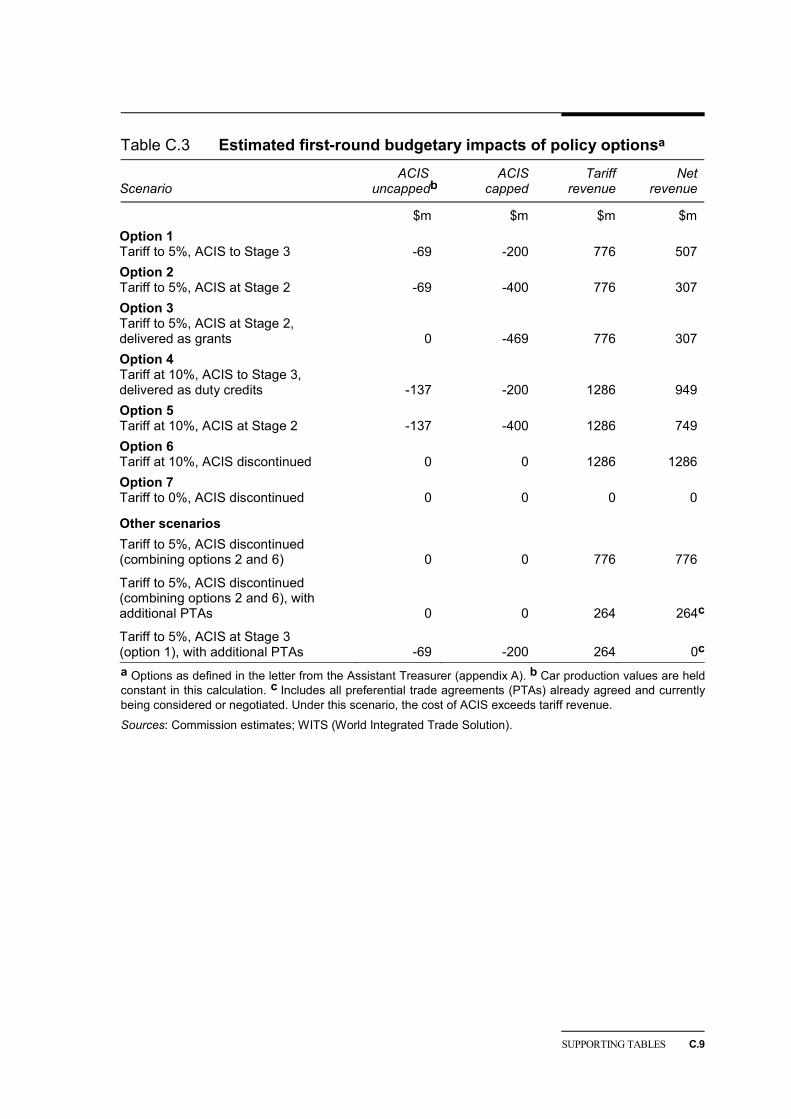
SUPPORTING TABLES C.9
Table C.3 Estimated first-round budgetary impacts of policy optionsa
Scenario ACIS uncappedb
ACIScapped
Tariff revenue
Netrevenue
$m $m $m $m Option 1 Tariff to 5%, ACIS to Stage 3 -69 -200 776 507 Option 2 Tariff to 5%, ACIS at Stage 2 -69 -400 776 307 Option 3 Tariff to 5%, ACIS at Stage 2, delivered as grants 0 -469 776 307 Option 4 Tariff at 10%, ACIS to Stage 3, delivered as duty credits -137 -200 1286 949 Option 5 Tariff at 10%, ACIS at Stage 2 -137 -400 1286 749 Option 6 Tariff at 10%, ACIS discontinued 0 0 1286 1286 Option 7 Tariff to 0%, ACIS discontinued 0 0 0 0
Other scenarios Tariff to 5%, ACIS discontinued (combining options 2 and 6) 0 0 776 776
Tariff to 5%, ACIS discontinued (combining options 2 and 6), with additional PTAs 0 0 264 264c
Tariff to 5%, ACIS at Stage 3 (option 1), with additional PTAs -69 -200 264 0c
a Options as defined in the letter from the Assistant Treasurer (appendix A). b Car production values are held constant in this calculation. c Includes all preferential trade agreements (PTAs) already agreed and currently being considered or negotiated. Under this scenario, the cost of ACIS exceeds tariff revenue.
Sources: Commission estimates; WITS (World Integrated Trade Solution).

DATABASE MODIFICATIONS
D.1
D Database modifications
In this appendix, the processes involved in updating the base year of the database, disaggregating the motor vehicle and parts industry, and incorporating ACIS in the model are described.
D.1 Updating the base year
The database was updated from 2001-02 to 2005-06 in four steps, to suit the MMRF model (figure D.1).
1. The 2001-02 ABS national input–output table for 109 industries was converted to a 172-sector database to be consistent with a simple general equilibrium (GE) model of the Australian economy (ORANI). This produced a national database with a structure that is broadly consistent with that of the regional database used in the MMRF model.
2. Industry value-added and trade flows were updated to 2005-06 using ABS national accounts and trade data.
3. The updated national database was disaggregated to 59 statistical-divisions, to form what is known as TERM. This was done using:
– 2006 Census data on employment by industry, to define the size of the 172 industries in each statistical division
– population size, to estimate household consumption per statistical division
– ABS 2002 Household Expenditure Survey data on regional consumption levels
– trade data from 49 ports to estimate international trade flows in and out of each statistical division.
4. The number of regions and industries in the TERM database was then aggregated to the State/Territory level to generate the eight-region MMRF database, with 58 industries (further details are found in Horridge et al. (2005)).
The resultant concordance of input–output and MMRF industries is shown in table D.1.

D.2 MODELLING AUTOMOTIVE ASSISTANCE
Figure D.1 Stages in updating an MMRF database to 2005-06
Stage Regions Industries
ABS 2001 1 109
manufacturing, agriculture and service industries disaggregated
ORANI G 1 172
no change
2005-2006 1 172
statistical division mining and services aggregated
TERM 59 144
State and Territories sectors aggregated
MMRF 8 58
Data source: Glyn Wittwer, Centre of Policy Studies, Monash University, pers. comm., 8 May 2008.

DATABASE MODIFICATIONS
D.3
Table D.1 Concordance — 2001-02 ABS national input–output and MMRF industries
Input–Output Description MMRF industry
0101 Sheep Sheep cattle 0102 Grains Grains 0103 Beef cattle Sheep cattle 0104 Dairy cattle Dairy 0105 Pigs Other animals 0106 Poultry Other animals 0107 Other agriculture Other agriculture 0200 Services to agriculture, hunting and trapping Fishing and services to agriculture0300 Forestry and logging Forestry 0400 Commercial fishing Fishing and services to agriculture1101 Coal Coal 1201 Oil and gas Oil, gas 1301 Iron ores Iron ore 1302 Non-ferrous metal ores Non iron ore 1400 Other mining Other mining 1500 Services to mining Other mining 2101 Meat and meat products Meat products 2102 Dairy products Other food 2103 Fruit and vegetable products Other food 2104 Oils and fats Other food 2105 Flour mill products and cereal foods Other food 2106 Bakery products Other food 2107 Confectionery Other food 2108 Other food products Other food 2109 Soft drinks, cordials and syrups Other food 2110 Beer and malt Other food 2113 Wine, spirits and tobacco products Other food 2201 Textile fibres, yarns and woven fabrics Textile, clothing and footwear 2202 Textile products Textile, clothing and footwear 2203 Knitting mill products Textile, clothing and footwear 2204 Clothing Textile, clothing and footwear 2205 Footwear Textile, clothing and footwear 2206 Leather and leather products Textile, clothing and footwear 2301 Sawmill products Wood products 2302 Other wood products Wood products 2303 Pulp, paper and paperboard Paper products 2304 Paper containers and products Paper products 2401 Printing and services to printing Printing 2402 Publishing, recorded media, etc. Printing 2501 Petroleum and coal products Gasoline, diesel, LPG, air fuel,
other fuel 2502 Basic chemicals Chemicals 2503 Paints Chemicals
(Continued next page)

D.4 MODELLING AUTOMOTIVE ASSISTANCE
Table D.1 (continued)
Input–Output Description MMRF industry 2504 Medicinal and pharmaceutical products,
pesticides Chemicals
2505 Soap and detergents Chemicals 2506 Cosmetics and toiletry preparations Chemicals 2507 Other chemical products Chemicals 2508 Rubber products Rubber and plastic 2509 Plastic products Rubber and plastic 2601 Glass and glass products Non-metallic minerals 2602 Ceramic products Non-metallic minerals 2603 Cement, lime and concrete slurry Cement 2604 Plaster and other concrete products Non-metallic minerals 2605 Other non-metallic mineral products Non-metallic minerals 2701 Iron and steel Steel 2702 Basic non-ferrous metal and products Alumina, aluminium, other metals 2703 Structural metal products Metal products 2704 Sheet metal products Metal products 2705 Fabricated metal products Metal products 2801 Motor vehicles and parts, other transport
equipment Motor vehicles and parts
2802 Ships and boats Other manufacturing 2803 Railway equipment Other manufacturing 2804 Aircraft Other manufacturing 2805 Photographic and scientific equipment Other manufacturing 2806 Electronic equipment Other manufacturing 2807 Household appliances Other manufacturing 2808 Other electrical equipment Other manufacturing 2809 Agricultural, mining, etc. machinery Other manufacturing 2810 Other machinery and equipment Other manufacturing 2901 Prefabricated buildings Other manufacturing 2902 Furniture Other manufacturing 2903 Other manufacturing Other manufacturing 3601 Electricity supply 3602 Gas supply Gas supply 3701 Water supply, sewerage and drainage services Water supply 4101 Residential building Construction 4102 Other construction Construction 4201 Construction trade services Construction 4501 Wholesale trade Trade 4502 Wholesale mechanical repairs Trade 4503 Other wholesale repairs Trade 5101 Retail trade Trade 5102 Retail mechanical repairs Trade 5103 Other retail repairs Trade 5701 Accommodation, cafes and restaurants Accommodation hotels 6101 Road transport Road transport
(Continued next page)

DATABASE MODIFICATIONS
D.5
Table D.1 (continued)
Input–Output Description MMRF industry
6201 Rail, pipeline and other transport Road freight 6301 Water transport Water transport 6401 Air and space transport Air transport 6401 Air and space transport Air transport 6601 Services to transport, storage Water transport 7101 Communication services Communication 7301 Banking Financial services 7302 Non-bank finance Financial services 7401 Insurance Financial services 7501 Services to finance, investment and insurance Financial services 7701 Ownership of dwellings Dwelling 7702 Other property services Business services 7801 Scientific research, technical and computer
services Business services
7802 Legal, accounting, marketing and business management services
Business services
7803 Other business services Business services 8101 Government administration Public services 8201 Defence Public services 8401 Education Public services 8601 Health services Public services 8701 Community services Public services 9101 Motion picture, radio and television services Other services 9201 Libraries, museums and the arts Other services 9301 Sport, gambling and recreational services Other services 9501 Personal services Other services 9601 Other services Other services
Source: MMRF database.
D.2 Disaggregating the automotive industry
The ABS categorises all industries into Input–Output Industry Groups (IOIGs) which can be linked (via the IOIG-ANZSIC (Australian and New Zealand Standard Industrial Classification) concordance) to a corresponding list of the products primarily produced by these industries, referred to as Input–Output Product Classification (IOPC) codes. These IOPCs form the basis for disaggregating the motor vehicle and parts industry in the MMRF database. ABS release 5215.0.55.001 (ABS 2006) provides detailed input-output information on the allocation of the supply of all IOPCs across all industry and final users in the economy.
The first step in the disaggregation was to examine the tariff rate imposed on each

D.6 MODELLING AUTOMOTIVE ASSISTANCE
IOPC relevant to the motor vehicle and parts industry. This was done via a concordance between the IOPCs, and the Harmonized System (HS) codes used by the Australian Customs Service in assigning tariffs to commodities. The car assembly and car components industry was defined to be all commodities that are subject to the 10 per cent Most-Favoured Nation (MFN) automotive tariff rate. All those commodities not subject to a 10 per cent tariff were defined as ‘other’.
Because the IOPC-HS concordance links a single IOPC to several HS commodities, in some cases a number of different tariff rates were connected to a single IOPC. In these cases, additional trade volume data were used to discern whether most of a commodity’s trade was subject to a 10 per cent tariff. If this was the case, the commodity was defined to be part of the car assembly and car component sector.
Car assembly and car components were then separated from each other, with ‘car assembly’ taken to be represented by the IOPC 28110010 (‘Finished motor vehicles with less than 10 persons capacity’), and the remainder defined as ‘components’. Table D.2 sets out the resulting disaggregation of motor vehicle and parts-related IOPCs into ‘assembly’, ‘components’ and ‘other’, and their concordance with HS commodities.
This sectoral split was then used to disaggregate demand in the MMRF database by intermediate industry users and final users (represented by the rows in the MMRF input–output tables) into the demand for ‘others’ and for ‘car assembly and components’. Except for trade variables, this was done using the national shares of supply of the relevant groups of IOPCs to each user from the ABS input–output product details, applied uniformly across all jurisdictions.1 Having specified shares for each component of the row in the MMRF database, the total sales split was then calculated as the weighted average share across all users.
1 For export and import shares, trade data by jurisdiction and commodity, at a HS 6-digit level,
were obtained from the ABS (unpublished data), and concorded with IOPCs. For other elements in the row for which no ABS shares were available, for example. inventories, the national total supply shares were used.

DATABASE MODIFICATIONS
D.7
Table D.2 Concordance — IOPC–HSa Sectorb IOPCs IOPC description HS6 codes
Cars 28110010 Finished motor vehicles with less than 10 persons capacity
870321, 870322, 870323, 870324, 870331, 870332, 870333, 870390
Components 28110071 Cranks, crank & cam shafts, gears and flywheels
848310, 848320, 848330, 848340, 848350, 848390
28130012 Motor vehicle and truck air conditioners 841520
28130014 Motor vehicle or motor cycle wiring
harnesses 854430
28130015 Motor vehicle starting, heaters, demisters, windscreen wipers; lighting/signalling equipment
851110, 851120, 851130, 851140, 851150, 851180, 851190, 851220, 851230, 851240, 851290
28190010 Motor vehicle transmission assemblies (excl associated with the manufacture of complete vehicles/engines)
870829, 870840, 870850, 870860, 870880, 870891, 870892, 870893, 870894, 870895, 870899
28190021 Cylinder blocks, pistons, connecting rods, valves (excl associated with the manufacture of complete vehicles/engines)
840991, 840999, 870829, 870840, 870850, 870880, 870891, 870892, 870894, 870895, 870899
28190022 Fuel, lubricating or cooling medium pumps (excl associated with the manufacture of complete vehicles or engines)
841330, 870829, 870840, 870850, 870880, 870891, 870892, 870894, 870895, 870899
28190023 Cranks, cam shafts, gears and flywheels (excl associated with the manufacture of complete vehicles/engines)
848310, 848320, 848330, 848340, 848350, 848360, 848390, 870829, 870840, 870850, 870880, 870891, 870892, 870894, 870895, 870899
28190024 Motor vehicle, tractor and truck gaskets (excl associated with the manufacture of complete vehicles or engines)
848410, 848490
28190025 Motor vehicle parts and equipment nec (excl associated with motor vehicle manufacturing)
840991, 840999, 848420, 870810, 870821, 870829, 870830, 870831, 870839, 870840, 870850, 870870, 870880, 870891, 870892, 870894, 870895, 870899
28190026 Motor vehicle body panels 870829
28299998 Unassembled motor vehicles nec na
Others 28110020 Finished motor vehicles with 10 or more person capacity
870210, 870290
28110030 Finished trucks, truck type vehicles,
utilities and panel vans 870421, 870422, 870423, 870431, 870432, 870490, 870510, 870520, 870530, 870540, 870590
28110060 Engines nec, for motor vehicles or tractors 840731, 840732, 840733, 840734,
840790, 840820
28110072 Motor vehicle, tractor and truck gaskets (associated with the manufacture of complete vehicles or engines)
848410, 848490
28110073
Motor vehicle, tractor & cycle parts nec (associated with the manufacture of complete vehicles & engines)
848420, 870810, 870821, 870899
(Continued next page)

D.8 MODELLING AUTOMOTIVE ASSISTANCE
Table D.2 (continued)
Sectorb IOPCs IOPC description HS6 codes
Others
28119010 Second hand motor vehicles 870321, 870322, 870323, 870324, 870331, 870332, 870333, 870390, 870431
28120011 Motor vehicle and truck bodies (coachwork) 870710, 870790
28120031 Agricultural self loading and unloading semi-
trailers (incl tippers) 871620
28120032 Other semi-trailers for the transport of goods & materials (incl tankers, vans, transporters, stock crates & jinkers)
870432, 871620, 871631, 871639
28120041 Trailers for the transport of goods and materials (incl box trailers, boat trailers and horse floats)
871631, 871639
28120042 Other trailers & semi-trailers nec (excl for the transport of goods & materials, & domestic type camper trailers)
871640
28120050 Body panels for trucks and buses 870829
28120060 Parts nec, for motor vehicle trailers and
semi-trailers 871690
28130013 Motor vehicle apparatus for making, breaking, protecting & making connections to/in electrical circuits (excl wiring)
853610, 853620, 853630
28130016 Motor vehicle, tractor and motor cycle
filament lamps and sealed beam lamps 853910, 853922, 853929
28130017 Motor vehicle & tractor gauges, revolution & production counters, speed indicators, thermostats & similar instruments
902519, 902610, 902620, 902680, 902910, 902920, 903033, 903039, 903210, 903281, 903289
28290010 Transport equipment, parts and accessories nec
870310, 871200, 871310, 871390, 871411, 871419, 871420, 871491, 871492, 871493, 871494, 871495, 871496, 871499, 871500, 871680
28298000 Motor scooters and motor cycles 871110, 871120, 871130, 871140,
871150, 871190
28291810 Royalties income and licence fees (2811-
2819, 2829) na
28291900 Repairing and servicing (2811-2819, 2829) na
28291920 Other income (2811-2819, 2829) na
28291950 Increase in stocks - work-in-progress (2811-
2819, 2829) na
a IOPC refers to Input–Output Product Classification codes. HS refers to the Harmonised System of product classification, presented here at the 6-digit-level of disaggregation. b These refer to the sectors as defined by the Commission for the purposes of disaggregating the MMRF database. nec not elsewhere classified. na not applicable.
To disaggregate the industry cost data (the columns of the MMRF database):
• the shares of total sales were imposed on total production costs (because total costs must equal total sales for the database to be balanced)
• capital and labour cost shares were estimated from ABS data on each industry’s

DATABASE MODIFICATIONS
D.9
value-added and wage costs in each jurisdiction (ABS 2005a-f, unpublished data).
• value-added was subtracted from total production costs for each industry in each jurisdiction, to obtain cost shares for the remaining inputs. As was suggested by the workshop referees (appendix B), the calculated cost structures were then compared to ABS data to check how well these corresponded (ABS 2005a-f, unpublished data).
The same procedure for splitting the rows and columns of the database was used to separate ‘car assembly’ from ‘car components’. This stage also involved:
• imposing a value of zero on the costs and sales of car assembly in all jurisdictions except Victoria and South Australia, as shown in Table 3.2
• setting the share of car assembly and components for both Victoria and South Australia equal to that calculated from ABS data on state production shares (ABS 2005b, ABS 2005d).
Four checks were performed to ensure the database was structurally sound before the modelling was undertaken.
• A basic accounting requirement is that total sales (the sum of the row elements) is equal to total production (the sum of the column elements).
– These figures for each sector were compared to ensure total sales equalled total costs.
• The diagonal element in intermediate demand — which refers to the respective value of cars and of components used in the production of cars and of components — was examined.
– As expected, the value of cars used in components was zero, with the value of components used in cars being the highest value.
• The tariff rates implicit in the tariff revenue matrix conformed to the trade-weighted average tariff rates which have been adjusted to take into account the impact of ACIS import duty credits on tariff revenue collected.
• The results of the disaggregation of the MMRF database were also compared with the 2001-02 ABS input–output product details (ABS 2006) as well as more recent data (2005-06) on production (ABS 2007).
D.3 Incorporating ACIS
The process for allocating ACIS capped and uncapped credits across jurisdictions and for incorporating these in the database is described below.

D.10 MODELLING AUTOMOTIVE ASSISTANCE
Allocating capped credits
In this study, it has been assumed that the total capped credits for Stage 2 are spread evenly across its five years — that is, $400 million in credits are distributed annually. The allocation has been undertaken in the following way.
• Consistent with the modulation process outlined in chapter 2, and because car assembly only occurs in Victoria and South Australia, the 55 per cent allocated to vehicle assemblers has been split across these two States, based on the estimates of total costs derived from the MMRF database.
• The remaining 45 per cent of capped funding was split according to each jurisdiction’s share of component production costs.
This process is consistent with the idea that the majority of capped ACIS funding is allocated according to production values. This process produces an average rate of subsidy for each sector, without recognising any disparities that might exist among firms within the sector.
Allocating uncapped credits
Given the total estimated ACIS funding of $537 million (chapter 2), after accounting for the $400 million in capped credits, $137 million in uncapped credits remain. These credits were allocated between Victoria and South Australia according to the estimates of production costs derived from the MMRF database.
The estimated shares of capped and uncapped ACIS funding allocated to car assembly and component manufacturing are consistent with the actual average distribution between 2005 and 2007, as reported by AusIndustry (table D.3).
Table D.3 Share of total ACIS funding by sector PC Distributiona AusIndustryb
Uncapped Capped Total Total
% % % % Car assembly 25 41 67 62 Components 0 34 33 36 a Although tool producers and service providers are entitled to receive ACIS, the proportion they are allocated is very small. Therefore, for modelling purposes, their allocation was assumed to be zero. Also, due to the nature of the MMRF industry split between cars and components, several component producers which are currently captured in ‘others’ have had their ACIS entitlements allocated to ‘components’ in the modelling. b This is the average split across car assembly and component manufacturers over the three years from 2005 to 2007. The shares do not sum to 100, as they exclude the proportion allocated to tool producers and service providers.
Sources: AusIndustry (unpublished data); Commission estimates.

DATABASE MODIFICATIONS
D.11
How ACIS was included in the database
ACIS-inclusive tariff rates (chapter 3) were used to derive the implicit import duties that should have been paid by the car assembly and components sectors under the normal tariff system. Since neither sector imports cars as intermediate inputs, the imputed import duties are paid exclusively on imported car parts.
• The uncapped ACIS value ($137 million) for the car assembly industry was modelled as a negative federal indirect tax on imports, and allocated according to the regional cost of car production. These subsidies are used to offset directly the import duties paid by the car industries in Victoria and South Australia.
• Capped ACIS funding was treated as a production subsidy (allocated across jurisdictions as outlined above), and included in the database as negative federal taxes on Other Cost Tickets (OCTS).
As the federal tax (OTXF) is included in OCTS in the database, the values of OCTS for car assembly and components industries had to be adjusted to maintain the original total cost values for the industries.
The total imputed import duties that should have been paid by the car assembly and components sectors are estimated to be $240 million, compared with actual industry receipts of $537 million. The surplus was assumed to have been sold by the industries to other importers of cars and components for capital investment (BAS2) and for final consumption (BAS3). Therefore, the corresponding import values in BAS2 and BAS3 needed to be adjusted to reflect the purchases of $297 million of ACIS credits from the assembly and components sectors.

ADDITIONAL SIMULATION RESULTS
E.1
E Additional simulation results
Reference cases
Table E.1 Simulation results — automotive industry, Victoria Percentage changes relative to the database
Scenario R1 R2 R3 R4
Tariffa to 5% to 5% 10% to 5%ACIS to 0 Stage 2 to 0 to 0Other settings Open economy
Automotive assembly Output -4.74 -3.19 -1.56 -4.70Employment -5.64 -3.83 -1.84 -5.55Domestic sales from domestic production -5.03
-3.89
-1.16
-5.00
Domestic sales — total -0.29 -0.17 -0.12 -0.28Export volume -2.86 1.26 -4.08 -2.77Import volume 4.36 3.72 0.63 4.33
Component manufacturing Output -1.73 -1.52 -0.21 -1.69Employment -2.08 -1.85 -0.22 -1.99Domestic sales from domestic production -2.23
-2.03
-0.21
-2.20
Domestic sales — total -0.29 -0.17 -0.12 -0.28Export volume 4.25 4.48 -0.22 4.37Import volume -1.31 -0.57 -0.75 -1.30a ‘to 5%’ means reducing automotive tariffs from 10% to 5%.

E.2 MODELLING AUTOMOTIVE ASSISTANCE
Table E.2 Simulation results — automotive industry, South Australia Percentage changes relative to the database
Scenario R1 R2 R3 R4
Tariffa to 5% to 5% 10% to 5%ACIS to 0 Stage 2 to 0 to 0Other settings Open economy
Automotive assembly Output -4.21 -2.19 -2.02 -4.16Employment -5.01 -2.64 -2.38 -4.91Domestic sales from domestic production -5.01
-4.08
-0.94
-4.98
Domestic sales — total -0.24 -0.07 -0.16 -0.23Export volume -2.86 1.02 -3.85 -2.77Import volume 4.39 3.83 0.55 4.36
Component manufacturing Output -1.66 -1.40 -0.26 -1.63Employment -2.03 -1.75 -0.28 -1.95Domestic sales from domestic production -1.90
-1.63
-0.26
-1.87
Domestic sales — total -0.24 -0.07 -0.16 -0.23Export volume 4.82 4.84 -0.02 4.93Import volume -1.27 -0.20 -1.08 -1.25a ‘to 5%’ means reducing automotive tariffs from 10% to 5%.

ADDITIONAL SIMULATION RESULTS
E.3
Table E.3 Simulation results — component manufacturing industry Percentage changes relative to the database
Scenario R1 R2 R3 R4
Tariffa to 5% to 5% 10% to 5%ACIS to 0 Stage 2 to 0 to 0Other settings Open economy
New South Wales Output -1.09 -0.87 -0.22 -1.09Employment -1.37 -1.11 -0.26 -1.32Domestic sales from domestic production -1.16
-0.95
-0.21
-1.16
Domestic sales — total 0.10 0.08 0.02 0.07Export volume 3.07 3.88 -0.78 3.08Import volume 4.98 4.85 0.12 4.97
Queensland Output -0.96 -0.76 -0.20 -1.03Employment -1.23 -0.99 -0.25 -1.25Domestic sales from domestic production -1.04
-0.84
-0.19
-1.10
Domestic sales — total 0.19 0.13 0.06 0.09Export volume 3.24 4.05 -0.78 3.15Import volume 4.88 4.72 0.16 4.81a ‘to 5%’ means reducing automotive tariffs from 10% to 5%.

E.4 MODELLING AUTOMOTIVE ASSISTANCE
Review options
Table E.4 Simulation results — automotive industry Percentage changes relative to the database
Scenario O1 O3 O4 O7 O8
Tariffa to 5% to 5% 10% to 0 to 5%ACIS Stage 3 Stage 2 Stage 3 to 0 Stage 3Other settings ACIS as
grants Commodity
price increase
Automotive assembly Output -3.44 -1.58 -0.51 -8.52 -11.18Employment -4.11 -1.91 -0.61 -10.14 -13.07Domestic sales from domestic production -4.27
-3.06
-0.34
-10.85
-6.86
Domestic sales — total 0.04 0.04 0.00 0.11 1.06Export volume -0.10 4.44 -1.23 0.97 -28.74Import volume 3.33 2.69 0.18 8.74 9.01
Component manufacturing Output -1.20 -1.65 -0.05 -3.12 -3.72Employment -1.59 -2.22 -0.06 -4.13 -6.57Domestic sales from domestic production -1.45
-1.93
-0.05
-3.76
-2.76
Domestic sales — total 0.04 0.04 0.00 0.11 1.06Export volume 4.43 4.86 0.00 11.77 -25.68Import volume 1.43 3.21 -0.16 3.76 2.88a ‘to 5%’ means reducing automotive tariffs from 10% to 5%.
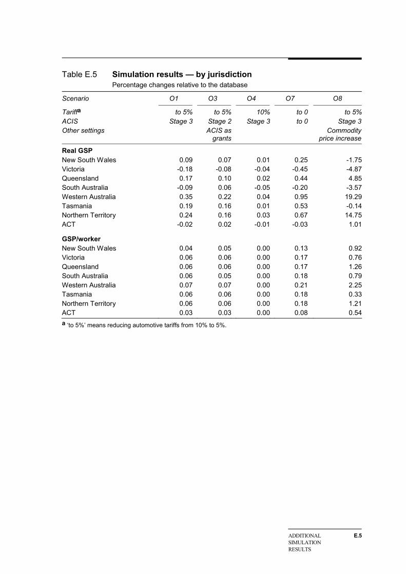
ADDITIONAL SIMULATION RESULTS
E.5
Table E.5 Simulation results — by jurisdiction Percentage changes relative to the database
Scenario O1 O3 O4 O7 O8
Tariffa to 5% to 5% 10% to 0 to 5%ACIS Stage 3 Stage 2 Stage 3 to 0 Stage 3Other settings ACIS as
grants Commodity
price increase
Real GSP New South Wales 0.09 0.07 0.01 0.25 -1.75Victoria -0.18 -0.08 -0.04 -0.45 -4.87Queensland 0.17 0.10 0.02 0.44 4.85South Australia -0.09 0.06 -0.05 -0.20 -3.57Western Australia 0.35 0.22 0.04 0.95 19.29Tasmania 0.19 0.16 0.01 0.53 -0.14Northern Territory 0.24 0.16 0.03 0.67 14.75ACT -0.02 0.02 -0.01 -0.03 1.01
GSP/worker New South Wales 0.04 0.05 0.00 0.13 0.92Victoria 0.06 0.06 0.00 0.17 0.76Queensland 0.06 0.06 0.00 0.17 1.26South Australia 0.06 0.05 0.00 0.18 0.79Western Australia 0.07 0.07 0.00 0.21 2.25Tasmania 0.06 0.06 0.00 0.18 0.33Northern Territory 0.06 0.06 0.00 0.18 1.21ACT 0.03 0.03 0.00 0.08 0.54a ‘to 5%’ means reducing automotive tariffs from 10% to 5%.

E.6 MODELLING AUTOMOTIVE ASSISTANCE
Table E.6 Simulation results — automotive industry, Victoria Percentage changes relative to the database
Scenario O1 O3 O4 O7 O8
Tariffa to 5% to 5% 10% to 0 to 5%ACIS Stage 3 Stage 2 Stage 3 to 0 Stage 3Other settings ACIS as
grants Commodity
price increase
Automotive assembly Output -3.66 -1.95 -0.48 -9.12 -10.62Employment -4.38 -2.37 -0.56 -10.90 -12.33Domestic sales from domestic production -4.24
-3.00
-0.35
-10.77
-7.47
Domestic sales — total -0.20 -0.10 -0.04 -0.51 -4.31Export volume -0.02 4.64 -1.26 1.24 -30.50Import volume 3.92 3.19 0.19 10.34 5.57
Component manufacturing Output -1.58 -2.34 -0.06 -4.10 -9.98Employment -1.92 -2.84 -0.06 -4.99 -11.63Domestic sales from domestic production -2.09
-2.95
-0.07
-5.46
-8.57
Domestic sales — total -0.20 -0.10 -0.04 -0.51 -4.31Export volume 4.50 5.02 0.01 12.04 -26.66Import volume -0.81 2.05 -0.25 -1.58 -3.63a ‘to 5%’ means reducing automotive tariffs from 10% to 5%.

ADDITIONAL SIMULATION RESULTS
E.7
Table E.7 Simulation results — automotive industry, South Australia Percentage changes relative to the database
Scenario O1 O3 O4 O7 O8
Tariffa to 5% to 5% 10% to 0 to 5%ACIS Stage 3 Stage 2 Stage 3 to 0 Stage 3Other settings ACIS as
grants Commodity
price increase
Automotive assembly Output -2.81 -0.52 -0.62 -6.76 -12.79Employment -3.37 -0.68 -0.73 -8.12 -15.02Domestic sales from domestic production -4.36
-3.33
-0.28
-11.16
-4.45
Domestic sales — total -0.12 0.04 -0.05 -0.28 -3.07Export volume -0.18 4.23 -1.18 0.69 -26.87Import volume 4.00 3.37 0.17 10.61 5.82
Component manufacturing Output -1.49 -2.31 -0.08 -3.90 -8.25Employment -1.84 -2.87 -0.09 -4.85 -9.91Domestic sales from domestic production -1.72
-2.60
-0.09
-4.53
-7.67
Domestic sales — total -0.12 0.04 -0.05 -0.28 -3.07Export volume 4.91 5.54 0.07 13.28 -24.05Import volume -0.55 2.87 -0.35 -0.73 -4.84a ‘to 5%’ means reducing automotive tariffs from 10% to 5%.
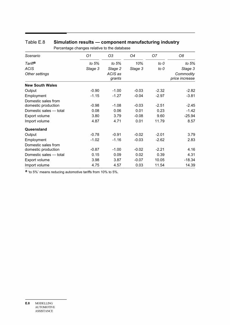
E.8 MODELLING AUTOMOTIVE ASSISTANCE
Table E.8 Simulation results — component manufacturing industry Percentage changes relative to the database
Scenario O1 O3 O4 O7 O8
Tariffa to 5% to 5% 10% to 0 to 5%ACIS Stage 3 Stage 2 Stage 3 to 0 Stage 3 Other settings ACIS as
grants Commodity
price increase
New South Wales Output -0.90 -1.00 -0.03 -2.32 -2.82Employment -1.15 -1.27 -0.04 -2.97 -3.81Domestic sales from domestic production -0.98
-1.08
-0.03
-2.51
-2.45
Domestic sales — total 0.08 0.06 0.01 0.23 -1.42Export volume 3.80 3.79 -0.08 9.60 -25.94Import volume 4.87 4.71 0.01 11.79 8.57
Queensland Output -0.78 -0.91 -0.02 -2.01 3.79Employment -1.02 -1.16 -0.03 -2.62 2.83Domestic sales from domestic production -0.87
-1.00
-0.02
-2.21
4.16
Domestic sales — total 0.15 0.09 0.02 0.39 4.31Export volume 3.98 3.87 -0.07 10.05 -18.34Import volume 4.75 4.57 0.03 11.54 14.39a ‘to 5%’ means reducing automotive tariffs from 10% to 5%.

ADDITIONAL SIMULATION RESULTS
E.9
Sensitivity analyses
Table E.9 Simulation results — automotive industry Percentage changes relative to the database
Scenario S1 S2 S3 S4 S5
Tariffa to 0% to 5% to 5% to 5% to 5%ACIS to 0 to 0 to 0 to 0 to 0Other settings General
tariff to 0%
Exportelasticity
of 5
Endogenous
budget
Rate of return
closure
Shortrun
closure
Automotive assembly Output -8.36 -4.27 -4.64 -4.54 -3.29Employment -10.04 -5.07 -5.52 -5.36 -5.17Domestic sales from domestic production -10.72
-5.00
-4.97
-5.05
-4.26
Domestic sales — total 0.22 0.02 0.06 -0.03 -0.03Export volume 1.24 -1.31 -3.30 -2.50 0.65Import volume 8.82 3.68 3.83 3.60 3.13
Component manufacturing Output -2.94 -1.47 -1.39 -1.37 -1.05Employment -4.07 -1.88 -1.80 -1.72 -1.66Domestic sales from domestic production -3.58
-1.63
-1.60
-1.63
-1.37
Domestic — total 0.22 0.02 0.06 -0.03 -0.03Export volume 12.02 2.30 3.65 4.50 6.26Import volume 3.77 1.23 1.20 1.09 1.20a ‘to 5%’ means reducing automotive tariffs from 10% to 5%.

E.10 MODELLING AUTOMOTIVE ASSISTANCE
Table E.10 Simulation results — by jurisdiction Percentage changes relative to the database
Scenario S1 S2 S3 S4 S5
Tariffa to 0% to 5% to 5% to 5% to 5%ACIS to 0 to 0 to 0 to 0 to 0 Other settings General
tariff to 0%
Exportelasticity
of 5
Endogenousbudget
Rate of return
closure
Short run
closure
Real GSP New South Wales 0.25 0.10 0.17 0.05 0.00Victoria -0.51 -0.23 -0.22 -0.28 0.00Queensland 0.68 0.21 0.21 0.14 0.00South Australia -0.28 -0.16 -0.17 -0.21 0.00Western Australia 1.63 0.37 0.24 0.42 0.00Tasmania 0.75 0.18 0.23 0.15 0.00Northern Territory 1.39 0.25 0.25 0.28 0.00ACT -0.01 -0.05 0.10 -0.15 0.00
GSP/worker
New South Wales 0.22 0.03 0.05 -0.01 0.00Victoria 0.26 0.05 0.07 0.01 0.00Queensland 0.30 0.05 0.06 0.01 0.00South Australia 0.28 0.06 0.08 0.03 0.00Western Australia 0.37 0.06 0.06 0.02 0.00Tasmania 0.29 0.05 0.06 0.02 0.00Northern Territory 0.35 0.05 0.06 0.02 0.00ACT 0.13 0.02 0.05 -0.03 0.00a ‘to 5%’ means reducing automotive tariffs from 10% to 5%.

REFERENCES R.1
References
Abayasiri-Silva, K. and Horridge, M. 1996, Economies of Scale and Imperfect Competition in an Applied General Equilibrium Model of the Australian Economy, Working Paper no. OP-84, , Centre of Policy Studies (CoPS), Monash University, IMPACT Centre, Melbourne.
ABARE (Australian Bureau of Agricultural and Resource Economics) 2007, Australian Commodity statistics 2007, Project no. 1059, Canberra.
ABS (Australian Bureau of Statistics) 2000, Australian National Accounts: Concepts, Sources and Methods, Cat. no. 5216.0, Canberra.
—— 2005a, Manufacturing Industry, New South Wales, 2001-02, Cat. no. 8221.1.55.001, Canberra.
—— 2005b, Manufacturing Industry, Victoria, 2001-02, Cat. no. 8221.2.55.001, Canberra.
—— 2005c, Manufacturing Industry, Queensland, 2001-02, Cat. no. 8221.3.55.001, Canberra.
—— 2005d, Manufacturing Industry, South Australia, 2001-02, Cat. no. 8221.4.55.001, Canberra.
—— 2005e, Manufacturing Industry, Western Australia, 2001-02, Cat. no. 8221.5.55.001, Canberra.
—— 2005f, Manufacturing Industry, Tasmania, 2001-02, Cat. no. 8221.6.55.001, Canberra.
—— 2005g, Year Book Australia, 2005, Cat. no. 1301.0, Canberra.
—— 2006, Australian National Accounts: Input-Output Tables – Electronic Publication 2001—02, Cat. no. 5209.0.55.001, Canberra.
—— 2007a, Manufacturing Industry, Australia, 2005-06, Cat. no. 8221.0, Canberra.
—— 2007b, Australian Labour Market Statistics, Jul 2007, Cat. no. 6105.0, Canberra.
—— 2007c, International Trade in Goods and Services, Australia, Jun 2007, Cat. no. 5368.0, Canberra.

R.2 MODELLING AUTOMOTIVE ASSISTANCE
—— 2007d, Australian System of National Accounts, 2006-07, Cat. no. 5204.0, Canberra.
—— 2008a, Australian National Accounts: Input-Output Tables – Electronic Publication, 2004-05 (Preliminary), Cat. no. 5209.0.55.001, Canberra.
—— 2008b, Balance of Payments and International Investment Position, Australia, Dec 2007, Cat. no. 5302.0, Canberra.
Adams, P.D., Horridge, M. and Wittwer, G. 2002, A Dynamic Multi-Regional Applied General Equilibrium Model of the Australian Economy, Draft documentation prepared for the Regional GE Modelling Course, Centre of Policy Studies, Monash University, 25-29 November.
ATO (Australian Taxation Office) 2008, Fringe benefits tax (FBT) rates and thresholds: car fringe benefits statutory formula, http://www.ato.gov.au/ businesses/content.asp?doc=/content/76140.htm&page=4&H4 (accessed 29 April 2008).
—— 2008a, Guide for taxpayers with luxury cars, Luxury car tax, How to meet your luxury car tax (LCT) obligations, http://www.ato.gov.au/content/ downloads/bus13288nat3394022008.pdf (accessed 16 May 2008).
AusIndustry 2008a, Automotive Competitiveness and Investment Scheme (ACIS) — Fact Sheet, http://www.ausindustry.gov.au/library/FactSheetACISUpdatedMar2 00620060324123702.pdf (accessed 18 April 2008).
—— 2008b, Fact Sheet: ACIS Duty Credits – Changes to the Method of Modulation in ACIS Stage 2, http://www.ausindustry.gov.au/library/FactSheet ChangesToModulationUpdatedNov200620061103053255.pdf (accessed 18 April 2008).
Australian Government 2007a, Global Integration: Changing Markets, New Opportunities, Industry Statement, Department of Industry, Tourism and Resources, Canberra.
—— 2007b, New elements of the R&D Tax Concession: Evaluation Report, Department of Industry, Tourism and Resources, Canberra.
—— 2008a, Green Vehicle Guide, http://www.greenvehicleguide.gov.au/ GVGPublicUI/ApplicationFirstStartTaskWebForm.aspx (accessed 18 April 2008).
—— 2008b, Budget Overview, 13 May 2008, http://www.budget.gov.au/2008-09/ content/overview/download/Budget_Overview.pdf (accessed 14 May 2008).
Australian Treasury 2007, Tax Expenditures Statement 2007, Canberra, http://www. treasury.gov.au/documents/1333/PDF/TES_2007_Combined.pdf (accessed 26 May 2008).

REFERENCES R.3
AutoCRC (Cooperative Research Centre for Advanced Automotive Technology) 2008, About AutoCRC, http://www.autocrc.com/about-autocrc.htm (accessed 23 May 2008).
Bracks (Committee to Review of Australia’s Automotive Industry) 2008a, Review of Australia’s Automotive Industry 2008: Background Paper, March.
—— 2008b, Review of Australia’s Automotive Industry 2008: Discussion Paper, March.
Caddy, V. 1976, Empirical Estimation of the Elasticity of Substitution: A Review, Preliminary Working Paper no. OP-09, Industries Assistance Commission, Melbourne.
Carr, K. (Shadow Minister for Industry, Innovation, Science and Research) 2007, An innovation future for Australian industry, Canberra.
Carr, K. (Minister for Innovation, Industry, Science and Research) 2008a, Government announces review of national innovation system, Media release, 22 January.
—— 2008b, Terms of Reference for the Review of the National Innovation System, 30 January, Canberra.
—— 2008c, Government announces review of automotive industry, Media release, 14 February.
—— 2008d, Greening the supply chain, Speech at General-Motors Holden, Port Melbourne, Victoria, 2 April.
Costello, P. (Treasurer) 2002, Response to Productivity Commission Report on Automotive Assistance, http://www.treasurer.gov.au/DisplayDocs.aspx?pageID= &doc=Publications/AutomotiveResponse.htm&min=phc (accessed 20 May 2008).
Crean, S. (Australian Minister for Trade) 2008, Australia and Chile conclude Free Trade Agreement, Media Release, 27 May, http://www.trademinister.gov.au/ releases/2008.sc_040.html (accessed 28 May 2008).
DFAT (Department of Foreign Affairs and Trade) 2007, Canada Country Brief — December 2007, http://www.dfat.gov.au/geo/canada/brief.html (accessed 15 May 2008).
DIISR (Department of Innovation, Industry, Science and Research) 1999, Key Automotive Statistics 1998, http://www.innovation.gov.au/Industry/Automotive/ Pages/AutomotiveIndustry.aspx (accessed 28 May 2008).
—— 2006, Key Automotive Statistics 2005, http://www.innovation.gov.au/Industry/ Automotive/Pages/AutomotiveIndustry.aspx (accessed 28 May 2008).

R.4 MODELLING AUTOMOTIVE ASSISTANCE
—— 2007, Key Automotive Statistics 2006, http://www.innovation.gov.au/Industry/ Automotive/Pages/AutomotiveIndustry.aspx (accessed 28 May 2008).
DITR (Department of Industry, Tourism and Resources) 2006, Submission to the Productivity Commission Study into Science and Innovation, http://www.pc.gov. au/_data/assets/pdf_file/0004/39775/subdr185.pdf (accessed 29 April 2008).
Dixon, P.B. 1978, ‘Economies of Scale, Commodity Disaggregation and the Costs of Protection’, Australian Economic Papers, vol. 17, no. 30, pp. 63–80.
Dixon, P., Parmenter, B.R., Sutton, J. and Vincent, D.P. 1997, ORANI: A multisectoral model of the Australian Economy, Amsterdam, Holland.
Dowling, J. 2008, ‘High road for Hilux’, The Sydney Morning Herald, 10 May, p. 5.
Econtech 2002, Economic Modelling of the Post-2005 Assistance Arrangements for the Automotive Manufacturing Sector, Canberra.
FAPM (Federation of Automotive Products Manufacturers) 2008, Introduction, http://www.fapm.com.au/site.php?id=6 (accessed 28 May 2008).
FCAI (Federal Chamber of Automotive Industries) 2007, Vehicle Sales: November 2007, at http://www.fcai.com.au/sales.php/2007/11/fuel.html (accessed 14 December 2007).
—— 2008a, Local Production Volumes, http://www.fcai.com.au/volumes (accessed 28 May 2008).
—— 2008b, 2007: a milestone year for motor vehicle sales, Media release, 7 January 2008, http://www.fcai.com.au/media/2008/01/00000152.html (accessed 29 April 2008).
Francois, J.F., McDonald, B. and Nordstrom, H. 1995, ‘Assessing the Uruguay Round’, in Martin, W. and Winters, L.A. (eds), The Uruguay Round and the Developing Economies, Discussion Paper no. 307, World Bank, Washington DC, pp. 117–214.
Gehlhar, M. 1997, ‘Historical analysis of growth and trade patterns in the Pacific Rim: An evaluation of the GTAP framework’, in Hertel, T. (ed), Global Trade Analysis: Modelling and Applications, Cambridge University Press, Cambridge, pp. 349–63.
Gordon, J. 2008, ‘Spring Street backs gas guzzlers in fleet extension’, The Age, 15 February.
Harris, R. G. (with the Assistance of Cox, D.) 1984, Trade, Industrial Policy, and Canadian Manufacturing, Ontario Economic Council, Toronto.
Hassall, D. 2008, Most Tonsley Park workers offered alternative jobs following innovative Job Expo, 28 March, http://www1.autotrader.com.au/mellor/mellor.

REFERENCES R.5
nsf/story/BAABC44CA08327A9CA25741A001A88E3?OpenDocument (accessed 7 May 2008).
Hertel, T. 1997 (ed.), Global Trade Analysis: Modelling and Applications, Cambridge University Press, Cambridge.
Hillberry, R., Anderson, M., Balistreri, E. and Fox, A. 2001, The Determinants of Armington Taste Parameters in CGE Models, or ‘Why You Love Canadian Vegetable Oil’, paper presented to Fourth Annual Conference on Global Economic Analysis, 27–29 June, Purdue University, West Lafayette.
HoR (House of Representatives Standing Committee on Employment, Workplace Relations and Workforce Participation) 2006, Shifting gears: employment in the automotive components manufacturing industry, December, Canberra.
Horridge, M. 1987, Increasing Returns to Scale and the Long Run Effects of a Tariff Reform, Preliminary Working Paper no. OP-62, Impact Research Centre, University of Melbourne.
Horridge, M., Madden, J. and Wittwer, G. 2005, ‘Using a highly disaggregated multi-regional single-country model to analyse the impacts of the 2002-03 drought on Australia’, Journal of Policy Modelling, vol. 27, no. 3, pp. 285–308.
Howard, J. (Prime Minister) 2006, Assistance to Ford Australia, Media Release, 5 May.
IAC (Industries Assistance Commission) 1974, Passenger motor vehicles, etc., Report no. 21, Canberra.
—— 1981, Passenger Motor Vehicles And Components — Post-1984 Assistance Arrangements, Report no. 267, Canberra.
IC (Industry Commission) 1990, The Automotive Industry, Report no. 5, Canberra.
—— 1997, The Automotive Industry, Report no. 58, Canberra.
IBISWorld 2008, Motor Vehicle Manufacturing in Australia, IBISWorld Industry Report, no. C2811.
ICA (The Institute of Chartered Accountants in Australia) 2008, Fringe benefit tax design: decision time, http://www.charteredaccountants.com.au/files/documents/ Institute_FBT_report_(150306).pdf (accessed 29 April 2008).
Innovation Australia 2007, Innovation Australia Annual Report 2006-07: Activities of the Industry Research & Development Board, Canberra.
MacFarlane, I. (Minister for Industry, Tourism and Resources) 2002, A Decade of Certainty for the Automotive Industry, Media Release, 13 December.
—— 2006, ‘$13.4 Million to Holden for Safety and Fuel Upgrades’, Media Release, 23 October.

R.6 MODELLING AUTOMOTIVE ASSISTANCE
McDonald, N. and Gover, P. 2008, ‘Crunch Time’, Herald Sun, Cars Guide, 25 April, p. 6.
Murphy, K. and Porter, I. 2008, ‘Car makers seek more green cash’, The Age, 10 May, p. 1.
nlc 2008, nlc pty ltd submission to the review of the Australian automotive industry 2008, submission no. 63 to the Bracks Review, May, http://www.innovatin.gov. au/automotivereview/Documents/63%20NLC%20140508.pdf (accessed 20 May 2008).
Norman, N. 2007, Rational delays in tariff reduction programmes: insights for trade policy from core economic models, Conference paper presented at the 36th Australian Conference of Economists, Hobart, 26 September.
Parmenter, B.R. 1982, The IMPACT Macro Package and Export Demand Elasticities, Preliminary Working Paper no. OP-36, IMPACT Project, Melbourne.
PC (Productivity Commission) 2000, ‘Modelling the effects of removing general tariffs’, Supplement to Inquiry Report, Review of Australia’s General Tariff.
—— 2002, Review of Automotive Assistance, Report no. 25, Canberra.
—— 2003, Review of TCF Assistance, Report no. 26, Canberra.
—— 2006, Potential Benefits of the National Reform Agenda, Report to the Council of Australian Governments, Research Paper, December, Canberra.
—— 2007a Productivity Commission Submission to the Prime Ministerial Task Group on Emissions Trading, March.
—— 2007b, Public Support for Science and Innovation , Research Report, Canberra.
—— 2007c, Trade & Assistance Review 2005-06, Annual Report Series 2005-06, Productivity Commission, Canberra, April.
—— 2008a, Trade & Assistance Review 2006-07, Annual Report Series, Productivity Commission, Canberra, March.
—— 2008b, What Role for Policies to Supplement an Emissions Trading Scheme?, Productivity Commission Submission to the Garnaut Climate Change Review, May.
Pottinger, P. 2008, ‘Australian-made loses lustre’, The Daily Telegraph, 9 May, p. 68.
PWC (PricewaterhouseCoopers) 2007, Global Automotive Financial Review, 2007 edition, October.

REFERENCES R.7
RBA (Reserve Bank of Australia) 2008, ‘Exchange Rates Since 1969’, http://www.rba.gov.au/Statistics/HistoricalExchangeRates/index.html (accessed 27 May 2008).
Shomos, A. 2005, Armington Elasticities for the Monash and Usage Models, Productivity Commission Research Memorandum, cat. no. GA 514, Melbourne, unpublished.
Snape, R. H. 1977, ‘Trade Policy in the Presence of Economies of Scale and Product Variety’, The Economic Record, vol. 53, no. 144, pp. 525–34.
Spurling, G. 2001, Report of the South Australian Task Force, Government of South Australia, May.
Toyota (Toyota Motor Corporation Australia) 2008, submission number 80 to the Bracks Review, May, http://www.innovation.gov.au/automotivereview/ Documents/80%20Toyota%20(Public)%20140508.pdf (accessed 22 May 2008).
Tyers, R. (2004), ‘Economy-wide analysis of regulatory and competition policy: a prototype general equilibrium model’, Working Papers in Economics and Econometrics No. 436, Australian National University, Canberra, January, http://ecocomm.anu.edu.au/research/papers/pdf/wp436.pdf (accessed 28 May 2008).
Victorian Government 2008, Victorian Government submission to the Automotive Review 2008, May, submission no. 35 to the Bracks Review, http://www.innovation.gov.au/automotivereview/Documents/35%20Victorian%20Govt%20130508.pdf (accessed 22 May 2008).