modelling of a slurry bubble column reactor for …
TRANSCRIPT
MODELLING OF A SLURRY BUBBLE COLUMN REACTOR FOR FISCHER-
TROPSCH SYNTHESIS
Botang Mamabolo
A dissertation submitted to the Faculty of Engineering and the Built Environment, University
of the Witwatersrand, in fulfilment of the requirements for the degree of Master of Science in
Engineering.
Johannesburg, 2018
i
Declaration
I, Botang Mamabolo, declare that this Dissertation is my own unaided work. It is being
submitted for the Degree of Master of Science in Engineering to the University of the
Witwatersrand, Johannesburg. It has not been submitted before for any degree or examination
to any other university.
Signature
Date

ii
Publications arising from this study Mamabolo, B. A., Nkazi, D. Hydrodynamics in a Slurry Bubble Column Reactor for Fischer-
Tropsch Synthesis: A Review. (Submitted for publication in the ACS journal)
Mamabolo, B. A., Nkazi, D. Modelling of a slurry bubble column reactor for Fischer-Tropsch
synthesis. (Submitted for publication in the ACS journal)
iii
Abstract
The slurry bubble column reactor (SBCR) is of particular interest in Fischer-Tropsch (FT)
reactor modelling because of its importance to gas-to-liquids processes and the technical
challenges it poses. Being one of the most important and complex Fischer-Tropsch Synthesis
(FTS) systems in use today, there is a need to improve the current knowledge and
understanding of the SBCR at a fundamental level, particularly the hydrodynamics of the
process. Accordingly, a mathematical model of a SBCR has been developed in this work. The
model is based on mass balances into which hydrodynamic, mass transfer and kinetic
parameters have been incorporated. The hydrodynamic model considers two distinct phases
in the SBCR, namely the gas and slurry phases with the liquid and solid phases treated as a
single pseudo-homogenous phase. The gas phase in the reactor was assumed to exist in the
form of distinctly large and small bubbles with each bubble class moving predominantly
upwards through the center of the reactor and down near the wall respectively. Material
balances were accordingly performed over three compartments including the slurry, large
bubbles and small bubbles compartments. Axial dispersion was assumed in both the slurry
and gas phases. The overall superficial gas velocity decrease along the axial direction was
taken into account using an overall gas balance. Species material balances, hydrodynamics,
kinetics and gas/liquid physicochemical property models were all coupled into a single SBCR
model. The model was able to produce simulations capable of describing the fate of the
reactant species, in the axial direction, in all three phases. Notably, the CO and H2
concentrations dropped by 62.01% and 64.13% respectively in the large bubble phase. A
sensitivity study revealed the negative dependence of syngas conversion on the superficial
gas velocity. A positive effect on the syngas conversion was evident with an increase in
reactor diameter, i.e., an increase in diameter between 6 m and 7.8 m resulted in an increase
in the syngas conversion between 38.3% and 90.78%. An increase in catalyst loading (0.28
to 0.38) resulted in a decrease in the syngas conversion (93.57% to 0.704%) due mainly to
the overall decrease in the bubble hold-up. The comparison of the model results with those
from literature was favorable with some noticeable discrepancies resulting from the inherent
differences between the models.

iv
Acknowledgements
I would like to thank my family and friends who have shown a great deal of patience and
support throughout the completion of this work.
I acknowledge my supervisor Dr. Diakanua Nkazi for his guidance throughout this work.
I also acknowledge the school of Chemical and Metallurgical Engineering for providing me
with the platform and necessary resources to carry out this study successfully.
v
Contents
Declaration ....................................................................................................................................... i
Publications arising from this study ............................................................................................... ii
Abstract .......................................................................................................................................... iii
Acknowledgements ......................................................................................................................... iv
List of Figures ............................................................................................................................... viii
List of Tables ................................................................................................................................ xiii
Nomenclature ............................................................................................................................... xiv
Chapter 1: Introduction .................................................................................................................. 1
1.1 History of Fischer-Tropsch .................................................................................................... 1
1.2 FT overview............................................................................................................................ 4
1.2.1 Product distribution ........................................................................................................ 4
1.2.2 Kinetics and mechanisms of FTS .................................................................................... 6
1.2.3 Reactors and catalysts used in FTS ................................................................................ 7
1.3 Problem Statement .............................................................................................................. 13
1.4 Research Aims and Objectives ............................................................................................ 13
Chapter 2: Literature Review ....................................................................................................... 14
2.1 Hydrodynamics .................................................................................................................... 14
2.1.1 Flow models ................................................................................................................... 14
2.1.2 Phase characterization .................................................................................................. 15
2.1.3 Bubble size distribution ................................................................................................ 16
2.2 Kinetics ................................................................................................................................. 28
2.2.1 Mass transfer controlled rate ........................................................................................ 29
2.2.2 Catalysts ........................................................................................................................ 37
2.3 Mass transfer ....................................................................................................................... 38
2.3.1 Mass transfer coefficients.............................................................................................. 39
2.4 Heat transfer ........................................................................................................................ 41
2.5 Hydrodynamic parameters .................................................................................................. 42
2.5.1 Gas hold-up ................................................................................................................... 42
2.5.2 Liquid hold-up............................................................................................................... 46
2.5.3 Superficial gas velocity .................................................................................................. 46
Chapter 3: Model development ..................................................................................................... 47
vi
3.1 Hydrodynamic model .......................................................................................................... 47
3.2 Material balances ................................................................................................................. 48
3.2.1 Boundary conditions ..................................................................................................... 52
3.3 Model assumptions summary .............................................................................................. 54
3.4 Parameter estimation ........................................................................................................... 54
3.4.1 Superficial velocity ........................................................................................................ 54
3.4.2 Hold-up .......................................................................................................................... 55
3.4.3 Dispersion coefficients ................................................................................................... 56
3.4.4 Mass transfer coefficients.............................................................................................. 56
3.4.5 Henry’s constants .......................................................................................................... 57
3.4.6 Kinetic constants ........................................................................................................... 58
3.5 Reactor feed conditions ........................................................................................................ 59
Chapter 4: Numerical Solution in Simulink ................................................................................. 60
4.1 Material balances ................................................................................................................. 60
4.1.1 Large bubble compartment .......................................................................................... 60
4.1.2 Small bubble compartment ........................................................................................... 63
4.1.3 Liquid compartment ..................................................................................................... 65
4.2 Hydrodynamics .................................................................................................................... 68
4.2.1 Superficial gas velocity .................................................................................................. 68
4.2.2 Hold-up .......................................................................................................................... 69
4.2.3 Axial dispersion coefficient ........................................................................................... 71
4.3 Kinetics ................................................................................................................................. 72
4.4 Mass transfer ....................................................................................................................... 74
4.5 Phase properties ................................................................................................................... 76
4.6 Overall Model ...................................................................................................................... 80
Chapter 5: Simulation results and discussion ............................................................................... 81
5.1 Results .................................................................................................................................. 81
5.2 Model Discussion ................................................................................................................. 84
5.2.1 Concentration gradients................................................................................................ 84
5.2.2 Sensitivity analysis ........................................................................................................ 98
Chapter 6: Model validation ....................................................................................................... 119
6.1 Sehabiague et al. (2008) ..................................................................................................... 119
6.2 Krishna and Sie (2000)....................................................................................................... 122
6.3 De Swart and Krishna (2002) ............................................................................................ 124
6.4 Vik et al. (2016) .................................................................................................................. 126
Chapter 7: Conclusion and Recommendations .......................................................................... 131
7.1 Conclusion .......................................................................................................................... 131
vii
7.2 Recommendations .............................................................................................................. 131
References .................................................................................................................................... 133
Appendix A: Simulink Boundary Condition Models ................................................................. 144
Large bubble phase ................................................................................................................. 144
Small bubble phase .................................................................................................................. 146
Liquid phase ............................................................................................................................ 147
viii
List of Figures Figure 1: Hydrocarbon product distribution with different chain growth probabilities ........... 5
Figure 2: Circulating fluidised bed reactor (Dry, 2002) ......................................................... 9
Figure 3: Fixed Fluidised bed reactor (Dry, 2002) ................................................................. 9
Figure 4: A multi-tubular fixed bed reactor (Dry, 2002) ...................................................... 10
Figure 5: Slurry bubble column reactor (Dry, 2002) ............................................................ 10
Figure 6: Liquid axial dispersion coefficient as a function of superficial gas velocity .......... 22
Figure 7: Radial liquid superficial velocity distribution ....................................................... 23
Figure 8: Single circulation cell spanning entire column height (Joshi, 2001) ...................... 27
Figure 9: Multiple cell structure along column height (Joshi, 2001) ..................................... 27
Figure 10: Species transport across three phases in SBCR ................................................... 29
Figure 11: Adsorption, reaction and desorption of FT species around catalyst ..................... 30
Figure 12: Surface carbide mechanism ................................................................................ 34
Figure 13: SBCR model structure ........................................................................................ 47
Figure 14: Illustration of the hydrodynamic model with respect to the large and small bubbles
behaviour. ........................................................................................................................... 48
Figure 15: Discretization with respect to height of SBCR column ....................................... 50
Figure 16: Simulink model for CO material balance in the large bubble compartment ......... 61
Figure 17: Simulink model for H2 material balance in the large bubble compartment .......... 61
Figure 18: Simulink boundary condition set-up for CO material balance in the large bubble
compartment ....................................................................................................................... 62
Figure 19: Simulink boundary condition set-up for H2 material balance in large bubble
compartment ....................................................................................................................... 62
Figure 20: Simulink model for CO material balance in the small bubble compartment ........ 63
Figure 21: Boundary condition model applied to the CO material balance model in the small
bubble compartment ............................................................................................................ 64
Figure 22: Simulink model for H2 material balance in the small bubble compartment.......... 64
Figure 23: Boundary condition model applied to the H2 material balance model in the small
bubble compartment ............................................................................................................ 65
Figure 24: Simulink model for CO material balance in the liquid compartment ................... 66
Figure 25: CO liquid phase material balance boundary condition Simulink model ............... 66
Figure 26: Simulink model for H2 material balance in the liquid compartment .................... 67
ix
Figure 27: H2 liquid phase material balance boundary condition Simulink model ................ 67
Figure 28: Simulink model for small bubble superficial velocity ......................................... 68
Figure 29: Simulink model of gas consumption in a SBCR ................................................. 69
Figure 30: Simulink model of total gas concentration .......................................................... 69
Figure 31: Simulink model of the small bubbles hold-up. .................................................... 70
Figure 32: Simulink model representing large bubbles hold-up ........................................... 70
Figure 33: Liquid phase axial dispersion coefficient ............................................................ 71
Figure 34: Large bubble axial dispersion coefficient Simulink model .................................. 72
Figure 35: FT kinetic rate law in Simulink .......................................................................... 73
Figure 36: FT kinetic rate constant Simulink model............................................................. 73
Figure 37: Simulink model of the FT adsorption rate constant ............................................. 74
Figure 38: CO Kla Simulink model for the large bubble compartment ................................. 74
Figure 39: CO Kla Simulink model for the small bubble compartment ................................ 75
Figure 40: Simulink model of H2 Kla in large bubble compartment ..................................... 75
Figure 41: Simulink model of H2 Kla in small bubble compartment .................................... 75
Figure 42: CO Henry’s constant Simulink model ................................................................ 76
Figure 43: H2 Henry’s constant Simulink model .................................................................. 76
Figure 44: Liquid density Simulink model ........................................................................... 77
Figure 45: Liquid viscosity Simulink model ........................................................................ 77
Figure 46: Liquid surface tension Simulink model............................................................... 78
Figure 47: Overall SBCR Simulink model ........................................................................... 79
Figure 48: SBCR Simulink model with inputs and outputs only .......................................... 80
Figure 49: CO concentration in large bubble phase across reactor height. ........................... 85
Figure 50: Large bubbles-liquid CO mass transfer coefficient across reactor height ............. 86
Figure 51: Large bubble hold-up as a function of reactor height .......................................... 86
Figure 52: Superficial gas velocity change over reactor height ............................................ 87
Figure 53: Interphase concentration difference between large bubble and liquid phases ....... 88
Figure 54: Axial change of CO concentration in the liquid phase......................................... 89
Figure 55: CO reaction rate as a function of reactor height .................................................. 90
Figure 56: Large bubble phase dispersion coefficient over height of the reactor .................. 91
Figure 57: rate of CO depletion in large bubbles over reactor height.................................... 92
Figure 58: CO concentration in large bubbles over extended height ..................................... 93
x
Figure 59: Rate of depletion of CO in the small bubbles over reactor height ........................ 94
Figure 60: CO concentration in small bubble phase as a function of reactor column height.. 95
Figure 61: Interphase CO concentration difference between small bubble and liquid phases 96
Figure 62: Rate of depletion of CO in the liquid phase over the height of the reactor ........... 97
Figure 63: Effect of Ug on ELB and EL ............................................................................... 100
Figure 64: Total gas hold-up as a function of superficial gas velocity ................................ 101
Figure 65: Relative sensitivities of superficial gas velocity and total gas hold-up to a change
in reactor height ................................................................................................................ 102
Figure 66: Effect of Ug on large bubble hold-up................................................................ 103
Figure 67: Comparative effects of large bubble hold-up on both the gas phase dispersion
coefficient and the large bubble-liquid mass transfer coefficient ........................................ 104
Figure 68: Effect of increasing inlet superficial gas velocity on syngas conversion ............ 105
Figure 69: Effect of reactor diameter on superficial gas velocity........................................ 106
Figure 70: Effect of reactor diameter on the gas and liquid axial dispersion coefficients .... 106
Figure 71: Effect of reactor diameter on syngas conversion ............................................... 107
Figure 72: Small bubble hold-up as a function of solids concentration ............................... 108
Figure 73: Effect of solids concentration on small bubbles mass transfer coefficient ......... 108
Figure 74: Effect of solid loading on reactant consumption rate ......................................... 109
Figure 75: Effect of solids concentration on syngas conversion ......................................... 110
Figure 76: Small bubble superficial velocity as a function of solids concentration ............. 110
Figure 77: Large bubble hold-up behaviour with increasing solids concentration............... 111
Figure 78: The total superficial gas velocity as a function of solids concentration.............. 112
Figure 79: Gaseous reactant concentrations as a function of solids concentration .............. 113
Figure 80: The rate of reaction as a function of solids concentration .................................. 113
Figure 81: Effect of temperature on the reaction rate constant ........................................... 114
Figure 82: Effect of temperature on the adsorption rate constant........................................ 114
Figure 83: Effect of temperature on the reaction rate ......................................................... 115
Figure 84: Liquid density as a function of temperature ...................................................... 115
Figure 85: Liquid surface tension as a function of temperature .......................................... 116
Figure 86: Liquid viscosity as a function of temperature .................................................... 116
Figure 87: Effect of temperature on the small bubble phase superficial velocity ................ 117
Figure 88: Effect of temperature on large bubble hold-up .................................................. 117
xi
Figure 89: Effect of temperature on the gas phase dispersion coefficient ........................... 118
Figure 90: Effect of temperature on syngas conversion ...................................................... 118
Figure 91: CO conversion as a function of reactor height based on current model simulation
(Ug=0.3 m/s, Cv=0.3 (v/v)) ................................................................................................ 120
Figure 92: CO conversion over reactor height from Simulation based on Sehabiague et al.
(2008) model (Ug=0.3 m/s, Cv=0.375 (wt%)) .................................................................... 121
Figure 93: Syngas conversion vs superficial gas velocity results from simulation on current
model (H=30 m, Cv=0.3 v/v, D=7 m) ................................................................................ 123
Figure 94: Syngas conversion as a function of superficial gas velocity based on simulation
from model by Krishna and Sie (2000) (Krishna and Sie, 2000) (H=30 m, Cv=0.3 (v/v), D=
7m) ................................................................................................................................... 124
Figure 95: Concentration of hydrogen as a function of reactor height from simulation based
on the present model (Ug=0.3 m/s, Cv=0.3 (v/v), D=7.5 m) ............................................... 125
Figure 96: Hydrogen concentration as a function of reactor height results from simulation
based on model by De Swart and Krishna (2002) (Deswart and Krishna, 2002) (Ug=0.3 m/s,
Cv=0.25 (v/v), D=7.5 m) ................................................................................................... 126
Figure 97: CO conversion as a function of reactor height based on simulation from current
model (Ug=0.3 m/s, Cv=0.3 (v/v), D=7 m) ......................................................................... 128
Figure 98: Reactor height vs CO conversion from simulation based on model by Vik et al.
(2016) for various feedstocks (Vik et al., 2016) (Ug=0.26 m/s) .......................................... 128
Figure 99: Superficial gas velocity drop over height of reactor based on simulation from
current model (Cv=0.3 (v/v), D=7 m) ................................................................................ 129
Figure 100: Ug vs height results from Vik et al. (2016) model ........................................... 129
Appendix
Figure A1: Large bubble CO inlet boundary condition Simulink model ............................. 144
Figure A2: Large bubble H2 inlet boundary condition Simulink model .............................. 144
Figure A3: Simulink model for the gas phase axial dispersion coefficient at the reactor inlet
......................................................................................................................................... 145
Figure A4: Small bubble CO inlet boundary condition Simulink model ............................. 146
Figure A5: Small bubble H2 inlet boundary condition Simulink model .............................. 146
Figure A6: Simulink model for the small bubble phase axial dispersion coefficient at the
reactor inlet ....................................................................................................................... 147

xii
Figure A7: Liquid phase CO inlet boundary condition Simulink model ............................. 147
Figure A8: Liquid phase H2 inlet boundary condition Simulink model .............................. 148
xiii
List of Tables Table 1: Industrial application of FTS technology ................................................................. 3
Table 2: Proposed reaction mechanisms for FTS (Chang et al., 2007).................................... 7
Table 3: Gas phase axial dispersion correlations .................................................................. 18
Table 4: Various liquid axial dispersion coefficients ............................................................ 21
Table 5: Main FTS reactions ............................................................................................... 33
Table 6: Typical SBCR operating conditions (Krishna and Sie, 2000 and Behkish et al., 2006)
........................................................................................................................................... 35
Table 7: Various Kinetic rate laws ....................................................................................... 37
Table 8: Volumetric mass transfer coefficient correlations .................................................. 40
Table 9: Gas hold-up correlations from literature ................................................................ 43
Table 10: Applicable range of conditions for Equation 7 (Behkish et al., 2006) ................... 45
Table 11: SBCR liquid phase properties as functions of temperature ................................... 55
Table 12: Henry’s constant correlations parameters (Soriano, 2005) .................................... 58
Table 13: Reaction rate and adsorption constants for Equations 90 and 91 (Sehabiague, 2012)
........................................................................................................................................... 59
Table 14: Input variables into Simulink model .................................................................... 82
Table 15: Model parameter change across reactor height ..................................................... 83
Table 16: Simulation results comparison between current and Sehabiague et al. (2008) SBCR
model ................................................................................................................................ 120
Table 17: Syngas conversion as a function of inlet superficial gas velocity between current
and Krishna and Sie’s (2000) model .................................................................................. 123
Table 18: Comparison between relative effects of reactor height on CO conversion between
present model and that from Vik et al. (2016) .................................................................... 127
xiv
Nomenclature 𝐶∗
𝑖,𝐿 Equilibrium liquid side interfacial concentration of species i (mol/m3)
kFT FT reaction rate constant (mol/gcat.s)
PCO2 Partial pressure of CO2 (Pa)
PH2 Partial pressure of H2 (Pa)
PH2𝑂 Partial pressure of H2𝑂 (Pa)
P𝐶𝑂 Partial pressure of 𝐶𝑂 (Pa)
𝐶∗ Total equilibrium liquid side interfacial concentration of species i (mol/m3)
𝐶𝑉 Solids concentration (v/v)
𝐶𝑖,𝐿 Concentration of species i in the liquid phase (mol/m3)
𝐷𝐶 Diameter of reactor column (m)
𝐷𝑔𝐿 Gas-liquid diffusivity (m2/s)
𝐷𝑟𝑒𝑓 Reference diffusivity (m2/s)
𝐸𝐺 Gas phase dispersion coefficient (m2/s)
𝐸𝑙 Liquid phase dispersion coefficient (m2/s)
𝐻𝑖 Henry’s constant of component i (m3.Pa/mol)
𝐾𝐴 Equilibrium adsorption constant for species A
𝐾𝐿𝑎,𝐿𝐵 Liquid-side mass transfer coefficient in the large bubbles compartment (s-1)
𝐾𝐿𝑎,𝑆𝐵 Liquid-side mass transfer coefficient in the small bubbles compartment (s-1)
𝐾𝑑 Gas sparger type constant
𝑀𝑤𝑔 Molecular weight of gas (g/mol)
𝑀𝑤𝑖 Molecular weight of component i (g/mol)
𝑁0 Number of orifices on sparger
𝑃𝑇 , 𝑃𝑆 Total pressure (Pa)
xv
𝑃𝑖 Partial pressure of component i (Pa)
𝑃𝑚 Specific energy dissipation rate (W/m3)
𝑃𝑣𝑎𝑝 Vapour pressure (Pa)
𝑅𝑖(𝐺𝑖) Rate of CO consumption of component i (mol/gcat.s)
𝑈𝑔,𝐿𝐵 Large bubbles superficial liquid velocity (m/s)
𝑈𝑔,𝑆𝐵 Small bubbles superficial velocity (m/s)
𝑈𝑔, 𝑈𝐺 Gas superficial velocity (m/s)
𝑋𝑊 Fraction of primary liquid in mixture (w/w)
𝑌𝑛 Molar fraction of hydrocarbons with carbon number ‘n’ in products
𝑑0 Sparger orifice diameter (m)
𝑑𝐿𝐵 Large bubble diameter (m)
𝑑𝑆𝐵 Small bubble diameter (m)
𝑑𝑏 Bubble diameter (m)
𝑑𝑝 Particle diameter (m)
𝑘3 Desorption rate constant (Pa-1)
𝑘𝐿 Mass transfer coefficient (m/s)
𝑘𝐿𝑎 Volumetric mass transfer coefficient (s-1)
𝑘𝑎𝑑𝑠 Adsorption rate constant (Pa-1)
𝑟𝑝 Rate of carbon chain propagation
𝑟𝑡 Rate of carbon chain termination
𝜌𝐿 Liquid density (kg/m3)
𝜌𝑔, 𝜌𝐺 Gas density (kg/m3)
𝜌𝑝 Particle density (kg/m3)
[∗]0 Total concentration of active sites on catalyst surface
xvi
[∗] Concentration of vacant active sites on catalyst surface
[𝐴 ∗] Concentration of active catalyst sites occupied by adsorbing species A
𝐷 Diffusivity (m2/s)
𝐻 Reactor bed Height (m)
𝐽 Molar flux (mol/m2.s)
𝐾 Liquid axial dispersion proportionality constant
𝑇 Temperature (K)
𝑈 Superficial velocity (m/s)
Greek
휀𝑆 Solids hold-up (v/v)
휀𝑔,𝐿𝐵 Large bubbles hold-up (v/v)
휀𝑔,𝑆𝐵,𝑟𝑒𝑓 Reference small bubbles hold-up (v/v)
휀𝑔,𝑆𝐵 Small bubbles hold-up (v/v)
휀𝑔 Gas hold-up (v/v)
𝜇𝐿 Liquid viscosity (kg/m.s)
𝜎𝐿 Liquid surface tension (N/m)
𝜎𝐿 Liquid surface tension (N/m)
ξ Dimensionless co-ordinate in the axial direction
𝛼 Product distribution constant
𝛾 Gas sparger type
𝛿 Mass transfer liquid film thickness (m)
휀 Hold-up (v/v)
𝜃 Species coverage on catalyst surface
xvii
Subscripts
𝑛 Carbon number of hydrocarbon molecule
𝐿 Liquid phase
𝑆𝐵 Small bubbles phase
𝐿𝐵 Large bubbles phase
𝑆 Solid phase
𝑖 Arbitrary species
𝑐𝑎𝑡 Catalyst particle
Dimensionless numbers
𝐵𝑜 Bond number
𝐺𝑎 Galilei number
𝐹𝑟 Froude number
𝑃𝑒 Peclet number

1
Chapter 1: Introduction
1.1 History of Fischer-Tropsch
In this chapter, a background to Fischer-Tropsch Synthesis (FTS) will be given so that its
importance to slurry bubble column reactors (SBCR) is contextualised. A brief history of FTS
will be explained followed by the science underpinning this process and the various
technologies that have been developed to commercialise it. This is intended to give the reader
an appreciation of the importance of SBCRs in the commercialisation of the process of FTS,
a chemical reaction system which is the cornerstone of this reactor type with regards to
converting syngas to liquid fuels.
The Fischer-Tropsch (FT) process has found application in the petrochemical industry since
its initial development in the 1920’s by a team of German chemists Franz Fischer and Hans
Tropsch. The two scientists realised through their experiments that long chain hydrocarbons
could be derived from a CO and H2 feedstock run over a Ni and Co catalyst (Steynberg and
Dry, 2004). This discovery saw the emergence of Fischer-Tropsch Synthesis (FTS) as an
important process that provided an alternative route to the production of liquid fuels. The
technology was spurred on by the determination of the German Nazi government for their
country to be fuel-independent. After a successful FT pilot plant study by Ruhrchemie AG,
several FT plants were constructed in Germany in efforts to relieve the nation’s dependence
on fuel imports (Steynberg and Dry, 2004). The technology found further development in
Europe, North America and Africa in the latter part of the 20th century despite a decline in
the oil price in the middle of the century (Maitlis and de Klerk, 2013). The South African
Coal, Oil and Gas Corporation, Ltd. (SASOL) saw an opportunity for FTS technology in the
face of oil export sanctions to South Africa and a resurgent oil price in the 1970’s. SASOL
has since established itself as a leader in the commercial application of FTS which has come
to be the main technology in its business.
SASOL as well as other international energy companies have since seen to the development
of this technology to commercial benefit. In addition to the rising oil price in the latter part of
the 20th century, other factors drove the interest in FTS technology well into the 21st century.
These include the growing realization that the current oil reserves alone will not be able to
meet the energy needs of a growing population. An alternative to crude oil as a primary
source of fuel is important in this respect. FT technology, through the gas-to-liquids (GTL)
2
process, is ideally placed to exploit gas reserves that are in areas too remote to be
economically transported to the market. The conversion of this stranded gas to liquid fuels
presents an opportunity to make use of the energy from the gas reserves whilst avoiding the
prohibitive costs of stranded natural gas transport (Speight, 2008; De Deugd, 2004). These
factors coupled with the significant advances that have been achieved, allowing for improved
economics, in FT technology have seen this process regain the popularity that it once enjoyed
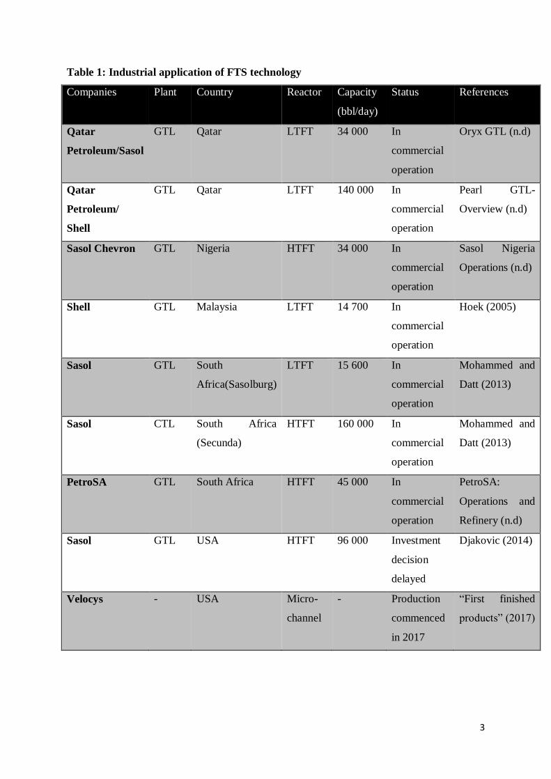
in the beginning and latter parts of the 20th century. A list of the various companies making
use of this technology today is presented in Table 1 to show how FTS has been applied
industrially since its discovery.
3
Table 1: Industrial application of FTS technology
Companies Plant Country Reactor Capacity
(bbl/day)
Status References
Qatar
Petroleum/Sasol
GTL Qatar LTFT 34 000 In
commercial
operation
Oryx GTL (n.d)
Qatar
Petroleum/
Shell
GTL Qatar LTFT 140 000 In
commercial
operation
Pearl GTL-
Overview (n.d)
Sasol Chevron GTL Nigeria HTFT 34 000 In
commercial
operation
Sasol Nigeria
Operations (n.d)
Shell GTL Malaysia LTFT 14 700 In
commercial
operation
Hoek (2005)
Sasol GTL South
Africa(Sasolburg)
LTFT 15 600 In
commercial
operation
Mohammed and
Datt (2013)
Sasol CTL South Africa
(Secunda)
HTFT 160 000 In
commercial
operation
Mohammed and
Datt (2013)
PetroSA GTL South Africa HTFT 45 000 In
commercial
operation
PetroSA:
Operations and
Refinery (n.d)
Sasol GTL USA HTFT 96 000 Investment
decision
delayed
Djakovic (2014)
Velocys - USA Micro-
channel
- Production
commenced
in 2017
“First finished
products” (2017)
4
1.2 FT overview
The FT process, named after the scientists that discovered it, is also commonly referred to as
the Fischer-Tropsch Synthesis. It involves the conversion of synthesis gas (gaseous mixture
of predominantly CO and H2) to hydrocarbon products over a metal catalyst. The synthesis
gas can be derived from coal gasification where coal is exposed to steam and/or oxygen
under elevated pressures [R1] or from a methane reforming process in which methane is
oxidized. Natural gas reforming can occur through partial oxidation [R2], steam reforming
[R3], carbon dioxide reforming [R4] or auto-thermal reforming [R5] depending on the H2/CO
ratio required in the syngas (Steynberg and Dry, 2004).
𝐶 + 𝐻2𝑂 = 𝐶𝑂 + 𝐻2 [R1]
𝐶𝐻4 +1
2𝑂2 = 𝐶𝑂 + 2𝐻2 [R2]
𝐶𝐻4 + 𝐻2𝑂 = 𝐶𝑂 + 3𝐻2 [R3]
𝐶𝐻4 + 𝐶𝑂2 = 2𝐶𝑂 + 2𝐻2 [R4]
2𝐶𝐻4 + 𝐶𝑂2 + 𝑂2 = 3𝐶𝑂 + 3𝐻2 + 𝐻2𝑂 [R5]
1.2.1 Product distribution
The products from the FT process include hydrocarbons of various chain lengths and
configurations that can be either straight or branched paraffins or olefins. These products are
described using a probability factor because of the multiple potential products that can be
formed. It is generally accepted that the formation of FT products follows a chain growth
path where an initiating molecule adsorbs onto the surface of a catalyst followed by a
propagation step where the molecule grows through the addition of a monomer species
(Todic et al, 2014). The molecule continues to grow until the termination step whereby the
molecule is released from the surface of the catalyst. In being released, this molecule either
takes the form of a paraffin or olefin depending on the extent of hydrogenation. It is clear that
the multiple possibilities in terms of the chain length and extent of hydrogenation make it
difficult to accurately predict the quality of product and it is for this reason that a chain
growth probability, α, is employed as a tool to describe the range of products formed from a
FTS reaction (Steynberg and Dry, 2004). The chain growth probability gives the rate of chain
propagation, 𝑟𝑝, relative to the sum of the rates of propagation and termination, 𝑟𝑡, as shown
in Equation 1 (van der Laan, 1999).
5
α =𝑟𝑝
(𝑟𝑝 + ∑ 𝑟𝑡)⁄ [1]
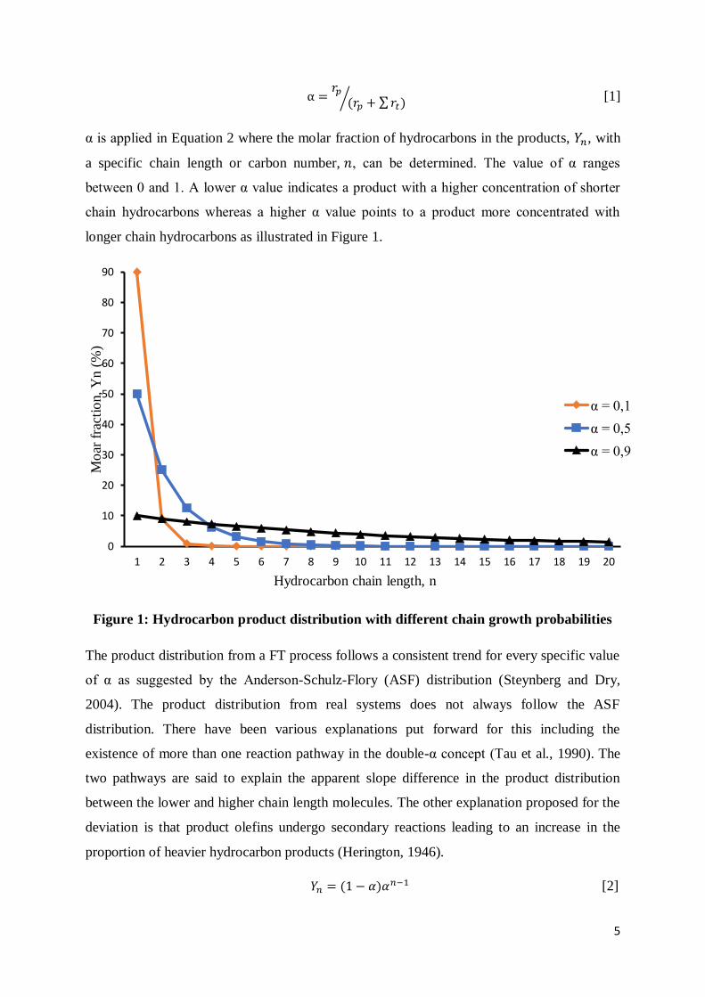
α is applied in Equation 2 where the molar fraction of hydrocarbons in the products, 𝑌𝑛, with
a specific chain length or carbon number, 𝑛, can be determined. The value of α ranges
between 0 and 1. A lower α value indicates a product with a higher concentration of shorter
chain hydrocarbons whereas a higher α value points to a product more concentrated with
longer chain hydrocarbons as illustrated in Figure 1.
Figure 1: Hydrocarbon product distribution with different chain growth probabilities
The product distribution from a FT process follows a consistent trend for every specific value
of α as suggested by the Anderson-Schulz-Flory (ASF) distribution (Steynberg and Dry,
2004). The product distribution from real systems does not always follow the ASF
distribution. There have been various explanations put forward for this including the
existence of more than one reaction pathway in the double-α concept (Tau et al., 1990). The
two pathways are said to explain the apparent slope difference in the product distribution
between the lower and higher chain length molecules. The other explanation proposed for the
deviation is that product olefins undergo secondary reactions leading to an increase in the
proportion of heavier hydrocarbon products (Herington, 1946).
𝑌𝑛 = (1 − 𝛼)𝛼𝑛−1 [2]
0
10
20
30
40
50
60
70
80
90
1 2 3 4 5 6 7 8 9 10 11 12 13 14 15 16 17 18 19 20
Mo
ar f
ract
ion, Y
n (
%)
Hydrocarbon chain length, n
α = 0,1
α = 0,5
α = 0,9
6
1.2.2 Kinetics and mechanisms of FTS
The kinetics in FTS rely on the reaction mechanism that is identified as the most suitable.
FTS, as mentioned in an earlier paragraph, is a polymerisation reaction with hydrocarbon
molecules coming together to form longer chain products. The difficulty in describing the
FTS reaction lies with the mechanism by which these long chain hydrocarbon products are
formed. Various mechanisms have been put forward to account for the way the hydrocarbon
products are formed and depending on the mechanism chosen, the rate equation will be
different. One of the mechanisms proposed is the surface carbide mechanism where
methylene acts as the monomer on which the propagation of chain growth is based (Brady
and Pettit, 1981; Ojeda et al., 2010; Fischer and Tropsch, 1926). In this mechanism, CO and
H2 adsorb dissociatively and the chain growth proceeds through the repeated insertion of the
monomer. Various mechanisms can be differentiated based on the type of monomers present
and the propagation pathways followed. Chang et al., (2007) describes six different reaction
mechanisms based upon these two factors (Table 2). In Table 2, 𝜃 refers to a catalyst active
site. The kinetics are also affected by the type of catalyst used with different rate equations
resulting from the use of either Fe or Co catalysts.
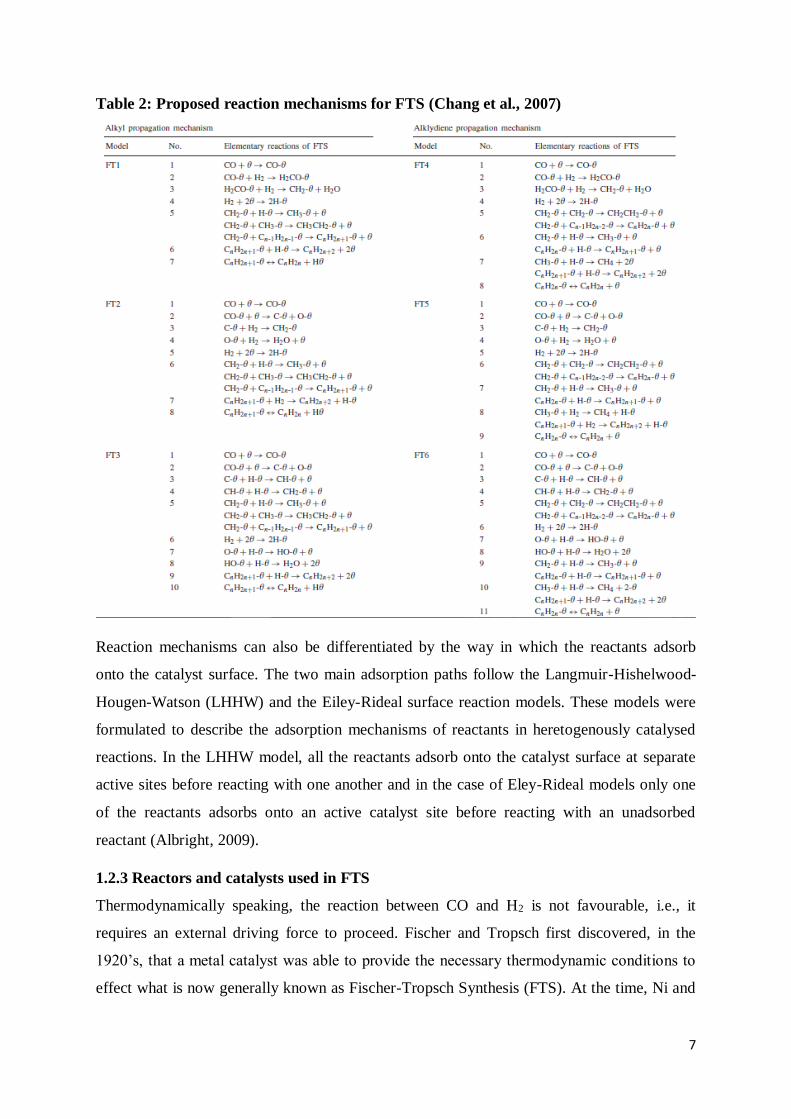
7
Table 2: Proposed reaction mechanisms for FTS (Chang et al., 2007)
Reaction mechanisms can also be differentiated by the way in which the reactants adsorb
onto the catalyst surface. The two main adsorption paths follow the Langmuir-Hishelwood-
Hougen-Watson (LHHW) and the Eiley-Rideal surface reaction models. These models were
formulated to describe the adsorption mechanisms of reactants in heretogenously catalysed
reactions. In the LHHW model, all the reactants adsorb onto the catalyst surface at separate
active sites before reacting with one another and in the case of Eley-Rideal models only one
of the reactants adsorbs onto an active catalyst site before reacting with an unadsorbed
reactant (Albright, 2009).
1.2.3 Reactors and catalysts used in FTS
Thermodynamically speaking, the reaction between CO and H2 is not favourable, i.e., it
requires an external driving force to proceed. Fischer and Tropsch first discovered, in the
1920’s, that a metal catalyst was able to provide the necessary thermodynamic conditions to
effect what is now generally known as Fischer-Tropsch Synthesis (FTS). At the time, Ni and
8
Co were identified as the main catalysts and these have since changed to Fe and Co. Selection
of the most appropriate catalyst is dependent on the objectives for FTS, i.e., the products that
are required, the operating conditions and type of reactor used amongst other factors. Middle
distillates (hydrocarbons with carbon numbers ranging between 9 and 16) may, for example,
be the required products in which case the operating conditions within the selected reactor
will have to be set and controlled accordingly. In selecting a reactor, two classes of FT
reactors are considered; High temperature Fischer-Tropsch (HTFT) and Low Temperature
Fischer-Tropsch (LTFT) reactors based on the prevailing temperature inside the reactor.
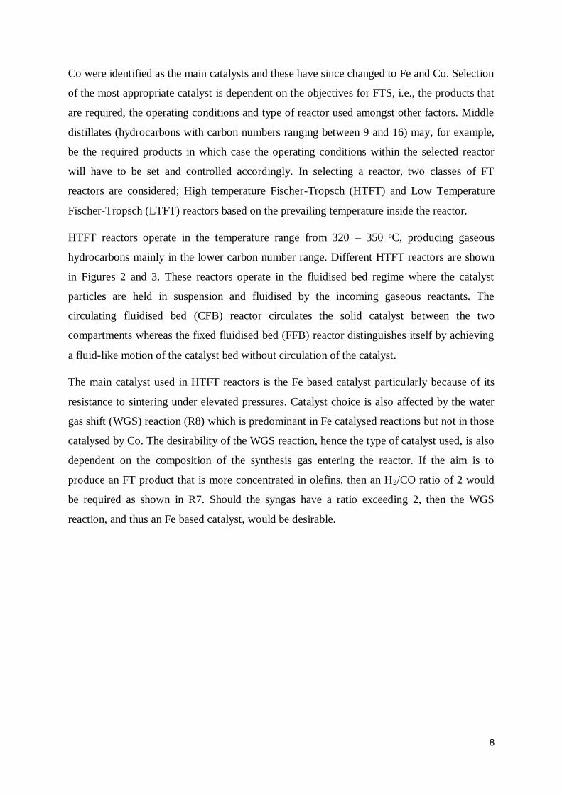
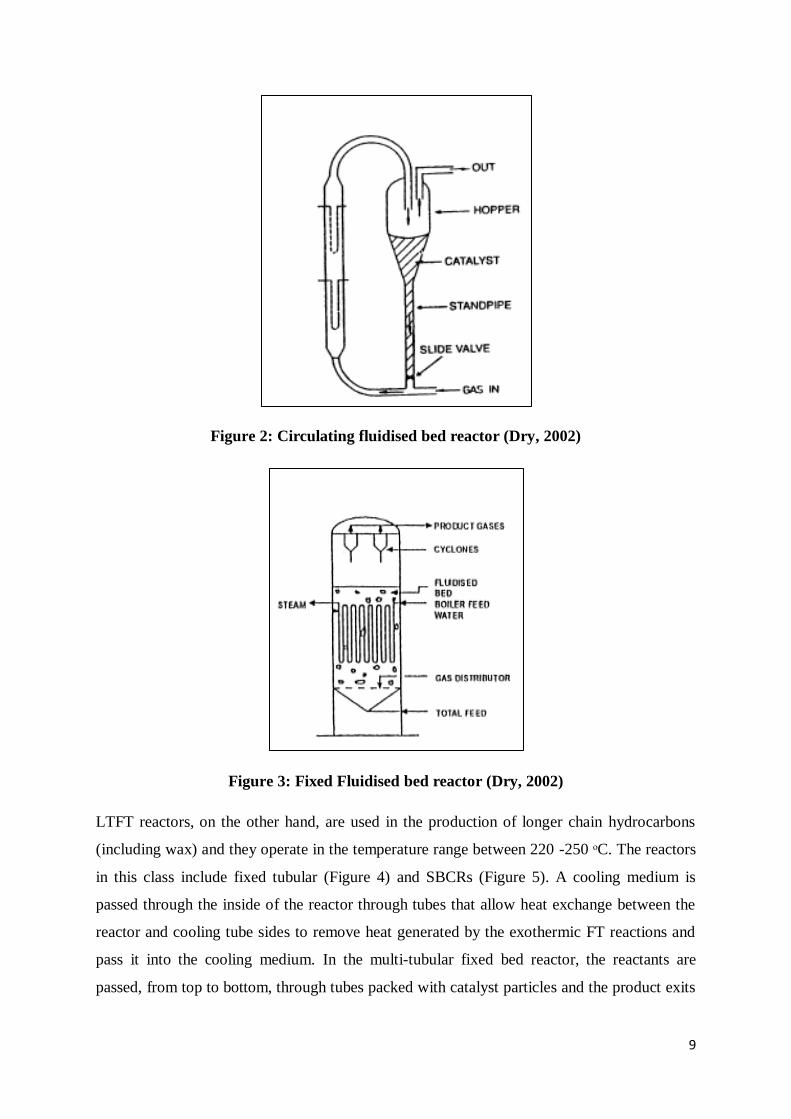
HTFT reactors operate in the temperature range from 320 – 350 ᵒC, producing gaseous
hydrocarbons mainly in the lower carbon number range. Different HTFT reactors are shown
in Figures 2 and 3. These reactors operate in the fluidised bed regime where the catalyst
particles are held in suspension and fluidised by the incoming gaseous reactants. The
circulating fluidised bed (CFB) reactor circulates the solid catalyst between the two
compartments whereas the fixed fluidised bed (FFB) reactor distinguishes itself by achieving
a fluid-like motion of the catalyst bed without circulation of the catalyst.
The main catalyst used in HTFT reactors is the Fe based catalyst particularly because of its
resistance to sintering under elevated pressures. Catalyst choice is also affected by the water
gas shift (WGS) reaction (R8) which is predominant in Fe catalysed reactions but not in those
catalysed by Co. The desirability of the WGS reaction, hence the type of catalyst used, is also
dependent on the composition of the synthesis gas entering the reactor. If the aim is to
produce an FT product that is more concentrated in olefins, then an H2/CO ratio of 2 would
be required as shown in R7. Should the syngas have a ratio exceeding 2, then the WGS
reaction, and thus an Fe based catalyst, would be desirable.
9
Figure 2: Circulating fluidised bed reactor (Dry, 2002)
Figure 3: Fixed Fluidised bed reactor (Dry, 2002)
LTFT reactors, on the other hand, are used in the production of longer chain hydrocarbons
(including wax) and they operate in the temperature range between 220 -250 ᵒC. The reactors
in this class include fixed tubular (Figure 4) and SBCRs (Figure 5). A cooling medium is
passed through the inside of the reactor through tubes that allow heat exchange between the
reactor and cooling tube sides to remove heat generated by the exothermic FT reactions and
pass it into the cooling medium. In the multi-tubular fixed bed reactor, the reactants are
passed, from top to bottom, through tubes packed with catalyst particles and the product exits
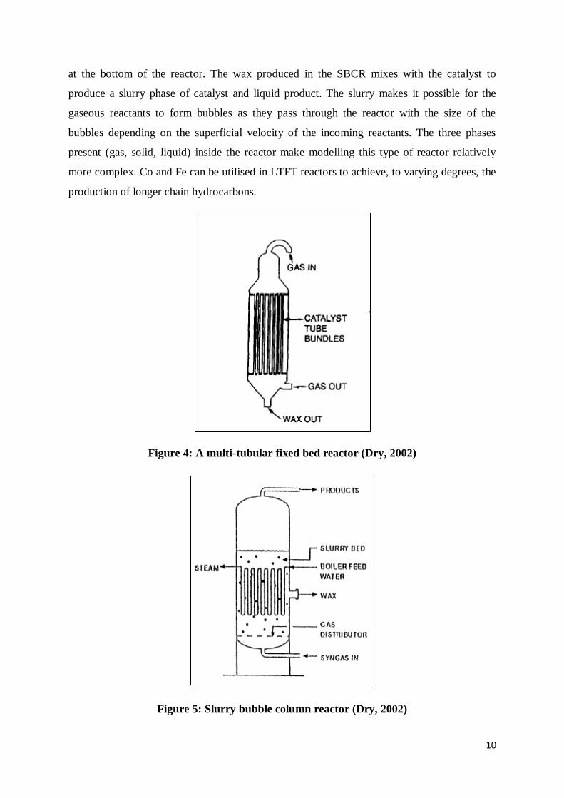
10
at the bottom of the reactor. The wax produced in the SBCR mixes with the catalyst to
produce a slurry phase of catalyst and liquid product. The slurry makes it possible for the
gaseous reactants to form bubbles as they pass through the reactor with the size of the
bubbles depending on the superficial velocity of the incoming reactants. The three phases
present (gas, solid, liquid) inside the reactor make modelling this type of reactor relatively
more complex. Co and Fe can be utilised in LTFT reactors to achieve, to varying degrees, the
production of longer chain hydrocarbons.
Figure 4: A multi-tubular fixed bed reactor (Dry, 2002)
Figure 5: Slurry bubble column reactor (Dry, 2002)
11
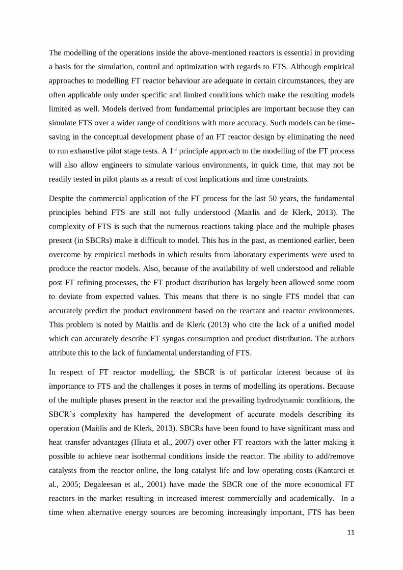
The modelling of the operations inside the above-mentioned reactors is essential in providing
a basis for the simulation, control and optimization with regards to FTS. Although empirical
approaches to modelling FT reactor behaviour are adequate in certain circumstances, they are
often applicable only under specific and limited conditions which make the resulting models
limited as well. Models derived from fundamental principles are important because they can
simulate FTS over a wider range of conditions with more accuracy. Such models can be time-
saving in the conceptual development phase of an FT reactor design by eliminating the need
to run exhaustive pilot stage tests. A 1st principle approach to the modelling of the FT process
will also allow engineers to simulate various environments, in quick time, that may not be
readily tested in pilot plants as a result of cost implications and time constraints.
Despite the commercial application of the FT process for the last 50 years, the fundamental
principles behind FTS are still not fully understood (Maitlis and de Klerk, 2013). The
complexity of FTS is such that the numerous reactions taking place and the multiple phases
present (in SBCRs) make it difficult to model. This has in the past, as mentioned earlier, been
overcome by empirical methods in which results from laboratory experiments were used to
produce the reactor models. Also, because of the availability of well understood and reliable
post FT refining processes, the FT product distribution has largely been allowed some room
to deviate from expected values. This means that there is no single FTS model that can
accurately predict the product environment based on the reactant and reactor environments.
This problem is noted by Maitlis and de Klerk (2013) who cite the lack of a unified model
which can accurately describe FT syngas consumption and product distribution. The authors
attribute this to the lack of fundamental understanding of FTS.
In respect of FT reactor modelling, the SBCR is of particular interest because of its
importance to FTS and the challenges it poses in terms of modelling its operations. Because
of the multiple phases present in the reactor and the prevailing hydrodynamic conditions, the
SBCR’s complexity has hampered the development of accurate models describing its
operation (Maitlis and de Klerk, 2013). SBCRs have been found to have significant mass and
heat transfer advantages (Iliuta et al., 2007) over other FT reactors with the latter making it
possible to achieve near isothermal conditions inside the reactor. The ability to add/remove
catalysts from the reactor online, the long catalyst life and low operating costs (Kantarci et
al., 2005; Degaleesan et al., 2001) have made the SBCR one of the more economical FT
reactors in the market resulting in increased interest commercially and academically. In a
time when alternative energy sources are becoming increasingly important, FTS has been

12
receiving renewed attention from academia and industry. Despite this increased attention,
there are still knowledge gaps in terms of the fundamental principles governing this process.
The SBCR is one of the more important and complex FTS systems in use today (Iliuta et al.,
2007) and to improve its operating efficiency, the current knowledge and understanding of
this process at a fundamental level, the hydrodynamics in particular, has to improve.
13
1.3 Problem Statement
In a time when alternative energy sources are becoming increasingly important, FTS has been
receiving renewed attention from academia and industry. Despite this increased attention,
there are still knowledge gaps in terms of the fundamental principles governing this process.
Due to the multiple phases present and the turbulent conditions within this reactor, it has been
difficult to develop a reliable model that can accurately describe the SBCR environment. The
SBCR is one of the more important and complex FTS systems in use today (Iliuta et al.,
2007) and to improve its operating efficiency, the current knowledge and understanding of
this process at a fundamental level, the hydrodynamics in particular, has to improve. A model
that can accurately describe the SBCR operations is needed. Taking due cognisance of the
above-mentioned problem, the question then becomes whether the development of a SBCR
mathematical model incorporating hydrodynamics can lead to;
A better understanding of the processes inside a SBCR
A better understanding of the FT process in general
The design of more efficient SBCRs
1.4 Research Aims and Objectives Given the problem statement above, the aim of this research project is the development of a
comprehensive mathematical model describing the processes in SBCRs. To this end the
following objectives have been set out.
Investigation of the transport phenomena inside a SBCR
Investigation of the reaction kinetics inside a SBCR
Analysis of the hydrodynamics inside a SBCR
Development and validation of a mathematical model, considering the above
mentioned governing principles, to comprehensively describe the processes in FT
SBCRs
14
Chapter 2: Literature Review
2.1 Hydrodynamics
2.1.1 Flow models
The flow of fluids in slurry bubble column reactors (SBCRs) poses a special challenge in
their design primarily due to the multiphase nature of the system. The gaseous reactants move
upward through the reactor in the form of bubbles. These bubbles interact with the slurry
phase consisting of liquid hydrocarbon products and catalyst particles to result in
hydrodynamics that are difficult to model accurately. The hydrodynamics in SBCRs are
therefore difficult to model. The interaction between the separate phases is still not clearly
understood and the extent of back mixing remains a point of debate. Do all the phases
significantly interact chemically and/or physically or is this interaction selective? What
contributes to the mixing action in the slurry phase? Considerable research effort has been
undertaken to determine the actual hydrodynamics in SBCRs and a lot of progress has been
made in improving the understanding of the fluid behavior in these reactors.
In beginning to conceptualize fluid behavior in a SBCR, the conditions inside it must be
determined so that a physical context for the conceptual model is established. The gaseous
syngas introduced to the reactor forms bubbles in the slurry bed as it makes its way upward
through the height of the reactor. The bubbles will move upward due to their significantly
lower density relative to that of the slurry. Several studies have found that under churn-
turbulent conditions, the bubbles that form vary considerably in size (Steynberg and Dry,
2004; van der Laan, 1999; Krishna and Sie, 2000; Schumpe and Grund, 1986). This is in
contrast to the bubble size distribution witnessed in bubbly flow of relatively lower
superficial gas velocities in which the bubbles exhibit a narrow size distribution (Steynberg
and Dry, 2004). The size distribution in churn-turbulent conditions can be simplified by
assigning two bubble classes according to large and small bubbles. It has been found that the
small bubbles reside mainly in the slurry phase while the large bubbles form a distinct gas
phase. It is important to accurately define the bubble size distribution as the size of the
bubbles is an important hydrodynamic parameter that influences the performance of the
reactor as shall be discussed below.
It is widely accepted that the large bubbles move upward through the center of the SBCR
while the small bubbles are immersed in the slurry phase and move downward along the wall
of the column (Deckwer, 1991). The mixing in SBCRs is generally of two forms; axial
15
dispersion or cell circulation. Both models seek to explain the mixing inside the reactor. The
axial dispersion model assigns a dispersion coefficient to the dispersive action that
contributes to axial concentration and temperature gradients. The cell circulation models on
the other hand attribute the mixing specifically to the circular movement of the slurry phase.
This section is dedicated to reviewing these mixing models, giving attention to their
advantages and disadvantages.
Axial Dispersion Model (ADM)
Axial dispersion can be described as the spatial gradient of matter and energy that exists in
the direction of the theoretical axis of the reactor. In a cylindrical SBCR the axial dispersion
will be along the height of the reactor. Dispersion in a SBCR is important in as far as
quantifying the extent of mixing in the reactor. Greater mixing would represent conditions
closer to those in CSTRs whereas less mixing would represent conditions that reflect a more
plug-flow system. In an ideal plug flow reactor system, a unit volume of reactants at a point z
in a column will have no interaction with a unit volume at a point z+∆z downstream in the
column (see Figure 14). This means that the unit volume that is at an advanced position will
not mix with or dilute the unit volume that precedes it. The consequence of this is a less
homogenous system in which the axial concentration gradients are pronounced. This should
lead to a higher reactant conversion rate than can be achieved in an ideal CSTR where the
perfect mixing results in no axial concentration gradients.
Use of the axial dispersion model implies the absence of dispersion in the radial direction.
The exclusion of radial dispersion in slurry bubble column hydrodynamic models is justified
by the relatively small radial dispersion coefficient in comparison with the axial dispersion
coefficient. According to Deckwer (1991), radial dispersion coefficients have been found to
be less than a tenth of the axial dispersion coefficient. This would suggest that radial
dispersion is an insignificant hydrodynamic parameter whose impact on SBCR performance
is unimportant. Deckwer (1991) further notes that radial dispersion will only affect reactor
performance when the reaction is not 1st order and heat effects are present.
2.1.2 Phase characterization
The presence of multiple phases requires the mixing/dispersion to be understood for each
individual phase. The phases in a SBCR are often reduced from three (gas-liquid-solid) to
two (gas-slurry) with the slurry phase assumed to be a pseudo-homogenous phase for the
purposes of simplicity. In modelling the hydrodynamics in slurry bubble column reactors in
16
the churn-turbulent regime, de Swart and Krishna (2002) adopted the two-phase model
initially proposed by Van Deemter (1961) for gas-solid fluidized beds. Van Deemter (1961)
identified dense and dilute phases as the predominant and hydrodynamically important
compartments in gas-solid fluidized beds where the dilute and dense phases consisted of the
fast-rising gas bubbles and solid catalyst particles respectively. de Swart and Krishna (2002)
adapted the two-phase model to slurry bubble column reactors by assigning the dilute phase
to the large rising bubbles and the dense phase to the small bubbles trapped in the slurry of
liquid and solid suspension.
Wang et al (2008) modelled the hydrodynamics in a SBCR by considering a gaseous and
liquid phase only, implicitly assuming that the liquid phase with small catalyst particles in
suspension would behave as a single phase. The existence of a pseudo-homogenous slurry
phase has been similarly accepted and applied in slurry bubble column models by various
authors (Grevskott et al., 1996; Matos et al., 2009; Jianping and Shonglin, 1998; van der
Laan, 1999; Schweitzer and Viguie, 2009). Despite the modelling convenience afforded by
the pseudo-homogenous assumption in SBCRs, some authors have modelled the process by
accounting for all three phases individually (Iliuta et al., 2007; Vik et al., 2016). In these
three-phase models, heat and mass transport would have to be modelled for each phase which
would add to the computing effort required to apply the model. The accuracy required from
the SBCR model will depend on the intended use of the model and time constraints. The two-
phase pseudo-homogenous model has proven to be capable of describing the hydrodynamics
in SBCRs relatively accurately and will be used as the model of choice in the development of
the mathematical model in this study, i.e., the axial dispersion will be defined in the pseudo-
homogenous slurry phase and not in the individual liquid phase.
2.1.3 Bubble size distribution
Various researchers have modelled the processes in SBCRs using a 2-class bubble size model
(Maretto and Krishna, 1999; van der Laan et al., 1999; Schumpe and Grund, 1986; Rados et
al., 2003; Sehabiague et al., 2008). This effectively divides the bubbles in the reactor into two
size classes; a large bubble class and a small bubble class usually assumed to be perfectly
mixed in the slurry phase (Steynberg and Dry, 2004; Krishna and Sie, 2000). In the churn-
turbulent regime, small bubbles coalesce to form larger bubbles and these in turn are broken
up into smaller bubbles. These two processes result in a net formation of two distinct bubble
sizes present as large and small bubbles ranging from a few millimetres to a few centimeters
in diameter (Matsuura and Fan, 1984). It should be noted that the 2-class bubble size model is
17
only a qualitative approximation of the conditions inside a SBCR rather than an accurate
quantitative reflection of the true nature of the bubble dynamics. In reality, a spectrum of
bubble sizes exists (Kantarci et al., 2005) but for the benefit of modelling the hydrodynamic
behaviour, it is sufficient to refer to relatively large and small bubbles with higher and lower
rise velocities respectively.
In all cases referred to above where the 2-class bubble model was adopted, a 2-phase system
with a pseudo-homogenous slurry phase is inherently implied. The 2-phase model divides the
reactor contents into a predominantly gaseous, large bubble phase and a slurry phase
consisting of a mixture of liquid and small bubbles holding a suspension of small solid
particles. The two models are therefore inextricably linked so that use of the 2-class bubble
model necessitates the application of the 2-phase model, although it does not necessarily
follow that the 2-class bubble model is necessary for application of the 2-phase pseudo-
homogenous model. The next concern in the hydrodynamic model then becomes the flow
model applicable in each phase.
The back-mixing present in the individual phases is an important variable in determining the
hydrodynamic behaviour and performance in SBCRs (Sehabiague, 2012) that must be
quantified. Concerning the dilute gas phase, most authors have adopted the view that large
bubbles move in a plug flow manner through the center of the reactor column, the implication
being that no dispersion occurs in the gas phase (Behkish, 1997, Schweitzer and Viguie,
2009; Basha et al, 2015; Gasche et al., 1990; Krishna and Sie, 2000; Sehabiague, 2012). The
upward central movement of the large bubble phase has been reported by Krishna and Sie
(2000) with Iliuta et al., (2007) treating the reactor as two cylindrical sections with a core and
an outer annulus with the large bubbles moving up through the core.
2.1.3.1 Gas phase dispersion
Few studies have incorporated axial mixing in the gas phase. Deckwer et al., (1980) reported
on the studies by Mangartz and Pilhofer (1980) (as cited in Deckwer et al., 1980) who
attributed the axial dispersion variables in the gas phase to the diameter of the column,
superficial gas velocity and gas hold-up. Deckwer et al., (1980) justifies the modelling of
axial dispersion in the gas phase only under conditions of high conversion in the reactor.
Iliuta et al., (2007) assumed the presence of axial dispersion in the gas phase in preparing a
SBCR model. Rados et al. (2005) also incorporated axial mixing in the gas phase in
18
developing a SBCR model. The author attributed the mixing to the interaction between
bubbles of the same class.
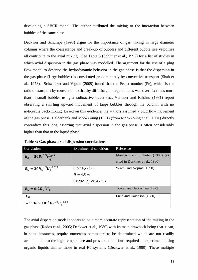
Deckwer and Schumpe (1993) argue for the importance of gas mixing in large diameter
columns where the coalescence and break-up of bubbles and different bubble rise velocities
all contribute to the axial mixing. See Table 3 (Schluter et al., 1992) for a list of studies in
which axial dispersion in the gas phase was modelled. The argument for the use of a plug
flow model to describe the hydrodynamic behavior in the gas phase is that the dispersion in
the gas phase (large bubbles) is constituted predominantly by convective transport (Shah et
al., 1978). Schweitzer and Viguie (2009) found that the Peclet number (Pe), which is the
ratio of transport by convection to that by diffusion, in large bubbles was over six times more
than in small bubbles using a radioactive tracer test. Vermeer and Krishna (1981) report
observing a swirling upward movement of large bubbles through the column with no
noticeable back-mixing. Based on this evidence, the authors assumed a plug flow movement
of the gas phase. Calderbank and Moo-Young (1961) (from Moo-Young et al., 1981) directly
contradicts this idea, asserting that axial dispersion in the gas phase is often considerably
higher than that in the liquid phase.
Table 3: Gas phase axial dispersion correlations
Correlation Experimental conditions Reference
𝑬𝒈 = 𝟓𝟎𝑫𝑪𝟏.𝟓(
𝑼𝒈
𝜺𝒈)𝟑 Mangartz and Pilhofer (1980) (as
cited in Deckwer et al., 1980)
𝑬𝑮 = 𝟐𝟎𝑫𝑪𝟏.𝟓𝑼𝒈
𝟎.𝟎𝟐𝟗 0.2< 𝐷𝐶 <0.5
𝐻 = 4.5 𝑚
0.029< 𝑈𝑔 <0.45 m/s
Wachi and Nojima (1990)
𝑬𝑮 = 𝟎. 𝟐𝑫𝑪𝟐𝑼𝒈 Towell and Ackerman (1972)
𝑬𝑮
= 𝟗. 𝟑𝟔 × 𝟏𝟎−𝟓𝑫𝑪𝟏.𝟑𝑼𝒈
𝟑.𝟓𝟔
Field and Davidson (1980)
The axial dispersion model appears to be a more accurate representation of the mixing in the
gas phase (Rados et al., 2005; Deckwer et al., 1980) with its main drawback being that it can,
in some instances, require numerous parameters to be determined which are not readily
available due to the high temperature and pressure conditions required in experiments using
organic liquids similar those in real FT systems (Deckwer et al., 1980). These multiple
19
parameters also compound the potential error that would be inherent in the model (Mponzi,
2011).
2.1.3.2 Liquid axial dispersion
The slurry phase dispersion can be attributed to various factors including liquid circulation,
turbulence due to entrapment of liquid in bubble wakes and eddy formations (Groen, 2004
and Degaleesan et al., 1997). When a bubble travels up a column of liquid, a wake forms
around the bubble which displaces the fluid in the immediate vicinity of the bubble. This
phenomenon induces dispersion in the liquid phase through convection, i.e., through the
movement of the liquid from one point in the column to another, following the path of the
bubble. The movement of a bubble through a fluid also induces eddy currents behind it which
create localized turbulence. This is particularly true under high velocity churn-turbulent
conditions (Deckwer, 1991). These contributors to liquid phase axial dispersion are lumped
together and defined by a single coefficient, the axial dispersion coefficient, 𝐸𝑙.
The axial dispersion coefficient is a quantitative representation of the back-mixing that occurs
in fluids inside slurry bubble column reactors. As mentioned above, one of the factors
contributing to dispersion in the slurry phase is the circulation of the liquid. Liquid
circulation occurs as a result of a radial gas hold-up profile that is prevalent in SBCRs under
churn-turbulent conditions. This point shall be discussed in more detail when the cell
circulation models are discussed. It is worth pointing out that the circulation model is
acknowledged in the ADM as a cause for the dispersion in the slurry phase. The main
difference between the ADM and the circulation model is that the ADM does not single out
any one factor but rather assigns a single parameter, the axial dispersion coefficient, to
describe the overall mixing.
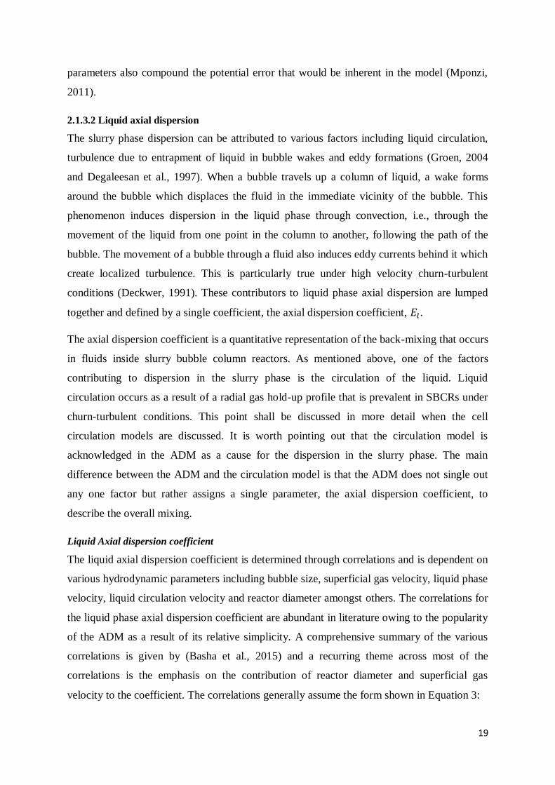
Liquid Axial dispersion coefficient
The liquid axial dispersion coefficient is determined through correlations and is dependent on
various hydrodynamic parameters including bubble size, superficial gas velocity, liquid phase
velocity, liquid circulation velocity and reactor diameter amongst others. The correlations for
the liquid phase axial dispersion coefficient are abundant in literature owing to the popularity
of the ADM as a result of its relative simplicity. A comprehensive summary of the various
correlations is given by (Basha et al., 2015) and a recurring theme across most of the
correlations is the emphasis on the contribution of reactor diameter and superficial gas
velocity to the coefficient. The correlations generally assume the form shown in Equation 3:
20
𝐸𝐿 = 𝐾𝐷𝐶𝑎𝑈𝑔
𝑏 [3]
Where the relative effects of 𝐷𝐶 and 𝑈𝑔 on the dispersion coefficient, 𝐸𝐿 , are represented by 𝑎
and 𝑏 respectively. K is a proportionality constant. Equation 3 forms the basis on which most
of the existing correlations are based (see Table 4). To quantify the constants in Equation 3,
tracer experiments are usually conducted. These involve introducing a trace substance into a
column with flowing liquid and sparged gas and measuring the distribution of the tracer. The
tests can be conducted in a steady-state or non-steady-state environment. Tracer tests have
been used to develop multiple correlations, by various authors, which deviate significantly
from each other. This deviation is due mainly to the different gas-liquid conditions employed
in the tests. Deckwer (1991) notes the geometry of the reactors and the liquid mixture used as
the biggest contributors to these apparent discrepancies. The conditions under which tracer
experiments are conducted in developing an axial dispersion coefficient correlation are
important and should therefore be considered carefully when selecting the most appropriate
correlation to use in modelling a specific reactor and in the case of the current study, a SBCR.
21
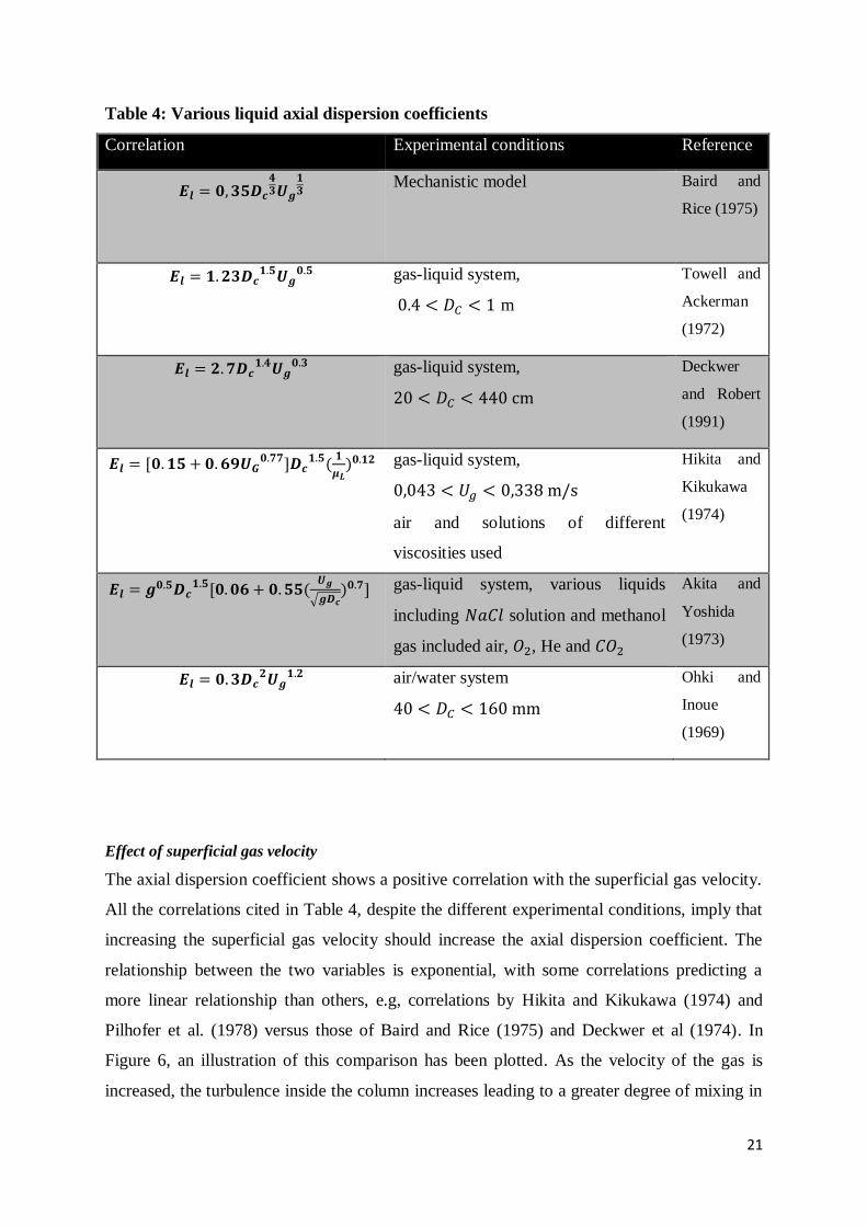
Table 4: Various liquid axial dispersion coefficients
Correlation Experimental conditions Reference
𝑬𝒍 = 𝟎, 𝟑𝟓𝑫𝒄
𝟒𝟑𝑼𝒈
𝟏𝟑
Mechanistic model Baird and
Rice (1975)
𝑬𝒍 = 𝟏. 𝟐𝟑𝑫𝒄𝟏.𝟓𝑼𝒈
𝟎.𝟓 gas-liquid system,
0.4 < 𝐷𝐶 < 1 m
Towell and
Ackerman
(1972)
𝑬𝒍 = 𝟐. 𝟕𝑫𝒄𝟏.𝟒𝑼𝒈
𝟎.𝟑 gas-liquid system,
20 < 𝐷𝐶 < 440 cm
Deckwer
and Robert
(1991)
𝑬𝒍 = [𝟎. 𝟏𝟓 + 𝟎. 𝟔𝟗𝑼𝑮𝟎.𝟕𝟕]𝑫𝒄
𝟏.𝟓(𝟏
𝝁𝑳)𝟎.𝟏𝟐 gas-liquid system,
0,043 < 𝑈𝑔 < 0,338 m/s
air and solutions of different
viscosities used
Hikita and
Kikukawa
(1974)
𝑬𝒍 = 𝒈𝟎.𝟓𝑫𝒄𝟏.𝟓[𝟎. 𝟎𝟔 + 𝟎. 𝟓𝟓(
𝑼𝒈
√𝒈𝑫𝒄)𝟎.𝟕] gas-liquid system, various liquids
including 𝑁𝑎𝐶𝑙 solution and methanol
gas included air, 𝑂2, He and 𝐶𝑂2
Akita and
Yoshida
(1973)
𝑬𝒍 = 𝟎. 𝟑𝑫𝒄𝟐𝑼𝒈
𝟏.𝟐 air/water system
40 < 𝐷𝐶 < 160 mm
Ohki and
Inoue
(1969)
Effect of superficial gas velocity
The axial dispersion coefficient shows a positive correlation with the superficial gas velocity.
All the correlations cited in Table 4, despite the different experimental conditions, imply that
increasing the superficial gas velocity should increase the axial dispersion coefficient. The
relationship between the two variables is exponential, with some correlations predicting a
more linear relationship than others, e.g, correlations by Hikita and Kikukawa (1974) and
Pilhofer et al. (1978) versus those of Baird and Rice (1975) and Deckwer et al (1974). In
Figure 6, an illustration of this comparison has been plotted. As the velocity of the gas is
increased, the turbulence inside the column increases leading to a greater degree of mixing in
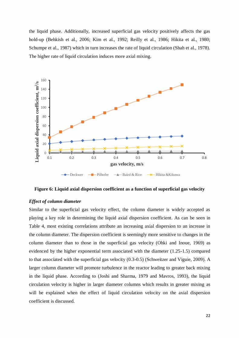
22
the liquid phase. Additionally, increased superficial gas velocity positively affects the gas
hold-up (Behkish et al., 2006; Kim et al., 1992; Reilly et al., 1986; Hikita et al., 1980;
Schumpe et al., 1987) which in turn increases the rate of liquid circulation (Shah et al., 1978).
The higher rate of liquid circulation induces more axial mixing.
Figure 6: Liquid axial dispersion coefficient as a function of superficial gas velocity
Effect of column diameter
Similar to the superficial gas velocity effect, the column diameter is widely accepted as
playing a key role in determining the liquid axial dispersion coefficient. As can be seen in
Table 4, most existing correlations attribute an increasing axial dispersion to an increase in
the column diameter. The dispersion coefficient is seemingly more sensitive to changes in the
column diameter than to those in the superficial gas velocity (Ohki and Inoue, 1969) as
evidenced by the higher exponential term associated with the diameter (1.25-1.5) compared
to that associated with the superficial gas velocity (0.3-0.5) (Schweitzer and Viguie, 2009). A
larger column diameter will promote turbulence in the reactor leading to greater back mixing
in the liquid phase. According to (Joshi and Sharma, 1979 and Mavros, 1993), the liquid
circulation velocity is higher in larger diameter columns which results in greater mixing as
will be explained when the effect of liquid circulation velocity on the axial dispersion
coefficient is discussed.
0
20
40
60
80
100
120
140
160
0.1 0.2 0.3 0.4 0.5 0.6 0.7 0.8
Liq
uid
axia
l d
isp
ersi
on
co
effi
cien
t, m
2/s
gas velocity, m/s
Deckwer Pilhofer Baird & Rice Hikita &Kikuwa
23
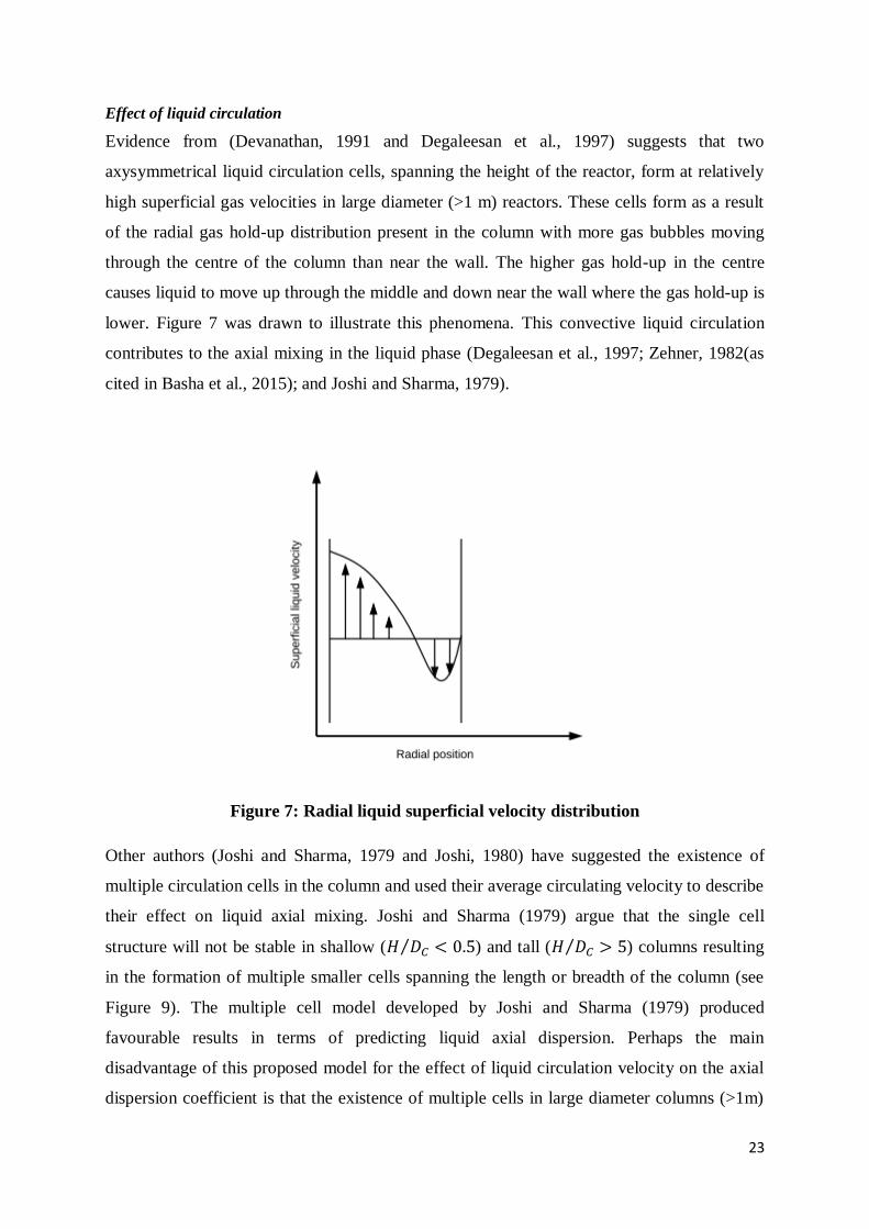
Effect of liquid circulation
Evidence from (Devanathan, 1991 and Degaleesan et al., 1997) suggests that two
axysymmetrical liquid circulation cells, spanning the height of the reactor, form at relatively
high superficial gas velocities in large diameter (>1 m) reactors. These cells form as a result
of the radial gas hold-up distribution present in the column with more gas bubbles moving
through the centre of the column than near the wall. The higher gas hold-up in the centre
causes liquid to move up through the middle and down near the wall where the gas hold-up is
lower. Figure 7 was drawn to illustrate this phenomena. This convective liquid circulation
contributes to the axial mixing in the liquid phase (Degaleesan et al., 1997; Zehner, 1982(as
cited in Basha et al., 2015); and Joshi and Sharma, 1979).
Figure 7: Radial liquid superficial velocity distribution
Other authors (Joshi and Sharma, 1979 and Joshi, 1980) have suggested the existence of
multiple circulation cells in the column and used their average circulating velocity to describe
their effect on liquid axial mixing. Joshi and Sharma (1979) argue that the single cell
structure will not be stable in shallow (𝐻 𝐷𝐶⁄ < 0.5) and tall (𝐻 𝐷𝐶⁄ > 5) columns resulting
in the formation of multiple smaller cells spanning the length or breadth of the column (see
Figure 9). The multiple cell model developed by Joshi and Sharma (1979) produced
favourable results in terms of predicting liquid axial dispersion. Perhaps the main
disadvantage of this proposed model for the effect of liquid circulation velocity on the axial
dispersion coefficient is that the existence of multiple cells in large diameter columns (>1m)
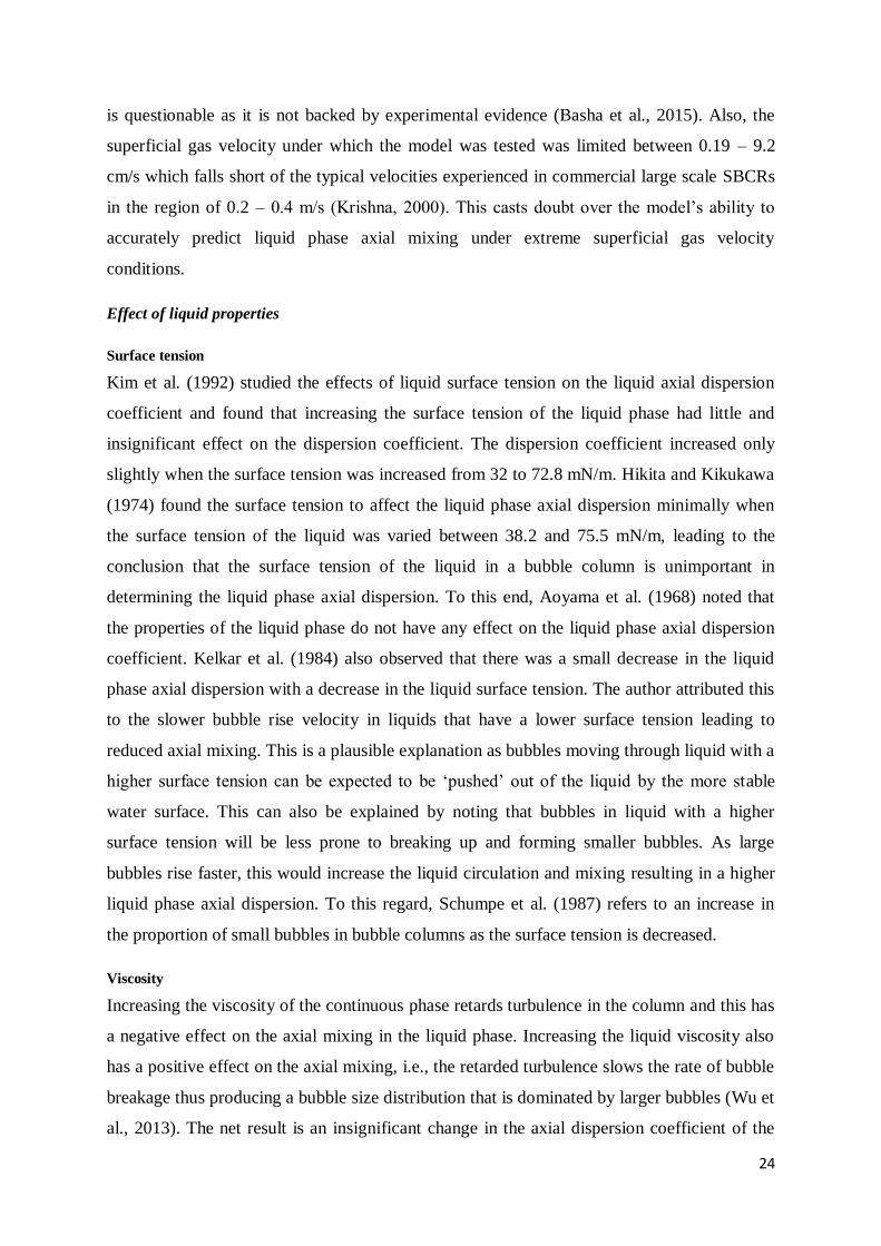
24
is questionable as it is not backed by experimental evidence (Basha et al., 2015). Also, the
superficial gas velocity under which the model was tested was limited between 0.19 – 9.2
cm/s which falls short of the typical velocities experienced in commercial large scale SBCRs
in the region of 0.2 – 0.4 m/s (Krishna, 2000). This casts doubt over the model’s ability to
accurately predict liquid phase axial mixing under extreme superficial gas velocity
conditions.
Effect of liquid properties
Surface tension
Kim et al. (1992) studied the effects of liquid surface tension on the liquid axial dispersion
coefficient and found that increasing the surface tension of the liquid phase had little and
insignificant effect on the dispersion coefficient. The dispersion coefficient increased only
slightly when the surface tension was increased from 32 to 72.8 mN/m. Hikita and Kikukawa
(1974) found the surface tension to affect the liquid phase axial dispersion minimally when
the surface tension of the liquid was varied between 38.2 and 75.5 mN/m, leading to the
conclusion that the surface tension of the liquid in a bubble column is unimportant in
determining the liquid phase axial dispersion. To this end, Aoyama et al. (1968) noted that
the properties of the liquid phase do not have any effect on the liquid phase axial dispersion
coefficient. Kelkar et al. (1984) also observed that there was a small decrease in the liquid
phase axial dispersion with a decrease in the liquid surface tension. The author attributed this
to the slower bubble rise velocity in liquids that have a lower surface tension leading to
reduced axial mixing. This is a plausible explanation as bubbles moving through liquid with a
higher surface tension can be expected to be ‘pushed’ out of the liquid by the more stable
water surface. This can also be explained by noting that bubbles in liquid with a higher
surface tension will be less prone to breaking up and forming smaller bubbles. As large
bubbles rise faster, this would increase the liquid circulation and mixing resulting in a higher
liquid phase axial dispersion. To this regard, Schumpe et al. (1987) refers to an increase in
the proportion of small bubbles in bubble columns as the surface tension is decreased.
Viscosity
Increasing the viscosity of the continuous phase retards turbulence in the column and this has
a negative effect on the axial mixing in the liquid phase. Increasing the liquid viscosity also
has a positive effect on the axial mixing, i.e., the retarded turbulence slows the rate of bubble
breakage thus producing a bubble size distribution that is dominated by larger bubbles (Wu et
al., 2013). The net result is an insignificant change in the axial dispersion coefficient of the
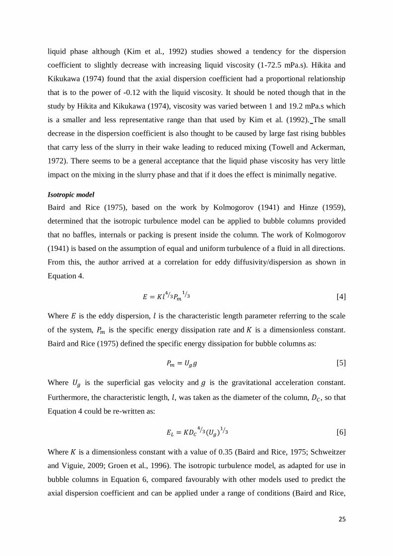
25
liquid phase although (Kim et al., 1992) studies showed a tendency for the dispersion
coefficient to slightly decrease with increasing liquid viscosity (1-72.5 mPa.s). Hikita and
Kikukawa (1974) found that the axial dispersion coefficient had a proportional relationship
that is to the power of -0.12 with the liquid viscosity. It should be noted though that in the
study by Hikita and Kikukawa (1974), viscosity was varied between 1 and 19.2 mPa.s which
is a smaller and less representative range than that used by Kim et al. (1992). The small
decrease in the dispersion coefficient is also thought to be caused by large fast rising bubbles
that carry less of the slurry in their wake leading to reduced mixing (Towell and Ackerman,
1972). There seems to be a general acceptance that the liquid phase viscosity has very little
impact on the mixing in the slurry phase and that if it does the effect is minimally negative.
Isotropic model
Baird and Rice (1975), based on the work by Kolmogorov (1941) and Hinze (1959),
determined that the isotropic turbulence model can be applied to bubble columns provided
that no baffles, internals or packing is present inside the column. The work of Kolmogorov
(1941) is based on the assumption of equal and uniform turbulence of a fluid in all directions.
From this, the author arrived at a correlation for eddy diffusivity/dispersion as shown in
Equation 4.
𝐸 = 𝐾𝑙4
3⁄ 𝑃𝑚1
3⁄ [4]
Where 𝐸 is the eddy dispersion, 𝑙 is the characteristic length parameter referring to the scale
of the system, 𝑃𝑚 is the specific energy dissipation rate and 𝐾 is a dimensionless constant.
Baird and Rice (1975) defined the specific energy dissipation for bubble columns as:
𝑃𝑚 = 𝑈𝑔𝑔 [5]
Where 𝑈𝑔 is the superficial gas velocity and 𝑔 is the gravitational acceleration constant.
Furthermore, the characteristic length, 𝑙, was taken as the diameter of the column, 𝐷𝐶 , so that
Equation 4 could be re-written as:
𝐸𝐿 = 𝐾𝐷𝐶4
3⁄ (𝑈𝑔)1
3⁄ [6]
Where 𝐾 is a dimensionless constant with a value of 0.35 (Baird and Rice, 1975; Schweitzer
and Viguie, 2009; Groen et al., 1996). The isotropic turbulence model, as adapted for use in
bubble columns in Equation 6, compared favourably with other models used to predict the
axial dispersion coefficient and can be applied under a range of conditions (Baird and Rice,
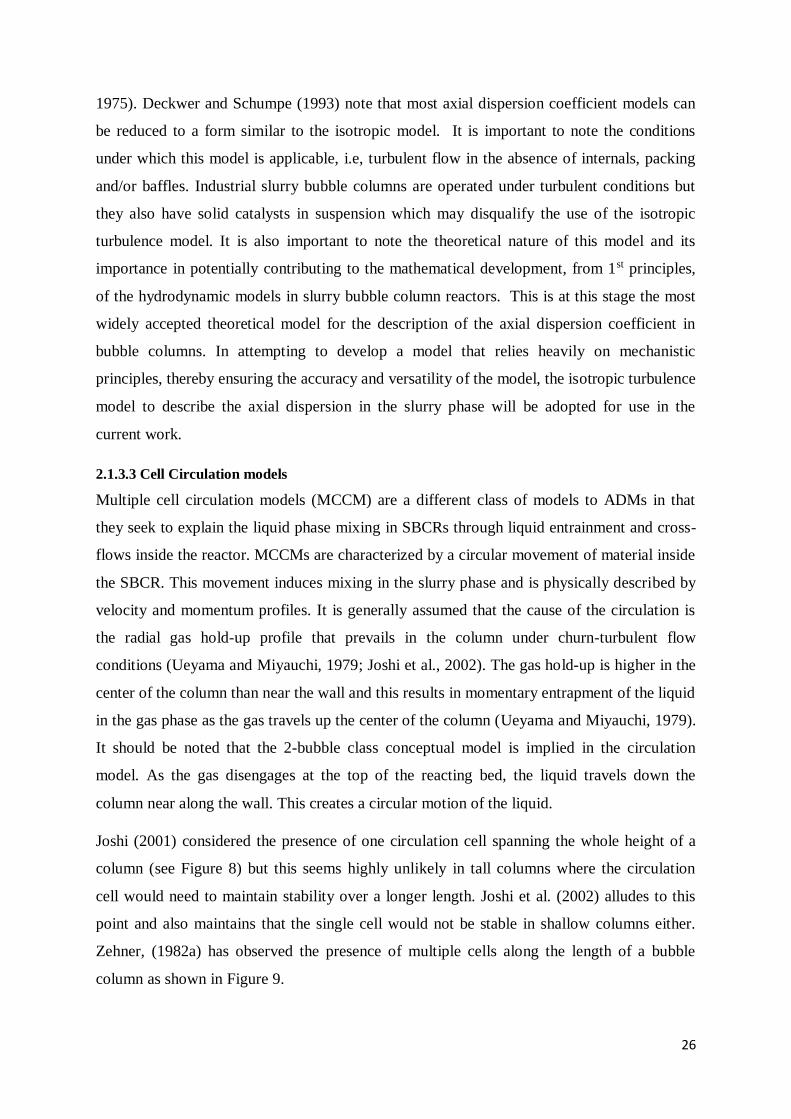
26
1975). Deckwer and Schumpe (1993) note that most axial dispersion coefficient models can
be reduced to a form similar to the isotropic model. It is important to note the conditions
under which this model is applicable, i.e, turbulent flow in the absence of internals, packing
and/or baffles. Industrial slurry bubble columns are operated under turbulent conditions but
they also have solid catalysts in suspension which may disqualify the use of the isotropic
turbulence model. It is also important to note the theoretical nature of this model and its
importance in potentially contributing to the mathematical development, from 1st principles,
of the hydrodynamic models in slurry bubble column reactors. This is at this stage the most
widely accepted theoretical model for the description of the axial dispersion coefficient in
bubble columns. In attempting to develop a model that relies heavily on mechanistic
principles, thereby ensuring the accuracy and versatility of the model, the isotropic turbulence
model to describe the axial dispersion in the slurry phase will be adopted for use in the
current work.
2.1.3.3 Cell Circulation models
Multiple cell circulation models (MCCM) are a different class of models to ADMs in that
they seek to explain the liquid phase mixing in SBCRs through liquid entrainment and cross-
flows inside the reactor. MCCMs are characterized by a circular movement of material inside
the SBCR. This movement induces mixing in the slurry phase and is physically described by
velocity and momentum profiles. It is generally assumed that the cause of the circulation is
the radial gas hold-up profile that prevails in the column under churn-turbulent flow
conditions (Ueyama and Miyauchi, 1979; Joshi et al., 2002). The gas hold-up is higher in the
center of the column than near the wall and this results in momentary entrapment of the liquid
in the gas phase as the gas travels up the center of the column (Ueyama and Miyauchi, 1979).
It should be noted that the 2-bubble class conceptual model is implied in the circulation
model. As the gas disengages at the top of the reacting bed, the liquid travels down the
column near along the wall. This creates a circular motion of the liquid.
Joshi (2001) considered the presence of one circulation cell spanning the whole height of a
column (see Figure 8) but this seems highly unlikely in tall columns where the circulation
cell would need to maintain stability over a longer length. Joshi et al. (2002) alludes to this
point and also maintains that the single cell would not be stable in shallow columns either.
Zehner, (1982a) has observed the presence of multiple cells along the length of a bubble
column as shown in Figure 9.
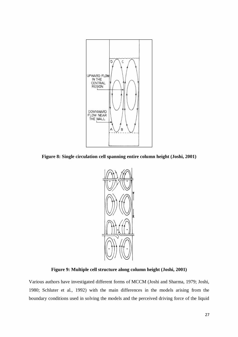
27
Figure 8: Single circulation cell spanning entire column height (Joshi, 2001)
Figure 9: Multiple cell structure along column height (Joshi, 2001)
Various authors have investigated different forms of MCCM (Joshi and Sharma, 1979; Joshi,
1980; Schluter et al., 1992) with the main differences in the models arising from the
boundary conditions used in solving the models and the perceived driving force of the liquid

28
phase circulation. Some, like Millies and Mewes (1994), attribute the circulation to the
turbulence induced by the non-uniform gas hold-up in the reactor. The extent of circulation is
dependent on the relative viscosities of the gas and liquid phases (De Nevers, 1968) and so it
is important that the model parameters used are determined from experiments conducted with
fluids similar to those in FTS and not air/water systems.
Circulation models give detailed attention to the velocity and momentum forces as the cause
of axial mixing in the slurry phase. There is no dispute that the slurry phase undergoes
extensive axial mixing or that circulation of the slurry phase occurs inside the SBCR. This
stems from the generally accepted notion that large bubbles move in bulk through the center
of the column while small bubbles are interspersed in the slurry phase. The main difference
between the circulation models and the ADM is the way the mixing is conceptualized and
characterized. In the circulation models, the concept is that the velocity of the circulating
cells is directly involved in the mixing and so its value is determined through application of
the continuity equation. The ADM on the other hand is based on the concept of a wholistic
description of the causes of mixing using a single parameter. This approach seems more
versatile as it attempts to describe the mixing as a sum of all possible causes. The main
disadvantage of the ADM is the lack of reliable correlations available for parameter
estimation. Most correlations have been derived from experiments conducted under
conditions greatly dissimilar to those in industrial settings as seen in Table 4. Despite this, the
ADM remains the most suitable hydrodynamic model for SBCR modelling given its ease of
application and versatility. The ADM will therefore be used as the model of choice in
developing the mathematical model in this work.
2.2 Kinetics
The SBCR is a heterogenous system and is thus represented kinetically by heterogenous
catalysis. Reactants enter the reactor in the gas phase and diffuse through the gas-liquid
interphase into the liquid phase and through the solid-liquid interphase into the solid phase
where the reaction occurs (see Figure 10). The overall kinetics of this system can be driven
by either of the processes shown in Figure 10. These processes can be further classified into
mass transfer and kinetic factors so that the overall kinetics are determined by the rate of
mass transfer or that of the surface kinetics.
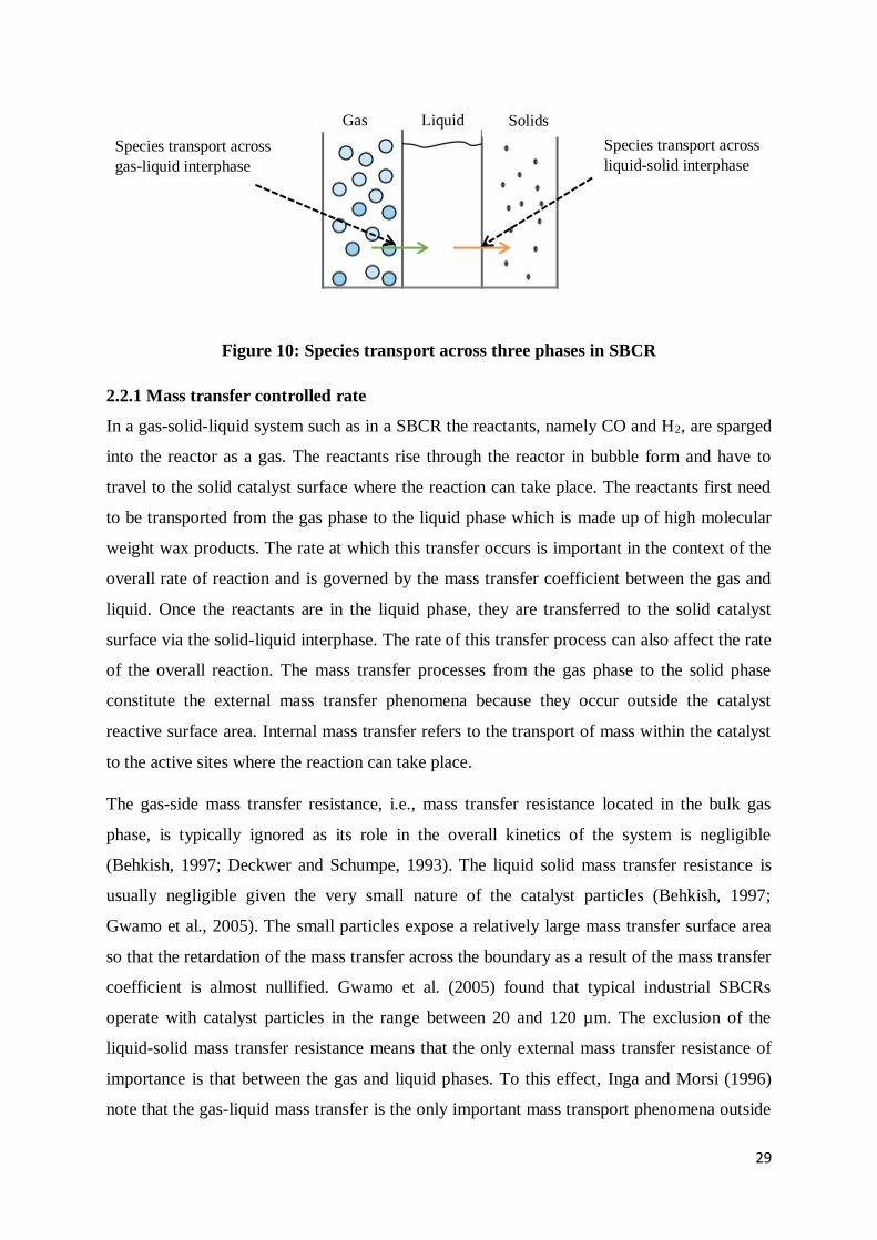
29
Figure 10: Species transport across three phases in SBCR
2.2.1 Mass transfer controlled rate
In a gas-solid-liquid system such as in a SBCR the reactants, namely CO and H2, are sparged
into the reactor as a gas. The reactants rise through the reactor in bubble form and have to
travel to the solid catalyst surface where the reaction can take place. The reactants first need
to be transported from the gas phase to the liquid phase which is made up of high molecular
weight wax products. The rate at which this transfer occurs is important in the context of the
overall rate of reaction and is governed by the mass transfer coefficient between the gas and
liquid. Once the reactants are in the liquid phase, they are transferred to the solid catalyst
surface via the solid-liquid interphase. The rate of this transfer process can also affect the rate
of the overall reaction. The mass transfer processes from the gas phase to the solid phase
constitute the external mass transfer phenomena because they occur outside the catalyst
reactive surface area. Internal mass transfer refers to the transport of mass within the catalyst
to the active sites where the reaction can take place.
The gas-side mass transfer resistance, i.e., mass transfer resistance located in the bulk gas
phase, is typically ignored as its role in the overall kinetics of the system is negligible
(Behkish, 1997; Deckwer and Schumpe, 1993). The liquid solid mass transfer resistance is
usually negligible given the very small nature of the catalyst particles (Behkish, 1997;
Gwamo et al., 2005). The small particles expose a relatively large mass transfer surface area
so that the retardation of the mass transfer across the boundary as a result of the mass transfer
coefficient is almost nullified. Gwamo et al. (2005) found that typical industrial SBCRs
operate with catalyst particles in the range between 20 and 120 µm. The exclusion of the
liquid-solid mass transfer resistance means that the only external mass transfer resistance of
importance is that between the gas and liquid phases. To this effect, Inga and Morsi (1996)
note that the gas-liquid mass transfer is the only important mass transport phenomena outside
Gas Liquid
(L)
Solids
Species transport across
gas-liquid interphase
Species transport across
liquid-solid interphase
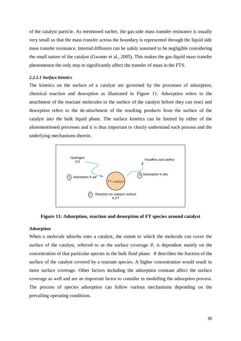
30
of the catalyst particle. As mentioned earlier, the gas-side mass transfer resistance is usually
very small so that the mass transfer across the boundary is represented through the liquid side
mass transfer resistance. Internal diffusion can be safely assumed to be negligible considering
the small nature of the catalyst (Gwamo et al., 2005). This makes the gas-liquid mass transfer
phenomenon the only step to significantly affect the transfer of mass in the FTS.
2.2.1.1 Surface kinetics
The kinetics on the surface of a catalyst are governed by the processes of adsorption,
chemical reaction and desorption as illustrated in Figure 11. Adsorption refers to the
attachment of the reactant molecules to the surface of the catalyst before they can react and
desorption refers to the de-attachment of the resulting products from the surface of the
catalyst into the bulk liquid phase. The surface kinetics can be limited by either of the
aforementioned processes and it is thus important to clearly understand each process and the
underlying mechanisms therein.
Figure 11: Adsorption, reaction and desorption of FT species around catalyst
Adsorption
When a molecule adsorbs onto a catalyst, the extent to which the molecule can cover the
surface of the catalyst, referred to as the surface coverage 𝜃, is dependent mainly on the
concentration of that particular species in the bulk fluid phase. 𝜃 describes the fraction of the
surface of the catalyst covered by a reactant species. A higher concentration would result in
more surface coverage. Other factors including the adsorption constant affect the surface
coverage as well and are an important factor to consider in modelling the adsorption process.
The process of species adsorption can follow various mechanisms depending on the
prevailing operating conditions.
31
Method of adsorption
An adsorbed reactant species will react with either another adsorbed species or with a species
from the bulk fluid phase. The former and latter phenomena are referred to as dual and single
site mechanisms respectively and ultimately affect the kinetics of the system. Furthermore,
the reacting molecules can adsorb competitively or non-competitively. In the case of multiple
reactants, the adsorbing molecules may compete for the same active site on the surface of the
catalyst or the reactants may react on separate classes of active sites. The surface coverage of
a reactant, which is the equivalent of concentration in homogenous reaction systems, is
determined with the use of an isotherm. The Langmuir isotherm described in Equation 7
relates the concentration of the reactant in the bulk liquid phase with the surface coverage by
introducing the adsorption constant. The Langmuir isotherm is predicated on a few
assumptions (Levenspiel, 1999);
1. The adsorption process is in equilibrium.
2. The catalyst surface behaves ideally, i.e., all sites have equal activity.
3. The adsorbed molecules do not interact with each other.
𝜃𝐴 =𝐾𝐴𝑃𝐴
1+𝐾𝐴𝑃𝐴 [7]
Where A is an arbitrary reactant species, 𝐾𝐴 is the adsorption equilibrium constant and 𝑃𝐴 is
the concentration of A in the bulk fluid phase which can also be represented by CA in the
event that the fluid phase is liquid. Equation 7 is specifically for a system where A adsorbs
onto the active catalyst site without competition. The surface coverage of A would be
retarded if more reactants where present to compete for the same site as shown in Equation 8.
𝜃𝐴 =𝐾𝐴𝑃𝐴
1+𝐾𝐴𝑃𝐴+𝐾𝐵𝑃𝐵+𝐾𝐶𝑃𝐶+⋯…+𝐾𝑚−1𝑃𝑚−1+𝐾𝑚𝑃𝑚 [8]
If the adsorption step is rate limiting, then the rate equation will take the form:
𝑅 = 𝑘𝑎𝑑𝑠[𝐴][∗] [9]
Where [∗] represents the concentration/number-density of vacant active sites on the catalyst
surface and 𝑘𝑎𝑑𝑠 represents the adsorption rate constant. [∗] can be determined through a
catalyst site balance by understanding that the total available sites are shared between
occupied and unoccupied sites thus:
[∗]0 = [∗] + [𝐴 ∗] [10]
32
Where [∗]0 denotes the total concentration of active sites on the catalyst surface and [𝐴 ∗]
represents the concentration of sites occupied by a reactant molecule which can in turn be
determined by understanding the definition of surface coverage as shown in Equation 11.
𝜃𝐴 =[𝐴∗]
[∗]0 [11]
Equation 9 is possible due to the assumption of pseudo-equilibrium for the surface reaction
rate and the desorption rate (Sinnot, 2005). It is common and reasonable practice to assume
that the other surface processes besides the rate limiting step are in pseudo-equilibrium
(Davis and Davis, 2003). Following the same logic and assuming pseudo-equilibrium for the
surface reaction and the adsorption step when the desorption step is rate-limiting; the overall
rate will take the form:
𝑅 =𝑘3𝐾2𝐾1[∗]0[𝐴]
1+(𝐾1+𝐾2𝐾1)[𝐴] [12]
Where 𝑘3 denotes the desorption rate constant, 𝐾1 and 𝐾2 represent the equilibrium
adsorption and reaction constants respectively.
Chemical reaction
The chemical reaction kinetics will depend on the surface coverage of the reacting species
which in turn depend on the adsorption isotherm. In simple homogenous elementary single
reactions, the rate law, i.e., the equation that defines the rate of reaction, is easy to determine.
The reactions in FTS are multiple and non-elementary, occurring on a catalyst surface. This
introduces a level of difficulty in determining a rate law that will satisfactorily model the rate
and thus the reactant conversion as a function of the prevailing reactor conditions. In
determining a rate law, the reaction constants of the elementary reactions must be known and
consolidated to give the resulting rate law for a particular reacting system. This means that
for FTS, in which multiple reactions take place and even more elementary reaction steps are
present, the task of determining the rate law is made difficult. To deal with this difficulty, FT
reactions are lumped together according to the products formed and the total number of
reactions is reduced accordingly. In general, the important reactions in FT are those that form
paraffins and olefins. The water-gas-shift (WGS) reaction is also important, along with the
reactions responsible for alcohol formation and the Boudouard reaction as seen in Table 5. In
SBCRs operating under the typical conditions as set out in Table 6, the FT reaction can be
represented generally by [R7].
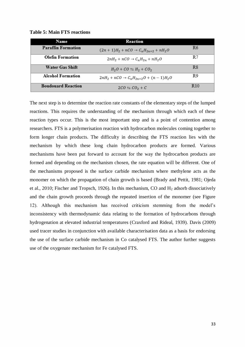
33
Table 5: Main FTS reactions
The next step is to determine the reaction rate constants of the elementary steps of the lumped
reactions. This requires the understanding of the mechanism through which each of these
reaction types occur. This is the most important step and is a point of contention among
researchers. FTS is a polymerisation reaction with hydrocarbon molecules coming together to
form longer chain products. The difficulty in describing the FTS reaction lies with the
mechanism by which these long chain hydrocarbon products are formed. Various
mechanisms have been put forward to account for the way the hydrocarbon products are
formed and depending on the mechanism chosen, the rate equation will be different. One of
the mechanisms proposed is the surface carbide mechanism where methylene acts as the
monomer on which the propagation of chain growth is based (Brady and Pettit, 1981; Ojeda
et al., 2010; Fischer and Tropsch, 1926). In this mechanism, CO and H2 adsorb dissociatively
and the chain growth proceeds through the repeated insertion of the monomer (see Figure
12). Although this mechanism has received criticism stemming from the model’s
inconsistency with thermodynamic data relating to the formation of hydrocarbons through
hydrogenation at elevated industrial temperatures (Craxford and Rideal, 1939). Davis (2009)
used tracer studies in conjunction with available characterisation data as a basis for endorsing
the use of the surface carbide mechanism in Co catalysed FTS. The author further suggests
use of the oxygenate mechanism for Fe catalysed FTS.
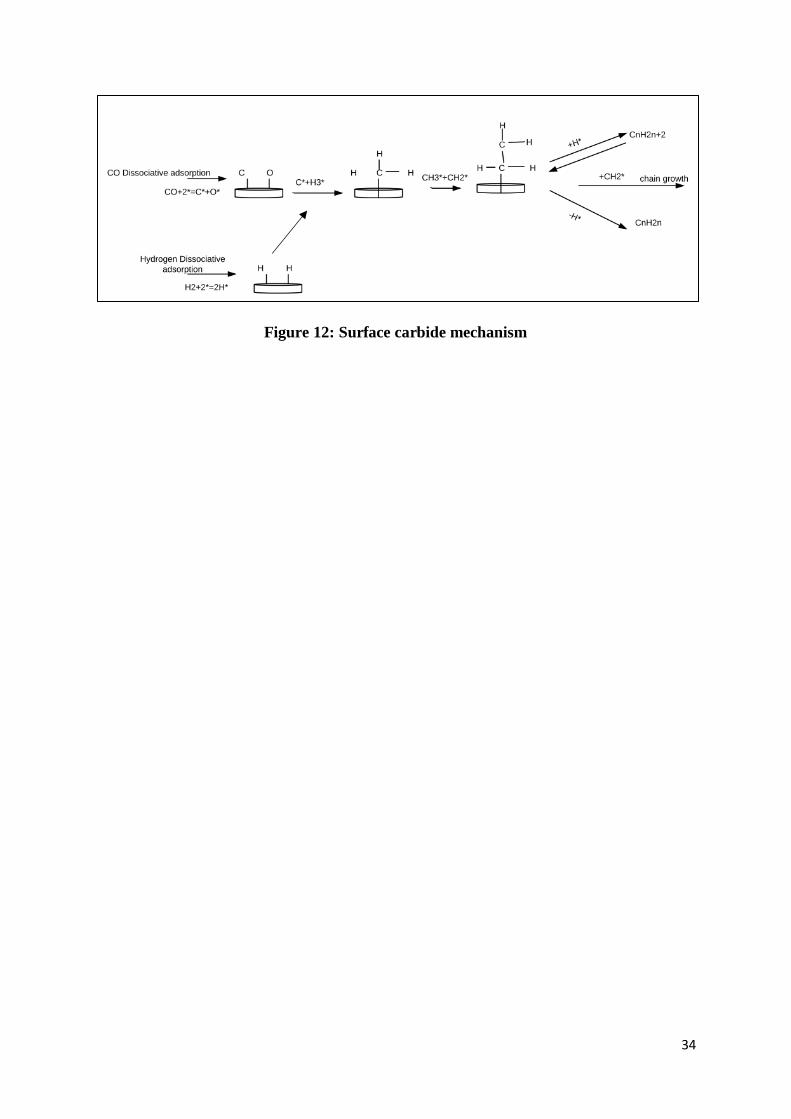
34
Figure 12: Surface carbide mechanism
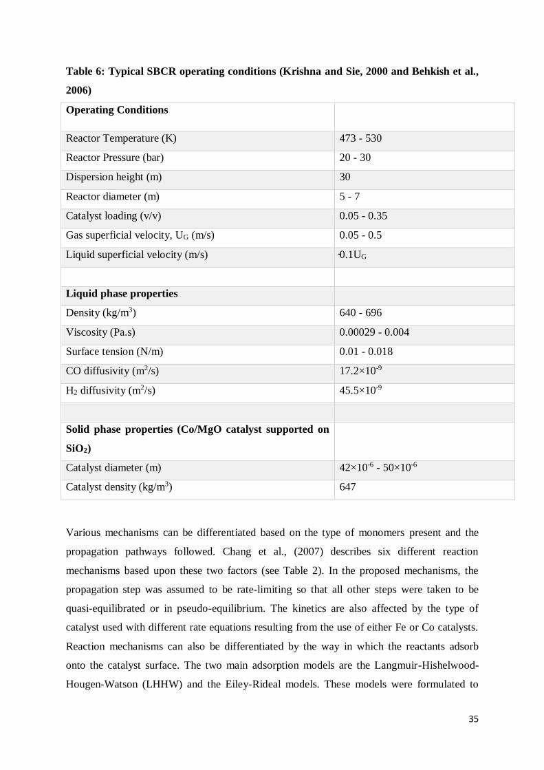
35
Table 6: Typical SBCR operating conditions (Krishna and Sie, 2000 and Behkish et al.,
2006)
Operating Conditions
Reactor Temperature (K) 473 - 530
Reactor Pressure (bar) 20 - 30
Dispersion height (m) 30
Reactor diameter (m) 5 - 7
Catalyst loading (v/v) 0.05 - 0.35
Gas superficial velocity, UG (m/s) 0.05 - 0.5
Liquid superficial velocity (m/s) ̴0.1UG
Liquid phase properties
Density (kg/m3) 640 - 696
Viscosity (Pa.s) 0.00029 - 0.004
Surface tension (N/m) 0.01 - 0.018
CO diffusivity (m2/s) 17.2×10⁻⁹
H2 diffusivity (m2/s) 45.5×10⁻⁹
Solid phase properties (Co/MgO catalyst supported on
SiO2)
Catalyst diameter (m) 42×10-6 - 50×10-6
Catalyst density (kg/m3) 647
Various mechanisms can be differentiated based on the type of monomers present and the
propagation pathways followed. Chang et al., (2007) describes six different reaction
mechanisms based upon these two factors (see Table 2). In the proposed mechanisms, the
propagation step was assumed to be rate-limiting so that all other steps were taken to be
quasi-equilibrated or in pseudo-equilibrium. The kinetics are also affected by the type of
catalyst used with different rate equations resulting from the use of either Fe or Co catalysts.
Reaction mechanisms can also be differentiated by the way in which the reactants adsorb
onto the catalyst surface. The two main adsorption models are the Langmuir-Hishelwood-
Hougen-Watson (LHHW) and the Eiley-Rideal models. These models were formulated to
36
describe the adsorption mechanisms of reactants in heretogenously catalysed reactions. In the
LHHW model, all the reactants adsorb onto the catalyst surface at separate active sites before
reacting with one another and in the case of Eley-Rideal models only one of the reactants
adsorbs onto an active catalyst site before reacting with an unadsorbed reactant (Albright,
2009). Eley-Rideal models are more important under extreme conditions, particularly in the
semiconductor production field whereas LHHW models are more common in catalysed
reactions (Davis and Davis, 2003).
Once a reaction mechanism is identified, the rate controlling step within that mechanism must
be identified to allow for the development of the rate law, provided the surface reaction is
rate limiting. Through the use of steady-state approximation, the overall rate law based on the
rate limiting step can be determined (Equation 13). The steady-state approximation is based
on the assumption that the concentration of an intermediate in a multiple elementary reaction
system is constant, i.e., its rate of formation is equal to its rate of consumption. The steady-
state approximation can greatly simplify the process of determining an overall surface
reaction rate when applied to the limiting reaction step and a quasi-equilibrated step. A quasi-
equilibrated step is a combination of the rest of the elementary reaction steps which are
assumed to be in equilibrium. This in effect reduces a complex system of multiple elementary
reactions to a simplified set of reactions on which the overall surface reaction rate can be
derived (Davis and Davis, 2003).
𝑅 =𝑟𝑖−𝑟−𝑖
𝜎𝑖 [13]
Where R is the overall rate, 𝑟𝑖 is the forward reaction rate, 𝑟−𝑖 is the reverse reaction rate and
𝜎𝑖 is the stoichiometric number of the elementary reaction step. The final equation should
take the form shown in Equation 14.
𝑅 =𝑘2𝐾𝑎𝑑𝑠[∗]0[𝐴]
1+𝐾𝑎𝑑𝑠[𝐴] [14]
Where 𝑘2 represents the reaction rate constant. Equation 14 exemplifies a typical LHHW rate
law given by:
𝑅𝑎𝑡𝑒 =(𝑘𝑖𝑛𝑒𝑡𝑖𝑐 𝑡𝑒𝑟𝑚)(𝑝𝑜𝑡𝑒𝑛𝑡𝑖𝑎𝑙 𝑡𝑒𝑟𝑚)
𝑎𝑑𝑠𝑜𝑟𝑝𝑡𝑖𝑜𝑛 𝑡𝑒𝑟𝑚 [15]
The overall rate law is usually determined empirically by assuming a reaction scheme and
determining the reaction and adsorption constants through regression analysis. According to
Levenspiel (1999), all possible reaction pathways with all possible rate-limiting steps should
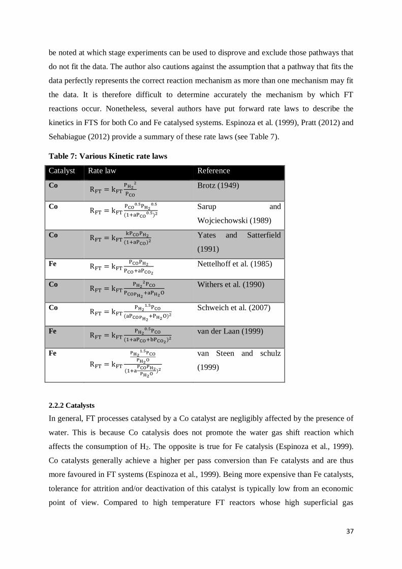
37
be noted at which stage experiments can be used to disprove and exclude those pathways that
do not fit the data. The author also cautions against the assumption that a pathway that fits the
data perfectly represents the correct reaction mechanism as more than one mechanism may fit
the data. It is therefore difficult to determine accurately the mechanism by which FT
reactions occur. Nonetheless, several authors have put forward rate laws to describe the
kinetics in FTS for both Co and Fe catalysed systems. Espinoza et al. (1999), Pratt (2012) and
Sehabiague (2012) provide a summary of these rate laws (see Table 7).
Table 7: Various Kinetic rate laws
Catalyst Rate law Reference
Co RFT = kFT
PH22
PCO
Brotz (1949)
Co RFT = kFT
PCO0.5PH2
0.5
(1+aPCO0.5)2
Sarup and
Wojciechowski (1989)
Co RFT = kFTkPCOPH2
(1+aPCO)2 Yates and Satterfield
(1991)
Fe RFT = kFTPCOPH2
PCO+aPCO2
Nettelhoff et al. (1985)
Co RFT = kFT
PH22PCO
PCOPH2+aPH2O
Withers et al. (1990)
Co RFT = kFT
PH21.5PCO
(aPCOPH2+PH2O)2
Schweich et al. (2007)
Fe RFT = kFT
PH20.5PCO
(1+aPCO+bPCO2)2 van der Laan (1999)
Fe
RFT = kFT
PH21.5PCO
PH2O
(1+aPCOPH2
PH2O
)2
van Steen and schulz
(1999)
2.2.2 Catalysts
In general, FT processes catalysed by a Co catalyst are negligibly affected by the presence of
water. This is because Co catalysis does not promote the water gas shift reaction which
affects the consumption of H2. The opposite is true for Fe catalysis (Espinoza et al., 1999).
Co catalysts generally achieve a higher per pass conversion than Fe catalysts and are thus
more favoured in FT systems (Espinoza et al., 1999). Being more expensive than Fe catalysts,
tolerance for attrition and/or deactivation of this catalyst is typically low from an economic
point of view. Compared to high temperature FT reactors whose high superficial gas
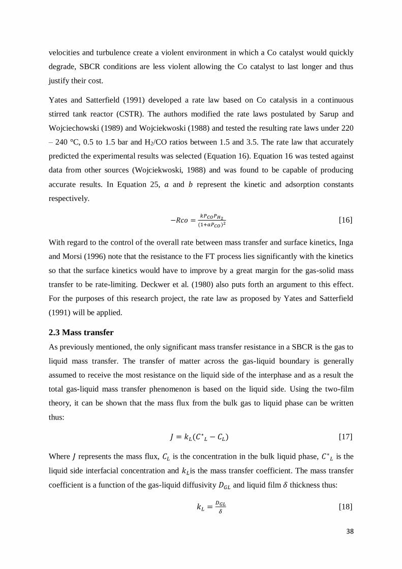
38
velocities and turbulence create a violent environment in which a Co catalyst would quickly
degrade, SBCR conditions are less violent allowing the Co catalyst to last longer and thus
justify their cost.
Yates and Satterfield (1991) developed a rate law based on Co catalysis in a continuous
stirred tank reactor (CSTR). The authors modified the rate laws postulated by Sarup and
Wojciechowski (1989) and Wojciekwoski (1988) and tested the resulting rate laws under 220
– 240 °C, 0.5 to 1.5 bar and H2/CO ratios between 1.5 and 3.5. The rate law that accurately
predicted the experimental results was selected (Equation 16). Equation 16 was tested against
data from other sources (Wojciekwoski, 1988) and was found to be capable of producing
accurate results. In Equation 25, 𝑎 and 𝑏 represent the kinetic and adsorption constants
respectively.
−𝑅𝑐𝑜 =𝑘𝑃𝐶𝑂𝑃𝐻2
(1+𝑎𝑃𝐶𝑂)2 [16]
With regard to the control of the overall rate between mass transfer and surface kinetics, Inga
and Morsi (1996) note that the resistance to the FT process lies significantly with the kinetics
so that the surface kinetics would have to improve by a great margin for the gas-solid mass
transfer to be rate-limiting. Deckwer et al. (1980) also puts forth an argument to this effect.
For the purposes of this research project, the rate law as proposed by Yates and Satterfield
(1991) will be applied.
2.3 Mass transfer
As previously mentioned, the only significant mass transfer resistance in a SBCR is the gas to
liquid mass transfer. The transfer of matter across the gas-liquid boundary is generally
assumed to receive the most resistance on the liquid side of the interphase and as a result the
total gas-liquid mass transfer phenomenon is based on the liquid side. Using the two-film
theory, it can be shown that the mass flux from the bulk gas to liquid phase can be written
thus:
𝐽 = 𝑘𝐿(𝐶∗𝐿 − 𝐶𝐿) [17]
Where 𝐽 represents the mass flux, 𝐶𝐿 is the concentration in the bulk liquid phase, 𝐶∗𝐿 is the
liquid side interfacial concentration and 𝑘𝐿is the mass transfer coefficient. The mass transfer
coefficient is a function of the gas-liquid diffusivity 𝐷𝐺𝐿 and liquid film 𝛿 thickness thus:
𝑘𝐿 =𝐷𝐺𝐿
𝛿 [18]

39
To represent the flux in units of mass/time, the volumetric mass transfer coefficient 𝑘𝐿𝑎 is
often used where 𝑎 denotes the interfacial area. The interfacial liquid phase concentration can
be related to the partial pressure in the bulk gas phase though Henry’s law with the
assumption that equilibrium exists between the two phases as shown in Equation 19.
𝐶∗𝑖,𝐿 =
𝑃𝑖
𝐻𝑖 [19]
Where 𝑃𝑖 is the partial pressure of species i in the gas phase and H is Henry’s constant for
species i and 𝐶∗𝑖,𝐿 is the concentration of species i in the gas phase at the gas-liquid
interphase under equilibrium conditions.
2.3.1 Mass transfer coefficients
Mass transfer and therefore the mass transfer coefficient depends strongly on the bubble size
so that small bubbles with a greater interfacial area allow more mass transfer than larger
bubbles with less area for mass transfer (Basha et al., 2015). Liquid phase dispersion can
influence the volumetric mass transfer coefficient (Inga, 1997) meaning that those variables
that affect dispersion will also have an impact on the mass transfer coefficient as well. These
include the column size and superficial gas velocity. Various correlations for volumetric mass
transfer coefficients are given in Table 8.

40
Table 8: Volumetric mass transfer coefficient correlations
Correlation Experimental conditions Reference
𝑲𝑳𝒂 = 𝟎. 𝟓𝜺𝒈 Vermeer and Krishna
(1981)
𝑲𝑳𝒂,𝑳𝑩 = 𝟎. 𝟓𝜺𝒈,𝑳𝑩√𝑫
𝑫𝒓𝒆𝒇
𝑲𝑳𝒂,𝑺𝑩 = 𝜺𝒈,𝑺𝑩√𝑫
𝑫𝒓𝒆𝒇
Vemeer and Krishna (1981)
𝑲𝑳𝒂 = 𝒄𝑫𝟎.𝟓(𝝁𝑳
𝝆𝑳)−𝟎.𝟔𝟐𝑫𝑪
𝟎.𝟏𝟕𝒈𝟎.𝟗𝟑𝜺𝒈𝟏.𝟏 𝐷𝐶 = 15.2 𝑐𝑚
𝐻 = 400 𝑐𝑚
Akita and Yoshida (1973)
𝑲𝑳𝒂 =
𝟔.𝟏𝟒×𝟏𝟎𝟒𝝆𝑳𝟎.𝟐𝟔𝝁𝑳
𝟎.𝟏𝟐𝜺𝒈𝟏.𝟐𝟏𝑫𝟎.𝟓𝜸𝟎.𝟏𝟏
𝝈𝟎.𝟓𝟐𝝆𝒈𝟎.𝟎𝟔𝑼𝒈
𝟎.𝟏𝟐𝒅𝒃𝟎.𝟎𝟓𝑻𝟎.𝟔𝟖
(𝑫𝑪
𝟏+𝑫𝑪)𝟎.𝟒
Lemoine et al. (2008)
𝑲𝑳𝒂 = 𝟒. 𝟒𝟏𝑼𝒈𝟎.𝟑𝟑𝟖𝜺𝑺
𝟎.𝟓𝟗𝟓(𝟏 −
𝝆𝑳
𝝆𝒑)𝟎.𝟑𝟑𝟕
0.0025 < 𝐷𝐶 < 0.05 𝑚/𝑠
𝐷𝐶 = 0.06 𝑚
Guo et al. (1997)
𝑲𝑳𝒂 = 𝟎. 𝟒𝑼𝒈𝟎.𝟔𝟐𝟓𝑼𝑳
𝟎.𝟐𝟔𝒆(𝟏.𝟒𝟕𝟕×𝟏𝟎−𝟓𝑯) 0.02 < 𝐷 < 0.04 𝑚/𝑠
𝐷𝐶 = 0.05 𝑚
Chen et al (2001)
Vermeer and Krishna (1981) have suggested a simple correlation for the mass transfer
coefficient that relates the coefficient only to the gas hold-up (Equation 20). Steynberg and
Dry (2004) recognise this correlation as a rule of thumb. Following a similar correlation,
Vermeer and Krishna (1981) and Letzel et al. (1999) have provided correlations for large and
small bubbles, making a clear distinction between the coefficients of the two size classes.
Krishna and Sie (2000) modified the correlation put forward by Letzel et al. (1999) by
introducing the liquid phase diffusive coefficient.
𝐾𝐿𝑎 = 0.5휀𝑔 [20]
Correlations by Akita and Yoshida (1973) and Calderbank and Moo-Young (1961) have
garnered a lot of popularity over the years but as Maretto, and Krishna (1999) and Schweitzer
and Viguie (2009) note, the correlations have limited applicability in SBCRs operating in the
heterogenous regime with predominantly large bubbles. The aforementioned authors
developed correlations for small bubbles in reactors operating in the homogenous regime.
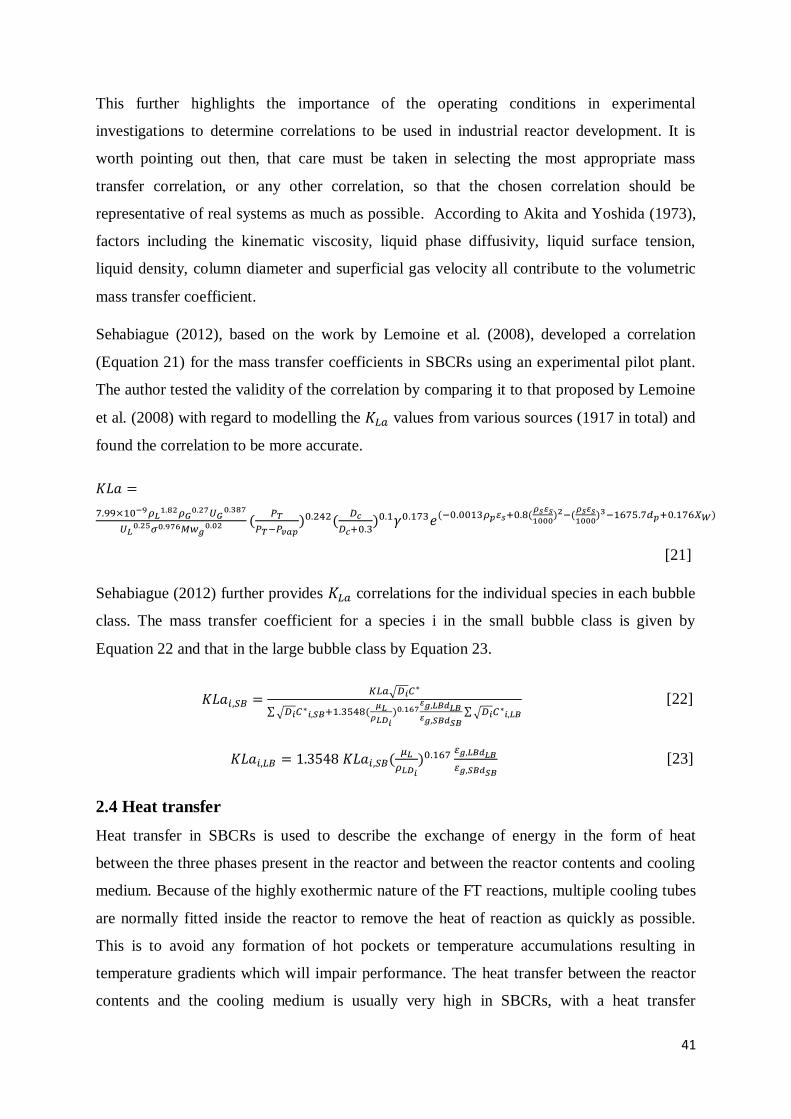
41
This further highlights the importance of the operating conditions in experimental
investigations to determine correlations to be used in industrial reactor development. It is
worth pointing out then, that care must be taken in selecting the most appropriate mass
transfer correlation, or any other correlation, so that the chosen correlation should be
representative of real systems as much as possible. According to Akita and Yoshida (1973),
factors including the kinematic viscosity, liquid phase diffusivity, liquid surface tension,
liquid density, column diameter and superficial gas velocity all contribute to the volumetric
mass transfer coefficient.
Sehabiague (2012), based on the work by Lemoine et al. (2008), developed a correlation
(Equation 21) for the mass transfer coefficients in SBCRs using an experimental pilot plant.
The author tested the validity of the correlation by comparing it to that proposed by Lemoine
et al. (2008) with regard to modelling the 𝐾𝐿𝑎 values from various sources (1917 in total) and
found the correlation to be more accurate.
𝐾𝐿𝑎 =
7.99×10⁻⁹𝜌𝐿1.82𝜌𝐺
0.27𝑈𝐺0.387
𝑈𝐿0.25𝜎0.976𝑀𝑤𝑔
0.02 (𝑃𝑇
𝑃𝑇−𝑃𝑣𝑎𝑝)0.242(
𝐷𝑐
𝐷𝑐+0.3)0.1𝛾0.173𝑒(−0.0013𝜌𝑝 𝑠+0.8(
𝜌𝑠𝜀𝑠1000
)2−(𝜌𝑠𝜀𝑠1000
)3−1675.7𝑑𝑝+0.176𝑋𝑊)
[21]
Sehabiague (2012) further provides 𝐾𝐿𝑎 correlations for the individual species in each bubble
class. The mass transfer coefficient for a species i in the small bubble class is given by
Equation 22 and that in the large bubble class by Equation 23.
𝐾𝐿𝑎𝑖,𝑆𝐵 =𝐾𝐿𝑎√𝐷𝑖𝐶∗
∑ √𝐷𝑖𝐶∗𝑖,𝑆𝐵+1.3548(
𝜇𝐿𝜌𝐿𝐷𝑖
)0.167𝜀𝑔,𝐿𝐵𝑑𝐿𝐵𝜀𝑔,𝑆𝐵𝑑𝑆𝐵
∑ √𝐷𝑖𝐶∗𝑖,𝐿𝐵
[22]
𝐾𝐿𝑎𝑖,𝐿𝐵 = 1.3548 𝐾𝐿𝑎𝑖,𝑆𝐵(𝜇𝐿
𝜌𝐿𝐷𝑖
)0.167 𝑔,𝐿𝐵𝑑𝐿𝐵
𝑔,𝑆𝐵𝑑𝑆𝐵
[23]
2.4 Heat transfer
Heat transfer in SBCRs is used to describe the exchange of energy in the form of heat
between the three phases present in the reactor and between the reactor contents and cooling
medium. Because of the highly exothermic nature of the FT reactions, multiple cooling tubes
are normally fitted inside the reactor to remove the heat of reaction as quickly as possible.
This is to avoid any formation of hot pockets or temperature accumulations resulting in
temperature gradients which will impair performance. The heat transfer between the reactor
contents and the cooling medium is usually very high in SBCRs, with a heat transfer

42
coefficient of approximately 1000 W/m2.K (Krishna and Sie, 2000), mainly because of the
turbulence that prevails in the reactor. This is one of the advantages of SBCRs over other FT
reactors. With this in mind, various authors (Dry, 2002; Satterfield and Huff, 1980; Kuo,
1983; Calderbank et al., 1963; Krishna and Sie, 2000) have deemed it safe to assume that
SBCRs operate isothermally, i.e., the heat of reaction is removed by the cooling medium as
quickly as it is produced. Also, the small size of the catalyst particles used in SBCRs means
temperature gradients can be assumed to be negligible in the catalyst pellets (Rahimpour et
al., 2012).
2.5 Hydrodynamic parameters
2.5.1 Gas hold-up
Gas hold-up is one of the more important parameters with regard to SBCR modelling
(Maretto and Krishna, 1999). It is the volume fraction of gas in the reactor at any one time. A
higher gas hold-up is generally desired as this means there is more gaseous reactant available
for Fischer-Tropsch Synthesis (FTS) per unit volume of the FT reactor bed. Several
correlations for determining the gas hold-up are found in literature (Iliuta et al., 2007;
Maretto and Krishna, 1999; Behkish, 1997). Care should be taken in selecting an appropriate
correlation because not all these correlations are applicable to the same situation. Some of
them are determined under experimental conditions using fluids different to those in FTS and
reactor dimensions much smaller than those in real industrial cases. The use of such
correlations is limited to models describing environments similar to those in the experiments
and this is not useful for developing models for real situations. Typical industrial FT-SBCR
conditions are shown in Table 6.
Gas hold-up is influenced by a variety of factors including operating conditions such
temperature, pressure and superficial gas velocity (Maretto and Krishna, 1999). Liquid
properties are also affect the gas hold-up and these include density, surface tension, viscosity
and vapour pressure (Basha et al., 2015). Structural properties including the column diameter
and sparger type can also have an influence on gas hold-up (Behkish et al., 2006). Gas hold-
up correlations as proposed by different authors are presented in Table 9. Most of these
correlations were developed in experimental conditions significantly different to those in
industrial settings. For example, Bach and Pilhofer (1978) conducted experiments under
ambient temperature and pressure conditions with superficial gas velocities up to 0.2 m/s.
Jordan and Schumpe (2001) and Fan et al. (1999) attempted to use represent real SBCR
operating conditions by using pressures and temperatures in the ranges 0.1-5.32 MPa and
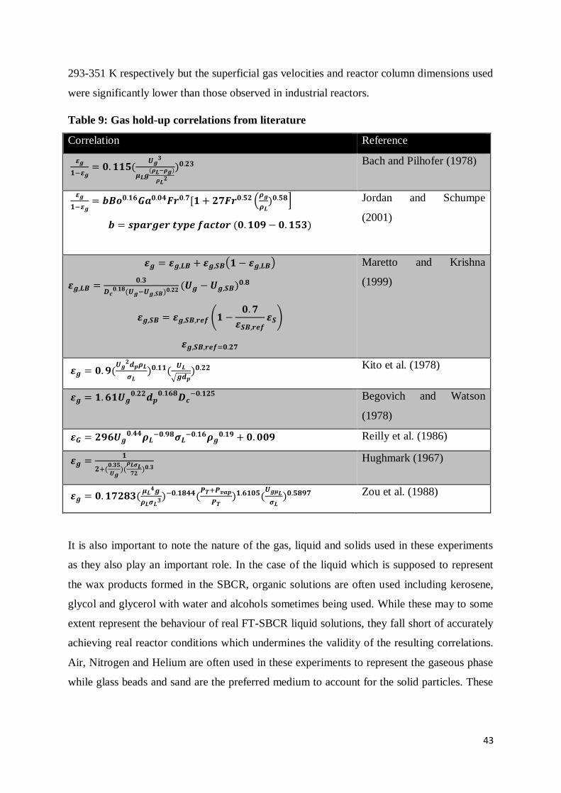
43
293-351 K respectively but the superficial gas velocities and reactor column dimensions used
were significantly lower than those observed in industrial reactors.
Table 9: Gas hold-up correlations from literature
Correlation Reference
𝜺𝒈
𝟏−𝜺𝒈= 𝟎. 𝟏𝟏𝟓(
𝑼𝒈𝟑
𝝁𝑳𝒈(𝝆𝑳−𝝆𝒈)
𝝆𝑳𝟐
)𝟎.𝟐𝟑 Bach and Pilhofer (1978)
𝜺𝒈
𝟏−𝜺𝒈= 𝒃𝑩𝒐𝟎.𝟏𝟔𝑮𝒂𝟎.𝟎𝟒𝑭𝒓𝟎.𝟕[𝟏 + 𝟐𝟕𝑭𝒓𝟎.𝟓𝟐 (
𝝆𝒈
𝝆𝑳)𝟎.𝟓𝟖]
𝒃 = 𝒔𝒑𝒂𝒓𝒈𝒆𝒓 𝒕𝒚𝒑𝒆 𝒇𝒂𝒄𝒕𝒐𝒓 (𝟎. 𝟏𝟎𝟗 − 𝟎. 𝟏𝟓𝟑)
Jordan and Schumpe
(2001)
𝜺𝒈 = 𝜺𝒈,𝑳𝑩 + 𝜺𝒈,𝑺𝑩(𝟏 − 𝜺𝒈,𝑳𝑩)
𝜺𝒈,𝑳𝑩 =𝟎.𝟑
𝑫𝒄𝟎.𝟏𝟖(𝑼𝒈−𝑼𝒈,𝑺𝑩)𝟎.𝟐𝟐
(𝑼𝒈 − 𝑼𝒈,𝑺𝑩)𝟎.𝟖
𝜺𝒈,𝑺𝑩 = 𝜺𝒈,𝑺𝑩,𝒓𝒆𝒇 (𝟏 −𝟎. 𝟕
𝜺𝑺𝑩,𝒓𝒆𝒇𝜺𝑺)
𝜺𝒈,𝑺𝑩,𝒓𝒆𝒇=𝟎.𝟐𝟕
Maretto and Krishna
(1999)
𝜺𝒈 = 𝟎. 𝟗(𝑼𝒈
𝟐𝒅𝒑𝝆𝑳
𝝈𝑳)𝟎.𝟏𝟏(
𝑼𝑳
√𝒈𝒅𝒑)𝟎.𝟐𝟐
Kito et al. (1978)
𝜺𝒈 = 𝟏. 𝟔𝟏𝑼𝒈𝟎.𝟐𝟐𝒅𝒑
𝟎.𝟏𝟔𝟖𝑫𝒄−𝟎.𝟏𝟐𝟓
Begovich and Watson
(1978)
𝜺𝑮 = 𝟐𝟗𝟔𝑼𝒈𝟎.𝟒𝟒𝝆𝑳
−𝟎.𝟗𝟖𝝈𝑳−𝟎.𝟏𝟔𝝆𝒈
𝟎.𝟏𝟗 + 𝟎. 𝟎𝟎𝟗 Reilly et al. (1986)
𝜺𝒈 =𝟏
𝟐+(𝟎.𝟑𝟓
𝑼𝒈)(
𝝆𝑳𝝈𝑳𝟕𝟐
)𝟎.𝟑 Hughmark (1967)
𝜺𝒈 = 𝟎. 𝟏𝟕𝟐𝟖𝟑(𝝁𝑳
𝟒𝒈
𝝆𝑳𝝈𝑳𝟑)−𝟎.𝟏𝟖𝟒𝟒(
𝑷𝑻+𝑷𝒗𝒂𝒑
𝑷𝑻)𝟏.𝟔𝟏𝟎𝟓(
𝑼𝒈𝝁𝑳
𝝈𝑳)𝟎.𝟓𝟖𝟗𝟕 Zou et al. (1988)
It is also important to note the nature of the gas, liquid and solids used in these experiments
as they also play an important role. In the case of the liquid which is supposed to represent
the wax products formed in the SBCR, organic solutions are often used including kerosene,
glycol and glycerol with water and alcohols sometimes being used. While these may to some
extent represent the behaviour of real FT-SBCR liquid solutions, they fall short of accurately
achieving real reactor conditions which undermines the validity of the resulting correlations.
Air, Nitrogen and Helium are often used in these experiments to represent the gaseous phase
while glass beads and sand are the preferred medium to account for the solid particles. These
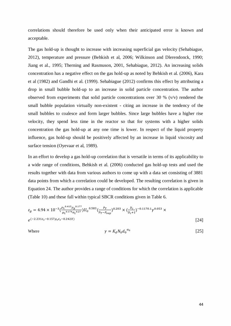
44
correlations should therefore be used only when their anticipated error is known and
acceptable.
The gas hold-up is thought to increase with increasing superficial gas velocity (Sehabiague,
2012), temperature and pressure (Behkish et al, 2006; Wilkinson and Dlerendonck, 1990;
Jiang et al., 1995; Therning and Rasmuson, 2001, Sehabiague, 2012). An increasing solids
concentration has a negative effect on the gas hold-up as noted by Behkish et al. (2006), Kara
et al (1982) and Gandhi et al. (1999). Sehabiague (2012) confirms this effect by attributing a
drop in small bubble hold-up to an increase in solid particle concentration. The author
observed from experiments that solid particle concentrations over 30 % (v/v) rendered the
small bubble population virtually non-existent - citing an increase in the tendency of the
small bubbles to coalesce and form larger bubbles. Since large bubbles have a higher rise
velocity, they spend less time in the reactor so that for systems with a higher solids
concentration the gas hold-up at any one time is lower. In respect of the liquid property
influence, gas hold-up should be positively affected by an increase in liquid viscosity and
surface tension (Oyevaar et al, 1989).
In an effort to develop a gas hold-up correlation that is versatile in terms of its applicability to
a wide range of conditions, Behkish et al. (2006) conducted gas hold-up tests and used the
results together with data from various authors to come up with a data set consisting of 3881
data points from which a correlation could be developed. The resulting correlation is given in
Equation 24. The author provides a range of conditions for which the correlation is applicable
(Table 10) and these fall within typical SBCR conditions given in Table 6.
휀𝑔 = 4.94 × 10⁻³(𝜌𝐿
0.415𝜌𝑔0.177
𝜇𝐿0.174𝜎𝐿
0.27 )𝑈𝐺0.583(
𝑃𝑇
𝑃𝑇−𝑃𝑣𝑎𝑝)0.203 × (
𝐷𝑐
𝐷𝑐+1)−0.1170.1𝛾0.053 ×
𝑒(−2.231 𝑠−0.157𝜌𝑠 𝑠−0.242𝑋) [24]
Where 𝛾 = 𝐾𝑑𝑁0𝑑0𝛼0 [25]
45
Table 10: Applicable range of conditions for Equation 7 (Behkish et al., 2006)
Behkish et al. (2006) determined a correlation for the hold-up of large bubbles in a similar
fashion by using a total of 1426 data points to arrive a correlation shown in Equation 26.
휀𝑔,𝐿𝐵 = 휀𝑔0.84(1 − 3.04 × 10⁻⁶ 𝜌𝐿
0.97
𝜇𝐿0.16 𝑒4.5𝑋𝑊−4.49 𝑠)
= 휀𝐺0.84𝐹 [26]
The small bubble hold-up is determined from the difference between the total gas and large
bubble hold-up thus:
휀g,SB = 휀𝑔 − 휀𝑔,𝐿𝐵 [27]
A condition of the use of Equations 26 and 27 is that 휀𝐺 ≤ 𝐹6.25, otherwise the small bubble
hold-up is low enough to be negligible so that Equation 27 becomes Equation 28. A clear
disadvantage of the correlations put forward by Behkish et al. (2006) is the large number of
parameters that need to be determined beforehand. 𝛾 in particular poses a challenge as the
parameters needed in Equation 25 are difficult to determine. Although sparger design effects
on hydrodynamics have been studied in other fields, there has not been significant work done
on sparger configuration effects in SBCRs presently and as a result Equation 25 should be
treated with caution.
휀𝑔 = 휀𝑔,𝐿𝐵 [28]
46
2.5.2 Liquid hold-up
The liquid phase hold-up can be determined from a balance of the total hold-up as in
Equation 29.
휀𝑙 = 1 − 휀𝐺 − 휀𝑠 [29]
2.5.3 Superficial gas velocity
The superficial gas velocity is divided between the velocities of the individual bubble classes
according to Equation 30. The small bubble superficial velocity can be determined using the
correlation by de Swart (1996) as in Equation 31. The large bubble superficial gas velocity
can then be determined from the difference between the overall and small bubble superficial
gas velocities following Equation 32.
𝑈𝑔 = 𝑈𝑔,𝑆𝐵 + 𝑈𝑔,𝐿𝐵 [30]
𝑈𝑔,𝑆𝐵 = 2.25𝜎𝐿
𝜇𝐿(
𝜎𝐿3𝜌𝐿
𝑔𝜇𝐿4 )−0.273(
𝜌𝐿
𝜌𝑔)0.03 [31]
𝑈𝑔,𝐿𝐵 = 𝑈𝐺 − 𝑈𝑔,𝑆𝐵 [32]
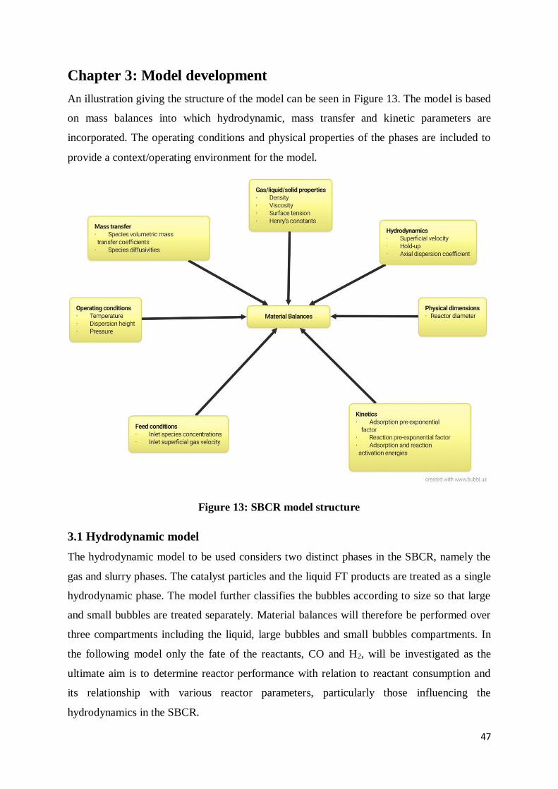
47
Chapter 3: Model development
An illustration giving the structure of the model can be seen in Figure 13. The model is based
on mass balances into which hydrodynamic, mass transfer and kinetic parameters are
incorporated. The operating conditions and physical properties of the phases are included to
provide a context/operating environment for the model.
Figure 13: SBCR model structure
3.1 Hydrodynamic model
The hydrodynamic model to be used considers two distinct phases in the SBCR, namely the
gas and slurry phases. The catalyst particles and the liquid FT products are treated as a single
hydrodynamic phase. The model further classifies the bubbles according to size so that large
and small bubbles are treated separately. Material balances will therefore be performed over
three compartments including the liquid, large bubbles and small bubbles compartments. In
the following model only the fate of the reactants, CO and H2, will be investigated as the
ultimate aim is to determine reactor performance with relation to reactant consumption and
its relationship with various reactor parameters, particularly those influencing the
hydrodynamics in the SBCR.
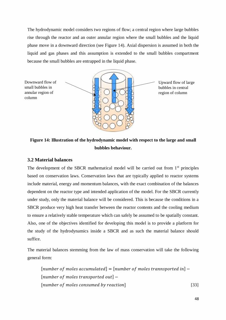
48
The hydrodynamic model considers two regions of flow; a central region where large bubbles
rise through the reactor and an outer annular region where the small bubbles and the liquid
phase move in a downward direction (see Figure 14). Axial dispersion is assumed in both the
liquid and gas phases and this assumption is extended to the small bubbles compartment
because the small bubbles are entrapped in the liquid phase.
Figure 14: Illustration of the hydrodynamic model with respect to the large and small
bubbles behaviour.
3.2 Material balances
The development of the SBCR mathematical model will be carried out from 1st principles
based on conservation laws. Conservation laws that are typically applied to reactor systems
include material, energy and momentum balances, with the exact combination of the balances
dependent on the reactor type and intended application of the model. For the SBCR currently
under study, only the material balance will be considered. This is because the conditions in a
SBCR produce very high heat transfer between the reactor contents and the cooling medium
to ensure a relatively stable temperature which can safely be assumed to be spatially constant.
Also, one of the objectives identified for developing this model is to provide a platform for
the study of the hydrodynamics inside a SBCR and as such the material balance should
suffice.
The material balances stemming from the law of mass conservation will take the following
general form:
[𝑛𝑢𝑚𝑏𝑒𝑟 𝑜𝑓 𝑚𝑜𝑙𝑒𝑠 𝑎𝑐𝑐𝑢𝑚𝑢𝑙𝑎𝑡𝑒𝑑] = [𝑛𝑢𝑚𝑏𝑒𝑟 𝑜𝑓 𝑚𝑜𝑙𝑒𝑠 𝑡𝑟𝑎𝑛𝑛𝑠𝑝𝑜𝑟𝑡𝑒𝑑 𝑖𝑛] −
[𝑛𝑢𝑚𝑏𝑒𝑟 𝑜𝑓 𝑚𝑜𝑙𝑒𝑠 𝑡𝑟𝑎𝑛𝑠𝑝𝑜𝑟𝑡𝑒𝑑 𝑜𝑢𝑡] −
[𝑛𝑢𝑚𝑏𝑒𝑟 𝑜𝑓 𝑚𝑜𝑙𝑒𝑠 𝑐𝑜𝑛𝑠𝑢𝑚𝑒𝑑 𝑏𝑦 𝑟𝑒𝑎𝑐𝑡𝑖𝑜𝑛] [33]
Upward flow of large
bubbles in central
region of column
Downward flow of
small bubbles in
annular region of
column
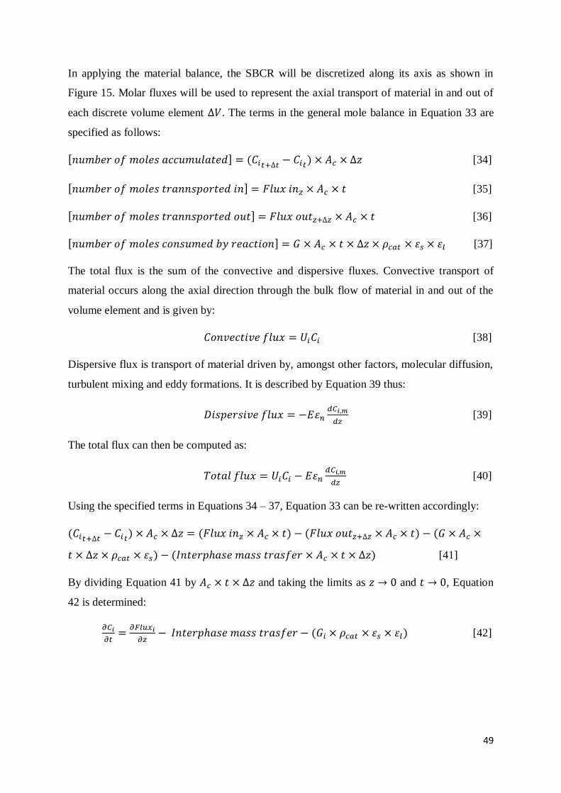
49
In applying the material balance, the SBCR will be discretized along its axis as shown in
Figure 15. Molar fluxes will be used to represent the axial transport of material in and out of
each discrete volume element ∆𝑉. The terms in the general mole balance in Equation 33 are
specified as follows:
[𝑛𝑢𝑚𝑏𝑒𝑟 𝑜𝑓 𝑚𝑜𝑙𝑒𝑠 𝑎𝑐𝑐𝑢𝑚𝑢𝑙𝑎𝑡𝑒𝑑] = (𝐶𝑖𝑡+∆𝑡− 𝐶𝑖𝑡
) × 𝐴𝑐 × ∆𝑧 [34]
[𝑛𝑢𝑚𝑏𝑒𝑟 𝑜𝑓 𝑚𝑜𝑙𝑒𝑠 𝑡𝑟𝑎𝑛𝑛𝑠𝑝𝑜𝑟𝑡𝑒𝑑 𝑖𝑛] = 𝐹𝑙𝑢𝑥 𝑖𝑛𝑧 × 𝐴𝑐 × 𝑡 [35]
[𝑛𝑢𝑚𝑏𝑒𝑟 𝑜𝑓 𝑚𝑜𝑙𝑒𝑠 𝑡𝑟𝑎𝑛𝑛𝑠𝑝𝑜𝑟𝑡𝑒𝑑 𝑜𝑢𝑡] = 𝐹𝑙𝑢𝑥 𝑜𝑢𝑡𝑧+∆𝑧 × 𝐴𝑐 × 𝑡 [36]
[𝑛𝑢𝑚𝑏𝑒𝑟 𝑜𝑓 𝑚𝑜𝑙𝑒𝑠 𝑐𝑜𝑛𝑠𝑢𝑚𝑒𝑑 𝑏𝑦 𝑟𝑒𝑎𝑐𝑡𝑖𝑜𝑛] = 𝐺 × 𝐴𝑐 × 𝑡 × ∆𝑧 × 𝜌𝑐𝑎𝑡 × 휀𝑠 × 휀𝑙 [37]
The total flux is the sum of the convective and dispersive fluxes. Convective transport of
material occurs along the axial direction through the bulk flow of material in and out of the
volume element and is given by:
𝐶𝑜𝑛𝑣𝑒𝑐𝑡𝑖𝑣𝑒 𝑓𝑙𝑢𝑥 = 𝑈𝑖𝐶𝑖 [38]
Dispersive flux is transport of material driven by, amongst other factors, molecular diffusion,
turbulent mixing and eddy formations. It is described by Equation 39 thus:
𝐷𝑖𝑠𝑝𝑒𝑟𝑠𝑖𝑣𝑒 𝑓𝑙𝑢𝑥 = −𝐸휀𝑛𝑑𝐶𝑖,𝑚
𝑑𝑧 [39]
The total flux can then be computed as:
𝑇𝑜𝑡𝑎𝑙 𝑓𝑙𝑢𝑥 = 𝑈𝑖𝐶𝑖 − 𝐸휀𝑛𝑑𝐶𝑖,𝑚
𝑑𝑧 [40]
Using the specified terms in Equations 34 – 37, Equation 33 can be re-written accordingly:
(𝐶𝑖𝑡+∆𝑡− 𝐶𝑖𝑡
) × 𝐴𝑐 × ∆𝑧 = (𝐹𝑙𝑢𝑥 𝑖𝑛𝑧 × 𝐴𝑐 × 𝑡) − (𝐹𝑙𝑢𝑥 𝑜𝑢𝑡𝑧+∆𝑧 × 𝐴𝑐 × 𝑡) − (𝐺 × 𝐴𝑐 ×
𝑡 × ∆𝑧 × 𝜌𝑐𝑎𝑡 × 휀𝑠) − (𝐼𝑛𝑡𝑒𝑟𝑝ℎ𝑎𝑠𝑒 𝑚𝑎𝑠𝑠 𝑡𝑟𝑎𝑠𝑓𝑒𝑟 × 𝐴𝑐 × 𝑡 × ∆𝑧) [41]
By dividing Equation 41 by 𝐴𝑐 × 𝑡 × ∆𝑧 and taking the limits as 𝑧 → 0 and 𝑡 → 0, Equation
42 is determined:
𝜕𝐶𝑖
𝜕𝑡=
𝜕𝐹𝑙𝑢𝑥𝑖
𝜕𝑧− 𝐼𝑛𝑡𝑒𝑟𝑝ℎ𝑎𝑠𝑒 𝑚𝑎𝑠𝑠 𝑡𝑟𝑎𝑠𝑓𝑒𝑟 − (𝐺𝑖 × 𝜌𝑐𝑎𝑡 × 휀𝑠 × 휀𝑙) [42]
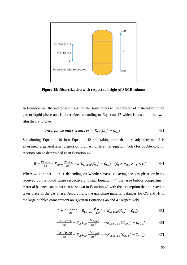
50
Figure 15: Discretization with respect to height of SBCR column
In Equation 42, the interphase mass transfer term refers to the transfer of material from the
gas to liquid phase and is determined according to Equation 17 which is based on the two-
film theory to give:
𝐼𝑛𝑡𝑒𝑟𝑝ℎ𝑎𝑠𝑒 𝑚𝑎𝑠𝑠 𝑡𝑟𝑎𝑛𝑠𝑓𝑒𝑟 = 𝐾𝐿𝑎(𝐶𝑖,𝐿∗ − 𝐶𝑖,𝐿) [43]
Substituting Equation 40 into Equation 42 and taking note that a steady-state model is
envisaged, a general axial dispersion ordinary differential equation (ode) for bubble column
reactors can be determined as in Equation 44.
0 =𝑈𝑑𝐶𝑖,𝑚
𝑑𝑧− 𝐸𝑚휀𝑚
𝑑2𝐶𝑖,𝑚
𝑑𝑧2 + 𝑎∗𝐾𝐿𝑎,𝑖,𝑚(𝐶𝑖,𝐿∗ − 𝐶𝑖,𝐿) – (𝐺𝑖 × 𝜌𝑐𝑎𝑡 × 휀𝑠 × 휀𝑙) [44]
Where 𝑎∗ is either 1 or -1 depending on whether mass is leaving the gas phase or being
received by the liquid phase respectively. Using Equation 44, the large bubble compartment
material balance can be written as shown in Equation 45 with the assumption that no reaction
takes place in the gas phase. Accordingly, the gas phase material balances for CO and H2 in
the large bubbles compartment are given in Equations 46 and 47 respectively.
0 =𝑈𝐿𝐵𝑑𝐶𝑖,𝐿𝐵
𝑑𝑧− 𝐸𝐿𝐵휀𝐿𝐵
𝑑2𝐶𝑖,𝐿𝐵
𝑑𝑧2 + 𝐾𝐿𝑎,𝑖,𝐿𝐵(𝐶𝑖,𝐿∗ − 𝐶𝑖,𝐿) [45]
𝑈𝐿𝐵𝑑𝐶𝐶𝑂,𝐿𝐵
𝑑𝑧− 𝐸𝐿𝐵휀𝐿𝐵
𝑑2𝐶𝐶𝑂,𝐿𝐵
𝑑𝑧2 = −𝐾𝐿𝑎,𝐶𝑂,𝐿𝐵(𝐶𝐶𝑂,𝐿∗ − 𝐶𝐶𝑂,𝐿) [46]
𝑈𝐿𝐵𝑑𝐶𝐻2,𝐿𝐵
𝑑𝑧− 𝐸𝐿𝐵휀𝐿𝐵
𝑑2𝐶𝐻2,𝐿𝐵
𝑑𝑧2 = −𝐾𝐿𝑎,𝐻2 ,𝐿𝐵(𝐶𝐻2 ,𝐿∗ − 𝐶𝐻2 ,𝐿) [47]
51
The small bubbles experience axial dispersion in a similar manner to the liquid phase because
of the assumption previously put forward that the liquid and small bubbles compartments can
be treated as a single pseudo-homogenous phase. The result of this is the inclusion of the
dispersion term in the small bubble compartment material balance. Similar to the large bubble
compartment, it is assumed that no reaction takes place in the small bubbles so that the
balance equation can be written as shown in Equation 48. The material balances for CO and
H2 in the small bubble compartment are given in Equations 49 and 50 respectively.
0 =𝑈𝑆𝐵𝑑𝐶𝑖,𝑆𝐵
𝑑𝑧− 𝐸𝑆𝐵휀𝑆𝐵
𝑑2𝐶𝑖,𝑆𝐵
𝑑𝑧2 + 𝐾𝐿𝑎(𝐶𝑖,𝐿∗ − 𝐶𝑖,𝐿) [48]
𝑈𝑆𝐵𝑑𝐶𝐶𝑂,𝑆𝐵
𝑑𝑧− 𝐸𝑆𝐵휀𝑆𝐵
𝑑2𝐶𝐶𝑂,𝑆𝐵
𝑑𝑧2 = −𝐾𝐿𝑎,𝐶𝑂,𝑆𝐵(𝐶𝑖,𝐿∗ − 𝐶𝑖,𝐿) [49]
𝑈𝑆𝐵𝑑𝐶𝐻2,𝑆𝐵
𝑑𝑧− 𝐸𝑆𝐵휀𝑆𝐵
𝑑2𝐶𝐻2,𝑆𝐵
𝑑𝑧2 = −𝐾𝐿𝑎,𝐻2,𝑆𝐵(𝐶𝑖,𝐿∗ − 𝐶𝑖,𝐿) [50]
It is assumed that the liquid phase experiences axial dispersion and that the FT reaction takes
place only in the liquid phase. Adopting R7 as a representative reaction for FT synthesis in
SBCRs, the consumption rate of H2, 𝐺𝐻2, is twice that of CO, 𝐺𝐶𝑂. The resulting material
balance equation for the liquid phase is written in Equation 51. The CO and H2 material
balances are given in Equations 52 and 53 respectively. In Equations 51 and 52, 𝐺, which
will be represented by Equation 16, is the reaction rate constant. As the gas concentration will
be treated in mol/m3 instead of Pa, the partial pressure terms will be converted to
concentration terms using the ideal gas law so that Equation 16 can be re-written as in
Equation 54.
0 =𝑈𝐿𝑑𝐶𝑖,𝐿
𝑑𝑧− 𝐸𝐿휀𝐿
𝑑2𝐶𝑖,𝐿
𝑑𝑧2 − 𝐾𝐿𝑎,𝑖,𝑆𝐵(𝐶𝑖,𝐿∗ − 𝐶𝑖,𝐿) – 𝐾𝐿𝑎,𝑖,𝐿𝐵(𝐶𝑖,𝐿
∗ − 𝐶𝑖,𝐿) − (𝐺𝑖 × 𝜌𝑐𝑎𝑡 × 휀𝑠 ×
휀𝑙) [51]
𝑈𝐿𝑑𝐶𝐶𝑂,𝐿
𝑑𝑧− 𝐸𝐿휀𝐿
𝑑2𝐶𝐶𝑂,𝐿
𝑑𝑧2 = +𝐾𝐿𝑎,𝐶𝑂,𝑆𝐵(𝐶𝑖,𝐿∗ − 𝐶𝑖,𝐿) + 𝐾𝐿𝑎,𝐶𝑂,𝐿𝐵(𝐶𝑖,𝐿
∗ − 𝐶𝑖,𝐿) + (𝐺𝐶𝑂 × 𝜌𝑐𝑎𝑡 ×
휀𝑠 × 휀𝑙) [52]
52
𝑈𝐿𝑑𝐶𝐻2,𝐿
𝑑𝑧− 𝐸𝐿휀𝐿
𝑑2𝐶𝐻2,𝐿
𝑑𝑧2 = +𝐾𝐿𝑎,𝐻2 ,𝑆𝐵(𝐶𝑖,𝐿∗ − 𝐶𝑖,𝐿) + 𝐾𝐿𝑎,𝐻2,𝐿𝐵(𝐶𝑖,𝐿
∗ − 𝐶𝑖,𝐿) + (𝐺𝐻2× 𝜌𝑐𝑎𝑡 ×
휀𝑠 × 휀𝑙) [53]
R =𝑘𝐶𝐶𝑂,𝐺𝐶𝐻2,𝐺(𝑅𝑇)2
(1+𝑏𝐶𝐶𝑂,𝐺𝑅𝑇)2 [54]
3.2.1 Boundary conditions
The solution to the six odes in Equations 46, 47, 49, 50, 52 and 53 requires the definition of
boundary conditions. Danckwerts-type boundary conditions will be used in this model. For
the odes describing the large bubble compartment, the boundary conditions are applied as
shown in Equations 55 – 57.
𝑎𝑡 𝑧 = 0, 𝐶𝑖,𝐿𝐵 = 𝐶𝑖,𝐺,0 [55]
so that
𝐶𝐶𝑂,𝐿𝐵 = 𝐶𝐶𝑂,𝐺,0 [56]
𝐶𝐻2,𝐿𝐵 = 𝐶𝐻2,𝐺,0 [57]
Similarly, the boundary conditions applicable to the small bubble compartment are defined in
Equations 58 –60.
𝑎𝑡 𝑧 = 0, 𝐶𝑖,𝑆𝐵 = 𝐶𝑖,𝐺,0 [58]
𝐶𝐶𝑂,𝑆𝐵 = 𝐶𝐶𝑂,𝐺,0 [59]
𝐶𝐻2,𝐿𝐵 = 𝐶𝐻2 ,𝐺,0 [60]
The ode’s describing the liquid and small bubble compartments are second order, thus
necessitating the use of two boundary conditions. The Danckwerts-type boundary conditions
were used in this regard. For the liquid phase the boundary conditions adopted are shown in
Equations 61 – 63 (Deckwer, 1991).
𝑑𝐶𝑖,𝐿
𝑑𝑧= −
𝐻𝑈𝐿𝐶𝑖,𝐿
𝐸𝐿 𝐿 [61]
so that
𝑑𝐶𝐶𝑂,𝐿
𝑑𝑧= −
𝐻𝑈𝐿𝐶𝐶𝑂,𝐿
𝐸𝐿 𝐿 [62]
53
𝑑𝐶𝐻2,𝐿
𝑑𝑧= −
𝐻𝑈𝐿𝐶𝐻2,𝐿
𝐸𝐿 𝐿 [63]
For the small bubble compartment, Danckwerts-type boundary conditions as suggested by
Sehabiage (2012) were applied. These are shown in Equations 64 to 66.
𝑈𝑆𝐵𝐶𝑖,𝑆𝐵 − 𝐸𝑆𝐵휀𝑆𝐵𝑑𝐶𝑖,𝑆𝐵
𝑑𝑧= 𝑈𝑆𝐵,0𝐶𝑖,𝑆𝐵,0 [64]
For CO:
𝑈𝑆𝐵𝐶𝐶𝑂,𝑆𝐵 − 𝐸𝑆𝐵휀𝑆𝐵𝑑𝐶𝐶𝑂,𝑆𝐵
𝑑𝑧= 𝑈𝑆𝐵,0𝐶𝐶𝑂,𝑆𝐵,0 [65]
For H2:
𝑈𝑆𝐵𝐶𝐻2 ,𝑆𝐵 − 𝐸𝑆𝐵휀𝑆𝐵𝑑𝐶𝐻2,𝑆𝐵
𝑑𝑧= 𝑈𝑆𝐵,0𝐶𝐻2 ,𝑆𝐵,0 [66]
Dankwerts type boundary conditions were also adopted for the large bubble compartment as
shown below (Sehabiague, 2012):
𝑈𝐿𝐵𝐶𝑖,𝐿𝐵 − 𝐸𝐿𝐵휀𝐿𝐵𝑑𝐶𝑖,𝐿𝐵
𝑑𝑧= 𝑈𝐿𝐵,0𝐶𝑖,𝐿𝐵,0 [67]
For CO:
𝑈𝐿𝐵𝐶𝐶𝑂,𝐿𝐵 − 𝐸𝐿𝐵휀𝐿𝐵𝑑𝐶𝐶𝑂,𝐿𝐵
𝑑𝑧= 𝑈𝐿𝐵,0𝐶𝐶𝑂,𝐿𝐵,0 [68]
For H2:
𝑈𝐿𝐵𝐶𝐻2,𝐿𝐵 − 𝐸𝐿𝐵휀𝐿𝐵𝑑𝐶𝐻2,𝐿𝐵
𝑑𝑧= 𝑈𝐿𝐵,0𝐶𝐻2,𝐿𝐵,0 [69]
54
3.3 Model assumptions summary
A summary of the relevant SBCR system assumptions that were adopted during the model
development phase are given below:
The system is in steady-state
No internal/intra-particle mass transfer resistance
External mass transfer resistance is only present across the gas-liquid interphase
Gas-liquid mass transfer resistance is located on the liquid side of the interphase
Only H2 and CO are present in the feed
No radial dispersion effects are present
Small bubbles hold-up and velocity are independent of axial position
System is isothermal and isobaric
Liquid and solid phases exist as a pseudo-homogenous slurry
3.4 Parameter estimation
3.4.1 Superficial velocity
The parameters included in the material balances need to be determined first before a solution
to the ode’s can be found. The superficial velocity of the small bubbles was calculated based
on the correlation provided by Sehabiague (2012). It is assumed that this parameter is
independent of axial position. It is predominantly affected by the properties of the liquid
phase as shown in Equation 31. The liquid phase in SBCRs operated under the typical
conditions given in Table 6 is mainly a wax product composed of long chain hydrocarbons.
Sehabiague’s (2012) study on the modelling of SBCR considered the liquid properties of a
Sasol wax product with an average carbon number of 80. This product was manufactured by
Moore and Munger, Inc. and is supposedly closely identical to the wax that Sasol produces in
their commercial FT SBCR reactors. This may be the most accurate representation of the
liquid phase properties outside of using a direct liquid sample from a commercially operated
FT SBCR. The surface tension, density and kinematic viscosity were measured under varying
temperatures (290 -500 K). These are given as functions of temperature in Table 11. The
density of the gas was taken to be 7 kg/m3 (Krishna and Sie, 2000). The large bubble
superficial gas velocity is determined from the difference between the overall and small
bubble velocities according to Equation 32.
55
Table 11: SBCR liquid phase properties as functions of temperature (Sehabiague, 2012)
Liquid Property Correlation
Density (kg/m3) ρL = 959.08-0.513T
Viscosity (kg/m.s) μL = e(-4.3284+
2319.4T
)
Surface tension (N/m) σL = 0.001(70.57-0.175T + (1.04 × 10⁻⁴T2)
The overall superficial gas velocity will decrease along the axial direction in the reactor as a
result of a decrease in the moles of total reactants due to consumption by the FT reaction.
This decrease can be modelled through an overall gas phase material balance, i.e.,
𝑑𝑈𝐺𝐶𝐺
𝑑𝑧=
𝑑𝑈𝑆𝐵𝐶𝐶𝑂,𝑆𝐵
𝑑𝑧+
𝑑𝑈𝐿𝐵𝐶𝐶𝑂,𝐿𝐵
𝑑𝑧+
𝑑𝑈𝑆𝐵𝐶𝐻2,𝑆𝐵
𝑑𝑧+
𝑑𝑈𝐿𝐵𝐶𝐻2,𝐿𝐵
𝑑𝑧 [70]
Where 𝑈𝐺 = 𝑈𝐺,0 𝑎𝑡 𝑧 = 0 [71]
And 𝐶𝐺 is the total gas concentration in both large and small bubble compartments:
𝐶𝐺 = 𝐶𝐶𝑂,𝑆𝐵 + 𝐶𝐶𝑂,𝐿𝐵 + 𝐶𝐻2,𝑆𝐵 + 𝐶𝐻2,𝐿𝐵 [72]
The liquid superficial velocity describes the velocity of liquid product as it is drawn from the
reactor and is generally much smaller than the superficial gas velocity, being an order of
magnitude smaller (Dudukovic et al., 1999 and Boyer et al., 2016)
3.4.2 Hold-up
The small bubbles hold-up correlation given in Equation 73 as postulated by Maretto and
Krishna (1999) will be used to determine the volume proportion of small bubbles relative to
the total reactor bed volume. In Equation 73, 휀𝑆𝐵,𝑟𝑒𝑓 refers to the small bubble hold-up in a
liquid phase void of any solid particles and is given as 0.27 for paraffin oil liquid. An 휀𝑆𝐵,𝑟𝑒𝑓
value for a wax product would be more preferable but because of the difficulty of obtaining
such a value, 0.27 will be used until such time that a more representative approximation of
the reference hold-up is determined. A key assumption in Equation 73 is that the small
bubbles hold-up is independent of axial position. The same author put forward a correlation
for the large bubble hold-up which depends on the geometry of the reactor and the velocity
difference between the large and small bubbles as shown in Equation 74. As a result of its
dependence on superficial gas velocity, the large bubbles hold-up will vary relative to axial
position in the reactor as the gas is consumed by the FT reaction. The dependence of the large
bubble hold-up on reactor diameter in Equation 74 only exists for diameters less than 1 m
56
(laboratory or pilot reactors), otherwise, Equation 75 is used instead. The total gas hold-up
will be computed by taking into account the large and small bubble hold-ups and applying
them in Equation 76 (Maretto and Krishna, 1999).
휀𝑆𝐵 = 휀𝑆𝐵 , 𝑟𝑒𝑓 (1 −0.7
𝑆𝐵,𝑟𝑒𝑓 휀𝑆) [73]
휀𝐿𝐵 = 0.3(𝑈𝑔−𝑈𝑔,𝑆𝐵)0.8
𝐷𝐶0.18(𝑈𝑔−𝑈𝑔,𝑆𝐵)0.22 [74]
휀𝐿𝐵 = 0.3(𝑈𝑔−𝑈𝑔,𝑆𝐵)0.8
(𝑈𝑔−𝑈𝑔,𝑆𝐵)0.22 [75]
휀 = 휀𝐿𝐵 + 휀𝑆𝐵(1 − 휀𝐿𝐵) [76]
The liquid phase hold-up can be determined according to Equation 77.
휀𝑙 = 1 − 휀𝑔 − 휀𝑠 [77]
3.4.3 Dispersion coefficients
3.4.3.1 Liquid axial dispersion coefficient
The axial dispersion coefficient for the liquid phase is determined according to the model of
isotropic turbulence developed by Baird and Rice (1975) described in Equation 6. The small
bubbles dispersion coefficient is assumed to be equal to that in the liquid pahse because the
small bubbles are trapped in the liquid phase as a result follow the movement of the liquid
phase (Steynberg and Dry, 2004). The small bubbles dispersion coefficient is given by
Equation 78.
𝐸𝑆𝐵 = 𝐾𝑑𝑐
43⁄ (𝑈𝑔𝑔)
13⁄ [78]
3.4.3.2 Gas phase axial dispersion coefficient
Given the importance of gas phase axial dispersion to SBCR systems exhibiting high
conversion rates, the correlation put forward by Mangartz and Pilhofer (1980) was adopted in
this work to represent the extent of back-mixing the large bubbles.
3.4.4 Mass transfer coefficients
The volumetric mass transfer coefficients through the large and small bubbles are determined
separately and the correlations proposed by Maretto and Krishna (1999) are used in this
regard. The mass transfer coefficient for the large bubbles can be determined through
57
Equation 79 and the coefficients for the specific CO and H2 species can then be calculated in
Equations 80 and 81 respectively.
𝐾𝐿𝑎,𝑖,𝐿𝐵 = 0.5휀𝐿𝐵√𝐷𝑖
𝐷𝑟𝑒𝑓 [79]
𝐾𝐿𝑎,𝐶𝑂,𝐿𝐵 = 0.5휀𝐿𝐵√𝐷𝐶𝑂
𝐷𝑟𝑒𝑓 [80]
𝐾𝐿𝑎,𝐻2,𝐿𝐵 = 0.5휀𝐿𝐵√𝐷𝐻2
𝐷𝑟𝑒𝑓 [81]
For the small bubbles, Equations 82 to 84 will be used for determining the mass transfer
coefficients of the reacting species. 𝐷 and 𝐷𝑟𝑒𝑓 refer to the diffusion coefficient and the
reference diffusion coefficient respectively. Studies by Vermeer and Krishna (1981) (from
Maretto and Krishna, 1999) were able to determine a consistent relationship between the
mass transfer coefficient and gas hold-up using N2-turpentine-5 as the liquid. To extend the
use of this relationship to systems using different fluids, correction factors incorporated into
Equations 79 and 82 were used.
𝐾𝐿𝑎,𝑖,𝑆𝐵 = 휀𝑆𝐵√𝐷𝑖
𝐷𝑟𝑒𝑓 [82]
𝐾𝐿𝑎,𝐶𝑂,𝑆𝐵 = 휀𝑆𝐵√𝐷𝐶𝑂
𝐷𝑟𝑒𝑓 [83]
𝐾𝐿𝑎,𝐻2,𝑆𝐵 = 휀𝑆𝐵√𝐷𝐻2
𝐷𝑟𝑒𝑓 [84]
3.4.5 Henry’s constants
In order to evaluate the mass transfer between the gas and liquid phases, 𝐶𝑖,𝐿∗ must be
converted to 𝐶𝑖,𝑔 with the use of Henry’s constants as in Equation 19. 𝐻𝑖 For gaseous
concentrations defined in moles/m3, as in the current study, 𝐻𝑖 can be expressed in
dimensionless form so that 𝐶𝑖,𝑔 instead of 𝑃𝑖 is determined from Equation 19. Consequently,
Equation 19 can be re-written for 𝐶𝑖,𝑔 (Equation 86) with application of the ideal gas law
(Equation 85). Henry’s constants are functions of temperature and Soriano’s (2005) equations
for CO and H2 Henry’s constants were used (see Equations 87 to 89). These equations were
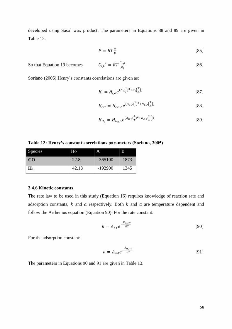
58
developed using Sasol wax product. The parameters in Equations 88 and 89 are given in
Table 12.
𝑃 = 𝑅𝑇𝑛
𝑉 [85]
So that Equation 19 becomes 𝐶𝑖,𝐿∗ = 𝑅𝑇
𝐶𝑖,𝑔
𝐻𝑖 [86]
Soriano (2005) Henry’s constants correlations are given as:
𝐻𝑖 = 𝐻𝑖,𝑜𝑒(𝐴𝑖(1
𝑇)2+𝐵𝑖(
1
𝑇))
[87]
𝐻𝐶𝑂 = 𝐻𝐶𝑂,𝑜𝑒(𝐴𝐶𝑂(1
𝑇)2+𝐵𝐶𝑂(
1
𝑇))
[88]
𝐻𝐻2= 𝐻𝐻2,𝑜𝑒(𝐴𝐻2(
1
𝑇)2+𝐵𝐻2(
1
𝑇))
[89]
Table 12: Henry’s constant correlations parameters (Soriano, 2005)
Species Ho A B
CO 22.8 -365100 1873
H2 42.18 -192900 1345
3.4.6 Kinetic constants
The rate law to be used in this study (Equation 16) requires knowledge of reaction rate and
adsorption constants, 𝑘 and 𝑎 respectively. Both 𝑘 and 𝑎 are temperature dependent and
follow the Arrhenius equation (Equation 90). For the rate constant:
𝑘 = 𝐴𝐹𝑇𝑒−𝐸𝑎,𝐹𝑇
𝑅𝑇 [90]
For the adsorption constant:
𝑎 = 𝐴𝑎𝑑𝑒−𝐸𝑎,𝑎𝑑
𝑅𝑇 [91]
The parameters in Equations 90 and 91 are given in Table 13.
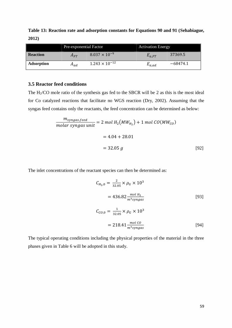
59
Table 13: Reaction rate and adsorption constants for Equations 90 and 91 (Sehabiague,
2012)
Pre-exponential Factor Activation Energy
Reaction 𝐴𝐹𝑇 8.037 × 10⁻⁹ 𝐸𝑎,𝐹𝑇 37369.5
Adsorption 𝐴𝑎𝑑 1.243 × 10⁻¹² 𝐸𝑎,𝑎𝑑 −68474.1
3.5 Reactor feed conditions
The H2/CO mole ratio of the synthesis gas fed to the SBCR will be 2 as this is the most ideal
for Co catalyzed reactions that facilitate no WGS reaction (Dry, 2002). Assuming that the
syngas feed contains only the reactants, the feed concentration can be determined as below:
𝑚𝑠𝑦𝑛𝑔𝑎𝑠,𝑓𝑒𝑒𝑑
𝑚𝑜𝑙𝑎𝑟 𝑠𝑦𝑛𝑔𝑎𝑠 𝑢𝑛𝑖𝑡= 2 𝑚𝑜𝑙 𝐻2(𝑀𝑊𝐻2
) + 1 𝑚𝑜𝑙 𝐶𝑂(𝑀𝑊𝐶𝑂)
= 4.04 + 28.01
= 32.05 𝑔 [92]
The inlet concentrations of the reactant species can then be determined as:
𝐶𝐻2,0 = 2
32.05× 𝜌𝐺 × 103
= 436.82𝑚𝑜𝑙 𝐻2
𝑚3𝑠𝑦𝑛𝑔𝑎𝑠 [93]
𝐶𝐶𝑂,0 = 1
32.05× 𝜌𝐺 × 103
= 218.41𝑚𝑜𝑙 𝐶𝑂
𝑚3𝑠𝑦𝑛𝑔𝑎𝑠 [94]
The typical operating conditions including the physical properties of the material in the three
phases given in Table 6 will be adopted in this study.
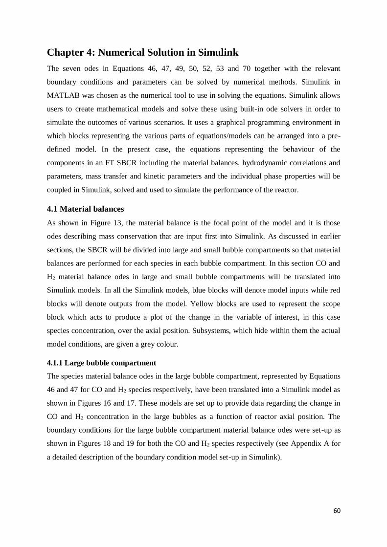
60
Chapter 4: Numerical Solution in Simulink
The seven odes in Equations 46, 47, 49, 50, 52, 53 and 70 together with the relevant
boundary conditions and parameters can be solved by numerical methods. Simulink in
MATLAB was chosen as the numerical tool to use in solving the equations. Simulink allows
users to create mathematical models and solve these using built-in ode solvers in order to
simulate the outcomes of various scenarios. It uses a graphical programming environment in
which blocks representing the various parts of equations/models can be arranged into a pre-
defined model. In the present case, the equations representing the behaviour of the
components in an FT SBCR including the material balances, hydrodynamic correlations and
parameters, mass transfer and kinetic parameters and the individual phase properties will be
coupled in Simulink, solved and used to simulate the performance of the reactor.
4.1 Material balances
As shown in Figure 13, the material balance is the focal point of the model and it is those
odes describing mass conservation that are input first into Simulink. As discussed in earlier
sections, the SBCR will be divided into large and small bubble compartments so that material
balances are performed for each species in each bubble compartment. In this section CO and
H2 material balance odes in large and small bubble compartments will be translated into
Simulink models. In all the Simulink models, blue blocks will denote model inputs while red
blocks will denote outputs from the model. Yellow blocks are used to represent the scope
block which acts to produce a plot of the change in the variable of interest, in this case
species concentration, over the axial position. Subsystems, which hide within them the actual
model conditions, are given a grey colour.
4.1.1 Large bubble compartment
The species material balance odes in the large bubble compartment, represented by Equations
46 and 47 for CO and H2 species respectively, have been translated into a Simulink model as
shown in Figures 16 and 17. These models are set up to provide data regarding the change in
CO and H2 concentration in the large bubbles as a function of reactor axial position. The
boundary conditions for the large bubble compartment material balance odes were set-up as
shown in Figures 18 and 19 for both the CO and H2 species respectively (see Appendix A for
a detailed description of the boundary condition model set-up in Simulink).
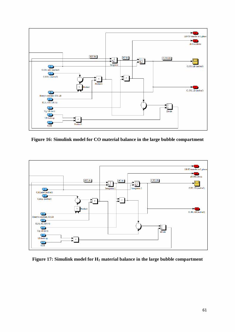
61
Figure 16: Simulink model for CO material balance in the large bubble compartment
Figure 17: Simulink model for H2 material balance in the large bubble compartment
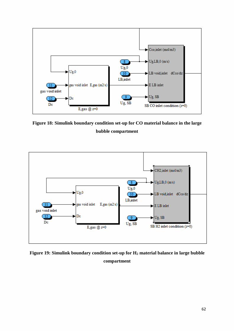
62
Figure 18: Simulink boundary condition set-up for CO material balance in the large
bubble compartment
Figure 19: Simulink boundary condition set-up for H2 material balance in large bubble
compartment
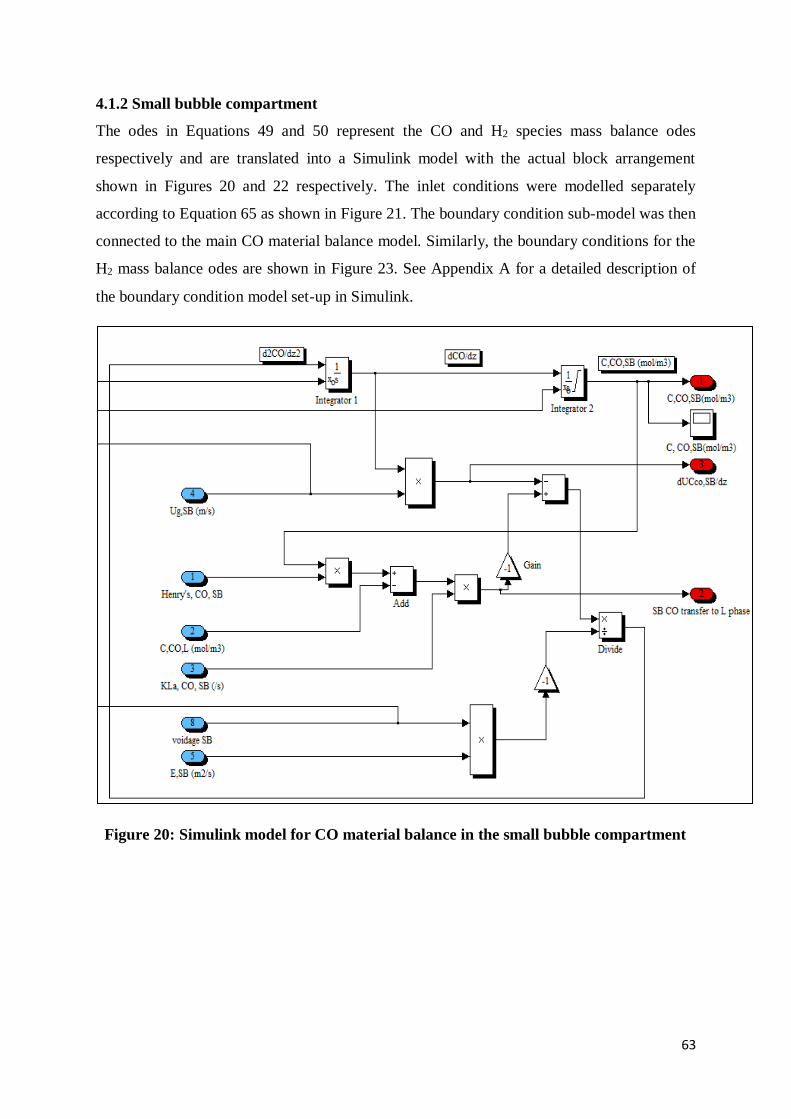
63
4.1.2 Small bubble compartment
The odes in Equations 49 and 50 represent the CO and H2 species mass balance odes
respectively and are translated into a Simulink model with the actual block arrangement
shown in Figures 20 and 22 respectively. The inlet conditions were modelled separately
according to Equation 65 as shown in Figure 21. The boundary condition sub-model was then
connected to the main CO material balance model. Similarly, the boundary conditions for the
H2 mass balance odes are shown in Figure 23. See Appendix A for a detailed description of
the boundary condition model set-up in Simulink.
Figure 20: Simulink model for CO material balance in the small bubble compartment
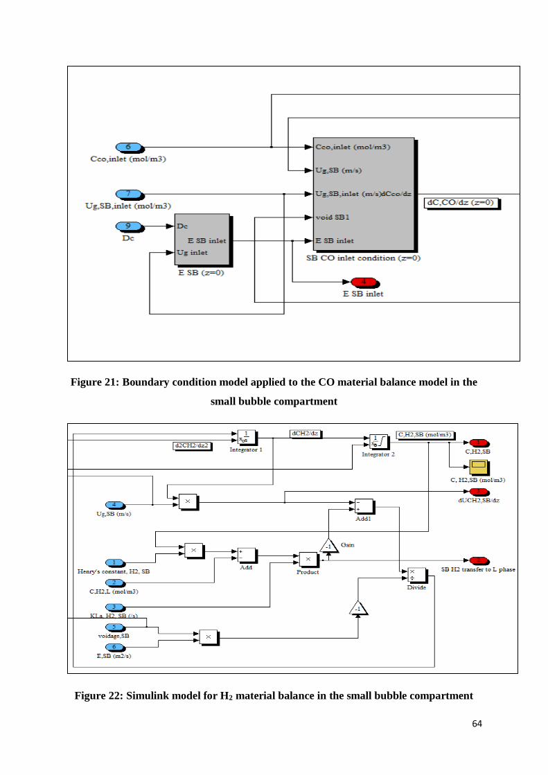
64
Figure 21: Boundary condition model applied to the CO material balance model in the
small bubble compartment
Figure 22: Simulink model for H2 material balance in the small bubble compartment
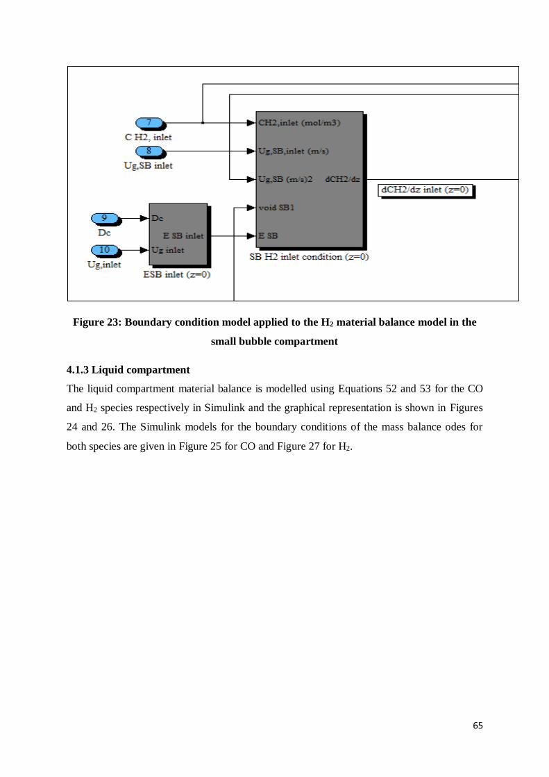
65
Figure 23: Boundary condition model applied to the H2 material balance model in the
small bubble compartment
4.1.3 Liquid compartment
The liquid compartment material balance is modelled using Equations 52 and 53 for the CO
and H2 species respectively in Simulink and the graphical representation is shown in Figures
24 and 26. The Simulink models for the boundary conditions of the mass balance odes for
both species are given in Figure 25 for CO and Figure 27 for H2.
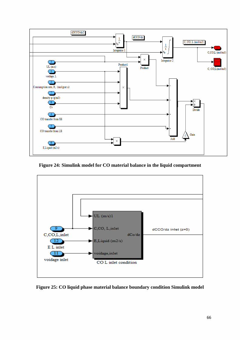
66
Figure 24: Simulink model for CO material balance in the liquid compartment
Figure 25: CO liquid phase material balance boundary condition Simulink model
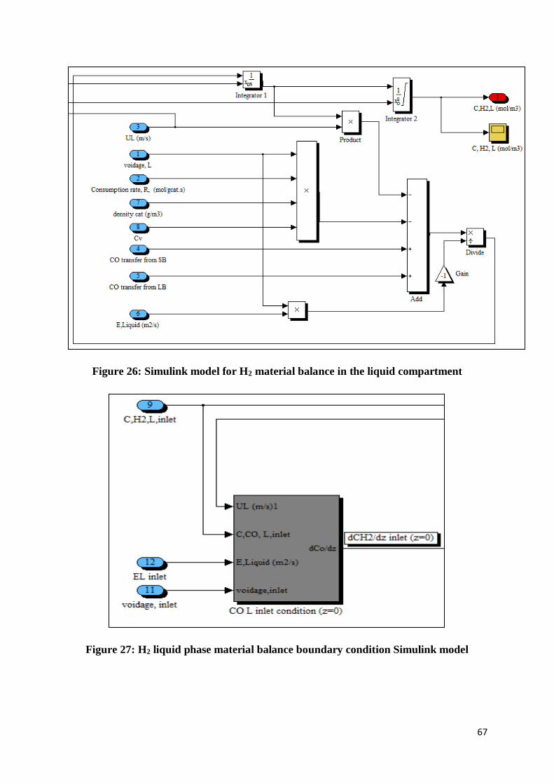
67
Figure 26: Simulink model for H2 material balance in the liquid compartment
Figure 27: H2 liquid phase material balance boundary condition Simulink model
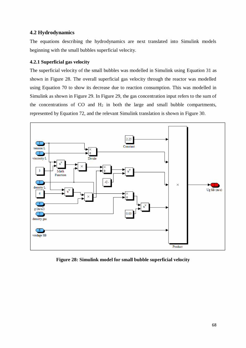
68
4.2 Hydrodynamics
The equations describing the hydrodynamics are next translated into Simulink models
beginning with the small bubbles superficial velocity.
4.2.1 Superficial gas velocity
The superficial velocity of the small bubbles was modelled in Simulink using Equation 31 as
shown in Figure 28. The overall superficial gas velocity through the reactor was modelled
using Equation 70 to show its decrease due to reaction consumption. This was modelled in
Simulink as shown in Figure 29. In Figure 29, the gas concentration input refers to the sum of
the concentrations of CO and H2 in both the large and small bubble compartments,
represented by Equation 72, and the relevant Simulink translation is shown in Figure 30.
Figure 28: Simulink model for small bubble superficial velocity
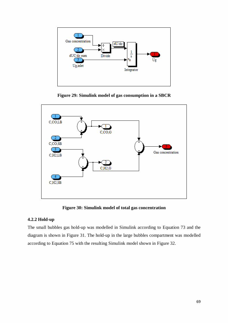
69
Figure 29: Simulink model of gas consumption in a SBCR
Figure 30: Simulink model of total gas concentration
4.2.2 Hold-up
The small bubbles gas hold-up was modelled in Simulink according to Equation 73 and the
diagram is shown in Figure 31. The hold-up in the large bubbles compartment was modelled
according to Equation 75 with the resulting Simulink model shown in Figure 32.
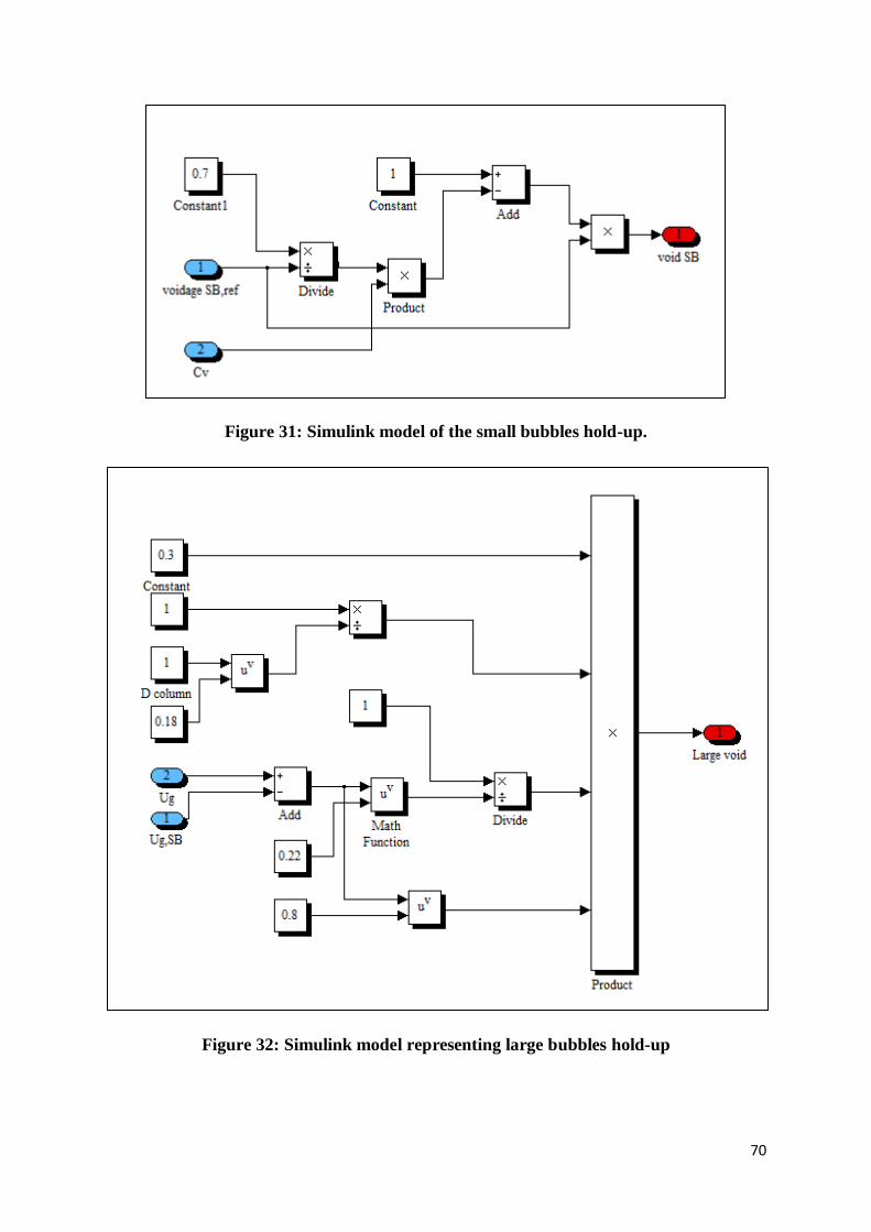
70
Figure 31: Simulink model of the small bubbles hold-up.
Figure 32: Simulink model representing large bubbles hold-up
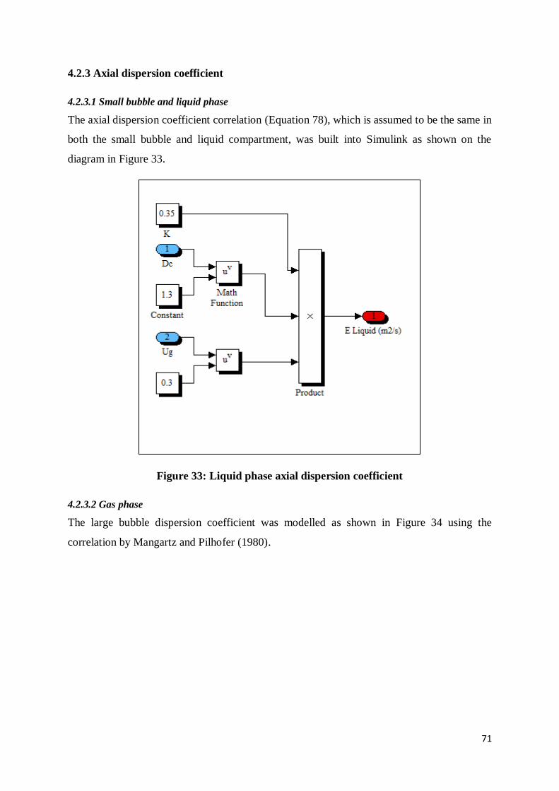
71
4.2.3 Axial dispersion coefficient
4.2.3.1 Small bubble and liquid phase
The axial dispersion coefficient correlation (Equation 78), which is assumed to be the same in
both the small bubble and liquid compartment, was built into Simulink as shown on the
diagram in Figure 33.
Figure 33: Liquid phase axial dispersion coefficient
4.2.3.2 Gas phase
The large bubble dispersion coefficient was modelled as shown in Figure 34 using the
correlation by Mangartz and Pilhofer (1980).
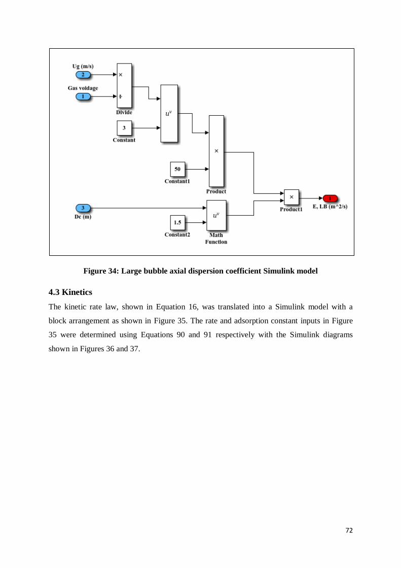
72
Figure 34: Large bubble axial dispersion coefficient Simulink model
4.3 Kinetics
The kinetic rate law, shown in Equation 16, was translated into a Simulink model with a
block arrangement as shown in Figure 35. The rate and adsorption constant inputs in Figure
35 were determined using Equations 90 and 91 respectively with the Simulink diagrams
shown in Figures 36 and 37.
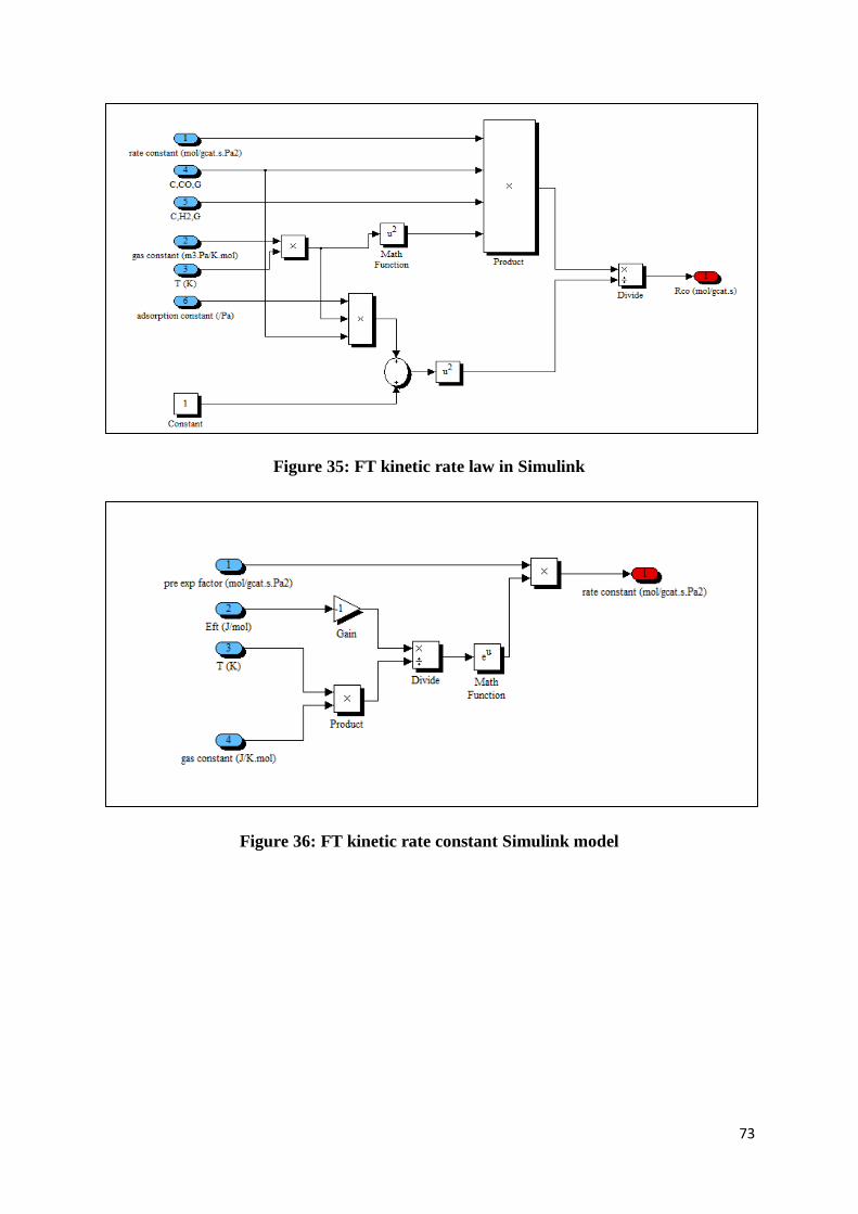
73
Figure 35: FT kinetic rate law in Simulink
Figure 36: FT kinetic rate constant Simulink model

74
Figure 37: Simulink model of the FT adsorption rate constant
4.4 Mass transfer
The gas-liquid volumetric mass transfer coefficient correlations for CO in the large (Equation
80) and small bubble (Equation 83) compartments were translated into Simulink models as
shown in Figures 38 and 39 respectively. Simulink models of the correlations for H2
volumetric mass transfer coefficients in the large and small bubble compartments according
to Equations 81 and 84 respectively, are shown in Figures 40 and 41.
Figure 38: CO Kla Simulink model for the large bubble compartment
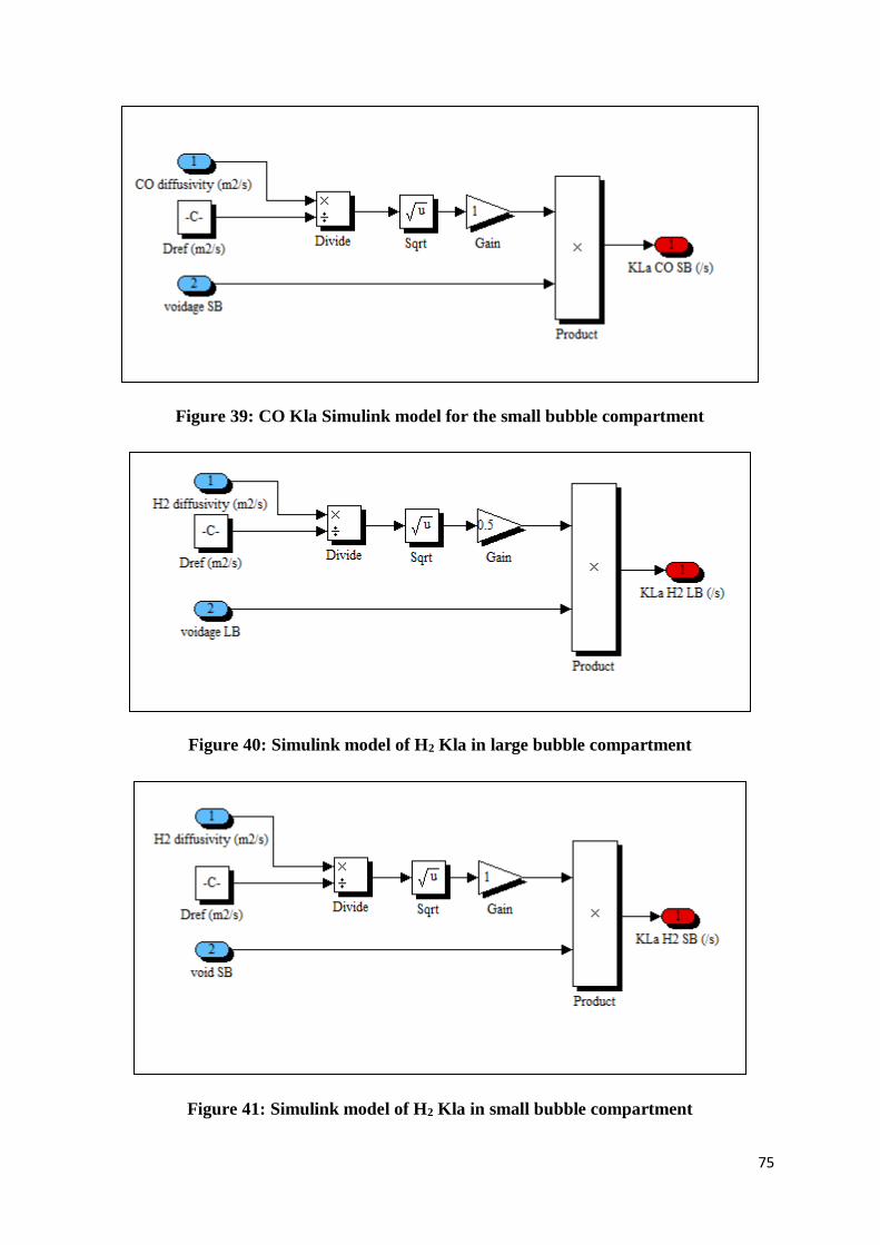
75
Figure 39: CO Kla Simulink model for the small bubble compartment
Figure 40: Simulink model of H2 Kla in large bubble compartment
Figure 41: Simulink model of H2 Kla in small bubble compartment
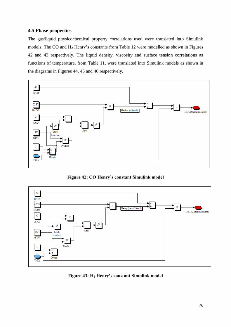
76
4.5 Phase properties
The gas/liquid physicochemical property correlations used were translated into Simulink
models. The CO and H2 Henry’s constants from Table 12 were modelled as shown in Figures
42 and 43 respectively. The liquid density, viscosity and surface tension correlations as
functions of temperature, from Table 11, were translated into Simulink models as shown in
the diagrams in Figures 44, 45 and 46 respectively.
Figure 42: CO Henry’s constant Simulink model
Figure 43: H2 Henry’s constant Simulink model
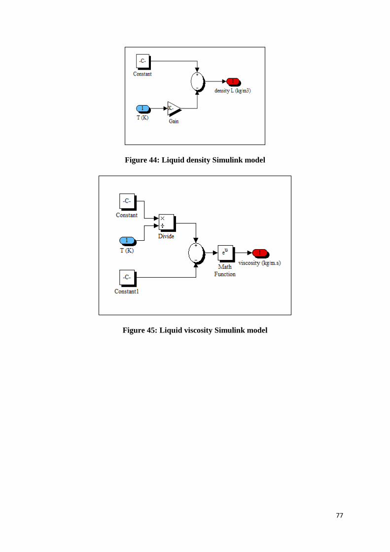
77
Figure 44: Liquid density Simulink model
Figure 45: Liquid viscosity Simulink model

78
Figure 46: Liquid surface tension Simulink model

79
Fig
ure
47
: O
ver
all
SB
CR
Sim
uli
nk
mod
el
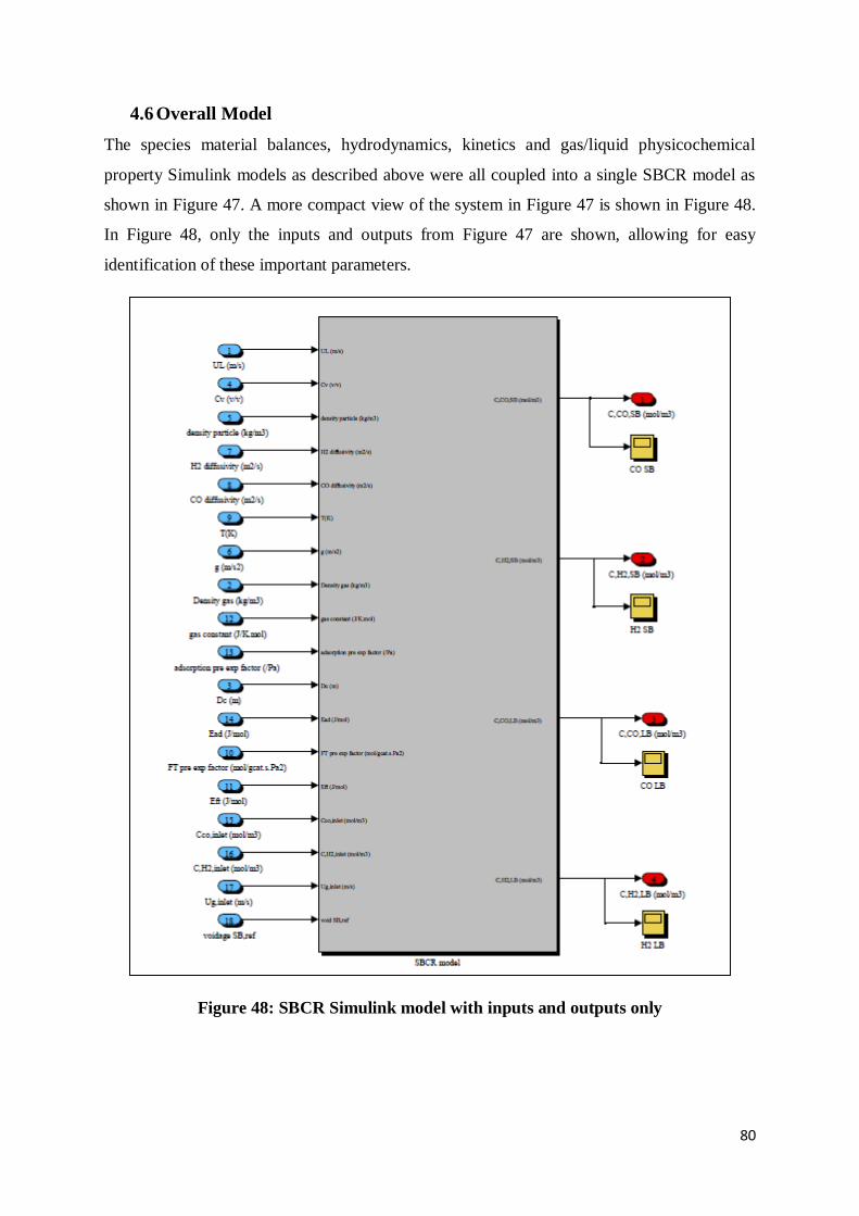
80
4.6 Overall Model
The species material balances, hydrodynamics, kinetics and gas/liquid physicochemical
property Simulink models as described above were all coupled into a single SBCR model as
shown in Figure 47. A more compact view of the system in Figure 47 is shown in Figure 48.
In Figure 48, only the inputs and outputs from Figure 47 are shown, allowing for easy
identification of these important parameters.
Figure 48: SBCR Simulink model with inputs and outputs only
81
Chapter 5: Simulation results and discussion
5.1 Results
The constructed model was simulated as per the typical SBCR conditions given in Table 6
and the feed conditions mentioned above. A detailed set of input conditions are given below
in Table 14. The Simulink simulation was run between a height of 0 and 30 m, resulting in
changes across the various reactor parameters. To provide a brief summary of the behaviour
of the SBCR according to the simulation, the affected parameters are given at the final height
of 30 m and compared to those at the inlet (H=0 m) in Table 15. A more detailed analysis of
the results will follow in the discussion section. The reactant concentrations in all phases
decrease over the height of the reactor as is expected, given the assumption of axial
dispersion in all phases. The zero species concentrations in the small bubbles and liquid
phases does not represent a total non-existence of the species in these phases but alludes to a
balance between the gas/liquid mass transfer and reaction rates at these points as shall be
discussed in the next section. The syngas conversion was calculated using Equation 95.
𝑋𝐶𝑂+𝐻2=
(𝐶𝐶𝑂+𝐶𝐻2 )𝑖𝑛𝑙𝑒𝑡−(𝐶𝐶𝑂+𝐶𝐻2)𝑜𝑢𝑡𝑙𝑒𝑡
(𝐶𝐶𝑂+𝐶𝐻2 )𝑖𝑛𝑙𝑒𝑡× 100 [95]
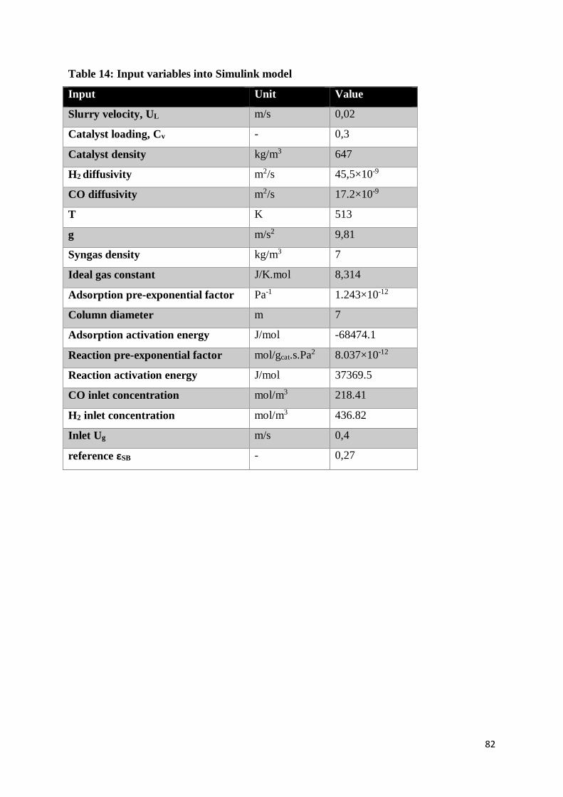
82
Table 14: Input variables into Simulink model
Input Unit Value
Slurry velocity, UL m/s 0,02
Catalyst loading, Cv - 0,3
Catalyst density kg/m3 647
H2 diffusivity m2/s 45,5×10⁻⁹
CO diffusivity m2/s 17.2×10⁻⁹
T K 513
g m/s2 9,81
Syngas density kg/m3 7
Ideal gas constant J/K.mol 8,314
Adsorption pre-exponential factor Pa-1 1.243×10⁻¹²
Column diameter m 7
Adsorption activation energy J/mol -68474.1
Reaction pre-exponential factor mol/gcat.s.Pa2 8.037×10⁻¹²
Reaction activation energy J/mol 37369.5
CO inlet concentration mol/m3 218.41
H2 inlet concentration mol/m3 436.82
Inlet Ug m/s 0,4
reference εSB - 0,27
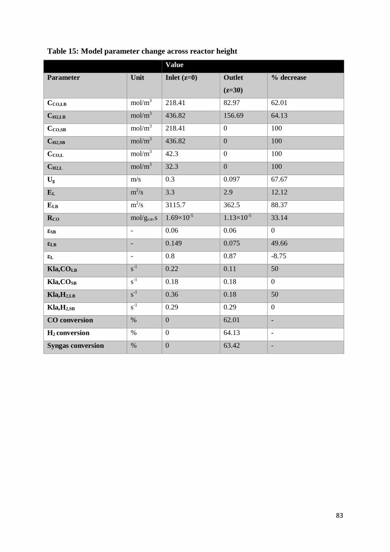
83
Table 15: Model parameter change across reactor height
Value
Parameter Unit Inlet (z=0) Outlet
(z=30)
% decrease
CCO,LB mol/m3 218.41 82.97 62.01
CH2,LB mol/m3 436.82 156.69 64.13
CCO,SB mol/m3 218.41 0 100
CH2,SB mol/m3 436.82 0 100
CCO,L mol/m3 42.3 0 100
CH2,L mol/m3 32.3 0 100
Ug m/s 0.3 0.097 67.67
EL m2/s 3.3 2.9 12.12
ELB m2/s 3115.7 362.5 88.37
RCO mol/gcat.s 1.69×10⁻⁵ 1.13×10⁻⁵ 33.14
εSB - 0.06 0.06 0
εLB - 0.149 0.075 49.66
εL - 0.8 0.87 -8.75
Kla,COLB s-1 0.22 0.11 50
Kla,COSB s-1 0.18 0.18 0
Kla,H2,LB s-1 0.36 0.18 50
Kla,H2,SB s-1 0.29 0.29 0
CO conversion % 0 62.01 -
H2 conversion % 0 64.13 -
Syngas conversion % 0 63.42 -
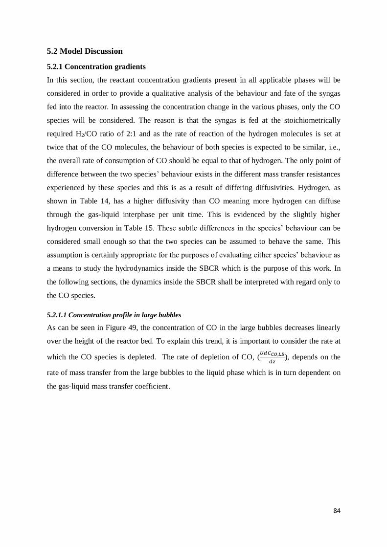
84
5.2 Model Discussion
5.2.1 Concentration gradients
In this section, the reactant concentration gradients present in all applicable phases will be
considered in order to provide a qualitative analysis of the behaviour and fate of the syngas
fed into the reactor. In assessing the concentration change in the various phases, only the CO
species will be considered. The reason is that the syngas is fed at the stoichiometrically
required H2/CO ratio of 2:1 and as the rate of reaction of the hydrogen molecules is set at
twice that of the CO molecules, the behaviour of both species is expected to be similar, i.e.,
the overall rate of consumption of CO should be equal to that of hydrogen. The only point of
difference between the two species’ behaviour exists in the different mass transfer resistances
experienced by these species and this is as a result of differing diffusivities. Hydrogen, as
shown in Table 14, has a higher diffusivity than CO meaning more hydrogen can diffuse
through the gas-liquid interphase per unit time. This is evidenced by the slightly higher
hydrogen conversion in Table 15. These subtle differences in the species’ behaviour can be
considered small enough so that the two species can be assumed to behave the same. This
assumption is certainly appropriate for the purposes of evaluating either species’ behaviour as
a means to study the hydrodynamics inside the SBCR which is the purpose of this work. In
the following sections, the dynamics inside the SBCR shall be interpreted with regard only to
the CO species.
5.2.1.1 Concentration profile in large bubbles
As can be seen in Figure 49, the concentration of CO in the large bubbles decreases linearly
over the height of the reactor bed. To explain this trend, it is important to consider the rate at
which the CO species is depleted. The rate of depletion of CO, (𝑈𝑑𝐶𝐶𝑂,𝐿𝐵
𝑑𝑧), depends on the
rate of mass transfer from the large bubbles to the liquid phase which is in turn dependent on
the gas-liquid mass transfer coefficient.
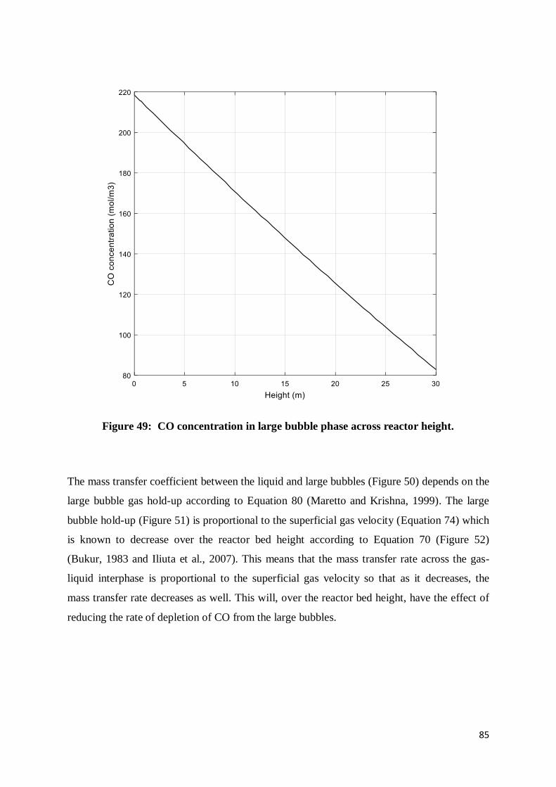
85
Figure 49: CO concentration in large bubble phase across reactor height.
The mass transfer coefficient between the liquid and large bubbles (Figure 50) depends on the
large bubble gas hold-up according to Equation 80 (Maretto and Krishna, 1999). The large
bubble hold-up (Figure 51) is proportional to the superficial gas velocity (Equation 74) which
is known to decrease over the reactor bed height according to Equation 70 (Figure 52)
(Bukur, 1983 and Iliuta et al., 2007). This means that the mass transfer rate across the gas-
liquid interphase is proportional to the superficial gas velocity so that as it decreases, the
mass transfer rate decreases as well. This will, over the reactor bed height, have the effect of
reducing the rate of depletion of CO from the large bubbles.
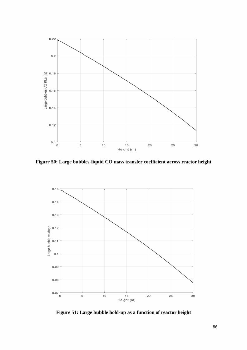
86
Figure 50: Large bubbles-liquid CO mass transfer coefficient across reactor height
Figure 51: Large bubble hold-up as a function of reactor height
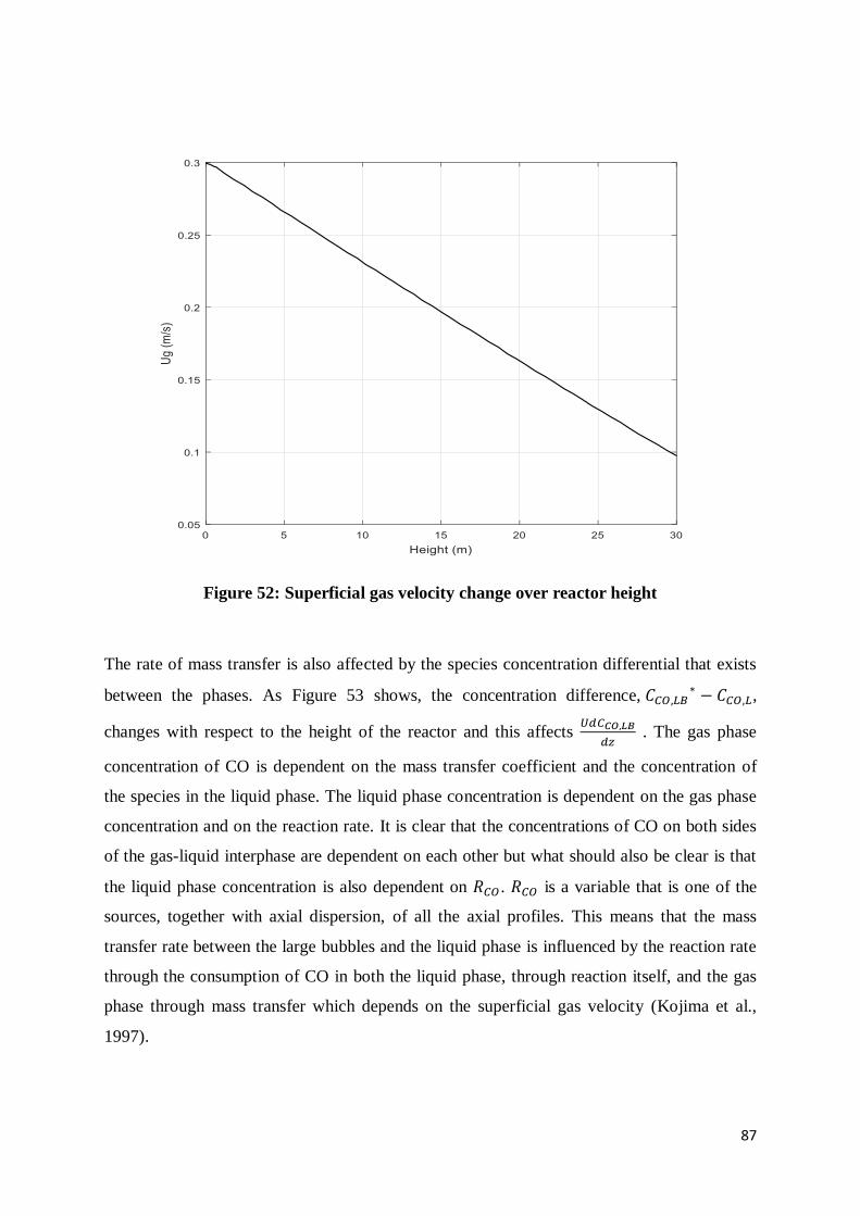
87
Figure 52: Superficial gas velocity change over reactor height
The rate of mass transfer is also affected by the species concentration differential that exists
between the phases. As Figure 53 shows, the concentration difference, 𝐶𝐶𝑂,𝐿𝐵∗ − 𝐶𝐶𝑂,𝐿,
changes with respect to the height of the reactor and this affects 𝑈𝑑𝐶𝐶𝑂,𝐿𝐵
𝑑𝑧 . The gas phase
concentration of CO is dependent on the mass transfer coefficient and the concentration of
the species in the liquid phase. The liquid phase concentration is dependent on the gas phase
concentration and on the reaction rate. It is clear that the concentrations of CO on both sides
of the gas-liquid interphase are dependent on each other but what should also be clear is that
the liquid phase concentration is also dependent on 𝑅𝐶𝑂. 𝑅𝐶𝑂 is a variable that is one of the
sources, together with axial dispersion, of all the axial profiles. This means that the mass
transfer rate between the large bubbles and the liquid phase is influenced by the reaction rate
through the consumption of CO in both the liquid phase, through reaction itself, and the gas
phase through mass transfer which depends on the superficial gas velocity (Kojima et al.,
1997).
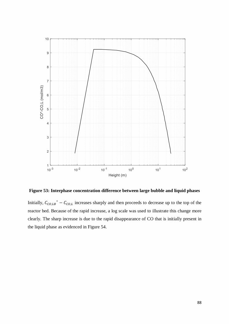
88
Figure 53: Interphase concentration difference between large bubble and liquid phases
Initially, 𝐶𝐶𝑂,𝐿𝐵∗ − 𝐶𝐶𝑂,𝐿 increases sharply and then proceeds to decrease up to the top of the
reactor bed. Because of the rapid increase, a log scale was used to illustrate this change more
clearly. The sharp increase is due to the rapid disappearance of CO that is initially present in
the liquid phase as evidenced in Figure 54.
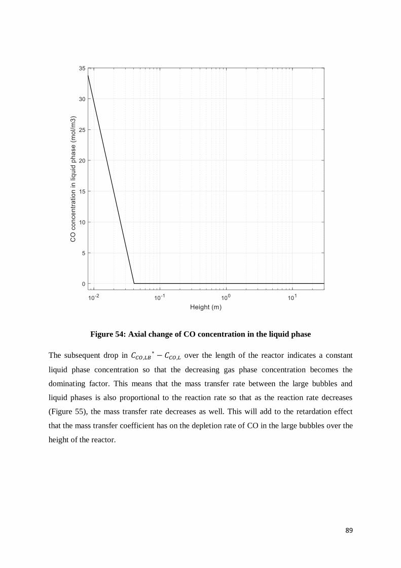
89
Figure 54: Axial change of CO concentration in the liquid phase
The subsequent drop in 𝐶𝐶𝑂,𝐿𝐵∗ − 𝐶𝐶𝑂,𝐿 over the length of the reactor indicates a constant
liquid phase concentration so that the decreasing gas phase concentration becomes the
dominating factor. This means that the mass transfer rate between the large bubbles and
liquid phases is also proportional to the reaction rate so that as the reaction rate decreases
(Figure 55), the mass transfer rate decreases as well. This will add to the retardation effect
that the mass transfer coefficient has on the depletion rate of CO in the large bubbles over the
height of the reactor.

90
Figure 55: CO reaction rate as a function of reactor height
𝑈𝑑𝐶𝐶𝑂,𝐿𝐵
𝑑𝑧 is also affected by the extent of dispersion in the large bubbles. According to
Equation 46, dispersion in the large bubble class depends on the large bubble hold-up (Figure
51) and the large bubbles dispersion coefficient (Figure 56).
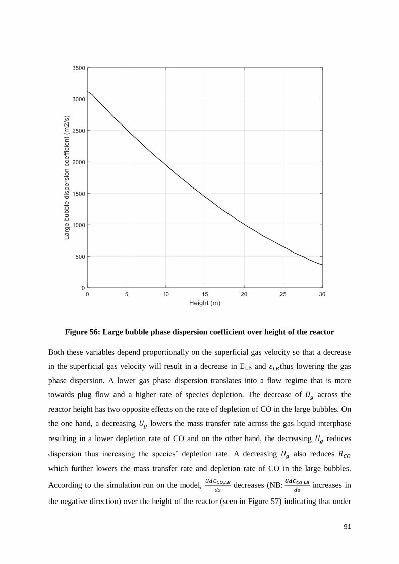
91
Figure 56: Large bubble phase dispersion coefficient over height of the reactor
Both these variables depend proportionally on the superficial gas velocity so that a decrease
in the superficial gas velocity will result in a decrease in ELB and 휀𝐿𝐵thus lowering the gas
phase dispersion. A lower gas phase dispersion translates into a flow regime that is more
towards plug flow and a higher rate of species depletion. The decrease of 𝑈𝑔 across the
reactor height has two opposite effects on the rate of depletion of CO in the large bubbles. On
the one hand, a decreasing 𝑈𝑔 lowers the mass transfer rate across the gas-liquid interphase
resulting in a lower depletion rate of CO and on the other hand, the decreasing 𝑈𝑔 reduces
dispersion thus increasing the species’ depletion rate. A decreasing 𝑈𝑔 also reduces 𝑅𝐶𝑂
which further lowers the mass transfer rate and depletion rate of CO in the large bubbles.
According to the simulation run on the model, 𝑈𝑑𝐶𝐶𝑂,𝐿𝐵
𝑑𝑧 decreases (NB:
𝑼𝒅𝑪𝑪𝑶,𝑳𝑩
𝒅𝒛 increases in
the negative direction) over the height of the reactor (seen in Figure 57) indicating that under
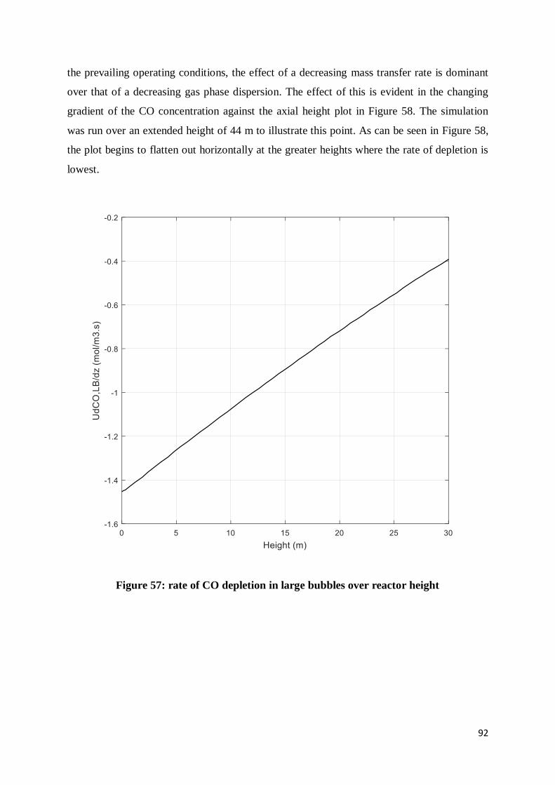
92
the prevailing operating conditions, the effect of a decreasing mass transfer rate is dominant
over that of a decreasing gas phase dispersion. The effect of this is evident in the changing
gradient of the CO concentration against the axial height plot in Figure 58. The simulation
was run over an extended height of 44 m to illustrate this point. As can be seen in Figure 58,
the plot begins to flatten out horizontally at the greater heights where the rate of depletion is
lowest.
Figure 57: rate of CO depletion in large bubbles over reactor height
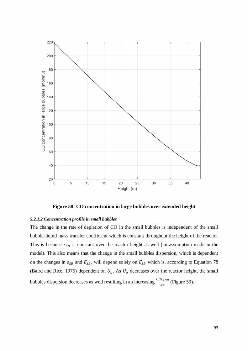
93
Figure 58: CO concentration in large bubbles over extended height
5.2.1.2 Concentration profile in small bubbles
The change in the rate of depletion of CO in the small bubbles is independent of the small
bubble-liquid mass transfer coefficient which is constant throughout the height of the reactor.
This is because 휀𝑆𝐵 is constant over the reactor height as well (an assumption made in the
model). This also means that the change in the small bubbles dispersion, which is dependent
on the changes in 휀𝑆𝐵 and 𝐸𝑆𝐵 , will depend solely on 𝐸𝑆𝐵 which is, according to Equation 78
(Baird and Rice, 1975) dependent on 𝑈𝑔. As 𝑈𝑔 decreases over the reactor height, the small
bubbles dispersion decreases as well resulting in an increasing 𝑈𝑑𝐶𝑖,𝑆𝐵
𝑑𝑧 (Figure 59).
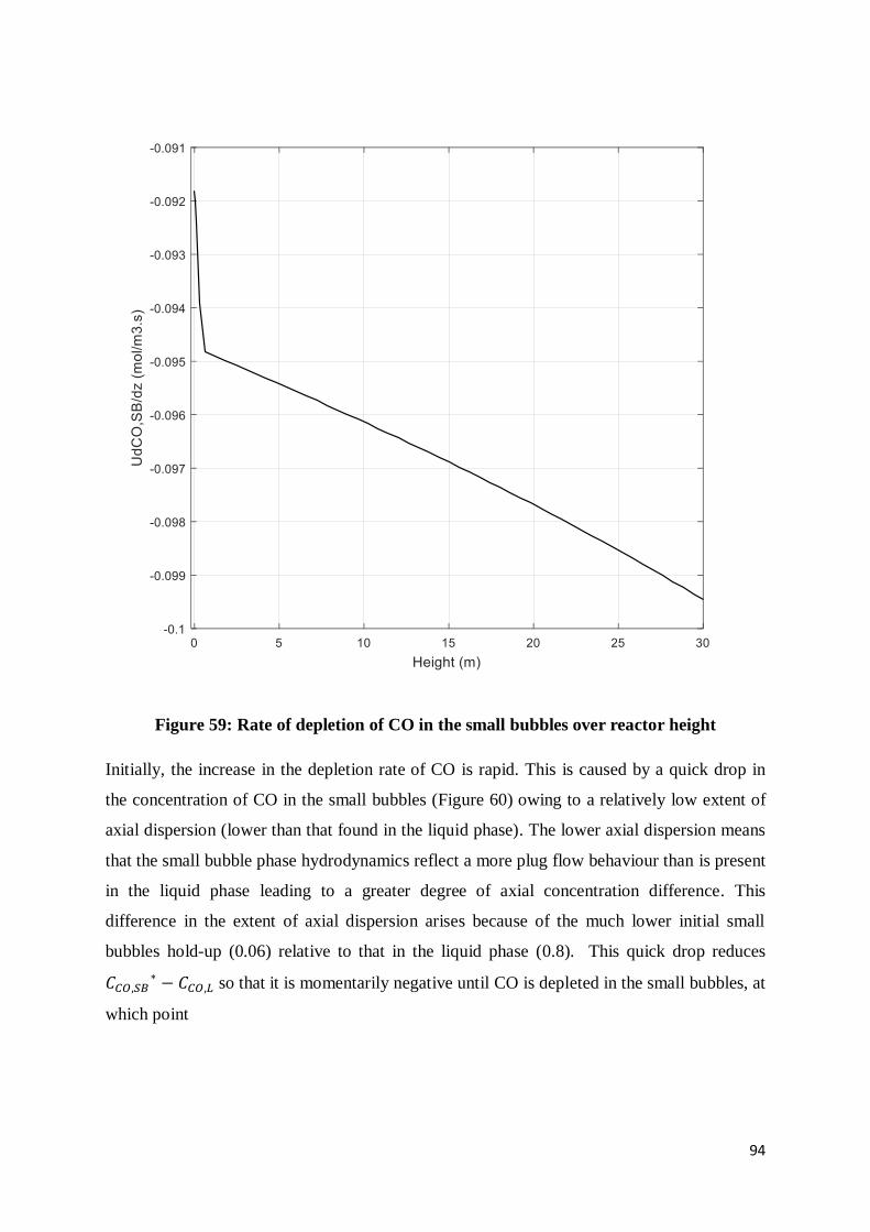
94
Figure 59: Rate of depletion of CO in the small bubbles over reactor height
Initially, the increase in the depletion rate of CO is rapid. This is caused by a quick drop in
the concentration of CO in the small bubbles (Figure 60) owing to a relatively low extent of
axial dispersion (lower than that found in the liquid phase). The lower axial dispersion means
that the small bubble phase hydrodynamics reflect a more plug flow behaviour than is present
in the liquid phase leading to a greater degree of axial concentration difference. This
difference in the extent of axial dispersion arises because of the much lower initial small
bubbles hold-up (0.06) relative to that in the liquid phase (0.8). This quick drop reduces
𝐶𝐶𝑂,𝑆𝐵∗ − 𝐶𝐶𝑂,𝐿 so that it is momentarily negative until CO is depleted in the small bubbles, at
which point
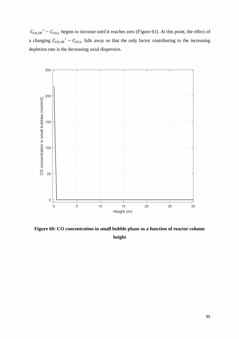
95
𝐶𝐶𝑂,𝑆𝐵∗ − 𝐶𝐶𝑂,𝐿 begins to increase until it reaches zero (Figure 61). At this point, the effect of
a changing 𝐶𝐶𝑂,𝑆𝐵∗ − 𝐶𝐶𝑂,𝐿 falls away so that the only factor contributing to the increasing
depletion rate is the decreasing axial dispersion.
Figure 60: CO concentration in small bubble phase as a function of reactor column
height
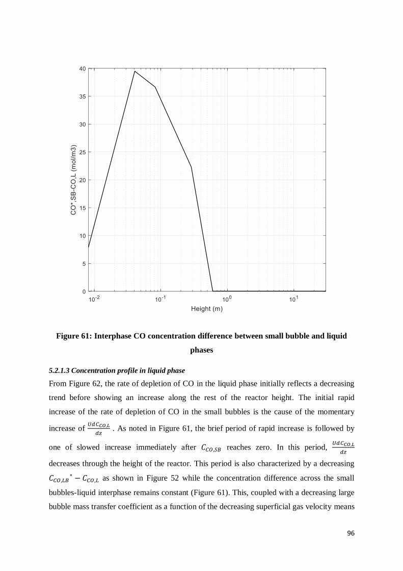
96
Figure 61: Interphase CO concentration difference between small bubble and liquid
phases
5.2.1.3 Concentration profile in liquid phase
From Figure 62, the rate of depletion of CO in the liquid phase initially reflects a decreasing
trend before showing an increase along the rest of the reactor height. The initial rapid
increase of the rate of depletion of CO in the small bubbles is the cause of the momentary
increase of 𝑈𝑑𝐶𝐶𝑂,𝐿
𝑑𝑧 . As noted in Figure 61, the brief period of rapid increase is followed by
one of slowed increase immediately after 𝐶𝐶𝑂,𝑆𝐵 reaches zero. In this period, 𝑈𝑑𝐶𝐶𝑂,𝐿
𝑑𝑧
decreases through the height of the reactor. This period is also characterized by a decreasing
𝐶𝐶𝑂,𝐿𝐵∗ − 𝐶𝐶𝑂,𝐿 as shown in Figure 52 while the concentration difference across the small
bubbles-liquid interphase remains constant (Figure 61). This, coupled with a decreasing large
bubble mass transfer coefficient as a function of the decreasing superficial gas velocity means
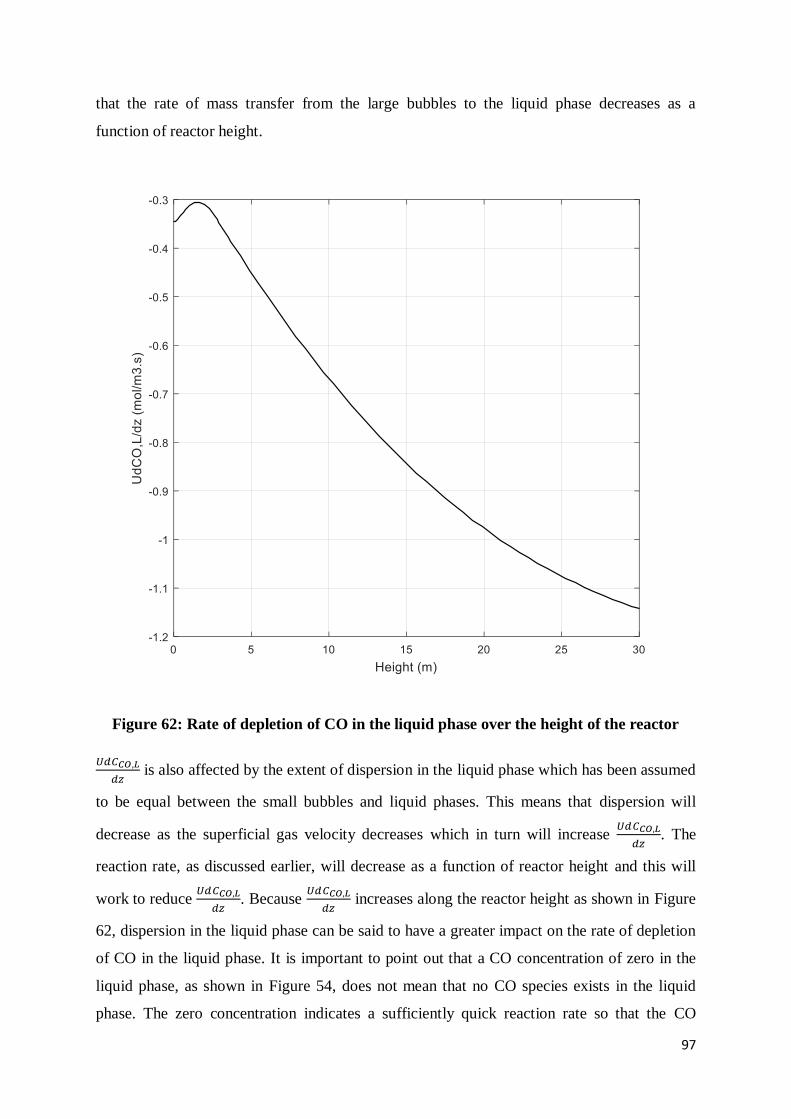
97
that the rate of mass transfer from the large bubbles to the liquid phase decreases as a
function of reactor height.
Figure 62: Rate of depletion of CO in the liquid phase over the height of the reactor
𝑈𝑑𝐶𝐶𝑂,𝐿
𝑑𝑧 is also affected by the extent of dispersion in the liquid phase which has been assumed
to be equal between the small bubbles and liquid phases. This means that dispersion will
decrease as the superficial gas velocity decreases which in turn will increase 𝑈𝑑𝐶𝐶𝑂,𝐿
𝑑𝑧. The
reaction rate, as discussed earlier, will decrease as a function of reactor height and this will
work to reduce 𝑈𝑑𝐶𝐶𝑂,𝐿
𝑑𝑧. Because
𝑈𝑑𝐶𝐶𝑂,𝐿
𝑑𝑧 increases along the reactor height as shown in Figure
62, dispersion in the liquid phase can be said to have a greater impact on the rate of depletion
of CO in the liquid phase. It is important to point out that a CO concentration of zero in the
liquid phase, as shown in Figure 54, does not mean that no CO species exists in the liquid
phase. The zero concentration indicates a sufficiently quick reaction rate so that the CO
98
species made available in the liquid phase is immediately consumed, i.e., the rate of mass
transfer of CO to the liquid phase is equal to the rate of consumption of CO by reaction. This
is essentially a steady-state condition in the absence of a solid-liquid interphase because of
the assumption of a pseudo-homogenous slurry phase. This is similarly the case in the small
bubbles. A zero concentration of CO therein, as shown in Figure 60, points to a steady-state
condition where the interphase between the small bubbles and liquid phases is rendered
insignificant by the high mass transfer coefficient. Had there been no initial CO species in the
small bubble and liquid phases, the species concentration would have been maintained at zero
in both phases.
It is clear that the decreasing superficial gas velocity, brought about by the consumption of
the reactant species along the height of the reactor, is the main contributor to the axial
profiles present in the SBCR. It affects the large bubble hold-up which is responsible for the
mass transfer and dispersion variations in the large bubble phase. It also directly affects the
large bubble dispersion in this phase. Its effect on the liquid and small bubble phase
dispersion is also evident. This emphasizes the crucial role that the superficial gas velocity
plays in the hydrodynamics and therefore the performance of the SBCR. The superficial gas
velocity is, however, not alone in affecting the performance of the SBCR in such a manner.
Other variables that are as important to the performance of the SBCR are discussed in the
next section where their relative effects are studied.
5.2.2 Sensitivity analysis
In order to gain further understanding into the effects of hydrodynamics on SBCR
performance, it is important to understand how various independent parameters affect the
hydrodynamics and how these in turn relate to the performance of the SBCR. In an attempt to
do this, a sensitivity analysis was carried out on the model to study the effects of specific
parameters on the performance of the SBCR. This should give an indication as to the relative
importance of such parameters in the design of SBCRs. In carrying out this task, independent
parameters were manipulated so that their effect could be assessed. These included the inlet
superficial gas velocity, reactor diameter, catalyst concentration and temperature. For a fair
assessment of each parameter’s effect on SBCR performance, only one parameter was
manipulated at a time so that in any one parameter analysis, only that parameter is being
varied and the rest are kept constant. The values of the parameters that are discussed in this
section are those stemming from a complete simulation, i.e., the values were obtained after a
99
simulation was conducted from z=0 to z=H. The independent parameters are an exception as
they are predetermined and are the basis of the sensitivity analysis.
5.2.2.1 Effect of superficial gas velocity
The superficial gas velocity is one of the most important determinants in the performance of
SBCRs as it influences a number of conditions which directly affect the hydrodynamics in
this reactor. In the first instance, 𝑈𝑔determines the flow regime that can be expected in a
SBCR which can either be bubbly or heterogenous. Higher values of 𝑈𝑔promote a
heterogenous flow regime so that the turbulence in the reactor is enhanced whereas a lower
value of 𝑈𝑔 will produce a mostly homogenous bubbly flow regime. These flow regimes have
a real impact on the performance of a SBCR that can be characterized by their influence on
the hydrodynamic parameters. A turbulent flow regime will promote back-mixing which has
direct consequences for the performance of the SBCR. A higher extent of axial dispersion
will negatively affect syngas conversion so that as 𝑈𝑔 is increased, the syngas conversion will
drop as well. This effect is illustrated in Figure 63 where the effects of 𝑈𝑔 on 𝐸𝐿 and 𝐸𝐺 are
shown respectively.
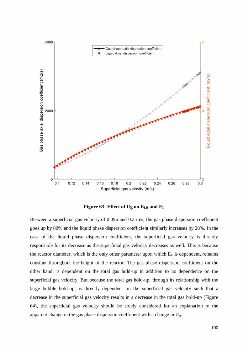
100
Figure 63: Effect of Ug on ELB and EL
Between a superficial gas velocity of 0.096 and 0.3 m/s, the gas phase dispersion coefficient
goes up by 80% and the liquid phase dispersion coefficient similarly increases by 28%. In the
case of the liquid phase dispersion coefficient, the superficial gas velocity is directly
responsible for its decrease as the superficial gas velocity decreases as well. This is because
the reactor diameter, which is the only other parameter upon which EL is dependent, remains
constant throughout the height of the reactor. The gas phase dispersion coefficient on the
other hand, is dependent on the total gas hold-up in addition to its dependence on the
superficial gas velocity. But because the total gas hold-up, through its relationship with the
large bubble hold-up, is directly dependent on the superficial gas velocity such that a
decrease in the superficial gas velocity results in a decrease in the total gas hold-up (Figure
64), the superficial gas velocity should be solely considered for an explanation to the
apparent change in the gas phase dispersion coefficient with a change in Ug.
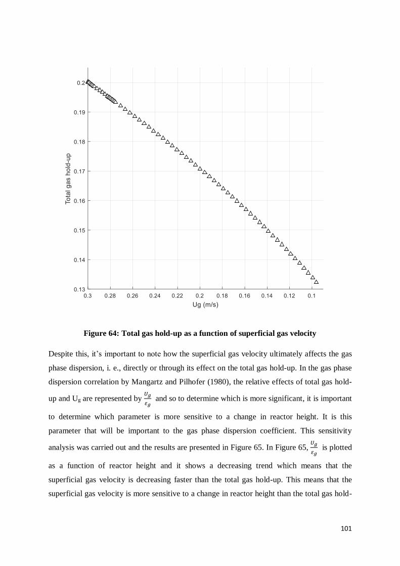
101
Figure 64: Total gas hold-up as a function of superficial gas velocity
Despite this, it’s important to note how the superficial gas velocity ultimately affects the gas
phase dispersion, i. e., directly or through its effect on the total gas hold-up. In the gas phase
dispersion correlation by Mangartz and Pilhofer (1980), the relative effects of total gas hold-
up and Ug are represented by 𝑈𝑔
𝑔 and so to determine which is more significant, it is important
to determine which parameter is more sensitive to a change in reactor height. It is this
parameter that will be important to the gas phase dispersion coefficient. This sensitivity
analysis was carried out and the results are presented in Figure 65. In Figure 65, 𝑈𝑔
𝑔 is plotted
as a function of reactor height and it shows a decreasing trend which means that the
superficial gas velocity is decreasing faster than the total gas hold-up. This means that the
superficial gas velocity is more sensitive to a change in reactor height than the total gas hold-
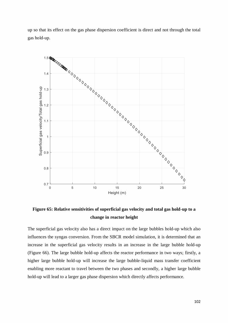
102
up so that its effect on the gas phase dispersion coefficient is direct and not through the total
gas hold-up.
Figure 65: Relative sensitivities of superficial gas velocity and total gas hold-up to a
change in reactor height
The superficial gas velocity also has a direct impact on the large bubbles hold-up which also
influences the syngas conversion. From the SBCR model simulation, it is determined that an
increase in the superficial gas velocity results in an increase in the large bubble hold-up
(Figure 66). The large bubble hold-up affects the reactor performance in two ways; firstly, a
higher large bubble hold-up will increase the large bubble-liquid mass transfer coefficient
enabling more reactant to travel between the two phases and secondly, a higher large bubble
hold-up will lead to a larger gas phase dispersion which directly affects performance.
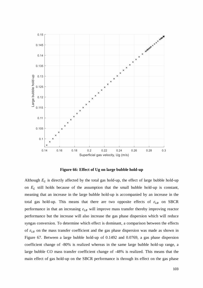
103
Figure 66: Effect of Ug on large bubble hold-up
Although 𝐸𝐺 is directly affected by the total gas hold-up, the effect of large bubble hold-up
on 𝐸𝐺 still holds because of the assumption that the small bubble hold-up is constant,
meaning that an increase in the large bubble hold-up is accompanied by an increase in the
total gas hold-up. This means that there are two opposite effects of 휀𝐿𝐵 on SBCR
performance in that an increasing 휀𝐿𝐵 will improve mass transfer thereby improving reactor
performance but the increase will also increase the gas phase dispersion which will reduce
syngas conversion. To determine which effect is dominant, a comparison between the effects
of 휀𝐿𝐵 on the mass transfer coefficient and the gas phase dispersion was made as shown in
Figure 67. Between a large bubble hold-up of 0.1492 and 0.0769, a gas phase dispersion
coefficient change of -80% is realized whereas in the same large bubble hold-up range, a
large bubble CO mass transfer coefficient change of -48% is realized. This means that the
main effect of gas hold-up on the SBCR performance is through its effect on the gas phase
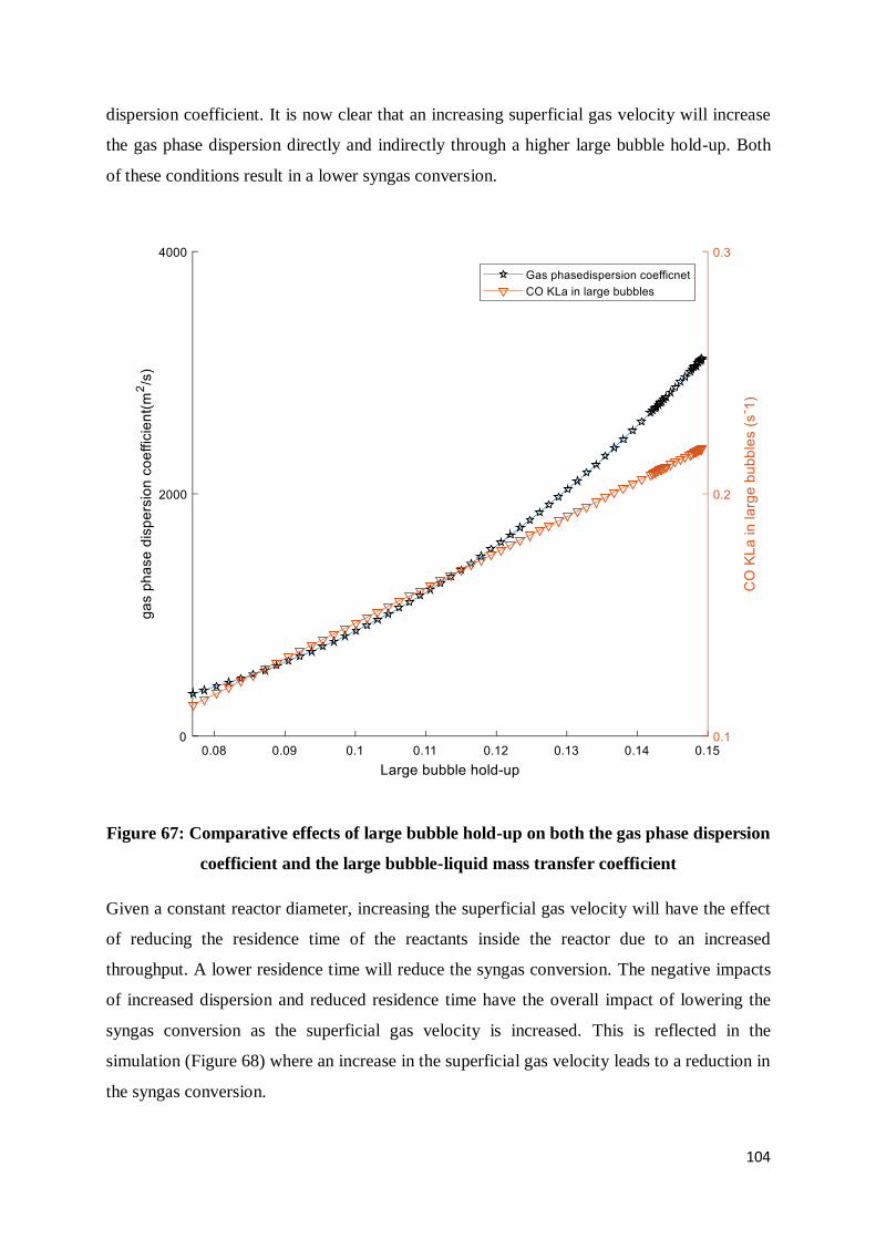
104
dispersion coefficient. It is now clear that an increasing superficial gas velocity will increase
the gas phase dispersion directly and indirectly through a higher large bubble hold-up. Both
of these conditions result in a lower syngas conversion.
Figure 67: Comparative effects of large bubble hold-up on both the gas phase dispersion
coefficient and the large bubble-liquid mass transfer coefficient
Given a constant reactor diameter, increasing the superficial gas velocity will have the effect
of reducing the residence time of the reactants inside the reactor due to an increased
throughput. A lower residence time will reduce the syngas conversion. The negative impacts
of increased dispersion and reduced residence time have the overall impact of lowering the
syngas conversion as the superficial gas velocity is increased. This is reflected in the
simulation (Figure 68) where an increase in the superficial gas velocity leads to a reduction in
the syngas conversion.
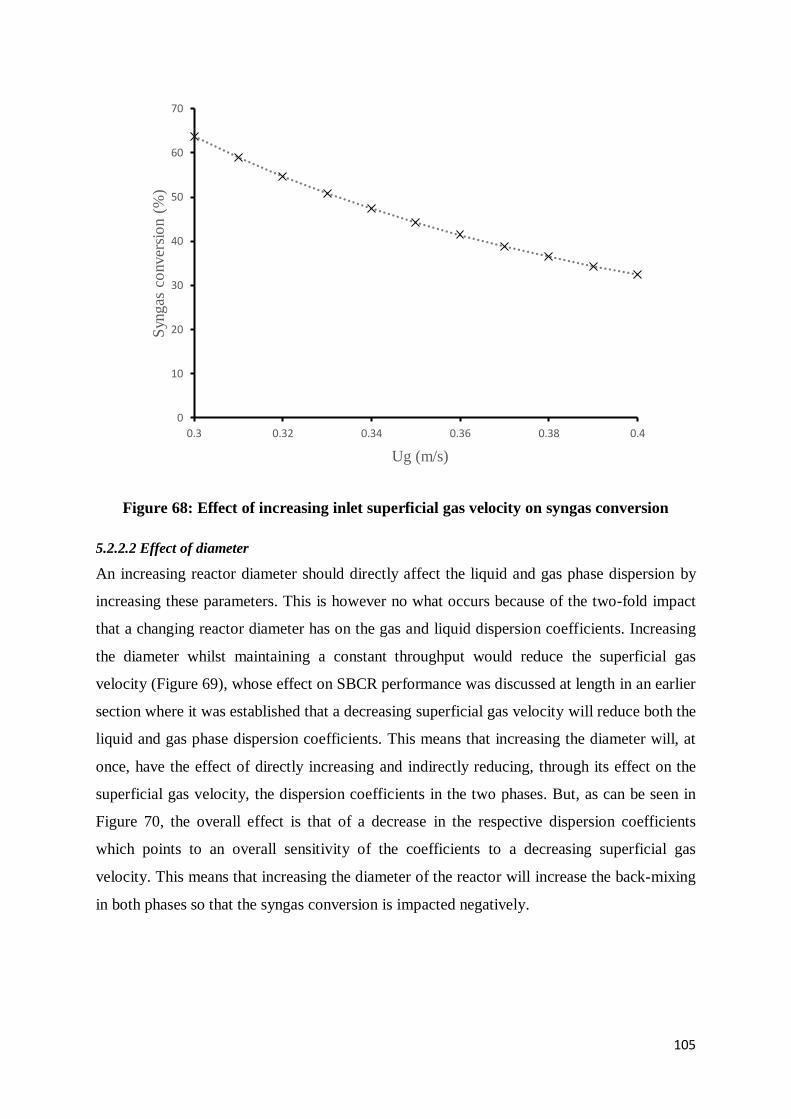
105
Figure 68: Effect of increasing inlet superficial gas velocity on syngas conversion
5.2.2.2 Effect of diameter
An increasing reactor diameter should directly affect the liquid and gas phase dispersion by
increasing these parameters. This is however no what occurs because of the two-fold impact
that a changing reactor diameter has on the gas and liquid dispersion coefficients. Increasing
the diameter whilst maintaining a constant throughput would reduce the superficial gas
velocity (Figure 69), whose effect on SBCR performance was discussed at length in an earlier
section where it was established that a decreasing superficial gas velocity will reduce both the
liquid and gas phase dispersion coefficients. This means that increasing the diameter will, at
once, have the effect of directly increasing and indirectly reducing, through its effect on the
superficial gas velocity, the dispersion coefficients in the two phases. But, as can be seen in
Figure 70, the overall effect is that of a decrease in the respective dispersion coefficients
which points to an overall sensitivity of the coefficients to a decreasing superficial gas
velocity. This means that increasing the diameter of the reactor will increase the back-mixing
in both phases so that the syngas conversion is impacted negatively.
0
10
20
30
40
50
60
70
0.3 0.32 0.34 0.36 0.38 0.4
Syngas
co
nver
sio
n (
%)
Ug (m/s)
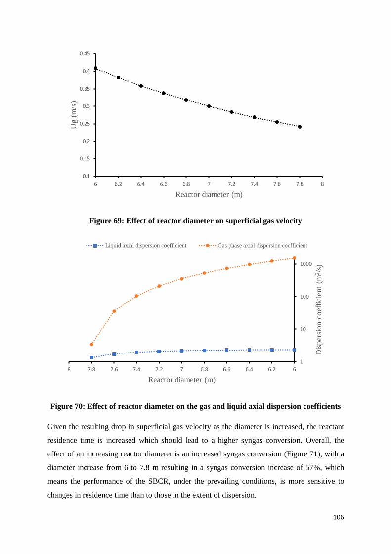
106
Figure 69: Effect of reactor diameter on superficial gas velocity
Figure 70: Effect of reactor diameter on the gas and liquid axial dispersion coefficients
Given the resulting drop in superficial gas velocity as the diameter is increased, the reactant
residence time is increased which should lead to a higher syngas conversion. Overall, the
effect of an increasing reactor diameter is an increased syngas conversion (Figure 71), with a
diameter increase from 6 to 7.8 m resulting in a syngas conversion increase of 57%, which
means the performance of the SBCR, under the prevailing conditions, is more sensitive to
changes in residence time than to those in the extent of dispersion.
0.1
0.15
0.2
0.25
0.3
0.35
0.4
0.45
6 6.2 6.4 6.6 6.8 7 7.2 7.4 7.6 7.8 8
Ug (
m/s
)
Reactor diameter (m)
1
10
100
1000
66.26.46.66.877.27.47.67.88
Dis
per
sio
n c
oef
ficie
nt
(m2/s
)
Reactor diameter (m)
Liquid axial dispersion coefficient Gas phase axial dispersion coefficient
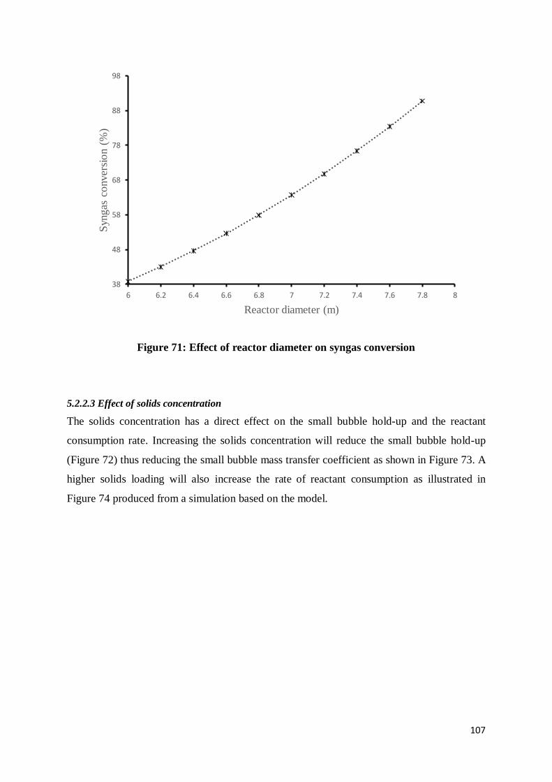
107
Figure 71: Effect of reactor diameter on syngas conversion
5.2.2.3 Effect of solids concentration
The solids concentration has a direct effect on the small bubble hold-up and the reactant
consumption rate. Increasing the solids concentration will reduce the small bubble hold-up
(Figure 72) thus reducing the small bubble mass transfer coefficient as shown in Figure 73. A
higher solids loading will also increase the rate of reactant consumption as illustrated in
Figure 74 produced from a simulation based on the model.
38
48
58
68
78
88
98
6 6.2 6.4 6.6 6.8 7 7.2 7.4 7.6 7.8 8
Syngas
co
nver
sio
n (
%)
Reactor diameter (m)
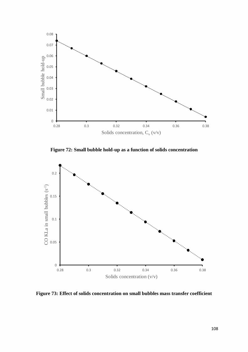
108
Figure 72: Small bubble hold-up as a function of solids concentration
Figure 73: Effect of solids concentration on small bubbles mass transfer coefficient
0
0.01
0.02
0.03
0.04
0.05
0.06
0.07
0.08
0.28 0.3 0.32 0.34 0.36 0.38
Sm
all
bubble
ho
ld-u
p
Solids concentration, Cv (v/v)
0
0.05
0.1
0.15
0.2
0.28 0.3 0.32 0.34 0.36 0.38
CO
KL
a in
sm
all
bubble
s (s
-1)
Solids concentration (v/v)
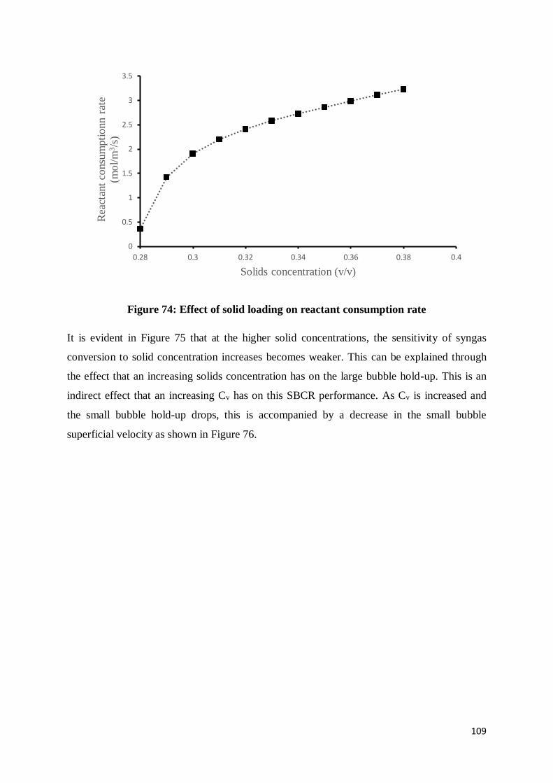
109
Figure 74: Effect of solid loading on reactant consumption rate
It is evident in Figure 75 that at the higher solid concentrations, the sensitivity of syngas
conversion to solid concentration increases becomes weaker. This can be explained through
the effect that an increasing solids concentration has on the large bubble hold-up. This is an
indirect effect that an increasing Cv has on this SBCR performance. As Cv is increased and
the small bubble hold-up drops, this is accompanied by a decrease in the small bubble
superficial velocity as shown in Figure 76.
0
0.5
1
1.5
2
2.5
3
3.5
0.28 0.3 0.32 0.34 0.36 0.38 0.4
Rea
ctan
t co
nsu
mpti
onn r
ate
(mo
l/m
3/s
)
Solids concentration (v/v)

110
Figure 75: Effect of solids concentration on syngas conversion
Figure 76: Small bubble superficial velocity as a function of solids concentration
The drop in small bubble superficial velocity will also cause an increase in the large bubble
hold-up (Figure 77) according to Equation 75 (Maretto and Krishna, 1999). As shown in
Figure 67, an increasing large bubble hold-up causes an increase in the gas phase dispersion
coefficient which is detrimental to syngas conversion.
0
10
20
30
40
50
60
70
80
90
100
0.28 0.3 0.32 0.34 0.36 0.38 0.4
Syngas
co
nver
sio
n (
%)
Solids concentration (v/v)
0
0.00005
0.0001
0.00015
0.0002
0.00025
0.0003
0.00035
0.28 0.3 0.32 0.34 0.36 0.38
Sm
all
bubble
super
ficia
l vel
oci
ty (
m/s
)
Cv (v/v)
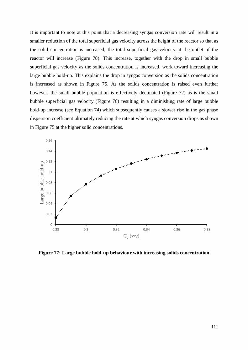
111
It is important to note at this point that a decreasing syngas conversion rate will result in a
smaller reduction of the total superficial gas velocity across the height of the reactor so that as
the solid concentration is increased, the total superficial gas velocity at the outlet of the
reactor will increase (Figure 78). This increase, together with the drop in small bubble
superficial gas velocity as the solids concentration is increased, work toward increasing the
large bubble hold-up. This explains the drop in syngas conversion as the solids concentration
is increased as shown in Figure 75. As the solids concentration is raised even further
however, the small bubble population is effectively decimated (Figure 72) as is the small
bubble superficial gas velocity (Figure 76) resulting in a diminishing rate of large bubble
hold-up increase (see Equation 74) which subsequently causes a slower rise in the gas phase
dispersion coefficient ultimately reducing the rate at which syngas conversion drops as shown
in Figure 75 at the higher solid concentrations.
Figure 77: Large bubble hold-up behaviour with increasing solids concentration
0
0.02
0.04
0.06
0.08
0.1
0.12
0.14
0.16
0.28 0.3 0.32 0.34 0.36 0.38
Lar
ge
bubble
ho
ld-u
p
Cv (v/v)
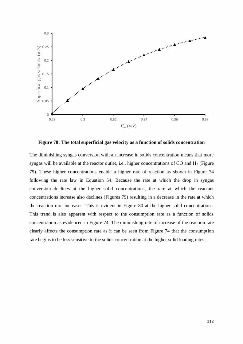
112
Figure 78: The total superficial gas velocity as a function of solids concentration
The diminishing syngas conversion with an increase in solids concentration means that more
syngas will be available at the reactor outlet, i.e., higher concentrations of CO and H2 (Figure
79). These higher concentrations enable a higher rate of reaction as shown in Figure 74
following the rate law in Equation 54. Because the rate at which the drop in syngas
conversion declines at the higher solid concentrations, the rate at which the reactant
concentrations increase also declines (Figures 79) resulting in a decrease in the rate at which
the reaction rare increases. This is evident in Figure 80 at the higher solid concentrations.
This trend is also apparent with respect to the consumption rate as a function of solids
concentration as evidenced in Figure 74. The diminishing rate of increase of the reaction rate
clearly affects the consumption rate as it can be seen from Figure 74 that the consumption
rate begins to be less sensitive to the solids concentration at the higher solid loading rates.
0
0.05
0.1
0.15
0.2
0.25
0.3
0.28 0.3 0.32 0.34 0.36 0.38
Sup
erfi
cal
gas
vel
oci
ty (
m/s
)
Cv (v/v)
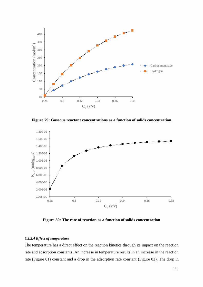
113
Figure 79: Gaseous reactant concentrations as a function of solids concentration
Figure 80: The rate of reaction as a function of solids concentration
5.2.2.4 Effect of temperature
The temperature has a direct effect on the reaction kinetics through its impact on the reaction
rate and adsorption constants. An increase in temperature results in an increase in the reaction
rate (Figure 81) constant and a drop in the adsorption rate constant (Figure 82). The drop in
10
60
110
160
210
260
310
360
410
0.28 0.3 0.32 0.34 0.36 0.38
Co
nce
ntr
atio
n (
mo
l/m
3)
Cv (v/v)
Carbon monoxide
Hydrogen
0.00E+00
2.00E-06
4.00E-06
6.00E-06
8.00E-06
1.00E-05
1.20E-05
1.40E-05
1.60E-05
1.80E-05
0.28 0.3 0.32 0.34 0.36 0.38
RC
O(m
ol/
gca
t.s)
Cv (v/v)
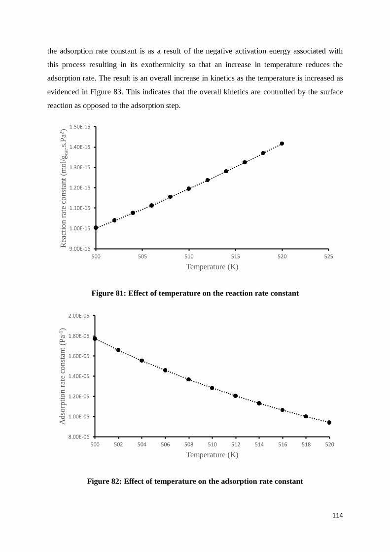
114
the adsorption rate constant is as a result of the negative activation energy associated with
this process resulting in its exothermicity so that an increase in temperature reduces the
adsorption rate. The result is an overall increase in kinetics as the temperature is increased as
evidenced in Figure 83. This indicates that the overall kinetics are controlled by the surface
reaction as opposed to the adsorption step.
Figure 81: Effect of temperature on the reaction rate constant
Figure 82: Effect of temperature on the adsorption rate constant
9.00E-16
1.00E-15
1.10E-15
1.20E-15
1.30E-15
1.40E-15
1.50E-15
500 505 510 515 520 525
Rea
ctio
n r
ate
const
ant
(mo
l/g
cat.s
.Pa2
)
Temperature (K)
8.00E-06
1.00E-05
1.20E-05
1.40E-05
1.60E-05
1.80E-05
2.00E-05
500 502 504 506 508 510 512 514 516 518 520
Adso
rpti
on r
ate
const
ant
(Pa-1
)
Temperature (K)
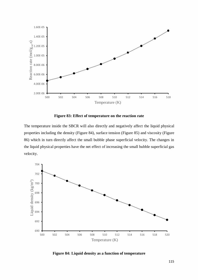
115
Figure 83: Effect of temperature on the reaction rate
The temperature inside the SBCR will also directly and negatively affect the liquid physical
properties including the density (Figure 84), surface tension (Figure 85) and viscosity (Figure
86) which in turn directly affect the small bubble phase superficial velocity. The changes in
the liquid physical properties have the net effect of increasing the small bubble superficial gas
velocity.
Figure 84: Liquid density as a function of temperature
2.00E-06
4.00E-06
6.00E-06
8.00E-06
1.00E-05
1.20E-05
1.40E-05
1.60E-05
500 502 504 506 508 510 512 514 516 518
Rea
ctio
n r
ate
(mo
l/g
cat.s
)
Temperature (K)
690
692
694
696
698
700
702
704
500 502 504 506 508 510 512 514 516 518 520
Liq
uid
den
sity
(kg/m
3)
Temperature (K)
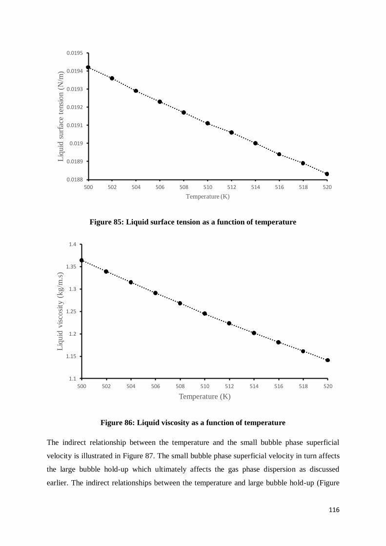
116
Figure 85: Liquid surface tension as a function of temperature
Figure 86: Liquid viscosity as a function of temperature
The indirect relationship between the temperature and the small bubble phase superficial
velocity is illustrated in Figure 87. The small bubble phase superficial velocity in turn affects
the large bubble hold-up which ultimately affects the gas phase dispersion as discussed
earlier. The indirect relationships between the temperature and large bubble hold-up (Figure
0.0188
0.0189
0.019
0.0191
0.0192
0.0193
0.0194
0.0195
500 502 504 506 508 510 512 514 516 518 520
Liq
uid
surf
ace
tensi
on (
N/m
)
Temperature (K)
1.1
1.15
1.2
1.25
1.3
1.35
1.4
500 502 504 506 508 510 512 514 516 518 520
Liq
uid
vis
cosi
ty (
kg
/m.s
)
Temperature (K)
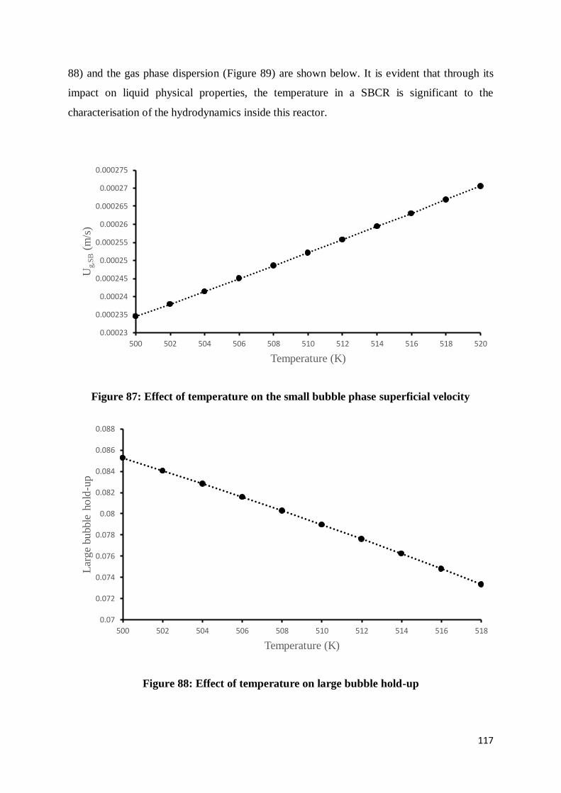
117
88) and the gas phase dispersion (Figure 89) are shown below. It is evident that through its
impact on liquid physical properties, the temperature in a SBCR is significant to the
characterisation of the hydrodynamics inside this reactor.
Figure 87: Effect of temperature on the small bubble phase superficial velocity
Figure 88: Effect of temperature on large bubble hold-up
0.00023
0.000235
0.00024
0.000245
0.00025
0.000255
0.00026
0.000265
0.00027
0.000275
500 502 504 506 508 510 512 514 516 518 520
Ug,S
B(m
/s)
Temperature (K)
0.07
0.072
0.074
0.076
0.078
0.08
0.082
0.084
0.086
0.088
500 502 504 506 508 510 512 514 516 518
Lar
ge
bubble
ho
ld-u
p
Temperature (K)
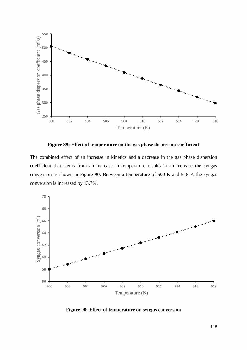
118
Figure 89: Effect of temperature on the gas phase dispersion coefficient
The combined effect of an increase in kinetics and a decrease in the gas phase dispersion
coefficient that stems from an increase in temperature results in an increase the syngas
conversion as shown in Figure 90. Between a temperature of 500 K and 518 K the syngas
conversion is increased by 13.7%.
Figure 90: Effect of temperature on syngas conversion
250
300
350
400
450
500
550
500 502 504 506 508 510 512 514 516 518
Gas
phas
e d
isp
ersi
on c
oef
ficie
nt
(m2/s
)
Temperature (K)
56
58
60
62
64
66
68
70
500 502 504 506 508 510 512 514 516 518
Syngas
co
nver
sio
n (
%)
Temperature (K)
119
Chapter 6: Model validation
In order to validate the presented model, data from similar reactor systems must be sourced
and compared to the current simulation results. Ideally, data from a large-scale commercial
SBCR would be used as a basis for the validation but this can prove to be difficult given the
intellectual property protection around real plant data. As an alternative, results from the
current simulation were compared with results from similar simulations on SBCR models
developed by various authors. A general agreement between the current simulation results
and those from the literature should serve to provide a level of confidence in the accuracy of
the present model. The SBCR model, as currently presented, is different from other models
form literature as it draws its constituent parts from various sources and brings them together
to form a unique model. This presents a challenge in comparing the model to other models
available in literature because the comparison is bound to be unfair. It is thus important to
emphasise that the relevance of the comparison of the model with those from literature is that
of a general indication regarding the accuracy of the model so that the model would require
further validation in the form of real plant data. This is a future concern and for the purposes
of the present model validation, comparison with literature models should suffice.
6.1 Sehabiague et al. (2008)
Sehabiague et al. (2008) developed a mathematical model for describing the operations in a
SBCR. In the model, the authors, assume the presence of axial dispersion in all phases and
include a sedimentation model to account for catalyst concentration axial gradients. A 2-class
bubble model is used with large and small bubbles distinctly characterised. The kinetics are
modelled using a Co catalyst. Temperature and pressure gradients are accounted for and only
the gas-liquid mass transfer is considered significant. The authors measured the performance
of the reactor in terms of, amongst other parameters, CO conversion and evaluated this
performance as a function of both superficial gas velocity and reactor dispersion height. The
results from the above-mentioned exercise have been compared to those of the current
simulation as shown in Table 16. In Figures 91 and 92, the same results are compared
graphically.
While the two sets of results show similar trends in that an increasing reactor height results in
greater CO conversion, Sehabiague et al. (2008) results consistently reflect a lower CO
conversion throughout the height of reactor. It is also worth noting the apparent slope change
in both Figures 91 and 92, indicating a decrease in the sensitivity of CO conversion to an
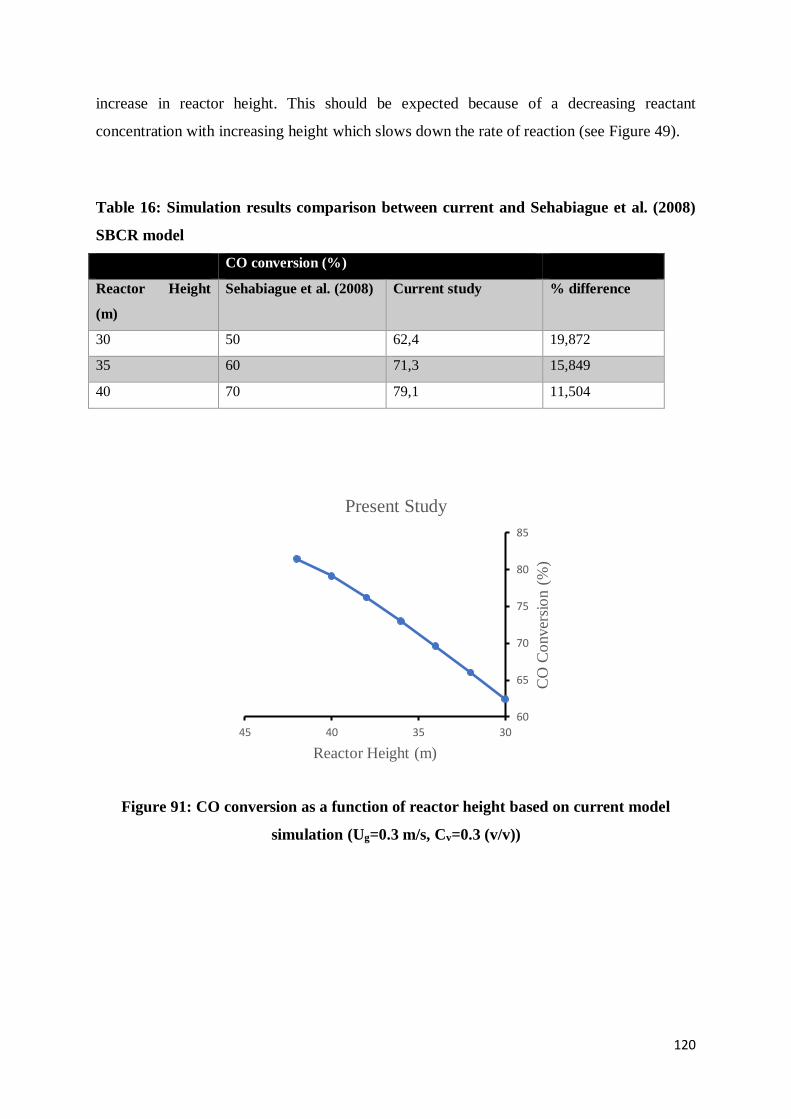
120
increase in reactor height. This should be expected because of a decreasing reactant
concentration with increasing height which slows down the rate of reaction (see Figure 49).
Table 16: Simulation results comparison between current and Sehabiague et al. (2008)
SBCR model
CO conversion (%)
Reactor Height
(m)
Sehabiague et al. (2008) Current study % difference
30 50 62,4 19,872
35 60 71,3 15,849
40 70 79,1 11,504
Figure 91: CO conversion as a function of reactor height based on current model
simulation (Ug=0.3 m/s, Cv=0.3 (v/v))
60
65
70
75
80
85
30354045
CO
Co
nver
sio
n (
%)
Reactor Height (m)
Present Study
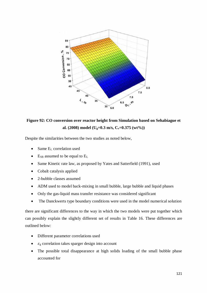
121
Figure 92: CO conversion over reactor height from Simulation based on Sehabiague et
al. (2008) model (Ug=0.3 m/s, Cv=0.375 (wt%))
Despite the similarities between the two studies as noted below,
Same EL correlation used
ESB assumed to be equal to EL
Same Kinetic rate law, as proposed by Yates and Satterfield (1991), used
Cobalt catalysis applied
2-bubble classes assumed
ADM used to model back-mixing in small bubble, large bubble and liquid phases
Only the gas-liquid mass transfer resistance was considered significant
The Danckwerts type boundary conditions were used in the model numerical solution
there are significant differences to the way in which the two models were put together which
can possibly explain the slightly different set of results in Table 16. These differences are
outlined below:
Different parameter correlations used
휀g correlation takes sparger design into account
The possible total disappearance at high solids loading of the small bubble phase
accounted for
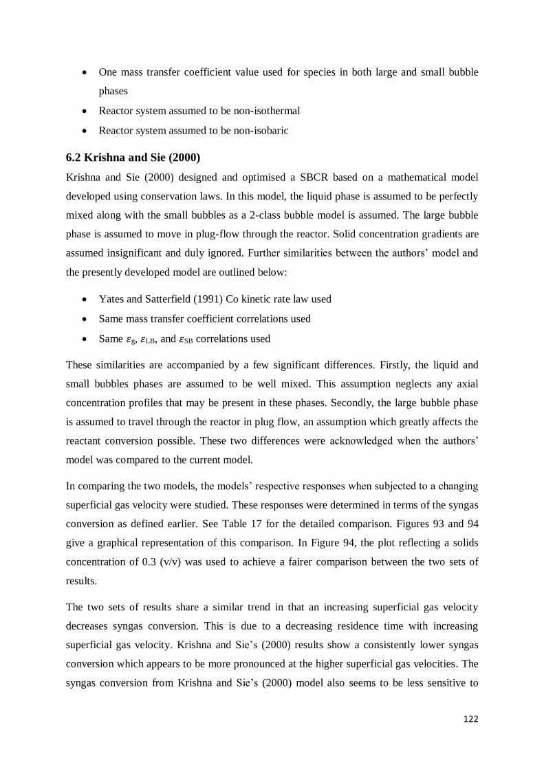
122
One mass transfer coefficient value used for species in both large and small bubble
phases
Reactor system assumed to be non-isothermal
Reactor system assumed to be non-isobaric
6.2 Krishna and Sie (2000)
Krishna and Sie (2000) designed and optimised a SBCR based on a mathematical model
developed using conservation laws. In this model, the liquid phase is assumed to be perfectly
mixed along with the small bubbles as a 2-class bubble model is assumed. The large bubble
phase is assumed to move in plug-flow through the reactor. Solid concentration gradients are
assumed insignificant and duly ignored. Further similarities between the authors’ model and
the presently developed model are outlined below:
Yates and Satterfield (1991) Co kinetic rate law used
Same mass transfer coefficient correlations used
Same 휀g, 휀LB, and 휀SB correlations used
These similarities are accompanied by a few significant differences. Firstly, the liquid and
small bubbles phases are assumed to be well mixed. This assumption neglects any axial
concentration profiles that may be present in these phases. Secondly, the large bubble phase
is assumed to travel through the reactor in plug flow, an assumption which greatly affects the
reactant conversion possible. These two differences were acknowledged when the authors’
model was compared to the current model.
In comparing the two models, the models’ respective responses when subjected to a changing
superficial gas velocity were studied. These responses were determined in terms of the syngas
conversion as defined earlier. See Table 17 for the detailed comparison. Figures 93 and 94
give a graphical representation of this comparison. In Figure 94, the plot reflecting a solids
concentration of 0.3 (v/v) was used to achieve a fairer comparison between the two sets of
results.
The two sets of results share a similar trend in that an increasing superficial gas velocity
decreases syngas conversion. This is due to a decreasing residence time with increasing
superficial gas velocity. Krishna and Sie’s (2000) results show a consistently lower syngas
conversion which appears to be more pronounced at the higher superficial gas velocities. The
syngas conversion from Krishna and Sie’s (2000) model also seems to be less sensitive to
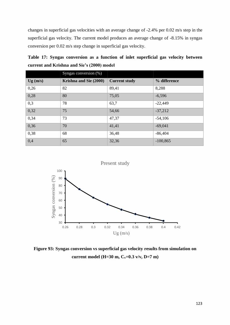
123
changes in superficial gas velocities with an average change of -2.4% per 0.02 m/s step in the
superficial gas velocity. The current model produces an average change of -8.15% in syngas
conversion per 0.02 m/s step change in superficial gas velocity.
Table 17: Syngas conversion as a function of inlet superficial gas velocity between
current and Krishna and Sie’s (2000) model
Syngas conversion (%)
Ug (m/s) Krishna and Sie (2000) Current study % difference
0,26 82 89,41 8,288
0,28 80 75,05 -6,596
0,3 78 63,7 -22,449
0,32 75 54,66 -37,212
0,34 73 47,37 -54,106
0,36 70 41,41 -69,041
0,38 68 36,48 -86,404
0,4 65 32,36 -100,865
Figure 93: Syngas conversion vs superficial gas velocity results from simulation on
current model (H=30 m, Cv=0.3 v/v, D=7 m)
30
40
50
60
70
80
90
100
0.26 0.28 0.3 0.32 0.34 0.36 0.38 0.4 0.42
Syngas
co
nver
sio
n (
%)
Ug (m/s)
Present study
124
Figure 94: Syngas conversion as a function of superficial gas velocity based on
simulation from model by Krishna and Sie (2000) (Krishna and Sie, 2000) (H=30 m,
Cv=0.3 (v/v), D= 7m)
6.3 De Swart and Krishna (2002)
De Swart and Krishna (2002) carried out the development of a mathematical model to
describe the SBCR and used the model to simulate the dynamic and steady-state conditions in
the reactor. In the model, the gas phase was theoretically divided into small and large bubble
classes. The ADM was applied in all phases of the reactor. Below is a list of the similarities
followed by the differences between the model developed by the above-mentioned authors
and that which was developed in the present study. The similarities are as follows:
ADM applied to all phases
Only gas-liquid mass transfer considered
No intra-particle temperature and concentration gradients present
Small bubbles velocity constant over height of reactor
Danckwerts type boundary conditions used in model numerical solution
And the differences which contribute to the disparity between the two models are as follows:
Catalyst distribution modelled using the sedimentation-dispersion model
Superficial gas velocity decrease due to reaction consumption accounted for using a
contraction factor
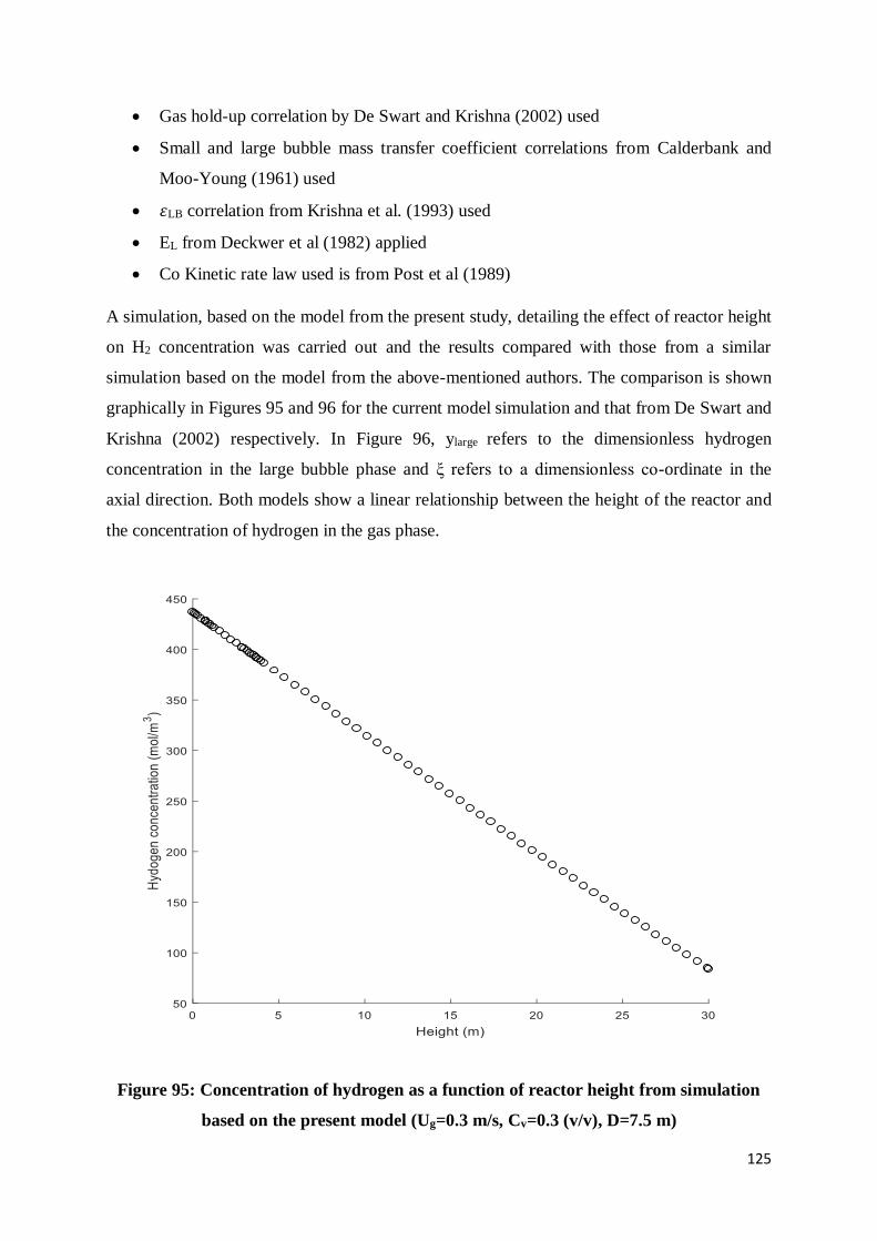
125
Gas hold-up correlation by De Swart and Krishna (2002) used
Small and large bubble mass transfer coefficient correlations from Calderbank and
Moo-Young (1961) used
휀LB correlation from Krishna et al. (1993) used
EL from Deckwer et al (1982) applied
Co Kinetic rate law used is from Post et al (1989)
A simulation, based on the model from the present study, detailing the effect of reactor height
on H2 concentration was carried out and the results compared with those from a similar
simulation based on the model from the above-mentioned authors. The comparison is shown
graphically in Figures 95 and 96 for the current model simulation and that from De Swart and
Krishna (2002) respectively. In Figure 96, ylarge refers to the dimensionless hydrogen
concentration in the large bubble phase and ξ refers to a dimensionless co-ordinate in the
axial direction. Both models show a linear relationship between the height of the reactor and
the concentration of hydrogen in the gas phase.
Figure 95: Concentration of hydrogen as a function of reactor height from simulation
based on the present model (Ug=0.3 m/s, Cv=0.3 (v/v), D=7.5 m)
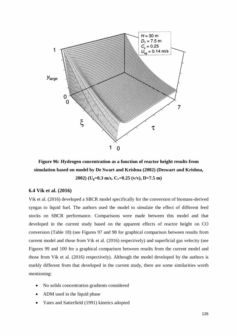
126
Figure 96: Hydrogen concentration as a function of reactor height results from
simulation based on model by De Swart and Krishna (2002) (Deswart and Krishna,
2002) (Ug=0.3 m/s, Cv=0.25 (v/v), D=7.5 m)
6.4 Vik et al. (2016)
Vik et al. (2016) developed a SBCR model specifically for the conversion of biomass-derived
syngas to liquid fuel. The authors used the model to simulate the effect of different feed
stocks on SBCR performance. Comparisons were made between this model and that
developed in the current study based on the apparent effects of reactor height on CO
conversion (Table 18) (see Figures 97 and 98 for graphical comparison between results from
current model and those from Vik et al. (2016) respectively) and superficial gas velocity (see
Figures 99 and 100 for a graphical comparison between results from the current model and
those from Vik et al. (2016) respectively). Although the model developed by the authors is
starkly different from that developed in the current study, there are some similarities worth
mentioning:
No solids concentration gradients considered
ADM used in the liquid phase
Yates and Satterfield (1991) kinetics adopted
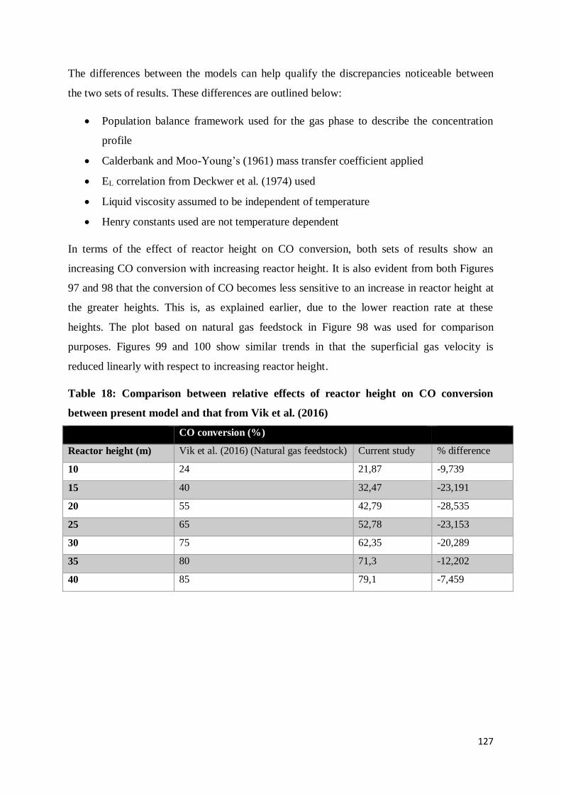
127
The differences between the models can help qualify the discrepancies noticeable between
the two sets of results. These differences are outlined below:
Population balance framework used for the gas phase to describe the concentration
profile
Calderbank and Moo-Young’s (1961) mass transfer coefficient applied
EL correlation from Deckwer et al. (1974) used
Liquid viscosity assumed to be independent of temperature
Henry constants used are not temperature dependent
In terms of the effect of reactor height on CO conversion, both sets of results show an
increasing CO conversion with increasing reactor height. It is also evident from both Figures
97 and 98 that the conversion of CO becomes less sensitive to an increase in reactor height at
the greater heights. This is, as explained earlier, due to the lower reaction rate at these
heights. The plot based on natural gas feedstock in Figure 98 was used for comparison
purposes. Figures 99 and 100 show similar trends in that the superficial gas velocity is
reduced linearly with respect to increasing reactor height.
Table 18: Comparison between relative effects of reactor height on CO conversion
between present model and that from Vik et al. (2016)
CO conversion (%)
Reactor height (m) Vik et al. (2016) (Natural gas feedstock) Current study % difference
10 24 21,87 -9,739
15 40 32,47 -23,191
20 55 42,79 -28,535
25 65 52,78 -23,153
30 75 62,35 -20,289
35 80 71,3 -12,202
40 85 79,1 -7,459
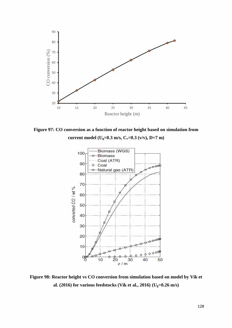
128
Figure 97: CO conversion as a function of reactor height based on simulation from
current model (Ug=0.3 m/s, Cv=0.3 (v/v), D=7 m)
Figure 98: Reactor height vs CO conversion from simulation based on model by Vik et
al. (2016) for various feedstocks (Vik et al., 2016) (Ug=0.26 m/s)
20
30
40
50
60
70
80
90
10 15 20 25 30 35 40 45
CO
co
nver
sio
n (
%)
Reactor height (m)
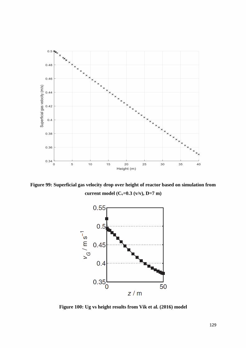
129
Figure 99: Superficial gas velocity drop over height of reactor based on simulation from
current model (Cv=0.3 (v/v), D=7 m)
Figure 100: Ug vs height results from Vik et al. (2016) model

130
From the presented validation exercise, it is clear that the current model compares well with
other literature models in as far as the general agreement between the models is concerned.
What is also clear, however, is the presence of quantitative discrepancies noticeable between
the models, i.e., the percentage deviations in simulation results between the models. This is
expected, given the different sub-models that were incorporated in the proposed and literature
SBCR models. Some confidence should be derived, however, from the similar trends
achieved in key parameters in the models being compared because this gives an indication
that the SBCR system is behaving in an expected and acceptable manner even though the
exact behaviours are different from model to model. As mentioned earlier, a natural
progression in the validation process should be to validate the model results against real
commercial scale SBCR results or at least those from a large-scale pilot plant. In the
unavailability of such data at present, the validation conducted above should be sufficient to
give some indication of the correctness and accuracy of the model.
131
Chapter 7: Conclusion and Recommendations
7.1 Conclusion
A mathematical model describing the SBCR environment has been developed. The model is
built around the principle of material conservation. Important hydrodynamic parameters
along with mass transfer and kinetic parameters were sourced from various sources and
incorporated into the model. The SBCR environment was conceptually divided into three
distinct phases including the small bubble, large bubble and slurry phase. Material axial
dispersion was accounted for in all phases to better reflect the mixing in these phases.
Contrary to suggestions by various authors, axial dispersion in the large bubble phase was
taken into account, occurring on a much larger scale than in the slurry phase. Simulink
software from MATLAB was used to produce a numerical solution to the ode-based model
formulations and the solution was used as a basis to study the dynamics inside a SBCR.
As a result of axial dispersion, the concentrations of the reactants show a gradual decrease in
the large bubble phase and steep decline in the small bubble and slurry phases. The
superficial gas velocity promotes axial dispersion in both the large bubble and slurry phases.
It also promotes large bubble hold-up and reduces reactant residence time resulting in a net
reduction in the syngas conversion. An increasing reactor diameter results in an overall
increase in the conversion of syngas and an increasing solids concentration decimates the
small bubble population and increases the large bubble hold-up resulting in a lower syngas
conversion. The model results were compared with those from different authors and were
found to show similar trends albeit with differing parameter values. This was expected as the
published models were not identical to the proposed model.
A mathematical model capable of describing the hydrodynamic behaviour in a SBCR has
been developed to aid in the study of this complex reactor. This model can also be used in the
preliminary design stages, helping to avoid costly experiments and save time by acting as a
platform on which to rule out specific design options.
7.2 Recommendations
Further work on this model including heat transfer and momentum effects can aid in making
the model more complete and robust but care should be taken as to the level of detail that is
incorporated as this can be difficult and time consuming. It is best to decide on the level of
detail in line with the user’s aims and objectives. In the present case, the objective was to

132
gain an understanding of the hydrodynamic behaviour in a SBCR and the factors that
influence it, to this end it was deemed fit to limit the detail in the model as has been done.
133
References
1. Akita, K., Yoshida, F. (1973). Gas holdup and volumetric mass transfer coefficient in
bubble columns. Effects of liquid properties. Industrial and Engineering Chemistry
Process Design and Development, 12, 76–80.
2. Albright, L. F. (2009). Albright’s Chemical Engineering Handbook. New York: CRC
Press, Taylor and Francis group.
3. Aoyama, Y., Ogushi, K., Koide, K., Kubota, H. (1968). Liquid Mixing in Concurrent
Bubble Columns. Journal of Chemical Engineering Japan, 1(2), 158-163.
4. Bach, H. F, Pilhofer, T. (1978). Variations of gas hold-up in bubble columns with
physical properties of liquids and operating parameters of column. German Chemical
Engineering, 1, 270–275.
5. Baird, M. H. I., Rice, R. G. (1975). Axial dispersion in large unbaffled columns. The
Chemical Engineering Journal, 9, 171-174.
6. Basha, O. M., Sehabiague, L., Abdel-Wahab, A., Morsi, B. I. (2015). Fischer–
Tropsch Synthesis in Slurry Bubble Column Reactors: Experimental Investigations
and Modeling – A Review. International Journal of Chemical Reactor Engineering,
13(3), 201–288.
7. Begovich, J. M., Watson, J. (1978). Hydrodynamic characteristics of three-phase
fluidized beds. Cambridge: Cambridge University Press.
8. Behkish, A. (1997). Hydrodynamic and Mass Transfer Parameters in Large-Scale
Slurry Bubble Column Reactors (Doctoral thesis, University of Pittsburg, USA).
9. Behkish, A., Lemoine, R., Oukaci, R., Morsi, I. B. (2006). Novel correlations for gas
holdup in large-scale slurry bubble column reactors operating under elevated
pressures and temperatures. Chemical Engineering Journal, 115, 157–171.
10. Boyer, C., Gazarian, J., Lecocq, V., Maury, S., Forret, A., Schweitzer, J., Souchon, V.
(2016). Development of the Fischer-Tropsch Process: From the Reaction Concept to
the Process Book. Oil and Gas Science and Technology - Revue d'IFP Energies
nouvelles, Institut Francais du Petrole, 71(44).
11. Brady, R. C. III, Pettit, R. (1981). Mechanism of the Fischer-Tropsch reaction. The
chain propagation step. Journal of the American Chemical Society, 103(5), 1287–
1289.
12. Brotz, W. Z. (1949). Zur Systematik der Fischer-Tropsch-Katalyse. Zeitschrift für
Elektrochemie, 5, 301-306.
134
13. Bukur, D. B. (1983). Some Comments on Models for Fischer-Tropsch Reaction in
Slurry Bubble Column Reactors. Chemical Engineering Science, 38(3),441-446.
14. Calderbank, P. H., Moo-Young, M. B. (1961). The continuous phase heat and mass
transfer properties of dispersions. Chemical Engineering Science, 16, 39-54.
15. Calderbank, P.H., Evans, F., Farley, R., Jepson, G., Poll, A. (1963). Rate processes in
the catalyst-slurry Fischer-Tropsch reaction. Catalysis in Practice, 66–74.
16. Chang, J., Bai, L., Teng, B. T., Zhang, R. L., Yang, J., Xu, Y. Y., Xiang, H. W., Li, Y.
W. (2007). Kinetic modeling of Fischer–Tropsch synthesis over Fe.Cu.K.SiO2
catalyst in slurry phase reactor. Chemical Engineering Science, 62, 4983 – 4991.
17. Chen, C. M., Leu, L. P. (2001). Hydrodynamics and mass transfer in threephase
magnetic fluidized beds. Powder Technology, 117, 198–206.
18. Craxford, S. R., Rideal, E. K. (1939). The mechanism of the synthesis of
hydrocarbons from water-gas. Journal of the Chemical Society, 1604-1614.
19. Davis, B. H. (2009). Fischer–Tropsch Synthesis: Reaction mechanisms for iron
catalysts. Catalysis Today, 141, 25–33.
20. Davis, M. E., Davis, R. J. (2003). Fundamentals of Chemical Reaction Engineering.
New York: McGraw Hill.
21. De Deugd, R. M. (2004). Fischer-Tropsch Synthesis Revisited; Efficiency and
Selectivity Benefits from Imposing Temporal and/or Spatial Structure in the Reactor
(Doctoral thesis, Technische Universiteit Delft, Netherlands).
22. De Nevers, N. (1968). Bubble driven fluid circulations. AIChE Journal, 14(2), 222–
226.
23. de Swart, J. W. A. (1996). Scale-Up of a Fischer-Tropsch Slurry Reactor (Doctoral
thesis, University of Amsterdam, Netherlands).
24. de Swart, J. W. A., Krishna, R. (2002). Simulation of the transient and steady state
behaviour of a bubble column slurry reactor for Fischer–Tropsch synthesis. Chemical
Engineering and Processing, 41, 35–47.
25. Deckwer, W. D., Robert, W. F (Ed). (1991). Bubble Column Reactors. New York:
John Wiley and Sons.
26. Deckwer, W. D., Burckhart, R., Zoll, G. (1974). Mixing and Mass Transfer in Tall
Bubble Columns. Chemical Engineering Science, 29, 2177-2188.
27. Deckwer, W. D., Louisi, Y., Zaidi, A., Ralek, M. (1980). Hydrodynamic Properties of
the Fischer-Tropsch Slurry Process. Industrial and Engineering Chemistry Process
Design and Development, 19, 699-708.
135
28. Deckwer, W. D., Schumpe, A. (1993). Improved Tools for Bubble Column Reactor
Design and Scale-up. Chemical Engineering Science, 48(5), 889-911.
29. Deckwer, W. D., Serpemen, Y., Ralek, M., Schmidt, B. (1982). Modeling the
Fischer–Tropsch synthesis in the slurry phase. Ind. Eng. Chem. Process Des. Dev. 21,
231–241.
30. Degaleesan, S., Dudukovic, M. P., Toseland, B. A., Bhatt, B. L. (1997). A Two-
Compartment Convective-Diffusion Model for Slurry Bubble Column Reactors.
Industrial and Engineering Chemistry Research, 36, 4670-4680.
31. Degaleesan, S., Dudukovic, M., Pan, Y. (2001). Experimental study of gas-induced
liquid-flow structures in bubble columns. AIChE Journal, 47(9), 1913–1931.
32. Devanathan, N. (1991). Investigation of Liquid Hydrodynamics in Bubble Columns
via Computer Automated Radioactive Particle Tracking (CARPT) (Doctoral thesis,
Washington University, USA).
33. Djakovic, D. (2014). Gas to Liquids: Unlocking Value From Natural Gas. Texas
A&M Gas and Fuels Research Initiative. Retrieved from http://gfrc.tamu.edu/wp-
content/uploads/2015/04/Djakovic.pdf
34. Dry, M. E. (2002). The Fischer–Tropsch process: 1950–2000. Catalysis Today, 71,
227–241.
35. Dudukovic, M. P., Larachi, F., Mills, P., L. (1999). Multiphase reactors – revisited.
Chemical Engineering Science, 54, 1975-1995.
36. Espinoza, R. L., Steynberg, A. P., Jager, B., Vosloo, A. C. (1999). Low temperature
Fischer–Tropsch synthesis from a Sasol perspective. Applied Catalysis A: General,
186, 13–26.
37. Fan, L. S., Yang, G. Q., Lee, D. J., Tsuchiya, K., Luo, X. (1999). Some aspects of
high-pressure phenomena of bubbles in liquid and liquid–solid suspensions. Chemical
Engineering Science, 54, 4681–4709.
38. Field, R. W., Davidson J. F. (1980). Axial dispersion in bubble columns. Transactions
of the Institution of Chemical Engineers, 58, 228–236.
39. First finished products at ENVIA Energy's GTL plant. (2017). Retrieved from
http://www.velocys.com/press/nr/nr170630.php
40. Fischer, F., and Tropsch, H. (1926). The Synthesis of Petroleum at Atmospheric
Pressures from Gasification Products of Coal. Brennstoff-Chemie, 7, 97-104.
41. Gandhi, B., Prakash, A., Bergougnou, M. A. (1999). Hydrodynamic behaviour of
slurry bubble column at high solids concentrations. Powder Technology, 103, 80–94.
136
42. Gasche, H., Edinger, E., Kompel, H., Hofmann, H. (1990). A Fluid-dynamically
Based Model of Bubble Column Reactors. Chemical Engineering Technology, 13,
341-349.
43. Grevskott S., Sannaes, B. H., Dudukovic, M. P., Hjarbo, K. W., Svendsen, H. F.
(1996). Liquid circulation, bubble size distributions, and solids movement in two- and
three-phase bubble columns. Chemical Engineering Science, 51, 1703–13.
44. Groen, J. S., Oldeman, R. G. C., Mudde, R. F., Van den Akker, H. E. A. (1996).
Coherent Structures and Axial Dispersion in Bubble Column Reactors. Chemical
Engineering Science, 51(10), 2511-2520.
45. Groen, J.S. (2004). Scales and Structures in Bubbly Flows: Experimental analysis of
the flow in bubble columns and in bubbling fluidized beds (Doctoral thesis, Delft
University of Technology, Netherlands)
46. Guo, Y. X., Rathor, M. N., Ti. H. C. (1997). Hydrodynamics and mass transfer studies
in a novel external-loop airlift reactor. Chemical Engineering Journal, 67, 205–14.
47. Gwamo, K. I., Gidaspow, D., Jung, J. (2005). Optimum Catalyst Size for Slurry
Bubble Column Reactors. Industrial and Engineering Chemistry Research, 44, 6393-
6402.
48. Herington, E. F. G. (1946). The Fischer-Tropsch synthesis considered as a
polymerization reaction. Chemistry and Industry, 65, 346-347.
49. Hikita, A., Kikukawa, H. (1974). Liquid-Phase Mixing in Bubble Columns: Effect of
Liquid Properties. The Chemical Engineering Journal, 8, 191-197.
50. Hikita, H., Asai, S., Tanigawa, K., Segawa, K., Kitao, M. (1980). Gas hold-up in
bubble columns, Chemical Engineering Journal, 20, 59–67.
51. Hinze, J. O. (1959). Turbulence. New York: McGraw Hill.
52. Hoek, A. (2005). The Shell GTL process: towards a world scale project in qatar.
Chemie Ingenieur Technik, 77(8), 1172-1172.
53. Hughmark, G. A. (1967). Holdup and mass transfer in bubble columns. Industrial and
Engineering Chemistry Process Design and Development, 6, 218–220.
54. Iliuta, I., Larachi, F., Anfray, J., Dromard, N., Schweic D. (2007). Multicomponent
Multicompartment Model for Fischer–Tropsch SCBR. AIChE Journal, 53(8), 2062–
2083.
55. Inga, J. R. (1997). Scale-up and scale-down of slurry reactors: A new methodology
(Doctoral thesis, University of Pittsburgh, USA).

137
56. Inga, J. R., Morsi, B. I. (1996). A Novel Approach for the Assessment of the Rate-
Limiting Step in Fischer-Tropsch Slurry Process. Energy and Fuels, 10, 566-572.
57. Jiang, P., Lin, T. J., Luo, X., Fan L. S. (1995). Flow visualization of high pressure (21
MPa) bubble column: bubble characteristics. Chemical Engineering Research and
Design, 73, 269–74.
58. Jianping, W., Shonglin, X. (1998). Local hydrodynamics in a gas-liquid-solid three-
phase bubble column reactor. Chemical Engineering Journal, 70, 81-4.
59. Jordan, U., Schumpe, A. (2001).The gas density effect on mass transfer in bubble
columns with organic liquids. Chemical Engineering Science, 56, 6267–6272.
60. Joshi, J. B. (1980). Axial mixing in multiphase Contactors—A unified correlation.
Transactions of Institution of Chemical Engineers, 58, 155–165.
61. Joshi, J. B. (2001). Computational flow modelling and design of bubble column
reactors. Chemical Engineering Science, 56, 5893–5933.
62. Joshi, J. B., Vitankar, V. S., Kulkarni, A. A., Dhotre, M. T., Ekambara, K. (2002).
Coherent flow structures in bubble column reactors. Chemical Engineering Science,
57, 3157–3183.
63. Joshi, J., Sharma, M. (1979). A circulation cell model for bubble columns. Chemical
Engineering Research and Design, 57, 244–51.
64. Kantarci, N., Borak, F., Ulgen, K. O. (2005). Bubble column reactors. Process
Biochemistry, 40, 2263–2283.
65. Kara, S., Kelkar, G. B., Shah, Y. T., Car, N. L. (1982). Hydrodynamics and Axial
Mixing in a Three-phase Bubble Column. Industrial and Engineering Chemistry
Process Design and Development, 21, 584-594.
66. Kelkar, B. O., Shah, Y. T., Carr, N. L. (1984). Industrial and Engineering Chemistry
Process Design and Development, 23, 308-313.
67. Kim, S. D., Kim, H. S., Han, J. H. (1992). Axial Dispersion Characteristics in Three-
phase Fluidised Beds. Chemical Engineering Science, 47(13/14), 3419-3426.
68. Kito, M., Tabei, K., Murata, K. (1978). Gas and liquid holdups in mobile beds under
the counter-current flow of air and liquid. ). Industrial and Engineering Chemistry
Process Design and Development, 17, 568–71.
69. Kojima, H., Sawai, J., Suzuki, H. (1997). Effect of pressure on volumetric mass
transfer coefficient and gas holdup in bubble column. Chemical Engineering Science,
52(21-22), 4111-4116.
138
70. Kolmogorov, A. (1941). The Local Structure of Turbulence in Incompressible
Viscous Fluid for Very Large Reynolds Numbers. Doklady Akademiia Nauk SSSR,
30, 301-305.
71. Krishna, R. (2000). A Scale-up Strategy for a Commercial Scale Bubble Column
Slurry Reactor for Fischer-Tropsch Synthesis. Oil and Gas Science and Technology,
55(4), 359-393.
72. Krishna, R., Ellenberger, J., Hennephof, D. E. (1993). Analogous description of gas–
solid fluidized beds and bubble columns. Chem. Engng. J, 53, 89–101.
73. Krishna, R., Sie, S. T. (2000). Design and scale-up of the Fischer–Tropsch bubble
column slurry reactor. Fuel Processing Technology, 64, 73–105.
74. Kuo, J. C. W. (1983). Slurry Fischer-Tropsch/Mobil two stage process of converting
syngas to high octane gasoline, Final report DOE-PC-3022-10, DOE 1983.
75. Lemoine, R., Behkish, A., Sehabiague, L., Heintz, Y. J., Oukaci, R., Morsi, B. I.
(2008). An Algorithm for Predicting the Hydrodynamic and Mass Transfer
Parameters in Bubble Column and Slurry Bubble Column Reactors. Fuel Processing
Technology, 89(4), 322-343.
76. Letzel, H. M., Schouten, J. C., Krishna, R., van den Bleek, C. M. (1999). Gas holdup
and mass transfer in bubble column reactors operated at elevated pressure. Chemical
Engineering Science, 54(13-14), 2237-2246.
77. Levenspiel, O. (1999). Chemical Reaction Engineering (3rd edition). New York:
Wiley.
78. Maitlis, P. M., and de Klerk, A (Eds.). (2013). Greener Fischer-Tropsch Processes
for Fuels and Feedstocks. Weinheim: 2013 Wiley-VCH Verlag and Co. KGaA.
79. Mangartz K. H., Pilhofer, T. H. (1980). Untersuchungen zur Gasphasendispersion in
Blasensaulenreaktoren. Verfahrenstechnik (Mainz).
80. Maretto, C., and Krishna, R. (1999). Modelling of a bubble column slurry reactor for
Fischer-Tropsch synthesis. Catalysis Today, 52, 279-289.
81. Matos, E. M., Guirardello, R., Mori, M., Nunhez, J. R. (2009). Modeling and
simulation of a pseudo-three-phase slurry bubble column reactor applied to the
process of petroleum hydrodesulfurization. Computer Chemical Engineering, 33,
1115–22.
82. Matsuura, A., Fan, L. S. (1984). Distribution of bubble properties in a gas–liquid–
solid fluidized bed. AIChE Journal, 30, 894–903.
139
83. Mavros, P. (1993). Mixing in Flotation Columns: Axial Dispersion Modelling.
Minerals Engineering, 6(5), 465-478.
84. Millies, M., Mewes, D. (1994). Zirkulationsströmungen und die Vermischung der
kontinuierlichen Phase in Blasensäulen. Chemie Ingenieur Technik, 66(3), 332–342.
85. Mohammed, S., Datt, M. (2013). Sasol: an industrial perspective. Retrieved from
http://cheminnerweb.ukzn.ac.za/Libraries/APCH221_Notes/Sasol_Slides.sflb.ashx
86. Moo-Young, M., Robinson, C. W., Vezina, C. (Eds). 1981. Advances in
Biotechnology: Scientific and Engineering Principles. New York: Pergamon Press.
87. Mponzi, P. (2011). Production of Biofuels by Fischer-Tropsch Synthesis (Doctoral
thesis, Lappeenranta University of Technology, Finland).
88. Nettelhoff, H., Ledakowics, S., Kokuun, R., Deckwer, W. D. (1985). Kinetics of the
Fischer-Tropsch Synthesis in the Slurry Phase on a Pottasium Promoted Iron catalyst.
Industrial and Engineering Chemistry Process Design and Development 24(4), 1043-
1049.
89. Ohki, Y., Inoue, H. (1969). Longitudinal mixing of the liquid phase in bubble
columns. Chemical Engineering Science, 25, 1-16.
90. Ojeda, M., Nabar, R., Nilekar, A. U., Ishikawa, A., Mavrikakis, M., Iglesia, E. (2010).
CO activation pathways and the mechanism of Fischer–Tropsch synthesis. Journal of
catalysis, 272(5), 287–297.
91. Oryx GTL. Retrieved from
https://www.qp.com.qa/en/QPActivities/Pages/SubsidiariesAndJointVenturesDetails.a
spx?aid=37 90
92. Oyevaar, M., De La Rie, T., Van der Sluijs, C., Westerterp, K. (1989). Interfacial
areas and gas hold-ups in bubble columns and packed bubble columns at elevated
pressures. Chemical Engineering and Processing: Process Intensification, 26, 1–14.
93. Pearl GTL Overview. Retrieved from http://www.shell.com/about-us/major-
projects/pearl-gtl/pearl-gtl-an-overview.html
94. PetroSA: Operations and Refinery. Retrieved from
http://www.petrosa.co.za/innovation_in_action/Pages/Operations-and-Refinery.aspx
95. Pilhofer, T. H., Bach, H. F., Mangartz, K. H. (1978). Determination of Fluid Dynamic
Parameters in Bubble Column Design. Fifth International Symposium on Chemical
Reaction Englneering, Houston, 31, 372–383.
96. Post, M. F., Van’t Hoog, A. C., Minderhout, J. K., Sie, S. T. (1989). Diffusion
limitations in Fischer–Tropsch catalysts. A.I.Ch.E.J. 35, 1107–1114.
140
97. Pratt, J. W. (2012). A Fischer-Tropsch Synthesis Reactor Model Framework for
Liquid Biofuels Production. SANDIA Report: SAND2012-7848.
98. Rados, N., Al-Dahhan, M. H., Dudukovic, M. P. (2003). Modelling of the Fischer-
Tropsch synthesis in slurry bubble column reactors. Catalysis Today, 79–80,211–18.
99. Rados, N., Al-Dahhan, M. H., Dudukovic, M. P. (2005). Dynamic Modeling of Slurry
Bubble Column Reactors. Industrial and Engineering Chemistry Research, 44, 6086-
6094.
100. Rahimpour, M. R., Jokar, S. M., Jamshidnejad, J. (2012). A novel slurry
bubble column membrane reactor concept for Fischer–Tropsch synthesis in GTL
technology. Chemical Engineering Research and Design, 90, 383–396.
101. Reilly, I. G., Scott, D. S., De Bruijn, T., Jain, A., Piskorz, J. (1986). A
correlation for gas holdup in turbulent coalescing bubble columns. Canadian Journal
of Chemical Engineering, 64, 705–717.
102. Sarup, B., Wojciechowski, B. W. (1989). Studies of the fischer-tropsch
synthesis on a cobalt catalyst II. Kinetics of carbon monoxide conversion to methane
and to higher hydrocarbons. The Canadian Journal of Chemical Engineering, 67(1),
62-74.
103. Sasol Nigeria Operations. Retrieved from http://www.sasol.com/nigeria
104. Satterfield, C. N., Huff, G. A. (1980). Effects of mass transfer on Fischer-
Tropsch synthesis in slurry reactors. Chemical Engineering Science, 35, 195–202.
105. Schluter, S., Weinspach, P. M., Steiff, A. (1992). Modeling and simulation of
bubble column reactors. Chemical Engineering and Processing, 31(2), 97-117.
106. Schumpe, A., Grund, G. (1986). The gas disengagement technique for
studying gas holdup structure in bubble columns. Canadian Journal of Chemical
Engineering, 64, 891–896.
107. Schumpe, A., Saxena, A. K., Fang, L. K. (1987). Gas/liquid mass transfer in a
slurry bubble column. Chemical Engineering Science, 42, 1787–1796.
108. Schweich, D., Fongarland, P., Anfray, J. (2007). Kinetic study and modeling
of Fischer-Tropsch reaction over a Co/Al2O3 catalyst in a slurry reactor. Chemical
Engineering Science, 62, 5353-5356.
109. Schweitzer, J. M., Viguie, J. C. (2009). Reactor Modeling of a Slurry Bubble
Column for Fischer-Tropsch Synthesis. Oil and Gas Science and Technology, 64(1),
63-77.
141
110. Sehabiague , L., Lemoine, R., Behkish, A., Heintz, Y. J., Sanoja, M., Oukaci,
R., Morsi, I. (2008) Modeling and optimization of a large-scale slurry bubble column
reactor for producing 10,000 bbl/day of Fischer–Tropsch liquid hydrocarbons.
Journal of the Chinese Institute of Chemical Engineers, 39, 169–179.
111. Sehabiague, L. (2012). Modeling, Scale-up and Optimization of Slurry Bubble
Column Reactors for Fischer-Tropsch Synthesis (Doctoral thesis, University of
Pittsburgh, USA).
112. Shah, Y. T., Stiegel, G. J., Sharma, M. M. (1978). Backmixing in Gas-Liquid
Reactors. AIChE Journal, 24(3), 369-400.
113. Sinnot, R. K. (2005). Chemical Engineering Design (Vol 6, 4th edition). Ney
York: Elsevier.
114. Soriano, J. P., (2005). Mass Transfer Characteristics in an Agitated Slurry
Reactor Operating Under Fischer-Tropsch Conditions (M.S. Thesis, University of
Pittsburgh, USA).
115. Speight, J. G. (2008). Synthetic Fuels Handbook: Properties, Process and
Performance. New York: The McGraw-Hill Companies.
116. Steynberg, A. P., and Dry, M. E (Eds.). (2004). Fischer-Tropsch Technology.
Elsevier Science and Technology Books.
117. Tau, L., Dabbagh, H., Bao, S., Davis, B. H. (1990). Fischer-Tropsch synthesis.
Evidence for two chain growth mechanisms. Catalysis Letters, 7, 127-140.
118. Therning, P., Rasmuson, A. (2001). Liquid dispersion, gas holdup and
frictional pressure drop in a packed bubble column at elevated pressures. Chemical
Engineering Journal, 81, 331–335.
119. Todic, B., Ma, W., Jacobs, G., Davis, B. H., Bukur, D. B. (2014). Effect of
process conditions on the product distribution of Fischer–Tropsch synthesis over a
Re-promoted cobalt-alumina catalyst using a stirred tank slurry reactor. Journal of
Catalysis, 311, 325–338.
120. Towell, G. D., Ackermann, G. H. (1972). Axial mixing of liquid and gas in
large bubble reactors. In: Proceedings of the Fifth European-Second International
Symposium on Chemical Reaction Engineering. Vol. B3-1. Elsevier, Amsterdam, the
Netherlands.
121. Ueyama, K. Miyauchi, T. (1979). Properties of Recirculating Turbulent Two
Phase Flow in Gas Bubble Columns. AlChE Journal, 25(2), 258-266.
142
122. Van Deemter, J. J. (1961). Mixing and contacting in gas–solid fluidized beds.
Chemical Engineering Science, 13, 143–165.
123. van der Laan, G. P. (1999). Kinetics, Selectivity and Scale Up of the Fischer-
Tropsch Synthesis (Doctoral thesis, University of Groningen, Netherlands).
124. van der Laan, G. P., Beenackers, A. A. C. M., Krishna, R. (1999).
Multicomponent reaction engineering model for Fe-catalyzed Fischer-Tropsch
synthesis in commercial scale slurry bubble column reactors. Chemical Engineering
Science, 54, 5013-5019.
125. van Steen, E., Schulz, H. (1999). Polymerisation kinetics of the Fischer-
Tropsch CO hydrogenation using iron and cobalt based catalysts. Applied Catalysis A:
General, 186, 309-320.
126. Vermeer, D. J., Krishna, R. (1981). Hydrodynamics and Mass Transfer in
Bubble Columns Operating in the Churn-Turbulent Regime. Industrial and
Engineering Chemistry Process Design and Development, 20, 475-482.
127. Vik, B. C., Solsvik, J., Hillestad, M., Jakobsen, H. A. (2016). Modelling of a
Slurry Bubble Column Reactor for the Production of Biofuels via the Fischer-Tropsch
Synthesis. Chemical Engineering Technology, 38(4), 690–700.
128. Wachi, S., Nojima, Y. (1990). Gas-phase dispersion in bubble columns.
Chemical Engineering Science, 45, 901-905.
129. Wang, J. (1987). Physical, chemical and catalytic properties of borided cobalt
Fischer-Tropsch catalysts (Dosctoral thesis, Brigham Young University, USA).
130. Wang, Y., Fan, W., Liu, Y., Zeng, Z., Hao, X., Ming, C., Zhang, C., Xu, Y.,
Xiang, H., Li, Y. (2008). Modeling of the Fischer–Tropsch synthesis in slurry bubble
column reactors. Chemical Engineering and Processing, 47, 222-228.
131. Wilkinson, P. M., Dlerendonck L. V. (1990). Pressure and gas density effects
on bubble break-up and gas hold-up in bubble columns. Chemical Engineering
Science, 45, 2309–2315.
132. Withers, H. P., Jr., Eliezer, K. F., Mitchell, J. W. (1990). Slurry-Phase Fischer-
Tropsch Synthesis and Kinetic Studies over Supported Cobalt Carbonyl Derived
Catalysts. Industrial and Engineering Chemistry Research, 29(9), 1807-1814.
133. Wojciekowski, B. W. (1988). The Kinetics of the Fischer-Tropsch Synthesis.
134. Wu, Q., Wang, X., Wang, T., Han, M., Sha Z., Wang, J. (2013). Effect of
Liquid Viscosity on Hydrodynamics and Bubble Behaviour of an External-loop Airlift
Reactor. Canadian Journal of Chemical Engineering, 91, 1957-1963.

143
135. Yates, I. C., Satterfield, C. N. (1991). Intrinsic Kinetics of the Fischer-Tropsch
Synthesis on a Cobalt Catalyst. Energy and Fuels, 5, 168-173.
136. Zehner, P. (1982). Impuls-, stoff- und wärmetransport in blasensäulen. Chemie
Ingenieur Technik, 54, 248–51.
137. Zehner, P. (1982)a. Momentum, mass and heat transfer in bubble columns.
International Chemical Engineers, 26, 22–35.
138. Zou, R., Jiang, X., Li, B., Zu, Y., Zhang, L. (1988). Studies on gas holdup in a
bubble column operated at elevated temperature. Industrial and Engineering
Chemistry Research, 27, 1910–1916.
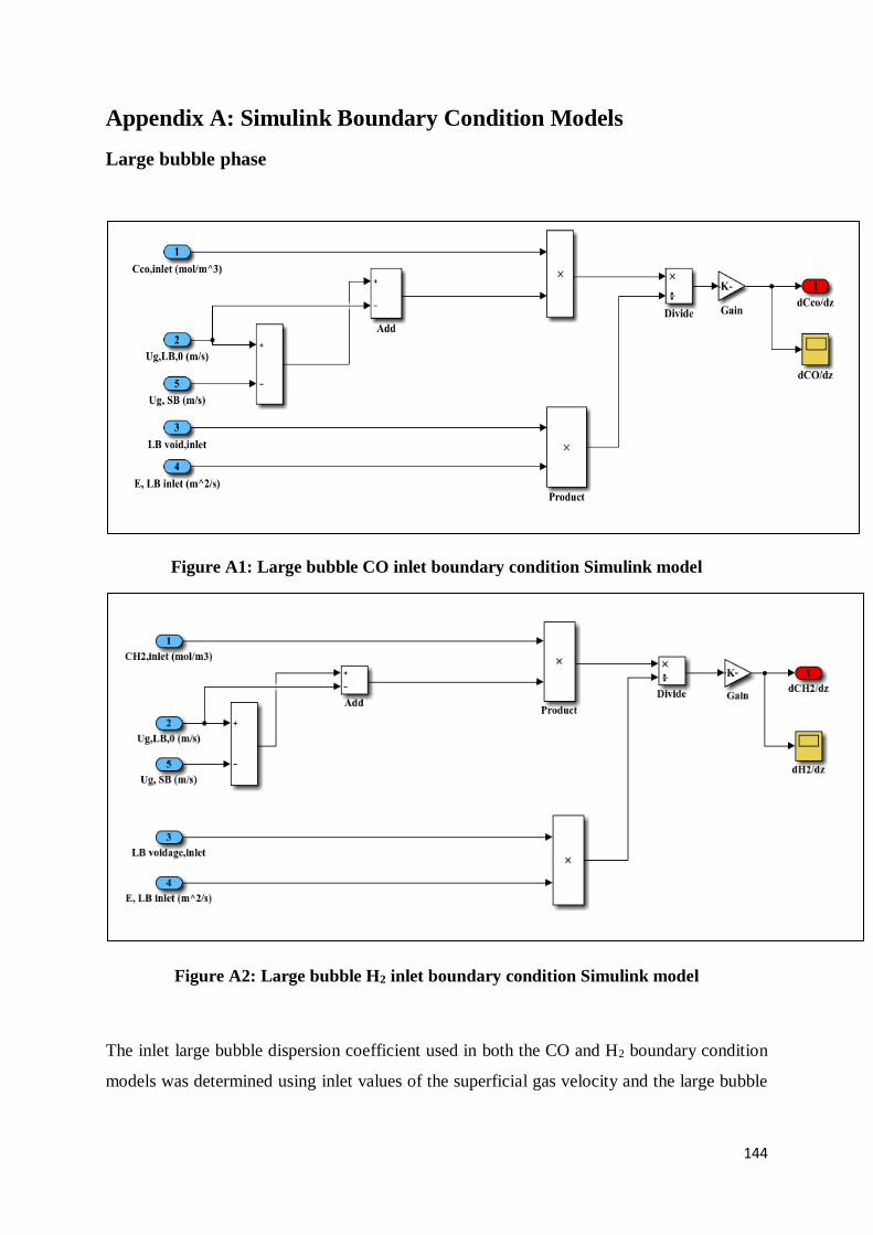
144
Appendix A: Simulink Boundary Condition Models
Large bubble phase
Figure A1: Large bubble CO inlet boundary condition Simulink model
Figure A2: Large bubble H2 inlet boundary condition Simulink model
The inlet large bubble dispersion coefficient used in both the CO and H2 boundary condition
models was determined using inlet values of the superficial gas velocity and the large bubble
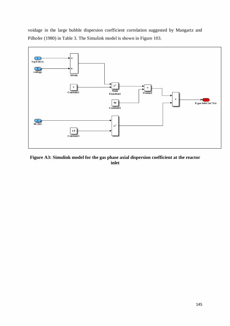
145
voidage in the large bubble dispersion coefficient correlation suggested by Mangartz and
Pilhofer (1980) in Table 3. The Simulink model is shown in Figure 103.
Figure A3: Simulink model for the gas phase axial dispersion coefficient at the reactor
inlet
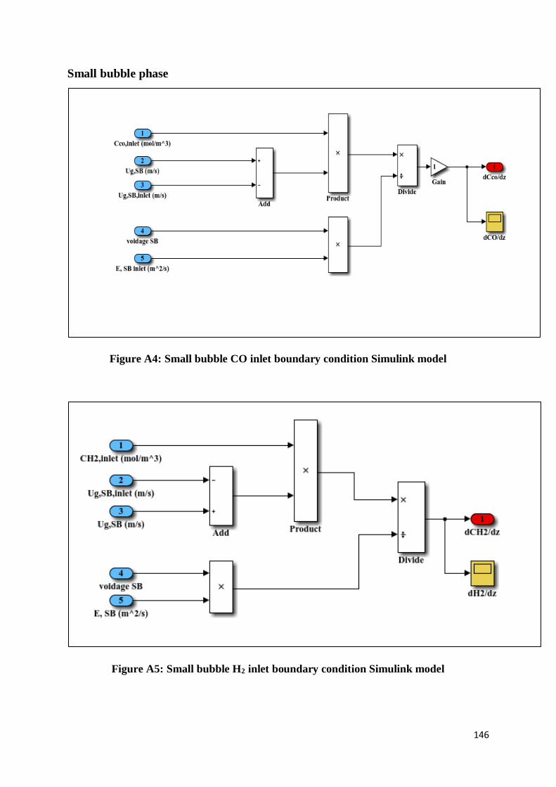
146
Small bubble phase
Figure A4: Small bubble CO inlet boundary condition Simulink model
Figure A5: Small bubble H2 inlet boundary condition Simulink model
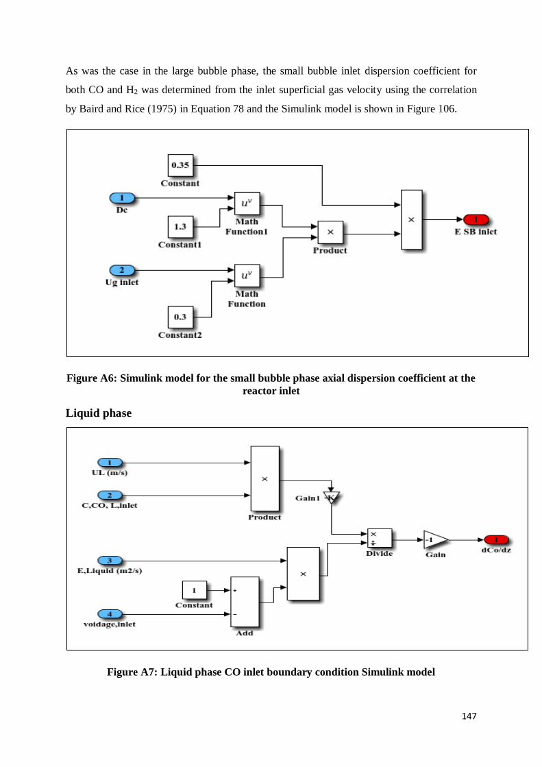
147
As was the case in the large bubble phase, the small bubble inlet dispersion coefficient for
both CO and H2 was determined from the inlet superficial gas velocity using the correlation
by Baird and Rice (1975) in Equation 78 and the Simulink model is shown in Figure 106.
Figure A6: Simulink model for the small bubble phase axial dispersion coefficient at the
reactor inlet
Liquid phase
Figure A7: Liquid phase CO inlet boundary condition Simulink model
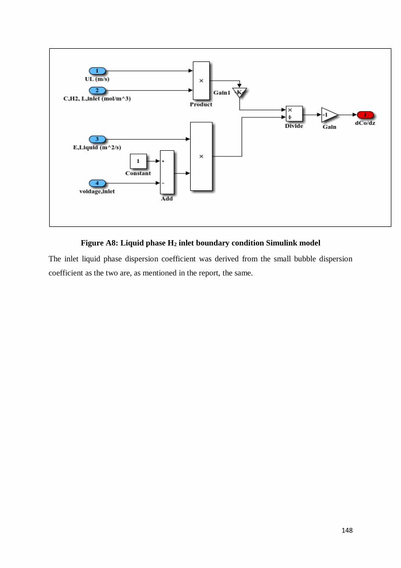
148
Figure A8: Liquid phase H2 inlet boundary condition Simulink model
The inlet liquid phase dispersion coefficient was derived from the small bubble dispersion
coefficient as the two are, as mentioned in the report, the same.