modelling of an efficient dynamic smart solar … photovoltaic power grid system ... while the...
TRANSCRIPT
Modelling of an Efficient Dynamic Smart
Solar Photovoltaic Power Grid System
Balogun Emmanuel Babajide
B.Sc (University of Lagos, Nigeria – UNILAG) (2005)
M.Sc(University of Lagos, Nigeria – UNILAG) (2010)
A Thesis Submitted in Requirement for the Degree of Doctor
of Philosophy (Information Science & Engineering)
at
University of Canberra.
Faculty of Education, Science, Technology and Mathematics
September 2015.
i
Abstract
A smart solar photovoltaic grid system is an advent of innovation coherence of information
and communications technology (ICT) with power systems control engineering via the internet
[1]. This thesis designs and demonstrates a smart solar photovoltaic grid system that is self-
healing, environmental and consumer friendly, but also with the ability to accommodate other
renewable sources of energy generation seamlessly, creating a healthy competitive energy
industry and optimising energy assets efficiency.
This thesis also presents the modelling of an efficient dynamic smart solar photovoltaic power
grid system by exploring the maximum power point tracking efficiency, optimisation of the
smart solar photovoltaic array through modelling and simulation to improve the quality of design
for the solar photovoltaic module. In contrast, over the past decade quite promising results have
been published in literature, most of which have not addressed the basis of the research questions
in this thesis.
The Levenberg-Marquardt and sparse based algorithms have proven to be very effective tools in
helping to improve the quality of design for solar photovoltaic modules, minimising the possible
relative errors in this thesis. Guided by theoretical and analytical reviews in literature, this
research has carefully chosen the MatLab/Simulink software toolbox for modelling and
simulation experiments performed on the static smart solar grid system. The auto-correlation
coefficient results obtained from the modelling experiments give an accuracy of 99% with
negligible mean square error (MSE), root mean square error (RMSE) and standard deviation.
This thesis further explores the design and implementation of a robust real-time online solar
photovoltaic monitoring system, establishing a comparative study of two solar photovoltaic
tracking systems which provide remote access to the harvested energy data. This research made a
landmark innovation in designing and implementing a unique approach for online remote access
solar photovoltaic monitoring systems providing updated information of the energy produced by
the solar photovoltaic module at the site location. In addressing the challenge of online solar
photovoltaic monitoring systems, Darfon online data logger device has been systematically
ii
integrated into the design for a comparative study of the two solar photovoltaic tracking systems
examined in this thesis. The site location for the comparative study of the solar photovoltaic
tracking systems is at the National Kaohsiung University of Applied Sciences, Taiwan, R.O.C.
The overall comparative energy output efficiency of the azimuthal-altitude dual-axis over the 450
stationary solar photovoltaic monitoring system as observed at the research location site is about
72% based on the total energy produced, estimated money saved and the amount of CO2
reduction achieved. Similarly, in comparing the total amount of energy produced by the two
solar photovoltaic tracking systems, the overall daily generated energy for the month of July
shows the effectiveness of the azimuthal-altitude tracking systems over the 450 stationary solar
photovoltaic system. It was found that the azimuthal-altitude dual-axis tracking systems were
about 68.43% efficient compared to the 450 stationary solar photovoltaic systems. Lastly, the
overall comparative hourly energy efficiency of the azimuthal-altitude dual-axis over the 450
stationary solar photovoltaic energy system was found to be 74.2% efficient.
Results from this research are quite promising and significant in satisfying the purpose of the
research objectives and questions posed in the thesis. The new algorithms introduced in this
research and the statistical measures applied to the modelling and simulation of a smart static
solar photovoltaic grid system performance outperformed other previous works in reviewed
literature. Based on this new implementation design of the online data logging systems for solar
photovoltaic monitoring, it is possible for the first time to have online on-site information of the
energy produced remotely, fault identification and rectification, maintenance and recovery time
deployed as fast as possible.
The results presented in this research as Internet of things (IoT) on smart solar grid systems are
likely to offer real-life experiences especially both to the existing body of knowledge and the
future solar photovoltaic energy industry irrespective of the study site location for the
comparative solar photovoltaic tracking systems. While the thesis has contributed to the smart
solar photovoltaic grid system, it has also highlighted areas of further research and the need to
investigate more on improving the choice and quality design for solar photovoltaic modules.
Finally, it has also made recommendations for further research in the minimization of the
absolute or relative errors in the quality and design of the smart static solar photovoltaic module.

v
Acknowledgements
This dissertation would have never been written, much less completed without acknowledging
the unmerited mercies, love and favour of the Almighty God for His unfailing grace, strength,
knowledge and wisdom throughout the learning process of my doctoral studies.
I would like to express sincere gratitude to my primary supervisor, Prof. Xu Huang, for his
excellent guidance and counsel, patience, providing insightful comments, valuable contribution
and support over the course of my research. I would also like to thank my co-supervisor A/Prof.
Dat Tran for his encouragement and moral support in every step of this research work. I wish to
express my indebtedness to fellow research colleagues, and all administrative staffs at the
National Kaohsiung University of Applied Sciences, Taiwan, the Republic of China for their
guidance, cooperation and support during my research visit for data collection.
My sincere thanks also go to Mrs Carmela Thambirajah Adisa and family for their timely and
invaluable support at the hour of distress during my study. I would also like to express sincere
gratitude to Dr Abayomi Adeniyi and family for their moral guidance and support. I would like
to thank every member and friends of the Ammish family, especially Dr Ammish Adu and Dr
Joyce Adu for their unflinching and unfailing assistance and encouragement to persevere in
finishing my doctoral research.
I would like to thank Dr Michael S. Adelana and all members of the Deeper Christian Life
Ministry, Australia for their timely and financial support in the period of crisis and ceaseless
prayers supporting me spiritually throughout this study period. I would like to thank my fellow
research mates for their thought-provoking discussions across all works of life, for the
opportunities to work together, and for all the fun in sports, we had in the last three years.
I am indebted to the Lagos State Government Scholarship Board, Nigeria for granting me the
opportunity to undertake this research study at the University of Canberra, Australia for their
financial commitment was invaluable to me in completing my doctoral studies. Special thanks to
all who have crossed my paths during this journey, who has in one way or another been a
blessing contributing to the successful completion of this dissertation.

vi
Last but not the least, I would like to thank my parents, especially my mother for her ceaseless
prayers and mobile calls since I left for this doctoral studies and my beloved wonderful sisters
for their concern on my study progress and unconditional support in taking good care of my dad.

vii
List of Acronyms AADAT Azimuth-Altitude Dual Axis Tracker
ANN Artificial Neural Network
CCD Charge Coupled Device
Cfcs Chlorofluorocarbons
CO2-e Carbondioxide Equivalent
CPV Concentrated Photovoltaic
CR Time Constant
CSP Concentrated Solar Power
CVR Conservation Voltage Reduction
DLS Damped Least-Squares
EPA Environment Protection Agency
EPRI Electric Power Research Institute
FDIR Fault Detection, Isolation And Restoration
GDP Gross Domestic Product
GHG Green House Gases
GM-Estimators Generalized M-Estimators
GNA Gaussian-Newton Algorithm
GPS Global Positioning System
GUI Graphical User Interface
HSAT Horizontal Single Axis Tracker
IAAS Infrastructure As A Service
ICT Information and Communication Technology
IP Internet Protocol
IREAs International Renewable Agencies
ISA International Society Of Automation
ISP Internet Service Providers
IVVCO Integrated Volt-Var Control Optimisation

viii
IoT Internet of Things
LAD Least Absolute Deviation
LDRs Light Dependent Resistors (Or Photo-Resistors),
LMA Levenberg-Marquadt Algorithm
LREs Large Renewable Energy Schemes
LT Local Times
LTS Least Trimmed Squares
MLP Multilayer Perceptron
MPPT Maximum Power Point Tracking
MSE Mean Square Error
NERC CIP North American Electric Reliability Corporation Critical Infrastructure Protection
NIPP National Infrastructure Protection Plan
NIST National Institute Of Standard And Technology
NREAP National Renewable Energy Action Plan
O&M Operations And Maintenance
OLS Ordinary Least Squares
PAAS Platform As A Service
PASAT Polar Aligned Single Axis Tracker
PC Personal Computers
P-I-N Diode Photo-Diode
PLC Programmable Logic Control
PSpice Personal Computer Simulation Program with Integrated Circuit Emphasis
PV Photo-Voltaic
QoS Quality of Service
RBF Radial Basis Function
REAs Renewable Energy Agencies
RECs Renewable Energy Credits
RES Renewable Energy Sources

ix
RETs Renewable Energy Targets
RMSE Root Mean Square Error
RPS Renewable Portfolio Standards
SAAS Software As A Service
SGN Smart Grid Network
SRES Small Renewable Energy Schemes
T&D Transmission And Distribution
TSAT Tilted Single Axis Tracker
TTDAT Tip-Tilt Dual Axis Tracker
UCAAS Unified Communication As A Service
UV UltraVoilet
VSAT Vertical Single Axis Tracker.
WCRE World Council For Renewable Energy

xi
List of Symbols
𝐼𝑝ℎ photo current generator
𝐼𝑜 leakage or reverse saturation current
q electron charge
V solar cell voltage
A ideality factor
k Boltzmann constant
𝑅𝑆 series cell resistance
𝑅𝑠ℎ shunt cell resistance
𝑇𝑎 ambient temperature
𝑤𝑠 wind speed
S solar irradiation
𝐼𝑜𝑟 𝐼𝑜 at reference temperature at 𝑇𝑟 = 301.18K
𝐸𝐺 band gap energy
𝑇𝑟 reference temperature
𝑇 solar cell temperature
𝐼𝑠𝑐𝑟 short circuit current at 𝑇𝑟
𝑘𝑖 short circuit current temperature coefficient
𝑉𝑂𝐶 open circuit voltage
𝑉𝑚𝑝 maximum power voltage
𝐼𝑚𝑝 maximum power current
𝑛𝑝 number of parallel modules
𝑛𝑠 number of series modules
P output power

xiii
List of Publications
Balogun, Emmanuel B., Xu Huang, and Dat Tran. "Efficiency of Sensor Devices Used
in Dynamic Solar Tracking System: Comparative Assessment Parameters
Review." Applied Mechanics and Materials 448 (2014): 1437-1445.
Balogun, Emmanuel B., Xu Huang, and Dat Tran "Solar optimisation based on different
tracking techniques". Proceedings of the 2013 International Conference on Agriculture
Science and Environment Engineering (ICASEE 2013), 19-20 December, Beijing, China.
DEStech Publications, Inc.
Balogun, Emmanuel B., Xu Huang, and Dat Tran. "A Revolution in Green Energy:
Solar Tracking System". Proceedings of the 2013 International Conference & Exhibition
on Clean Energy (ICCE 2013), 9-13 September, Ottawa, Canada.
Balogun, Emmanuel B., Xu Huang, and Dat Tran. "The Prospective Grid: The Smart
Grid Network". Proceedings of the 2014 International Conference & Exhibition on Clean
Energy (ICCE 2014), 20-24 October, Quebec city, Canada.
Balogun, Emmanuel B., Xu Huang, and Dat Tran. "Comparative Study of Different
Artificial Neural Networks Methodologies on Static Solar Photovoltaic Module."
"International Journal of Emerging Technology and Advanced Engineering" Volume 4,
Issue 10, October 2014(ISSN 2250-2459(Online)): 674-685.
Balogun, Emmanuel B., Xu Huang, Dat Tran, Yun-Chuan Lin, Mingyu Liao, and
Michael Adaramola. "Regression estimation modelling techniques on static solar
photovoltaic module" "International Journal of Emerging Technology and Advanced
Engineering" Volume 5, Issue 4, April 2015 (ISSN 2250-2459(Online)): 451-461.
Balogun, Emmanuel B., Xu Huang, Dat Tran, Yun-Chuan Lin, Mingyu Liao, and
Michael Adaramola. "A robust real-time online comparative monitoring of an azimuthal-
altitude dual axis GST 300 and a 45° fixed solar photovoltaic energy tracking systems."
In SoutheastCon 2015, pp. 1-10. IEEE, 2015.
Balogun, Emmanuel B., Xu Huang, Dat Tran, Yun-Chuan Lin, Mingyu Liao, and
Michael Adaramola. "Power quality improvement by integration of Distributed
Networks" "International Journal of Emerging Technology and Advanced Engineering"
Volume 5, Issue 7, July 2015 (ISSN 2250-2459(Online)): 465-471.

xv
Table of Contents Abstract .......................................................................................................................................................... i
Certificate of Authorship of Thesis .............................................................................................................. iii
Acknowledgements ....................................................................................................................................... v
List of Acronyms ........................................................................................................................................ vii
List of Symbols ............................................................................................................................................ xi
List of Publications .................................................................................................................................... xiii
List of Tables ............................................................................................................................................. xix
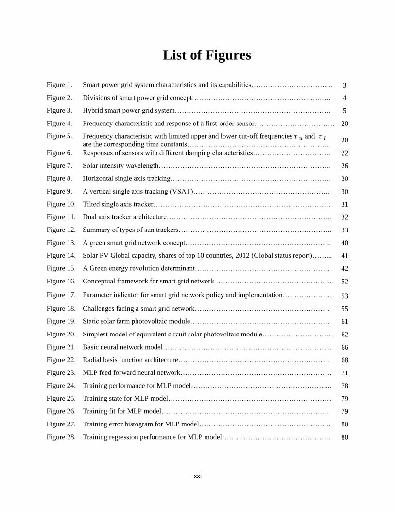
List of Figures ............................................................................................................................................ xxi
Chapter 1 Introduction ................................................................................................................................. 1
1.1 Introduction to the Study ................................................................................................................... 1
1.2 Characteristics of the Term Smart Power Grid ................................................................................. 2
1.3 Smart Power Grid Concept ................................................................................................................ 3
1.4 Evolution in the Power Grid Systems ................................................................................................ 5
1.5 Background and Context .................................................................................................................... 6
1.6 Research Objectives and Questions .................................................................................................... 9
1.6.1 Research Objectives ..................................................................................................................... 9
1.6.2 Research Questions ...................................................................................................................... 9
1.7 Research Methods ............................................................................................................................ 10
1.8 Research Works, Contribution and Justification .............................................................................. 11
1.9 Limitation and Assumptions ............................................................................................................ 13
1.10 The Outline of this Thesis .............................................................................................................. 14
1.11 Conclusion ..................................................................................................................................... 16
Chapter 2 Literature Review ...................................................................................................................... 17
2.1 Introduction ...................................................................................................................................... 17
2.2 Solar Photovoltaic Sensor and Tracking Optimisation Devices ...................................................... 18
2.2.1 Dynamic Characteristics of Solar Photovoltaic Sensors ........................................................... 19
2.2.2 Assessments of Physical Sensor Parameters ............................................................................. 22
2.3 Solar Photovoltaic Tracking Optimisation Techniques ................................................................... 28
2.3.1 Dynamic Single axis Tracking Optimisation ............................................................................ 29
2.3.2 Dynamic Dual- axis Solar Tracker ............................................................................................ 31
xvi
2.4 Smart Solar Power Grid System ...................................................................................................... 33
2.4.1 Smart Solar Photovoltaic Power Grid Network ........................................................................ 33
2.4.2 Concept of the Smart Solar Photovoltaic Grid Network ........................................................... 34
2.4.3 Challenges and Issues on the Smart Solar Photovoltaic Grid System ...................................... 36
2.5 Green Energy Revolution and Policy ............................................................................................... 38
2.5.1 Overview of the State of Evolution ........................................................................................... 38
2.5.2 Determinants of Green Energy Revolution .............................................................................. 41
2.5.3 Impacts of Green Renewable Energy ...................................................................................... 45
2.6 The Prospective Grid: A Smart Grid Network ................................................................................. 48
2.6.1 The Smart Grid Network .......................................................................................................... 48
2.6.2 Conceptual Framework of the Smart Grid Network ................................................................ 50
2.6.3. A Smart Grid Network Policy and Implementation Guidelines .............................................. 52
2.6.4. The Smart Grid Network Challenges ....................................................................................... 53
2.6.5. Benefits of the Smart Grid Network ........................................................................................ 54
2.7 Conclusion ...................................................................................................................................... 55
Chapter 3 Modelling and Simulation Techniques for a Solar Photovoltaic System .................................. 59
3.1 Introduction ...................................................................................................................................... 59
3.2 Static Solar Photovoltaic Modules Modelling and Simulation Performance .................................... 59
3.3 Static Solar Farm Photovoltaic Modules Modelling ........................................................................ 61
3.4 Solar Photovoltaic Module Simplest Model and Parameter Definitions ......................................... 61
3.4.1 Solar Photovoltaic Module Simplest Model ............................................................................. 61
3.4.2 Module Parameter Definitions .................................................................................................. 62
3.5 Proposed Research Methodology..................................................................................................... 65
3.5.1 Neural Network Model ............................................................................................................ 65
3.5.2 Sparse Based Algorithm........................................................................................................... 81
3.6 Conclusion ..................................................................................................................................... 100
Chapter 4 Astronomical and Analytical Derivation for Solar Photovoltaic Tracking Systems ................ 101
4.1 Introduction .................................................................................................................................... 101
4.2 An Astronomy of Dynamic Solar Photovoltaic Tracking System ................................................. 101
4.3 Geometric Modelling Equation Derivations for Dynamic Smart Solar Photovoltaic Systems ..... 104
4.4 Simulink Modelling Approach....................................................................................................... 111
4.5 Simulink Implementation for Smart Solar Photovoltaic Systems .................................................. 112

xvii
4.5.1 Simulink Implementation of a Solar Photovoltaic Module ..................................................... 112
4.5.2 Simulink Implementation of a Static Smart Solar Photovoltaic off-grid model ..................... 117
4.5.3 General Photovoltaic Model Characteristics ........................................................................... 121
4.5.4 Simulink Implementation of Five thousand Solar Photovoltaic Modules .............................. 126
4.6 Conclusion ...................................................................................................................................... 129
Chapter 5 Robust Real-Time Online Solar Photovoltaic Data Monitoring Systems ............................... 131
5.1 Introduction .................................................................................................................................... 131
5.2 An Overview of Robust Real-Time Remote Solar Photovoltaic Monitoring and Tracking Systems
.............................................................................................................................................................. 131
5.3 Robust Real-Time Online Solar Photovoltaic Monitoring Infrastructure ...................................... 133
5.4 Solar Photovoltaic Data Monitoring and Acquisition Energy System ........................................... 137
5.5 Comparative Solar Photovoltaic Tracking Systems under Investigation ....................................... 140
5.6 Data Management and Presentation of a Solar Photovoltaic Tracking System ............................. 145
5.7 Presentation of Results and Discussions ........................................................................................ 148
5.8 Conclusion ...................................................................................................................................... 151
Chapter 6 Conclusion ............................................................................................................................... 153
6.1 Introduction .................................................................................................................................... 153
6.2 Impacts and Conceptualisation Benefits of this Research Study ................................................... 154
6.3 Significance of Classical Modelling Algorithms on solar photovoltaic systems ........................... 155
6.4 Significance of the Simulink Solar Photovoltaic Design Model.................................................... 156
6.5 Benefits of Robust Online Cloud Computing Solar Photovoltaic Tracking Systems .................... 157
6.6 Evaluation of Simulation Smart Solar Photovoltaic Tracking Systems ......................................... 158
6.7 Significance of this Research ......................................................................................................... 159
6.8 Recommendations for Future Research ......................................................................................... 161
Bibliography ............................................................................................................................................. 163
Appendix A .............................................................................................................................................. 173
Thesis Appendices ................................................................................................................................ 173
A.1 Regression Algorithm Model ..................................................................................................... 173
A.2 Real-time online Solar photovoltaic monitoring data ............................................................... 178

xix
List of Tables
Table 1. The existing traditional power grid system compared with the Smart power grid
system …..……………………………………………………………………………….. 6
Table 2. A Summary of sensor assessment parameters…………………………………………... 23
Table 3. Conceptual framework for the smart grid network …..………………………………..... 51
Table 4. Summary of the sub-sections of literature chapter review………………………. 56
Table 5. Parameter definitions used in solar photovoltaic model……………………………........ 62
Table 6. Photovoltaic parameters used in the simulation experiments ……………....................... 76
Table 7. The summary of the experimental results…………………………………...................... 77
Table 8. Comparison of standard error estimates of the static solar photovoltaic module……….. 96
Table 9. Comparison of the MSE and RMSE regression methods of the static solar photovoltaic
module…………………………………………………………………………………… 96
Table 10. The simulated output characteristics at ten different irradiance levels………………….. 127
Table 11. Stationary 450 solar photovoltaic obtained raw data……………………………………. 176
Table 12. Dual-axis solar photovoltaic obtained raw data………………………………………… 193
Table 13. Comparative total energy generated for a month……………………………………….. 211
Table 14. Comparative hourly energy efficiency………………………………………………….. 212
xxi
List of Figures
Figure 1. Smart power grid system characteristics and its capabilities…………………………..… 3
Figure 2. Divisions of smart power grid concept……………………………………………….…. 4
Figure 3. Hybrid smart power grid system………………………………………………………… 5
Figure 4. Frequency characteristic and response of a first-order sensor……………………………. 20
Figure 5. Frequency characteristic with limited upper and lower cut-off frequencies 𝜏 𝑢 and 𝜏 𝐿
are the corresponding time constants……………………………………………………. 20
Figure 6. Responses of sensors with different damping characteristics…………………………… 22
Figure 7. Solar intensity wavelength………………………………………………………………. 26
Figure 8. Horizontal single axis tracking………………………………………………………….. 30
Figure 9. A vertical single axis tracking (VSAT)…………………………………………………. 30
Figure 10. Tilted single axis tracker………………………………………………………………… 31
Figure 11. Dual axis tracker architecture……………………………………………………………. 32
Figure 12. Summary of types of sun trackers……………………………………………………….. 33
Figure 13. A green smart grid network concept…………………………………………………….. 40
Figure 14. Solar PV Global capacity, shares of top 10 countries, 2012 (Global status report)……... 41
Figure 15. A Green energy revolution determinant………………………………………………… 42
Figure 16. Conceptual framework for smart grid network …………………………………………. 52
Figure 17. Parameter indicator for smart grid network policy and implementation…………………. 53
Figure 18. Challenges facing a smart grid network………………………………………………… 55
Figure 19. Static solar farm photovoltaic module…………………………………………………… 61
Figure 20. Simplest model of equivalent circuit solar photovoltaic module………………………… 62
Figure 21. Basic neural network model……………………………………………………………... 66
Figure 22. Radial basis function architecture……………………………………………………….. 68
Figure 23. MLP feed forward neural network………………………………………………………. 71
Figure 24. Training performance for MLP model…………………………………………………... 78
Figure 25. Training state for MLP model…………………………………………………………… 79
Figure 26. Training fit for MLP model……………………………………………………………... 79
Figure 27. Training error histogram for MLP model……………………………………………….. 80
Figure 28. Training regression performance for MLP model………………………………………. 80
xxii
Figure 29. RBF Training window……………………………………………………………….. 81
Figure 30. Dispersion diagram of Pmp vs. S…………………………………………………….. 97
Figure 31. Dispersion diagram of Vmp vs. S……………………………………………………. 97
Figure 32. Dispersion diagram of Imp vs. S……………………………………………………... 98
Figure 33. Dispersion diagram of Vmp vs. S……………………………………………………. 98
Figure 34. Dispersion diagram of Pmp vs. S…………………………………………………….. 99
Figure 35. Dispersion diagram of Imp vs. S……………………………………………………… 99
Figure 36. The Solar tracking elevation and azimuth angles…………………….………………. 102
Figure 37. Geometrical setup of a concentrated solar photovoltaic system using two
mirror-symmetrically disposed on the left (M1) and right (M2)…….…..…………… 105
Figure 38. Euler’s observatory angle compared to altazimuthal coordinate system…………….. 106
Figure 39. Simplest model of an equivalent circuit solar photovoltaic module………………….. 112
Figure 40. PV cell photocurrent, Iph Matlab/Simulink subsystem……………………………….. 114
Figure 41. PV cell photocurrent, Iph Matlab/Simulink masked subsystem………………………. 114
Figure 42. Diode reverse saturation current, Io Matlab/Simulink subsystem…………………… 115
Figure 43. Diode reverse saturation current, Io Matlab/Simulink masked subsystem…………… 115
Figure 44. Simulink model of the characteristics equation of the solar photovoltaic module……. 116
Figure 45. Masked Simulink model of the characteristics equation of the solar photovoltaic
module………………………………………………………………………………… 116
Figure 46. I-V & P-V characteristics of solar photovoltaic module……………………………… 117
Figure 47. A series connection of ten solar photovoltaic modules……………………………….. 119
Figure 48. Masked subsystem of the series connection…………………………………………… 119
Figure 49. Functional block parameter of a solar PV cell………………………………………… 120
Figure 50. Functional block parameter of a solar PV cell………………………………………… 120
Figure 51. Masked subsystem block units of a hundred solar photovoltaic modules……………... 120
Figure 52. Simulink Model of a single block of hundred solar photovoltaic modules…………..... 120
Figure 53. A five thousand series-parallel configurations of solar photovoltaic modules………..... 122
Figure 54. Solar photovoltaic array model for GUI environment of Simulink…………………… 123
Figure 55. I-V Characteristics behaviour of the solar photovoltaic model………………………. 124
Figure 56. P-V characteristics behaviour of the solar photovoltaic model………………………. 124
Figure 57. I-V characteristics of the parallel configuration model………………………………. 125
Figure 58. P-V characteristics of the parallel configuration model……………………………… 125
Figure 59. Masked subsystem for the five thousand solar photovoltaic module………………… 126
Figure 60. Full Simulink model for the five thousand solar photovoltaic modules arrangement... 126
xxiii
Figure 61. Simulation results of the output current, power and voltage against simulation time…. 127
Figure 62. Output power, voltage generated with increased irradiance level……………………... 128
Figure 63. Output current generated with increased irradiance level……………………………... 128
Figure 64. A robust real-time online solar monitoring system at roof building platform…….…… 135
Figure 65. A schematic solar photovoltaic monitoring wiring system architecture…….….…….. 136
Figure 66. Client/server internet architecture……………………………………………………… 137
Figure 67. Client/server intranet architecture……………………………………………………… 137
Figure 68. Real-time solar monitoring and acquisition infrastructure architecture………………. 138
Figure 69. Basic fundamental cloud computing service model…………………………………… 139
Figure 70. Fixed solar energy system installed at a 450 inclination……………………………..... 141
Figure 71. GST 300 tracker deployed at the roof platform……………………………………….. 144
Figure 72. Architectural framework of the GST 300 tracker……………………………………… 145
Figure 73. Graphic User Interface of the remote Darfon data logger…………………………….. 147
Figure 74. An overview of the solar photovoltaic modules installed on roof building…………….. 147
Figure 75. GUI for the 450 stationary solar systems……………………………………………… 148
Figure 76. GUI for the azimuthal-altitude dual solar systems…………………………………… 148
Figure 77. Daily profile of the mean daily total energy for the azimuthal-altitude solar systems... 150
Figure 78. Daily profile of the mean daily total energy for 450 stationary solar systems………... 150
Figure 79. Hourly profile of the mean daily total energy for 450 stationary solar systems………. 151
Figure 80. Hourly profile of the mean daily total energy for the azimuthal-altitude solar systems 151
Figure 81. Ordinary Least Regression algorithm………………………………………………… 174
Figure 82. Logistic Robustfit regression code……………………………………………………. 176
Figure 83. Least Trimmed Squares regression code………………………………………………. 178

Modelling of an Efficient Dynamic Smart Solar Photovoltaic Power Grid System
1
Chapter 1 Introduction
1.1 Introduction to the Study
This research explores one of the fast growing renewable energy sources globally, a smart
solar photovoltaic energy system. This energy system has increased the reliability of
providing a more secure and guaranteed source of power generation in many parts of the
world today. The smart solar photovoltaic energy system has received global research
attention due to the sun’s natural abundance, lack of noise pollution, non-emission of
greenhouse gases (GHG), unlike fossil and coal powered generation sources which affect the
climatic conditions causing global warming. The smart solar photovoltaic energy system is
emerging as a convergence of information and communications technology in electrical
power and control system engineering making it an intelligent energy solution system.
The electrical power grid system is undergoing a transformation driven by a number of
demands. There is an exigent demand for reliability, availability, energy security and
conservation, and environmental compliance in protecting the climate from further
deterioration. In particular, the transformation has been significant in power generation over
the past two decades globally. This is because of the increase in energy demand for industrial
and domestic purposes from the existing traditional power generation which has contributed
immensely to the emission of greenhouse gases, affecting the climate and giving rise to
global warming [2].
As a result of these demands, technological transformations and innovations have been
witnessed in the electrical power generation industry by the birth of this new power grid
system called the "smart power grid system". There are several definitions of the term, "smart
power grid system" but as applied to our research investigations in modelling and simulation
implementation to better improve the optimisation and efficiency of the smart solar power
grid system, are critical for this research. The "smart power grid system" comprises of an
organically intelligent, fully integrated environment involving an end-to-end communication
of tasks, objectives and implementation replacing the traditional power grid system [3]. The
comparative analysis of the output characteristics and efficiency between the static and
dynamic online remote solar photovoltaic power monitoring systems investigation are
significant in real life circumstances to determine the exact energy generated, fault location

Modelling of an Efficient Dynamic Smart Solar Photovoltaic Power Grid System
2
and detection of the energy system. As a contribution to the existing body of knowledge, it is
closely addressed in this thesis.
1.2 Characteristics of the Term Smart Power Grid
For clarity in our discussion, we present the following characteristics of the smart power grid
[3-5]:
A smart power grid is referred to as a grid that accommodates a wide variety of
generation options, e.g. central, distributed, intermittent, and mobile.
A smart power grid provides an interface between consumer appliances and the
traditional assets in a power system. This implies it encourages a two-way
communication channel for its operational decisions.
A smart power grid is designed to be semi-autonomous enabling much faster
operations when handling interruptions, failures in the power system and
reconfiguration to mitigate contingencies.
A smart power grid optimises the assets of the electrical power system employing
responsive operating protocols along the existing transmission links, thereby
improving the system reliability and forecasting for long-term investments.
A smart power grid refers to a completely modernised electricity delivery system
which monitors, protects and optimises the operation of its interconnected elements
from end to end.
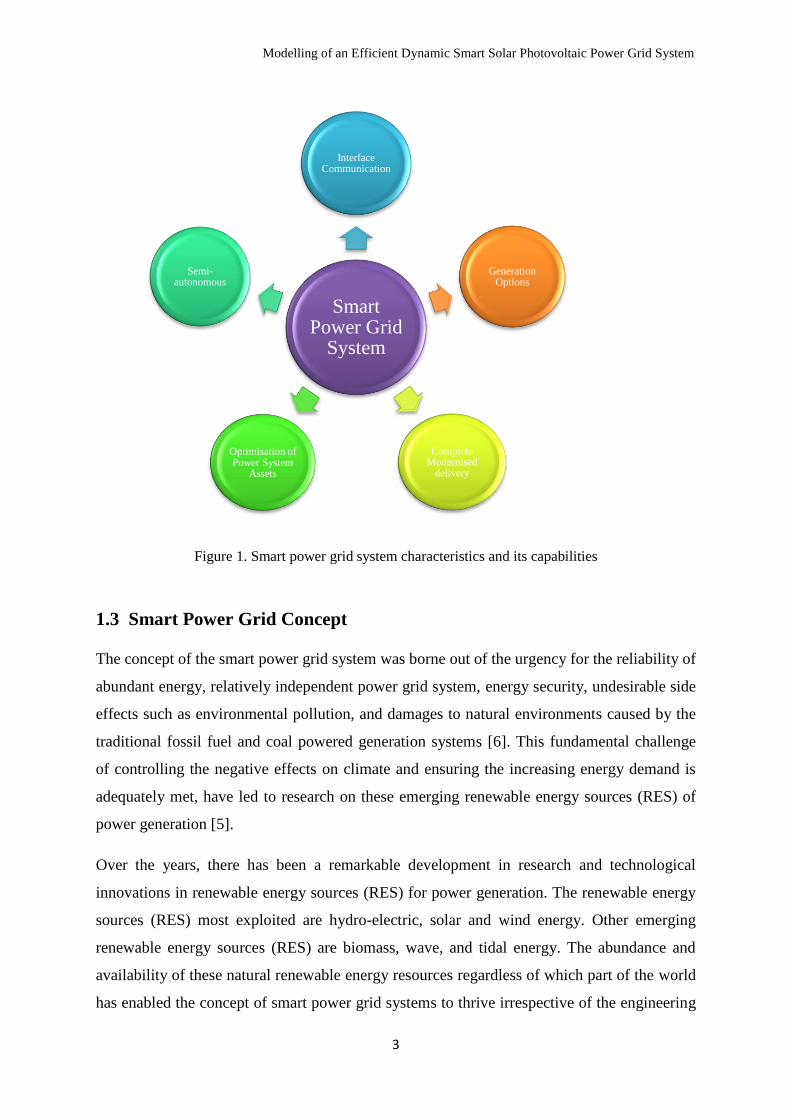
Figure 1 represents the key characteristics of the smart power grid system as highlighted
above. This is fundamental in resolving the increasing complexity of traditional power
grids, growing demand and requirements for significant reliability, better operational
decisions, and most importantly, environmental and energy sustainability.
Modelling of an Efficient Dynamic Smart Solar Photovoltaic Power Grid System
3
Figure 1. Smart power grid system characteristics and its capabilities
1.3 Smart Power Grid Concept
The concept of the smart power grid system was borne out of the urgency for the reliability of
abundant energy, relatively independent power grid system, energy security, undesirable side
effects such as environmental pollution, and damages to natural environments caused by the
traditional fossil fuel and coal powered generation systems [6]. This fundamental challenge
of controlling the negative effects on climate and ensuring the increasing energy demand is
adequately met, have led to research on these emerging renewable energy sources (RES) of
power generation [5].
Over the years, there has been a remarkable development in research and technological
innovations in renewable energy sources (RES) for power generation. The renewable energy
sources (RES) most exploited are hydro-electric, solar and wind energy. Other emerging
renewable energy sources (RES) are biomass, wave, and tidal energy. The abundance and
availability of these natural renewable energy resources regardless of which part of the world
has enabled the concept of smart power grid systems to thrive irrespective of the engineering
Smart Power Grid
System
Interface Communication
Semi-autonomous
Optimisation of Power System
Assets
Complete Modernised
delivery
Generation Options
Modelling of an Efficient Dynamic Smart Solar Photovoltaic Power Grid System
4
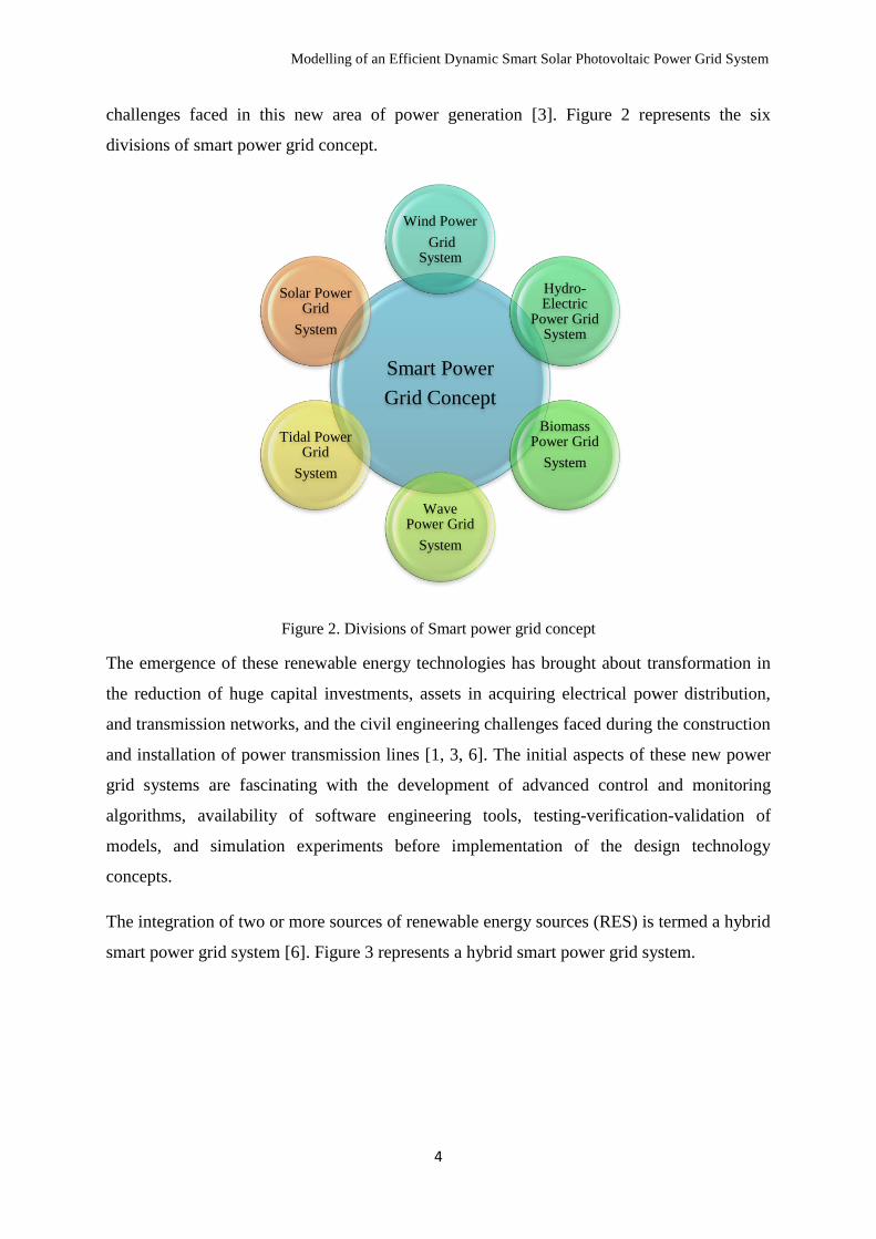
challenges faced in this new area of power generation [3]. Figure 2 represents the six
divisions of smart power grid concept.
Figure 2. Divisions of Smart power grid concept
The emergence of these renewable energy technologies has brought about transformation in
the reduction of huge capital investments, assets in acquiring electrical power distribution,
and transmission networks, and the civil engineering challenges faced during the construction
and installation of power transmission lines [1, 3, 6]. The initial aspects of these new power
grid systems are fascinating with the development of advanced control and monitoring
algorithms, availability of software engineering tools, testing-verification-validation of
models, and simulation experiments before implementation of the design technology
concepts.
The integration of two or more sources of renewable energy sources (RES) is termed a hybrid
smart power grid system [6]. Figure 3 represents a hybrid smart power grid system.
Smart Power
Grid Concept
Wind Power
Grid System
Hydro-Electric
Power Grid System
Biomass Power Grid
System
Wave Power Grid
System
Tidal Power Grid
System
Solar Power Grid
System

Modelling of an Efficient Dynamic Smart Solar Photovoltaic Power Grid System
5
Figure 3. Hybrid Smart power grid system
The problems associated with power grid integration of two different power configurations in
a hybrid smart power grid system have been resolved with advanced control and monitoring
systems, the introduction of smart sensor integration, and embedded intelligence encapsulated
components which have enabled a two-way communication link. The ease at which these
grids are integrated through the plug-and-play integration of the different renewable energy
sources (RES), makes the system an intelligent power grid system [6].
1.4 Evolution in the Power Grid Systems
The transformation in the power grid system is inevitably massive as the transition from the
traditional power grid generations are gradually been phased out with smart power grid
systems, or upgraded to a smart power grid system. The existing traditional power grid
systems have about 8% of output generated energy lost through transmission power lines,
huge capital investments in the installation of massive power transmission towers, and
manual delay in restoration of power failures. The smart power grid system is expected to
address most of these shortcomings, providing full visibility, pervasive control and
automation, reliable and efficient systems meeting the demand for services [7, 8].
Table 1 depicts the comparative analysis between the traditional power grid system and the
smart power grid system within the context of the new capabilities, communication and data
management, in-built intelligence and flexibility experienced in the use of IT (information
technology) to optimise monitoring and control of the grid system minimising operational
and maintenance costs. It is observed from Table 1 that the smart grid power system has
advantages over the existing traditional power grid as the smart grid power system involves a
Solar Power Grid
System
Wind Power Grid
System
Hybrid Smart Power Grid System

Modelling of an Efficient Dynamic Smart Solar Photovoltaic Power Grid System
6
two-way communication process providing access to the exact energy generated and
distributed with other capabilities as highlighted in the table.
Table 1. The existing Traditional power grid system compared with the Smart power grid system [7]
Existing Traditional Power Grid Smart Grid Power System
Electromechanical Digital
One-Way communication Two-Way Communication
Centralised Generation Distributed Generation
Hierarchical Network
Few sensors Sensor Throughout
Blind Self-monitoring
Manual Restoration Self-healing
Failures and Blackouts Adaptive and Islanding
Manual Check Remote Check
Limited Control Pervasive Control
Few Customer Choices Many Customer Choices
1.5 Background and Context
There have been increasing energy demands for constant supply of electricity for both
domestic and industrial purposes. Since inception, the traditional power grid system has
been driven by fossil fuels and coal contributing immensely to the emission of
greenhouse gases (carbon dioxide, chlorofluorocarbons (CFCs), methane, nitrous oxide
and ozone) affecting global changes observed in temperature rises, the climatic condition
of the earth and adverse effects on humans and the planet. The impact of the energy
demand from the traditional power generation has contributed to the present global
warming crisis, changes observed in weather, and climate conditions in the world.
Research developments in smart solar power grid systems have proven that the new
intelligent power grid system would definitely eliminate the problem of emissions of
greenhouse gases in the atmosphere.
The ability to design and model smart solar power grid systems with different software
packages available, optimising the efficiency of the system before implementation and
validating analysed results through modelling and simulation processes, has provided a
cutting edge for the industry. The extent of research work and results achieved thus far

Modelling of an Efficient Dynamic Smart Solar Photovoltaic Power Grid System
7
has taken the industry to this level with remarkable positive impacts attained in reducing
the effects of global warming and environmental power generation pollution. There is
ongoing research in this field and the results published have been notable both in the
academic environment and in the industry.
This research was spawned out of the need to efficiently and economically utilise the
abundant energy resources from the sun by improving and promoting the smart solar
photovoltaic grid concept. The MatLab/Simulink software tool is employed in this
research for the assessment and optimisation of solar photovoltaic module performance to
achieve the desired maximum power point tracking (MPPT) energy and minimization of
relative errors in the design and quality of solar photovoltaic module production. This
software tool has been employed in various research fields to handle complex non-
linearities, uncertainties and variations in the input parameters in a controlled system.
Unlike, all other renewable sources which are scarce in some parts or regions of the
world, the energy from the sun is universal and in preferential abundance compared to
other renewable sources of energy. Irrespective of its abundance in nature, research has
intensified on different algorithms and approaches in maximising the output efficiency of
the energy generated by solar photovoltaic (PV) modules. The smart solar photovoltaic
power grid system has contributed to rural electrification in many parts of the
undeveloped world because of its availability to the people within that geographical
region, changing the concept of their civilisation and livelihood.
Despite the demonstrated importance for this research investigation, there are several
issues that are of concern. These concerns include a high unpredictable rate in the
production costs and sales of solar photovoltaic modules. As a result, the new smart solar
photovoltaic grid system has been hampered by displacement of interests from private
and corporate people, thereby dampening commitment and investment participation
because of the first cost barrier experienced in connecting to the grid system. The
apparent less competitive solar photovoltaic energy market globally has allowed the price
to be overvalued and variability experienced in the quality of solar photovoltaic
production technology. Another major concern is the level of support and slow rate of
participation by policy decision makers in the industry to alleviate and remove the
financial and institutional burdens faced by solar photovoltaic manufacturers. It has been
observed that the price of the solar photovoltaic module has been experiencing a decline

Modelling of an Efficient Dynamic Smart Solar Photovoltaic Power Grid System
8
of 4% per annum and future predictions show further price reductions are expected in the
years ahead [9].
As described in more detail in the literature review that follows (chapter 2), this research
considers the different solar photovoltaic tracking techniques for efficiency improvement
to boost the collected energy at different times in the year, irrespective of geographical
locations and conditions. However, within the broad categorisation the solar photovoltaic
tracking techniques, modelling and simulation techniques are classified and analysed in
terms of their performance in the review. While the growing body of literature and
research on the smart solar photovoltaic power grid system indicates an increased interest,
there is little research that specifically investigates efficiency optimisation, minimization
of relative errors in design and quality by using the various algorithms as deployed in this
research. This will be highlighted in chapter 3 and the statistical results thus presented.
Similarly, comparative studies between the two main solar photovoltaic tracking
mechanism modes namely static and dynamic solar photovoltaic tracking systems, have
attracted extensive research. While some of the previous research have focused on the
off-line comparative study of the two solar photovoltaic tracking modes and the
efficiency benefits each of these modes have over the other. This thesis thoroughly
examines through the lens, a robust real-time online solar photovoltaic monitoring system
of the two tracking modes framework. This framework is explained in more detail in
chapter 5. As noted in section 1.3, the smart grid concept needs the support of all
stakeholders, partnership and commitment, especially the government in policy
implementation and regulation, providing necessary subsidies and incentives, promoting
an enabling healthy financial environment and market for the new intelligent power grid
to thrive amidst initial challenges experienced at the establishment of the industry.
This research aims to address the clear gaps observed in the literature reviewed by the
chosen approach in the research methodology in chapters 3, 4 and 5 of this thesis. A
systematic approach and tool have been carefully chosen and developed. Its applicability
across a wide range of parameters in improving the efficiency optimisation of smart solar
photovoltaic grid systems have also been tested and these results are thus presented in this
thesis.

Modelling of an Efficient Dynamic Smart Solar Photovoltaic Power Grid System
9
1.6 Research Objectives and Questions
1.6.1 Research Objectives
The primary research objective is to examine, using various modelling and simulation
processes to optimise the efficiency of the solar photovoltaic module with the use of the
Matlab/Simulink software package to achieve maximum power point tracking (MPPT).
The second phase of the research comparatively measures the output efficiency of a real-
time robust online solar photovoltaic monitoring system between a static and dynamic
solar photovoltaic installed system establishing the significance of such a monitoring
network approach.
1.6.2 Research Questions
In examining the modelling and simulation of the smart solar photovoltaic power grid
system to achieve the best optimisation efficiency for maximum power point tracking
(MPPT), the following research questions are put forward in the thesis to achieving our
research objectives:
1. Which of the algorithm models can achieve the best maximum power point
tracking (MPPT) using the neural network for smart solar photovoltaic grid
system?
2. Which of the algorithm models can achieve the best maximum power point
tracking (MPPT) using the sparse based regression estimation algorithm to
evaluate the mean square error (MSE) and the root mean square error (RMSE)
for smart solar photovoltaic grid system?
3. What is the comparative output efficiency for the robust real-time online solar
monitoring between the static and dynamic solar photovoltaic tracking systems?
4. What will be the resultant effect of the proposed algorithm model for the
maximum power point tracking (MPPT) on the extraction of available power from
the smart solar photovoltaic system?
Modelling of an Efficient Dynamic Smart Solar Photovoltaic Power Grid System
10
1.7 Research Methods
In answering the above research questions, the research uses an artificial neural network
(ANN) approach in modelling and simulation on the static solar photovoltaic module
under variable input parameters and conditions. This tool was chosen because of its
capacity to perform nonlinear mathematical and statistical modelling effectively between
dependent and independent variables. A comparative study of two artificial neural
networks was conducted using the Levenberg-Marquardt algorithm to evaluate the
performance and output efficiency within the respective networks. The mean square error
and autocorrelation coefficient parameters were used in the comparison of the two
networks performance under evaluation. These two parameters were chosen to explicitly
analyse in such a way that the best optimal efficiency characteristics for the solar
photovoltaic module are exploited in this thesis. The results are presented on a very large
scale for all operating conditions to confirm the validity of the model.
In addition, this research evaluates three different regression modelling techniques
namely ordinary least squares, logistic robustfit and least trimmed squares respectively.
They are discussed elaborately in this thesis using the sparse based regression estimation
algorithm on the static solar photovoltaic module. The regression modelling techniques
were used to predict on a large scale the most suitable of the three, based on manufacturer
solar photovoltaic parameters to determine the performance, efficiency, and reliability of
these models. The performance evaluation parameters are carried out using the mean
square error (MSE), root mean square error (RMSE), and standard deviation estimate to
determine the maximum power point tracking (MPPT). These were chosen to explicitly
analyse the performance of the solar photovoltaic module for the maximum power point
tracking. The maximum power point tracking current, voltage and power is obtained for
the static solar photovoltaic array in the simulation and modelling experiments.
As part of the research collaborations in this thesis, a robust real-time online solar
photovoltaic monitoring system was carefully designed via cloud computing devices, to
remotely access the solar photovoltaic data information installed on-site over mobile
phones, tablets, PCs and notebooks. The research implementation was deployed at the
National Kaohsiung University of Applied Sciences, Taiwan, R.O.C. We obtained raw
data information comparing the static and dynamic solar photovoltaic tracking systems.
The research reveals that there is a significant increase in the optimisation performance in

Modelling of an Efficient Dynamic Smart Solar Photovoltaic Power Grid System
11
the comparative data, and on the graphic user interface of the data analysis obtained
between the two measuring solar photovoltaic tracking modes.
1.8 Research Works, Contribution and Justification
The research works related to this thesis are based on three theoretical frameworks
including optimisation, improving the efficiency performance and minimization of errors
in a smart solar photovoltaic module. Hence, it increases the output efficiency of the
maximum power point tracking for the current, voltage and power characteristics. The
three frameworks are described in detail in chapters 3, 4 and 5 of this thesis respectively.
While the frameworks have a strong backbone of research associated with them, the
existing research provides insufficient answers to the research questions in this thesis.
Extensive research works have been undertaken over the years in solar photovoltaic grid
systems, a comparative study between the static and dynamic solar photovoltaic tracking
systems have been critically examined in this research, providing a robust real-time
online exact generated energy data in a real-life scenario is thoroughly examined in this
research. The research investigation has fully established an online solar photovoltaic
monitoring database system for scholars and the industry world. Additionally, the use of a
newly developed solar photovoltaic monitoring real-time data online logger allows this
research to contribute to the existing body of knowledge.
The research investigation on modelling and simulation experiments has made significant
contributions to the existing background knowledge in creating an excellent output
performance for a smart solar photovoltaic module and comparative study of the static
and dynamic solar photovoltaic tracking systems. The optimisation of the efficiency and
maximisation of the power point tracking for the solar photovoltaic module is of immense
value. The established facts in literature have led to the foundation of research in this
area. It is imperative to evaluate on the minimization of the occurrence of relative errors
in solar photovoltaic modules using the statistical measuring parameters such as mean
square error (MSE), root mean square error (RMSE), and the standard deviation of
estimate to better improve the performance of the solar photovoltaic module.
In any case, optimising the efficiency of the solar photovoltaic module is important in
light of the contemporary challenges such as the high-cost price of solar photovoltaic

Modelling of an Efficient Dynamic Smart Solar Photovoltaic Power Grid System
12
modules, increasing the overall maximum output energy expected from the photovoltaic
module, and the concern over the nonlinear characteristics of the photovoltaic module.
There is a pressing need for government and corporate policy collaboration and support in
solar renewable energy for more intensive research activities on the existing structure,
thereby improving the quality of solar photovoltaic module design. The smart solar
photovoltaic grid policy substantially makes a contribution complementing the existing
traditional grid system in a wider context. The theoretical frameworks of the smart grid
policy provide clean, noise pollution-free power generation, energy security assurance
and environmental friendly grid systems. These have received increased acceptance by
the public, research development and innovation over the last two decades. Government
policies in renewable energy solutions and participation have greatly promoted awareness
by corporate and private individuals of the newly intelligent power grid system.
The outcomes are thus presented in this thesis, the output performance of the simulation
and modelling investigations. The comparative study and analyses of the smart solar
photovoltaic grid system on a very large scale with real solar photovoltaic manufacturer’s
data is conducted. Statistical measures were used for the evaluation of the algorithm
employed in the modelling and simulation techniques in this research. The obtained
online raw data results from the comparative study of the two solar photovoltaic systems
at the National Kaohsiung University of Applied Sciences, Taiwan, R.O.C are thus
presented reflecting the merits and disadvantages of the system under investigation.
In summary, this research work makes a significant contribution to both the academic
field of research in smart solar photovoltaic energy and offers a real-life experience for
the future solar photovoltaic energy industry application. The use of MatLab/Simulink
software tool further enhances future investigation in ways to better optimise the
efficiency, improving the performance of the smart solar photovoltaic grid system.
Moreover, robust real-time online solar photovoltaic monitoring systems complement the
findings of the modelling and simulation experiments for further research.
Modelling of an Efficient Dynamic Smart Solar Photovoltaic Power Grid System
13
1.9 Limitation and Assumptions
A number of limitations and assumptions are introduced in the research methods in
modelling and simulation experiments conducted in this research investigation. For
example, the experiments conducted on modelling and simulation using Levenberg-
Marquardt algorithm and sparse based algorithm, the input parameters of the artificial
neural network were assumed for the neural network training to solve the nonlinear and
implicit general equation for a solar photovoltaic module. In our analyses, the two
assumed input parameters are solar irradiation (S) and the wind speed (ws) respectively.
The solar radiation, S was increased in steps of 10 units from 10 to maximum of 1000
m/s2 and the wind speed, ws was increased in steps of 2 units from 1 to maximum of 20
m/s2. These assumptions often employed in modelling and simulation, predict a regular
pattern and behaviour of the solar photovoltaic system under evaluation. The increment in
steps of units was introduced to improve the simulation performance of the solar
photovoltaic array to justify the variable weather that occur to a real-life scenario in our
simulation experiments and results.
However, in a real-life situation, the results obtained in this research establish a
remarkable correlation difference between the simulated results and real-life raw data
collected. The research investigation conducted on a robust real-time online solar
photovoltaic monitoring system had a challenge broadcasting via the internet at night but
resumes broadcasting in the early hours during daylight. The system has been designed in
such a way that when no irradiation is observed, the system will shut down automatically.
Another drawback experienced during the data collection is the frequent interruption of
the internet service during abnormal weather conditions such as typhoon and torrential
rainfall.
A further limitation in this research investigation acknowledged is that the results
obtained from the robust real-time online solar photovoltaic monitoring system were set
up at the National Kaohsiung University of Applied Sciences, Taiwan, R.O.C and is most
valid based on that geographical location but can be inferred anywhere in the world as a
contribution to the existing body of knowledge. The challenge to restoring faults of the
solar photovoltaic monitoring system could take longer time and so, data may not be
accessible during this period. Though data obtained are practically valid for the solar

Modelling of an Efficient Dynamic Smart Solar Photovoltaic Power Grid System
14
photovoltaic energy industry, its applicability is a challenge due to the variable weather
conditions in other parts of the world.
It is noted in this research that modelling and simulation experiments were established on
the assumption of varying two input variables in a well-defined unit steps increase as
described in Chapter 3 of this thesis. These experiments were carried out with the chosen
algorithms that will help in the optimisation of the efficiency design, minimization of
relative errors in the solar photovoltaic modules. It is expected that this will improve the
quality of production of the solar photovoltaic modules, predictions and forecasting of the
output energy of the system and will provide answers to the research questions posed in
this thesis.
1.10 The Outline of this Thesis
The thesis consists of six chapters and the structure of the thesis is as revealed below:
1. Introduction
2. Literature Review
3. Modelling and Simulation Techniques for a Solar Photovoltaic System
4. Astronomical and Analytical Derivation for Solar Photovoltaic Tracking Systems
5. Robust Real-Time Online Solar Photovoltaic Data Monitoring Systems
6. Conclusion, Discussion and Recommendations
In this preliminary chapter, a background of the study has been provided in which a smart
solar photovoltaic power grid system has been described. Thus, definitions of the term the
smart power grid as it relates to this research and the smart power grid concept were
highlighted. Moreover, the evolution in the power grid system has been described and
comparative analysis between traditional and smart grid power systems were also
emphasized. The background and the context of this research led to the research goals and
questions that formed the basis of this research providing a brief outline of the proposed
methods for the research and importantly, the justification and contribution of this study
were identified. Further, an outline of the limitations and assumptions related to this
research was also included.
The next chapter, literature review, provides a contextual review of related literature and
research investigation into the area of smart solar photovoltaic grid systems, and
optimisation of sun-tracking methods for maximum output examined. Other aspects of the

Modelling of an Efficient Dynamic Smart Solar Photovoltaic Power Grid System
15
literature covered in this chapter, include energy gains in solar photovoltaic tracking
systems, sun-tracking methods, and classification of sun tracking systems.
In addition, chapter 2 also includes a review of solar photovoltaic energy policies,
benefits and reliability perspectives of the smart grid systems. This chapter as well
presents the concept of the prospective grid, the smart grid network, the conceptual
framework of the smart grid network, smart grid policy and implementation guidelines
and benefits of the smart grid network. This chapter concludes by highlighting the gaps in
the current body of knowledge describing how and where the current study fits in relation
with the existing research.
Chapter 3 primarily focuses on modelling and simulation techniques for a static solar
photovoltaic system employing the Levenberg-Marquardt algorithm on the chosen neural
network model and sparse based algorithms to decide how best to optimise the output
efficiency of the solar photovoltaic module; using different statistical measures to
evaluate the performance on a very large scale to achieve maximum power point tracking
for this research. One section in this chapter focuses on discussion of research results
validity and reliability. Each of the modelling and simulation techniques discussed
provides a clear outline of how the research was undertaken and why. The results
achieved answer the research questions posed as the context of the research investigation
are thus presented.
Chapter 4 examines the astronomy and analytical derivation for solar photovoltaic
tracking systems, tracker definitions and taxonomy, tracker system elements and the
simulink design implementation for the smart solar photovoltaic array model. This
chapter concludes by presenting the results of the simulated models and charts on the
implemented solar photovoltaic array designed in this research.
Chapter 5 provides a detailed analysis of the experimental setup and results of a robust
real-time online comparative study of the static and dynamic solar photovoltaic tracking
energy system at National Kaohsiung University of Applied Sciences, Taiwan, R.O.C.
The research findings address the research questions within the context of the thesis. As
well, the chapter gives a significant contribution to the existing body of knowledge and
research.

Modelling of an Efficient Dynamic Smart Solar Photovoltaic Power Grid System
16
The last chapter, chapter 6, conclusion and discussion, places the results of this research
within the context of the existing research being described in chapters 2, 3, 4 and 5. A
link was established between this new research with the existing research. The
contributions made in relation to academic knowledge in the optimisation of the output
harvested energy involves the use of statistical measures to evaluate the improvement on
the quality of solar photovoltaic module design. The results obtained from the robust real-
time online comparative monitoring are likely to offer a real-life experience for the future
solar photovoltaic energy industry applications. Additionally, the significance of this
research in the context of the smart grid system is to offer an energy security assurance
and eco-friendly grid system. Suggestions for further research are also provided.
Following the last chapter of this thesis, the reference list and appendix is included. The
reference list in the thesis includes more than 165 academics, government and industry
sources. The results achieved from chapter 5 are thus provided for in the appendices.
1.11 Conclusion
This introductory chapter of the thesis, presents the research foundation, a theoretical
framework on which the research is based, the research objectives, research questions to
be answered, and the significance of this research. This chapter addresses the need for the
smart power grid system to help in providing energy security assurance, reliable and
available efficient grid systems, optimisation of output efficiency ensuring high quality
standard solar photovoltaic modules. The drive for evolution from traditional power grid
systems to the smart power grid systems in many of the developed countries of the world
and its acceptance globally have been remarkable, increasing a wide range of research
growth and development encouraging corporate and private individual participation into
the new intelligent power grid system. In conclusion, the research has provided the
opportunity to use different simulation and modelling techniques to improve the
optimisation and efficiency of the smart solar photovoltaic module, evaluating the best
performance approach and technique in each of the algorithms employed. The research
outcomes are likely to offer real-life solutions for the future solar energy industry not only
in Australia or Taiwan but also in any part of the world.
The next chapter provides with more detail a review of the current literature and the
research methods employed, crucial to answering the research questions upon which the
study and the results are thus presented and established.

Modelling of an Efficient Dynamic Smart Solar Photovoltaic Power Grid System
17
Chapter 2 Literature Review
2.1 Introduction
The purpose of this chapter, chapter 2 is to survey literature relevant to the scope of this
research and discuss in brief the existing relevant previous research works. In particular, this
chapter looks at literature relating to smart solar photovoltaic grid systems, sun tracking
optimisation and solar photovoltaic energy policy. It also examines in perspective, reliability
of the smart power grid systems and discuss the theoretical frameworks that provide the basis
for this research. The aim of this chapter is to provide theoretical insights with content
outlined as follows:
Section 2.2: Solar photovoltaic sensor tracking optimisation devices.
Section 2.3: Sun photovoltaic tracking optimisation techniques. In this section, an
overview of literature sources is provided and the modelling and simulations
framework is given attention particularly to focus on the basis of this research.
Section 2.4: Smart solar power grid system. Here, the concept of the smart power
grid system is described, definitional issues and challenges are also highlighted.
Section 2.5: Solar photovoltaic energy policy. The solar photovoltaic energy provides
the regulation policy and support for the smart solar photovoltaic grid system. In this
section, the environmental and global warming challenges are discussed and the
policies for curbing these are addressed.
Section 2.6: Reliability perspective of the smart grid system. In this section, the
frameworks of the grid system and its benefits are outlined and discussed.
Section 2.7: Conclusion.
This literature overview provides the necessary background and context for the research in
modelling and simulation of smart solar photovoltaic grid systems. Furthermore, it has
demonstrated gaps in the literature from which the research questions emerged as itemised in
subsection 1.62.
Modelling of an Efficient Dynamic Smart Solar Photovoltaic Power Grid System
18
2.2 Solar Photovoltaic Sensor and Tracking Optimisation Devices
Solar photovoltaic module tracking optimisation is one of the alternative renewable energy
sources and its major source the radiated solar energy is unlimited. However, electricity
power generation has faced daunting new challenges in its implementation of abundant and
clean energy supplies for the future. This is underpinned by positive and negative predictions
of the extinction of the fossils fuels by the year 2030 – 2040 [10].
As reported in the Kyoto Protocol, the rate of consumption of the world’s fossil energy has
risen tremendously due to increasing energy demand for consumer satisfaction across all
sectors of the economy (domestic, commercial and industrial uses); hence the negative
impacts on the environment. Similarly, the International Energy Agency has predicted that
about 33% of the global energy demand after 2060 may be produced from solar photovoltaic
energy technologies, reducing greatly the CO2 emissions and other greenhouse gases to a
precise low level [10].
The term ‘solar photovoltaic tracking optimisation’ involves the use of solar sensor tracking
components or devices, microcontroller devices, and sun-tracking mirrors (heliostats),
coupled with tracking servo motor (or d.c motor) to reflect and focus the concentrated solar
irradiance at the perpendicular position throughout the daylight period. These optimisation
components and devices are expressed in terms of their optimal maximum energy efficiency
achievable for electricity generation or thermal processes.
In describing the solar photovoltaic sensor tracking device, the solar sensor device shall be
defined. The dynamic characteristics of the sensors, assessment of the physical sensor
parameters and the solar tracking mechanism devices respectively are highlighted in section
2.2.2. The solar sensor is a device that detects a physical quantity (light) and converts it into a
signal which can be perceived by the controlling unit of the system or a corresponding output
system [11]. The sunlight ray falls on the solar sensor and responds by a feedback signal to
the control mechanism unit (processor). This controls the direction of rotation of the solar
photovoltaic module reception in orthogonal position with the solar irradiance linked
alongside the other system networks, thereby enhancing the efficiency of the solar
photovoltaic module tracking throughout the day.
With the existence and growing body of literature and research on solar photovoltaic tracking
sensors and systems, concerted interest has grown in the last two decades in research
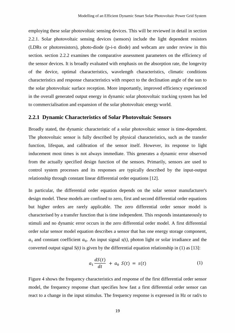
Modelling of an Efficient Dynamic Smart Solar Photovoltaic Power Grid System
19
employing these solar photovoltaic sensing devices. This will be reviewed in detail in section
2.2.1. Solar photovoltaic sensing devices (sensors) include the light dependent resistors
(LDRs or photoresistors), photo-diode (p-i-n diode) and webcam are under review in this
section. section 2.2.2 examines the comparative assessment parameters on the efficiency of
the sensor devices. It is broadly evaluated with emphasis on the absorption rate, the longevity
of the device, optimal characteristics, wavelength characteristics, climatic conditions
characteristics and response characteristics with respect to the declination angle of the sun to
the solar photovoltaic surface reception. More importantly, improved efficiency experienced
in the overall generated output energy in dynamic solar photovoltaic tracking system has led
to commercialisation and expansion of the solar photovoltaic energy world.
2.2.1 Dynamic Characteristics of Solar Photovoltaic Sensors
Broadly stated, the dynamic characteristic of a solar photovoltaic sensor is time-dependent.
The photovoltaic sensor is fully described by physical characteristics, such as the transfer
function, lifespan, and calibration of the sensor itself. However, its response to light
inducement most times is not always immediate. This generates a dynamic error observed
from the actually specified design function of the sensors. Primarily, sensors are used to
control system processes and its responses are typically described by the input-output
relationship through constant linear differential order equations [12].
In particular, the differential order equation depends on the solar sensor manufacturer's
design model. These models are confined to zero, first and second differential order equations
but higher orders are rarely applicable. The zero differential order sensor model is
characterised by a transfer function that is time independent. This responds instantaneously to
stimuli and no dynamic error occurs in the zero differential order model. A first differential
order solar sensor model equation describes a sensor that has one energy storage component,
𝑎1 and constant coefficient 𝑎0. An input signal s(t), photon light or solar irradiance and the
converted output signal S(t) is given by the differential equation relationship in (1) as [13]:
𝑎1𝑑𝑆(𝑡)
𝑑𝑡 + 𝑎0 𝑆(𝑡) = 𝑠(𝑡) (1)
Figure 4 shows the frequency characteristics and response of the first differential order sensor
model, the frequency response chart specifies how fast a first differential order sensor can
react to a change in the input stimulus. The frequency response is expressed in Hz or rad/s to
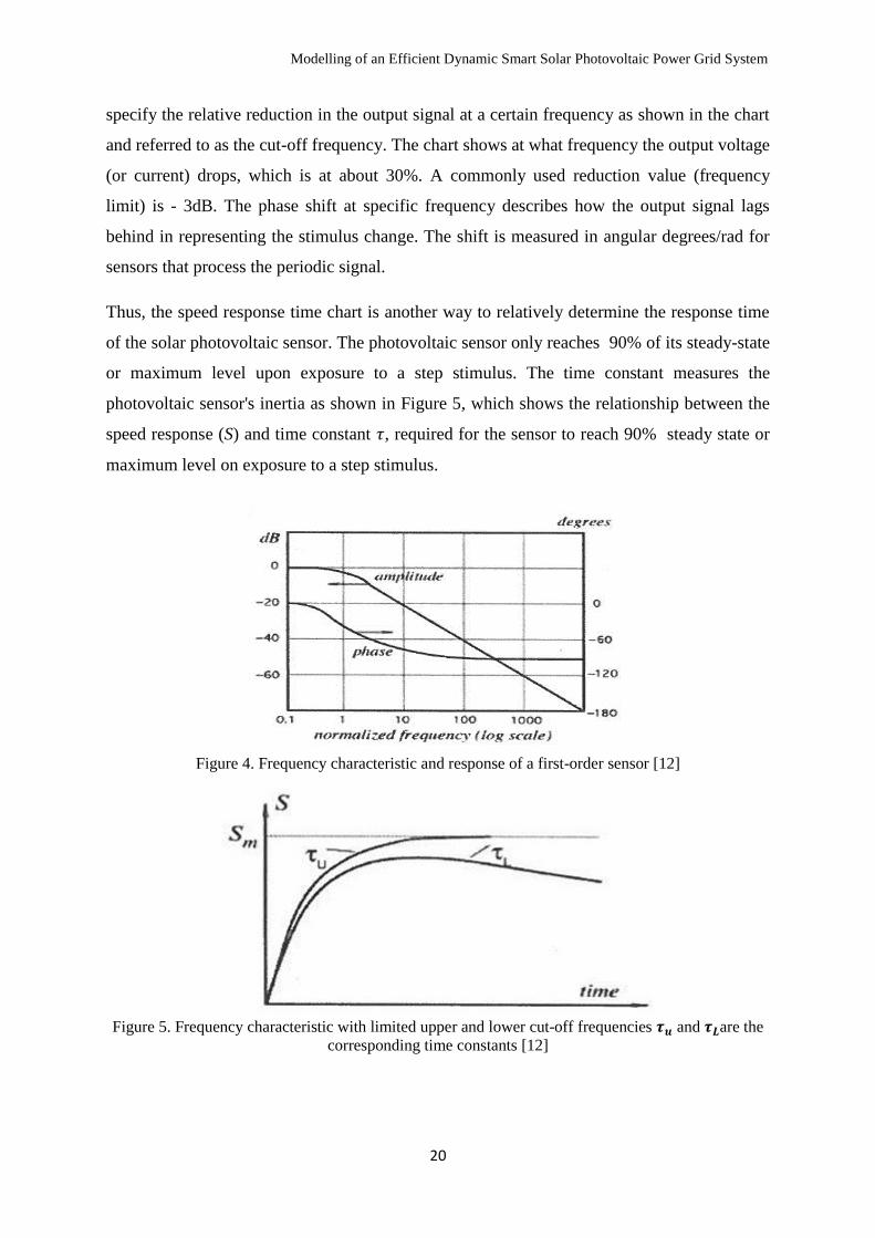
Modelling of an Efficient Dynamic Smart Solar Photovoltaic Power Grid System
20
specify the relative reduction in the output signal at a certain frequency as shown in the chart
and referred to as the cut-off frequency. The chart shows at what frequency the output voltage
(or current) drops, which is at about 30%. A commonly used reduction value (frequency
limit) is - 3dB. The phase shift at specific frequency describes how the output signal lags
behind in representing the stimulus change. The shift is measured in angular degrees/rad for
sensors that process the periodic signal.
Thus, the speed response time chart is another way to relatively determine the response time
of the solar photovoltaic sensor. The photovoltaic sensor only reaches 90% of its steady-state
or maximum level upon exposure to a step stimulus. The time constant measures the
photovoltaic sensor's inertia as shown in Figure 5, which shows the relationship between the
speed response (S) and time constant 𝜏, required for the sensor to reach 90% steady state or
maximum level on exposure to a step stimulus.
Figure 4. Frequency characteristic and response of a first-order sensor [12]
Figure 5. Frequency characteristic with limited upper and lower cut-off frequencies 𝝉𝒖 and 𝝉𝑳are the
corresponding time constants [12]
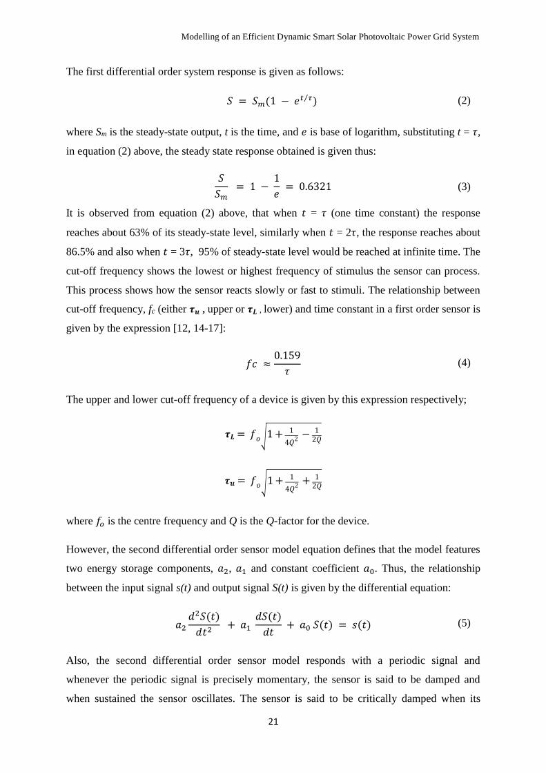
Modelling of an Efficient Dynamic Smart Solar Photovoltaic Power Grid System
21
The first differential order system response is given as follows:
𝑆 = 𝑆𝑚(1 − 𝑒𝑡 𝜏⁄ ) (2)
where Sm is the steady-state output, t is the time, and 𝑒 is base of logarithm, substituting t = 𝜏,
in equation (2) above, the steady state response obtained is given thus:
𝑆
𝑆𝑚 = 1 −
1
𝑒 = 0.6321 (3)
It is observed from equation (2) above, that when 𝑡 = 𝜏 (one time constant) the response
reaches about 63% of its steady-state level, similarly when 𝑡 = 2𝜏, the response reaches about
86.5% and also when 𝑡 = 3𝜏, 95% of steady-state level would be reached at infinite time. The
cut-off frequency shows the lowest or highest frequency of stimulus the sensor can process.
This process shows how the sensor reacts slowly or fast to stimuli. The relationship between
cut-off frequency, fc (either 𝝉𝒖 , upper or 𝝉𝑳 , lower) and time constant in a first order sensor is
given by the expression [12, 14-17]:
𝑓𝑐 ≈0.159
𝜏 (4)
The upper and lower cut-off frequency of a device is given by this expression respectively;
𝝉𝑳 = 𝑓𝑜√1+1
4𝑄2 − 1
2𝑄
𝝉𝒖 = 𝑓𝑜√1+1
4𝑄2 + 1
2𝑄
where 𝑓𝑜 is the centre frequency and Q is the Q-factor for the device.
However, the second differential order sensor model equation defines that the model features
two energy storage components, 𝑎2, 𝑎1 and constant coefficient 𝑎0. Thus, the relationship
between the input signal s(t) and output signal S(t) is given by the differential equation:
𝑎2𝑑2𝑆(𝑡)
𝑑𝑡2 + 𝑎1
𝑑𝑆(𝑡)
𝑑𝑡 + 𝑎0 𝑆(𝑡) = 𝑠(𝑡) (5)
Also, the second differential order sensor model responds with a periodic signal and
whenever the periodic signal is precisely momentary, the sensor is said to be damped and
when sustained the sensor oscillates. The sensor is said to be critically damped when its
Modelling of an Efficient Dynamic Smart Solar Photovoltaic Power Grid System
22
response happens so quickly without an overshoot as shown in Figure 6 of the oscillating
response for the second order differential equation [12, 14-17]. The oscillating response
shows the overdamped, critically damped and underdamped phases of the second order
sensor speed (S) response to time constants (𝜏).
Figure 6. Responses of sensors with different damping characteristics [12]
2.2.2 Assessments of Physical Sensor Parameters
The assessment of the physical sensor parameters in solar photovoltaic tracking optimisation
is important in understanding the relationship between the physical device and rate of
sensitivity, thus determining the effectiveness of the sensor tracking device impact on the
output energy efficiency of the solar photovoltaic module. The advancements made in solar
photovoltaic sensor tracking technology are occurring simultaneously in solar photovoltaic
energy research, requiring a standard benchmark on which the performance and efficiency of
the solar sensors are categorised. These improvements are undertaken to ensure an
appreciable output energy from the huge investments in the solar photovoltaic energy
tracking systems.
The assessment and quality evaluation parameters of the solar photovoltaic sensor device
offer a measurable factor in determining the improved efficiency and output energy generated
in the dynamic solar photovoltaic tracking systems, compared with the static solar
photovoltaic energy system. Based on these measurable factors, the solar sensor
characteristics are closely examined under the following seven parameters. As a result, a
classification summary of the sensor assessment parameters is thus presented in Table 2.
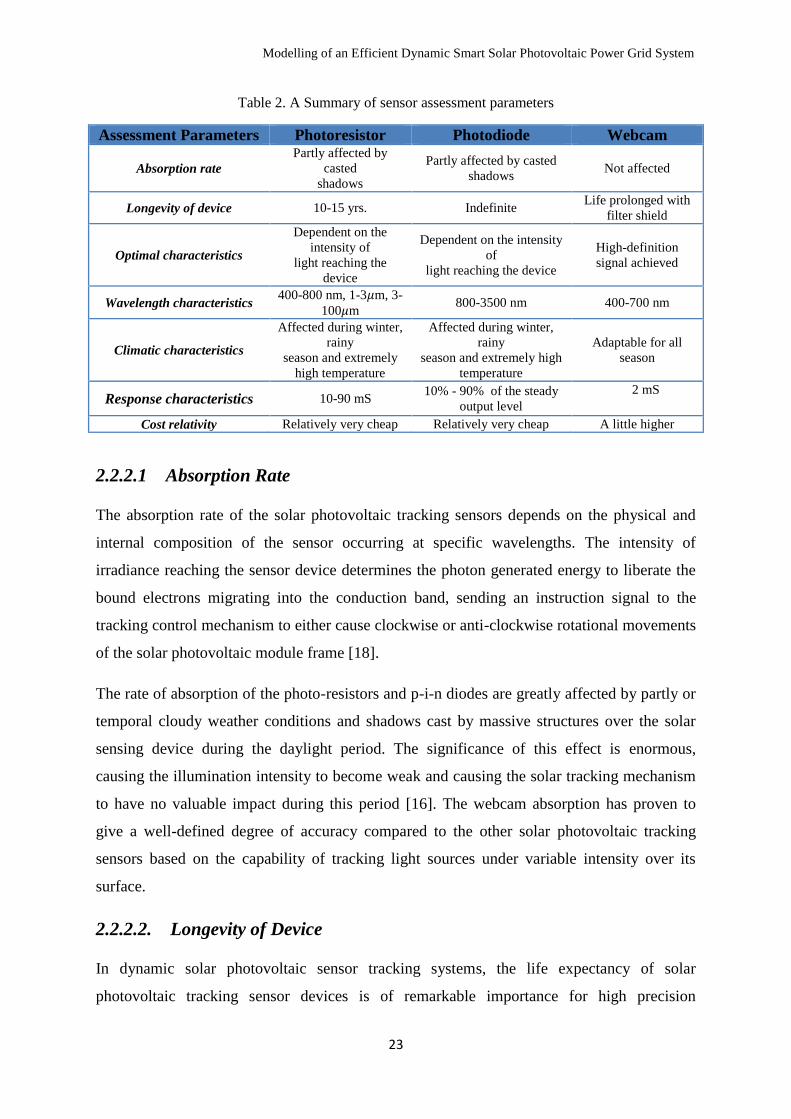
Modelling of an Efficient Dynamic Smart Solar Photovoltaic Power Grid System
23
Table 2. A Summary of sensor assessment parameters
Assessment Parameters Photoresistor Photodiode Webcam
Absorption rate Partly affected by
casted
shadows
Partly affected by casted
shadows Not affected
Longevity of device 10-15 yrs. Indefinite Life prolonged with
filter shield
Optimal characteristics
Dependent on the
intensity of
light reaching the
device
Dependent on the intensity
of
light reaching the device
High-definition
signal achieved
Wavelength characteristics 400-800 nm, 1-3𝜇m, 3-
100𝜇m 800-3500 nm 400-700 nm
Climatic characteristics
Affected during winter,
rainy
season and extremely
high temperature
Affected during winter,
rainy
season and extremely high
temperature
Adaptable for all
season
Response characteristics 10-90 mS 10% - 90% of the steady
output level 2 mS
Cost relativity Relatively very cheap Relatively very cheap A little higher
2.2.2.1 Absorption Rate
The absorption rate of the solar photovoltaic tracking sensors depends on the physical and
internal composition of the sensor occurring at specific wavelengths. The intensity of
irradiance reaching the sensor device determines the photon generated energy to liberate the
bound electrons migrating into the conduction band, sending an instruction signal to the
tracking control mechanism to either cause clockwise or anti-clockwise rotational movements
of the solar photovoltaic module frame [18].
The rate of absorption of the photo-resistors and p-i-n diodes are greatly affected by partly or
temporal cloudy weather conditions and shadows cast by massive structures over the solar
sensing device during the daylight period. The significance of this effect is enormous,
causing the illumination intensity to become weak and causing the solar tracking mechanism
to have no valuable impact during this period [16]. The webcam absorption has proven to
give a well-defined degree of accuracy compared to the other solar photovoltaic tracking
sensors based on the capability of tracking light sources under variable intensity over its
surface.
2.2.2.2. Longevity of Device
In dynamic solar photovoltaic sensor tracking systems, the life expectancy of solar
photovoltaic tracking sensor devices is of remarkable importance for high precision
Modelling of an Efficient Dynamic Smart Solar Photovoltaic Power Grid System
24
concentration and uninterrupted dynamic solar photovoltaic module tracking systems. This is
due to the fact that huge capital investments are involved in both small and large-scale solar
photovoltaic renewable energy generation. Furthermore, it is important to minimise the risk
of frequent maintenance and replacement of the installed tracking sensors to prevent loss of
tracking.
Over the years, the solar sensor technology industry has been producing cost efficient and
high quality solar photovoltaic tracking sensors. The light dependent resistors (LDRs) have a
life expectancy of 10 - 15 years. The photodiode lasts for an indefinite period of time when
used in accordance to the manufacturer's specification [19]. The webcam optical sensors used
in solar photovoltaic sensor tracking systems are specially designed with a polarised filter
shield to prevent frequent saturation of the charge-coupled device (CCD) when the heat
intensity of the sunlight rays is very high during the daytime, prolonging its life expectancy.
The filter shield creates a real-time pre-binarisation image process for the monitoring system
in tracking the location of the sun [20].
2.2.2.3 Optimal Characteristics
The optimal characteristic of the solar photovoltaic sensor device offers rotational and control
signal stability for the dynamic solar photovoltaic tracking systems to achieve maximum
optimality criterion objectives. This criterion consists of a set of differential equations
describing the variable paths that minimise the control boundary restrictions on the premise
of achieving the best possible results. The optimal characteristics of the sensors are
subdivided into two categories the static and the dynamic characteristics.
The static optimal characteristic of the sensors ensures accuracy, discrimination, precision,
drift, sensitivity, linearity and hysteresis properties while the dynamic optimal characteristics
of the sensors are modelled by a constant-coefficient linear differential equation and are
confined to zero, first and second order variable inputs controlling the movement of the solar
photovoltaic module with the tracking mechanism device ensuring constant orthogonal
positioning relative to the sunlight rays [12, 14-17].
Based on the existing literature, the optimal properties of the LDRs is achieved when there is
a decrease in the resistance value of LDR with a corresponding increase in the incident light
intensity [21]. Photo-diode (p-i-n diode) optimal characteristics occur when the intensity of
light striking the crystal lattice causes the release of holes and electrons drawn away from the
Modelling of an Efficient Dynamic Smart Solar Photovoltaic Power Grid System
25
wide depletion region by reverse bias producing the needed signal response for the solar
photovoltaic tracking system [22]. Webcam optimal characteristics produce high definition
and resolutions images transferred by means of Hi-speed USB 2.0.
2.2.2.4 Wavelength Characteristics
The wavelength characteristics of the solar photovoltaic sensor devices define the electrical
tracking signal response sent to the tracking control mechanism unit of the solar photovoltaic
tracking system. There are different kinds of solar photovoltaic sensor devices with specific
wavelengths used in solar photovoltaic tracking systems in previous research. Figure 7
shows the solar spectrum energy density that penetrates the atmosphere [23].
This figure describes the sensitivity wavelength range of sensors used in the solar
photovoltaic tracking system. These wavelengths are subdivided into three regions: the
ultraviolet region (300-400 nm), the visible region (400-700 nm), and the near infrared region
(700-2500 nm). Based on this classification, the sunlight rays emission consists of infrared
and ultraviolet rays at the earth’s surface and are filtered by the earth’s atmosphere, bringing
visibility on the earth’s surface. Therefore, sensors built within the specified wavelength
region would best provide an efficient dynamic solar photovoltaic tracking focus compared to
others outside the regions.
The LDRs are made of different chemical combinational elements such as Cadmium (II)
Sulphide and Cadmium (II) Selenide (CdS-CdSe) having wavelengths within the range of
400-850 nm (visible spectrum), Lead (II) Sulphide and Lead (II) Selenide (PbS-PbSe) having
wavelengths within the range of 1-3𝜇m (near IR field) and Indium (III) Antimonide–Indium
(III) Arsenide (InSb-InAs) having wavelengths within the range of 3-1000 𝜇m (middle and
far IR field) [24].
Likewise, the photodiodes are made of single or chemical combination elements having
different wavelengths sensitivity and characteristics. Germanium has a wavelength within the
range of 800-1700nm, Indium gallium arsenide has a wavelength within the range of 800nm-
2600nm, lead (II) Sulphide has a wavelength within the range of ~1000-3500nm and silicon
within the range of 190-1100 nm [22].
The webcam wavelength for visible light rays ranges from about 400-700 nm within the
visible spectrum region [25].
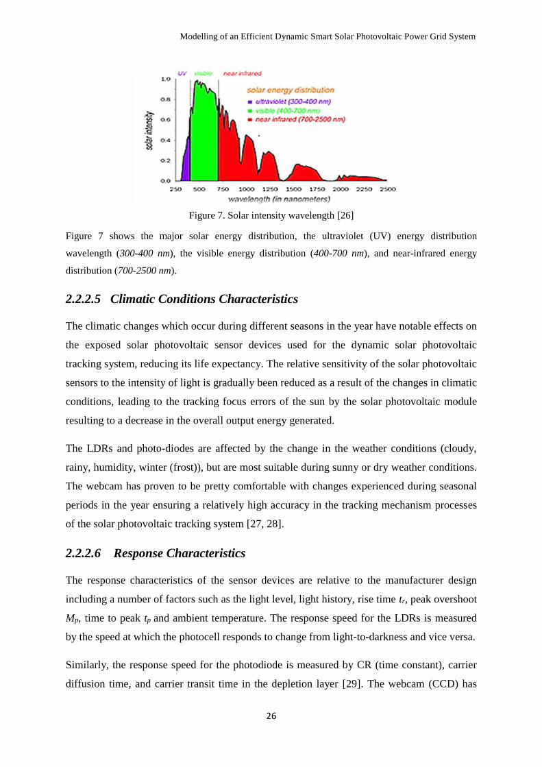
Modelling of an Efficient Dynamic Smart Solar Photovoltaic Power Grid System
26
Figure 7. Solar intensity wavelength [26]
Figure 7 shows the major solar energy distribution, the ultraviolet (UV) energy distribution
wavelength (300-400 nm), the visible energy distribution (400-700 nm), and near-infrared energy
distribution (700-2500 nm).
2.2.2.5 Climatic Conditions Characteristics
The climatic changes which occur during different seasons in the year have notable effects on
the exposed solar photovoltaic sensor devices used for the dynamic solar photovoltaic
tracking system, reducing its life expectancy. The relative sensitivity of the solar photovoltaic
sensors to the intensity of light is gradually been reduced as a result of the changes in climatic
conditions, leading to the tracking focus errors of the sun by the solar photovoltaic module
resulting to a decrease in the overall output energy generated.
The LDRs and photo-diodes are affected by the change in the weather conditions (cloudy,
rainy, humidity, winter (frost)), but are most suitable during sunny or dry weather conditions.
The webcam has proven to be pretty comfortable with changes experienced during seasonal
periods in the year ensuring a relatively high accuracy in the tracking mechanism processes
of the solar photovoltaic tracking system [27, 28].
2.2.2.6 Response Characteristics
The response characteristics of the sensor devices are relative to the manufacturer design
including a number of factors such as the light level, light history, rise time tr, peak overshoot
Mp, time to peak tp and ambient temperature. The response speed for the LDRs is measured
by the speed at which the photocell responds to change from light-to-darkness and vice versa.
Similarly, the response speed for the photodiode is measured by CR (time constant), carrier
diffusion time, and carrier transit time in the depletion layer [29]. The webcam (CCD) has
Modelling of an Efficient Dynamic Smart Solar Photovoltaic Power Grid System
27
been experiencing an overall improved performance in design and production ensuring an
enhanced high sensitivity response [30].
The response time and accuracy of the sensor devices used for solar photovoltaic tracking
systems are of high significance. Each of these solar sensor devices has their rise and fall
time. The rise time, tr of LDRs is defined as the time necessary for light conductance of the
photocell to reach 1- 1/ 𝑒 (or about 63%) of its final value. The fall time is defined as the
time necessary for the light conductance of the photocell to decay to 1/ 𝑒 (or about 37%) of
its illuminated state. For a typical LDR such as the CdS, the rise time is 90mS and fall time is
10mS [31].
The rise time of a p-i-n diode is defined as a measure of the response time of a photodiode to
an input stepped light and the required time for the output to change from 10 to 90% of the
steady output level [32]. The response time of the webcam sensor is about two milliseconds
(2 mS) which is quite fast [30].
2.2.2.7 Cost Relativity
Price relativity of the solar photovoltaic sensor device plays a vital role in the choices made
in some of the literature. The major challenge confronting the global solar photovoltaic
industry is the high price market value of solar photovoltaic modules, insufficient
government policy support initiatives and supply chains among manufacturing industries.
The high initial installation cost revealed in some of the literature determines the choice of
solar photovoltaic sensor device employed, thereby defining the results achieved in the past
two decades.
Comparatively, the price of the LDRs and p-i-n diodes are relatively cheap. However,
additional circuit design and construction costs for the integration of the electronic circuits
and power supply are a further cost for consideration. Thus, it implies that, if there are n-
number of solar panels correspondingly, there would be n-number of electronic circuits built
for the solar sensing devices. The webcam has an inbuilt electronic circuit and is easily
adaptable for use without the need of power supply construction.
Modelling of an Efficient Dynamic Smart Solar Photovoltaic Power Grid System
28
2.3 Solar Photovoltaic Tracking Optimisation Techniques
The solar photovoltaic tracking optimisation techniques improve the output energy efficiency
of the solar photovoltaic system, ensuring that a concentrated amount of sunlight reaches the
solar photovoltaic module throughout the day. The sun tracking optimisation techniques
involve the use of a solar photovoltaic tracker device orientating the solar photovoltaic
module towards the sunlight rays. This technique increases the amount of energy produced as
compared to the fixed solar photovoltaic systems in reviewed literature.
The term “solar photovoltaic tracking optimisation” is often called dynamic solar
photovoltaic tracking system as compared to the traditional fixed solar photovoltaic tracking
system. Over the last decade, there have been recent technological developments and
improvement in research to positively justify the cost investments in the dynamic solar
photovoltaic tracking system. These tracking techniques have been applied to concentrated
photovoltaic (CPV) and concentrated solar thermal (power) (CSP) applications enabling the
optical tracking component to orientate appropriately and ensuring accurate alignment of the
solar photovoltaic surface to harvest the solar energy.
Amidst the concept of solar photovoltaic tracking optimisation, the solar photovoltaic
tracking device is either installed on a floating concrete foundation or on the ground surface.
Some of the solar photovoltaic trackers are permanently mounted on the solar photovoltaic
alloy bracket with the capability to withstand the wind pressure at extreme weather
conditions. The significance and introduction of the solar photovoltaic tracker optimisation
are to ensure a high tracking accuracy to approximately deliver about 90% of the rated output
power of the expected solar photovoltaic module throughout the day.
With the current status in research, the dynamic solar photovoltaic tracking system has been
classified into two major divisions offering a wide range of emerging solar photovoltaic
tracking modes and techniques. The two classifications are closely examined in detail in the
following subsections. Section 2.3.1, dynamic single-axis tracking optimisation definition,
characteristics and types are carefully looked into. In section 2.3.2, the dual-axis tracking
optimisation definition, characteristics, types and benefits over the single axis tracker are
examined.
Modelling of an Efficient Dynamic Smart Solar Photovoltaic Power Grid System
29
2.3.1 Dynamic Single axis Tracking Optimisation
A dynamic single axis tracking optimisation involves a tracking technique with only one
degree of rotational axis aligned along the north meridian. The path of rotation is azimuthally
from east to west following the path of the sun during the day. The overall objective of the
single axis tracker is to effectively improve the efficiency performance and reliability of solar
photovoltaic module, thereby reducing the cost of electricity utility and the negative
environmental impact of greenhouse gases.
There has been on-going research to ensure higher energy efficiency is collected for the
dynamic solar photovoltaic tracking systems at a comparative cost relative to the fixed solar
photovoltaic tracking system. The performance of the dynamic solar photovoltaic tracking
system has increased research investigation expanding the controller and drive capabilities,
structural design studies leading to increased energy production within the range of 15-35%.
The expanded controller and device capabilities have global positioning system (GPS)
capabilities embedded into the controller for remote access and real-time tracking
information eliminating the possibilities of configuration errors.
With the recent industrial innovations in the dynamic single-axis tracking technology, this
technology eliminates the frequent repairs reducing the impact of any single point failure,
simplifying operations and maintenance (O&M) reducing service and repairs costs. Further
classification and divisions of the dynamic single axis tracking are discussed briefly in the
following subdivisions.
2.3.1.1 Horizontal Single axis Tracker (HSAT)
This is one of the most common single-axis trackers, the conventional axis of rotation is an
east to west horizontal movement with respect to the ground. The tracking technology is
mostly used and proven to be very effective in low-latitude regions. The system simply uses a
set of drives and controllers to achieve automatic tracking for the solar photovoltaic module
ensuring an equal uniform loading without experiencing excessive self-shading. Figure 8
shows a horizontal single-axis tracking architecture with rows of solar photovoltaic module
orientation in a north-south line rotating from east to west [33, 34].
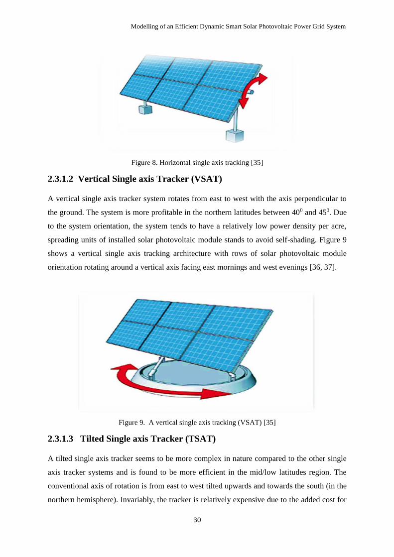
Modelling of an Efficient Dynamic Smart Solar Photovoltaic Power Grid System
30
Figure 8. Horizontal single axis tracking [35]
2.3.1.2 Vertical Single axis Tracker (VSAT)
A vertical single axis tracker system rotates from east to west with the axis perpendicular to
the ground. The system is more profitable in the northern latitudes between 400 and 450. Due
to the system orientation, the system tends to have a relatively low power density per acre,
spreading units of installed solar photovoltaic module stands to avoid self-shading. Figure 9
shows a vertical single axis tracking architecture with rows of solar photovoltaic module
orientation rotating around a vertical axis facing east mornings and west evenings [36, 37].
Figure 9. A vertical single axis tracking (VSAT) [35]
2.3.1.3 Tilted Single axis Tracker (TSAT)
A tilted single axis tracker seems to be more complex in nature compared to the other single
axis tracker systems and is found to be more efficient in the mid/low latitudes region. The
conventional axis of rotation is from east to west tilted upwards and towards the south (in the
northern hemisphere). Invariably, the tracker is relatively expensive due to the added cost for
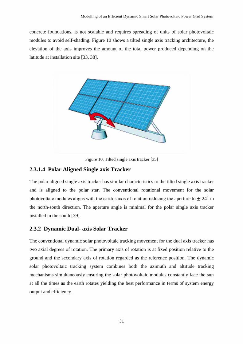
Modelling of an Efficient Dynamic Smart Solar Photovoltaic Power Grid System
31
concrete foundations, is not scalable and requires spreading of units of solar photovoltaic
modules to avoid self-shading. Figure 10 shows a tilted single axis tracking architecture, the
elevation of the axis improves the amount of the total power produced depending on the
latitude at installation site [33, 38].
Figure 10. Tilted single axis tracker [35]
2.3.1.4 Polar Aligned Single axis Tracker
The polar aligned single axis tracker has similar characteristics to the tilted single axis tracker
and is aligned to the polar star. The conventional rotational movement for the solar
photovoltaic modules aligns with the earth’s axis of rotation reducing the aperture to ± 240 in
the north-south direction. The aperture angle is minimal for the polar single axis tracker
installed in the south [39].
2.3.2 Dynamic Dual- axis Solar Tracker
The conventional dynamic solar photovoltaic tracking movement for the dual axis tracker has
two axial degrees of rotation. The primary axis of rotation is at fixed position relative to the
ground and the secondary axis of rotation regarded as the reference position. The dynamic
solar photovoltaic tracking system combines both the azimuth and altitude tracking
mechanisms simultaneously ensuring the solar photovoltaic modules constantly face the sun
at all the times as the earth rotates yielding the best performance in terms of system energy
output and efficiency.
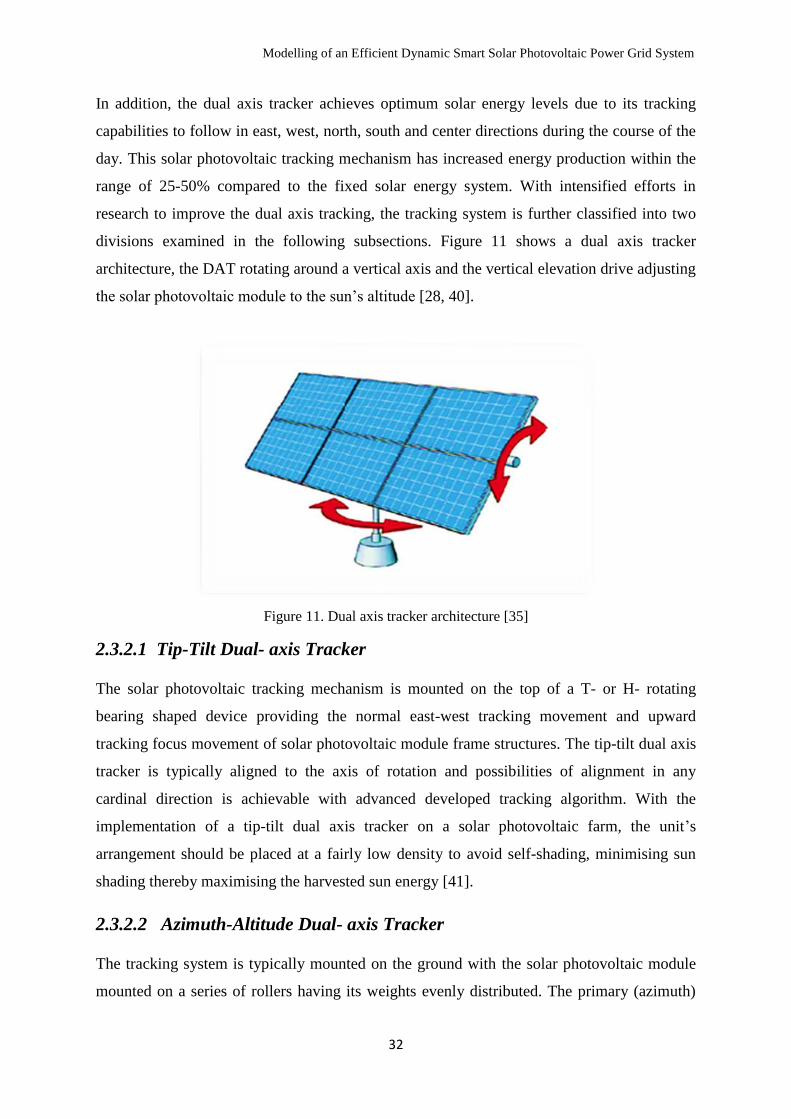
Modelling of an Efficient Dynamic Smart Solar Photovoltaic Power Grid System
32
In addition, the dual axis tracker achieves optimum solar energy levels due to its tracking
capabilities to follow in east, west, north, south and center directions during the course of the
day. This solar photovoltaic tracking mechanism has increased energy production within the
range of 25-50% compared to the fixed solar energy system. With intensified efforts in
research to improve the dual axis tracking, the tracking system is further classified into two
divisions examined in the following subsections. Figure 11 shows a dual axis tracker
architecture, the DAT rotating around a vertical axis and the vertical elevation drive adjusting
the solar photovoltaic module to the sun’s altitude [28, 40].
Figure 11. Dual axis tracker architecture [35]
2.3.2.1 Tip-Tilt Dual- axis Tracker
The solar photovoltaic tracking mechanism is mounted on the top of a T- or H- rotating
bearing shaped device providing the normal east-west tracking movement and upward
tracking focus movement of solar photovoltaic module frame structures. The tip-tilt dual axis
tracker is typically aligned to the axis of rotation and possibilities of alignment in any
cardinal direction is achievable with advanced developed tracking algorithm. With the
implementation of a tip-tilt dual axis tracker on a solar photovoltaic farm, the unit’s
arrangement should be placed at a fairly low density to avoid self-shading, minimising sun
shading thereby maximising the harvested sun energy [41].
2.3.2.2 Azimuth-Altitude Dual- axis Tracker
The tracking system is typically mounted on the ground with the solar photovoltaic module
mounted on a series of rollers having its weights evenly distributed. The primary (azimuth)
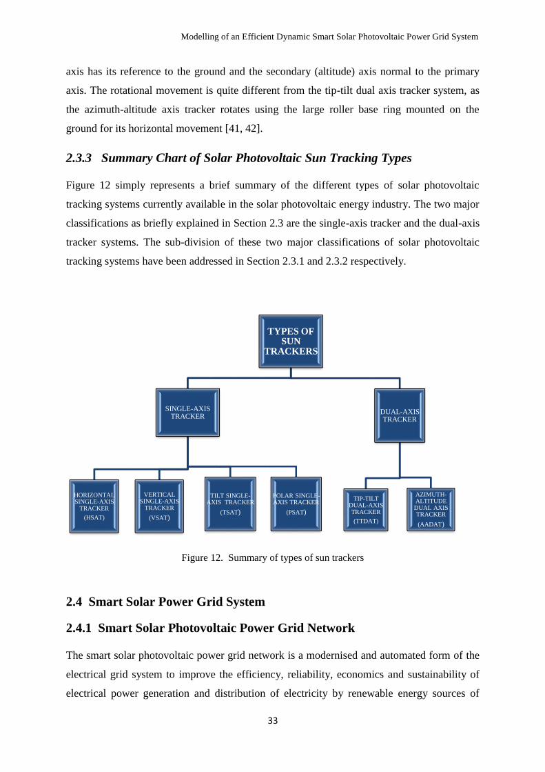
Modelling of an Efficient Dynamic Smart Solar Photovoltaic Power Grid System
33
axis has its reference to the ground and the secondary (altitude) axis normal to the primary
axis. The rotational movement is quite different from the tip-tilt dual axis tracker system, as
the azimuth-altitude axis tracker rotates using the large roller base ring mounted on the
ground for its horizontal movement [41, 42].
2.3.3 Summary Chart of Solar Photovoltaic Sun Tracking Types
Figure 12 simply represents a brief summary of the different types of solar photovoltaic
tracking systems currently available in the solar photovoltaic energy industry. The two major
classifications as briefly explained in Section 2.3 are the single-axis tracker and the dual-axis
tracker systems. The sub-division of these two major classifications of solar photovoltaic
tracking systems have been addressed in Section 2.3.1 and 2.3.2 respectively.
Figure 12. Summary of types of sun trackers
2.4 Smart Solar Power Grid System
2.4.1 Smart Solar Photovoltaic Power Grid Network
The smart solar photovoltaic power grid network is a modernised and automated form of the
electrical grid system to improve the efficiency, reliability, economics and sustainability of
electrical power generation and distribution of electricity by renewable energy sources of
TYPES OF SUN
TRACKERS
SINGLE-AXIS TRACKER
HORIZONTAL SINGLE-AXIS
TRACKER
(HSAT)
VERTICAL SINGLE-AXIS
TRACKER
(VSAT)
TILT SINGLE-AXIS TRACKER
(TSAT)
POLAR SINGLE-AXIS TRACKER
(PSAT)
DUAL-AXIS TRACKER
TIP-TILT DUAL-AXIS TRACKER
(TTDAT)
AZIMUTH-ALTITUDE DUAL AXIS TRACKER
(AADAT)

Modelling of an Efficient Dynamic Smart Solar Photovoltaic Power Grid System
34
power generation. This is unlike the traditional power grid system driven by coal, gas, oil
fired and fossil fuels constructed as a centralised, unidirectional systems of electrical power
generation, electricity transmission, electricity distribution and demand driven [43].
The traditional power grid system is strategically sited and a permanent structure erected at
sites close to the source and supply reserves. For instance, hydropower stations are situated
closer to where there is abundance availability of water throughout the year. Another major
factor in the establishment of the traditional grid system is the nearness to the source of fuel
supply, access to rail, road and paths for easy transmission and distribution to its major and
minor consumers [44].
The growing energy demand for industrial and domestic satisfaction has continually
increased hence, the demand for reliable energy supplies from the traditional grid systems
especially at peak periods, and the redundancy of the grid system at lesser peak periods have
resulted in the high tariffs passed onto the electricity consumers. In many situations at peak
periods, the energy demand results in poor power quality resulting in blackouts, power cuts
and brownouts. The high energy demand from the traditional grid system for consumers’
satisfaction has contributed to the emission of greenhouse gases affecting the climate leading
to global warming crisis [45].
The smart solar photovoltaic grid network policy offers rebate options from the government
to private individuals and corporate business organisations willing to upgrade from the
traditionally powered electricity sources to sustainable green energy such as solar
photovoltaic energy installation by improving on the property value cost dramatically by
about 3.5%. The grid system provides a reduction of carbon footprints, saving consumers’
money from monthly or quarterly power utility bills and offering off-grid solutions for rural,
urban communities, agricultural and other industries [46].
2.4.2 Concept of the Smart Solar Photovoltaic Grid Network
The concept of the smart solar photovoltaic grid network has identified energy security and
efficiency as a critical component in its approach in dealing with climate change challenges,
the capacity to achieve substantial energy demand, cost-effective energy solutions and
relatively rapid reductions in greenhouse gas emissions across the sectors of the economy.
This new grid system represents the cutting edge of energy efficient technologies applied in

Modelling of an Efficient Dynamic Smart Solar Photovoltaic Power Grid System
35
power generation, distribution and finally to the consumers with the intent of securing a low-
carbon future providing a more reliable, with fewer and shorter blackouts [47].
The vision of the grid system comprises application suites and technologies currently at
different levels of technical innovation and developments for cost-effective emissions
reduction, attaining economic maturity, with accrued financial and non-financial benefits.
The grid system provides greater transparency on energy use to various levels of consumers
improving the quality of energy supply. This system offers consumers the advantage to be no
longer passive receivers of bulk power monthly or quarterly utility bills distributed by
existing traditional grid system [48].
The grid system capabilities address the global call by the environmental protection agency
(EPA) to reduce the overall amount of greenhouse gases, including the tons of carbon dioxide
equivalent (CO2-e) produced from traditional electrical power generation, predominantly
altering the climate and affecting the environment. The regulatory bodies are reforming
existing energy policies to increase electricity system reliability, resilience and resource
diversity incorporation over time in order to decarbonise energy production [49].
The dynamic uncertainties and benefits accrued to deployment and implementation of the
smart solar photovoltaic grid system on a large scale, the stakeholders and policy makers
have clearly suggested and identified the concepts, central targets in enhancing the global
acceptance of the new grid system as highlighted [49]:
Efficiency optimisation and prioritising applications and innovations for societal
benefits.
Commercialisation deployment on a large scale to determine the business viabilities.
Synergy collaboration of research institutions and industries.
Public awareness promotion by concerned agencies and full commitment of
government programme and participation.
Instrument and parameter measures to address seemingly difficult technical and
business challenges.
Government declaration and support for private and public adoption of the new grid
system providing attractive incentives and loans.
Modelling of an Efficient Dynamic Smart Solar Photovoltaic Power Grid System
36
Establish a universal standard smart solar applications and solutions as a cardinal
reference to the global world.
The smart solar photovoltaic grid system is building and leveraging on existing smart
meter trials. The programs on distributed solar renewable generation are on moderate
large scale solar farms for the purpose of measurements and establishing a future grid
database. Smart solar photovoltaic substation grids and feeder monitoring have been
under intensive research investigation for the purpose of fault detection, isolation and
restoration (FDIR) before full commercialization commencement. The FDIR enhances
system reliability saving costs for periodic maintenance costs. This is achieved with the
aid of automation of smart system detection via wireless communication to mobile
devices and PCs for online monitoring. However, pilots tests are been monitored on
integrated volt-var control optimisation (IVVCO) and conservation voltage reduction
(CVR) for dynamic voltage management [50].
Furthermore, the prime concept of the grid system is making a tremendous effort in
ensuring the consortium of the smart solar photovoltaic energy consultants establishes an
agreed universal interoperability protocol among cross vendors design and technology.
This ensures maximum efficiency optimisation of the smart solar photovoltaic grid
system with an open standard application layer protocol and network layer with the
capabilities of solving cyber security challenges creating a seamless interface
communication exchange on the basic fundamental architecture of the grid system.
However, the smart solar photovoltaic grid system promotes energy security, reliability
integration of information and communications technology ensuring almost zero
decarbonisation emission and eco-friendly environment [51, 52].
2.4.3 Challenges and Issues on the Smart Solar Photovoltaic Grid System
The smart solar photovoltaic grid system is one of the renewable energy sources. Smart solar
photovoltaic system has been widely accepted and prominently deployed among other
renewable energy sources as a result of the global renaissance interests in effectively
reducing greenhouse gases emission and decarbonisation of energy pollution from the
existing traditional powered generation. The renewable energy power generation is
undoubtedly confronted by challenges and issues because its source of energy (the fuel
source) cannot be manoeuvred manually either by increasing or decreasing on demand.

Modelling of an Efficient Dynamic Smart Solar Photovoltaic Power Grid System
37
Hence, the source of energy is not dispatchable unlike the conventional traditional fossil
powered energy systems [53].
In addressing the major challenges and issues of non-controllability of dispatchable energy
sources, has resulted into various solar photovoltaic tracking techniques as discussed in
section 2.3. The use of solar photovoltaic sensor tracking devices has been examined in
section 2.2 to significantly maximise and improve the energy harvested. The introduction of
advanced control techniques is a vital key enabling the deployments of optimised high
performance and steady operation of the grid system to its maximum capacity. However,
controversial proposed future policy reforms stating that renewable energy credits (RECs) for
private homeowners will be permanently withdrawn and will no longer be able to claim tariff
compensation for energy contributed to the national grid is another bane discouraging the
development and promotion of the smart solar photovoltaic grid system [54].
The challenge of establishing a link between the non-dispatchable and penetration smart solar
photovoltaic grid system has necessitated the need for the renewable portfolio standards
(RPS). Several countries in the world have achieved relatively high standards due to
governmental support and policies encouraging the adoption of these smart solar photovoltaic
energy by introducing attractive incentives and subsidies. The renewable portfolio standard
(RPS) mandate has specific targets to be achieved for the pre-configured fraction of energy
capacity produced from installed smart solar photovoltaic grid system over a stated period.
This depends on the following factors: geographical location, provision of a close match to
peak load demands, provision of generation and load balancing services, provision of resilient
power for critical infrastructure, differing transmission and distribution upgrade investments
on existing traditional power grid system, high preferential support for carbon-neutral
generation, optimal efficiency and energy cost saving on tariffs and provision of ancillary
services to the grid [55, 56].
In the meantime, the detrimental impacts of solar photovoltaic grid system involve real and
reactive power imbalances, inverter control loop feedback, incessant exposure of utility
devices to seasonal weather conditions and the compensation of dynamic voltage level
fluctuations requires huge capital investments and civil works for the upgrade of the grid
system to become smart [57]. These challenges affect the optimal performance and efficiency
of the primary smart solar grid concept to safely and reliably distribute steady power through
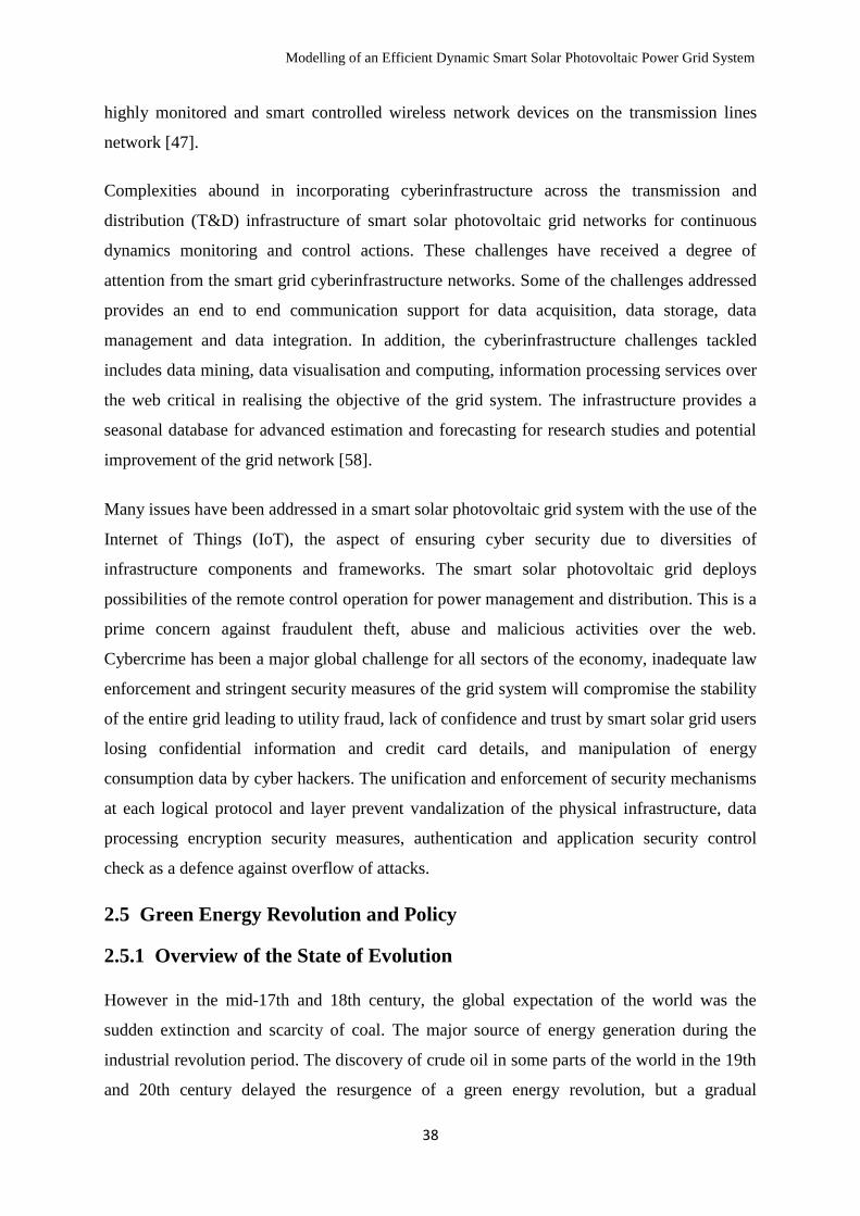
Modelling of an Efficient Dynamic Smart Solar Photovoltaic Power Grid System
38
highly monitored and smart controlled wireless network devices on the transmission lines
network [47].
Complexities abound in incorporating cyberinfrastructure across the transmission and
distribution (T&D) infrastructure of smart solar photovoltaic grid networks for continuous
dynamics monitoring and control actions. These challenges have received a degree of
attention from the smart grid cyberinfrastructure networks. Some of the challenges addressed
provides an end to end communication support for data acquisition, data storage, data
management and data integration. In addition, the cyberinfrastructure challenges tackled
includes data mining, data visualisation and computing, information processing services over
the web critical in realising the objective of the grid system. The infrastructure provides a
seasonal database for advanced estimation and forecasting for research studies and potential
improvement of the grid network [58].
Many issues have been addressed in a smart solar photovoltaic grid system with the use of the
Internet of Things (IoT), the aspect of ensuring cyber security due to diversities of
infrastructure components and frameworks. The smart solar photovoltaic grid deploys
possibilities of the remote control operation for power management and distribution. This is a
prime concern against fraudulent theft, abuse and malicious activities over the web.
Cybercrime has been a major global challenge for all sectors of the economy, inadequate law
enforcement and stringent security measures of the grid system will compromise the stability
of the entire grid leading to utility fraud, lack of confidence and trust by smart solar grid users
losing confidential information and credit card details, and manipulation of energy
consumption data by cyber hackers. The unification and enforcement of security mechanisms
at each logical protocol and layer prevent vandalization of the physical infrastructure, data
processing encryption security measures, authentication and application security control
check as a defence against overflow of attacks.
2.5 Green Energy Revolution and Policy
2.5.1 Overview of the State of Evolution
However in the mid-17th and 18th century, the global expectation of the world was the
sudden extinction and scarcity of coal. The major source of energy generation during the
industrial revolution period. The discovery of crude oil in some parts of the world in the 19th
and 20th century delayed the resurgence of a green energy revolution, but a gradual

Modelling of an Efficient Dynamic Smart Solar Photovoltaic Power Grid System
39
development in research innovations and technologies has been experienced in the last 50
years [59]. The drive behind the green energy revolution has been the global concern of
protecting the climate by replacing the fossil fuels, eliminating the greenhouse gas and CO2-
equivalent emissions ensuring energy security and economic growth [60].
The current global state of the ozone layer and the extreme consequences for continuous
usage of the fossil energies in power generation have led the green energy research
institutions increasing the search for sustainable and justifiable alternatives means of power
generation. This revolution has created renewable energy solutions through decentralisation
of power generation and grid expansions. In addition, it has led energy institutions enacting
global standard regulation and policy reforms for the energy world, providing eco-friendly
energy alternatives as compared to the traditional means of power generation, increasing
intensive research and development for renewable energy sources.
The energy world is gradually shifting it base and switching to available green energy
sources, though a larger percentage of the world energy generation still relies on fossil fuels
and coal as it major means of power generation. The recognition and assessments of the
devastating impacts on climate change, global temperature increase have helped developed
countries to enact laws to support and promote the concept of the green energy revolution.
The global energy demand and consumption are on the rise leading to decentralisation of
green smart-grid networks of renewable energy power generation and distribution [61]. A
green smart grid network concept is as shown in Figure 13. The rapid growth and
implementation of the five (5) major sources of green energy have increased the hope of
energy security, long-term security for investments, the establishment of access to smaller
microgrids by the combination of one or two green energy sources forming a hybrid smart
grid energy system.
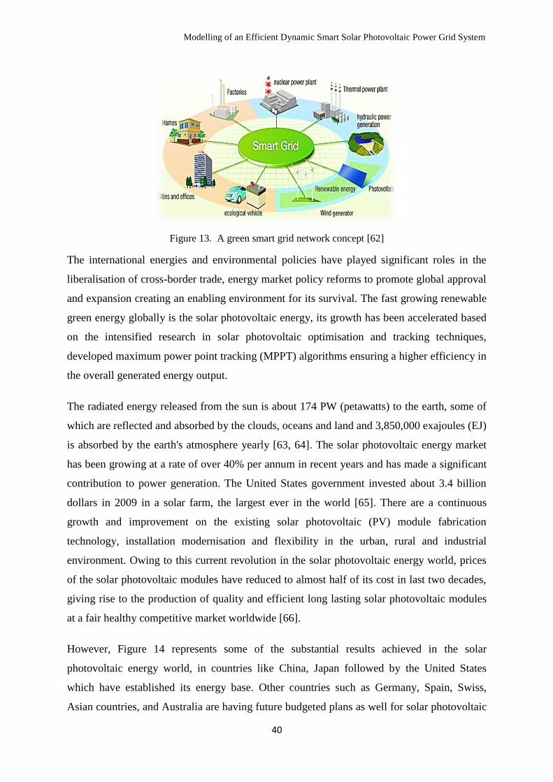
Modelling of an Efficient Dynamic Smart Solar Photovoltaic Power Grid System
40
Figure 13. A green smart grid network concept [62]
The international energies and environmental policies have played significant roles in the
liberalisation of cross-border trade, energy market policy reforms to promote global approval
and expansion creating an enabling environment for its survival. The fast growing renewable
green energy globally is the solar photovoltaic energy, its growth has been accelerated based
on the intensified research in solar photovoltaic optimisation and tracking techniques,
developed maximum power point tracking (MPPT) algorithms ensuring a higher efficiency in
the overall generated energy output.
The radiated energy released from the sun is about 174 PW (petawatts) to the earth, some of
which are reflected and absorbed by the clouds, oceans and land and 3,850,000 exajoules (EJ)
is absorbed by the earth's atmosphere yearly [63, 64]. The solar photovoltaic energy market
has been growing at a rate of over 40% per annum in recent years and has made a significant
contribution to power generation. The United States government invested about 3.4 billion
dollars in 2009 in a solar farm, the largest ever in the world [65]. There are a continuous
growth and improvement on the existing solar photovoltaic (PV) module fabrication
technology, installation modernisation and flexibility in the urban, rural and industrial
environment. Owing to this current revolution in the solar photovoltaic energy world, prices
of the solar photovoltaic modules have reduced to almost half of its cost in last two decades,
giving rise to the production of quality and efficient long lasting solar photovoltaic modules
at a fair healthy competitive market worldwide [66].
However, Figure 14 represents some of the substantial results achieved in the solar
photovoltaic energy world, in countries like China, Japan followed by the United States
which have established its energy base. Other countries such as Germany, Spain, Swiss,
Asian countries, and Australia are having future budgeted plans as well for solar photovoltaic
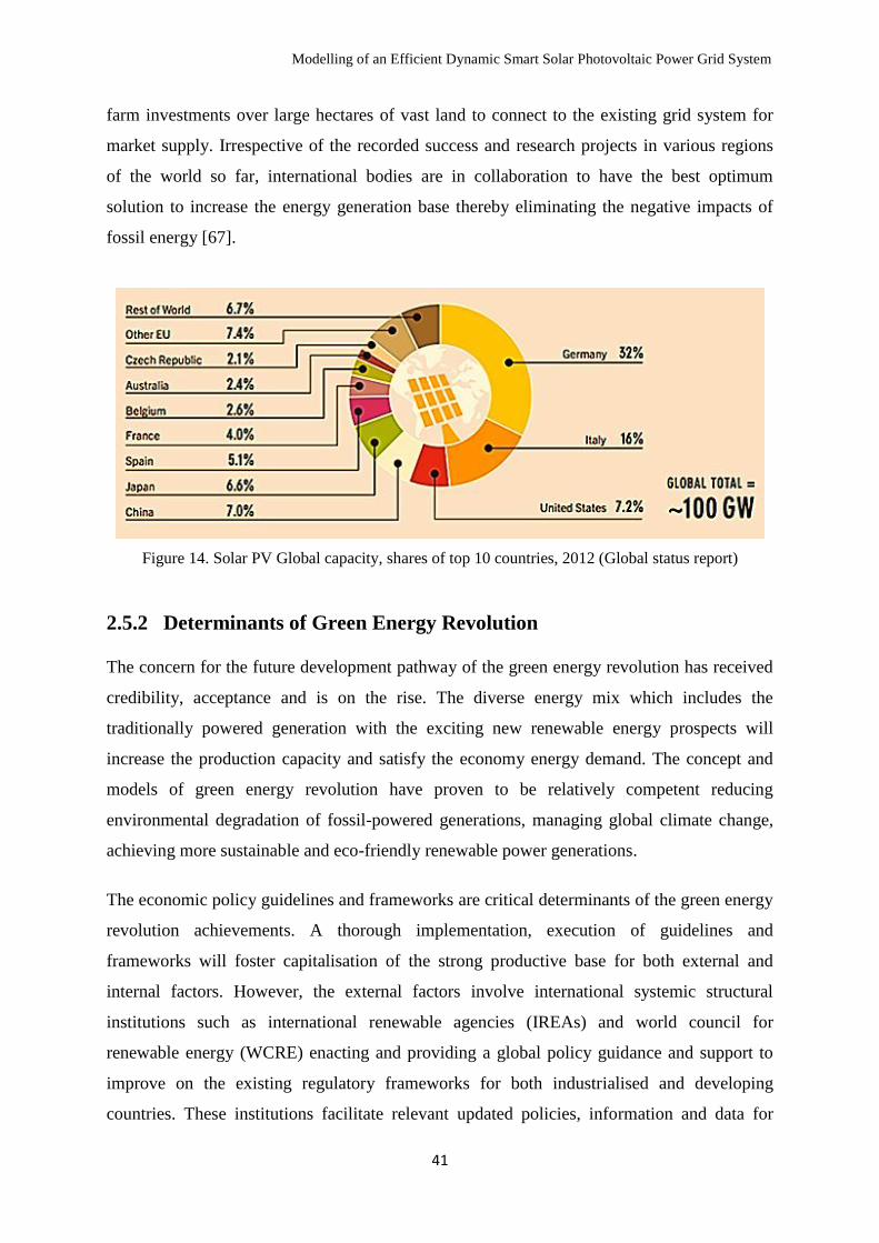
Modelling of an Efficient Dynamic Smart Solar Photovoltaic Power Grid System
41
farm investments over large hectares of vast land to connect to the existing grid system for
market supply. Irrespective of the recorded success and research projects in various regions
of the world so far, international bodies are in collaboration to have the best optimum
solution to increase the energy generation base thereby eliminating the negative impacts of
fossil energy [67].
Figure 14. Solar PV Global capacity, shares of top 10 countries, 2012 (Global status report)
2.5.2 Determinants of Green Energy Revolution
The concern for the future development pathway of the green energy revolution has received
credibility, acceptance and is on the rise. The diverse energy mix which includes the
traditionally powered generation with the exciting new renewable energy prospects will
increase the production capacity and satisfy the economy energy demand. The concept and
models of green energy revolution have proven to be relatively competent reducing
environmental degradation of fossil-powered generations, managing global climate change,
achieving more sustainable and eco-friendly renewable power generations.
The economic policy guidelines and frameworks are critical determinants of the green energy
revolution achievements. A thorough implementation, execution of guidelines and
frameworks will foster capitalisation of the strong productive base for both external and
internal factors. However, the external factors involve international systemic structural
institutions such as international renewable agencies (IREAs) and world council for
renewable energy (WCRE) enacting and providing a global policy guidance and support to
improve on the existing regulatory frameworks for both industrialised and developing
countries. These institutions facilitate relevant updated policies, information and data for
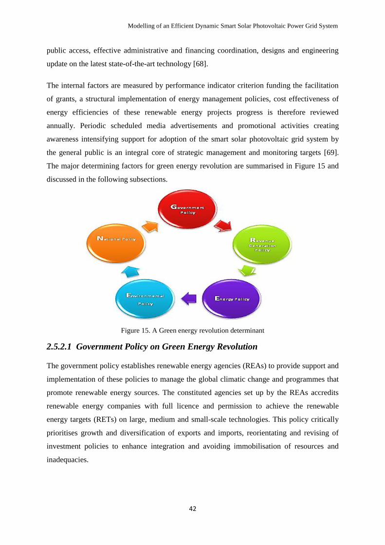
Modelling of an Efficient Dynamic Smart Solar Photovoltaic Power Grid System
42
public access, effective administrative and financing coordination, designs and engineering
update on the latest state-of-the-art technology [68].
The internal factors are measured by performance indicator criterion funding the facilitation
of grants, a structural implementation of energy management policies, cost effectiveness of
energy efficiencies of these renewable energy projects progress is therefore reviewed
annually. Periodic scheduled media advertisements and promotional activities creating
awareness intensifying support for adoption of the smart solar photovoltaic grid system by
the general public is an integral core of strategic management and monitoring targets [69].
The major determining factors for green energy revolution are summarised in Figure 15 and
discussed in the following subsections.
Figure 15. A Green energy revolution determinant
2.5.2.1 Government Policy on Green Energy Revolution
The government policy establishes renewable energy agencies (REAs) to provide support and
implementation of these policies to manage the global climatic change and programmes that
promote renewable energy sources. The constituted agencies set up by the REAs accredits
renewable energy companies with full licence and permission to achieve the renewable
energy targets (RETs) on large, medium and small-scale technologies. This policy critically
prioritises growth and diversification of exports and imports, reorientating and revising of
investment policies to enhance integration and avoiding immobilisation of resources and
inadequacies.

Modelling of an Efficient Dynamic Smart Solar Photovoltaic Power Grid System
43
The survival and success of a green energy revolution substantially rest on the support of
favourable government policies. The positive influence and contribution of these policies in
the transformation process of the energy sector revolution are massive. It induces mechanism
to advocate for the coalition, promoting the green energy revolution, networking constitution
of technological and business oriented minds, setting up institutional norms and rules
regulating the interaction of the sector, encouraging individual, corporate actors and investors
fusion in ensuring a more self-sustained green energy revolution [70].
2.5.2.2 Revenue Generation Policy on Green Energy Revolution
The green energy revolution is highly capital-intensive, and the energy industry needs an
effective driver for revenue and economic generation policy to sustain the long-term assets
privately-owned and operated by individuals, corporate organisations and government
establishments. The biggest factor driving renewable energy targets (RETs) is ensuring
decarbonisation of electricity generation by significantly promoting renewable energy
business trends, forecasting the economic implication features including investment costs,
energy prices, industrial competitiveness, gross domestic product (GDP) and employment
opportunities.
The relevant government instituted bodies are responsible for identifying market revenue
generation policies to address intensive commercial investments and deployment providing
tenor debts suitable for the renewable infrastructure in large, medium and small-scale
projects. The different renewable energy institutions setup provide consultation,
administrative advice and special investments risk control competence facilitator across all
portfolios for international investors and multinational companies.
The dynamic possibilities of renewable energy efficiency innovation technologies in green
energy have caused government policy makers to strategically invest extensively and support
the commercialisation of patent green technologies for rural, urban and industrial sectors of
the economy. The exportation of the renewable energy products is integral to the sources of
revenue generation for short and long term investments to align with the vision and mission
of the government in advancing the natural greenhouse gases emission reduction objectives
[71].
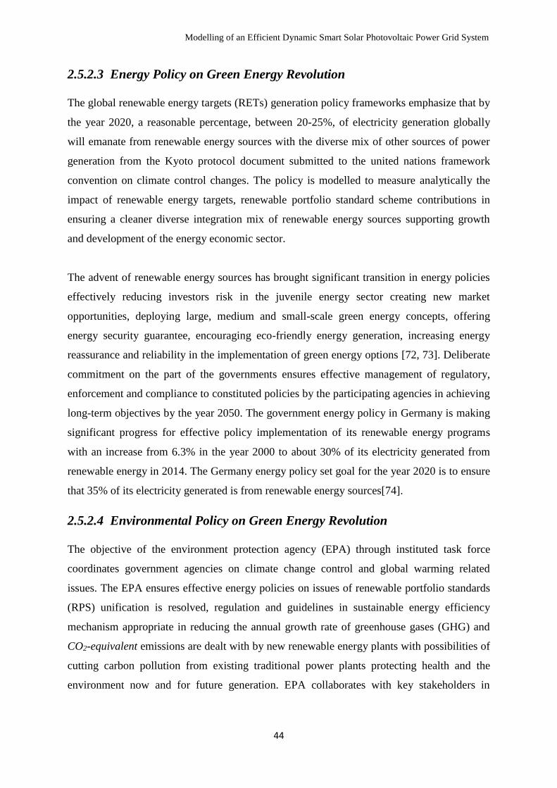
Modelling of an Efficient Dynamic Smart Solar Photovoltaic Power Grid System
44
2.5.2.3 Energy Policy on Green Energy Revolution
The global renewable energy targets (RETs) generation policy frameworks emphasize that by
the year 2020, a reasonable percentage, between 20-25%, of electricity generation globally
will emanate from renewable energy sources with the diverse mix of other sources of power
generation from the Kyoto protocol document submitted to the united nations framework
convention on climate control changes. The policy is modelled to measure analytically the
impact of renewable energy targets, renewable portfolio standard scheme contributions in
ensuring a cleaner diverse integration mix of renewable energy sources supporting growth
and development of the energy economic sector.
The advent of renewable energy sources has brought significant transition in energy policies
effectively reducing investors risk in the juvenile energy sector creating new market
opportunities, deploying large, medium and small-scale green energy concepts, offering
energy security guarantee, encouraging eco-friendly energy generation, increasing energy
reassurance and reliability in the implementation of green energy options [72, 73]. Deliberate
commitment on the part of the governments ensures effective management of regulatory,
enforcement and compliance to constituted policies by the participating agencies in achieving
long-term objectives by the year 2050. The government energy policy in Germany is making
significant progress for effective policy implementation of its renewable energy programs
with an increase from 6.3% in the year 2000 to about 30% of its electricity generated from
renewable energy in 2014. The Germany energy policy set goal for the year 2020 is to ensure
that 35% of its electricity generated is from renewable energy sources[74].
2.5.2.4 Environmental Policy on Green Energy Revolution
The objective of the environment protection agency (EPA) through instituted task force
coordinates government agencies on climate change control and global warming related
issues. The EPA ensures effective energy policies on issues of renewable portfolio standards
(RPS) unification is resolved, regulation and guidelines in sustainable energy efficiency
mechanism appropriate in reducing the annual growth rate of greenhouse gases (GHG) and
CO2-equivalent emissions are dealt with by new renewable energy plants with possibilities of
cutting carbon pollution from existing traditional power plants protecting health and the
environment now and for future generation. EPA collaborates with key stakeholders in

Modelling of an Efficient Dynamic Smart Solar Photovoltaic Power Grid System
45
designing, implementing clean energy policies, cost-effective technologies solution
delivering environmental and economic benefits [75].
The environmental protection agency communicates through various media options giving
warning signals and rapid emergency responses about the current devastating impacts of
climate change either increasing or decreasing the annual expected rainfall. This directly or
indirectly affects agricultural crop yields, the human health and causes changes in forests,
ecosystem and energy supply. The government environmental policy gives reassurance and
support to corporate business organisations committed to investing in green technologies by
setting reasonable minimum green energy tax to encourage environmentally friendly
technologies fostering competitiveness stimulating the market development for energy
efficient technologies and products [76].
2.5.2.5 National Policy on Green Energy Revolution
A national renewable energy action plan (NREAP) policy is established to promote regional
and economic sectoral renewable energy targets (RETs), achievable renewable energy mix,
policy direction path and reform measures to overcoming the peculiar challenges in achieving
successful renewable energy targets. However, the NREAP evaluates the track record and
progress made by other advancing nationals as a relative benchmark to surpass and improve
on their national targets.
Consequently, the NREAP makes a distinct administrative classification of the renewable
energy scheme responsibilities by publishing the national electricity rules and economic
regulation providing policy advice for international business trade, tax incentives initiatives
promoting awareness nationally and strong support for environmental protection in
establishing the growth of green energy [76, 77].
2.5.3 Impacts of Green Renewable Energy
The national renewable energy action plan (NREAP) policy and other various renewable
energy bodies unwinds by evaluating the impacts of renewable energy sources in
substantially minimising the harm, and the intensity of the environmental impacts the fossil
fuel power generations contributed to air and water pollution, damages to public health,
extinction of wildlife and habitat species as a resultant consequence of global warming.
Several studies conducted have shown that by increasing the supply of renewable energy

Modelling of an Efficient Dynamic Smart Solar Photovoltaic Power Grid System
46
generation network mix, there is a direct knock-on effect in the replacement of carbon-
intensive energy sources significantly reducing global warming emissions by a much more
reasonable percentage [78].
The potential impacts and substantial benefits of green renewable energy significantly
address the current and potential environmental issues, reducing carbon-cutdowns and global
warming emissions and its harmful impacts on our health, environment, and climate. The
transition in the renewable energy sector is gradually experiencing a result-oriented process
owing to the fortification of environment protection agency (EPA) enforcing strict rules and
regulations on carbon pollution from traditional energy power plants contributing one-third of
the world’s energy emissions and accelerating a clean energy economy. Due to uninterrupted
running processes of traditional energy plants, the atmosphere has been overloaded with
carbon dioxide and other global warming emissions steadily trapping heat and increasing
instability experienced in climate [79, 80].
However, electricity generation boosts from renewable energy are gradually replacing
carbon-intensive energy sources due to the negative environmental impacts on climate
change and global warming. Electricity generation from fossil fuels significantly contributes
to air and water borne diseases such as breathing problems, heart attacks, neurological
changes, cancer and premature mortality rates. Power generation from renewable energy
sources from solar, wind and hydroelectric systems are known not to be associated with air
pollution emissions. Especially, the solar and wind energy sources require no water for their
operation, hence water resources are free from pollution for domestic and other water
demands [81, 82].
The advent of green renewable energies has contributed and provided thousands of job
globally to skilled and semi-skilled workers on the full-time and part-time basis. Based on
global renewable energy targets, more jobs will be created in the future improving the gross
domestic product (GDP) of the economy. The jobs created spread across diverse sectors of
the economy industries and capacities such as the manufacturing sector, civil and site
construction sector, including full and part-time workers, project management and
development sector, operation and maintenance departments, transportation and logistics,
financial sector, legal and consulting services sectors either directly or indirectly linked to the
supply chain capabilities of the renewable energy and their economic benefits [83].

Modelling of an Efficient Dynamic Smart Solar Photovoltaic Power Grid System
47
The renewable energy sources of power generation installation in rural and urban settlements
in large renewable energy schemes (LRES) and small renewable energy schemes (SRES)
have immensely contributed affordable electricity tariffs especially to rural and remote
regions by reducing the financial burden of civil construction and erection of high power
transmission towers and lines. As a result, the cost of renewable energy solutions is
experiencing a decline due to government subsidies and support for eco-friendly electricity
generation. However, the renewable energy sector will further experience future growth as
the market matures and a good percentage of acceptance from the public relieving huge
burdens on electricity tariffs [84].
Renewable energy sources are found to be more reliable and resilient than coal, natural gas,
nuclear and fossil fuel power plants in the face of probable disruption events such as
droughts, earthquakes waves, severe wildfires and extreme storms and weather events. In
conclusion, high dependence on energy sources other than renewable energy runs the risk of
long blackouts until full restoration, maintenance and repairs are carried out. This is not the
state in renewable energy sources operating independently irrespective of extreme weather
conditions. Most often renewable energy sources promote diversification of energy
generation reducing overdependence on imported fuels and toxic carbon emission sources of
power generation [84, 85].
2.5.3.1 Environmental Impacts on Green Renewable Energy
The environmental impacts of green renewable energy are diverse and emphasis on the
positive benefits is due to its strong capacity of curbing and ensuring zero-carbon emissions,
non-toxic gases, liquid pollutions and global warming emissions. In most cases, the
renewable energy sources are found in abundance, are inexhaustible and affordable most
often throughout the year. This makes green renewable energy viable for small and large
scale means of energy production, compared to fossil fuels, natural gas-fired and other toxic
emission sources of energy production.
Based on recent research studies, a comprehensive report presented on the amount of CO2
emissions from green renewable energy generation has shown considerable reductions due to
compliance to renewable energy targets. The solar photovoltaic energy production emission
is found to be with low emission of CO2, the nuclear energy production follows next, whilst
the wind energy is found to be third lowest CO2 emission and hydroelectricity produces the

Modelling of an Efficient Dynamic Smart Solar Photovoltaic Power Grid System
48
lowest CO2 emissions. The green energy concept has been designed to mitigate the negative
impacts of traditional power plants on local eco-system [86, 87].
2.5.3.2 Market Policy Impacts on Green Renewable Energy
The economic regulatory and financial policy makers in green energy markets may either
increase or impede the expansion and acceptance of green renewable energies. Financial
institutions play an integral role in the economy and energy sector offering some of the
necessary tools to support a smooth transition to sustainable renewable energy schemes by
providing laws, equity, insurance and other financial services to individual and corporate
organisations.
This policy mandates premium rate reimbursement for electricity fed back into the electricity
grid from renewable energy sources of electricity generation. The feed-in tariff is meant to
resolve the market failures and encourage the wider participation of the larger society
providing incentives for adopting the renewable energy [88]. In addition, the policy mandates
electricity suppliers to include a percentage of renewable green energy sources with the
existing traditional power generation fostering an energy mix from electricity suppliers,
thereby increasing the growth of green energy [54].
However, the policy varies from one country to another encouraging existing electricity
suppliers using depletable energy sources to reconsider investing in environmentally friendly
energy sources by introducing heavy tax fines on defaulters. This indirectly decreases the
price of electricity by creating incentives for renewable energy adopters ensuring energy
security, reliability, efficiency reducing the demand on the national grid [89].
2.6 The Prospective Grid: A Smart Grid Network
2.6.1 The Smart Grid Network
The global concern on the current changes experienced through climate change has driven
scientific research and policy makers to promote the growth and expansion of eco-friendly
grid systems known as the smart grid network (SGN). There are other definitions of the term
smart grid network as established in several research works for this new grid network. A
smart grid network is a network consisting of renewable energy sources of power generation
as its bedrock incorporating online automation, remote control access technology and
information and communications technology seamlessly to enhance the grid network. The

Modelling of an Efficient Dynamic Smart Solar Photovoltaic Power Grid System
49
renewable energy sources of power generation are subdivided into solar energy, wind energy,
wave or ocean energy, geothermal energy and hydrogen and fuel cells energy [78, 90, 91].
The focal intervention point for the SGN policy makers was established on these tripod
targets; assess to up-to-date scientific data and information, evaluating the environmental and
socio-economic implication and formulating policies promoting the concept of the SGN [92].
The existing traditional power generation since inception has depended on fossil fuels,
natural gas and coal-fired power plants [93]. This has significantly contributed to higher
carbon emissions and losses experienced during transmission and distribution of energy
generated before reaching the final consumers [94, 95]. The demand for SGNs is gradually
increasing due to the ageing of most of the existing traditional power grid infrastructures,
desire for quality of service (QoS), energy reliability, growing demand for constant electricity
supply, alarming concern for environmental protection and energy sustainability [96, 97].
An SGN has brought transformation by redefining the old norms of traditional power
generation introducing decentralisation, flexible database management, distribution,
integration and operation of variable renewable energies to form a hybrid SGN, interface
relationship in real-time between the consumers and the grid to adjust the energy use and
costs of electricity consumed [98-101]. The core foundations of the smart grids are built on
network management, intelligent applications, intelligent agents, two-way communication,
smart sensors, distributed remote and automated control [3, 4].
These foundations have enhanced an end-to-end interaction, full integration and installation
of smart sensor technologies into electricity business and services optimising capital assets
and minimising operational and recurrent maintenance costs [102, 103]. An SGN has been on
the rise due to the provisions and support of government policies enacting regulations for the
new grid network to survive. An SGN has been supported in many countries of the world
such as the United States of America, Spain, Japan, China, Australia and Canada and also in
most European countries [104, 105]. Several research works have shown that the smart grid
networks have been widely accepted in some of these countries based on these three factors
[85, 106]:
I. The awareness of the benefits of renewable energy resources for climate change
control, environmental protection and compliance, and energy sustainability.
II. Government incentives for private partnership participation investing in SGN paying
interest in a premium price for energy produced.

Modelling of an Efficient Dynamic Smart Solar Photovoltaic Power Grid System
50
III. Public patriotism and endorsement of smart grid companies as their supplier of energy
to their respective homes.
Overall, SGNs have brought technological innovations, changing economic and
environmental regulatory policies leading to distributed smart grid networks. This has
contributed to the development of distributed generation technologies, increased and efficient
energy generation, energy market liberalisation and reduction in the overhead cost of
installation of transmission lines.
2.6.2 Conceptual Framework of the Smart Grid Network
The conceptual framework of the smart grid network envisioned is highly dynamic since
inception. The standard and building blocks of the smart grid network have been undergoing
revisions to add new functionalities, unifying layer and protocols, developing a universally
acceptable standard and interoperability smart grid network framework among all
stakeholders. However, the concept of the smart grid network framework has been
established based on these three key factors [107-109]:
Engaging a forum of expertise in various fields of smart grid network to harmonise
the complex nature of the grid network.
Promoting a consensus for smart grid network interoperability standards.
Providing an open source domain for contribution from experts in harmonising and
interfacing the three layers, physical, communications, and information of the smart
grid fields.
The primary objective of establishing a framework for the smart grid network is to ensure a
broad range of technology options, interoperability of the different options of smart grid
systems, ability to maintain the smooth running of the grid system throughout its lifetime.
The possibility of an upgrade enhancement of the existing grid, accommodation of new
innovative energy systems, support for development of scaled pattern systems, establishment
of structural integration, legacy migration system, ensuring strict security protection for the
energy system, allowing flexibility and interoperability within the system, dependable policy
implementation for system operation and affordability of a smart grid equipment in a large
market. The conceptual framework attributes of a smart grid network include [110]:
Self-healing capabilities with resilience from power uncertainties.

Modelling of an Efficient Dynamic Smart Solar Photovoltaic Power Grid System
51
Real-time participation by consumers’ demand response.
Resilient cybersecurity against malicious attacks.
Guaranteeing reliability and quality constant power supply.
Accommodating and integration of new renewable energy sources and provision for
storage options
Creating an enabling environment for new products, services and markets.
Maximum optimisation and utilisation of assets to it full productivity.
The framework for an SGN as defined by the national institute of standard and technology
(NIST) is subdivided into seven domains and each domain has specific actors and tasks to be
executed [109].
Each domain has an established communication link protocol and application allowing
transfer of data and information across each of the seven domains. Table 3 presents the
domains and actors in the conceptual framework for the SGN model and Figure 16 depicts
the pictorial representation of the conceptual framework for the SGN.
Table 3. Conceptual framework for the smart grid network [24]
Domain Actors Functionality
Customers The end users of electricity. May also generate, store, and manage the
use of energy.
Markets The operators and participants in electricity markets.
Service Providers The organisations providing services to electrical customers and to
utilities
Operations The managers of the movement of electricity
Bulk generation The generators of electricity in bulk quantities. May also store energy
for later distribution.
Transmission The carriers of bulk electricity over long distances. May also store and
generate electricity.
Distribution The distributors of electricity to and from customers. May also store and
generate electricity.
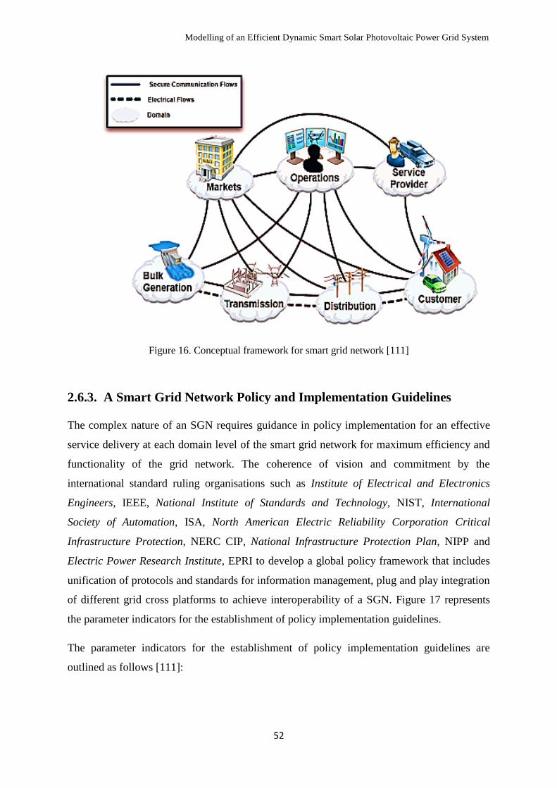
Modelling of an Efficient Dynamic Smart Solar Photovoltaic Power Grid System
52
Figure 16. Conceptual framework for smart grid network [111]
2.6.3. A Smart Grid Network Policy and Implementation Guidelines
The complex nature of an SGN requires guidance in policy implementation for an effective
service delivery at each domain level of the smart grid network for maximum efficiency and
functionality of the grid network. The coherence of vision and commitment by the
international standard ruling organisations such as Institute of Electrical and Electronics
Engineers, IEEE, National Institute of Standards and Technology, NIST, International
Society of Automation, ISA, North American Electric Reliability Corporation Critical
Infrastructure Protection, NERC CIP, National Infrastructure Protection Plan, NIPP and
Electric Power Research Institute, EPRI to develop a global policy framework that includes
unification of protocols and standards for information management, plug and play integration
of different grid cross platforms to achieve interoperability of a SGN. Figure 17 represents
the parameter indicators for the establishment of policy implementation guidelines.
The parameter indicators for the establishment of policy implementation guidelines are
outlined as follows [111]:

Modelling of an Efficient Dynamic Smart Solar Photovoltaic Power Grid System
53
Identification of challenges during policy development and implementation
Governance responsibilities for monitoring, review and upgrade of policy
Risk management in policy implementation
Strategic implementation planning and management milestones
Procurement monitoring and contract management
Managing stakeholder interactions and conflicts
Managing of financial and system resources
Standard communication handshake within the layers of protocols
Monitoring and review of policy before implementation
Figure 17. Parameter indicators for a smart grid network policy and implementation
2.6.4. The Smart Grid Network Challenges
A smart grid network is fast growing with new advancements in technology and innovation
having the potential to provide energy reliability and sustainability curbing carbon emissions.
It is evident that an SGN is key for future energy generation systems. However, in spite of the
Policy development
Governance
Risk management
Planning for implementation
Stakeholder management
Procurement and contract management
Communication
Monitoring and review
Resources

Modelling of an Efficient Dynamic Smart Solar Photovoltaic Power Grid System
54
smart grid benefits and advantages, there are challenges to be tackled in ensuring the
expected targets and goals are achieved. The challenges of a smart grid network are broadly
classified into four categories as illustrated in Figure 18 [3, 7]:
Regulatory challenges
Commercial challenges
Technology challenges
Political challenges
2.6.5. Benefits of the Smart Grid Network
The concept and benefits of a smart grid network have received a lot of attention with the
flexible combination of renewable energy sources of power generation, integration of smart
sensors devices, intelligent communication networks, automatic protection switching, remote
control monitoring for online real-time structures and assessment of a grid system. The
potentials and design perspective of the smart grid network include [109, 112, 113]:
Improved reliability and power quality.
Ensuring proper coordination of the variety of renewable energy configuration.
Ability to automatically reconfigure interconnected grid network.
Achieving better reliability and asset management.
Ability to relieve optimal power flow constraints.
Ability to establish scalability, broad applications and distinct way to full deployment
for solutions.
Improved outage restoration time.
Increased customer service options.
Private partnership investments to fund smart grid projects.
Peak demand reduction.
Reduction in line losses
Self-healing capabilities
In-built resistant against cyber attacks
Creates competitive energy market competition
Lower environmental pollution impacts
Economic productivity
Energy independence
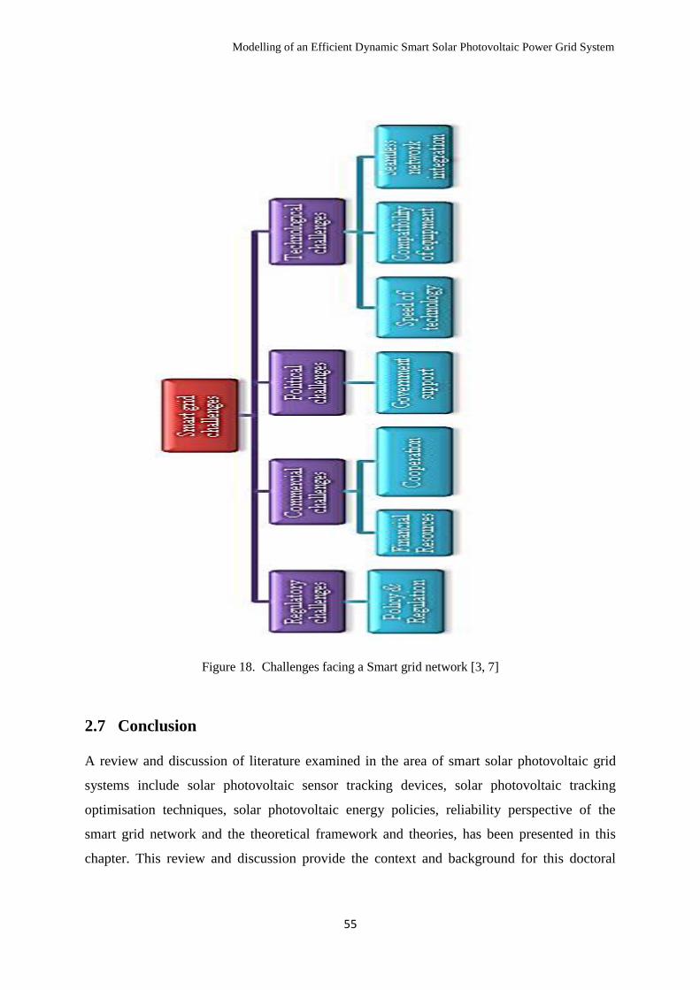
Modelling of an Efficient Dynamic Smart Solar Photovoltaic Power Grid System
55
Figure 18. Challenges facing a Smart grid network [3, 7]
2.7 Conclusion
A review and discussion of literature examined in the area of smart solar photovoltaic grid
systems include solar photovoltaic sensor tracking devices, solar photovoltaic tracking
optimisation techniques, solar photovoltaic energy policies, reliability perspective of the
smart grid network and the theoretical framework and theories, has been presented in this
chapter. This review and discussion provide the context and background for this doctoral

Modelling of an Efficient Dynamic Smart Solar Photovoltaic Power Grid System
56
research. In exploring the simulation and modelling of smart solar photovoltaic grid systems,
a thorough investigation and understanding of the existing research is imperative.
The review of these accessible literature sources highlights the gaps in the existing research,
particularly in relation to understanding the positive benefits of renewable energy systems,
the role and advantages the smart solar photovoltaic grid system concept provides ensuring
zero carbon emission policy. Furthermore, the reviewed literature has provided substantial
evidence and potential benefits of these non-depletable energy sources.
The following chapter (chapter 3) describes the simulation and modelling techniques
undertaken to answer the research questions describing the research paradigm that directed
the chosen methods.
Table 4: Summary of the Sub-sections of Literature Chapter Review
Section
Division
Sub-Headings Achieved Target
Section 2.1 Introduction An overview of the literature
chapter.
Section 2.2 Solar Photovoltaic Sensor and Tracking Optimisation
Devices
Dynamic Characteristics of Solar Photovoltaic
Sensors
Assessments of Physical Sensor Parameters
o Absorption Rate
o Longevity of Device
o Optimal Characteristics
o Wavelength Characteristics
o Climatic Condition Characteristics
o Response Characteristics
o Cost Relativity
Assessment of the physical
characteristics of solar
photovoltaic sensors parameters
described.
Section 2.3 Solar Photovoltaic Tracking Optimisation Techniques
Dynamic Single axis Tracking Optimisation
o Horizontal Single Axis Tracker
(HSAT)
o Vertical Single Axis Tracker (VSAT)
o Tilted Single Axis Tracker (TSAT)
o Polar Aligned Single Axis Tracker
(PASAT)
Dynamic Dual- axis Solar Tracker
o Tip-Tilt Dual-axis Tracker
o Azimuth-Altitude Dual-axis Tracker
o Summary Chart of Solar Photovoltaic
Sun Tracking Types
A concise classification of two
solar Photovoltaic Tracking
Optimisation Techniques.
Section 2.4 Smart Solar Power Grid System
Smart Solar Photovoltaic Grid Network
Concept of the Smart Solar Photovoltaic Grid
Network
Challenges and Issues on Solar Smart
Photovoltaic Grid System
Describing the SGN Concept,
Challenges and Issues.

Modelling of an Efficient Dynamic Smart Solar Photovoltaic Power Grid System
57
Section 2.5 Green Energy Revolution and Policy
Overview of the State of Evolution
Determinants of Green Energy Revolution
o Government Policy on Green Energy
Revolution
o Revenue Generation Policy on Green
Energy Revolution
o Energy Policy on Green Energy
Revolution
o Environmental Policy on Green Energy
Revolution
o National Policy on Green Energy
Revolution
Impacts of Green Renewable Energy
o Environmental Impacts on Green
Renewable Energy
o Market Policy Impacts on Green
Renewable Energy
The major determinants of
Green Energy Revolution and
its impacts are uncovered.
Section 2.6 The Prospective Grid: A Smart Grid Network
The Smart Grid Network
Conceptual Framework of the Smart Grid
Network
A Smart Grid Network Policy and
Implementation Guidelines
The Smart Grid Network Challenges
Benefits of the Smart Grid Network
The components, conceptual
framework, policy and
implementation and benefits of
the SGN are discussed
elaborately.
Section 2.7 Conclusion A brief summary of the
subsections in the literature
chapter was ensured.
Modelling of an Efficient Dynamic Smart Solar Photovoltaic Power Grid System
59
Chapter 3 Modelling and Simulation Techniques for a Solar
Photovoltaic System
3.1 Introduction
This chapter describes the proposed neural network and sparse based algorithm simulation
modelling techniques employed on a smart solar photovoltaic grid system. In particular, the
research methodology is described and justified with cognisance reference to its ability to
answer the research questions. Two classical methods have been chosen for the neural
network and three methods chosen for the sparse based algorithm simulation and modelling
techniques.
These two techniques were chosen for their predictive capabilities on the nonlinear nature of
the solar photovoltaic module for effective validation and implementation in establishing a
tradition in forecasting for this research by comparing techniques on the basis of empirical
results, convergence capability to establish a generalisation and stability iterative pattern.
The neural network technique is exclusively discussed in this chapter, including its
implementation and analyses. This chapter also describes sparse algorithm implementations
on a smart solar photovoltaic grid network to improve the optimisation and output efficiency
of solar photovoltaic modules.
3.2 Static Solar Photovoltaic Modules Modelling and Simulation
Performance
The solar photovoltaic module naturally exhibits nonlinear current-voltage (I-V) and power-
voltage (P-V) characteristics, which has raised the need for modelling its design and
simulation to achieve maximum power point tracking (MPPT) for photovoltaic system
applications. However, due to the nonlinear characteristics nature of the solar photovoltaic
module, extensive research employing different modelling and simulation techniques to
provide reliable and increased output efficiency of the solar photovoltaic module near its
maximum power point based on analytical and numerical techniques to solve this challenge is
crucially important.
Based on recent literature, simulation and modelling techniques have been performed using
various application tools such as Labview, PSpice and Matlab/Simulink to solve the complex
nonlinear characteristics of the solar photovoltaic array based on the standard simplest

Modelling of an Efficient Dynamic Smart Solar Photovoltaic Power Grid System
60
mathematical generalised model equation [114, 115]. The neural network techniques have
been employed in various research fields suitable in handling complex nonlinearities,
uncertainties and variations in the input parameters in a controlled system. Therefore, the
neural network is employed in a comparative modelling and simulation of the static solar
photovoltaic module on a large scale system.
The two neural networks employed in this comparative methodology investigation are the
radial basis function (RBF) and multilayer perceptron (MLP) for the static solar photovoltaic
system. These two networks were chosen because of its simpler network structures, faster
learning algorithm and better approximation capabilities. Both networks use the same training
algorithm which is backpropagation based on the Levenberg-Marquardt minimization method
(the corresponding Matlab function is trainlm).
The static solar photovoltaic system in this research methodology consists of ten thousand
identical photovoltaic cells connected in series, having ten branches of the photovoltaic array
connected in parallel. The results of each of these performance models are empirically based.
However, the versatility and accuracy of these models are presented and discussed based on a
general simplest mathematical model derived equation of a solar photovoltaic module.
The objective of modelling and simulation of the nonlinear characteristics equation of the
solar photovoltaic module is to ensure the solar photovoltaic module performance overcomes
the limitations of environmental factors in a real-life situation. In addition, to effectively
design a reliable solar photovoltaic module capable of withstanding variable factors offering
the possibility of predicting the output efficiency of the photovoltaic module before its final
production and installation. The determination of the solar photovoltaic modules performance
has been a major concern necessitating different modelling and simulation techniques.
Solar photovoltaic modules in the global market are built of crystalline silicon materials with
the presence of impurities affecting their performance. However, modelling and simulation of
the solar photovoltaic module are vital because of the unpredictable nature of the module and
its dependence on the weather and climatic changes resulting in energy variations produced
over time. Sequentially, to efficiently and economically harness the energy from the sun,
assessment and optimisation of the solar photovoltaic module performance is required to
achieve the desired ultimate energy from the solar photovoltaic system.
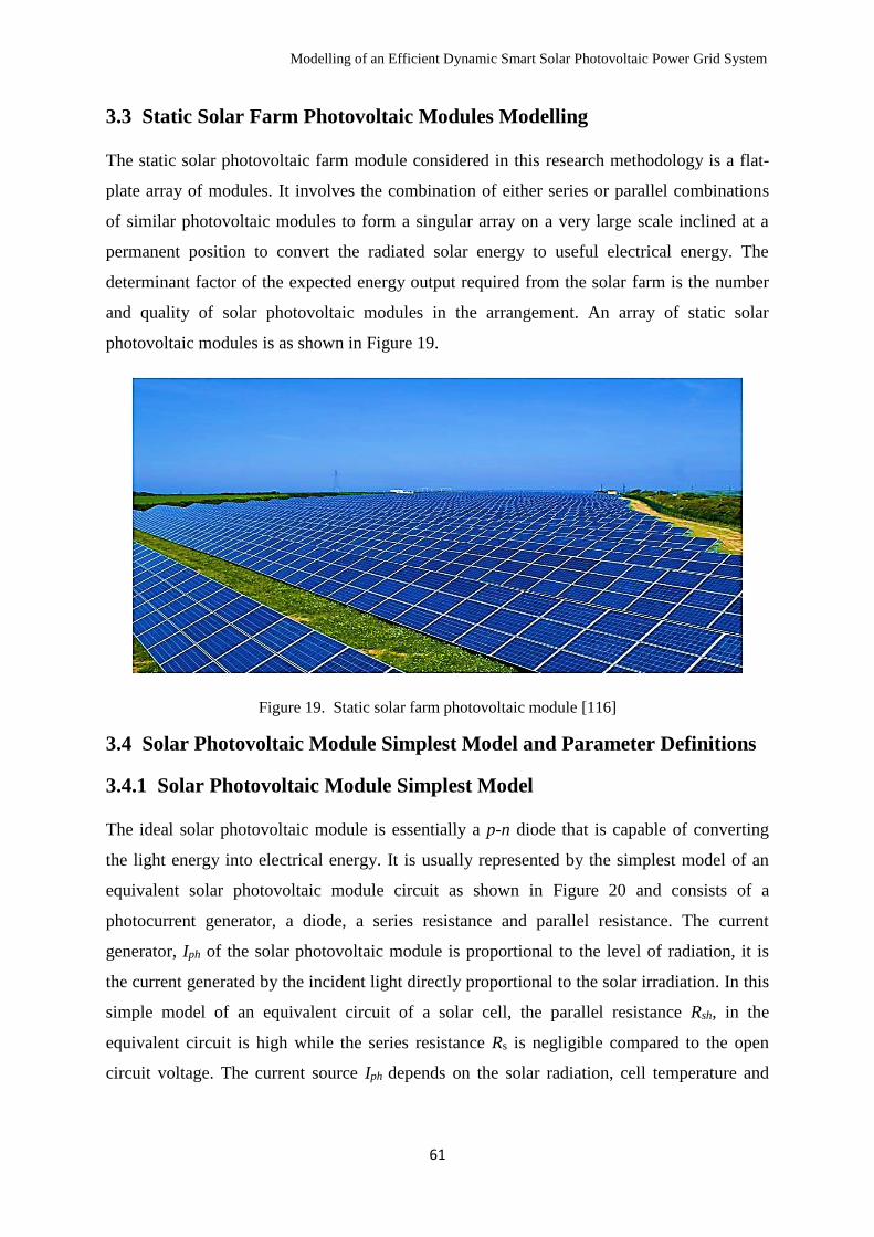
Modelling of an Efficient Dynamic Smart Solar Photovoltaic Power Grid System
61
3.3 Static Solar Farm Photovoltaic Modules Modelling
The static solar photovoltaic farm module considered in this research methodology is a flat-
plate array of modules. It involves the combination of either series or parallel combinations
of similar photovoltaic modules to form a singular array on a very large scale inclined at a
permanent position to convert the radiated solar energy to useful electrical energy. The
determinant factor of the expected energy output required from the solar farm is the number
and quality of solar photovoltaic modules in the arrangement. An array of static solar
photovoltaic modules is as shown in Figure 19.
Figure 19. Static solar farm photovoltaic module [116]
3.4 Solar Photovoltaic Module Simplest Model and Parameter Definitions
3.4.1 Solar Photovoltaic Module Simplest Model
The ideal solar photovoltaic module is essentially a p-n diode that is capable of converting
the light energy into electrical energy. It is usually represented by the simplest model of an
equivalent solar photovoltaic module circuit as shown in Figure 20 and consists of a
photocurrent generator, a diode, a series resistance and parallel resistance. The current
generator, Iph of the solar photovoltaic module is proportional to the level of radiation, it is
the current generated by the incident light directly proportional to the solar irradiation. In this
simple model of an equivalent circuit of a solar cell, the parallel resistance Rsh, in the
equivalent circuit is high while the series resistance Rs is negligible compared to the open
circuit voltage. The current source Iph depends on the solar radiation, cell temperature and
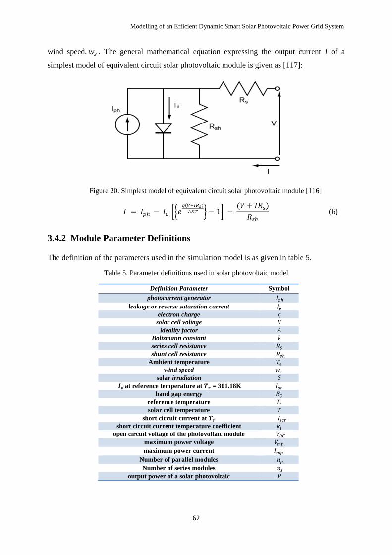
Modelling of an Efficient Dynamic Smart Solar Photovoltaic Power Grid System
62
wind speed, 𝑤𝑠 . The general mathematical equation expressing the output current I of a
simplest model of equivalent circuit solar photovoltaic module is given as [117]:
Figure 20. Simplest model of equivalent circuit solar photovoltaic module [116]
𝐼 = 𝐼𝑝ℎ − 𝐼𝑜 [{𝑒𝑞(𝑉+𝐼𝑅𝑠)
𝐴𝐾𝑇 } − 1] − (𝑉 + 𝐼𝑅𝑠)
𝑅𝑠ℎ (6)
3.4.2 Module Parameter Definitions
The definition of the parameters used in the simulation model is as given in table 5.
Table 5. Parameter definitions used in solar photovoltaic model
Definition Parameter Symbol
photocurrent generator 𝐼𝑝ℎ
leakage or reverse saturation current 𝐼𝑜
electron charge q
solar cell voltage V
ideality factor A
Boltzmann constant k
series cell resistance 𝑅𝑆
shunt cell resistance 𝑅𝑠ℎ
Ambient temperature 𝑇𝑎
wind speed 𝑤𝑠 solar irradiation S
𝑰𝒐 at reference temperature at 𝑻𝒓 = 301.18K 𝐼𝑜𝑟
band gap energy 𝐸𝐺
reference temperature 𝑇𝑟
solar cell temperature 𝑇
short circuit current at 𝑻𝒓 𝐼𝑠𝑐𝑟
short circuit current temperature coefficient 𝑘𝑖 open circuit voltage of the photovoltaic module 𝑉𝑂𝐶
maximum power voltage 𝑉𝑚𝑝
maximum power current 𝐼𝑚𝑝
Number of parallel modules 𝑛𝑝
Number of series modules 𝑛𝑠 output power of a solar photovoltaic P
Modelling of an Efficient Dynamic Smart Solar Photovoltaic Power Grid System
63
The nonlinear and implicit equation is given in equation (6) depends on the insolation, the
cell temperature and the manufacturer’s standard reference values provided.
The efficiency of a PV device depends on the spectral distribution of the solar radiation. The
sun is a light source whose radiation spectrum may be compared to the spectrum of a black
body near 6000 K. The solar radiation is composed of photons of different energies. Photons
with energies lower than the bandgap of the PV cell are useless and generate no voltage or
electric current. The intensity and spectral distribution of the solar radiation depend on the
geographical positioning, time, day of the year, climate conditions, compositions of the
atmosphere, altitude and many other factors [118].
The rate of generation of electric carriers in the PV cell depends on the flux of incident light
and the capacity of absorption depends on the semiconductor energy bandgap on the PV
surface, on the intrinsic concentration of carriers of the semiconductor, on electronic
mobility, on the temperature, and on several other factors.
The temperature of the solar photovoltaic module T varies with solar irradiation, S and wind
speed, 𝑤𝑠 is given as in equation (7) [24]:
𝑇 = 3.12 + 0.25𝑆 + 0.899𝑇𝑎 − 1.3𝑤𝑠 + 273 (7)
where 𝑇𝑎 = ambient temperature
𝑤𝑠 = wind speed
S = solar irradiation
𝐼𝑜 , leakage or reverse saturation current in equation (8) depends on the temperature of the
solar photovoltaic module according to the equation as given in (8) [117]:
𝐼𝑜 = 𝐼𝑜𝑟 (𝑇
𝑇𝑟)3x 𝑒
{𝑞𝐸𝐺𝑘𝐴
(1
𝑇𝑟−1
𝑇)}
(8)
where 𝐼𝑜𝑟 = 𝐼𝑜 reverse saturation current at reference temperature at 𝑇𝑟 = 301.18K
𝐸𝐺 = band gap energy is the band-gap energy of the semiconductor of the PV
𝑇𝑟 = reference temperature
𝑇 = solar cell temperature
𝐼𝑝ℎ, photocurrent generator in equation (6) is a function of the incident solar radiation and
cell temperature and is given as [25]:
Modelling of an Efficient Dynamic Smart Solar Photovoltaic Power Grid System
64
𝐼𝑝ℎ = {𝐼𝑠𝑐𝑟 + 𝑘𝑖(𝑇 − 𝑇𝑟)}𝑠
100 (9)
where 𝐼𝑠𝑐𝑟 = short circuit current at 𝑇𝑟 and radiation
𝑘𝑖 = short circuit current temperature coefficient
𝑠 = solar radiation
The open circuit voltage, 𝑉𝑂𝐶 corresponds to the voltage drop across the diode (p-n junction),
when it is traversed by the photocurrent 𝐼𝑝ℎ ( namely 𝐼𝑝ℎ = 𝐼𝐿, namely when the generated
current I = 0). It reflects the voltage of the solar photovoltaic module in the night.
𝑉𝑂𝐶, open circuit voltage of the photovoltaic module is given as [119]:
𝑉𝑂𝐶 = 𝐴𝐾𝑇
𝑞 ln (
𝐼𝑝ℎ
𝐼𝑜) = 𝑎𝑉𝑇 ln (
𝐼𝑝ℎ
𝐼𝑜) (10)
The maximum power point is the operating point at which the power dissipated in the
resistive power dissipated in the resistive load is maximum.
The maximum power voltage, 𝑉𝑚𝑝, is given as:
𝑉𝑚𝑝 ≅ 𝑉𝑜𝑐 (1 − ln 𝑐
𝑐) (11)
where the value of c is given as [25]:
𝑐 = 1 + ln 𝐼𝑝ℎ
𝐼𝑑 (126)
where 𝐼𝑑 = shockey-diode current = 𝐼𝑜 [{𝑒𝑞(𝑉+𝐼𝑅𝑠)
𝐴𝐾𝑇 } − 1]
𝐼𝑚𝑝 , maximum power current is given as:
𝐼𝑚𝑝 = 𝐼𝑝ℎ(1 − 𝑐−𝑑) (13)
where 𝑑 = 𝑐
𝑐 + 1 (14)
where c and d are parameters values chosen to determine 𝑉𝑚𝑝 and 𝐼𝑚𝑝 as shown above and
have no units. The above equation (13) is used in determination of the maximum power point
current of the solar photovoltaic module during the simulation and modelling experiments,
which will be shown in the following sections. For a solar photovoltaic array formed by a
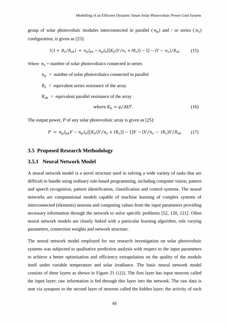
Modelling of an Efficient Dynamic Smart Solar Photovoltaic Power Grid System
65
group of solar photovoltaic modules interconnected in parallel ( 𝑛𝑝) and / or series ( 𝑛𝑠)
configuration, is given as [25]:
𝐼(1 + 𝑅𝑆 𝑅𝑠ℎ⁄ ) = 𝑛𝑝𝐼𝑝ℎ − 𝑛𝑝𝐼𝑂[{𝐾𝑂(𝑉 𝑛𝑠⁄ + 𝐼𝑅𝑠)} − 1] − (𝑉 − 𝑛𝑠) 𝑅𝑠ℎ⁄ (15)
Where 𝑛𝑠 = number of solar photovoltaics connected in series
𝑛𝑝 = number of solar photovoltaics connected in parallel
𝑅𝑆 = equivalent series resistance of the array
𝑅𝑠ℎ = equivalent parallel resistance of the array
where 𝐾𝑂 = 𝑞 𝐴𝑘𝑇⁄ . (16)
The output power, P of any solar photovoltaic array is given as [25]:
𝑃 = 𝑛𝑝𝐼𝑝ℎ𝑉 − 𝑛𝑝𝐼𝑂[{𝐾𝑂(𝑉 𝑛𝑠⁄ + 𝐼𝑅𝑠)} − 1]𝑉 − (𝑉 𝑛𝑠⁄ − 𝐼𝑅𝑠)𝑉 𝑅𝑠ℎ⁄ (17)
3.5 Proposed Research Methodology
3.5.1 Neural Network Model
A neural network model is a novel structure used in solving a wide variety of tasks that are
difficult to handle using ordinary rule-based programming, including computer vision, pattern
and speech recognition, pattern identification, classification and control systems. The neural
networks are computational models capable of machine learning of complex systems of
interconnected (elements) neurons and computing values from the input parameters providing
necessary information through the network to solve specific problems [52, 120, 121]. Often
neural network models are closely linked with a particular learning algorithm, rule varying
parameters, connection weights and network structure.
The neural network model employed for our research investigation on solar photovoltaic
systems was subjected to qualitative prediction analysis with respect to the input parameters
to achieve a better optimisation and efficiency extrapolation on the quality of the module
itself under variable temperature and solar irradiance. The basic neural network model
consists of three layers as shown in Figure 21 [122]. The first layer has input neurons called
the input layer; raw information is fed through this layer into the network. The raw data is
sent via synapses to the second layer of neurons called the hidden layer; the activity of each
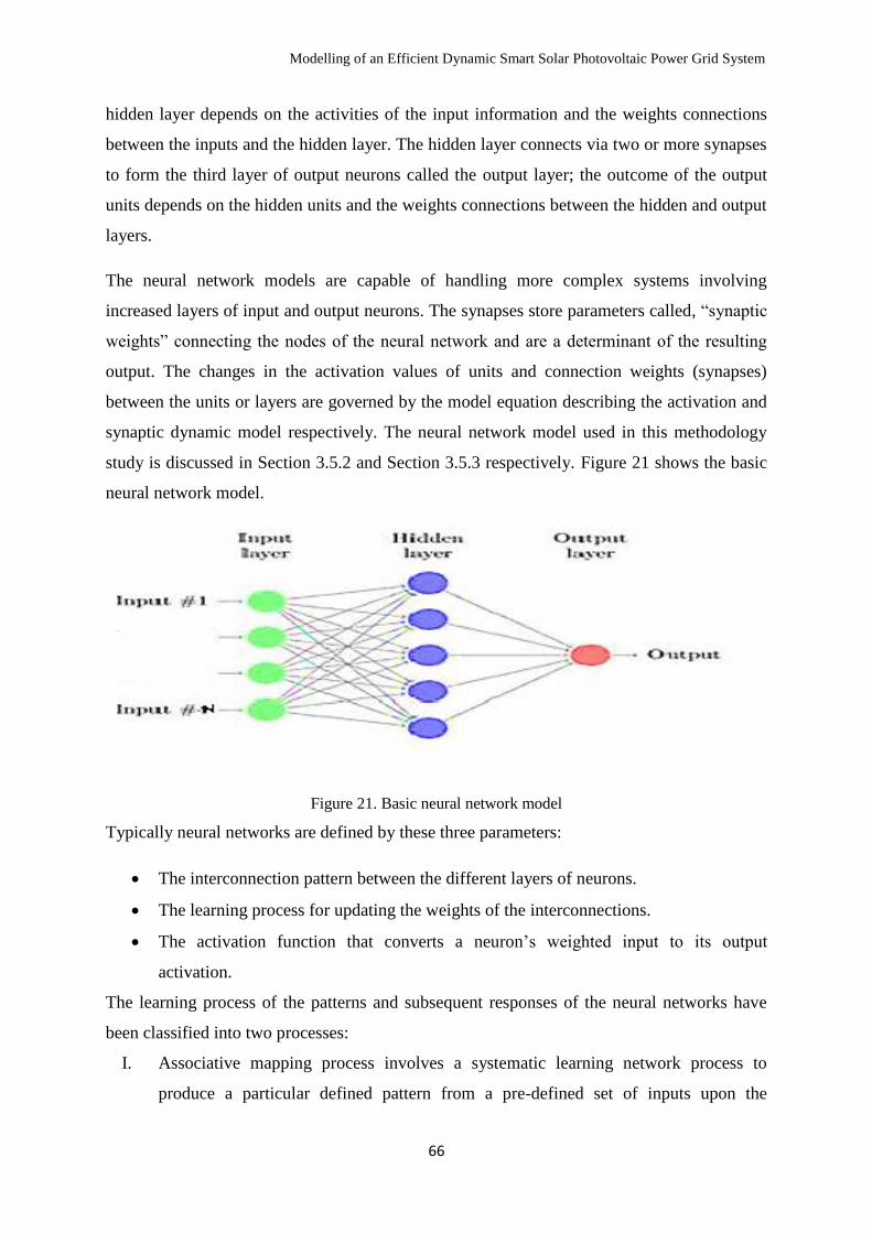
Modelling of an Efficient Dynamic Smart Solar Photovoltaic Power Grid System
66
hidden layer depends on the activities of the input information and the weights connections
between the inputs and the hidden layer. The hidden layer connects via two or more synapses
to form the third layer of output neurons called the output layer; the outcome of the output
units depends on the hidden units and the weights connections between the hidden and output
layers.
The neural network models are capable of handling more complex systems involving
increased layers of input and output neurons. The synapses store parameters called, “synaptic
weights” connecting the nodes of the neural network and are a determinant of the resulting
output. The changes in the activation values of units and connection weights (synapses)
between the units or layers are governed by the model equation describing the activation and
synaptic dynamic model respectively. The neural network model used in this methodology
study is discussed in Section 3.5.2 and Section 3.5.3 respectively. Figure 21 shows the basic
neural network model.
Figure 21. Basic neural network model
Typically neural networks are defined by these three parameters:
The interconnection pattern between the different layers of neurons.
The learning process for updating the weights of the interconnections.
The activation function that converts a neuron’s weighted input to its output
activation.
The learning process of the patterns and subsequent responses of the neural networks have
been classified into two processes:
I. Associative mapping process involves a systematic learning network process to
produce a particular defined pattern from a pre-defined set of inputs upon the

Modelling of an Efficient Dynamic Smart Solar Photovoltaic Power Grid System
67
introduction of a new pattern on the set of inputs. The mapping network process
stores the relationship among these patterns.
II. Regularity detection process involves a systematic learning process by which units
learn to respond to particular properties of input patterns.
The connecting weights matrix of the neural network contains stored information for the
learning process of the neural network. The learning process networks is categorised into two
major networks:
I. Fixed networks – the connecting weights cannot be altered; i.e dW/dt = 0.
II. Adaptive networks – the connecting weights can be altered; i.e dW/dt ≠ 0.
The learning ability of the neural network is characterised by the algorithm method chosen
for training. These training methods are basically categorised into three divisions [123]:
Unsupervised learning – the learning process is performed by itself without any external
interference. The generated outputs are not fed back into the network to measure against the
predictive performance of input parameters of the model.
Reinforcement learning – the learning process in this neural network architecture in the
hidden layer is randomly arranged and then reshuffled as the network learns its nearness to
the exact solution. This learning differs from the standard supervised learning due to the fact
the correct input/output are not presented nor sub-optimal actions explicitly adjusted.
Back propagation learning (supervised) – the learning process integrates the filtered errors
into the system readjusting the link between the network layers improving the performance of
the network.
For our research investigation on neural network modelling and simulation of a solar
photovoltaic system, the back propagation learning algorithm was employed to compare the
best efficiency of the two chosen methods. This was chosen because of its capabilities to
learn multiple-layer networks and nonlinear transfer functions such as gaussian function,
sigmoid function or any approximate functions.
There are currently various neural network model functions employed in research for
investigating the different solar photovoltaic module parameters. Careful choice of the best
suitable functions to investigate the fundamental physics as stated in section 3.2 associated
with solar photovoltaic module characteristics is thoughtfully chosen and examined for our
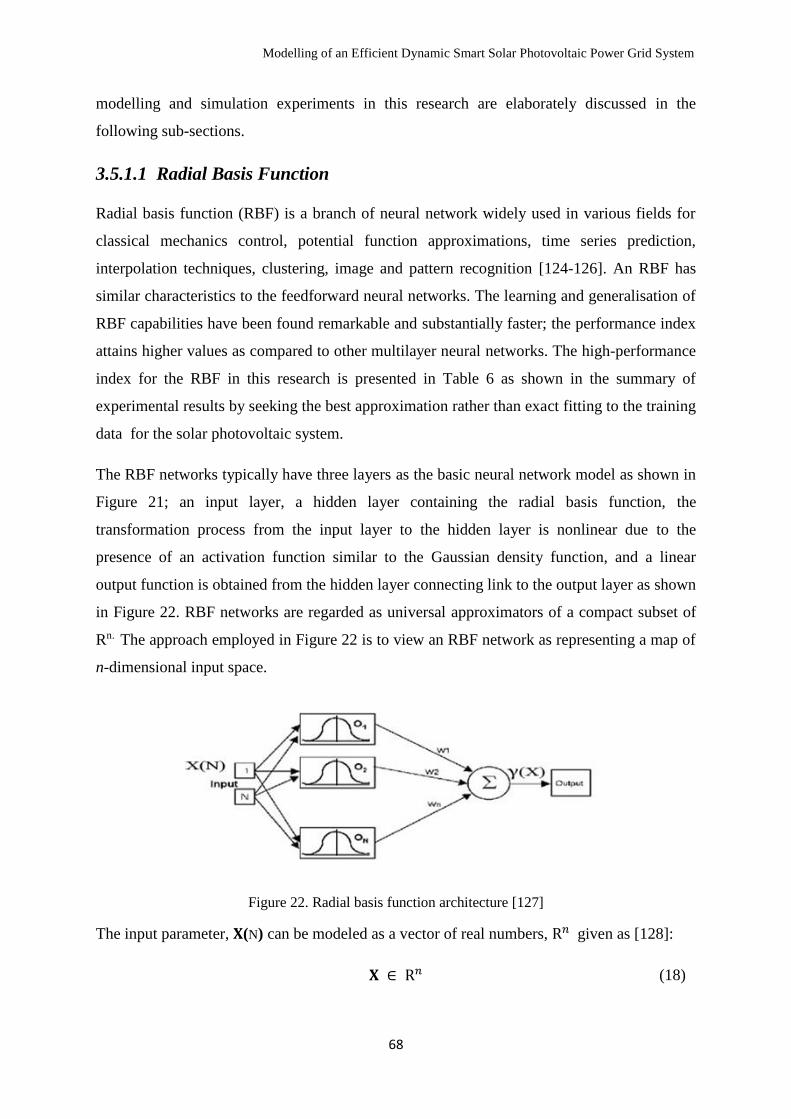
Modelling of an Efficient Dynamic Smart Solar Photovoltaic Power Grid System
68
modelling and simulation experiments in this research are elaborately discussed in the
following sub-sections.
3.5.1.1 Radial Basis Function
Radial basis function (RBF) is a branch of neural network widely used in various fields for
classical mechanics control, potential function approximations, time series prediction,
interpolation techniques, clustering, image and pattern recognition [124-126]. An RBF has
similar characteristics to the feedforward neural networks. The learning and generalisation of
RBF capabilities have been found remarkable and substantially faster; the performance index
attains higher values as compared to other multilayer neural networks. The high-performance
index for the RBF in this research is presented in Table 6 as shown in the summary of
experimental results by seeking the best approximation rather than exact fitting to the training
data for the solar photovoltaic system.
The RBF networks typically have three layers as the basic neural network model as shown in
Figure 21; an input layer, a hidden layer containing the radial basis function, the
transformation process from the input layer to the hidden layer is nonlinear due to the
presence of an activation function similar to the Gaussian density function, and a linear
output function is obtained from the hidden layer connecting link to the output layer as shown
in Figure 22. RBF networks are regarded as universal approximators of a compact subset of
Rn. The approach employed in Figure 22 is to view an RBF network as representing a map of
n-dimensional input space.
Figure 22. Radial basis function architecture [127]
The input parameter, 𝐗(N) can be modeled as a vector of real numbers, R𝑛 given as [128]:
𝐗 ∈ R𝑛 (18)
Modelling of an Efficient Dynamic Smart Solar Photovoltaic Power Grid System
69
The network parameters are regulated so that the training fits the network model as much as
possible. In radial basis function, all inputs are connected to each hidden neuron. The norm is
taken to be the euclidean distance and the radial basis function is considered as the Gaussian
function expressed in equation (19) [129].
𝜌(‖𝑋 − 𝐶𝑖‖) = 𝑒[−𝛽‖𝑋− 𝐶𝑖‖] (19)
The Gaussian basis functions are local to the center vector in the sense that;
lim‖𝑥‖→∞
𝜌(‖𝑋 − 𝐶𝑖‖) = 0 (20)
where N is the number of neurons in the hidden layer, 𝐶𝑖 is the center vector for neuron i, and
𝑤𝑖 is the weight of neuron i in the linear output neuron. The parameters 𝑤𝑖, 𝐶𝑖 and 𝛽𝑖 are
determined in a manner that best optimises the fit between the output 𝛾 and the data. The
RBF network is used in the function interpolations and approximations where optimisation is
more complex and determination for choice of centres is difficult. The output of the RBF
network is then a scalar function of the input, 𝛾 ∶ Rn→ R given as [128]:
𝛾(X) = ∑ 𝑤𝑖𝜌(‖𝑋 − 𝐶𝑖‖)𝑁𝑖=1 (21)
The parameters of the radial basis function are determined by three significant factors [129]:
Unit centers are determined using clustering algorithms such as k-means;
Widths are determined using the nearest neighbour method; and
Weights in the output layer are determined using the sum squared error to
minimise output outcomes.
RBF networks can be used to interpolate a function h: Rn→ R when the values of that function
are known from a finite number of points: h(𝐶𝑖) = 𝑑𝑖, i = 1,……,N. The known centres points
𝐶𝑖 of the radial basis functions are used in evaluating the values of the basis functions at the
same points 𝑝𝑖𝑗 = (‖𝑋𝑗 − 𝐶𝑖‖), the weights can be solved using the interpolation matrix from
the equation given as [129]:

Modelling of an Efficient Dynamic Smart Solar Photovoltaic Power Grid System
70
[
𝑝11𝑝21
𝑝12𝑝22
⋯ ⋯
⋮ ⋮ ⋱𝑝𝑁1 𝑝𝑁2 ⋯
𝑝1𝑁𝑝2𝑁⋮𝑝𝑁𝑁
] [
𝑤1𝑤2⋮𝑤𝑁
] = [
𝑑1𝑑2⋮𝑑𝑁
] (22)
The interpolation matrix in the above equation is non-singular if the points 𝐶𝑖 are distinct, and
thus the weights 𝑾 can be solved by simple linear algebra given as:
𝑾 = 𝑃−1𝑑 (23)
3.5.1.2 Multilayer Perceptron
Multilayer perceptron is a branch of neural network chosen for this research because of its
analogous characteristics with radial basis function using back-propagation algorithm and its
ability to learn from initial data provided yielding decision function directly via training.
Multilayer perceptron (MLP) is one of the classifications of feedforward neural network
connecting a set of input weights unit arranged in layers completely linked to the hidden
neuron layers, thus generating the appropriate output units. The MLP consists of three or
more layers, the input layer, with one or more hidden layers of non-linearity activation nodes
and an output layer. Most applications in MLP use a supervised learning algorithm called
back-propagation for training the network [130, 131].
The MLP model correctly maps the input to the output using the stored information to
generate the output when the desired output is unknown. The generated output is compared
with the desired output and the error is computed. The computed error is fed back into the
neural network causing an adjustment in the synaptic weights minimising the error with each
iteration until the expected output gets closer to the desired output. The error minimization
process is a function based on traditional gradient descent technique.
A typical MLP feedforward neural network has a similar architecture with the basic neural
network is shown in Figure 21, the input layer and the output layer with one or more hidden
layers having nonlinear activation functions tanh or sigmoid function as shown in Figure 23
[132]. The presence of the hidden layers provides regularisation to address overfitting of the
trained data. The training data set consists of N training patterns, where p is the pattern
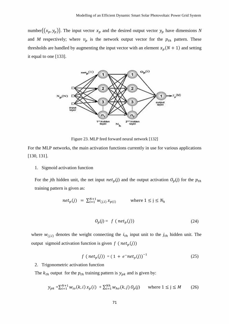
Modelling of an Efficient Dynamic Smart Solar Photovoltaic Power Grid System
71
number{(𝑥𝑝, 𝑦𝑝)}. The input vector 𝑥𝑝 and the desired output vector 𝑦𝑝 have dimensions N
and M respectively; where 𝑣𝑝 is the network output vector for the 𝑝𝑡ℎ pattern. These
thresholds are handled by augmenting the input vector with an element 𝑥𝑝(𝑁 + 1) and setting
it equal to one [133].
Figure 23. MLP feed forward neural network [132]
For the MLP networks, the main activation functions currently in use for various applications
[130, 131].
1. Sigmoid activation function
For the jth hidden unit, the net input 𝑛𝑒𝑡𝑝(j) and the output activation 𝑂𝑝(j) for the 𝑝𝑡ℎ
training pattern is given as:
𝑛𝑒𝑡𝑝(𝑗) = ∑ 𝑤(𝑗,𝑖)𝑁+1𝑖=1 𝑥𝑝(𝑖) where 1 ≤ j ≤ 𝑁ℎ
𝑂𝑝(j) = f ( 𝑛𝑒𝑡𝑝(𝑗)) (24)
where 𝑤(𝑗,𝑖) denotes the weight connecting the 𝑖𝑡ℎ input unit to the 𝑗𝑡ℎ hidden unit. The
output sigmoid activation function is given f ( 𝑛𝑒𝑡𝑝(𝑗))
f ( 𝑛𝑒𝑡𝑝(𝑗)) = ( 1 + 𝑒−𝑛𝑒𝑡𝑝(𝑗))−1
(25)
2. Trigonometric activation function
The 𝑘𝑡ℎ output for the 𝑝𝑡ℎ training pattern is 𝑦𝑝𝑘 and is given by:
𝑦𝑝𝑘 =∑ 𝑤𝑖𝑜(𝑘, 𝑖)𝑁+1𝑖=1 𝑥𝑝(𝑖) + ∑ 𝑤ℎ𝑜(𝑘, 𝑗)
𝑁ℎ𝑖=1 𝑂𝑝(j) where 1 ≤ j ≤ 𝑀 (26)

Modelling of an Efficient Dynamic Smart Solar Photovoltaic Power Grid System
72
where 𝑤𝑖𝑜(𝑘, 𝑖) denotes the output weight connecting the 𝑖𝑡ℎ input unit to the 𝑘𝑡ℎ output
unit and 𝑤ℎ𝑜(𝑘, 𝑗) denotes the output weight connecting the 𝑗𝑡ℎ hidden unit to the 𝑘𝑡ℎ
output unit. The mapping error for the 𝑝𝑡ℎ pattern is given as:
𝐸𝑝 = ∑ (𝑡𝑝𝑘 − 𝑦𝑝𝑘)2𝑀
𝑘=1 (27)
where 𝑡𝑝𝑘 represents the 𝑘𝑡ℎ element of the 𝑝𝑡ℎ desired output vector. In order to train a
neural network in batch mode, the mapping error for the 𝑘𝑡ℎ output unit is given as:
𝐸(𝑘)= 1
𝑁𝑣 ∑ (𝑡𝑝𝑘 − 𝑦𝑝𝑘)
2𝑁𝑣𝑝=1 (28)
The overall performance of the MLP is determined by the mean square error and is given as:
𝐸 = ∑𝐸(𝑘)
𝑀
𝑘=1
= 1
𝑁𝑣∑𝐸𝑝
𝑁𝑣
𝑘=1
(29)
The basic steps in implementing the MLP learning algorithm is as described below:
i. Initialize the network, with all weights set to random numbers between -1 and +1.
ii. Perform the first training process, and obtain the desired output.
iii. Compare the network with the desired output.
iv. Propagate the error backwards.
(a) Correct the output layer of weights using the following formula.
𝑤ℎ𝑘 = 𝑤ℎ𝑘 + (𝜂𝛿𝑘𝑘ℎ) (30)
where 𝑤ℎ𝑘 is the weight connecting hidden units h with output unit k, η is the learning rate,
𝑘ℎ is the output at hidden unit h. 𝛿𝑘 is given by the following.
𝛿𝑘 = 𝑘0(1 − 𝑘0) ( 𝑡0 − 𝑘0) (31)
where 𝑘0 is the output at node 0 of the output layer, and 𝑡0 is the target output for that node.
(b) Correct the input weights using the following formula.
𝑤𝑝𝑘 = 𝑤ℎ𝑘 + (𝜂𝛿𝑘𝑘ℎ) (32)

Modelling of an Efficient Dynamic Smart Solar Photovoltaic Power Grid System
73
where 𝑤𝑝𝑘 is the weight connecting node I of the input layer with node h of the hidden layer,
𝑘0 is the input at node I of the input layer, η is the learning rate. 𝛿𝑗 is calculated for and is
given by the expression:
𝛿𝑘 = 𝑘0(1- 𝑘0) ∑ (𝛿𝑘𝑘ℎ)𝑜 (33)
v. Determine the error, by taking the difference of the mean of the expected output and
the actual output obtained.
𝐸𝑟𝑟𝑜𝑟𝑑𝑒𝑡 = √∑ (𝑘0− 𝑘𝑘)
2𝑝𝑛=1
𝑝 (34)
where 𝑝 is the number of units in the output layer.
vi. Repeat from (ii) for each pattern in the training set to complete one epoch.
vii. The training set is randomly selected to prevent influence by the arrangement of data.
viii. Repeat from step (ii) for a set number of epochs, or until the error ceases to change.
3.5.1.3 Levenberg-Marquardt Algorithm (LMA)
The radial basis function and multilayer perceptron use back-propagation for training the
network by employing Levenberg-Marquardt algorithm in the Matlab software function
lm.m. The respective equations (18-29) for the radial basis function and multilayer perceptron
are individually integrated into the Levenberg-Marquardt algorithm for comparative analyses
of the solar photovoltaic array under investigation. The Levenberg-Marquardt algorithm
(LMA) is widely used for many nonlinear inverse applications in solving generic curve fitting
problems. The LMA involves an iteration technique locating the minimum multivariate
function expression as the sum of squares of nonlinear real-valued functions. The LMA is an
algorithm combining the steepest descent and gaussian-newton method, when the obtained
solution is far from the expected solution, the algorithm behaves like a steepest descent
method and is said to be quadratically convergent.
Similarly, when the solution is close to the expected solution, it is considered as a gaussian-
newton method using the trust-region technique. This algorithm is also known as the damped
least-squares (DLS) method. The LMA is more robust than the gaussian-newton algorithm
Modelling of an Efficient Dynamic Smart Solar Photovoltaic Power Grid System
74
(GNA) since it finds a steady and convergence solution far off the final minimum using
iterative techniques [134].
The LMA interpolates between the GNA and the method of gradient descent. Like other
numeric minimization algorithms, the LMA employs an iterative procedure. In other to start a
minimisation process, an initial assumption for the parameter vector, 𝜷 , has to be made and
in cases with only one minimum, a uniform assumption is given as :
The parameter vector is given as 𝜷𝒕 = (1, 1, ……1) (35)
In some other cases with multiple minima, the algorithm converges only if the initial
assumption is very close to the final solution. In each iteration step, the parameter
optimisation vector, 𝜷, is replaced by a new estimate, 𝜷 + 𝜹. To determine the 𝜹, the
functions f(𝑥𝑖 , 𝜷 + 𝜹) are approximated by their linearisations [135]:
𝑓(𝑥𝑖 , 𝜷 + 𝜹) ≈ 𝑓(𝑥𝑖 , 𝜷) + 𝐽𝑖𝜹 (36)
where the Jacobian matrix vector, 𝐽𝑖 = 𝜕𝑓(𝑥𝑖 , 𝜷)
𝜕𝜷 (37)
𝐽𝑖 is the gradient of f with respect to 𝜷.
The sum of squares at minimum is given as S(𝜷), the gradient of S with respect to 𝛿 will be
zero. The above first-order approximation of f(𝑥𝑖 , 𝜷 + 𝜹) gives [135]:
𝑆(𝜷 + 𝜹) ≈ ∑(𝑦𝑖 − 𝑓(𝑥𝑖 , 𝜷) − 𝐽𝑖𝜹)2
𝑚
𝑖=1
(38)
Or in vector notation,
𝑆(𝜷 + 𝜹) ≈ ‖𝑦 − 𝑓(𝜷) − 𝐽𝜹‖2 (39)
Taking the derivative with respect to 𝜹 in (39) and setting the result to zero gives;
(𝐉𝐓𝐉) 𝜹 = 𝐉𝐓 [𝑦 − 𝑓(𝜷)] (40)
This becomes a set of linear equations which can be solved for 𝜹.
where J is the Jacobian matrix whose 𝑖𝑡ℎ row equals 𝐽𝑖, and where f and y are the vectors with
𝑖𝑡ℎ component 𝑓(𝑥𝑖 , 𝜷) and 𝑦𝑖 respectively.
Upon introducing the damped LMA into the above equation, the equation then becomes:

Modelling of an Efficient Dynamic Smart Solar Photovoltaic Power Grid System
75
(𝐉𝐓𝐉 + 𝜆𝐈) 𝜹 = 𝐉𝐓 [𝑦 − 𝑓(𝜷)] (41)
where I is the identity matrix, giving the increment as, 𝜹, and the estimated parameter
vector, 𝜷. The damping factor, 𝜆 is adjusted at each iteration. If the reduction of S is rapid, a
smaller value is used bringing the LMA closer to the GNA, whereas if the iteration gives
insufficient reduction in the residual, 𝜆 can be increased, giving a step closer to the gradient
descent direction.
Therefore, the gradient of S with respect to 𝜹 = -2 (𝐉𝐓 [𝑦 − 𝑓(𝜷)])𝑇 (42)
For larger values of 𝜆, the inverting 𝐉𝐓𝐉 + 𝜆𝐈 is not used at all; the convergence tends toward
the direction of a small gradient. The identity matrix, I is then replaced with the diagonal
matrix consisting of the diagonal elements of 𝐉𝐓𝐉 , the resulting LMA is given as[135]:
(𝐉𝐓𝐉 + 𝜆𝐝𝐢𝐚𝐠(𝐉𝐓𝐉)) 𝜹 = 𝐉𝐓 [𝑦 − 𝑓(𝜷)] (43)
The Levenberg-Marquardt algorithm is chosen to train the radial basis function and
multilayer perceptron because it is considered as one of the fastest method algorithms for
training moderate-sized feedforward networks. The above LMA equation is used to forecast a
more accurate model using statistical parameters as the mean square error (MSE) and the
newrbe performance on the solar photovoltaic array as presented in the following sections.
3.5.1.4 Model Comparison and Performance
A comparative study of two neural network models is under consideration in this research
using Matlab/Simulink program for the simulation process. Each of the models is validated
based on the established current-voltage (I-V) characteristics mathematical model
implemented by iterative analysis comparing the conventional model and simulated results of
the model. The data sets used for this simulation are divided into training, validation and
verification sets for evaluating the model performance.
The training and validation data applied in each of this model, map the entire characteristics
of the simplest model of the equivalent circuit of a static solar photovoltaic system. In this
research, the training data were obtained from a solar photovoltaic manufacturer data manual.
The photovoltaic manufacturer parameters employed in this comparative study for the
simulation experiments are shown in Table 6. The static solar photovoltaic system under
consideration was constructed by connecting ten cell branches in parallel (np = 10). As each
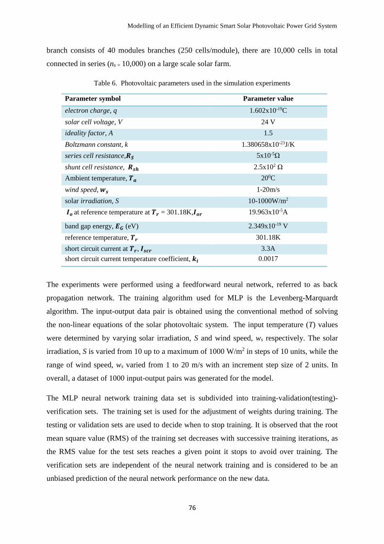
Modelling of an Efficient Dynamic Smart Solar Photovoltaic Power Grid System
76
branch consists of 40 modules branches (250 cells/module), there are 10,000 cells in total
connected in series (ns = 10,000) on a large scale solar farm.
Table 6. Photovoltaic parameters used in the simulation experiments
Parameter symbol Parameter value
electron charge, q 1.602x10⁻¹⁹C
solar cell voltage, V 24 V
ideality factor, A 1.5
Boltzmann constant, k 1.380658x10⁻²³J/K
series cell resistance,𝑹𝑺 5x10⁻⁵Ω
shunt cell resistance, 𝑹𝒔𝒉 2.5x10² Ω
Ambient temperature, 𝑻𝒂 200C
wind speed, 𝒘𝒔 1-20m/s
solar irradiation, S 10-1000W/m2
𝑰𝒐 at reference temperature at 𝑻𝒓 = 301.18K,𝑰𝒐𝒓 19.963x10⁻⁵A
band gap energy, 𝑬𝑮 (eV) 2.349x10⁻¹⁹ V
reference temperature, 𝑻𝒓 301.18K
short circuit current at 𝑻𝒓, 𝑰𝒔𝒄𝒓 3.3A
short circuit current temperature coefficient, 𝒌𝒊 0.0017
The experiments were performed using a feedforward neural network, referred to as back
propagation network. The training algorithm used for MLP is the Levenberg-Marquardt
algorithm. The input-output data pair is obtained using the conventional method of solving
the non-linear equations of the solar photovoltaic system. The input temperature (T) values
were determined by varying solar irradiation, S and wind speed, ws respectively. The solar
irradiation, S is varied from 10 up to a maximum of 1000 W/m2 in steps of 10 units, while the
range of wind speed, ws varied from 1 to 20 m/s with an increment step size of 2 units. In
overall, a dataset of 1000 input-output pairs was generated for the model.
The MLP neural network training data set is subdivided into training-validation(testing)-
verification sets. The training set is used for the adjustment of weights during training. The
testing or validation sets are used to decide when to stop training. It is observed that the root
mean square value (RMS) of the training set decreases with successive training iterations, as
the RMS value for the test sets reaches a given point it stops to avoid over training. The
verification sets are independent of the neural network training and is considered to be an
unbiased prediction of the neural network performance on the new data.
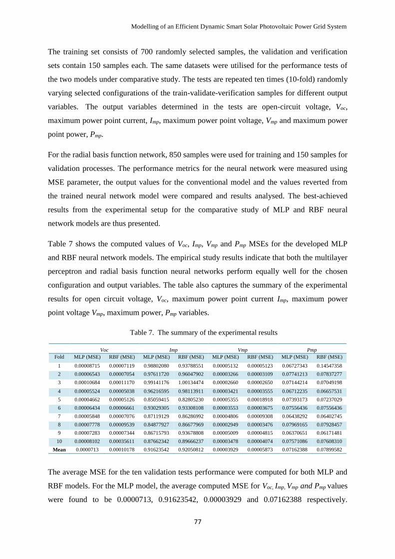
Modelling of an Efficient Dynamic Smart Solar Photovoltaic Power Grid System
77
The training set consists of 700 randomly selected samples, the validation and verification
sets contain 150 samples each. The same datasets were utilised for the performance tests of
the two models under comparative study. The tests are repeated ten times (10-fold) randomly
varying selected configurations of the train-validate-verification samples for different output
variables. The output variables determined in the tests are open-circuit voltage, Voc,
maximum power point current, Imp, maximum power point voltage, Vmp and maximum power
point power, Pmp.
For the radial basis function network, 850 samples were used for training and 150 samples for
validation processes. The performance metrics for the neural network were measured using
MSE parameter, the output values for the conventional model and the values reverted from
the trained neural network model were compared and results analysed. The best-achieved
results from the experimental setup for the comparative study of MLP and RBF neural
network models are thus presented.
Table 7 shows the computed values of Voc, Imp, Vmp and Pmp MSEs for the developed MLP
and RBF neural network models. The empirical study results indicate that both the multilayer
perceptron and radial basis function neural networks perform equally well for the chosen
configuration and output variables. The table also captures the summary of the experimental
results for open circuit voltage, Voc, maximum power point current Imp, maximum power
point voltage Vmp, maximum power, Pmp variables.
Table 7. The summary of the experimental results
Voc Imp Vmp Pmp
Fold MLP (MSE) RBF (MSE) MLP (MSE) RBF (MSE) MLP (MSE) RBF (MSE) MLP (MSE) RBF (MSE)
1 0.00008715 0.00007119 0.98802080 0.93788551 0.00005132 0.00005123 0.06727343 0.14547358
2 0.00006543 0.00007054 0.97611720 0.96047902 0.00003266 0.00003109 0.07741213 0.07837277
3 0.00010684 0.00011170 0.99141176 1.00134474 0.00002660 0.00002650 0.07144214 0.07049198
4 0.00005524 0.00005038 0.96216595 0.98113911 0.00003421 0.00003555 0.06712235 0.06657531
5 0.00004662 0.00005126 0.85059415 0.82805230 0.00005355 0.00018918 0.07393173 0.07237029
6 0.00006434 0.00006661 0.93029305 0.93308108 0.00003553 0.00003675 0.07556436 0.07556436
7 0.00005848 0.00007076 0.87119129 0.86286992 0.00004806 0.00009308 0.06438292 0.06402745
8 0.00007778 0.00009539 0.84877927 0.86677969 0.00002949 0.00003476 0.07969165 0.07928457
9 0.00007283 0.00007344 0.86715793 0.93678808 0.00005009 0.00004815 0.06370651 0.06171481
10 0.00008102 0.00035611 0.87662342 0.89666237 0.00003478 0.00004074 0.07571086 0.07608310
Mean 0.0000713 0.00010178 0.91623542 0.92050812 0.00003929 0.00005873 0.07162388 0.07899582
The average MSE for the ten validation tests performance were computed for both MLP and
RBF models. For the MLP model, the average computed MSE for Voc, Imp, Vmp and Pmp values
were found to be 0.0000713, 0.91623542, 0.00003929 and 0.07162388 respectively.
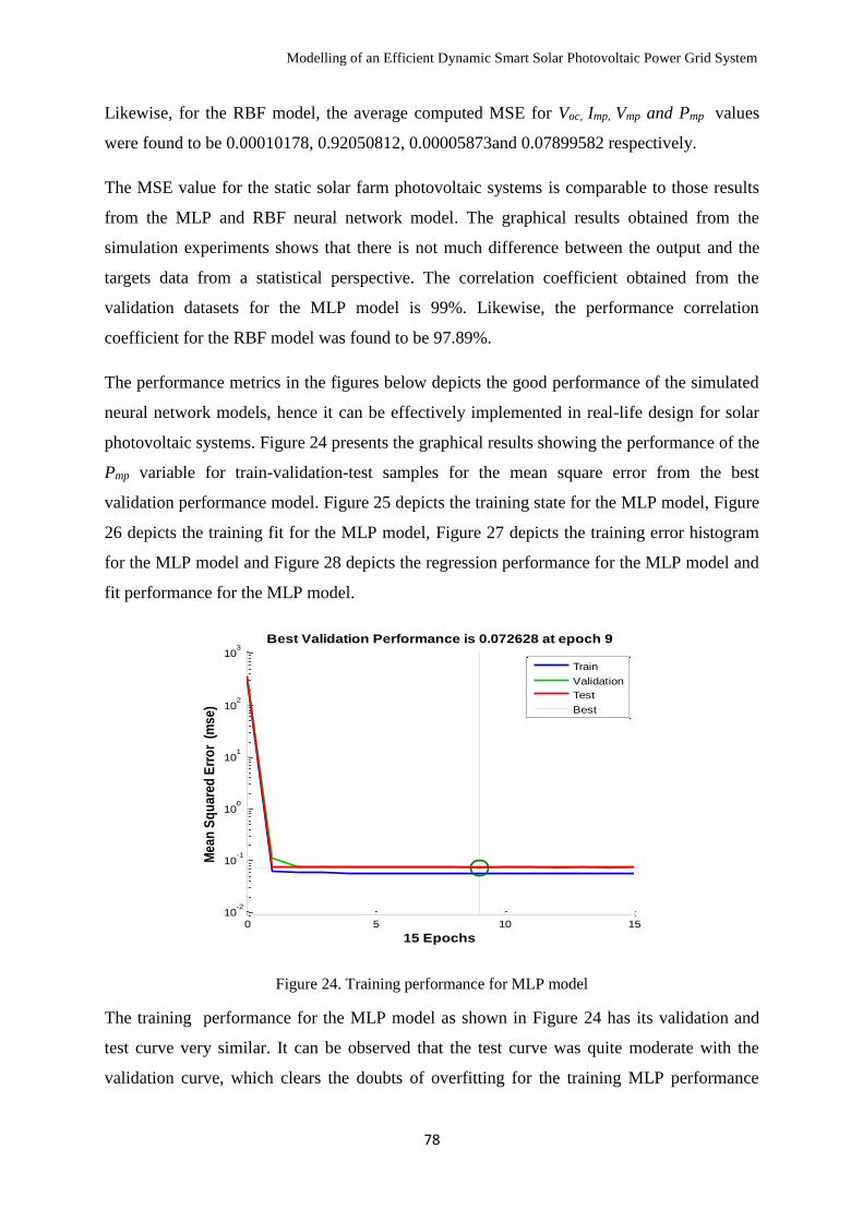
Modelling of an Efficient Dynamic Smart Solar Photovoltaic Power Grid System
78
Likewise, for the RBF model, the average computed MSE for Voc, Imp, Vmp and Pmp values
were found to be 0.00010178, 0.92050812, 0.00005873and 0.07899582 respectively.
The MSE value for the static solar farm photovoltaic systems is comparable to those results
from the MLP and RBF neural network model. The graphical results obtained from the
simulation experiments shows that there is not much difference between the output and the
targets data from a statistical perspective. The correlation coefficient obtained from the
validation datasets for the MLP model is 99%. Likewise, the performance correlation
coefficient for the RBF model was found to be 97.89%.
The performance metrics in the figures below depicts the good performance of the simulated
neural network models, hence it can be effectively implemented in real-life design for solar
photovoltaic systems. Figure 24 presents the graphical results showing the performance of the
Pmp variable for train-validation-test samples for the mean square error from the best
validation performance model. Figure 25 depicts the training state for the MLP model, Figure
26 depicts the training fit for the MLP model, Figure 27 depicts the training error histogram
for the MLP model and Figure 28 depicts the regression performance for the MLP model and
fit performance for the MLP model.
Figure 24. Training performance for MLP model
The training performance for the MLP model as shown in Figure 24 has its validation and
test curve very similar. It can be observed that the test curve was quite moderate with the
validation curve, which clears the doubts of overfitting for the training MLP performance
0 5 10 1510
-2
10-1
100
101
102
103
Best Validation Performance is 0.072628 at epoch 9
Me
an
Sq
ua
red
Err
or
(m
se
)
15 Epochs
Train
Validation
Test
Best
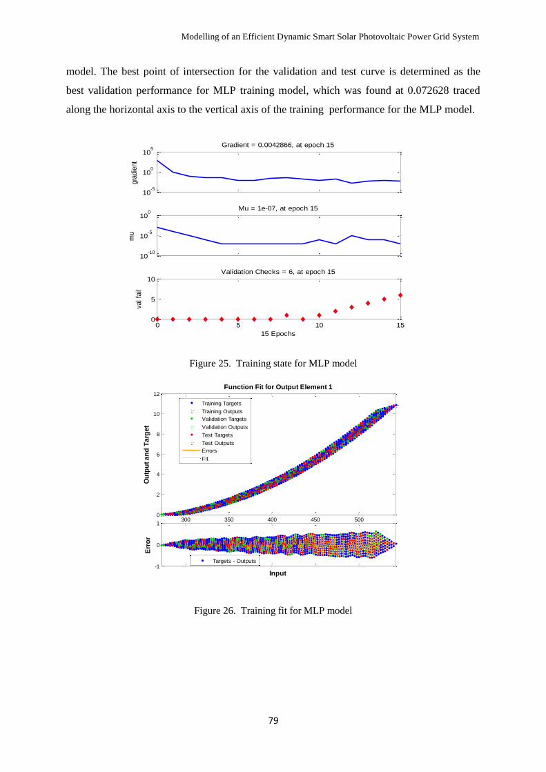
Modelling of an Efficient Dynamic Smart Solar Photovoltaic Power Grid System
79
model. The best point of intersection for the validation and test curve is determined as the
best validation performance for MLP training model, which was found at 0.072628 traced
along the horizontal axis to the vertical axis of the training performance for the MLP model.
Figure 25. Training state for MLP model
Figure 26. Training fit for MLP model
10-5
100
105
gra
die
nt
Gradient = 0.0042866, at epoch 15
10-10
10-5
100
mu
Mu = 1e-07, at epoch 15
0 5 10 150
5
10
val fa
il
15 Epochs
Validation Checks = 6, at epoch 15
300 350 400 450 5000
2
4
6
8
10
12
Function Fit for Output Element 1
Ou
tpu
t a
nd
Ta
rge
t
-1
0
1
Err
or
Input
Training Targets
Training Outputs
Validation Targets
Validation Outputs
Test Targets
Test Outputs
Errors
Fit
Targets - Outputs
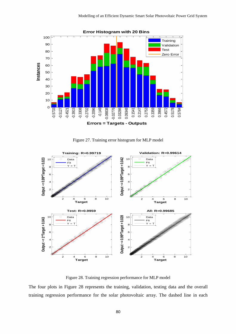
Modelling of an Efficient Dynamic Smart Solar Photovoltaic Power Grid System
80
Figure 27. Training error histogram for MLP model
Figure 28. Training regression performance for MLP model
The four plots in Figure 28 represents the training, validation, testing data and the overall
training regression performance for the solar photovoltaic array. The dashed line in each
0
10
20
30
40
50
60
70
80
90
100
Error Histogram with 20 Bins
Inst
ance
s
Errors = Targets - Outputs
-0.5
733
-0.5
127
-0.4
521
-0.3
915
-0.3
308
-0.2
702
-0.2
096
-0.1
49
-0.0
8838
-0.0
2776
0.03
286
0.09
348
0.15
41
0.21
47
0.27
53
0.33
59
0.39
66
0.45
72
0.51
78
0.57
84
Training
Validation
Test
Zero Error
2 4 6 8 10
2
4
6
8
10
Target
Out
put ~
= 0.
99*T
arge
t + 0
.023
Training: R=0.99719
Data
Fit
Y = T
2 4 6 8 10
2
4
6
8
10
Target
Out
put ~
= 0.
99*T
arge
t + 0
.042
Validation: R=0.99614
Data
Fit
Y = T
2 4 6 8 10
2
4
6
8
10
Target
Out
put ~
= 1*
Targ
et +
0.0
43
Test: R=0.9959
Data
Fit
Y = T
2 4 6 8 10
2
4
6
8
10
Target
Out
put ~
= 0.
99*T
arge
t + 0
.028
All: R=0.99685
Data
Fit
Y = T
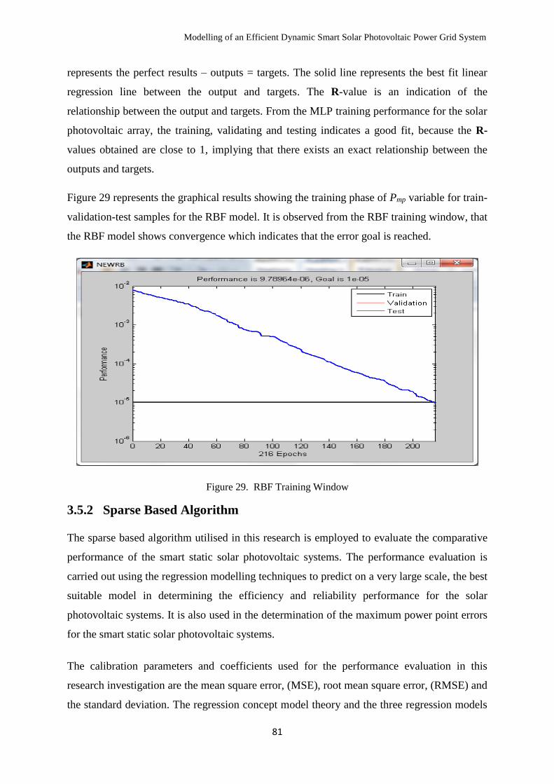
Modelling of an Efficient Dynamic Smart Solar Photovoltaic Power Grid System
81
represents the perfect results – outputs = targets. The solid line represents the best fit linear
regression line between the output and targets. The R-value is an indication of the
relationship between the output and targets. From the MLP training performance for the solar
photovoltaic array, the training, validating and testing indicates a good fit, because the R-
values obtained are close to 1, implying that there exists an exact relationship between the
outputs and targets.
Figure 29 represents the graphical results showing the training phase of Pmp variable for train-
validation-test samples for the RBF model. It is observed from the RBF training window, that
the RBF model shows convergence which indicates that the error goal is reached.
Figure 29. RBF Training Window
3.5.2 Sparse Based Algorithm
The sparse based algorithm utilised in this research is employed to evaluate the comparative
performance of the smart static solar photovoltaic systems. The performance evaluation is
carried out using the regression modelling techniques to predict on a very large scale, the best
suitable model in determining the efficiency and reliability performance for the solar
photovoltaic systems. It is also used in the determination of the maximum power point errors
for the smart static solar photovoltaic systems.
The calibration parameters and coefficients used for the performance evaluation in this
research investigation are the mean square error, (MSE), root mean square error, (RMSE) and
the standard deviation. The regression concept model theory and the three regression models

Modelling of an Efficient Dynamic Smart Solar Photovoltaic Power Grid System
82
considered under this comparative research investigation are briefly introduced and discussed
in the following sub-sections 3.5.2.1, 3.5.2.2, 3.5.2.3 and 3.5.2.4 respectively.
3.5.2.1 Regression Concept and Theory
Regression is one of the most commonly used statistical techniques applied in various
research fields. The regression tool is suitable for analysing, predicting, forecasting,
investigating, hypothesis testing and modelling the relationship between a scalar dependent
variable and an independent variable [136, 137]. The regression analysis tries to fit a model
to one dependent variable based on one or more independent variables. One of the most
common regression models is the simple linear regression model. Simple linear regression is
a statistical method providing a result between two quantitative variables.
The linear regression concept assumes a linear relationship between an independent variable
(predictor) and a dependent variable (response). The linear relationship is represented by a
regression straight line fitting through the set of points in such a way making the sum of the
squared residuals of the model to have the smallest possible error. The best fitting line is
known as the regression line. There are a lot of methods in determining the best-fit line, one
of the methods considered for this research investigation is termed the least square method.
Multi-linear regression exhibits linear characteristics equation with two or more predictor
variables. Non-linear regression depends on multiple independent variables modelled by non-
linear functional combination model parameters.
The characteristics of a good regression model possesses a high regression 𝐑 - value fairly
close to unity [138]. This regression model predicts the best fitting line for the data and
overall summary of the model performance [136]. The plotting of residuals is a tool used in
checking the adequacies of fitted multiple linear regressions based on determined standard
deviation. The data used for analysis covers the entire range of response values for analysis
and prediction.
The simple linear regressions are classified into three groups namely linear, quadratic and
cubic [139];
Linear: 𝒀𝑳 = 𝑎0 + 𝑎1x
Quadratic: 𝒀𝑸 = 𝑎0 + 𝑎1𝑥1 + 𝑎2𝑥2
Cubic: 𝒀𝑪 = 𝑎0 + 𝑎1𝑥1 + 𝑎2𝑥2 + 𝑎3𝑥3
(44)
Modelling of an Efficient Dynamic Smart Solar Photovoltaic Power Grid System
83
The linear parameters 𝑎0 and 𝑎1 represent the y-intercept and the slope of the equation
respectively.
The multi-linear regression model performs linear and non-linear regressions functions with
two or more independent variables. The multi-linear regression model is classified into two
groups namely, multiple and involving interactions [139];
Multiple: 𝒀𝑴 = 𝑎0 + 𝑎1𝑥1 + 𝑎2𝑥2 + 𝑎3𝑥3
Involving interactions: 𝒀𝑰 = 𝑎0 + 𝑎1𝑥1 + 𝑎2𝑥2 + 𝑎3𝑥1𝑥2 (45)
The non-linear regression model assumes any type of relationship between the dependent
variable and independent variables. The model function uses the least squares approach for
computing the regression. The regression model is classified into two groups namely sine
wave and exponential [139];
Sine Waves: 𝒀𝑺 = 𝑎0 + sin(𝑎1𝑥1)
Exponential: 𝒀𝑬 = 𝑎0 + 𝑒(𝑎1/𝑥1) (46)
3.5.2.2. Regression-type Model
The regression algorithm model considered in the estimation technique of the static solar
photovoltaic module is a sparsely based regression algorithm. The sparsely based algorithm
has established itself among the state of the art algorithm in supervised learning. It learns
classifiers constructed as weighted linear combinations of basis functions. The weights are
estimated in the presence of the training data selected either significantly large or exactly zero
which necessarily removes irrelevant basis functions.
The sparsely based regression algorithm is embedded into our previous Levenberg-Marquardt
algorithm neural network training in subsection 3.5.1.4 [140]. The primary emphasis of the
introduction of the sparsely based algorithm was based on its flexibility and efficiency
performance. The sparsely based algorithm incorporates an iterative linear system solver for
minimising the number of iterations for the model.
Considering a data matrix P and a column vector function k, the optimisation problem is
solved by obtaining a weight of vector w of variables for a sparse based algorithm [141, 142].
𝑚𝑖𝑛‖𝑤‖1, s. t. 𝐏𝒘 = 𝒌 (47)
Modelling of an Efficient Dynamic Smart Solar Photovoltaic Power Grid System
84
where 1-norm ‖𝑤‖1 is defined as ∑ |𝑤𝑖|𝑀𝑖=1
The optimal solution of equation (47) is denoted by 𝒘𝒐. The absolute value for each entry of
𝒘𝒐 reflects the contribution of its corresponding variable to the regression between the data
matrix P and column vector function k.
where k 𝜖 𝑅𝑁 is a given signal vector and P 𝜖 𝑅𝑁∗𝑀 (N <M) is a basis matrix.
The objective of the sparsely based algorithm is to find a solution w 𝜖 𝑅𝑀 for equation (47).
The assumption for the sparsely based algorithm is set for the non-negatives as [141, 142];
Setting w = u – v , where u = [𝑢1, …… . , 𝑢𝑘0] 𝑇 , v = [𝑣1, …… . , 𝑣𝑘0]
𝑇 𝜖 𝑅𝑀 are non-
negatives
The non-negative expressions can be converted to equivalent linear solvable programming
problems using the Matlab optimisation toolbox [141, 142].
𝑚𝑖𝑛∑(𝑢𝑖 + 𝑣𝑖)
𝑘0
𝑖=1
, s. t. [𝑷, − 𝑷][𝑢𝑇 , 𝑣𝑇]𝑇 = 𝒌, u, v ≥ 0 (48)
The sparse weight identifies the relevant variables or the supposed regression vectors. The
sparsely based algorithm is categorised into two correlations: time series correlated with the
output and time series not significantly correlated with output. There are quite a few
parameter estimators developed in linear regression differing in the simplicity of the
algorithm, robustness in heavy-tailed distributions, theoretical assumptions and close form
solutions to validate asymptotic efficiency and consistency [141, 142].
A brief review of three regression estimation techniques under assessment in this research
investigation employed in the simulation and modelling of the static solar photovoltaic
module using the sparse based algorithm are described in the following sub-sections.
3.5.2.3. Ordinary Least Squares Regression
The ordinary least squares (OLS) is also referred to as linear least squares. This regression
estimator method is applied to analyse both experimental and observational data in the
estimation of unknown parameters in a linear regression model. The OLS minimises the sum
of squared residuals between the observed and predicted responses from the datasets by linear
approximation. Several assumptions occur in OLS to validate predicted and the estimated
model.

Modelling of an Efficient Dynamic Smart Solar Photovoltaic Power Grid System
85
The residual is determined from the difference between the predicted and the real data; when
a large distortion occurs it is referred to as outliers. These outliers influence the error
variance, the standard deviation and the final estimation to become asymptotically
inconsistent. One of the several assumptions generated is the normality of the residuals along
the parallel line and the other is ensuring the normality of the residuals make the estimation
of significance impaired. In the OLS regression model, it is primarily assumed that there is
zero or negligible errors in the independent variables [143, 144].
Considering a data consisting of n observations [𝑦𝑖, 𝑥𝑖]𝑖=1𝑛 . Each observation includes a scalar
response 𝑦𝑖 and vector p predictors 𝑥𝑖. In a linear regression model the response variable is a
linear function of the regressors:
𝑦𝑖 = 𝑥𝑖𝑇𝛽 + 휀𝑖
where 𝛽 is a px1vector of unknown parameters; 휀𝑖’s are unobserved scalar random variables
which account for discrepancy between the actually observed responses 𝑦𝑖 and the predicted
outcomes 𝑥𝑖𝑇𝛽 and 𝑇 denotes the matrix transpose, so that 𝑥𝑇𝛽 is the dot product between
the vectors x and 𝛽. This model can be written in matrix notation as [143, 144]:
y = X 𝛽 + 휀 (49)
where y and 휀 are nx1 vectors, and X is an n x p matrix of regressors, known as design
matrix.
In the ordinary least squares estimation, an assumption is considered in the determination of
the sum of residuals for the measure of the overall model fit. A b-value is considered for
parameter 𝛽. The quantity 𝑦𝑖 − 𝑥𝑖𝑇𝑏 is called the residual for the i-th observation measuring
the vertical distance between the data point (𝑥𝑖 , 𝑦𝑖), and the hyper plane y = 𝑥𝑖𝑇𝑏 .
The sum squared error is a measure of the overall model fit given by [143, 144]:
𝑺(𝑏) = ∑(𝑦𝑖 − 𝑥𝑖𝑇𝑏)2
n
i=1
= (𝑦 − 𝑿𝑏)𝑇(𝑦 − 𝑿𝑏) (50)
T in the above equation denotes the matrix transpose. The value of 𝑏 minimises this sum
called the OLS estimator for 𝛽. The function possess a global minimum at b = 𝛽 and the
expression for the estimated unknown parameter 𝛽:
Modelling of an Efficient Dynamic Smart Solar Photovoltaic Power Grid System
86
𝛽 = (𝑿𝑇𝑿)−1𝑿𝑇𝑦 (51)
Or equivalently the explicit expression for the estimated unknown parameter 𝛽 is given by:
𝛽 = (1
n∑xixi
′
n
i=1
)
−1
.1
n ∑xi
n
i=1
yi (52)
The predicted value from the regression is given by the expression:
�̂� = 𝑿�̂� = 𝑨𝑦 (53)
where A =(𝑿𝑇𝑿)−1𝑿𝑇 is the projection matrix. The residual from the regression is given by:
�̂� = 𝑦 − 𝑿�̂� (54)
A simple linear regression model containing two variables, a constant and a scalar
regressor, 𝑿 is given in equation (55). The vector parameters in the model is two-dimensional
and denoted by 𝛽0, 𝛽1 respectively;
𝑌 = 𝛽0𝑿 + 𝛽1 (55)
𝛽1 =(∑ 𝑌𝑖
𝑁𝑖=1 )(∑ 𝑿𝑖
𝑁𝑖=1 ) − (∑ 𝑿𝑖
𝑁𝑖=1 )(∑ 𝑿𝑖𝑌𝑖
𝑁𝑖=1 )
𝑁 ∑ 𝑿2𝑖𝑛𝑖=1 − (∑ 𝑋𝑖
𝑛𝑖=1 )2
(56)
𝛽0 =𝑁∑ 𝑿𝑖𝑌𝑖
𝑁𝑖=1 − (∑ 𝑿𝑖
𝑁𝑖=1 )(∑ 𝑌𝑖
𝑁𝑖=1 )
𝑁∑ 𝑿2𝑖𝑁𝑖=1 − (∑ 𝑿𝑖
𝑁𝑖=1 )2
(57)
The correlation coefficient, r and the standard deviation, S-expressions for the simple linear
regression are given by the following equations respectively:
𝒓 =
𝑁∑ 𝑿𝑖𝑌𝑖𝑁𝑖=1 − (∑ 𝑿𝑖
𝑁𝑖=1 )(∑ 𝑌𝑖
𝑁𝑖=1 )
√[𝑁 ∑ 𝑿2𝑖𝑁𝑖=1 − (∑ 𝑿𝑖
𝑁𝑖=1 )2][𝑁 ∑ 𝑌2𝑖
𝑁𝑖=1 − (∑ 𝑌𝑖
𝑁𝑖=1 )2]
(58)
𝒔 = √∑ 𝑌2𝑖𝑁𝑖=1 − 𝛽1∑ 𝑌𝑖
𝑁𝑖=1 − 𝛽0 ∑ 𝑿𝑖𝑌𝑖
𝑁𝑖=1
𝑁 (59)
The respective equations (49-59) of the ordinary least squares are employed in the simulation
and computational regression experiments in sub-section 3.5.2.6 and the results presented in
Tables 7 and 8 respectively.

Modelling of an Efficient Dynamic Smart Solar Photovoltaic Power Grid System
87
3.5.2.4. Robust Fit Regression
The robust fit regression is an advanced statistical technique developed to overcome the
influence of outliers. This regression type enhances provision for resistant results in the
presence of outliers in order to achieve the expected stability. The robust fit regression
approach employs a fitting criterion not as vulnerable as the least squares to unusual data.
The robust regression is basically resolved to address these three key challenges:
I. Solving problems with outliers in the y-direction.
II. Solving problems with multivariate outliers in the covariant space (x-space).
III. Solving problems with outliers in both y-direction and the x-space.
The robustness of a data is measured by two criteria, the first is the breakdown point and the
second is the influence curve. The breakdown point of an estimate is the smallest fraction of
the data damped by an arbitrarily large amount causing an arbitrarily large change in the
estimate. The influence curve for a statistical function measures how much an individual
observation changes the value of the estimator. It measures the dependence of the estimator
on the values of each of the points in the sample. The theoretical background for the robust
estimates is described as follows [145]:
Let X = (𝑥𝑖𝑗) denote an n x p matrix, y = (𝑦1, ………𝑦𝑛)𝑇 a given n-vector of responses, and
θ = (𝜃𝑖 …………𝜃𝑝)𝑇 an unknown p-vector of parameters or coefficients whose components
have to be estimated. The matrix X is called a design matrix.
Considering the normal linear model;
𝑦 = 𝑿𝜃 + 𝑒 (60)
where e = (𝑒1……… . 𝑒𝑛)𝑇 is an n-vector of unknown errors. It is assumed that (for given X)
the components 𝑒𝑖 of e are independent and identically distributed according to a distribution
L(./𝜎), where 𝜹 is a scale parameter (usually unknown). Often L(./𝜎) = Ф (.), the standard
normal distribution with density is given as [145] :
𝜙(𝑠) = 1
√2𝜋𝑒(−𝑠2
2⁄ ) (61)
Modelling of an Efficient Dynamic Smart Solar Photovoltaic Power Grid System
88
The robust distance uses the robust multivariate location and scatter estimates for leverage-
point detection, defined as [145]:
𝑅𝑑(𝑥𝑖) = [(𝑥𝑖 − 𝑇(𝑋))𝑇𝐶(𝑋)−1(𝑋𝑖 − 𝑇(𝑋))]
1/2
(62)
where 𝑇(𝑋) and C(𝑋) are the robust location and scatter matrix for the multivariates. The
leverage points of robust fit is a measure of how far an independent variable deviates from its
mean. High leverage points can have a great amount of effect on the estimate of regression
coefficients. In determining the high leverage points the following assumptions are made
[145]:
Let 𝐶(𝑝) = √𝑥𝑝;1−𝛼2 be the cut − off value (63)
Hence, the leverage variable is defined as:
Leverage = { 0 𝑖𝑓 𝑅𝑑 (𝑥𝑖) ≤ 𝐶(𝑝)
1 𝑜𝑡ℎ𝑒𝑟𝑤𝑖𝑠𝑒 (64)
The outliers response for the robust regression residuals 𝑟𝑖 , i =1,……., n is detected based on
the robust estimates 𝜎. Therefore, the variable outlier is defined as;
Outlier = { 0 𝑖𝑓 |𝑟| ≤ 𝑘𝜎1 𝑜𝑡ℎ𝑒𝑟𝑤𝑖𝑠𝑒
(65)
where k denotes the observation which constitutes the outliers
The robust measure of goodness of fit and model selection is defined by the expression as:
𝑅2 = ∑𝜌
(𝑦𝑖−𝜇)
𝑠−∑𝜌
(𝑦𝑖−𝑥𝑖𝑇𝜃)
𝑠
∑𝜌(𝑦𝑖−𝜇)
𝑠
(66)
where 𝜌 is the objective function for the robust estimate, 𝜃 is the high breakdown value
estimate, 𝜇 is the robust location estimator, and s is the robust scale estimator in the full
model. The robust deviance, D is defined as the optimal value of the objective function on the
𝜎2- scale:
𝐷 = 2(𝑠)2∑𝜌(𝑦𝑖 − 𝑥𝑖
𝑇𝜃
𝑠) (67)
Modelling of an Efficient Dynamic Smart Solar Photovoltaic Power Grid System
89
There are a few known robust estimators such as least mean squares (LMS), least trimmed
squares (LTS), M-estimators, S-estimators and many others. The LMS and LTS have
breakdown points of zero. The introduction of weight functions on the influence curve result
in estimators bounded influence or generalised M-estimators (GM-estimators).
The significance of the weight function is to reduce the impact of a high leverage point
resulting in an increased efficiency of the estimate. The weight function is chosen most
frequently to minimise the asymptotic variance of the estimators. This leads to weights of the
form, for matrix A.
𝑊(𝑥) = ‖Ax‖−1 (68)
Often, the breakdown points for these estimates is better than the M-estimate, but it cannot
exceed 1 ⁄ 𝑝 , where p is the rank of X.
The higher the breakdown point of an estimator, the more robust performance is achieved.
The weighting functions provided in the robust fit Matlab software application gives a
coefficient estimates that is approximately 95% and is statistically regarded as efficient for
the OLS estimates, provided the response has a normal distribution with outliers. This
fundamental principle applies to the overall output efficiency. As the tuning constant
decreases, the weight function increases and vice-versa [146-148].
3.5.2.5. Least Trimmed Squares
The least trimmed squares (LTS) is a robust statistical technique for estimation of unknown
parameters of a linear regression model and provides a robust alternative to classical
regression method based on minimising the sum of squared residuals [149]. The LTS is
considered as one of the most efficient regression estimators. The LTS fits a function to a set
of data and is unduly affected by the presence of outliers. The LTS estimator belongs to the
class of affine-equivariant estimators converging at √𝑛 with the same asymptotic efficiency
under normal conditions.
The LTS has received a lot of attention for its strong consistency, sensitivity analysis,
asymptotic distributions, small-sample corrections, bootstrap and computational methods.
The LTS in non-linear regression model (i = 1,….., n) is defined by [150]:
𝑦𝑖 = (xi,𝜷′) + 휀𝑖 (69)
Modelling of an Efficient Dynamic Smart Solar Photovoltaic Power Grid System
90
where 𝑦𝑖 represents the dependent variable, (xi,𝜷′) is a regression function, and 𝜷′ ∈ Rp
denotes the underlying parameter value. The vector 𝜷 of the unknown parameters is assumed
to belong to a parametric space S ⊆ Rp. Therefore, the nonlinear least trimmed squares
estimator 𝜷(𝑙𝑡𝑠,ℎ,𝑛) is defined by the expression [150]:
𝜷(𝑙𝑡𝑠,ℎ,𝑛) = argmin∑ 𝑟2(𝑖)(𝜷)h
i=1 (70)
= argmin∑ 𝑟2(𝑖)(𝜷)n
i=1𝐴 = 𝜋𝑟2{𝑟2(𝑖)(𝜷) ≤ 𝑟2ℎ(𝜷)} (71)
where 𝑟2(𝑖)(𝜷) represents the ordered absolute residuals 𝑟2(𝑖)(𝜷)= (y𝑖 − ℎ (𝑥𝑖 , 𝜷))2. The
trimming constant, h must satisfy n/2< ℎ ≤n and determines the breakdown point of the LTS
estimator implies that n→h observations with the largest residuals do not affect the estimator.
The choice of the trimming constant, h vary with the sample size n.
However, the least trimmed squares estimator achieves robustness by trimming away
observations with large residuals. The assumed standard regression model is given as [151]:
𝑦𝑖 = 𝑥𝑖′𝜷 + 휀𝑖 (72)
where y = (𝑦𝑖 …… . 𝑦𝑛)′ be the response and X = (𝑥𝑖𝑗)1≤𝑛,1≤𝑗≤𝑝 the matrix of predictor
variables, where n denotes the number of observations and p the number of variables. The
regression parameter is denoted by 𝜷 = (𝛽1, ………𝛽𝑝)′ and the error terms ε𝑖 have zero
expected value. The penalty parameter, λ is introduced, the least absolute shrinking operator
and selector operator of 𝜷 is given as [150];
𝜷 = 𝑎𝑟𝑔𝑚𝑖𝑛∑ ( yi − 𝑥𝑖′𝛽 )2𝑛
𝑖=1 + n λ∑ |𝛽𝑗|𝑝𝑗=1 (73)
The 𝐿1 penalty allows some coefficients to shrink to zero. The LTS estimator is quite fast to
compute and is one of the most popular robust regression estimator. The vector squared
residuals is denoted by the expression:
𝑟2(𝜷) = ( 𝑟12, …………𝑟𝑛
2) (74)
with 𝑟𝑖2 = ( yi − 𝑥𝑖′𝜷 )
2, i=1,………,n.
Modelling of an Efficient Dynamic Smart Solar Photovoltaic Power Grid System
91
The LTS estimator, 𝜷𝐿𝑇𝑆 is defined by the expression as [151]:
𝜷𝐿𝑇𝑆 = 𝑎𝑟𝑔𝑚𝑖𝑛 ∑( 𝑟2(𝛽))𝑖:𝑛
ℎ
𝑖=1
, (74)
where ( 𝑟2(𝜷))𝑖:𝑛 ≤………≤ ( 𝑟2(𝜷))𝑛:𝑛 is the order statistic of the squared residuals and h
≤ 𝑛.
A regularised sparse version of the LTS is obtained by adding an 𝐿1 penalty with the penalty
parameter, λ to give the sparse LTS estimator, 𝛽𝑠𝑝𝑎𝑟𝑠𝑒𝐿𝑇𝑆 [151].
𝛽𝑠𝑝𝑎𝑟𝑠𝑒𝐿𝑇𝑆 = 𝑎𝑟𝑔𝑚𝑖𝑛 ∑( 𝑟2(𝜷))𝑖:𝑛
ℎ
𝑖=1
+ ℎ λ ∑|𝜷𝒋|
𝑝
𝑗=1
(75)
The sparse LTS has a high breakdown point resistant to multiple regression outliers and
leverage points. The sparse LTS is efficiently robust compared to the other estimators based
on these following factors [151]:
(i) The prediction performance is much improved through variance reduction relative
to the data size.
(ii) The provision of simultaneous model selection leads to higher interpretability.
(iii) The exclusion of computational probability for traditional robust regression
methods.
It is observed from equation (76) when h = n it yields a lasso solution. The least absolute
deviation (LAD) type of estimator called LAD-lasso, 𝛽𝐿𝐴𝐷−𝑙𝑎𝑠𝑠𝑜 is given as [151]:
𝛽𝐿𝐴𝐷−𝑙𝑎𝑠𝑠𝑜 = 𝑎𝑟𝑔𝑚𝑖𝑛 ∑ | yi − 𝑥𝑖′𝜷|𝑛𝑖=1 + n λ ∑ |𝜷𝑗|
𝑝𝑗=1 (76)
The breakdown point of the sparse LTS estimator is also known as the replacement finite
simple breakdown point, and is given as [151]:
Let 𝒛 = (X, y) (77)
For a regression estimator 𝜷, the breakdown point is defined as [151]
ε∗(𝜷; 𝒛) = min {𝑚
𝑛: �̃�𝑠𝑢𝑝 ‖𝜷(�̃�)‖2 = ∞} (78)
Modelling of an Efficient Dynamic Smart Solar Photovoltaic Power Grid System
92
where 𝒛 is the computed data obtained from �̃� by replacing m of the original n-data points by
arbitrary values.
For a fixed penalty parameter λ, the objective function is defined as:
Q(H, 𝛽) = ∑( yi − 𝑥𝑖′𝛽 )2
𝑖∈𝐻
+ ℎ𝜆∑|𝛽𝑗|
𝑝
𝑗=1
(79)
The 𝐿1 penalized sum of squares based on the assumption is given as:
H ⊆ (1,……………,n) with |𝐻|=h
𝛽𝐻 = 𝑎𝑟𝑔𝑚𝑖𝑛𝑄 (𝐻, 𝛽𝐻) (80)
Furthermore, to increase the efficiency a reweighting step is introduced which weighs down
the outliers detected by the sparse LTS. The sparse LTS estimator is known to be biased,
therefore, we need to determine the centre of residuals. A natural estimate for the center of
the residuals is given as [151]:
𝜇𝑟𝑎𝑤 = 1
ℎ∑ 𝑟𝑖𝑖∈𝐻𝑜𝑝𝑡 (81)
where 𝑟𝑖 = yi − 𝑥𝑖′𝛽𝑠𝑝𝑎𝑟𝑠𝑒𝐿𝑇𝑆 and 𝐻𝑜𝑝𝑡 is the optimal subset from (81). Therefore, the
residual scale estimate associated to the raw sparse LTS estimator is given by:
𝜎𝑟𝑎𝑤 = 𝑘𝛼√1
ℎ∑ (𝑟𝑐
2)𝑖:𝑛ℎ𝑖=1 (82)
where 𝜎𝑟𝑎𝑤 is a consistent estimate of the standard deviation at the normal model.
The squared central residuals 𝑟𝑖2= ((𝑟1 − 𝜇𝑟𝑎𝑤 )
2,………… (𝑟𝑛 − 𝜇𝑟𝑎𝑤 )2)′, and
𝑘𝛼= (1
𝛼∫ 𝑢2𝛷−1 (
𝛼+1
2)
−𝛷−1(𝛼+1
2)
𝑑Φ(𝑢))
−1 2⁄
(83)
The binary weights are defined by this formulation:
𝑤𝑖 = {1, 𝑖𝑓 |(𝑟𝑖 − 𝜇𝑟𝑎𝑤 )/𝜎𝑟𝑎𝑤| ≤ 𝛷
−1(1 − 𝛿),
0, 𝑖𝑓 |(𝑟𝑖 − 𝜇𝑟𝑎𝑤 )/𝜎𝑟𝑎𝑤| > 𝛷−1(1 − 𝛿),
𝑖 = 1,…… , 𝑛 (84)
Modelling of an Efficient Dynamic Smart Solar Photovoltaic Power Grid System
93
The reweighted sparse LTS estimator is given by the weighted lasso fit as [151];
𝛽𝑟𝑒𝑤𝑒𝑖𝑔ℎ𝑡𝑒𝑑 = argmin∑ 𝑤𝑖( yi − 𝑥𝑖′𝛽 )2𝑛
𝑖=1 + 𝑛𝑤 λ∑ |𝛽𝑗|𝑝𝑗=1 (85)
with 𝑛𝑤 = ∑ 𝑤𝑖𝑛𝑖=1 is the sum of the weights.
Considering other weighting schemes, the residual center estimates is given as [151];
𝜇𝑟𝑒𝑤𝑒𝑖𝑔ℎ𝑡𝑒𝑑 = 1
𝑛𝑤∑ 𝑤𝑖( yi − 𝑥𝑖′𝛽𝑟𝑒𝑤𝑒𝑖𝑔ℎ𝑡𝑒𝑑 )𝑛𝑖=1 (86)
Therefore, the residual scale estimate of the re-weighted sparse LTS estimator is given as
[151];
𝜎𝑟𝑒𝑤𝑒𝑖𝑔ℎ𝑡𝑒𝑑 = 𝑘𝛼𝑤√1
𝑛𝑤∑ 𝑤𝑖( yi − 𝑥𝑖′𝛽𝑟𝑒𝑤𝑒𝑖𝑔ℎ𝑡𝑒𝑑 − 𝜇𝑟𝑒𝑤𝑒𝑖𝑔ℎ𝑡𝑒𝑑)
2𝑛𝑖=1 (87)
where 𝑘𝛼𝑤is the consistency factor from 𝑘𝛼 with 𝛼𝑤 = 𝑛𝑤/𝑛
The objective of the sparse model estimation is to improve performance prediction using
estimators to determine the root mean squared prediction error (RMSPE). The respective
sampling data without outliers is generated as test data for each simulation experiment. The
RMSPE is given as;
RMSPE (𝛽) = √1
𝑛∑(𝑦𝑖
∗ − 𝑥𝑖∗′𝛽)2
𝑛
𝑖=1
(88)
where 𝑦𝑖∗ and 𝑥𝑖
∗′, i = 1,………,n, denotes the observation of the response and predictor
variables in the test data, respectively.
3.5.2.6. Computational Regression Experiments
The regression model performance is achieved by employing the Levenberg-Marquardt
algorithm in the neural network training in section 3.5.1.4 to solve the nonlinear and implicit
equation of the solar photovoltaic array. The input parameters for the experimental setup
were obtained by varying the solar radiation, S and wind speed, ws, to obtain a new
temperature value, T. The solar radiation, S is increased in steps of 10 units from 10 to
maximum of 1000 W/m2 and the wind speed increased in steps of 2 units from 1 to maximum
of 20 m/s2.
Modelling of an Efficient Dynamic Smart Solar Photovoltaic Power Grid System
94
A data set of 1000 input-output pairs is generated for the experimental setup. The
experimental data set is subdivided into three categories. The data categories are training,
validation and test data sets. For the experiment, 70% of the total samples randomly were
used for our training set, 15% of the remaining samples were used for validation and test
respectively. A tenfold cross-validation procedure is used for training and testing the solar
photovoltaic array model.
The comparative study performance of the proposed regression estimation algorithm has the
least square loss L1 – norm regularisation and L2 – norm regularisation parameters employed
in solving the non-linear equation of the solar photovoltaic array.
min12‖𝐴𝑋 − 𝑌‖ + 1
2λ1‖𝑋‖2
2 +λ2‖𝑋‖1 (89)
A- Matrix of size m x n
Y - Response vector (of size m x 1)
λ 1- 𝐿1 norm regularization parameter (λ 1 ≥0)
λ 2 - 𝐿2 norm regularization parameter (λ 2= 0)
Output parameters
X - Co-efficient Solution
funVal- Function value during iterations
The maximum number of iterations used during the experiments is 100. The expected
maximum output characteristics for the solar photovoltaic array for the regression models
maximum power current, 𝐼𝑚𝑝 , maximum power voltage, 𝑉𝑚𝑝 and maximum power, 𝑃𝑚𝑝
were obtained respectively.
The performance of the proposed regression estimation techniques on the static solar
photovoltaic array is implemented using the sparse based regression algorithm to compare
three different models. The three regression models under comparison are the ordinary least
squares (OLS), robust fit and least trimmed squares (LTS). The reported performance is
based on two benchmarks; the mean square error (MSE) and root mean squared error
(RMSE). The maximum number of iterations is set at 100 for the experiment while the
dimension for each regression input is 910. The values for temperatures are randomly
obtained from the corresponding solar irradiance, S and wind speed, 𝑤𝑠 given as:
𝑇 = 3.12 + 0.25𝑆 + 0.899𝑇𝑎 − 1.3𝑤𝑠 + 273 (90)
Modelling of an Efficient Dynamic Smart Solar Photovoltaic Power Grid System
95
The evaluation for the regression method is obtained by a simple linear regression equation
providing corresponding 𝑃𝑚𝑝, 𝑉𝑚𝑝 and 𝐼𝑚𝑝 values versus solar irradiance, S respectively. The
dispersion diagram for the OLS 𝑃𝑚𝑝, 𝑉𝑚𝑝 and 𝐼𝑚𝑝 versus solar irradiance, S are as shown in
Figure 30, Figure 31 and Figure 32 respectively. The regression standard error estimate
values are 0.96015, 0.0047247, 0.96587 for 𝑃𝑚𝑝, 𝑉𝑚𝑝 and 𝐼𝑚𝑝 respectively. The standard
estimate value for 𝑉𝑚𝑝 in the linear OLS is not exact due to the presence of unfiltered outliers.
The obtained equation for 𝑃𝑚𝑝, 𝑉𝑚𝑝 and 𝐼𝑚𝑝 from the OLS regression model is given as:
{
𝑃𝑚𝑝 = −26.9195 + 0.0849𝑆
𝑉𝑚𝑝 = −0.1823 + 0.0015𝑆
𝐼𝑚𝑝 = −37.7989 + 0.1320𝑆 (91)
and the mean square error (MSE) and root mean squared error (RMSE) for 𝑃𝑚𝑝 are 0.9219
and 0.9602 respectively; the MSE and RMSE for 𝑉𝑚𝑝 are 2.232 x 10⁻⁵ and 0.0047
respectively; and the MSE and RMSE for 𝐼𝑚𝑝 are 0.9329 and 0.9659 respectively.
The dispersion diagram for the logistic robust fit regression method for 𝑃𝑚𝑝, 𝑉𝑚𝑝 and 𝐼𝑚𝑝
versus solar irradiance, S are shown in Figure 33, Figure 34, and Figure 35 respectively. The
regression standard error estimate values are 0.96134, 0.004774, 0.96593 for 𝑃𝑚𝑝, 𝑉𝑚𝑝 and
𝐼𝑚𝑝 respectively. The standard error estimate value for 𝑉𝑚𝑝, in the Logistic robustfit is not
exact due to the presence of unfiltered outliers.
The obtained equations for 𝑃𝑚𝑝, 𝑉𝑚𝑝 and 𝐼𝑚𝑝 from the logistic robustfit regression model is
given as:
{
𝑃𝑚𝑝 = −26.9941 + 0.0850𝑆
𝑉𝑚𝑝 = −0.01780 + 0.0015𝑆
𝐼𝑚𝑝 = −37.7299 + 0.1318𝑆 (92)
and the MSE and RMSE for 𝑃𝑚𝑝 are 0.9242 and 0.9613 respectively; the MSE and RMSE for
𝑉𝑚𝑝 are 2.2824 x 10⁻⁵ and 0.0048 respectively; and MSE and RMSE for 𝐼𝑚𝑝 are 0.9330 and
0.9659 respectively.
The LTS regression standard error estimate values is 0.9871, 0.47638, 0.41815 for 𝑃𝑚𝑝, 𝑉𝑚𝑝
and 𝐼𝑚𝑝 respectively. The standard estimate value for 𝑉𝑚𝑝 in the LTS is not exact due to the
presence of unfiltered outliers.
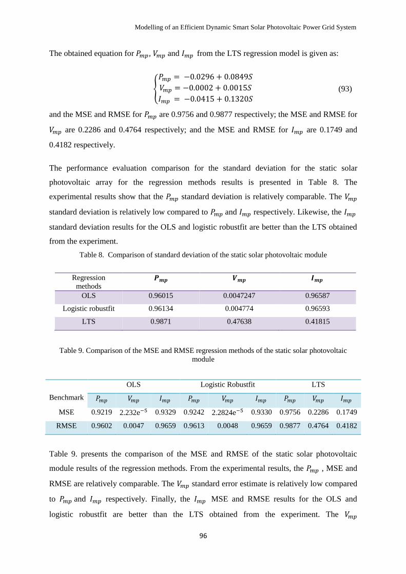
Modelling of an Efficient Dynamic Smart Solar Photovoltaic Power Grid System
96
The obtained equation for 𝑃𝑚𝑝, 𝑉𝑚𝑝 and 𝐼𝑚𝑝 from the LTS regression model is given as:
{
𝑃𝑚𝑝 = −0.0296 + 0.0849𝑆
𝑉𝑚𝑝 = −0.0002 + 0.0015𝑆
𝐼𝑚𝑝 = −0.0415 + 0.1320𝑆 (93)
and the MSE and RMSE for 𝑃𝑚𝑝 are 0.9756 and 0.9877 respectively; the MSE and RMSE for
𝑉𝑚𝑝 are 0.2286 and 0.4764 respectively; and the MSE and RMSE for 𝐼𝑚𝑝 are 0.1749 and
0.4182 respectively.
The performance evaluation comparison for the standard deviation for the static solar
photovoltaic array for the regression methods results is presented in Table 8. The
experimental results show that the 𝑃𝑚𝑝 standard deviation is relatively comparable. The 𝑉𝑚𝑝
standard deviation is relatively low compared to 𝑃𝑚𝑝 and 𝐼𝑚𝑝 respectively. Likewise, the 𝐼𝑚𝑝
standard deviation results for the OLS and logistic robustfit are better than the LTS obtained
from the experiment.
Table 8. Comparison of standard deviation of the static solar photovoltaic module
Regression
methods 𝑷𝒎𝒑 𝑽𝒎𝒑 𝑰𝒎𝒑
OLS 0.96015 0.0047247 0.96587
Logistic robustfit 0.96134 0.004774 0.96593
LTS 0.9871 0.47638 0.41815
Table 9. Comparison of the MSE and RMSE regression methods of the static solar photovoltaic
module
Benchmark
OLS Logistic Robustfit LTS
𝑃𝑚𝑝 𝑉𝑚𝑝 𝐼𝑚𝑝 𝑃𝑚𝑝 𝑉𝑚𝑝 𝐼𝑚𝑝 𝑃𝑚𝑝 𝑉𝑚𝑝 𝐼𝑚𝑝
MSE 0.9219 2.232e−5 0.9329 0.9242 2.2824e−5 0.9330 0.9756 0.2286 0.1749
RMSE 0.9602 0.0047 0.9659 0.9613 0.0048 0.9659 0.9877 0.4764 0.4182
Table 9. presents the comparison of the MSE and RMSE of the static solar photovoltaic
module results of the regression methods. From the experimental results, the 𝑃𝑚𝑝 , MSE and
RMSE are relatively comparable. The 𝑉𝑚𝑝 standard error estimate is relatively low compared
to 𝑃𝑚𝑝 and 𝐼𝑚𝑝 respectively. Finally, the 𝐼𝑚𝑝 MSE and RMSE results for the OLS and
logistic robustfit are better than the LTS obtained from the experiment. The 𝑉𝑚𝑝
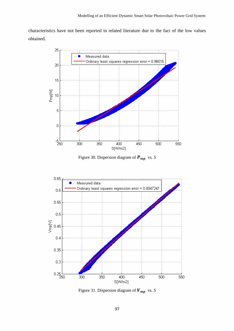
Modelling of an Efficient Dynamic Smart Solar Photovoltaic Power Grid System
97
characteristics have not been reported in related literature due to the fact of the low values
obtained.
Figure 30. Dispersion diagram of 𝑷𝒎𝒑 vs. S
Figure 31. Dispersion diagram of 𝑽𝒎𝒑 vs. S
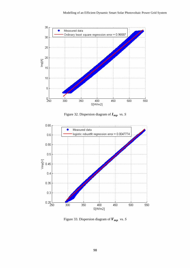
Modelling of an Efficient Dynamic Smart Solar Photovoltaic Power Grid System
98
Figure 32. Dispersion diagram of 𝑰𝒎𝒑 vs. S
Figure 33. Dispersion diagram of 𝑽𝒎𝒑 vs. S
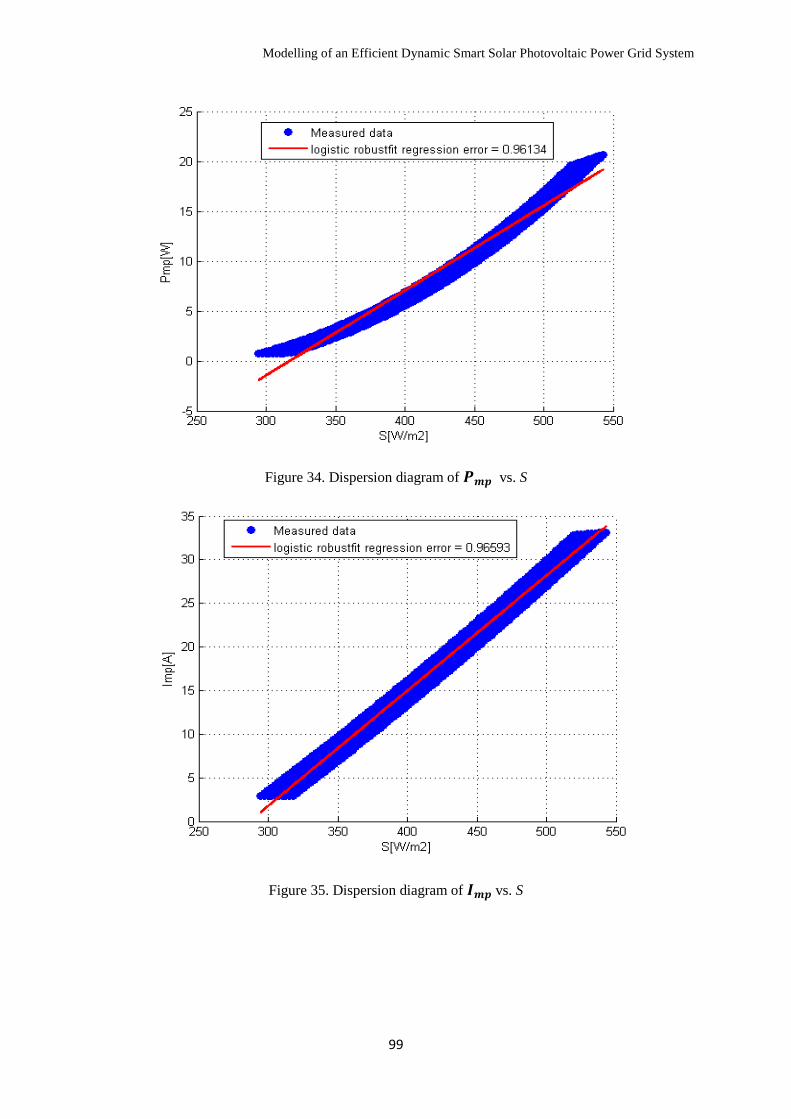
Modelling of an Efficient Dynamic Smart Solar Photovoltaic Power Grid System
99
Figure 34. Dispersion diagram of 𝑷𝒎𝒑 vs. S
Figure 35. Dispersion diagram of 𝑰𝒎𝒑 vs. S

Modelling of an Efficient Dynamic Smart Solar Photovoltaic Power Grid System
100
3.6 Conclusion
A broad expository of the two proposed simulation algorithms employed on smart static solar
photovoltaic arrays has been presented in this chapter. It also provides the context and
background of the neural network and sparsed based algorithms, a detailed understanding of
the concept of the comparative measures determining the optimisation efficiency of the solar
photovoltaic module.
This chapter highlights the significance of modelling and simulation algorithms on smart
static solar photovoltaic systems and the achieved results from the proposed algorithms. In
light of these gaps, as outlined in chapter 1, the questions guiding the optimisation modelling
and simulation of the solar photovoltaic module have been answered in this chapter. The
following chapter (chapter 4) describes the analytical and theoretical derivations for dynamic
solar tracking systems and the simulink design implementation for the smart solar
photovoltaic array model.
Modelling of an Efficient Dynamic Smart Solar Photovoltaic Power Grid System
101
Chapter 4 Astronomical and Analytical Derivation for Solar
Photovoltaic Tracking Systems
4.1 Introduction
This chapter describes the astronomy, analytical derivations and simulink modelling
approach for smart solar photovoltaic systems. In particular, the diurnal and seasonal earth’s
revolution is explicitly addressed in this chapter as it affects the solar radiation intensity of
the solar photovoltaic systems. In understanding the dynamism context of the earth’s rotation,
the sun tracker devices compensate by helping to keep the best orientation of the solar
photovoltaic module relative to the sun’s position.
The sun tracking devices improve the efficiency optimisation and the harvested energy by the
solar photovoltaic array. Analyses on minimisation of the misalignment occurrence effect on
the tracking motion device orientation are also presented. Furthermore, the simulink model
design implementation supports the experimental analysis under variable conditions and
credence for the implemented model is quite significant.
4.2 An Astronomy of Dynamic Solar Photovoltaic Tracking System
The historical astronomy study and observations play a vital role in the success achieved so
far in the dynamic smart solar photovoltaic tracking systems. The mathematical expressions,
calculations and algorithms developed have seemingly helped thus far to solve and reduce the
uncertainties in determining the relative sun’s position and precise solar photovoltaic tracking
orientation device. The conventional progress has enabled the scientific solar photovoltaic
research community to have a database server to resolve challenges and inconsistencies
experienced. This has helped in establishing a universal standard algorithm pattern having a
relative solar position with one set of coefficients to calculate the solar incidence angle for an
arbitrary surface orientation valid for a long period.
The earth revolves counterclockwise about the sun in an elliptical orbit observed from a
vantage point above the north pole in a predictable trajectory. The earth completes one
revolution per day around the polar axis and the earth’s orbit is relatively stable over a long
period. The earth’s inclination axis of rotation is tilted at an angle 휀 ≈ 23.450 and the axis
orientation is time dependent. The daily rotation of the earth is defined by its rotation about
the polar axis, and the instant position of the sun is described by the hour angle, 𝜔. The
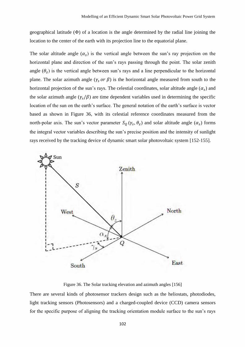
Modelling of an Efficient Dynamic Smart Solar Photovoltaic Power Grid System
102
geographical latitude (Φ) of a location is the angle determined by the radial line joining the
location to the center of the earth with its projection line to the equatorial plane.
The solar altitude angle (𝛼𝑠) is the vertical angle between the sun’s ray projection on the
horizontal plane and direction of the sun’s rays passing through the point. The solar zenith
angle (𝜃𝑧) is the vertical angle between sun’s rays and a line perpendicular to the horizontal
plane. The solar azimuth angle (𝛾𝑠 𝑜𝑟 𝛽) is the horizontal angle measured from south to the
horizontal projection of the sun’s rays. The celestial coordinates, solar altitude angle (𝛼𝑠) and
the solar azimuth angle (𝛾𝑠/𝛽) are time dependent variables used in determining the specific
location of the sun on the earth’s surface. The general notation of the earth’s surface is vector
based as shown in Figure 36, with its celestial reference coordinates measured from the
north-polar axis. The sun’s vector parameter 𝑆𝑄 (𝛾𝑠, 𝜃𝑧) and solar altitude angle (𝛼𝑠) forms
the integral vector variables describing the sun’s precise position and the intensity of sunlight
rays received by the tracking device of dynamic smart solar photovoltaic system [152-155].
Figure 36. The Solar tracking elevation and azimuth angles [156]
There are several kinds of photosensor trackers design such as the heliostats, photodiodes,
light tracking sensors (Photosensors) and a charged-coupled device (CCD) camera sensors
for the specific purpose of aligning the tracking orientation module surface to the sun’s rays

Modelling of an Efficient Dynamic Smart Solar Photovoltaic Power Grid System
103
and position. The solar photosensors and tracker device compensate for the sun’s diurnal
motion through spectroscopic analyses measuring the direct incident solar irradiation
ensuring orthogonal orientation of the solar photovoltaic module surface, thereby optimising
the efficiency of the collected energy. The optimisation control for the solar photovoltaic
tracking system is significant in achieving correct orthogonal orientation and alignment of the
solar photovoltaic module surface constantly towards the sun throughout the day [157, 158].
The sectional view of the celestial coordinates shown in Figure 36 is represented in three
dimensional x, y, z coordinates respectively showing the sun’s elevation, azimuth angle and
zenith angle. The mathematical expressions are programmed into the solar photovoltaic
tracking database system and are thus defined as follows [159];
Ecliptic longitude of the sun: The ecliptic longitude of the sun, 𝜆 is the angle
between vector 𝑆̅ and the horizontal axis plane. The mathematical expression used in
determining the ecliptic longitude of the sun is given as [159];
𝑠𝑖𝑛 𝜆 = 𝑠𝑖𝑛 [3600 (284+ 𝑛
365.25)] (00 ≤ 𝜆 < 3600) (94)
where n is the number of the day, 𝑆̅ is the Sun’s orthogonal horizontal reference plane
on solar photovoltaic module, such that n = 1 on the 1st of January, this implies the
values of 𝜆 constantly varies and is daily computed for accuracy.
Sun elevation angle: The sun’s elevation angle as shown in Figure 36, 𝛼𝑠 is the
vertical angle between the horizontal plane and the connecting plane to the sun. The
mathematical expression is given as [159];
𝑠𝑖𝑛 𝛼𝑠 = 𝑐𝑜𝑠 𝜔 𝑐𝑜𝑠 𝛿 𝑐𝑜𝑠 𝛷 + 𝑠𝑖𝑛 𝛷 𝑠𝑖𝑛 𝜔 (95)
where Φ is the geographical latitude of the site location, 𝜔 denotes the hour angle
and 𝛿 denotes the declination of the sun.
The Hour angle: The hour angle, 𝜔 is defined as the angular distance the earth
rotates in a particular day. The values for each hour of the day is constantly changing
and at noon day, the hour angle, 𝜔 = 00. The mathematical expression is given as
[159];
𝜔 = 150( hour – 12) (96)
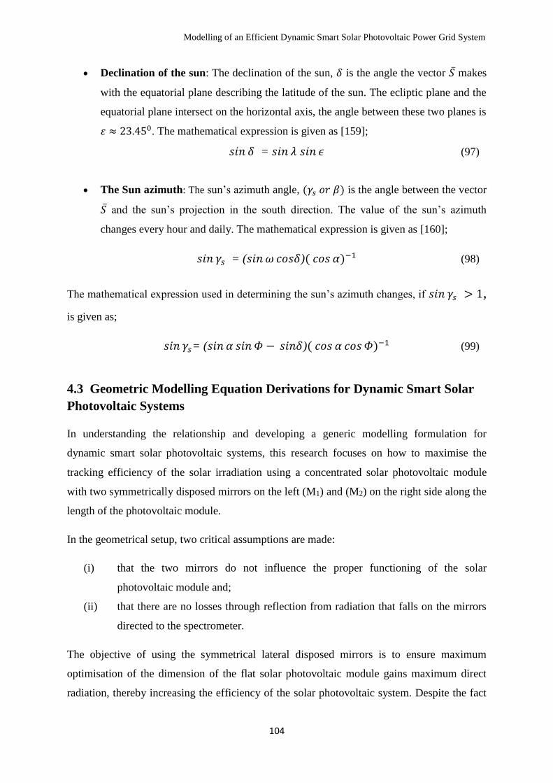
Modelling of an Efficient Dynamic Smart Solar Photovoltaic Power Grid System
104
Declination of the sun: The declination of the sun, 𝛿 is the angle the vector 𝑆̅ makes
with the equatorial plane describing the latitude of the sun. The ecliptic plane and the
equatorial plane intersect on the horizontal axis, the angle between these two planes is
휀 ≈ 23.450. The mathematical expression is given as [159];
𝑠𝑖𝑛 𝛿 = 𝑠𝑖𝑛 𝜆 𝑠𝑖𝑛 𝜖 (97)
The Sun azimuth: The sun’s azimuth angle, (𝛾𝑠 𝑜𝑟 𝛽) is the angle between the vector
𝑆̅ and the sun’s projection in the south direction. The value of the sun’s azimuth
changes every hour and daily. The mathematical expression is given as [160];
𝑠𝑖𝑛 𝛾𝑠 = (𝑠𝑖𝑛 𝜔 𝑐𝑜𝑠𝛿)( 𝑐𝑜𝑠 𝛼)−1 (98)
The mathematical expression used in determining the sun’s azimuth changes, if 𝑠𝑖𝑛 𝛾𝑠 > 1,
is given as;
𝑠𝑖𝑛 𝛾𝑠= (𝑠𝑖𝑛 𝛼 𝑠𝑖𝑛 𝛷 − 𝑠𝑖𝑛𝛿)( 𝑐𝑜𝑠 𝛼 𝑐𝑜𝑠 𝛷)−1 (99)
4.3 Geometric Modelling Equation Derivations for Dynamic Smart Solar
Photovoltaic Systems
In understanding the relationship and developing a generic modelling formulation for
dynamic smart solar photovoltaic systems, this research focuses on how to maximise the
tracking efficiency of the solar irradiation using a concentrated solar photovoltaic module
with two symmetrically disposed mirrors on the left (M1) and (M2) on the right side along the
length of the photovoltaic module.
In the geometrical setup, two critical assumptions are made:
(i) that the two mirrors do not influence the proper functioning of the solar
photovoltaic module and;
(ii) that there are no losses through reflection from radiation that falls on the mirrors
directed to the spectrometer.
The objective of using the symmetrical lateral disposed mirrors is to ensure maximum
optimisation of the dimension of the flat solar photovoltaic module gains maximum direct
radiation, thereby increasing the efficiency of the solar photovoltaic system. Despite the fact
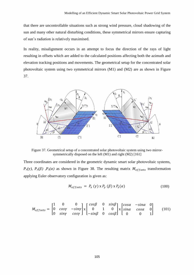
Modelling of an Efficient Dynamic Smart Solar Photovoltaic Power Grid System
105
that there are uncontrollable situations such as strong wind pressure, cloud shadowing of the
sun and many other natural disturbing conditions, these symmetrical mirrors ensure capturing
of sun’s radiation is relatively maximised.
In reality, misalignment occurs in an attempt to focus the direction of the rays of light
resulting in offsets which are added to the calculated positions affecting both the azimuth and
elevation tracking positions and movements. The geometrical setup for the concentrated solar
photovoltaic system using two symmetrical mirrors (M1) and (M2) are as shown in Figure
37.
Figure 37. Geometrical setup of a concentrated solar photovoltaic system using two mirror-
symmetrically disposed on the left (M1) and right (M2) [161]
Three coordinates are considered in the geometric dynamic smart solar photovoltaic systems,
Px(𝛾), Py(𝛽) ,Pz(𝛼) as shown in Figure 38. The resulting matrix 𝑀𝑜𝑓𝑓𝑠𝑒𝑡𝑠 transformation
applying Euler observatory configuration is given as:
𝑀𝑜𝑓𝑓𝑠𝑒𝑡𝑠 = 𝑃𝑥 (𝛾) x 𝑃𝑦 (𝛽) x 𝑃𝑧(𝛼) (100)
𝑀𝑜𝑓𝑓𝑠𝑒𝑡𝑠 = [1 0 00 𝑐𝑜𝑠𝛾 −𝑠𝑖𝑛𝛾0 𝑠𝑖𝑛𝛾 𝑐𝑜𝑠𝛾
] x [𝑐𝑜𝑠𝛽 0 𝑠𝑖𝑛𝛽0 1 0
−𝑠𝑖𝑛𝛽 0 𝑐𝑜𝑠𝛽] x [
𝑐𝑜𝑠𝛼 −𝑠𝑖𝑛𝛼 0𝑠𝑖𝑛𝛼 𝑐𝑜𝑠𝛼 00 0 1
] (101)
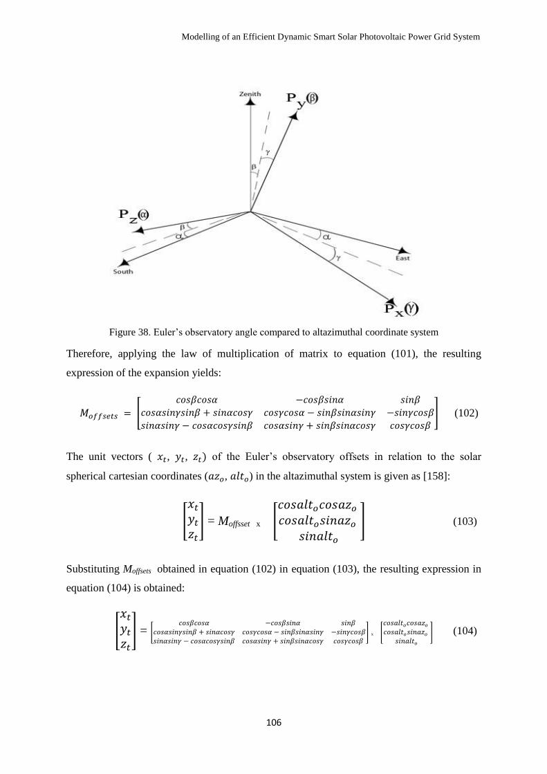
Modelling of an Efficient Dynamic Smart Solar Photovoltaic Power Grid System
106
Figure 38. Euler’s observatory angle compared to altazimuthal coordinate system
Therefore, applying the law of multiplication of matrix to equation (101), the resulting
expression of the expansion yields:
𝑀𝑜𝑓𝑓𝑠𝑒𝑡𝑠 = [𝑐𝑜𝑠𝛽𝑐𝑜𝑠𝛼 −𝑐𝑜𝑠𝛽𝑠𝑖𝑛𝛼 𝑠𝑖𝑛𝛽
𝑐𝑜𝑠𝛼𝑠𝑖𝑛𝛾𝑠𝑖𝑛𝛽 + 𝑠𝑖𝑛𝛼𝑐𝑜𝑠𝛾 𝑐𝑜𝑠𝛾𝑐𝑜𝑠𝛼 − 𝑠𝑖𝑛𝛽𝑠𝑖𝑛𝛼𝑠𝑖𝑛𝛾 −𝑠𝑖𝑛𝛾𝑐𝑜𝑠𝛽
𝑠𝑖𝑛𝛼𝑠𝑖𝑛𝛾 − 𝑐𝑜𝑠𝛼𝑐𝑜𝑠𝛾𝑠𝑖𝑛𝛽 𝑐𝑜𝑠𝛼𝑠𝑖𝑛𝛾 + 𝑠𝑖𝑛𝛽𝑠𝑖𝑛𝛼𝑐𝑜𝑠𝛾 𝑐𝑜𝑠𝛾𝑐𝑜𝑠𝛽] (102)
The unit vectors ( 𝑥𝑡, 𝑦𝑡, 𝑧𝑡) of the Euler’s observatory offsets in relation to the solar
spherical cartesian coordinates (𝑎𝑧𝑜, 𝑎𝑙𝑡𝑜) in the altazimuthal system is given as [158]:
[
𝑥𝑡𝑦𝑡𝑧𝑡] = Moffsset x [
𝑐𝑜𝑠𝑎𝑙𝑡𝑜𝑐𝑜𝑠𝑎𝑧𝑜 𝑐𝑜𝑠𝑎𝑙𝑡𝑜𝑠𝑖𝑛𝑎𝑧𝑜
𝑠𝑖𝑛𝑎𝑙𝑡𝑜
] (103)
Substituting Moffsets obtained in equation (102) in equation (103), the resulting expression in
equation (104) is obtained:
[
𝑥𝑡𝑦𝑡𝑧𝑡] = [
𝑐𝑜𝑠𝛽𝑐𝑜𝑠𝛼 −𝑐𝑜𝑠𝛽𝑠𝑖𝑛𝛼 𝑠𝑖𝑛𝛽𝑐𝑜𝑠𝛼𝑠𝑖𝑛𝛾𝑠𝑖𝑛𝛽 + 𝑠𝑖𝑛𝛼𝑐𝑜𝑠𝛾 𝑐𝑜𝑠𝛾𝑐𝑜𝑠𝛼 − 𝑠𝑖𝑛𝛽𝑠𝑖𝑛𝛼𝑠𝑖𝑛𝛾 −𝑠𝑖𝑛𝛾𝑐𝑜𝑠𝛽𝑠𝑖𝑛𝛼𝑠𝑖𝑛𝛾 − 𝑐𝑜𝑠𝛼𝑐𝑜𝑠𝛾𝑠𝑖𝑛𝛽 𝑐𝑜𝑠𝛼𝑠𝑖𝑛𝛾 + 𝑠𝑖𝑛𝛽𝑠𝑖𝑛𝛼𝑐𝑜𝑠𝛾 𝑐𝑜𝑠𝛾𝑐𝑜𝑠𝛽
] x [
𝑐𝑜𝑠𝑎𝑙𝑡𝑜𝑐𝑜𝑠𝑎𝑧𝑜 𝑐𝑜𝑠𝑎𝑙𝑡𝑜𝑠𝑖𝑛𝑎𝑧𝑜
𝑠𝑖𝑛𝑎𝑙𝑡𝑜
] (104)
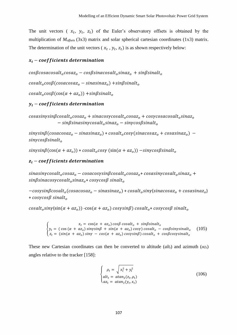
Modelling of an Efficient Dynamic Smart Solar Photovoltaic Power Grid System
107
The unit vectors ( 𝑥𝑡, 𝑦𝑡, 𝑧𝑡) of the Euler’s observatory offsets is obtained by the
multiplication of Moffsets (3x3) matrix and solar spherical cartesian coordinates (1x3) matrix.
The determination of the unit vectors ( 𝑥𝑡 , 𝑦𝑡, 𝑧𝑡) is as shown respectively below:
𝒙𝒕 − 𝒄𝒐𝒆𝒇𝒇𝒊𝒄𝒊𝒆𝒏𝒕𝒔 𝒅𝒆𝒕𝒆𝒓𝒎𝒊𝒏𝒂𝒕𝒊𝒐𝒏
𝑐𝑜𝑠𝛽𝑐𝑜𝑠𝛼𝑐𝑜𝑠𝑎𝑙𝑡𝑜𝑐𝑜𝑠𝑎𝑧𝑜 − 𝑐𝑜𝑠𝛽𝑠𝑖𝑛𝛼𝑐𝑜𝑠𝑎𝑙𝑡𝑜𝑠𝑖𝑛𝑎𝑧𝑜 + 𝑠𝑖𝑛𝛽𝑠𝑖𝑛𝑎𝑙𝑡𝑜
𝑐𝑜𝑠𝑎𝑙𝑡𝑜𝑐𝑜𝑠𝛽(𝑐𝑜𝑠𝛼𝑐𝑜𝑠𝑎𝑧𝑜 − 𝑠𝑖𝑛𝛼𝑠𝑖𝑛𝑎𝑧𝑜) +𝑠𝑖𝑛𝛽𝑠𝑖𝑛𝑎𝑙𝑡𝑜
𝑐𝑜𝑠𝑎𝑙𝑡𝑜𝑐𝑜𝑠𝛽(cos (𝛼 + 𝑎𝑧𝑜)) +𝑠𝑖𝑛𝛽𝑠𝑖𝑛𝑎𝑙𝑡𝑜
𝒚𝒕 − 𝒄𝒐𝒆𝒇𝒇𝒊𝒄𝒊𝒆𝒏𝒕𝒔 𝒅𝒆𝒕𝒆𝒓𝒎𝒊𝒏𝒂𝒕𝒊𝒐𝒏
𝑐𝑜𝑠𝛼𝑠𝑖𝑛𝛾𝑠𝑖𝑛𝛽𝑐𝑜𝑠𝑎𝑙𝑡𝑜𝑐𝑜𝑠𝑎𝑧𝑜 + 𝑠𝑖𝑛𝛼𝑐𝑜𝑠𝛾𝑐𝑜𝑠𝑎𝑙𝑡𝑜𝑐𝑜𝑠𝑎𝑧𝑜 + 𝑐𝑜𝑠𝛾𝑐𝑜𝑠𝛼𝑐𝑜𝑠𝑎𝑙𝑡𝑜𝑠𝑖𝑛𝑎𝑧𝑜− 𝑠𝑖𝑛𝛽𝑠𝑖𝑛𝛼𝑠𝑖𝑛𝛾𝑐𝑜𝑠𝑎𝑙𝑡𝑜𝑠𝑖𝑛𝑎𝑧𝑜 − 𝑠𝑖𝑛𝛾𝑐𝑜𝑠𝛽𝑠𝑖𝑛𝑎𝑙𝑡𝑜
𝑠𝑖𝑛𝛾𝑠𝑖𝑛𝛽(𝑐𝑜𝑠𝛼𝑐𝑜𝑠𝑎𝑧𝑜 − 𝑠𝑖𝑛𝛼𝑠𝑖𝑛𝑎𝑧𝑜) + 𝑐𝑜𝑠𝑎𝑙𝑡𝑜𝑐𝑜𝑠𝛾(𝑠𝑖𝑛𝛼𝑐𝑜𝑠𝑎𝑧𝑜 + 𝑐𝑜𝑠𝛼𝑠𝑖𝑛𝑎𝑧𝑜) −
𝑠𝑖𝑛𝛾𝑐𝑜𝑠𝛽𝑠𝑖𝑛𝑎𝑙𝑡𝑜
𝑠𝑖𝑛𝛾𝑠𝑖𝑛𝛽(cos (𝛼 + 𝑎𝑧𝑜)) + 𝑐𝑜𝑠𝑎𝑙𝑡𝑜𝑐𝑜𝑠𝛾 (sin (𝛼 + 𝑎𝑧𝑜)) −𝑠𝑖𝑛𝛾𝑐𝑜𝑠𝛽𝑠𝑖𝑛𝑎𝑙𝑡𝑜
𝒛𝒕 − 𝒄𝒐𝒆𝒇𝒇𝒊𝒄𝒊𝒆𝒏𝒕𝒔 𝒅𝒆𝒕𝒆𝒓𝒎𝒊𝒏𝒂𝒕𝒊𝒐𝒏
𝑠𝑖𝑛𝛼𝑠𝑖𝑛𝛾𝑐𝑜𝑠𝑎𝑙𝑡𝑜𝑐𝑜𝑠𝑎𝑧𝑜 − 𝑐𝑜𝑠𝛼𝑐𝑜𝑠𝛾𝑠𝑖𝑛𝛽𝑐𝑜𝑠𝑎𝑙𝑡𝑜𝑐𝑜𝑠𝑎𝑧𝑜+ 𝑐𝑜𝑠𝛼𝑠𝑖𝑛𝛾𝑐𝑜𝑠𝑎𝑙𝑡𝑜𝑠𝑖𝑛𝑎𝑧𝑜 +
𝑠𝑖𝑛𝛽𝑠𝑖𝑛𝛼𝑐𝑜𝑠𝛾𝑐𝑜𝑠𝑎𝑙𝑡𝑜𝑠𝑖𝑛𝑎𝑧𝑜+ 𝑐𝑜𝑠𝛾𝑐𝑜𝑠𝛽 𝑠𝑖𝑛𝑎𝑙𝑡𝑜
−𝑐𝑜𝑠𝛾𝑠𝑖𝑛𝛽𝑐𝑜𝑠𝑎𝑙𝑡𝑜(𝑐𝑜𝑠𝛼𝑐𝑜𝑠𝑎𝑧𝑜 − 𝑠𝑖𝑛𝛼𝑠𝑖𝑛𝑎𝑧𝑜) + 𝑐𝑜𝑠𝑎𝑙𝑡𝑜𝑠𝑖𝑛𝛾(𝑠𝑖𝑛𝛼𝑐𝑜𝑠𝑎𝑧𝑜 + 𝑐𝑜𝑠𝛼𝑠𝑖𝑛𝑎𝑧𝑜)
+ 𝑐𝑜𝑠𝛾𝑐𝑜𝑠𝛽 𝑠𝑖𝑛𝑎𝑙𝑡𝑜
𝑐𝑜𝑠𝑎𝑙𝑡𝑜𝑠𝑖𝑛𝛾(sin (𝛼 + 𝑎𝑧𝑜)) -cos (𝛼 + 𝑎𝑧𝑜) 𝑐𝑜𝑠𝛾𝑠𝑖𝑛𝛽) 𝑐𝑜𝑠𝑎𝑙𝑡𝑜+ 𝑐𝑜𝑠𝛾𝑐𝑜𝑠𝛽 𝑠𝑖𝑛𝑎𝑙𝑡𝑜
{
𝑥𝑡 = cos(𝛼 + 𝑎𝑧𝑜) 𝑐𝑜𝑠𝛽 𝑐𝑜𝑠𝑎𝑙𝑡𝑜 + 𝑠𝑖𝑛𝛽𝑠𝑖𝑛𝑎𝑙𝑡𝑜𝑦𝑡 = ( cos (𝛼 + 𝑎𝑧𝑜) 𝑠𝑖𝑛𝛾𝑠𝑖𝑛𝛽 + 𝑠𝑖𝑛(𝛼 + 𝑎𝑧𝑜) 𝑐𝑜𝑠𝛾) 𝑐𝑜𝑠𝑎𝑙𝑡𝑜 − 𝑐𝑜𝑠𝛽𝑠𝑖𝑛𝛾𝑠𝑖𝑛𝑎𝑙𝑡𝑜𝑧𝑡 = (𝑠𝑖𝑛(𝛼 + 𝑎𝑧𝑜) 𝑠𝑖𝑛𝛾 − 𝑐𝑜𝑠(𝛼 + 𝑎𝑧𝑜) 𝑐𝑜𝑠𝛾𝑠𝑖𝑛𝛽) 𝑐𝑜𝑠𝑎𝑙𝑡𝑜 + 𝑐𝑜𝑠𝛽𝑐𝑜𝑠𝛾𝑠𝑖𝑛𝑎𝑙𝑡𝑜
(105)
These new Cartesian coordinates can then be converted to altitude (altt) and azimuth (αzt)
angles relative to the tracker [158]:
{
𝜌𝑡 = √ 𝑥𝑡2 + 𝑦𝑡
2
𝑎𝑙𝑡𝑡 = 𝑎𝑡𝑎𝑛2(𝑧𝑡 , 𝜌𝑡)
𝑎𝑧𝑡 = 𝑎𝑡𝑎𝑛2(𝑦𝑡 , 𝑥𝑡)
(106)

Modelling of an Efficient Dynamic Smart Solar Photovoltaic Power Grid System
108
In the above equation, atan2(y,x) is available in many programming languages, stands for the
argument of the complex number x + iy. It is closely related to the arctangent of y/x, but it
indicates unambiguously the quadrant of this angle on the trigonometric circle.
The introduction of the general sun tracking modelling expression above helps in tracking the
sun’s position accurately and provides a cost effective solution regardless of the
misalignment which occurs in the altitude and azimuth configurations setup of the solar
photovoltaic tracking systems. As a result the misalignment optical nonlinear compensation
for the error which occurs during the onsite installation is taken into consideration by
adjusting the values of the orientation angles 𝜑, λ and ζ respectively. The sun tracking
accuracy of the system is highly reliant on the precision of the input parameters of the sun-
tracking algorithm: latitude angle (Φ), hour angle (𝜔) and the declination angle (𝛿) as defined
in section 4.2 is thus introduced in the developed tracking program in the microntroller of the
tracking system.
The Euler’s angles in mathematics are also used to describe the orientation of a frame of
reference typically a coordinate system relative to another. They are typically denoted
𝛼, 𝛽, 𝛾, or 𝜑, 𝜆 and ζ [162]. The orientation angles 𝜑, λ and ζ compensates for the daily sun-
tracking error induced as a result of misalignment of sun tracking axes. The analytical
solutions for the three orientation angles is necessary to compensate for the misalignment
which occurs during the solar photovoltaic system installation on site location and can be
obtained by determining the unit vectors of the sun’s position relative to the successive
transformation matrices coordinates for the orientation angles. Therefore, the unit vector sun
𝑆̅ , relative to the earth position is given as [163];
[𝑆̅] = [𝜑][λ][ζ][𝛷] [𝑆] (107)
[
𝑠𝑖𝑛𝛼𝑠𝑖𝑛𝛽𝑐𝑜𝑠𝛼𝑐𝑜𝑠𝛽𝑐𝑜𝑠𝛼
] = [1 0 00 𝑐𝑜𝑠𝜑 −𝑠𝑖𝑛𝜑0 𝑠𝑖𝑛𝜑 𝑐𝑜𝑠𝜑
] x [𝑐𝑜𝑠𝜆 −𝑠𝑖𝑛𝜆 0𝑠𝑖𝑛𝜆 𝑐𝑜𝑠𝜆 00 0 1
] x [𝑐𝑜𝑠ζ 0 𝑠𝑖𝑛ζ0 1 0
−𝑠𝑖𝑛ζ 0 𝑐𝑜𝑠ζ]
x [𝑐𝑜𝑠𝛷 0 𝑠𝑖𝑛𝛷0 1 0
−𝑠𝑖𝑛𝛷 0 𝑐𝑜𝑠𝛷] x [
𝑐𝑜𝑠𝜔𝑐𝑜𝑠𝛿−𝑠𝑖𝑛𝜔𝑐𝑜𝑠𝛿
𝑠𝑖𝑛𝛿]
(108)
The introduced variables 𝛼, 𝛽, 𝜔, 𝛿 and 𝛷 have been defined in section 4.2. Where 𝛼 is the
elevation angle, (𝛾𝑠 𝑜𝑟 𝛽) is azimuth angle, 𝜔 is hour angle, 𝛿 is the declination angle, Φ is
the latitude at which the solar collector is located as well as 𝜑, λ and ζ are the three
orientation angles of two-orthogonal driving axes of the solar photovoltaic collector.
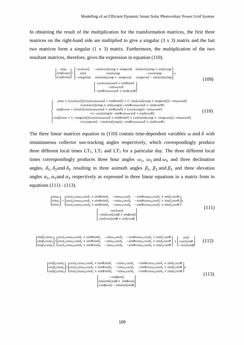
Modelling of an Efficient Dynamic Smart Solar Photovoltaic Power Grid System
109
In obtaining the result of the multiplication for the transformation matrices, the first three
matrices on the right-hand side are multiplied to give a singular (3 x 3) matrix and the last
two matrices form a singular (1 x 3) matrix. Furthermore, the multiplication of the two
resultant matrices, therefore, gives the expression in equation (110).
[
𝑠𝑖𝑛𝛼𝑠𝑖𝑛𝛽𝑐𝑜𝑠𝛼𝑐𝑜𝑠𝛽𝑐𝑜𝑠𝛼
]= [
𝑐𝑜𝑠𝜆𝑐𝑜𝑠ζ −𝑠𝑖𝑛𝜆𝑐𝑜𝑠ζ𝑐𝑜𝑠𝜑+ 𝑠𝑖𝑛𝜑𝑠𝑖𝑛ζ 𝑠𝑖𝑛𝜆𝑐𝑜𝑠ζ𝑠𝑖𝑛𝜑+ 𝑠𝑖𝑛ζ𝑐𝑜𝑠𝜑 𝑠𝑖𝑛𝜆 𝑐𝑜𝑠𝜆𝑐𝑜𝑠𝜑 −𝑐𝑜𝑠𝜆𝑠𝑖𝑛𝜑
−𝑠𝑖𝑛𝜑𝑠𝑖𝑛ζ 𝑠𝑖𝑛𝜆𝑠𝑖𝑛ζ𝑐𝑜𝑠𝜑+ 𝑠𝑖𝑛𝜑𝑐𝑜𝑠ζ 𝑐𝑜𝑠𝜑𝑐𝑜𝑠ζ − 𝑠𝑖𝑛𝜆𝑠𝑖𝑛ζ𝑠𝑖𝑛𝜑] x
[𝑐𝑜𝑠𝜆𝑐𝑜𝑠𝜔𝑐𝑜𝑠𝛿 + 𝑠𝑖𝑛𝛷𝑠𝑖𝑛𝛿
−𝑠𝑖𝑛𝜔𝑐𝑜𝑠𝛿−𝑠𝑖𝑛𝛷𝑐𝑜𝑠𝜔𝑐𝑜𝑠𝛿 + 𝑠𝑖𝑛𝛿𝑐𝑜𝑠𝛷
]
(109)
{
𝑠𝑖𝑛𝛼 = (𝑐𝑜𝑠𝜆𝑐𝑜𝑠ζ)(𝑐𝑜𝑠𝜆𝑐𝑜𝑠𝜔𝑐𝑜𝑠𝛿 + 𝑠𝑖𝑛𝛷𝑠𝑖𝑛𝛿) + (−𝑠𝑖𝑛𝜆𝑐𝑜𝑠ζ𝑐𝑜𝑠𝜑+ 𝑠𝑖𝑛𝜑𝑠𝑖𝑛ζ)(−𝑠𝑖𝑛𝜔𝑐𝑜𝑠𝛿)+(𝑠𝑖𝑛𝜆𝑐𝑜𝑠ζ𝑠𝑖𝑛𝜑+ 𝑠𝑖𝑛ζ𝑐𝑜𝑠𝜑)(−𝑠𝑖𝑛Φ𝑐𝑜𝑠𝜔𝑐𝑜𝑠𝛿 + 𝑠𝑖𝑛𝛿𝑐𝑜𝑠Φ)
𝑠𝑖𝑛𝛽𝑐𝑜𝑠𝛼 = (𝑠𝑖𝑛𝜆)(𝑐𝑜𝑠𝜆𝑐𝑜𝑠𝜔𝑐𝑜𝑠𝛿 + 𝑠𝑖𝑛Φ𝑠𝑖𝑛𝛿) + (𝑐𝑜𝑠𝜆𝑐𝑜𝑠𝜑)(−𝑠𝑖𝑛𝜔𝑐𝑜𝑠𝛿) +(−𝑐𝑜𝑠𝜆𝑠𝑖𝑛𝜑)(−𝑠𝑖𝑛Φ𝑐𝑜𝑠𝜔𝑐𝑜𝑠𝛿 + 𝑠𝑖𝑛𝛿𝑐𝑜𝑠Φ)
𝑐𝑜𝑠𝛽𝑐𝑜𝑠𝛼 = (−𝑠𝑖𝑛𝜑𝑠𝑖𝑛ζ)(𝑐𝑜𝑠𝜆𝑐𝑜𝑠𝜔𝑐𝑜𝑠𝛿 + 𝑠𝑖𝑛Φ𝑠𝑖𝑛𝛿) + (𝑠𝑖𝑛𝜆𝑠𝑖𝑛ζ𝑐𝑜𝑠𝜑+ 𝑠𝑖𝑛𝜑𝑐𝑜𝑠ζ)(−𝑠𝑖𝑛𝜔𝑐𝑜𝑠𝛿)+(𝑐𝑜𝑠𝜑𝑐𝑜𝑠ζ − 𝑠𝑖𝑛𝜆𝑠𝑖𝑛ζ𝑠𝑖𝑛𝜑)(−𝑠𝑖𝑛Φ𝑐𝑜𝑠𝜔𝑐𝑜𝑠𝛿 + 𝑠𝑖𝑛𝛿𝑐𝑜𝑠Φ)
(110)
The three linear matrices equation in (110) contain time-dependent variables 𝜔 and 𝛿 with
instantaneous collector sun-tracking angles respectively, which correspondingly produce
three different local times LT1, LT2 and LT3 for a particular day. The three different local
times correspondingly produces three hour angles 𝜔1, 𝜔2 and 𝜔3 and three declination
angles, 𝛿1, 𝛿2and 𝛿3 resulting in three azimuth angles 𝛽1, 𝛽2 and 𝛽3 and three elevation
angles 𝛼1, 𝛼2and 𝛼3 respectively as expressed in three linear equations in a matrix form in
equations (111) - (113).
[
𝑠𝑖𝑛𝛼1𝑠𝑖𝑛𝛼2𝑠𝑖𝑛𝛼3
] = [
𝑐𝑜𝑠𝜆1𝑐𝑜𝑠𝜔1𝑐𝑜𝑠𝛿1 + 𝑠𝑖𝑛Φ𝑠𝑖𝑛𝛿1 −𝑠𝑖𝑛𝜔1𝑐𝑜𝑠𝛿1 −𝑠𝑖𝑛Φ𝑐𝑜𝑠𝜔1𝑐𝑜𝑠𝛿1 + 𝑠𝑖𝑛𝛿1𝑐𝑜𝑠Φ 𝑐𝑜𝑠𝜆2𝑐𝑜𝑠𝜔2𝑐𝑜𝑠𝛿2 + 𝑠𝑖𝑛Φ𝑠𝑖𝑛𝛿2 −𝑠𝑖𝑛𝜔2𝑐𝑜𝑠𝛿2 −𝑠𝑖𝑛Φ𝑐𝑜𝑠𝜔2𝑐𝑜𝑠𝛿2 + 𝑠𝑖𝑛𝛿2𝑐𝑜𝑠Φ 𝑐𝑜𝑠𝜆3𝑐𝑜𝑠𝜔3𝑐𝑜𝑠𝛿3 + 𝑠𝑖𝑛Φ𝑠𝑖𝑛𝛿3 −𝑠𝑖𝑛𝜔3𝑐𝑜𝑠𝛿3 −𝑠𝑖𝑛Φ𝑐𝑜𝑠𝜔3𝑐𝑜𝑠𝛿3 + 𝑠𝑖𝑛𝛿3𝑐𝑜𝑠Φ
]x
[
𝑐𝑜𝑠𝜆𝑐𝑜𝑠ζ−𝑠𝑖𝑛𝜆𝑐𝑜𝑠ζ𝑐𝑜𝑠∅ + 𝑠𝑖𝑛∅𝑠𝑖𝑛ζ𝑠𝑖𝑛𝜆𝑐𝑜𝑠ζ𝑠𝑖𝑛∅ + 𝑠𝑖𝑛ζ𝑐𝑜𝑠∅
]
(111)
[
𝑠𝑖𝑛𝛽1𝑐𝑜𝑠𝛼1𝑠𝑖𝑛𝛽2𝑐𝑜𝑠𝛼2𝑠𝑖𝑛𝛽3𝑐𝑜𝑠𝛼3
]=[
𝑐𝑜𝑠𝜆1𝑐𝑜𝑠𝜔1𝑐𝑜𝑠𝛿1 + 𝑠𝑖𝑛Φ𝑠𝑖𝑛𝛿1 −𝑠𝑖𝑛𝜔1𝑐𝑜𝑠𝛿1 −𝑠𝑖𝑛𝛷𝑐𝑜𝑠𝜔1𝑐𝑜𝑠𝛿1 + 𝑠𝑖𝑛𝛿1𝑐𝑜𝑠Φ 𝑐𝑜𝑠𝜆2𝑐𝑜𝑠𝜔2𝑐𝑜𝑠𝛿2 + 𝑠𝑖𝑛Φ𝑠𝑖𝑛𝛿2 −𝑠𝑖𝑛𝜔2𝑐𝑜𝑠𝛿2 −𝑠𝑖𝑛𝛷𝑐𝑜𝑠𝜔2𝑐𝑜𝑠𝛿2 + 𝑠𝑖𝑛𝛿2𝑐𝑜𝑠Φ 𝑐𝑜𝑠𝜆3𝑐𝑜𝑠𝜔3𝑐𝑜𝑠𝛿3 + 𝑠𝑖𝑛Φ𝑠𝑖𝑛𝛿3 −𝑠𝑖𝑛𝜔3𝑐𝑜𝑠𝛿3 −𝑠𝑖𝑛𝛷𝑐𝑜𝑠𝜔3𝑐𝑜𝑠𝛿3 + 𝑠𝑖𝑛𝛿3𝑐𝑜𝑠Φ
] x [𝑠𝑖𝑛𝜆
𝑐𝑜𝑠𝜆𝑐𝑜𝑠∅−𝑐𝑜𝑠𝜆𝑠𝑖𝑛∅
] (112)
[
𝑐𝑜𝑠𝛽1𝑐𝑜𝑠𝛼1𝑐𝑜𝑠𝛽2𝑐𝑜𝑠𝛼2𝑐𝑜𝑠𝛽3𝑐𝑜𝑠𝛼3
]=[
𝑐𝑜𝑠𝜆1𝑐𝑜𝑠𝜔1𝑐𝑜𝑠𝛿1 + 𝑠𝑖𝑛𝛷𝑠𝑖𝑛𝛿1 −𝑠𝑖𝑛𝜔1𝑐𝑜𝑠𝛿1 −𝑠𝑖𝑛𝛷𝑐𝑜𝑠𝜔1𝑐𝑜𝑠𝛿1 + 𝑠𝑖𝑛𝛿1𝑐𝑜𝑠Φ 𝑐𝑜𝑠𝜆2𝑐𝑜𝑠𝜔2𝑐𝑜𝑠𝛿2 + 𝑠𝑖𝑛𝛷𝑠𝑖𝑛𝛿2 −𝑠𝑖𝑛𝜔2𝑐𝑜𝑠𝛿2 −𝑠𝑖𝑛𝛷𝑐𝑜𝑠𝜔2𝑐𝑜𝑠𝛿2 + 𝑠𝑖𝑛𝛿2𝑐𝑜𝑠Φ 𝑐𝑜𝑠𝜆3𝑐𝑜𝑠𝜔3𝑐𝑜𝑠𝛿3 + 𝑠𝑖𝑛𝛷𝑠𝑖𝑛𝛿3 −𝑠𝑖𝑛𝜔3𝑐𝑜𝑠𝛿3 −𝑠𝑖𝑛𝛷𝑐𝑜𝑠𝜔3𝑐𝑜𝑠𝛿3 + 𝑠𝑖𝑛𝛿3𝑐𝑜𝑠Φ
]x
[
−𝑠𝑖𝑛∅𝑠𝑖𝑛ζ𝑠𝑖𝑛𝜆𝑠𝑖𝑛ζ𝑐𝑜𝑠∅+ 𝑠𝑖𝑛∅𝑐𝑜𝑠ζ𝑐𝑜𝑠∅𝑐𝑜𝑠ζ − 𝑠𝑖𝑛𝜆𝑠𝑖𝑛ζ𝑠𝑖𝑛∅
]
(113)
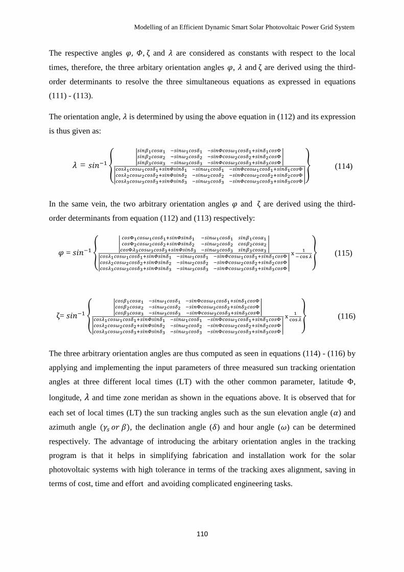
Modelling of an Efficient Dynamic Smart Solar Photovoltaic Power Grid System
110
The respective angles 𝜑, 𝛷, ζ and 𝜆 are considered as constants with respect to the local
times, therefore, the three arbitary orientation angles 𝜑, 𝜆 and ζ are derived using the third-
order determinants to resolve the three simultaneous equations as expressed in equations
(111) - (113).
The orientation angle, 𝜆 is determined by using the above equation in (112) and its expression
is thus given as:
𝜆 = 𝑠𝑖𝑛−1 {|
𝑠𝑖𝑛𝛽1𝑐𝑜𝑠𝛼1 −𝑠𝑖𝑛𝜔1𝑐𝑜𝑠𝛿1 −𝑠𝑖𝑛𝛷𝑐𝑜𝑠𝜔1𝑐𝑜𝑠𝛿1+𝑠𝑖𝑛𝛿1𝑐𝑜𝑠Φ
𝑠𝑖𝑛𝛽2𝑐𝑜𝑠𝛼2 −𝑠𝑖𝑛𝜔2𝑐𝑜𝑠𝛿2 −𝑠𝑖𝑛𝛷𝑐𝑜𝑠𝜔2𝑐𝑜𝑠𝛿2+𝑠𝑖𝑛𝛿2𝑐𝑜𝑠Φ
𝑠𝑖𝑛𝛽3𝑐𝑜𝑠𝛼3 −𝑠𝑖𝑛𝜔3𝑐𝑜𝑠𝛿3 −𝑠𝑖𝑛𝛷𝑐𝑜𝑠𝜔3𝑐𝑜𝑠𝛿3+𝑠𝑖𝑛𝛿3𝑐𝑜𝑠Φ |
|
𝑐𝑜𝑠𝜆1𝑐𝑜𝑠𝜔1𝑐𝑜𝑠𝛿1+𝑠𝑖𝑛𝛷𝑠𝑖𝑛𝛿1 −𝑠𝑖𝑛𝜔1𝑐𝑜𝑠𝛿1 −𝑠𝑖𝑛𝛷𝑐𝑜𝑠𝜔1𝑐𝑜𝑠𝛿1+𝑠𝑖𝑛𝛿1𝑐𝑜𝑠Φ
𝑐𝑜𝑠𝜆2𝑐𝑜𝑠𝜔2𝑐𝑜𝑠𝛿2+𝑠𝑖𝑛𝛷𝑠𝑖𝑛𝛿2 −𝑠𝑖𝑛𝜔2𝑐𝑜𝑠𝛿2 −𝑠𝑖𝑛𝛷𝑐𝑜𝑠𝜔2𝑐𝑜𝑠𝛿2+𝑠𝑖𝑛𝛿2𝑐𝑜𝑠Φ
𝑐𝑜𝑠𝜆3𝑐𝑜𝑠𝜔3𝑐𝑜𝑠𝛿3+𝑠𝑖𝑛𝛷𝑠𝑖𝑛𝛿3 −𝑠𝑖𝑛𝜔3𝑐𝑜𝑠𝛿3 −𝑠𝑖𝑛𝛷𝑐𝑜𝑠𝜔3𝑐𝑜𝑠𝛿3+𝑠𝑖𝑛𝛿3𝑐𝑜𝑠Φ |
} (114)
In the same vein, the two arbitrary orientation angles 𝜑 and ζ are derived using the third-
order determinants from equation (112) and (113) respectively:
𝜑 = 𝑠𝑖𝑛−1 {|
𝑐𝑜𝑠Φ1𝑐𝑜𝑠𝜔1𝑐𝑜𝑠𝛿1+𝑠𝑖𝑛𝛷𝑠𝑖𝑛𝛿1 −𝑠𝑖𝑛𝜔1𝑐𝑜𝑠𝛿1 𝑠𝑖𝑛𝛽1𝑐𝑜𝑠𝛼1
𝑐𝑜𝑠Φ2𝑐𝑜𝑠𝜔2𝑐𝑜𝑠𝛿2+𝑠𝑖𝑛𝛷𝑠𝑖𝑛𝛿2 −𝑠𝑖𝑛𝜔2𝑐𝑜𝑠𝛿2 𝑐𝑜𝑠𝛽2𝑐𝑜𝑠𝛼2
𝑐𝑜𝑠Φ𝜆3𝑐𝑜𝑠𝜔3𝑐𝑜𝑠𝛿3+𝑠𝑖𝑛𝛷𝑠𝑖𝑛𝛿3 −𝑠𝑖𝑛𝜔3𝑐𝑜𝑠𝛿3 𝑠𝑖𝑛𝛽3𝑐𝑜𝑠𝛼3 |
|
𝑐𝑜𝑠𝜆1𝑐𝑜𝑠𝜔1𝑐𝑜𝑠𝛿1+𝑠𝑖𝑛𝛷𝑠𝑖𝑛𝛿1 −𝑠𝑖𝑛𝜔1𝑐𝑜𝑠𝛿1 −𝑠𝑖𝑛𝛷𝑐𝑜𝑠𝜔1𝑐𝑜𝑠𝛿1+𝑠𝑖𝑛𝛿1𝑐𝑜𝑠Φ
𝑐𝑜𝑠𝜆2𝑐𝑜𝑠𝜔2𝑐𝑜𝑠𝛿2+𝑠𝑖𝑛𝛷𝑠𝑖𝑛𝛿2 −𝑠𝑖𝑛𝜔2𝑐𝑜𝑠𝛿2 −𝑠𝑖𝑛𝛷𝑐𝑜𝑠𝜔2𝑐𝑜𝑠𝛿2+𝑠𝑖𝑛𝛿2𝑐𝑜𝑠Φ
𝑐𝑜𝑠𝜆3𝑐𝑜𝑠𝜔3𝑐𝑜𝑠𝛿3+𝑠𝑖𝑛𝛷𝑠𝑖𝑛𝛿3 −𝑠𝑖𝑛𝜔3𝑐𝑜𝑠𝛿3 −𝑠𝑖𝑛𝛷𝑐𝑜𝑠𝜔3𝑐𝑜𝑠𝛿3+𝑠𝑖𝑛𝛿3𝑐𝑜𝑠Φ |
x 1
−cos𝜆} (115)
ζ= 𝑠𝑖𝑛−1 {|
𝑐𝑜𝑠𝛽1𝑐𝑜𝑠𝛼1 −𝑠𝑖𝑛𝜔1𝑐𝑜𝑠𝛿1 −𝑠𝑖𝑛Φ𝑐𝑜𝑠𝜔1𝑐𝑜𝑠𝛿1+𝑠𝑖𝑛𝛿1𝑐𝑜𝑠Φ
𝑐𝑜𝑠𝛽2𝑐𝑜𝑠𝛼2 −𝑠𝑖𝑛𝜔2𝑐𝑜𝑠𝛿2 −𝑠𝑖𝑛Φ𝑐𝑜𝑠𝜔2𝑐𝑜𝑠𝛿2+𝑠𝑖𝑛𝛿2𝑐𝑜𝑠Φ
𝑐𝑜𝑠𝛽3𝑐𝑜𝑠𝛼3 −𝑠𝑖𝑛𝜔3𝑐𝑜𝑠𝛿3 −𝑠𝑖𝑛Φ𝑐𝑜𝑠𝜔3𝑐𝑜𝑠𝛿3+𝑠𝑖𝑛𝛿3𝑐𝑜𝑠Φ|
|
𝑐𝑜𝑠𝜆1𝑐𝑜𝑠𝜔1𝑐𝑜𝑠𝛿1+𝑠𝑖𝑛𝛷𝑠𝑖𝑛𝛿1 −𝑠𝑖𝑛𝜔1𝑐𝑜𝑠𝛿1 −𝑠𝑖𝑛Φ𝑐𝑜𝑠𝜔1𝑐𝑜𝑠𝛿1+𝑠𝑖𝑛𝛿1𝑐𝑜𝑠Φ
𝑐𝑜𝑠𝜆2𝑐𝑜𝑠𝜔2𝑐𝑜𝑠𝛿2+𝑠𝑖𝑛𝛷𝑠𝑖𝑛𝛿2 −𝑠𝑖𝑛𝜔2𝑐𝑜𝑠𝛿2 −𝑠𝑖𝑛Φ𝑐𝑜𝑠𝜔2𝑐𝑜𝑠𝛿2+𝑠𝑖𝑛𝛿2𝑐𝑜𝑠Φ
𝑐𝑜𝑠𝜆3𝑐𝑜𝑠𝜔3𝑐𝑜𝑠𝛿3+𝑠𝑖𝑛𝛷𝑠𝑖𝑛𝛿3 −𝑠𝑖𝑛𝜔3𝑐𝑜𝑠𝛿3 −𝑠𝑖𝑛Φ𝑐𝑜𝑠𝜔3𝑐𝑜𝑠𝛿3+𝑠𝑖𝑛𝛿3𝑐𝑜𝑠Φ |
x 1
cos𝜆} (116)
The three arbitrary orientation angles are thus computed as seen in equations (114) - (116) by
applying and implementing the input parameters of three measured sun tracking orientation
angles at three different local times (LT) with the other common parameter, latitude Φ,
longitude, 𝜆 and time zone meridan as shown in the equations above. It is observed that for
each set of local times (LT) the sun tracking angles such as the sun elevation angle (𝛼) and
azimuth angle (𝛾𝑠 𝑜𝑟 𝛽), the declination angle (𝛿) and hour angle (𝜔) can be determined
respectively. The advantage of introducing the arbitary orientation angles in the tracking
program is that it helps in simplifying fabrication and installation work for the solar
photovoltaic systems with high tolerance in terms of the tracking axes alignment, saving in
terms of cost, time and effort and avoiding complicated engineering tasks.

Modelling of an Efficient Dynamic Smart Solar Photovoltaic Power Grid System
111
4.4 Simulink Modelling Approach
The nature of simulation design implementation is fast growing in engineering applications
for smart solar photovoltaic systems. The vast nature is interesting as various approaches are
considered for the ability to simulate continuously variable time-step integration algorithm
and discretized systems. The peculiar characteristics nature of the solar photovoltaic module
has made it necessary for modelling, designing and simulating in ensuring maximum power
point tracking (MPPT) is achieved using the SimPower system tool in the Matlab/Simulink
software package to integrate the photovoltaic component design with other electronic
component designs to establish a high performance model [164, 165].
The Matlab/Simulink developed by Mathworks is a proficient software tool for modelling,
simulating and analysing multi-domain static and dynamic systems. The SimPower system
tool is flexible enough to accommodate different simulation inputs, interfaces and to monitor
various signal levels at any point in the designed model. The software tool allows the design
engineer to perform complex post-processing on simulation results while simulation
processes are running. This tool allows the user the opportunity to independently build
schematics and simulate the built design model visualising the results through connected
simulink scopes and displays provided in the simulink block library [166, 167].
The simulink modelling approach is realised using the generalised photovoltaic user-friendly
masked block module with other Matlab/Simulink block sets in the simulink library for the
design implementation of connecting five thousand solar photovoltaic modules in series and
parallel configuration on a virtual solar farm.
Hence, the focus of this design is to use the simulink model forecast the estimated amount of
energy harvest expected without any physical hardware involvement, overcoming
shortcomings and improving the overall system reliability, ruggedness and dynamic
performance of the pre-site installation. Finally, the performance of the proposed design is
accessed and verified experimentally using the SimPower system tool. This helps the project
designer and site engineer to have a foreknowledge of the expected outcome in a real-life
scenario. This attracts the interest of local and foreign investors on the possibilities and
advantages of the solar renewable energy.

Modelling of an Efficient Dynamic Smart Solar Photovoltaic Power Grid System
112
4.5 Simulink Implementation for Smart Solar Photovoltaic Systems
This section describes the simulink implementation and design of a solar photovoltaic module
from its general non-mathematical relationship of the current-voltage (I–V) output
characteristics for the developed static smart solar photovoltaic power off-grid system design.
The SimPower system tool is used in the design implementation and simulated results for the
proposed model using Matlab/Simulink software package are thus presented in the following
sub-sections.
4.5.1 Simulink Implementation of a Solar Photovoltaic Module
The simplest model for the solar photovoltaic module based on its physical behaviour as a
diode is employed to determine maximum power point tracking (MPPT) and control
techniques for the current-voltage (I–V) characteristics and power-voltage (P-V)
characteristics performance under variable solar irradiance and cell temperature conditions.
Figure 39. Simplest model of an equivalent circuit solar photovoltaic module [116]
The equivalent circuit-based model of a solar photovoltaic module has been described in the
previous chapter, Chapter 3, and the implementation design consists of a photocurrent, a
diode, a parallel resistor expressing a leakage current, and a series resistor describing the
internal resistance of current flow through the circuit. The simplest equivalent circuit-based
model of a solar photovoltaic is reproduced in Figure 39 from page 62 to make a clear
understanding for the simulink design implementation. The characteristics equation for a
given generalised model of a solar photovoltaic module is given by the mathematical
expression as [117]:
𝐼 = 𝐼𝑝ℎ − 𝐼𝑜 [{𝑒𝑞(𝑉+𝐼𝑅𝑠)
𝐴𝐾𝑇 } − 1] − (𝑉 + 𝐼𝑅𝑠)
𝑅𝑠ℎ (117)
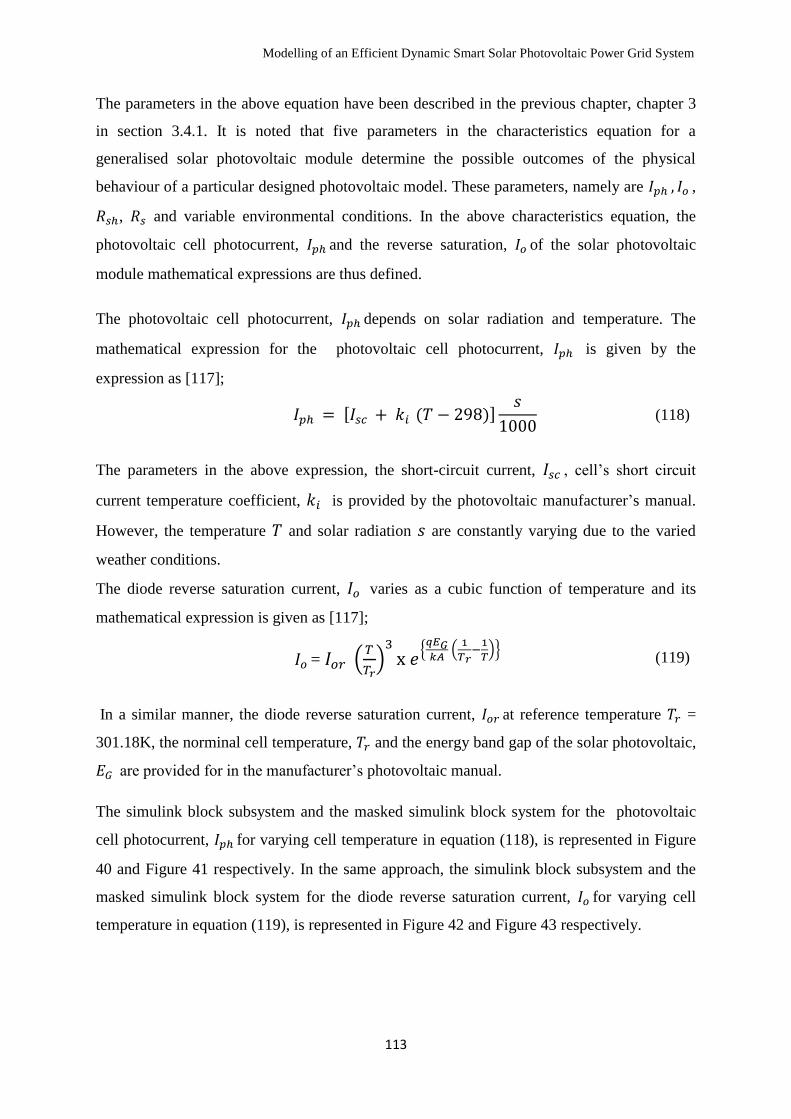
Modelling of an Efficient Dynamic Smart Solar Photovoltaic Power Grid System
113
The parameters in the above equation have been described in the previous chapter, chapter 3
in section 3.4.1. It is noted that five parameters in the characteristics equation for a
generalised solar photovoltaic module determine the possible outcomes of the physical
behaviour of a particular designed photovoltaic model. These parameters, namely are 𝐼𝑝ℎ , 𝐼𝑜 ,
𝑅𝑠ℎ, 𝑅𝑠 and variable environmental conditions. In the above characteristics equation, the
photovoltaic cell photocurrent, 𝐼𝑝ℎ and the reverse saturation, 𝐼𝑜 of the solar photovoltaic
module mathematical expressions are thus defined.
The photovoltaic cell photocurrent, 𝐼𝑝ℎ depends on solar radiation and temperature. The
mathematical expression for the photovoltaic cell photocurrent, 𝐼𝑝ℎ is given by the
expression as [117];
𝐼𝑝ℎ = [𝐼𝑠𝑐 + 𝑘𝑖 (𝑇 − 298)]𝑠
1000 (118)
The parameters in the above expression, the short-circuit current, 𝐼𝑠𝑐 , cell’s short circuit
current temperature coefficient, 𝑘𝑖 is provided by the photovoltaic manufacturer’s manual.
However, the temperature 𝑇 and solar radiation 𝑠 are constantly varying due to the varied
weather conditions.
The diode reverse saturation current, 𝐼𝑜 varies as a cubic function of temperature and its
mathematical expression is given as [117];
𝐼𝑜 = 𝐼𝑜𝑟 (𝑇
𝑇𝑟)3x 𝑒
{𝑞𝐸𝐺𝑘𝐴
(1
𝑇𝑟−1
𝑇)}
(119)
In a similar manner, the diode reverse saturation current, 𝐼𝑜𝑟 at reference temperature 𝑇𝑟 =
301.18K, the norminal cell temperature, 𝑇𝑟 and the energy band gap of the solar photovoltaic,
𝐸𝐺 are provided for in the manufacturer’s photovoltaic manual.
The simulink block subsystem and the masked simulink block system for the photovoltaic
cell photocurrent, 𝐼𝑝ℎ for varying cell temperature in equation (118), is represented in Figure
40 and Figure 41 respectively. In the same approach, the simulink block subsystem and the
masked simulink block system for the diode reverse saturation current, 𝐼𝑜 for varying cell
temperature in equation (119), is represented in Figure 42 and Figure 43 respectively.
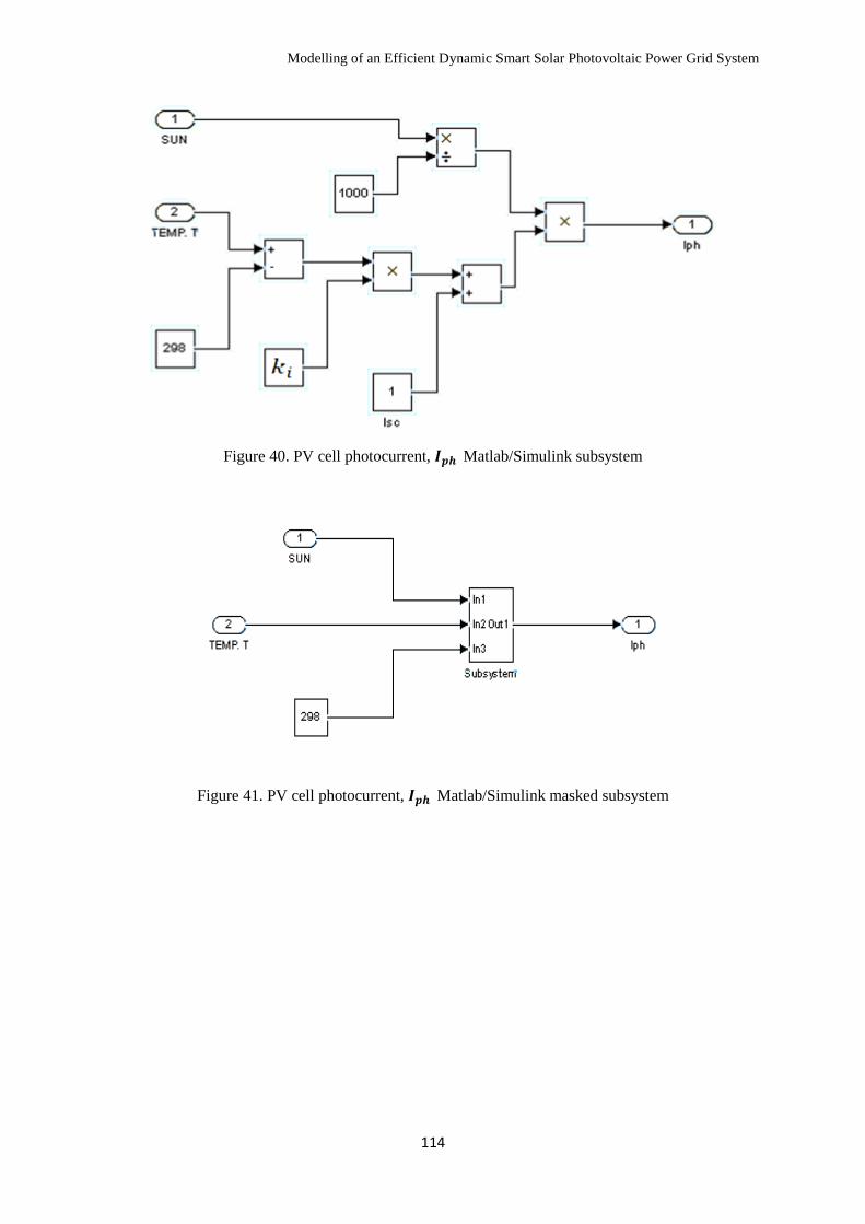
Modelling of an Efficient Dynamic Smart Solar Photovoltaic Power Grid System
114
Figure 40. PV cell photocurrent, 𝑰𝒑𝒉 Matlab/Simulink subsystem
Figure 41. PV cell photocurrent, 𝑰𝒑𝒉 Matlab/Simulink masked subsystem
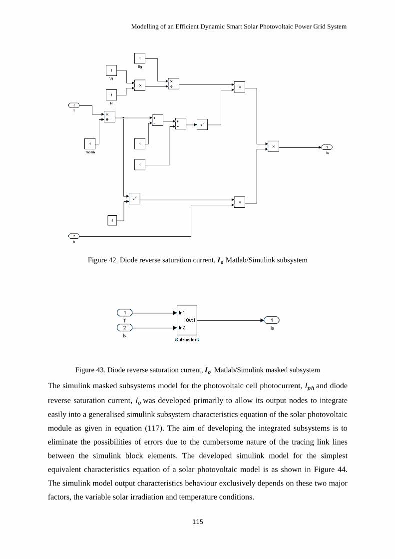
Modelling of an Efficient Dynamic Smart Solar Photovoltaic Power Grid System
115
Figure 42. Diode reverse saturation current, 𝑰𝒐 Matlab/Simulink subsystem
Figure 43. Diode reverse saturation current, 𝑰𝒐 Matlab/Simulink masked subsystem
The simulink masked subsystems model for the photovoltaic cell photocurrent, 𝐼𝑝ℎ and diode
reverse saturation current, 𝐼𝑜 was developed primarily to allow its output nodes to integrate
easily into a generalised simulink subsystem characteristics equation of the solar photovoltaic
module as given in equation (117). The aim of developing the integrated subsystems is to
eliminate the possibilities of errors due to the cumbersome nature of the tracing link lines
between the simulink block elements. The developed simulink model for the simplest
equivalent characteristics equation of a solar photovoltaic model is as shown in Figure 44.
The simulink model output characteristics behaviour exclusively depends on these two major
factors, the variable solar irradiation and temperature conditions.
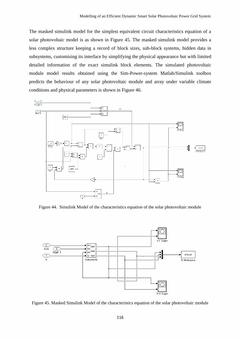
Modelling of an Efficient Dynamic Smart Solar Photovoltaic Power Grid System
116
The masked simulink model for the simplest equivalent circuit characteristics equation of a
solar photovoltaic model is as shown in Figure 45. The masked simulink model provides a
less complex structure keeping a record of block sizes, sub-block systems, hidden data in
subsystems, customising its interface by simplifying the physical appearance but with limited
detailed information of the exact simulink block elements. The simulated photovoltaic
module model results obtained using the Sim-Power-system Matlab/Simulink toolbox
predicts the behaviour of any solar photovoltaic module and array under variable climate
conditions and physical parameters is shown in Figure 46.
Figure 44. Simulink Model of the characteristics equation of the solar photovoltaic module
Figure 45. Masked Simulink Model of the characteristics equation of the solar photovoltaic module
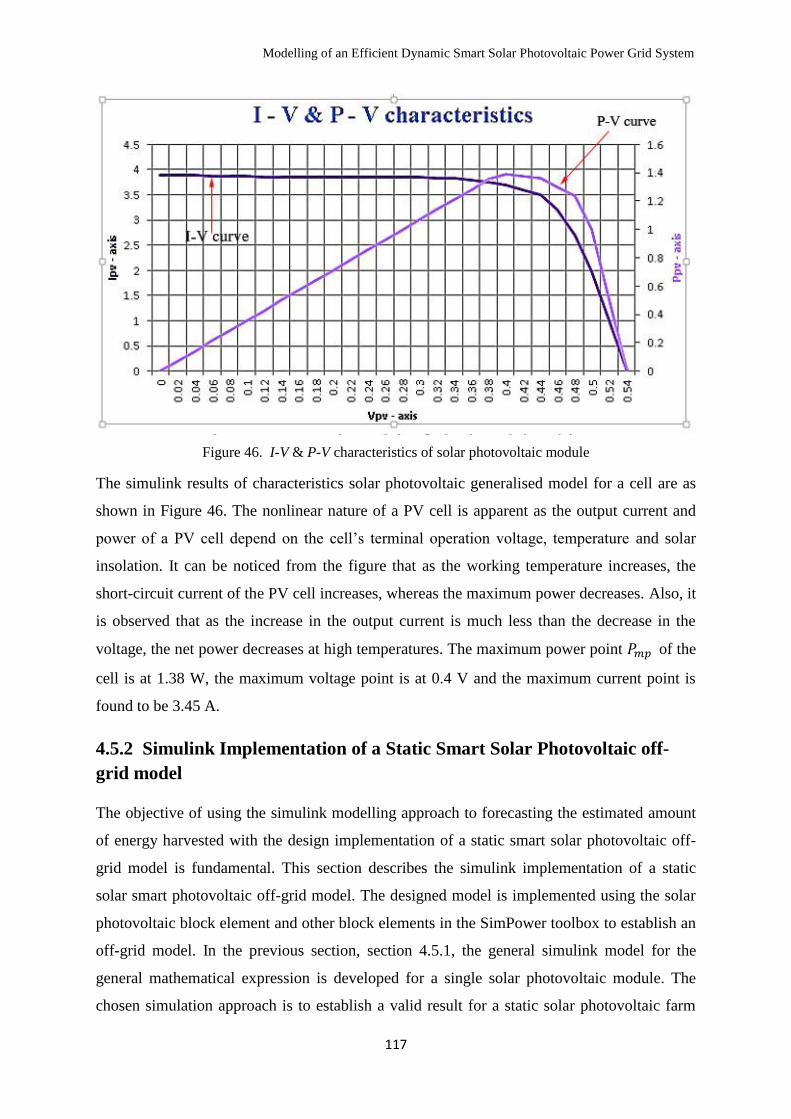
Modelling of an Efficient Dynamic Smart Solar Photovoltaic Power Grid System
117
Figure 46. I-V & P-V characteristics of solar photovoltaic module
The simulink results of characteristics solar photovoltaic generalised model for a cell are as
shown in Figure 46. The nonlinear nature of a PV cell is apparent as the output current and
power of a PV cell depend on the cell’s terminal operation voltage, temperature and solar
insolation. It can be noticed from the figure that as the working temperature increases, the
short-circuit current of the PV cell increases, whereas the maximum power decreases. Also, it
is observed that as the increase in the output current is much less than the decrease in the
voltage, the net power decreases at high temperatures. The maximum power point 𝑃𝑚𝑝 of the
cell is at 1.38 W, the maximum voltage point is at 0.4 V and the maximum current point is
found to be 3.45 A.
4.5.2 Simulink Implementation of a Static Smart Solar Photovoltaic off-
grid model
The objective of using the simulink modelling approach to forecasting the estimated amount
of energy harvested with the design implementation of a static smart solar photovoltaic off-
grid model is fundamental. This section describes the simulink implementation of a static
solar smart photovoltaic off-grid model. The designed model is implemented using the solar
photovoltaic block element and other block elements in the SimPower toolbox to establish an
off-grid model. In the previous section, section 4.5.1, the general simulink model for the
general mathematical expression is developed for a single solar photovoltaic module. The
chosen simulation approach is to establish a valid result for a static solar photovoltaic farm

Modelling of an Efficient Dynamic Smart Solar Photovoltaic Power Grid System
118
for a five thousand solar photovoltaic array of modules connected in series and parallel
configurations to determine the expected maximum output harvested energy in a real life
scenario under variable environmental conditions. The two major environmental conditions
considered in this design are solar irradiation and temperature; others conditions such as the
wind, humidity etc. are ignored.
However, practical experience and challenges in a real life scenario, a few times do not
correspond in perfect terms with simulated results but the processes and benefits accrued to
site engineers having a foreknowledge and expectation of probable results with direct
relevance to current site practice is an added advantage. The capabilities of simulink
computational processes are steadily gaining recognition in the engineering field due to the
technological breakthroughs achieved over the years. The simulink model representation is a
convenient approach for modelling linear and non-linear block elements using the continuous
power graphic user interface (powergui) as the model simulator to display the steady state
conditions and output characteristics.
In establishing the design model for the simulink implementation for the five thousand solar
photovoltaic modules, a series connection arrangement of ten solar photovoltaic modules is
constructed and a masked subsystem block unit of the array formed is shown in Figure 47 and
Figure 48 respectively. The functional block parameters for the solar photovoltaic module
with the double exponential model is shown in Figure 49 and Figure 50 respectively. The
model consists of a light photocurrent source, two diodes, a series resistance and a parallel
resistance. In the physical characteristics behaviour of the solar photovoltaic cell model, the
shunt resistance, 𝑅𝑠ℎ is inversely related with shunt leakage current to the ground and most
times it is assumed to be infinity (inf) and a small variation in 𝑅𝑠 significantly affects the
output photovoltaic output power. Consequently, ten similar masked subsystem block units of
ten solar photovoltaic modules are connected in series to establish a series connection of a
hundred units of solar photovoltaic modules on a single lane as shown in Figure 51. The
negative PV terminal in Figure 51 has been shortened in words as negative PV term, to allow
the Figure fits into the page.
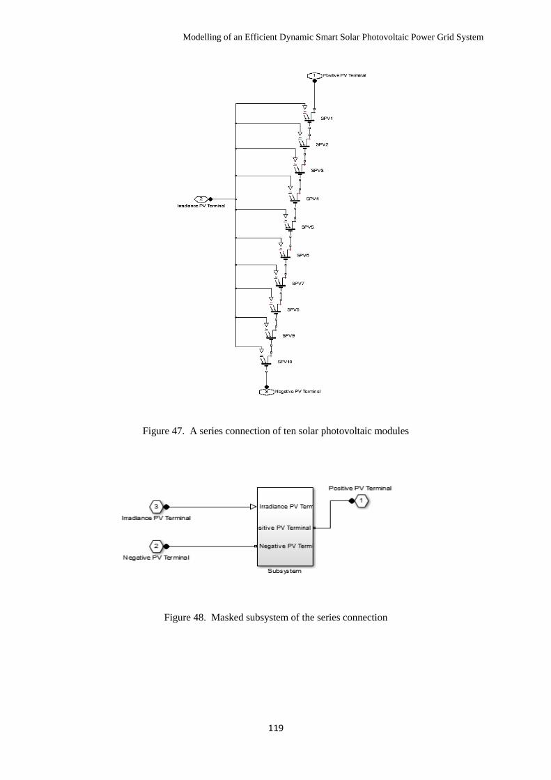
Modelling of an Efficient Dynamic Smart Solar Photovoltaic Power Grid System
119
Figure 47. A series connection of ten solar photovoltaic modules
Figure 48. Masked subsystem of the series connection
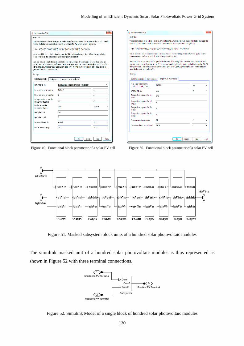
Modelling of an Efficient Dynamic Smart Solar Photovoltaic Power Grid System
120
Figure 49. Functional block parameter of a solar PV cell Figure 50. Functional block parameter of a solar PV cell
Figure 51. Masked subsystem block units of a hundred solar photovoltaic modules
The simulink masked unit of a hundred solar photovoltaic modules is thus represented as
shown in Figure 52 with three terminal connections.
Figure 52. Simulink Model of a single block of hundred solar photovoltaic modules
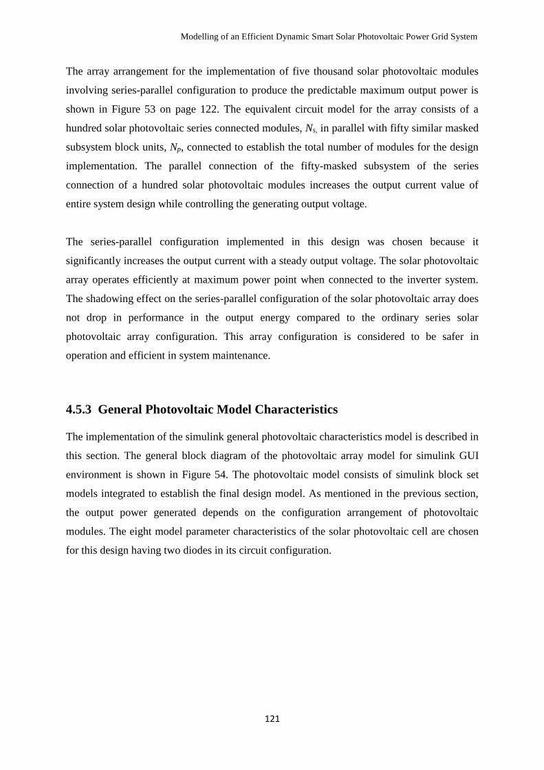
Modelling of an Efficient Dynamic Smart Solar Photovoltaic Power Grid System
121
The array arrangement for the implementation of five thousand solar photovoltaic modules
involving series-parallel configuration to produce the predictable maximum output power is
shown in Figure 53 on page 122. The equivalent circuit model for the array consists of a
hundred solar photovoltaic series connected modules, Ns, in parallel with fifty similar masked
subsystem block units, Np, connected to establish the total number of modules for the design
implementation. The parallel connection of the fifty-masked subsystem of the series
connection of a hundred solar photovoltaic modules increases the output current value of
entire system design while controlling the generating output voltage.
The series-parallel configuration implemented in this design was chosen because it
significantly increases the output current with a steady output voltage. The solar photovoltaic
array operates efficiently at maximum power point when connected to the inverter system.
The shadowing effect on the series-parallel configuration of the solar photovoltaic array does
not drop in performance in the output energy compared to the ordinary series solar
photovoltaic array configuration. This array configuration is considered to be safer in
operation and efficient in system maintenance.
4.5.3 General Photovoltaic Model Characteristics
The implementation of the simulink general photovoltaic characteristics model is described in
this section. The general block diagram of the photovoltaic array model for simulink GUI
environment is shown in Figure 54. The photovoltaic model consists of simulink block set
models integrated to establish the final design model. As mentioned in the previous section,
the output power generated depends on the configuration arrangement of photovoltaic
modules. The eight model parameter characteristics of the solar photovoltaic cell are chosen
for this design having two diodes in its circuit configuration.
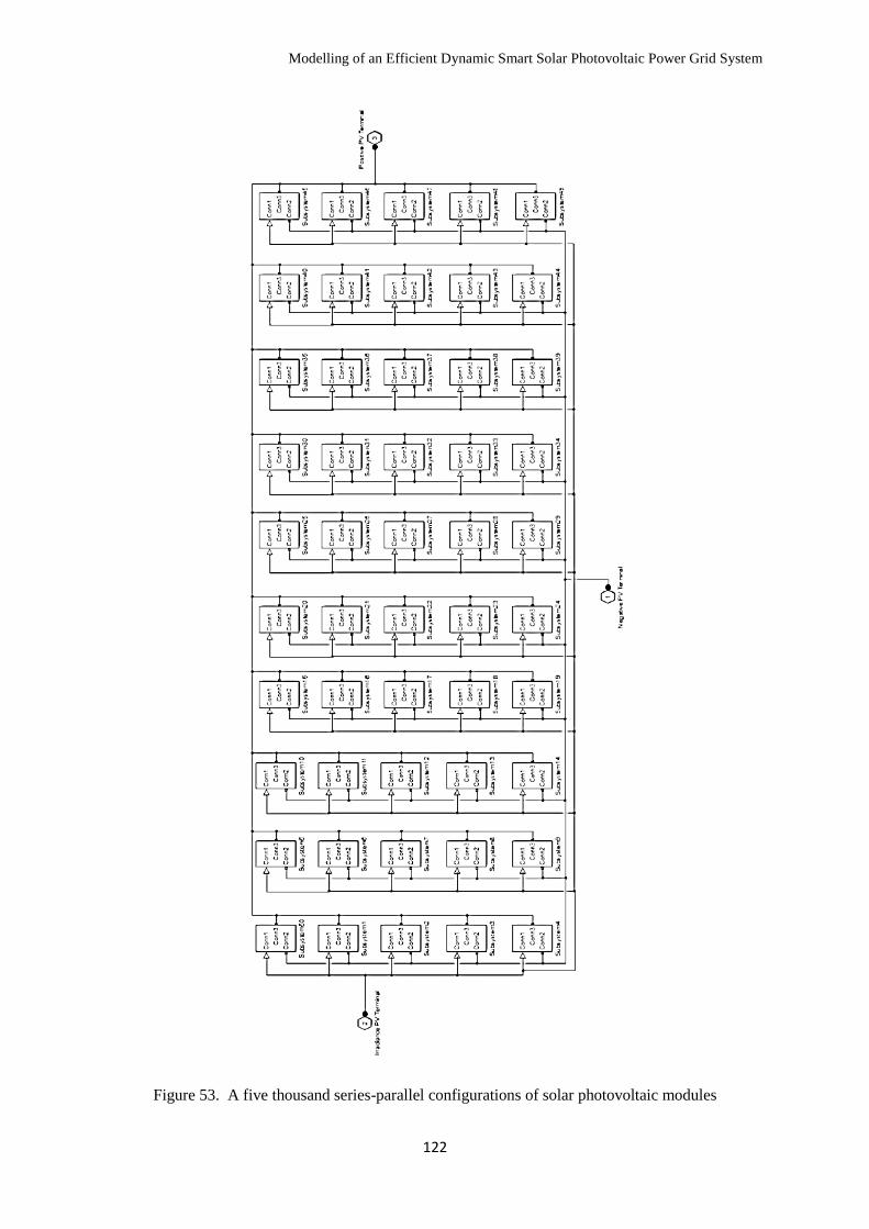
Modelling of an Efficient Dynamic Smart Solar Photovoltaic Power Grid System
122
Figure 53. A five thousand series-parallel configurations of solar photovoltaic modules
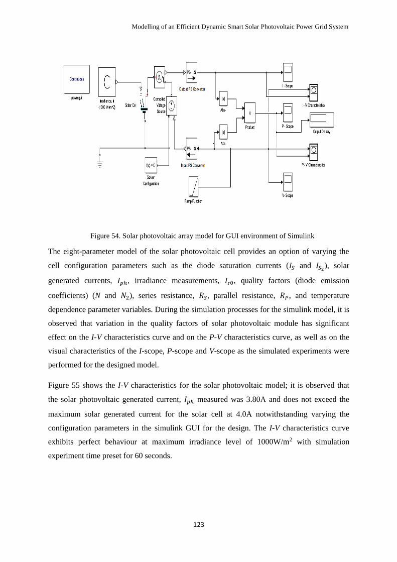
Modelling of an Efficient Dynamic Smart Solar Photovoltaic Power Grid System
123
Figure 54. Solar photovoltaic array model for GUI environment of Simulink
The eight-parameter model of the solar photovoltaic cell provides an option of varying the
cell configuration parameters such as the diode saturation currents (𝐼𝑆 and 𝐼𝑆2), solar
generated currents, 𝐼𝑝ℎ, irradiance measurements, 𝐼r0, quality factors (diode emission
coefficients) (N and 𝑁2), series resistance, 𝑅𝑆, parallel resistance, 𝑅𝑃, and temperature
dependence parameter variables. During the simulation processes for the simulink model, it is
observed that variation in the quality factors of solar photovoltaic module has significant
effect on the I-V characteristics curve and on the P-V characteristics curve, as well as on the
visual characteristics of the I-scope, P-scope and V-scope as the simulated experiments were
performed for the designed model.
Figure 55 shows the I-V characteristics for the solar photovoltaic model; it is observed that
the solar photovoltaic generated current, 𝐼𝑝ℎ measured was 3.80A and does not exceed the
maximum solar generated current for the solar cell at 4.0A notwithstanding varying the
configuration parameters in the simulink GUI for the design. The I-V characteristics curve
exhibits perfect behaviour at maximum irradiance level of 1000W/m2 with simulation
experiment time preset for 60 seconds.
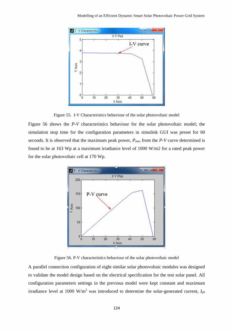
Modelling of an Efficient Dynamic Smart Solar Photovoltaic Power Grid System
124
Figure 55. I-V Characteristics behaviour of the solar photovoltaic model
Figure 56 shows the P-V characteristics behaviour for the solar photovoltaic model; the
simulation stop time for the configuration parameters in simulink GUI was preset for 60
seconds. It is observed that the maximum peak power, Pmax from the P-V curve determined is
found to be at 163 Wp at a maximum irradiance level of 1000 W/m2 for a rated peak power
for the solar photovoltaic cell at 170 Wp.
Figure 56. P-V characteristics behaviour of the solar photovoltaic model
A parallel connection configuration of eight similar solar photovoltaic modules was designed
to validate the model design based on the electrical specification for the test solar panel. All
configuration parameters settings in the previous model were kept constant and maximum
irradiance level at 1000 W/m2 was introduced to determine the solar-generated current, Iph
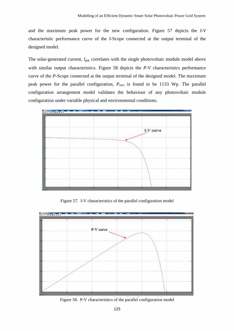
Modelling of an Efficient Dynamic Smart Solar Photovoltaic Power Grid System
125
and the maximum peak power for the new configuration. Figure 57 depicts the I-V
characteristic performance curve of the I-Scope connected at the output terminal of the
designed model.
The solar-generated current, 𝐼𝑝ℎ correlates with the single photovoltaic module model above
with similar output characteristics. Figure 58 depicts the P-V characteristics performance
curve of the P-Scope connected at the output terminal of the designed model. The maximum
peak power for the parallel configuration, Pmax is found to be 1133 Wp. The parallel
configuration arrangement model validates the behaviour of any photovoltaic module
configuration under variable physical and environmental conditions.
Figure 57. I-V characteristics of the parallel configuration model
Figure 58. P-V characteristics of the parallel configuration model
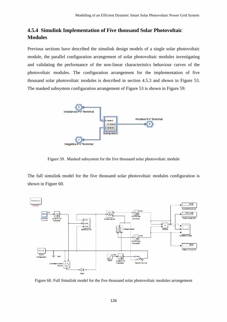
Modelling of an Efficient Dynamic Smart Solar Photovoltaic Power Grid System
126
4.5.4 Simulink Implementation of Five thousand Solar Photovoltaic
Modules
Previous sections have described the simulink design models of a single solar photovoltaic
module, the parallel configuration arrangement of solar photovoltaic modules investigating
and validating the performance of the non-linear characteristics behaviour curves of the
photovoltaic modules. The configuration arrangement for the implementation of five
thousand solar photovoltaic modules is described in section 4.5.3 and shown in Figure 53.
The masked subsystem configuration arrangement of Figure 53 is shown in Figure 59.
Figure 59. Masked subsystem for the five thousand solar photovoltaic module
The full simulink model for the five thousand solar photovoltaic modules configuration is
shown in Figure 60.
Figure 60. Full Simulink model for the five thousand solar photovoltaic modules arrangement
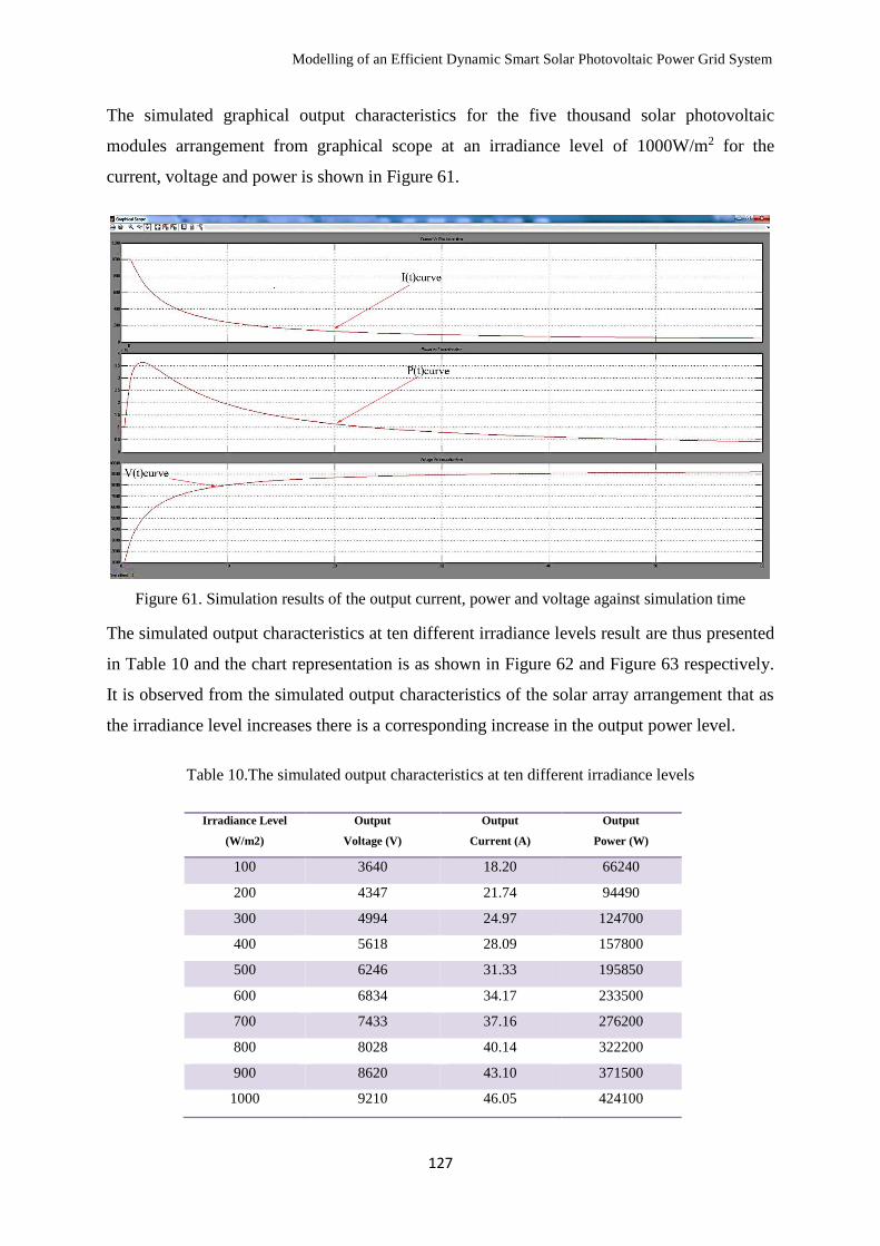
Modelling of an Efficient Dynamic Smart Solar Photovoltaic Power Grid System
127
The simulated graphical output characteristics for the five thousand solar photovoltaic
modules arrangement from graphical scope at an irradiance level of 1000W/m2 for the
current, voltage and power is shown in Figure 61.
Figure 61. Simulation results of the output current, power and voltage against simulation time
The simulated output characteristics at ten different irradiance levels result are thus presented
in Table 10 and the chart representation is as shown in Figure 62 and Figure 63 respectively.
It is observed from the simulated output characteristics of the solar array arrangement that as
the irradiance level increases there is a corresponding increase in the output power level.
Table 10.The simulated output characteristics at ten different irradiance levels
Irradiance Level
(W/m2)
Output
Voltage (V)
Output
Current (A)
Output
Power (W)
100 3640 18.20 66240
200 4347 21.74 94490
300 4994 24.97 124700
400 5618 28.09 157800
500 6246 31.33 195850
600 6834 34.17 233500
700 7433 37.16 276200
800 8028 40.14 322200
900 8620 43.10 371500
1000 9210 46.05 424100
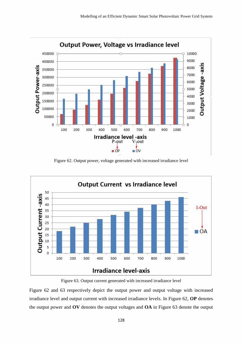
Modelling of an Efficient Dynamic Smart Solar Photovoltaic Power Grid System
128
Figure 62. Output power, voltage generated with increased irradiance level
Figure 63. Output current generated with increased irradiance level
Figure 62 and 63 respectively depict the output power and output voltage with increased
irradiance level and output current with increased irradiance levels. In Figure 62, OP denotes
the output power and OV denotes the output voltages and OA in Figure 63 denote the output

Modelling of an Efficient Dynamic Smart Solar Photovoltaic Power Grid System
129
current for the simulink model of the 5000 solar photovoltaic module arrangement. A distinct
look into these figures; gives a clear understanding of the chart, that as the irradiance level is
increased in steps of 100 W/m2 to the maximum irradiance level at 1000 W/m2 for the
Simulink design implementation, there is a corresponding increase in the output current,
voltage and power in the chart represented. The simulink design implementation provides a
vital information for the designer in helping to determine the exact output current, voltage
and power correspondence at any given irradiance under the condition of which the
simulation experiments were performed.
4.6 Conclusion
Analysis and the theoretical basis for the governing equations for dynamic smart solar
photovoltaic tracking systems have been carefully examined in this chapter. In addition, the
determined arbitrary angles are programmed into the solar photovoltaic database system
controller ensuring that constant orthogonal positioning of the sun’s position is achieved
throughout the day. Furthermore, the simulink design and implementation of a single solar
photovoltaic module, the parallel configuration of solar photovoltaic array arrangement and
implementation of simulink design for five thousand solar photovoltaic arrays, are thus
presented in this chapter. The respective results of the modelled experiments performed are
shown in the Figures in this chapter and contributions have been clearly stated.
The following chapter (chapter 5) presents a robust real-time online comparative solar
photovoltaic monitoring of the static and dynamic solar photovoltaic systems. The research
was conducted at the National Kaohsiung University of Applied Sciences, Taiwan, Republic
of China. The results and findings are presented in the same chapter.
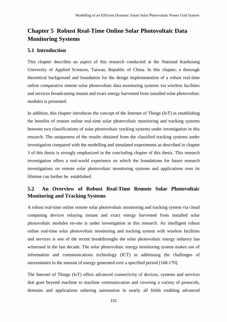
Modelling of an Efficient Dynamic Smart Solar Photovoltaic Power Grid System
131
Chapter 5 Robust Real-Time Online Solar Photovoltaic Data
Monitoring Systems
5.1 Introduction
This chapter describes an aspect of this research conducted at the National Kaohsiung
University of Applied Sciences, Taiwan, Republic of China. In this chapter, a thorough
theoretical background and foundation for the design implementation of a robust real-time
online comparative remote solar photovoltaic data monitoring systems via wireless facilities
and services broadcasting instant and exact energy harvested from installed solar photovoltaic
modules is presented.
In addition, this chapter introduces the concept of the Internet of Things (IoT) in establishing
the benefits of remote online real-time solar photovoltaic monitoring and tracking systems
between two classifications of solar photovoltaic tracking systems under investigation in this
research. The uniqueness of the results obtained from the classified tracking systems under
investigation compared with the modelling and simulated experiments as described in chapter
3 of this thesis is strongly emphasized in the concluding chapter of this thesis. This research
investigation offers a real-world experience on which the foundations for future research
investigations on remote solar photovoltaic monitoring systems and applications over its
lifetime can further be established.
5.2 An Overview of Robust Real-Time Remote Solar Photovoltaic
Monitoring and Tracking Systems
A robust real-time online remote solar photovoltaic monitoring and tracking system via cloud
computing devices relaying instant and exact energy harvested from installed solar
photovoltaic modules on-site is under investigation in this research. An intelligent robust
online real-time solar photovoltaic monitoring and tracking system with wireless facilities
and services is one of the recent breakthroughs the solar photovoltaic energy industry has
witnessed in the last decade. The solar photovoltaic energy monitoring system makes use of
information and communications technology (ICT) in addressing the challenges of
uncertainties in the amount of energy generated over a specified period [168-170].
The Internet of Things (IoT) offers advanced connectivity of devices, systems and services
that goes beyond machine to machine communication and covering a variety of protocols,
domains and applications ushering automation in nearly all fields enabling advanced
Modelling of an Efficient Dynamic Smart Solar Photovoltaic Power Grid System
132
applications in smart grid networks [171]. This new concept in smart grid networks and
systems provides automation which has led to expansion, generating large amounts of data
from diverse distributed smart grid networks and systems aggregating quickly, thereby
increasing the need for better index, storage and process such data [172].
The remote monitoring devices for stationary and dynamic hybrid solar photovoltaic tracking
systems is achieved via the internet on mobile phones, tablets, PCs and notebooks through
installed software tracking applications. The introduction of robust adaptive devices has
significantly increased the optimisation, performance and high sun’s concentration on the
hybrid solar photovoltaic tracking modules based on developed solar movement algorithm
models. This research investigates the design of an efficient robust online real-time
comparative data and visual analysis for both stationary and the hybrid solar photovoltaic
tracking and monitoring systems over the lifetime of the installation.
The solar photovoltaic monitoring system consists of two main components: the
programmable logic controller (PLC) box and the data logger connected via the router for
remotely accessing and transfer real-time solar photovoltaic data information generated. A
data acquisition and monitoring system are deployed for this research investigation at the
National Kaohsiung University of Applied Sciences, Taiwan, the Republic of China for
optimal solar photovoltaic energy harvesting to forecast sustainable solar photovoltaic
management policies and validate simulation models. The research outcomes are likely to
offer real-world experience on the future solar photovoltaic energy industry applications not
only in Taiwan but also worldwide.
These robust adaptive devices reduce the extent of energy loss liable to occur due to faulty
devices and parts connected to the solar photovoltaic array providing an expedient, efficient
maintenance and replacement so as to restore to full capacity. The availability and provision
of multi-vendor cloud-based data setup centers globally, various software support
applications developed have brought immense potentials and significant performance in
reducing the response time and cost savings in the solar photovoltaic energy industry [173].
A key component of the solar photovoltaic monitoring system is the provision of cloud
platforms referred to as power management data centers. This provides the ability to enhance
remote visibility, automated integration of energy management and policies, power metering
capabilities, safety and control mechanisms, early fault detection and location resulting in
minimal loss of harvested energy. The cloud platform architecture addresses challenges such
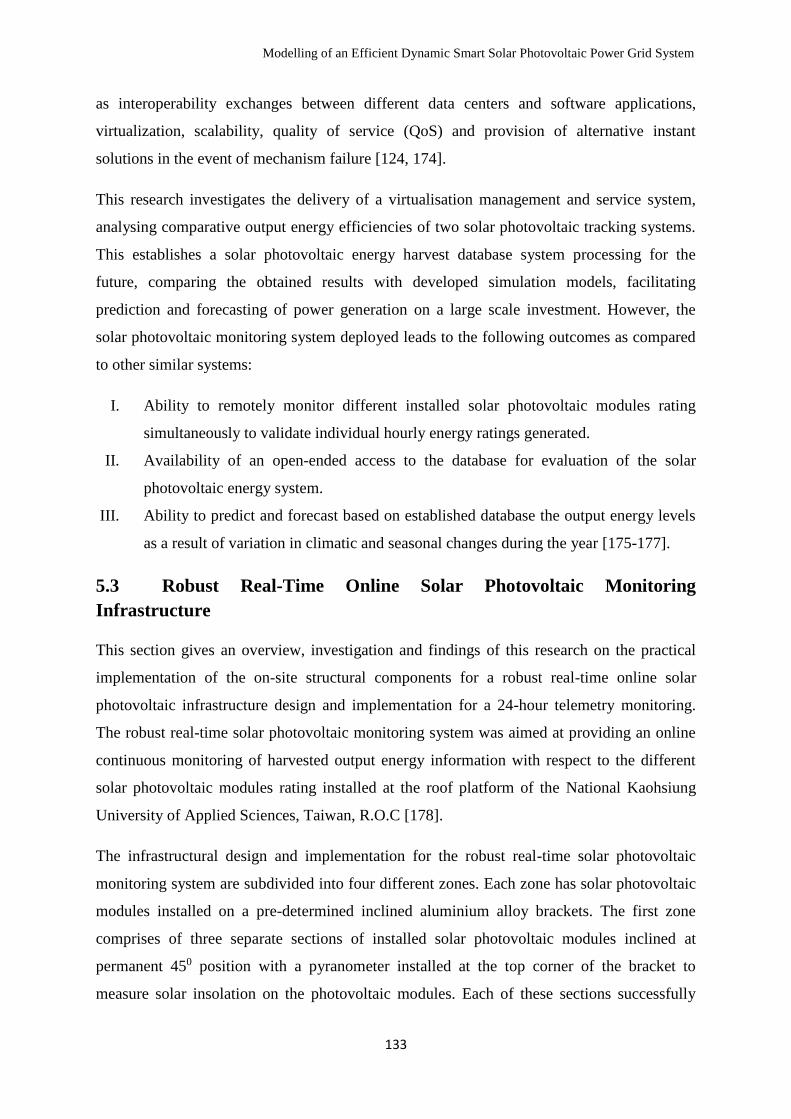
Modelling of an Efficient Dynamic Smart Solar Photovoltaic Power Grid System
133
as interoperability exchanges between different data centers and software applications,
virtualization, scalability, quality of service (QoS) and provision of alternative instant
solutions in the event of mechanism failure [124, 174].
This research investigates the delivery of a virtualisation management and service system,
analysing comparative output energy efficiencies of two solar photovoltaic tracking systems.
This establishes a solar photovoltaic energy harvest database system processing for the
future, comparing the obtained results with developed simulation models, facilitating
prediction and forecasting of power generation on a large scale investment. However, the
solar photovoltaic monitoring system deployed leads to the following outcomes as compared
to other similar systems:
I. Ability to remotely monitor different installed solar photovoltaic modules rating
simultaneously to validate individual hourly energy ratings generated.
II. Availability of an open-ended access to the database for evaluation of the solar
photovoltaic energy system.
III. Ability to predict and forecast based on established database the output energy levels
as a result of variation in climatic and seasonal changes during the year [175-177].
5.3 Robust Real-Time Online Solar Photovoltaic Monitoring
Infrastructure
This section gives an overview, investigation and findings of this research on the practical
implementation of the on-site structural components for a robust real-time online solar
photovoltaic infrastructure design and implementation for a 24-hour telemetry monitoring.
The robust real-time solar photovoltaic monitoring system was aimed at providing an online
continuous monitoring of harvested output energy information with respect to the different
solar photovoltaic modules rating installed at the roof platform of the National Kaohsiung
University of Applied Sciences, Taiwan, R.O.C [178].
The infrastructural design and implementation for the robust real-time solar photovoltaic
monitoring system are subdivided into four different zones. Each zone has solar photovoltaic
modules installed on a pre-determined inclined aluminium alloy brackets. The first zone
comprises of three separate sections of installed solar photovoltaic modules inclined at
permanent 450 position with a pyranometer installed at the top corner of the bracket to
measure solar insolation on the photovoltaic modules. Each of these sections successfully

Modelling of an Efficient Dynamic Smart Solar Photovoltaic Power Grid System
134
accommodates three standard 250Wp solar photovoltaic modules with different photovoltaic
characteristics ratings to compare and determine the output energy harvested.
The second zone consists of a manual incremental adjustable aluminium alloy frame structure
having its horizontal base specially marked for incremental elevation angles from 00, 150, 250,
350, 450, 550 and 750 respectively. This zone has three different standard photovoltaic module
ratings installed to compare and determine the output energy generated from each of the
photovoltaic modules as the elevation angle for the framed structure is either increased or
decreased at different periods during the year.
The third zone is designed to have two manually adjustable aluminium alloy frame structures
having the horizontal base specially marked for incremental elevation angles at 450 and 700
respectively. The framed structure accommodates three standard solar photovoltaic modules
of different power ratings to compare and determine the output energy generated and the best
elevation position to obtain maximum efficiency for the manually static solar photovoltaic
modules.
The fourth zone consists of a two-axis controlled flat surface hybrid solar photovoltaic
tracking stepper motor rotating device having a solar sensor installed at the centre top of the
rectangular aluminium framed structure with a programmable logic controller box attached at
the base of the concrete pole. A robust real-time online solar photovoltaic monitoring
schematic system at the roof building platform is shown in Figure 64 [178].
In this research, the first and the fourth zone arrangements of the schematic figure is under
comparative analysis in determining the advantage and benefits of the solar photovoltaic
tracking systems in terms of the maximum efficiency of the output energy harvested.
The solar photovoltaic monitoring schematic system described on the roof site setup has four
solar photovoltaic modules representing four zones. The Darfon MIG 240 micro-inverter is
installed on the aluminium alloy framed structure at the rear side of each of the zones
consisting three standard solar photovoltaic module ratings [179]. The Darfon MIG 240
micro-inverter device has an inbuilt integral surge protector against induced voltage sparks
preventing damage of the solar photovoltaic monitoring system. The Darfon MIG 240
converts directly the DC power generated from the solar photovoltaic module to
synchronising AC power into the electricity grid network without the need of a high DC
voltage wiring and a central inverter system.
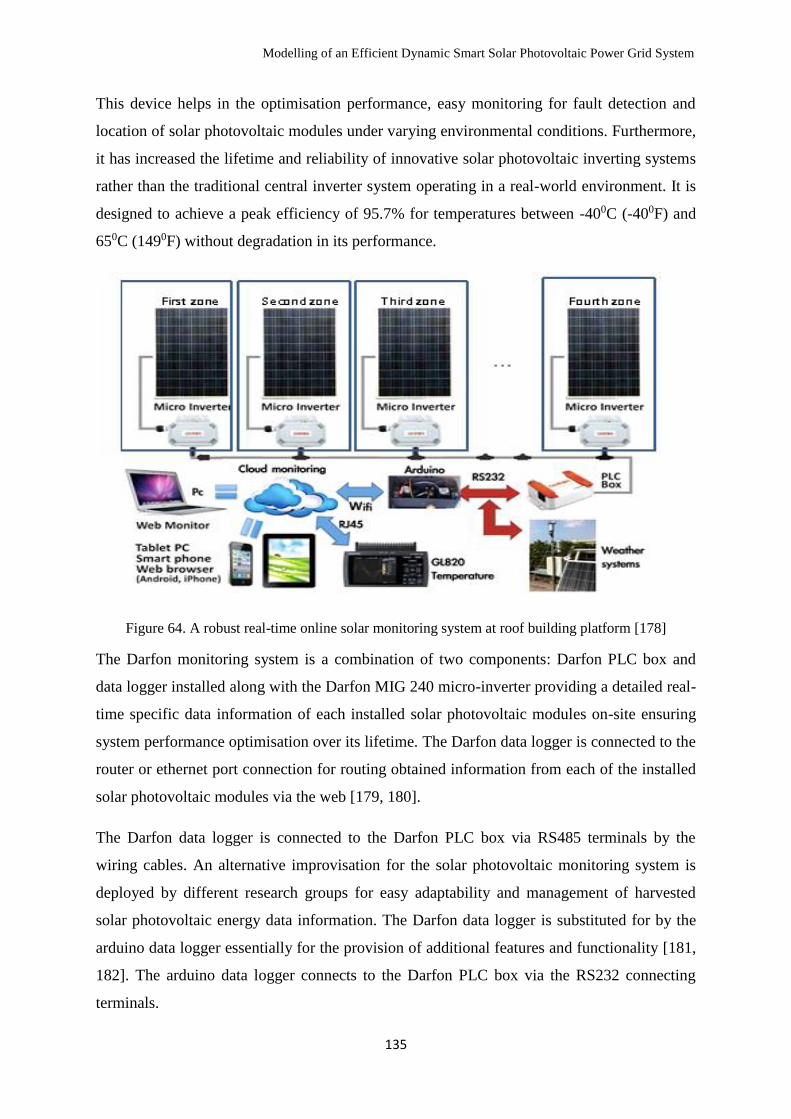
Modelling of an Efficient Dynamic Smart Solar Photovoltaic Power Grid System
135
This device helps in the optimisation performance, easy monitoring for fault detection and
location of solar photovoltaic modules under varying environmental conditions. Furthermore,
it has increased the lifetime and reliability of innovative solar photovoltaic inverting systems
rather than the traditional central inverter system operating in a real-world environment. It is
designed to achieve a peak efficiency of 95.7% for temperatures between -400C (-400F) and
650C (1490F) without degradation in its performance.
Figure 64. A robust real-time online solar monitoring system at roof building platform [178]
The Darfon monitoring system is a combination of two components: Darfon PLC box and
data logger installed along with the Darfon MIG 240 micro-inverter providing a detailed real-
time specific data information of each installed solar photovoltaic modules on-site ensuring
system performance optimisation over its lifetime. The Darfon data logger is connected to the
router or ethernet port connection for routing obtained information from each of the installed
solar photovoltaic modules via the web [179, 180].
The Darfon data logger is connected to the Darfon PLC box via RS485 terminals by the
wiring cables. An alternative improvisation for the solar photovoltaic monitoring system is
deployed by different research groups for easy adaptability and management of harvested
solar photovoltaic energy data information. The Darfon data logger is substituted for by the
arduino data logger essentially for the provision of additional features and functionality [181,
182]. The arduino data logger connects to the Darfon PLC box via the RS232 connecting
terminals.
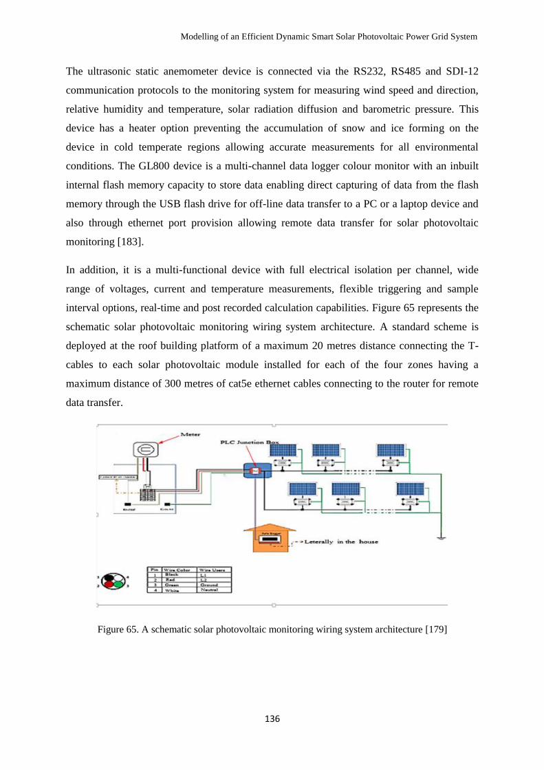
Modelling of an Efficient Dynamic Smart Solar Photovoltaic Power Grid System
136
The ultrasonic static anemometer device is connected via the RS232, RS485 and SDI-12
communication protocols to the monitoring system for measuring wind speed and direction,
relative humidity and temperature, solar radiation diffusion and barometric pressure. This
device has a heater option preventing the accumulation of snow and ice forming on the
device in cold temperate regions allowing accurate measurements for all environmental
conditions. The GL800 device is a multi-channel data logger colour monitor with an inbuilt
internal flash memory capacity to store data enabling direct capturing of data from the flash
memory through the USB flash drive for off-line data transfer to a PC or a laptop device and
also through ethernet port provision allowing remote data transfer for solar photovoltaic
monitoring [183].
In addition, it is a multi-functional device with full electrical isolation per channel, wide
range of voltages, current and temperature measurements, flexible triggering and sample
interval options, real-time and post recorded calculation capabilities. Figure 65 represents the
schematic solar photovoltaic monitoring wiring system architecture. A standard scheme is
deployed at the roof building platform of a maximum 20 metres distance connecting the T-
cables to each solar photovoltaic module installed for each of the four zones having a
maximum distance of 300 metres of cat5e ethernet cables connecting to the router for remote
data transfer.
Figure 65. A schematic solar photovoltaic monitoring wiring system architecture [179]
Modelling of an Efficient Dynamic Smart Solar Photovoltaic Power Grid System
137
5.4 Solar Photovoltaic Data Monitoring and Acquisition Energy System
The recent growth in internet networks and infrastructure has enhanced the development of
solar photovoltaic energy industry over the last decade in data monitoring and acquisition
systems for on-site, remote data collection and transfer via the internet for evaluating solar
photovoltaic module efficiencies, improving optimisation performance and operational
flexibility, achieving advanced control capabilities, periodic maintenance, fault detection and
location [184].
The solar photovoltaic energy industry transformation is evolving in data monitoring and
acquisition architecture from a client/server architecture employed for distributed measuring
instruments where acquired data is available in the server station and retrieved any time
needed through the internet network by clients as shown in Figure 66 [185]. In an alternative
arrangement as shown in Figure 67, clients access and obtain solar photovoltaic data via
intranet networking from the server station [186].
Figure 66. Client/server internet architecture
Figure 67. Client/server intranet architecture
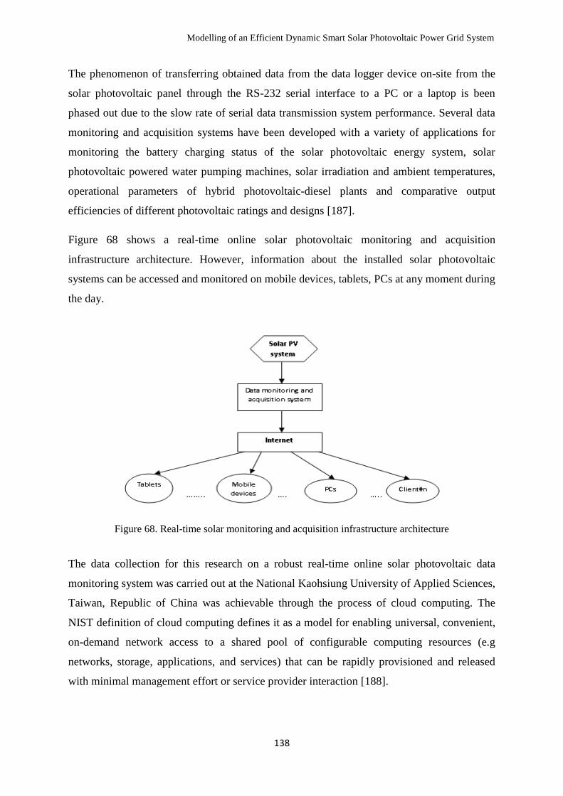
Modelling of an Efficient Dynamic Smart Solar Photovoltaic Power Grid System
138
The phenomenon of transferring obtained data from the data logger device on-site from the
solar photovoltaic panel through the RS-232 serial interface to a PC or a laptop is been
phased out due to the slow rate of serial data transmission system performance. Several data
monitoring and acquisition systems have been developed with a variety of applications for
monitoring the battery charging status of the solar photovoltaic energy system, solar
photovoltaic powered water pumping machines, solar irradiation and ambient temperatures,
operational parameters of hybrid photovoltaic-diesel plants and comparative output
efficiencies of different photovoltaic ratings and designs [187].
Figure 68 shows a real-time online solar photovoltaic monitoring and acquisition
infrastructure architecture. However, information about the installed solar photovoltaic
systems can be accessed and monitored on mobile devices, tablets, PCs at any moment during
the day.
Figure 68. Real-time solar monitoring and acquisition infrastructure architecture
The data collection for this research on a robust real-time online solar photovoltaic data
monitoring system was carried out at the National Kaohsiung University of Applied Sciences,
Taiwan, Republic of China was achievable through the process of cloud computing. The
NIST definition of cloud computing defines it as a model for enabling universal, convenient,
on-demand network access to a shared pool of configurable computing resources (e.g
networks, storage, applications, and services) that can be rapidly provisioned and released
with minimal management effort or service provider interaction [188].

Modelling of an Efficient Dynamic Smart Solar Photovoltaic Power Grid System
139
The component parts for a robust real-time online solar photovoltaic monitoring system at the
roof building platform has been discussed in detail in section 5.3 and as shown in Figure 64
in this Chapter. The aspect of cloud computing becomes relevant in this research because the
solar photovoltaic data collection and monitoring were achieved over the internet. The
deployment for this research was provided on a private cloud model by the institution.
The four basic fundamental cloud computing service models as shown in Figure 69 are: (i)
Infrastructure as a service (IaaS), (ii) Platform as a service (PaaS), (iii) Software as a service
(SaaS) and (iv) Unified communication as a service (UcaaS) [188, 189].
Figure 69. Basic fundamental cloud computing service model [188]
Each of the cloud computing service model levels is briefly defined as follows:
IaaS – This is a service infrastructure model maintained by the cloud as virtualised hardware
known as computing infrastructure providing virtual multitude server space, network
connections, bandwidths, IP addresses and load balancers distributed across several virtual
data centers.
PaaS – This allows customers to develop a personal software application for flexibility, run
and manage Web applications or rather choose a friendly pre-configured software support
service application developed on the network by periodically upgrading the applications in a
structured, managed and secured database system.
SaaS – This platform is built on international standards protocol for interoperability allowing
customised applications and access to software applications over the internet for a wide range
of needs such as monitoring, planning, forecasting and other related services on mobile apps
devices and PCs without restriction in any part of the world.
Modelling of an Efficient Dynamic Smart Solar Photovoltaic Power Grid System
140
UcaaS – This platform is outsourced to a third-party and co-ordinated by the internet service
providers (ISP) over the network for multi-platform communications such as IP telephony,
video conferencing and unified messaging on mobile devices, tablets and PCs.
The fundamental objective is to employ the provision of cloud computing service models to
achieve the primary purpose of retrieving solar photovoltaic data information and monitoring
remotely via the internet through the IaaS service model. This research basically employs the
IaaS model to achieve its objective. The IaaS service model provides the capability of
processing, storage, networks and other fundamental services.
The Darfon MIG 240 micro-inverter, Data logger and PLC box runs on an arbitrary software
on Java platform adaptable to retrieve solar photovoltaic data information via the internet
from the IaaS service model of each installed solar photovoltaic module. This is made
possible with access to the internet service platform provided by the private cloud model to
the institution. The Darfon data logger provides a user-friendly and flexible GUI for clients
usage on mobile apps devices, tablets and PCs for instant overall assessments of system
performance and retrieving solar photovoltaic data information.
The comparative study of the two solar photovoltaic tracking systems presented in section 5.7
was achieved via cloud computing. The cloud computing process provided access to the
energy data generated by the solar photovoltaic systems through virtualised resources,
parallel processing, security and data service integration with retrievable scalable data
storage. The cloud computing platform has minimised the cost and restriction for automation
and computerisation by individuals and enterprises on a large-scale, thus providing a
reduction in infrastructure maintenance cost, efficient management and friendly user access
of the energy generated data.
5.5 Comparative Solar Photovoltaic Tracking Systems under Investigation
In this section, two of the four zones described in Section 5.3, are evaluated and
comparatively analysed by observing the same physical and environmental conditions. The
two solar photovoltaic tracking systems under investigation are the 450 stationary inclined
solar photovoltaic systems and azimuthal-altitude GST 300-axis solar tracking system. The
output energy efficiencies of the solar energy harvested are compared between the two solar
photovoltaic tracking systems. The azimuthal-altitude dual GST 300-axis is classified as a
dynamic solar photovoltaic energy system whilst the 450 stationary inclined solar
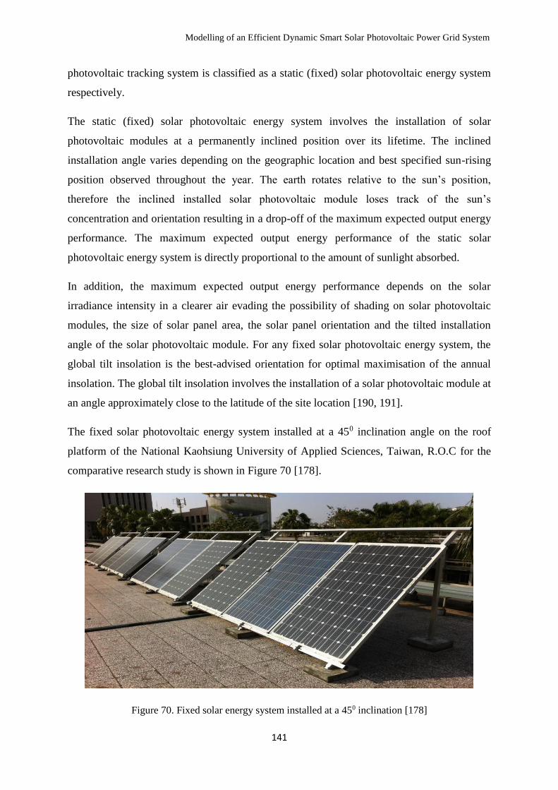
Modelling of an Efficient Dynamic Smart Solar Photovoltaic Power Grid System
141
photovoltaic tracking system is classified as a static (fixed) solar photovoltaic energy system
respectively.
The static (fixed) solar photovoltaic energy system involves the installation of solar
photovoltaic modules at a permanently inclined position over its lifetime. The inclined
installation angle varies depending on the geographic location and best specified sun-rising
position observed throughout the year. The earth rotates relative to the sun’s position,
therefore the inclined installed solar photovoltaic module loses track of the sun’s
concentration and orientation resulting in a drop-off of the maximum expected output energy
performance. The maximum expected output energy performance of the static solar
photovoltaic energy system is directly proportional to the amount of sunlight absorbed.
In addition, the maximum expected output energy performance depends on the solar
irradiance intensity in a clearer air evading the possibility of shading on solar photovoltaic
modules, the size of solar panel area, the solar panel orientation and the tilted installation
angle of the solar photovoltaic module. For any fixed solar photovoltaic energy system, the
global tilt insolation is the best-advised orientation for optimal maximisation of the annual
insolation. The global tilt insolation involves the installation of a solar photovoltaic module at
an angle approximately close to the latitude of the site location [190, 191].
The fixed solar photovoltaic energy system installed at a 450 inclination angle on the roof
platform of the National Kaohsiung University of Applied Sciences, Taiwan, R.O.C for the
comparative research study is shown in Figure 70 [178].
Figure 70. Fixed solar energy system installed at a 450 inclination [178]

Modelling of an Efficient Dynamic Smart Solar Photovoltaic Power Grid System
142
The dynamic solar photovoltaic tracking system involves the movement of solar photovoltaic
modules to constantly be in perpendicular alignment to solar irradiance throughout the day.
The dynamic solar photovoltaic tracking system increases the amount of energy harvested as
compared to the fixed solar photovoltaic tracking system for the same configuration. This
solar photovoltaic tracking system involves the combination of the use of solar sensors and
programmable-logic-controller for its tracking system. The combination of the solar sensor
and the use of programmable-logic-controller tracking system is known as a hybrid dynamic
solar photovoltaic tracking system. This has proven to be very effective and efficient for the
dual-axis solar photovoltaic tracking system [38, 192].
The movement of the dynamic solar photovoltaic tracking system is thus classified into two
categories:
(i) The single axis sun tracking system and
(ii) the dual-axis sun tracking system [193].
The single-axis dynamic solar photovoltaic tracking system implementation involves the
movement of the solar photovoltaic module along one degree of freedom. The dynamic
single-axis solar photovoltaic tracking system implementation is categorised into four
distinctive tracking systems:
(i) the horizontal single axis tracking system (HSAT),
(ii) the vertical single axis tracking system(VSAT),
(iii) the tilt single axis tracking system (TSAT) and
(iv) the polar aligned single axis tracking system (PASAT) [194].
HSAT- In the horizontal single axis tracking system, the axis of rotation is along the
horizontal with respect to the ground, to apparently track the motion of the sun through the
day.
VSAT- In the vertical single axis tracking system, the axis of rotation is along the vertical
with respect to the ground; it apparently tracks the sun by rotating the solar photovoltaic
module from east to west through the day.
TSAT- In the tilt single axis tracking system, the axis of rotation is along the horizontal and
vertical along a fixed plane tracking the sun through the day.
Modelling of an Efficient Dynamic Smart Solar Photovoltaic Power Grid System
143
PASAT- In the polar single axis tracking system, the axis of rotation aligns with the earth’s
axis of rotation, tracking the sun at the site latitude through the day.
Dual-axis solar tracking implementation involves the movement of the solar photovoltaic
module along two degrees of freedom acting on the axis of rotation. The output energy
efficiencies of the dual axis tracking system, as compared to the single axis tracking system,
has proven to be more efficient.
The two common dual-axis solar tracking systems are:
(i) the tip-tilt dual axis tracker (TTDAT) and
(ii) Azimuthal-altitude dual axis tracker (AADAT) [195, 196].
TTDAT- The tip-tilt dual axis tracker – has its primary axis horizontal to the ground and the
secondary axis is typically normal to the primary axis. The axes of rotation are typically
aligned either along a true north meridian or an east-west line of latitude with the possibility
of an advanced tracking algorithm aligning in any cardinal direction.
AADAT- The azimuthal-altitude dual axis tracker – has it primary axis vertical to the ground
and the secondary axis is typically normal to the primary axis.
The azimuthal-altitude dual-axis solar photovoltaic GST 300 tracking system deployed for
the evaluation and comparative data analysis on the roof platform at the National Kaohsiung
University of Applied Sciences, Taiwan, R.O.C is shown in Figure 71[178]. A solar
photovoltaic module as shown in Figure 71 is installed on the aluminium framed structure of
the dual-axis solar photovoltaic tracking system having a Darfon MIG 240 inverter device
mounted at the backside of the photovoltaic module. All electrical wiring connections for
online solar photovoltaic energy data monitoring and comparative analysis with the 450
stationary inclined solar photovoltaic tracking system is being set up for investigation in this
chapter.

Modelling of an Efficient Dynamic Smart Solar Photovoltaic Power Grid System
144
Figure 71. GST 300 tracker deployed at the roof platform [178]
The architectural design for the dual-axis solar tracking frame structure is shown in Figure 72
[178]. The solar photovoltaic sensor is connected to the centre of the top of the aluminium
rectangular frame structure to effectively track the sun’s path and relative position for energy
optimisation increasing the efficiency of harvested solar energy. In addition, the
programmable logic controller junction box is installed at the base of the pole with a pre-
programmed analytical derivation of the sun’s tracking position in the database system to
cause rotational movement of the tracking structure in synchronisation with the solar
photovoltaic sensor at the centre of the top of the aluminium framed structure tracking
system.
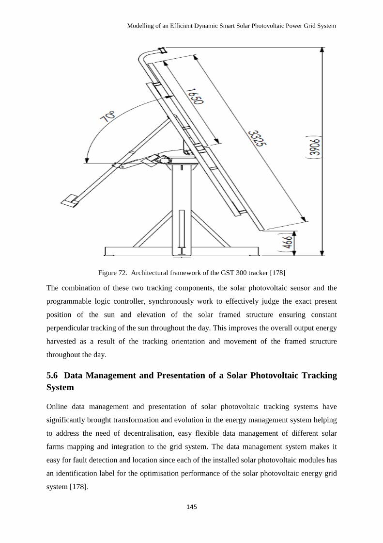
Modelling of an Efficient Dynamic Smart Solar Photovoltaic Power Grid System
145
Figure 72. Architectural framework of the GST 300 tracker [178]
The combination of these two tracking components, the solar photovoltaic sensor and the
programmable logic controller, synchronously work to effectively judge the exact present
position of the sun and elevation of the solar framed structure ensuring constant
perpendicular tracking of the sun throughout the day. This improves the overall output energy
harvested as a result of the tracking orientation and movement of the framed structure
throughout the day.
5.6 Data Management and Presentation of a Solar Photovoltaic Tracking
System
Online data management and presentation of solar photovoltaic tracking systems have
significantly brought transformation and evolution in the energy management system helping
to address the need of decentralisation, easy flexible data management of different solar
farms mapping and integration to the grid system. The data management system makes it
easy for fault detection and location since each of the installed solar photovoltaic modules has
an identification label for the optimisation performance of the solar photovoltaic energy grid
system [178].

Modelling of an Efficient Dynamic Smart Solar Photovoltaic Power Grid System
146
In addition, the data management system provides a uniform platform interface for
determining simultaneously the output energy efficiencies of different solar photovoltaic
modules under the same physical and environmental conditions at a glance. The data
management system supports the integration and management of information from a web-
based architectural design and technologies defining each specific photovoltaic module
design with the end user support. The data acquisition, processing, storing and reporting are
transmitted through a dedicated IP address gateway for remote access logging and control on
mobile devices, tablets and PCs.
In particular, the solar photovoltaic data information obtained is time specific based on multi-
threaded functionalities to manage and monitor multiple online requests by remote users of
the output solar photovoltaic characteristics [197]. Remote users and operators have easy
access to database information at the solar farm site via the web through the proprietary
Darfon or any alternative software applications. Remote users and operators have no
permission rights and authority to alter any configuration of the solar photovoltaic model
information in the database system; the administrator has the sole authorization. The GUI
provides the individual input and output solar photovoltaic characteristics measurement for
each of the solar photovoltaic modules connected to the Darfon micro inverter [178].
The GUI provides direct information about the solar insolation parameters available at any
period of the day such as the inverter ID, Eac today, VpvA, IpvA, PpvA, VacA, IacA, PacA and
FacA respectively. The GUI appearance for gaining access to the processed harvested solar
energy database information for each of the installed solar photovoltaic module
characteristics at any remote location is as shown in Figure 73 & Figure 74 respectively.
Figure 73 shows the graphical user interface for the remote Darfon data logger solar solution.
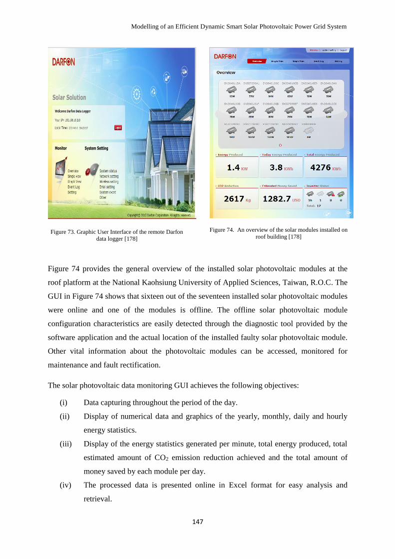
Modelling of an Efficient Dynamic Smart Solar Photovoltaic Power Grid System
147
Figure 73. Graphic User Interface of the remote Darfon
data logger [178]
Figure 74. An overview of the solar modules installed on
roof building [178]
Figure 74 provides the general overview of the installed solar photovoltaic modules at the
roof platform at the National Kaohsiung University of Applied Sciences, Taiwan, R.O.C. The
GUI in Figure 74 shows that sixteen out of the seventeen installed solar photovoltaic modules
were online and one of the modules is offline. The offline solar photovoltaic module
configuration characteristics are easily detected through the diagnostic tool provided by the
software application and the actual location of the installed faulty solar photovoltaic module.
Other vital information about the photovoltaic modules can be accessed, monitored for
maintenance and fault rectification.
The solar photovoltaic data monitoring GUI achieves the following objectives:
(i) Data capturing throughout the period of the day.
(ii) Display of numerical data and graphics of the yearly, monthly, daily and hourly
energy statistics.
(iii) Display of the energy statistics generated per minute, total energy produced, total
estimated amount of CO2 emission reduction achieved and the total amount of
money saved by each module per day.
(iv) The processed data is presented online in Excel format for easy analysis and
retrieval.
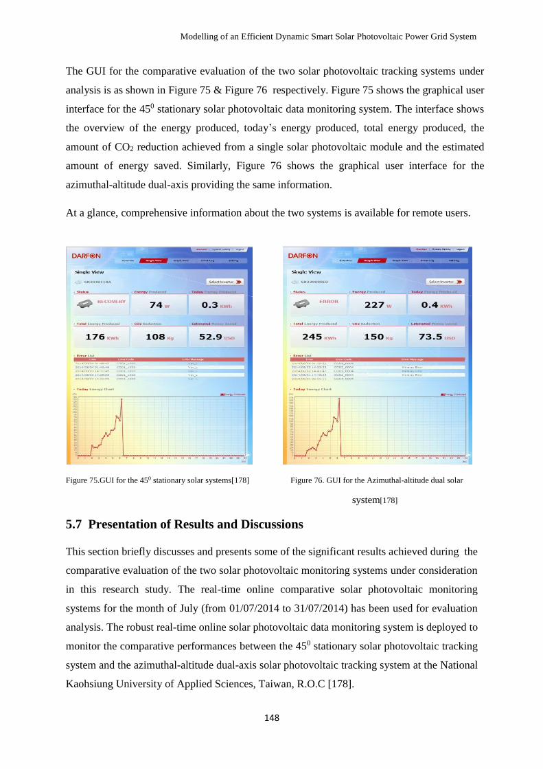
Modelling of an Efficient Dynamic Smart Solar Photovoltaic Power Grid System
148
The GUI for the comparative evaluation of the two solar photovoltaic tracking systems under
analysis is as shown in Figure 75 & Figure 76 respectively. Figure 75 shows the graphical user
interface for the 450 stationary solar photovoltaic data monitoring system. The interface shows
the overview of the energy produced, today’s energy produced, total energy produced, the
amount of CO2 reduction achieved from a single solar photovoltaic module and the estimated
amount of energy saved. Similarly, Figure 76 shows the graphical user interface for the
azimuthal-altitude dual-axis providing the same information.
At a glance, comprehensive information about the two systems is available for remote users.
Figure 75.GUI for the 450 stationary solar systems[178] Figure 76. GUI for the Azimuthal-altitude dual solar
system[178]
5.7 Presentation of Results and Discussions
This section briefly discusses and presents some of the significant results achieved during the
comparative evaluation of the two solar photovoltaic monitoring systems under consideration
in this research study. The real-time online comparative solar photovoltaic monitoring
systems for the month of July (from 01/07/2014 to 31/07/2014) has been used for evaluation
analysis. The robust real-time online solar photovoltaic data monitoring system is deployed to
monitor the comparative performances between the 450 stationary solar photovoltaic tracking
system and the azimuthal-altitude dual-axis solar photovoltaic tracking system at the National
Kaohsiung University of Applied Sciences, Taiwan, R.O.C [178].
Modelling of an Efficient Dynamic Smart Solar Photovoltaic Power Grid System
149
The overall comparative energy output efficiency of the azimuthal-altitude dual-axis over the
450 stationary solar photovoltaic monitoring system as observed in Figure 75 and Figure 76
respectively is approximately 72% based on the total energy produced, estimated money
saved and the amount of CO2 reduction achieved.
In particular, Figure 77 and Figure 78 respectively shows the daily profile for the mean daily
total energy produced for the month of July 2014. It is observed from these figures that the
daily total energy produced for the azimuthal-altitude dual-axis for the month of July was
found to be 39.93 KWH is relatively higher than the 450 stationary solar photovoltaic
tracking systems which were found to be 21.85KWH subject to variation in solar insolation
level and temperature during each day. In comparing the total amount of energy produced by
the two tracking systems, it was found that the azimuthal-altitude dual-axis tracking systems
was 68.43% efficient considering the overall daily generated energy for the month.
Moreover, it is be observed that energy produced from day 16 to day 21 for the month of July
2014 was almost relatively zero due to the typhoon and bad weather condition during this
period [178].
Similarly, a 24-hourly graphical energy chart generated by the 450 stationary and the
azimuthal-altitude dual-axis solar photovoltaic tracking systems are as shown in Figure 77
and Figure 78 respectively under the same solar insolation, temperature, humidity and wind
direction for the last day of the month in July. A close-by visual observation of the figures
clearly underscores a significant increase in the amount of harvested energy by the dual-axis
solar photovoltaic tracking system as compared with the 450 stationary solar photovoltaic
tracking system from the second to the fifteenth hour with corresponding wattage energy
generated during this last day of the month.

Modelling of an Efficient Dynamic Smart Solar Photovoltaic Power Grid System
150
Figure 77. Daily profile of the mean daily total energy
450 for the stationary solar systems [178]
Figure 78. Daily profile of the mean daily total energy
for the Azimuthal-altitude dual solar system [178]
Another critical aspect of the result of the comparative analysis study is the initial cost
implementation and installation period for the two solar photovoltaic tracking systems under
evaluation. The initial installation setup period and cost implication for the azimuthal-altitude
dual-axis solar photovoltaic energy system is relatively high as compared to the 450 stationary
solar photovoltaic energy system.
Based on the achieved and calculated results for the month of July, the estimated hourly
profile for the 450 stationary solar photovoltaic energy system was found to be 1124W and for
the azimuthal-altitude solar photovoltaic energy system, it was found to be 1515W. The
overall comparative hourly energy efficiency of the azimuthal-altitude dual-axis over the 450
stationary solar photovoltaic energy system is approximately 74.2%. It is evident that over
the installation lifetime as observed in Figure 79 and Figure 80 respectively, the energy
harvested from the dual-axis solar photovoltaic system throughout its lifetime will
significantly outweigh the 450 stationary solar photovoltaic energy system in terms of
estimated amount of money saved hourly irrespective of physical and environmental
conditions.
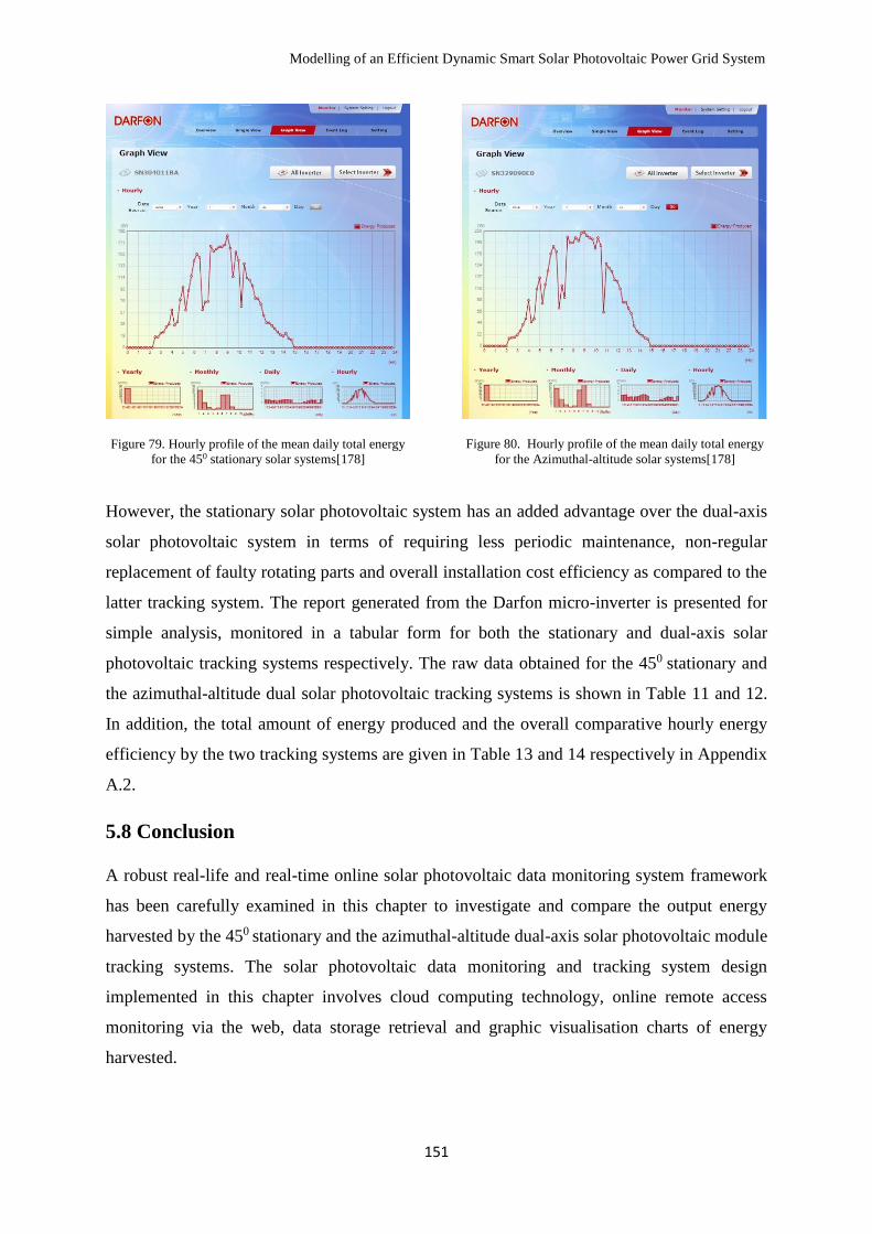
Modelling of an Efficient Dynamic Smart Solar Photovoltaic Power Grid System
151
Figure 79. Hourly profile of the mean daily total energy
for the 450 stationary solar systems[178]
Figure 80. Hourly profile of the mean daily total energy
for the Azimuthal-altitude solar systems[178]
However, the stationary solar photovoltaic system has an added advantage over the dual-axis
solar photovoltaic system in terms of requiring less periodic maintenance, non-regular
replacement of faulty rotating parts and overall installation cost efficiency as compared to the
latter tracking system. The report generated from the Darfon micro-inverter is presented for
simple analysis, monitored in a tabular form for both the stationary and dual-axis solar
photovoltaic tracking systems respectively. The raw data obtained for the 450 stationary and
the azimuthal-altitude dual solar photovoltaic tracking systems is shown in Table 11 and 12.
In addition, the total amount of energy produced and the overall comparative hourly energy
efficiency by the two tracking systems are given in Table 13 and 14 respectively in Appendix
A.2.
5.8 Conclusion
A robust real-life and real-time online solar photovoltaic data monitoring system framework
has been carefully examined in this chapter to investigate and compare the output energy
harvested by the 450 stationary and the azimuthal-altitude dual-axis solar photovoltaic module
tracking systems. The solar photovoltaic data monitoring and tracking system design
implemented in this chapter involves cloud computing technology, online remote access
monitoring via the web, data storage retrieval and graphic visualisation charts of energy
harvested.

Modelling of an Efficient Dynamic Smart Solar Photovoltaic Power Grid System
152
The uniqueness and robustness in the design implementation of the Darfon micro-inverter
installed at the back of the solar photovoltaic module for seamless conversion of DC power to
AC power from each solar photovoltaic module removes the need for a separate central
inverter system reducing installation lifetime inefficiency and costs implications.
In addition, this chapter makes a clear distinction from previously proposed research by
contributing to academic knowledge, the newly robust real-time online solar photovoltaic
data monitoring devices to assess performances in determining the maximum energy
harvested from each of the solar photovoltaic modules under varying physical and
environmental conditions over the lifetime of the installation. The results of the newly
proposed online real-time comparative solar photovoltaic data tracking systems for the
energy forecast database is thus presented with detailed figures in this chapter and
appendices.
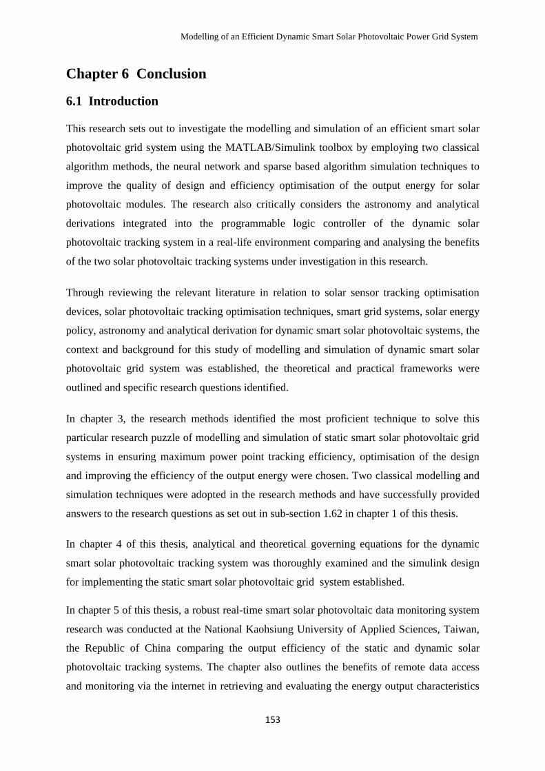
Modelling of an Efficient Dynamic Smart Solar Photovoltaic Power Grid System
153
Chapter 6 Conclusion
6.1 Introduction
This research sets out to investigate the modelling and simulation of an efficient smart solar
photovoltaic grid system using the MATLAB/Simulink toolbox by employing two classical
algorithm methods, the neural network and sparse based algorithm simulation techniques to
improve the quality of design and efficiency optimisation of the output energy for solar
photovoltaic modules. The research also critically considers the astronomy and analytical
derivations integrated into the programmable logic controller of the dynamic solar
photovoltaic tracking system in a real-life environment comparing and analysing the benefits
of the two solar photovoltaic tracking systems under investigation in this research.
Through reviewing the relevant literature in relation to solar sensor tracking optimisation
devices, solar photovoltaic tracking optimisation techniques, smart grid systems, solar energy
policy, astronomy and analytical derivation for dynamic smart solar photovoltaic systems, the
context and background for this study of modelling and simulation of dynamic smart solar
photovoltaic grid system was established, the theoretical and practical frameworks were
outlined and specific research questions identified.
In chapter 3, the research methods identified the most proficient technique to solve this
particular research puzzle of modelling and simulation of static smart solar photovoltaic grid
systems in ensuring maximum power point tracking efficiency, optimisation of the design
and improving the efficiency of the output energy were chosen. Two classical modelling and
simulation techniques were adopted in the research methods and have successfully provided
answers to the research questions as set out in sub-section 1.62 in chapter 1 of this thesis.
In chapter 4 of this thesis, analytical and theoretical governing equations for the dynamic
smart solar photovoltaic tracking system was thoroughly examined and the simulink design
for implementing the static smart solar photovoltaic grid system established.
In chapter 5 of this thesis, a robust real-time smart solar photovoltaic data monitoring system
research was conducted at the National Kaohsiung University of Applied Sciences, Taiwan,
the Republic of China comparing the output efficiency of the static and dynamic solar
photovoltaic tracking systems. The chapter also outlines the benefits of remote data access
and monitoring via the internet in retrieving and evaluating the energy output characteristics
Modelling of an Efficient Dynamic Smart Solar Photovoltaic Power Grid System
154
of the dual-axis solar photovoltaic tracking system over the static solar photovoltaic tracking
system.
This concluding chapter presents a concise deduction integrating all the results achieved in
the previous chapters. Furthermore, significant outcomes in the earlier chapters are discussed
and suggestions made for future research to further contribute to the existing body of
knowledge in understanding the robust real-time online dynamic smart solar photovoltaic
monitoring and tracking systems.
6.2 Impacts and Conceptualisation Benefits of this Research Study
Some of the key concepts and impacts of this research are briefly highlighted and discussed
in context and background of the existing research. The relevance and timeliness of the
research in light of the abundance of solar energy reaching the earth unlike other sources of
power generation which are scarce in some regions of the world. The global awareness of the
impacts and concepts of the solar photovoltaic energy industry has metamorphosized into
many innovative research institutions, creative solar power generation inventions and
contributions in helping to reduce the mammoth emissions of greenhouse gases (carbon
dioxide, chlorofluorocarbons (CFCs), methane, nitrous oxides and ozone) from the
conventional power generation stations contributing to the present crisis of global warming,
climate changes and weather conditions.
The results presented in chapter 5 clearly show the impacts and the benefits of the solar
photovoltaic energy industry, in terms of the total amount of energy produced, estimated
amount of money saved, energy produced from a solar photovoltaic module, inverter status of
the smart solar photovoltaic grid system and the amount of CO2 reduction achieved. The
solar photovoltaic energy policies with government provisional support schemes on rebates
and grants for homes and businesses encourages private participation to reduce carbon
footprints in small and large-scale systems by promoting clean energy generation, thereby
helping owners save a substantial sum on utility bills now and in the future.
The concepts and potentials of using computational modelling in simulating solar
photovoltaic module systems are equally important for improving its overall performance
before actual installation. This facilitates efficient solar photovoltaic module design and
quality improvement by ensuring maximum power point tracking (MPPT) is achieved under

Modelling of an Efficient Dynamic Smart Solar Photovoltaic Power Grid System
155
any environmental conditions (variable solar irradiance and temperature) due to the peculiar
nonlinear characteristics nature of the solar photovoltaic module. The computational
modelling approach offers remarkable progress in many research fields providing scholars
with a powerful software tool in understanding the characteristic behaviour through cognitive
learning theory with graphical representation and interpretations. Furthermore, the
computational approach helps in analysing built models and making inferences to generic
modelling equations to validate the relationship between structural mathematical equations
underlying the model and research hypotheses.
The energy market is moving from being environmentally green to economically green. The
assessment impacts of small and large-scale photovoltaic systems installed in remote areas
improve the power quality through dispersed renewable generation contributing to
sustainable development of human activities. The ongoing global campaign and support for
environmentally renewable energy sources against conventional power generation options are
obvious because of its negative contribution to air pollution, climate change, water and land
pollution, landscape degradation and harmful radiation emissions. The socio-economic
benefits are massive, providing job opportunities and security for teeming unemployed
citizens and diversification in renewable energy supply encouraging decentralisation of
national grid networks into regional grid networks.
6.3 Significance of Classical Modelling Algorithms on solar photovoltaic
systems
The classical modelling algorithm employs tools from mathematical logic to answer
modelling and theoretical questions arising from algorithmic issues in nonlinear mathematical
structures, modelling data and computations. The classical modelling algorithm in solar
photovoltaic systems provide solutions for complex non-linear mathematical equation models
offering accurate predictions and generalisation under variable input parameters and
conditions.
As has been thoroughly examined in chapter 3, the significance of the two classical
modelling algorithms on the smart static solar photovoltaic module, namely neural network
and sparse based algorithm model in the optimisation improvement and design of high
quality efficient long lasting solar photovoltaic modules, is fundamental for solar

Modelling of an Efficient Dynamic Smart Solar Photovoltaic Power Grid System
156
photovoltaic manufacturers. The algorithm model ensures a high tolerance level achieving
superlative output consistency and quality checks of the solar photovoltaic modules.
However, classical modelling and simulation explores and estimates the crystal structure and
electrical behaviour of the solar photovoltaic module with respect to changes on
environmental parameters such as temperature and irradiance level. The solar photovoltaic
simulation model uses iterative analysis to evaluate the characteristics model compared with
the conventional model. The datasets for simulation are subdivided into three distinctive
segments namely training, validation and verification sets to assess the performance of the
model. This provides a relatively low-cost way of collecting information for efficiency
optimisation in design due to the complex nature of the solar photovoltaic modules.
6.4 Significance of the Simulink Solar Photovoltaic Design Model
The Mathworks simulink tool is used in various research fields for design processes, image
and pattern recognition, image tracking processes, constructing models for detailed analysis
and code generation, capturing model performances characteristics and integration of
simulink block components versatility in model testing capabilities. This tool enables
flexibility for software application users and engineers working on complex models, control
models, unrealistic applications to design an algorithm process providing a unique solution
by employing advanced methodologies derived from adaptive, nonlinear and robust control
theories to achieve the intended objectives.
The simulink solar photovoltaic model concepts are built on the implementation of open-
system and user-friendly simblock sets in the Matlab toolbox with the flexibility of
modifying the design to accommodate future expansion. The simblock sets are used in power
engineering fields to build the intended design model by assembling different simulink block
component models suitably creating a user-friendly system validating the model with the time
domain solver configuration. The simulink block libraries permit the designer to select and
connect block models of choice from the library parameters and components facilitating
analysis, testing interfaces and nodes, displaying graphical and numerical figures and
variables respectively at connected terminal scopes.
However, the Matlab/Simulink implementation orientates from a perceived process to
address a particular challenge, having a foreknowledge of the intended design objectives,

Modelling of an Efficient Dynamic Smart Solar Photovoltaic Power Grid System
157
understanding complex requirements and concepts to be transformed into an expected desired
solution. The software tool makes handling complex dynamic analysis in engineering and
non-engineering designs easier with advantages of simulating intended designs with
possibilities of making what is abstract real in its final output presentation. The
Matlab/Simulink software tool is a powerful, versatile and portable tool providing an easy
transition from model-based integration design environment to real-world state-of-the-art
solutions where performance has precedence over price, especially in research fields.
6.5 Benefits of Robust Online Cloud Computing Solar Photovoltaic
Tracking Systems
The emergence of cloud computing technologies in smart solar photovoltaic tracking systems
has made a tremendous impact in the smart solar photovoltaic energy industry through the
use of information and communications technology (ICT) devices for hosting and delivering
energy data information via the web. This platform has been very powerful, reliable and cost-
efficient revealing the current state-of-the-art implementation redefining and making the
renewable energy industry attractive to private, public, foreign and government investors.
Since the inception of cloud computing technologies, many definitions have emerged from
literature; the national institute of standards and technology (NIST) describes it as a model
for enabling ubiquitous, convenient, on-demand network access to a shared pool of
configurable computing resources (e.g. networks, servers, storage, applications, and services)
that can be rapidly provided with minimal management effort and service provider
interaction.
The cloud computing technology is similar to grid computing established on two foundations;
namely information technology (IT) and commercial dexterity. IT is constantly evolving with
fast innovations driven by scientific computational intensive applications in scalable physical
and virtual hardware resources of high-speed processor computers, servers, tablets, mobile
devices, etc. and user-friendly, flexible software resources. The commercial dexterity
perspective of cloud computing challenges the energy industry in providing a cutting-edge
technological cloud solutions functionality and interactive applications responding in real-
time for users globally for rapidly scalable deployment. The stakeholders of commercial
cloud computing offer transaction deals, installation agreements, awarding licensing to
Modelling of an Efficient Dynamic Smart Solar Photovoltaic Power Grid System
158
private and public organisations, consultation and periodic maintenance services of
technological expansion.
Clouding computing technology architecture has independently revolutionised the smart solar
photovoltaic tracking systems by helping to solve the daunting challenges for up-to-date
access of harvested energy data remotely without a physical presence at the installation site.
The advent of cloud computing technology significantly reduces the complexities of
information technology, recurring maintenance, operational and management services costs.
It has significantly reduced the logistic implication of access to huge energy data centers via
the web backbone and cheap power withdrawing physical computer data infrastructure within
the premises of installation. This technology has been able to ensure the provision and
protection of data security, privacy protection, retrieval of energy data and standardizing the
interfaces between various applications over the seamless web network.
The benefits of cloud computing architecture in robust online comparative solar photovoltaic
tracking and monitoring systems cannot be overemphasized; this has been extensively
discussed in chapter 5 of this research. For instance, in section 5.6, the overview of the
installed solar photovoltaic systems is remotely monitored providing an online and offline
status of any of the solar photovoltaic modules on-site. The GUI for the solar photovoltaic
module, provides data information about each of the installed solar photovoltaic modules,
providing detailed information about the amount of energy produced, the daily energy
produced, total energy produced, CO2 reduction, estimated money saved and graphical
energy chart on a daily, monthly and yearly basis. Hence, this gives any authorised user
access to solar photovoltaic data information via the web, to have an instant situation report
of the status of the solar photovoltaic plant system for fault detection and urgent need for
restoration of the plant system to its full capacity and for regular periodic service
maintenance.
6.6 Evaluation of Simulation Smart Solar Photovoltaic Tracking Systems
Computational modelling of the non-linear solar photovoltaic module characteristics has
received much attention in the recent literature using mathematical equations or numerical
approximations for validation of module characteristics under variable insolation levels,
temperatures and degradation conditions. The Matlab/Simulink software tool is employed to
determine the maximum power point tracking (MPPT) of the solar photovoltaic module for

Modelling of an Efficient Dynamic Smart Solar Photovoltaic Power Grid System
159
optimal operation, which strongly depends on the matching load and tracker characteristics
resulting in a better overall performance.
The software tool used in modelling possesses the capabilities of being flexible, compatible
and user-friendly with the intent of validating the proof-of-concept for solar photovoltaic
modules prototypes. The computational simulation for the virtual solar photovoltaic module
emulates the expected response in real-life situations, validating the experimental data of
commercial photovoltaic arrays. The results of the simulation experiments performed on the
solar photovoltaic module using the neural network and sparse based algorithm have been
presented in chapter 3 of this thesis.
Furthermore, computational modelling has enhanced advancement in theory and research on
complex behaviours and systems, developing better performance evaluation by using the
software tool to improve the optimal efficiencies in qualitative engineering design attributes,
minimising drawbacks in real-life circumstances to achieve the potential benefits through the
modelling process. This modelling approach significantly facilitates new framework designs
to surpass obsolete proved validated results by improving on the existing underpinning
research areas at low-cost and in a more convenient environment.
Simulation offers abstraction mechanisms for researchers to critically examine models
without mutilating simulators, ratifying abstractions by comparing detailed and abstract
results. Simulator tools can be integrated seamlessly with emulator interface to improve the
expected quality of design in order to achieve desired results. Nonetheless, irrespective of
whatever complex systems are undertaken by the simulator and emulator interface, the
performance results can be dynamically and visually presented in a unique and very clear
way for understanding. The expandability of boundaries of the simulator and emulator
software tool to accommodate new additional functionalities to explore and achieve an
improved and unique design make computational modelling interesting to researchers in
various fields.
6.7 Significance of this Research
Several smart solar photovoltaic simulation and modelling algorithms have been proposed in
the literature. However, all converge towards emphasizing the common graphical charts of
the current-voltage (I-V) and power-voltage (P-V) solar photovoltaic characteristics under
variable insolation levels and temperatures. In the process of answering the research

Modelling of an Efficient Dynamic Smart Solar Photovoltaic Power Grid System
160
questions as identified in chapter 1 of this thesis, this doctoral research makes a number of
significant contributions, academically and to the commercial solar photovoltaic energy
industry by achieving an accuracy of about 99% with the statistical parameters chosen. The
primary aim of this research was to present a novel cloud computing robust real-time online
comparative monitoring of two solar photovoltaic module tracking systems using simulation
and modelling approach employing the neural network and sparse based regression algorithm
to improve the quality design of photovoltaic modules.
This thesis has presented a cloud computing robust real-time online comparative solar
photovoltaic tracking systems which have been extensively discussed in chapter 5, relating
the innovative research measures of accessing energy data remotely on mobiles, tablets and
PCs at any period of the day. The robust adaptive and tracking devices have substantially
improved on the optimisation, performance and high concentration of harvested energy in
hybrid solar photovoltaic tracking systems. The cloud computing architectural design for the
robust real-time online solar photovoltaic monitoring system is deployed on the roof platform
at the National Kaohsiung University of Applied Sciences, Taiwan, R.O.C, which has been
described in chapter 5. The design combination phase is supported by a unique
interconnectivity of robust electronic component devices and tracking system devices.
This research proposed a new simulation and modelling approach based on a comparative
study of two classical neural network methods for the static solar photovoltaic module
(SSPV) under variable input parameters and conditions. The comparative analysis and
performance were based on the general mathematical model equation of the simplest model
of an equivalent circuit solar photovoltaic module. The mean square error (MSE) and
autocorrelation coefficient metrics were employed to measure the output performance and an
accuracy of approximately 99% was achieved with negligible mean square error value
providing precise prediction and generalisation on the quality lifespan of the solar
photovoltaic module in the face of degradation.
Similarly, a sparse based regression algorithm estimation simulation and modelling were
conducted on the static solar photovoltaic module (SSPV) to measure the performance,
efficiency and reliability of the photovoltaic module. The mean square error (MSE), root
mean square error (RMSE) and standard error of estimate metrics were used to measure the
performance of the three regression methods under investigation to evaluate the maximum
power point tracking for current, voltage and power respectively. Statistical based data results

Modelling of an Efficient Dynamic Smart Solar Photovoltaic Power Grid System
161
of the feasibility and performance studies are reported in chapter 3 evaluating the
performance of these three regression methods.
Alongside the simulation and modelling benefits, this research has proffered transforming
possibilities of information and communications technology (ICT) integration with seamless
remote energy data transmission and accessibility has been established. The solar renewable
research engineers and managers have the opportunity of a first-hand information about the
installed solar photovoltaic array onsite providing interdependent remote access to the
harvested energy data through monitoring on hourly, daily, monthly and yearly basis without
a physical presence at the site location, thereby solving the perennial fundamental challenge
of retrieving accurate harvested energy data. This development framework and innovations in
robust real-time solar photovoltaic modules have increased the validity of energy data
harvested, output efficiency of the system and response feedback performance assessment.
Finally, this research has reviewed the smart solar photovoltaic grid tracking system devices,
solar photovoltaic energy policies, reliability perspective of the theoretical frameworks in
context and background. This doctoral research has made a valuable contribution to both the
academic world in published papers and commercially to the solar photovoltaic energy
industry. The research outcomes have been rationally presented as well in the chapters of this
thesis, some of the results are presented in the appendices. The robust real-time online solar
photovoltaic tracking systems integration with cloud computing technologies was
implemented at the National Kaohsiung University of Applied Sciences, Taiwan, R.O.C,
presenting a new innovation concept and design for the solar energy industry.
6.8 Recommendations for Future Research
While the study has made valuable contributions to both the academic world and the
commercial solar photovoltaic energy industry, it also highlights the need for further research
in a number of areas. Taking into consideration some of the research challenges such as
timeframes, manpower and cost implications of equipment required for this research
implementation, it was a challenge to cover all the scope of the research through a broader
perspective. Additionally, it was not feasible to perform simulation and modelling
experiments with other relevant engineering software applications due to costs and limited
funds allocation for this doctoral research study.

Modelling of an Efficient Dynamic Smart Solar Photovoltaic Power Grid System
162
Further research work is required to enhance and improve on the novel robust real-time
online cloud computing solar photovoltaic monitoring system deployment on a large scale. In
addition, the introduction of newly robust adaptive tracking devices and designs for
maximum optimisation of the solar photovoltaic tracking system would provide a more
proficient way of accessing harvested energy information via the web overcoming the
outmoded energy data report challenges. Given the importance of this novel discovery of
accessing harvested solar energy data from solar photovoltaic arrays on mobiles, tablets, PCs
and other devices remotely, this study can be extended and applied to other renewable energy
sources of power generation enhancement in small, medium and large-scale deployment.
Other areas for future research extension are in the introduction and application of newly
developed software engineering tools on methodologies to improve the conducted model tests
and quality of the solar photovoltaic module design. Research on the new software
applications needs to be monitored by employing the same simple standard equivalent circuit
with the mathematical equation for a solar photovoltaic module to validate and improve on
the results. The use of this new software will determine how much improvement is
achievable on the quality of the design model for the solar photovoltaic module. This
research has developed an empirical model fit in the simulation and modelling experiments
performed in chapters 3 and 4 respectively, though this needs further improvement to
establish its validity and reliability across a wider range of software application tools.
In conclusion, there is a growing body of knowledge and interest in this new aspect of cloud
computing technology integration with solar photovoltaic energy providing real-time
harvested energy data. This should be encouraged in energy conferences and journal research
institutions to participate in further discovery of new qualitative and innovative design
concepts in this industry. Furthermore, additional simulation and modelling experiments need
to be carried out with the introduction of new engineering software application tools
identifying the demand for a holistic approach to quality improvement and assurance of the
solar photovoltaic module. The solar photovoltaic energy industry is continuously undergoing
review in ensuring the renewable energy targets (RETs) for the industry is achievable. The
RETs welcome collaboration with other sustainable clean energy projects for pioneering
research efforts mainly to fill the gap in solving the global climate control challenges and
greenhouse gases (GHG) emissions contributed by the power generation industry.

Modelling of an Efficient Dynamic Smart Solar Photovoltaic Power Grid System
163
Bibliography
1. Moslehi, K. and R. Kumar. Smart grid-a reliability perspective. in Innovative Smart Grid
Technologies (ISGT). 2010. IEEE.
2. Seo, G.-S., et al. Modeling and analysis of DC distribution systems. in Power Electronics and
ECCE Asia (ICPE & ECCE), 2011 IEEE 8th International Conference on. 2011. IEEE.
3. Farhangi, H., The path of the smart grid. Power and Energy Magazine, IEEE, 2010. 8(1): p.
18-28.
4. Moslehi, K. and R. Kumar, A reliability perspective of the smart grid. Smart Grid, IEEE
Transactions on, 2010. 1(1): p. 57-64.
5. Potter, C.W., A. Archambault, and K. Westrick. Building a smarter smart grid through better
renewable energy information. in Power Systems Conference and Exposition, 2009. PSCE'09.
IEEE/PES. 2009. IEEE.
6. Natsheh, E.M., A. Albarbar, and J. Yazdani. Modeling and control for smart grid integration
of solar/wind energy conversion system. in Innovative Smart Grid Technologies (ISGT
Europe), 2011 2nd IEEE PES International Conference and Exhibition on. 2011. IEEE.
7. Ipakchi, A. and F. Albuyeh, Grid of the future. Power and Energy Magazine, IEEE, 2009.
7(2): p. 52-62.
8. Administration, E.I., How much electricity is lost in transmission and distribution in the
United States? Energy Data & Statistics, 2014, May 7. Online.
9. Oliver, M. and T. Jackson, The market for solar photovoltaics. Energy Policy, 1999. 27(7): p.
371-385.
10. Protocol, K., United Nations framework convention on climate change. Kyoto Protocol,
Kyoto, 1997.
11. King, D.L., J. Kratochvil, and W.E. Boyson. Measuring solar spectral and angle-of-incidence
effects on photovoltaic modules and solar irradiance sensors. in Photovoltaic Specialists
Conference, 1997., Conference Record of the Twenty-Sixth IEEE. 1997. IEEE.
12. Fraden, J., Handbook of modern sensors: physics, designs, and applications. 2004: Springer
Science & Business Media.
13. Balogun, E.B., X. Huang, and D. Tran. Efficiency of Sensor Devices Used in Dynamic Solar
Tracking System: Comparative Assessment Parameters Review. in Applied Mechanics and
Materials. 2014. Trans Tech Publ.
14. Brignell, J.E. and N.M. White, Intelligent Sensor Systems: 2nd. 1996: institute of Physics
Publishing.
15. Taylor, H.R., Data acquisition for sensor systems. Vol. 5. 1997: Springer Science & Business
Media.
16. Webster, J.G. and H. Eren, Measurement, Instrumentation, and Sensors Handbook: Spatial,
Mechanical, Thermal, and Radiation Measurement. Vol. 1. 2014: CRC press.
17. Pallas-Areny, R. and J.G. Webster, Sensors and Signal Conditioning. illustrated, annotated
ed. 1993: Wiley,. 416.
18. Diffenderfer, R., Electronic Devices: System and Applications. Vol. 1. 2005, 5 Maxwell
Drive, P.O.Box 8007, Clifton Park NY 12605-8007: Thomson Delmar Learning Executive
Woods.
19. Optoelectronics, Basic PIN Photodiode Characteristics;
http://www.osioptoelectronics.com/technology-corner/frequently-asked-questions/basic-pin-
photodiode-characteristics.aspx.
20. Arturo, M.M. and G.P. Alejandro. High-precision solar tracking system. in Proceedings of
the World Congress on Engineering. 2010.
21. Papalias, T.A. and M. Wong, Making Sense of Light Sensors. Application notes, CA: Intersil
Americas Inc, 2007.
22. Poole, I., Resources and Analysis for Electronics Engineers; http://www.radio-
electronics.com/, in Adrio Communications Ltd. 2012.
23. Wikipedia, Nantenna Spectral wavelength images, http://en.wikipedia.org/wiki/Nantenna.
Wikipedia, 2012(Wikipedia Foundation, Inc.).Retrieved on 02/03/2014.
Modelling of an Efficient Dynamic Smart Solar Photovoltaic Power Grid System
164
24. Kalantar-zadeh, K. and B. Fry, Nanotechnology-Enabled Sensors. 1 ed. 2008: Springer US.
XII, 492.
25. Collins, D. and J. Faust, CCD Video Camera and Imaging Techniques for Stellar Photometry.
International Amateur-Professional Photoelectric Photometry Communications, 1989. 36: p.
22.
26. Berland, B., Photovoltaic technologies beyond the horizon: optical rectenna solar cell. 2003,
NREL/SR-520-33263.
27. Bakos, G.C., Design and construction of a two-axis Sun tracking system for parabolic trough
collector (PTC) efficiency improvement. Renewable energy, 2006. 31(15): p. 2411-2421.
28. Lynch, W.A. and Z.M. Salameh, Simple electro-optically controlled dual-axis sun tracker.
Solar Energy, 1990. 45(2): p. 65-69.
29. Ghosh, D., Structurally Integrated Luminescence Based Oxygen Sensors with Organic
LED/oxygen Sensitive Dye and PECVD Grown Thin Film Photodetectors. 2008: ProQuest.
30. Dell, An advanced 55cm (21.5") Full HD monitor, http://www.dell.com/ed/business/p/dell-
sx2210wfp/pd. 2012.
31. PerkinElmer Photoconductive Cells and Photoconductive Cells and Analog Optoisolators (V
Analog Optoisolators (Vactrols®) actrols®);
http://www.alltronics.com/mas_assets/acrobat/28S004.pdf. PerkinElmer Optoelectronics,
2001. 77. Retrieved on 12/04/2013.
32. Wikipedia, Diode, https://en.wikipedia.org/wiki/Diode. The free encyclopedia,
2012.Retrieved on 12/04/2013
33. Cuevas, A., The Recombination Parameter J0. Energy Procedia, 2014. 55(0): p. 53-62.
34. Bowden, C.H.a.S., Welcome to the Photovoltaic Education Network, http://pveducation.org/.
35. Energy, R.G., Renewable Global Energy. a division of MBE Services Inc. Online, Online.
Online.
36. NJCEP. NEW JERSEY'S CLEAN ENERGY PROGRAM; http://www.njcleanenergy.com/.
[Online] 2012 [cited Online; Available from: http://www.njcleanenergy.com/. Retrieved on
15/02/2014
37. Duckat, R. and G. Nord-Süd-Initiative eV, CO_1tn2-Abscheidung und-Lagerung als Beitrag
zum Klimaschutz?: Ergebnisse des" IPCC Workshop on Carbon Dioxide Capture and
Storage" vom November 2002 und Bewertung durch Germanwatch. 2004: Germanwatch.
38. Benghanem, M., Optimization of tilt angle for solar panel: Case study for Madinah, Saudi
Arabia. Applied Energy, 2011. 88(4): p. 1427-1433.
39. Duerr, F., Y. Meuret, and H. Thienpont, Tracking integration in concentrating photovoltaics
using laterally moving optics. Optics express, 2011. 19(103): p. A207-A218.
40. Tassen, D., Sun tracker with dual axis support for diurnal movement and seasonal
adjustment. 1979, Google Patents.
41. Catarius, A., Azimuth-Altitude Dual Axis Solar Tracker. 2010, WORCESTER
POLYTECHNIC INSTITUTE. p. 88.
42. Rhif, A., A position control review for a photovoltaic system: Dual axis Sun Tracker. IETE
Technical Review, 2011. 28(6): p. 479-485.
43. Sood, V., et al. Developing a communication infrastructure for the smart grid. in Electrical
Power & Energy Conference (EPEC), 2009 IEEE. 2009. IEEE.
44. Varaiya, P.P., F.F. Wu, and J.W. Bialek, Smart operation of smart grid: Risk-limiting
dispatch. Proceedings of the IEEE, 2011. 99(1): p. 40-57.
45. Ewing, R.H., et al., Best development practices: a primer for smart growth. 1998: Smart
Growth Network Washington, DC.
46. Kolhe, M., Smart grid: charting a new energy future: research, development and
demonstration. The Electricity Journal, 2012. 25(2): p. 88-93.
47. Gellings, C.W., The smart grid: enabling energy efficiency and demand response. 2009: The
Fairmont Press, Inc.
48. Berman, F., et al., The GrADS project: Software support for high-level grid application
development. International Journal of High Performance Computing Applications, 2001.
15(4): p. 327-344.
Modelling of an Efficient Dynamic Smart Solar Photovoltaic Power Grid System
165
49. Spiegel, R., et al., Emissions reduction data for grid-connected photovoltaic power systems.
Solar energy, 2000. 68(5): p. 475-485.
50. Lo, C.-H. and N. Ansari, The progressive smart grid system from both power and
communications aspects. Communications Surveys & Tutorials, IEEE, 2012. 14(3): p. 799-
821.
51. Fan, Z., et al., Smart grid communications: Overview of research challenges, solutions, and
standardization activities. Communications Surveys & Tutorials, IEEE, 2013. 15(1): p. 21-
38.
52. Hossain, E., Z. Han, and H.V. Poor, Smart grid communications and networking. 2012:
Cambridge University Press.
53. Fox-Penner, P., Smart Power Anniversary Edition: Climate Change, the Smart Grid, and the
Future of Electric Utilities. 2014: Island Press.
54. Johnstone, N., I. Haščič, and D. Popp, Renewable energy policies and technological
innovation: evidence based on patent counts. Environmental and Resource Economics, 2010.
45(1): p. 133-155.
55. Carley, S., State renewable energy electricity policies: An empirical evaluation of
effectiveness. Energy Policy, 2009. 37(8): p. 3071-3081.
56. Sioshansi, F.P., Smart grid: integrating renewable, distributed & efficient energy. 2011:
Academic Press.
57. Zhong, Q.-C. and T. Hornik, Control of Power Inverters in Renewable Energy and Smart
Grid Integration. 2012, New York, United States: John Wiley & Sons, Ltd.
58. Knapp, E.D. and R. Samani, Applied Cyber Security and the Smart Grid: Implementing
Security Controls Into the Modern Power Infrastructure. 2013: Newnes.
59. Wikipedia, Sustainable energy;https://en.wikipedia.org/wiki/Sustainable_energy. Energy
economics, 2012(Online). Retrieved on 23/07/2013.
60. Armaroli, N. and V. Balzani, The future of energy supply: challenges and opportunities.
Angewandte Chemie International Edition, 2007. 46(1‐2): p. 52-66.
61. Geller, H., Energy revolution: policies for a sustainable future. 2012: Island Press.
62. Next, H.I.t., Corporate Information-Environmental Activities. Online, Online.
63. Kumbhar, M.M., et al., Smart Grid: New Era of Electricity Distribution Network.
International Proceedings of Computer Science & Information Technology, 2012. 28.
64. Smil, V., General energetics: energy in the biosphere and civilization, in General energetics:
energy in the biosphere and civilization. John Wiley & Sons; 1991. p. 369. Retrieved on
02/03/2013.
65. Smil, V., Energy at the Crossroads. Scientific Challenges for Energy Research, 2006: p. 1-28.
66. Churchill, S., Department of Energy Announces $1.6B for Smart Grid Projects;
http://www.dailywireless.org/2009/11/24/doe-announces-1-6b-for-smart-grid-projects/, in
Newsletter. 2009. Retrieved on 12/03/2014.
67. Bird, L., R. Wüstenhagen, and J. Aabakken, A review of international green power markets:
recent experience, trends, and market drivers. Renewable and Sustainable Energy Reviews,
2002. 6(6): p. 513-536.
68. Kaundinya, D.P., P. Balachandra, and N. Ravindranath, Grid-connected versus stand-alone
energy systems for decentralized power—a review of literature. Renewable and Sustainable
Energy Reviews, 2009. 13(8): p. 2041-2050.
69. Krarup, S. and S. Ramesohl, Voluntary Agreements in Energy Policy-Implementation and
Efficiency; http://www.sei.ie/uploadedfiles/InfoCentre/voluntaryagreementsfinalreport.pdf.
2000, AKF Forlaget; . p. 1-72. Retrieved on 15/07/2013.
70. Jacobsson, S. and A. Bergek, Transforming the energy sector: the evolution of technological
systems in renewable energy technology. Industrial and corporate change, 2004. 13(5): p.
815-849.
71. Urpelainen, J., Export orientation and domestic electricity generation: Effects on energy
efficiency innovation in select sectors. Energy Policy, 2011. 39(9): p. 5638-5646.
72. de Alegría Mancisidor, I.M., et al., European Union's renewable energy sources and energy
efficiency policy review: The Spanish perspective. Renewable and Sustainable Energy
Reviews, 2009. 13(1): p. 100-114.
Modelling of an Efficient Dynamic Smart Solar Photovoltaic Power Grid System
166
73. Wüstenhagen, R. and E. Menichetti, Strategic choices for renewable energy investment:
Conceptual framework and opportunities for further research. Energy Policy, 2012. 40: p. 1-
10.
74. Haas, R., et al., A historical review of promotion strategies for electricity from renewable
energy sources in EU countries. Renewable and sustainable energy reviews, 2011. 15(2): p.
1003-1034.
75. Stavins, R.N., Harnessing market forces to protect the environment. Environment: Science
and Policy for Sustainable Development, 1989. 31(1): p. 5-35.
76. DeSimone, L.D. and F. Popoff, Eco-efficiency: the business link to sustainable development.
2000: MIT press.
77. Langnib, O., Green Power and Public Support: An Analysis of the Interactions. 2001. 4, no.
99: p. 275–284. Retrieved on 27/03/2014.
78. Beurskens, L., M. Hekkenberg, and P. Vethman, Renewable energy projections as published
in the national renewable energy action plans of the European member states. European
Research Centre of the Netherlands (ECN) and European Environmental Agency (EEA),
Petten, 2011.
79. Frondel, M., et al., Economic impacts from the promotion of renewable energy technologies:
The German experience. Energy Policy, 2010. 38(8): p. 4048-4056.
80. Ringquist, E.J., Environmental protection at the state level: Politics and progress in
controlling pollution. 1993: ME Sharpe.
81. Baranzini, A., J. Goldemberg, and S. Speck, A future for carbon taxes. Ecological economics,
2000. 32(3): p. 395-412.
82. Bernard, S.M., et al., The potential impacts of climate variability and change on air pollution-
related health effects in the United States. Environmental health perspectives, 2001.
109(Suppl 2): p. 199.
83. Hoffert, M.I., et al., Energy implications of future stabilization of atmospheric CO2 content.
Nature, 1998. 395(6705): p. 881-884.
84. Patwardhan, A.P., et al., Global Energy Assessment: Toward a Sustainable Future. 2012:
Cambridge University Press.
85. Omer, A.M., Energy, environment and sustainable development. Renewable and sustainable
energy reviews, 2008. 12(9): p. 2265-2300.
86. Kothari, R., D. Buddhi, and R. Sawhney, Comparison of environmental and economic aspects
of various hydrogen production methods. Renewable and Sustainable Energy Reviews, 2008.
12(2): p. 553-563.
87. Peattie, K., Green consumption: behavior and norms. Annual Review of Environment and
Resources, 2010. 35(1): p. 195.
88. Mendonça, M., S. Lacey, and F. Hvelplund, Stability, participation and transparency in
renewable energy policy: Lessons from Denmark and the United States. Policy and Society,
2009. 27(4): p. 379-398.
89. Neuhoff, K., K.K. Martinez, and M. Sato, Allocation, incentives and distortions: the impact of
EU ETS emissions allowance allocations to the electricity sector. Climate Policy, 2006. 6(1):
p. 73-91.
90. Banks, D. and J. Schäffler, The potential contribution of renewable energy in South Africa.
Draft Update Report, 2006.
91. Panwar, N., S. Kaushik, and S. Kothari, Role of renewable energy sources in environmental
protection: a review. Renewable and Sustainable Energy Reviews, 2011. 15(3): p. 1513-1524.
92. Houghton, J.T., B.A. Callander, and S.K. Varney, Climate change 1992: the supplementary
report to the IPCC scientific assessment. 1992: Cambridge University Press.
93. Hoffmann, V.H., Eu ets and investment decisions:: The case of the german electricity
industry. European Management Journal, 2007. 25(6): p. 464-474.
94. Greene, N. and R. Hammerschlag, Small and clean is beautiful: exploring the emissions of
distributed generation and pollution prevention policies. The Electricity Journal, 2000. 13(5):
p. 50-60.
95. Weisser, D., A guide to life-cycle greenhouse gas (GHG) emissions from electric supply
technologies. Energy, 2007. 32(9): p. 1543-1559.
Modelling of an Efficient Dynamic Smart Solar Photovoltaic Power Grid System
167
96. Hawken, P., A.B. Lovins, and L.H. Lovins, Natural capitalism: the next industrial revolution.
2013: Routledge.
97. Pratt, R.G., et al., The smart grid: An estimation of the energy and CO2 benefits. 2010:
Pacific Northwest National Laboratory.
98. Alanne, K. and A. Saari, Distributed energy generation and sustainable development.
Renewable and Sustainable Energy Reviews, 2006. 10(6): p. 539-558.
99. Baer, W.S., S. Hassell, and B.A. Vollaard, Electricity requirements for a digital society. 2002:
Rand Corporation.
100. Franco, A. and P. Salza, Strategies for optimal penetration of intermittent renewables in
complex energy systems based on techno-operational objectives. Renewable energy, 2011.
36(2): p. 743-753.
101. Lasseter, R.H., Microgrids and distributed generation. Journal of Energy Engineering, 2007.
133(3): p. 144-149.
102. Fang, X., et al., Smart grid—The new and improved power grid: A survey. Communications
Surveys & Tutorials, IEEE, 2012. 14(4): p. 944-980.
103. Harrison, C., et al., Foundations for smarter cities. IBM Journal of Research and
Development, 2010. 54(4): p. 1-16.
104. Kirkegaard, J.F., L. Weischer, and T. Hanemann, It should be a breeze: harnessing the
potential of open trade and investment flows in the wind energy industry. Peterson Institute
for International Economics working paper, 2009(09-14).
105. Patel, M.R., Wind and solar power systems: design, analysis, and operation. 2005: CRC
press.
106. Hamilton, K., Unlocking Finance for Clean Energy: The Need for'investment Grade'Policy.
2009: Chatham House London.
107. Foster, I., C. Kesselman, and S. Tuecke, The anatomy of the grid: Enabling scalable virtual
organizations. International journal of high performance computing applications, 2001. 15(3):
p. 200-222.
108. Lyon, L., Dealing with Data: Roles, Rights, Responsibilities and Relationships. Consultancy
Report. 2007.
109. Von Dollen, D., Report to NIST on the smart grid interoperability standards roadmap.
Prepared by the Electric Power Research Institute for NIST (June 2009), 2009.
110. Bichlien, H., Smart Power Grids–Talking about a Revolution;
https://www.ieee.org/about/technologies/emerging/emerging_tech_smart_grids.pdf. 2006-
2012, IEEE Emerging Technology portal: IEEE Emerging Technology portal. Retrieved on
22/02/2015.
111. SGIP, Smart Grid Conceptual Model; http://www.sgip.org/Introduction-to-The-Smart-Grid-
Conceptual-Model.
112. Khurana, H., et al., Smart-grid security issues. IEEE Security & Privacy, 2010(1): p. 81-85.
113. Momoh, J.A. Smart grid design for efficient and flexible power networks operation and
control. in Power Systems Conference and Exposition, 2009. PSCE'09. IEEE/PES. 2009.
IEEE.
114. Gergaud, O., B. Multon, and H.B. Ahmed. Analysis and experimental validation of various
photovoltaic system models. in ELECTRIMACS. 2002.
115. Koutroulis, E. and K. Kalaitzakis, Development of an integrated data-acquisition system for
renewable energy sources systems monitoring. Renewable Energy, 2003. 28(1): p. 139-152.
116. Hall, M. Canadian Solar moves away from direct panel sales; http://www.pv-
magazine.com/news/details/beitrag/canadian-solar-moves-away-from-direct-panel-
sales_100009592/. PV Magazine Global [PV Magazine Newsletter] 2012 14 DECEMBER
Newsletter]; 14 DECEMBER 2012: Retrieved on 16/06/2013.
117. Rauschenbach, H.S., Solar cell array design handbook-The principles and technology of
photovoltaic energy conversion. 1980.
118. Villalva, M.G. and J.R. Gazoli, Comprehensive approach to modeling and simulation of
photovoltaic arrays. Power Electronics, IEEE Transactions on, 2009. 24(5): p. 1198-1208.
119. González-Longatt, F.M., Model of Photovoltaic Module in Matlab™;
https://www.academia.edu/875827/Model_of_Photovoltaic_Module_in_Matlab, in 2nd Latin

Modelling of an Efficient Dynamic Smart Solar Photovoltaic Power Grid System
168
American Congress Of Students Of Electrical Engineering, Electronics And Computing (II
Cibelec 2005). 2005, personnel.univ-reunion.fr. p. 5. Retrieved on 20/04/2014.
120. Kalogirou, S.A., Artificial neural networks in renewable energy systems applications: a
review. Renewable and sustainable energy reviews, 2001. 5(4): p. 373-401.
121. Patterson, D.W., Artificial Neural Networks: Theory And Applications Prentice-Hall Series in
Advanced Communications. illustrated, reissue ed. 1996, the University of California:
Prentice Hall. 477.
122. Fauske, K.M. Neural Network. Texample.Net [Online] 2006-12-07; Available from:
http://www.texample.net/tikz/examples/neural-network/.Retrieved on 05/05/2014.
123. Klerfors, D., Artificial neural networks. St. Louis University, St. Louis, Mo, 1998.
124. Broomhead, D.S. and D. Lowe, Radial basis functions, multi-variable functional
interpolation and adaptive networks. 1988, DTIC Document. Retrieved on 22/08/2014.
125. Casdagli, M., Nonlinear prediction of chaotic time series. Physica D: Nonlinear Phenomena,
1989. 35(3): p. 335-356.
126. Poggio, T. and F. Girosi, Networks for approximation and learning. Proceedings of the IEEE,
1990. 78(9): p. 1481-1497.
127. DTREG. DTREG Pedictive Modeling Software-RBF Neural Networks ; . Online 2014;
Available from: https://www.dtreg.com/solution/view/25.
128. Wikipedia, Radial basis function network;
https://en.wikipedia.org/wiki/Radial_basis_function_network. Wikipedia, 2013. Retrieved on
22/05/2014.
129. Davies, D.L. and D.W. Bouldin, A cluster separation measure. Pattern Analysis and Machine
Intelligence, IEEE Transactions on, 1979(2): p. 224-227.
130. Looney, C.G., Pattern recognition using neural networks: theory and algorithms for
engineers and scientists. 1997: Oxford University Press, Inc.
131. Reed, R.D. and R.J. Marks, Neural smithing: supervised learning in feedforward artificial
neural networks. 1998: Mit Press.
132. Foroozesh, J., et al., Application of artificial intelligence (AI) in kinetic modeling of methane
gas hydrate formation. Journal of the Taiwan Institute of Chemical Engineers, 2014. 45(5): p.
2258-2264. Retrieved on 16/09/2014.
133. Almonacid, F., et al., Estimating the maximum power of a high concentrator photovoltaic
(HCPV) module using an artificial neural network. Energy, 2013. 53: p. 165-172.
134. Ilonen, J., J.-K. Kamarainen, and J. Lampinen, Differential evolution training algorithm for
feed-forward neural networks. Neural Processing Letters, 2003. 17(1): p. 93-105.
135. Wikipedia, Levenberg–Marquardt algorithm;
https://en.wikipedia.org/wiki/Levenberg%E2%80%93Marquardt_algorithm. 2013. Retrieved
on 19/09/2013.
136. Anselin, L., Spatial econometrics: methods and models. Vol. 4. 1988: Springer Science &
Business Media.
137. Sen, A. and M. Srivastava, Regression analysis. 1990: Springer Science & Business Media.
138. MathWorks, MathWorks Documentation. (Support).
139. B.Balogun1, E., et al., Regression Estimation Modelling Techniques on Static Solar
Photovoltaic Module. ISO 9001:2008 Certified Journal, 2015. Volume 5(Issue 4).
140. Balogun, E.B., X. Huang, and D. Tran, Comparative Study of Different Artificial Neural
Networks Methodologies on Static Solar Photovoltaic Module.
141. Li, Y., et al., A sparse representation-based algorithm for pattern localization in brain
imaging data analysis. 2012.
142. Li, Y., et al., Voxel selection in fMRI data analysis based on sparse representation.
Biomedical Engineering, IEEE Transactions on, 2009. 56(10): p. 2439-2451.
143. Hadi, A.S. and J.S. Simonoff, Procedures for the identification of multiple outliers in linear
models. Journal of the American Statistical Association, 1993. 88(424): p. 1264-1272.
144. Weisberg, S., Applied Linear Regression Volume 528 of Wiley Series in Probability and
Statistics. 3, illustrated ed. 2005: John Wiley & Sons.
145. Chen, C., Robust regression and outlier detection with the ROBUSTREG procedure. SUGI
Paper, 2002(265-27).
Modelling of an Efficient Dynamic Smart Solar Photovoltaic Power Grid System
169
146. Cleveland, W.S. and S.J. Devlin, Locally weighted regression: an approach to regression
analysis by local fitting. Journal of the American Statistical Association, 1988. 83(403): p.
596-610.
147. Li, G., Robust regression. Exploring data tables, trends, and shapes, 1985. 281: p. U340.
148. Rousseeuw, P.J. and A.M. Leroy, Robust regression and outlier detection. Vol. 589. 2005:
John Wiley & Sons.
149. Čížek, P. and J.Á. Víšek, Least trimmed squares. 2000: Springer.
150. Doornik, J.A., Robust Estimation Using Least Trimmed Squares. 2011, Oxford, UK: Oxford
Martin School.
151. Alfons, A., C. Croux, and S. Gelper, Sparse least trimmed squares regression for analyzing
high-dimensional large data sets. The Annals of Applied Statistics, 2013. 7(1): p. 226-248.
152. Chong, K. and C. Wong, General formula for on-axis sun-tracking system and its application
in improving tracking accuracy of solar collector. Solar Energy, 2009. 83(3): p. 298-305.
153. Kacira, M., et al., Determining optimum tilt angles and orientations of photovoltaic panels in
Sanliurfa, Turkey. Renewable energy, 2004. 29(8): p. 1265-1275.
154. Lee, C.-Y., et al., Sun tracking systems: a review. Sensors, 2009. 9(5): p. 3875-3890.
155. Mousazadeh, H., et al., A review of principle and sun-tracking methods for maximizing solar
systems output. Renewable and Sustainable Energy Reviews, 2009. 13(8): p. 1800-1818.
156. Tracking, S., Solar tracking elevation and azimuth angles images. (Solar tracking elevation
and azimuth angles images).
157. Luque-Heredia, I., et al., 11 Inspira’s CPV Sun Tracking. Concentrator Photovoltaics, 2007.
130: p. 221.
158. Merlaud, A., et al., Equations for solar tracking. Sensors, 2012. 12(4): p. 4074-4090.
159. Prinsloo, G. and R. Dobson, Sun Tracking and Solar Renewable Energy Harvesting: Solar
Energy Harvesting, Trough, Pinpointing and Heliostat Solar Collecting Systems. Vol. 2.
Gerro Prinsloo.
160. Xie, F. and G. Zhang. Simulation and Analysis of Computer Control Tracking System Based
on Solar Geometric for Fresnel Lenses Concentration Photovoltics. in Intelligent Human-
Machine Systems and Cybernetics (IHMSC), 2011 International Conference on. 2011. IEEE.
Retrieved on 13/01/2014.
161. Hermenean, I., et al., MODELLING AND OPTIMIZATION OF A CPV SYSTEM WITH
EQUATORIAL TRACKING. Bulletin of the Transilvania University of Braşov• 2010. 3: p. 52.
162. Wikipedia, Euler angles (2013). https://en.wikipedia.org/wiki/Euler_angles. Web. Retrieved on
11/06/2014.
163. Chong, K.-K., et al., Integration of an on-axis general sun-tracking formula in the algorithm
of an open-loop sun-tracking system. Sensors, 2009. 9(10): p. 7849-7865.
164. Gow, J. and C. Manning. Development of a photovoltaic array model for use in power-
electronics simulation studies. in Electric Power Applications, IEE Proceedings-. 1999. IET.
165. Tsai, H.-L., Insolation-oriented model of photovoltaic module using Matlab/Simulink. Solar
energy, 2010. 84(7): p. 1318-1326.
166. Khan, M. and M. Iqbal, Dynamic modeling and simulation of a small wind–fuel cell hybrid
energy system. Renewable energy, 2005. 30(3): p. 421-439.
167. Kim, S.-K., et al., Modeling and simulation of a grid-connected PV generation system for
electromagnetic transient analysis. Solar Energy, 2009. 83(5): p. 664-678.
168. Banos, R., et al., Optimization methods applied to renewable and sustainable energy: A
review. Renewable and Sustainable Energy Reviews, 2011. 15(4): p. 1753-1766.
169. Williams, D., Seldads: An Operational Real-Time Solar-Terrestrial Environment Monitoring
System. Technical Report. 1976, National Oceanic and Atmospheric Administration, Boulder,
CO (USA). Space Environment Lab. p. 65. Retrieved on 06/03/2015.
170. Wüstenhagen, R., M. Wolsink, and M.J. Bürer, Social acceptance of renewable energy
innovation: An introduction to the concept. Energy policy, 2007. 35(5): p. 2683-2691.
171. Holler, J., et al., From Machine-to-machine to the Internet of Things: Introduction to a New
Age of Intelligence. 2014: Academic Press.
172. Zanella, A., et al., Internet of things for smart cities. Internet of Things Journal, IEEE, 2014.
1(1): p. 22-32.

Modelling of an Efficient Dynamic Smart Solar Photovoltaic Power Grid System
170
173. Foster, I., et al. Cloud computing and grid computing 360-degree compared. in Grid
Computing Environments Workshop, 2008. GCE'08. 2008. Ieee.
174. Krauter, K., R. Buyya, and M. Maheswaran, A taxonomy and survey of grid resource
management systems for distributed computing. Software: Practice and Experience, 2002.
32(2): p. 135-164.
175. Andersson, B.A. and S. Jacobsson, Monitoring and assessing technology choice: the case of
solar cells. Energy Policy, 2000. 28(14): p. 1037-1049.
176. Foster, I., et al., Grid services for distributed system integration. Computer, 2002. 35(6): p.
37-46.
177. Wheeler, M.C. and H.H. Hendon, An all-season real-time multivariate MJO index:
Development of an index for monitoring and prediction. Monthly Weather Review, 2004.
132(8): p. 1917-1932.
178. Balogun, E.B., et al. A robust real-time online comparative monitoring of an azimuthal-
altitude dual axis GST 300 and a 45° fixed solar photovoltaic energy tracking systems. in
SoutheastCon 2015. 2015. IEEE.
179. Darfon, MIG240 On-Grid Micro Inverter; http://www.darfonsolar.com/productdetail/?pid=7.
2011(Model Number: MIG240).
180. Nachamkin, J. and G.T. Sheehan, Integrated voltaic energy system. 2011, Google Patents.
181. Hicks, S.D., A.K. Aufdenkampe, and D.S. Montgomery. Sensor Networks, Dataloggers, And
Other Handy Gadgets Using Open-Source Electronics For The Christina River Basin Critical
Zone Observatories (CZO); https://criticalzone.org/images/national/associated-
files/Christina/Publications/AGU2011_Poster.pdf. in Fall Meeting, American Geophysical
Union. 2011. Retrieved on 02/03/2015.
182. Tyler, S., Data Acquisition of Extrusion Processes;
http://researchrepository.murdoch.edu.au/21900/. 2014. Retrieved on 29/05/2015.
183. Kim, S., et al., Thermal performance enhancement of mortar mixed with octadecane/xGnP
SSPCM to save building energy consumption. Solar Energy Materials and Solar Cells, 2014.
122: p. 257-263.
184. Kim, Y.-J., et al., A secure decentralized data-centric information infrastructure for smart
grid. Communications Magazine, IEEE, 2010. 48(11): p. 58-65.
185. Bibinagar, N. and W.-j. Kim, Switched Ethernet-based real-time networked control system
with multiple-client–server architecture. Mechatronics, IEEE/ASME Transactions on, 2013.
18(1): p. 104-112.
186. Milosavljevic, B. and D. Tešendic, Software architecture of distributed client/server library
circulation system. The Electronic Library, 2010. 28(2): p. 286-299.
187. Kalogirou, S.A., Solar energy engineering: processes and systems. 2013: Academic Press.
188. Mell, P. and T. Grance, The nist definition of cloud computing, 2011. National Institute of
Standards and Technology Special Publication, 2014: p. 800-145.
189. Subashini, S. and V. Kavitha, A survey on security issues in service delivery models of cloud
computing. Journal of network and computer applications, 2011. 34(1): p. 1-11.
190. Mondal, M.A.H. and A.S. Islam, Potential and viability of grid-connected solar PV system in
Bangladesh. Renewable energy, 2011. 36(6): p. 1869-1874.
191. Seme, S., G. Stumberger, and J. Vorsic, Maximum efficiency trajectories of a two-axis sun
tracking system determined considering tracking system consumption. Power Electronics,
IEEE Transactions on, 2011. 26(4): p. 1280-1290.
192. Parida, B., S. Iniyan, and R. Goic, A review of solar photovoltaic technologies. Renewable
and sustainable energy reviews, 2011. 15(3): p. 1625-1636.
193. Koussa, M., et al., Measured and modelled improvement in solar energy yield from flat plate
photovoltaic systems utilizing different tracking systems and under a range of environmental
conditions. Applied Energy, 2011. 88(5): p. 1756-1771.
194. Rahman, S., et al., Design & implementation of a dual axis solar tracking system. American
Academic & Scholarly Research Journal, 2013. 5(1): p. 47-54.
195. Alexandru, C. and C. Pozna, Simulation Of A Dual-Axis Solar Tracker For Improving The
Performance Of A Photovoltaic Panel. Proceedings of the Institution of Mechanical
Engineers, Part A: Journal of Power and Energy, 2010. 224(6): p. 797-811.

Modelling of an Efficient Dynamic Smart Solar Photovoltaic Power Grid System
171
196. Mishra, R., P. Baredar, and B. Gupta, Analysis of Tracking Mechanism for PV System.
International Journal of Advanced Research in Computer Science and Electronics
Engineering (IJARCSEE), 2014. 3(5): p. pp: 253-257.
197. Kamel, M.R., G.Y. Hanna, and P.W. Donahue, Systems And Methods To Assess And Optimize
Energy Usage For A Facility. 2012, Google Patents.

Modelling of an Efficient Dynamic Smart Solar Photovoltaic Power Grid System
173
Appendix A
Thesis Appendices
A.1 Regression Algorithm Model
The programming algorithm used in implementing the three regression models for the static
solar photovoltaic array to generate the output performance for the tabular and graphical
characteristics shown in Section 3.5.2.6 for the Ordinary Least Squares regression , Logistic
Robustfit regression and Least Trimmed Squares regression is written using the
Matlab/Simulink software package and are giving in Figure 81, Figure 82 and Figure 83
respectively.
clear all
clc
inputs =[ ]; T = [ ];
Io = [ ];
Iph = [ ]; I_init = 2.8;
VT = [ ];
Voc = [ ]; c = [ ];
d = [ ];
Vmp = [ ]; Imp = [ ];
N = [ ];
ki = [ ]; a = [ ];
Ish = [ ]; % constants
Ior = 19.963*10^(-5);
q = 1.602*10^(-19); k = 1.380658*10^(-23);
Tr = 301.18;
A = 1.50; Iscr = 3.3;
Ns = 1000;
Np =10; Eg = 2.349*10^(-19);
Ta = 20;
Rs = 5*10^(-1000); Rsh =2.5*10^(3.8);
V = 12;
last = 1; T(1) = 0 ;
for s = 100:10:1000 for Ws =1:2:20
T(last)= 3.21 + 0.25*s + 0.899*Ta - 1.3*Ws + 273; inputs(last,:) = T(last) ; %[s T(last) Ws];
Io(last) = Ior*(T(last)/Tr)^3*exp(q*Eg/(k*A)*(1/Tr-1/T(last)));
N = Ns + Np; a(last) = (A*k*T(last)*Ns)/q;
ki(last) = 0.0017 ; %(a(last)*q/(A*T(last)*N));
Iph(last) = ( Iscr + (ki(last)*(T(last)-Tr))) * (s/100); c(last) = 1 + log(Iph(last)/Io(last));
d(last) = c(last)/(c(last)+1);
Imp(last) = Iph(last)*(1 - c(last)^(-d(last))); VT(last) = ((k*T(last))/q);
if (last == 1)
%I(last) = Iph(last) - Io(last)*(exp((V + I_init*Rs)/(a(last))) - 1) - (V + I_init*Rs)/Rsh; I(last) = Np*Iph(last) - Np*Io(last)*(exp((V + I_init*Rs)/(a(last))) - 1) - (V + I_init*Rs)/Rsh;
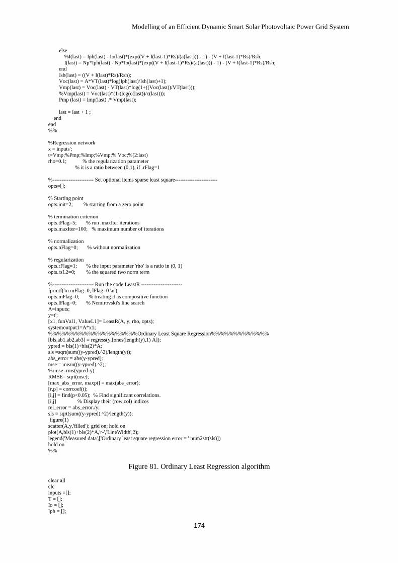
Modelling of an Efficient Dynamic Smart Solar Photovoltaic Power Grid System
174
else
%I(last) = Iph(last) - Io(last)*(exp((V + I(last-1)*Rs)/(a(last))) - 1) - (V + I(last-1)*Rs)/Rsh;
I(last) = Np*Iph(last) - Np*Io(last)*(exp((V + I(last-1)*Rs)/(a(last))) - 1) - (V + I(last-1)*Rs)/Rsh;
end
Ish(last) = ((V + I(last)*Rs)/Rsh); Voc(last) = A*VT(last)*log(Iph(last)/Ish(last)+1);
Vmp(last) = Voc(last) - VT(last)*log(1+((Voc(last))/VT(last)));
%Vmp(last) = Voc(last)*(1-(log(c(last))/c(last))); Pmp (last) = Imp(last) .* Vmp(last);
last = last + 1 ; end
end
%%
%Regression network
x = inputs'; t=Vmp;%Pmp;%Imp;%Vmp;% Voc;%(2:last)
rho=0.1; % the regularization parameter
% it is a ratio between (0,1), if .rFlag=1
%----------------------- Set optional items sparse least square------------------------
opts=[];
% Starting point
opts.init=2; % starting from a zero point
% termination criterion opts.tFlag=5; % run .maxIter iterations
opts.maxIter=100; % maximum number of iterations
% normalization
opts.nFlag=0; % without normalization
% regularization
opts.rFlag=1; % the input parameter 'rho' is a ratio in (0, 1)
opts.rsL2=0; % the squared two norm term
%----------------------- Run the code LeastR -----------------------
fprintf('\n mFlag=0, lFlag=0 \n'); opts.mFlag=0; % treating it as compositive function
opts.lFlag=0; % Nemirovski's line search
A=inputs;
y=t';
[x1, funVal1, ValueL1]= LeastR(A, y, rho, opts);
systemoutput1=A*x1; %%%%%%%%%%%%%%%%%%%%Ordinary Least Square Regression%%%%%%%%%%%%%
[bls,ab1,ab2,ab3] = regress(y,[ones(length(y),1) A]);
ypred = bls(1)+bls(2)*A; sls =sqrt(sum((y-ypred).^2)/length(y));
abs_error = abs(y-ypred);
mse = mean((y-ypred).^2); %rmse=rms(ypred-y)
RMSE= sqrt(mse);
[max_abs_error, maxpt] = max(abs_error); [r,p] = corrcoef(t);
[i,j] = find(p<0.05); % Find significant correlations.
[i,j] % Display their (row,col) indices rel_error = abs_error./y;
sls = sqrt(sum((y-ypred).^2)/length(y));
figure(1) scatter(A,y,'filled'); grid on; hold on
plot(A,bls(1)+bls(2)*A,'r-','LineWidth',2);
legend('Measured data',['Ordinary least square regression error = ' num2str(sls)])
hold on
%%
Figure 81. Ordinary Least Regression algorithm
clear all clc
inputs =[];
T = []; Io = [];
Iph = [];

Modelling of an Efficient Dynamic Smart Solar Photovoltaic Power Grid System
175
I_init = 2.8;
VT = [];
Voc = [ ];
c = [];
d = []; Vmp = [];
Imp = [];
N = []; ki = [];
a = [];
Ish = []; % constants
Ior = 19.963*10^(-5);
q = 1.602*10^(-19); k = 1.380658*10^(-23);
Tr = 301.18;
A = 1.50; Iscr = 3.3;
Ns = 1000;
Np =1; Eg = 2.349*10^(-19);
Ta = 20;
Rs = 5*10^(-1000);
Rsh =2.5*10^(3.8);
V = 12;
last = 1; T(1) = 0 ;
for s = 100:10:1000
for Ws =1:2:20
T(last)= 3.21 + 0.25*s + 0.899*Ta - 1.3*Ws + 273;
inputs(last,:) = T(last) ; %[s T(last) Ws];
Io(last) = Ior*(T(last)/Tr)^3*exp(q*Eg/(k*A)*(1/Tr-1/T(last))); N = Ns + Np;
a(last) = (A*k*T(last)*Ns)/q;
ki(last) = 0.0017 ; %(a(last)*q/(A*T(last)*N)); Iph(last) = ( Iscr + (ki(last)*(T(last)-Tr))) * (s/100);
c(last) = 1 + log(Iph(last)/Io(last));
d(last) = c(last)/(c(last)+1); Imp(last) = Iph(last)*(1 - c(last)^(-d(last)));
VT(last) = ((k*T(last))/q);
if (last == 1)
%I(last) = Iph(last) - Io(last)*(exp((V + I_init*Rs)/(a(last))) - 1) - (V + I_init*Rs)/Rsh;
I(last) = Np*Iph(last) - Np*Io(last)*(exp((V + I_init*Rs)/(a(last))) - 1) - (V + I_init*Rs)/Rsh;
else %I(last) = Iph(last) - Io(last)*(exp((V + I(last-1)*Rs)/(a(last))) - 1) - (V + I(last-1)*Rs)/Rsh;
I(last) = Np*Iph(last) - Np*Io(last)*(exp((V + I(last-1)*Rs)/(a(last))) - 1) - (V + I(last-1)*Rs)/Rsh;
end Ish(last) = ((V + I(last)*Rs)/Rsh);
Voc(last) = A*VT(last)*log(Iph(last)/Ish(last)+1);
Vmp(last) = Voc(last) - VT(last)*log(1+((Voc(last))/VT(last))); %Vmp(last) = Voc(last)*(1-(log(c(last))/c(last)));
Pmp (last) = Imp(last) .* Vmp(last);
last = last + 1 ;
end
end %%
%Regression network
x = inputs'; t =
Imp;%Vmp;%Pmp;%Vmp;%Pmp;%Imp;%Pmp;%Vmp;%Pmp;%Imp;%Vmp;%Pmp;%Vmp;%Imp;%Vmp;%Pmp;%Vmp;%Imp;%Voc;%I
mp;%Vmp;%Pmp;%Imp;%Voc;%(2:last)
rho=0.1; % the regularization parameter
% it is a ratio between (0,1), if .rFlag=1
%----------------------- Set optional items sparse least square------------------------
opts=[];
% Starting point
opts.init=2; % starting from a zero point
% termination criterion
opts.tFlag=5; % run .maxIter iterations

Modelling of an Efficient Dynamic Smart Solar Photovoltaic Power Grid System
176
opts.maxIter=100; % maximum number of iterations
% normalization
opts.nFlag=0; % without normalization
% regularization
opts.rFlag=1; % the input parameter 'rho' is a ratio in (0, 1)
opts.rsL2=0; % the squared two norm term
%----------------------- Run the code LeastR -----------------------
fprintf('\n mFlag=0, lFlag=0 \n'); opts.mFlag=0; % treating it as compositive function
opts.lFlag=0; % Nemirovski's line search
A=inputs; y=t';
[x1, funVal1, ValueL1]= LeastR(A, y, rho, opts);
systemoutput1=A*x1; %%
%%%%%%%%%%%%%%%%%%%%%%%%%%%%%%%%%%%%logistic regression%%%%%
[bls,ab1,ab2,ab3] = regress(y,[ones(length(y),1) A]); %ypred = bls(1)+bls(2)*A;
[brob] = robustfit(A,y,'logistic');
ypred = brob(1)+brob(2)*A;
sls =sqrt(sum((y-ypred).^2)/length(y));
abs_error = abs(y-ypred);
mse = mean((y-ypred).^2); %rmse=rms(ypred-y)
RMSE = sqrt(mse); [max_abs_error, maxpt] = max(abs_error);
rel_error = abs_error./y;
srob = sqrt(sum((y-ypred).^2)/length(y)); figure(2)
scatter(A,y,'filled'); grid on; hold on
plot(A,bls(1)+bls(2)*A,'r-','LineWidth',2); legend('Measured data',['logistic Regression error = ' num2str(sls)])
legend()
hold on
Figure 82. Logistic Robustfit regression code
clear all
clc inputs =[];
T = [];
Io = []; Iph = [];
I_init = 2.8;
VT = []; Voc = [ ];
c = [];
d = []; Vmp = [];
Imp = [];
N = []; ki = [];
a = [];
Ish = []; % constants
Ior = 19.963*10^(-5);
q = 1.602*10^(-19); k = 1.380658*10^(-23);
Tr = 301.18;
A = 1.50; Iscr = 3.3;
Ns = 1000;
Np =1; Eg = 2.349*10^(-19);
Ta = 20;
Rs = 5*10^(-1000); Rsh =2.5*10^(3.8);
V = 12;
last = 1; T(1) = 0 ;
for s = 100:10:1000 for Ws =1:2:20
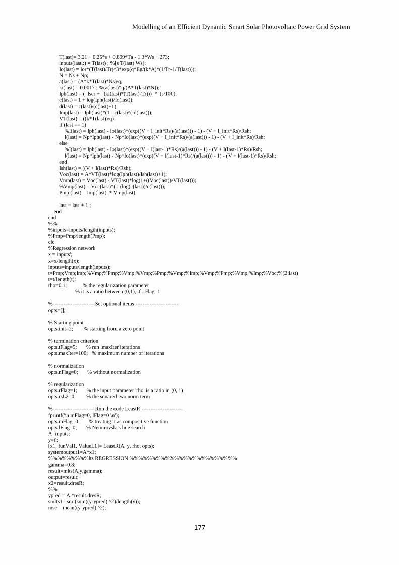
Modelling of an Efficient Dynamic Smart Solar Photovoltaic Power Grid System
177
T(last)= 3.21 + 0.25*s + 0.899*Ta - 1.3*Ws + 273;
inputs(last,:) = T(last) ; %[s T(last) Ws];
Io(last) = Ior*(T(last)/Tr)^3*exp(q*Eg/(k*A)*(1/Tr-1/T(last)));
N = Ns + Np; a(last) = (A*k*T(last)*Ns)/q;
ki(last) = 0.0017 ; %(a(last)*q/(A*T(last)*N));
Iph(last) = ( Iscr + (ki(last)*(T(last)-Tr))) * (s/100); c(last) = 1 + log(Iph(last)/Io(last));
d(last) = c(last)/(c(last)+1);
Imp(last) = Iph(last)*(1 - c(last)^(-d(last))); VT(last) = ((k*T(last))/q);
if (last == 1)
%I(last) = Iph(last) - Io(last)*(exp((V + I_init*Rs)/(a(last))) - 1) - (V + I_init*Rs)/Rsh; I(last) = Np*Iph(last) - Np*Io(last)*(exp((V + I_init*Rs)/(a(last))) - 1) - (V + I_init*Rs)/Rsh;
else
%I(last) = Iph(last) - Io(last)*(exp((V + I(last-1)*Rs)/(a(last))) - 1) - (V + I(last-1)*Rs)/Rsh; I(last) = Np*Iph(last) - Np*Io(last)*(exp((V + I(last-1)*Rs)/(a(last))) - 1) - (V + I(last-1)*Rs)/Rsh;
end
Ish(last) = ((V + I(last)*Rs)/Rsh); Voc(last) = A*VT(last)*log(Iph(last)/Ish(last)+1);
Vmp(last) = Voc(last) - VT(last)*log(1+((Voc(last))/VT(last)));
%Vmp(last) = Voc(last)*(1-(log(c(last))/c(last)));
Pmp (last) = Imp(last) .* Vmp(last);
last = last + 1 ; end
end %%
%inputs=inputs/length(inputs);
%Pmp=Pmp/length(Pmp); clc
%Regression network
x = inputs'; x=x/length(x);
inputs=inputs/length(inputs);
t=Pmp;Vmp;Imp;%Vmp;%Pmp;%Vmp;%Vmp;%Pmp;%Vmp;%Imp;%Vmp;%Pmp;%Vmp;%Imp;%Voc;%(2:last) t=t/length(t);
rho=0.1; % the regularization parameter
% it is a ratio between (0,1), if .rFlag=1
%----------------------- Set optional items ------------------------
opts=[];
% Starting point
opts.init=2; % starting from a zero point
% termination criterion
opts.tFlag=5; % run .maxIter iterations opts.maxIter=100; % maximum number of iterations
% normalization opts.nFlag=0; % without normalization
% regularization opts.rFlag=1; % the input parameter 'rho' is a ratio in (0, 1)
opts.rsL2=0; % the squared two norm term
%----------------------- Run the code LeastR -----------------------
fprintf('\n mFlag=0, lFlag=0 \n');
opts.mFlag=0; % treating it as compositive function opts.lFlag=0; % Nemirovski's line search
A=inputs;
y=t';
[x1, funVal1, ValueL1]= LeastR(A, y, rho, opts);
systemoutput1=A*x1;
%%%%%%%%%lts REGRESSION %%%%%%%%%%%%%%%%%%%%%%%% gamma=0.8;
result=mlts(A,y,gamma);
output=result; x2=result.dresR;
%%
ypred = A.*result.dresR; smlts1 =sqrt(sum((y-ypred).^2)/length(y));
mse = mean((y-ypred).^2);

Modelling of an Efficient Dynamic Smart Solar Photovoltaic Power Grid System
178
rmse = sqrt(mse);
abs_error = abs(y-ypred);
rel_error = abs_error./y;
figure(1)
scatter(A,y,'filled'); grid on; hold on plot(A,ypred,'r','LineWidth',2);
legend('Measured data',['MLTS regression error = ' num2str(smlts1)])
hold on %%
Figure 83. Least Trimmed Squares regression code
A.2 Real-time online Solar photovoltaic monitoring data
In this section, the online generated report from the comparative study for both the stationary
and dual-axis solar photovoltaic tracking system are presented in Table x and y respectively.
The obtained data were raw data obtained from the research study conducted at the National
Kaohsiung University of Applied Sciences, Taiwan, R.O.C.
Table 11 and 12 below shows the real-time online remote raw data obtained for the stationary
and dual-axis solar photovoltaic tracking system during one of the days. The GUI chart for
this specific day as been presented in comparison in Section 5.7.
Table 11. Stationary 450 Solar Photovoltaic Obtained Raw data
Time Temperature Eac_Today Vpv Ipv Ppv Vac Iac Pac Fac Eac_Total
31-07-14 2:10 24 0 22.1 0.95 0 218.5 0.065 0 60 172.16
31-07-14 2:11 24 0 24.8 0.95 0 218.7 0.065 0 59.96 172.16
31-07-14 2:12 24 0 26.1 0.76 20 218.6 0.067 14.6 59.96 172.16
31-07-14 2:13 24 0 23.9 0.86 20 218.8 0.069 14.6 59.96 172.16
31-07-14 2:14 24 0 26.6 0.95 0 218.6 0.066 0 59.96 172.16
31-07-14 2:15 24 0 29.3 1 0 218.8 0.065 0 59.99 172.16
31-07-14 2:16 24 0 23.1 0.91 21 218.8 0.07 14.8 60.04 172.16
31-07-14 2:17 24 0 22.8 0.95 21 218.7 0.07 15 59.99 172.16
31-07-14 2:18 24 0 26.2 0.88 22 218.6 0.068 18.7 60.04 172.16
31-07-14 2:19 24 0 22.3 0.95 21 218.5 0.071 15.2 59.98 172.16
31-07-14 2:20 24 0 24.6 0.87 21 218.4 0.072 15 60.02 172.16
31-07-14 2:21 24 0 24.3 0.91 22 218.4 0.082 17.4 59.98 172.16
31-07-14 2:22 24 0 22.4 1 22 218.8 0.083 17.2 60.12 172.16
31-07-14 2:23 24 0 30.3 1.04 0 219.1 0.066 0 60.04 172.16
31-07-14 2:24 24 0 28.3 0.78 22 219 0.078 17 60.04 172.16
31-07-14 2:25 24 0 30.5 1 0 219 0.065 0 60.06 172.16
31-07-14 2:26 24 0 28.3 0.78 22 219 0.08 16.8 60.05 172.16
31-07-14 2:27 24 0 28 0.81 22 219 0.081 18.1 60 172.16
31-07-14 2:28 24 0 27.1 0.81 22 219.2 0.079 18.4 60 172.16
31-07-14 2:29 24 0 26.6 0.84 22 219.1 0.077 18.1 59.94 172.16
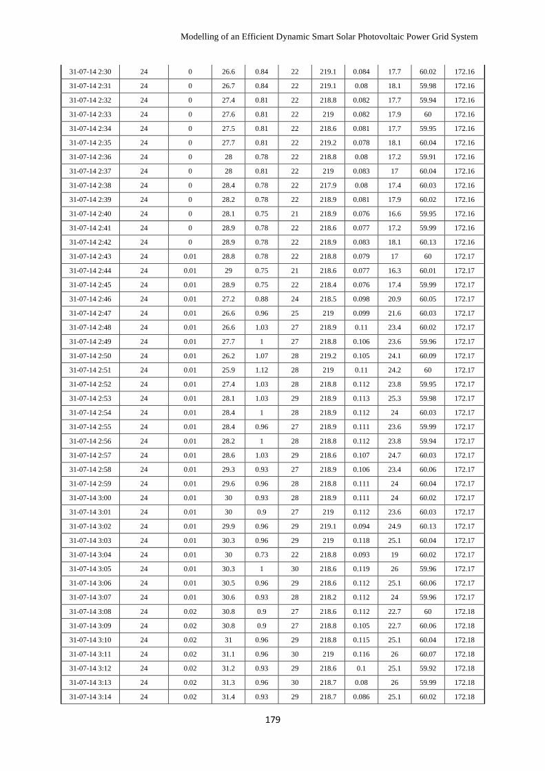
Modelling of an Efficient Dynamic Smart Solar Photovoltaic Power Grid System
179
31-07-14 2:30 24 0 26.6 0.84 22 219.1 0.084 17.7 60.02 172.16
31-07-14 2:31 24 0 26.7 0.84 22 219.1 0.08 18.1 59.98 172.16
31-07-14 2:32 24 0 27.4 0.81 22 218.8 0.082 17.7 59.94 172.16
31-07-14 2:33 24 0 27.6 0.81 22 219 0.082 17.9 60 172.16
31-07-14 2:34 24 0 27.5 0.81 22 218.6 0.081 17.7 59.95 172.16
31-07-14 2:35 24 0 27.7 0.81 22 219.2 0.078 18.1 60.04 172.16
31-07-14 2:36 24 0 28 0.78 22 218.8 0.08 17.2 59.91 172.16
31-07-14 2:37 24 0 28 0.81 22 219 0.083 17 60.04 172.16
31-07-14 2:38 24 0 28.4 0.78 22 217.9 0.08 17.4 60.03 172.16
31-07-14 2:39 24 0 28.2 0.78 22 218.9 0.081 17.9 60.02 172.16
31-07-14 2:40 24 0 28.1 0.75 21 218.9 0.076 16.6 59.95 172.16
31-07-14 2:41 24 0 28.9 0.78 22 218.6 0.077 17.2 59.99 172.16
31-07-14 2:42 24 0 28.9 0.78 22 218.9 0.083 18.1 60.13 172.16
31-07-14 2:43 24 0.01 28.8 0.78 22 218.8 0.079 17 60 172.17
31-07-14 2:44 24 0.01 29 0.75 21 218.6 0.077 16.3 60.01 172.17
31-07-14 2:45 24 0.01 28.9 0.75 22 218.4 0.076 17.4 59.99 172.17
31-07-14 2:46 24 0.01 27.2 0.88 24 218.5 0.098 20.9 60.05 172.17
31-07-14 2:47 24 0.01 26.6 0.96 25 219 0.099 21.6 60.03 172.17
31-07-14 2:48 24 0.01 26.6 1.03 27 218.9 0.11 23.4 60.02 172.17
31-07-14 2:49 24 0.01 27.7 1 27 218.8 0.106 23.6 59.96 172.17
31-07-14 2:50 24 0.01 26.2 1.07 28 219.2 0.105 24.1 60.09 172.17
31-07-14 2:51 24 0.01 25.9 1.12 28 219 0.11 24.2 60 172.17
31-07-14 2:52 24 0.01 27.4 1.03 28 218.8 0.112 23.8 59.95 172.17
31-07-14 2:53 24 0.01 28.1 1.03 29 218.9 0.113 25.3 59.98 172.17
31-07-14 2:54 24 0.01 28.4 1 28 218.9 0.112 24 60.03 172.17
31-07-14 2:55 24 0.01 28.4 0.96 27 218.9 0.111 23.6 59.99 172.17
31-07-14 2:56 24 0.01 28.2 1 28 218.8 0.112 23.8 59.94 172.17
31-07-14 2:57 24 0.01 28.6 1.03 29 218.6 0.107 24.7 60.03 172.17
31-07-14 2:58 24 0.01 29.3 0.93 27 218.9 0.106 23.4 60.06 172.17
31-07-14 2:59 24 0.01 29.6 0.96 28 218.8 0.111 24 60.04 172.17
31-07-14 3:00 24 0.01 30 0.93 28 218.9 0.111 24 60.02 172.17
31-07-14 3:01 24 0.01 30 0.9 27 219 0.112 23.6 60.03 172.17
31-07-14 3:02 24 0.01 29.9 0.96 29 219.1 0.094 24.9 60.13 172.17
31-07-14 3:03 24 0.01 30.3 0.96 29 219 0.118 25.1 60.04 172.17
31-07-14 3:04 24 0.01 30 0.73 22 218.8 0.093 19 60.02 172.17
31-07-14 3:05 24 0.01 30.3 1 30 218.6 0.119 26 59.96 172.17
31-07-14 3:06 24 0.01 30.5 0.96 29 218.6 0.112 25.1 60.06 172.17
31-07-14 3:07 24 0.01 30.6 0.93 28 218.2 0.112 24 59.96 172.17
31-07-14 3:08 24 0.02 30.8 0.9 27 218.6 0.112 22.7 60 172.18
31-07-14 3:09 24 0.02 30.8 0.9 27 218.8 0.105 22.7 60.06 172.18
31-07-14 3:10 24 0.02 31 0.96 29 218.8 0.115 25.1 60.04 172.18
31-07-14 3:11 24 0.02 31.1 0.96 30 219 0.116 26 60.07 172.18
31-07-14 3:12 24 0.02 31.2 0.93 29 218.6 0.1 25.1 59.92 172.18
31-07-14 3:13 24 0.02 31.3 0.96 30 218.7 0.08 26 59.99 172.18
31-07-14 3:14 24 0.02 31.4 0.93 29 218.7 0.086 25.1 60.02 172.18
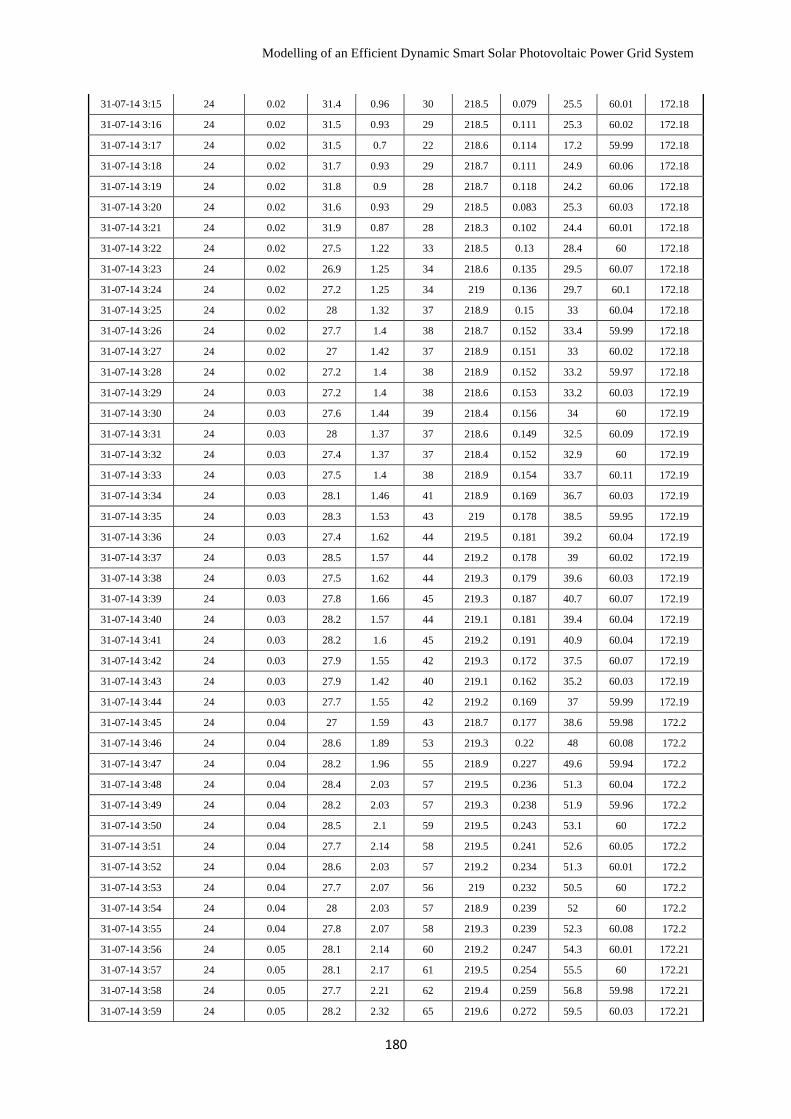
Modelling of an Efficient Dynamic Smart Solar Photovoltaic Power Grid System
180
31-07-14 3:15 24 0.02 31.4 0.96 30 218.5 0.079 25.5 60.01 172.18
31-07-14 3:16 24 0.02 31.5 0.93 29 218.5 0.111 25.3 60.02 172.18
31-07-14 3:17 24 0.02 31.5 0.7 22 218.6 0.114 17.2 59.99 172.18
31-07-14 3:18 24 0.02 31.7 0.93 29 218.7 0.111 24.9 60.06 172.18
31-07-14 3:19 24 0.02 31.8 0.9 28 218.7 0.118 24.2 60.06 172.18
31-07-14 3:20 24 0.02 31.6 0.93 29 218.5 0.083 25.3 60.03 172.18
31-07-14 3:21 24 0.02 31.9 0.87 28 218.3 0.102 24.4 60.01 172.18
31-07-14 3:22 24 0.02 27.5 1.22 33 218.5 0.13 28.4 60 172.18
31-07-14 3:23 24 0.02 26.9 1.25 34 218.6 0.135 29.5 60.07 172.18
31-07-14 3:24 24 0.02 27.2 1.25 34 219 0.136 29.7 60.1 172.18
31-07-14 3:25 24 0.02 28 1.32 37 218.9 0.15 33 60.04 172.18
31-07-14 3:26 24 0.02 27.7 1.4 38 218.7 0.152 33.4 59.99 172.18
31-07-14 3:27 24 0.02 27 1.42 37 218.9 0.151 33 60.02 172.18
31-07-14 3:28 24 0.02 27.2 1.4 38 218.9 0.152 33.2 59.97 172.18
31-07-14 3:29 24 0.03 27.2 1.4 38 218.6 0.153 33.2 60.03 172.19
31-07-14 3:30 24 0.03 27.6 1.44 39 218.4 0.156 34 60 172.19
31-07-14 3:31 24 0.03 28 1.37 37 218.6 0.149 32.5 60.09 172.19
31-07-14 3:32 24 0.03 27.4 1.37 37 218.4 0.152 32.9 60 172.19
31-07-14 3:33 24 0.03 27.5 1.4 38 218.9 0.154 33.7 60.11 172.19
31-07-14 3:34 24 0.03 28.1 1.46 41 218.9 0.169 36.7 60.03 172.19
31-07-14 3:35 24 0.03 28.3 1.53 43 219 0.178 38.5 59.95 172.19
31-07-14 3:36 24 0.03 27.4 1.62 44 219.5 0.181 39.2 60.04 172.19
31-07-14 3:37 24 0.03 28.5 1.57 44 219.2 0.178 39 60.02 172.19
31-07-14 3:38 24 0.03 27.5 1.62 44 219.3 0.179 39.6 60.03 172.19
31-07-14 3:39 24 0.03 27.8 1.66 45 219.3 0.187 40.7 60.07 172.19
31-07-14 3:40 24 0.03 28.2 1.57 44 219.1 0.181 39.4 60.04 172.19
31-07-14 3:41 24 0.03 28.2 1.6 45 219.2 0.191 40.9 60.04 172.19
31-07-14 3:42 24 0.03 27.9 1.55 42 219.3 0.172 37.5 60.07 172.19
31-07-14 3:43 24 0.03 27.9 1.42 40 219.1 0.162 35.2 60.03 172.19
31-07-14 3:44 24 0.03 27.7 1.55 42 219.2 0.169 37 59.99 172.19
31-07-14 3:45 24 0.04 27 1.59 43 218.7 0.177 38.6 59.98 172.2
31-07-14 3:46 24 0.04 28.6 1.89 53 219.3 0.22 48 60.08 172.2
31-07-14 3:47 24 0.04 28.2 1.96 55 218.9 0.227 49.6 59.94 172.2
31-07-14 3:48 24 0.04 28.4 2.03 57 219.5 0.236 51.3 60.04 172.2
31-07-14 3:49 24 0.04 28.2 2.03 57 219.3 0.238 51.9 59.96 172.2
31-07-14 3:50 24 0.04 28.5 2.1 59 219.5 0.243 53.1 60 172.2
31-07-14 3:51 24 0.04 27.7 2.14 58 219.5 0.241 52.6 60.05 172.2
31-07-14 3:52 24 0.04 28.6 2.03 57 219.2 0.234 51.3 60.01 172.2
31-07-14 3:53 24 0.04 27.7 2.07 56 219 0.232 50.5 60 172.2
31-07-14 3:54 24 0.04 28 2.03 57 218.9 0.239 52 60 172.2
31-07-14 3:55 24 0.04 27.8 2.07 58 219.3 0.239 52.3 60.08 172.2
31-07-14 3:56 24 0.05 28.1 2.14 60 219.2 0.247 54.3 60.01 172.21
31-07-14 3:57 24 0.05 28.1 2.17 61 219.5 0.254 55.5 60 172.21
31-07-14 3:58 24 0.05 27.7 2.21 62 219.4 0.259 56.8 59.98 172.21
31-07-14 3:59 24 0.05 28.2 2.32 65 219.6 0.272 59.5 60.03 172.21
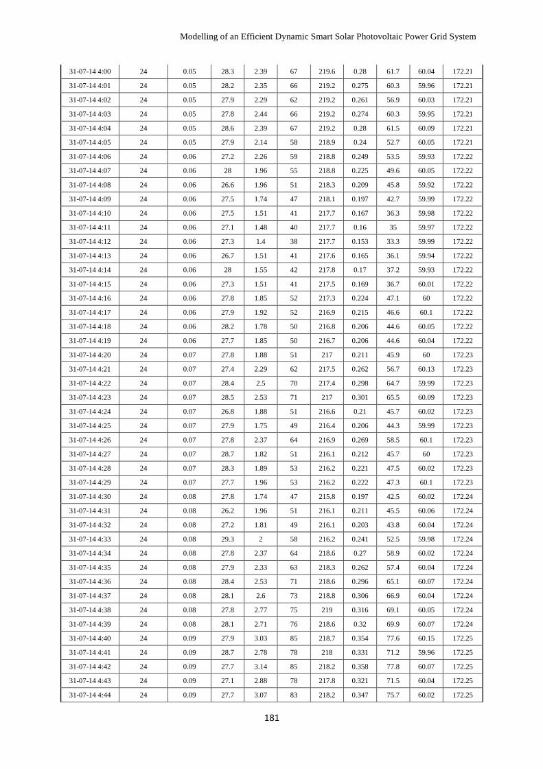
Modelling of an Efficient Dynamic Smart Solar Photovoltaic Power Grid System
181
31-07-14 4:00 24 0.05 28.3 2.39 67 219.6 0.28 61.7 60.04 172.21
31-07-14 4:01 24 0.05 28.2 2.35 66 219.2 0.275 60.3 59.96 172.21
31-07-14 4:02 24 0.05 27.9 2.29 62 219.2 0.261 56.9 60.03 172.21
31-07-14 4:03 24 0.05 27.8 2.44 66 219.2 0.274 60.3 59.95 172.21
31-07-14 4:04 24 0.05 28.6 2.39 67 219.2 0.28 61.5 60.09 172.21
31-07-14 4:05 24 0.05 27.9 2.14 58 218.9 0.24 52.7 60.05 172.21
31-07-14 4:06 24 0.06 27.2 2.26 59 218.8 0.249 53.5 59.93 172.22
31-07-14 4:07 24 0.06 28 1.96 55 218.8 0.225 49.6 60.05 172.22
31-07-14 4:08 24 0.06 26.6 1.96 51 218.3 0.209 45.8 59.92 172.22
31-07-14 4:09 24 0.06 27.5 1.74 47 218.1 0.197 42.7 59.99 172.22
31-07-14 4:10 24 0.06 27.5 1.51 41 217.7 0.167 36.3 59.98 172.22
31-07-14 4:11 24 0.06 27.1 1.48 40 217.7 0.16 35 59.97 172.22
31-07-14 4:12 24 0.06 27.3 1.4 38 217.7 0.153 33.3 59.99 172.22
31-07-14 4:13 24 0.06 26.7 1.51 41 217.6 0.165 36.1 59.94 172.22
31-07-14 4:14 24 0.06 28 1.55 42 217.8 0.17 37.2 59.93 172.22
31-07-14 4:15 24 0.06 27.3 1.51 41 217.5 0.169 36.7 60.01 172.22
31-07-14 4:16 24 0.06 27.8 1.85 52 217.3 0.224 47.1 60 172.22
31-07-14 4:17 24 0.06 27.9 1.92 52 216.9 0.215 46.6 60.1 172.22
31-07-14 4:18 24 0.06 28.2 1.78 50 216.8 0.206 44.6 60.05 172.22
31-07-14 4:19 24 0.06 27.7 1.85 50 216.7 0.206 44.6 60.04 172.22
31-07-14 4:20 24 0.07 27.8 1.88 51 217 0.211 45.9 60 172.23
31-07-14 4:21 24 0.07 27.4 2.29 62 217.5 0.262 56.7 60.13 172.23
31-07-14 4:22 24 0.07 28.4 2.5 70 217.4 0.298 64.7 59.99 172.23
31-07-14 4:23 24 0.07 28.5 2.53 71 217 0.301 65.5 60.09 172.23
31-07-14 4:24 24 0.07 26.8 1.88 51 216.6 0.21 45.7 60.02 172.23
31-07-14 4:25 24 0.07 27.9 1.75 49 216.4 0.206 44.3 59.99 172.23
31-07-14 4:26 24 0.07 27.8 2.37 64 216.9 0.269 58.5 60.1 172.23
31-07-14 4:27 24 0.07 28.7 1.82 51 216.1 0.212 45.7 60 172.23
31-07-14 4:28 24 0.07 28.3 1.89 53 216.2 0.221 47.5 60.02 172.23
31-07-14 4:29 24 0.07 27.7 1.96 53 216.2 0.222 47.3 60.1 172.23
31-07-14 4:30 24 0.08 27.8 1.74 47 215.8 0.197 42.5 60.02 172.24
31-07-14 4:31 24 0.08 26.2 1.96 51 216.1 0.211 45.5 60.06 172.24
31-07-14 4:32 24 0.08 27.2 1.81 49 216.1 0.203 43.8 60.04 172.24
31-07-14 4:33 24 0.08 29.3 2 58 216.2 0.241 52.5 59.98 172.24
31-07-14 4:34 24 0.08 27.8 2.37 64 218.6 0.27 58.9 60.02 172.24
31-07-14 4:35 24 0.08 27.9 2.33 63 218.3 0.262 57.4 60.04 172.24
31-07-14 4:36 24 0.08 28.4 2.53 71 218.6 0.296 65.1 60.07 172.24
31-07-14 4:37 24 0.08 28.1 2.6 73 218.8 0.306 66.9 60.04 172.24
31-07-14 4:38 24 0.08 27.8 2.77 75 219 0.316 69.1 60.05 172.24
31-07-14 4:39 24 0.08 28.1 2.71 76 218.6 0.32 69.9 60.07 172.24
31-07-14 4:40 24 0.09 27.9 3.03 85 218.7 0.354 77.6 60.15 172.25
31-07-14 4:41 24 0.09 28.7 2.78 78 218 0.331 71.2 59.96 172.25
31-07-14 4:42 24 0.09 27.7 3.14 85 218.2 0.358 77.8 60.07 172.25
31-07-14 4:43 24 0.09 27.1 2.88 78 217.8 0.321 71.5 60.04 172.25
31-07-14 4:44 24 0.09 27.7 3.07 83 218.2 0.347 75.7 60.02 172.25
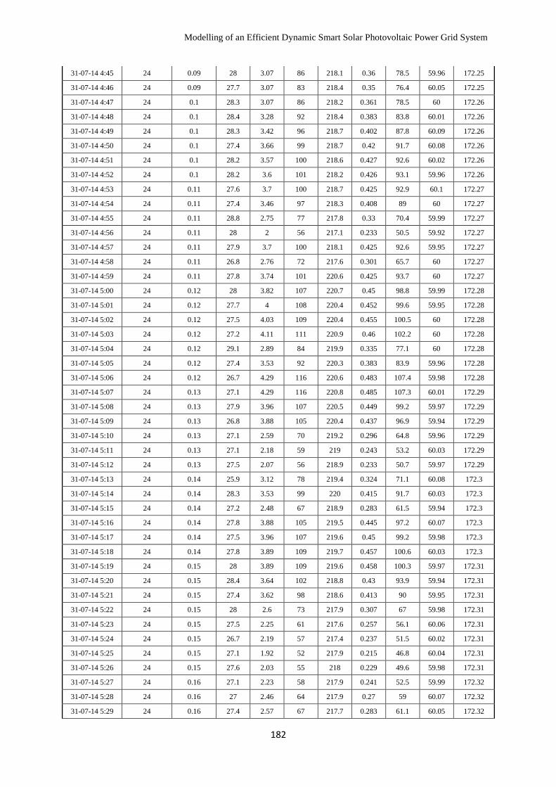
Modelling of an Efficient Dynamic Smart Solar Photovoltaic Power Grid System
182
31-07-14 4:45 24 0.09 28 3.07 86 218.1 0.36 78.5 59.96 172.25
31-07-14 4:46 24 0.09 27.7 3.07 83 218.4 0.35 76.4 60.05 172.25
31-07-14 4:47 24 0.1 28.3 3.07 86 218.2 0.361 78.5 60 172.26
31-07-14 4:48 24 0.1 28.4 3.28 92 218.4 0.383 83.8 60.01 172.26
31-07-14 4:49 24 0.1 28.3 3.42 96 218.7 0.402 87.8 60.09 172.26
31-07-14 4:50 24 0.1 27.4 3.66 99 218.7 0.42 91.7 60.08 172.26
31-07-14 4:51 24 0.1 28.2 3.57 100 218.6 0.427 92.6 60.02 172.26
31-07-14 4:52 24 0.1 28.2 3.6 101 218.2 0.426 93.1 59.96 172.26
31-07-14 4:53 24 0.11 27.6 3.7 100 218.7 0.425 92.9 60.1 172.27
31-07-14 4:54 24 0.11 27.4 3.46 97 218.3 0.408 89 60 172.27
31-07-14 4:55 24 0.11 28.8 2.75 77 217.8 0.33 70.4 59.99 172.27
31-07-14 4:56 24 0.11 28 2 56 217.1 0.233 50.5 59.92 172.27
31-07-14 4:57 24 0.11 27.9 3.7 100 218.1 0.425 92.6 59.95 172.27
31-07-14 4:58 24 0.11 26.8 2.76 72 217.6 0.301 65.7 60 172.27
31-07-14 4:59 24 0.11 27.8 3.74 101 220.6 0.425 93.7 60 172.27
31-07-14 5:00 24 0.12 28 3.82 107 220.7 0.45 98.8 59.99 172.28
31-07-14 5:01 24 0.12 27.7 4 108 220.4 0.452 99.6 59.95 172.28
31-07-14 5:02 24 0.12 27.5 4.03 109 220.4 0.455 100.5 60 172.28
31-07-14 5:03 24 0.12 27.2 4.11 111 220.9 0.46 102.2 60 172.28
31-07-14 5:04 24 0.12 29.1 2.89 84 219.9 0.335 77.1 60 172.28
31-07-14 5:05 24 0.12 27.4 3.53 92 220.3 0.383 83.9 59.96 172.28
31-07-14 5:06 24 0.12 26.7 4.29 116 220.6 0.483 107.4 59.98 172.28
31-07-14 5:07 24 0.13 27.1 4.29 116 220.8 0.485 107.3 60.01 172.29
31-07-14 5:08 24 0.13 27.9 3.96 107 220.5 0.449 99.2 59.97 172.29
31-07-14 5:09 24 0.13 26.8 3.88 105 220.4 0.437 96.9 59.94 172.29
31-07-14 5:10 24 0.13 27.1 2.59 70 219.2 0.296 64.8 59.96 172.29
31-07-14 5:11 24 0.13 27.1 2.18 59 219 0.243 53.2 60.03 172.29
31-07-14 5:12 24 0.13 27.5 2.07 56 218.9 0.233 50.7 59.97 172.29
31-07-14 5:13 24 0.14 25.9 3.12 78 219.4 0.324 71.1 60.08 172.3
31-07-14 5:14 24 0.14 28.3 3.53 99 220 0.415 91.7 60.03 172.3
31-07-14 5:15 24 0.14 27.2 2.48 67 218.9 0.283 61.5 59.94 172.3
31-07-14 5:16 24 0.14 27.8 3.88 105 219.5 0.445 97.2 60.07 172.3
31-07-14 5:17 24 0.14 27.5 3.96 107 219.6 0.45 99.2 59.98 172.3
31-07-14 5:18 24 0.14 27.8 3.89 109 219.7 0.457 100.6 60.03 172.3
31-07-14 5:19 24 0.15 28 3.89 109 219.6 0.458 100.3 59.97 172.31
31-07-14 5:20 24 0.15 28.4 3.64 102 218.8 0.43 93.9 59.94 172.31
31-07-14 5:21 24 0.15 27.4 3.62 98 218.6 0.413 90 59.95 172.31
31-07-14 5:22 24 0.15 28 2.6 73 217.9 0.307 67 59.98 172.31
31-07-14 5:23 24 0.15 27.5 2.25 61 217.6 0.257 56.1 60.06 172.31
31-07-14 5:24 24 0.15 26.7 2.19 57 217.4 0.237 51.5 60.02 172.31
31-07-14 5:25 24 0.15 27.1 1.92 52 217.9 0.215 46.8 60.04 172.31
31-07-14 5:26 24 0.15 27.6 2.03 55 218 0.229 49.6 59.98 172.31
31-07-14 5:27 24 0.16 27.1 2.23 58 217.9 0.241 52.5 59.99 172.32
31-07-14 5:28 24 0.16 27 2.46 64 217.9 0.27 59 60.07 172.32
31-07-14 5:29 24 0.16 27.4 2.57 67 217.7 0.283 61.1 60.05 172.32
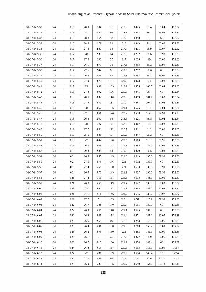
Modelling of an Efficient Dynamic Smart Solar Photovoltaic Power Grid System
183
31-07-14 5:30 24 0.16 28.9 3.6 101 218.3 0.425 93.4 60.04 172.32
31-07-14 5:31 24 0.16 28.1 3.42 96 218.1 0.403 88.1 59.98 172.32
31-07-14 5:32 24 0.16 28.8 3.2 93 218.3 0.398 85.1 60 172.32
31-07-14 5:33 24 0.16 28.8 2.79 81 218 0.343 74.1 60.02 172.32
31-07-14 5:34 24 0.16 27.8 2.37 64 217.7 0.271 58.9 60.07 172.32
31-07-14 5:35 24 0.17 28 2.37 64 217.3 0.272 58.6 59.98 172.33
31-07-14 5:36 24 0.17 27.8 2.03 55 217 0.225 49 60.02 172.33
31-07-14 5:37 24 0.17 26.1 2.73 71 217.5 0.303 65.2 59.99 172.33
31-07-14 5:38 24 0.17 27.6 2.44 66 219.6 0.272 60.6 60 172.33
31-07-14 5:39 24 0.17 26.9 2.34 61 219.3 0.253 55.7 59.97 172.33
31-07-14 5:40 24 0.17 27.9 3.74 101 220.5 0.423 93 60.08 172.33
31-07-14 5:41 24 0.17 29 3.89 109 219.9 0.455 100.7 60.04 172.33
31-07-14 5:42 24 0.18 27.3 3.92 106 220.3 0.445 98.4 60 172.34
31-07-14 5:43 24 0.18 28.5 3.92 110 220.3 0.459 101.7 60.03 172.34
31-07-14 5:44 24 0.18 27.6 4.33 117 220.7 0.487 107.7 60.02 172.34
31-07-14 5:45 24 0.18 28 4.62 125 221.1 0.526 116.9 60.04 172.34
31-07-14 5:46 24 0.18 27.1 4.66 126 220.9 0.528 117.3 59.98 172.34
31-07-14 5:47 24 0.18 26.5 2.07 54 218.9 0.221 48.5 60.04 172.34
31-07-14 5:48 24 0.19 28 3.5 98 220 0.407 89.4 60.02 172.35
31-07-14 5:49 24 0.19 27.7 4.51 122 220.7 0.511 113 60.06 172.35
31-07-14 5:50 24 0.19 25.6 3.85 104 220.3 0.447 96.2 60 172.35
31-07-14 5:51 24 0.19 27 4.44 120 220.5 0.503 110.9 59.96 172.35
31-07-14 5:52 24 0.19 26.7 5.25 142 221.8 0.595 132.7 60.09 172.35
31-07-14 5:53 24 0.19 29.3 2.89 84 219.9 0.329 76.5 60.03 172.35
31-07-14 5:54 24 0.2 26.8 5.57 145 221.3 0.613 135.6 59.99 172.36
31-07-14 5:55 24 0.2 27.6 5.4 146 221 0.612 135.9 60 172.36
31-07-14 5:56 24 0.2 27.4 5.55 150 221 0.633 139.8 59.99 172.36
31-07-14 5:57 24 0.2 26.5 5.73 149 221.1 0.627 138.8 59.98 172.36
31-07-14 5:58 24 0.21 27.2 5.59 151 221.5 0.638 141.3 60.06 172.37
31-07-14 5:59 24 0.21 26.8 5.51 149 221.4 0.627 138.9 60.03 172.37
31-07-14 6:00 24 0.21 27 5.62 152 221.1 0.645 142.2 60.08 172.37
31-07-14 6:01 24 0.21 27.1 5.4 146 221.2 0.615 136.2 59.97 172.37
31-07-14 6:02 24 0.22 27.7 5 135 220.4 0.57 125.9 59.98 172.38
31-07-14 6:03 24 0.22 26.7 5.38 140 220.7 0.595 130.9 60 172.38
31-07-14 6:04 24 0.22 26.9 5.69 148 221.1 0.625 137.9 60 172.38
31-07-14 6:05 24 0.22 26.6 5.85 158 221.4 0.671 147.2 60.07 172.38
31-07-14 6:06 24 0.23 26.5 2.65 69 219 0.293 64.1 60.06 172.39
31-07-14 6:07 24 0.23 26.4 6.46 168 221.3 0.708 156.9 60.03 172.39
31-07-14 6:08 24 0.23 26.2 6.4 160 221 0.683 149.1 60.01 172.39
31-07-14 6:09 24 0.23 26.1 3 75 218.9 0.327 68.9 60.06 172.39
31-07-14 6:10 24 0.23 26.7 6.15 160 221.2 0.674 149.4 60 172.39
31-07-14 6:11 24 0.24 26.4 6.3 164 220.8 0.693 153.3 59.99 172.4
31-07-14 6:12 24 0.24 27 5.88 159 220.6 0.674 148.4 60.11 172.4
31-07-14 6:13 24 0.24 27.7 3.55 96 219 0.4 87.6 60.11 172.4
31-07-14 6:14 24 0.25 26.9 6.34 165 220.7 0.699 154.2 60.13 172.41
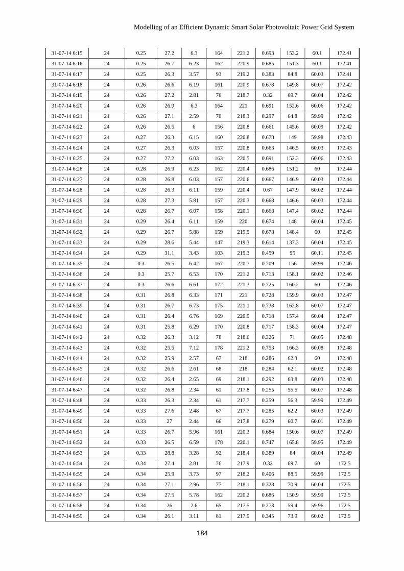
Modelling of an Efficient Dynamic Smart Solar Photovoltaic Power Grid System
184
31-07-14 6:15 24 0.25 27.2 6.3 164 221.2 0.693 153.2 60.1 172.41
31-07-14 6:16 24 0.25 26.7 6.23 162 220.9 0.685 151.3 60.1 172.41
31-07-14 6:17 24 0.25 26.3 3.57 93 219.2 0.383 84.8 60.03 172.41
31-07-14 6:18 24 0.26 26.6 6.19 161 220.9 0.678 149.8 60.07 172.42
31-07-14 6:19 24 0.26 27.2 2.81 76 218.7 0.32 69.7 60.04 172.42
31-07-14 6:20 24 0.26 26.9 6.3 164 221 0.691 152.6 60.06 172.42
31-07-14 6:21 24 0.26 27.1 2.59 70 218.3 0.297 64.8 59.99 172.42
31-07-14 6:22 24 0.26 26.5 6 156 220.8 0.661 145.6 60.09 172.42
31-07-14 6:23 24 0.27 26.3 6.15 160 220.8 0.678 149 59.98 172.43
31-07-14 6:24 24 0.27 26.3 6.03 157 220.8 0.663 146.5 60.03 172.43
31-07-14 6:25 24 0.27 27.2 6.03 163 220.5 0.691 152.3 60.06 172.43
31-07-14 6:26 24 0.28 26.9 6.23 162 220.4 0.686 151.2 60 172.44
31-07-14 6:27 24 0.28 26.8 6.03 157 220.6 0.667 146.9 60.03 172.44
31-07-14 6:28 24 0.28 26.3 6.11 159 220.4 0.67 147.9 60.02 172.44
31-07-14 6:29 24 0.28 27.3 5.81 157 220.3 0.668 146.6 60.03 172.44
31-07-14 6:30 24 0.28 26.7 6.07 158 220.1 0.668 147.4 60.02 172.44
31-07-14 6:31 24 0.29 26.4 6.11 159 220 0.674 148 60.04 172.45
31-07-14 6:32 24 0.29 26.7 5.88 159 219.9 0.678 148.4 60 172.45
31-07-14 6:33 24 0.29 28.6 5.44 147 219.3 0.614 137.3 60.04 172.45
31-07-14 6:34 24 0.29 31.1 3.43 103 219.3 0.459 95 60.11 172.45
31-07-14 6:35 24 0.3 26.5 6.42 167 220.7 0.709 156 59.99 172.46
31-07-14 6:36 24 0.3 25.7 6.53 170 221.2 0.713 158.1 60.02 172.46
31-07-14 6:37 24 0.3 26.6 6.61 172 221.3 0.725 160.2 60 172.46
31-07-14 6:38 24 0.31 26.8 6.33 171 221 0.728 159.9 60.03 172.47
31-07-14 6:39 24 0.31 26.7 6.73 175 221.1 0.738 162.8 60.07 172.47
31-07-14 6:40 24 0.31 26.4 6.76 169 220.9 0.718 157.4 60.04 172.47
31-07-14 6:41 24 0.31 25.8 6.29 170 220.8 0.717 158.3 60.04 172.47
31-07-14 6:42 24 0.32 26.3 3.12 78 218.6 0.326 71 60.05 172.48
31-07-14 6:43 24 0.32 25.5 7.12 178 221.2 0.753 166.3 60.08 172.48
31-07-14 6:44 24 0.32 25.9 2.57 67 218 0.286 62.3 60 172.48
31-07-14 6:45 24 0.32 26.6 2.61 68 218 0.284 62.1 60.02 172.48
31-07-14 6:46 24 0.32 26.4 2.65 69 218.1 0.292 63.8 60.03 172.48
31-07-14 6:47 24 0.32 26.8 2.34 61 217.8 0.255 55.5 60.07 172.48
31-07-14 6:48 24 0.33 26.3 2.34 61 217.7 0.259 56.3 59.99 172.49
31-07-14 6:49 24 0.33 27.6 2.48 67 217.7 0.285 62.2 60.03 172.49
31-07-14 6:50 24 0.33 27 2.44 66 217.8 0.279 60.7 60.01 172.49
31-07-14 6:51 24 0.33 26.7 5.96 161 220.3 0.684 150.6 60.07 172.49
31-07-14 6:52 24 0.33 26.5 6.59 178 220.1 0.747 165.8 59.95 172.49
31-07-14 6:53 24 0.33 28.8 3.28 92 218.4 0.389 84 60.04 172.49
31-07-14 6:54 24 0.34 27.4 2.81 76 217.9 0.32 69.7 60 172.5
31-07-14 6:55 24 0.34 25.9 3.73 97 218.2 0.406 88.5 59.99 172.5
31-07-14 6:56 24 0.34 27.1 2.96 77 218.1 0.328 70.9 60.04 172.5
31-07-14 6:57 24 0.34 27.5 5.78 162 220.2 0.686 150.9 59.99 172.5
31-07-14 6:58 24 0.34 26 2.6 65 217.5 0.273 59.4 59.96 172.5
31-07-14 6:59 24 0.34 26.1 3.11 81 217.9 0.345 73.9 60.02 172.5
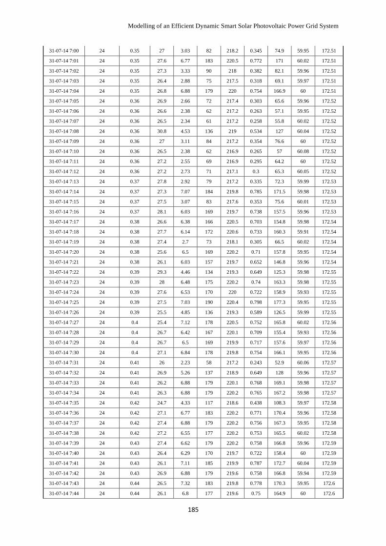
Modelling of an Efficient Dynamic Smart Solar Photovoltaic Power Grid System
185
31-07-14 7:00 24 0.35 27 3.03 82 218.2 0.345 74.9 59.95 172.51
31-07-14 7:01 24 0.35 27.6 6.77 183 220.5 0.772 171 60.02 172.51
31-07-14 7:02 24 0.35 27.3 3.33 90 218 0.382 82.1 59.96 172.51
31-07-14 7:03 24 0.35 26.4 2.88 75 217.5 0.318 69.1 59.97 172.51
31-07-14 7:04 24 0.35 26.8 6.88 179 220 0.754 166.9 60 172.51
31-07-14 7:05 24 0.36 26.9 2.66 72 217.4 0.303 65.6 59.96 172.52
31-07-14 7:06 24 0.36 26.6 2.38 62 217.2 0.263 57.1 59.95 172.52
31-07-14 7:07 24 0.36 26.5 2.34 61 217.2 0.258 55.8 60.02 172.52
31-07-14 7:08 24 0.36 30.8 4.53 136 219 0.534 127 60.04 172.52
31-07-14 7:09 24 0.36 27 3.11 84 217.2 0.354 76.6 60 172.52
31-07-14 7:10 24 0.36 26.5 2.38 62 216.9 0.265 57 60.08 172.52
31-07-14 7:11 24 0.36 27.2 2.55 69 216.9 0.295 64.2 60 172.52
31-07-14 7:12 24 0.36 27.2 2.73 71 217.1 0.3 65.3 60.05 172.52
31-07-14 7:13 24 0.37 27.8 2.92 79 217.2 0.335 72.3 59.99 172.53
31-07-14 7:14 24 0.37 27.3 7.07 184 219.8 0.785 171.5 59.98 172.53
31-07-14 7:15 24 0.37 27.5 3.07 83 217.6 0.353 75.6 60.01 172.53
31-07-14 7:16 24 0.37 28.1 6.03 169 219.7 0.738 157.5 59.96 172.53
31-07-14 7:17 24 0.38 26.6 6.38 166 220.5 0.703 154.8 59.98 172.54
31-07-14 7:18 24 0.38 27.7 6.14 172 220.6 0.733 160.3 59.91 172.54
31-07-14 7:19 24 0.38 27.4 2.7 73 218.1 0.305 66.5 60.02 172.54
31-07-14 7:20 24 0.38 25.6 6.5 169 220.2 0.71 157.8 59.95 172.54
31-07-14 7:21 24 0.38 26.1 6.03 157 219.7 0.652 146.8 59.96 172.54
31-07-14 7:22 24 0.39 29.3 4.46 134 219.3 0.649 125.3 59.98 172.55
31-07-14 7:23 24 0.39 28 6.48 175 220.2 0.74 163.3 59.98 172.55
31-07-14 7:24 24 0.39 27.6 6.53 170 220 0.722 158.9 59.93 172.55
31-07-14 7:25 24 0.39 27.5 7.03 190 220.4 0.798 177.3 59.95 172.55
31-07-14 7:26 24 0.39 25.5 4.85 136 219.3 0.589 126.5 59.99 172.55
31-07-14 7:27 24 0.4 25.4 7.12 178 220.5 0.752 165.8 60.02 172.56
31-07-14 7:28 24 0.4 26.7 6.42 167 220.1 0.709 155.4 59.93 172.56
31-07-14 7:29 24 0.4 26.7 6.5 169 219.9 0.717 157.6 59.97 172.56
31-07-14 7:30 24 0.4 27.1 6.84 178 219.8 0.754 166.1 59.95 172.56
31-07-14 7:31 24 0.41 26 2.23 58 217.2 0.243 52.9 60.06 172.57
31-07-14 7:32 24 0.41 26.9 5.26 137 218.9 0.649 128 59.96 172.57
31-07-14 7:33 24 0.41 26.2 6.88 179 220.1 0.768 169.1 59.98 172.57
31-07-14 7:34 24 0.41 26.3 6.88 179 220.2 0.765 167.2 59.98 172.57
31-07-14 7:35 24 0.42 24.7 4.33 117 218.6 0.438 108.3 59.97 172.58
31-07-14 7:36 24 0.42 27.1 6.77 183 220.2 0.771 170.4 59.96 172.58
31-07-14 7:37 24 0.42 27.4 6.88 179 220.2 0.756 167.3 59.95 172.58
31-07-14 7:38 24 0.42 27.2 6.55 177 220.2 0.753 165.5 60.02 172.58
31-07-14 7:39 24 0.43 27.4 6.62 179 220.2 0.758 166.8 59.96 172.59
31-07-14 7:40 24 0.43 26.4 6.29 170 219.7 0.722 158.4 60 172.59
31-07-14 7:41 24 0.43 26.1 7.11 185 219.9 0.787 172.7 60.04 172.59
31-07-14 7:42 24 0.43 26.9 6.88 179 219.6 0.758 166.8 59.94 172.59
31-07-14 7:43 24 0.44 26.5 7.32 183 219.8 0.778 170.3 59.95 172.6
31-07-14 7:44 24 0.44 26.1 6.8 177 219.6 0.75 164.9 60 172.6
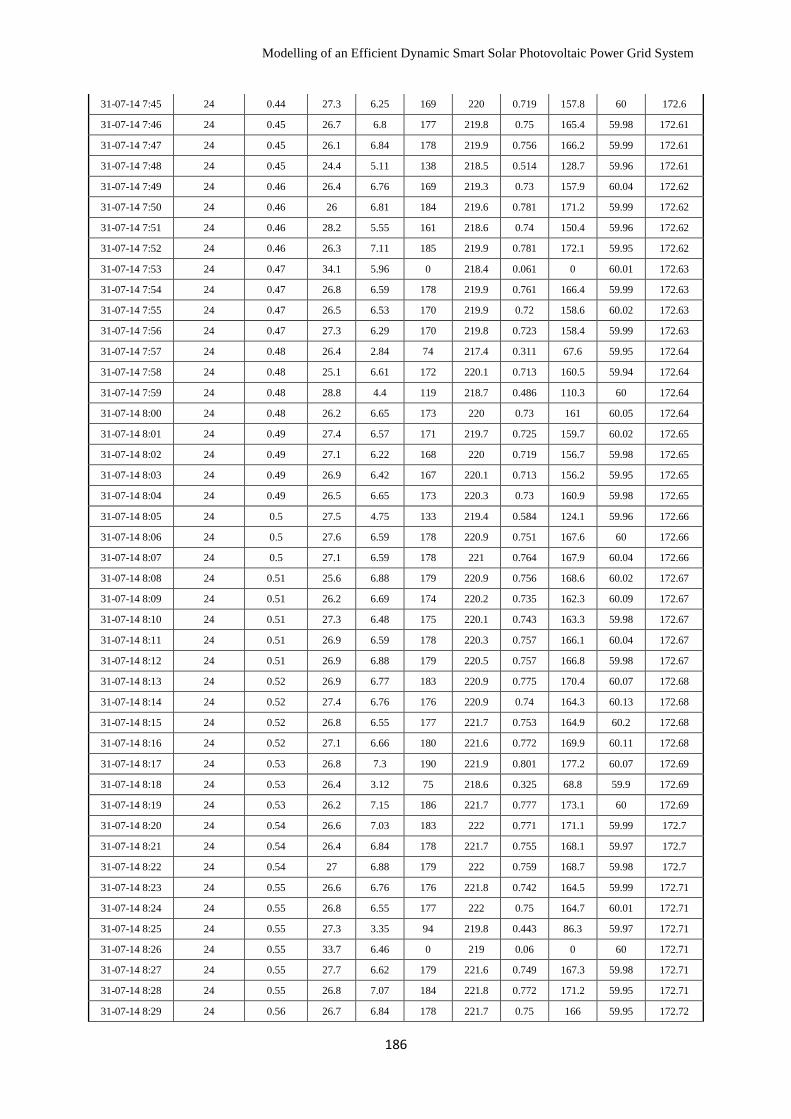
Modelling of an Efficient Dynamic Smart Solar Photovoltaic Power Grid System
186
31-07-14 7:45 24 0.44 27.3 6.25 169 220 0.719 157.8 60 172.6
31-07-14 7:46 24 0.45 26.7 6.8 177 219.8 0.75 165.4 59.98 172.61
31-07-14 7:47 24 0.45 26.1 6.84 178 219.9 0.756 166.2 59.99 172.61
31-07-14 7:48 24 0.45 24.4 5.11 138 218.5 0.514 128.7 59.96 172.61
31-07-14 7:49 24 0.46 26.4 6.76 169 219.3 0.73 157.9 60.04 172.62
31-07-14 7:50 24 0.46 26 6.81 184 219.6 0.781 171.2 59.99 172.62
31-07-14 7:51 24 0.46 28.2 5.55 161 218.6 0.74 150.4 59.96 172.62
31-07-14 7:52 24 0.46 26.3 7.11 185 219.9 0.781 172.1 59.95 172.62
31-07-14 7:53 24 0.47 34.1 5.96 0 218.4 0.061 0 60.01 172.63
31-07-14 7:54 24 0.47 26.8 6.59 178 219.9 0.761 166.4 59.99 172.63
31-07-14 7:55 24 0.47 26.5 6.53 170 219.9 0.72 158.6 60.02 172.63
31-07-14 7:56 24 0.47 27.3 6.29 170 219.8 0.723 158.4 59.99 172.63
31-07-14 7:57 24 0.48 26.4 2.84 74 217.4 0.311 67.6 59.95 172.64
31-07-14 7:58 24 0.48 25.1 6.61 172 220.1 0.713 160.5 59.94 172.64
31-07-14 7:59 24 0.48 28.8 4.4 119 218.7 0.486 110.3 60 172.64
31-07-14 8:00 24 0.48 26.2 6.65 173 220 0.73 161 60.05 172.64
31-07-14 8:01 24 0.49 27.4 6.57 171 219.7 0.725 159.7 60.02 172.65
31-07-14 8:02 24 0.49 27.1 6.22 168 220 0.719 156.7 59.98 172.65
31-07-14 8:03 24 0.49 26.9 6.42 167 220.1 0.713 156.2 59.95 172.65
31-07-14 8:04 24 0.49 26.5 6.65 173 220.3 0.73 160.9 59.98 172.65
31-07-14 8:05 24 0.5 27.5 4.75 133 219.4 0.584 124.1 59.96 172.66
31-07-14 8:06 24 0.5 27.6 6.59 178 220.9 0.751 167.6 60 172.66
31-07-14 8:07 24 0.5 27.1 6.59 178 221 0.764 167.9 60.04 172.66
31-07-14 8:08 24 0.51 25.6 6.88 179 220.9 0.756 168.6 60.02 172.67
31-07-14 8:09 24 0.51 26.2 6.69 174 220.2 0.735 162.3 60.09 172.67
31-07-14 8:10 24 0.51 27.3 6.48 175 220.1 0.743 163.3 59.98 172.67
31-07-14 8:11 24 0.51 26.9 6.59 178 220.3 0.757 166.1 60.04 172.67
31-07-14 8:12 24 0.51 26.9 6.88 179 220.5 0.757 166.8 59.98 172.67
31-07-14 8:13 24 0.52 26.9 6.77 183 220.9 0.775 170.4 60.07 172.68
31-07-14 8:14 24 0.52 27.4 6.76 176 220.9 0.74 164.3 60.13 172.68
31-07-14 8:15 24 0.52 26.8 6.55 177 221.7 0.753 164.9 60.2 172.68
31-07-14 8:16 24 0.52 27.1 6.66 180 221.6 0.772 169.9 60.11 172.68
31-07-14 8:17 24 0.53 26.8 7.3 190 221.9 0.801 177.2 60.07 172.69
31-07-14 8:18 24 0.53 26.4 3.12 75 218.6 0.325 68.8 59.9 172.69
31-07-14 8:19 24 0.53 26.2 7.15 186 221.7 0.777 173.1 60 172.69
31-07-14 8:20 24 0.54 26.6 7.03 183 222 0.771 171.1 59.99 172.7
31-07-14 8:21 24 0.54 26.4 6.84 178 221.7 0.755 168.1 59.97 172.7
31-07-14 8:22 24 0.54 27 6.88 179 222 0.759 168.7 59.98 172.7
31-07-14 8:23 24 0.55 26.6 6.76 176 221.8 0.742 164.5 59.99 172.71
31-07-14 8:24 24 0.55 26.8 6.55 177 222 0.75 164.7 60.01 172.71
31-07-14 8:25 24 0.55 27.3 3.35 94 219.8 0.443 86.3 59.97 172.71
31-07-14 8:26 24 0.55 33.7 6.46 0 219 0.06 0 60 172.71
31-07-14 8:27 24 0.55 27.7 6.62 179 221.6 0.749 167.3 59.98 172.71
31-07-14 8:28 24 0.55 26.8 7.07 184 221.8 0.772 171.2 59.95 172.71
31-07-14 8:29 24 0.56 26.7 6.84 178 221.7 0.75 166 59.95 172.72
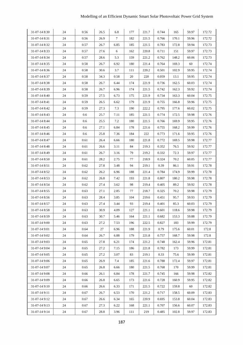
Modelling of an Efficient Dynamic Smart Solar Photovoltaic Power Grid System
187
31-07-14 8:30 24 0.56 26.5 6.8 177 221.7 0.744 165 59.97 172.72
31-07-14 8:31 24 0.56 26.9 7 182 221.5 0.766 170.1 59.96 172.72
31-07-14 8:32 24 0.57 26.7 6.85 185 221.5 0.783 172.8 59.94 172.73
31-07-14 8:33 24 0.57 27.6 6 162 220.8 0.711 151 59.97 172.73
31-07-14 8:34 24 0.57 28.6 5.3 159 221.2 0.762 148.2 60.06 172.73
31-07-14 8:35 24 0.58 26.7 6.92 180 221.4 0.764 169.3 60 172.74
31-07-14 8:36 24 0.58 30.6 3.7 111 220.2 0.501 102.9 59.95 172.74
31-07-14 8:37 24 0.58 34.3 0.58 20 220 0.059 13.1 59.95 172.74
31-07-14 8:38 24 0.58 26.7 6.44 174 221.9 0.736 162.5 60.03 172.74
31-07-14 8:39 24 0.58 26.7 6.96 174 221.5 0.742 162.3 59.92 172.74
31-07-14 8:40 24 0.59 27.5 6.73 175 221.9 0.734 163.3 60.04 172.75
31-07-14 8:41 24 0.59 26.5 6.62 179 221.9 0.755 166.8 59.96 172.75
31-07-14 8:42 24 0.59 27.3 7.3 190 222.2 0.795 177.6 60.02 172.75
31-07-14 8:43 24 0.6 25.7 7.11 185 221.5 0.774 172.5 59.98 172.76
31-07-14 8:44 24 0.6 25.5 7.2 180 221.5 0.766 169.9 59.95 172.76
31-07-14 8:45 24 0.6 27.1 6.84 178 221.6 0.755 168.2 59.99 172.76
31-07-14 8:46 24 0.6 25.8 7.36 184 222 0.773 171.6 59.95 172.76
31-07-14 8:47 24 0.61 26.4 6.66 180 221.8 0.772 169.5 59.98 172.77
31-07-14 8:48 24 0.61 26.6 3.11 84 219.3 0.352 76.5 59.92 172.77
31-07-14 8:49 24 0.61 26.7 3.16 79 219.2 0.332 72.3 59.97 172.77
31-07-14 8:50 24 0.61 28.2 2.75 77 218.9 0.324 70.2 60.05 172.77
31-07-14 8:51 24 0.62 27.8 3.48 94 219.1 0.39 86.1 59.91 172.78
31-07-14 8:52 24 0.62 26.2 6.96 188 221.4 0.784 174.9 59.99 172.78
31-07-14 8:53 24 0.62 26.8 7.42 193 221.8 0.807 180.2 59.98 172.78
31-07-14 8:54 24 0.62 27.4 3.62 98 219.4 0.405 89.2 59.92 172.78
31-07-14 8:55 24 0.63 27.1 2.85 77 218.7 0.325 70.2 59.98 172.79
31-07-14 8:56 24 0.63 28.4 3.85 104 219.6 0.451 95.7 59.93 172.79
31-07-14 8:57 24 0.63 27.4 3.44 93 219.4 0.401 85.3 60.03 172.79
31-07-14 8:58 24 0.63 30.9 4.09 127 221.1 0.601 118.6 59.98 172.79
31-07-14 8:59 24 0.63 30.7 5.46 164 221.1 0.682 153.3 59.88 172.79
31-07-14 9:00 24 0.63 27.2 7.53 196 222.5 0.827 183 59.99 172.79
31-07-14 9:01 24 0.64 27 6.96 188 221.9 0.79 175.6 60.01 172.8
31-07-14 9:02 24 0.64 26.7 6.88 179 221.8 0.757 168.7 59.98 172.8
31-07-14 9:03 24 0.65 27.8 6.21 174 221.2 0.748 162.4 59.96 172.81
31-07-14 9:04 24 0.65 27.2 7.15 186 221.8 0.782 173 59.99 172.81
31-07-14 9:05 24 0.65 27.2 3.07 83 219.1 0.33 75.6 59.99 172.81
31-07-14 9:06 24 0.65 26.9 7.4 185 221.6 0.788 172.4 59.97 172.81
31-07-14 9:07 24 0.65 26.8 6.66 180 221.5 0.768 170 59.99 172.81
31-07-14 9:08 24 0.66 26.1 6.84 178 221.7 0.745 166 59.98 172.82
31-07-14 9:09 24 0.66 26.8 6.65 173 221.6 0.728 160.9 59.95 172.82
31-07-14 9:10 24 0.66 26.6 6.33 171 221.5 0.722 159.8 60 172.82
31-07-14 9:11 24 0.67 26.7 6.53 170 221.2 0.717 158.5 60.09 172.83
31-07-14 9:12 24 0.67 26.6 6.34 165 220.9 0.695 153.8 60.04 172.83
31-07-14 9:13 24 0.67 27.3 6.22 168 221.1 0.707 156.6 60.07 172.83
31-07-14 9:14 24 0.67 28.8 3.96 111 219 0.485 102.8 59.97 172.83
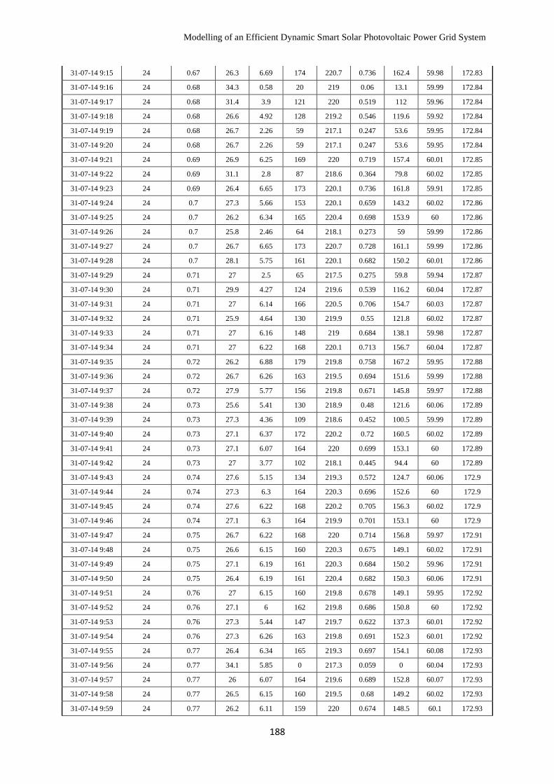
Modelling of an Efficient Dynamic Smart Solar Photovoltaic Power Grid System
188
31-07-14 9:15 24 0.67 26.3 6.69 174 220.7 0.736 162.4 59.98 172.83
31-07-14 9:16 24 0.68 34.3 0.58 20 219 0.06 13.1 59.99 172.84
31-07-14 9:17 24 0.68 31.4 3.9 121 220 0.519 112 59.96 172.84
31-07-14 9:18 24 0.68 26.6 4.92 128 219.2 0.546 119.6 59.92 172.84
31-07-14 9:19 24 0.68 26.7 2.26 59 217.1 0.247 53.6 59.95 172.84
31-07-14 9:20 24 0.68 26.7 2.26 59 217.1 0.247 53.6 59.95 172.84
31-07-14 9:21 24 0.69 26.9 6.25 169 220 0.719 157.4 60.01 172.85
31-07-14 9:22 24 0.69 31.1 2.8 87 218.6 0.364 79.8 60.02 172.85
31-07-14 9:23 24 0.69 26.4 6.65 173 220.1 0.736 161.8 59.91 172.85
31-07-14 9:24 24 0.7 27.3 5.66 153 220.1 0.659 143.2 60.02 172.86
31-07-14 9:25 24 0.7 26.2 6.34 165 220.4 0.698 153.9 60 172.86
31-07-14 9:26 24 0.7 25.8 2.46 64 218.1 0.273 59 59.99 172.86
31-07-14 9:27 24 0.7 26.7 6.65 173 220.7 0.728 161.1 59.99 172.86
31-07-14 9:28 24 0.7 28.1 5.75 161 220.1 0.682 150.2 60.01 172.86
31-07-14 9:29 24 0.71 27 2.5 65 217.5 0.275 59.8 59.94 172.87
31-07-14 9:30 24 0.71 29.9 4.27 124 219.6 0.539 116.2 60.04 172.87
31-07-14 9:31 24 0.71 27 6.14 166 220.5 0.706 154.7 60.03 172.87
31-07-14 9:32 24 0.71 25.9 4.64 130 219.9 0.55 121.8 60.02 172.87
31-07-14 9:33 24 0.71 27 6.16 148 219 0.684 138.1 59.98 172.87
31-07-14 9:34 24 0.71 27 6.22 168 220.1 0.713 156.7 60.04 172.87
31-07-14 9:35 24 0.72 26.2 6.88 179 219.8 0.758 167.2 59.95 172.88
31-07-14 9:36 24 0.72 26.7 6.26 163 219.5 0.694 151.6 59.99 172.88
31-07-14 9:37 24 0.72 27.9 5.77 156 219.8 0.671 145.8 59.97 172.88
31-07-14 9:38 24 0.73 25.6 5.41 130 218.9 0.48 121.6 60.06 172.89
31-07-14 9:39 24 0.73 27.3 4.36 109 218.6 0.452 100.5 59.99 172.89
31-07-14 9:40 24 0.73 27.1 6.37 172 220.2 0.72 160.5 60.02 172.89
31-07-14 9:41 24 0.73 27.1 6.07 164 220 0.699 153.1 60 172.89
31-07-14 9:42 24 0.73 27 3.77 102 218.1 0.445 94.4 60 172.89
31-07-14 9:43 24 0.74 27.6 5.15 134 219.3 0.572 124.7 60.06 172.9
31-07-14 9:44 24 0.74 27.3 6.3 164 220.3 0.696 152.6 60 172.9
31-07-14 9:45 24 0.74 27.6 6.22 168 220.2 0.705 156.3 60.02 172.9
31-07-14 9:46 24 0.74 27.1 6.3 164 219.9 0.701 153.1 60 172.9
31-07-14 9:47 24 0.75 26.7 6.22 168 220 0.714 156.8 59.97 172.91
31-07-14 9:48 24 0.75 26.6 6.15 160 220.3 0.675 149.1 60.02 172.91
31-07-14 9:49 24 0.75 27.1 6.19 161 220.3 0.684 150.2 59.96 172.91
31-07-14 9:50 24 0.75 26.4 6.19 161 220.4 0.682 150.3 60.06 172.91
31-07-14 9:51 24 0.76 27 6.15 160 219.8 0.678 149.1 59.95 172.92
31-07-14 9:52 24 0.76 27.1 6 162 219.8 0.686 150.8 60 172.92
31-07-14 9:53 24 0.76 27.3 5.44 147 219.7 0.622 137.3 60.01 172.92
31-07-14 9:54 24 0.76 27.3 6.26 163 219.8 0.691 152.3 60.01 172.92
31-07-14 9:55 24 0.77 26.4 6.34 165 219.3 0.697 154.1 60.08 172.93
31-07-14 9:56 24 0.77 34.1 5.85 0 217.3 0.059 0 60.04 172.93
31-07-14 9:57 24 0.77 26 6.07 164 219.6 0.689 152.8 60.07 172.93
31-07-14 9:58 24 0.77 26.5 6.15 160 219.5 0.68 149.2 60.02 172.93
31-07-14 9:59 24 0.77 26.2 6.11 159 220 0.674 148.5 60.1 172.93
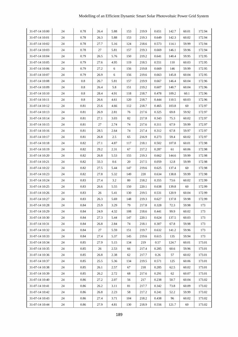
Modelling of an Efficient Dynamic Smart Solar Photovoltaic Power Grid System
189
31-07-14 10:00 24 0.78 26.4 5.88 153 219.9 0.651 142.7 60.01 172.94
31-07-14 10:01 24 0.78 26.3 5.88 153 219.3 0.649 142.3 60.02 172.94
31-07-14 10:02 24 0.78 27.7 5.16 124 218.6 0.573 114.1 59.99 172.94
31-07-14 10:03 24 0.78 27 5.81 157 219.3 0.669 146.1 59.96 172.94
31-07-14 10:04 24 0.79 26.5 5.76 150 219.2 0.641 140.4 59.95 172.95
31-07-14 10:05 24 0.79 27.6 4.95 119 218.5 0.551 110 60.03 172.95
31-07-14 10:06 24 0.79 27.2 6 156 219.8 0.669 146 59.99 172.95
31-07-14 10:07 24 0.79 26.9 6 156 219.6 0.663 145.8 60.04 172.95
31-07-14 10:08 24 0.8 26.7 5.81 157 219.9 0.667 146.4 60.04 172.96
31-07-14 10:09 24 0.8 26.4 5.8 151 219.2 0.607 140.7 60.04 172.96
31-07-14 10:10 24 0.8 28.4 4.91 118 218.7 0.478 109.2 60.1 172.96
31-07-14 10:11 24 0.8 26.6 4.61 120 218.7 0.444 110.5 60.03 172.96
31-07-14 10:12 24 0.81 25.6 4.66 112 218.7 0.465 103.8 60 172.97
31-07-14 10:13 24 0.81 26.9 2.81 76 217.6 0.325 69.8 59.92 172.97
31-07-14 10:14 24 0.81 27.1 3.03 82 217.8 0.343 75.3 60.02 172.97
31-07-14 10:15 24 0.81 27 2.74 74 217.6 0.311 67.9 59.99 172.97
31-07-14 10:16 24 0.81 28.5 2.64 74 217.4 0.312 67.8 59.97 172.97
31-07-14 10:17 24 0.81 26.8 2.5 65 216.9 0.273 59.4 60.02 172.97
31-07-14 10:18 24 0.82 27.1 4.87 117 218.1 0.502 107.8 60.01 172.98
31-07-14 10:19 24 0.82 29.2 2.31 67 217.2 0.287 61 60.06 172.98
31-07-14 10:20 24 0.82 26.8 5.53 155 219.3 0.662 144.6 59.99 172.98
31-07-14 10:21 24 0.82 33.3 0.6 20 217.5 0.059 12.8 59.99 172.98
31-07-14 10:22 24 0.82 27.5 5.44 147 219.6 0.625 137.4 60 172.98
31-07-14 10:23 24 0.82 27.8 5.32 149 220 0.634 138.8 59.99 172.98
31-07-14 10:24 24 0.83 27.4 3.2 80 218.2 0.355 73.6 60.02 172.99
31-07-14 10:25 24 0.83 26.6 5.55 150 220.1 0.638 139.8 60 172.99
31-07-14 10:26 24 0.83 26 5.41 130 219.5 0.531 120.9 60.04 172.99
31-07-14 10:27 24 0.83 26.3 5.69 148 219.3 0.627 137.8 59.98 172.99
31-07-14 10:28 24 0.84 25.9 3.29 79 217.8 0.328 72.3 59.98 173
31-07-14 10:29 24 0.84 24.9 4.32 108 218.6 0.441 99.9 60.02 173
31-07-14 10:30 24 0.84 27.3 5.44 147 220.1 0.624 137.5 60.03 173
31-07-14 10:31 24 0.84 26.8 2.84 74 218.1 0.307 67.8 59.98 173
31-07-14 10:32 24 0.84 27 5.59 151 219.7 0.632 141.2 59.96 173
31-07-14 10:33 24 0.84 27.4 5.37 145 219.6 0.615 135 59.94 173
31-07-14 10:34 24 0.85 27.9 5.15 134 219 0.57 124.7 60.01 173.01
31-07-14 10:35 24 0.85 26 2.53 66 217.4 0.285 60.6 59.96 173.01
31-07-14 10:36 24 0.85 26.8 2.38 62 217.7 0.26 57 60.02 173.01
31-07-14 10:37 24 0.85 25.5 5.36 134 219.5 0.571 125 60.06 173.01
31-07-14 10:38 24 0.85 26.1 2.57 67 218 0.285 62.5 60.02 173.01
31-07-14 10:39 24 0.85 26.2 2.72 68 217.6 0.291 62 60.07 173.01
31-07-14 10:40 24 0.86 27.2 2.07 56 217 0.238 50.7 60.04 173.02
31-07-14 10:41 24 0.86 26.2 3.11 81 217.7 0.342 73.8 60.09 173.02
31-07-14 10:42 24 0.86 26.8 2.23 58 217.2 0.241 52.2 59.99 173.02
31-07-14 10:43 24 0.86 27.4 3.71 104 218.2 0.438 96 60.02 173.02
31-07-14 10:44 24 0.86 27.9 4.81 130 218.9 0.556 121.7 60 173.02
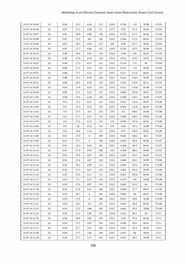
Modelling of an Efficient Dynamic Smart Solar Photovoltaic Power Grid System
190
31-07-14 10:45 24 0.86 29.2 4.24 123 218.9 0.526 114 59.98 173.02
31-07-14 10:46 24 0.87 27.5 2.68 67 217.3 0.29 61.3 59.95 173.03
31-07-14 10:47 24 0.87 26.8 4.84 126 219.3 0.535 117.7 60.02 173.03
31-07-14 10:48 24 0.87 25.2 4.8 120 218.5 0.504 111.2 60.02 173.03
31-07-14 10:49 24 0.87 29.5 4.03 117 219 0.48 107.7 60.05 173.03
31-07-14 10:50 24 0.87 27.7 4.46 125 218.9 0.529 115.1 59.96 173.03
31-07-14 10:51 24 0.88 29.6 3.93 114 218.9 0.48 105 60.01 173.04
31-07-14 10:52 24 0.88 27.6 4.59 124 219.4 0.522 114.5 59.97 173.04
31-07-14 10:53 24 0.88 27.5 4.51 122 219.1 0.519 113 60 173.04
31-07-14 10:54 24 0.88 27.2 4.51 122 219.5 0.515 113 59.96 173.04
31-07-14 10:55 24 0.88 27.7 4.32 121 219.7 0.511 111.8 60.01 173.04
31-07-14 10:56 24 0.88 27.3 4.59 124 219.7 0.522 114.4 59.92 173.04
31-07-14 10:57 24 0.89 28.5 4.28 120 219.5 0.501 110.4 60.11 173.05
31-07-14 10:58 24 0.89 27.9 4.28 120 219.2 0.512 110.8 59.98 173.05
31-07-14 10:59 24 0.89 27.5 4.25 115 219.2 0.483 105.8 60.07 173.05
31-07-14 11:00 24 0.89 27.9 4.44 120 218.9 0.506 110.5 59.99 173.05
31-07-14 11:01 24 0.9 27.2 4.51 122 219.2 0.513 112.6 60.07 173.06
31-07-14 11:02 24 0.9 27.3 4.55 123 219.3 0.505 113.8 60.05 173.06
31-07-14 11:03 24 0.9 27.7 4.4 119 219 0.5 109.5 59.96 173.06
31-07-14 11:04 24 0.9 27.5 4.25 115 219.3 0.485 106.5 60.04 173.06
31-07-14 11:05 24 0.9 27.6 4.14 116 219 0.492 107.4 60.02 173.06
31-07-14 11:06 24 0.9 28 4.22 114 219 0.48 105.3 59.98 173.06
31-07-14 11:07 24 0.9 26.6 4.14 112 219.6 0.47 103.6 60.02 173.06
31-07-14 11:08 24 0.91 27.8 4 108 219.8 0.456 100.2 60.1 173.07
31-07-14 11:09 24 0.91 27.7 4 108 219.6 0.453 99.4 60.06 173.07
31-07-14 11:10 24 0.91 29.3 3.03 88 218.7 0.368 80.4 60.01 173.07
31-07-14 11:11 24 0.91 27.4 4.03 109 219 0.458 100.5 59.99 173.07
31-07-14 11:12 24 0.91 27.8 4.07 110 219.2 0.465 101.7 60.02 173.07
31-07-14 11:13 24 0.92 27.6 4.07 110 219.2 0.466 102.1 59.99 173.08
31-07-14 11:14 24 0.92 28.3 3.96 111 219.5 0.463 102.3 60.05 173.08
31-07-14 11:15 24 0.92 27.5 4.07 110 219.7 0.463 101.2 59.99 173.08
31-07-14 11:16 24 0.92 27.6 4.11 111 219.8 0.467 102.6 60.06 173.08
31-07-14 11:17 24 0.92 27.3 4.22 114 219.7 0.479 105 59.98 173.08
31-07-14 11:18 24 0.93 27.6 4.07 110 219.2 0.462 101.2 60 173.09
31-07-14 11:19 24 0.93 27.8 3.92 106 218.7 0.449 97.7 60.01 173.09
31-07-14 11:20 24 0.93 26.7 4 104 218.8 0.443 96 60.01 173.09
31-07-14 11:21 24 0.93 27.9 4 108 219.1 0.457 99.9 59.98 173.09
31-07-14 11:22 24 0.93 25.5 4.2 105 219.2 0.441 96.9 60.02 173.09
31-07-14 11:23 24 0.93 27.5 3.88 105 219.7 0.443 97.5 59.98 173.09
31-07-14 11:24 24 0.94 27.6 3.96 107 219.8 0.451 99.1 60 173.1
31-07-14 11:25 24 0.94 28.4 3.81 103 219.7 0.43 95.3 60.02 173.1
31-07-14 11:26 24 0.94 27.1 3.81 103 219.2 0.436 95.6 60.01 173.1
31-07-14 11:27 24 0.94 27.7 3.81 103 219.3 0.437 95.3 59.95 173.1
31-07-14 11:28 24 0.94 27.7 3.85 104 219.7 0.437 96 59.93 173.1
31-07-14 11:29 24 0.94 27.7 3.77 102 219.7 0.427 94.2 59.98 173.1
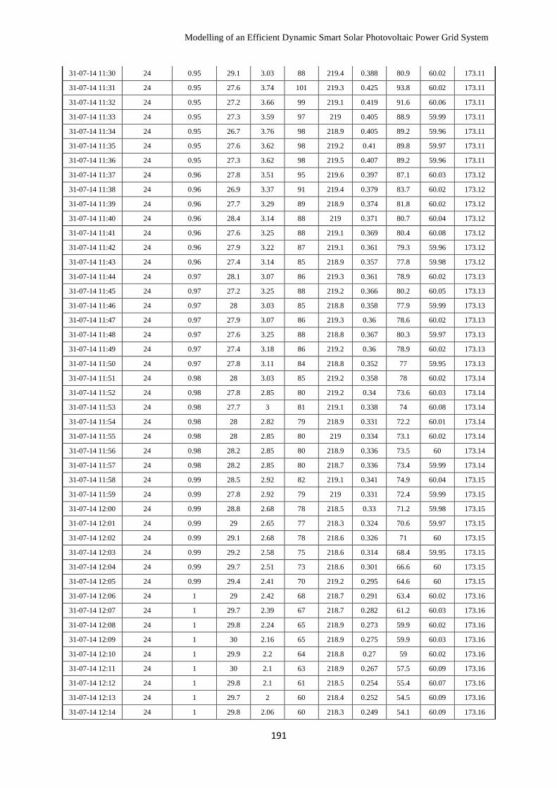
Modelling of an Efficient Dynamic Smart Solar Photovoltaic Power Grid System
191
31-07-14 11:30 24 0.95 29.1 3.03 88 219.4 0.388 80.9 60.02 173.11
31-07-14 11:31 24 0.95 27.6 3.74 101 219.3 0.425 93.8 60.02 173.11
31-07-14 11:32 24 0.95 27.2 3.66 99 219.1 0.419 91.6 60.06 173.11
31-07-14 11:33 24 0.95 27.3 3.59 97 219 0.405 88.9 59.99 173.11
31-07-14 11:34 24 0.95 26.7 3.76 98 218.9 0.405 89.2 59.96 173.11
31-07-14 11:35 24 0.95 27.6 3.62 98 219.2 0.41 89.8 59.97 173.11
31-07-14 11:36 24 0.95 27.3 3.62 98 219.5 0.407 89.2 59.96 173.11
31-07-14 11:37 24 0.96 27.8 3.51 95 219.6 0.397 87.1 60.03 173.12
31-07-14 11:38 24 0.96 26.9 3.37 91 219.4 0.379 83.7 60.02 173.12
31-07-14 11:39 24 0.96 27.7 3.29 89 218.9 0.374 81.8 60.02 173.12
31-07-14 11:40 24 0.96 28.4 3.14 88 219 0.371 80.7 60.04 173.12
31-07-14 11:41 24 0.96 27.6 3.25 88 219.1 0.369 80.4 60.08 173.12
31-07-14 11:42 24 0.96 27.9 3.22 87 219.1 0.361 79.3 59.96 173.12
31-07-14 11:43 24 0.96 27.4 3.14 85 218.9 0.357 77.8 59.98 173.12
31-07-14 11:44 24 0.97 28.1 3.07 86 219.3 0.361 78.9 60.02 173.13
31-07-14 11:45 24 0.97 27.2 3.25 88 219.2 0.366 80.2 60.05 173.13
31-07-14 11:46 24 0.97 28 3.03 85 218.8 0.358 77.9 59.99 173.13
31-07-14 11:47 24 0.97 27.9 3.07 86 219.3 0.36 78.6 60.02 173.13
31-07-14 11:48 24 0.97 27.6 3.25 88 218.8 0.367 80.3 59.97 173.13
31-07-14 11:49 24 0.97 27.4 3.18 86 219.2 0.36 78.9 60.02 173.13
31-07-14 11:50 24 0.97 27.8 3.11 84 218.8 0.352 77 59.95 173.13
31-07-14 11:51 24 0.98 28 3.03 85 219.2 0.358 78 60.02 173.14
31-07-14 11:52 24 0.98 27.8 2.85 80 219.2 0.34 73.6 60.03 173.14
31-07-14 11:53 24 0.98 27.7 3 81 219.1 0.338 74 60.08 173.14
31-07-14 11:54 24 0.98 28 2.82 79 218.9 0.331 72.2 60.01 173.14
31-07-14 11:55 24 0.98 28 2.85 80 219 0.334 73.1 60.02 173.14
31-07-14 11:56 24 0.98 28.2 2.85 80 218.9 0.336 73.5 60 173.14
31-07-14 11:57 24 0.98 28.2 2.85 80 218.7 0.336 73.4 59.99 173.14
31-07-14 11:58 24 0.99 28.5 2.92 82 219.1 0.341 74.9 60.04 173.15
31-07-14 11:59 24 0.99 27.8 2.92 79 219 0.331 72.4 59.99 173.15
31-07-14 12:00 24 0.99 28.8 2.68 78 218.5 0.33 71.2 59.98 173.15
31-07-14 12:01 24 0.99 29 2.65 77 218.3 0.324 70.6 59.97 173.15
31-07-14 12:02 24 0.99 29.1 2.68 78 218.6 0.326 71 60 173.15
31-07-14 12:03 24 0.99 29.2 2.58 75 218.6 0.314 68.4 59.95 173.15
31-07-14 12:04 24 0.99 29.7 2.51 73 218.6 0.301 66.6 60 173.15
31-07-14 12:05 24 0.99 29.4 2.41 70 219.2 0.295 64.6 60 173.15
31-07-14 12:06 24 1 29 2.42 68 218.7 0.291 63.4 60.02 173.16
31-07-14 12:07 24 1 29.7 2.39 67 218.7 0.282 61.2 60.03 173.16
31-07-14 12:08 24 1 29.8 2.24 65 218.9 0.273 59.9 60.02 173.16
31-07-14 12:09 24 1 30 2.16 65 218.9 0.275 59.9 60.03 173.16
31-07-14 12:10 24 1 29.9 2.2 64 218.8 0.27 59 60.02 173.16
31-07-14 12:11 24 1 30 2.1 63 218.9 0.267 57.5 60.09 173.16
31-07-14 12:12 24 1 29.8 2.1 61 218.5 0.254 55.4 60.07 173.16
31-07-14 12:13 24 1 29.7 2 60 218.4 0.252 54.5 60.09 173.16
31-07-14 12:14 24 1 29.8 2.06 60 218.3 0.249 54.1 60.09 173.16
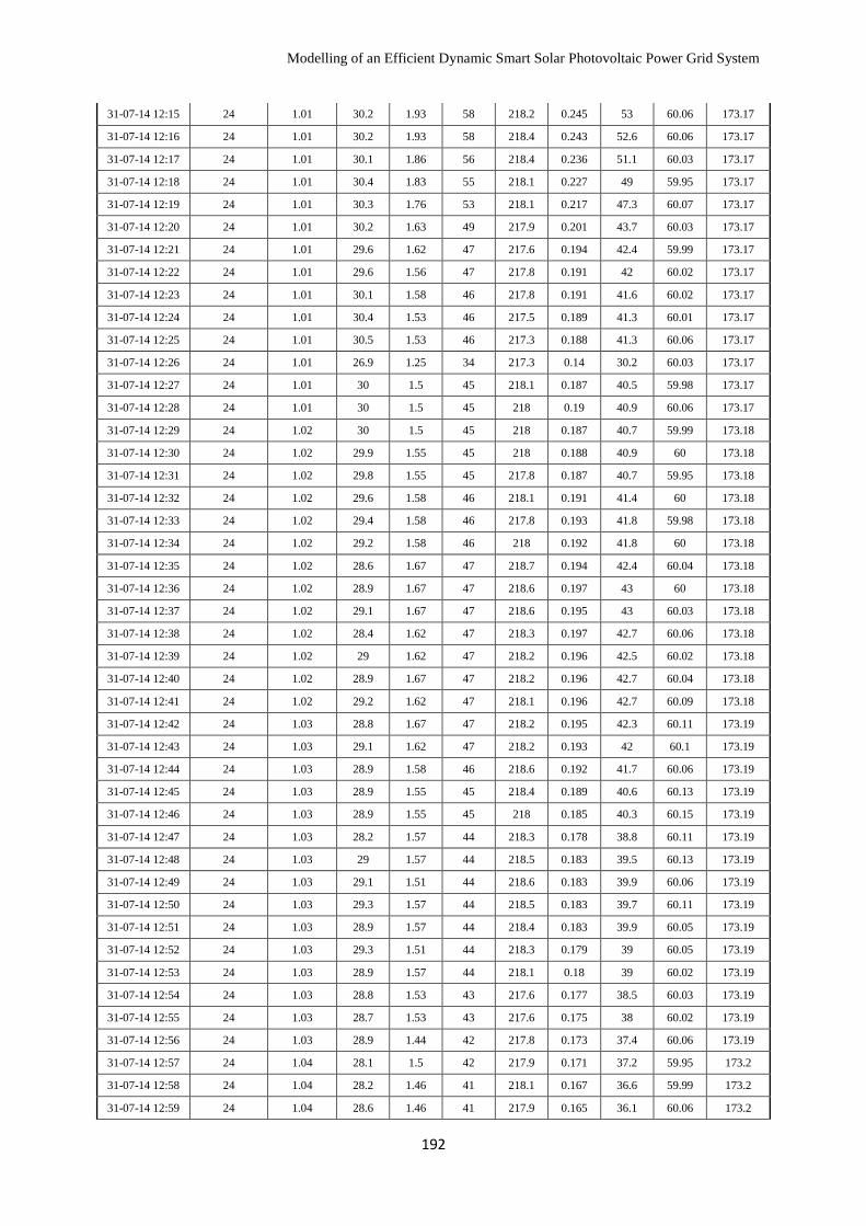
Modelling of an Efficient Dynamic Smart Solar Photovoltaic Power Grid System
192
31-07-14 12:15 24 1.01 30.2 1.93 58 218.2 0.245 53 60.06 173.17
31-07-14 12:16 24 1.01 30.2 1.93 58 218.4 0.243 52.6 60.06 173.17
31-07-14 12:17 24 1.01 30.1 1.86 56 218.4 0.236 51.1 60.03 173.17
31-07-14 12:18 24 1.01 30.4 1.83 55 218.1 0.227 49 59.95 173.17
31-07-14 12:19 24 1.01 30.3 1.76 53 218.1 0.217 47.3 60.07 173.17
31-07-14 12:20 24 1.01 30.2 1.63 49 217.9 0.201 43.7 60.03 173.17
31-07-14 12:21 24 1.01 29.6 1.62 47 217.6 0.194 42.4 59.99 173.17
31-07-14 12:22 24 1.01 29.6 1.56 47 217.8 0.191 42 60.02 173.17
31-07-14 12:23 24 1.01 30.1 1.58 46 217.8 0.191 41.6 60.02 173.17
31-07-14 12:24 24 1.01 30.4 1.53 46 217.5 0.189 41.3 60.01 173.17
31-07-14 12:25 24 1.01 30.5 1.53 46 217.3 0.188 41.3 60.06 173.17
31-07-14 12:26 24 1.01 26.9 1.25 34 217.3 0.14 30.2 60.03 173.17
31-07-14 12:27 24 1.01 30 1.5 45 218.1 0.187 40.5 59.98 173.17
31-07-14 12:28 24 1.01 30 1.5 45 218 0.19 40.9 60.06 173.17
31-07-14 12:29 24 1.02 30 1.5 45 218 0.187 40.7 59.99 173.18
31-07-14 12:30 24 1.02 29.9 1.55 45 218 0.188 40.9 60 173.18
31-07-14 12:31 24 1.02 29.8 1.55 45 217.8 0.187 40.7 59.95 173.18
31-07-14 12:32 24 1.02 29.6 1.58 46 218.1 0.191 41.4 60 173.18
31-07-14 12:33 24 1.02 29.4 1.58 46 217.8 0.193 41.8 59.98 173.18
31-07-14 12:34 24 1.02 29.2 1.58 46 218 0.192 41.8 60 173.18
31-07-14 12:35 24 1.02 28.6 1.67 47 218.7 0.194 42.4 60.04 173.18
31-07-14 12:36 24 1.02 28.9 1.67 47 218.6 0.197 43 60 173.18
31-07-14 12:37 24 1.02 29.1 1.67 47 218.6 0.195 43 60.03 173.18
31-07-14 12:38 24 1.02 28.4 1.62 47 218.3 0.197 42.7 60.06 173.18
31-07-14 12:39 24 1.02 29 1.62 47 218.2 0.196 42.5 60.02 173.18
31-07-14 12:40 24 1.02 28.9 1.67 47 218.2 0.196 42.7 60.04 173.18
31-07-14 12:41 24 1.02 29.2 1.62 47 218.1 0.196 42.7 60.09 173.18
31-07-14 12:42 24 1.03 28.8 1.67 47 218.2 0.195 42.3 60.11 173.19
31-07-14 12:43 24 1.03 29.1 1.62 47 218.2 0.193 42 60.1 173.19
31-07-14 12:44 24 1.03 28.9 1.58 46 218.6 0.192 41.7 60.06 173.19
31-07-14 12:45 24 1.03 28.9 1.55 45 218.4 0.189 40.6 60.13 173.19
31-07-14 12:46 24 1.03 28.9 1.55 45 218 0.185 40.3 60.15 173.19
31-07-14 12:47 24 1.03 28.2 1.57 44 218.3 0.178 38.8 60.11 173.19
31-07-14 12:48 24 1.03 29 1.57 44 218.5 0.183 39.5 60.13 173.19
31-07-14 12:49 24 1.03 29.1 1.51 44 218.6 0.183 39.9 60.06 173.19
31-07-14 12:50 24 1.03 29.3 1.57 44 218.5 0.183 39.7 60.11 173.19
31-07-14 12:51 24 1.03 28.9 1.57 44 218.4 0.183 39.9 60.05 173.19
31-07-14 12:52 24 1.03 29.3 1.51 44 218.3 0.179 39 60.05 173.19
31-07-14 12:53 24 1.03 28.9 1.57 44 218.1 0.18 39 60.02 173.19
31-07-14 12:54 24 1.03 28.8 1.53 43 217.6 0.177 38.5 60.03 173.19
31-07-14 12:55 24 1.03 28.7 1.53 43 217.6 0.175 38 60.02 173.19
31-07-14 12:56 24 1.03 28.9 1.44 42 217.8 0.173 37.4 60.06 173.19
31-07-14 12:57 24 1.04 28.1 1.5 42 217.9 0.171 37.2 59.95 173.2
31-07-14 12:58 24 1.04 28.2 1.46 41 218.1 0.167 36.6 59.99 173.2
31-07-14 12:59 24 1.04 28.6 1.46 41 217.9 0.165 36.1 60.06 173.2
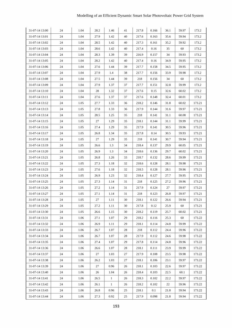
Modelling of an Efficient Dynamic Smart Solar Photovoltaic Power Grid System
193
31-07-14 13:00 24 1.04 28.2 1.46 41 217.8 0.166 36.1 59.97 173.2
31-07-14 13:01 24 1.04 27.9 1.42 40 217.6 0.163 35.6 59.94 173.2
31-07-14 13:02 24 1.04 28.5 1.42 40 217.3 0.161 35.2 59.92 173.2
31-07-14 13:03 24 1.04 28.6 1.42 40 217.4 0.16 35 60 173.2
31-07-14 13:04 24 1.04 28.3 1.39 39 216.9 0.157 34 59.93 173.2
31-07-14 13:05 24 1.04 28.2 1.42 40 217.4 0.16 34.9 59.95 173.2
31-07-14 13:06 24 1.04 27.6 1.44 39 217.7 0.158 34.5 59.95 173.2
31-07-14 13:07 24 1.04 27.9 1.4 38 217.7 0.156 33.9 59.98 173.2
31-07-14 13:08 24 1.04 27.5 1.44 39 218 0.156 34 60 173.2
31-07-14 13:09 24 1.04 27.9 1.37 37 217.7 0.151 32.8 59.99 173.2
31-07-14 13:10 24 1.04 28 1.32 37 217.6 0.15 32.6 60.02 173.2
31-07-14 13:11 24 1.04 27.6 1.37 37 217.6 0.148 32.4 60.01 173.2
31-07-14 13:12 24 1.05 27.7 1.33 36 218.2 0.146 31.8 60.02 173.21
31-07-14 13:13 24 1.05 27.8 1.33 36 217.9 0.144 31.6 59.97 173.21
31-07-14 13:14 24 1.05 28.5 1.25 35 218 0.141 31.1 60.08 173.21
31-07-14 13:15 24 1.05 27 1.29 35 218.1 0.144 31.1 59.99 173.21
31-07-14 13:16 24 1.05 27.4 1.29 35 217.9 0.141 30.5 59.96 173.21
31-07-14 13:17 24 1.05 26.8 1.34 35 217.8 0.14 30.5 59.93 173.21
31-07-14 13:18 24 1.05 27 1.29 35 218 0.141 30.7 59.94 173.21
31-07-14 13:19 24 1.05 26.6 1.3 34 218.4 0.137 29.9 60.05 173.21
31-07-14 13:20 24 1.05 26.9 1.3 34 218.6 0.136 29.7 60.02 173.21
31-07-14 13:21 24 1.05 26.8 1.26 33 218.7 0.132 28.6 59.99 173.21
31-07-14 13:22 24 1.05 27.3 1.18 32 218.6 0.128 28.1 59.98 173.21
31-07-14 13:23 24 1.05 27.6 1.18 32 218.5 0.128 28.1 59.96 173.21
31-07-14 13:24 24 1.05 26.9 1.23 32 218.4 0.127 27.7 59.95 173.21
31-07-14 13:25 24 1.05 27.3 1.14 31 218 0.125 27.2 59.96 173.21
31-07-14 13:26 24 1.05 27.2 1.14 31 217.9 0.124 27 59.97 173.21
31-07-14 13:27 24 1.05 27.1 1.14 31 218 0.123 26.8 59.97 173.21
31-07-14 13:28 24 1.05 27 1.11 30 218.1 0.122 26.6 59.94 173.21
31-07-14 13:29 24 1.05 27.2 1.11 30 217.8 0.12 25.9 60 173.21
31-07-14 13:30 24 1.05 26.6 1.15 30 218.2 0.119 25.7 60.02 173.21
31-07-14 13:31 24 1.06 27.1 1.07 29 218.2 0.116 25.3 60 173.22
31-07-14 13:32 24 1.06 26.9 1.11 29 218.1 0.114 24.8 59.99 173.22
31-07-14 13:33 24 1.06 26.7 1.07 28 218 0.112 24.4 59.96 173.22
31-07-14 13:34 24 1.06 26.7 1.07 28 217.9 0.112 24.6 59.98 173.22
31-07-14 13:35 24 1.06 27.4 1.07 29 217.8 0.114 24.8 59.96 173.22
31-07-14 13:36 24 1.06 26.6 1.07 28 218.1 0.111 23.9 59.99 173.22
31-07-14 13:37 24 1.06 27 1.03 27 217.9 0.108 23.5 59.98 173.22
31-07-14 13:38 24 1.06 26.2 1.03 27 218.1 0.106 23.1 59.97 173.22
31-07-14 13:39 24 1.06 27 0.96 26 218.1 0.103 22.6 59.97 173.22
31-07-14 13:40 24 1.06 26 1.04 26 218.4 0.103 22.5 60.1 173.22
31-07-14 13:41 24 1.06 26.5 1 26 218.3 0.102 22.2 59.97 173.22
31-07-14 13:42 24 1.06 26.1 1 26 218.2 0.102 22 59.96 173.22
31-07-14 13:43 24 1.06 26.8 0.96 25 218.1 0.1 21.8 59.94 173.22
31-07-14 13:44 24 1.06 27.3 0.92 25 217.9 0.098 21.8 59.94 173.22
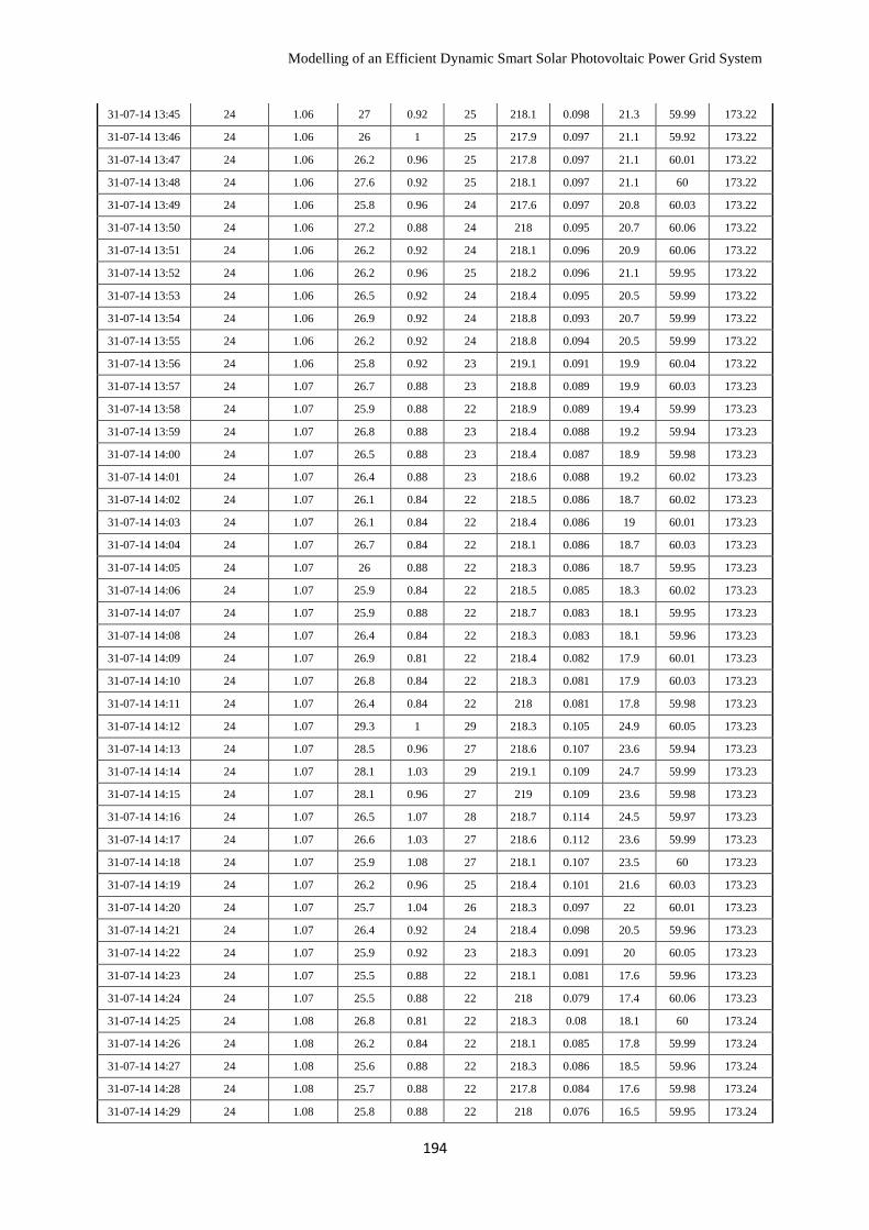
Modelling of an Efficient Dynamic Smart Solar Photovoltaic Power Grid System
194
31-07-14 13:45 24 1.06 27 0.92 25 218.1 0.098 21.3 59.99 173.22
31-07-14 13:46 24 1.06 26 1 25 217.9 0.097 21.1 59.92 173.22
31-07-14 13:47 24 1.06 26.2 0.96 25 217.8 0.097 21.1 60.01 173.22
31-07-14 13:48 24 1.06 27.6 0.92 25 218.1 0.097 21.1 60 173.22
31-07-14 13:49 24 1.06 25.8 0.96 24 217.6 0.097 20.8 60.03 173.22
31-07-14 13:50 24 1.06 27.2 0.88 24 218 0.095 20.7 60.06 173.22
31-07-14 13:51 24 1.06 26.2 0.92 24 218.1 0.096 20.9 60.06 173.22
31-07-14 13:52 24 1.06 26.2 0.96 25 218.2 0.096 21.1 59.95 173.22
31-07-14 13:53 24 1.06 26.5 0.92 24 218.4 0.095 20.5 59.99 173.22
31-07-14 13:54 24 1.06 26.9 0.92 24 218.8 0.093 20.7 59.99 173.22
31-07-14 13:55 24 1.06 26.2 0.92 24 218.8 0.094 20.5 59.99 173.22
31-07-14 13:56 24 1.06 25.8 0.92 23 219.1 0.091 19.9 60.04 173.22
31-07-14 13:57 24 1.07 26.7 0.88 23 218.8 0.089 19.9 60.03 173.23
31-07-14 13:58 24 1.07 25.9 0.88 22 218.9 0.089 19.4 59.99 173.23
31-07-14 13:59 24 1.07 26.8 0.88 23 218.4 0.088 19.2 59.94 173.23
31-07-14 14:00 24 1.07 26.5 0.88 23 218.4 0.087 18.9 59.98 173.23
31-07-14 14:01 24 1.07 26.4 0.88 23 218.6 0.088 19.2 60.02 173.23
31-07-14 14:02 24 1.07 26.1 0.84 22 218.5 0.086 18.7 60.02 173.23
31-07-14 14:03 24 1.07 26.1 0.84 22 218.4 0.086 19 60.01 173.23
31-07-14 14:04 24 1.07 26.7 0.84 22 218.1 0.086 18.7 60.03 173.23
31-07-14 14:05 24 1.07 26 0.88 22 218.3 0.086 18.7 59.95 173.23
31-07-14 14:06 24 1.07 25.9 0.84 22 218.5 0.085 18.3 60.02 173.23
31-07-14 14:07 24 1.07 25.9 0.88 22 218.7 0.083 18.1 59.95 173.23
31-07-14 14:08 24 1.07 26.4 0.84 22 218.3 0.083 18.1 59.96 173.23
31-07-14 14:09 24 1.07 26.9 0.81 22 218.4 0.082 17.9 60.01 173.23
31-07-14 14:10 24 1.07 26.8 0.84 22 218.3 0.081 17.9 60.03 173.23
31-07-14 14:11 24 1.07 26.4 0.84 22 218 0.081 17.8 59.98 173.23
31-07-14 14:12 24 1.07 29.3 1 29 218.3 0.105 24.9 60.05 173.23
31-07-14 14:13 24 1.07 28.5 0.96 27 218.6 0.107 23.6 59.94 173.23
31-07-14 14:14 24 1.07 28.1 1.03 29 219.1 0.109 24.7 59.99 173.23
31-07-14 14:15 24 1.07 28.1 0.96 27 219 0.109 23.6 59.98 173.23
31-07-14 14:16 24 1.07 26.5 1.07 28 218.7 0.114 24.5 59.97 173.23
31-07-14 14:17 24 1.07 26.6 1.03 27 218.6 0.112 23.6 59.99 173.23
31-07-14 14:18 24 1.07 25.9 1.08 27 218.1 0.107 23.5 60 173.23
31-07-14 14:19 24 1.07 26.2 0.96 25 218.4 0.101 21.6 60.03 173.23
31-07-14 14:20 24 1.07 25.7 1.04 26 218.3 0.097 22 60.01 173.23
31-07-14 14:21 24 1.07 26.4 0.92 24 218.4 0.098 20.5 59.96 173.23
31-07-14 14:22 24 1.07 25.9 0.92 23 218.3 0.091 20 60.05 173.23
31-07-14 14:23 24 1.07 25.5 0.88 22 218.1 0.081 17.6 59.96 173.23
31-07-14 14:24 24 1.07 25.5 0.88 22 218 0.079 17.4 60.06 173.23
31-07-14 14:25 24 1.08 26.8 0.81 22 218.3 0.08 18.1 60 173.24
31-07-14 14:26 24 1.08 26.2 0.84 22 218.1 0.085 17.8 59.99 173.24
31-07-14 14:27 24 1.08 25.6 0.88 22 218.3 0.086 18.5 59.96 173.24
31-07-14 14:28 24 1.08 25.7 0.88 22 217.8 0.084 17.6 59.98 173.24
31-07-14 14:29 24 1.08 25.8 0.88 22 218 0.076 16.5 59.95 173.24
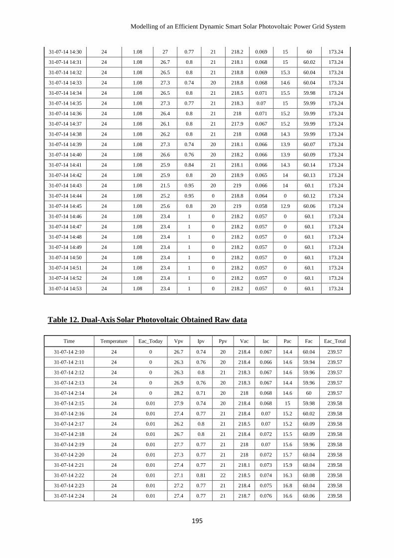
Modelling of an Efficient Dynamic Smart Solar Photovoltaic Power Grid System
195
31-07-14 14:30 24 1.08 27 0.77 21 218.2 0.069 15 60 173.24
31-07-14 14:31 24 1.08 26.7 0.8 21 218.1 0.068 15 60.02 173.24
31-07-14 14:32 24 1.08 26.5 0.8 21 218.8 0.069 15.3 60.04 173.24
31-07-14 14:33 24 1.08 27.3 0.74 20 218.8 0.068 14.6 60.04 173.24
31-07-14 14:34 24 1.08 26.5 0.8 21 218.5 0.071 15.5 59.98 173.24
31-07-14 14:35 24 1.08 27.3 0.77 21 218.3 0.07 15 59.99 173.24
31-07-14 14:36 24 1.08 26.4 0.8 21 218 0.071 15.2 59.99 173.24
31-07-14 14:37 24 1.08 26.1 0.8 21 217.9 0.067 15.2 59.99 173.24
31-07-14 14:38 24 1.08 26.2 0.8 21 218 0.068 14.3 59.99 173.24
31-07-14 14:39 24 1.08 27.3 0.74 20 218.1 0.066 13.9 60.07 173.24
31-07-14 14:40 24 1.08 26.6 0.76 20 218.2 0.066 13.9 60.09 173.24
31-07-14 14:41 24 1.08 25.9 0.84 21 218.1 0.066 14.3 60.14 173.24
31-07-14 14:42 24 1.08 25.9 0.8 20 218.9 0.065 14 60.13 173.24
31-07-14 14:43 24 1.08 21.5 0.95 20 219 0.066 14 60.1 173.24
31-07-14 14:44 24 1.08 25.2 0.95 0 218.8 0.064 0 60.12 173.24
31-07-14 14:45 24 1.08 25.6 0.8 20 219 0.058 12.9 60.06 173.24
31-07-14 14:46 24 1.08 23.4 1 0 218.2 0.057 0 60.1 173.24
31-07-14 14:47 24 1.08 23.4 1 0 218.2 0.057 0 60.1 173.24
31-07-14 14:48 24 1.08 23.4 1 0 218.2 0.057 0 60.1 173.24
31-07-14 14:49 24 1.08 23.4 1 0 218.2 0.057 0 60.1 173.24
31-07-14 14:50 24 1.08 23.4 1 0 218.2 0.057 0 60.1 173.24
31-07-14 14:51 24 1.08 23.4 1 0 218.2 0.057 0 60.1 173.24
31-07-14 14:52 24 1.08 23.4 1 0 218.2 0.057 0 60.1 173.24
31-07-14 14:53 24 1.08 23.4 1 0 218.2 0.057 0 60.1 173.24
Table 12. Dual-Axis Solar Photovoltaic Obtained Raw data
Time Temperature Eac_Today Vpv Ipv Ppv Vac Iac Pac Fac Eac_Total
31-07-14 2:10 24 0 26.7 0.74 20 218.4 0.067 14.4 60.04 239.57
31-07-14 2:11 24 0 26.3 0.76 20 218.4 0.066 14.6 59.94 239.57
31-07-14 2:12 24 0 26.3 0.8 21 218.3 0.067 14.6 59.96 239.57
31-07-14 2:13 24 0 26.9 0.76 20 218.3 0.067 14.4 59.96 239.57
31-07-14 2:14 24 0 28.2 0.71 20 218 0.068 14.6 60 239.57
31-07-14 2:15 24 0.01 27.9 0.74 20 218.4 0.068 15 59.98 239.58
31-07-14 2:16 24 0.01 27.4 0.77 21 218.4 0.07 15.2 60.02 239.58
31-07-14 2:17 24 0.01 26.2 0.8 21 218.5 0.07 15.2 60.09 239.58
31-07-14 2:18 24 0.01 26.7 0.8 21 218.4 0.072 15.5 60.09 239.58
31-07-14 2:19 24 0.01 27.7 0.77 21 218 0.07 15.6 59.96 239.58
31-07-14 2:20 24 0.01 27.3 0.77 21 218 0.072 15.7 60.04 239.58
31-07-14 2:21 24 0.01 27.4 0.77 21 218.1 0.073 15.9 60.04 239.58
31-07-14 2:22 24 0.01 27.1 0.81 22 218.5 0.074 16.3 60.08 239.58
31-07-14 2:23 24 0.01 27.2 0.77 21 218.4 0.075 16.8 60.04 239.58
31-07-14 2:24 24 0.01 27.4 0.77 21 218.7 0.076 16.6 60.06 239.58
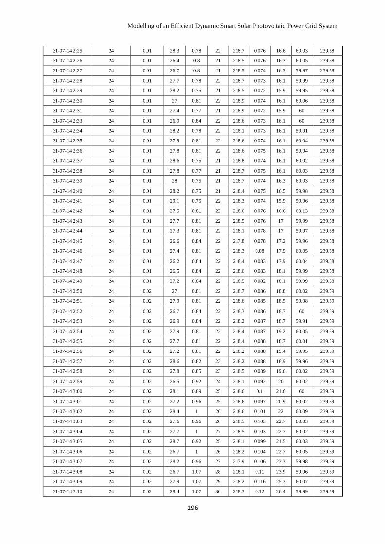
Modelling of an Efficient Dynamic Smart Solar Photovoltaic Power Grid System
196
31-07-14 2:25 24 0.01 28.3 0.78 22 218.7 0.076 16.6 60.03 239.58
31-07-14 2:26 24 0.01 26.4 0.8 21 218.5 0.076 16.3 60.05 239.58
31-07-14 2:27 24 0.01 26.7 0.8 21 218.5 0.074 16.3 59.97 239.58
31-07-14 2:28 24 0.01 27.7 0.78 22 218.7 0.073 16.1 59.99 239.58
31-07-14 2:29 24 0.01 28.2 0.75 21 218.5 0.072 15.9 59.95 239.58
31-07-14 2:30 24 0.01 27 0.81 22 218.9 0.074 16.1 60.06 239.58
31-07-14 2:31 24 0.01 27.4 0.77 21 218.9 0.072 15.9 60 239.58
31-07-14 2:33 24 0.01 26.9 0.84 22 218.6 0.073 16.1 60 239.58
31-07-14 2:34 24 0.01 28.2 0.78 22 218.1 0.073 16.1 59.91 239.58
31-07-14 2:35 24 0.01 27.9 0.81 22 218.6 0.074 16.1 60.04 239.58
31-07-14 2:36 24 0.01 27.8 0.81 22 218.6 0.075 16.1 59.94 239.58
31-07-14 2:37 24 0.01 28.6 0.75 21 218.8 0.074 16.1 60.02 239.58
31-07-14 2:38 24 0.01 27.8 0.77 21 218.7 0.075 16.1 60.03 239.58
31-07-14 2:39 24 0.01 28 0.75 21 218.7 0.074 16.3 60.03 239.58
31-07-14 2:40 24 0.01 28.2 0.75 21 218.4 0.075 16.5 59.98 239.58
31-07-14 2:41 24 0.01 29.1 0.75 22 218.3 0.074 15.9 59.96 239.58
31-07-14 2:42 24 0.01 27.5 0.81 22 218.6 0.076 16.6 60.13 239.58
31-07-14 2:43 24 0.01 27.7 0.81 22 218.5 0.076 17 59.99 239.58
31-07-14 2:44 24 0.01 27.3 0.81 22 218.1 0.078 17 59.97 239.58
31-07-14 2:45 24 0.01 26.6 0.84 22 217.8 0.078 17.2 59.96 239.58
31-07-14 2:46 24 0.01 27.4 0.81 22 218.3 0.08 17.9 60.05 239.58
31-07-14 2:47 24 0.01 26.2 0.84 22 218.4 0.083 17.9 60.04 239.58
31-07-14 2:48 24 0.01 26.5 0.84 22 218.6 0.083 18.1 59.99 239.58
31-07-14 2:49 24 0.01 27.2 0.84 22 218.5 0.082 18.1 59.99 239.58
31-07-14 2:50 24 0.02 27 0.81 22 218.7 0.086 18.8 60.02 239.59
31-07-14 2:51 24 0.02 27.9 0.81 22 218.6 0.085 18.5 59.98 239.59
31-07-14 2:52 24 0.02 26.7 0.84 22 218.3 0.086 18.7 60 239.59
31-07-14 2:53 24 0.02 26.9 0.84 22 218.2 0.087 18.7 59.91 239.59
31-07-14 2:54 24 0.02 27.9 0.81 22 218.4 0.087 19.2 60.05 239.59
31-07-14 2:55 24 0.02 27.7 0.81 22 218.4 0.088 18.7 60.01 239.59
31-07-14 2:56 24 0.02 27.2 0.81 22 218.2 0.088 19.4 59.95 239.59
31-07-14 2:57 24 0.02 28.6 0.82 23 218.2 0.088 18.9 59.96 239.59
31-07-14 2:58 24 0.02 27.8 0.85 23 218.5 0.089 19.6 60.02 239.59
31-07-14 2:59 24 0.02 26.5 0.92 24 218.1 0.092 20 60.02 239.59
31-07-14 3:00 24 0.02 28.1 0.89 25 218.6 0.1 21.6 60 239.59
31-07-14 3:01 24 0.02 27.2 0.96 25 218.6 0.097 20.9 60.02 239.59
31-07-14 3:02 24 0.02 28.4 1 26 218.6 0.101 22 60.09 239.59
31-07-14 3:03 24 0.02 27.6 0.96 26 218.5 0.103 22.7 60.03 239.59
31-07-14 3:04 24 0.02 27.7 1 27 218.5 0.103 22.7 60.02 239.59
31-07-14 3:05 24 0.02 28.7 0.92 25 218.1 0.099 21.5 60.03 239.59
31-07-14 3:06 24 0.02 26.7 1 26 218.2 0.104 22.7 60.05 239.59
31-07-14 3:07 24 0.02 28.2 0.96 27 217.9 0.106 23.3 59.98 239.59
31-07-14 3:08 24 0.02 26.7 1.07 28 218.1 0.11 23.9 59.96 239.59
31-07-14 3:09 24 0.02 27.9 1.07 29 218.2 0.116 25.3 60.07 239.59
31-07-14 3:10 24 0.02 28.4 1.07 30 218.3 0.12 26.4 59.99 239.59

Modelling of an Efficient Dynamic Smart Solar Photovoltaic Power Grid System
197
31-07-14 3:11 24 0.02 27.9 1.14 31 218.3 0.123 27 60.02 239.59
31-07-14 3:12 24 0.02 28.9 1.14 32 218.3 0.13 28.3 59.94 239.59
31-07-14 3:13 24 0.02 28.6 1.21 34 218.6 0.136 29.9 60.07 239.59
31-07-14 3:14 24 0.02 29.1 1.17 33 218.3 0.133 29 60 239.59
31-07-14 3:15 24 0.03 28.7 1.21 34 218.3 0.135 29.4 60.02 239.6
31-07-14 3:16 24 0.03 28 1.17 33 218.2 0.131 28.3 60.03 239.6
31-07-14 3:17 24 0.03 28 1.21 34 218.2 0.138 30 60.04 239.6
31-07-14 3:18 24 0.03 28.2 1.25 35 218.3 0.143 31.2 60.03 239.6
31-07-14 3:19 24 0.03 28.5 1.28 36 218.3 0.148 32 60.06 239.6
31-07-14 3:20 24 0.03 30.6 1.17 34 217.8 0.138 30.9 59.99 239.6
31-07-14 3:21 24 0.03 30.4 1.3 39 217.8 0.157 34.2 59.99 239.6
31-07-14 3:22 24 0.03 30.4 1.33 40 218.2 0.16 35.1 59.98 239.6
31-07-14 3:23 24 0.03 30 1.29 40 218.2 0.168 36.2 60.08 239.6
31-07-14 3:24 24 0.03 30.5 1.25 39 218.5 0.171 37.5 60.07 239.6
31-07-14 3:25 24 0.03 31.1 1.48 46 218.5 0.188 41 60.06 239.6
31-07-14 3:26 24 0.03 31 1.51 47 218.4 0.198 43 60.02 239.6
31-07-14 3:27 24 0.03 30.8 1.63 49 218.6 0.201 43.7 60.04 239.6
31-07-14 3:28 24 0.03 30.5 1.51 47 218.5 0.195 42.8 60 239.6
31-07-14 3:29 24 0.03 29.3 1.62 47 218.5 0.184 41.5 60.07 239.6
31-07-14 3:30 24 0.04 30.2 1.53 46 218.3 0.187 41.2 60.02 239.61
31-07-14 3:31 24 0.04 29.8 1.58 46 218.3 0.191 41.9 60.13 239.61
31-07-14 3:32 24 0.04 30.7 1.53 46 218.2 0.189 41.2 60 239.61
31-07-14 3:33 24 0.04 30.3 1.56 47 218.6 0.193 41.2 60.1 239.61
31-07-14 3:34 24 0.04 30.9 1.7 53 218.5 0.217 47.4 60.04 239.61
31-07-14 3:35 24 0.04 31.1 1.83 55 218.6 0.235 50.9 59.96 239.61
31-07-14 3:36 24 0.04 28.8 2.32 65 218.8 0.272 59.5 60.06 239.61
31-07-14 3:37 24 0.04 28.8 2.24 65 219.2 0.276 59.8 60.05 239.61
31-07-14 3:38 24 0.04 28.6 2.28 64 219 0.27 58.6 60 239.61
31-07-14 3:39 24 0.04 29 2.24 65 219.2 0.271 59.1 60.04 239.61
31-07-14 3:40 24 0.04 28.1 2.14 60 218.9 0.25 54.9 60.05 239.61
31-07-14 3:41 24 0.04 28 2 56 218.8 0.24 53.6 60.07 239.61
31-07-14 3:42 24 0.05 28.7 1.85 52 219 0.216 47 60.05 239.62
31-07-14 3:43 24 0.05 28.4 1.75 51 218.7 0.209 45.9 60.03 239.62
31-07-14 3:44 24 0.05 28.4 1.96 55 218.9 0.228 49.9 60.11 239.62
31-07-14 3:45 24 0.05 28.3 2.03 59 218.4 0.242 52.8 59.96 239.62
31-07-14 3:46 24 0.05 30.1 2.46 74 219 0.313 68.1 60.07 239.62
31-07-14 3:47 24 0.05 30.1 2.53 76 218.7 0.315 68.9 60.03 239.62
31-07-14 3:48 24 0.05 31.2 2.06 62 219 0.268 58 60.07 239.62
31-07-14 3:49 24 0.05 30.2 2.12 66 218.9 0.268 59.1 60 239.62
31-07-14 3:50 24 0.05 30.6 2.43 73 219.2 0.303 66.6 60.07 239.62
31-07-14 3:51 24 0.06 29.1 2.82 79 219 0.334 72.6 59.98 239.63
31-07-14 3:52 24 0.06 27.5 2.82 79 219.1 0.334 72.3 60.02 239.63
31-07-14 3:53 24 0.06 28 2.82 79 218.6 0.331 72.5 60.02 239.63
31-07-14 3:54 24 0.06 28.3 2.96 83 218.9 0.349 76.6 59.99 239.63
31-07-14 3:55 24 0.06 26.5 3 84 219 0.346 76.4 60.1 239.63
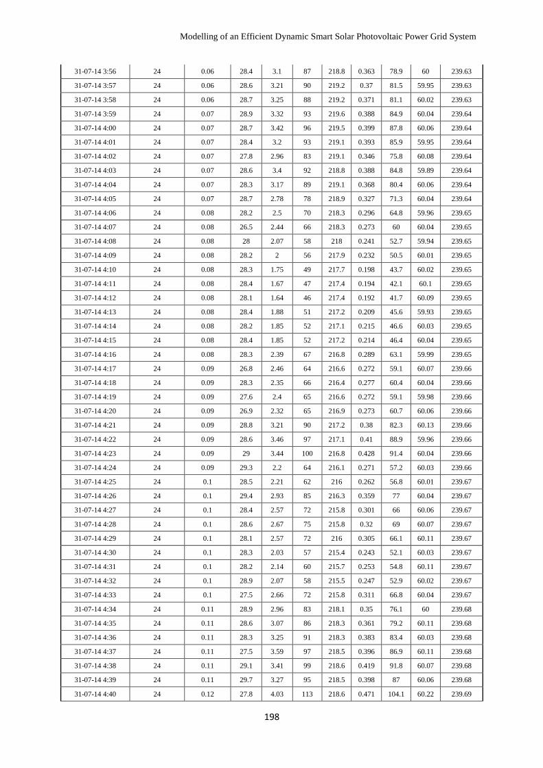
Modelling of an Efficient Dynamic Smart Solar Photovoltaic Power Grid System
198
31-07-14 3:56 24 0.06 28.4 3.1 87 218.8 0.363 78.9 60 239.63
31-07-14 3:57 24 0.06 28.6 3.21 90 219.2 0.37 81.5 59.95 239.63
31-07-14 3:58 24 0.06 28.7 3.25 88 219.2 0.371 81.1 60.02 239.63
31-07-14 3:59 24 0.07 28.9 3.32 93 219.6 0.388 84.9 60.04 239.64
31-07-14 4:00 24 0.07 28.7 3.42 96 219.5 0.399 87.8 60.06 239.64
31-07-14 4:01 24 0.07 28.4 3.2 93 219.1 0.393 85.9 59.95 239.64
31-07-14 4:02 24 0.07 27.8 2.96 83 219.1 0.346 75.8 60.08 239.64
31-07-14 4:03 24 0.07 28.6 3.4 92 218.8 0.388 84.8 59.89 239.64
31-07-14 4:04 24 0.07 28.3 3.17 89 219.1 0.368 80.4 60.06 239.64
31-07-14 4:05 24 0.07 28.7 2.78 78 218.9 0.327 71.3 60.04 239.64
31-07-14 4:06 24 0.08 28.2 2.5 70 218.3 0.296 64.8 59.96 239.65
31-07-14 4:07 24 0.08 26.5 2.44 66 218.3 0.273 60 60.04 239.65
31-07-14 4:08 24 0.08 28 2.07 58 218 0.241 52.7 59.94 239.65
31-07-14 4:09 24 0.08 28.2 2 56 217.9 0.232 50.5 60.01 239.65
31-07-14 4:10 24 0.08 28.3 1.75 49 217.7 0.198 43.7 60.02 239.65
31-07-14 4:11 24 0.08 28.4 1.67 47 217.4 0.194 42.1 60.1 239.65
31-07-14 4:12 24 0.08 28.1 1.64 46 217.4 0.192 41.7 60.09 239.65
31-07-14 4:13 24 0.08 28.4 1.88 51 217.2 0.209 45.6 59.93 239.65
31-07-14 4:14 24 0.08 28.2 1.85 52 217.1 0.215 46.6 60.03 239.65
31-07-14 4:15 24 0.08 28.4 1.85 52 217.2 0.214 46.4 60.04 239.65
31-07-14 4:16 24 0.08 28.3 2.39 67 216.8 0.289 63.1 59.99 239.65
31-07-14 4:17 24 0.09 26.8 2.46 64 216.6 0.272 59.1 60.07 239.66
31-07-14 4:18 24 0.09 28.3 2.35 66 216.4 0.277 60.4 60.04 239.66
31-07-14 4:19 24 0.09 27.6 2.4 65 216.6 0.272 59.1 59.98 239.66
31-07-14 4:20 24 0.09 26.9 2.32 65 216.9 0.273 60.7 60.06 239.66
31-07-14 4:21 24 0.09 28.8 3.21 90 217.2 0.38 82.3 60.13 239.66
31-07-14 4:22 24 0.09 28.6 3.46 97 217.1 0.41 88.9 59.96 239.66
31-07-14 4:23 24 0.09 29 3.44 100 216.8 0.428 91.4 60.04 239.66
31-07-14 4:24 24 0.09 29.3 2.2 64 216.1 0.271 57.2 60.03 239.66
31-07-14 4:25 24 0.1 28.5 2.21 62 216 0.262 56.8 60.01 239.67
31-07-14 4:26 24 0.1 29.4 2.93 85 216.3 0.359 77 60.04 239.67
31-07-14 4:27 24 0.1 28.4 2.57 72 215.8 0.301 66 60.06 239.67
31-07-14 4:28 24 0.1 28.6 2.67 75 215.8 0.32 69 60.07 239.67
31-07-14 4:29 24 0.1 28.1 2.57 72 216 0.305 66.1 60.11 239.67
31-07-14 4:30 24 0.1 28.3 2.03 57 215.4 0.243 52.1 60.03 239.67
31-07-14 4:31 24 0.1 28.2 2.14 60 215.7 0.253 54.8 60.11 239.67
31-07-14 4:32 24 0.1 28.9 2.07 58 215.5 0.247 52.9 60.02 239.67
31-07-14 4:33 24 0.1 27.5 2.66 72 215.8 0.311 66.8 60.04 239.67
31-07-14 4:34 24 0.11 28.9 2.96 83 218.1 0.35 76.1 60 239.68
31-07-14 4:35 24 0.11 28.6 3.07 86 218.3 0.361 79.2 60.11 239.68
31-07-14 4:36 24 0.11 28.3 3.25 91 218.3 0.383 83.4 60.03 239.68
31-07-14 4:37 24 0.11 27.5 3.59 97 218.5 0.396 86.9 60.11 239.68
31-07-14 4:38 24 0.11 29.1 3.41 99 218.6 0.419 91.8 60.07 239.68
31-07-14 4:39 24 0.11 29.7 3.27 95 218.5 0.398 87 60.06 239.68
31-07-14 4:40 24 0.12 27.8 4.03 113 218.6 0.471 104.1 60.22 239.69
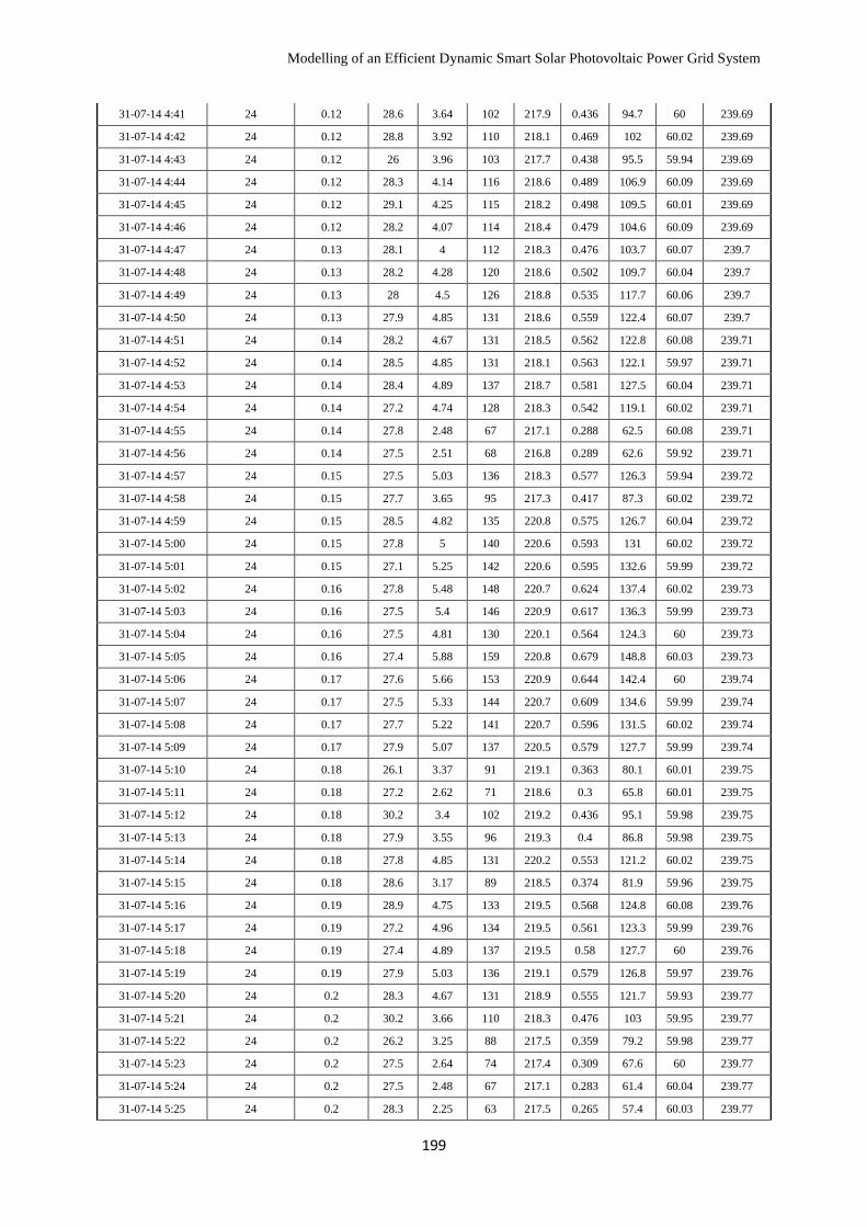
Modelling of an Efficient Dynamic Smart Solar Photovoltaic Power Grid System
199
31-07-14 4:41 24 0.12 28.6 3.64 102 217.9 0.436 94.7 60 239.69
31-07-14 4:42 24 0.12 28.8 3.92 110 218.1 0.469 102 60.02 239.69
31-07-14 4:43 24 0.12 26 3.96 103 217.7 0.438 95.5 59.94 239.69
31-07-14 4:44 24 0.12 28.3 4.14 116 218.6 0.489 106.9 60.09 239.69
31-07-14 4:45 24 0.12 29.1 4.25 115 218.2 0.498 109.5 60.01 239.69
31-07-14 4:46 24 0.12 28.2 4.07 114 218.4 0.479 104.6 60.09 239.69
31-07-14 4:47 24 0.13 28.1 4 112 218.3 0.476 103.7 60.07 239.7
31-07-14 4:48 24 0.13 28.2 4.28 120 218.6 0.502 109.7 60.04 239.7
31-07-14 4:49 24 0.13 28 4.5 126 218.8 0.535 117.7 60.06 239.7
31-07-14 4:50 24 0.13 27.9 4.85 131 218.6 0.559 122.4 60.07 239.7
31-07-14 4:51 24 0.14 28.2 4.67 131 218.5 0.562 122.8 60.08 239.71
31-07-14 4:52 24 0.14 28.5 4.85 131 218.1 0.563 122.1 59.97 239.71
31-07-14 4:53 24 0.14 28.4 4.89 137 218.7 0.581 127.5 60.04 239.71
31-07-14 4:54 24 0.14 27.2 4.74 128 218.3 0.542 119.1 60.02 239.71
31-07-14 4:55 24 0.14 27.8 2.48 67 217.1 0.288 62.5 60.08 239.71
31-07-14 4:56 24 0.14 27.5 2.51 68 216.8 0.289 62.6 59.92 239.71
31-07-14 4:57 24 0.15 27.5 5.03 136 218.3 0.577 126.3 59.94 239.72
31-07-14 4:58 24 0.15 27.7 3.65 95 217.3 0.417 87.3 60.02 239.72
31-07-14 4:59 24 0.15 28.5 4.82 135 220.8 0.575 126.7 60.04 239.72
31-07-14 5:00 24 0.15 27.8 5 140 220.6 0.593 131 60.02 239.72
31-07-14 5:01 24 0.15 27.1 5.25 142 220.6 0.595 132.6 59.99 239.72
31-07-14 5:02 24 0.16 27.8 5.48 148 220.7 0.624 137.4 60.02 239.73
31-07-14 5:03 24 0.16 27.5 5.4 146 220.9 0.617 136.3 59.99 239.73
31-07-14 5:04 24 0.16 27.5 4.81 130 220.1 0.564 124.3 60 239.73
31-07-14 5:05 24 0.16 27.4 5.88 159 220.8 0.679 148.8 60.03 239.73
31-07-14 5:06 24 0.17 27.6 5.66 153 220.9 0.644 142.4 60 239.74
31-07-14 5:07 24 0.17 27.5 5.33 144 220.7 0.609 134.6 59.99 239.74
31-07-14 5:08 24 0.17 27.7 5.22 141 220.7 0.596 131.5 60.02 239.74
31-07-14 5:09 24 0.17 27.9 5.07 137 220.5 0.579 127.7 59.99 239.74
31-07-14 5:10 24 0.18 26.1 3.37 91 219.1 0.363 80.1 60.01 239.75
31-07-14 5:11 24 0.18 27.2 2.62 71 218.6 0.3 65.8 60.01 239.75
31-07-14 5:12 24 0.18 30.2 3.4 102 219.2 0.436 95.1 59.98 239.75
31-07-14 5:13 24 0.18 27.9 3.55 96 219.3 0.4 86.8 59.98 239.75
31-07-14 5:14 24 0.18 27.8 4.85 131 220.2 0.553 121.2 60.02 239.75
31-07-14 5:15 24 0.18 28.6 3.17 89 218.5 0.374 81.9 59.96 239.75
31-07-14 5:16 24 0.19 28.9 4.75 133 219.5 0.568 124.8 60.08 239.76
31-07-14 5:17 24 0.19 27.2 4.96 134 219.5 0.561 123.3 59.99 239.76
31-07-14 5:18 24 0.19 27.4 4.89 137 219.5 0.58 127.7 60 239.76
31-07-14 5:19 24 0.19 27.9 5.03 136 219.1 0.579 126.8 59.97 239.76
31-07-14 5:20 24 0.2 28.3 4.67 131 218.9 0.555 121.7 59.93 239.77
31-07-14 5:21 24 0.2 30.2 3.66 110 218.3 0.476 103 59.95 239.77
31-07-14 5:22 24 0.2 26.2 3.25 88 217.5 0.359 79.2 59.98 239.77
31-07-14 5:23 24 0.2 27.5 2.64 74 217.4 0.309 67.6 60 239.77
31-07-14 5:24 24 0.2 27.5 2.48 67 217.1 0.283 61.4 60.04 239.77
31-07-14 5:25 24 0.2 28.3 2.25 63 217.5 0.265 57.4 60.03 239.77
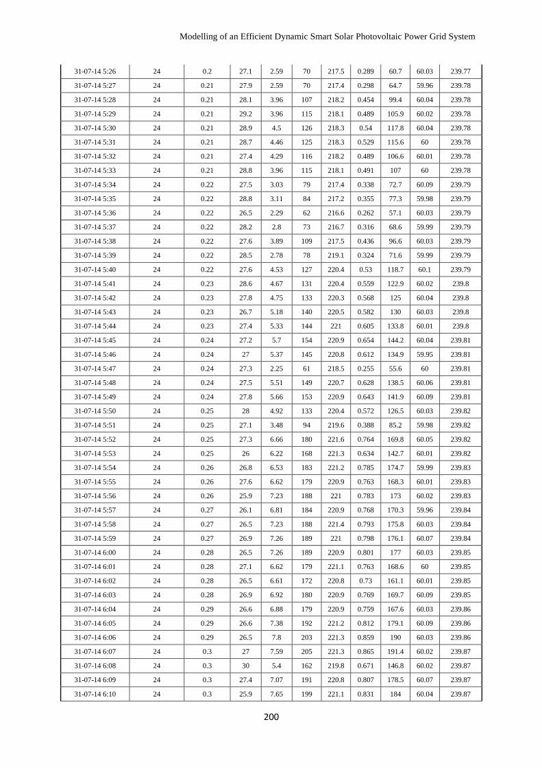
Modelling of an Efficient Dynamic Smart Solar Photovoltaic Power Grid System
200
31-07-14 5:26 24 0.2 27.1 2.59 70 217.5 0.289 60.7 60.03 239.77
31-07-14 5:27 24 0.21 27.9 2.59 70 217.4 0.298 64.7 59.96 239.78
31-07-14 5:28 24 0.21 28.1 3.96 107 218.2 0.454 99.4 60.04 239.78
31-07-14 5:29 24 0.21 29.2 3.96 115 218.1 0.489 105.9 60.02 239.78
31-07-14 5:30 24 0.21 28.9 4.5 126 218.3 0.54 117.8 60.04 239.78
31-07-14 5:31 24 0.21 28.7 4.46 125 218.3 0.529 115.6 60 239.78
31-07-14 5:32 24 0.21 27.4 4.29 116 218.2 0.489 106.6 60.01 239.78
31-07-14 5:33 24 0.21 28.8 3.96 115 218.1 0.491 107 60 239.78
31-07-14 5:34 24 0.22 27.5 3.03 79 217.4 0.338 72.7 60.09 239.79
31-07-14 5:35 24 0.22 28.8 3.11 84 217.2 0.355 77.3 59.98 239.79
31-07-14 5:36 24 0.22 26.5 2.29 62 216.6 0.262 57.1 60.03 239.79
31-07-14 5:37 24 0.22 28.2 2.8 73 216.7 0.316 68.6 59.99 239.79
31-07-14 5:38 24 0.22 27.6 3.89 109 217.5 0.436 96.6 60.03 239.79
31-07-14 5:39 24 0.22 28.5 2.78 78 219.1 0.324 71.6 59.99 239.79
31-07-14 5:40 24 0.22 27.6 4.53 127 220.4 0.53 118.7 60.1 239.79
31-07-14 5:41 24 0.23 28.6 4.67 131 220.4 0.559 122.9 60.02 239.8
31-07-14 5:42 24 0.23 27.8 4.75 133 220.3 0.568 125 60.04 239.8
31-07-14 5:43 24 0.23 26.7 5.18 140 220.5 0.582 130 60.03 239.8
31-07-14 5:44 24 0.23 27.4 5.33 144 221 0.605 133.8 60.01 239.8
31-07-14 5:45 24 0.24 27.2 5.7 154 220.9 0.654 144.2 60.04 239.81
31-07-14 5:46 24 0.24 27 5.37 145 220.8 0.612 134.9 59.95 239.81
31-07-14 5:47 24 0.24 27.3 2.25 61 218.5 0.255 55.6 60 239.81
31-07-14 5:48 24 0.24 27.5 5.51 149 220.7 0.628 138.5 60.06 239.81
31-07-14 5:49 24 0.24 27.8 5.66 153 220.9 0.643 141.9 60.09 239.81
31-07-14 5:50 24 0.25 28 4.92 133 220.4 0.572 126.5 60.03 239.82
31-07-14 5:51 24 0.25 27.1 3.48 94 219.6 0.388 85.2 59.98 239.82
31-07-14 5:52 24 0.25 27.3 6.66 180 221.6 0.764 169.8 60.05 239.82
31-07-14 5:53 24 0.25 26 6.22 168 221.3 0.634 142.7 60.01 239.82
31-07-14 5:54 24 0.26 26.8 6.53 183 221.2 0.785 174.7 59.99 239.83
31-07-14 5:55 24 0.26 27.6 6.62 179 220.9 0.763 168.3 60.01 239.83
31-07-14 5:56 24 0.26 25.9 7.23 188 221 0.783 173 60.02 239.83
31-07-14 5:57 24 0.27 26.1 6.81 184 220.9 0.768 170.3 59.96 239.84
31-07-14 5:58 24 0.27 26.5 7.23 188 221.4 0.793 175.8 60.03 239.84
31-07-14 5:59 24 0.27 26.9 7.26 189 221 0.798 176.1 60.07 239.84
31-07-14 6:00 24 0.28 26.5 7.26 189 220.9 0.801 177 60.03 239.85
31-07-14 6:01 24 0.28 27.1 6.62 179 221.1 0.763 168.6 60 239.85
31-07-14 6:02 24 0.28 26.5 6.61 172 220.8 0.73 161.1 60.01 239.85
31-07-14 6:03 24 0.28 26.9 6.92 180 220.9 0.769 169.7 60.09 239.85
31-07-14 6:04 24 0.29 26.6 6.88 179 220.9 0.759 167.6 60.03 239.86
31-07-14 6:05 24 0.29 26.6 7.38 192 221.2 0.812 179.1 60.09 239.86
31-07-14 6:06 24 0.29 26.5 7.8 203 221.3 0.859 190 60.03 239.86
31-07-14 6:07 24 0.3 27 7.59 205 221.3 0.865 191.4 60.02 239.87
31-07-14 6:08 24 0.3 30 5.4 162 219.8 0.671 146.8 60.02 239.87
31-07-14 6:09 24 0.3 27.4 7.07 191 220.8 0.807 178.5 60.07 239.87
31-07-14 6:10 24 0.3 25.9 7.65 199 221.1 0.831 184 60.04 239.87
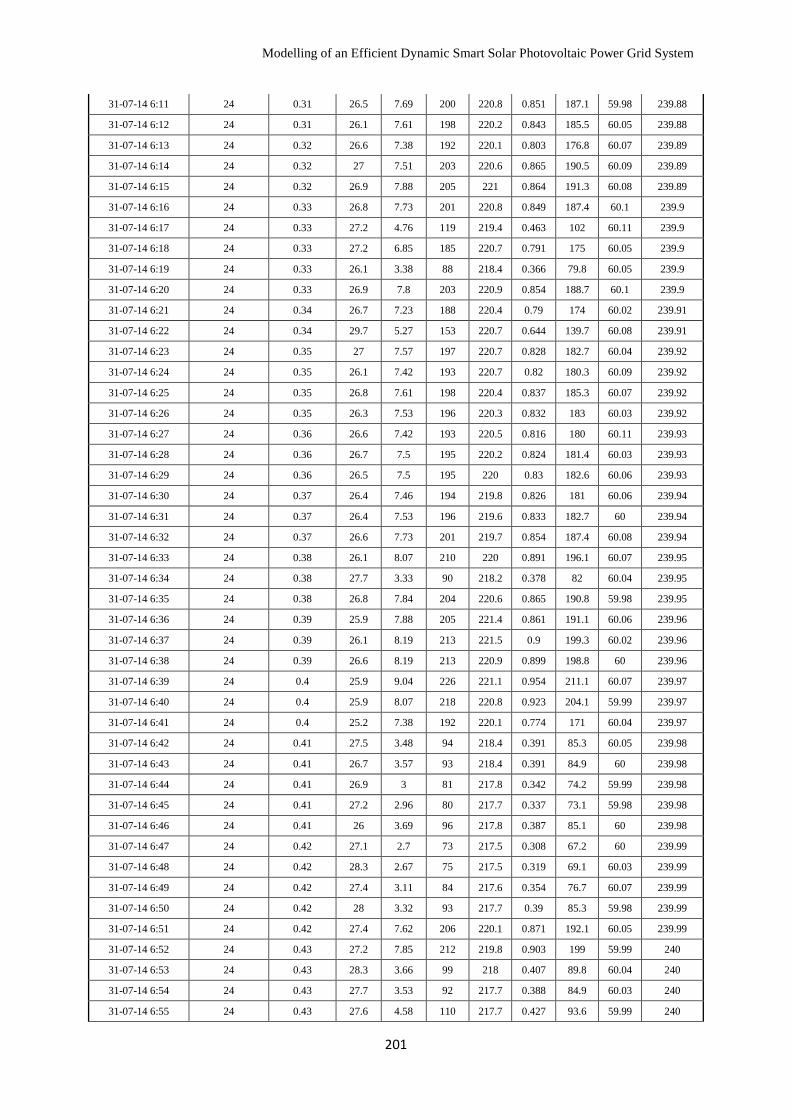
Modelling of an Efficient Dynamic Smart Solar Photovoltaic Power Grid System
201
31-07-14 6:11 24 0.31 26.5 7.69 200 220.8 0.851 187.1 59.98 239.88
31-07-14 6:12 24 0.31 26.1 7.61 198 220.2 0.843 185.5 60.05 239.88
31-07-14 6:13 24 0.32 26.6 7.38 192 220.1 0.803 176.8 60.07 239.89
31-07-14 6:14 24 0.32 27 7.51 203 220.6 0.865 190.5 60.09 239.89
31-07-14 6:15 24 0.32 26.9 7.88 205 221 0.864 191.3 60.08 239.89
31-07-14 6:16 24 0.33 26.8 7.73 201 220.8 0.849 187.4 60.1 239.9
31-07-14 6:17 24 0.33 27.2 4.76 119 219.4 0.463 102 60.11 239.9
31-07-14 6:18 24 0.33 27.2 6.85 185 220.7 0.791 175 60.05 239.9
31-07-14 6:19 24 0.33 26.1 3.38 88 218.4 0.366 79.8 60.05 239.9
31-07-14 6:20 24 0.33 26.9 7.8 203 220.9 0.854 188.7 60.1 239.9
31-07-14 6:21 24 0.34 26.7 7.23 188 220.4 0.79 174 60.02 239.91
31-07-14 6:22 24 0.34 29.7 5.27 153 220.7 0.644 139.7 60.08 239.91
31-07-14 6:23 24 0.35 27 7.57 197 220.7 0.828 182.7 60.04 239.92
31-07-14 6:24 24 0.35 26.1 7.42 193 220.7 0.82 180.3 60.09 239.92
31-07-14 6:25 24 0.35 26.8 7.61 198 220.4 0.837 185.3 60.07 239.92
31-07-14 6:26 24 0.35 26.3 7.53 196 220.3 0.832 183 60.03 239.92
31-07-14 6:27 24 0.36 26.6 7.42 193 220.5 0.816 180 60.11 239.93
31-07-14 6:28 24 0.36 26.7 7.5 195 220.2 0.824 181.4 60.03 239.93
31-07-14 6:29 24 0.36 26.5 7.5 195 220 0.83 182.6 60.06 239.93
31-07-14 6:30 24 0.37 26.4 7.46 194 219.8 0.826 181 60.06 239.94
31-07-14 6:31 24 0.37 26.4 7.53 196 219.6 0.833 182.7 60 239.94
31-07-14 6:32 24 0.37 26.6 7.73 201 219.7 0.854 187.4 60.08 239.94
31-07-14 6:33 24 0.38 26.1 8.07 210 220 0.891 196.1 60.07 239.95
31-07-14 6:34 24 0.38 27.7 3.33 90 218.2 0.378 82 60.04 239.95
31-07-14 6:35 24 0.38 26.8 7.84 204 220.6 0.865 190.8 59.98 239.95
31-07-14 6:36 24 0.39 25.9 7.88 205 221.4 0.861 191.1 60.06 239.96
31-07-14 6:37 24 0.39 26.1 8.19 213 221.5 0.9 199.3 60.02 239.96
31-07-14 6:38 24 0.39 26.6 8.19 213 220.9 0.899 198.8 60 239.96
31-07-14 6:39 24 0.4 25.9 9.04 226 221.1 0.954 211.1 60.07 239.97
31-07-14 6:40 24 0.4 25.9 8.07 218 220.8 0.923 204.1 59.99 239.97
31-07-14 6:41 24 0.4 25.2 7.38 192 220.1 0.774 171 60.04 239.97
31-07-14 6:42 24 0.41 27.5 3.48 94 218.4 0.391 85.3 60.05 239.98
31-07-14 6:43 24 0.41 26.7 3.57 93 218.4 0.391 84.9 60 239.98
31-07-14 6:44 24 0.41 26.9 3 81 217.8 0.342 74.2 59.99 239.98
31-07-14 6:45 24 0.41 27.2 2.96 80 217.7 0.337 73.1 59.98 239.98
31-07-14 6:46 24 0.41 26 3.69 96 217.8 0.387 85.1 60 239.98
31-07-14 6:47 24 0.42 27.1 2.7 73 217.5 0.308 67.2 60 239.99
31-07-14 6:48 24 0.42 28.3 2.67 75 217.5 0.319 69.1 60.03 239.99
31-07-14 6:49 24 0.42 27.4 3.11 84 217.6 0.354 76.7 60.07 239.99
31-07-14 6:50 24 0.42 28 3.32 93 217.7 0.39 85.3 59.98 239.99
31-07-14 6:51 24 0.42 27.4 7.62 206 220.1 0.871 192.1 60.05 239.99
31-07-14 6:52 24 0.43 27.2 7.85 212 219.8 0.903 199 59.99 240
31-07-14 6:53 24 0.43 28.3 3.66 99 218 0.407 89.8 60.04 240
31-07-14 6:54 24 0.43 27.7 3.53 92 217.7 0.388 84.9 60.03 240
31-07-14 6:55 24 0.43 27.6 4.58 110 217.7 0.427 93.6 59.99 240
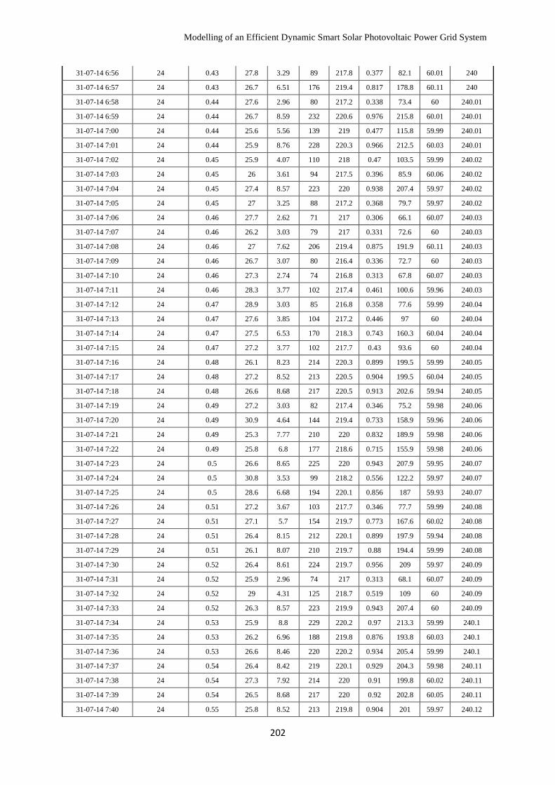
Modelling of an Efficient Dynamic Smart Solar Photovoltaic Power Grid System
202
31-07-14 6:56 24 0.43 27.8 3.29 89 217.8 0.377 82.1 60.01 240
31-07-14 6:57 24 0.43 26.7 6.51 176 219.4 0.817 178.8 60.11 240
31-07-14 6:58 24 0.44 27.6 2.96 80 217.2 0.338 73.4 60 240.01
31-07-14 6:59 24 0.44 26.7 8.59 232 220.6 0.976 215.8 60.01 240.01
31-07-14 7:00 24 0.44 25.6 5.56 139 219 0.477 115.8 59.99 240.01
31-07-14 7:01 24 0.44 25.9 8.76 228 220.3 0.966 212.5 60.03 240.01
31-07-14 7:02 24 0.45 25.9 4.07 110 218 0.47 103.5 59.99 240.02
31-07-14 7:03 24 0.45 26 3.61 94 217.5 0.396 85.9 60.06 240.02
31-07-14 7:04 24 0.45 27.4 8.57 223 220 0.938 207.4 59.97 240.02
31-07-14 7:05 24 0.45 27 3.25 88 217.2 0.368 79.7 59.97 240.02
31-07-14 7:06 24 0.46 27.7 2.62 71 217 0.306 66.1 60.07 240.03
31-07-14 7:07 24 0.46 26.2 3.03 79 217 0.331 72.6 60 240.03
31-07-14 7:08 24 0.46 27 7.62 206 219.4 0.875 191.9 60.11 240.03
31-07-14 7:09 24 0.46 26.7 3.07 80 216.4 0.336 72.7 60 240.03
31-07-14 7:10 24 0.46 27.3 2.74 74 216.8 0.313 67.8 60.07 240.03
31-07-14 7:11 24 0.46 28.3 3.77 102 217.4 0.461 100.6 59.96 240.03
31-07-14 7:12 24 0.47 28.9 3.03 85 216.8 0.358 77.6 59.99 240.04
31-07-14 7:13 24 0.47 27.6 3.85 104 217.2 0.446 97 60 240.04
31-07-14 7:14 24 0.47 27.5 6.53 170 218.3 0.743 160.3 60.04 240.04
31-07-14 7:15 24 0.47 27.2 3.77 102 217.7 0.43 93.6 60 240.04
31-07-14 7:16 24 0.48 26.1 8.23 214 220.3 0.899 199.5 59.99 240.05
31-07-14 7:17 24 0.48 27.2 8.52 213 220.5 0.904 199.5 60.04 240.05
31-07-14 7:18 24 0.48 26.6 8.68 217 220.5 0.913 202.6 59.94 240.05
31-07-14 7:19 24 0.49 27.2 3.03 82 217.4 0.346 75.2 59.98 240.06
31-07-14 7:20 24 0.49 30.9 4.64 144 219.4 0.733 158.9 59.96 240.06
31-07-14 7:21 24 0.49 25.3 7.77 210 220 0.832 189.9 59.98 240.06
31-07-14 7:22 24 0.49 25.8 6.8 177 218.6 0.715 155.9 59.98 240.06
31-07-14 7:23 24 0.5 26.6 8.65 225 220 0.943 207.9 59.95 240.07
31-07-14 7:24 24 0.5 30.8 3.53 99 218.2 0.556 122.2 59.97 240.07
31-07-14 7:25 24 0.5 28.6 6.68 194 220.1 0.856 187 59.93 240.07
31-07-14 7:26 24 0.51 27.2 3.67 103 217.7 0.346 77.7 59.99 240.08
31-07-14 7:27 24 0.51 27.1 5.7 154 219.7 0.773 167.6 60.02 240.08
31-07-14 7:28 24 0.51 26.4 8.15 212 220.1 0.899 197.9 59.94 240.08
31-07-14 7:29 24 0.51 26.1 8.07 210 219.7 0.88 194.4 59.99 240.08
31-07-14 7:30 24 0.52 26.4 8.61 224 219.7 0.956 209 59.97 240.09
31-07-14 7:31 24 0.52 25.9 2.96 74 217 0.313 68.1 60.07 240.09
31-07-14 7:32 24 0.52 29 4.31 125 218.7 0.519 109 60 240.09
31-07-14 7:33 24 0.52 26.3 8.57 223 219.9 0.943 207.4 60 240.09
31-07-14 7:34 24 0.53 25.9 8.8 229 220.2 0.97 213.3 59.99 240.1
31-07-14 7:35 24 0.53 26.2 6.96 188 219.8 0.876 193.8 60.03 240.1
31-07-14 7:36 24 0.53 26.6 8.46 220 220.2 0.934 205.4 59.99 240.1
31-07-14 7:37 24 0.54 26.4 8.42 219 220.1 0.929 204.3 59.98 240.11
31-07-14 7:38 24 0.54 27.3 7.92 214 220 0.91 199.8 60.02 240.11
31-07-14 7:39 24 0.54 26.5 8.68 217 220 0.92 202.8 60.05 240.11
31-07-14 7:40 24 0.55 25.8 8.52 213 219.8 0.904 201 59.97 240.12
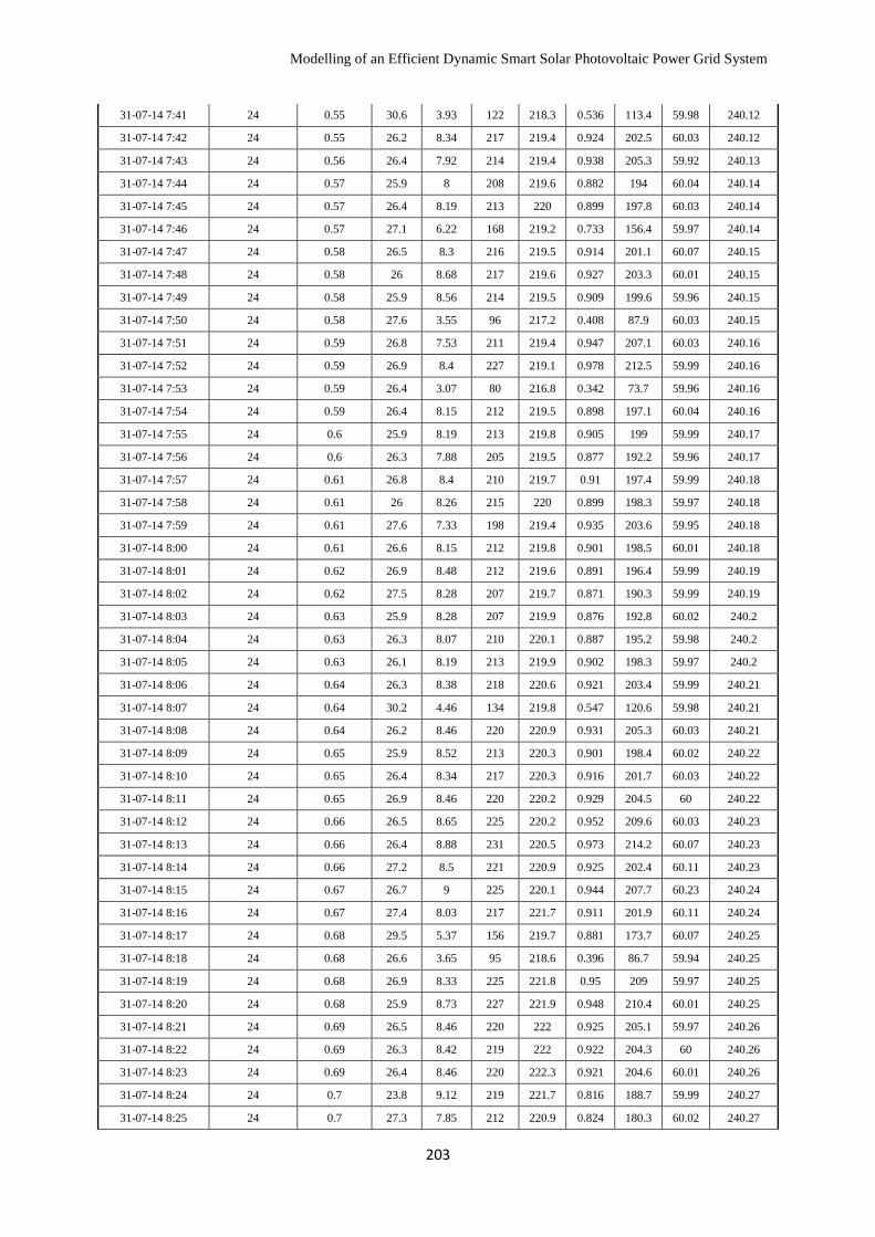
Modelling of an Efficient Dynamic Smart Solar Photovoltaic Power Grid System
203
31-07-14 7:41 24 0.55 30.6 3.93 122 218.3 0.536 113.4 59.98 240.12
31-07-14 7:42 24 0.55 26.2 8.34 217 219.4 0.924 202.5 60.03 240.12
31-07-14 7:43 24 0.56 26.4 7.92 214 219.4 0.938 205.3 59.92 240.13
31-07-14 7:44 24 0.57 25.9 8 208 219.6 0.882 194 60.04 240.14
31-07-14 7:45 24 0.57 26.4 8.19 213 220 0.899 197.8 60.03 240.14
31-07-14 7:46 24 0.57 27.1 6.22 168 219.2 0.733 156.4 59.97 240.14
31-07-14 7:47 24 0.58 26.5 8.3 216 219.5 0.914 201.1 60.07 240.15
31-07-14 7:48 24 0.58 26 8.68 217 219.6 0.927 203.3 60.01 240.15
31-07-14 7:49 24 0.58 25.9 8.56 214 219.5 0.909 199.6 59.96 240.15
31-07-14 7:50 24 0.58 27.6 3.55 96 217.2 0.408 87.9 60.03 240.15
31-07-14 7:51 24 0.59 26.8 7.53 211 219.4 0.947 207.1 60.03 240.16
31-07-14 7:52 24 0.59 26.9 8.4 227 219.1 0.978 212.5 59.99 240.16
31-07-14 7:53 24 0.59 26.4 3.07 80 216.8 0.342 73.7 59.96 240.16
31-07-14 7:54 24 0.59 26.4 8.15 212 219.5 0.898 197.1 60.04 240.16
31-07-14 7:55 24 0.6 25.9 8.19 213 219.8 0.905 199 59.99 240.17
31-07-14 7:56 24 0.6 26.3 7.88 205 219.5 0.877 192.2 59.96 240.17
31-07-14 7:57 24 0.61 26.8 8.4 210 219.7 0.91 197.4 59.99 240.18
31-07-14 7:58 24 0.61 26 8.26 215 220 0.899 198.3 59.97 240.18
31-07-14 7:59 24 0.61 27.6 7.33 198 219.4 0.935 203.6 59.95 240.18
31-07-14 8:00 24 0.61 26.6 8.15 212 219.8 0.901 198.5 60.01 240.18
31-07-14 8:01 24 0.62 26.9 8.48 212 219.6 0.891 196.4 59.99 240.19
31-07-14 8:02 24 0.62 27.5 8.28 207 219.7 0.871 190.3 59.99 240.19
31-07-14 8:03 24 0.63 25.9 8.28 207 219.9 0.876 192.8 60.02 240.2
31-07-14 8:04 24 0.63 26.3 8.07 210 220.1 0.887 195.2 59.98 240.2
31-07-14 8:05 24 0.63 26.1 8.19 213 219.9 0.902 198.3 59.97 240.2
31-07-14 8:06 24 0.64 26.3 8.38 218 220.6 0.921 203.4 59.99 240.21
31-07-14 8:07 24 0.64 30.2 4.46 134 219.8 0.547 120.6 59.98 240.21
31-07-14 8:08 24 0.64 26.2 8.46 220 220.9 0.931 205.3 60.03 240.21
31-07-14 8:09 24 0.65 25.9 8.52 213 220.3 0.901 198.4 60.02 240.22
31-07-14 8:10 24 0.65 26.4 8.34 217 220.3 0.916 201.7 60.03 240.22
31-07-14 8:11 24 0.65 26.9 8.46 220 220.2 0.929 204.5 60 240.22
31-07-14 8:12 24 0.66 26.5 8.65 225 220.2 0.952 209.6 60.03 240.23
31-07-14 8:13 24 0.66 26.4 8.88 231 220.5 0.973 214.2 60.07 240.23
31-07-14 8:14 24 0.66 27.2 8.5 221 220.9 0.925 202.4 60.11 240.23
31-07-14 8:15 24 0.67 26.7 9 225 220.1 0.944 207.7 60.23 240.24
31-07-14 8:16 24 0.67 27.4 8.03 217 221.7 0.911 201.9 60.11 240.24
31-07-14 8:17 24 0.68 29.5 5.37 156 219.7 0.881 173.7 60.07 240.25
31-07-14 8:18 24 0.68 26.6 3.65 95 218.6 0.396 86.7 59.94 240.25
31-07-14 8:19 24 0.68 26.9 8.33 225 221.8 0.95 209 59.97 240.25
31-07-14 8:20 24 0.68 25.9 8.73 227 221.9 0.948 210.4 60.01 240.25
31-07-14 8:21 24 0.69 26.5 8.46 220 222 0.925 205.1 59.97 240.26
31-07-14 8:22 24 0.69 26.3 8.42 219 222 0.922 204.3 60 240.26
31-07-14 8:23 24 0.69 26.4 8.46 220 222.3 0.921 204.6 60.01 240.26
31-07-14 8:24 24 0.7 23.8 9.12 219 221.7 0.816 188.7 59.99 240.27
31-07-14 8:25 24 0.7 27.3 7.85 212 220.9 0.824 180.3 60.02 240.27

Modelling of an Efficient Dynamic Smart Solar Photovoltaic Power Grid System
204
31-07-14 8:26 24 0.7 29.9 4.3 129 220 0.56 120.3 60.03 240.27
31-07-14 8:27 24 0.71 26.7 8.5 221 221.7 0.935 207.5 60 240.28
31-07-14 8:28 24 0.71 31.9 4.29 133 219.9 0.57 125.7 59.95 240.28
31-07-14 8:29 24 0.71 26.5 8.73 227 221.9 0.951 211.2 59.95 240.28
31-07-14 8:30 24 0.72 25.9 8.3 216 221.9 0.908 201.7 60 240.29
31-07-14 8:31 24 0.72 25.9 9.04 226 221.5 0.955 211.3 59.99 240.29
31-07-14 8:32 24 0.73 27.1 4.11 107 219.5 0.49 102.4 60.01 240.3
31-07-14 8:33 24 0.73 26.3 7.46 194 219.4 0.569 125.4 59.95 240.3
31-07-14 8:34 24 0.73 25.9 5.92 154 220 0.541 117.5 60.09 240.3
31-07-14 8:35 24 0.73 27.7 6.64 186 221.6 0.841 182.2 59.99 240.3
31-07-14 8:36 24 0.74 28.4 4.71 132 220.5 0.573 123.4 60.03 240.31
31-07-14 8:37 24 0.74 27.2 3.44 93 219.3 0.396 86.6 60.01 240.31
31-07-14 8:38 24 0.74 25.9 8.72 218 222 0.916 203.3 60.05 240.31
31-07-14 8:39 24 0.75 26.4 8.3 216 221.4 0.91 202 59.94 240.32
31-07-14 8:40 24 0.75 26.8 7.85 212 221.7 0.909 199.3 60 240.32
31-07-14 8:41 24 0.75 27 8.65 225 222.3 0.941 208.2 59.95 240.32
31-07-14 8:42 24 0.76 29.2 3.37 98 220.5 0.423 89.6 59.94 240.33
31-07-14 8:43 24 0.76 26.3 8.61 224 221.8 0.952 210.2 59.99 240.33
31-07-14 8:44 24 0.77 26.4 8.29 224 221.7 0.886 199.6 59.99 240.34
31-07-14 8:45 24 0.77 26.1 8.92 232 221.9 0.976 216.3 59.98 240.34
31-07-14 8:46 24 0.77 26.1 8.92 232 221.9 0.964 214.3 59.96 240.34
31-07-14 8:47 24 0.78 25.3 8.61 224 221.5 0.864 192 60.04 240.35
31-07-14 8:48 24 0.78 26.7 6.61 172 220.6 0.721 156.9 59.98 240.35
31-07-14 8:49 24 0.78 25.9 9 234 222.1 0.975 218.2 59.97 240.35
31-07-14 8:50 24 0.79 27.2 3.85 104 219.1 0.439 96.4 59.98 240.36
31-07-14 8:51 24 0.79 27.2 3.76 98 218.9 0.461 94 59.88 240.36
31-07-14 8:52 24 0.79 26.9 8.88 231 221.7 0.973 215.7 59.99 240.36
31-07-14 8:53 24 0.79 26.6 8.23 214 221.5 0.949 206.6 59.96 240.36
31-07-14 8:54 24 0.8 27.3 6.92 194 221.3 0.947 202.3 59.98 240.37
31-07-14 8:55 24 0.8 27.6 5.29 143 219 0.472 100.6 59.99 240.37
31-07-14 8:56 24 0.8 27.1 5.24 152 219.2 0.809 170.1 59.91 240.37
31-07-14 8:57 24 0.81 27.1 9.38 244 221.3 1.023 227.2 60.02 240.38
31-07-14 8:58 24 0.81 25.5 8.69 226 221.6 0.872 196.7 59.94 240.38
31-07-14 8:59 24 0.81 28 3.5 98 219 0.417 90.8 59.92 240.38
31-07-14 9:00 24 0.82 26.6 9.03 235 222.6 0.983 218.8 60.02 240.39
31-07-14 9:01 24 0.82 26.3 9.36 234 222.2 0.983 218.5 59.97 240.39
31-07-14 9:02 24 0.82 26.4 8.46 220 222.1 0.939 208 59.96 240.39
31-07-14 9:03 24 0.83 26.2 8.84 230 221.7 0.96 213.2 59.95 240.4
31-07-14 9:04 24 0.83 26.5 8.96 233 221.9 0.981 217.5 59.98 240.4
31-07-14 9:05 24 0.83 26.2 3.76 98 218.7 0.442 96.2 60 240.4
31-07-14 9:06 24 0.84 26.2 9.11 237 221.8 0.993 221.1 60.06 240.41
31-07-14 9:07 24 0.84 27.1 8.69 226 221.4 0.95 210.3 59.99 240.41
31-07-14 9:08 24 0.84 25.9 8.53 222 221.6 0.934 206.9 59.94 240.41
31-07-14 9:09 24 0.85 26.2 8.92 223 221.6 0.94 208 60 240.42
31-07-14 9:10 24 0.85 26.3 8.3 216 221.8 0.91 201.1 60.02 240.42
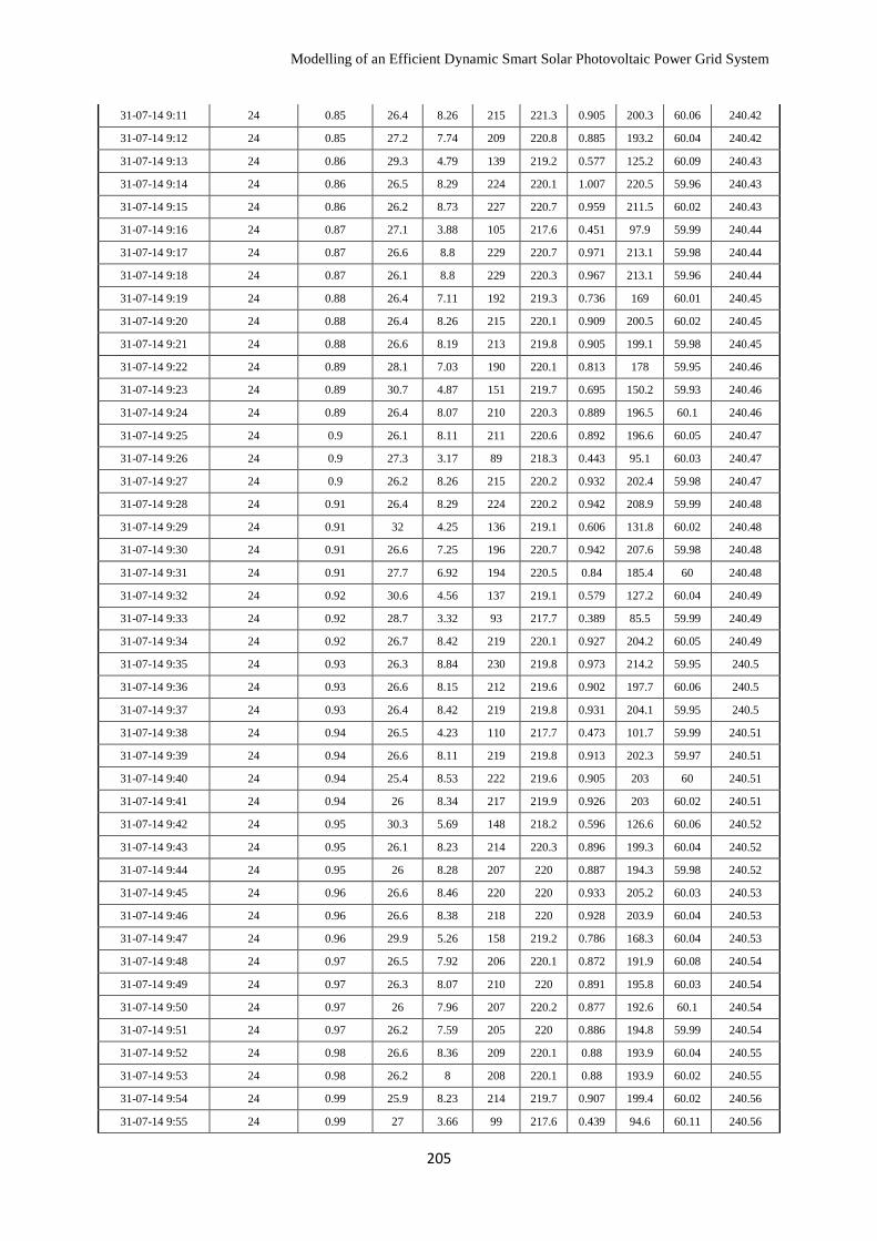
Modelling of an Efficient Dynamic Smart Solar Photovoltaic Power Grid System
205
31-07-14 9:11 24 0.85 26.4 8.26 215 221.3 0.905 200.3 60.06 240.42
31-07-14 9:12 24 0.85 27.2 7.74 209 220.8 0.885 193.2 60.04 240.42
31-07-14 9:13 24 0.86 29.3 4.79 139 219.2 0.577 125.2 60.09 240.43
31-07-14 9:14 24 0.86 26.5 8.29 224 220.1 1.007 220.5 59.96 240.43
31-07-14 9:15 24 0.86 26.2 8.73 227 220.7 0.959 211.5 60.02 240.43
31-07-14 9:16 24 0.87 27.1 3.88 105 217.6 0.451 97.9 59.99 240.44
31-07-14 9:17 24 0.87 26.6 8.8 229 220.7 0.971 213.1 59.98 240.44
31-07-14 9:18 24 0.87 26.1 8.8 229 220.3 0.967 213.1 59.96 240.44
31-07-14 9:19 24 0.88 26.4 7.11 192 219.3 0.736 169 60.01 240.45
31-07-14 9:20 24 0.88 26.4 8.26 215 220.1 0.909 200.5 60.02 240.45
31-07-14 9:21 24 0.88 26.6 8.19 213 219.8 0.905 199.1 59.98 240.45
31-07-14 9:22 24 0.89 28.1 7.03 190 220.1 0.813 178 59.95 240.46
31-07-14 9:23 24 0.89 30.7 4.87 151 219.7 0.695 150.2 59.93 240.46
31-07-14 9:24 24 0.89 26.4 8.07 210 220.3 0.889 196.5 60.1 240.46
31-07-14 9:25 24 0.9 26.1 8.11 211 220.6 0.892 196.6 60.05 240.47
31-07-14 9:26 24 0.9 27.3 3.17 89 218.3 0.443 95.1 60.03 240.47
31-07-14 9:27 24 0.9 26.2 8.26 215 220.2 0.932 202.4 59.98 240.47
31-07-14 9:28 24 0.91 26.4 8.29 224 220.2 0.942 208.9 59.99 240.48
31-07-14 9:29 24 0.91 32 4.25 136 219.1 0.606 131.8 60.02 240.48
31-07-14 9:30 24 0.91 26.6 7.25 196 220.7 0.942 207.6 59.98 240.48
31-07-14 9:31 24 0.91 27.7 6.92 194 220.5 0.84 185.4 60 240.48
31-07-14 9:32 24 0.92 30.6 4.56 137 219.1 0.579 127.2 60.04 240.49
31-07-14 9:33 24 0.92 28.7 3.32 93 217.7 0.389 85.5 59.99 240.49
31-07-14 9:34 24 0.92 26.7 8.42 219 220.1 0.927 204.2 60.05 240.49
31-07-14 9:35 24 0.93 26.3 8.84 230 219.8 0.973 214.2 59.95 240.5
31-07-14 9:36 24 0.93 26.6 8.15 212 219.6 0.902 197.7 60.06 240.5
31-07-14 9:37 24 0.93 26.4 8.42 219 219.8 0.931 204.1 59.95 240.5
31-07-14 9:38 24 0.94 26.5 4.23 110 217.7 0.473 101.7 59.99 240.51
31-07-14 9:39 24 0.94 26.6 8.11 219 219.8 0.913 202.3 59.97 240.51
31-07-14 9:40 24 0.94 25.4 8.53 222 219.6 0.905 203 60 240.51
31-07-14 9:41 24 0.94 26 8.34 217 219.9 0.926 203 60.02 240.51
31-07-14 9:42 24 0.95 30.3 5.69 148 218.2 0.596 126.6 60.06 240.52
31-07-14 9:43 24 0.95 26.1 8.23 214 220.3 0.896 199.3 60.04 240.52
31-07-14 9:44 24 0.95 26 8.28 207 220 0.887 194.3 59.98 240.52
31-07-14 9:45 24 0.96 26.6 8.46 220 220 0.933 205.2 60.03 240.53
31-07-14 9:46 24 0.96 26.6 8.38 218 220 0.928 203.9 60.04 240.53
31-07-14 9:47 24 0.96 29.9 5.26 158 219.2 0.786 168.3 60.04 240.53
31-07-14 9:48 24 0.97 26.5 7.92 206 220.1 0.872 191.9 60.08 240.54
31-07-14 9:49 24 0.97 26.3 8.07 210 220 0.891 195.8 60.03 240.54
31-07-14 9:50 24 0.97 26 7.96 207 220.2 0.877 192.6 60.1 240.54
31-07-14 9:51 24 0.97 26.2 7.59 205 220 0.886 194.8 59.99 240.54
31-07-14 9:52 24 0.98 26.6 8.36 209 220.1 0.88 193.9 60.04 240.55
31-07-14 9:53 24 0.98 26.2 8 208 220.1 0.88 193.9 60.02 240.55
31-07-14 9:54 24 0.99 25.9 8.23 214 219.7 0.907 199.4 60.02 240.56
31-07-14 9:55 24 0.99 27 3.66 99 217.6 0.439 94.6 60.11 240.56
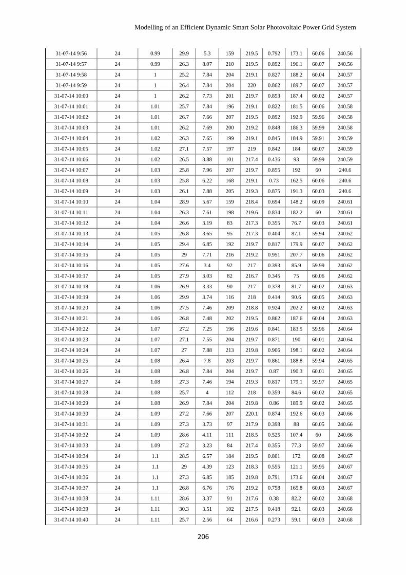
Modelling of an Efficient Dynamic Smart Solar Photovoltaic Power Grid System
206
31-07-14 9:56 24 0.99 29.9 5.3 159 219.5 0.792 173.1 60.06 240.56
31-07-14 9:57 24 0.99 26.3 8.07 210 219.5 0.892 196.1 60.07 240.56
31-07-14 9:58 24 1 25.2 7.84 204 219.1 0.827 188.2 60.04 240.57
31-07-14 9:59 24 1 26.4 7.84 204 220 0.862 189.7 60.07 240.57
31-07-14 10:00 24 1 26.2 7.73 201 219.7 0.853 187.4 60.02 240.57
31-07-14 10:01 24 1.01 25.7 7.84 196 219.1 0.822 181.5 60.06 240.58
31-07-14 10:02 24 1.01 26.7 7.66 207 219.5 0.892 192.9 59.96 240.58
31-07-14 10:03 24 1.01 26.2 7.69 200 219.2 0.848 186.3 59.99 240.58
31-07-14 10:04 24 1.02 26.3 7.65 199 219.1 0.845 184.9 59.91 240.59
31-07-14 10:05 24 1.02 27.1 7.57 197 219 0.842 184 60.07 240.59
31-07-14 10:06 24 1.02 26.5 3.88 101 217.4 0.436 93 59.99 240.59
31-07-14 10:07 24 1.03 25.8 7.96 207 219.7 0.855 192 60 240.6
31-07-14 10:08 24 1.03 25.8 6.22 168 219.1 0.73 162.5 60.06 240.6
31-07-14 10:09 24 1.03 26.1 7.88 205 219.3 0.875 191.3 60.03 240.6
31-07-14 10:10 24 1.04 28.9 5.67 159 218.4 0.694 148.2 60.09 240.61
31-07-14 10:11 24 1.04 26.3 7.61 198 219.6 0.834 182.2 60 240.61
31-07-14 10:12 24 1.04 26.6 3.19 83 217.3 0.355 76.7 60.03 240.61
31-07-14 10:13 24 1.05 26.8 3.65 95 217.3 0.404 87.1 59.94 240.62
31-07-14 10:14 24 1.05 29.4 6.85 192 219.7 0.817 179.9 60.07 240.62
31-07-14 10:15 24 1.05 29 7.71 216 219.2 0.951 207.7 60.06 240.62
31-07-14 10:16 24 1.05 27.6 3.4 92 217 0.393 85.9 59.99 240.62
31-07-14 10:17 24 1.05 27.9 3.03 82 216.7 0.345 75 60.06 240.62
31-07-14 10:18 24 1.06 26.9 3.33 90 217 0.378 81.7 60.02 240.63
31-07-14 10:19 24 1.06 29.9 3.74 116 218 0.414 90.6 60.05 240.63
31-07-14 10:20 24 1.06 27.5 7.46 209 218.8 0.924 202.2 60.02 240.63
31-07-14 10:21 24 1.06 26.8 7.48 202 219.5 0.862 187.6 60.04 240.63
31-07-14 10:22 24 1.07 27.2 7.25 196 219.6 0.841 183.5 59.96 240.64
31-07-14 10:23 24 1.07 27.1 7.55 204 219.7 0.871 190 60.01 240.64
31-07-14 10:24 24 1.07 27 7.88 213 219.8 0.906 198.1 60.02 240.64
31-07-14 10:25 24 1.08 26.4 7.8 203 219.7 0.861 188.8 59.94 240.65
31-07-14 10:26 24 1.08 26.8 7.84 204 219.7 0.87 190.3 60.01 240.65
31-07-14 10:27 24 1.08 27.3 7.46 194 219.3 0.817 179.1 59.97 240.65
31-07-14 10:28 24 1.08 25.7 4 112 218 0.359 84.6 60.02 240.65
31-07-14 10:29 24 1.08 26.9 7.84 204 219.8 0.86 189.9 60.02 240.65
31-07-14 10:30 24 1.09 27.2 7.66 207 220.1 0.874 192.6 60.03 240.66
31-07-14 10:31 24 1.09 27.3 3.73 97 217.9 0.398 88 60.05 240.66
31-07-14 10:32 24 1.09 28.6 4.11 111 218.5 0.525 107.4 60 240.66
31-07-14 10:33 24 1.09 27.2 3.23 84 217.4 0.355 77.3 59.97 240.66
31-07-14 10:34 24 1.1 28.5 6.57 184 219.5 0.801 172 60.08 240.67
31-07-14 10:35 24 1.1 29 4.39 123 218.3 0.555 121.1 59.95 240.67
31-07-14 10:36 24 1.1 27.3 6.85 185 219.8 0.791 173.6 60.04 240.67
31-07-14 10:37 24 1.1 26.8 6.76 176 219.2 0.758 165.8 60.03 240.67
31-07-14 10:38 24 1.11 28.6 3.37 91 217.6 0.38 82.2 60.02 240.68
31-07-14 10:39 24 1.11 30.3 3.51 102 217.5 0.418 92.1 60.03 240.68
31-07-14 10:40 24 1.11 25.7 2.56 64 216.6 0.273 59.1 60.03 240.68
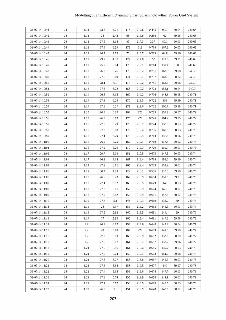
Modelling of an Efficient Dynamic Smart Solar Photovoltaic Power Grid System
207
31-07-14 10:41 24 1.11 28.6 4.21 118 217.6 0.445 99.7 60.04 240.68
31-07-14 10:42 24 1.11 28 2.42 68 216.8 0.286 62 59.98 240.68
31-07-14 10:43 24 1.11 27.5 3.14 85 217.3 0.37 80.1 60.03 240.68
31-07-14 10:44 24 1.12 27.9 6.59 178 219 0.768 167.8 60.03 240.69
31-07-14 10:45 24 1.12 26.7 2.59 70 216.7 0.299 64.8 59.96 240.69
31-07-14 10:46 24 1.12 29.2 4.37 127 217.8 0.55 121.6 59.91 240.69
31-07-14 10:47 24 1.12 25.9 6.84 178 219.1 0.714 159.4 60 240.69
31-07-14 10:48 24 1.13 26.8 6.76 176 219.2 0.751 163.5 59.98 240.7
31-07-14 10:49 24 1.13 27.5 6.69 174 219.1 0.737 161.9 60.02 240.7
31-07-14 10:50 24 1.13 28.1 6.8 177 219.2 0.741 162.6 59.98 240.7
31-07-14 10:51 24 1.13 27.3 6.22 168 219.2 0.723 158.1 60.04 240.7
31-07-14 10:52 24 1.14 26.5 6.15 160 219.2 0.706 148.8 59.98 240.71
31-07-14 10:53 24 1.14 27.3 6.29 170 219.5 0.722 159 59.99 240.71
31-07-14 10:54 24 1.14 27.3 6.37 172 219.6 0.732 160.7 59.98 240.71
31-07-14 10:55 24 1.15 26.4 6.25 169 220 0.725 159.9 60.07 240.72
31-07-14 10:56 24 1.15 26.9 6.73 175 220 0.745 164.2 59.99 240.72
31-07-14 10:57 24 1.15 27.8 6.29 170 219.7 0.724 158.8 60.03 240.72
31-07-14 10:58 24 1.16 27.3 6.88 172 219.4 0.736 160.8 60.03 240.73
31-07-14 10:59 24 1.16 27.1 6.29 170 219.4 0.714 156.8 60.06 240.73
31-07-14 11:00 24 1.16 26.9 6.25 169 219.1 0.719 157.8 60.02 240.73
31-07-14 11:01 24 1.16 27.2 6.29 170 219.3 0.729 159.7 60.03 240.73
31-07-14 11:02 24 1.17 29.7 5.03 151 219.5 0.675 147.5 60.03 240.74
31-07-14 11:03 24 1.17 26.3 6.18 167 219.4 0.714 156.2 59.99 240.74
31-07-14 11:04 24 1.17 27.2 6.11 165 219.4 0.703 153.9 60.02 240.74
31-07-14 11:05 24 1.17 30.4 4.23 127 218.1 0.556 118.8 59.98 240.74
31-07-14 11:06 24 1.18 26.6 6.23 162 218.9 0.694 151.5 59.91 240.75
31-07-14 11:07 24 1.18 27.1 5.92 160 219.5 0.679 149 60.03 240.75
31-07-14 11:08 24 1.18 27.2 5.81 157 219.9 0.664 146.3 60.07 240.75
31-07-14 11:09 24 1.18 27.9 5.42 152 219.9 0.651 142.8 60.02 240.75
31-07-14 11:10 24 1.19 27.6 5.1 143 219.3 0.619 135.2 60 240.76
31-07-14 11:11 24 1.19 28 5.57 156 219.2 0.665 145.9 60.03 240.76
31-07-14 11:12 24 1.19 27.6 5.92 160 219.5 0.681 149.4 60 240.76
31-07-14 11:13 24 1.19 27 5.92 160 219.4 0.681 149.6 59.98 240.76
31-07-14 11:14 24 1.2 26.4 6.12 153 219.6 0.648 143.2 60.04 240.77
31-07-14 11:15 24 1.2 28 5.78 162 220 0.689 149.5 59.99 240.77
31-07-14 11:16 24 1.2 27.3 6.03 163 219.9 0.692 152.6 60.09 240.77
31-07-14 11:17 24 1.2 27.6 6.07 164 219.7 0.697 153.2 59.96 240.77
31-07-14 11:18 24 1.21 27.5 5.96 161 219.4 0.685 150.7 60.03 240.78
31-07-14 11:19 24 1.21 27.5 5.74 155 219.1 0.663 144.7 59.98 240.78
31-07-14 11:20 24 1.21 27.8 5.77 156 218.8 0.667 145.3 60.03 240.78
31-07-14 11:21 24 1.21 27.6 5.64 158 219.5 0.677 149 59.97 240.78
31-07-14 11:22 24 1.22 27.4 5.85 158 219.6 0.674 147.7 60.03 240.79
31-07-14 11:23 24 1.22 27.3 5.74 155 219.9 0.654 144.1 60.02 240.79
31-07-14 11:24 24 1.22 27.7 5.77 156 219.9 0.665 145.5 60.03 240.79
31-07-14 11:25 24 1.22 26.8 5.8 151 219.9 0.648 140.6 60.02 240.79
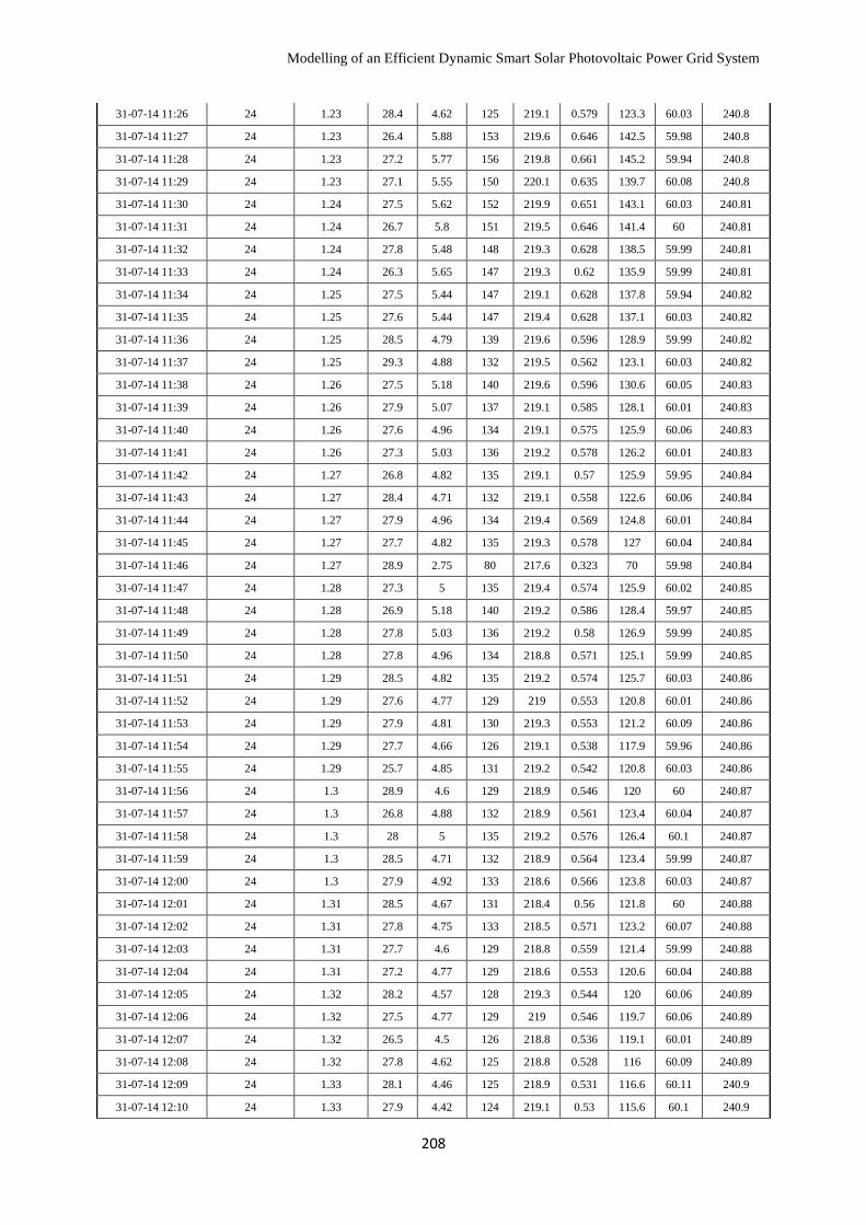
Modelling of an Efficient Dynamic Smart Solar Photovoltaic Power Grid System
208
31-07-14 11:26 24 1.23 28.4 4.62 125 219.1 0.579 123.3 60.03 240.8
31-07-14 11:27 24 1.23 26.4 5.88 153 219.6 0.646 142.5 59.98 240.8
31-07-14 11:28 24 1.23 27.2 5.77 156 219.8 0.661 145.2 59.94 240.8
31-07-14 11:29 24 1.23 27.1 5.55 150 220.1 0.635 139.7 60.08 240.8
31-07-14 11:30 24 1.24 27.5 5.62 152 219.9 0.651 143.1 60.03 240.81
31-07-14 11:31 24 1.24 26.7 5.8 151 219.5 0.646 141.4 60 240.81
31-07-14 11:32 24 1.24 27.8 5.48 148 219.3 0.628 138.5 59.99 240.81
31-07-14 11:33 24 1.24 26.3 5.65 147 219.3 0.62 135.9 59.99 240.81
31-07-14 11:34 24 1.25 27.5 5.44 147 219.1 0.628 137.8 59.94 240.82
31-07-14 11:35 24 1.25 27.6 5.44 147 219.4 0.628 137.1 60.03 240.82
31-07-14 11:36 24 1.25 28.5 4.79 139 219.6 0.596 128.9 59.99 240.82
31-07-14 11:37 24 1.25 29.3 4.88 132 219.5 0.562 123.1 60.03 240.82
31-07-14 11:38 24 1.26 27.5 5.18 140 219.6 0.596 130.6 60.05 240.83
31-07-14 11:39 24 1.26 27.9 5.07 137 219.1 0.585 128.1 60.01 240.83
31-07-14 11:40 24 1.26 27.6 4.96 134 219.1 0.575 125.9 60.06 240.83
31-07-14 11:41 24 1.26 27.3 5.03 136 219.2 0.578 126.2 60.01 240.83
31-07-14 11:42 24 1.27 26.8 4.82 135 219.1 0.57 125.9 59.95 240.84
31-07-14 11:43 24 1.27 28.4 4.71 132 219.1 0.558 122.6 60.06 240.84
31-07-14 11:44 24 1.27 27.9 4.96 134 219.4 0.569 124.8 60.01 240.84
31-07-14 11:45 24 1.27 27.7 4.82 135 219.3 0.578 127 60.04 240.84
31-07-14 11:46 24 1.27 28.9 2.75 80 217.6 0.323 70 59.98 240.84
31-07-14 11:47 24 1.28 27.3 5 135 219.4 0.574 125.9 60.02 240.85
31-07-14 11:48 24 1.28 26.9 5.18 140 219.2 0.586 128.4 59.97 240.85
31-07-14 11:49 24 1.28 27.8 5.03 136 219.2 0.58 126.9 59.99 240.85
31-07-14 11:50 24 1.28 27.8 4.96 134 218.8 0.571 125.1 59.99 240.85
31-07-14 11:51 24 1.29 28.5 4.82 135 219.2 0.574 125.7 60.03 240.86
31-07-14 11:52 24 1.29 27.6 4.77 129 219 0.553 120.8 60.01 240.86
31-07-14 11:53 24 1.29 27.9 4.81 130 219.3 0.553 121.2 60.09 240.86
31-07-14 11:54 24 1.29 27.7 4.66 126 219.1 0.538 117.9 59.96 240.86
31-07-14 11:55 24 1.29 25.7 4.85 131 219.2 0.542 120.8 60.03 240.86
31-07-14 11:56 24 1.3 28.9 4.6 129 218.9 0.546 120 60 240.87
31-07-14 11:57 24 1.3 26.8 4.88 132 218.9 0.561 123.4 60.04 240.87
31-07-14 11:58 24 1.3 28 5 135 219.2 0.576 126.4 60.1 240.87
31-07-14 11:59 24 1.3 28.5 4.71 132 218.9 0.564 123.4 59.99 240.87
31-07-14 12:00 24 1.3 27.9 4.92 133 218.6 0.566 123.8 60.03 240.87
31-07-14 12:01 24 1.31 28.5 4.67 131 218.4 0.56 121.8 60 240.88
31-07-14 12:02 24 1.31 27.8 4.75 133 218.5 0.571 123.2 60.07 240.88
31-07-14 12:03 24 1.31 27.7 4.6 129 218.8 0.559 121.4 59.99 240.88
31-07-14 12:04 24 1.31 27.2 4.77 129 218.6 0.553 120.6 60.04 240.88
31-07-14 12:05 24 1.32 28.2 4.57 128 219.3 0.544 120 60.06 240.89
31-07-14 12:06 24 1.32 27.5 4.77 129 219 0.546 119.7 60.06 240.89
31-07-14 12:07 24 1.32 26.5 4.5 126 218.8 0.536 119.1 60.01 240.89
31-07-14 12:08 24 1.32 27.8 4.62 125 218.8 0.528 116 60.09 240.89
31-07-14 12:09 24 1.33 28.1 4.46 125 218.9 0.531 116.6 60.11 240.9
31-07-14 12:10 24 1.33 27.9 4.42 124 219.1 0.53 115.6 60.1 240.9
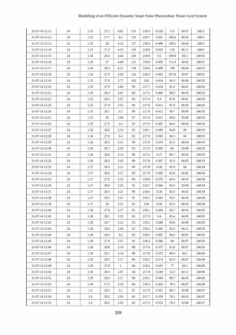
Modelling of an Efficient Dynamic Smart Solar Photovoltaic Power Grid System
209
31-07-14 12:11 24 1.33 27.2 4.62 125 218.9 0.526 115 60.07 240.9
31-07-14 12:12 24 1.33 27.7 4.4 119 218.7 0.501 109.6 60.05 240.9
31-07-14 12:13 24 1.33 28 4.33 117 218.4 0.498 108.5 60.04 240.9
31-07-14 12:14 24 1.33 27.3 4.25 119 218.8 0.505 110 60.11 240.9
31-07-14 12:15 24 1.34 26.6 4.44 120 218.8 0.5 109.8 60.1 240.91
31-07-14 12:16 24 1.34 27 4.48 121 218.8 0.495 111.4 60.02 240.91
31-07-14 12:17 24 1.34 28.2 4.21 118 218.8 0.498 109 60.04 240.91
31-07-14 12:18 24 1.34 27.9 4.29 116 218.3 0.495 107.8 59.97 240.91
31-07-14 12:19 24 1.35 27.8 3.77 102 218 0.434 94.3 60.06 240.92
31-07-14 12:20 24 1.35 27.9 3.66 99 217.7 0.419 91.2 60.01 240.92
31-07-14 12:21 24 1.35 28.3 3.42 96 217.5 0.406 88.5 60.03 240.92
31-07-14 12:22 24 1.35 28.3 3.55 96 217.4 0.4 87.8 60.01 240.92
31-07-14 12:23 24 1.35 27.9 3.55 96 217.8 0.411 87.9 60.03 240.92
31-07-14 12:24 24 1.35 28.1 3.5 98 217.8 0.412 89.7 60.06 240.92
31-07-14 12:25 24 1.35 28 3.46 97 217.4 0.411 88.9 59.99 240.92
31-07-14 12:26 24 1.35 27.9 3.4 92 217.9 0.387 84.3 60.04 240.92
31-07-14 12:27 24 1.36 28.6 3.32 93 218.1 0.389 84.8 60 240.93
31-07-14 12:28 24 1.36 27.9 3.4 92 217.9 0.385 84.3 60 240.93
31-07-14 12:29 24 1.36 28.3 3.21 90 217.9 0.379 82.5 60.04 240.93
31-07-14 12:30 24 1.36 28.7 3.28 92 217.9 0.385 84 59.99 240.93
31-07-14 12:31 24 1.36 28.6 3.14 88 217.6 0.37 80.7 60.03 240.93
31-07-14 12:32 24 1.36 28.9 3.42 89 217.8 0.367 81.9 60.05 240.93
31-07-14 12:33 24 1.37 28.3 3.21 90 217.8 0.38 82.9 60 240.94
31-07-14 12:34 24 1.37 28.6 3.21 90 217.9 0.382 82.8 60.02 240.94
31-07-14 12:35 24 1.37 27.9 3.33 90 218.8 0.379 82.6 60.03 240.94
31-07-14 12:36 24 1.37 28.6 3.25 91 218.7 0.384 83.5 59.99 240.94
31-07-14 12:37 24 1.37 28.5 3.21 90 218.6 0.38 82.6 60.02 240.94
31-07-14 12:38 24 1.37 28.2 3.25 91 218.2 0.383 83.5 60.04 240.94
31-07-14 12:39 24 1.37 28 3.37 91 218 0.38 83.2 60.03 240.94
31-07-14 12:40 24 1.38 27.9 3.37 91 218.1 0.384 83.7 60.03 240.95
31-07-14 12:41 24 1.38 28.1 3.32 93 217.9 0.4 85.4 60.05 240.95
31-07-14 12:42 24 1.38 28.7 3.32 93 218.2 0.388 84.8 60.06 240.95
31-07-14 12:43 24 1.38 28.9 3.28 92 218.5 0.385 83.6 60.11 240.95
31-07-14 12:44 24 1.38 28.5 3.4 92 218.5 0.387 84.5 60.07 240.95
31-07-14 12:45 24 1.38 27.9 3.37 91 218.3 0.386 84 60.07 240.95
31-07-14 12:46 24 1.38 28.8 3.14 88 217.6 0.375 81.8 60.07 240.95
31-07-14 12:47 24 1.39 28.1 3.14 88 217.8 0.375 80.4 60.1 240.96
31-07-14 12:48 24 1.39 28.5 3.17 89 218.5 0.374 81.6 60.07 240.96
31-07-14 12:49 24 1.39 27.9 3 84 218.3 0.347 77 60.1 240.96
31-07-14 12:50 24 1.39 28.3 2.07 58 217.8 0.249 52.5 60.11 240.96
31-07-14 12:51 24 1.39 28.2 3.17 89 218.3 0.369 80.7 60.03 240.96
31-07-14 12:52 24 1.39 27.5 3.18 86 218.3 0.365 78.3 60.07 240.96
31-07-14 12:53 24 1.4 28.3 3.1 87 217.9 0.367 80.1 59.99 240.97
31-07-14 12:54 24 1.4 29.2 2.93 85 217.7 0.359 78.1 60.03 240.97
31-07-14 12:55 24 1.4 28.5 2.92 82 217.5 0.352 76.3 59.98 240.97
Modelling of an Efficient Dynamic Smart Solar Photovoltaic Power Grid System
210
31-07-14 12:56 24 1.4 28.6 2.96 83 217.6 0.351 76.5 60.02 240.97
31-07-14 12:57 24 1.4 28.1 2.96 83 217.5 0.352 76.3 59.98 240.97
31-07-14 12:58 24 1.4 28.2 2.96 80 217.9 0.335 72.5 60.05 240.97
31-07-14 12:59 24 1.4 27.6 2.85 80 217.8 0.33 71.4 60.07 240.97
31-07-14 13:00 24 1.4 28.3 2.82 79 217.8 0.333 72.4 59.97 240.97
31-07-14 13:01 24 1.4 27.6 2.82 79 217.4 0.331 72.6 59.93 240.97
31-07-14 13:02 24 1.41 26.1 2.8 73 217.1 0.31 67.1 59.92 240.98
31-07-14 13:03 24 1.41 27.6 2.85 77 217.1 0.323 70.5 60.03 240.98
31-07-14 13:04 24 1.41 28.6 2.66 72 217.1 0.313 67.4 59.93 240.98
31-07-14 13:05 24 1.41 27.2 2.71 76 217.3 0.321 70.1 59.98 240.98
31-07-14 13:06 24 1.41 28.7 2.64 74 217.6 0.312 67.8 59.98 240.98
31-07-14 13:07 24 1.41 28.8 2.53 71 217.5 0.304 66.3 59.97 240.98
31-07-14 13:08 24 1.41 28.2 2.57 72 217.4 0.305 66.3 59.96 240.98
31-07-14 13:09 24 1.41 28.5 2.42 68 217.5 0.29 62.6 60.03 240.98
31-07-14 13:10 24 1.42 28.8 2.5 70 217.4 0.297 64.5 59.99 240.99
31-07-14 13:11 24 1.42 28.3 2.5 70 217.5 0.297 64.3 60.06 240.99
31-07-14 13:12 24 1.42 28.1 2.55 69 218.1 0.292 63.4 60.04 240.99
31-07-14 13:13 24 1.42 28 2.42 68 218 0.291 63.4 60 240.99
31-07-14 13:14 24 1.42 28.2 2.51 68 218.1 0.291 63.2 60.03 240.99
31-07-14 13:15 24 1.42 29.1 2.42 68 218 0.287 62.1 59.92 240.99
31-07-14 13:16 24 1.42 27.9 2.48 67 217.9 0.287 62.5 59.96 240.99
31-07-14 13:17 24 1.42 28.8 2.39 67 218.1 0.285 62.3 59.96 240.99
31-07-14 13:18 24 1.42 27.8 2.51 68 218 0.288 62.5 59.96 240.99
31-07-14 13:19 24 1.43 27.5 2.44 66 218.5 0.277 60.4 60.05 241
31-07-14 13:20 24 1.43 28.3 2.25 63 218.2 0.267 58 59.9 241
31-07-14 13:21 24 1.43 28.5 2.25 63 218.8 0.265 57.9 60.03 241
31-07-14 13:22 24 1.43 27.3 2.29 62 218.6 0.256 56.1 59.94 241
31-07-14 13:23 24 1.43 28.8 2.25 63 218.3 0.262 57 60.02 241
31-07-14 13:24 24 1.43 27.5 2.29 62 218.5 0.26 56.8 59.94 241
31-07-14 13:25 24 1.43 28.5 2.17 61 218.1 0.253 55.3 59.95 241
31-07-14 13:26 24 1.43 28.8 2.07 58 218 0.244 53.1 59.98 241
31-07-14 13:27 24 1.43 28.9 2 56 217.7 0.233 50.7 59.99 241
31-07-14 13:28 24 1.44 28.9 1.96 55 217.7 0.231 50.3 59.96 241.01
31-07-14 13:29 24 1.44 28.4 1.85 52 217.7 0.214 46.5 60.01 241.01
31-07-14 13:30 24 1.44 28.6 1.57 44 218 0.18 39 60.03 241.01
31-07-14 13:31 24 1.44 28.2 1.46 41 217.9 0.167 36.1 60 241.01
31-07-14 13:32 24 1.44 28.3 1.39 39 217.5 0.156 33.9 60.02 241.01
31-07-14 13:33 24 1.44 27.7 1.35 38 217.3 0.155 33.2 59.94 241.01
31-07-14 13:34 24 1.44 28.3 1.32 37 217.6 0.15 32.8 59.99 241.01
31-07-14 13:35 24 1.44 28 1.35 38 217.6 0.154 33.7 59.98 241.01
31-07-14 13:36 24 1.44 27.6 1.33 36 217.5 0.148 32.3 60 241.01
31-07-14 13:37 24 1.44 27.6 1.25 35 217.6 0.145 31.7 60.02 241.01
31-07-14 13:38 24 1.44 27.7 1.29 35 217.6 0.142 30.8 60.01 241.01
31-07-14 13:39 24 1.44 27.8 1.29 35 217.9 0.14 30.5 60.06 241.01
31-07-14 13:40 24 1.44 26 1.3 34 218.1 0.135 29.2 60.04 241.01
Modelling of an Efficient Dynamic Smart Solar Photovoltaic Power Grid System
211
31-07-14 13:41 24 1.44 27.3 1.25 34 218 0.137 29.8 60.01 241.01
31-07-14 13:42 24 1.44 27.9 1.22 33 217.6 0.135 29.3 59.97 241.01
31-07-14 13:43 24 1.44 26.9 1.26 33 217.7 0.13 28.5 59.98 241.01
31-07-14 13:44 24 1.45 26.6 1.22 33 217.8 0.131 28.9 60.07 241.02
31-07-14 13:45 24 1.45 27.4 1.22 33 217.7 0.132 28.5 60.03 241.02
31-07-14 13:46 24 1.45 28.4 1.14 32 217.5 0.13 28 59.95 241.02
31-07-14 13:47 24 1.45 28 1.22 33 217.5 0.129 28 60.03 241.02
31-07-14 13:48 24 1.45 27.6 1.18 32 217.4 0.129 28.2 59.92 241.02
31-07-14 13:49 24 1.45 26.4 1.19 31 217.3 0.127 27.3 60.03 241.02
31-07-14 13:50 24 1.45 27.5 1.14 32 217.4 0.128 27.6 60.06 241.02
31-07-14 13:51 24 1.45 26.1 1.23 32 217.8 0.122 27.2 60.02 241.02
31-07-14 13:52 24 1.45 27.5 1.14 32 218 0.128 27.6 59.94 241.02
31-07-14 13:53 24 1.45 27.3 1.14 31 218.1 0.124 27.4 59.95 241.02
31-07-14 13:54 24 1.45 27.9 1.14 31 218.4 0.124 26.8 60.08 241.02
31-07-14 13:55 24 1.45 28.9 1.07 30 218.6 0.121 26.2 59.99 241.02
31-07-14 13:56 24 1.45 27.4 1.11 30 218.6 0.118 25.5 60.02 241.02
31-07-14 13:57 24 1.45 27.4 1.07 29 218.4 0.116 25.1 59.92 241.02
31-07-14 13:58 24 1.45 27.7 1.07 29 218.4 0.114 24.8 60 241.02
31-07-14 13:59 24 1.45 27.8 1.03 28 218.5 0.112 24.2 60.05 241.02
31-07-14 14:00 24 1.45 28.4 1 28 218.2 0.11 24 59.94 241.02
31-07-14 14:01 24 1.45 28.9 0.96 27 218.4 0.106 23.3 59.95 241.02
31-07-14 14:02 24 1.45 27 1.03 28 218.3 0.11 24 60 241.02
31-07-14 14:03 24 1.45 28.5 0.96 27 218.4 0.107 23.5 60.02 241.02
31-07-14 14:04 24 1.45 27.7 1 27 218.1 0.105 22.8 59.98 241.02
31-07-14 14:05 24 1.45 27.4 1 27 218 0.106 23.3 59.98 241.02
31-07-14 14:06 24 1.46 27.5 1 27 218.5 0.104 22.9 60 241.03
31-07-14 14:07 24 1.46 27.7 0.92 26 218.4 0.105 22.7 59.95 241.03
31-07-14 14:08 24 1.46 26.1 1 26 218.5 0.101 22.2 60 241.03
31-07-14 14:09 24 1.46 26.5 0.96 25 218.5 0.101 22 60.06 241.03
31-07-14 14:10 24 1.46 27.8 0.92 25 217.9 0.099 21.7 60.03 241.03
31-07-14 14:11 24 1.46 28.4 0.89 25 217.9 0.099 21.3 59.94 241.03
31-07-14 14:12 24 1.46 28 0.89 25 218.2 0.096 20.9 60.02 241.03
31-07-14 14:13 24 1.46 27.9 0.88 24 218.3 0.095 20.5 60.01 241.03
31-07-14 14:14 24 1.46 27.4 0.88 24 218.8 0.094 20.3 60.01 241.03
31-07-14 14:15 24 1.46 26.5 0.88 23 218.9 0.092 20.1 59.99 241.03
31-07-14 14:16 24 1.46 26.5 0.88 23 218.3 0.091 19.6 59.95 241.03
31-07-14 14:17 24 1.46 26.6 0.88 23 217.9 0.088 19.1 59.96 241.03
31-07-14 14:18 24 1.46 26.4 0.88 23 218 0.088 19.1 59.98 241.03
31-07-14 14:19 24 1.46 26.6 0.84 22 218 0.083 18.3 60.06 241.03
31-07-14 14:20 24 1.46 27.3 0.81 22 218 0.083 18.3 59.94 241.03
31-07-14 14:21 24 1.46 26.3 0.84 22 217.9 0.083 18 60.02 241.03
31-07-14 14:22 24 1.46 27.4 0.81 22 218.1 0.081 17.6 59.98 241.03
31-07-14 14:23 24 1.46 26.8 0.84 22 217.9 0.078 17.2 59.99 241.03
31-07-14 14:24 24 1.46 27.3 0.77 21 217.9 0.076 16.5 60.09 241.03
31-07-14 14:25 24 1.46 26.3 0.8 21 218 0.077 16.7 60 241.03
Modelling of an Efficient Dynamic Smart Solar Photovoltaic Power Grid System
212
31-07-14 14:26 24 1.46 26.9 0.8 21 217.9 0.076 16.7 60.03 241.03
31-07-14 14:27 24 1.46 26.6 0.84 22 218.3 0.076 16.5 59.95 241.03
31-07-14 14:28 24 1.46 26.4 0.8 21 217.7 0.076 16.7 60.05 241.03
31-07-14 14:29 24 1.46 26.9 0.8 21 217.8 0.072 15.8 59.99 241.03
31-07-14 14:30 24 1.46 27.9 0.75 21 217.8 0.071 15.4 59.96 241.03
31-07-14 14:31 24 1.46 27 0.77 21 217.8 0.073 15.6 60.02 241.03
31-07-14 14:32 24 1.46 27.1 0.77 21 218.4 0.071 15.7 60.03 241.03
31-07-14 14:33 24 1.46 27.9 0.77 21 218.4 0.07 15.5 59.99 241.03
31-07-14 14:34 24 1.46 28.1 0.75 21 218.2 0.071 15.7 59.95 241.03
31-07-14 14:35 24 1.46 28.3 0.75 21 217.9 0.072 15.4 59.98 241.03
31-07-14 14:36 24 1.46 28 0.77 21 217.6 0.071 15.2 59.95 241.03
31-07-14 14:37 24 1.47 26.7 0.8 21 217.5 0.07 15.4 59.99 241.04
31-07-14 14:38 24 1.47 28 0.75 21 217.5 0.069 14.7 60.04 241.04
31-07-14 14:39 24 1.47 27 0.8 21 217.9 0.069 14.8 60.05 241.04
31-07-14 14:40 24 1.47 28.1 0.75 21 217.6 0.066 14.5 60.09 241.04
31-07-14 14:41 24 1.47 26.7 0.8 21 217.7 0.067 14.5 60.15 241.04
31-07-14 14:42 24 1.47 26.5 0.8 21 218.4 0.068 14.8 60.1 241.04
31-07-14 14:43 24 1.47 26.1 0.8 21 218.5 0.068 14.6 60.05 241.04
31-07-14 14:44 24 1.47 26.6 0.8 21 218.6 0.066 14.8 60.11 241.04
31-07-14 14:45 24 1.47 28.5 0.71 20 218.6 0.06 13.1 60.1 241.04
31-07-14 14:46 24 1.47 26.4 0.8 21 218.3 0.068 15 60.05 241.04
31-07-14 14:47 24 1.47 25.8 0.76 20 218.3 0.061 13.5 60.1 241.04
31-07-14 14:48 24 1.47 25.8 0.76 20 218.3 0.061 13.5 60.1 241.04
31-07-14 14:49 24 1.47 25.8 0.76 20 218.3 0.061 13.5 60.1 241.04
31-07-14 14:50 24 1.47 25.8 0.76 20 218.3 0.061 13.5 60.1 241.04
31-07-14 14:51 24 1.47 25.8 0.76 20 218.3 0.061 13.5 60.1 241.04
31-07-14 14:52 24 1.47 25.8 0.76 20 218.3 0.061 13.5 60.1 241.04
31-07-14 14:53 24 1.47 25.8 0.76 20 218.3 0.061 13.5 60.1 241.04
31-07-14 14:54 24 1.47 25.8 0.76 20 218.3 0.061 13.5 60.1 241.04
31-07-14 14:55 24 1.47 25.8 0.76 20 218.3 0.061 13.5 60.1 241.04
31-07-14 14:56 24 1.47 25.8 0.76 20 218.3 0.061 13.5 60.1 241.04
31-07-14 14:57 24 1.47 25.8 0.76 20 218.3 0.061 13.5 60.1 241.04
31-07-14 18:16 0 0 0 0 0 0 0 0 0 241.04
Modelling of an Efficient Dynamic Smart Solar Photovoltaic Power Grid System
213
Table 12: Comparative Total Energy Generated For a Month
Total Energy Generated For a Month
DAY Azimuthal-altitude
(KWh)
45 Stationary
(KWh)
1 1.80 1.10
2 1.80 1.00
3 1.90 1.10
4 1.30 0.75
5 1.40 0.80
6 1.45 0.90
7 0.30 0.20
8 1.45 0.90
9 1.45 0.95
10 1.5 1.00
11 1.75 1.10
12 2.00 1.15
13 1.98 1.15
14 1.90 1.10
15 1.45 1.00
16 0.10 0.10
17 0.10 0.10
18 0.10 0.10
19 0.10 0.10
20 0.10 0.10
21 0.10 0.10
22 0.50 0.40
23 0.25 0.20
24 0.80 0.70
25 1.00 0.70
26 1.30 1.00
27 1.05 1.00
28 1.25 0.80
29 0.10 1.00
30 0.15 0.15
31 1.50 1.10
31.93 21.85

Modelling of an Efficient Dynamic Smart Solar Photovoltaic Power Grid System
214
Table 13: Comparative Hourly Energy Efficiency
Hourly Energy Efficiency
Hour Azimuthal-altitude(KWh) 45 Stationary(KWh)
1 0 0
2 0 0
3 22 22
4 88 60
5 132 95
6 176 140
7 118 76
8 198 160
9 220 185
10 185 145
11 154 110
12 130 74
13 70 38
14 22 19
15 0 0
16 0 0
17 0 0
18 0 0
19 0 0
20 0 0
21 0 0
22 0 0
23 0 0
24 0 0
1515 1124