modelling, optimisation and model predictive control … · imperial college london department of...
TRANSCRIPT

Imperial College London
Department of Chemical Engineering
Modelling, Optimisation and
Model Predictive Control of Insulin Delivery
Systems in Type 1 Diabetes Mellitus
Stamatina Zavitsanou
October 2014
Supervised by Professor Stratos Pistikopoulos
Submitted in part fulfilment of the requirements for the degree of
Doctor of Philosophy in Chemical Engineering of Imperial College London and the Diploma
of Imperial College London

2

3
Declaration
I herewith certify that all material in this dissertation which is not my own work has been
properly acknowledged.
Zavitsanou, Stamatina
© The copyright of this thesis rests with the author and is made available under a Creative Commons
Attribution Non-Commercial No Derivatives licence. Researchers are free to copy, distribute or
transmit the thesis on the condition that they attribute it, that they do not use it for commercial
purposes and that they do not alter, transform or build upon it. For any reuse or redistribution,
researchers must make clear to others the licence terms of this work.

4
Abstract
Type 1 Diabetes Mellitus is a metabolic disease requiring lifelong treatment with exogenous
insulin which significantly affects patient’s lifestyle. Therefore, it is of paramount importance
to develop novel drug delivery techniques that achieve therapeutic efficacy and ensure patient
safety with a minimum impact on their quality of life. Motivated by the challenge to improve
the living standard of a diabetic patient, the idea of an artificial pancreas that mimics the
endocrine function of a healthy pancreas has been developed in the scientific society.
Towards this direction, model predictive control has been established as a very promising
control strategy for blood glucose regulation in a system that is dominated by high intra- and
inter-patient variability, long time delays, and presence of unknown disturbances such as diet,
physical activity and stress levels.
This thesis presents a framework for blood glucose regulation with optimal insulin infusion
which consists of the following steps: 1. Development of a novel physiologically based
compartmental model analysed up to organ level that describes glucose-insulin interactions in
type 1 diabetes, 2. Derivation of an approximate model suitable for control applications, 3.
Design of an appropriate control strategy and 4. In-silico validation of the closed loop control
performance. The developed model’s accuracy and prediction ability is evaluated with data
obtained from the literature and the UVa/Padova Simulator model, the model parameters are
individually estimated and their effect on the model’s measured output, the blood glucose
concentration, is identified. The model is then linearised and reduced to derive low-order
linear approximations of the underlying system suitable for control applications.
The proposed control design aims towards an individualised optimal insulin delivery that
consists of a patient-specific model predictive controller, a state estimator, a personalised
scheduling level and an open loop optimisation problem subjected to patient specific process
model and constraints. This control design is modifiable to address the case of limited patient
data availability resulting in an “approximation” control strategy. Both designs are validated
in-silico in the presence of predefined, measured and unknown meal disturbances using both
the proposed model and the UVa/Padova Simulator model as a virtual patient. The robustness
of the control performance is evaluated in several conditions such as skipped meals,
variability in the meal content, time and metabolic uncertainty.
The simulation results of the closed loop validation studies indicate that the proposed control
strategies can achieve promising glycaemic control as demonstrated by the study data.

5
However, further prospective validation of the closed loop control strategy with real patient
data is required.

Acknowledgements
First and foremost, I would like to thank my supervisor Professor Stratos Pistikopoulos for
his continuous support and encouragement during the good and difficult times of my studies.
His advice and enthusiasm have been very motivating to structure and develop my own ideas.
Additionally, I would like to thank Professor Michael Georgiadis for his support and good
advice.
The financial support from the European Research Council (MOBILE, ERC Advanced
Grant, No: 226462) and the CPSE Industrial Consortium is gratefully acknowledged.
During the years I spent at Imperial College I met a number of people who have
contributed substantially to the quality of my personal and professional time. I would really
like to thank the “senior Greek committee” of the group –Dr. Kouramas, Dr.Panos, Dr.
Kyparissides, Dr. Koutinas and Dr. Pefani- who have made the first years of my PhD very
enjoyable. Especially, I am very grateful to Dr. Kouramas and Dr. Panos for their feedback
and support for my project. I would also like to thank my colleagues of the MOBILE group
and the newer members of the group who have been very helpful. The good advice, support
and friendship of Dr. Krieger, has been invaluable to me and for which I am extremely
grateful.
Finally, I would like to thank my good friends Chara and Emma, for always being by my
side during my studies.
Last but not least, I am mostly grateful to my family for their love and encouragement.
This effort is dedicated to the memory of T. Livitsanos

7
Contents
Abstract .................................................................................................................................. 4
Acknowledgements ................................................................................................................ 6
Notation ................................................................................................................................ 10
List of Tables ........................................................................................................................ 15
List of Figures ...................................................................................................................... 16
1. Introduction & Motivation ............................................................................................ 21
1.1 Introduction .................................................................................................................... 21
1.2 The Artificial Pancreas ................................................................................................... 22
1.2 Project deliverables ........................................................................................................ 23
1.3 Structure of the thesis ..................................................................................................... 26
2. Modelling the T1DM System - An Overview ............................................................... 28
2.1 Introduction to Diabetes Mellitus ................................................................................... 28
Classification .................................................................................................................... 28
Prevalence and incidence of T1DM ................................................................................. 29
2.1.1 Physiology ................................................................................................................... 30
2.1.1.a Glucose ................................................................................................................. 30
2.1.1.b Pancreas: insulin, glucagon .................................................................................. 32
2.1.1.c The Liver ............................................................................................................... 35
2.1.2 Pathophysiology and T1DM ....................................................................................... 36
2.1.2.a Complications of T1DM ....................................................................................... 36
2.1.2.b Symptoms of T1DM ............................................................................................. 37
2.1.2.c Diagnostic Tests for T1DM .................................................................................. 38
2.1.2. d Treatment ............................................................................................................. 39
2.1.2.e Types of insulin .................................................................................................... 40
2.2 Literature Review ........................................................................................................... 43
2.2.1 Modelling the drug delivery system ........................................................................ 43
2.2.2 Modelling the glucose-insulin system in T1DM ..................................................... 43
3. Mathematical Model Development ............................................................................... 53
3.1 Introduction .................................................................................................................... 53
3.2 Physiologically based Compartmental Model of Glucose Metabolism ......................... 53
Endogenous Glucose Production (EGP)........................................................................... 56
Rate of glucose appearance (Ra) ....................................................................................... 57
Glucose Renal excretion (excretion) ................................................................................ 58
Glucose diffusion in the periphery ................................................................................... 58
8
3.3 Insulin Kinetics .............................................................................................................. 61
3.4 Concluding Remarks ...................................................................................................... 65
4. Model Analysis and Dynamic Optimisation ................................................................. 66
4.1 Introduction .................................................................................................................... 66
4.2 Insulin Kinetics: Model Selection .................................................................................. 66
4.2.1 Methods ................................................................................................................... 66
4.2.2. Parameter Estimation .............................................................................................. 66
4.2.3 Model Selection ....................................................................................................... 68
Key Points......................................................................................................................... 71
4.3 Endogenous Glucose Production: Parameter Estimation ............................................... 71
4.4 Global Sensitivity Analysis ............................................................................................ 72
4.5 Parameter Estimation ..................................................................................................... 77
4.6 Simulation Results.......................................................................................................... 78
Key Points......................................................................................................................... 83
4.7 Time Delays in the system ............................................................................................. 83
4.8 Dynamic optimisation of insulin delivery ...................................................................... 86
4.9 Alternative insulin infusion ............................................................................................ 91
Key Points......................................................................................................................... 94
4.10 Concluding Remarks .................................................................................................... 94
5. Closed Loop Control in T1DM- An Overview ............................................................. 95
5.1 Introduction .................................................................................................................... 95
5.2 Literature review ............................................................................................................ 95
PID .................................................................................................................................... 96
MPC .................................................................................................................................. 97
Other Algorithms ............................................................................................................ 100
5.3 Challenges of the closed loop design ........................................................................... 100
5.4 Model Predictive Control ............................................................................................. 102
5.5 Kalman Filter................................................................................................................ 103
5.6 Model Approximation .................................................................................................. 105
5.7 Concluding Remarks .................................................................................................... 108
6. Model Predictive Control Studies in T1DM............................................................... 109
6.1 Introduction .................................................................................................................. 109
6.2 Control Objective ......................................................................................................... 109
6.3 Model Predictive Control Strategy for insulin delivery in T1DM ............................... 110
6.4 Systematic Strategy (I): Control designs ...................................................................... 111
6. 4.1 (CD1) Dynamic Optimisation: Predefined Disturbances (dp) ............................... 112

9
6.4.2 (CD2) Online MPC with Scheduling Level: Announced Disturbances (da) .......... 113
6.4.3 (CD3) Optimisation and Correction MPC: Unknown Disturbances (du) ............... 114
6.4.4 (CD4) Online MPC with Scheduling Level: Unknown Disturbances (du) ............ 117
6.5 Performance analysis of the four control designs CD1-CD4 ........................................ 118
6.5.1 Control Design 1 (CD1): Dynamic Optimisation .................................................. 118
6.5.2 Control Design 2 (CD2): Online MPC with Scheduling Level ............................. 121
6.5.2.1 Case Study: Skipped Meal .................................................................................. 123
6.5.3 Control Design 3 (CD3): Optimisation and Correction MPC ................................ 123
Key Results for the Systematic Strategy Control Designs ............................................. 126
6.6 “Approximation” Strategy (II): Control Designs ........................................................ 127
6.6.1 Comparison of CD3: Strategy I and Strategy II......................................................... 129
Key Results for the “Approximation” Strategy Control Designs ................................... 131
6.7 Case Study: Skipped Meal ........................................................................................... 131
6.8 Case Study: Variable Meal Time ................................................................................. 134
6.9 Case Study: Intra-patient Variability............................................................................ 138
6.10 Conclusions ................................................................................................................ 141
6.11 Concluding Remarks .................................................................................................. 142
7. Concluding Remarks & Future Directions ................................................................ 143
7.1 Project summary ........................................................................................................... 143
7.2 Key contributions of this thesis .................................................................................... 145
7.3 Publications from this thesis ........................................................................................ 147
7.3 On-going and Future Directions ................................................................................... 148
APPENDIX A ....................................................................................................................... 153
A.1 Model of UVa/Padova Simulator ................................................................................ 153
A.2 Model Predictive Control Framework ......................................................................... 155
APPENDIX B ....................................................................................................................... 169
B.1 Parameter Estimation ................................................................................................... 169
B.2 MPC to QP .................................................................................................................. 172
APPENDIX C ....................................................................................................................... 177
Concluding Remarks ...................................................................................................... 180
APPENDIX D ....................................................................................................................... 181
Bibliography ......................................................................................................................... 182

10
Notation
Modelling, Model Analysis & Optimisation
List of Acronyms
ADA American Diabetes Association
AP Artificial Pancreas
ATP Adenosine triphosphate
CF Correction Factor
CGMs Continuous Glucose Monitoring systems
CHO Carbohydrates
CID Correction Insulin Dose
CL Closed Loop
CR Carb Factor
CSII Continuous Subcutaneous Insulin Infusion
FDA Food and Drug Administration
GSA Global Sensitivity Analysis
HDMR High dimensional model representation
IDDM Insulin-dependent diabetes mellitus
IVGTT Intravenous glucose tolerance test
JDRF Juvenile Diabetes Research Foundation
M1,M2,M3 Model 1, Model 2, Model 3 (Insulin kinetics)
LADA Latent autoimmune diabetes in adults
NIDDM Non-insulin-dependent diabetes mellitus
OGTT Oral glucose tolerance test
OL Open Loop
RS-HDMR Random sampling - high dimensional model representation
T1DM Type 1 diabetes mellitus
TBV Total Blood Volume
TDD Total Daily Dose
WM Wilinska Model (Insulin kinetics)
11
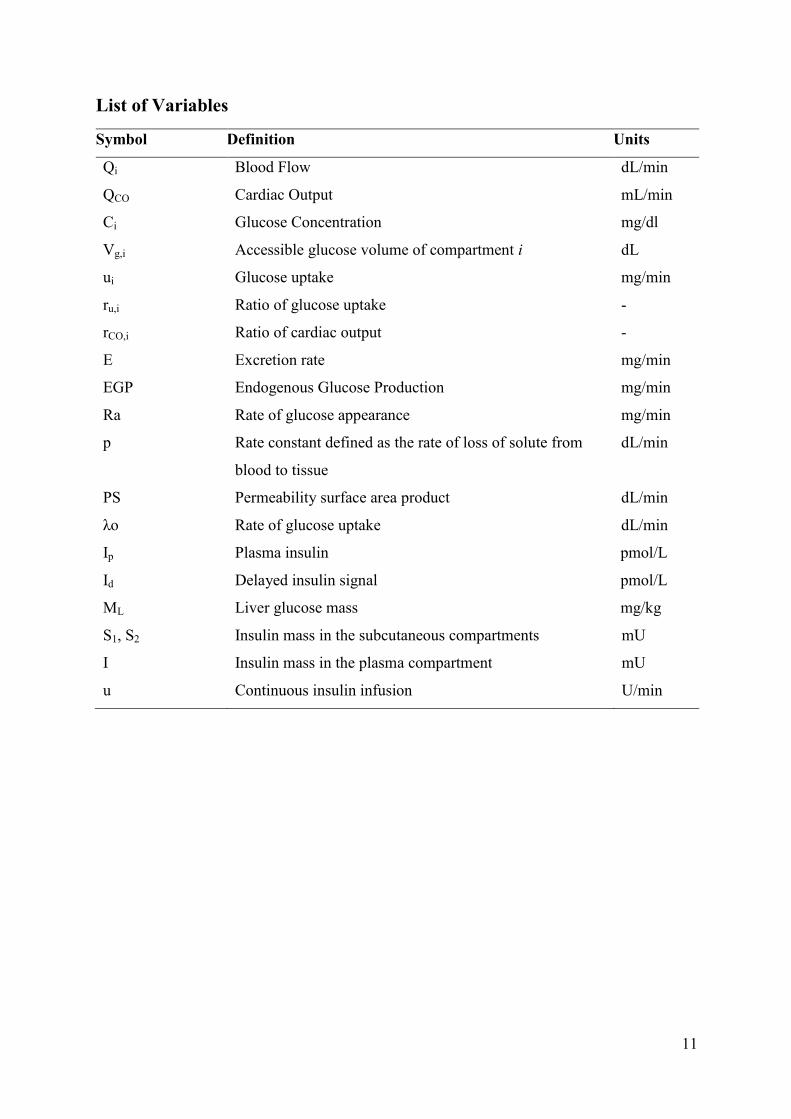
List of Variables
Symbol Definition Units
Qi Blood Flow dL/min
QCO Cardiac Output mL/min
Ci Glucose Concentration mg/dl
Vg,i Accessible glucose volume of compartment i dL
ui Glucose uptake mg/min
ru,i Ratio of glucose uptake -
rCO,i Ratio of cardiac output -
E Excretion rate mg/min
EGP Endogenous Glucose Production mg/min
Ra Rate of glucose appearance mg/min
p Rate constant defined as the rate of loss of solute from
blood to tissue
dL/min
PS Permeability surface area product dL/min
λo Rate of glucose uptake dL/min
Ip Plasma insulin pmol/L
Id Delayed insulin signal pmol/L
ML Liver glucose mass mg/kg
S1, S2 Insulin mass in the subcutaneous compartments mU
I Insulin mass in the plasma compartment mU
u Continuous insulin infusion U/min

12
List of Parameters
Insulin Kinetics
ksub Intercompartmental transfer rate constant min-1
Vdist Insulin distribution volume L/Kg
kelim Elimination rate constant min-1
Glucose Diffusion in the Periphery
k1 Rate parameter of insulin dependent glucose uptake dL
2 per
pmol·min2
k2 Rate parameter of glucose uptake min-1
k2_PS Rate constant of permeability surface are product min-1
k1_PS Rate constant describing the effect of insulin on
permeability surface are product
dL2 per
pmol·min2
Endogenous Glucose Production
kp1 Extrapolated EGP at zero glucose and insulin mg/kg/min
kp2 Liver glucose effectiveness min-1
kp3 Lnsulin action on the liver
mg/kg/min per
pmol/L
ki Rate parameters for the delay between insulin
signal and action min
-1
BW Body Weight kg
Rate of Glucose appearance
kmax Max gastric emptying min-1
kmin Min gastric emptying min-1
kabs Rate constant of intestinal absorption min-1
kgri Rate constant of grinding min-1
kempt Rate of gastric emptying min-1
b Percentage of dose for which kempt decreases at
(kmax-kmin)/2 -
d Percentage of dose for which kempt is back to
(kmax-kmin)/2 -
f Fraction of intestinal absorption -
Glucose Excretion
CLrenal Renal glucose clearance dl/min

13
Variable subscript denotation
Subscript Denotation Subscript Denotation
i Organ-Compartment H Heart
B Brain P Periphery
K Kidney Pt Periphery tissue
L Liver P,ISF Interstitial Periphery
G Gut

14
Model Predictive Control
List of Acronyms
CD Control design
MPC Model predictive control
QP Quadratic Programming
CVGA Control Variability Grid Analysis
List of Variables
Symbol Denotation
A State matrix
B Input matrix
Bd Input disturbance matrix
C Output matrix
Cd Output disturbance matrix
di disturbance
M Prediction Horizon
N Control Horizon
Q Weight Matrix for the states
QKF Process noise covariance matrix of Kalman Filter
QR Weight Matrix for the output
R Weight Matrix for the input
RKF Measurement noise covariance matrix of Kalman Filter
R1 Weight Matrix for the change in the control input
ts Sampling time
u Control input
Δu Step change in control input
υ Measurement noise
w Process noise
x System states
y System output
yR
Reference point

15
List of Tables
Table 2.1: The mechanisms of energy production through glucose ....................................... 31
Table 2.2: Characteristics of Insulin(American Diabetes Association) .................................. 41
Table 2.3: Commercially available types of insulin and their mixtures ................................. 42
Table 2.4: The most common types of empirical pharmacodynamics models (adapted from
(Holford and Sheiner, 1982) .................................................................................................... 46
Table 2.5: Mathematical models of glucose-insulin system ................................................... 52
Table 3.1: Ratio of cardiac output at rest (Ferrannini and DeFronzo, 2004) .......................... 56
Table 3.2: Ratio of glucose uptake (Ferrannini and DeFronzo, 2004) ................................... 56
Table 3.3: Ratio of capillary volume ...................................................................................... 60
Table 3.4: Density of muscles and adipose tissue ................................................................... 61
Table 3.5: Variable and parameter definition of Model 1 and Model 2 ................................. 62
Table 3.6: Variable and parameter definition of Model 3 ....................................................... 63
Table 3.7: Variable and parameter definition of Wilinska Model .......................................... 64
Table 4.1: Goodness of fit of proposed models and model selection ..................................... 68
Table 4.2: Correlation Matrix of the parameters of Model 1 .................................................. 69
Table 4.3: Correlation Matrix of Wilinska Model .................................................................. 69
Table 4.4: Correlation Matrix of Model 3............................................................................... 70
Table 4.5: Optimal Mean Parameter Estimates and standard deviations reported in
parenthesis. Initial guess and lower-upper bounds of the parameters used for estimation are
reported in the 2nd column. ..................................................................................................... 70
Table 4.6: Parameter estimation results .................................................................................. 72
Table 4.7: Model parameters default values and range. SIs for of all parameters and for those
related to intra-patient variability calculated with GUI-HDMR toolbox................................. 74
Table 4.8: Optimal parameter estimates presented as mean value (lower-upper) value for the
10 patients ................................................................................................................................ 78
Table 4.9: Insulin bolus to compensate for 50 g of CHO ....................................................... 88
Table 4.10:Area under the curve (outside the normal range) ................................................. 90
Table 5.1: Clinically Evaluated PID controllers ..................................................................... 96
Table 5.2: MPC control Algorithms evaluated in clinical trials ............................................. 99
Table 5.3: definitions of symbols found in ( 5.1).................................................................. 103
Table 6.1: Meal disturbance types ........................................................................................ 111
Table 6.2: Glucose regulation designs .................................................................................. 112

16
Table 6.3: Prediction Horizon (N) for the 10 patients .......................................................... 112
Table 6.4: Specifications of MPC and the Kalman Filter ..................................................... 117
Table 6.5: Comparison of the time spent outside the normal glucose range when optimisation
of insulin infusion is performed and conventional optimal insulin dosing is administered .. 120
Table 6.6: Evaluation of CD3 with two meal scenarios ....................................................... 123
Table 6.7: CD3 predefined reference meal plan (Scenario 1) ............................................... 124
Table 6.8:CD4 unknown disturbances (Scenario 1) .............................................................. 124
Table A.2.1: Identified parameters of transfer function models……………………………157
Table A.2.2: Estimated parameters of linearised model for10 adults……………… ..……162
Table A.2.3: Specifications of MPC 2 and the Kalman Filter……………………………...164
Table A.2.4: CD3 (predefined meal plan)………………………………………………......166
Table A.2.5: CD4 (unmeasured)………………………………………………………...….166
Table B.1: The optimal estimated values for each parameter for the 10 patients and the
corresponding (95%) confidence interval that indicates that there is 0.95 probability the value
of the parameter to be within the interval…………………………………………………...169
Table B.2: The optimal estimated values for sub model EGP for the 10 patients, the standard
deviation and the confidence interval……………………………………………………….170
Table B.3: The optimal estimated values for sub model Ra for the 10 patients, the standard
deviation and the confidence interval……………………………………………………….171
Table D.1: MPC tuning parameters and specifications for CD2 CD3 and CD4……………...181
List of Figures
Figure 1.1: Schematic representation of an Artificial Pancreas .............................................. 23
Figure 1.2: Framework for MPC controllers design adapted from (Pistikopoulos 2012) ...... 24
Figure 2.1: Incidence of T1DM worldwide, data from (Onkamo et al., 1999) ...................... 30
Figure 2.2: Islets of Langerhans adapted from (Parlerm, 2003) ............................................. 32
Figure 2.3: Impact of insulin and other counter regulatory hormones on glucose levels ....... 35
Figure 2.4: The overall flow of fuels and the actions of insulin in the liver, muscles and
adipose tissue, adapted from (Pocock, Richards and Richard, 2006) ...................................... 36
Figure 2.5: Single Compartment (left hand side), two compartmental approach (right hand
side) .......................................................................................................................................... 44
Figure 2.6: physiological modelling, adapted from
(http://aiche.confex.com/aiche/2008/webprogram/Paper138436.html) ................................... 45

17
Figure 2.7: Organ compartmental analysis ............................................................................. 45
Figure 3.1: Structure of the physiologically based compartmental model of glucose
metabolism in T1DM ............................................................................................................... 54
Figure 3.2. Detailed glucose uptake in the periphery ............................................................. 58
Figure 3.3. Schematic representation of model 1.................................................................... 63
Figure 3.4. Schematic representation of model 2.................................................................... 63
Figure 3.5: Schematic representation of model 3 ................................................................... 64
Figure 3.6: Schematic representation of Willinska model ...................................................... 65
Figure 4.1: Comparison of Model 1, 2, 3 and Wilinska model with experimental data ......... 67
Figure 4.2: Weighted Residuals of the four models ............................................................... 68
Figure 4.3. Effect of subcutaneous insulin injection on endogenous glucose production ...... 71
Figure 4.4: Time varying SIs when all parameters are considered ......................................... 76
Figure 4.5: Time varying SIs when intra-patient variability related parameters are considered
.................................................................................................................................................. 76
Figure 4.6: Comparison of blood glucose concentration (mg/dl) as predicted from the
proposed model with the Simulator, for the 10 adults when a meal plan of 45g, 70g and 70g
of carbohydrates are considered at 420min, 720min and 1080min respectively. The insulin
infusion (U) is shown at the right axis for every patient. ......................................................... 80
Figure 4.7: Glucose concentration profiles in the organs for a 45 g of CHO meal and a 6.5 U
insulin bolus ............................................................................................................................. 81
Figure 4.8: Rate of glucose absorption from the organs for a 45 g of CHO meal and a 6.5 U
insulin bolus ............................................................................................................................. 81
Figure 4.9: Grey area presents the EGP profiles of a stochastic simulation performed in
UVa/Padova Simulator for 20% variation of the parameters from their mean value and the
dashed line the EGP profile as obtained from the proposed model using the estimated
parameter values. ..................................................................................................................... 82
Figure 4.10: Grey area presents the Ra profiles of a stochastic simulation performed in
UVa/Padova Simulator for 20% variation of the parameters from their mean value and the
dashed line the Ra profile as obtained from the proposed model using the estimated parameter
values. ...................................................................................................................................... 82
Figure 4.11: Time delay in the system .................................................................................... 84
Figure 4.12: Patient dependent time delay.............................................................................. 85
Figure 4.13 : Time delay dependence on patient and bolus (adult 3-low insulin sensitive) ... 85
Figure 4.14: Time delay dependence on patient and bolus (adult 4-high insulin sensitive)... 86

18
Figure 4.15: Optimisation of bolus timing; light grey: optimised glucose profile using the
T1DMS, grey: optimised glucose profile using the proposed model and black line: glucose
profile when bolus given simultaneously with food using the T1DMS. ................................. 90
Figure 4.16: Optimal glucose profiles when insulin is given as a bolus and as a piecewise
constant infusion (adult 3) ....................................................................................................... 92
Figure 4.17: Optimal glucose profiles when insulin is given as a bolus and as a piecewise
constant infusion (adult 5) ....................................................................................................... 93
Figure 5.1: Schematic of Model Predictive Control ............................................................. 102
Figure 5.2: Comparison of original model, linearised model and reduced model when 50 g of
carbohydrates are consumed and a 5 U bolus is given to patient no2 ................................... 107
Figure 6.1: General proposed control strategy that consists of three blocks, MPC, State
Estimator and optimisation that are activated depending on the nature of the meal
disturbances. In the case of predefined disturbances (dp) the problem of optimal insulin
delivery is an output optimisation problem, in the case of announced disturbances (da) the
problem is a state feedback MPC involving a scheduling feature for upper insulin constraint.
For unknown disturbances (du) the entire strategy is activated involving an output feedback
MPC. ...................................................................................................................................... 111
Figure 6.2: Control design CD2 ............................................................................................ 114
Figure 6.3: Control design CD3 ............................................................................................ 115
Figure 6.4: Control design CD4 ............................................................................................ 118
Figure 6.5: Glucose profiles for the 10 adults (upper graph) when optimal insulin infusion
(lower graph) is delivered ...................................................................................................... 119
Figure 6.6: MPC control for 10 adults in the presence of announced disturbances.; Upper
graphs blood glucose concentration (mg/dl) profiles; lower graphs control action, insulin
(U/min). The black lines show the results when CD2 is validated against the proposed model
while the grey lines the results against the UVa/Padova Simulator. ..................................... 122
Figure 6.7: Skipped breakfast and skipped lunch for adult 5 ............................................... 123
Figure 6.8: Comparison of glucose regulation with CD3 and CD4 for adult 1. The meals are
given 420, 720 and 1080 and contain 75, 100 and 90 g of carbohydrates respectively
(Scenario 1) ............................................................................................................................ 125
Figure 6.9: Comparison of glucose regulation with CD3 and CD4 for adult 1. The meals are
given 420, 720 and 1080 and contain 45, 75 and 60 g of carbohydrates respectively (Scenario
2) ............................................................................................................................................ 126
Figure 6.10: General control design for “Approximation” Strategy .................................... 127

19
Figure 6.11: CVGA of CD3 for patient specific approximate model (black dots) versus mean
approximate model (white dots) ............................................................................................ 128
Figure 6.12: Cumulative distribution of blood glucose concentration. The light grey area
shows the range of closed loop glucose distribution when the mean approximate model is
used for the ten patients; whereas the dark grey area shows the range of closed loop glucose
distribution when the exact patient model is used (Strategy I). The dashed line is the mean
cumulative glucose distribution of the light grey area while the dash-dot line the mean of the
dark grey area. ........................................................................................................................ 129
Figure 6.13: CVGA of CD3 for patient specific approximate model (black dots), Strategy I,
versus mean approximate model (white dots) and versus CD3 Strategy II (white circles) .... 130
Figure 6.14: Cumulative distribution of blood glucose concentration. The light grey area
shows the range of closed loop glucose distribution of Strategy II for the ten patients; whereas
the dark grey area shows the range of closed loop glucose distribution for Strategy I. The
dashed line is the mean cumulative glucose distribution of the light grey area while the dash-
dot line the mean of the dark grey area. ................................................................................. 130
Figure 6.15: Comparison of glucose regulation with CD3 for both Strategy I and Strategy II
applied on adult 1. The meals are given 420, 720 and 1080 and contain 75, 100 and 90 g of
carbohydrates respectively (Scenario 1) ................................................................................ 131
Figure 6.16: Skipped lunch for adult 1 and Scenario 2 ........................................................ 133
Figure 6.17: Skipped lunch for adult 1 and Scenario 1 ........................................................ 134
Figure 6.18: Evaluation of CD3 with Systematic Strategy (I) when a meal of 50 g is given 30
min in advance, 30 min after and simultaneously with the reference meal of 30 g ............... 135
Figure 6.19: Evaluation of CD3 with “Approximation” Strategy (II) when a meal of 50 g is
given 30min in advance, 30 min after and simultaneous with the reference meal of 30 g .... 136
Figure 6.20: Evaluation of CD3 with Systematic Strategy (I) when a meal of 80 g is given 30
min in advance, 30 min after and simultaneous with the reference meal of 30 g .................. 137
Figure 6.21: Evaluation of CD3 with “Approximation” Strategy (II) when a meal of 80 g is
given 30 min in advance, 30 min after and simultaneous with the reference meal of 30 g ... 137
Figure 6.22: Complete circadian cycle of k1 with a 30% change in magnitude .................. 138
Figure 6.23: glucose profile when CD1 is applied with no considered variability and CD1 in
the presence of variability for Scenario 2 adult 1. ................................................................. 139
Figure 6.24: CD3 performance in the presence of intra-parient variability for Strategy I and
Strategy II, comparison of glucose profile when CD1 is applied in the presence of variability
for Scenario 2 adult 1. ............................................................................................................ 140

20
Figure 7.1: Framework of closed loop validation studies in the context of model predictive
control .................................................................................................................................... 144
Figure A.2.1: Framework for MPC controllers design…………………………………......156
Figure A.2.2: Comparison of original model and TF for meal effect on glucose when 90 g of
carbohydrates are consumed…………………..…………………………………………….157
Figure A.2.3: Comparison of original model and TF for insulin effect on glucose when a
bolus of 10 U is given……………………………………………………………………….158
Figure A.2.4: Comparison of original model and state space model………………………158
Figure A.2.5: Comparison of full state and reduced linearised model for patient no2…….161
Figure A.2.6: Comparison of original model and linearised model when 50 g of
carbohydrates are consumed and a 5 U bolus is given to patient no2……………...…….…161
Figure A.2.7: Proposed control strategy to compensate for unknown meal disturbances
consisting of two controllers, the reference control that regulates glucose for a reference meal
plan and the correction control that regulates the difference of the glucose due to real and
reference meal plan………………………………………………………………………….163
Figure A.2.8: MPC control for 10 adults of UVa/Padova Simulator for measured and
announced meal disturbances; Upper graphs blood glucose concentration (mg/dl) profiles;
lower graphs control action, insulin (U/min)………………………………………………..165
Figure A.2.9: Comparison of glucose regulation with control design 1 and 2 for adult 6. The
meals are given at 420, 720and 1080 min and contain 75, 100 and 90 grams of carbohydrates
respectively………………………………………………………………………………….167
Figure A.2.10: Evaluation of CD3 when a meal of 50grams is given 30min in advance, 30
min after and simultaneous with the reference meal of 30grams…………………………...168
Figure C.1: Proposed framework for closed loop insulin delivery (see section 6.4.3)…….177
Figure C.2: Performance of mpMPC controller for adult 6, when 45, 80 and 70 g of
carbohydrates are consumed at 420, 720 and 1080 min……………………………...……..178
Figure C.3: Skipped meal at 720 min. Breakfast 45 g and lunch 60 g at 420 and 1080
min…………………………………………………………………………………………..179

Chapter 1: Introduction & Motivation
21
1. Introduction & Motivation
1.1 Introduction
Diabetes type 1 is one of the most prevalent severe chronic diseases of childhood. According
to Diabetes UK, it is estimated that in the UK 2.6 million people have been diagnosed with
diabetes in 2009, 15% of which have type 1 diabetes mellitus (T1DM) and according to
(Patterson et al., 2009) the incidence of T1DM is increasing worldwide reaching epidemic
proportion (yearly incidence 15 cases per 100.000 people younger than 18 years old, in the
United States). T1DM is a metabolic disorder that is characterised by insufficient or absent
insulin circulation, elevated levels of glucose in the plasma and beta cells inability to respond
to metabolic stimulus. It results from autoimmune destruction of beta cells in the pancreas
which is responsible for secretion of insulin, the hormone that contributes to glucose
distribution in the human cells. T1DM can cause serious complications in the major organs of
the body such as heart, kidneys, eyes and nerves which develop gradually over the years.
Hence, it is important to define effective management strategies of treating T1DM. Patients
with T1DM rely on exogenous insulin administration to maintain their blood glucose
concentration within a normal range (80-140mg/dl). Insulin is administered either with daily
subcutaneous insulin injections or with an insulin pump. Due to the nature of the treatment
the controlled T1DM is reformulated from preventing hyperglycaemia to preventing
hypoglycaemia. Hypoglycaemia is a life threatening condition that results from inadequate
supply of glucose to the brain and causes 4-5% of deaths in T1DM. In order to overcome
these complications improved glycaemic control is required. This can only be achieved when
the patient continuously adjusts their insulin dose according to their blood glucose
measurements. However, this manual control method is subject to several limitations, such as
the requirement for patient’s appropriate education and adherence to a specific lifestyle and
increased risk of poor glycaemic control leading to hyper or hypoglycaemia. Inevitably
patient lifestyle and quality of life are significantly affected by the treatment. Motivated by
the challenge to improve the living conditions of a diabetic patient and actually to adapt the
insulin treatment to patient’s life rather than the opposite, the idea of an artificial pancreas
that would mimic the endocrine function of a healthy pancreas has been well established in
the scientific society.

Chapter 1: Introduction & Motivation
22
1.2 The Artificial Pancreas
Currently the most advanced insulin therapy for diabetic patients is the use of an insulin
pump. The insulin pump delivers a basal dose of rapid acting insulin and several bolus doses
according to the meal plan of the patient. Good glycaemic control requires 4-6 measurements
of blood glucose per day. These measurements, taken either by standalone fingersticks meters
or by continuous glucose monitoring systems (CGMs), are entered into the pump usually by
the user or by wireless connection. These measurements are an indicator whether insulin
administration needs adjustment. A wireless connection of the pump data with a personal
computer offers a good programming of the pump settings (Medronic, 2008).
The appropriate basal dose for a specific patient is set by the physician and can be modified to
several profiles (week days, weekends). The bolus doses are set by the patient themselves,
depending on the meal content, and indicated by the blood glucose levels.
The automation of this therapy constitutes the concept of the artificial pancreas. Essentially,
the artificial pancreas is a device composed of a continuous glucose sensor, which reports
blood glucose concentration approximately every 5 minutes; a controller implemented on
smartphone, tablet or pc, which computes the appropriate insulin delivery rate according to
the provided data from the sensor and signals the insulin pump to carry out the appropriate
delivery of insulin. The insulin pump, the controller and the CGMs are wirelessly connected.
This representation of an artificial pancreas is presented in Figure 1.1.

Chapter 1: Introduction & Motivation
23
Figure 1.1: Schematic representation of an Artificial Pancreas
Many research groups worldwide have believed in this idea and the research society has
directed their focus on the development of the key components for the production of the
artificial pancreas. Pump and CGMs manufactures, as well as FDA (Food and Drug
Administration) and several organisations for Diabetes, such as JDRF (Juvenile Diabetes
Research Foundation) are involved in projects, by encouraging collaborations and solving
practical issues in order to accelerate the design of the artificial pancreas. The challenges lie
in the improvement of the control algorithms, the development of reliable platforms that
incorporate the three features (controller, pump, CGMs) and resolving issues related mainly
to the sensor technology.
1.2 Project deliverables
Towards the development of an artificial pancreas, this thesis focuses on two levels. The first
level is the development of a detailed mathematical model that describes in depth the
complexity of the glucoregulatory system in T1DM, presents adaptability to patient
variability and demonstrates adequate capture of the dynamic response of the patient to
various clinical conditions (normoglycaemia, hyperglycaemia, hypoglycaemia). The second
level is the development of reliable model-based controllers that ensure safe and tight glucose

Chapter 1: Introduction & Motivation
24
regulation. The closed loop insulin delivery system is formulated as a model predictive
control problem, aiming to reach the desired target of blood glucose concentration subject to
safety and operational constraints.
The general framework used for the control design to regulate the blood glucose
concentration is presented in Figure 1.2 as modified by (Pistikopoulos, 2012) It involves the
development of a high fidelity model that predicts the glucose-insulin dynamics in T1DM, the
simplification of the original model with linearisation and model order reduction techniques
to derive a reliable approximation of the system dynamics and finally the design of the
appropriate control strategy. The involved steps are described analytically in the chapters
mentioned in Figure 1.2.
Figure 1.2: Framework for MPC controllers design adapted from (Pistikopoulos 2012)
Mathematical models are used to explain a system, analyse the effect of different components
and predict future behaviours of the investigated system. In this context, an informative
mathematical model of glucose-insulin interactions in T1DM is developed to understand the
system physiology, investigate the effect of insulin and meal disturbances on glucose
dynamics and use it as a predictive tool for optimisation and control studies. The proposed
physiologically based model combines actual anatomical compartments to describe glucose
metabolism and simple compartmental representation to describe insulin administration
through the subcutaneous route. The reason why this approach was selected is to increase the
level of understanding of the system’s physiology using individualised parameterisation
obtained from fundamental biomedical properties without the need for complex experimental
evidence. Simultaneously, the limitation of experimental data to describe the involved

Chapter 1: Introduction & Motivation
25
mechanisms of insulin diffusion, dissociation and absorption induced the use of simpler
models that produce the desired output. Global sensitivity analysis is performed to investigate
the influence of the parameters on the prediction ability of the model. The model parameters
are estimated using data obtained from the UVa/Padova Simulator (B. P. Kovatchev, M.
Breton, et al., 2009) which are treated as real patient data. The UVa/Padova T1DMS has been
accepted by the FDA for preclinical closed-loop control experiments by substituting animal
trials as well as for clinical trials of closed-loop control based entirely on silico tests. Both the
proposed model and the UVa/Padova model are simulated and programmed in gPROMS
(PSE, 2011b). Issues of model identifiability are analysed and the parameter correlations are
quantified in order to evaluate the robustness and validity of the proposed model. This
process provides an indication whether the proposed equations require reformulation or re-
parameterisation. The model describing individual dynamic responses can be used as a virtual
patient for closed loop control validation studies.
Optimisation of insulin dosing minimises the risk of possible hypoglycaemia (over-dosing)
and avoids hyperglycaemia (under-dosing). Rigorous optimisation studies are performed in
gPROMS (PSE, 2011a) for 10 patients with T1DM on an insulin pump, using both the
proposed model as well as the T1DMS model as the process model. The insulin bolus, given
to compensate for food consumption, is optimised in terms of time to maximum effect. These
results are compared with conventional insulin dosing and finally the insulin regimen that
normalises the glucose curve more effectively – maintain blood glucose concentration within
the normal range – is determined. Additionally, an alternative to bolus insulin dosing is
evaluated and the two dosing types are compared in terms of their effect on glucose
concentration. This study intends to identify the most effective dosing strategy to be further
used as a background guideline in closed loop studies.
The original proposed model has 16 states. The model is simplified to a linear state-space
model suitable for MPC and the control design is developed and evaluated in closed loop
validation studies for different scenarios against firstly the original model and secondly the
UVa/Padova T1DMS. Model based control design is a suitable control method for the studied
system since it can handle constraints, which is the most crucial aspect of glucose regulation
and it is able to control time delayed systems and disturbances. Therefore, there has been a
wide use of MPC in the context of glucose regulation and many MPC strategies have been
clinically evaluated (Hovorka et al., 2014), (B. P. Kovatchev et al., 2013), (Russell et al.,
2012), (Breton et al., 2012), (Dassau et al., 2013). The promising results indicate that MPC
can be a potential strategy towards the artificial pancreas, and therefore the research on this

Chapter 1: Introduction & Motivation
26
field has been intensified. The inherent complications of the system such as the occurrence of
disturbances that have a major impact on the system’s dynamics, the large time delays and the
patient variability make the use of a simple controller insufficient for the optimal solution of
the closed loop. Therefore, advanced control techniques are required to safely regulate the
system. A generalised control framework is proposed which involves four parts, an MPC a
state estimator, an optimiser/or a second MPC and a scheduler. Depending on the nature of
the imposed disturbances different parts are activated. Two approaches are investigated i) a
systematic approach which aims towards an individualised closed loop insulin delivery and ii)
an “approximation” approach which aims towards a generalised applicability of the closed
loop system.
1.3 Structure of the thesis
The rest of the thesis is organised as follows: Chapter 2 presents an introduction to the
physiology of glucose regulation, the pathophysiology of T1DM and the current treatment
approaches. An introduction to modelling of a biomedical system is presented, providing the
theoretical background of pharmacokinetic and pharmacodynamic modelling. Finally, a
literature review of the specific system of glucose-insulin interactions is presented. Chapter 3
involves the mathematical development of the proposed model for glucose metabolism and
four alternative models of insulin kinetics. In Chapter 4 the most suitable model of insulin
kinetics is selected by performing a series of model analysis tests. Additionally, a global
sensitivity analysis of the entire model is performed to investigate the influence of the model
parameters on the uncertainty of the model’s prediction ability. The model parameters are
estimated using data obtained from the UVa/Padova Simulator and the analytical results for
all patients are presented in Appendix B1. Moreover, Chapter 4 presents open loop
optimisation studies that on one hand deepen the understanding of the involved time delays of
the system and on the other hand can be deemed as an alternative to model validation studies.
Chapter 5 describes the available control methods evaluated in the literature as well as a brief
introduction to MPC and Kalman Filter. Details about MPC can be found in Appendix B2.
The derivation of the approximate model is presented in Chapter 5. Chapter 6 describes the
proposed control strategies and the evaluation of the closed loop control performance. The
conclusions of this thesis are presented in Chapter 7. Appendix A presents the model of
UVa/Padova simulator and the control framework and studies performed using exclusively
this model. Appendix B presents tabulations of the model parameters values for the studied
patients. Finally, Appendix C describes an example of mpMPC in the context of closed loop

Chapter 1: Introduction & Motivation
27
insulin delivery and Appendix D presents the MPC control specifications used in the
proposed control strategies.

Chapter 2: Modelling the system of T1DM
28
2. Modelling the T1DM System - An Overview
2.1 Introduction to Diabetes Mellitus
Diabetes Mellitus is a group of metabolic diseases characterised by elevated blood glucose
levels. The pathogenesis of diabetes involves a defect in insulin secretion, action or both.
Insulin is a hormone which is released from the pancreas and is responsible for glucose
transportation in the body cells. Diabetes is a chronic medical condition, meaning that
although it can be controlled, it lasts for a lifetime.
Classification
There are two main types of diabetes. Type 1, or previously known as Insulin-dependent
diabetes mellitus (IDDM), and type 2 or as formally called non-insulin-dependent diabetes
mellitus (NIDDM). The terms IDDM and NIDDM are no longer used because, according to
the revised classification of the World Health Organization (World Health Organization,
1999) and the ADA (American Diabetes Association, 2008), these terms have been confusing
since they categorised the patients based on the treatment rather than the pathogenesis. Hence,
according to the revised classification T1DM, which results from autoimmune mediated
destruction of the beta cells of the pancreas, is called Type 1A. It is usually diagnosed in
children and young adults, which is why it was previously known as juvenile diabetes. The
rate of beta cell destruction is quite variable. In children and adolescents it is very rapid,
while there is a form of slow deterioration of metabolic control that may occur later in life
called latent autoimmune diabetes in adults (LADA). Additionally, there are some forms of
T1DM that have no known aetiology. Clinical conditions such as permanent insulinopenia
and proneness to ketoacidosis may appear, but no evidence of autoimmunity is observed,
especially among individuals of African and Asian origin. This form is called either Type 1B
diabetes or idiopathic type 1 Diabetes.
Type 2 diabetes is the most common form of diabetes. Its key pathognomonic feature is
relative (rather than absolute) deficiency of insulin. It is more prevalent in people aged over
40, but nowadays it is becoming more common in children and young people of all
ethnicities. The aetiology of type 2 diabetes is still not fully understood but several
predisposing factors have been identified, such as obesity, sedentary lifestyle etc. This type

Chapter 2: Modelling the system of T1DM
29
of diabetes frequently remains undiagnosed for many years, because its symptoms are not
severe enough to provoke noticeable evidence of the disease.
Another common type of diabetes is gestational diabetes, which can occur transiently during
pregnancy. This type of diabetes includes cases in which glucose intolerance is first
recognised during pregnancy and also cases that glucose intolerance may precede pregnancy
but has not been previously recognised. In most cases, gestational diabetes resolves after
delivery but these patients are high risk for developing diabetes type 2 later in life.
Other specific types of diabetes have also been recognised and attributed to different causes
such as genetic, exocrine pancreatic, endocrine and drug- or chemically- induced.
Prevalence and incidence of T1DM
Prevalence of a disease in a statistical population is the proportion of people in the population
who have the disease at a given time. It is a factor that represents how common a condition is
within a population. According to American Diabetes Association, 1 in 400-600 children and
adolescents in the USA have T1DM. Internationally, Scandinavia has the highest prevalence
rates for T1DM (20% of the total number of people with DM), while China and Japan have
the lowest prevalence rates, with less than 1% of all people with diabetes (Khardori, 2014).
Incidence is the rate at which new cases of the disease appear in a population (usually
100.000 persons) within a specified time period (i.e. per annual). According to (Onkamo et
al., 1999) and (Patterson et al., 2009) the incidence is increasing worldwide and not only in
the populations with high incidence such as Finland (2010: 50/100000 a year) but also in low
incidence populations (30/100000 a year).
The incidence of T1DM is dependent on the geographic location, ethnicity, gender and age
(Steck and Rewers, 2004). The incidence presents wide variability in geographic location,
with higher incidence in the Northern hemisphere exceeding 15/100000. There is also an
additional within-country variability, for example in the US, non-Hispanic Whites are 1.5
times as likely to develop T1DM as African Americans or Hispanics (Steck and Rewers,
2004) which indicates that T1DM is related to racial composition of the population. But a
study showing that migrants presented adaptability to the incidence of the country in which
they are living reflects an impact of environmental factors on the disease aetiology.
According to “The Diamond Group Project” (The DIAMOND Project Group, 2006) there is
no significant difference in the risk of developing T1DM among males and females, but there
is a difference in incidence rate between age groups, with a peak occurring at puberty.
Chapter 2: Modelling the system of T1DM
30
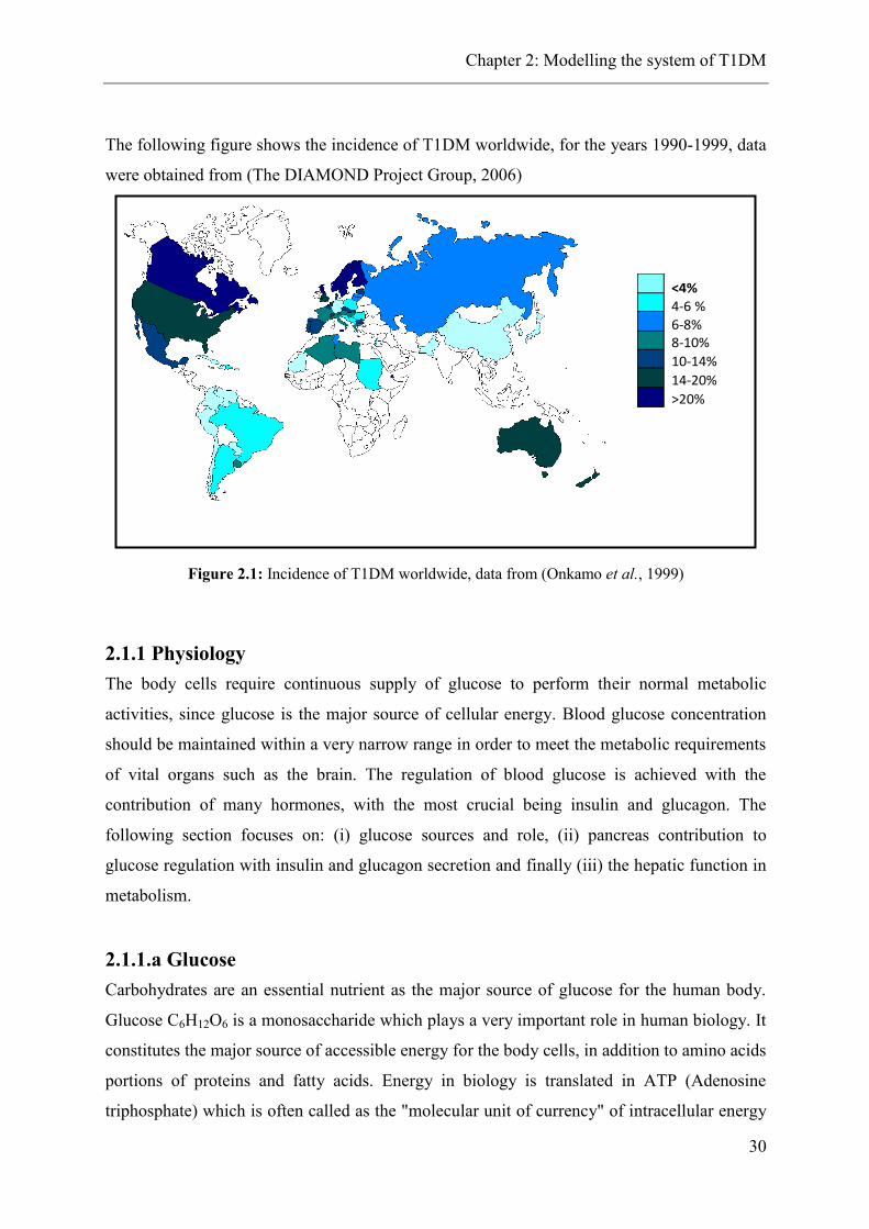
The following figure shows the incidence of T1DM worldwide, for the years 1990-1999, data
were obtained from (The DIAMOND Project Group, 2006)
Figure 2.1: Incidence of T1DM worldwide, data from (Onkamo et al., 1999)
2.1.1 Physiology
The body cells require continuous supply of glucose to perform their normal metabolic
activities, since glucose is the major source of cellular energy. Blood glucose concentration
should be maintained within a very narrow range in order to meet the metabolic requirements
of vital organs such as the brain. The regulation of blood glucose is achieved with the
contribution of many hormones, with the most crucial being insulin and glucagon. The
following section focuses on: (i) glucose sources and role, (ii) pancreas contribution to
glucose regulation with insulin and glucagon secretion and finally (iii) the hepatic function in
metabolism.
2.1.1.a Glucose
Carbohydrates are an essential nutrient as the major source of glucose for the human body.
Glucose C6H12O6 is a monosaccharide which plays a very important role in human biology. It
constitutes the major source of accessible energy for the body cells, in addition to amino acids
portions of proteins and fatty acids. Energy in biology is translated in ATP (Adenosine
triphosphate) which is often called as the "molecular unit of currency" of intracellular energy
<4%
4-6 %
6-8%8-10%
10-14%
14-20%
>20%

Chapter 2: Modelling the system of T1DM
31
transfer. The overall reaction that takes place is the oxidation of fuel substrates to carbon
dioxide and water in the presence of oxygen:
Glucose + Oxygen →Energy + Carbon dioxide + Water
Table 2.1: The mechanisms of energy production through glucose
Metabolic Mechanism Location Description
1.Glycolysis
Glucose is converted to
pyruvate through a series of
10 enzymatic reactions. 7 of
these reactions are reversible
(gluconeogenic direction). In
organs where gluconeogenesis
can take place (liver, kidney)
there are enzymes which
activate the reverse direction
of the irreversible glycolytic
reaction.
Cytoplasm
2.Pyruvate decarboxylation
Pyruvate enters the
mitochondria and through an
enzymatic reaction activated
by pyruvate dehydrogenase
complex it is converted to
acetyl-CoA.
Mitochondrion Matrix
3.Krebs Cycle
During the chain of the
enzymatic reactions that
constitute the tricarboxylic
acid cycle (TCA) the
metabolic fuel is oxidised.
Generally fatty acids and
amino acids can also be
oxidised through the TCA
cycle.(DeFronzo, 2004) The
TCA cycle activates electrons
transportation (following
mechanism)
Mitochondrion Matrix
Pyruvate
Acetyl
CoA
acetyl-
CoA
Citric
Acid
NA
D+
5 C
NAD
H
4 C
H+
4 C
CoA
Oxaloac
etic acid
CO2
NA
D+
NAD
H
H+
NA
D+
NAD
H H+
NA
D+
NAD
H H+
ADP + Phosphate
AT
P
CO2
FADH2 FAD
Phosphorylated
2 sugar
phosphate
Glucose
2 Pyruvate
NA
D+
NAD
H
2
2
H+
4 AT
P
-2 AT
P
CoA

Chapter 2: Modelling the system of T1DM
32
4. Oxidative
phosphoryliation
Process during which ATP is
produced, by using the energy
released in the electron
transport chain (Smeitink,
2004)
Inner Mitochondrion
Membrane
Table 2.1 presents a brief description of aerobic respiration. In cases of insufficient oxygen,
for example during intense exercise, muscle cells can perform anaerobic respiration, which
incorporates all the metabolic paths described previously, but instead of O2 as an electron
receptor, other electronegative substances are used.
2.1.1.b Pancreas: insulin, glucagon
One of the most important organs that are responsible for glucose regulation is the pancreas.
A small region (2% approximately) of the pancreas mass, called the Islets of Langerhans, is
responsible for the production of the endocrine hormones. It contains 3 types of cells, a-cell
where glucagon is synthesised, b-cell for insulin and amylin synthesis and d-cells for
somatostatin synthesis and the PP cells which secrete pancreatic polypeptide. The remaining
98% of the pancreas mass is responsible for exocrine secretions.
Figure 2.2: Islets of Langerhans adapted from (Parlerm, 2003)
ADP
H2O O2
ATP
e-
Electron transport chain
oxidative phosphoryliation

Chapter 2: Modelling the system of T1DM
33
The insulin molecule
Synthesised in b-cells of the pancreas, insulin is a dipeptide consisting of A and B amino
chains. Initially a precursor molecule, preproinsulin, is synthesised (Ferrannini and DeFronzo,
2004) which is translated to proinsulin. In this form the A and B chains are linked to a
polypeptide, known as a connecting peptide or C-peptide. C peptide is released and insulin is
produced. Because both insulin and C-peptide are secreted from b-cells, C-peptide can be
used as an indicator of the levels of endogenous insulin production when exogenous insulin is
administrated.
Insulin action
Insulin is an anabolic hormone which plays a vital role in human metabolism. The main
anabolic actions which insulin performs are:
1. enabling glucose uptake by muscle cells and adipose tissue
Insulin acts as a key that opens up the cell so as to accept glucose. Insulin binds to insulin
receptors located on the cellular membrane and a complex series of protein reactions is
activated, leading to the translocation of GLUT-4, a glucose receptor, from the intracellular
area to the cell membrane and finally the influx of glucose into the cell, where glucose is
metabolised and supplies the cell with energy (Nussey and Whitehead, 2002).
2. glycogenesis (glycogen synthesis)
Insulin has several effects which stimulate glycogen synthesis in the liver and in the muscles,
such as activation of glucose phosphorylase (required enzyme for the synthesis) and
inhibition of the reverse action. Glucose uptake from the liver is not dependent on insulin
because the responsible glucose receptor of the hepatocytes is GLUT2, which is not activated
by insulin, contrary to glucose uptake from the muscles (Nussey and Whitehead, 2002).
3. glycolysis
Insulin regulates glycolysis, because it provides the metabolic path with available substrate
(glucose) and it affects the rate of transcription of the enzymes which catalyse some steps of
glycolysis (Meisler and Howard, 1989), (Iynedjian, Gjinovci and Renold, 1988).

Chapter 2: Modelling the system of T1DM
34
4. lipogenesis (adipocytes)
Insulin stimulates the convertion of acetyl CoA to fatty acids and then to triglycerides, by the
activation of glycolytic enzymes (Kersten, 2001). Lipogenesis is also amplified because
insulin enhances glucose uptake from adipocytes.
5. protein synthesis
Insulin determines protein synthesis by increasing the content of ribosomes with amino acids
and by restricting protein breakdown.
6. amino acids transport into cells
The transport rate of amino acids into the cells is increased due to insulin.
Apart from anabolic effects insulin contributes to preventing catabolic actions. In particular,
in the liver insulin inhibits glyconeogenesis, glycogenolysis and ketogenesis; in the muscles
the breakdown of proteins and in the adipose tissue the breakdown of lipids.
Generally, the body detects that blood glucose levels rise and normally the pancreas secrete
insulin to account for that alteration in glucose concentration, as a response to several
stimulators. Initially an increase in blood glucose concentration provokes an immediate
release of insulin that has already been synthesised and stored in the b-cells. This response is
the distinct first phase of the biphasic insulin secretion. Then the newly synthesised insulin is
released for as long as the glucose levels are elevated. There are other factors that function as
b-cells stimulators, such as certain amino acids, fatty acids, several gastrointestinal hormones
and activity of the parasympathetic nervous system. While insulin is being released, glucose
can enter the body cells, can be stored as glycogen in the liver until the concentration is
between the normal range and insulin release can be stopped.
Glucagon
Another important hormone controlling glucose metabolism is glucagon known as counter-
regulatory hormone, because it acts in opposition to insulin, being the major hormone
regulating the fuel mobilisation and catabolism. Glucagon’s action is located specifically in
the liver and is responsible for stimulating the breakdown of glycogen to glucose and for the
production of glucose from lactate, glycerol and mainly amino acids. These pathways are the

Chapter 2: Modelling the system of T1DM
35
mechanisms of hepatic glucose production (Griffin and Ojeda, 2004). These mechanisms are
better understood than that of insulin (Storey, 2005). Furthermore glucagon is responsible for
regulating the rate of oxidation of free fatty acids that enter the liver, and the consequent
production of ketones which enter the bloodstream.
Glucagon release is regulated by both insulin and glucose. In case of low blood glucose
levels, hypoglycaemia, due to fasting or exercise, the a-cells of the pancreas produce and
release glucagon that activates the conversion of glycogen to glucose. Normally, the release
of glucagon occurs when blood glucose concentration is 50mg/dl. When blood glucose levels
rise above 150 mg/dl glucose production is minimised, with a mechanism which is not fully
understood (Storey, 2005).
Other counter regulatory hormones which have catabolic action, similar to glucagon can be
seen in Figure 2.3.
Figure 2.3: Impact of insulin and other counter regulatory hormones on glucose levels
2.1.1.c The Liver
The liver is the main regulator of glucose metabolism. It can store glucose as glycogen when
glucose levels are high and release glucose when it is required. Hepatic glucose production is
the second source of glucose in the blood apart from exogenous glucose influx, derived from
carbohydrates breakdown. In healthy people, hepatic glucose production is high during the
fasting state. This rate decreases in response to the rise of blood glucose and the consequent
insulin secretion from beta cells. Net hepatic glucose production is defined as the difference
between the pathways which stimulate glucose formation (gluconeogenesis, glycogenolysis)
and those that contribute to glucose consumption or storage (glycogen synthesis, glycolysis,
pentose monophosphate shunt). As it has already been mentioned, the hormones controlling
these actions are insulin and glucagon, insulin contributes to glucose disposal and glucagon to
glucose production.
In Figure 2.4 the overall flow of fuels and the actions of insulin and glucagon in the liver,
muscles and adipose tissue are illustrated:
GLUCOSE
Glucagon Cortisol Growth hormone Epinephrine Thyroid hormones
Insulin

Chapter 2: Modelling the system of T1DM
36
Figure 2.4: The overall flow of fuels and the actions of insulin in the liver, muscles and adipose
tissue, adapted from (Pocock, Richards and Richard, 2006)
2.1.2 Pathophysiology and T1DM
T1DM is a catabolic disorder characterised by insufficient or absent insulin circulation,
elevated levels of glucagon in the plasma and b-cells inability to respond to metabolic
stimulus. It results from autoimmune destruction of b-cells originates from genetic or
environmental factors.
It is suggested (Knip et al., 2005) that there is a genetic susceptibility to the disease
development, and the exposure to environmental agents triggers the onset of diabetes type 1.
A preclinical period up to 13 years has also been identified. This is characterised by
hyperglycaemia for a few years progressing to clinical diabetes when the complications begin
to appear (Steck and Rewers, 2004), (Khardori, 2014).
2.1.2.a Complications of T1DM
T1DM can cause serious complications in the major organs of the body. Problems in the
heart, kidney, eyes and nerves can potentially develop gradually over years. The risk of the
complications can be decreased only by optimal glycaemic control. In detail, the long-terms
complications encompass:

Chapter 2: Modelling the system of T1DM
37
Macro vascular complications (disease of any large (macro) blood vessels)
An environment of high glucose conditions stimulates the adhesion of monocytes to arterial
endothelial cells. The monocytes, in turn, take up lipids and their accumulation in the artery
walls lead to increased levels of atherosclerosis (Chait and Bornfeldt, 2009).
Depending on the location of the affected artery, the following diseases can occur:
- Coronary artery disease (coronary arteries-ischemic heart disease)
- Cerebral vascular disease (carotid artery-stroke, Transient ischemic attack)
- Intermittent claudication (iliofemoral and smaller arteries of the lower legs-gangrene)
Micro vascular complications
Caused by wall thickening of small arterioles and capillaries and include:
- Diabetic retinopathy (can lead to glaucoma, cataracts or even blindness)
- Diabetic nephropathy (can lead to chronic renal failure)
- Diabetic neuropathy (leads to ulceration-diabetic foot)
Other complications may include skin infections, hearing complications, increased risk
fordeveloping osteoporosis and complications during pregnancy.
2.1.2.b Symptoms of T1DM
Diabetes type 1 onset can be very sudden and usually the symptoms and signs are very
obvious and can develop over a few weeks. The most common symptoms are polyuria,
polydipsia, polyphagia with weight loss, tiredness, muscle cramps and blurred vision.
Main Symptoms
Polyuria: due to osmotic diuresis (increase in the osmotic pressure within the kidney tubules,
caused by the presence of glucose, that leads to a reduced reabsorption of water and to an
increased urine output) leading to nocturnal enuresis especially in young children.
Polydipsia: usually as a result of osmotic diuresis (with the amount of water leaving the body
being greater than the amount being taken in) leading to dehydration.
Polyphagia with weight loss: weight loss in the presence of normal or increased appetite is
due to stored fat breakdown as an alternative supply of energy to the body cells.

Chapter 2: Modelling the system of T1DM
38
Tiredness: caused by muscle wasting, hypovolemia (decrease in volume of blood plasma due
to dehydration), hypokalaemia (urinary loss).
Other Symptoms
Muscle cramps: due to muscle fatigue and electrolyte imbalance (hypokalaemia)
Blurred vision: caused by the lens of the eyes becoming very dry
Itchiness around the vagina or penis: caused by glucose excess in the urine
Gastrointestinal symptoms: Nausea, abdominal discomfort or pain, constipation, usually
accompany other causes such as neuropathy, pancreatitis, DKA
Younger children ( <7years old) present more severe symptoms because they lose
approximately the 80% of the islets compared to 60% in children 7-14 years old and 40% in
children older than 14 years old.
2.1.2.c Diagnostic Tests for T1DM
Diagnosis of T1DM
- Blood Glucose Test
Fasting Plasma glucose: 2 samples greater than 125mg/dl (i.e. 6.99 mmol/L) according to
ADA
Random plasma glucose (for symptomatic patients): 200mg/dl
- Urinalysis for glucose, ketones and protein
- Physical examination
On-going monitoring of diabetes control
- Glycosylated haemoglobin (Hb) or Hb A1c: Glucose molecules react with
haemoglobin, forming glycated haemoglobin. Once a haemoglobin molecule is
glycated, it remains that way. The HbA1c level is proportional to average blood
glucose concentration over the previous four weeks to three months, a period which
reflects the life span of a red blood cell. (HbA1c>6.5% indicates DM)

Chapter 2: Modelling the system of T1DM
39
- Fructosamine blood test: Glucose molecules react with the amino group of proteins,
forming fructosamines which reflect glucose control in the previous 1-3 weeks
- Oral glucose tolerance test with insulin levels
- C-peptide/ insulin level test
- Islet cell antibodies
- Self-managed blood glucose testing
- Fingerpick blood drop blood glucose tests
- Urine glucose home testing
- Urine ketone home testing
2.1.2. d Treatment
Diabetes type 1 requires administration of exogenous insulin, which replaces the body’s own
insulin in order to maintain the blood glucose within a normal range. In general, for patients
with T1DM, intensive insulin treatment is recommended. Conventional (standard) insulin
therapy is suggested only in special cases. In order to achieve tight blood sugar control,
intensive insulin therapy requires frequent insulin injections or the use of an insulin pump, to
check blood glucose concentration at least 4 times a day and to follow specific eating and
exercise plans.
Occasionally, there is a period following the diagnosis of diabetes that the patient doesn’t
present any symptoms of the previously mentioned and the blood sugar levels improve to
normal or near-normal, levels. This so- called "Honeymoon period" is due to remaining islets
of Langerhans which begin to recover their ability to produce endogenous insulin. This period
may last for several weeks or months.
Insulin schedules
Insulin schedules consist of multiple subcutaneous insulin injections which are administrated
throughout the day with regard to blood glucose control (avoid hyperglycaemia or
hypoglycaemia). Usually a background or long acting insulin is taken at bedtime, and rapid
acting insulin is taken before meals. The schedule is individualised depending on the patient’s

Chapter 2: Modelling the system of T1DM
40
characteristics and needs (meal plan, activities). It should also be flexible to adjust to
changing daily routines (holidays, fasting).
CSII
Continuous subcutaneous insulin infusion (CSII) therapy or insulin pump is a small, battery-
operated pump that is worn on the body and infuses continuously rapid-acting insulin
(Medronic, 2008) through a cannula inserted under the skin. The pump can provide the
patient with a continuous basal rate of insulin and manually the patient can administrate bolus
doses before each meal, according to the current blood glucose level and the content of
carbohydrates in the meal.
It can be stated that successful treatment of diabetes type 1 requires the contribution of a
physician, nurse, dietician and the patient’s and family’s appropriate education and
motivation. Particularly important is the patient’s diet that should be configured according to
the patient’s nutrition habits, but should consist of a specific caloric plan and specific daily
intake of carbohydrates, proteins and fat subjected to timing, size and composition
management of each meal. Furthermore daily activity is highly recommended to patients and
adjustment of insulin therapy and nutrition should be taken into account.
2.1.2.e Types of insulin
There are three kinds of insulin, according to its origin: a. animal insulin, b. recombinant
insulin or "Human" insulin and c. insulin analogues (Mohan, 2002). Animal insulin is
extracted from the pancreas of healthy animals (such as beef, pork and salmon) and then is
highly purified. Although this product is very cheap (Mohan, 2002) it is used less frequently
in the developed countries due to fear of immunogenic reactions caused by contaminated
preparations and due to the rapid increase of the demand during the 70s, that could not be
covered by the existing supplies. Consequently biosynthetic methods of synthesizing insulin
were developed to ensure that there would always be available supplies. The production of
"Human" insulin is based on either recombinant DNA technology by using E. coli and yeast
cells, or on alteration of the structure of animal insulin. Ultimately, insulin analogues are
genetically produced starting from "Human" insulin with further alteration in the amino
chains that finally are different from any occurring in nature. These modifications can
produce two types of insulin, the rapid acting insulin which is monomeric and hence it is
easily absorbed and biologically active; and the long acting insulin, preparations which

Chapter 2: Modelling the system of T1DM
41
contain a high proportion of hexamers and its slow diffusion is appropriate to cover the daily
basal rate.
Insulin, regardless of the preparation method, can be classified according to the following
three characteristics: the onset (length of time before insulin reaches the bloodstream and
begins lowering blood glucose), the peak time (time during which insulin is at maximum
strength in terms of lowering blood glucose), and duration (how long insulin continues to
lower blood glucose). In Table 2.2 the characteristics of the typical types of insulin can be
observed.
Table 2.2: Characteristics of Insulin(American Diabetes Association)
Rapid acting Regular Intermediate-acting Long-acting
Onset 5min 30min 2-4hr 6-10hr
Peak time 1hr 2-3hr 4-12hr Peakless profile
Duration 2-4hr 3-6hr 3-6hr 20-24hr
The following table shows in detail the commercially available types of insulin and their
mixtures.

Chapter 2: Modelling the system of T1DM
42
Table 2.3: Commercially available types of insulin and their mixtures
Generic name
(U-100 except where noted)
Brand name Form Manufacturer Cloudy or
Clear
Rapid acting
Insulin glulisine Adidra* analog Sanofi-Aventis Clear
Insulin lispro Humalog* analog Eli Lilly Clear
Insulin aspart Novolog* analog Novo Nordisk Clear
Regular
Regular Humulin R ** human Eli Lilly Clear
Regular Novolin R*,
ReliOn (Wal-
Mart)
human Novo Nordisk Clear
Intermediate-acting
NPH Humulin N* human Eli Lilly Cloudy
NPH Novolin N*,
ReliOn(Wal-Mart)
human Novo Nordisk Cloudy
Long-acting
Insulin detemir Levemir* analog Novo Nordisk Clear
Insulin glargine Lantus* analog Sonofi-Aventis Clear
Mixtures
70%NPH/30%regular Humulin 70/30* human Eli Lilly Cloudy
70%NPH/30%regular Novolin 70/30*#,
ReliOn(Wal-Mart)
analog Novo Nordisk Cloudy
50%lispro
protamine/50%insulin lispro
Humalog Mix
50/50*
analog Eli Lilly Cloudy
75%lispro
protamine(NPL)/25%lispro
Humalog Mix
75/25*
analog Eli Lilly Cloudy
70%aspart
protamine/30%aspart
NovoLog Mix
70/30*#
analog Novo Nordisk Cloudy
Less commonly used insulin
Regular Humalin R U-
500**$
human Eli Lilly Clear
50%NPH/50%regular human Eli Lilly Cloudy
* Available in prefilled, disposable pens or cartridges for reusable pens
** Note difference between Humulin R and Humulin R U-500
#Note difference between Novolin 70/30 (70% NPH/30% regular) and NovoLog Mix 70/30 (70% aspart protamine/30%
aspart)
$U-500 and U-100 are different concentrations of insulin. U-500 is typically used in very insulin-resistant people

Chapter 2: Modelling the system of T1DM
43
2.2 Literature Review
2.2.1 Modelling the drug delivery system
From the moment a therapeutic agent is administered in the human body until the desired
therapeutic effect becomes apparent, there are numerous mechanisms and factors involved
that play a substantial role to the drug’s therapeutic efficacy. In an effort to maximise the
drug’s efficacy and increase the patient’s safety, modelling the entire drug delivery process
has become a very useful tool for understanding, simulating, optimising and predicting
patient’s response to the drug. This is achieved through pharmacokinetic and
pharmacodynamic studies. The pharmacokinetics describe mechanisms such as drug
metabolism, transport, absorption, distribution, diffusion and elimination, (the effect of the
body on the drug). The pharmacodynamics, on the other hand, describe the effect of the drug
on the body and is usually expressed mathematically by dose-response relations. A brief
description of the established ways to model the pharmacokinetics and pharmacodynamics is
presented below.
2.2.1.a Pharmacokinetic Modelling
Compartmental Models
One of the most common modelling approaches to describe the pharmacokinetic process is
the compartmental modelling. This approach assumes that the drug molecules act inside the
considered compartments, and explicit mathematical expressions of the drug concentration in
each compartment are determined (Hladky, 1990). The simplest case is to represent the
human body as a single compartment in which the drug is administered and eliminated, as
shown on the left hand side of Figure 2.5. The basic assumption in compartmental modelling
is that the concentration of the drug inside the compartment is constant, in other words, there
is instant homogeneous distribution of materials within a compartment. A single compartment
can be considered only when there is a very rapid distribution of the drug from the central
compartment (the plasma) to the peripheral compartment (the equilibrating tissues). Usually,
this approach describes intravenously injected well-diffused drugs whose elimination follows
first-order kinetics. If that is not the case, usually because of slow diffusion of the drug to the
peripheral tissues, additional compartments should be considered (right hand side of Figure
2.5). There are several drawbacks of the compartmental analysis, such as the correlation of
the model parameters (e.g. transfer coefficients) to physiological parameters, as well as

Chapter 2: Modelling the system of T1DM
44
difficulties related to the determination of the appropriate number of compartments that
should be used to represent the pharmacokinetics of the entire population.
Figure 2.5: Single Compartment (left hand side), two compartmental approach (right hand side)
Physiological Models
To overcome the difficulty of relating the model parameters (compartment’s volume, transfer
rate between compartments) to physiological features in compartmental modelling,
physiological models have been developed. The physiological models take advantage of a
priori knowledge of the mechanisms involved in the drug action and the mathematical
representation reflects the administration, diffusion and elimination of a drug in every organ
of the body. This approach requires deeper understanding of the physiology but provides
detailed and explicit representation of the drug delivery system. The advantages of
physiologically based models over compartmental/empirical models include the ability to be
extrapolated between different species and different drug dosages (Saltzman, 2001),
(Cashman et al., 1996). The main drawback of physiologically based models is that
sometimes certain parameters cannot be measured and their values are difficult to be
accurately predicted.
Figure 2.6 illustrates a schematic of a physiological pharmacokinetic model. The grey arrows
represent the routes of a drug administration: inhaled, intravenous, oral, intramuscular. The
black arrows show the elimination from several compartments depending on the route of
administration.

Chapter 2: Modelling the system of T1DM
45
Figure 2.6: physiological modelling, adapted from
(http://aiche.confex.com/aiche/2008/webprogram/Paper138436.html)
Simplifications in the previous schemes can be made depending on the exact system which is
studied. In Figure 2.6, organs which do not contain important amounts of the drug agent can
be neglected (Saltzman, 2001). Every organ can be described with more than one
compartment when a more detailed representation is required. Accordingly, the scheme of
Figure 2.7 can be changed in cases where wall permeability of either the capillary or cell
membrane or both is high, and the corresponding transport through the membranes is rapid.
In such cases, the respective compartments can be lumped in two or just one (Sorensen,
1978).
Figure 2.7: Organ compartmental analysis
Vascular (Blood)
Interstitial
Intracellular

Chapter 2: Modelling the system of T1DM
46
2.2.1.b Pharmacodynamic Modelling
Modelling the pharmacodynamics of a system (i.e. the effect of a drug on the human body) is
essentially connected to pharmacokinetic modelling because the profile of drug concentration
(pharmacokinetic model) is required to estimate the parameters that describe the consequent
effect. Usually, precise measurements of the drug effect cannot be easily obtained, so in
practice the pharmacodynamic model is determined by testing potential models and
estimating the parameters when a reference pharmacokinetic model is used.
Pharmacodynamic models assume that the concentration of the drug is in equilibrium with the
effect site, which could only hold at steady state, and therefore the pharmacodynamic
expression cannot be complete without the combined usage of a pharmacokinetic model.
Table 2.4 briefly presents types of empirical pharmacodynamic models proposed in the
literature:
Table 2.4: The most common types of empirical pharmacodynamics models (adapted from (Holford
and Sheiner, 1982)
Model Model Equations Description
Fixed Effect
Model Effect: Present (1) or Absent (0), or degree of effect
Linear Model oECSE E=drug effect, C=drug concentration, S=slope
parameter, Eo= initial drug effect
Log-linear
Model ICSE log
E=drug effect, C=drug concentration, S=slope
parameter, I=constant
EmaxModel CEC
CEEE o
50
max
E= drug effect, C=drug concentration, Emax=
maximum drug effect, Eo= initial drug effect
from previous application, EC50=concentration
producing half of the maximum drug effect
Sigmoid
Emaxmodel nn
n
CEC
CEE
50
max
E= drug effect, C=drug concentration, Emax=
maximum drug effect, Eo= initial drug effect
from previous application, EC50=concentration
producing half of the maximum drug effect,n=
constant affecting the shape of the drug effect-
concentration curve
2.2.1.c Applications
A model of a biomedical process is an analogue of the studied system. The reason why a
process is modelled determines the complexity of a proposed model. Two of the most
common applications of modelling of biomedical systems are the development of virtual
patients or patient simulators and the development of reliable predictive tools for control
studies. A patient simulator is used for educational purposes such as AIDA developed by
(Lehmann & Deutsch, 1992) or it can substitute clinical trials to determine optimal drug doses
that produce effective and safe responses, such as the UVa/Padova Simulator (B. P.

Chapter 2: Modelling the system of T1DM
47
Kovatchev, M. D. Breton, et al., 2009) These models have a strong relevance to physiology.
The models derived for control purposes are usually simpler and can also be empirical. The
aim of these software tools is to provide the doctor with a decision advice, acting as a
therapeutic advisory system in a model based control context.
2.2.2 Modelling the glucose-insulin system in T1DM
In the last 35 years a large number of models describing the glucose-insulin interaction
system have been developed. Usually, the system is divided in insulin pharmacokinetics and
glucose metabolism, which describes mathematically the mechanisms of glucose absorption,
distribution and production in the relevant organs. Glucose appears in the blood either as a
result of carbohydrates consumption or by being released by the liver. Insulin is administered
externally in the subcutaneous tissue. Insulin contributes to glucose metabolism in the liver,
where it suppresses the endogenous glucose production and in the adipose tissue and muscle
cells where insulin-dependent glucose uptake is taking place. Consequently, the main
components that contribute to the entire description of the process are: glucose absorption
from the blood through the gastrointestinal tract, insulin absorption from the blood through
the subcutaneous tissue, endogenous glucose production, glucose excretion and glucose
uptake. The models encountered in the literature describe these processes with several
approaches. A selection of models can be seen in Table 2.5. Detailed description of the
available models of glucose-insulin interactions is presented below:
Models based on Minimal Model
Modelling the glucose-insulin system for normal and diabetic subjects started in 1970s, when
Dr. R. Bergman and co-workers introduced the Minimal model (Bergman, Phillips and
Cobelli, 1981), which essentially is a method to estimate pancreatic effectiveness and insulin
sensitivity. The model describes the dynamics during an intravenous glucose tolerance test
(IVGTT) or an oral glucose tolerance test (OGTT). It consists of two subsystems describing
insulin and glucose kinetics at a level of minimal complexity. Glucose subsystem
encompasses a plasma compartment and a remote compartment in which insulin is inserted to
transfer glucose into the periphery and liver and to inhibit hepatic glucose production; the
insulin minimal subsystem involves only a single plasma compartment. Although this model
contributed fundamentally to later research work, it has several drawbacks regarding the
modelling approach. For example, Caumo (1993) has indicated that the minimal model
presents an abnormal behaviour of endogenous glucose production and limited validity in the

Chapter 2: Modelling the system of T1DM
48
unsteady state. Furthermore Cobelli et al., (2009) state that the assumption of insulin
secretion in proportion to glucose concentration cannot be experimentally verified. Generally,
the model simplifies the complexity of the metabolic system and its validity is restricted to
the description of insulin-glucose dynamics during an IVGTT or OGTT (Van Herpe et al.,
2007).
In Fisher (1991) two more terms were introduced in the minimal model. One represents the
effect of glucose intake from meal consumption; and the other represents exogenous insulin
infusion. The limitations of this approach are derived from the limitations of the minimal
model approach, such as fixed values of the model parameters. Furthermore this approach has
not been validated clinically, but the results are consistent with the literature.
Fabietti et al. (2006) modified the minimal model to focus on patients with T1DM. The
glucose kinetics model consists of two compartments, insulin kinetics is described by two
compartments, one representing the exogenous, subcutaneous administration of insulin and
the other a remote one. External inputs such as meals and glucose boluses are assumed
together with liver glucose uptake. A drawback as mentioned by (Wilinska and Hovorka,
2008) is that the model is not capable of representing personalised results, following real
time changes of the patient’s physiological responses. However, it is able to represent within
patient variability, by considering circadian insulin sensitivity variation.
Several models have been introduced which retained the core of the minimal model but
altered specific parts to account for certain aspects, such as descriptive representation of the
glucose kinetics according to experimental data (Caumo and Cobelli, 1993). Van Herpe et al.
(2007) have evolved the MM so as to take into consideration the critical ill patients
(intravenous glucose and insulin administration).
Further compartmental approaches
Berger and Rodbard (1991) have developed a simulation and optimisation program
(GLUCOJECT) for insulin therapy in patients with T1DM. The model used in this program is
consistent of two subsystems describing insulin and glucose kinetics at a level of minimal
complexity. The insulin subsystem describes the pharmacokinetics of insulin within 3
compartments: subcutaneous insulin depot, plasma insulin compartment and a remote
compartment. Glucose kinetics is described by a single compartment of plasma glucose. This
program stores glucose values and insulin doses and can reproduce an average 24h glucose
and insulin profile. There are no published data referring to its clinical evaluation. The
pharmacokinetic model of insulin action of this model was used by (E D Lehmann and

Chapter 2: Modelling the system of T1DM
49
Deutsch, 1992) in combination with a model describing glucose pharmacodynamics, which is
based on experimental data from the literature and presented by (Guyton et al., 1978) to
describe glucose-insulin interaction of T1DM. This model was used by AIDA, an online
educational tool. The authors of AIDA model suggested a generic subcutaneous absorption of
insulin (Lehmann et al., 2007). This model is suggested initially from Tarín et al. (2005) and
it is incorporated alongside the existing model of insulin kinetics and disposal from Berger
and Rodbard. In this way, novel insulin analogues can be simulated and the current insulin
dose can exceed the limit of 40 IU per injection, which was assumed in the previous model.
This tool, as mentioned by the authors, should be used only for patients’ education and not as
a treatment tool. Currently, further developments are considered to account for the existing
limitations.
Two of the most commonly used physiologically-based compartmental models are those
developed by the groups of Hovorka and Cobelli.
The model of the glucoregulatory system developed by Hovorka et al. (2002) and Hovorka et
al. (2004) considers the glucose subsystem using 2 compartments representing the accessible
and non-accessible pool; the insulin subsystem with a chain of three compartments to
describe the rapid acting insulin infusion and distribution (Willinska et al., 2010) and finally a
subsystem of insulin action on glucose transport, disposal, and production. Additionally the
glucose absorption from the gut as well as the interstitial glucose kinetics have been
modelled. This model so far has been validated in the sense that it can reproduce the results
obtained from a clinical study of a closed loop insulin delivery in patients with T1DM. The
model and its parameters represent a virtual patient. The simulation environment is currently
fully validated in order to be used for the development of closed loop insulin delivery
systems.
Another simulation environment has been developed from the Universities of Padova and
Virginia (Dalla Man et al., 2007), (B. P. Kovatchev, M. Breton, et al., 2009). This model
describes accurately the glucose and insulin dynamics during a meal. It consists of a glucose
and an insulin subsystem. Glucose subsystem encompasses two compartments while the
insulin dynamics are also represented by two compartments. The modelling of glucose rate of
appearance coming from the food consumption as well as the endogenous glucose production
and glucose utilisation are addressed. One issue that should be taken into account is the
diurnal variability of the parameters. This simulator has been accepted by FDA for preclinical
closed-loop control experiments by substituting animal trials as well as for clinical trials of
closed-loop control based entirely on silico tests.

Chapter 2: Modelling the system of T1DM
50
Models in the form of delay differential equations
There are two kinds of time delays in the physiology of glucose-insulin system. The first
delay is related to insulin production triggered by increased glucose levels as well as the time
required for insulin to become accessible for utilisation. The other one is the delay between
the appearance of insulin in the plasma and its inhibitory effect on the hepatic glucose
production. Regarding the pathophysiology of T1DM, there is another delay concerning the
exogenous insulin infusion; it represents the required time of subcutaneous infused insulin to
be absorbed. These delays can be represented implicitly or explicitly. In other words, they can
be expressed by either separating insulin/glucose in two compartments, by using auxiliary
variables, or by introducing time delay terms in the functions describing insulin production
and endogenous glucose production.
Models assuming physiological delays in the system of insulin – glucose have been
developed. In these models circadian insulin secretion oscillations are analysed in the form of
differential equations. The initial model suggesting that behaviour has been developed by
(Sturis et al., 1991). The delays are modelled by assuming insulin action in two separate
compartments and by assuming auxiliary variables representing insulin effects on endogenous
glucose production. The model equations were modified by (Tolić, Mosekilde and Sturis,
2000) and insulin secretion was represented as a sigmoid function of glucose concentration.
In order to examine whether oscillatory insulin supply is more efficient, as it mimics the
pulsatile secretion of hormones in the endocrine system, Tolić et al. (2000) have suggested
that insulin infusion should be sinusoidal. Actually, it was proved that only when hepatic
glucose release is near the upper limit oscillatory, will insulin supply be more efficient;
otherwise oscillatory and constant insulin infusion produce similar effects.
Bennett and Gourley (2004) instead of the three auxiliary linear equations, proposed in the
previous model, introduced a time delay of insulin effect on hepatic glucose production,
explicitly in the model. The two-compartment approach for insulin production/utilization
delay was maintained. Engelborghs et al. (2001) assumed only the delay related to insulin
effect on hepatic glucose production, which was represented explicitly in the model. Because
this model is not physiologically complete, it is not further considered. Li et al. (2006)
suggested a two time delay model that introduces two explicit time delays in the system.
Finally, Chen et al. (2010) have developed a model for diabetic patients in which the time
delays for hepatic glucose production and insulin release from beta cells are maintained, but

Chapter 2: Modelling the system of T1DM
51
exogenous inputs of meal and insulin are described, as well as the effects of hyperglycaemia.
Further modifications have been proposed by (Chen and Tsai, 2010).
Physiological Models
One of the most important models developed is the physiological model of Sorensen (1978).
It contributed in the understanding of the physiology of the glucoregulatory system and it has
been a reference point for subsequent research studies on modelling of the system. It is based
on the work of Guyton et al. (1978) and was modified by Parker et al. (1999). Although it
describes the complexity of the metabolism it cannot represent the intra-patient variability.
Empirical Models-Hybrid Models
Several research groups have worked on data driven models, in an attempt to overcome the
assumptions and simplifications that physiological and physiologically based compartmental
models are by default subject to. An approach of using Volterra Models to describe the
glucoregulatory system has been proposed by Mitsis et al. (2009). For the particular study the
data are obtained from simulation results of the Minimal Model. Eren-Oruklu et al. (2009)
have used an ARMA (autoregressive moving-average) model to describe the glucose-insulin
dynamics in order to capture the between patients variability. Additionally Ghosh and Maka
(2009) has described the system by a NARX model by using data obtained from IVGTT.
Finally Mougiakakou et al. (2005) have proposed the combination of compartmental models
and artificial Neural Networks as an individualised representation of the glucose metabolism.

Chapter 2: Modelling the system of T1DM
52
Table 2.5: Mathematical models of glucose-insulin system
Mathematical Models
Compartmental Models
Number of compartments
Glucose
Kinetics
Insulin
Kinetics Validation Comments Reference
1 2 IVGTT data Minimal complexity
Healthy subjects
(Bergman, Phillips and
Cobelli, 1981)
1 2 Literature data Minimal model for
T1DM (Fisher, 1991)
2 2 IVGTT data Healthy subjects (Caumo and Cobelli, 1993)
1 3 Literature data No published data for
clinical evaluation (Berger and Rodbard, 1991)
1 2 Literature data AIDA: educational
tool
(E D Lehmann and Deutsch,
1992)
1 1 Literature data experimental data on
critical ill patients (Hann et al., 2005)
2 2 Literature data
average patient
Circadian SI
variation
(Fabietti et al., 2006)
2 3 Literature data critical ill patients (Van Herpe et al., 2007)
2
3
3 effect of
insulin action
Clinical study of closed
loop insulin delivery in
young people with T1DM
Validated simulation
environment (Willinska et al., 2010)
2 2 Experiments FDA approval
(Dalla Man, Rizza and
Cobelli, 2007), (Dalla Man et
al., 2007)
Physiological Models
6 6 Literature data average 70kg man (Sorensen, 1978)
6 6 Literature data
average 70kg man
Includes a meal
submodel
(Parker, Doyle and Peppas,
1999)
Models in the form of delayed differential equation
1
2
3 delayed
insulin effect
Literature data Healthy subjects
Implicit delays
(Tolić, Mosekilde and Sturis,
2000)
1 2 Literature data Healthy subjects
explicit delays (Bennett and Gourley, 2004)
1 2 Literature data Healthy subject
explicit delay (Engelborghs et al., 2001)
1 2 Literature data Healthy subjects
Explicit/implicit (Li, Kuang and Mason, 2006)
1
2 Literature data T1DM
explicit delay
(Chen, Tsai and Wong, 2010)
Empirical Models
Volterra Model Literature data (Mitsis, Markakis and Marmarelis, 2009)
ARMA model Literature data (Eren-Oruklu et al., 2009)
NARX model Literature data (Ghosh and Maka, 2009)
Compartmental-Neural
Networks Literature data (Mougiakakou, Prountzou and Nikita, 2005)

Chapter 3: Mathematical Model Formulation
53
3. Mathematical Model Development
3.1 Introduction
An essential step for the design of model predictive control is the development of a reliable
mathematical model. The model presented in this section is describing glucose metabolism
and insulin kinetics for a patient with T1DM in a detailed compartmental approach. The
system is analysed at organ-level aiming to provide thoughtful insight and understanding of
the physiology. Additionally, in an effort to reduce the intra-patient variability and describe
the individualised glucose metabolism, patient-specific variables that are functions of the
patient’s individual characteristics such as gender, age, weight, height and hematocrit are
introduced. However, the pharmacodynamic variables that are related to the effect of insulin
on glucose remain uncertain and present inter and intra- patient variability. In the next
chapter, the uncertainty in the predictability of blood glucose is investigated by using model
analysis techniques to prioritise the variables that need to be identified first to successfully
predict the patient’s current state.
3.2 Physiologically based Compartmental Model of Glucose Metabolism
The proposed model describes glucose distribution in the involved body compartments, as
presented in Figure 3.1, and the effect of insulin on glucose uptake and suppression of
endogenous glucose production. The structure of the proposed model is inspired by the
Sorensen’s model (Sorensen, 1978) that describes the glucose metabolism with actual
anatomical compartments. The body is considered to be divided in six compartments, brain,
heart, liver, gut, periphery and kidney, where glucose is distributed via blood circulation. The
periphery compartment that lumps the muscles and adipose tissue is described by two sub
compartments, the interstitial fluid and the tissue, in order to highlight the dependence of
glucose diffusion on the prevailing blood flow and capillary permeability as well as the
dependence of glucose tissue uptake on insulin concentration. At steady state, an
approximation of constant physiological conditions, the blood glucose concentration reflects
the net balance of endogenous glucose release in the circulation and glucose uptake. When
food is consumed, the contained carbohydrates break down into glucose in the gastrointestinal
tract which is absorbed through the small intestine into the bloodstream. Physiologically, an
increase in blood glucose triggers pancreatic insulin release, which activates glucose

Chapter 3: Mathematical Model Formulation
54
transporters to mediate glucose translocation into the insulin-sensitive cells (adipose tissue,
skeletal and cardiac muscles) and additionally suppresses the endogenous glucose production.
In T1DM the pancreatic insulin secretion is replaced by optimal administration of exogenous
insulin that mimics the pancreatic response. Glucose appearance in the gut after meal
consumption, endogenous glucose production in the liver and glucose excretion from the
kidney are described with additional sub models that are well-established in the literature and
are embedded into the structure of the model to entirely describe glucose metabolism.
Figure 3.1: Structure of the physiologically based compartmental model of glucose metabolism in
T1DM
For the highly perfused organs (brain, liver, gut, kidney) glucose concentration is considered
to be in equilibrium with the tissue glucose concentration. The periphery compartment lumps
the adipose tissue and muscle cells. Glucose transfer from the blood capillaries to the
interstitial fluid and glucose uptake in the periphery is described with two compartments.
Homogeneity and instant mixing is assumed for every compartment, imposing all the exiting
fluxes to be in equilibrium with the compartment. For the insulin insensitive organs glucose
uptake is assumed to be a constant ratio of the available glucose. The core of the model is
described with (3.1)-(3.6) and the definition of the involved variables is presented in detail in
the notation section at the beginning of this thesis.

Chapter 3: Mathematical Model Formulation
55
The driving force for glucose transport into the compartments is the blood-tissue
concentration difference. The concentration in every organ is given by mass balances in every
compartment.
Brain (B)
, ( )Bg B B H B B
dCV Q C C u
dt (3.1)
Kidney (K)
, ( )kg K K H K K
dCV Q C C u excretion
dt (3.2)
Liver (L)
, ( )Lg L L H G G L G L L
dCV Q C Q C Q Q C u BW EGP
dt
(3.3)
Gut (G)
g, ( )GG G H G G a
dCV Q C C u BW R
dt (3.4)
Heart (H)
,H
g H B B L L P P K K CO H H
dCV Q C Q C Q C Q C Q C u
dt
(3.5)
Periphery (P)
,
, ,
( ) ( )
( )
( )
Pg Pc P H P P Pt
Ptg P ISF P Pt P
P o Pt
dCV Q C C p C C
dt
dCV p C C u
dt
u C
(3.6.1)
(3.6.2)
(3.6.3)
where the Ci is the glucose concentration (mg/dl) in i compartment, Vg,i the accessible
glucose volume (dL) of i compartment, Qi the blood flow (dL/min) in i compartment, ui the
glucose uptake (mg/min), EGP the endogenous glucose production (mg/kg/min), Ra the rate
of glucose appearance in the blood (mg/kg/dL) through the interstitial wall and λο the rate of
glucose uptake (dL/min).

Chapter 3: Mathematical Model Formulation
56
For (3.1)-(3.6) the blood flow in every organ i is described by (3.7). The ratio of cardiac
output perfusing every organ is presented in Table 3.1.
,i CO i COQ r Q (3.7)
Table 3.1: Ratio of cardiac output at rest (Ferrannini and DeFronzo, 2004)
Similarly the glucose uptake in every organ is described with (3.8) and the ratio of glucose
uptake 𝑟𝑢,𝑖 is presented in Table 3.2.
, _i u iu r Total uptake (3.8)
Table 3.2: Ratio of glucose uptake (Ferrannini and DeFronzo, 2004)
Tissue (ru,i)
Brain 0.45
Liver 0.13
Kidneys 0.02
Gut 0.07
Periphery 0.30
Heart 0.03
In the following section the sub models of glucose metabolism functions are described in
more detail.
Endogenous Glucose Production (EGP)
Glucose is produced endogenously in the liver with a percentage of approximately 80%
through gluconeogenesis and glycogenolysis, and in the cortex of kidney with a percentage of
20% (Cano, 2002). mainly through glyconeogenesis (Gerich, 2010), (Gerich et al., 2001). In
this study it is assumed that glucose is entirely produced in the liver, due to limited data
availability. Generally, in diabetes, the insufficiency of insulin causes liver to function as
being in fasting condition, where the rate of glucose production is high. In particular, when
glucose is consumed, there is no indicator to suppress hepatic glucose production (Newgard,
2004). In T1DM, the rate of EGP depends on adequate control of the disease (Roden and
Bernroider, 2003). When referring to intensive insulin therapy, it can be assumed that EGP is
approximately the same as in normal humans (Roden and Bernroider, 2003), (Davis, Fowler
Tissue (rco,i)
Brain 0.11
Liver 0.20
Kidneys 0.13
Gut 0.15
Periphery 0.40

Chapter 3: Mathematical Model Formulation
57
and Costa, 2000). The model describing the endogenous glucose production in T1DM and
used in (3.3) is adapted from (Dalla Man, Rizza and Cobelli, 2007).
1 2 3( )p p L p dEGP k k M k I (3.9)
11( )i p
dIk I I
dt
(3.10)
1( )di d
dIk I I
dt
(3.11)
ML (mg/kg) denotes the liver glucose mass and Id (pmol/l) denotes the delayed insulin signal
described by a chain of two compartments (I1, Id). The model parameters are estimated using
available literature data (Boden, Cheung and Homko, 2003).
Rate of glucose appearance (Ra)
The model describing the rate of glucose appearing in the circulation when food is consumed
is adopted from (Dalla Man, Camilleri and Cobelli, 2006). This model describes glucose
transit from the stomach with two compartments representing the solid and liquid phase, to
the upper small intestine which is described with one compartment.
1 2sto sto stoq q q (3.12)
121 1
( )( ) ( )sto
sto
dq tk q t D t
dt (3.13)
22 1
( )( ) ( )sto
empt sto gri sto
dq tk q t k q t
dt (3.14)
2
( )( ) ( )
gut
abs gut empt sto
dq tk q t k q t
dt (3.15)
max minmin
-( ) {tanh[ ( - )]- tanh[ ( - )] 2}
2empt sto sto
k kk t k a q bD q cD (3.16)
( )( )
abs gut
a
fk q tR t
BW (3.17)
5
2 (1 )a
D b
(3.18)
5
2 D c
(3.19)
with qsto1, qsto2 (mg) the glucose mass in solid and liquid phase, qsto (mg) the overall glucose
mass in the stomach, qgut (mg) is the glucose mass in the small intestine, kempt (min-1
) is the
rate of gastric emptying, α and β are model parameters, kmax, kmin (min-1
) are the max and min

Chapter 3: Mathematical Model Formulation
58
gastric emptying, kabs (min-1
) is the rate constant of intestinal absorption, kgri is the rate
constant of grinding, f (dimensionless) is the fraction of intestinal absorption, b and d are
percentages of the dose and D (mg) is the amount of ingested meal.
Glucose Renal excretion (excretion)
In diabetes, the threshold of renal glucose reabsorption is exceeded when glucose
concentration increases above 180mg/dl and glucose gets excreted by the kidney. It is
assumed that renal glucose excretion (mg/min) increases proportionally to increasing blood
glucose concentration (Willinska et al., 2010), (Rave et al., 2006).
If 180 /KG mg dL (3.20)
If 180 /KG mg dL (3.21)
CLrenal (dl/min) is renal glucose clearance.
Glucose diffusion in the periphery
The structure presented in Figure 3.2 is considered to model glucose distribution and uptake
in the periphery compartment:
Figure 3.2. Detailed glucose uptake in the periphery
It is assumed that glucose is extracted from the arterial flux with a rate factor given in the
current literature (Crone, 1965), (Regittnig et al., 2003):
(1 exp( / ))P Pp Q PS Q (3.22)
PS is the permeability across the capillary wall, a product of permeability of exchange surface
to glucose P and exchange surface area S. This rate factor can increase in case of increased
blood flow to the periphery or increased perfusion due to increased capillary exchange area
during for example exercise. According to Gudbjornsdottir et al. (2003) PS was increased
( 180)( )
0
renal KCL GE t

Chapter 3: Mathematical Model Formulation
59
significantly during a one-step hyperinsulinemic clamp. The following equation describes the
effect of insulin on glucose permeability across the capillary wall.
2, 1,PS PS p
dPSk PS k I
dt
(3.23)
When glucose enters the interstitial fluid it is absorbed by the tissues to provide them with
energy, (3.6). The rate of uptake, λο (dL/min) is dependent on insulin concentration in the
blood and insulin effect is described with (3.24).
12 1
2
(0)=oo p o basal pbasal
d kk k I with I
dt k
(3.24)
1 2/IS k k
(3. 25)
SI represents the patient’s sensitivity to insulin.
Adaptation to the individual patient
1) Total Blood Volume
The total blood volume (TBV) (dL) is adapted to the patient’s height, weight and gender to
account for the differences between obese and underweight patients and for males and
females. The formula used for men is (Wennesland et al., 1959):
0.285 0.316 2.820MTBV h m (3.26)
and for women (Brown et al., 1962)
0.1652 0.3846 1.369FTBV h m
(3.27)
where the height (h) is in centimeters and weight (m) in kilograms
2) Cardiac Output
The cardiac output (mL/min) can be efficiently approximated as a proportional relationship to
the patient’s weight BW (kg) according to the equation (Ederle et al., 2000):
3/4224COQ BW
(3.28)
3) Compartmental Volume
Plasma proteins comprise approximately 8% of the plasma volume and the erythrocytes about
38% of the total packed red blood cells volume or Haematocrit (Ferrannini and DeFronzo,

Chapter 3: Mathematical Model Formulation
60
2004), (Hemat). This percentage of the total blood volume is inaccessible to glucose.
Consequently the accessible glucose volume in every compartment is determined as:
, V, ,1 0.08 (1 ) 0.38 ( )g i i C iV Hemat Hemat V V (3.29)
The blood volume of the every compartment i is defined as the sum of venous and capillary
volume. The glucose venous volume equals 60% of total blood volume and the capillary the
10% of total blood volume (Gerich et al., 2001), (Enderle, 2011). The compartmental venous
and capillary volumes are defined as:
, , 0.6V i f iV r TBV (3.30)
, , 0.1C i c iV r TBV (3.31)
Where ,f ir refers to the ratio of total venous volume in compartment i. The compartmental
venous blood volume is calculated by distributing the total venous blood volume at the body
organs at the basis of fractional blood flows (Sorensen, 1978) (3.32):
, /f i i ir Q Q (3.32)
and ,c ir refers to the ratio of total capillary volume respectively (Sorensen, 1978) and is
presented in Table 3.3.
Table 3.3: Ratio of capillary volume
Tissue (rc,i)
Brain 0.071
Liver 0.18
Kidneys 0.08
Gut 0.13
Periphery 0.53
4) Peripheral Interstitial Volume
The total regional volume for the adipose tissue is defined as
,P ,P ,PP Capillary Interstitial IntracellularV V V V
(3.33)
According to Man and Uribarri (Man and Uribarri, 2006) the interstitial volume represents
28% of the total body water while the intracellular volume 60%. Hence,
0.47Interstitial IntracellularV V . The adipose tissue mass is described by:
1.2 10.8 0.23 5.4 0.01ATm BMI sex age BW
(Deurenberg, et al., 1991) (3.34)

Chapter 3: Mathematical Model Formulation
61
with /i i id m V (3.35)
The interstitial volume of the adipose tissue and the muscles is considered to be 10% of the
total tissue volume according to (Eckel, 2003) and (Johnson, 2003) respectively. Muscle mass
is considered to be approximately 40% of the total body weight (3.36), according to Ackland,
Elliott and Bloomfield (2009).
0.4musclesm BW
(3.36)
The peripheral volume of the interstitial fluid is calculated via (3.37), using Table 3.4:
, , , ,g P ISF Interstitial AT Interstitial muscV V V
(3.37)
Table 3.4: Density of muscles and adipose tissue
Tissue Density (kg/L) Reference
Adipose Tissue (dAT) 0.92 (Gallagher et al., 1998)
Muscles (dmuscles) 1.04 (Gallagher et al., 1998)
3.3 Insulin Kinetics
When pump therapy is used, rapid/short acting insulin is continuously infused through the
subcutaneous tissue. The amount of insulin delivered is programmed and administered at a
basal rate which varies depending on the patient’s daily requirements, and additional bolus
doses that compensate for blood glucose level increase when meal is consumed. The
formulation of rapid acting insulin reduces the tendency of insulin monomers to dimerize and
further associate into hexamers (Leslie, Taylor and Pozzilli, 1997). Hence, the diffusion in the
blood is enhanced with onset of action within 10-20min and maximum serum concentration
reached in 45min (Home, 2012). However, the absorption of insulin from the subcutaneous
tissue is dependent on the blood flow in the tissue, which causes variable time of onset and
maximum effect. Hence, insulin kinetics describe the mechanisms involved from the moment
insulin is administered in the subcutaneous tissue until it is fully eliminated from the body.
Several models have been proposed in the literature (Tarín et al., 2005), (Kraegen and
Chisholm, 1984), (Kuang and Li, 2008), (Nucci and Cobelli, 2000), with compartmental
modelling being the most common approach. In this study, the structure to describe insulin
kinetics is investigated when an insulin pump is used. Four alternative compartmental models
are presented in this section that describe experimental data of insulin kinetics and compared
in terms of identifiability, parameter correlations and accuracy, as presented in the following
chapter. The models of insulin kinetics are linked with the glucose metabolism model (3.1-
3.37) via equations 3.10 and 3.24 which represent, respectively, insulin action on endogenous
glucose production and glucose absorption from the periphery.

Chapter 3: Mathematical Model Formulation
62
Model 1
This model considers two different channels for insulin transport for basal infusion and bolus
dose, Figure 3.3.
1_1 1sub
dSbolus k S
dt
(3.38)
2_ 2 2sub
dSbasal k S
dt
(3.39)
_1 1 _ 2 2
lim
p sub sub
e pdist
dI k S k Sk I
dt V
(3.40)
Model 2
This model describes insulin transport for the bolus dose as one compartment and the basal
infusion is considered as a direct input to the plasma compartment as a proportion of the
initial basal rate, assuming that rest of the dose is degraded in the subcutaneous tissue, Figure
3.4.
1_ 2 1sub
dSbolus k S
dt
(3.41)
1lim
p subin e p
dist
dI k Sk basal k I
dt V
(3.42)
The variable and parameter definitions for both models are shown in Table 3.5.
Table 3.5: Variable and parameter definition of Model 1 and Model 2
Symbol Definitions
S1, S2 Insulin mass(mU) in the subcutaneous compartments
ksub_1, ksub_2 intercompartmental transfer rate constants (min-1
)
kelim elimination rate constant (min-1
)
Vdist insulin distribution volume (L/kg)
kin Proportion of the initial basal rate as direct input
basal Continuous insulin infusion (U/min)
bolus Pulse insulin infusion (U/min)

Chapter 3: Mathematical Model Formulation
63
Figure 3.3. Schematic representation of model 1 Figure 3.4. Schematic representation of model 2
Model 3
This model consists of three compartments in series, namely two compartments to describe
insulin absorption through the subcutaneous tissue (S1, S2) and a single compartment for
insulin in the plasma (I). This model of insulin kinetics has been widely used in the literature
(Wilinska et al., 2005), (Willinska et al., 2010)
11sub
dSu k S
dt
(3.43)
21 2sub sub
dSk S k S
dt (3.44)
𝑑𝐼
𝑑𝑡= 𝑘𝑠𝑢𝑏𝑆2 − 𝑘𝑒𝑙𝑖𝑚𝐼 (3.45)
𝐼𝑝 =𝐼
𝑉𝑑𝑖𝑠𝑡 (3.46)
The variables and parameter definitions are presented in Table 3.6 and the schematic
representation in Figure 3.5
Table 3.6: Variable and parameter definition of Model 3
Symbol Definitions
S1, S2 Insulin mass(mU) in the subcutaneous compartments
I Insulin mass(mU) in the plasma compartment
ksub Intercompartmental transfer rate constant (min-1
)
kelim Elimination rate constant (min-1
)
Vdist Insulin distribution volume (L/kg)
u Continuous insulin infusion (U/min)

Chapter 3: Mathematical Model Formulation
64
Figure 3.5: Schematic representation of model 3
Wilinska Model (Wilinska et al., 2005)
This model assumes a slow channel of insulin absorption Q1a,, Q2 and a fast absorption
channel Q1b,.
max, 11
1 1
, 1
LD aaa a
M LD a
V QdQku k Q
dt k Q
(3.47)
max, 112 1
, 1
(1- ) - -LD bb
a b
M LD b
V QdQk u k Q
dt k Q
(3.48)
21 1 1 2a a a
dQk Q k Q
dt (3.49)
31 2 2 1 3a a b e
dQk Q k Q k Q
dt (3.50)
3
dist
QI
V (3.51)
The variables and parameter definitions are presented in Table 3.7 and the schematic
representation in Figure 3.6.
Table 3.7: Variable and parameter definition of Wilinska Model
Symbol Definitions
Q1, Q2, Q3 Insulin mass(mU) in the accessible, non-accessible
subcutaneous compartment, plasma
Vmax,LD ,kM,LD Michaelis-Menten coefficients describing saturated
degradation
ka1, ka2, ke transfer rate constants (min-1
)
Vdist insulin distribution volume (L/kg)
k proportion of insulin flux entering the slow channel
u Continuous insulin infusion (U/min)
a, b insulin mass administered as continuous infusion and bolus
respectively

Chapter 3: Mathematical Model Formulation
65
Figure 3.6: Schematic representation of Willinska model
The most suitable model to describe the insulin kinetics through the subcutaneous tissue to
the plasma is found in the following chapter.
3.4 Concluding Remarks
In this chapter a mathematical model describing glucose metabolism in T1DM is presented.
The core of the model consists of six compartments representing the most important organs
associated with glucose metabolism, as introduced in Sorensen (1978). Glucose appearance
in the gut after meal consumption, endogenous glucose production in the liver and the kidney
as well as glucose excretion from the kidney are described with additional sub models that are
well-established in the literature and are embedded into the structure of the model to entirely
describe glucose metabolism. The compartmental accessible glucose volumes, the cardiac
output and the total blood volume are expressed as functions of patient characteristics,
leading towards an individualised representation of the system’s dynamics. Unlike Sorensen’s
model, insulin administration and absorption through the subcutaneous route is considered as
simple compartmental representation, due to limited availability of experimental data to
describe the involved mechanisms of insulin diffusion, dissociation and absorption. In the
next chapter, the most appropriate model to describe the insulin kinetics is selected and the
entire model is analysed in terms of influential parameters and variables, parameters
correlations and estimation.

Chapter 4: Model Analysis & Dynamic Optimisation
66
4. Model Analysis and Dynamic Optimisation
4.1 Introduction
In this chapter, the most suitable model for insulin kinetics is selected by performing a series
of analysis tests. Experimental data obtained in the literature are used to estimate the model
parameters. Additionally, the suggested structure of the EGP sub model is evaluated in terms
of reliability, using experimental data from the literature to estimate the model parameters
and confirm the model’s accuracy. Subsequently, the previously presented entire
mathematical model of glucose metabolism is analysed in order to identify the most
influential parameters that contribute to the model’s uncertainty. This uncertainty originates
to a large extent from the high intra- and inter-patient variability that dominates the system.
Global sensitivity analysis, parameter estimation and correlation are performed to evaluate
the model’s ability to represent the glucoregulatory system’s physiology. Additionally, the
model’s adaptability to the specific patient and predictive ability are evaluated with data
available in the literature and data provided from the UVa/Padova T1DMS simulator.
4.2 Insulin Kinetics: Model Selection
4.2.1 Methods
The experimental plasma insulin concentration profiles used to investigate the accuracy of the
proposed insulin kinetic models were obtained by (Boden, Cheung and Homko, 2003). Nine
subjects with T1DM (Sex (M/F) 1/8, Age (years), 24±3, Weight (kg), 68.8± 3.1, Height (cm),
169± 4 BMI (kg/m2), 24.2 ±1.2, duration of T1DM (years), 7.5± 1.5, HbA1c (%),7.6 ± 0.7,
insulin dose (units/24 h), 33.3± 5.1) were hospitalised to perform the particular study, which
involved an euglycaemic clamp to determine the effect of insulin excess on gluconeogenesis
(GNG), glycogenolysis (GL), or both, by measuring GNG (with 2H
2O) and GL (EGP-GNG)
and during insulin deficiency that developed after approximately 5 to 8h of the subcutaneous
insulin injection. Boden et al.(2003) report the mean plasma insulin concentration profiles
averaged over all nine patients which were used to evaluate the suggested models.
4.2.2. Parameter Estimation
The values of the parameters of the four models of insulin kinetics listed in Table 4.5 are
identified via parameter estimation, performed in gPROMS. The solution method used in

Chapter 4: Model Analysis & Dynamic Optimisation
67
gPROMS to obtain the optimal parameter estimates is to minimise the maximum log
likelihood objective function (PSE, 2011a) by solving an optimisation problem.
The goodness of the fit of the proposed model to the experimental data is evaluated with a
Pearson’s chi-squared test (𝑥2) (PSE, 2011a), the accuracy of the estimates of the parameters
was evaluated with a t-test and the reliability of the estimated values with the confidence
intervals. The structural identifiability of the models is investigated by analysing the
correlation matrix of the model parameters. Finally, the most suitable model to represent the
experimental data was selected by applying the principle of parsimony and the Akaike
criterion (Akaike, 1974) is tested.
Figure 4.1 shows the plasma insulin concentration (Ip) profiles produced by the suggested
models versus the experimental data. Generally, we can conclude that all models describe
relatively well the experimental data. However, a more in-depth analysis reveals the strengths
and the weaknesses of each model.
Figure 4.1: Comparison of Model 1, 2, 3 and Wilinska model with experimental data
Figure 4.2 shows the weighted residuals of the models which present more clearly the
deviation of each model from the experimental level. The residuals for all models are small in
magnitude and thus it is difficult to conclude whether a model is better than the other.
0
50
100
150
200
250
0 50 100 150 200 250 300 350 400 450 500
Pla
sma
Insu
lin C
om
centr
atio
n (
Ip)
(pm
ol/
l)
Time (min)
Experimental Data
Model 1
Model 2
Model 3
Wilinska Model

Chapter 4: Model Analysis & Dynamic Optimisation
68
Figure 4.2: Weighted Residuals of the four models
A Pearson’s chi-squared test (𝑥2) is performed and the result that all models describe
relatively well the experimental data in Figure 4.1 is confirmed in Figure 4.2. For N-p degrees
of freedom, where N is the number of experimental data and p the number of parameters, the
𝑥2-value is obtained for a 95% confidence level. The calculated 𝑥2 are smaller than the
reference 𝑥2-value, which indicates that the fit of the considered model is good.
Table 4.1: Goodness of fit of proposed models and model selection
Model 1 Model 2 Wilinska Model Model 3
Pearson’s chi-squared test(𝑥2) 23.404 9.1041 13.362 9.0727
𝑥2-Value ( 95%, k) 27.587 27.587 23.685 28.869
Akaike Criterion 11.28 13.19 15.56 5.13
4.2.3 Model Selection
The Akaike criterion (AIC) is applied in order to select the most appropriate model that
represents the experimental data. The test is presented in (4.1).
AIC = Nln(WRSS) + 2K (4.1)
N denotes the number of data points, K the number of parameters and WRSS the weighted
residuals sum of squares.
The Akaike values shown in Table 4.1 indicate that Model 1, Wilinska model and Model 3
are suitable to describe the available experimental data. Model 2 is excluded from the
-4
-3
-2
-1
0
1
2
3
0 50 100 150 200 250 300 350 400 450
Wei
gh
ted
Res
idu
als
Time (min)
Model 1
Model 2
Wilinska Model
Model 3

Chapter 4: Model Analysis & Dynamic Optimisation
69
selection since it has the maximum Akaike value for the same number of model parameters as
Model 1 (p=4). In principle, Model 3 should be selected since the AIC value is the smaller,
but this choice is verified by analyzing further the remaining three models in terms of
structural identifiability. The correlation matrix of the remaining models is calculated. The
elements of the correlation matrix C are:
ij
ij
ii jj
VC
V V
(4.2)
with ijv the elements of the variance-covariance matrix. A value of cij of the elements off-the
diagonal close to 1 indicates that there is high correlation between the parameters i and j,
whereas a value equal to 0 indicates no correlation.
Table 4.2: Correlation Matrix of the parameters of Model 1
ksub1 ksub2 kelim Vdist
ksub1 1.00 -0.94 0.98 -0.98
ksub2 -0.94 1.00 -0.99 0.99
kelim 0.98 -0.99 1.00 -0.99
Vdist -0.98 0.99 -0.99 1.00
The correlation matrix of the parameters of model 1 indicates that there is a high correlation
among all pairs of estimated parameters, and therefore each parameter cannot be estimated
independently. This implies that there are concerns related to the structural identifiability of
the model and hence, the structure of the model may be inappropriate to describe the
experimental data.
The correlation matrices of Wilinska Model and Model 3 are presented in Table 4.3 and
Table 4.4.
Table 4.3: Correlation Matrix of Wilinska Model
k ka1 ka2 kelim km Vdist VmaxLD k 1.00 -0.57 -0.60 0.14 0.99 -0.90 0.97
ka1 -0.57 1.00 -0.10 0.65 -0.64 0.24 -0.69
ka2 -0.60 -0.10 1.00 -0.78 -0.56 0.88 -0.48
kelim 0.14 0.65 -0.78 1.00 0.06 -0.53 -0.05
km 0.99 -0.64 -0.56 0.06 1.00 -0.86 0.99
Vdist -0.90 0.24 0.88 -0.53 -0.86 1.00 -0.81
VmaxLD 0.97 -0.69 -0.48 -0.05 0.99 -0.81 1.00
The correlation matrix of Wilinska Model shows that there is high correlation between the
parameters k and km, k and kmand VmaxLD and ka2. Whereas, the correlation matrix for Model 3
shows that parameters Vdist and kelim cannot be estimated independently.

Chapter 4: Model Analysis & Dynamic Optimisation
70
Table 4.4: Correlation Matrix of Model 3
k1 kelim Vdist
k1 1.00 -0.67 0.70
kelim -0.67 1.00 -0.90
Vdist 0.70 -0.90 1.00
In the Wilinska Model and Model 3 there are significant correlations between pairs of
parameters. But the model structures can be considered acceptable since both pass the
goodness of fit test and both describe adequately the complexity of the physiology (Wilinska
et al., 2005). The mean of the parameter estimates for all models are presented in Table 4.5.
Table 4.5: Optimal Mean Parameter Estimates and standard deviations reported in parenthesis. Initial
guess and lower-upper bounds of the parameters used for estimation are reported in the 2nd column.
Parameter Initial Guess
[Lower-Upper] Model 1 Model 2 Wilinska Model Model 3
ksub1 0.1
[0.05-1.5]
0.36
(±0.28) - - -
ksub2 0.05
[0.001-0.1]
0.016
(±0.048)
0.042
(±0.012) - -
kin 0.5
[0-1] -
0.59
(±0.3)
kelim
[M1,M2]
0.015
[0.001-0.1]
0.017
(±0.0065)
0.011
(±0.004)
Vdist
[M1,M2]
1.5
[0.1-5]
3.46
(±1.57)
2.76
(±0.5)
kelim
[WM]
0.037
[0.011-0.1]**
0.012 (±0.023)
-
Vdist
[WM]
0.42
[0.17-1.25]**
1.12
(±0.3) -
k 0.67
[0.45-0.82]** - -
0.51*
(±0.07) -
ka1 0.011
[0.004-0.029]* - -
0.003
(±0.001) -
ka2 0.021
[0.011-0.040]* - -
0.03
(±0.006) -
km 62.6
[62.6-62.6]* - -
65.66
(±28.87) -
VmaxLD 3.4
[0.06-7.5]** - -
7.09*
(±3.4) -
kelim
[M3]
0.33
[0.067-1.34]*
0.418
(±0.338)
Vdist
[M3]
0.054
[0.016-0.25]*
0.087
(±0.072)
ksub 0.016
[0.01-0.026]*
0.025
(±0.0017)
*Obtained from (Wilinska et al., 2005)
**Bounds relaxed
°M1 refers to Model 1, M2 to Model , M3 to Model 3 and WM to Wilinska Model

Chapter 4: Model Analysis & Dynamic Optimisation
71
The values of the estimated parameters for Wilinska model and Model 3 are in good
accordance with the literature (Wilinska et al., 2005).
Key Points
Good fit to experimental data for the four models as verified from the Pearson’s chi-
squared test
Model 3 is selected according to the Akaike Criterion
Estimated parameters of Model 3 in good accordance with the literature
4.3 Endogenous Glucose Production: Parameter Estimation
The experimental data used for parameter estimation for the EGP submodel (3.9-3.11) are
obtained from (Boden, Cheung and Homko, 2003). The purpose of this experiment was to
study the mechanisms of endogenous glucose production (3.9-3.11) during insulin excess and
insulin deficiency, while maintaining blood glucose concentration constant. Therefore, the
parameter related to the effect of glucose to the suppression of EGP, kp2, was kept constant
and equal to the mean value obtained from the literature (Dalla Man, Rizza and Cobelli,
2007).
Figure 4.3. Effect of subcutaneous insulin injection on endogenous glucose production
0 50 100 150 200 250 300 350 400 4501
1.5
2
2.5
3
3.5
Time (min)
EG
P (
mg/
kg/m
in)
Endogenous Glucose Production
experimental data
model prediction

Chapter 4: Model Analysis & Dynamic Optimisation
72
Figure 4.3 shows that the model fits well the experimental data and the values of the
estimated model parameters can be seen in Table 4.6. A t-test was performed that indicates
accurate estimates of the parameters since the t-value is larger than the reference t-value for
95% confidence level. Additionally, the confidence interval shows the precision of the
estimated values for the corresponding parameters and is calculated with (4.3)
Confidence Interval=± 𝑡𝑎
2(𝑛 − 1)
𝑆𝐷
√𝑛, (4.3)
Considering a a=95% confidence level
Table 4.6: Parameter estimation results
Symbol Optimal Estimate
(mean±SD)
Confidence
Interval* (95%)
95%
t-value
ki 0.024±0.0034 0.0085 2.82
kp1 3.058±0.17 0.42 7.33
kp3 0.014±0.0022 0.0053 2.7
Reference t-value (95%):1.94
4.4 Global Sensitivity Analysis
The model’s reliability is evaluated with the performance of global sensitivity analysis. The
uncertain factors that have a relative influence on the model’s measurable output are
determined and provide information on the proposed model’s structure, in an effort to reduce
the model’s uncertainty by examining the most influential parameters. The GSA has been
performed with the GUI-HDMR software (Ziehn and Tomlin, 2009) which uses an expansion
of high dimensional model representation (RS-HDMR) method. This software calculates the
sensitivity index (SI) for the parameter of interest. The RS-HDMR method maps the input
(parameters) and output relationship as a function of orthonormal polynomials, the
metamodel, using random sampling. The metamodel contains up to second order interactions,
expressed as components of the orthonormal basis function as derived with ANOVA
decomposition. The sensitivity indices are determined from the coefficients of the polynomial
approximation. Sobol’s sampling set is preferred because it provides evenly uniform
distributed points of the input space. The samplings was performed by simulating the model
in gPROMS via gO: MATLAB interface, developed by Krieger et al. (Krieger et al., 2014).
The SI is scaled between 0 and 1, with a SI=0 indicating a non-influential parameter. The
parameters values vary between their upper and lower bounds and for every GSA, a set of

Chapter 4: Model Analysis & Dynamic Optimisation
73
20000 Sobol’s distributed points within the range were used to calculate the SI for specified
time points. The sum of all the SI converges to 1.
In this study, the effect of the parameters on blood glucose concentration (CH) was evaluated
in two cases. In the first case the sensitivity indices were calculated for all the parameters to
investigate their influence in a system with respect to intra- and inter-patient variability. In the
second case only the parameters related to the intra-patient variability were included
assuming that the weight, the organ volumes, the insulin distribution and the meal absorption
can be considered constants for an individual patient and were fixed at their default values.
The results are presented in Table 4.7.
Individual Model Parameters
The model parameters are shown in Table 4.7. The range of the parameters Qco and Vg,i is
calculated from (3.29)-(3.33) when considering the body weight of 50-115 kg, height of 150-
190 cm and age of 18-80 years. The default values are set for a male patient of 170 cm height,
50 years old and 94 kg. The range of the parameters related to the Ra and EGP is adapted
from the Uva/Padova Simulator. The default values of the parameters for these subsystems
were set at the mean value. The ratio of cardiac output and the ratio of glucose uptake were
considered to vary ±5%, a value chosen when performing a series of stochastic simulation
studies, while the default values were obtained from Table 3.1 and Table 3.2. The range and
the default value of the parameters for insulin kinetics was obtained from (Wilinska et al.,
2005). A big variation of the default value in the parameters k1 and k2 was assumed to
evaluate the predictability of the model. Finally a ±20% variation was assumed for k1,PS and
k2,PS. The initial guess of the values of the parameters k1, k2, and k1,PS, k2,PS was selected
when performing a set of stochastic simulation studies in comparison with the simulation
results provided by the simulator.

Chapter 4: Model Analysis & Dynamic Optimisation
74
Table 4.7: Model parameters default values and range. SIs for of all parameters and for those related to intra-
patient variability calculated with GUI-HDMR toolbox
Symbol Default Range Sensitivity Index Units
All parameters Intra-patient parameters
480min 720min 480min 720min
ka1 1.66×10-02
(1.0-2.66 )×10-2
0 0 - - min-1
Vdist 5.38×10-02
(1.16-25.08) ×10-2
1.12E-06 5.07E-07 - - L/Kg
kelim 3.02×10-01
(6.79-134.55) ×10-2
0 0 - - min-1
k1 3.00×10-04
(0.40-1.00)×10-03
0.263565 0.340726 0.791256 0.445745 dL
2 per
pmol·min2
k2 2.00×10-01
(0.50-5.00)×10-01
0.096337 0.418659 0.154249 0.565001 min-1
kp1 5.38×10+00
(3.56-7.20)×10+00
0 0 7.93E-06 3.21E-05 mg/kg/min
kp2 5.23×10-03
(2.44-8.02)×10-03
0 0.000721 0 0 min-1
kp3 1.43×10-02
(0.46-2.39)×10-02
0.301874 0.005473 0.11209 0.039743 mg/kg/min
per pmol/L
ki 0.78×10-02
(0.29-1.62)×10-02
3.51E-06 4.19E-05 0 0.000163 min-1
k2_PS 4.00×10-03
(3.20-4.80)×10-03
0.015557 0.004761 0 3.37E-05 min-1
k1_PS 5.00×10-04
(4.00-6.00)×10-04
0.000932 0.000138 3.64E-05 2.27E-05 dL
2 per
pmol·min2
kmax 3.01×10-01
(0.21-5.82)×10-01
0 0 - - min-1
kmin 4.00×10-02
(2.19-5.82)×10-02
0 0.000127 - - min-1
kabs 8.84×10-03
(0.28-1.49)×10-02
0.160871 1.67E-05 - - min-1
kgri 4.00×10-02
(2.19-5.82)×10-02
0 8.23E-05 - - min-1
B 7.95×10-01
(6.27-9.62)×10-01
3.63E-05 0.001582 - - -
D 2.15×10-01
(0.92-3.37)×10-01
0 0.001022 - - -
CLrenal 5.00×10-05
(4.00-6.00)×10-01
1.33E-04 0 6.32 E-05 0 dL/min
Qco 6.04×10+03
(3.76-7.02)×10+03
0.003759 0.003217 6.69E-05 2.64E-05 mL/min
VK 3.90×10+00
(2.24-4.86)×10+00
0.000289 0.000225 - - dL
VG 4.44×10+00
(2.55-5.54)×10+00
0.012974 0.008315 - - dL
VP 1.09×10+01
(0.63-1.37)×10+01
0 0.000374 - - dL
VB 3.06×10+00
(1.76-3.82)×10+00
6.78E-05 0.010876 - - dL
VL 5.62×10+00
(3.23-7.02)×10+00
0 0.00272 - - dL
VH 1.34×10+01
(1.27-1.35)×10+01
3.38E-05 0.000164 - - dL
rco,K 1.78×10-01
(1.69-1.87)×10-01
1.33E-05 0.000539 1.16E-05 0.006560 -
rco,G 1.95×10-01
(1.85-2.05)×10-01
0.067301 0.004797 0 3.68E-05 -
rco,P 4.39×10-01
(4.17-4.61)×10-01
4.28E-05 0.00048 6.26E-05 0.003743 -
rco,B 1.38×10-01
(1.31-1.45)×10-01
0.000107 0.003262 1.29E-05 2.34E-06 -
rco,L 2.44×10-01
(2.32-2.56)×10-01
2.75E-05 0.018778 1.04E-05 0.000398 -
ru,K 2.00×10-02
(1.90-2.10)×10-02
0 0.00064 0.000774 0.003097 -
ru,G 7.00×10-02
(6.65-7.35)×10-02
0.02257 0.001398 0.008611 0.003169 -
ru,L 1.30×10-01
(1.24-1.37)×10-01
0.052423 0.137398 0.027909 0.001827 -
ru,H 1.80×10-02
(1.71-1.89)×10-02
0.000969 0.033467 0.000112 0.025256 -

Chapter 4: Model Analysis & Dynamic Optimisation
75
A meal containing 50 g of carbohydrates and a 10 U bolus were given at 420min. The time
points in Table 4.7 refer to 1 hour and 5 hours after meal consumption and were chosen to
investigate the influence of the parameters when the sub models of meal absorption and bolus
insulin kinetics are active and when all the external disturbances are absorbed and the system
is relatively balanced. For the first case the most influential parameters are the k1, k2, kp3, kabs
and ru,L at 480min and k1, k2, ru,L and ru,H at 720min. Hence, the parameters related to glucose
absorption from the periphery k1, k2 as a function of insulin concentration (3.24) are the most
critical since they are related to the patient’s sensitivity to insulin and therefore their ability to
absorb glucose. For the second case the parameters k1, k2, ru,L and ru,H are the most
influential.
The time varying parameters for the two cases defined in Table 4.7 are shown in Figure 4.4
and Figure 4.5. Only the parameters with the highest sensitivities are included in the graphs.
For both cases, the sensitivities of parameters k1 and k2 remain high throughout the
performance analysis while both are increased after meal and bolus administration. The
sensitivity of kp3, as expected, increases during bolus administration and decreases at the
postprandial state when insulin concentration decreases after the bolus peak. Additionally for
kabs, a parameter that indicates how fast the blood glucose is absorbed from the small
intestine, the sensitivity increases with meal consumption and decreases when glucose has
been absorbed. For the ratio of glucose absorption from the liver the sensitivity is high at the
fasting state and decreases relatively at the postprandial state. While the ratio of glucose
absorption from the heart increases after meal consumption, indicating that both of these
parameters influence the glucose regulation in accordance with (3.3) and (3.5).

Chapter 4: Model Analysis & Dynamic Optimisation
76
Figure 4.4: Time varying SIs when all parameters are considered
Figure 4.5: Time varying SIs when intra-patient variability related parameters are considered
As a conclusion, it can be stated that the parameters with the most influential role are those
related to insulin effect on glucose. The parameters related to insulin distribution, absorption
and elimination through the subcutaneous tissue, as well as the parameters related to glucose
distribution in the various compartments can be considered as non-influential compared to the
insulin-effect related parameters.

Chapter 4: Model Analysis & Dynamic Optimisation
77
4.5 Parameter Estimation
The performance of the proposed model is evaluated with detailed simulation studies
performed in gPROMS and its predictive ability is verified by comparison with results from
the simulator UVa/Padova T1DMS. In order to obtain individual parameter estimates, an
experiment is designed and the following information is required: duration of the experiment
(24h), CGMs blood glucose concentration measurements and the time the measurements were
taken, time varying control inputs (bolus, basal doses, meal amount,), their variation profiles
(timing, meal duration) and plasma insulin concentration profile after a subcutaneous insulin
injection. The insulin regimen is set for every patient using their total daily dose (TDD), and
the standard clinical rules (5.4-5.8). Although the blood glucose concentration measurements
and the control input information can be collected and recorded easily, measurements of
plasma insulin concentration require invasive experimental design. However, the GSA
concluded that the parameters of insulin kinetics are not as influential and therefore a mean
value of the parameters can be considered. In this work individual parameter estimation
studies are performed using plasma insulin concentration measurements coming from the
“virtual patient” in order to estimate precisely the range of all the parameters. Additionally, it
is considered that the patient is not taking any exercise during the experiment.
To demonstrate the prediction ability of the proposed model, a specific diet plan of 45g of
carbohydrates for breakfast, 70 g for lunch and 70 g for dinner is set and the simulation
results are shown for the ten patients. The same experimental conditions are applied in the
simulator and the blood glucose and plasma insulin concentration profiles are used as
“experimental” data to estimate the most influential model parameters. Hence, the individual
parameters of model 3 for insulin kinetics and k1, k2, ru,L and kp3 and kabs of glucose
metabolism are estimated as shown in Table 4.8. The rest of the parameters of the sub model
Ra and EGP are estimated for each patient to obtain patient-specific glucose-insulin
dynamics. Parameters Qco and Vi are calculated for every patient using (3.28-3.29),
parameters ru,K, ru,G and ru,H are calculated according to the estimated value of ru,L to maintain
the initial ratio as in Table 3.2 and parameters k1,PS, k2_PS, rco,i are set to their default values as
specified in Table 4.7. The estimated parameter values for all the patients are presented in
detail in Appendix B.1.

Chapter 4: Model Analysis & Dynamic Optimisation
78
Table 4.8: Optimal parameter estimates presented as mean value (lower-upper) value for the 10
patients
Symbol Value Units Symbol Value Units
k1 1.58×10
-04
(2.11-38.4) ×10-05
dL2 per
pmol·min
ki 8.15×10-03
(0.294-1.34) ×10-02
min-1
k2 2.35×10
-02
(1.17-4.53) ×10-02
min
-1
kp1 5.65
(3.97-7.2) mg/kg/min
ru,L 1.7×10
-01
(0.6-1.9) ×10-01
-
kp2 4.73×10-03
(2.44-7.72) ×10-03
min
-1
kmax 3.53×10-02
(2.19-5.82) ×10-02
min
-1
kp3 1.49×10-02
(0.0551-2.39) ×10-02
mg/kg/min
per pmol/L
kmin 7.62×10-03
(0.373-1.16) ×10-02
min
-1 kelim 1.36
(0.2996-2.1433)
min-1
kabs 1.14×10-01
(0.214-5.82) ×10-01
min
-1
ksub 1.86×10-02
(1.21-2.46) ×10-02
min-1
b 8.27×10-01
(7.36-9.29) ×10-01
- Vdist 1.54×10-02
(1.00-5.16) ×10-02
L/Kg
d 1.91×10-02
(0.98-3.32) ×10-01
-
4.6 Simulation Results
The glucose profiles of the proposed model compared to the simulator are shown in Figure
4.6 for the ten patients. A meal plan of 45g, 70g and 70g of carbohydrates is considered at
420min, 720min and 1080min. The right-hand side y-axis represents insulin amount (U). The
amount of insulin bolus given to compensate for the glucose increase after each meal is
shown with the insulin pulses colored in black. The left-hand side y-axis represents the blood
glucose concentration (mg/dl). The glucose profiles as calculated by both models for the
particular meal plan and insulin treatment are compared. The black curve shows the glucose
profile calculated by the simulator and the grey curve the glucose profile calculated using the
proposed model.
0 200 400 600 800 1000 1200 1400
80
100
120
140
160
180
200
220Patient 1
Time (min)
Glu
cose
(mg/
dl)
0 200 400 600 800 1000 1200 14000
2
4
6
8
10
12
14
16
18
20
Insu
lin B
olus
(U
)
Simulator UVa/T1DM
Model Prediction
0 200 400 600 800 1000 1200 140080
100
120
140
160
180Patient 2
Time (min)
Glu
cose
(mg/
dl)
0 200 400 600 800 1000 1200 14000
2
4
6
8
10
12
14
16
18
20
Insu
lin B
olus
(U
)
Simulator UVa/T1DM
Model Prediction

Chapter 4: Model Analysis & Dynamic Optimisation
79
0 200 400 600 800 1000 1200 140080
100
120
140
160
180
200
220Patient 3
Time (min)
Glu
cose
(mg
/dl)
0 200 400 600 800 1000 1200 14000
2
4
6
8
10
12
14
16
18
20
Insu
lin
Bol
us
(U)
Simulator UVa/T1DM
Model Prediction
0 200 400 600 800 1000 1200 140080
100
120
140
160
180
200
220Patient 4
Time (min)
Glu
cose
(mg/
dl)
0 200 400 600 800 1000 1200 14000
2
4
6
8
10
12
14
16
18
20
Insu
lin B
olus
(U
)
Simulator UVa/T1DM
Model Prediction
0 200 400 600 800 1000 1200 140080
100
120
140
160
180
200
220Patient 5
Time (min)
Glu
cose
(mg
/d)
0 200 400 600 800 1000 1200 14000
2
4
6
8
10
12
14
16
18
20
Insu
lin
Bo
lus
(U)
Simulator UVa/T1DM
Model Prediction
0 200 400 600 800 1000 1200 140060
80
100
120
140
160
180
200Patient 6
Time (min)
Glu
cose
(mg/
dl)
0 200 400 600 800 1000 1200 14000
2
4
6
8
10
12
14
16
18
20
Insu
lin B
olus
(U
)
Simulator UVa/T1DM
Model Prediction
0 200 400 600 800 1000 1200 140080
100
120
140
160
180
200
220Patient 7
Time (min)
Glu
cose
(mg/
dl)
0 200 400 600 800 1000 1200 14000
2
4
6
8
10
12
14
16
18
20
Insu
lin B
olus
(U
)
Simulator UVa/T1DM
Model Prediction
0 200 400 600 800 1000 1200 140080
100
120
140
160
180
200
220Patient 8
Time (min)
Glu
cose
(mg/
dl)
0 200 400 600 800 1000 1200 14000
2
4
6
8
10
12
14
16
18
20
Insu
lin B
olus
(U
)
Simulator UVa/T1DM
Model Prediction

Chapter 4: Model Analysis & Dynamic Optimisation
80
Figure 4.6: Comparison of blood glucose concentration (mg/dl) as predicted from the proposed model
with the Simulator, for the 10 adults when a meal plan of 45g, 70g and 70g of carbohydrates are
considered at 420min, 720min and 1080min respectively. The insulin infusion (U) is shown at the
right axis for every patient.
The simulation results indicate that the proposed model can predict accurately the daily blood
glucose concentration profile. The good fit of the model to the UVa/Padova Simulator shows
that the estimated values of the most influential parameters, as identified from the previous
section are well adjusted for all cases.
In Figure 4.7 the glucose concentration profile in all organs is presented for adult 5, in the
presence of 45 g of meal and 6.5 U of insulin bolus. The concentration in the liver is higher as
expected since liver can store and produce glucose and thus the capacity of glucose
accumulation is higher. It is shown that the concentration in the gut increases rapidly when
the meal is consumed before being absorbed into the blood.
0 200 400 600 800 1000 1200 140080
100
120
140
160
180
200
220Patient 9
Time (min)
Glu
cose
(mg
/dl)
0 200 400 600 800 1000 1200 14000
2
4
6
8
10
12
14
16
18
20
Insu
lin
Bo
lus
(U)
Simulator UVa/T1DM
Model Prediction
0 200 400 600 800 1000 1200 140080
100
120
140
160
180
200
220
Patient 10
Time (min)
Glu
cose
(mg/
dl)
0 200 400 600 800 1000 1200 14000
2
4
6
8
10
12
14
16
18
20
Insu
lin
Bol
us (
U)
Simulator UVa/T1DM
Model Prediction

Chapter 4: Model Analysis & Dynamic Optimisation
81
Figure 4.7: Glucose concentration profiles in the organs for a 45 g of CHO meal and a 6.5 U insulin
bolus
In Figure 4.8 the rate of glucose uptake by the body organs is presented. The rate of glucose
uptake by the brain is considered constant since the brain’s glucose requirements remain
continuously the same and account for approximately 46% of the total available glucose to be
absorbed. Glucose absorption by the periphery account for 29% and the remaining percentage
is absorbed by the rest of the organs.
Figure 4.8: Rate of glucose absorption from the organs for a 45 g of CHO meal and a 6.5 U insulin
bolus
0 200 400 600 800 1000 1200 1400100
120
140
160
180
200
Time (min)
Glu
cose
con
cent
ratio
n(m
g/dL
)
kidney
Gut
Periphery
Brain
Heart
LiverG
luco
se c
once
ntr
atio
n (m
g/d
l)
0 200 400 600 800 1000 1200 14000
0.2
0.4
0.6
0.8
1
1.2
1.4
1.6
1.8
Time (min)
Glu
cose
Upt
ake(
mg/
kg/m
in)
kidney
Gut
Periphery
Brain
Heart
Liver

Chapter 4: Model Analysis & Dynamic Optimisation
82
Figure 4.9 and Figure 4.10 present the EGP profile and the Ra respectively, of 45 g of CHO
and 6.5 U of insulin bolus for adult 5. Since the parameters were estimated using the glucose
profiles as presented in section 4.5, and no exact EGP and Ra profiles were considered, the
profiles of two sub models for adult 5 are compared with the area produced when performing
a series of 50 simultaneous stochastic simulations at the UVa/Padova simulator with the
corresponding parameters of each model varying 20% of their mean values.
Figure 4.9: Grey area presents the EGP profiles of a stochastic simulation performed in UVa/Padova
Simulator for 20% variation of the parameters from their mean value and the dashed line the EGP
profile as obtained from the proposed model using the estimated parameter values.
Figure 4.10: Grey area presents the Ra profiles of a stochastic simulation performed in UVa/Padova
Simulator for 20% variation of the parameters from their mean value and the dashed line the Ra
profile as obtained from the proposed model using the estimated parameter values.
0 200 400 600 800 1000 1200 14000
0.5
1
1.5
2
2.5
3
3.5
4
Time(min)
EGP(
mg/
kg/m
in)

Chapter 4: Model Analysis & Dynamic Optimisation
83
Figure 4.9 and Figure 4.10 show that the model parameters of Ra and EGP sub models as
estimated using only blood glucose concentration profiles are well adjusted and the prediction
of Ra and EGP profiles is very adequate. Additionally, Figure 4.9 and Figure 4.10
demonstrate that there is a high inter-patient variability.
Key Points
The simulation results indicate that the proposed model can accurately represent
individual glucose-insulin dynamics
The model states describe the involved physiology of glucose metabolism and insulin
interactions at organ level
The model can be regarded as an educational and simulation tool that increases the
level of understanding for the particular system
4.7 Time Delays in the system
Time delay in a system is the time that intervenes from the instant the input, the control or a
force is applied until the instant the effect is observed. One of the great challenges of an
automated system of insulin delivery is the delayed insulin absorption and action. That means
that there is a time lag between the time insulin is given and the time to cause the maximum
effect. This time lag is related to the type of insulin used, the route of administration, the
detection of a glucose fluctuation and the patient’s sensitivity to insulin. The difference in the
glycaemic response produced by the same dose of insulin in different individuals indicates
that there is a high intra-patient variability involved in glucose-insulin interactions. When this
variability is low then a more predictable glycaemic response can be determined, which is
important for a closed loop system. In order to reduce the factors that cause variability and
deteriorate the prediction of the glycaemic response, open loop simulation analysis is
performed to gain deep knowledge of the particular system and use the conclusions as a
guideline for the closed loop studies, studied in the next chapter.
In this particular system the input is the insulin dose and the effect is the decrease in the blood
glucose concentration. Figure 4.11 reveals the complexity of blood glucose regulation when
subcutaneous rapid acting insulin is used. Rapid acting insulin is a human insulin analogue
that, due to its chemical structure, reduces aggregation of insulin molecules and therefore
accelerates the absorption process. Assuming that the sampling time Ts is 5min (available
measurements of glucose concentration in the blood by the sensor), it can be noticed that

Chapter 4: Model Analysis & Dynamic Optimisation
84
insulin requires up to 15min to initiate the decrease of blood glucose concentration,
practically to observe a 1mg/dl change of the concentration. This time involves the absorption
of rapid acting insulin through the subcutaneous tissue and insulin action can take up to 1-3
hours for its maximum effect.
Figure 4.11: Time delay in the system
In Figure 4.12, 1U bolus of rapid acting insulin is given at 60min in four patients. It can be
noticed that the time to observe a 10mg/dl decrease of blood glucose concentration is not
equal for the four patients. This can be explained since every patient responds differently to
insulin and has a different ability to increase the body’s glucose uptake by the various tissues.
This can be quantified with insulin sensitivity index. The more sensitive to insulin the patient
is, the less amount of insulin is required. Patients 4 and 7 with high insulin sensitivity index
require less time for their blood glucose to be decreased than patients 3 and 6.
0 10 20 30 40 50 60 70 80 90 100 110 120 130 140 150 160 170 18080
100
120
140
160
0 30 60 90 120 150 1800
1
2
3
4
5
6
t
y(k) y(k+3)
τ
15minTime(min)
Time(min)
Blo
od
Glu
cose
Con
cen
trati
on
(mg/d
l)In
suli
n B
olu
s (U
)
kTs (k+3)Ts
Ts

Chapter 4: Model Analysis & Dynamic Optimisation
85
Figure 4.12: Patient dependent time delay
In Figure 4.13 and Figure 4.14 for two patients, low and high insulin sensitive, 3 different
bolus doses are given at 400min without considering meal consumption. It can be noticed that
the time required for glucose to be decreased by 10mg/dl is dependent on the amount of bolus
given. The delayed insulin effect decreases while the amount of insulin bolus increases. This
implies that the time delay property cannot be considered constant for an individual patient.
Figure 4.13 : Time delay dependence on patient and bolus (adult 3-low insulin sensitive)
Time (min)

Chapter 4: Model Analysis & Dynamic Optimisation
86
Figure 4.14: Time delay dependence on patient and bolus (adult 4-high insulin sensitive)
In conclusion, the dynamic system involves inherent time delays. These include the delayed
insulin absorption and action and also the approximately 10 min delayed glucose appearance
in the blood after food consumption due to interstitial glucose kinetics, meaning the route
from the mouth to the small intestine and then to the blood. Apart from these delays, there are
additional technical delays which involve the delayed detection of blood glucose
concentration change because the continuous glucose monitoring devices calculate blood
glucose concentration by measuring interstitial fluid (ISF) glucose concentration (Keenan et
al., 2009). Hence the time lag of the displayed glucose value and the real blood glucose value
consists of the time lag between ISF and blood glucose accounting for the processing
requirements as well. This analysis has motivated the performance of patient-specific
optimisation studies, to find the optimal timing of insulin dosing to maintain the patient’s
glycaemic target.
4.8 Dynamic optimisation of insulin delivery
From the previous analysis, it has been evident that, in order for the patients to maintain their
blood glucose close to their glycaemic target, the timing of the bolus insulin administration
must be optimally decided to achieve safe glycaemic regulation. It has also been evident that
each patient presents a unique response to insulin and therefore must be treated differently.
Hence, patient-specific optimisation studies are performed to obtain the optimal insulin
profile that minimizes the time over which glucose is outside of the normal range. The
mathematical formulation of the optimisation problem has the following general form:
Time (min)

Chapter 4: Model Analysis & Dynamic Optimisation
87
1 2
0
min ( )
f
i
t
dw w dt
(5.1)
s.t.
.
( ( ), ( ), ( ), ( ), ) G f x t x t y t u t di (5.2)
int
1
1, 0,1
N
i i
i
d d
(5.3)
1 1 max0, w w G G (5.3.a)
2 2 min0, w w G G (5.3.b)
where tf is the time horizon, G is the blood glucose concentration described by the nonlinear
process model presented in Chapter 3, Gmax (140 mg/dl), Gmin (70mg/dl) are the upper and
lower glucose concentration bounds. (5.3.a) and (5.3.b) are the blood glucose constraints
imposed to prevent severe health complications related to hyperglycaemia and hypoglycemia.
A window of 4h before the meal was considered, which is long enough to cover the cases of
patients with extremely low insulin sensitivity. This time span was discretised every 2min,
which is the time the pump requires to deliver an insulin bolus, hence resulting in 120 control
intervals. A time invariant, binary variable di was considered to be 1 if a bolus was given over
time interval i, and 0 otherwise. The Mixed Integer Nonlinear Programming problem was
implemented and solved in gPROMS.
At t0=400 mins a breakfast meal of 50 g of carbohydrates is given to the 10 patients. The
optimal amount of insulin that can compensate for the forthcoming glucose increase due to
the meal intake is calculated using standard medical rules for optimal insulin dosing:
Conventional Optimal Insulin Dosing:
Basal Dose = 60% of the TDD (Walsh and Roberts, 2006) (5.4)
Bolus Dose = CHO/CR+CID (Walsh and Roberts, 2006) (5.5)
where CHO is the carbohydrate meal size in g, CR (g/U) is the carb factor (calculated with
the 500 Rule as 500/TDD) which defines the amount of carbohydrates (in g) covered by 1U
of insulin. The Correction Insulin Dose, CID, is given to compensate for the difference of
high blood glucose from the desired value (target) and is calculated as:

Chapter 4: Model Analysis & Dynamic Optimisation
88
CID=(Current BG-Target BG)/CF (5.6)
where BG refers to blood glucose and equals to CH in the model (3.5). The correction factor
(CF) is calculated with the 1800 Rule as 1800/TDD.
The TDD is set for every patient from their physician. Appropriate adjustments, if necessary,
are also defined by their physician.
The values of TDD, CF, CR, CID are obtained from the UVa/Padova Simulator for each
patient. Hence the administered insulin boluses, calculated as CHO/CR, are:
Table 4.9: Insulin bolus to compensate for 50 g of CHO
Patient
1 Patient
2 Patient
3 Patient
4 Patient
5 Patient
6 Patient
7 Patient
8 Patient
9 Patient1
0
5.57U 3.165U 5U 6.27U 10U 5.02U 2.27U 3.87U 10U 10U
The optimisation results are presented in Figure 4.15 for 8 patients. The grey line shows the
optimised glucose profile while the black line shows the simulated profile when the bolus is
given simultaneously with meal; the light dotted grey line is the optimised glucose profile
when the T1DMS model is used instead of the proposed model in the optimisation, for
comparison. The optimal timing of insulin administration for every patient is summarised in
Table 4.10. When the bolus is given at the optimal time the glucose profile is improved in
terms of maintenance of the concentration within the normal range for all the patients. In
Table 4.10 the area between the upper glucose bound and the glucose profile is calculated.
0 400 800 1200100
130
160
190
Patient 1
Time (min)
Glu
co
se(m
g/d
l)
0 400 800 1200110
140
170Patient 2
Time (min)
Glu
co
se(m
g/d
l)

Chapter 4: Model Analysis & Dynamic Optimisation
89
0 400 800 1200110
130
150
170
Patient 3
Time (min)
Glu
cose
(mg
/dl)
0 400 800 120080
110
140
170
200
Patient 4
Time (min)
Glu
cose
(mg
/dl)
0 400 800 1200110
130
150
170
Patient 5
Time (min)
Glu
cose
(mg
/dl)
0 400 800 1200110
140
170
Patient 6
Time (min)
Glu
co
se(m
g/d
l)
0 400 800 1200110
140
170Patient 7
Time (min)
Glu
co
se(m
g/d
l)
0 400 800 120090
120
150
180Patient 8
Time (min)
Glu
co
se(m
g/d
l)

Chapter 4: Model Analysis & Dynamic Optimisation
90
Simultanously
with meal T1DMS
Optimised glucose
profile with T1DMS
Optimised glucose
profile with proposed
model
Upper
glucose
limit
Figure 4.15: Optimisation of bolus timing; light grey: optimised glucose profile using the T1DMS,
grey: optimised glucose profile using the proposed model and black line: glucose profile when bolus
given simultaneously with food using the T1DMS.
Table 4.10:Area under the curve (outside the normal range)
Glucose
curve
Optimised
Glucose curve
(T1DMS)
Optimised
Glucose curve
(proposed model)
Optimal
bolus time
(T1DMS)
Optimal bolus
time
(proposed model)
Pat1 8.330e+03 5.126e+03 4.751e+03 140min 110min
Pat2 2.191e+03 1.321e+03 1.8536e+03 36min 16min
Pat 3 5.174e+03 4.482e+03 4.527e+03 32min 32min
Pat4 6.708e+04 5.892e+03 1.195e+04 66min 84min
Pati5 4.064e+03 1.718e+03 2.355e+03 62min 64min
Pati6 2.096e+05 3.945e+03 2.420e+03 62min 48min
Pat7 2.083e+05 2.785e+02 3.266e+02 52min 44min
Pat8 5.972e+04 1.209e+03 1.075e+03 100min 140min
Pat 9 1.165e+04 8.913e+03 3.537e+03 74min 68min
Pat10 1.493e+04 1.262e+04 1.672+04 72min 72min
As illustrated in Figure 4.15 improved glycaemic control can be achieved for both the
examined models when the time to provide the insulin dose is optimised. This result is
confirmed with Table 4.10, which shows that the area under the curve for the optimised
curves is smaller than the simulated curves indicating that the time glucose is spent above the
upper glucose bound is less. Additionally, hypoglycemic events are not observed for any of
0 400 800 1200100
130
160
190
Patient 9
Time (min)
Glu
co
se(m
g/d
l)
0 400 800 1200100
130
160
190
Patient 10
Time (min)
Glu
co
se(m
g/d
l)

Chapter 4: Model Analysis & Dynamic Optimisation
91
the patients, despite the considerable difference of the bolus timing between them. This is
related to the sensitivity of the patient to insulin as mentioned before and for the specific
optimal dose the patient would not reach the lower glucose bound.
If we either compare the graphs or the results in Table 4.10, we can notice that the solution of
the optimisation problem using the proposed model or the T1DMS may be different. For
some of the patients the optimisation results are similar, indicating a good fit of the
parameters, but for other patients (such as patient 4 or patient 2) the optimal time to
administer the dose differs from 20 to 40min. This demonstrates that additional experimental
data, apart from glucose and insulin profiles are required to capture entirely the dynamics of
each patient. However, the trend of the glucose profiles as well as the approximately same
timing range confirms that the reliability of the proposed model is acceptable and that it can
predict individual patient dynamics.
4.9 Alternative insulin infusion
An alternative to bolus dosing is considered as a piecewise constant infusion rate that holds a
constant value over 5 min time intervals. The profile is calculated with optimising criterion
the minimum range of glucose outside the normal bounds. The results are demonstrated for
two adults, adult 3 and adult 5 for illustrative purposes. Figure 4.17, for patient 3 includes the
optimised glucose profile when the bolus is given at the time calculated with the previous
optimisation problem (a), the glucose profile when a piecewise approach is considered (d)
with time frame of 32 min (Table 4.10) and both are compared with the glucose profile when
bolus is given simultaneously with meal (b). The two approaches produce the same effect on
glucose, indicating that a stepwise infusion could be considered as a possible mechanism
since it provides flexibility and can be better adjusted in an automated delivery system. In
Figure 4.17, for patient 5, in order to avoid a big time frame (64 min) which can be restricting
from a control point of view and to overcome the issues related to pre-bolusing (risk of
hypoglycaemia) a time frame of 30 min is considered. The glucose profiles are compared and
additionally the profile when bolus is given 30min in advance (c) is included. The stepwise
approach (d) and the 30 min bolus in advance (c) produce comparatively the same results.
This case of adult 5 although it is not the optimal, can still be regarded as a considerable
alternative for control design.

Chapter 4: Model Analysis & Dynamic Optimisation
92
Figure 4.16: Optimal glucose profiles when insulin is given as a bolus and as a piecewise constant
infusion (adult 3)
0 200 400 600 800 1000 1200 1400100
110
120
130
140
150
160
170
180
190
Patient 1
Time (min)
Blo
od G
luco
se C
once
ntra
tion
(mg/
dl)
bolus at optimal time
bolus at meal time
alternative infusion
upper bound

Chapter 4: Model Analysis & Dynamic Optimisation
93
Figure 4.17: Optimal glucose profiles when insulin is given as a bolus and as a piecewise constant
infusion (adult 5)
0 200 400 600 800 1000 1200 1400100
110
120
130
140
150
160
170
180
190
Patient 5
Time (min)
Blo
od G
luco
se C
once
ntra
tion
(mg/
dl)
bolus at optimal time
bolus at meal time
bolus 30min ahead
alternative infusion
upper bound

Chapter 4: Model Analysis & Dynamic Optimisation
94
The two figures indicate that the alternative to bolus dosing insulin infusion can produce the
exact same effect on blood glucose concentration. Therefore, the stepwise insulin infusion is a
potential delivery mechanism that will be considered in the closed loop insulin delivery. The
MINLP problem is simplified to NLP reducing the complexity introduced by the binary
variables.
Key Points
Delayed insulin effect on blood glucose (after effect)
Inter-patient and intra-patient variability of insulin effect
MINLP solution to identify the optimal time to administer an insulin bolus dose
Tight glycaemic control when the time lag is considered
Alternative insulin infusion to be used in the closed loop insulin delivery system
4.10 Concluding Remarks
In this Chapter, the model presented in Chapter 3 is analysed in terms of structure, parameter
correlations and identifiability and physiological relevance. GSA was used to determine the
most influential model parameters that were estimated from glucose and insulin concentration
profiles for each patient. The simulation studies demonstrated that the model is reliable in
terms of flexibility and predictive ability. The inherent time lags due to delayed insulin
absorption and action have been quantified for the 10 patients and it has been shown that for
the same insulin dose the delayed effect on glucose is patient dependent. Therefore, patient-
specific optimisation studies were performed to find the optimal timing to give the bolus
dose. An alternative, stepwise insulin regimen has been considered and the optimisation
results indicate that it can be an attractive alternative for closed loop applications.
Chapter 5: Closed Loop Model Predictive Control
95
5. Closed Loop Control in T1DM- An Overview
5.1 Introduction
In this Chapter an overview of the existing methodologies for closed loop insulin delivery in
T1DM is presented. The concept of the artificial pancreas (AP) has been widely considered as
the potential treatment of T1DM and many research groups have been extensively working
towards this direction. The state-of-the art on the topics related to the AP technology can be
found in: (Kovatchev et al., 2010), (Dassau et al., 2013), (Thabit and Hovorka, 2013), (Soru
et al., 2012), (Cobelli et al., 2012), (Breton et al., 2012),(Herrero et al., 2013). The Chapter
continues with a brief introduction to the theoretical background of Model Predictive Control
(MPC) and finally the control oriented model for the application of MPC for insulin delivery
is presented.
5.2 Literature review
In the past decades a great effort has been made to develop suitable control algorithms which
calculate the appropriate insulin administration rate to maintain the blood glucose
concentration within the normal range. Many approaches have been evaluated as can be seen
in the following reviews: (Lee and Bequette, 2009), (Bequette, 2005), (El Youssef, Castle and
Ward, 2009), (Takahashi, Xiao and Hu, 2008), (Valletta, Chipperfield and Byrne, 2009),
(Cobelli et al., 2009), (Doyle, Jovanovic and Seborg, 2007), (Doyle et al., 2014), (Thabit and
Hovorka, 2014).
The first clinical approach to automatically regulate blood glucose concentration is the
Biostator which was developed in the 1970s, was approved by the Food and Drug
Administration (FDA) and made commercially available by Miles Laboratory. Although it is
an actual artificial pancreas that reports efficient external glucose control in hospitalised
patients (Reece, Coustan and Gabbe, 2004), (Cobelli, Renard and Kovatchev, 2011), the
invasive intravenous route of insulin delivery and glucose sensing as well as its large size
makes this system inappropriate for everyday use.
The development of more efficient techniques for blood glucose control is inseparable from:
the development of fast-acting insulin analogues (e.g. insulin lispro, insulin aspart), which
have minimized the time to maximum insulin effect; the use of the less invasive subcutaneous
route instead of the intravenous one, which accelerated the progress in the technology of

Chapter 5: Closed Loop Model Predictive Control
96
glucose monitoring systems and insulin pumps; and finally the development of computer-
based algorithms, which has enhanced the quality of therapeutic advisory systems.
Several control methodologies have been suggested in the literature such as Proportional-
Integral-Derivative (PID), Model Predictive Control (MPC), adaptive control, Sliding Model
Control (SMC), fuzzy logic and neural network, as presented in more detail below:
PID
PID control has been widely used as a potential method for blood glucose regulation. The
PID controllers operate on the error (difference between the measured output and the desired
glucose concentration) in a feedback system and suggest a control signal (insulin infusion)
that is applied to the system (patient). The relatively simple implementation has established
the PID control as an important alternative for blood glucose regulation. Several clinical trials
have been conducted to evaluate overnight glucose control, the effect of exercise, the addition
of glucagon, the intraperitoneal infusion etc.
Table 5.1: Clinically Evaluated PID controllers
Control
Algorithm
Control Algorithm
Reference Clinical Trial Summary
ePID with Insulin
Feedback (IFB)
(Steil et al., 2006),
(Weinzimer et al.,
2008), (Steil et al.,
2011),
1.(O’Grady et al.,
2012)
2.(Sherr et al., 2013)
1. In-clinic overnight closed loop
trial suggests 78% of time glucose
spent in normal range
2. Effect of afternoon exercise on
nocturnal hypoglycaemia: CL better
than OL
Fading Memory
Proportional
Derivative
algorithm
(FMPD)
(Gopakumaran et al.,
2005),
(Ward et al., 2008)
(Castle et al., 2010)
Insulin plus glucagon: reduced
frequency of carbohydrate
treatment
PID
Several PID
algorithms were
evaluated
(Dauber et al., 2013)
In-clinic closed loop control in
children. Improvements in time
spent above 300mg/dl and total
AUC compared to open loop.
PID (Steil et al., 2006) (Renard et al., 2010) Intraperitoneal insulin infusion
ePID (Steil et al., 2006) (Weinzimer et al.,
2012)
Evaluation of the effects of
pramlintide on CL-delayed time to
peak BG and reduced magnitude of
BG peak
Although it was reported that glucose spends adequate amount of time in normoglycaemia
for several experimental conditions with PID controllers (Doyle et al., 2014), it has also been
reported that there is an increased risk of hypoglycaemia due to inappropriate dosing coming
Chapter 5: Closed Loop Model Predictive Control
97
from the integral feature (Bequette, 2005), (Marchetti et al., 2008). Hence, PD controllers are
considered instead. However, PD controllers require complementary components such as
fault detection algorithms, pump shut-off or feedforward control to address the issue of
maintenance of glucose within the upper and the lower level. Another limitation of a PID
controller is that it cannot include the inherent time delays of the system, which can lead to
hypoglycaemia.
MPC
The limitations of PID control as well as the ability of MPC i) to handle constraints ii) of
straightforward applicability iii) to handle time delays and complex nonlinear systems and iv)
to calculate the control action in anticipation of the future output, have motivated its wide use
for blood glucose regulation. In Parker et al. (1999) a linear MPC for optimal insulin dosing
is designed based on the Sorensen model (Sorensen, 1978) which incorporates a state
estimator. Additionally, a nonlinear quadratic dynamic matrix control with state estimation is
evaluated that takes advantage of the information coming from the nonlinear model.
Magni et al. (2007) evaluated an unconstrained MPC with the internal predictive model being
a linearised reduced state space of (Dalla Man, Rizza and Cobelli, 2006) with linear
representation of kempt (A.10). Three clinical studies were based on this MPC control design.
The first study was conducted in 2008-2009 (n=20 adults, length=14.5h). The study resulted
in reduced hypoglycaemic events with closed loop compared to open loop and better
glycaemic maintenance in the target range. The second clinical study evaluated a fully
integrated artificial pancreas (Breton et al., 2012), (n=11 adolescents and 27 adults, length =
22h). This trial involved the testing of two modular closed-loop control designs, the standard
control to range and the enhanced control to range. Both designs are based on combining a
range correction module (RCM) and a safety supervision module (SSM). The RCM involves
an unconstrained linear MPC algorithm as described in Magni et al. (2009) that calculates the
correction insulin infusion of a predetermined nominal open-loop profile. The SSM aims to
prevent hypoglycaemia, therefore it involves features such as risk analysis of blood glucose
data (Kovatchev et al., 2000) and IOB (Insulin On Board) constraints (Ellingsen et al., 2009).
The clinical study resulted in an ived glycaemic control with enhanced CTR achieving a 97%
near normoglycaemia. Finally, a clinical study (B. Kovatchev et al., 2013) was conducted
using an integrated modular control, as explained in Patek et al. (2012), to evaluate the
performance of the integrated artificial pancreas in outpatient settings. The system consists of
a continuous safety module, a control module and an interface module. The safety module is

Chapter 5: Closed Loop Model Predictive Control
98
similar to the one considered in the previous study (Breton et al., 2012), whereas the control
module involves the same principles of range correction module as in (L. Magni, Forgione, et
al., 2009) and (Magni et al., 2007), as described above, but the control design is
individualised in terms of individual cost function. The results indicated no significant
difference of the control performance between inpatient and outpatient settings.
In Hovorka et al. (2004) a nonlinear MPC is designed that estimates on line the model
parameters which vary with time using Bayesian techniques. A series of clinical studies were
conducted using an adaptive algorithm based on MPC as described in Bequette (2005) to
evaluate mainly the closed loop performance during the night. In Hovorka et al. (2010) an
overnight closed loop study is described which concluded that the applied MPC strategy can
reduce the time spent in hypoglycaemia compared to standard open-loop therapy. In (Elleri et
al., 2011), (Elleri et al., 2012), (Elleri et al., 2013) overnight studies in children and
adolescents are performed using a fully automated closed-loop strategy to investigate the
influence of initiation timing after regular meals and exercise. The results indicated that
earlier time of closed-loop initiation can achieve tighter glucose control; nonetheless the
impact of exercise remains a challenge for the closed loop system.
In Soru et al., (Soru et al., 2012) a model derived by linearising the original (Dalla Man,
Rizza and Cobelli, 2007) model around the basal conditions was used. Two MPC approaches
were designed to individualise the closed loop system. The first involves the tuning of the
cost function and the second the derivation of individual approximate models from system
identification and optimal tuning of cost function from real life experiments, such as
reference input-output, signals and weights of cost function. An adaptive MPC algorithm
including an IOB feature using an ARMAX internal model has been clinically evaluated
(Turksoy et al., 2013), (n=3, length (h)=32 or 60h). The study indicated that 62% of the
observations were spent in the near normoglycemic range.
Multi-parametric MPC for blood glucose concentration was evaluated in (Dua, Doyle and
Pistikopoulos, 2006), (Dua, Doyle and Pistikopoulos, 2009). In mpMPC the online
optimisation problem is solved off line via parametric programming (Bemporad et al., 2002)
and the objective function as well as the future control actions are obtained as a function of
the measured output or states, i.e. the parameters, and the regions in the state or output space
were the parameters are valid; hence all the possible control trajectories are calculated in
advance, minimising the required computational effort of online MPC. A clinical trial (n=17,
length =6.3h) was conducted to evaluate the performance of a personalised artificial pancreas
(Dassau et al., 2013) based on linear multi-parametric MPC including an IOB feature

Chapter 5: Closed Loop Model Predictive Control
99
(Ellingsen et al., 2009). The internal linear model (Percival et al., 2010) used in the control
design is identified from individual patient data of 3days of open loop studies while the
control algorithm is described in (Dua, Doyle and Pistikopoulos, 2006), (Dua, Doyle and
Pistikopoulos, 2009), (Dua et al., 2008), (Bemporad et al., 2002). The study resulted in an
average of 70% of the trial time in near normoglycemia ensuring the ability of the control
design to be further investigated.
A control approach based on zone-MPC was clinically evaluated (Harvey et al., 2014).
Details about the “control-to-range” algorithm are described in (Grosman et al., 2010). The
internal control-relevant model is individually tuned using a priori clinical information (van
Heusden et al., 2012). A supportive health monitoring system (Harvey et al., 2012) was used
in addition to zone-MPC to prevent hypoglycaemia episodes and to increase the safety of the
system. The study (length=24h) involved unannounced meals and exercise as well as an
overnight period which resulted in an average of 80% of the trial time near normoglycaemia.
Table 5.2 describes a selection of MPC designs evaluated in clinical trials.
Table 5.2: MPC control Algorithms evaluated in clinical trials
Clinical Studies Reference Summary
(Hovorka et al., 2014), (Elleri et al.,
2012),
(Elleri et al., 2013),
(Elleri et al., 2011), (Hovorka et al.,
2010)
The MPC design of this study is based on (Bequette,
2005) using internal model (Hovorka et al., 2002).
(Kovatchev et al., 2010),
(B. Kovatchev et al., 2013)
The linear MPC design is described in (Magni et al.,
2007). The model used for validation is found in (Dalla
Man, Rizza and Cobelli, 2007) but modified adequately
for T1DM. This model is linearised at average
population basal conditions. The MPC specifications are
tailored to each patient. An interface and safety module
are included in (Patek et al., 2012).
(Russell et al., 2012)
Bihormonal closed loop system (El-Khatib et al., 2010)
insulin administration with MPC control and glucagon
with PD. The internal model is ARMAX with identified
model parameters.
(Dassau et al., 2013)
The linear mpMPC design is described in (Percival et
al., 2010), the model used is a transfer function with
patient-specific parameters. More details on the explicit
MPC can be found in (Dua, Doyle and Pistikopoulos,
2006)
(Harvey et al., 2014) Zone-MPC as described in (Grosman et al., 2010) in

Chapter 5: Closed Loop Model Predictive Control
100
parallel with health monitoring system (Harvey et al.,
2012)
(Breton et al., 2012) (B. Kovatchev et al., 2009) range correction module and
safety supervision module
Although the applied MPC theory for glucose regulation has reduced the occurrence of
hypoglycaemic episodes in most clinical studies (Doyle et al., 2014), the challenge remains
when the patient is examined in free living conditions (Bequette, 2012), subjected to
unannounced disturbances such as a meal. This involves the risk of direct prandial
hyperglycaemia that leads to aggressive insulin action and possible postprandial
hypoglycaemia. Another important issue is the high intra and inter-patient variability that
dominates the system. To address this problem patient specific approximations of the original
system (L. Magni, Raimondo, et al., 2009), (van Heusden et al., 2012), and control
specifications are considered. Although this approach has minimised the effect of intra-
patient variability on the prediction ability of the internal model, inter-patient variability
remains an important source of uncertainty that requires advanced control techniques such as
robust control (Sakizlis, Dua, et al., 2004), (Pistikopoulos et al., 2009) or complementary
components (Breton et al., 2012) to incorporate the effect and control its impact on the
system.
Other Algorithms
Fuzzy Logic control has been evaluated as a potential approach for blood glucose regulation.
Control-to-range and control-to-target modules have been incorporated in the MD-Logic
Artificial pancreas (Atlas et al., 2010) which was tested in a clinical trial. A series of clinical
trials based on MD-Logic AP were conducted (Nimri et al., 2014), (Nimri et al., 2012),
(Nimri et al., 2013), (Phillip et al., 2013) and the study is still on-going but the results suggest
that closed-loop can be implemented as standard overnight treatment. A pump shut off
algorithm is proposed using a Kalman filter for blood glucose value and rate of change
estimation (Cameron et al., 2012) and evaluated in an in-patient study. A sliding model
control has also been considered (Abu-Rmileh, Garcia-Gabin and Zambrano, 2010) which
presents simplicity in the implementation but more robust performance compared to a PID.
5.3 Challenges of the closed loop design
The purpose of the artificial pancreas is to ameliorate the living standards of a patient with
T1DM. This can be translated to the following requirements of a closed loop system:

Chapter 5: Closed Loop Model Predictive Control
101
1. Safety of the patient
2. Flexibility to adapt to changing patient characteristics
3. Reduced side-effects
4. Minimally invasive therapeutic devices and minimum patient requirements for
initialisation and individualisation
These requirements can be very challenging for the development of a fully automated insulin
delivery system regardless of the chosen type of control algorithm. The challenges are
summarised below:
Complexity of the system: nonlinearities, time delays, patient specific dynamics,
which make the development of representative mathematical models relatively
difficult especially models that capture the dynamics of different patients with
different characteristics and on top of that the derivation of reliable linear approximate
models.
Delayed insulin absorption due to the subcutaneous route that produces an after effect
of insulin on glucose that should be taken into consideration.
High intra- and inter-patient variability: source of uncertainty that should be taken into
account in the control strategy.
Personalised control design due to high intra and inter-patient variability: there is high
demand to develop patient-specific therapeutic methods towards a more personalised
health-care that treats every patient according to their needs.
Hard constraints on glucose concentration. Violation of the constraints can have
serious acute and chronic health complications.
The presence of disturbances such as meal, exercise, stress, illness that have a
significant effect on the insulin-glucose dynamics, factors of everyday life that should
be taken into account either in the model or the control design.
Once insulin is delivered to the body it cannot be removed, which makes the
development of the automated system very challenging. Glucagon has been suggested
as a complementary hormone to counteract the insulin effect.
The uncertainty of free living conditions that requires a robust control strategy.

Chapter 5: Closed Loop Model Predictive Control
102
5.4 Model Predictive Control
The suggested control strategy for glucose regulation with manipulating insulin infusion,
refers to model predictive control theory (Dua, Doyle and Pistikopoulos, 2006, 2009). The
standard approach of all the MPC methodologies is the use of a mathematical representation
of the controlled system (model) to predict the system’s output/states, for a finite time horizon
(prediction horizon). The model is used for the formulation of an optimisation problem that
minimises an appropriately chosen objective function. Decision variables of this problem are
the predicted values of the manipulated variable (insulin) in a generally smaller future time
horizon, the control horizon. When the optimal sequence of the future control actions is
determined, only the first value is applied on the system and the optimisation problem is then
reformulated and solved at the next time instant, when new information of the system is
available. The basic concept of MPC is illustrated Figure 5.1.
Figure 5.1: Schematic of Model Predictive Control
The appropriate current control action is obtained by solving on-line, at each sampling
instant, the finite horizon open-loop optimal control problem:
t t+1 t+M+1 t+2 t+N-1 t+M t+N t-1
Control Horizon M
Output Horizon M
Past Present Future
ut-2
ut-1
ut
ut+1
ut+2
ut+M ut+N-1
yRt-2
yRt-1
yRt yRt+1 yRt+2
yRt+N
yt+1
yt
yt+2
yt+M yt+N-1 yt+N
Past Control Input
Predicted Control Input
Measured Output
Predicted Output Reference trajectory

Chapter 5: Closed Loop Model Predictive Control
103
minx,y,u
𝐽 = ∑ xk′ Qkxk
N−1
k=1
+ ∑(yk − yR)′QRk(yk − yR)
N−1
k=1
+ ∑ uk′ Rkuk
M−1
k=1
+ ∑ Δuk′ R1kΔuk
M−1
k=1
(5.1)
s.t.
xk+1 = Axk + Buk + Edk
yk = Cxk
ymin ≤ yk ≤ ymax
umin ≤ uk ≤ umax
Δumin ≤ uk+1 − uk ≤ 𝛥umax
The problem is formulated as a quadratic programming problem (APPENDIX B.2) that is
solved using established functions and tools in MATLAB.
Table 5.3: definitions of symbols found in ( 5.1)
Symbol Definition
A State matrix
B Input matrix
C Output matrix
E Disturbance matrix
N Prediction Horizon
M Control Horizon
Q Weight Matrix for the states
QR Weight Matrix for the output deviation from the reference point
(blood glucose concentration)
R Weight Matrix for the input (insulin infusion rate)
R1 Weight Matrix for the change in the control input
y System output (blood glucose concentration)
yR Reference point
x System states
u Control input (insulin infusion rate)
Δu Step change in control input
The MPC specifications used in the following chapter are presented in detail for each patient
in Appendix D.
5.5 Kalman Filter
System Uncertainty
There are two main sources of uncertainty in a wide class of systems that cause a limited
ability to accurately represent the real process with a mathematical model:

Chapter 5: Closed Loop Model Predictive Control
104
Observation uncertainty (measurement “noise”)
Process uncertainty (unmodeled disturbances)
A simple way to describe these two sources of uncertainty is the formulation of a linear state
space model as a stochastic system (Rawlings and Mayne, 2009):
1k k k k
k k k
x Ax Bu Gw
y Cx
with
0(0)x x (5.2)
The random variable 𝑤k ∈ ℝℊ is introduced to describe the process uncertainty while the
variable 𝜐𝑘 models the noise of the measurement device. Matrix 𝐺 ∈ ℝ𝑛×ℊ is used to fine
tune the effect of the process uncertainty on the states.
Kalman Filter
The linear Kalman Filter is a widely used method for unconstrained state estimation for the
system of (5.2) of normally distributed with zero mean process disturbance 𝑤𝑘 and
measurement noise 𝜐𝑘 :
𝑤(0)~𝑁(0, 𝑄) and 𝜐(0)~𝛮(0, 𝑅)
The zero mean is chosen for w and υ because the disturbances and the effects with nonzero
mean are considered to be included in the model.
The optimal state estimation is calculated using the following algorithm (5.3-5.7) which
includes a two steps approach (Chui and Chen, 2008). The first step predicts the state and
covariance estimates using the model equations and previous estimates while the second
updates the prediction using information from the observations.
1) Time Update / “Prediction”
State Prediction:
�̂�𝑘 − = 𝐴�̂�𝑘−1 + 𝐵𝑢𝑘−1 (5.3)
Projection of the error covariance:
𝑃𝑘− = 𝐴𝑃𝑘−1𝐴
𝑇 + 𝑄𝐾𝐹 (5.4)
2) Measurement Update/ “Correction”
Computation of the Kalman gain:
𝐾𝑘 = 𝑃𝑘−𝐻𝑇(𝐻𝑃𝑘
−𝐻𝑇 + 𝑅𝐾𝐹)−1 (5.5)
State estimate update:
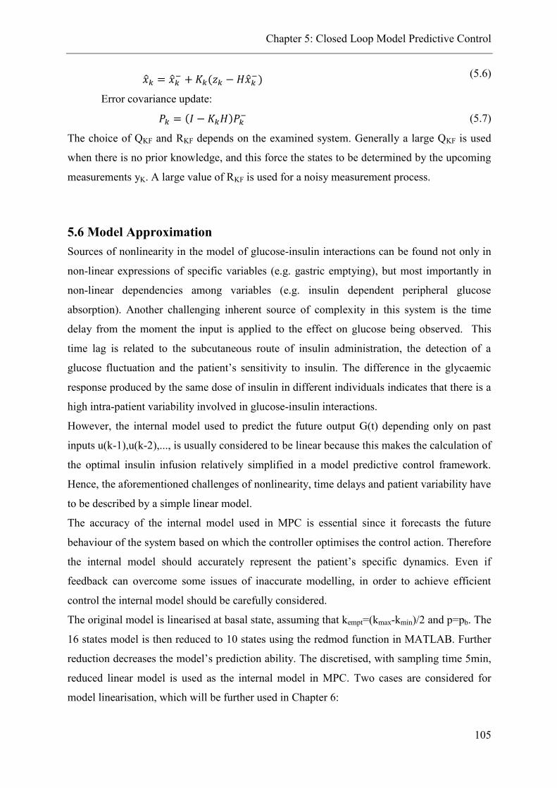
Chapter 5: Closed Loop Model Predictive Control
105
�̂�𝑘 = �̂�𝑘 − + 𝐾𝑘(𝑧𝑘 − 𝐻�̂�𝑘
−) (5.6)
Error covariance update:
𝑃𝑘 = (𝐼 − 𝐾𝑘𝐻)𝑃𝑘− (5.7)
The choice of QKF and RKF depends on the examined system. Generally a large QKF is used
when there is no prior knowledge, and this force the states to be determined by the upcoming
measurements yK. A large value of RKF is used for a noisy measurement process.
5.6 Model Approximation
Sources of nonlinearity in the model of glucose-insulin interactions can be found not only in
non-linear expressions of specific variables (e.g. gastric emptying), but most importantly in
non-linear dependencies among variables (e.g. insulin dependent peripheral glucose
absorption). Another challenging inherent source of complexity in this system is the time
delay from the moment the input is applied to the effect on glucose being observed. This
time lag is related to the subcutaneous route of insulin administration, the detection of a
glucose fluctuation and the patient’s sensitivity to insulin. The difference in the glycaemic
response produced by the same dose of insulin in different individuals indicates that there is a
high intra-patient variability involved in glucose-insulin interactions.
However, the internal model used to predict the future output G(t) depending only on past
inputs u(k-1),u(k-2),..., is usually considered to be linear because this makes the calculation of
the optimal insulin infusion relatively simplified in a model predictive control framework.
Hence, the aforementioned challenges of nonlinearity, time delays and patient variability have
to be described by a simple linear model.
The accuracy of the internal model used in MPC is essential since it forecasts the future
behaviour of the system based on which the controller optimises the control action. Therefore
the internal model should accurately represent the patient’s specific dynamics. Even if
feedback can overcome some issues of inaccurate modelling, in order to achieve efficient
control the internal model should be carefully considered.
The original model is linearised at basal state, assuming that kempt=(kmax-kmin)/2 and p=pb. The
16 states model is then reduced to 10 states using the redmod function in MATLAB. Further
reduction decreases the model’s prediction ability. The discretised, with sampling time 5min,
reduced linear model is used as the internal model in MPC. Two cases are considered for
model linearisation, which will be further used in Chapter 6:

Chapter 5: Closed Loop Model Predictive Control
106
Case 1: Development of patient-specific approximate model
It is assumed that the available patient data are informative enough to estimate the original
model parameters as presented in the parameters estimation section (4.5) and develop an
approximate model that accurately predicts the patient’s dynamics. Hence, the individual
model parameters are considered in the linear state-space model.
Case 2: Development of an adjusted mean approximate model
In this case, it is assumed that a priori knowledge of the patient’s dynamics cannot be
obtained and that only standard clinical tests are available, such as CGMS glucose profiles,
TDD, patient characteristics and meal information. Then the approximate model with mean
values of the parameters is used but adjusted accordingly for the specific patient. The
adjustable parameter is kp1 and is an element of the second column of Bd matrix which
determines the constant terms of the states that are considered in the linearisation. The
individual parameters of the control design that are individually tuned when using the mean
approximate model are the body weight, the total daily dose and the upper insulin constraint,
the weights of the objective function and the control horizon.
𝑥 = [𝐶𝐾 𝐶𝐺 𝐶𝑃 𝐶𝐵 𝐶𝐻 𝐶𝐿 𝐶𝑃𝑡 𝑈 𝐼𝑑 𝐼1 𝑆1 𝐼𝑏 𝑆2 𝑄𝑠𝑡𝑜1 𝑄𝑠𝑡𝑜2 𝑄𝑔𝑢𝑡]′
𝐴 =
[ −
𝑄𝐾
𝑉𝑔,𝐾0 0 0
𝑄𝐾
𝑉𝑔,𝐾
𝑘𝑝2𝑟𝑢,𝐾
𝑉𝑔,𝐾0 0
𝑘𝑝3𝑟𝑢,𝐾𝐵𝑊
𝑉𝑔,𝐾0 0 0 0 0 0 −
𝑓𝑘𝑎𝑏𝑠𝑟𝑢,𝐾
𝑉𝑔,𝐾
0 −𝑄𝐺
𝑉𝑔,𝐺0 0
𝑄𝐺
𝑉𝑔,𝐺
𝑘𝑝2𝑟𝑢,𝐺
𝑉𝑔,𝐺0 0
𝑘𝑝3𝑟𝑢,𝐺𝐵𝑊
𝑉𝑔,𝐺0 0 0 0 0 0
(1−𝑟𝑢,𝐺)𝑓𝑘𝑎𝑏𝑠
𝑉𝑔,𝐺
0 0 −(𝑄𝑃−𝑝)
𝑉𝑔,𝑃0
𝑄𝑃
𝑉𝑔,𝑃0
𝑝
𝑉𝑔,𝑃0 0 0 0 0 0 0 0 0
0 0 0 −𝑄𝐵
𝑉𝑔,𝐵
𝑄𝐵
𝑉𝑔,𝐵0 0 0 0 0 0 0 0 0 0 0
𝑄𝐾
𝑉𝑔,𝐻0
𝑄𝑃
𝑉𝑔,𝐻
𝑄𝐵
𝑉𝑔,𝐻−
𝑄𝐻
𝑉𝑔,𝐻
𝑄𝐿
𝑉𝑔,𝐻0 0
𝑘𝑝3𝑟𝑢,𝐻𝐵𝑊
𝑉𝑔,𝐻0 0 0 0 0 0 −
𝑓𝑘𝑎𝑏𝑠𝑟𝑢,𝐻
𝑉𝑔,𝐻
0𝑄𝐺
𝑉𝑔,𝐿0 0
𝑄𝐿
𝑉𝑔,𝐿−
𝑄𝐿
𝑉𝑔,𝐿+
(1−𝑟𝑢,𝐿)𝑘𝑝2
𝑉𝑔,𝐿0 0
(1−𝑟𝑢,𝐿)𝑘𝑝3𝐵𝑊
𝑉𝑔,𝐿0 0 0 0 0 0 −
𝑓𝑘𝑎𝑏𝑠𝑟𝑢,𝐿
𝑉𝑔,𝐿
0 0𝑝
𝑉𝑔,𝑃,𝐼𝑆𝐹0 0 0 −
(𝑝+𝑈)
𝑉𝑔,𝑃,𝐼𝑆𝐹
−1
𝑉𝑔,𝑃,𝐼𝑆𝐹0 0 0 −
𝑘1
6.945𝑉𝑔,𝑃,𝐼𝑆𝐹0 0 0 0
0 0 0 0 0 0 0 −𝑘2 0 0 0𝑘1
6.9450 0 0 0
0 0 0 0 0 0 0 0 −𝑘𝑖 𝑘𝑖 0 0 0 0 0 00 0 0 0 0 0 0 0 0 −𝑘𝑖 0 𝑘𝑖 ∗ 6.945 0 0 0 00 0 0 0 0 0 0 0 0 0 −𝑘𝑠𝑢𝑏 0 0 0 0 0
0 0 0 0 0 0 0 0 0 0 0 −𝑘𝑒𝑙𝑖𝑚𝑘𝑠𝑢𝑏
𝑘𝑒𝑙𝑖𝑚0 0 0
0 0 0 0 0 0 0 0 0 0 𝑘𝑠𝑢𝑏 0 −𝑘𝑠𝑢𝑏 0 0 00 0 0 0 0 0 0 0 0 0 0 0 0 −𝑘𝑔𝑟𝑖 0 0
0 0 0 0 0 0 0 0 0 0 0 0 0 𝑘𝑔𝑟𝑖 −𝑘𝑒𝑚𝑝𝑡 0
0 0 0 0 0 0 0 0 0 0 0 0 0 0 𝑘𝑒𝑚𝑝𝑡 −𝑘𝑎𝑏𝑠 ]

Chapter 5: Closed Loop Model Predictive Control
107
𝐵 =
[ 0000000000
1000
𝐵𝑊
00000 ]
, 𝐵𝑑 =
[ 0 −
𝑟𝑢,𝐾𝐵𝑊𝑘𝑝1
𝑉𝑔,𝐾
0 −𝑟𝑢,𝐺𝐵𝑊𝑘𝑝1
𝑉𝑔,𝐺
0 0
0 −𝑢𝐵
𝑉𝑔,𝐵
0 −𝑟𝑢,𝐻𝐵𝑊𝑘𝑝1
𝑉𝑔,𝐻
0(1−𝑟𝑢,𝐿)𝐵𝑊𝑘𝑝1
𝑉𝑔,,𝐿
0 00 00 00 00 00 00 01
𝑚𝑒𝑎𝑙_𝑑𝑢𝑟𝑎𝑡𝑖𝑜𝑛0
0 00 0 ]
, C=[0 0 0 0 1 0 0 0 0 0 0 0 0 0 0 0]
𝐷 = [0]
The accuracy of the patient specific approximate model is presented in Figure 5.2 for patient
no2.
Figure 5.2: Comparison of original model, linearised model and reduced model when 50 g of
carbohydrates are consumed and a 5 U bolus is given to patient no2
A measure to calculate the goodness of the fit between the original, the linearised and the
reduced model is the normalised mean square error as presented in (5.8).
𝐹𝑖𝑡 = (1 −∑ |𝑦𝑖 − 𝑦𝑖|̂𝑁𝑖=1
∑ |𝑦𝑖 − 𝑦|̅𝑁𝑖=1
) × 100 (5.8)
The fit is of the patient specific linearised approximate model to the original model is 93.6%.
Therefore, the linearised model accurately approximates the original model. The reduced
linear model fits at 99.7% the full-states linearised model.

Chapter 5: Closed Loop Model Predictive Control
108
5.7 Concluding Remarks
In this Chapter an overview of the existing methodologies to address the blood glucose
regulation problem with a closed loop insulin delivery system was presented. Emphasis is
given on the MPC control designs, because MPC will be further used in this thesis. The
challenges of an automated system are described of which the uncertainty originated by high
patient variability and the unknown disturbances are the most crucial. The theoretical
background of MPC formulation and the Kalman filter is presented and more details can be
found in Appendix B.2, which will be used in the following Chapter. The proposed model
described in Chapter 3 is linearised and reduced to be further used in the control design
presented in the next Chapter.

Chapter 6: Model Predictive Control in T1DM
109
6. Model Predictive Control Studies in T1DM
6.1 Introduction
In this chapter the design of a closed loop insulin delivery system for T1DM is presented. The
aim is to maintain the blood glucose concentration within the normal range (80-140mg/dl) by
manipulating the control input, the insulin infusion rate. Insulin is given not as the
conventional basal/bolus pattern but as a piecewise constant infusion rate that holds a value
for specific time intervals. The performance of the developed control design is evaluated in
the presence of meal disturbances and other uncertain factors. Apart from the MPC,
additional components are introduced to meet the specific requirements of blood glucose
regulation under unknown meal disturbances as explained in the following sections.
6.2 Control Objective
The aim of the developed control designs that are presented in the following sections is to
efficiently regulate the blood glucose concentration. However, the issues that make glucose
regulation rather challenging are the following:
Complexity of the inherent dynamics (Chapter 3 and 4)
Time delays (sections 4.7-4.9)
Intra -patient variability (section 4.5-4.9)
The need of a closed loop system to perform efficiently under free living conditions adds up
the following challenges:
Presence of unknown meal disturbances
Metabolic uncertainty
Therefore, with the proposed control designs we aim to:
Develop personalised insulin delivery systems
Take into account the involved time delays
Compensate for the unknown meal disturbances
Address the issue of uncertainty

Chapter 6: Model Predictive Control in T1DM
110
6.3 Model Predictive Control Strategy for insulin delivery in T1DM
Two general strategies for blood glucose regulation are studied. The first is a systematic
strategy which aims for personalised blood glucose control, whereas the second is an
“approximation” strategy that can be considered for blood glucose regulation in the absence
of informative patient data.
I. Systematic Strategy
It involves the following steps:
Step 1: Collection of CGMs data with available inputs (insulin, meal, exercise) and
plasma insulin concentration profile
Step 2: Estimation of the original model parameters for each patient (as described in
section 4.5)
Step3: Derivation of linearized patient specific models (as described in section 5.6)
Step 4: Systematic Strategy: Control design
II. “Approximation” Strategy
It involves the following two steps:
Step 1: Mean approximate model (mean values of the parameters of the linearized
model – section 5.6)
Step 2: “Approximation” Strategy: Control design
The control designs for the two strategies are different because the first strategy uses the a
priori knowledge of the patient dynamics to enhance the closed loop performance in the
presence of unknown disturbances and variability by solving an open loop optimisation
problem. On the other hand, the second strategy overcomes the effect of inaccurate modelling
with feedback by considering an additional controller. The inherent time delays of the system
are described with the linear approximate model presented in section 5.6. The internal model
predicts the delayed insulin effect and therefore, the efficacy of glucose regulation depends on
the controller’s ability to compensate for the after effect. The parameters of the control
formulation that are individually specified in both cases are the body weight, the total insulin
daily dose and the upper insulin constraint, the weights of the objective function and the
prediction horizon.

Chapter 6: Model Predictive Control in T1DM
111
The control designs for each strategy are described in detail in the following sections:
6.4 Systematic Strategy (I): Control designs
In Figure 6.1 a general control strategy to regulate blood glucose concentration is presented.
It consists of four parts that are activated depending on the type of meal disturbances di, as
defined in Table 6.1; an optimisation problem, an MPC controller, a state estimator and a
scheduling level. Depending on the type of meal disturbances different combinations of the
components are activated to efficiently regulate blood glucose concentration.
Figure 6.1: General proposed control strategy that consists of three blocks, MPC, State Estimator and
optimisation that are activated depending on the nature of the meal disturbances. In the case of
predefined disturbances (dp) the problem of optimal insulin delivery is an output optimisation
problem, in the case of announced disturbances (da) the problem is a state feedback MPC involving a
scheduling feature for upper insulin constraint. For unknown disturbances (du) the entire strategy is
activated involving an output feedback MPC.
Table 6.1: Meal disturbance types
Symbol Disturbance Type
dp Predefined
da Announced
du Unknown
Hence, the following control designs (CDs), as presented in Table 6.2 are evaluated for
different types of meal disturbances, di. When the meal plan is predefined and known in
advance then the regulation problem becomes an open-loop dynamic optimisation problem
and only the grey block dp is activated (CD1). The optimisation problem is solved and the
optimal insulin infusion rate that acts to maintain the blood glucose concentration within the

Chapter 6: Model Predictive Control in T1DM
112
normal range is calculated. CD2 involves a regulation level with a state feedback MPC and a
scheduling level that enhances the overall control performance. This design is activated when
the size of meal disturbances becomes known at the moment of meal consumption. CD3
combines an optimisation problem for a known reference meal plan and a correction output
feedback MPC to address the presence of unknown disturbances, which are estimated with a
state estimator as explained below. And finally, CD4 involves the MPC, the scheduling level
and the state estimator and is tested in comparison to CD3 for unknown disturbances.
Table 6.2: Glucose regulation designs
Control Designs Description Disturbance type
CD1 Dynamic Optimisation-Open-loop Control Predefined
CD2 Online MPC with scheduling level Announced
CD3 Optimisation and Correction MPC Unknown
CD4 Online MPC with scheduling level Unknown
Prediction Horizon
The system involves high input and disturbance delays, as was explained in section 4.7.
Therefore, in order to predict the after effect of a given input, the prediction horizon should be
at least equal to the time lag. However, every patient has different glucose-insulin dynamics
and the time delay factor should be considered as patient-specific. Although the time lag is
dependent on the insulin dose (section 4.7) for the insulin infusion rates considered in the
closed loop system an assumption of constant patient specific time delays is reasonable. Table
6.3 shows the prediction horizon of the 10 patients that is calculated as the average time to
observe a 1mg/dl change in blood glucose concentration when simulation studies of a step
change of 0.5U/h insulin dose from 0 to 5U/h were performed.
Table 6.3: Prediction Horizon (N) for the 10 patients
Patient N Patient N
Patient 1 13 ≜ 65min Patient 6 10 ≜ 50min
Patient 2 11 ≜ 55min Patient 7 8 ≜ 40min
Patient 3 7 ≜ 35min Patient 8 11 ≜ 55min
Patient 4 10 ≜ 50min Patient 9 14 ≜ 70min
Patient 5 13 ≜ 65min Patient 10 13 ≜ 65min
6.4.1 (CD1) Dynamic Optimisation: Predefined Disturbances (dp)
When a patient follows an exact meal plan, meaning that the exact amount and the time of the
meal is known in advance, then this information is introduced in the general regulation design

Chapter 6: Model Predictive Control in T1DM
113
as predefined meal plan and the optimisation block in Figure 6.1 is activated. Hence, if the
only uncertainty in the system is caused by the meal disturbances, then in the case of
predefined meal plan the feedback control and the open loop control are equivalent (Rawlings
and Mayne, 2009). The following optimisation problem is solved:
min𝑢𝑖
∫ (𝑤1 + 𝑤2)𝑑𝑡𝑡𝑓
0
(6.1)
s.t 𝐺 = 𝑓( 𝑥(𝑡),̇ 𝑥(𝑡), 𝑦(𝑡), 𝑢(𝑡)) (6.2)
∑𝑢2𝑖 = 𝑇𝐷𝐷
𝑁
𝑖=1
(6.3)
𝑤1 ≥ 0, 𝑤1 ≥ 𝐺 − 𝐺𝑚𝑎𝑥 𝑎𝑛𝑑 𝑤2 ≥ 0, 𝑤2 ≥ 𝐺𝑚𝑖𝑛 − 𝐺 (6.4)
where tf is the 24h time horizon, G is the blood glucose concentration described by the
nonlinear process model (6.2) for every patient (3.1-3.15); Gmax (140 mg/dl) and Gmin
(80mg/dl) are the maximum and minimum glucose concentration bounds. The optimal insulin
infusion, u2, appropriate to compensate for the forthcoming glucose increase due to the meal
intake can change every 5min, therefore the time intervals are N= 288. The TDD is the total
daily insulin dose for every patient. The optimisation studies were formed and solved in
gPROMS (PSE, 2011c).
The advantages and disadvantages of CD1 are summarised as follows:
Personalised insulin delivery
Feed forward insulin action to account for delayed insulin effect
No compensation for unknown disturbances
Metabolic uncertainty is not considered
6.4.2 (CD2) Online MPC with Scheduling Level: Announced Disturbances
(da)
When information concerning the amount of meal is made available only at the time it is
given, then the disturbance is considered as “announced” and the control strategy involves a
scheduling and a regulation level to enhance the performance of the controller, Figure 6.2.

Chapter 6: Model Predictive Control in T1DM
114
The day is divided in 4 periods, and in each period the maximum insulin delivery is different.
It is assumed that the meal plan follows a specific trend in terms of carbohydrates
consumption and for this case it is considered that the maximum amount of carbohydrates is
consumed during lunch according to Figure 6.2.
Figure 6.2: Control design CD2
For each period (sleeping, breakfast, lunch, dinner), the upper insulin limit is changed and
therefore a different optimisation problem is solved. The amount of the maximum delivered
insulin as determined in the scheduling level can be tailored to every patient according to
their lifestyle. This information aims to facilitate the prediction beyond the considered
horizon and hence to improve glucose regulation. A fine tuning of the control specifications
for every patient R, R1, QR ensures the maintenance of glucose concentration within the
normal range, the total insulin delivery to be less than the specified dose and prevent
hypoglycaemia in the case of a skipped meal.
The advantages and disadvantages of CD2 are summarised as follows:
Personalised insulin delivery (patient-specific approximate model, scheduling level
tailored to patient’s diet)
Prevention of hypoglycaemia
Cannot prevent immediate prandial hyperglycaemia due to delayed insulin effect
No compensation for unknown disturbances
Metabolic uncertainty is not considered
6.4.3 (CD3) Optimisation and Correction MPC: Unknown Disturbances (du)
In the case of unmeasured meal disturbances, there is no information concerning the amount
and the time of the meal. In this case, a nominal controller reacts aggressively to regulate the

Chapter 6: Model Predictive Control in T1DM
115
glucose deviation from the reference point, which means increased insulin infusion as long as
glucose violates the constraints. But this control action involves the risk of postprandial
hypoglycaemia due to insulin after effect and also immediate prandial hyperglycaemia.
Therefore, a different control design is proposed to compensate for unmeasured disturbances
as illustrated in Figure 6.3. It consists of the patient model, an optimizer acting as a reference
regulator, an MPC controller acting as the correction control, and a state estimator.
Figure 6.3: Control design CD3
The proposed control design regulates the glucose concentration when a reference meal plan
is considered and additionally responds appropriately to compensate for the deviation from
the reference meal when a different size meal is consumed. A similar approach which
involves a feedforward and a feedback part has been reposted in (Boiroux et al., 2010). But in
our work this approach is used for unknown meal disturbances and the feedforward part is
used to enhance the response of the controller due to the delayed insulin absorption. The
CGM error is simulated with white Gaussian noise using a signal-to-noise ratio equal to 30.
Optimizer: Reference Regulator
The desired glucose value Gref is set for every patient. A predefined reference meal plan is
considered to trigger the control action. Feedback about the current state is obtained by the
approximate model output yopt, . yopt is calculated when the optimisation problem for the
original non- linear model is solved for the predefined meal plan (described in section 6.4.1)
and the optimal insulin infusion is applied to the approximate model.
MPC: Correction Control

Chapter 6: Model Predictive Control in T1DM
116
MPC aims to find the optimal insulin infusion rate to regulate the difference of glucose as a
real measurement coming from the patient, G, and glucose as calculated when solving the
reference optimisation problem, yopt. This difference can be regarded as an unknown
disturbance of the system that leads to an offset in the set point, Gref,2=0. So the correction
control is described as a disturbance rejection problem. In order to remove the offset and the
nonzero disturbances the original system is augmented with a disturbance model, as presented
in (6.6). The output feedback of the patient is obtained as the difference of the actual
measurement and the reference control output (G-yopt), from which the state and the
integrating disturbance are estimated using a state estimator.
[𝑥𝑘+1𝑑𝑘+1
] = [𝐴 𝐵𝑑0 𝐼
] [𝑥𝑘𝑑𝑘] + [
𝐵0] 𝑢𝑘 + 𝑤𝑘
(6.6)
𝑦𝑘 = [𝐶 𝐶𝑑] [𝑥𝑘𝑑𝑘] + 𝜐𝑘
where dk is the integrating disturbance. The matrix 𝐵𝑑 ∈ ℝ𝑛×𝑛𝑑 is chosen to be the second
column of Bd matrix presented in section 5.6 and matrix 𝐶𝑑 = 𝐼 ∈ ℝ𝑛𝑑×𝑛𝑑. The variances of
variables w and υ are adjusted according to the output data (Odelson, Rajamani and Rawlings,
2006). The new derived augmented linear model (𝑛 = 10, 𝑛𝑑 = 1) is detectable, see (6.7),
which means that the states will converge to the real states when a Kalman filter is used,
hence this strategy can be employed:
𝑟𝑎𝑛𝑘 [𝐼 − 𝐴 −𝐵𝑑𝐶 𝐶𝑑
] = 𝑛 + 𝑛𝑑 = 11 (6.7)
The objective function is modified accordingly to include the nonzero disturbance d.
minx,y,u 𝐽 =∑ (Cxk + Cddk − Gref,2)′QR(Cxk + Cddk − Gref,2)
N−1k=1 + ∑ u1,k
′ Ru1,kM−1k=1 (6.8)
𝑠. 𝑡. �̂�𝑘+1 = 𝐴�̂�𝑘 + 𝐵𝑢1,𝑘 + 𝑤𝑘 (6.9)
𝑦2,𝑘 = 𝐶�̂�𝑘 + 𝜐𝑘 (6.10)
y2,min ≤ y2,k ≤ y2,max (6.11)
umin ≤ uk ≤ umax (6.12)
Where the estimated states are:
�̂� = [𝑥1 𝑥2 𝑥3 𝑥4 𝑥5 𝑥6 𝑥7 𝑥8 𝑥9 𝑥10 𝑑]′
And 𝑦2 = 𝐺 − 𝑦𝑜𝑝𝑡. The control specifications for MPC are presented in Table 6.4

Chapter 6: Model Predictive Control in T1DM
117
Table 6.4: Specifications of MPC and the Kalman Filter
Variable Value Variable Value Variable Value
y2,min -10 mg/dl umin 0 U/min 𝑄𝐾𝐹 100
Y2,max 10 mg/dl umax 0.2TDD U/min 𝑅𝐾𝐹 5
The advantages and disadvantages of CD3 are summarised as follows:
Personalised insulin delivery (patient-specific approximate model, Kalman Filter)
Feed forward insulin action to account for delayed insulin effect
Compensation for unknown disturbances
Account for metabolic uncertainty as unmeasured disturbance
A reference meal plan is always considered
6.4.4 (CD4) Online MPC with Scheduling Level: Unknown Disturbances
(du)
Control design CD4 applies the same principles of zero-offset design as CD3, but instead of
the optimizer it includes the scheduling level to enhance the control performance. Therefore,
the unknown disturbances are estimated using the augmented system in the state estimator,
but now the output and input used for the estimation is the glucose measurement, G, and u1,
respectively, presented in Figure 6.4 for clarity. The CGM error is simulated with white
Gaussian noise using a signal-to-noise ratio equal to 30.
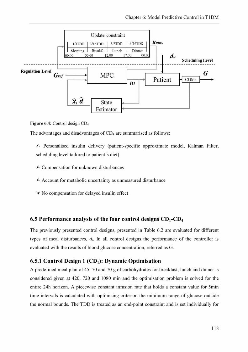
Chapter 6: Model Predictive Control in T1DM
118
Figure 6.4: Control design CD4
The advantages and disadvantages of CD4 are summarised as follows:
Personalised insulin delivery (patient-specific approximate model, Kalman Filter,
scheduling level tailored to patient’s diet)
Compensation for unknown disturbances
Account for metabolic uncertainty as unmeasured disturbance
No compensation for delayed insulin effect
6.5 Performance analysis of the four control designs CD1-CD4
The previously presented control designs, presented in Table 6.2 are evaluated for different
types of meal disturbances, di. In all control designs the performance of the controller is
evaluated with the results of blood glucose concentration, referred as G.
6.5.1 Control Design 1 (CD1): Dynamic Optimisation
A predefined meal plan of 45, 70 and 70 g of carbohydrates for breakfast, lunch and dinner is
considered given at 420, 720 and 1080 min and the optimisation problem is solved for the
entire 24h horizon. A piecewise constant infusion rate that holds a constant value for 5min
time intervals is calculated with optimising criterion the minimum range of glucose outside
the normal bounds. The TDD is treated as an end-point constraint and is set individually for

Chapter 6: Model Predictive Control in T1DM
119
every patient. The optimisation problem is solved in gPROMS. The results are presented for
all patients in Figure 6.5.
Figure 6.5: Glucose profiles for the 10 adults (upper graph) when optimal insulin infusion
(lower graph) is delivered
It can be concluded that very tight glycaemic control is achieved for most of the patients
when the meals are known in advance and the patient follows the exact predefined plan. In
more detail, the percentage of the time spent outside the euglycaemic range is presented in
Table 6.5 for all adults. As confirmed by Figure 6.5, it is difficult to maintain the blood

Chapter 6: Model Predictive Control in T1DM
120
glucose levels of adults no 4 and no 10 within the normal range. However, if these results are
compared to the time spent in normoglycaemia when conventional optimal insulin dosing is
applied, it can be stated that superior glucose control can be achieved with optimised insulin
infusion for all patents.
Table 6.5: Comparison of the time spent outside the normal glucose range when optimisation of
insulin infusion is performed and conventional optimal insulin dosing is administered
%Time Ad 1 Ad 2 Ad 3 Ad 4 Ad 5 Ad 6 Ad 7 Ad 8 Ad 9 Ad10 Mean
Optimised Insulin Infusion
G <70 0 0 0 0 0 0 0 0 0 0 0
G <80 0.9 0 0 15.9 0 0 0 0 0 0.9 1.8
80<G<140 99.0 100 96.1 53.5 76.2 90.1 99 90.1 95 48.5 84.7
140<G<180 0 0 3.9 29.8 23.7 9.9 0.99 9.9 4.9 50.5 13.3
180<G<250 0 0 0 2.9 0 0 0 0 0 0 0.29
G >250 0 0 0 0 0 0 0 0 0 0 0
Gmin 79 80 87 71 112 89 90 90 80 79 86
Gmax 139 137 147 192 145 146 140 146 144 153 149
Conventional Optimal Insulin Dosing
G <70 0 0 0 0 0 0 0 0 0 0 0
G <80 0 0 0 0 0 0 0 0 0 0 0
80<G<140 52.2 73.7 42.7 48.9 49.9 52.8 75.8 50.7 26.7 30.9 50.43
140<G<180 40.9 26.2 57.2 41.6 50.1 42.7 24.1 49.2 62.6 58.4 45.3
180<G<250 6.8 0 0 9.5 0 4.4 0 0 10.6 10.6 4.19
G >250 0 0 0 0 0 0 0 0 0 0 0
Gmin 100 95 102 99 99 103 102 88 93 96 97.7
Gmax 201 157 175 204 169 186 162 166 216 196 183.2
In more detail, no event of hypoglycaemia occurs for either the optimised insulin infusion or
the conventional optimal insulin dosing. The time period during which glucose is above
140mg/dl is 36% longer with the conventional insulin dosing than with the optimised insulin
infusion, while the time spent above 150mg/dl is 24% larger with the conventional insulin
dosing. Hence, when the exact meal plan is known in advance, then the administration of
insulin as calculated by the solution of the optimisation problem is a reliable way to tightly
maintain the blood glucose concentration within the normal range. However, CD1 assumes
that not only the meal plan is known in advance (something which is not always easy to
achieve in practice), but also that there is no model mismatch in terms of patient individual
dynamics and that there is no intra-patient variability. However, free living conditions deviate
significantly from the ideal simulated conditions. These assumptions are reconsidered and
examined in the following sections.

Chapter 6: Model Predictive Control in T1DM
121
6.5.2 Control Design 2 (CD2): Online MPC with Scheduling Level
In this section the control design CD2 for announced disturbances is evaluated for the 10
patients. The patient models are developed in gPROMS, while the control design in
MATLAB, gO:MATLAB is used to exchange data between the two environments. The
design is validated against:
A. The proposed model
B. The UVa/Padova Simulator
The considered meal plan is 45, 70 and 60 g of carbohydrates for breakfast, lunch and dinner
and the meals are given at 420, 720 and 1080 min as previously.
0 200 400 600 800 1000 1200 140040
60
80
100
120
140
160
180
0 200 400 600 800 1000 1200 14000
0.025
0.05
0.075
0.1
0.12
0 200 400 600 800 1000 1200 140060
80
100
120
140
160
180
200
0 200 400 600 800 1000 1200 14000
0.025
0.05
0.075
0.1
0 200 400 600 800 1000 1200 140060
80
100
120
140
160
180
200
0 200 400 600 800 1000 1200 14000
0.025
0.05
0.075
0.1
0 200 400 600 800 1000 1200 14006080
100120140160180200220240
0 200 400 600 800 1000 1200 14000
0.025
0.05
0.075
0.1
0 200 400 600 800 1000 1200 140060
80
100
120
140
160
180
200
0 200 400 600 800 1000 1200 14000
0.025
0.05
0.075
0.1
0.12
0 200 400 600 800 1000 1200 14006080
100120140160180200220240
0 200 400 600 800 1000 1200 14000
0.025
0.05
0.075
0.1
0.12
Adult 2
Adult 3 Adult 4
Adult 5 Adult 6
Adult 1

Chapter 6: Model Predictive Control in T1DM
122
A. Against the Proposed Model
B. Against UVa/Padova Simulator
Figure 6.6: MPC control for 10 adults in the presence of announced disturbances.; Upper graphs
blood glucose concentration (mg/dl) profiles; lower graphs control action, insulin (U/min). The black
lines show the results when CD2 is validated against the proposed model while the grey lines the
results against the UVa/Padova Simulator.
The purpose of Figure 6.6 is first to compare the results produced by CD2 when evaluated
against the proposed model and the UVa/Padova Simulator and second to examine the
reliability of CD2. The results of A and B are very similar, which implies that the proposed
model could be generally viewed as a reliable equivalent to the UVa/Padova Simulator. The
approximate model used as the internal MPC model can predict the current states for both
models and the controller suggests a similar control action for all patients. The observed
differences could be due to inaccuracies in the parameter estimation of the proposed model
due to the lack of informative data of different meal sizes and insulin infusions. As far as the
efficiency of CD2 is concerned, the results suggest that this strategy is not flexible enough to
handle the fluctuations of glucose concentration. The controller suggests the maximum
insulin infusion at the announcement of the disturbance, which cannot prevent the prandial
hyperglycaemia. The control specifications are fine tuned to ensure the avoidance of
hypoglycaemia.
0 200 400 600 800 1000 1200 1400406080
100120140160180200220
0 200 400 600 800 1000 1200 14000
0.025
0.05
0.075
0 200 400 600 800 1000 1200 140060
80
100
120
140
160
180
200
0 200 400 600 800 1000 1200 14000
0.025
0.05
0.075
0.1
0 200 400 600 800 1000 1200 140060
80
100
120
140
160
180
200
0 200 400 600 800 1000 1200 14000
0.025
0.05
0.075
0.1
0.125
0.15
0 200 400 600 800 1000 1200 14006080
100120140160180200220240
0 200 400 600 800 1000 1200 14000
0.025
0.05
0.075
0.1
Adult 8
Adult 9 Adult 10
Adult 7

Chapter 6: Model Predictive Control in T1DM
123
6.5.2.1 Case Study: Skipped Meal
CD2 is evaluated in the case of a skipped meal. As it can be verified from Figure 6.7 the
controller reacts accordingly when the breakfast or the lunch are skipped at 420 and 720 min
respectively.
Figure 6.7: Skipped breakfast and skipped lunch for adult 5
6.5.3 Control Design 3 (CD3): Optimisation and Correction MPC
In this section the CD3 control design as explained before is evaluated. The ability of the
controller to maintain the blood glucose concentration in the normal range is tested for large
meal sizes of 75, 100 and 90 g and for normal meal sizes of 45, 75 and 60 g of carbohydrates
given for breakfast at 420 min, lunch at 720 min and dinner at 1080 min respectively, as
shown in Table 6.6. The reference meal plan is 20, 30 and 25 g respectively. The total insulin
amount does not exceed the TDD for each patient plus approximately 6 U to compensate for
the large meal sizes. The results from CD3 are compared to the CD4 for the same meal sizes
and presented in Table 6.7 and Table 6.8.
Table 6.6: Evaluation of CD3 with two meal scenarios
Scenario 1 Scenario 2
Breakfast 75 g 45 g
Lunch 100 g 75 g
Dinner 90g 60 g
0 200 400 600 800 1000 1200 140060
80
100
120
140
160
180
200
Patient 5
Time (min)Blo
od
Glu
co
se C
on
cen
trati
on
(m
g/d
l)
0 200 400 600 800 1000 1200 14000
0.02
0.04
0.06
0.08
0.1
0.12
Time (min)
Insu
lin
un
fusi
on
rate
(U
/min
)
0 200 400 600 800 1000 1200 140060
80
100
120
140
160
180
200
Patient 5
Time (min)Blo
od
Glu
co
se C
on
cen
trati
on
(m
g/d
l)
0 200 400 600 800 1000 1200 14000
0.02
0.04
0.06
0.08
Time (min)
Insu
lin
un
fusi
on
rate
(U
/min
)

Chapter 6: Model Predictive Control in T1DM
124
Table 6.7: CD3 predefined reference meal plan (Scenario 1)
% time
<70
% time
<80
% time
80<G <140
% time
140<G <180
% time
180<G <250
% time
>250
Gmin
(mg/dl)
Gmax
(mg/dl)
Adult1 0 1.3 72.9 18.3 8.6 0 89 203
Adult2 0 0 71.5 22.9 5.5 0 81 190
Adult3 0 2.3 65.0 20.5 12.0 0 70 228
Adult4 0 0.3 25.0 56.9 17.8 0 76 247
Adult5 0 0 55.5 29.2 14.9 0 79 239
Adult6 0 3.1 60.4 14.6 21.9 0 71 226
Adult7 0 0 67.0 20.1 12.8 0 82 205
Adult8 0 4.9 68.4 19.5 7.0 0 77 194
Adult9 0 1.4 59.2 23.4 13.1 2.8 72 265
Adult10 0 2.4 50.3 23.4 24.8 2.4 76 259
Mean 0 1.6 59.5 24.9 13.8 0.52 77 226
SD 0 1.6 14.1 11.9 6.2 1.1 5.7 26.9
Table 6.8:CD4 unknown disturbances (Scenario 1)
% time
<70
% time
<80
% time
80<G <140
% time
140<G <180
% time
180<G <250
% time
>250
Gmin
(mg/dl)
Gmax
(mg/dl)
Adult1 1.4 4.5 53.8 22.2 19.4 0 62 238
Adult2 4.5 7.9 54.9 25.3 11.8 0 63 202
Adult3 4.1 5.5 45.8 37.1 11.4 0 46 249
Adult4 5.2 12.8 52.7 12.5 7.6 14.2 62 326
Adult5 0 0 43.1 29.8 27.1 0 85 246
Adult6 6.3 12.7 52.4 9.9 20.9 3.9 54 270
Adult7 6.6 12.8 52.8 9.1 16.1 8.6 58 288
Adult8 5.2 9.3 51.7 29.5 9.4 0 65 199
Adult9 0 0 39.2 33.7 20.5 6.5 90 303
Adult10 0 2.1 36.1 27.1 29.5 5.2 72 281
Mean 3.4 6.8 48.3 23.6 17.4 3.8 66 260
SD 2.6 5.1 6.7 10.0 7.4 4.9 13.4 41.4
Table 6.7 shows that with CD3, on average 59.5% of the time is spent within the normal
glucose range, while with CD4 the percentage of the time spent in the normal range is 48.3%.
With CD3 there is no event of hypoglycaemia and the minimum observed glucose value is
71mg/dl for adult 6, in contrast to CD4 where an average 3.4% of the time is spent in
hypoglycaemia with a minimum observed glucose value of 46 mg/dl. Additionally, the time
spent in hyperglycaemia ( >180mg/dl ) is much higher for CD4 with a 21.2% of the time,
while for CD3 the respective percentage is 14.3%. The 10 adults respond, as expected,
relatively different from each other, but as it can be observed from Table 6.7 there is no event
of hypoglycaemia in all the studied adults and only adult 9 and adult 10 spend time above 250
mg/dl. However, for CD4 the results are significantly different with the glucose values being
distributed towards the extremes for most of the adults. A Mann-Whitney test was performed
to compare CD3 and CD4. The p-value is calculated for each glucose range and for the ranges
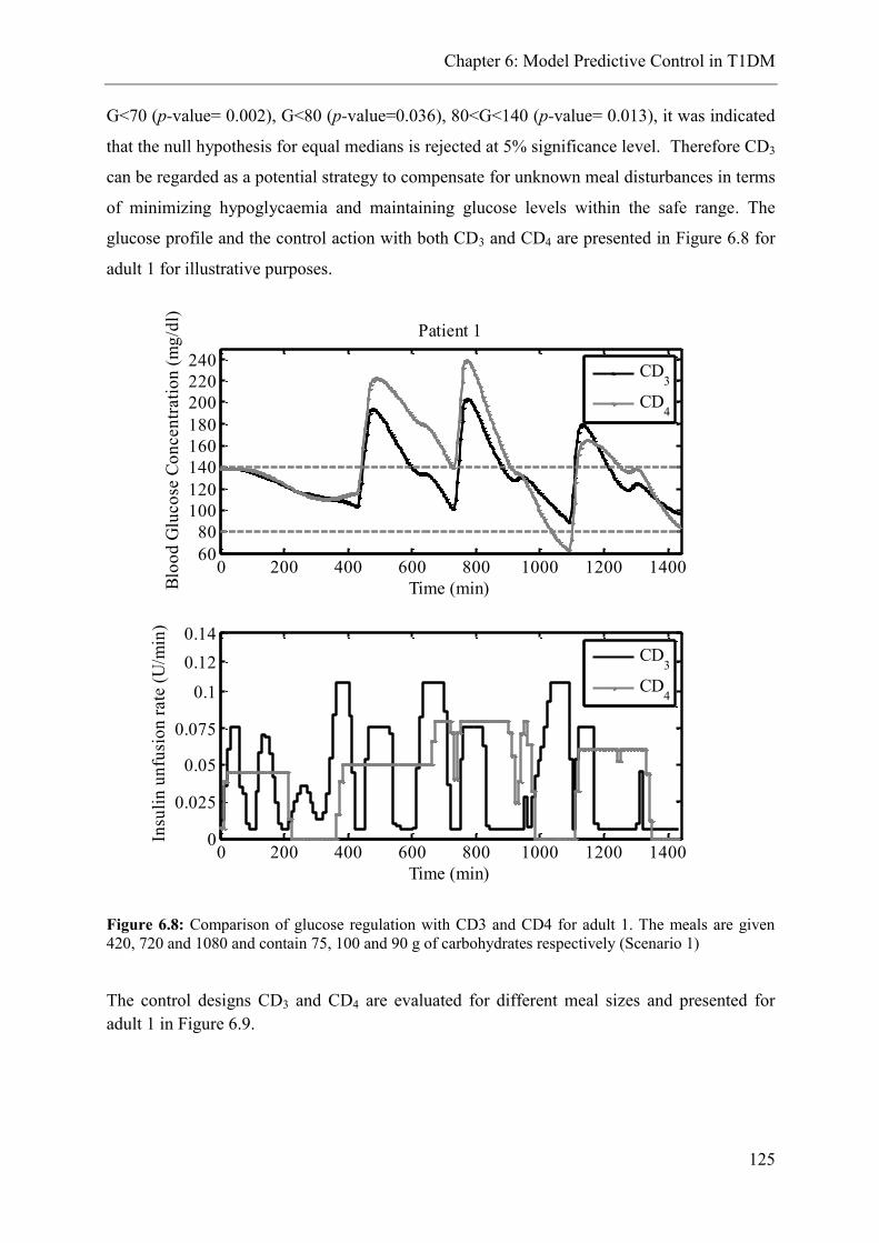
Chapter 6: Model Predictive Control in T1DM
125
G<70 (p-value= 0.002), G<80 (p-value=0.036), 80<G<140 (p-value= 0.013), it was indicated
that the null hypothesis for equal medians is rejected at 5% significance level. Therefore CD3
can be regarded as a potential strategy to compensate for unknown meal disturbances in terms
of minimizing hypoglycaemia and maintaining glucose levels within the safe range. The
glucose profile and the control action with both CD3 and CD4 are presented in Figure 6.8 for
adult 1 for illustrative purposes.
Figure 6.8: Comparison of glucose regulation with CD3 and CD4 for adult 1. The meals are given
420, 720 and 1080 and contain 75, 100 and 90 g of carbohydrates respectively (Scenario 1)
The control designs CD3 and CD4 are evaluated for different meal sizes and presented for
adult 1 in Figure 6.9.
0 200 400 600 800 1000 1200 140060
80
100
120
140
160
180
200
220
240
Patient 1
Time (min)Blo
od
Glu
co
se C
on
cen
trati
on
(m
g/d
l)
0 200 400 600 800 1000 1200 14000
0.025
0.05
0.075
0.1
0.12
0.14
Time (min)
Insu
lin
un
fusi
on
rate
(U
/min
)
CD3
CD4
CD3
CD4

Chapter 6: Model Predictive Control in T1DM
126
Figure 6.9: Comparison of glucose regulation with CD3 and CD4 for adult 1. The meals are given 420,
720 and 1080 and contain 45, 75 and 60 g of carbohydrates respectively (Scenario 2)
Figure 6.8 and Figure 6.9 confirm that tighter glycaemic control can be achieved when CD3 is
used and a feed forward reference action is applied to enhance the control performance in the
presence of unknown disturbances.
Key Results for the Systematic Strategy Control Designs
Control Design 1: Tight glycaemic control
Control Design 2: Not flexible enough, but no event of hypoglycaemia for the study data
Control Design 3: Good glycaemic control; 85% of the time spent near normoglycaemia
for Scenario 1; no event of hypoglycaemia for the study data
Control Design 4: Not efficient glycaemic control; 72% of the time spent near
normoglycaemia for Scenario 1, with 3.4% in hypoglycaemia
0 200 400 600 800 1000 1200 140060
80
100
120
140
160
180
200Patient 1
Time (min)Blo
od
Glu
co
se C
on
cen
trati
on
(m
g/d
l)
CD3
CD4
0 200 400 600 800 1000 1200 14000
0.025
0.05
0.075
0.1
0.12
0.14
Time (min)
Insu
lin
un
fusi
on
rate
(U
/min
)
CD3
CD4

Chapter 6: Model Predictive Control in T1DM
127
6.6 “Approximation” Strategy (II): Control Designs
In this section the “approximation” strategy is evaluated and compared with the systematic
strategy. The general control design applied in this approach is presented in Figure 6.10. This
design differs from Figure 6.1 in the grey box that now instead of an optimisation problem a
second MPC is considered. Additionally, the yopt becomes yref, as calculated when the
reference tracking problem with known meal disturbance is solved and the optimal insulin
infusion is applied. Finally, CD2 and CD4 are the same as presented previously.
Figure 6.10: General control design for “Approximation” Strategy
Effect of Mean Approximate model
In order to illustrate the effect of using the mean approximate model instead of the patient-
specific approximate model, we consider the control design CD3 of section 6.4.3 but
assuming that the internal control model is now the mean approximate model. This
assumption in the context of Strategy I is not correct since, if there is no information of the
exact patient dynamics, the optimisation problem will not calculate the optimal insulin
infusion for each patient. However, for analysis purposes, assuming that u2 is available and
can be applied, we investigate the effect of using mean approximate internal models rather
than exact in the control design. Figure 6.11 is a control variability grid analysis (CVGA) plot
(Magni et al., 2008) which has been established as a very useful tool to evaluate the
performance of different control strategies in a population of patients. The area is divided in
zones, each one representing the level of euglycaemic maintenance. For each patient a dot is
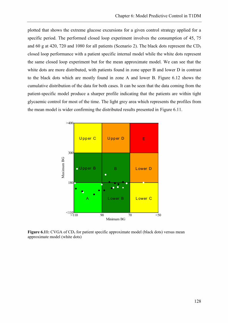
Chapter 6: Model Predictive Control in T1DM
128
plotted that shows the extreme glucose excursions for a given control strategy applied for a
specific period. The performed closed loop experiment involves the consumption of 45, 75
and 60 g at 420, 720 and 1080 for all patients (Scenario 2). The black dots represent the CD3
closed loop performance with a patient specific internal model while the white dots represent
the same closed loop experiment but for the mean approximate model. We can see that the
white dots are more distributed, with patients found in zone upper B and lower D in contrast
to the black dots which are mostly found in zone A and lower B. Figure 6.12 shows the
cumulative distribution of the data for both cases. It can be seen that the data coming from the
patient-specific model produce a sharper profile indicating that the patients are within tight
glycaemic control for most of the time. The light grey area which represents the profiles from
the mean model is wider confirming the distributed results presented in Figure 6.11.
Figure 6.11: CVGA of CD3 for patient specific approximate model (black dots) versus mean
approximate model (white dots)
>110 90 70 <50<110
180
300
>400
A
U pp er B
U pp er C
L ower B
B
U pp er D
L ower C
L ower D
E
Minimum BG
Max
imu
m B
G

Chapter 6: Model Predictive Control in T1DM
129
Figure 6.12: Cumulative distribution of blood glucose concentration. The light grey area shows the
range of closed loop glucose distribution when the mean approximate model is used for the ten
patients; whereas the dark grey area shows the range of closed loop glucose distribution when the
exact patient model is used (Strategy I). The dashed line is the mean cumulative glucose distribution
of the light grey area while the dash-dot line the mean of the dark grey area.
6.6.1 Comparison of CD3: Strategy I and Strategy II
The performance of CD3 for Strategy I and Strategy II is compared in Figure 6.13 for
Scenario 2 for all patients. It can be noticed that the results of Strategy II are undoubtedly
satisfactory since all patients are in zones A and B. When compared to the results from CD3
of Strategy I with mean model (as explained above) we can see that the additional MPC acts
efficiently to compensate for the effects of poor model and tighter glycaemic control can be
achieved. Figure 6.14 shows the cumulative distribution of CD3 for Strategy I and II. We can
observe that both areas are very sharp and tight indicating that most of the time glucose is
maintained tightly within the normal range.

Chapter 6: Model Predictive Control in T1DM
130
Figure 6.13: CVGA of CD3 for patient specific approximate model (black dots), Strategy I, versus
mean approximate model (white dots) and versus CD3 Strategy II (white circles)
Figure 6.14: Cumulative distribution of blood glucose concentration. The light grey area shows the
range of closed loop glucose distribution of Strategy II for the ten patients; whereas the dark grey area
shows the range of closed loop glucose distribution for Strategy I. The dashed line is the mean
cumulative glucose distribution of the light grey area while the dash-dot line the mean of the dark grey
area.
>110 90 70 <50<110
180
300
>400
A
U pp er B
U pp er C
L ower B
B
U pp er D
L ower C
L ower D
E
Minimum BG
Max
imu
m B
G
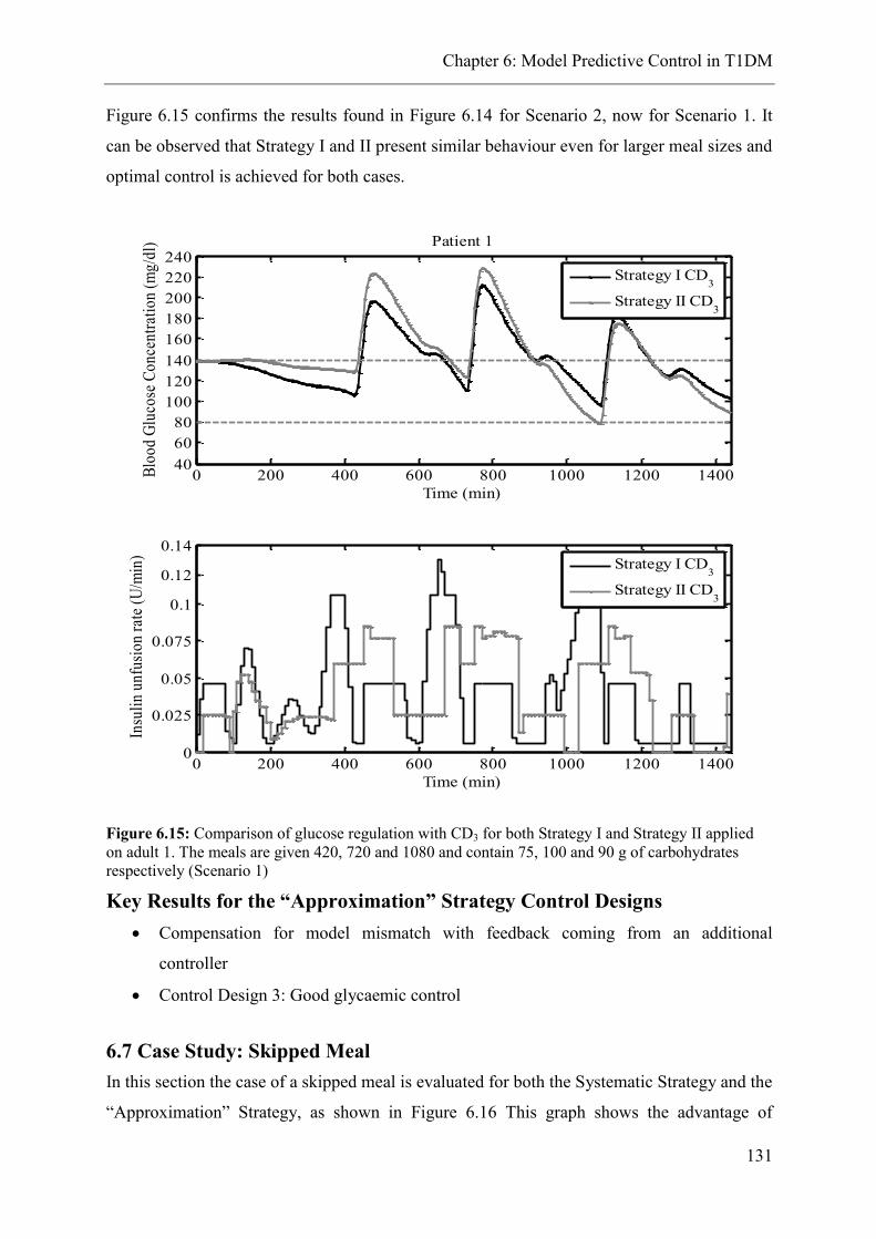
Chapter 6: Model Predictive Control in T1DM
131
Figure 6.15 confirms the results found in Figure 6.14 for Scenario 2, now for Scenario 1. It
can be observed that Strategy I and II present similar behaviour even for larger meal sizes and
optimal control is achieved for both cases.
Figure 6.15: Comparison of glucose regulation with CD3 for both Strategy I and Strategy II applied
on adult 1. The meals are given 420, 720 and 1080 and contain 75, 100 and 90 g of carbohydrates
respectively (Scenario 1)
Key Results for the “Approximation” Strategy Control Designs
Compensation for model mismatch with feedback coming from an additional
controller
Control Design 3: Good glycaemic control
6.7 Case Study: Skipped Meal
In this section the case of a skipped meal is evaluated for both the Systematic Strategy and the
“Approximation” Strategy, as shown in Figure 6.16 This graph shows the advantage of
0 200 400 600 800 1000 1200 140040
60
80
100
120
140
160
180
200
220
240Patient 1
Time (min)
Blo
od
Glu
cose
Co
nce
ntr
atio
n (
mg
/dl)
Strategy I CD3
Strategy II CD3
0 200 400 600 800 1000 1200 14000
0.025
0.05
0.075
0.1
0.12
0.14
Time (min)
Insu
lin
un
fusi
on
rat
e (U
/min
)
Strategy I CD3
Strategy II CD3

Chapter 6: Model Predictive Control in T1DM
132
Strategy I over Strategy II. We can see that optimisation of the insulin delivery over the entire
horizon is much more efficient than the optimisation over the prediction horizon in such an
unstable system with long time delays. The insulin action proposed by the solution of the
optimisation problem is adequate for each sampling period since the reference meal
disturbance is known in advance and insulin is delivered smoothly long before the occurrence
of glucose fluctuation. Therefore in the case of a skipped meal the drop of glucose profile is
not as severe as in the “Approximation” Strategy because the compensation for a meal
disturbance starts early having a smooth effect on glucose. On the other hand, in the
“Approximation” Strategy the reference meal announcement is obtained within the
framework of the prediction horizon and the action of the controller although it is produced
earlier than the meal disturbance, it is sharper than in Strategy I, causing a big drop on blood
glucose concentration.

Chapter 6: Model Predictive Control in T1DM
133
Figure 6.16: Skipped lunch for adult 1 and Scenario 2
0 200 400 600 800 1000 1200 140040
60
80
100
120
140
160
180Patient 1
Time (min)
Blo
od
Glu
co
se C
on
cen
trati
on
(m
g/d
l)
Strategy I CD3
Strategy II CD3
0 200 400 600 800 1000 1200 14000
0.025
0.05
0.075
0.1
0.12
0.14
Time (min)
Insu
lin
un
fusi
on
rate
(U
/min
)
Strategy I CD3
Strategy II CD3

Chapter 6: Model Predictive Control in T1DM
134
Figure 6.17: Skipped lunch for adult 1 and Scenario 1
The same conclusions are supported with Figure 6.17 for Scenario 1. The drop in glucose
concentration is greater since the considered meal disturbances are bigger which means more
insulin is required to compensate for the glucose increase. Therefore, the reference meal plan
can be adequately adjusted according to the patient’s meal habits in case of normal
consumption of larger meals.
6.8 Case Study: Variable Meal Time
Figure 6.18 shows the glucose profile for adult 1 for the Systematic Strategy when a meal of
50 g is given 30min before or 30min after, or simultaneously with the predefined 30 g
reference meal. It can be noticed that good glycaemic control is achieved even at the case
0 200 400 600 800 1000 1200 140040
6080
100
120140160
180200220240
Patient 1
Time (min)Blo
od
Glu
cose
Co
nce
ntr
atio
n (
mg
/dl)
Strategy I CD3
Strategy II CD3
0 200 400 600 800 1000 1200 14000
0.025
0.05
0.075
0.1
0.12
0.14
Time (min)
Insu
lin
un
fusi
on
rat
e (U
/min
)
Strategy I CD3
Strategy II CD3
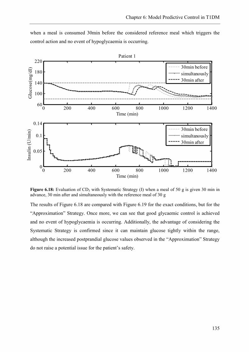
Chapter 6: Model Predictive Control in T1DM
135
when a meal is consumed 30min before the considered reference meal which triggers the
control action and no event of hypoglycaemia is occurring.
Figure 6.18: Evaluation of CD3 with Systematic Strategy (I) when a meal of 50 g is given 30 min in
advance, 30 min after and simultaneously with the reference meal of 30 g
The results of Figure 6.18 are compared with Figure 6.19 for the exact conditions, but for the
“Approximation” Strategy. Once more, we can see that good glycaemic control is achieved
and no event of hypoglycaemia is occurring. Additionally, the advantage of considering the
Systematic Strategy is confirmed since it can maintain glucose tightly within the range,
although the increased postprandial glucose values observed in the “Approximation” Strategy
do not raise a potential issue for the patient’s safety.
0 200 400 600 800 1000 1200 140060
100
140
180
220Patient 1
Time (min)
Glu
co
se(m
g/d
l)
30min before
simultanously
30min after
0 200 400 600 800 1000 1200 14000
0.05
0.1
0.14
Time (min)
Insu
lin
(U
/min
)
30min before
simultanously
30min after
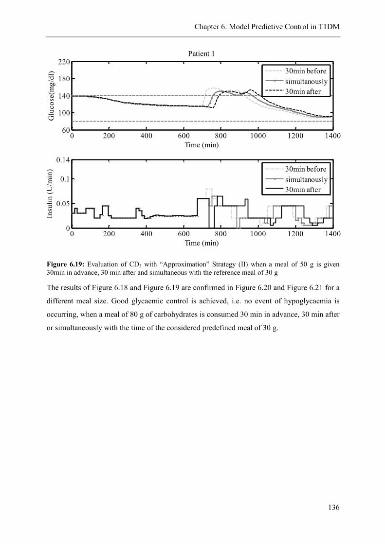
Chapter 6: Model Predictive Control in T1DM
136
Figure 6.19: Evaluation of CD3 with “Approximation” Strategy (II) when a meal of 50 g is given
30min in advance, 30 min after and simultaneous with the reference meal of 30 g
The results of Figure 6.18 and Figure 6.19 are confirmed in Figure 6.20 and Figure 6.21 for a
different meal size. Good glycaemic control is achieved, i.e. no event of hypoglycaemia is
occurring, when a meal of 80 g of carbohydrates is consumed 30 min in advance, 30 min after
or simultaneously with the time of the considered predefined meal of 30 g.
0 200 400 600 800 1000 1200 140060
100
140
180
220Patient 1
Time (min)
Glu
co
se(m
g/d
l)
30min before
simultanously
30min after
0 200 400 600 800 1000 1200 14000
0.05
0.1
0.14
Time (min)
Insu
lin
(U
/min
)
30min before
simultanously
30min after

Chapter 6: Model Predictive Control in T1DM
137
Figure 6.20: Evaluation of CD3 with Systematic Strategy (I) when a meal of 80 g is given 30 min
in advance, 30 min after and simultaneous with the reference meal of 30 g
Figure 6.21: Evaluation of CD3 with “Approximation” Strategy (II) when a meal of 80 g is given 30
min in advance, 30 min after and simultaneous with the reference meal of 30 g
0 200 400 600 800 1000 1200 140060
100
140
180
220Patient 1
Time (min)
Glu
co
se(m
g/d
l)
30min before
simultanously
30min after
0 200 400 600 800 1000 1200 14000
0.05
0.1
0.14
Time (min)
Insu
lin
(U
/min
)
30min before
simultanously
30min after
0 200 400 600 800 1000 1200 140060
100
140
180
220Patient 1
Time (min)
Glu
co
se(m
g/d
l)
30min before
simultanously
30min after
0 200 400 600 800 1000 1200 14000
0.05
0.1
0.14
Time (min)
Insu
lin
(U
/min
)
30min before
simultanously
30min after

Chapter 6: Model Predictive Control in T1DM
138
The main assumption of CD3 is that all the predefined meals will be consumed. Nonetheless,
the reference meal plan can be determined individually depending on the patient’s lifestyle.
6.9 Case Study: Intra-patient Variability
The impact of intra-patient variability on glucose regulation is evaluated by imposing a
circadian sinusoidal variation on the parameter k1 (3.24). This is related to insulin dependent
glucose absorption and is very influential according to the sensitivity analysis presented in
Chapter 4. The choice of the parameter as well as the imposed variation is in good agreement
with the literature (Fabietti et al., 2006). The amplitude of the wave is 30% of the nominal
value of k1, according to (6.13):
𝑘1 = 𝑘1,𝑚𝑒𝑎𝑛 (1 − 0.3𝑠𝑖𝑛 (2𝜋
24)) , 0 ≤ 𝑡 ≤ 24 (6.13)
The complete circadian cycle of parameter k1 is presented in Figure 6.22 for adult1.
Figure 6.22: Complete circadian cycle of k1 with a 30% change in magnitude
The impact of parameter k1 variation on glucose concentration is shown in Figure 6.23. The
light grey line shows the glucose concentration profile when CD1 is applied with no intra-
patient variability considered. This profile is compared to the darker grey line that shows the
influence of intra-patient variation on glucose profile, when no further control action is
applied, but only CD1. It can be noticed that the profile changes according to the sinusoidal
variation with increased values of glucose concentration when the value of k1 decreases and
low values of glucose concentration with the increase of k1.
0 200 400 600 800 1000 1200 14004
5
6
7
8
x 10-5
Time (min)
k 1

Chapter 6: Model Predictive Control in T1DM
139
Figure 6.23: glucose profile when CD1 is applied with no considered variability and CD1 in
the presence of variability for Scenario 2 adult 1.
To address this fluctuation in the case of unknown meal plan, CD3 is applied for both
Systematic and “Approximation” strategies. The results are presented in Figure 6.24.
0 200 400 600 800 1000 1200 140050
70
90
110
130
150
170
190
210Patient 1
Time (min)
Glu
cose
(mg/
dl)
CD
1
CD1 variability
0 200 400 600 800 1000 1200 14000
0.025
0.05
0.075
0.1
0.12
0.14
0.16
0.18
Time (min)
Insu
lin(
U/m
in)
CD
1
CD1 variability

Chapter 6: Model Predictive Control in T1DM
140
Figure 6.24: CD3 performance in the presence of intra-parient variability for Strategy I and
Strategy II, comparison of glucose profile when CD1 is applied in the presence of variability
for Scenario 2 adult 1.
It can be observed that both control strategies respond accordingly to decrease the glucose
concentration when it tends to increase due to the imposed variability. Additionally, when
glucose tends to decrease, both control designs achieve to maintain the concentrations above
the hypoglycaemic level. This graph also shows the flexibility of “Approximation” Strategy
when glucose concentration tends to decrease due to the imposed variability. The two
considered controllers respond adequately so as not to deliver more insulin than required,
whereas in the “Systematic” Strategy the reference insulin delivery is pre-calculated and
administered anyway. Therefore, in this strategy the controller cannot act to prevent the
impact of the variability, however in the presence of unknown disturbances and imposed
variability the controller maintains glucose concentration within the normal range.
0 200 400 600 800 1000 1200 140050
70
90
110
130
150
170
190
210Patient 1
Time (min)
Glu
cose
(mg/
dl)
CD
1 variability
Strategy I CD3
Strategy II CD3
0 200 400 600 800 1000 1200 14000
0.025
0.05
0.075
0.1
0.12
0.14
0.16
0.18
Time (min)
Insu
lin(
U/m
in)
Strategy I CD
3
Strategy II CD3

Chapter 6: Model Predictive Control in T1DM
141
6.10 Conclusions
The key actions taken to address the control objectives presented in Section 6.2 are
summarised as follows for the control designs of the Systematic Strategy and the
“Approximation” Strategy:
Actions Systematic
Strategy
“Approximation”
Strategy
Develop personalised insulin delivery systems
- Development of patient-specific approximate models
- Specify individually the parameters: BW,TDD,umax,
QR,R,R1
- Scheduling level tailored to patient’s diet
- Solution of patient-specific optimisation problem
- Patient-specific prediction horizon
- Flexibility to determine the reference meal plan
according to patient’s diet
Take into account the involved time delays
- Describe the inherent time delays in the linear
approximate models
- Include the time lag in the prediction horizon
- Enhance the feed forward action of the controller
Compensate for the unknown meal disturbances
- Consider an augmented state space system to describe
the unknown disturbance as extra state using a Kalman
filter
Address the issue of uncertainty
- Metabolic uncertainty as unmeasured disturbance
- Evaluation of performance robustness in several
conditions

Chapter 6: Model Predictive Control in T1DM
142
6.11 Concluding Remarks
Two general strategies of glucose regulation are presented. The Systematic Strategy involves
the steps towards a patient-specific closed loop insulin delivery that takes advantage of the a
priori knowledge of the system dynamics. The “Approximation” Strategy compensates for the
effect of poor knowledge of the patient’s dynamics with the inclusion of an additional
controller.
The complications of the system such as the occurrence of disturbances that have a major
effect on the system’s dynamics, the large time delays and the patient variability make the use
of a simple controller for the solution of the closed loop inappropriate as this can lead to poor
control performance. Therefore, the proposed frameworks involve an MPC, a state estimator,
an optimizer/MPCref and a scheduling feature.
In the case that the disturbances are known in advance, the results indicate that good control
can be achieved. In particular, glucose can be maintained within or close to the normal range
despite intra- patient variability, differences in meal sizes and/or timing and skipped meals.
The proposed methodology of Optimisation and Correction MPC (Control Design 3)
considers that a reference meal is given and thus it is assumed that the patient always
consumes a breakfast, a lunch and a dinner. In the case of skipping one of these meals it was
shown that efficient glycaemic control cannot be achieved, especially by the
“Approximation” Strategy. On the contrary, when the meal is announced at the time it is
given then the controller responds adequately in the case of a skipped meal. The proposed
methodology can be formulated according to the patient’s needs and the issue of skipping a
meal can be addressed either by manually providing this information or by compensating for
the after effect.

Chapter 7: Concluding Remarks & Future Directions
143
7. Concluding Remarks & Future Directions
7.1 Project summary
The proposed mathematical model of glucose-insulin interactions in T1DM is a
physiologically based compartmental model that describes glucose metabolism in actual
anatomical compartments, inspired by the work of (Sorensen, 1978). Glucose is distributed
in six organs (heart, brain, liver, kidney, gut, and periphery) via blood circulation and it is
absorbed by the tissue cells to provide them with energy. Insulin, through the subcutaneous
route, is distributed via the blood circulation to enhance glucose uptake by the periphery
(adipose tissue and muscle cells) and to signal the liver to suppress the endogenous glucose
production and therefore, maintain the blood glucose concentration within the normal range.
The pharmacokinetic parameters and variables of glucose metabolism (distribution volumes,
blood flows, and cardiac output) are expressed as functions of age, weight, gender and height
to account for the individual patient characteristics. The rate of glucose appearance in the
blood after meal consumption, the endogenous glucose production and the glucose excretion
from the kidneys are described with models obtained by the literature that have been
clinically validated and are embedded in the proposed model structure. Regarding the insulin
kinetics, four potential models are presented, and a series of evaluation tests have indicated
the most suitable model to describe experimental data obtained by the literature (Boden,
Cheung and Homko, 2003). Additionally, the model used for endogenous glucose production
was evaluated with clinical data, obtained again by the literature (Boden, Cheung and
Homko, 2003). A global sensitivity analysis was performed to determine which model
parameters have a significant influence on the measured output. The GSA specified that the
most influential parameters are those related to insulin effect on glucose. Particularly the
parameters k1 and k2, linked to insulin sensitivity, have the most significant effect on blood
glucose concentration.
The model of UVa/Padova simulator (Dalla Man, Rizza and Cobelli, 2006) was implemented
and simulated in gPROMS. The commercial version of the T1DMS was used to obtain the
patient-specific glucose-insulin profiles. These profiles, for 10 examined adult patients, were
treated as experimental data to estimate the parameters of the proposed model and obtain
individualised dynamic glucose and insulin profiles. The estimated parameters were the most
influential ones as identified using GSA. The parameters of the Ra and EGP sub models were

Chapter 7: Concluding Remarks & Future Directions
144
also estimated. The remaining, non-influential parameters were kept at their mean values.
The simulated results indicated that the proposed model can accurately predict individualised
glucose profiles and that the model parameters are well adjusted for all patients.
Therefore, this model is used as a virtual patient for closed loop studies, and after
simplification, as a predictive tool in the context of model based control, according to the
framework presented in Figure 7.1:
Figure 7.1: Framework of closed loop validation studies in the context of model predictive control
The meal disturbances in the system have a significant effect on glucose dynamics and trigger
the system away from the steady state. Depending on the nature of the meal disturbances
different control designs are developed. In the presence of known disturbances the problem
becomes an open loop optimisation problem over the entire examined time horizon. When the
disturbance is announced at the time it occurs then the control design involves an MPC
controller and a scheduling level which specifies several time periods according to the daily
meal plan of the patient during which the upper insulin bound is different; a different
optimisation problem is solved in each time period. Finally, in the case of unknown
disturbances it became obvious that a nominal state feedback MPC controller is inadequate to
efficiently regulate the blood glucose concentration, and hence a different control design is
proposed. The feed forward ability of MPC that acts in anticipation of the future fluctuations
due to disturbances is enhanced when considering a reference meal plan of specific size and
time that is always given to the patient. This is inspired by the function of the healthy
pancreas that provides the system with already stored insulin when receiving a signal of
increased blood glucose and then it produces new insulin to compensate for the rest of the
increased glucose. Therefore, in the case of the artificial pancreas, the system is ready to
provide the optimal insulin infusion to compensate for a small reference meal, in order to
overcome the effect of long time delays and to prevent the prandial hyperglycaemia induced

Chapter 7: Concluding Remarks & Future Directions
145
by a large meal. An open loop optimisation problem is solved for the considered meal plan
and the solution is incorporated into the control action. Then an MPC controller acts on the
difference of glucose concentration, resulting from the unknown meal disturbance, and the
expected glucose, resulting from the reference meal plan when the optimal insulin infusion is
given. The performance of this control design presents a significant improvement over the
nominal state feedback MPC for unknown disturbances. Cases of imposed variability in the
meal time, variability in the parameters related to insulin sensitivity and skipped meals are
tested to evaluate the reliability of the proposed control design.
In the case of limited patient information of the glucose-insulin dynamics a mean
approximate model with adjusted parameters related to obvious patient characteristics is
considered. The performance of this control strategy is evaluated for all the aforementioned
disturbance types and cases. Necessary modifications in the general control design are
considered. It was evident that even though the patient-specific control design outperforms
the approximate control design, the approximate strategy shows a general applicability
towards the development of closed loop artificial pancreas.
7.2 Key contributions of this thesis
The key contributions of this work are summarised:
Modelling & Model Analysis (Chapters 3 and 4)
Development of a novel physiologically based compartmental model of glucose-
insulin interactions in T1DM that combines actual anatomical compartments and
functions that have already been validated in the literature.
Description of fundamental pharmacokinetic properties with individual patient
characteristics.
Original insights of the insulin kinetics model, in terms of model identifiability,
parameter estimation and correlation. The model structure was developed by
comparison of alternative models with experimental data and a series of model
analysis tests.
Determination of the model parameters with the most influential effect on the
measured output through global sensitivity analysis. The results confirmed that the
influence of pharmacodynamic parameters is more significant than the influence of
pharmacokinetic parameters.

Chapter 7: Concluding Remarks & Future Directions
146
Estimation of the patient parameters for 10 adult patients using data obtained from the
UVa/Padova T1DMS treated as clinical data. Ten individual glucose-insulin dynamic
systems that describe precisely the glucose-insulin interactions are developed.
Investigation of time delays on the system was investigated with open loop
optimisation studies. Solution of an MINLP problem to find the optimal timing to
administer a bolus insulin dose. A continuous insulin infusion as an alternative to the
conventional basal- bolus insulin treatment was considered and the optimisation
results showed that it can be applied in closed loop studies.
Closed loop control for optimal insulin delivery (Chapters 5-6, Appendix A, C)
Development of two general control strategies: a systematic strategy that aims towards
a personalised insulin delivery system and an “approximation” strategy that
compensates for lack of patient information.
Inclusion of features such as a scheduling level which is modifiable for each patient,
the personalised reference optimisation problem, the patient specific MPC controller,
to develop individual closed loop insulin delivery systems.
Consideration of the known disturbance rejection problem as a personalised open loop
optimisation problem.
Assessment of unknown disturbances as disturbance rejection with zero offset towards
a robust MPC design.
Investigation of the effect of uncertain factors such as variability in the meal time and
size, skipped meal and variability in insulin sensitivity on the system in the closed
loop formulation. The control design presents feasible performance under the imposed
uncertainty which encourages its further consideration.
Evaluation of the performance of the control strategies by triggering the system with
large meal sizes.
Preliminary results using explicit Model Predictive Control for closed loop insulin
delivery.

Chapter 7: Concluding Remarks & Future Directions
147
7.3 Publications from this thesis
Journal Articles
Stamatina Zavitsanou, Nicki Panoskaltsis, Athanasios Mantalaris, Michael C. Georgiadis,
Alexandra Bargiota, Georgios Koukoulis, Efstratios N. Pistikopoulos, A modelling
framework for the control of type 1 diabetes, submitted to Journal of Process Control.
Stamatina Zavitsanou, Athanasios Mantalaris, Michael C. Georgiadis, Efstratios N.
Pistikopoulos, In-silico Closed Loop Control Validation Studies for Optimal Insulin Delivery
in T1DM, submitted to IEEE Transactions on Biomedical Engineering.
Book Chapters
Eirini G. Velliou, Stamatina Zavitsanou, Eleni Pefani, Alexandra Krieger, Michael C.
Georgiadis, Efstratios N. Pistikopoulos, A framework for modelling, optimization and control
of biomedical systems, Chapter 1 in Modelling, Control and Optimization of Biomedical
Systems (in preparation).
Stamatina Zavitsanou, A. Mantalaris, Michael C. Georgiadis, Efstratios N. Pistikopoulos,
Type I Diabetes Mellitus: Modelling, Model Analysis, Optimisation and Glucose Regulation,
Chapter 5 in Modelling, Control and Optimization of Biomedical Systems (in preparation).
Conference Proceedings
Stamatina Zavitsanou, Athanasios Mantalaris, Michael C. Georgiadis, Efstratios N.
Pistikopoulos, 2014, Optimisation of insulin dosing in patients with type 1 diabetes mellitus,
Computer Aided Process Engineering, Vol.33, Elsevier, pp 1459-1464,
Stamatina Zavitsanou, Nicki Panoskaltsi, Athanasios Mantalaris, Michael C. Georgiadis,
Efstratios N.Pistikopoulos, 2011, Modelling of the Insulin Delivery System for patients with
Type 1 Diabetes Mellitus, Computer Aided Process Engineering, Vol. 29, Elsevier, pp.1499-
1503
Oral Presentations
Stamatina Zavitsanou, Athanasios Mantalaris, Michael C. Georgiadis, Efstratios N.
Pistikopoulos , Modelling and Robust Model Predictive Control of Insulin Delivery in Type 1
DM, 2012 AIChE Annual Meeting, Pittsburgh, PA, US. 28 October - 2 November 2012.
Poster Presentations
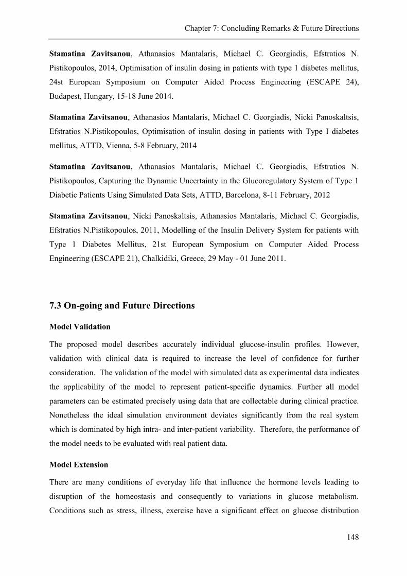
Chapter 7: Concluding Remarks & Future Directions
148
Stamatina Zavitsanou, Athanasios Mantalaris, Michael C. Georgiadis, Efstratios N.
Pistikopoulos, 2014, Optimisation of insulin dosing in patients with type 1 diabetes mellitus,
24st European Symposium on Computer Aided Process Engineering (ESCAPE 24),
Budapest, Hungary, 15-18 June 2014.
Stamatina Zavitsanou, Athanasios Mantalaris, Michael C. Georgiadis, Nicki Panoskaltsis,
Efstratios N.Pistikopoulos, Optimisation of insulin dosing in patients with Type I diabetes
mellitus, ATTD, Vienna, 5-8 February, 2014
Stamatina Zavitsanou, Athanasios Mantalaris, Michael C. Georgiadis, Efstratios N.
Pistikopoulos, Capturing the Dynamic Uncertainty in the Glucoregulatory System of Type 1
Diabetic Patients Using Simulated Data Sets, ATTD, Barcelona, 8-11 February, 2012
Stamatina Zavitsanou, Nicki Panoskaltsis, Athanasios Mantalaris, Michael C. Georgiadis,
Efstratios N.Pistikopoulos, 2011, Modelling of the Insulin Delivery System for patients with
Type 1 Diabetes Mellitus, 21st European Symposium on Computer Aided Process
Engineering (ESCAPE 21), Chalkidiki, Greece, 29 May - 01 June 2011.
7.3 On-going and Future Directions
Model Validation
The proposed model describes accurately individual glucose-insulin profiles. However,
validation with clinical data is required to increase the level of confidence for further
consideration. The validation of the model with simulated data as experimental data indicates
the applicability of the model to represent patient-specific dynamics. Further all model
parameters can be estimated precisely using data that are collectable during clinical practice.
Nonetheless the ideal simulation environment deviates significantly from the real system
which is dominated by high intra- and inter-patient variability. Therefore, the performance of
the model needs to be evaluated with real patient data.
Model Extension
There are many conditions of everyday life that influence the hormone levels leading to
disruption of the homeostasis and consequently to variations in glucose metabolism.
Conditions such as stress, illness, exercise have a significant effect on glucose distribution

Chapter 7: Concluding Remarks & Future Directions
149
and absorption from the involved organs. In the case of T1DM, the complications increase
because glucose regulation with exogenous insulin under these conditions can be very
challenging. In order to achieve tight glycaemic control with exogenous insulin, the patient
needs to fully understand the underlying phenomena of alterations in insulin sensitivity
during exercise, the different metabolic effect during mild and vigorous exercise, the role of
epinephrine that triggers the release of stored glucose in the blood stream under stressful
conditions or illness. The determination of indicators for such conditions has been proposed
in the literature in order to enhance the prediction of blood glucose concentration under free
living conditions. A multivariable model including the galvanic skin response and the energy
expenditure as additional inputs was proposed by Turksoy et al. (Turksoy et al., 2013) for the
closed loop system. Towards this direction an extended version of the proposed model
including the representation of glucose dynamics during exercise could decrease the
uncertainty of glucose predictability. Stress and illness, which do not constitute a
deterministic condition, can be regarded as model uncertainty that should be addressed in the
closed-loop system.
Robust closed loop insulin delivery
One of the key challenging issues of closed loop insulin delivery is the high intra- and inter-
patient variability. Even though there has been an effort towards patient-specific glucose
dynamics predictions with the introduction of patient-specific variables and parameters, as
well as personalised glucose regulation with the determination of time horizons, TDD,
scheduling feature and weights of the cost function tailored for each patient, the glycaemic
variability remains an unpredictable quantity. The factors that influence the ability to predict
the blood glucose concentration are summarised in Kildegaard et al. (2009) and involve the
metabolic variability, meal variability, insulin and glucose monitoring variability and lifestyle
variability. All these factors can significantly affect the blood glucose predictability and make
the system very challenging to control. In the context of MPC there is a need towards robust
control designs for insulin delivery systems. Robust control concerns the systems that are
uncertain in the sense that the actual behaviour of the system cannot be described with
predictions based on the nominal system (Rawlings and Mayne, 2009). Therefore, in the
presence of uncertain predictions, robust control ensures that the control actions do not
violate the constraints and that the optimisation solution always exists (Richards, 2005). The
uncertainty of the system can be due to unknown additive disturbances, model mismatch and

Chapter 7: Concluding Remarks & Future Directions
150
simplifications (Rawlings and Mayne, 2009). The system can be expressed as the LTI system
with unmeasured disturbance (Bemporad and Morari, 1999):
𝑥𝑡+1 = 𝐴𝑥𝑡 + 𝐵𝑢𝑡 + 𝐻𝑤𝑡, 𝑥(0) = 𝑥0 (7.1)
𝑦𝑡 = 𝐶𝑥𝑡 + 𝐾𝑤𝑡
With 𝑤(𝑡) ∈ 𝑊 and W is a bounded set.
Another way to include the uncertainty in the system is with parametric uncertainty:
𝑥𝑡+1 = 𝐴(𝜃)𝑥𝑡 + 𝐵(𝜃)𝑢𝑡 (7.2)
𝛩 = {𝜃𝑙𝑏 ≤ 𝜃𝑘 ≤ 𝜃𝑢𝑏; ∀𝜃 ∈ ℝ𝑞}
[𝐴(𝜃), 𝛣(𝜃)] ∈ 𝛺, where Ω is a pre-specified polytope.
These types of uncertainties (7.1-7.2) can occur in the same application. The problem
traditionally is approached by minimising the worst-case scenario (maximum w) based on
open loop predictions but this can lead to over-conservative control performance (Sakizlis,
M.P. Kakalis, et al., 2004), (Bemporad and Morari, 1999). Many different proposals of
feedback Robust MPC have been proposed and can be found in the literature (Rawlings and
Mayne, 2009), (Langson et al., 2004), (Maciejowski, 2002).
On-line parameter estimation
A complementary approach to decrease the system uncertainty is to estimate on-line the
model parameters which contribute significantly to the system dynamics. This method aims to
address the uncertainty originated from the metabolic variability such as alterations in insulin
sensitivity. A Bayesian approach was used by (Hovorka et al., 2004) to update the values of
certain parameters. An on-line parameter estimation formulated as a least-squares problem is
evaluated in (Krieger and Pistikopoulos, 2014) for the case of anaesthesia. The relevance of
the underlying physiology to the model parameters that need to be updated provides useful
directions for the problem simplification.
Model reduction techniques
In the considered insulin-delivery system the internal model used for the control design is a
large linear model. Combined with the involved large time horizons the development of the
optimal control design (offline; development of mpMPC) can be indeed very challenging due

Chapter 7: Concluding Remarks & Future Directions
151
to the increased computational complexity. Model reduction techniques can be used as an
alternative to overcome the limitations of large or inaccurate models by deriving simple but
precise models to describe the dynamics of non-linear, complex systems. In this case, the
development of explicit multi-parametric MPC could be feasible.
Explicit Model Predictive Control / Robust mp-MPC
In order to overcome the significant online computations involved in the closed-loop optimal
control implementation an alternative solution of the on-line optimisation problem has been
proposed (Pistikopoulos et al., 2002), (Pistikopoulos, Georgiadis and Dua, 2007a),
(Pistikopoulos, Georgiadis and Dua, 2007b), which relies on a parametric optimisation-based
approach. In essence, the online solution of the optimisation problem is replaced by the off
line derivation of the explicit mapping of the optimal decisions in the space of the plant
uncertainty. The ability to solve off-line the MPC optimisation problem makes the mp-MPC
technology ideal for implementation on a simple hardware like a chip, “MPC-on-a-chip”, for
portable or embedded devices (Pistikopoulos, 2012). For the closed loop insulin delivery
system, although there has been tremendous progress in the involved device technology
(insulin pump, smartphones, CGMS) and their interconnectivity a controller solved offline
through simple function evaluation and implemented on a chip can enhance the reliability of
the entire system. In Dassau et al. (2013) the performance of mp-MPC has been clinically
evaluated for the closed loop delivery of insulin resulting in very encouraging outcomes using
this technology. Appendix C focuses with the development of mpMPC controllers in the
context of the proposed control designs presented in section 6.4.3. Further in-silico validation
studies are required to gain confidence in the mpMPC control formulation. The derivation of
robust mp-MPC has gained vast consideration in the literature. The combination of the two
involved theories has been examined in (Bemporad, Borrelli and Morari, 2003),
(Manthanwar, Sakizlis and Pistikopoulos, 2005), (Sakizlis, M.P. Kakalis, et al., 2004),
(Kouramas, Sakizlis and Pistikopoulos, 2009), and can be a promising potential for the
challenging system of insulin delivery.
Further Developments towards the Artificial Pancreas
Towards the development of an artificial pancreas the validation of the proposed closed loop
strategy in a real experimental set-up is required. This implies firstly the validation of the
proposed model and secondly the derived control strategy. The use of the UVa/Padova
Simulator for the derivation of the approximate model as well as the virtual patient has

Chapter 7: Concluding Remarks & Future Directions
152
presented efficient glucose regulation in the closed loop system (Appendix A.2).
Additionally, the testing of the derived control strategy on the UVa/Padova Simulator as the
virtual patient in many cases has shown good control performance. Further in-silico
validation can increase the level of confidence for the proposed closed loop design. The
substitution of online MPC in the presented control designs with mpMPC will improve the
reliability of the automated closed loop insulin delivery system. Towards this direction
Appendix C explains the formulation of the system but further simulation studies are required
to define efficiently the system’s specifications to achieve tight glycaemic control.
Additionally, incorporation of complementary components such as Insulin-on-Board and
hypoglycaemia alarms could improve the closed loop control performance especially in the
case of skipped meals.

APPENDIX A
153
APPENDIX A
A.1 Model of UVa/Padova Simulator
Glucose Metabolism: A two compartment model is used to model the glucose subsystem
with Gp and Gt representing the plasma and tissue glucose mass (mg/kg) respectively.
𝑑𝐺𝑝
𝑑𝑡= 𝐸𝐺𝑃 + 𝑅𝑎 − 𝑈𝑖𝑖 − 𝐸 − 𝑘1𝐺𝑝 + 𝑘2𝐺𝑡 Gp(0)=Gpb (A.1)
𝑑𝐺𝑡
𝑑𝑡= 𝑘1𝐺𝑝 − 𝑘2𝐺𝑡 − 𝑈𝑖𝑑 Gt(0)=Gtb (A.2)
𝐺 =𝐺𝑝
𝑉𝑔 G(0)=Gb (A.3)
The EGP (mg/kg/min) is the endogenous glucose production, the Ra (mg/kg/min)the rate of
glucose appearance in the bloodstream after meal consumption, Uii and Uid (mg/kg/min) are
the insulin independent and insulin dependent glucose utilisation, E(mg/kg/min) is the renal
glucose excretion, k1,k2 (min-1
) are rate parameters of glucose kinetics and Vg(dl) is the
glucose distribution volume.
Rate of glucose appearance (Ra) from meal
𝑑𝑄𝑠𝑡𝑜1
𝑑𝑡= −𝑘𝑘𝑔𝑟𝑖𝑄𝑠𝑡𝑜1 +𝐷𝛿(𝑡) Qsto1(0)=0 (A.4)
𝑑𝑄𝑠𝑡𝑜2
𝑑𝑡= −𝑘𝑒𝑚𝑝𝑡𝑄𝑠𝑡𝑜2 + 𝑘𝑔𝑟𝑖𝑄𝑠𝑡𝑜1 Qsto2(0)=0 (A.6)
𝑑𝑄𝑔𝑢𝑡
𝑑𝑡= −𝑘𝑎𝑏𝑠𝑄𝑔𝑢𝑡 + 𝑘𝑒𝑚𝑝𝑡𝑄𝑠𝑡𝑜2 Qgut(0)=0 (A.7)
𝑄𝑠𝑡𝑜 = 𝑄𝑠𝑡𝑜1 + 𝑄𝑠𝑡𝑜2 Qsto(0)=0 (A.8)
𝑅𝑎 =𝑓𝑘𝑎𝑏𝑠𝑄𝑔𝑢𝑡 (𝑡)
𝐵𝑊 Ra(0)=0 (A.9)
𝑘𝑒𝑚𝑝𝑡 = 𝑘𝑚𝑖𝑛 +𝑘𝑚𝑎𝑥−𝑘𝑚𝑖𝑛
2{tanh (𝑎1(𝑄𝑠𝑡𝑜 − 𝑏 ∙ 𝐷(𝑡))) − tanh (𝑏1(𝑄𝑠𝑡𝑜 − 𝑑 ∙ 𝐷(𝑡))) + 2}
(A.10)
a1 =5
2∙𝐷∙(1−𝑏) (A.11)
b1 =5
2∙𝐷∙𝑑 (A.12)
With Qsto1, Qsto2 (mg) the glucose mass in solid and liquid phase, Qsto (mg) the overall glucose
mass in the stomach, Qgut (mg) is the glucose mass in the small intestine, kempt (min-1
) is the

APPENDIX A
154
rate of gastric emptying, a1 and b1 are model parameters, kmax, kmin (min-1
)are the max and
min gastric emptying, kabs (min-1
) is the rate constant of intestinal absorption, kgri is the rate
constant of grinding, f (dimensionless) is the fraction of intestinal absorption, b and d are
percentages of the dose and D (mg) is the amount of ingested meal.
Endogenous Glucose Production (EGP)
𝐸𝐺𝑃 = 𝑘𝑝1 − 𝑘𝑝2𝐺𝑝 − 𝑘𝑝3𝐼𝑑𝑒𝑙2 EGP(0)=EGPb (A.13)
𝑑𝐼𝑑𝑒𝑙1
𝑑𝑡= −𝑘𝑖(𝐼𝑑𝑒𝑙1 − 𝐼𝑝) I1(0)=Ipb (A.14)
𝑑𝐼𝑑𝑒𝑙2
𝑑𝑡= −𝑘𝑖(𝐼𝑑𝑒𝑙2 − 𝐼𝑑𝑒𝑙1) Id(0)=Ipb (A.15)
With Idel2 (pmol/l) the delayed insulin signal (chain of two compartments), kp1 (mg/kg/min)
the extrapolated EGP at zero glucose and insulin, kp2 (min-1) the liver glucose effectiveness,
kp3 (mg/kg/min per pmol/l) the insulin action on the liver and ki (min-1
) the rate parameter for
the delay between insulin signal and action
Insulin dependent glucose utilization
𝑈𝑖𝑑 =𝑉𝑚𝐺𝑡
𝑘𝑚0+𝐺𝑡 Uid(0)=Uidb (A.16)
𝑉𝑚 = 𝑉𝑚0 + 𝑉𝑚𝑥𝑋𝑑𝑖𝑠𝑝 Vm(0)=Vm0 (A.17)
𝑑𝑋𝑑𝑖𝑠𝑝
𝑑𝑡= −𝑝2𝑢𝑋𝑑𝑖𝑠𝑝 + 𝑝2𝑢(𝐼𝑝 − 𝐼𝐵𝐴𝑆𝐴𝐿) Xdisp(0)=0 (A.18)
𝑈𝑡𝑜𝑡 = 𝑈𝑖𝑖 + 𝑈𝑖𝑑 (A.19)
With Xdisp (pmol/L) insulin in the interstitial fluid, Vm0 (mg/kg/min) and km0 (mg/kg) the
Michaelis–Menten related parameters, Vmx (mg/kg/min per pmol/liter) the disposal of insulin
sensitivity and p2u (min-1) the rate constant of insulin action on peripheral glucose utilization.
Glucose Renal Excretion
𝐸 = {𝑘𝑒1(𝐺𝑝 − 𝑘𝑒2)
0 𝑖𝑓 𝐺𝑝 > 𝑘𝑒2𝑖𝑓 𝐺𝑝 ≤ 𝑘𝑒2
E(0)=0 (A.20)
With ke1 (min-1
) the glomelural filtration rate and ke2(mg/kg) the glucose renal threshold
Insulin Kinetics
𝑑𝐼𝑠𝑐1
𝑑𝑡= −(𝑘𝑑 + 𝑘𝑎1) ∙ 𝐼𝑠𝑐1 + 𝑢(𝑡) Isc1(0)=Isc1ss (A.21)

APPENDIX A
155
𝑑𝐼𝑠𝑐2
𝑑𝑡= 𝑘𝑑𝐼𝑠𝑐1 − 𝑘𝑎2𝐼𝑠𝑐2 Isc2(0)=Isc2ss (A.22)
𝑑𝐼𝑙
𝑑𝑡= −(𝑚1 +𝑚3)𝐼𝑙 +𝑚2𝐼𝑝 Il(0)=Ilb (A.23)
𝑑𝐼𝑝
𝑑𝑡= −(𝑚2 +𝑚4)𝐼𝑝 +𝑚1𝐼𝑙 + 𝑘𝑎1𝐼𝑠𝑐1 + 𝑘𝑎2𝐼𝑠𝑐2 Ip(0)=Ipb (A.24)
𝐼 =𝐼𝑝
𝑉𝑖 I(0)=Ib (A.25)
𝑚3 =𝐻𝐸𝑏𝑚1
1−𝐻𝐸𝑏 (A.26)
With Il (pmol/kg)the insulin mass in liver, Ip (pmol/kg) insulin mass in the plasma, I (pmol/l)
the plasma insulin concentration, Isc1(pmol/kg) the amount of non-monomeric insulin in the
subcutaneous space, Isc2 (pmol/kg) the amount of monomeric insulin in the subcutaneous
space, u(t) (pmol/kg/min) the exogenous insulin infusion rate, m1,m2,m3,m4 (min-1
) the rate
parameters of insulin kinetics, VI (L/kg) the insulin distribution volume, kd (min-1
) the rate
constant of insulin dissociation, ka1 (min-1
) the rate constant of non- monomeric insulin
absorption and ka2 (min-1
) the rate constant of monomeric insulin absorption.
A.2 Model Predictive Control Framework
The general framework used for the control design to regulate the BG concentration is
presented in Figure A.2.1, as also showed in Chapter 7. It involves the development of a high
fidelity model that accurately predicts the glucose-insulin dynamics in T1DM, the
simplification of the original model with system identification or model order reduction
techniques to derive a reliable approximation of the system dynamics and finally the design
of the appropriate control strategy. In the MPC formulation one of the key components is the
approximate model that needs to be relatively simple to facilitate the computational
complexity, but also very informative to include the entire system dynamics. In this section,
the involved steps of closed loop insulin delivery are presented while emphasis is given on
the importance of developing a reliable, patient-specific approximate model for MPC.

APPENDIX A
156
Figure A.2.1: Framework for MPC controllers design
1. “High Fidelity” Model
The mathematical model used in this study as a virtual patient for closed loop control
validation studies as well as to derive approximate models necessary for model based control
is the model developed by the Cobelli group (Dalla Man, Rizza and Cobelli, 2007), (Dalla
Man et al., 2007), and presented in section A.1. The model is simulated in gPROMS using
individual patient parameters obtained from the commercial UVa/Padova Simulator for 10
adults.
2. The Approximate Model
Two methods are employed to derive an accurate linear approximate model suitable for
control purposes. The first presented method is system identification and the second model
linearisation and reduction.
System Identification
The linear model describing the dynamics of the glucose-insulin interactions was determined
using the System Identification Toolbox of MATLAB. Due to the complexity caused by the
inherent nonlinearities of the system the linear model was built by identifying two separate
transfer functions describing the insulin-glucose and food-glucose interactions. The two
models are then combined by taking into account the involved time delays for each
component and then it is converted in a state space formulation.
zdelayU
p1 p2 p3
delayF
p1 p2 p3
p
zp
(1+T )sG(s) = k exp(-T s)×Insulin(s)
(1+T s)(1+T s)(1+T s)
(1+T )sG(s) = k exp(-T s)×Food(s)
(1+T s)(1+T s)(1+T s)
(A.27)

APPENDIX A
157
The time delays are replaced with a second order Padé approximation:
exp(−𝜃𝑠) ≈1 − 𝑘1𝑠 − 𝑘2𝑠
2
1 + 𝑘1𝑠 + 𝑘2𝑠2
(A.28)
The applied methodology is presented for patient no2. Input/ Output data obtained from
simulating the original model are used to identify the process model. The identified values of
the model parameters of (A.27) are shown in Table A.2.1
Table A.2.1: Identified parameters of transfer function models
Effect of Insulin Effect of Meal
Symbol Value Symbol Value
kp 4.271e-07 kp 1.933
Tz -13.931 Tz 1.917e+05
Tp1 51.953 Tp1 1.214e+07
Tp2 5.912 e+02 Tp2 1.295e+02
Tp3 1.184e+10 Tp3 1.297e+02
Tdelay 50 Tdelay 16.8
The accuracy of the identified transfer functions is shown in Figure A.2.2 for the effect of a
meal containing 90 g of carbohydrates on BG concentration and in Figure A.2.3 for the effect
of 10U of insulin. The approximation error is 11.79% and 6.8% respectively.
Figure A.2.2: Comparison of original model and TF for meal effect on glucose when 90 g of
carbohydrates are consumed
8000 8200 8400 8600 8800 9000 9200 9400 9600 9800 10000120
140
160
180
200
220
240
260
280
Time (min)
Blo
od
Glu
co
se C
on
cen
trati
on
(m
g/d
L)
predicted output
original output

APPENDIX A
158
Figure A.2.3: Comparison of original model and TF for insulin effect on glucose when a bolus of 10U
is given
The involved time delays are included in the converted state space model as additional states.
The resulting continuous state space model is discretised with sampling time ts = 5 min that
represents the time to receive a BG reading with a continuous blood glucose monitoring
system.
The glucose profile when 45 g of carbohydrates and 6U of insulin are given is shown in
Figure A.2.4 for the original model and the identified state space model.
Figure A.2.4: Comparison of original model and state space model
The fit of the model to the original data is calculated with (5.8) and is: Fit=84.5%
The identified model as seen in Figure A.2.4 represents accurately the system dynamics in the
presence of meal disturbances. Hence, it can be regarded as a reliable prediction tool for
closed loop studies.
The advantage of this model is that it distinguishes the time delay factors coming from insulin
and from food; hence it can be used straightforwardly in time delay control approaches. The
disadvantage is that the resulting state space model is large (10 states) and that the states are
15000 15400 15800 16200 16600 17000 17400 17800 18200 18600 1900070
80
90
100
110
120
130
140
Time (min)
Blo
od G
lucose C
oncentr
ati
on (
mg/d
L)
predicted output
original output

APPENDIX A
159
artificial in terms of not describing the physiological states and therefore the information
inside the system is limited.
Linearisation
The model of UVa/Padova Simulator is linearised. The linear model involves 12 states:
𝑥 = [𝐺𝑝 𝐺𝑡 𝑋𝑑𝑖𝑠𝑝 𝑄𝑠𝑡𝑜1 𝑄𝑠𝑡𝑜2 𝑄𝑔𝑢𝑡 𝐼𝑑𝑒𝑙1 𝐼𝑑𝑒𝑙2 𝐼𝑠𝑐1 𝐼𝑠𝑐2 𝐼𝑙 𝐼𝑝]′
When the model is linearised at the steady state, an approximation of constant physiological
conditions, the glucose concentration does not coincide with the profile of the original model
in the presence of meal disturbances and insulin boluses, resulting in large off-set. To
overcome the difficulty to find stable equilibrium points during meal consumption and insulin
absorption, that trigger the system away from the steady state, and to capture the dynamics of
the system during fasting, prandial and postprandial conditions of different meal size and
insulin boluses, a series of parameter estimation studies are performed to estimate the values
of specific parameters of the linear model related to meal and insulin absorption that are
described with nonlinear equations. The parameter estimation studies are performed in
gPROMS and involve the design of patient specific in silico experiments of different meal
plans and insulin regimens that take into consideration:
1) Effect of one meal on BG concentration- no bolus is considered (Experiment A)
2) Effect of one bolus on BG concentration –no meal is considered (Experiment B)
3) Effect of one meal and bolus given simultaneously (Experiment C)
4) Steady state –no bolus and meal are considered (Experiment D)
5) Day simulation with different meal sizes and bolus doses (Experiment E)
The values of the estimated parameters are presented in Table A.2 for the 10 adults.
Physiologically based Model Reduction
In order to reduce the computational complexity in a control application caused by the
relatively large size of the previously presented 12 states linear physiological model,
physiologically based model order reduction is used to mathematically transform the model
equations such that to provide the same dynamical behaviour but in a smaller size system.
The involved time delays of the system both in glucose absorption from food and in insulin
absorption through the subcutaneous tissue does not allow the lumping of many
compartments and further simplification of the model. The equations to be reduced are the
states [Isc1 Isc2 Il Ip]′. The compartments Isc1 and Ip are forced to be left unmodified since
they are used in other equations in the model.

APPENDIX A
160
The linear equations are described with the general formulation:
dy
𝑑𝑡= 𝐾𝑦 (A.29)
where y= 1 2[ ]T
sc sc l pI I I I and K=
0 0 01
0 02
0 0 ( )1 3 2
( )1 2 1 2 4
k kad
k kad
m m m
k k m m ma a
The new system is described by (A.31) where K̂ is the new set of parameters with rank n = 2.
The new parameters are found by solving a maximum likelihood parameter estimation
problem in gPROMS that determines the values of the new set of parameters that maximise
the probability that the new mathematical equations will predict the dynamics of the original
model that is used to specify suitable experiments obtained from the experiments.
𝑑�̂�
𝑑𝑡= �̂�𝑦 (A.30)
The set of the reduced equations is defined as:
𝑑
𝑑𝑡⌊𝐼𝑠𝑐1𝐼𝑝
⌋ = ⌊𝐴(9,9) 𝐴(9,10)𝐴(10,9) 𝐴(10,10)
⌋ ⌊𝐼𝑠𝑐1𝐼𝑝
⌋
The values of the parameters are presented in Table A.2 for the 10 patients.
Hence, the states of the reduced model are:
𝑥𝑟𝑒𝑑 = [𝐺𝑝 𝐺𝑡 𝑋𝑑𝑖𝑠𝑝 𝑄𝑠𝑡𝑜1 𝑄𝑠𝑡𝑜2 𝑄𝑔𝑢𝑡 𝐼𝑑𝑒𝑙1 𝐼𝑑𝑒𝑙2 𝐼𝑠𝑐1 𝐼𝑝]′
Further reduction of the model states lead to loss of the system dynamics. The model is
discretised with ts=5 min. Figure A.5 compares the dynamic model with the state space
reduced order model and Figure A.6 shows the accuracy of the linearised model.

APPENDIX A
161
Figure A.2.5: Comparison of full state and reduced linearised model for patient no2.
Figure A.2.6: Comparison of original model and linearised model when 50 g of carbohydrates are
consumed and a 5 U bolus is given to patient no 2
The model accuracy is calculated using (5.8) for patient no 2 is 81%. Although the
performance error for both models is similar, the linearised model is used for the rest of this
study, since it enfolds information of the states of the original model, and the patient specific
parameters can by identified with a systematic approach.
Time (min)
0 200 400 600 800 1000 1200 1400
Blo
od G
luco
se C
once
ntr
atio
n (
mg/d
l)
100
120
140
160
180
200
220
240
linear model
reduced linear model
0 200 400 600 800 1000 1200120
130
140
150
160
170
Time (min)
Blo
od G
lucose
Concentr
ati
on (
mg/d
L)
original model
linearized model

APPENDIX A
162
Table A.2.2: Estimated parameters of linearised model for10 adults
Experim. Patient 1 Patient 2 Patient 3 Patient 4 Patient 5
A(2,2) C,D,E -0.10475 -0.12086 -0.30005 -0.1493 -0.21861
A(2,3) C,D,E -0.01763 -0.01307 -0.01682 -0.065476 -0.00679
A(5,5) A -0.00516 -0.01893 -0.00897 -0.018062 -0.00361
A(6,4) A 0.01314 0.00157 0.00314 0.0098701 0.01552
Bd(2,1) C,D,E 1.627 0.17399 2.2616 3.9858 0.50847
Reduced Model
A(9,9) B,E -0.043407 -0.018901 -0.020299 -0.018992 -0.025647
A(9,10) B,E 2.8998E-5 0.0 -1.073E-6 -6.346E-6 2.2079E-5
A(10,9) B,E 0.003991 0.001407 0.0010587 0.0024120 0.004241
A(10,10) B,E -0.026149 -0.021764 -0.01929 -0.021041 -0.04864
Patient 6 Patient 7 Patient 8 Patient 9 Patient 10
A(2,2) C,D,E -0.07788 -0.13319 -0.08963 -0.17237 -0.21344
A(2,3) C,D,E -0.024081 -0.049294 -0.01747 -0.00375 -0.01069
A(5,5) A -0.015856 -0.014347 -0.00743 -0.02216 -0.01217
A(6,4) A -0.000119 6.3868E-4 0.00442 -3.458E-7 -1.407E-5
Bd(2,1) C,D,E 3.516 1.5165 1.4351 0.72648 2.1189
Reduced Model
A(9,9) B,E -0.012480 -0.020122 -0.025168 -0.018841 -0.017661
A(9,10) B,E -4.983E-8 -1.460E-8 -2.548E-8 -1.053E-7 -3.308E-8
A(10,9) B,E 8.2755E-4 0.001284 0.0018019 0.001677 0.001356
A(10,10) B,E -0.018837 -0.013686 -0.014726 -0.030188 -0.022085
The advantage of the linearised model over the previously presented model is that the states
represent the states of the original model and therefore the deep knowledge of the system’s
behaviour facilitates the design of control studies. Yet again, this model is large which makes
the design of explicit MPC relatively difficult.
The matrices of the linear state space model are presented below. The matrix Bd accounts for
the basal level of the states.
A=
( ) 0 0 0 / 0 0 0 0 02 1 2 3
( , , ) ( , , ) 0 0 0 0 0 0 0 0 01 2 0 00 0 0 0 0 0 0 0 0 0 /2 20 0 0 0 0 0 0 0 0 0 0
0 0 0 0 0 0 0 0 0 0
0 0 0 0 0 0 0 0 0
0 0 0 0 0 0 0 0 0 0
0 0 0 0 0 0 0 0 0 0 /
0 0 0 0 0 0 0 0 1
k k k k f BW kp abs p
k k f V k G f V k Gm km t mx km tp p Vu u i
k gri
k kgri empt
k k kest empt abs
k ki ik k Vi i i
k kd a
0 0 0
0 0 0 0 0 0 0 0 0 020 0 0 0 0 0 0 0 0 0 1 3 20 0 0 0 0 0 0 0 1 2 1 2 4
k kd am m m
k k m m ma a

APPENDIX A
163
B=
0 0
0 0
0 0
10
0 0
0 0
60000
0 0
0 0
0 0
D
BW
, Bd=
1
1
*2
0
0
0
0
0
0
0
0
0
k Up ii
kest
p Iu BASAL
, C=1
0 0 0 0 0 0 0 0 0 0 0
Vg
, D= 0 0
3. Control Design
The proposed control design regulates the glucose concentration when a reference meal plan
is considered and additionally responds appropriately to compensate for the deviation from
the reference meal when a different size meal is consumed.
Figure A.2.7: Proposed control strategy to compensate for unknown meal disturbances consisting of
two controllers, the reference control that regulates glucose for a reference meal plan and the
correction control that regulates the difference of the glucose due to real and reference meal plan.
MPC 1: Reference Control
The desired glucose value Gref1 is set by the endocrinologist for every patient. A predefined
reference meal plan is considered to trigger the control action. Feedback about the current
state is obtained by the model output yref as calculated when the reference tracking problem
with announced disturbance is solved and the optimal insulin infusion is applied.
MPC 2: Correction Control
MPC 2 aims to find the optimal insulin infusion rate to regulate the difference of glucose as a
real measurement coming from the patient, G and glucose as calculated when solving the
MPC 1
Patient
u1
G
Gref1
d
, ̂
MPC 2
State
Estimator u2
Gref2
Reference Control
Correction Control
yref
G-yref

APPENDIX A
164
reference control problem, yref. This difference can be regarded as an unmeasured disturbance
of the system, that leads to an offset in the set point, Gref,2=0. So the correction control is
described as a disturbance rejection problem. In order to remove the offset and the nonzero
disturbances the original system is augmented with a disturbance model, as presented in
Chapter 8. In order to reduce the computational effort the states describing the meal
absorption [Qsto1 Qsto2 Qgut]′ are removed from the state space model. The output
feedback of the patient is obtained as the difference of the actual measurement and the
reference control output (G-yref) and the state feedback is obtained by a state estimator that
provides information about the current state of the patient and the additional disturbance.
The matrix 𝐵𝑑 ∈ ℝ𝑛×𝑛𝑑 is chosen to be the Bd matrix of Section A.3 and matrix𝐶𝑑 =
𝐼 ∈ ℝ𝑛𝑑×𝑛𝑑. The new derived augmented linear model (𝑛 = 7, 𝑛𝑑 = 1) is detectable, see
(A.31), which means that the states will converge to the real states when a Kalman filter is
used, hence this strategy can be employed:
𝑟𝑎𝑛𝑘 [𝐼 − 𝐴 −𝐵𝑑𝐶 𝐶𝑑
] = 𝑛 + 𝑛𝑑 = 8 (A.31)
The estimated states are:
�̂� = [𝐺𝑝 𝐺𝑡 𝑋𝑑𝑖𝑠𝑝 𝐼𝑑𝑒𝑙1 𝐼𝑑𝑒𝑙2 𝐼𝑠𝑐1 𝐼𝑝 𝑑]′
And 𝑦2 = 𝐺 − 𝑦𝑟𝑒𝑓. The control specifications for MPC 2 are presented in Table A.2.3:
Table A.2.3: Specifications of MPC 2 and the Kalman Filter
Variable Value Variable Value Variable Value
y2,min -10 mg/dl umin 0 U/min �̂� 100
Y2,max 10 mg/dl umax 0.02 U/min �̂� 5
4. Simulation Results
In this section the control designs are evaluated for predefined, announced and unknown
disturbances for 10 adults with T1DM, provided by the Simulator. The model is developed in
gPROMS, while the control designs in MATLAB and gO:MATLAB to exchange data
between the two environments. The control designs are denoted as follows:
CD1 Online MPC, with predefined disturbance
CD2 Online MPC with scheduling level for announced disturbance
CD3 Reference and Correction MPC for unmeasured disturbance
CD4 Online MPC, with unmeasured disturbance

APPENDIX A
165
A. Predefined and Announced Disturbances
The results are illustrated in Figure A.2.8. Meal of 45 70 and 60 g of carbohydrates is
consumed at 420, 720 and 1080 min.
Figure A.2.8: MPC control for 10 adults of UVa/Padova Simulator for measured and announced meal
disturbances; Upper graphs blood glucose concentration (mg/dl) profiles; lower graphs control action,
insulin (U/min)
It can be noticed that tight glycaemic control can be achieved in the presence of predefined or
announced disturbances.
0 200 400 600 800 1000 1200 14006080
100120140160180200
0 200 400 600 800 1000 1200 14000
0.025
0.05
0.075
0.1
0 200 400 600 800 1000 1200 14006080
100120140160180200
0 200 400 600 800 1000 1200 14000
0.0250.05
0.0750.1
0.1250.15
0 200 400 600 800 1000 1200 14006080
100120140160180200
0 200 400 600 800 1000 1200 14000
0.025
0.05
0.075
0.1
0 200 400 600 800 1000 1200 14006080
100120140160180200
0 200 400 600 800 1000 1200 14000
0.025
0.05
0.075
0.1
0 200 400 600 800 1000 1200 14006080
100120140160180200
0 200 400 600 800 1000 1200 14000
0.025
0.05
0.075
0.1
0 200 400 600 800 1000 1200 14006080
100120140160180200220
0 200 400 600 800 1000 1200 14000
0.025
0.05
0.075
0.1
Adult 5 Adult 6
Adult 7 Adult 8
Adult 9
Predefined Disturbance Announced Disturbance
Adult 10

APPENDIX A
166
B. Unknown Disturbance rejection
In this section the CD3 control design as explained before is evaluated. The ability of the
controller to maintain the blood glucose concentration in the normal range is tested for large
meal sizes of 75, 100 and 90 g of carbohydrates given for breakfast at 7:00 am, lunch at 13:00
pm and dinner at 18:00pm respectively. The reference meal plan is 20, 30 and 25 g
respectively. The results are compared to the CD4 for the same meal sizes and presented in
Table A.2.4 and Table A.2.5.
Table A.2.4: CD3 (predefined meal plan)
% time
<70
% time
<80
% time
80<G <140
% time
140<G <180
% time
180<G <250
% time
>250
Gmin
(mg/dl)
Gmax
(mg/dl)
Adult1 0 1.7 44.4 38.9 14.9 0 72 247
Adult2 0 0 68.4 28.4 3.1 0 83 187
Adult3 0 5.9 36.4 49.3 8.3 0 76 233
Adult4 0 0 52.8 44.8 2.4 0 87 181
Adult5 0 1.7 59.7 18.4 20.1 0 76 228
Adult6 0 5.5 56.6 14.9 22.9 0 76 226
Adult7 0 0 67.0 20.1 12.8 0 82 205
Adult8 0 6.2 57.6 28.8 7.3 0 75 226
Adult9 0 2 57.6 27 12.5 0 71 250
Adult10 0 2.1 45.5 24.0 21.9 6.5 76 276
Mean 0 2.5 54.6 29.46 12.62 0.65 77.4 225.9
SD 0 2.4 10.1 11.4 7.4 2.0 5.0 28.9
Table A.2.5:CD4 (unmeasured)
% time
<70
% time
<80
% time
80<G <140
% time
140<G <180
% time
180<G <250
% time
>250
Gmin
(mg/dl)
Gmax
(mg/dl)
Adult1 0.3 2.4 54.5 15.3 24.3 3.5 69 269
Adult2 0 2.1 54.5 25.7 17.7 0 74 205
Adult3 4.5 5.9 44.4 38.2 10.1 1.4 43 256
Adult4 7.6 10.7 20.5 46.2 22.6 0 59 249
Adult5 0 0 49.6 23.6 26.7 0 83 237
Adult6 4.8 6.2 48.2 11.4 31.5 2.4 53 252
Adult7 6.6 12.8 52.8 9.1 16.1 8.6 58 288
Adult8 7.6 9.7 50.3 32.3 6.9 0 59 208
Adult9 0 0 44.7 35 14.2 5.9 85 283
Adult10 0 2.8 31.0 30.0 30.2 6.2 73 295
Mean 3.1 5.3 45.0 26.7 20.0 2.8 65.6 254.2
SD 3.4 4.6 11.0 12.0 8.4 3.1 13.4 31.2
Table A.2.4 shows that with CD3, on average the 54% of the time is spent within the normal
glucose values, while with CD4 the percentage of the time spent in the normal rage in 45%.
With CD3 there is no event of hypoglycaemia and the minimum observed glucose value is
71mg/dl for adult 9, in opposition to CD4 that an average 3.1% of the time is spent in
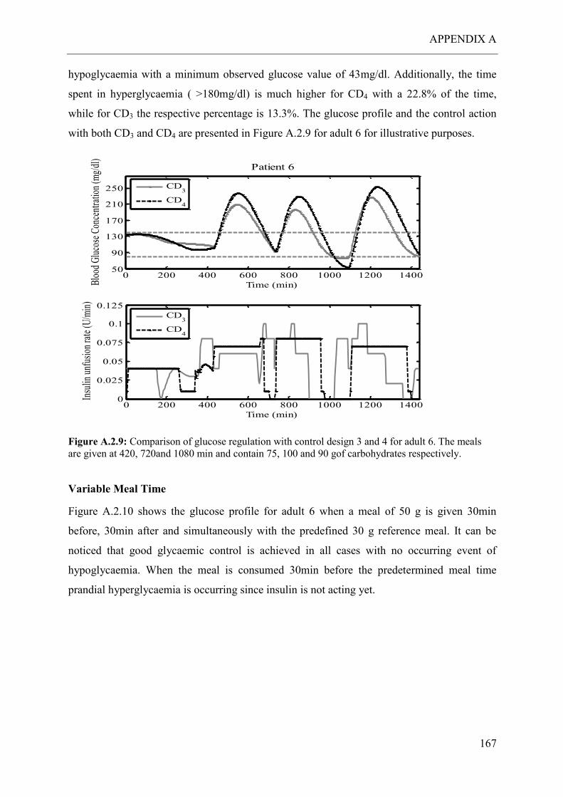
APPENDIX A
167
hypoglycaemia with a minimum observed glucose value of 43mg/dl. Additionally, the time
spent in hyperglycaemia ( >180mg/dl) is much higher for CD4 with a 22.8% of the time,
while for CD3 the respective percentage is 13.3%. The glucose profile and the control action
with both CD3 and CD4 are presented in Figure A.2.9 for adult 6 for illustrative purposes.
Figure A.2.9: Comparison of glucose regulation with control design 3 and 4 for adult 6. The meals
are given at 420, 720and 1080 min and contain 75, 100 and 90 gof carbohydrates respectively.
Variable Meal Time
Figure A.2.10 shows the glucose profile for adult 6 when a meal of 50 g is given 30min
before, 30min after and simultaneously with the predefined 30 g reference meal. It can be
noticed that good glycaemic control is achieved in all cases with no occurring event of
hypoglycaemia. When the meal is consumed 30min before the predetermined meal time
prandial hyperglycaemia is occurring since insulin is not acting yet.
0 200 400 600 800 1000 1200 140050
90
130
170
210
250
Time (min)Blo
od G
luco
se C
once
ntra
tion
(mg/
dl)
Patient 6
CD3
CD4
0 200 400 600 800 1000 1200 14000
0.025
0.05
0.075
0.1
0.125
Time (min)
Insu
lin u
nfus
ion
rate
(U/m
in)
CD3
CD4
APPENDIX A
168
Figure A.2.10: Evaluation of CD3 when a meal of 50 g is given 30min in advance, 30 min after and
simultaneous with the reference meal of 30 g
C. Concluding Remarks
The closed loop control validation studies show that the proposed control design CD3 can
efficiently regulate the blood glucose concentration when tested for large meal sizes. There is
no reported event of hypoglycaemia while the mean maximum glucose value being 226
mg/dl. When this control design is compared with CD4 it becomes obvious that superior
control can be achieved when the feed forward action of the MPC controller is enhanced in
the presence of unknown meal disturbances. Further closed loop validation studies are
required to verify the reliability of the proposed control performance. Hence, the proposed
control strategy can be regarded as a potential strategy to compensate for the unknown meal
disturbances since the validation studies performed for the UVa/Padova Simulation model as
well as the proposed model, shown in Chapter 6, indicate promising closed loop glucose
regulation.
0 200 400 600 800 1000 1200 140060
100
140
180
Time (min)
Blo
od G
luco
se C
once
ntra
tion
(m
g/dl
)
0 200 400 600 800 1000 1200 14000
0.025
0.05
0.075
0.1
Time (min)
Insu
lin
unfu
sion
rat
e (U
/min
)
30min before
30min after
simultanously
30min before
30min after
simultanously

APPENDIX B
169
APPENDIX B
B.1 Parameter Estimation
The estimated parameters for each patient are presented in detail in the following tables. The
reported confidence interval for each value is a measure of the estimated precision, indicating
that the smaller the interval the more reliable the estimated value is.
Table B.1: The optimal estimated values for each parameter for the 10 patients and the corresponding (95%)
confidence interval that indicates that there is 0.95 probability the value of the parameter to be within the
interval
Patient k1 k2 kelim ksub Vdist ru,L
Estimate 6.29E-05 1.17E-02 8.96E-01 1.21E-02 2.24E-02 0.15
1 SD 1.18E-06 4.37E-04 1.44E-01 3.08E-05 3.58E-03 3.74E-02
CI (±2.32E-06) (±8.57E-04) (±2.81E-01) (±6.04E-05) (±7.03E-03) (±0.073)
Estimate 1.09E-04 1.42E-02 1.35E+00 2.04E-02 1.00E-02 0.22
2 SD 1.59E-06 2.45E-04 1.14E-01 2.75E-05 8.51E-04 0.036
CI (±3.12E-06) (±4.79E-04) (±2.24E-01) (±5.40E-05) (±1.67E-03) (±0.051)
Estimate 2.67E-04 4.53E-02 3.00E-01 1.88E-02 5.16E-02 0.12
3 SD 6.03E-06 1.06E-03 2.83E-03 1.17E-05 4.88E-04 1.20E-02
CI (±1.188E-05) (±2.09E-03) (±5.56E-03) (±2.31E-05) (±9.61E-04) (±0.002)
Estimate 2.74E-04 2.22E-02 1.97E+00 1.97E-02 1.00E-02 0.11
4 SD 2.20E-05 2.05E-03 8.32E-02 8.71E-06 4.23E-04 4.70E-03
CI (±4.33E-05) (±4.03E-03) (±1.63E-01) (±1.71E-05) (±8.30E-04) (±0.009)
Estimate 4.59E-05 1.63E-02 1.34E+00 1.94E-02 1.01E-02 0.17
5 SD 1.98E-06 1.62E-03 1.10E-01 2.47E-05 8.31E-04 1.20E+02
CI (±3.88E-06) (±3.17E-03) (±2.15E-01) (±4.85E-05) (±1.63E-03) (±0.042)
Estimate 1.79E-04 3.40E-02 2.14E+00 1.51E-02 1.03E-02 0.06
6 SD 8.44E-06 1.62E-03 1.06E-01 5.79E-06 5.10E-04 4.70E+00
CI (±1.68E-05) (±3.18E-03) (±2.09E-01) (±1.14E-05) (±1.00E-03) (±0.001)
Estimate 3.83E-04 2.94E-02 1.47E+00 1.66E-02 1.00E-02 0.19
7 SD 2.19E-05 1.69E-03 7.83E-02 1.05E-05 5.32E-04 2.90E-02
CI (±4.29E-05) (±3.32E-03) (±1.54E-01) (±2.06E-05) (±1.04E-03) (±0.057)
Estimate 1.56E-04 2.07E-02 1.21E+00 1.96E-02 1.00E-02 0.19
8 SD 2.80E-05 3.29E-03 5.61E-02 1.52E-05 4.64E-04 6.84E-03
CI (±5.51E-05) (±6.45E-03) (±1.10E-01) (±2.98E-05) (±9.10E-04) (±0.13)
Estimate 2.11E-05 1.66E-02 1.13E+00 2.46E-02 1.00E-02 0.07
9 SD 2.79E-06 2.34E-03 1.85E-02 9.23E-06 1.64E-04 5.43E-03
CI (±5.47E-06) (±4.59E-03) (±3.62E-02) (±1.81E-05) (±3.22E-04) (±0.001)
Estimate 7.86E-05 2.44E-02 1.76E+00 1.98E-02 1.00E-02 0.17
10 SD 1.37E-05 3.89E-03 1.12E-01 1.53E-05 6.35E-04 3.24E-02
CI (±2.69E-05) (±7.63E-03) (±2.19E-01) (±2.99E-05) (±1.25E-03) (±0.063)
Mean ± SD 1.58E-04
±1.18E-04
2.35E-02
±1.03E-02
1.36E+00
±7.26E-01
1.86E-02
±4.48E-03
1.54E-02
±1.80E-02
1.7E-1
±0.07

APPENDIX B
170
Table B.2: The optimal estimated values for sub model EGP for the 10 patients, the
standard deviation and the confidence interval
ki kp1 kp2 kp3
Estimate 3.58E-03 6.52E+00 6.12E-03 2.08E-02
1 SD 6.34E-05 2.28E-02 1.34E-04 1.42E-04
CI (±1.24E-04) (±4.46E-02) (±2.63E-04) (±2.79E-04)
Estimate 2.94E-03* 5.03E+00 6.13E-03 1.13E-02
2 SD 2.17E-02 1.03E-04 1.03E-04
CI (±4.25E-02) (±2.02E-04) (±2.01E-04)
Estimate 1.30E-02 5.26E+00 2.44E-03* 1.08E-02
3 SD 7.81E-05 6.52E-03 2.48E-05
CI (±1.53E-04) (±1.28E-02) (±4.86E-05)
Estimate 1.34E-02 7.19E+00 2.44E-03* 2.39E-02*
4 SD 3.66E-04 4.93E-02
CI (±7.17E-04) (±9.67E-02)
Estimate 8.18E-03 4.00E+00 7.72E-03 6.64E-03
5 SD 2.15E-04 6.49E-02 3.78E-04 2.69E-04
CI (±4.21E-04) (±1.27E-01) (±7.40E-04) (±5.27E-04)
Estimate 1.19E-02 6.53E+00 2.44E-03 1.70E-02
6 SD 1.07E-04 1.37E-02 5.76E-05
CI (±2.11E-04) (±2.69E-02) (±1.13E-04)
Estimate 1.24E-02 7.20E+00* 2.44E-03* 2.39E-02*
7 SD 1.69E-04
CI (±3.31E-04)
Estimate 4.44E-03 6.42E+00 6.01E-03 2.17E-02
8 SD 2.56E-04 7.99E-01 3.10E-03 2.46E-03
CI (±5.02E-04) (±1.57E+00) (±6.08E-03) (±4.82E-03)
Estimate 4.32E-03 3.97E+00 6.63E-03 7.62E-03
9 SD 9.26E-05 5.63E-02 2.50E-04 1.19E-04
CI (±1.82E-04) (±1.10E-01) (±4.89E-04) (±2.33E-04)
Estimate 7.29E-03 4.35E+00 4.99E-03 5.51E-03
10 SD 9.23E-04 4.93E-01 1.55E-03 5.79E-04
CI (±1.81E-03) (±9.66E-01) (±3.03E-03) (±1.13E-03)
Mean ± SD 8.15E-03
±4.23E-03
5.65E+00
±1.28E+00
4.73E-03
±2.09E-03
1.49E-02
±7.35E-03
*Optimal value at bound

APPENDIX B
171
*Optimal value at bound
Table B.3: The optimal estimated values for sub model Ra for the 10 patients, the standard
deviation and the confidence interval
b D kabs kmax kmin
Estimate 8.80E-01 2.93E-01 5.82E-01* 2.19E-02* 4.55E-03
1 SD 9.91E-04 7.88E-04 2.01E-05
CI (±1.94E-03) (±1.55E-03) (±3.93E-05)
Estimate 7.47E-01 2.00E-01 2.14E-02* 3.04E-02 1.04E-02
2 SD 8.79E-03 4.84E-03 4.83E-04 1.53E-04
CI (±1.72E-02) (±9.49E-03) (±9.46E-04) (±2.99E-04)
Estimate 8.50E-01 1.88E-01 3.25E-02 5.82E-02* 5.72E-03
3 SD 3.08E-03 9.28E-04 6.79E-04 3.48E-05
CI (±6.04E-03) (±1.82E-03) (±1.33E-03) (±6.82E-05)
Estimate 7.36E-01 1.75E-01 5.31E-01 2.51E-02 8.93E-03
4 SD 7.62E-03 6.59E-03 1.43E-01 4.72E-04 2.21E-04
CI (±1.49E-02) (±1.29E-02) (±2.80E-01) (±9.26E-04) (±4.34E-04)
Estimate 7.71E-01 2.01E-01 2.21E-02 4.47E-02 5.03E-03
5 SD 8.71E-03 4.47E-03 1.45E-03 2.62E-03 1.58E-04
CI (±1.71E-02) (±8.76E-03) (±2.85E-03) (±5.14E-03) (±3.11E-04)
Estimate 8.15E-01 1.09E-01 2.14E-02* 4.32E-02 1.16E-02
6 SD 1.39E-02 3.72E-03 2.16E-03 1.27E-04
CI (±2.72E-02) (±7.28E-03) (±4.23E-03) (±2.49E-04)
Estimate 9.29E-01 1.73E-01 2.14E-02* 2.19E-02* 9.63E-03
7 SD 1.83E-03 2.84E-03 9.72E-05
CI (±3.59E-03) (±5.57E-03) (±1.91E-04)
Estimate 8.60E-01 1.38E-01 4.71E-02 2.81E-02 5.73E-03
8 SD 1.28E-02 8.56E-03 5.53E-03 2.14E-03 2.42E-04
CI (±2.51E-02) (±1.68E-02) (±1.09E-02) (±4.20E-03) (±4.75E-04)
Estimate 8.25E-01 3.32E-01 8.34E-02 2.36E-02 3.73E-03
9 SD 8.16E-03 1.23E-02 7.21E-03 8.05E-04 1.41E-04
CI (±1.60E-02) (±2.41E-02) (±1.41E-02) (±1.58E-03) (±2.76E-04)
Estimate 8.54E-01 9.82E-02 4.40E-02 5.61E-02 1.09E-02
10 SD 1.59E-02 7.87E-03 9.05E-03 8.30E-03 3.70E-04
CI (±3.12E-02) (±1.54E-02) (±1.77E-02) (±1.63E-02) (±7.26E-04)
Mean ± SD 8.27E-01
±6.10E-02
1.91E-01
±7.40E-02
1.41E-01
±2.20E-01
3.53E-02
±1.41E-02
7.62E-03
±2.95E-03

APPENDIX B
172
B.2 MPC to QP
The MPC problem, as presented in section 5.4, is formulated in:
minx,y,u
𝐽 = ∑ xk′ Qkxk
N−1
k=1
+ ∑(yk − ykR)
′QRk(yk − yk
R)
N−1
k=1
+ ∑ uk′ Rkuk
M−1
k=1
+ ∑ Δuk′ R1kΔuk
M−1
k=1
s.t
xk+1 = Axk + Buk + Edk A.4.1
yk = Cxk A.4.2
The prediction of y is obtained by the iteration of the model A.4.1-A.4.2 that can be written in
matrix –vector form:
[ 𝑥1𝑥2𝑥3⋮𝑥𝑁]
=
[ 𝐴𝐴2
𝐴3
⋮𝐴𝑁]
𝑥0 +
[
𝐵 0 … 0 0𝐴𝐵 𝐵 … 0 0𝐴2𝐵 𝐴𝐵 … 0 0⋮ ⋮ … … …
𝐴𝑁−1𝐵 𝐴𝑁−2𝐵 … 𝐴𝐵 𝐵]
[ 𝑢0𝑢1𝑢2⋮
𝑢𝑁−1]
+
[
𝐸 0 … 0 0𝐴𝐸 𝐸 … 0 0𝐴2𝐸 𝐴𝐸 … 0 0⋮ ⋮ … … …
𝐴𝑁−1𝐸 𝐴𝑁−2𝐸 … 𝐴𝐸 𝐸]
[ 𝑑0𝑑1𝑑3⋮
𝑑𝑁−1]
The predictions of y are obtained by:
[ 𝑦1𝑦2𝑦3⋮𝑦𝑁]
= [
𝐶 0 … 00 𝐶 … 0⋮ ⋮ ⋱ ⋮0 0 … 𝐶
]
[ 𝑥1𝑥2𝑥3⋮𝑥𝑁]
Hence, in a general form:
Y=Φx0+ΓU+ΓdD A.4.4
Where:
�̅� ∈ ℝ𝑁𝑛𝑥×𝑛𝑥0
�̅� ∈ ℝ𝑁𝑛𝑥×𝑁𝑛𝑑 𝐷
A.4.3
�̅� ∈ ℝ𝑁𝑛𝑥×𝑁𝑛𝑢

APPENDIX B
173
Φ=
[ 𝐶𝐴𝐶𝐴2
𝐶𝐴3
⋮𝐶𝐴𝑁]
∈ ℝ𝑁𝑛𝑥×1, Γ=
[
𝐶𝐵 0 … 0 0𝐶𝐴𝐵 𝐶𝐵 … 0 0𝐶𝐴2𝐵 𝐶𝐴𝐵 … 0 0⋮ ⋮ … … …
𝐶𝐴𝑁−1𝐵 𝐶𝐴𝑁−2𝐵 … 𝐶𝐴𝐵 𝐶𝐵]
∈ ℝ𝑁𝑛𝑥×𝑁𝑛𝑦, and
Γd=
[
𝐶𝐸 0 … 0 0𝐶𝐴𝐸 𝐶𝐸 … 0 0𝐶𝐴2𝐸 𝐶𝐴𝐸 … 0 0⋮ ⋮ … … …
𝐴𝐶𝑁−1𝐸 𝐶𝐴𝑁−2𝐸 … 𝐶𝐴𝐸 𝐶𝐸]
∈ ℝ𝑁𝑛𝑑×𝑁𝑛𝑦
R is introduced to include the setpoints:
R=
[ 𝑦1𝑅
𝑦2𝑅
𝑦3𝑅
⋮𝑦𝑁𝑅]
The weighing matrices Q, R, QR and R1 are given by:
�̅� = 𝑑𝑖𝑎𝑔(𝑄,… , 𝑄, 𝑃) ∈ ℝ𝑁𝑛𝑥×𝑁𝑛𝑥
�̅� = 𝑑𝑖𝑎𝑔(𝑅,… , 𝑅) ∈ ℝ𝑀𝑛𝑢×𝑀𝑛𝑢
𝑄𝑅̅̅ ̅̅ = 𝑑𝑖𝑎𝑔(𝑄𝑅,… , 𝑄𝑅) ∈ ℝ𝑁𝑛𝑦×𝑁𝑛𝑦
𝑅1̅̅ ̅ = 𝑑𝑖𝑎𝑔(𝑅1, … , 𝑅1) ∈ ℝ𝑀𝑛𝑢×𝑀𝑛𝑢
The objective function is written as:
minx,y,u
𝐽 = 𝜑𝑥 + 𝜑𝑦 + 𝜑𝑢 + 𝜑𝛥𝑢
Where:
𝜑𝑥 = X′Q̅X
𝜑𝑦 = (Y − R)′QR̅̅ ̅̅ (Y − R)
𝜑𝑢 = U′R̅U
𝜑𝛥𝑢 = 𝛥𝑈′𝑅1̅̅ ̅𝛥𝑈
Hence, the problem is formulated as a QP problem, (Rawlings and Mayne, 2009),
(Maciejowski, 2002):

APPENDIX B
174
States
𝜑𝑥 = (�̅�𝑥0 + �̅�𝑈 + �̅�𝐷)′�̅�(�̅�𝑥0 + �̅�𝑈 + �̅�𝐷)
= (�̅�𝑈 + 𝑏)′�̅�(�̅�𝑈 + 𝑏) With 𝑏 = �̅�𝑥0 + �̅�𝐷
= (𝑈′�̅�′ + 𝑏′)�̅�(�̅�𝑈 + 𝑏) = 𝑈′𝐵′̅̅ ̅�̅��̅�𝑈 + 𝑏′�̅��̅�𝑈 + 𝑈′�̅�′�̅�𝑏 + 𝑏′�̅�𝑏
= 𝑈′�̅�′�̅��̅�𝑈 + 2(𝑏′�̅��̅�)𝑈 + 𝑏′�̅�𝑏 = 𝑈′[�̅�′�̅��̅�]𝑈 + [2𝑏′�̅��̅�]𝑈 + 𝑏′�̅�𝑏
𝐻𝑥 = �̅�′�̅��̅�
𝐺𝑥 = 2𝑏′�̅��̅� = 2(�̅�𝑥0 + �̅�𝐷)′�̅��̅� = 𝑁𝑥𝑥0 + 𝑁𝑑𝐷
With 𝑁𝑥 = 2�̅�′�̅��̅� and 𝑁𝑑 = 2(�̅�)′�̅��̅�
Output tracking error
𝜑𝑦 = (𝑌 − 𝑅)′𝑄𝑅̅̅ ̅̅ (𝑌 − 𝑅) = (𝛷𝑥0 + 𝛤𝑈 + 𝛤𝑑𝐷 − 𝑅)′𝑄𝑅̅̅ ̅̅ (𝛷𝑥0 + 𝛤𝑈 + 𝛤𝑑𝐷 − 𝑅)
= (𝛤𝑈 − (𝑅 − 𝛷𝑥0 − 𝛤𝑑𝐷))′𝑄𝑅̅̅ ̅̅ ((𝛤𝑈 − (𝑅 − 𝛷𝑥0 − 𝛤𝑑𝐷)) With 𝑏𝑦 = 𝑅 −𝛷𝑥0 −
𝛤𝑑𝐷
= (𝑈′𝛤′ − 𝑏𝑦′ )𝑄𝑅̅̅ ̅̅ (𝛤𝑈 − 𝑏𝑦)
= 𝑈′𝛤′𝑄𝑅̅̅ ̅̅ 𝛤𝑈 − 𝑏𝑦′𝑄𝑅̅̅ ̅̅ 𝛤𝑈 − 𝑈′𝛤′𝑄𝑅̅̅ ̅̅ 𝑏𝑦 + 𝑏𝑦
′𝑄𝑅̅̅ ̅̅ 𝑏𝑦 = 𝑈′[𝛤′𝑄𝑅̅̅ ̅̅ 𝛤]𝑈 − [2𝑏𝑦′𝑄𝑅̅̅ ̅̅ 𝛤]𝑈 +
𝑏𝑦′𝑄𝑅̅̅ ̅̅ 𝑏𝑦
𝐻𝑦 = 𝛤′𝑄𝑅̅̅ ̅̅ 𝛤
𝐺𝑦 = 2𝑏𝑦′𝑄𝑅̅̅ ̅̅ 𝛤 = 2(𝑅 − 𝛷𝑥0 − 𝛤𝑑𝐷)
′𝑄𝑅̅̅ ̅̅ 𝛤 = 𝛭𝜒𝜒0 +𝑀𝑑𝐷
With 𝑀𝑥 = −2𝛷′𝑄𝑅̅̅ ̅̅ 𝛤 and 𝛭𝑑 = −2𝛤𝑑′𝑄𝑅̅̅ ̅̅ 𝛤
Input
𝜑𝑢 = U′R̅U
𝐻𝑢 = �̅�
Input step change

APPENDIX B
175
𝛥𝑈 = [𝛥𝑢0 𝛥𝑈1…𝛥𝑢𝑀−1]′
Δu0 is defined as u-1-u0
𝛥𝑈 =
[ 1 0 0 … 0 0−1 1 0 ⋯ 0 00 −1 1 … 0 0⋮ ⋮ ⋮ ⋱ 0 ⋮0 0 0 ⋯ −1 1]
𝑈 +
[ −100⋮0 ]
𝑢−1
𝐻𝛥𝑢 = 𝐻𝑅1′𝑅1𝐻𝑅1
𝐺𝛥𝑢 = 𝐺𝑅1′𝑅1𝐺𝑅1
Hence the MPC problem is reformulated in the general QP problem:
min𝑈 𝐽 =1
2𝑈′𝐻𝑈 + 𝐺𝑄𝑃
′ 𝑈 + 𝑐 A.4.4
With
𝐻 = 𝐻𝑥 + 𝐻𝑢 +𝐻𝑦 + 𝐻𝛥𝑢
𝐺𝑄𝑃 = 𝐺𝑥 + 𝐺𝑢 + 𝐺𝑦 + 𝐺𝛥𝑢
Constraints
Constraints are imposed on the input, u, the output y, and the input step change Δu. In the QP
formulation they are expressed as:
𝐺𝑈 ≤ 𝑊 A.4.5
Constraints on the states
𝑋𝑚𝑖𝑛 ≤ 𝑥1, 𝑥2. . 𝑥𝑁 ≤ 𝑋𝑚𝑎𝑥
With 𝑋𝑚𝑖𝑛 = [
𝑥𝑚𝑖𝑛
𝑥𝑚𝑖𝑛
⋮𝑥𝑚𝑖𝑛
], 𝑋𝑚𝑎𝑥 = [
𝑥𝑚𝑎𝑥
𝑥𝑚𝑎𝑥
⋮𝑥𝑚𝑎𝑥
]
But using A.4.3, it becomes:
𝐻𝑅1
𝐺𝑅1

APPENDIX B
176
[ �̅�−�̅�
]𝑈 ≤ [𝑋𝑚𝑎𝑥
−𝑋𝑚𝑖𝑛] + [−�̅�
𝐴] 𝑥0 + [−�̅�
�̅�] 𝐷
Constraints on the outputs
𝑌𝑚𝑖𝑛 ≤ 𝑦1, 𝑦2. . 𝑦𝑁 ≤ 𝑌𝑚𝑎𝑥
With 𝑌𝑚𝑖𝑛 = [
𝑦𝑚𝑖𝑛
𝑦𝑚𝑖𝑛
⋮𝑦𝑚𝑖𝑛
], 𝑌𝑚𝑎𝑥 = [
𝑦𝑚𝑎𝑥
𝑦𝑚𝑎𝑥
⋮𝑦𝑚𝑎𝑥
]
Using A.4.4, we have:
[ 𝛤−𝛤
]𝑈 ≤ [𝛶𝑚𝑎𝑥
−𝛶𝑚𝑖𝑛] + [
−𝛷𝛷
] 𝑥0 + [−𝛤𝑑𝛤𝑑
] 𝐷
Constraints on the inputs
𝑈𝑚𝑖𝑛 ≤ 𝑢0, 𝑢1, . . 𝑢𝑁 ≤ 𝑈𝑚𝑎𝑥
Which is written as:
[𝐼−𝐼
]𝑈 ≤ [𝑈𝑚𝑎𝑥
−𝑈𝑚𝑖𝑛]
With 𝑈𝑚𝑖𝑛 = [
𝑢𝑚𝑖𝑛
𝑢𝑚𝑖𝑛
⋮𝑢𝑚𝑖𝑛
], 𝑈𝑚𝑎𝑥 = [
𝑢𝑚𝑎𝑥
𝑢𝑚𝑎𝑥
⋮𝑢𝑚𝑎𝑥
]
Constraints on the input step change
𝛥𝑈𝑚𝑖𝑛 ≤ 𝛥𝑢0, 𝛥𝑢1, . . 𝛥𝑢𝑁 ≤ 𝛥𝑈𝑚𝑎𝑥
[𝛨𝑅1
−𝐻𝑅1] 𝛥𝑈 ≤ [
𝛥𝑈𝑚𝑎𝑥
−𝛥𝑈𝑚𝑖𝑛] + [
𝐺𝑅1−𝐺𝑅1
] 𝑢−1

APPENDIX C
177
APPENDIX C
Multi parametric MPC is an ideal control method for drug delivery applications and in
particular for the system of automated insulin delivery for T1DM. The ability to obtain the
control actions, as functions of the patient measurements, on-line via simple function
evaluations makes the mpMPC suitable for portable applications (Pistikopoulos et al., 2002),
(Pistikopoulos, Georgiadis and Dua, 2007b), (Pistikopoulos, Georgiadis and Dua, 2007a) In
essence, in mpMPC the online solution of the optimisation problem is replaced by the off line
derivation of the explicit mapping of the optimal decisions in the space of the plant
uncertainty. mpMPC is applied in the context of Optimisation and Correction MPC (Control
design 3) presented in Section 6.4.3. The framework is illustrated in Figure.C.1:
Figure C.1: Proposed framework for closed loop insulin delivery (see section 6.4.3)
An example is illustrated for adult 6. The virtual patient is the UVa/Padova Simulator. A
nominal mp-MPC is designed using the linear state-space model presented in Appendix A.2
with estimated states:
�̂� = [𝐺𝑝 𝐺𝑡 𝑋𝑑𝑖𝑠𝑝 𝐼𝑑𝑒𝑙1 𝐼𝑑𝑒𝑙2 𝐼𝑠𝑐1 𝐼𝑝 𝑑]′
The exact formulation of section 6.4.3 is applied here.
The MPC problem is given in equation 6.8. The explicit solution of the quadratic problem
(QP) (Bemporad et al., 2002) is obtained:
min𝑈 𝐽(𝜃) =1
2𝑈′𝐻𝑈 + 𝜃′𝐹𝑈 +
1
2𝜃′𝑌𝜃 (C.1)
s.t. 𝐺𝑈 ≤ 𝑊 + 𝐸𝜃

APPENDIX C
178
For the specific example the parameters θ of the mp-QP problem are defined as:
𝜃 = [𝐺𝑝 𝐺𝑡 𝑋𝑑𝑖𝑠𝑝 𝐼𝑑𝑒𝑙1 𝐼𝑑𝑒𝑙2 𝐼𝑠𝑐1 𝐼𝑝 𝑑 𝐺 𝑦𝑠𝑒𝑡]
The multi-parametric Quadratic Programming (mp-QP) problem and can be solved with
standard multi-parametric programming techniques (Pistikopoulos, Georgiadis and Dua,
2007b).In this study, Parametric Optimization Software was used (Parametric Optimization
Solutions (ParOS) Ltd, 2003) to obtain the explicit controller description, which is the
optimal map of the control variables as function of the parameters of the system. This optimal
map consists of 8 critical regions and the corresponding control laws. Each of the critical
regions is described by a number of linear inequalities Aix ≤ bi for 𝑖 ∈ {1… , 𝑛𝐶𝑅} , where nCR
is the number of critical regions and the corresponding control lows are piecewise linear
functions of the parameters: U = Ki θ + ci, where i is the index of solutions.
The performance of the controller is illustrated in the following graph:
Figure C.2: Performance of mpMPC controller for adult 6, when 45, 80 and 70 g of
carbohydrates are consumed at 420, 720 and 1080 min
Glucose regulation is achieved with 92.7% of the time spent between 80 and 180mg/dl and no
event of hypoglycaemia occurs.
Figure C.3 shows the performance of the controller in the case of a skipped meal at 720 min.
We can see that 12.8% of time is spent in hypoglycaemia with a minimum glucose value of
0 200 400 600 800 1000 1200 140050
70
90
110
130
150
170
190
Time (min)
Glu
co
se (
mg
/dl)
0 200 400 600 800 1000 1200 14000
0.025
0.05
0.075
0.1
0.125
0.15
Time (min)
Insu
lin
(U
/min
)

APPENDIX C
179
50mg/dl. It is obvious that further improvement of the control specifications is required to
prevent the deep drop in glucose concentration.
Figure C.3: Skipped meal at 720 min. Breakfast 45 g and lunch 60 g at 420 and 1080 min
An example of the function to obtain the control law and the description of the CR is
presented below:
---------- Feasible region 7 ---------- U1 = -7.49397*Gp +6.48152*Gt -0.800111*xdisp -0.597714*Idel1 -0.0377123*Idel2 -0.00655881*Isc1 -
2.9359*Ip +399.73*d +35.048*G -35.048*Gp0 -0.000779129 U2 = +0.02 -0.0187475*Gp +0.0162147*Gt -0.00200163*xdisp -0.00149529*Idel1 -9.43444e-05*Idel2 -1.64081e-
05*Isc1 -0.00734469*Ip +1*d +0.0876791*G -0.0876791*Gp0 <= +5.19828e-05 +0.0187475*Gp -0.0162147*Gt +0.00200163*xdisp +0.00149529*Idel1 +9.43444e-05*Idel2 +1.64081e-
05*Isc1 +0.00734469*Ip -1*d -0.0876791*G +0.0876791*Gp0 <= -1.94914e-06 +0.00487771*Gp -0.00437426*Gt +0.00024091*xdisp +0.000336128*Idel1 +9.02606e-06*Idel2
+7.02158e-08*Isc1 +0.00030467*Ip -0.199185*d -0.0350229*G +1*Gp0 <= +48.2489 +0.0241355*Gp -0.0216076*Gt +0.00125817*xdisp +0.0016757*Idel1 +4.83288e-05*Idel2 +1.33944e-
06*Isc1 +0.00188703*Ip -1*d -0.170413*G -0.00718897*Gp <= +0.888008 -0.0244884*Gp +0.0219608*Gt -0.00120948*xdisp -0.00168752*Idel1 -4.5315e-05*Idel2 -3.52516e-
07*Isc1 -0.00152959*Ip +1*d +0.175831*G -0.175831*Gp0 <= -0.000168087 -1*Gp <= +50 +1*Gp <= +250 -1*Gt <= +50 +1*Gt <= +300 -1*xdisp <= +700 +1*xdisp <= +100 -1*Idel1 <= +50 +1*Idel1 <= +100
0 200 400 600 800 1000 1200 140050
70
90
110
130
150
170
190
Time (min)
Glu
co
se (
mg
/dl)
0 200 400 600 800 1000 1200 14000
0.025
0.05
0.075
0.1
0.125
0.15
Time (min)
Insu
lin
(U
/min
)

APPENDIX C
180
-1*Idel2 <= +50 +1*Idel2 <= +100 -1*Isc1 <= +50 +1*Isc1 <= +150 -1*Ip <= +50 +1*Ip <= +80 -1*G <= +10 +1*G <= +10
Concluding Remarks
The advantages of using mpMPC control method in drug delivery systems are summarised:
Suitable for portable applications
Testing off-line of different scenarios to ensure the patient’s safety
Advantages of MPC over other control designs
Further in-silico validation is required to improve the mpMPC performance in the context of
the proposed framework.

APPENDIX D
181
APPENDIX D
Table D.1: MPC tuning parameters and specifications for CD2 CD3 and CD4
Adult1 Adult2 Adult3 Adult4 Adult5 Adult6 Adult7 Adult8 Adult9 Adult10
ts (min) 5 5 5 5 5 5 5 5 5 5
N (min) 65 55 35 50 65 50 40 55 70 65
M(min) 60 40 30 40 40 45 35 50 40 40
CD3
QR 100000 100000 10000 100000 100000 1000 10000 100000 100000 1000000
R 1 0.01 0.001 1 0.01 0.001 1 1 0.001 0.01
R1 1 0.01 1 1 0.01 0.01 1 1 0.001 1
umax
(U/min) 0.2TDD 0.2TDD 0.2TDD 0.2TDD 0.2TDD 0.2TDD 0.2TDD 0.2TDD 0.2TDD 0.2TDD
umin
(U/min) 0 0 0 0 0 0 0 0 0 0
ymax
(mg/dl) 10 10 10 10 10 10 10 10 10 10
ymin
(mg/dl) -10 -10 -10 -10 -10 -10 -10 -10 -10 -10
CD2 - CD4
QR 100000 10000 10000 1000 100000 1000 100000 100000 1000 100000
R 0.1 0.001 0.001 0.0001 0.01 0.001 0.001 0.01 0.001 0.001
R1 0.05 0.001 0.001 0.0001 0.01 0.001 0.0 0.01 0.01 0.001
Δumax
(U/min) 0.01 0.01 0.01 0.008 0.01 0.01 0.008 0.008 0.008 0.008
Δumin
(U/min) -0.01 -0.01 -0.01 -0.005 -0.01 -0.01 -0.005 -0.005 -0.005 -0.005
umax-CD2
(U/min) 0.1 0.15 0.1 0.05 0.15 0.1 0.08 0.1 0.1 0.12
umax CD4
(U/min) - - - - - - - - - -
umin
(U/min) 0 0 0 0 0 0 0 0 0 0
ymax
(mg/dl) 140 140 140 140 140 140 140 140 140 140
ymin
(mg/dl) 80 80 80 80 80 80 80 80 80 80

Bibliography
182
Bibliography
Abu-Rmileh, A., Garcia-Gabin, W. and Zambrano, D. (2010) ‘A robust sliding mode
controller with internal model for closed-loop artificial pancreas.’, Medical & biological
engineering & computing, 48(12), pp. 1191–201.
Ackland, T. R., Elliott, B. and Bloomfield, J. (2009) Applied Anatomy and Biomechanics in
sport. 2nd edn, Choice Reviews Online.. Champaign, IL : Human Kinetics, pp.67-85
Akaike, H. (1974) ‘A New Look at the Statistical Model Identification’, IEEE Transactions
on Automatic Control, AC-16(6), pp. 716–723.
American Diabetes Association (2008) ‘Diagnosis and classification of diabetes mellitus’,
Diabetes care, 31 Suppl 1, pp. S55–60.
Atlas, E., Nimri, R., Miller, S., Grunberg, E. and Phillip, M. (2010) ‘MD-Logic Artificial
Pancreas System A pilot study in adults with type 1 diabetes’, Diabetes Care, 33, pp. 1072–
1076.
Bemporad, A., Borrelli, F. and Morari, M. (2003) ‘Min–Max Control of Constrained
Uncertain Discrete-Time Linear Systems’, IEEE Transactions on Automatic Control, 48(9),
pp. 1600–1606.
Bemporad, A. and Morari, M. (1999) ‘Robust Model Predictive Control : A Survey
Optimizer’, Lecture Notes in Control and Information Sciences, 245, pp. 207–226.
Bemporad, A., Morari, M., Dua, V. and Pistikopoulos, E. N. (2002) ‘The explicit linear
quadratic regulator for constrained systems’, Automatica, 38, pp. 3–20.
Bennett, D. L. and Gourley, S. A. (2004) ‘Asymptotic properties of a delay differential
equation model for the interaction of glucose with plasma and interstitial insulin’, Applied
Mathematics and Computation, 151(1), pp. 189–207.
Bequette, B. W. (2005) ‘A Critical Assessment of Algorithms and Challenges in the
Development of a Closed-Loop Artificial Pancreas’, Diabetes Technology & Therapeutics,
7(1), pp. 28–47.
Bequette, B. W. (2012) ‘Challenges and Recent Progress in the Development of a Closed-
loop Artificial Pancreas.’, Annual reviews in control. Elsevier Ltd, 36(2), pp. 255–266.
Berger, M. P. and Rodbard, D. (1991) ‘A pharmacodynamic approach to optimizing insulin
therapy.’, Computer methods and programs in biomedicine, 34(4), pp. 241–53.
Bergman, R. N., Phillips, L. S. and Cobelli, C. (1981) ‘Physiologic evaluation of factors
controlling glucose tolerance in man’, J. Clinic Investigation, 68, pp. 1456–1467.

Bibliography
183
Boden, G., Cheung, P. and Homko, C. (2003) ‘Effects of Acute Insulin Excess and
Deficiency on Gluconeogenesis and Glycogenolysis in Type 1 Diabetes’, Diabetes, 52.
Boiroux, D., Finan, D. a, Bagterp, J., Kjølstad, N. and Henrik, P. (2010) ‘Implications and
Limitations of Ideal Insulin Administration for People with Type 1 Diabetes’, in UKACC
International Conference on CONTROL. Coventry: IET, pp. 1–6.
Breton, M., Farret, A., Bruttomesso, D., Anderson, S., Magni, L., Patek, S., Dalla Man, C.,
Place, J., Demartini, S., Del Favero, S., Toffanin, C., Hughes-Karvetski, C., Dassau, E.,
Zisser, H., Doyle, F. J., De Nicolao, G., Avogaro, A., Cobelli, C., Renard, E. and Kovatchev,
B. (2012) ‘Fully integrated artificial pancreas in type 1 diabetes: modular closed-loop glucose
control maintains near normoglycemia.’, Diabetes, 61(9), pp. 2230–7.
Brown, B. E., Hopper, J., Hodges, J. L., Bradley, B., Wennesland, R. and Yamauchi, H.
(1962) ‘Red cell, plasma, and blood volume in healthy women measured by radiochromium
cell labeling and hematocrit’, Journal of Clinical Investigation, 41(12), pp. 2182–2190.
Cameron, F., Wilson, D. M., Buckingham, B. a, Arzumanyan, H., Clinton, P., Chase, H. P.,
Lum, J., Maahs, D. M., Calhoun, P. M. and Bequette, B. W. (2012) ‘Inpatient studies of a
Kalman-filter-based predictive pump shutoff algorithm.’, Journal of diabetes science and
technology, 6(5), pp. 1142–7.
Cano, N. (2002) ‘Bench-to-bedside review : Glucose production from the kidney’, Critical
Care, 6, pp. 317–321.
Cashman, J. R., Perotti, B. Y., Berkman, C. E. and Lin, J. (1996) ‘Pharmacokinetics and
molecular detoxication.’, Environmental health perspectives, 104 Suppl, pp. 23–40.
Castle, J. R., Engle, J. M., Youssef, J. El, Massoud, R., Yuen, K. C. J., Kagan, R. and Ward,
W. K. (2010) ‘Novel Use of Glucagon in a Closed-Loop System for Prevention of
Hypoglycemia in Type 1 Diabetes’, Diabetes Care, 33, pp. 1282–1287.
Caumo, A. and Cobelli, C. (1993) ‘Hepatic glucose production estimation by deconvolution
during the labeled IVGTT : with a new minimal model’, Modeling in physiology, 264(27), pp.
E829–E841.
Chait, A. and Bornfeldt, K. E. (2009) ‘Diabetes and atherosclerosis: is there a role for
hyperglycemia?’, Journal of lipid research, 50 Suppl, pp. S335–9.
Chen, C.-L. and Tsai, H.-W. (2010) ‘Modeling the physiological glucose-insulin system on
normal and diabetic subjects.’, Computer methods and programs in biomedicine, 97(2), pp.
130–40.
Chen, C.-L., Tsai, H.-W. and Wong, S.-S. (2010) ‘Modeling the physiological glucose-insulin
dynamic system on diabetics.’, Journal of theoretical biology. Elsevier, 265(3), pp. 314–22.
Chui, C. K. and Chen, G. (2008) Kalman Filtering. Edited by Springer. InTech.

Bibliography
184
Cobelli, C., Man, C. D., Sparacino, G., Magni, L., De Nicolao, G. and Kovatchev, B. P.
(2009) ‘Diabetes: Models, Signals, and Control.’, IEEE reviews in biomedical engineering, 2,
pp. 54–96.
Cobelli, C., Renard, E. and Kovatchev, B. (2011) ‘Artificial pancreas: past, present, future.’,
Diabetes, 60(11), pp. 2672–82.
Cobelli, C., Renard, E., Kovatchev, B. P., Keith-Hynes, P., Ben Brahim, N., Place, J., Del
Favero, S., Breton, M., Farret, A., Bruttomesso, D., Dassau, E., Zisser, H., Doyle III, F. J.,
Patek, S. D. and Avogaro, A. (2012) ‘Pilot Studies of Wearable Outpatient Artificial Pancreas
in Type 1 Diabetes’, Diabetes Care, 35(9), pp. 65–67.
Crone, C. (1965) ‘Facilitated Transfer of glucose from blood into brain tissue’, J. Physiol.,
181, pp. 103–113.
Dalla Man, C., Camilleri, M. and Cobelli, C. (2006) ‘A system model of oral glucose
absorption: validation on gold standard data.’, IEEE transactions on bio-medical engineering,
53(12 Pt 1), pp. 2472–8.
Dalla Man, C., Raimondo, D. M., Rizza, R. a and Cobelli, C. (2007) ‘GIM, simulation
software of meal glucose-insulin model.’, Journal of diabetes science and technology, 1(3),
pp. 323–30.
Dalla Man, C., Rizza, R. a and Cobelli, C. (2006) ‘Mixed meal simulation model of glucose-
insulin system.’, Annual International Conference of the IEEE Engineering in Medicine and
Biology Society. IEEE Engineering in Medicine and Biology Society. Conference, 1, pp. 307–
10.
Dalla Man, C., Rizza, R. and Cobelli, C. (2007) ‘Meal simulation model of glucose-insulin
system.’, IEEE Transactions on Biomedical Engineering, 54(10), pp. 1740–1749.
Dassau, E., Zisser, H., Harvey, R., Percival, M. W., Grosman, B., Bevier, W., Atlas, E.,
Miller, S., Nimri, R., Jovanovič, L. and Doyle III, F. J. (2013) ‘Clinical Evaluation of a
Personalized Artificial Pancreas’, Diabetes Care, 36(4), pp. 801–809.
Dauber, A., Corcia, L., Safer, J., Agus, M., Einis, S. and Steil, G. M. (2013) ‘Closed-Loop
Insulin Therapy Improves Glycemic Control in Children Aged<7 Years: A randomized
controlled trial’, Diabetes Care, 36, pp. 222–227.
Davis, S. N., Fowler, S. and Costa, F. (2000) ‘Hypoglycemic Counterregulatory Responses
Diffe r Between Men and Women With Type 1 Diabetes’, Diabetes, 49, pp. 65–72.
Deurenberg, P., Weststrate, J. A. and Seidell, J. C. (1991) ‘Body mass index as a measure of
body fatness : age- and sex- specific prediction formulas’, British Journal of Nutrition, 65, pp.
105–114.
Doyle, F. J., Huyett, L. M., Lee Bok, J., Zisser, H. and Dassau, E. (2014) ‘Closed-loop
artificial pancreas systems: engineering the algorithms.’, Diabetes care, 37(5), pp. 1191–7.

Bibliography
185
Doyle, F., Jovanovic, L. and Seborg, D. (2007) ‘Glucose control strategies for treating type 1
diabetes mellitus’, Journal of Process Control, 17(7), pp. 572–576.
Dua, P., Doyle, F. J. and Pistikopoulos, E. N. (2006) ‘Model-based blood glucose control for
Type 1 diabetes via parametric programming.’, IEEE transactions on bio-medical
engineering, 53(8), pp. 1478–91.
Dua, P., Doyle, F. J. and Pistikopoulos, E. N. (2009) ‘Multi-objective blood glucose control
for type 1 diabetes.’, Medical & biological engineering & computing, 47(3), pp. 343–52.
Dua, P., Kouramas, K., Dua, V. and Pistikopoulos, E. N. (2008) ‘MPC on a chip—Recent
advances on the application of multi-parametric model-based control’, Computers &
Chemical Engineering, 32(4-5), pp. 754–765.
Eckel, R. H. (2003) Obesity: Mechanisms and Clinical Management, Mayo Clinic
Proceedings. Philadelphia, USA: Lippincott Williams & Wilkins.
Ederle, J., Blanchard, S. and Bronzino, J. (2000) ‘Cardiovascular Mechanics’, in Ederle, J.,
Blanchard, S., and Bronzino, J. (eds) Introduction to biomedical engineering. San Diego:
Academic Press, pp. 467–536.
El-Khatib, F. H., Russell, S. J., Nathan, D. M., Sutherlin, R. G. and Damiano, E. R. (2010) ‘A
bihormonal closed-loop artificial pancreas for type 1 diabetes.’, Science translational
medicine, 2(27), p. 27ra27.
Elleri, D., Allen, J. M., Biagioni, M., Kumareswaran, K., Leelarathna, L., Caldwell, K.,
Nodale, M., Wilinska, M. E., Acerini, C. L., Dunger, D. B. and Hovorka, R. (2012)
‘Evaluation of a portable ambulatory prototype for automated overnight closed-loop insulin
delivery in young people with type 1 diabetes.’, Pediatric diabetes, 13(6), pp. 449–53.
Elleri, D., Allen, J. M., Kumareswaran, K., Leelarathna, L., Nodale, M., Caldwell, K., Cheng,
P., Kollman, C., Haidar, A., Murphy, H. R., Willinska, M. E., Acerini, C. L., Dunger, D. B.
and Hovorka, R. (2013) ‘Closed-Loop Basal Insulin Delivery Over 36 Hours in Adolescents
With Type 1 Diabetes: Randomized clinical trial’, Diabetes Care, 36, pp. 838–844.
Elleri, D., Allen, J. M., Nodale, M., Wilinska, M. E., Mangat, J. S., Larsen, A. M. F., Acerini,
C. L., Dunger, D. B. and Hovorka, R. (2011) ‘Automated overnight closed-loop glucose
control in young children with type 1 diabetes.’, Diabetes technology & therapeutics, 13(4),
pp. 419–24.
Ellingsen, C., Dassau, E., Zisser, H., Grosman, B., Percival, M. W., Jovanovič, L. and Doyle
III, F. J. (2009) ‘Safety Constraints in an Artificial Pancreatic β Cell: An Implementation of
Model Predictive Control with Insulin on Board’, Journal of diabetes science and technology,
3(3), pp. 536–544.
Enderle, J. (2011) ‘Compartmental Modeling’, in Enderle, J. and Bronzino, J. (eds)
Introduction to biomedical engineering. 3rd edn. Oxford,UK: Elsevier, pp. 360–447.

Bibliography
186
Engelborghs, K., Lemaire, V., Bélair, J. and Roose, D. (2001) ‘Numerical bifurcation analysis
of delay differential equations arising from physiological modeling.’, Journal of
mathematical biology, 42(4), pp. 361–85.
Eren-Oruklu, M., Cinar, A., Quinn, L. and Smith, D. (2009) ‘Adaptive control strategy for
regulation of blood glucose levels in patients with type 1 diabetes’, Journal of Process
Control. Elsevier Ltd, 19(8), pp. 1333–1346.
Fabietti, P. G., Canonico, V., Federici, M. O., Benedetti, M. M. and Sarti, E. (2006) ‘Control
oriented model of insulin and glucose dynamics in type 1 diabetics.’, Medical & biological
engineering & computing, 44(1-2), pp. 69–78.
Ferrannini, E. and DeFronzo, R. A. (2004) ‘Insulin Action In Vivo: Glucose Metabolism’, in
DeFronzo, R. A., Ferrannini, E., Keen, H., and Zimmet, P. (eds) International textbook of
diabetes mellitus. 3rd edn. Chichester: Wiley, pp. 277–301.
Fisher, M. E. (1991) ‘A semiclosed-loop algorithm for the control of blood glucose levels in
diabetics.’, IEEE transactions on bio-medical engineering, 38(1), pp. 57–61.
Gallagher, D., Belmonte, D., Deurenberg, P., Wang, Z., Krasnow, N., Pi-Sunyer, F. X. and
Heymsfield, S. B. (1998) ‘Organ-tissue mass measurement allows modeling of REE and
metabolically active tissue mass’, American journal of physiology, Endocrinology and
metabolism, 275, pp. E249–E258.
Gerich, J. E. (2010) ‘Role of the kidney in normal glucose homeostasis and in the
hyperglycaemia of diabetes mellitus: therapeutic implications.’, Diabetic medicine : a journal
of the British Diabetic Association, 27(2), pp. 136–42.
Gerich, J. E., Meyer, C., Woerle, H. J. and Stumvoll, M. (2001) ‘Renal Gluconeogenesis: Its
importance in human glucose homeostasis’, Diabetes Care, 24(2), pp. 382–391.
Ghosh, S. and Maka, S. (2009) ‘A NARX modeling-based approach for evaluation of insulin
sensitivity’, Biomedical Signal Processing and Control, 4(1), pp. 49–56.
Gopakumaran, B., Duman, H. M., Overholser, D. P., Federiuk, I. F., Quinn, M. J., Wood, M.
D. and Ward, W. K. (2005) ‘A novel insulin delivery algorithm in rats with type 1 diabetes:
the fading memory proportional-derivative method.’, Artificial organs, 29(8), pp. 599–607.
Griffin, J. E. and Ojeda, S. R. (2004) Textbook of Endocrine Physiology. Oxford University
Press.
Grosman, B., Dassau, E., Zisser, H. C., Jovanovič, L. and Doyle, F. J. (2010) ‘Zone model
predictive control: a strategy to minimize hyper- and hypoglycemic events.’, Journal of
diabetes science and technology, 4(4), pp. 961–75.
Gudbjornsdottir, S., Sjostrand, M., Strindberg, L., Wahren, J. and Lonnroth, P. (2003) ‘Direct
Measurements of the Permeability Surface Area for Insulin and Glucose in Human Skeletal
Muscle’, Journal of Clinical Endocrinology & Metabolism, 88(10), pp. 4559 – 4564.

Bibliography
187
Guyton, J. R., Foster, R. O., Soeldner, J. S., Tan, M. H., Kahn, C. B., Koncz, L. and Gleason,
R. E. (1978) ‘A model of glucose-insulin homeostasis in man that incorporates the
heterogeneous fast pool theory of pancreatic insulin release’, Diabetes, pp. 1027–1042.
Hann, C. E., Chase, J. G., Lin, J., Lotz, T., Doran, C. V. and Shaw, G. M. (2005) ‘Integral-
based parameter identification for long term dynamic verification of a glucose-insulin system
model.’, Computer methods and programs in biomedicine, 77(3), pp.259-70.
Harvey, R. a, Dassau, E., Bevier, W. C., Seborg, D. E., Jovanovič, L., Doyle, F. J. and Zisser,
H. C. (2014) ‘Clinical evaluation of an automated artificial pancreas using zone-model
predictive control and health monitoring system.’, Diabetes technology & therapeutics, 16(6),
pp. 348–57.
Harvey, R. A., Dassau, E., Ph, D., Zisser, H., Seborg, D. E., Ph, D., Jovanovič, L., Iii, F. J. D.
and Ph, D. (2012) ‘Design of the Health Monitoring System for the Artificial Pancreas: Low
Glucose Prediction Module’, Journal of diabetes science and technology, 6(6), pp. 1345–
1354.
Van Herpe, T., Espinoza, M., Haverbeke, N., Moor, B. De and den Berghe, G. Van (2007)
‘Glycemia prediction in critically ill patients using an adaptive modeling approach.’, Journal
of diabetes science and technology, 1(3), pp. 348–56.
Herrero, P., Georgiou, P., Oliver, N., Reddy, M., Johnston, D. and Toumazou, C. (2013) ‘A
composite model of glucagon-glucose dynamics for in silico testing of bihormonal glucose
controllers.’, Journal of diabetes science and technology, 7(4), pp. 941–51.
Van Heusden, K., Dassau, E., Zisser, H. C., Seborg, D. E. and Doyle, F. J. (2012) ‘Control-
relevant models for glucose control using a priori patient characteristics.’, IEEE transactions
on bio-medical engineering, 59(7), pp. 1839–49.
Hladky, S. B. (1990) ‘Pharmacokinetics.’ Manchester University Press.
Holford, N. H. G. and Sheiner, L. B. (1982) ‘Kinetics of pharmacologic response’, Pharmac.
Ther., 16, pp. 143–166.
Home, P. D. (2012) ‘The pharmacokinetics and pharmacodynamics of rapid-acting insulin
analogues and their clinical consequences’, Diabetes Obesity Metabolism, 14(9), pp. 780–8.
Hovorka, R., Allen, J. M., Elleri, D., Chassin, L. J., Harris, J., Xing, D., Kollman, C.,
Hovorka, T., Larsen, A. M. F. and Nodale, M. (2010) ‘Manual closed-loop insulin delivery in
children and adolescents with type 1 diabetes: a phase 2 randomised crossover trial’, The
Lancet, 375(9716), pp. 743–751.
Hovorka, R., Canonico, V., Chassin, L. J., Haueter, U., Massi-Benedetti, M., Federici, M. O.,
Pieber, T. R., Schaller, H. C., Schaupp, L., Vering, T. and Wilinska, M. E. (2004) ‘Nonlinear
model predictive control of glucose concentration in subjects with type 1 diabetes’,
Physiological Measurement, 25(4), pp. 905–920.
Hovorka, R., Elleri, D., Thabit, H., Allen, J. M., Leelarathna, L., El-Khairi, R.,
Kumareswaran, K., Caldwell, K., Calhoun, P., Kollman, C., Murphy, H. R., Acerini, C. L.,
Bibliography
188
Wilinska, M. E., Nodale, M. and Dunger, D. B. (2014) ‘Overnight closed-loop insulin
delivery in young people with type 1 diabetes: a free-living, randomized clinical trial.’,
Diabetes care, 37(5), pp. 1204–11.
Hovorka, R., Shojaee-Moradie, F., Carroll, P. V, Chassin, L. J., Gowrie, I. J., Jackson, N. C.,
Tudor, R. S., Umpleby, a M. and Jones, R. H. (2002) ‘Partitioning glucose
distribution/transport, disposal, and endogenous production during IVGTT.’, American
journal of physiology. Endocrinology and metabolism, 282(5), pp. E992–1007.
Iynedjian, P. B., Gjinovci, a and Renold, a E. (1988) ‘Stimulation by insulin of glucokinase
gene transcription in liver of diabetic rats.’, The Journal of biological chemistry, 263(2), pp.
740–4.
Johnson, L. R. (2003) Essential Medical Physiology. 3rd edn. Edited by E. (USA). San
Diego, California: Academic Press.
Keenan, D. B., Mastrototaro, J. J., Voskanyan, G. and Steil, G. M. (2009) ‘Delays in
Minimally Invasive Continuous Glucose Monitoring Devices:A Review of Current
Technology’, Journal of diabetes science and technology, 3(5), pp. 1207–1214.
Kersten, S. (2001) ‘Mechanisms of nutritional and hormonal regulation of lipogenesis.’,
EMBO reports, 2(4), pp. 282–6.
Khardori, R. (2014) Type 1 diabetes mellitus, emedicine.medscape.com.
Kildegaard, J., Christensen, T. F. and Hejlesen, O. K. (2009) ‘Sources of glycemic
variability--what type of technology is needed?’, Journal of diabetes science and technology,
3(4), pp. 986–91.
Knip, M., Veijola, R., Virtanen, S. M., Hyo, H., Vaarala, O. and Åkerblom, H. K. (2005)
‘Environmental Triggers and Determinants of Type 1 Diabetes’, Diabetes, 54(Sup.2), pp.
S125–S136.
Kouramas, K. I., Sakizlis, V. and Pistikopoulos, E. N. (2009) ‘Design of robust model-based
controllers via parametric programming’, Encyclopedia of Optimization, pp. 677–687.
Kovatchev, B., Cobelli, C., Renard, E., Anderson, S., Breton, M., Patek, S., Clarke, W.,
Bruttomesso, D., Maran, A., Costa, S., Avogaro, A., Man, C. D., Facchinetti, A., Magni, L.,
Nicolao, G. De, Place, J. and Farret, A. (2010) ‘Multinational study of subcutaneous model-
predictive closed-loop control in type 1 diabetes mellitus: summary of the results.’, Journal of
diabetes science and technology, 4(6), pp. 1374–81.
Kovatchev, B. P., Breton, M. D., Dalla Man, C. and Cobelli, C. (2009) ‘In Silico Preclinical
Trials: A Proof of Concept in Closed-Loop Control of Type 1 Diabetes’, Journal of Diabetes
Science and Technology, 3(1), pp. 44–55.
Kovatchev, B. P., Breton, M., Dalla Man, C. and Cobelli, C. (2009) ‘In Silico Preclinical
Trials: A Proof of Concept in Closed-Loop Control of Type 1 Diabetes’, Journal of diabetes
science and technology, 3(1), pp. 44–55.

Bibliography
189
Kovatchev, B. P., Renard, E., Cobelli, C., Zisser, H. C., Keith-Hynes, P., Anderson, S. M.,
Brown, S. A., Chernavvsky, D. R., Breton, M., Farret, A., Pelletier, M.-J., Place, J.,
Bruttomesso, D., Del Favero, S., Visentin, R., Filippi, A., Scotton, R., Avogaro, A. and Doyle
III, F. J. (2013) ‘Feasibility of Outpatient Fully Integrated Closed-Loop Control First studies
of wearable artificial pancreas’, Diabetes Care, 36, pp. 1851–1858.
Kovatchev, B. P., Straume, M., Cox, D. J. and Farhy, L. S. (2000) ‘Risk Analysis of Blood
Glucose Data : A Quantitative Approach to Optimizing the Control of Insulin Dependent
Diabetes’, (803), pp. 1–10.
Kovatchev, B., Patek, S., Dassau, E., Doyle, F. J., Magni, L., De Nicolao, G. and Cobelli, C.
(2009) ‘Control to range for diabetes: functionality and modular architecture.’, Journal of
diabetes science and technology, 3(5), pp. 1058–65.
Kovatchev, B., Renard, E., Cobelli, C., Zisser, H. C., Keith-Hynes, P., Anderson, S. M.,
Brown, S. A., Chernavvsky, D. R., Breton, M. D., Farret, A., Pelletier, M.-J., Place, J.,
Bruttomesso, D., Favero, S. Del, Visentin, R., Filippi, A., Scotton, R., Avogaro, A. and Doyle
III, F. J. (2013) ‘Feasibility of Outpatient Fully Integrated Closed-Loop Control’, Diabetes
Care, 36, pp. 1851–1858.
Kraegen, E. W. and Chisholm, D. J. (1984) ‘Insulin responses to varying profiles of
subcutaneous insulin infusion: kinetic modelling studies’, Diabetologia, 26, pp. 208–213.
Krieger, A., Panoskaltsis, N., Mantalaris, A., Georgiadis, M. C. and Pistikopoulos, E. N.
(2014) ‘Modeling and analysis of individualized pharmacokinetics and pharmacodynamics
for volatile anesthesia.’, IEEE transactions on bio-medical engineering, 61(1), pp. 25–34.
Krieger, A. and Pistikopoulos, E. N. (2014) ‘Model predictive control of anesthesia under
uncertainty’, Computers & Chemical Engineering. Elsevier Ltd.
Kuang, Y. and Li, J. (2008) ‘Systemically modeling the dynamics of plasma insulin in
subcutaneous injection of insulin analogues for type 1 diabetes’, Mathematical Biosciences
and Engineering, 6(1), pp. 41–58.
Langson, W., Chryssochoos, I., Raković, S. V. and Mayne, D. Q. (2004) ‘Robust model
predictive control using tubes’, Automatica, 40(1), pp. 125–133.
Lee, H. and Bequette, B. W. (2009) ‘A closed-loop artificial pancreas based on model
predictive control: Human-friendly identification and automatic meal disturbance rejection’,
Biomedical Signal Processing and Control, 4(4), pp. 347–354.
Lehmann, E. D. and Deutsch, T. (1992) ‘A physiological model of glucose-insulin interaction
in type 1 diabetes mellitus.’, Journal of biomedical engineering, 14(3), pp. 235–42.
Lehmann, E. D. and Deutsch, T. (1992) ‘AIDA: An Automated Insulin Dosage Advisor’, in
Annual Symposium on Computer Application in Medical Care, pp. 818–819.
Lehmann, E. D., Tarín, C., Bondia, J., Teufel, E. and Deutsch, T. (2007) ‘Incorporating a
generic model of subcutaneous insulin absorption into the AIDA v4 diabetes simulator: 1. a

Bibliography
190
prospective collaborative development plan.’, Journal of diabetes science and technology,
1(3), pp. 423–35.
Leslie, R. D., Taylor, R. and Pozzilli, P. (1997) ‘The role of insulin resistance in the natural
history of type 1 diabetes.’, Diabetic medicine, 14(4), pp. 327–31.
Li, J., Kuang, Y. and Mason, C. C. (2006) ‘Modeling the glucose-insulin regulatory system
and ultradian insulin secretory oscillations with two explicit time delays.’, Journal of
theoretical biology, 242(3), pp. 722–35.
Maciejowski, J. M. (2002) Predictive Control: With Constraints. Pearson Education.
Magni, L., Forgione, M., Toffanin, C., Dalla Man, C., Kovatchev, B., De Nicolao, G. and
Cobelli, C. (2009) ‘Run-to-run tuning of model predictive control for type 1 diabetes subjects:
in silico trial.’, Journal of diabetes science and technology, 3(5), pp. 1091–8.
Magni, L., Raimondo, D. M., Bossi, L., Man, C. D., De Nicolao, G., Kovatchev, B. and
Cobelli, C. (2007) ‘Model predictive control of type 1 diabetes: an in silico trial.’, Journal of
diabetes science and technology, 1(6), pp. 804–12.
Magni, L., Raimondo, D. M., Dalla Man, C., De Nicolao, G., Kovatchev, B. and Cobelli, C.
(2009) ‘Model predictive control of glucose concentration in type I diabetic patients: An in
silico trial’, Biomedical Signal Processing and Control, 4(4), pp. 338–346.
Magni, L., Raimondo, D. M., Man, C. D., Breton, M., Patek, S., Nicolao, G. De, Cobelli, C.
and Kovatchev, B. P. (2008) ‘Evaluating the efficacy of closed-loop glucose regulation via
control-variability grid analysis.’, Journal of diabetes science and technology, 2(4), pp. 630–
635.
Man, S. O. and Uribarri, J. (2006) ‘Special dietary components’, in Shils, M. S., Shike, M.,
Ross, C. A., Caballero, B., and Cousins, R. J. (eds) Modern nutrition in health and disease.
10th edn. New York: Lippicott Williams&Wilkins, pp. 149–194.
Manthanwar, A. M., Sakizlis, V. and Pistikopoulos, E. N. (2005) ‘Robust Parametric
Predictive Control Design for Polytopically Uncertain Systems’, pp. 3994–3999.
Marchetti, G., Barolo, M., Jovanovič, L., Zisser, H. and Seborg, D. E. (2008) ‘A
Feedforward-Feedback Glucose Control Strategy for Type 1 Diabetes Mellitus.’, Journal of
process control, 18(2), pp. 149–162.
Medronic (2008) Insulin Pump User Guide.
Meisler, M. H. and Howard, G. (1989) ‘Effects of insulin on gene transcription.’, Annual
review of physiology, 51, pp. 701–14.
Mitsis, G. D., Markakis, M. G. and Marmarelis, V. Z. (2009) ‘Nonlinear modeling of the
dynamic effects of infused insulin on glucose: comparison of compartmental with Volterra
models.’, IEEE transactions on bio-medical engineering, 56(10), pp. 2347–58.
Bibliography
191
Mohan, V. (2002) ‘Which insulin to use? Human or animal?’, Current Science, 83(12), pp.
1544–1547.
Mougiakakou, S., Prountzou, K. and Nikita, K. (2005) ‘A real time simulation model of
glucose-insulin metabolism for type 1 diabetes patients.’, in 27th Annual International
Conference of the IEEE Engineering in Medicine and Biology Society. IEEE Engineering in
Medicine and Biology Society, pp. 298–301.
Newgard, C. . (2004) ‘Regulation of glucose metabolism in the liver’, in DeFronzo, R. A.,
Ferrannini, E., Keen, H., and Zimmet, P. (eds) International textbook of diabetes mellitus. 3rd
edn. Chichester: Wiley, pp. 253–275.
Nimri, R., Atlas, E., Ajzensztejn, M., Miller, S., Oron, T. and Phillip, M. (2012) ‘Feasibility
study of automated overnight closed-loop glucose control under MD-logic artificial pancreas
in patients with type 1 diabetes: the DREAM Project.’, Diabetes technology & therapeutics,
14(8), pp. 728–35.
Nimri, R., Danne, T., Kordonouri, O., Atlas, E., Bratina, N., Biester, T., Avbelj, M., Miller,
S., Muller, I., Phillip, M. and Battelino, T. (2013) ‘The “Glucositter” overnight automated
closed loop system for type 1 diabetes: a randomized crossover trial.’, Pediatric diabetes,
14(3), pp. 159–67.
Nimri, R., Muller, I., Atlas, E., Miller, S., Kordonouri, O., Bratina, N., Tsioli, C., Stefanija,
M. a, Danne, T., Battelino, T. and Phillip, M. (2014) ‘Night glucose control with MD-Logic
artificial pancreas in home setting: a single blind, randomized crossover trial-interim
analysis.’, Pediatric diabetes, 15(2), pp. 91–9.
Nucci, G. and Cobelli, C. (2000) ‘Models of subcutaneous insulin kinetics. A critical
review.’, Computer methods and programs in biomedicine, 62(3), pp. 249–57.
Nussey, S. S. and Whitehead, S. A. (2002) Endocrinology: An Integrated Approach, Mayo
Clinic Proceedings. BIOS Scientific Publishers.
O’Grady, M. J., Retterath, A. J., Keenan, D. B., Kurtz, N., Cantwell, M., Spital, G.,
Kremliovsky, M. N., Roy, A., Davis, E. a, Jones, T. W. and Ly, T. T. (2012) ‘The use of an
automated, portable glucose control system for overnight glucose control in adolescents and
young adults with type 1 diabetes.’, Diabetes care, 35(11), pp. 2182–7.
Odelson, B. J., Rajamani, M. R. and Rawlings, J. B. (2006) ‘A new autocovariance least-
squares method for estimating noise covariances’, Automatica, 42(2), pp. 303–308.
Onkamo, P., Väänänen, S., Karvonen, M. and Tuomilehto, J. (1999) ‘Worldwide increase in
incidence of Type I diabetes--the analysis of the data on published incidence trends.’,
Diabetologia, 42(12), pp. 1395–403.
Parametric Optimization Solutions (ParOS) Ltd (2003) ‘Parametric Optimization
Programming (POP) Toolbox.’ www.parostech.co.uk.

Bibliography
192
Parker, R. S., Doyle, F. J. and Peppas, N. a (1999) ‘A model-based algorithm for blood
glucose control in type I diabetic patients.’, IEEE transactions on bio-medical engineering,
46(2), pp. 148–57.
Parlerm, C. C. (2003) Drug infusion control: An extended direct model reference adaptive
control strategy.
Patek, S. D., Magni, L., Dassau, E., Karvetski, C., Toffanin, C., De Nicolao, G., Del Favero,
S., Breton, M., Man, C. D., Renard, E., Zisser, H., Doyle, F. J., Cobelli, C. and Kovatchev, B.
P. (2012) ‘Modular closed-loop control of diabetes.’, IEEE transactions on bio-medical
engineering, 59(11), pp. 2986–99.
Patterson, C. C., Dahlquist, G. G., Gyürüs, E., Green, A. M., Soltész, G. and Group, the E. S.
(2009) ‘Incidence trends for childhood type 1 diabetes in Europe during 1989—2003 and
predicted new cases 2005—20: a multicentre prospective registration study’, The Lancet,
373(9680), pp. 2027–2033.
Percival, M. W., Wang, Y., Grosman, B., Dassau, E., Zisser, H., Jovanovič, L. and Doyle III,
F. J. (2010) ‘Development of a multi-parametric model predictive control algorithm for
insulin delivery in type 1 diabetes mellitus using clinical parameters’, Journal of Process
Control, 21, pp. 391–404.
Phillip, M., Battelino, T., Atlas, E., Kordonouri, O., Bratina, N., Miller, S., Biester, T.,
Stefanija, M. A., Muller, I., Nimri, R. and Danne, T. (2013) ‘Nocturnal glucose control with
an artificial pancreas at a diabetes camp.’, The New England journal of medicine, 368(9), pp.
824–33.
Pistikopoulos, E. N. (2012) ‘From multi-parametric programming theory to MPC-on-a-chip
multi-scale systems applications’, Computers & Chemical Engineering. Elsevier Ltd, 47, pp.
57–66.
Pistikopoulos, E. N., Dua, V., Bozinis, N. A., Bemporad, A. and Morari, M. (2002) ‘On-line
optimization via off-line parametric optimization tools’, 26, pp. 175–185.
Pistikopoulos, E. N., Faisca, N. P., Kouramas, K. I. and Panos, C. (2009) ‘Explicit Robust
Model Predictive Control’, in Proceedings of the International Symposium on Advanced
Control of Chemical Process (ADCHEM).
Pistikopoulos, E. N., Georgiadis M.C and Dua, V. (2007a) Multi-Parametric Model-Based
Control Theory and Applications. Weinhaim: Wiley.
Pistikopoulos, E. N., Georgiadis M.C and Dua, V. (2007b) Multi-parametric programming
theory, algorithms, and applications. Weinhaim: Wiley-VCH.
Pocock, G., Richards, C. D. and Richard, D. A. (2006) Human physiology. 3rd edn. Oxford
University Press.
PSE (2011a) ‘gPROMS Model Validation Guide.’ London, UK:
http://www.psenterprise.com.

Bibliography
193
PSE (2011b) ‘gPROMS ModelBuilder Guide.’ London, UK: http://www.psenterprise.com.
PSE (2011c) ‘gPROMS Optimisation Guide.’ London, UK: http://www.psenterprise.com.
Rave, K., Nosek, L., Posner, J., Heise, T. and Roggen, K. (2006) ‘Renal glucose excretion as
a function of blood glucose concentration in subjects with type 2 diabetes — results of a
hyperglycaemic glucose clamp study’, Nephrol Dial Transplant, 21, pp. 2166–2171.
Rawlings, J. B. and Mayne, D. Q. (2009) Model Predictive Control: Theory and Design.
Madison,Wisconsin: Nob Hill Publishing, LLC.
Reece, A., Coustan, D. R. and Gabbe, S. G. (2004) Diabetes in Women: Adolescence,
Pregnancy and Menopause. 3d edn. Edited by L. Williams&Wilkins. Philadelphia, USA.
Regittnig, W., Ellmerer, M., Fauler, G., Sendlhofer, G., Leis, H., Schaupp, L., Wach, P. and
Pieber, T. R. (2003) ‘Assessment of transcapillary glucose exchange in human skeletal
muscle and adipose tissue’, Am J Physiol Endocrinol Metab, 285, pp. E241–E251.
Renard, E., Place, J., Cantwell, M., Chevassus, H. and Palerm, C. C. (2010) ‘Closed-Loop
Insulin Delivery Using a Subcutaneous Glucose Sensor and Intraperitoneal Insulin Delivery’,
Diabetes Care, 33(1), pp. 121–127.
Richards, G. (2005) Robust Constrained Model Predictive Control. Massachusetts Institute of
Technology.
Roden, M. and Bernroider, E. (2003) ‘Hepatic glucose metabolism in humans—its role in
health and disease’, Best Practice & Research Clinical Endocrinology & Metabolism, 17(3),
pp. 365–383.
Russell, S. J., El-Khatib, F. H., Nathan, D. M., Magyar, K. L., Jiang, J. and Damiano, E. R.
(2012) ‘Blood Glucose Control in Type 1 Diabetes With a Bihormonal Bionic Endocrine
Pancreas’, Diabetes Care, 35, pp. 2148–2155.
Sakizlis, V., Dua, V., Perkins, J. D. and Pistikopoulos, E. N. (2004) ‘Robust model-based
tracking control using parametric programming’, Computers & Chemical Engineering, 28(1-
2), pp. 195–207.
Sakizlis, V., M.P. Kakalis, N., Dua, V., D. Perkins, J. and Pistikopoulos, E. N. (2004) ‘Design
of robust model-based controllers via parametric programming’, Automatica, 40(2), pp. 189–
201.
Saltzman, W. M. (2001) ‘Drug Delivery: Engineering Principles for Drug Therapy
Engineering.’ Oxford University Press, pp. 171–196.
Sherr, J. L., Cengiz, E., Palerm, C. C., Clark, B., Kurtz, N., Roy, A., Carria, L., Cantwell, M.,
Tamborlane, W. V and Weinzimer, S. A. (2013) ‘Reduced Hypoglycemia and Increased Time
in Target Using Closed-Loop Closed-Loop InsulinDeliveryDuringNightsWith or
WithoutAntecedent Afternoon Exercise in Type1Diabetes’, Diabetes Care, 36, pp. :2909–
2914.

Bibliography
194
Sorensen, J. T. (1978) A physiological model of glucose metabolism in man and its use to
design and assess improved insulin therapies for diabetes, Chemical Engineering. MIT.
Soru, P., De Nicolao, G., Toffanin, C., Dalla Man, C., Cobelli, C. and Magni, L. (2012)
‘MPC based Artificial Pancreas: Strategies for individualization and meal compensation’,
Annual Reviews in Control. Elsevier Ltd, 36(1), pp. 118–128.
Steck, A. K. and Rewers, M. J. (2004) ‘Epidemiology and Geography of Type 1 Diabetes
Mellitus’, in DeFronzo, R. A., Ferrannini, E., Keen, H., and Zimmet, P. (eds) International
textbook of diabetes mellitus. Internatio. Chichester: Wiley, pp. 15–31.
Steil, G. M., Palerm, C. C., Kurtz, N., Voskanyan, G., Roy, A., Paz, S. and Kandeel, F. R.
(2011) ‘The effect of insulin feedback on closed loop glucose control.’, The Journal of
clinical endocrinology and metabolism, 96(5), pp. 1402–8.
Steil, G. M., Rebrin, K., Darwin, C., Hariri, F. and Saad, M. F. (2006) ‘Feasibility of
automating insulin delivery for the treatment of type 1 diabetes.’, Diabetes, 55(12), pp. 3344–
50.
Storey, K. B. (2005) ‘Functional Metabolism Regulation and Adaptation.’ Wiley Online
Library, pp. 1–24.
Sturis, J., Polonsky, K. S., Mosekilde, E. and Van, C. E. (1991) ‘Computer model for
mechanisms underlying oscillations of insulin and glucose ultradian oscillations of insulin
and glucose’, American journal of physiology, Endocrinology and metabolism, 260, pp.
E801–E809.
Takahashi, D., Xiao, Y. and Hu, F. (2008) ‘A Survey of Insulin-Dependent Diabetes-Part II:
Control Methods.’, International journal of telemedicine and applications, 2008, p. 739385.
Tarín, C., Teufel, E., Picó, J., Bondia, J. and Pfleiderer, H.-J. (2005) ‘Comprehensive
pharmacokinetic model of insulin Glargine and other insulin formulations.’, IEEE
transactions on bio-medical engineering, 52(12), pp. 1994–2005.
Thabit, H. and Hovorka, R. (2013) ‘Closed-loop Insulin Delivery in Type 1 Diabetes’,
Endocrinol Metab Clin North Am., 41(1), pp. 105–117.
Thabit, H. and Hovorka, R. (2014) ‘Bringing closed-loop home: recent advances in closed-
loop insulin delivery.’, Current opinion in endocrinology, diabetes, and obesity, 21(2), pp.
95–101.
The DIAMOND Project Group (2006) ‘Incidence and trends of childhood Type 1 diabetes
worldwide 1990-1999.’, Diabetic medicine, 23(8), pp. 857–66.
Tolić, I. M., Mosekilde, E. and Sturis, J. (2000) ‘Modeling the insulin-glucose feedback
system: the significance of pulsatile insulin secretion.’, Journal of theoretical biology, 207(3),
pp. 361–75.
Bibliography
195
Turksoy, K., Bayrak, E. S., Quinn, L., Littlejohn, E. and Cinar, A. (2013) ‘Multivariable
adaptive closed-loop control of an artificial pancreas without meal and activity
announcement.’, Diabetes technology & therapeutics, 15(5), pp. 386–400.
Valletta, J. J., Chipperfield, A. J. and Byrne, C. D. (2009) ‘Gaussian Process modelling of
blood glucose response to free-living physical activity data in people with type 1 diabetes.’,
Annual International Conference of the IEEE Engineering in Medicine and Biology Society.
IEEE Engineering in Medicine and Biology Society. Conference, 2009, pp. 4913–6.
Walsh, J. and Roberts, R. (2006) Pumping Insulin: Everything You Need for Success on a
Smart Insulin Pump. Torrey Pines Press (ed.), pp.117-127.
Ward, W. K., Engle, J., Duman, H. M., Bergstrom, C. P., Kim, S. F., Federiuk, I. F. and
Preparation, A. A. (2008) ‘The Benefit of Subcutaneous Glucagon During Closed-Loop
Glycemic Control in Rats With Type 1 Diabetes’, 8(1), pp. 89–96.
Weinzimer, S. a, Sherr, J. L., Cengiz, E., Kim, G., Ruiz, J. L., Carria, L., Voskanyan, G., Roy,
A. and Tamborlane, W. V (2012) ‘Effect of pramlintide on prandial glycemic excursions
during closed-loop control in adolescents and young adults with type 1 diabetes.’, Diabetes
care, 35(10), pp. 1994–9.
Weinzimer, S. a, Steil, G. M., Swan, K. L., Dziura, J., Kurtz, N. and Tamborlane, W. V
(2008) ‘Fully automated closed-loop insulin delivery versus semiautomated hybrid control in
pediatric patients with type 1 diabetes using an artificial pancreas.’, Diabetes care, 31(5), pp.
934–9.
Wennesland, R., Brown, E., Hopper, J., Hodges, J. ., Guttentag, O. E., Scott, K. G., Tucker, I.
N. and Bradley, B. (1959) ‘Red cell, plasma and blood volume in healthy men measured by
radiochromium ( Cr51 ) cell tagging and hematocrit:influence of age, somatotype and habits
of physical activityon the variance after regression of volumes to height and weight
combined’, Journal of Clinical Investigation, 38(7), pp. 1065–1077.
Wilinska, M. E., Chassin, L. J., Schaller, H. C., Schaupp, L., Pieber, T. R. and Hovorka, R.
(2005) ‘Insulin kinetics in type-I diabetes: continuous and bolus delivery of rapid acting
insulin.’, IEEE transactions on bio-medical engineering, 52(1), pp. 3–12.
Wilinska, M. E. and Hovorka, R. (2008) ‘Simulation models for in silico testing of closed-
loop glucose controllers in type 1 diabetes’, Drug Discovery Today: Disease Models, 5(4),
pp. 289–298.
Willinska, M. E., Chassin, L. J., Acerini, C. L., Allen, J. M., Dunger, D. B. and Hovorka, R.
(2010) ‘Simulation Environment to Evaluate Closed-Loop Insulin Delivery Systems in Type
1 Diabetes’, Journal of diabetes science and technology, 4(1), pp. 132–144.
World Health Organization (1999) ‘Definition, Diagnosis and Classification of Diabetes
Mellitus and its Complications Part 1: Diagnosis and Classification of Diabetes Mellitus.’
El Youssef, J., Castle, J. and Ward, W. K. (2009) ‘A Review of Closed-Loop Algorithms for
Glycemic Control in the Treatment of Type 1 Diabetes’, Algorithms, 2(1), pp. 518–532.

Bibliography
196
Ziehn, T. and Tomlin, a. S. (2009) ‘GUI–HDMR – A software tool for global sensitivity
analysis of complex models’, Environmental Modelling & Software. Elsevier Ltd, 24(7), pp.
775–785.