Modelling the Global Solar Corona: Filament Chirality

Anthony R. Yeates and Duncan H Mackay

School of Mathematics and Statistics,University of St. Andrews

• Two types of chirality : Sinistral and Dextral.

Northern Hemisphere - Dextral

Southern Hemisphere - Sinistral

(Martin et al. 1995, Leroy 1983,1984)

• Differential rotation produces the opposite results. What other global effects could cause

the hemispheric pattern ?

As exceptions to hemispheric pattern occur – model must predict them as well.

Hemispheric Pattern

Previous Simulations.

• Simulations ran in NH for 54 days – vary initial helicity.

Day 0 Day 54

• Graph of Fraction of Skew vs Tilt angle (Joys Law).

Negative Helicity(-0.2) Positive Helicity (+0.2)

Long Term Simulations• Previous work (Mackay and van Ballegooijen 2005) indicates that:

Dominant Chirality : Dominant Helicity & Tilt Angles.

Minority Chirality : Minority Helicity & Large +ve tilt angles.

• Theory requires testing with actual observations – part of PhD thesis of Mr Anthony Yeates.

• Aims:

- Determine the chirality and location of all filaments (6 month).

- Continuous sim. (without resetting the photo/coronal field) to

simulate the evolution of the photo/coronal fields (flux emergence).

- Test the chirality produced by model with observed chirality

at the exact observed location of each filament.

Observational Data• Filament Chirality Observations: 255 filaments (123 definite chirality) - tested from barbs (7 days, statistical test) Position added to Kitt-Peak magnetograms (CR1949-1954, 1999).

• N-hemisphere – 88% follow hemispheric pattern. S-hemisphere – 73% follow hemispheric pattern.

Observational Data (cont.)• Photopsheric flux distribution:

6 KP synoptic maps (CR1949-1954)

Used to produce a continuous series

of photopsheric boundary conditions.

- Start from rotation 1949.

- Evolve forward in time using

flux transport effects.

differential

rotationmeridional

flow

Supergranular diffusion

flux emergence

(119 bipoles)

Coupled 3D Model.

• Evolve, Suns large-scale field, B, through the induction equation.

• Flux Transport Model : at the photosphere the field is subject to differential rotation, meridonal flows and surface diffusion.

Shears the surface fields ~ coronal field diverges from equilibrium. Physical time scale.• Magneto-Frictional Relaxation : in the corona use a magneto-frictional

method along with a radial outflow velocity at source surface. Coronal field relaxes to a non-linear

force-free field, j x B = 0. Relaxation time scale ~ not physical

3D Inserting Bipoles

Day 250 Day 251

• Bipoles are inserted as an isolated field containing either +ve or -ve helicity both in the photosphere and corona.

Skew Comparison

Results with Hemispheric Distribution of Twist

Shapes:

observed chirality

Colours:

correct wrong

109 filaments

dextral

* sinistral

Up to 96.9% correct

• Results improve the longer the simulation is run.

Conclusions

• Convincing explanation for the hemispheric pattern of filaments through: flux emergence, surface transport and reconnection of large scale active region fields.

• Transport of helicity from low to high latitudes over many months is a fundamental element of the coronal evolution – agreement gets better the longer the simulations are run (Sun has long term memory).

• Long term continuous simulation of coronal field (rather a independent extrapolations).

• Immediate improvements: Better description of flux emergence. Include observed active region twist.

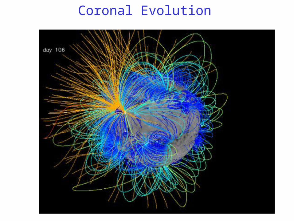
Coronal Evolution

Observed Chiralities

*

dextral

sinistral

undetermined.

123 with definite chirality (255).

88 % follow pattern (N hemi).

73% follow pattern (S Hemi).

Emerging flux

• Use a semi-automated procedure:– compare successive magnetograms;

– find “new” bipolar regions;

– measure key properties;

– insert as ideal bipoles into simulation.

CR1948

CR1948 rotated

CR1949Total: 118 bipolar regions

Potential Field?

Potential Field Force-Free Field

• Coronal fields in Simulation are far from potential (low heights).

Bipole Twist

= 0 >0

Untwisted Positive Helicity

Simulated Hemispheric Pattern

*

dextral

sinistral

weak.

207 locations

71 % follow

pattern (N hemi)

75 % follow

pattern (s hemi)

Results with Opposite Twist

Shapes:

observed chirality

109 filaments

Colours:

correct wrong

Only

61.5% correct

dextral

* sinistral

undetermined.

Flux Transport Model(2).• Form of Coronal Diffusion.

• Outflow Velocity.

• Resolution : nx= 361, ny=293,nz=53• Bipole Description.

Statistical Test for Filament Chirality• T-test: used to classifify chirality from individual barbs. n : no. of barbs (x1, x2, x3, ….., xn) xi = +1 (dextral) ; -1 (sinistral)

The number of dextral barbs is ns = n – nd

Now assume nd following a binomial distribution with parameters (n,p) and assume p = 0.5

is 0 if neither chirality is significant. The classification scheme is then

where we choose T = 1.5 (For large n, t should approximate a normal distribution with mean n and

variance 1)