modelling the impact of small reservoirs … modelling the impact of small reservoirs in the upper...
TRANSCRIPT

MODELLING THE IMPACT OF SMALL
RESERVOIRS IN THE UPPER EAST REGION OF GHANA
Master Thesis _________________________________________________________________
ISAAC HAGAN
May 2007
Examensarbete TVVR 07/5008
Division of Water Resources Engineering
Department of Building and Environmental
Technology

Modelling the Impact of Small Reservoirs in the Upper East Region of Ghana
Division of Water Resources Engineering Department of Building and Environmental Technology
Lund University, Sweden May 2007
Supervisor: Associate Professor Rolf Larsson
Examiner: Professor Ronny Berndtsson
Picture on front page:
A Small Reservoirs in the Upper East Region of Ghana(SRP
website, 2006).
Master Thesis by:
Isaac Hagan
Avdelning för Teknisk Vattenresurslära ISRN ISSN

Copyright ©. Isaac Hagan
Report TVVR 07/5008
Master of Science Thesis in Water Resources
Division of Water Resources Engineering
Faculty of Engineering, Lund University
Box 118 SE - 221 00 Lund
Sweden
Phone: +46 46 222 000
Web Address: http://aqua.tvrl.lth.se

i
ABSTRACT
Reservoirs are precious assets in semi arid and arid regions of the world. The Upper East Region
of Ghana by virtue of its climatic condition is classified as a semi arid region. It has a total of 160
small reservoirs located on streams and rivers which are in the upstream of the Ghana portion of
the Volta Basin. There have been significant reductions in the flow of water from all the three
main tributaries to the Volta Lake which is further downstream and contains the Akosombo
Hydro- power dam the main source of the countries electricity supply.
The effect of many small reservoirs in the Upper East Region of Ghana was investigated using
the WEAP model. A total of 61 small reservoirs were identified on streams and rivers in the
region. This number was achieved by adding very small reservoirs together. They were classified
as Small Reservoir 1, 2 and 3 (SR1, SR2 and SR3) corresponding with their sizes.
The model was first adapted to the region and calibrated using measured discharge values. Then
three different scenarios were created to access the impact of the small reservoirs on the White
Volta River.
The results obtained indicate that the reservoirs have low impact on the flow of the White Volta
River. However the creation of bigger reservoirs on the river could have significant effect on the
flow of the WVR and reduces its contribution to the Akosombo Lake which is further
downstream in the Volta Basin.

ii
ACKNOWLEDGEMENTS
Sincere thanks go to the Almighty God for making this thesis a success. This project work would
not have been possible without the help of Prof.dr.ir. Nick van de Giesen of Delft for his
directions and support. I will also like to thank Mr. Ampomah of the Ghana Water Resources
Commission who assisted me with the data.
Sincere thanks also go to my supervisor Dr. Rolf Larsson. Great thanks also go to my sponsors,
my family and all my friends for their immense contributions.

iii
LIST OF FIGURES
Figure 2.1 A sketch of a small reservoir showing the various part
Figure 3.1 Map showing the Upper East Region in relation to Ghana (adapted from Leibe 2002)
Figure 3.2 Network of Rivers and streams in the UER.
Figure 3.3 Map showing the distribution of Reservoirs in the UER (J. Leibe et al.)
Figure 3.4 Monthly net potential evaporation and volume depth relationship of reservoirs in the
UER (Leibe 2002).
Figure 4.1 Schematic view of WEAP model showing the various nodes.
Figure 5.1 A detailed schematic view of the study area in the WEAP model
Figure 5.2 An overview of the UER in the WEAP model
Figure 6.1 The flow of water from the various streams in billion m3 in the UER for the current
account year 2004.
Figure 6.2 Chart of stream flow for streams in the UER in million m3
Figure 6.3 Reservoirs storage volumes for various months in million m3
Figure 6.4 Stream Flow for Increase in Demand scenario.
Figure 6.5 Stream flow for Increased Demand Scenario and the Reference Scenario
Figure 6.6 Demand site coverage for year 2010 for some selected reservoirs in the very dry year.
Figure 6.7 Demand coverage 2013 for some selected reservoirs.
Figure 6.8 Unmet demands
Figure 6.9 Reservoir storage volumes Mm3.

iv
LIST OF TABLES
Table 2.1 Organisations and their roles in the White Volta Basin (UNESCO, 2006).
Table 2.2 Existing Irrigation sites and their water requirements in Ghana (Kwabena Wiafe, 1997)
Table 3.1 Various tributaries of the White Volta Basin and their areas and length (UNESCO,
2006)
Table 3.2 Rainfall and annual runoff for selected stations (Andah et al, 2005).
Table 3.3 Distribution of small reservoirs by districts. (Leibe, 2002)
Table 5.1 Categories of the reservoirs and their properties.
Table 5.2 Water use and irrigated areas of two small scale irrigation sites in the UER (Faulkner,
2006)
Table 5.3 Water Year Method for various years under scenarios
Table 5.4 New Reservoirs and their properties.

v
LIST OF ABBREVIATIONS
UN United Nation
UER Upper East Region
WEAP Water Evaluation and Planning Model
SRP Small Reservoir Project
WVB White Volta Basin
WVR White Volta River
PMP Probable Maximum Precipitation
PMF Probable Maximum Flood
WMO World Metrological Organisation
DA District Assembly
IFAD International Fund for Agricultural Development
FAO Food and Agricultural Organisation
GWP Global Water Partnership

vi
TABLE OF CONTENTS ABSTRACT……………………………………………………………………………………i ACKNOWLEDGEMENTS…………………………………………………………………..ii LIST OF FIGURES…………………………………………………………………………..iii LIST OF TABLES……………………………………………………………………………iv LIST OF ABBREVIATIONS………………………………………………………………...v TABLE OF CONTENTS……………………………………………………………………..vi 1 INTRODUCTION………………………………………………………………………….1 1.1 Background………………………………………………………………………………...1 1.2 Research Problem…………………………………………………………………………2 1.3 Objective…………………………………………………………………………………. 2 1.4 Scope of Work…………………………………………………………………………….2 1.5 Review of Previous Work………………………………………………………………....3 1.6 Limitations………………………………………………………………………………...3 1.7 Structure of report…………………………………………………………………………4 2 LITERATURE REVIEW………………………………………………………………….5 2.1 Importance of Reservoirs and Dams……………………………………………………... 5 2.2 Technical aspects of Small Reservoirs…………………………………………………… 5 2.3 Environmental Aspects of Small Reservoirs……………………………………………...6 2.4 Institutional Framework of Small Reservoirs……………………………………………. 7 2.5 Economic Analysis of Small Reservoirs………………………………………………….7 2.6 Integrated Water Resources Management of the White Volta Basin…………………….7 2.7 Irrigation and crop water requirements in the basin……………………………………...10 3 STUDY AREA……………………………………………………………………………..12 3.1 General Overview………………………………………………………………………...12 3.2 Climate and Rainfall Patterns………………………………………………………….....13 3.3 White Volta Basin………………………………………………………………………...13 3.4 General Reservoir Properties and Distribution…………………………………………...17 3.4.1 Potential Evaporation of reservoirs in the UER………………………………………...18 3.5 Land Cover and Use………………………………………………………………………19 3.6 Water Uses in the UER…………………………………………………………………...19 3.7 Downstream of the White Volta…………………………………………………………..20 4. WEAP MODEL…………………………………………………………………………...21 4.1 Introduction and Development of WEAP………………………………………………....21 4.2 Model Structure……………………………………………………………………………21 4.3 Modelling Process of WEAP……………………………………………………………...23 4.4 Applications of the WEAP model………………………………………………………....23 5 METHOD…………………………………………………………………………………...25 5.1 Input Data………………………………………………………………………………….25 5.2 Modelling Process ……………………………………………………………………… 25 5.2.1 Calibration of the Model……………………………………………………………… 25 5.2.2 Assumptions Made………………………………………………………………………27 5.3 Creation of Scenarios………………………………………………………………………29 5.3.1 Scenario 1; Increase in the Number of Small reservoirs………………………………...30 5.3.2 Scenario 2; Increase in irrigated Land/Increase in Demand……………………………...31 5.3.3 Scenario 3; Increase in Demand during the wet months…………………………………31 6 RESULTS AND DISCUSSION…………………………………………………………….32
vii
6.1 Introduction……………………………………………………………………………….. 32 6.2 Calibration results………………………………………………………………………….32 6.2.1 Stream Flow……………………………………………………………………………...32 6.2.3 Reservoir storage capacities……………………………………………………………...34 6.2.4 Demand site coverage……………………………………………………………………35 6.3 Simulation Results…………………………………………………………………………36 6.3.1 Scenario 2 Increase Demand…………………………………………………………….36 6.3.1.1 Stream Flow……………………………………………………………………………36 6.3.1.2 Demand Coverage……………………………………………………………………. .47 6.3.1.3 Reservoir Storage volume……………………………………………………………...40 6.3.2 Scenario 3; Increase in Demand during the Wet Season………………………………...40 6.3.2.1 Demand Coverage……………………………………………………………………...40 6.3.2.1 Reservoir Storage volume……………………………………………………………...41 6.3.3 Scenario 2; Increase in reservoirs……………………………………………………….41 6.3.3.1 Stream flow…………………………………………………………………………….41 6.3.3.2 Reservoir Storage Volume……………………………………………………………..41 6.4 Evaluation ………………………………………………………………………………..41 6.5 Planning ………………………………………………………………………………..42 7 CONCLUSIONS…………………………………………………………………………....43 8 REFEERENCES……………………………………………………………………………44 APPENDIX…………………………………………………………………………………....47 Appendix 1 Results of Stream flow for the current account year……………………………...47 Appendix 2 Results for Reservoirs storage volumes for the current account year in Mm3………………………………………………………………………………………....48 Appendix 3 Results of demand site coverage in percentage for the current account year……………………………………………………………………………………………..49 Appendix 4 Results of the demand site coverage in percentage for the year 2010…………….50 Appendix 5 Results of the storage volume of reservoirs for scenario 3; Increase in demand during the wet months……………………………………………………..51 Appendix 6 Results of the demand in percentage of the additional reservoirs as described in scenario 2………………………………………………………………………….52 Appendix 7 Discharge values for some selected gauge stations………………………………..53

1
1 INTRODUCTION
1.1 Background
“Water is an essential life sustaining element. It pervades our lives and is deeply embedded in our
cultural backgrounds” (UN World Water Development Report, 2006).
Water is required by all living creatures for survival. It is also required for economic growth and
development. The achievement of the millennium development goals depend largely on improved
water supply and sanitation in the developing countries. Issues of drought, flood, and extreme
climate change have dominated the news in recent times and have caused the death of thousands
of people. This has caused governments of certain countries such as Ghana to take more stringent
action on water resources management. The management of water resources is the concern of all
stakeholders involved. Most of the rivers in the world have been dammed to serve as water
storage facilities for hydropower generation, drinking water supply and irrigation purposes.
Reservoirs are indispensable storage facilities in arid and semi-arid regions of the world where
there is irregular rainfall. Extreme drought and floods characterize these areas resulting in
insecure livelihood.
Small multi purpose reservoirs are used widely for the provision of drinking water and irrigation
purposes. In the rural areas of Ghana where surface water is scarce, reservoirs are used for daily
activities to improve the livelihood of the people. The Upper East Region of Ghana and other
Northern Regions of Ghana where there is irregular rainfall patterns, small dams have been
constructed on small rivers and streams to ensure a year round growing season and also water
supply for livestock and domestic purposes as well.
Small dam development in the Northern regions of Ghana have been considered as one of the
solutions for curtailing the higher incidence of poverty by improving the standard of living of the
people through improved smallholder irrigation techniques and livestock production. They are
seen as important tool in achieving some of the goals of vision 2020 of Ghana and also the United
Nations Millennium Development goals of poverty reduction.
1.2 Research Problem
There have been major developments of a large number of small reservoirs in all the six riparian
countries of the Volta Basin. These are mainly situated on the upstream portion of the basin
depending on the country. Burkina Faso and Ghana are the countries with a greater portion of the
basin in terms of areas and major development of small dams are peculiar in these countries.
They are used mainly for water supply and for irrigation purposes. The developments of small
reservoirs have significant effect on the flow of the rivers on which they are situated. For the case
of the Volta basin where the reservoirs are located upstream there is the possibility of inadequate

2
flows in the downstream portion of the basin and other hydrological problems such as increased
evaporation leading to rapid dry up of some of the streams generating serious repercussions.
There is also the problem of location of small reservoirs to ensure adequate water throughout the
year to meet irrigation and livestock demands.
There is the need to ascertain the impact of this large number of small reservoirs on the Volta
basin with regards to the downstream communities and the general flow condition of the rivers.
This can assist in the construction and planning of these small reservoirs in order to minimize the
effect on the downstream users.
There is also the need to find out how these small reservoirs in the upstream portion of the basin
affect the hydro-power dam located in Akosombo which is downstream of the Volta River.
1.3 Objective
The main objective of this thesis work is to find out the extents to which the large numbers of
small reservoirs affect the downstream users. The other objective will be to find a way of
evaluating and planning the construction of many of these small reservoirs to ensure efficient use
of the water resources in the Upper East Region of Ghana.
These objectives will be achieved using the Water Evaluation and Planning Model (WEAP
Model).
1.4 Scope of Work
The thesis work will cover the Upper East Region of Ghana which has a large number of small
reservoirs, 160 in number (J. Leibe et al, 2005) with the Tano and Vea being the biggest. The
study will cover reservoirs which are located on the various streams in the region. That means
that small reservoirs which are not located on any river or stream will not be considered in this
study. The Tano and Vea reservoirs will not be included in this study because according to their
areas they are not classified as small reservoirs. This may produce some discrepancies in the
results.
The thesis will involve the following
• Identification of the various reservoirs and their locations in the region
• Quantification of water for farming and livestock production purposes
• Calibration of the WEAP model
• Creation of scenarios and evaluation.

3
1.5 Review of Previous Work
There are a lot of research activities going on in the whole Volta Basin. The Small Reservoir
Project (SRP) is currently undertaking research works on planning and evaluating ensembles of
small, multi-purpose reservoirs for the improvement of smallholder livelihoods and food security:
tools and procedures (SRP website, 2006).
The SRP is part of the Challenge Programme for water and food. Research works already
conducted in the UER of Ghana includes estimation of reservoirs storage capacities and
evaporation losses from small reservoirs in which various categories of small reservoirs were
identified according to their storage capacities and their surface areas. Evaporation losses from
these reservoirs were also identified (J. Leibe et al, 2005). There have been studies into the water
use, productivity, and profitability of small scale irrigation schemes in UER. The study involved
two irrigation farming sites with two different technologies. It also involved the measurement of
water released per area of farmland (Faulkner, 2006)
1.6 Limitations
The data obtained were from previous field studies conducted by individuals and organisations
working on the various projects on the main Volta Basin and specifically in the Upper East region
of Ghana. These differences in data may generate some differences in the data set. The total
number of reservoirs in the Upper East region was not considered since most of them are located
on the small streams which have no or inadequate flow data. This will affect the result obtained
from the simulation. Moreover the exclusion of the two big reservoirs Tano and Vea will affect
the results significantly because they store a large volume of water for a large scale irrigation
purposes. This thesis work was also limited to 61 reservoirs out of a total of 160 reservoirs in the
Region.

4
1.7 Structure of report
This report is made up of eight chapters. The first chapter is introduction which describes the
objectives of the study. The second chapter is the literature review and talks about integrated
water resources in the White Volta Basin and general reservoir properties construction and its
importance. The third chapter is a description of the study area and talks about the general living
conditions in the study area, the rainfall characteristics, land use, uses of water and the White
Volta basin.
The fourth chapter describes the WEAP model, it characteristics and applications. Its also
describes how the model works and some application of the model. The next chapter is the
method of the thesis and describes the steps taken to achieve the objectives of the thesis. The
chapter that follows this present the results and discussion of the thesis which is also followed by
conclusion and recommendation chapters, reference chapter and the appendix.
5
2 LITERATURE REVIEW
2.1 Importance of Reservoirs and Dams.
A reservoir is a man-made lake which is created when a dam is built on a river or a stream. The
river or stream water back up behind the dam creating a reservoir which is used for various
purposes. The reservoir is equipped with an outlet structure which is constructed with concrete or
pipe. They are mostly constructed for the following purposes
• To hold water for domestic use, agricultural purposes (irrigation) and for industrial use.
When water is retained in reservoirs they are made to go through a period of self
purification since sedimentation is allowed to take place. The water is then clear to some
extent to be used for domestic purposes.
• To hold water to prevent flooding when there is intense rainfall that can cause flooding to
a community. Reservoirs commonly used for this purposes are called attenuation
reservoirs and are used to prevent flooding of low lying areas. They store water during
periods with abnormally high rainfall and gradually release the water during periods of
low rainfall.
• To hold water for the purposes of electricity generation and for powering wind mills. The
reservoirs for this purpose are equipped with turbines which generate the electricity.
Reservoirs can be constructed for secondary purposes as recreation such as sailing, fishing and
water skiing.
2.2 Technical aspects of Small Reservoirs
Small reservoirs (size approximately 0.01 km3) ( SRP Website, 2006) are a result of small dams
constructed on streams or rivers to impound water and are mostly constructed with earth materials
such as clay, gravels, rocks or sometimes boulders. Most reservoirs normally use clay which has
been well compacted as the water proofing element which prevent loss of water through seepage.
The banks of the reservoirs can be of gravel or boulders depending on the condition of the
existing soil type and the purpose of the reservoir. A simple small reservoir is shown in the figure
2.1. The use of good earth material is a prerequisite for long lasting reservoirs and also for
efficient utilization. That is to say that the efficiency of the reservoir is dependent on the materials
used in the construction.
Proper surveying and field studies should be conducted before the construction begins. Field
studies involves the selection of site and the determination of slope of the reservoir which is
another important steps since this is required to ensure constant flow into and out of the reservoir.
.

6
Figure 2.1 A sketch of a small reservoir showing the various part
The spillway is the part that is used to empty the reservoirs when too much water has been stored
in the reservoir. It normally consists of an outlet pipe made of either caste concrete or PVC pipes.
The lining of the reservoir could be of well compacted clay or a water proofing material such as
polyethene. The riverbed could be gravels bed with a good slope to ensure adequate flow into the
reservoir.
Small reservoirs in the UER of Ghana are mostly constructed with compacted earth mostly clay
material with the people in the communities providing the labour during construction. The
embankment is also made of clay. The spillways are designed based on the Probable Maximum
Flood (PMF) which is estimated from the PMP (Probable Maximum Precipitation). The PMP is
defined according to WMO in 1986 as “the greatest depth of precipitation for a given duration
that is meteorologically possible for a given size storm area at a given particular location at a
particular time of year” (WMO, 1986).
The size of the small reservoir in a community is normally driven by the budget allocation of the
institutions providing the funds and not necessarily on the intending uses of the reservoir.
2.3 Environmental Aspects of Small Reservoirs
The proper functioning of an ecosystem depends to a large extent on water. Water is therefore
indispensable in an ecosystem and it flora and fauna (A. B. Avakyan et al 2001). It is an
important aspect of the ecosystem providing a breeding place for birds and sustenance of other
wildlife.
Small reservoirs which are not properly managed can serve as breeding grounds for mosquitoes
and thereby increasing the prevalence of malaria in that community. There is the need to
understand the interaction between the reservoirs and the ecosystem in order to conserve and also
improve it thereby eliminating the negative effect of small reservoirs.
During periods of floods, erosion of the banks of the reservoirs can cause significant damage to
the reservoirs and the nearby farmland can be inundated. Another environmental problem
associated with small reservoirs is their inability to flush out pollutants from the communities as a
Incoming Stored water Lining of reservoir
Spill gate

7
result of nutrients generated from the use of chemicals for farming. This makes the community
susceptible to water borne diseases.
2.4 Institutional Framework of Small Reservoirs
The reservoirs in the UER and the most of the other northern part of Ghana were constructed
through project funded by various Non - governmental organisations which are undertaken
various developmental projects. There is therefore little or no coordination among these
organisations in the management of these reservoirs (SRP website, 2006). The management of
these reservoirs is a duty of the communities which are benefiting from the projects. The districts
assemblies (DA’s) play an important role when it comes to the management of these reservoirs by
training personal in the communities in the management of the reservoirs. The agricultural
department of the district assemblies are normally responsible for the training. The Vea and Tano
reservoirs in the UER have a good management body which undertake their own maintenance
and management aspect.
2.5 Economic Analysis of Small Reservoirs.
Reservoirs in the region are used for smallholder irrigation and livestock production. The farmers
do not have to pay for the use of these small reservoirs and do not have to spend some of their
profit on the maintenance of the reservoirs. The little profit generated from the sale of their
produce goes a long way to improve the standard of living of the people.
A lot of benefits are derived from the construction of small reservoirs as already mentioned. They
can be a good avenue for the eradication of poverty in the communities if they are properly
managed and maintained.
Net returns of USD 109 and USD 53 for plots of 0.05 ha of tomato and onion, respectively
pertains in the UER which is very substantial if one considers the poverty situation in the region.
(IFAD, 2006)
2.6 Integrated Water Resources Management of the White Volta Basin
Integrated water resources management encompasses water resources as an integral part of the
ecosystem and also as natural resources. According to the Global Water Partners (GWP) IWRM
is defined as (GWP website, 2006) “the process which promotes the co-coordinated development
and management of water, land and related resources, in order to maximize the resultant
economic and social welfare in an equitable manner without compromising the sustainability of
vital ecosystems.” There are various other definitions of IWRM.
The water resource users in a watershed or basin form part of the management of the entire basin.
There are various guidelines or principles under the concept of IWRM. The Dublin Principles are
generally used as a set of guidelines for IWRM. These principles have been carefully formulated
8
and have been internationally accepted as guidelines for IWRM. The Dublin guidelines are
outlined below. (GWP, 2006)
• Water is a finite and vulnerable resource essential to sustain life, environment and
development. The principle requires a holistic approach to water resources management.
All the elements of the hydrologic cycle and their interaction with the ecosystem should
be taken into account in addressing issues of IWRM.
• Water development and management should be based on a participatory approach,
involving users, planners and policymakers at all levels. The principle recognizes water
as a resources in which all stakeholders should be involved in it management. A
stakeholder in the water sector includes everyone since everyone uses water. In this
regards various communities forming part of a river basin should be involved in the
decision making of the management of the river basin.
• Women play a central part in the provision, management and safeguarding of water. It
has been widely accepted that women play a very important role when it comes to
collection, use and safeguarding of water resources for domestic and agricultural use.
Women should therefore be involved in the decision making processes of water resources
management.
• Water has an economic value in all its competing uses and should be recognized as an
economic good. If water is recognized as an economic good more value would be placed
on water resources. This could ensure efficient use of water resources since people would
be made to recognized how expensive it is in the provision of water for domestic,
agricultural and industrial purposes
There are a lot of organizations which are responsible for Integrated Water Resources
Management of the White Volta basin. Table 2.1 shows the various organizations and their roles
in the White Volta Basin.
9
Table 2.1 Organisations and their roles in the White Volta Basin (UNESCO, 2006).
Organization Role
The Ghana Water Resources
Commission Implementation and dissemination of IWRM
District Assemblies Provision of Socio-economic infrastructures.
Non Governmental organization e.g.
TRAX, Rural Aid, World vision
international
Provides financial as well as technical works.
International Water Management
Institute IWMI
Undertaking small dams projects in the Basin
ECOWAS Responsible for the eradication of
Onchocerciasis
CGIAR: Challenge Program International Research on food and water
WVBB White Volta Basin Board, Ghana
IUCN/EU Volta Governance, International
ZEF: GLOWA-Volta Project Decision Support System
These organizations are working in collaboration to solve a lot of pressing issues in the Basin.
Hydrological and water management issues such as small scale irrigation, Climate change for
water management, Sporadic drought spells, Small hand-dug wells, Inclusion of Women and
other marginalized groups in decision making process, Coordination of Water Management
activities at the Basin Level and other environmental and livelihood issues are been addressed as
well. Under the WVB pilot project the following activities have been undertaken: (UNESCO,
2006)
• Public Awareness creation of IWRM issues
• Identification, registration, permitting and billing of water users
• Building of a Decision Support System (DSS) as planning and decision tool
• Strengthening of stakeholders capacities for IWRM and planning
• Stakeholder process involving government agencies, district authorities, water
institutions, traditional authorities, NGOs and actual water users
Some of these activities have already been carried out

10
2.7 Irrigation and crop water requirements in the basin
Agriculture is the backbone of most developing countries in the world and Ghana is not an
exception. Irrigation technologies allow more crops to be cultivated all year round with less
dependent on rainfall. According to the FAO Ghana has a renewable water resource of 53.2km3
(FAO, 2006) Water used for crop production is 0.25 km3.This shows a very low rate of irrigation
in the country. Irrigation in Ghana is practiced on the small scale basis and is informal. The
cultivable area in Ghana is about 42% of the total area of the country out of which 4.25% of the
area is under cultivation (FAO, 2006).
Table 2.2 Existing Irrigation sites and their water requirements in Ghana (Kwabena Wiafe, 1997)
Project
Region
Water Source
Irrigable area ( ha)
Crops
Irrigation water requirements ( Mm
3)
Asutsuare
G/Accra
Main Volta
660
Rice
17.16
Dawhenya
A
404
Rice
10.5
Tano
U/East
2,207
Rice/ Vegetables
39.78
Afife
Volta
Agali
880
Rice/okra
22.88
Vea
U/East
Yagaratanga
850
Rice/ Vegetables
7.14
Bontanga
Northern
450
Rice /okro
11.7
Afram plains
Eastern
Volta
101
Groundnuts/vegetables
0.85
Ashaiman
G/Accra
117
Rice/okra
3.04
Aveyime
Volta
Volta
63
Rice
1.64
Kpando- Torkor
Volta
Main Volta
40
Okra
0.34
Small schemes Libga Golinga
Northern Northern
16 26
Rice/ Vegetables
0.13 0.68

11
Ghana has the potential of developing 384,000 ha of irrigation based on water and soil
availability. (World Bank Report, 2005). There is the possibility of developing approximately
300,000 ha of irrigable land in the White Volta Basin and this is going to require close to 3600
million cubic meters of water. (Kwabena Wiafe, 1997)
The Irrigation Company of the Upper East Region of Ghana manages the biggest irrigation
scheme in Ghana which is the Tano and Vea Irrigation schemes (Kwabena Wiafe, 1997). The two
dams on the Vea and the Tano Rivers were constructed in the 1980’s and have since then become
the largest managed irrigation schemes in the country. Agriculture contributes approximately
60% of the Gross National Product (G.N.P) of the country and the livelihood of 80% of the
people depends largely on agriculture (Kwabena Wiafe 1997). This has necessitated the
development of irrigation in major areas of the country where rainfall is erratic can only support
one planting season.

12
3 STUDY AREA
3.1 General Overview.
The Upper East Region of Ghana is one of the most deprived or poorest regions (Ghana
Statistical Department). It is situated in the centre of the Volta Basin in the north-eastern corner
of Ghana and is bordered by Burkina Faso to the north and Togo to the eastern part. It has a
population of 920,089 people according to the 2000 national census and has a population density
of 96.6 inhabitants/km2 and a growth rate of 3 %.( Asenso-Okyere et al, 2002). The region is the
second lowest ranked in terms of mean annual income of approximately USD157. This is a little
higher than the adjacent region which is Upper West Region. According to the Statistical
Department of Ghana report in 1998 the Upper East Region has a poverty incidence of 88%. This
means the region has the highest number of poor people in the country.
The regional capital is Bolgatanga with other important towns such as Bawku, Navrongo and
Paga. It is made up of 8 districts and has a land size of 8842 km2 which is approximately 3.4% of
the total land mass of Ghana and is predominantly rural (87%). The map showing the UER is
shown in figure 3.1. The UER has the highest elevation of 455m in the northern part and the
lowest of 122m in the southern part of the region. (Leibe 2002)
Figure 3.1 Map showing the Upper East Region in relation to Ghana (adapted from Leibe, 2002)

13
3.2 Climate and Rainfall Patterns
The region just like the other Northern regions of Ghana have variable rainfall pattern with
extreme cases of drought and sporadic flood and has an annual average rainfall of 1044mm which
is suitable for a single wet season crops. Rainfall is usually between the months of July and
September unlike the southern part of the country which has a relatively longer period of rainfall.
The temperature is between 27°C and 36°C in the northern part and 24°C and 34°C in the
southern part. The region is therefore characterised as a semi-arid.
Most of the rains in the region fall as thunderstorm originating from squall lines (Eldridge, 1957;
Hayward and Oguntoyinbo, 1987; Friesen, 2002). The region has a rainfall intensity which
normally exceeds the infiltration capacity of the soil. This means that runoff occurs even without
the soil been moist implying that groundwater is not replenished (J. Leibe et al, 2005) The UER
has an average annual potential evaporation of 2025mm.
3.3 White Volta Basin
The UER falls within the White Volta basin which is a sub basin of the Volta Basin and has been
classified as an Operational HELP Basin.( Hydrology for Environment Life and Policy) HELP is
a joint initiative between United Nation Educational Scientific Organisation (UNESCO) and the
World Metrological Organisation(WMO) and is led by the International Hydrological
Programme. The objective of the HELP programme is to create new approaches to water basin
managements through the creation of framework for water law and expert, water resources
managers and water scientists to work together in solving water related problems. (UNESCO
website, 2006). A basin is considered as an Operational HELP if it fulfils the following criteria;
(UNESCO, website 2006)
• “It has implemented the HELP philosophy
• Has involved the HELP stakeholders in the management of the basin
• is substantially functioning across several HELP key issues in an integrated manner;
• demonstrates an active interface between science and water managers, and society;
• has established mechanisms for unrestricted information and data access and exchange;
• Follows the WMO Resolution 25 on international exchange of hydrological and related
data.”

14
It is one of the main tributaries of the Volta River and has a total area of 104,749 km2.The area
in Ghana is 45804 km2 and that in Burkina Faso is 58945 km2. It is located upstream of the lake
Volta in Northern Ghana and southern part of Burkina Faso (UNESCO, website 2006). The area
of the various tributaries of the White Volta basin and their length is shown in table 3.1. The
network of the rivers and streams in the UER is also shown in figure 3.2
Table 3.1 Various tributaries of the White Volta Basin and their areas and length (UNESCO, 2006)
Name Area(Km2) Length(km)
White Volta 49,230 (106,740)* 1,140
Tamne 880 50
Morago 620 (1,610)* 80
Mole 5970 200
Kulpawn 10,600 (10,640)* 320
Sisili 5,180 (8,950)* 310
Red Volta 590 (11,370)* 310
Asibilika 1,520 (1,820)* 100
Agrumatue 1,410 (1,790)* 90
Nasia 5240 180
Nabogo 2960 70
* Total area including catchment outside Ghana

15
Figure 3.2 Network of Rivers and streams in the UER.
The total annual discharge leaving Burkina Faso through the Red and White Volta Rivers is
estimated at 3.7 km³/year (FAO Corporate Document Repository website, 2006). The land is
predominantly flat, particularly in the southern part which is 0.1% (S.Wagner et al, 2002)
There are a lot of projects going on in the White Volta basin. Among these is the Small Reservoir
Project (SRP), the GLOWA Volta project, the Ghana Water Resource Commission and the
CGIAR Challenge Program on Food and Water which are all aimed at improving the livelihood
of the growing population in the region through intensive Research work. The White Volta falls

16
within the interior savannah ecological zone. The geologic formation of the basin is Voltain and
granite and there is generally low groundwater yield from dug wells and boreholes in the basin
between 5.23 x10⁻⁴ to 1.05 x 10⁻³ m3/sec and an average depth of 38m (Kwabena Wiafe, 1997).
According to Andah Runoff coefficients are generally low; meaning that direct recharge of
aquifers from precipitation is less than 20% across the Basin. This figure means that less runoff
end up as recharge for groundwater. (Andah et al, 2005)
The White Volta River is one of the main tributaries of the Volta River which forms part of the
Volta Lake. The Akosombo and Kpong dams use water from the Volta Lake for hydro-power
production. Downstream of these dams, there are substantial farming activities which use water
from these dams for irrigation practices.
The Volta Lake is by far the largest man-made lake ever to be constructed in the world and is also
the largest regulated Lake in the world. (Dams under Debate, 2006)
The Akosombo Hydro power plant produces 912MW of electricity at it full capacity whiles the
Kpong dam produces 160MW.( VRA website, 2006)
In recent years there has been a significant reduction in the contribution of runoff from the white
Volta river and the other rivers in the basin to the main Volta river (P. Gyau-Boakye, 2000) due
to a lot of factors which include exploitation of water resources in the upstream of the white Volta
river. Table 3.2 shows the mean annual runoff of the main rivers of the Volta Basin. The mean
annual flow of the WVR is 9.57 billion m3
Table 3.2 Rainfall and annual runoff for selected stations (Andah et al, 2005).
Sub-basins Total area (km2) Mean Annual
Rainfall (mm)
Mean annual
runoff (x106m3 )
Runoff
coefficient (%)
Length (km)
Black Volta 149,015 10.23.3-1,348.0 767 8.3 1,363.3
White Volta 104,749 929.7-1,054.2 9,565 10.8 1,136.7
Oti 72,778 1,150.0-1,350.0 11,215 14.8 936.7
Lower Volta 62,651 1,050.0-1,500.0 9,842 17.0
Total 400,710 876.3-1,565.0
Runoff Coefficient is related to different land covers and hydrological soil types

17
3.4 General Reservoir Properties and Distribution.
In northern Ghana and other semi-arid regions of the world reservoirs are most precious assets.
There are lots of reservoirs used for various purposes in the UER of Ghana. This is an important
and most easy way to overcome rampant drought and floods in the area and also give hope to the
growing population. There are a total of 160 small reservoirs in the UER which have different
storage surface areas ranging from 1 to 35 ha (J. Leibe et al).Many of these reservoirs were
constructed by different organisations, mostly NGO’S undertaking various developmental
projects in the UER. There is little or no coordination among the organisations undertaking the
construction of these reservoirs (SRP website, 2006). This often makes the maintenance of the
reservoirs a problem. Some are left to dry up and a lot of investment are left to go waste. The
distribution of small reservoirs in the region is represented in figure 3.3.
Figure 3.3 Map showing the distribution of Reservoirs in the UER (J. Leibe et al.)
The number of reservoirs in the region varies from district to district. Table 3.3 shows the
reservoir distribution according to districts and their surface areas. The Bawku East district has
the highest number of small reservoirs with a total area of 323 ha. The reservoirs are categorized
into three with category 1 having an area between 1 and 2.79 ha. Categories 2 and 3 have area
between 2.88 and 6.93 ha and 7.02 and 35 ha respectively.

18
Table 3.3 Distribution of small reservoirs by districts. (Leibe, 2002)
No. of
Reservoirs
Total
Surface Area (ha)
District cat1 cat 2 cat3 Cat 1 Cat 2 Cat 3 Total
Bawku East 6 17 17 40 11.34 72.36 239.40 323.10
Bawku West 1 1 13 15 2.79 5.67 177.93 186.39
Bolgatanga 10 8 4 22 19.35 37.71 44.46 101.52
Bongo 10 7 2 19 17.91 35.91 34.38 88.20
Builsa 10 6 7 23 14.94 30.51 93.06 138.51
Kassena-
Nankani
14 14 7 35 28.17 67.77 65.88 161.82
TOTAL 51 53 50 159 94.5 249.93 655.11 999.54
3.4.1 Potential Evaporation of reservoirs in the UER
The monthly potential evaporation and the volume depth relationship according to Leibe, 2002 of
the UER of Ghana are shown in figure 3.4. The net monthly potential evaporation was recorded
over a period of ten years. The minimum and maximum evaporation was compared with the
Meteorological station data of Navrongo.
Figure 3.4 Monthly net potential evaporation and volume depth relationship of reservoirs in the UER
(Leibe 2002).

19
3.5 Land Cover and Use
Land cover in a detailed sense refers to the attributes of a part of the earth’s surface and
immediate subsurface, including biota, soil, topography, surface and ground water, and human
structures((IGBP/IHDP, 1993).
Land plays an important part of the development of agriculture for the sustenance of livelihood.
The region falls within the Guinea Savannah ecological zone and is one of the erosion prone areas
in Ghana. The soil is relatively dry due to less percolation from rainfall. The economic activities
in the region is mostly agriculture. Majors crops cultivated are watermelons, cashew nuts;
vegetables: tomatoes, onions. Livestock production is also predominant in the region with the
rearing of animals such as cattle, sheep, goat, poultry and pigs.
The land use in the UER and the whole of the White Volta basin is predominantly extensive land
rotation cultivation approximately 3.2 to 9.6 km away from the village and extensive grazing of
livestock. (FAO, 1991). Grazing lands are generally poor due to bush fires. Land sizes are usually
small, often in the range of 1.2 ha. (Andah et al, 2005). In the UER and the whole of Ghana land
is mostly owned by chiefs and traditional elders in the various communities. This creates a lot of
problems with regards to the management and release of land. There is generally inadequate
information on land use in the UER and the whole of the White Volta basin.
3.6 Water Uses in the UER
The region has it main source of water from streams and rivers with little contribution from
groundwater. Agriculture production uses most of the water for mainly irrigation and livestock
production. Boreholes are the major sources of water supply for domestic purposes for the people
of the UER although the yield of groundwater is generally low. The water use for agriculture and
livestock production is mainly from reservoirs which are used to store water during the wet
season.
The water demand in the UER is expected to increase due to an anticipated increase in the
population, urbanization and improved standard of living of the people. Irrigation accounts for
approximately 80 percent of the water use in the UER of Ghana and the entire Volta basin
(Shiklomanov, 1999). Crops mostly grown in the area are maize, millet, rice and vegetables.
Urban and rural water use is less at the moment. The rate of water use for domestic purpose is
approximately 0.11 m3/s while that for irrigation purposes is 2m3/s. (Kwabena Wiafe, 1997).The
type of irrigation mostly practiced in the UER is the gravity flow irrigation system with fewer
technologies such as sprinkler and pump irrigation schemes.

20
3.7 Downstream of the White Volta
The downstream water use of the White Volta River is basically the hydro-power generation at
the Akosombo dam. The White Volta basin is a major contributor to the hydropower generation.
With a contribution of more than one third of the total flow into the lake Volta, the White Volta
River is considered very important in the electricity generation. (Andah et al, 2004)
Other use of the White Volta River is for irrigation purposes and drinking water supply. These
uses are most of the time dependent on the upstream flow conditions. More upstream flow means
more downstream uses and more contribution to the hydropower generation. Irregular flow
upstream means less water would be expected in the downstream portion of the river. This
implies that activities upstream are a major contributing factor to the downstream activities.
In recent years there have been low water levels in the Akosombo dam. This prompted the Volta
River Authorities to shut down some of their turbines and thereby introducing power shedding in
some parts of the country. This has been primarily attributed to low flow from the major rivers
into the Akosombo dam.
The White Volta River is also dammed in the Burkina Faso portion indicating that the flow to the
downstream users is, to a large extent, regulated.

21
4. WEAP MODEL
4.1 Introduction and Development of WEAP
Water Evaluation and Planning System (WEAP) is a microcomputer tool for integrated water
resources planning (WEAP User guide 2005). It is easy to use and offers a comprehensive
approach to water resources management.
Various organizations have been responsible for the development of the WEAP model. The
Stockholm Environmental Institute SEI provided primary support and the US Army Corps of
Engineers provided funding for the development of the model.
A number of agencies were involved in the development of the Model. They include The World
Bank, USAID, and the Global Infrastructure Fund of Japan (WEAP User guide 2005).
The model functions on the principle of water balancing. Since the first version of the model was
developed in 1990 the model has been applied in a lot of research work. It has been applied
primarily in a number of studies concerning;
• Agricultural systems
• Municipal systems
• Single catchments or complex Trans-boundary river systems
4.2 Model Structure
The structure of the model is such that, the water resource system is represented in terms of
groundwater, reservoirs withdrawal, transmission and wastewater treatment facilities; ecosystem
requirements, water demands and pollution generation. The analyst can choose the level of
complexity to meet the requirements of a particular analysis. This customization can also be used
to reflect the limits caused by restricted data (Sieber et al, 2005).
The model consists of five main views:
Schematic
The study area is defined in the schematic view. It is a GIS based tool which allows vector or
raster layers to be imported and used as background layers. Its uses a drag and drop method in
which objects such as demand nodes, reservoirs, groundwater supply, etc can be positioned. This
allows for changes and modifications to be made in the area with ease. A sample of the schematic
view is shown in figure 4.1.

22
Figure 4.1 Schematic view of WEAP model showing the various nodes.
Data
The data view is where data is entered into the program. It allows variables and various
assumptions to be created using mathematical relationships. Data can also be imported from
Excel.
Result
Results are easily accessed. Every model output is displayed. This can also be exported to Excel
for further modification.
Overview
This allows for easy accessibility of key indicators in the model.
Note.
Notes can be added to the model for documentation of the key assumptions.

23
4.3 Modelling Process of WEAP
The modelling of a watershed using the WEAP consists of the following steps (Levite, 2003).
• Definition of the study area and time frame. The setting up of the time frame includes the
last year of scenario creation and the initial year of application.
• Creation of the Current Account which is more or less the existing water resources
situation of the study area. Under the current account available water resources and
various existing demand nodes are specified. This is very important since it forms the
basis of the whole modelling process. This can be used for calibration of the model to
adapt it to the existing situation of the study area.
• Creation of scenarios based on future assumptions and expected increases in the various
indicators. This forms the core or the heart of the WEAP model since this allows for
possible water resources management processes to be adopted from the results generated
from running the model. The scenarios are used to address a lot of “what if situations”,
like what if reservoirs operating rules are altered, what if groundwater supplies are fully
exploited, what if there is a population increase. Scenarios creation can take into
consideration factors that change with time.
• Evaluation of the scenarios with regards to the availability of the water resources for the
study area. Results generated from the creation of scenarios can help the water resources
planner in decision making.
4.4 Applications of the WEAP model
The model has been applied to quite a number of basins in different countries of the world and
still active in a lot of countries. It has been applied to Lake Naivasha in Kenya to develop an
integrated water resource management model in order to attain both economical and ecological
sustainability (Alfara 2004). The model was used to identify possible scenarios which can
improve the current situation of the lake.
It has also been applied in the complex situation of the Aral Sea to evaluate water resources
development policies. By using the features of the scenario creation the WEAP model was used
to provide a structured approach to integrated water- demand analysis (P. Raskin, et al 1990)
Another application of the model is on the Volta Basin under the ADAPT project which is the
Adaptation of Strategies for Changing Environment. Under the ADAPT project the model was
used to investigate the effect of changing climate on the already stressed water resources, food
security and the environment and the consequence on the socio- economic situation on the people
living in the basin.(Andah et al, 2003)
24
The model has also been applied in the following other areas:
• In the United State of America the model has been used for a number of research projects
and is still active in some States.
• South Africa on water demand management scenario in a water stressed basin.
• Limpopo and the Volta River Basins in Zimbabwe and West Africa for Planning and
evaluating ensembles of small, multi-purpose reservoirs for the improvement of
smallholder livelihoods and food security tools and procedures (SRP website, 2006).

25
5 METHOD
5.1 Input Data
A GIS based vector layers of the area of UER of Ghana and the whole of the Volta Basin was
obtained from the Volta Basin Starter Kit July 2006. The kit was compiled by the International
Water Management Institute (IWMI) and the Challenge Program on Water and Food. The Starter
kit also provided information on the runoff data and a range of other useful information.
The year chosen for the current account was 2004. The runoff data for the year 2004 was obtained
from the starter kit and other sources. Boundaries of the UER area were set using the raster layer
of the whole Volta Basin which was also obtained from the Basin Starter Kit. Streams in the area
were redrawn by using the drag and drop button of the river button on the WEAP model.
Data on the water use and areas of irrigation was obtained from the study conducted on water use
and irrigation of some selected areas of the UER of Ghana. (Faulkner 2006)
5.2 Modelling Process
5.2.1 Calibration of the Model.
The current account year was used to calibrate the model. Reservoirs were categorized into three
groups namely SR1, SR2 and SR3. Small Reservoir category three (SR3) has the biggest surface
area in the range of 7.02 – 35 ha and SR2 have areas in the range of 2.88 to 6.93 ha while that of
SR1 is in the range of 1–2.79 ha.(Leibe et al, 2005).
An average value was obtained from this and the calculation of the storage capacity was done
using the relation;
Volume = 0.00857 x Area1.4367 m3. (J. Leibe et al, 2005).Where the area is in meter square.
All the reservoirs in the model were assigned a volume according to table 5.1.

26
Table 5.1 Categories of the reservoirs and their properties.
Reservoir Category Area (Ha) Average Area (m2) Average Volume (m3)
SR1 1-2.79 1,8950 11,984
SR2 2.88-6.93 4,9050 46,991.8
SR3 7.02-35 210,100 374,935.9
SR4 SR 3+ SR 1
SR5 SR 3 + SR 2
Most of the reservoirs are located on the second and third order streams which have limited
rainfall data. The streams and rivers were named River 1 to River 49 and include the major rivers
which are White and Red Volta rivers. The reservoirs which are not located on any of the streams
were not included in the study since they don’t have any hydrological links to any of the streams
and therefore have no impact on the streams. This will reduce significantly the total amount of
storage capacity for all the reservoirs, which 186 billion m3.
Demand sites were limited to agricultural use for small scale irrigation systems. This is because
80% of the water in the district is spent on growing crops and for livestock production. The
demand sites in the model were denoted with the corresponding name of the town where the
demand is located and with a number 1, 2 or 3 corresponding to the small reservoir close to the
area.
The demand priority was set to 1 in the model. The model uses demand priorities which can be
set between 1 and 99 depending on the priority of the demand sites. The highest demand priority
is 1 with the minimum being 99. A demand priority of 1 means that as long as there is flow in the
river or streams that demand must be satisfied.
Faulkner (2006) conducted a study into the water use and availability in the UER of Ghana. The
results obtained in the study of two reservoirs and farming communities are presented in the table
5.2.
According to Faulkner the water release per area irrigated was found to be 11,365 m3/ha for the
Weega system of irrigation which was a well managed system. The value obtained for the Tanga
system of irrigation was 32,901m3/ha for the same crops as the Weega system. The Tanga system
was described as a poorly managed system (Faulkner 2006).The average value of water released
for the two systems was used in the model for all the reservoirs as their annual water use rate. The
areas of land cultivated for the places where there are SR 3 type reservoirs were chosen to be
approximately 9 ha. And that for SR2 and SR1 type reservoirs was set to be 2.6 ha and 1.6
respectively. These values were used in the model based on the assumption that all the areas with

27
SR3 type reservoirs have the same irrigated areas. The SR 4 type reservoir is a combination of
SR3 and SR1 while the SR5 reservoirs is that of SR 3 and SR 2
Table 5.2 Water use and irrigated areas of two small scale irrigation sites in the UER (Faulkner,
2006)
Area under
Cultivation (ha)
Total Water Released for
Season (m3)
Water Released per Area
Irrigated (m3/ha)
Tanga Canal A 0.8629 34121 39542
Tanga Canal B 0.7591 19245 25352
Tanga Total 1.6220 53366 32901
Weega Canal A 2.8824 32373 11231
Weega Canal B 3.1245 35895 11488
Weega Total 6.0069 68268 11365
The figures 5.1 and 5.2 show an overview and a detail sample of the study area in the WEAP
model. It shows the major rivers and streams in the UER. The detailed sample of the schematic
view shows the demand sites as Red dots with the name of the town and the number 1, 2 or 3
depicting the kind or reservoir closed to that demand site. This also shows the names of the
various towns in the UER.
The average monthly evaporation for the small reservoirs was obtained from figure 3.4 which
was adapted from Leibe (2002). The value obtained was 152.5mm/month and this value was used
to represent all the reservoirs in the district.
In all a total of 61 reservoirs were located on streams in the region. This value is far lower than
186 million m3 of the total storage capacity of reservoirs (Leibe et al 2002). The difference may
be attributed to the fact that not all the reservoirs in the region were considered. Only the
reservoirs on streams and rivers were considered.
5.2.2 Assumptions Made
In the modelling of the reservoirs in the study area, some assumptions were made regarding some
of the input data. The runoff data obtained was only on some selected stations from various towns
in the whole basin. For streams with no gauge stations their runoff data were deduced from the
neighbouring stations. This was done by taking into consideration the catchement area of the
stream. Concerning water use in the region, it was assumed that the water use for domestic
purposes was negligible and that water in the region is basically for irrigation and livestock
production.

28
With regards to the areas of irrigated land in the various towns, it was assumed that the land sizes
were the same as 9 ha for SR3 type and that for SR2 and SR1 type reservoirs was set to be 2.6 ha
and 1.6 respectively. The rate of water use was also assumed to be the same as 22,133m3/ha for
all the reservoirs.
Figure 5.1 A detailed schematic view of the study area in the WEAP model

29
Figure 5.2 An overview of the UER in the WEAP model
5.3 Creation of Scenarios
The following scenarios were created in order to ascertain the impact of these small reservoirs on
the flow of the streams in the study area. In creating these scenarios the water year method was
used to specify different climate conditions in the given period of the scenario analysis. This is
shown in table 5.3 and was used to represent all the three scenarios created. The values were
chosen based on an assumption. The model gives the values for the water year as Normal = 1,
Wet =1.3, Very wet = 1.45, Dry =0.8, Very Dry = 0.7. This means that the discharge values are
multiplied by these factors.

30
Table 5.3 Water Year Method for various years under scenario
Year Water Year Type
2005 Normal
2006 Normal
2007 Wet
2008 Wet
2009 Dry
2010 Very dry
2011 Dry
2012 Wet
2013 Very wet
2014 Dry
2015 Normal
5.3.1 Scenario 1; Increase in the Number of Small reservoirs
The increase in the number of small reservoirs could be considered a business as usual scenario
where there are more reservoirs constructed and more irrigated lands exploited. The impact on the
runoff would be achieved by increasing the number of reservoirs in accordance with expected
population growth over a period of time. A total of 8 reservoirs were assumed to be added to the
existing number. These additional reservoirs were assumed to be of higher storage capacities than
the SR3 type category with a storage capacity as defined in table 5.4 and were located on the
main White Volta River.
Table 5.4 New Reservoirs and their properties.
Name of Reservoir Storage Capacity (Million m3) Irrigated land(ha) Start up Year.
Naga MR 1 45 2008
Zarre MR 0.9 45 2008
Pwalugu MR 0.9 45 2008
Wiaga MR 0.9 45 2008
Balungu MR 0.9 30 2008
Kugli MR 0.9 30 2010
MR3 0.9 30 2010
Nangodi 0.9 43 2012

31
5.3.2 Scenario 2; Increase in irrigated Land/Increase in Demand
The effect of an increase in irrigated land and a corresponding increase in amount of water use
would also be applied to find out how they impact on the runoff. According to the International
Fund for Agricultural Development (IFAD) report, for there to be a significant growth in the
Basic Need Income (BNI) smallholder irrigation, the existing areas of irrigated lands which are
below 1.6 ha should be increased to 2.4 ha. (IFAD Report).
In the creation of this scenario, the irrigated areas were increased from 9 ha for every SR3 type
reservoir to 13 ha. For SR1 and SR2 type reservoirs the increase was from 1.6 ha to 2.4 ha and
2.4 ha to 5 ha respectively.
5.3.3 Scenario 3; Increase in Demand during the wet months
This scenario looks at complimentary irrigation during the wet seasons of June, July and August.
Under this scenario the demand rate for irrigation was increased during the specified months. It
assumes that the reservoirs would be used for other irrigation purposes than the normal irrigation.
The demand rate was increased from 22317 m3/ha to 32000m3/ha to access the possibility of
using the reservoirs for more irrigation for better economic gains. This was achieved by using the
monthly variation principle in the WEAP model. The months of June, July, and August were
varied to allow for more irrigation by increasing the activity level.

32
6 RESULTS AND DISCUSSION
6.1 Introduction
This chapter describes the results obtained from the model. This includes both the results
obtained from the calibration of the model and also when scenarios were created. The results are
represented in tables and charts.
6.2 Calibration results
Calibration of the model was done to adapt the model to the UER taking into consideration all the
necessary indicators such as the water use and annual activity level of the irrigated areas. This
also included the storage capacity of the reservoirs.
6.2.1 Stream Flow
The total flow from the WVR observed at the point where river leaves the UER was 10.7 billion
m3 for the calibration of the model which is year 2004. The measured flow for the same river
according to the gauge station reading is 9.565 billion m3. This shows a difference of
approximately 1 billion cubic meters. The difference between the two values may be due to the
fact that the water uses for domestic purposes were not included in the study. Figure 6.1 shows
the results obtained from the model for stream flow of the various rivers and streams. The White
Volta River is shown as the thick blue line.

33
Figure 6.1 The flow of water from the various streams in billion m3 in the UER for the current
account year 2004.
The table in appendix 1 depicts the flow condition of the White Volta River and all its tributaries
and shows the annual flow in billion cubic meters. The same result is represented in figure 6.2

34
2004
Streamflow (below node or reach listed)Scenario: Reference, All months, All Rivers
Div . 1 0. Headflow Riv er 13 14. Reach Riv er 23 22. Reach Riv er 29 4. Reach Riv er 36 0. Headflow Riv er 6 8. Reach White Volta 28. Reach
Milli
on C
ubic
Met
er10,500
10,000
9,500
9,000
8,500
8,000
7,500
7,000
6,500
6,000
5,500
5,000
4,500
4,000
3,500
3,000
2,500
2,000
1,500
1,000
500
0
Figure 6.2 Chart of stream flow for streams in the UER in million m3
6.2.3 Reservoir storage capacities
The results for the various small reservoir storage volumes showed that some of the reservoirs are
50 % full in the dry months of January, February, and March. During those months the demand
for water is not totally reached. However, reservoirs with labels Kpasenkpe Sc, Naga Sc, Naga
Sc3 showed 100% volume in all the months including the dry periods. The storages of the various
reservoirs are presented in appendix 2. The demand priority given to all the reservoirs in the
WEAP model was 1. In the wet seasons all the reservoirs were filled with water. Figure 6.3 shows
the storages of reservoirs in the UER. This excludes all reservoirs with 100% storages throughout
the year.

35
Kpasenkpe Sc gfedcNaga Sc. gfedcNaga Sc.3 gfedcNasia SR 3 gfedcNingo Sc gfedcSR 5 gfedcSandema SR3 gfedcSc.3 gfedcSokoti SR3 gfedcTula Sc 3 gfedcYinduri Sc gfedcZarre Sc 3 gfedcAll Others gfedcb
Reservoir Storage VolumeScenario: Reference, All months
January February March April May June July August September October Nov ember December
Thou
sand
Cub
ic M
eter
16,000
15,000
14,000
13,000
12,000
11,000
10,000
9,000
8,000
7,000
6,000
5,000
4,000
3,000
2,000
1,000
0
Figure 6.3 Reservoirs storage volumes for various months in million m3
6.2.4 Demand site coverage
Appendix 3 shows the percentage of the demand sites covered by the streams for the twelve
months in the current account year of 2004. The percentages vary from 0 to 100. The demand
sites with total coverage are denoted with 100% and vary with the various months. Some of the
demand sites showed low coverage in the months of January, February, and March. However the
sites were all covered in the wet season periods. Reservoirs located on the upstream of small
streams that finally joins the main White Volta River showed low demand coverage during the
mean months unlike the reservoirs located on the main White Volta River which showed all year
round coverage. This could be attributed to the fact that since the small streams have small
catchement area the flow generated is less and thus less water is stored in the reservoirs. But the
reservoirs downstream were located at places where all the flows from the small streams meet
thus having more water in the whole year.
36
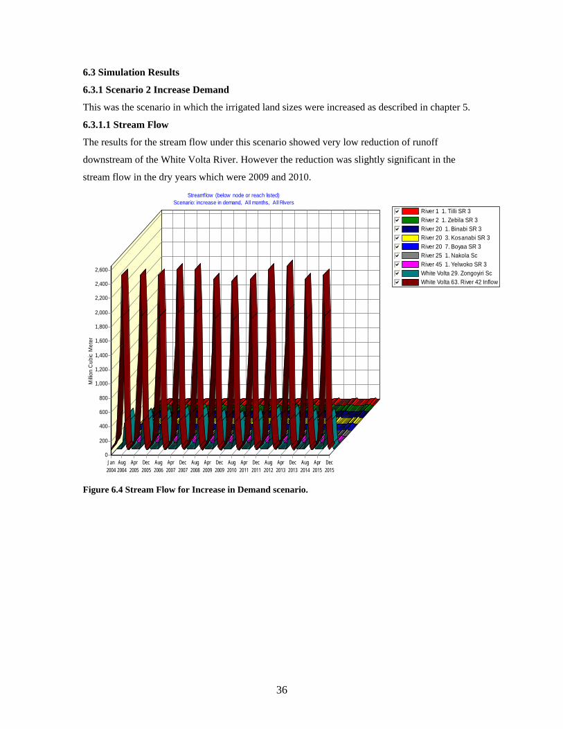
6.3 Simulation Results
6.3.1 Scenario 2 Increase Demand
This was the scenario in which the irrigated land sizes were increased as described in chapter 5.
6.3.1.1 Stream Flow
The results for the stream flow under this scenario showed very low reduction of runoff
downstream of the White Volta River. However the reduction was slightly significant in the
stream flow in the dry years which were 2009 and 2010.
River 1 1. Tilli SR 3gfedcbRiver 2 1. Zebila SR 3gfedcbRiver 20 1. Binabi SR 3gfedcbRiver 20 3. Kosanabi SR 3gfedcbRiver 20 7. Boyaa SR 3gfedcbRiver 25 1. Nakola ScgfedcbRiver 45 1. Yelwoko SR 3gfedcbWhite Volta 29. Zongoyiri ScgfedcbWhite Volta 63. River 42 Inflowgfedcb
Streamflow (below node or reach listed)Scenario: increase in demand, All months, All Rivers
Jan2004
Aug2004
Apr2005
Dec2005
Aug2006
Apr2007
Dec2007
Aug2008
Apr2009
Dec2009
Aug2010
Apr2011
Dec2011
Aug2012
Apr2013
Dec2013
Aug2014
Apr2015
Dec2015
Milli
on C
ubic
Met
er
2,600
2,400
2,200
2,000
1,800
1,600
1,400
1,200
1,000
800
600
400
200
0
Figure 6.4 Stream Flow for Increase in Demand scenario.

37
Reference gfedcbincrease in demand gfedcb
Streamflow (below node or reach listed)White Volta Nodes and Reaches: Below White Volta Headflow , All months, River: White Volta
Jan2004
Jul2004
Jan2005
Jul2005
Jan2006
Jul2006
Jan2007
Jul2007
Jan2008
Jul2008
Jan2009
Jul2009
Jan2010
Jul2010
Jan2011
Jul2011
Jan2012
Jul2012
Jan2013
Jul2013
Jan2014
Jul2014
Jan2015
Jul2015
Milli
on C
ubic
Met
er
150
140
130
120
110
100
90
80
70
60
50
40
30
20
10
0
Figure 6.5 Stream flow for Increased Demand Scenario and the Reference Scenario
6.3.1.2 Demand Coverage
The analysis for three different years 2010, 2013 and 2015 was considered. The year 2010 was
chosen to represent year with less rainfall as described in the table 5.3. The demand coverage for
the months of January, February, March and April were extremely low. The percentage ranges
between 69 % in Jan and 29% in April for reservoirs located on small streams (second order
streams). The January coverage was higher although it is part of the dry months. This could be
attributed to the fact that the reservoirs were able to store up some amount of water during the
previous year’s wet season thus making some amount of water available in the dry season. The
reservoirs located on the main White Volta River showed 100% coverage for all demand sites.
Year 2010 is considered to be a very dry year according to table 5.3. The results showed less
demand coverage in the dry months as shown in figure 6.6. This is because less water was stored
during the previous year’s wet season but the end of the wet season and the dry months for the
preceding year saw better demand coverage.

38
Bui Sc 3 gfedcbDatoko Sc gfedcbNakola Sc gfedcbZoko Sc. gfedcb
Demand Site Coverage (% of requirement met)Scenario: increase in demand, All months
January February March April May June July August September October Nov ember December
Perc
ent
100
95
90
85
80
75
70
65
60
55
50
45
40
35
30
25
20
15
10
5
0
Figure 6.6 Demand site coverage for year 2010 for some selected reservoirs in the very dry year.
The year 2015 was chosen to be a normal year with normal runoff for the various streams in the
Region .The results for unmet demand that is percentage of demand areas which are not met are
also represented in figure 6.8. This shows an increase over the period of study in agreement with
the demand increases. As the demand goes up the unmet demand also increases.

39
Bui Sc 3 gfedcbDatoko Sc gfedcbNakola Sc gfedcbZoko Sc. gfedcb
Demand Site Coverage (% of requirement met)Scenario: increase in demand, All months
Jan2013
Feb2013
Mar2013
Apr2013
May2013
Jun2013
Jul2013
Aug2013
Sep2013
Oct2013
Nov2013
Dec2013
Perc
ent
100
95
90
85
80
75
70
65
60
55
50
45
40
35
30
25
20
15
10
5
0
Figure 6.7 Demand Coverage 2013 for some selected reservoirs.
Bugri 1 gfedcbChiana Sc gfedcbDua 2 gfedcbFumbisi 1 gfedcbGbedema 1 gfedcbKaadi 1 gfedcbKpasen Sc. gfedcbPelungu 2 gfedcbSugudi 1 gfedcbTili 1 gfedcbYorogo 2 gfedcbZebila 1 gfedcbAll Others gfedcb
Unmet DemandScenario: increase in demand, All months
Jan2004
Aug2004
Apr2005
Dec2005
Aug2006
Apr2007
Dec2007
Aug2008
Apr2009
Dec2009
Aug2010
Apr2011
Dec2011
Aug2012
Apr2013
Dec2013
Aug2014
Apr2015
Dec2015
Thou
sand
Cub
ic M
eter
220
200
180
160
140
120
100
80
60
40
20
0
Figure 6.8 Unmet Demand

40
6.3.1.3 Reservoir Storage volume
The storages for the various reservoirs agree with the demand coverage of the same reservoirs.
The dry months showed less storages and less demand coverage through out the years under
study. This is represented in figure 6.9
Kpasenkpe Sc gfedcbNaga Sc. gfedcbNaga Sc.3 gfedcbNasia SR 3 gfedcbNingo Sc gfedcbSR 5 gfedcbSandema SR3 gfedcbSc.3 gfedcbSokoti SR3 gfedcbTula Sc 3 gfedcbYinduri Sc gfedcbZarre Sc 3 gfedcbAll Others gfedcb
Reservoir Storage VolumeScenario: increase in demand, All months
Jan2004
Aug2004
Apr2005
Dec2005
Aug2006
Apr2007
Dec2007
Aug2008
Apr2009
Dec2009
Aug2010
Apr2011
Dec2011
Aug2012
Apr2013
Dec2013
Aug2014
Apr2015
Dec2015
Thou
sand
Cub
ic M
eter
16,00015,00014,00013,00012,00011,00010,0009,0008,0007,0006,0005,0004,0003,0002,0001,000
0
Figure 6.9 Reservoir Storage Volume Mm3.
6.3.2 Scenario 3; Increase in Demand during the Wet Season.
This scenario as described in chapter 5 shows an increase in the demand during the wet seasons
of June, July and August.
6.3.2.1 Demand Coverage
The results showed 100% coverage for the months of Jun, July and August though there were
increases in demand. There was enough water to serve more irrigated lands during those months.
The reservoirs that were located on the main river showed continuous coverage throughout the
period. The unmet demand for these months was zero.

41
6.3.2.1 Reservoir Storage volume
The reservoirs were all full in wet months just like the demand coverage. However two reservoirs
located at Yorogo SR1 and Dua SR1 showed zero volumes in the months of Feb, Mar, April.
These reservoirs were however filled during the wet months. This is represented in appendix 5.
6.3.3 Scenario 2; Increase in reservoirs
This is described in chapter 5 and shows the case when the number of reservoirs are increased
according to table 5.4
6.3.3.1 Stream flow
The results obtained for the stream flow showed a reduction in the main White Volta River in the
monthly average values. The difference in the stream flow for the month of December between
the current account year and the “more reservoirs added scenario was 0.5 Mm3 while that of
February was 1M m3. The highest difference was seen in the month of March which was 5 Mm3.
6.3.3.2 Reservoir Storage Volume
The additional reservoirs were filled through out the period in which they were in operation. They
were filled to full capacity in all the months.
The demands for the additional reservoirs were also met during the period.
6.4 Evaluation
The results obtained from the model showed that not all the demand sites were covered during the
dry months of the year. Most of the demand sites on the second order streams are clear examples
of sites which were not covered throughout the year. However the reservoirs located on the main
White Volta River showed a constant supply of water in all the years under study and under all
the scenarios created. Some of the reservoirs located on the small streams were able to store some
amount of water during the wet season which is utilized during the dry months however not all
the demand requirement is met in the dry months. The later part of the dry season received very
little coverage.
The volume of the reservoirs behaved in a similar manner as the demand coverage. The reservoirs
were filled to higher volumes during the wet months however the dry months showed less
volume. When the demand sites were increased in the wet months, the reservoirs were able to
handle the increase. This indicates that the reservoirs, particularly those located on the main river,
can support complimentary irrigation during the wet seasons.

42
The increase in demand scenario showed an increase in the unmet demand in the dry months.
This was increasing with the years under study according to figure 6.8 because the demand was
increased in accordance with the years. Approximately 180,000 m3 of water would be required to
satisfy irrigation during the dry months.
The total annual flow from the river was not affected in any significant way in all the three
scenarios. However the flows from the second order streams showed a significant reduction
during the dry months. Thus the flow in the main river showed a very small difference in the dry
months when compared to the current account year.
The third scenario which is the Increase in Number of Reservoirs Scenario showed a reduction in
the flow values for the White Volta River. The reduction is in the range of 0.5 Mm3 to 0.5 Mm3
depending on the month. Although this reduction is insignificant compared to the monthly flow,
the value can increase and cause a major reduction in the flow downstream when more reservoirs
and demand sites are created on the main rivers.
6.5 Planning
In the planning of these small reservoirs, their location is of much importance in order to ensure
demand coverage. This is much hindered by proximity since all the farmers cannot be located on
the reservoirs located on the main rivers. However various farming groups can be created near
reservoirs with constant supply of water and the reservoirs in those areas can be expanded to store
more water for irrigation in all the farming seasons.

43
7 CONCLUSIONS
Water is a priceless commodity in the arid and semi-arid regions of the world where irregular
rainfall is predominant. Creation of reservoirs is however a tool for ensuring adequate supply of
water throughout the year. In the UER of Ghana where there is a higher incidence of poverty as
compared to the other regions, small reservoirs are a major component of the people’s farming
activities. Development of small reservoirs is an efficient way of developing agriculture in the
arid region of the world.
The aim of this study was to determine the impact of the large number of these small reservoirs
on the downstream flow condition. From the results obtained for all the scenarios created, small
reservoirs in the UER have relatively low impact on the downstream flow of the White Volta
River. However reduction of the flow can be significant in the advent of the creation of larger
reservoirs and more demand sites which may be located on the WVR as presented in the creation
of more reservoirs with higher storage capacities and bigger demand sites scenario.
The reservoirs can also be used for other purposes such as more irrigated lands and more
livestock production in the months of June, July, and August. More flow is realised in the streams
during those months and so there is a possibility of making use of more water for other purposes.
The WEAP Model was a very good tool for this thesis. It is easy to use and offers a wide range of
possibilities to be analysed under the scenario creation.

44
8 REFERENCES
Asenso-Okyere, W.K., Twum-Baah, K.A., Kasanga A., Anum, J. and Portner C., 2000.
Ghana Living Standards Survey. Report of the Fourth Round (GLSS 4),
Ghana Statistical Service, Accra.
A. B. Avakyan and S. A. Podol’skii, 2001 Impact of Reservoirs on the Fauna
Swedish Research Council for Environment, Agricultural Science and Spatial Planning,
2006 Dams under Debate
Ghana Statistical Service, 2000. Poverty trends in Ghana in the 1990s.
Ghana Statistical Service, Accra.
Global Water Partnership, 2006 Integrated Water Resources Management
[Online]
[Available on www.gwp.org]
[Cited on December 2006]
IGBP/IHDP (1993) Relating Land Use and Global Land Cover Change. IHDP.
IFAD, 2006, Upper East Region Land Conservation and Smallholder Rehabilitation
Project(LACOSREP) [Online ] Report. No 5
[Available on http://www.ifad.org/governance/index.htm]
[Cited November 2006]
J. Liebe N. van de Giesen M. Andreini, 2005 Estimation of small reservoir storage capacities
in a semi-arid environment A case study in the Upper East Region of Ghana.[Online]
Available from www.smallreservoirs.org
[Cited November 2006]
Jack Sieber, Chris Swartz, Annette Huber-Lee, 2005 WEAP User guide Stockholm
Environmental Institute

45
Kwabena Wiafe, 1997 Irrigation, Volta Basin Starter Kit July, 2006 Compiled by P.Drechsel,B
Barry, A Bahri and W.Andah
P. Raskin, E. Hansen, and Z. Zhu, M. IWRA, D. Stavisky, Simulation of Water Supply and
Demand in the Aral Sea Region [Online] pp 55-67
[Available on http://www.weap21.org/downloads/aralsea.pdf]
[Cited December 2006]
P. Gyau-Boakye ,2000 Environmental impacts of the Akosombo dam and
Effects of climate change on the lake level.
Environment, Development and Sustainability 3: 17–29, Kluwer Academic Publishers.
Printed in the Netherlands.
Shiklomanov, I.A. 1999. World Water Resources: A New Appraisal and
Assessment for the 21st Century.
Rapport du Programme Hydrologique International (PHI), Paris. UNESCO
.
Winston E.I. Andah Francis Gichuki, Volta River Basin: Enhancing Agricultural Water
Productivity through Strategic Research, Report No 8
Winston E.I. Andah, Nick van de Giesen, Charles A. Biney, 2005 Water, Climate, Food, and
Environment in the Volta Basin Contribution to the project ADAPT Adaptation strategies to
changing environments
[Online][Available on http://www.weap21.org/index.asp?doc=05]
[Cited on December 2006]
World Metrological Organization, 1986. Manual for Estimation of Probable Maximum
Precipitation, 269 pp. WMO No. 332 (1986) [Online]
[Available on http://www.wmo.ch/pages/prog/hwrp/homs/Components/English/k15201.htm]
[Cited on December 2006]
UN World Water Development 2006, Water a Shared Responsibility,
Report No. 2

46
UNESCO and Berghahn Books.
UNESCO Water Portal [Online]
[Available on http://assistive.usablenet.com/tt/www.unesco.org/water/]
[Cited on December 2006]
Volta Basin Starter Kit July, 2006 Compiled by P.Drechsel,B Barry, A Bahri and W.Andah
Volta River Authority [Online]
[Available on www.vra.com]
[Cited on December, 2006]
Internet Sources
FAO Coporate document Respository [Online]
[Available on www.fao.org]
[Cited in December 2006]
Small Reservoir Project. [Online]
[Available on http://www.smallreservoirs.org/]
[Cited on December 2006]

47
8 APPENDIX
Appendix 1 Results of Stream flow for the current account year.
0. Headflow gfedcb1. River 4 Inflow gfedcb2. Reach gfedcb3. Yarugu SR 3 gfedcb4. Reach gfedcb5. Withdrawal Node 2 gfedcb6. Reach gfedcb7. Bazua SR 3 gfedcb8. Reach gfedcb9. Withdrawal Node 3 gfedcb10. Reach gfedcb11. Timonde SR 3 gfedcb12. Reach gfedcb13. Withdrawal Node 5 gfedcb14. Reach gfedcb15. River 3 Inflow gfedcb16. Reach gfedcb17. Atoba SR 3 gfedcb18. Reach gfedcb19. Withdrawal Node 4 gfedcb20. Reach gfedcb21. River 2 Inflow gfedcb22. Reach gfedcb23. River 1 Inflow gfedcb24. Reach gfedcb25. River 20 Inflow gfedcb26. Reach gfedcb27. River 6 Inflow gfedcb28. Reach gfedcb
Streamflow (below node or reach listed)Scenario: Reference, All months, River: White Volta
January February March April May June July August September Nov ember
Milli
on C
ubic
Met
er
3,200
3,000
2,800
2,600
2,400
2,200
2,000
1,800
1,600
1,400
1,200
1,000
800
600
400
200
0

48
Appendix 2 Results for Reservoirs storage volumes for the current account year in Mm3
Jan-04 Feb-
04
Mar-
04
Apr-
04
May-
04
Jun-04 Jul-04 Aug-
04
Sep-
04
Oct-04 Nov-
04
Dec-
04
Kpasenkpe Sc 500 500 500 500 500 500 500 500 500 500 500 500
Naga Sc. 380 380 380 380 380 380 380 380 380 380 380 380
Naga Sc.3 380 380 380 380 380 380 380 380 380 380 380 380
Nasia SR 3 380 380 380 380 380 380 380 380 380 380 380 380
Ningo Sc 380 380 380 380 380 380 380 380 380 380 380 380
SR 5 1000 1000 1000 1000 1000 1000 1000 1000 1000 1000 1000 1000
Sandema SR3 380 380 380 380 380 380 380 380 380 380 380 380
Sc.3 380 380 380 380 380 380 380 380 380 380 380 380
Sokoti SR3 380 380 380 380 380 380 380 380 380 380 380 380
Tula Sc 3 380 380 380 380 380 380 380 380 380 380 380 380
Yinduri Sc 380 380 380 380 380 380 380 380 380 380 380 380
Zarre Sc 3 380 380 380 380 380 380 380 380 380 380 380 380
All Others 8512 7904 6992 7376 16370 16370 16370 16370 16370 16267 14815 13297
Sum 13812 13204 12292 12676 21670 21670 21670 21670 21670 21567 20115 18597

49
Appendix 3 Results of demand site coverage in percentage for the current account year
Jan Feb Mar April May June July Aug Sept Oct Nov Dec
Agric3 100 100 100 100 100 100 100 100 100 100 100 100
Asungi 1 100 100 100 100 100 100 100 100 100 100 100 100
Atoba 1 100 100 100 100 100 100 100 100 100 100 100 100
Bansi Sc 59.6 50.3 43.2 36.3 100 100 100 100 100 100 86.2 72.9
Bazua 1 100 100 100 100 100 100 100 100 100 100 100 100
Binaba 1 98.9 95.0 93.5 56.7 100 100 100 100 100 100 100 100
Bisigu Sc 100 100 100 100 100 100 100 100 100 100 100 100
Bolga 1 100 100 100 100 100 100 100 100 100 100 100 100
Boyaa 1 98.9 98.1 96.4 86.3 100 100 100 100 100 100 100 100
Bugri 1 63.6 53.4 45.4 38.2 100 100 100 100 100 100 88.0 76.4
Bui Sc 3 100 100 100 100 100 100 100 100 100 100 100 100
Chiana Sc 0 0 0 0 0 0 0 0 0 0 0 0
Corner 1 66.0 56.5 48.2 40.9 100 100 100 100 100 100 89.0 78.2
Datoko Sc 68.7 60.2 51.9 100.0 100 100 100 100 100 100 89.9 80.2
Dua 2 34.5 20.0 7.8 0.0 100 100 100 100 100 100 71.4 53.0
Fumbisi 1 60.0 51.9 44.4 37.3 100 100 100 100 100 89.7 79.9 70.4
Gbedema 1 60.0 51.9 44.4 37.3 100 100 100 100 100 89.7 79.9 70.4
Kaadi 1 58.8 48.5 41.7 35.3 100 100 100 100 100 100 86.0 72.5
Kaadi Sc 66.1 56.6 48.3 41.8 100 100 100 100 100 100 89.0 78.2
Kadema 1 68.3 59.6 51.3 43.9 100 100 100 100 100 100 89.8 79.9
Kadema
Sc.3
100.0 100.0 100.0 100.0 100 100 100 100 100 100 100.0 100.0
Kagbiri Sc 63.6 53.5 45.6 39.2 100 100 100 100 100 100 88.0 76.4
Kalbeo 2 100.0 100.0 100.0 100.0 100 100 100 100 100 100 100 100
Katigri 100.0 98.8 97.0 96.1 100 100 100 100 100 100 100 100
Kayile 1 100.0 100.0 100.0 100.0 100 100 100 100 100 100 100 100
Kayoro 1 76.9 67.9 58.9 100.0 100 100 100 100 100 100 100 89.651
Kpasen Sc. 0 0 0 0 0 0 0 0 0 0 0 0
Kugurago 1 66.0 56.5 48.2 41.4 100.0 100.0 100.0 100.0 100.0 100.0 89.0 78.2
Naga Sc 100.0 100.0 100.0 100.0 100.0 100.0 100.0 100.0 100.0 100.0 100.0 100.0
Naga Sc. 100.0 100.0 100.0 100.0 100.0 100.0 100.0 100.0 100.0 100.0 100.0 100.0

50
Nakola Sc 68.6 60.0 51.8 44.4 100.0 100.0 100.0 100.0 100.0 100.0 89.9 80.1
Nakong 1 68.3 59.6 51.3 100.0 100.0 100.0 100.0 100.0 100.0 100.0 89.8 79.9
Nasia 1 100.0 100.0 100.0 100.0 100.0 100.0 100.0 100.0 100.0 100.0 100.0 100.0
Navrongo 1 68.6 60.0 51.8 44.4 100.0 100.0 100.0 100.0 100.0 100.0 89.9 80.1
Ningo Sc 100.0 100.0 100.0 100.0 100.0 100.0 100.0 100.0 100.0 100.0 100.0 100.0
Pelungu 2 12.8 0.0 0.0 100.0 100.0 100.0 100.0 100.0 100.0 100.0 63.9 34.8
Sambolgu2 100.0 100.0 100.0 100.0 100.0 100.0 100.0 100.0 100.0 100.0 100.0 100.0
Sandema 1 100.0 100.0 100.0 100.0 100.0 100.0 100.0 100.0 100.0 100.0 100.0 100.0
Sc 3 100.0 100.0 100.0 100.0 100.0 100.0 100.0 100.0 100.0 100.0 100.0 100.0
Sekoti 1 100.0 100.0 100.0 100.0 100.0 100.0 100.0 100.0 100.0 100.0 100.0 100.0
Seshi1 100.0 100.0 100.0 100.0 100.0 100.0 100.0 100.0 100.0 100.0 100.0 100.0
Sherigu 1 100.0 100.0 100.0 100.0 100.0 100.0 100.0 100.0 100.0 100.0 100.0 100.0
Sikiri Sc 58.8 47.3 40.9 34.9 100.0 100.0 100.0 100.0 100.0 100.0 86.2 72.8
Sinensi Sc 69.0 60.4 52.2 100.0 100.0 100.0 100.0 100.0 100.0 100.0 90.0 80.4
Sugudi 1 58.9 48.7 41.8 35.2 100.0 100.0 100.0 100.0 100.0 100.0 86.0 72.5
Tili 1 58.2 47.8 41.1 34.9 100.0 100.0 100.0 100.0 100.0 100.0 86.0 72.5
Timonde 1 100.0 100.0 100.0 100.0 100.0 100.0 100.0 100.0 100.0 100.0 100.0 100.0
Tula sc 100.0 100.0 100.0 100.0 100.0 100.0 100.0 100.0 100.0 100.0 100.0 100.0
Uwasi 1 100.0 98.8 91.7 91.7 100.0 100.0 100.0 100.0 100.0 100.0 100.0 100.0
Wrinyanga1 68.3 59.6 51.3 43.9 100.0 100.0 100.0 100.0 100.0 100.0 89.8 79.9
Yarugu 2 100.0 100.0 100.0 100.0 100.0 100.0 100.0 100.0 100.0 100.0 100.0 100.0
Yelwoko 1 68.2 59.5 51.2 43.7 100.0 100.0 100.0 100.0 100.0 100.0 89.7 79.8
Yinduri Sc 100.0 100.0 100.0 100.0 100.0 100.0 100.0 100.0 100.0 100.0 100.0 100.0
Yorogo 2 92.2 20.0 7.8 0.0 100.0 100.0 100.0 100.0 100.0 100.0 100.0 100.0
Zarre Sc 100.0 100.0 100.0 100.0 100.0 100.0 100.0 100.0 100.0 100.0 100.0 100.0
Zebila 1 58.7 47.9 41.2 34.9 100.0 100.0 100.0 100.0 100.0 100.0 86.0 72.5
Zoko Sc. 67.1 58.1 49.0 40.3 100.0 100.0 100.0 100.0 100.0 100.0 89.3 79.0
Zongoyiri
Sc
100.0 100.0 100.0 100.0 100.0 100.0 100.0 100.0 100.0 100.0 100.0 100.0

51
Appendix 4 Results of the demand site coverage in percentage for the year 2010
Jan-
10
Feb-
10
Mar-
10
Apr-
10
May-
10
Jun-
10
Jul-
10
Aug-
10
Sep-
10
Oct-
10
Nov-
10
Dec-
10
Agric3 100 100 100 100 100 100 100 100 100 100 100 100
Asungi 1 100 100 100 100 100 100 100 100 100 100 100 100
Atoba 1 100 100 100 100 100 100 100 100 100 100 100 100
Bansi Sc 61 51 44 37 100 100 100 100 100 100 86 73
Bazua 1 100 100 100 100 100 100 100 100 100 100 100 100
Binaba 1 100 100 91 59 100 100 100 100 100 100 100 100
Bisigu Sc 100 100 100 100 100 100 100 100 100 100 100 100
Bolga 1 100 100 100 100 100 100 100 100 100 100 100 100
Boyaa 1 100 100 91 80 100 100 100 100 100 100 100 100
Bugri 1 64 54 46 38 100 100 100 100 100 100 88 76
Bui Sc 3 100 100 100 100 100 100 100 100 100 100 100 100
Chiana Sc 0 0 0 0 0 0 0 0 0 0 0 0
Corner 1 66 55 47 39 100 100 100 100 100 100 88 76
Datoko Sc 71 62 53 100 100 100 100 100 100 100 90 80
Dua 2 33 16 4 0 100 100 100 100 100 100 69 49
Fumbisi 1 59 51 43 35 100 100 100 100 100 89 78 68
Gbedema 1 59 51 43 36 100 100 100 100 100 89 78 68
Kaadi 1 59 48 41 34 100 100 100 100 100 100 85 71
Kaadi Sc 66 55 47 40 100 100 100 100 100 100 88 76
Kadema 1 68 59 51 43 100 100 100 100 100 100 89 78
Kadema
Sc.3
100 100 100 100 100 100 100 100 100 100 100 100
Kagbiri Sc 64 54 46 39 100 100 100 100 100 100 88 76
Kalbeo 2 100 100 100 100 100 100 100 100 100 100 100 100
Katigri 100 100 100 100 100 100 100 100 100 100 100 100
Kayile 1 100 100 100 100 100 100 100 100 100 100 100 100
Kayoro 1 78 69 59 100 100 100 100 100 100 100 100 89
Kpasen Sc. 0 0 0 0 0 0 0 0 0 0 0 0
Kugurago 1 66 55 47 39 100 100 100 100 100 100 88 76
Naga Sc 100 100 100 100 100 100 100 100 100 100 100 100

52
Naga Sc. 100 100 100 100 100 100 100 100 100 100 100 100
Nakola Sc 70 61 52 45 100 100 100 100 100 100 89 79
Nakong 1 68 59 51 100 100 100 100 100 100 100 89 78
Nasia 1 100 100 100 100 100 100 100 100 100 100 100 100
Navrongo 1 70 61 52 45 100 100 100 100 100 100 89 79
Ningo Sc 100 100 100 100 100 100 100 100 100 100 100 100
Pelungu 2 9 0 0 100 100 100 100 100 100 100 61 30
Sambolgu2 100 100 100 100 100 100 100 100 100 100 100 100
Sandema 1 100 100 100 100 100 100 100 100 100 100 100 100
Sc 3 100 100 100 100 100 100 100 100 100 100 100 100
Sekoti 1 100 100 100 100 100 100 100 100 100 100 100 100
Seshi1 100 100 100 100 100 100 100 100 100 100 100 100
Sherigu 1 100 100 100 100 100 100 100 100 100 100 100 100
Sikiri Sc 60 48 41 35 100 100 100 100 100 100 86 73
Sinensi Sc 71 62 54 100 100 100 100 100 100 100 90 80
Sugudi 1 59 48 41 34 100 100 100 100 100 100 85 71
Tili 1 57 47 40 34 100 100 100 100 100 100 85 71
Timonde 1 100 100 100 100 100 100 100 100 100 100 100 100
Tula sc 100 100 100 100 100 100 100 100 100 100 100 100
Uwasi 1 100 100 100 100 100 100 100 100 100 100 100 100
Wrinyanga1 68 59 51 43 100 100 100 100 100 100 89 78
Yarugu 2 100 100 100 100 100 100 100 100 100 100 100 100
Yelwoko 1 68 59 50 43 100 100 100 100 100 100 89 78
Yinduri Sc 100 100 100 100 100 100 100 100 100 100 100 100
Yorogo 2 94 16 4 0 100 100 100 100 100 100 100 100
Zarre Sc 100 100 100 100 100 100 100 100 100 100 100 100
Zebila 1 58 48 41 34 100 100 100 100 100 100 85 71
Zoko Sc. 69 60 51 43 100 100 100 100 100 100 89 79
ZongoyiriSc 100 100 100 100 100 100 100 100 100 100 100 100

53
Appendix 5 Results of the storage volume of reservoirs for scenario 3; Increase in demand
during the wet months.
Kpasenkpe Sc gfedcbNaga Sc. gfedcbNaga Sc.3 gfedcbNasia SR 3 gfedcbNingo Sc gfedcbSR 5 gfedcbSandema SR3 gfedcbSc.3 gfedcbSokoti SR3 gfedcbTula Sc 3 gfedcbYinduri Sc gfedcbZarre Sc 3 gfedcbAll Others gfedcb
Reservoir Storage VolumeScenario: increase in demand, All months
Jan2004
Aug2004
Apr2005
Dec2005
Aug2006
Apr2007
Dec2007
Aug2008
Apr2009
Dec2009
Aug2010
Apr2011
Dec2011
Aug2012
Apr2013
Dec2013
Aug2014
Apr2015
Dec2015
Thou
sand
Cub
ic M
eter
16,00015,00014,00013,00012,00011,00010,0009,0008,0007,0006,0005,0004,0003,0002,0001,000
0

54
Appendix 6 Results of the demand in percentage of the additional reservoirs as described in
scenario 2
Demand coverage of new reservoirs.
Balungu MR gfedcbKugli MR gfedcbMR 3 gfedcbNaga MR gfedcbNangodi MR gfedcbPwalugu gfedcbWiaga MR gfedcbZarre MR gfedcb
Demand Site Coverage (% of requirement met)Scenario: more reservoirs, All months
Jan2004
Jun2004
Dec2004
Jun2005
Dec2005
Jun2006
Dec2006
Jun2007
Dec2007
Jun2008
Dec2008
Jun2009
Dec2009
Jun2010
Dec2010
Jun2011
Dec2011
Jun2012
Dec2012
Jun2013
Dec2013
Jun2014
Dec2014
Jun2015
Dec2015
Perc
ent
100
95
90
85
80
75
70
65
60
55
50
45
40
35
30
25
20
15
10
5
0

55
Appendix 7 Discharge values for some selected gauge stations.
Month Flow
m3/s
Month Flow m3/s
Jan 0 Jan 0
Feb 0 Feb 0
March 0 March 0
April 0 April 0
May 6.8 May 14.76
June 40.2 June 22.81
July 37.9 July 12.85
August 27.5 August 47.266
Sept 34 Sept 3.5
Oct 3.64 Oct 0
Nov 0 Nov 0
Dec. 0 Dec 0
Month Flow m3/s Month m3/s
Jan 0 Jan 20.84
Feb 0 Feb 1.68
March 0 March 1.15
April 0 April 1.27
May 0.67 May 2.47
June 5.57 June 10.75
July 12.6 July 48.42
August 102.57 August 137.19
Sept 87.485 Sept 75.87
Oct 5.445 Oct 10.68
Nov 0 Nov 3.5
Dec. 0 Dec. 14.35
White Volta
headflow
Yakala
River 47 Gagaba Gaba

56
White Volta below River 21 Pwalugu
Month Flow m3/s Month Flow m3/s
Jan 18.25 Jan 0
Feb 32.86 Feb 0
March 39.03 March 0
April 53.27 April 0
May 66.55 May 0.85
June 87.06 June 1.89
July 168.05 July 0.579
August 271.17 August 3.5
Sept 241.49 Sept 4.97
Oct 53.56 Oct 0.51
Nov 28.95 Nov 0
Dec 23.67 Dec 0

57

58