Modeling Transformations with Neural Networks

Presented by Dinghuang Ji

(Deep Learning Journal Club 04/12/2016)

Outline

• Modeling transformations

• Transforming autoencoder

• Spatial transformer networks

• Deep symmetry networks

Modeling transformations

2D Classification and Recognition

3D reconstruction

Temporal sequence analysis

3D deformable objects Registration

Transformation types

(C) ROTATION IN DEPTH (D) ILLUMINATION

Affine transformations

Non-affine transformations

Related Works

• Hand-crafted features like SIFT, SURF, ORB etc.

• Denoising autoencoder (for noisy data)

• Convolutional training (for shift-invariance)

• Transformation equivariant methods

• Matchnet: Unifying Feature and Metric Learning for Patch-Based Matching

• Discriminative Learning of Deep Convolutional Feature Point Descriptors

Related Works

• Hand-crafted features like SIFT, SURF, ORB etc.

• Denoising autoencoder (for noisy data)

• Convolutional training (for shift-invariance)

• Transformation equivariant methods

• Matchnet: Unifying Feature and Metric Learning for Patch-Based Matching

• Discriminative Learning of Deep Convolutional Feature Point Descriptors

How convolutional neural network works

⁺ The feature extraction layers are interleaved with sub-sampling layers that throw away information about precise position in order to achieve some translation invariance.

- Sub-sampling loses the precise spatial relationships between higher-level parts such as a nose and a mouth in faces. The precise spatial relationships are needed for identity recognition.

- They cannot extrapolate their understanding of geometric relationships to radically new viewpoints.

Equivariance vs Invariance

X Sub-sampling tries to make the neural activities invariant for small changes in viewpoint. – This is a silly goal, motivated by the fact that the final label needs to

be viewpoint-invariant.

It’s better to aim for equivariance: Changes in viewpoint lead to corresponding changes in neural activities. – In the perceptual system, its the weights that code viewpoint-invariant

knowledge, not the neural activities.

Outline

• Modeling transformations

• Transforming autoencoder

• Spatial transformer networks

• Deep symmetry networks

Transforming Auto-encoder

• “Current methods for recognizing objects in images perform poorly and use methods that are intellectually unsatisfying”

• Capsules

– learns to recognize an implicitly defined visual entity over a limited domain of viewing conditions and deformations.

– provide a simple way to recognize wholes by recognizing their parts.

Learning the lowest level capsules

• We are given a pair of images related by a known translation.

Step 1: Compute the capsule outputs for the first image. o Each capsule uses its own set of “recognition” hidden units to extract

the x and y coordinates of the visual entity it represents (and also the probability of existence)

Step 2: Apply the transformation to the outputs of each capsule

o Just add Δx to each x output and Δy to each y output

Step 3: Predict the transformed image from the transformed outputs of the capsules

o Each capsule uses its own set of “generative” hidden units to compute its contribution to the prediction.

Training the network

Why it has to work

• When the net is trained with back-propagation, the only way it can get the transformations right is by using x and y in a way that is consistent with the way we are using Δx and Δy.

• This allows us to force the capsules to extract the coordinates of visual entities without having to decide what the entities are or where they are.

Equivariance vs Invariance

• When the capsule is working properly, the probability of the visual entity being present is locally invariant – it does not change as the entity moves over the manifold of possible appearances within the limited domain covered by the capsule.

• The instantiation parameters, however, are “equivariant” – as the viewing conditions change and the entity moves over the appearance manifold, the instantiation parameters change by a corresponding amount because they are representing the intrinsic coordinates of the entity on the appearance manifold.

Experiments

• We trained a network with 30 capsules each of which had 10 recognition units and 20 generation units. Each capsule sees the whole of an MNIST digit image.

• Both the input and the output images are shifted randomly by -2, -1, 0, +1, or +2 pixels in the x and y directions.

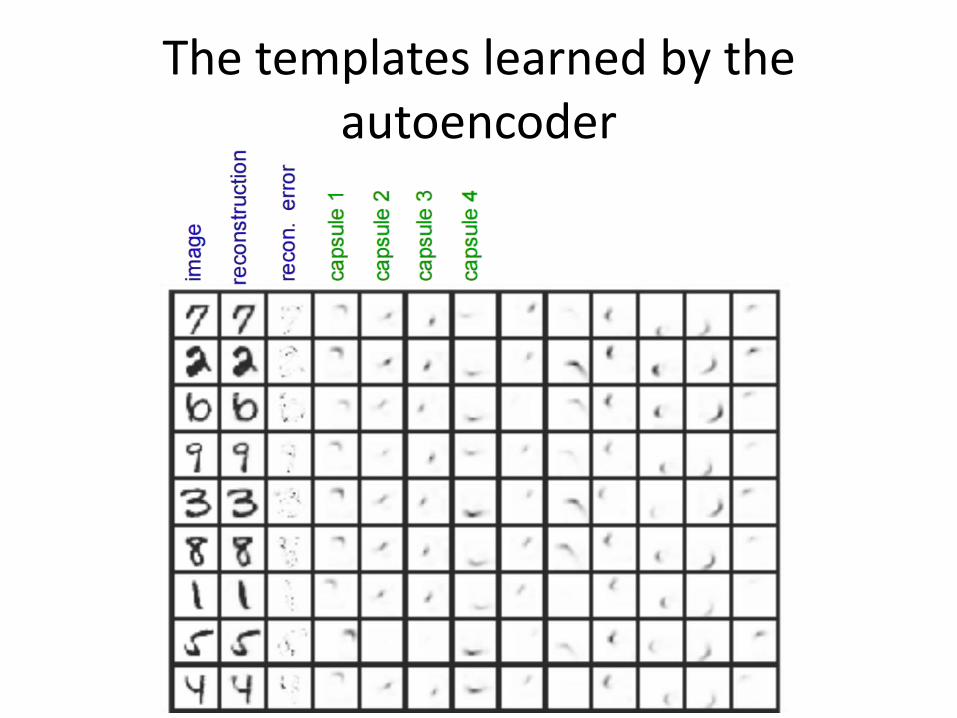
The templates learned by the autoencoder

More Complex Transformations

• 2D affine matrix

• Modeling Changes in 3-D Viewpoint

– Use CG to generate stereo images of various types of car from many different viewpoints

– The transforming autoencoder consisted of 900 capsules, each with two layers (32 then 64) of rectified linear recognition units and single layer of 128 generative rectified linear units.

Modeling Changes in 3-D Viewpoint

Discussions

• For non-affine transformation, maybe highly nonlinear activation function will be more helpful.

• Transfer learning can be readily tried given a working auto-encoder model.

• Transforming auto-encoders have potential application in video compressing, and semantic hashing.

Outline

• Modeling transformations

• Transforming autoencoder

• Spatial transformer networks

• Deep symmetry networks

Spatial Transformers

• Performs spatial transform on feature map during single forward pass

• Transformation is conditional on input feature maps, spatially warp images – Transforms data to a normalized space expected by

subsequent layers – Intelligently select features of interest (attention) – Invariant to more generic warping

• Can be placed anywhere

– Transform meaningful images (inputs) or more abstract representations (feature maps)

Spatial Transformers

• Localization network – Small neural network – Takes feature map input, outputs transformation

parameters

• Grid Generator

– Pixel map defining where to sample input

• Sampler

– Takes transformation parameters and grid as inputs, produces output of spatial transformer network

Design

• Input

• Learned function – 𝑓𝑙𝑜𝑐() can take any form – Final layer must be 𝜃 regressor

• Output

– 𝜃 can be any transformation parameters

Localization Network

𝑈 ∈ ℝ𝐻×𝑊×𝐶

H

W

C

U

H

W

C

U 𝑓𝑙𝑜𝑐(𝑈) 𝜃 Any type of network

𝜃 =

𝑎11 𝑎12 𝑡𝑥𝑎21 𝑎22 𝑡𝑦0 0 1

or … or 𝜃 =

ℎ11 ℎ12 ℎ13ℎ21 ℎ22 ℎ23ℎ31 ℎ32 ℎ33

• Transformations of the network can be parameterized: 1. Scaling

2. Rotation

3. Cropping

4. Projective transformations

Localization Network

Sampling Grid

Sampling Grid

• General form of sampling function

𝑉𝑖𝑐 = 𝑈𝑛,𝑚

𝑐 𝑘(𝑥𝑖𝑠

𝑊

𝑚

−𝑚; Φ𝑥)𝑘(𝑦𝑖𝑠 − 𝑛; Φ𝑦)

𝐻

𝑛

∀ 𝑖 ∈ 1 …𝐻′𝑊′ , ∀ 𝑐 ∈ 1…𝐶

• 𝑈𝑛,𝑚𝑐 is input pixel at (n,m,c)

• (𝑥𝑖𝑠, 𝑦𝑖𝑠) is coordinate in input image where sampling applied

• 𝑘() defines image interpolation

Differentiable Sampling

• bilinear interpolation • Gradients

𝜕𝑉𝑖𝑐

𝜕𝑈𝑛,𝑚𝑐 = max (0, 1 − |𝑥𝑖

𝑠

𝑊

𝑚

− 𝑚|)max (0, 1 − |𝑦𝑖𝑠 − 𝑛|)

𝐻

𝑛

𝜕𝑉𝑖𝑐

𝜕𝑥𝑖𝑠 = 𝑈𝑛,𝑚

𝑐

𝑊

𝑚

𝐻

𝑛

max 0, 1 − 𝑦𝑖𝑠 − 𝑛

0 𝑖𝑓 𝑚 − 𝑥𝑖𝑠 ≥ 1

1 𝑖𝑓 𝑚 ≥ 𝑥𝑖𝑠

−1 𝑖𝑓 𝑚 < 𝑥𝑖𝑠

Similar for 𝜕𝑉𝑖

𝑐

𝜕𝑦𝑖𝑠

Differentiable Sampling

Experiments

• MNIST Distorted Numbers

• MNIST Addition

• Street View House Numbers

• Fine-Grained Classification

• 3D Distorted Numbers recognition

• Warp dataset (Training data: 6000 examples of each digit, Testing data: 10k images ) – Rotation (R) – Rotation, scale, and translation (RTS) – Projective transformation (P) – Elastic warping (E)

• Add ST immediately following input to fully-connected (ST-FCN) and convolutional (ST-CNN) networks

• All ST use bilinear sampling, but differ in transformations

– Affine (Aff) – Projective (Proj) – 16-point thin plate spline (TPS) [2]

MNIST Distorted Numbers

MNIST Distorted Numbers

a) Inputs to networks b) Predicted transformations visualized by the grid c) The outputs of the spatial transformers

Note: FCN means fully-connected network

Also went further and tested MNIST Addition See section A.1 in the paper for details

Add digits in two images

• MNIST digits under rotation, translation and scale

Add digits in two images

MNIST Addition

Animation

• 200k real world images with 1-5 numbers each

• Baseline CNN model: 11 hidden layers, 5 softmax classifiers

• ST-CNN Single – ST just following input – Localization network is 4 convolutional layers

• ST-CNN Multi – Add ST before each of first 4 convolutional layers – Localization network has two 32 unit, fully connected layers – Idea is to predict transformation on better features than just raw

pixels

Street View House Numbers

Street View House Numbers [5]

• Test images were 64x64px and 128x128px crops

– 128x128 has more background

• Major improvement in 128x128px crops due to ST’s ability to localize object

Results in percent error (a) ST-CNN Multi architecture (b) L-R: Input, predicted transform, and output. The bounding box is composition of 4 affine transforms

• CUB-200-2011 birds dataset – 6k training images – 5.8k test images – 200 species classes

• 2xST-CNN architecture

• Single 𝑓𝑙𝑜𝑐() predicts 2 parameters corresponding to location of two 224x224px crops

• 4xST-CNN predicts 4 parameters similarly

Fine-Grained Classification

• Surpassed baseline CNN which used state-of-the-art inception architecture

• Previous efforts had explicitly defined parts of bird, but ST-CNN learned part detectors without extra training

• ST allowed 448px inputs with limited performance degradation by downsampling to 224px before processing

Fine-Grained Classification

Top: Predicted transformations for 2xST-CNN Bottom: Predicted transformations for 4xST-CNN Red boxes = head detectors Green boxes = body detectors

• ST not limited to 2D transforms

• 3D extension of differentiable bilinear sampling becomes

𝑉𝑖𝑐 = max (0, 1

𝐷

𝑙

− |𝑥𝑖𝑠

𝑊

𝑚

− 𝑚|)max (0, 1 − |𝑦𝑖𝑠 − 𝑛|)max (0, 1 − |𝑧𝑖

𝑠 − 𝑙|)

𝐻

𝑛

• Now 𝑈 ∈ ℝ𝐻×𝑊×𝐷×𝐶 and V ∈ ℝ𝐻′×𝑊′×𝐷′×𝐶

• Similarly sampling grid now 3D

• Transformations now of the form

𝜃11 𝜃12𝜃21 𝜃22𝜃31 𝜃23

𝜃13 𝜃14𝜃23 𝜃24𝜃33 𝜃34

Extensions into 3D

• 3D to 2D projections

• Useful for reducing dimensionality of data in recognition tasks

• Also good for 3D tasks like projecting scene onto camera plane

Extensions into 3D

• Authors placed random MNIST digit inside 60x60x60 volume

• ST network provided flattened, oriented output with classification

Outline

• Modeling transformations

• Transforming autoencoder

• Spatial transformer networks

• Deep symmetry networks

Any comments or questions?