Models with a Kronecker Product Covariance Structure: Estimation and Testing

Muni S. Srivastava, Tatjana Nahtman, and Dietrich von Rosen

Research Report Centre of Biostochastics Swedish University of Report 2007:7 Agricultural Sciences ISSN 1651-8543

Models with a Kronecker Product Covariance Structure:Estimation and Testing

Muni S. SrivastavaDepartment of Statistics, University of Toronto, Canada

Tatjana NahtmanInstitute of Mathematical Statistics, University of Tartu, Estonia;

Department of Statistics, Stockholm University, Sweden

Dietrich von Rosen1

Centre of Biostochastics, Swedish University of Agricultural Sciences, Sweden

Abstract

In this article we consider a pq-dimensional random vector x distributednormally with mean vector θ and the covariance matrix Λ, assumed tobe positive definite. On the basis of N independent observations on therandom vector x, we wish to estimate parameters and test the hypothesisH: Λ = Ψ ⊗Σ, where Ψ = (ψij) : q × q and Σ = (σij) : p × p, and Λ =(ψijΣ), the Kronecker product of Ψ and Σ. That is instead of 1

2pq(pq+1)parameters, it has only 1

2p(p + 1) + 12q(q + 1) − 1 parameters. When

this model holds, we test the hypothesis that Ψ is an identity matrix,a diagonal matrix or of intraclass correlation structure. The maximumlikelihood estimators (MLE) are obtained under the hypothesis as wellas under the alternatives. Using these estimators the likelihood ratiotests (LRT) are obtained. Moreover, it is shown that the estimators areunique.

Keywords: Covariance structure, flip-flop algorithm, intraclass correlationstructure, Kronecker product structure, likelihood ratio test, maximum likeli-hood estimators, repeated measurements.

AMS classification: 62F30, 62J10, 62F99.

1E-mail address to the correspondence author: Dietrich.von.Rosen@bt.slu.se

1 Introduction

When analyzing multivariate data it is often assumed that the m-dimensionalrandom vector x is normally distributed with mean vector θ and covariancematrix Λ. In many data analysis, it is often required to assume that Λ hasthe intraclass correlation structure, that is,

Λ = σ2[(1− ρ)Im + ρ1m1′m],

where − 1m−1 < ρ < 1, σ2 > 0, Im is the m×m identity matrix, and 1m is an

m-vector of ones, 1m = (1, . . . , 1)′. In other cases it is assumed that Λ has ablock compound symmetry structure which, when m = pq, can be written as

Λ =

A B · · · B...

. . ....

.... . .

...B B · · · A

,

where A : p × p is a positive definite (written later A > 0), and B = B′ suchthat Λ > 0.

The estimation and testing problems that arise in the intraclass correlationmodel and compound symmetry models have been considered extensively inthe literature, see for example, Wilks (1946), Votaw (1948), Srivastava (1965),Olkin (1973), and Arnold (1973).

However, not much work has been done for a positive definite block co-variance matrix Λ, namely when Λ = Ψ ⊗ Σ, where Ψ ⊗ Σ is the Kroneckerproduct of a q × q matrix Ψ = (ψij) with a p× p matrix Σ = (σij) given by

Λ = (ψijΣ) : pq × pq, m = pq.

When Λ is unstructured the model belongs to the exponential family whereaswhen Λ = Ψ ⊗ Σ it belongs to the curved exponential family. Thus we mayexpect that estimation and testing are more complicated under the ”Kroneckerstructure” than in the unstructured case.

As an example of a block covariance matrix, consider a p-dimensionalrandom vector x representing an observation vector at p time-points on acharacteristic of an individual or a subject. If we take observations on qcharacteristics at p time-points, then these observations can be representedas x(1), . . . , x(q), where x(i)’s are p-vectors. Since the observations have beentaken on the q characteristics of the same individual, x(i)’s may not be inde-pendently distributed. If the mean vector of x(i) is µ

(i), then we need to define

1

the parameter

cov(x(i), x(j)) = E[(x(i) − µ(i)

)(x(j) − µ(j)

)′],

i, j = 1, . . . , q, called the covariance between the p-vectors x(i) and x(j).When we choose

cov(x(i), x(j)) = (ψijΣ), i, j = 1, . . . , q (1.1)

and assume normality, then the distribution of the pq random vectors

(x′(1), . . . , x′(q))

′ ∼ Npq(µ, Ψ⊗ Σ), (1.2)

where

µ = (µ′1, . . . , µ′

q)′. (1.3)

It may be noted that we have used the standard notation for defining thevectorization of a matrix, namely,

vec(x(1), . . . , x(q)) = (x′(1), . . . , x′(q))

′.

As noted in the literature, see e.g. Galecki (1994) and Naik and Rao (2001),since (cΨ) ⊗ (c−1Ψ) = Ψ ⊗ Σ, all the parameters of Ψ and Σ are not defineduniquely. Thus, without any loss of generality we assume that

ψqq = 1. (1.4)

The MLE of Ψand Σ are not available in the literature. The condition(1.4) orequivalently if we assume that for Σ = (σij) : p×p, σpp = 1 instead of ψqq = 1,makes it technically more difficult to obtain the MLE of Ψ and Σ.

To distinguish between different cases we shall write Ψ∗ when ψqq = 1 andwrite Ψρ when ψii = 1, i = 1, . . . , q. Similarly, we shall write Σ∗ when therestriction σpp = 1 is imposed, and Ψ remains unrestricted. Naik and Rao(2001) have also considered the problem but did not obtain the MLE of Σ andΨ∗.

Furthermore, Roy and Khattree (2005) gave many references where Ψ⊗Σ isconsidered, in particular when Ψ has a compound symmetry structure. In timeseries analysis (e.g. see Shitan and Brockwell, 1995) one has also considered the”Kronecker structure” but unlike this paper one usually has only 1 observationmatrix and hence has to impose various structures on Ψ⊗ Σ.

In many cases, it is very likely that

ψii = 1, i = 1, . . . , q, (1.5)

2

instead of only ψqq = 1. That is, x(1), . . . , x(q), have the same covariancematrix Σ. When this assumption is made we shall write the covariance matrixof the pq-vector (x′(1), . . . , x

′(q))

′ as

Ψρ ⊗ Σ, Ψρ = (ψij), with ψii = 1, i = 1, . . . , q. (1.6)

For estimation and testing we require N iid (independent and identicallydistributed) observations on the pq-vector (x′(1), . . . , x

′(q))

′. These N observa-tion vectors will be denoted by

(x′(1)j , . . . , x′(q)j)

′, j = 1, . . . , N. (1.7)

Let

Xj = (x(1)j , . . . , x(q)j) : p× q, j = 1, . . . , N, (1.8)M = (µ

1, . . . , µ

q) : p× q (1.9)

and

X = (X1, . . . , XN ) : p× qN. (1.10)

It has been shown by Srivastava and Khatri (1979, pp.170–171) that

vec(Xj) = (x′(1)j , . . . , x′(q)j)

′ ∼ Npq(vec(M), Ψ∗ ⊗ Σ)

if and only if its pdf is given by

(2π)−12pq|Σ|− 1

2q|Ψ∗|− 1

2petr{−1

2Σ−1(Xj −M)Ψ∗−1(Xj −M)′}, (1.11)

where etr{A} stands for the exponential of the trace of the matrix A, tr{A} =∑pi=1 aii, A = (aij). Srivastava and Khatri (1979, pp. 54–55, pp. 170–171)

used the pdf (1.11) to define the distribution of the random matrix Xj andused the notation

Xj ∼ Np,q(M, Σ,Ψ∗) (1.12)

to write the pdf of Xj given in (1.11) which is also the pdf of vec(Xj). Weshall follow the same notation.

From the pdf (1.11) it is clear that the role of Σ and Ψ can be interchangedby considering the vectorization of X ′

j . For example, from (1.11), the pdf ofvec(X ′

j) will be given by

(2π)−12pq|Σ|− 1

2q|Ψ∗|− 1

2petr{−1

2Ψ∗−1(Xj −M)′Σ−1(Xj −M)}, (1.13)

3

and

X ′j ∼ Nq,p(M ′, Ψ∗, Σ). (1.14)

Thus, if we wish to test a hypothesis about Σ = (σij), we may assume thatσpp = 1 for the general case and σii = 1, i = 1, . . . , p, for the second case withno restrictions on the elements of Ψ, or, any other representation that may behelpful in estimation and testing problems.

The organization of this paper is as follows. In Section 2, we present amethod of estimating M or µ, Σ and Ψρ, that is Ψ with diagonal elementsequal to one. The maximum likelihood method is rather messy and so weprovide a heuristic method in giving consistent estimators of Ψρ and Σ. Theseestimators, however, may also be useful in taking as the initial values in solvingthe maximum likelihood equations iteratively for the general case when onlyψqq=1, which is done in Section 3. In Section 4, we test the hypothesis thatthe general pq × pq covariance matrix Λ = Ψ⊗Σ against the alternative thatthe covariance matrix is not of Kronecker product structure, when N > pq.The three other testing problems concerning the Ψ matrix are considered inSections 5 and 6. The testing problems concerning the means which mayfollow the growth curve models of Pothoff and Roy (1964) as discussed in theworks of Srivastava and Khatri (1979) and Kollo and von Rosen (2005) willbe considered in a subsequent communication. In Section 7 a small simulationstudy is presented and finally in Section 8 fundamental results concerning theuniqueness of the MLEs from sections 3 and 5 are verified.

2 Estimation of M, Σ and Ψρ: heuristic method

Let X1, . . . , XN be iid Np,q(M, Σ, Ψ∗), N > max(p, q). Then the pdf of X =(X1, . . . , XN ) is given by

(2π)−12pq|Σ|− 1

2Nq|Ψ∗|− 1

2Npetr{−1

2Σ−1[

N∑

j=1

(Xj −M)Ψ∗−1(Xj −M)′]}. (2.1)

Let

X̄ =1N

N∑

j=1

Xj . (2.2)

4

Then

N∑

j=1

(Xj −M)Ψ∗−1(Xj −M)′ =N∑

j=1

(Xj − X̄)Ψ∗−1(Xj − X̄)′

+ N(X̄ −M)Ψ∗−1(X̄ −M)′. (2.3)

Hence, the maximum likelihood estimator of M is given by

M̂ = X̄. (2.4)

Next consider the case when the diagonal elements of Ψ are all equal to one,that is, when Ψ is Ψρ given in (1.6). In this case, we can estimate Σ by

Σ̃ = S =1

Nq

N∑

j=1

(Xj − X̄)(Xj − X̄)′. (2.5)

It will be shown later that (N/n)S, with n = N − 1, is an unbiased andconsistent estimator of Σ. Writing

X̄ = (x̄(1), . . . , x̄(q)),

we find that

S =1

Nq

N∑

j=1

q∑

i=1

(x(i)j − x̄(i))(x(i)j − x̄(i))′. (2.6)

Similarly, we can estimate ψik, i 6= k, by

ψ̃ik =1

Np

N∑

j=1

tr{S−1(x(i)j − x̄(i))(x(k)j − x̄(k))′}. (2.7)

It will be shown that it is a consistent estimator of ψik.To show the unbiasedness of the estimator (N/n)Σ̃ and the consistency of

Σ̃ and ψ̃ik, we proceed as follows. Let Γ′ be an N ×N orthogonal matrix withfirst row as 1′N/

√N and the ith row given by

g′i−1

=

(1√

(i− 1)i, . . . ,

1√(i− 1)i

,− i− 1√(i− 1)i

, 0, . . . , 0

), i = 2, . . . , N.(2.8)

That is, if

G = (g1, . . . , g

n) : N × n, n = N − 1, (2.9)

5

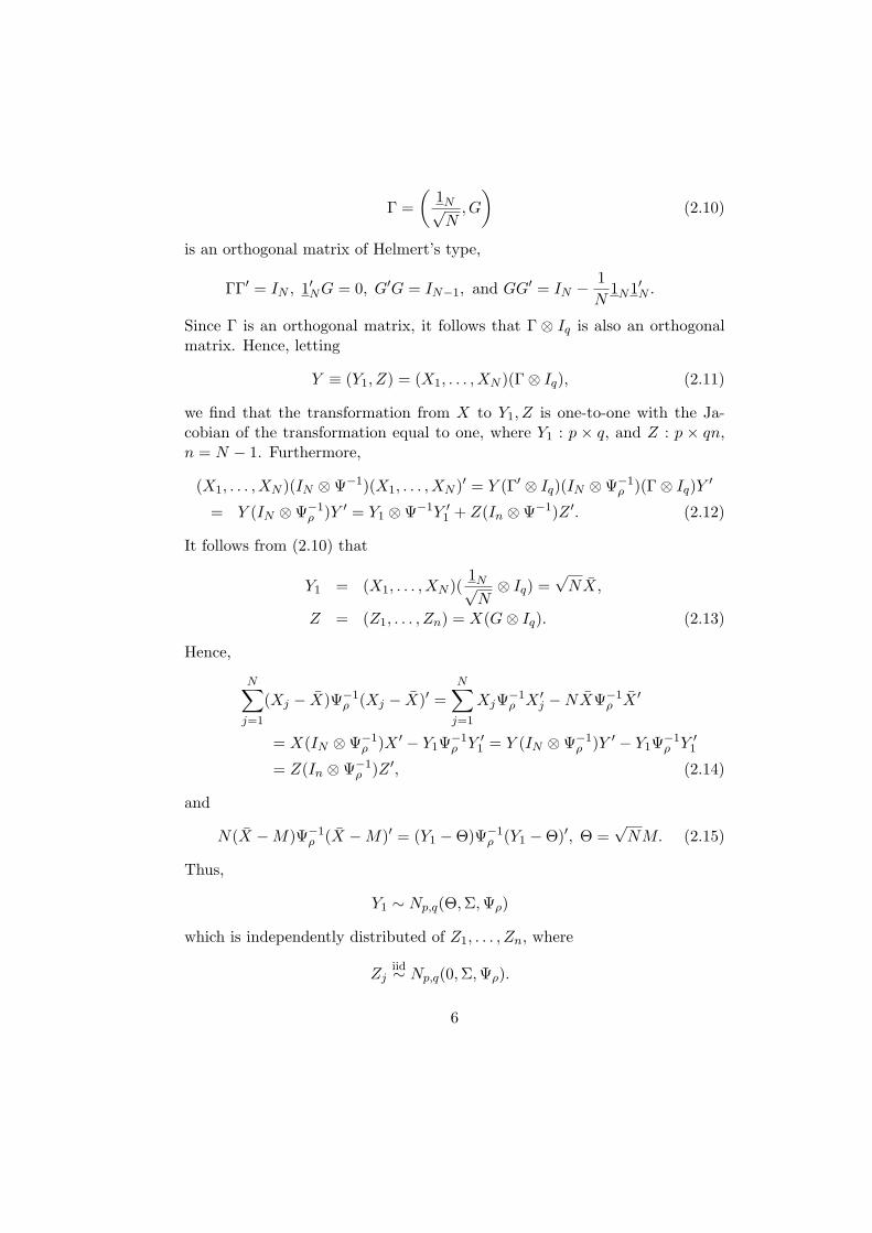
Γ =(

1N√N

,G

)(2.10)

is an orthogonal matrix of Helmert’s type,

ΓΓ′ = IN , 1′NG = 0, G′G = IN−1, and GG′ = IN − 1N

1N1′N .

Since Γ is an orthogonal matrix, it follows that Γ ⊗ Iq is also an orthogonalmatrix. Hence, letting

Y ≡ (Y1, Z) = (X1, . . . , XN )(Γ⊗ Iq), (2.11)

we find that the transformation from X to Y1, Z is one-to-one with the Ja-cobian of the transformation equal to one, where Y1 : p × q, and Z : p × qn,n = N − 1. Furthermore,

(X1, . . . , XN )(IN ⊗Ψ−1)(X1, . . . , XN )′ = Y (Γ′ ⊗ Iq)(IN ⊗Ψ−1ρ )(Γ⊗ Iq)Y ′

= Y (IN ⊗Ψ−1ρ )Y ′ = Y1 ⊗Ψ−1Y ′

1 + Z(In ⊗Ψ−1)Z ′. (2.12)

It follows from (2.10) that

Y1 = (X1, . . . , XN )(1N√N⊗ Iq) =

√NX̄,

Z = (Z1, . . . , Zn) = X(G⊗ Iq). (2.13)

Hence,

N∑

j=1

(Xj − X̄)Ψ−1ρ (Xj − X̄)′ =

N∑

j=1

XjΨ−1ρ X ′

j −NX̄Ψ−1ρ X̄ ′

= X(IN ⊗Ψ−1ρ )X ′ − Y1Ψ−1

ρ Y ′1 = Y (IN ⊗Ψ−1

ρ )Y ′ − Y1Ψ−1ρ Y ′

1

= Z(In ⊗Ψ−1ρ )Z ′, (2.14)

and

N(X̄ −M)Ψ−1ρ (X̄ −M)′ = (Y1 −Θ)Ψ−1

ρ (Y1 −Θ)′, Θ =√

NM. (2.15)

Thus,

Y1 ∼ Np,q(Θ, Σ,Ψρ)

which is independently distributed of Z1, . . . , Zn, where

Zjiid∼ Np,q(0, Σ, Ψρ).

6

Let

Zj = (z(1)j , . . . , z(q)j) : p× q, j = 1, . . . , n, n = N − 1.

Then

E[z(i)j , z′(i)j)] = ψρiiΣ, and E(ZjZ

′j) = (trΨρ)Σ.

Also, from (2.5)

S =1

Nq[

N∑

j=1

XjX′j −NX̄X̄ ′] =

1Nq

[XX ′ − Y1Y′1 ]

=1

Nq[Y Y ′ − Y1Y

′1 ] =

1Nq

ZZ ′ =1

Nq

n∑

j=1

ZjZ′j , n = N − 1. (2.16)

Hence,

N

nE(S) = (

1qtrΨρ)Σ = Σ, if ψρii = 1, i = 1, . . . , q.

Since (ZjZ′j/q) are iid with mean Σ, when ψρii = 1, i = 1, . . . , q, S is a

consistent estimator of Σ. Thus, we get the following theorem.

Theorem 2.1. Let X1, . . . , XN be iid Np,q(M, Σ, Ψρ), where Ψρ = (ψρij),ψρii = 1, i = 1, . . . , q. Then,

N

nS =

1nq

N∑

j=1

(Xj − X̄)(Xj − X̄)′, n = N − 1,

is an unbiased estimator of Σ as well as consistent, if N →∞.

Corollary 2.1. When Ψ = I, S is the maximum likelihood estimator of Σ.Similarly, in terms of z(i)j,

ψ̃ρik =1

Nptr{S−1

n∑

j=1

z(i)jz′(k)j}, i 6= k.

Since, when ψρii = 1, i = 1, . . . , q, S → Σ in probability andΣ−

12 z(k)jz

′(i)jΣ

− 12 , j = 1, . . . , N , are independently distributed with means

ψρikIp, it follows that ψ̃ρik are consistent estimators of ψik when all the diag-onal elements of Ψρ are all one. Thus, we have the following theorem.

Theorem 2.2. Let X1, . . . , XN be iid Np,q(M, Σ, Ψρ), where Ψρ has all thediagonal elements equal to one. Then, ψ̃ρik defined in (2.7) is a consistentestimator of ψρik, i 6= k, (i, k) = 1, . . . , q.

7

3 Maximum Likelihood Estimators of M , Σ and Ψ∗

(ψqq = 1)

We consider the same model as in Section 2 except that now the q× q matrixΨ∗ is of the general form. That is, for Ψ∗ = (ψij), we only assume thatψqq = 1. The MLE of M remains the same as in (2.4) and therefore we startwith the likelihood

(2π)−12pqN |Σ|−1

2 qN |Ψ∗|−12pNetr{−1

2

N∑

i=1

Σ−1XicΨ∗−1X ′ic}, (3.1)

where

Xic = Xi − X̄, i = 1, . . . , N. (3.2)

Due to the constraint ψqq = 1, it needs special attention. Let

Ψ∗ =

(Ψ11 ψ

1q

ψ′1q

ψqq

), Ψ11 : (q − 1)× (q − 1). (3.3)

From Srivastava and Khatri (1979, Corollary 1.4.2 (i), p. 8), it follows sinceψqq = 1, that

Ψ∗−1 =(

0 00 1

)+

(Iq−1

−ψ′1q

)Ψ−1

1•q(

Iq−1 : −ψ1q

),

where

Ψ1•q = Ψ11 − ψ1q

ψ′1q

: (q − 1)× (q − 1). (3.4)

Moreover,

|Ψ∗| = |Ψ1•q| = |Ψ11 − ψ1q

ψ′1q|.

Thus (3.1) equals

(2π)−12pqN |Σ|−1

2 qN |Ψ1•q|−12pN ×

etr{−12

∑Ni=1 Σ−1(XicqX

′icq + Xic

(Iq−1

−ψ′1q

)Ψ−1

1•q(

Iq−1 : −ψ1q

)X ′

ic)},

8

where Xic = (Xic1 : Xicq): (p× (q−1) : p×1). By differentiation with respectto the upper triangle of Σ−1 and Ψ−1

1•q as well as differentiation with respectto ψ

1qwe obtain after some manipulations

NqΣ̂ =N∑

i=1

(XicqX′icq + Xic

(Iq−1

−ψ̂′1q

)Ψ̂−1

1•q(

Iq−1 −ψ̂1q

)X ′

ic), (3.5)

NpΨ̂1•q =N∑

i=1

(Iq−1 : −ψ̂

1q

)X ′

icΣ̂−1Xic

(Iq−1

−ψ̂′1q

)(3.6)

and

ψ̂1q

=N∑

i=1

X ′ic1Σ̂

−1Xicq(N∑

i=1

X ′icqΣ̂

−1Xicq)−1. (3.7)

We first show that the scalar quantity in (3.7),

N∑

i=1

X ′icqΣ̂

−1Xicq = Np. (3.8)

To prove (3.8), we post-multiply (3.5) by Σ̂−1 and take the trace. This gives

Nqp =N∑

i=1

X ′icqΣ̂

−1Xicq

+ tr{N∑

i=1

Ψ̂−11•q

(Iq−1 : −ψ̂

1q

)(X ′

icΣ̂−1Xic

(Iq−1

−ψ̂′1q

))}

=N∑

i=1

X ′icqΣ̂

−1Xicq + Np tr{Iq−1},

using (3.6). This proves (3.8). Thus, we get

ψ̂1q

=1

Np

N∑

i=1

X ′ic1Σ̂

−1Xicq. (3.9)

Next, we simplify (3.6). Using (3.8) we get after some calculations

NpΨ̂1•q =N∑

i=1

X ′ic1Σ̂

−1Xic1 −Npψ̂1q

ψ̂′1q

. (3.10)

9

Thus,

NpΨ̂11 =N∑

i=1

X ′ic1Σ̂

−1Xic1.

Hence, using (3.8), we get

Ψ̂ =

(Ψ̂11 ψ̂

1q

ψ̂′1q

1

)(3.11)

=1

Np

( ∑Ni=1 X ′

ic1Σ̂−1Xic1

∑Ni=1 X ′

ic1Σ̂−1Xicq∑N

i=1 X ′icqΣ̂

−1Xic1∑N

i=1 X ′icqΣ̂

−1Xicq

)

=1

Np

N∑

i=1

X ′icΣ̂

−1Xic. (3.12)

With Ψ̂ defined in (3.11), we can rewrite (3.5) as

Σ̂ =1

Nq

N∑

i=1

XicΨ̂−1X ′ic. (3.13)

Thus, we solve (3.12) and (3.13) directly subject to the condition (3.8). Thiswe shall call the ”flip-flop” algorithm. The starting value of Σ̂ can be basedon the estimators obtained in Section 2 and satisfying (3.8).

The next theorem which is proven in Section 8 provides us with an im-portant result concerning the flip-flop algorithm and the MLEs. For relatedworks we refer to Lu and Zimmerman (2005) and Dutilleul (1999), where alsoother references are given.

Theorem 3.1. Let Σ̂ and Ψ̂ satisfy the flip-flop algorithm given in (3.12) and(3.13), satisfying the condition (3.8). If N >max(p, q), then there is only onesolution and the MLEs based on the likelihood given in (3.1) are unique.

The theorem is interesting because in general uniqueness of MLEs in curvedexponential families may not hold. For example, see Drton (2006) where theSUR-model is discussed.

4 Testing that the Kronecker model holds

Let X1, . . . , XN be iid normally distributed p × q matrices. If the Kroneckermodel holds, then Xj has the pdf given in (1.11). However, in general the

10

pq-random vector

vec(Xj) ∼ Npq(vecM,Λ), (4.1)

where Λ is a pq×pq unstructured covariance matrix. It is assumed that Λ>0.To estimate Λ, it is required that N > pq. We shall therefore assume in thissection that N >pq. Thus, we wish to test the hypothesis

H : Λ = Ψ∗ ⊗ Σ

against the alternative A 6= H. The maximum likelihood estimators of Ψ∗ andΣ have been obtained in Section 3. The MLE of Λ, under the alternative, isgiven by

Λ̂ =1N

N∑

i=1

(vecXcj)(vecXcj)′, N > pq. (4.2)

Thus, the likelihood ratio test (LRT) for H against A is given by

λ1 =|Λ̂| 12N

|Ψ̂∗| 12Np|Σ̂| 12Nq.

From asymptotic theory,

−2logλ1 ∼ χ2( 12pq(pq+1)− 1

2p(p+1)− 1

2q(q+1)+1)

.

This result may be compared with the result obtained in Roy and Khattree(2005). Note that if we do not assume ψqq = 1 then we are in a testing situationwhere not all parameters can be identified under the null distribution, and thusstandard asymptotic results for the LRT are not at disposal (e.g. see Ritz andSkovgaard, 2005).

5 Testing that Ψ is of intraclass correlation struc-ture

In order to test that Ψ is of the intraclass correlation structure, we eitherassume that

Ψ = (1− ρ)Iq + ρ1q1′q, and Σ = (σij) > 0, (5.1)

or assume that

Ψ = σ2[(1− ρ)Iq + ρ1q1′q], and σpp = 1. (5.2)

11

We consider the model (5.2) with N iid observation matrices Xj , j = 1, . . . , N ,N > max(p, q), and since σpp = 1 we denote Σ by Σ∗. The approach of Section3 will be adopted with suitable modifications. In particular the uniqueness ofthe estimators has to be shown in a somewhat different way. The pdf ofX = (X1, . . . , XN ) is given by (2.1). After maximazing with respect to M ,the likelihood function is given by

(2π)−12pqN |Σ∗|− 1

2Nq|Ψ|− 1

2Npetr{−1

2Σ∗−1

N∑

i=1

XicΨ−1X ′ic}.

Making the transformation

Ui = XicH,

where H is a q × q orthogonal matrix of the Helmert’s type used earlier inSection 2. Then

H ′Ψ−1H = (H ′ΨH)−1 =(

τ−11 0

0 τ−12 Iq−1

)≡ D−1

τ ,

where

τ1 = σ2(1 + (q − 1)ρ),τ2 = σ2(1− ρ).

Hence, the likelihood is given by

(2π)−12Npqτ

− 12Np

1 τ− 1

2Np(q−1)

2 |Σ1•p|−12Nqetr{−1

2

N∑

i=1

Σ∗−1UiD−1τ U ′

i}, (5.3)

where

Σ∗−1 = dpd′p +

(Ip−1

−σ′1q

)Σ−1

1•p(

Ip−1 : −σ1q

)

and dp is the pth unit base vector of size p. If ek denotes the kth unit basevector of size q then

tr{Σ∗−1UiD−1τ U ′

i} = τ−11 tr{Σ∗−1Uie1e

′1U

′i}

+τ−12

q∑

k=2

tr{Σ∗−1Uieke′kU

′i} (5.4)

12

as well as

tr{Σ∗−1UiD−1τ U ′

i} = tr{dpd′pUiD

−1τ U ′

i}

+tr{(

Ip−1

−σ′1q

)Σ−1

1•p(

Ip−1 : −σ1q

)UiD

−1τ U ′

i}. (5.5)

Put U = (U1, U2, . . . , UN ) and Ui = (U ′j1 : U ′

ip)′. By using (5.4) and (5.5)

the likelihood in (5.3) leads after some manipulations to the following ML-equations:

τ̂1 =1

Np

N∑

i=1

tr{Σ̂∗−1Uie1e′1U

′i} =

1Np

tr{Σ̂∗−1U(IN ⊗ e1e′1)U

′}, (5.6)

τ̂2 =1

Np(q − 1)

N∑

i=1

q∑

k=2

tr{Σ̂∗−1Uieke′kU

′i}

=1

Np(q − 1)tr{Σ̂∗−1U(IN ⊗

q∑

k=2

eke′k)U

′}, (5.7)

σ̂1p =N∑

i=1

Ui1D̂−1τ U ′

ip(N∑

i=1

UipD̂−1τ U ′

ip)−1, (5.8)

Σ̂1•p =1

Nq

N∑

i=1

(Ip−1 : −σ′1q

)UiD̂

−1τ U ′

i

(Ip−1

−σ′1q

). (5.9)

In the next, in correspondence with (3.8), we are going to show that

Nq =N∑

i=1

UipD̂−1τ U ′

ip =N∑

i=1

d′pUiD̂−1τ U ′

idp. (5.10)

Equation (5.9) implies

NqIp−1 =N∑

i=1

(Ip−1 : −σ̂′1q

)UiD̂

−1τ U ′

i

(Ip−1

−σ̂1q

)Σ̂−1

1•p

13

and taking the trace yields

Nq(p− 1) =N∑

j=1

tr{Σ̂−11•p

(Ip−1 : −σ̂1q

)UiD̂

−1τ U ′

i

(Ip−1

−σ̂′1q

)}

= Np−N∑

i=1

tr{dpd′pUiτ̂

−11 e1e

′1U

′i}+Np(q−1)−

N∑

i=1

q∑

k=2

tr{dpd′pUiτ̂

−12 eke

′kU

′i}

= Npq −N∑

i=1

d′pUiD̂−1τ U ′

idp (5.11)

which implies (5.10). In (5.11) we used that τ̂1 and τ̂2 respectively can bewritten

Npτ̂1 =N∑

i=1

tr{dpd′pUie1e

′1U

′i}

+ tr{(

Ip−1

−σ̂′1q

)Σ̂−1

1•p(

Ip−1 : −σ̂1q

)Uie1e

′1U

′i},

Np(q − 1)τ̂2 =N∑

i=1

q∑

k=2

tr{dpd′pUieke

′kU

′i}

+ tr{(

Ip−1

−σ̂′1q

)Σ̂−1

1•p(

Ip−1 : −σ̂1q

)Uieke

′kU

′i}.

Thus,

σ̂1p =1

Nq

N∑

i=1

Ui1D̂−1τ U ′

i1

which implies that

Σ̂∗ =1

Nq

N∑

i=1

UiD̂−1τ U ′

i =1

NqU(IN ⊗ D̂−1

τ )U ′. (5.12)

Thus, similarly to Theorem 3.1 we have the following result which also isproven in Section 8:

Theorem 5.1. Let Σ̂∗, τ̂1 and τ̂2 satisfy (5.12), (5.6) and (5.7), with σpp = 1supposed to hold. If N > max(p, q), then there is only one solution and theMLEs based on the likelihood given in (5.3) are unique.

14

Next we obtain the MLE of Ψ with no restriction on the elements of Ψ.On the lines of Section 3, it follows that for given Σ∗, the MLE of Ψ is givenby

Ψ̂ =1

Np

N∑

i=1

X ′icΣ

∗−1Xic.

Let

L =N∑

i=1

XicΨ̂−1X ′ic =

(L11 l1p

l′1p lpp

).

Then the MLE of Σ1.p, Σ11, σ1p for a given Ψ are given by

Σ̂1•p =1

Nq[L11 −

l1pl′1p

Nq(p− 1)],

Σ̂11 = Σ̂1•p +l1pl

′1p

(Nq(p− 1))2,

σ̂1p =l1p

Nq(p− 1),

Σ̂∗ =(

Σ̂11 σ̂1p

σ̂1p 1

).

Thus, the maximum of the likelihood function under the alternative hypothesisthat Ψ is not of the intraclass correlation model is given by

(2π)−12pqN |Σ̂1•p|−

12qN |Ψ̂|− 1

2pNe−

12pqN . (5.13)

Similarly, the maximum of the likelihood function under the hypothesis thatΨ is of intraclass correlation model is given by

(2π)−12pqN |Σ̂1•p(H)|− 1

2qN (τ̂1)−

12pN (τ̂2)−

12p(q−1)Ne−

12pqN , (5.14)

where Σ̂1•p(H) stands for the MLE of Σ1•p under the null hypthesis. Thus,the likelihood ratio test for testing the hypothesis that Ψ is of the intraclasscorrelation structure is given by

λ2 = [Σ̂1•pΣ̂−11•p(H)]−

12qN |Ψ̂| 12pN (τ̂1)−

12pN (τ̂2)−

12p(q−1)N . (5.15)

From asymptotic theory, it follows that −2logλ2 is distributed as chisquarewith 1

2q(q + 1) − 2 degrees of freedom. These results may be compared withresults obtained in Naik and Rao (2001) and Roy and Khattree (2005).

15

6 Testing the hypothesis that Ψ∗=I and Ψρ=I

In most practical situations, it would be desirable to test the hypothesis

H1 : Ψ∗ = I, against the alternative A1 6= H1

and

H2 : Ψρ = I, against the alternative A2 6= H2.

We first consider the hypothesis H1 vs A1. For this we use the likelihoodratio procedure. The maximum likelihood estimators Σ̂ and Ψ̂ of Σ and Ψ aregiven in Section 3. From Corollary 2.1, the maximum likelihood estimator ofΣ when Ψ = I is S. Hence, the log of the likelihood rates under the hypothesisand under the alternative is given by

log λ3 =|Ψ̂∗| 12pN |Σ̂| 12 qN

|S| 12 qN

and

−2 log λ3 ∼ χ212q(q+1)−1

asymptotically under the hypothesis H1.For testing the hypothesis H2 against the alternative A2 when ψii = 1, i =

1, . . . , q, we consider the estimator Ψ̃ik of Ψik given in Section 2. Under thehypothesis H2,

tik =√

np Ψ̃ik, i 6= k

which are independently normally distributed with mean 0 and variance one.Hence,

T =

∑i<j t2ij − 1

2q(q − 1)√q(q − 1)

is asymptotically normally distributed with mean zero and variance one.

7 Simulation study

In this section we present a small simulation study indicating that the proposedalgorithm in Section 3 is working practically when finding the MLEs. It is

16

interesting to note that in all simulations the estimators were close to thetrue value. We present results when the sample sizes equal either 100 or 250,which are relatively small numbers when taking into account the number ofparameters. The number of observations equals 250 when either p = 15 orq = 15. We have also performed a number of simulations (not presented here)with N = 1000 and the results agree with those presented in this paper.

In Tables 1-6, the results based on 300 replications are presented, for sixdifferent settings of p, q, and N in the likelihood (3.1). Estimators are foundaccording to the proposed algorithm in Section 3. Only the estimators of theunknown diagonal elements of Σ and Ψ are presented together with the truevalue, the standard deviation (std) as well as the minimum and maximumvalues of the replications.

Table 1. p = 5, q = 5 and N = 100.

parameter true value MLE std min maxσ11 6.02 5.90 0.52 4.65 7.59σ22 5.42 5.36 0.47 4.14 7.05σ33 3.11 3.06 0.27 2.40 3.83σ44 3.63 3.59 0.31 2.73 4.73σ55 2.05 2.01 0.18 1.60 2.60ψ11 0.43 0.45 0.04 0.34 0.60ψ22 0.54 0.55 0.05 0.40 0.69ψ33 0.28 0.29 0.03 0.21 0.37ψ44 0.46 0.46 0.04 0.34 0.61

Table 2. p = 7, q = 5 and N = 100.

parameter true value MLE std min maxσ11 6.99 6.86 0.52 5.54 8.37σ22 7.41 7.27 0.55 5.75 8.86σ33 3.80 3.75 0.30 2.92 4.91σ44 5.42 5.34 0.43 4.39 6.52σ55 6.44 6.33 0.47 5.10 8.10σ66 5.49 5.40 0.40 4.36 6.71σ77 11.37 11.12 0.87 8.98 13.91ψ11 0.11 0.11 0.01 0.09 0.14ψ22 0.21 0.22 0.02 0.17 0.27ψ33 0.26 0.26 0.02 0.21 0.32ψ44 0.37 0.37 0.03 0.30 0.44

17

Table 3. p = 15, q = 5 and N = 250.

parameter true value MLE std min maxσ11 14.56 14.53 0.66 12.70 16.33σ22 10.06 10.20 0.45 8.62 11.36σ33 12.83 12.80 0.60 10.98 14.70σ44 12.84 12.77 0.60 11.35 14.82σ55 10.81 10.77 0.47 9.52 12.40σ66 7.35 7.31 0.35 6.29 8.45σ77 13.32 13.32 0.59 11.81 14.87σ88 17.45 17.44 0.80 15.59 19.70σ99 10.89 10.83 0.49 9.29 11.94σ1010 13.17 13.15 0.58 11.71 14.99σ1111 25.35 25.28 1.15 22.49 29.34σ1212 17.37 17.27 0.79 14.95 19.38σ1313 18.72 18.62 0.83 16.31 21.12σ1414 7.84 7.82 0.37 6.87 8.87σ1515 12.09 12.03 0.51 10.58 13.36ψ11 0.73 0.73 0.02 0.66 0.79ψ22 0.14 0.14 0.004 0.13 0.15ψ33 0.87 0.87 0.03 0.80 0.94ψ44 0.23 0.23 0.01 0.21 0.25

18

Table 4. p = 15, q = 7 and N = 250.

parameter true value MLE std min maxσ11 10.95 10.87 0.41 9.45 12.06σ22 13.00 12.97 0.57 11.56 14.67σ33 13.14 13.08 0.52 11.60 14.64σ44 13.90 13.83 0.51 12.53 14.95σ55 17.50 17.52 0.70 15.56 19.39σ66 11.34 11.31 0.45 10.06 12.49σ77 13.83 13.71 0.57 12.28 15.57σ88 13.25 13.19 0.54 11.60 14.62σ99 13.43 13.38 0.51 11.83 14.66σ1010 7.15 7.14 0.31 6.46 7.84σ1111 10.47 10.46 0.39 9.59 12.18σ1212 29.49 29.43 1.15 26.35 32.64σ1313 17.17 17.07 0.69 15.38 18.68σ1414 19.49 19.37 0.75 17.30 21.13σ1515 15.35 15.33 0.57 13.71 16.78ψ11 0.68 0.68 0.02 0.62 0.73ψ22 0.76 0.76 0.03 0.70 0.82ψ33 0.93 0.94 0.03 0.86 1.01ψ44 0.56 0.56 0.02 0.51 0.61ψ55 0.55 0.55 0.02 0.50 0.60ψ66 0.92 0.93 0.03 0.86 1.01

19

Table 5. p = 5, q = 7 and N = 100.

parameter true value MLE std min maxσ11 6.02 5.86 0.48 4.40 7.18σ22 5.42 5.33 0.44 4.35 6.79σ33 3.11 3.03 0.26 2.16 3.97σ44 3.64 3.56 0.30 2.79 4.45σ55 2.05 1.99 0.17 1.45 2.48ψ11 0.60 0.61 0.06 0.48 0.80ψ22 0.65 0.66 0.06 0.54 0.89ψ33 0.49 0.50 0.04 0.40 0.63ψ44 1.03 1.05 0.10 0.83 1.43ψ55 0.24 0.24 0.02 0.20 0.32ψ66 0.42 0.43 0.04 0.34 0.56

Table 6. p = 5, q = 15 and N = 250.

parameter true value MLE std min maxσ11 2.45 2.39 0.12 2.07 2.83σ22 1.46 1.43 0.07 1.25 1.63σ33 5.66 5.50 0.26 4.81 6.45σ44 3.01 2.94 0.15 2.56 3.39σ55 2.94 2.87 0.14 2.46 3.33ψ11 1.06 1.08 0.06 0.92 1.34ψ22 0.77 0.72 0.05 0.59 0.87ψ33 0.73 0.75 0.05 0.63 0.88ψ44 0.83 0.84 0.04 0.72 0.99ψ55 0.56 0.58 0.04 0.48 0.68ψ66 0.60 0.62 0.03 0.54 0.69ψ77 1.16 1.19 0.07 0.97 1.42ψ88 0.37 0.38 0.02 0.32 0.45ψ99 0.52 0.54 0.03 0.45 0.64ψ1010 0.73 0.75 0.04 0.64 0.89ψ1111 0.71 0.72 0.04 0.62 0.84ψ1212 0.84 0.86 0.05 0.72 1.02ψ1313 1.08 1.11 0.06 0.88 1.30ψ1414 0.94 0.96 0.05 0.82 1.14

20

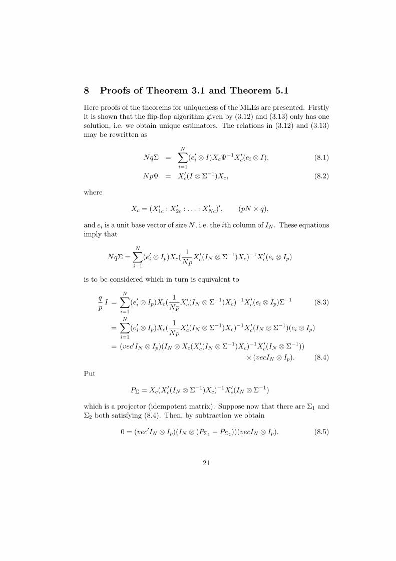
8 Proofs of Theorem 3.1 and Theorem 5.1

Here proofs of the theorems for uniqueness of the MLEs are presented. Firstlyit is shown that the flip-flop algorithm given by (3.12) and (3.13) only has onesolution, i.e. we obtain unique estimators. The relations in (3.12) and (3.13)may be rewritten as

NqΣ =N∑

i=1

(e′i ⊗ I)XcΨ−1X ′c(ei ⊗ I), (8.1)

NpΨ = X ′c(I ⊗ Σ−1)Xc, (8.2)

where

Xc = (X ′1c : X ′

2c : . . . : X ′Nc)

′, (pN × q),

and ei is a unit base vector of size N , i.e. the ith column of IN . These equationsimply that

NqΣ =N∑

i=1

(e′i ⊗ Ip)Xc(1

NpX ′

c(IN ⊗ Σ−1)Xc)−1X ′c(ei ⊗ Ip)

is to be considered which in turn is equivalent to

q

pI =

N∑

i=1

(e′i ⊗ Ip)Xc(1

NpX ′

c(IN ⊗ Σ−1)Xc)−1X ′c(ei ⊗ Ip)Σ−1 (8.3)

=N∑

i=1

(e′i ⊗ Ip)Xc(1

NpX ′

c(IN ⊗ Σ−1)Xc)−1X ′c(IN ⊗ Σ−1)(ei ⊗ Ip)

= (vec′IN ⊗ Ip)(IN ⊗Xc(X ′c(IN ⊗ Σ−1)Xc)−1X ′

c(IN ⊗ Σ−1))× (vecIN ⊗ Ip). (8.4)

Put

PΣ = Xc(X ′c(IN ⊗ Σ−1)Xc)−1X ′

c(IN ⊗ Σ−1)

which is a projector (idempotent matrix). Suppose now that there are Σ1 andΣ2 both satisfying (8.4). Then, by subtraction we obtain

0 = (vec′IN ⊗ Ip)(IN ⊗ (PΣ1 − PΣ2))(vecIN ⊗ Ip). (8.5)

21

Our task is to show that the only solution of (8.5) is given by Σ1 = Σ2. It maybe noted that Σ1 = cΣ2, c 6= 1 is not a possibility since ψqq = 1 and equation(3.13) has to be satisfied by all the solutions. Let

QΣ = IpN − PΣ = (IN ⊗ Σ)Xoc (Xo′

c (IN ⊗ Σ)Xoc )−1Xo′

c ,

where Xoc is defined to be any matrix which under the standard inner product

generates the orthogonal complement to the column space generated by Xc.Then,

PΣ1 − PΣ2 = PΣ1(IpN − PΣ2) = PΣ1QΣ2

= Xc(X ′c(IN ⊗ Σ−1

1 )Xc)−1X ′c(IN ⊗ Σ−1

1 )

×(IN ⊗ Σ2)Xoc (Xo′

c (IN ⊗ Σ2)Xoc )−1Xo′

c .

Suppose for a while that (8.5) holds if and only if PΣ1−PΣ2=0, i.e. PΣ1QΣ2=0,which is equivalent to

X ′c(IN ⊗ Σ−1

1 Σ2)Xoc = 0. (8.6)

There are two possibilities for (8.6) to hold. Either Σ1 = cΣ2 or the columnspace, denoted C(•), generated by Xo

c is invariant with respect to IN⊗Σ−11 Σ2,

i.e. the space is generated by the eigenvectors of IN ⊗Σ−11 Σ2. However, since

the matrix of eigenvectors is of the form IN ⊗Γ for some Γ it shows, since thecolumn space of Xo

c is a function of the observations, that IN ⊗ Γ does notgenerate the space, unless N = 1. Thus, in order for (8.6) to hold Σ1 = cΣ2

and we have already noted that in this case c = 1, i.e. Σ1 = Σ2.It remains to show that (8.5) is true only if PΣ1 − PΣ2 = PΣ1QΣ2 = 0, i.e.

0 = (vec′IN ⊗ Ip)(IN ⊗ PΣ1)(IN ⊗QΣ2)(vecIN ⊗ Ip). (8.7)

Since, in (8.6) we have the two projections (IN ⊗PΣ1) and (IN ⊗QΣ2) we willstudy the effect of them via column spaces. Using Theorem 1.2.16 in Kollo &von Rosen (2005) gives

C((IN⊗ P ′Σ1

)(vecIN ⊗ Ip)) = C(IN ⊗ P ′Σ1

)∩{C(IN ⊗ PΣ1)⊥+ C(~IN ⊗ Ip)}

= C(IN ⊗ (IN ⊗ Σ−11 )Xc)∩{C(IN ⊗Xo

c ) + C(vecIN ⊗ Ip)}, (8.8)

C((IN⊗QΣ2)(vecIN ⊗ Ip)) = C(IN ⊗QΣ2)∩{C(IN ⊗Q′Σ2

)⊥+ C(~IN ⊗ Ip)}= C(IN ⊗ (IN ⊗ Σ2)Xo

c )∩{C(IN ⊗Xc) + C(vecIN ⊗ Ip)}. (8.9)

If (8.7) should hold the spaces presented in (8.8) and (8.9), respectively, mustbe orthogonal. Thus,

C(IN ⊗ (IN ⊗ Σ−11 )Xc) ∩ {C(IN ⊗Xo

c ) + C(vecIN ⊗ Ip)}⊆ C(IN ⊗ (IN ⊗ Σ2)Xo

c )⊥ + C(IN ⊗Xc)⊥ ∩ C(vecIN ⊗ Ip)⊥. (8.10)

22

However, the following trivial facts hold:

C(IN ⊗ (IN ⊗ Σ−11 )Xc) ∩ {C(IN ⊗Xo

c ) + C(vecIN ⊗ Ip)}⊆ C(IN ⊗ (IN ⊗ Σ−1

1 )Xc)C(IN ⊗ (IN ⊗ Σ2)Xo

c )⊥

⊆ C(IN ⊗ (IN ⊗ Σ2)Xoc )⊥ + C(IN ⊗Xc)⊥ ∩ C(vecIN ⊗ Ip)⊥.

Hence, if

C(IN ⊗ (IN ⊗ Σ−11 )Xc) ⊆ C(IN ⊗ (IN ⊗ Σ2)Xo

c )⊥ (8.11)

does not hold (8.10) as well as (8.8) can not be valid and therefore (8.11)must always be true which is the same as stating that PΣ1QΣ2 = 0. Thus, theflip-flop algorithm provides us with unique solutions.

Turning to Theorem 5.1 we will show that estimators satisfying

Σ =1

NqU(IN ⊗D−1

τ )U ′, (8.12)

where

Dτ = τ1e1e′1 +

q∑

k=2

τ1e1e′1 (8.13)

with

τ1 =1

Nptr{Σ−1U(IN ⊗ e1e

′1)U

′}, (8.14)

τ2 =1

Np(q − 1)tr{Σ−1U(IN ⊗

q∑

k=2

eke′k)U

′} (8.15)

are unique. The above given equations imply that

Σ =p

q(tr{Σ−1U(IN ⊗ e1e

′1)(IN ⊗ e1e

′1)U

′})−1U(IN ⊗ e1e′1)(IN ⊗ e1e

′1)U

′

+p(q − 1)

q(

q∑

k=2

tr{Σ−1U(IN ⊗ eke′k)(IN ⊗ eke

′k)U

′})−1

×q∑

k=2

U(IN ⊗ eke′k)(IN ⊗ eke

′k)U

′. (8.16)

23

Postmultiplying (8.16) by Σ−1 and putting

A = U(IN ⊗ e1e′1), B =

q∑

k=2

U(IN ⊗ eke′k)

we obtain

I =p

q(tr{Σ−1AA′})−1AA′Σ−1 +

p(q − 1q

(tr{Σ−1BB′})−1BB′Σ−1. (8.17)

Note that AB′ = 0 implies that C(A) ∩ C(B) = {0}. Now suppose that thereexist Σ1 and Σ2, Σ1 6= cΣ2, for any positive constant c 6= 1, satisfying (8.17).The case Σ1 = cΣ2, c 6= 1 is of no interest since σpp = 1 is supposed to hold.Thus, it follows that

0=p

q((tr{Σ−1

1 AA′})−1AA′Σ−11 − (tr{Σ−1

2 AA′})−1AA′Σ−12 )

+p(q − 1)

q((tr{Σ−1

1 BB′})−1BB′Σ−11 − (tr{Σ−1

2 BB′})−1BB′Σ−12 ). (8.18)

Since C(AA′Σ̂i) = C(A), C(BB′Σ̂i) = C(B), i=1, 2, and C(A)∩C(B)={0},the two terms in (8.18) may be considered separately, i.e.

(tr{Σ−11 AA′})−1AA′Σ−1

1 = (tr{Σ−12 AA′})−1AA′Σ−1

2 ,

(tr{Σ−11 BB′})−1BB′Σ−1

1 = (tr{Σ−12 BB′})−1BB′Σ−1

2 . (8.19)

Because of symmetry it is enough to exploit (8.19) which, since AA′ withprobability 1 is of full rank p, is identical to

Σ2 =tr{Σ−1

1 AA′}tr{Σ−1

2 AA′}Σ1. (8.20)

This implies that Σ1 = cΣ2 which according to the assumptions should nothold except when c = 1. Hence, there exist only one solution to (8.18).

Acknowledgement

The work of Tatjana Nahtman is supported by grant GMTMS6702 of theEstonian Research Foundation.

24

References

[1] Arnold, S. (1973). Applications of the theory of products of problems tocertain patterned covariance matrices. Annals of Statistics, 1, 682–699.

[2] Drton, M. (2006). Computing all roots of the likelihood equations ofseemingly unrelated regressions. Journal of Symbolic Computation, 41,245–254.

[3] Dutilleul, P. (1999). The MLE algorithm for the matrix normal distribu-tion. Journal of Statistical Computation and Simulation, 64, 105–123.

[4] Galecki, A.T. (1994). General class of covariance structures for two ormore repeated factors in longitudinal data analysis. Comunications inStatistics - Theory and Methods, 23, 3105–3119.

[5] Kollo, T. and von Rosen, D. (2005). Advanced Multivariate Statistics withMatrices, Dordrecht: Springer.

[6] Lu, N. and Zimmerman, D.L. (2005). The likelihood ratio test for a sep-arable covariance matrix. Statistics and Probability Letters, 73, 449–457.

[7] Naik, D.N. and Rao, S. (2001). Analysis of multivariate repeated measuresdata with a Kronecker product structured covariance matrix. Journal ofApplied Statistics, 28, 91–105.

[8] Olkin, I. (1973). Testing and estimation for structures which are circularlysymmetric in blocks. Multivariate Statistical Inference, (Eds. D.G. Kabe,R.P. Gupta), 183–195, North-Holland, Amsterdam.

[9] Potthoff, R.F. and Roy, S.N. (1964). A generalized multivariate analysis ofvariance model useful especially for growth curve problems. Biometrika,51, 313–326.

[10] Ritz, C. and Skovgaard, I.M. (2005). Likelihood ratio tests in curvedexponential families with nuisance parameters present only under thealternative. Biometrika, 92, 507–517.

[11] Roy, A. and Khattree, R. (2005). On implementation of a test for Kro-necker product covariance structure for multivariate repeated measuresdata. Statistical Methodology, 2, 297–306.

[12] Shitan, M. and Brockwell, P.J. (1995). An asymptotic test for separabilityof a spatial autoregressive model. Comunications in Statistics - Theoryand Methods, 24, 2027–2040.

[13] Srivastava, M.S. (1965). Some tests for the intraclass correlation model.The Annals of Mathematical Statistics, 36, 1802–1806.

[14] Srivastava, M.S. and Khatri, C.G. (1979). An Introduction to MultivariateStatistics, North Holland, New York.

25

[15] Votaw, D.F. (1948). Testing compound symmetry in a normal multivari-ate distribution. Annals of Mathematical Statistics, 19, 447–473.

[16] Wilks, S.S. (1946). Sample criteria for testing equality of means, equalityof variances and equality of covariances in a normal multivariate distri-bution. Annals of Mathematical Statistics, 17, 257–281.

26