modflow-2000, the u.s. geological survey modular ground-water
TRANSCRIPT

MODFLOW-2000, THE U.S. GEOLOGICAL SURVEY MODULAR GROUND-WATER MODEL—USER GUIDE TO THE LMT6 PACKAGE, THE LINKAGE WITH MT3DMS FOR MULTI-SPECIES MASS TRANSPORT MODELING Open-File Report 01-82
U.S. Department of the Interior U.S. Geological Survey
MODFLOW-2000, THE U.S. GEOLOGICAL SURVEY MODULAR GROUND-WATER MODEL—USER GUIDE TO THE LMT6 PACKAGE, THE LINKAGE WITH MT3DMS FOR MULTI-SPECIES MASS TRANSPORT MODELING By Chunmiao Zheng1, Mary C. Hill2, and Paul A. Hsieh3 ___________________________________________________________________________ U.S. GEOLOGICAL SURVEY Open File Report 01-82
Denver, Colorado 2001
1 University of Alabama, Tuscaloosa, AL 2 U.S. Geological Survey, Lakewood, CO 3 U.S. Geological Survey, Menlo Park, CA

U.S. DEPARTMENT OF THE INTERIOR GALE A. NORTON, Secretary
U.S. GEOLOGICAL SURVEY
Charles G. Groat, Director
The use of trade, product, industry, or firm names is for descriptive purposes only and does not imply endorsement by the U.S. Government.
For additional information write to: Office of Ground Water U.S. Geological Survey 411 National Center Reston, VA 20192 (703) 648-5001
Copies of this report can be purchased from: U.S. Geological Survey Branch of Information Services Box 25286 Denver, CO 80225-0425

Preface
This report describes a computer code and related procedures that link MODFLOW-2000, the U.S. Geological Survey modular ground-water model, with MT3DMS, the modular multi-species mass transport model developed at the University of Alabama for the U.S. Department of Defense. The performance of the linkage program has been tested in a variety of applications. Future applications, however, might reveal errors that were not detected in the test simulations. Users are requested to notify the U.S. Geological Survey of any errors found in this User Guide or the computer program using the address on the back of the title page. Updates might occasionally be made to both the Users Guide and to the computer code. Users can check for updates on the Internet at URL’s http://water.usgs.gov/software/ground_water.html/ and http://hydro.geo.ua.edu/mt3d.
Preface iii

Contents iv

CONTENTS
Preface ...................................................................................................................................................iii Abstract .................................................................................................................................................. 1 Introduction ............................................................................................................................................ 1
Purpose and Scope ...........................................................................................................................2 Acknowledgments ...........................................................................................................................3
Documentation of the LINK-MT3DMS Package .................................................................................. 3 Program Design Concepts................................................................................................................3 Activating the Link-MT3DMS Package ..........................................................................................4 A Note for Users of MODFLOW-96 and MODFLOW-88 .............................................................4 Input Instructions for the Link-MT3DMS Package.........................................................................5
Explanation of Variables Read by the LMT6 Package......................................................5 Example Input Files for the LMT6 Package .......................................................................7
Description of the Link-MT3DMS Package....................................................................................8 Implementing the Link-MT3DMS Package in MODFLOW-2000 .................................................9
Running MT3DMS with a MODFLOW-2000 Produced Link File ..................................................... 11 Procedures to Start an MT3DMS Simulation ................................................................................11
Previously Existing Procedures ..........................................................................................11 File Name Prompting........................................................................................................11 Response File....................................................................................................................12
New Procedure Using the Name File.................................................................................12 Name File Construction ....................................................................................................12 Explanation of Variables in the Name File.......................................................................12
Effect of New MODFLOW-2000 Input Requirements on MT3DMS...........................................15 Spatial Discretization ...........................................................................................................15 Temporal Discretization ......................................................................................................16
Support of Additional Sink/Source Packages ................................................................................17 Application Examples .......................................................................................................................... 20
Dual-Domain Mass Transfer and Sorption ....................................................................................20 Field Application at the Massachusetts Military Reservation Site ................................................23
Flow Simulation....................................................................................................................23 Transport Simulation............................................................................................................27 Comparison of Model Results .................................................................................................30
Post-Simulation Visualization and Animation Using Model Viewer................................................... 32 Illustrative Examples .....................................................................................................................33 Unformatted Concentration (UCN) File ........................................................................................35 Model Configuration (CNF) File ...................................................................................................36
References ............................................................................................................................................ 37 Appendix: Contents of the Flow-Transport Link File .......................................................................... 39
Contents v

FIGURES Figure 1. Comparison of the calculated concentrations with the analytical solutions....................23
Figure 2. Location of the CS-10 model at the Massachusetts Military Reservation site in Cape Cod, Massachusetts. The outline of the trichloroethylene (TCE) plume is based on the data for 1997-98 from Jacobs Engineering Group (U.S. Air Force Center for Environmental Excellence, 1999). ........................................................................24
Figure 3. Contoured concentrations of trichloroethylene (TCE), in parts per billion (ppb),
and elements of the pump-and-treat system for the CS-10 plume. The solid dots (•) denote existing in-plume wells. The open dots ( ) represent perimeter wells still under consideration. The pumped water, after treatment, is to be reinjected into the infiltration trenches. The triangles along the Sandwich Road indicate an existing remedial well fence. ...............................................................................................................25
Figure 4. Total trichloroethylene (TCE) mass removal by all wells simulated by MODFLOW-SURFACT and MODFLOW-MT3DMS..........................................................30
Figure 5. Water-table levels for the second stress period simulated using (a) MODFLOW-SURFACT and (b) MODFLOW-2000. Contours are in feet above sea level. .......................................................................................................................................31
Figure 6. Trichloroethylene (TCE) concentrations in model layer 12 simulated using (a) MODFLOW-SURFACT and (b) MT3DMS. Concentrations are in parts per billion (ppb). ......................................................................................................................................31
Figure 7. Simulation of solute transport from a point source at one corner of a cube to a sink at the opposite corner. The three snapshots represent the plume distribution at three successive times. ...........................................................................................................34
Figure 8. Three-dimensional visualization of the simulated trichloroethylene (TCE) plume at the CS-10 site on the Massachusetts Military Reservation 1 year after a proposed pump-and-treat system is assumed to be operational. Concentrations are shown in parts per billion (ppb). The transparent brown shell indicates the 5 ppb isoconcentration surface. Concentration values above 100 ppb are shown as red. ................35
TABLES Table 1. MODFLOW packages and their support status by Link-MT3DMS ................................10 Table 2. Preserved unit numbers for various file types in MT3DMS…………………………… 14 Table 3. Chemical and transport input data used in the CS-10 trichloroethylene (TCE)
transport model.......................................................................................................................27
Contents vi

MODFLOW-2000, The U.S. Geological Survey Modular Ground-Water Model—User Guide to the LMT6 Package, the Linkage with MT3DMS for Multi-Species Mass Transport Modeling By Chunmiao Zheng, Mary C. Hill, and Paul A. Hsieh
ABSTRACT
MODFLOW-2000, the newest version of MODFLOW, is a computer program that numerically solves the three-dimensional ground-water flow equation for a porous medium using a finite-difference method. MT3DMS, the successor to MT3D, is a computer program for modeling multi-species solute transport in three-dimensional ground-water systems using multiple solution techniques, including the finite-difference method, the method of characteristics (MOC), and the total-variation-diminishing (TVD) method. This report documents a new version of the Link-MT3DMS Package, which enables MODFLOW-2000 to produce the information needed by MT3DMS, and also discusses new visualization software for MT3DMS. Unlike the Link-MT3D Packages that coordinated previous versions of MODFLOW and MT3D, the new Link-MT3DMS Package requires an input file that, among other things, provides enhanced support for additional MODFLOW sink/source packages and allows list-directed (free) format for the flow model produced flow-transport link file. The report contains four parts: (a) documentation of the Link-MT3DMS Package Version 6 for MODFLOW-2000; (b) discussion of several issues related to simulation setup and input data preparation for running MT3DMS with MODFLOW-2000; (c) description of two test example problems, with comparison to results obtained using another MODFLOW-based transport program; and (d) overview of post-simulation visualization and animation using the U.S. Geological Survey’s Model Viewer.
INTRODUCTION
MODFLOW-2000 is a significantly enhanced new version of the U.S. Geological Survey (USGS) modular finite-difference ground-water flow model (Harbaugh and others, 2000). MODFLOW-2000 introduces the new Layer Property Flow (LPF) Package, which, when used, replaces the Block-Centered Flow (BCF) Package. One advantage of LPF is that all data input quantities are fully three-dimensional instead of the quasi-three-dimensional values needed in some circumstances in BCF (although MODFLOW always has been capable of fully three-dimensional simulation of ground-water flow). Fully three-dimensional input has a variety of advantages for other processes, for future capabilities, for graphical user interfaces, and for interaction with hydrogeologic models. The latter is the subject of the new Hydrogeologic-Unit Flow (HUF) Package (Anderman and Hill, 2000), which would be used instead of the BCF or LPF Package.
Additionally, for many data input quantities, MODFLOW-2000 allows definition using
parameter values, each of which can be applied to data input for many grid cells. In combination with the new multiplication and zone array capabilities, the parameters facilitate modifying data
1

input values for large parts of a model. Defined parameters also can have associated sensitivities calculated and can be modified to attain the closest possible fit of modeled to measured hydraulic heads, flows, and advective travel. This is accomplished using the Observation, Sensitivity, and Parameter-Estimation Processes of MODFLOW-2000, which are documented by Hill and others (2000) and Anderman and Hill (2001).
MT3DMS is the successor to the modular three-dimensional transport model referred to as
MT3D, which was originally developed by Zheng (1990), and subsequently documented for the Robert S. Kerr Environmental Research Laboratory of the U.S. Environmental Protection Agency. MT3DMS was developed by Zheng and Wang (1999) for the U.S. Army Engineer Research and Development Center under the Strategic Environmental Research and Development Program (SERDP). Like MT3D, MT3DMS simulates solute transport in three-dimensional ground-water systems using multiple solution techniques, including the finite-difference method and the method of characteristics (MOC). New features in MT3DMS include (1) a third-order total-variation-diminishing (TVD) scheme for solving the advection term that is mass conservative but does not introduce excessive numerical dispersion and artificial oscillation; (2) an efficient iterative solver based on generalized conjugate gradient methods to remove stability constraints on the transport time step size; (3) options for accommodating nonequilibrium sorption and dual-domain advection-diffusion mass transport; and (4) a multi-component program structure that can accommodate add-on reaction packages for modeling general biological and geochemical reactions.
Like MT3D, the MT3DMS code itself does not contain a flow simulator. Instead, these codes
are stand-alone transport simulators that can be used with any finite-difference ground-water model. However, for various reasons, all versions of MT3D and MT3DMS have been used almost exclusively in conjunction with MODFLOW. The linkage between MODFLOW and MT3DMS is through an add-on package that saves the flow solution required for the transport simulation.
Purpose and Scope
This report first documents a new version (version 6) of the Link-MT3DMS Package that has been modified to work with MODFLOW-2000. The new version is referred to as LMT6. The LMT6 Package supports the two new internal flow packages for MODFLOW-2000: the Layer- Property Flow (LPF) Package and the Hydrogeological Unit Flow (HUF) Package. The LMT6 Package also provides a simple mechanism to support any sink/source package that is added to MODFLOW, such as the Reservoir (RES) Package (Fenske and others, 1996) and the Transient Specified Flow and Head Boundary (FHB) Package (Leake and Lilly, 1997). In addition, the LMT6 Package has a new capability to save the flow-transport link file in list-directed (free) format.
The second part of the report describes the simulation setup and operational procedures for
joint MODFLOW and MT3DMS simulations and highlights several aspects of a joint flow-transport simulation that warrants special attention. It also documents the modifications to the input instructions of MT3DMS required to support new MODFLOW sink/source packages. The third part of the report presents a benchmark test problem and a field-scale application example involving MODFLOW-2000 and MT3DMS. Finally, the report discusses the use of MT3DMS with the new USGS ground-water model visualization and animation software referred to as Model Viewer developed by Paul Hsieh and Richard Winston.
2

This report is intended only to serve as a supplement to the existing documentations and user guides for respective models and software. The users are referred to Harbaugh and others (2000) and Hill and others (2000) for more information on MODFLOW-2000, and to Zheng and Wang (1999) for more information on MT3DMS.
Acknowledgments
A preliminary version of this report was completed while the first author was on sabbatical at Stanford University and the U.S. Geological Survey in Menlo Park. He is grateful to Steve Gorelick and Paul Hsieh for making the sabbatical such an enjoyable experience.
DOCUMENTATION OF THE LINK-MT3DMS PACKAGE
This chapter of the report describes the linkage between MODFLOW-2000 and MT3DMS in the form of the Link-MT3DMS Package. First, the previous and new design concepts are discussed. Second, the instructions for the new LMT6 Package input file are described. Third, the subroutines included in the LMT6 Package are documented. Finally, the procedure for adding the LMT6 Package to the MODFLOW-2000 code is described. The complete contents of flow-transport link file produced by the LMT6 Package are presented in the appendix.
Program Design Concepts
MT3D, the predecessor to MT3DMS, was originally designed to be used in conjunction with any block-centered finite-difference flow model (Zheng, 1990). A Flow-Model-Interface (FMI) Package was developed as part of the original MT3D code to function as the receiver of a flow-transport link file produced by a flow model. For a given flow model, subroutines together referred to as the Link-MT3D Package are needed to produce the flow-transport link file. These subroutines are inserted into the flow model source code to save the flow information needed by MT3D for transport simulation. The flow information is saved in a universal structure consistent with the MT3D FMI Package. Thus, no modification to MT3D would be required regardless of the flow model used.
In the previous versions of the Link-MT3D Package (see Zheng, 1990; Zheng and Wang,
1999) designed for MODFLOW-88 and MODFLOW-96, no input file to the Link-MT3D Package is required. The flow-transport link file produced by the Link-MT3D Package can only be saved as an unformatted (binary) file. Moreover, the file cannot support additional sink/source packages that have been developed more recently for MODFLOW such as the Transient Specified Flow and Head Boundary Package (Leake and Lilly, 1997) and the Reservoir Package (Fenske and others, 1996).
The new version of the Link-MT3D Package, renamed as the Link-MT3DMS Package
(LMT6), has been modified to work with MODFLOW-2000. While most of the modifications, such as those made to accommodate the new LPF and HUF Packages, are not apparent to users, the LMT6 Package needs an input file, and this will affect all users. Previous versions required no input file. The input data to the LMT6 Package give users greater control on how the flow-transport link file should be saved and provide support for additional MODFLOW sink/source packages in transport simulation. The name of the flow-transport link file produced by the LMT6
3

Package and other control options specified in the LMT6 Package input file are discussed in a subsequent section.
Activating the Link-MT3DMS Package
The input file for the LMT6 Package is associated with the file type “LMT6” in the name file. To activate the LMT6 Package in MODFLOW-2000, the user needs to insert a line (shown in bold typeface below) into the Name file of MODFLOW-2000:
# # Name file for test case # # Output files global 11 test1.glo list 12 test1.lst # # Link-MT3DMS input file lmt6 66 test1.lmt # # Global input files dis 31 test1.dis mult 32 test1.mlt zone 33 test1.zon # # Flow process input files bas6 41 test1.bas lpf 42 test1.lpf wel 43 test1.wel ……
In the example above, the file named ‘test1.lmt’ in the inserted line is an existing input file containing the user-specified options for controlling how to save the flow model produced flow-transport link file. The LMT6 Package input data are read on unit 66 as specified in the inserted line. The name and unit of the flow-transport link file will be specified in the LMT6 Package input file.
A Note for Users of MODFLOW-96 and MODFLOW-88
The procedure for activating the LMT6 Package in MODFLOW-2000 as described in the proceeding section is similar to that used in MODFLOW-96 (Harbaugh and McDonald, 1996). The Link-MT3D Package is activated in MODFLOW-96 by adding a line such as the one shown below:
lmt 55 test1.lmt
into the Name file of MODFLOW-96. In the above line, ‘lmt’ is the file type associated with the Link-MT3D Package for MODFLOW-96. However, unlike the procedure with MODFLOW-2000, the unit number and file name specified after the ‘LMT’ file type are directly used as the unit number and file name for the flow-transport link file produced by MODFLOW-96. The procedure used in MODFLOW-96 is abandoned in favor of the new procedure in MODFLOW-2000 for two reasons. First, MODFLOW-2000 does not allow an output file to be associated
4

with a package file type in the Name file. More importantly, the new procedure for MODFLOW-2000 gives users greater flexibility in controlling how the flow-transport link is saved and provides support for additional MODFLOW sink/source packages. If an existing Name file for MODFLOW-96 is used for MODFLOW-2000, an error message will be written to the MODFLOW-2000 LIST output file and the program execution terminated because the file type supported by MODFLOW-2000 is ‘LMT6’ not ‘LMT’ as before.
Note that the original version of the Link-MT3D Package developed for MODFLOW-88 (McDonald and Harbaugh, 1988) was implemented through the IUNIT array specified in the Basic Package. To activate the LMT Package, the user enters a positive integer number in the 22nd slot of the IUNIT array designated for the LMT Package. This instructs MODFLOW-88 to save the flow-transport link file. The positive integer specified by the user also serves as the unit number on which the unformatted flow-transport link file is saved. The name of the flow-transport link file is entered from keyboard or through a response file during the program execution. The input for the IUNIT array is no longer needed by MODFLOW-2000.
Input Instructions for the Link-MT3DMS Package
Input to the Link-MT3DMS Package is read from the file that has the file type “LMT6” in the name file. All input records are preceded by keywords shown in bold italics. The keywords must be entered exactly as shown except that they may be entered in uppercase, lowercase, or a combination. The underscore character must not be skipped. Optional parts of input records are shown in brackets. The total length of each input record must not exceed 199 characters.
FOR EACH SIMULATION
0. [#Text] Item 0 is optional — “#” must be in column 1. Item 0 can be repeated multiple times. 1. Any combination of the following records:
OUTPUT_FILE_NAME [Fname] OUTPUT_FILE_UNIT [INFTL] OUTPUT_FIlE_HEADER [Fheader] OUTPUT_FILE_FORMAT [Fformat]
Explanation of Variables Read by the LMT6 Package
Text — is a character variable (up to 199 characters) that starts in column 2. Any characters can be included in Text. The “#” character must be in column 1. Fname — is the name of the flow-transport link file produced by MODFLOW-2000 through the LMT6 Package for use by the MT3DMS transport model. Directory path names may be specified as part of Fname as in D:\MF2K\DATA\TWRI\TWRI.FTL. The convention for the file extension of the LMT6 Package produced output file is designated as ‘FTL’ for ‘Flow-Transport Link’. If Fname is not specified (left blank) after the keyword ‘OUTPUT_FILE_NAME’, or if the entire record including the keyword is missing, the output file is assigned the default name RootName.FTL where RootName is whatever file name is assigned to the LMT6 Package input
5

file. For example, if the input file to the LMT6 Package is named TEST1.LMT, then the name for the LMT6 Package produced output file is TEST1.FTL by default. INFTL — is the unit number on which the LMT6 Package produced output file will be saved. A positive, unique integer must be used that has not been associated with any other file. If an invalid input is entered, an error message is written to the MODFLOW-2000 LIST output file and the program execution is terminated. If INFTL is not specified by the user, or if the entire record including the keyword is missing, the output file will be saved on the default unit number of 333. Fheader — a character value that specifies the header structure of the LMT6 Package produced flow-transport link file. Only two input values are allowed (in either uppercase or lowercase):
Standard – the standard header is saved, compatible with all versions of MT3D and MT3DMS since 1996. The flow-transport link file with the standard header supports those sink/source packages that have been part of MODFLOW since 1988 (MODFLOW-88), namely, Well, Drain, River, General Head Boundary, Recharge, Evapotranspiration. Note that the Time-Variant Specified Head (CHD) Package (Leake and Prudic, 1991) is automatically supported since its functionality is implemented through an internal flow package such as the Block-Centered Flow (BCF) Package. In addition, the Stream-Routing (STR) Package (Prudic, 1989) is supported if it is not used concurrently with the River Package in the same simulation.
Extended – an extended header is saved, only recognized by MT3DMS Version 4.0 or later. The flow-transport link file with the extended header is capable of supporting most sink/source packages that have been added to MODFLOW-96 and MODFLOW-2000, such as the Specified Flow and Head Boundary (FHB) Package (Leake and Lilly, 1997) and the Reservoir (RES) Package (Fenske and others, 1996). In addition, the Stream-Routing (STR) Package can be supported along with the River Package in the same simulation.
If Fheader is not specified by the user, or if the entire record including the keyword is missing, Fheader will be assigned to Standard by default. Note that if the standard header is specified and a sink/source package that is not supported by the standard header is used in the flow simulation, an error message is written to the MODFLOW-2000 LIST output file and the program execution is terminated. Fformat — is a character value that specifies the form of the LMT6 Package produced flow-transport link file. Only two input values are allowed (in either uppercase or lowercase):
Unformatted – the flow-transport link file is saved as an unformatted (binary) file, compatible with all versions of MT3D and MT3DMS.
Formatted – the flow-transport link file is saved as an ASCII (text) file with list-directed (free) format, which can only be read by MT3DMS Version 4.0 or later.
The default value is Unformatted if Fformat is not specified by the user or if the entire record including the keyword is missing. The unformatted file is preferable because it is much smaller in size than an equivalent ASCII text file. The ASCII text file should be used only when the user needs to check the contents of the file. An ASCII text file also may be necessary when the unformatted file produced by the MODFLOW-2000 executable code is not compatible with that of the MT3DMS executable code. This can happen in two cases: (a) when the MODFLOW-2000 and MT3DMS codes are compiled by two FORTRAN compilers that use incompatible styles for their unformatted files, or (b) when the two codes are run on different computer platforms such as UNIX based workstations and Microsoft Windows based personal computers.
6
Whereas a file designated as ‘unformatted’ consists of binary characters, it differs from the so-called ‘true’ binary file available as a nonstandard extension in certain FORTRAN compilers such as Compaq Visual FORTRAN. The ‘true’ binary file format is somewhat more transportable between different compilers. The nonstandard binary file format is supported by MODFLOW-2000 since version 1.2 and MT3DMS since version 4.0.
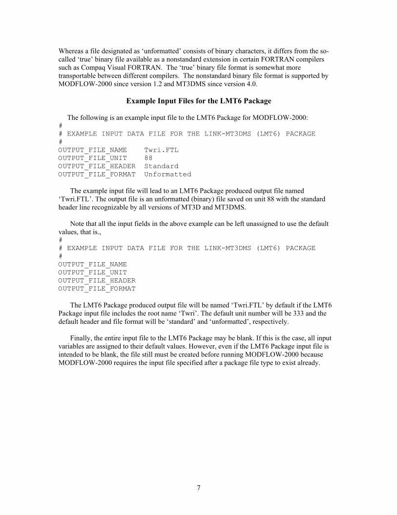
Example Input Files for the LMT6 Package The following is an example input file to the LMT6 Package for MODFLOW-2000:
# # EXAMPLE INPUT DATA FILE FOR THE LINK-MT3DMS (LMT6) PACKAGE # OUTPUT_FILE_NAME Twri.FTL OUTPUT_FILE_UNIT 88 OUTPUT_FILE_HEADER Standard OUTPUT_FILE_FORMAT Unformatted
The example input file will lead to an LMT6 Package produced output file named
‘Twri.FTL’. The output file is an unformatted (binary) file saved on unit 88 with the standard header line recognizable by all versions of MT3D and MT3DMS.
Note that all the input fields in the above example can be left unassigned to use the default values, that is., # # EXAMPLE INPUT DATA FILE FOR THE LINK-MT3DMS (LMT6) PACKAGE # OUTPUT_FILE_NAME OUTPUT_FILE_UNIT OUTPUT_FILE_HEADER OUTPUT_FILE_FORMAT
The LMT6 Package produced output file will be named ‘Twri.FTL’ by default if the LMT6
Package input file includes the root name ‘Twri’. The default unit number will be 333 and the default header and file format will be ‘standard’ and ‘unformatted’, respectively.
Finally, the entire input file to the LMT6 Package may be blank. If this is the case, all input
variables are assigned to their default values. However, even if the LMT6 Package input file is intended to be blank, the file still must be created before running MODFLOW-2000 because MODFLOW-2000 requires the input file specified after a package file type to exist already.
7

Description of the Link-MT3DMS Package
The source code for the new version (version 6) of the LMT Package consists of two FORTRAN files, LMT6.INC and LMT6.F. The first file contains a series of CALL statements to be added to the main program of MODFLOW-2000, and the second file contains independent subroutines that compute and save the saturated cell thickness, cell-by-cell flow terms, and locations and flow rates of various sink/source terms in the flow-transport link file for use by MT3DMS. While most of these subroutines are functionally identical to the Budget (BD) modules of various internal flow and sink/source packages in MODFLOW-2000, the LMT6 Package ensures a seamless linkage between MODFLOW-2000 and MT3DMS, and allows the output files from the Budget modules to be produced as needed for other purposes.
The LMT6 Package includes a basic subroutine and subroutines for an internal flow package
(BCF, LPF or HUF) and various source-term packages (such as WEL, RCH, GHB, and so on) of MODFLOW-2000. Only MODFLOW packages with a Budget (BD) module require corresponding subroutines in the LMT6 Package. For example, the Time-Variant Specified-Head (CHD) Package (Leake and Prudic, 1991) does not have a Budget module because the influence on flow budgets is accounted for by the active internal flow package (BCF, LPF or HUF). Thus, there is no corresponding subroutine in the LMT6 Package for the CHD Package. Similarly, the Horizontal Flow Barrier (HFB) Package (Hsieh and Freckleton, 1993) has neither a Budget module nor a corresponding LMT6 subroutine, and the influence on the budget is accounted for through BCF or LPF.
The basic subroutine for the LMT6 Package is named LMT6BAS6 where LMT6 stands for
the Link-MT3DMS Package Version 6, BAS6 designates the basic subroutine and its version number. LMT6BAS6 reads the input file to the LMT6 Package, gathers key information from the flow model, and saves a header line in the LMT6 Package produced flow-transport link file. Other subroutines in the LMT6 Package are named LMT6XXXn, where XXX is the name of the corresponding MODFLOW package for which the LMT6XXXn subroutine is designed and n is the version number. For example, the Link-MT3DMS subroutine for the MODFLOW-2000 BCF (version 6) and LPF (version 1) Packages are named LMT6BCF6 and LMT6LPF1, respectively. The MODFLOW-2000 internal flow and external source-terms packages and their current status of support by the LMT6 Package are listed in table 1.
8
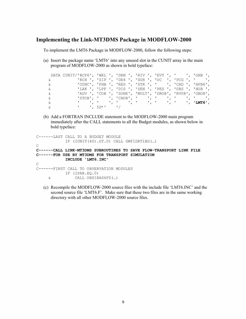
Implementing the Link-MT3DMS Package in MODFLOW-2000
To implement the LMT6 Package in MODFLOW-2000, follow the following steps: (a) Insert the package name ‘LMT6’ into any unused slot in the CUNIT array in the main
program of MODFLOW-2000 as shown in bold typeface:
DATA CUNIT/'BCF6', 'WEL ', 'DRN ', 'RIV ', 'EVT ', ' ', 'GHB ', & 'RCH ', 'SIP ', 'DE4 ', 'SOR ', 'OC ', 'PCG ', ' ', & 'CONC', 'FHB ', 'RES ', 'STR ', ' ', 'CHD ', 'HFB6', & 'LAK ', 'LPF ', 'DIS ', 'SEN ', 'PES ', 'OBS ', 'HOB ', & 'ADV ', 'COB ', 'ZONE', 'MULT', 'DROB', 'RVOB', 'GBOB', & 'STOB', ' ', 'CHOB', ' ', ' ', ' ', ' ', & ' ', ' ', ' ', ' ', ' ', ' ', 'LMT6', & ' ', 50*' '/
(b) Add a FORTRAN INCLUDE statement to the MODFLOW-2000 main program immediately after the CALL statements to all the Budget modules, as shown below in bold typeface:
C------LAST CALL TO A BUDGET MODULE IF (IUNIT(40).GT.0) CALL GWF1DRT1BD(…) C C------CALL LINK-MT3DMS SUBROUTINES TO SAVE FLOW-TRANSPORT LINK FILE C------FOR USE BY MT3DMS FOR TRANSPORT SIMULATION INCLUDE 'LMT6.INC' C C------FIRST CALL TO OBSERVATION MODULES IF (IPAR.EQ.0) & CALL OBS1BAS6FD(…)
(c) Recompile the MODFLOW-2000 source files with the include file ‘LMT6.INC’ and the second source file ‘LMT6.F’. Make sure that these two files are in the same working directory with all other MODFLOW-2000 source files.
9

Table 1. MODFLOW packages and their support status by Link-MT3DMS
MODFLOW package name (above double line, documented in Harbaugh and others, 2000; others referenced in
that work (p. 19), or as noted)
File type of MODFLOW-2000
name file
LINK-MT3DMS subroutine
name
LINK-MT3DMS support status as of this writing
Block-Centered Flow BCF6 LMT6BCF6 Yes
Layer Property Flow LPF LMT6LPF1 Yes
Horizontal Flow Barrier HFB None Yes
River RIV LMT6RIV6 Yes
Recharge RCH LMT6RCH6 Yes
Well WEL LMT6WEL6 Yes
Drain DRN LMT6DRN6 Yes
Evapotranspiration EVT LMT6EVT6 Yes
General-Head Boundary GHB LMT6GHB6 Yes
Time-Variant Constant Head Boundary CHD None Yes
Hydrogeologic Unit Flow (Anderman and Hill, 2000)
HUF LMT6HUF1 Yes
Streamflow-Routing STR LMT6STR6 Yes
Reservoir RES LMT6RES1 Yes
Specified Flow and Head Boundary FHB LMT6FHB1 Yes
Interbed Storage IBS LMT6IBS1 No
Transient Leakage TLK LMT6TLK1 No
Lake (Merritt and Konikow, 2000) LAK LMT6LAK1 No
Drain with Return Flow (Banta, 2000) DRT LMT6DRT1 No
Evapotranspiration with a Segmented Function (Banta, 2000) ETS LMT6ETS1 No
10
RUNNING MT3DMS WITH A MODFLOW-2000 PRODUCED LINK FILE
This chapter describes several issues related to the simulation setup and input data preparation for running MT3DMS with a flow-transport link file produced using MODFLOW-2000. These are (1) the previously existing and new methods to start a MT3DMS simulation; (2) the effect of new input requirements for MODFLOW-2000 on MT3DMS; and (3) the modifications to the MT3DMS Sink/Source Mixing (SSM) Package to support additional sink/source packages of MODFLOW-2000. The readers are encouraged to consult Zheng and Wang (1999) for background information and complete input instructions on MT3DMS.
Procedures to Start an MT3DMS Simulation
After the flow-transport link file is created by MODFLOW-2000 through the LMT6 Package, the user may proceed to run the transport simulation with MT3DMS. There are three ways to start a simulation, one of which is new. All three ways are described in the following sections.
Previously Existing Procedures
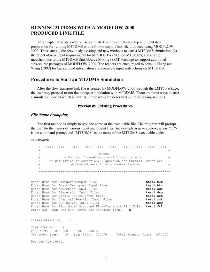
File Name Prompting
The first method is simply to type the name of the executable file. The program will prompt the user for the names of various input and output files. An example is given below, where “C:\>” is the command prompt and “MT3DMS” is the name of the MT3DMS executable code: C:\>MT3DMS +++++++++++++++++++++++++++++++++++++++++++++++++++++++++++++++++++++++ + + + MT3DMS + + A Modular Three-Dimensional Transport Model + + For Simulation of Advection, Dispersion and Chemical Reactions + + of Contaminants in Groundwater Systems + + + +++++++++++++++++++++++++++++++++++++++++++++++++++++++++++++++++++++++ Enter Name for Standard Output File: test1.m3d Enter Name for Basic Transport Input File: test1.btn Enter Name for Advection Input File: test1.adv Enter Name for Dispersion Input File: test1.dsp Enter Name for Sink & Source Input File: test1.ssm Enter Name for Chemical Reaction Input File: test1.rct Enter Name for GCG Solver Input File: test1.gcg Enter Name for Flow Model Produced Flow-Transport Link File: test1.ftl Print out Heads and Flow Terms for Checking (Y/N)? N STRESS PERIOD NO. 1 TIME STEP NO. 1 FROM TIME = 0.00000 TO 100.00 Transport Step: 10 Step Size: 10.000 Total Elapsed Time: 100.000 Program Completed.
11
Response File
The second method is to create a response file that contains the names of input and output files in the order required by MT3DMS. The content of such a response file (RUN.FIL) for the example shown above would be as follows:
test1.m3d test1.btn test1.adv test1.dsp test1.ssm test1.rct test1.gcg test1.ftl N
Then, at the command prompt, type: C:\>MT3DMS < RUN.FIL
New Procedure Using the Name File
A new method is added to MT3DMS Version 4.0 to start a simulation through a name file
that is similar to the name file used by MODFLOW-2000. The name file contains the names of most input and output files used in a model simulation and controls the parts of the model program that are active. The name file is read on unit 99, which is specified in the MT3DMS main program.
Name File Construction
The name file is constructed as follows: FOR EACH SIMULATION
1. Ftype Nunit Fname [options]
The Name file contains one of the above records (item 1) for each file. All variables are free format. The length of each record must be 199 characters or less. The records can be in any order except for the record where Ftype (file type) is ‘LIST’ as described below. Comment records are indicated by the # character in column 1 and can be located anywhere in the file. Any text characters can follow the # character. Comment records have no effect on the simulation; their purpose is to allow users to provide documentation about a particular simulation. All comment records after the first item-1 record are written in the listing file.
Explanation of Variables in the Name File Ftype - is the file type, which must be one of the following character values. Ftype may be entered in all uppercase, all lowercase, or any combination.
LIST for the standard MT3DMS output file – the Name file for MT3DMS must always
include a record that specifies ‘LIST’ for Ftype and the LIST record must be the first non-comment record.
12

BTN for the MT3DMS Basic Transport Package. ADV for the MT3DMS Advection Package. DSP for the MT3DMS Dispersion Package. SSM for the MT3DMS Sink/Source Mixing Package. RCT for the MT3DMS Reaction Package. GCG for the MT3DMS Generalized Conjugate-Gradient Solver Package. FTL for the flow model produced flow-transport link file. DATA(BINARY) for binary (unformatted) files such as those used for input of
concentrations saved in a previous simulation as the initial condition for a continuation run.
DATA for formatted (text) files such as those used to save formatted concentrations at
observation points and mass budget summaries or for input of data from files that are separate from the primary package input files.
Various output control options of MT3DMS can be set up to save four optional output
files: the unformatted (binary) concentration file, the formatted concentration observation file, the formatted mass budget summary file, and the model configuration file. MT3DMS always assigns default names to these files with the conventions listed below. These default names can be overridden, as explained in the next paragraph. MT3Dnnn.UCN for the unformatted concentration files where nnn is the species index number such as 001 for species 1, 002 for species 2, and so on; MT3Dnnn.OBS for the formatted concentration observation files; MT3Dnnn.MAS for the formatted mass budget summary files; and MT3D.CNF for storing the model configuration (spatial discretization) information needed by post-processing programs. This output file is always saved along with the UCN files.
Nunit - is the FORTRAN unit to be used when reading from or writing to the file. Any valid unit number on the computer being used can be specified except for the unit numbers that have been internally preserved by the MT3DMS program, as listed in table 2. To use the preserved unit number for a particular file, simply set Nunit associated with that file to 0. If a preserved unit for another file is used, an error message is written to the LIST output file and the program execution is terminated.
As pointed out previously, MT3DMS assigns the default file names for ‘UCN’, ‘OBS’, ‘MAS’, and ‘CNF’ files as MT3Dnnn.UCN, MT3Dnnn.OBS, MT3Dnnn.MAS, and MT3D.CNF. To keep the results from a previous simulation, these files need to be renamed before starting a new simulation in the same directory. Otherwise, they will be overwritten by the files from the new simulation. Override these default names by specifying a different name in the MT3DMS name file. For example, to name an unformatted ‘UCN’ file NewRun.UCN, the following line can be added to the MT3DMS name file: DATA(BINARY) Nunit NewRun.UCN where Nunit must be a preserved unit for a particular species. For example, if the NewRun.UCN is intended for saving the unformatted concentration of species 1, then
13

Nunit must be set to 201, the unit preserved for species 1 (see table 2). Similarly, if the NewRun.UCN is intended for species 2, then Nunit must be set to 202. To specify a different name for the formatted ‘OBS’, ‘MAS’, and ‘CNF’ files, add a line as shown below into the MT3DMS Name file DATA Nunit NewRun.OBS where again Nunit must be a preserved unit for a particular species. For example, if NewRun.OBS is intended for saving the species 1 concentrations at the observation points, then Nunit must be set to 401, the unit preserved for species 1 (see table 2). Similarly, if the NewRun.OBS is intended for species 2, then Nunit must be set to 402.
Table 2. Preserved unit numbers for various file types in MT3DMS
MT3DMS package or output options
File type Preserved unit
Output Listing File LIST 16
Package options Basic Transport BTN 1 Advection ADV 2 Dispersion DSP 3 Sink/Source Mixing SSM 4 Reaction RCT 8 Generalized Conjugate Gradient
GCG 9
Flow-Transport Link FTL 10 Output Files
Model Configuration File CNF 17 Unformatted Concentration File UCN 200+species index Concentrations Observation File OBS 400+species index Mass Budget Summary File MAS 600+species index
Fname - is the name of the input/output file, which is a character value. Pathnames may be specified as part of Fname. [Options] – optional keywords that may be used for the corresponding input/output file. Currently, only one such keyword may be specified in conjunction with the flow-transport link (FTL) file. The keyword Free indicates that the FTL input file for MT3DMS is in list-directed (free) format, that is, produced by the LMT6 Package with the option OUTPUT_FILE_FORMAT set to formatted. If no keyword is specified after the FTL file name, the FTL file is assumed to be unformatted (binary) by default. An example of the MT3DMS Name file is shown below: # # MT3DMS Name File for a test problem #
14
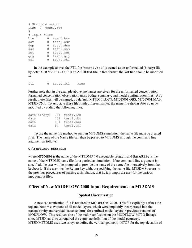
# Standard output list 0 test1.out # # Input files btn 0 test1.btn adv 0 test1.adv dsp 0 test1.dsp ssm 0 test1.ssm rct 0 test1.rct gcg 0 test1.gcg ftl 0 test1.ftl
In the example above, the FTL file ‘test1.ftl’ is treated as an unformatted (binary) file by default. If ‘test1.ftl’ is an ASCII text file in free format, the last line should be modified as ftl 0 test1.ftl Free Further note that in the example above, no names are given for the unformatted concentration, formatted concentration observation, mass budget summary, and model configuration files. As a result, these files will be named, by default, MT3D001.UCN, MT3D001.OBS, MT3D001.MAS, MT3D.CNF. To associate these files with different names, the name file shown above can be modified by adding the following lines: data(binary) 201 test1.ucn data 401 test1.obs data 601 test1.mas data 17 test1.cnf
To use the name file method to start an MT3DMS simulation, the name file must be created first. The name of the Name file can then be passed to MT3DMS through the command line argument as follows:
C:\>MT3DMS4 NameFile
where MT3DMS4 is the name of the MT3DMS 4.0 executable program and NameFile is the name of the MT3DMS name file for a particular simulation. If no command line argument is specified, the user will be prompted to provide the name of the name file interactively from the keyboard. If the user hits the Return key without specifying the name file, MT3DMS resorts to the previous procedures of starting a simulation, that is, it prompts the user for the various input/output files.
Effect of New MODFLOW-2000 Input Requirements on MT3DMS
Spatial Discretization
A new ‘Discretization’ file is required in MODFLOW-2000. This file explicitly defines the top and bottom elevations of all model layers, which were implicitly incorporated into the transmissivity and vertical leakance terms for confined model layers in previous versions of MODFLOW. This resolves one of the major confusions on the MODFLOW-MT3D linkage since MT3D has always required the complete definition of the model geometry. MT3D/MT3DMS uses two arrays to define the vertical geometry: HTOP for the top elevation of
15

the first model layer, and DZ for the cell thickness of all model layers. In contrast, MODFLOW-2000 uses the TOP and BOTM arrays for the same purpose.
The HTOP array of MT3D/MT3DMS is equivalent to the TOP array of MODFLOW-2000.
If no quasi-three-dimensional confining beds are included in a MODFLOW-2000 simulation, then the following relation holds, where i, j, and k define the row, column, and layer of a finite-difference cell:
DZj,i,k [MT3DMS] = BTOMj,i,k-1-BOTMj,i,k [MODFLOW-2000] However, a conceptual difficulty arises if the flow model includes one or more quasi-three-
dimensional confining beds. As pointed out in Zheng and Bennett (1995, p. 218), it is not advisable to adopt the quasi-three-dimensional approach for flow modeling if the flow solution is intended for use by transport simulation. This is because while the quasi-three-dimensional approach may be adequate to represent the confining beds in a flow simulation, it cannot account for the important solute transport effects of the confining beds (travel time and mass storage) if these confining beds are not explicitly represented in the flow model. An MT3DMS simulation can be set up for a flow model even if it contains one or more quasi-three-dimensional confining beds, by letting the layer thickness DZ array in MT3DMS equal the thickness of the active model layer plus that of the underlying confining bed in MODFLOW-2000, or by neglecting the thickness of the confining bed. If solute transport does not occur across the confining beds in question, the approximation is reasonable. However, if this is not the case, serious errors can result. Thus, it is strongly recommended that the quasi-three-dimensional approach be avoided for all solute transport modeling purposes.
Temporal Discretization Generally, MODFLOW and MT3DMS models should have the same number of stress
periods. The number of time steps used to obtain the flow solution in each stress period, referred to as “flow time steps” in the MT3DMS manual, should be specified in the transport model as well, so that the velocity field and sink/source information can be updated in the transport model properly. Thus, the following input specified for each stress period of MODFLOW should be specified for the corresponding input in MT3DMS:
PERLEN, NSTP, TSMULT
where PERLEN is the length of a stress period, NSTP is the number of time steps in the stress period, and TSMULT is the multiplier for the length of successive time steps.
When the flow model is steady-state with only one stress period and one time step, the MT3DMS code allows the flow and transport models to have different numbers of stress periods. This is because, when the flow model is steady-state, the velocity and sink/source information needs to be updated only once at the beginning of the simulation. In this case, the transport model is allowed to have as many stress periods as necessary to accommodate time-varying sink/source concentrations, while the flow rates of sinks/sources remain unchanged. The length of the stress period, PERLEN, in the flow model can be arbitrary.
Time-varying sink/source concentrations cannot vary within a stress period of a transient
MODFLOW-2000 run. Thus, for a given flow/transport simulation, if flow conditions are constant over a period, but transport conditions are not, then the temporal discretization in
16
MODFLOW should assign enough stress periods to the flow simulation to accommodate the transport simulation.
In MODFLOW-2000, one or more stress periods may be defined as steady-state but the rest
as transient using the input option “ss/tr” in the Discretization file. For MT3DMS, however, only those flow models with one stress period and one time step and with the steady-state flag set to “ss” are treated as true steady-state models. Thus, whenever there is more than one stress period or more than one time step in the flow model, regardless of how the flag “ss/tr” is set, the numbers of stress periods and time steps specified for the MODFLOW-2000 should be identical to those specified for the corresponding input variables in MT3DMS. Furthermore, the length of a transient stress period in MODFLOW-2000 must be exactly reflected in MT3DMS, while the length of a steady-state stress period in MODFLOW-2000 may be reset to a different value in MT3DMS. The latter is allowed because it is customary and convenient to set the length of a steady-state stress period in MODFLOW-2000 to unity, but the length of any stress period in MT3DMS must be the actual length of the user-desired simulation time.
Support of Additional Sink/Source Packages
MT3DMS prior to version 4.0 supports the following sink/source packages: RIV, RCH, WEL, DRN, EVT, and GHB (table 1). The Streamflow-Routing (STR) Package (version 1) is supported through the River option. This is done by associating the River sink/source type in MT3DMS with the STR Package instead of the RIV Package in MODFLOW. For this reason, the RIV and STR Packages cannot be used concurrently in the same flow model for subsequent transport simulation.
In the new LMT6 Package documented in this report, the flow terms by additional
sink/source packages developed for MODFLOW can be saved in the flow-transport link file through the extended header option. To provide support for these additional MODFLOW sink/source packages, corresponding changes are made to the Flow-Model-Interface (FMI) Package and the Sink/Source Mixing (SSM) Package of MT3DMS version 4.0. The changes to the FMI Package do not alter any input requirement or the way MT3DMS is operated. The changes to the SSM Package require some slight modifications to the input instructions of the SSM Package as described below.
Versions up to 3.5: D1 Record: FWEL, FDRN, FRCH, FEVT, FRIV, FGHB, (FNEW(n), n=1,4)
Format: 10L2 FWEL is a logical flag for the Well option; FDRN is a logical flag for the Drain option; FRCH is a logical flag for the Recharge option; FEVT is a logical flag for the Evapotranspiration option; FRIV is a logical flag for the River option (or the STR option); FGHB is a logical flag for General-Head-Dependent Boundary option; and FNEW are logical flags reserved for additional sink/source options. If any of these options is used in the flow model, its respective flag must be set to T (for True); otherwise, set to F (False).
Versions since 4.0:
17
D1 Record: [sink/source package names] The input values for this record are no longer required as MT3DMS determines whether or not a particular sink/source package is used in MODFLOW from the header line of the flow-transport link file. However, a blank line or a line with any arbitrary characters still must be present in the input file. A good practice would be to enter in this record the names of the sink/source packages active in the flow simulation for identification purposes. For example, if the Well, Drain, Recharge, Evapotranspiration, and Reservoir Packages are used in the flow simulation, the input record for D1 could consist of the following characters: WEL DRN RCH EVT RES.
Versions up to 3.5: D8 Record: KSS, ISS, JSS, CSS, ITYPE, (CSSMS(n), n=1, NCOMP)
Format: 3I10, F10.0, I10, [free] KSS, ISS, JSS, are the cell locations of the point sources whose concentrations must be
specified. The point sources whose concentrations are not specified here are assumed to have zero concentration, while the point sinks are assumed to have the same concentrations as the aquifer at the sink cell locations.
CSS is the user-specified concentration for a single-species simulation. For multi-species simulations, the concentration must be specified for each species through CSSMS.
ITYPE is an integer code indicating the type of the point source as listed below: ITYPE =-1, constant-concentration cell. = 1, constant-head cell;
= 2, well; = 3, drain; = 4, river (or stream); = 5, general-head boundary cell; = 15, mass-loading source.
Versions since 4.0: D8 Record: KSS, ISS, JSS, CSS, ITYPE, (CSSMS(n), n=1, NCOMP)
Format: 3I10, F10.0, I10, [free] No changes in the input requirements except for the newly added ITYPE codes (in
italics): ITYPE =-1, constant-concentration cell. = 1, constant-head cell;
= 2, well; = 3, drain; = 4, river (or stream); = 5, general-head boundary cell; =15, mass-loading source; =21, stream (if both RIV and STR Packages are used in the flow model); =22, reservoir (from the RES Package); =23, transient specified flow boundary cells (from the FHB Package); =24, interbed storage (from the IBS Package); =25, transient leakage (from the TLK Package); =26, lake (from the LAK Package); =28, drain with return flow (from the DRT Package); =29, evapotranspiration with a segmented function (from the ETS
18

Package); =51, cell with the first user-defined flow term (designated as USR1); =52, cell with the second user-defined flow term (designated as USR2); =53, cell with the third user-defined flow term (designated as USR3).
19
APPLICATION EXAMPLES
This chapter describes two examples in which MODFLOW-2000 and MT3DMS are applied to model solute transport in a hypothetical dual-domain system and at a large-scale field site. The concentration solutions obtained by MT3DMS are compared with the analytical solutions and with the numerical solutions by another transport model. The application examples are intended to illustrate the simulation setup and operation procedures and demonstrate some of the capabilities available in the MODFLOW-2000 and MT3DMS pair of ground-water models.
Dual-Domain Mass Transfer and Sorption
This benchmark problem is designed to test the capabilities of MT3DMS to simulate solute transport in a dual-domain system in the presence of first-order decay and linear sorption. The governing equation for this problem is as follows (Zheng and Wang, 1999, p. 14):
imimimimmmmmmm
mim
imimm
mm CRCRx
CqxCD
tCR
tCR θλ−θλ−
∂∂
−∂∂
θ=∂∂
θ+∂∂
θ 2
2
(1)
( ) imimimimimmim
imim CRCCt
CR θλ−−ζ=∂∂
θ (2)
where, mC and C are the dissolved concentrations in the mobile and immobile domains, respectively,
[MLim
-3]; mθ and are the porosities of the mobile and immobile domains, respectively,
[dimensionless]; imθ
mλ and λ are the first-order decay rates for the mobile-liquid and immobile-liquid phases, respectively, [T
im-1];
mR and are the retardation factors for the mobile and immobile domains, respectively, [dimensionless]; and
imR
ζ is the first-order mass transfer rate coefficient between the mobile and immobile domains, [T-1].
A general analytical solution for one-dimensional solute transport in a dual-domain system,
implemented in a computer code CXTFIT 2.0, is available from Toride and others (1995). The one-dimensional problem considered in this section involves the following initial condition for both mobile-liquid and immobile-liquid phases:
( )( ) 000,
0,0 0
>==
xxCCC
(3)
and a first-type boundary condition:
20

( )
( ) 00,0
0,0
0
00
>=∂∞∂
><<
=
tx
tCttttC
tC (4)
where, C is concentration, t is time, and C0 is the concentration at time t0.
A numerical flow and transport model is developed using MODFLOW-2000 and MT3DMS. The model consists of 101 columns, 1 row and 1 layer and is used to solve the problem for comparison with the analytical solution for the same initial and boundary conditions as described above. In the flow model, the first and last columns are constant-head boundaries. Arbitrary hydraulic heads are used to establish the required uniform hydraulic gradient. In the transport model, the first column is a constant-concentration boundary with a relative concentration of one. The last column is sufficiently far away from the source to approximate a semi-infinite one-dimensional flow domain as assumed in the analytical solution. The model parameters used in the simulation are listed below.
Cell width along rows ( = 10 m (meters) )∆x
Cell width along columns ( = 1 m ))
))
∆y
Layer thickness ( = 1 m ∆z
Specific discharge (Darcy flux) ( = 0.06 m/day )q
Longitudinal dispersivity = 10 m
Porosity of mobile domain = 0.2 ( mθ
Porosity of immobile domain ( = 0.05 imθ
First-order mass transfer rate coefficient between the mobile and immobile domains ( )ζ = 10-3 day-1
Source duration ( = 1,000 days )ot
Total simulation time ( )t = 10,000 days
The name files of MODFLOW-2000 and MT3DMS used in this example application are
shown below. # MODFLOW-2000 Name file for dual-domain example # # Output files list 12 dm.lst # Global input files dis 31 dm.dis # Link-MT3DMS input file
21

lmt6 66 dm.lmt # Flow process input files bas6 41 dm.bas bcf6 42 dm.bcf pcg 44 dm.pcg # MT3DMS Name file for the dual-domain example # # Output file list 0 dm.m3d # Transport process input files btn 0 dm.btn adv 0 dm.adv dsp 0 dm.dsp ssm 0 dm.ssm rct 0 dm.rct gcg 0 dm.gcg ftl 0 dm.ftl Five scenarios are simulated with the following first-order decay rate λ (assumed constant
for all phases) and retardation factor R (assumed constant for both domains): Case 1: No sorption, day 310−=λ -1 Case 2: 0,5 =λ== imm RRCase 3: day 410,5 −=λ== imm RR -1
Case 4: day 4105,5 −×=λ== imm RR -1
Case 5: day 310,5 −=λ== imm RR -1 In MT3DMS, the fraction of sorption sites in contact with mobile water is assumed to equal
the ratio of mobile to total porosities so that the retardation factor for the mobile domain is identical to that for the immobile domain. In addition, the rate constant for the first-order irreversible reaction (radioactive decay or biodegradation) is assumed to be the same for both mobile and immobile domains. However, different rate constants can be specified for the dissolved (liquid) and solid (sorbed) phases.
22
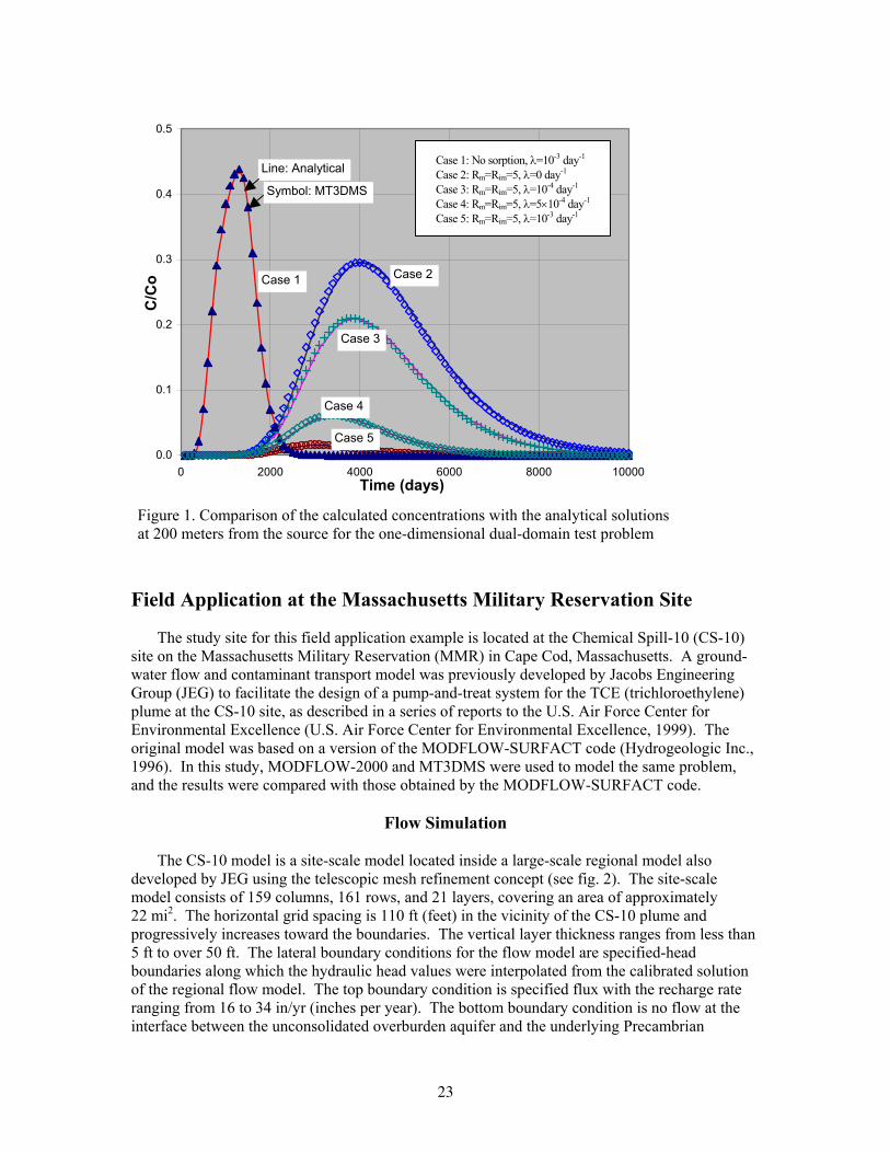
All cases are solved using the TVD option for the advection term and the GCG solver of MT3DMS for all other terms. The closure criterion for the Generalized Conjugate Gradient (GCG) solver is set at 10-6 and the modified incomplete Cholesky preconditioner is selected. For ease of comparison, a fixed transport step size of 1 day is used for all cases. A close match between the analytical (solid lines) and numerical solutions (symbols) is obtained for all cases (fig. 1). Only the concentrations of the mobile-liquid phase are plotted. The other three phases, mobile-sorbed, immobile-liquid, and immobile-sorbed, are tracked internally by MT3DMS, which also computes and maintains a global mass budget for all four phases. Mass balance errors are negligible for all the cases considered in this example.
0.0
0.1
0.2
0.3
0.4
0.5
0 2000 4000 6000 8000 10000Time (days)
C/C
o Case 1
Case 5
Case 4
Case 3
Case 2
Line: Analytical
Symbol: MT3DMS
Case 1: No sorption, λ=10-3 day-1 Case 2: Rm=Rim=5, λ=0 day-1
Case 3: Rm=Rim=5, λ=10-4 day-1
Case 4: Rm=Rim=5, λ=5×10⁻⁴ day-1
Case 5: Rm=Rim=5, λ=10-3 day-1
Figure 1. Comparison of the calculated concentrations with the analytical solutions at 200 meters from the source for the one-dimensional dual-domain test problem
Field Application at the Massachusetts Military Reservation Site
The study site for this field application example is located at the Chemical Spill-10 (CS-10) site on the Massachusetts Military Reservation (MMR) in Cape Cod, Massachusetts. A ground-water flow and contaminant transport model was previously developed by Jacobs Engineering Group (JEG) to facilitate the design of a pump-and-treat system for the TCE (trichloroethylene) plume at the CS-10 site, as described in a series of reports to the U.S. Air Force Center for Environmental Excellence (U.S. Air Force Center for Environmental Excellence, 1999). The original model was based on a version of the MODFLOW-SURFACT code (Hydrogeologic Inc., 1996). In this study, MODFLOW-2000 and MT3DMS were used to model the same problem, and the results were compared with those obtained by the MODFLOW-SURFACT code.
Flow Simulation
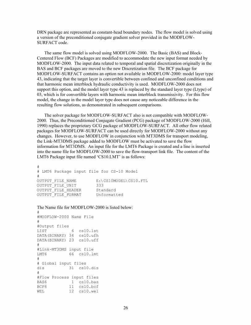
The CS-10 model is a site-scale model located inside a large-scale regional model also
developed by JEG using the telescopic mesh refinement concept (see fig. 2). The site-scale model consists of 159 columns, 161 rows, and 21 layers, covering an area of approximately 22 mi2. The horizontal grid spacing is 110 ft (feet) in the vicinity of the CS-10 plume and progressively increases toward the boundaries. The vertical layer thickness ranges from less than 5 ft to over 50 ft. The lateral boundary conditions for the flow model are specified-head boundaries along which the hydraulic head values were interpolated from the calibrated solution of the regional flow model. The top boundary condition is specified flux with the recharge rate ranging from 16 to 34 in/yr (inches per year). The bottom boundary condition is no flow at the interface between the unconsolidated overburden aquifer and the underlying Precambrian
23

bedrock. The overburden aquifer is comprised of Quaternary glacial outwash with a total thickness varying from less than 150 ft to the north and more than 400 ft to the south.
840000 845000 850000 855000 860000 865000 870000 875000 880000
EASTING (FT)
215000
220000
225000
230000
235000
240000
245000
250000
255000
260000
NO
RTH
ING
(FT)
CS-10 Zoom Model Boundary
TCEPlume
MMR Base Boundary
Figure 2. Location of the CS-10 model at the Massachusetts Military Reservation site in Cape Cod, Massachusetts. The outline of the trichloroethylene (TCE) plume is based on the data for 1997-98 from Jacobs Engineering Group (U.S. Air Force Center for Environmental Excellence, 1999).
The hydraulic conductivity (K) distribution used in the flow model was interpolated from
field test data by JEG. The K values range from less than 10 ft/day for silts to over 300 ft/day for coarse sands. The ground-water flow is predominantly horizontal with a general flow direction to the south-southwest. The average horizontal hydraulic gradient is around 0.001 in the vicinity of the plume. The ground-water velocities range from 1 to more than 4 ft/day.
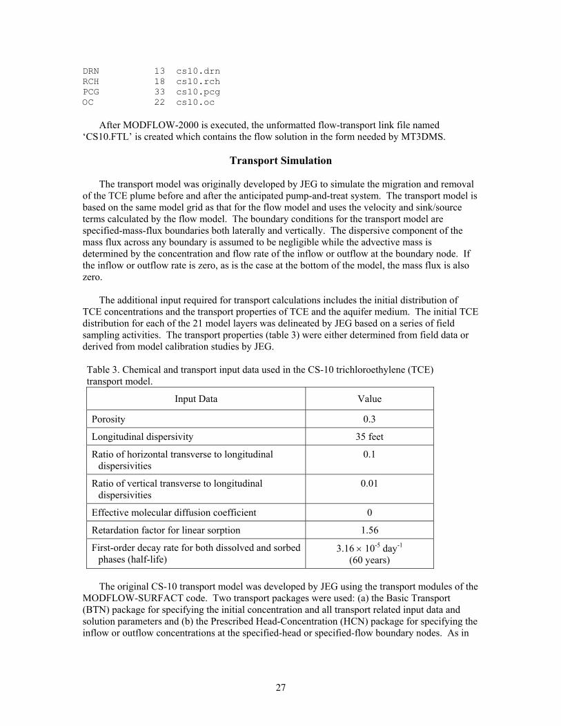
The CS-10 flow model was designed by JEG to simulate the steady-state condition of the
flow field. Two stress periods are included in the model: the first period is assumed to represent the existing flow field prior to the installation of an anticipated pump-and-treat system for the CS-10 plume (fig. 3), and the second stress period to represent the flow field after the pump-and-treat system is operational. The first stress period is 1 year long while the second period is to last as
24

long as the planning horizon for the pump-and-treat system. The only difference between the first and second stress periods in the flow model is the addition of new extraction wells and infiltration trenches (modeled as injection wells) for the anticipated pump-and-treat system.
0 5000 10000 15000 20000
DISTANCE ALONG X AXIS (FT)
0
5000
10000
15000
20000
25000
DIS
TAN
CE
ALO
NG
Y A
XIS
(FT) 5ppb
50ppb
250ppb
MMR Base Boundary
Initial TCE Plume
Infiltration Trench
Sandwich Road
Well Fence
Figure 3. Contoured concentrations of trichloroethylene (TCE), in parts per billion (ppb), and elements of the pump-and-treat system for the CS-10 plume. The solid dots (•) denote existing in-plume wells. The open dots ( ) represent perimeter wells still under consideration. The pumped water, after treatment, is to be reinjected into the infiltration trenches. The triangles along the Sandwich Road indicate an existing remedial well fence.
The CS-10 flow model was originally developed using the flow simulation modules of the MODFLOW-SURFACT code, which is functionally identical to the standard MODFLOW code with several enhancements. The sink/source packages used for the CS-10 flow model are the Well (WEL) package for simulating existing and anticipated remediation wells; the Recharge (RCH) package for simulating the specified recharge conditions; and the Drain (DRN) package for simulating surface ponds. Those surface ponds and depressions that are not included in the
25
DRN package are represented as constant-head boundary nodes. The flow model is solved using a version of the preconditioned conjugate gradient solver provided in the MODFLOW-SURFACT code.
The same flow model is solved using MODFLOW-2000. The Basic (BAS) and Block-
Centered Flow (BCF) Packages are modified to accommodate the new input format needed by MODFLOW-2000. The input data related to temporal and spatial discretization originally in the BAS and BCF packages are moved to the new Discretization file. The BCF package for MODFLOW-SURFACT contains an option not available in MODFLOW-2000: model layer type 43, indicating that the target layer is convertible between confined and unconfined conditions and that harmonic mean interblock hydraulic conductivity is used. MODFLOW-2000 does not support this option, and the model layer type 43 is replaced by the standard layer type (Ltype) of 03, which is for convertible layers with harmonic mean interblock transmissivity. For this flow model, the change in the model layer type does not cause any noticeable difference in the resulting flow solutions, as demonstrated in subsequent comparisons.
The solver package for MODFLOW-SURFACT also is not compatible with MODFLOW-
2000. Thus, the Preconditioned Conjugate Gradient (PCG) package of MODFLOW-2000 (Hill, 1990) replaces the proprietary GCG package of MODFLOW-SURFACT. All other flow related packages for MODFLOW-SURFACT can be used directly for MODFLOW-2000 without any changes. However, to use MODFLOW in conjunction with MT3DMS for transport modeling, the Link-MT3DMS package added to MODFLOW must be activated to save the flow information for MT3DMS. An input file for the LMT6 Package is created and a line is inserted into the name file for MODFLOW-2000 to save the flow-transport link file. The content of the LMT6 Package input file named ‘CS10.LMT’ is as follows:
# # LMT6 Package input file for CS-10 Model # OUTPUT_FILE_NAME E:\CS10MODEL\CS10.FTL OUTPUT_FILE_UNIT 333 OUTPUT_FILE_HEADER Standard OUTPUT_FILE_FORMAT Unformatted
The Name file for MODFLOW-2000 is listed below: # #MODFLOW-2000 Name File # #Output files LIST 6 cs10.lst DATA(BINARY) 34 cs10.ufh DATA(BINARY) 23 cs10.uff # #Link-MT3DMS input file LMT6 66 cs10.lmt # # Global input files dis 31 cs10.dis # #Flow Process input files BAS6 1 cs10.bas BCF6 11 cs10.bcf WEL 12 cs10.wel
26
DRN 13 cs10.drn RCH 18 cs10.rch PCG 33 cs10.pcg OC 22 cs10.oc
After MODFLOW-2000 is executed, the unformatted flow-transport link file named ‘CS10.FTL’ is created which contains the flow solution in the form needed by MT3DMS.
Transport Simulation
The transport model was originally developed by JEG to simulate the migration and removal
of the TCE plume before and after the anticipated pump-and-treat system. The transport model is based on the same model grid as that for the flow model and uses the velocity and sink/source terms calculated by the flow model. The boundary conditions for the transport model are specified-mass-flux boundaries both laterally and vertically. The dispersive component of the mass flux across any boundary is assumed to be negligible while the advective mass is determined by the concentration and flow rate of the inflow or outflow at the boundary node. If the inflow or outflow rate is zero, as is the case at the bottom of the model, the mass flux is also zero.
The additional input required for transport calculations includes the initial distribution of
TCE concentrations and the transport properties of TCE and the aquifer medium. The initial TCE distribution for each of the 21 model layers was delineated by JEG based on a series of field sampling activities. The transport properties (table 3) were either determined from field data or derived from model calibration studies by JEG.
Table 3. Chemical and transport input data used in the CS-10 trichloroethylene (TCE) transport model.
Input Data Value
Porosity 0.3
Longitudinal dispersivity 35 feet
Ratio of horizontal transverse to longitudinal dispersivities
0.1
Ratio of vertical transverse to longitudinal dispersivities
0.01
Effective molecular diffusion coefficient 0
Retardation factor for linear sorption 1.56
First-order decay rate for both dissolved and sorbed phases (half-life)
3.16 × 10⁻⁵ day-1 (60 years)
The original CS-10 transport model was developed by JEG using the transport modules of the
MODFLOW-SURFACT code. Two transport packages were used: (a) the Basic Transport (BTN) package for specifying the initial concentration and all transport related input data and solution parameters and (b) the Prescribed Head-Concentration (HCN) package for specifying the inflow or outflow concentrations at the specified-head or specified-flow boundary nodes. As in
27
the flow model, the transport model also is solved using a version of the preconditioned conjugate gradient solver provided in MODFLOW-SURFACT.
With MODFLOW-SURFACT, most of the transport related information is specified through
the input file to the Basic Transport (BTN) package. Additional information is contained in the input files to the Prescribed Head-Concentration (HCN) Package and Preconditioned Conjugate Gradient solver (PCG) Packages. With MT3DMS, the transport related information is specified through the input files to six packages, including the Basic Transport (BTN), Advection (ADV), Dispersion (DSP), Sink and Source Mixing (SSM), Chemical Reaction (RCT), and Generalized Conjugate Gradient solver (GCG) packages.
The input file for the MT3DMS BTN package contains basic model information such as
model dimension, boundary condition, initial concentration, transport step size control, and output control options. The input information needed for the MT3DMS BTN package is gathered from the input files to the BAS and BCF Packages of MODFLOW and the input file to the BTN package of MODFLOW-SURFACT.
The input file for the MT3DMS ADV package contains the solution option for the advection
term of the transport equation. The MT3DMS code is implemented with three classes of solution techniques, including the standard finite-difference method (either upstream or central weighting), a third-order TVD method, and particle-tracking based Eulerian-Lagrangian methods. The standard, implicit finite-difference method and particle-tracking based methods have no stability constraints and, thus, can be used with any transport step size as long as the solution accuracy can be assured. The third-order TVD method as implemented in MT3DMS is explicit; thus, it is only conditionally stable.
The CS-10 transport model based on the MODFLOW-SURFACT code uses an implicit
second-order TVD scheme for solving the advection term. When converted to MT3DMS, the implicit second-order TVD scheme used in MODFLOW-SURFACT is changed to the implicit upstream finite-difference method in MT3DMS. As demonstrated in subsequent comparisons, this change in the advection solution option does not cause any noticeable difference in the model results. This is because the TVD scheme and particle-tracking based solution options are designed to minimize numerical dispersion errors for advection-dominated transport problems. The CS-10 transport model, with a longitudinal dispersivity of 35 ft and a grid spacing of 110 ft in the detailed study area, has a grid Peclet number of less than four. The finite-difference method has been shown to be sufficiently accurate for transport problems with a grid Peclet number less than four (Zheng and Bennett, 1995).
The input file for the MT3DMS DSP package contains the dispersivity terms for the CS-10
transport model, as given in table 3. The input file for the MT3DMS SSM package contains information related to the various fluid sink/source terms. With MT3DMS, the concentration of any source inflow, if not specified by the user, is assumed zero by default. The concentration of any sink outflow is assumed to have the concentration of the aquifer at the sink location. One exception is evapotranspiration whose concentration can be specified by the user. For the CS-10 model, all fluid sources (recharge, injection wells, and inflow from the specified-head boundaries) have a zero concentration while all fluid sinks (extraction wells, drains, and outflow to the specified-head boundaries) have the concentration of the aquifer at the sink locations. Thus, these sources and sinks need not be specified in the input file for the SSM package. Furthermore, the prescribed head-concentration (HCN) input file for MODFLOW-SURFACT is not necessary for MT3DMS since the specified-head boundaries in MODFLOW are automatically treated as specified-mass-flux boundaries in MT3DMS.
28
The input file for the MT3DMS RCT package contains information on sorption and first-
order decay. The CS-10 transport model for TCE includes linear sorption with a uniform retardation factor of 1.56, and first-order decay for both dissolved and sorbed phases with a rate coefficient of 3.16 × 10⁻⁵ day-1 (or a half-life of 60 years).
The input file for the MT3DMS GCG Package contains the solution control options for the
GCG matrix solver. The GCG Package is similar to the PCG Packages for MODFLOW and MODFLOW-SURFACT. The GCG Package contains three preconditioners, Jacobi, successive slice over-relaxation (SSOR), and modified incomplete Cholesky (MIC). For large transport models, the SSOR preconditioner is a good compromise between solver performance and memory requirement. Since no nonlinear reaction is involved, the maximum number of outer iterations should be set to one, while a value of 100 is sufficient, under most circumstances, as the maximum number of inner iterations. A relative concentration closure criterion of 10-4 is generally adequate. Finally, the option of lumped dispersion cross terms should be chosen to greatly reduce the solver memory requirement with little loss of accuracy. In the CS-10 model based on MODFLOW-SURFACT, the dispersion cross terms are neglected.
29

Comparison of Model Results
The total TCE mass removal by wells at different times simulated by MODFLOW-SURFACT and MODFLOW-MT3DMS is shown in figure 4. The close agreement indicates that the model after conversion to MODFLOW-MT3DMS is as accurate as the MODFLOW-SURFACT model in terms of the mass removal by wells, in spite of the fact MODFLOW-MT3DMS runs much faster and requires less than half of the computer memory. Other mass budgets simulated by the original and converted models also agree closely with each other.
The water tables for the second stress period simulated by the original and converted models
are shown in figure 5. The simulated TCE concentrations in model layer 12 at the end of the second stress period, 25 years after the planned pump-and-treat system is operational, are shown in figure 6. The heads and TCE concentrations simulated by the original MODFLOW-SURFACT and the MODFLOW-MT3DMS models are in very close agreement.
0
1000
2000
3000
4000
0 5 10 15 20 25Time after the pump-and-treat system is in operation (years)
Tota
l TC
E M
ass
Rem
oval
by
Wel
ls (k
ilogr
am)
MODFLOW-SURFACT
MODFLOW-MT3DMS
Figure 4. Total trichloroethylene (TCE) mass removal by all wells simulated by MODFLOW-SURFACT and MODFLOW-MT3DMS.
30

5000 10000 15000 20000
X Axis (ft)
5000
10000
15000
20000
25000
Y Ax
is (f
t)CS-10 Zoom Model Boundary
5000 10000 15000 20000
X Axis (ft)
5000
10000
15000
20000
25000
Y Ax
is (f
t)
CS-10 Zoom Model Boundary
MMR Base Boundary
MMR Base Boundary
(a) MODFLOW-SURFACT (b) MODFLOW-2000
Figure 5. Water-table levels for the second stress period simulated using (a) MODFLOW-SURFACT and (b) MODFLOW-2000. Contours are in feet above sea level.
CS-10 Zoom Model BoundaryCS-10 Zoom Model Boundary
5000 10000 15000 20000
X Axis (ft)
5000
10000
15000
20000
25000
Y Ax
is (f
t)
1ppb 5ppb
5000 10000 15000 20000
X Axis (ft)
5000
10000
15000
20000
25000
Y Ax
is (f
t)
MMR Base Boundary
MMR Base Boundary
(a) MODFLOW-SURFACT (b) MT3DMS
Figure 6. Trichloroethylene (TCE) concentrations in model layer 12 simulated using (a) MODFLOW-SURFACT and (b) MT3DMS. Concentrations are in parts per billion (ppb).
31

POST-SIMULATION VISUALIZATION AND ANIMATION USING MODEL VIEWER
The USGS has developed a software package, known as Model Viewer, which can be used to visualize and animate simulation results obtained with several flow and transport models, including MODFLOW, MT3DMS, MOC3D (Konikow and others, 1996), and SUTRA (Voss, 1984). Here, a brief introduction to using Model Viewer with MT3DMS is provided. At the time of preparation of this report, Model Viewer is undergoing beta testing. When officially released, the software and user guide can be downloaded from the USGS ground-water software site (http://water.usgs.gov/software/ground_water.html).
When set up to display results from MT3DMS, Model Viewer obtains data from two output files
from MT3DMS, the model configuration (CNF) file and the unformatted concentration (UCN) file. These two files are saved by MT3DMS when the output control option for saving concentrations to unformatted files (SAVUCN) is set to T (for True) in the input file of the MT3DMS Basic Transport (BTN) Package. By default, MT3DMS names the model configuration file ‘MT3D.CNF’ and the unformatted concentration files ‘MT3Dnnn.UCN’ where nnn is the species index number such as 001 for species 1 and 002 for species 2. Because the UCN files for different species are structurally identical, the simulation results can be visualized one species at a time by selecting MT3D001.UCN, MT3D002.UCN, and so on in Model Viewer. For the previous versions of MT3D, the default name for the UCN file is ‘MT3D.UCN’ since the versions prior to MT3DMS do not support the multi-species capability.
Depending on which FORTRAN compiler was used to compile the MT3DMS executable file, the
structure of the unformatted (binary) concentration file may be different. Specifying a correct data structure is necessary for the UCN file to be read properly by Model Viewer. Three types of the unformatted file structure supported by Model Viewer are:
(a) Visual FORTRAN (PC-Windows), (b) Lahey FORTRAN-90 (PC-Windows), and (c) Big Endian (UNIX). Most users on the PC-Windows platform have used the MT3DMS executables compiled with either
the Lahey FORTRAN compiler or the Visual FORTRAN compiler previously from Digital Equipment Corporation and now from Compaq. Choice b on the list above is also applicable to the Lahey FORTRAN-77 compiler since Lahey FORTRAN-77 and FORTRAN-90 compilers use the same unformatted file structure. However, the Lahey FORTRAN-95 compiler has adopted the same unformatted file structure as that of Visual FORTRAN. Thus, choice a on the list above is also applicable to the Lahey FORTRAN-95 compiler.
The UCN files may contain the simulated concentrations at multiple transport time steps. By default,
MT3DMS saves the concentration results at the end of each stress period, if the SAVUCN option is activated. To save the concentrations at other times, the user needs to specify appropriate values for the input records NPRS and TIMPRS in the MT3DMS BTN Package input file. If NPRS is given a negative value, the concentrations are saved whenever the number of transport steps is an even multiple of |NPRS|. If NPRS is assigned a positive value, the concentrations are saved at total elapsed times from the beginning as specified through TIMPRS. Using Model Viewer, users may display the concentration distribution at a specified time step or sequentially display the concentration at successive time steps to create an animation.
32

Although the unformatted (binary) head or drawdown files saved by MODFLOW are not used by
MT3DMS (the flow-transport link file saved by the LMT6 package is used instead), heads or drawdowns can nonetheless be viewed in Model Viewer when it is set to display the MT3DMS results. This is because the form of the MT3DMS UCN file is identical to that used by the unformatted head or drawdown file saved by MODFLOW. Thus, when prompted for the name of the UCN file, the user may specify instead the name of the unformatted head or drawdown file created by MODFLOW. Model View will then display the three-dimensional distribution of hydraulic head or drawdown instead of concentration.
The general approach to visualizing the three-dimensional distribution of concentration is to use a
color scale (blue to red) to represent concentration values and to apply a combination of techniques such as thresholding, isosurface construction, and cropping. These techniques are illustrated by the examples below. Thresholding refers to the removal of regions where concentration is below a minimum value and/or above a maximum value. Thresholding is useful for illustrating the spatial extent of a contaminant plume. This can be done by setting the minimum threshold to a value below which the water is considered “clean” or “uncontaminated”. An isosurface is a surface of equal concentration value and is the three-dimensional counterpart of a contour line. Cropping refers to the removal of a region that lies beyond a cropping plane. Cropping is useful for examining the concentration distribution inside a contaminant plume.
Illustrative Examples
Two examples are included in this section to illustrate the visualization of MT3DMS simulation results. The first example involves three-dimensional flow and transport in a cubical flow field bound by no-flow boundaries on all sides of the cube. An injection well is located at one corner of the cube and an extraction well at the opposite corner. The injected fluid has a concentration of 100 (arbitrary units). After a certain time, the concentration of the injected fluid is set to zero while the injection flow rate is kept the same. Three snapshots of the plume evolution as displayed by Model Viewer are shown in figure 7. The concentration threshold minimum is set to remove regions where concentration is less than 5. The display is cropped along a vertical plane oriented along the cube diagonal to better illustrate the concentration distribution between the source and the sink. Figure 7(a) shows the plume at an early time when the injected solute is moving steadily away from the point source. Because a small dispersivity value has been specified in the simulation, the plume has a sharp front as indicated by a narrow transition zone. Figure 7(b) shows the plume distribution after the inflow concentration is changed from 100 to zero, that is, clean water is flushing through the cube. Figure 7(c) shows the plume at a late time when a significant volume of the cube is filled with the clean water and the center of the plume has been pushed toward the sink.
The second example involves three-dimensional flow and transport at the CS-10 site on the
Massachusetts Military Reservation (MMR), as described earlier in the report. The simulated TCE plume 1 year after a proposed pump-and-treat system goes into operation is shown in figure 8. The model mesh is shown on the figure as the background. The color scale is set to illustrate concentration values ranging from 5 to 100 parts per billion (ppb). Concentration values above 100 ppb are shown as red. The concentration threshold minimum is set to remove regions where concentration is less than 5 ppb. The spatial extent of the TCE plume, as defined by the 5 ppb isoconcentration surface, is illustrated by the transparent brown shell. Inside this shell, two cropping planes, one horizontal and the other vertical (oriented along the direction of plume movement), reveal the high concentration pockets in the TCE plume. The visualization and animation of the MT3DMS results are intended to aid modelers in
33

developing a complete conceptualization of the modeled system and in designing effective remediation systems.
Figure 7. Simulation of solute transport from a point source at one corner of a cube to a sink at the opposite corner. The three snapshots represent the plume distribution at three successive times.
34

Figure 8. Three-dimensional visualization of the simulated trichloroethylene (TCE) plume at the CS-10 site on the Massachusetts Military Reservation 1 year after a proposed pump-and-treat system is assumed to be operational. Concentrations are shown in parts per billion (ppb). The transparent brown shell indicates the 5 ppb isoconcentration surface. Concentration values above 100 ppb are shown as red.
Unformatted Concentration (UCN) File
In MT3DMS, one unformatted concentration file is saved for each species, with the default names MT3Dnnn.UCN where nnn is the species index number as in MT3D001.UCN, MT3D002.UCN, and so on. The unformatted concentration files are saved by setting the flag SAVUCN to T (for True) in the BTN input file. The structure and contents of the unformatted concentration files are shown below.
MT3Dnnn.UCN (unformatted):
For each transport step saved:
For each layer of the three-dimensional concentration matrices: Record 1: NTRANS,KSTP,KPER,TIME2,TEXT,NCOL,NROW,ILAY Record 2: ((CNEW(J,I,ILAY),J=1,NCOL),I=1,NROW)
where NTRANS is the transport step at which the concentration is saved, integer; KSTP is the time step at which the concentration is saved, integer; KPER is the stress period at which the concentration is saved, integer; TIME2 is the total elapsed time at which the concentration is saved, real; TEXT is a character string (character*16) set equal to “CONCENTRATION”; NCOL is the total number of columns, integer; NROW is the total number of rows, integer; ILAY is the layer at which the concentration is saved, integer; and
35
CNEW is the calculated concentration, real. The real values are saved in single precision. The header line above (Record 1) is slightly different from that used by MODFLOW, which has the header as follows,
KSTP,KPER,PERTIM,TIME2,TEXT,NCOL,NROW,ILAY
where PERTIM is the time elapsed since the beginning of the current stress period.
Model Configuration (CNF) File
The model configuration file, named MT3D.CNF by default, is saved automatically by MT3DMS along with MT3Dnnn.UCN after the output flag SAVUCN is set to T. To process the unformatted head or drawdown file saved by MODFLOW before MT3DMS is used, the CNF file must be created manually using a text editor. The structure and contents of the model configuration file are shown below. MT3D.CNF (free format):
Record 1: NLAY, NROW, NCOL Record 2: (DELR(J), J=1,NCOL) Record 3: (DELC(I),I=1,NROW) Record 4: ((HTOP(J,I), J=1,NCOL),I=1,NROW) Record 5: (((DZ(J,I,K), J=1,NCOL),I=1,NROW),K=1,NLAY) Record 6: CINACT, CDRY
where NLAY is the total number of layers, integer; DELR is the width of columns (along the rows or x axis), real; DELC is the width of rows (along the columns or y axis), real; HTOP is a two-dimensional array defining the top elevation of the first model layer, real; DZ is a three-dimensional array defining the thickness of each model cell, real; CINACT is the value used in the model for indicating inactive cells at the beginning of the
simulation, real; CDRY is the value used in the model for indicating the cells that go dry during the
simulation, real.
The input values in the model configuration file are arranged in list-directed (or free) format. Therefore, each record should begin at a new line, and a record can occupy as many lines as needed. Either blank space or comma can be used to separate values within a record. In addition, input by free format permits the use of a repeat count in the form, n*d, where n is an positive, non-zero integer constant (do not use a +), and the input n*d causes n consecutive values of d to be entered. For example, 5*101.2 would cause the value 101.2 to be entered five times.
HTOP is a two-dimensional array, and its values should be arranged in the order of column first,
sweeping from column 1 to column NCOL along the first row; then continuing onto row 2, row 3, ..., until row NROW. DZ is a three-dimensional array, and its values for each layer should be arranged similarly to those for HTOP, starting from the first layer, then continuing onto layer 2, layer 3, ..., until layer NLAY. If one is only interested in creating data files for selected layers in plan view, then HTOP and DZ are never used. Numbers need to be entered for HTOP and DZ, but dummy numbers can be used with the use of repeat counts.
36

REFERENCES
Anderman, E.R., and Hill, M.C., 2000, MODFLOW-2000, the U.S. Geological Survey modular ground-water model – Documentation of the Hydrogeologic Unit Flow (HUF) Package: U.S. Geological Survey Open-File Report 00-342, 89 p.
----------2001, MODFLOW-2000, the U.S. Geological Survey modular ground-water model – Documentation of the Advective-transport observation (ADV2) package, version 2: U.S. Geological Survey Open-File Report 01-54, 67 p.
Banta, E.R. 2000, MODFLOW-2000, the U.S. Geological Survey modular ground-water model – Documentation of Packages for simulating evapotranspiration with a segmented function (ETS1) and drains with return flow (DRT1): U.S. Geological Survey OFR ))-466, 127 p.
Fenske, J.P., Leake, S.A., and Prudic, D.E., 1996, Documentation of a computer program (RES1) to simulate leakage from reservoirs using the modular finite-difference ground-water flow model (MODFLOW): U.S. Geological Survey Open-File Report 96-364, 51 p.
Harbaugh, A.W., Banta, E.R., Hill, M.C., and McDonald, M.G., 2000, MODFLOW-2000, the U.S. Geological Survey modular ground-water model—User guide to modularization concepts and the ground-water flow processes: U.S. Geological Survey Open-File Report 00-92, 121 p.
Harbaugh, A.W., and McDonald, M.G., 1996, User's documentation for MODFLOW-96, an update to the U.S. Geological Survey modular finite-difference ground-water flow model: U.S. Geological Survey Open-File Report 96-485, 56 p.
Hill, M.C., 1990, Preconditioned conjugate gradient 2(PCG2), a computer program for solving ground- water flow equations, U.S. Geological Survey Water-Resources Investigations Report 90-4048, 43 p.
Hill, M.C., Banta, E.R., Harbaugh, A.W., and Anderman, E.R., 2000, MODFLOW-2000, the U.S. Geological Survey modular ground-water model—User guide to the observation, sensitivity, and parameter-estimation processes and three post-processing programs: U.S. Geological Survey Open-File Report 00-184, 210 p.
Hsieh, P.A., and Freckleton, J.R., 1993, Documentation of a computer program to simulate horizontal-flow barriers using the U.S. Geological Survey modular three-dimensional finite-difference ground-water flow model: U.S. Geological Survey Open-File Report 92-477, 32 p.
Hydrogeologic Inc., 1996, MODFLOW-SURFACT software (version 1.2) Documentation: Herndon, Virginia, 170 p.
Konikow, L.F., Goode, D.J., and Hornberger, G.Z., 1996, A three-dimensional method-of-characteristics solute-transport model (MOC3D): U.S. Geological Survey Water-Resources Investigations Report 96-4267, 87 p.
Leake, S.A., and Lilly, M.R., 1997, Documentation of a computer program (FHB1) for assignment of transient specified-flow and specified-head boundaries in applications of the modular finite-difference ground-water flow model (MODFLOW): U.S. Geological Survey Open-File Report 97-571, 50 p.
Leake, S.A., and Prudic, D.E., 1991, Documentation of a computer program to simulate aquifer-system compaction using the modular finite-difference ground-water flow model: U.S. Geological Survey Techniques of Water-Resources Investigations, book 6, chap. A2, 68 p.
McDonald, M.G., and Harbaugh, A.W., 1988, A modular three-dimensional finite-difference ground-water flow model: U.S. Geological Survey Techniques of Water-Resources Investigations, book 6, chap. A1, 586 p.
Merritt, M.L., and Konikow, L.F., 2000, Documentation of a computer program to simulate lake-aquifer interaction using the MODFLOW ground-water flow model and the MOC3D solute-transport model: U.S. Geological Survey Water-Resources Investigations Report 00-4167, 146 p.
Prudic, D.E., 1989, Documentation of a computer program to simulate stream-aquifer relations using a modular, finite-difference, ground-water flow model: U.S. Geological Survey Open-File Report 88-729, 113 p.
37

Toride, E., Leij, F.J., and van Genuchten, M. Th., 1995, The CXTFIT code for estimating transport parameters from laboratory or field tracer experiments, version 2.0: Riverside, Calif., U.S. Salinity Laboratory, Research Report 137, 121 p.
U.S. Air Force Center for Environmental Excellence (AFCEE), 1999, CS-10 in-plume remedial system design groundwater modeling report, Document no. AFC-J23-35S18405-M17-0002: Prepared by Jacobs Engineering Group for ACCEE/MMR Installation Restoration Program, Otis Air National Guard Base, Mass., 110 p.
Voss, C.I., 1984, A finite-element simulation model for saturated-unsaturated, fluid-density-dependent ground-water flow with energy transport or chemically-reactive single-species solute transport: U.S. Geological Survey Water-Resources Investigations Report 84-4369, 409 p.
Zheng, Chunmiao, 1990, MT3D: A modular three-dimensional transport model for simulation of advection, dispersion and chemical reactions of contaminants in groundwater systems: Report prepared at S. S. Papadopulos & Associates, Inc for the U.S. Environmental Protection Agency, Ada, Okla., 171 p.
Zheng, Chunmiao, and Bennett, G.D., 1995, Applied Contaminant Transport Modeling: Theory and Practice: New York, Van Nostrand Reinhold (John Wiley & Sons), 440 p.
Zheng, Chunmiao, and Wang, P.P., 1999, MT3DMS: A modular three-dimensional multi-species transport model for simulation of advection, dispersion and chemical reactions of contaminants in groundwater systems; Documentation and user’s guide: Contract report SERDP-99-1: Vicksburg, Miss., U.S. Army Engineer Research and Development Center, 169 p. (Available at http://hydro.geo.ua.edu).
38
APPENDIX: CONTENTS OF THE FLOW-TRANSPORT LINK FILE
The flow-transport link file is rarely edited or opened by users, but its contents are described here for those who wish to access it.
FOR EACH SIMULATION:
Either the Standard Header Line (for all versions of MT3D/MT3DMS)
F0. VERSION, MTWEL, MTDRN, MTRCH, MTEVT, MTRIV, MTGHB, MTCHD, MTISS, MTNPER Or the Extended Header Line (only for MT3DMS since version 4.0)
F0. VERSION, MTWEL, MTDRN, MTRCH, MTEVT, MTRIV, MTGHB, MTCHD, MTISS, MTNPER, MTSTR, MTRES, MTFHB, MTDRT, MTETS, MTIBS, MTTLK, MTLAK, MTMAW, MTUSR1, MTUSR2, MTUSR3
Explanation of variables
VERSION (character*11)—a character string used by MT3DMS to identify the flow model
produced flow-transport link. For the Standard Header Line, VERSION=’MT3D3.00.99’. For the Extended Header Line, VERSION=’MT3D4.00.00’.
MTWEL—an integer flag indicating whether wells (the WEL package) are included in the
MODFLOW simulation: MTWEL>0, wells are included in the MODFLOW simulation; MTWEL=0, wells are not included in the MODFLOW simulation.
MTDRN—an integer flag indicating whether drains (the DRN package) are included in the MODFLOW simulation. The convention is the same as that for MTWEL.
MTRCH—an integer flag indicating whether recharge (the RCH package) is included in the
MODFLOW simulation. The convention is the same as that for MTWEL. MTEVT—an integer flag indicating whether evapotranspiration (the EVT package) is included in
the MODFLOW simulation. The convention is the same as that for MTWEL. MTRIV—an integer flag indicating whether rivers (the RIV package) are included in the
MODFLOW simulation. The convention is the same as that for MTWEL. Note that for the standard header option, MTRIV can represent either the RIV package or the Stream (STR) package since only one of these two packages can be present in the same simulation. For the extended header option, a separate entry MTSTR is used to indicate the STR package.
MTGHB—an integer flag indicating whether general-head-dependent boundaries (the GHB
package) are included in the MODFLOW simulation. The convention is the same as that for MTWEL.
MTCHD—an integer flag indicating whether any constant-head boundary cells are included in
the MODFLOW simulation. The convention is the same as that for MTWEL.
39
MTISS—an integer flag indicating whether the flow simulation is steady-state or transient:
MTISS>0, the flow simulation is steady-state. MTISS=0, the flow simulation is transient in one or more stress periods.
MTNPER—the number of stress periods used in the flow simulation.
MTSTR—an integer flag indicating whether streams (the STR package) are included in the MODFLOW simulation. The convention is the same as that for MTWEL. This flag is saved only for the extended header line.
MTRES—an integer flag indicating whether reservoirs (the RES package) are included in the MODFLOW simulation. The convention is the same as that for MTWEL. This flag is saved only for the extended header line.
MTFHB—an integer flag indicating whether transient specified flow and head boundaries (the FHB package) are included in the MODFLOW simulation. The convention is the same as that for MTWEL. This flag is saved only for the extended header line.
MTDRT—an integer flag indicating whether the drain with return flow (DRT) package is included in the MODFLOW simulation. The convention is the same as that for MTWEL. This flag is saved only for the extended header line.
MTETS—an integer flag indicating whether the evapotranspiration with a segmented function (ETS) package is included in the MODFLOW simulation. The convention is the same as that for MTWEL. This flag is saved only for the extended header line.
MTIBS—an integer flag indicating whether the interbed storage (IBS) package is included in the MODFLOW simulation. The convention is the same as that for MTWEL. This flag is saved only for the extended header line.
MTTLK—an integer flag indicating whether the transient leakage (TLK) package is included in the MODFLOW simulation. The convention is the same as that for MTWEL. This flag is saved only for the extended header line.
MTLAK—an integer flag indicating whether lakes (the LAK package) are included in the MODFLOW simulation. The convention is the same as that for MTWEL. This flag is saved only for the extended header line.
MTMAW—an integer flag indicating whether multi-aquifer wells (the MAW package) is included in the MODFLOW simulation. The convention is the same as that for MTWEL. This flag is saved only for the extended header line.
MTUSR1—an integer flag indicating whether a user-defined sink/source (USR1) package other than those listed above is included in the MODFLOW simulation. The convention is the same as that for MTWEL. This flag is saved only for the extended header line.
MTUSR2—an integer flag indicating whether a second user-defined sink/source (USR2) package other than one listed above is included in the MODFLOW simulation. The convention is the same as that for MTWEL. This flag is saved only for the extended header line.
40

MTUSR3—an integer flag indicating whether a third user-defined sink/source (USR3) package other than one listed above is included in the MODFLOW simulation. The convention is the same as that for MTWEL. This flag is saved only for the extended header line.
FOR EACH TIME STEP OF THE FLOW SOLUTION:
F1. KPER, KSTP, NCOL, NROW, NLAY, LABEL F2. THKSAT(NCOL,NROW,NLAY)
KPER—the stress period at which the cell saturated thicknesses are saved. KSTP—the time step at which the cell saturated thicknesses are saved. NCOL, NROW, NLAY—the numbers of columns, rows and layers, respectively. LABEL(character*16)—a character string equal to ‘THKSAT’, the identifier for the
saturated cell thickness array. THKSAT—Saturated thickness of unconfined cells. For inactive cells, the value must be
set equal to 1.E30. For confined cells, the value must be set to –111. (If NCOL=1, skip F3 and F4) F3. KPER, KSTP, NCOL, NROW, NLAY, LABEL F4. QX(NCOL,NROW,NLAY)
LABEL(character*16)—a character string equal to ‘QXX’, the identifier for the QX array.
QX—volumetric flow rates (L3T-1) between cells at cell interfaces along rows (or the x-axis). Positive in the direction of increasing J indexes. Start at the right face of column 1.
(If NROW=1, skip F5 and F6) F5. KPER, KSTP, NCOL, NROW, NLAY, LABEL F6. QY(NCOL,NROW,NLAY)
LABEL(character*16)—a character string equal to ‘QYY’, the identifier for the QY array.
QY—volumetric flow rates (L3T-1) between cells at cell interfaces along columns (or the y-axis). Positive in the direction of increasing I indexes. Start at the lower face of row 1.
(If NLAY=1, skip F7 and F8) F7. KPER, KSTP, NCOL, NROW, NLAY, LABEL F8. QZ(NCOL,NROW,NLAY)
LABEL(character*16)—a character string equal to ‘QZZ’, the identifier for the QZ array. QZ—volumetric flow rates (L3T-1) between cells at cell interfaces along layers (or the z
axis). Positive in the direction of increasing K indexes. Start at the bottom face of layer 1.
(If MTISS>0, skip F9 and F10) F9. KPER, KSTP, NCOL, NROW, NLAY, LABEL F10. QSTO(NCOL,NROW,NLAY)
LABEL(character*16)—a character string equal to ‘STO’, the identifier for the QSTO array.
QSTO—volumetric flow rates (L3T-1) released from or accumulated in transient groundwater storage. Positive for release and negative for accumulation.
41

F11. KPER, KSTP, NCOL, NROW, NLAY, LABEL, NCNH LABEL(character*16)—a character string equal to ‘CNH’, the identifier for constant-
head boundaries. NCNH—total number of constant-head boundary cells.
(If NCNH>0, there must be NCNH records of F12) F12. KCNH, ICNH, JCNH, QCNH
KCNH, ICNH, JCNH—cell indices of each constant-head boundary cell. QCNH—volumetric net flow rate (L3T-1) out of or into each constant-head cell, including
the exchange between neighboring constant-heads cells. Positive if the flow is out of the constant-head cell, negative otherwise.
(If wells are not present in the flow model, skip F13 and F14) F13. KPER, KSTP, NCOL, NROW, NLAY, LABEL, NWEL
LABEL(character*16)—a character string equal to ‘WEL’, the identifier for wells. NWEL—total number of wells.
(If NWEL>0, there must be NWEL records of F14) F14. KWEL, IWEL, JWEL, QWEL
KWEL, IWEL, JWEL—cell indices of each well. QWEL—volumetric flow rate (L3T-1) of each well. Positive if the flow is into the cell,
negative otherwise. (The same convention is followed by the rest of sink/source terms).
(If drains are not present in the flow model, skip F15 and F16) F15. KPER, KSTP, NCOL, NROW, NLAY, LABEL, NDRN
LABEL(character*16)—a character string equal to ‘DRN’, the identifier for drains. NDRN—total number of drains.
(If NDRN>0, there must be NDRN records of F16) F16. KDRN, IDRN, JDRN, QDRN
KDRN, IDRN, JDRN—cell indices of each drain. QDRN—volumetric flow rate (L3T-1) of each drain.
(If recharge is not present in the flow model, skip F17, F18 and F19) F17. KPER, KSTP, NCOL, NROW, NLAY, LABEL F18. IRCH(NCOL,NROW) F19. RECH(NCOL,NROW)
LABEL(character*16)—a character string equal to ‘RCH’, the identifier for recharge. IRCH—layer indices of the recharge flux. RECH—volumetric recharge rate (L3T-1).
(If evapotranspiration is not present in the flow model, skip F20, F21, and F22) F20. KPER, KSTP, NCOL, NROW, NLAY, LABEL F21. IEVT(NCOL,NROW) F22. EVTR(NCOL,NROW)
LABEL(character*16)—a character string equal to ‘EVT’, the identifier for evapotranspiration.
IEVT—layer indices of the evapotranspiration flux. EVTR—volumetric evapotranspiration rate (L3T-1).
42
(If rivers are not present in the flow model, skip F23 and F24) F23. KPER, KSTP, NCOL, NROW, NLAY, LABEL, NRIV
LABEL(character*16)—a character string equal to ‘RIV’, the identifier for rivers. NRIV—total number of rivers.
(If NRIV>0, there must be NRIV records of F24) F24. KRIV, IRIV, JRIV, QRIV
KRIV, IRIV, JRIVN—cell indices of each river (or stream) cell. QRIV—volumetric flow rate (L3T-1) of each river (or stream) cell.
(If general-head-dependent boundaries are not present in the flow model, skip F25 and F26) F25. KPER, KSTP, NCOL, NROW, NLAY, LABEL, NGHB
LABEL(character*16)—a character string equal to ‘GHB’, the identifier for general-head-dependent boundaries. NGHB—total number of GHB cells.
(If NGHB>0, there must be NGHB records of F26) F26. KGHB, IGHB, JGHB, QGHB
KGHB, IGHB, JGHB—cell indices of each general-head-dependent boundary cell. QGHB—volumetric flow rate (L3T-1) of each general-head-dependent boundary cell.
(If streams are not present in the flow model, skip F27 and F28) F27. KPER, KSTP, NCOL, NROW, NLAY, LABEL, NSTR
LABEL(character*16)—a character string equal to ‘STR’, the identifier for streams. NSTR—total number of STR cells.
(If NSTR>0, there must be NSTR records of F28) F28. KSTR, ISTR, JSTR, QSTR
KSTR, ISTR, JSTR—cell indices of each stream cell. QSTR—volumetric flow rate (L3T-1) of each stream cell.
(If reservoirs are not present in the flow model, skip F29 and F30) F29. KPER, KSTP, NCOL, NROW, NLAY, LABEL, NRES
LABEL(character*16)—a character string equal to ‘RES’, the identifier for reservoirs. NRES—total number of reservoir cells.
(If NRES>0, there must be NRES records of F30) F30. KRES, IRES, JRES, QRES
KRES, IRES, JRES—cell indices of each reservoir cell. QRES—volumetric flow rate (L3T-1) of each reservoir cell.
(If the FHB package is not present in the flow model, skip F31 and F32) F31. KPER, KSTP, NCOL, NROW, NLAY, LABEL, NFHB
LABEL(character*16)—a character string equal to ‘FHB’, the identifier for the FHB flow term. NFHB—total number of transient specified-flow cells.
(If NFHB>0, there must be NFHB records of F32) F32. KFHB, IFHB, JFHB, QFHB
KFHB, IFHB, JFHB—cell indices of each transient specified-flow cell. QFHB—volumetric flow rate (L3T-1) of each transient specified-flow cell.
43

44