modélisation et recherche de graphes visuels: une approche
TRANSCRIPT

HAL Id: tel-00996067https://tel.archives-ouvertes.fr/tel-00996067
Submitted on 26 May 2014
HAL is a multi-disciplinary open accessarchive for the deposit and dissemination of sci-entific research documents, whether they are pub-lished or not. The documents may come fromteaching and research institutions in France orabroad, or from public or private research centers.
L’archive ouverte pluridisciplinaire HAL, estdestinée au dépôt et à la diffusion de documentsscientifiques de niveau recherche, publiés ou non,émanant des établissements d’enseignement et derecherche français ou étrangers, des laboratoirespublics ou privés.
Modélisation et recherche de graphes visuels : uneapproche par modèles de langue pour la reconnaissance
de scènesTrong-Ton Pham
To cite this version:Trong-Ton Pham. Modélisation et recherche de graphes visuels : une approche par modèles de languepour la reconnaissance de scènes. Information Retrieval [cs.IR]. Université de Grenoble, 2010. English.�tel-00996067�

INSTITUT NATIONAL POLYTECHNIQUE DE GRENOBLE
No attribue par la bibliotheque| | | | | | | | | | |
Ecole DoctoraleMathematiques, Sciences et Technologies de l’Information, Informatique
THESE
pour obtenir le grade de
DOCTEUR DE L’UNIVERSITE DE GRENOBLE
Specialite : Informatique
preparee au LABORATOIRE INFORMATIQUE DE GRENOBLE
presentee et soutenue publiquement par
PHAM T RONG-TON
02 December 2010
—————————————————
Visual Graph Modeling and Retrieval: A
Language Model Approach for Scene Recognition
—————————————————
Co-directeurs de these:
Dr. Philippe MULHEM et Dr. Joo-Hwee LIM
Composition du jury :
M. Augustin LUX PresidentM. Mohand BOUGHANEM RapporteurM. Salvatore-Atoine TABBONE RapporteurM. Florent PERRONNIN ExaminateurM. Philippe MULHEM Directeur de theseM. Joo-Hwee LIM Co-directeur de these

ii

This thesis is dedicated to my beloved parents, Pham Trong-Kiem and NguyenThi-Hien.
Special thanks to my co-supervisors Philippe Mulhem and LimJoo-Hwee, Prof.Eric Gaussier, Loic Maisonnasse, Nicolas Maillot, Andy Tseng, Rami Albatal, myfamily and friends for their helps and encouragements.
Grenoble, December 2010.
iii

iv

Abstract
Content-based image indexing and retrieval(CBIR) system needs to considerseveral types of visual features and spatial information among them (i.e., differentpoint of views) for better image representation. This thesis presents a novelapproach that exploits an extension of the language modeling approach frominformation retrieval to the problem of graph-based image retrieval. Such versatilegraph model is needed to represent the multiple points of views of images. Thisgraph-based framework is composed of three main stages:
Image processing stageaims at extracting image regions from the image. Italso consists of computing the numerical feature vectors associated with imageregions.
Graph modeling stageconsists of two main steps. First, extracted image re-gions that are visually similar will be grouped into clusters using an unsupervisedlearning algorithm. Each cluster is then associated with a visual concept. Thesecond step generates the spatial relations between the visual concepts. Eachimage is represented by a visual graph captured from a set of visual conceptsand a set of spatial relations among them.
Graph retrieval stageis to retrieve images relevant to a new image query.Query graphs are generated following the graph modeling stage. Inspired bythe language model for text retrieval, we extend this framework for matching thequery graph with the document graphs from the database. Images are then rankedbased on the relevance values of the corresponding image graphs.
Two instances of the visual graph model have been applied to the problem ofscene recognitionandrobot localization. We performed the experiments on twoimage collections: one contained 3,849 touristic images and another composed of3,633 images captured by a mobile robot. The achieved results show that usingvisual graph model outperforms the standard language modeland the SupportVector Machine method by more than 10% in accuracy.
Keywords: Graph Theory, Image Representation, Information Retrieval,Language Modeling, Scene Recognition, Robot Localization.
v

vi

Table of Contents
1 Introduction 11.1 Motivations . . . . . . . . . . . . . . . . . . . . . . . . . . . . . 41.2 Problem statements. . . . . . . . . . . . . . . . . . . . . . . . . 61.3 Main contributions . . . . . . . . . . . . . . . . . . . . . . . . . 71.4 Thesis outline. . . . . . . . . . . . . . . . . . . . . . . . . . . . 8
I State of The Art 11
2 Image Indexing 132.1 Introduction. . . . . . . . . . . . . . . . . . . . . . . . . . . . . 132.2 Image representation. . . . . . . . . . . . . . . . . . . . . . . . 14
2.2.1 Grid partitioning . . . . . . . . . . . . . . . . . . . . . . 152.2.2 Region segmentation. . . . . . . . . . . . . . . . . . . . 152.2.3 Interest point detection. . . . . . . . . . . . . . . . . . . 16
2.3 Visual features . . . . . . . . . . . . . . . . . . . . . . . . . . . 172.3.1 Color histogram . . . . . . . . . . . . . . . . . . . . . . 172.3.2 Edge histogram. . . . . . . . . . . . . . . . . . . . . . . 182.3.3 Scale Invariant Feature Transform (SIFT). . . . . . . . . 20
2.4 Indexing Models . . . . . . . . . . . . . . . . . . . . . . . . . . 222.4.1 Vector space model. . . . . . . . . . . . . . . . . . . . . 222.4.2 Bag-of-words model. . . . . . . . . . . . . . . . . . . . 232.4.3 Latent Semantic Indexing. . . . . . . . . . . . . . . . . 25
2.5 Conclusion . . . . . . . . . . . . . . . . . . . . . . . . . . . . . 26
3 Image Modeling and Learning 273.1 Introduction. . . . . . . . . . . . . . . . . . . . . . . . . . . . . 273.2 Generative approaches. . . . . . . . . . . . . . . . . . . . . . . 28
3.2.1 Naive Bayes . . . . . . . . . . . . . . . . . . . . . . . . 283.2.2 Probabilistic Latent Semantic Analysis (pLSA). . . . . . 29
3.3 Language modeling approach. . . . . . . . . . . . . . . . . . . . 30
vii

3.3.1 Unigram model. . . . . . . . . . . . . . . . . . . . . . . 303.3.2 Smoothing techniques. . . . . . . . . . . . . . . . . . . 323.3.3 n-gram model. . . . . . . . . . . . . . . . . . . . . . . . 333.3.4 Language modeling for image classification. . . . . . . . 34
3.4 Discriminative approaches. . . . . . . . . . . . . . . . . . . . . 353.4.1 Nearest neighbors approach. . . . . . . . . . . . . . . . 353.4.2 Support Vector Machines (SVM). . . . . . . . . . . . . . 35
3.5 Structured representation approaches. . . . . . . . . . . . . . . . 383.5.1 Graph for image modeling. . . . . . . . . . . . . . . . . 383.5.2 Matching methods on graphs. . . . . . . . . . . . . . . . 40
3.6 Our proposition within graph-based framework. . . . . . . . . . 443.7 Conclusion . . . . . . . . . . . . . . . . . . . . . . . . . . . . . 45
II Our Approach 47
4 Proposed Approach 494.1 Framework overview. . . . . . . . . . . . . . . . . . . . . . . . 494.2 Image processing. . . . . . . . . . . . . . . . . . . . . . . . . . 50
4.2.1 Image decomposition. . . . . . . . . . . . . . . . . . . . 514.2.2 Feature extraction. . . . . . . . . . . . . . . . . . . . . . 52
4.3 Visual graph modeling. . . . . . . . . . . . . . . . . . . . . . . 534.3.1 Visual concept learning. . . . . . . . . . . . . . . . . . . 534.3.2 Visual graph construction. . . . . . . . . . . . . . . . . 55
4.4 Visual graph retrieval. . . . . . . . . . . . . . . . . . . . . . . . 574.5 Discussion. . . . . . . . . . . . . . . . . . . . . . . . . . . . . . 58
5 Visual Graph Modeling and Retrieval 595.1 Introduction. . . . . . . . . . . . . . . . . . . . . . . . . . . . . 595.2 Visual graph formulation. . . . . . . . . . . . . . . . . . . . . . 60
5.2.1 Definition. . . . . . . . . . . . . . . . . . . . . . . . . . 605.2.2 Graph instance 1. . . . . . . . . . . . . . . . . . . . . . 635.2.3 Graph instance 2. . . . . . . . . . . . . . . . . . . . . . 64
5.3 Graph matching for image retrieval. . . . . . . . . . . . . . . . . 665.3.1 Query likelihood ranking. . . . . . . . . . . . . . . . . . 665.3.2 Matching of weighted concept set. . . . . . . . . . . . . 685.3.3 Matching of weighted relation set. . . . . . . . . . . . . 705.3.4 Graph matching example. . . . . . . . . . . . . . . . . . 71
5.4 Ranking with relevance status value. . . . . . . . . . . . . . . . 745.5 Conclusion . . . . . . . . . . . . . . . . . . . . . . . . . . . . . 75
viii

III Applications 77
6 Scene Recognition 796.1 Introduction. . . . . . . . . . . . . . . . . . . . . . . . . . . . . 79
6.1.1 Objectives. . . . . . . . . . . . . . . . . . . . . . . . . . 806.1.2 Outline . . . . . . . . . . . . . . . . . . . . . . . . . . . 81
6.2 The STOIC-101 collection. . . . . . . . . . . . . . . . . . . . . 826.3 Proposed models. . . . . . . . . . . . . . . . . . . . . . . . . . 83
6.3.1 Image modeling . . . . . . . . . . . . . . . . . . . . . . 836.3.2 Visual graph models. . . . . . . . . . . . . . . . . . . . 84
6.4 Experimental results. . . . . . . . . . . . . . . . . . . . . . . . 856.4.1 Classification accuracy. . . . . . . . . . . . . . . . . . . 856.4.2 The impact of multiple training/query images. . . . . . . 856.4.3 The impact of the relations. . . . . . . . . . . . . . . . . 866.4.4 Comparing to the SVM method. . . . . . . . . . . . . . 86
6.5 Discussion. . . . . . . . . . . . . . . . . . . . . . . . . . . . . . 876.5.1 Smoothing parameter optimization. . . . . . . . . . . . . 876.5.2 Implementation. . . . . . . . . . . . . . . . . . . . . . . 89
6.6 Summary . . . . . . . . . . . . . . . . . . . . . . . . . . . . . . 90
7 Robot Localization 917.1 Introduction. . . . . . . . . . . . . . . . . . . . . . . . . . . . . 91
7.1.1 Objectives. . . . . . . . . . . . . . . . . . . . . . . . . . 937.1.2 Outline . . . . . . . . . . . . . . . . . . . . . . . . . . . 93
7.2 The IDOL2 collection. . . . . . . . . . . . . . . . . . . . . . . . 937.3 Proposed models. . . . . . . . . . . . . . . . . . . . . . . . . . 95
7.3.1 Image modeling . . . . . . . . . . . . . . . . . . . . . . 967.3.2 Visual graph models. . . . . . . . . . . . . . . . . . . . 96
7.4 Experimental results. . . . . . . . . . . . . . . . . . . . . . . . 977.4.1 Evaluation methods. . . . . . . . . . . . . . . . . . . . . 977.4.2 Impact of the spatial relation. . . . . . . . . . . . . . . . 987.4.3 Impact on room classification. . . . . . . . . . . . . . . 997.4.4 Comparing to SVM method. . . . . . . . . . . . . . . . 100
7.5 Discussion. . . . . . . . . . . . . . . . . . . . . . . . . . . . . . 1007.5.1 Validation process. . . . . . . . . . . . . . . . . . . . . 1007.5.2 Post-processing of the results. . . . . . . . . . . . . . . . 1017.5.3 Submitted runs to the ImageCLEF 2009. . . . . . . . . . 104
7.6 Summary . . . . . . . . . . . . . . . . . . . . . . . . . . . . . . 105
ix
x
IV Conclusion 107
8 Conclusions and Perspectives 1098.1 Summary . . . . . . . . . . . . . . . . . . . . . . . . . . . . . . 1108.2 Contributions . . . . . . . . . . . . . . . . . . . . . . . . . . . . 1118.3 Future works . . . . . . . . . . . . . . . . . . . . . . . . . . . . 112
8.3.1 Short-term perspectives. . . . . . . . . . . . . . . . . . . 1128.3.2 Long-term perspectives. . . . . . . . . . . . . . . . . . . 114
Appendix A: Publication of the Author 117
Bibliography 119

Chapter 1
Introduction
Napoleon once declared that he preferred a drawing to a long report. Today, Iam certain he would say that he would prefer a photograph.
Brassaı
As an old saying goes,“A picture is worth a thousand words”, pictorialinformation is a crucial information complementary to the textual information.Brassaı, a photo-journalist, had captured the same importance of the visualinformation for his interview forCameramagazine in 1974. Indeed, human tendsto prefer using visual information to express their ideas and their communicationneeds.
In recent years, the number of image acquired is growing rapidly, thanks tothe invention of digital cameras and the creation of photo sharing sites such asFlickr1, Picasa2, Photobucket3, etc. Digital cameras are becoming cheaper andmore friendly to the amateurs. This fact has encouraged the users to explore theimage world and generate more and more visual contents. Reported by MediaCulpa4 that Flickr, one of the best social photo sharing sites, has reached themilestone of5 billions photos uploaded to their website in September 2010. Theincrease in terms of the number of photos uploaded is very steep over the years.Other social networking sites, such as Facebook5, has also claimed to have2.5billion photos uploaded per month in February 2010.
As consequence, a user will need an effective system for organizing theirphotos, searching for a particular photo or automatically tagging their photos with
1http://www.flickr.com2http://www.picasa.com3http://www.photobucket.com4http://www.kullin.net/2010/09/flickr-5-billion-photos/5http://www.facebook.com
1

2 Chapter 1. Introduction
Figure 1.1: Example of the current state-of-the-art systems in image search. (1)Google Images, (2) Bing Image by Microsoft, (3) Flikr photo byYahoo, (4) FIREvisual search engine and (5) ALIPR photo tagging and image search
some keywords. This raises an important challenge for research and industry.Eventually, Annotation-Based Image Retrieval (ABIR) is widelyused in the real-world image search thanks to the success of the web search engine such as Googleor Bing. Figure1.1 shows some current state-of-the-art engines used for imagesearch. Some of the current ABIR systems are:
• Google Images Search6: As of today, Google has indexed more than 10billion7 of images on the Web. The success of the web search engine ledGoogle to create an image search engine. However their search engine isstill heavily based on textual metadata related to the imagesuch as image
6http://www.google.com7http://googleblog.blogspot.com/2010/07/ooh-ahh-google-images-presents-nicer.html

3
title, description, or links. Recently, Google has added some new searchfeatures with the image option panel. They implemented somesimpleimage filters based on thecolor information(full color vs. black & white)andpicture type(photos, drawing, etc.) andface detectionengine.
• Bing Images Search8: Similar to Google’s engine, the Microsoft searchengine mainly uses the textual information to index their photos. Imagesresults can be narrowed down by some options such asimage size(big,medium, small),image layout(square, rectangle), and the integrating offace detection technology.
• Flickr photo : In order to deal with a large amount of photos uploadedto their website, Flickr allows users to addtags to their photos or toorganize them intogroups and setsof photos or to localize using thegeographical information(i.e., GPS coordination). However, the providedtextual information is subjective. Hence, the search results rarely satisfieduser’s needs.
Another type of image search is based principally on the analysis of the visualimage content. These systems are known as Content Based Image Retrieval(CBIR) engines. However, we observe that there are only few CBIR systemsthat have been implemented in the real-world context. Most of the systems are forexperimental research purposes. Some of these systems are:
• Flexible Image Retrieval Engine (FIRE)9: This is one of the visual searchengines that used several image features such as color, texture and shapeinformation for similar image searching. Moreover, the system allows userto fine-tune their queries by using a relevant feedback mechanism (i.e.,scoring the search result with positive or negative indication). This systemproduces encouraging results, although it is far from perfect.
• Automatic Photo Tagging and Visual Image Search (ALIPR)10: Thisis the first automatic image tagging engine developed by researchers atthe Penn State University. This engine will automatically analyze andassociate with some keywords to the photos (such as a “person” or “car”or a more general “outdoors” or “manmade”) according to their visualcontent. In return, these keywords are used to index the photos for searchinglater. The researchers claimed that the system achieved a high accuracy(approximately 98% of all photo analyzed). However, ALIPR system tendsto assign more general and higher frequency terms.
8http://www.bing.com/images9http://www-i6.informatik.rwth-aachen.de/deselaers/cgi bin/fire.cgi
10http://www.alipr.com

4 Chapter 1. Introduction
Even though the text retrieval field has received an enormously success, imageindexing and retrieval is still a very challenging problem and requires a lot ofresearch efforts. The need for a reliable image retrieval system is the researchtrends for the decade. In the scope of this dissertation, we intend to add some newperspectives to this challenging puzzle.
1.1 Motivations
CBIR is an active research domain for more than 20 years. CBIR systemsare complex retrieval platforms which combine multiple areas of expertises fromcomputer vision and machine learning to information retrieval (Figure 1.2).Achievements have been made to contribute to the advancement of the domain.However, a good CBIR system is still far from a reality.
Figure 1.2: Content Based Image Retrieval (CBIR) in the intersection of differentresearch fields.
On the other hand, still image representations for computerare about combin-ing multiple points of views. A broader perspective for multimedia documentindexing and retrieval is given by R. Datta, D. Joshi, J. Li, and J. Z. Wangin [Dattaet al.2008]: “The future lies in harnessing as many channels ofinformation as possible, and fusing them in smart, practical ways to solvereal problems. Principled approaches to fusion, particularly probabilistic ones,can also help provide performance guarantees which in turn convert to qualitystandards for public-domain systems”

1.1. Motivations 5
This reflexion also holds in the specific context of image indexing andretrieval. The points of views of images rely on different regions extracted,different features generated and different ways to integrate these aspects in orderto annotate or retrieve images based on their visual similarity.
Let us present a short overview of the diversity of approaches encounteredin the image indexing and retrieval domain. Image indexing and retrieval mayuse predefined segmentation in blocks [Chuaet al.1997], or try to consider seg-mentation techniques based on color/texture [Felzenszwalb & Huttenlocher 2004]or point of interest like the well-known work of D. Lowe [Lowe 2004]. Thefeature considered are mostly represented using histograms of features (colors,textures or shapes) or ofbag-of-word (BoW) [Sivic & Zisserman 2003] or oflatent semantic analysis (LSA) [Phamet al.2007]. Other approach may considerspatial relationships between regions [Smith & Chang 1996]. When consideringmore complex representations, other approach may useconceptual graphrepre-sentations [Ounis & Pasca 1998].
A short survey on the state-of-the-art leads us to several thinking:
• Integration of spatial relation . Most of current image representation isbased on the flat and numerical vector presentation of BoW model. Theinformation on the spatial relations between visual elements is not wellconsidered. Therefore, we believe that a complete image representation ofimage contents should include in the right way this important informationtogether with the visual features.
• Graph-based image representation. While studying the graph theory,we think that it should be appropriate to use this type of representationto combine the visual contents and the relations among them.Graph hasbeen used as a general framework for structural infomation representa-tion [Sowa 1984, Ballard & Brown 1982]. Considering image content as aspecial source of information (i.e., visual features, spatial relations), graphis a well-suited representation for image contents.
• Bridging the semantic gap. An important underlying issue that we wouldlike to address is to reduce the “semantic gap” between high-level ofknowledge representation (e.g., text description, conceptual information)and the middle-level of image representation (e.g., BoW model, visualconcept detection). Indeed, the graph-based image representation will addan intermediate layer to fill this gap.
• Graph matching with probabilistic framework . Classical graph match-ing algorithm is a main bottleneck for the graph-based knowledge repre-sentation. However, probabilistic approaches (such as Bayesian methods,

6 Chapter 1. Introduction
Probabilistic Latent Semantic Analysis (pLSA), Language Modeling, etc.)have been developed widely in the information retrieval field for thedecades. We think that it should be interesting and important to expressthe graph matching process with the probabilistic matchingframework.
Therefore, the objective of this thesis aims to answer a part(if not all) of theabove mentioned questions.
1.2 Problem statements
In this dissertation, we address two specific problems, namely a graph-basedimage representationand agenerative graph matching method.
1. First, we focus on a representation of image content, moreprecisely graph-based representation, which is able to represent differentpoints of views(namely several visual representations and spatial relationships betweenregions). Despite the fact that selecting relevant regionsand extractinggood features are very difficult tasks, we believe that the waywe representdifferent points of views of the image (like several segmentations and/orseveral features for instance) will also have a great impacton imageannotation and image retrieval.
Considering a graph that represents the visual features which are intendedto preserve the diversity of content when needed. In fact, such graphsare versatile, because they can handle early fusion-like approaches whenconsidering several representations in an integrated matching process aswell as late fusion-like approaches when considering matching on specificsub-graphs before fusion.
2. Second, we define a language model on such graphs that tackles theproblem of retrieval and classification of images. The interest of consideringlanguage models for such graphs lies in the fact that it benefits from thissuccessful research field of information retrieval since the end of the 90s andin particular the seminal work of Ponte and Croft in [Ponte & Croft 1998].Such language models are well-defined theoretically, and also have showninteresting experimental results, as synthesized in [Manninget al.2009].Therefore, our main focus is to propose an extension of language modelsin the context of graph-based representation for image content.
On the practical side, we will apply the above graph model in two applications(Figure1.3): scene recognition systemandrobot self-localizing system:

1.3. Main contributions 7
Figure 1.3: Two applications of this thesis: (a) a scene identification system formobile phone and (b) a self-localization system for mobile robot.
1. The first application is ascene recognition systemfor mobile phone service,for instance the Snap2Tell system developed by the IPAL lab11. This systemenables user to take a picture of a monument with their cameraphone,send it to Snap2Tell’s server and to receive in return touristic informationabout the monument. To do so, a set of images taken from 101 Singaporelandscapes has been collected and used for experimental purposes. Themain task of the recognition system is to match a query image to one of the101 different scenes (or 101 classes).
2. The second application is arobot self-localizing systemusing only visualinformation, known as the RobotVision12 task in ImageCLEF internationalbenchmark and competition. The robot has to determine in real-time itstopological location based on the images acquired. The image acquisitionwas performed within an indoor laboratory environment consisting of fiverooms of different functionality under various illumination conditions. Themain task of the localization system is to identify the correct rooms of therobot in anunknowncondition and with different time spans.
1.3 Main contributions
Coping with the specific problems as stated above, the contributions of thisthesis are as follows:
• First, we present aunified graph-based framework for image represen-tation which allows us to integrate different types of visual concepts anddifferent spatial relations among them. This graph can be used for differentimage points of views in the very flexible way. Actually, thisvisual graph
11http://www.ipal.i2r.a-star.edu.sg12http://www.imageclef.org/2009/robot

8 Chapter 1. Introduction
model is a higher layer of image representation that approaches the imagesemantics.
• Second, we extensively study theextension of language model for graphmatching which allows a more reliable matching based on a well studiedtheory of information retrieval. The matching method allows matching acomplex graph composed of multiple concept sets and multiple relationsset. We also propose a smoothing method that adapts to the specific graphmodel.
• Finally, the experimental results, performed on STOIC-101 and RobotVi-sion ’09 image collections, confirm theperformance and the effective-ness of the proposed visual graph modeling. The proposed methodoutperforms the standard language modeling and the state-of-the-art SVMmethods in both cases.
The results of this work have been published in the Journal onMultimediaTools and Applications (2011), the proceeding of IEEE International Workshopon Content Based Multimedia Indexing (CBMI 2010), the proceeding of ACMConference on Research and Development in Information Retrieval (postersession of SIGIR 2010), the proceeding of Singaporean-French IPAL Symposium(SinFra 2009) and the proceeding of ACM Conference on Information andKnowledge Management (CIKM 2007).
Our participation in RobotVision track, part of ImageCLEF 2009 internationalevaluation, also led to good results. The technical methodshave been reported ina working note for the ImageCLEF 2009 workshop and a book chapter in LectureNotes for Computer Science (LNCS) published by Springer. A complete list ofpublications can be found in the Appendix A.
1.4 Thesis outline
We describe here the structure of this thesis. This thesis has six chapters:Chapter 2 introduces the early works on image indexing and retrieval.We
will give an overview of the image processing such as image decomposition (gridpartition, region segmentation or local keypoints), visualfeature extraction (color,edge histogram and local invariant features). A preliminary indexing modelsbased on the Bag-of-Word (BoW) model is also introduced. We describe how thevisual concepts are constructed from the low-level visual features and quantizedwith the vector model. How latent semantic technique was used successfully withthe BoW model is also discussed. Our goal is to present in this chapter the basic

1.4. Thesis outline 9
steps in representing image contents. Based on these elementary steps, we presentin chapter 3 the different learning methods of visual concepts in the literature.
Chapter 3 concentrates on different machine learning techniques based onthe numerical representation of an image. We review two mainapproaches ininformation retrieval: generative-based model and discriminative-based model.The generative models include two main methods: Naive Bayes and ProbabilisticLatent Semantic Analysis (pLSA). The discriminative models include two mainmethods: k-NN classification and the famous Support Vector Machine (SVM). Wealso mention in this chapter how the structure been capturedto represent imagecontent with the graph-based model. One important model that our method reliedon is Language Modeling (LM) method will be detailed in this chapter.
Chapter 4 gives an overview of our proposed approach. The proposed modelincludes 3 main stages:
• Image processing stageaims at extracting image regions and keypointsfrom the image. It also consists of computing the numerical feature vectorsassociated with image regions or keypoints.
• Graph modeling stageconsists of grouping similar visual features intoclusters using the unsupervised learning algorithm. The visual conceptsare generated for each type of visual feature. Then, the spatial relationsbetween the visual concepts are extracted. Finally, an image is representedby a visual graph composed of a set of visual concepts and a setof spatialrelations.
• Graph retrieval stage is to retrieve the relevant graphs to a new imagequery. Inspired by the language model, we extend this framework formatching the query graph with the trained graph from the database. Imagesare then ranked based on their probability likelihoods.
Chapter 5 details the proposed visual graph model. We formalize thedefinition of visual graph model and give examples of two graph instance. Thegraph matching model takes the query graph model and the document graph modelas input to rank the image based on their probability likelihood. The matchingmodel is an extended version of the language modeling to graphs. We alsoexplain how we transform the normal probability into the log-probability domainto compute the relevance status value of image.
Chapter 6 presents the first application using the proposed approach:outdoorscene recognition system. We will present the proposed visual graph modelsadapted for the STOIC collection. The experimental result will be studied withdifferent impacts of the relation and of multiple image queries on the classificationperformance. We will describe different techniques for optimizing the smoothing

10 Chapter 1. Introduction
parameter with cross validation technique and optimization based on the test set.The implementation of the scene recognition system will also be detailed in thischapter.
Chapter 7 demonstrates the second application of the visual graph model,namelymobile robot localization. The proposed visual graph models adapted tothis image collection will be presented. We will provide theexperimental resultswith different impacts of the relation and of the room classification accuracies.We also give a comparison of the proposed model with the SVM method. Then,we will discuss on how validation set has been used to choose the appropriatefeatures for representing the image contents. The post-processing step and theofficial results of the run submitted to the ImageCLEF will alsobe discussed.
Chapter 8 concludes this dissertation with the discussion on the contributionand also on the perspective of the future works.

Part I
State of The Art
11


Chapter 2
Image Indexing
To take photographs means to recognize - simultaneously andwithin a fraction ofa second - both the fact itself and the rigorous organizationof visually perceived
forms that give it meaning.Henri Cartier-Bresson.
2.1 Introduction
In [Marr 1982], Marr described the three layers of a classical paradigm inmachine vision: theprocessing layer(1), themapping layer(2), thehigh-levelinterpretation layer(3) (detailed in Figure2.1). These three layers can be alignedto the three levels of image representation in CBIR, namelyfeature layer(lowlevel), conceptual layer(middle level) andsemantics layer(high level). Thefeature layer concerns how to extract good visual feature from the pictorial dataof an image. This layer is close to the actual computer representation of image.The conceptual layer maps the low-level signal informationto a higher visualperception form, called visual concept. A visual concept isrepresented for a setof homogenous group of visual features. The semantics layerrepresents imagewith the highest form of knowledge representation which is close to the humanunderstanding, i.e., textual description or textual concept.
For this reason, the “semantic gap” is often referred to “the lack of co-incidence between the information that one can extract from the visual dataand the interpretation that the same data have for a user in a given situation”[Smeulderset al.2000]. More precisely, it is the lack of knowledge representationbetween the low-level feature layer and the high-level semantics layer. Since thisproblem is still unsolved, our objective is to inject a newintermediate-levelofimage representation in between conceptual layer and semantics layer. We believethat will help to reduce thisgap.
13

14 Chapter 2. Image Indexing
Figure 2.1: Illustration of Marr’s paradigm [Marr 1982] for a vision system.
In this chapter, we will describe the works concerning mostly the first twolayers (visual feature layer and conceptual layer) in a CBIR system. In thenext section, we will present three different methods for region extraction:grid partitioning, region segmentation and interest pointdetection. Section2.3provides the information on the visual features extractionstep. Section2.4 givesmore details on the indexing models, such as vector model, bag-of-words modeland latent semantics indexing model, from the CBIR fields. Finally, section2.5will summarize this chapter.
2.2 Image representation
In CBIR, images are often divided into smaller parts to extract visual featuresfrom each part. The objective of image partitioning aims at obtaining moreinformative features by selecting a smaller subset of pixelto represent a wholeimage. Several image representations have been proposed. In this section, we

2.2. Image representation 15
summarize some frequently used methods in CBIR such as uniformpartitioninginto regular grid, region segmentation or local region extraction.
2.2.1 Grid partitioning
This is a simple method for segmenting an image. A rectangulargrid withfixed-size [Fenget al.2004] slides over (can be overlap) the image (see Figure2.2). For each rectangular grid, a feature vector is extracted.The rectangularsize can be variable to make a multi-scale version [Lim & Jin 2005] of gridpartitioning. Combining overlapping and multi-scale partitioning enables to copewith changes in object positions and image scale changes.
Figure 2.2: An image decomposed into 5x5 sub-images using regular grid
Using grid provides a number of advantages. The performanceof rectangulargrid as pointed out in [Fenget al.2004] is better than the method based on regionsegmentation in annotation tasks. In addition, there is a significant reduction inthe computational time required for segmenting the image. Grid partitioning (withmore regions than produced by the segmentation algorithm) allows the model tolearn how to associate visual features with images using a much larger set oftraining samples.
2.2.2 Region segmentation
Segmenting an image into regions may help to find out the relations betweenvisual features and objects contained in the image. Image segmentation freesus from considering every pixel of the image but rather only groups of pixelsthat condense more information during subsequent processing. As defined in[Smeulderset al.2000], there are two types of image segmentation:
• Strong segmentationis a division of the image data into regions in such away that region T contains the pixels of the object O (T = O).

16 Chapter 2. Image Indexing
• Weak segmentationis a grouping of the image data in conspicuous regionsT internally homogeneous according to some criterion, hopefully with T asubset of O (T ⊂ O).
These segmentation algorithms are based on some homogeneity criterion ineach region such as color and texture. It is also difficult to obtain a strongsegmentation so that each region contains an object. The weaksegmentation helpsto eliminate this problem and sometimes helps to identify better objects in image[Carsonet al.1999].
Many algorithms have been proposed for region segmentation. A graph-based algorithm has been used to find minimum normalized-cut(or N-cut)[Shi et al.1998] in a pixel graph of image. ANormalized-cutalgorithm givesbad results with cluttered background as they use only coloras homogeneouscriterion. The computational time of N-cut algorithm is alsoexcessive due to theoperation based on complex graph. The Blobworld system [Carsonet al.1999]used this algorithm to build image tokens (often called blobs).
Figure 2.3: Example of image segmentation using the Mean-shift algorithm
Likewise, themean-shift segmentation[Comaniciu & Meer 2002] algorithmsearchs for a higher density of data distribution in images.The mean-shiftsegmentation algorithm is recognized as a very flexible algorithm (user can choosedifferent parameters: window size, filter kernel, region threshold, etc...) andperhaps the best segmentation technique to date.
2.2.3 Interest point detection
Saliency-based models have been studied for image indexingand retrieval by[Schmid & Mohr 1997, Hare & Lewis 2005] for several years and later have been
2.3. Visual features 17
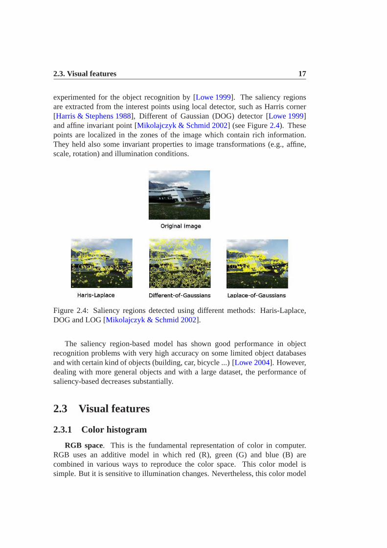
experimented for the object recognition by [Lowe 1999]. The saliency regionsare extracted from the interest points using local detector, such as Harris corner[Harris & Stephens 1988], Different of Gaussian (DOG) detector [Lowe 1999]and affine invariant point [Mikolajczyk & Schmid 2002] (see Figure2.4). Thesepoints are localized in the zones of the image which contain rich information.They held also some invariant properties to image transformations (e.g., affine,scale, rotation) and illumination conditions.
Figure 2.4: Saliency regions detected using different methods: Haris-Laplace,DOG and LOG [Mikolajczyk & Schmid 2002].
The saliency region-based model has shown good performancein objectrecognition problems with very high accuracy on some limited object databasesand with certain kind of objects (building, car, bicycle ...) [Lowe 2004]. However,dealing with more general objects and with a large dataset, the performance ofsaliency-based decreases substantially.
2.3 Visual features
2.3.1 Color histogram
RGB space. This is the fundamental representation of color in computer.RGB uses an additive model in which red (R), green (G) and blue (B)arecombined in various ways to reproduce the color space. This color model issimple. But it is sensitive to illumination changes. Nevertheless, this color model

18 Chapter 2. Image Indexing
in widely used in object recognition [Duffy & Crowley 2000] and in region-basedcolor retrieval systems [Carsonet al.1999].
HSV1 space. Artists sometimes prefer to use the HSV color model overalternative models such as RGB or CMYK2 space, because of its similarities tothe human color perception. HSV encapsulates more information about a color.Using this color model in object representation has shown its efficiency and itsinvariance to illumination changes.
L*a*b space. The CIE 1976 L*a*b color model, defined by the InternationalCommission on Illumination (Commission Internationale d’Eclairage, hence itsCIE initialism), is the most complete color model used conventionally to describeall the colors visible to the human eye. The three parametersin the modelrepresent the lightness of the colorL, its position between magenta and greena∗ and its position between yellow and blueb∗. This color description is veryinteresting in the sense that computer perceives the color close to the humanvision.
According to a color sapce, acolor histogramis then extracted for eachimage. Considering a three-dimensional color space(x, y, z), quantized on eachcomponent to a finite set of colors which correspond to the number of binsNx,Ny, Nz, the color of the imageI is the joint probability of the intensities ofthe three color channels. Leti ∈ [1, Nx], j ∈ [1, Ny] and k ∈ [1, Nz]. Then,h(i, j, k) = Card{p ∈ I | color(p) = (i, j, k)}. The color histogramH of imageI is then defined as the vectorH(I) = (..., h(i, j, k), ...).
In [Swain & Ballard 1991], an image is represented by its color histogram.Similar images are identified by matching theirs color histograms with thecolor histogram of the sample image. The matching is performed by his-togram intersection. Similar approach has been installed in the QBIC3 system[Flickneret al.1995]. This is also the first commercial image retrieval systemdeveloped by IBM. This method is robust to changes in the orientation, scale,partial occlusion and changes of the viewing position. However, the maindrawback of the method is its sensitivity to illumination conditions as it reliesonly on color information.
2.3.2 Edge histogram
Edge or shape in images constitutes an important feature to represent theimage content. Also, human eyes are sensitive to edge features for object recog-nition. Several algorithms have been applied for edge detection using different
1Hue Saturation Value2Cyan Magneta Yellow blacK3http://wwwqbic.almaden.ibm.com/
2.3. Visual features 19
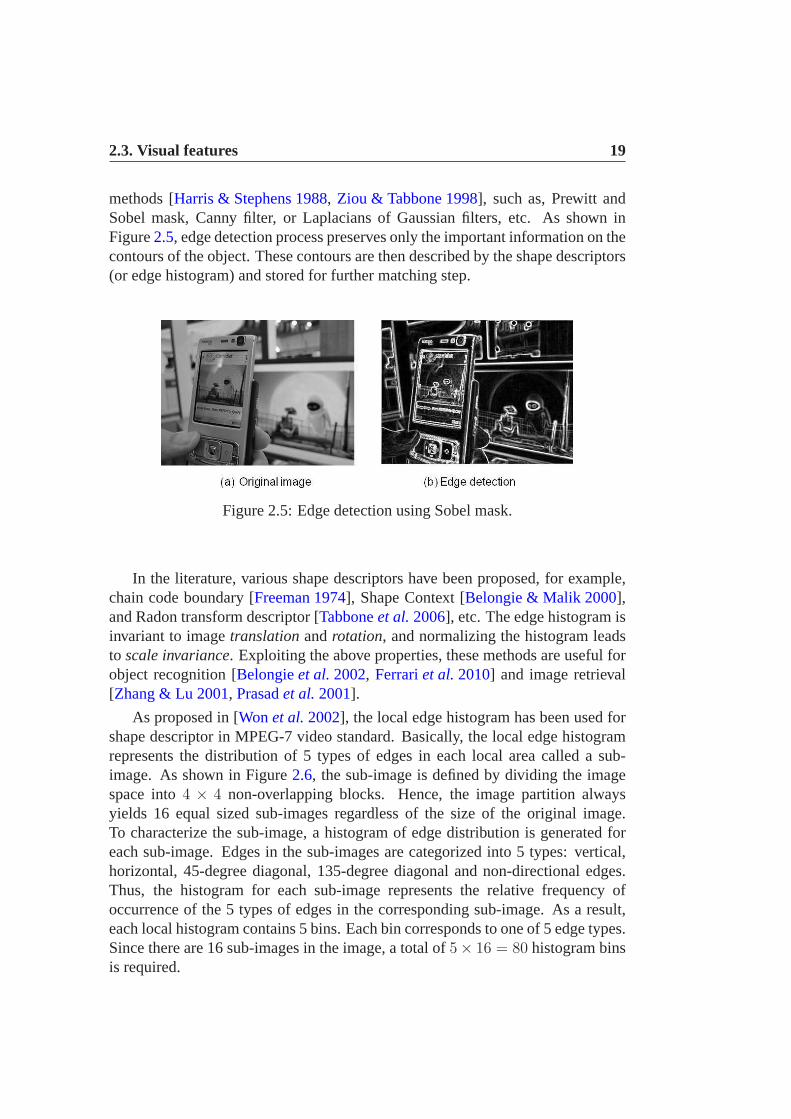
methods [Harris & Stephens 1988, Ziou & Tabbone 1998], such as, Prewitt andSobel mask, Canny filter, or Laplacians of Gaussian filters, etc. As shown inFigure2.5, edge detection process preserves only the important information on thecontours of the object. These contours are then described bythe shape descriptors(or edge histogram) and stored for further matching step.
Figure 2.5: Edge detection using Sobel mask.
In the literature, various shape descriptors have been proposed, for example,chain code boundary [Freeman 1974], Shape Context [Belongie & Malik 2000],and Radon transform descriptor [Tabboneet al.2006], etc. The edge histogram isinvariant to imagetranslationandrotation, and normalizing the histogram leadsto scale invariance. Exploiting the above properties, these methods are usefulforobject recognition [Belongieet al.2002, Ferrariet al.2010] and image retrieval[Zhang & Lu 2001, Prasadet al.2001].
As proposed in [Wonet al.2002], the local edge histogram has been used forshape descriptor in MPEG-7 video standard. Basically, the local edge histogramrepresents the distribution of 5 types of edges in each localarea called a sub-image. As shown in Figure2.6, the sub-image is defined by dividing the imagespace into4 × 4 non-overlapping blocks. Hence, the image partition alwaysyields 16 equal sized sub-images regardless of the size of the original image.To characterize the sub-image, a histogram of edge distribution is generated foreach sub-image. Edges in the sub-images are categorized into 5 types: vertical,horizontal, 45-degree diagonal, 135-degree diagonal and non-directional edges.Thus, the histogram for each sub-image represents the relative frequency ofoccurrence of the 5 types of edges in the corresponding sub-image. As a result,each local histogram contains 5 bins. Each bin corresponds to one of 5 edge types.Since there are 16 sub-images in the image, a total of5× 16 = 80 histogram binsis required.

20 Chapter 2. Image Indexing
Figure 2.6: Local edge histogram extraction for an image with MPEG-7 standard[Wonet al.2002].
2.3.3 Scale Invariant Feature Transform (SIFT)
SIFT extractor has been first introduced in [Lowe 1999]. These features be-long to the class of local image features. They are well adapted for characterizingsmall details. Moreover, they are invariant to imagescaling, imagetranslation,and partially invariant toillumination changesand affine for 3D projection.Thanks to these invariant properties, SIFTs are become moreand more popularvisual features for image and video retrieval [Lazebniket al.2006, Lowe 2004].
First, features are detected through a staged filtering approach that identifiesstable points in scale space. The result of this detection isa set of key localregions. Then, given a stable location, scale, and orientation for each key point,it is possible to describe the local image regions in a mannerinvariant to thesetransformations. Key locations are selected at maxima and minima of a differenceof Gaussians (DOG) applied in scale space. The input imageI is first convolvedwith the Gaussians function to give an imageA. This is then repeated a secondtime with a further incremental smoothing to give a new imageB. The differenceof Gaussians function is obtained by subtracting imageB fromA. This differenceof Gaussians is formally expressed as:
D(x, y, σ) = (G(x, y, kσ)−G(x, y, σ)) ∗ I(x, y)

2.3. Visual features 21
with k corresponding to the strength of smoothing and
G(x, y, σ) =1
2πσ2exp−(x2 + y2)/2σ2
Figure 2.7: Construction of the scale space pyramid.
This differentiation process is repeated with different values ofk. A change ofscale consists of sampling the smoothed images by using a bilinear interpolation.The combination of scaling and smoothing produces a scale space pyramid. Anoverview of the scale/space construction is shown in Figure2.7.
Minima and extrema detection ofD(x, y, σ) uses this scale space pyramid andis achieved by comparing each sample point to its neighbors in the current imageand 9 neighbors in the scale above and below. It is selected only if it is larger thanall its neighbors or smaller than all its neighbors. The result of this selection isa set of key-points which are assigned a location, a scale andan orientation (i.e.obtained by gradient orientation computation).
The last step consists of assigning a numerical vector to each keypoint. The16 × 16 neighborhood around the key location is divided into 16 sub-regions.Each sub-region is used to compute an orientation histogram. Each bin of a givenhistogram corresponds to the sum of the gradient magnitude of the pixels in thesub-region. The final numerical vector is of dimension 128.

22 Chapter 2. Image Indexing
2.4 Indexing Models
For the past two decades, several indexing models have been proposed in theliterature. The objective of image indexing is to store images effectively in thedatabase and to retrieve similar images from a database for agiven query image.Image can be indexed using directly the extracted visual features (such as, color,texture and shape) with the vector representation. Recently, the bag-of-visual-features (or bag-of-words) inspired from textual indexingdraw more attention forits simplicity and effectiveness on storing visual content. This section is dedicatedto the presentation some of these indexing methods.
2.4.1 Vector space model
This is a the simplest model in CBIR system. Images are represented by theirfeature vectors. These vectors have the same dimension and normalized with thesame scale (usually between 0 and 1). Thetf.idf4 normalization is often usedin information retrieval and text mining. This technique has also adopted widelyin CBIR systems. This weighting scheme comes from a statistical measure toevaluate how important a word is to a document in a collectionor corpus. Theimportance increases proportionally to the number of timesa word appears in thedocument but is offset by the frequency of the word in the corpus.
Given 2 feature vectorsV q andV d extracted from image queryq and imagedocumentd, the visual similarity is computed using two different measurementfunctions:Euclidian distanceor cosines similarity.
Euclidean distanceThe Euclidean distance is probably the most common approachto compare
directly two images. GivenV q andV d are two vectors in Euclideann-space, thenthe metric distance of two imagesp andq is given by:
d(V q, V d) = ||V q − V d|| =√
||V q||2 + ||V d||2 − 2V q • V d
The smaller distance indicates the closer of two images are.This value reflectsthe visual similarity of the two images.
Cosine similarityIn contrast to the distance measure, two vectorsV q andV d can be considered
to be similar if the angle between their vectors is small. To compute the cosinesimilarity, the normalized scalar product is used to measure the angle between twovectors :
4term frequency, inverse document frequency

2.4. Indexing Models 23
cos(θ) =V q • V d
||V q||||V d||
In information retrieval, the cosine similarity of two documents will rangefrom 0 to 1. A similarity of 0 implies that documents are identical, and a similarityof 1 implies they are unrelated.
2.4.2 Bag-of-words model
A simple approach to indexing images is to treat them as a collectionof regions, describing only their statistical distribution of typical regions andignoring their spatial structure. Similar models have beensuccessfully used inthe text community for analyzing documents and are known as “bag-of-words”(BoW) models, since each document is represented by a distribution over fixedvocabulary.
Figure 2.8: Image is represented by a collection of visual words[Fei-Fei & Perona 2005].
The construction of this model is based on four main steps:
1. Image segmentation consists of dividing image into smaller parts. Asintroduced in previous section2.2, we can consider different types of imagesegmentation such as pixels, regions or interested points.
2. Feature extraction step consists of representing each image region by a setof visual features as detailed in section2.3. Each feature is quantized andnormalized by a vector with fixed size.

24 Chapter 2. Image Indexing
3. Visual vocabulary construction step converts feature vector representedimage regions to “visual words” or “ visual concepts” (analogy to wordsin text documents), which also produces a “visual dictionary” (analogy toa word dictionary). A visual word can be considered as a representative ofseveral similar image regions. One simple method is performing k-meansclustering over all the vectors. Visual words are then defined as the centersof the clusters. The number of the clustersk is the vocabulary size.
4. Each image region is mapped to a certain visual word through a clusteringprocess and the image can be represented by the quantized vector of thevisual vocabulary.
In step 3, k-means clusteringis performed on a set of visual features toconstruct the visual words. We present in the following a brief description ofthis algorithm.
K-means clusteringis a popular technique for automatic data partitioning inmachine learning. The goal is to findk centroid vectorsµ1, ..., µk for representingeach cluster. The basic idea of this interactive algorithm is to assign each featurevectorx to the cluster such that the sum of squared errorErr is minimum
Err =k
∑
i=1
Nj∑
j=1
||xij − µi||2
wherexij is thejth point in theith cluster,µi is the mean vector ofith cluster andNj is the number of pattern in thejth cluster. In general, the k-means clusteringalgorithm works as follows:
1. Select an initial mean vector for each ofk clusters.
2. Partition data intok clusters by assigning each patternxn to its closestcluster centroidµi.
3. Compute new mean clustersµ1, ..., µk as the centroids ofk clusters.
4. Repeat step 2 and 3 until the cluster criterion is reached.
The initial mean vectors can be chosen randomly fromk seed points in the datain the first step. The partitioning is then performed from these initial points. Inthe second step, to measure the distance between two patterns, different metricdistances (e.g., Hamming distance, Euclidean distance, etc.) can be applied.Usually, the Euclidean distance is good enough to measure the distance betweentwo vectors in the same feature space. In step 3, the centroidµi for each cluster isre-estimated by computing the mean of cluster members. The number of iterations

2.4. Indexing Models 25
can be used in the last step as a convergence criterion. The k-means algorithm hasa time complexity ofO(nk) for each iteration. Only one parameter which needsto be fixed is the number of clustersk.
As demonstrated in [Fei-Fei & Perona 2005], this model is simple but yeteffective for image indexing. However, the lack of spatial relation and locationinformation of visual words are the mains drawbacks of this model. Usingthis representation, methods based on latent semantics extraction, such as latentsemantic analysis [Monay & Gatica-Perez 2003, Phamet al.2007] and proba-bilistic latent semantic analysis [Monay & Gatica-Perez 2004] and latent Dirichletallocation [Blei et al.2003], are able to extract coherent topics within documentcollections in an unsupervised manner. Other approaches are based on discrim-inative methods with annotated or slightly annotated examples, such as supportvector machine [Vapnik 1995] and nearest neighbors [Shakhnarovichet al.2005].In the next chapter, we will review of some of these learning methods.
2.4.3 Latent Semantic Indexing
Latent Semantic Analysis (LSA) was first introduced as a textretrievaltechnique [Deerwesteret al.1990] and motivated by problems in textual domain.A fundamental problem was that users wanted to retrieve documents on the basisof their conceptual meanings, and individual terms providelittle reliability aboutthe conceptual meanings of a document. This issue has two aspects:synonymyandpolysemy. Synonymydescribes the fact that different terms can be used to referto the same concept.Polysemydescribes the fact that the same term can refer todifferent concepts depending on the context of appearance of the term. LSA is saidto overcome these deficiencies because of the way it associates meaning to wordsand groups of words according to the mutual constraints embedded in the contextwhich they appear. In addition, this technique is similar with the popular techniquefor dimension reduction, i.e., principal component analysis [Gorbanet al.2007],in data mining. It helps to analyze the document-by-term matrix by mapping theoriginal matrix into lower dimensional space. Hence, the computational cost isalso contracted.
Considering each image as a document, a coocurrence matrix ofdocument-by-termM , a concatenation of vectors extracted from all document with model BoWis built. Following the analogy between textual document and image document,given a coocurrencce document-by-term matrixM rankr, M is decomposed into3 matrices using Singular Value Decomposition (SVD) as follows:
M = UΣV t

26 Chapter 2. Image Indexing
where
U : is the matrix of eigenvectors derived fromMM t
V t : is the matrix of eigenvectors derived fromM tMΣ : is anr × r diagonal matrix of singular valuesσ.σ : are the positive square roots of the eigen-values ofMM t orM tM
This transformation divides matrixM into two parts. One is related to thedocuments and the second related to the terms. By selecting only k largest valuesfrom matrixΣ and keep the corresponding column inU andV , the reduced matrixMk is given by:
Mk = UkΣkVtk
wherek < r is the dimensionality of the concept space. Indeed, the choice ofparameterk is not obvious and depends on each data collection. It shouldbe largeenough to allow fitting the characteristics of the data. On the other hand, it must besmall enough to filter out the non-relevant representation details. To rank a givendocument, the query vectorq is then projected into the latent space to obtain apseudo-vector, qk = q ∗ Uk, with dimension reduced.
Recently, LSA has been applied for scene modeling [Quelhaset al.2007],image annotation [Monay & Gatica-Perez 2003], improving multimedia docu-ments retrieval [Phamet al.2007, Monay & Gatica-Perez 2007] and indexingof video shots [Souvannavonget al.2004]. In [Monay & Gatica-Perez 2003],Monay and Gatica-Perez have demonstrated that the LSA outperformed the pLSAof more than 10% on annotation and retrieval task based on CORELcollection.Unfortunately, LSA lacks a clear probabilistic interpretation comparing to othergenerative models such as probabilistic latent semantic analysis.
2.5 Conclusion
In this chapter, we have introduced the basic steps in constructing an imageindexing system. Images are decomposed into image regions and then visualfeatures are extracted for indexing. Each type of image representation and visualfeatures described in this chapter represents apoint of viewof an image. It canbe combined in different ways for effective use of the retrieval process. Most ofthe current approach are based on the early fusion method which relies on thevector combination for the image indexing. Next chapter will discuss on how themachine learning methods will be used for image modeling andretrieval.

Chapter 3
Image Modeling and Learning
3.1 Introduction
In the previous chapter, we presented the popular techniques that have beenused for image indexing. An image is decomposed in several ways (from pixelsto image regions) for faciliting visual feature extraction. From the extractedimage regions, several visual features have been considered, such as colorhistogram, edge histogram and SIFT. The early image indexing model with vectorrepresentation of the bag-of-word model were also described.
In this chapter, we study some machine learning methods usedfor imagemodeling in the literature. Following the paradigm of Marr [Marr 1982], thesesteps correspond to themapping layerand theinterpretation layer.
First, we will give an overview on the state-of-the-art of the two majorbranches of learning models: generative approaches and discriminative ap-proaches. The important theory of language modeling for text retrieval willalso be presented. Structured image representation has been introduced earlyin the computer vision [Ballard & Brown 1982] and then applied for imagemodeling [Boutellet al.2007, Aksoy 2006, Ounis & Pasca 1998]. The main issueof structured image representation is the matching methodsbased on graph.Classical approaches on sub-graph isomorphism [Ullmann 1976] are costly andineffective, with its computational complexity cast as NP-complete problem.Modern approaches, such as kernel based and 2D HMMs, expressthe graphmatching by classifying ofpathsandwalkswith SVM kernel or as the stochasticprocess of Markov’s model.
Currently, the generative model, such as language modeling [Wu et al.2007,Maisonnasseet al.2009] are extensively studied for the generative matchingprocess. We will also give a discussion on this active topic.From these pivots,we propose an approach that takes the advantage of both graph-based image
27

28 Chapter 3. Image Modeling and Learning
representation and the generative matching process to construct the visual graphmodeling. With this approach, we hope to add a new layer to reduce the semanticgap discussed in the literature.
Section3.2 presents two methods of generative approaches:Naive Bayesand Probabilistic Latent Semantic Analysis(pLSA). The language modelingapproach from information retrieval will be detailed in section 3.3. Two othersmethods of discriminative approaches, namelyNearest Neighborsand SupportVector Machine(SVM), will be described in section3.4. Then, section3.5concentrates on the structured representation of the imagewith the graph model,such asConceptual Graph(CG) andAttributed Relation Graph(ARG). We willalso introduce some graph matching techniques developed inthe literature, forexmple, (sub)graph isomorphism, kernel basedmethods andtwo dimensionalmultiresolution hidden Markov models(2D MHMMs). Finally, based on thereview of the state-of the art, we propose our graph-based image representationapproach and the matching method inspired from the languagemodeling insection3.6.
3.2 Generative approaches
3.2.1 Naive Bayes
Naive Bayes is a simple probabilistic classifier based on Bayes’s theorem. Ithas a strong condition on the class where each feature is estimated independently.In general, the probability model for a classifier is a conditional model over adependent class variableC with a small number of classes, conditional on severalfeature variablesF1 throughFn. Using Bayes’ theorem, we write:
p(C|F1, . . . , Fn) =p(C) p(F1, . . . , Fn|C)
p(F1, . . . , Fn)
Asume that each featureFi is conditionally independent of every other featureFj for j 6= i. This leads to
p(C|F1, . . . , Fn) =1
Zp(C)
n∏
i=1
p(Fi|C)
where Z is a scaling factor dependent only onF1, . . . , Fn. Finally, thecorresponding classifier is defined as follows:
classify(f1, . . . , fn) = argmaxc
p(C = c)n∏
i=1
p(Fi = fi|C = c)

3.2. Generative approaches 29
This is known as themaximum a posteriori(MAP) decision rule. This modelis popular in text analysis and retrieval, for example: SPAMemail detectionand document classification. Despite the strong independence assumption,the naive Bayes classifier has successfuly been used for text classification[Iwayama & Tokunaga 1995] and scene categorization [Fei-Fei & Perona 2005].A hierarchical version of this classifier has been developedby David Blei[Blei 2004] and been applied to both text and image data.
3.2.2 Probabilistic Latent Semantic Analysis (pLSA)
pLSA is a statistical technique for the analysis of co-occurrence data whichevolved from Latent Semantic Analysis (LSA) [Deerwesteret al.1990], proposedinitally by Jan Puzicha and Thomas Hofmann [Hofmann & Puzicha 1998]. Incontrast to standard latent semantic analysis which stems from linear algebra anddownsizes the occurrence tables (usually via a singular value decomposition),probabilistic latent semantic analysis is based on a mixture decomposition derivedfrom a latent class model. This results in a more principled approach which has asolid foundation in statistics.
Considering observations in the form of co-occurrences (w,d) of words anddocuments, pLSA models the probability of each co-occurrence as a mixture ofconditionally independent multinomial distributions:
P (d, w) = P (d)P (w|d)
andP (w|d) =
∑
z∈Z
P (w|z)P (z|d)
wherez is the latent variable or hidden topic extracted from a set oftopicsZ ofimage documents.
The standard procedure for maximum likelihood estimation in latent variablemodels is the Expectation Maximization (EM) algorithm. EM alternates twosteps: (i) an expectation (E) step where posterior probabilities are computedfor the latent variablesz, based on the current estimates of the parameters, (ii)an maximization (M) step, where parameters are updated for given posteriorprobabilities computed in the previous (E) step. However itis reported that thepLSA has severe over fitting problems. The number of parameters grows linearlywith the number of documents.
pLSA methods are very popular for text indexing and retrieval [Hofmann 1999]thanks to its solid probabilistic foundation. This technique was also adopted by theCBIR community [Lienhartet al.2009, Lu et al.2010] and for image annotation

30 Chapter 3. Image Modeling and Learning
[Monay & Gatica-Perez 2004, Monay & Gatica-Perez 2007]. However, estimat-ing parameter using E-M step is a very costly process which isa main limitationof this method.
The following section present the principal theory of the language modelingwhich is a key model of this thesis. We also give a short surveyof the applicationof the language modeling for image classification.
3.3 Language modeling approach
Language modeling (LM) was first introduced in linguistic technologies,such as speech recognition, machine translation and handwriting recognition[Rosenfeld 2000]. Ponte and Croft [Ponte & Croft 1998] applied the probabilisticlanguage modeling in text retrieval and obtained good retrieval accuracies onTREC collections. Similar to the previous generative models, the documentsare ranked by the probability that the query could be generated by the documentmodels. The query likelihoodP (D|Q) is computed by using Bayes’ Rule:
P (D|Q) =P (Q|D)P (D)
P (Q)
We can ignore the normalizing constantP (Q), the former fomular leads to
P (D|Q) ∝ P (Q|D)P (D)
whereP (D) is the prior probability of a document, which is assumed to beuniform in most cases. Therefore, the documents are ranked equivalent to thejoint probability of P (Q|D). This is known asmaximum a posteriori(MAP)technique which selects the most probable documentD to maximize the posteriordistribution ofP (D|Q).
3.3.1 Unigram model
The simplest form of language modeling is the unigram model where eachword is estimated independently of each other. To estimate the probability of aword in the documents, one has to make an assumption about thedistributionof the data. In the literature, a number of different assumptions have beenmade about the distribution of words in document. Themultiple-Bernoullidistribution captures a set of binary events that some word appears in thedocument or not. Therefore, the document can be representedby a binaryvector of 0 and 1 to indicate the occurrence of a corresponding word. Themultiple-Bernoulli distribution is well suited for representing the presence of

3.3. Language modeling approach 31
query word and insisting on the explicit negation of words (e.g. apple but notorange). In [Ponte & Croft 1998], the original language modeling for IR wasbased on multiple-Bernoulli distribution assumption. Givenmultiple-Bernoulliassumption, the query likelihood gives:
P (Q|D) =∏
w∈q1,...,qk
P (w|D)∏
w/∈q1,...,qk
(1− P (w|D))
wherew is a word in documentD. This assumption is simple and straightforward.However, one limitation of this distribution is that the latter does not deal withthe importance (i.e. the frequency of occurrence) of word inthe document. Forthis reason, most of the current modeling assumptions in IR are now centered onmultinomial distributions.
Themultinomial distributiontakes into account the number of occurrences ofwords (e.g.apple appears 3 times andorange appears 2 times in the document).This suggests that the document can be encoded by a vector with the number oftimes each word appears in the document. Assuming a multinomial distributionover words, we can compute the query likelihood using unigram model. The querylikelihood is then calculated using unigram model for the document as follows
P (Q|D) =m∏
i=1
P (qi|D)
whereqi is a query word andm is the number of word in the query. To calculatethis score, probability of query wordqi is estimated from the document
P (qi|D) =#(qi, D)
#(∗, D)
where#(qi, D) is the number of times wordqi occurs in documentD, and#(∗, D) is the total number of words inD. For a multinomial distribution,maximum likelihood refers to the estimate that makes the observed value of(qi, D) most likely.
One problem with this estimate is that if any of the query words is missingfrom the document, the score of query likelihood will be zero. This is notappropriate for long query which may have frequently “missing words”. Inthis case, it should not yield a zero score. To overcome this problem, onesolution is to give a small probability for missing words which will enable thedocument to receive a non-zero score. In fact, this small probability is takenfrom the prior information of the document collection. Thissolution is known assmoothingtechniques ordiscountingtechniques. We will address this problem inthe following section.

32 Chapter 3. Image Modeling and Learning
3.3.2 Smoothing techniques
Smoothingis a popular technique used in information retrieval to avoid theprobability estimation problem and to overcome the data sparity of collection.Typically, we do not have large amount of data to use for the model estimation.The general idea is to lower (ordiscount) the probability estimates for words thatare observed in the collection and apply that probability tothe unseen words inthe document.
A simple method is known as theJelinek-Mercer smoothing[Jelineket al.1991]involving the linear interpolation of the LM from the whole collectionC. GivenP (qi|C) is the probability of query wordqi estimated from the collectionC andλis the smoothing coefficient assigned to the unseen word, theestimate probabilityof query from document model becomes:
P (qi|D) = (1− λ)P (qi|D) + λP (qi|C)
The collection model for estimating the query wordqi is P (qi|C) = #(qi,C)#(∗,C)
,where#(qi, C) is the number of time query wordqi appears in collectionC and#(∗, C) is the total number of words in the whole collection. Substituting thisprobability in the query likelihood gives:
P (Q|D) =m∏
i=1
((1− λ)#(qi, D)
#(∗, D)+ λ
#(qi, C)
#(∗, C))
The smoothed probabilities of document model still verify∑n
i=1 P (qi|D) = 1.This smoothing method is simple and straightforward. However, it is moresensitive toλ for the long queries than the short queries. The reason is longqueries need more smoothing and less emphasis on the weighting of words.
Another smoothing technique calledDirichlet smoothingtakes into accountthe document length. The parameterλ becomes
λ =µ
#(∗, D) + µ
whereµ is a parameter whose value is set empirically. The probability estimationof query wordqi leads to:
P (qi|D) =#(qi, D) + µ#(qi,C)
#(∗,C)
#(∗, D) + µ
Similar to Jelinek-Mercer smoothing, parameterµ gives more importance to therelative weighting of words for small values. On the other hand, this parameteralso takes into account the prior knowledge of long documents. Therefore,Dirichlet smoothing is generally more effective than Jelinek-Mercer, especiallyfor short queries that are common in the current retrieval engines.

3.3. Language modeling approach 33
3.3.3 n-gram model
The extension of unigram to the higher order language model is known asn-gram language model. In n-gram model, the probability of estimate for wordqi depends on then − 1 preceding words. Hence, it is able to model not onlyoccurrences of independent words like unigram model, but also the fact thatseveral words often occur together. This effect is interesting in text retrievalbecause the combination of words can have different meaningcomparing to thesame words used independently (e.g. “swimming pool” or “Wall Street Journal”).The n-gram models will help to capture efficiently this cooccurrence information.
The query likelihood probabilityP (Q|D) of observing the queryQ =(q1, . . . , qm) is approximated as:
P (Q|D) =m∏
i=1
P (qi|q1, . . . , qi−1, D)
Following the assumption that the probability of observingthe wordqi in thecontext history of the precedingi−1words can be approximated by the probabilityof observing it in the precedingn− 1 words (nth order Markov property):
P (Q|D) ≈m∏
i=1
P (qi|qi−(n−1), . . . , qi−1, D)
The conditional probability can be calculated from n-gram frequency counts:
P (qi|qi−(n−1), . . . , qi−1, D) =#(qi−(n−1), . . . , qi−1, qi, D)
#(qi−(n−1), . . . , qi−1, D)
Thebigramandtrigram language models correspond to language models withn = 2 andn = 3, respectively. Similar to the unigram model, n-gram modelsalsosuffer from the problem of probability estimation. Hence, smoothing technique isalso required to overcome this problem. The occurrence of bigrams or trigramsin the document to some extent are rather rare comparing to the unigram. Moredetails on the smoothing techniques with n-gram models (suchas Good-Turingdiscounting, Witten-Bell discounting, etc.) can be found in[Jelinek 1998].
Although the standard language models have yielded good performance intext retrieval, several works have investigated further the use of more advancedrepresentations of words within this framework. Gao [Gaoet al.2004] and Lee[Leeet al.2006] proposed to incorporate syntactic dependencies structure in thelanguage model. These models defined alinkage over query terms which isrelated automatically through a parse in document. However, there is a certainambiguity in the way the linkage is used in this model. As pointed out in
34 Chapter 3. Image Modeling and Learning
[Maisonnasseet al.2008], this model is theoretically inconsistent to representgraphical structure in the language modeling approach to IR.
In contrast, Maisonnasse [Maisonnasseet al.2008] relied on the notion ofgraph model to integrate the relation between concepts in the language modeling.Concepts and semantic relations are extracted from knowledge source suchas UMLS1 for medical concepts. The authors also proved that the use ofconcept and the semantic relation on graph achieved a substantial improvementover purely term-based language models (such as unigram andn-gram model).Based on this work, we will extend the graph-based language modeling in[Maisonnasseet al.2009] to take into account of the visual elements and theirspatial relations in a unified framework for image retrieval.
3.3.4 Language modeling for image classification
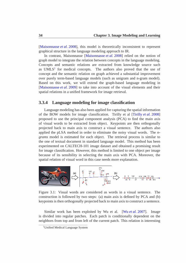
Language modeling has also been applied for capturing the spatial informationof the BOW models for image classification. Tirilly et al [Tirilly et al.2008]proposed to use the principal component analysis (PCA) to findthe main axisof visual words to be extracted from object. Keypoints are then orthogonallyprojected back to main axis to construct a visual sentence. The authors alsoapplied the pLSA method in order to eliminate the noisy visualwords. Then-gramsmodel is estimated for each object. The retrieval process issimilar tothe one of textual document in standard language model. Thismethod has beenexperimented on CALTECH-101 image dataset and obtained a promising resultfor image classification. However, this method is limited toone object per imagebecause of its sensibility in selecting the main axis with PCA. Moreover, thespatial relation of visual word in this case needs more explanation.
Figure 3.1: Visual words are considered as words in a visual sentence. Theconstruction is followed by two steps: (a) main axis is definedby PCA and (b)keypoints is then orthogonally projected back to main axis to construct a sentence.
Similar work has been exploited by Wu et al. [Wu et al.2007]. Imageis divided into regular patches. Each patch is conditionally dependent on theneighbors from top and from left of the current patch. This relation is interesting
1Unified Medical Language System

3.4. Discriminative approaches 35
in the sense that it captures the most basic relation in imagewhich is analogous tothe relation of words in a document. Three language models (unigram, bigramsandtrigrams) constructed follow strictly the theoretical language model. For thisreason, the model is hard to extend for more complicated relation between visualwords.
3.4 Discriminative approaches
Unlike the generative approach, which is based on the probabilistic principle,the discriminative approach treats each document as a pointin some geometricspace. There is no explicit assumption on the data itself. The principle is ”letdata speaks”, which means the model will find the decision boundary to separateautomatically the annotated samples for the training set and the generalizes to thetest sets.
3.4.1 Nearest neighbors approach
Nearest neighbors ( or k-NN) is a well-known method for objectclassificationin pattern recognition [Shakhnarovichet al.2005]. The main principle is to matcha test sample to the given training samples. An object is classified by amajorityvoteof its neighbors, with the object being assigned to the classmost commonamongst itsk nearest neighbors (k is usually small). Ifk = 1, then the object issimply assigned to the class of its nearest neighbors.
A drawback to the basicmajority votingclassification is that classes with themore frequent examples tend to dominate the prediction of the new sample, asthey tend to come up in thek nearest neighbors when the neighbors are computeddue to their large number. One way to overcome this problem isto weight theclassification taking into account the distance from the test point to each of itsknearest neighbors.
3.4.2 Support Vector Machines (SVM)
SVM is the most popular discriminative algorithm for classification. In-troduced by Vapnik in 1995 [Vapnik 1995], SVM has since become one ofthe most developed classification algorithms, especially for pattern recognition.The strength of SVM is twofold: in terms of maximizing the margins aroundthe separator hyperplane it provides good capacity of generalization and theapplication of kernel allow it to solve the problem of non linear separable space.
Figure3.2 illustrates the operation of SVM for classification in a linear spaceof two dimensions.H denotes the hyperplane which separated white dots and

36 Chapter 3. Image Modeling and Learning
Figure 3.2: SVM is to search for the maximal margin that separates the trainingset in a linear space of two dimensions. In this case, the training set is separable.
black dots.Let L be the set of training points, where each pointxi has m attributes (i.e.
vector of dimensionality m) and belongs to one of two classesyi ∈ {−1,+1}.Here we assume the data are linearly separable, meaning thatwe can draw ahyperplane on the spaceL. This hyperplane can be described byw · xi − b = 0where:
• w is normal to the hyperplane.
• b||w||
is the perpendicular distance from the hyperplane to the origin.
Then the goal is to minimize the value||w|| of the margin such that the objec-tive function is maximum. Minimizing||w|| is equivalent to minimizing1
2||w||2
and the use of this term makes it possible to perform Quadratic Programming (QP)optimization . Therefore, we need to find:
min1
2||w||2
subject toyi(w · xi − b)− 1 ≥ 0, ∀i
In order to cater for the constraints in this minimization, we need to allocatethem Lagrange multipliersαi. It can be shown that this is equivalent to theminimization of:
minw,b,α
{12‖w‖2 −
n∑
i=1
αi[yi(w · xi − b)− 1]}

3.4. Discriminative approaches 37
with αi ≥ 0 and under constraint∑n
i=1 αiyi = 0. This can be achieved bythe use of standard QP methods. Once we obtained the solutionvectorα0 of theminimization problem, the optimal hyperplane(w0, b0) will be defined by:
w0 =i=1∑
n
α0i yixi
Points corresponding to solutionα0 are calledsupport vectors. The decisionrule for new pointx is then defined by functionf(x) :
f(x) =i=1∑
n
α0i yixi · x− b0
The sign of f(x) is usually used as binary decision. If it is positive (respectivelynegative), the test pointx belongs to the class of training set with label +1(respectively -1 ).
This approach can also be applied to non linear separable data with somemapping functionsΦ(x) of the input feature vectors into a high-dimensionalfeature space (see Figure3.3). This technique is calledkernel trick. The kerneltrick is useful because there are many classification/regression problems that arenot linearly separable/repressible in the space of the input features.
Figure 3.3: Example of Radial Basis Function (RBF) kernel mapping data fromnon linear separable space to high-dimensional separable space.
The kernel is expressed by the dot product of mapping function which givesK(xi, xj) = Φ(xi) · Φ(xj). Once kernelK satisfying the Mercer condition2, theoutput function then becomes:
2symmetric and positive matrix

38 Chapter 3. Image Modeling and Learning
f(x) =i=1∑
n
α0i yiK(xi, xj)− b0
There are different types of kernel, such as polynomial kernel, sigmoid kerneland radial basis kernel. But the most commonly used in patternrecognition isradial basis function (RBF) kernel, defined as follows:
K(x, y) = e−||x−y||2
2σ2
where||.|| isL2-norm of two vectorsx andy andσ is the smoothing parameter ofGaussian function. In general, this parameter is estimatedby cross validation onthe data from training set.
3.5 Structured representation approaches
Most of the learning methods described previously are basedon the bag-of-words models, thus taking into account only the visual information in theform of vector representation. The spatial information among visual featuresis disregarded. Although this representation is simplistic, the result provedsurprisingly promising. Some efforts have been attempted to go beyond thisprimitive and flat representation ofbag-of-wordsmodel by adding visual featurecorrelation information [Lazebniket al.2006]. However, none of them reallyconsidered the spatial relationship between image regions. This section aimsat introducing some state-of-the-art in graph representation, which is popular ininterpreting structural information, and learning methods for image matching.
3.5.1 Graph for image modeling
Graph is one of the most formal representations of structural information incomputer vision [Marr 1982]. It is a natural way to encode the relation betweenobjects. A famous example of graph is presented in a book of computer vision byBallard and Brown [Ballard & Brown 1982]. The idea is to represent structuralinformation of face by a set oftemplatesconnected bysprings. Nodes representthe instances of face, for example: eyes, nose, mouth, hair,etc. Edges indicatethe structural relations between these instances. This is one of the most primitiveforms for representing a graph where nodes and edges indicate the object instancesand links between them respectively. However, suffering from the combinatorialexplosion issue in graph matching, the classical graph representation has not beenused widely for image modeling in image retrieval.

3.5. Structured representation approaches 39
Figure 3.4: An example of graph representation for human face[Ballard & Brown 1982].
For real image representation, nodes and edges are associated with a set oflabels. Harchaoui and Bach [Harchaoui & Bach 2007] presented their imagesby a planar graph where each node corresponds to a segmented region andedge corresponds to a link between two connected regions. One interestingconstraint is all the regions are non-overlapping, thus creating a planar graph.This representation is simple and intuitive, although the inferring process on thesegraph representations is challenging problem. A method to reduce the complexityof this graph, combining with kernel methods, will be introduced in the nextsection.
Figure 3.5: An example of planar graph extracted from an image. Segmentedregions are obtained by using the median RGB color. [Harchaoui & Bach 2007]
Conceptual graphs have been first introduced in the early 80’sto modelknowledge representation. In [Sowa 1984], Sowa presented the theoreticalformalism for conceptual graph which was consistent and flexible for knowledgerepresentation. This framework can capture semantic representation of data and itoffers some useful extension which is likely applicable forother knowledge-basedrepresentation such as semantic web or data mining.

40 Chapter 3. Image Modeling and Learning
Conceptual graphs are widely considered as a chanel to express the represen-tation of image content. Figure3.6 illustrates an example of conceptual graphextracted from a landscape scene. Nodes represent the visual entities composedof image and directed arcs indicate semantic relations between these nodes.Conceptual graphs have also been used for scene recognition [Boutellet al.2007]and for image retrieval [Ounis & Pasca 1998]. With the integrating of semanticrelations, conceptual graph allows to describe better the nature of image contents[Mulhemet al.2001, Boutellet al.2007].
Figure 3.6: Example of a conceptual graph extracted from natural scene: (a)original image, (b) manual segmented image, (c) conceptualgraph representation.
An extension of conceptual graph is attributed relational graph (ARG) wherenodes and relations are associated with some attributes represented by theirweights or their probability of contribution [Mulhemet al.2001]. Attributedrelational graphs have been widely used for image modeling [Aksoy 2006] andnear duplicated image detection [Zhang & Chang 2004]. One advantage of theARG is that it can be used to represent complex visual content in the veryflexible way. Node and link can be easily embedded with some properties, suchas weight, numeric or symbolic value or even with the estimated probabilities[Boutellet al.2007].
Figure 3.7 presents some of the attributes used for representing the spatialrelations between two image regions. With this representation, the spatialrelationships among regions are expressed with more details, for instance,symbolic relationsnear andfar, or relative distanced = 0.35 and relative anglea = π/3, etc. However, matching the attributes relation graphs requires a specialtechnique to adapt to some specific problems. We will presentin the next sectionsome matching algorithms for graph-based image presentation in the literature.
3.5.2 Matching methods on graphs
After defining a graph based on their representation, several matching processon graph have been summarized in [Ballard & Brown 1982]:

3.5. Structured representation approaches 41
Figure 3.7: Spatial relationships of region pairs:disjoined, bordering, invaded by,surrounded by, near, far, right, left, aboveandbelow[Aksoy 2006].
• Exact matching: graph isomorphism, subgraph isomorphism (see Figure3.8).
• Inexact matching: partial graph matching, attributed graph matching.
Figure 3.8: Exact graph matching: graph (a) has an isomorphism with graph (b)and has various subgraph isomorphism with graph(c) [Ballard & Brown 1982].
Graph matching is related to string theory [Gusfield 1997] (such as substringmatching and edit distances) which is complex and costly operation. Therefore,exact graph matching is a combinatorial problem and subgraph matching is a NP-complete problem [Ullmann 1976]. The deterministic algorithms run (in the worstcase) in time exponential with the size of the constructed graphs. Several works[Shokoufandehet al.2002, Cordellaet al.1998] have been involved to solve thegraph matching problem in polynomial time. However, these algorithms are verycomplicated in implementation. Soft graph matching have toadapt to the natureof the application [Shokoufandehet al.2002]. Hence, most of works so far havefocused on finding the approximate solutions to this problem.

42 Chapter 3. Image Modeling and Learning
To compute the similarity of conceptual graph, several matching methods havebeen proposed, such as: partial subgraph isomorphism [Ullmann 1976], error cor-rection graph matching [Mulhemet al.2001], median graphs [Jianget al.2001].As demonstrated in [Ballard & Brown 1982] the matching algorithms of con-ceptual graph may also suffer from the computational problems as they usedbasically the morphological matching algorithm. In [Ounis & Pasca 1998],authors proposed to use inverted file for indexing and retrieval of conceptualgraph extracted manually from images to accelerate the performance of graphmatching. Recently, Kostin et al. [Kostinet al.2005] have applied probabilisticrelaxation matching technique for object recognition. Despite the fact that graphmatching is still a challenging problem, graphs are very promising for structuralimage representation.
Recently, applications of kernel-based methods are widely used for semi-supervised learning [Shawe-Taylor & Cristianini 2004, Bachet al.2004] and incomputer vision [Suardet al.2005]. In [Harchaoui & Bach 2007], authors pro-posed a method to combine graph planarity with a kernel of a SVM classifierfor image classification. Image is represented as a planar graph in which labelednodes correspond to segmented regions and edges are the neighboring regions.Image graphs are fixed with the same number of segments. Figure 3.9 shows asimple planar graph constructed for an image. Each color represents a differentlabel and each edge encodes a spatial relation.
Figure 3.9: Enumeration of paths and walks from a simple graph. Walk is a finitesequence of neighboring vertices, while apath is a walk such that all its verticesare distinct (inside the rectangle) [Harchaoui & Bach 2007].
Kernel graph is an efficient way to solve the graph matching problem bysoft-matching tree-walks in order toobtain kernels computable in polynomial

3.5. Structured representation approaches 43
time [Harchaoui & Bach 2007]. The kernels keep the underlying topologicalstructures of graph throughwalks and paths (see Figure3.9). Moreover, thekernels also embed the local information of the segments (such as color histogramof local features). Due to the computational operation onpaths, the authors chooseto implement only the kernels withwalks. After defining a corresponding walkskernel (for example Dirac kernel for exact graph matching) between two graphs,these parameters are then fed to SVM classifiers for training. This work showedvery promising results on image classification.
Likewise, Li and Wang [Li & Wang 2003] introduced a statistical modelingapproach to the problem of automatic linguistic indexing ofpictures. A twodimensional multiresolution hidden Markov models(2D MHMMs) is used tomodel the stochastic process of associating an image with the textual descriptionof a concept. First of all, each image is summarized by a collection of featurevectors extracted and spatially arranged on a pyramid grid (see Figure3.10).The 2D MHMM aims at describing statical dependence of the feature vectorsat multiresolution and their spatial relations in the same resolution. The numberof block is reduced by half at each lower resolution. Blocks atlower resolutioncover spatially more abstract information of the image.
Figure 3.10: The hierarchical statistical dependence across different resolutions[Li & Wang 2003].
Images are trained based on given concepts. For example, conceptParis/Franceincludes images with category description such as “Paris, european, historicalbuilding, beach, landscape, water”. This helps to improve statically the 2DMHMM profile for each visual concept. For a test image, feature vectors areextracted from the pyramid grid. The likelihood of the feature vectors beinggenerated by each profiling 2D MHMM is computed. Images are ranked based

44 Chapter 3. Image Modeling and Learning
on their likelihood with each image concept. This approach is interesting in thesense that it considers a statistical model for each group ofimages. Moreover, ittakes into account the spatial information throughout the 2D HMM framework.This method has shown good accuracy and also has a high potential for automaticimage annotation. However, it is limited for image retrievalas the matchingprocess based on the Markov’s model is time consuming.
3.6 Our proposition within graph-based framework
Firstly, we aim to provide an alternative method for image modeling whichcan consider different type of image representations and different visual features.The need of a model that could take several image points of views is one of ourobjectives. We are also motivated by the fact that there is still a gap between thelow-level features model and that of the high-level semantic ones. We create anintermediate-level image representation layer between image semantics and themiddle-level of concepts included various visual featuresalong with the spatialrelations among them. Such image representation layer can easily describe theimage contents, for example, “building is in the left of the tree”, “ cloud is in thetop of the building”, etc.
Secondly, generative models have been around for decades and been appliedsuccessfully to textual retrieval. These methods are both practical in terms ofimplementation and effective in term of computational cost. Moreover, the ex-tension of the generative matching process does exist for the complex knowledgerepresentation, such as for conceptual graph [Maisonnasseet al.2008]. To thebest of our knowledge, no one has tried to use generative methods for graphmatching process. In this regard, our second objective is tostudy the effect andbenefit of using a probabilistic framework for matching of the graph-based imagerepresentation.
Therefore, our proposition graph-based framework will include the followingoriginal contributions to the current state-of-the art:
• A unified graph-based representation for image modeling. Our goalis to automatically deduce for each image a visual graph representing theimage contents. For this, image regions are automatically associated withthe visual concepts, and spatial relations are used for creating links betweenthese regions and keypoints. The frequency of visual concepts and theirrelations are also captured as the weights in our visual graphs.
The advantage of this model is that it offers an intuitive representationof image content. Moreover, by allowing the user to select the image
3.7. Conclusion 45
representations (such as visual concepts) and the spatial relations to beconsidered it can be more easily matched to a particular image category.
• A generative matching method using language modeling. To reduce thecomputational cost, we propose to use the language modelingfor generativegraph matching process. Unfortunately, the current conceptual languagemodeling framework is limited to only a set of concept and a set of relation[Maisonnasseet al.2008]. Therefore, we will extend the theory of thisframework in order to take in to account of multiple concept sets andmultiple relation sets. To do that, we have to make several independenceassumptions based on the concept sets and relation set. We also proposea simple smoothing method for the probability estimation ofconcept andrelation in this framework.
3.7 Conclusion
To summarize, in this chapter we surveyed the current learning models,such as generative approaches and discriminative approaches. The importanttheoretical aspect of the language modeling inspired from information retrievalis also provided in section3.3. Furthermore, we have investigated differentstructured image representations on image modeling, for instance conceptualgraph and attributed relational graph. We have also studiedsome graph matchingmethods based on discriminative approach (such as embedding of paths and walksin kernel based classification) or generative approaches (such as Markov’s modeland language modeling). Motivated by the limitation of the current state-of-the-art methods, we have proposed a new approach based on the graph-based imagerepresentation and a generative process for graph matching.
The next part contributes on designing the proposal method.As said, chapter4 explains how the framework works with three principal steps: image processing,graph modeling and graph retrieval. Chapter5 details the graph formulation andthe graph matching based on the language modeling. We will give some examplesto illustrate the constructed graph and how we compute the likelihood probabilityfor a pair of graphs.

46 Chapter 3. Image Modeling and Learning

Part II
Our Approach
47


Chapter 4
Proposed Approach
Design is not just what it looks like and feels like. Design is how it works.Steve Jobs
4.1 Framework overview
Inspired by the bag-of-word model, images are modeled as a setof visualwords (concepts) described and supported by different visual features and rep-resentations.. As we explained previously, our goal is to automatically deduce,from a given image, a graph that represents the image content. Such a graph willcontain concepts directly associated with the elements present in the image, aswell as spatial relations which express how concepts are related in the image.
The reason that we have choosen graph as the image representation isdue to its capacity of embedding complex symbolic relationsand attributes ofconcepts (such as numerical value or probability estimation). Alternatively, withthis presentation we can apply an extension of language modeling, which is agenerative probabilistic model, for the graph retrieval process.
To do so, we present in this section the system architecture that consists ofthree main stages (see Figure4.1).
1. Image processingaims at extracting image regions (i.e., segmentation, gridpartition or saliency point detection) from the image. It also consists ofcomputing the numerical feature vectors (e.g., color, edgehistogram, andlocal feature information) associated with regions or saliency points.
2. Graph modeling consists of two main steps. First, extracted imageregions that are visually similar will be grouped into clusters using anunsupervised learning algorithm (e.g., k-means clustering). Each clusteris then associated with a visual concept. The second processconsists of
49

50 Chapter 4. Proposed Approach
Figure 4.1: System architecture of the graph-based model for image retrieval.
generating the spatial relations between the visual concepts. After thesetwo steps, each image is represented by a visual graph generated from a setof visual concepts and a set of spatial relations among the visual concepts.
3. Graph retrieval is to retrieve images relevant to a new image query. Querygraphs are generated following the graph modeling step described above.Inspired by the language model for text retrieval, we extendthis frameworkfor matching the query graph with the trained graph from the database.Images are then ranked based on their probabilities of the correspondinggraphs.
Indeed, these three phrases are clearly distinct from each other. They canbe associated with the three layers of a classical paradigm in machine vision ofMarr as introduced in chapter2: theprocessing layer(1), themapping layer(2),the high-level interpretation layer(3). Our contributions are mainly related tothe graph modeling and graph retrieval problem. In the graphmodeling step, wepropose a unified graph-based framework for image representation. After that,we propose a graph matching algorithm based on the extensionof the languagemodel that was initially proposed in the information retrieval community. We willdescribe these steps in the following sections.
4.2 Image processing
Given an imageI, finding a good representation of image content is a difficulttask. In the literature, we can find various techniques for image segmentation.In this section, we present three segmentation techniques of image content thathave been applied in our experimentations. As we concentrate more on thegraph modeling process, we choose simple and popular techniques for imagesegmenting, such as pixel sampling, grid partitioning and keypoint detection.

4.2. Image processing 51
Imagedecomposition
Featureextraction
Feature sets
1 2
Image collection
Figure 4.2: Image processing pipeline: (1) Image decomposition, (2) Featureextraction.
From these primitive regions, we extract different visual features (such ascolor, edge orientation and scale invariant features). These features are associatedwith one type of image region to represent an image representation (or a point ofview). Our objective is to provide a common framework to effectively representthe different viewpoints of image contents using a graph model.
4.2.1 Image decomposition
Image region is the primitive part of image representation.Classical ap-proaches for image representation consider image as a wholein order to takeinto account of the global visual information of image content. Recently,local region approaches try to represent an image as a composition of differentobjects (or different parts of object). Several segmentation techniques have beenproposed (e.g., N-cut segmentation [Shi et al.1998] and mean-shift segmentation[Comaniciu & Meer 2002]). However, these techniques are more computation-ally consuming compared to the simple technique such as gridpartitioning[Lim & Jin 2005]. Therefore, we present here three types of image regions usedin our work as depicted in figure4.3.
• Pixel sampling is the basic form of image representation. The idea is todown-sample the image into smaller set of pixels (i.e., image thumbnail).Considering equal size rectangles, each image is decomposedinto a set ofn×m regular rectangles. For each of these rectangles, only the center pixelis considered to represent the contents of this image region. This methodrequires less computational effort as the features are already computed.However, large amount of visual information is reduced after the sampling.
• Grid partitioning divides the image inton × m regular rectangles withthe same size. For example, we apply a regular grid partitioning resultingin 5 × 5 sub-windows. This value yields 25 rectangular patches for each

52 Chapter 4. Proposed Approach
Figure 4.3: Image decomposing into pixel or region: (a) pixel sampling, (b) gridpartioning and (c) keypoint detection.
image which is a good tradeoff between the visual content andthe patchsize. In contrast to the pixel sampling, this method preserves all the visualinformation contained in the image patches. However, it requires muchmore effort to extract good visual features from these patches.
• Keypoint detection identifies the locations in the image which contain richinformation according to some invariant features. These points possesssome invariant properties to image transformations (e.g.,affine, scale androtation). The salient points have shown good performancesin objectrecognition with very high accuracy on certain kind of rigidobjects(building, car, bicycle, etc.) [Lowe 2004]. Salient points are detected basedon the multi-scale filters (e.g., Different of Gaussian (DOG)) in the scalespace. The result is a set of keypoints associated with theirlocations andscales.
Indeed, invariant keypoints give a good compromise betweenpixel sam-pling and grid segmenting for image representation. It not only keeps theimportant regions of an image but also reduces the computational cost togenerate a set of visual feartures.
4.2.2 Feature extraction
The feature extraction step aims at representing each region as a set of featurevectors for clustering purposes. We consider here several visual features (i.e.,several points of views) extracted from one pixel or for an image region. Wedenoted the set of visual features asF , which f is a specific visual feature fromF extracted from an image region.
For the pixel sampling method, each region is represented byits central pixel.

4.3. Visual graph modeling 53
The HSV color value of this pixel can be used as visual featureto representimages. Each pixel is represented by a 3 dimensional vector .We choose to focuson the HSV color space because of its robustness against illumination changes.
For image regions, several visual features can be extracted. Color histogramsand edge descriptors [Wonet al.2002] are frequently used as visual featuresfor image patches as mentioned in chapter2. For the keypoint extraction,SIFT descriptors [Lowe 1999] are extracted within a given radius around thekeypoint. Note that, we can extract the same visual features(e.g., color and edgehistogram) for the keypoint knowing the region covering around this keypoint.The dimensionality for each type of visual feature is summarized in Table4.1.
Table 4.1: Summary of visual features used for each type of representation.
Feature typef Quantization Dimensions(H,S,V) value 3 bins 3
HSV histogram 4 x 4 x 4 bins 64Edge histogram 16 patches x 5 edge types 80SIFT descriptor 16 patches x 8 orientations 128
4.3 Visual graph modeling
After the image processing step, we obtain a set of visual features extractedfrom image regions. These features are used for visual concept learning using theunsupervised learning method. These visual concepts, together with the spatialrelations, allow us to form the visual graph which better represents the imagecontent. Figure4.4shows the pipeline of our graph modeling process.
4.3.1 Visual concept learning
Given a set of featuresF extracted from regions or keypoints, the goal of thetraining stage is to classify these feature vectors into thehomogenous groups thatcan be represented by a set of visual concepts. For this purpose, we apply thek-means algorithm to the pool of feature setsF and cluster them to thek clusters.The clustering algorithm is applied to the set of feature vectors. The result isa set of numerical labelci associated with each image region or keypoint. Foreach visual featuref ∈ F , a corresponding visual vocabularyCf is created. Thenumber of clusters is the number of visual concepts containedin the correspondingvisual vocabulary.

54 Chapter 4. Proposed Approach
Image processing
k-Meansclustering
Visual conceptlearning
Visual graphconstruction
Visual graphs G
Feature sets
Visual vocabulary C
Image collection
1
2
Figure 4.4: Visual graph modeling pipeline for image collection.
The reasons why we choose thek − means clustering method, as presentedin chapter2, for visual concept learning over the other methods, such asEMclustering[Moore 1998], are twofold:
• It is a popular technique used in image retrieval thanks to its simpleimplementation and it requires minimum number of paremeterto operate.
• For language modeling, an important assumption over the visual concepts isthat the probability follows themultinomial distributionwhere the randomvariables have discrete values. Therefore, other segmentation techniquesare not valid under this framework.
The visual concept learning step will be discussed further in the future works inchapter8. Meanwhile, we rely on the common bag-of-words representation.
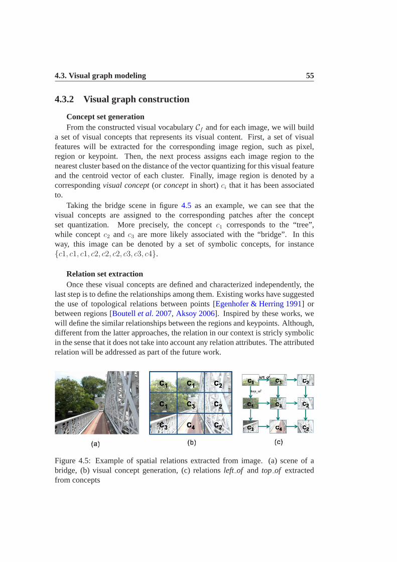
4.3. Visual graph modeling 55
4.3.2 Visual graph construction
Concept set generationFrom the constructed visual vocabularyCf and for each image, we will build
a set of visual concepts that represents its visual content.First, a set of visualfeatures will be extracted for the corresponding image region, such as pixel,region or keypoint. Then, the next process assigns each image region to thenearest cluster based on the distance of the vector quantizing for this visual featureand the centroid vector of each cluster. Finally, image region is denoted by acorrespondingvisual concept(or conceptin short)ci that it has been associatedto.
Taking the bridge scene in figure4.5 as an example, we can see that thevisual concepts are assigned to the corresponding patches after the conceptset quantization. More precisely, the conceptc1 corresponds to the “tree”,while conceptc2 and c3 are more likely associated with the “bridge”. In thisway, this image can be denoted by a set of symbolic concepts, for instance{c1, c1, c1, c2, c2, c2, c3, c3, c4}.
Relation set extractionOnce these visual concepts are defined and characterized independently, the
last step is to define the relationships among them. Existingworks have suggestedthe use of topological relations between points [Egenhofer & Herring 1991] orbetween regions [Boutellet al.2007, Aksoy 2006]. Inspired by these works, wewill define the similar relationships between the regions and keypoints. Although,different from the latter approaches, the relation in our context is stricly symbolicin the sense that it does not take into account any relation attributes. The attributedrelation will be addressed as part of the future work.
Figure 4.5: Example of spatial relations extracted from image. (a) scene of abridge, (b) visual concept generation, (c) relationsleft of and top of extractedfrom concepts

56 Chapter 4. Proposed Approach
We denote a labeled relation asl and a set of labeled relations asL. Figure4.5 gives an example of spatial relations between visual concepts with STOICcollection used in chapter6. Relation setsL = {left of, top of} are extractedfrom the two connected concepts. These relations help to capture the spatial co-occurrence information of two visual concepts. For example, instances of theconcept “sky” are usually in thetop of instances of the concept “tree”, whileinstances of concept “tree” appears more frequently in theleft of instances ofconcept “bridge”. If the number of training images is large enough, the graphframework will capture the statistical consistency for this type of relation.
Similar to the above, we can denote these relation sets usingsymbolic repre-sentation, for example{(c1,c1,leftof), (c1,c2,leftof), (c1,c3,leftof), (c3,c2,leftof)},(c3,c4,leftof), (c4,c2,leftof) and {(c1,c1,topof), (c1,c3,topof), (c1,c3,topof),(c3,c4,topof)}, (c2,c2,topof), (c2,c2,topof).
Graph formulation
At the end of the graph construction procedure, we obtain a set of visualconceptsCf and a set of predefined relationsEl for each type of conceptf andrelation l. Each concept is associated with a weight that represents its numberof occurrences in the image. Similarly, each relation is alsogiven a weightcorresponding to the number of times this relation has occurred in the image.We will denote the weighted concepts set byWCf and the weighted relations setby WEl. As we may have several image representations (or point of views) anddifferent kind of spatial relationships between them, we denote a set of weightedconcept sets asSWCF
=⋃
f∈F WCf and a set of weighted relation sets asSWEL
=⋃
l∈LWEl for an imageI.
Given a graph which is represented theoreticaly by a set of nodes and a set ofarcs. We map the set of concept setsSWCF
and the set of relation setsSWELto the
set of nodes and to the set of arcs respectively. In our case, we denote this graphas a visual graphG =< SWCF
, SWEL>. The weight of concepts and relations
are also mapped with the corresponding nodes and arcs. Thesevisual graphs arethen stored in the graph database.
By using the graph-based representation, we can include several imagerepresentations (i.e., different point of views) into thisgeneric framework. Notethat we tend to choose different representations for image regions (i.e., patch,keypoint) and visual features (i.e., color, edge, SIFT) which are consideredvisually independent of each other to represent image content. Therefore, conceptsetsWCf are disjoint. From this stand point, we will make an independentassumption based on the set of weighted concept setsSWCF
. The similarassumption is also applied to weighted relation setsSWEL
. The details of graphformulation will be given in section5.2of the next chapter.

4.4. Visual graph retrieval 57
4.4 Visual graph retrieval
Once the visual graphs are established based on the concept sets and therelation sets, the next question is how we can compare a new image against thedocument graphs stored in our database. Figure4.6 shows the pipeline for ourgraph retrieval scheme. The retrieval scheme includes three main stages:
Document graphs
Visual graphconstruction
Graphmatching
1
Query graph
2
Graphranking
3
Query image
Rankedlist
Figure 4.6: Graph retrieval pipeline for a query image
1. Given a query imageIq, we follow the same process ofgraph modelingasabove to extract the visual feature and cluster them into visual concepts. Thesame type of spatial relations are also extracted from the concepts. Fromthese concept sets and relation sets, a visual graph for userimageGIq isautomatically generated.
2. Graph matching consists of comparing the user query graphGIq with thetrained graphsGId stored in our database. Inspired by the language model
58 Chapter 4. Proposed Approach
from the IR domain, which is a generative model, we extend this frameworkto take into the account of the multiple concepts and multiple relationsembedded in our graph-based model. We compute the probabilities ofgenerating of the concept sets and the relation sets assuming concept setsand relation set are independent.
3. Graph ranking consists of the computing of relevance status values of thedocument graph and the query graph in the log-probability space. Finally,document images are ranked based on their relevance values associated withthe documents graphs.
4.5 Discussion
In this chapter, we have given an overview of the system implemented inour work. It includes three main layers: theimage processinglayer, thegraphmodelinglayer and thegraph matchinglayer. The main contributions of thisthesis are related to the graph modeling layer and the graph matching layer.These contributions rely on the graph-based presentation of image content andthe extension of language modeling for graph matching.
The graph modeling consists steps of visual concepts construction and spatialrelation extraction. The visual concepts are learned from the low-level features(e.g., color, edge, and local features) which are computed directly from differenttype of image representations such as pixels, patches or local keypoints, etc.The visual concepts learning phrase which consists of mapping the low-levelimage features into a discrete space of the visual vocabulary is done by thek-means clustering algorithm. In the other words, the visual concepts represent themiddle layer of image representation. To complete the graph-based representation,spatial relations are extracted from the visual concepts. It should be consideredthat our visual graph model, which adds another layer above the conceptuallayer, represents theintermediate layerof image representation approaching thesemantics layer.
The graph matching stage consists of generating the probabilities of newgraph from the trained graphs in our database. The classicalapproaches of graphmatching are usually complicated and time consuming. Therefore, we wouldlike to address another perspective of graph matching basedon thegenerativeprobabilistic frameworkof language modeling. This approach is simple in termof computational perfomance, as well as a well-founded theory from IR fields.The language model has been successful in the text retrievaldomain. Moreover,the extension of this model is straightforward from our graph-based model. Thenext chapter will detail our proposed approach for image retrieval.

Chapter 5
Visual Graph Modeling andRetrieval
5.1 Introduction
In the previous chapter, we have presented an overview of ourgraph-basedsystem. This system composes of three main stages: theimage processing step,the visual graph modeling stepand thevisual graph retrieval step. The imageprocessing step provides the tool for extracting the low-level visual features (suchas color, texture or edge). The visual graph modeling step includes two processes.First, it automatically induces a set of visual concept froma set of visual featuresbased on the unsupervised learning algorithm, e.g., k-means clustering. Second,the relation extractor generates a set of spatial relationsfrom the constructed visualconcepts. Finally, a visual graph is formulated from these set of concepts and setof relations. The visual graph retrieval process consists of matching the queryimage graph with the graphs stored in the database and ranks the results usingtheir probability values.
The goal of this chapter is to define formally the visual graphmodel and todescribe the matching process based on the formalism of language modeling. Wewill show some examples of graph instance derived from the general graph model.As we have shown in the chapter3, the main bottleneck of using the graph-basedimage representation is the matching step. In the literature, graph matching withclassical algorithm is a costly process. To avoid that problem and to provide amore reliable matching algorithm, we rely on the idea of language modeling forgenerating the query graph from the document graphs in the database. Graphsare then ranked with their corresponding probability likelihood values. As aconsequence, images are ranked in the lists with the same order of their relevancevalues. As we will show in chapter6, the proposed graph model may also be used
59

60 Chapter 5. Visual Graph Modeling and Retrieval
for image categorization. The category of a query image is decided based on theclass of the image which maximizes this probability likelihood.
This chapter is structured into 5 sections. Section5.2 introduces a formaldefinition of our visual graph. Also, we give some examples ofgraph instancesused in our application. Section5.3 will show how visual graphs are matchedusing our extended language modeling framework. We also give an example onhow we compute the probability likelihood in section5.3.4. Then, section5.4discusses how we actually rank our graph retrieval results using the relevancestatus value. Finally, we conclude the chapter and give someinsight discussionsin section5.5.
5.2 Visual graph formulation
5.2.1 Definition
In this section, we introduce a set of formal definitions associated with thevisual graph. To facilitate reading, the following notations will be used:
I : an imageGI : visual graph for imageIF : set of visual features associated with an image regionf : a low-level visual feature,f ∈ FL : set of possible labeled relationsl : label of relation,l ∈ LCf : set of concepts (or visual vocabulary) extracted for a featurefc : a visual concept,c ∈ CfEl : set of concept pairs extracted for a relation labeledlc, c′, l : a labeled relation,c ∈ Cf , c′ ∈ Cf ′ , l ∈ LWCf : weighted concept setWEl : weighted relation setSWCF
: set of weighted concept setWCf
SWEL: set of weighted relation setWEl
Our visual graph may contain different sets of visual concepts sets anddifferent sets of relation sets, which reflects multiple points of views (i.e., imagedecompositions and low-level visual features). Each visualconcept is constructedfor each type of image region and its low-level feature from the collection as insection4.2. Figure5.1shows how we formulate the set of concept set and the setof relation set from a collectionC and then transfer them to the formulation ofimageI.

5.2. Visual graph formulation 61
Figure 5.1: Formulation of the set of concept set and set of relation set from theimage collectionC and for the imageI.
Definition 1 Let F be the set of low-level features. For each featuref ∈ F , CIf
is the concept set extracted for featuref of an imageI:
CIf = {c|c ∈ Cf , I}
where c is a visual concept that characterizes imageI. Assuming theconcept set independent hypothesis, we have:
⋂
f∈F
CIf = ∅
Definition 2 Given the concept setCIf , WCI
f denotes a weighted concept setwhich contains a set of pairs(c,#(c, I)):
WCIf = {(c,#(c, I))|c ∈ CI
f}where#(c, I) is the number of times a visual conceptc occurs in the imageI. The weight of concept captures the importance of this concept in theimage. By default,WCI
f captures only the visual conceptc that appears inthe image, which means#(c, I) > 0.
Definition 3 The set of weighted concept setsSIWCF
is a union of weightedconcept setsWCI
f :
SIWCF
=⋃
f∈F
WCIf

62 Chapter 5. Visual Graph Modeling and Retrieval
Assuming the concept set independent hypothesis, the weighted conceptsets are disjoint. We get:
⋂
f∈F
WCIf = ∅
Similarly, we define the relation sets extracted from the visual concepts for animageI as follows.
Definition 5 Let L be the set of the possible labels. For each labeled relationl ∈ L, the relation setEI
l is defined by:
EIl = {((c, c′), l)|(c, c′) ∈ CI
f × CIf ′ , l ∈ L}
where(c, c′) is a pair of concept extracted from two concept setsCIf and
CIf ′, andl is a relation that occurs in the imageI.
If a pair of concepts(c, c′) comes from the same concept set (i.e.,CIf = CI
f ′),we refer this relation set asintra-relation set. Otherwise, if it comes fromtwo concept sets extracted from different visual features (i.e., CI
f 6= CIf ′),
we refer this relation set asinter-relationset.
Assuming the relation set independent hypothesis, we have:⋂
l∈L
EIl = ∅
Definition 6 Given relation setEIl , WEI
l denotes a weighted relation set whichrepresented by a set of triplet((c, c′), l,#(c, c′, l, I)):
WEIl = {((c, c′), l,#(c, c′, l, I))|(c, c′) ∈ CI
f × CIf ′ , l ∈ L}
where#(c, c′, l, I) is the number of timesc andc′ are related with labellin imageI. The weight of relation signifies the relation importance asthefrequency appeared in the image. By default, we capture only the relationthat appears in the imageI, therefore,#(c, c′, l, I) > 0.
Definition 7 The set of weighted relation setsSIWEL
is a union of weightedrelation setsWEI
l :
SIWEL
=⋃
l∈L
WEIl
Assuming the relation set independent hypothesis, the relation sets aredisjoint. We have:
⋂
l∈L
WEIl = ∅

5.2. Visual graph formulation 63
Definition 3 and7 are important as they provide the generality of our visualgraph model. As pointed out earlier, the visual graph can integrate smoothlydifferent image points of views, as well as the relations among them. Moreover,extracting visual concepts and spatial relation from imagecontent is a difficulttask (like in text retrieval domain). Visual concepts and relations are sometimesdefined in a subjective way. Therefore, the independence hypotheses based on theconcept sets and relation sets have been stated clearly to facilitate our propositionof graph retrieval in the next section.
Finally, the set of concept setsSIWCF
and the set of relation setsSIWEL
aremapped to the set of nodes and the set of arcs respectively, inour graph-basedframework. The following is the definition of visual graph for imageI.
Definition 9 Given a set of weighted concept setsSIWCF
and a set of weightedrelation setsSI
WELfor an imageI, the visual graphGI is defined by:
GI =< SIWCF
, SIWEL
>
The definition of our visual graph model provides a general framework whichallows us to derive to different graph instances. Dependingon the visual contentsof image, for example: outdoor scenary, building or indoor photos, we can createdifferent visual graph instances to fit the image content in this graph framework.In the next section, we will present two graph examples used in our experiments.
5.2.2 Graph instance 1
In this section, we illustrate how the visual graph model is constructed fromone concept set and two relation sets. This graph instance isused in ourexperiment with the STOIC-101 image collection. Most of the photos are capturedfamous scenes of Singapore landmarks and are mostly outdoors. We build theconcept set based on the patch-based division and extract the color informationfrom these patches. We denote this concept set asCcolor = {c1, c2, c3, ..., cN},whereN are the number of concept defined for this visual vocabulary.
Nevertheless, spatial information embedded in these photos is an importantfactor. Firstly, these photos were taken for touristic purposes. Most of thephotos are centered with the main object. Second, images aremostly in portraitor landscape mode. Therefore, the vertical and horizontal information are veryuseful clues for recognizing of the image content. For example, the sky isabove the buildings, trees are next to the statue, river is below the bridge etc.For these reasons, we decide to choose two type of spatial relations, denotedL = {left of, top of}, extracted from the concept setCcolor. Theleft of indicates

64 Chapter 5. Visual Graph Modeling and Retrieval
Figure 5.2: Example of a visual graph extracted from STOIC image collection.Concepts are represented by nodes and spatial relations are expressed by directedarcs. Nodes and arcs are weighted by the number of times they appear in theimage.
the horizontal relation between a pair of concepts. In the same way, thetop ofindicates the vertical relation between a pair of concepts.
Figure5.2shows an example of the visual graph constructed from an image ofa bridge scene. This example corresponds to a visual graph containing one visualconcept setCcolor and two intra-relation setsEleft of andEtop of . The visual graphfor an imageGI =< SI
WCF, SI
WEL> is composed of:
• The set of concept set contains one weighted concept setWCcolor extractedfrom color feature, denotedSI
WCL= WCcolor. In the figure, each node
corresponds to a concept and the number of time it occurs in the image.For example, conceptc1 appeared 3 times in the image and is denoted by(c1, 3), conceptc2 appeared 2 times in the image and is denoted by(c2, 2)etc.
• The set of relation setSIWEL
contains two intra-relation setsEleft of andEtop of extracted from two spatial relationsl1 = left of andl2 = top of ,denoted bySI
WEL= WEleft of
⋃
WEtop of . The relation between a coupleof concepts is captured by the directed arcs in this graph. Precisely, theblue arcs express the relationleft of and the green arcs express the relationtop of between two concepts. For example, conceptc1 is related to conceptc2 with the relationtop of 2 times and is related to itself by the relationleft of 2 times. It is denoted by(c1, c2, top of, 2) and(c1, c1, left of, 2).
5.2.3 Graph instance 2
The second example is a graph instance extracted from two concept setsand one relation set. The idea is to integrate different image representations

5.2. Visual graph formulation 65
(such as patch division and keypoints as described in chapter 2) together withtheir relations to represent a unique view of image contents. Image patchesare characterized by a set of visual features, such as color features and edgefeatures. These features capture the global information ofthe objects. On theother hand, the visual feature extracted from keypoints represent the details ofthe objects. We denote two concept sets asCpatch = {p1, p2, p3, ..., pN} andCsift = {s1, s2, s3, ..., sM}, whereN,M are the number of visual conceptsdefined for each visual vocabulary. The co-occurrence information between twoconcept set is denoted by the relationL = {inside} if one keypoint is localizedinside the area of an image patch.
Figure 5.3: Example of a visual graph extracted from two different visual conceptsets and related by a set of relationinside.
Figure5.3shows an example of an image and the corresponding visual graphconstructed. The above graph example corresponds to a visualgraph containingtwo visual concept setsCpatch, Csift and one inter-relation setEinside. The visualgraph for an imageGI =< SI
WCF, SI
WEL> is then composed of:
• The set of concept set contains two weighted concept setsWCpatch andWCsift extracted from color and edge features and SIFT features, denotedSIWCF
= WCpatch
⋃
WCsift. In the figure, the set of node abovecorresponds to a concept setCpatch and the set of node below corresponds toa concept setCsift. For each node, the weight is calculated by the numberof time its occurrence in the image. For example, concepts1 of concept setCsift appeared 5 times in the image and is denoted by(s1, 5). Conceptp2 ofconcept setCpatch appeared 2 times in the image and is denoted by(p2, 2)
• The set of relation set contains a weighted inter-relation setsWEinside ex-tracted from two concept setsCpatch andCsift, denotedSI
WEL= WEinside.
Similar to above, the relation between a couple of concepts is also capturedby the directed arcs in this graph. For example, concepts1 is linked toconceptp1 with the relationinside for 1 times and is related to concept

66 Chapter 5. Visual Graph Modeling and Retrieval
p2 for 2 times. These relations are denoted by(s1, p1, inside, 1) and(s1, p2, inside, 2).
After defining the representation for graphs, we turn to the problem ofmatching a query graph with the document graphs. The language model definedover the conceptual graph proposed in [Maisonnasseet al.2009] is consideredonly one concept set and one relation set in the same time. In the next sectionwe will explain how we extend this framework to take into account of multipleconcept sets and multiple relation sets in our visual graph matching method.
5.3 Graph matching for image retrieval
For a new image query, our objective is to provide the relevant photos from thecollection that match the user needs. Inspired by the information retrieval theory,we define here three models:
• Document graph modelGId is extracted from the document imageId inthe collection.
• Query graph modelGIq is constructed for a new query imageIq with thesame configuration as the document graph model.
• Matching model M(GIq, GId) includes a ranking function that computesthe probability for generating query graph modelGIq from the documentgraph modelGId.
Figure 5.4 provides the common diagram for image indexing and retrievalprocess in our graph-based model. First, we generate for theset of imagedocuments in the collection a set of corresponding graphs. These models are thenstored in our database for matching purpose. A graph model isalso constructedfor the image query. Then, the matching model takes into account of bothquery graph model and document graph model to compute the similarity of thesegraph models. Finally, images are ranked based on their similarity values of thedocument graph models.
5.3.1 Query likelihood ranking
Inspired by the language modeling approach proposed in Section 3.3, thematching modelM(GIq, GId) ranks the image documents based on the probabil-ity of generating the query graph model from the document graph models, whichis defined by:
M(GIq, GId) = rankId∈C{P (GIq|GId), Id} (5.1)

5.3. Graph matching for image retrieval 67
User
?
Query graphmodel (Gq)
Graph Indexing
Document graphmodels (Gd)
Query image (Iq)
Document images (Id)
Graph Retrieval
MatchingModel (M)
Image Ranking
Figure 5.4: Flowchart for graph indexing and graph retrieval in our system.
This is a generative model in the sense that the probability of query graphgeneration is measured based on the probability taken from the document graphmodel. The probabilityP (GIq|GId) indicates how likely the document graphGId
is close to the query graphGIq. In [Maisonnasseet al.2009], the probabilityPhas been calculated for a conceptual unigram model. However, our graph modelis composed of multiple concept sets, as well as, multiple relation sets. To expandthis framework, we present here an extension of the matchingmodelM thathandles both set of concept sets and set of relation sets.
In other words, the probability for a query graph modelGIq =< SIqWCF
, SIqWEL
>
to be generated from a document graphGId is composed of the probability ofgenerating independently the set of concept set and the set of relation set. Usingthe conditional probability rule, this can be written as:
P (GIq|GId) = P (SIqWCF
, SIqWEL
|GId)
= P (SIqWCF
|GId)× P (SIqWEL
|SIqWCF
, GId) (5.2)

68 Chapter 5. Visual Graph Modeling and Retrieval
whereP (SIqWCf
|GId) is the probability of generating set of concept sets from the
document graph, andP (SIqWEl
|SIqWCf
, GId) is the probability of generating set of
relation set given the set of concept setSIqWCf
from the document graphGId.To calculate this score, we will estimate separately the twoprobabilities: theprobability of generating concept set and probability of generating relation set.
5.3.2 Matching of weighted concept set
For generating the probability of query concept sets from the documentmodelP (SIq
WCf|GId), we assume a concept set independence hypothesis (related
explanation in section5.2). The probability can thus be estimated as:
P (SIqWCF
|GId) =∏
WCfIq∈SIq
WCF
P (WCfIq|GId) (5.3)
Assumingconcept independencewhich is standard in information retrieval, thenumber of occurrences of the concepts (i.e., the weights considered previously)are integrated through the use of amultinomialdistribution model. We computeP (WCf
Iq|GId) as follows:
P (WCfIq|GId) =
(∑
c #(c, Iq))!∏
c#(c, Iq)!
∏
c∈Cf
P (c|GId)#(c,Iq)
where#(c, Iq) denotes the number of times conceptc occurs in the query graphGIq. This contribution corresponds to the unigram conceptual probability asproposed in [Maisonnasseet al.2009].
The proportion in the above equation will not affect the ranking of thedocument images for the given query imageIq. By omitting the constant valueα,the equation leads to:
P (WCfIq|GId) ∝
∏
c∈Cf
P (c|GId)#(c,Iq) (5.4)
To calculate this score, we need to estimate the probabilitiesP (c|GId) from thedocument graph model. The maximum likelihood estimate would be:
P (c|GId) =#(c, Id)
#(|D|, Id)
where the quantity#(c, Id) represents the number of timesc occurs in thedocument imageId. The quantity#(|D|, Id) is the total number of concept inthe document image and equal to
∑
c #(c, Id).

5.3. Graph matching for image retrieval 69
The major problem with this probability estimation is that if any of theconcepts in the query image is missing from the document, theprobability ofP (WCf
Iq|GId) will be zero(as refered in section3.3). Consequently, the scoregiven by the query likelihoodP (GIq|GId) becomeszero probability. This isclearly not appropriate for ranking this type of image whileit should have a smallvalue instead. To avoid this bottleneck, the quantityP (c|GId) is estimated throughmaximum likelihood usingJelinek-Mercer smoothing:
P (c|GId) = (1− λf )P (c|GId) + λfP (c|C)
= (1− λf )#(c, Id)
#(|D|, Id) + λf#(c, C)
#(|C|, C)(5.5)
whereλf is the smoothing parameter for each concept setCf . Similarly, thequantities#(c, C) and#(|C|, C) are defined over the whole collectionC (i.e.,over the union of all images in the collection).
We choose to use theJelinek-Mercer smoothingfor its simplicity and itsproved effectiveness in the text retrieval domain. In general, the parameterλf
can depend on the nature of the document such as the used visual feature, imagecategory, etc. In our case, this parameter can be optimized using a validation setor a cross-validation technique.
In order to respect the consistency of multinomial distribution, the probabili-ties of the concepts must sum to one, i.e.
∑
c P (c|GId) = 1 . It’s been provedthat theJelinek-Mercer smoothingrespects this prior condition. To illustrate, weconsider a simple example with only 3 concepts,c1, c2 andc3, in the concept set.Supposing that the probabilities for these concepts in the document graph are 0.6,0.4 and 0.0. The probabilities estimated for these conceptsin the collection are0.3, 0.5 and 0.2. Given a smoothing value, for exampleλf = 0.2, the smoothedprobability for the document graph are:
P (c1|GId) = 0.6× (1− λf ) + 0.3× λf = 0.54
P (c2|GId) = 0.4× (1− λf ) + 0.5× λf = 0.42
P (c3|GId) = 0.0× (1− λf ) + 0.2× λf = 0.04
Note that conceptc3 has zero probability. Even though, the smoothed probabilityof conceptc3 has non-zero score thanks to the background probability estimatedfrom the collection. In the end, we get:
∑
c
P (c|GId) = P (c1|GId) + P (c2|GId) + P (c3|GId)
= 0.54 + 0.42 + 0.04
= 1.0

70 Chapter 5. Visual Graph Modeling and Retrieval
which confirms that the probabilities using Jelinek-Mercersmoothing method areconsistent.
5.3.3 Matching of weighted relation set
As shown in the previous section, we follow a similar processfor generatingthe probability of the relation sets from document graph model. Assuming therelation set independence (cf. section5.2), this leads to:
P (SIqWEL
|SIqWCF
, GId) =∏
WEIql
∈SIqWEL
P (WEIql |SIq
WCF, GId) (5.6)
For the probability of generating query relation set from the document graph,we assume that a relation depends only on the two linked concept sets. Assumingthat the relation sets are conditionally independent according to the set of conceptsetSIq
WCFand the graph documentGId, and following amultinomial distribution
model, we can compute:
P (WEIql |SIq
WCF, GId) =
(∑
(c,c′,l) #(c, c′, l, Iq))!∏
(c,c′,l) #(c, c′, l, Iq)!×
∏
(c,c′,l)∈Cf×Cf ′×L
P (L(c, c′) = l|WCIqf ,WCIq
f ′ , GId)#(c,c′,l,Iq)
where the quantity#(c, c′, l, Iq) is the number of time the relationl of conceptpair (c, c′) appears in the query graphGIq.
Similar to the concept set, the first proportion in the above equation will notaffect the final ranking. By eliminating the constant value, this equation leads to:
P (WEIql |SIq
WCf, GId) ∝ (5.7)
∏
(c,c′,l)∈Cf×Cf ′×L
P (L(c, c′) = l|WCIqf ,WCIq
f ′ , GId)#(c,c′,l,Iq)
wherec ∈ Cf , c′ ∈ Cf ′ andL(c, c′) are variables which values inL reflects thepossible relation labels betweenc andc′, in this relation set.
Similar to the concept set, the relation set suffers the sameproblem of zeroprobability when a relation is missing from the document graph. Hence, thesmoothing technique has been applied for the relation set. The probabilitiesP (L(c, c′) = l|WCIq
f ,WCIqf ′ , GId) are estimated by maximum likelihood with
Jelinek-Mercer smoothingmethod, giving:
P (L(c, c′) = l|WCIqf ,WCIq
f ′ , GId) = (5.8)
(1− λl)#(c, c′, l, Id)
#(c, c′, |D|, Id) + λl#(c, c′, l, C)
#(c, c′, |C|, C)

5.3. Graph matching for image retrieval 71
whereλl is the smoothing parameter for each relation setEl. The quantity#(c, c′, l, Id) represents the number of times conceptsc and c′ are linked withlabel l in the document imageId, and the quantity#(c, c′, |D|, Id) is equal to∑
l∈L #(c, c′, l, Id). In the same way, this parameter can be optimized by thecross-validation technique for each relation. Note that ifone of the two conceptsdoes not appear in the imaged, it yields:
#(c, c′, l, Id)
#(c, c′, |D|, Id) = 0
Again, the quantities#(c, c′, l, C) and#(c, c′, |C|, C) are counted in a similarway but computed on the whole collectionC (i.e., over the union of all the graphsfrom all the documents in the collection).
This graph model is a generalization of the model defined in [Phamet al.2010]which corresponds to the case where only one concept set is used. In somespecial cases, our model corresponds to the standard language model usedin [Phamet al.2009] where relations are not considered (i.e., documents andqueries correspond to multiple bag-of-words model). In thenext section, we willgive an example of graph matching with our graph models.
5.3.4 Graph matching example
For a better understanding of the graph matching function, we provide here asimple example of matching with three graph models. These graphs are generatedwith the graph instance 1 introduced in the previous section. In the figure5.5, G1andG2 are the document graphs andG is the query graph. Intuitively, graphG1is closer to the query graphG than the latter.G1 contains the same set of conceptand have similar relation set as query graphG. While,G2 is missing a conceptc4and have less relation than the query graphG. The collectionC is then defined ontwo graphsG1 andG2.
Supposing that the visual graphs are constructed from 4 visual concepts(c1, c2, c3, c4) and two relations(l1 = left of, l2 = top of). Graph models

72 Chapter 5. Visual Graph Modeling and Retrieval
are described as follows:
G1 = < {(c1, 3), (c2, 3), (c3, 2), (c4, 1)};{(c1, c1, l1, 2), (c2, c3, l1, 2), (c4, c3, l1, 2),(c1, c2, l2, 1), (c2, c4, l2, 1), (c1, c3, l2, 2), (c3, c3, l2, 2)} >
G2 = < {(c1, 4), (c2, 3), (c3, 2)};{(c2, c3, l1, 2), (c2, c2, l1, 4), (c1, c2, l2, 2), (c1, c3, l2, 2), (c3, c3, l2, 2)} >
G = < {(c1, 3), (c2, 2), (c3, 2), (c4, 2)};{(c1, c1, l1, 2), (c2, c2, l1, 1), (c2, c3, l1, 1), (c4, c3, l1, 2),(c1, c2, l2, 2), (c2, c4, l2, 2), (c1, c3, l2, 1), (c3, c3, l2, 1)} >
c13
c32
c23
c41
top_of, 2top_of, 1
top_of, 1
left_of, 2
left_of, 2
left_of, 2
c14
c32
c23
top_of, 2
top_of, 2
top_of, 2
left_of, 4
left_of, 2
c13
c32
c22
c42
top_of, 1
top_of, 1
top_of, 2
top_of, 2
left_of, 2
left_of, 1
left_of, 2
left_of, 1
G1 G2
top_of, 2
C
Document graphs
Query graph G
Figure 5.5: Example of matching graph with our model.G1 andG2 are thedocument graphs from collectionC andG is the query graph.
Assuming the multinomial distribution, we calculate the probability likelihood

5.3. Graph matching for image retrieval 73
for query graph to be generated by the document graphG1:
P (G|G1) =P (c1|G1)3P (c2|G1)2P (c3|G1)2P (c4|G1)2×P (L(c1, c1) = l1|G1)2P (L(c2, c2) = l1|G1)P (L(c2, c3) = l1|G1)
P (L(c4, c3) = l1|G1)2P (L(c1, c2) = l2|G1)2P (L(c2, c4) = l2|G1)2
P (L(c3, c3) = l2|G1)P (L(c1, c3) = l2|G1)
Assuming a small value of the smoothing parameters (i.e.,λf = λl = 0.2),the probabilities are estimated with the Jenlinek-Mercer smoothing method. Wecalculate the probabilities for each concept, for exampleP (c1|G1), as follows:
P (c1|G1) = (1− 0.2)× P (c1|G1) + 0.2× P (c1|C)
= 0.8× 3/9 + 0.2× 7/18
= 0.344
For estimating the probabilities of the relations, for exampleP (c1, c1, l1|G1) andP (c1, c2, l2|G1), we have:
P (L(c1, c1) = l1|G1) = (1− 0.2)× P (L(c1, c1) = l1|G1) + 0.2× P (L(c1, c1) = l1|C)
= 0.8× 2/6 + 0.2× 2/12
= 0.3
P (L(c1, c2) = l2|G1) = (1− 0.2)× P (L(c1, c2) = l2|G1) + 0.2× P (L(c1, c2) = l2|C)
= 0.8× 2/6 + 0.2× 2/12
= 0.183
Note that the relation(c2, c2, l1|G1) does not appear in the document graph G1.Although, it still obtain a non-zero probability of 0.067 which has been leveragedfrom the collection. The final score for graph G1 is:
P (G|G1) =(0.344)3(1/3)2(2/9)2(0.1)2 × (0.3)2(0.067)(1/3)(0.3)2×(0.183)2(0.15)2(1/3)(1/3)
P (G|G1) ≈3.377× 10⁻¹⁴
Similar to the graphG1, we calculate the probability likelihood for querygraph to be generated by the document graphG2:
P (G|G2) =P (c1|G2)3P (c2|G2)2P (c3|G2)2P (c4|G2)2×P (L(c1, c1) = l1|G2)2P (L(c2, c2) = l1|G2)P (L(c2, c3) = l1|G2)
P (L(c4, c3) = l1|G2)2P (L(c1, c2) = l2|G2)2P (L(c2, c4) = l2|G2)2
P (L(c3, c3) = l2|G2)P (L(c1, c3) = l2|G2)

74 Chapter 5. Visual Graph Modeling and Retrieval
Also note that the conceptc4 does not appear in the document graphG1. Howeverit still get a small value of 0.0111 from the collection. The final score for graphG2 is:
P (G|G2) =(0.433)3(1/3)2(2/9)2(0.011)2 × (0.033)2(0.6)(0.6)(0.033)2×(0.316)2(0.017)2(1/3)(1/3)
P (G|G2) ≈6.464× 10⁻²⁰
As we can observe from the above scores, graphG1 obtains a larger scorevalue compared to graphG2, which is consistent with our initial intuition.
5.4 Ranking with relevance status value
In practice, multiplying many small numbers may lead to numerical precisionproblems. Moreover, the multiply operation is considered more costly when com-pared to the addition operation. As usual in IR, we can use logarithm function toturn the likelihood score into rank-preserving sum. As donein [Phamet al.2009],the relevance status value (RSV) of a document imageId for query imageIq is computed in the log-probability domain. In the context ofmultinomialdistributions, we have:
RSVlog(GIq|GId) = logP (GIq|GId)
= log(P (SIqWCF
|GId)× P (SIqWEL
|SIqWCF
, GId))
= logP (SIqWCF
|GId) + logP (SIqWEL
|SIqWCF
, GId)
By submitting the probabilities of the set of concept set and the set of relation setin equation with the equations5.3and5.6, it leads to:
RSVlog(GIq|GId) =
∑
WCFIq∈SIq
WCF
logP (WCfIq|GId)+
∑
WEIql
∈SIqWEL
logP (WEIql |SIq
WCF, GId)

5.5. Conclusion 75
Again, by approximating the probabilities of the concept setand the relation setin the equations5.4and5.8, we get:
RSVlog(GIq|GId) ∝
∑
WCfIq∈SIq
WCF
∑
c∈Cf
logP (c|GId)#(c,Iq)+
∑
WEIql
∈SIqWEL
∑
(c,c′,l)∈Cf×Cf ′×L
logP (L(c, c′) = l|WCIqf ,WCIq
f ′ , GId)#(c,c′,l,Iq)
∝∑
WCfIq∈SIq
WCF
∑
c∈Cf
#(c, Iq)× logP (c|GId)+
∑
WEIql
∈SIqWEL
∑
(c,c′,l)∈Cf×Cf ′×L
#(c, c′, l, Iq)× logP (L(c, c′) = l|WCIqf ,WCIq
f ′ , GId)
Finally, the probabilities of the concept and relation of the graph document areestimated using the Jelinek-Mercer smoothing as seen in theprevious sections.
For image categorization, document images are categorizedinto a specificclasses, for example: “person”, “animal”, “nature”, “sport”, etc.Query imageIq is matched against the document images and then classified into the class ofthe closest document imageId given by the following estimate:
class(Iq) = class(argmaxId∈C
RSVlog(GIq|GId)) (5.9)
More details on the classification task will be given in the experiment part of thenext chapter.
5.5 Conclusion
We have presented in this chapter the formulation of the visual graph modeland the graph matching algorithm inspired by the language modeling frominformation retrieval. The visual graph is defined from a setof concept sets anda set of relation sets. The visual concept set is achieved by image segmentation,feature extraction and by visual concept learning. The relation set is generatedbased on the predefined extraction rules. The proposed graphmodel reflects themodern approach in the contend-based image retrieval, whichtry to combinemultiple viewpoints of the visual content. This can be done in several ways,such as vector combination for BoW model or kernel fusion for SVM method.However, these approaches lack the capacities of integrating efficiently the spatialinformation, which is crucial to represent the image content, among the visualconcepts. On the contrary, with our general visual graph framework, one can

76 Chapter 5. Visual Graph Modeling and Retrieval
integrate smoothly different types of visual concept and also the spatial relationamong them.
One limitation of this approach is that the relation betweenconcepts is definedmanually and varies depending on the nature of the image collection or applicationused. For this reason, two graph instances have been shown with differentconfiguration that adapted to the visual content. Once again, this also proves theflexibility and the expendability of our visual graph model.
Section5.3 showed how the document graphs are matched against the querygraph using the extension of the language modeling framework. Indeed, thematching model not only takes into account a set of concepts but also a multipleconcept sets and a multiple relation sets. We have made several hypotheses inorder to adapt to the specific context of the image. The smoothing technique is alsomodified to fit into our visual graph framework. Finally, we have demonstrated anexample of graph matching to illustrate the idea.
The next chapter is dedicated to the application of our proposed approach.We will present two applications of the image categorization problem. Thefirst application is a system for scene recognition of the Singapore’s famouslandmarks. Different graph models will be created to take into account of differentvisual features. We will also show how the spatial relationsare improvingthe accuracy of the recognition process. We also discuss on the aspect ofoptimizing the smoothing parameters using the cross-validation technique. Thesecond application is a self-localizing system of a mobile robot in an indoorenvironment. We will show how the graph model has been created to adapt todifferent environment conditions (such as light changing,object moving, etc.).Finally, in both applications we will show that visual graphmodels are actuallyperforming better than the state-of-the-art SVM methods.

Part III
Applications
77


Chapter 6
Scene Recognition
Imagination is more important than knowledge ...Albert Einstein
6.1 Introduction
The first application of the theoretical approach is anoutdoor scene recog-nition system. This work has been done in the context of French-Singaporeancollaboration. This has been partly realized at the Image Perception and Accesslab (IPAL) in Singapore and at the Multimedia Modeling Information Retrieval(MRIM) team in Grenoble. Part of the project was funded by the Merlionprogramme, supported by the French embassy in Singapore.
Figure 6.1: Snap2Tell application is a prototype of an image-based mobile tourguide [Lim et al.2007].
79

80 Chapter 6. Scene Recognition
One application of this scene recognition systems is for mobile touristic sceneidentification, called Snap2Tell [Lim et al.2007], developed by IPAL lab. A useruploads an image taken with a hand-phone and sends it as a query to the Snap2Tellsystem. The Snap2Tell system will be able to identify the particular scene andsends back the tourist information. The Snap2Tell prototype is implementedas 2-tier architecture: client-server protocol. The client provides a mobileuser interface and has functionalities to capture images and interact with theserver. The client-server protocol is developed for communication over wirelessconnection (such as WiFi and GPRS) as depicted in figure6.1.
On the server-side, the recognition system identifies the captured scene,retrieves and sends back the scene descriptions. The imagesfrom collectionare matched against the user query. Finally, information related to the matchedscenes (i.e. text or audio) will be sent back to the user mobile through the wirelessconnections.
In this regard, our works concentrate on developinga good scene recognitionenginewhich needs to address the following challeging issues:
• No prior knowledge of the image content and of the categorization ofobjects/scenes;
• Difficulty to separate foreground and background;
• Occlusion and moving objects, for example: people, vehicles, trees, etc.;
• Variation of viewpoint, scale, lighting condition;
• Fast and reliable response to the user query given a limited computingresources.
6.1.1 Objectives
Our first objective is to build for this specific image collection an adequatevisual graph model that compromises both visual features and spatial relations.We will show that with the integration of spatial relation, our visual graph modelobtains a better performance versus the standard conceptual model. Moreover, wewill compare the proposed model with the state-of-the-art SVM method on theimage classification.
Second, as user can take one or several images of the same scene and query thesystem, we have considered several usage scenarios for training and query: withsingle image (I) or with multiple images (S). Therefore, oursecond objective is todemonstrate that with multiple image queries, which accumulated viewpoints ofthe scene, will help to improve significantly the recognition accuracy. Table6.1summarizes the different scenarios implemented in our experiments.

6.1. Introduction 81
Figure 6.2: Different viewpoints of the Merlion statue. User can use single imageor multiple images as a query.
Table 6.1: Summary of experiments on STOIC-101 collection. Ascene (S)corresponds to a group of images and (I) corresponds to a single query image.
Training by (I) Training by (S)
Query by (I)√ √
Query by (S)√ √
Last but not least, we will discuss on how we optimize the smoothingparameters with 3-fold cross validation on the training set. Comparing to theaposteriorioptimized methods, we will show that the effect of the cross validationparameters is not significant. Issues related to technical implementation will alsobe discussed.
6.1.2 Outline
In the next section, we will describe the STOIC-101 image collection usedin our experiments. Then, we present the proposed visual graph models adaptedfor the image collection in section6.3. The experimental result will be shown insection6.4 with different impacts of the relation and multiple image queries onthe classification performance. In section6.5, we will discuss on how we used thecross validation technique on training set to optimize the smoothing parameters.Finally, we summarize the chapter in section6.6

82 Chapter 6. Scene Recognition
Figure 6.3: Images of STOIC-101 collection are taken from different locationsacross Singapore [Lim et al.2007].
6.2 The STOIC-101 collection
The Singapore Tourist Object Identification Collection (STOIC) has beencollected for the experimental purpose of the Snap2Tell application. STOICcollection contains of 3,849 images taken from 101 popular tourist landmarksin Singapore (mostly outdoor). These images were taken, mainly with consumerdigital cameras in a manner typical of a casual tourist, from3 distances and 4angles in natural light, with a mix of occlusions and cluttered background toensure a minimum of 16 images per scene. Images in the collection are affected bydifferent weather patterns and different image capturing styles. Figure6.3showssome example images taken from the STOIC collection. Note that some imagesin the collection have been rotated into the correct orientation (for portrait andlandscape layouts).
For experimental purposes, the STOIC-101 collection has been divided intoa training set containing 3,189 images (82.8% of the collection) and a test setcontaining 660 images (17.2% of the collection). The average number of imagesper class for training is 31.7, and 6.5 for testing respectively. In the test set, theminimum number of images per class is 1, and the maximum is 21.Table6.2summarizes some key statistics on the STOIC-101 collection.

6.3. Proposed models 83
Table 6.2: Statistics of the STOIC-101 collection
Training Test Overall
Number of scenes 101 101 101Number of images 3189 660 3849Percentage 82.85% 17.15% 100%Mean (per scene) 31.57 6.53 38.11Maximum (per scene) 160 21 181Minimum (per scene) 5 1 8
6.3 Proposed models
6.3.1 Image modeling
Several studies on the STOIC collection have shown that color plays adominant role, and should be preferred to other visual features such as edgeor texture [Lim et al.2007]. Furthermore, color histogram can be easily andefficiently extracted. For these reasons, we rely only on HSVcolor features inour experiments. In order to assess the validity of our methodology, we followeddifferent ways to divide image into regions as proposed in chapter 4 and weretained:
1. A division of medium grain, where blocks of 10x10 pixels are used, thecenter pixel being considered as a representative for the region. We refer tothis division asmg.
2. A patch division where the image is divided into 5x5 regions of equal size.We refer to this division asgg.
For mg divisions, we used the (H, S, V) values as a feature vector foreachpixel. Similarly, each patch ingg division is quantized by a HSV histogram(4 bins/channel) that yields a 64 dimensional vector for eachregion. We thenclustered the HSV feature vectors of all regions intok = 500 classes withk-meansclustering algorithm. This results in a hard assignment of each region toone concept. The set of weighted concepts,WC, is then obtained by countinghow many times a given concept occurs in the image. The choiceof k = 500 ismotivated by the fact that we want a certain granularity in the number of conceptsused to represent an image. With too few concepts, one is likely to miss importantdifferences between images, whereas too many concepts willtend to make similarimages look different.
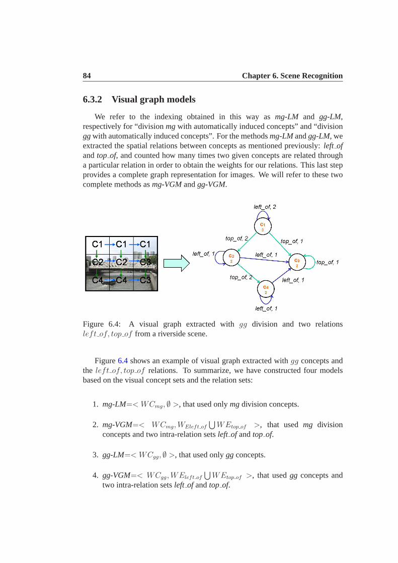
84 Chapter 6. Scene Recognition
6.3.2 Visual graph models
We refer to the indexing obtained in this way asmg-LM and gg-LM,respectively for “divisionmgwith automatically induced concepts” and “divisionggwith automatically induced concepts”. For the methodsmg-LMandgg-LM, weextracted the spatial relations between concepts as mentioned previously:left ofandtop of, and counted how many times two given concepts are related througha particular relation in order to obtain the weights for our relations. This last stepprovides a complete graph representation for images. We will refer to these twocomplete methods asmg-VGMandgg-VGM.
Figure 6.4: A visual graph extracted withgg division and two relationsleft of, top of from a riverside scene.
Figure6.4 shows an example of visual graph extracted withgg concepts andthe left of, top of relations. To summarize, we have constructed four modelsbased on the visual concept sets and the relation sets:
1. mg-LM=< WCmg, ∅ >, that used onlymgdivision concepts.
2. mg-VGM=< WCmg,WEleft of
⋃
WEtop of >, that usedmg divisionconcepts and two intra-relation setsleft of andtop of.
3. gg-LM=< WCgg, ∅ >, that used onlyggconcepts.
4. gg-VGM=< WCgg,WEleft of
⋃
WEtop of >, that usedgg concepts andtwo intra-relation setsleft of andtop of.
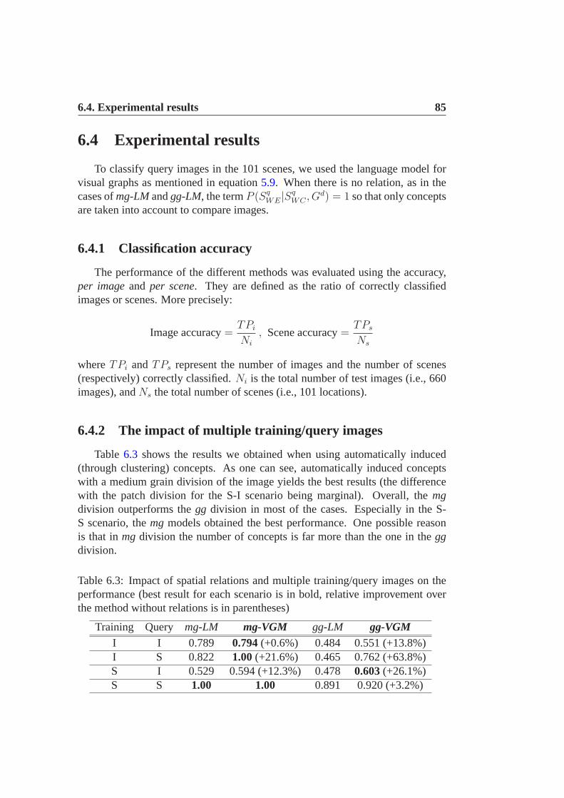
6.4. Experimental results 85
6.4 Experimental results
To classify query images in the 101 scenes, we used the language model forvisual graphs as mentioned in equation5.9. When there is no relation, as in thecases ofmg-LMandgg-LM, the termP (Sq
WE|SqWC , G
d) = 1 so that only conceptsare taken into account to compare images.
6.4.1 Classification accuracy
The performance of the different methods was evaluated using the accuracy,per imageand per scene. They are defined as the ratio of correctly classifiedimages or scenes. More precisely:
Image accuracy=TPi
Ni
, Scene accuracy=TPs
Ns
whereTPi andTPs represent the number of images and the number of scenes(respectively) correctly classified.Ni is the total number of test images (i.e., 660images), andNs the total number of scenes (i.e., 101 locations).
6.4.2 The impact of multiple training/query images
Table 6.3 shows the results we obtained when using automatically induced(through clustering) concepts. As one can see, automatically induced conceptswith a medium grain division of the image yields the best results (the differencewith the patch division for the S-I scenario being marginal). Overall, themgdivision outperforms thegg division in most of the cases. Especially in the S-S scenario, themg models obtained the best performance. One possible reasonis that inmg division the number of concepts is far more than the one in theggdivision.
Table 6.3: Impact of spatial relations and multiple training/query images on theperformance (best result for each scenario is in bold, relative improvement overthe method without relations is in parentheses)
Training Query mg-LM mg-VGM gg-LM gg-VGMI I 0.789 0.794(+0.6%) 0.484 0.551 (+13.8%)I S 0.822 1.00(+21.6%) 0.465 0.762 (+63.8%)S I 0.529 0.594 (+12.3%) 0.478 0.603(+26.1%)S S 1.00 1.00 0.891 0.920 (+3.2%)

86 Chapter 6. Scene Recognition
This being said, there is a difference between the I-S and S-Iscenarios:The system is queried with more information in the I-S scenario than in the S-I scenario. This difference results in a performance which is, for all methods,worse for the S-I scenario than for the other ones. We conjecture that this is whythe results obtained for themg-VGMmethod on S-I are not as good as the onesfor I-I. There seems to be a plateau for this scenario around 0.6, a hypothesis wewant to explore in future work.
6.4.3 The impact of the relations
We also assessed the usefulness of spatial relationships bycomparing theresults obtained with the different methods that include ornot such relations.These results are displayed in Table6.3. As one can note, except for the S-Sscenario with themg division, the use of spatial relations always improves theaccuracy of the classifier. This justifies the framework we developed in section5.3of language model for visual graphs including automatically induced concepts andspatial relations among them.
6.4.4 Comparing to the SVM method
In order to confirm the validity of our methods, we have compared theresults with the state-of-the-art method in image categorization such as SVMclassification method (implemented thanks to thelibsvm1). We applied the samevisual features used for graph model in our experiment. The input vector in SVMclassifier is the early fusion of the multiple bag-of-word models. Then, each imageclass was trained with a corresponding SVM classifier using radial basis function(RBF) kernel. To optimize the kernel parameters, we trained SVM classifierswith 3-fold cross validation on the training set. Finally, these classifiers are usedto classify the new query image.
Similar to above, we refer to the model with only the contribution of conceptas LM and model with the spatial relation as VGM. We choose themgconceptsas a comparison model.
Table 6.4: Results on categorizing STOIC-101 collections comparing to SVMmethod using I-I scenario.
#class SVM LM VGMSTOIC 101 0.744 0.789 (+ 6.0%)0.794(+ 6.3%)
1http://www.csie.ntu.edu.tw/cjlin/libsvm/

6.5. Discussion 87
Table6.4 summarizes the results obtained from collection STOIC-101 withthree methods: SVM, LM, and VGM. We can see that in all cases the VGMoutperforms other methods. More precisely, with the integration of spatial relationinto VGM helps improving the accuracy of classical approaches of LM by 6.0%.Moreover, VGM increases roughly the accuracies of 6.3% comparing to SVMmethod. This proves that the proposed methods (LM and VGM) are consistentlyperforming better than the state-of-the-art SVM.
6.5 Discussion
In this section, we will give some discussion on how we optimizea posteriorithe smoothing parameter based on the test set. We also employed the crossvalidation technique on the training set to optimizea priori these parameters.We will show that the difference in term of parameter values and classificationaccuracy is not significant among the two methods.
6.5.1 Smoothing parameter optimization
The results presented above are optimizeda posteriori, i.e., we exhaustivelytested the parameters on the test set to get the best configuration. We vary thevalue of each parameter in between[0, 1.0] with the increment of 0.1 for eachstep. Then, we test these values against the test set and choose the configurationwhich gives the best results. However, this approach overestimates the proposedalgorithms, by giving an upper bound of the evaluation results and not a correctestimation.
In a way to estimate more precisely the results, we optimizedthe smoothingparameters on a validation set for themgdivision models because this approachgives the best results. To achieve this optimization, a 3-fold cross validationwas performed. Once the parameters were optimized for each of the threetraining/validation sets, we processed the test set using the whole training set.This technique is called optimizinga priori of the smoothing parameters.
Table6.5 compare the two techniques mentioned above for parameter opti-mization. For the modelmg-LM, only the concept smoothing parameterλc hasbeen tested. We can see that there are only two cases that the optimized parametersare different, e.g., for the I-I and I-S scenarios. However,the gap between theaposterioriand thea priori is not significant (with the difference of 0.1).
Similar with the modelmg-VGM, two parametersλc andλl have been tested.Note that we applied specifically the same parameter valueλl for both relationleft of andtop of as they contribute an equal role in the graph model. We observethat it obtained almost the same values in all cases, except in the case of I-S

88 Chapter 6. Scene Recognition
Table 6.5: Comparison of the smoothing parameters obtained by cross validationset (a priori) and by test set (a posteriori) with modelmg-LM and modelmg-VGM. Bold values signify the different cases of the two methods.
Training Query λc λl
a posteriori a priori a posteriori a priori
mg-LMI I 0.1 0.2 - -I S 0.8 0.7 - -S I 0.1 0.1 - -S S 0.2 0.2 - -
mg-VGMI I 0.2 0.2 0.3 0.3I S 0.7 0.7 0.9 1.0S I 0.1 0.1 0.7 0.7S S 0.2 0.2 1.0 1.0
scenario with the relation smoothing parameterλl. This proves that the smoothingparameters obtained with thea posteriorioptimization technique are consistentcompared to thea priori optimization technique.
Table6.6 shows the average (Avg) and standard deviation (Std-dev) ofthe 3results obtained. The last column of the table exhibits the difference (Diff) inpercentage for the evaluation measurement between the 3-fold results and theaposteriorioptimization. As shown in the table, the results obtained bythe crossvalidation and by a posteriori optimization are very similar. If we focus on theresults of the I-I, S-I and S-S configurations, the differences are smaller than1%, and for the configuration I-S the 3-fold results are 4.46%lower. So, theoptimization used on the validation sets provides satisfying results for a mediumgrain and for automatically defined visual concepts.
Table 6.6: Comparison of the resultsmg-LM-valon 3-fold cross validation, andpercentage of difference in accuracy compared to thea posteriorioptimizationmodelmg-LM
Training Query mg-LM mg-LM-val DiffAvg Std-dev
I I 0.789 0.784 5.8× 10⁻³ -0.68%I S 0.822 0.785 5.8× 10⁻³ -4.46%S I 0.529 0.529 0.0 0%S S 1.00 0.990 1.7× 10⁻² -0.01%

6.5. Discussion 89
We also tested 3-fold cross validation with relationships,as presented inTable6.7. Here again the results with the cross validations are very close to thea posteriorioptimized results: the S-I and S-S results are almost equal.A smalldifference is observed as in the case of I-I and I-S.
Table 6.7: Comparison of the resultsmg-VGM-valon 3-fold cross validation, andpercentage of difference in accuracy compared to thea posteriorioptimizationmodelmg-VGM
Training Query mg-VGM mg-VGM-val DiffAvg Std-dev
I I 0.794 0.788 6.4× 10⁻³ -2.64%I S 1.00 0.939 5.3× 10⁻² -6.07%S I 0.594 0.594 0.0 0%S S 1.00 0.990 1.7× 10⁻² -0.01%
Another conclusion drawn from Tables6.6 and 6.7 is that, with a crossvalidation procedure, the usage of relationships still outperforms the resultswithout relationships: +0.5% for the case I-I, +19.6% for I-S, and +12.3% forS-I. For the case S-S no improvement is achieved, which is also consistent withthea posteriorioptimized results.
6.5.2 Implementation
The system is implemented in C/C++ with the LTI-Lib2 and compiled ona Linux platform. LTI-lib is a well designed and well documented for imageprocessing library, developed by the Aachen University of Technology. Imageindexing and querying are performed on a computer with 3.0 GHz quad-coreCPU and 8.0 Gb of memory. Training step takes about 2 hours for the wholetraining images set from extracting visual features, clustering the concepts andmodeling trained graphs. For the query step, it takes about 0.22 second on average(or 5 images/second) for computing the likelihood of graph query with all thegraphs stored in database. However, the computation is highly parallelizable givengraph models are stored and are processed independently. Itshows that the graphmatching step is very reliable for image matching comparingto classical graphmatching algorithm.
2http://ltilib.sourceforge.net/

90 Chapter 6. Scene Recognition
6.6 Summary
We have shown in this chapter the first application of the visual graph model,namely theoutdoor scene recognition. The context in which this work has beenrealized is to develop a scene recognition engine for the Snap2Tell prototype,an image-based mobile tourist guide. For this purpose, we have tested ourproposed graph models on the STOIC collection containing of101 famous scenesof Singapore.
We have proposed different visual graph models in order to adapt to thespecific visual contents of the image collection. The proposed graphs wereconstructed based on thecolor conceptsand two spatial relationsleft of andtop of. The results obtained shown that the integration of spatialrelations intothe visual graph model outperformed the standard language model and the SVMclassification which based only on the visual concept. A key strength of theproposed approach is the possibility of combining several images for trainingand for querying. The results have shown clearly an improvement in term ofaccuracy of the multiple image queries comparing to that of the single imagequery. This also confirmed theflexibility and extenbility of this new graph-theoretic framework.
Finally, we have discussed the process of optimizing the smoothing parameterwith the cross validation technique. Parallel to thea posteriorioptimizing methodbased on the test set, it has shown a very small difference in result with theparameter optimized withcross validation technique. This fact confirmed theconsistency of the proposedJelinek-Mercer smoothingmethod. In fact, we alsowish to study the cross validating with other smoothing method (such asDirichletsmoothing) as referred in the state-of-the-art. This should be considered in ourfuture works. Some details on the implementing of the systemhave also providedto prove thereliability of the graph-based framework.
In the next chapter, we will present the second application of our methodto the self-localizing of a mobile robot in an indoor environment. Coping withthe specific condition of theindoor and laboratory environment, we experimentanother instance of the proposed graph model. We will show how it can be adaptedto the indoor changes (such as lighting condition, object moving, human involvingand theunknownroom).
Chapter 7
Robot Localization
7.1 Introduction
RobotVision1 track is organized by the ImageCLEF2 evaluation campagin.The main task is to exploit the location information within aknown environmentof a mobile robot based only on the visual information [Luo et al.2006]. Thischapter focuses on applying the proposed visual graph modeling for the RobotVi-sion track of the ImageCLEF 2009. This works was partly fundedby the AVEIR3
(Automatic annotation and Visual concept Extraction for Image Retrieval) project,supported by l’Agence Nationale de la Recherche (ANR).
The challenge was to build a system able to answer the question “Where areyou?” for a mobile robot. The visual system has to determine the topologicallocalization of a mobile robot based on a sequence of training image. Onedifficulty of this task is that the robot has to recognize a room in differentillumination conditions and adapt as the environment changes (such as movingpeople or objects, new furniture added over the time, etc.).This might pose aproblem for a visual recognition system as the trained data usually obtained ata fixed time. Meanwhile, the system has to provide the location of the robot inreal-time and in different time spans (6 months to 20 months)(see figure7.1).
Several classical approaches in computer vision have been proposed for thisproblem. In [Pronobiset al.2008], the authors suggested an appearance-basedmethod using Support Vector Machine (SVM) to cope with illumination and posechanges. This method achieved a satisfactory performance when considering ashort time interval between training and testing phrases. Other possible approachis to detect the interest point (such as SIFT, Harris-Laplace, etc.) and do a
1http://www.imageclef.org/2009/robot2http://www.imageclef.org/3http://aveir.lip6.fr/
91
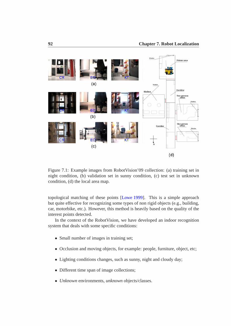
92 Chapter 7. Robot Localization
Figure 7.1: Example images from RobotVision’09 collection:(a) training set innight condition, (b) validation set in sunny condition, (c)test set in unknowncondition, (d) the local area map.
topological matching of these points [Lowe 1999]. This is a simple approachbut quite effective for recognizing some types of non rigid objects (e.g., building,car, motorbike, etc.). However, this method is heavily basedon the quality of theinterest points detected.
In the context of the RobotVision, we have developed an indoorrecognitionsystem that deals with some specific conditions:
• Small number of images in training set;
• Occlusion and moving objects, for example: people, furniture, object, etc;
• Lighting conditions changes, such as sunny, night and cloudy day;
• Different time span of image collections;
• Unknownenvironments,unknownobjects/classes.

7.2. The IDOL2 collection 93
7.1.1 Objectives
To participate in this competition, we apply our visual language model (VLM)with the enhancement to cope with specific conditions of thistask. We will showtherobustnessand theadaptabilityof the proposed models with different kind ofimage representations as well as different type of visual features. The validatingprocess helps us to choose the appropriate features for our VLM. The relevancestatus value (RSV) proposed in section5.4 will be also employed for rankingthe results. In order to enhance the classification quality,we will perform somepost-processing of the ranked results based on their relevance values. We willalso provide the official results of our runs submitted to theImageCLEF 2009campaign.
The visual graph model (VGM) with the addition of spatial relation tothe VLM was done after the competition. However, VGMs have shown aclear improvement comparing to the VLMs. We will show that the impact ondifferent room accuracies provedstability of the VGM. Finally, we compare bothapproaches (VLM and VGM) with the SVM method for image classification.
7.1.2 Outline
Next section describes the IDOL2 image collection used in for the RobotVi-sion experiments. Then, we present the proposed visual graph models adaptedfor this image collection in section7.3. The experimental results will be shownin section7.4with different impacts of the relation and of the room classificationaccuracies. We also give a comparison of the proposed model with the SVMmethod. Section7.5 discusses how we used the validation set to choose theappropriate features for representing the image contents.The post-processingstep and the official results of the run submitted will also bedetailed. Finally,we conclude this chapter in section7.6.
7.2 The IDOL2 collection
The RobotVision collection consists of a subset of the IDOL2 database4. Theimage sequences in the IDOL2 database were captured with a Canon VC-C4perspective camera with the resolution of 320x240 pixels, mounted on a mobilerobot platform. The robot was manually driven through roomswhile continuouslyacquiring images (see figure7.2). The acquisition was performed in a five roomof a laboratory environment and oneunknownroom for test set. These roomswas captured under three different illumination conditions: in cloudyweather, in
4http://cogvis.nada.kth.se/IDOL2/
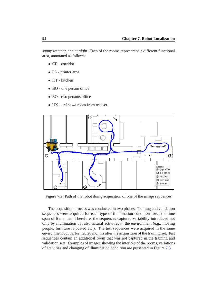
94 Chapter 7. Robot Localization
sunnyweather, and atnight. Each of the rooms represented a different functionalarea, annotated as follows:
• CR - corridor
• PA - printer area
• KT - kitchen
• BO - one person office
• EO - two persons office
• UK - unknownroom from test set
Figure 7.2: Path of the robot doing acquisition of one of the image sequences
The acquisition process was conducted in two phases. Training and validationsequences were acquired for each type of illumination conditions over the timespan of 6 months. Therefore, the sequences captured variability introduced notonly by illumination but also natural activities in the environment (e.g., movingpeople, furniture relocated etc.). The test sequences wereacquired in the sameenvironment but performed 20 months after the acquisition of the training set. Testsequences contain an additional room that was not captured in the training andvalidation sets. Examples of images showing the interiors of the rooms, variationsof activities and changing of illumination condition are presented in Figure7.3.

7.3. Proposed models 95
Figure 7.3: Example images from IDOL2 collection: (a) variation of illuminationchanging, (b) variation over time span.
For experimental purpose, the RobotVision collection consists of three imagesets: training set, validation set and test set. Training set contains a sequence of1,034 images and validation set contains a sequence of 909 images. Training andvalidation sets consist of five rooms across a span of 6 months. The official testwas released as a sequence of 1,690 images with an additionalroom and recorded20 months later.
7.3 Proposed models
The system we used for the RobotVision competition was composed of twoprocesses: a recognition step and a post-processing step. However, we describe

96 Chapter 7. Robot Localization
and evaluate here only the recognition step, in such a way to assess the impact ofthe proposed model. The post-processing step of the resultswill be discussed inthe section7.5.2. The robot was trained with a sequence of images taken in thenight condition. Then, we used a validation set captured in sunny condition toestimate the system parameters.
7.3.1 Image modeling
As described in chapter4, the concept sets and relation sets were extractedfrom the image collection as follows:
1. Each image was divided into 5x5 patches. We extracted for each patch aHSV color histogram and an edge histogram as in section4.2. Then, thevisual vocabulary of 500 visual concepts was constructed byusing k-meansclustering algorithm. From this vocabulary, we built the weighted conceptsetWCpatch.
2. Similar to the previous step except that the visual features were extractedfrom the local keypoints. To be more precise, we detected scale invariantkeypoints using SIFT detector [Lowe 2004] for each images. Local featureswere then used to create the weighted concept setWCsift.
3. Using the two previous features we defined an inter-relation set{inside}between patch concepts and SIFT concepts, denoted asWEinside, if onekey-point is locatedinside the area of a corresponding patch.
7.3.2 Visual graph models
Similar to above, we referred to the model without relation as LM (simply theproduction of probability generated by different concept sets) and the graph modelwith the spatial relation as VGM (with the contributing of relation probability tograph model). Based on this definition, we have implemented several graphs tomeasure the performance of our proposed model:
1. LMP =< WCpatch, ∅ >, that used only patch concepts.
2. LMS =< WCsift, ∅ >, that used only SIFT feature concepts.
3. LMS.P =< WCsift
⋃
WCpatch, ∅ >, that used both patch and SIFT featureconcepts.
4. V GMS→P =< WCsift
⋃
WCpatch,WEinside >, that used patch concepts,SIFT feature concepts and theinside relations between them.

7.4. Experimental results 97
Figure 7.4: Graph model constructed for RobotVision includes two type of imagerepresentation and one type of relation.
Figure7.4gives an example of the graph extracted from the concept setsandrelation sets defined above. In fact, the first three models were estimated followingthe equation presented in section5.3.2. The fourth model is the fusion graphcombined with spatial relation. Its probability was computed according to theequation defined in section5.3.3.
7.4 Experimental results
7.4.1 Evaluation methods
The image sequences used in the competition were annotated with groundtruth. The annotations of the training and validation sequences were available tothe participants, while the ground truth for the test sequence was released after theresults were announced. Each image in the sequences was labeled according tothe position of the robot during acquisition as belonging toone of the rooms usedfor training or as an unknown room. The ground truth was then used to calculatea score indicating the performance of an algorithm on the testsequence. We haveapplied two methods for the evaluating of the system performance.
Room accuracy In order to compare our method with other classical ap-proaches and for the validation purpose, we also adopt the evaluation based onthe classification accuracy as proposed for STOIC collection (section6.4.1). Thismeasurement is computed as follows:
Room accuracy=TProom
Nroom
whereTProom represents the number of images correctly classified for thespecificroom. Nroom is the total number of images annotated for this room (i.e., 1034

98 Chapter 7. Robot Localization
images for corridor CR) in the test collection.
Recognition score (official measurement)The recognition score measured the differences between theactual room id
and the one classified by the systems. The following rules were used whencalculating the official score for a test sequence:
• +1.0 pointsfor each correctly classified image
• -0.5 pointsfor each misclassified image
• 0 points for unclassified image (the algorithm refrained from the decision)
This score is more strict in the sense that the robot will get penalty point (-0.5point) for an uncorrected guest. Each participant has to decide their strategy toadapt to this specific context. Similar to the room accuracy,higher score meanshigher accuracy.
7.4.2 Impact of the spatial relation
Table 7.1 describes the results in terms of score value for each model.Asexpected, the two basic modelsLMP and LMS gave a good score for thevalidation set. However, the modelLMP did not perform well on the test set dueto the introduction of new room and new arrangement of interior furniture. Thesimple fusion modelLMS.P underperformed the best results ofLMP andLMS.However, this result was more robust in the sense that it leveraged on the spuriouseffects of each visual feature (i.e.,LMS.P outperformed the averaged result ofLMP andLMS in both cases). Moreover, the introduction ofinside relationsto the completed graphV GMS→P boosted its results respectively by 39.5% and40.1% comparing to the fusion graphLMS.P for both validation set and test set.This fact confirmed that the integration of relations playeda significant role toimprove the results. In addition, it showed that the link between object details andits global presentation provides a better abstraction for image content.
Table 7.1: Recognition scores of different graph models
Graph model LMP LMS LMS.P VGMS→P
Validation 345 285 334.5 466.5(+39.5%)Test 80.5 263 209.5 293.5(+40.1%)

7.4. Experimental results 99
7.4.3 Impact on room classification
We present in detail the classification accuracies for each class (representedby its room id) as categorized by our algorithms in Table7.2. For each class, theaccuracy is computed by the number of correctly labeled images divided by thetotal number of images belonging to this class. Note that we only consider theclassification accuracies of 5 rooms as we did not treat theunknownroom in thetest sequence at this step. The post-processing step of the results will be discussedin the section7.5.2.
Generally, the graph model for SIFT conceptsLMS performs better than thegraph model for patch conceptsLMP . This leads us to conclude that the detailsof object are important clues for scene recognition. In addition, the simple fusionmodelLMS.P tried to leverage the effect on both modelLMS andLMP andimproved the results only in the case of two-person office (EO). All four modelsgave good accuracies for the corridor (CR) regardless of brutal changes in lightconditions. We also noted that the number of training imagesfor corridor (CR)was the highest (483/1034 images) comparing to other classes. It suggests that thehigher the number of image samples, the more robust the performance is.
Table 7.2: Classification accuracies of graph models for eachroom. Bold valuesindicate the best results obtained for each class.
BO CR EO KT PA Mean
Validation setLMP 0.257 0.779 0.524 0.450 0.434 0.489LMS 0.354 0.658 0.581 0.426 0.402 0.484LMS.P 0.398 0.679 0.613 0.519 0.426 0.527V GMS→P 0.416 0.829 0.702 0.550 0.492 0.598
Test setLMP 0.163 0.701 0.385 0.236 0.279 0.353LMS 0.331 0.721 0.478 0.5090.348 0.477LMS.P 0.206 0.756 0.484 0.410 0.286 0.428V GMS→P 0.369 0.736 0.540 0.516 0.344 0.501
As a whole, the visual graph with spatial relationsV GMS→P led to higheraccuracies in all cases except in the cases of corridor (CR) andprinter area (PA)in test set. However, the difference was not significant comparing to other models(only 2% less than theLMS.P graph model). Furthermore, the mean accuracy ofmodelV GMS→P achieved on the test set and the validation set were the best offour models, with more than 7% better than the simple fusion modelV GMS.P .This result confirms again the strength of spatial relationships that contributed to

100 Chapter 7. Robot Localization
our graph model.
7.4.4 Comparing to SVM method
Similar to above, we refer to the model with only the contribution of conceptas LM and model with the spatial relation as VGM. For RobotVision collection,we choose the modelLMS.P as LM andV GMS→P as VGM.
Table 7.3: Results on categorizing with different methods
#class SVM LM VGMValidation 5 0.535 0.579 (+ 8.2%)0.675(+ 26.2%)
Test 6 0.439 0.416 (– 5.2%)0.449(+ 22.8%)
Table 7.3 summarizes the results obtained from collection RobotVision’09.We can see that in all cases our VGMs outperform other methods. More precisely,with the integration of spatial relation into VGM helps to improve the accuracy ofclassical LM approaches by more than 8%. The LMs perform roughly similar tothe SVMs. Likewise, VGMs increase sharply the accuracies from 22.8% to 26.2%comparing to those of SVMs for both the test and validation sets respectively.Once again, this fact confirms that if we can integrate the relation in a smart way,it could increase the overall performance of the recognition systems.
7.5 Discussion
In this section, we will discuss on how we choose the visual features forgenerating the language model based on the validations setswith different weatherconditions. Then we will describe the post processing step for enhancing thequality of the results. Finally, we report the result of our submissions to the officialevaluation ImageCLEF campaign.
7.5.1 Validation process
The validation aims at evaluating robustness of the algorithms to visualvariations that occur over time due to the changing conditions and human activity.We trained our system with the night condition set and testedagainst all the otherconditions from validation set. Our objective is to understand the behavior ofour system with the changing conditions and with different types of features.Moreover, the validation process can help us to fine-tune themodel parametersthat the latter will be used for the official test.

7.5. Discussion 101
We built 3 different language models corresponding with 3 types of visualfeatures. The training set used isnight set. Model Mc and Me correspond tocolor histogram and edge histogram extracted from image with the division of5x5 patches. Model Ms corresponds to SIFT color feature extracted from interestpoints. We measure the precision of system using the accuracy rate. Summary ofthe results is reported in Table7.4.
Table 7.4: Results obtained on different conditions with 3 visual language models
Training Validation HSV(Mc) Edge(Me) SIFT color(Ms)
Night Night 84.24% 59.45% 79.20%Night Cloudy 39.33% 58.62% 60.60%Night Sunny 29.04% 52.37% 54.78%
We noticed that, under the same condition (e.g. night-night), the HSV colorhistogram Mc outperformed all the other models. However, under differentconditions, the result of this model dropped significantly (from 84% to 29%).It showed that the color information is very sensitive with the changing ofillumination condition. On the other hand, the edge model (Me) and the SIFTcolor model (Ms) are practically robust with the changing ofthe illuminationcondition. In the worst condition (night-sunny), we still obtained a quite goodrecognition rate of 52% for Me and 55% for Ms. As the result, edge histogramand SIFT feature are chosen as the appropriate features for our recognition system.
7.5.2 Post-processing of the results
For the official evaluation, the algorithm must be able to provide informationabout the location of the robot separately for each test image (obligatory task)(e.g. when only some of the images from the test sequences areavailable).This corresponds to the problem of global topological localization. However,results can also be reported for the case when the algorithm is allowed to exploitcontinuity of the sequences and rely on the test images acquired before theclassified image (optional task). The reported results will be compared separatelyfor each task.
We have performed some fine-tuning steps of these results in order to enhancethe accuracy of our system. Figure7.5shows the flowchart of the post-processingof the results come from different models. This flowchart includes four mainfunctions:
1. Linear fusion: we take the advantage of the different features extractedfrom the images. We represent an image by a set of concept setsCi

102 Chapter 7. Robot Localization
Fusion
1
Regrouping
2
Filtering
3
Ranking listR1
Ranking listR2
Smoothing
4
Obligatory results
Optional results
Figure 7.5: Post-processing steps of the results. Blue scheme is for the obligatorytrack and red scheme is the for optional track
and eachCi corresponds to a visual feature. Assuming the concepts setsindependence, we fuse the relevance status values (RSV) fromthe rankedlist of the individual concepts sets using sum operator:
RSV (Q,D) =∑
i
RSV (qi, di) (7.1)
whereQ = {qi} andD = {di} are the set of concept sets correspondingto the query image and to the document image respectively. This stepcorresponds to the visual graph fusion with the absent of therelation asdeveloped in the above section.
2. Regrouping by room id: On the basis that using only the closest imageto determine the room id of a query image is not enough, we proposed togroup the results of the n-best images for each room. We compute a rankedlist of roomRL instead of an image list:
RL = {R,RSV (Q,R)} (7.2)
with
RSV (Q,R) =∑
fn−best(Qj ,R)
RSV (Q,D) (7.3)
whereR correspond to a room andfn−best is a function that select thenimages with the best RSV belonging to the roomR.

7.5. Discussion 103
3. Filtering the “unknown” room : we measured a difference from the scoreof the 4th room to the 1st room in the room list RL. If the difference is bigenough (> thresholdβ) we keep this image. Otherwise we remove it fromthe list (or consider as an ”unknown” room). In our experiment, we choosethe valueβ = 0.003 as a threshold.
4. Smoothing window: we exploited the continuity in a sequence of imagesby smoothing the result in the temporal dimension. To do that, we use asmoothing window sliding on the classified image sequences.Here, wechoose the width of windoww = 40 (i.e. 20 images before and after theclassified image). So, the score of the smoothed image is the mean value oftheir neighborhood images.
RSVwindow(Qi, R) =
∑
j∈[j−w/2;j+w/2] RSV (Qj, R)
w(7.4)
wherew is the width of the smoothing window. In the real case, we couldonly use a semi smoothing window which considers the images before thecurrent classified image. This leads to:
RSVsemi−window(Qi, R) =
∑
j∈[j−w;j] RSV (Qj, R)
w(7.5)
wherew is the width of the semi-window.
Below is the result for the post-processing step (see Table7.5) based on theranked lists provide by two models Me and Ms from the validation process. Thetraining and validation conditions used for post-processing are innight andsunnyrespectively.
Table 7.5: Result of the post-processing step based on 2 models Me and Ms
Me Ms Fusion Regrouping Filtering Smoothingn− best = 15 β = 0.003 w = 20
52.37 % 54.78 % 62% 67% 72% 92%
As we can see, the linear fusion of these 2 models gives overall of 8% ofimprovement. The regrouping step helped to pop-up some prominent rooms fromthe score list by averaging fromn-bestroom’s scores. The filtering takes part ineliminating some of the uncertain decisions base on the difference of their scoreafter the regrouping step. Finally, the smoothing step (which is an optional step)helps to increase significantly the performance of a sequence of images by 20%.

104 Chapter 7. Robot Localization
7.5.3 Submitted runs to the ImageCLEF 2009
Participating in this competition, we have built 3 graph models based on theprevious validating process. We eliminated the HSV histogram model because ofits poor performance on different lighting conditions. We used the same visualvocabulary of 500 visual concepts generated for night condition set. Each modelprovided a ranked result corresponding with the test sequence released. The post-processing steps were performed similar to the validating process employing thesame configuration. The visual language models built for thecompetition arelisted as follows:
• Me1: visual language model based on edge histogram extracted from 10x10patches division
• Me2: visual language model based on edge histogram extracted from 5x5patches division
• Ms: visual language model based on color SIFT local features
Based on the 3 visual models constructed, we have submitted 5 runs to theImageCLEF evaluation:
• 01-LIG-Me1Me2Ms: linear fusion of the results coming from 3 models(Score = 328)
• 02-LIG-Me1Me2Ms-Rk15: re-ranking the result of 01-LIG-Me1Me2Mswith the regrouping of top 15 scores for each room (Score = 415)
• 03-LIG-Me1Me2Ms-Rk15-Fil003: if the result of the 1st and the 4th inthe ranked list is too small (i.e.β <0.003), we remove image that from thelist. We refrain the decision from some cases other than to mark them asunknown room (Score = 456.5)
• 04-LIG-Me1Me2Ms-Rk2-Diff20: re-ranking the result of 01-LIG-Me1Me2Mswith the regrouping of top 2 scores for each room and using smoothingwindow (20images/frame) to update the room-id from image sequences(Score = 706)
• 05-LIG-Me1Ms-Rk2-Diff20 : same as 04-LIG-Me1Me2Ms-Rk2-Diff20but with the fusion of 2 model Me1 and Ms (Score = 697)
Our best run03-LIG-Me1Me2Ms-Rk15-Fil003 for the obligatory track isranked at10th place among all the 21 runs submitted. The best run in thecompetition (score = 793 points) was obtained with an approach based on local

7.6. Summary 105
feature matching. Run04-LIG-Me1Me2Ms-Rk2-Diff20 had not met the criteriaof the optional task which only used the sequence before the classified image.Nevertheless, this run has increased by roughly 250 points from the best obligatoryrun. It means that we still have room to improve the performance of our systemswith the valid smoothing window.
7.6 Summary
To summarize, we have shown in this chapter the second application of thevisual graph model, namelymobile robot self-localization. Coping with thespecific condition of anindoor laboratory environment, we have implementedanother instance of the proposed graph model. The proposed visual graph modelshave to adapt to the specific visual contents of the image collection, as well asadapt to the environment changes (such as lighting condition, object moving,human involving and theunknownroom).
We have constructed different graph models based onpatch conceptsandSIFTconceptswhich represented the abstract form and the object details respectively.A particular relation between the two concepts is also included to capture theco-occurrence information among the concepts. The resultsobtained shown thatthe integration of spatial relations into the visual graph model outperformed thestandard language model and the SVM classification which based only on thevisual concept.
We have also performed a validation process based on the validation setsto choose the best visual features adapting to the environment changes. Post-processing step of the ranked list was also studied. Finally, we provided theofficial results of our submitted run to the ImageCLEF 2009 forum.
In the next chapter, we will conclude our thesis and give someperspectivesinto the future works.

106 Chapter 7. Robot Localization

Part IV
Conclusion
107


Chapter 8
Conclusions and Perspectives
We are not interested in the unusual, but in the usual seen unusually.
Beaumont Newhall
Content-Based Image Retrieval (CBIR) has been an open problem for the pasttwo decades. Several attempts have been made to overcome theinformationgap between low-level visual features and the semantics layer of image. In[Marr 1982], Marr proposed a common paradigm for designing a visual recog-nition system which includes three sub-modules:image processing, mappingandhigh-level interpretation. Our works aimed at solving the two latter problems.
In this thesis, we have introduced a graph-based model for representing imagecontent which added an intermediate layer to image representation. This graphcaptured the spatial relations among visual concepts associated with extractedregions of images. The graph matching process is based on theextension ofunigram conceptual modeling, proposed initially in [Maisonnasseet al.2008].Theoretically, our model fits within the language modeling approach for infor-mation retrieval, and expands previous proposals for graph-based representation.
Even though we have chosen to illustrate the proposed approach with the scenerecognition problems, this method is not fundamentally tiedto a specific type ofimages. The designed framework can be extended for several types of imagerepresentations, as well as several applications in different fields, such as,imageretrieval/annotation, object recognition, video classification/categorization, ormedical imaging classification. This list, by all means, is not exhautive. Assuggested by Nicolas Maillot, the combination with a reasoning layer or anontology network [Maillot 2005] will equippe the graph model with the capacityof understanding the scenic contents. The system is then able to detect multipleobject instances embeded in a particular scene, e.g, car, people, building, street ...
109

110 Chapter 8. Conclusions and Perspectives
8.1 Summary
We summarize here some main points mentioned in this dissertation:
Part I introduced the current state-of-the-art in the Content-Based Image Retrievalfield.
In chapter2, we gave a survey on different methods of image processing suchas: image decomposition and visual features extraction. This is a basic step inrepresenting of the image contents. Based in the extracted visual fetures, thebag-of-wordsmodel has been introduced. The bag-of-words model often representsimage content by a sparse vector of visual concepts. Images are matched basedon the Euclidean distances or the cosine similarity of the quantized vectors. Thebag-of-words model is simple but lacks the information on the spatial relationsbetween visual concepts.
In chapter3, we reviewed two principal branches of learning methods basedon the conceptual representation:generative approachesand discriminativeapproaches. Important approaches, such as, Naive Bayes, Language Modeling,Support Vector Machines, have also been introduced. Then, we discussed on theneed of embedding the structural information of visual concepts into a graph-based image representation. We also investigated some current graph matchingalgorithms and their limitations. Finally, an initial proposal of the graph-basedimage retrieval framework was sketched.
Part II described the proposed approach based on thegraph-based imagerepresentationand agenerative matching algorithm.
In chapter4, we presented the system architecture for the graph-based imagemodeling. This framework included three main stages:image processing, graphmodelingandgraph retrieval. The image processing stepaims at extracting thedifferent visual features from image regions to build a set of visual vocabularies.The graph modeling stepconsists of visual concepts construction and spatialrelation extraction. Each image is then represented by a corresponding visualgraph. Finally, thegraph retrieval stagegenerates the probabilities likelihood forthe query image from the trained graphs in the database. Images are ranked basedon their relevance values.
Chapter5 defined formally the visual graph model based on a set of conceptsets and a set of relation sets. Two instances of the visual graph models wereused to illustrate the adaptability of the latter to the realapplications. Then, weshowed how the document graphs are matched against the querygraph using theextension of the language modeling framework. For better understanding, we havedemonstrated with an intuitive example of graph matching. Finally, we showedhow visual graphs were actually ranked in the log-probability space.

8.2. Contributions 111
Part III demonstrated the proposed approach inPart II with two applications:scene recognitionand robot localization. These experimentations aimed atassessing the validity of our approach in certain aspects. We have conducted thetest on two image collections: STOIC-101 and RobotVision’09.
In chapter6, the consideration of regions and associated concepts allowsus to gain generality in the description of images, a generality which maybe beneficial when the usage of the system slightly differs from its trainingenvironment. This is likely to happen with image collections that, for example,use one or several images to represent a scene. The proposed model ableto adequately match images and sets of images represented bygraphs. Aswe conjectured, being able to abstract from a low level description enablesrobustness with respect to the usage scenarios. On the otherhand, querying aspecific location with a group of images is very promising forfuture applications(such as mobile localization services) that allows higher accuracy score withless computational effort comparing to video sequence. In addition, the wayof combining different image representations/features inthe graph framework ismore versatile comparing to other fusion approaches. On theexperimental side,we have proved a positive impact of the relations, as well as of multiple imagequeries. We also discussed on the smoothing parameter optimization with a crossvalidation technique based on the training image set.
In chapter7, we showed that integrating inter-relations between two differentconcept sets to represent images led to a significant improvement in the results.We hoped that the combination of the two different image representations (suchas patch and keypoints) can take advantage of the different visual features ofboth the abstract-level of the scene as well as the details ofthe objects. Thestrength of our approach is that this fusion-like model can be expressed naturallythrough the links of graph-based model. The experimental results confirmedthe superiority of the visual graph model comparing to the conceptual modelingapproach. We also showed that the graph models performed better than the state-of-the-art SVM method for image classification. Finally, the proposed approachhas been validated and submitted to the ImageCLEF for the evaluation.
8.2 Contributions
From the point of view of agraph-based framework, the major contributionsof our approach are:
• A well-founded graph representation for image retrieval. We havepresented a unified graph-based framework for image representation whichis able to integrate different types of visual concepts and spatial relations

112 Chapter 8. Conclusions and Perspectives
among them. Such graph can represent different image point of views in avery flexible way. Indeed, the visual graph model representsan intermediatelayer of image representation that could fill thesemantic gapbetween high-level knowledge and visual concepts.
• A simple and effective graph matching process. We have extendedthe language model in infomation retrieval for graph matching. Thelanguage modeling has been studied extensively for text retrieval andproved its effectiveness. Standing from this well-foundeness framework,our proposed method allowed matching of complex graph composed ofmultiple concept setsandmultiple relations sets. This can be done undercertain independence hypotheses of the concept sets and relation sets.Furthermore, we used theJelinek-Mercer smoothing method, which isa popular approximation technique for re-estimating of theprobabilitydistribution.
• Application to the problem of image categorization. We have shown howthe proposed approach can be applied to the problem ofscene recognitionandrobot localization. Different graph instances have been developed foreach application to adapt to the image contents. The experimental resultsperformed on two image collections (STOIC-101 and RobotVision) haveconfirmed the good performance and the effectiveness of the visual graphmodeling. Moreover, the proposed method also outperformedboth thestandard language modeling and the state-of-the-art SVM methods. Theresults obtained show a promising direction for the image categorization.
8.3 Future works
Our objectives aim at designing a graph-based framework which gains thecapable ofgenerality, re-usabilityandexpendabilityin different contexts. In thefuture, several aspects can be considered to extend our visual graph model.
8.3.1 Short-term perspectives
Integration of textual information for multimedia retriev al/annotationFirst of all, as the language model is coming from textual domain, we could
combine the graph representation of image with the graph representation of theannotated text as done in ImageCLEF photographic retrieval track. Hence, multi-modalities image indexing and retrieval should be a promising direction for thefuture model extension.

8.3. Future works 113
In our case, the integration should be done smoothly as they shared thesame probabilistic framework. The conceptual language modeling has beeninvestigated successfully in [Maisonnasseet al.2009] with the use of UMLS(Unified Medical Language System) for conceptual relation extraction in medicaldocument retrieval. Therefore, we wish to fuse these two approaches in the samegraph-based framework in order to enhance the system performance.
Moreover, the common framework between textual/visual graph makes it pos-sible to learn the mutual information for each text category/ image topic. Similarto [Phamet al.2007], the proposed graph can be used for image annotation withthe COREL image collection. For each image topic, we can train arepresentativegraph for a set of visual graphs with a specific classifier (for example SVMclassifier). Then, this representative graph can be used forclassifying of the newimages with the associating annotations.
The need of further study on visual concepts and spatial relationsIn chapter4, we have shown that the choice of visual concepts and relations
are subjective. Hence, the future work should include more types of visualconcepts and their relations and study the effect of these concepts and relationson the accuracy. Then the selection of good visual features (using LSAtechniques to eliminate thesynonymy/polysemyeffects on the visual concepts)and spatial relations can be processed. This should be adapted following aspecific image context or towards a typical scenario of the application. We alsowish to investigate different possible couplings of the low-level and high-levelrepresentations, with the hope to come up with a single representation that couldbe used in a general case.
Study the impact on the number of visual conceptsAnother technical issue that we would like to address is the choice of number
of clusters for visual concept learning. This number might affect the quality of theconstructed visual concepts. Actually, this parameter hasbeen chosen empiricallyand fixed for each application. As done in [Pham 2006], a practical study on thisaspect is needed for subsequent step of building visual graph models.
Evaluation of the proposed approach for object/video retrievalLast but not least, experiment on a large collection of imagesis necessary to
test thescalability and thestability of the proposed method. In the near future,the graph-based model can be used to tackle the video retrieval applications(e.g., TRECVID collection). Moreover, the graph instance proposed in chapter5 (with the combination of patches and keypoints) seems appropriate for objectclassification. Hence, the proposed graph could be applied for VOC challengetask which comprises of more than 10K images in training and test sets.

114 Chapter 8. Conclusions and Perspectives
8.3.2 Long-term perspectives
The long-term perspectives of this work cover a broad-rangeof theoreticalextensions, as well as the practical aspects, for example: integration of aninteractive relevant feedback and a prototype user-interface for retrieval platform.
Relevance feedback modeling using information divergenceAlthough the query likelihood model has a number of advantages, it is limited
in terms of how it models the user needs. It is difficult to incorporate informationabout the relevant documents to a specific query using the current rankingalgorithm. However, it is possible to extend the current query-based model to thepseudo-relevance feedbackmodel with the measure of divergence between querymodels and document models. A well-known measure from information theory istheKullback-Liebler (KL) divergencewhich measures the difference between twoprobability distributions. Hence, the first theoretical aspect we want to address isto incorporate this measurement in our graph-based framework. Similarly, the KLdivergences should be computed independently for the concept set distributionsand the relation set distribution respectively.
Extension of the current probabilistic frameworkAs explained in chapter5, the proposed approach relies mainly on the
theoretical assumption that the concept sets and relation sets are following themultinomial probability distribution. This assumption is widely used for textretrieval domain where the random variable takes only the discrete values (i.e.,0, 1, 2...N ). The k-means clustering defines ahard versionof visual concept forvisual vocabulary construction. Thus, the multinomial distribution assumptionstill holds true.
However, the visual concepts can be defined differently fromthe textualconcept, for example usingfuzzy c-meansor EM clustering[Moore 1998], whichcan create asoft versionof visual concept that is likely to be closer to thereality. It means that a visual concept might belong to several clusters withdifferent weights/probabilities. For example, a visual concept could belongto clusterc1 with a probability of 0.8 and to clusterc2 with a probability of0.2. In this case, the multinomial probability distribution is no longer valid andDirichlet distribution seems more suitable for modeling of the random variable.As a consequence, the concept independence hypothesis is not correct anymore.Therefore, one theoretical direction is to extend the current framework with theDirichlet probability distribution.
Graph clustering for visual concept navigationOne of the current trends in CBIR system is automatically regrouping image
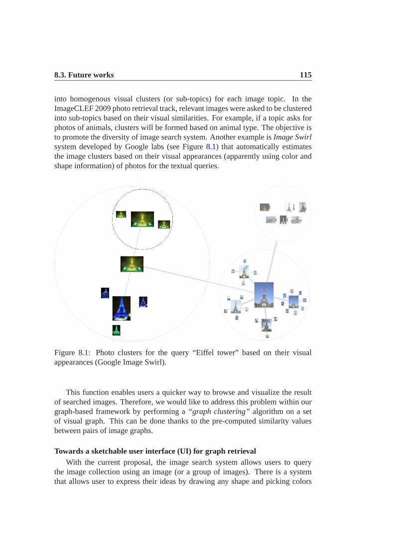
8.3. Future works 115
into homogenous visual clusters (or sub-topics) for each image topic. In theImageCLEF 2009 photo retrieval track, relevant images were asked to be clusteredinto sub-topics based on their visual similarities. For example, if a topic asks forphotos of animals, clusters will be formed based on animal type. The objective isto promote the diversity of image search system. Another example isImage Swirlsystem developed by Google labs (see Figure8.1) that automatically estimatesthe image clusters based on their visual appearances (apparently using color andshape information) of photos for the textual queries.
Figure 8.1: Photo clusters for the query “Eiffel tower” based on their visualappearances (Google Image Swirl).
This function enables users a quicker way to browse and visualize the resultof searched images. Therefore, we would like to address thisproblem within ourgraph-based framework by performing a“graph clustering” algorithm on a setof visual graph. This can be done thanks to the pre-computed similarity valuesbetween pairs of image graphs.
Towards a sketchable user interface (UI) for graph retrievalWith the current proposal, the image search system allows users to query
the image collection using an image (or a group of images). There is a systemthat allows user to express their ideas by drawing any shape and picking colors

116 Chapter 8. Conclusions and Perspectives
from a limited selection, such as Retrievr1 system (see Figure8.2). One possibledirection for the graph-based framework application is that we can design an UIthat allows user to generate their own visual graph providing a set of annotatedvisual concepts from the visual vocabulary and a set of relations. Concept andrelation can be assigned with a weight/probability based ontheir importance.Finally, users can arrange these inputs to form a visual graph/subgraph and queryit against the visual graph database.
Figure 8.2: Retrievr’s user interface allows user retrieving photos by drawing asimple sketch.
Finally, we believe that the work achieved in this thesis as well as the futureworks will allow to create image retrieval systems withbetter quality, easier toextendandmore interactive.
1http://labs.systemone.at/retrievr/

Appendix A: Publication of theAuthor
Journal Peer-reviewed Articles
1. Trong-Ton Pham, Philippe Mulhem, Loic Maisonnasse, EricGaussier, Joo-Hwee Lim. Visual Graph Modeling for Scene Recognition and RobotLocalization. Journal on Multimedia Tools and Applications, pages 20,Springer, January 2011.
2. Trong-Ton Pham, Loic Maisonnasse, Philippe Mulhem, EricGaussier.Modele de graphe et modele de langue pour la reconnaissance de scenesvisuelles. Numero special du revu Document Numerique, Vol 13 (211-228),Lavoisier, Juin 2010.
International Peer-reviewed Conference Articles
1. Trong-Ton Pham, Philippe Mulhem, Loic Maisonnasse. Spatial Relation-ships in Visual Graph Modeling for Image Categorization. Proceedings ofthe 33rd ACM SIGIR’10, pages 729-730, Geneva, Switzerland, 2010.
2. Trong-Ton Pham, Philippe Mulhem, Loic Maisonnasse, EricGaussier, AliAit-Bachir. Integration of Spatial Relationship in Visual Language Modelfor Scene Retrieval. IEEE 8th International Workshop on Content-BasedMultimedia Indexing (CBMI), pages 6, Grenoble, France, 2010.
3. Trong-Ton Pham, Loic Maisonnasse, Philippe Mulhem, EricGaussier.Visual Language Model for Scene Recognition. Singaporean-French IPALSymposium (SinFra’09), Singapore, 2009.
4. Trong-Ton Pham, Nicolas Maillot, Joo-Hwee Lim, Jean-Pierre Chevallet.Latent Semantic Fusion Model for Image Retrieval and Annotation. ACM16th Conference on Information and Knowledge Management (CIKM),pages 439-444, Lisboa, Portugal, 2007.
117

118 Chapter 8. Appendix A: Publication of the Author
National Peer-reviewed Conference Articles
1. Trong-Ton Pham, Philippe Mulhem et Loic Maisonnasse. Relationsexplicites entre differentes representations d’image dans un modele degraphe visuel. Actes de la conference CORIA, pages 211-222, Sousse,Tunisie, 2010.
2. Trong-Ton Pham, Loic Maisonnasse, Philippe Mulhem, EricGaussier.Modele de langue visuel pour la reconnaissance de scenes. Actes de laconference CORIA, pages 99-112, Giens, France, 2009.
3. Trong-Ton Pham, Jean-Pierre Chevallet, Joo-Hwee Lim. Fusion de multi-modalites et reduction par semantique latente: Applicationa la recherchede documents multimedia eta l’annotation automatique d’images. Actes dela conference CORIA, pages 39-53, Tregastel, France, 2008.
Working Notes, Book chapter
1. Trong-Ton Pham, Philippe Mulhem, Loic Maisonnasse, Jean-Pierre Cheval-let, Georges Quenot and Rami Albatal. MRIM-LIG at ImageCLEF 2009:Robot Vision, Image annotation and retrieval tasks. LectureNotes forComputer Science, pages 324-331, Springer, 2010.
2. Trong-Ton Pham, Loic Maisonnasse and Philippe Mulhem. Visual Lan-guage Modeling for Mobile Localization: LIG Participationin RobotVi-sion’09. Working Notes for ImageCLEF ’09, Corfu, Greece, 2009.

Bibliography
[Aksoy 2006] Selim Aksoy.Modeling of Remote Sensing Image Content usingAttributed Relational Graphs. In IAPR International Workshop onStructural and Syntactic Pattern Recognition, volume 4109,pages 75–483, 2006.
[Bachet al.2004] F. Bach, R. Thibaux and M. I. Jordan.Computing regulariza-tion paths for learning multiple kernels. Advances in Neural InformationProcessing Systems (NIPS), 2004.
[Ballard & Brown 1982] Dana Ballard and Chris Brown. Computer vision.Prentice-Hall, 1982.
[Belongie & Malik 2000] Serge Belongie and Jitendra Malik.Matching withShape Contexts. In Proceedings of the IEEE Workshop on Content-basedAccess of Image and Video Libraries, page 20, 2000.
[Belongieet al.2002] S. Belongie, J. Malik and J. Puzicha.Shape Matching andObject Recognition Using Shape Contexts. IEEE Transactions on PatternAnalysis and Machine Intelligence, vol. 24, pages 509–522,2002.
[Blei et al.2003] D. Blei, A. Ng and M. Jordan.Latent Dirichlet Allocation.Journal of Machine Learning Research, pages 993–1022, January 2003.
[Blei 2004] D. Blei. Probabilistic Models of Text and Images. PhD thesis, U.C.Berkeley, 2004.
[Boutell et al.2007] M. R. Boutell, J. Luo and C. M. Brown.Scene Parsing UsingRegion-Based Generative Models. IEEE Transactions on Multimedia,vol. 9, no. 1, pages 136–146, 2007.
[Carsonet al.1999] Chad Carson, Megan Thomas, Serge Belongie, Joseph M.Hellerstein and Jitendra Malik.Blobworld: A system for region-basedimage indexing and retrieval. In Third International Conference on VisualInformation Systems. Springer, 1999.
119

120 BIBLIOGRAPHY
[Chuaet al.1997] T.-S. Chua, K.-L. Tan and B. C. Ooi.Fast Signature-BasedColor-Spatial Image Retrieval. In ICMCS 1997, pages 362–369, 1997.
[Comaniciu & Meer 2002] Dorin Comaniciu and Peter Meer.Mean Shift: ARobust Approach Toward Feature Space Analysis. PAMI, vol. 24, no. 5,pages 603–619, May 2002.
[Cordellaet al.1998] L.P. Cordella, P. Foggia, C. Sansone, F. Tortorella andM. Vento. Graph Matching: A Fast Algorithm and its Evaluation. Proc.of the 14th International Conference on Pattern Recognition,Brisbane,Australia, pages 1582–1584, 1998.
[Dattaet al.2008] R. Datta, D. Joshi, J. Li and J. Z. Wang.Image Retrieval:Ideas, Influences, and Trends of the New Age. ACM Computing Surveys,vol. 40, no. 2, pages 1–60, 2008.
[Deerwesteret al.1990] Scott C. Deerwester, Susan T. Dumais, Thomas K.Landauer, George W. Furnas and Richard A. Harshman.Indexing byLatent Semantic Analysis. JASIS, vol. 41, no. 6, pages 391–407, 1990.
[Duffy & Crowley 2000] N. Duffy and James L. Crowley.Object DetectionUsing Colour. In International Conference on Pattern Recognition, pages1700–1706, Barcelona, 2000.
[Egenhofer & Herring 1991] M. Egenhofer and J. Herring.Categorizing binarytopological relationships between regions, lines and points in geographicdatabases. In A Framework for the Definition of Topological Relation-ships and an Approach to Spatial Reasoning within this Framework, SantaBarbara, CA, 1991.
[Fei-Fei & Perona 2005] Li. Fei-Fei and P. Perona.A Bayesian HierarchicalModel for Learning Natural Scene Categories. CVPR, pages 524–531,2005.
[Felzenszwalb & Huttenlocher 2004] P. F. Felzenszwalb and D. P. Huttenlocher.Efficient Graph-Based Image Segmentation. International Journal ofComputer Vision, vol. 59, no. 2, pages 167–181, 2004.
[Fenget al.2004] S. Feng, V. Lavrenko and R. Manmatha.Multiple BernoulliRelevance Models for Image and Video Annotation.CVPR’04, 2004.
[Ferrariet al.2010] Vittorio Ferrari, Frederic Jurie and Cordelia Schmid.Fromimages to shape models for object detection. International Journal ofComputer Vision, vol. 87, no. 3, pages 284–303, 2010.

BIBLIOGRAPHY 121
[Flickneret al.1995] Myron Flickner, Harpreet Sawhney, Wayne Niblack,Jonathan Ashley, Qian Huang, Byron Dom, Monika Gorkani, Jim Hafner,Denis Lee, Dragutin Petkovic, David Steele and Peter Yanker. Query byImage and Video Content: The QBIC System. Computer, vol. 28, no. 9,pages 23–32, 1995.
[Freeman 1974] H. Freeman.Computer processing of line-drawing images.Computing Surveys, vol. 6, pages 57–97, 1974.
[Gaoet al.2004] Jianfeng Gao, Jian-Yun Nie, Guangyuan Wu and Guihong Cao.Dependence language model for information retrieval. In Research andDevelopment in Information Retrieval, pages 170–177, 2004.
[Gorbanet al.2007] A. Gorban, B. Kegl, D. Wunsch and A. Zinovyev.PrincipalManifolds for Data Visualisation and Dimension Reduction. Springer,Berlin Heidelberg, vol. 58, 2007.
[Gusfield 1997] D. Gusfield. Algorithms on strings, trees, and sequences.Cambridge Univ. Press, 1997.
[Harchaoui & Bach 2007] Z. Harchaoui and F. Bach.Image classification withsegmentation graph kernels. Proceedings of the Conference on ComputerVision and Pattern Recognition (CVPR), page 8, 2007.
[Hare & Lewis 2005] J. S. Hare and P. H. Lewis.Saliency-based Models ofImage Content and their Application to Auto-Annotation by SemanticPropagation (Speech). Proceedings of Multimedia and the Semantic Web,2005.
[Harris & Stephens 1988] C. Harris and M. Stephens.A combined corner andedge detector. Proceedings of the 4th Alvey Vision Conference, pages147–151, 1988.
[Hofmann & Puzicha 1998] Thomas Hofmann and Jan Puzicha.StatisticalModels for Co-occurrence Data. A.I. Memo No. 1625, page 8, 1998.
[Hofmann 1999] Thomas Hofmann.Probabilistic latent semantic indexing. InACM conference on Research and development in information retrieval,pages 50–57, 1999.
[Iwayama & Tokunaga 1995] Makoto Iwayama and Takenobu Tokunaga. Hi-erarchical Bayesian clustering for automatic text classification. InProceedings of the 14th international joint conference on Artificialintelligence, pages 1322–1327, 1995.

122 BIBLIOGRAPHY
[Jelineket al.1991] F. Jelinek, R.L. Mercer and S. Roukos.Principles of LexicalLanguage Modeling for Speech Recognition. In Advances in SpeechSignal Processing, pages 651–700, 1991.
[Jelinek 1998] JF. Jelinek. Statistical methods for speechrecognition. MIT Press,Boston, 1998.
[Jianget al.2001] Xiaoyi Jiang, Andreas Muunger and Horst Bunke.On MedianGraphs: Properties, Algorithms, and Applications. IEEE Trans. PatternAnal. Mach. Intell., vol. 23, no. 10, pages 1144–1151, 2001.
[Kostin et al.2005] Alexey Kostin, Josef Kittler and William Christmas.Objectrecognition by symmetrised graph matching using relaxation labellingwith an inhibitory mechanism. Pattern Recogn. Lett., vol. 26, no. 3, pages381–393, 2005.
[Lazebniket al.2006] S. Lazebnik, C. Schmid and J. Ponce.Beyond Bagsof Features: Spatial Pyramid Matching for Recognizing Natural SceneCategories. In CVPR, pages 2169–2178, 2006.
[Leeet al.2006] Changki Lee, Gary Geunbae Lee and Myung Gil Jang.De-pendency structure language model for information retrieval. In ETRIjournal, 2006.
[Li & Wang 2003] J. Li and J. Wang.Automatic linguistic indexing of pictures bya statistical modeling approach. In IEEE Trans. on Pattern Analysis andMachine Intelligence, pages 1075–1088, 2003.
[Lienhartet al.2009] Rainer Lienhart, Stefan Romberg and Eva Horster. Multi-layer pLSA for multimodal image retrieval. In CIVR ’09: Proceeding ofthe ACM International Conference on Image and Video Retrieval,pages1–8, 2009.
[Lim & Jin 2005] Joo-Hwee Lim and Jesse S. Jin.A structured learningframework for content-based image indexing and visual query. InMultimedia System, volume 10, pages 317–331. Springer-Verlag, 2005.
[Lim et al.2007] J. Lim, Y. Li, Y. You and J. Chevallet.Scene Recognition withCamera Phones for Tourist Information Access. In ICME, pages 100 –103, 2007.
[Lowe 1999] David G. Lowe. Object Recognition from Local Scale-InvariantFeatures. In Proc. of the International Conference on Computer VisionICCV, Corfu, pages 1150–1157, 1999.

BIBLIOGRAPHY 123
[Lowe 2004] David G. Lowe. Distinctive image features from scale-invariantkeypoints. In International Journal of Computer Vision, pages 91–110,2004.
[Lu et al.2010] Zhiwu Lu, Yuxin Peng and Horace Ip.Image categorization viarobust pLSA. Pattern Recognition Letter, vol. 31, no. 1, pages 36–43,2010.
[Luo et al.2006] J. Luo, A. Pronobis, B. Caputo and P. Jensfelt.The KTH-IDOL2 database. In Technical Report, Kungliga Tekniska Hoegskolan,CVAP/CAS, 2006.
[Maillot 2005] Nicolas Eric Maillot. Ontology Based Object Learning andRecognition. PhD thesis, Universite de Nice - Sophia Antipolis, 2005.
[Maisonnasseet al.2008] Loic Maisonnasse, Eric Gaussier and Jean-PierreChevallet. Multiplying Concept Sources for Graph Modeling. InAdvances in Multilingual and Multimodal Information Retrieval, pages585–592. Springer-Verlag., 2008.
[Maisonnasseet al.2009] Loic Maisonnasse, Eric Gaussier and Jean-PierreChevallet. Model Fusion in Conceptual Language Modeling. In 31stEuropean Conference on Information Retrieval (ECIR 09), pages240–251, Toulouse (France), 2009.
[Manninget al.2009] C. D. Manning, P. Raghavan and H. Schtze.LanguageModels for Information Retrieval. In An Introduction to InformationRetrieval, pages 237–252. Cambridge University Press, 2009.
[Marr 1982] D. Marr. Vision: A computational investigationinto the humanrepresentation and processing of visual information. W. H.Freeman,1982.
[Mikolajczyk & Schmid 2002] Krystian Mikolajczyk and Cordelia Schmid. Anaffine invariant interest point detector. In ECCV, pages 128–142.Springer, 2002. Copenhagen.
[Monay & Gatica-Perez 2003] Florent Monay and Daniel Gatica-Perez. Onimage auto-annotation with latent space models. In ACM Multimedia,pages 275–278, 2003.
[Monay & Gatica-Perez 2004] F. Monay and D. Gatica-Perez.PLSA-basedImage Auto-Annotation: Constraining the Latent Space. In Proc. ACMInt. Conf. on Multimedia, pages 348–351, 2004.

124 BIBLIOGRAPHY
[Monay & Gatica-Perez 2007] Florent Monay and Daniel Gatica-Perez. Mod-eling Semantic Aspects for Cross-Media Image Indexing. IEEE Trans.Pattern Anal. Mach. Intell., vol. 29, no. 10, pages 1802–1817, 2007.
[Moore 1998] Andrew Moore.Very Fast EM-based Mixture Model ClusteringUsing Multiresolution kd-trees. In Advances in Neural InformationProcessing Systems 11, pages 543–549. MIT Press, 1998.
[Mulhemet al.2001] Philippe Mulhem, Wee Kheng Leow and Yoong KeokLee. Fuzzy conceptual graphs for matching images of natural scenes.In Proceedings of the 17th international joint conference on Artificialintelligence, pages 1397–1402, 2001.
[Ounis & Pasca 1998] Iadh Ounis and Marius Pasca.RELIEF: CombiningExpressiveness and Rapidity into a Single System. In ACM SIGIRConference on Research and Development in Information Retrieval,Melbourne, Australia, pages 266–274. ACM, 1998.
[Phamet al.2007] Trong-Ton Pham, Nicolas Maillot, Joo-Hwee Lim and Jean-Pierre Chevallet.Latent semantic fusion model for image retrieval andannotation. In CIKM, pages 439–444, 2007.
[Phamet al.2009] T. T. Pham, L. Maisonnasse and P. Mulhem.Visual LanguageModeling for Mobile Localization: LIG Participation in RobotVision09.In CLEF working notes 2009, Corfu, Greece, 2009.
[Phamet al.2010] Trong-Ton Pham, Loic Maisonnasse, Philippe Mulhem andEric Gaussier. Integration of Spatial Relationship in Visual LanguageModel for Scene Retrieval. In 8th IEEE Int. Workshop on Content-BasedMultimedia Indexing, page 6, 2010.
[Pham 2006] Trong-Ton Pham.Automatic Image Annotation: Towards a Fusionof Region-based and Saliency-based Models. Master Thesis, Universityof Paris 6, 2006.
[Ponte & Croft 1998] J. M. Ponte and W. B. Croft.A Language ModelingApproach to Information Retrieval. In Research and Development inInformation Retrieval, pages 275–281, 1998.
[Prasadet al.2001] B. G. Prasad, S. K. Gupta and K. K. Biswas.Color andShape Index for Region-Based Image Retrieval. In Proceedings of the 4thInternational Workshop on Visual Form, pages 716–728, 2001.

BIBLIOGRAPHY 125
[Pronobiset al.2008] A. Pronobis, O. Martnez Mozos and B. Caputo.SVM-based discriminative accumulation scheme for place recognition. InProceedings of the IEEE International Conference on RoboticsandAutomation (ICRA08), pages 522–529, 2008.
[Quelhaset al.2007] Pedro Quelhas, Florent Monay, Jean-Marc Odobez, DanielGatica-Perez and Tinne Tuytelaars.A Thousand Words in a Scene. IEEETrans. Pattern Anal. Mach. Intell., vol. 29, no. 9, pages 1575–1589, 2007.
[Rosenfeld 2000] R. Rosenfeld.Two Decades Of Statistical Language Modeling:Where Do We Go From Here?Proceedings of the IEEE, vol. 88, no. 8,pages 1270–1278, 2000.
[Schmid & Mohr 1997] Cordelia Schmid and Roger Mohr.Local Greyvalue In-variants for Image Retrieval. Pattern Analysis and Machine Intelligence,vol. 19, no. 5, May 1997.
[Shakhnarovichet al.2005] G. Shakhnarovich, T. Darrell and P. Indyk. Nearest-neighbor methods in learning and vision. MIT Press, 2005.
[Shawe-Taylor & Cristianini 2004] J. Shawe-Taylor and N. Cristianini. Kernelmethods for pattern analysis. Cambridge Univ. Press, 2004.
[Shi et al.1998] J. Shi, S. Belongie, T. Leung and J. Malik.Image and VideoSegmentation: The Normalized Cut Framework. IEEE Int’l Conf onImage Processing, pages 943–947, 1998.
[Shokoufandehet al.2002] Ali Shokoufandeh, Sven Dickinson, Clas Jnsson,Lars Bretzner and Tony Lindeberg.On the Representation and Matchingof Qualitative Shape at Multiple Scales. Proceedings of ECCV, pages759–775, 2002.
[Sivic & Zisserman 2003] J. Sivic and A. Zisserman.Video Google: A TextRetrieval Approach to Object Matching in Videos. In Proceedings of theInternational Conference on Computer Vision, volume 2, pages1470–1477, October 2003.
[Smeulderset al.2000] Arnold W. M. Smeulders, Marcel Worring, SimoneSantini, Amarnath Gupta and Ramesh Jain.Content-Based ImageRetrieval at the End of the Early Years. IEEE Trans. Pattern Anal. Mach.Intell., vol. 22, no. 12, pages 1349–1380, 2000.
[Smith & Chang 1996] J. R. Smith and S. F. Chang.VisualSEEk: a fullyautomated content-based image query system. In Proceedings ACM MM,pages 87–98, 1996.

126 BIBLIOGRAPHY
[Souvannavonget al.2004] Fabrice Souvannavong, Bernard Merialdo andBenoit Huet. Improved Video Content Indexing by Multiple LatentSemantic Analysis. In CIVR, pages 483–490, 2004.
[Sowa 1984] J. F. Sowa. Conceptual structures: information processing in mindand machine. Addison-Wesley Longman Publishing Co., Inc., Boston,MA, USA, 1984.
[Suardet al.2005] F. Suard, V. Guigue, A. Rakotomamonjy, and A. Benshrair.Pedestrian detection using stereo-vision and graph kernels. IEEESymposium on Intelligent Vehicule, 2005.
[Swain & Ballard 1991] Michael J. Swain and Dana H. Ballard.Color indexing.International Journal of Computer Vision, vol. 7, pages 11–32, 1991.
[Tabboneet al.2006] S. Tabbone, L. Wendling and J.-P. Salmon.A new shapedescriptor defined on the Radon transform. Computer Vision and ImageUnderstanding, vol. 102, pages 42–51, 2006.
[Tirilly et al.2008] Pierre Tirilly, Vincent Claveau and Patrick Gros.Languagemodeling for bag-of-visual words image categorization. ACM Interna-tional Conference on Image and Video Retrieval (CIVR), pages 249–258,2008.
[Ullmann 1976] J. R. Ullmann.An algorithm for subgraph isomorphism. Journalof the ACM, pages 31–42, 1976.
[Vapnik 1995] Vladimir Vapnik. The nature of statistical learning theory.Springer-Verlag, 1995.
[Won et al.2002] Chee Sun Won, Dong Kwon Park and Soo-Jun Park.EfficientUse of MPEG-7 Edge Histogram Descriptor. ETRI Journal, vol. 24, no. 1,pages 23–30, 2002.
[Wu et al.2007] Lei Wu, Mingjing Li, Zhiwei Li, Wei-Ying Ma and NenghaiYu.Visual language modeling for image classification. In Proceedings of theinternational workshop on multimedia information retrieval, pages 115–124, 2007.
[Zhang & Chang 2004] D. Q. Zhang and S. F. Chang.Detecting Image Near-Duplicate by Stochastic Attributed Relational Graph Matching withLearning. In ACM conference of Multimedia, pages 877–884, 2004.

BIBLIOGRAPHY 127
[Zhang & Lu 2001] Dengsheng Zhang and Guojun Lu.Content-Based ShapeRetrieval Using Different Shape Descriptors: A ComparativeStudy. IEEEInternational Conference on Multimedia and Expo, pages 1139–1142,2001.
[Ziou & Tabbone 1998] Djemel Ziou and Salvatore Tabbone.Edge DetectionTechniques - An Overview. International Journal of Pattern Recognitionand Image Analysis, vol. 8, pages 537–559, 1998.